Diffusion Coefficients from Molecular Dynamics Simulations in Binary and Ternary Mixtures

Int J Thermophys (2013) 34:1169–1196DOI 10.1007/s10765-013-1482-3

Diffusion Coefficients from Molecular DynamicsSimulations in Binary and Ternary Mixtures

Xin Liu · Sondre K. Schnell · Jean-Marc Simon ·Peter Krüger · Dick Bedeaux · Signe Kjelstrup ·André Bardow · Thijs J. H. Vlugt

Received: 12 December 2012 / Accepted: 21 June 2013 / Published online: 18 July 2013© Springer Science+Business Media New York 2013

Abstract Multicomponent diffusion in liquids is ubiquitous in (bio)chemicalprocesses. It has gained considerable and increasing interest as it is often the ratelimiting step in a process. In this paper, we review methods for calculating diffusioncoefficients from molecular simulation and predictive engineering models. The mainachievements of our research during the past years can be summarized as follows: (1)we introduced a consistent method for computing Fick diffusion coefficients usingequilibrium molecular dynamics simulations; (2) we developed a multicomponentDarken equation for the description of the concentration dependence of Maxwell–Stefan diffusivities. In the case of infinite dilution, the multicomponent Darken equa-tion provides an expression for D̄xk→1

i j which can be used to parametrize the general-ized Vignes equation; and (3) a predictive model for self-diffusivities was proposed forthe parametrization of the multicomponent Darken equation. This equation accurately

X. Liu · S. K. Schnell · S. Kjelstrup · A. Bardow · T. J. H. Vlugt (B)Process and Energy Laboratory, Delft University of Technology, Leeghwaterstraat 44,2628 CA Delft, The Netherlandse-mail: [email protected]

X. Liu · A. BardowLehrstuhl für Technische Thermodynamik, RWTH Aachen University, Schinkelstraße 8,52062 Aachen, Germany

J.-M. Simon · P. KrügerLaboratoire Interdisciplinaire Carnot de Bourgogne, UMR 6303 CNRS-Université de Bourgogne,Dijon, France

P. KrügerGraduate School of Advanced Integration Science, Chiba University, Chiba 263-8522, Japan

D. Bedeaux · S. KjelstrupDepartment of Chemistry, Norwegian University of Science and Technology, Trondheim, Norway

123

1170 Int J Thermophys (2013) 34:1169–1196

describes the concentration dependence of self-diffusivities in weakly associating sys-tems. With these methods, a sound framework for the prediction of mutual diffusionin liquids is achieved.

Keywords Matrix of thermodynamic factors · Maxwell–Stefan diffusion ·Molecular dynamics · Predictive models · Transport diffusion

1 Introduction

Mass transport by diffusion is a phenomenon that occurs due to a gradient in the chem-ical potential of a component in the system. Diffusion can be a slow process. The slowrate of diffusion is responsible for its importance. In many processes, diffusion occurssimultaneously with other phenomena, such as chemical reactions. When diffusionis the slowest step, it limits the overall rate of the process [1,2]. The necessity ofpredicting diffusion rates therefore arises.

It is important to make the distinction between self-diffusion and transport (ormutual) diffusion. Self-diffusion describes the mean-squared displacements of indi-vidual molecules in a medium, while transport/mutual diffusion describes the nettransport of a collection of molecules due to a driving force. The generalized Fick’slaw describes the mass flux due to transport diffusion as a linear combination of com-position gradients. For an n-component system, the molar flux Ji of component ifollows from

Ji = −ct

n−1∑

j=1

Di j ∇x j , (1)

in which ct is the total molar concentration, Di j are Fick diffusivities which depend onconcentration but not on the magnitude of the driving forces, and x j is the mole fractionof component j [3]. In gases, diffusion coefficients are typically around 10−5 m2 ·s−1.In liquids, diffusion coefficients are about 10−9 m2 · s−1. In solids, diffusion is evenslower [3–5]. In Eq. 1, the reference frame for the diffusion fluxes is the average molarvelocity, so that

∑ni=1 Ji = 0. Other reference frames, like the barycentric, the mean

volume or the solvent frames of reference, are alternatively used depending on theirconvenience for experimental conditions. We refer to Refs. [3,6] for the transformationrules from one reference frame to the other. In binary mixtures, the fluxes Ji are relatedto the mole fraction gradients by the constitutive relations,

J1 = −ct D11∇x1, (2)

J2 = −ct D22∇x2, (3)

which is Fick’s first law of diffusion. As J1 + J2 = 0 and x1 + x2 = 1, we haveD11 = D22 ≡ D, so diffusion in a binary system can be described by a singletransport coefficient. Fick diffusion coefficients in binary systems are the same for allreference frames provided that one uses the gradient of the appropriate concentrationmeasure [3].

123

Int J Thermophys (2013) 34:1169–1196 1171

In the modeling of multicomponent transport diffusion in liquids, the Maxwell–Stefan (MS) approach is often more convenient [3,6,7]. The key point of this approachis that the driving force for diffusion of component i , i.e., the chemical potentialgradient ∇μi at constant temperature and pressure, is balanced by friction forces,resulting in the following equation:

− 1

RT∇μi =

n∑

j=1, j �=i

x j (ui − u j )

D̄i j, (4)

in which R and T are the gas constant and absolute temperature, respectively. Thefriction force between components i and j is proportional to the difference in averagevelocities of the components, (ui − u j ). The MS diffusivity D̄i j is an inverse frictioncoefficient describing the magnitude of friction between components i and j . We high-light some features of multicomponent Fick and MS diffusivities: (1) MS diffusivitiesdo not depend on a reference frame while Fick diffusivities explicitly depend on a ref-erence frame; (2) MS diffusivities usually depend less strongly on concentration thanFick diffusivities [3]; (3) MS diffusivities are symmetric, i.e., D̄i j = D̄ ji while Fickdiffusivities are not, i.e., Di j �= D ji , except for binary systems. In a system containingn components, n(n − 1)/2 MS diffusivities are sufficient to describe mass transportwhile (n − 1)2 Fick diffusivities are needed. This suggests that for n > 2, the Fickdiffusivities are not independent; and (4) In multicomponent systems (n > 2), MSdiffusivities can be estimated using the MS diffusivities obtained from binary mix-tures. Multicomponent Fick diffusivities are not related to their binary counterparts.Therefore, it is very difficult to predict multicomponent Fick diffusivities using onlythe knowledge of binary systems. Clearly, it is convenient to use MS diffusivities fordescribing mass transport in multicomponent systems; however, MS diffusion coeffi-cients cannot be directly obtained from experiments as chemical potential gradientscannot be measured directly.

As generalized Fick’s law and the MS theory describe the same physical process, itis possible to relate the corresponding transport coefficients [3,7,8]. The correspondingequation to relate the diffusion coefficients in Eqs. 1 and 4 is

[D] = [B]−1[Γ ], (5)

in which [D] is the (n − 1) × (n − 1) matrix of Fick diffusivities. The elements of thematrix [B] are given by [3,8,9]

Bii = xi

D̄in+

n∑

j=1, j �=i

x j

D̄i j, with i = 1, · · · , (n − 1)

Bi j = −xi

(1

D̄i j− 1

D̄in

), with i, j = 1, · · · , (n − 1) and i �= j. (6)

123

1172 Int J Thermophys (2013) 34:1169–1196

The elements of the so-called matrix of thermodynamic factors [Γ ] are defined by[3,7,10]

Γi j = δi j + xi

(∂ ln γi

∂x j

)

T,p,∑ , (7)

in which δi j is the Kronecker delta, and γi is the activity coefficient of component i .The symbol � indicates that the partial differentiation of ln γi with respect to the molefraction x j is carried out at constant mole fraction of all other components except thenth one, so that

∑ni=1 xi = 1 during the differentiation [3,10]. For ideal mixtures, we

have Γi j = δi j . For any diluted system, one can show that Γ xi →0i i = 1 and Γ

xi →0i j, j �= i = 0.

In binary mixtures, the following relation holds between Fick and MS diffusivities:

D = Γ × D̄12, (8)

in which D is the binary Fick diffusivity, D̄12 is the MS diffusivity, and Γ is thethermodynamic factor given by [3]

Γ = 1 + x1

(∂ ln γ1

∂x1

)

T,p,∑ = 1 + x2

(∂ ln γ2

∂x2

)

T,p,∑ . (9)

The latter equality follows from the Gibbs–Duhem equation. In the limits x1 → 1and x2 → 1, Γ = 1. In practice, Fick diffusivities are more easily accessible inexperiments as they directly relate to the measurable quantities, i.e., concentrations.In fact, in all mutual diffusion experiments Fick diffusion coefficients are measured.Several experimental techniques can be used to study transport diffusion, e.g., Ramanspectroscopy [11,12], the diaphragm cell technique [13,14], interferometry [15–18],microfluidics [19], Quasi-elastic neutron scattering (QENS) experiments [20], and theTaylor dispersion method [21,22], etc. However, the investigation of the concentrationdependence of diffusivities is tedious. Experimental data on multicomponent diffusionin liquids are therefore limited [23–30]. Due to the difficulties in experiments [5], in thiswork, we focus on the prediction of diffusion coefficients using molecular simulationand predictive engineering models.

This review paper is organized as follows: in Sect. 2, we present molecular simula-tion approaches for computing mutual diffusivities. The advantages and disadvantagesof these approaches are discussed. Compared to simulation approaches, engineeringpredictive models are often preferred and convenient for the description of the masstransport by diffusion. In Sect. 3, we review and discuss predictive models for diffu-sion coefficients. We earlier derived a multicomponent Darken equation to predict theconcentration dependence of MS diffusivities. The multicomponent Darken equationrequires self-diffusivities. We have proposed a model for self-diffusivities to para-metrize the multicomponent Darken equation. Using MS diffusivities and the matrixof thermodynamic factors, measurable Fick diffusivities can be calculated. MS dif-fusivities can be computed in MD simulations while the matrix of thermodynamicfactors can be obtained from simulations in the grand-canonical ensemble [31–34].

123

Int J Thermophys (2013) 34:1169–1196 1173

The currently used algorithms for computing the matrix of thermodynamic factorsfrom molecular simulations are inefficient. The thermodynamic factors can also beobtained from experimentally determined equations of state [35–37] or excess Gibbsenergy models [3,10]. However, the combination of computed MS diffusivities andexperimentally determined thermodynamic factors is inconsistent [38–40]. In Sect. 4,we present a new method for computing thermodynamic factors from equilibriumMD simulations. This method could also be used to study the activity coefficients byintegrating the matrix of thermodynamic factors. In Sect. 5, we summarize the mainachievements of our work on diffusion in liquids.

2 Molecular Simulation of Self- and Transport Diffusion

Molecular dynamics (MD) simulation is a computational technique which uses a (usu-ally classical) force field to compute equilibrium and transport properties of a many-body system. The classical force field uses a functional form to describe the interactionbetween particles (atoms or molecules), i.e., bonded and non-bonded potentials. Therequired parameters are usually derived from experiments and/or quantum mechani-cal calculations. In this paper, bonded interactions typically consist of bond stretch-ing, bond bending, and torsion interactions while non-bonded interactions consist ofWeeks–Chandler–Andersen (WCA) [41], Lennard-Jones (LJ), and Coulombic inter-actions. For studying diffusion, simulations using quantum mechanical interactionsare not yet feasible due to the required time scale (i.e., ≥100 ns). The key idea of MDsimulations is to compute observable quantities from the time evolution of the system.In MD simulations, the equations of motion (Newton’s second law) are integratednumerically [42–44]. Newton’s second law states that the acceleration of a particle isproportional to the net force on the particle and inversely proportional to its mass,

ai = Fi

mi= d2ri

d t2 , (10)

in which ai is the acceleration of particle i, Fi is the net force acting on particle i, mi

is the mass of particle i, ri is the position of particle i , and t is the time. To integrate theequations of motion, several algorithms are available. For example, the time-reversiblevelocity Verlet algorithm is often used [42,43],

ri (t + �t) = ri (t) + vi (t)�t + Fi (t)

2mi�t2, (11)

vi (t + �t) = vi (t) + Fi (t + �t) + Fi (t)

2mi�t, (12)

in which ri (t) and vi (t) are the position and velocity of particle i at time t , respectively.The velocities of particles are related to the temperature [42]. �t is the time step forintegration and the typical value for �t is 10−15 s [42]. Fi (t) is the net force acting onparticle i at time t and can be calculated using a (classical) force field. Typically, we usehundreds to a few thousand molecules in MD simulation. Periodic boundary conditions

123

1174 Int J Thermophys (2013) 34:1169–1196

are usually applied [42–44]. By integrating the equation of motion, typical trajectoriesare obtained. From these trajectories, thermodynamic and transport properties canbe computed. Details are explained in Sect. 2.2. The time scale of MD simulationdepends on the properties of interest and typically ranges from a few to hundredsof nanoseconds. For more details on MD simulations, the reader is referred to someexcellent standard textbooks [42–45].

2.1 Non-equilibrium Molecular Dynamics

Non-equilibrium MD (NEMD) simulation has been treated as the most intuitive wayto obtain transport diffusion from MD simulations as some algorithms are similar tophysical experiments [46–55]. There are several different NEMD diffusion algorithmsthat have been used to obtain transport diffusion coefficients [46–52]. The algorithmscan be categorized by the method of perturbation used to drive the flux of species.In this section, we briefly review the most often used two methods: inhomogeneousNEMD and homogeneous NEMD, see Fig. 1.

Boundary-driven NEMD is an often used inhomogeneous method. Typically, ituses a simulation cell involving reservoirs where the concentration of molecules ofa given type is either higher or lower compared to its concentration averaged overthe system. Concentration gradients induced by these reservoirs lead to a steady-state

Fig. 1 Schematic overview of computational schemes for obtaining diffusion coefficients. Fick’s law andthe MS theory are often used to describe mass transport by diffusion. The two formalisms are relatedvia the matrix of thermodynamic factors [Γ ]. Fick diffusivities can be obtained from inhomogeneousNEMD simulations. MS diffusivities can be obtained from equilibrium MD and homogeneous NEMDsimulations. The matrix of thermodynamic factors can be predicted using grand-canonical Monte Carlo(GCMC) simulations. Our recent study shows that it is also possible to obtain the thermodynamic factorsfrom equilibrium MD simulations [38–40,111,112,119,123]

123

Int J Thermophys (2013) 34:1169–1196 1175

flux of molecules. To maintain the concentration difference inside the simulation box,a molecule entering one of the reservoirs has to be deleted from one of the otherreservoirs. By calculating the steady-state flux and the concentration gradients in thesystem, transport coefficients can be evaluated directly. This method has been appliedto study diffusion in zeolites [56], membranes [57,58], polymers [59], microporouscarbon [60,61], fluid systems [46,47], and across surfaces of different nature [62–64].Another inhomogeneous NEMD method for computing mutual diffusivities involvesthe use of gradient relaxation MD techniques [48,65,66]. In these methods, a concen-tration gradient is set up within a simulation cell. The system is relaxed using MD[48,65,66]. The relaxation rate of the concentration gradient is monitored and fittedto the continuum solution of the time-dependent diffusion equation, i.e., in the binarysystem,

∂ci

∂t= D∇2ci , (13)

in which t is the time, D is the Fick diffusivity, and ci is the concentration of componenti as a function of position and time. This method is conceptually simpler and has asound physical basis. However, it suffers from the following issues: (1) a large numberof molecules must be tracked to obtain continuum like behavior [48]; (2) many initialconditions should be used to determine whether the simulations were taking place inthe linear regime [48]; and (3) the concentration dependence of diffusivities is noteasily captured [48,67,68].

In homogeneous NEMD (field-driven NEMD), an external field is applied to thesimulation cell. This field is connected to particle properties (e.g., molar mass) to obtainthe properties corresponding to a bulk system. Therefore, in principle, concentrationgradients are not present in the system. The role of this field is to exert a body forceon the molecules. A thermostat is required in order to keep the temperature of thesystem constant [49]. Diffusivities corresponding to zero field can be obtained byextrapolation [52]. The advantages of this method are that it is easy to implement,computationally efficient, and a range of driving forces may be used. The latter featureenables one to examine both linear and nonlinear responses [49–52]. The disadvantageof this method is that the thermostat interacts with the net motion or flux of eachcomponent. The manifestation of this interaction, under large fields, is a free energyadvantage to partial phase separation of the system. The system tends to form “trafficlanes” like the opposing lanes of traffic on a road as this reduces the effective frictionbetween molecules of different species (that have different average net velocities).This phase-separation artifact can be suppressed by a minor change to the couplingof the thermostat to the particle momenta [49]. In electrolyte systems, i.e., aqueousKCl and NaCl, homogeneous NEMD is claimed to be more efficient compared toequilibrium MD [52].

2.2 Equilibrium Molecular Dynamics

Equilibrium MD simulations can be used to directly compute the MS diffusivitiesD̄i j from the motion of molecules inside the simulation box. The so-called Onsager

123

1176 Int J Thermophys (2013) 34:1169–1196

coefficients Λi j can be obtained directly from the equilibrium motion of the moleculesin MD [7,8,69–79]:

Λi j = 1

6lim

m→∞1

N

1

m · �t×

⟨⎛

⎝Ni∑

l=1

(rl,i (t + m · �t) − rl,i (t))

⎞

⎠

⎛

⎝N j∑

k=1

(rk, j (t + m · �t) − rk, j (t))

⎞

⎠⟩

. (14)

In this equation, N is the total number of molecules in the simulation, and i, j arethe molecule types. rl,i (t) is the position of lth molecule of component i at timet . The mean-squared displacement (MSD) can be efficiently updated with differentfrequencies according to the order-n algorithm described in Refs. [42,80]. By plottingthe MSD as a function of time on a log–log scale [81], one can determine the timescalefor the diffusive regime and extract diffusivities. The diffusive regime starts whenthe slope in this plot equals 1 provided that the MSD is sufficiently large (MSD >

(box size)2). An alternative but equivalent expression for obtaining Λi j is

Λi j = 1

3N

∞∫

0

dt ′⟨ Ni∑

l=1

vl,i (t) ·N j∑

k=1

vk, j (t + t ′)⟩

, (15)

in which vl,i (t) is the velocity of the lth molecule of type i at time t . Note thatthe matrix [Λ] is symmetric, i.e., Λi j = Λ j i and that the Onsager coefficients areconstrained by

∑i MiΛi j = 0 in which Mi is the molar mass of component i [8]. The

MS diffusivities directly follow from the Onsager coefficients Λi j . In binary systems,the MS diffusivity D̄12 is related to the Onsager coefficients by [8]

D̄12 = x2

x1Λ11 + x1

x2Λ22 − 2Λ12. (16)

For ternary and quaternary systems, the expressions are more complex and we referthe reader to Refs. [8,82]. As MS diffusivities relate to a collective property of movingmolecules, usually long simulations are required to obtain accurate data, i.e. >100 ns[38,39,83]. In principle, MS diffusivities obtained from equilibrium MD and NEMDare identical. This agreement has been observed for the NaCl–water system [52] andmethane diffusing in silicalite [48].

Unlike MS diffusivities that describe collective mass transport, self-diffusivitiesdescribe the motion of individual molecules. The self-diffusivity Di,self of componenti is related to the average molecular displacements described by the Einstein equation[42]

Di,self = 1

6Nilim

m→∞1

m · �t

⟨ Ni∑

l=1

(rl,i (t + m · �t) − rl,i (t))2

⟩(17)

123

Int J Thermophys (2013) 34:1169–1196 1177

= 1

3Ni

∞∫

0

dt ′⟨ Ni∑

i=1

(vl,i (t) · vl,i (t + t ′))⟩

, (18)

in which Ni is the number of molecules of component i . It is much easier to obtainaccurate self-diffusivities than to obtain MS diffusivities. In a system containing Ni

molecules of component i , the statistics for obtaining self-diffusivities is improvedas one can take the average over all molecules of component i . However, at eachpoint in time, there is only one data point for the Onsager coefficients Λi j . Due tothe much better statistics in self-diffusivities, simulations of a few nanoseconds areusually sufficient to obtain accurate self-diffusion data [38,39,83]. In the limit ofinfinite dilution (x j → 1), MS, Fick, and self-diffusivities become identical for a

binary system, i.e., D̄x j →1i j = Dx j →1 = D

x j →1i,self . There are several predictive models

available for Dx j →1i,self of which the Wilke–Chang equation is still the most popular

[4,84].

3 Predictive Models for Maxwell–Stefan and Self-Diffusion Coefficients

In Fig. 2, we present several models for obtaining diffusion coefficients that have beencategorized as Darken-type and Vignes-type equations. These models are discussedin the following.

3.1 Darken-Type Models

The Darken relation postulates that the composition dependence of the binary MSdiffusivity is given by [8,85,86]

D̄i j = xi D j,self + x j Di,self , (19)

where Di,self denotes the self-diffusion coefficient of species i in the mixture whichdepends on the composition. The appeal of the Darken equation originates from the factthat self-diffusivities are more easily accessible than mutual diffusivities, both exper-imentally [9] and computationally [8]. While often regarded as empirical, the Darkenequation can be rigorously derived based on the linear response theory and Onsager’sreciprocal relations [83,87,88]. Considering the Green-Kubo form of Onsager coeffi-cients (Eq. 15), for the terms Λi i , we can write [82]

Λi i = 1

3N

∞∫

0

dt ′⟨ Ni∑

l=1

vl,i (t) ·Ni∑

g=1

vg,i (t + t ′)⟩

= 1

3N

∞∫

0

dt ′⟨ Ni∑

l=1

vl,i (t) · vl,i (t + t ′)⟩

123

1178 Int J Thermophys (2013) 34:1169–1196

Fig. 2 Schematic overview of predictive models for diffusion coefficients. The Darken-type and the Vignes-type equations are often used to describe the concentration dependence of MS diffusivities D̄i j . The Darkenequation requires self-diffusivities, i.e., Di,self while the Vignes-type equation requires MS diffusivities at

infinite dilution, i.e., D̄x j →1i j and D̄

xk→1i j . As in the limit of infinite dilution, self-diffusivities are identical

to the MS diffusivities, i.e., D̄x j →1i j = Di,self , the Darken-type equation can be used to parametrize the

Vignes equation

+ 1

3N

∞∫

0

dt ′⟨ Ni∑

l=1

Ni∑

g=1,g �=l

vl,i (t) · vg,i (t + t ′)⟩

≈ xi Cii + x2i NC

i i , (20)

in which Cii and Ci i account for self- and cross-correlations of the velocities of

molecules of component i , respectively. One can assume here that N 2i − Ni ≈ N 2

i .From Eqs. 18 and 20, it follows that

Cii = Di,self . (21)

For Λi j with i �= j , i.e., the correlations between unlike molecules, we can write [82]

Λi j = 1

3N

∞∫

0

dt ′⟨ Ni∑

l=1

vl,i (t) ·N j∑

k=1

vk, j (t + t ′)⟩

123

Int J Thermophys (2013) 34:1169–1196 1179

≈ Ni N j

3N

∞∫

0

dt ′⟨v1,i (t) · v1, j (t + t ′)

⟩ = N xi x j Ci j . (22)

For ideal-diffusing mixtures, it can be assumed that the velocity cross-correlations,i.e., Ci j and C

i i are small compared to self-correlations Cii at finite concentrations.Using this assumption, one can obtain a multicomponent Darken equation for ann-component system:

D̄i j = Di,self D j,self

n∑

i=1

xi

Di,self, (23)

For binary systems (n = 2), the multicomponent Darken equation reduces to theDarken equation (Eq. 19) [8,86,89–91]. In WCA fluids in which the molar massdifferences between components are small (i.e., M j/Mi ≤ 10), the velocity cross-correlations are small compared to the self-correlations, Cii , while in the n-hexane–cyclohexane–toluene system, velocity cross-correlations are comparable to the self-correlations [82,83]. In the highly associating methanol–ethanol–water system andionic liquid systems, these cross-correlations are particularly strong due to the collec-tive motion of molecules, i.e., formation of hydrogen bonds and electrostatic interac-tions [82,83,92]. The coefficients Cii , Ci j , and C

i i , can be used to quantitatively studythe association of molecules and form the basis for developing predictive models fordiffusion.

3.2 Vignes-Type Models

The Vignes-type equation is another way to describe the concentration dependenceof MS diffusivities [93]. However, the Vignes equation is purely empirical. In binarysystems, the Vignes equation is

D̄i j =(

D̄xi →1i j

)xi(

D̄x j →1i j

)x j. (24)

The terms D̄xi →1i j and D̄

x j →1i j describe the interactions between components i and j if

one component is infinitely diluted in the other one. These binary diffusion coefficientsare easily obtained from both simulations and (semi-)empirical equations [86,94–98].For systems containing three and more components, a generalization of the Vignesequation was proposed by Wesselingh and Krishna [99]:

D̄i j =(

D̄xi →1i j

)xi(

D̄x j →1i j

)x jn∏

k=1,k �=i, j

(D̄xk→1

i j

)xk. (25)

The term D̄xk→1i j describes the interactions between components i and j while both i

and j are infinitely diluted in a third component k. This diffusion coefficient D̄xk→1i j

123

1180 Int J Thermophys (2013) 34:1169–1196

is not directly accessible in experiments. The past 20 years, several predictive modelshave been proposed for D̄xk→1

i j [8,10,99,100]. These models suggest to predict D̄xk→1i j

using either (1) the friction between solutes, i.e., D̄xi →1i j and D̄

x j →1i j [99]. For example,

(2) the friction between solute and solvent, i.e., D̄xk→1ik and D̄xk→1

jk [8,10], or (3) acombination of the first two categories [100]. Since there is no physical basis for anyof these models, it is unclear which one to use for a specific system. A physicallybased model can be obtained from the multicomponent Darken equation (Eq. 23). Inthe limit of infinite dilution, one can easily show that the multicomponent Darkenequation is reduced to [82]

D̄xk→1i j = Dxk→1

i,self · Dxk→1j,self

Dxk→1k,self

. (26)

This equation is valid if the cross-correlations are small compared to the self-correlations. Equation 26 allows us to predict the ternary diffusivity D̄xk→1

i j based

on binary diffusion coefficients D̄xk→1ik and D̄xk→1

jk and the pure component self-diffusivity Dk,self . The quality of this equation has been tested for several systems.For all cases, Eq. 26 is as least as good as the other empirical equations. For WCAfluids, Eq. 26 is very accurate resulting in a maximal deviation of 7 % compared toD̄xk→1

i j [82]. In the system n-hexane–cyclohexane–toluene in which molecules areweakly associated, the error of the prediction using Eq. 26 is less than 23 % [82]. Inthe system ethanol–methanol–water in which molecules are highly associating, Eq. 26leads to an error of 78 % [82]. As hydrogen bonding becomes even more importantin systems with ionic liquids, water and DMSO, Eq. 26 cannot accurately predict themagnitude of MS diffusivities at infinite dilution for these systems, suggesting thevelocity cross-correlations should be taken into account [92]. The rigorous derivationof Eq. 26 allows the identification of the physical cause of its failure which was notpossible for the previous empirical models.

It is important to note that errors introduced by modeling the concentration depen-dence of MS diffusivities using the generalized Vignes equation (Eq. 25) may be eitherreduced or enhanced by a particular choice for a model for D̄xk→1

i j [9,92,101]. In the

limit of xk → 1, the quality of the model for predicting D̄xk→1i j determines whether the

generalized Vignes equation (Eq. 25) is accurate. For finite concentrations, the qualityof the generalized Vignes equation (Eq. 25) and Eq. 26 play a role in the prediction ofthe concentration dependence of D̄i j .

In Fig. 3, we compare predicted MS diffusivities in a ternary WCA system usingEqs. 23 and 25 to the computed MS diffusivities from MD. Good agreement betweenthe multicomponent Darken equation (Eq. 23) and simulations was observed. The gen-eralized Vignes equation does not accurately describe the concentration dependenceof MS diffusivities, especially not for D̄13 and D̄23. In quaternary WCA systemsand in the n-hexane–cyclohexane–toluene system, Eq. 23 also accurately describesthe MS diffusivities as a function of concentration. Data for more systems can befound in Ref. [83]. The multicomponent Darken equation should therefore be viewed

123

Int J Thermophys (2013) 34:1169–1196 1181

0.5

0.6

0.7

0.8

0.9

1.0

1.1

1.2

0 0.2 0.4 0.6 0.8 1

12

x1

Generalized Vignes

Multicomponent Darken

MD

0.5

0.6

0.7

0.8

0.9

1.0

1.1

1.2

0 0.2 0.4 0.6 0.8 1

23

x1

Generalized Vignes

Multicomponent Darken

MD

0.5

0.6

0.7

0.8

0.9

1.0

1.1

1.2

0 0.2 0.4 0.6 0.8 1

13

x1

Generalized Vignes

Multicomponent Darken

MD

(a) (b)

(c)

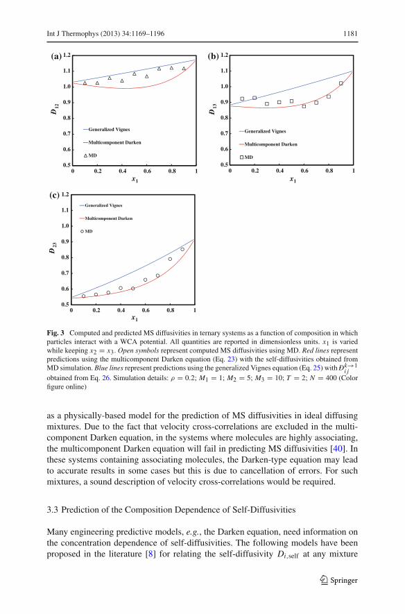
Fig. 3 Computed and predicted MS diffusivities in ternary systems as a function of composition in whichparticles interact with a WCA potential. All quantities are reported in dimensionless units. x1 is variedwhile keeping x2 = x3. Open symbols represent computed MS diffusivities using MD. Red lines representpredictions using the multicomponent Darken equation (Eq. 23) with the self-diffusivities obtained fromMD simulation. Blue lines represent predictions using the generalized Vignes equation (Eq. 25) with D̄k→1

i jobtained from Eq. 26. Simulation details: ρ = 0.2; M1 = 1; M2 = 5; M3 = 10; T = 2; N = 400 (Colorfigure online)

as a physically-based model for the prediction of MS diffusivities in ideal diffusingmixtures. Due to the fact that velocity cross-correlations are excluded in the multi-component Darken equation, in the systems where molecules are highly associating,the multicomponent Darken equation will fail in predicting MS diffusivities [40]. Inthese systems containing associating molecules, the Darken-type equation may leadto accurate results in some cases but this is due to cancellation of errors. For suchmixtures, a sound description of velocity cross-correlations would be required.

3.3 Prediction of the Composition Dependence of Self-Diffusivities

Many engineering predictive models, e.g., the Darken equation, need information onthe concentration dependence of self-diffusivities. The following models have beenproposed in the literature [8] for relating the self-diffusivity Di,self at any mixture

123

1182 Int J Thermophys (2013) 34:1169–1196

composition to the self-diffusivity in a infinitely diluted solution Dx j →1i,self :

Di,self =n∑

j=1

x j Dx j →1i,self , (27)

Di,self =n∑

j=1

w j Dx j →1i,self , (28)

Di,self =n∑

j=1

v j Dx j →1i,self . (29)

In these equations, w j is the mass fraction, v j is the volume fraction, and Dx j →1i,self

is the self-diffusivity of component i in an i- j mixture when the mole fraction ofcomponent j is approaching one. In liquid mixtures of linear alkanes [8], the massweighted equation (Eq. 28) is the best for describing MD simulation data. In Ref. [83],we proposed a model for the self-diffusivity of species i in the mixture as the inversemole-fraction weighted sum of its pure component value and its values at infinitedilution [83],

1

Di,self=

n∑

j=1

x j

Dx j →1i,self

. (30)

One can show that in the limit xi → 0, Eq. 30 is exact [82,101]. The validationof Eq. 30 in ternary WCA fluids is shown in Fig. 4. The predictions using Eq. 30perfectly agree with the computed self-diffusivities. This excellent agreement was alsoobserved for the binary systems acetone–methanol and acetone–tetrachloromethane;see Fig. 5. In Fig. 6, we compared the computed self-diffusivities to the predictionsfrom Eq. 30 in the ternary system chloroform–acetone–methanol. We observed thatover the whole concentration range, Eq. 30 quantitatively agrees with the computedself-diffusivities. The averaged absolute differences are approximately 10 %. The goodagreement between predictions and computed self-diffusivities suggests that Eq. 30can be used to describe the composition dependence of self-diffusivities, even forsystems that show moderately strong interactions. Recently, Vrabec and co-workershave shown that Eq. 30 works less well for systems with strong hydrogen bonding[102].

4 Thermodynamic Factors

The matrix of thermodynamic factors (Eq. 7) describes how ideal a solution is. Knowl-edge of the thermodynamic factors allows one to relate Fick to MS diffusivities (Eq. 5).By integrating the thermodynamic factors, activity coefficients can be obtained. Inthis section, we briefly review the methods for obtaining thermodynamic factors fromexperiments and simulations.

123

Int J Thermophys (2013) 34:1169–1196 1183

0.0

0.2

0.4

0.6

0.8

1.0

1.2

1.4

1.6D

i,sel

f

x1

0.0

0.2

0.4

0.6

0.8

1.0

1.2

1.4

1.6

Di,s

elf

x3

0.0

0.2

0.4

0.6

0.8

1.0

1.2

1.4

1.6

0.0 0.2 0.4 0.6 0.8 1.0

0.0 0.2 0.4 0.6 0.8 1.0

0.0 0.2 0.6 0.8 1.0

Di,s

elf

x2

(a) (b)

(c)

Fig. 4 Computed and predicted self-diffusivities in ternary systems in which particles interact with aWCA potential. All quantities are reported in dimensionless units. Open symbols represent computedself-diffusivities using MD. Solid lines represent predictions using Eq. 30. Blue triangles represent theself-diffusivities of component 1. Red squares represent the self-diffusivities of component 2. Green circlesrepresent the self-diffusivities of component 3. (a) x1 varies, x2/x3 = 1; (b) x2 varies, x1/x3 = 1; and (c)x3 varies, x1/x2 = 1. Simulation details: ρ = 0.2; M1 = 1; M2 = 5; M3 = 10; T = 2; N = 400 (Colorfigure online)

4.1 Experimental Determination

Typically, the matrix of thermodynamic factors [Γ ] can be calculated if activity coef-ficients are known (Eq. 7). By differentiation of the activity coefficients with respectto composition, the matrix of thermodynamic factors can be calculated [3,10]. Experi-mental vapor–liquid equilibrium data [103] and experimentally determined equationsof state [35–37] are often used to obtain activity coefficients. The most importantadvantages of using equations of state are: (1) they lead to simple expressions andenable fast calculations; (2) they are applicable over a wide range of pressures andtemperatures; and (3) many existing databases and correlations are available. How-ever, there are still limitations: (1) predictions for binary and multicomponent systemsare difficult and often rely on mixing rules [104]: and (2) predictions are sometimesinaccurate, especially in the presence of associating molecules [105].

123

1184 Int J Thermophys (2013) 34:1169–1196

1

2

3

4

5D

i,sel

f , 1

0 -9

m2 .s-1

x1

1

2

3

4

5

0 0,2 0,4 0,6 0,8 1 0 0,2 0,4 0,6 0,8 1

Di,s

elf, 1

0 -9

m2

. s-1

x1

(a) (b)

Fig. 5 Self-diffusivities in binary liquid systems (a) acetone (1)–methanol (2) and (b) acetone (1)–CCl4 (2)mixtures at 298 K, 1 atm. Filled symbols are the computed self-diffusivities using MD simulations. Squaresare the self-diffusivities of acetone. Triangles are the self-diffusivities of either methanol or CCl4. Solidlines are the predictions using Eq. 30. Details of the used force field can be found in Refs. [38,39]

0

2

4

6

Di,s

elf, 1

0 -9m

2 .s-1

x1

D1,self D2,self D3,self

1 2 3

D2,selfD1,self

D3,self

D1,self D

2,selfD

3,self

0

2

4

6

Di,s

elf, 1

0 -9

m2 .

s-1

x3

D1,self D2,self D3,self

Series4 Series5 Series6D1,self

D3,self

D1,self D

2,self

D3,selfD

2,self

0

2

4

6

0,0 0,2 0,4 0,6 0,8 1,0

0,0 0,2 0,4 0,6 0,8 1,0

0,0 0,2 0,4 0,6 0,8 1,0

Di,s

elf, 1

0 -9

m2 .

s-1

x2

D1,self D2,self D3,self

1 2 3D1,self

D3,self

D1,self D

2,self

D3,selfD

2,self

(a) (b)

(c)

Fig. 6 Self-diffusivities in ternary liquid systems chloroform (1)–acetone (2)–methanol (3) at 298 K, 1 atm.Open symbols are the computed self-diffusivities using MD simulations. Solid lines are the predictions usingEq. 30. Details of the used force field can be found in Ref. [40]

123

Int J Thermophys (2013) 34:1169–1196 1185

Obtaining the matrix of thermodynamic factors from physical models (e.g., excessGibbs energy (GE) models, equations of state) suffers from large uncertainties. Uncer-tainties in Γi j of more than 20 % are expected [3,106]. That is, even if a GE modelshows an excellent fit to activity coefficients determined from experimental vapor liq-uid equilibria data, the calculated elements of the matrix of thermodynamic factorsmay deviate significantly. In Ref. [106], Taylor and Kooijman further illustrate thedangers of estimating thermodynamic factors using GE models: i.e., in the binary sys-tem 2-butanone–water, the Margules, van Laar, and NRTL models provide a negativevalue of Γ around an equimolar composition implying demixing, while the Wilsonmodel provides a positive Γ (no demixing) in the same concentration range. DifferentGE models may also lead to different behavior of [Γ ].

4.2 Widom’s Test Particle Insertion Method

The conventional Widom test particle insertion method can be used to obtain thematrix of thermodynamic factors from molecular simulations [31–33]. Essentially,calculating the thermodynamic factor involves second derivatives of the Gibbs energywith respect to the number of particles. In the frame of Widom’s test particle inser-tion method, this corresponds to the simultaneous insertion of two test particles. Thedisadvantages of Widom’s test particle insertion method applied to two test particlesis that it is very inefficient to insert test particles into high density systems. Recently,a permuted Widom test particle insertion method has been developed by Balaji et al.[107,108]. The permuted Widom’s test particle insertion method involves the use ofcombinatorics to make the Widom’s method more efficient for the simulations inser-tion of two test particles [107,108]. So far, the method has been applied only to WCAsystems although, in principle, it is applicable to any system.

4.3 Kirkwood–Buff Integrals

The thermodynamic factors [Γ ] can be calculated using the so-called Kirkwood–Buff(KB) coefficients. The KB coefficients can be obtained from density fluctuations inthe grand-canonical ensemble [88]:

Gi j = V

⟨Ni N j

⟩ − 〈Ni 〉⟨N j

⟩

〈Ni 〉⟨N j

⟩ − V δi j

〈Ni 〉 , (31)

in which V is the volume and δi j is the Kronecker delta. The brackets 〈· · · 〉 denote anensemble average in the grand-canonical ensemble. The thermodynamic factors arerelated to the KB coefficients Gi j [38–40,109]. In binary systems, the thermodynamicfactor Γ is related to the KB coefficients Gi j by [38,39,109]

Γ = 1 − xic j (Gii + G j j − 2Gi j )

1 + c j xi (Gii + G j j − 2Gi j ). (32)

in which c j = 〈N j 〉/V . The expression relating the thermodynamic factors [Γ ] tothe KB coefficients Gi j in multicomponent systems can be found in Refs. [82,109].

123

1186 Int J Thermophys (2013) 34:1169–1196

Kirkwood and Buff showed that in the thermodynamic limit (V → ∞), the KBcoefficients can be related to the integrals of radial distribution functions over volume[109,110], resulting in the following expression [111,112]:

G∞i j = 4π

∞∫

0

[gi j (r) − 1

]r2dr. (33)

In this equation, gi j (r) is the radial distribution function for molecules of type i andj . As one usually does not have data for gi j (r) for an infinite range, it is commonpractice to truncate the integration at a distance R:

Gi j (R) = 4π

R∫

0

[gi j (r) − 1

]r2dr. (34)

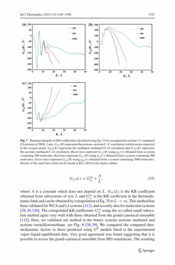
It is important to note several issues associated with Eq. 34: (1) Eq. 34 only has aphysical meaning when the upper bound of the integration is infinity, and thereforeit can only be applied to infinitely large systems (this issue is further discussed inSect. 4.5); (2) gi j (r) is the radial distribution function in an open system while MDsimulations usually consider closed systems; (3) for infinitely large systems, gi j (r) →1 for r → ∞. For finite systems with periodic boundary conditions, gi j (r) does notconverge to 1 for large r , and therefore the convergence of the integral is often slowand poor [109]. It is very difficult to find a plateau in a plot of Gi j (R). In Fig. 7,we show that the computed function Gi j (R) obtained using Eq. 34 for systems of(200, 500, and 5800) molecules. It is clear that even with a system of 5800 molecules,one cannot obtain an accurate estimate for the KB coefficients. Some effort has beenmade to solve the problem regarding to the poor convergence of Eq. 34 [113–115].The simplest and in the past frequently used approach is to simply use a switchingfunction to force the radial distribution function g(r) to converge to 1 for large distancer . However, it turns out that the final result depends on the choice of the switchingfunction [115,116]. Other approaches use the extension of g(r) due to the method byVerlet [43,113,117].

4.4 Scaling of Small System Fluctuations

Recently, Schnell et al. developed an alternative approach to compute Gi j from thelocal density fluctuations in small subsystems of volume V embedded in the simulationbox (Eq. 31) [111,112]. As these small subsystems can exchange energy and particleswith the rest of the system, it can be considered as grand-canonical like. In this way,KB coefficients follow directly from Eq. 31 in which concentrations, particle numbers,and volume refer to those inside the subvolume V . One can show that Eq. 31 scales as1/L , where L is the linear length of subvolume V in one dimension [112,118,119]. Toobtain KB coefficients in the thermodynamic limit (G∞

i j ), one can fit the simulationdata to [112,118,119]

123

Int J Thermophys (2013) 34:1169–1196 1187

-300

-250

-200

-150

-100

-50

0

50

100G

11(R

) , Å

3

R , Å

200

500

5800

-300

-250

-200

-150

-100

-50

0

50

100

G12

(R)

, Å3

R , Å

200

500

5800

-500

-400

-300

-200

-100

0

100

200

0 10 20 30 40 50

0 10 20 30 40 50

0 10 20 30 40 50

G22

(R)

, Å3

R , Å

200

500

5800

(a) (b)

(c) 150

300

Fig. 7 Running integrals of KB coefficients calculated using Eq. 34 for an equimolar acetone (1)–methanol(2) mixture at 298 K, 1 atm. G11(R) represents the acetone–acetone C–C correlation (carbon atom connectedto the oxygen atom). G22(R) represents the methanol–methanol O–O correlation and G12(R) representsthe acetone–methanol C–O correlation. Black lines represent Gi j (R) using gi j (r) obtained from a systemcontaining 200 molecules. Red lines represent Gi j (R) using gi j (r) obtained from a system containing 500molecules. Green lines represent Gi j (R) using gi j (r) obtained from a system containing 5800 molecules.Details of the used force field can be found in Ref. [40] (Color figure online)

Gi j (L) = G∞i j + A

L, (35)

where A is a constant which does not depend on L , Gi j (L) is the KB coefficientobtained from subsystems of size L and G∞

i j is the KB coefficient in the thermody-namic limit and can be obtained by extrapolation of Eq. 35 to L → ∞. This method hasbeen validated for WCA and LJ systems [112], and recently also for molecular systems[38,39,120]. The extrapolated KB coefficients G∞

i j using the so-called small subsys-tem method agree very well with those obtained from the grand-canonical ensemble[112]. Here, we validated our method in the binary systems acetone–methanol andacetone–tetrachloromethane, see Fig. 8 [38,39]. We compared the computed ther-modynamic factors to those predicted using GE models fitted to the experimentalvapor–liquid equilibrium data. Very good agreement was found suggesting that it ispossible to access the grand-canonical ensemble from MD simulations. The resulting

123

1188 Int J Thermophys (2013) 34:1169–1196

0.0

0.2

0.4

0.6

0.8

1.0

1.2

x1

EMD

Margules

MD

0.4

0.5

0.6

0.7

0.8

0.9

1.0

1.1

0 0.2 0.4 0.6 0.8 1 0.0 0.2 0.4 0.6 0.8 1.0

x1

EMD

Margules

MD(a) (b)

Fig. 8 Thermodynamic factor Γ in the binary systems (a) acetone (1)–methanol (2) and (b) acetone (1)–tetrachloromethane (2) at 298 K, 1 atm. Open symbols are the computed Γ using MD simulations. The solidlines represent Γ calculated from the Margules model fitted to experimental vapor–liquid equilibrium data[125]. Details of the used force field can be found in Refs. [38,39]

0

2

4

6

8

D, 1

0 -9

m2 .s-1

x1 x1

EMD

experiment

MD

Experiment

0

1

2

3

4

5

0 0,2 0,4 0,6 0,8 1 0 0,2 0,4 0,6 0,8 1

D, 1

0 -9

m2

. s-1

MD

Experiment

(a) (b)

Fig. 9 Fick diffusivities in binary systems (a) acetone (1)–methanol (2) and (b) acetone (1)–tetrachloromethane (2) at 298 K, 1 atm. Open symbols are Fick diffusivities D calculated using D̄12 and Γ ,both computed from equilibrium MD simulations. The solid lines represent Fick diffusivities D obtainedfrom experiments [23,126]. Details of the used force field can be found in Refs. [38,39]

Fick diffusivities for the systems acetone–methanol and acetone–tetrachloromethaneobtained via the computed MS diffusivities and the matrix of thermodynamic factorsare in excellent agreement with the experimental data as shown in Fig. 9. We appliedthis method also to the ternary system chloroform–acetone–methanol [40]. The com-puted thermodynamic factors using the small subsystem method are compared topredictions obtained from the COSMO-SAC theory [121,122]. In Fig. 10, the concen-tration of chloroform increases while the concentration of acetone and methanol areidentical. For the whole concentration range, the data obtained from MD simulationare in excellent agreement with experiments. The COSMO-SAC theory qualitativelydescribes the concentration dependence of thermodynamic factors; however, errors ofmore than 100 % were observed. The resulting Fick diffusivities for the ternary system

123

Int J Thermophys (2013) 34:1169–1196 1189

-1.0

-0.5

0.0

0.5

1.0

1.5

2.0Γ 1

1

MD COSMO-SAC NRTL

-1.0

-0.5

0.0

0.5

1.0

1.5

2.0

Γ 12

MD COSMO-SAC NRTL

-1.0

-0.5

0.0

0.5

1.0

1.5

2.0

Γ 21

x1 x1

x1 x1

MD COSMO-SAC NRTL

-1.0

-0.5

0.0

0.5

1.0

1.5

2.0

0.0 0.2 0.4 0.6 0.8 1.0 0.0 0.2 0.4 0.6 0.8 1.0

0.0 0.2 0.4 0.6 0.8 1.0 0.0 0.2 0.4 0.6 0.8 1.0

Γ22

MD COSMO-SAC NRTL

(a)

(c) (d)

(b)

Fig. 10 Thermodynamic factors Γi j in the ternary system chloroform (1)–acetone (2)–methanol (3) at1 atm. Open circles are the computed values of Γi j using MD simulations at 298 K. Filled circles are thecomputed values of Γi j using the COSMO-SAC approach at 298 K. Solid lines represent Γi j calculatedfrom the NRTL model fitted to experimental vapor–liquid equilibrium data at 303 K of Ref. [127]. x1 isvaried while keeping x2 = x3. Details of the used force field can be found in Ref. [40]

acetone–methanol–chloroform can be found in Fig. 11 [40]. It can be observed that:(1) the diagonal Fick diffusivities are always positive and the off-diagonal Fick dif-fusivities may be negative; (2) the diagonal Fick diffusivities are about one order ofmagnitude larger than the off-diagonal Fick diffusivities meaning the diffusion flux ofcomponent i mainly depends on its own concentration gradient while the concentrationgradients of other components play a minor role. This behavior is in accordance withthe bound placed on off-diagonal coefficients by the entropy production for ternarydiffusion [2].

4.5 Kirkwood–Buff Integrals in Finite Systems

As discussed in Sect. 4.3, density fluctuations in the grand-canonical ensemble canbe related to integrals of the radial distribution function over volume. Kirkwood andBuff have shown this for systems in the thermodynamic limit (Eq. 33). However, inmolecular simulation one deals with systems of finite-size, so very often Eq. 34 is used

123

1190 Int J Thermophys (2013) 34:1169–1196

-2

0

2

4

6D

ij, 1

0 -9

m2 .

s-1

x1

11 12 21 22

-2

0

2

4

6

Dij

, 10

-9m

2 .s-1

x3

11 12 21 22

-2

0

2

4

6

0,0 0,2 0,4 0,6 0,8 1,0

0,0 0,2 0,4 0,6 0,8 1,0

0,0 0,2 0,4 0,6 0,8 1,0

Dij

, 10

-9m

2 .s-1

x2

11 12 21 22

(a) (b)

(c)

Fig. 11 Fick diffusivities in the ternary system chloroform (1)–acetone (2)–methanol (3) at 298 K, 1 atm.Fick diffusivities Di j are calculated using the computed D̄i j and Γi j . (a) x1 varies while keeping x2 = x3,(b) x2 varies while keeping x1 = x3, (c) x3 varies while keeping x1 = x2. Details of the used force fieldcan be found in Ref. [40]

as an approximation. Recently, Krüger et al. [123] have shown that the approximationof Eq. 34 is in fact incorrect for finite-size systems, and significantly deviates fromG∞

i j . This can be understood as follows. Consider a finite and open system of volume

V . We assume that this volume is spherical with a radius R. The KB coefficients GVi j

for this finite system are defined as:

GVi j ≡ V

⟨Ni N j

⟩ − 〈Ni 〉⟨N j

⟩

〈Ni 〉⟨N j

⟩ − V δi j

〈Ni 〉 (36)

= 1

V

∫

V

∫

V

(gi j (r12) − 1)dr1dr2 (37)

in which r12 = |r1 − r2| and gi j (r12) is the radial distribution function for i, j pairs.For an infinitely large system, the double integral of Eq. 37 can be reduced to a singleintegral by the transformation r2 → r = r1 − r2 leading directly to Eq. 33. For a

123

Int J Thermophys (2013) 34:1169–1196 1191

finite-size system, one cannot apply this transformation because the integration domainof r depends on r1. In this case, the correct integral becomes

GVi j = 1

V

∫

V

∫

V

(gi j (r12) − 1)dr1dr2 (38)

= 4π

2R∫

0

[gi j (r) − 1

] (1 − 3r

4R+ r3

16R3

)r2dr. (39)

which is only identical to Eq. 33 when R → ∞. One can show that [GVi j (R) − G∞

i j ]scales as 1/R [123]. Note that the KB coefficients in Eqs. 31 and 36 correspond to thegrand-canonical ensemble, and so gi j (r) must, in principle, be calculated in an infinitesystem. The radial distribution functions computed in a finite, closed system, do notconverge to one for r → ∞, which leads to a divergence of the KB coefficients,as discussed in Sect. 4.3. However, the radial distribution functions of the infinitesystem, g∞

i j (r) can be accurately estimated from those of two finite, closed systemswith particle numbers N1 and N2. This is based on the fact that in the expansion,

gNi j (r) ≈ g∞

i j (r) + c(r)

N, (40)

the function c(r) does not depend on N [118]. Therefore, c(r) and thus g∞i j (r) can be

readily estimated from gNi j (r) computed for two different system sizes N1 and N2.

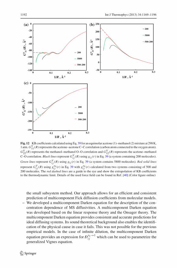
In Fig. 12, we compare the KB coefficients calculated using Eq. 39, using exactlythe same radial distribution functions as in Fig. 7. We computed GV

i j (R) using gi j (r)

obtained from a finite system, and also using g∞i j (r) defined in Eq. 40. Using gi j (r)

obtained from a finite system in Eq. 39 has the disadvantage that it is difficult todetermine the linear regime for which [GV

i j (R) − G∞i j ] scales as 1/R. This problem

becomes less severe by using a very large system. Using g∞i j (r) in Eq. 39, Fig. 12

clearly shows that it is much easier to find the linear regime and extrapolate the KBcoefficients to the thermodynamic limit. To obtain g∞

i j (r), two small systems aresufficient and simulations of large systems are not needed.

5 Conclusions

In this work, we briefly reviewed methods for predicting mutual diffusion coefficients[38–40,82,83,92,101,124]. The main achievements of our research team can be sum-marized as follows:

– We introduced a consistent method for computing Fick diffusion coefficients usingMD simulations. In experiments, Fick diffusivities are measured while molecularsimulation usually provides MS diffusivities. These diffusivities are related via thematrix of thermodynamic factors which is usually known only with large uncertain-ties. This leaves a gap between experiment and molecular simulation. To overcomethis problem, we calculated thermodynamic factors from MD simulations using

123

1192 Int J Thermophys (2013) 34:1169–1196

200

-140

-120

-100

-80

-60

-40

-20

0G

V 11(R

) , Å

3

1/R , Å-1

200

5800

500-200

0.1 0.2 0.3

-200

-150

-100

-50

0

GV 12

(R) ,

Å3

1/R , Å-1

200

5800

500-200

0.1 0.2 0.30

0

(a)

(c)

-50

0

50

100

150

200

250

GV 22

(R) ,

Å3

1/R , Å-1

200

5800

500-200

0.1 0.2 0.30

-250

(b)

Fig. 12 KB coefficients calculated using Eq. 39 for an equimolar acetone (1)–methanol (2) mixture at 298 K,1 atm. GV

11(R) represents the acetone–acetone C–C correlation (carbon atom connected to the oxygen atom).

GV22(R) represents the methanol–methanol O–O correlation and GV

12(R) represents the acetone–methanol

C–O correlation. Black lines represent GVi j (R) using gi j (r) in Eq. 39 (a system containing 200 molecules).

Green lines represent GVi j (R) using gi j (r) in Eq. 39 (a system contains 5800 molecules). Red solid lines

represent GVi j (R) using g∞

i j (r) in Eq. 39 with g∞i j (r) calculated from two systems consisting of 500 and

200 molecules. The red dashed lines are a guide to the eye and show the extrapolation of KB coefficientsto the thermodynamic limit. Details of the used force field can be found in Ref. [40] (Color figure online)

the small subsystem method. Our approach allows for an efficient and consistentprediction of multicomponent Fick diffusion coefficients from molecular models.

– We developed a multicomponent Darken equation for the description of the con-centration dependence of MS diffusivities. A multicomponent Darken equationwas developed based on the linear response theory and the Onsager theory. Themulticomponent Darken equation provides consistent and accurate predictions forideal diffusing systems. Its sound theoretical background also enables the identifi-cation of the physical cause in case it fails. This was not possible for the previousempirical models. In the case of infinite dilution, the multicomponent Darkenequation provides an expression for D̄xk→1

i j which can be used to parametrize thegeneralized Vignes equation.

123

Int J Thermophys (2013) 34:1169–1196 1193

– Eq. 30 for self-diffusivities was proposed for parametrization of the multicompo-nent Darken equation. This equation accurately describes the concentration depen-dence of self-diffusivities in weakly associating systems.

– The Kirkwood–Buff (KB) theory is correct and applicable for any open system.The original KB integrals, which are valid only for infinite systems, have oftenincorrectly been applied to finite systems. We have shown that with Eqs. 39 and40, KB integrals can be calculated accurately for open systems of any finite vol-ume, requiring only radial distribution functions computed in closed systems ofmoderate size.

The presented methods thus provide a hierarchy of tools to predict multicomponentdiffusion. For ideal diffusing mixtures, the multicomponent Darken equation allows fora physically based comprehensive engineering model. In combination with Eq. 30 forself-diffusivities, multicomponent diffusion coefficients can be predicted using binarydata of infinite dilution and pure component data. For non-ideal diffusion mixtures,MD allows one to quantify the complex diffusion behavior. The small subvolumemethod opens the route for efficient determination of Fick diffusion coefficients fromMD.

Acknowledgments This work was performed as part of the Cluster of Excellence “Tailor-Made Fuelsfrom Biomass”, which is funded by the Excellence Initiative by the German federal and state governmentsto promote science and research at German universities. TJHV, SKS, and SK acknowledge financial supportfrom NWO-CW through an ECHO grant. This work was also sponsored by the Stichting Nationale Com-puterfaciliteiten (National Computing Facilities Foundation, NCF) for the use of supercomputing facilities,with financial support from the Nederlandse Organisatie voor Wetenschappelijk onderzoek (NetherlandsOrganization for Scientific Research, NWO).

References

1. S. Kjelstrup, D. Bedeaux, E. Johannessen, J. Gross, Non-equilibrium Thermodynamics for Engineers,1st edn. (World Science Publishing Co. Pte. Ltd., Singapore, 2010)

2. S. Kjelstrup, D. Bedeaux, Non-equilibrium Thermodynamics of Heterogeneous Systems, 1st edn.(World Science Publishing Co. Pte. Ltd., Singapore, 2008)

3. R. Taylor, R. Krishna, Multicomponent Mass Transfer, 1st edn. (Wiley, New York, 1993)4. B. Poling, J. Prausnitz, J.P.O. O’Connell, The Properties of Gases and Liquids, 5th edn. (McGraw-Hill,

New York, 2004)5. E.L. Cussler, Diffusion, Mass Transfer in Fluid Systems, 3rd edn. (Cambridge University Press, New

York, 2005)6. G.D.C. Kuiken, Thermodynamics of Irreversible Processes: Applications to Diffusion and Rheology,

1st edn. (Wiley, New York, 1994)7. R. Krishna, J.A. Wesselingh, Chem. Eng. Sci. 52, 861 (1997)8. R. Krishna, J.M. van Baten, Ind. Eng. Chem. Res. 44, 6939 (2005)9. A. Bardow, E. Kriesten, M.A. Voda, F. Casanova, B. Blümich, W. Marquardt, Fluid Phase Equilib.

278, 27 (2009)10. H.A. Kooijman, R. Taylor, Ind. Eng. Chem. Res. 30, 1217 (1991)11. A. Bardow, V. Göke, H.J. Koß, W. Marquardt, AIChE J. 52, 4004 (2006)12. A. Bardow, W. Marquardt, V. Göke, H.J. Koß, K. Lucas, AIChE J. 49, 323 (2003)13. R.L. Robinson Jr, W.C. Edmister, F.A.L. Dullien, J. Phys. Chem. 69, 258 (1965)14. R.H. Stokes, J. Am. Chem. Soc. 72, 763 (1950)15. M.L. Wagner, H. Scheraga, J. Phys. Chem. 60, 1066 (1956)16. W.J. Thomas, I.A. Furzer, Chem. Eng. Sci. 17, 115 (1962)17. H.Z. Cummins, N. Knable, Y. Yeh, Phys. Rev. Lett. 12, 150 (1964)

123

1194 Int J Thermophys (2013) 34:1169–1196

18. D. Ehlich, M. Takenaka, T. Hashimoto, Macromolecules 26, 492 (1993)19. E. Häusler, P. Domagalski, M. Ottens, A. Bardow, Chem. Eng. Sci. 72, 45 (2012)20. H. Jobic, N. Laloué, C. Laroche, J.M. van Baten, R. Krishna, J. Phys. Chem. B 110, 2195 (2006)21. I.M.J.J. van de Ven-Lucassen, M.F. Kemmere, P.J.A.M. Kerkhof, J. Solut. Chem. 26, 1145 (1997)22. I.M.J.J. van de Ven-Lucassen, F.G. Kieviet, P.J.A.M. Kerkhof, J. Chem. Eng. Data 40, 407 (1995)23. A. Alimadadian, C.P. Colver, Can. J. Chem. Eng. 54, 208 (1976)24. H.T. Cullinan, H.L. Toor, J. Phys. Chem. 69, 3941 (1965)25. T.K. Kett, D.K. Anderson, J. Phys. Chem. 73, 1268 (1969)26. F. Shuck, H.L. Toor, J. Phys. Chem. 67, 540 (1963)27. R.A. Graff, T.B. Drew, Ind. Eng. Chem. Fundam. 7, 490 (1968)28. A. Sethy, H.T. Cullinan, AIChE J. 21, 571 (1975)29. S. Käshammer, H. Weingärtner, H. Hertz, Phys. Chem. Chem. Phys. 187, 233 (1994)30. J. Butchard, H. Toor, J. Phys. Chem. 66, 2015 (1980)31. B. Widom, J. Chem. Phys. 39, 2808 (1963)32. A. Lotfi, J. Fischer, Mol. Phys. 66, 199 (1989)33. A. Lotfi, J. Fischer, Mol. Phys. 71, 1171 (1990)34. J. Vrabec, H. Hasse, Mol. Phys. 100, 3375 (2002)35. M.K. Kozlowska, B. Jurgens, C.S. Schacht, J. Gross, T.W. de Loos, J. Phys. Chem. B 113, 1022

(2009)36. C.S. Schacht, C. Schuell, H. Frey, T.W. de Loos, J. Gross, J. Chem. Eng. Data 56, 2927 (2011)37. J. Gross, G. Sadowski, Ind. Eng. Chem. Res. 40, 1244 (2001)38. X. Liu, S.K. Schnell, J.M. Simon, D. Bedeaux, S. Kjelstrup, A. Bardow, T.J.H. Vlugt, J. Phys. Chem.

B 115, 12921 (2011)39. X. Liu, S.K. Schnell, J.M. Simon, D. Bedeaux, S. Kjelstrup, A. Bardow, T.J.H. Vlugt, J. Phys. Chem.

B 116, 6070 (2012)40. X. Liu, A. Martín-Calvo, E. McGarrity, S.K. Schnell, S. Calero, J.M. Simon, D. Bedeaux, S. Kjelstrup,

A. Bardow, T.J.H. Vlugt, Ind. Eng. Chem. Res. 51, 10247 (2012)41. J.D. Weeks, D. Chandler, H.C. Andersen, J. Chem. Phys. 54, 5237 (1971)42. D. Frenkel, B. Smit, Understanding Molecular Simulation: from Algorithms to Applications, 2nd edn.

(Academic Press, San Diego, 2002)43. M.P. Allen, D.J. Tildesley, Computer Simulation of Liquids, 1st edn. (Oxford University Press, New

York, 1987)44. M.E. Tuckerman, Statistical Mechanics: Theory and Molecular Simulation, 2nd edn. (Oxford Uni-

versity Press, Oxford, 2010)45. D. Rapaport, The Art of Molecular Dynamics Simulation, 2nd edn. (Cambridge University Press,

Cambridge, 2004)46. A.P. Thompson, D.M. Ford, G.S. Heffelfinger, J. Chem. Phys. 109, 6406 (1998)47. A.P. Thompson, G.S. Heffelfinger, J. Chem. Phys. 110, 10693 (1999)48. E.J. Maginn, A.T. Bell, D.N. Theodorou, J. Phys. Chem. 97, 4173 (1993)49. D.J. Evans, G.P. Morriss, Statistical Mechanics of Nonequilibrium Liquids, 2nd edn. (Academic Press,

London, 1990)50. D. MacGowan, D.J. Evans, Phys. Rev. A 34, 2133 (1984)51. S. Sarman, D.J. Evans, Phys. Rev. A 45, 2370 (1992)52. D.R. Wheeler, J. Newman, J. Phys. Chem. B 108, 18362 (2004)53. T. Ikeshoji, B. Hafskjold, Mol. Phys. 81, 251 (1994)54. B. Hafskjold, T. Ikeshoji, S.K. Ratkje, Mol. Phys. 80, 1389 (1993)55. B. Hafskjold, S.K. Ratkje, J. Stat. Phys. 78, 463 (1995)56. J.R. Hill, A.R. Minihan, E. Wimmer, C.J. Adams, Phys. Chem. Chem. Phys. 2, 4255 (2000)57. J.M.D. MacElroy, J. Chem. Phys. 101, 5274 (1994)58. J.M.D. MacElroy, M.J. Boyle, Chem. Eng. J. 74, 85 (1999)59. D.M. Ford, G.S. Heffelfinger, Mol. Phys. 94, 673 (1998)60. R.F. Cracknell, D. Nicholson, N. Quirke, Phys. Rev. Lett. 74, 2463 (1995)61. D. Nicholson, R.F. Cracknell, Langmuir 12, 4050 (1996)62. I. Inzoli, S. Kjelstrup, D. Bedeaux, J.M. Simon, Chem. Eng. Sci. 66, 4533 (2011)63. I. Inzoli, S. Kjelstrup, D. Bedeaux, J.M. Simon, Microporous Mesoporous Mater. 125, 112 (2009)64. J.M. Simon, D. Bedeaux, S. Kjelstrup, J. Xu, E. Johannessen, J. Phys. Chem. B 110, 18528 (2006)65. I. Inzoli, J.M. Simon, S. Kjelstrup, D. Bedeaux, J. Colloid Interface Sci. 313, 563 (2007)

123

Int J Thermophys (2013) 34:1169–1196 1195

66. J.M. Simon, A.A. Decrette, J.B. Bellat, J.M. Salazar, Mol. Simul. 30, 621 (2004)67. M. Tsige, G.S. Grest, J. Chem. Phys. 120, 2989 (2004)68. M. Tsige, G.S. Grest, J. Chem. Phys. 121, 7513 (2004)69. G. Guevara-Carrion, J. Vrabec, H. Hasse, Int. J. Thermophys. 33, 449 (2012)70. G.A. Fernandez, J. Vrabec, H. Hasse, Int. J. Thermophys. 26, 1389 (2005)71. G. Guevara-Carrion, C. Nieto-Draghi, J. Vrabec, H. Hasse, J. Phys. Chem. B 112, 16664 (2008)72. G.A. Fernandez, J. Vrabec, H. Hasse, Int. J. Thermophys. 25, 175 (2004)73. G. Guevara-Carrion, J. Vrabec, H. Hasse, Fluid Phase Equilib. 316, 46 (2012)74. G. Guevara-Carrion, J. Vrabec, H. Hasse, J. Chem. Phys. 134, 074508 (2011)75. R. Krishna, J.M. van Baten, Chem. Eng. Technol. 29, 516 (2006)76. R. Krishna, J.M. van Baten, Chem. Eng. Sci. 64, 3159 (2009)77. R. Krishna, J. Phys. Chem. C 113, 19756 (2009)78. R. Krishna, J.M. van Baten, J. Membr. Sci. 360, 476 (2010)79. R. Krishna, J.M. van Baten, Langmuir 26, 10854 (2010)80. D. Dubbeldam, D.C. Ford, D.E. Ellis, R.Q. Snurr, Mol. Simul. 35, 1084 (2009)81. D. Dubbeldam, E. Beerdsen, T.J.H. Vlugt, B. Smit, J. Chem. Phys. 122, 224712 (2005)82. X. Liu, A. Bardow, T.J.H. Vlugt, Ind. Eng. Chem. Res. 50, 4776 (2011)83. X. Liu, T.J.H. Vlugt, A. Bardow, Ind. Eng. Chem. Res. 50, 10350 (2011)84. C.R. Wilke, P. Chang, AIChE J. 1, 264 (1955)85. L.S. Darken, Transactions of the American Institute of Mining and Metallurgical Engineers 175, 184

(1948)86. R. Krishna, J.M. van Baten, Chem. Eng. Technol. 29, 761 (2006)87. H.J.V. Tyrell, K.R. Harris, Diffusion in Liquids, 2nd edn. (Butterworths, London, 1984)88. M. Schoen, C. Hoheisel, Mol. Phys. 53, 1367 (1984)89. Y.H. Zhou, G.H. Miller, J. Phys. Chem. 100, 5516 (1996)90. Z.A. Makrodimitri, D.J.M. Unruh, I.G. Economou, J. Phys. Chem. B 115, 1429 (2011)91. M.A. Granato, M. Jorge, T.J.H. Vlugt, A.E. Rodrigues, Chem. Eng. Sci. 65, 2656 (2010)92. X. Liu, T.J.H. Vlugt, A. Bardow, J. Phys. Chem. B 115, 8506 (2011)93. A. Vignes, Ind. Eng. Chem. Fundam. 5, 189 (1966)94. D.J. Keffer, A. Adhangale, Chem. Eng. J. 100, 51 (2004)95. D.J. Keffer, B.J. Edwards, P. Adhangale, J. Non-Newton. Fluid Mech. 120, 41 (2004)96. A. Leahy-Dios, A. Firoozabadi, AIChE J. 53, 2932 (2007)97. D. Bosse, H. Bart, Ind. Eng. Chem. Res. 45, 1822 (2006)98. J.A. Wesselingh, A.M. Bollen, Chem. Eng. Res. Des. 75, 590 (1997)99. J.A. Wesselingh, R. Krishna, Elements of Mass Transfer, 1st edn. (Ellis Hoewood, Chichester, 1990)

100. S. Rehfeldt, J. Stichlmair, Fluid Phase Equilib. 256, 99 (2007)101. X. Liu, T.J.H. Vlugt, A. Bardow, Fluid Phase Equilib. 301, 110 (2011)102. S. Parez, G. Guevara-Carrion, H. Hasse, J. Vrabec, Phys. Chem. Chem. Phys. 15, 3985 (2013)103. J.M. Smith, H.C. van Ness, M.M. Abbott, Introduction to Chemical Engineering Thermodynamics,

6th edn. (McGraw-Hill, New York, 2001)104. G.M. Kontogeorgis, G.K. Folas, Thermodynamic Models for Industrial Applications, 1st edn. (Wiley,

New York, 2010)105. J. Gmehling, R. Wittig, J. Lohmann, Ind. Eng. Chem. Res. 41, 1678 (2002)106. R. Taylor, H.A. Kooijman, Chem. Eng. Commun. 102, 87 (1991)107. S.P. Balaji, S.K. Schnell, E.S. McGarrity, T.J.H. Vlugt, Mol. Phys. 111, 285 (2013)108. S.P. Balaji, S.K. Schnell, T.J.H. Vlugt, Theor. Chem. Acc. 132, 1333 (2013)109. A. Ben-Naim, Molecular Theory of Solutions, 2nd edn. (Oxford University Press, Oxford, 2006)110. J.G. Kirkwood, F.P. Buff, J. Chem. Phys. 19, 774 (1951)111. S.K. Schnell, T.J.H. Vlugt, J.M. Simon, D. Bedeaux, S. Kjelstrup, Chem. Phys. Lett. 504, 199 (2011)112. S.K. Schnell, X. Liu, J.M. Simon, A. Bardow, D. Bedeaux, T.J.H. Vlugt, S. Kjelstrup, J. Phys. Chem.

B 115, 10911 (2011)113. R. Wedberg, J.P.O. Connell, G.H. Peters, J. Abildskov, J. Chem. Phys. 135, 084113 (2011)114. J.W. Nichols, S.G. Moore, D.R. Wheeler, Phys. Rev. E 80, 051203 (2009)115. D. Mukherji, N.F.A. van der Vegt, K. Kremer, L. Delle Site, J. Chem. Theory Comput. 8, 375 (2012)116. A. Perera, L. Zoranic, F. Sokolic, R. Mazighi, J. Mol. Liq. 159, 52 (2011)117. R. Wedberg, J.P. O’Connell, G.H. Peters, J. Abildskov, Mol. Simul. 36, 1243 (2010)118. J.J. Salacuse, A.R. Denton, P.A. Egelstaff, Phys. Rev. E 53, 2382 (1996)

123

1196 Int J Thermophys (2013) 34:1169–1196

119. S.K. Schnell, T.J.H. Vlugt, J.M. Simon, D. Bedeaux, S. Kjelstrup, Mol. Phys. 110, 1069 (2012)120. P. Ganguly, N.F.A. van der Vegt, J. Chem. Theory Comput. 9, 1347 (2013)121. S.T. Lin, S.I. Sandler, Ind. Eng. Chem. Res. 41(5), 899 (2002)122. C.M. Hsieh, S.I. Sandler, S.T. Lin, Fluid Phase Equilib. 297, 90 (2010)123. P. Krüger, S.K. Schnell, D. Bedeaux, S. Kjelstrup, T.J.H. Vlugt, J.M. Simon, J. Phys. Chem. Lett. 4,

235 (2013)124. X. Liu, A. Bardow, T.J.H. Vlugt, Diffusion-fundamentals.org 16, 81 (2011)125. J. Gmehling, U. Onken, Vapor–Liquid Equilibrium Data Collection, 1st edn. (DECHEMA, Frankfurt,

2005)126. D.K. Anderson, J.R. Hall, A.L. Babb, J. Phys. Chem. 62, 404 (1958)127. P. Oracz, S. Warycha, Fluid Phase Equilib. 137, 149 (1997)

123