Differential Quadrature Solution for Parabolic Structural Shell Elements

III European Conference on Computational Mechanics Solids, Structures and Coupled Problems in Engineering

C.A. Mota Soares et.al. (eds.) Lisbon, Portugal, 5–8 June 2006

DIFFERENTIAL QUADRATURE SOLUTION FOR PARABOLIC STRUCTURAL SHELL ELEMENTS

Francesco Tornabene1, Erasmo Viola2

1 DISTART - Department, Faculty of Engineering, University of Bologna Viale Risorgimento 2, 40136 Bologna, Italy

e-mail: [email protected]

2 DISTART - Department, Faculty of Engineering, University of Bologna Viale Risorgimento 2, 40136 Bologna, Italy

e-mail: [email protected]

Keywords: GDQ method, sampling point distribution, free vibrations, parabolic shells, FSD theory.

Abstract. This work deals with the dynamical behaviour of complete parabolic shells of revo-lution and parabolic shell panels. The First-order Shear Deformation Theory (FSDT) is used to analyze the above moderately thick structural elements. The treatment is conducted within the theory of linear elasticity, when the material behaviour is assumed to be homogeneous and isotropic. The governing equations of motion, written in terms of internal resultants, are expressed as functions of five kinematic parameters, by using the constitutive and the congru-ence relationships. The boundary conditions considered are clamped (C) and free (F) edge. Numerical solutions have been computed by means of the technique known as the Generalized Differential Quadrature (GDQ) Method. The solution is given in terms of generalized dis-placement components of the points lying on the middle surface of the shell. At the moment it can only be pointed out that by using the GDQ technique the numerical statement of the prob-lem does not pass through any variational formulation, but deals directly with the governing equations of motion. Referring to the formulation of the dynamic equilibrium in terms of har-monic amplitudes of mid-surface displacements and rotations, in this paper the system of sec-ond-order linear partial differential equations is solved, without resorting to the one-dimensional formulation of the dynamic equilibrium of the shell. The discretization of the sys-tem leads to a standard linear eigenvalue problem, where two independent variables are in-volved. Several examples of parabolic shell elements are presented to illustrate the validity and the accuracy of GDQ method. The convergence rate of the natural frequencies is shown to be very fast and the stability of the numerical methodology is very good. The accuracy of the method is sensitive to the number of sampling points used, to their distribution and to the boundary conditions. The effect of the distribution choice of sampling points on the accuracy of GDQ solution is investigated. GDQ results, which are based upon the FSDT, are compared with the ones obtained using commercial programs such as Ansys, Femap/Nastran, Abaqus, Straus, Pro/Engineer.

Francesco Tornabene, Erasmo Viola

2

1 INTRODUCTION Structures of shell revolution type have been widespread in many fields of engineering,

where they give rise to optimum conditions for dynamical behaviour, strength and stability. Pressure vessels, cooling towers, water tanks, dome-shaped structures, dams, turbine engine components and so forth, perform particular functions over different branches of structural engineering.

The purpose of this paper is to study the dynamic behaviour of structures derived from shells of revolution. The equations given here incorporate the effects of transverse shear de-formation and rotary inertia.

The geometric model refers to a moderately thick shell. The solution is obtained by using the numerical technique termed GDQ method, which leads to a generalized eigenvalue prob-lem. The main features of the numerical technique under discussion, as well as its historical development, are illustrated in section 3. The solution is given in terms of generalized dis-placement components of the points lying on the middle surface of the shell. Numerical re-sults will also be computed by using commercial programs.

It should be noted that there are various two-dimensional theories of thin shells. Any two-dimensional theory of shells is an approximation of the real three-dimensional problem. Start-ing from Love’s theory about the thin shells, which dates back to 100 years ago, a lot of con-tributions on this topic have been made since then. The main purpose has been that of seeking better and better approximations for the exact three-dimensional elasticity solutions for shells.

In the last fifty years refined two-dimensional linear theories of thin shells have developed including important contributions by Sanders [1], Flügge [2], Niordson [4]. In these refined shell theories the deformation is based on the Kirchhoff-Love assumption. In other words, this theory assumes that normals to the shell middle-surface remain normal to it during deforma-tions and unstretched in length.

It is worth noting that when the refined theories of thin shells are applied to thick shells, the errors could be quite large. With the increasing use of thick shells in various engineering applications, simple and accurate theories for thick shells have been developed. With respect to the thin shells, the thick shell theories take the transverse shear deformation and rotary iner-tia into account. The transverse shear deformation has been incorporated into shell theories by following the work of Reissner [4] for the plate theory.

Several studies have been presented earlier for the vibration analysis of such revolution shells and the most popular numerical tool in carrying out these analyses is currently the finite element method. The generalized collocation method based on the ring element method has also been applied [5,6]. With regard to the latter method each static and kinematic variable is transformed into a theoretically infinite Fourier series of harmonic components, with respect to the circumferential co-ordinates.

In this paper, the governing equations of motion are a set of five bi-dimensional partial dif-ferential equations with variable coefficients. These fundamental equations are expressed in terms of kinematic parameters and can be obtained by combining the three basic sets of equa-tions, namely balance, congruence and constitutive equations.

Referring to the formulation of the dynamic equilibrium in terms of harmonic amplitudes of mid-surface displacements and rotations, in this paper the system of second-order linear partial differential equations is solved. The discretization of the system leads to a standard lin-ear eigenvalue problem, where two independent variables are involved. In this way it is possi-ble to compute the complete assessment of the modal shapes corresponding to natural frequencies of structures.


3

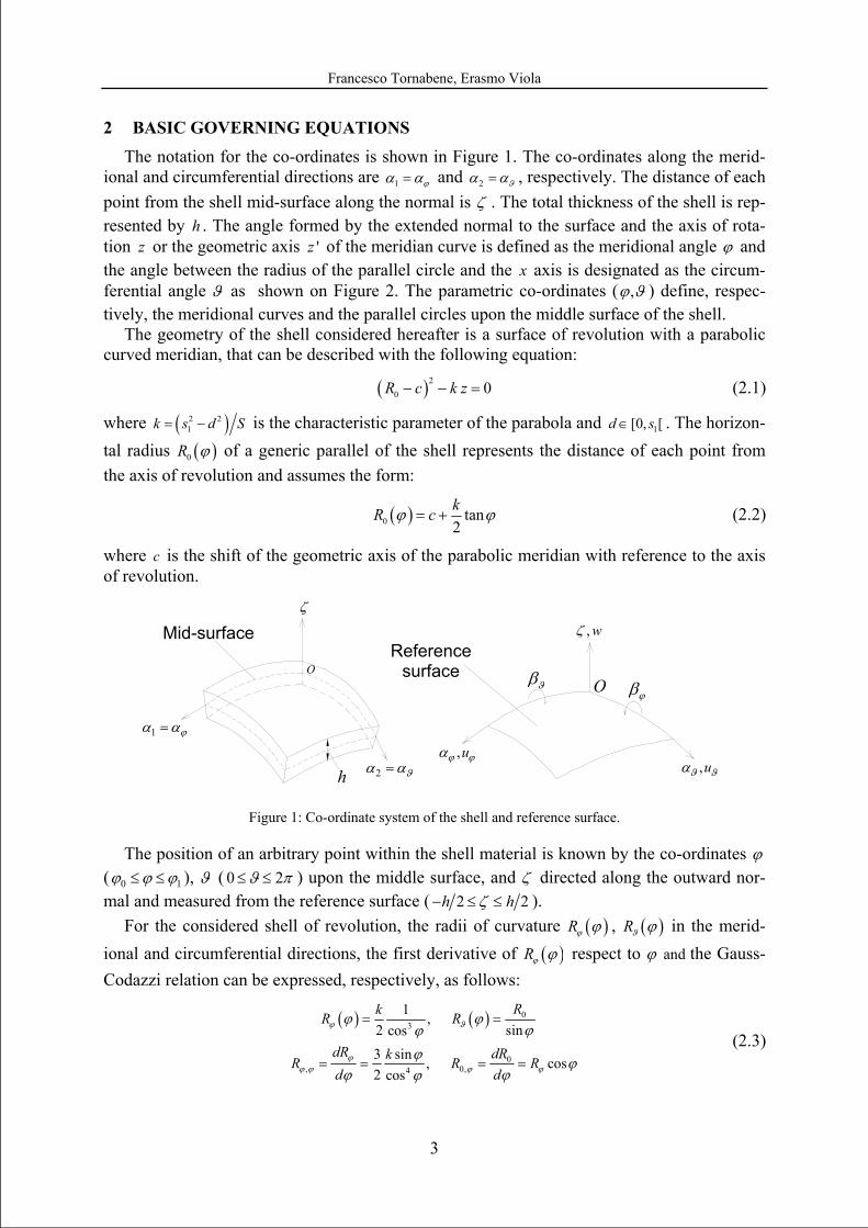
2 BASIC GOVERNING EQUATIONS The notation for the co-ordinates is shown in Figure 1. The co-ordinates along the merid-

ional and circumferential directions are 1 ϕα α= and 2 ϑα α= , respectively. The distance of each point from the shell mid-surface along the normal is ζ . The total thickness of the shell is rep-resented by h . The angle formed by the extended normal to the surface and the axis of rota-tion z or the geometric axis 'z of the meridian curve is defined as the meridional angle ϕ and the angle between the radius of the parallel circle and the x axis is designated as the circum-ferential angle ϑ as shown on Figure 2. The parametric co-ordinates ( ,ϕ ϑ ) define, respec-tively, the meridional curves and the parallel circles upon the middle surface of the shell.

The geometry of the shell considered hereafter is a surface of revolution with a parabolic curved meridian, that can be described with the following equation:

( )20 0R c k z− − = (2.1)

where ( )2 21k s d S= − is the characteristic parameter of the parabola and 1[0, [d s∈ . The horizon-

tal radius ( )0R ϕ of a generic parallel of the shell represents the distance of each point from the axis of revolution and assumes the form:

( )0 tan2kR cϕ ϕ= + (2.2)

where c is the shift of the geometric axis of the parabolic meridian with reference to the axis of revolution.

Figure 1: Co-ordinate system of the shell and reference surface.

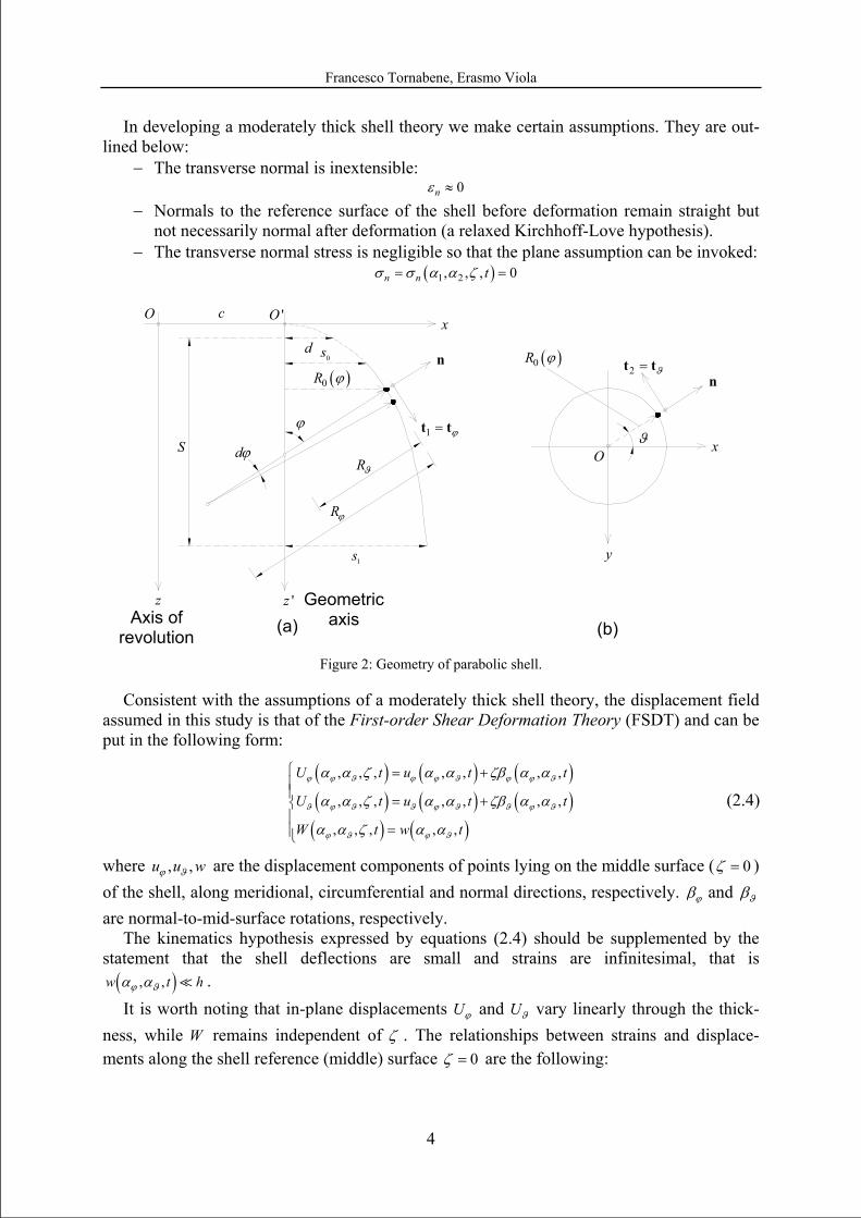
The position of an arbitrary point within the shell material is known by the co-ordinates ϕ ( 0 1ϕ ϕ ϕ≤ ≤ ), ϑ ( 0 2ϑ π≤ ≤ ) upon the middle surface, and ζ directed along the outward nor-mal and measured from the reference surface ( 2 2h hζ− ≤ ≤ ).

For the considered shell of revolution, the radii of curvature ( )Rϕ ϕ , ( )Rϑ ϕ in the merid-ional and circumferential directions, the first derivative of ( )Rϕ ϕ respect to ϕ and the Gauss-Codazzi relation can be expressed, respectively, as follows:

( ) ( ) 0

3

0, 0,4

1 ,2 sincos3 sin , cos2 cos

RkR R

dR dRkR R Rd d

ϕ ϑ

ϕϕ ϕ ϕ ϕ

ϕ ϕϕϕ

ϕ ϕϕ ϕϕ

= =

= = = = (2.3)

O

1 ϕα α=

2 ϑα α=

ζ Mid-surface

h ,uϕ ϕα

, wζ

O

Reference surface

,uϑ ϑα

ϕβ ϑβ


4

In developing a moderately thick shell theory we make certain assumptions. They are out-lined below:

− The transverse normal is inextensible: 0nε ≈

− Normals to the reference surface of the shell before deformation remain straight but not necessarily normal after deformation (a relaxed Kirchhoff-Love hypothesis).

− The transverse normal stress is negligible so that the plane assumption can be invoked: ( )1 2, , , 0n n tσ σ α α ζ= =

Figure 2: Geometry of parabolic shell.

Consistent with the assumptions of a moderately thick shell theory, the displacement field assumed in this study is that of the First-order Shear Deformation Theory (FSDT) and can be put in the following form:

( ) ( ) ( )( ) ( ) ( )( ) ( )

, , , , , , ,

, , , , , , ,

, , , , ,

U t u t t

U t u t t

W t w t

ϕ ϕ ϑ ϕ ϕ ϑ ϕ ϕ ϑ

ϑ ϕ ϑ ϑ ϕ ϑ ϑ ϕ ϑ

ϕ ϑ ϕ ϑ

α α ζ α α ζβ α α

α α ζ α α ζβ α α

α α ζ α α

⎧ = +⎪⎪ = +⎨⎪

=⎪⎩

(2.4)

where , ,u u wϕ ϑ are the displacement components of points lying on the middle surface ( 0ζ = ) of the shell, along meridional, circumferential and normal directions, respectively. ϕβ and ϑβ

are normal-to-mid-surface rotations, respectively. The kinematics hypothesis expressed by equations (2.4) should be supplemented by the

statement that the shell deflections are small and strains are infinitesimal, that is ( ), ,w t hϕ ϑα α . It is worth noting that in-plane displacements Uϕ and Uϑ vary linearly through the thick-

ness, while W remains independent of ζ . The relationships between strains and displace-ments along the shell reference (middle) surface 0ζ = are the following:

z 'z

y

x 'O

( )0R ϕ

x ϕ

ϑ

(b)

Rϑ

1 ϕ=t t

n2 ϑ=t t

n

dϕ

(a)

( )0R ϕ

S

d

1s

Rϕ

O

O

c

Axis of revolution

Geometric axis

0s


5

0 0

0 0

0

1 1 1 1, cos sin , cos

1 1 1 1, cos , cos

1 1, sinn n

u uu uw u w u

R R R R

R R R R

w wu uR R

ϕ ϕϑ ϑϕ ϑ ϕ ϕϑ ϑ

ϕ ϕ

ϕ ϕϑ ϑϕ ϑ ϕ ϕϑ ϑ

ϕ ϕ

ϕ ϕ ϕ ϑ ϑϕ

ε ε ϕ ϕ γ ϕϕ ϑ ϕ ϑ

β ββ βκ κ β ϕ κ β ϕ

ϕ ϑ ϕ ϑ

γ β γ ϕϕ ϑ

∂ ∂⎛ ⎞ ⎛ ⎞∂ ∂⎛ ⎞= + = + + = + −⎜ ⎟ ⎜ ⎟⎜ ⎟∂ ∂ ∂ ∂⎝ ⎠⎝ ⎠ ⎝ ⎠∂ ∂⎛ ⎞∂ ∂⎛ ⎞= = + = + −⎜ ⎟⎜ ⎟∂ ∂ ∂ ∂⎝ ⎠ ⎝ ⎠⎛ ⎞∂ ∂⎛= − + = −⎜ ⎟∂ ∂⎝⎝ ⎠

ϑβ⎞ +⎜ ⎟⎠

(2.5)

In the above equations (2.5), the first three strains , ,ϕ ϑ ϕϑε ε γ are in-plane meridional, circumferential and shearing components, , ,ϕ ϑ ϕϑκ κ κ are the analogous curvature changes. The last two components are transverse shearing strains.

The shell material assumed in the following is a mono-laminar elastic isotropic one. Ac-cordingly, the following constitutive equations relate internal stress resultants and internal couples with generalized strain components on the middle surface:

( ) ( ) ( )

( ) ( ) ( )

( ) ( )

1, ,

21

, ,2

1 1,

2 2

n

n

N K M D Q K

N K M D Q K

N N K M M D

ϕ ϕ ϑ ϕ ϕ ϑ ϕ ϕ

ϑ ϑ ϕ ϑ ϑ ϕ ϑ ϑ

ϕϑ ϑϕ ϕϑ ϕϑ ϑϕ ϕϑ

νε νε κ νκ γ

χν

ε νε κ νκ γχ

ν νγ κ

−= + = + =

−= + = + =

− −= = = =

(2.6)

where 2(1 )K Eh ν= − , 3 2(12(1 ))D Eh ν= − are the membrane and bending rigidity, respec-tively. E is the Young modulus, ν is the Poisson ratio and χ is the shear factor which for isotropic materials is usually taken as 6 5χ = . In equations (2.6), the first three components

, ,N N Nϕ ϑ ϕϑ are the in-plane meridional, circumferential and shearing force resultants, , ,M M Mϕ ϑ ϕϑ are the analogous couples, while the last two ,Q Qϕ ϑ are the transverse shears.

Following the direct approach or the Hamilton’s principle in dynamic version and remem-bering the Gauss-Codazzi relations for the shells of revolution 0 / cosdR d Rϕϕ ϕ= , five equa-tions of dynamic equilibrium in terms of internal actions can be written for the shell element:

( )

( )

0 10 0

0 10 0 0

00 0 0

1 20 0

1 1 cos

1 1 cos sin2

1 1 cos sin

1 1 cos

1

N N QN N I u I

R R R R

N N N Q I u IR R R R

Q NQ Q N I wR R R R R

M MM M Q I u I

R R R

MR

ϕ ϕϑ ϕϕ ϑ ϕ ϕ

ϕ ϕ

ϕϑ ϑϕϑ ϑ ϑ ϑ

ϕ

ϕ ϕϑϕ ϑ

ϕ ϕ

ϕ ϕϑϕ ϑ ϕ ϕ ϕ

ϕ

ϕ

ϕ

ϕ βϕ ϑ

ϕ ϕ βϕ ϑ

ϕ ϕϕ ϑ

ϕ βϕ ϑ

∂ ∂+ + − + = +

∂ ∂

∂ ∂+ + + = +

∂ ∂

∂ ∂+ + − − =

∂ ∂

∂ ∂+ + − − = +

∂ ∂

∂1 2

0 0

1 cos2M M Q I u IR R

ϑ ϑϕϑ ϑ ϑ ϑ

ϕ βϕ ϑ

∂+ + − = +

∂ ∂

(2.7)

where:

2 2

3 30 1 2

1 1 11 , ,12 12 12 12 80

h hI h I h I hR R R R R Rϕ ϑ ϕ ϑ ϕ ϑ

μ μ μ⎛ ⎞ ⎛ ⎞ ⎛ ⎞

= + = + = +⎜ ⎟ ⎜ ⎟ ⎜ ⎟⎜ ⎟ ⎜ ⎟ ⎜ ⎟⎝ ⎠ ⎝ ⎠ ⎝ ⎠

(2.8)

are the mass inertias and μ is the mass density of the material per unit volume. The first three equations (2.7) represent translational equilibriums along meridional, circumferential and


6

normal directions, while the last two are rotational equilibrium equations about the ϕ and ϑ directions.

The three basic sets of equations, namely the kinematic, the equilibrium and the constitu-tive equations may be combined to give the fundamental system of equations, also known as the governing system equations. Substituting the definition equations (2.5) into the constitu-tive equations (2.6) and the result of this substitution into the equilibrium equations (2.7), the complete equations of motion in terms of displacements can be written in the extended form as:

( ) ( )

( ) ( )

( )

2 2 2,

2 2 2 2 20 00

20 0

2

20 0 0

1 1 cos2 2

1 31 sin cos12 2

11 sin cos 1 1 cos2

Ru u uuK K K KR R R RR R R

uK w KR R R R

RK u K

R R R R RR

ϕ ϕϕ ϕ ϕϑ

ϕ ϕϕ ϕ

ϑ

ϕ ϕ

ϕϕ

ϕ ϕϕ

ν ν ϕϕ ϑ ϕϕ ϑ

ν νν ϕ ϕχ ϕ ϑ

νν ϕ ϕ ϕχ

⎛ ⎞∂ ∂ ∂− + ∂ ⎜ ⎟+ + + − +⎜ ⎟∂ ∂ ∂∂ ∂ ⎝ ⎠

⎡ ⎤⎛ ⎞− − ∂∂+ + + − +⎢ ⎥⎜ ⎟⎜ ⎟ ∂ ∂⎢ ⎥⎝ ⎠⎣ ⎦

⎡ ⎤⎛ ⎞ −⎢ ⎥− + + + −⎜ ⎟⎜ ⎟⎢ ⎥⎝ ⎠⎣ ⎦

( )

,2 2

0

23

sin cos

1 1 112 12 12 12

wR R

K hh u hR R R R R

ϕ

ϕ

ϕ ϕ ϕϕ ϕ ϑ ϕ ϑ

ϕ ϕ

νβ μ μ β

χ

⎡ ⎤⎛ ⎞⎢ ⎥⎜ ⎟ − +

⎜ ⎟⎢ ⎥⎝ ⎠⎣ ⎦⎛ ⎞ ⎛ ⎞−

+ = + + +⎜ ⎟ ⎜ ⎟⎜ ⎟ ⎜ ⎟⎝ ⎠ ⎝ ⎠

(2.9)

( ) ( ) ( )

( ) ( )

( ) ( )

22 2,

2 2 2 2 20 00

20 00

22

0 0

1 1 1 cos2 2 2

3 1cos sin 12 2

1 1sin 1 sin sincos2 2

Ruu u uK K K KR R R RR R R

u K wKR R RR

K u KR R R

ϕ ϕϕϑ ϑ ϑ

ϕ ϕϕ ϕ

ϕ

ϕ

ϑϕ

ν ν ν ϕϕ ϑ ϕϕ ϑ

ν νϕ ν ϕϑ χ ϑ

ν νϕ ϕ ϕϕχ χ

⎛ ⎞∂− + −∂ ∂ ∂⎜ ⎟+ + + − +⎜ ⎟∂ ∂ ∂∂ ∂ ⎝ ⎠

⎡ ⎤⎛ ⎞∂− − ∂+ + + + +⎢ ⎥⎜ ⎟⎜ ⎟∂ ∂⎢ ⎥⎝ ⎠⎣ ⎦

⎡ ⎤⎛ ⎞− −+ − + +⎢ ⎥⎜ ⎟⎜ ⎟⎢ ⎥⎝ ⎠⎣ ⎦ 0

23 1 11

12 12 12

R

hh u hR R R R

ϑ

ϑ ϑϕ ϑ ϕ ϑ

β

μ μ β

=

⎛ ⎞ ⎛ ⎞= + + +⎜ ⎟ ⎜ ⎟⎜ ⎟ ⎜ ⎟

⎝ ⎠ ⎝ ⎠

(2.10)

( ) ( ) ( )

( ) ( ) ( )

( )

2 2

2 2 2 200

,2

0 0 0

0 0 0

1 1 11 sin12 2 2

1 1 1cos sin 12 2 2

1 cos sin2

uK w K w KR R RR R

R uK w K KR R R R R RR

K KR R R R

ϕ

ϕ ϕϕ

ϕ ϕ ϕ ϑ

ϕ ϕ ϕϕ

ϑ

ϕ

ν ν ν ν ϕχ χ χ ϕϕ ϑ

βν ν νϕ ν ϕχ ϕ χ ϕ χ ϑ

ν β ϕ ϕ νχ ϑ

⎡ ⎤⎛ ⎞ ∂− − −∂ ∂+ − + + +⎢ ⎥⎜ ⎟⎜ ⎟ ∂∂ ∂ ⎢ ⎥⎝ ⎠⎣ ⎦

⎛ ⎞ ⎡ ⎤⎛ ⎞∂− − − ∂∂⎜ ⎟+ − + − + + +⎢ ⎥⎜ ⎟⎜ ⎟⎜ ⎟ ∂ ∂ ∂⎢ ⎥⎝ ⎠⎝ ⎠ ⎣ ⎦

⎛− ∂+ − +

∂( )

( )

,2

0

2 2

20 00

1 1 cos2

11 1 2 sin sin cos 12 12

Ru

R R R

hK w K h wR R R R R RR

ϕ ϕϕ

ϕ ϕ

ϕϕ ϕ ϕ ϑ

ν ϕχ

νν ϕ ϕ ϕ β μχ

⎡ ⎤⎛ ⎞⎞ −⎢ ⎥⎜ ⎟+ − +⎜ ⎟⎜ ⎟ ⎜ ⎟⎢ ⎥⎝ ⎠ ⎝ ⎠⎣ ⎦

⎡ ⎤⎛ ⎞ ⎛ ⎞−⎢ ⎥− + + + = +⎜ ⎟ ⎜ ⎟⎜ ⎟ ⎜ ⎟⎢ ⎥⎝ ⎠ ⎝ ⎠⎣ ⎦

(2.11)

( ) ( ) ( )

( ) ( )

( )

2 2 2

2 2 2 200

,2 2

0 0

23 3

0 0

1 1 12 2 2

3 1cos cos2 2

1sin cos 1 1 12 12 12 12

D D D K wR R RR R

RD KD uR R RR R

D hK h u hR R R R R

ϕ ϕ ϑ

ϕ ϕϕ

ϕ ϕ ϕ ϑϕ

ϕ ϕϕ

ϕ ϕϕ ϕ ϑ

β βν ν νβϕ ϑ χ ϕϕ ϑ

β ν νβϕ ϕϕ ϑ χ

νν ϕ ϕ β μ μχ

∂ ∂− + −∂ ∂+ + − +

∂ ∂ ∂∂ ∂

⎛ ⎞ ∂ − −∂⎜ ⎟+ − − + +⎜ ⎟ ∂ ∂⎝ ⎠

⎡ ⎤⎛ ⎞ ⎛ ⎞−⎢ ⎥− + + = + + +⎜ ⎟ ⎜ ⎟⎜ ⎟ ⎜ ⎟⎢ ⎥⎝ ⎠ ⎝ ⎠⎣ ⎦

2

80R R ϕϕ ϑ

β⎛ ⎞⎜ ⎟⎜ ⎟⎝ ⎠

(2.12)


7

( ) ( ) ( )

( ) ( ) ( )

( ) ( )

22 2,

2 2 2 2 20 00

20 00

23

0 0

1 1 1 cos2 2 2

1 3 1cos sin2 2 2

1 1sin cos 1 12 2 12 12

RD D D DR R R RR R R

K w D K uR RR

D K hR R R R R

ϕ ϕϕϑ ϑ ϑ

ϕ ϕϕ ϕ

ϕϑ

ϑϕ ϕ ϑ

βν ν νβ β βϕϕ ϑ ϕϕ ϑ

βν ν νϕ ϕχ ϑ ϑ χ

ν νϕ ϕ β μχ

⎛ ⎞∂− + −∂ ∂ ∂⎜ ⎟+ + + − +⎜ ⎟∂ ∂ ∂∂ ∂ ⎝ ⎠

∂− − −∂− + + +

∂ ∂

⎡ ⎤⎛ ⎞ ⎛ ⎞− −⎢ ⎥+ − − = +⎜ ⎟ ⎜ ⎟⎜ ⎟ ⎜ ⎟⎢ ⎥⎝ ⎠ ⎝ ⎠⎣ ⎦

23 1

12 80hu hR Rϑ ϑϕ ϑ

μ β⎛ ⎞

+ +⎜ ⎟⎜ ⎟⎝ ⎠

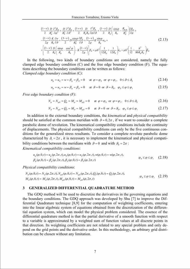
(2.13)

In the following, two kinds of boundary conditions are considered, namely the fully clamped edge boundary condition (C) and the free edge boundary condition (F). The equa-tions describing the boundary conditions can be written as follows: Clamped edge boundary condition (C):

0 1 00 at or , 0u u wϕ ϑ ϕ ϑβ β ϕ ϕ ϕ ϕ ϑ ϑ= = = = = = = ≤ ≤ (2.14)

0 0 10 at 0 or ,u u wϕ ϑ ϕ ϑβ β ϑ ϑ ϑ ϕ ϕ ϕ= = = = = = = ≤ ≤ (2.15)

Free edge boundary condition (F):

0 1 00 at or , 0N N Q M Mϕ ϕϑ ϕ ϕ ϕϑ ϕ ϕ ϕ ϕ ϑ ϑ= = = = = = = ≤ ≤ (2.16)

0 0 10 at 0 or ,N N Q M Mϑ ϕϑ ϑ ϑ ϕϑ ϑ ϑ ϑ ϕ ϕ ϕ= = = = = = = ≤ ≤ (2.17)

In addition to the external boundary conditions, the kinematical and physical compatibility should be satisfied at the common meridian with 0,2ϑ π= , if we want to consider a complete parabolic dome of revolution. The kinematical compatibility conditions include the continuity of displacements. The physical compatibility conditions can only be the five continuous con-ditions for the generalized stress resultants. To consider a complete revolute parabolic dome characterized by 0 2ϑ π= , it is necessary to implement the kinematical and physical compati-bility conditions between the meridians with 0ϑ = and with 0 2ϑ π= : Kinematical compatibility conditions:

0 1

( ,0, ) ( , 2 , ), ( ,0, ) ( , 2 , ), ( ,0, ) ( , 2 , ),

( ,0, ) ( , 2 , ), ( ,0, ) ( , 2 , )

u t u t u t u t w t w t

t t t tϕ ϕ ϑ ϑ

ϕ ϕ ϑ ϑ

ϕ ϕ π ϕ ϕ π ϕ ϕ πϕ ϕ ϕ

β ϕ β ϕ π β ϕ β ϕ π

= = =≤ ≤

= = (2.18)

Physical compatibility conditions:

0 1

( ,0, ) ( , 2 , ), ( ,0, ) ( , 2 , ), ( ,0, ) ( , 2 , ),

( ,0, ) ( , 2 , ), ( ,0, ) ( , 2 , )

N t N t N t N t Q t Q t

M t M t M t M tϑ ϑ ϕϑ ϕϑ ϑ ϑ

ϑ ϑ ϕϑ ϕϑ

ϕ ϕ π ϕ ϕ π ϕ ϕ πϕ ϕ ϕ

ϕ ϕ π ϕ ϕ π

= = =≤ ≤

= = (2.19)

3 GENERALIZED DIFFERENTIAL QUADRATURE METHOD The GDQ method will be used to discretize the derivatives in the governing equations and

the boundary conditions. The GDQ approach was developed by Shu [7] to improve the Dif-ferential Quadrature technique [8,9] for the computation of weighting coefficients, entering into the linear algebraic system of equations obtained from the discretization of the differen-tial equation system, which can model the physical problem considered. The essence of the differential quadrature method is that the partial derivative of a smooth function with respect to a variable is approximated by a weighted sum of function values at all discrete points in that direction. Its weighting coefficients are not related to any special problem and only de-pend on the grid points and the derivative order. In this methodology, an arbitrary grid distri-bution can be chosen without any limitation.


8

The GDQ method is based on the analysis of a high-order polynomial approximation and the analysis of a linear vector space [10]. For a general problem, it may not be possible to ex-press the solution of the corresponding partial differential equation in a closed form. This so-lution function can be approximated by the two following types of function approximation: high-order polynomial approximation and Fourier series expansion (harmonic functions). It is well known that a smooth function in a domain can be accurately approximated by a high-order polynomial in accordance with the Weierstrass polynomial approximation theorem. In fact, from the Weierstrass theorem, if ( )f x is a real valued continuous function defined in the closed interval [ , ]a b , then there exists a sequence of polynomials ( )rP x which converges to

( )f x uniformly as r goes to infinity. In practical applications, a truncated finite polynomial may be used. Thus, if ( )f x represents the solution of a partial differential equation, then it can be approximated by a polynomial of a degree less than or equal to 1N − , for N large enough. The conventional form of this approximation is:

( ) ( ) ( )1

N

N j jj

f x P x d p x=

≅ =∑ (3.1)

where jd is a constant. Then, it is easy to show that the polynomial ( )NP x constitutes an N -dimensional linear vector space NV with respect to the operation of vector addition and scalar multiplication. Obviously, in the linear vector space NV , ( )jp x is a set of base vectors.

It can be seen that, in the linear polynomial vector space, there exist several sets of base polynomials and each set of base polynomials can be expressed uniquely by another set of base polynomials in the space. Using vector space analysis, the method for computing the weighting coefficients can be generalized by a proper choice of base polynomials in a linear vector space. For generality, the Lagrange interpolation polynomials are chosen as the base polynomials. As a result, the weighting coefficients of the first order derivative are computed by a simple algebraic formulation without any restriction on the choice of the grid points, while the weighting coefficients of the second and higher order derivatives are given by a re-currence relationship.

When the Lagrange interpolated polynomials are assumed as a set of vector space base functions, the approximation of the function ( )f x can be written as:

( ) ( ) ( )1

N

j jj

f x p x f x=

≅ ∑ (3.2)

where N is the number of grid points in the whole domain, jx , 1, 2,...,j N= , are the co-ordinates of grid points in the variable domain and ( )jf x are the function values at the grid points. ( )jp x are the Lagrange interpolated polynomials, which can be defined by the follow-ing formula:

( ) ( )( ) ( )(1)

, 1,2,...,jj j

xp x j N

x x x= =

−

LL

(3.3)

where:

(1)

1 1,

( ) ( ), ( ) ( )N N

i j j ii i i j

x x x x x x= = ≠

= − = −∏ ∏L L (3.4)


9

Differentiating equation (3.2) with respect to x and evaluating the first derivative at a cer-tain point of the function domain, it is possible to obtain:

( ) ( ) ( ) ( ) ( ) ( ) ( )1 1 1

1 1, 1,2,...,

N N

i j i j ij jj j

f x p x f x f x i Nς= =

≅ = =∑ ∑ (3.5)

where ( )1ijς are the GDQ weighting coefficients of the first order derivative and ix denote the

co-ordinates of the grid points. In particular, it is worth noting that the weighting coefficients of the first order derivative can be computed as:

( )(1)

(1) (1)(1)

( ) , , 1,2,..., ,( ) ( )

ij i ij

i j j

xp x i j N i jx x x

ς= = = ≠−L

L (3.6)

From equation (3.6), ( )1ijς ( i j≠ ) can be easily computed. However, the calculation of ( )1

iiς is not easy to compute. According to the analysis of a linear vector space, one set of base func-tions can be expressed uniquely by a linear sum of another set of base functions. Thus, if one set of base polynomials satisfy a linear equation like (3.5), so does another set of base poly-nomials. As a consequence, the equation system for determining ( )1

ijς and derived from the La-grange interpolation polynomials should be equivalent to that derived from another set of base polynomials, i.e. ( ) 1j

jp x x −= , 1, 2,...,j N= . Thus, ( )1ijς satisfies the following equation, which is

obtained by the base polynomials ( ) 1jjp x x −= , when 1j = :

(1) (1) (1)

1 1,

0 , , 1,2,...,N N

ij ii ijj j j i

i j Nς ς ς= = ≠

= ⇒ = − =∑ ∑ (3.7)

Equations (3.6) and (3.7) are two formulations to compute the weighting coefficients ( )1ijς .

It should be noted that, in the development of these two formulations, two sets of base poly-nomials were used in the linear polynomial vector space NV . Finally, the nth order derivative of function ( )f x with respect to x at grid points ix , can be approximated by the GDQ ap-proach:

( )

1

( ) ( ), 1,2,...,i

Nnn

ij jnjx x

d f x f x i Ndx

ς==

= =∑ (3.8)

where ( )nijς are the weighting coefficients of the nth order derivative. Similar to the first order

derivative and according to the polynomial approximation and the analysis of a linear vector space, it is possible to determine a recurrence relationship to compute the second and higher order derivatives. Thus, the weighting coefficients can be generated by the following recur-rent formulation:

( 1)

( ) ( 1) (1) , , 2,3,..., 1, , 1,2,...,n

ijn nij ii ij

i jn i j n N i j N

x xς

ς ς ς−

−⎛ ⎞

= − ≠ = − =⎜ ⎟⎜ ⎟−⎝ ⎠ (3.9)

( ) ( ) ( )

1 1,

0 , 2,3,..., 1, , 1,2,...,N N

n n nij ii ij

j j j i

n N i j Nς ς ς= = ≠

= ⇒ = − = − =∑ ∑ (3.10)

It is obvious from the above equations that the weighting coefficients of the second and higher order derivatives can be determined from those of the first order derivative. Further-


10

more, it is interesting to note that, the preceding coefficients ( )nijς are dependent on the deriva-

tive order n , on the grid point distribution jx , 1, 2,...,j N= , and on the specific point ix , where the derivative is computed. There is no need to obtain the weighting coefficients from a set of algebraic equations which could be ill-conditioned when the number of grid points is large.

Furthermore, this set of expressions for the determination of the weighting coefficients is so compact and simple that it is very easy to implement them in formulating and program-ming, because of the recurrence feature.

3.1 Grid distributions Another important point for successful application of the GDQ method is how to distribute

the grid points. In fact, the accuracy of this method is usually sensitive to the grid point distri-bution. The optimal grid point distribution depends on the order of derivatives in the bound-ary condition and the number of grid points used. The grid point distribution also plays an essential role in determining the convergence speed and stability of the GDQ method. In this paper, the effects of the grid point distribution will be investigated for the vibration analysis of parabolic shells. The natural and simplest choice of the grid points through the computa-tional domain is the one having equally spaced points in the co-ordinate direction of the com-putational domain. However, it is demonstrated that non-uniform grid distribution usually yields better results than equally spaced distribution. Quan and Chang [11,12] compared nu-merically the performances of the often-used non-uniform meshes and concluded that the grid points originating from the Chebyshev polynomials of the first kind are optimum in all the cases examined there. The zeros of orthogonal polynomials are the rational basis for the grid points. Shu [10] have used other choice which has given better results than the zeros of Che-byshev and Legendre polynomials. Bert and Malik [13] indicated that the preferred type of grid points changes with problems of interest and recommended the use of Chebyshev-Gauss-Lobatto grid for the structural mechanics computation. With Lagrange interpolating polyno-mials, the Chebyshev-Gauss-Lobatto sampling point rule proves efficient for numerical rea-sons [14] so that for such a collocation the approximation error of the dependent variables decreases as the number of nodes increases.

In this study, different grid point distributions are considered to investigate their effect on the GDQ solution accuracy, convergence speed and stability. The typical distributions of grid points, which are commonly used in the literature, in normalized form are reported as follows:

Equally spaced or uniform distribution

1 , 1, 2,...,1i

ir i NN−

= =−

(3.11)

Roots of Chebyshev polynomials of the first kind (C I°)

1

1

2 1, cos , 1,2,...,2

ii i

N

g g ir g i Ng g N

π− ⎛ − ⎞⎛ ⎞= = =⎜ ⎟⎜ ⎟− ⎝ ⎠⎝ ⎠

(3.12)

Roots of Chebyshev polynomials of the second kind (C II°)

1

1

, cos , 1,2,...,1

ii i

N

g g ir g i Ng g N

π− ⎛ ⎞= = =⎜ ⎟− +⎝ ⎠ (3.13)

Roots of Legendre polynomials (Leg)

12 3

1

1 1 4 1, 1 cos , 1,2,...,4 28 8

ii i

N

g g ir g i Ng g NN N

π− −⎛ ⎞ ⎛ ⎞= = − + =⎜ ⎟ ⎜ ⎟− +⎝ ⎠ ⎝ ⎠

(3.14)


11

Quadratic sampling points distribution (Quad)

2

2

1 12 1,2,....,1 2

1 1 12 4 1 1,...,1 1 2

i

i NiN

ri i Ni NN N

⎧ − +⎛ ⎞ =⎪ ⎜ ⎟−⎝ ⎠⎪= ⎨⎛ ⎞− − +⎛ ⎞ ⎛ ⎞ ⎛ ⎞⎪ − + − = +⎜ ⎟⎜ ⎟ ⎜ ⎟ ⎜ ⎟⎪⎜ ⎟− −⎝ ⎠ ⎝ ⎠ ⎝ ⎠⎝ ⎠⎩

(3.15)

Chebyshev-Gauss-Lobatto sampling points (C-G-L)

11 cos1 , 1, 2,...,

2i

iNr i N

π−⎛ ⎞− ⎜ ⎟−⎝ ⎠= = (3.16)

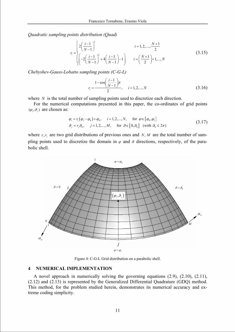
where N is the total number of sampling points used to discretize each direction. For the numerical computations presented in this paper, the co-ordinates of grid points

( , )i jϕ ϑ are chosen as:

( ) [ ][ ]

1 0 0 0 1

0 0 0

, 1, 2,..., , for ,

, 1, 2,..., , for 0, (with 2 )i i

j j

r i N

r j M

ϕ ϕ ϕ ϕ ϕ ϕ ϕ

ϑ ϑ ϑ ϑ ϑ π

= − + = ∈

= = ∈ ≤ (3.17)

where ,i jr r are two grid distributions of previous ones and ,N M are the total number of sam-pling points used to discretize the domain in ϕ and ϑ directions, respectively, of the para-bolic shell.

Figure 4: C-G-L Grid distribution on a parabolic shell.

4 NUMERICAL IMPLEMENTATION A novel approach in numerically solving the governing equations (2.9), (2.10), (2.11),

(2.12) and (2.13) is represented by the Generalized Differential Quadrature (GDQ) method. This method, for the problem studied herein, demonstrates its numerical accuracy and ex-treme coding simplicity.

1

j

M N

ϑα

ϕα

i

( ),i jϕ ϑ

0ϕ ϕ=

1ϕ ϕ=

0ϑ ϑ= 0ϑ =

1


12

In the following, only the free vibration of parabolic dome or panel will be studied. So, us-ing the method of variable separation, it is possible to seek solutions that are harmonic in time and whose frequency is ω ; then, the displacements and the rotations can be written as follows:

( , , ) ( , )

( , , ) ( , )

( , , ) ( , )

( , , ) ( , )

( , , ) ( , )

i t

i t

i t

i t

i t

u t U e

u t U e

w t W e

t B e

t B e

ϕ ωϕ ϕ ϑ ϕ ϑ

ϑ ωϑ ϕ ϑ ϕ ϑ

ζ ωϕ ϑ ϕ ϑ

ϕ ωϕ ϕ ϑ ϕ ϑ

ϑ ωϑ ϕ ϑ ϕ ϑ

α α α α

α α α α

α α α α

β α α α α

β α α α α

=

=

=

=

=

(4.1)

where the vibration spatial amplitude values ( ( , )U ϕϕ ϑα α , ( , )Uϑ

ϕ ϑα α , ( , )W ζϕ ϑα α , ( , )Bϕ

ϕ ϑα α , ( , )Bϑ

ϕ ϑα α ) fulfill the fundamental differential system. The basic steps in the GDQ solution of the free vibration problem of parabolic shell type

structures are as in the following: − Discretization of independent variables 0 1 0 0[ , ], [0, ] (with 2 )ϕ ϕ ϕ ϑ ϑ ϑ π∈ ∈ ≤ . − The spatial derivatives are approximated according to GDQ rule. − The differential governing systems (2.9), (2.10), (2.11), (2.12), and (2.13) are trans-

formed into linear eigenvalue problems for the natural frequencies. The boundary condi-tions are imposed in the sampling points corresponding to the boundary. All these relations are imposed pointwise.

− The solution of the previously stated discrete system in terms of natural frequencies and mode shape components is worked out. For each mode, local values of dependent vari-ables are used to obtain the complete assessment of the deformed configuration.

The simple numerical operations illustrated here, applying the GDQ procedure, enable one to write the equations of motion in discrete form, transforming any space derivative into a weighted sum of node values of dependent variables. Each of the approximated equations is valid in a single sampling point.

The governing equations can be discretized as:

( ) ( ) ( ) ( ) ( ) ( ) ( )

( ) ( ) ( )

,2 1 12 12 2 2

0 001 1 1 1 1

1

0 1

1 1 cos2 2

1 3sin cos1 12 2

N M N M Ni i

kj jm mj jm km kjik ik iki i i ii i ik m k m k

Ni i

kjiki i i k

RK K K KU U U UR R R RR R R

K W KR R R

ϕ ϕϕ ϕ ϕϑ ϑϕ ϕ ϑ ϕ

ϕ ϕϕ ϕ

ϕ ζ

ϕ ϕ

ν ν ϕς ς ς ς ς

ν νν ϕ ϕςχ

= = = = =

=

⎛ ⎞⎛ ⎞− + ⎜ ⎟⎜ ⎟+ + + − +⎜ ⎟⎜ ⎟

⎝ ⎠ ⎝ ⎠⎡ ⎤⎛ ⎞− −

+ + + −⎢ ⎥⎜ ⎟⎜ ⎟⎢ ⎥⎝ ⎠⎣ ⎦

∑ ∑ ∑ ∑ ∑

∑ ( )

( )

( )

120 1

2 ,

2 2 20 0 0 0

22 2 3

1sin cos cos sin cos1 1 12

1 1 112 12 12 12

M

jm imi m

i i i i i iij ij

i i i i ii i i

ij iji i i i i

UR

RK U K W

R R R R RR R R

K hB h U hR R R R R

ϑ ϑ

ϕ ϕϕ ζ

ϕ ϕϕ ϕ

ϕ ϕ

ϕ ϕ ϑ ϕ ϑ

ς

νν ϕ ϕ ϕ ϕ ϕχ

νω μ ω μ

χ

=

+

⎡ ⎤⎛ ⎞⎡ ⎤⎛ ⎞ − ⎢ ⎥⎜ ⎟⎢ ⎥− + + + − − +⎜ ⎟ ⎢ ⎥⎜ ⎟ ⎜ ⎟⎢ ⎥⎝ ⎠⎣ ⎦ ⎢ ⎥⎝ ⎠⎣ ⎦⎛ ⎞−

+ = − + − +⎜ ⎟⎜ ⎟⎝ ⎠

∑

ijBϕ⎛ ⎞⎜ ⎟⎜ ⎟⎝ ⎠

(4.2)

( ) ( ) ( ) ( ) ( ) ( )

( ) ( ) ( ) ( )

( )

2 12 12 2

001 1 1 1

, 1 12 2

0 01 1

0 0

1 12 2

1 3cos cos2 2

1sin 12

N M N M

kj jm im jm kmik iki ii ik m k m

N Mi i i

kj jm imiki i i ik m

i

i i i

K K KU U UR RR R

RK U K UR R R R

KR R R

ϕ ϕϑ ϑϑ ϑ ϕ

ϕϕ

ϕ ϕ ϕ ϑϑ ϕ

ϕ ϕ

ϕ

ν νς ς ς ς

ν νϕ ϕς ς

νϕνχ

= = = =

= =

⎛ ⎞− +⎜ ⎟+ + +⎜ ⎟⎝ ⎠

⎛ ⎞− −⎜ ⎟+ − + +⎜ ⎟⎝ ⎠

⎛ ⎞−+ + +⎜ ⎟⎜ ⎟

⎝ ⎠

∑ ∑ ∑ ∑

∑ ∑

( ) ( )

( )

1

01

2 22 2 2 3

0 0

1 sin2

1 sin sin1 1 1cos 12 12 12 12

Mi

jm im ijim

i ii ij ij ij

i i i i i i i

W K BR

K hU h U h BR R R R R R R

ϑ ζ ϑ

ϑ ϑ ϑ

ϕ ϕ ϑ ϕ ϑ

ν ϕςχ

ν ϕ ϕϕ ω μ ω μχ

=

⎡ ⎤ −+ +⎢ ⎥

⎢ ⎥⎣ ⎦⎡ ⎤ ⎛ ⎞ ⎛ ⎞⎛ ⎞−

+ − + = − + − +⎜ ⎟ ⎜ ⎟⎢ ⎥⎜ ⎟⎜ ⎟ ⎜ ⎟ ⎜ ⎟⎢ ⎥⎝ ⎠ ⎝ ⎠ ⎝ ⎠⎣ ⎦

∑

(4.3)


13

( ) ( ) ( ) ( ) ( ) ( )

( ) ( ) ( ) ( )

2 122 2

001 1 1

, 1 12

0 0 01 1

1 1 1 sin1 12 2 2

1 1cos sin 12 2

N M Ni

kj jm im kjik iki i ii ik m k

N Ni i i

kj kjik iki i i i i ii k k

K K KW W UR R RR R

RK K KW BR R R R R RR

ϕ ϕϑζ ζ ϕ

ϕ ϕϕ

ϕ ϕ ϕ ϕζ ϕ

ϕ ϕ ϕϕ

ν ν ν ν ϕς ς ςχ χ χ

ν νϕ ϕνς ςχ χ

= = =

= =

⎡ ⎤⎛ ⎞− − −+ − + + +⎢ ⎥⎜ ⎟⎜ ⎟⎢ ⎥⎝ ⎠⎣ ⎦

⎛ ⎞− −⎜ ⎟+ − + − + +⎜ ⎟⎝ ⎠

∑ ∑ ∑

∑ ∑ ( ) ( )

( ) ( ) ( )

( )

1

1

,12

0 0 0 01

2

20 0

12

1 1cos sin cos12 2

12 sin sin1 12

M

jm imm

Mi i i i

jm im iji i i i i i im

i iij

i i i i

U

RK B K UR R R R R R R

K W KR R R R

ϑ ϑ

ϕ ϕϑ ϑ ϕ

ϕ ϕ ϕ

ζ

ϕ ϕ

νς

χ

ν νϕ ϕ ϕνςχ χ

νν ϕ ϕ

=

=

⎡ ⎤⎛ ⎞−+⎢ ⎥⎜ ⎟⎜ ⎟⎢ ⎥⎝ ⎠⎣ ⎦

⎡ ⎤⎛ ⎞⎛ ⎞− −⎢ ⎥⎜ ⎟+ − + + − +⎜ ⎟⎢ ⎥⎜ ⎟ ⎜ ⎟⎝ ⎠⎢ ⎥⎝ ⎠⎣ ⎦⎡ ⎤⎛ ⎞ −⎢ ⎥− + + +⎜ ⎟⎜ ⎟⎢ ⎥⎝ ⎠⎣ ⎦

∑

∑2

2

0

cos 112

iij ij

i i i

hB h WR R R

ϕ ζ

ϕ ϑ

ϕ ω μχ

⎛ ⎞= − +⎜ ⎟⎜ ⎟

⎝ ⎠

(4.4)

( ) ( ) ( ) ( ) ( ) ( )

( ) ( ) ( ) ( ) ( )

( )

2 12 12 2

001 1 1 1

,1 1 12 2

0 01 1 1

1 12 2

1 3cos cos2 2

12

N M N M


N N Mi i i

kj kj jm imik iki i i i ik k m

iji

D D DB B BR RR R

RK DW B D BR R R R R

K UR

ϕ ϕϑ ϑϕ ϕ ϑ

ϕϕ

ϕ ϕϕ ϕ ϑζ ϕ ϑ

ϕ ϕ ϕ

ϕ

ν νς ς ς ς

ν νϕ ϕς ς ςχ

νχ

= = = =

= = =

⎛ ⎞− +⎜ ⎟+ + +⎜ ⎟⎝ ⎠

⎛ ⎞− −⎜ ⎟− + − − +⎜ ⎟⎝ ⎠

−+

∑ ∑ ∑ ∑

∑ ∑ ∑( )2 2

2 3 2 3

0 0

1sin cos 1 1 12 12 12 12 80

i iij ij ij

i i i i i i i

D hK B h U h BR R R R R R R

ϕ ϕ ϕ ϕ

ϕ ϕ ϑ ϕ ϑ

νν ϕ ϕ ω μ ω μχ

⎡ ⎤⎛ ⎞ ⎛ ⎞ ⎛ ⎞−⎢ ⎥− + + = − + − +⎜ ⎟ ⎜ ⎟ ⎜ ⎟⎜ ⎟ ⎜ ⎟ ⎜ ⎟⎢ ⎥⎝ ⎠ ⎝ ⎠ ⎝ ⎠⎣ ⎦

(4.5)

( ) ( ) ( ) ( ) ( ) ( )

( ) ( ) ( ) ( ) ( ) ( )

( )

2 12 12 2

001 1 1 1

, 1 1 12 2

0 0 01 1 1

1 12 2

1 1 3cos cos2 2 2

1 si2

N M N M


N M Mi i i

kj jm im jm imiki i ii ik m m

D D DB B BR RR R

RD KB W D BR R RR R

K

ϕ ϕϑ ϑϑ ϑ ϕ

ϕϕ

ϕ ϕ ϕ ϑ ϑϑ ζ ϕ

ϕ ϕ

ν νς ς ς ς

ν ν νϕ ϕς ς ςχ

νχ

= = = =

= = =

⎛ ⎞− +⎜ ⎟+ + +⎜ ⎟⎝ ⎠

⎛ ⎞− − −⎜ ⎟+ − − + +⎜ ⎟⎝ ⎠

−+

∑ ∑ ∑ ∑

∑ ∑ ∑( ) ( )2 2

2 3 2 3

0 0 0

1 1n sin cos 1 1 12 2 12 12 12 80

i i iij ij ij ij

i i i i i i i i

D hU K B h U h BR R R R R R R R

ϑ ϑ ϑ ϑ

ϕ ϕ ϑ ϕ ϑ

ν νϕ ϕ ϕ ω μ ω μχ

⎡ ⎤⎛ ⎞ ⎛ ⎞ ⎛ ⎞− −⎢ ⎥+ − − = − + − +⎜ ⎟ ⎜ ⎟ ⎜ ⎟⎜ ⎟ ⎜ ⎟ ⎜ ⎟⎢ ⎥⎝ ⎠ ⎝ ⎠ ⎝ ⎠⎣ ⎦

(4.6)

where 2,3,..., 1i N= − , 2,3,..., 1j M= − and ( )1ikϕς , ( )1

jmϑς , ( )2

ikϕς and ( )2

jmϑς are the weighting coefficients

of the first and second derivatives in ϕ and ϑ directions, respectively. On the other hand, ,N M are the total number of grid points in ϕ and ϑ directions. Applying the GDQ methodology, the discretized forms of the boundary conditions are

given as follows: Clamped edge boundary condition (C):

0 for 1, and 1,2,...,

0 for 1, and 1, 2,...,aj aj aj aj aj

ib ib ib ib ib

U U W B B a N j M

U U W B B b M i N

ϕ ϑ ζ ϕ ϑ

ϕ ϑ ζ ϕ ϑ

= = = = = = =

= = = = = = = (4.7)

Free edge boundary condition (F):

( ) ( )

( ) ( )

( )

( )

1 1

01 1

1 1

01 1

1

1

1

01

1 cos sin 0

1 1 cos 0

1 0

1

N M

ak kj aj jm am aj a aj aa ak m

N M

ak kj jm am aj aa ak m

N

ak kj aj aja k

N

ak kj ja ak

U W U U WR R

U U UR R

W U BR

BR R

ϕ ϑϕ ζ ϑ ϕ ζ

ϕ

ϕ ϑϑ ϕ ϑ

ϕ

ϕ ζ ϕ ϕ

ϕ

ϕ ϕ

ϕ

νς ς ϕ ϕ

ς ς ϕ

ς

νς ς

= =

= =

=

=

⎛ ⎞ ⎛ ⎞+ + + + =⎜ ⎟ ⎜ ⎟⎜ ⎟ ⎜ ⎟

⎝ ⎠ ⎝ ⎠⎛ ⎞

+ − =⎜ ⎟⎜ ⎟⎝ ⎠

⎛ ⎞− + =⎜ ⎟⎜ ⎟

⎝ ⎠

+

∑ ∑

∑ ∑

∑

∑ ( )

( ) ( )

1

1

1 1

01 1

for 1, and 1, 2,...,

cos 0

1 1 cos 0

M

m am aj am

N M

ak kj jm am aj aa ak m

a N j M

B B

B B BR R

ϑ ϑ ϕ

ϕ ϑϑ ϕ ϑ

ϕ

ϕ

ς ς ϕ

=

= =

⎧⎪⎪⎪⎪⎪⎪⎪⎪ = =⎨⎪⎪ ⎛ ⎞⎪ + =⎜ ⎟⎜ ⎟⎪ ⎝ ⎠⎪⎪ ⎛ ⎞⎪ + − =⎜ ⎟⎜ ⎟⎪ ⎝ ⎠⎩

∑

∑ ∑

(4.8)


14

( ) ( )

( ) ( )

( )

( )

1 1

0 1 1

1 1

01 1

1

0 1

1

0 1

1 cos sin 0

1 1 cos 0

1 sin 0

1

M N

bm im ib i ib i ik kb ibi im k

N M

ik kb bm im ib ii ik m

M

bm im ib i ibi m

M

bm imi m

U U W U WR R

U U UR R

W U BR

B BR

ϑ ϕϑ ϕ ζ ϕ ζ

ϕ

ϕ ϑϑ ϕ ϑ

ϕ

ϑ ζ ϑ ϑ

ϑ ϑ

νς ϕ ϕ ς

ς ς ϕ

ς ϕ

ς

= =

= =

=

=

⎛ ⎞ ⎛ ⎞+ + + + =⎜ ⎟ ⎜ ⎟⎜ ⎟ ⎜ ⎟

⎝ ⎠ ⎝ ⎠⎛ ⎞

+ − =⎜ ⎟⎜ ⎟⎝ ⎠

⎛ ⎞− + =⎜ ⎟⎜ ⎟

⎝ ⎠

+

∑ ∑

∑ ∑

∑

∑ ( )

( ) ( )

1

1

1 1

01 1

for 1, and 1, 2,...,

cos 0

1 1 cos 0

N

ib i ik kbi k

M N

bm im ik kb ib ii im k

b M i N

BR

B B BR R

ϕϕ ϕ

ϕ

ϕ ϑϑ ϕ ϑ

ϕ

νϕ ς

ς ς ϕ

=

= =

⎧⎪⎪⎪⎪⎪⎪⎪⎪ = =⎨⎪⎪ ⎛ ⎞⎪ + =⎜ ⎟⎜ ⎟⎪ ⎝ ⎠⎪⎪ ⎛ ⎞⎪ + − =⎜ ⎟⎜ ⎟⎪ ⎝ ⎠⎩

∑

∑ ∑

(4.9)

Kinematical and physical compatibility conditions:

( ) ( )

( ) ( )

1 1 1 1 1

1 11 1 1 1 1

0 1 1

1 1

0 1 1

, , , ,

1 cos sin

1 cos sin

i iM i iM i iM i iM i iM

M N

m im i i i i ik k ii im k

M N

bm im iM i iM i ik kM iMi im k

U U U U W W B B B B

U U W U WR R

U U W U WR R

ϕ ϕ ϑ ϑ ζ ζ ϕ ϕ ϑ ϑ

ϑ ϕϑ ϕ ζ ϕ ζ

ϕ

ϑ ϕϑ ϕ ζ ϕ ζ

ϕ

νς ϕ ϕ ς

νς ϕ ϕ ς

= =

= =

= = = = =

⎛ ⎞ ⎛ ⎞+ + + + =⎜ ⎟ ⎜ ⎟⎜ ⎟ ⎜ ⎟

⎝ ⎠ ⎝ ⎠⎛ ⎞ ⎛

= + + + +⎜ ⎟⎜ ⎟⎝ ⎠

∑ ∑

∑ ∑( ) ( ) ( ) ( )

( ) ( )

1 1 1 11 1 1

0 01 1 1 1

1 11 1 1

0 01 1

1 1 1 1cos cos

1 1sin sin

N M N M

ik k m im i i ik kM Mm im iM ii i i ik m k m

M M

m im i i i Mm im iM i iMi im m

U U U U U UR R R R

W U B W U BR R

ϕ ϑ ϕ ϑϑ ϕ ϑ ϑ ϕ ϑ

ϕ ϕ

ϑ ϑζ ϑ ϑ ζ ϑ

ς ς ϕ ς ς ϕ

ς ϕ ς ϕ

= = = =

= =

⎞⎜ ⎟⎜ ⎟⎝ ⎠

⎛ ⎞ ⎛ ⎞+ − = + −⎜ ⎟ ⎜ ⎟⎜ ⎟ ⎜ ⎟

⎝ ⎠ ⎝ ⎠⎛ ⎞ ⎛ ⎞

− + = − +⎜ ⎟ ⎜ ⎟⎜ ⎟ ⎜ ⎟⎝ ⎠ ⎝ ⎠

∑ ∑ ∑ ∑

∑ ∑( ) ( ) ( ) ( )

( ) ( ) ( ) ( )

1 1 1 11 1 1

0 01 1 1 1

1 1 1 11 1 1

0 01 1 1

1 1cos cos

1 1 1 1cos

M N M N

m im i i ik k Mm im iM i ik kMi i i im k m k

M N M

m im ik k i i Mm im ik kMi i i im k m

B B B B B BR R R R

B B B B BR R R R

ϑ

ϑ ϕ ϑ ϕϑ ϕ ϕ ϑ ϕ ϕ

ϕ ϕ

ϕ ϑ ϕ ϑϑ ϕ ϑ ϑ ϕ

ϕ ϕ

ν νς ϕ ς ς ϕ ς

ς ς ϕ ς ς

= = = =

= = =

⎛ ⎞ ⎛ ⎞+ + = + +⎜ ⎟ ⎜ ⎟⎜ ⎟ ⎜ ⎟

⎝ ⎠ ⎝ ⎠⎛ ⎞

+ − = +⎜ ⎟⎜ ⎟⎝ ⎠

∑ ∑ ∑ ∑

∑ ∑ ∑1

cos

for 2,..., 1

N

iM ik

B

i N

ϑ ϕ=

⎧⎪⎪⎪⎪⎪⎪⎪⎪⎪⎪⎨⎪⎪⎪⎪⎪⎪⎪

⎛ ⎞⎪−⎜ ⎟⎪ ⎜ ⎟⎪ ⎝ ⎠⎩

= −

∑

(4.10)

Applying the differential quadrature procedure, the whole system of differential equations has been discretized and the global assembling leads to the following set of linear algebraic equations:

2bb bd b b

db dd d dd dω

⎡ ⎤ ⎡ ⎤ ⎡ ⎤ ⎡ ⎤=⎢ ⎥ ⎢ ⎥ ⎢ ⎥ ⎢ ⎥

⎢ ⎥ ⎢ ⎥ ⎢ ⎥ ⎢ ⎥⎣ ⎦ ⎣ ⎦ ⎣ ⎦ ⎣ ⎦

K K δ 0 0 δK K δ 0 M δ (4.11)

In the above matrices and vectors, the partitioning is set forth by subscripts b and d, refer-ring to the system degrees of freedom and standing for boundary and domain, respectively. In order to make the computation more efficient, kinematic condensation of non-domain degrees of freedom is performed:

( )( )-1 2dd db bb bd d dd dω− =K K K K δ M δ (4.12)

The natural frequencies of the structure considered can be determined by making the fol-lowing determinant vanish:

( )( )-1 2 0dd db bb bd ddω− − =K K K K M (4.13)


15

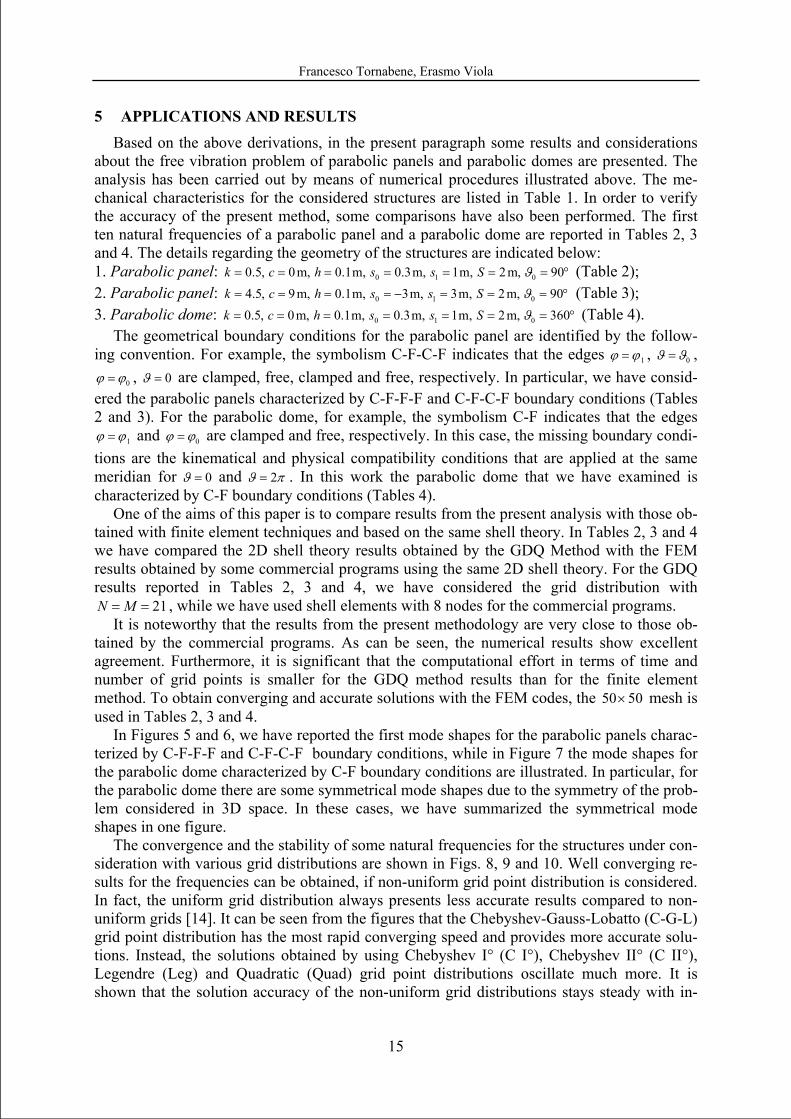
5 APPLICATIONS AND RESULTS Based on the above derivations, in the present paragraph some results and considerations

about the free vibration problem of parabolic panels and parabolic domes are presented. The analysis has been carried out by means of numerical procedures illustrated above. The me-chanical characteristics for the considered structures are listed in Table 1. In order to verify the accuracy of the present method, some comparisons have also been performed. The first ten natural frequencies of a parabolic panel and a parabolic dome are reported in Tables 2, 3 and 4. The details regarding the geometry of the structures are indicated below: 1. Parabolic panel: 0 1 00.5, 0m, 0.1m, 0.3m, 1m, 2m, 90k c h s s S ϑ= = = = = = = ° (Table 2); 2. Parabolic panel: 0 1 04.5, 9m, 0.1m, 3m, 3m, 2m, 90k c h s s S ϑ= = = = − = = = ° (Table 3); 3. Parabolic dome: 0 1 00.5, 0m, 0.1m, 0.3m, 1m, 2m, 360k c h s s S ϑ= = = = = = = ° (Table 4).

The geometrical boundary conditions for the parabolic panel are identified by the follow-ing convention. For example, the symbolism C-F-C-F indicates that the edges 1ϕ ϕ= , 0ϑ ϑ= ,

0ϕ ϕ= , 0ϑ = are clamped, free, clamped and free, respectively. In particular, we have consid-ered the parabolic panels characterized by C-F-F-F and C-F-C-F boundary conditions (Tables 2 and 3). For the parabolic dome, for example, the symbolism C-F indicates that the edges

1ϕ ϕ= and 0ϕ ϕ= are clamped and free, respectively. In this case, the missing boundary condi-tions are the kinematical and physical compatibility conditions that are applied at the same meridian for 0ϑ = and 2ϑ π= . In this work the parabolic dome that we have examined is characterized by C-F boundary conditions (Tables 4).

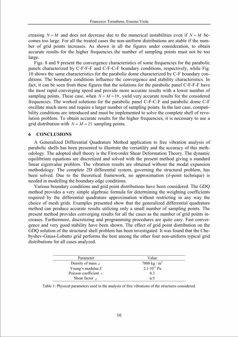
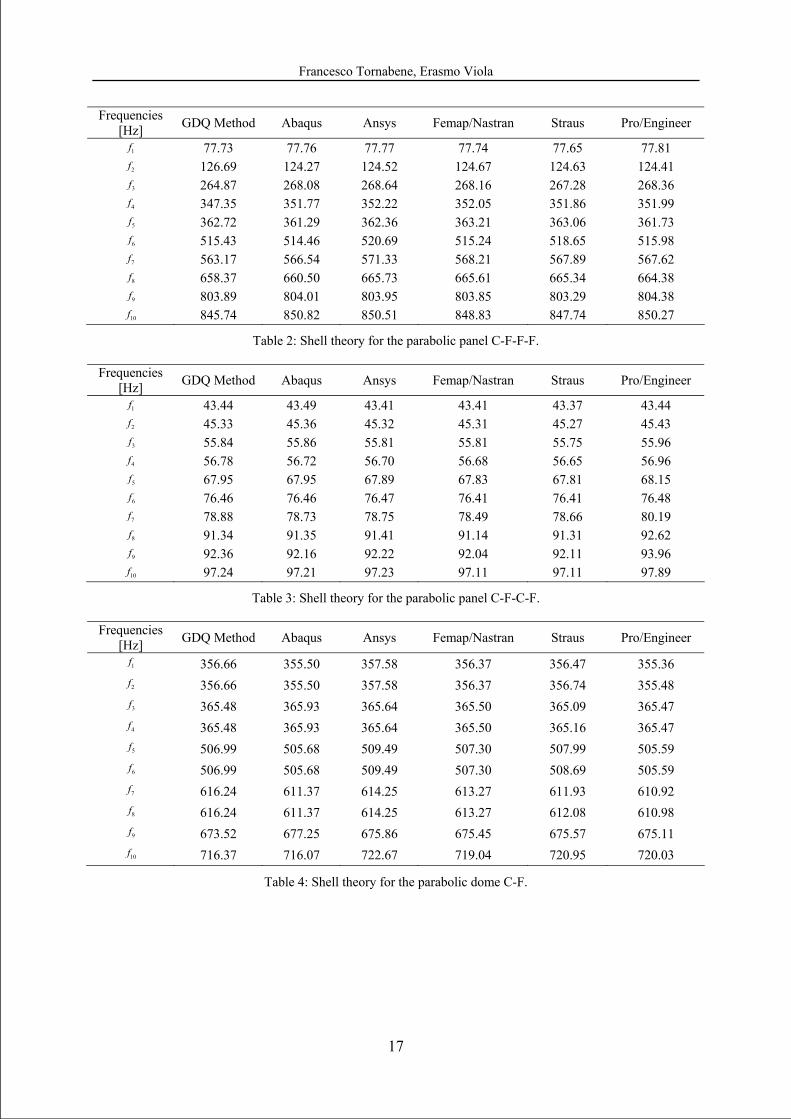
One of the aims of this paper is to compare results from the present analysis with those ob-tained with finite element techniques and based on the same shell theory. In Tables 2, 3 and 4 we have compared the 2D shell theory results obtained by the GDQ Method with the FEM results obtained by some commercial programs using the same 2D shell theory. For the GDQ results reported in Tables 2, 3 and 4, we have considered the grid distribution with

21N M= = , while we have used shell elements with 8 nodes for the commercial programs. It is noteworthy that the results from the present methodology are very close to those ob-

tained by the commercial programs. As can be seen, the numerical results show excellent agreement. Furthermore, it is significant that the computational effort in terms of time and number of grid points is smaller for the GDQ method results than for the finite element method. To obtain converging and accurate solutions with the FEM codes, the 50 50× mesh is used in Tables 2, 3 and 4.

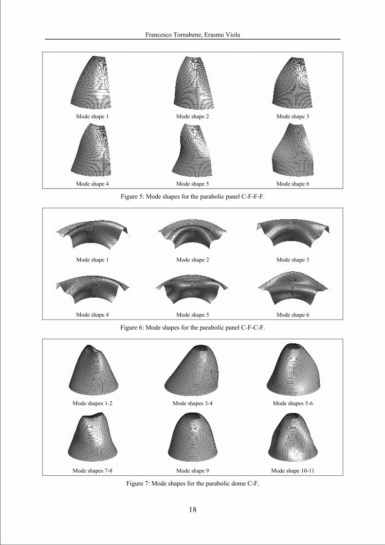
In Figures 5 and 6, we have reported the first mode shapes for the parabolic panels charac-terized by C-F-F-F and C-F-C-F boundary conditions, while in Figure 7 the mode shapes for the parabolic dome characterized by C-F boundary conditions are illustrated. In particular, for the parabolic dome there are some symmetrical mode shapes due to the symmetry of the prob-lem considered in 3D space. In these cases, we have summarized the symmetrical mode shapes in one figure.

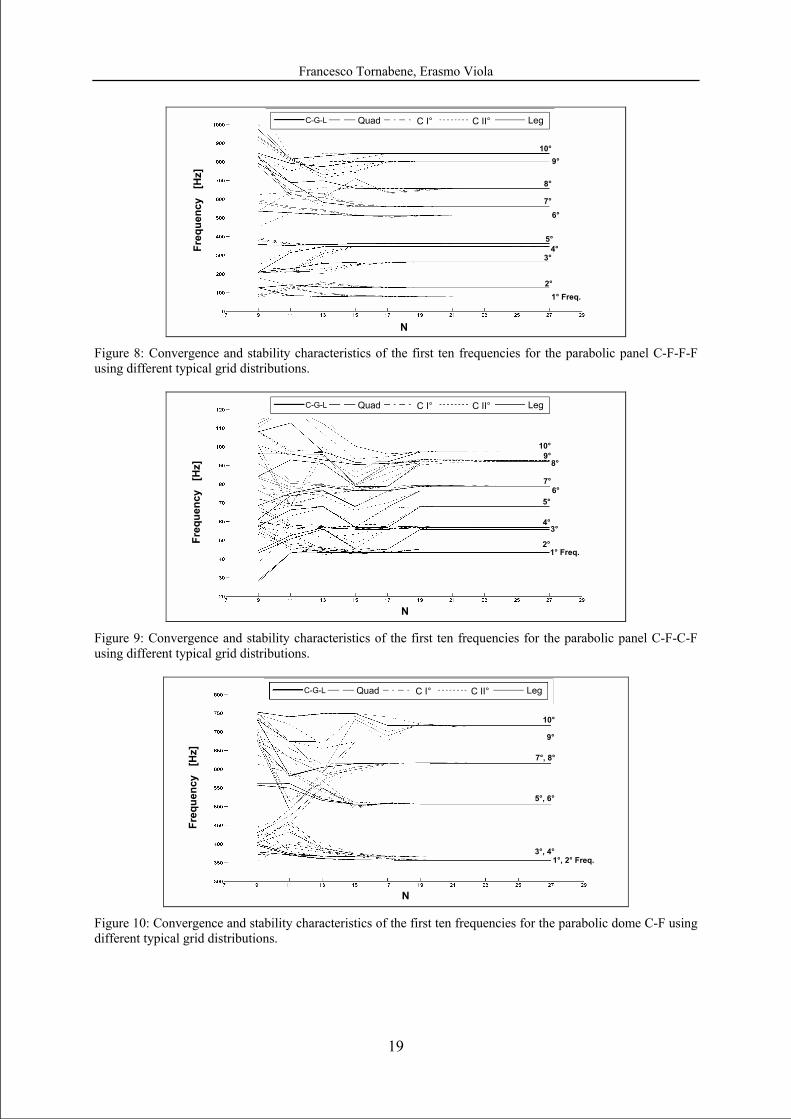
The convergence and the stability of some natural frequencies for the structures under con-sideration with various grid distributions are shown in Figs. 8, 9 and 10. Well converging re-sults for the frequencies can be obtained, if non-uniform grid point distribution is considered. In fact, the uniform grid distribution always presents less accurate results compared to non-uniform grids [14]. It can be seen from the figures that the Chebyshev-Gauss-Lobatto (C-G-L) grid point distribution has the most rapid converging speed and provides more accurate solu-tions. Instead, the solutions obtained by using Chebyshev I° (C I°), Chebyshev II° (C II°), Legendre (Leg) and Quadratic (Quad) grid point distributions oscillate much more. It is shown that the solution accuracy of the non-uniform grid distributions stays steady with in-


16

creasing N M= and does not decrease due to the numerical instabilities even if N M= be-comes too large. For all the treated cases the non-uniform distributions are stable if the num-ber of grid points increases. As shown in all the figures under consideration, to obtain accurate results for the higher frequencies the number of sampling points must not be too large.

Figs. 8 and 9 present the convergence characteristics of some frequencies for the parabolic panels characterized by C-F-F-F and C-F-C-F boundary conditions, respectively, while Fig. 10 shows the same characteristics for the parabolic dome characterized by C-F boundary con-ditions. The boundary conditions influence the convergence and stability characteristics. In fact, it can be seen from these figures that the solutions for the parabolic panel C-F-F-F have the most rapid converging speed and provide more accurate results with a lower number of sampling points. These case, when 19N M= = , yield very accurate results for the considered frequencies. The worked solutions for the parabolic panel C-F-C-F and parabolic dome C-F oscillate much more and require a larger number of sampling points. In the last case, compati-bility conditions are introduced and must be implemented to solve the complete shell of revo-lution problem. To obtain accurate results for the higher frequencies, it is necessary to use a grid distribution with 21N M= = sampling points.

6 CONCLUSIONS A Generalized Differential Quadrature Method application to free vibration analysis of

parabolic shells has been presented to illustrate the versatility and the accuracy of this meth-odology. The adopted shell theory is the First-order Shear Deformation Theory. The dynamic equilibrium equations are discretized and solved with the present method giving a standard linear eigenvalue problem. The vibration results are obtained without the modal expansion methodology. The complete 2D differential system, governing the structural problem, has been solved. Due to the theoretical framework, no approximation (δ-point technique) is needed in modelling the boundary edge conditions.

Various boundary conditions and grid point distributions have been considered. The GDQ method provides a very simple algebraic formula for determining the weighting coefficients required by the differential quadrature approximation without restricting in any way the choice of mesh grids. Examples presented show that the generalized differential quadrature method can produce accurate results utilizing only a small number of sampling points. The present method provides converging results for all the cases as the number of grid points in-creases. Furthermore, discretizing and programming procedures are quite easy. Fast conver-gence and very good stability have been shown. The effect of grid point distribution on the GDQ solution of the structural shell problem has been investigated. It was found that the Che-byshev-Gauss-Lobatto grid performs the best among the other four non-uniform typical grid distributions for all cases analyzed.

Parameter Value Density of mass μ 7800 kg / m3 Young’s modulus E 2.1·1011 Pa

Poisson coefficient ν 0.3 Shear factor χ 6/5

Table 1: Physical parameters used in the analysis of free vibrations of the structures considered.


17

Frequencies [Hz] GDQ Method Abaqus Ansys Femap/Nastran Straus Pro/Engineer

1f 77.73 77.76 77.77 77.74 77.65 77.81 2f 126.69 124.27 124.52 124.67 124.63 124.41 3f 264.87 268.08 268.64 268.16 267.28 268.36 4f 347.35 351.77 352.22 352.05 351.86 351.99 5f 362.72 361.29 362.36 363.21 363.06 361.73 6f 515.43 514.46 520.69 515.24 518.65 515.98 7f 563.17 566.54 571.33 568.21 567.89 567.62 8f 658.37 660.50 665.73 665.61 665.34 664.38 9f 803.89 804.01 803.95 803.85 803.29 804.38

10f 845.74 850.82 850.51 848.83 847.74 850.27

Table 2: Shell theory for the parabolic panel C-F-F-F.


1f 43.44 43.49 43.41 43.41 43.37 43.44 2f 45.33 45.36 45.32 45.31 45.27 45.43 3f 55.84 55.86 55.81 55.81 55.75 55.96 4f 56.78 56.72 56.70 56.68 56.65 56.96 5f 67.95 67.95 67.89 67.83 67.81 68.15 6f 76.46 76.46 76.47 76.41 76.41 76.48 7f 78.88 78.73 78.75 78.49 78.66 80.19 8f 91.34 91.35 91.41 91.14 91.31 92.62 9f 92.36 92.16 92.22 92.04 92.11 93.96

10f 97.24 97.21 97.23 97.11 97.11 97.89

Table 3: Shell theory for the parabolic panel C-F-C-F.


1f 356.66 355.50 357.58 356.37 356.47 355.36 2f 356.66 355.50 357.58 356.37 356.74 355.48 3f 365.48 365.93 365.64 365.50 365.09 365.47 4f 365.48 365.93 365.64 365.50 365.16 365.47 5f 506.99 505.68 509.49 507.30 507.99 505.59 6f 506.99 505.68 509.49 507.30 508.69 505.59 7f 616.24 611.37 614.25 613.27 611.93 610.92 8f 616.24 611.37 614.25 613.27 612.08 610.98 9f 673.52 677.25 675.86 675.45 675.57 675.11

10f 716.37 716.07 722.67 719.04 720.95 720.03

Table 4: Shell theory for the parabolic dome C-F.


18

Mode shape 1

Mode shape 2

Mode shape 3

Mode shape 4

Mode shape 5

Mode shape 6

Figure 5: Mode shapes for the parabolic panel C-F-F-F.

Mode shape 1

Mode shape 2

Mode shape 3

Mode shape 4

Mode shape 5

Mode shape 6

Figure 6: Mode shapes for the parabolic panel C-F-C-F.

Mode shapes 1-2

Mode shapes 3-4

Mode shapes 5-6

Mode shapes 7-8

Mode shape 9

Mode shape 10-11

Figure 7: Mode shapes for the parabolic dome C-F.


19

Figure 8: Convergence and stability characteristics of the first ten frequencies for the parabolic panel C-F-F-F using different typical grid distributions.

Figure 9: Convergence and stability characteristics of the first ten frequencies for the parabolic panel C-F-C-F using different typical grid distributions.

Figure 10: Convergence and stability characteristics of the first ten frequencies for the parabolic dome C-F using different typical grid distributions.

C-G-L Quad C I° C II° Leg

N

Freq

uenc

y [

Hz]

N

Freq

uenc

y [

Hz]

1° Freq.

3° 4°

6°

8°

10°

2°

5°

9°

7°




N

Freq

uenc

y [

Hz]

1°, 2° Freq. 3°, 4°

5°, 6°

7°, 8°

9°

10°


1° Freq.

3°

6°

8°

10°

2°

5°

9°

7°

4°


20

ACKNOWLEDGMENT This research was supported by the Italian Ministry for University and Scientific, Technologi-cal Research MIUR (40% and 60%). The research topic is one of the subjects of the Centre of Study and Research for the Identification of Materials and Structures (CIMEST)-“M.Capurso”.

REFERENCES [1] J. L. Sanders, An improved first approximation theory of thin shells. NASA Report 24,

1959.

[2] W. Flügge, Stress in Shells. Springer, New York, 1960.

[3] F. I. Niordson, Shell Theory. North-Holland, Amsterdam, 1985.

[4] E. Reissner, The effect of transverse shear deformation on the bending of elastic plates. Journal of Applied Mechanics ASME 12, 66-77, 1945.

[5] E. Artioli, P. Gould and E. Viola, Generalized collocation method for rotational shells free vibration analysis. The Seventh International Conference on Computational Struc-tures Technology. Lisbon, Portugal, September 7 - 9, 2004.

[6] E. Viola and E. Artioli, The G.D.Q. method for the harmonic dynamic analysis of rota-tional shell structural elements. Structural Engineering and Mechanics 17, 789-817, 2004.

[7] C. Shu, Generalized differential-integral quadrature and application to the simulation of incompressible viscous flows including parallel computation. PhD Thesis, University of Glasgow, 1991.

[8] R. Bellman and J. Casti, Differential quadrature and long-term integration. Journal of Mathematical Analysis and Applications 34, 235-238, 1971.

[9] R. Bellman, B. G. Kashef and J. Casti, Differential quadrature: a technique for the rapid solution of nonlinear partial differential equations. Journal of Computational Physic 10, 40-52, 1972.

[10] C. Shu, Differential Quadrature and Its Application in Engineering. Springer, Berlin, 2000.

[11] J. R. Quan and C. T. Chang, New insights in solving distributed system equations by the quadrature method – I. Analysis. Computers and Chemical Engineering 13, 779-788, 1989.

[12] J. R. Quan and C. T. Chang, New insights in solving distributed system equations by the quadrature method – II. Numerical experiments. Computers and Chemical Engineering 13, 1017-1024, 1989.

[13] C. Bert and M. Malik, Differential quadrature method in computational mechanics. Ap-plied Mechanical Reviews 49, 1-27, 1996.

[14] C. Shu, W. Chen, H. Xue and H. Du, Numerical study of grid distribution effect on ac-curacy of DQ analysis of beams and plates by error estimation of derivative approxima-tion. International Journal for Numerical Methods in Engineering 51, 159-179, 2001.

Differential Quadrature Solution for Parabolic Structural Shell Elements

Documents