Differential Profiling of Volatile Organic Compound … Differential Profiling of Volatile Organic Compound Biomarker Signatures Utilizing a Logical Statistical Filter-Set and Novel

AFRL-RH-WP-JA-2012-0040

Differential Profiling of Volatile Organic Compound Biomarker

Signatures Utilizing a Logical Statistical Filter-Set and Novel Hybrid

Evolutionary Classifiers

Claude C. Grigsby, Ryan M. Kramer

Human Signatures Branch

Forecasting Division

Michael A. Zmuda

Department of Computer Science and Software Engineering

Miami University

Derek W. Boone, Tyler C. Highlander, Mateen M. Rizki

Department of Computer Science and Software

Wright State University

APRIL 2012

Interim Report

Distribution A: Approved for public release; distribution is unlimited.

See additional restrictions described on inside pages

AIR FORCE RESEARCH LABORATORY

711TH

HUMAN PERFORMANCE WING,

HUMAN EFFECTIVENESS DIRECTORATE,

WRIGHT-PATTERSON AIR FORCE BASE, OH 45433

AIR FORCE MATERIEL COMMAND

UNITED STATES AIR FORCE

NOTICE AND SIGNATURE PAGE

Using Government drawings, specifications, or other data included in this document for any purpose

other than Government procurement does not in any way obligate the U.S. Government. The fact that

the Government formulated or supplied the drawings, specifications, or other data does not license

the holder or any other person or corporation; or convey any rights or permission to manufacture, use,

or sell any patented invention that may relate to them.

This report was cleared for public release by the 88th

Air Base Wing Public Affairs Office and is

available to the general public, including foreign nationals. Copies may be obtained from the Defense

Technical Information Center (DTIC) (http://www.dtic.mil).

AFRL-RH-WP-JA-2012-0040 HAS BEEN REVIEWED AND IS APPROVED FOR

PUBLICATION IN ACCORDANCE WITH ASSIGNED DISTRIBUTION STATEMENT.

//signature// //signature//

_________________________________ ________________________

Claude C. Grigsby, Work Unit Manager Louise A. Carter, PhD

Human Signatures Branch Chief, Forecasting Division

Human Effectiveness Directorate

711th

Human Performance Wing

Air Force Research Laboratory

This report is published in the interest of scientific and technical information exchange, and its

publication does not constitute the Government’s approval or disapproval of its ideas or findings.

i

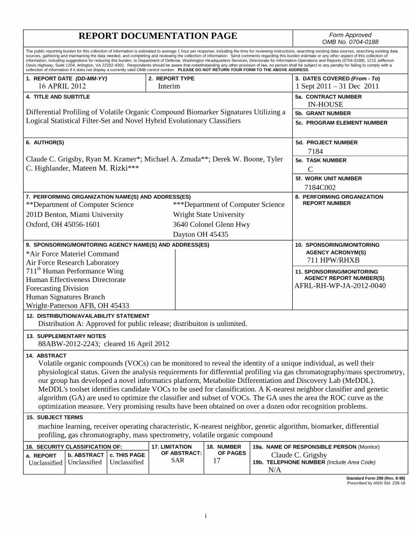
REPORT DOCUMENTATION PAGE Form Approved OMB No. 0704-0188

The public reporting burden for this collection of information is estimated to average 1 hour per response, including the time for reviewing instructions, searching existing data sources, searching existing data sources, gathering and maintaining the data needed, and completing and reviewing the collection of information. Send comments regarding this burden estimate or any other aspect of this collection of information, including suggestions for reducing this burden, to Department of Defense, Washington Headquarters Services, Directorate for Information Operations and Reports (0704-0188), 1215 Jefferson Davis Highway, Suite 1204, Arlington, VA 22202-4302. Respondents should be aware that notwithstanding any other provision of law, no person shall be subject to any penalty for failing to comply with a collection of information if it does not display a currently valid OMB control number. PLEASE DO NOT RETURN YOUR FORM TO THE ABOVE ADDRESS.

1. REPORT DATE (DD-MM-YY) 2. REPORT TYPE 3. DATES COVERED (From - To)

16 APRIL 2012 Interim 1 Sept 2011 – 31 Dec 2011

4. TITLE AND SUBTITLE

Differential Profiling of Volatile Organic Compound Biomarker Signatures Utilizing a

Logical Statistical Filter-Set and Novel Hybrid Evolutionary Classifiers

5a. CONTRACT NUMBER

IN-HOUSE 5b. GRANT NUMBER

5c. PROGRAM ELEMENT NUMBER

6. AUTHOR(S)

Claude C. Grigsby, Ryan M. Kramer*; Michael A. Zmuda**; Derek W. Boone, Tyler

C. Highlander, Mateen M. Rizki***

5d. PROJECT NUMBER

7184 5e. TASK NUMBER

C

5f. WORK UNIT NUMBER

7184C002

7. PERFORMING ORGANIZATION NAME(S) AND ADDRESS(ES) 8. PERFORMING ORGANIZATION

**Department of Computer Science ***Department of Computer Science

201D Benton, Miami University Wright State University

Oxford, OH 45056-1601 3640 Colonel Glenn Hwy

Dayton OH 45435

REPORT NUMBER

9. SPONSORING/MONITORING AGENCY NAME(S) AND ADDRESS(ES) 10. SPONSORING/MONITORING

*Air Force Materiel Command

Air Force Research Laboratory

711th Human Performance Wing

Human Effectiveness Directorate

Forecasting Division

Human Signatures Branch

Wright-Patterson AFB, OH 45433

AGENCY ACRONYM(S)

711 HPW/RHXB

11. SPONSORING/MONITORING AGENCY REPORT NUMBER(S)

AFRL-RH-WP-JA-2012-0040

12. DISTRIBUTION/AVAILABILITY STATEMENT

Distribution A: Approved for public release; distribuiton is unlimited.

13. SUPPLEMENTARY NOTES

88ABW-2012-2243; cleared 16 April 2012

14. ABSTRACT

Volatile organic compounds (VOCs) can be monitored to reveal the identity of a unique individual, as well their

physiological status. Given the analysis requirements for differential profiling via gas chromatography/mass spectrometry,

our group has developed a novel informatics platform, Metabolite Differentiation and Discovery Lab (MeDDL).

MeDDL's toolset identifies candidate VOCs to be used for classification. A K-nearest neighbor classifier and genetic

algorithm (GA) are used to optimize the classifier and subset of VOCs. The GA uses the area the ROC curve as the

optimization measure. Very promising results have been obtained on over a dozen odor recognition problems.

15. SUBJECT TERMS

machine learning, receiver operating characteristic, K-nearest neighbor, genetic algorithm, biomarker, differential

profiling, gas chromatography, mass spectrometry, volatile organic compound

16. SECURITY CLASSIFICATION OF: 17. LIMITATION OF ABSTRACT:

SAR

18. NUMBER OF PAGES

17

19a. NAME OF RESPONSIBLE PERSON (Monitor)

a. REPORT

Unclassified

b. ABSTRACT

Unclassified

c. THIS PAGE

Unclassified

Claude C. Grigsby 19b. TELEPHONE NUMBER (Include Area Code)

N/A Standard Form 298 (Rev. 8-98)

Prescribed by ANSI Std. Z39-18

ii

THIS PAGE IS INTENTIONALLY LEFT BLANK

iii

TABLE OF CONTENTS

ABSTRACT ........................................................................................................................................... 1

1.0 INTRODUCTION ..................................................................................................................... 1

2.0 BACKGROUND / APPROACH .............................................................................................. 2

2.1 Background .................................................................................................................................. 2

2.2 Peak Registration, Alignment, and Filtering ............................................................................... 2 2.3 Classification ............................................................................................................................... 3 2.4 Modified K-Nearest Neighbor Classifier .................................................................................... 4 2.5 Learning Algorithm for Feature Selection .................................................................................. 5

3.0 EXPERIMENTAL DESIGN .................................................................................................... 7

3.1 Materials / Methods ..................................................................................................................... 7 3.2 Results ......................................................................................................................................... 7

4.0 CONCLUSION .......................................................................................................................... 10

ACKNOWLEDGEMENTS .................................................................................................................. 10

REFERENCES ...................................................................................................................................... 11

LIST OF FIGURES

Figure 1. Example data and plot of data. ....................................................................................................... 4

Figures 2a-b. ROC Curves. Figure 2a shows a typical ROC curve. Figure 2b shows the perfect ROC

curve. ............................................................................................................................................................. 5

Figure 3. Modified KNN pseudocode. .......................................................................................................... 5

Figure 4. Reduction of Training Data. The topmost figure shows the entire set of data. The middle figure

shows one bitstring produced by the GA. The bottommost figure shows the training data without the

excluded features. .......................................................................................................................................... 6

Figure 5. PCA of C57 and DBA filtered intersect (peakset 4) results. ......................................................... 8

Figure 6. MeDDL tool machine learning implementation and GA settings. ................................................ 9

Figure 7. Hybrid GA results. Vertical line is user adjustable slider to determine T threshold values. ......... 9

Figure 8. Boxplot of hybrid GA VOC feature output selected by classifier. .............................................. 10

iv

THIS PAGE IS INTENTIONALLY LEFT BLANK

1

Distribution A: Approved for public release; distribuiton is unlimited. 88ABW-2012-2243; cleared 16 April 2012

Differential profiling of volatile organic compound biomarker signatures

utilizing a logical statistical filter-set and novel hybrid evolutionary

classifiers Claude C. Grigsby

*a, Michael A. Zmuda

b, Derek W. Boone

c, Tyler C. Highlander

c, Ryan M. Kramer

a,

Mateen M. Rizkic

aHuman Biosignatures Branch, 711

th Human Performance Wing, Air Force Research Lab, 2510 Fifth

Street, Area B, Bld 840, Wright-Patterson AFB, OH 45433-7913; bDepartment of Computer Science and

Software Engineering, 201D Benton, Miami University, Oxford, OH 45056-1601; cDepartment of

Computer Science and Engineering, Wright State University, 3640 Colonel Glenn Hwy, Dayton, OH

45435

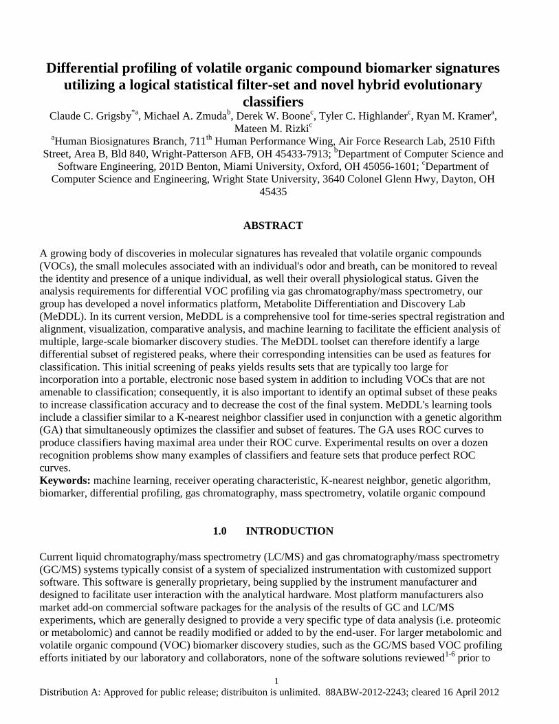
ABSTRACT

A growing body of discoveries in molecular signatures has revealed that volatile organic compounds

(VOCs), the small molecules associated with an individual's odor and breath, can be monitored to reveal

the identity and presence of a unique individual, as well their overall physiological status. Given the

analysis requirements for differential VOC profiling via gas chromatography/mass spectrometry, our

group has developed a novel informatics platform, Metabolite Differentiation and Discovery Lab

(MeDDL). In its current version, MeDDL is a comprehensive tool for time-series spectral registration and

alignment, visualization, comparative analysis, and machine learning to facilitate the efficient analysis of

multiple, large-scale biomarker discovery studies. The MeDDL toolset can therefore identify a large

differential subset of registered peaks, where their corresponding intensities can be used as features for

classification. This initial screening of peaks yields results sets that are typically too large for

incorporation into a portable, electronic nose based system in addition to including VOCs that are not

amenable to classification; consequently, it is also important to identify an optimal subset of these peaks

to increase classification accuracy and to decrease the cost of the final system. MeDDL's learning tools

include a classifier similar to a K-nearest neighbor classifier used in conjunction with a genetic algorithm

(GA) that simultaneously optimizes the classifier and subset of features. The GA uses ROC curves to

produce classifiers having maximal area under their ROC curve. Experimental results on over a dozen

recognition problems show many examples of classifiers and feature sets that produce perfect ROC

curves.

Keywords: machine learning, receiver operating characteristic, K-nearest neighbor, genetic algorithm,

biomarker, differential profiling, gas chromatography, mass spectrometry, volatile organic compound

1.0 INTRODUCTION

Current liquid chromatography/mass spectrometry (LC/MS) and gas chromatography/mass spectrometry

(GC/MS) systems typically consist of a system of specialized instrumentation with customized support

software. This software is generally proprietary, being supplied by the instrument manufacturer and

designed to facilitate user interaction with the analytical hardware. Most platform manufacturers also

market add-on commercial software packages for the analysis of the results of GC and LC/MS

experiments, which are generally designed to provide a very specific type of data analysis (i.e. proteomic

or metabolomic) and cannot be readily modified or added to by the end-user. For larger metabolomic and

volatile organic compound (VOC) biomarker discovery studies, such as the GC/MS based VOC profiling

efforts initiated by our laboratory and collaborators, none of the software solutions reviewed1-6

prior to

2


development offered the ability to compare multiple time point and exposure groups, or handle data sets

in significant sample numbers. This bottleneck in data handling initiated the described development and

evolution of the Metabolite Differentiation and Discovery Lab (MeDDL) tool7, allowing us to

differentiate metabolite and VOC profiles in multiple differential biomarker discovery studies and

facilitated the ability to visualize collected data for a global view of an entire experiment while

maintaining the ability to focus on individual compounds and spectra for subsequent identification. The

latest version of MeDDL incorporates a variety of additional features, described below, which focus on

expanding the GC/MS analysis capability

*[email protected]; phone (937)938-3721; fax (937)656-6898;

www.wpafb.af.mil/afrl/711HPW/ of the platform in support of VOC based biomarker research on-going

in our laboratory. The goal of this work was to enhance the capability of the MeDDL tool for use in

differential metabolite profiling through generation of a suite of logically driven filters and machine

learning tools for feature down-selection, allowing for optimally targeted unknown compound

identification and potential subsequent incorporation into sensor platforms.

2.0 BACKGROUND / APPROACH

2.1 Background

Both small molecule and VOC based metabolite profiling are an attractive approach to the study of

multivariate metabolic responses to such things as pathophysiological processes by which biological and

chemical agents can cause perturbations in the concentrations and flux of endogenous metabolites

involved in critical cellular pathways. Thus, cells and entire organisms respond to toxic insult or other

stressors by altering their intra-and/or extra-cellular environment in an attempt to maintain a homeostatic

intracellular environment, some of which translate to differences in measurable volatile compounds

emitted. This metabolic alteration is expressed as a "fingerprint" of biochemical perturbations that may be

characteristic of the type and target of a toxic insult or disease process. Additionally, if a significant

number of trace molecules can be identified and monitored, the overall pattern produced may be more

consistent and predictive than any single biomarker, which would prove of great value in the development

of targeted sensing platforms. To illustrate our approach to these studies, we present the below urine

based VOC comparison of the two parental strains of the BXD mouse model8, C57 and DBA. This

described methodology is representative of our approach and is applicable to a wide range of VOC and

small molecule based biomarker discovery applications such as human performance monitoring, odor

based biometrics, medical diagnostics, and targeted materials detection.

2.2 Peak Registration, Alignment, and Filtering

The MeDDL platform is an freeware informatics package currently implemented in MATLAB v2011a

(The MathWorks Inc., Natick, MA) that allows for registration of “peaks,” which are defined here as a

single ion or measured mass/charge (m/z) at a given retention time, mass and chromatographic time

alignment, and a suite of statistical and pattern recognition tools selected for biomarker screening studies.

In brief, the MeDDL tool reads in lists of CDF (common data format) conversions of the raw LC/MS and

GC/MS data files, registers peaks based on user-defined parameters in terms of mass sensitivity and

accuracy thresholds as well as chromatographic reproducibility tailored to the performance of the

3


analytical platform, and performs alignment of the generated peak lists in both time and mass. Following

the spectral registration and alignment previously described7, the data was analyzed using several of the

principal analytical methodologies included in MeDDL: unsupervised clustering via principal component

analysis9; differential down selection of peaks through combination of a set of logical filters; and

utilization of machine learning based tools for significant VOC “feature” identification.

MeDDL was originally created for the analysis of LC/MS data. The ionization techniques generally

employed for LC/MS are termed “soft” and impart low energy to eluting ions, resulting in fairly simple

mass spectra: often comprised of just the ionized analyte, or “parent” ion. Modifications to the original

implementation of MeDDL were required to aid in the analysis of the more complex mass spectra in

GC/MS resulting from the “hard ionization” induced by the electron impact (EI) fragmentation process in

the mass spectrometer’s ion source. A reductionist approach for this analysis was required for the

efficient determination of changes observed between sample groups. To address this issue, we created a

supplementary time-binning filter allowing the analyst to specify both a time window and lower bound

threshold of peak intensities. The comparison then proceeds as follows: an averaged, composite image of

each user-defined comparative group is generated (i.e. the surface obtained from samples comprising each

comparative group); the most intense peak from all groups is evaluated across all aligned images using a

0.1 minute window and 100,000 absolute (total ion count) threshold; once the comparison is completed,

this “time slice” based upon the peak apex ± ½ of the specified time window is removed from further

analysis and the next most intense set of peaks are compared. An additional filter applied in the

differential analysis of groups in this study included a fold change filter limiting results to only those

peaks which demonstrated at least 2 fold or greater change in intensity between strains. It must be noted

that although the MeDDL tool contains a wide variety of implemented statistical filters for feature down-

selection, we limited their use to only the 2 filters listed to allow for optimal feature selection by the

classifier. Once both of these filters were applied to the grouped, global data set, a Boolean "AND" was

added to the resulting filtered peak sets to identify the logical intersection, an approach similar to that

used in generation of a Venn diagram. These reduced data sets were then used for further classification

described below.

2.3 Classification

The filtered, numerical data sets, or feature vectors, produced by the preprocessing described in the

previous section must be used to perform classification on unknown samples for optimal results.

However, performing classification with these features still presents several problems. First, the filtered

features include noisy, irrelevant features, despite the preprocessing steps taken to identify features that

have both intra-class similarity and inter-class dissimilarity. Second, the set of filtered features include

those that are highly correlated and therefore are redundant. These two observations suggest the

classification system should produce a classifier, but should also down select the incoming feature set to a

small set of cooperative features that are amenable to classification.

The following sections describe the approach used in this paper. A modified K-Nearest Neighbor (KNN)

classifier is used as the basic classification algorithm. Feature selection is determined by the use of a

genetic algorithm (GA) to identify a small set of features that enable the KNN to obtain good

classification results. The GA is driven by the area under the KNN’s receiver operator characteristic curve

(ROC curve), where the ideal ROC curve has an area of 1. The following sections describe each aspect in

more detail.

4


2.4 Modified K-Nearest Neighbor Classifier

The basic KNN is a two-class classifier that is often used in situations where the data distributions are

generally unknown10

. KNN training is performed by using all samples of the training data as labeled

prototypes. Unknown samples are classified by comparing the distance of the unknown sample to the k

nearest prototypes, where k is a small user-defined integer (e.g., 3). In binary classification (i.e., -two

class classification), choosing an odd value for k avoids a potential tie vote. The method of computing

distance with N-dimensional data is commonly done in two different ways: Euclidean distance and L1

norm, or Manhattan/Minkowski distance formula using p = 2. This work uses Euclidean distance, but the

L1 norm appeared to provide similar results. The three nearest prototypes then vote on the unknown’s

class label. Figure 1 illustrates this process in two dimensions. In this sample, the training data contains 5

samples, which includes 3 positive samples and 2 negative samples. The three closest samples to the

unknown are S1, S3, and S4, with the majority those samples being positives; consequently, the unknown

would be labeled as positive.

Figure 1. Example data and plot of data.

One unique objective of this work was to develop a classifier that has one or more parameters that control

the classifier’s behavior. For example, it may be important to correctly classify positives, with an

increased tolerance for false alarms. Conversely, it may be deemed acceptable to miss a couple positives,

if the increased number of false alarms is kept small. The k parameter in the KNN classifier does not

provide such a parameter. k simply denotes the number of voters and does not provide a way to

increase/decrease the sensitivity toward the class boundaries. Further, the number of prototypes is

typically quite small in biological studies and therefore modulating the number of voters would have

limited utility.

For an appropriately configurable classifier, a ROC curve visually illustrates the possible tradeoffs

between the rates of true positives and false positives. Figures 2a and 2b illustrate a typical ROC curve

and the perfect ROC curve. Figure 2a depicts the tradeoffs of a hypothetical classifier. The figure shows

that the classifier has a parameter that can allow it to obtain a 0.75 true positive rate, while simultaneously

having a false alarm rate of 0.25. Should the operational situation require 0.9 rate of recognizing true

positives, the rate of false alarms would reach a predicted level of approximately 0.75. ROC curves are

monotonically increasing. The perfect classifier would obtain a rate of 1.0 for positives with a false alarm

rate of 0.0. This perfect ROC curve is shown in Figure 2b.

5


Figures 2a-b. ROC Curves. Figure 2a shows a typical ROC curve. Figure 2b shows the perfect ROC

curve.

To provide for an adjustable parameter, the KNN’s decision rule is modified (Figure 3). Whereas, the basic KNN’s decision

rule is to count the votes to the nearest k prototypes, the modified decision rule uses the distance value to influence its decision.

This is approach assumes that being closer to a prototype indicates that it is more likely to be of that category. The definition

for the modified KNN decision rule is as follows, where T is the configurable parameter and k is an integer > 0:

Figure 3. Modified KNN pseudocode.

The classification rule takes the ratio between the total distances to the closest positive prototypes and the closest negative

prototypes. If the unknown happens to be a positive, it is expected that posDistance would be small and negDistance would be

large, producing a small value for ratio. By adjusting T to a small value, the criteria for declaring “positive” becomes more

stringent, in that the unknown’s distance from the positives must be quite small while simultaneously its distance from the

negatives must be relatively large. Conversely, setting T to a large value allows more samples to be classified as positives. In

the extreme case, T = infinity, all unknown samples will be classified as positives.

2.5 Learning Algorithm for Feature Selection

After preprocessing, the set of filtered features is sent to the classification system. As mentioned in section 2.2, the potential

exists for reducing this set to an even smaller number. Ideally, this reduction would produce a less costly system and produce a

subset of features that are more effective than using the entire set as a whole. The ideal subset would contain features with

general properties such as: mutual independence, inter-class dissimilarity, and intra-class similarity. Rather than applying more

filters to achieve this, our approach is to use the modified KNN classifier to assess the quality of a feature subset; where good

subsets will provide good classification and poor subsets will not be very accurate.

The process of selecting a subset from a large set uses a sequence of 0’s and 1’s to represent the subset. Here the bit positions

containing a 1 or 0 indicate features to be included or excluded. Figure 4 shows a diagram illustrating how one bitstring is used

to down-select the features and how that down-selection affects the resulting data set that is fed to the KNN learning algorithm.

In this example, the bitstring happens to have three on-bits located at positions 2, 4, and 5, indicating that only features 2, 4,

and 5 are used and features 1 and 3 are ignored. The down-selected data is then used to form the modified KNN.

6


Figure 4. Reduction of Training Data. The topmost figure shows the entire set of data. The middle figure

shows one bitstring produced by the GA. The bottommost figure shows the training data without the

excluded features.

A GA is a natural learning algorithm to apply to this problem11, 12

since it operates on a bitstring. The

reader is referred to the text by Goldberg13

for a more complete treatment of GAs. For our purposes, it

suffices to say that the GA is a method for optimizing a sequence of 0’s and 1’s. In order to achieve this,

the GA requires a method for evaluating the quality of the sequence. By assigning a numeric score to a

sequence, and many other sequences, the GA navigates the search space to find sequences that are better

than the ones it is currently is examining.

Leave-one-out (LOO) cross validation10, 14

is a common method for estimating the quality of a classifier

using only training data. LOO iterates over all the training samples, where each sample is temporarily

removed from the training set. This smaller set is then used to train the classifier, which is then applied to

the sample that was held out. Ideally, the classifier will correctly classify the sample. By repeating this

process over all training samples, it is possible to assess the generality of the learning technique. If the

LOO algorithm shows solid performance over a large percentage of the samples, it can be assumed that

the learning technique generalizes to truly unknown samples.

On each iteration of the LOO algorithm, the bitstring in question ultimately results in a KNN that is used

to classify the sample temporarily removed. Instead of classifying the sample, the ratio between

posDistance and negDistance is recorded. The set of ratios can be used to create a ROC curve that

predicts the final system’s ROC curve, where the final system refers to the modified KNN that is obtained

by using all of the training data. The area under the predicted ROC curve is used as the bitstring’s

evaluation score. Naturally, a score of 1 corresponds to a perfect ROC curve, which indicates that the

feature set forms an effective KNN classifier.

7


3.0 EXPERIMENTAL DESIGN

3.1 Materials / Methods

Animal use in this study was conducted in accordance with the principles stated in the Guide for the Care

and Use of Laboratory Animals, National Research Council, 1996, and the Animal Welfare Act of 1966,

as amended. BXD mice parental strains (DBA and C57) utilized for this study were singly housed in

metabolic cages which are approximately 9 cm in diameter and urine and feces were separated and

isolated. Individual mouse urine samples were collected using 1 mL disposable transfer pipettes (Thermo

Fisher Scientific) and placed in 2 mL Eppendorf Snap-Cap Microcentrifuge Safe-Lock tubes. The urine

was then stored frozen at -80°C and thawed on ice prior to analysis. For the BXD VOC baseline set

described, 170 individual samples representing the two parental strains (C57 N = 81, DBA N = 89), and

six additional test samples (C57 N = 3, DBA N = 3) were processed by aliquoting 200 uL of urine into a

10 ml crimp-top headspace vial (National Scientific). The vials were immediately crimped with Red

PTFE/white silicone crimp seals (Fisher). The bench-top GC/MS system utilized for sample analysis was

a Thermo Fisher Trace GC Ultra gas chromatograph interfaced to a Thermo Triplus autosampler

configured for automated SPME headspace sampling and in-line with a Thermo DSQII single quadrupole

mass spectrometer. Collection of organic volatiles from the urine was accomplished using a 2cm

CAR/DVB/PDMS solid phase micro extraction fiber (SPME), Supelco supplier, inserted by the Triplus

autosampler into the head-space of the sample vials. The headspace samples were incubated at 60°C for

15 minutes, followed by extraction at 60°C for 30 minutes and automated direct injection. Volatiles

gathered by the SPME fiber were analyzed through desorption of the fiber by heating to elevated

temperature and separation with a Restek Stabilwax 30m, 0.25mm ID column. Helium was used as the

carrier gas at a flow-rate of 1.5 ml/min. A narrow bore SPME injector liner (0.75 mm I.D.) was used

(Thermo). The following conditions were utilized for sample analysis: desorption for 2 min via a PTV

injector held at 230°C; oven temperature program 50°C (4 min); 5°C/min to 230°C; hold 30 minutes

giving a total run time of 70 minutes. The DSQII MS transfer line was held at 230°C and the instrument

was operated in positive scan mode from 41 to 400 amu. The raw data was collected in centroid mode and

the resulting chromatograms and mass spectra (raw files) were then converted to CDF format and

subsequently analyzed through MeDDL. Due to the fact that SPME extraction is a competitive process

leading to mutual displacement from the adsorption sites between different analytes or analytes and

matrix constituents, the results of this study as described report data semi-quantitatively based on relative

peak heights.

3.2 Results

A total of 170 BXD parental urine samples (DBA and C57 “teaching set”) were collected and analyzed

over a four month period with the six unregistered “unknown”, test samples utilized below acquired over

12 months later. Following GC/MS analysis, CDF conversion, and MeDDL registration, the samples in

the “teaching set” were filtered for a 2-fold change and time binned (0.1 min window, 100K absolute

threshold minimum cutoff). The filter results are shown in Table 1, with peakset 1 comprising all

registered peaks, peakset 2 comprising time binning, peakset 3 comprising fold change, and peakset 4 the

resultant intersection of the two applied filters.

8


Table 1. BXD parental strain peak registration and peakset (PkSet) filter results.

This subset of 52 VOC features, or peaks, were first screen by PCA (Figure 5) to demonstrate group

separation prior to analysis by the hybrid GA classifier. Principal component analysis is a mathematical

procedure that uses an orthogonal transformation to convert a set of observations of possibly correlated

variables into a set of values of linearly uncorrelated variables called principal components. This

technique is often difficult in usage to identify the individual subset of features responsible for group

separation, but is quite useful as a screening technique as shown below.

Figure 5. PCA of C57 and DBA filtered intersect (peakset 4) results.

MeDDL offers users the ability to utilize several different types of classification methods and separately

store the resulting output for classification of additional, unregistered unknowns. These methods use a

combination of pre-coded Matlab classifiers, Waikato Environment for Knowledge Analysis (WEKA)

classifiers, and the novel, in-house developed hybrid GA classifier, implemented in Java and Matlab,

described in this study (Figure 6). The internal data classification allows users to teach the classifiers from

peak sets generated using the tool. The external data classification is currently designed to process both

CDF format files and comma separated value files (.CSV). All classification methods support classifying

intensities or ratios of intensities though application of appropriate data filters.

9


Figure 6. MeDDL tool machine learning implementation and GA settings.

In testing the hybrid GA for this study (Figure 7), setting k = 2, minimum features = 4, and maximum

features = 10 provided both perfect classification of C57 versus DBA for both the 170 teaching samples

as well as the 6 “unknown” external samples. Reverse classification (DBA versus C57) using these same

settings resulted in 2 mis-classifications of the “unknowns” illustrating the need to optimize the GA

settings for each classifier result.

Figure 7. Hybrid GA results. Vertical line is user adjustable slider to determine T threshold values.

Results of the hybrid GA classifier were comprised of 10 VOC “features”, which is the maximum features

size allowed by the GA settings. An example of one of the selected VOCs is shown in Figure 8. In an

focused biomarker study, each resultant peak would then be preliminarily identified through comparison

to the National Institute of Standards and Technologies (NIST) 08 database and Wiley libraries and

verified though expert, manual spectral analysis and comparison with purchased standards.

10


Figure 8. Boxplot of hybrid GA VOC feature output selected by classifier.

4.0 CONCLUSION

Given the unique requirements for large-scale, LC/MS and GC/MS based biomarker studies and currently

available software limitations, a logically designed and successfully implemented comprehensive tool for

time-series spectral registration, spectral and chromatographic alignment, visualization, and comparative

analysis facilitates and allows the efficient and methodical analysis of multiple, large-scale biomarker

discovery studies. The MeDDL platform has been markedly improved from the original version and

greatly streamlines the analysis of multi-group comparisons through the addition of a more intuitive

interface, the ability to dynamically alter group definitions and group comparative displays, and the

creation of definable, group comparative graphics. Through a combination of the base MeDDL

registration and alignment algorithms and the described additional functionality, MeDDL now offers the

analytical chemist the potential for visualizing data in new ways, providing novel insight into the

experimental results, and expediting LC/MS and GC/MS based biomarker discovery. Modifications to the

current implementation of the tool are on-going, with automated iteration across available “unknowns” for

optimization of the hybrid GA parameter settings planned. A compiled version of MeDDL is provided

free of charge to all interested parties and is available at the following URL along with a Wiki

(http://meddl.cs.wright.edu/) covering many of the features described above.

ACKNOWLEDGEMENTS

The authors would like to thank: Dr. Louis Tamburino, Dr. Pavel Shiyanov, and Ms. Rhonda Pitsch for

their invaluable help in creation of the MeDDL tool; Monell Chemical Senses Center collaborators Dr.

George Preti and Dr. Jae Kwak for their guidance and shared expertise in the generation of the current

GC/MS implementation; Dr. Gerald Alter and the WSU Biomedical Sciences Program; and Dr. David

Cool and Dr. Thomas Lamkin for their continued support. This research was supported in part by an

appointment to the Student Research Participation Program at the AFRL administered by the Oak Ridge

Institute for Science and Education through an interagency agreement between the DoE and AFRL.

11


REFERENCES

[1] M. Katajamaa, and M. Oresic, “Processing methods for differential analysis of LC/MS profile

data,” BMC Bioinformatics 6, 179 (2005).

[2] R. Baran, H. Kochi, N. Saito et al., “MathDAMP: a package for differential analysis of metabolite

profiles,” BMC Bioinformatics 7, 530 (2006).

[3] C. D. Broeckling, I. R. Reddy, A. L. Duran et al., “MET-IDEA: data extraction tool for mass

spectrometry-based metabolomics,” Anal Chem 78(13), 4334-41 (2006).

[4] B. Bunk, M. Kucklick, R. Jonas et al., “MetaQuant: a tool for the automatic quantification of

GC/MS-based metabolome data,” Bioinformatics 22(23), 2962-5 (2006).

[5] C. A. Smith, E. J. Want, G. O'Maille et al., “XCMS: processing mass spectrometry data for

metabolite profiling using nonlinear peak alignment, matching, and identification,” Anal Chem

78(3), 779-87 (2006).

[6] A. Luedemann, K. Strassburg, A. Erban et al., “TagFinder for the quantitative analysis of gas

chromatography--mass spectrometry (GC-MS)-based metabolite profiling experiments,”

Bioinformatics 24(5), 732-7 (2008).

[7] C. Grigsby, M. Rizki, L. Tamburino et al., “Metabolite Differentiation and Discovery Lab

(MeDDL): A New Tool for Biomarker Discovery and Mass Spectral Visualization,” Analytical

Chemistry 82(11), 4386-4395 (2010).

[8] L. L. Peters, R. F. Robledo, C. J. Bult et al., “The mouse as a model for human biology: a resource

guide for complex trait analysis,” Nature Reviews Genetics 8(1), 58-69 (2007).

[9] B. Richmond, L. Optican, M. Podell et al., “Temporal encoding of two-dimensional patterns by

single units in primate inferior temporal cortex. I. Response characteristics,” Journal of

Neurophysiology 57(1), 132 (1987).

[10] R. O. Duda, P. E. Hart, and D. G. Stork, [Pattern classification] Wiley, New York (2001).

[11] C. L. Huang, and C. J. Wang, “A GA-based feature selection and parameters optimizationfor

support vector machines,” Expert Systems with applications 31(2), 231-240 (2006).

[12] J. Lu, T. Zhao, and Y. Zhang, “Feature selection based-on genetic algorithm for image

annotation,” Knowledge-Based Systems 21(8), 887-891 (2008).

[13] D. E. Goldberg, [Genetic algorithms in search, optimization, and machine learning] Addison-

wesley, (1989).

[14] S. J. Russell, and P. Norvig, [Artificial intelligence: a modern approach] Prentice hall, (2010).

Differential Profiling of Volatile Organic Compound … Differential Profiling of Volatile Organic Compound Biomarker Signatures Utilizing a Logical Statistical Filter-Set and Novel

Documents