Differential evolution with dynamic parameters selection for optimization problems

Copyright (c) 2013 IEEE. Personal use is permitted. For any other purposes, permission must be obtained from the IEEE by emailing [email protected].

This article has been accepted for publication in a future issue of this journal, but has not been fully edited. Content may change prior to final publication. Citation information: DOI10.1109/TEVC.2013.2281528, IEEE Transactions on Evolutionary Computation

1

Abstract—Over the last few decades, a number of Differential Evolution (DE) algorithms have been proposed with excellent performance on mathematical benchmarks. However, like any other optimization algorithm, the success of DE is highly dependent on its search operators and control parameters which are often decided a priori. The selection of the parameter values is itself a combinatorial optimization problem. Although a considerable number of investigations have been conducted with regards to parameter selection, it is known to be a tedious task. In this paper, a DE algorithm is proposed that uses a new mechanism to dynamically select the best performing combinations of parameters (amplification factor, crossover rate and the population size) for a problem during the course of a single run. The performance of the algorithm is judged by solving three well-known sets of optimization test problems (two constrained and one unconstrained). The results demonstrate that the proposed algorithm not only saves the computational time, but also shows better performance over the state-of-the-art algorithms. The proposed mechanism can easily be applied to other population based algorithms. Index Terms—Constrained optimization, differential evolution, parameter selection, parameter adaptation.

I. INTRODUCTION

PTIMIZATION is a challenging area of research spanning across the fields of computer science,

operations research, and engineering. Optimization problems can be either constrained or unconstrained. Constrained optimization is different from its unconstrained counterpart, as it needs to optimize the objective function while satisfying the functional constraints and variable bounds. Constrained optimization problems (COPs) can be classified into many different categories based on the nature of problems and their mathematical properties. In any problem, the type of constraint can be either equality or inequality or both. The objective and constraint functions may possess different properties such as linear and/or nonlinear, continuous or discontinuous, and unimodal or multimodal. The feasible space could be a single bounded region or a collection of multiple disjoint regions. The feasible region could even be unbounded in some problems. The optimal solution may exist either on the boundary or in the interior of the feasible space. A large number of variables and constraints may also add to the complexity of the problem.

Evolutionary algorithms (EAs), such as genetic algorithms (GA)[1], differential evolution (DE)[2], evolution strategies (ES) [3], and evolutionary The authors are with the School of Engineering and Information Technology, University of New South Wales, ADFA Campus, Canberra

2600, Australia (e-mails: [email protected], [email protected], [email protected]) Copyright (c) 2012 IEEE

programming (EP) [4], have a long history of successfully solving optimization problems. Among EAs, DE has shown significant success in solving different numerical optimization problems (both constrained and unconstrained, and black-box ) [5-6] . However, the choice of the control parameters plays a pivotal role in the performance of DE algorithms. While both the choice of the search operators and the control parameters affect the performance, our focus in this paper is on the control parameters (such as amplification factor, crossover rate and the population size) and not on the search operators (such as mutation and crossover variants). In solving any optimization problem, the selection of the right combination of parameters is itself a combinatorial optimization problem. Parameter tuning, which is a trial-and-error approach, is widely used for parameter selection and is known to be tedious [7]. Using such a trial and error approach, a single set of parameters is usually selected based on the average performance of the algorithm over the class of test problems. Due to the variability of the underlying mathematical properties of the optimization problems, a fixed set of control parameters that suits well for one problem, or a class of problems does not guarantee that it will work well for another class, or range of problems. That is, the best set of parameters is problem dependent. To ensure best performance of the algorithm, one must choose the right set of parameters for each and every problem which is a non-trivial task. In addition, a set of parameters that works well at the early stages of the evolution process may not perform well at the later stages and vice versa.

The idea of parameter adaptation was introduced at least two decades ago in the context of GA [8]. In DE, many different mechanisms have been introduced to select and/or manage the dynamic changes of the control parameters. Based on how the control parameters are adapted, the mechanisms can be classified into three classes[9]. These classes are briefly described as follows: Deterministic Parameter Control: parameters are changed based on some deterministic rules, regardless of any feedback from the algorithm, i.e. the time-dependent change of the mutation rates [10], Adaptive Parameter Control: parameters are dynamically updated, based on learning from the evolution process [11-12], and Self-adaptive Parameter Control: parameters are directly encoded within individuals and undergo recombination. The adaptive and self-adaptive mechanisms outperformed the classical DE algorithms (without parameter control), in terms of the reliability and rate of convergence for many benchmark problems [11-13]. Some of these algorithms have been applied to unconstrained problems, where it dynamically adapted either one of the three control parameters (crossover rate, amplification factor, or the population size), or two of them together (crossover rate

Differential Evolution with Dynamic Parameters Selection for Optimization Problems

Ruhul A. Sarker, Saber M. Elsayed, and Tapabrata Ray

O

Copyright (c) 2013 IEEE. Personal use is permitted. For any other purposes, permission must be obtained from the IEEE by emailing [email protected].

This article has been accepted for publication in a future issue of this journal, but has not been fully edited. Content may change prior to final publication. Citation information: DOI10.1109/TEVC.2013.2281528, IEEE Transactions on Evolutionary Computation

2

and amplification factor). To the best of our knowledge, only a few algorithms reported in literature adapted all three control parameters together [14-15]. In addition, existing investigations usually suggested a single set of parameters for all the problems under consideration. Note that some of the investigations, that determine the parameters using the traditional parametric analysis concept, require a huge number of trials.

In this paper, a DE algorithm with dynamic selection of three control parameters is proposed for solving optimization problems. We introduce the algorithm as DE-DPS. In the proposed algorithm, three sets of parameters are considered: the first set is for the amplification factor, the second is for the crossover rate, while the third is for the population size. Each individual in the population is assigned a random combination of amplification factor (F) and crossover rate (Cr). The success rate of each combination is recorded for a certain number of generations and the better performing combinations are applied for a number of subsequent generations. This process is recognized as a cycle. Based on the success rate, the number of combination is reduced in subsequent cycles. At the beginning of each cycle, the success rates of the current combinations are re-initialized to zero and after every few cycles, the process restarts with all combination of parameters.

To judge the efficiency of the proposed algorithm, three well-known sets of optimization test problems (from IEEE CEC competition problem sets: CEC2006 [16] and CEC2010 constrained problem sets [17], and CEC2005 unconstrained problem set [18]) have been solved. The proposed algorithm shows consistently better performance in comparison to other state-of-the-art algorithms. Interestingly, on a single run basis, the proposed algorithm reduces the average computational time significantly in comparison to a DE with a single set of parameters. The approach outlined in this paper not only offers an excellent choice for parameter selection but also offers a better solution with lower computational effort. The comparisons based on the Performance Profiles indicate that the proposed algorithm performs consistently better for not only the constrained optimization problems but also for the unconstrained problem sets considered in this study.

This paper is organized as follows. After the introduction, section II presents the DE algorithm with an overview of its parameters. Section III describes the design of the proposed algorithm. The experimental results and the analysis of those results are presented in section IV. Finally, conclusions and the future work are given in section V.

II. DIFFERENTIAL EVOLUTION

In this section, the commonly used operators and parameters of DE are discussed.

At first, we define the key terms that are used in this section. A target vector ( , ) is a parent vector in

generation t of an individual z. A mutant vector ( , is the vector obtained through the mutation operation, which is also known as the donor vector. A trial vector ( ) is an

offspring which is obtained by recombining the mutant vector with the parent vector.

A. Mutation

In the simplest form of mutation, , is generated by multiplying the amplification factor by the difference of two random vectors, and the result is added to another third random vector (Equation 1).

, , . , , (1)

where , , are random numbers {1,2, ..., PS},, is a decision vector, PS is the population

size, t is the current generation and F is a positive control parameter (amplification factor) for scaling the difference vector.

This operation enables DE to explore the search space and maintain diversity. There are many strategies for mutation, such as DE/rand-to-best/2 [12], rand/2/dir [19], DE/current-to- best/1[20], and DE/Current-to-pbest [21]. For more details, readers are referred to Das and Suganthan [5].

B. Crossover

In DE, two crossover operators (Exponential and Binomial) are commonly used. These crossover operators are briefly discussed below.

In an exponential crossover, an integer l is randomly chosen within the range {1, D}, where D is the number of decision variables. This integer acts as a starting point in , , from where the crossover or exchange of

components with , starts. Another integer L is chosen from the interval {1, D-l} [5].

The trial vector ( is formed by inheriting the values of variables in locations l to from the mutant vector and the remaining ones from the parent vector.

The binomial crossover is performed on each of the variables whenever a randomly picked number

(between 0 and 1) is less than or equal to a crossover rate (Cr). The generation number is indicated here by t. In this case, the number of parameters inherited from the donor has a (nearly) binomial distribution.

,, ,

, , (2)

where ∈ 0,1 , and ∈ 1, 2, … , is a randomly chosen index, which ensures , gets at least

one component from ,

C. A Brief Review and Analysis

In this subsection, we provide a brief review on the selection of DE parameters and strategies.

C.1. DE Parameters Settings

Various studies recommended different values for each parameter (the amplification factor , the crossover rate

, and population size ). For example, Storn and Price [2] recommended a population size of 5D–20D (D denotes the number of variables of the problem) and a F value of

Copyright (c) 2013 IEEE. Personal use is permitted. For any other purposes, permission must be obtained from the IEEE by emailing [email protected].

This article has been accepted for publication in a future issue of this journal, but has not been fully edited. Content may change prior to final publication. Citation information: DOI10.1109/TEVC.2013.2281528, IEEE Transactions on Evolutionary Computation

3

0.5. Gamperle et al.[22] evaluated different parameter settings of DE, where they found that a plausible choice of is between 3 and8 , with the amplification factor 0.6 and the crossover rate bounded between [0.3,

0.9]. Ronkkonenet al. [23] indicated that the amplification factor (F) is typically between 0.40 and 0.95 with F = 0.9 being a good first choice. Furthermore the value of the crossover rate ( ) typically lies in the range [0, 0.2] when the function is separable and within the range of [0.9, 1] when the function’s variables are dependent.

Abbass [24] proposed a self-adaptive operator (crossover and mutation) for multi-objective optimization problems, where the amplification factor is generated using a Gaussian distribution 0, 1 . This technique has been modified in [25]. Zaharie [26] proposed a parameter adaptation strategy for DE (ADE) based on the idea of controlling the population diversity, and implemented a multiple population approach. Qin et al. [12] proposed a novel differential evolution algorithm (SaDE), where the choice of the learning strategy and the two control parameters F and are not required to be pre-specified. The parameter F, in SaDE, is approximated by a normal distribution N (0.5, 0.3), and truncated to the interval (0, 2]. Such an approach could maintain both the intensification (with small F values) and diversity (with large F values) during the course of search. The crossover probabilities were randomly generated according to an independent normal distribution with mean and standard deviation 0.1. The values remain fixed for five generations before the next re-generation. was initialized to 0.5, and it was updated every 25 generations based on the recorded successful Cr values since the last

update.

Using fuzzy logic controllers, Liu and Lampinen [27] introduced a fuzzy adaptive differential evolution, whose inputs incorporated the relative function values and individuals of successive generations to adapt the parameters for mutation and crossover.

Brest et al. [11] proposed a self-adaptation scheme for the DE control parameters, known as jDE. The control parameters were adjusted by means of evolution of F and Cr. In jDE, a set of F and Cr values was assigned to each individual in the population, augmenting the dimensions of each vector. In jDE, new and were calculated as follows:

. ,if

, ,otherwise (3)

,if

, ,otherwise (4)

where , , , are uniform random values ∈ 0, 1 , 0.1, 0.9, 0.1

Zhang et al. [21] proposed an adaptive differential evolution algorithm with optional external memory (JADE). In JADE, at each generation, the crossover probability of each individual was independently generated according to a normal distribution of mean μCr and standard deviation of 0.1, i.e.

, 0.1 (5)

and then truncated to [0, 1]. μCr was initialized at a value of 0.5 and updated as follows:

1 . . (6)

where c is a positive constant between 0 and 1 and mean A(.) is the usual arithmetic mean, SCr is the set of all successful crossover probabilities at generation t.

Similarly, of each individual was independently generated according to a Cauchy distribution with location parameter μF and scale parameter 0.1.

, 0.1 (7)

and then truncated to be 1 if 1, or regenerated if 0. SF is the set of all successful mutation factors at

generation t. The location parameter μF was initialized to 0.5 and subsequently updated at the end of each generation as:

1 . . (8)

where mean L(.) is the Lehmer mean:

∑ ∈

∑ ∈ (9)

Das et al.[28] introduced two schemes for adapting the scale factor F in DE. In the first scheme (called DERSF: DE with a random scale factor), was randomly chosen between 0.5 and 1.0. In the second scheme, was initialized with a value of 1.0, and then linearly reduced to 0.1 during the process of evolution. Zamuda et al. [29] introduced differential evolution with self-adaptation and local search for the constrained multiobjective optimization algorithm (DECMOSA-SQP), which incorporates a self-adaptive mechanism from DEMOwSA algorithm and a SQP local search.

C.2. DE Operators

Yong et al. [30] developed a composite DE algorithm (CoDE), wherein a new trial vector was created by randomly combining three trial DE strategies with three control parameter settings at each generation. Thus, three trial vectors were generated for each target vector and the best among them made its way to the population of the next generation if it was better than its target vector. The algorithm demonstrated competitive performance on a set of unconstrained test problems.

Fialho et al.[31] proposed an adaptive strategy selection (AdapSS) paradigm, in which an on-line selection of the mutation strategy was performed for the generation of each new individual. AdapSS used two components: (1) credit assignment scheme; and (2) strategy selection method. The algorithm was assessed on the BBOB test suite and demonstrated good performance.

Gong et al.[32] used two different techniques (probability matching and adaptive pursuit) within DE to separately select the most suitable DE strategy. Furthermore, four credit assignment methods were assessed based on their relative fitness improvements. The two variants were evaluated on a set of unconstrained problems, and showed superior performance over other state-of-the-art algorithms.

Copyright (c) 2013 IEEE. Personal use is permitted. For any other purposes, permission must be obtained from the IEEE by emailing [email protected].

This article has been accepted for publication in a future issue of this journal, but has not been fully edited. Content may change prior to final publication. Citation information: DOI10.1109/TEVC.2013.2281528, IEEE Transactions on Evolutionary Computation

4

Da Silva et al.[33] proposed a DE algorithm with an adaptive penalty technique for solving a set of constrained problems. Moreover, they introduced a dynamic mechanism to select the best performing mutation operator, out of four, during the process of evolution.

Yang et al. [34] introduced a self-adaptive clustering-based DE with composite trial vector generation strategies (SaCoCDE), in which the population was divided into different subsets by a clustering algorithm. The algorithm was tested on a set of unconstrained problems and showed highly competitive performance when compared with the state-of-the-art DE algorithms.

Zamuda and Brest [35] proposed an algorithm that incorporated two multiple mutation strategies into jDE, and introduced a population reduction methodology in [15]. The algorithm was tested on 22 real-world applications. The algorithm showed better performance over two other algorithms.

Based on the original version in [36], Tvrdík and Poláková [37] proposed a DE based algorithm for solving a set of constrained optimization problems. In their algorithm, with a probability ( ), one set of control parameters was selected out of 12 available sets, and during the evolution process, was updated based on the success rate in previous steps. The algorithm was ranked as 8th in the CEC2010 competition.

Mallipeddi and Suganthan [38] proposed an ensemble of parallel populations based on a DE algorithm, in which three different population sizes were used. Each population was assigned a prescribed number of fitness evaluations, which were adaptively updated according to the population’s success in the previous generation.

Mallipeddi et al. [39] proposed an ensemble of mutation strategies and control parameters within DE (EPSDE). In EPSDE, a pool of distinct mutation strategies, along with a pool of values for each control parameter, coexists throughout the evolution process and competes to produce offspring. The algorithm has been used to solve a set of unconstrained problems.

III. DE WITH DYNAMIC PARAMETERS SELECTION

In this section, the proposed algorithm (DE-DPS) is described, followed by the details of the constraint handling technique used in this study.

A. The Algorithm

In this paper, our purpose is to find the most appropriate parameters (F, Cr, and PS) during various stages of evolution process for any given problem. The sets for the parameters F, Cr, and PS are defined as

, and , where, , , … , , , , … , , , , …,

. Here is assumed to be larger than , ∀ , 1, … , 2, and , and refer to the cardinality of the set of amplification factors, crossover rates, and population sizes, respectively. Note that the population size ) is not only smaller than , but also a subset of . Similarly, is a subset of

and so on.

parameter combinations

∈ ∈

∈ ∈

… ….. …..

∈ ∈

Fig. 1. The F and Cr assignment (each and is randomly selected from and )

The pseudo code of the algorithm is presented in Table I. In the first step, (i.e. the population with the largest size considered in this paper) random individuals are generated within the variable bounds. Each individual in the population is assigned a random F (Fz) and a random Cr (Crz) (see Fig.1). The number of combinations ( . ) for F and Cr is equal to a . Note that there are population sizes.

For each zth individual in the population, a new offspring is generated first via a mutation operator which is further modified via a crossover operation. To perform mutation, three individuals are used, two of which are randomly selected from the population, while the third base parent is selected from between [a, b], where a is set to 10% and b is set to 50% in this study i.e. the performance of the base parent is between 10% and 50% of the individuals in the population (note that the population is sorted, based on the fitness function and/or constraint violation, before the mutation step). Following the mutation operation, the crossover is performed between the individual generated via the above mutation process and the zth individual in the population. Mathematically, the process can be presented as follows:

,

, . , , ,

, ,

(10)

where is a random integer number within a range [a, b]. The introduction of these parameters ( , a, and b), as discussed above, will have a balancing effect between two mutation strategies DE/rand/1 and DE/best/1. They are further discussed in the next section. ∈ 1, 2, … , and and are random integer numbers ∈{1, 2, ..., PS}, .

If the new offspring is better than its parent i.e. the ith individual in the population, it will be accepted and the success of a combination y . is increased by one, i.e. . . 1, where 1, 2,… , . .

The above process is repeated for CS generations. At the end of CS generations, the better performing PSnps-1 individuals are kept in the population, while the remaining individuals are transferred to an archive. The number of combinations of and values is also reduced to half i.e. the better combinations of and are preserved

Copyright (c) 2013 IEEE. Personal use is permitted. For any other purposes, permission must be obtained from the IEEE by emailing [email protected].

This article has been accepted for publication in a future issue of this journal, but has not been fully edited. Content may change prior to final publication. Citation information: DOI10.1109/TEVC.2013.2281528, IEEE Transactions on Evolutionary Computation

5

TABLE I. DE-DPS ALGORITHM

STEP 1: At generation 1, generate an initial random population of size . The variables of all individuals (z) must be within a range as shown below:

, , , , , , ,, where , , , , , are the lower and upper bounds of the decision variable , and rand is a random number, ∈ 0,1 .

STEP 2: Set , , … , , set period = 0 , PS_period=0, and

STEP 3: Set , , … , , , , … , STEP 4: Generate new offspring as follows:

4.1 Each individual is assigned a random combination (y) of parameters, ∈ , and is the combination of all and .

4.2 Generate the offspring vector , using mutation and binomial crossover operators as in (10), and update the fitness evaluations (FEs).

4.3 If is better than its parent, then: .. 1

4.4 period= period +1; 4.5 PS_period= PS_period +1;

STEP 5: If period% CS=0 and period<( ×CS): 5.1 Select the best half combination to be used in the

evolution process [based on the rankings using

equation (11)] and update .

5.2 Set each . 0, and go to Step 4.

Else If period% ( ×CS) = 0 5.3 Set each . 0 and period =0

STEP 6: If PS_period % CS=0 and 0 6.1 calculate using:

∑ ∑ ..

If 6.2 archive the worst individuals 6.3 Set 6.4 Set =

STEP 7: If i =0 and PS_period= 7.1 Set PS to the one with the best

STEP 8: If PS_period= ×CS 8.1 Set PS_period=0, and 7.2 Use individuals from the archive as required. 7.3 Clear the archive

STEP 8: Stop if the termination criterion is met; else, set 1 and go to STEP 4.

based on the success of the combination. The ranking of any combination (y) is calculated using the following equation.

.

(11)

where a higher value of is a better performing combination.

Individuals in the population of size PSnps-1 are randomly assigned and values from this reduced list. The process of evolution uses the same mutation and crossover strategy and is allowed to evolve for CS generations. This process is repeated until all population sizes are considered. At the end of this stage, the performance ranking of all population sizes are computed, using the equation shown in Step 6.1 in Table I, to decide the appropriate population size. The performance ranking of any population size represents the average performance per individual in the population for all parameter combinations over CS generations.

In the event PSnps is selected, the best individuals from the archive are added to make the current population size (PSi) equal to PSnps. The number of combinations of and

values are also reduced to half based on the success as described earlier. The selected population of size (PSi) is allowed to evolve for ×CS generations wherein after every CS generations, the number of combinations of

and are reduced to half until the number of combinations reaches 1. The above steps are referred to a cycle. At the end of each cycle, the success tables and the archives are reset to null, the total number of combinations is reset to tot.com, and the population size is reset to PSnps. The cycles continue until the termination criterion is met. To clarify, an example with two population sizes (100 and 75, i.e. nps = 2) and 64 combinations of is considered. The population size 100 will evolve for CS generations with 64 combinations, then the population size 75 will evolve for CS generations with 32 combinations, and finally the selected population size (either 100 or 75) will be fixed for the next 2 4 generations.

B. Discussions on Related Issues

In this section, we discuss few issues relevant to the algorithm design and implementation.

In the evolution process, for a given problem, the relative performance of each combination may vary with the progression of generations. This behavior means that one combination may work well at the early (or some) stages of the search process and may poorly perform at the later (or some other) stages, or vice-versa. So, it is inappropriate to give equal emphasis on all of the combinations throughout the entire process of evolution. To give a higher emphasis on the better performing combinations in a given stage of the evolution process, it is proposed that the random assignment of the parameter combinations is applied for a fixed number of generations (say CS).

The parameter combinations are assigned randomly to individuals without replacement. That means, one combination will be assigned strictly to one individual if the population size is less than or equal to the number of combinations. If the population size is larger than the number of combinations, all combinations are assigned to at least one individual. Depending on the number of combinations and population size, one combination may be assigned to more than one individual and there is a possibility that some combinations may not be assigned at all. The ranking of any assigned combination (y) is calculated using the equation (11) and the ranking of any unassigned combination is set to zero.

C. Constraint Handling

In this paper, one of the most popular constraint handling technique proposed by Deb [40] has been used. The method of comparison relies on the use of the following conditions i) between two feasible solutions, the fittest one (according to fitness function) is better, ii) a feasible solution is always better than an infeasible one, iii) between two infeasible solutions, the one having the smaller sum of constraint violation is preferred.

Copyright (c) 2013 IEEE. Personal use is permitted. For any other purposes, permission must be obtained from the IEEE by emailing [email protected].

This article has been accepted for publication in a future issue of this journal, but has not been fully edited. Content may change prior to final publication. Citation information: DOI10.1109/TEVC.2013.2281528, IEEE Transactions on Evolutionary Computation

6

In this research, the sum of constraint violation is calculated as follows:

Θ∑ 0, ∑ 0, | | (12)

where is the kth inequality constraints, is the eth equality constraint. The equality constraints are transformed to inequalities of the form, where is a small value:

, 1, … , (13)

Note that the superiority of feasible solutions constraint handling technique [40] does not require user-defined parameters. However, it may lead to premature convergence [41].

IV. EXPERIMENTAL RESULTS

In this section, the computational results of different algorithms are presented and analyzed using three different benchmark problem sets. Two of them are constrained optimization problem sets taken from IEEE-CEC competition held in CEC2006 [16] and CEC2010 [17], while the third is an unconstrained problem set used in CEC2005 [18] competition. First, we ran different variants of DE for solving 24 benchmark problems from CEC2006 [16] and analyzed their results. The effect of the number of parameter combinations as well as the number of population sizes is analyzed. All the algorithms have been coded using Matlab 7.8.0 (R2009a), and have been run on a PC with a 3.0 GHz Core 2 Duo processor, a 3.5GB RAM, and windows XP.

For convenience of reading, the parameter symbols and their possible values considered in this research are provided in Table II.

TABLE II. SYMBOLS, MEANING AND POSSIBLE VALUES OF ALL PARAMETERS USED IN THE PROPOSED ALGORITHM

Symbols Meaning Possible values Set of all the possible

amplification values Up to 9 values are used here, which each value is >0 and 1

Set of all the crossover rates

Up to 9 values are used here, which each value is >0 and 1

Set of all possible population sizes

Up to two values are used here.

. The total number of combinations

9, 16, 36, 49, 63 combinations are used.

CS Reducing the number of combinations

Here, CS = 10, 25, 50, and 75

×CS Restart point, in which the number of combinations is set as its initial setting.

= 3, 4, 5 and 6

A. DE with Different parameters

Here, a DE algorithm with eight different parameter combinations is tested. The DE uses equation (10) as a mutation operator and utilizes the binomial crossover. The eight variants are shown in Table III. These values are selected based on the literature discussed in Section II.C.

The motivation of this section is to show that there is no single combination of DE parameters that is always better for all types of problems. To add to this, our purpose

TABLE III. USED F AND CrVALUES FOR 7 DE VARIANTS

Variant F and Cr values DE1 =0.95 and Cr= 0.95

DE2 is a random number between 0.4 and 0.9, = 0.95

DE3 =0.5 and = 0.5

DE4 =0.7 and = 0.7

DE5 =0.4 andCr= 0.8

DE6 =0.9 and = 0.5

DE7 =0.9 and = 0.2

DE8 =0.99 and = 0.99

is to show that the proposed algorithm is better than such DE algorithms, in regard to the quality of solutions and the computation time across a variety of problems.

Considering parameters settings, is a random integer number within a range [a, b], a = 10% and b = 50% of PS, where PS was set to 100 individuals. 25 independent runs were conducted for each DE variant. For the equality constraints, the parameter was set to 0.0001. The stopping criterion was to run each test problem for up to 240,000 fitness evaluations (FEs). The detailed results (best, median, average, worst and standard deviation (St.d)) are available in the supplementary document (link is provided at the end of the paper).

None of the variants could solve g20 and g22 test problems and hence these two problems were removed from our analysis. Considering the remaining 22 test problems, the results of the proposed algorithm are the best for DE1 and DE8 with a 100% feasibility ratio. The feasibility ratios for all the variants are presented in Table IV.

TABLE IV. FEASIBLITY RATIO OF EACH VARIANTDE1 DE2 DE3 DE4 DE5 DE6 DE7 DE8 100%

96.18%

95.45%

95.64%

92.00%

90.91%

68.00%

100%

Based on the number of optimal solutions obtained, DE1 and DE8 performed the best. The number of optimal solutions for all variants is shown in Table V. As can be seen from the Tables IV and V, although DE5’s feasibility ratio is lower than DE2, DE3 and DE4, it is able to obtain optimality in more test problems. It is also clear that the reduction of crossover rate leads to worse results, as is seen in DE7.

TABLE V. NUMBER OF TEST PROBLEMS THAT EACH VARIANT IS ABLE TO OBTIAN OPTIMALITY

DE1 DE2 DE3 DE4 DE5 DE6 DE7 DE8 19 14 14 14 17 10 8 19

Considering the best and the average results, a comparative analysis is presented in Table VI. To explain the results, for example, the variants DE1 and DE2 obtained the best fitness values in 9 and 7 test problems respectively. Both the variants obtained equal fitness in 13 test problems. From this table, it is clear that DE1 and DE8 are the best variants although they are worse for few different problems.

To compare the performance of these algorithms graphically, the performance profiles [42] are plotted. The performance profiles are a tool to compare the performance, of a set of algorithms using a set of test

Copyright (c) 2013 IEEE. Personal use is permitted. For any other purposes, permission must be obtained from the IEEE by emailing [email protected].

This article has been accepted for publication in a future issue of this journal, but has not been fully edited. Content may change prior to final publication. Citation information: DOI10.1109/TEVC.2013.2281528, IEEE Transactions on Evolutionary Computation

7

TABLE VI. COMPARISON AMONG 8 DE VARIANTS (THE NUMBERS SHOWN IN THE TABLE ARE FOR THE FIRST

ALGORITHM IN COLUMN ONE), WHERE DEC. IS THE STATISTICAL DECISION

Comparison Fitness Better Equal Worse Dec.

DE1– to – DE2 Best 9 13 0 +

Average 10 11 1 +

DE1– to – DE3 Best 8 14 0 +

Average 9 12 1 +

DE1– to – DE4 Best 8 14 0 +

Average 8 13 1 +

DE1– to – DE5 Best 3 15 4

Average 10 11 1 +

DE1– to – DE6 Best 12 10 0 +

Average 12 9 1 +

DE1– to – DE7 Best 14 8 0 +

Average 13 8 1 +

DE1– to – DE8 Best 1 19 2

Average 3 18 1

DE2– to – DE3 Best 7 12 3

Average 6 11 5

DE2– to – DE4 Best 7 12 3

Average 5 11 6

DE2– to – DE5 Best 2 11 9

Average 5 9 8

DE2– to – DE6 Best 11 9 2 +

Average 11 9 2 +

DE2– to – DE7 Best 14 8 0 +

Average 13 8 1 +

DE2– to – DE8 Best 1 13 8 -

Average 2 11 9

DE3– to – DE4 Best 3 14 5

Average 1 13 8 -

DE3– to – DE5 Best 2 11 9

Average 5 9 8

DE3– to – DE6 Best 11 11 0 +

Average 12 10 0 +

DE3– to – DE7 Best 13 9 0 +

Average 12 9 1 +

DE3– to – DE8 Best 1 14 7 -

Average 1 12 9 -

DE4– to – DE5 Best 2 11 9

Average 5 10 7

DE4– to – DE6 Best 12 10 0 +

Average 12 10 0 +

DE4– to – DE7 Best 14 8 0 +

Average 13 9 0 +

DE4– to – DE8 Best 1 14 7 -

Average 1 13 8 -

DE5– to – DE6 Best 13 8 1 +

Average 12 7 3 +

DE5– to – DE7 Best 14 7 1 +

Average 13 7 2 +

DE5– to – DE8 Best 4 15 3

Average 3 11 8

problems, using a comparison goal (such as the computational time and the average number of fitness evaluations) to obtain a certain level of a performance indicator (such as optimal fitness). In this section, our goal

is , .

that is achieved by an algorithm

( ) on a test problem to obtain the optimal fitness with a threshold of 0.0001. Here, the performance ratio is:

,,

, ∶ ∈, where , is the best , and

| ∈ : , is the

probability for algorithm ∈ that a performance ratio , is within a factor Tau ( ∈ of the best possible

ratio. The function ) is the (cumulative) distribution function for the performance ratio.

Based on the above mentioned measure, the performance profiles of eight variants of DE are depicted in Fig. 2. From this figure, although DE5 has the highest probability to be the optimal variant at the beginning, DE1 and DE8 are able to reach probability of 1 first with of 11 and 11.2, respectively.

Fig. 2. Performance profiles of DE variants with eight differenct parameters settings

To study the difference between any two stochastic algorithms in a more meaningful way, a test based on the statistical significance of the results is performed. A non- parametric test, Wilcoxon Signed Rank Test [43], is chosen that allows us to judge the difference between paired scores when assumptions required by the paired-samples t test may not be valid, such as a normally distributed population. As a null hypothesis, it is assumed that there is no significant difference between the best and/or mean values of two samples. Whereas the alternative hypothesis is that there is a significant difference in the best and/or mean fitness values of the two samples, with a significance level of 5%. Based on the test results, one of three signs (+, -, and ) is assigned for the comparison of any two algorithms (shown in the last column), where the “+” sign means the first algorithm is significantly better than the second, the “-” sign means that the first algorithm is significantly worse, and the “”sign means that there is no significant difference between the two algorithms. The results are shown in Table VI (the last column). From this table, it is clear that DE1 and DE8 are the best.

To continue our analysis, the average computational time for each algorithm are compared. The computational time was calculated as the average time consumed to reach the best known solutions with an error 0.0001, i.e. the stopping criteria is ∗ 0.0001 , where ∗ is the best known solutions, over all test problems. The summary results are shown in Table VII. From this table, DE1 is the best. Also, all variants of the proposed algorithm are faster than a DE algorithm.

Copyright (c) 2013 IEEE. Personal use is permitted. For any other purposes, permission must be obtained from the IEEE by emailing [email protected].

This article has been accepted for publication in a future issue of this journal, but has not been fully edited. Content may change prior to final publication. Citation information: DOI10.1109/TEVC.2013.2281528, IEEE Transactions on Evolutionary Computation

8

TABLE VII. AVERAGE COMPUTATION TIME FOR DIFFERENT VARIANTS (TIME IS IN SECONDS)

Algorithms DE1 DE2 DE3 DE4 DE5 DE6 DE7 DE8 5.902 6.729 7.063 6.913 6.337 7.540 9.493 5.905

Finally, as sample, a convergence plot for all of the variants, for problem g02 and g10, are presented in Fig.3. It can be seen from this figure that DE5 is able to converge quickly for these two problems.

(a) g02

(b) g10, the x-axis is in a log scale

Fig.3. The convergence plots for 8 different DE variants of (a) g02 and (b) g10, for only the first 150,000 FEs

B. The effect of

As introduced earlier, in generating individuals with equation (10), we used a parameter φ that will make a balance between DE/rand/1 and DE/best/1. Here, we would like to show the impact of this new individual generation scheme by comparing the DE variant with the proposed scheme (named as DE1) with both DE/rand/1 and DE/best/1. To do this, 22 test problems from the

CEC2006 set were solved by each of these three variants with = 0.95, =0.95, 25 runs and 240K FEs.

Based on the computational results, DE1 is better than DE/rand/1 for 8 and 7 test problems in regard to the best and average results, respectively, and both variants are the same for the rest of test problems. Considering the best results obtained, DE1 shows its superiority to DE/best/1 for 2 problems, while it is worse for only one test problem. In addition, DE1 is better than DE/best/1 for 11 test problems, based on the average results, while both of them are able to obtain the same average results for the remaining test problems.

Based on the Wilcoxon test, DE1 is statistically better than DE/rand/1 for both the best and the average results. Moreover, DE1 is statistically better than DE/best/1 in regard to the average results, while there is no significant difference based on the best results. From the above analysis, it is clear that the new individual generation scheme has a positive impact on the performance of the proposed algorithm.

C. Analyzing the effect of the number of combinations

The affect of the number of combinations ( . ) on the performance of DE-DPS is analyzed. For this reason, the benchmark problems are solved using different variants of DE-DPS with the following parameter combinations:

1. DE-DPS-9: . =9, in which = {0.4, 0.9, 0.99} and = {0.4, 0.9, 0.99}, while = {75, 100}.

2. DE-DPS-16: . =16, in which = {0.4, 0.5, 0.9, 0.99} and = {0.4, 0.5, 0.9, 0.99}, while

= {75, 100}.

3. DE-DPS-36: . = 36, in which = {0.4,

0.5, 0.7, 0.8, 0.9, 0.99} and = {0.4, 0.5, 0.7, 0.8, 0.9, 0.99}, while = {75, 100}.

4. DE-DPS-49: . = 49, in which = {0.4, 0.5, 0.6, 0.7, 0.8, 0.9, 0.99} and = {0.4, 0.5, 0.6, 0.7, 0.8, 0.9, 0.99}, while = {75, 100}.

5. DE-DPS-63: . = 63, in which = {0.4, 0.5, 0.6, 0.7, 0.8, 0.9, 0.99} and = {0.2, 0.3, 0.4, 0.5, 0.6, 0.7, 0.8, 0.9, 0.99}, while = {75, 100}.

All of these variants are compared with DE1. All of the parameters setting are set as those in the previous section, with extra parameter: CS was set to 10 generations (this means that the restart point is every 40 generations). The detailed results (best, median, average, worst, St.d) are presented in the supplementary document (link is provided at the end of the paper).

As seen from the results obtained, that none of the versions could solve g20 and g22. From the literature, there is no feasible solution for g20, while for g22 it is rare to come across a feasible solution [16]. So these 2 problems are excluded from these comparisons.

As observed, all variants are able to obtain a 100% feasibility ratio. The variants DE-DPS-36, DE-DPS-49

Copyright (c) 2013 IEEE. Personal use is permitted. For any other purposes, permission must be obtained from the IEEE by emailing [email protected].

This article has been accepted for publication in a future issue of this journal, but has not been fully edited. Content may change prior to final publication. Citation information: DOI10.1109/TEVC.2013.2281528, IEEE Transactions on Evolutionary Computation

9

and DE-DPS-63 obtained the optimal solution for all of the 22 test problems. However, DE-DPS-9 and DE-DPS-16 obtained the optimal solution for 21 test problems. All these variants are compared to each other, with respect to the best and the average fitness values, in Table VIII. Generally speaking, increasing the number of combinations leads to slightly better results.

Based on the Wilcoxon test, as is shown in Table VIII, there is no significant difference among all of the algorithms, except that DE-DPS-49 and DE-DPS-63 are statistically superior to DE-DPS-9.

The average computational time is also recorded in Table IX. From Table IX, DE-DPS-63 and DE-DPS-49 are the best with saving in time 9.0101% and 9.0104% in comparison to DE1. It is worth mentioning here that all variants are faster than the DE1. Interestingly, with the higher the number of combinations it consumes a lower average computational time per generation. However, the overall average time to converge to a quality solution is lower than the variants with fewer parameter combinations.

TABLE VIII. COMPARISON AMONG DIFERENT VARIANTS AND DE1 (THE NUMBERS SHOWN IN THE TABLE ARE FOR

THE FIRST ALGORITHM IN COLUMN ONE)

Comparison Fitness Better Equal Worse Dec.

DE-DPS-9–to –DE1

Best 3 19 0 Average 1 16 5

DE-DPS-9–to –DE-DPS-16

Best 0 21 1 Average 0 18 4

DE-DPS-9–to –DE-DPS-36

Best 0 21 1 Average 1 16 5

DE-DPS-9–to –DE-DPS-49

Best 0 21 1

Average 0 17 5 -

DE-DPS-9–to –DE-DPS-63

Best 0 21 1 Average 0 17 5 -

DE-DPS-16–to–DE1

Best 3 19 0 Average 2 17 3

DE-DPS-16–to–DE-DPS-36

Best 0 21 1 Average 1 18 3

DE-DPS-16–to–DE-DPS-49

Best 0 21 1 Average 0 19 3

DE-DPS-16–to–DE-DPS-63

Best 0 21 1 Average 0 19 3

DE-DPS-36–to–DE1

Best 3 19 0 Average 4 17 1

DE-DPS-36–to–DE-DPS-49

Best 0 22 0 Average 0 19 3

DE-DPS-36–to –DE-DPS-63

Best 0 22 0 Average 0 19 3

DE-DPS-49–to–DE1

Best 3 19 0 Average 4 17 1

DE-DPS-49–to –DE-DPS-63

Best 0 22 0 Average 0 20 2

DE-DPS-63–to–DE1

Best 3 19 0 Average 4 17 1

TABLE IX. AVERAGE COMPUTATIONAL TIME COMPARISON FOR DIFFEENT DE-DPS VARIANTS

DE1 DE-

DPS-9 DE-

DPS-16 DE-

DPS-36 DE-DPS-

49 DE-DPS-

63

5.902 5.761 5.708 5.466 5.369802 5.36979

a) g01 (up to 8000 FES), the x-axis is in a log scale

b) g02, the x-axis is in a log scale

Fig.4. The convergence plots of all of the proposed variants, for (a) g01 and (b) g02

This finding justifies the research considering many parameter combinations. From the analysis, it is clear that, the increase in the number of combinations leads to better results as well as saving in the computational time.

To this end, few convergence patterns for all variants are presented in Fig. 4. This figure reveals that DE-DPS-63 is able to quickly reach the optimality. For ease of explanation, DE-DPS is referred to DE-DPS-63 in the remaining sections of this paper.

D. Analyzing the effect of CS

In this section, the effect of CS, which decides the reduction of the number of combinations, is analyzed. To do this, different experiments were run by setting CS to 10, 25, 50, and 75 generations. All other parameters are set as those in the previous section. The detailed results are shown in the supplementary document (link is provided at the end of the paper). For all the 22 test problems considered earlier, all of those versions could obtain a 100% feasibility ratio. Based on the best results, all of the

Copyright (c) 2013 IEEE. Personal use is permitted. For any other purposes, permission must be obtained from the IEEE by emailing [email protected].

This article has been accepted for publication in a future issue of this journal, but has not been fully edited. Content may change prior to final publication. Citation information: DOI10.1109/TEVC.2013.2281528, IEEE Transactions on Evolutionary Computation

10

variants were able to obtain the optimal solution for 22 test problems, except DE-DPS with CS = 10, which obtained the optimal solution for 21 test problems. The average results are presented in Table X, while the performance profiles are depicted in Fig. 5. Based on these results, although using CS=50 has the second highest probability at the begining, using this value has the ability to solve all problems first, i.e. reaching a probabiliy of 1 when equals to 1.31.

These results show that DE-DPS with CS = 50 is slightly better. However, the Wilcoxon test does not show any significant difference among the variants.

In regard to the average computational time (see Table XI), it is clear that DE-DPS with CS = 50 is the fastest one. This means that DE-DPS with CS = 50 is able to save the computational time by 14.48% in comparison to DE1.

TABLE X. COMPARISION AMONG DE-DPS WITH DIFFERENT CS

VALUES (10, 25, 50 AND 75). THE COMPARISON IS BASED ONLY ON THE

AVERAGE RESULTS (THE NUMBERS SHOWN IN THE TABLE ARE FOR THE

FIRST ALGORITHM IN COLUMN ONE)

Algorithms Better Equal Worse

DE-DPS (CS=10) –TO- DE-DPS (CS=25)

1 19 2

DE-DPS(CS=10) –TO- DE-DPS (CS=50)

0 19 3

DE-DPS(CS=10) –TO- DE-DPS (CS=75)

3 18 1

DE-DPS(CS=25) –TO- DE-DPS (CS=50)

0 19 3

DE-DPS(CS=25) –TO- DE-DPS (CS=75)

3 18 1

DE-DPS(CS=50) –TO- DE-DPS (CS=75)

4 18 0

Fig. 5. Performance profiles comparing DE-DPS with different CS values.

TABLE XI. AVERAGE COMPUTATIONAL TIME FOR DE-DPS WITH

DIFFERENT CS VALUES DE-DPS(CS=10)

DE-DPS(CS=25)

DE-DPS(CS=50)

DE-DPS(CS=75)

5.5818(SEC) 5.3698(SEC) 5.0254 (SEC) 5.1089(SEC)

E. Analyzing the effect of

As mentioned earlier, after generations, all parameters are initialized to their initial settings. Therefore, in this section, the effect of is analyzed. Note that, the maximum value of is calculated as follows:

. (15)

For instance, if . is 64, then is 6 (the reduction in each step is as follows: 64 32 16 8 4 2 1). Thus, to analyze the effect of this parameter, different experiments were run by changing to three, four, five, and six. This means that the restart point will be at 150, 200, 250 and 300 generations, respectively, and a comparison summary among these variants is presented in Table XII. Based on these results, it is clear that DE-DPS with = 4 is the best choice. Furthermore, both the Wilcoxon test results, in table XII, and the performance profiles based on the average results, in Fig.6, confirm this conclusion.

TABLE XII. COMPARISION AMONG DE-DPS WITH DIFFERENT

VALUES OF Algorithms Fitness Better Equal Worse Dec.

–TO-

Best 0 20 2

Average 0 18 4 –TO-

Best 1 21 0

Average 5 17 0 –TO-

Best 2 20 0

Average 2 19 1 –TO-

Best 1 21 0

Average 5 17 0 –TO-

Best 1 21 0

Average 5 16 1 –TO-

Best 1 20 1

Average 3 16 3

TABLE XIII. AVERAGE COMPUTATIONAL TIME OF DE-DPS

WITH DIFFERENT VALUES

5.63 5.0254 5.49 5.77

The average computational time of each DE-DPS with its value is reported in Table XIII. From this table, it is clear that DE-DPS with = 4 is the fastest one.

It is also important to observe the variation of F and Cr during the course of evolution. To do this, the corresponding best parameter values during the evolution process, for different test problems, are presented in Fig.6. From this figure, it is clear that no fixed combination is the best during the entire evolution process for all test problems. For instance, ∈ 0.9 0.99 is favorable for g03, while it not the case for g23. As a consequence, the proposed algorithm is able to adapt the parameters based on the problem type which is the main purpose of this research.

F. Comparison to the state-of-the-art Algorithms

The first 13 problems of the CEC2006 test set have been widely used for performance testing. The detailed results of DE-DPS (DE-DPS-63, with CS = 50, = {75, 100} and 4) are provided in Appendix A, along with that of the state-of-the-art algorithms such as (1) modified differntial evolution (MDE) [44], (2) self-

Copyright (c) 2013 IEEE. Personal use is permitted. For any other purposes, permission must be obtained from the IEEE by emailing [email protected].

This article has been accepted for publication in a future issue of this journal, but has not been fully edited. Content may change prior to final publication. Citation information: DOI10.1109/TEVC.2013.2281528, IEEE Transactions on Evolutionary Computation

11

g01 g02

g03 g10

g21 g23

Fig. 6. The best parameters values for different test problems during the evolution process.

adaptive multi-operator differential evolution (SAMO-DE) [25], (3) adaptive penalty formulation with GA (APF-GA) [45], (4) Ensemble of constraint handling techniques based on evolutionary programming (ECHT-EP2) [46], (5)self-adaptive differential evolution (jDE2) [47], (6) Self-adaptive differential evolution (SaDE) [13], and (7) aAdaptive tradeoff model with evolution strategy (ATMES) [48].

It should be mentioned here that DE-DPS, SAMO-DE, ECHT-EP2, ATEMS used 240K FEs, while MDE, APF-GA, jDE and SaDE use 500K FEs. The parameter for DE-DPS, SAMO-DE, ECHT-EP2, APF-GA, MDE, jDE2 and SaDE was set to 1.0E-04, while it was set to 5.0E-06

for ATMES. All algorithms solved 22 test problems, except ATMES, in which only the 13 test problems were solved.

From Appendix A, as indicated earlier, DE-DPS was able to obtain the optimal solutions for all of the test problems, while the algorithms MDE, SAMO-DE, APF-GA, ECHT-EP2, jDE2 and SaDE were able to obtain the optimal solutions for 20, 21, 17, 19, 20 and 22 test problems, respectively. However, ATMES obtained the optimal solutions for 11, out of 13, test problems.

In regard to the average results, DE-DPS is superior to MDE, SAMO-DE, APF-GA, ECHT-EP2, jDE2 and SaDE for 3, 7, 8 , 7, 9 and 7 test problems respectively, while

Copyright (c) 2013 IEEE. Personal use is permitted. For any other purposes, permission must be obtained from the IEEE by emailing [email protected].

This article has been accepted for publication in a future issue of this journal, but has not been fully edited. Content may change prior to final publication. Citation information: DOI10.1109/TEVC.2013.2281528, IEEE Transactions on Evolutionary Computation

12

DE-DPS is inferior to MDE, SAMO-DE and ECHT-EP2 for only one test problem. Moreover, DE-DPS is superior to ATMES for 8, out of 13, test problems, respectively.

Furthermore, the performance profile is presented in Fig. 7. From this figure, it is concluded that DE-DPS is the first algorithm which is able to solve all problems when equals to 38.4. jDE2, SaDE, and MDE are competitive, while SAMO-DE and APF-GA are the worst.

It is also interesting to show the significant difference between DE-DPS and all other algorithms, based on the statistical test. For this purpose, the results summary is presented in Table XIV. This table reveals that DE-DPS is superior to APF-GA, jDE2, SaDE and ATMES, in regards to the average results, while there is no significant difference based on the best average results. Furthermore, there is no significance difference between DE-DPS and all other algorithms based on the best and average fitness values.

Fig. 7. Performance profiles comparing DE-DPS with different state-of-the-art algorithms based on the average results.

TABLE XIV. THE WILCOXON SIGN RANK TEST RESULTS FOR DE-DPSS AGAINST MDE, SAMO-DE, APF-GA, ECHT-

EP2, JDE, SADE ANDATMES Algorithms Fitness Decision

DE-DPS– to – MDE Best

Average

DE-DPS – to – SAMO-DE Best

Average

DE-DPS – to – APF-GA Best

Average +

DE-DPS – to – ECHT-EP2 Best

Average

DE-DPS – to – jDE2 Best

Average +

DE-DPS – to – SaDE Best

Average +

DE-DPS – to –ATMES Best

Average +

DE-DPS – to –SMES Best +

Average +

G. Solving the CEC2010 Constrained Problems

As indicated earlier, we also solved another set of 36 test instances (18 problems each with 10 and 30 dimensions) that were introduced in CEC2010 [17], and have compared our results with a DE algorithm which won the CEC2010 constrained optimization competition, as well other two other algorithms that used dynamic mechanisms to tune the DE parameters. The algorithm was run 25 times for each test problem, where the stopping criterion was to run for up to 200K FEs for 10D instances, and 600K FEs for 30D.

The detailed computational results for both the 10D and the 30D instances are shown in Appendix B with the detailed results of DEag [49] (CEC2010 competition winner), and other two DE algorithms that use a mechanism to adapt the control parameters. These two algorithms are ensemble of constrained handling techniques based on a DE algorithm (ECHT-DE) [50] and improved jDE (jDEsoco) [51]. It is important to highlight that DE-DPS was able to reach 100% feasibility ratio for both the 10D and 30D instances, but DEag attained 100% feasibility ratio for only 35 out of the 36 test instances, while it only obtained a 12% feasibility ratio for C12 with 30D. The average feasibility ratio for ECHT-DE is less than 100% for 10D and 30D, while jDEsoco obtained a 98% feasibility ratio. Note that, the “*” in Appendix B, for C12, means that it includes infeasible solutions in calculating means and other parameters.

Considering the quality of the solutions obtained, a summary is reported in Table XV. From this table, DE-DPS shows superior performance to the other algorithms for majority of the test problems, especially for the 30D instances.

TABLE XV. COMPARISION AMONG DE-DPS, AND DEAG, ECHT-DE AND JDESOCO (THE NUMBERS SHOWN IN THE TABLE ARE FOR THE FIRST ALGORITHM IN COLUMN 1)

D Comparison Fitness Better Equal Worse Dec.

10D

DE-DPS – to – DEag

Best 3 14 1

Average 10 7 1

DE-DPS – to –

ECHT-DE

Best 4 14 0

Average 14 3 1

DE-DPS – to –

jDEsoco

Best 6 12 0

Average 16 1 1

30D

DE-DPS – to – DEag

Best 16 1 1

Average 16 0 2

DE-DPS – to –

ECHT-DE

Best 7 3 8

Average 16 1 1

DE-DPS – to –

jDEsoco

Best 12 0 6

Average 16 0 2

Due to lack of appropriate data from the published algorithms, the performance profiles are defined in this section with a different comparison goal. In these cases, the optimal solutions are not known for many problems and no algorithm recorded the fitness evaluations used to obtain a predefinded fitness value. For this reason, the comparison goal is defined as the average fitness value obtained after running the algorithms for a fixed number

Copyright (c) 2013 IEEE. Personal use is permitted. For any other purposes, permission must be obtained from the IEEE by emailing [email protected].

This article has been accepted for publication in a future issue of this journal, but has not been fully edited. Content may change prior to final publication. Citation information: DOI10.1109/TEVC.2013.2281528, IEEE Transactions on Evolutionary Computation

13

of fitness evaluations (such as 200K and 600K FEs for the 10D and 30D problems, respectively). The performance profiles are depicted in Fig. 8. This figure shows that DE-DPS has the probability of 0.9 or more to obtain the best fitness value for both the 10D and 30D problems, and reached 1 with equals to 1700 and 45000, respectively. It is also clear that DEag has the second best performing algorithm for the 10D. In addition to this, with small values of , ECHT-DE shows competitive performance with jDEsoco. However, jDEsoco is better than ECHT-DE with higher value of .

(a) 10D

(b) 30D

Fig. 8. Average fitness values performance profiles comparing DE-DPS with different state-of-the-art algorithms for both 10D and 30D problems, in (a) and (b), respectively. Note that the x-axis is in a log scale.

Furthermore, the performance of DE-DPS is statistically better than DEag, in regard to both the best and average results for the 30D test problems, while the performance of DE-DPS is statistically better in regard to the average results for the 10D test problems. The

performance of DE-DPS is also better than ECHT-DE with regard to the average results, for both the 10D and the 30D test problems. In comparison to jDEsoco, DE-DPS outperforms jDEsoco with regard both the best and average results.

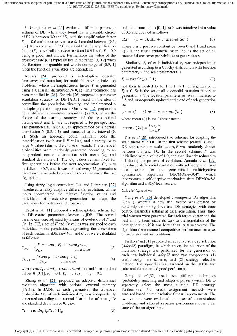
H. Scaling Analysis

In this analysis, the relationship between the dimensionality of the test problem and the average number of function evaluations needed to find solutions with the tolerance limit (here is equal to 0.0001) is derived. Two test problems from CEC 2010 i.e. C07 and C09 have been chosen for the purpose. The problems are known to be difficult as the the objective function is non-separable, multi-modal and is shifted by a matrix . Considering the constraints, C07, contains an in-equality constraint that is separable, multi-modal and also shifted by the same matrix, while C09 contains an equality constraint with the same properties as in C07. The optimal solutions of these two problems are at ∗ 0.

Both problems have been solved using different dimensions, i.e. D = 5, 10, 15, 20, 25 and 30 variables. For each D, the algorithm was run over 50 trials, and the average fitness evaluations were recorded to reach the stopping criteria. It must be mentioned here that up to only 30 variables are used, as the available data are up to 30 dimensions.

Figure 9 shows the average fitness functions for each dimension. For a further investigation, the regression line [52] is fitted to help readers to approximate the average fitness evaluations that are required for different dimensions.

So, the regression equation for C07 is:

208.58 4147 9465.6 (16)

and the coefficient of determination [52] is equal to 98.25%. This means that the line is highly fitted to predict future values.

The regression equation for C09 is:

146.37 5363.2 – 13417 (17)

and the coefficient of determination is equal to 98.84%, this means that the line is highly fitted.

This encouraging results demonstrating that the algorithm is efficient and scales well with increasing dimension. In addition, the presented lines appear quite smooth, suggesting that DE-DPS is well designed.

I. Solving Unconstrained Problems (CEC2005)

In this section, we solve and analyze the algorithm on 25 unconstrained problems (from CEC2005 competition) with 30 dimensions [18]. These problems have different mathematical properties, in which 01to 05 are shifted and/or rotated unimodal problems, 06 to 12 are shifted and/or rotated multimodal problems, 13 to 25 are hybrid composition of different problems with different difficult properties. Results on all of these test problems were derived based on 25 runs, where the maximum fitness evaluations were set to 300K. The values of the

Copyright (c) 2013 IEEE. Personal use is permitted. For any other purposes, permission must be obtained from the IEEE by emailing [email protected].

This article has been accepted for publication in a future issue of this journal, but has not been fully edited. Content may change prior to final publication. Citation information: DOI10.1109/TEVC.2013.2281528, IEEE Transactions on Evolutionary Computation

14

(a) C07

(b) C09

Fig.9. Average number of function evaluations versus the problem dimension for C07 and C09 using 50 runs. The dashed lines represent the quadratic regression fitting of the data.

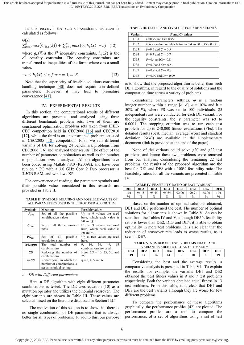
parameters are same as used in the previous sections. We have reported the mean error values from the optimal solutions of our algorithm, as reported by other researchers, along with other algorithms JADE [21], jDE [11], SaDE [12], EPSDE [39] and CoDE [28], in Appendix C.

A comparison summary is shown in table XVI. From this table, DE-DPS is clearly better for majority of the test problems. Furthermore, the performance of DE-DPS is statistically better than all other algorithms, except EPSDE, in which there is no significance difference.

TABLE XVI. COMPARISION AMONG DE-DPS, AND JADE, jDE, SaDE, EPSDE, AND CoDE

(THE NUMBERS SHOWN IN THE TABLE ARE FOR THE FIRST ALGORITHM IN COLUMN 1)

Algorithms Better Equal Worse Dec. DE-DPS- to- JADE 14 9 2 DE-DPS- to- jDE 15 9 1

DE-DPS- to- SaDE 18 4 3 DE-DPS- to- EPSDE 17 2 6 DE-DPS- to- CoDE 14 9 2

The performance profiles are depicted in Fig.10 with the comparison goal as the average fitness values after

300,000 fitness evaluations. Note that the data are not available to consider other comparison goals. Based on this figure, DE-DPS is the best algorithm, as it is able to reach 1 when 6.25. To add to this, all JADE, SaDE

Fig. 10. The average fitness values performance profiles comparing DE-DPS with various DE algorithms

and CODE are competetive, while both jDE and EPSDE are the worst algorithms.

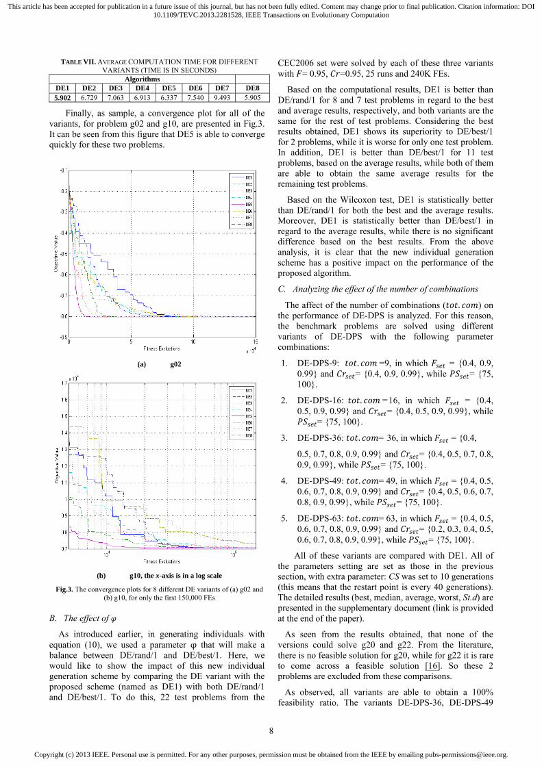
To this end, a sample of different convergence plots of DE-DPS is presented in Fig. 11.

Fig. 11. Convergence plot of DE-DSP for various test problems.

J. The contribution of population size switching

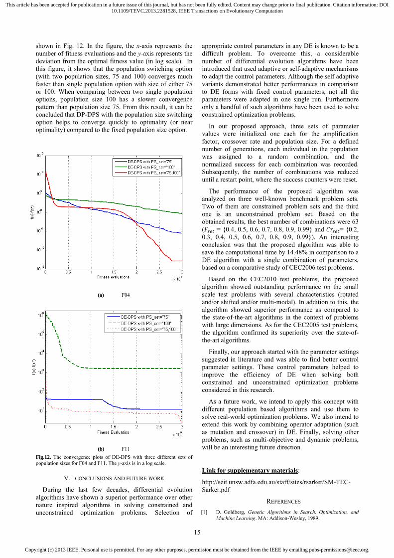
The benefit of switching the population size, during the evolution process, is demonstrated using two test problems (F04 and F11). We have solved these two test problems using our algorithm with fixed population sizes of 75 and 100 (i.e., without population adaptation option), and with an option of switching between these two population sizes (as of the proposed DP-DPS algorithm). The convergence plots, comparing these three population size options, are

Copyright (c) 2013 IEEE. Personal use is permitted. For any other purposes, permission must be obtained from the IEEE by emailing [email protected].

This article has been accepted for publication in a future issue of this journal, but has not been fully edited. Content may change prior to final publication. Citation information: DOI10.1109/TEVC.2013.2281528, IEEE Transactions on Evolutionary Computation

15

shown in Fig. 12. In the figure, the x-axis represents the number of fitness evaluations and the y-axis represents the deviation from the optimal fitness value (in log scale). In this figure, it shows that the population switching option (with two population sizes, 75 and 100) converges much faster than single population option with size of either 75 or 100. When comparing between two single population options, population size 100 has a slower convergence pattern than population size 75. From this result, it can be concluded that DP-DPS with the population size switching option helps to converge quickly to optimality (or near optimality) compared to the fixed population size option.

(a) F04

(b) F11

Fig.12. The convergence plots of DE-DPS with three different sets of population sizes for F04 and F11. The y-axis is in a log scale.

V. CONCLUSIONS AND FUTURE WORK

During the last few decades, differential evolution algorithms have shown a superior performance over other nature inspired algorithms in solving constrained and unconstrained optimization problems. Selection of

appropriate control parameters in any DE is known to be a difficult problem. To overcome this, a considerable number of differential evolution algorithms have been introduced that used adaptive or self-adaptive mechanisms to adapt the control parameters. Although the self adaptive variants demonstrated better performances in comparison to DE forms with fixed control parameters, not all the parameters were adapted in one single run. Furthermore only a handful of such algorithms have been used to solve constrained optimization problems.

In our proposed approach, three sets of parameter values were initialized one each for the amplification factor, crossover rate and population size. For a defined number of generations, each individual in the population was assigned to a random combination, and the normalized success for each combination was recorded. Subsequently, the number of combinations was reduced until a restart point, where the success counters were reset.

The performance of the proposed algorithm was analyzed on three well-known benchmark problem sets. Two of them are constrained problem sets and the third one is an unconstrained problem set. Based on the obtained results, the best number of combinations were 63 ( = {0.4, 0.5, 0.6, 0.7, 0.8, 0.9, 0.99} and = {0.2, 0.3, 0.4, 0.5, 0.6, 0.7, 0.8, 0.9, 0.99}). An interesting conclusion was that the proposed algorithm was able to save the computational time by 14.48% in comparison to a DE algorithm with a single combination of parameters, based on a comparative study of CEC2006 test problems.

Based on the CEC2010 test problems, the proposed algorithm showed outstanding performance on the small scale test problems with several characteristics (rotated and/or shifted and/or multi-modal). In addition to this, the algorithm showed superior performance as compared to the state-of-the-art algorithms in the context of problems with large dimensions. As for the CEC2005 test problems, the algorithm confirmed its superiority over the state-of-the-art algorithms.

Finally, our approach started with the parameter settings suggested in literature and was able to find better control parameter settings. These control parameters helped to improve the efficiency of DE when solving both constrained and unconstrained optimization problems considered in this research.

As a future work, we intend to apply this concept with different population based algorithms and use them to solve real-world optimization problems. We also intend to extend this work by combining operator adaptation (such as mutation and crossover) in DE. Finally, solving other problems, such as multi-objective and dynamic problems, will be an interesting future direction.

Link for supplementary materials:

http://seit.unsw.adfa.edu.au/staff/sites/rsarker/SM-TEC-Sarker.pdf

REFERENCES

[1] D. Goldberg, Genetic Algorithms in Search, Optimization, and Machine Learning. MA: Addison-Wesley, 1989.

Copyright (c) 2013 IEEE. Personal use is permitted. For any other purposes, permission must be obtained from the IEEE by emailing [email protected].

This article has been accepted for publication in a future issue of this journal, but has not been fully edited. Content may change prior to final publication. Citation information: DOI10.1109/TEVC.2013.2281528, IEEE Transactions on Evolutionary Computation

16

[2] R. Storn and K. Price, “Differential Evolution - A simple and efficient adaptive scheme for global optimization over continuous spaces,” International Computer Science Institute Technical Report, TR-95-012, 1995.

[3] I. Rechenberg, Evolutions strategie: Optimierung Technischer Systeme nach Prinzipien der biologischen Evolution. Stuttgart: Fromman-Holzboog, 1973.

[4] L. Fogel, J. Owens, and M. Walsh, Artificial Intelligence Through Simulated Evolution. New York: John Wiley & Sons, 1966.

[5] S. Das and P. N. Suganthan, “Differential Evolution: A Survey of the State-of-the-Art,” IEEE Transactions on Evolutionary Computation, vol. 15, pp. 4-31, 2011.

[6] N. Hansen, A. Auger, S. Finck, and R. Ros, “Real-parameter black-box optimization benchmarking: Noiseless functions definitions,” INRIA, 2009.

[7] J. A. Vrugt, B. A. Robinson, and J. M. Hyman, “Self-Adaptive Multimethod Search for Global Optimization in Real-Parameter Spaces,” IEEE Transactions on Evolutionary Computation, vol. 13, pp. 243-259, 2009.

[8] L. Davis, “Adapting operator probabilities in genetic algorithms,” presented at the Proceedings of the third international conference on Genetic algorithms, George Mason University, United States, 1989.

[9] A. E. Eiben and J. E. Smith, Introduction to Evolutionary Computing: Springer, 2003.

[10] J. H. Holland, Adaptation in Natural and Artificial Systems: An Introductory Analysis with Applications to Biology, Control and Artificial Intelligence. Ann Arbor. Michigan: University of Michigan Press, 1975.

[11] J. Brest, S. Greiner, B. Boskovic, M. Mernik, and V. Zumer, “Self-Adapting Control Parameters in Differential Evolution: A Comparative Study on Numerical Benchmark Problems,” IEEE Transactions on Evolutionary Computation, vol. 10, pp. 646-657, 2006.

[12] A. K. Qin, V. L. Huang, and P. N. Suganthan, “Differential Evolution Algorithm With Strategy Adaptation for Global Numerical Optimization,” IEEE Transactions on Evolutionary Computation, vol. 13, pp. 398-417, 2009.

[13] V. L. Huang, A. K. Qin, and P. N. Suganthan, “Self-adaptive Differential Evolution Algorithm for Constrained Real-Parameter Optimization,” in proceeding IEEE Congress on Evolutionary Computation, 2006, pp. 17-24.

[14] J. Teo, “Exploring dynamic self-adaptive populations in differential evolution,” Soft Computing, vol. 10, pp. 673-686, 2006/06/01 2006.

[15] J. Brest and M. Sepesy Maučec, “Population size reduction for the differential evolution algorithm,” Applied Intelligence, vol. 29, pp. 228-247, 2008.

[16] J. J. Liang, T. P. Runarsson, E. Mezura-Montes, M. Clerc, P. N. Suganthan, C. A. Coello Coello, and K. Deb, “Problem Definitions and Evaluation Criteria for the CEC 2006 Special Session on Constrained Real-Parameter Optimization,” Technical Report, Nanyang Technological University, Singapore, 2005.

[17] R. Mallipeddi and P. N. Suganthan, “Problem definitions and evaluation criteria for the CEC 2010 competition and special session on single objective constrained real-parameter optimization,” Technical Report, Nangyang Technological University, Singapore, 2010.

[18] P. N. Suganthan, N. Hansen, J. J. Liang, K. Deb, Y.-P. Chen, A. Auger, and S. Tiwari, “Problem Definitions and Evaluation Criteria for the CEC 2005 Special Session on Real-Parameter Optimization,” Nanyang Technological University and Kanpur, Singapore and India, 2005.

[19] V. Feoktistov and S. Janaqi, “Generalization of the strategies in differential evolution,” in proceeding Parallel and Distributed Processing Symposium, 2004. Proceedings. 18th International, 2004, p. 165.

[20] K. V. Price, R. M. Storn, and J. A. Lampinen, Differential evolution: a practical approach to global optimization. Berlin: Springer, 2005.

[21] Z. Jingqiao and A. C. Sanderson, “JADE: Adaptive Differential Evolution With Optional External Archive,” IEEE Transactions on Evolutionary Computation, vol. 13, pp. 945-958, 2009.

[22] R. Gämperle, S. D. Müller, and P. Koumoutsakos, “Parameter study for differential evolution,” in proceeding WSEAS Int. Conf. on Advances in Intelligent Systems, Fuzzy Systems, Evolutionary Computation 2002, pp. 293–298.

[23] J. Rönkkönen, “Continuous Multimodal Global Optimization with Differential Evolution-Based Methods,” Thesis for the degree of Doctor of Science, Lappeenranta University of Technology, Lappeenranta, Finland, ISBN 978-952-214-851-3, 2009.

[24] H. A. Abbass, “The self-adaptive Pareto differential evolution algorithm,” in proceeding IEEE Congress on Evolutionary Computation., 2002, pp. 831-836.

[25] S. M. Elsayed, R. A. Sarker, and D. L. Essam, “Multi-operator based evolutionary algorithms for solving constrained optimization Problems,” Computers and Operations Research, vol. 38, pp. 1877-1896, 2011.

[26] D. Zaharie, “Control of population diversity and adaptation in differential evolution algorithms,” in proceeding the 9th International Conference on Soft Computing, 2003, pp. 41–46.

[27] J. Liu and J. Lampinen, “A Fuzzy Adaptive Differential Evolution Algorithm,” Soft Computing - A Fusion of Foundations, Methodologies and Applications, vol. 9, pp. 448-462, 2005.

[28] S. Das, A. Konar, and U. K. Chakraborty, “Two improved differential evolution schemes for faster global search,” presented at the the 2005 conference on Genetic and evolutionary computation, Washington DC, USA, 2005.

[29] A. Zamuda, J. Brest, B. Boskovic, and V. Zumer, “Differential Evolution with Self-adaptation and Local Search for Constrained Multiobjective Optimization,” in proceeding IEEE Congress on Evolutionary Computation., 2009, pp. 195-202.

[30] W. Yong, C. Zixing, and Z. Qingfu, “Differential Evolution With Composite Trial Vector Generation Strategies and Control Parameters,” IEEE Transactions on Evolutionary Computation, vol. 15, pp. 55-66, 2011.

[31] Á. Fialho, R. Ros, M. Schoenauer, and M. Sebag, “Comparison-based adaptive strategy selection with bandits in differential evolution,” presented at the Proceedings of the 11th international conference on Parallel problem solving from nature: Part I, 2010.

[32] W. Gong, Á. Fialho, Z. Cai, and H. Li, “Adaptive strategy selection in differential evolution for numerical optimization: An empirical study,” Inf. Sci., vol. 181, pp. 5364-5386, 2011.

[33] E. da Silva, H. Barbosa, and A. Lemonge, “An adaptive constraint handling technique for differential evolution with dynamic use of variants in engineering optimization,” Optimization and Engineering, vol. 12, pp. 31-54, 2011.

[34] X. Yang and G. Liu, “Self-adaptive Clustering-Based Differential Evolution with New Composite Trial Vector Generation Strategies. Proceedings of the 2011 2nd International Congress on Computer Applications and Computational Science.” vol. 144, F. L. Gaol and Q. V. Nguyen, Eds., ed: Springer Berlin / Heidelberg, 2012, pp. 261-267.

[35] A. Zamuda and J. Brest, “Population Reduction Differential Evolution with Multiple Mutation Strategies in Real World Industry Challenges. Swarm and Evolutionary Computation.” vol. 7269, L. Rutkowski, et al., Eds., ed: Springer Berlin / Heidelberg, 2012, pp. 154-161.

[36] J. Tvrdík, “Adaptation in differential evolution: A numerical comparison,” Applied Soft Computing, vol. 9, pp. 1149-1155, 2009.

[37] J. Tvrdík and R. Poláková, “Competitive differential evolution for constrained problems,” in proceeding EEE Congress on Evolutionary Computation (CEC), 2010, pp. 1-8.

[38] R. Mallipeddi and P. N. Suganthan, “Differential evolution algorithm with ensemble of populations for global numerical optimization,” OPSEARCH, vol. 46, pp. 184–213, 2009.

[39] R. Mallipeddi, S. Mallipeddi, P. N. Suganthan, and M. F. Tasgetiren, “Differential evolution algorithm with ensemble of parameters and mutation strategies,” Applied Soft Computing, vol. 11, pp. 1679-1696, 2011.

[40] K. Deb, “An Efficient Constraint Handling Method for Genetic Algorithms,” Computer Methods in Applied Mechanics and Engineering, vol. 186, pp. 311-338, 2000.

[41] E. Mezura-Montes and C. A. Coello Coello, “Constraint-handling in nature-inspired numerical optimization: Past, present and future,” Swarm and Evolutionary Computation, vol. 1, pp. 173-194, 2011.

[42] H. J. C. Barbosa, H. S. Bernardino, and A. M. S. Barreto, “Using performance profiles to analyze the results of the 2006 CEC constrained optimization competition,” in proceeding IEEE Congress on Evolutionary Computation (CEC), 2010, pp. 1-8.

[43] G. W. Corder and D. I. Foreman, Nonparametric Statistics for Non-Statisticians: A Step-by-Step Approach. Hoboken, NJ: John Wiley, 2009.

Copyright (c) 2013 IEEE. Personal use is permitted. For any other purposes, permission must be obtained from the IEEE by emailing [email protected].

This article has been accepted for publication in a future issue of this journal, but has not been fully edited. Content may change prior to final publication. Citation information: DOI10.1109/TEVC.2013.2281528, IEEE Transactions on Evolutionary Computation

17

[44] E. Mezura-Montes, J. Velazquez-Reyes, and C. A. Coello Coello, “Modified Differential Evolution for Constrained Optimization,” in proceeding IEEE Congress on Evolutionary Computation, 2006, pp. 25-32.

[45] B. Tessema and G. G. Yen, “An Adaptive Penalty Formulation for Constrained Evolutionary Optimization,” IEEE Transactions on Systems, Man and Cybernetics, Part A: Systems and Humans, vol. 39, pp. 565-578, 2009.

[46] R. Mallipeddi and P. N. Suganthan, “Ensemble of Constraint Handling Techniques,” IEEE Transactions on Evolutionary Computation, vol. 14, pp. 561-579, 2010.

[47] J. Brest, V. Zumer, and M. S. Maucec, “Self-Adaptive Differential Evolution Algorithm in Constrained Real-Parameter Optimization,” in proceeding IEEE Congress on Evolutionary Computation, 2006, pp. 215-222.

[48] W. Yong, C. Zixing, Z. Yuren, and Z. Wei, “An Adaptive Tradeoff Model for Constrained Evolutionary Optimization,” IEEE Transactions on Evolutionary Computation, vol. 12, pp. 80-92, 2008.

[49] T. Takahama and S. Sakai, “Constrained optimization by the ε constrained differential evolution with an archive and gradient-based mutation,” in proceeding IEEE Congress on Evolutionary Computation, 2010, pp. 1-9.

[50] R. Mallipeddi and P. N. Suganthan, “Differential evolution with ensemble of constraint handling techniques for solving CEC 2010 benchmark problems,” in proceeding IEEE Congress on Evolutionary Computation, 2010, pp. 1-8.

[51] J. Brest, B. Boškovič, and V. Žumer, “An improved self-adaptive differential evolution algorithm in single objective constrained real-parameter optimization,” in proceeding IEEE Congress on Evolutionary Computation 2010, pp. 1-8.

[52] D. C. Montgomery, E. A. Peck, and G. G. Vining, Introduction to Linear Regression Analysis, 4th Edition. New York: John Wiley and Sons, 2006.

Copyright (c) 2013 IEEE. Personal use is permitted. For any other purposes, permission must be obtained from the IEEE by emailing [email protected].

This article has been accepted for publication in a future issue of this journal, but has not been fully edited. Content may change prior to final publication. Citation information: DOI10.1109/TEVC.2013.2281528, IEEE Transactions on Evolutionary Computation

18

APPENDIX A FUNCTION VALUES OBTAINED BY DE-DPS, MDE, SAMO-DE, APF-GA, ECHT-EP2, JDE-2, ATMES AND SMES FOR THE CEC2006 TEST

PROBLEMS

P. Criteria DE-DPS MDE SAMO-DE APF-GA ECHT-EP2 jDE-2 SaDE ATMES

FEs 240,000 500,000 240,000 500,000 240,000 500,000 500,000 240,000

g01

best -15.0000 -15.0000 -15.0000 -15.0000 -15.0000 -15.0000 -15.0000 -15.0000 Avg. -15.0000 -15.0000 -15.0000 -15.0000 -15.0000 -15.0000 -15.0000 -15.0000 St. d 0.00E+00 0.00E+00 0.00E+00 0.00E+00 0.00E+00 0.00E+00 0.00E+00 1.6E-14

g02

best -0.8036191 -0.8036191 -0.8036191 -0.803601 -0.8036191 -0.8036191 -0.8036191 -0.803339 Avg. -0.8036191 -0.78616 -0.79873521 -0.803518 -0.7998220 -0.8027382 -0.8015631 -0.790148 St. d 9.06255E-08 1.26E-02 8.8005E-03 1.00E-04 6.29E-03 3.0488E-03 4.9786E-03 1.3E-02

g03

best -1.0005 -1.0005 -1.0005 -1.001 -1.0005 -0.9115 -1.0005 -1.000 Avg. -1.0005 -1.0005 -1.0005 -1.001 -1.0005 -0.66242 -1.000486 -1.000 St. d 0.00E+00 0.00E+00 0.00E+00 0.00E+00 0.00E+00 1.014E-01 3.4743E-005 5.9E-05

g04

best -30665.539 -30665.539 -30665.5386 -30665.539 -30665.539 -30665.539 -30665.539 -30665.539 Avg. -30665.539 -30665.539 -30665.5386 -30665.539 -30665.539 -30665.539 -30665.539 -30665.539 St. d 0.00E+00 0.00E+00 0.00E+00 1.00E-04 0.00E+00 0.00E+00 1.8550E-12 7.4E-12

g05

best 5126.497 5126.497 5126.497 5126.497 5126.497 5126.497 5126.497 5126.498 Avg. 5126.497 5126.497 5126.497 5127.5423 5126.497 5127.5726 5126.497 5127.648 St. d 0.00E+00 0.00E+00 0.00E+00 1.4324E+00 0.00E+00 2.4193 1.8190E-13 1.8E+00

g06

best -6961.814 -6961.814 -6961.813875 -6961.814 -6961.814 -6961.814 -6961.814 -6961.814 Avg. -6961.814 -6961.814 -6961.813875 -6961.814 -6961.814 -6961.814 -6961.814 -6961.814St. d 0.00E+00 0.00E+00 0.00E+00 0.00E+00 0.00E+00 0.00E+00 0.00E+00 4.6E-12

g07

best 24.3062 24.3062 24.3062 24.3062 24.3062 24.3062 24.3062 24.306 Avg. 24.3062 24.3062 24.3096 24.3062 24.3063 24.3062 24.3062 24.316 St. d 0.00E+00 0.00E+00 1.5888E-03 0.00E+00 3.19E-05 1.7405E-15 1.4993E-05 1.1E-02

g08

best -0.095825 -0.095825 -0.095825 -0.095825 -0.095825 -0.095825 -0.095825 -0.095825 Avg. -0.095825 -0.095825 -0.095825 -0.095825 -0.095825 -0.095825 -0.095825 -0.095825 St. d 0.00E+00 0.00E+00 0.00E+00 0.00E+00 0.0E+00 1.2580E-32 3.8426E-18 2.8E-17

g09

best 680.630 680.630 680.630 680.630 680.630 680.630 680.630 680.630Avg. 680.630 680.630 680.630 680.630 680.630 680.630 680.630 680.639 St. d 0.00E+00 0.00E+00 1.1567E-05 0.00E+00 2.61E-08 4.2538E-14 7.9851E-14 1.0E-02

g10

best 7049.24802 7049.24802 7049.24802 7049.24802 7049.2483 7049.24802 7049.24802 7052.253 Avg. 7049.24802 7049.24802 7059.81345 7077.6821 7049.2490 7049.24802 7049.24802 7250.437 St. d 0.00E+00 0.00E+00 7.856E+00 5.1240E+01 6.60E-04 9.1279E-08 1.5244E-06 1.2E+02

g11

best 0.7499 0.7499 0.7499 0.7499 0.7499 0.7499 0.7499 0.75 Avg. 0.7499 0.7499 0.7499 0.7499 0.7499 0.7499000091 0.7499 0.75 St. d 0.00E+00 0.00E+00 0.00E+00 0.00E+00 0.00E+00 4.5540E-04 0.00E+00 3.4E-04

g12

best -1.0000 -1.0000 -1.0000 -1.0000 -1.0000 -1.0000 -1.0000 -1.0000 Avg. -1.0000 -1.0000 -1.0000 -1.0000 -1.0000 -1.0000 -1.0000 -1.0000 St. d 0.00E+00 0.00E+00 0.00E+00 0.00E+00 0.00E+00 0.00E+00 0.00E+00 1.0E-03

g13

best 0.053942 0.053942 0.053942 0.053942 0.053942 0.350942 0.053942 0.053950Avg. 0.053942 0.053942 0.053942 0.053942 0.053942 0.745422 0.053942 0.053959 St. d 0.00E+00 0.00E+00 1.7541E-08 0.00E+00 1.00E−12 2.2376E-01 2.7832E-07 1.3E-05

g14

best -47.764888 -47.764887 -47.76489 -47.76479 -47.7649 -47.764888 -47.764888 - Avg. -47.764888 -47.764874 -47.68115 -47.76479 -47.7648 -47.764888 -47.764841 - St. d 0.00E+00 1.400E-05 4.043E-02 1.00E-04 2.72E-05 3.4809E-15 6.4986E-005 -

g15

best 961.71502 961.71502 961.71502 961.71502 961.71502 961.71502 961.71502 - Avg. 961.71502 961.71502 961.71502 961.71502 961.71502 961.719424 961.71502 - St. d 0.00E+00 0.00E+00 0.00E+00 0.00E+00 2.01E-13 2.2020E-02 0.00E+00 -

g16

best -1.905155 -1.905155 -1.905155 -1.905155 -1.905155 -1.905155 -1.905155 - Avg. -1.905155 -1.905155 -1.905155 -1.905155 -1.905155 -1.905155 -1.905155 - St. d 0.00E+00 0.00E+00 0.00E+00 0.00E+00 1.12E-10 0.00E+00 0.00E+00 -

g17

best 8853.5397 8853.5397 8853.5397 8853.5398 8853.5397 8853.5397 8853.5397 - Avg. 8883.77467 8853.5397 8853.5397 8888.4876 8853.5397 8853.5397 8923.2097 - St. d 3.56207E+01 0.00E+00 1.1500E-05 29.0347 2.13E−08 3.6822E-17 1.6168E+01 -

g18

best -0.866025 -0.866025 -0.866025 -0.866025 -0.866025 -0.866025 -0.866025 - Avg. -0.866025 -0.866025 -0.866024 -0.865925 -0.866025 -0.866025 -0.850741 - St. d 0.00E+00 0.00E+00 7.043672E-07 0000 1.00E-09 3.6822E-17 5.2898E-02 -

g19

best 32.655593 32.655693 32.655593 32.655593 32.6591 32.655593 32.655593 - Avg. 32.655593 33.34125 32.757340 32.655593 32.6623 32.655593 32.655593 - St. d 2.52789E-07 8.475E-01 6.145E-02 0.00E+00 3.4E−03 1.0531E-13 7.2976E-10 -

g21

best 193.72451 193.72451 193.724510 196.63301 193.7246 193.7246 193.72451 - Avg. 193.72451 193.72451 193.771375 199.51581 193.7438 204.2026 193.72528 - St. d 0.00E+00 0.00E+00 1.9643E-02 2.3565E+00 1.65E-02 3.6266E+01 1.5058E-03 -

g23

best -400.0551 -400.0551 -396.165732 -399.7624 -398.9731 -400.0551 -400.0551 - Avg. -400.0551 -400.0551 -360.817656 -394.7627 -373.2178 -387.9531 -400.054979 - St. d 0.00E+00 0.00E+00 1.9623E+01 3.8656E+00 3.37E+01 5.9983E+01 3.4116E-04 -

g24

best -5.508013 -5.508013 -5.508013 -5.508013 -5.508013 -5.508013 -5.508013 - Avg. -5.508013 -5.508013 -5.508013 -5.508013 -5.508013 -5.508013 -5.508013 - St. d 0.00E+00 0.00E+00 0.00E+00 0.00E+00 1.8E-15 1.9323E-29 0.00E+00 -

Copyright (c) 2013 IEEE. Personal use is permitted. For any other purposes, permission must be obtained from the IEEE by emailing [email protected].

This article has been accepted for publication in a future issue of this journal, but has not been fully edited. Content may change prior to final publication. Citation information: DOI10.1109/TEVC.2013.2281528, IEEE Transactions on Evolutionary Computation

19

APPENDIX B FUNCTION VALUES ACHIEVED BY DE-DPS, ΕDEAG, ECHT-DE AND JDEsoco FOR THE CEC2010 TEST PROBLEMS

Prob. Alg. 10D 30D

Best Mean St. d Best Mean St. d C01 DE-DPS -7.473104E-01 -7.473104E-01 2.26623E-16 -0.8218843 -0.8212036 1.79648E-03

εDEag -7.473104E-01 -7.470402E-01 1.323339E-03 -8.218255E-01 -8.208687E-01 7.103893E-04 ECHT-DE -0.7473 -0.7470 0.0014 -0.8217 -0.7994 0.0179jDEsoco -0.7473103 -7.3836E-01 1.6006E-02 -0.8218841 -8.1238E-01 1.3187E-02

C02 DE-DPS -2.277711 -2.277512 2.54035E-04 -2.280671 -2.244631 5.20548E-02 εDEag -2.277702E+00 -2.269502E+00 2.3897790E-02 -2.169248E+00 -2.151424E+00 1.197582E-02

ECHT-DE -2.2777 -2.2744 0.0067 -2.2251 -1.9943 0.2099jDEsoco -1.1176240 5.6359E-01 1.1044 0.6792295 1.5603 8.4705E-01

C03 DE-DPS 0.000000E+00 0.000000E+00 0.0000000E+00 1.6200E-19 1.8479E-13 4.17994E-13 εDEag 0.000000E+00 0.000000E+00 0.0000000E+00 2.867347E+01 2.883785E+01 8.047159E-01

ECHT-DE 0.00000E+00 0.00000E+00 0.00000E+00 3.2433E-21 9.8920E+01 6.2594E+01 jDEsoco 0.00000E+00 7.8105 2.9437 9.993685E-22 6.1447E+01 5.7577E+01

C04 DE-DPS -1.000000E-05 -1.000000E-05 9.09633E-15 -3.3318E-06 -3.3123E-06 2.03926E-08 εDEag -9.992345E-06 -9.918452E-06 1.5467300E-07 4.698111E-03 8.162973E-03 3.067785E-03

ECHT-DE -1.00000E-05 -1.00000E-05 0.00000E+00 -3.3015E-06 -1.0257E-06 9.0135E-02 jDEsoco -1.00000E-05 -1.00000E-05 9.4831E-16 8.0490978E-05 3.5187E-04 2.3948E-04

C05 DE-DPS -4.836106E+02 -4.836106E+02 1.25826E-10 -4.836106E+02 -4.836106E+02 4.42074E-06 εDEag -4.836106E+02 -4.836106E+02 3.89035E-13 -4.531307E+02 -4.495460E+02 2.899105E+00

ECHT-DE -483.6106 -411.4532 76.3137 -213.6844 -106.4228 167.1481 jDEsoco -483.6106247 -3.0217E+02 3.0256E+02 -19.9503700 1.0822E+02 1.5203E+02

C06 DE-DPS -5.786624E+02 -578.6621 8.05379E-04 -530.63785 -530.6329 5.89364E-03 εDEag -5.786581E+02 -5.786528E+02 3.6271690E-03 -5.285750E+02 -5.279068E+02 4.748378E-01

ECHT-DE -578.6624 -562.4688 45.1479 -295.7192 -137.6152 98.8995 jDEsoco -578.662366 -5.7408E+02 1.6461E+01 -530.6377271 -4.7284E+02 1.2743E+02

C07 DE-DPS 0.00000E+00 0.000000E+00 0.0000000E+00 5.48786E-20 1.03359E-13 2.20540E-13 εDEag 0.00000E+00 0.000000E+00 0.0000000E+00 1.147112E-15 2.603632E-15 1.233430E-15

ECHT-DE 0.00000E+00 0.00000E+00 0.00000E+00 0.00000E+00 0.1329 0.7279 jDEsoco 0.00000E+00 6.4192E-27 1.3515E-26 4.2197747E-26 8.7396E-24 3.2529E-23

C08 DE-DPS 0.00000E+00 3.950387E+00 5.01904E+00 4.575719E-13 3.447568E-09 8.86366E-09 εDEag 0.00000E+00 6.727528E+00 5.560648E+00 2.518693E-14 7.831464E-14 4.855177E-14

ECHT-DE 0.00000E+00 6.1566E+00 6.4527E+00 0.00000E+00 3.3585E+01 1.1072E+02 jDEsoco 0.00000E+00 3.7421 1.0330E+01 7.2310934E-26 8.2585E+01 2.4395E+02

C09 DE-DPS 0.00000E+00 0.000000E+00 0.0000000E+00 3.81580E-23 5.29059E-14 1.27939E-13 εDEag 0.00000E+00 0.000000E+00 0.0000000E+00 2.770665E-16 1.072140E+01 2.821923E+01

ECHT-DE 0.00000E+00 1.4691E-01 8.0482E-01 0.00000E+00 4.2441E+01 1.3762E+02 jDEsoco 0.00000E+00 5.2898E-01 1.4620 2.7729234E-25 2.4743 8.7782

C10 DE-DPS 0.000000E+00 0.000000E+00 0.0000000E+00 1.63778E-21 2.23928E-13 6.24058E-13 εDEag 0.000000E+00 0.000000E+00 0.0000000E+00 3.252002E+01 3.326175E+01 4.545577E-01

ECHT-DE 0.00000E+00 1.7117E+00 7.6554E+00 0.00000E+00 5.3381E+01 8.8308E+01jDEsoco 0.00000E+00 3.1712E+01 1.8188E+01 1.0862047E-25 2.9386E+01 7.1786

C11 DE-DPS -1.52271E-03 -1.52271E-03 3.14275E-12 -3.923438E-04 -3.923423E-04 8.77688E-10 εDEag -1.52271E-03 -1.52271E-03 6.3410350E-11 -3.268462E-04 -2.863882E-04 2.707605E-05

ECHT-DE -0.0015 -0.0044* 0.0157 -0.0004 0.0026 0.0060 jDEsoco -0.0015227 -8.2555E-03* 2.3807E-02 -0.0003920 1.1667E-03 5.2690E-03

C12 DE-DPS -1.9925E-01 -1.9925E-01 4.19599E-10 -1.992635E-01 -1.9926E-01 2.60287E-08 εDEag -5.700899E+02 -3.367349E+02 1.7821660E+02 -1.991453E-01 3.562330E+02 2.889253E+02

ECHT-DE -0.1992 -171.8714* 221.0436 -0.1993 -25.1292* 136.5593 jDEsoco -0.1992457 -2.2365E+01* 1.1083E+02 -0.1992634 -1.9925E-01 2.3453E-05

C13 DE-DPS -6.842937E+01 -6.842937E+01 0.0000000E+00 -68.429362 -66.331412 2.08493E+00 εDEag -6.842937E+01 -6.842936E+01 1.0259600E-06 -6.642473E+01 -6.535310E+01 5.733005E-01

ECHT-DE -68.4294 -65.1208 2.3750 -68.4294 -64.5831 1.6690 jDEsoco -68.4293648 -6.8315E+01 5.7018E-01 -68.4293209 -6.7537E+01 5.0553E-01

C14 DE-DPS 0.000000E+00 0.000000E+00 0.0000000E+00 8.925796E-21 5.137406E-14 1.31791E-13 εDEag 0.000000E+00 0.000000E+00 0.0000000E+00 5.015863E-14 3.089407E-13 5.608409E-13

ECHT-DE 0.00000E+00 7.0242E+05 3.1937E+06 0.00000E+00 1.2368E+05 6.7736E+05jDEsoco 0.00000E+00 9.1221E-01 2.4538 5.7101696E-26 1.5946E-01 7.9732E-01

C15 DE-DPS 0.000000E+00 5.438912E-26 2.19329E-25 6.336258E-20 1.957805E-13 5.22687E-13 εDEag 0.000000E+00 1.798980E-01 8.8131560E-01 2.160345E+01 2.160376E+01 1.104834E-04

ECHT-DE 0.00000E+00 2.3392E+13 5.2988E+13 1.9922E+09 1.9409E+11 4.3524E+11 jDEsoco 2.0257948E-26 1.2452E+09 3.8127E+09 9.6993452E-16 1.5357E+09 1.6045E+09

C16 DE-DPS 0.000000E+00 0.000000E+00 0.0000000E+00 0.000000E+00 0.000000E+00 0.0000000E+00 εDEag 0.000000E+00 3.702054E-01 3.7104790E-01 0.000000E+00 2.168404E-21 1.062297E-20

ECHT-DE 0.00000E+00 3.9327E-02 4.2815E-02 0.00000E+00 0.00000E+00 0.00000E+00 jDEsoco 0.000000E+00 4.1102E-01 3.8359E-01 0.0812907 7.3206E-01 2.9943E-01

C17 DE-DPS 0.000000E+00 1.061273E-24 3.88726E-24 3.236013E-12 8.766191E-02 1.55966E-01 εDEag 1.463180E-17 1.249561E-01 1.9371970E-01 2.165719E-01 6.326487E+00 4.986691E+00

ECHT-DE 0.00000E+00 1.1152E-01 3.3152E-01 0.00000E+00 2.7496E-01 3.7832E-01 jDEsoco 0.0302187 8.8958E+01 9.9131E+01 2.9943E-01 5.0398E+02 4.4832E+02

C18 DE-DPS 0.000000E+00 3.209082E-23 7.12457E-23 6.747743E-13 9.459914E-08 1.91224E-07 εDEag 3.731440E-20 9.678765E-19 1.8112340E-18 1.226054E+00 8.754569E+01 1.664753E+02

ECHT-DE 0.00000E+00 0.00000E+00 0.00000E+00 0.00000E+00 0.00000E+00 0.00000E+00 jDEsoco 0.1100901 4.0500E+02 7.3762E+02 17.5655328 3.0849E+02 3.0538E+02

Copyright (c) 2013 IEEE. Personal use is permitted. For any other purposes, permission must be obtained from the IEEE by emailing [email protected].

This article has been accepted for publication in a future issue of this journal, but has not been fully edited. Content may change prior to final publication. Citation information: DOI10.1109/TEVC.2013.2281528, IEEE Transactions on Evolutionary Computation

20

APPENDIX C

THE MEAN ERROR TO THE OPTIMAL SOLUTIONS AND STANDARD DEVIATION RESULTS OF DE-DPS, JADE, JDE, SADE, EPSDE, AND CODE OVER 25 INDEPENDENT RUNS ON 25 TEST FUNCTIONS WITH 30 VARIABLES FOR

CEC2005 TEST SET WITH 300 000 FES

Problem (optimal)

Criteria Algorithms

DE-DPS JADE jDE SaDE EPSDE CoDE F1

(-450) Mean Error

(St. d) 0.00E+00

(0.00E+00) 0.00E+00

(0.00E+00) 0.00E+00

(0.00E+00) 0.00E+00

(0.00E+00) 0.00E+00

(0.00E+00) 0.00E+00

(0.00E+00) F2

(-450) Mean Error

(St. d) 0.00E+00

(0.00E+00) 1.07E-28

(1.00E-28) 1.11E-06

(1.96E-06) 8.26E-06

(1.65E-05) 4.23E-26

(4.07E-26) 1.69E-15

(3.95E-15) F3

(-450) Mean Error

(St. d) 5.02E+04

(2.24E+04) 8.42E+03

(7.26E+03)1.98E+05

(1.10E+05) 4.27E+05

(2.08E+05) 8.74E+05

(3.28E+06) 1.05E+05

(6.25E+04) F4

(-310) Mean Error

(St. d) 0.00E+00

(0.00E+00) 1.73E-16

(5.43E-16) 4.40E-02

(1.26E-01) 1.77E+02

(2.67E+02) 3.49E+02

(2.23E+03) 5.81E-03

(1.38E-02) F5

(-310) Mean Error

(St. d) 5.68E-14

(2.05E-13) 8.59E-08

(5.23E-07) 5.11E+02

(4.40E+02) 3.25E+03

(5.90E+02) 1.40E+03

(7.12E+02) 3.31E+02

(3.44E+02) F6

(390) Mean Error

(St. d) 0.00E+00

(0.00E+00) 1.02E+01

(2.96E+01) 2.35E+01

(2.50E+01) 5.31E+01

(3.25E+01) 6.38E-01

(1.49E+00) 1.60E-01

(7.85E-01) F7

(-180) Mean Error

(St. d) 3.75E-03

(4.39E-03) 8.07E-03

(7.42E-03) 1.18E-02

(7.78E-03) 1.57E-02

(1.38E-02) 1.77E-02

(1.34E-02) 7.46E-03

(8.55E-03) F8

(-140) Mean Error

(St. d) 2.09E+01 (4.08E-02) 

2.09E+01 (1.68E-01)

2.09E+01 (4.86E-02)

2.09E+01 (4.95E-02)

2.09E+01 (5.81E-02)

2.01E+01 (1.41E-01)

F9 (-330)

Mean Error (St. d)

0.00E+00 (0.00E+00)

0.00E+00 (0.00E+00)

0.00E+00 (0.00E+00)

2.39E-01 (4.33E-01)

3.98E-02 (1.99E-01)

0.00E+00 (0.00E+00)

F10 (-330)

Mean Error (St. d)

2.29E+01 (6.14E+00)

2.41E+01 (4.61E+00)

5.54E+01 (8.46E+00)

4.72E+01 (1.01E+01)

5.36E+01 (3.03E+01)

4.15E+01 (1.16E+01)

F11 (90)

Mean Error (St. d)

9.27E+00 (3.24E+00) 

2.53E+01 (1.65E+00)

2.79E+01 (1.61E+00)

1.65E+01 (2.42E+00)

3.56E+01 (3.88E+00)

1.18E+01 (3.40E+00)

F12 (-460)

Mean Error (St. d))

1.01E+03 (1.40E+03) 

6.15E+03 (4.79E+03)

8.63E+03 (8.31E+03)

3.02E+03 (2.33E+03)

3.58E+04 (7.05E+03)

3.05E+03 (3.80E+03)

F13 (-130)

Mean Error (St. d). d)

1.99E+00 (4.13E-01)

1.49E+00 (1.09E-01)

1.66E+00 (1.35E-01)

3.94E+00 (2.81E-01)

1.94E+00 (1.46E-01)

1.57E+00 (3.27E-01)

F14 (-300)

Mean Error (St. d)

1.23E+01 (5.05E-01) 

1.23E+01 (3.11E-01)

1.30E+01 (2.00E-01)

1.26E+01 (2.83E-01)

1.35E+01 (2.09E-01)

1.23E+01 (4.81E-01)

F15 (120)

Mean Error (St. d)

3.08E+02 (9.092E+01)

3.51E+02 (1.28E+02)

3.77E+02 (8.02E+01)

3.76E+02 (7.83E+01)

2.12E+02 (1.98E+01)

3.88E+02 (6.85E+01)

F16 (120)

Mean Error (St. d)

5.20E+01 (8.80E+00)

1.01E+02 (1.24E+02)

7.94E+01 (2.96E+01)

8.57E+01 (6.94E+01)

1.22E+02 (9.19E+01)

7.37E+01 (5.13E+01)

F17 (120)

Mean Error (St. d)

5.35E+01 (2.40E+01) 

1.47E+02 (1.33E+02)

1.37E+02 (3.80E+01)

7.83E+01 (3.76E+01)

1.69E+02 (1.02E+02)

6.67E+01 (2.12E+01)

F18 (10)

Mean Error (St. d)

9.04E+02 (2.85E-01)

9.04E+02 (1.03E+00)

9.04E+02 (1.08E+01)

8.68E+02 (6.23E+01)

8.20E+02 (3.35E+00)

9.04E+02 (1.04E+00)

F19 (10)

Mean Error (St. d)

9.04E+02 (3.64E-01)

9.04E+02 (8.40E-01)

9.04E+02 (1.11E+00)

8.74E+02 (6.22E+01)

8.21E+02 (3.35E+00)

9.04E+02 (9.42E-01)

F20 (10)

Mean Error (St. d)

9.04E+02 (3.25E-01) 

9.04E+02 (8.47E-01)

9.04E+02 (1.10E+00)

8.78E+02 (6.03E+01)

8.22E+02 (4.17E+00)

9.04E+02 (9.01E-01)

F21 (360)

Mean Error (St. d)

5.00E+02 (0.00E+00)

5.00E+02 (4.67E-13)

5.00E+02 (4.80E-13)

5.52E+02 (1.82E+02)

8.33E+02 (1.00E+02)

5.00E+02 (4.88E-13)

F22 (360)

Mean Error (St. d)

8.60E+02 (3.61E+01) 

8.66E+02 (1.91E+01)

8.75E+02 (1.91E+01)

9.36E+02 (1.83E+01)

5.07E+02 (7.26E+00)

8.63E+02 (2.43E+01)

F23 (360)

Mean Error (St. d)

5.34E+02 (3.86E-04) 

5.50E+02 (8.05E+01)

5.34E+02 (2.77E-04)

5.34E+02 (3.57E-03)

8.58E+02 (6.82E+01)

5.34E+02 (4.12E-04)

F24 (220)

Mean Error (St. d)

2.00E+02 (0.00E+00)

2.00E+02 (2.85E-14)

2.00E+02 (2.85E-14)

2.00E+02 (6.20E-13)

2.13E+02 (1.52E+00)

2.00E+02 (2.85E-14)

F25 (220)

Mean Error (St. d)

2.10E+02 (4.85E-01)

2.11E+02 (7.92E-01)

2.11E+02 (7.32E-01)

2.14E+02 (2.00E+00)

2.13E+02 (2.55E+00)

2.11E+02 (9.02E-01)

Copyright (c) 2013 IEEE. Personal use is permitted. For any other purposes, permission must be obtained from the IEEE by emailing [email protected].

This article has been accepted for publication in a future issue of this journal, but has not been fully edited. Content may change prior to final publication. Citation information: DOI10.1109/TEVC.2013.2281528, IEEE Transactions on Evolutionary Computation

21