Differential approximation of min sat, max sat and related problems

Differential approximation of MIN SAT, MAX SAT and

related problems

Bruno Escoffier, Vangelis Paschos

To cite this version:

Bruno Escoffier, Vangelis Paschos. Differential approximation of MIN SAT, MAX SAT andrelated problems. 2005. <hal-00003901v2>

HAL Id: hal-00003901

https://hal.archives-ouvertes.fr/hal-00003901v2

Submitted on 21 Jan 2005

HAL is a multi-disciplinary open accessarchive for the deposit and dissemination of sci-entific research documents, whether they are pub-lished or not. The documents may come fromteaching and research institutions in France orabroad, or from public or private research centers.

L’archive ouverte pluridisciplinaire HAL, estdestinee au depot et a la diffusion de documentsscientifiques de niveau recherche, publies ou non,emanant des etablissements d’enseignement et derecherche francais ou etrangers, des laboratoirespublics ou prives.

Differential approximation of MIN SAT, MAX SAT and related

problems

Bruno Escoffier Vangelis Th. Paschos

LAMSADE, Université Paris-DauphinePlace du Maréchal De Lattre de Tassigny, 75775 Paris Cedex 16, France

{escoffier,paschos}@lamsade.dauphine.fr

22nd June 2004

Abstract

We present differential approximation results (both positive and negative) for optimal satisfiability,optimal constraint satisfaction, and some of the most popular restrictive versions of them. As an impor-tant corollary, we exhibit an interesting structural difference between the landscapes of approximabilityclasses in standard and differential paradigms.

1 Introduction and preliminaries

In this paper we deal with the approximation of some of the most famous and classical problems in the

domain of the polynomial time approximation theory, the and as well as the and

and some of their restricted versions, namely and k and k and and k and

k. We study their approximability using the so-called differential approximation ratio which, informally,

for an instance x of a combinatorial optimization problem Π, measures the relative position of the value of anapproximated solution in the interval between the worst-value of x, i.e., the value of a worst feasible solution of x,and optimal-value of x, i.e., the value of a best solution of x.

Given a set of clauses (i.e., disjunctions) C1, . . . , Cm on n variables x1, . . . , xn, (resp.,

) consists of determining a truth assignment to the variables that maximizes (minimizes) the number of

clauses satisfied. On the other hand, given a set of cubes (i.e., conjunctions) C1, . . . , Cm on n variables

x1, . . . , xn, (resp., ) consists of determining a truth assignment to the variables that

maximizes (minimizes) the number of conjunctions satisfied. For an integer k > 2, k, k,

k, k (resp., k, k, k, k) are the versions of

, , , where each clause or conjunction has size at most (resp., exactly) k; we

denote by k, k, k and k, the problems variants where clauses or cubes

have size at least k. Finally, let us quote two particular weighted satisfiability versions, namely, and

. In the former, given a set of clauses C1, . . . , Cm on n variables x1, . . . , xn, with non-negative

integer weights w(x) on any variable x, we wish to compute a truth assignment to the variables that both

satisfies all the clauses and maximizes the sum of the weights of the variables set to 1. We consider that the

assignment setting all the variables to 0 (even if it does not satisfy all the clauses) is feasible and represents

the worst-value solution for the problem. The latter problem is similar to the former one, up to the fact that

we wish to minimize the sum of the weights of the variables set to 1 and that feasible is now considered the

assignment setting all the variables to 1.

A problem Π in NPO is a quadruple (IΠ, SolΠ, mΠ, opt(Π)) where:

• IΠ is the set of instances (and can be recognized in polynomial time);

1

• given x ∈ IΠ, SolΠ(x) is the set of feasible solutions of x; the size of a feasible solution of x is

polynomial in the size |x| of the instance; moreover, one can determine in polynomial time if a solution

is feasible or not;

• given x ∈ IΠ and y ∈ SolΠ(x), mΠ(x, y) denotes the value of the solution y of the instance x; mΠ is

called the objective function, and is computable in polynomial time; we suppose here that mΠ(x, y) ∈N;

• opt(Π) ∈ {min, max}.

Given an instance x of an optimization problem Π and a feasible solution y ∈ SolΠ(x), we denote

by optΠ(x) the value of an optimal solution of x, and by ωΠ(x) the value of a worst solution of x. The

standard approximation ratio of y is defined as rΠ(x, y) = mΠ(x, y)/ optΠ(x), while the differential approx-imation ratio of y is defined as δΠ(x, y) = |mΠ(x, y) − ωΠ(x)|/| optΠ(x) − ωΠ(x)|.

For a function f of |x|, an algorithm is a standard f -approximation algorithm (resp., differential f -approximation algorithm) for a problem Π if, for any instance x of Π, it returns a solution y such that

r(x, y) 6 f(|x|), if opt(Π) = min, or r(x, y) > f(|x|), if opt(Π) = max (resp., δ(x, y) > f(|x|)).With respect to the best approximation ratios known for them, NPO problems can be classified into

approximability classes. The most notorious among them are the following:

APX or DAPX: the class of problems for which there exists a polynomial algorithm achieving standard

or differential approximation ratio f(|x|) where function f is constant (it does not depend on any

parameter of the instance);

PTAS or DPTAS: the class of problems admitting a polynomial time approximation schema; such a schema

is a family of polynomial algorithms Aε, ε ∈]0, 1], any of them guaranteeing approximation ratio

1 − ε (under the differential approximation paradigm and under the standard one in the case where

opt(Π) = max), or 1 + ε (under the standard approximation paradigm in the case where opt(Π) =min);

FPTAS and DFPTAS: the class of problems admitting a fully polynomial time approximation schema; such

a schema is a polynomial time approximation schema (Aε)ε∈]0,1], where the complexity of any Aε is

polynomial in both the size of the instance and in 1/ε.

We now define a kind of reduction, called affine reduction and denoted by AF, which, as we will see, is very

natural in the differential approximation paradigm.

Definition 1. Let Π and Π′ be two NPO problems. Then, Π AF-reduces to Π′ (Π ≤AF Π′), if there exist

two functions f and g such that:

1. for any x ∈ IΠ, f(x) ∈ IΠ;

2. for any y ∈ SolΠ′(x), g(x, y) ∈ SolΠ(x); moreover, SolΠ(x) = g(x, SolΠ′(f(x)));

3. for any x ∈ IΠ, there exist K ∈ R and k ∈ R⋆ (k > 0 if opt(Π) = opt(Π′), k < 0, otherwise) such

that, for any y ∈ SolΠ′(f(x)), mΠ′(f(x), y) = kmΠ(x, g(x, y)) + K.

If Π ≤AF Π′ and Π′ ≤AF Π, then Π and Π′ are called affine equivalent. This equivalence will be denoted by

Π ≡AF Π′.

It is easy to see that differential approximation ratio is stable under affine reduction. Formally, if, for Π, Π′ ∈NPO, R = (f, g) is an AF-reduction from Π to Π′, then for any x ∈ IΠ and for any y ∈ SolΠ′(f(x)),δΠ(x, g(x, y)) = δΠ′(f(x), y). Indeed, by Condition 2 of Definition 1, worst and optimal solutions in xand f(x) coincide. Since the value of any feasible solution of Π′ is an affine transformation of the same

solution seen as a solution of Π, the differential ratios for y and g(x, y) coincide also. Hence, the following

holds.

2

Proposition 1. If Π ≡AF Π′, then, for any constant r, any r-differential approximation algorithm for one ofthem is an r-differential approximation algorithm for the other one.

Optimization satisfiability problems as and are of great interest from both theoretical

and practical points of view. On the one hand, the satisfiability problem () is the first complete prob-

lem for NP and , have generalizations or restrictions that are the first problems proved

complete for numerous approximation classes under various approximability preserving reductions ([4, 19]).

For instance, 3 is APX-complete under the AP-reduction and Max-SNP-complete under the L-

reduction ([17]), and are NPO-complete under the AP-reduction ([8]), etc. In

general, many optimal satisfiability problems have for the polynomial approximation theory the same status

as for NP-completeness theory. On the other hand, many problems in mathematical logic and in arti-

ficial intelligence can be expressed in terms of versions of ; constraints satisfaction is one such version.

Also problems in database integrity constraints, query optimization, or in knowledge bases can be seen as op-

timization satisfiability problems. Finally, some approaches to inductive inference can be modelled as M

S problems ([13, 14]). The interested reader can be referred to [5] for a survey on standard approximability

of optimization satisfiability problems.

Let us note that differential approximability of the problems dealt here, has already been studied in [6].

There, among other results, it was shown that and , as well as and

are equivalent for the differential approximation, that all these problems are not solvable by polynomial time

differential approximation schemata, unless P = NP, and, finally, that cannot be approximately

solved within differential approximation ratio 1/m1−ǫ, for any ǫ > 0 (where m is the number of the clauses

in its instance), unless NP = co-RP. Finally, let us mention here that both and belong

to 0-DAPX, the class of the problems for which no algorithm can guarantee differential approximation ratio

strictly greater than 0, unless P = NP ([16]). This class has been also introduced in [6].

Approximation ratios Inapproximability bounds

4.34/(m + 4.34) /∈ DAPX

2 17.9/(m + 19.3) 11/12

3 4.57/(m + 5.73) 1/2

3 8/(m + 8) 1/2

k 2k/(m + 2k) 1/p, p the largest prime such that 3(p − 1) 6 k 2/(m + 2) ()k 2k/((2k−1 − 1)m + 2k) 1/p, p the largest prime such that 3(p − 1) 6 k 2 4/(m + 4) 11/12

Table 1: Summary of the main results of the paper.

In this paper, we further study differential approximability of , , and

, and give approximation results and inapproximability bounds for several versions of these problems. A

summary of the main results obtained is presented in Table 1. As one can see from the second column of the

first line of this table, is not approximable within a constant approximation ratio, unless P = NP.

This result is very interesting since it indicates that Max-NP ([17]) is not included in DAPX. This is an

important difference with the standard approximability classes landscape where Max-NP ⊂ APX. Another

assessment with respect to our results is that the gap between lower and upper approximation bounds for the

problems dealt is still large. However, this paper undertakes a systematic study of satisfiability problems in

the differential paradigm, it extends the results of [6] and shows that none of the most classical satisfiability

problems is in 0-DAPX. This approximability class has been introduced in [6] and represents the worst

3

possible configuration for differential approximation since it includes the problems for which no polynomial

time approximation algorithm can guarantee differential ratio greater than 0. Inclusion of the problems dealt

here in 0-DAPX or not, was a major question we handled since [6].

2 Affine reductions between optimal satisfiability problems

Let us first note that there does not exist general technique in order to transfert approximation results from

differential (resp., standard) paradigm to standard (resp., differential) one, except for the case of maximization

problems and for transferts between differential and standard paradigms. Proposition 2 just below deals with

this last case.

Proposition 2. If a maximization problem Π can be solved within differential approximation ratio δ, then itcan be solved within standard approximation ratio δ, also.

Proof. Consider any differential polynomial time approximation algorithm A guaranteeing differential-

approximation ratio δ for any instance x of a maximization problem Π. Denote by A(x), a solution computed

by A when running on x. Then,

m(x, A(x)) − ω(x)

opt(x) − ω(x)> δ =⇒ m(x, A(x)) > δ opt(x) + (1 − δ)ω(x)

δ61

ω(x)>0=⇒

m(x, A(x))

opt(x)> δ

and the claim of the proposition is proved.

Corollary 1. Any standard inapproximability bound for a maximization problem Π is also a differentialinapproximability bound for Π.

We give in this section some affine reductions and equivalencies between the problems dealt in the paper.

These results will allow us to focus ourselves only in the study of , and their restrictions

without studying explicitly and . We first recall a result already proved in [6].

Proposition 3. ([6]) ≡AF and ≡AF .

The following proposition shows that one can affinely pass from k to (k + 1). This,

allows us to transfert inapproximability bounds from 3 to k, for any k > 4.

Proposition 4. k ≤AF (k + 1).

Proof. Consider an instance ϕ of k on n variables x1, . . . , xn and m clauses C1, . . . , Cm. Con-

sider also a new variable y and build formula ϕ′, instance of (k + 1) as follows: for any clause

Ci = (ℓi1 , . . . , ℓik) of ϕ, where, for j = 1, . . . , k, ℓij is a literal associated with xij , ϕ′ contains two

new clauses (ℓi1 , . . . , ℓik , y) and (ℓi1 , . . . , ℓik , y). Hence, ϕ′ is the conjunction of 2m clauses of size

k + 1 on n + 1 variables. Assume any truth assignment T on the variables of ϕ and denote by (T, 1)(resp., (T, 0)) the extension of T on ϕ′ by setting y = 1 (resp., y = 0). Then, it is easy to see that

m(ϕ′, (T, 1)) = m(ϕ′, (T, 0)) = m + m(ϕ, T ).In other words, reduction just described, associating to any assignment T ′ of ϕ′ its restriction T on

variables x1, . . . , xn as assignment for ϕ, is affine and the proof of the proposition is complete.

We now show that, for k fixed, problems k and k are affine equivalent.

Proposition 5. For any fixed k, k, k, k, k, k, k, k and k are all affine equivalent.

4

Proof. We first prove affine equivalence between k and k. Given n variables x1, . . . , xn,

denote by Ck the set of clauses of size k and by C6k the set of clauses of size at most k on the set {x1, . . . , xn}.

Let us remark that any truth assignment verifies the same number vk of clauses on Ck and the same num-

ber v6k of clauses on C6k. Note also that, since k is assumed fixed, sets Ck and C6k are of polynomial

size.

Let ϕ be an instance of k on variable-set {x1, . . . , xn} and on a set C = {C1, . . . , Cm}of m clauses. Consider instance ϕ′ on the clause-set C′ = Ck \ C. Then, for any truth assignment T on

{x1, . . . , xn}: m(ϕ, S) + m(ϕ′, S) = vk; in other words, reduction just described is an affine reduction

from k to k. Considering ϕ as instance of k this time, the above describe an

affine reduction from k to k.

Furthermore, if C is an instance of k, then we can see the clause-set C6k \ C as an instance of

k and the same arguments conclude an affine reduction from the former to the latter problem.

We now prove equivalence between versions of and the corresponding versions of . Given a

clause C = (ℓi1 ∨ . . .∨ ℓik) on k literals, we build the cube (conjunction) D = (ℓi1 ∧ . . .∧ ℓik). Any truth

assignment T on ℓij verifies C, if and only if it does not verify D, i.e., m(C, T ) = m − m(D, T ). This

specifies an affine reduction between k and k, k and k, k

and k and between k and k.

We finally show equivalence between k and k. We first notice that the latter problem

being a sub-problem of the former one, direction k ≤AF k is immediate. On the other

hand, as in Proposition 4, given an instance of k, one can construct, for any clause of size at most k,

a set of clauses of size exactly k, in such a way that this reduction is affine.

Combination of equivalencies shown above completes the proof of the proposition.

It is shown in [12], respectively (see also [4]), that 3 is inapproximable within standard approx-

imation ratio (7/8) + ǫ, for any ǫ > 0, and 2 is inapproximable within standard approximation

ratio (21/22) + ǫ, for any ǫ > 0 (in what follows for such results we will use, for simplicity, expression

“within better than”). Discussion above, together with these bounds leads to the following result.

Proposition 6. 2, 2, 2, 2, 2, 2, 2 and 2 are inapproximable within differential approximation ratio better than 21/22. Furthermore, for anyk > 3, k, k, k and k, k, k, k and

k, are inapproximable within differential approximation ratio better than 7/8.

Proof. Concerning 2 and associates, Corollary 1 extends the result of [12] to the differential

paradigm. Then, Proposition 5 suffices to conclude the proof.

For k and associates, Corollary 1 extends the result of [15] to the differential paradigm, for

3 and Proposition 5 transferts it to 3. Then, Proposition 4 extends it for any k > 4. Finally,

Proposition 5 suffices to conclude the proof.

Since the satisfiability problems stated in Proposition 6 are particular cases either of , or of

, or of , or, finally, of , application of Proposition 6 and of Proposition 3 concludes the

following corollary.

Corollary 2. , , and are inapproximable within differential approxima-tion 7/8.

Results of Corollary 2 are not the best ones. In Section 4, we strengthen the one for . On the

other hand, as it is proved in [6], is inapproximable within differential ratio better than mǫ−1,

for any ǫ > 0. Proposition 5 has to be used with some precautions in order to yield positive or negative

approximation results. Indeed, if one of the problem stated in it is approximable within constant differential

approximation ratio (i.e., within ratio that does not depend on an instance parameter), then this ratio is

naturally transferred to all the other problems. A contrario, one can see in the proof of Proposition 5 that in

many cases the number of the clauses for the derived instance can be much larger that the one for the initial

5

instance. In such cases, if we deal with ratios functions of m the form of these ratios is certainly preserved

but not their value. For instance, assume that some problem Π among the ones stated Proposition 5 is

approximable within ratio f(|ϕ|), where |ϕ| denotes the number of clauses, or cubes, in ϕ, and f decreases

with |ϕ|. Assume also that there exists another problem Π′ (among the ones stated in Proposition 5) such

that Π′ ≤AF Π and, furthermore, that this affine reduction transforms a formula ϕ′ of Π′ into a formula ϕfor Π. Then, it transforms an approximation ratio f(|ϕ|) for the latter into an approximation ratio f(|ϕ′|)for the former but, if the values |ϕ| and |ϕ′| are very different the one from the other, then the values of the

corresponding ratios do so.

In fact, one can easily observe that affine reductions of Proposition 5 perform the following differential

ratio transformations:

• reduction from k to k transforms ratios f(m, n) into f((2n)k − m, n);

• reduction from k to k transforms ratios f(m, n) into f((2n + 1)k − m, n);

• reductions between and are invariant for approximation ratios;

• reduction from k to k transforms ratios f(m, n) into f(2k−1m, n + k − 1).

In other words, dealing with common approximability of the problems stated in Proposition 5, the following

remarks hold:

• if one of these problems is in DAPX, then all the other ones are so;

• problems k, k, k and k are approximable within differential

ratios of O(f(m)) for a function f strictly decreasing with m if and only if one of them is O(f(m))differentially approximable for f(m) = O(mα), for some α > 0, or f(m) = O(log m); the same

holds for the quadruple k, k, k and k;

• all problems are in Log-DAPX (the class of problems differentially approximable within ratios

of O(1/ log |x|)) if and only if one of them is so (observe that reductions dealt transform differ-

ential ratios of O(log m) into ratios of the form O(log m) or of O(log n), and ratios of O(log n)into ratios of the same form).

Finally, reduction of Proposition 4 transforms ratios f(m, n) into f(2m, n + 1).

3 Positive results

3.1 Maximum satisfiability

Consider an instance ϕ of an optimal satisfiability problem, defined on n variables x1, . . . , xn and m clauses

C1, . . . , Cm; consider also algorithm RSAT assigning at any variable value 1 with probability 1/2 and, obvi-

ously, value 0 with probability 1/2.Then, denoting by Sol(ϕ), the set of the 2n possible truth assignments

for ϕ, and by E(RSAT(ϕ)) the expectation of a solution computed by RSAT when running on ϕ, the follow-

ing holds: E(RSAT(ϕ)) =∑

T∈Sol(ϕ) m(ϕ, T )/2n.

Algorithm RSAT can be derandomized by the following technique denoted by DSAT. For i = 1, . . . , n:

• compute E′i = E(m(ϕ, T )|xi = 1) and E′′

i = E(m(ϕ, T )|xi = 0), where T is a random assign-

ment and the values of the i − 1 first variables have already been fixed in iterations 1, . . . i − 1;

• set xi = 1, if E′i > E′′

i ; otherwise, set xi = 0.

Lemma 1. m(ϕ, DSAT(ϕ)) > E(RSAT(ϕ)).

6

Proof. It is easy to see that E(RSAT(ϕ)) = (E′1/2) + (E′′

1/2); hence max{E′1, E

′′1} > E(RSAT(ϕ)).

Furthermore, at any of the n steps of DSAT, max{E′i, E

′′i } = (E′

i+1/2) + (E′′i+1/2) 6 max{E′

i+1, E′′i+1}.

We so have E(RSAT(ϕ)) 6 max{E′1, E

′′1} 6 max{E′

n, E′′n} = DSAT(ϕ), that concludes the proof of the

lemma.

Note finally, that DSAT is polynomial since, for any i = 1, . . . , n, computation of E′i and E′′

i is per-

formed in polynomial time. Indeed, for any such computation it suffices to determine with what probability

any clause of ϕ is satisfied and to sum these probabilities over all the clauses of ϕ.

We are ready now to state and prove positive differential approximation results for the problems dealt

here.

Proposition 7. Algorithm DSAT achieves for k differential approximation ratio 2k/(opt(ϕ) + 2k).This ratio is bounded below by 2k/(m + 2k).

Proof. Note first that we can assume that opt(ϕ) > ω(ϕ) (otherwise, k would be polynomial

on ϕ). Then,

ω(ϕ) < E(RSAT(ϕ)) 6 m(ϕ, DSAT(ϕ)) (1)

From (1) and given that feasible values of k are integer, we get:

m(ϕ, DSAT(ϕ)) − ω(ϕ) > 1 (2)

Since clauses in ϕ are of size k, the expectation that any of them is satisfied equals 1 − 2−k. Hence,

m(ϕ, DSAT(ϕ)) > E(RSAT(ϕ)) = m

(

1 −1

2k

)

> opt(ϕ)

(

1 −1

2k

)

(3)

Using (2) and (3), we get:

δ(ϕ, DSAT(ϕ)) > max

{

1

opt(ϕ) − ω(ϕ),opt(ϕ)

(

1 − 12k

)

− ω(ϕ)

opt(ϕ) − ω(ϕ)

}

(4)

The first term in (4) is increasing with ω(ϕ), while the second one is decreasing. Equality holds when

ω(ϕ) = (opt(ϕ)(1 − 2−k)) − 1. In this case, (4) gives

δ(ϕ, DSAT(ϕ)) >2k

opt(ϕ) + 2k>

2k

m + 2k(5)

Last inequality in (5) holding thanks to the fact that opt(ϕ) 6 m, qed.

Notice that the ratio claimed by Proposition 7 increases with k. This is quite natural since for k >log m, k is polynomial. Indeed, using (3) with such a k, we get m(ϕ, DSAT(ϕ)) > opt(ϕ) −(opt(ϕ)/m) > opt(ϕ) − 1, i.e., m(ϕ, DSAT(ϕ)) = m, since the feasible values of k are integer.

We now propose a reduction transferring approximation results for problems from standard to

differential paradigm. It will be used in order to achieve differential approximation results for ,

3 and 2.

Proposition 8. If a maximum satisfiability problem is approximable on an instance ϕ, within standard approx-imation ratio ρ, then it is approximable in ϕ within differential approximation ratio ρ/((1 − ρ)ω(ϕ) + 1).

Proof. Fix any maximum satisfiability problem Π, sharing the ones dealt until now, and assume that there

exists a polynomial time algorithm achieving standard approximation ratio ρ for Π. Consider an instance ϕof Π, run both A and DSAT on ϕ and retain assignment T satisfying the maximum number of clauses

7

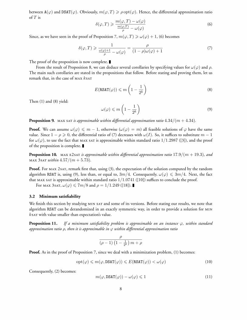
between A(ϕ) and DSAT(ϕ). Obviously, m(ϕ, T ) > ρ opt(ϕ). Hence, the differential approximation ratio

of T is

δ(ϕ, T ) >m(ϕ, T ) − ω(ϕ)m(ϕ,T )

ρ− ω(ϕ)

(6)

Since, as we have seen in the proof of Proposition 7, m(ϕ, T ) > ω(ϕ) + 1, (6) becomes

δ(ϕ, T ) >1

ω(ϕ)+1ρ

− ω(ϕ)=

ρ

(1 − ρ)ω(ϕ) + 1(7)

The proof of the proposition is now complete.

From the result of Proposition 8, we can deduce several corollaries by specifying values for ω(ϕ) and ρ.

The main such corollaries are stated in the propositions that follow. Before stating and proving them, let us

remark that, in the case of k

E(RSAT(ϕ)) 6 m

(

1 −1

2k

)

(8)

Then (1) and (8) yield:

ω(ϕ) 6 m

(

1 −1

2k

)

(9)

Proposition 9. is approximable within differential approximation ratio 4.34/(m + 4.34).

Proof. We can assume ω(ϕ) 6 m − 1, otherwise (ω(ϕ) = m) all feasible solutions of ϕ have the same

value. Since 1 − ρ > 0, the differential ratio of (7) decreases with ω(I). So, it suffices to substitute m − 1for ω(ϕ), to use the fact that is approximable within standard ratio 1/1.2987 ([3]), and the proof

of the proposition is complete.

Proposition 10. 2 is approximable within differential approximation ratio 17.9/(m + 19.3), and 3 within 4.57/(m + 5.73).

Proof. For 2, remark first that, using (3), the expectation of the solution computed by the random

algorithm RSAT is, using (9), less than, or equal to, 3m/4. Consequently, ω(ϕ) 6 3m/4. Next, the fact

that is approximable within standard ratio 1/1.0741 ([10]) suffices to conclude the proof.

For 3, ω(ϕ) 6 7m/8 and ρ = 1/1.249 ([18]).

3.2 Minimum satisfiability

We finish this section by studying and some of its versions. Before stating our results, we note that

algorithm RSAT can be derandomized in an exactly symmetric way, in order to provide a solution for

k with value smaller than expectation’s value.

Proposition 11. If a minimum satisfiability problem is approximable on an instance ϕ, within standardapproximation ratio ρ, then it is approximable in ϕ within differential approximation ratio

ρ

(ρ − 1)(

1 − 12k

)

m + ρ

Proof. As in the proof of Proposition 7, since we deal with a minimization problem, (1) becomes:

opt(ϕ) 6 m(ϕ, DSAT(ϕ)) 6 E(RSAT(ϕ)) < ω(ϕ) (10)

Consequently, (2) becomes:

m(ϕ, DSAT(ϕ)) − ω(ϕ) 6 1 (11)

8

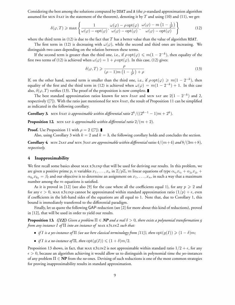
Considering the best among the solutions computed by DSAT and A (the ρ-standard approximation algorithm

assumed for k in the statement of the theorem), denoting it by T and using (10) and (11), we get:

δ(ϕ, T ) > max

{

1

ω(ϕ) − opt(ϕ),ω(ϕ) − ρ opt(ϕ)

ω(ϕ) − opt(ϕ),ω(ϕ) − m

(

1 − 12k

)

ω(ϕ) − opt(ϕ)

}

(12)

where the third term in (12) is due to the fact that T has a better value than the value of algorithm RSAT.

The first term in (12) is decreasing with ω(ϕ), while the second and third ones are increasing. We

distinguish two cases depending on the relation between these terms.

If the second term is greater than the third one, i.e., if ρ opt(ϕ) 6 m(1 − 2−k), then equality of the

first two terms of (12) is achieved when ω(ϕ) = 1 + ρ opt(ϕ). In this case, (12) gives:

δ(ϕ, T ) >ρ

(ρ − 1)m(

1 − 12k

)

+ ρ(13)

If, on the other hand, second term is smaller than the third one, i.e., if ρ opt(ϕ) > m(1 − 2−k), then

equality of the first and the third term in (12) is achieved when ω(ϕ) = m(1 − 2−k) + 1. In this case

also, δ(ϕ, T ) verifies (13). The proof of the proposition is now complete.

The best standard approximation ratios known for k and are 2(1 − 2−k) and 2,

respectively ([7]). With the ratio just mentioned for k, the result of Proposition 11 can be simplified

as indicated in the following corollary.

Corollary 3. k is approximable within differential ratio 2k/((2k−1 − 1)m + 2k).

Proposition 12. is approximable within differential ratio 2/(m + 2).

Proof. Use Proposition 11 with ρ = 2 ([7]).

Also, using Corollary 3 with k = 2 and k = 3, the following corollary holds and concludes the section.

Corollary 4. 2 and 3 are approximable within differential ratios 4/(m+4) and 8/(3m+8),respectively.

4 Inapproximability

We first recall some basics about 3p that will be used for deriving our results. In this problem, we

are given a positive prime p, n variables x1, . . . , xn in Z/pZ, m linear equations of type αiℓxiℓ + αjℓxjℓ

+αkℓ

xkℓ= βℓ and our objective is to determine an assignment on x1, . . . , xn, in such a way that a maximum

number among the m equations is satisfied.

As it is proved in [12] (see also [9] for the case where all the coefficients equal 1), for any p > 2 and

for any ǫ > 0, 3p cannot be approximated within standard approximation ratio (1/p) + ǫ, even

if coefficients in the left-hand sides of the equations are all equal to 1. Note that, due to Corollary 1, this

bound is immediately transferred to the differential paradigm.

Finally, let us quote the following GAP-reduction (see [2] for more about this kind of reductions), proved

in [12], that will be used in order to yield our results.

Proposition 13. ([12]) Given a problem Π ∈ NP and a real δ > 0, there exists a polynomial transformation gfrom any instance I of Π into an instance of 32 such that:

• if I is a yes-instance of Π (we use here classical terminology from [11]), then opt(g(I)) > (1 − δ)m;

• if I is a no-instance of Π, then opt(g(I)) 6 (1 + δ)m/2.

Proposition 13 shows, in fact, that 32 is not approximable within standard ratio 1/2 + ǫ, for any

ǫ > 0, because an algorithm achieving it would allow us to distinguish in polynomial time the yes-instances

of any problem Π ∈ NP from the no-ones. Devising of such reductions is one of the most common strategies

for proving inapproximability results in standard approximation.

9

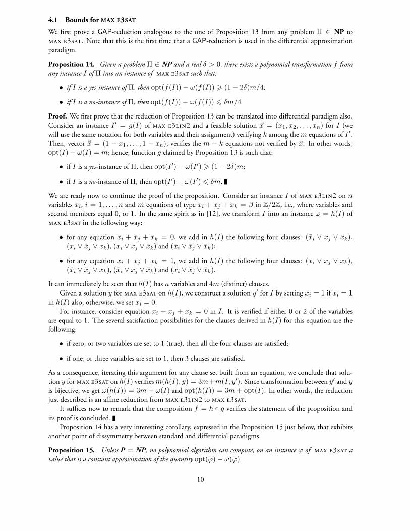
4.1 Bounds for MAX E3SAT

We first prove a GAP-reduction analogous to the one of Proposition 13 from any problem Π ∈ NP to

3. Note that this is the first time that a GAP-reduction is used in the differential approximation

paradigm.

Proposition 14. Given a problem Π ∈ NP and a real δ > 0, there exists a polynomial transformation f fromany instance I of Π into an instance of 3 such that:

• if I is a yes-instance of Π, then opt(f(I)) − ω(f(I)) > (1 − 2δ)m/4;

• if I is a no-instance of Π, then opt(f(I)) − ω(f(I)) 6 δm/4

Proof. We first prove that the reduction of Proposition 13 can be translated into differential paradigm also.

Consider an instance I ′ = g(I) of 32 and a feasible solution ~x = (x1, x2, . . . , xn) for I (we

will use the same notation for both variables and their assignment) verifying k among the m equations of I ′.Then, vector ~x = (1 − x1, . . . , 1 − xn), verifies the m − k equations not verified by ~x. In other words,

opt(I) + ω(I) = m; hence, function g claimed by Proposition 13 is such that:

• if I is a yes-instance of Π, then opt(I ′) − ω(I ′) > (1 − 2δ)m;

• if I is a no-instance of Π, then opt(I ′) − ω(I ′) 6 δm.

We are ready now to continue the proof of the proposition. Consider an instance I of 32 on nvariables xi, i = 1, . . . , n and m equations of type xi + xj + xk = β in Z/2Z, i.e., where variables and

second members equal 0, or 1. In the same spirit as in [12], we transform I into an instance ϕ = h(I) of

3 in the following way:

• for any equation xi + xj + xk = 0, we add in h(I) the following four clauses: (xi ∨ xj ∨ xk),(xi ∨ xj ∨ xk), (xi ∨ xj ∨ xk) and (xi ∨ xj ∨ xk);

• for any equation xi + xj + xk = 1, we add in h(I) the following four clauses: (xi ∨ xj ∨ xk),(xi ∨ xj ∨ xk), (xi ∨ xj ∨ xk) and (xi ∨ xj ∨ xk).

It can immediately be seen that h(I) has n variables and 4m (distinct) clauses.

Given a solution y for 3 on h(I), we construct a solution y′ for I by setting xi = 1 if xi = 1in h(I) also; otherwise, we set xi = 0.

For instance, consider equation xi + xj + xk = 0 in I . It is verified if either 0 or 2 of the variables

are equal to 1. The several satisfaction possibilities for the clauses derived in h(I) for this equation are the

following:

• if zero, or two variables are set to 1 (true), then all the four clauses are satisfied;

• if one, or three variables are set to 1, then 3 clauses are satisfied.

As a consequence, iterating this argument for any clause set built from an equation, we conclude that solu-

tion y for 3 on h(I) verifies m(h(I), y) = 3m+m(I, y′). Since transformation between y′ and yis bijective, we get ω(h(I)) = 3m + ω(I) and opt(h(I)) = 3m + opt(I). In other words, the reduction

just described is an affine reduction from 32 to 3.

It suffices now to remark that the composition f = h ◦ g verifies the statement of the proposition and

its proof is concluded.

Proposition 14 has a very interesting corollary, expressed in the Proposition 15 just below, that exhibits

another point of dissymmetry between standard and differential paradigms.

Proposition 15. Unless P = NP, no polynomial algorithm can compute, on an instance ϕ of 3 avalue that is a constant approximation of the quantity opt(ϕ) − ω(ϕ).

10

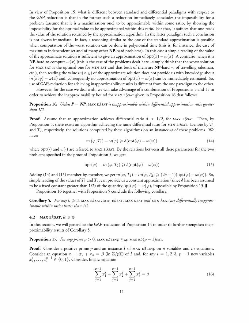
In view of Proposition 15, what is different between standard and differential paradigms with respect to

the GAP-reduction is that in the former such a reduction immediately concludes the impossibility for a

problem (assume that it is a maximization one) to be approximable within some ratio, by showing the

impossibility for the optimal value to be approximated within this ratio. For that, it suffices that one reads

the value of the solution returned by the approximation algorithm. In the latter paradigm such a conclusion

is not always immediate. In fact, a reasoning similar to the one of the standard approximation is possible

when computation of the worst solution can be done in polynomial time (this is, for instance, the case of

maximum independent set and of many other NP-hard problems). In this case a simple reading of the value

of the approximate solution is sufficient to give an approximation of opt(x)− ω(x). A contrario, when it is

NP-hard to compute ω(x) (this is the case of the problems dealt here –simply think that the worst solution

for is the optimal one for and that both of them are NP-hard –, of travelling salesman,

etc.), then reading the value m(x, y) of the approximate solution does not provide us with knowledge about

m(x, y)− ω(x) and, consequently no approximation of opt(x) − ω(x) can be immediately estimated. So,

use of GAP-reduction for achieving inapproximability results is different from the one paradigm to the other.

However, for the case we deal with, we will take advantage of a combination of Propositions 5 and 15 in

order to achieve the inapproximability bound for 3 given in Proposition 16 that follows.

Proposition 16. Unless P = NP, 3 is inapproximable within differential approximation ratio greaterthan 1/2.

Proof. Assume that an approximation achieves differential ratio δ > 1/2, for 3. Then, by

Proposition 5, there exists an algorithm achieving the same differential ratio for 3. Denote by T1

and T2, respectively, the solutions computed by these algorithms on an instance ϕ of these problems. We

have:

m (ϕ, T1) − ω(ϕ) > δ(opt(ϕ) − ω(ϕ)) (14)

where opt(·) and ω(·) are referred to 3. By the relations between all these parameters for the two

problems specified in the proof of Proposition 5, we get:

opt(ϕ) − m (ϕ, T2) > δ(opt(ϕ) − ω(ϕ)) (15)

Adding (14) and (15) member-by-member, we get m(ϕ, T1)−m(ϕ, T2) > (2δ− 1)(opt(ϕ)−ω(ϕ)). So,

simple reading of the values of T1 and T2, can provide us a constant approximation (since δ has been assumed

to be a fixed constant greater than 1/2) of the quantity opt(ϕ) − ω(ϕ), impossible by Proposition 15.

Proposition 16 together with Proposition 5 conclude the following corollary.

Corollary 5. For any k > 3, k, k, k and k are differentially inapprox-imable within ratios better than 1/2.

4.2 MAX EkSAT, k > 3

In this section, we will generalize the GAP-reduction of Proposition 14 in order to further strengthen inap-

proximability results of Corollary 5.

Proposition 17. For any prime p > 0, 3p ≤AF 3(p − 1).

Proof. Consider a positive prime p and an instance I of 3p on n variables and m equations.

Consider an equation x1 + x2 + x3 = β (in Z/pZ) of I and, for any i = 1, 2, 3, p − 1 new variables

x1i , . . . , x

p−1i ∈ {0, 1}. Consider, finally, equation

p−1∑

j=1

xj1 +

p−1∑

j=1

xj2 +

p−1∑

j=1

xj3 = β (16)

11

It is easy to see that (16) is verified if and only if the number of variables set to 1 is either β or β + p, or,

finally, β + 2p.

Consider now the set of all the possible clauses on 3(p − 1) literals issued from variables x1i , . . . , x

p−1i ,

i = 1, 2, 3. Any truth assignment will satisfy all but one clause. For example, if any variable is assigned

with 1, the only unsatisfied clause is the one where all variables appear negative.

What is of interest for us is to specify when the number of variables set to 1 is either β or β+p, or, β+2p.

For this, denote by Ck the set of clauses on 3(p − 1) literals issued from variables x1i , . . . , x

p−1i , i = 1, 2, 3

with exactly k negative literals. Then, a truth assignment setting k variables to 1, verifies |Ck| − 1 clauses

of Ck, while any other truth assignment on the variables of Ck verifies all the |Ck| clauses. So, for an equation

x1 + x2 + x3 = β, we will add in the instance of 3(p− 1) the set Ck, for k ∈ {0, . . . , 3(p− 1)}and k /∈ {β, β + p, β + 2p}. Hence, if a truth assignment for these clauses has β, or β + p, or β + 2pvariables set to 1, it will verify all the clauses constructed, otherwise it will verify all but one of these clauses.

In all, for any of the variables x1i , . . . , x

p−1i we will build one new variable and we will transform any

of the m equations of I into an equation as in (16). Then, for any of these new equations we add in the

instance of 3(p − 1) the set of clauses as built just above. The instance ϕ of 3(p − 1)

so constructed has n(p − 1) variables and, since the number of clauses issued from any equation is no more

than 23(p−1), ϕ will have at most mϕ 6 m23(p−1) clauses.

Given a truth assignment T on the variables of ϕ, we set xi = |{xki : xk

i = 1 in T}|. Discussion above

leads to m(ϕ, T ) = mϕ − m + m(I, S). On the other hand, it is easy to see that our reduction implies

that any solution S of I is transformed into a truth assignment T on the variables of ϕ such that the relation

between the values of S and T given just above is always satisfied. This relation confirms that the reduction

specified is an affine one from 3p to 3(p − 1).

Finally, let us remark that it is possible that formula ϕ contains many times the same clause. This, for

instance, is the case if I simultaneously contains equations say x1 + x2 + x3 = β1 and x1 + x2 + x3 = β2,

for β1 6= β2. In this case, we can modify the construction described, by building the subset of Ck or

k ∈ {0, . . . , 3(p − 1)} and k /∈ {β1, β1 + p, β1 + 2p, β2, β2 + p, β2 + 2p}. This concludes the proof of

the proposition.

The result of Proposition 17 together with the result of [12] stated in the beginning of the section and

Proposition 1, lead to the following corollary.

Corollary 6. For any prime p, 3(p− 1) is inapproximable within differential ratio greater than 1/p.

Furthermore, Propositions 4 and 5 allow us to rewrite Proposition 17 as follows.

Proposition 18. For any k > 3, neither k, nor k can be approximately solved withindifferential ratio greater than 1/p, where p is the largest positive prime such that 3(p − 1) 6 k.

Easy consequences of Proposition 18 are the following differential inapproximability bounds for several in-

stantiations of maximum and minimum k-satisfiability:

• and 3 4 and 5 are differentially inapproximable within ratio better than 1/2;

• and 6, . . . , 11 are differentially inapproximable within ratio better than 1/3;

• and 12, . . . , 17 are differentially inapproximable within ratio than 1/5, . . .

Finally, being harder to approximate than any k problem, the following result holds and

concludes the section.

Proposition 19. /∈ DAPX.

12

In [17] is defined a logical class of NPO maximization problems called MAX-NP. A maximization prob-

lem Π ∈ NPO belongs to Max-NP if and only if there exist two finite structures (U, I) and (U,S), a

quantifier-free first order formula ϕ and two constants k and ℓ such that, the optima of Π can be logically

expressed as:

maxS∈S

∣

∣

∣

{

x ∈ Uk : ∃y ∈ U ℓ, ϕ(I, S, x, y)}∣

∣

∣(17)

The predicate-set I draws the set of instances of Π, set S the solutions on I and ϕ the feasibility conditions

for the solutions of Π. In the same article is proved that ∈ Max-NP and that MAX-NP ⊂ APX.

It is easy to see that (17) can be identically used in both standard and differential paradigms. So, Propo-

sition 19 draws an important structural difference in the landscape of approximation classes in the two

paradigms, since an immediate corollary of this proposition is that MAX-NP 6⊂ DAPX. We conjecture

that the same holds for the other one of the celebrated logical classes of [17], the class MAX-SNP, i.e., we

conjecture that MAX-SNP 6⊂ DAPX

4.3 MAX E2SAT

We have already seen in Proposition 6 that 2 is differentially inapproximable within ratio 21/22.

In this section, we improve this result by operating an affine reduction from 22 to 2.

Indeed, consider an instance I of the former problem (on n variables and m equations) and an equation

x1 + x2 = 0 in I . Add in ϕ (the instance of 2 under construction) clauses x1 ∨ x2 and x1 ∨ x2.

On the other hand, for an equation x1 + x2 = 1, add in ϕ clauses x1 ∨ x2 and x1 ∨ x2. Performing this

transformation for any equation in I , we finally build a formula ϕ of 2 on n variables and 2mclauses. Moreover, for any truth assignment T on the variables of ϕ, one gets a solution S for I such that

m(ϕ, T ) = m + m(I, S), qed.

It is shown in [12] that 22 is inapproximable within standard approximation ratio better

than 11/12. By Proposition 2, this bound is transferred to the differential paradigm. Then, the affine

reduction just described concludes the following result.

Proposition 20. 22 ≤AF 2. Consequently, 2 is differentially inapproximablewithin ratio greater than 11/12.

5 Ideas for further research

We give in this concluding section a few ideas about possible ways for further improving results of the paper

or for yielding new ones.

Consider a graph G(V, E) of order n and with maximum degree ∆. We construct an instance ϕ of

on n variable x1, . . . , xn and n cubes C1, . . . , Cn as follows: for any vertex vi ∈ V , with neighbors

vi1 , . . . , viδi, we add in ϕ clause xi ∧ xi1 ∧ . . . ∧ xiδi

. Let T be a truth assignment satisfying k cubes, say

Cj1 , . . . , Cjk. Then, obviously, the vertex-set V ′ = {vj1 , . . . , vjk

} is an independent set for G (of size k).

Conversely, given an independent set of G of size k consisting of vertices vj1 , . . . , vjk, the truth assignment

setting variables xj1 , . . . , xjkto 1 and any othe variable of ϕ in 0 satisfies k cubes. Observe finally that the

size of the cubes built for ϕ is bounded by ∆+1. In all we have just exhibited an affine reduction from

-∆ (i.e., on graphs with maximum degree bounded by ∆) to

∆ + 1.

On the other hand, there exists an ǫ > 0 such that, for any ∆ > 3, -∆ is not

approximable within approximation ratio 1/∆ǫ ([1]). Since standard and differential approximation ratios

coincide for (the worst independent set in a graph is the empty set), the result of [1]

holds immediately for differential paradigm and can be used in order to conclude that there exists an ǫ > 0such that, for any k > 4, k is not differentially approximable within ratio greater than 1/kǫ. This

recovers the result of Proposition 19, namely, that /∈ DAPX.

13

If one wishes to improve this result, a possible issue is the following. Recall that transformation of

k to k of Proposition 5, consists of substituting any cube of size ℓ by 2ℓ−1 clauses of size ℓ. We

so can affinely (but not polynomially) reduce to by building an instance ϕof the latter on n variabes and at most n2∆+1 clauses. But, if ∆ is bounded by log n, then this reduction is

polynomial. In other words, if one obtains an inapproximability bound for -logn(for example a bound of the type 1/ logǫ n, for some positive ǫ), then one can extend it immediately to

improving so the bound of the paper.

References

[1] N. Alon, U. Feige, A. Wigderson, and D. Zuckerman. Derandomized graph products. ComputationalComplexity, 5:60–75, 1995.

[2] S. Arora and C. Lund. Hardness of approximation. In D. S. Hochbaum, editor, Approximation algo-rithms for NP-hard problems, chapter 10, pages 399–446. PWS, Boston, 1997.

[3] T. Asano, K. Hori, T. Ono, and T. Hirata. A theoretical framework of hybrid approaches to max sat.

In Proc. International Symposium on Algorithms and Computation, ISAAC’97, volume 1350 of LectureNotes in Computer Science, pages 153–162. Springer, 1997.

[4] G. Ausiello, P. Crescenzi, G. Gambosi, V. Kann, A. Marchetti-Spaccamela, and M. Protasi. Complexityand approximation. Combinatorial optimization problems and their approximability properties. Springer,

Berlin, 1999.

[5] R. Battiti and M. Protasi. Algorithms and heuristics for max-sat. In D. Z. Du and P. M. Pardalos, edi-

tors, Handbook of Combinatorial Optimization, volume 1, pages 77–148. Kluwer Academic Publishers,

1998.

[6] C. Bazgan and V. Th Paschos. Differential approximation for optimal satisfiability and related prob-

lems. European J. Oper. Res., 147(2):397–404, 2003.

[7] D. Bertsimas, C-P. Teo, and R. Vohra. On dependent randomized rounding algorithms. In Proc.International Conference on Integer Programming and Combinatorial Optimization, IPCO, volume 1084

of Lecture Notes in Computer Science, pages 330–344. Springer-Verlag, 1996.

[8] P. Crescenzi, V. Kann, R. Silvestri, and L. Trevisan. Structure in approximation classes. SIAM J. Com-put., 28(5):1759–1782, 1999.

[9] L. Engebretsen. Approximate Constraint Satisfaction. Phd thesis, Dept. of Numerical Analysis and

Computing Science, Royal Institute of Technology, Stockholm, Sweden, 2000.

[10] U. Feige and M. X. Goemans. Approximating the value of two prover proof systems, with applications

to max 2sat and max dicut. In Proc. Israel Symposium on Theory of Computing and Systems, ISTCS’95,

pages 182–189, 1995.

[11] M. R. Garey and D. S. Johnson. Computers and intractability. A guide to the theory of NP-completeness.W. H. Freeman, San Francisco, 1979.

[12] J. Håstad. Some optimal inapproximability results. J. Assoc. Comput. Mach., 48:798–859, 2001.

[13] J. N. Hooker. Resolution vs. cutting plane solution of inference problems: some computational expe-

rience. Oper. Res. Lett., 7(1):1–7, 1988.

[14] A. P. Kamath, N. K. Karmarkar, K. G. ramakrishnan, and M. G. Resende. Computational experience

with an interior point algorithm on the satisfiability problem. Ann. Oper. Res., 25:43–58, 1990.

14

[15] H. Karloff and U. Zwick. A 7/8-approximation for max 3sat? In Proc. FOCS’97, pages 406–415, 1997.

[16] J. Monnot, V. Th. Paschos, and S. Toulouse. Approximation polynomiale des problèmes NP-difficiles :optima locaux et rapport différentiel. Informatique et Systèmes d’Information. Hermès, Paris, 2003.

[17] C. H. Papadimitriou and M. Yannakakis. Optimization, approximation and complexity classes. J. Com-put. System Sci., 43:425–440, 1991.

[18] L. Trevisan, G. B. Sorkin, M. Sudan, and D. P. Williamson. Gadgets, approximation, and linear

programming. In Proc. FOCS’96, pages 617–626, 1996.

[19] V. Vazirani. Approximation algorithms. Springer, Berlin, 2001.

15