Difference based estimators and infill statistics Differences and infill statistics

Noname manuscript No.(will be inserted by the editor)

Difference based estimators and infill statistics

Differences and infill statistics

Jose R. Leon · Carenne Ludena

Abstract Infill statistics, that is, statistical inference based on very dense observa-

tions over a fixed domain has become of late a subject of growing importance. On

the other hand, it is a known phenomenon that in many cases infill statistics do not

provide optimal rates. The degree of sub-optimality is related to how much parameter-

related information is lost because of dense sampling, which in turn is related to sample

path regularity. In the stationary Gaussian case this is determined by the large value

behaviour of the spectral density and its derivatives. Moreover, many interesting non

stationary examples such as non linear functionals of stationary Gaussian processes or

diffusion processes driven by a stationary increment Gaussian process can also be seen

to depend on the large value behaviour of the spectral density of the underlying pro-

cess. In this article we discuss several examples in a unified frequency domain approach

providing a general framework relating sample path regularity to estimation rates. This

includes examples such as volatility estimation for diffusions and fractional diffusions,

multifractals and non-linear functions of Gaussian processes. As a final example we

include the problem of estimation in the presence of an additive white noise, known as

the nugget effect or micro-structure error.

Keywords gaussian processes, diffusions and fractional diffusions, increasing domain

asymptotics, infill statistics, microergodicity, multifractals, non-linear functionals of

gaussian processes, nugget effect, spatial statistics, spectral analysis · volatility

Mathematics Subject Classification (2000) 62F12, 62M15 · 62M30

The authors would like to thank Proyecto LOCTI (Ministerio de Ciencia Tecnologıa e Inno-vacion de Venezuela) “Estudio del transporte de contaminantes en el Lago de Valencia”

Jose R. Leon E-mail: [email protected] de Matematicas, Facultad de Ciencias UCV, Caracas, Venezuela.

Carenne Ludena E-mail: [email protected] de Matematicas, Facultad de Ciencias UCV, Caracas, Venezuela.

2

Contents

1 Introduction . . . . . . . . . . . . . . . . . . . . . . . . . . . . . . . . . . . . . . . . . 2

2 Maximum likelihood estimation . . . . . . . . . . . . . . . . . . . . . . . . . . . . . . 4

3 Stationary Gaussian processes . . . . . . . . . . . . . . . . . . . . . . . . . . . . . . 5

4 Estimators based on increments in the non stationary case . . . . . . . . . . . . . . . 16

5 An application to fields . . . . . . . . . . . . . . . . . . . . . . . . . . . . . . . . . . 25

6 The nugget effect . . . . . . . . . . . . . . . . . . . . . . . . . . . . . . . . . . . . . . 29

1 Introduction

Consider an L2 process Xt, with t ∈ Rd, whose law depends on a certain parameter θ ∈Θ but that is only observed over D ⊂ Rd. The fact that observations are restricted to

the bounded areaD means that statistical inference on θ must be based on progressively

more densely sampled points as the sample size increases over the fixed domain. This is

referred to as infill statistics following Cressie (1993) or fixed domain asymptotics Stein

(1999). As is well known (see for example Stein , 1999; Zhang and Zimmerman , 2005;

Chan and Wood , 2004 and references therein), this restriction may yield suboptimal

rates.

We assume we observe Xti with the multi–index ti defined by

ti := (i1∆, . . . , id∆), 1 ≤ ij ≤ n, j = 1, . . . , d so the total number of observations

is nd. Purely infill asymptotics are characterized by n∆ → C as n → ∞ for a certain

positive constant C.

Without loss of generality assume C = 1. Even under very mild regularity assumptions

on X, as ∆ → 0 there is less information available as follows from the underlying

regularity. However, despite the growing literature in the infill setting, there seems to

be no general rule assessing estimation performance based on model assumptions.

With this in mind, in this article we consider a series of one dimensional examples

of infill based statistical inference (we also include higher dimensional generalizations

whenever available), based on q-order differences in a frequency domain framework.

Differences are important in infill statistics because they provide a method for “de-

regularizing” the original data, hence increasing the amount of information available.

Our main goal is to try to provide insights as to what the main issues are, expectable

results and what may be interesting problems for further developments. To this end we

hope to illustrate the intimate yet not thoroughly exploited relationship between spatial

statistics and increment or variations based statistics including recent very powerful

tools based on Malliavin calculus (see for example Nualart and Ortiz-La Torre , 2008;

Tudor and Viens , 2009, and the references therein).

Let Pθ be the law of Xt, t ∈ D. Consider a certain function of the parameter,

h = h(θ). Following Stein Stein (1999), Section 6.2, a necessary although not sufficient

condition for consistently estimating h is that it is microergodic. Given the class of

probability models Pθ, θ ∈ Θ and a function h : Θ → Rq, then h is defined to be

microergodic if h(θ1) 6= h(θ2)⇒ Pθ1 ⊥ Pθ2 .

3

In general, as will be discussed in more detail in Section 3 and in the example below,

any function h that requires precise information on the low frequencies requires precise

information on the full range of values of X (which is not observable over an a priori

fixed domain) and hence will not be consistently estimable in a purely infill framework

and will not be microergodic.

To develop this idea we shall dwell on the following example proposed by Stein (1999).

Example 1 Estimating the variance of the sample mean Stein (1999) pp. 144-148: let

Z(t) be a centered stationary Gaussian process with spectral density f = f(θ). Assume

that we split D = [0, 1]d into nd sub-cubes of side 1/n and set ti to be the center of

each sub-cube. Further assume we only observe process Z at points ti. Consider the

quantity of interest to be the (non-observable) random variable I(Z) =∫Z(t)dt. A

natural choice is of course to approximate I(Z) by the observable Zn = 1/nd∑i Z(ti)

and study the approximation error of this procedure which is measured by its variance

Vn := V ar(I(Z)− Zn) =

∫f(w)gn(w)dw,

gn(w) = (1−d∏j=1

2n sin(wj/(2n))

wj)2

d∏j=1

sin2(wj/2)

n2 sin2(wj/(2n)).

The problem is then assessing the rate of convergence of Vn and constructing consistent

estimators for the correctly normalized variance.

Both problems will depend on the smoothness of process Z. If f(w) ∼ θ|w|−4 as

|w| → ∞ then

n4Vn → 1/144

∫w2 sin2(w/2)f(w)dw. (1)

Moreover, since the limiting quantity depends on f over all its range it is not consis-

tently estimable based on the observations. However, if f is less regular, i.e. f(w) ∼θ|w|−2p as |w| → ∞ for d = 1, 2 and d/2 < p < 2, then n2pV ar(I(Z) − Zn)) → C(θ)

where C(θ) is the optimal variance (see Theorems 2 and 4 in Sections 5.2 and 5.3 in

Stein , 1999) which only depends on the high frequency behaviour of f and whence

can be estimated as developed below in detail in the one dimensional case.

Set d = 1. Consistent estimation of parameter θ for f(w) ∼ θ|w|−2p as |w| → ∞ can be

achieved by considering successive applications of the difference operator ∆nZ(t) :=

Z(t+ 1/n)− Z(t). Indeed, following Stein (1999), page 167, the following statistic

1

Cp

∑i

[(∆n)pZ(ti)]2

is seen to be a consistent estimator of θ with Cp =∫∞−∞ |w|

−2p(2 sin(w/2))2pdw, which

only depends on the behaviour of f for large values of w. The trick here is that using

successive increments introduces sin(w/2n) instead of sin(w/2) and thus only the large-

value behaviour of f is relevant, provided it is of the stated form.

We remark that in a non strictly infill domain (if Cn := ∆/n→∞) it is always possible

to construct estimators of the variance of the sample mean which attain√Cn rates

under general ergodicity conditions.

4

The above discussion introduces several points we will develop throughout the article.

The first is estimating rough signals is easier than estimating regular signals in an

infill setting, whence the need to de-regularize. The second is that differentiating the

observed series provides estimators which depend only on high frequency behaviour in

many interesting cases as in the example discussed above. The third is that any esti-

mation problem that requires knowledge on the low frequencies in general will not be

consistent so that the process will not be microergodic. The fourth is that whether the

infill setting provides the same estimation rates as the classical ergodic setting, i.e. if the

Fisher information matrix is asymptotically equivalent to the conditional information

matrix (see Section 2 below for more details), can be determined in many cases based

on whether the parameters of interest can be estimated using sufficiently higher order

differences of the original observations. In this article we assume the sampling strategy

is regular and follow a spectral approach in order to establish asymptotic results. Regu-

larly spaced observations (perhaps with missing observations) are a standard restriction

for stationary or stationary increment process and typical preprocessing techniques re-

quire converting the irregular sample into a regular one (see for example Cressie , 1993,

Section 2.4). In the non stationary case on the other hand, for example when estimat-

ing volatilities for diffusions or fractional diffusions, there has been much more interest

in developing estimators based on non regular samples. For completeness sake a brief

discussion on non regular samples will also be included.

Most of the examples discussed in this article are closely related to work the authors

have developed in diverse frameworks dealing with statistical inference for densely sam-

pled data based on q-order differences. However, the main thread follows the results

of Stein (1999) or more recently of Zhang and Zimmerman (2005) in their thorough

review of maximum likelihood estimation in the infill case, comparing infill to increas-

ing domain statistics. The article is organized as follows. In Section 2 we discuss ML

estimation and its relation to microergodicity. In Section 3 we review certain known re-

sults for infill estimation of stationary and stationary increment Gaussian process and

state the main result of the article: namely a characterization of the convergence rates

of successive differences according to the tail behaviour of regularly varying spectral

densities. Although this result is not strictly speaking new, we believe it is important

for practitioners as it establishes obtainable rates in a unified framework. In Section 4

we generalize these results to a certain class of non-stationary processes which can be

written as Y = XW with W a stationary, or stationary increment gaussian process and

discuss several examples including volatility estimation, non linear functions of Gaus-

sian processes and applications to multifractals. In Section 5 we consider an application

to fields and finally in Section 6 we discuss certain results concerning inference in the

presence of a “nugget effect”, which can be written as Y = X + Z with X possibly

non stationary and Z a white noise process. Many of the examples can be extended to

t ∈ Rd, but we will restrict our attention to the case d = 1, indicating whenever higher

dimensional results are available.

2 Maximum likelihood estimation

In this section we give a quick overview of maximum likelihood estimation in the fixed

domain setting and relate microergodicity to the properties of the MLE.

5

Let Xt = Xt(θ) be a spatial process and consider the problem of estimating θ based

on the likelihood Ln. Let ln stand for the log-likelihood and In for the Information

matrix. In an increasing domain setting (fixed ∆) I−1/2n (

∂ln(θ)∂θ ) → N(0, I) under

certain general regularity conditions including that the diagonal terms of I−1n → 0.

On the other hand assume, quite generally, that Xt is observed over a series of domains

D1 ⊂ . . . ⊂ Dn ⊂ . . . ⊂ D. Let Fn = σXt, t ∈ Dn. Then ∂ln(θ)∂θ ,Fn, n ≥ 1 is a

martingale under certain general conditions (see Prop. 6.1 in Hall and Heyde , 1980 as

cited by Zhang and Zimmerman , 2005). Let In be the conditional information matrix

given Fn then I−1/2n (∂ln(θ)∂θ ) → N(0, I). Hence the maximum likelihood estimators

will have the same asymptotic properties if In and In are aymptotically equivalent.

Since the MLE cannot be consistent for any θ that is not microergodic, that the asymp-

totic properties in both settings are equal implies microergodicity. In the stationary

Gaussian case, as we will see below, microergodicity is equivalent to certain conditions

over the covariance kernel or the spectral density.

Non sufficiency of microergodicity for consistency is discussed in Zhang and Zimmer-

man (2005), pp. 924-925. The authors develop an example in which they consider a

two dimensional parameter φ = (θ, ν) such that Pφ1⊥ Pφ2

for ν1 = ν2 as long as

θ1 6= θ2 (Pφ1≡ Pφ2

if and only if θ1 = θ2). Set φ0 = (θ0, ν0) to be the true value of

the parameter. The authors show the MLE based on very dense observations consis-

tently estimates θ0. However the MLE of ν0, ν, maximizes P(θ0,ν)/P(θ0,ν0). That is, ν

is actually the maximum likelihood estimator of ν0 when θ0 is known and thus it is

typically not a consistent estimator of ν0.

As an example of the above construction they consider the O.U. process Xt solution

of

dXt = −νXtdt+√

2θdWt,

for Wt a Brownian motion.

Then the MLE θ is consistent but ν = ν(θ) =∫XtdXt/

∫X2t dt is not a consistent

estimate of ν.

In the next sections we will review microergodicity for stationary and stationary incre-

ment Gaussian processes.

3 Stationary Gaussian processes

Following the results of Chapter 4 in Stein (1999) two Gaussian processes with continu-

ous mean functions and continuous positive covariance kernels are always either equiv-

alent or orthogonal. We shall see that this property allows establishing both necessary

and sufficient conditions over a certain class of covariance kernels for the equivalence

of the underlying measures and whence establishing necessary and sufficient conditions

for microergodicity.

More precisely, consider two zero mean stationary Gaussian measures Pθj , j = 1, 2

defined by the corresponding covariance kernel Kj with spectral density fj . If one of

the spectral densities possess a Laplace transform in a neighbourhood of the origin

then both measures are either equivalent or orthogonal on any bounded region. Also,

6

if for j0 ∈ 1, 2 fj0 is such that fj0(w) ∼ |φ(w)|2 as |w| → ∞, where φ is the

Fourier transform of a square integrable function with bounded support (for example

if fj0(w) ∼ |w|−2α, α > 1 as |w| → ∞), then for any bounded region R both measures

will be equivalent over R if there exists C = C(R) such that∫|w|>C

(f1(w)− f2(w))2

f2j0(w)dw <∞. (2)

Condition (2) states the measures will be equivalent over a bounded domain whenever

the high frequency behaviour of the spectral density of the difference of both processes

is negligible relative to the tail behaviour of the spectral density f of one of them. The

converse result is not true, but as Stein (1999) points out a reasonable conjecture is

that if (2) does not hold then it is possible to find some bounded region R′ such that

the measures will not be equivalent over it, and whence be orthogonal.

If for j0 ∈ 1, 2, there exists a positive even integer α such that fj0(w) ∼ |w|−α, then

in the one-dimensional case, and any finite T , both measures will be equivalent over

[0, T ] if and only if k(t) := K1(t) −K2(t) is almost everywhere α times differentiable

(k(α−1) exists and is absolutely continuous over (−T, T )) and∫ T

0

(k(α)(t))2(T − t)dt <∞

(Theorems 13 and 14 in Ibragimov and Rozanov , 1978 as cited by Stein , 1999, p.

122). Moreover, as Stein (1999) goes on to remark, under the stated condition K1

does not have α derivatives at t = 0. Hence, the difference must be more regular than

each covariance function. Typical examples include

1. Consider the covariance kernels K1(t) = e−|t| and K2(t) = (1−|t|)+. The first has

spectral density f1(w) = c/(1 + |w|2) which satisfies the stated condition for α = 2

and the difference has an absolutely continuous derivative over (−1, 1) but it is not

continuously differentiable at t = 1.

2. Let Pθ,ν be the centered Gaussian measure defined by K(t) = θe−ν|t|. Then

h(θ, ν) = θν is microergodic but g(θ, ν) = θ is not.

Results in this section allow for the following concluding remark. In the Gaussian case

h is microergodic if

Ph(θ) ≡ Ph(θ′) ⇐⇒ θ = θ′.

If for all θ ∈ Θ the spectral density fθ exists and is assumed to be regularly varying

of order α = α(θ) (see Definition 32), then h is microergodic if and only if h(θ) 6=h(ν) ⇐⇒ k

(α)θ,ν is not square integrable over some small interval containing 0, where

kθ,ν = Kθ −Kν is the difference of the associated covariance kernels.

3.1 Convergence rates for estimators based on differences

In this Section we look in more detail at the case d = 1 and f(w, θ) ∼C(γ)L(w, θ)w−(1+γ) as w → ∞ with L a slowly varying function at w = 0 with

7

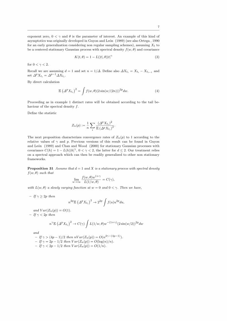
exponent zero, 0 < γ and θ is the parameter of interest. An example of this kind of

asymptotics was originally developed in Guyon and Leon (1989) (see also Ortega , 1990

for an early generalization considering non regular sampling schemes), assuming Xt to

be a centered stationary Gaussian process with spectral density f(w, θ) and covariance

K(t, θ) = 1− L(|t|, θ)|t|γ (3)

for 0 < γ < 2.

Recall we are assuming d = 1 and set n = 1/∆. Define also ∆Xti = Xti −Xti−1 and

set ∆pXti = ∆p−1∆Xti .

By direct calculation

E(∆pXti

)2=

∫f(w, θ)(2 sin(w/(2n)))2pdw. (4)

Proceeding as in example 1 distinct rates will be obtained according to the tail be-

haviour of the spectral density f .

Define the statistic

Zn(p) :=1

n

∑i

(∆pXti)2

E (∆pXti)2.

The next proposition characterizes convergence rates of Zn(p) to 1 according to the

relative values of γ and p. Previous versions of this result can be found in Guyon

and Leon (1989) and Chan and Wood (2000) for stationary Gaussian processes with

covariance C(h) = 1 − L(h)|h|γ , 0 < γ < 2, the latter for d ≤ 2. Our treatment relies

on a spectral approach which can then be readily generalized to other non stationary

frameworks.

Proposition 31 Assume that d = 1 and X is a stationary process with spectral density

f(w, θ) such that

limw→∞

f(w, θ)w1+γ

L(1/w, θ)= C(γ),

with L(w, θ) a slowly varying function at w = 0 and 0 < γ. Then we have,

– If γ ≥ 2p then

n2pE(∆pXti

)2 → 22p∫f(u)u2pdu,

and V ar(Zn(p)) = O(1).

– If γ < 2p then

nγE(∆pXti

)2 → C(γ)

∫L(1/w, θ)w−(1+γ)(2 sin(w/2))2pdw

and

– If γ > (4p− 1)/2 then nV ar(Zn(p)) = O(n2γ−(4p−1)).

– If γ = 2p− 1/2 then V ar(Zn(p)) = O(log(n)/n).

– If γ < 2p− 1/2 then V ar(Zn(p)) = O(1/n).

8

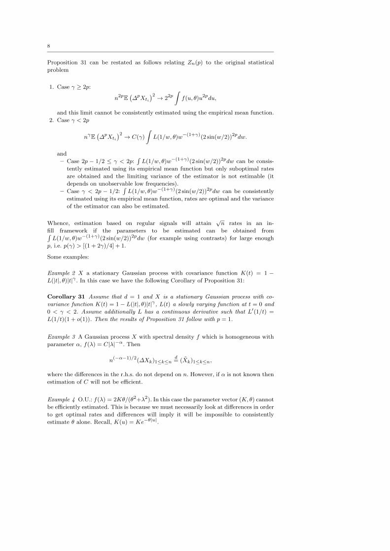
Proposition 31 can be restated as follows relating Zn(p) to the original statistical

problem

1. Case γ ≥ 2p:

n2pE(∆pXti

)2 → 22p∫f(u, θ)u2pdu,

and this limit cannot be consistently estimated using the empirical mean function.

2. Case γ < 2p

nγE(∆pXti

)2 → C(γ)

∫L(1/w, θ)w−(1+γ)(2 sin(w/2))2pdw.

and

– Case 2p − 1/2 ≤ γ < 2p:∫L(1/w, θ)w−(1+γ)(2 sin(w/2))2pdw can be consis-

tently estimated using its empirical mean function but only suboptimal rates

are obtained and the limiting variance of the estimator is not estimable (it

depends on unobservable low frequencies).

– Case γ < 2p − 1/2:∫L(1/w, θ)w−(1+γ)(2 sin(w/2))2pdw can be consistently

estimated using its empirical mean function, rates are optimal and the variance

of the estimator can also be estimated.

Whence, estimation based on regular signals will attain√n rates in an in-

fill framework if the parameters to be estimated can be obtained from∫L(1/w, θ)w−(1+γ)(2 sin(w/2))2pdw (for example using contrasts) for large enough

p, i.e. p(γ) > [(1 + 2γ)/4] + 1.

Some examples:

Example 2 X a stationary Gaussian process with covariance function K(t) = 1 −L(|t|, θ)|t|γ . In this case we have the following Corollary of Proposition 31:

Corollary 31 Assume that d = 1 and X is a stationary Gaussian process with co-

variance function K(t) = 1− L(|t|, θ)|t|γ , L(t) a slowly varying function at t = 0 and

0 < γ < 2. Assume additionally L has a continuous derivative such that L′(1/t) =

L(1/t)(1 + o(1)). Then the results of Proposition 31 follow with p = 1.

Example 3 A Gaussian process X with spectral density f which is homogeneous with

parameter α, f(λ) = C|λ|−α. Then

n(−α−1)/2(∆Xk)1≤k≤nd= (Xk)1≤k≤n,

where the differences in the r.h.s. do not depend on n. However, if α is not known then

estimation of C will not be efficient.

Example 4 O.U.: f(λ) = 2Kθ/(θ2+λ2). In this case the parameter vector (K, θ) cannot

be efficiently estimated. This is because we must necessarily look at differences in order

to get optimal rates and differences will imply it will be impossible to consistently

estimate θ alone. Recall, K(u) = Ke−θ|u|.

9

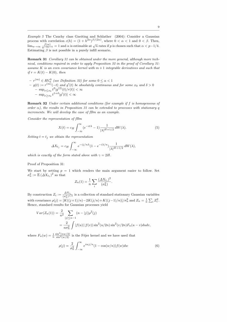
Example 5 The Cauchy class Gneiting and Schlather (2004): Consider a Gaussian

process with correlation c(h) = (1 + h2α)β/(2α), where 0 < α < 1 and 0 < β. Then,

limw→∞f(w)

w−2α−1 = 1 and α is estimable at√n rates if p is chosen such that α < p−1/4.

Estimating β is not possible in a purely infill scenario.

Remark 31 Corollary 31 can be obtained under the more general, although more tech-

nical, conditions required in order to apply Proposition 32 in the proof of Corollary 31:

assume K is an even covariance kernel with m+ 1 integrable derivatives and such that

if r = K(t)−K(0), then

– r(m) ∈ RV 0α (see Definition 32) for some 0 ≤ α < 1

– g(t) := r(m)(−t) and g′(t) be absolutely continuous and for some x0 and δ > 0

– supx≤x0t2|g(2)(t)/r(t)| <∞

– supx≥x0t1+δ|g′(t)| <∞

Remark 32 Under certain additional conditions (for example if f is homogeneous of

order α), the results in Proposition 31 can be extended to processes with stationary q

increments. We will develop the case of fBm as an example.

Consider the representation of fBm

X(t) = cH

∫ ∞−∞

(e−itλ − 1)1

|λ|H+1/2dW (λ). (5)

Setting t = tj we obtain the representation

∆Xtj = cH

∫ ∞−∞

e−ij/nλ(1− e−iλ/n)1

|λ|H+1/2dW (λ),

which is exactly of the form stated above with γ = 2H.

Proof of Proposition 31:

We start by setting p = 1 which renders the main argument easier to follow. Set

σ2n := E (∆Xt1)2 so that

Zn(1) =1

n

∑i

(∆Xti)2

(σ2n).

By construction Zi :=∆Xti

(σ2n)

1/2 is a collection of standard stationary Gaussian variables

with covariance ρ(j) = [K((j+1)/n)−2K(j/n)+K((j−1)/n)]/σ2n and Zn = 1n

∑i Z

2i .

Hence, standard results for Gaussian processes yield

V ar(Zn(1)) =2

n2

∑|j|≤n−1

(n− |j|)ρ2(j)

=2

nσ2n

∫|f(u)| |f(v)| sin2(u/2n) sin2(v/2n)Fn(u− v)dudv,

where Fn(w) = 1n

sin2(nw/2)sin2(w/2)

is the Fejer kernel and we have used that

ρ(j) =2

σ2n

∫ ∞−∞

eiwj/n(1− cos(w/n))f(w)dw (6)

10

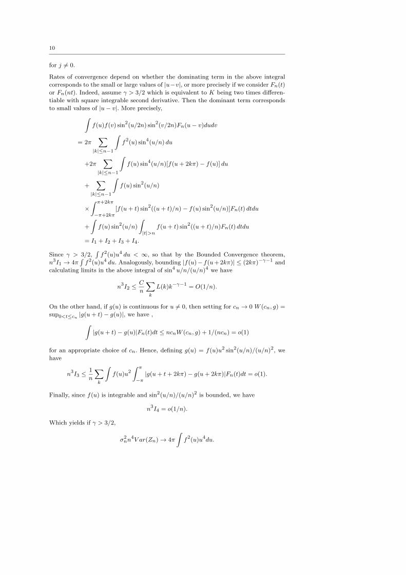
for j 6= 0.

Rates of convergence depend on whether the dominating term in the above integral

corresponds to the small or large values of |u−v|, or more precisely if we consider Fn(t)

or Fn(nt). Indeed, assume γ > 3/2 which is equivalent to K being two times differen-

tiable with square integrable second derivative. Then the dominant term corresponds

to small values of |u− v|. More precisely,∫f(u)f(v) sin2(u/2n) sin2(v/2n)Fn(u− v)dudv

= 2π∑

|k|≤n−1

∫f2(u) sin4(u/n) du

+2π∑

|k|≤n−1

∫f(u) sin4(u/n)[f(u+ 2kπ)− f(u)] du

+∑

|k|≤n−1

∫f(u) sin2(u/n)

×∫ π+2kπ

−π+2kπ

[f(u+ t) sin2((u+ t)/n)− f(u) sin2(u/n)]Fn(t) dtdu

+

∫f(u) sin2(u/n)

∫|t|>n

f(u+ t) sin2((u+ t)/n)Fn(t) dtdu

= I1 + I2 + I3 + I4.

Since γ > 3/2,∫f2(u)u4 du < ∞, so that by the Bounded Convergence theorem,

n3I1 → 4π∫f2(u)u4 du. Analogously, bounding |f(u)− f(u+ 2kπ)| ≤ (2kπ)−γ−1 and

calculating limits in the above integral of sin4 u/n/(u/n)4 we have

n3I2 ≤C

n

∑k

L(k)k−γ−1 = O(1/n).

On the other hand, if g(u) is continuous for u 6= 0, then setting for cn → 0 W (cn, g) =

sup0<t≤cn |g(u+ t)− g(u)|, we have ,∫|g(u+ t)− g(u)|Fn(t)dt ≤ ncnW (cn, g) + 1/(ncn) = o(1)

for an appropriate choice of cn. Hence, defining g(u) = f(u)u2 sin2(u/n)/(u/n)2, we

have

n3I3 ≤1

n

∑k

∫f(u)u2

∫ π

−π|g(u+ t+ 2kπ)− g(u+ 2kπ)|Fn(t)dt = o(1).

Finally, since f(u) is integrable and sin2(u/n)/(u/n)2 is bounded, we have

n3I4 = o(1/n).

Which yields if γ > 3/2,

σ2nn4V ar(Zn)→ 4π

∫f2(u)u4du.

11

We remark this integral depends on the whole integration interval and not just the

large values of |u|. On the other hand, if γ < 3/2 then the dominant term is off- the

diagonal. We shall give the proof for L(u) = 1 in order to simplify notation, but proofs

follow likewise. Recall∫f(u)f(v) sin2(u/2n) sin2(v/2n)Fn(u− v)dudv

= n3∫f(nu)f(nv) sin2(u/2) sin2(v/2)Fn(n(u− v)) dudv

In this case we shall use that by hypothesis f(u)→ u−γ−1 as u→∞, so that setting

p(u) = f(u)/u−γ−1 we have the last integral is equal to

= n−2γ+1∫u−γ−1v−γ−1p(nu)p(nv) sin2(u/2) sin2(v/2)Fn(n(u− v))dudv

= 2πn−2γ+1[

∫p(nu)u−γ−1 sin2(u/2) du]2

+2πn−2γ+1∫p(nu)u−γ−1 sin2(u/2) du

×(

∞∑k=−∞

1

np(2kπ)(2kπ/n)−γ−1 sin2(2kπ/2n)−

∫p(nv)v−γ−1 sin2(v) dv)

+n−2γ+1∫p(nu)u−γ−1 sin2(u/2)

×∞∑

k=−∞

∫ (π+2kπ)/n

(−π+2kπ)/n

[p(n(u+ t))(u+ t)−γ−1 sin2((u+ t)/2)

−p(n(u+ 2kπ/n)) sin2((u+ 2kπ/n)/2)(u+ 2kπ/n)−γ−1]Fn(nt) dt

+2πn−2γ+1 1

n

∫p(nu)u−γ−1 sin2(u/2)

×[

∞∑k=−∞

p(n(u+ 2kπ/n)) sin2((u+ 2kπ/n)/2)(u+ 2kπ/n)−γ−1

−∞∑

k=−∞p(2kπ)(2kπ/n)−γ−1 sin2(2kπ/2n)]

= J1 + J2 + J3 + J4.

Here we have used that∫ π/n−π/n Fn(nt)dt = 2π/n.

Using p(u) < A and limn→∞ p(nu) = 1, by the Bounded Convergence Theorem,

n2γ−1J1 → 2π[

∫u−γ−1 sin2(u/2) du]2.

On the other hand n2γ−1J2 → 0 and n2γ−1J4 → 0 as follows from the integrability

of h(u) = p(nu)u−γ−1 sin2(u). In order to check convergence to zero of the remaining

12

term, define

An(u, t, k) := |(u+ t+ 2kπ/n)−γ−1 sin2((u+ t+ 2kπ/n)/2)

−(u+ 2kπ/n)−γ−1 sin2((u+ 2kπ/n)/2)|≤ (γ + 1)(u+ 2kπ/n)−γ−2 sin2((u+ 2kπ/n)/2)t,

for k 6= 0.

Set Bn = k ∈ Z : |u + 2kπ/n| < 1. Over this set we have An(u, t, k) ≤ (γ + 1)|u +

2kπ/n|−γt, and∑Bn

∫An(u, t, k)Fn(nt)dt ≤ Cnγn1−γ

∫tFn(nt)dt.

And for k 6∈ Bn we may bound∑Bcn

∫An(u, t, k)Fn(nt)dt ≤ Cnγ+2n−γ−1

∫tFn(nt)dt.

Whence, since ∫ π/n

−π/ntFn(tn)dt = C

log(n)

n3,

for some positive constant C, as follows from the change of variable w = tn and the

bounds Fn(u) ≤ n and Fn(u) ≤ C/nu2 for some universal constant C, we have

∫ π/n

−π/n

∑k>0

An(u, t, k)Fn(nt)dt ≤ Cn log(n)/n3.

For k = 0, f(2kπ/n) = 0 so that in this case we must bound

|∫ π/n

−π/n[(u+ t)−γ−1 sin2((u+ t)/2)− (u)−γ−1 sin2(u/2)]Fn(nt)dt|.

The second integral equals 1/n(u)−γ−1 sin2(u/2), so that we may use the fact that∫ π

−πu−2γ+2 <∞

for γ < 3/2 to show∫[u−γ−1 sin2(u/2)]2

∫ π/n

−π/nFn(nt)dt = O(1/n).

For the first term, we may bound (t + u)−γ−1 sin2((t + u)/2) ≤ inf(u−γ+1, (u +

π/n)−γ+1, u−γ−1), according to the values of γ and u, and the same bounds may

be applied.

Hence, for k 6= 0

n2γ−1J3 ≤nγ+1 log(n)

n3→ 0

and for k = 0

n2γ−1J3 ≤ C/n→ 0

13

as long as γ < 3/2. Thus

σ2nn2γ+1V ar(Zn(1))→ 4π[

∫u−γ−1 sin2(u) du]2.

Remark in this case, the above calculations only depend on limu→∞ f(u), so the vari-

ance can be estimated consistently from the data.

Finally, if γ = 3/2 consider as for the case γ > 3/2∫f(u)f(v) sin2(u/2n) sin2(v/2n)Fn(u− v)dudv

= 2π∑

|k|≤n−1

∫f(u) sin4(u/n)f(u+ 2kπ)du+ I3 + I4.

The first term is seen to be O(log(n)n3 ) because of the choice of γ and the latter are

o(log(n)n3 ) as was shown above.

Thus, since the variance term σ2n = n−2γ [∫u−γ−1 sin2(u/2) du]2 we have

V ar(Zn(1)) = O(1/n) if γ < 3/2, V ar(Zn(1)) = O(log(n)/n) if γ = 3/2 and

V ar(Zn(1)) = O(n2(γ−2)) if γ > 3/2. We remark 2(2− γ) < 1 in this case.

We may now return to Zn(p). First remark that using the spectral representation of

the stationary centered process Xt with spectral density f(λ, θ) we have

∆pXt =

∫eiλt(1− eiλ/n)p

√f(λ, θ) dλ.

Calculating expectations we have the following analogue of equation (4)

E(∆pXtj

)2=

∫|f(w, θ)|(2 sin(w/2n))2pdw.

On the other hand

V ar(Zn(p)) =2

n2

∑|j|≤n−1

(n− |j|)ρ2p(j)

=2

nσ2n

∫|f(u)| |f(v)| sin2p(u/2n) sin2p(v/2n)Fn(u− v)dudv,

where Fn(w) is the Fejer kernel and we have used the analogue of equation (6)

ρp(j) =2

σ2n

∫ ∞−∞

eiwj/n(cos(w/n)− 1)2pf(w)dw

for j 6= 0. Then, as above, two limiting behaviours are possible according to the fol-

lowing integral∫u2pf(u) du is finite or not. That is, if γ ≥ 2p or not.

In the latter case

nγE(∆pXti

)2 → ∫L(1/w)w−(1+γ)(2 sin(w/2))2pdw.

14

Also, for γ < 2p the procedure developed above for p = 1 can be repeated exactly

to obtain V ar(Zn(p)) = O(n2γ−(4p−2)) if∫f2(u) sin4p(u) du < ∞, that is if γ >

(4p− 1)/2. If not, V ar(Zn(p)) = O(1/n) (with a log term if γ = (4p− 1)/2). As above

the former rates are slower and the variance of the estimator depends on f over the

whole integration interval.

If γ ≥ 2p

n2pE(∆pXti

)2 → 22p∫f(u)u2pdu,

so that σ2n = O(n−2p). Moreover, we will have,

V ar(Zn(p)) =2

nσ2n

∫f(u)f(v)(2 sin(u/2n))2p(2 sin(v/2n))2pFn(u− v)dudv

=24p+1

nσ2n2π

∑|k|≤n−1

∫f2(u) sin4p(u/n) du

=2

nσ2nO(n−2p+1) = O(1).

This ends the proof.

Proof of Corollary 31: We start by including the following result due to Cline (1991),

along with the next three definitions needed to state the result.

Definition 31 A function g(t) is said to be regularly varying at infinity with exponent

α (g ∈ RV∞α ) if

limt→∞

g(yt)

g(t)= yα.

Definition 32 A function g(t) is said to be regularly varying at zero with exponent α

(g ∈ RV 0α ) if

limt→0

g(yt)

g(t)= yα for all y > 0.

Definition 33 Let h, g be real or complex functions over (−∞,∞). Then g is said to

belong to I(II2)0h if for some x0 > 0,

supx≤x0

sup0≤w≤v≤1

|g((u+ w + v)x)− g((u+ v)x)− g((u+ w)x) + g(ux)

h(x)|,

is integrable for u ∈ [1,∞).

A function g is said to be in QV 0α if g ∈ RV 0

α , 0 ≤ α < 1 and g ∈ I(II2)0g.

With this notation we have.

Proposition 32 (Corollary 2 in Cline , 1991) Assume g has m+ 1 integrable deriva-

tives, m ≥ 0. Let r1(t) = g(m)(t) − g(m)(0). If r1(t) ∈ QV 0α , 0 ≤ α < 1 and

r1(−t) ∈ I(II2)0r1 , then

limw→∞

wmf(w)/r1(1/w) = Γ (1 + α)

15

Also, by Corollary 3 in Cline (1991), a sufficient condition for g ∈ I(II2)0h with

h ∈ RV 0α , 0 ≤ α < 1 is that g and g′ be absolutely continuous and for some x0 and

δ > 0

1. supx≤x0t2|g(2)(t)/h(t)| <∞

2. supx≥x0t1+δ|g′(t)| <∞

With this result and notation we are able to continue with the proof.

Function K(·) defined in equation (3) satisfies K(0) = 1, is even and the assumptions

of Proposition 31 are satisfied whenever 0 < γ < 2. If 0 < γ < 1, then m = 0 and

limw→∞

w(1+γ)f(w)

L(1/w)= Γ (γ + 1) cos((γ + 1)π/2).

If 1 < γ < 2, then m = 1 and it is necessary to require an additional smoothness

condition over L(t) namely that L′(1/t) = L(1/t)(1 + o(1)). In this case,

limw→∞

w(1+γ)f(w)

L(1/w)= iΓ (γ + 1) sin((γ + 1)π/2).

If γ = 1, we get

limw→∞

w2f(w)

L(1/w)= Γ (2).

So that under the stated conditions

limw→∞

w(1+γ)f(w)

L(1/w)= C(γ)

and Proposition 31 ends the proof for p = 1.

3.2 Non regular samples

Assume observations are not sampled over a regular grid, and set t1, . . . , tn to be

the sample points, which may be random or deterministic. Let sj := tj − tj−1 and

define, for any positive integer q and u ∈ Rq the empirical measure dSn(q, u) :=1n

∑nj=1

∏q−1`=0 δnsj−`(u). We shall require the following assumption over the sampling

scheme

AS For each positive and fixed positive integer q there exists a positive measure Sqsuch that for any bounded continuous function g,

∫g(u)dSn(q, u)→

∫g(u)dSq(u)

a.s.

If the sample is not random a.s. convergence is just convergence in R.

Example 6 If the increments nsj are i.i.d. random variables with joint distribution

Sq(u) = P (sj ≤ u1, . . . , sj+1−q ≤ uq) then assumption AS holds true by the Law of

Large Numbers.

16

We have the following lemma

Lemma 33 Assume that d = 1 and that X is a stationary process with spectral density

f(w, θ) such that

limw→∞

f(w, θ)w1+γ

L(1/w, θ)= C(γ),

with L(w, θ) a slowly varying function at w = 0 with exponent zero and 0 < γ. Assume

additionally that AS holds and set sync(x) := sin(x)/x. Then if γ < 2p

nγE(∆pXti

)2→ C(γ)

∫L(1/w, θ)w2p−1−γ [

∫ p−1∏`=0

sync2(wuj−`/2)

p−1∏`=0

u2j−` dSp(u)]dw

Characterization of rates, that is calculating the variance of Zn(p) for non regular

samples is highly more technical and would unnecessarily complicate notation, although

results analogous to those obtained in Proposition 31 can be obtained under certain

conditions over the sampling scheme. In Section 4.1 we include references to the problem

of estimating volatilities for non regular samples.

Proof of Lemma 33: For 0 < u set ∆u(f)(t) = f(t+u)−f(u). Then, for positive integer

p and a collection of positive u1, . . . , up define the successive differences operator

∆u1,...,up := ∆up . . .∆u1 .

Let j > p. Using the spectral representation of the stationary centered process Xt with

spectral density f(λ, θ) we have

∆sj ,...,sj+1−pXt =

∫eiλt

p−1∏`=0

(1− eiλsj−`)√f(λ, θ) dλ.

Calculating expectations we have the following analogue of equation (4)

E(∆sj ,...,sj+1−pXtj

)2=

∫|f(w, θ)|

p−1∏`=0

(2 sin(wsj−`/(2n)))2dw.

The proof follows exactly as that of Proposition 31 for the high frequency characteri-

zation.

4 Estimators based on increments in the non stationary case

In this section we consider a special class of non-stationary processes that appear in

many applications. Assume ∆Xti ∼ σ(ti, ν)∆Wti,θ, where W is stationary or has

stationary increments. Here σ, known as the volatility, may be deterministic, random

but independent of the process W or σ = σ(X), for example when looking at diffusion

or fractional diffusion processes with random volatilities. The parameters of interest are

17

assumed to be θ and ν which by construction gives rise to and identifiability problem

up to multiplicative constants. The volatility σ is assumed non constant which would

lead to the original stationary or stationary increment problem discussed above. A first

remark is that in this case infill based estimation will depend on the, possibly random,

collection σ(ti, ν) which is only observed once. In this Section we will discuss some

examples and establish consistency results in the spirit of Section 3.

Let d = 1 and assume that gm(t) is a piece-wise constant function defined over [0, T ] ,

gm(t) = aj , t ∈ Ij , Ij = [sj−1, sj),

for a certain collection aj , sj , j = 1, . . . ,m and s0 = 0, with |Ij | denoting the length

of each interval. Assume that Xt is such that ∆Xti = gm(ti)∆Wti(1 + en(ti)) where

∆Wt is a stationary gaussian process with spectral density f and en(·) is a bounded

sequence such that en = oP (1). Then ∆pXti = gm(ti)∆pWti(1 + oP (1)) since gm

is piecewise constant. Set Zn(p) = 1n

∑i

(∆pXti )2

E(∆pWti)2 . We have the following technical

Lemma.

Lemma 41

limn

E (Zn(p)) =

∫g2pm (t)dt.

and

V ar(Zn(p)) =2

nσ2n

∫f(u)f(v)(2 sin2(u/2n))2p(2 sin2(v/2n))2pFn(u− v)dudv

×[

m∑j=1

a4pj |Ij |] + o(1/n)

Proof of Lemma 41: The first assertion follows from the definition. The second is a

simple Corollary of Proposition 31. It is enough to remark that for any two adjacent

intervals Ij = [sj−1, sj) and Ij+1 = [sj , sj+1) the covariance term

Cj,j+1 = Cov(1

n

∑i∈Ij

(∆pXti)2

E (∆pWti)2,

1

n

∑i∈Ij+1

(∆pXti)2

E (∆pWti)2

)

is negligible relative to the variance terms. Indeed we have

Cj,j+1 ≤ a2pj+1a2pj max(|Ij |, |Ij+1|)

× 2

nσ2n|∫f(u)f(v)(2 sin(u/2n))2p(2 sin(v/2n))2pGn(u− v)dudv|

where Gn(u) := 2n

∑n−1j=1 je

iju. Unlike the Fejer kernel,∫ π−π Gn(u)du = 0 and it also

satisfies,

– Gn(0) = (n− 1)

– |Gn(u)| ≤ A/u, where A is a universal constant, as follows by remarking that Gn(u)

is a constant times the derivative of the Dirichlet kernel.

18

Hence, the proof of Proposition 31 can be repeated, as follows from the properties of

kernel Gn(u) and observing that the terms I`, ` = 1, . . . , 4 (or J`, respectively) will

not appear because∫ π−π Gn(u)du = 0.

This leads to the following result.

Proposition 42 Assume that d = 1 and Xt is such that ∆Xti = σ(ti, ν)(1 +

oP (1))∆Wti , where W is a stationary process with spectral density f(w, θ) such that

limw→∞

f(w, θ)w1+γ

L(1/w, θ)= C(γ),

with L(w, θ) a slowly varying function at w = 0 with exponent zero and 0 < γ. Assume

also σ4p is an integrable function over [0, T ]. Then we have,

– If γ ≥ 2p then

n2pE(∆pXti

)2 → (

∫ T

0

σ2p(t, ν)dt)(22p∫f(u, θ)u2pdu),

and V ar(Zn(p)) = O(1).

– If γ < 2p then

nγE(∆pXti

)2 → (

∫ T

0

σ2p(t, ν)dt)(

∫L(1/w, θ)w−(1+γ)(2 sin(w/2))2pdw)

and

– If γ > (4p− 1)/2 then nV ar(Zn(p)) = O(n2γ−(4p−1)).

– If γ = 2p− 1/2 then V ar(Zn(p)) = O(log(n)/n).

– If γ < 2p− 1/2 then V ar(Zn(p)) = O(1/n).

Proof of Proposition 42: Considering piece-wise constant approximations of function σ

we have

E (Zn(p)) = (

∫f(w, θ)(2 sin(w/(2n)))2pdw)(

∫ T

0

σ2p(t, ν)dt(1 + o(1)))

and

V ar(Zn(p)) =2

nσ2n

∫f(u)f(v)(2 sin(u/2n))2p(2 sin(v/2n))2pFn(u− v)dudv

×∫ T

0

σ4p(t, ν)dt+ o(1/n),

where σ2n and the proof of 31 may be continued to obtain the stated results.

The rates established in Proposition 42 will be the same as those obtained in 31. In

many examples encountered in this setting θ is assumed to be known and the parameter

of interest is ν. Consistent, optimal rate estimation of this parameter is possible if ν

can be recovered from I(p) for large enough p.

If σ(·) is random then the above discussion suggests that the correct centering term is

not the expectation E (Zn(p)) but rather I(p) (or its discretization 1/n∑j σ

2p(tj , ν)),

19

which is random. If σ and W are independent, then I(p) = limn→∞

Eσ (Zn(p)). Although

it is generally not true that both processes are independent, in many situations they

are asymptotically so, so that Eσ ((Zn(p)))→ I(p) anyway. Estimation rates for ν will

then depend on whether I(p) exists for large enough p. In the following subsections we

include several examples where this is so.

4.1 Estimating volatility for diffusion and fractionary-diffusion processes

There exist quite a number of results addressing the problem of estimating the diffu-

sion coefficient or volatility using contrasts or non parametric approaches for diffusion

processes (see for example Genon-Catalot & Jacod , 1993 for one of the first results in

this direction). Consider the model

dXt = b(t,Xt)dt+ σ(θ, t,Xt)dWt,

where b and σ are assumed to satisfy the necessary conditions to assure the existence

of a strong solution Xt. Assume the number of observations is n = T/∆. In Genon-

Catalot & Jacod (1993) the authors obtain√n rates and show that the estimation

problem satisfies the LANM property, and in particular is consistent. Namely, consider

Zn =1

n

n∑i=1

|∆Xi∆1/2

|2 ∼ 1

n

∑i

|σ(θ, i∆,Xi∆)∆Wi

∆1/2|2,

Then, conditionally on X,√n(Zn − 1

T

∫ T0σ2(θ, t,Xt)dt) converges stably to a Gaus-

sian r.v. with conditional variance Γ 2 = 1T

∫ T0σ4(θ, t,Xt)dt, where

∫ T0σ2(θ, t,Xt)dt is

known as the integrated volatility. Results for contrasts follow from here.

Although in general the variance is random, if σ = σ(θ,Xt) does not depend on t

(and the solution is assumed to be stationary and ergodic), then Γ 2 converges to

E(σ4(θ,X0)

), as |T | → ∞.

On the other hand, consider the problem of estimating α and β in the model

dXt = b(Xt, α)dt+ σ(Xt, β)dWt,

which is assumed to have a stationary solution. The best possible rates (see for ex-

ample Sorensen Sorensen , 2004) are√n for β and

√n∆ for α so that, in this case

completely infill statistics are not possible. Intuitively, this result is not surprising since

the covariance of ∆Xi does not depend on α. In fact, that an absolutely continuous

change of measure changes the distribution of X to the zero drift distribution assures

that estimation of α cannot be microergodic, and whence cannot be consistent.

Estimating the integrated volatility or the volatility associated parameter θ for diffusion

processes has been less studied in the case of non regular samples for high frequency

data, because of the technical difficulties associated with the characterization of the

limiting behaviour of the estimators. This problem is discussed in depth in Hayashi

et al. (2011), where deterministic, random but independent and data dependent non

regular sampling schemes are considered.

20

It is also possible to consider diffusions driven by fractional Brownian motion (fBm).

That is, solutions to

dXt = b(Xt, α)dt+ σ(Xt, β)dWHt ,

where WHt is a fBm with Hurst parameter 0 < H < 1.

There are several ways to define integration with respect to fBm. If H > 1/2 a pathwise

approach is possible for sufficiently regular σ (see Dai and Heyde , 1996,Lin , 1995,

Zahle , 1998). Existence and pathwise properties of the solution Xt are shown in

Nualart and Rascanu (2002). Based on these properties and the results in section

4. it follows that it is possible to construct efficient estimators for β based on Zn(2) ∼1/n(

∑j σ

2(Xtj , β)[∆2WHtj ]2) Leon and Ludena (2007) for all 1/2 < H < 1. Analogous

results for estimators based on first order differences only hold for 1/2 < H < 3/4,

that is 1 < γ < 3/2 as follows from equation (5). The proof is based on studying the

variance of

Zmn (p) :=1

ngtj (W

Hs1 , . . . ,W

Hsm)[∆2WH

tj ]2,

where gt = σ(Xmt ) and Xm

t is an approximation of the solution Xt which depends

only on a finite collection WHsk , k = 1, . . . ,m and then showing

E(Zmn (p)− Zn(p)

)2 → 0.

Consistent estimation of α is again not possible in a strictly infill scenario. In fact, set

Xt = h(BHt ) where h satisfies the O.D.E

h(t) = σ(h(t))dt

h(0) = x0

and consider BH,1t = BHt y(t) where y(t) solves the random O.D.E.

dy(t) =b(h(BHt ), t)

σ(h(BHt ))

with y(0) = 0. With this notation Xt = h(BH,1t + y(t)) and solves the equation

Xt = x0 +

∫ T

0

b(s,Xs)ds+

∫ T

0

σ(Xs)dBH,1s .

The above stochastic integral is well defined as BH,1 has the same pathwise properties

as BH . By Theorem 6.1 in Decreusefond and Ustunel (1999) there exists a probability

measure P1 which is absolutely continuous with respect to P and such that the law of

BH,1 under P1 is the same as the law of BH under P , as long as y satisfies certain

bounds (Theorem 4 in Leon and Ludena , 2007; Lemma 9 in Gloter and Hoffmann ,

2004). Namely, that there exists δ such that

E

(eC∫ 10

(∫|s−u|<δ

y′(u)−y′(s)(u−s)H+1/2

)2)<∞.

As for the diffusion case the absolutely continuous change of measure to the zero drift

case assures that estimation of α is not microergodic.

21

For H < 1/2 the pathwise approach is no longer possible and generally in this case

the solution is interpreted in the sense of Decreusefond and Ustunel (1999). The

latter also includes the case H > 1/2, but since, except for deterministic σ(β,Xt),

both solutions do not coincide, we have preferred to stick to the former in this case.

Existence and properties of a strong solution have also been developed based on this

definition for H < 1/2 (see Coutin , 2007 for a thorough review). A number of results

dealing with parameter estimation of diffusions driven by fBm have appeared recently.

However most of them are related to establishing consistency results for MLE when

T →∞ (see Tudor and Viens , 2009 and the references therein) for all 0 < H < 1. As

above, purely infill statistics in this domain will be consistent only for volatility related

parameters. A generalization of the Girzanov absolutely continuous change of measure

(see Theorem 1 in Tudor and Viens , 2009) once again assures that the problem of

estimating drift related parameters cannot be microergodic.

Another closely related example was developed in Barndorff-Nielsen et al. (2009). In

this article the authors consider processes

Xt = X0 +

∫φsdGs,

where G is a centered stationary increment Gaussian process with

R(t) := V ar(Gt+s −Gs) = L0(t)tγ ,

0 < γ < 2 and L0 a slowly varying function at zero. Here the integral is defined in a

pathwise sense for any φ with bounded q variation, q < 1/(1 − γ/2) (see Barndorff-

Nielsen et al. , 2009 for details on the construction). The authors show convergence

in probability for quadratic variations, and higher order powers, of the increments of

process X as well as a conditional CLT.

4.2 Estimating volatility for γ unknown

A special case of volatility estimation occurs when ∆Xti = σ(ti, ν)(1 + oP (1))∆Wti ,,

with W a stationary process with spectral density f(w, γ) such that

limw→∞

f(w, γ)w1+γ

L(1/w)= C(γ),

with L(w) a slowly varying function at w = 0 and γ unknown. Since by Proposition

42 if 0 < γ < 2p− 1/2 then

nγE(∆pXti

)2 → (

∫ T

0

σ2p(t, ν)dt)(

∫L(1/w)w−(1+γ)(2 sin(w/2))2pdw)

and the variance of the mean squared p−order differences will be O(1/n), a reasonable

strategy is a two step procedure estimating γ based on the logarithm of the said mean

squared p−order differences and then using this estimated value in order to estimate

parameter ν.

22

More precisely, recalling ∆ to be the sample lag, consider estimators Zn(p, j) based on

observations sampled at lags j∆ for j = 1, . . . ,m and consider

γ =∑

αjZn(p, j),

with the sequence αj satisfying

–∑j αj = 0

–∑j αj log(j) = 1.

Then, from Proposition 42, γ is seen to be a consistent estimator of γ with O(1/n)

variance whenever 0 < γ < 2p− 1/2.

The estimated parameter γ can then be used to build estimators for ν based on∫ T0σ2p(t, ν)dt. However, estimation for ν will achieve O(

√n/ log(n)) rates instead of√

n. The interested reader is encouraged to review Istas and Lang (1997), Zhu and

Taqqu (2006), Berzin et al. (2012), Chan and Wood (2000) and Zhu and Stein (2002),

the latter two dealing with extensions of these ideas to fields.

4.3 Non linear functions stationary Gaussian processes

The next example, closely related to volatility estimation, deals with infill statistics

based on the increments of a nonlinear function of a stationary Gaussian process. Let

Xt be a stationary Gaussian process with covariance function γ(t, θ) = 1−|t|γ(θ)L(t, θ)

as above (H = γ/2). Assume instead of Xi we observe Yi = G(Xi) with G a certain

nonlinear function and that we are interested in estimating θ based on the increments

of the indirect observations, that is, ∆Yi ∼ G′(Xi)∆Xi. This scenario has been studied

in detail in Chan and Wood (2004) where log based estimators of the exponent γ are

considered. The authors go on to consider two dimensional isotropic fields and estima-

tors of γ built on quadratic variations of spacial increments following their previous

work in Chan and Wood (2000).

Based on Proposition 31 consistency results can then be obtained for estimators based

on quadratic variations of p order differences under certain regularity conditions over

G, namely that G′ ∈ C4(R) with polynomial tails (see for example Theorem 1 in

Leon and Ludena (2004)). The basic idea is to show a.s. convergence to zero of the

conditional variance, given the process Xt, of

Zn(p) =1

n

n∑i=1

[G′(Xti)]2[∆pXi − EXti

(∆pXi

)]2,

based on the results developed in Section 3.1 and the asymptotic independence of the

process and its increments in the Gaussian case. By construction, Zn is centered and

the conditional variance will depend only on the conditional covariance structure of

the p order increments. By the asymptotic independence the conditional covariance

converges to the non conditional covariance. Conditional Central Limit Theorems will

also hold in this case.

23

4.4 Multifractals

Another interesting framework for comparing infill and increasing domain statistics is

the estimation of the scale function in multifractal models. Recall ∆Xi = Xti+1 −Xtiand ∆ = ti+1− ti stands for the fixed sampling lag. If we define the scale function ζ(q)

as

ζ(q) := − lim∆→0

logE((∆Xi)

q) / log(∆),

process X is considered a multifractal if ζ(q) is not linear. Two very popular examples

are Multiplicative cascades (MC) introduced Mandelbrot (1974) (see Ossiander and

Waymire , 2000 for a thorough account on estimation procedures) and Multifractal

Random Measures (MRM) introduced in Bacry et al. (2003) or more generally a Mul-

tifractal Random Walk process (MRW) Bacry et al. (2001, 2003); Ludena (2008). It

is assumed that ∆ = 2−m and L = 2ξm, with ξ ≥ 0, and that the total number of ob-

servations is n = L/∆. As for the estimation of a random volatility coefficient, or non

linear functionals of Gaussian processes, the difference operator ∆Xti ∼ Yti∆Wti,θ

where the r.v. ∆Wti,θ are conditionally independent and independent of the variables

Yti . However, the latter exhibit a very complex dependence structure unlike the previ-

ously considered diffusion like examples. As mentioned, the parameter of interest in this

setting is the scaling function ζ(q), but the natural empirical mean-based estimator is

biased by a non-observable random term and it is necessary to subtract an appropriate

centering term in order to eliminate the bias. For MC this can be achieved by consid-

ering the difference of the square increments for two successive scales, which consists

namely in eliminating the conditional expectation. This new unbiased estimator will

still have a random variance in the purely infill framework though. On the other hand,

in the increasing domain framework, the asymptotic variance of the estimator will be

deterministic. For MRM or MRW the above estimation procedure is no longer useful

in the purely infill scenario. In the increasing domain case, because of the deterministic

limiting variance√n∆ rates and a Central Limit Theorem can be obtained under quite

general assumptions (Ludena and Soulier , 2012).

Very succinctly, MC are constructed as follows.

Consider a collection Wr, r ∈ 0, 1mm ≥ 1 of independent random variables with

common law W such that E (W ) = 1 and E (W log2W ) < 1. For each m ≥ 1 consider

the random measure defined by

λm(I) = 2−m∑

r∈0,1m∩I

m∏i=1

Wr|i ,

for any I a Borel subset of [0, 1], and each r = (r1, . . . , rm) ∈ 0, 1m identified to

the real number∑mi=1 ri2

m−k. Here r|i stands for the restriction of r to its first i

components. It can be seen (see Kahane and Peyriere (1976), Ossiander and Waymire

(2000) for details on the construction and main results) that there exists a random

measure λ∞, such that

P(λn ⇒ λ∞ as n→∞) = 1 ,

where⇒ stands for vague convergence. The limiting measure verifies E (λ∞([0, 1])) = 1

under the stated assumptions for the r.v. W .

24

Moreover, let q > 1 be such that E (W q) <∞ and set ψ(q) = log2(E (W q)). Consider

the sequence

λm,q(I) = 2−m(1−q+ψ(q)) ∑r∈0,1m∩I

m∏i=1

W qr|i

Let q0 be the largest value of q such that

qψ′(q) < ψ(q) + 1 . (7)

Then if q < q0, Proposition 2.2 in Ossiander and Waymire (2000), yields the existence

or a certain random measure λ∞,q such that λm,q ⇒ λ∞,q. The limiting measure

satisfies E (λ∞,q([0, 1])]) = 1 under the stated assumptions for the r.v. W .

Also, as follows from Proposition 2.1 in Ossiander and Waymire (2000), there exists

a sequence of i.d. random variables aj , such that

[λ∞(([j2−m, (j + 1)2−m])])]q = 2m(1−q+ψ(q))aqjλm,q(([j2−m, (j + 1)2−m])]).

Hence, since E(λm,q([0, 2

−m]))

= 2−m,

E(

[λ∞(([j2−m, (j + 1)2−m])])]q)

= 2m(−q+ψ(q))E(aqj

)and it follows from the above definition of the scale function that ζ(q) = q − ψ(q).

The measure can be extended to the whole real line by considering I(j) := [j, (j + 1)]

for each j ∈ Z. Over each I(j) we construct an independent multiplicative cascade λ(j)∞

as defined above an set λ∞ :=∑j∈Z λ

(j)∞ . With this notation, set Xt = λ∞([0, t]).

Let τ(q) = ζ(q)− 1 and set

Zm(p, q) :=1

2m(1+ξ)

∑i

(∆pXti)q.

Since the parameter of interest is the scaling function it is reasonable to consider the

estimator

τ(q) :=log2(Zm(1, q))

log2(∆).

This estimator is however biased and it turns out it is better to consider instead the

ratio based estimator:

τ(q) := log2

(Zm(1, q)

Zm+1(1, q)

).

The case L = 1, that is in the purely infill framework, has been thoroughly dealt with

for multiplicative cascades in Ossiander and Waymire (2000). The authors show that

τ(q) and τ(q) are consistent estimators of τ(q) for q < q0.

Rates however are very different for both estimators. In fact, Corollary 4.4 in Ossiander

and Waymire (2000) states that if 2q < q0 then there exists a positive r.v. C such that

2m(1−ζ(q)+ζ(2q))/2

C1/2(τ(q)− τ(q)−m−1 log2(bn))→ N(0, 1).

25

Here log2(bn) is an unobservable sequence of (a.s. bounded) random variables so that

the estimator has a bias of order m−1 which is much larger than the error rate

2−m(1−ζ(q)+ζ(2q))/2.

On the other hand, Corollaries 4.6and 4.7 in Ossiander and Waymire (2000) imply

that there exists a positive r.v. D such that

2m(1−ζ(q)+ζ(2q))/2

D1/2(τ(q)− τ(q))→ N(0, 1).

Looking at the logarithm of ratios as in the definition of τ , that is, at the normal-

ized differences of the increments to the power q at different levels m and m + 1, in-

stead of simply at the increments to the power q, eliminates the random bias term

by subtracting the appropriate random centering. Indeed, let cm = E (Zm), then

Zm/cm − Zm+1/cm+1 can be written as a sum of conditionally independent and cen-

tered random variables. However, the variance will still be random.

The increasing domain framework for multiplicative cascades has been recently studied

in Bacry et al. (2008). The authors show that if L = [2nχ], where [x] stands for greatest

integer m ≤ x with χ > 0, then τM (q) is consistent for q < qχ where qχ is the largest

value of q such that

qψ′(q)− ψ(q) < χ+ 1 , (8)

or equivalently ζ(q) − pζ′(q) < χ + 1. However, as before there exists a bias term

bn := E[Mq1 ]/n, which, although this time is deterministic, again entails slower rates of

convergence of the estimator. In analogy to the purely infill asymptotic framework it is

reasonable to consider ratio based estimators such as τ in order to improve convergence

rates. It can be seen Ludena and Soulier (2012) that τM (q)→ τ(q)−χ, a.s. Moreover,

a non conditional CLT can be seen to hold for 2q < qχ. This is because in contrast to

the case L = 1 the mixed asymptotic framework provides a non random variance term.

5 An application to fields

The results in this Section are basically results developed in the spectral domain given

in Bierme et al. (2011) which allow for quite general polynomial based functionals of

the underlying field. However, earlier versions of these results dealing with several two

dimensional differences, including those considered in this section, have been studied

by Chan and Wood (2000) and Zhu and Stein (2002). Consider the bi-dimensional

random field in R2 with spectral representation

X(t) =

∫R2

(eit.ξ − 1)f12 (ξ)dWξ.

Here ξ = (ξ1, ξ2), |ξ| =√ξ21 + ξ22 and the spectral density f is defined by

f(ξ) =Ω(ξ)

|ξ|2H+2, (9)

26

where function Ω is homogeneous of degree 0. Consider the direction in the plane

defined by the angle ϕ. Looking at the field X restricted to the line t2 = tanϕ t1 where

t = (t1, t2), we obtain the one dimensional process Y ϕ defined by

Y ϕ(t1) =

∫R2

(eit.ξ − 1)f12 (ξ)dW (ξ1, ξ2)

=

∫R2

(eit1(ξ1+tanϕξ2) − 1)f12 (ξ1, ξ2)dW (ξ1, ξ2).

This can be written formally as

Y ϕ(u) =

∫R2

(eiu|ξ|cosϕ cos(ϕ−θ) − 1)

Ω12 (θ)

|ξ|H+1dW ((|ξ| cos θ, |ξ| sin θ),

for u ≥ 0.

Consider the second order increment which can be written as

Z(k, ϕ) := Y ϕ(k + 1

n)− 2Y ϕ(

k

n) + Y ϕ(

k − 1

n)

=

∫R2

eik|ξ|n cosϕ cos(ϕ−θ)2(cos(

|ξ|n cosϕ

cos(ϕ− θ))− 1)Ω

12 (θ)

|ξ|H+1dW ((|ξ| cos θ, |ξ| sin θ).

With the change of variable in R2 defined by 1cosϕξ = λ using the homogeneity of Ω

and the scaling properties of W we get that

Z(k, φ) =2

(| cosϕ|)H

∫R2

eik/n|λ| cos(ϕ−θ)(cos(|λ|/n cos(ϕ− θ))− 1)

× Ω12 (θ)

|λ|H+1dW ((|λ| cos θ, |λ| sin θ).

Define eζ = (cos ζ, sin ζ). The integral can then be written as

=2

(| cosϕ|)H

∫R2

eikρ<eϕ,eθ>(cos(ρ < eϕ, eθ >)− 1)Ω

12 (θ)

|λ|H+1dW ((|λ| cos θ, |λ| sin θ).

Whence, changing to polar coordinates in the above representation yields

ρϕ(j) := Z(k, ϕ)Z(0, ϕ)

=4

(| cosϕ|)2H

∫ ∞0

∫ 2π

0

eik/nρ cos θ(cos(ρ/n cos θ)− 1)2Ω(θ + ϕ)

ρ2H+2ρdθdρ.

and σ2n,ϕ := V ar(Z(0, ϕ)) = 4(| cosϕ|)2H

∫∞0

∫ 2π0

(cos(ρ/n cos θ) − 1)2Ω(θ+ϕ)ρ2H+2 ρdθdρ. In

the isotropic case we can specialize our computations obtaining

σ2n,ϕ =4

(| cosϕ|)2H

∫ ∞0

∫ 2π

0

(cos(ρ/n cos θ)− 1)21

ρ2H+1dθdρ

=2π

(| cosϕ|)2H

∫ ∞0

4∑j=0

(4

j

)(−1)jJ0((2− j)ρ/n)

1

ρ2H+1dρ

27

and also

ρϕ(j) =4

(| cosϕ|)2H

∫ ∞0

∫ 2π

0

eik/nρ cos θ(cos(ρ/n cos θ)− 1)21

ρ2H+1dθdρ

=2π

(| cosϕ|)2H

∫ ∞0

4∑j=0

(4

j

)(−1)jJ0((k + (2− j))ρ/n)

1

ρ2H+1dρ

Where J0(x) = 1π

∫ π0

cos(x sin(τ))dτ stands for the 0-Bessel function. As,

limx→0(J0(x)− 1)/x = 1, the above expressions are asymptotically equivalent to

ρ(j) = 2

∫ ∞−∞

eiwj/n(cos(w/n)− 1)f(w)dw

defined in equation (6) and σ2n. Hence, the one dimensional results obtained in Sec-

tion 3.1 can be applied to the directional p order differences in order to establish the

following consistency results.

Consider the process Y ϕt obtained by restricting the field X to the line t2 = tanϕ t1,

the direction in the plane defined by the angle ϕ. Let

Zn(p, ϕ) :=1

n

∑i

(∆pY ϕti )2

∆pY ϕti2.

We have the following result.

Proposition 51 Set γ = 2H. Then,

– If γ > 2p then V ar(Zn(p, ϕ)) = O(1).

– If γ > (4p− 1)/2 then nV ar(Zn(p, ϕ)) = O(n2γ−(4p−1)).

– If γ = (4p− 1)/2 then V ar(Zn(p, ϕ)) = O(logn/n).

– If γ < 2p− 1/2 then V ar(Zn(p, ϕ)) = O(1/n).

Other examples of infill asymptotic can be considered by introducing other types of

increments whose nature is strictly bi-dimensional.

Let us follow the works of Chan & Wood and Zu & Stein (Chan and Wood , 2000; Zhu

and Stein , 2002). For 1 ≤ k, j ≤ n let us define the following double increments:

– Vertical V nk,j(X) = X( kn ,j−1n )− 2X( kn ,

jn ) +X( kn ,

j+1n ).

– Horizontal V nk,j(X) = X(k−1n , jn )− 2X( kn ,jn ) +X(k+1

n , jn ).

– Superficial nk,j(X) = X(k−1n , j−1n )−X( kn ,j−1n )−X(k−1n , jn ) +X( kn ,

jn ).

Under the condition that f the spectral density of process X satisfies hypothesis (9),

and denoting by Ink,j(X) any of the preceding random variables, we will study the

asymptotic behaviour of the 2-variations

S2,n =1

(n− 1)2

n∑k=2

n∑j=2

(Ink,j(X)

σn)2,

28

where σ2n = E(Ink,j(X))2. For simplicity we will only consider the case of superficial

increments, the other cases can be treated similarly. Therefore we can write with some

abuse of notation

ht1,t2(X) = X(t1 − h, t2 − h)−X(t1, t2 − h)−X(t1 − h, t2) +X(t1, t2),

and by using the spectral representation we get

ht1,t2(X) =

∫R2

ei(t1ξ1+t2ξ2)

×[e−i(hξ1+hξ2) − e−ihξ1 − e−ihξ2 + 1

]√f(ξ1, ξ2)dW (ξ1, ξ2).

By defining the polynomial

P (z1, z2) := z1z2 − z1 − z2 + 1,

the above integral can be written

ht1,t2(X) =

∫R2

ei(t1ξ1+t2ξ2)P (e−ihξ1 , e−ihξ2)√f(ξ1, ξ2)dW (ξ1, ξ2).

By taking h = 1n , t1 = k

n and t2 = jn we obtain the following equality in distribution

nk,j(X) = n

∫R2

ei(kξ1+jξ2)P (e−iξ1 , e−iξ2)√f(nξ1, nξ2)dW (ξ1, ξ2).

The Ito-Wiener isometry yields

E(nk,j(X))2 = n2∫

R2|P (e−iξ1 , e−iξ2)|2f(nξ1, nξ2)dξ1dξ2.

By using hypothesis (9) we get

n2Hσ2n →∫

R2|P (e−iξ1 , e−iξ2)|2Ω(ξ1, ξ2)

|ξ|2H+2dξ1dξ2.

And also

n2HE(n0,0(X)nk,j(X))→∫

R2ei(kξ1+jξ2)|P (e−iξ1 , e−iξ2)|2Ω(ξ1, ξ2)

|ξ|2H+2dξ1dξ2.

Considering the quadratic variation

S2,n =1

(n− 1)2

n∑k=2

n∑j=2

(nk,j(X)

σn)2.

The following two results were obtained in Bierme et al. (2011)

(i)V arS2,n → 0 and (ii) (n− 1)(S2,n − E(S2,n))d→ N(0, 2(2π)4(|g|2per)∗2(0)).

Where for a function h we denote h∗2 = h ∗ h. Moreover

|g|2per(ξ) = |g|2(ξ) +∑

(k,j)6=(0,0)

|g|2(ξ1 + 2kπ, ξ2 + 2jπ),

and

g(ξ) =P (e−iξ1 , e−iξ2)

√f(ξ)

(∫

R2 |P (e−iξ1 , e−iξ2)|2f(ξ)dξ1dξ2)1/2.

29

6 The nugget effect

Another related problem is that of the “Nugget effect”. That is, we assume that rather

than observing Xt we observe Yt := Xt + Zt, where Xt and Zt are independent and

Zt is independent of Zs for all s, t in the sampling set. Hence if V ar(Zt) = σ20 , then

Cov(Yt, Ys) = Cov(Xt, Xs) and V ar(Yt) = V ar(Xt) + σ20 .

Of course, there is no limiting process with this covariance structure for all t ∈ T .

Stein, Stein (1999) suggests an alternative model considering a microstructure error

term. That is a process Y ′t := Xt +Z′t where as above both processes are independent

and Cov(Z′t, Z′s) = 0 if |s − t| > δ. For practical purposes if we assume the sampling

size is greater than δ both models will yield the same results.

The basic phenomena related to the nugget effect is described in the following example

developed by Chen et al (2000). They consider the model

Y (s) = Z(θ, s) + ε(η, s),

where Z(s) is an Orstein Uhlembeck process, i.e., Cov(Z(θ, s), Z(θ, t)) = e−θ|s−t| and

ε is a white noise process with variance η2. Or, incorporating a deterministic trend,

Y (s) = βtf(s) + Z(s) + ε(s).

The authors show n1/2 rates for η2 and n1/4 rates for θ. They report similar results

for a scale changed Brownian motion with an additional white noise.

The same results are true if we observe

Y (s) = W (σ, s) + ε(η, s),

where W (σ, ·) is a Wiener process with variance σ2, Stein (1990).

In both cases results are based on likelihood methods: i.e. the covariance structure of

the densely sampled Gaussian process and these rates are optimal.

Clearly then the increasing domain setting will be different from the infill one. Indeed,

even in the absence of the additional noise term, infill statistics as we have seen can

only hope to be consistent if the parameters of interest are identifiable based on some

derivative of the original process. The additional noise term, or its differences, adds an

unobservable bias term of the same rate as the variance, whence statistics based solely

on the differences can not be consistent and it is necessary to consider an appropriate

random centering. Unlike the models studied up until now, with a multiplicative struc-

ture Y = XW , the additional unobservable noise term introduces an additive structure.

Whereas in the first case a reasonable approach consists of considering the randomly

centered terms Y ′ = Y −XE (W ) and some kind of logarithmic transformation, in the

latter, this is no longer possible.

The approach followed by Zhang (2006) provides an alternative class of estimators

as well as an important insight to what reasonable estimation strategies should be

for models with a non multiplicative structure. The authors consider the problem of

estimating the volatility in a noise corrupted model

Y (s) = X(s) + ε(s),

30

with dX(s) = µds + σ(s)dBs and ε ∼ N(0, η2). In this case the parameter of interest

is θ =∫σ2(s)ds (which can be random). Consider the difference based estimator

Zn =1

n

∑i

(∆Yi)2.

Then,

Zn =1

n

∑i

(∆Xi)2 +

2

n

∑i

Xiεi +1

n

∑i

ε2i .

The first term has the multiplicative structure studied above, the second is a sum

of conditionally independent and centered random variables and thus tends to zero

in probability whenever X is square integrable and the third term is an unavoidable

and unobservable bias term. To eliminate the bias, the authors consider a multiscale

approach. That is, instead of considering the differences at step 1/n they consider

differences at a series of scales kj , j = 1, . . . ,M . Call Zn(j) the corresponding estimator

at scale kj . The final estimator is

Zan =∑j

anj Zn(j)

with∑j a

nj = 1 and

∑j wja

nj → 0, where wj are the weights corresponding to the

different normalizations for each scale. The morale is that for each scale Zn(j) =1nj

∑i(∆kjXi)

2 +Rn(j) + En.

Where1

nj

∑i

(∆kjXi)2 =

∫σ2(s)ds+Bn(j)

and the weights should be such that∑anj Bn(j) → 0,

∑anj Rn(j) → 0 and∑

j anj En(j) ∼ η2

∑j a

nj wj by the independence of ε. An appropriate balance be-

tween the rates for∑j a

nj wj and

∑j a

nj Bn(j) yields the cited rates (Theorem 4 in

Zhang , 2006).

In a related work Gloter and Jacod (2001) construct estimators for the volatility of a

diffusion processes in the presence of microstructure noise. Their model assumes

Yti = Xti,θ +√ηnεi

with ε a white noise process and X the stationary solution of a diffusion process with

volatility σ(·, θ). The authors obtain√n rates for θ if ηnn → u with 0 ≤ u < ∞ and

rates of order (n/ηn)1/4 if ηnn→∞ with sup ηn <∞.

These results can be extended to consider a dependent microstructure noise At-Sahalia

et al. (2011) and a recent application to financial data dealing with microstructure

noise in the non continuous case can be found in Fan and Wang (2007).

In a slightly different framework, in Lu et al. (2008) the authors assume that they

observe Yt,s, s ∈ D ⊂ R2 and t ≥ 1. For each t, Yt,s, s ∈ D is an independent

replica. The proposed model is Yt,s = m(s,Xt,s) + εt,s and the problem they consider

is estimating m = m(θ(s)) where θ may be a parameter or a smooth function.

In this setting there are two options

31

– Purely ergodic: estimating m(s) (or θ(s)) for each s.

– Infill: estimating m(s0) (or θ(s0)) by smoothing m(s) over a small window.

The authors main results establish that if there is a nugget effect then infill statistics

reduces the variance for both parametric and nonparametric estimators .

These results allow the following interpretation. If there is no nugget effect smoothing

just gives the same result (the observations are about the same). The nugget acts

as an extra random term, thus smoothing provides an estimator for the conditional

expectation. If no smoothing is considered there will be an extra random term, hence a

bigger variance. Although both problems are different, smoothing acts as the multiscale

approach in the former setting in terms of eliminating the extra random variables by

using appropriate weights.

6.1 A spectral approach

Let Y (s) = X(s)+ε(s) with X stationary. It is also possible to think of X with station-

ary increments or even a volatility like process, but we will only consider the former

case. The spectral density of p order differences is given by fY,p = fX,p+fε,p and in the

notation of Section 3 information concerning the process X or the noise ε will depend

on the large value behaviour of fY,p, or more precisely on the ratio of fX,p/fε,p, relating

the large value behaviour of each term. Indeed, recall asymptotics for the p variation

depend on the expectation E (∆Yti)2p =

∫[fX(w) +fε(w)](2 sin(w/(2n)))2pdw and on

the variance

24p+1/n

∫[fX(u) + fε(u)][fX(v) + fε(v)] sin2p(u/2n) sin2p(v/2n)Fn(u− v)dudv.

Of course the interesting case is given when ε(s) is less regular: the noise related

parameters can be efficiently estimated by looking at higher order differences, but not

the parameters related to fX . The latter requires a two step procedure such as described

in the previous subsection, which in all cases amount to considering appropriate filters

for the higher frequency terms.

As a final comment, we remark that in the microstructure setting εs and εt are un-

correlated if |s − t| > η, but η is required to be smaller than the sample lag 1/n > η,

whence the spectral density fε actually depends on the sample. An interesting problem

to pursue is the relationship between the appropriate filtering procedure in this case.

References

At-Sahalia, Y., Mykland, P. & Zhang, L. (2011) Ultra high frequency volatility

estimation with dependent microstructure noise. Journal of Econometrics, 160(1),

pp. 160-175.

Bacry, E., Delour, J. & Muzy, J.F. (2001) Multifractal random walk. Phys. Rev.

E, 64, 026103 pp. 1-4.

Bacry, E. & Muzy, J.F. (2003). Log-infinitely divisible multifractal processes.

Comm. Math. Phys. 236, pp. 449-475.

32

Bacry, E., Gloter, A., Hoffmann, M. & Muzy, J.F. (2010) Multifractal analysis

in a mixed asymptotic framework. Ann. Appl. Probab. 20(5), pp. 1729-1760.

Bacry, E., Delour, J. & Muzy, J.F. (2001) Multifractal random walk. Phys. Rev.

E, 64, 026103 pp. 1-4.

Barndorff-Nielsen, O. E.; Corcuera, J.M. & Podolskij, M. (2009) Power vari-

ation for Gaussian processes with stationary increments. Stochastic Process. Appl.

119(6), pp. 1845-1865.

Berzin, C., Latour, A. & Leon, J.R. (2012) Inference on the Hurst parameter of

the variance of diffusions driven by fractional Brownian motion. Notes. In editorial

consideration.

Bierme, H., Bonami, A. & Leon, J.R. (2011) Central Limit Theorems and Quadratic

Variations in Terms of Spectral Density. EJP, 16, pp. 362-395.

Cressie, N. (1993) Statistics for spatial data. Revised reprint of the 1991 edition. Wi-

ley Series in Probability and Mathematical Statistics: Applied Probability and Statis-

tics. A Wiley-Interscience Publication. John Wiley & Sons, Inc., New York.

Chan, G. & Wood, A.(2000) Increment-based estimators of fractal dimension for

two-dimensional surface data. Statistica Sinica, 10, pp. 343-376.

Chan, G. & Wood, A.(2004) Estimation of fractal dimension for a class of non-

Gaussian stationary processes and fields. The Annals of Statistics, 32(3), pp.

1222-1260.

Cline, D. B.H. (1991) Abelian and Tauberian theorems relating the local behaviour

of an integrable function and the Tail behaviour of its Fourier transform. Journal of

Mathematical Analysis and applications, 154, pp. 55-76.

Coutin, L. (2007) An introduction to (stochastic) calculus with respect to fractional

Brownian motion. Seminaire de Probabilites XL, 3–65, Lecture Notes in Math., 1899,

Springer, Berlin.

Chen, H, Simpson, D. & Ying, Z. (2000) Infill asymptotics for a stochastic process

with measurement errors. Stat. Sinica, 10, pp. 141-156.

Dai, W. & Heyde, C. C. (1996). Ito’s formula with respect to fractional Brownian

motion and its application. J. Appl. Math. Stochastic Anal., 9, pp. 439-448.

Decreusefond, L. & Ustunel, A. S.(1999) Stochastic analysis of the fractional

Brownian motion. Potential Anal., 10(2), pp. 177–214.

Fan, J. & Wang, Y. (2007) Multi-scale jump and volatility analysis for high-frequency

financial data. J. Am. Stat. Assoc., 102 (480) , pp. 1349-1362.

Gneiting, T & Schlather, M (2004) Stochastic Models That Separate Fractal Di-

mension and the Hurst Effect. SIAM Review, 46 (2), pp. 269–282.

Genon-Catalot, V. & Jacod, J. (1993) On the estimation of the diffusion coefficient

for multi-dimensional diffusion processes. Ann. Inst. H. Poincare Probab. Statist., 29

(1), pp. 119-151.

Gloter, A. & Hoffmann, M. (2004) Stochastic volatility and fractional Brownian

motion. Stochastic Process. Appl., 113 (1), pp. 143-172.

Gloter, A. & Jacod, J. (2001) Diffusions with measurement errors II. Optimal esti-

mators. ESAIM P & S 5, pp. 243–260.

Guyon, X. & Leon, J.R. (1989) Convergence en loi des H-variations d’un processus

gaussien stationnaire sur R. Ann. Inst. H. Poincare Probab. Statist., 25(3), pp.

265–282.

Kahane, J.P. & Peyriere, J. (1976) Sur certaines martingales de Benoit Mandelbrot.

Advances in Math., 22(2), pp. 131–145.

33

Hall, P. & Heyde, C.C. (1980) Martingale limit theory and its application. Probability

and Mathematical Statistics. Academic Press, New York-London.

Ibragimov,I.A. & Rozanov, Y.A. (1978) Gaussian Random Processes, trans. A.B.

Aries. Springer-Verlag, NY.

Istas, J. & Lang, G. (1997) Quadratic variations and estimation of the local Holder

index of a Gaussian process. Ann. Inst. Henri Poincare, 33, pp. 407-436.

Hayashi, T., Jacod, J. & Yoshida, Y. (2011) Irregular sampling and central limit

theorems for power variations: The continuous case. Ann. Inst. H. Poincar Probab.

Statist., 47(4), pp. 1197-1218.

Leon, J.R. & Ludena, C. (2004) Stable convergence of certain functionals of fBm.

Stochastic Analysis and Applications, 22, pp. 289-314.

Leon, J.R. & Ludena, C. (2007) Limits for weighted p-variations and likewise func-

tionals of fractional diffusions with drift. Stochastic Process. Appl., 117(3), pp. 271–

296.

Ludena, C.(2008) Lp-variations for multifractal fractional random walks. Ann. Appl.

Probab., 18(3), pp. 1138–1163.

Ludena, C. & Soulier, P. (2012) Estimating the scaling function of multifractal

measures and multifractal random walks using ratios. Preprint.

Lin, S. (1995) Stochastic analysis of fractional Brownian motion. Stochastics Rep.,

55, pp. 121-140.

Lu, Z., Thosteim, D. & Yao, Q. (2008) Spatial smoothing, Nugget effect and Infill

asymptotics. Statistics and Probability letters, 78, pp. 3145-3151.

Mandelbrot, B. (1974) Intermittent turbulence in self-similar cascades: Divergence

of high moments and dimension of the carrier. J. Fluid Mech., 62, pp. 331-358.

Nualart, D. & Rascanu, A. (2002) Differential equations driven by fractional brow-

nian motion. Collect. Math., 53(1), pp. 55-81.

Nualart, D. & Ortiz-La Torre, (2008) Central limit theorems for multiple stochas-

tic integrals and Malliavin calculus. Stoch. Processes and its Appl., 118, pp. 614-628.

Ortega, J. (1990) Sur la variation des processus gaussiens. (On the variation of Gaus-

sian processes). (French) [J] C. R. Acad. Sci., Paris, Sr. I 310, No.12, 835-838. ISSN

0764-4442

Ossiander, M. & Waymire, E. (2000) Statistical Estimation for Multiplicative Cas-

cades. Ann. Stat., 28, pp. 1533-1560.

Sørensen, H. (2004). Parametric inference for diffusion processes observed at discrete

points in time: a survey. International Statistical Review, 72, pp. 337-354.

Stein, M. (1990) A comparison of generalized cross validation and modified log likeli-

hood for estimating the parameters of a stochastic process. The Annal. Stat., 18(3),

pp. 1139-1157.

Stein, M. (1999) Interpolation of spatial data. Some theory for Kriging. Springer Series

in Statistics. Springer-Verlag, New York.

Tudor, C. & Viens, F. (2009) Variations and estimators for self-similarity parameters

via Malliavin calculus. Ann. Probab., 37(6), pp. 2093–2134.

Zahle, M. (1998) Integration with respect to fractal functions and stochastic calculus.

J. Probab. Theory Related Fields, 111, pp. 333-374.

Zhang, H & Zimmerman, D. (2005) Towards reconciling two asymptotic frameworks

in spatial statistics. Biometrika, 92(4), pp. 921–936.

Zhang, L. (2006) Efficient estimation of stochastic volatility using noisy observations:

a multi-scale approach. Bernoulli, 12(6), pp. 1019-1043.

34

Zhu, Z. & Stein, M. (2002) Parameter Estimation for Fractional Brownian Surfaces,

Statistica Sinica, 12, pp. 863–883.

Zhu, Z. & Taqqu, M. (2006) Impact of the sampling rate on the estimation of the

parameters of fractional Brownian motion. J. Time Ser. Anal. 27(3), pp. 367-380.