Did Housing Policies Cause the Postwar Boom in Homeownership? · DID HOUSING POLICIES CAUSE THE POSTWAR BOOM IN ... Shawn Kantor, Olmo Silva, Dennis Snowden, ... Did Housing Policies

NBER WORKING PAPER SERIES

DID HOUSING POLICIES CAUSE THE POSTWAR BOOM IN HOMEOWNERSHIP?

Matthew ChambersCarlos Garriga

Donald E. Schlagenhauf

Working Paper 18821http://www.nber.org/papers/w18821

NATIONAL BUREAU OF ECONOMIC RESEARCH1050 Massachusetts Avenue

Cambridge, MA 02138February 2013

We acknowledge the useful comments of Daniel Fetter, Price Fishback, David Genesove, Martin Gervais,Shawn Kantor, Olmo Silva, Dennis Snowden, Dave Wheelock, and Eugene White. Some of the ideasin the text have been presented at the 6th Meeting of the Urban Economics Association, 2011 Societyfor Economic Dynamics Meetings, 2011 Society for the Advancement of Economic Theory Meetings,1st European Meeting of the Urban Economics Association, 2011 NBER-URC’s Housing and MortgageMarkets in Historical Perspective Conference, Fifth Annual NBER Conference on MacroeconomicsAcross Time and Space. The editorial comments from Judith Ahlers have been useful. Don Schlagenhaufacknowledges the travel support from De Voe Moore Center. The views expressed herein do not necessarilyreflect those of the Federal Reserve Bank of St. Louis, the Federal Reserve System, or the NationalBureau of Economic Research.

NBER working papers are circulated for discussion and comment purposes. They have not been peer-reviewed or been subject to the review by the NBER Board of Directors that accompanies officialNBER publications.

© 2013 by Matthew Chambers, Carlos Garriga, and Donald E. Schlagenhauf. All rights reserved. Shortsections of text, not to exceed two paragraphs, may be quoted without explicit permission providedthat full credit, including © notice, is given to the source.

Did Housing Policies Cause the Postwar Boom in Homeownership?Matthew Chambers, Carlos Garriga, and Donald E. SchlagenhaufNBER Working Paper No. 18821February 2013JEL No. E32,N1,R20

ABSTRACT

After the collapse of housing markets during the Great Depression, the U.S. government played a largerole in shaping the future of housing finance and policy. Soon thereafter, housing markets witnessedthe largest boom in recent history. The objective in this paper is to quantify the contribution of governmentinterventions in housing markets in the expansion of U.S. homeownership using an equilibrium modelof tenure choice. In the model, home buyers have access to a menu of mortgage choices to financethe acquisition of a house. The government also provides special programs through provisions of thetax code. The parameterized model is consistent with key aggregate and distributional features observedin the 1940 U.S. economy and is capable of accounting for the boom in homeownership in 1960. Thedecomposition suggests that government policies have significant importance. For example, the expansionin maturity of the fixed-rate mortgage to 30 years can account for 12 percent of the increase. Housingpolicies, such as the introduction of the mortgage interest deduction or the taxation of housing servicescan have significant effects on homeownership.

Matthew ChambersTowson UniversityDepartment of EconomicsTowson, MD [email protected]

Carlos GarrigaFederal Reserve Bank of St. LouisP.O. Box 442St. Louis, MO [email protected]

Donald E. SchlagenhaufDepartment of EconomicsFlorida State UniversityTallahassee, FL [email protected]

Contents

1 Introduction 3

2 Government Programs and Housing Markets 52.1 The FHA and the Regulation of Housing Finance . . . . . . . . . . . . . . 52.2 Tax Treatment of Owner-Occupied Housing . . . . . . . . . . . . . . . . . 9

3 Model 103.1 Households . . . . . . . . . . . . . . . . . . . . . . . . . . . . . . . . . . . 103.2 Mortgage Lending Sector . . . . . . . . . . . . . . . . . . . . . . . . . . . . 163.3 Construction Sector . . . . . . . . . . . . . . . . . . . . . . . . . . . . . . . 173.4 Production of Final Goods . . . . . . . . . . . . . . . . . . . . . . . . . . . 173.5 Government Activities . . . . . . . . . . . . . . . . . . . . . . . . . . . . . 173.6 Stationary Equilibrium . . . . . . . . . . . . . . . . . . . . . . . . . . . . . 18

4 Quantitative Analysis 184.1 Parameterization . . . . . . . . . . . . . . . . . . . . . . . . . . . . . . . . 184.2 Baseline Economy: 1940 . . . . . . . . . . . . . . . . . . . . . . . . . . . . 224.3 Baseline Economy: 1960 . . . . . . . . . . . . . . . . . . . . . . . . . . . . 234.4 Policy Intervention in Housing Finance . . . . . . . . . . . . . . . . . . . . 244.5 Housing Policy: The Tax Treatment of Housing . . . . . . . . . . . . . . . 27

4.5.1 The Home Mortgage Interest Deduction . . . . . . . . . . . . . . . 294.5.2 Taxation of Owner-Occupied Housing Service Flows . . . . . . . . . 30

5 Conclusions 30

6 Appendix 346.1 1900-30s: The Emergence of Mortgage Finance . . . . . . . . . . . . . . . . 346.2 1930s: Government Intervention after the Great Depression . . . . . . . . . 34

6.2.1 Federal Home Loan Bank Act . . . . . . . . . . . . . . . . . . . . . 346.2.2 Federal Housing Administration (FHA) . . . . . . . . . . . . . . . . 356.2.3 Secondary Mortgage Markets . . . . . . . . . . . . . . . . . . . . . 35

6.3 1940s: Recovering from the Great Depression . . . . . . . . . . . . . . . . 366.4 1950s: Housing Boom . . . . . . . . . . . . . . . . . . . . . . . . . . . . . . 36

2

1 Introduction

From a historical perspective, the recent expansion homeownership is small comparedwith the one that started in 1940. Before the Great Depression there was little federalinvolvement in U.S. housing except for land grants and the regulation of commercialbanks. As a result of the foreclosure problem that coincided with the 1929 stock marketcollapse, the role of government in residential housing expanded.1 The government playeda large role in shaping the future of U.S. housing finance and housing policy.Before the Great Depression many mortgages were short term (5-7 years), balloon-

type (non-amortizing) with large down payment requirements (50-60 percent). As a resultof New Deal policies, government agencies began to offer standard fixed-rate mortgage(FRM) contracts with longer maturities (20-30 years) and a higher loan-to-value ratio (80percent and above). A government agency was established to create a secondary marketto provide liquidity and expand credit by buying primarily FHA-insured loans.During this period the government also changed the treatment of owner-occupied

housing in the federal income tax system. This policy changed the effective price of owner-occupied housing services because of the deductibility of local property taxes, mortgageinterest payments, and by the omission of imputed rents from adjusted gross income. Allof these interventions coincided with a significant expansion in homeownership (Figure1). Between 1940 and 1960, the percentage of owner-occupied households increased from44 to 62 percent.

Figure 1: Homeownership Rate: United States (1900-2010)

1900 1920 1940 1960 1980 2000 202040

45

50

55

60

65

70

Source: Census

Perc

ent

It is important to determine the contribution of government intervention in the expan-sion in the homeownership rate. An extensive empirical literature shows the importantcontribution of various government programs. Yearns (1976) argues that the increase inhomeownership can be explained by the increased availability of mortgage funds from Fed-eral Housing Administration (FHA) and the Veterans Administration (VA), and the easymonetary policy of the Federal Reserve System. Housing provisions in the tax code have

1For example, the Home Owners Loan Act of 1933 and the National Housing Act of 1934 weredesigned to stabilize the financial system. The National Housing Act established the Federal HousingAdministration (FHA) with the objective of regulating the terms of mortgages.

3

also contributed to increased ownership. Rosen and Rosen (1980) estimate that between1949 and 1974 about one-fourth of the increase in homeownership was a result of implicitsubsidies toward housing embedded in the personal income tax code. Hendershott andShilling (1982) support this claim by their finding that the decline in the cost of owninga home relative to the cost of renting during the period 1955 to 1979 was due to incometax provisions.Some historians have credited passage of the Serviceman’s Readjustment Act of 1994

(the GI bill) with playing a vital role in opening the doors of higher education to millionsand helping set the stage for the decades of widely shared prosperity that followed WWII.Almost 70 percent of men who turned 21 between 1940 and 1955 were guaranteed anessentially free college education under one of the two GI Bills.2 Fetters (2010) hasestimated that the VA policy of making zero down payment mortgage loans available toWorld War II and the KoreanWar veterans after 1946 accounts for a 10 percent increase inhomeownership. The aforementioned research has attempted to measure the importanceof a particular factor using a regression-based framework that attempts to hold otherpotential factors constant. As is known, the results from this empirical approach dependon the availability of data and the degree of interaction between the various factors.This study employs a different empirical approach; we use a dynamic general equilib-

rium model and focus on the contributions of government interventions in housing marketsto the expansion of U.S. homeownership. The interventions include the role in housingfinancing as well as subsidies toward housing embedded in the federal income tax code.The framework is a modification of the life-cycle mortgage choice framework developed byChambers, Garriga, and Schlagenhauf (2009a). This approach allows the different factorsto dynamically interact and thus provides a laboratory to study the effects of changes ingovernment regulation on individual incentives and relative prices. It also allows us toperform counterfactual experiments.3

The model includes ex-ante households that differ in education status and incomerisk. These households purchase consumption goods and housing services and invest incapital and/or housing. The purchase of housing services is intertwined with tenure andduration decisions. Housing is a lumpy investment that requires a down payment andlong-term mortgage financing, and receives preferential tax treatment. The model allowseconomic agents to make optimal decisions in an environment that reflects the economicand institutional environment of the relevant time period. Home buyers have access tomultiple types of mortgage loans. These loans are provided by a centralized financial sectorthat receives deposits from households and lends capital to private firms. The model hasa homeowner-based rental market that allows the house price-to-rental price ratio to beendogenous. The production sector uses a neoclassical technology with capital and laborthat produces consumption/investment goods and residential investment. In the model,a government implements a housing policy through various programs and collects revenuevia a progressive income tax system. The baseline model is (1) parameterized to match

2The 70% estimate is based on self-reported military service during WWII or the Korean War amongmales in the 1970 census.

3This paper follows the tradition of Amaral and MacGee (2002), Cole and Ohanian (2002,2004),Hayashi and Prescott (2002), Ohanian (1997), and Perri and Quadrini (2002), who used quantitativetechniques in the study of historical events.

4

the key features of the U.S. economy during the late 1930s, and then (2) used to determinethe contribution of various government policies for the expansion of homeownership.In the early 1940s, government-sponsored mortgages tended to be 20-year duration

contracts. By 1960, the duration of government-sponsored contracts increased to 30years. The model suggests that the length of the mortgage contract sponsored by theFHA can account for roughly 12 percent of the total increase in homeownership. Whencombined with a narrowing mortgage interest rate wedge, the total impact of mortgageinnovation is approximately 21 percent. Given the role of housing finance in ownership,the implications of longer-maturity mortgage contracts are also studied. The model indi-cates that increasing the maturity beyond 30 years has only a marginal (negative) effecton ownership. These results raise the question: “Why was the FRM not more effectivein increasing homeownership in the 1940s?”The model suggests that the slow incomegrowth and the relatively high house prices made this contract less attractive.Housing policies in the tax code have significant impact in the incentives to own a

house, but the magnitude depends on the size of the general equilibrium effects. Inparticular, the elimination of the mortgage deduction only reduces ownership when pricesare fixed and the tax surplus is not rebated back to the household sector. The taxationof housing services always reduces the ownership.This paper is organized into five sections. Section 2 presents a brief economic history

from 1930 to 1960 as well as some data for this period. Section 3 develops our modeleconomy. In order to conduct a historical decomposition analysis the model must becalibrated and estimated to the late 1930s. This is discussed in Section 4 which alsodiscusses data used to calibrate the model to 1960 in order to conduct our decompositionanalysis. Section 5 conducts and discusses the results of the decomposition analysis. Thefinal section concludes.

2 Government Programs and Housing Markets

In the late 1930s, and early 1940s, the economy was recovering from the Great Depression.Not surprising, the economic environment substantially changed in the following years.This section describes some of the policy changes that occurred between 1930 and 1960.

2.1 The FHA and the Regulation of Housing Finance

In 1900, mortgage lenders consisted of mutual savings banks, life insurance companies,savings and loan associations(S&Ls), and commercial banks. Mutual savings banks werethe dominate lenders, whereas commercial banks played a small role. After 1900 theimportance of mutual saving banks declined while life insurance companies and savingsand S&Ls substantially increased their market shares. Commercial banks did not becomedominant mortgage lenders until after World War II. The reason commercial banks werea relatively unimportance source of mortgage funds is the National Banking Act, whichmade real estate loans inconsistent with sound banking practice. Hence, any commercialbank mortgage loans were restricted to state-chartered banks. In 1913, the Federal ReserveAct liberalized restrictions that limited participation in the mortgage market for nationalbanks. As a result, the importance of commercial banks in this market steadily increased.

5

Perhaps a more important change occurred in the structure of the mortgage contract.LTV ratios, length of contract, and contract structure as related to amortization werechanging. For the period 1920 to 1940, a common belief is that mortgage loans were non-amortizing and characterized by a short-term balloon payment with a high LTV ratio.Grebler, Blank, and Winnick (1956) examine data from life insurance companies, com-mercial banks, and S&Ls and find that partially amortizing loans did exist during thisperiod. Between 1920 and 1940, approximately 50 percent of mortgage loans issued bycommercial banks were non-amortized contracts. For life insurance companies, approx-imately 20 percent of mortgage contracts in the period 1920-1934 were non-amortizing.For the same period, the percent of this type of loans issued by saving and loan associa-tions did not exceed 7 percent. However, by the early 1940s, Saulnier (1950) reports that95 percent of mortgage loans issued by saving and loan associations were fully amortizing.Over approximately the same period, Behrens (1952) claims 73 percent of loans issued bycommercial banks were fully amortized, and Edwards (1950) finds 99.7 percent of savingand loan association contracts were fully amortized.The belief that mortgage contracts before 1950 were of shorter duration and with lower

LTV ratios compared with the postwar period is accurate. Table 1 presents mortgagedurations for loans originated by life insurance companies, commercial banks, and S&Ls.For the period 1920 to 1930, the average duration was between 6 and 11 years. After1934, mortgage lengths (terms) increased and started to approach 20 year mortgages; thiswas especially true for mortgages offered by life insurance companies. LTV ratios alsochanged over this period and were around 50. After 1934, LTV ratios began to increase,and by 1947 approached 80 percent.

Table 1: Properties of Mortgage Contracts between 1920 and 1950

Mortgage Duration (Years) Loan-to-Value Ratio (Percent)Life Insurance Commercial S & L Life Insurance Commercial S & L

Period Companies Bank Associations Companies Bank Associations1920-24 6.4 2.8 11.1 47 50 581925-29 6.4 3.2 11.2 51 52 591930-34 7.4 2.9 11.1 51 52 601935-39 16.4 11.4 11.4 63 63 621940-44 21.1 13.1 13.1 78 69 691945-47 19.5 12.3 14.8 73 75 75

Source: Data for life insurance companies are from Sailn ier,(1950), for commercia l banks from Behrens (1952), and S&Ls from Morton (1956)

An obvious question is why did mortgage contracts start to change after 1934? Before1930, there was little federal involvement in housing except for grants as exemplified bythe 1862 Homestead Act. The Great Depression changed government’s role in residen-tial housing. As a result of the foreclosure problem that coincided with the 1929 stockmarket collapse, Congress responded initially with Home Loan Bank Act of 1932. Thisact brought thrift institutions under the federal regulation umbrella. The Home OwnersBank Act and the National Housing Act of 1934 were enacted. These acts were designedto stabilize the financial system. The National Housing Act established the FHA which

6

introduced a government guarantee in hopes of spurring construction.4 The FHA homemortgage was initially a 20-year, fully amortizing loan with a maximum LTV ratio of 80percent. Carliner (1998) argues that the introduction of this loan contract influenced thebehavior of existing lenders, thus partially explaining the data trends in Table 1. Thechanges in contract structuring took time to be implemented as state laws limiting LTVratios had to be modified. The FHA also added restricted design, construction, and un-derwriting standards. These government programs, part of the "New Deal" legislation,are thought to have increased homeowner participation.A second government policy with the potential to affect homeownership, especially

after 1950, was the federal guarantee for individual mortgage loans. Because public viewsthat World War I veterans received few benefits except the promise of a delayed bonuspayment,5 Congress passed the Servicemen’s Readjustment Act of 1944, or the "GI Bill."6

The new program included a housing benefit to veterans. Initially no down payments wererequired, based on the theory that soldiers were not paid enough to accumulate savingsand did not have an opportunity to establish a credit rating. Under the original VA loanguarantee program, the maximum amount of guarantee was limited to 50% of the loanand was not to exceed $2,000. Loan durations were limited to 20 years, with a maximuminterest rate of 4%. These ceilings were eliminated when market interest rates greatlyexceeded this ceiling. The VA also set a limit on the price of the home. Because of risinghouse prices in 1945 the maximum amount of the guarantee to lenders was increased to$4,000 for home loans. The maximum maturity for real estate loans was extended to 25years for residential homes. In 1950, the maximum amount of guarantee was increased to60% of the amount of the loan with a cap of $7,500. The maximum length of a loan wasagain lengthened to 30 years.Were these programs quantitatively significant? In Table 2, the values of FHA and

VA mortgages are reported as well as the relative importance of these mortgages in thetotal home mortgage market. While the impact of government mortgage programs wasnot immediate, by 1940 FHA and VA mortgages accounted for 13.5 percent of mortgages,and by 1945 these mortgages accounted for nearly 25 percent of mortgages. In 1950 thehome mortgage share of FHA and VA mortgages was 41.9 percent. The increased role ofthese government programs is due to the growth of VA mortgage contracts. Between 1949

4Eccles (1951), who was a central figure in the development of the FHA, made it clear the main intentof the program was "pump-priming" and not reform of the mortgage market.

5The 1920 Fordney Bill, a broader benefits program that would have allowed WWI veterans to chooseamong a cash bonus, education grants, or payments toward buying a home or farm, was defeated bythe Senate. In 1924 Congress passed the Adjusted Compensation Act (the Bonus Bill), which promisedWorld War I veterans a bonus. The plan was intended to compensate veterans for wages lost whileserving in the military during the war, but the bonus (paid as a bond) was to be deferred until 1945.In 1932, thousands of veterans (the "Bonus Army") marched on Washington and set up an encampmentto urge the government to pay the bonus earlier. The Bonus Army was forced by the military to leaveWashington, and the early payments (averaging about $800 per veteran) were not authorized by Congressfor another four years.

6A "veteran" was an individual who served at least 90 days on active duty and was discharged orreleased under conditions other than dishonorable. The qualifying service time was much higher for anindividual who was in the military but not on active duty. For World War II active duty was betweenSeptember 1940 and July 1947. For the Korean conflict was the active duty period was June 1950 toJanuary 1955.

7

and 1953, VA mortgage loans averaged 24.0 percent of the market. Clearly, these statisticssuggest the VAmortgage programmay have had a significant effect on homeownership andseem to support Fetter’s (2010) claim that the VA program led to a 10 percent increasein the homeownership rate.

Table 2: The Role of Government Mortgage Debtfor Home Mortgages: 1936 to 1953∗

Total FHA and VA HomeFHA VA Combined Home Mortgages Mortgages (% total)

1936 $203 $203 15,615 1.31937 594 594 15,673 3.81938 967 967 15,852 6.11939 1755 1755 16,402 10.71940 2349 2349 17,400 13.51941 3030 3030 18,364 16.51942 3742 3742 18,254 20.51943 4060 4060 17,807 22.81944 4190 4190 17,983 23.31945 4078 $500 4578 18,534 24.71946 3692 2,600 6292 23,048 27.31947 3781 5,800 9581 28,179 34.01948 5269 7,200 12469 33,251 37.51949 6906 8,100 15006 37,515 40.01950 8563 10,300 18863 45,019 41.91951 9677 13,200 22877 51,875 44.11952 10770 14,600 25370 58,188 43.61953 11990 16,100 28090

∗Values expressed in m illions of dollars. Source: G reb ler, B lank, and W innick (1956), p243.

The important changes in the mortgage market could have implications for mortgageinterest rates. Unfortunately, mortgage interest rates are more diffi cult to find for thisperiod. Grebler, Blank, and Winnick (1956, Table O-1, p. 496) report a mortgage rateseries for Manhattan between 1900 and 1953 as well as a bond yield. Figure 2 shows themortgage interest rate was 5.11 percent in 1900, while the bond yield was 3.25.

8

Figure 2: Bond and Mortgage Rates (1900-1953)

1900 1910 1920 1930 1940 1950 19602

2.5

3

3.5

4

4.5

5

5.5

6

Source: Grebler, Blank, and Winnick (1956)

Perc

ent

MortgageBond

Between 1900 and 1930, both interest rates had increasing trends. After 1930 mortgageinterest rates declined from 5.95 percent to around 4.9 percent. This partially reflected aneasy money policy clearly seen in the large decline in bond yields over this period. Someeconomic historians have used this information to argue that an easy money policy playeda large role in the increase in homeownership, but it could also be due to the eliminationof regional lending and a more homogeneous credit market.

2.2 Tax Treatment of Owner-Occupied Housing

During this period the U.S. government used the tax code to promote owner-occupiedhousing. The most prominent provisions were the deductibility from taxable income ofmortgage interest payments and property taxes, and the exclusion of the imputed rentalvalue of owner-occupied housing from taxable income. A large body of empirical andquantitative research evaluates the tax treatment of housing. This literature indicatesthat the elimination of the prominent provisions would have significant effects for tenureand housing consumption. These provisions introduce a wedge into the decision to investin housing relative to real capital, as well as the tenure (owner vs. renter) decision.Laidler (1969), Aaron (1972), and Rosen and Rosen (1980) estimate that the eliminationof these tax provisions has sizable effects on the homeownership rate. There is alsoa growing literature that uses equilibrium models to assess the impact of changing suchprovisions and estimate significant effects. For example, Berkovec and Fullerton (1992) usea static disaggregated general equilibriummodel and find that eliminating these provisionsgenerates a decline of owner-occupied housing consumption ranging between 3 and 6percent. Chambers, Garriga, and Schlagenhauf (2009c) find that the elimination of theseprovisions could increase the ownership rate if the resulting increase in government revenueis rebated to households. However, most of the empirical research on the implications ofthe tax treatment of owner-occupied housing are either estimated or calibrated to thepostwar period. In addition, these studies in general ignore the implications of mortgagechoice.The progressivity of the income tax code changed significantly between 1940 and

1960. The Tax Foundation has constructed marginal tax rates by income level for 1940

9

and 1960. As Figure 3 shows the marginal tax rates were substantially lower in 1940than in the immediate post-war period. This should not be surprising given that the debtaccumulated from World War II and the Korean War.

Figure 3: Marginal Tax Rates in 1940 and 1960

0 50 100 150 200 250 300 350 400 450 5000

10

20

30

40

50

60

70

80

90

100

IncomeSource: Tax Foundation

Perc

ent

19401960

Source: Tax Foundation (http://www.taxfoundation.org)

The highest marginal tax rate in 1940 was 63 percent for tax households earning $2million or more. In contrast, the top marginal rate was 91 percent for households earningover $200,000 in 1960. During this period, income also changed significantly. Chambers,Garriga, and Schlagenhauf (2013) document the importance of education and incomein ownership. The basic idea is that conditional on a certain level of income, a highermarginal tax rate increases the benefit for homeownership due to the tax break from thedeductibility of mortgage interest payments and property taxes. This distortion not onlyprovides an additional benefit of owning, but also an incentive to own larger homes.

3 Model

The model is based on the overlapping-generations economy with housing and long-termmortgages developed in Chambers, Garriga, and Schlagenhauf (2009a). A more detailedversion for the pre-World War II period can be found in Chambers, Garriga, and Schla-genhauf (2011). The economy consists of households, a final goods-producing sector, arental property sector, a mortgage lending sector, and the government.

3.1 Households

Age Structure. The economy is populated by life-cycle households that are ex-anteheterogeneous. The heterogeneity is due to different education levels. Let i denote theeducation level of an individual and j represent the age. The term J represents the maxi-mum number of periods a household can live. At every period, a household faces mortalityrisk and uninsurable wage earning uncertainty. The survival probability, conditional onbeing alive at age j, is denoted by ψj+1 ∈ [0, 1], with ψ1 = 1, and ψJ+1 = 0. For simplicity,

10

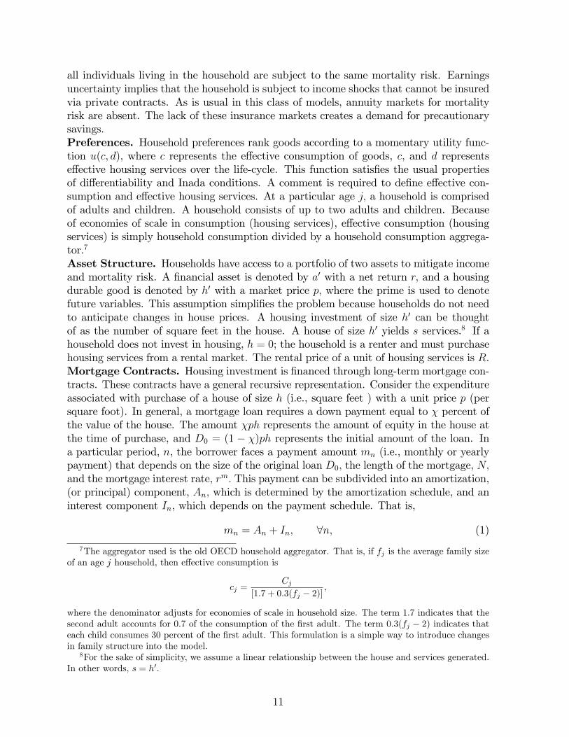
all individuals living in the household are subject to the same mortality risk. Earningsuncertainty implies that the household is subject to income shocks that cannot be insuredvia private contracts. As is usual in this class of models, annuity markets for mortalityrisk are absent. The lack of these insurance markets creates a demand for precautionarysavings.Preferences. Household preferences rank goods according to a momentary utility func-tion u(c, d), where c represents the effective consumption of goods, c, and d representseffective housing services over the life-cycle. This function satisfies the usual propertiesof differentiability and Inada conditions. A comment is required to define effective con-sumption and effective housing services. At a particular age j, a household is comprisedof adults and children. A household consists of up to two adults and children. Becauseof economies of scale in consumption (housing services), effective consumption (housingservices) is simply household consumption divided by a household consumption aggrega-tor.7

Asset Structure. Households have access to a portfolio of two assets to mitigate incomeand mortality risk. A financial asset is denoted by a′ with a net return r, and a housingdurable good is denoted by h′ with a market price p, where the prime is used to denotefuture variables. This assumption simplifies the problem because households do not needto anticipate changes in house prices. A housing investment of size h′ can be thoughtof as the number of square feet in the house. A house of size h′ yields s services.8 If ahousehold does not invest in housing, h = 0; the household is a renter and must purchasehousing services from a rental market. The rental price of a unit of housing services is R.Mortgage Contracts. Housing investment is financed through long-term mortgage con-tracts. These contracts have a general recursive representation. Consider the expenditureassociated with purchase of a house of size h (i.e., square feet ) with a unit price p (persquare foot). In general, a mortgage loan requires a down payment equal to χ percent ofthe value of the house. The amount χph represents the amount of equity in the house atthe time of purchase, and D0 = (1 − χ)ph represents the initial amount of the loan. Ina particular period, n, the borrower faces a payment amount mn (i.e., monthly or yearlypayment) that depends on the size of the original loan D0, the length of the mortgage, N,and the mortgage interest rate, rm. This payment can be subdivided into an amortization,(or principal) component, An, which is determined by the amortization schedule, and aninterest component In, which depends on the payment schedule. That is,

mn = An + In, ∀n, (1)

7The aggregator used is the old OECD household aggregator. That is, if fj is the average family sizeof an age j household, then effective consumption is

cj =Cj

[1.7 + 0.3(fj − 2)],

where the denominator adjusts for economies of scale in household size. The term 1.7 indicates that thesecond adult accounts for 0.7 of the consumption of the first adult. The term 0.3(fj − 2) indicates thateach child consumes 30 percent of the first adult. This formulation is a simple way to introduce changesin family structure into the model.

8For the sake of simplicity, we assume a linear relationship between the house and services generated.In other words, s = h′.

11

where the interest payments are calculated by In = rmDn.9 An expression that determines

how the remaining debt, Dn, changes over time can be written as

Dn+1 = Dn − An, ∀n. (2)

This formula shows that the level of outstanding debt at the start of period n is reducedby the amount of any principal payment. A principal payment increases the level of equityin the home. If the amount of equity in a home at the start of period n is defined as Hn,a payment of principal equal to An increases equity in the house available in the nextperiod to Hn+1. Formally,

Hn+1 = Hn + An, ∀n, (3)

where H0 = χph denotes the home equity in the initial period.Before the Great Depression the typical mortgage contract was characterized by no

amortization and a balloon payment at termination. A balloon loan is a very simplecontract in which the entire principal borrowed is paid in full in the last period, N. Theamortization schedule for this contract can be written as

An =

0 ∀n < N

(1− χ)ph n = N.

This means that the mortgage payment in all periods except the last one, is equal to theinterest rate payment, In = rmD0. Hence, the mortgage payment for this contract can bespecified as

mn =

In ∀n < N

(1 + rm)D0 n = N,

where D0 = (1− χ)ph. The evolution of the outstanding level of debt can be written as

Dn+1 =

Dn, ∀n < N0, n = N.

.

With an interest-only loan and no changes in house prices, the homeowner never ac-crues additional equity beyond the initial down payment until the final mortgage paymentis made. Hence, An = 0 and mn = In = rmD0 for all n. In essence, the homeowner effec-tively rents the property from the lender and the mortgage (interest) payments are theeffective rental cost. As a result, the monthly mortgage payment is minimized becauseno periodic payments toward equity are made. A homeowner is fully leveraged with thebank with this type of contract. If the homeowner itemizes tax deductions, a large interestdeduction is an attractive by-product of this contract.After the Great Depression, the FHA sponsored a new mortgage contract characterized

by a longer duration, lower down payment requirements (i.e., higher LTV ratios), and self-amortization with a mortgage payment comprised of both interest and principal. This loanproduct is characterized by a constant mortgage payment over the term of the mortgage,

9The calculation of the mortgage payment depends on the characteristics of the contract, but for allcontracts the present value of the payments must be equal to the total amount borrowed, D0 ≡ χph =∑N

n mn/(1 + r)n.

12

m ≡ m1 = ... = mN . This value, m, must be consistent with the condition that thepresent value of mortgage payments repays the initial loan. That is,

D0 ≡ χph =∑N

n

m

(1 + r)n.

If this equation is solved for m, we can write m = λD0, where λ = rm[1− (1 + rm)−N ]−1.Because the mortgage payment is constant each period and m = At + It, the outstandingdebt decreases over time, D0 > ... > DN . This means the fixed payment contract front-loads interest rate payments,

Dn+1 = (1 + rm)Dn −m, ∀n,

and thus back-loads principal payments, An = m−rmDn. The equity in the house increaseseach period by the mortgage payment net of the interest payment component: Hn+1 =Hn + [m− rmDn] every period.Household Income. Household income varies over the life-cycle and depends on (1)whether the household is a worker or a retiree, (2) the return from savings and transferprograms, and (3) the income generated from the decision to rent property when a home-owner. Households supply their time endowment inelastically to the labor market andearn wage income, w, per effective unit of labor. The effective units of labor depend onthe education level and the age of the household. The deterministic component of incomeis denoted by υij and a transitory type-dependent idiosyncratic component, εij, drawnfrom a probability distribution, Πij(εij). The expectations about income uncertainty aredrawn from this distribution. For an individual younger than j∗, labor earnings are thenwεijυij. Households of age j∗ or older receive a social security transfer that is proportionalto average labor income and is defined as θ. Pretax labor earnings are defined as yw, where

yw(ε, i, j) =

wεijυij, if j < j∗

θ, if j ≥ j∗.

A second source of income is available to households that invest in housing and decideto rent part of their investment. A household that does not consume all housing services,h′ > d, can pay a fixed cost, $ > 0, and receive rental income yR(h′, d); this is denoted as

yR(h′, d) =

R(h′ − d)−$, if h′ > d

0, if h′ = d

Savings and transfers provide additional sources of income. Households with positivesavings receive (1 + r)a. The transfers are derived from the households that die withpositive wealth. The value of all these assets is uniformly distributed to the householdsthat remain alive in an equal lump sum amount of tr. The (pretax) income of a household,y, is simply

y(h′, a, ε, d, i, j) = yw(ε, i, j) + yR(h′, d) + (1 + r)a+ tr.

The various income sources generate a tax obligation of T, which depends on laborincome, yw , net interest earnings from savings, ra, and rental income, yR, less deduc-tions available in the tax code, Ω. Examples of deductions could be the interest payment

13

deduction on mortgage loans or maintenance expenses associated with tenant-occupiedhousing. Total tax obligations are denoted as

T = T (yw(ε, i, j) + ra+ yR(h′, d)− Ω).

The Household Decision Problem. A single household’s budget constraint cannot beeasily written for this problem because such households make discrete tenure decisions.In each period, a renter could purchase a home or a homeowner could change the size ofthe house or even become a renter. Hence, the household’s budget constraint dependson the value of the current state variables. The relevant information at the start of theperiod is the education level (i.e., fewer than 8 years of education; 8 years of education;fewer than 12 years of education; and 12 0r more years of education), i, household’s age,j, the level of asset holding, a, the housing investment, h, the mortgage choice, z, themortgage balance with the bank, n, and the income shock ε(i, j),which is contingent onage and education, written as ε. To simplify notation, let x = (i, a, h, z, n, j, ε) summarizethe household’s state vector. A household could face a number of budget constraintsdepending on the tenure decision. Individuals make decisions over consumption goods, c,housing services, d, and investment in assets, a′, and housing, h′. Table 3 summarizes thefive distinct decision problems that a household must solve with respect to shelter.

Table 3: Choice Diagram for the Household

Current renter: h = 0

Continues renting: h′ = 0

Purchases a house: h′ > 0

Current owner: h > 0

Stays in house: h′ = h

Change house size (upsize or downsize): h′ 6= h

Sell house and rent: h′ = 0

This problem can be better understood by considering the problem of an individualwho starts a period as a renter and then considering the problem of an individuals whostarts a period as a home owner.

• Renters: A household that is currently renting, (h = 0), has two options: continuerenting (h′ = 0) or purchase a house (h

′> 0). This is a discrete choice in ownership

that can easily be captured by the value function v (present and future utility) asso-ciated with these two options. Given the relevant information x = (i, j, a, 0, 0, 0, ε),the individual chooses the option with the higher value, which can be expressed as

v(x) = maxvr, vo.

14

The value associated with continued renting is determined by solving

vr(x) = max[u(c, d) + βj+1Eijv(x′)], (4)

s.t. c+ a′ +Rd = y(x)− T.The household is subject to non-negativity constraints on c, d, and a′. These con-straints are present in all possible cases and are not explicitly stated in the othercases.10 The current decisions determine the state vector tomorrow x′ = (i, j +1, a, 0, 0, 0, ε′).

A household that purchases a house solves a different problem as choices must nowbe made over h

′> 0. This decision problem can be written as

vo(x) = max[u(c, d) + βj+1Eijv(x′)], (5)

s.t. c+ a′ + (φb(z, x) + χ(z, x))ph′ +m(h′, n; p) = y(x)− T.The purchase of a home requires use of a long-term loan. The mortgage contract isa function that specifies the length of the contract, N, the down payment fraction,χ(z, x) ∈ [0, 1], and the payment schedule, m. The decision to buy a house ofvalue ph′ implies total borrowing must equal DN = (1 − χ(z, x))ph′. The paymentstructure depends on the mortgage available in any given period. The purchase of ahouse requires only an expenditure of the down payment and associated transactioncosts, φb(z, x). The model formulation is fairly general and allows for downpaymentand transaction costs to depend on the mortgage choice, and potentially educationstatus. The relevant continuation state is x′ = (i, j + 1, a′, h, z,N − 1, ε′)

• Owners: The decision problem for a household that currently owns a house (h > 0),has a similar structure. However, a homeowner faces a different set of options: stayin the same house (h′ = h), purchase a different house (h′ 6= h), or sell the houseand acquire housing services through the rental market (h′ = 0). Given the relevantinformation state x, the individual solves

v(x) = maxvs, vc, vr.

Each of these three different values is calculated by solving three different decisionproblems.

1. If the homeowner decides to stay in the current house the optimization problemcan be written as

vs(x) = max[u(c, h′) + βj+1Eijv(x′)] (6)

s.t. c+ a′ +m(h, n; p) = y(x)− T.This problem is very simple because the homeowner must make decisionsonly on consumption and saving after making the mortgage payment. Ifthe mortgage has been paid off (i.e., n = 0), then m(h, n; p) = 0. Other-wise, the mortgage payment is positive. The next period state is given byx′ = (i, j + 1, a′, h, z, n′, ε′), where n′ = maxn− 1, 0.

10The change in the size of rental property (flow) is not subject to transaction costs; only the changein housing investment (stock) is subject to frictions.

15

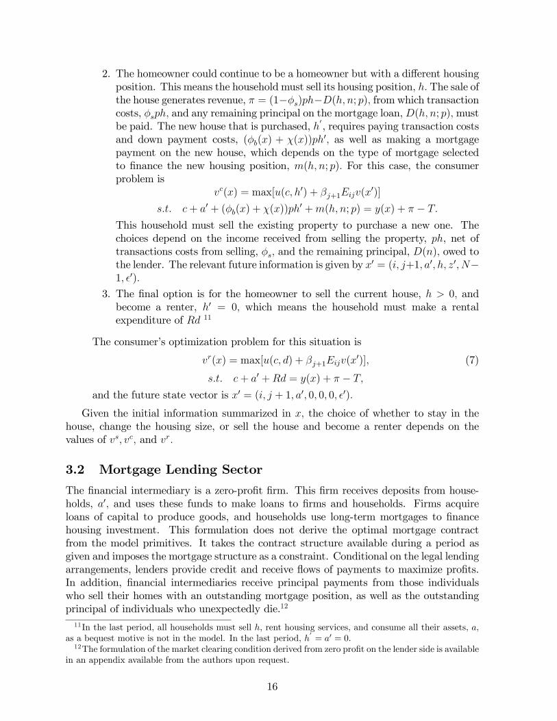
2. The homeowner could continue to be a homeowner but with a different housingposition. This means the household must sell its housing position, h. The sale ofthe house generates revenue, π = (1−φs)ph−D(h, n; p), from which transactioncosts, φsph, and any remaining principal on the mortgage loan, D(h, n; p),mustbe paid. The new house that is purchased, h

′, requires paying transaction costs

and down payment costs, (φb(x) + χ(x))ph′, as well as making a mortgagepayment on the new house, which depends on the type of mortgage selectedto finance the new housing position, m(h, n; p). For this case, the consumerproblem is

vc(x) = max[u(c, h′) + βj+1Eijv(x′)]

s.t. c+ a′ + (φb(x) + χ(x))ph′ +m(h, n; p) = y(x) + π − T.This household must sell the existing property to purchase a new one. Thechoices depend on the income received from selling the property, ph, net oftransactions costs from selling, φs, and the remaining principal, D(n), owed tothe lender. The relevant future information is given by x′ = (i, j+1, a′, h, z′, N−1, ε′).

3. The final option is for the homeowner to sell the current house, h > 0, andbecome a renter, h′ = 0, which means the household must make a rentalexpenditure of Rd 11

The consumer’s optimization problem for this situation is

vr(x) = max[u(c, d) + βj+1Eijv(x′)], (7)

s.t. c+ a′ +Rd = y(x) + π − T,and the future state vector is x′ = (i, j + 1, a′, 0, 0, 0, ε′).

Given the initial information summarized in x, the choice of whether to stay in thehouse, change the housing size, or sell the house and become a renter depends on thevalues of vs, vc, and vr.

3.2 Mortgage Lending Sector

The financial intermediary is a zero-profit firm. This firm receives deposits from house-holds, a′, and uses these funds to make loans to firms and households. Firms acquireloans of capital to produce goods, and households use long-term mortgages to financehousing investment. This formulation does not derive the optimal mortgage contractfrom the model primitives. It takes the contract structure available during a period asgiven and imposes the mortgage structure as a constraint. Conditional on the legal lendingarrangements, lenders provide credit and receive flows of payments to maximize profits.In addition, financial intermediaries receive principal payments from those individualswho sell their homes with an outstanding mortgage position, as well as the outstandingprincipal of individuals who unexpectedly die.12

11In the last period, all households must sell h, rent housing services, and consume all their assets, a,as a bequest motive is not in the model. In the last period, h

′= a′ = 0.

12The formulation of the market clearing condition derived from zero profit on the lender side is availablein an appendix available from the authors upon request.

16

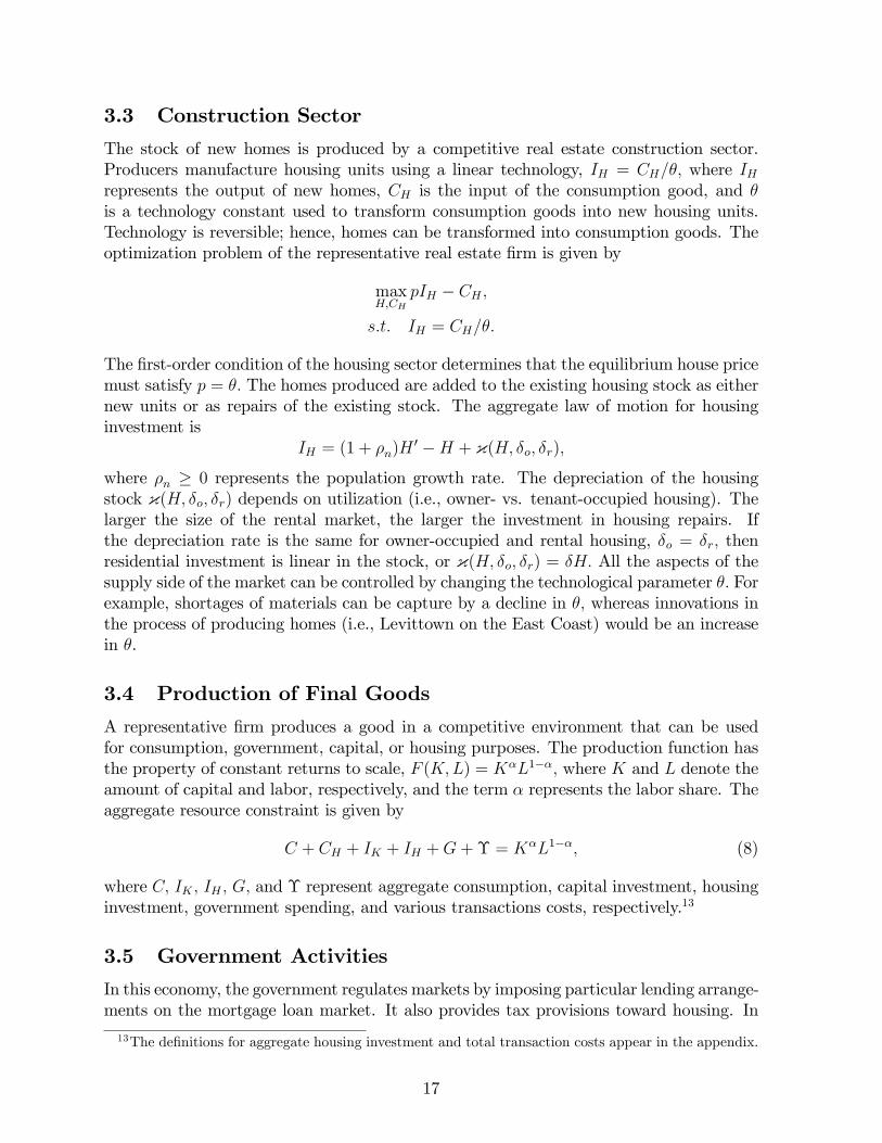
3.3 Construction Sector

The stock of new homes is produced by a competitive real estate construction sector.Producers manufacture housing units using a linear technology, IH = CH/θ, where IHrepresents the output of new homes, CH is the input of the consumption good, and θis a technology constant used to transform consumption goods into new housing units.Technology is reversible; hence, homes can be transformed into consumption goods. Theoptimization problem of the representative real estate firm is given by

maxH,CH

pIH − CH ,

s.t. IH = CH/θ.

The first-order condition of the housing sector determines that the equilibrium house pricemust satisfy p = θ. The homes produced are added to the existing housing stock as eithernew units or as repairs of the existing stock. The aggregate law of motion for housinginvestment is

IH = (1 + ρn)H ′ −H + κ(H, δo, δr),

where ρn ≥ 0 represents the population growth rate. The depreciation of the housingstock κ(H, δo, δr) depends on utilization (i.e., owner- vs. tenant-occupied housing). Thelarger the size of the rental market, the larger the investment in housing repairs. Ifthe depreciation rate is the same for owner-occupied and rental housing, δo = δr, thenresidential investment is linear in the stock, or κ(H, δo, δr) = δH. All the aspects of thesupply side of the market can be controlled by changing the technological parameter θ. Forexample, shortages of materials can be capture by a decline in θ, whereas innovations inthe process of producing homes (i.e., Levittown on the East Coast) would be an increasein θ.

3.4 Production of Final Goods

A representative firm produces a good in a competitive environment that can be usedfor consumption, government, capital, or housing purposes. The production function hasthe property of constant returns to scale, F (K,L) = KαL1−α, where K and L denote theamount of capital and labor, respectively, and the term α represents the labor share. Theaggregate resource constraint is given by

C + CH + IK + IH +G+ Υ = KαL1−α, (8)

where C, IK , IH , G, and Υ represent aggregate consumption, capital investment, housinginvestment, government spending, and various transactions costs, respectively.13

3.5 Government Activities

In this economy, the government regulates markets by imposing particular lending arrange-ments on the mortgage loan market. It also provides tax provisions toward housing. In

13The definitions for aggregate housing investment and total transaction costs appear in the appendix.

17

addition to these passive regulatory roles, the government plays a more active role throughother programs. First, retirement benefits are provided through a pay-as-you-go socialsecurity program. Social security contributions are used to finance a uniform transferupon retirement that represents a fraction of average income. Second, exogenous govern-ment expenditure is financed by using a nonlinear income tax scheme. The financing ofgovernment expenditure and social security is conducted under different budgets. Finally,the government redistributes the wealth (housing and financial assets) of individuals whodie unexpectedly. Both housing and financial assets are sold and any outstanding debton housing is paid off. The remaining value of these assets is distributed to the survivinghouseholds as a lump-sum payment, tr.

3.6 Stationary Equilibrium

In the model, a stationary equilibrium includes optimal decisions that are a functionof the individual state variables, x = (i, j, a, h, z, n, ε), prices r, w,R, market clearingconditions, and a distribution over the state space Φ(x) that are constant over time.14

4 Quantitative Analysis

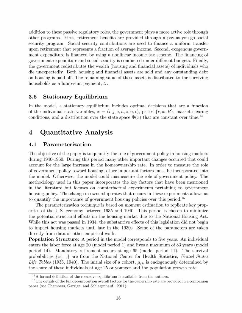
4.1 Parameterization

The objective of the paper is to quantify the role of government policy in housing marketsduring 1940-1960. During this period many other important changes occurred that couldaccount for the large increase in the homeownership rate. In order to measure the roleof government policy toward housing, other important factors must be incorporated intothe model. Otherwise, the model could mismeasure the role of government policy. Themethodology used in this paper incorporates the key factors that have been mentionedin the literature but focuses on counterfactual experiments pertaining to governmenthousing policy. The change in ownership rates that occurs in these experiments allows usto quantify the importance of government housing policies over this period.15

The parameterization technique is based on moment estimation to replicate key prop-erties of the U.S. economy between 1935 and 1940. This period is chosen to minimizethe potential structural effects on the housing market due to the National Housing Act.While this act was passed in 1934, the substantive effects of this legislation did not beginto impact housing markets until late in the 1930s. Some of the parameters are takendirectly from data or other empirical work.Population Structure: A period in the model corresponds to five years. An individualenters the labor force at age 20 (model period 1) and lives a maximum of 83 years (modelperiod 14). Mandatory retirement occurs at age 65 (model period 11). The survivalprobabilities ψj+1 are from the National Center for Health Statistics, United StatesLife Tables (1935, 1940). The initial size of a cohort, µij, is endogenously determined bythe share of these individuals at age 25 or younger and the population growth rate.

14A formal definition of the recursive equilibrium is available from the authors.15The details of the full decomposition overall factors for the ownership rate are provided in a companion

paper (see Chambers, Garriga, and Schlagenhauf , 2011).

18

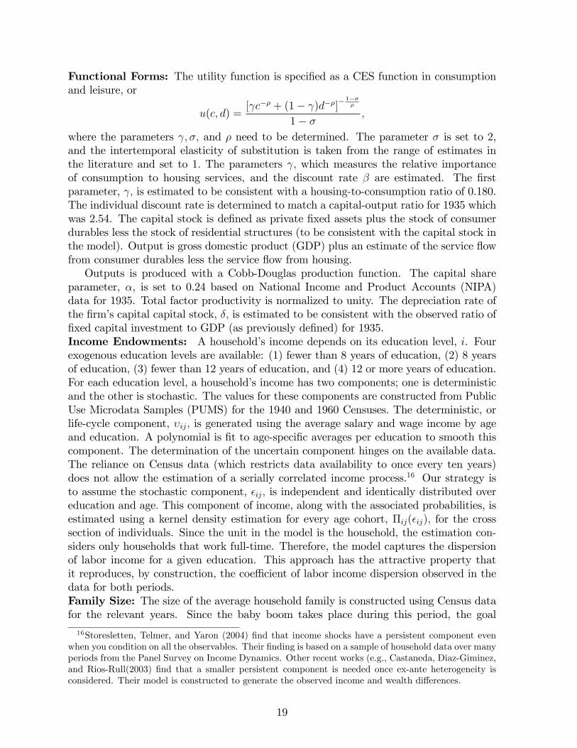
Functional Forms: The utility function is specified as a CES function in consumptionand leisure, or

u(c, d) =[γc−ρ + (1− γ)d−ρ]

− 1−σρ

1− σ ,

where the parameters γ, σ, and ρ need to be determined. The parameter σ is set to 2,and the intertemporal elasticity of substitution is taken from the range of estimates inthe literature and set to 1. The parameters γ, which measures the relative importanceof consumption to housing services, and the discount rate β are estimated. The firstparameter, γ, is estimated to be consistent with a housing-to-consumption ratio of 0.180.The individual discount rate is determined to match a capital-output ratio for 1935 whichwas 2.54. The capital stock is defined as private fixed assets plus the stock of consumerdurables less the stock of residential structures (to be consistent with the capital stock inthe model). Output is gross domestic product (GDP) plus an estimate of the service flowfrom consumer durables less the service flow from housing.Outputs is produced with a Cobb-Douglas production function. The capital share

parameter, α, is set to 0.24 based on National Income and Product Accounts (NIPA)data for 1935. Total factor productivity is normalized to unity. The depreciation rate ofthe firm’s capital capital stock, δ, is estimated to be consistent with the observed ratio offixed capital investment to GDP (as previously defined) for 1935.Income Endowments: A household’s income depends on its education level, i. Fourexogenous education levels are available: (1) fewer than 8 years of education, (2) 8 yearsof education, (3) fewer than 12 years of education, and (4) 12 or more years of education.For each education level, a household’s income has two components; one is deterministicand the other is stochastic. The values for these components are constructed from PublicUse Microdata Samples (PUMS) for the 1940 and 1960 Censuses. The deterministic, orlife-cycle component, υij, is generated using the average salary and wage income by ageand education. A polynomial is fit to age-specific averages per education to smooth thiscomponent. The determination of the uncertain component hinges on the available data.The reliance on Census data (which restricts data availability to once every ten years)does not allow the estimation of a serially correlated income process.16 Our strategy isto assume the stochastic component, εij, is independent and identically distributed overeducation and age. This component of income, along with the associated probabilities, isestimated using a kernel density estimation for every age cohort, Πij(εij), for the crosssection of individuals. Since the unit in the model is the household, the estimation con-siders only households that work full-time. Therefore, the model captures the dispersionof labor income for a given education. This approach has the attractive property thatit reproduces, by construction, the coeffi cient of labor income dispersion observed in thedata for both periods.Family Size: The size of the average household family is constructed using Census datafor the relevant years. Since the baby boom takes place during this period, the goal

16Storesletten, Telmer, and Yaron (2004) find that income shocks have a persistent component evenwhen you condition on all the observables. Their finding is based on a sample of household data over manyperiods from the Panel Survey on Income Dynamics. Other recent works (e.g., Castaneda, Diaz-Giminez,and Rios-Rull(2003) find that a smaller persistent component is needed once ex-ante heterogeneity isconsidered. Their model is constructed to generate the observed income and wealth differences.

19

is to allow for the effects of changing household family size in the demand for owner-occupied housing. In a more detailed theory, changes in institutional arrangements couldaffect fertility decisions. In the model, the demographic structure is taken as exogenouslydetermined and does not depend on education types.Government and the Income Tax Function: In 1940, the U.S. Social Security pro-gram was in its infancy. The payroll tax rate for a worker was 1 percent of wage income.In addition, wage income for payroll tax purposes was capped at $3,000. The model usesa 30 percent replacement rate.The income tax code in 1940 differentiated income from total net taxable income,

which is equal to wage, rental, and interest income less interest payments such as mortgageinterest payments. In addition, each household receives an earned income credit. Thiscredit is equal to 10 percent of wage income as long as net income is less than $3,000.If net income exceeds $3,000, the credit is calculated as 10 percent of the minimum ofwage income or total taxable income. The tax credit is capped at $1,400. In additionto the earned income credit, each household received a personal exemption of $800. Ifthese two credits are subtracted from total net taxable income, adjusted taxable income isdetermined. The actual tax schedules for 1940 and 1960 are programmed to determine ahousehold’s tax obligation. The tax functions for 1940 and 1960 are summarized in Figure3. For the 1940 tax code, the marginal tax rate is 0.79 which is applicable to income levelsexceeding $500,000. In 1940, an income tax surcharge is equal to an additional 10 percentmust be included in the income tax obligation. The documentation for the 1940 tax codeis the Internal Revenue Service and the Tax Foundation. To ensure that the income taxfunction generates the proper amount of revenue for 1940, an adjustment factor must beadded to the tax code. This parameter can be considered as adding an intercept to thetax function. If too much revenue is generated, this parameter, τ 0, can be reduced. Thisfactor is estimated by targeting the personal income tax revenue-to-GDP ratio. In 1935,this ratio was 0.01.Housing: In the baseline model, homeowners have two mortgages choices: a short-duration balloon loan restricted to 10 years with a 50 percent down payment and a20-year FRM with a 20 percent down payment. Formally, χ(1) = 0.5 and χ(2) = 0.2.The transaction costs from buying and selling property are φs = 0 and φb = 0.06. Theminimum house size, h, is estimated to be consistent with the set of specified targets.The values δo and δr are from Chambers, Garriga, and Schlagenhauf (2009), where theannual depreciation rates for owner and tenant-occupied housing are δo = 0.0106 andδr = 0.0135, respectively.Wealth Endowments: Bequests appear to have been an important source of homeown-ership for young households in 1940. Table 4 presents IRS data on real estate bequests in

20

both 1940 and 1960.17

Table 4: Real Estate Bequests in the United States (1940-1960)

Gross Mortgages NetYear Returns Bequest Value($) and Debts($) Bequest Value($)1940 16,156 2,649,492,000 229,866,000 2,419,626,0001960 52,070 2,857,330,000 690,038,000 1,867,292,000

Source: Internal Revenue Service, Historical Data

Although the number of returns tripled between 1940 and 1960, the total gross valueof real estate bequests grew by less that 10 percent. However, the amount of outstandingdebt on bequeathed real estate more than tripled in the same 20-year period. As a result,the net value of real estate bequests actually dropped by 23 percent between 1940 and1960. The apparent importance of real estate bequests in 1940 requires the introductionof an additional parameter W0 to the model. This parameter represents the percentageof age 1 households that receive a bequest of a minimum size home. The percentageis adjusted so that the model generates a homeownership rate for young households issimilar to that found in the data. The value of transfers from accidental death is adjustedto equal the amount of housing bequests to individuals.The estimation of the set structural parameters (δ, γ, β, h, τ 0,W0) for 1940 is based

on an exactly identified method of moments approach plus the computation of marketclearing (capital market and rental market) under the restriction that the governmentbudget constraint is balanced. Table 5 reports the parameter values that generate ag-gregate statistics consistent with the U.S. economy. Parameters are estimated within 1percent error for all the observed targets.

17The data in Table 5 are from the U. S. Treasury Department, Bureau of Internal Revenue, Statisticson Income for 1940, Part 1. These data are compiled from individual income tax returns, taxable fiduciaryincome and defense tax returns, and estate tax returns prepared under the direction of the Commissionerof Revenue by the statistics section, income tax unit. A similar document is used for 1960.

21

Table 5: Parameterization of Model

Statistic Target ModelRatio of wealth to gross domestic product (K/Y ) 2.540 2.5470Ratio of housing services to consumption of goods (Rsc/c) 0.180 0.1800Ratio of fixed capital investment to GDP (δK/Y ) 0.112 0.1120Homeownership Rate 0.436 0.4350Ratio of personal income tax revenue to output (T (ay)/Y ) 0.010 0.0099Balanced bequests 0.000 0.0003

Variable Parameter ValueIndividual discount rate β 0.928Share of consumption goods in the utility function γ 0.947Depreciation rate on capital δ 0.197Minimum housing size h 0.637Lump-sum tax transfer τ 0 0.081Initial-period bequested homes W0 0.565

4.2 Baseline Economy: 1940

The model can be evaluated from various perspectives. The objective is to measure theperformance by considering the homeownership rate statistics for the various years andage groups. As Table 6 shows, the homeownership rate in 1930 was 48.1 percent, whereasafter the Great Depression it ranged between 42.7 and 45.5 percent. Since the baselinemodel attempts to focus on the home ownership rate prior to the impact of the NationalHousing Act, the targeted homeownership rate is 45.5 percent.

Table 6: Homeownership (%) by Age

Age Data Model1930 1940-43 1940

Under 35 years 20.0 19.1 22.736-45 years 48.5 42.1 49.546-55 years 57.7 51.0 61.856-65 years 65.1 57.5 69.565 years and over 69.7 60.3 69.4Total 48.1 42.7-45.5 45.7

Source: US. Census Bureau

Since the aggregate homeownership rate is an estimation target, it not surprising thatthe baseline model generates a number close to the selected moment. The age-specifichomeownership rates also can be used to evaluate the model. The model captures thehump-shaped behavior observed in the data. The lowest homeownership rate is for theyoungest age cohort; this pattern is apparent in 1930 and 1940 with the difference that

22

homeownership rates are higher in 1930. The model does generate a pattern by age cohortconsistent with the Census estimates. The model also makes predictions about mortgageholdings. Table 7 summarizes some aggregate statistics about housing finance.

Table 7: Housing Finance

Statistics Model 1940Homeownership rate 45.7No Mortgage (%) 83.5Mortgage loan (%) 16.5

Share balloon (5 year) 100.0Share FRM (20 year) 0.0

It is diffi cult to find micro data for specific mortgage contracts, but given the shortduration and the predominance of balloon, this contract would be the expected to be thedominant in the model. In the model the majority of homeowners (83.5 percent) do nothave a mortgage. In the model all the homeowners purchase the housing using the balloonloan. The share of FRMs predicted by the model for 1940 is zero.

4.3 Baseline Economy: 1960

Many factors could have been important in the determination of the ownership boom. Theobjective of this section is to isolate the contribution of government programs from otherrelevant factors that could influence the increase in ownership. Government programspotentially affect homeownership through policies that have an impact on financing ofhousing, changes in the federal income tax structure, the role of the mortgage interestrate deduction, and the reduction of transaction costs in mortgage rates. To measure thecontribution of these government policies, the model must account for other factors thathave been argued as critical.18 The relevant factors that changed between 1940 and 1960are summarized as follows:

1. Demographic factors: Included are changes in the survival probabilities, educa-tion composition, and family structure.

18The federal income tax code changed significantly by 1960. Using data from the Tax Foundation andthe the U.S. Treasury Department Internal Revenue Service publication No. 17, it is possible to constructa representative tax function. This tax function had to account for the fact that renters were not likelyto itemize their deductions. A model assumption is that in 1960 all renters did not itemize deductions.As a result, these individuals used tax tables different from the households that did itemize. In fact,non-itemizing households with income levels under $5,000 were able to use a tax table that differed fromnon-itemizers with income over $5,000. Individuals were allowed an individual deduction worth $600 thatcould be used to minimize the tax obligation. If a household itemized expenses because of the mortgageinterest rate deduction, another tax table was to be used to calculate the income tax obligation wheretaxable income excluded the mortgage deduction and the individual exemption. The tax adjustmentcoeffi cient, τ0, is set to be consistent with a federal income tax-to-GDP ratio of 7.73 percent. Incometax obligations were much higher in 1960 and marginal tax rates were higher (See Figure 3). The topmarginal tax rate in 1960 was 91 percent for income over $2 million. The payroll tax increased to 1.5percent of wage income up to a cap of $4,800.

23

2. Endowments: Included are the change in the distribution of the i.i.d. idiosyncraticincome component, the effi ciency units, and the size of the real wage income increase.

3. House prices: According to Case-Shiller price data, real house prices increased by41.5 percent. Since house prices in the model are determined by the productivityparameter in the construction sector, this parameter can be adjusted to generatethe increased cost of housing per unit.

4. Housing finance: Changes include the extension of the FRM maturity from 20to 30 years and a decline in the spread between the mortgage interest rate and therisk-free rate from 2.53 to 1.63 percent annualized.

5. Taxation: Included are changes in the tax code.

Table 8 summarizes the implications of allowing all factors to change in the model.19

The model accounts for a significant amount of the total change in ownership (level) aswell as the compositional differences across age groups. It is important to note that theseare endogenous variables, not a result of estimating the parameters for 1960

Table 8: Model Prediction for Homeownership Rate 1940-60

Age Data(%) Model(%)Cohort 1940 1960 Difference 1940 1960 Difference

Under 35 years 19.1 56.2 37.1 22.7 53.5 30.836-45 years 42.1 68.1 26.0 49.5 80.0 30.546-55 years 51.0 69.5 18.5 61.8 86.5 24.756-65 years 57.5 69.3 11.8 69.5 85.4 15.965-72 years 60.3 69.8 9.5 69.4 73.3 3.9Total 45.5 62.5 18.9 45.7 63.5 17.8

For example, the actual aggregate housing participation rate in 1960 was 62.5 percentand the model predicts a similar magnitude. The model-generated age-cohort ownershiprates have a more pronounced hump compared with actual 1960 data, but this is likelydue to the fact that homeowners do not face mobility or health shocks that could requirethem to sell their house and rent. Despite the small differences in levels, the changebetween both periods in the model and data is quite similar, suggesting that this modelof tenure and mortgage choice provides a useful laboratory to assess the importance ofgovernment interventions in housing finance and housing policy.

4.4 Policy Intervention in Housing Finance

In this section, the model is used to measure the contribution of federal housing policiesto the increased homeownership rate.20 The focus is on the importance of amortizing19In 1960, households have mortgage choice between a 30-year FRM mortgage and a balloon contract.

In equilibrium, households do not hold the balloon- type contract. In other words, the FRM contract isa dominant contract.20It is interesting to note that Gebler, Blank, and Winnick (1956, p. 238) stated that the "precise

effects of the Federal Housing Administration and Veterans Administration programs on the volume of

24

contracts, mortgage duration, and mortgage interest rate costs. Chambers, Garriga,Schlagenhauf (2009a,b) found that mortgage market innovation was the key factor inexplaining the increase in the homeownership rate between 1996 and 2005. More pre-cisely, the introduction of highly leveraged loans with graduated mortgage payments wasfound important as this type of contract attracted first-time buyers to the housing market,while more established households still had the availability of the standard 30-year FRMcontract. Significant mortgage contract innovation also occurred in the mortgage marketbetween 1930 and 1960. As discussed previously, stimulating the flow of mortgage fundsto residential construction was a goal of federal housing policies since the early 1930s.Grebler, Blank, and Winnick, (1956, p238) state:

Stimulating the flow of mortgage funds to residential construction has beenthe principal aim of federal housing policies since the early and middle thir-ties. ..[T]hese policies in fact have operated almost exclusively through theuse of various devices influencing the flow of private institutional mortgagesfunds, that is, mortgage insurance or guarantee and improved marketability ofloans through the Federal National Mortgage Association. ... Another majorobjective of federal housing policies has been to reduce the periodic paymentsof mortgage borrowers, by lowering interest rates and lengthening contractterms. Policy makers looked to easier borrowing as a way to increase demandfor new residential construction.

As noted in the previous section, the starting point is the benchmark model where the1940 estimated parameters are used with all factors at their 1960 values. Households haveaccess to a 30-year FRM mortgage with a 20 percent down payment requirement as wellas a 10-year balloon contract with a 50 percent down payment. As documented earlier,the homeownership rate would be at 63.5 percent. Since the baseline model captures themagnitude of the increase in ownership, one way to measure the contribution of the 30-year FRM is to replace this contract with a 20-year FRM contract. This latter contractcorresponds to the initial offering of FRMs in the 1940s.As Table 9 shows, the model predicts that the aggregate homeownership rate should

fall from 63.5 percent to 61.6 percent. The model suggests that the extension of the FRMcontract from 20 to 30 years can explain around 12 percent of the increase in ownership.The effect is more dramatic by age cohorts, particular in young and middle-aged buyers.For these groups, the access of a more leveraged contract reduces the magnitude of themortgage payments and makes housing more attractive. In both economies, the fractionof individuals who use the balloon loan with 50 percent down payment is zero.

residential mortgage lending are as indeterminable as their impact on residential building activity."

25

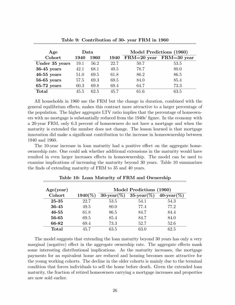
Table 9: Contribution of 30- year FRM in 1960

Age Data Model Predictions (1960)Cohort 1940 1960 1940 FRM=20 year FRM=30 year

Under 35 years 19.1 56.2 22.7 50.7 53.536-45 years 42.1 68.1 49.5 78.7 80.046-55 years 51.0 69.5 61.8 86.2 86.556-65 years 57.5 69.3 69.5 84.0 85.465-72 years 60.3 69.8 69.4 64.7 73.3Total 45.5 62.5 45.7 61.6 63.5

All households in 1960 use the FRM but the change in duration, combined with thegeneral equilibrium effects, makes this contract more attractive to a larger percentage ofthe population. The higher aggregate LTV ratio implies that the percentage of homeown-ers with no mortgage is substantially reduced from the 1940s’figure. In the economy witha 20-year FRM, only 6.3 percent of homeowners do not have a mortgage and when thematurity is extended the number does not change. The lesson learned is that mortgageinnovation did make a significant contribution to the increase in homeownership between1940 and 1960.The 10-year increase in loan maturity had a positive effect on the aggregate home-

ownership rate. One could ask whether additional extensions in the maturity would haveresulted in even larger increases effects in homeownership. The model can be used toexamine implications of increasing the maturity beyond 30 years. Table 10 summarizesthe finds of extending maturity of FRM to 35 and 40 years.

Table 10: Loan Maturity of FRM and Ownership

Age(year) Model Predictions (1960)Cohort 1940(%) 30-year(%) 35-year(%) 40-year(%)25-35 22.7 53.5 54.1 54.336-45 49.5 80.0 77.4 77.246-55 61.8 86.5 84.7 84.456-65 69.5 85.4 84.7 84.066-82 69.4 73.3 52.7 52.6Total 45.7 63.5 63.0 62.5

The model suggests that extending the loan maturity beyond 30 years has only a verymarginal (negative) effect in the aggregate ownership rate. The aggregate effects masksome interesting distributional implications. As the maturity increases, the mortgagepayments for an equivalent home are reduced and housing becomes more attractive forthe young working cohorts. The decline in the older cohorts is mainly due to the terminalcondition that forces individuals to sell the home before death. Given the extended loanmaturity, the fraction of retired homeowners carrying a mortgage increases and propertiesare now sold earlier.

26

Overall, the introduction of the 30-year FRM can account for roughly 12 percentof the total change in ownership. The model suggests that the length of the mortgagecontract sponsored by FHA had a significant effect on ownership; however, increasingthe maturity beyond 30 years seems to have a small negative effect in ownership. SinceFRM contracts already existed in the 1940s and 1950s, an obvious question is why theFRM contracts were not more popular in the 1940s when this type contract first becameavailable? As documented in Chambers, Garriga, and Schlagenhauf (2013), given thataverage household income was lower in 1940 than 1960 by a significant factor, the 1940household might not have been financially able to take advantage of the leverage featuresavailable in a FRM contract.In addition to federal policies that impacted homeownership through mortgage con-

tract structure, Grebler, Blank, and Winnick (1956) argue that a policy of lower mortgageinterest rates and increased mortgage market effi ciencies were important in the increase inhomeownership. Data for 1940 and 1960 suggest the spread between the mortgage interestrate and risk-free rate declined 85 basis points. The model can be used to quantify theimportance of the decline in the spread that resulted from an improved mortgage market.The test maintains the baseline model for 1960 but assumes the 1940 spread. If the in-terest spread is increased to the 1940 value, while maintaining the other factors at their1960 values, the model-predicted ownership rate would be 62.1 percent as summarized inTable 11. The decrease in the spread accounts for a 8.5 percent change in homeownership.

Table 11: The Importance of the Interest Rate Spread

Experimental Factors Ownership(%)1. Baseline: 1960 factors, 1940 parameters, 30-year FRM, 1960 spread 63.52. Model: 1960 factors, 1940 parameters, 30-year FRM, 1940 spread 62.1

4.5 Housing Policy: The Tax Treatment of Housing

This section explores the direct role of housing policy, taking as given the innovations inhousing finance. The purpose is to use the model to understand how housing tenure andinvestment decisions can be affected by housing policy embedded in the tax code. Part ofthe analysis is based on Chambers, Garriga, and Schlagenhauf (2009c). The key differenceis that the model abstracts from mortgage choice, and while the current framework allowsmortgage choice which turn out to be an important consideration.Understanding how this type of housing policy affects a household’s tenure and dura-

tion decisions requires examination of the household’s budget constraint. Some additionalnotation is required. Let κo and κr represent the taxable fraction of housing services con-sumed by owner- and tenant-occupied housing, respectively. The terms ιo and ιr representthe fraction of maintenance expenses from owner- and tenant-occupied housing that aredeductible. Given these definitions, taxable income can be defined in the model as

y = ω + ra+ κrR(h′ − d) + κoRd− ιrδrp(h′ − d)− ιoδ0pd− Ω, (9)

where Ω represents other type of deductions. The mortgage interest rate deduction would

27

enter through this variable as it obviously reduces taxable income.21 For homeowners whodo not pay the fixed entry cost ($ > 0), the definition of taxable income is reduced to

y = ω + ra+ κoRd− ιoδ0pd− Ω, (10)

as h′ = d.The first-order condition of a household that supplies rental housing services to the

market can be expressed as

uduc

= R− p∆δ + T ′(y)[p(ιrδr − ιoδo)−R(κr − κo)], (11)

where uc measures the marginal utility with respect to consumption c, and ud representsthe marginal utility with respect to housing services consumption, d. The first term onthe right-hand side is the rental price of a unit of housing, R, and measures the benefit toa household of forgoing a unit of housing services. This benefit is reduced the greater thespread in the depreciation rate for renter- and owner-occupied housing, ∆δ = (δr − δo).Ignoring tax considerations, the effective cost of owner-occupied housing services is Re =R − p(δr − δo). The implicit moral hazard problem makes renting more expensive thanowning as in Henderson and Ioannides (1983). The last two terms on the right-hand sideof the equation reflect the asymmetric treatment of owner- and tenant-occupied housing.The benefit from supplying services to the rental market is reduced when the spread inthe fraction of rental income relative to owner-occupied imputed income is larger. Inaddition, the benefit increases when the spread between maintenance expenses on renter-and owner-occupied housing increases. Removing the asymmetries, ιr = ιoδo/δr andκr = κo, and eliminating the progressivity of income taxation, T ′(y), reduces the benefitsfrom housing policy. As a result, the first-order condition without distortions is:

uduc

= R− p∆δ. (12)

The U.S. tax code has explicit provisions toward housing that imply κo = ιo = 0and κr = ιr = 1. That is, the income from the consumption of tenant-occupied housingservices is taxable, whereas owner-consumed housing services are not taxable. Mainte-nance expenses are treated asymmetrically in the tax code. Owner-occupied maintenanceexpenses cannot be deducted whereas maintenance expenses incurred with respect totenant-occupied housing are deductible. Under the U.S. code, the first-order conditionbecomes

uduc

= R[1− T ′(y)] + p[T ′(y)δr −4δ]. (13)

In addition to the asymmetric distortions just discussed and housing deductions, Ω, thataffect adjusted gross income, y, the degree of progressivity of the marginal tax rates, T ′(y),affects housing decisions. For example, under a more progressive tax code, the taxationeffects are large, which changes the incentives to own and supply rental property. At theaggregate level some of these incentives can disappear due to general equilibrium effects.Since the model has mortgage choice, changes in the tax code can change the incentiveson when to buy and the size of the house.21These terms are relevant only for homeowners since renters are not affected because they cannot be

property owners in the model.

28

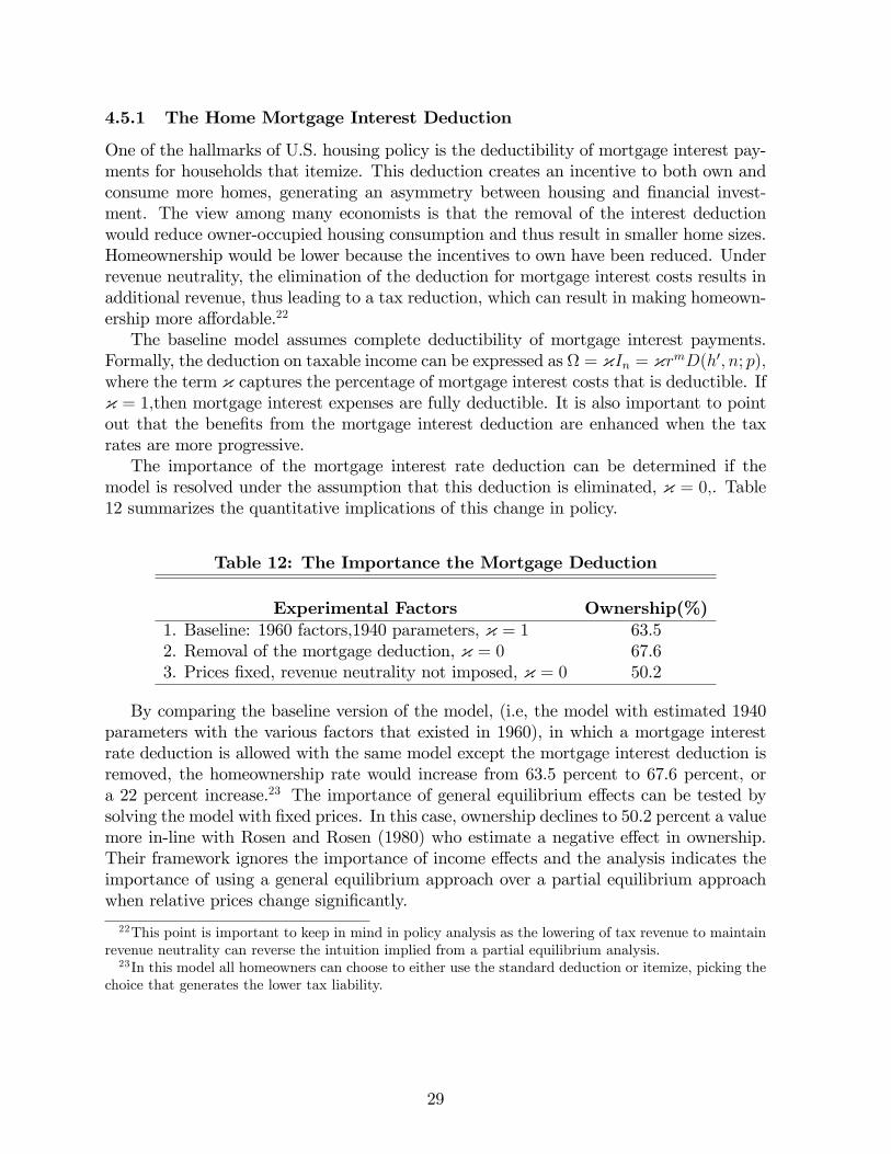
4.5.1 The Home Mortgage Interest Deduction

One of the hallmarks of U.S. housing policy is the deductibility of mortgage interest pay-ments for households that itemize. This deduction creates an incentive to both own andconsume more homes, generating an asymmetry between housing and financial invest-ment. The view among many economists is that the removal of the interest deductionwould reduce owner-occupied housing consumption and thus result in smaller home sizes.Homeownership would be lower because the incentives to own have been reduced. Underrevenue neutrality, the elimination of the deduction for mortgage interest costs results inadditional revenue, thus leading to a tax reduction, which can result in making homeown-ership more affordable.22

The baseline model assumes complete deductibility of mortgage interest payments.Formally, the deduction on taxable income can be expressed as Ω = κIn = κrmD(h′, n; p),where the term κ captures the percentage of mortgage interest costs that is deductible. Ifκ = 1,then mortgage interest expenses are fully deductible. It is also important to pointout that the benefits from the mortgage interest deduction are enhanced when the taxrates are more progressive.The importance of the mortgage interest rate deduction can be determined if the

model is resolved under the assumption that this deduction is eliminated, κ = 0,. Table12 summarizes the quantitative implications of this change in policy.

Table 12: The Importance the Mortgage Deduction

Experimental Factors Ownership(%)1. Baseline: 1960 factors,1940 parameters, κ = 1 63.52. Removal of the mortgage deduction, κ = 0 67.63. Prices fixed, revenue neutrality not imposed, κ = 0 50.2

By comparing the baseline version of the model, (i.e, the model with estimated 1940parameters with the various factors that existed in 1960), in which a mortgage interestrate deduction is allowed with the same model except the mortgage interest deduction isremoved, the homeownership rate would increase from 63.5 percent to 67.6 percent, ora 22 percent increase.23 The importance of general equilibrium effects can be tested bysolving the model with fixed prices. In this case, ownership declines to 50.2 percent a valuemore in-line with Rosen and Rosen (1980) who estimate a negative effect in ownership.Their framework ignores the importance of income effects and the analysis indicates theimportance of using a general equilibrium approach over a partial equilibrium approachwhen relative prices change significantly.

22This point is important to keep in mind in policy analysis as the lowering of tax revenue to maintainrevenue neutrality can reverse the intuition implied from a partial equilibrium analysis.23In this model all homeowners can choose to either use the standard deduction or itemize, picking the

choice that generates the lower tax liability.

29

4.5.2 Taxation of Owner-Occupied Housing Service Flows

Many economists argue that the primary distortion in the current tax code is the treatmentof housing services. Previous studies for the postwar period suggest that the eliminationof this asymmetry should lead to the consumption of smaller homes and lower home-ownership. For example, Berkovic and Fullerton (1992) find that the taxation of housingservices should reduce average housing consumption between 3 and 6 percent, whereasGervais (2002) finds that taxing imputed rents of owner-occupied housing would increasethe capital stock by more than 6 percent but decrease the housing stock by 8 percent.Under the current tax code, income generated from rental property is subject to tax-

ation, but the implicit income from owner-occupied housing is not taxed. As shown inEquation (13), this policy introduces an asymmetry in the tax treatment of owners andlandlords that favors the consumption of owner-occupied housing services and reduces theincentive to supply rental property. The landlord supply decision when housing servicesare taxed at different rates is determined by

uduc

= [R− p∆δ] + T ′(y)pδr − T ′(y)R(κr − κo). (14)

The U.S. tax code for the period 1940-60 would set κo = 0 and κr = 1. In Equation (14),the term T ′(y)R(κr−κo)measures the impact of the failure to tax housing services. As canbe seen, this term reduces the effective cost of owner-occupied housing and thus introducesa bias toward owner-occupied housing consumption. This asymmetry is eliminated whenthe fraction of imputed rental income from owner- and tenant-occupied housing is taxedat the same rate, κr = κo, but not necessarily zero. The analysis considers the case wherethe imputed rental income (measured as Rd) is fully taxed, κo = κr = 1. Table 13 presentsthese results.

Table 13: The Importance of Taxation Housing Services

Experimental Factors Ownership(%)1. Baseline: 1960 factors,1940 parameters, κo = 0 and κr = 1 63.52. Taxation of services, κo = κr = 1 60.43. Prices fixed, revenue neutrality not imposed, κo = κr = 1 55.9

The model suggests that the lack of taxation of housing services has an important im-pact in accounting for the increase in homeownership. The model suggests that if housingservices were taxed, the homeownership rate would be 21 percent lower. Again, a partialequilibrium analysis would overstate the importance of the policy of not taxing owner-occupied housing services. With fixed prices, the taxation of housing services reduces thehomeownership rate to 55.9.

5 Conclusions

After the collapse of housing markets during the Great Depression, the government, aspart of the New Deal, played a large role in shaping the future of housing finance. By

30

1960, the housing market had more than recovered as the homeownership rate soared toover 60 percent. This paper quantifies the role of government intervention in housingmarkets in explaining the expansion in U.S. homeownership between 1940 and 1960; thisrole is quantified with an equilibrium model of tenure choice. In the model, home buyershave access to a menu of mortgage choices to finance the acquisition of the house. Thegovernment also provides special programs, consistent with the provisions in the tax code.The parameterized model is consistent with key aggregate and distributional features inthe U.S. in 1940. The model can account for the boom in homeownership when adjustedto a 1960 economy.Government intervention via the mortgage market was a key part of the housing boom.

The model suggests that moving from a 20-year to a 30-year FRM accounts for roughly12 percent of the increase in homeownership. When combined with a narrowing mortgageinterest rate wedge, the total impact of mortgage innovation is approximately 21 percent.Government intervention via tax policy was also a significant factor in the housing boom.The model suggests that housing policy can have important effects on ownership. Forexample, the elimination of the mortgage deduction only reduces ownership when pricesare fixed and the tax surplus is not rebated back to the household sector. The taxationof housing services always reduces the ownership.These estimates have ignored the implications of the GI Bill for U.S. housing markets.

This legislation could affect housing markets in two ways. First, the GI Bill made hous-ing markets more accessible to veterans through down payment and mortgage paymentsubsidies. Fetters (2010) presents some empirical findings on this question. Second, thisbill provided benefits for human capital investment. The increase in number of collegegraduates increased substantially under this program. This means an individual with thislevel of human capital will operate on a higher income path in expected terms than anindividual with less education, which has implications for housing investment. The quan-titative implications of these policies are analyzed in more detail in Chambers, Garriga,and Schlagenhauf (2013).

References

[1] H. Aaron, (1972) Shelter and Subsides, Brookings Institution, Washington, D.C.

[2] P. S. Amaral and J. C. MacGee, (2002) "The Great Depression in Canada and theUnited States: A Neoclassical Perspective," Review of Economic Dynamics, 5(1),45-72.

[3] C. F. Behrens, (1952) Commercial Bank Activities in Urban Mortgage Financing,National Bureau of Economic Research.

[4] J. Berkovec and D. Fullerton, (1992) "A General Equilibrium Model of Housing,Taxes and Portfolio Choice," Journal of Political Economy, 100(2), 390-429.

[5] M. S. Carliner, (1998) "Development of Federal Home Ownership Policy," HousingPolicy Debate, 9(2), 299-321

31

[6] M. S. Carliner, (1998) "Inside Rising Home Ownership," Housing Economics 36(1),6-9.

[7] A. Castaneda, J. Diaz-Gimenez, and J.V. Rios-Rull, (2003) "Accounting for the U.S.Earnings and Wealth Inequality," Journal of Political Economy, 111(4), 818-857.

[8] H. L. Cole and L. E. Ohanian, (2002) "The Great U.K. Depression: A Puzzle andPossible Resolution," Review of Economic Dynamics, 5(1), 19-45.

[9] H. L. Cole and L. E. Ohanian, (2004) "New Deal Policies and the Persistenceof the Great Depression: A General Equilibrium Analysis, " Journal of PoliticalEconomy,112(4),779-816.

[10] M. Chambers, C. Garriga, and D. Schlagenhauf, (2009a) "Accounting for Changesin the home ownership Rate," International Economic Review, 50(3), 677-726.

[11] M. Chambers, C. Garriga, and D. Schlagenhauf, (2009b) "The Loan Structure andHousing Tenure Decisions in an Equilibrium Model of Mortgage Choice." Review ofEconomic Dynamics, 12(5), 444-468.

[12] M. Chambers, C. Garriga, and D. Schlagenhauf, (2009c) "Housing Policy and theProgressivity of Income Taxation, Journal of Monetary Economics, 56(8), 1116-1134.\

[13] M. Chambers, C. Garriga, and D. Schlagenhauf, (2013) "The New Deal, the GI Bill,and the Post-War Housing", working paper, Florida State University.

[14] A. Chevan, (1989) "The Growth of Home Ownership: 1940-1980, Demography, 26(2)249-265.

[15] M. Eccles, (1951) Beckoning Frontiers, Knopf, New York.

[16] E. Edwards, (1950) "Urban Real Estate Financing by Savings and Loan Associa-tions," Working Paper, National Bureau of Economic Research.

[17] D. K. Fetters, (2010) "Housing Finance and the Mid-century Transformation in USHome Ownership: the VA home loan program, Unpublished Paper, Harvard Univer-sity.

[18] M. Gervais, (2002) "Housing Taxation and Capital Accumulation," Journal of Mon-etary Economics, 49(7), 1461-89.

[19] L. Grebler, D. M. Blank, and L. Winnick, (1956) Capital Formation in Residen-tial Real Estate, National Bureau of Economic Research, Princeton N.J.: PrincetonUniversity Press.

[20] F. Hayashi and E. Prescott, (2002) "The 1990s in Japan: A Lost Decade," Reviewof Economic Dynamics, 5(1), 206-236.

[21] P. H. Hendershott and J. D. Shilling, (1982) "The Economics of Tenure Choice, 1955-1979," in C. Sirmans (ed.) Research in Real Estate, Greenwich, Conn: JAI Press.

32

[22] J. V. Henderson and Y. M. Ioannides, (1883) "A Model of Housing Tenure Choice,"American Economic Review, 73(1),98-113.

[23] Herzog, J.P and James S. Earley (1970) Home Mortgage Delinquency and Foreclo-sure, New York: Columbia University Press.

[24] J. F. Kain, (1983) "America’s Housing Crisis: Errors in Analysis and Policy," Annu-als, 465: 136-148.

[25] G. Katona (1964), The Mass Consumption Society, New York: McGraw-Hill.

[26] S. Klaman, (1961) The Postwar Residential Mortgage Market, Princeton, N.J.:Princeton University Press.

[27] D. Laidler, (1969) "Income Taxation Incentives for Owner-Occupied Housing," in A.Harberger, M. Bailey (eds.), The Taxation of Income from Capital, Washington D.C.: Brookings Institution, 50-76.

[28] J. E. Morton, (1956) Urban Mortgage Lending: Comparative Markets and Experience.National Bureau of Economic Research, Princeton N.J.: Princeton University Press.

[29] L. Ohanian, (1997) "The Macroeconomic Effects of War Finance in the UnitedStates," American Economic Review, 87(1), 23-40.

[30] F. Perri and V. Quadrini, (2002) "The Great Depression in Italy: Trade Restrictionsand Real Wage Rigidities," Review of Economic Dynamics, 5(1), 128-151.

[31] R. Ratcliff, D. Rathbun and J. Honnold, (1957) Residential Finance, 1950, New YorkN.Y.: John Wiley & Sons.

[32] H. Rosen, and K.T. Rosen, (1980) "Federal Taxes and home ownership: Evidencefrom Time Series," Journal of Political Economy, 88(1), 59-75.

[33] R. J. Saulnier, (1950) Urban Mortgage Lending by Life Insurance Companies, Na-tional Bureau of Economic Research.

[34] M. P. Semer, J.H. Zimmerman, and J. M. Frantz, (1976) "Legislative History. Housingin the Seventies," National Housing Policy Review, 3-180.

[35] K. Storesletten, C. Telmer, and A.Yaron, (2004) "Consumption and Risk SharingOver the Life Cycle," Journal of Monetary Economics, 51(3), 609-633.

[36] M. H. Yearns, (1976) "Governmental Housing Programs: A Brief Review," in C.S. Wedin and L.G. Nygren (eds.), Housing Perspectives: Individuals and Families,Minneapolis: Burgess Publishing.

33

6 Appendix

6.1 1900-30s: The Emergence of Mortgage Finance

The influence of mortgage lending institutions on housing markets began at the start ofthe twentieth century. Developments, particularly the role of the Federal government,during the first half of this Century only enhanced the role of these lending institutions.During this period there was an important process of creation of agencies, structures,programs, and regulations designed to make investment in the housing market secure andprofitable for households, and especially financial intermediaries and lenders.The growth in mortgage financing for residential real estate was a result of banks

incentives to look for new profit opportunities. Before the 1930’s the large down paymentrequirements and the lack of long-term financing (mortgage contracts were only three tofive years) made housing ownership diffi cult even for middle-class families.

6.2 1930s: Government Intervention after the Great Depression

The Great Depression had an important impact on the housing sector, particularly onthe mortgage market. The depression had a double effect on homeowners who lost theirsources of income and landlords who could not charge higher rents. Consequently, prop-erty owners could not maintain their mortgage payments without drawing on their sav-ings. However, the banks had liquidity problems and homeowners could not withdrawtheir funds. Unable to meet their payments, owners’properties foreclosed were by banks,which were then stuck unsellable homes they could not sell. In addition, the few fundsavailable were withdrawn to satisfy depositors eliminating the possibility of issuing newmortgage loans.The objective of government intervention in the 1930s was to develop institutions that

could provide funding to lenders in the housing market. Three main institutions resultingfrom this intervention were the

1. Federal Home Loan Bank Act and Federal Savings and Loan Insurance Corporation,

2. Federal Housing Administration (FHA), and

3. Secondary mortgage markets.

6.2.1 Federal Home Loan Bank Act

This institution was the creation of a unified national mortgage market by centralizing,stabilizing, and insuring mortgage banking operations. The Federal Home Loan BankAct was passed in 1932. The objective was to make the mortgage market more effi cient,predictable, and profitable. An important aspect was to separate mortgage lenders fromthe liability to their depositors, with the objective of avoiding the problems faced duringthe Great Depression. The system was organized into 12 regional Home Loan Banks. Inaddition, this act developed the Federal Savings and Loan Insurance Corporation (FSLIC).Membership in this corporation was open to financial institutions and commercial banksthat engaged in long-term financing. Each regional Home Loan Bank was to behave as

34

reserve banks for the members by accepting deposits and making loans. This had the effectof allowing mortgage companies to engage in profitable investments by cheap borrowing.To attract funds, the FSLIC allowed member banks to withdraw their investment at

anytime regardless of the bank performance, (i.e., similar to deposit insurance device thatprovides liquidity in the market). Consequently, member banks where able to attractmore funds for investment and reduce their obligations with depositors. In 1933, theHome Owners Loan Corporation was established to help lending institutions with liquidityproblems by purchasing the mortgages that were about to be foreclosed.Over roughly 20 years, the total capital in S&Ls increased by a factor of 6. This

growth was used to provide the needed funds for the housing market and can partiallyexplain the boom in the real estate market during this period.

6.2.2 Federal Housing Administration (FHA)

The second institution was the FHA, established by the National Housing Act of 1934.The objectives of the FHA was to (1) insure mortgage lenders against default risk onapproved mortgage loans and (2) increase the profitability of mortgage lenders. Theimportant aspect of this institution is that the funds provided for mortgage insurancewere not provided by taxes or mortgage lenders, but rather the borrower. With thisprotection, lenders had incentives to expand the mortgage terms, making it possible formany households to purchase a home.

6.2.3 Secondary Mortgage Markets

One of the main problems with mortgage lending, before the National Housing Act, wasthat the investment in housing was not very liquid. Given new investment opportunities,mortgage lenders found it diffi cult to liquidate these holdings (say, due to higher interestrates), and undertake new investment opportunities. The National Housing Act alsoestablished a standardized secondary mortgage market. In 1938 the Federal NationalMortgage Association (FNMA) was founded.Before 1930, a secondary mortgage market existed in which lenders could sell their

assets to other investors. The main problem was in the great variation of mortgage char-acteristics and risk, which rendered the market ineffective. The objective of FNMA wasto provide uniformity and security. The initial endowment was used to buy insured mort-gages from approved lending institutions. As a result, FNMA gave lenders the liquidityto make profits even after the mortgage had been sold by servicing the loan and receivinga fee of 0.25% to 1% for doing so. A large pool of insured mortgages was created, andinvestment in this pool became quite profitable.After the boom in real estate, FNMA became so profitable that there was a great

pressure to privatize this institution. In 1968 the Housing Act completed the process andFNMA, became known as the private firm known as Freddie Mac, (the Federal HomeLoan Mortgage Corporation).

35

6.3 1940s: Recovering from the Great Depression

In 1944 the FHA mortgage-insurance system, together with the VA had the priority tohelp returning veterans purchase housing. The program reduced the down payment to 10percent (or in some cases no down payment), as well as providing long-term financing for25 years. This program and the guarantee program provided by the VA allowed veteranfamilies to become homeowners.In 1946 the Farmers Home Administration organized as part of the Department of

Agriculture, was authorized to make direct loans to families to purchase and rehabilitatefarm homes. The formation of this institution created 1,750 county offi ces that wereimportant for rural housing.

6.4 1950s: Housing Boom

During this period housing programs were reduced by the budget cuts imposed by theKorean War. Despite these financing issues, the market continued to boom. The govern-ment objective during this period was to improve existing programs instead of creatingnew ones. Some small programs were authorized to make below market interest rate loansto nonprofit sponsors of rental units used by elderly and handicapped persons. The pur-pose of these programs was to reduce the rental fee paid by these tenants. This was thefirst time that the government developed programs group of households that likely hadinsuffi cient resources to purchase a private home, but had too many resources to qualifyfor public housing.

36