Dictionary learning of sound speed profilesnoiselab.ucsd.edu/ECE228/slides/Bianco2017.pdf · SSP estimates. In this paper, it is shown that dictionary learning, a form of unsupervised

Dictionary learning of sound speed profiles

Michael Biancoa) and Peter GerstoftScripps Institution of Oceanography, University of California San Diego, La Jolla, California 92093–0238,USA

(Received 21 August 2016; revised 6 January 2017; accepted 17 February 2017; published online13 March 2017)

To provide constraints on the inversion of ocean sound speed profiles (SSPs), SSPs are often mod-eled using empirical orthogonal functions (EOFs). However, this regularization, which uses the lead-ing order EOFs with a minimum-energy constraint on the coefficients, often yields low resolutionSSP estimates. In this paper, it is shown that dictionary learning, a form of unsupervised machinelearning, can improve SSP resolution by generating a dictionary of shape functions for sparse proc-essing (e.g., compressive sensing) that optimally compress SSPs; both minimizing the reconstructionerror and the number of coefficients. These learned dictionaries (LDs) are not constrained to beorthogonal and thus, fit the given signals such that each signal example is approximated using fewLD entries. Here, LDs describing SSP observations from the HF-97 experiment and the South ChinaSea are generated using the K-SVD algorithm. These LDs better explain SSP variability and requirefewer coefficients than EOFs, describing much of the variability with one coefficient. Thus, LDsimprove the resolution of SSP estimates with negligible computational burden.VC 2017 Acoustical Society of America. [http://dx.doi.org/10.1121/1.4977926]

[ZHM] Pages: 1749–1758

I. INTRODUCTION

Inversion for ocean sound speed profiles (SSPs) usingacoustic data is a non-linear and highly underdeterminedproblem.1 To ensure physically realistic solutions whilemoderating the size of the parameter search, SSP inversionhas often been regularized by modeling SSP as the sum ofleading order empirical orthogonal functions (EOFs).2–7

However, regularization using EOFs often yields low resolu-tion estimates of ocean SSPs, which can be highly variablewith fine scale fluctuations. In this paper, it is shown that theresolution of SSP estimates are improved using dictionarylearning,8–13 a form of unsupervised machine learning, togenerate a dictionary of regularizing shape functions fromSSP data for parsimonious representation of SSPs.

Many signals, including natural images,14,15 audio,16

and seismic profiles17 are well approximated using sparse(few) coefficients, provided a dictionary of shape functionsexist under which their representation is sparse. Given aK-dimensional signal, a dictionary is defined as a set of N,‘2-normalized vectors which describe the signal using fewcoefficients. The sparse processor is then an ‘2-norm costfunction with an ‘0-norm penalty on the number of non-zero coefficients. Signal sparsity is exploited for a numberof purposes including signal compression and denoising.9

Applications of compressive sensing,18 one approximationto the ‘0-norm sparse processor, have in ocean acousticsshown improvements in beamforming,19–22 geoacousticinversion,23 and estimation of ocean SSPs.24

Dictionaries that approximate a given class of signalsusing few coefficients can be designed using dictionary learn-ing.9 Dictionaries can be generated ad hoc from common

shape functions such as wavelets or curvelets, however exten-sive analysis is required to find an optimal set of prescribedshape functions. Dictionary learning proposes a more directapproach: given enough signal examples for a given signalclass, learn a dictionary of shape functions that approximatesignals within the class using few coefficients. These learneddictionaries (LDs) have improved compression and denoisingresults for image and video data over ad hoc dictionaries.9,11

Dictionary learning has been applied to denoising problemsin seismics25 and ocean acoustics,26,27 as well as to structuralacoustic health monitoring.28

The K-SVD algorithm,12 a popular dictionary learningmethod, finds a dictionary of vectors that optimally partitionthe data from the training set such that the few dictionary vec-tors describe each data example. Relative to EOFs which arederived using principal component analysis (PCA),29,30 theseLDs are not constrained to be orthogonal. Thus, LD’s providepotentially better signal compression because the vectors areon average, nearer to the signal examples (see Fig. 1).13

In this paper, LDs describing one dimensional (1D)ocean SSP data from the HF-97 experiment,31,32 and fromthe South China Sea (SCS)33 are generated using the K-SVDalgorithm and the reconstruction performance is evaluatedagainst EOF methods. In Sec. II, EOFs, sparse reconstructionmethods, and compression are introduced. In Sec. III, theK-SVD dictionary learning algorithm is explained. In Sec.IV, SSP reconstruction results are given for LDs and EOFs. Itis shown that each shape function within the resulting LDsexplain more SSP variability than the leading order EOFstrained on the same data. Further, it is demonstrated thatSSPs can be reconstructed up to acceptable error using as fewas one non-zero coefficient. This compression can improvethe resolution of ocean SSP estimates with negligible compu-tational burden.a)Electronic mail: [email protected]

J. Acoust. Soc. Am. 141 (3), March 2017 VC 2017 Acoustical Society of America 17490001-4966/2017/141(3)/1749/10/$30.00

Notation: In the following, vectors are represented bybold lower-case letters and matrices by bold uppercase

letters. The ‘p-norm of the vector x 2 RN is defined

as kxkp ¼ ðPN

n¼1 jxnjpÞ1=p. Using similar notation, the

‘0-norm is defined as kxk0 ¼PN

n¼1 jxnj0 ¼PN

n¼1 1jxnj>0. The

‘p-norm of the matrix A 2 RK$M is defined as kAkp

¼ ðPM

m¼1

PKk¼1 jam

k jpÞ1=p. The Frobenius norm (‘2-norm) of

the matrix A is written as kAkF . The hat symbol ^ appearing

above vectors and matrices indicates approximations to thetrue signals or coefficients.

II. EOFS AND COMPRESSION

A. EOFs and PCA

Empirical orthogonal function (EOF) analysis seeks toreduce the dimension of continuously sampled space-timefields by finding spatial patterns which explain much of thevariance of the process. These spatial patterns or EOFs cor-respond to the principal components, from principal compo-nent analysis (PCA), of the temporally varying field.29 Here,the field is a collection of zero-mean ocean SSP anomalyvectors Y ¼ ½y1;…; yM& 2 RK$M, which are sampled over Kdiscrete points in depth and M instants in time. The mean

value of the M original observations is subtracted to obtainY. The variance of the SSP anomaly at each depth sample k,r2

k , is defined as

r2k ¼

1

M

XM

m¼1

ykm

! "2; (1)

where ½yk1;…; yk

M& are the SSP anomaly values at depth sam-ple k for M time samples.

The singular value decomposition (SVD)34 finds theEOFs as the eigenvectors of YYT by

YYT ¼ PK2PT; (2)

where P ¼ ½p1;…; pL& 2 RK$L are EOFs (eigenvectors) andK2 ¼ diagð½k2

1;…; k2L&Þ 2 RL$L are the total variances of the

data along the principal directions defined by the EOFs pl with

XK

k¼1

r2k ¼

1

Mtr K2ð Þ: (3)

The EOFs pl with k21 ' ( ( ( ' k2

L are spatial features of theSSPs which explain the greatest variance of Y. If the numberof training vectors M'K, L¼K and [p1,…,pL] form a basisin RK .

B. SSP reconstruction using EOFs

Since the leading-order EOFs often explain much of thevariance in Y, the representation of anomalies ym can becompressed by retaining only the leading order EOFs P< L,

ym ¼ QPxP;m; (4)

where QP 2 RK$P is here the dictionary containing the Pleading-order EOFs and xP;m 2 RP is the coefficient vector.Since the entries in QP are orthonormal, the coefficients aresolved by

xP;m ¼ QTPym: (5)

For ocean SSPs, usually no more than P¼ 5 EOF coeffi-cients have been used to reconstruct ocean SSPs.4,7

C. Sparse reconstruction

A signal ym, whose model is sparse in the dictionaryQN ¼ ½q1;…; qN& 2 RK$N (N-entry sparsifying dictionaryfor Y), is reconstructed to acceptable error using T)K vec-tors qn.9 The problem of estimating few coefficients in xm

for reconstruction of ym can be phrased using the canonicalsparse processor

xm ¼ arg minxm2RN

kym *Qxmk2 subject to kxmk0 + T: (6)

The ‘0-norm penalizes the number of non-zero coefficientsin the solution to a typical ‘2-norm cost function. The ‘0-norm constraint is non-convex and imposes combinatorialsearch for the exact solution to Eq. (6). Since exhaustive

FIG. 1. (Color online) (a) EOF vectors [u1, u2] and (b) overcomplete LDvectors [q1,…,qN] for arbitrary 2D Gaussian distribution relative to arbitrary2D data observation ym.

1750 J. Acoust. Soc. Am. 141 (3), March 2017 Michael Bianco and Peter Gerstoft

search generally requires a prohibitive number of computa-tions, approximate solution methods such as matching pursuit(MP) and basis pursuit (BP) are preferred.9 In this paper,orthogonal matching pursuit (OMP)35 is used as the sparsesolver. For small T, OMP achieves similar reconstruction accu-racy relative to BP methods, but with much greater speed.9

It has been shown that non-orthogonal, overcompletedictionaries QN with N>K (complete, N¼K) can bedesigned to minimize both error and number of non-zerocoefficients T, and thus provide greater compression overorthogonal dictionaries.9,13,16 While overcomplete dictionar-ies can be designed by concatenating ortho-bases of waveletsor Fourier shape functions, better compression is oftenachieved by adapting the dictionary to the data under analysisusing dictionary learning techniques.12,13 Since Eq. (6) pro-motes sparse solutions, it provides criteria for the design ofdictionary Q for adequate reconstruction of ym with a mini-mum number of non-zero coefficients. Rewriting Eq. (7) with

minQ

minXkY*QXk2

F subject to 8m; kxmk0 + Tn o

; (7)

where X¼ [x1,…,xM] is the matrix of coefficient vectors cor-responding to examples Y¼ [y1,…,yM], reconstruction erroris minimized relative to the dictionary Q as well as relativeto the sparse coefficients.

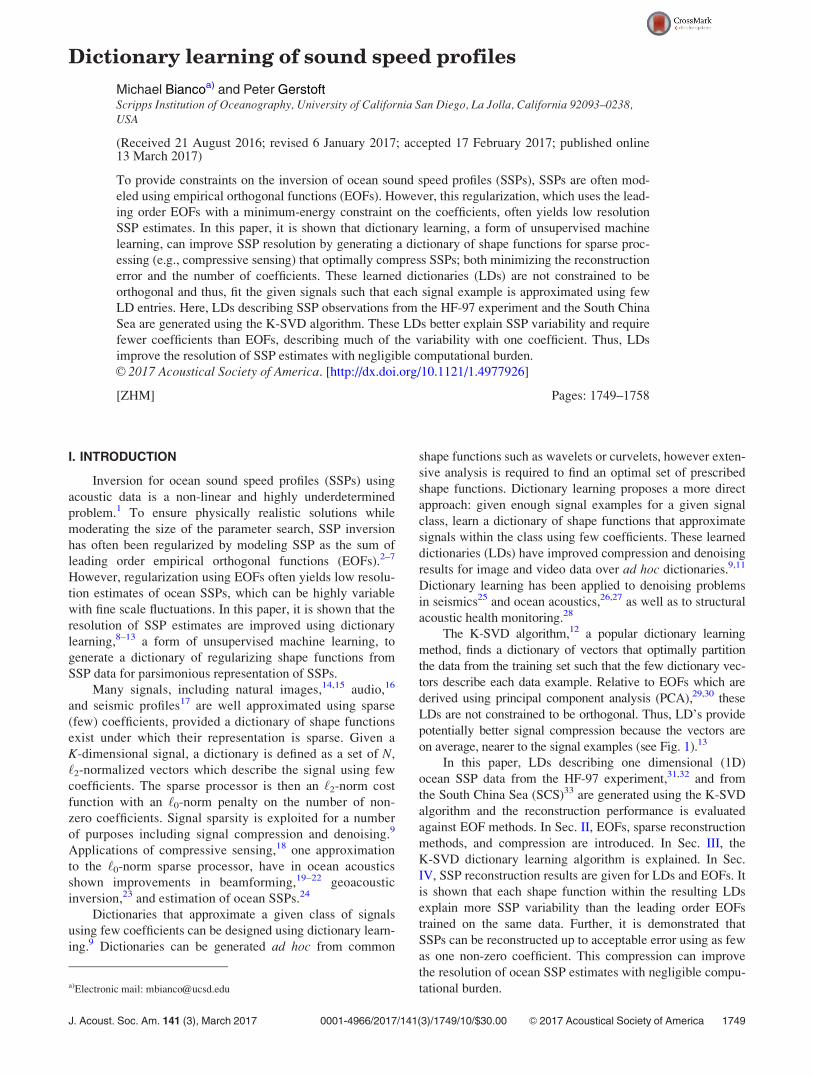
In this paper, the K-SVD algorithm, a clustering baseddictionary learning method, is used to solve Eq. (7). The K-SVD is an adaptation of the K-means algorithm for vectorquantization (VQ) codebook design (a.k.a. the generalizedLloyd algorithm).16 The LD vectors qn from this techniquepartition the feature space of the data rather than RK , increas-ing the likelihood that ym is as a linear combination of fewvectors qn in the solution to Eq. (6) (see Fig. 1). By increasingthe number of vectors N'K for overcomplete dictionaries,and thus the number of partitions in feature space, the sparsityof the solutions can be increased further.13

D. Vector quantization

VQ (Ref. 16) compresses a class of K-dimensional signalsY ¼ ½y1;…; yM& 2 RK$M by optimally mapping ym to a set ofcode vectors C ¼ ½c1;…; cN& 2 RK$N for N<M, called acodebook. The signals ym are then quantized or replaced bythe best code vector choice from C.16 The mapping that mini-mizes mean squared error (MSE) in reconstruction

MSE Y; Y! "

¼ 1

NkY* Yk2

F ; (8)

where Y ¼ ½y1;…; yM& is the vector quantized Y, is theassignment of each vector ym to the code vectors cn based onminimum ‘2-distance (nearest neighbor metric). Thus the ‘2-distances from the code vectors cn define a set of partitionsðR1;…;RNÞ 2 RK (called Voronoi cells)

Rn ¼ fij8l 6¼n; kyi * cnk2 < kyi * clk2g; (9)

where if yi falls within the cell Rn, yi is cn. These cells areshown in Fig. 2(a). This is stated formally by defining aselector function Sn as

SnðymÞ ¼1 if ym 2 Rn

0 otherwise:

(

(10)

The vector quantization step is then

ym ¼XN

n¼1

SnðymÞcn: (11)

The operations in Eqs. (9) and (10) are analogous tosolving the sparse minimization problem:

xm ¼ arg minxm2RN

kym * Cxmk2 subject to kxmk0 ¼ 1; (12)

where the non-zero coefficients xnm ¼ 1. In this problem,

selection of the coefficient in xm corresponds to mapping theobservation vector ym to cn, similar to the selector functionSn. The vector quantized ym is thus written, alternately fromEq. (11), as

ym ¼ Cxm: (13)

E. K-means

Given the MSE metric [Eq. (8)], VQ codebook vectors[c1,…,cN] which correspond to the centroids of the data

FIG. 2. (Color online) Partitioning of Gaussian random distribution(r1¼ 0.75, r2¼ 0.5) using (a) five codebook vectors (K-means, VQ) andwith (b) five dictionary vectors from dictionary learning (K-SVD, T¼ 1).

J. Acoust. Soc. Am. 141 (3), March 2017 Michael Bianco and Peter Gerstoft 1751

Y within (R1,…, RN) minimize the reconstruction error. Theassignment of cn as the centroid of yj 2 Rn is

cn ¼1

jRnjX

j2Rn

yj; (14)

where jRnj is the number of vectors yj 2 Rn.The K-means algorithm shown in Table I, iteratively

updates C using the centroid condition Eq. (14) and the ‘2

nearest-neighbor criteria Eq. (9) to optimize the code vectorsfor VQ. The algorithm requires an initial codebook C0. Forexample, C0 can be N random vectors in RK or selectedobservations from the training set Y. The K-means algorithmis guaranteed to improve or leave unchanged the MSE dis-tortion after each iteration and converges to a localminimum.12,16

III. DICTIONARY LEARNING

Two popular algorithms for dictionary learning, themethod of optimal directions (MOD)13 and the K-SVD,12

are inspired by the iterative K-means codebook updates forVQ (Table I). The N columns of the dictionary Q, like theentries in codebook C, correspond to partitions in RK .However, they are constrained to have unit ‘2-norm and thusseparate the magnitude (coefficients xn) from the shapes(dictionary entries qn) for the sparse processing objectiveEq. (6). When T¼ 1, the ‘2-norm in Eq. (6) is minimized bythe dictionary entry qn that has the greatest inner productwith example ym.9 Thus for T¼ 1, [q1,…,qN] define radialpartitions of RK . These partitions are shown in Fig. 2(b) fora hypothetical 2D (K¼ 2) random data set. This correspondsto a special case of VQ, called gain-shape VQ.16 However,for sparse processing, only the shapes of the signals arequantized. The gains, which are the coefficients xm, aresolved. For T> 1, the sparse solution is analogous to VQ,assigning examples ym to dictionary entries in Q for up to Tnon-zero coefficients in xm.

Given these relationships between sparse processingwith dictionaries and VQ, the MOD13 and K-SVD12 algo-rithms attempt to generalize the K-means algorithm to

optimization of dictionaries for sparse processing for T' 1.They are two-step algorithms which reflect the two updatesteps in the K-means codebook optimization: (1) partitiondata Y into regions (R1,…,RN) corresponding to cn and (2)update cn to centroid of examples ym 2 RN. The K-meansalgorithm is generalized to the dictionary learning problemEq. (7) as two steps:

(1) Sparse coding: Given dictionary Q, solve for up to Tnon-zero coefficients in xm corresponding to examplesym for m¼ [1,…,M].

(2) Dictionary update: Given coefficients X, solve for Qwhich minimizes reconstruction error for Y.

The sparse coding step (1), which is the same for bothMOD and K-SVD, is accomplished using any sparse solutionmethod, including matching pursuit and basis pursuit. Thealgorithms differ in the dictionary update step.

A. The K-SVD algorithm

The K-SVD algorithm is here chosen for its computa-tional efficiency, speed, and convergence to local minima (atleast for T¼ 1). The K-SVD algorithm sequentially opti-mizes the dictionary entries qn and coefficients xm for eachupdate step using the SVD, and thus also avoids the matrixinverse. For T¼ 1, the sequential updates of the K-SVD pro-vide optimal dictionary updates for gain-shape VQ.12,16

Optimal updates to the gain-shape dictionary will, likeK-means updates, either improve or leave unchanged theMSE and convergence to a local minimum is guaranteed.For T> 1, convergence of the K-SVD updates to a local min-imum depends on the accuracy of the sparse-solver used inthe sparse coding stage.12

In the K-SVD algorithm, each dictionary update step isequentially improves both the entries qn 2 Qi and the coef-ficients in xm 2 Xi, without change in support. Expressingthe coefficients as row vectors xn

T 2 RN and xjT 2 RN , which

relate all examples Y to qn and qj, respectively, the ‘2-pen-alty from Eq. (7) is rewritten as

kY*QXk2F ¼

####Y*XN

n¼1

qnxnT

####2

F

¼ kEj * qjxjTk

2F ; (15)

where

Ej ¼ Y*X

n 6¼j

qnxnT

$ %: (16)

Thus, in Eq. (15) the ‘2-penalty is separated into an errorterm Ej ¼ ½ej;1;…; ej;M& 2 RK$M, which is the error for allexamples Y if qj is excluded from their reconstruction, andthe product of the excluded entry qj and coefficientsxj

T 2 RN .An update to the dictionary entry qj and coefficients xj

T

which minimizes Eq. (15) is found by taking the SVD ofEj, which provides the best rank-1 approximation of Ej.However, many of the entries in xj

T are zero (correspondingto examples which do not use qj). To properly update qj and

TABLE I. The K-means algorithm (Ref. 16).

Given: training vectors Y ¼ ½y1;…; yM& 2 RK$M

Initialize: index i¼ 0, codebook C0 ¼ ½c01;…; c0

N & 2 RK$N ,

MSE0 solving Eq. (8)–(11)

I: Update codebook

1. Partition Y into N regions (R1,…, RN) by

Rn ¼ fij8l 6¼n; kyi * cink2 < kyi * ci

lk2g [Eq. (9)]

2. Make code vectors centroids of yj in partitions Rn

ciþ1n ¼ 1

jRinjX

j2Rin

yj

II. Check error

1. Calculate MSEiþ1 from updated codebook Ciþ1

2. If jMSEiþ1 *MSEij < gi¼ iþ 1, return to I

else

end

1752 J. Acoust. Soc. Am. 141 (3), March 2017 Michael Bianco and Peter Gerstoft

xjT with SVD, Eq. (15) must be restricted to examples ym

which use qj,

kERj * qjx

jRk

2F ; (17)

where ERj and xj

R are entries in Ej and xjT , respectively, corre-

sponding to examples ym which use qj, and are defined as

ERj ¼ fej;lj8l; xj

l 6¼ 0g; xjR ¼ fx

jlj 8l; xj

l 6¼ 0g: (18)

Thus for each K-SVD iteration, the dictionary entries andcoefficients are sequentially updated as the SVD ofER

j ¼ USVT. The dictionary entry qij is updated with the first

column in U and the coefficient vector xjR is updated as the

product of the first singular value S(1, 1) with the first col-umn of V. The K-SVD algorithm is given in Table II.

The dictionary Q is initialized using N randomlyselected, ‘2-normalized examples from Y.9,12 During theiterations, one or more dictionary entries may becomeunused. If this occurs, the unused entries are replaced usingthe most poorly represented examples ym (‘2-normlized),determined by reconstruction error.

IV. EXPERIMENTAL RESULTS

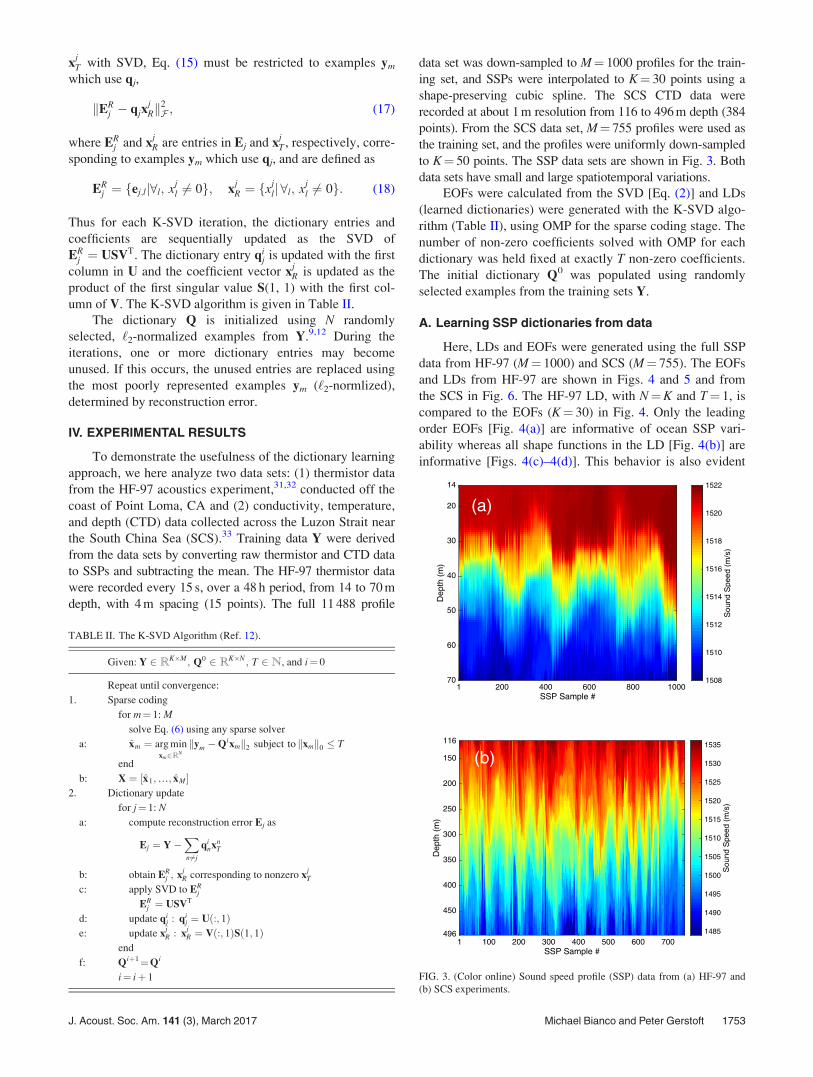
To demonstrate the usefulness of the dictionary learningapproach, we here analyze two data sets: (1) thermistor datafrom the HF-97 acoustics experiment,31,32 conducted off thecoast of Point Loma, CA and (2) conductivity, temperature,and depth (CTD) data collected across the Luzon Strait nearthe South China Sea (SCS).33 Training data Y were derivedfrom the data sets by converting raw thermistor and CTD datato SSPs and subtracting the mean. The HF-97 thermistor datawere recorded every 15 s, over a 48 h period, from 14 to 70 mdepth, with 4 m spacing (15 points). The full 11 488 profile

data set was down-sampled to M¼ 1000 profiles for the train-ing set, and SSPs were interpolated to K¼ 30 points using ashape-preserving cubic spline. The SCS CTD data wererecorded at about 1 m resolution from 116 to 496 m depth (384points). From the SCS data set, M¼ 755 profiles were used asthe training set, and the profiles were uniformly down-sampledto K¼ 50 points. The SSP data sets are shown in Fig. 3. Bothdata sets have small and large spatiotemporal variations.

EOFs were calculated from the SVD [Eq. (2)] and LDs(learned dictionaries) were generated with the K-SVD algo-rithm (Table II), using OMP for the sparse coding stage. Thenumber of non-zero coefficients solved with OMP for eachdictionary was held fixed at exactly T non-zero coefficients.The initial dictionary Q0 was populated using randomlyselected examples from the training sets Y.

A. Learning SSP dictionaries from data

Here, LDs and EOFs were generated using the full SSPdata from HF-97 (M¼ 1000) and SCS (M¼ 755). The EOFsand LDs from HF-97 are shown in Figs. 4 and 5 and fromthe SCS in Fig. 6. The HF-97 LD, with N¼K and T¼ 1, iscompared to the EOFs (K¼ 30) in Fig. 4. Only the leadingorder EOFs [Fig. 4(a)] are informative of ocean SSP vari-ability whereas all shape functions in the LD [Fig. 4(b)] areinformative [Figs. 4(c)–4(d)]. This behavior is also evident

TABLE II. The K-SVD Algorithm (Ref. 12).

Given: Y 2 RK$M; Q0 2 RK$N ; T 2N, and i¼ 0

Repeat until convergence:

1. Sparse coding

for m¼ 1: M

solve Eq. (6) using any sparse solver

a: xm ¼ arg minxm2RN

kym *Qixmk2 subject to kxmk0 + T

end

b: X ¼ ½x1;…; xM&2. Dictionary update

for j¼ 1: N

a: compute reconstruction error Ej as

Ej ¼ Y*X

n6¼j

qinxn

T

b: obtain ERj ; xj

R corresponding to nonzero xjT

c: apply SVD to ERj

ERj ¼ USVT

d: update qij : qi

j ¼ Uð:; 1Þe: update xj

R : xjR ¼ Vð:; 1ÞSð1; 1Þ

end

f: Qiþ1¼Qi

i¼ iþ 1 FIG. 3. (Color online) Sound speed profile (SSP) data from (a) HF-97 and(b) SCS experiments.

J. Acoust. Soc. Am. 141 (3), March 2017 Michael Bianco and Peter Gerstoft 1753

for the SCS data set (Fig. 6). The EOFs (K¼ 50) calculatedfrom the full training set are shown in Fig. 6(a), and the LDentries for N¼ 50 and T¼ 1 sparse coefficient are shown inFig. 6(b). The overcomplete LDs for the HF-97 data shownin Fig. 5 and for the SCS data in Fig. 6(c).

As illustrated in Fig. 1, by relaxing the requirement oforthogonality for the shape functions, the shape functions canbetter fit the data and thereby achieve greater compression.The Gram matrix G, which gives the coherence of matrix col-umns, is defined for a matrix A with unit ‘2-norm columns asG ¼ jATAj. The Gram matrix for the EOFs [Fig. 4(e)] showsthe shapes in the EOF dictionary are orthogonal (G¼ I, bydefinition), whereas those of the LD [Fig. 4(f)] are not.

B. Reconstruction of SSP training data

In this section, EOFs and LDs are trained on the fullSSP data sets Y¼ [y1,…,yM]. Reconstruction performance

of the EOF and LDs are then evaluated on SSPs within thetraining set, using a mean error metric.

The coefficients for the learned Q and initial Q0 dictio-naries xm are solved from the sparse objective [Eq. (6)] usingOMP. The least squares (LS) solution for the T leading-ordercoefficients xL 2 RT from the EOFs P were solved by Eq.(5). The best combination of T EOF coefficients was solvedfrom the sparse objective [Eq. (6)] using OMP. Given thecoefficients X¼ [x1,…,xm] describing examplesY¼ [y1,…,ym], the reconstructed examples Y ¼ ½y1;…; ym&are given by Y ¼ QX. The mean reconstruction error (ME)for the training set is then

ME ¼ 1

KMkY* Yk1: (19)

We here use the ‘1-norm to stress the robustness of the LDreconstruction.

FIG. 4. (Color online) HF-97: (a) EOFs and (b) LD entries (N¼K and T¼ 1, sorted by variance r2qn

). Fraction of (c) total SSP variance explained by EOFsand (d) SSP variance explained for examples using LD entries. Coherence of (e) EOFs and (f) LD entries.

1754 J. Acoust. Soc. Am. 141 (3), March 2017 Michael Bianco and Peter Gerstoft

To illustrate the optimality of LDs for SSP compression,the K-SVD algorithm was run using EOFs as the initial dic-tionary Q0 for T¼ 1 non-zero coefficient. The convergenceof ME for the K-SVD iterations is shown in Fig. 7(a). After

30 K-SVD iterations, the mean error of the M¼ 1000 profiletraining set is decreased by nearly half. The convergence ismuch faster for Q0 consisting of randomly selected examplesfrom Y.

For LDs, increasing the number of entries N or increasingthe number of sparse coefficients T will always reduce thereconstruction error (N and T are decided with computational

FIG. 5. (Color online) HF-97: LD entries (a) N¼ 60 and T¼ 1, (b) N¼ 90and T¼ 1, and (c) N¼ 90 and T¼ 5. Dictionary entries are sorted indescending variance r2

qn.

FIG. 6. (Color online) SCS: EOFs (a) and LD entries, (b) N¼K¼ 50 andT¼ 1, and (c) N¼ 150 and T¼ 1. Dictionary entries are sorted in descendingvariance r2

qn.

J. Acoust. Soc. Am. 141 (3), March 2017 Michael Bianco and Peter Gerstoft 1755

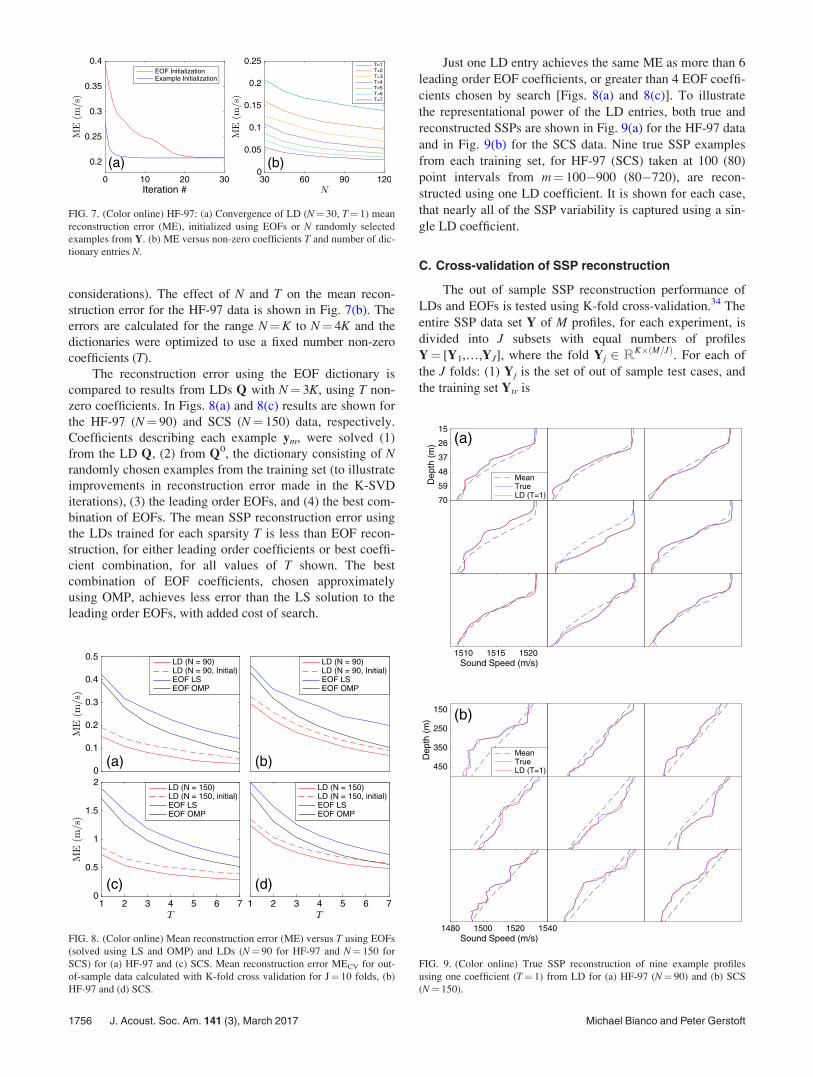
considerations). The effect of N and T on the mean recon-struction error for the HF-97 data is shown in Fig. 7(b). Theerrors are calculated for the range N¼K to N¼ 4K and thedictionaries were optimized to use a fixed number non-zerocoefficients (T).

The reconstruction error using the EOF dictionary iscompared to results from LDs Q with N¼ 3K, using T non-zero coefficients. In Figs. 8(a) and 8(c) results are shown forthe HF-97 (N¼ 90) and SCS (N¼ 150) data, respectively.Coefficients describing each example ym, were solved (1)from the LD Q, (2) from Q0, the dictionary consisting of Nrandomly chosen examples from the training set (to illustrateimprovements in reconstruction error made in the K-SVDiterations), (3) the leading order EOFs, and (4) the best com-bination of EOFs. The mean SSP reconstruction error usingthe LDs trained for each sparsity T is less than EOF recon-struction, for either leading order coefficients or best coeffi-cient combination, for all values of T shown. The bestcombination of EOF coefficients, chosen approximatelyusing OMP, achieves less error than the LS solution to theleading order EOFs, with added cost of search.

Just one LD entry achieves the same ME as more than 6leading order EOF coefficients, or greater than 4 EOF coeffi-cients chosen by search [Figs. 8(a) and 8(c)]. To illustratethe representational power of the LD entries, both true andreconstructed SSPs are shown in Fig. 9(a) for the HF-97 dataand in Fig. 9(b) for the SCS data. Nine true SSP examplesfrom each training set, for HF-97 (SCS) taken at 100 (80)point intervals from m¼ 100*900 (80*720), are recon-structed using one LD coefficient. It is shown for each case,that nearly all of the SSP variability is captured using a sin-gle LD coefficient.

C. Cross-validation of SSP reconstruction

The out of sample SSP reconstruction performance ofLDs and EOFs is tested using K-fold cross-validation.34 Theentire SSP data set Y of M profiles, for each experiment, isdivided into J subsets with equal numbers of profilesY¼ [Y1,…,YJ], where the fold Yj 2 RK$ðM=JÞ. For each ofthe J folds: (1) Yj is the set of out of sample test cases, andthe training set Ytr is

FIG. 7. (Color online) HF-97: (a) Convergence of LD (N¼ 30, T¼ 1) meanreconstruction error (ME), initialized using EOFs or N randomly selectedexamples from Y. (b) ME versus non-zero coefficients T and number of dic-tionary entries N.

FIG. 8. (Color online) Mean reconstruction error (ME) versus T using EOFs(solved using LS and OMP) and LDs (N¼ 90 for HF-97 and N¼ 150 forSCS) for (a) HF-97 and (c) SCS. Mean reconstruction error MECV for out-of-sample data calculated with K-fold cross validation for J¼ 10 folds, (b)HF-97 and (d) SCS.

FIG. 9. (Color online) True SSP reconstruction of nine example profilesusing one coefficient (T¼ 1) from LD for (a) HF-97 (N¼ 90) and (b) SCS(N¼ 150).

1756 J. Acoust. Soc. Am. 141 (3), March 2017 Michael Bianco and Peter Gerstoft

Ytr ¼ fYlj 8l 6¼jg; (20)

(2) the LD Qj and EOFs are derived using Ytr; and (3) coeffi-cients estimating test samples Yj are solved for Qj withsparse processor Eq. (6), and for EOFs by solving for leadingorder terms and by solving with sparse processor. The out ofsample error from cross validation MECV for each method isthen

MECV ¼1

KM

XJ

j¼1

kYj * Yjk1: (21)

The out of sample reconstruction error MECV increasesover the within-training-set estimates for both the learnedand EOF dictionaries, as shown in Figs. 8(b) and 8(d) forJ¼ 10 folds. The mean reconstruction error using the LDs,as in the within-training-set estimates, is less than the EOFdictionaries. For both the HF-97 (SCS) data, more than two(2) EOF coefficients, choosing best combination by search,or more than three (equal to 3) leading-order EOF coeffi-cients solved with LS, are required to achieve the same outof sample performance as one LD entry.

D. Solution space for SSP inversion

Acoustic inversion for ocean SSP is a non-linear problem.One approach is coefficient search using genetic algorithms.1

Discretizing each coefficient into H values, the number ofcandidate solutions for T fixed coefficients indices is

Sfixed ¼ HT : (22)

If the coefficient indices for the solution can vary, as perdictionary learning with LD Q 2 RK$N , the number of can-didate solutions Scomb is

Scomb ¼ HT N!

T! N * Tð Þ!: (23)

Using a typical H¼ 100 point discretization of the coeffi-cients, the number of possible solutions for fixed and combi-natorial dictionary indices are plotted in Fig. 10. Assumingan unknown SSP similar to the training set, the SSP may beconstructed up to acceptable resolution using one coefficientfrom the LD (104 possible solutions, see Fig. 10). To achievethe similar ME, seven EOFs coefficients are required (1014

possible solutions, Fig. 10) using fixed indices and the bestEOF combination requires five EOFs (1017 possible solu-tions, Fig. 10).

V. CONCLUSION

Given sufficient training data, dictionary learning gener-ates optimal dictionaries for sparse reconstruction of a givensignal class. Since these LDs are not constrained to be orthog-onal, the entries fit the distribution of the data such that signalexample is approximated using few LD entries. Relative toEOFs, each LD entry is informative to the signal variability.

The K-SVD dictionary learning algorithm is applied toocean SSP data from the HF-97 and SCS experiments. It is

shown that the LDs generated describe ocean SSP variabilitywith high resolution using fewer coefficients than EOFs. Asfew as one coefficient from a LD describes nearly all the vari-ability in each of the observed ocean SSPs. This performancegain is achieved by the larger number of informative elementsin the LDs over EOF dictionaries. Provided sufficient SSPtraining data are available, LDs can improve SSP inversionresolution with negligible computational expense. This couldprovide improvements to geoacoustic inversion,1 matchedfield processing,36,37 and underwater communications.31

ACKNOWLEDGMENTS

The authors would like to thank Dr. Robert Pinkel forthe use of the South China Sea CTD data. This work issupported by the Office of Naval Research, Grant No.N00014-11-1-0439.

1P. Gerstoft, “Inversion of seismoacoustic data using genetic algorithmsand a posteriori probability distributions,” J. Acoust. Soc. Am. 95(2),770*782 (1994).

2L. R. LeBlanc and F. H. Middleton, “An underwater acoustic sound veloc-ity data model,” J. Acoust. Soc. Am. 67(6), 2055*2062 (1980).

3M. I. Taroudakis and J. S. Papadakis, “A modal inversion scheme forocean acoustic tomography,” J. Comp. Acoust. 1(4), 395*421 (1993).

4P. Gerstoft and D. F. Gingras, “Parameter estimation using multifrequencyrange-dependent acoustic data in shallow water,” J. Acoust. Soc. Am.99(5), 2839*2850 (1996).

5C. Park, W. Seong, P. Gerstoft, and W. S. Hodgkiss, “Geoacoustic inver-sion using backpropagation,” IEEE J. Ocean. Eng. 35(4), 722*731(2010).

6B. A. Tan, P. Gerstoft, C. Yardim, and W. S. Hodgkiss, “Broadband syn-thetic aperture geoacoustic inversion,” J. Acoust. Soc. Am. 134(1),312*322 (2013).

7C. F. Huang, P. Gerstoft, and W. S. Hodgkiss, “Effect of ocean soundspeed uncertainty on matched-field geoacoustic inversion,” J. Acoust. Soc.Am. 123(6), EL162–EL168 (2008).

8R. Rubinstein, A. M. Bruckstein, and M. Elad, “Dictionaries for sparserepresentation modeling,” Proc. IEEE 98(6), 1045*1057 (2010).

9M. Elad, Sparse and Redundant Representations (Springer, New York,2010).

10I. Tosic and P. Frossard, “Dictionary learning,” IEEE Sig. Proc. Mag.28(2), 27*38 (2011).

FIG. 10. (Color online) Number of candidate solutions S for SSP inversionversus T, Sfixed using fixed indices and Scomb best combination of coeffi-cients. Each coefficient is discretized with H¼ 100 for dictionary Q2 RK$N with N¼ 100.

J. Acoust. Soc. Am. 141 (3), March 2017 Michael Bianco and Peter Gerstoft 1757

11K. Schnass, “On the identifiability of overcomplete dictionaries via theminimisation principle underlying K-SVD,” Appl. Comput. HarmonicAnal. 37(3), 464*491 (2014).

12M. Aharon, M. Elad, and A. Bruckstein “K-SVD: An algorithm fordesigning overcomplete dictionaries for sparse representation,” IEEETrans. Signal Process. 54(11), 4311*4322 (2006).

13K. Engan, S. O. Aase, and J. H. Husøy, “Multi-frame compression:Theory and design,” Signal Process. 80(10), 2121*2140 (2000).

14A. Hyv€arinen, J. Hurri, and P. O. Hoyer, Natural Image Statistics: AProbabilistic Approach to Early Computational Vision (Springer Scienceand Business Media, London, 2009).

15C. Christopoulos, A. Skodras, and T. Ebrahimi, “The JPEG2000 stillimage coding system: An overview,” IEEE Trans. Cons. Elec. 46(4),1103*1127 (2000).

16A. Gersho and R. M. Gray, Vector Quantization and Signal Compression(Kluwer Academic, Norwell, MA, 1991).

17H. L. Taylor, S. C. Banks, and J. F. McCoy, “Deconvolution with the‘1–norm,” Geophysics 44(1), 39*52 (1979).

18E. Cand"es, “Compressive sampling,” in Proceedings of the InternationalCongress of Mathematicians (2006), Vol. 3, pp. 1433*1452.

19G. Edelmann and C. Gaumond, “Beamforming using compressivesensing,” J. Acoust. Soc. Am. 130(4), EL232*EL237 (2011).

20A. Xenaki, P. Gerstoft, and K. Mosegaard, “Compressive beamforming,”J. Acoust. Soc. Am. 136(1), 260*271 (2014).

21P. Gerstoft, A. Xenaki, and C. F. Mecklenbr€auker, “Multiple and singlesnapshot compressive beamforming,” J. Acoust. Soc. Am. 138(4),2003*2014 (2015).

22Y. Choo and W. Song, “Compressive spherical beamforming for localiza-tion of incipient tip vortex cavitation,” J. Acoust. Soc. Am. 140(6),4085*4090 (2016).

23C. Yardim, P. Gerstoft, W. S. Hodgkiss, and J. Traer, “Compressive geoa-coustic inversion using ambient noise,” J. Acoust. Soc. Am. 135(3),1245*1255 (2014).

24M. Bianco and P. Gerstoft, “Compressive acoustic sound speed profileestimation,” J. Acoust. Soc. Am. 139(3), EL90–EL94 (2016).

25S. Beckouche and J. Ma, “Simultaneous dictionary learning and denoisingfor seismic data,” Geophysics 79(3), A27*A31 (2014).

26M. Taroudakis and C. Smaragdakis, “De-noising procedures for invertingunderwater acoustic signals in applications of acoustical oceanography,”in Euronoise 2015 Maastricht (2015), pp. 1393*1398.

27T. Wang and W. Xu, “Sparsity-based approach for ocean acoustic tomog-raphy using learned dictionaries,” in OCEANS 2016 Shanghai IEEE, pp.1*6 (2016).

28K. S. Alguri and J. B. Harley, “Consolidating guided wave simulationsand experimental data: A dictionary leaning approach,” Proc. SPIE 9805,98050Y (2016).

29A. Hannachi, I. T. Jolliffe, and D. B. Stephenson, “Empirical orthogonalfunctions and related techniques in atmospheric science: A review,” Int. J.Climatol. 27(9), 1119*1152 (2007).

30A. H. Monahan, J. C. Fyfe, M. H. Ambaum, D. B. Stephenson, and G. R.North, “Empirical orthogonal functions: The medium is the message,”J. Clim. 22(24), 6501*6514 (2009).

31N. Carbone and W. S. Hodgkiss, “Effects of tidally driven temperaturefluctuations on shallow-water acoustic communications at 18kHz,” IEEEJ. Ocean. Eng. 25(1), 84*94 (2000).

32W. S. Hodgkiss, W. A. Kuperman, and D. E. Ensberg, “Channel impulseresponse fluctuations at 6 kHz in shallow water,” in Impact of LittoralEnvironmental Variability of Acoustic Predictions and SonarPerformance (Springer, Netherlands, 2002), pp. 295*302.

33C. T. Liu, R. Pinkel, M. K. Hsu, J. M. Klymak, H. W. Chen, and C.Villanoy, “Nonlinear internal waves from the Luzon Strait,” Eos Trans.AGU 87(42), 449*451 (2006).

34T. Hastie, R. Tibshirani, and J. Friedman, The Elements of Statistical Learning:Data Mining, Inference and Prediction, 2nd ed. (Springer, New York, 2009).

35Y. C. Pati, R. Rezaiifar, and P. S. Krishnaprasad, “Orthogonal matchingpursuit: Recursive function approximation with applications to waveletdecomposition,” in IEEE Proc. 27th Annu. Asilomar Conf. Signals,Systems and Computers (1993), pp. 40*44.

36A. B. Baggeroer, W. A. Kuperman, and P. N. Mikhalevsky, “An overviewof matched field methods in ocean acoustics,” IEEE J. Ocean. Eng. 18(4),401*424 (1993).

37C. M. Verlinden, J. Sarkar, W. S. Hodgkiss, W. A. Kuperman, and K. G.Sabra, “Passive acoustic source localization using sources of opportunity,”J. Acoust. Soc. Am. 138(1), EL54–EL59 (2015).

1758 J. Acoust. Soc. Am. 141 (3), March 2017 Michael Bianco and Peter Gerstoft