Diagnostics for the Bootstrap and Fast Double Bootstrap

Diagnostics for the Bootstrap and Fast Double Bootstrapby

Russell Davidson

Department of Economics and CIREQMcGill University

Montreal, Quebec, CanadaH3A 2T7

AMSE-GREQAMCentre de la Vieille Charite

2 Rue de la Charite13236 Marseille cedex 02, France

[email protected]

Abstract

The bootstrap is typically much less reliable in the context of time-series models withserial correlation of unknown form than it is when regularity conditions for the conven-tional IID bootstrap, based on resampling, apply. It is therefore useful for practitionersto have available diagnostic techniques capable of evaluating bootstrap performancein specific cases. The techniques suggested in this paper are closely related to thefast double bootstrap, and, although they inevitably rely on simulation, they are notcomputationally intensive. They can also be used to gauge the performance of the fastdouble bootstrap itself. Examples of bootstrapping time series are presented whichillustrate the diagnostic procedures, and show how the results can cast light on boot-strap performance, not only in the time-series context.

Keywords: Bootstrap, fast double bootstrap, diagnostics for bootstrap, timeseries, autocorrelation of unknown form

JEL codes: C10, C15, C22, C63

This research was supported by the Canada Research Chair program (Chair in Economics,

McGill University) and by a grant from the Fonds de Recherche du Quebec - Societe et

Culture.

November 2014

1. Introduction

While the bootstrap can provide spectacularly reliable inference in many cases, thereare others for which results are much less reliable. Intuition can often suggest reasonsfor this state of affairs, and the asymptotic theory of bootstrap refinements does so aswell; see Hall (1992) and Horowitz (1997) among many other relevant references.

It has often been remarked that heavy-tailed distributions give rise to difficulties forthe bootstrap; see Davidson (2012) and the discussion of that paper in Schluter (2012).Autocorrelation of unknown form also presents a severe challenge to the bootstrap. Sofar, no bootstrap has been proposed that, in the presence of autocorrelation of unknownform, can deliver performance comparable to what can be obtained in its absence. Per-haps in consequence, a considerable number of bootstrap methods have been proposed,some a good deal better than others. By far the most popular of these are the variousversions of the block bootstrap, which was originally proposed by Kunsch (1989); seealso Hall, Horowitz, and Jing (1995), Lahiri (1999) and (2003). However, it has beenseen that the block bootstrap often works poorly, while, in some circumstances, otherschemes may work better. These include (versions of) the sieve bootstrap (see forinstance Buhlmann (1997) and (2002)), frequency-domain bootstraps (Kreiss and E.Paparoditis (2003), Kirch and Politis (2011)), and the recently-proposed dependentwild bootstrap, Shao (2010).

Simulation experiments can of course be used to study the performance of differentbootstrap procedures in different circumstances. In this paper, simulation-based di-agnostic methods are proposed, intended to determine when a given procedure workswell or not, and, if not, provide an analysis of why. Asymptotic theory, includingthe theory of bootstrap refinements characterised by a rate at which the bootstrapdiscrepancy tends to zero, is not very useful for this purpose. One obvious reason isthat the bootstrap is a finite-sample procedure, not an asymptotic one. To be useful,therefore, a diagnostic technique should be based on finite-sample arguments only. Apaper that does not seem to be very widely known that proposes such a techniqueis Beran (1997). It is not oriented towards econometrics, but contains ideas that aredeveloped differently here.

Despite the rapidly growing power of computing machinery, it would be more usefulfor practitioners if a diagnostic technique was no more CPU-intensive, or at leastvery little more intensive, than simply undertaking a bootstrap test or constructinga bootstrap confidence set. The techniques outlined here satisfy that requirement,although simulations are performed that are more CPU-intensive, for the purpose ofevaluating the reliability of the diagnostic methods themselves.

The paper is organised as follows. In Section 2, definitions and notation appropriatefor theoretical study of the bootstrap are given. The wild bootstrap is presented inSection 3, and its use in the context of a regression model with disturbances that followan GARCH(1,1) process studied. It turns out that the wild bootstrap is capable ofgiving essentially perfect inference even with very small samples, and so, in Section 4,once the diagnostic methods are explained, they are applied to this setup and the

– 1 –

results illustrated graphically. Section 5 looks at an interesting failure, namely themaximum-entropy bootstrap proposed in Vinod (2006). There is nothing wrong, andmuch right, with the maximum-entropy idea, but its application to time series withautocorrelation of unknown form fails to yield reliable inference. The reason for thisdisappointing fact is clearly revealed by the diagnostic analysis.

There is a close link between the principle underlying the diagnostics and that under-lying the fast double bootstrap of Davidson and MacKinnon (2007). This is broughtout in Section 6, where it is seen that, at a cost of some increase in CPU time, thefast double bootstrap itself can be diagnosed. In Section 7, a very simple and specialcase of a version of the sieve bootstrap is considered. Its performance and that ofits fast double counterpart are diagnosed, as well as a procedure combining the sievebootstrap and the wild bootstrap. Finally, some concluding remarks are presented inSection 8.

2. Definitions and Notation

A model is a collection of data-generating processes (DGPs). If M denotes a model,it may also represent a hypothesis, namely that the true DGP, µ say, belongs to M.Alternatively, we say that M is correctly specified.

We almost always want to define a parameter-defining mapping θ, which maps themodel M into a parameter space Θ, which is usually a subset of Rk for some finitepositive integer k. For any DGP µ ∈ M, the k--vector θ(µ), or θµ, is the parametervector that corresponds to µ. Sometimes the mapping θ is one-one, as, for instance,with models estimated by maximum likelihood. More often, θ is many-one, so thata given parameter vector does not uniquely specify a DGP. Supposing that θ existsimplies that no identification problems remain to be solved.

In principle, a DGP specifies the probabilistic behaviour of all deterministic functionsof the random data it generates – estimators, standard errors, test statistics, etc. Ify denotes a data set, or sample, generated by a DGP µ, then a statistic τ(y) is arealisation of a random variable τ of which the distribution is determined by µ. Astatistic τ is a pivot, or is pivotal, relative to a model M if its distribution under anyDGP µ ∈ M is the same for all µ ∈ M.

We can denote by M0 the set of DGPs that represent a null hypothesis we wish totest. The test statistic used is denoted by τ . Unless τ is a pivot with respect to M0,it has a different distribution under the different DGPs in M0, and it certainly has adifferent distribution under DGPs in the model, M say, that represents the alternativehypothesis. I assume as usual that M0 ⊂ M.

It is conventional to suppose that τ is defined as a random variable on some suitableprobability space, on which we define a different probability measure for each differentDGP. Rather than using this approach, we define a single probability space (Ω,F , P ),

– 2 –

with just one probability measure, P . Then we treat the test statistic τ as a stochasticprocess with the set M as index set. We have

τ : M× Ω → R.

Leaving aside questions of just what real-world randomness – if it exists – might be,we can take the probability space Ω to be that of a random number generator. Arealisation of the test statistic is written as τ(µ, ω), for some µ ∈ M and ω ∈ Ω.

For notational convenience, we suppose that the range of τ is the [0, 1] interval ratherthan the whole real line, and that the statistic takes the form of an approximateP value, which leads to rejection when the statistic is too small. Let R0 : [0, 1]×M0 →[0, 1] be the cumulative distribution function (CDF) of τ under any DGP µ ∈ M0:

R0(x, µ) = Pω ∈ Ω | τ(µ, ω) ≤ x

. (1)

Suppose that we have a statistic computed from a data set that may or may not havebeen generated by a DGP µ0 ∈ M0. Denote this statistic by t. Then the ideal P valuethat would give exact inference is R0(t, µ0). If t is indeed generated by µ0, R0(t, µ0)is distributed as U(0,1) if the distribution of τ is absolutely continuous with respectto Lebesgue measure – as we assume throughout – but not, in general, if t comes fromsome other DGP. The quantity R0(t, µ0) is available by simulation only if τ is a pivotwith respect to M0, since then we need not know the precise DGP µ0. When it isavailable, it permits exact inference.

The principle of the bootstrap is that, when we want to use some function or functionalof an unknown DGP µ0, we use the same function or functional of an estimate of µ0.Analogously to the stochastic process τ , we define the DGP-valued process

β : M× Ω → M0.

The estimate of µ0, which we call the bootstrap DGP, is β(µ, ω), where ω is the samerealisation as in t = τ(µ, ω). We write b = β(µ, ω). Then the bootstrap statistic thatfollows the U(0,1) distribution approximately is R0(t, b), where t and b are observed,or rather can be computed from the observed data. In terms of the two stochasticprocesses τ and β, the bootstrap P value is another stochastic process:

p1(µ, ω) = R0

(τ(µ, ω), β(µ, ω)

). (2)

Normally, the bootstrap principle must be implemented by a simulation experiment,and so, analogously to (1), we may define

R0(x, µ) =1

B

B∑j=1

I(τ(µ, ω∗

j ) < x),

– 3 –

where the ω∗j are independent realisations of the random numbers needed to compute

the statistic. As the number of bootstrap repetitions B → ∞, R0(x, µ) tends almostsurely to R0(x, µ). Accordingly, the bootstrap P value is estimated by R0(t, b).

Since by absolute continuity R0 is a continuous function, it follows that p1 also hasan absolutely continuous distribution. We denote the continuous CDF of p1(µ, ω) byR1(·, µ). This CDF can also be estimated by simulation, but that is very compu-tationally intensive. The double bootstrap uses this approach, using the bootstrapprinciple by replacing the unknown true DGP µ by the bootstrap DGP b. An idealdouble bootstrap P value that would give exact inference is R1

(p1(µ, ω), µ

), which is

distributed as U(0,1). The double bootstrap P value is, analogously, R1

(R0(t, b), b

).

3. The Wild Bootstrap

Models that incorporate heteroskedasticity can be bootstrapped effectively by use ofthe wild bootstrap. Early references to this procedure include Wu (1986), Liu (1988),and Mammen (1993). For the linear regression

y = Xβ + u, (3)

the wild bootstrap DGP can be written as

y∗ = Xβ + u∗,

where, as usual, stars denote simulated quantities, and β is a vector of restrictedestimates that satisfy the possibly nonlinear null hypothesis under test. The bootstrapdisturbances are defined by u∗

t = |ut|s∗t , where ut is the residual for observation tobtained by estimating the restricted model, and the s∗t are IID drawings from adistribution such that E(s∗t ) = 0, Var(s∗t ) = 1.

Davidson and Flachaire (2008) recommend the Rademacher distribution, defined asfollows:

s∗t =

1 with probability 1/2−1 with probability 1/2,

(4)

for the wild bootstrap. When the Rademacher distribution is used, the covariancestructure of the squared bootstrap disturbances is the same as that of the squaredresiduals from the original sample. This is because the squared bootstrap disturbancesare always just the squared residuals, so that any relationship among the squared resid-uals, like that given by any GARCH model, is preserved unchanged by the Rademacherwild bootstrap.

In order to study the consequences of this fact for a simple GARCHmodel, a simulationexperiment was conducted for the model

yt = a+ ρyt−1 + ut, (5)

– 4 –

where ut are GARCH(1,1) disturbances, defined by the recurrence relation

σ2t = α+ (δ + γε2t−1)σ

2t−1;

ut = σtεt, (6)

with the εt standard normal white noise, and the recurrence initialised by σ21 =

α/(1 − γ − δ), which is the unconditional stationary expectation of the process. Theparameters of the DGP used in the experiment were a = 1.5, y0 = 0, α = 1, γ = 0.4,and δ = 0.45, with very small sample size n = 10, and ρ = 0.3. In order to test thehypothesis that ρ = ρ0, the test statistic used was

τ =ρ− ρ0σρ

,

where ρ is the OLS estimate from (5), run over observations 2 to n. The standarderror σρ was obtained by use of the HC2 variant of the Eicker-White HCCME; seeWhite (1980) and Eicker (1963).

The bootstrap DGP is determined by first running the constrained regression

yt − ρ0yt−1 = a+ ut, t = 2, . . . , n,

in order to obtain the estimate a, and the constrained residuals ut, t = 2, . . . n. Abootstrap sample is defined by

y∗1 = y1 and y∗t = a+ ρ0y∗t−1 + s∗t ut, t = 2, . . . , n,

where the s∗t are IID realisations from the Rademacher distribution. The bootstrapstatistics are

τ∗j =ρ∗ − ρ0

σ∗ρ

, j = 1, . . . , B

with ρ∗ and σ∗ρ defined as the bootstrap counterparts of ρ and σρ respectively. The

bootstrap P value is the proportion of the τ∗j that are more extreme than τ . Theperformance of the bootstrap test, as revealed by experiments with N = 100,000replications with B = 399 bootstrap samples for each, is excellent. This will be seenin the context of the diagnostic procedures presented in the next section, in preferenceto presenting results here in tabular form.

Davidson and Flachaire (2008) show that there is a special setup where the wildbootstrap can deliver perfect inference. If one wishes to test the hypothesis that theentire vector β in the linear regression (3) is zero when the disturbances u may beheteroskedastic, the obvious test statistic is

τ ≡ y⊤X(X⊤ΩX)−1X⊤y, (7)

where the dependent variable y is the vector of restricted residuals under the nullhypothesis, and Ω is one of the inconsistent estimates of the covariance matrix of the

– 5 –

disturbances used in the HCCME. When the Rademacher distribution (4) is used,the wild bootstrap P value is uniformly distributed under the null up to discretenessdue to a finite sample size. In what follows, simulation results are presented fora few different bootstrap procedures that are found in the literature, with a setupsimilar to the above. The model is a linear regression with disturbances that arepossibly serially correlated as well as heteroskedastic, with null hypothesis that all theregression parameters are zero, and a test statistic with the form of (7), but with aHAC covariance matrix estimator instead of the HCCME. It serves as a useful testbed, as it allows us to compare the performance of these bootstrap tests with theperfect inference obtainable with only heteroskedasticity and the wild bootstrap.

4. Diagnostic Procedures

A standard way of evaluating bootstrap performance by simulation is to graph theP value and P value discrepancy plots for a test based on the bootstrap P value;see Davidson and MacKinnon (1998). The former is just a plot of the CDF of thisP value; the latter a plot of the CDF minus its argument. Perfect inference appearsas a P value plot that coincides with the diagonal of the unit square, or a P valuediscrepancy plot that coincides with the horizontal axis.

If the bootstrap discrepancy, that is, the ordinate of the P value discrepancy plot, isacceptably small, there is no need to look further. But, if not, it is useful to see why,and it is for this purpose that we may use the procedures of this section. A simulationexperiment that provides the information for a P value plot also provides the infor-mation needed for these. Suppose that there are N replications in the experiment,with B bootstrap repetitions for each replication. The data for each replication aregenerated using a DGP denoted by µ, which satisfies the null hypothesis, and with achosen specification of the joint distribution of the random elements needed to gen-erate a bootstrap sample. Let τj , j = 1, . . . , N , be the IID realisations of the teststatistic (7), and let τ∗j , j = 1, . . . , N , be a single bootstrap statistic taken from theB bootstrap statistics computed for replication j, the first perhaps, or the last, or onechosen at random.

The next step is to graph kernel-density estimates of the distribution of the statis-tic τ and that of the bootstrap statistic τ∗. If these are not similar, then clearly thebootstrap DGP fails to mimic the true DGP at all well. Bootstrap failure is then aconsequence of this fact. Another diagnostic is based on running an OLS regressionof the τ∗j on a constant and the τj . Suppose without loss of generality that τ itselfis in nominal P value form, so that the rejection region is on the left. The bootstrapP value for replication j is

Pj =1

B

B∑i=1

I(τ∗ji < τj), (8)

where the τ∗ji, i = 1, . . . , B, are the bootstrap statistics computed for replication j,and I(·) is the indicator function. A significant constant in the regression indicates

– 6 –

that the distribution of τ∗ is shifted relative to that of τ , and this typically causesunder-rejection in one tail and over-rejection in the other. Next, suppose that thisregression reveals that, for the data generated on any one replication, τ is stronglypositively correlated with τ∗. The positive correlation then implies that, if τj is small,then the τ∗ji tend to be small as well. It follows from (8) that the P value is greaterthan it would be in the absence of the correlation, and that the bootstrap tests under-rejects. Similarly, on the right-hand side of the distribution of the P value, there ismore probability mass than there would be with no or smaller correlation. A similarargument shows that, mutatis mutandis, a negative correlation leads to over-rejection.

The presence or otherwise of a significant correlation is related to the extent of boot-strap refinements. An argument borrowed from Davidson and MacKinnon (2006) canhelp shed light on this point. The argument assumes that the distribution of τ isabsolutely continuous for any DGP that satisfies the null hypothesis. Under DGP µ,the CDF of τ , which is supposed to be in approximate P value form, is denoted byR0(·, µ), and the inverse quantile function by Q0(·, µ). A bootstrap test based on τrejects at nominal level α if τ < Q0(α, µ

∗), where µ∗ denotes the bootstrap DGP, or,equivalently, if R0(τ, µ

∗) < α.

Let the random variable p be defined as p = R0(τ, µ). Since R0(·, µ) is the CDF of τunder µ, p is distributed as U(0, 1). Further, for a given α, define the random variable qas q = R0

(Q0(α, µ

∗), µ)−α, so that q is just the difference in the rejection probabilities

under µ according to whether the bootstrap critical value or the true critical value for µis used. These variables allow another representation of the rejection event: p < α+ q.

Let F (q | p) denote the CDF of q conditional on p. The rejection probability (RP) ofthe bootstrap test at nominal significance level α under µ is then

Prµ(p < α+ q) = Eµ

(I(q > p−α) | p

)= Eµ

(1−F (p−α | p)

)= 1−

∫ 1

0

F (p−α | p) dp.

On integrating by parts and changing variables, we find that the RP of the bootstraptest is∫ 1

0

p dF (p− α | p) =∫ 1−α

−α

(x+ α) dF (x |α+ x) = α+

∫ 1−α

−α

x dF (x |α+ x). (9)

The integral in the rightmost expression above is the bootstrap discrepancy.

If we use an asymptotic construction such that µ∗ converges to µ as n → ∞, thenq tends to zero asymptotically, the conditional CDF corresponds to a degenerate dis-tribution at zero, and the bootstrap discrepancy vanishes. The usual criterion for the(asymptotic) validity of the bootstrap is that this happens for all α ∈ [0, 1].

The bootstrap discrepancy in (9) can be interpreted as the expectation of q conditionalon the bootstrap P value being equal to α, that is, being at the margin betweenrejection and non-rejection at level α. The random variable p is random throughthe statistic τ , while q is random only through the bootstrap DGP µ∗. If p and q

– 7 –

were independent, then the τj and the τ∗j of the simulation experiment would also beindependent, and so uncorrelated. Independence is unlikely to hold exactly in finitesamples, but it often holds asymptotically, and so presumably approximately, in finitesamples.

When p and q are approximately independent, the conditional expectation of q isclose to the unconditional expectation, which is not in general zero. Conventionalbootstrap refinements arise when the unconditional expectation tends to zero suffi-ciently fast as the sample size grows. The conditional expectation can be expectedto tend to zero more slowly than the unconditional expectation, except when thereis near-independence, in which case there is a further refinement; see Davidson andMacKinnon (1999). The comparison of the densities of τ and τ∗ reveals a non-zerounconditional expectation of q in the form of a shift of the densities, while a significantcorrelation reveals a failure of the condition for the second refinement.

The Model with GARCH(1,1) disturbances

As a first example of the diagnostic tests, results are given here for the test of ρ = ρ0in the model specified by (5) and (6), parametrised as described there, with ρ = 0.3and n = 10. First, the P value and P value discrepancy plots. They appear below.Since the test has only one degree of freedom, it was possible to look separately at aone-tailed test that rejects to the right and the two-tailed test. The curves in red arefor a two-tailed test; those in green for a one-tailed test that rejects to the right. Itcan be seen that use of a two-tailed test confers no significant advantage.

..

0.1

.

0.3

.

0.5

.

0.7

.

0.9

.

−0.004

.0.000 .

0.004

.

0.008

.

0.012

.

two-tailed

.

one-tailed

. α.

Discrepancy

..0.1.

0.3.

0.5.

0.7.

0.9.0.0 .

0.2

.

0.4

.

0.6

.

0.8

.

1.0

.

two-tailed

.

one-tailed

. α.

Rejection rate

It is reasonable to claim that the discrepancy is acceptably small, even though it doesnot seem to be exactly zero. For α = 0.05, its simulated value is 0.011 for the one-tailedtest, and -0.005 for the two-tailed test.

Next the results of the diagnostic procedure. Below are plotted the kernel densityestimates of the distributions of the statistic and the bootstrap statistic for both cases.

– 8 –

..−4

.−3

.−2

.−1

.0.

1.

2.

3.

4. 0.0.

0.1

.

0.2

.

0.3

.

τ∗

.

τ

..

0

.

1

.

2

.

3

.

4

.0.1

.

0.3

.

0.5

.

0.7

.

τ∗

.

τ

For the one-tailed test, the regression of the bootstrap statistic τ∗ on a constant and τgives (standard errors in parentheses)

τ∗ = −0.637 + 0.0015τ, centred R2 = 2× 10−6

(0.005) (0.003)

so that the constant is highly significant, but the coefficient of τ is completely insignif-icant. For the two-tailed test, the result is

τ∗ = 1.024 + 0.044τ, centred R2 = 0.002(0.005) (0.003)

Here, both estimated coefficients are significant, although the overall fit of the re-gression is very slight. The negative constant for the one-tailed test means that thedistribution of the bootstrap statistic is to the left of that of τ , leading to over-rejectionsince the test rejects to the right. Similarly the positive constant for the two-tailedtest explains the under-rejection for interesting values of α.

5. An Interesting Failure: the Maximum-Entropy Bootstrap

The principle of maximum entropy was propounded by Jaynes (1957) as an interpreta-tion of statistical mechanics that treats the problems of thermodynamics as problemsof statistical inference on the basis of extremely limited information. One applicationof the principle was proposed by Theil and Laitinen (1980), for the estimation, froma random IID sample, of the underlying distribution, under the assumption that thedistribution is continuous and is almost everywhere differentiable. For a brief discus-sion of the method, see the more accessible Fiebig Denzil and Theil (1982). For asample of size n, with order statistics x(i), i = 1, . . . , n, the estimated distributionhas, except in the tails, a continuous piecewise linear CDF that assigns probabilitymass 1/n to each interval Ii ≡ [(x(i−1) + x(i)/2, (x(i) + x(i+1))/2], for i = 2, . . . , n− 1.The distribution is exponential in the tails, defined as the intervals I1 from −∞ to(x(1) + x(2))/2, and In from (x(n−1) + xn))/2 to +∞. Each of the infinite intervalsreceives a probability mass of 1/n, and the lower interval is constructed to have anexpectation of 0.75x(1) + 0.25x(2), the upper an expectation of 0.25x(n−1) + 0.75x(n).

– 9 –

This way of estimating a distribution was picked by Vinod (2006), who bases a tech-nique for bootstrapping time series on it. He modifies the procedure described aboveso as to allow for the possibility of a bounded rather than an infinite support, but Icannot follow the details of his discussion. Aside from this, his method proceeds asfollows:

1. Define an n × 2 sorting matrix S1 and place the index set T0 = 1, 2, . . . , n inthe first column and the observed time series xt in the second column.

2. Sort the matrix S1 with respect to the numbers in its second column whilecarrying along the numbers in the first column. This yields the order statisticsx(i) in the second column and a vector Trev of sorted T0 in the first column.From the x(i) construct the intervals Ii defined above.

3. Denote by F the CDF of the maximum-entropy distribution defined above. Gen-erate n random numbers pi, i = 1, . . . , n distributed uniformly on [0, 1]. Obtaina resample x∗i as the pi quantiles of F , i = 1, . . . , n.

5. Define another n×2 sorting matrix S2. Sort the x∗i in increasing order and placethe result in column 1 of S2. Place the vector Trev in column 2.

6. Sort the S2 matrix with respect to the second column to restore the order1, 2, . . . , n there. Redefine the x∗i as the elements of the jointly sorted col-umn 1 of S2.

The idea is clearly to preserve as much of the correlation structure of the original seriesas possible. It is a pity that Vinod went on directly to apply his method to real data,as it turns out that altogether too many of the specific properties of the original seriesare retained in each bootstrap sample, so that there is not enough variability in thebootstrap DGP.

I have described this method in full because, although it does not work, it shows up anumber of interesting things. First, resampling from the continuous distribution F canvery well be employed instead of resampling from the discrete empirical distribution.Rescaling, and other operations that specify higher moments, can easily be incorpo-rated into the maximum entropy algorithm. Although in most cases one may expectthere to be little difference relative to conventional resampling, there are situations inwhich it may be necessary to impose the continuity of the bootstrap distribution.

The other reason for my dwelling on this method is that the diagnostic proceduresshow clearly what is wrong with it. Consider the following model, which I will use asa test case for this and other bootstrapping methods.

y = Xβ + u, ut = ρut−1 + vt. (10)

The regressor matrix X includes a constant and three other variables, constructed sothat they are serially correlated with autocorrelation coefficient ρ1. The disturbancesfollow an AR(1) process. The null hypothesis is that the full coefficient vector β = 0;just as in the case of the exact result with the wild bootstrap with heteroskedasticity

– 10 –

only. The test statistic is the asymptotic chi-squared statistic, with four degrees offreedom:

τ = y⊤X(X⊤ΩX)−1X⊤y, (11)

where Ω is the well-known Newey-West HAC covariance matrix estimator based onthe Bartlett kernel; see Newey and West (1987).

..0.1.

0.3.

0.5.

0.7.

0.9.

−0.2

.0.0 .

0.2

. α.

Discrepancy

..0.1.

0.3.

0.5.

0.7.

0.9.0.0 .

0.2

.

0.4

.

0.6

.

0.8

.

1.0

. α.

Rejection rate

Above are the P value discrepancy and P value plots for n = 50, ρ = 0.9, ρ1 = 0.8,and a lag-truncation parameter p = 20 for Ω. There are 100,000 replications with399 bootstrap repetitions each. It is quite clear that something is badly wrong! Thereis severe under-rejection for small α, and equally severe over-rejection for large α.There are at least two possible reasons for this. The first is that, if the distributionof the bootstrap statistic is on average more dispersed than that of the statistic itself,then the mass in the bootstrap distribution to the right of τ is too great for largevalues of τ , so that the P value is too small, leading to over-rejection, and it is toosmall when τ is small, so that the the P value is too great, leading to under-rejection.A second possible explanation is that, for each replication, the bootstrap statistics arestrongly positively correlated with τ . In that event, when τ is large, the bootstrapdistribution is shifted right, and conversely.

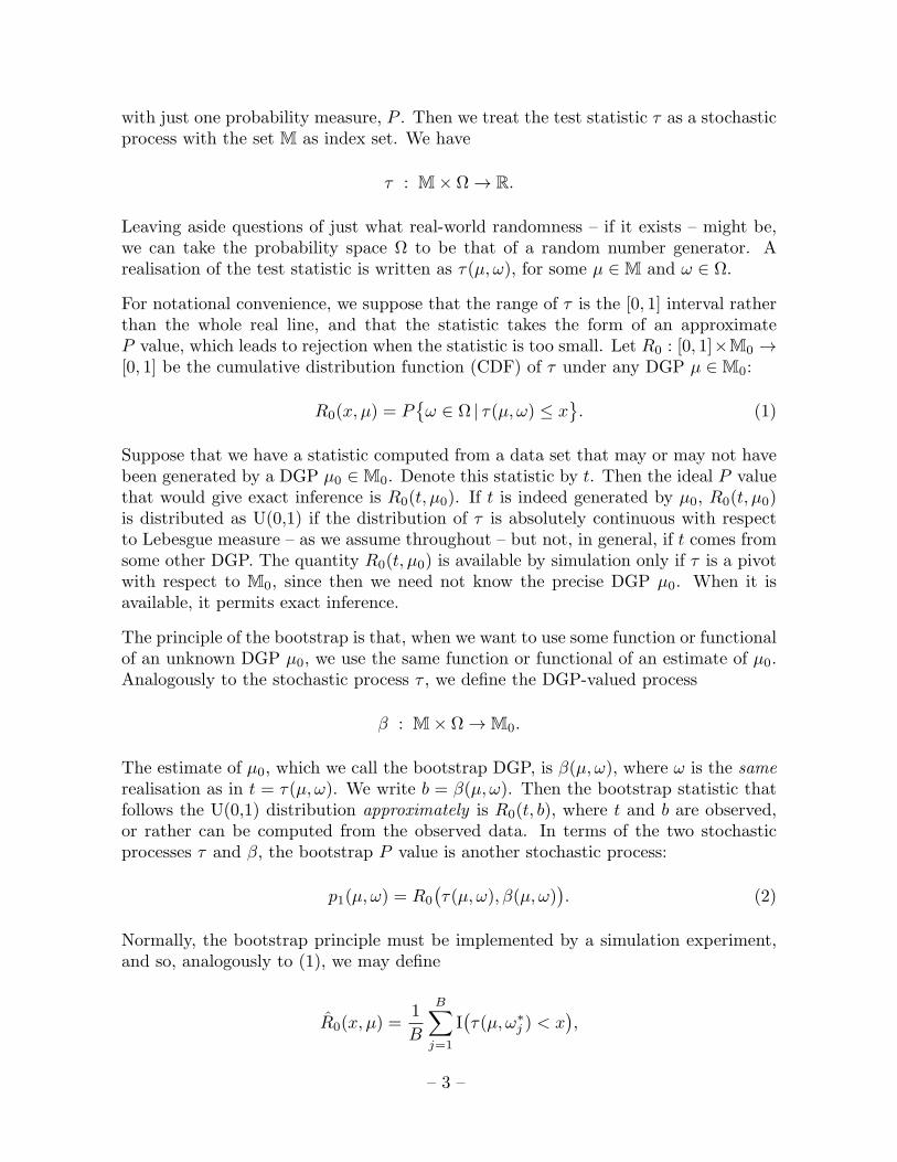
Below are presented the kernel density plots of the statistics τ and τ∗; for τ in red,for τ∗ in green. The distributions are clearly almost identical, thus ruling out the firstpossible explanation.

The regression of τ∗ on τ gave (standard errors in parentheses):

τ∗ = 0.531 + 0.802τ, centred R2 = 0.659(0.005) (0.002)

Both coefficients are highly significant. Thus this is clear evidence of the secondpossible explanation: τ∗ is indeed strongly positively correlated with τ . What thisshows is that the attempt to make the bootstrapped time series mimic the real seriesis too successful, and so there is too little variation in the bootstrap distribution.

– 11 –

..0.

1.

2.

3.

0.5

.

1.0

.

1.5

.

τ∗

.

τ

6. The Fast Approximation

The idea behind the diagnostic procedures discussed here is closely related to the fastdouble bootstrap (FDB) of Davidson and MacKinnon (2007). It is convenient at thispoint to review the FDB.

As a stochastic process, the bootstrap P value can be written as p1(µ, ω), as in (2). Thedouble bootstrap bootstraps this bootstrap P value, as follows: If R1(·, µ) is the CDFof p1(µ, ω), then the random variable R1

(p1(µ, ω), µ

)follows the U(0,1) distribution.

Since µ is unknown in practice, the double bootstrap P value follows the bootstrapprinciple by replacing it by the bootstrap DGP, β(µ, ω). We define the stochasticprocess

p2(µ, ω) = R1

(p1(µ, ω), β(µ, ω)

). (12)

Of course it is computationally expensive to estimate the CDF R1 by simulation, asit involves two nested loops.

Davidson and MacKinnon (2007) suggested a much less expensive way of estimat-ing R1, based on two approximations. The first arises by treating the random variablesτ(µ, ω) and β(µ, ω), for any µ ∈ M0, as independent. Of course, this independencedoes not hold except in special circumstances, but it holds asymptotically in manycommonly encountered situations. By definition,

R1(α, µ) = Pω ∈ Ω | p1(µ, ω) < α

= E

[I(R0(τ(µ, ω), β(µ, ω)) < α

)]. (13)

Let Q0(·, µ) be the quantile function corresponding to the distribution R0(·, µ). SinceR0 is absolutely continuous, we have

R0

(Q0(α, µ), µ

)= α = Q0

(R0(α, µ), µ

).

Use of this relation between R0 and Q0 lets us write (13) as

R1(α, µ) = E[I(τ(µ, ω) < Q0(α, β(µ, ω)

)]– 12 –

If τ(µ, ω) and β(µ, ω) are treated as though they were independent, then we have

R1(α, µ) = E[E[I(τ(µ, ω) < Q0(α, β(µ, ω))

)|β(µ, ω)

]]≈ E

[R0

(Q0(α, β(µ, ω)), µ

)](14)

Define the stochastic process

τ1 : M× (Ω1 × Ω2) → R,

where Ω1 and Ω2 are two copies of the outcome space, by the formula

τ1(µ, ω1, ω2) = τ(β(µ, ω1), ω2

).

Thus τ1(µ, ω1, ω2) can be thought of as a realisation of the bootstrap statistic whenthe underlying DGP is µ. We denote the CDF of τ1 under µ by R1(·, µ). Thus

R1(α, µ) = Pr(ω1, ω2) ∈ Ω1 × Ω2 | τ

(β(µ, ω1), ω2) < α

= E

[I(τ(β(µ, ω1), ω2) < α

)]= E

[E[I(τ(β(µ, ω1), ω2) < α

)| F1

]]= E

[R0

(α, β(µ, ω1)

)]. (15)

Here F1 denotes the sigma-algebra generated by functions of ω1.

The second approximation underlying the fast method can now be stated as follows:

E[R0

(Q0(α, β(µ, ω)), µ

)]≈ R0

(Q1(α, µ), µ

), (16)

where Q1(·, µ) is the quantile function inverse to the CDF R1(·, µ). See Davidson andMacKinnon (2007) for the reasoning that leads to this approximation.

On putting the two approximations, (14) and (16), together, we obtain

R1(α, µ) ≈ R0

(Q1(α, µ), µ

)≡ Rf

1 (α, µ).

The fast double bootstrap substitutes Rf1 for R1 in the double bootstrap P value (12).

The FDB P value is therefore

pf2 (µ, ω) = Rf1

(p1(µ, ω), β(µ, ω)

)= R0

(Q1(p1(µ, ω), β(µ, ω)), β(µ, ω)

). (17)

Estimating it by simulation involves only one loop.

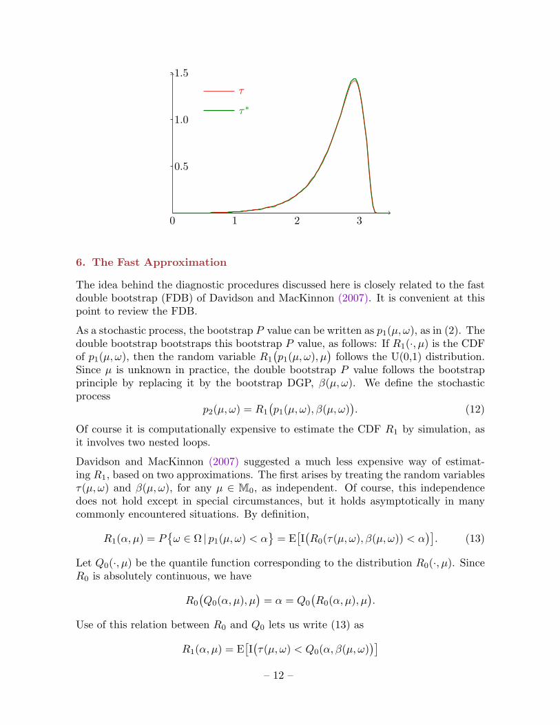
A way to see to what extent the FDB may help improve reliability is to compare the(estimated) distribution of the bootstrap P value and the fast approximation to thatdistribution. The graphs below perform this comparison for the wild bootstrap appliedto the model of Section 4. On the right are plotted the distribution estimated directly

– 13 –

(in green) and the fast approximation (in red). On the left the same thing, but indeviations from the uniform distribution.

..

0.1

.

0.3

.

0.5

.

0.7

.

0.9

.0.000 .

0.004

.

0.008

.

0.012

.

fast

.

direct

. α.

Discrepancy

..0.1.

0.3.

0.5.

0.7.

0.9.0.0 .

0.2

.

0.4

.

0.6

.

0.8

.

1.0

.

fast

.

direct

. α.

Rejection rate

Such differences as are visible are clearly within the simulation noise of the experiment.

7. The Sieve Bootstrap

The sieve bootstrap most commonly used with time series when there is serial cor-relation of unknown form is based on the fact that any linear invertible time-seriesprocess can be approximated by an AR(∞) process. The idea is to estimate a station-ary AR(p) process and use this estimated process, perhaps together with resampledresiduals from the estimation of the AR(p) process, to generate bootstrap samples. Forexample, suppose we are concerned with the static linear regression model (3), but thecovariance matrix Ω is no longer assumed to be diagonal. Instead, it is assumed thatΩ can be well approximated by the covariance matrix of a stationary AR(p) process,which implies that the diagonal elements are all the same.

In this case, the first step is to estimate the regression model, possibly after imposingrestrictions on it, so as to generate a parameter vector β and a vector of residuals uwith typical element ut. The next step is to estimate the AR(p) model

ut =

p∑i=1

ρi ut−i + εt (18)

for t = p + 1, . . . , n. In theory, the order p of this model should increase at a certainrate as the sample size increases. In practice, p is most likely to be determined eitherby using an information criterion like the AIC or by sequential testing. Care shouldprobably be taken to ensure that the estimated model is stationary. This may requirethe use of full maximum likelihood to estimate (18), rather than least squares.

Estimation of (18) yields residuals and an estimate σ2ε of the variance of the εt, as well

as the estimates ρi. We may use these to set up a variety of possible bootstrap DGPs,all of which take the form

y∗t = Xtβ + u∗t .

– 14 –

There are two choices to be made, namely, the choice of parameter estimates β andthe generating process for the bootstrap disturbances u∗

t . One choice for β is justthe OLS estimates from running (3). But these estimates, although consistent, arenot efficient if Ω is not a scalar matrix. We might therefore prefer to use feasibleGLS estimates. An estimate Ω of the covariance matrix can be obtained by solvingthe Yule-Walker equations, using the ρi in order to obtain estimates of the auto-covariances of the AR(p) process. Then a Cholesky decomposition of Ω−1 providesthe feasible GLS transformation to be applied to the dependent variable y and theexplanatory variables X in order to compute feasible GLS estimates of β, restrictedas required by the null hypothesis under test.

For observations after the first p, the bootstrap disturbances are generated as follows:

u∗t =

p∑i=1

ρiu∗t−i + ε∗t , t = p+ 1, . . . , n, (19)

where the ε∗t can either be drawn from the N(0, σ2ε ) distribution for a parametric

bootstrap or resampled from the residuals εt from the estimation of (18), preferablyrescaled by the factor

√n/(n− p). Before we can use (19), of course, we must generate

the first p bootstrap disturbances, the u∗t , for t = 1, . . . , p.

One way to do so is just to set u∗t = ut for the first p observations of each bootstrap

sample. We initialize (19) with fixed starting values given by the real data. Unless weare sure that the AR(p) process is really stationary, rather than just being characterizedby values of the ρi that correspond to a stationary covariance matrix, this is the onlyappropriate procedure.

If we are happy to impose full stationarity on the bootstrap DGP, then we may drawthe first p values of the u∗

t from the p--variate stationary distribution. This is easy todo if we have solved the Yule-Walker equations for the first p autocovariances, providedthat we assume normality. If normality is an uncomfortably strong assumption, thenwe can initialize (19) in any way we please and then generate a reasonably large number(say 200) of bootstrap disturbances recursively, using resampled rescaled values of theεt for the ε

∗t . We then throw away all but the last p of these disturbances and use those

to initialize (19). In this way, we approximate a stationary process with the correctestimated stationary covariance matrix, but with no assumption of normality.

We again consider our test-bed case, with model (10) and test statistic (11). As thedisturbances are AR(1), we set p = 1 in the AR(p) model estimated with the OLSresiduals. It would have been possible, and, arguably, better to let P be chosen in adata-driven way. Otherwise, the setup is identical to that used with the maximum-entropy bootstrap. The graphs following show the P value and P value discrepancyplots, on the left, and the kernel density plots on the right.

– 15 –

..

0.1

.

0.3

.

0.5

.

0.7

.

0.9

.0.0 .

0.2

.

0.4

.

0.6

.

0.8

.

1.0

.

P value

.

discrepancy

.

α

.

Rejection rate

..0.

1.

2.

3.

4.

0.5

.

1.0

.

1.5

.

τ∗

.

τ

Overall, the bootstrap test performs well, although there is significant distortion inthe middle of the distribution of the P value. In the left-hand tail, on the other hand,there is very little. The distributions of τ and τ∗ are very similar.

The regression of τ∗ on τ gave (OLS standard errors in parentheses):

τ∗ = 2.57 + 0.05τ, centred R2 = 0.003(0.008) (0.003)

The next graphs show the comparison between the P value plot as estimated directlyby simulation (in green) and as estimated using the fast method (in red) on the right,and that for the P value discrepancy plot, on the left.

..0.1.

0.3.

0.5.

0.7.

0.9.

−0.06

.

−0.04

.

−0.02

.0.00 .

fast

.direct

. α.

Discrepancy

..0.1.

0.3.

0.5.

0.7.

0.9.0.0 .

0.2

.

0.4

.

0.6

.

0.8

.

1.0

.

fast

.

direct

. α.

Rejection rate

It is clear that the fast method gives results very close indeed to those obtained bydirect simulation, and this suggests that the FDB could improve performance substan-tially. This is also supported by the insignificant correlation between τ and τ∗, andthe fact that there is no visible shift in the density plot for τ and that for τ∗, although

– 16 –

the significant positive constant in the regression shows that τ∗ tends to be greaterthan τ , which accounts for the under-rejection in the middle of the distribution.

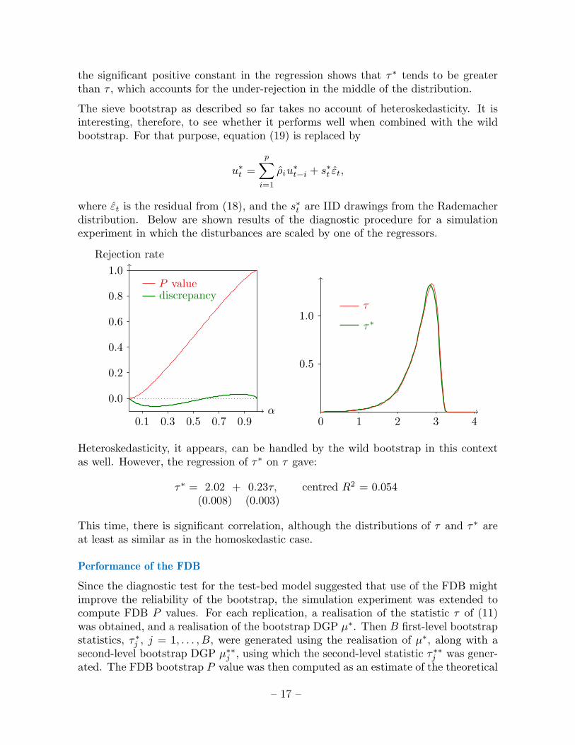
The sieve bootstrap as described so far takes no account of heteroskedasticity. It isinteresting, therefore, to see whether it performs well when combined with the wildbootstrap. For that purpose, equation (19) is replaced by

u∗t =

p∑i=1

ρiu∗t−i + s∗t εt,

where εt is the residual from (18), and the s∗t are IID drawings from the Rademacherdistribution. Below are shown results of the diagnostic procedure for a simulationexperiment in which the disturbances are scaled by one of the regressors.

..

0.1

.

0.3

.

0.5

.

0.7

.

0.9

.0.0 .

0.2

.

0.4

.

0.6

.

0.8

.

1.0

.

P value

.

discrepancy

.

α

.

Rejection rate

..0.

1.

2.

3.

4.

0.5

.

1.0

.

τ∗

.

τ

Heteroskedasticity, it appears, can be handled by the wild bootstrap in this contextas well. However, the regression of τ∗ on τ gave:

τ∗ = 2.02 + 0.23τ, centred R2 = 0.054(0.008) (0.003)

This time, there is significant correlation, although the distributions of τ and τ∗ areat least as similar as in the homoskedastic case.

Performance of the FDB

Since the diagnostic test for the test-bed model suggested that use of the FDB mightimprove the reliability of the bootstrap, the simulation experiment was extended tocompute FDB P values. For each replication, a realisation of the statistic τ of (11)was obtained, and a realisation of the bootstrap DGP µ∗. Then B first-level bootstrapstatistics, τ∗j , j = 1, . . . , B, were generated using the realisation of µ∗, along with asecond-level bootstrap DGP µ∗∗

j , using which the second-level statistic τ∗∗j was gener-ated. The FDB bootstrap P value was then computed as an estimate of the theoretical

– 17 –

formula (17): the function R0 estimated as the empirical distribution of the τ∗j , and

the quantile function Q1 as an empirical quantile of the τ∗∗j .

Below on the left is a comparison of the P value discrepancy plots for the singlebootstrap (in red) and the FDB (in green). There is a slight improvement, but it isnot very impressive. On the right are the kernel density plots for τ (red), τ∗ (green),and τ∗∗ (blue). All three are very similar, but the densities of τ∗ and τ∗∗ are closerthan is either of them to the density of τ . This fact is probably the explanation ofwhy the FDB does not do a better job.

..0.1.

0.3.

0.5.

0.7.

0.9.

−0.06

.

−0.04

.

−0.02

.0.00 .

fast

.direct

. α.Discrepancy

..0.

1.

2.

3.

4.

0.5

.

1.0

.

1.5

.

τ∗

.

τ

.

τ∗∗

The three statistics are at most very weakly correlated, as seen in the regression results:

τ∗ = 2.57 + 0.05τ, centred R2 = 0.003(0.008) (0.003)

τ∗∗ = 2.50 + 0.08τ∗, centred R2 = 0.006(0.009) (0.003)

τ∗∗ = 2.60 + 0.04τ, centred R2 = 0.002(0.008) (0.003)

The significant constants, though, are indicators of shifts in the distributions that arenot visible in the kernel density plots, and contribute to the under-rejection by bothsingle and fast double bootstrap P values.

8. Concluding Remarks

The diagnostic techniques proposed in this paper do not rely in any way on asymptoticanalysis. Although they require a simulation experiment for their implementation,this experiment is hardly more costly than undertaking bootstrap inference in thefirst place. Results of the experiment can be presented graphically, and can often beinterpreted very easily. A simple OLS regression constitutes the other part of thediagnosis. It measures to what extent the quantity being bootstrapped is correlatedwith its bootstrap counterpart, and to what extent the distributions of this quantityand its bootstrap counterpart are shifted relative to each other. Significant correlation

– 18 –

not only takes away the possibility of an asymptotic refinement, but also degradesbootstrap performance, as shown by a finite-sample analysis.

Since bootstrapping time series is an endeavour fraught with peril, the examples forwhich the diagnostic techniques are applied in this paper all involve time series. Insome cases, the bootstrap method is parametric; in others it is intended to be robustto autocorrelation of unknown form. Such robustness can be difficult to obtain, andthe reasons for this in the particular cases studied here are revealed by the diagnosticanalysis.

The methods of the paper can, of course, be applied equally well in circumstances thatdo not necessarily involve time series, but in which the bootstrap seems not to workvery well.

References

Beran, R. (1997) “Diagnosing Bootstrap Success”, Annals of the Institute ofStatistical Mathematics, 49, 1–24.

Buhlmann, P. (1997). “Sieve bootstrap for time series”, Bernoulli 3, 123–148.

Buhlmann, P. (2002). “Bootstraps for time series”, Statistical Science 17, 52–72.

Davidson, R. (2012). “Statistical Inference in the Presence of Heavy Tails”,Econometrics Journal, 15, C31–C53.

Davidson, R. and E. Flachaire (2008). “The wild bootstrap, tamed at last”, Journalof Econometrics, 146, 162–9.

Davidson, R. and J. G. MacKinnon (1998). “Graphical Methods for Investigatingthe Size and Power of Hypothesis Tests,” The Manchester School, 66, 1-26.

Davidson, R. and J. G. MacKinnon (1999). “The Size Distortion of BootstrapTests,” Econometric Theory, 15, 361-376.

Davidson, R. and J. G. MacKinnon (2006). “The power of bootstrap and asymptotictests”, Journal of Econometrics, 133, 421–441.

Davidson, R. and J. G. MacKinnon (2007). “Improving the Reliability of BootstrapTests with the Fast Double Bootstrap”, Computational Statistics and DataAnalysis, 51, 3259–3281.

Eicker, F. (1963). “Asymptotic normality and consistency of the least squaresestimators for families of linear regressions,” The Annals of MathematicalStatistics, 34, 447–456.

– 19 –

Fiebig Denzil, G. and H. Theil (1982). Comment, Econometric Reviews 1:2, 263–269

Hall, P. (1992) The Bootstrap and Edgeworth Expansion. New York: Springer-Verlag.

Hall, P., J. L. Horowitz, and B.-Y. Jing (1995). “On blocking rules for the bootstrapwith dependent data”, Biometrika 82, 561–574.

Horowitz, J. L. (1997). “Bootstrap methods in econometrics: Theory and numericalperformance,” in D. M. Kreps and K. F. Wallis (ed.), Advances in Economics andEconometrics: Theory and Applications: Seventh World Congress, Cambridge,Cambridge University Press.

Jaynes. E. T. (1957). “Information Theory and Statistical Mechanics”, PhysicalReview 106, 620–630.

Kirch, C. and D. N. Politis (2011). “TFT Bootstrap: Resampling time series in thefrequency domain to obtain replicates in the time domain”, Annals of Statistics39, 1427–1470.

Kreiss, J. P. and E. Paparoditis (2003). “Autoregressive-aided periodogrambootstrap for time series”, Annals of Statistics 31, 1923-1955.

Kunsch, H. R. (1989). “The jackknife and the bootstrap for general stationaryobservations”, Annals of Statistics 17, 1217–1241.

Lahiri, S. N. (1999). “Theoretical comparisons of block bootstrap methods”, Annalsof Statistics 27, 386–404.

Lahiri, S. N. (2003). Resampling Methods for Dependent Data, New York: Springer.

Liu, R. Y. (1988). “Bootstrap procedures under some non-I.I.D. models”, Annals ofStatistics 16, 1696–1708.

Mammen, E. (1993). “Bootstrap and wild bootstrap for high dimensional linearmodels”, Annals of Statistics 21, 255–285.

Newey, W. K. and K. D. West (1987). “A simple, positive semi-definite, het-eroskedasticity and autocorrelation consistent covariance matrix”, Econometrica55, 703–8.

Schluter, C. (2012) “Discussion of S. G. Donald et al and R. Davidson”, Economet-rics Journal, 12, C54-C57

Shao, X. (2010). “The Dependent Wild Bootstrap”, Journal of the AmericanStatistical Association 105, 218–235.

– 20 –

Theil, H. and K. Laitinen (1980). “Singular moment matrices in applied econo-metrics”, in Mu1tivariate Analysis - V (P.R. Krishnaiah, Ed. ). Amsterdam:North-Holland Pub1ishing Co., 629–649.

Vinod, H.D. (2006). “Maximum entropy ensembles for time series inference ineconomics”, Journal of Asian Economics 17, 955–978.

White, H. (1980). “A heteroskedasticity-consistent covariance matrix estimator anda direct test for heteroskedasticity,” Econometrica, 48, 817–838.

Wu, C. F. J. (1986). “Jackknife, bootstrap and other resampling methods inregression analysis”, Annals of Statistics 14, 1261–1295.

– 21 –