Diagnostics and Prognostics Method for Analog Electronic Circuits

IEEE TRANSACTIONS ON INDUSTRIAL ELECTRONICS, VOL. 60, NO. 11, NOVEMBER 2013 5277

Diagnostics and Prognostics Method forAnalog Electronic Circuits

Arvind Sai Sarathi Vasan, Member, IEEE, Bing Long, and Michael Pecht, Fellow, IEEE

Abstract—Analog circuits play a vital role in ensuring theavailability of industrial systems. Unexpected circuit failures insuch systems during field operation can have severe implications.To address this concern, we developed a method for detectingfaulty circuit condition, isolating fault locations, and predictingthe remaining useful performance of analog circuits. Through thesuccessive refinement of the circuit’s response to a sweep signal,features are extracted for fault diagnosis. The fault diagnosticsproblem is posed and solved as a pattern recognition problem us-ing kernel methods. From the extracted features, a fault indicator(FI) is developed for failure prognosis. Furthermore, an empiricalmodel is developed based on the degradation trend exhibited bythe FI. A particle filtering approach is used for model adaptationand RUP estimation. This method is completely automated andhas the merit of implementation simplicity. Case studies on twoanalog filter circuits demonstrating this method are presented.

Index Terms—Analog circuits, least squares support vectormachines (SVMs) (LS-SVMs), parametric faults, particle filters(PFs).

I. INTRODUCTION

ANALOG CIRCUITS are used in industrial systems forimplementing controllers [1], conditioning signals [2],

protecting critical modules [3], [4], and more [5]. The occur-rence of circuit failures during field operation can affect systemfunctionality, and the cost of failure can be enormous [6], [7]. Inmost cases, these failures can be related to a fault in a system’sanalog circuitries, where “fault” refers to a drift in the valueof a circuit component from its nominal value, which leadsto a failure of the whole circuit. These faults could either becatastrophic (open and short circuit) or parametric (fractionaldeviation in circuit components from their nominal values) [8].For example, the degradation of electrolytic capacitors in LCfilters will cause the switching-mode power converters to fail[9]. An increase in the parametric resistance offered by the com-ponents within filter circuits due to the degradation of solderjoints will affect the frequency band being filtered out [10].

Manuscript received March 5, 2012; revised June 16, 2012; acceptedSeptember 3, 2012. Date of publication October 10, 2012; date of currentversion June 6, 2013.

A. Sai Sarathi Vasan is with the Center for Advanced Life Cycle En-gineering, University of Maryland, College Park, MD 20742 USA (e-mail:[email protected]).

B. Long is with the School of Automation Engineering, University ofElectronic Science and Technology of China, Chengdu 611731, China (e-mail:[email protected]).

M. Pecht is with the Center for Advanced Life Cycle Engineering, Universityof Maryland, College Park, MD 20742 USA, and also with the Prognosticsand Health Management Center, City University of Hong Kong, Kowloon,Hong Kong (e-mail: [email protected]).

Color versions of one or more of the figures in this paper are available onlineat http://ieeexplore.ieee.org.

Digital Object Identifier 10.1109/TIE.2012.2224074

The prevention of circuit failures during field operation re-quires methods for the following: 1) the early detection andisolation of faults and 2) the prediction of the remaining usefulperformance (RUP) of the failing circuit [11]. Here, RUP refersto the remaining time that the circuit performance guaranteessystem operation. In the past, there have been many reports onprognostics and system health management (PHM) techniquesfor individual components of an analog circuit. For example,Chen et al. [9] proposed an online failure prediction methodfor electrolytic capacitors in an LC filter of a switching-modepower converter. Alam et al. [12] proposed model-based anddata-driven prognostics methods for predicting the failure timefor embedded planar capacitors. Kwon et al. [13] proposed aprobabilistic approach for predicting the failure of intercon-nects. Although there are PHM strategies for predicting thefailure of individual components, it becomes impractical toimplement a PHM system for each and every component in acomplex system. It is desirable to have a cost-effective expertsystem for the PHM of electronic circuits at the system level sothat maintenance decisions can be made on a conditional basisand maintenance personnel can be given ample forewarningbefore a circuit failure occurs.

Most of the related research for analog circuits has aimedat diagnosing faults in circuits during the manufacturing pro-cess. These approaches do not address the fault diagnosticsproblem from a field-operation (real-time) perspective. Hence,they suffer from shortcomings (listed in Section II) which limittheir implementation in onboard applications. Furthermore, nomethod has been suggested for predicting the remaining timeuntil circuit failure. System-level prognostic techniques havebeen successfully implemented for other applications [14]–[19]. However, it is not clear how these techniques can beextended to perform RUP estimation for analog circuits.

In this paper, a new diagnostics and prognostics method foranalog circuits is proposed, aiming at “in-circuit” real-timefault detection, isolation, and RUP estimation. A kernel-basedmachine learning (ML) approach is employed for the earlydetection and isolation of faults, where early fault detectionrefers to the detection of component variations just outside theirtolerance range. For failure prognosis, a fault indicator (FI)reflecting the evolution of a fault in any of the circuit’s criticalcomponents is developed. Then, a model adaptation schemeusing particle filters (PFs) is devised for tracking the evolutionof the FI and predicting the circuit’s RUP.

This paper is organized as follows. Section II presents asurvey of the literature pertaining to fault diagnostics andfailure prognostics of analog circuits. Section III briefly de-scribes our multistage PHM framework. Here, we also describe

0278-0046/$31.00 © 2012 IEEE

5278 IEEE TRANSACTIONS ON INDUSTRIAL ELECTRONICS, VOL. 60, NO. 11, NOVEMBER 2013

our approach for extracting features and constructing the FI.Section IV provides the theoretical background on a kernel-based fault classifier and the PF approach used in the proposedPHM framework for fault diagnostics and RUP estimation,respectively. Section V presents the performance results of theproposed PHM framework on two filter circuits. Concludingremarks and possible directions for future work are presentedin Section VI.

II. LITERATURE REVIEW

Fault diagnostics and failure prognostics in analog circuitsare made challenging by the presence of component tolerances,the complex nature of the fault mechanisms, and the effects ofthe operational and environmental stresses [20].

Traditionally, analog circuit fault diagnosis has been carriedout using simulation-after-test (SAT) or simulation-before-test(SBT) strategies [6], [21]–[23]. In the SAT approach, faultdetection is based on the derived circuit transfer function equa-tions, and fault isolation is realized by estimating the circuitparameters from the circuit’s response to a test stimulus [24]–[30]. This technique is time consuming and suffers from draw-backs associated with the parameter estimation procedure whendealing with complex nonlinear circuits. Many SBT diagnosticmethods have been proposed in the past. These are either basedon derived circuit equations at selected nodes [31]–[33] or onthe ML approach [34]–[45]. Fault diagnosis based on circuitequations is not suitable for nonlinear analog circuits and islimited in application due to the poor accessibility to internalnodes of integrated circuits (ICs) [46].

ML-based SBT approaches typically provide faster resultscompared to SAT approaches during the diagnostics phase[23]. This makes an ML-based approach appealing for onlinefault diagnostics. Spina and Upadhyaya [35] used a backward-error-propagation neural network (NN) for analog circuit faultdiagnosis. In [35], features extracted from the circuit’s responseto white noise were used as input to the NN without any datapreprocessing. This resulted in an NN with a large architec-ture. Later, Aminian and Aminian [36]–[38] improved the NNapproach using data preprocessing techniques such as waveletdecomposition and principal component analysis (PCA). Otherefforts in NN-based fault diagnosis include the use of kurtosisand entropy [39], kernel PCA [40], multiresolution decom-position [42], and L1-norm optimization [43] as preproces-sors for improving performance. In recent years, researchershave also used support vector machines (SVMs) instead ofan NN for fault detection and isolation in analog circuits[44], [45], [47], [48].

Although several fault diagnostic approaches for analog cir-cuits have been reported in the literature, no work has been doneon prognostics for analog circuits. Even among the preferredML-based fault diagnostics methods, there are shortcomingsthat confine their implementation in real-time applications. Inthese methods, features are extracted from the circuit’s responseto an impulse signal. Although this allows the extraction of acircuit’s frequency response directly from its output, in order tocapture the circuit’s output, a high sampling rate and expensivedata acquisition equipment are required, irrespective of the

bandwidth of the circuit [37]. Furthermore, these ML-basedSBT approaches are tested and trained using data collectedfrom only one fault value under each fault class or condition.In practice, it is common to encounter fault values that arenot seen during training. The diagnosability of these ML-based SBT approaches in such scenarios is still unknown. Bydiagnosability, we mean the ability to detect faulty conditionsand isolate fault locations [27].

To solve these problems, a new diagnostics and prognosticsmethod for analog circuits is proposed. The contributions ofthis paper are summarized as follows. First, a new featureextraction method is proposed to enable the real-time testingof analog circuits. Second, a systematic process was estab-lished for constructing a FI for circuit prognostics. Finally, adegradation model and model adaptation scheme have beenfurnished to assess the RUP of analog circuits. Together, thesecontributions will allow systems to autonomously assess theiranalog circuitries during field operation.

III. PHM FRAMEWORK

Developing PHM strategies for analog circuits is a chal-lenging task due to the unavailability of fault models [37].This makes the application of data-driven techniques appealingbecause they do not require knowledge of material properties,structures, or failure mechanisms. Here, we focus on the de-velopment of a PHM framework that can be built on board asan “in-circuit” testing strategy. An overview of our proposeddata-driven PHM method for analog circuits is schematicallyrepresented in Fig. 1.

The proposed approach involves two phases: training andtesting. During the training phase, frequently occurring faultsare investigated to identify faults of interest. The circuit undertest (CUT) is then replicated for these hypothesized fault con-ditions and excited by a test stimulus to extract features that arestored in a fault dictionary for use during the online detection offaults. From the extracted features, a FI is built whose trend isidentified under different fault conditions. Anomaly and failurethresholds are identified for the FI during the training mode.

In the testing mode, the FI is calculated from the mostrecently extracted features. When the FI crosses the anomalythreshold, the prognostics algorithm is triggered, which esti-mates the RUP as a probability density function (pdf). Simulta-neously, the fault detection and isolation algorithm is triggered,where the features extracted and normalized are comparedwith those stored in the fault dictionary. This comparison isperformed using a kernel-based classifier that has been pre-viously trained. The output of the classifier indicates whetherthe circuit is faulty or not. If the circuit is faulty, the classi-fier also identifies the faulty component. Thus, the proposedsolution presents a single tool for fault detection, isolation,and prognosis, thereby eliminating the need to develop eachseparately. The following sections describe the steps involvedin our proposed multistage process.

A. Test Signal Generator

For analog circuits, the behavioral characteristics are as-sumed to be embedded in the time and frequency response.

SAI SARATHI VASAN et al.: DIAGNOSTICS AND PROGNOSTICS METHOD FOR ANALOG ELECTRONIC CIRCUITS 5279

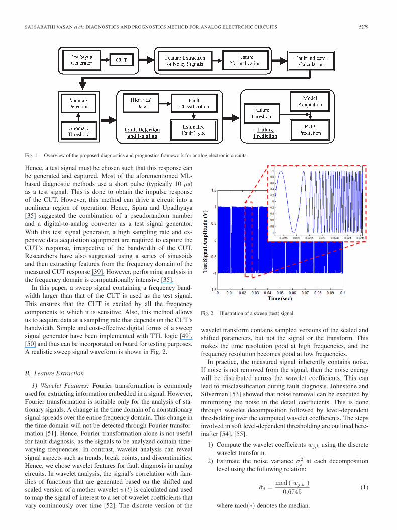
Fig. 1. Overview of the proposed diagnostics and prognostics framework for analog electronic circuits.

Hence, a test signal must be chosen such that this response canbe generated and captured. Most of the aforementioned ML-based diagnostic methods use a short pulse (typically 10 μs)as a test signal. This is done to obtain the impulse responseof the CUT. However, this method can drive a circuit into anonlinear region of operation. Hence, Spina and Upadhyaya[35] suggested the combination of a pseudorandom numberand a digital-to-analog converter as a test signal generator.With this test signal generator, a high sampling rate and ex-pensive data acquisition equipment are required to capture theCUT’s response, irrespective of the bandwidth of the CUT.Researchers have also suggested using a series of sinusoidsand then extracting features from the frequency domain of themeasured CUT response [39]. However, performing analysis inthe frequency domain is computationally intensive [35].

In this paper, a sweep signal containing a frequency band-width larger than that of the CUT is used as the test signal.This ensures that the CUT is excited by all the frequencycomponents to which it is sensitive. Also, this method allowsus to acquire data at a sampling rate that depends on the CUT’sbandwidth. Simple and cost-effective digital forms of a sweepsignal generator have been implemented with TTL logic [49],[50] and thus can be incorporated on board for testing purposes.A realistic sweep signal waveform is shown in Fig. 2.

B. Feature Extraction

1) Wavelet Features: Fourier transformation is commonlyused for extracting information embedded in a signal. However,Fourier transformation is suitable only for the analysis of sta-tionary signals. A change in the time domain of a nonstationarysignal spreads over the entire frequency domain. This change inthe time domain will not be detected through Fourier transfor-mation [51]. Hence, Fourier transformation alone is not usefulfor fault diagnosis, as the signals to be analyzed contain time-varying frequencies. In contrast, wavelet analysis can revealsignal aspects such as trends, break points, and discontinuities.Hence, we chose wavelet features for fault diagnosis in analogcircuits. In wavelet analysis, the signal’s correlation with fam-ilies of functions that are generated based on the shifted andscaled version of a mother wavelet ψ(t) is calculated and usedto map the signal of interest to a set of wavelet coefficients thatvary continuously over time [52]. The discrete version of the

Fig. 2. Illustration of a sweep (test) signal.

wavelet transform contains sampled versions of the scaled andshifted parameters, but not the signal or the transform. Thismakes the time resolution good at high frequencies, and thefrequency resolution becomes good at low frequencies.

In practice, the measured signal inherently contains noise.If noise is not removed from the signal, then the noise energywill be distributed across the wavelet coefficients. This canlead to misclassification during fault diagnosis. Johnstone andSilverman [53] showed that noise removal can be executed byminimizing the noise in the detail coefficients. This is donethrough wavelet decomposition followed by level-dependentthresholding over the computed wavelet coefficients. The stepsinvolved in soft level-dependent thresholding are outlined here-inafter [54], [55].

1) Compute the wavelet coefficients wj,k using the discretewavelet transform.

2) Estimate the noise variance σ2j at each decomposition

level using the following relation:

σ̂j =med (|wj,k|)

0.6745(1)

where med(∗) denotes the median.

5280 IEEE TRANSACTIONS ON INDUSTRIAL ELECTRONICS, VOL. 60, NO. 11, NOVEMBER 2013

3) Compute the threshold Tj at each decomposition levelusing the following relation:

Tj = σ̂j√(2 ln 2j). (2)

4) The soft level-dependent thresholding is performed withthe function

dj,k =

{sgn(wj,k) (|wj,k| − Tj) , if |wj,k| > Tj

0, otherwise(3)

where dj,k denotes the kth detail coefficient at the jthlevel of decomposition.

In this paper, through discrete wavelet transformation, wedecompose the response of the CUT stimulated by a sweepsignal into the approximation and detail signals using multiratefilter banks [56]. Then, we remove noise from the detailedcoefficients using the classical wavelet denoising procedureoutlined earlier. The information contained in the circuit’s re-sponse is represented using features extracted by computing theenergy contained in the detail coefficients (with noise removed)at various levels of decomposition [47]. This is expressed asfollows:

Ej =∑k

|dj,k|2, j = 1 : J (4)

where Ej denotes the energy in the detail coefficient at the jthlevel of decomposition.

2) Statistical Features: The second set of features extractedincludes the kurtosis and entropy of the CUT’s response. Kurto-sis is a statistical property which is defined as the standardizedfourth moment about the mean. It provides a measure of theheaviness of the tails in the pdf of a signal, which is relatedto the abrupt changes in the signal having high values andappearing in the tails of the distribution [57]. Kurtosis is math-ematically described as follows:

kurt(x) =E [x− E[x]]4[E [x− E[x]]2

]2 . (5)

On the other hand, entropy provides a measure of the in-formation capacity of a signal, which denotes the uncertaintyassociated with the selection of an event from a set of possibleevents whose probabilities of occurrences are known [56], [57].It is defined for a discrete-time signal as

H(x) = −∑i

P (x = ai) logP (x = ai) (6)

where ai denotes the possible values of x and P (∗) denotes theassociated probabilities.

C. Feature Scaling

The goal of the feature extractor is to characterize a circuit’sfault condition such that the feature vector values remain asfollows: 1) similar for all of the circuit topologies belongingto the same fault condition and 2) different for circuit topolo-

gies under different fault conditions. This demands the featureelements to be invariant with respect to scale.

Hence, once the features are extracted, we scale the featuresfor the purpose of enhancing the inputs to the fault classifier.Feature scaling helps in avoiding issues due to unexpectedchanges in the dynamic ranges of the feature elements [36],[60]. In our investigation, scaling the feature vector that wasextracted using wavelet decomposition to have a zero mean andunit standard deviation resulted in efficient classification.

D. FI

When implementing prognostics at the component level,usually a FI parameter is identified to monitor the degradationof the component in real time. This parameter (e.g., the ON-state VCE of an insulated-gate bipolar transistor (IGBT) [61]and the RF impedance for interconnects [13]) is chosen basedon an understanding of the degradation process [9].

For a complex system, multiple parameters corresponding toall the critical components/subsystems need to be monitoredand processed in real time to perform prognostics. This is notpossible in applications such as analog circuits, where there is aconstraint on the available resources. In order to address thischallenge, we have developed a method to construct a FI torepresent circuit degradation. Here, circuit degradation refers tothe degradation in any of a circuit’s critical components whichleads to the deviation of the component’s value from its nominalvalue. The procedure for calculating the FI is based on the well-known Mahalanobis–Taguchi (MT) methodology [62], [63].

The FI calculation starts with the collection of the two featuresets (wavelet and statistical features) under a no-fault condition(circuit components are allowed to vary within their standardtolerance range). For both feature sets, two individual Maha-lanobis spaces (MSs) are constructed using their normalizedfeature elements and correlation coefficients.

Let F1= {f1

1 , f12 , . . . , f

1l } and F

2= {f2

1 , f22 } denote the

wavelet and statistical features, respectively, where f1i ; i = 1 : l

denotes the energy of the detail coefficients at the ith decompo-sition level, l is the number of decomposition levels, and f2

1

and f22 are the kurtosis and entropy of the CUT’s response. A

data set formed using the feature set [F1j , F

2j ]; j = 1 : n with

n observations made during the no-fault condition is used astraining data.

The mean and standard deviation of each feature elementare calculated using the training data, from which the trainingfeature sets in the no-fault condition are normalized

Z1i,j =

f1i,j − x̄1

i

s1iZ2k,j =

f2k,j − x̄2

k

s2k,

i = 1 : l; k = 1, 2; j = 1 : n (7)

where

x̄1i =

∑nj=1 f

1i,j

n

x̄2k =

∑nj=1 f

2k,j

n

SAI SARATHI VASAN et al.: DIAGNOSTICS AND PROGNOSTICS METHOD FOR ANALOG ELECTRONIC CIRCUITS 5281

Fig. 3. Illustration of fault propagation on the MS.

s1i =

(∑nj=1

(f1i,j − x̄1

i

)2n− 1

) 12

s2k =

⎛⎜⎝∑n

j=1

(f2k,j − x̄2

k

)2

n− 1

⎞⎟⎠

12

. (8)

After normalizing the feature sets, the Mahalanobis distances(MDs) are calculated during the no-fault condition using thefollowing mathematical expressions:

MD1j =C−1

(Z1i,j

)T(Σ1)

−1 (Z1k,j

)MD2

j =C−1(Z2k,j

)T(Σ2)

−1 (Z2k,j

)(9)

where Σ1 and Σ2 represent the correlation matrices for thewavelet and statistical features, respectively, and are calculatedfrom the normalized feature sets as

Σ1i,j =

1

n− 1

n∑m=1

Z1i,mZ1

j,m

Σ2i,j =

1

n− 1

n∑m=1

Z2i,mZ2

j,m (10)

where C denotes the total number of classes, i.e., the faultconditions and the no-fault condition.

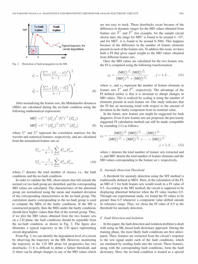
In order to validate the MS, observations that fall outside thenormal (or) no-fault group are identified, and the correspondingMD values are calculated. The characteristics of the abnormalgroup are normalized using the mean and standard deviationof the corresponding characteristics in the no-fault group. Thecorrelation matrix corresponding to the no-fault group is usedto compute the MDs of the faulty conditions. If the MS isconstructed properly, then the MDs under the faulty conditionsshould have higher values than that of the normal group. Thus,if we plot the MD values obtained from the two feature setson a 2-D plane, the fault conditions should be separable fromthe no-fault condition, as shown in Fig. 3. The figure alsoillustrates a typical trajectory in the 2-D space representingcircuit degradation.

From Fig. 3, we can identify the degradation level of a circuitby observing the trajectory on the MS. However, monitoringthe trajectory in the 2-D MS alone for prognostics has twodrawbacks: 1) It is difficult to define a failure threshold, and2) there can be abrupt changes in any of the MD values which

are not easy to track. These drawbacks occur because of thedifference in dynamic ranges for the MD values obtained fromfeature sets F

1and F

2(for example, for the sample circuit

shown later, the range for MD1 is found to be around 0−106,and for MD2, it is found to be around 0–500). This happensbecause of the difference in the number of feature elementspresent in each of the feature sets. To address this issue, we havebuilt a FI that gives equal weight to the MD values obtainedfrom different feature sets.

Once the MD values are calculated for the two feature sets,the FI is computed using the following transformation:

℘j =

(MD1

j

) 1n1

(MD2

j

) 1n2(

MD1j

) 1n1 +

(MD2

j

) 1n2

, j = 1, 2 . . . (11)

where n1 and n2 represent the number of feature elements infeature sets F

1and F

2, respectively. The advantage of the

FI defined earlier is that it is invariant to abrupt changes inMD values. This is realized by scaling it using the number ofelements present in each feature set. Our study indicates thatthe FI has an increasing trend with respect to the amount ofdeviation in the faulty component from its nominal value.

In the future, new feature sets might be suggested for faultdiagnosis. Even if new feature sets are proposed, the previouslysuggested FI calculation method can still be made compatibleby extending (11) as follows:

℘j =

(MD1

j

) 1n1

(MD2

j

) 1n2 . . .

(MDr

j

) 1nr(

MD1j

) 1n1 +

(MD2

j

) 1n2 + · · ·+

(MDr

j

) 1nr

,

j = 1, 2 . . . (12)

where r denotes the total number of feature sets extracted andni and MDi denote the total number of feature elements and theMD values corresponding to the feature set i, respectively.

E. Anomaly Detection Threshold

A threshold for anomaly detection using the MT method istraditionally defined as MD1. Here, in the calculation of the FI,an MD of 1 for both feature sets would result in a FI value of0.5. According to the MT method, the circuit is supposed to bedisplaying abnormal behavior when the FI value reaches 0.5.Through our experimental study, we found the FI values to begreater than 0.5 whenever a component value drifted outsideits tolerance range. Thus, we chose the FI value of 0.5 as thethreshold for anomaly detection.

F. Fault Detection and Isolation

In this paper, the fault detection and isolation problem is dealtwith using an ML-based fault dictionary approach. During thetraining phase, the most likely fault conditions are first antici-pated. Then, features are extracted from the circuit’s responseto the test signal under each of the fault conditions, whichare emulated by seeding faults into the circuit. These features,along with the corresponding fault conditions, form the faultdictionary. Here, the no-fault condition is treated as a special

5282 IEEE TRANSACTIONS ON INDUSTRIAL ELECTRONICS, VOL. 60, NO. 11, NOVEMBER 2013

form of fault condition and thus forms a separate class in thefault dictionary.

We employ a one-against-one (OAO) multiclass least squaresSVM (LS-SVM) to learn from the extracted features (inputs)and the corresponding fault conditions (labels). The classifier’smodel parameters are identified during the training phase. Dur-ing the diagnosis phase, the extracted features are comparedwith the features stored in the fault dictionary using the trainedclassifier. Since the no-fault condition is treated as a separateclass, the output of the classifier will indicate whether theextracted features belong to a faulty or no-fault condition.The output of the classifier also denotes the faulty component.The theoretical background pertaining to the classifier used isprovided in the next section.

G. Failure Prognostics

The remaining useful life (RUL) of a system/component isdefined as the duration from the current time to the end of usefullife. In the case of analog circuits, a circuit is considered to havefailed when one or more critical components in the circuit havedeviated in their value beyond a permissible level, as defined bythe circuit designer. However, this definition of failure does notliterally refer to a functional failure of the critical component.The critical component that is claimed to have failed may stillfunction, but not within the permissible operation range. Hence,it is appropriate to refer to the time to circuit failure as theRUP instead of RUL, as it indicates the time that the circuitperformance will ensure system operation.

In this paper, RUP is estimated from the FI’s evolution, as,at any time instant, its value reflects the amount of deviation inany of the critical components. The RUP estimation is assistedby employing an appropriate prognostics method. A variety ofonline prognostics methods have been proposed in the past.However, in applications where fault models are not available,statistical data-driven prognostic approaches are employed be-cause they exhibit mathematical properties that are effectivein managing uncertainties. Statistical data-driven prognosticapproaches rely on available past and present observed data andstatistical models to estimate the RUP in a probabilistic way.One such approach is PF, which has become a popular choicein the PHM community due to its ability to model nonlinearnon-Gaussian systems, ease of implementation, and support foruncertainty management. A PF approach (also known as theBayesian Monte Carlo approach) is employed in this paper forestimating the RUP of a circuit. The second part of Section IVcovers the theory behind PF and the concept of RUP estimationusing PF.

IV. THEORETICAL BACKGROUND

A. Fault Classifier

The SVM classifier theory developed by Vapnik [64] uses akernel function to map the input samples to a higher dimensionfeature space. The input samples become linearly separable inhigher dimension feature space (see Fig. 4). However, this clas-sifier is obtained by solving a complex quadratic-programming

Fig. 4. Illustration of binary fault classification using an SVM.

problem. In contrast, the LS-SVM classifier introduced bySuykens and Vandewalle [65], [66] reduces the complexity andcomputations involved in SVM.

Given a set of input and output training pairs {ri, yi}ni=1,with ri ∈ �N and yi ∈ {−1,+1} being the input vectors andoutput labels, respectively, the LS-SVM approach aims to con-struct a binary classifier of the form

y(r) = sign[wTΓ(r) + b

](13)

where w is a weight vector and b is a bias term which areestimated by solving the following cost function:

minw,b,ξ J(w, ξ) =1

2wTw +

1

2λ

n∑i=1

ξ2i (14)

subjected to the equality constraint yi − wTΓ(ri)− b = ξi;for i = 1 : n. However, the weight vector w can be infinitedimensional. Hence, the optimization problem in (14) is solvedin the dual space using the Lagrangian function

L(w, b, ξ, α) = J(w, ξ)

−n∑

i=1

αi

{yi[wTΓ(ri) + b

]− 1 + ξi

}(15)

where αi are the Lagrange multipliers. With this definitionof the Lagrangian function and optimality conditions, theLS-SVM classifier in the dual space takes the followingrepresentation:

y(r) = sign [Σni=1αiyiK(r, ri) + b] (16)

where αi and b are the model parameters and K is the kernelfunction. In the LS-SVM settings, the model parameters areobtained by solving the following system of linear equations:[

0 Y T

Y Ω+ λ−1I

] [bα

]=

[01

](17)

where Ω = [Ωij ] = [yiyjK(xi, xj)], Y = [y1, . . . , yn]T , α =

[α1, . . . , αn]T , and 1 = [1, . . . , 1]T .

1) Multiclass Classification: In a multiclass setting, the in-put data and class labels are defined as {ri, yci }

ni=1, where

ri ∈ �N , yci ∈ {1, . . . , C}, and C refers to the total numberof classifiable classes. The commonly used multiclass LS-SVM classification techniques are the OAO, the one-against-rest [67], and the directed-acyclic-graph [68] LS-SVM. TheOAO LS-SVM classifier provides the best balance between the

SAI SARATHI VASAN et al.: DIAGNOSTICS AND PROGNOSTICS METHOD FOR ANALOG ELECTRONIC CIRCUITS 5283

sample numbers of both classes under consideration. An OAOtechnique for C class classification constitutes C(C − 1)/2classifiers, where each classifier is trained by the data fromtwo classes alone according to the LS-SVM algorithm. Votingis used during the testing phase, after all the classifiers areconstructed, which is based on the following decision function[69], [70]:

yij(r) = sign[wT

ijΓ(r) + bij]

(18)

where wij and bij are the weight vector and bias term of theith and jth classes, respectively. The weight vector wij is foundonly from the data samples belonging to the ith and jth classesalone. During the testing phase, the test data are classified intotheir corresponding classes based on the following relation:

argmaxi=1:C fi(r), where fi(x) =C∑

i=1,j �=i

yij(r). (19)

If (19) is satisfied for one i, then r is classified into class i;otherwise, if the equation is satisfied for plural i’s, then r iscategorized under the class with the least label.

B. Failure Prognostics

Failure prognosis is often performed by generating long-term predictions of the FI signal until a predetermined failurethreshold is reached [71]–[73]. Since uncertainty is inherent insuch prediction processes, the evolution of the FI is generallymodeled as a stochastic process, and estimates of the RUPare made in the form of pdfs [15], [74]. Stochastic nonlinearfilters have received attention in the research community. Theprocedure for estimating RUP using stochastic filters involvesestimating the current health state of the system and thenperforming p-step predictions on the future health state. Thesetwo steps are discussed in the following sections.

1) Nonlinear Filtering: To define the problem of currenthealth state estimation, consider the evolution of the FI,{xk, k ∈ N}, to be based on the following dynamical model:

xk = fk(xk−1, vk−1) zk = hk(xk, nk−1) (20)

where fk : �nx×nn → �nx and hk : �nx×nn → �nz areknown nonlinear functions and {vk} and {nk} are the processand measurement noise, respectively. The objective is to recur-sively estimate the health state xk from the measurements zkup to time k (i.e., the posterior pdfp(xk|z1:k)).

In principle, the nonlinear filter computes the posterior pdfusing the system model and prior pdfp(xk−1|z1:k−1) at time kvia the Chapman–Kolmogorov equation [75]:

p(xk|z1:k−1) =

∫p(xk|xk−1)p(xk−1|z1:k−1) dxk−1. (21)

When a new measurement zk is available, then the estimateon xk is updated via Bayes’ rule as follows:

p(xk|z1:k) =p(zk|xk)p(xk|z1:k−1)

p(zk|z1:k−1)(22)

where the denominator acts as a normalizing constant thatdepends on the likelihood function p(zk|xk) defined by themeasurement model and noise as follows:

p(zk|z1:k−1) =

∫p(zk|xk)p(xk|z1:k−1) dxk. (23)

The relations in (21) and (23) form the basis for computingthe Bayesian estimate of the FI from the measurements. How-ever, it is not feasible to determine the aforementioned relationsin the analytical sense due to the infinite dimensionality of theposterior pdfs. Hence, approximate forms of nonlinear filtersare used to obtain estimates of the posterior pdf.

2) PF: One of the most commonly used forms of approx-imate nonlinear filters in the PHM field is the PF. Manyvariations of the PF are available. However, we shall focus onthe sampling and importance resampling form of the PF. Theidea is to represent the posterior pdf using a set of random

samples with associated weights {x(i)0:k, w

(i)k }

N

i=1; w(i)k ≥ 0, ∀k.

The Bayesian estimates are computed based on these samples(or particles) and their weights

N∑i=1

w(i)k δ

(xk − x

(i)k

)−−−−→N→∞ p(xk|z1:k) (24)

where δ(∗) is the Dirac delta function. In practice, p(xk|z1:k)is usually not known. Hence, the samples x(i)

0:k are chosen fromthe importance density q(∗), and their associated (normalizedsuch that Σiw

(i)k = 1) weights are chosen using the principle of

importance sampling, which is expressed as [73]

w(i)k =

p(zk|x(i)

k

)p(x(i)k

)q(x(i)k |z1:k

) . (25)

If the importance density function is chosen to beq(x

(i)k |x(i)

k−1, z1:k) = p(x(i)k |x(i)

k−1), then the weights can be up-dated using the following relation:

w(i)k = w

(i)k−1p

(zk|x(i)

k

). (26)

Resampling is used to address issues introduced by thedegeneracy of particles, where, after a few iterations, all butone of the particles have negligible weights. During resampling,particles with small weights are eliminated, allowing us toconcentrate on the particles with larger weights.

3) RUP Estimation: When the threshold for anomaly hasbeen reached, the p-step prediction is generated using thesystem model in (20) and the current health state p(xk|z1:k).During the prediction process, the weights of the samples arekept constant and are not updated as there are no measurements.At each prediction step, the predicted health state is checkedwith the failure threshold. The prediction time at which theFI crosses the failure threshold denotes the time at which thesystem is predicted to fail. A RUP estimate is obtained bycomputing the distance between the predicted time of failureand the current time instant. The pdf for RUP is obtained byfinding the RUP for all N paths traversed by the N -particlesand then associating them with their weights.

5284 IEEE TRANSACTIONS ON INDUSTRIAL ELECTRONICS, VOL. 60, NO. 11, NOVEMBER 2013

We can approximate a prediction distribution (p-steps for-ward) as follows:

p(xk+p|z1:k) ≈N∑i=1

w(i)k δ

(x(i)k+p

)dxk+p. (27)

V. IMPLEMENTATION RESULTS AND DISCUSSION

We demonstrated our PHM framework on two analog cir-cuits. Since a single-fault situation has a higher probability ofoccurrence than a multiple-fault situation, the proposed methodcan be generalized for multiple-fault situations if it worksfor single-fault cases [22]. Hence, in this demonstration, wefocused on the detection, isolation, and prognosis of single-faultcases in the presence of component tolerances.

A 50% deviation from the nominal value of a circuit elementhas been considered as a fault in most of the previously reporteddiagnostic techniques [22], [35]–[45], irrespective of the toler-ance range of their circuit elements. These works do not explic-itly state the diagnosability achieved using their fault diagnostictechnique when the circuit element value deviates within theintervals [0.5Xn to (1− t)Xn] and [(1 + t)Xn to 1.5Xn],where t is the tolerance range and Xn is the nominal value ofthe circuit element. Catelani and Fort [23] did consider the pre-viously shown deviation ranges in their definition of the circuitfault and performed a simulation study. In that study, the au-thors extracted features for faulty circuit conditions by assum-ing a uniform distribution (defined in the intervals [0.1Xn to(1− t)Xn] and [(1 + t)Xn to 2Xn]) for the deviation in theircircuit element’s value and demonstrated a 94% diagnosability.However, the authors did not mention the performance of theirfault diagnostics method in situations where the deviation incircuit element value was just beyond their tolerance range.Furthermore, their method, along with the aforementioned faultdiagnostic methods, has been validated using simulation data.Aminian and Aminian [37] showed that the performance of afault diagnostic method over experimental data will be lesserthan that using simulation data (from the SPICE model) due tothe inherent differences between a real circuit and its SPICEmodel. Hence, the performances of the aforementioned faultdiagnostic methods during implementation become uncertain.

We considered a circuit to be faulty when its critical elementsdeviate beyond their tolerance range, i.e., X < (1− t)Xn andX > (1 + t)Xn, where X is the value of a circuit element.We demonstrated the diagnosability of the proposed techniqueusing experiments performed on actual circuits. Based on thisdefinition for circuit faults, we defined the minimum detectablefault size (MDFS) to be 2t. MDFS refers to the minimum frac-tional deviation in the circuit parameter from its nominal valuefor the fault to be detectable with all other circuit parametersheld within their tolerance range.

The experimental setup for demonstrating our approach isshown in Fig. 5. The circuit was excited with a sweep signal(1 Vp−p) ranging from 1 to 100 kHz for 100 ms using anAgilent 33250 A arbitrary waveform generator. The circuit re-sponse was captured at the output using a National Instruments(NI) USB-6212 data acquisition board with a sampling rate of200 kS/s. The data were recorded using LabView. An Agilent

Fig. 5. Experimental setup for demonstrating the developed approach.

Fig. 6. Sample circuits used with their component’s nominal value.(a) 25-kHz Sallen–Key bandpass filter. (b) Biquad low-pass filter with an uppercutoff frequency of 10 kHz.

54853 A digital oscilloscope was used to monitor the signal’sconsistency.

A Sallen–Key bandpass filter centered at 25 kHz and a biquadlow-pass filter with a 10-kHz upper cutoff frequency are thesample circuits was used for testing our approach (see Fig. 6).The circuit elements had a tolerance range of 10%. Hence, theMDFS was considered to be 20%. Features extracted when allthe components varied within their tolerance range belonged tothe no-fault (NF) class. Faulty responses were obtained whenany of the critical components varied beyond the MDFS range.Tables I and II show the fault classes and the correspondingfault values used in this analysis.

In previous studies [35]–[45] (except for [21]), the resistorsand capacitors were assumed to have tolerances of 5% and 10%,

SAI SARATHI VASAN et al.: DIAGNOSTICS AND PROGNOSTICS METHOD FOR ANALOG ELECTRONIC CIRCUITS 5285

TABLE IFAULT CLASSES FOR SALLEN–KEY BANDPASS FILTER

TABLE IIFAULT CLASSES FOR BIQUAD LOW-PASS FILTER

respectively. Alippi et al. [21] assumed the circuit componentsto have a tolerance of 1%. Large tolerance ranges (∼10%)would increase the possibility of the CUT’s transfer functionsto overlap under different fault classes. This would pose achallenge for fault classification. We wanted to demonstratereliable fault classification even under a worst case scenario.Hence, circuit elements with 10% tolerance were chosen in thisstudy.

A. Fault Diagnosis

For validation, we intentionally introduced faulty compo-nents (see Tables I and II for the fault values introduced) inboth circuits to generate fault-free and faulty responses. Thiswas done using variable resistors and capacitors and manuallycontrolling their value (which was verified using a digital mul-timeter) to represent different fault classes. For each fault valueunder each fault class, 50 and 10 responses were generated forthe bandpass and the low-pass filter circuit, respectively. Thiscorresponds to 150 and 50 feature vectors for each fault classunder the bandpass (3 fault values × 50 responses for eachfault value) and low-pass (5 fault values × 10 responses foreach fault value) filter circuits, respectively. For the low-passfilter circuit, only 10 responses were generated, in contrast to50 responses for the bandpass circuit. This was done in orderto test the proposed fault diagnostics method’s diagnosabilityunder a situation with fewer training data.

The terminologies used for evaluating the performance of theproposed fault diagnostics method are defined as follows:

1) false negative: number of cases in which there was afault, but the classifier distinguished it as a no-fault case;

TABLE IIIFAULT DETECTION AND ISOLATION PERFORMANCE IN

BANDPASS FILTER CIRCUIT

TABLE IVFAULT DETECTION AND ISOLATION PERFORMANCE IN

BIQUAD LOW-PASS FILTER CIRCUIT

2) false positive: number of cases in which there was nofault, but the classifier indicated a fault in the circuit;

3) precision: of all the cases that actually were detected tobe faulty, the fraction of cases that were actually faulty;

4) fault diagnosability: of all the fault cases, the fraction ofcases which were correctly detected to have a fault;

5) accuracy: ratio of correctly classified test cases to all thetest cases.

Two types of analyses were carried out to evaluate theproposed fault diagnosis approach. In the first analysis, thefault classifier’s ability to classify faulty conditions when com-ponents vary within their tolerance range was tested. For thispurpose, data collected under each fault value were divided intotwo equal halves for training and testing. Thus, for the bandpasscircuit, there were 75 no-fault and 600 faulty cases, and for thelow-pass circuit, there were 25 no-fault and 325 faulty casesfor training and testing. The training and testing features wereextracted from the different circuit responses that were obtainedunder the same fault classes and fault values. However, the datasets were extracted when all other components were randomlyvarying within their tolerance range. The results of this analysisare shown in Tables III and IV, respectively.

The second type of analysis was carried out to verify therobustness of our approach in detecting fault values that werenot seen during the training phase. In practice, it is not possibleto generate training data for all fault values in all fault classes.Only a representative set of fault values can be chosen fortraining. However, this should not affect the diagnosabilityof the fault classifier for unseen fault values. Hence, in thisanalysis, the fault classifier was trained with fault values thatdeviated by 40% and 60% from the nominal value, and wetested the responses obtained under the fault value of 20%. The

5286 IEEE TRANSACTIONS ON INDUSTRIAL ELECTRONICS, VOL. 60, NO. 11, NOVEMBER 2013

TABLE VPERFORMANCE RESULTS OF THE DEVELOPED PHM METHOD FOR

FAULT DETECTION AND ISOLATION IN ANALOG CIRCUITS

results for both analyses are shown in Table V. Similar resultswere obtained when validation was performed with 20% and40% deviations for training and a 60% deviation for testing.

From Tables III and IV, it can be seen that the proposedapproach accurately (100%) detected faulty conditions in boththe Sallen–Key bandpass and the biquad low-pass filter circuit.For fault isolation, the proposed approach was able to isolatefaulty components with an accuracy of 99.7% and 95.7% inthe Sallen–Key bandpass and the biquad low-pass filter circuit,respectively (for accuracy values, see Table V).

Some of the previously proposed diagnostic approaches [21],[36]–[39] have shown higher classification accuracy than theproposed approach for the biquad low-pass filter. However,in [36]–[39], validation has been performed with a 50% faultdeviation, and the diagnosability when critical components varyjust beyond MDFS range has not been explored. Alippi et al.[21] considered variation around MDFS during their validation;they considered only 7 fault classes for validation, in contrastto the 13 fault classes in this paper. Furthermore, the resultsshown in the diagnostic approaches [21], [36]–[39] are based onSPICE simulation studies instead of using response data fromreal circuits. In addition, in the analysis of a low-pass filter, thenumber of training vectors selected was smaller than the train-ing vectors considered in [21] and [36]–[39]. Even with smallertraining samples, the developed fault diagnostics method candetect faulty circuit conditions and isolate faulty componentswith an accuracy of 100% and 96%, respectively. This provesthat our fault diagnostics method can generalize well andis capable of performing reliably using a small training set.

Furthermore, we investigated the misclassified fault types.From Tables III and IV, it can be seen that there are 2 and 14misclassifications for the bandpass and low-pass filters, respec-tively. Misclassification in the low-pass filter always occurredbetween fault classes F3 and F11. These classes correspond tothe faults in components C2 and R4. Our study indicated thatthe transfer function of the low-pass circuit under fault classesF3 and F11 overlaps, thereby leading to misclassification. If wecombine the fault classes depicting faults in C2 and R4 into oneambiguity group, then we can realize 100% accuracy in faultclassification.

Irrespective of the circuit type, our approach performedwell in distinguishing faulty from fault-free conditions. In thecases investigated, our approach did not fail to detect faultsin the bandpass and low-pass filter circuits (see Table V).The proposed approach accurately (100%) identified the faultycomponent even if the component value was closer to theMDFS. From the results shown in Table V, we can also infer

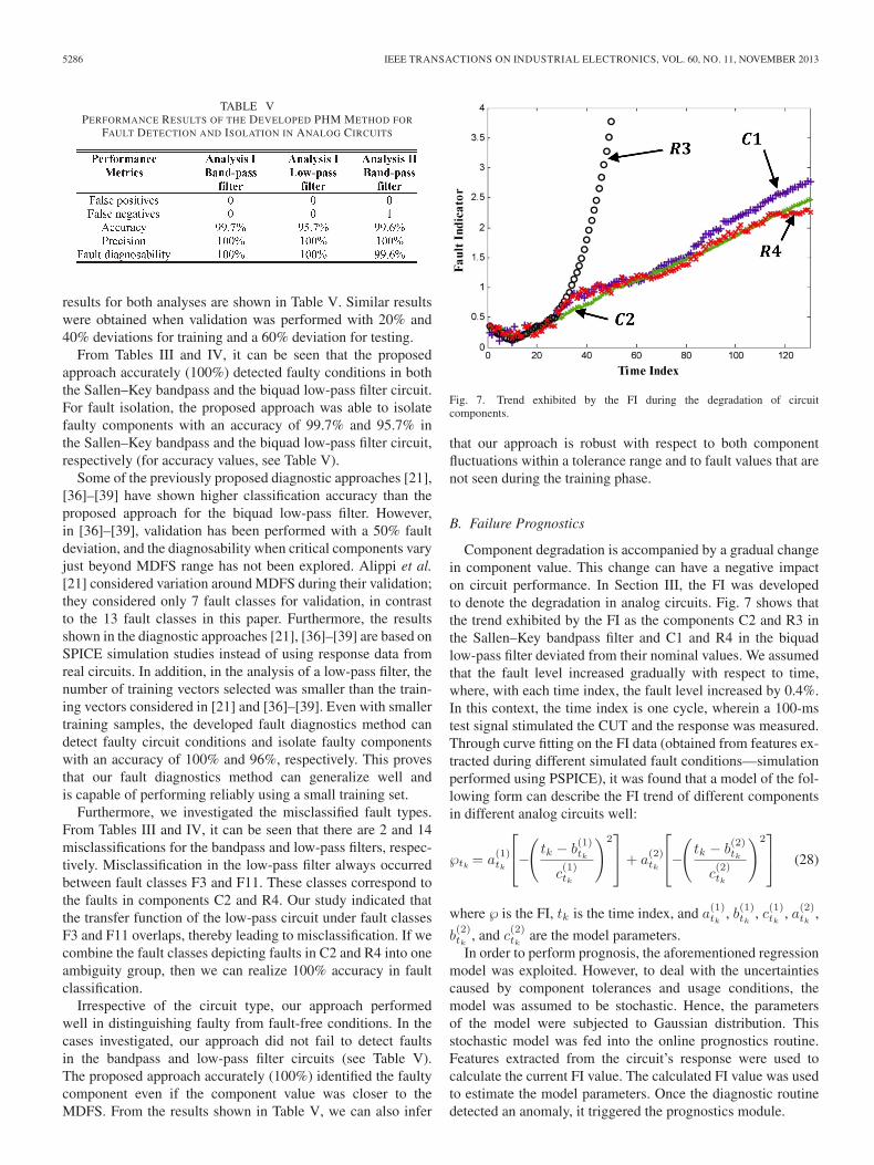
Fig. 7. Trend exhibited by the FI during the degradation of circuitcomponents.

that our approach is robust with respect to both componentfluctuations within a tolerance range and to fault values that arenot seen during the training phase.

B. Failure Prognostics

Component degradation is accompanied by a gradual changein component value. This change can have a negative impacton circuit performance. In Section III, the FI was developedto denote the degradation in analog circuits. Fig. 7 shows thatthe trend exhibited by the FI as the components C2 and R3 inthe Sallen–Key bandpass filter and C1 and R4 in the biquadlow-pass filter deviated from their nominal values. We assumedthat the fault level increased gradually with respect to time,where, with each time index, the fault level increased by 0.4%.In this context, the time index is one cycle, wherein a 100-mstest signal stimulated the CUT and the response was measured.Through curve fitting on the FI data (obtained from features ex-tracted during different simulated fault conditions—simulationperformed using PSPICE), it was found that a model of the fol-lowing form can describe the FI trend of different componentsin different analog circuits well:

℘tk = a(1)tk

⎡⎣−

(tk − b

(1)tk

c(1)tk

)2⎤⎦+ a

(2)tk

⎡⎣−

(tk − b

(2)tk

c(2)tk

)2⎤⎦ (28)

where ℘ is the FI, tk is the time index, and a(1)tk

, b(1)tk, c(1)tk

, a(2)tk,

b(2)tk

, and c(2)tk

are the model parameters.In order to perform prognosis, the aforementioned regression

model was exploited. However, to deal with the uncertaintiescaused by component tolerances and usage conditions, themodel was assumed to be stochastic. Hence, the parametersof the model were subjected to Gaussian distribution. Thisstochastic model was fed into the online prognostics routine.Features extracted from the circuit’s response were used tocalculate the current FI value. The calculated FI value was usedto estimate the model parameters. Once the diagnostic routinedetected an anomaly, it triggered the prognostics module.

SAI SARATHI VASAN et al.: DIAGNOSTICS AND PROGNOSTICS METHOD FOR ANALOG ELECTRONIC CIRCUITS 5287

The model parameters were incorporated as the elements of astate vector. Random walk was employed to estimate the modelparameters

a(1)tk

= a(1)tk−1

+ ω1,k; ω1,k ∼ N(0, σ1)

b(1)tk

= b(1)tk−1

+ ω2,k; ω2,k ∼ N(0, σ2)

c(1)tk

= c(1)tk−1

+ ω3,k; ω3,k ∼ N(0, σ3)

a(2)tk

= a(2)tk−1

+ ω4,k; ω4,k ∼ N(0, σ4)

b(2)tk

= b(2)tk−1

+ ω5,k; ω5,k ∼ N(0, σ5)

c(3)tk

= c(3)tk−1

+ ω6,k; ω6,k ∼ N(0, σ6)

℘tk = a(1)tk

⎡⎣−

(tk − b

(1)tk

c(1)tk

)2⎤⎦+ a

(2)tk

⎡⎣−

(tk − b

(2)tk

c(2)tk

)2⎤⎦

+ εk; ε ∼ N(0, σε) (29)

where ℘tk is the measured value of the FI variable at time indextk and N(0, σ) is a Gaussian distribution with mean zero andstandard deviation σ. Using the PF, the future values of FI arecalculated. The RUP was calculated based on the time index atwhich the predicted FI value crosses the failure threshold. Inthis demonstration, we found that, by the time that the FI valuereaches a value of 2, the fault level for most of the componentshas crossed 40%. Hence, in this paper, we chose a value of 2 forthe FI as the failure threshold. A threshold value of 2 for the FIis a qualitative threshold. In the future, a method to establish afailure threshold needs to be developed. Also, the initial valuesof the model parameters (obtained from curve fitting) and theirstandard deviations were assumed to be known for the sake ofsimplicity. In practice, an efficient method needs to be devisedto choose these values for the model parameters.

The results for fault progression in component C2 of theSallen–Key bandpass filter circuit are shown in Fig. 8. Fig. 8(a)shows the RUP estimation at the time instant that an anomalywas detected (i.e., ℘ > 0.5). This occurred at time index 31.Thus, the data from the first 31 time indices alone are used toupdate the model. The estimated RUP is 73; thus, the predictedend of life (EOL) is 104, and the actual failure occurs at the106th time index. In Fig. 8(b), the prognostics results performedat time index 70 are shown. The predicted EOL is the 105thtime index. Thus, the error in prediction is only 1. Also, theprediction pdf becomes narrower as we get closer to the failuretime, indicating the improvement in prediction confidence.Fig. 8(c) shows the RUP estimates at different time indices with95% confidence bounds.

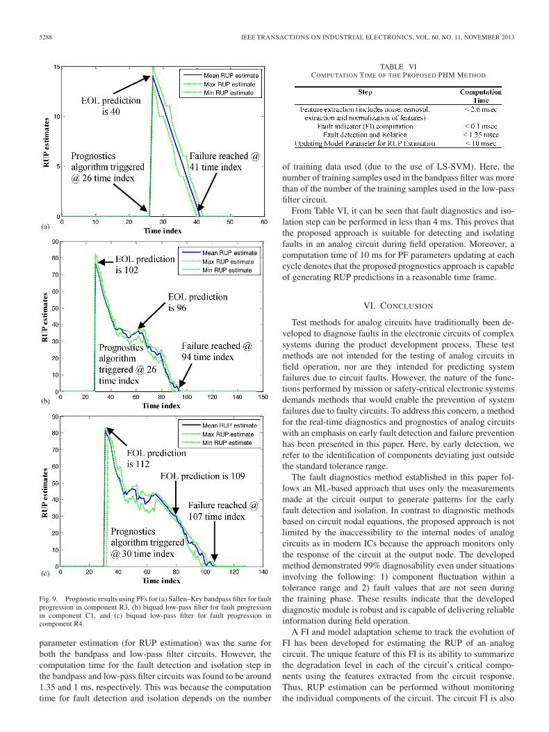
In order to show the applicability of the proposed approachfor different components and circuits, the RUP estimation atdifferent time indices for the component R3 in the Sallen–Keybandpass filter circuit and the components C1 and R4 in thebiquad low-pass filter circuit is shown in Fig. 9.

C. Computation Time

The computation time involved for the developed PHMmethod was investigated so as to analyze its applicability to

Fig. 8. Prognostics results using PFs for the Sallen–Key bandpass filter forfault progression in component C2. (a) Prediction result at time index 31.(b) Prediction result at time index 70. (c) RUL estimation at every time index.

circuits in field operation. Table VI shows the computation timeinvolved in the individual steps of the proposed PHM frame-work. The computation time was computed on a MATLAB2010 environment which was run on an Intel Core 2 Duo E75002.93-GHz processor with 2-GB RAM.

In the case study, it was found that the computation timeinvolved in feature extraction, FI calculation, and model

5288 IEEE TRANSACTIONS ON INDUSTRIAL ELECTRONICS, VOL. 60, NO. 11, NOVEMBER 2013

Fig. 9. Prognostic results using PFs for (a) Sallen–Key bandpass filter for faultprogression in component R3, (b) biquad low-pass filter for fault progressionin component C1, and (c) biquad low-pass filter for fault progression incomponent R4.

parameter estimation (for RUP estimation) was the same forboth the bandpass and low-pass filter circuits. However, thecomputation time for the fault detection and isolation step inthe bandpass and low-pass filter circuits was found to be around1.35 and 1 ms, respectively. This was because the computationtime for fault detection and isolation depends on the number

TABLE VICOMPUTATION TIME OF THE PROPOSED PHM METHOD

of training data used (due to the use of LS-SVM). Here, thenumber of training samples used in the bandpass filter was morethan of the number of the training samples used in the low-passfilter circuit.

From Table VI, it can be seen that fault diagnostics and iso-lation step can be performed in less than 4 ms. This proves thatthe proposed approach is suitable for detecting and isolatingfaults in an analog circuit during field operation. Moreover, acomputation time of 10 ms for PF parameters updating at eachcycle denotes that the proposed prognostics approach is capableof generating RUP predictions in a reasonable time frame.

VI. CONCLUSION

Test methods for analog circuits have traditionally been de-veloped to diagnose faults in the electronic circuits of complexsystems during the product development process. These testmethods are not intended for the testing of analog circuits infield operation, nor are they intended for predicting systemfailures due to circuit faults. However, the nature of the func-tions performed by mission or safety-critical electronic systemsdemands methods that would enable the prevention of systemfailures due to faulty circuits. To address this concern, a methodfor the real-time diagnostics and prognostics of analog circuitswith an emphasis on early fault detection and failure preventionhas been presented in this paper. Here, by early detection, werefer to the identification of components deviating just outsidethe standard tolerance range.

The fault diagnostics method established in this paper fol-lows an ML-based approach that uses only the measurementsmade at the circuit output to generate patterns for the earlyfault detection and isolation. In contrast to diagnostic methodsbased on circuit nodal equations, the proposed approach is notlimited by the inaccessibility to the internal nodes of analogcircuits as in modern ICs because the approach monitors onlythe response of the circuit at the output node. The developedmethod demonstrated 99% diagnosability even under situationsinvolving the following: 1) component fluctuation within atolerance range and 2) fault values that are not seen duringthe training phase. These results indicate that the developeddiagnostic module is robust and is capable of delivering reliableinformation during field operation.

A FI and model adaptation scheme to track the evolution ofFI has been developed for estimating the RUP of an analogcircuit. The unique feature of this FI is its ability to summarizethe degradation level in each of the circuit’s critical compo-nents using the features extracted from the circuit response.Thus, RUP estimation can be performed without monitoringthe individual components of the circuit. The circuit FI is also

SAI SARATHI VASAN et al.: DIAGNOSTICS AND PROGNOSTICS METHOD FOR ANALOG ELECTRONIC CIRCUITS 5289

compatible with future changes in the extracted features. Thus,even if new features (for circuit fault diagnosis) are introducedin the future, RUP estimates can still be obtained using thecircuit FI developed in this paper.

The challenges in estimating the RUP of an analog circuit arethe presence of uncertainties that are introduced by componenttolerances and the time-varying nature of the environment. Toaddress this challenge, we have developed a model adaptivestatistical approach for providing real-time predictions of thecircuit’s RUP. RUP estimates are given in the form of prob-ability distributions, indicating the confidence levels in theprediction. Preventive maintenance actions can be performedusing the estimated RUP information for avoiding unexpectedsystem failures due to faults in circuits.

ACKNOWLEDGMENT

The authors would like to thank the more than 100 companiesthat support research activities at the Center for Advanced LifeCycle Engineering, University of Maryland, annually.

REFERENCES

[1] G. Escobar, P. R. Matinez, and J. Leyva-Ramos, “Analog circuits toimplement repetitive controllers with feedforward for harmonic com-pensation,” IEEE Trans. Ind. Electron., vol. 54, no. 1, pp. 567–573,Feb. 2007.

[2] O. Vainio and S. J. Ovaska, “A class of predictive analog filters forsensor signal processing and control instrumentation,” IEEE Trans. Ind.Electron., vol. 44, no. 4, pp. 565–570, Aug. 1997.

[3] S. Ostroznik, P. Bajec, and P. Zajec, “A study of a hybrid filter,” IEEETrans. Ind. Electron., vol. 57, no. 3, pp. 935–942, Mar. 2010.

[4] B. Singh, K. Al-Haddad, and A. Chandra, “A review of active filters forpower quality improvement,” IEEE Trans. Ind. Electron., vol. 46, no. 5,pp. 960–971, Oct. 1999.

[5] K. Wagner and T. Williams, “Design for testability of analog/digitalnetworks,” IEEE Trans. Ind. Electron., vol. 36, no. 2, pp. 227–230,May 1989.

[6] M. Pecht and R. Jaai, “A prognostics and health management roadmap forinformation and electronics-rich systems,” Microelectron. Reliab., vol. 50,no. 3, pp. 317–323, Mar. 2010.

[7] J. Sikorska, M. Hodkiewicz, and L. Ma, “Prognostic modeling options forremaining useful life estimation by industry,” Mech. Syst. Signal Process.,vol. 25, no. 5, pp. 1803–1836, Jul. 2011.

[8] J. Bandler, “Fault diagnosis of analog circuits,” Proc. IEEE, vol. 73, no. 8,pp. 1279–1325, Aug. 1985.

[9] Y.-M. Chen, H.-C. Wu, M.-W. Chou, and K.-Y. Lee, “Online failureprediction of electrolytic capacitors for LC filter of switching-mode powerconverters,” IEEE Trans. Ind. Electron., vol. 55, no. 1, pp. 400–406,Jan. 2008.

[10] D. Brown, P. Kalgren, C. Byington, and M. Roemer, “Electronicprognostics—A case study using Global Positioning System (GPS),”Microelectron. Reliab., vol. 47, no. 12, pp. 1874–1881, Dec. 2007.

[11] P. Lall, C. Bhat, M. Hande, V. More, R. Vaidya, and K. Goebel, “Prog-nostication of residual life and latent damage assessment in lead-freeelectronics under thermomechanical loads,” IEEE Trans. Ind. Electron.,vol. 58, no. 7, pp. 2605–2616, Jul. 2011.

[12] M. A. Alam, M. H. Azarian, M. Osterman, and M. Pecht, “Prognostics offailures in embedded planar capacitors using model-based and data-drivenapproaches,” J. Intell. Mater. Syst. Struct., vol. 22, no. 12, pp. 1293–1304,Aug. 2011.

[13] D. Kwon, M. Azarian, and M. Pecht, “Prognostics of interconnect degra-dation using RF impedance monitoring and sequential probability ratiotest,” Int. J. Perform. Eng., vol. 6, no. 5, pp. 443–452, Sep. 2010.

[14] W. Wang and M. Pecht, “Economic analysis of canary-based prognosticsand health management,” IEEE Trans. Ind. Electron., vol. 58, no. 7,pp. 3077–3089, Jul. 2011.

[15] C. Chen, B. Zhang, G. Vachtsevanos, and M. Orchard, “Machine con-dition prediction based on adaptive neuro-fuzzy and high-order particle

filtering,” IEEE Trans. Ind. Electron., vol. 58, no. 9, pp. 4353–4364,Sep. 2011.

[16] O. F. Eker, F. Camci, A. Guclu, H. Yilboga, M. Sevkli, and S. Baskan,“A simple state-based prognostic model for railway turnout systems,”IEEE Trans. Ind. Electron., vol. 58, no. 5, pp. 1718–1726, May 2011.

[17] E. G. Strangas, S. Aviyente, and S. S. H. Zaidi, “Time-frequencyanalysis for efficient fault diagnosis and failure prognosis for interiorpermanent—Magnet ac motors,” IEEE Trans. Ind. Electron., vol. 55,no. 12, pp. 4191–4199, Dec. 2008.

[18] Y. Xiong, X. Cheng, Z. J. Shen, C. Mi, H. Wu, and V. K. Garg, “Prognos-tic and warning system for power-electronic modules in electric, hybridelectric, and fuel-cell vehicles,” IEEE Trans. Ind. Electron., vol. 55, no. 6,pp. 2268–2276, Jun.. 2008.

[19] S. S. H. Zaidi, S. Aviyente, M. Salman, K.-K. Shin, and E. G. Strangas,“Prognosis of gear failures in dc starter motors using hidden Markovmodels,” IEEE Trans. Ind. Electron., vol. 58, no. 5, pp. 1695–1706,May 2011.

[20] A. Vasan, B. Long, and M. Pecht, “Experimental validation of LS-SVMbased fault identification in analog circuits using frequency features,” inProc. 6th Annu. Conf. World Congr. Eng. Asset Manage., Cincinnati, OH,Oct. 2011, pp. 1–6.

[21] C. Alippi, M. Catelani, and M. Mugnaini, “SBT soft fault diagnosis inanalog electronic circuits: A sensitivity-based approach for randomizedalgorithms,” IEEE Trans. Instrum. Meas., vol. 51, no. 5, pp. 1116–1125,Oct. 2002.

[22] C. Yang, S. Tian, B. Long, and F. Chen, “Methods of handling the toler-ance and test-point selection problem for analog-circuit fault diagnosis,”IEEE Trans. Instrum. Meas., vol. 60, no. 1, pp. 176–185, Jan. 2011.

[23] M. Catelani and A. Fort, “Soft fault detection and isolation in analogcircuits: Some results and a comparison between a fuzzy approach andradial basis function networks,” IEEE Trans. Instrum. Meas., vol. 51,no. 2, pp. 196–202, Apr. 2002.

[24] J. A. Starzyk and J. W. Bandler, “Multiport approach to multiple-faultlocation in analog circuits,” IEEE Trans. Circuits Syst, vol. CAS-30,no. 10, pp. 762–765, Oct. 1983.

[25] G. Fedi, R. Giomi, A. Luchetta, S. Manetti, and M. C. Piccirilli, “On theapplication of symbolic techniques to the multiple fault location in lowtestability analog circuits,” IEEE Trans. Circuits Syst. II, Analog Digit.Signal Process., vol. 45, no. 10, pp. 1383–1388, Oct. 1998.

[26] W. Toczek, R. Zielonko, and A. Adamczyk, “A method for fault diagnosisof nonlinear electronic circuits,” Measurement, vol. 24, no. 2, pp. 79–86,Sep. 1998.

[27] J. Starzyk, J. Pang, S. Manetti, M. Piccirilli, and G. Fedi, “Finding ambi-guity groups in low testability analog circuits,” IEEE Trans. Circuits Syst.I, Fundam. Theory Appl., vol. 47, no. 8, pp. 1125–1137, Aug. 2000.

[28] M. Tadeusiewicz, S. Halgas, and M. Korzybski, “An algorithm forsoft-fault diagnosis of linear and nonlinear circuits,” IEEE Trans. Cir-cuits Syst. I, Fundam. Theory Appl., vol. 49, no. 11, pp. 1648–1653,Nov. 2002.

[29] D. Liu and J. A. Starzyk, “A generalized fault diagnosis method indynamic analog circuits,” Int. J. Circuit Theory Appl., vol. 30, no. 5,pp. 487–510, Sep./Oct. 2002.

[30] B. Cannas, A. Fanni, and A. Montisci, “Algebraic approach to ambiguity-group determination in nonlinear analog circuits,” IEEE Trans. CircuitsSyst. I, Reg. Papers, vol. 57, no. 2, pp. 438–447, Feb. 2010.

[31] L. Zhou, Y. Shi, G. Zhao, W. Zhang, H. Tang, and L. Su, “Soft-fault diag-nosis of analog circuit with tolerance using mathematical programming,”J. Commun. Comput., vol. 7, no. 5, pp. 50–59, May 2010.

[32] M. Hu, H. Wang, G. Hu, and S. Yang, “Soft fault diagnosis for analogcircuits based on slope fault feature and BP neural networks,” TsinghuaSci. Technol., vol. 12, no. S1, pp. 26–31, Jul. 2007.

[33] S. Halgas, “Multiple soft fault diagnosis of nonlinear circuits using thefault dictionary approach,” Bull. Pol. Acad. Sci., vol. 56, no. 1, pp. 53–57,Mar. 2008.

[34] J. Cui and Y. Wang, “A novel approach of analog circuit fault diagnosisusing support vector machines classifier,” Measurement, vol. 44, no. 1,pp. 281–289, Jan. 2011.

[35] R. Spina and S. Upadhyaya, “Linear circuit fault diagnosis using neuro-morphic analyzers,” IEEE Trans. Circuits Syst. II, Analog Digit. SignalProcess., vol. 44, no. 3, pp. 188–196, Mar. 1997.

[36] M. Aminian and F. Aminian, “Neural-network based analog-circuit faultdiagnosis using wavelet transform as preprocessor,” IEEE Trans. CircuitsSyst. II, Analog Digit. Signal Process., vol. 47, no. 2, pp. 151–156,Feb. 2000.

[37] F. Aminian and M. Aminian, “Analog fault diagnosis of actual circuitsusing neural networks,” IEEE Trans. Instrum. Meas., vol. 51, no. 3,pp. 544–550, Jun. 2002.

5290 IEEE TRANSACTIONS ON INDUSTRIAL ELECTRONICS, VOL. 60, NO. 11, NOVEMBER 2013

[38] M. Aminian and F. Aminian, “A modular fault-diagnostic system foranalog electronic circuits using neural networks with wavelet transformas a preprocessor,” IEEE Trans. Instrum. Meas., vol. 56, no. 5, pp. 1546–1554, Oct. 2007.

[39] L. Yuan, Y. He, J. Huang, and Y. Sun, “A new neural-network-based faultdiagnosis approach for analog circuits by using kurtosis and entropy as apreprocessor,” IEEE Trans. Instrum. Meas., vol. 59, no. 3, pp. 586–595,Mar. 2010.

[40] Y. Xiao and Y. He, “A novel approach for analog fault diagnosis basedon neural networks and improved kernel PCA,” Neurocomputing, vol. 74,no. 7, pp. 1102–1115, Mar. 2011.

[41] Y. Xiao and L. Feng, “A novel neural-network approach of ana-log fault diagnosis based on kernel discriminant analysis and particleswarm optimization,” Appl. Soft Comput., vol. 12, no. 2, pp. 904–920,Feb. 2012.

[42] Y. He, Y. Tan, and Y. Sun, “Wavelet neural network approach for faultdiagnosis of analogue circuits,” Proc. Inst. Elect. Eng.—Circuits DevicesSyst., vol. 151, no. 4, pp. 379–384, Aug. 2004.

[43] Y. He and Y. Sun, “Neural network-based L1-norm optimization ap-proach for fault diagnosis of nonlinear circuits with tolerance,” Proc.Inst. Elect. Eng.—Circuits Devices Syst., vol. 148, no. 4, pp. 223–228,Aug. 2001.

[44] J. Huang, X. Hu, and F. Yang, “Support vector machine with geneticalgorithm for machinery fault diagnosis of high voltage circuit breaker,”Measurement, vol. 44, no. 6, pp. 1018–1027, Jul. 2011.

[45] B. Long, J. Huang, and S. Tian, “Least squares support vector ma-chine based analog-circuit fault diagnosis using wavelet transform aspreprocessors,” in Proc. Int. Conf. Commun., Circuits Syst., 2008,pp. 1026–1029.

[46] A. Birolini, Quality and Reliability of Technical Systems. New York:Springer-Verlag, 1997.

[47] B. Long, S. L. Tian, Q. Miao, and M. Pecht, “Research on features fordiagnostics of filtered analog circuits based on LS-SVM,” in Proc. IEEEAUTOTESTCON, 2011, pp. 360–366.

[48] B. Long, S. Tian, and H. Wang, “Diagnostics of filtered analog circuitswith tolerance based on LS-SVM using frequency features,” J. Electron.Test.: Theory Appl., vol. 28, no. 3, pp. 291–300, Jun. 2012.

[49] P. Pedersen, “Digital generation of coherent sweep signals,” IEEE Trans.Instrum. Meas., vol. 39, no. 1, pp. 90–95, Feb. 1990.

[50] A. A. Hiasat, “New digital sweep oscillator structures,” Proc. Inst. Elect.Eng.—Circuits Devices Syst., vol. 150, no. 3, pp. 179–184, Jun. 2003.

[51] O. Rioul and M. Vetterli, “Wavelets and signal processing,” IEEE SignalProcess. Mag., vol. 8, no. 4, pp. 14–38, Oct. 1991.

[52] O. Rioul, “A discrete-time multiresolution theory,” IEEE Trans. SignalProcess., vol. 41, no. 8, pp. 2591–2606, Aug. 1993.

[53] I. M. Johnstone and B. W. Silverman, “Wavelet threshold estimators fordata with correlated noise,” J. Roy. Stat. Soc., B, vol. 59, no. 2, pp. 319–351, 1997.

[54] A. C. To, J. R. Moore, and S. D. Glaser, “Wavelet denoising techniqueswith applications to experimental geophysical data,” Signal Process.,vol. 89, no. 2, pp. 144–160, Feb. 2009.

[55] R. Yang and M. Ren, “Wavelet denoising using principal componentanalysis,” Expert Syst. Appl., vol. 38, no. 1, pp. 1073–1076, Jan. 2011.

[56] S. Mallat, “A theory for multiresolution signal decomposition: Thewavelet representation,” IEEE Trans. Pattern Anal. Mach. Intell., vol. 11,no. 7, pp. 674–693, Jul. 1989.

[57] L. DeCarlo, “On the meaning and use of kurtosis,” Psychol. Methods,vol. 2, no. 3, pp. 292–307, Sep. 1997.

[58] C. Shannon, “A mathematical theory of communication,” Bell Syst. Tech.J., vol. 27, no. 3, pp. 379–423, Jul. 1948.

[59] J.-F. Bercher and C. Vignat, “Estimating the entropy of a signal withapplications,” IEEE Trans. Signal Process., vol. 48, no. 6, pp. 1687–1694,Jun. 2000.

[60] R. Duda, P. Hart, and D. Stork, Pattern Classification. New York: Wiley,2001.

[61] N. Patil, J. Celaya, D. Das, K. Goebel, and M. Pecht, “Precursor param-eter identification for insulated gate bipolar transistor prognostics,” IEEETrans. Rel., vol. 58, no. 2, pp. 271–276, Jun. 2009.

[62] G. Taguchi and R. Jugulum, The Mahalanobis-Taguchi Strategy. NewYork: Wiley, 2002.

[63] A. Soylemezoglu, S. Jagnnathan, and C. Saygin, “Mahalanobis Taguchisystem as a prognostic tool for rolling element bearing failures,” J. Manuf.Sci. Eng., vol. 132, no. 5, pp. 051014–1–051014–12, Oct. 2010.

[64] V. Vapnik, “An overview of statistical learning theory,” IEEE Trans. Neu-ral Netw., vol. 10, no. 5, pp. 988–999, Oct. 1999.

[65] J. Suykens and J. Vandewalle, “Least squares support vector machineclassifiers,” Neural Process. Lett., vol. 9, no. 3, pp. 293–300, Jun. 2000.

[66] J. Suykens and J. Vandewalle, “Recurrent least squares support vectormachines,” IEEE Trans. Circuits Syst. I, Fundam. Theory Appl., vol. 47,no. 7, pp. 1109–1114, Jul. 2000.

[67] V. Vapnik, Statistical Learning Theory. New York: Wiley, 1998.[68] J. Platt, N. Cristianini, and J. S. Taylor, “Large margin DAGs for mul-

ticlass classification,” in Advances in Neural Information ProcessingSystems, vol. 12. Cambridge, MA: MIT Press, 2000, pp. 547–553.

[69] C.-W. Hsu and C.-J. Lin, “A comparison of methods for multiclass supportvector machines,” IEEE Trans. Neural Netw., vol. 13, no. 2, pp. 415–425,Mar. 2002.

[70] D. Tsujinishi and S. Abe, “Fuzzy least squares support vector machinesfor multiclass problems,” Neural Netw., vol. 16, no. 5/6, pp. 785–792,Jun. 2003.

[71] M. Pecht, Prognostics and Health Management of Electronics. NewYork: Wiley, 2008.

[72] G. Vachtsevanos, F. Lewis, M. Roemer, A. Hess, and B. Wu, IntelligentFault Diagnosis and Prognosis for Engineering Systems. Hoboken, NJ:Wiley, 2006.

[73] C. Chen, G. Vachtsevanos, and M. Orchard, “Machine remaining usefullife prediction: An integrated adaptive neuro-fuzzy and high-order particlefiltering approach,” Mech. Syst. Signal Process., vol. 28, pp. 597–607,Apr. 2012.

[74] M. Orchard and G. Vachtsevanos, “A particle-filtering approach foron-line fault diagnosis,” Trans. Inst. Meas. Control, vol. 31, no. 3/4,pp. 221–246, Jun.–Aug. 2009.

[75] M. Arulampalam, S. Maskell, N. Gordon, and T. Clapp, “A tutorial onparticle filters for online/non-Gaussian Bayesian tracking,” IEEE Trans.Signal Process., vol. 50, no. 2, pp. 174–188, Feb. 2002.

Arvind Sai Sarathi Vasan (M’12) received theB.E. degree in electronics and communication en-gineering from Sri Sivasubramaniya Nadar (SSN)Institutions, Chennai, India. He is currently workingtoward the Ph.D. degree in mechanical engineeringin the Center for Advanced Life Cycle Engineering,University of Maryland, College Park.

From October 2011 to September 2012, he servedas the student chair for the Prognostics and HealthManagement (PHM) society. In 2011, he was oneamong the ten graduate students to have been se-

lected for the PHM society doctoral consortium. He was a part of the team thatwon the 2012 IEEE PHM data challenge contest. He is currently involved in thedevelopment of the IEEE standard P1856 for the PHM of electronic systems.His main areas of interest include the prognostics of electronics, diagnostics,and machine learning.

Bing Long was born in Chengdu, China, in July1974. He received the Ph.D. degree in aerospacescience from the Harbin Institute of Technology,Harbin, China, in 2005.

He is currently an Associate Professor withthe School of Automation Engineering, Universityof Electronic Science and Technology of China,Chengdu. His research interests include the testabil-ity analysis and fault diagnosis of electronic devicesystem.

SAI SARATHI VASAN et al.: DIAGNOSTICS AND PROGNOSTICS METHOD FOR ANALOG ELECTRONIC CIRCUITS 5291

Michael Pecht (M’83–SM’90–F’92) received theM.S. and Ph.D. degrees in engineering mechanicsfrom the University of Wisconsin, Madison.

He is the Founder of the Center for AdvancedLife Cycle Engineering, University of Maryland,College Park, which is funded by over 150 of theworld’s leading electronics companies at more thanU.S. $6 million/year. He is also a Chair Professor inmechanical engineering and a Professor in appliedmathematics with the University of Maryland. Heis the Chief Editor for Microelectronics Reliability.

He has written more than 20 books on electronic product development, use,and supply chain management and over 500 technical articles. He consults for22 major international electronics companies, providing expertise in strategicplanning, design, test, prognostics, IP, and risk assessment of electronic prod-ucts and systems.

Dr. Pecht is a Professional Engineer, an American Society of Me-chanical Engineers (ASME) Fellow, a Society of Automotive Engineers(SAE) Fellow, and an International Microelectronics and Packaging Society(IMAPS) Fellow. Prior to 2008, he was the recipient of European Microand Nano-Reliability Award for outstanding contributions to reliability re-search, the 3M Research Award for electronics packaging, and the IMAPSWilliam D. Ashman Memorial Achievement Award for his contributions inelectronics reliability analysis. In 2008, he was the recipient of the highestreliability honor, the IEEE Reliability Society’s Lifetime Achievement Award.In 2010, he was the recipient of the IEEE Exceptional Technical AchievementAward. He served as a Chief Editor of the IEEE TRANSACTIONS ON RELI-ABILITY for eight years and on the Advisory Board of IEEE Spectrum. Heis an Associate Editor for the IEEE TRANSACTIONS ON COMPONENTS AND

PACKAGING TECHNOLOGY.