DIAGNOSTIC TESTING AND EVALUATION OF MAXIMUM …

Journal of Econometrics 30 (1985) 415-443. North-Holland

DIAGNOSTIC TESTING AND EVALUATION OF MAXIMUM LIKELIHOOD MODELS*

George TAUCHEN

Duke University, Durham, NC 27706, USA

The paper develops a unified theory of maximum likelihood specification testing based on M-estimators of auxiliary parameters. The theory is sufficiently general to encompass a wide class of specification tests including moment-based tests, Pearson-type goodness of fit tests, the information matrix test, and the Cox test. The paper also presents a framework based on Frechet differentiation for determining the effects of misspecification on the almost sure limits of parameter estimates and specification test statistics.

1. Introduction

This paper develops the asymptotic distribution theory for a class of specification tests for the non-linear maximum likelihood model. The ideas that motivate consideration of this class of specification tests have their origins in Hausman’s (1978) paper. Hausman suggested that in general, i.e., not only for the ML model, a useful specification test can be based upon the difference between two estimates of the vector of parameters of interest. This idea, however, is somewhat difficult to apply in a multivariate context when the likelihood function depends upon the parameters in a highly non-linear fashion. The difficulty lies in finding a computationally tractable form for the second ‘specification-robust’ estimate of the parameter vector that is required to implement Hausman’s test. White (1982) suggests a different but related approach. Specifically, White derives a test that is based not upon difference between two estimates of the parameters of direct interest, but instead is based upon the difference between the two natural estimates of the expected informa- tion matrix. This paper extends White’s work further by deriving the asymp- totic properties of an entire class of specification tests that includes as a special case the information matrix test, and other specification tests, e.g., the Cox test [Aguirre-Torres and Gallant (1983)] and the Lagrange multiplier test [Engle

*Helpful comments were obtained from Ronald Gallant, James Heckman, James Mackinnon, Richard Robb, Robin Sickles, Donald Waldman, Dudley Wallace. Adonis Yatchew, and two referees. Earlier versions of this paper were presented at seminars at the University of Chicago, the University of Pennsylvania, Queen’s University, the University of Toronto, the Triangle Area Econometrics Seminar, and the 1984 Austin Conference on Model Selection.

0304-4076/85/$3.30~1985, Elsevier Science Publishers B.V. (North-Holland)

416 G. Tauchen, Maximum likelihood specijication tests

(1982)]. The asymptotic theory developed here is sufficiently general to include in the class of allowable tests those that are based upon non-differentiable and even discontinuous functions of the data and the parameter vector. In particu- lar, the class of tests includes Pearson-type goodness of fit tests with random cell boundaries [Moore and Spruill (1975)].

This paper also develops a framework based on Frechet differentiation for characterizing the non-null behavior of these various specification tests. Within this framework, ‘directions’ of r&specification are identified against which the various specification tests can be expected to have maximum or minimum power.

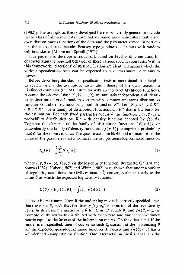
Before describing the class of specification tests in more detail, it is helpful to review briefly the asymptotic distribution theory of the quasi-maximum likelihood estimator (the ML estimator with an incorrect likelihood function). Assume the observed data Y,, Y,, . . . , Y, are mutually independent and identi- cally distributed m X 1 random vectors with common unknown distribution function G and density function g, both defined on R". Let { F(y, 0): y E R"'. 8 E 8 C RP} be a family of distribution functions on R" that is the basis for the estimation. For each fixed parameter vector B the function F(y, 0) is a probability distribution on R" with density function denoted by f(y, 0). Together the elements of the family of distribution functions { F( y, e)}, or

equivalently the family of density functions { f(y, e)}, comprise a probability model for the observed data. The quasi-maximum likelihood estimator 8, is the value of the parameter that maximizes the sample quasi-loglikelihood function

-Ue) = fCcr,e), 1

where 1( y, 0) = log(f( y, 0)) is the log-density function. Burguette, Gallant and Souza (1982) Huber (1967) and White (1982)*have shown that under a variety of regularity conditions the QML estimator 0, converges almost surely to the value 6 at which the expected log-density function,

L(e) = E[ohe)l =/h@dGb), (2)

achieves its maximum. Now, if the underlying model is correctly specified, then there exists a 0, such that the density f(y, 0,) is a version of the true density g(y). In this case the maximizing e for L in (2) equals 0, and fi( 8, - f3,) is asymptotically normally distributed with mean zero and variance-covariance matrix equal to the inverse of the information matrix. On the other hand, if the model is misspecified, then of course no such 6, exists; but the maximizing t? for the expected quasi-loglikelihood function still exists and fi(e,, - 8) has a well-defined asymptotic distribution. One interpretation for 8 is that it is the

‘true’ parameter value that is induced directly by the estimation procedure

itself. The class of specification tests considered in this paper consists of those tests

based on the magnitude of the statistic

(3)

where O,, is the QML estimator and where the vector-valued function c satisfies

/ c(y,B)df'(y,fl)=O, (4)

for all 8. The condition (4) says that the function c( y, 0) has mean zero with respect to each distribution function in the probability model. A function that

satisfies this condition will be called an auxiliary criterion /unction. As will become clearer below, for any given family of distribution functions { F( y, f?)} there are many auxiliary criterion functions. In practice, the better auxiliary criterion functions will be those for which the magnitude of the elements of the vector ?,, in (3) provide useful diagnostic information about the specification of the model. A strategy for getting an informative ?,, is to construct the auxiliary criterion function in such a way that the components of ?,, equal the differences between two estimates of some statistical quantities of interest.

The statistic +, is useful for specification testing because it converges almost surely to zero when the model is correctly specified and it converges to a non-zero quantity when the model is incorrectly specified. This result is proved in section 2, but it is intuitively clear from inspection of the expressions (3) and (4). In the former case when 8, exists,

which is zero by construction of the auxiliary criterion function. In the latter case,

which in general is non-zero. As shown in section 3, the statistic +,, also has a well defined asymptotic distribution in either case. Its asymptotic variance- covariance matrix can be expressed as the sum of two parts, one of which corresponds to the variability in (l/n)Cyc( q, 8) about 7 and the other to the variability in 8, about 8.

418 G. Tuuchen, Maximum likehhood specijicution tests

The following three examples help to illustrate the practical applications of the general results in this paper:

Example I (low-order moments)

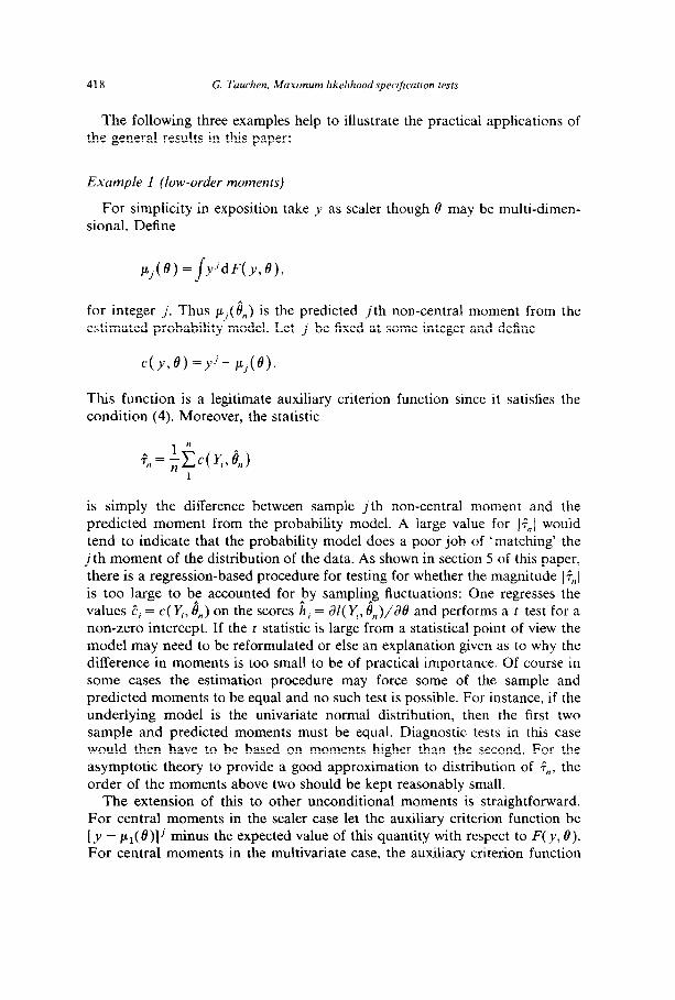
For simplicity in exposition take y as scaler though P may be multi-dimen- sional. Define

for integer j. Thus ~,(8,,) is the predicted jth non-central moment from the estimated probability model. Let j be fixed at some integer and define

This function is a legitimate auxiliary criterion function since it satisfies the condition (4). Moreover, the statistic

is simply the difference between sample jth non-central moment and the predicted moment from the probability model. A large value for ]+,J would tend to indicate that the probability model does a poor job of ‘matching’ the

jth moment of the distribution of the data. As shown in section 5 of this paper, there is a regression-based procedure for testing for whether the magnitude I?,,1 is too large to b$ accounted for by sampling fluctuations: One regresses the values P, = c(Y, 6,) on the scores h, = al( Yi, d,)/afl and performs a t test for a non-zero intercept. If the t statistic is large from a statistical point of view the model may need to be reformulated or else an explanation given as to why the difference in moments is too small to be of practical importance. Of course in some cases the estimation procedure may force some of the sample and predicted moments to be equal and no such test is possible. For instance, if the underlying model is the univariate normal distribution, then the first two sample and predicted moments must be equal. Diagnostic tests in this case would then have to be based on moments higher than the second. For the asymptotic theory to provide a good approximation to distribution of ?,,, the order of the moments above two should be kept reasonably small.

The extension of this to other unconditional moments is straightforward. For central moments in the scaler case let the auxiliary criterion function be [y - pi(e)]’ minus the expected value of this quantity with respect to F( y, 0). For central moments in the multivariate case, the auxiliary criterion function

G. Touchen, Maximum likelihoodspe~ifi~utlott test.s 419

would be the distinct elements of the j-fold Kronecker product of the vector

y - pi( 0) with itself minus the expectation with respect to F( .y, 6). As noted by Newey (1984) in an independent paper, moment conditions can

be used to form useful auxiliary criterion functions when the data vector is partitioned as y’ = (w’, x’) and the probability model is f,( wlx, 8). Here w is a vector of jointly dependent variables and x is a vector of exogenous variables. The marginal density f,(x) for x is not specified by the model. A function of the form

c( w, x, 8) = (&Jogf,(wlx. 6+(X. B),

where a(x, 0) depends only on x and 8, satisfies (4). A test based on this auxiliary criterion function is an ‘instrumented score test’. Newey examines in detail the statistical properties of such tests and presents useful applications for regression models and limited dependent variable models.

Example 2 (tail areas)

In some applied work it is important to have information on how well the probability model predicts tail areas. An auxiliary criterion function that provides such information can be constructed along the following lines. Assume for simplicity in exposition that _r is scalar though 8 may be multi- dimensional. Let p( 0) and a(8) denote the mean and standard deviation of the distribution F( y, 6). Fix (Y as a small probability and let z, satisfy

prob,[y-~(6)La(B)z,] =(x,

where the subscript F is self-explanatory. Now put

where I[ .] is the O-l indicator function. Then the statistic

is the difference between the observed and the predicted frequency with which right-hand extreme values occur.

As illustrated in section 5, an asymptotically valid test for no difference in the frequencies can be computed by regressing the values F, = (Y, 8,) on the ‘scores’, i.e., the gradients Jf(Y,, ~?,,)/a@ of the log-density function, and then performing the usual t test for no intercept. Interestingly, the square of this t

420 G. Tuuchen, Muximum likelihood specijcutron tests

statistic is asymptotically a &i-square variate with one degree of freedom, but the t 2 does not equal the classical Pearson statistic. The reason is that this t ’ statistic properly accounts for the randomness in 6,, where the classical statistic does not. The classical Pearson procedure implicitly assumes that the asymptotic variance is (~(1 - CY) which exceeds the true variance. [When the

model is +(y - CL), where + is the standard normal pdf, then the variance is a(1 - CX) - (p(1z,)2.] Put another way, the classical procedure ignores the ran- domness in O,, and treats (I/n)C~c(~, 8,) as if it has the same asymptotic distribution as (l/n)C;c( Y,, 0,) which is a ‘Durbin’ problem that leads to the incorrect expression for the asymptotic variance.

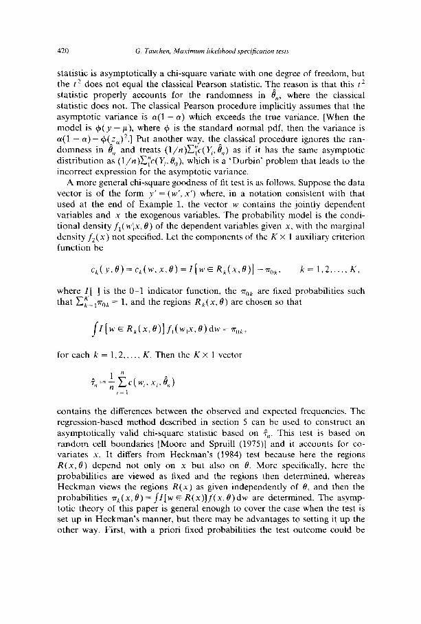
A more general &i-square goodness of fit test is as follows. Suppose the data vector is of the form y’ = (w’, x’) where, in a notation consistent with that used at the end of Example 1, the vector w contains the jointly dependent variables and x the exogenous variables. The probability model is the condi- tional density f,( wlx, 0) of the dependent variables given x, with the marginal density f2( x) not specified. Let the components of the K x 1 auxiliary criterion function be

c,(y,8)=c,(w,x,8)=I[wER~(x,8)] -v()or. k= I,2 ,..., K,

where Z[ ] is the O-l indicator function, the rO’ok are fixed probabilities such

that cc= trO, = 1, and the regions Rk( x, 6) are chosen so that

Jf Z wER,(x,e)]f,(w)x,8)dw=~~,,

for each k = 1,2,. . . , K. Then the K x 1 vector

?n=;-c(w,,x,,8n) r=l

contains the differences between the observed and expected frequencies. The regression-based method described in section 5 can be used to construct an asymptotically valid chi-square statistic based on ?,,. This test is based on random cell boundaries [Moore and Spruill (1975)] and it accounts for co- variates X. It differs from Heckman’s (1984) test because here the regions R(x, 0) depend not only on x but also on 13. More specifically, here the probabilities are viewed as fixed and the regions then determined, whereas Heckman views the regions R(x) as given independently of 0, and then the probabilities T~( x, 6) = ]Z[ w E R( x)]f( x, 8) dw are determined. The asymp- totic theory of this paper is general enough to cover the case when the test is set up in Heckman’s manner, but there may be advantages to setting it up the other way. First, with a priori fixed probabilities the test outcome could be

G. Tuuehen, Maximum likelihood speci&~~tron tests 421

easier to interpret and provide better diagnostic information. Second, with this setup the user can choose the probabilities so that noOk = l/K, i.e., so that the

regions are equiprobable, which is a method that has been shown to have optimum properties [Kendall and Stewart (1973, ch. 30)] in the case with no covariates.

Example 3 (White’s information matrix test)

To include White’s test in this setup, take as the auxiliary criterion function c( y, B) the vector function comprised of the distinct elements of the symmetric matrix function

where h( y, S) = dl( y, 0)/&9 is the gradient of the log-density function. With the function c defined in this fashion the vector

contains all of the differences between the distinct elements of the two natural estimates of the information matrix. White derives an estimator for the asymptotic variance-covariance matrix of this ?,, that requires the user to calculate analytical third-order partial derivatives of the log-density function. In section 3 it is shown that there is an extension of the classical information equality which, as also noted by Chesher (1983) and Lancaster (1984) eliminates the need for third partials and leads to regression based procedures for conducting White’s test.

The remainder of this paper is organized as follows. Sections 2 and 3 present the consistency and asymptotic normality results. Section 4 examines some measures of the performance of the specification tests. Section 5 presents the

regression-based procedure for conducting the specification tests discussed here. Section 6 contains some concluding remarks.

For the sake of completeness, the various assumptions which were either implicit or explicit in this introduction are now listed in one place.

Assumption 1

(9

(ii)

The observed data Y,. Y,, . . _, Y, are iid m X 1 random vectors with distribution function G on Rm.

The probability model is the family of distribution .functions { F( y, 8): y E R”, 13 E 0 c RP}, where the parameter space 0 is a compact convex subset of RP with a non-empty interior.

422

(iii)

(iv)

G. Tauchen, Maximum likelihood specijcation tests

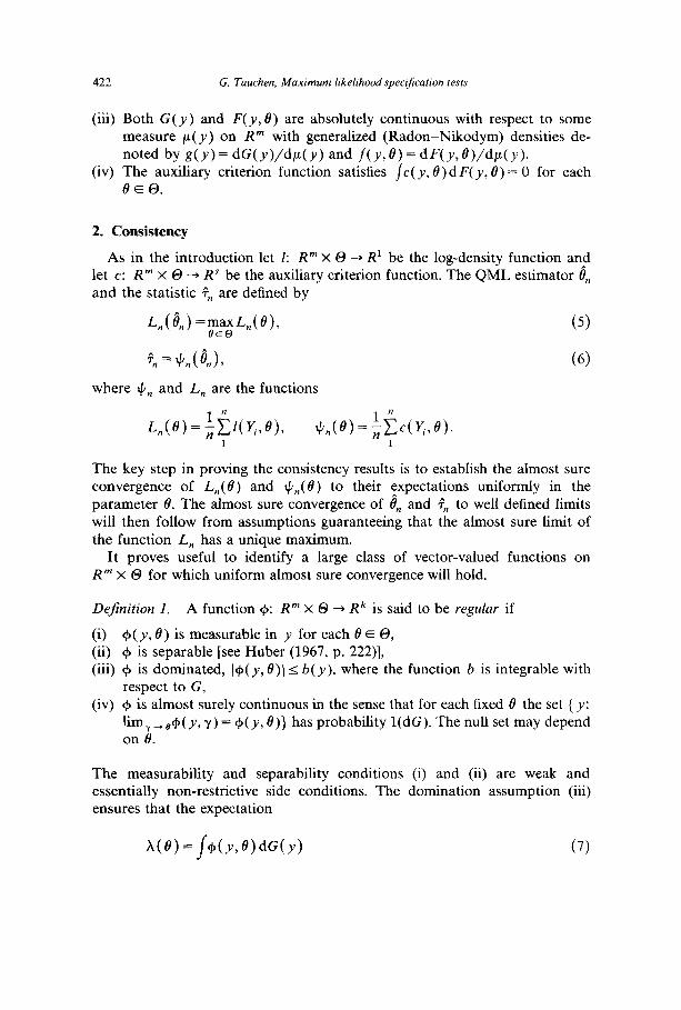
Both G(y) and F( y, 8) are absolutely continuous with respect to some measure p(y) on Rm with generalized (Radon-Nikodym) densities de-

noted by g(y) = dG(y)/dp(y) and f(y, 0) = dF(y, W/dp(y). The auxiliary criterion function satisfies /c( y, 0) dF( y, 0) = 0 for each ee 0.

2. Consistency

As in the introduction let 1: R” X 0 + R ’ be the log-density function and let c: R” X 0 + R” be the auxiliary criterion function. The QML estimator 8, and the statistic +,, are defined by

(9

where 4, and L, are the functions

L,(e)=J&q,e), +,(e) = $L(r;,e). 1 1

The key step in proving the consistency results is to establish the almost sure convergence of L,(B) and #,(e) to their expectations uniformly in the parameter 8. The almost sure convergence of 8, and +” to well defined limits will then follow from assumptions guaranteeing that the almost sure limit of the function L, has a unique maximum.

It proves useful to identify a large class of vector-valued functions on R” x 0 for which uniform almost sure convergence will hold.

Dejinition 1. A function +: R” x 0 + Rk is said to be regular if

(iii)

(iv)

+(y, 0) is measurable in y for each 8 E 0, (p is separable [see Huber (1967, p. 222)], (p is dominated, Ic#J( y, 0)l I b(y), where the function b is integrable with respect to G, + is almost surely continuous in the sense that for each fixed 8 the set { y: lim y _ &( y, y) = $( y, 0)) has probability l(dG). The null set may depend on e.

The measurability and separability conditions (i) and (ii) are weak and essentially non-restrictive side conditions. The domination assumption (iii) ensures that the expectation

x(e) = j-~bJ+Wy) (7)

G. Tuuchen, Maximum likelihood specificatmn tests 423

exists, while the almost sure continuity condition (iv) implies by dominated convergence that A is a continuous function of 8. As the following lemma indicates, sample averages of $( yl, 8) have the requisite convergence properties if C#I is regular.

Lemma I. If 9 is regular, then the function

converges uniformly dmost surely to function h in (7), (Proof: Appendix.)

The next two assumptions contain the conditions for consistency of 8, and n . 7n-

Assumption 2. The auxiliary criterion function c is regular and the log-density function I satisfies (i)-(iii) of Definition 1 and a stronger version of (iv), namely, I( y, C?) is continuous in 8 for all y.

The stronger continuity assumption is needed for the log-density function in order to ensure that the maximizing 0, for L, in (5) exists for all n. The weaker continuity condition for the auxiliary criterion function c suffices

because the existence of 4,, in (6) is guaranteed once the existence of 8, is established.

Define the functions

L(B) = E[f(K, e>] = j-lb, 0) dG(y), (gal

4(e) = E[c@‘P)] =jc(y,+=(y), (8b)

both of which exist and are continuous by Assumption 2. From Lemma 1 it is

known that L,,(B)zL(B) and q,(O)= (l/n)Cyc(y, e)~‘$(O) uniformly in 8.

By continuity and compactness the limiting function L achieves its maximum at least once in the parameter space 0. For the limit of the estimator d,, to be well defined, it is necessary to assume that there is only one such maximum.

Assumption 3. The limiting quasi-loglikelihood function L achieves its maxi- mum uniquely at 8 in the interior of the parameter space.

424 G. Tauchen, Maximum likelihood specijicution tests

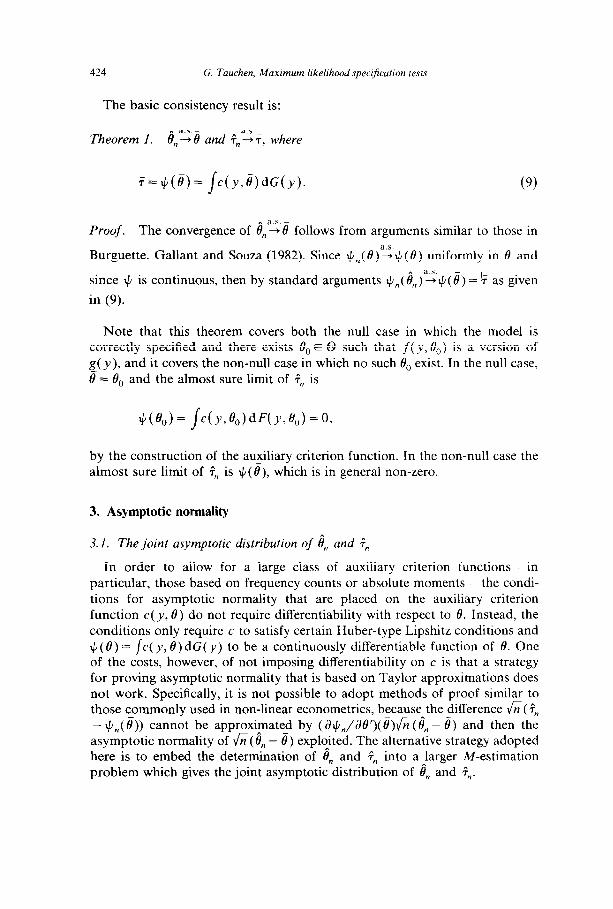
The basic consistency result is:

,. a.s.- Theorem 1. 0, * 0 and F,,‘:?, where

-f=J,@)= /c(y,@dG(y). (9)

n a.s.-

Proof. The convergence of 8,+0 follows from arguments similar to those in a.s.

Burguette, Gallant and Souza (1982). Since qn( 8) --) #( 0) uniformly in 6 and

since J/ is continuous, then by standard arguments #,(r?,)“z#(a) = !F as given

in (9).

Note that this theorem covers both the null case in which the model is correctly specified and there exists 8, E 0 such that f (y, 0,) is a version of g( y ), and it covers the non-null case in which no such 0, exist. In the null case, #= 8, and the almost sure limit of ?, is

by the construction of the auxiliary criterion function. In the non-null case the almost sure limit of +, is It/(e), which is in general non-zero.

3. Asymptotic normality

3.1. The joint asymptotic distribution of 8, and F,,

In order to allow for a large class of auxiliary criterion functions - in particular, those based on frequency counts or absolute moments - the condi- tions for asymptotic normality that are placed on the auxiliary criterion function c( y, 0) do not require differentiability with respect to 8. Instead, the conditions only require c to satisfy certain Huber-type Lipshitz conditions and G(0) = /c( y, 8)dG( y) to be a continuously differentiable function of 8. One of the costs, however, of not imposing differentiability on c is that a strategy for proving asymptotic normality that is based on Taylor approximations does not work. Specifically, it is not possible to adopt methods of proof similar to those commonly used in non-linear econometrics, because the difference 6( ?,, - q,(e)) cannot be approximated by (~3$,/&?‘)(&)fi(6, - 8) and then the asymptotic normality of &( 8, - 3) exploited. The alternative strategy adopted here is to embed the determination of 8, and F,, into a larger M-estimation problem which gives the joint asymptotic distribution of 8, and ?,,.

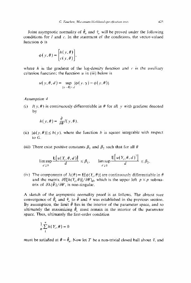
Joint asymptotic normality of 6, and +,, will be proved under the following conditions for I and c. In the statement of the conditions. the vector-valued function $ is

where h is the gradient of the log-density function and C’ is the auxiliary criterion function; the function u in (iii) below is

Assumption 4

(i) I(y, 0) is continuously differentiable in 19 for all y with gradient denoted

by a

h(y,d)= J#(Y,~).

(ii) I+(y, 8)l I b(y), where the function b is square integrable

to G.

(iii) There exist positive constants /?, and & such that for all 8

with respect

(iv) The components of x(e) = E[+( y, 6’)] are continuously differentiable in 8 and the matrix aE[h( y, O)]/aO’jB, which is the upper left p x p subma- trix of ax(@/aef, is non-singular.

A sketch of the asymptotic normality proof is as follows. The almost sure . convergence of 0, and F,, to 8 and 7 was established in the previous section. By assumption, the limit 8 lies in the interior of the parameter space, and so ultimately the maximizing 8, must remain in the interior of the parameter space. Thus, ultimately the first-order condition

$h(r;,B)=O 1

must be satisfied at 8 = 8,. Now let T be a non-trivial closed ball about 7, and

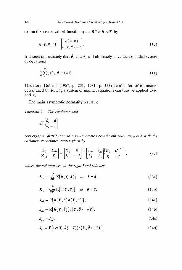
define the vector-valued function TJ on R”’ x 0 x T by

?j(y,tQT)= h(yJ) [ 1 C(Y,d)--7

It is seen immediately that 8,, and ?, will ultimately solve the expanded system of equations

;&r;.e.+o. 1

Therefore Huber’s (1967, p. 231; 1981, p. 133) results for M-estimators determined by solving a system of implicit equations can thus be applied to 8,, and F,,.

The main asymptotic normality result is:

Theorem 2. The random vector

converges in distribution to a multivariate normal with mean zero and with the

variance-covariance matrix given by

where the submatrices on the right-hand side are

a K,= ;ieiE[h(y,O)] at t!l=fl,

Kc= -&E[c(y,O)] at 8 = 8,

Jhh=E[h(Y,,B)h(Y,,8)~],

J,.=E[h(Y,,B)(c(Y,,8)-7)~],

JCh = JLr,

J,.,=E[(c(Y,,i+7)(~(Y,,8)-7)~].

(12)

(134

(13b)

(14a)

(14b)

(14c)

(14d)

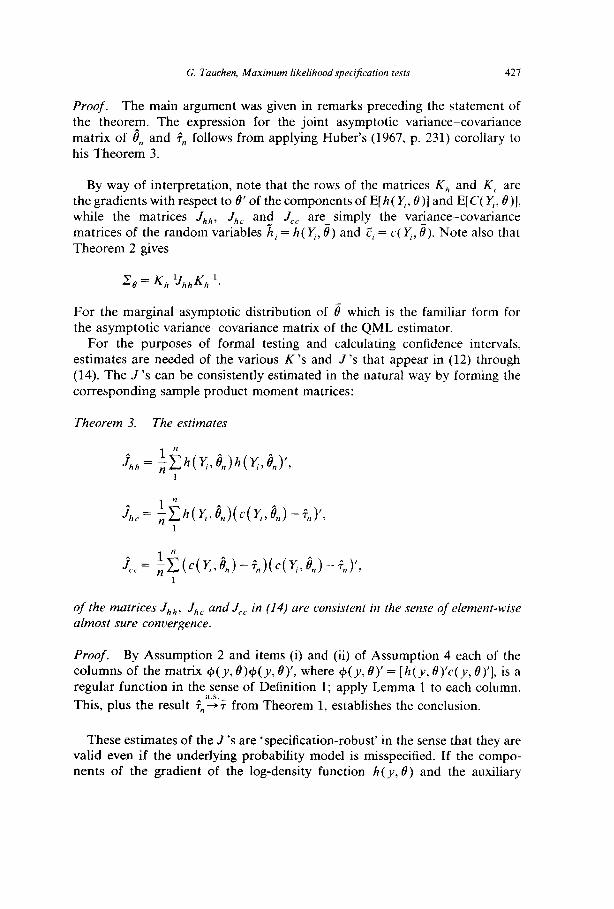
G. Tuuchen, Muximum likelihood specification tests 427

Proof. The main argument was given in remarks preceding the statement of the theorem. The expression for the joint asymptotic variance-covariance matrix of 8, and +, follows from applying Huber’s (1967, p. 231) corollary to his Theorem 3.

By way of interpretation, note that the rows of the matrices Kh and K, are the gradients with respect to 8’ of the components of E[h( y, O)] and E[C( y:, B)], while the matrices Jh,,, Jhr and J,, are simply the variance-covariance

matrices of the random variables A, = h( y, e) and c”, = c( y, 8). Note also that Theorem 2 gives

For the marginal asymptotic distribution of 8 which is the familiar form for the asymptotic variance-covariance matrix of the QML estimator.

For the purposes of formal testing and calculating confidence intervals, estimates are needed of the various K’s and J’s that appear in (12) through (14). The J’s can be consistently estimated in the natural way by forming the corresponding sample product moment matrices:

Theorem 3. The estimates

of the matrices J,,,,, JhC and JCC in (14) are consistent in the sense of element-wise almost sure convergence.

Proof. By Assumption 2 and items (i) and (ii) of Assumption 4 each of the columns of the matrix Cp(_y, O)+(y, O)‘, where $(y, 0) = [h( y, e)‘c( y, fl)‘], is a regular function in the sense of Definition 1; apply Lemma 1 to each column.

a.s. _ This, plus the result +,,-T from Theorem 1, establishes the conclusion.

These estimates of the J ‘s are ‘specification-robust’ in the sense that they are valid even if the underlying probability model is misspecified. If the compo- nents of the gradient of the log-density function h(y, 8) and the auxiliary

428 C. Tuuchen, Maximum likelihoodspecijicutron tests

criterion function c( y, 8) are continuously differentiable in 8, then there are similar natural specification-robust estimates of the K ‘s.

Theorem 4. Assume that the components of h( y, 0) and c( y, 0) are continu-

ously difSerentiable in 0 for ally andput I?,,( y, 0) = ah( y, /3)/&Y and I?-,.( y, 0) =

ac( y, tl)/ZJ’. If the columns of the matrix functions Kh and I?,. are regular as dejined in Dejinition 1 (note that continuity of the columns in 8 is presupposed in

the hypotheses of this theorem), then the random matrices

(15’4

are consistent estimates of K, and K,. in the sense of element-wise almost sure

convergence.

Proof. The proof is entirely analogous to that for Theorem 3.

In most applied work the log-density function I( y, S) satisfies the differen- tiability condition in the hypotheses of Theorem 4, and so the natural estimate Z?, in (15a) is nearly always available. If the auxiliary criterion is reasonably smooth - as would usually be the case if the model evaluation is based on the difference between predicted and sample moments - then the estimate iC in (15b) is also available. In these cases, then, Theorems 3 and 4 lead to a specification-robust estimate 2,.

3.2. The generalized information equality and the estimation of 2, under correct specification

An estimate of 2, that is valid under the maintained hypothesis that the probability model is correctly specified turns out to be very easy to compute, even if the auxiliary criterion function is not differentiable in 8. The reduction in computational burden is brought about by the availability of an extension of the classical information equality. This equality says that under suitable regularity conditions the expected information matrix equals minus the ex- pected Hessian matrix. In the notation of Theorem 4, the information equality can be expressed as

G. Tuuchen, Muximum likelihood spea~cutiort tests 429

where the superscript o means that these are the J,,,, and K, matrices in (13a) and (13b) when the model is correctly specified and #, exists.

To motivate the generalization of the information equality, consider

and note that the equality holds identically in 0. Now, if differentiation could be brought freely in and out of the integration, then the usual Cramer calculus gives

or

where the subscript 8’ on c and f in the first equality denotes partial differentiation. The last equality is more compactly written

K:’ + Jph = 0, (17)

where as in (16) the superscript o means that these are the corresponding K, and Jc,, matrices whenever 8, exists. The next theorem states that both the basic information equality and its generalization in (17) are valid even if c(y, 8) is not differentiable in 8 and the differentiation cannot in general be brought inside the integration.

Theorem 5 (generalized information equality). Assume (i): 0, exists such

that f(y, 0,) is a uersion of g(y), and (ii): the function

4(y,B)=f(y,8)/f(y,8,) (18)

satis$es (8q( y, O)/~?ej 5 b(y), where b is square integrable with respect to F(y, 6,). Then both equalities (16) and (I 7) hold. (Proof: Appendix.)

The following corollary gives a simple method for getting null-consistent estimates of the asymptotic variance-covariance matrix of +“.

Corollary 5.1. If the hypotheses of Theorem 5 hold, then

(19)

430 G. Tauchen, Maximum likelihood specification tests

is the asymptotic variance-covariance matrix of &?n. Moreover, the natural estimator

(20)

with the j’s as in Theorem 3, is consistent in the sense of element-wise almost sure convergence.

Proof. Apply the two equalities (16) and (17) to the expression (12) and then select off the lower right-hand corner of the joint variance-covariance matrix that corresponds to F,,; the convergence of (20) follows from Theorem 3.

Interestingly, the estimate 2: in (20) is simply the usual estimate of the residual variance-covariance matrix from a seemingly unrelated regression of the components of P, = c( y., d,,) on the ‘scores’ h, = h( x, a,,).

4. The local behavior of 7 under misspecification

In the previous sections it was established that the estimator I?,, and the statistic +, converge almost surely to

(21)

f= c(y,+-%% / (22)

and that h(an - 8) and &( ?, - 7) have a joint asymptotic normal distribu- tion with variance and covaria.nce matrices Z,, Z,, Ze7, as given in Theorem 2

above. When the model is correctly specified and G(y) = F( y, 0,) for some 8,, then e = 6, and 7 = 0. Under m&specification however, 8 need not equal B,, and likewise 7 will be non-zero, which is where the specification tests gets its power.

In this section we will investigate the ability of the test to detect misspecifica- tion by examining the local behavior of the 7 for small deviations of the idealized model from the true model. These deviations are generated in the following manner. Consider alternative true distributions G, given by

dG,(_v) = [l + U(Y)] W,(y), (23)

where v is a function on R” and dF,( y) = dF(y, 0,). The parameter value 0, is fixed throughout, while v will vary over a class of functions on R”, with

G. Tuuchen, Maximum likelihood spectf&tion tests 431

each u giving rise to an alternative true model or distribution of the data. The particular class of functions are the elements of the following space.

Notation. Let V denote the set of functions u: R” + R’ such that

(9 1 +u(v)20, forall y,

(ii) I u(y)d6b(y) =O,

(iii) / +)*dFo(y) < cc.

The first two of these conditions simply ensure that G,, is a bona fide distribution function. The third condition ensures that a random variable of

the form u(Y), with Y - F,, has finite variance, which proves to be convenient below. The norm of the space V is taken to be the natural L,(F,) norm,

IluII~ = (lu(y)2dMu))“2. In this setup, then, for each u E V there is a true distribution G,. given by

(23). For any non-zero u in V the probability model is n-&specified since there will in general be no ti in 0 such that G,(v) = F( y, 8). However, at u = 0 the model is correctly specified with G,(r) = F,(y) = F( y, S,,), by construction. Although this setup does restrict the true distribution to be absolutely continu- ous with respect to the distribution F,, it does nonetheless generate a very wide class of alternative models. Furthermore one might argue that absolute con- tinuity is no restriction at all, since any region in R” over which the true distribution puts positive probability mass will ultimately be discovered in

large samples anyways. Under suitable regularly conditions both 8, and ?,, will, for each G,. with u

fixed. have almost sure limits

(24)

f,,“%(u)= /c(y,$(u))dG,(y). (25)

The almost surely here means with probability one with respect to the joint distribution of {Y}, where the Y are independent and have common distribu- tion function G,.

Both s(u) and 7(u) are functionals on V that are highly non-linear in u, which makes a complete analysis of them difficult to obtain. However, an

432 G. Tuuchen, Muxmum likelihood specification tests

analysis of their local behavior near v = 0, i.e., near a correctly specified model, is tractable and gives several interesting insights into the characteristics of the estimator and the specification test under m&specification. The analysis pro-

ceeds by examining the Frechet derivatives [Wouk (1979, ch. 12)] of I?( U) and 7(v) at v = 0. These derivatives are by definition linear functionals, De and D?, on V such that

In other words, e(v) and 7(u) can each be approximated by a linear function of u up to an approximation error that is o( ])u]]~); the analogy is that a first-term Taylor approximation to an ordinary function. Strictly speaking, V itself is not a linear space for the domains of the linear operators De and D7. But this is not a problem because the derivatives are actually defined for all v E L2( F,), while here we are only restricting their domains to those values of v for which the G, is a genuine distribution function.

Three recent papers that have also undertaken local specification analysis are Kiefer and Skoog (1984) Newey (1984) and Davidson and Mackinnon (1984a). The Kiefer-Skoogpaper analyzes the effects of misspecification on the limiting parameter value 8 for a set of finite-dimensional ‘directions’ of misspecifica- tion generated by incorrect parametric restrictions. Here we study the effects of

misspecification on both 8 and 7 for the more extensive infinite-dimensional set of directions generated by incorrect distributional assumptions. The Newey and Davidson-Mackinnon papers also use an infinite-dimensional set of directions, but the emphasis in these papers is more of studying the behavior of the limiting &i-square non-centrality parameter, while here we focus more on t? and 7. Also, the mathematical methods of these other two papers are different than those used here. These papers use concepts of differentiation similar to the Gateaux derivative, whereas here we use the Frechet derivative [see Wouk (1979, ch. 12)]. The requirements for the existence of the Frechet derivative are more stringent than those for the Gateaux derivative - e.g., a Cobb-Douglas production function has Gateaux derivatives at the origin in all directions in the positive orthant but does not have a Frechet derivative there - and establishing the existence of the Frechet derivative entails more detailed arguments. However, because the Frechet derivative, or more precisely the corresponding linear functional, is independent of the direction at which it is evaluated, the qualitative predictions based on it are stronger. For instance, suppose it is found that a specification test locally has zero power in two different directions. Then, if the appropriate Frechet derivatives exist, the test will also be guaranteed to have zero power locally in all directions that are linear combinations of these two directions. A similar guarantee is not avail- able if only the Gateaux derivatives exist and thus conclusions based on the

weaker concept of differentiation could potentially be misleading in some cases.

The main results for the Frechet derivatives are in Theorem 6 below, which is proceeded by a technical lemma:

Lemma 2. Let Assumptions l-4 hold for each G,, of the form dG,. =

P + dr)ldF,,(y) andw

where

h(‘A u) = jh( y, 6) dG,,(y)> h,(d, u> = /c(y. e)dG,,(y)

Then the Frechet derivative of CI at (8, r, 0) E 0 X TX V exists and is given by

where (Ad, Ar, u) E 0 X TX V, with the norm on 0 X TX V being iA81 + [ATI

+ IIv1j2. In addition, DCX is continuous in (0,~). (Proof: Appendix.)

Theorem 6. Let Assumptions_ l-4 hold for each G,.;, let condition (ii) of Theorem 5 hold ai B,, and let 8(u) and 7(u) be the impli’ed almost sure limits of 0, and +X. Then B(u) and 7(u) are Frechet diflerentiable in u at v = 0, with the

derivatives given hi

D+[u] = / c(y, 4h(y)W,(y) -Jph D&&

where, in the notation of the previous section,

434 G. Tuuchen, Muxrmum likehhood specljiccrtion tests

Proof. Use Lemma 2 to apply the implicit function theorems for Frechet derivatives [Wouk (1979, Theorem 12,4.1, p. 294; Corollary 1, p. 296)] and the extended information equalities (16) and (17).

Note that implicit in the hypotheses of this theorem are the assumed existence and uniqueness of e(u) and F(u). Clarke (1983) provides a set of regularity conditions, albeit stronger than those assumed here, that guarantee existence and uniqueness.

An interesting way to express these derivatives is to put I!?,, = De[u] and 7,, = D$[ u], and write them as

(26)

where

By analogy with least squares, the derivative <, is the vector of regression coefficients in a regression of a random variable u = u(Y) on a random

variable h = h (Y, 0,), with Y - F( y, 8,). Thus, misspecification of the model leads to an inconsistent estimate of 0,, except when the n&specification is in a direction u that is orthogonal to the gradient of the log-density function in the sense that cov( u( Y ), h( Y, 0,)) = 0 under F( y, 6,). The special set of directions in which orthogonality holds corresponds to estimation situations in which the distributional assumptions implicit in the hypothesized model for the data are fi incorrect but the estimator 0, is still consistent (i.e., its genuine quasi-maxi- mum likelihood). One well-known example of this in econometrics is FIML applied to a linear simultaneous equations system under the assumption of normally distributed errors when in fact the errors are not normal. Another is Phillips’s (1982) example consisting of a two-equation non-linear simultaneous system and a family of non-normal error distributions. Phillips shows that FIML estimation of his system under a normality assumption gives consistent estimates of the parameters despite the failure of the distributional assump- tions. The essential feature of Phillips’s example is that each true model generated by an error distribution in the family of allowable distributions lies in a direction u that is uncorrelated with h under a normality assumption. Such an example, however, is clearly special and misspecification in general can lie in directions that are not orthogonal to h, so that the limiting value 6 is directly affected by r&specification. An example of this more serious type of m&specification would be an omitted variable from a simultaneous equations system.

G. Tuuchen, Muximum likelihood specificcrfion tests 435

Considering the derivative FU in (27) we see that under m&specification the limit 7 is perturbed away from zero in ways. The first is through J$, which is the covariance under F, between c( Y, 13~) and u(Y); the second is through 8, i.e., through the effect that the misspecification has on the limit of the estimated parameters. In the special case when the model is wrong but the derivative u is uncorrelated with h under F, and gc, = 0, the specification test will detect the failure of the distributional assumptions so long as the auxiliary criterion function has some covariance with u. An example of this use would be applying White’s information matrix test under the maintained model Y - N(p, u2) when the true distribution is symmetric about p but with tails ‘thicker’ than those of the normal. In this example the ML estimators p and 3 2 are consistent, but White’s test would detect the departure from normality via the failure of the fourther moment about the mean to equal three times the square of the second moment. Again, though, this type of example is clearly special and in general n&specification will perturb 8 away from 8, and the second term in (27) will be non-zero.

The derivative FL, also has interesting interpretations based on a least squares analogy. Substitution of (26) into (27) gives

where BCh = JC%( Jhoh)-‘. The matrix Bch is simply the matrix of regression coefficients in a regression of the random vector c = c(Y, 19,) on the vector h = h( Y, 8,), with Y - F,(y). That is, B,., = E,[ch’](E,[hh’])-‘, where the expectation E,[ -1 is under d F,. Thus TV is the covariance between u and the auxiliary criterion function c, after the linear effects of h have been removed from c. Intuitively, the reason that the direction h is ‘parsed out’ of c, so to speak, is that the condition E,[h( Y, f$)] = 0 was imposed directly in the estimation, and thus no specification test can be based on this direction.

5. Procedures for application

5.1. Outline

The following three-step algorithm for diagnostic testing and model evalua- tion summarizes the method for applying Theorems 1-5:

Step I: Calculate f by maximum likelihood and retain for subsequent use the ‘scores’ h, = h( y, B), which are the gradients of the log-density function evaluated at the ML estimate.

Step 2: Choose a set of k auxiliarv criterion functions, ck(y, B), for k = 1,2,. . . , K. Each of the ck( y, 8) should have the property that a large absolute

436 G. Tauchen, Muximum likelihood specificution tests

value for ?, = (l/n)Cyc,(Y,, 6) would tend to cast some doubt on the assump- tions underlying the likelihood model.

Step 3: Form E,, = ck(yI, f?) and regress the F’s on the scores. Specifically, estimate for each k the parameters of the equation

Zki = PI& + i:p, + u;, i= 1,2 ,...,n, (29)

where ui represents the err:r, and pkO and Pk are the constant and the slope coefficients. The estimates POk of the intercepts in the regression equations will be the +k. Furthermore, individual t tests for non-zero intercepts in the regressions using the printed standard errors will be asymptotically valid tests for whether or not the corresponding $, are significantly different from zero. Finally, the statistic ?‘(fi/n))‘?, where i is the vector of i, and $ is the

K x K cross-equation residual covariance matrix, is an appropriate &i-square statistic for testing whether or not all of the intercepts are jointly statistically significantly different from zero.

This regression-based procedure is the multivariate extension of a method proposed by Cox (1962, p. 411) for calculating the test statistic for his test for separate families. The procedure differs somewhat from that proposed by White (1982), Chesher (1983) Davidson and Mackinnon (1984b) and others for specification tests that are special cases of those considered here. In the other procedure the user calculates a single chi-square statistic equal to nR2 (uncentered) for a regression of an n x 1 column of ones on the n x (K + p)

matrix whose ith row is (Z:, it;), where ?: = (Zt,, Z Z ,,..., Fkr) and A: is the transposed score vector. A major advantage of the procedure outlined above is that the individual t tests on the intercepts provide the user with detailed information on the statistical significance of each of the components i,. Using the other procedure the user obtains information only on the joint significance of all components taken together. A disadvantage, however, is that to get the chi-square statistic ?‘( h/n)) ‘i for joint significance the user must calculate a quadratic form in the residual covariance matrix for K separate regressions, while for the other procedure the user only calculates nR* for a single regression. Interestingly, the two &i-square statistics from the procedures are only asymptotically equivalent but not computationally equivalent in finite . samples. If no degree of adjustment is used in calculating L!, then least squares algebra shows that the statistics satisfy ?‘(fi/n))‘? 2 nR2. With a degree of freedom adjustment, however, the inequality can go in either direction for finite n. Clearly, further work on the small sample properties of the &i-square statistics would be useful.

437

5.2. Empirical example

The potential uses of the type of specification tests considered in this paper can be illustrated with an application from the study of price behavior on speculative markets. One of the major stylized facts that has emerged from extensive research into the characteristics of short-term price movements on futures and equity markets is that the price changes generally have mean zero and are independent of one another, but their probability distribution is not a normal distribution. In particular, the pdf of the price changes has thick tails or is leptokurtic relative to the normal pdf. It is interesting, then, to see if the types of specification tests discussed here do in fact detect departure from

normality in speculative price changes. Suppose that the maintained model for the daily price change is A P, -

N(0, u 2). Given n observations on A P,, the ML estimate of u 2 is

-2_ a - +kAP,2. 1

Under weak conditions that do not require normality the estimater s2 is consistent. However, the model A P, - N(0, u 2, when viewed as a probability model for the data is misspecified if the A P, are not normally distributed, and may give biased and misleading predictions. Consider the following four auxiliary criterion functions for detecting misspecification of the probability model:

c,(AP,a)=AP4-3u4,

c,(AP,u)=(APJ- @a,

c,(AP,u)=Z[(AP,‘u~~z,,,]-0.80,

c,(AP,u)=I[~AP/a/~z,,,,]-0.01,

where I[ .] denotes the O-l indicator function, and where z0.40 and z,,~~ are upper critical points of the normal distribution. Elementary calculations show

that each of the c,(AP, a) integrates to zero under AP - N(0, u2). Now put

n Ckr = ck(Ap,, h), i=l,...,n,

,. l &I> rk = n k=1,...,4. I=1

The random variable ?r is the difference between the observed and predicted fourth moments; +2 is the difference between the observed and predicted absolute first moments; +3 is the difference between the observed and the predicted fraction of the observations for which the magnitude IAP,J lies more

438 G. Tauchen, Maximum likelihood specijcution tests

than zn.40 standard deviations above zero; and ?4 is analogously defined for

ZO.005.

These quantities were evaluated using 876 observations on the daily price change for the T-bills futures markets, 1976-79, from a data set described more fully in Tauchen and Pitts (1983). The results are as follows:

(1) (2) (3) (4)

Fourth moment Abs. first moment Outer 80% Outer 1%

Observed Predicted

0.0124 0.0063 0.153 0.171 0.728 0.800 0.027 0.010

Difference (i,)

0.0061 - 0.017 - 0.072

0.017

The first two rows of this display suggest that the actual fourth moment is somewhat larger than what is predicted by the probability model, while the absolute first moment is somewhat smaller. The last two rows indicate that there are too few observations above 6z,,, in magnitude and too many above A (JZ~,~~ than would be expected on the basis of the normal distribution.

To determine the statistical significance of each of the four C,, we simply test for a non-zero intercept in the appropriate auxiliary regression

Pik = & + &Jr, + error, i=1,2 ,..., n,

where ?r, = al( A P,, 6 2)/aa2 is the gradient of the log-density function. Specifi- cally,

A, = - +( e-2 - ~p,26-4), i=1,2 ,..., 876,

with 6 = 0.214. The results are:

(1) (2) (3) (4)

Fourth moment Abs. first moment Outer 80% Outer 1%

r&&dJ 0.0061(0.0011)

- 0.0170 (0.0020) - 0.0717 (0.0145)

0.0174(0.0033)

&Ad) 0.0026 (0.000047) 0.0056 (0.000089) 0.0050 (0.00060) 0.0055 (0.00014)

The magnitudes of each of the four estimated intercepts exceeds twice their standard errors, which suggests that the four tk are statistically significantly different from zero. The normal distribution thus appears to be inadequate as an approximation of the pdf of the AP,.

G. Tuuchen, Muximum likelihood specifcu~ron tests 439

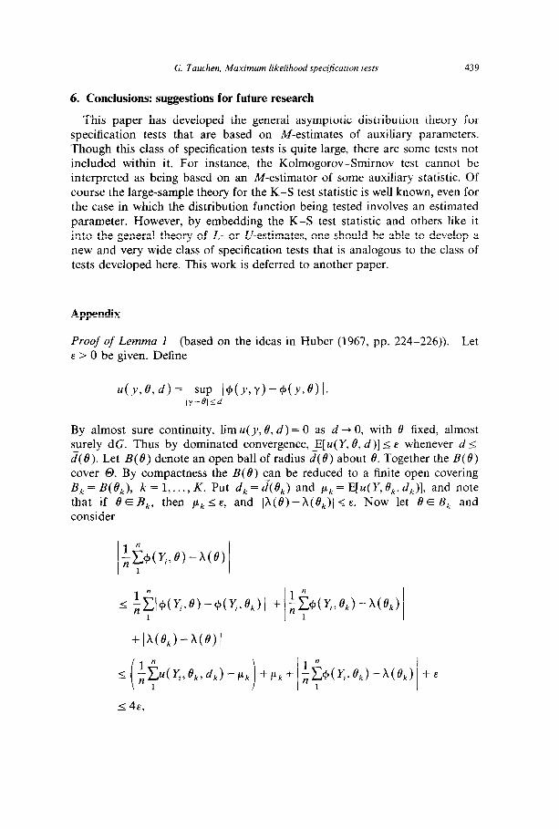
6. Conclusions: suggestions for future research

This paper has developed the general asymptotic distribution theory for specification tests that are based on M-estimates of auxiliary parameters. Though this class of specification tests is quite large, there are some tests not included within it. For instance, the Kolmogorov-Smirnov test cannot be interpreted as being based on an M-estimator of some auxiliary statistic. Of course the large-sample theory for the K-S test statistic is well known, even for the case in which the distribution function being tested involves an estimated parameter. However, by embedding the K-S test statistic and others like it into the general theory of L- or U-estimates, one should be able to develop a new and very wide class of specification tests that is analogous to the class of tests developed here. This work is deferred to another paper.

Appendix

Proof of Lemma 1 (based on the ideas in Huber (1967, pp. 224-226)). Let E > 0 be given. Define

By almost sure continuity, lim u(,v, 8, d) = 0 as d-+ 0, with 13 fixed, almost surely dG. Thus by dominated convergence, E[u(Y, 8, d)] I E whenever d I d(8). Let B(B) denote an open ball of radius j(8) about 0. Together the B( 0) cover 0. By compactness the B(B) can be reduced to a finite open covering B,=B(e,), k=l,..., K. Put d,=d(8,) and pk=E[U(Y,Bk,dk)], and note that if 8 E B,, then P~IE, and IA(e)--A(B,)(<e. Now let BEBk and consider

+lw,)-wl

440 G. Tuuchen, Maximum likelihood specijicution tests

whenever n 2 Nk(&) almost surely, by applying twice the strong law of large numbers and using pk I E. Thus

whenever n 2 maxkNk(E) almost surely, which proves the result.

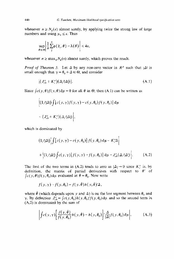
Proof of Theorem 5. Let A by any non-zero vector in RP such that JA( is small enough that y = 6, + A E 0, and consider

Since /c( y, t9)f(y, e)dp = 0 for all 19 in 0, then (A.l) can be written as

I J WI4 [c(Y~Y)~(Y,Y)-c(Y,~~)~(Y,~,)] dp

which is dominated by

+ (~/lAO~c(y,~)[f(~.,~)-f(y,e,)]dl*- J:;, (A/VI> . (A.21

The first of the two terms in (A.2) tends to zero as IAJ + 0 since KP is, by

definition, the matrix of partial derivatives with respect to 8’ of

MY, e)f(y, 4)d p evaluated at 0 = 0,. Now write

f(~,~)-f(y,eo)=f(~,e>h(y,e)‘A,

where 8 (which depends upon y and A) is on the line segment between 8, and y. By definition J,9, = /c( y, B,)h( y, O,)‘f( y, 0,) dp and so the second term in (A.2) is dominated by the sum of

441

and

From (ii) of Assumption 4 the expected value of (c(y, y)l” with respect to j( _~,8,) is uniformly bounded in y, and so by the Schwarz inequality the square of the term (A.3) is dominated by a constant times

The second hypothesis of the theorem and (ii) of Assumption 4 imply that the squared term in this integral is dominated by a function integrable with respect to f (y, 6,) dp. Thus by dominated convergence this integral, and hence (A.3) tends to zero as [Al 4 0. Finally, since c satisfies the Lipshitz conditions in Assumption 4 and Jhl2 is dominated, the term (A.4) is O(lA(“2).

In summary, the matrix J,P, + K,? satisfies for any non-zero A E Rp

,?fm,i( J:h + KP)(A/lAl) 1 = 0,

irrespective of how /Al + 0; hence it equals zero because it maps every vector of unit length into zero.

Proof of Lemma 2. Put S = [Ah’/ + 1A~l-t Iju(12, and consider

d-* x,(e+Ae,U>-x,(e,o)-(ah,/ae’)(e,o)de

- (A.5)

We must show that the right-hand side of this inequality tends to zero as 6 + 0. Now the first term on the right-hand side of the inequality (A.5) cannot

442 G. Tuuchen. Maximum lrkelihood specificuticm tats

exceed the sum of

and

(‘4.6)

64.7)

From the definition of ax,/&)‘, the expression (A.6) must tend to zero with 6. On the other hand, the expression (A.7) is dominated by

(A.81

and by the second Lipshitz condition (iii) in Assumption 4 there is a constant /I such that (A.8) is of the form

which tends to zero with 6. In an exactly analogous manner the second term on the right-hand side of the initial inequality (A.5) (the term corresponding to X,) tends to zero with 6, and so the existence of the Frechet derivative of cx with respect to 8, r, u at (0, r,O) has been established. The continuity of the derivative in (0, r) is presupposed in (iv) of Assumption 4.

References

Aguirre-Torres, V. and A.R. Gallant, 1983, The null and non-null asymptotic distribution of the Cox test for multivariate nonlinear regression, Journal of Econometrics 21, l-33.

Burguette, J.F., A.R. Gallant and G. Souza, 1982, On unification of the asymptotic theory of nonlinear econometric models, Econometric Review 1, 151-190.

Chesher, Andrew, 1983, The information matrix test: Simplified calculation via a score interpreta- tion, Economics Letters 13, 45-48.

Clarke, Brenton R., 1983, Uniqueness and Frechet differentiability of functional solutions to maximum likelihood type equations, Annals of Statistics 11, 1196-1205.

Cox, D.R., 1962, Further results on tests of separate families of hypotheses, Journal of the Royal Statistical Society B 24, 406-424.

Davidson, R. and J. Mackinnon, 1984a, Implicit alternatives and the local power of test statistics, Queen’s University discussion paper no. 556.

Davidson, R. and J. Mackinnon, 1984b. Model specification tests based on artificial linear regressions, International Economic Review 25, 485-502.

Engle, Robert F., 1982, A general approach to Lagrange multiplier model diagnostics, Journal of Econometrics 20, 83-104.

Hausman, J., 1978, Specification tests in econometrics, Econometrica 46, 1251-1271. Heckman, J., 1984, The x2 goodness of fit for models with parameters estimated from microdata,

Econometrica 52,1543-1548.

G. Tuuchen, Maximum Irkellhoodspeci~~ution tests 443

Huber, Peter J.. 1967, The behavior of maximum likelihood estimates under nonstandard condi- tions, in: Lucien M. LeCam and Jetty Neyman, eds., Proceedings of the fifth Berkeley symposium on mathematical statistics and probability, Vol. 1 (University of California Press, Berkeley, CA) 221-234.

Huber. Peter J., 1981. Robust statistics (Wiley, New York). Kendall, M.G. and A. Stuart, 1973, The advanced theory of statistics, 3rd rd. (Griffin, London). Kiefer, N. and G. Skoog, Local asymptotic specification error analysis, Econometrica 52, 873-8X6. Lancaster, T., 1984, The covatiance matrix of the information matrix text, Econometrica 52,

1051-1054. Moore, D.S. and M.C. Spruill, 1975, Unified large-sample of general chi-squared statistics for tests

of fit, Annals of Statistics 3, 599-616. Newey. W.K., 1984, Maximum likelihood specification testing and instrumented score tests,

Prmceton University mimeo. Phillips, P.C.B., 1982, On the consistency of FIML, Econometrica 50, 1307-1324. Tauchen. George and M. Pitts, 1983, The price variability-volume relationship on speculative

markets, Econometrica 51, 485-505. White, H., 1982, Maximum likelihood estimation of misspecified models, Econometrica 50, l-26. Wouk. A., 1979, A course of applied functional analysis (Wiley, New York).