Development of Revolute-Joint Element with Rotation Limits, Locking, Resistive Moment and Damping

Engineering with Computers (2002) 18: 1–13Ownership and Copyright 2002 Springer-Verlag London Limited

Development of Revolute-Joint Element with Rotation Limits, Locking,Resistive Moment and Damping

S. V. Wong1, A. M. S. Hamouda1 and M. S. J. Hashmi2

1Department of Mechanical and Manufacturing Engineering, Universiti Putra Malaysia, Malaysia; 2School of Mechanical andManufacturing Engineering, Dublin City University, Dublin, Ireland

Abstract. The revolute-joint is an important component ofa mechanical system. Thus, the motion simulation of multi-bodies connected with revolute-joints is of common interest.A simple revolute-joint can be easily represented in a numeri-cal way, whereby the bending moment at the particularjoint equals zero. Formulation becomes complicated wheninvolving bending limits, the resistive moment and the damp-ing effect. Furthermore, several bodies connected with revol-ute-joints form a complex system. This has been particularlyuseful for simulating a multibody system. A novel revolute-joint model is proposed in this paper. Several possiblemethods are suggested to handle bending limits. The incor-poration of the resistive moment and damping effects are alsopresented. The numerical stability of the revolute element isdiscussed, and a stability criterion suggested. The revolute-joint element is incorporated into an explicit finite differencecode developed by the authors. Numerical examples areshown for different methods and conditions.

Keywords. Adaptive stiffness method; Finite differ-ence model; Locking mechanism; Numerical stab-ility criterion; Revolute joint algorithm; Revolutejoint element

1. Introduction

Many machine components and devices consist ofinterconnected rigid bodies. Revolute-joints areamong the most common connecting joints, and thesimplest. In kinematics terms, a revolute-joint hasonly one primary degree of freedom, which is arotation about the revolute axis. For a revolute-

Correspondence and offprint requests to: Dr Shaw Voon Wong,Department of Mechanical & Manufacturing Engineering, Univer-siti Putra Malaysia, UPM 43400, Serdang, Selangor, Malaysia.E-mail: wongsv�eng.upm.edu.my

joint, rotational limits, rotational friction and viscousdamping have to be considered. For a more compli-cated situation like human joint modelling, theeffects of the muscles will contribute to the buildingof resistive moment at the respective joint.

The revolute-joint limits are where the connectedlinks/bodies cannot rotate any further, because ofthe physical constraints in the nature of the revolute-joint. In reality, the system may be designed tohave rotational limits for some specific reasons.Furthermore, a joint locking mechanism may berequired. One common example is the locking ofindividual solar arrays of a satellite during deploy-ment. This operation results in a redistribution oftotal momentum that may lead to impulsive forcesand moments on the system. Strong vibrations mayoccur, especially involving light flexible structures.Damping is a crucial factor in many mechanicalsystems, including the revolute-joint, where thedamping will stabilize any post-limit oscillationand excitation.

A great deal of work has been carried out indeveloping mathematical models and numericalsimulation systems to study the structural flexibilityof members during their motion. Differentapproaches were employed, among them being thefinite element method [1,2], the assumed modemethod [3] and the lumped parameter approach[4]. Several authors [5–7] studied the post-impactbehaviour of closed loop mechanisms and a singleflexible link. Momentum balance was used, but theapplication of a restitution coefficient was notinvolved. Locking and rotational limits were notstudied. Not much work has been done on dealingwith locking and/or rotational limits. Nagaraj et al.[8] studied the dynamics of a two-link flexible sys-tem with a locking mechanism. Two revolute-jointswith a torsion spring were employed. Mathematicalmodels with the momentum balanced were shown,and comparisons to experimental results made.

2 S. V. Wong et al.

The computational formulation of a revolute-jointelement is rare in the literature. Revolute-joint prob-lems are normally modelled as physical constraintsapplied on nodes. To achieve an idealized fixed-point revolute-joint, linear displacement constraintsare applied, and one of the rotational displacementsis released at the coincide nodes of the connectedbodies. Things become more complicated when therevolute-joint connects two or more free bodies. Theglobal constraints cannot be applied in this situation.Simple constraints (both local and global) will nolonger be capable of handling complex problems,which involve rotation limits, locking, the resistivemoment and damping.

A complete revolute element can be found inANSYS, a well-known commercial finite elementsystem, known as COMBIN7 [9]. The element con-sists of two primary nodes and three optional nodes.Figure 1 shows the main components of the ANSYSrevolute element. The term K is the rotational springstiffness when the element is locked or reaching itslimit. The term Tf is the frictional torque, and C isthe coefficient of rotational viscous damping coef-ficient. �U and �L are the upper (forward) rotationlimit and the lower (reverse) rotation limit, respect-ively. The figure shows clearly that the rotation ofthe connected bodies is constrained with a highstiffness rotational spring. The impact phenomenonis similar to the penalty method of the contact-impact element, where the normal contact force isdependent on the contact stiffness. Thus, the revolutemodel suffers a similar shortcoming to the penaltymethod, when a predefined stiffness value from theuser is required. Low stiffness may cause significantrotational penetration, even to penetrate through theconstraint. High stiffness may cause over-excitation,which gives an unrealistic response. As a commonpractice, initial rotational spring stiffness whilelocking is selected arbitrarily. Fine-tuning has tobe carried out through trial and error to obtain abetter result. A similar method may be applied tohandle the torsion effect of connected bodies at the

Fig. 1. ANSYS COMBIN7 revolute-joint element behavior dia-gram.

revolute-joint, where the user defines the springs’stiffness beforehand. The constant Tf defines theresistive rotation stiffness of the revolute system.The revolute element can only handle constantrotational stiffness. Furthermore, the coexistence ofthe rotational stiffness and resistive moment is pro-hibited with the ANSYS element. The ANSYSelement also does not handle the locking mechanism.

A new revolute model is proposed by the authors.The model is capable of handling rotation limits,locking, resistive torque and the viscous dampingeffect. The new model can handle complex situ-ations, such as constant resistive torque at a parti-cular range of rotational displacement and havingcontact stiffness at the other. Rotation limits andthe locking effect are handled with an adaptivemethod developed by the authors, in which the userdoes not need to prescribe the spring stiffness.Several other possible models are also suggested:the forced-displacement, momentum-balanced andenergy-conservation methods. The forced-displace-ment method is a common method for handlingphysical constraints. The momentum-balancedmethod is a common method in predicting the over-all post-contact response. A new way ofimplementing the momentum-balanced method atthe element level is described. Another alternativemethod, called the energy conservation method, isa new suggestion. Comparisons among thesemethods are made, and for simplicity, the torsioneffect is omitted and the 2D space is used. Therevolute element proposed is incorporated into a 1DFD element developed by Wong et al. [10], namelythe Node-Layer model, while solving the numericalproblems in this paper. Central difference temporalintegration is applied.

Section 2 shows the components of the newrevolute element. Formulations of the adaptive stiff-ness model and others are presented in Section 3.Formulations of the locking mechanism, resistivetorque and damping are then explained, and contact,locking and releasing conditions presented. Further-more, the computational stability of the revolute-joint element is discussed. Section 4 shows a com-parison among the penalty-like method, adaptivestiffness model, momentum-balanced model, forced-displacement model and energy conservation model.The respective pros, cons and limitations are dis-cussed, and a simple numerical problem is solvedfor comparison. In Section 5, a numerical exampleis simulated and comparisons with both experimentaland mathematical results from the literature [8] aremade. Finally, concluding remarks are presented inSection 6.

3Development of Revolute-Joint Elements

2. Element Structure

The new revolute element has a similar basic struc-ture as the COMBIN7 element of the ANSYS. Table1 shows the primary variables and a brief descriptionof their use in the new revolute element. � is therotary location of body 2 (represented by Node Jand Node L) relative to body 1 (represented byNode I and Node K) about the joint. The validrange of � is from 0 to 360 degrees (not including360 degrees), and being calculated by the systemwith the location of nodes I, J, K and L. Incrementalrotary displacement can be used, which is onlyrequired for nodes I and J, and the valid range of� is from −180 to 180 degrees. The former is usedto define � in the formulation section of this paper.

Nodes I and J are at coincident positions for anideal situation, where no linear displacement isallowed in between the two nodes. Selection ofnodes K and L as a reference should form a rotaryrigid reference towards nodes I and J. This meansthe lines formed by nodes I-K and nodes J-L areassumed not to undergo any rotary deformationabout the other axes, besides the revolute axis(bending in most cases). For the 3D-space element,an additional reference node is required to handlethe above-mentioned assumption. The terms I1 and I2

are the local rotary or moment inertia of respectiveconnecting elements. Figure 2 shows a typical situ-ation of the two connected bodies with a revolute-joint.

Compared to the ANSYS COMBIN 7 element,the parameter Tf in Fig. 1 is replaced by variableresistive torque with respect to the rotary location.The rotary location-torque array stores information

Table 1. Revolute element structure

Variable Description

� Rotary location (0–360 degree)I1, I2 Moment (rotary) inertia of body 1 and

body 2Node I, J Connecting nodesNode K, L Reference nodes of node I and J, respect-

ively�i, �i ith element of rotary location array and

corresponding ith element of resistivetorque array

�f Rotational forward limit�r Rotational reverse limitBlock Locking flagC Coefficient of viscous damping

Fig. 2. General configuration of revolute-joint element.

about the required resistive torque at a particularrotary location.

Two rotary locations are used to define the for-ward and reverse rotary limits: �f and �r, respect-ively. A flag, bLock, needs to be set to activatethe locking mechanism after the rotary limit. Thelocking/rotary limit’s spring stiffness, K in Fig. 1,can be predicted by the adaptive stiffness method,or by other conventional methods. The conventionalpenalty-like method (used by COMBIN7 of ANSYS)can still be applied to the suggested element bydefining the torque-location array. The locking rotarylimit stiffness may vary accordingly with the newarrangement. Viscous damping is included as afunction of rotary velocity, which involves the coef-ficient of damping, C. The COMBIN7 element onlyincludes viscous friction instead of viscous damping.

3. Element Formulations

The formulations of the proposed revolute elementare explained in this section. The variables shownin Table 1 are input variables, except for the rotarylocation, �. The rotary inertia, I1 and I2, can beprescribed or calculated for a simple beam elementand any 1D element. For simplification purposes,the formulations in this section are based on 2Dspace with the revolute-joint rotate around the globalz-axis. The 3D space can be achieved with furtherinterpretation of the rotating axis, where a referencenode is required. Figure 3 is considered for theformulation of the following. A revolute joint isplaced between two link elements, link 1 and link2. Nodes I and J of the revolute-joint element areat coincident locations. The other node of the linkelements is chosen as the reference nodes (K andL) of the revolute element. The terms �1 and �2

are the resultant torque of the links after reachingrotary limits or locking (used in Section 3.4). Theparameters �

·i and �

· �i are the rotary velocities

immediately before and after reaching the rotarylimits of the body i (used in Sections 3.3 and 3.4).

4 S. V. Wong et al.

Fig. 3. Schematic diagram of the revolute-joint element formu-lations.

3.1. Rotary Displacement

The rotary position of body 2 relative to body 1,�, is calculated with the equation:

� = tan2−1 �uTr Y

uTr X� (1)

where ur is the local relative displacement of nodeL to node K with rotary orientation of the I-Jhorizon. ur is calculated with the equation:

ur = �cos� −sin� 0

sin� cos� 0

0 0 1� �(UL − UJ)T X

(UL − UJ)T Y

(UL − UJ)T Z� (2)

� = tan−1 �(Uk − UI)T Y(Uk − UI)T X� (3)

The,Y, X and Z are the normal vector of the globalY-axis, X-axis and Z-axis, respectively. Ui is theglobal displacement vector of node i.

3.2. Variable Resistive Torque(s)

To cope with variable resistive torque, the value ofTf in Fig. 1 varies with respect to rotary location.The resistive torque-location relation is discretizedinto finite sets of data and stored in two separatearrays, � and �. Linear interpolation is applied tofind the corresponding resistive torque at any rotarylocation in between the rotary locations of the array.The corresponding torque � at rotary location � isgiven by the equation:

� = �n−1

i=0

(4)

��i +� − �i

�i+1 − �i

(�i+1 − �i), if �i � � � �i+1

0, otherwise

where n is the size of the array starting from zero.Duplicating the range of � in the array is allowed.Thus, a summation function is used in Eq. (1). Fora simple case, which is a normal scenario, the arrayis arranged in such a way that �i � �i+1, �0 = 0degrees, and �n = 360 degrees. Rotary spring stiff-ness at a specific range of rotary displacement canbe defined with the following simple relation:

Ki =�i+1 − �i

�i+1 − �i

(5)

The formulation can handle the constant resistivetorque and/or rotary spring stiffness at the sametime. A conventional penalty-like method for hand-ling rotary limits can be achieved with the newformulation of variable Tf. A high stiffness can beapplied (defined in the formulation of Eq. (4)) toresist the rotary movement after reaching the rotarylimits. An overlapping definition of the resistivetorque with rotary displacement is allowed.

3.3. Rotary Limits and Locking Conditions

Rotary limits consist of forward and reversed limits.Forward and reverse refer to the direction of therotary displacement (�): forward is anti-clockwiseof � with a positive value in the following formu-lations, and vice versa. Figure 4 shows a typical

Fig. 4. Backward constrained revolute-joint.

5Development of Revolute-Joint Elements

configuration of a revolute element with rotationallimits. Limiting conditions are fired where the rotarydisplacement of both connected bodies reaches thelimits (forward and reverse). Figure 5 shows anotherpossible configuration of the rotary limits. �f islarger than �r with the former configuration, andvice versa. To reach a limit, the following conditionshave to be met:

bLimit = (6)

�true, if (�f � �r) � (� � �f � � � �r)

� if (�f � �r) � (�f � � � �r)

false

The symbols � and � stand for the AND and ORBoolean operators, respectively. A status flag isused to represent different situations of the revoluteelement. The status flag, Lflag, is defined by the equ-ation:

Lflag = (7)

�0 = free to move

1 = forward limit reached, if bLimit = true � �·

� 0

2 = reverse limit reached, if bLimit = true � �·

� 0

3 = locked, if bLimit = true � bLock = true

where �·

is the relative rotary velocity of link 2 tolink 1. The bLock is a Boolean flag to indicateactivation of the locking mechanism. The Lflag willbe revised with the releasing conditions below, pro-vided Lflag is not equal to 3:

if Lflag = 1 � � � �f (8)

if Lflag = 2 � � � �r (9)

Another alternative set of releasing conditions canbe used and stated as:

if Lflag = 1 � �·

� 0 (10)

Fig. 5. Forward constrained revolute-joint.

if Lflag = 2 � �·

� 0 (11)

The effects of different releasing conditions will bediscussed in Section 4. The combined validations ofrotary limits, locking with the former set of releasingconditions, can be stated as:

Lflag = (12)

�1, if bLimit = true � (Lp

flag = 1 � Lpflag = 0 � �

·� 0)

2, if bLimit = true � (Lpflag = 2 � Lp

flag = 0 � �·

� 0)

3, if bLimit = true � bLock = true � Lpflag = 3

0

where Lflag and Lpflag are the present and previous

status flags. For the later set of releasing conditions,the following is considered:

Lflag = (13)

�1, if bLimit = true � (Lp

flag = 1 � Lpflag = 0) � �

·� 0

2, if bLimit = true � (Lpflag = 2 � Lp

flag = 0) � �·

� 0

3, if bLimit = true � bLock = true � Lpflag = 3

0

3.4. Rotary Limit Response Methods

Several methods can be used to predict the post-limit response of the connected elements. They arethe COMBIN7 penalty-like method, the adaptivestiffness method, the momentum-balanced method,the forced-displacement method and the energy-con-servation method.

3.4.1. Adaptive Stiffness MethodAn adaptive method is suggested to predict therotary limit responses. No user-defined parameter isrequired. Rotary penetration of connected bodiesshould be avoided after the rotary limits. Thus, therotary stiffness should be able to push back theconnected elements effectively. At the contactingtime step t, the following equations are establishedwith reference to the central difference temporalintegration scheme at the time when the two bodiesare in ‘contact’ at the limit boundary:

d�· t

1 =�t

1dtI1

(14)

-�· t

2 =�t

2dtI2

(15)

where d�· t

1 and d�· t

2 are the change in the rotaryvelocity of bodies (links in this case) 1 and 2,

6 S. V. Wong et al.

respectively, at contacting time step t, and dt is thetime step size. d�

· t1 and d�

· t2 are defined by the equa-

tions:

d�· t

1 = �· t+0.5

1 + �· t−0.5

1 (16)

d�· t

2 = �· t+0.5

2 + �· t−0.5

2 (17)

where �· t+0.5

1 and �· t+0.5

2 are the rotary velocities oflinks 1 and 2, respectively, at time step t+0.5. Thechange in the velocity should push back the rotatinglinks to the limit contact boundary. Thus, the follow-ing relationship is used:

(d�· t

2 − d�· t

1) dt = p (18)

where p is the rotary penetration calculated withthe equation:

p = ��f − �, if Lflag = 1

�r − �, if Lflag = 2(19)

Also, knowing

�1 = −�2 (20)

with Eqs (14)–(20), the recommended contact stiff-ness is given as:

KAP =I1I2

(I1 + I2)dt2(21)

Similar to the COMBIN7 penalty-like method, themagnitude of the resultant torque of both links isthen given as:

�1 = −�2 = −KAPp (22)

In general, the value of dt should not be too large,where the links penetrate though the constraintregion in one time step without meeting any of therotary limit conditions.

3.4.2. Momentum-Balanced MethodThe momentum-balanced method applies conser-vation of the momentum principle. The rotarymomentum of both links before and after the impactat the limit boundary should be equal. The coef-ficient of restitution is involved, and the equationsbelow are used:

�· �

2 =�·

2(I2 − I1�) + I1�·

1(1 + �)I2 + I1

(23)

�· �

1 = �· �

2 − �(�·

1 − �·

2) (24)

The post-contact rotary velocity of the links isdenoted as �

· �1 and �

· �2. The coefficient of restitution

is denoted as � in Eqs (23) and (24). The displace-ment of the free node of a respective link isupdated accordingly.

3.4.3. Forced-Displacement MethodThe forced displacement method has limited usage.The rotary displacement of the links is altered physi-cally to cope with the rotary constraints. Changesin implementation are normally required from oneproblem to another. In addition, accurate post-con-tact response has to be known beforehand by theuser, in order to direct the response of the rotarydisplacement. This method is not practical for solv-ing complicated problems.

3.4.4. Energy Conservation MethodConservation of energy is used to predict the impactresponse of the rotating bodies at the limit boundary.An assumption is made that both the bodies willrotate at the same post-contact rotary velocity, andno energy is lost. The method is achieved with thefollowing equations:

�· II =

I1�· 2

1�·

1

��· 1�+

I2�· 2

2�·

2

��· 2�I1 + I2

(25)

�· �

1 = �· �

2 = ��· II��· II

��· II�(26)

where �· II is a signed square of the predicted rotary

velocities, and is a transitional value. The displace-ment of the respective free node is updated accord-ing to the above equations.

3.5. Locking

Locking can be activated where no further rotarymotion is allowed after reaching the rotary limits.Thus, recovery is impossible for the rest of thesimulation motion. A user-prescribed Boolean,bLock, is used. When locking, one of the above-mentioned methods can be used for both directions(forward and reverse), and no releasing is possible.Vibration is expected to accompany the lockingmechanism.

3.6. Viscous Damping

Rotary viscous damping is included in the element,and damping coefficient C is used. The viscousdamping torque is defined as:

�C,1 = −�C,2 = C(�·

2 − �·

1) (27)

3.7. Stability of the Revolute Element

Stability is an important issue in computationalmechanics. The stability of the central difference

7Development of Revolute-Joint Elements

temporal integration scheme is given as the follow-ing, according to the Courant–Friedrichs–Levy cri-terion [11]:

tcritical =LC

(28)

where L is the minimum link length of the 1Delement, and C is the maximum wave propagationvelocity. Based on this fact, a new criterion issuggested by the authors when involving the revol-ute element:

tcritical = min �LC

, ILK � (29)

where , I and K are the minimum density, mini-mum second moment of area around the neutralaxis and the rotary spring stiffness involved of bothconnected bodies. The development of the criterionis inspired by the relation among bending moment�, Young’s modulus E, and bending angle �:

� = �h/2

h/2

E�bL

r2dr (30)

where b, h and L are the width, height and length ofthe link element, respectively. The adaptive stiffnessvalue should be revised with the following relationwhen involving locking:

K �0.81IL

dt2 (31)

Instability may be observed if the criterion is notfollowed by the revolute element, especially wheninvolving a very long contact time and lockingmechanism. Further investigation has to be carriedout to have full coverage of the revolute elementstability with a central difference temporal inte-gration scheme. The criterion can be used for pre-liminary checking.

4. Characterizations of Rotary LimitResponse Methods

Comparisons are made among the adaptive methoddeveloped, the conventional penalty-like method, themomentum-balanced method, the forced-displace-ment method and the energy conservation method.The characteristics of the models are comparedwhile solving a numerical problem.

Fig. 6. Schematic diagram of the simple revolute-joint problem.

4.1. Characteristics Discussion

To study the characteristics of the revolute element,a simple problem was solved with different methodsand releasing methods. Figure 6 shows the schematicdiagram of the problem. Two links are connectedwith a revolute-joint with an initial rotary velocityof �

·o. L is the link length and �o is the initial rotary

displacement of the right link to the left link. Therevolute-joint reverse limit is denoted as�r. Thecross-section of the link is denoted as H and W.Each link is discretized into 10 elements. Thematerial of the links is perfect elastic with thedensity and stiffness of aluminum, 70 GN/m2 and2710 kg/m3, respectively. Table 2 shows the numeri-cal value of all parameters used for both structural

Table 2. Parametric values of characterisation example

Parameter Value

Link length, L 1 mHeight, H 0.2 mWidth, W 0.05 mDensity, 2710 kg/m3

Young’s modulus, E 70 G PaInitial rotary displacement, �o 180°Reverse rotary limit, �r 176°Time step size, dt 15e-6 sec

8 S. V. Wong et al.

and revolute models. An approximated analyticaltime-response relation is derived. Figure 7 shows aschematic diagram of the proposed analytical modelfrom the time a link starts contacting the limitboundary until its maximum deflection. L and V arethe link length and maximum deflection, respect-ively. The maximum deflection is predicted withthe formula:

V =FL3

3EI(32)

where F is the force applied at the tip of the linkto cause the deflection of V. The term I is thesecond moment of area around the neutral axis. Themodel is approximated with the assumption that thedeflection V is very small compared to the linklength L (where � � V/L). The approximated naturalfrequency of the system is given as:

�n =H2L 3E

(L2 + H2)(33)

With Eqs (28) and (29), the following rotationaldisplacement response of nodes K and L (the pre-ceding and succeeding nodes of the joint node) atthe connected joint of the link can then bedeveloped:

� = ��·

ot, t � tL

�·

otL, tL � t � tR

�·

otL − �·

o(t − tR), t � tR

(34)

tL =(�o − �r)

�·

o(35)

tR = tL +4 LH 3E

(L2 + H2)(36)

Characteristics of different user-defined stiffnesswith the COMBIN7 penalty-like method are shownin Fig. 8. Releasing conditions of Eq. (13) (RC13)were used. The refined stiffness value of 5 GNm/radshows a great compromise with the exact solution.The refinement in search of the optimal stiffnessvalue was done through trial and error. A lowstiffness value may cause an unacceptable and sig-

Fig. 7. Deformation after reaching rotary limit.

Fig. 8. Rotary displacement history with ANSYS COMBIN7(penalty-like method).

nificant rotary penetration, and may even penetratethrough the entire limit range. The graph also showsthe over-response with a high stiffness value. For asimple problem, a trial and error method can beused to obtain a proper stiffness value, which yieldsgood results. However, you cannot obtain a refinedstiffness value through trial and error when handlinga complicated problem. This is particularly truewhen one cannot tell the proper response of thesystem beforehand. Responses with different releas-ing conditions with the penalty-like method areshown in Fig. 9. The releasing conditions of Eq. (12)(RC12) show a more sensitive response compared toRC13 with the same stiffness response. A lowerstiffness value can be used to obtain a satisfactoryresult, which is shown in the figure.

The adaptive stiffness method shows good corre-lation to the exact solution in Fig. 10. Both theadaptive stiffness and penalty-like (with the optim-ized stiffness value) methods can be considered aspredicting the same response. A maximum pen-etration of 0.0045 rad can be observed in bothmethods, with the same releasing condition of Eq.(13). The releasing conditions of Eq. (12) are not

Fig. 9. Penalty-like method with different releasing conditions.

9Development of Revolute-Joint Elements

Fig. 10. Rotary displacement history with adaptive stiffness method.

suitable, although they give less penetration in mag-nitude. It yields extra excitation towards the wholesystem, which can be observed in Fig. 10. Theadaptive stiffness method with RC13 predicts anexcellent stiffness value.

Figure 11 shows the response of the momentum-balanced method. Only the releasing conditions ofEq. (13) are suitable for this method. With studies ofthree different coefficients of restitution, the perfectplastic model is more suitable. The other two modelscreate extra excitation, especially with the perfectelastic momentum-balanced method. The methodwith a zero coefficient of restitution is good enoughto use, and a good response is predicted with azero coefficient of restitution, where no significantpenetration is observed.

Corresponding to the forced-displacement andenergy conservation methods, Fig. 12 is plotted.Both methods show premature excitation comparedto the exact solution. The excitation produced bythe forced-displacement method is higher than thatgiven by the energy conservation method. Fromthis context, the forced-displacement method is not

Fig. 11. Rotary displacement history with momentum-balancedmethod (e = coefficient of restitution).

Fig. 12. Rotary displacement history with energy conservationand forced-displacement methods.

always the best/safest method (in terms of flexibility)to solve a constrained problem.

The problem was then amended to handle a rotarycontact-impact problem with a long contact time.The value of H in the system is decreased down to0.05m, which results in a longer contact time.Different rotary limit models are used to solve theproblem. Figure 13 shows the rotary velocity profileof the preceding and succeeding nodes of the jointnode. The post-contact sinusoidal response is dueto internal vibrations of the connected structures (links).It is clear that energy conservation method excites thesystem, and is not suitable for use compared to theothers. The adaptive stiffness, momentum-balancedand forced-displacement methods predict similarresponses. There is no significant change in velocityprofiles during contact with these methods. Again,rotary displacements with the different methods areshown in Fig. 14. Deviation from the exact solutionis expected due to the assumption made duringdevelopment of the exact formulation. All but theenergy method give a good response.

For a more complicated problem, such as that

Fig. 13. Rotary velocity profiles of different methods in solvingthe simple revolute-joint problem with thin thickness (long con-tact time).

10 S. V. Wong et al.

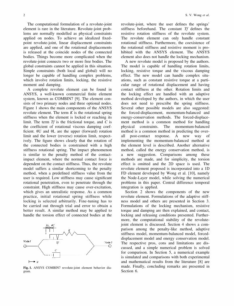
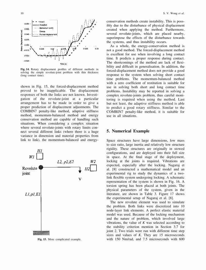
Fig. 14. Rotary displacement profiles of different methods insolving the simple revolute-joint problem with thin thickness(long contact time).

shown in Fig. 15, the forced-displacement methodproved to be inapplicable. The displacementresponses of both the links are not known. Investi-gation of the revolute-joint at a particulararrangement has to be made in order to give aproper prediction of displacement adjustments. TheCOMBIN7 penalty-like method, adaptive stiffnessmethod, momentum-balanced method and energyconservation method are capable of handling suchsituations. When considering a complex situationwhere several revolute-joints with rotary limits con-nect several different links (where there is a hugevariance in dimension and material properties fromlink to link), the momentum-balanced and energy-

Fig. 15. More complicated example.

conservation methods create instability. This is poss-ibly due to the disturbance of physical displacementcreated when applying the method. Furthermore,several revolute-joints, which are placed nearby,superimpose the effects of the disturbance towardsthe systems, and thus instability occurs.

As a whole, the energy-conservation method isnot a good method. The forced-displacement methodis excellent for use when involving a long contacttime. It predicts a proper response during contact.The shortcomings of the method are lack of flexi-bility and difficult in generalisation. In addition, theforced-displacement method does not provide a goodresponse to the system when solving short contacttime problems. The momentum-balanced methodwith a zero coefficient of restitution is suitable foruse in solving both short and long contact timeproblems. Instability may be reported in solving acomplex revolute-joints problem, thus careful moni-toring is required when using the method. Lastbut not least, the adaptive stiffness method is ableto predict a good rotary stiffness. Similar to theCOMBIN7 penalty-like method, it is suitable foruse in all situations.

5. Numerical Example

Space structures have large dimensions, low massto size ratio, large inertia and relatively low structurerigidity. These structures are originally in stowedconfigurations, and are deployed into their full sizein space. At the final stage of the deployment,locking at the joints is required. Vibrations areexpected, especially after the locking. Nagaraj etal. [8] constructed a mathematical model and anexperimental rig to study the dynamics of a two-link flexible system undergoing locking. A schematicrepresentation of the system is shown in Fig. 16. Atorsion spring has been placed at both joints. Thephysical parameters of the system, given in theliterature, are shown in Table 3. Figure 17 showsthe experimental setup of Nagaraj et al. [8].

The new revolute element was used to simulatethe problem. Both links were discretized into 10node-layer link elements. A perfect elastic materialmodel was used. Because of the locking mechanismand the nature of problem, which involved largevibrations, the value of K was selected according tothe stability criterion mention in Section 3.7 forjoint 2. Two trials were run with different time stepsizes and values of K. They are 15 microsecondswith 150 Nm/rad, and 7.5 microseconds with 600

11Development of Revolute-Joint Elements

Fig. 16. Schematic diagram of the two-link undergoing locking problem.

Table 3. Physical parameters of numerical example [8]

Link 1 and Joint 1

Length (m) 1.006423Cross-sectional area (m2) 1.78076e-4Thickness (m) 4.4519e-3Area moment of inertia (m4) 2.94113e-10Rotary inertia (kgm2) 8.5948e-4Flexural rigidity 20.5879Young’s Modulus 7e10Link mass (kg) 0.52334Tip Mass (kg) 1.2Rotary Friction – Torque (Nm) 0.03825Torsion spring stiffness (Nm/rad) 0.0789Pre-rotation angle (°) 300Initial rotary displacement (°) 0Locking rotary displacement (°) 90

Link 2 and Joint 2

Length (m) 0.9945Cross-sectional area (m2) 1.7748e-4Thickness (m) 4.437e-3Area moment of inertia (m4) 2.9117e-10Rotary inertia (kgm2) 9.256e-4Flexural rigidity 20.3819Young’s Modulus 7e10Link mass (kg) 0.42958Tip Mass (kg) 0.336Rotary Friction – Torque (Nm) 0.0225Torsion spring stiffness (Nm/rad) 0.0768Pre-rotation angle (°) −60Initial rotary displacement (°) 180Locking rotary displacement (°) 0

Nm/rad. The forced-displacement method was usedfor joint 1.

Figures 18 and 19 show the rotary displacementhistories at both joints. Experimental results, anexact solution (rigid model) and Nagaraj et al.’smodel is compared to the authors’ model. It isobvious from Fig. 18 that the model of Nagaraj etal., and the present models compromise each other

Fig. 17. (a) Experimental setup of the two-link undergoing lock-ing problem; (b) first joint assembly initial configuration [8].

Fig. 18. Rotary displacement profile at joint 1 of the two-linkundergoing locking problem.

12 S. V. Wong et al.

Fig. 19. Rotary displacement profile at joint 2 of the two-linkundergoing locking problem.

before the locking at joint 2 occurs. After locking,the present models tend to follow the path of therigid model [8], whereas the model of Nagaraj etal. deviates from the rigid model and follows theexperimental result. An additional consideration wasapplied by Nagaraj et al., where a part of the kineticenergy of link 2 is transformed into flexural strainenergy and flexural kinetic energy. This caused ahigh peak tip displacement of up to 20.5% of thetotal length after locking [8]. As a perfect elasticmaterial model was used in the present solutions,the responses are expected to follow the rigid model.The use of a smaller time step size with a higherrotary stiffness produced a slightly faster recoveryfrom the locking. The difference is small, and thepeak of the vibration profile is very close to thesmaller time step size model. Figure 19 shows thatthe present models have a closer response to theexperimental result compared to Nagaraj et al.’smodel. After locking, a smaller time step size witha higher rotary stiffness gives a more stable responsein terms of the rigidity of locking joint 2. A smallamplitude of oscillation is observed with a lowerrotary stiffness model. Note that the model of Naga-raj et al. stopped predicting after reaching the rotarylimit (approximately at time = 3 seconds).

All simulation results, from both the present mod-els as well as Nagaraj et al.’s model, for joint 1before locking are different from the experimentalresult. The authors incorporate additional frictionaltorque with zero damping at both joints; 0.175 N-m and 0.008 N-m for joints 1 and 2, respectively.An excellent correlation between the new simulationmodel and the experimental result is obtained. Figure20 illustrates the simulation results of the presentmodel with and without additional joint frictions,and the experimental result. This shows that theexperimentally determined joint frictions (see Table3) may be inaccurate, especially at joint 1.

Fig. 20. Rotary displacement profile at joint 1 with/withoutadditional friction of the two-link undergoing locking problem.

6. Summary and Conclusion

The development of an explicit revolute-jointelement is explained in detail in this paper. Theelement is capable of handling revolute-joints withrotary limits, locking, resistive moment and dampingeffects. The authors show the effects of differentcontact and releasing conditions. Several possibleways of handling the rotary limits have been shownand validated. Two novel methods to tackle therotary limits are presented: the adaptive stiffnessmethod and the energy method. A new implemen-tation of the momentum-balanced method has beensuccessfully implemented. The conventional COM-BIN7 penalty-like method and the forced-displace-ment method are included. Studies on the character-istics of the methods have been carried out whilesolving numerical problems. Several drawbacks andlimitations of the methods were briefly discussed.A new stability criterion has been suggested forwhen using a revolute-joint, especially when involv-ing a locking mechanism. Further study in the com-putational stability of the revolute-joint is required.

The energy method is not a good method,although it can prevent the rotating links from col-lapsing. The conventional forced-displacementmethod is good, but suffers from flexibility, andshows inefficiency in solving problems with a shortcontact time. The penalty-like method needs user-defined parameters, which are normally unknownand are not important to the user. The authors haveshown the capability of the new adaptive stiffnessmethod to predict a proper rotary stiffness to handlerotary limits, which are better compared to the user-defined values in the penalty-like method. The useof the momentum-balanced method with a coef-ficient of restitution ranging from perfect plasticto perfect elastic has also been shown. From theresults of simulation, the perfect plastic momentum-

13Development of Revolute-Joint Elements

balanced method is recommended. In short, theadaptive stiffness method with releasing conditionsof Eq. (13) and the perfect plastic momentum-balanced method predicted an excellent responsewhen compared to the exact solution.

An example from the literature, which involveda locking mechanism, was solved with the node-layer link element, an explicit finite differencemodel, and the new revolute element. The stiffnessvalue was predicted from the stability criterion. Thenumerical results show very good correlation to theexact solution. When compared to the experimentalresults, a reasonable prediction was given as a per-fect elastic material model was used.

The new revolute-joint element can be incorpor-ated into any implicit, explicit, finite difference orfinite element solver. In addition, the new adaptivestiffness method with releasing conditions of Eq.(13) can be used as a replacement to the conven-tional penalty-like method. When involving a lock-ing mechanism, the proposed stability criterionshould be used to prevent instability, and the stiff-ness value has to be revised.

References

1. Gauitier, P. E., Cleghorn, W. L. (1992) A spatiallytranslating and rotating beam element for modelingflexible manipulators. Mechanism and MachineTheory, 27, 415–433

2. Sunada, W. H., Dubowsky, S. (1983) The application

of finite element methods to the dynamics of flexiblelinkage systems. ASME Journal of Mechanical Design,103, 643–651

3. Theodore, R. J., Ghosal, A. (1995) Comparison ofassumed mode and finite element method for flexiblemultilink manipulators. International Journal of Robot-ics Research, 14, 91–111

4. Wang, Y., Huston, R. L. (1994) A lumped parametermethod in the nonlinear analysis of flexible multibodysystems. Computers and Structures, 50, 421–432

5. Khulief, Y. A., Shabana, A. A. (1986), Dynamicanalysis of a constrained system of rigid and flexiblebodies with intermittent motion. ASME Journal ofMechanism, Transmission and Automation in Design,108, 38–45

6. Rismantab-sany, J., Shabana, A. A. (1990) On theuse of momentum balance in the impact analysis ofconstrained elastic systems. ASME Journal ofVibration and Acoustics, 112, 119–126

7. Yigit A. S., Ulsoy, A. G., Scoot, R. A. (1990) Spring-dashpot models for the dynamics of a dynamics of aradially rotating beam with impact. Journal of Soundand Vibration, 142, 515–525

8. Nagaraj, B.P., Nataraju, B.S., Ghosal, A. (1997)Dynamics of a two-link flexible system undergoinglocking: mathematical modeling and comparison withexperiments. Journal of Sound and Vibration, 207,567–589

9. Kohnke, P. (1997) ANSYS Theory Reference Release5.4: 8th Edition. ANSYS, Inc.

10. Wong, S. V., Hamouda, A. M. S., Hashmi, M. S. J.(2000) Structural dynamic responses with generalizedexplicit finite difference models. Proceedings of theInternational Crashworthiness Conference, London,UK, 186–197

11. Hallquist, J. O. (1991) LS-DYNA3D Theoretical Manual.Livermore Software Technology, Livermore