Development of Parallel Pseudo-Spectral Solver Using Influence Matrix Method and Application to Boundary Layer Transition

Engineering Applications of Computational Fluid Mechanics Vol. 8, No. 1, pp. 158–177 (2014)

158

DEVELOPMENT OF PARALLEL PSEUDO-SPECTRAL SOLVER

USING INFLUENCE MATRIX METHOD AND APPLICATION TO

BOUNDARY LAYER TRANSITION

S. Bhushan+*

and D. K. Walters

#

+Center for Advanced Vehicular Systems, Mississippi State University, Starkville, MS 39762, USA

#Department of Mechanical Engineering, Mississippi State University, Starkville, MS 39762, USA

*E-Mail: [email protected] (Corresponding Author)

ABSTRACT: The performance of a pseudo-spectral solver, which uses FFT in the streamwise and spanwise

directions and Chebyshev polynomials in the wall-normal direction, is improved by implementing MPI domain

decomposition for the Chebyshev collocation method using the influence matrix method. The parallel code is

validated for LES of plane channel flow at Re=590 and 2003, and applied for temporally developing flat plate

transition simulations. The domain decomposition using the influence matrix method is implemented to achieve C1

continuity of the velocity across the domain interface. The method provides super linear scalability of solver

computational performance. The predictions show kinks in the turbulent statistics on coarser grids, but agree very

well with DNS data for finer grids. It is found that accurate turbulent predictions require a minimum of 48

collocation points per subdomain for Re ~ 105, with higher numbers required for Re ~ 10

6. The flat plate transitional

flow simulation is performed for a freestream turbulence intensity of 1.8%, which predicts the beginning of bypass

transition at Rex=9.2×105, turbulent overshoot in the wall shear stress profile for Rex=1.42-1.72×10

6, and a fully

developed turbulent region for higher Rex. Analysis of vortical structure show that the transition occurs due to the

formation of turbulent spots, which are in return formed due to the merger of near wall low strength elongated

structures. The growth of the turbulent spot is sustained by ejection sweep events from the wall. The results

demonstrate that a temporally developing simulation is a viable, inexpensive alternative to the commonly used

spatially developing approach for boundary layer transition prediction.

Keywords: parallel solver, pseudo-spectral solver, influence matrix method, channel flow, boundary layer

transition

1. INTRODUCTION

Bypass transition flows are common in

engineering systems, for which Reynolds

averaged Navier-Stokes (RANS) solvers are

typically used for design applications. RANS

transition modeling methods range from

correlation-based to physics-based models

(Walters and Cokljat, 2008; Yakinthos, 2013).

However, the available models are not mature

enough to be used with confidence for a wide

range of applications, and often parametric study

is performed to identify the most accurate

combination of numerical schemes and models,

e.g., the Baxevanou and Fidaros (2008) study for

wind turbine applications. Walters and Cokljat

(2008) suggest that one key reason for the

uncertainty in transition modeling is the limited

availability of detailed, large-scale validation

datasets from either experiments or state-of-the-

art numerical methods such as Large Eddy

Simulation (LES) or Direct Numerical Simulation

(DNS). The motivation of this study is to develop

a scalable pseudo-spectral solver for DNS/LES of

flat plate boundary layer transition flows, and use

it to generate a large-scale parametric dataset for

use by model developers. This study is a first step

towards this goal and focuses on parallelization of

a pseudo-spectral solver using a hybrid

MPI/OpenMP approach, and demonstration of

temporally developing simulations as a viable

approach for flat plate boundary layer

simulations. The following provides a review of

the LES/DNS studies for flat plate boundary layer

transition available in the literature.

1.1 Literature review

To date, high fidelity numerical studies of flat

plate boundary layers have helped to highlight the

underlying transitional flow physics. Studies

agree that freestream disturbances enter the

boundary layer and induce low-frequency stream-

wise vortices or streaks in the pre-transitional

region (referred to as Klebanoff modes), which

lift from the wall causing ejection events.

Transition occurs due to the formation of

turbulent spots which are associated with multiple

Received: 5 Nov. 2012; Revised: 31 Oct. 2013; Accepted: 25 Nov. 2013

Engineering Applications of Computational Fluid Mechanics Vol. 8, No. 1 (2014)

159

head hairpin type vortices with U- or -shaped

structures underneath them. However, studies

have not reached a consensus regarding the

turbulent spot formation and turbulence

production mechanisms. Singer and Joslin (1994)

concluded that the hairpin vortices are formed

due to the initial disturbances, and are not related

to the near-wall ejection process. Wu and Moin

(2009) arrived at a similar conclusion regarding

turbulent spot generation, and proposed that the

self-sustained auto-regeneration of the hairpin

structures is responsible for turbulence

production. They also suggested that the hairpin

structures leave behind elongated streak like

structures as they are ejected from the wall, thus

streaks are merely a kinematic feature (symptom)

not the cause of breakdown. The auto-

regeneration of hairpin vortices as a key

turbulence production mechanism has also been

supported by Kim et al. (2008) for turbulent

channel flow at relatively low Reynolds number

(Re = 395) and by Wallace et al. (2010) in

transitional flow studies. Zaki and Durbin (2005)

and Jacobs and Durbin (2010) proposed that the

spots exhibit Kelvin-Helmholtz type instability

and are formed due to the interaction of lifting

streaks and the high-frequency freestream

disturbances at the edge of boundary layer.

Schlatter et al. (2008) proposed that the spots are

formed due to streak secondary instability,

wherein the streaks interact to first form -shaped

structures, which evolve into hairpin structures.

This process is sustained by the advection of

turbulence via ejection events. Jeong et al. (1997)

also identified ejection/sweep events as the

primary cause of turbulence production for

turbulent channel flow simulations at Re = 180.

But they did not observe hairpin vortices,

probably because the study focused only on the

sub- and buffer layer regions.

DNS and LES of canonical flows such as flat

plate boundary layers are well suited for

understanding transition flow physics and

obtaining detailed datasets for model validation.

However, very limited datasets are available in

the open literature, and these are typically

performed for moderate Reynolds numbers (Rex ~

105) and high freestream turbulence intensities

(FSTI 5%) (Wu and Moin, 2009; Jacobs and

Durbin, 2001; Schlatter et al., 2008). Real

applications involving bypass transition may

include a broad range of turbulent intensities from

1% to 10% or more, and transition is expected to

occur at much higher Reynolds number (Rex ~

2×106) for low FSTI values. Further, prior

simulations have often been performed by

imposing manufactured/controlled instabilities

(Schlatter et al., 2008) or bursts of isotropic

fluctuations (Wu and Moin, 2009), and have

mostly focused on the analysis of boundary layer

breakdown rather than the dissemination of

parameterized statistical data for model

development. The study most relevant to this

work is that of Brandt et al. (2004) wherein DNS

was performed for FSTI of 1.5% to 4.7% with

integral length scales of 2.5 to 7.5 times the

displacement thickness. The lack of a

comprehensive dataset is likely due to the high

computational cost associated with DNS/LES,

which require: (a) highly accurate numerical

schemes for accurate prediction of the small-scale

turbulent structures; and (b) large numbers of grid

points and small time steps, which increase

significantly for higher Re.

Pseudo-spectral methods provide an accurate

scheme for DNS/LES of canonical

incompressible flows. The most commonly used

solvers are based on Fourier modes to represent

the flow field along homogenous streamwise and

spanwise directions, and Chebyshev polynomials

along the non-homogenous wall-normal direction

(Kim et al., 1987; Moser et al., 1999). One

drawback of these solvers is that they are not well

suited for parallel domain decomposition. This is

because spectral methods require all of the data

along a given grid direction to obtain derivatives,

thus data transfer requirements are large.

Schlatter et al. (2008) performed DNS of

transitional flows for relatively low Re = 4.1×104

using a pseudo-spectral solver parallelized only

along one of the homogeneous directions.

Schlatter et al. (2009) extended the solver to

include domain decomposition along both

homogenous directions and applied it for

turbulent boundary layer simulations at Re =

1.2×106. Some recent studies have used finite

difference solvers, probably due to the scalability

limitations of pseudo-spectral solvers. Hoyas and

Jimenez (2006) performed DNS of plane channel

flow at Re = 4.86×104 using a pseudo-spectral

solver which used a seven-point compact finite

difference scheme in the wall-normal direction.

Wu and Moin (2009) performed DNS of a

transitional boundary layer at Re = 3.85×105

using a 2nd

order finite-difference solver. Borell et

al. (2011) recently developed a solver for

turbulent boundary layer simulations that uses a

fourth-order compact finite difference scheme in

the streamwise and wall normal directions and

FFT along the spanwise direction.

Engineering Applications of Computational Fluid Mechanics Vol. 8, No. 1 (2014)

160

Multi-domain techniques for Chebyshev

collocation methods for parallel computations

have been documented by Peyret (2001). They

discuss influence matrix and iterative methods. In

both approaches, the governing equations are

decomposed on different domains along with

interface conditions to satisfy continuity of both

the variable and its derivatives at the domain

interface. In the influence matrix method, the

variable is decomposed into two components: one

with predefined null boundary conditions and a

second to satisfy the boundary and interface

conditions. The solution of the second component

requires evaluation of influence coefficients,

which change with the interface conditions. In the

iterative approach, the equations on one side of

the domain interface are solved using Dirichlet

type boundary condition, and on the other side

using Neumann type conditions. The equations

are solved iteratively until the interface conditions

are satisfied. As expected, the iterative method is

significantly more expensive compared to the

influence matrix method, thus the latter has been

used in several studies. Raspo et al. (1996)

applied the technique for laminar flow simulation

within a cavity type configuration with a

singularity. They reported that the single-domain

simulation predicts large Gibbs oscillations due to

the singularity, whereas the multi-domain

simulations minimize the oscillations. Gibbs

oscillations have also been reported in several

other studies for problems which exhibit rapid

spatial variation in the solution (refer to Yang and

Shizgal, 1994). The multi-domain approach helps

to overcome this limitation, as it limits the

influence of large gradients within each sub-

domain thereby enhancing convergence. Sabbah

and Pasquetti (1998) developed a 3D solver using

multi-domain Chebyshev polynomials in two

directions and FFT along the third direction. The

method was validated for Rayleigh-Bernard

convection in a cavity of large aspect ratio at

Rayleigh number Ra = 3000, which involved

smooth laminar flow. The solver has also been

successfully applied for LES of turbulent flow

past a square cylinder and an Ahmed body by

Minguez et al. (2008 and 2011).

High computational costs associated with

transitional flow studies in the literature are also

due to the use of a spatially developing approach,

which requires a relatively large flow domain in

order to resolve the entire region of the boundary

layer that contains the relevant flow physics. In

addition, such simulations with a pseudo-spectral

solver require a fringe region in the streamwise

direction so that the periodic flow can be mapped

to appropriate inlet boundary conditions (Spalart,

1988; Khurajadze and Oberlack, 2004; Schlatter

et al., 2008). Such mapping requires

decomposition and transformation of the

governing equations, which does not accurately

represent turbulent straining as pointed out by Wu

and Moin (2009).

Temporally developing simulations represent an

alternative to the spatially developing approach.

In this approach, the numerical domain moves

along with the developing flow in the streamwise

direction due to the use of periodic boundary

conditions, and it has been applied successfully

for DNS/LES of mixing layer and jet flows

(Ansari, 1997; Akhavan et al., 2000; Bhushan et

al., 2006). Malik and Hussaini (1990) used this

approach for transitional and turbulent boundary

layer simulations, including study of the

interaction of Gortler vortices and Tollmein-

Schlichting waves in a boundary layer developing

on a concave surface. Overall, the temporally

developing simulations are less numerically

expensive than their spatially developing

counterparts, as they require an order of

magnitude smaller domain along streamwise

direction. Further, they do not involve a debatable

fringe region for purposes of recycling the

boundary conditions. A smaller number of grid

points along the streamwise direction also means

less data communication for FFT calculations,

when domain decomposition is used along FFT

directions, and better parallel performance. In

addition, input/output (I/O) file sizes and time are

reduced, and averaged quantities at any instant

can be obtained from the solutions along

homogeneous directions. The relative

disadvantages of the temporally developing

approach include a larger required number of

time steps and more frequent I/O than the

spatially developing simulations.

1.2 Objectives and approach

The objectives of this study are to: (1) implement

and validate a hybrid MPI/OpenMP

parallelization to a pseudo-spectral solver, and (2)

demonstrate that a temporally developing

approach is a viable method for transitional

boundary layer simulations. The pseudo-spectral

solver used herein was previously developed and

validated for channel and free-shear flows

(Bhushan and Warsi, 2005; Bhushan et al., 2007).

In this study, the computational performance of

the solver is improved by using OpenMP thread

parallelization for FFT, and MPI parallelization

along the wall-normal direction using the

Engineering Applications of Computational Fluid Mechanics Vol. 8, No. 1 (2014)

161

influence matrix method for the Chebyshev

collocation method, as discussed in the following

section. In section 3, the parallel solver is

validated for plane channel flow LES predictions

at Re = 590 and 2003 using DNS datasets. In

section 4, the scalability of the solver is studied

and performance bottlenecks are identified. The

solver is applied for LES of a temporally

developing transitional flat plate boundary layer

in section 5, and results validated for prediction

of integral quantities. Conclusions of the study

and future work are summarized in section 6.

2. NUMERICAL METHOD

LES requires solution of the filtered Navier–

Stokes equations:

(1a)

The term on the right hand side is the subgrid

stress (SGS) tensor, which in the present study is

obtained using the Dynamic Smagorinsky model

(DSM) (Lilly, 1992). The equations are

discretized using the pseudo-spectral method

employing Fourier series in the streamwise (x1)

and spanwise (x3) directions and Chebyshev

polynomials in the wall-normal direction (x2). The

equations are solved using a fractional step

method, where the equations at every time step

are solved in three steps. The procedure is

summarized here; readers are referred to Bhushan

et al. (2007) for details.

The first step marches the convective term using

the second-order Adams Bashforth method,

where the superscript (1) (or 2 as used below)

implies the level of the fractional step, (N) the

time iteration level and t is the time step size.

The second step is the pressure correction step

which imposes incompressibility. The equations

solved in this step are:

(3a)

(3b)

Employing the Fourier transform along x1 and x3,

where the transform is defined as below for a

variable :

(4)

Eqs. (3a and b) reduces in wave number space

as:

(5a)

(5b)

(5c)

(5d)

The third step incorporates the viscous and

subgrid stresses, which in wave number space is:

where l = 1,2,3 and are computed from .

The calculation of the 2nd

and 3rd

terms on the

right-hand side of Eq. (2) and the turbulent

stresses in Eq. (6) involve convolution in the

wave number space, which is complicated to

perform. Thus, they are computed in physical

space using the 3/2 dealiasing rule, and hence the

solver is called “pseudo-spectral.” This procedure

requires inverse FFT computations of 3 velocity

and 6 derivative components to move data from

wave number to physical space. After the

convective (or stress) terms are computed, they

are transferred to the wave number space; this

requires 3 FFT computations for the convective

step and 6 for the viscous step. The FFT’s are

performed using FFTW subroutines version 3.3

(Frigo and Johnson, 2011).

The high performance computing of the solver

includes shared memory OpenMP thread

parallelization for the FFT calculations using the

FFTW multi-thread library (Frigo and Johnson,

2011). Message Passing Interface (MPI)

parallelization along the x2-direction using

influence matrix method is discussed in section

2.3.

2.1 Solution of 1-D Helmholtz equation using

Chebyshev collocation method

Equations (5a) and (6) are 1-D Helmholtz

equations for each point, which are solved

using the Chebyshev collocation method. The

following summarizes the solution procedure for

a general equation with general Robin-type

boundary conditions (refer to Peyret, 2001):

(7)

The numerical domain is algebraically mapped

to a solution domain as discussed in

Section 2.2. The simulation domain is discretized

(1b)

(2)

(6)

Engineering Applications of Computational Fluid Mechanics Vol. 8, No. 1 (2014)

162

into N grid points, which are the Gauss-Lobatto

points :

(8)

The mapping of Eq. (7) results in:

(9a)

(9b)

(9c)

where, , , and are coefficients

associated with boundary conditions. The

derivatives are calculated using a collocation

method wherein,

(10a)

(10b)

(11b)

Thus Eq. (7) is discretized as:

Equations (12a and b) can be combined as (N+1)

algebraic equations:

(13)

Equation (13) is solved by a matrix

diagonalization method. In this approach, first the

matrix is decomposed as:

(14)

where is the right eigenvector matrix and is

the diagonal matrix consisting of eigenvalues .

Since is a function of grid only, its

eigenvalues and vectors are computed at the

beginning of the simulation using LAPACK subroutines (Anderson et al., 1995) and stored.

Equation (14) is solved in three simple matrix multiplication steps:

(a)

(b) (15)

(c).

2.2 Mapping of numerical domain to

Chebyshev solution domain

The numerical domain ( ) is mapped to the

Chebyshev solution domain ( ) via the following

algebraic functions:

Channel flow:

; and (16a)

Flat plate boundary layer:

; ;

(16b)

where, and .

2.3 Multi-domain solution of 1-D Helmholtz

equation using influence matrix method

Multi-domain solution of Eqs. (9a-c) using the

influence matrix method is summarized below,

readers are referred to Peyret (2001) for further

details. First assume M sub-domain partitions

each with

points, where a0 = -1 and aM = 1. The

points in each sub-domain are mapped to Gauss-

Lobatto points :

(17)

which are then mapped to the domain by a

linear mapping:

(18a)

(18b)

(18c)

The 1-D Helmholtz equation for each sub-domain

is expressed in algebraic form, similar to those

discussed in Section 2.1.

where

and is solved with interface conditions:

(11a)

(12a)

(12b)

: (19a)

(19b)

Engineering Applications of Computational Fluid Mechanics Vol. 8, No. 1 (2014)

163

and boundary conditions:

(19e)

(19f)

Solutions of the above equations are sought in the

form:

The part of the solution is obtained by

solving the equation:

(21b)

The part of the solution is obtained as:

where are the influence matrix coefficients.

The solutions and are obtained by

solving:

(23b)

(23d)

It must be noted that both and

solutions do not depend on the instantaneous

solution, and can be solved at the beginning of the

iterations and saved. Substituting , and

in Eqs. 19(c-f), the equations for the

influence matrix are obtained:

Eqs. (24a-c) constitute an (M+1) algebraic system

of equations:

[ (25)

where [ is a tridiagonal matrix, which is a

function of and , and is calculated

before the numerical iteration. is a vector

array of unknowns , and is a

vector function of . The influence matrix is

computed as:

(26)

where the inverse of the matrix is obtained using

the LAPACK subroutines. The final solution is

obtained by using the λi values in Eq. (22) and

from superposition of solutions in Eq. (20).

Summary. The steps involved in the

implementation of the multi-domain Helmholtz

solver using Chebyshev collocation method are:

1. Partition solution domain into M sub-

domains . Distribute

points in each sub-domain on Gauss-Lobatto

points . Obtain an analytic mapping

function to map to . Obtain the

matrix in Eqs. (19) and compute associated

eigenvalues and eigenvectors.

2. Solve Eqs. (23) following the methodology

presented in Eqs. (15) and save

and .

3. Evaluate matrix [ from Eqs. (24), and

compute [ to be used in Eq. (26). Both

the steps 2 and 3 do not change with time

step, thus is performed before the numerical

iteration and results are saved.

4. Evaluate , which is the RHS term in

Eqs. 5(a) and (6), and solve Eqs. (21)

following Eq. (15) to obtain .

5. Compute the derivative of and use the

values at the domain interfaces along with

boundary condition coefficients , ,

and to obtain in Eq. (25). Then, solve

Eq. (26) to obtain influence matrix

coefficients .

6. Use and saved variables and

to obtain from Eq. (22).

7. Obtain updated solution using Eq. (20) from

solutions obtained from steps 4 and 6. Note

(19c)

(19d)

(20)

(21a)

(22)

(23a)

(23c)

: (24a)

(24b)

(24c)

Engineering Applications of Computational Fluid Mechanics Vol. 8, No. 1 (2014)

164

that Eq. (20) also includes the velocities at the

interface, so Eqs. (19c and d) are satisfied.

8. For solution at next time iteration repeat steps

4-7.

Note that step 5 is solved by the root processor

only, which broadcasts λi values to other

processors. Thus, MPI parallelization requires a

total of 2×x1×x3×M data transfers, i.e., each

processor sends values at the sub-domain

interfaces to the root processor.

2.4 Validation of multi-domain solver for 1-D

Helmholtz equation

The multi-domain solver was first implemented

and tested for a model equation:

(27)

where, and the boundary

conditions are . The

analytic solution of the above equation is:

where

and

(28b)

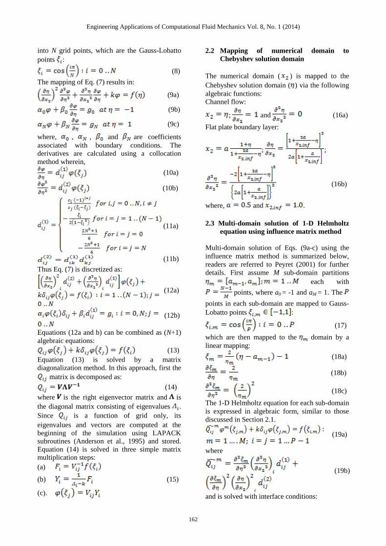
Test simulations are performed using 193 points

partitioned into 1 to 16 sub-domains with as few

as 13 points per sub-domain.

The numerical predictions compared very well

with the analytic simulations for all the domains,

as shown in Fig. 1. In Fig. 1a, the L2 norm of the

error (difference between the analytic and

numerical predictions) decreases approximately

two orders of magnitude as the number of sub-

domains is increased from 1 to 16. Consistent

with previous studies, improved convergence is

expected in the multi-domain simulations, since

the predictions depend only on the gradients

within each sub-domain (Yang and Shizgal,

1994). Figs. 1b-1e show the different solution

components, the influence matrix coefficients,

and comparison of the numerical results with the

analytic solution for the 8 sub-domain

simulations. It is evident that the influence matrix

coefficients play a significant role in the solution

process, wherein very simple curves are

combined to obtain complex solutions.

3. TURBULENT CHANNEL FLOW

SIMULATIONS

The first LES test case is turbulent channel flow

at Re = 590 (Re = 1.26×104). Results are

compared to available DNS data (Moser et al.,

1999). The study seeks to evaluate the effect of

MPI domain decomposition on the solution and

determine appropriate grid requirements for the

turbulent flow simulations. The solver is then

applied for a higher Re = 2003 (Re = 4.86×104)

case. The predictions are validated using DNS

data (Hoyas and Jimenez, 2006) and compared

with the Re = 590 predictions. The vortical and

turbulent structures of the flow are analyzed and

compared with DNS predictions for Re = 180

(Jeong et al., 1997). Both channel flow

simulations were performed using a domain

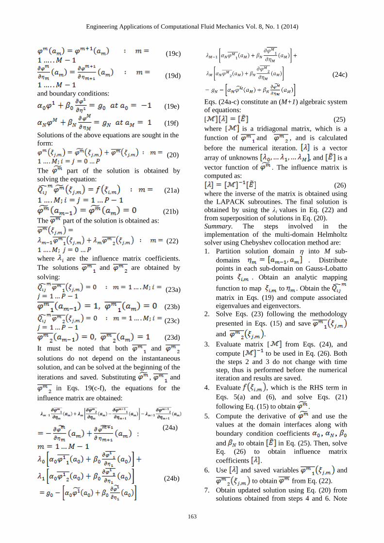
extent of 0 ≤ x1 ≤ 2, 0 ≤ x3 ≤ and -1 ≤ x2 ≤ 1. A

representative illustration showing the flow

domain, grid distribution and boundary conditions

is shown in Fig. 2(a). Grid points are uniformly

distributed in the streamwise and spanwise

directions. The grid in the wall normal direction

is refined near the wall and at domain interfaces

for appropriate near wall resolution and accurate

calculation of influence matrix coefficients,

respectively. The simulations use periodic

boundary conditions in x1 and x3 directions, and

no-slip boundary conditions at x2 = -1 and 1. The

grids used for this study are summarized in

Table1.

3.1 Re = 590 results

The Re = 590 case was performed on a

64×97×64 grid using 1, 2 and 4 processors along

the x2 direction, which are referred to as cases

Ch1-G4, Ch1-G3 and Ch1-G2, respectively. The

Ch1-G4, Ch1-G3 and Ch1-G2 cases consist of 97,

49 and 25 points in the x2 direction for each sub-

domain, respectively. Two additional finer grids

along the x2 direction, namely Ch1-G1 and Ch1-

G0, are also used. The former consists of 2 sub-

domains with 65 points in x2 and the latter has 3

sub-domains with 49 points in x2. The normalized

grid resolution for the simulations is x1+ = 58,

x3+ = 29, x2,min

+ = 0.6 and x2,max

+ = 23, where

the normalization is performed using friction

velocity u and kinematic viscosity . The grids

are about 150 times coarser than the DNS grid

(Moser et al., 1999) and are considered adequate

for LES.

(28a)

Engineering Applications of Computational Fluid Mechanics Vol. 8, No. 1 (2014)

165

1.E-07

1.E-06

1.E-05

1.E-04

0 4 8 12 16

Err

or

L2

No

rm(D

iffe

ren

ce b

etw

een

nu

meri

ca

l an

d a

na

lyti

c p

rofi

les)

Number of Sub-domain (a)

0

0.003

0.006

0.009

-1 -0.5 0 0.5 1

ᵠ-tild

e

y (b)

0

0.25

0.5

0.75

1

-1 -0.5 0 0.5 1

ᵠ 1

y (c)

0

0.25

0.5

0.75

1

-1 -0.5 0 0.5 1

ᵠ 2

y (d)

0

0.03

0.06

0.09

0.12

-1 -0.5 0 0.5 1

φ

y

Analytic

#Sub-domain = 8

(e)

Fig. 1 Test of multi-domain 1-D Helmholtz solver

using model equation: (a) L2 norm of the error;

(b-d) Component solutions for 8 multi-domain

case, and (e) Comparison of 8 multi-domain

predictions with analytic results. The inset in (e)

shows the influence matrix coefficients.

Fig. 2 Representative domain, subdomain

decomposition, grid distribution and boundary

conditions for (a) channel flow LES cases and

(b) flat-plate transitional boundary layer

simulation.

0

5

10

15

20

25

0.1 1 10 100

u+

y+

DNS

Ch1-G2

Ch1-G3

Ch1-G4

Ch1-G1

Ch1-G0

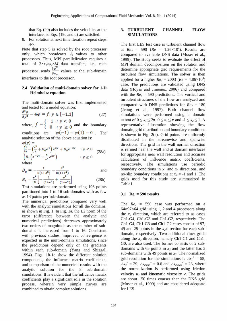
Fig. 3 Mean velocity profile predictions for Re = 590

compared with DNS (Moser et al., 1999).

As shown in Fig. 3, Ch1-G2, G3 and G4 mean

velocity predictions overall agree well with DNS

in the sub- and log-layers, but are under

predictive in the buffer and lower log-layers.

Ch1-G3 and G4 show errors of about 7%,

whereas Ch1-G2 shows error of about 15%. As

shown in Fig. 4, the turbulence intensity and

shear stress profiles predicted for the Ch1-G3 and

Ch1-G4 cases compare well with the DNS, except

Engineering Applications of Computational Fluid Mechanics Vol. 8, No. 1 (2014)

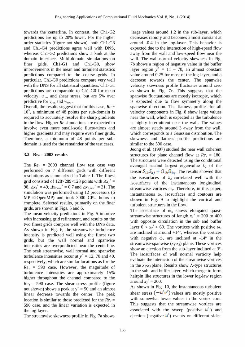
166

towards the centerline. In contrast, the Ch1-G2

predictions are up to 20% lower. For the higher

order statistics (figure not shown), both Ch1-G3

and Ch1-G4 predictions agree well with DNS,

whereas Ch1-G2 predictions show a kink at the

domain interface. Multi-domain simulations on

finer grids, Ch1-G1 and Ch1-G0, show

improvements in the mean and turbulent statistics

predictions compared to the coarse grids. In

particular, Ch1-G0 predictions compare very well

with the DNS for all statistical quantities. Ch1-G1

predictions are comparable to Ch1-G0 for mean

velocity, urms and shear stress, but are 5% over

predictive for vrms and wrms.

Overall, the results suggest that for this case, Re ~

105, a minimum of 48 points per sub-domain is

required to accurately resolve the sharp gradients

in the flow. Higher Re simulations are expected to

involve even more small-scale fluctuations and

higher gradients and may require even finer grids.

Therefore, a minimum of 48 points per sub-

domain is used for the remainder of the test cases.

3.2 Re = 2003 results

The Re = 2003 channel flow test case was

performed on 7 different grids with different

resolutions as summarized in Table 1. The finest

grid consisted of 128×289×128 points with x1+ =

98, x3+ = 49, x2,min

+ = 0.7 and x2,max

+ = 21. The

simulation was performed using 12 processors (6

MPI×2OpenMP) and took 3000 CPU hours to

complete. Selected results, primarily on the finer

grids, are shown in Figs. 5 and 6.

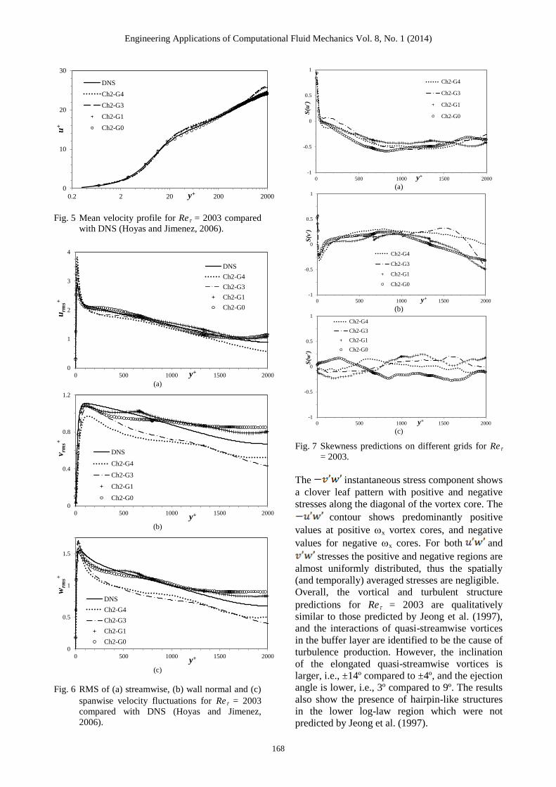
The mean velocity predictions in Fig. 5 improve

with increasing grid refinement, and results on the

two finest grids compare well with the DNS data.

As shown in Fig. 6, the streamwise turbulence

intensity is predicted well using the finest two

grids, but the wall normal and spanwise

intensities are overpredicted near the centerline.

The peak streamwise, wall normal and spanwise

turbulence intensities occur at y+ = 12, 70 and 40,

respectively, which are similar locations as for the

Re = 590 case. However, the magnitude of

turbulence intensities are approximately 15%

higher throughout the channel compared to the

Re = 590 case. The shear stress profile (figure

not shown) shows a peak at y+ = 50 and an almost

linear decrease towards the center. The peak

location is similar to those predicted for the Re =

590 case, and the linear variation is expected in

the log-layer.

The streamwise skewness profile in Fig. 7a shows

large values around 1.2 in the sub-layer, which

decreases rapidly and becomes almost constant at

around -0.4 in the log-layer. This behavior is

expected due to the interaction of high-speed flow

away from the wall and low-speed flow near the

wall. The wall-normal velocity skewness in Fig.

7b shows a region of negative value in the buffer

layer region y+ = 11 – 70, an almost constant

value around 0.25 for most of the log-layer, and a

decrease towards the center. The spanwise

velocity skewness profile fluctuates around zero

as shown in Fig. 7c. This suggests that the

spanwise fluctuations are mostly isotropic, which

is expected due to flow symmetry along the

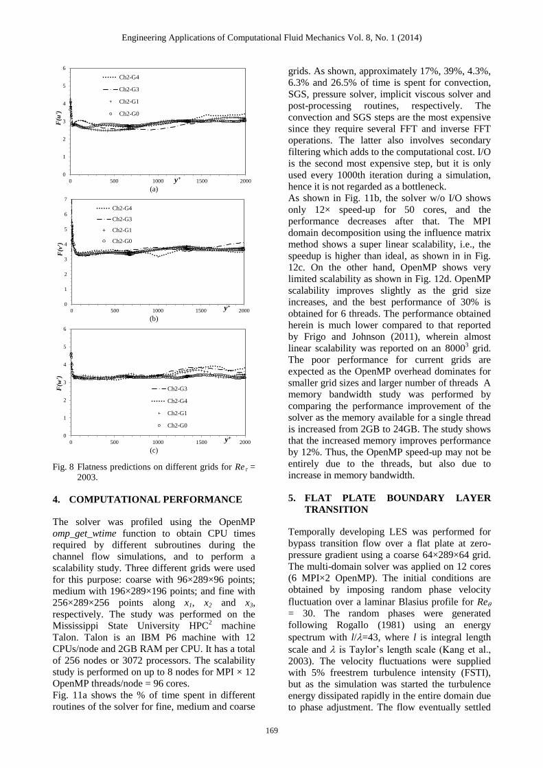
spanwise direction. The flatness profiles for all

velocity components in Fig. 8 show large values

near the wall, which is expected as the turbulence

is highly intermittent near the wall. The values

are almost steady around 3 away from the wall,

which corresponds to a Gaussian distribution. The

skewness and flatness profile predictions are

similar to the 590 case.

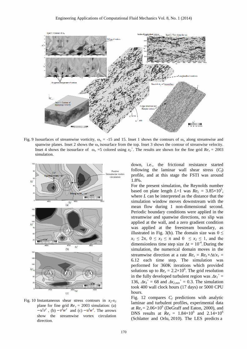
Jeong et al. (1997) studied the near wall coherent

structures for plane channel flow at Re = 180.

The structures were detected using the conditional

averaged second largest eigenvalue λ2 of the

tensor . The results showed that

the isosurfaces of λ2 correlated well with the

isosurfaces of the instantaneous longitudinal

streamwise vortices x. Therefore, in this paper,

instantaneous x isosurfaces and contours are

shown in Fig. 9 to highlight the vortical and

turbulent structures in the flow.

The isosurface of x shows elongated quasi-

streamwise structures of length x1+ = 200 to 400

with opposite circulation in the sub and buffer

layer 0 < x2+

< 60. The vortices with positive x

are inclined at around +14º, whereas the vortices

with negative x are inclined at -14º in the

streamwise-spanwise (x1-x3) plane. These vortices

show an ejection from the sub-layer inclined at 3º.

The isosurfaces of wall normal vorticity help

evaluate the interaction of the streamwise vortices

in the x1-x3 plane. Results show -type structures

in the sub- and buffer layer, which merge to form

hairpin like structures in the lower log-law region

around x2+ = 200.

As shown in Fig. 10, the instantaneous turbulent

shear stress values are mostly positive

with somewhat lower values in the vortex core.

This suggests that the streamwise vortices are

associated with the sweep (positive ) and

ejection (negative ) events on different sides.

Engineering Applications of Computational Fluid Mechanics Vol. 8, No. 1, pp. 158–177 (2014)

167

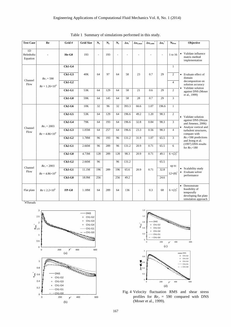
Table 1 Summary of simulations performed in this study.

Test Case Re Grid # Grid Size Nx Ny Nz x1+

x2,max+ x2,min

+ x3

+ NProc Objective

1D

Helmholtz

Equation

- He-G0 193 - 193 - - - - - 1 to 16 Validate influence

matrix method implementation

Channel

Flow

Re = 590

Re = 1.26×104

Ch1-G4

40K 64 97 64 58 23 0.7 29

1

Evaluate effect of

domain

decomposition on solution accuracy

Validate solution

against DNS (Moser

et al., 1999)

Ch1-G3 2

Ch1-G2 4

Ch1-G1 53K 64 129 64 58 21 0.6 29 2

Ch1-G0 59K 64 145 64 58 28 0.7 29 3

Channel

Flow

Re = 2003

Re = 4.86×104

Ch2-G6 10K 32 96 32 393.3 66.6 1.07 196.6 1

Validate solution against DNS (Hoyas

and Jimenez, 2006)

Analyze vortical and turbulent structures,

compare with

Re=590 predictions and Jeong et al.

(1997) DNS results

for Re=180

Ch2-G5 53K 64 129 64 196.6 49.2 1.20 98.3 2

Ch2-G4 79K 64 193 64 196.6 32.8 0.84 98.3 3

Ch2-G3 1.05M 64 257 64 196.6 23.3 0.56 98.3 4

Ch2-G2 1.78M 96 193 96 131.2 31.9 1.07 65.5 3

Ch2-G1 2.66M 96 289 96 131.2 20.9 0.71 65.5 6

Ch2-G0 4.73M 128 289 128 98.3 20.9 0.71 49.1 6 ×(2)*

Channel

Flow

Re = 2003

Re = 4.86×104

Ch3-G2 2.66M 96

289

96 131.2

20.9 0.71

65.5

up to

12×(8)*

Scalability study

Evaluate solver performance

Ch3-G1 11.1M 196 196 65.6 32.8

Ch3-G0 18.9M 256 256 49.2 24.6

Flat plate Re 2.2×106 FP-G0 1.18M 64 289 64 136 - 0.3 68 6 ×(2)

*

Demonstrate

feasibility of

temporally developing flat plate

simulation approach *

#Threads

0

0.5

1

1.5

2

2.5

3

0 200 400 600

urm

s+

y+

DNS

Ch1-G2

Ch1-G3

Ch1-G4

Ch1-G1

Ch1-G0

(a)

0

0.2

0.4

0.6

0.8

1

0 200 400 600

v rm

s+

y+

DNS

Ch1-G2

Ch1-G3

Ch1-G4

Ch1-G1

Ch1-G0

(b)

0

0.3

0.6

0.9

1.2

1.5

0 200 400 600

wrm

s+

y+

DNS

Ch1-G2

Ch1-G3

Ch1-G4

Ch1-G1

Ch1-G0

(c)

0

0.2

0.4

0.6

0.8

1

0 200 400 600

(uv+ 1

2)/ w

y+

DNS

Ch1-G2

Ch1-G3

Ch1-G4

Ch1-G1

Ch1-G0

(d)

Fig. 4 Velocity fluctuation RMS and shear stress

profiles for Re = 590 compared with DNS

(Moser et al., 1999).

Engineering Applications of Computational Fluid Mechanics Vol. 8, No. 1 (2014)

Engineering Applications of Computational Fluid Mechanics Vol. 8, No. 1 (2014)

168

0

10

20

30

0.2 2 20 200 2000

u+

y+

DNS

Ch2-G4

Ch2-G3

Ch2-G1

Ch2-G0

Fig. 5 Mean velocity profile for Re = 2003 compared

with DNS (Hoyas and Jimenez, 2006).

0

1

2

3

4

0 500 1000 1500 2000

urm

s+

y+

DNS

Ch2-G4

Ch2-G3

Ch2-G1

Ch2-G0

(a)

0

0.4

0.8

1.2

0 500 1000 1500 2000

v rm

s+

y+

DNS

Ch2-G4

Ch2-G3

Ch2-G1

Ch2-G0

(b)

0

0.5

1

1.5

0 500 1000 1500 2000

wrm

s+

y+

DNS

Ch2-G4

Ch2-G3

Ch2-G1

Ch2-G0

(c)

Fig. 6 RMS of (a) streamwise, (b) wall normal and (c)

spanwise velocity fluctuations for Re = 2003

compared with DNS (Hoyas and Jimenez,

2006).

-1

-0.5

0

0.5

1

0 500 1000 1500 2000

S(u

')

y+

Ch2-G4

Ch2-G3

Ch2-G1

Ch2-G0

(a)

-1

-0.5

0

0.5

1

0 500 1000 1500 2000

S(v

')

y+

Ch2-G4

Ch2-G3

Ch2-G1

Ch2-G0

(b)

-1

-0.5

0

0.5

1

0 500 1000 1500 2000

S(w

')

y+

Ch2-G4

Ch2-G3

Ch2-G1

Ch2-G0

(c)

Fig. 7 Skewness predictions on different grids for Re

= 2003.

The instantaneous stress component shows

a clover leaf pattern with positive and negative

stresses along the diagonal of the vortex core. The

contour shows predominantly positive

values at positive x vortex cores, and negative

values for negative x cores. For both and

stresses the positive and negative regions are

almost uniformly distributed, thus the spatially

(and temporally) averaged stresses are negligible.

Overall, the vortical and turbulent structure

predictions for Re = 2003 are qualitatively

similar to those predicted by Jeong et al. (1997),

and the interactions of quasi-streamwise vortices

in the buffer layer are identified to be the cause of

turbulence production. However, the inclination

of the elongated quasi-streamwise vortices is

larger, i.e., ±14º compared to ±4º, and the ejection

angle is lower, i.e., 3º compared to 9º. The results

also show the presence of hairpin-like structures

in the lower log-law region which were not

predicted by Jeong et al. (1997).

Engineering Applications of Computational Fluid Mechanics Vol. 8, No. 1 (2014)

169

0

1

2

3

4

5

6

0 500 1000 1500 2000

F(u

')

y+

Ch2-G4

Ch2-G3

Ch2-G1

Ch2-G0

(a)

0

1

2

3

4

5

6

7

0 500 1000 1500 2000

F(v

')

y+

Ch2-G4

Ch2-G3

Ch2-G1

Ch2-G0

(b)

0

1

2

3

4

5

6

0 500 1000 1500 2000

F(w

')

y+

Ch2-G3

Ch2-G4

Ch2-G1

Ch2-G0

(c)

Fig. 8 Flatness predictions on different grids for Re =

2003.

4. COMPUTATIONAL PERFORMANCE

The solver was profiled using the OpenMP

omp_get_wtime function to obtain CPU times

required by different subroutines during the

channel flow simulations, and to perform a

scalability study. Three different grids were used

for this purpose: coarse with 96×289×96 points;

medium with 196×289×196 points; and fine with

256×289×256 points along x1, x2 and x3,

respectively. The study was performed on the

Mississippi State University HPC2 machine

Talon. Talon is an IBM P6 machine with 12

CPUs/node and 2GB RAM per CPU. It has a total

of 256 nodes or 3072 processors. The scalability

study is performed on up to 8 nodes for MPI × 12

OpenMP threads/node = 96 cores.

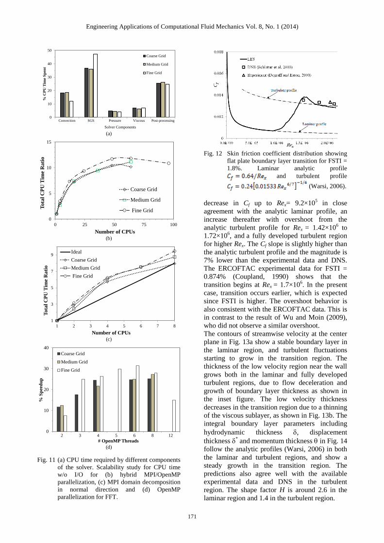
Fig. 11a shows the % of time spent in different

routines of the solver for fine, medium and coarse

grids. As shown, approximately 17%, 39%, 4.3%,

6.3% and 26.5% of time is spent for convection,

SGS, pressure solver, implicit viscous solver and

post-processing routines, respectively. The

convection and SGS steps are the most expensive

since they require several FFT and inverse FFT

operations. The latter also involves secondary

filtering which adds to the computational cost. I/O

is the second most expensive step, but it is only

used every 1000th iteration during a simulation,

hence it is not regarded as a bottleneck.

As shown in Fig. 11b, the solver w/o I/O shows

only 12× speed-up for 50 cores, and the

performance decreases after that. The MPI

domain decomposition using the influence matrix

method shows a super linear scalability, i.e., the

speedup is higher than ideal, as shown in in Fig.

12c. On the other hand, OpenMP shows very

limited scalability as shown in Fig. 12d. OpenMP

scalability improves slightly as the grid size

increases, and the best performance of 30% is

obtained for 6 threads. The performance obtained

herein is much lower compared to that reported

by Frigo and Johnson (2011), wherein almost

linear scalability was reported on an 80003 grid.

The poor performance for current grids are

expected as the OpenMP overhead dominates for

smaller grid sizes and larger number of threads A

memory bandwidth study was performed by

comparing the performance improvement of the

solver as the memory available for a single thread

is increased from 2GB to 24GB. The study shows

that the increased memory improves performance

by 12%. Thus, the OpenMP speed-up may not be

entirely due to the threads, but also due to

increase in memory bandwidth.

5. FLAT PLATE BOUNDARY LAYER

TRANSITION

Temporally developing LES was performed for

bypass transition flow over a flat plate at zero-

pressure gradient using a coarse 64×289×64 grid.

The multi-domain solver was applied on 12 cores

(6 MPI×2 OpenMP). The initial conditions are

obtained by imposing random phase velocity

fluctuation over a laminar Blasius profile for Re

= 30. The random phases were generated

following Rogallo (1981) using an energy

spectrum with l/=43, where l is integral length

scale and is Taylor’s length scale (Kang et al.,

2003). The velocity fluctuations were supplied

with 5% freestrem turbulence intensity (FSTI),

but as the simulation was started the turbulence

energy dissipated rapidly in the entire domain due

to phase adjustment. The flow eventually settled

Engineering Applications of Computational Fluid Mechanics Vol. 8, No. 1, pp. 158–177 (2014)

170

Fig. 9 Isosurfaces of streamwise vorticity, x = -15 and 15. Inset 1 shows the contours of x along streamwise and

spanwise planes. Inset 2 shows the x isosurface from the top. Inset 3 shows the contour of streanwise velocity.

Inset 4 shows the isosurface of y =5 colored using x2+. The results are shown for the fine grid Re = 2003

simulation.

Fig. 10 Instantaneous shear stress contours in x2-x3

plane for fine grid Re = 2003 simulation: (a)

, (b) and (c) . The arrows

show the streamwise vortex circulation

direction.

down, i.e., the frictional resistance started

following the laminar wall shear stress (Cf)

profile, and at this stage the FSTI was around

1.8%.

For the present simulation, the Reynolds number

based on plate length L=1 was ReL = 3.85×105,

where L can be interpreted as the distance that the

simulation window moves downstream with the

mean flow during 1 non-dimensional second.

Periodic boundary conditions were applied in the

streamwise and spanwise directions, no slip was

applied at the wall, and a zero gradient condition

was applied at the freestream boundary, as

illustrated in Fig. 3(b). The domain size was 0 ≤

x1 ≤ 2, 0 ≤ x3 ≤ and 0 ≤ x2 ≤ 1, and the

dimensionless time step size t = 10-4

. During the

simulation, the numerical domain moves in the

streamwise direction at a rate Rex = ReL×t/x1 =

6.12 each time step. The simulation was

performed for 360K iterations which provided

solutions up to Rex = 2.2×106. The grid resolution

in the fully developed turbulent region was x1+ =

136, x3+ = 68 and x2,min

+ = 0.3. The simulation

took 400 wall clock hours (17 days) or 5000 CPU

hours.

Fig. 12 compares Cf predictions with analytic

laminar and turbulent profiles, experimental data

at Rex = 2.06×106 (DeGraff and Eaton, 2000), and

DNS results at Rex = 1.84×106 and 2.14×10

6

(Schlatter and Orlu, 2010). The LES predicts a

Postive

Streamwise vortex

circulation

Engineering Applications of Computational Fluid Mechanics Vol. 8, No. 1 (2014)

Engineering Applications of Computational Fluid Mechanics Vol. 8, No. 1 (2014)

171

0

10

20

30

40

50

Convection SGS Pressure Viscous Post-processing

% C

PU

Tim

e S

pen

t

Solver Components

Coarse Grid

Medium Grid

Fine Grid

(a)

0

5

10

15

0 25 50 75 100

To

tal

CP

U T

ime

Ra

tio

Number of CPUs

Coarse Grid

Medium Grid

Fine Grid

(b)

1

3

5

7

9

1 2 3 4 5 6 7 8

To

tal

CP

U T

ime

Ra

tio

Number of CPUs

Ideal

Coarse Grid

Medium Grid

Fine Grid

(c)

0

10

20

30

40

2 3 4 5 6 8 12

% S

pee

du

p

# OpenMP Threads

Coarse Grid

Medium Grid

Fine Grid

(d)

Fig. 11 (a) CPU time required by different components

of the solver. Scalability study for CPU time

w/o I/O for (b) hybrid MPI/OpenMP

parallelization, (c) MPI domain decomposition

in normal direction and (d) OpenMP

parallelization for FFT.

Fig. 12 Skin friction coefficient distribution showing

flat plate boundary layer transition for FSTI =

1.8%. Laminar analytic profile

and turbulent profile

(Warsi, 2006).

decrease in Cf up to Rex= 9.2×105 in close

agreement with the analytic laminar profile, an

increase thereafter with overshoot from the

analytic turbulent profile for Rex = 1.42×106 to

1.72×106, and

a fully developed turbulent region

for higher Rex. The Cf slope is slightly higher than

the analytic turbulent profile and the magnitude is

7% lower than the experimental data and DNS.

The ERCOFTAC experimental data for FSTI =

0.874% (Coupland, 1990) shows that the

transition begins at Rex = 1.7×106. In the present

case, transition occurs earlier, which is expected

since FSTI is higher. The overshoot behavior is

also consistent with the ERCOFTAC data. This is

in contrast to the result of Wu and Moin (2009),

who did not observe a similar overshoot.

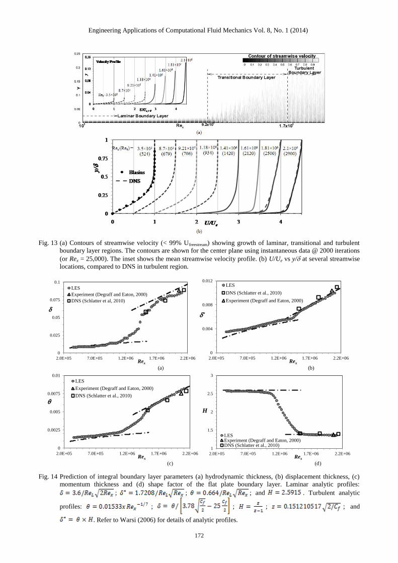
The contours of streamwise velocity at the center

plane in Fig. 13a show a stable boundary layer in

the laminar region, and turbulent fluctuations

starting to grow in the transition region. The

thickness of the low velocity region near the wall

grows both in the laminar and fully developed

turbulent regions, due to flow deceleration and

growth of boundary layer thickness as shown in

the inset figure. The low velocity thickness

decreases in the transition region due to a thinning

of the viscous sublayer, as shown in Fig. 13b. The

integral boundary layer parameters including

hydrodynamic thickness , displacement

thickness * and momentum thickness in Fig. 14

follow the analytic profiles (Warsi, 2006) in both

the laminar and turbulent regions, and show a

steady growth in the transition region. The

predictions also agree well with the available

experimental data and DNS in the turbulent

region. The shape factor H is around 2.6 in the

laminar region and 1.4 in the turbulent region.

Engineering Applications of Computational Fluid Mechanics Vol. 8, No. 1, pp. 158–177 (2014)

172

Fig. 13 (a) Contours of streamwise velocity (< 99% Ufreestream) showing growth of laminar, transitional and turbulent

boundary layer regions. The contours are shown for the center plane using instantaneous data @ 2000 iterations

(or Rex = 25,000). The inset shows the mean streamwise velocity profile. (b) U/Ue vs y/ at several streamwise

locations, compared to DNS in turbulent region.

0

0.025

0.05

0.075

0.1

2.0E+05 7.0E+05 1.2E+06 1.7E+06 2.2E+06Rex

LES

Experiment (Degraff and Eaton, 2000)

DNS (Schlatter et al, 2010)

0

0.004

0.008

0.012

2.0E+05 7.0E+05 1.2E+06 1.7E+06 2.2E+06Rex

*

LES

DNS (Schlatter et al., 2010)

Experiment (Degraff and Eaton, 2000)

(a) (b)

0

0.0025

0.005

0.0075

0.01

2.0E+05 7.0E+05 1.2E+06 1.7E+06 2.2E+06Rex

LES

Experiment (Degraff and Eaton, 2000)

DNS (Schlatter et al., 2010)

1

1.5

2

2.5

3

2.0E+05 7.0E+05 1.2E+06 1.7E+06 2.2E+06Rex

H

LESExperiment (Degraff and Eaton, 2000)DNS (Schlatter et al., 2010)

(c) (d)

Fig. 14 Prediction of integral boundary layer parameters (a) hydrodynamic thickness, (b) displacement thickness, (c)

momentum thickness and (d) shape factor of the flat plate boundary layer. Laminar analytic profiles:

; ; ; and . Turbulent analytic

profiles: ; ; ; ; and

. Refer to Warsi (2006) for details of analytic profiles.

Engineering Applications of Computational Fluid Mechanics Vol. 8, No. 1 (2014)

Engineering Applications of Computational Fluid Mechanics Vol. 8, No. 1 (2014)

173

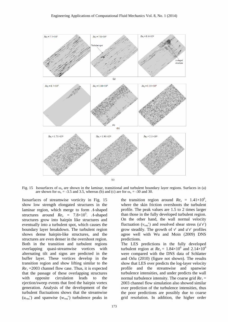
Fig. 15 Isosurfaces of x are shown in the laminar, transitional and turbulent boundary layer regions. Surfaces in (a) are shown for x = -3.5 and 3.5, whereas (b) and (c) are for x = -30 and 30.

Isosurfaces of streamwise vorticity in Fig. 15

show low strength elongated structures in the

laminar region, which merge to form -shaped

structures around Rex = 7.8×105. -shaped

structures grow into hairpin like structures and

eventually into a turbulent spot, which causes the

boundary layer breakdown. The turbulent region

shows dense hairpin-like structures, and the

structures are even denser in the overshoot region. Both in the transition and turbulent regions

overlapping quasi-streamwise vortices with

alternating tilt and signs are predicted in the

buffer layer. These vortices develop in the

transition region and show lifting similar to the

Re =2003 channel flow case. Thus, it is expected

that the passage of these overlapping structures

with opposite circulation leads to the

ejection/sweep events that feed the hairpin vortex

generation. Analysis of the development of the

turbulent fluctuations shows that the streamwise

(urms) and spanwise (wrms) turbulence peaks in

the transition region around Rex = 1.41×106,

where the skin friction overshoots the turbulent

profile. The peak values are 1.5 to 2 times larger

than those in the fully developed turbulent region.

On the other hand, the wall normal velocity

fluctuation (vrms) and resolved shear stress (uv)

grow steadily. The growth of v and uv profiles

agree well with Wu and Moin (2009) DNS

predictions.

The LES predictions in the fully developed

turbulent region at Rex = 1.84×106 and 2.14×10

6

were compared with the DNS data of Schlatter

and Orlu (2010) (figure not shown). The results

show that LES over predicts the log-layer velocity

profile and the streamwise and spanwise

turbulence intensities, and under predicts the wall

normal turbulence intensity. The coarse grid Re =

2003 channel flow simulation also showed similar

over prediction of the turbulence intensities, thus

the poor predictions are possibly due to coarse

grid resolution. In addition, the higher order

(b)

Engineering Applications of Computational Fluid Mechanics Vol. 8, No. 1 (2014)

174

statistics shows kinks similar to channel flow

simulations with low number of collocation points

for each subdomain. Fine grids with larger

numbers of collocation points in each subdomain

are likely required for improved predictions.

6. CONCLUSIONS, DISCUSSIONS AND

FUTURE WORK

6.1 Summary and conclusions

Computational performance of a pseudo-spectral

solver has been improved by implementing

OpenMP thread parallelization for FFT

calculations and MPI domain decomposition for

the Chebyshev collocation method using the

influence matrix method. The solver is validated

for LES of turbulent plane channel flows using

the dynamic Smagorinsky model at Re = 590 and

2003 by comparison to DNS data, and applied for

flat plate boundary layer transition flow for FSTI

= 1.8% and Rex up to 2.2×106. The viability of the

temporally developing approach, opposed to the

commonly used spatially developing approach, is

investigated to reduce the computational cost of

the transition simulations.

The turbulent channel flow study shows that the

increase in the number of MPI subdomains for a

fixed grid (which results in a decrease of

collocation points in each subdomain) results in

loss of solution accuracy, in particular showing

kinks in higher order turbulent statistics at the

domain interfaces. One should expect similar

behavior for (pressure, shear or shock) waves

present in the flow, i.e., higher order features of

the waves would show kinks on coarse grids. The

channel flow results on sufficiently finer grids

compare very well with the DNS data. This

suggests that accurate solution for turbulent

statistics can be obtained if the number of

collocation points in each subdomain is

sufficiently high. Similar conclusions were drawn

by Sabbah and Pasquetti (2008) for high Re non-

stationary flows. It is estimated that a minimum

of 48 collocation points per subdomain are

required for Re ~ 105, and even larger numbers for

Re ~ 106. For sufficiently fine grids, the accuracy

of the multi-domain Chebyshev collocation

method is expected to improve with an increase in

the number of subdomains, as the range of

gradients to be resolved within each domain

decreases. Overall, the study validates the

accuracy of the MPI domain decomposition for

Chebyshev polynomial method using the

influence matrix method for turbulent flows.

The MPI domain decomposition using the

influence matrix method shows a super linear

scalability, and the speedup of the Poisson solvers

is almost exponential. In contrast, OpenMP thread

parallelization of FFT shows performance

improvement of only 30% on 6 threads, and

almost 12% of that is due to increased memory

bandwidth. Overall, the solver shows 12× speed-

up on 50 cores.

The flat plate simulation shows that the transition

begins at Rex= 9.2×105, overshoots the turbulent

skin friction profile for Rex = 1.42×106 to

1.72×106, and achieves a fully developed

turbulent region for higher Rex. The transition

trends are consistent with ERCOFTAC

experimental data. The integral boundary layer

parameters are in good agreement with the

analytic profiles, experimental data and DNS in

the laminar and turbulent regions, and show a

steady growth in the transition region. However,

the predictions do not compare very well with the

DNS in fully developed turbulent region, due to

coarse grid resolution. Overall, the results suggest

that the temporally developing approach may be a

viable alternative for transitional flow

simulations.

6.2 Discussions and future work

In this study, the Chebyshev approximate

equations are solved using the influence matrix

method to attain C1 continuity of the velocity at

domain interfaces. Ideally, C2 continuity is

required for Navier-Stokes solutions, and the

influence matrix method can be extended to

include multiple point overlap to allow such

continuity (Peyret, 2001). However, specification

of higher order continuity is expected to be

susceptible to numerical instabilities (Subbah and

Pasqutti, 2008), and requires additional numerical

expense. Subbah and Pasqutti (2008) identified

enforcing mass conservation at the interface using

specification of C0

continuity of pressure and C

1

continuity of velocity to be sufficient for turbulent

flows. In spectral element methods described by

Deville et al. (2002) the governing equations are

expressed in variational form and only C0

continuity of velocity is satisfied. Studies using

such codes have shown reasonable results on

sufficiently fine grids. Considering the results

presented in this study and those in the literature,

C1 continuity of velocity is identified to be a

sufficient boundary condition for the influence

matrix method.

Analysis of the vortical structures for the flat plate

Engineering Applications of Computational Fluid Mechanics Vol. 8, No. 1 (2014)

175

case shows that the turbulent spots are formed due

to the merger of near wall low strength elongated

structures to -shaped structures, which grow into

hairpin like structures. Further, both the transition

and turbulent regions show overlapping quasi-

streamwise vortices with alternating tilt and signs

in the buffer layer, and the passage of these

structures leads to the ejection/sweep events to

feed the hairpin vortex generation, similar to

those in the turbulent channel flow. The transition

mechanism predicted in this study agrees most

closely to the conceptual model of Schlatter et al.

(2008).

Future solver performance improvement effort

will focus on MPI domain decomposition along

FFT directions and OpenMP parallelization of the

entire solver. The former would involve data

transposition and transfer for FFT calculations for

the convection and viscous solvers (Xu, 2007).

OpenMP thread parallelization can be used to

improve performance of convection, pressure

projection and viscous subroutines, wherein

different wall normal planes can be solved

simultaneously on threads.

Future work for transition simulations includes:

(a) specification of more appropriate initial

freestream turbulence conditions, and (b)

performance of simulations on finer grids

matching the ERCOFTAC dataset. The

freestream condition generated in this study used

random phase perturbations, which lead to a sharp

decay in turbulence at the beginning. This is

expected, as such methods do not account for the

flow inhomogeneity due to the presence of the

wall (Brandt et al. 2004). Future study will use

freestream turbulence generated using

superposition of modes of the continuous

spectrum of the linearized Orr–Sommerfeld and

Squire operators, which allows accurate decay of

freestream turbulence (Jacobs and Durbin, 2001;

Brandt et al., 2004). In addition, in temporal

simulations spatial decay is based on the velocity

of the reference frame. Since, the boundary layer

and the free-stream have different velocities, it is

expected that their decay rates will be out of

phase. Further investigation is required to clarify

the need for transformation/external forcing to

achieve a consistent turbulence decay or growth

of boundary layer (Spalart 1988).

Future work for the analysis of the transition flow

results will focus on: (a) implementation of better

vortex identification techniques, such as second

largest eigenvalue λ2 of the tensor

, and (b) turbulence kinetic

energy and stress budgets to identify dominant

terms and study the intercomponent energy

transfer mechanism (Kim et al., 2008).

ACKNOWLEDGEMENT

This research was funded by NSF under Grant

No. EPS-0903787 and by NASA under Grant No.

NNX10AN06A.

REFERENCES

1. Akhavan R, Ansari A, Kang S, Mangiavacchi

N (2000). Subgrid-scale interactions in a

numerically simulated planar turbulent jet and

implications for modeling. J. Fluid Mech.

408: 83–120.

2. Anderson E, Bai Z, Bischof C, Demmel J,

Dongarra J, Croz JD, Greenbaum A,

Hammarling S, McKenney A, Ostrouchov S,

Sorensen D (1995). LAPACK Users' Guide. Second Edition, SIAM, Philadelphia, PA.

3. Ansari A (1997). Self-similarity and mixing

characteristics of turbulent mixing layers

starting from laminar initial conditions. Phys.

Fluids 9(6): 1714–28. 4. Baxevanou CA and Fidaros DK. (2008).

Validation of numerical schemes and turbulence models combinations for transient

flow around airfoil. Engineering Applications of Computational Fluid Mechanics 2:208-

221. 5. Bhushan S, and Warsi, ZUA (2005). Large

eddy simulation of turbulent channel flow using an algebraic model. International

Journal for Numerical Methods in Fluids, 49: 489-519.

6. Bhushan S, Warsi ZUA, Walters DK (2006). Estimating backscatter in subgrid scale

turbulence through algebraic modeling. AIAA Journal 44(4): 837-847.

7. Bhushan S, Warsi ZUA (2007). Large eddy

simulation of free-shear flows using an algebraic model. Computers and Fluids

36(8): 1384-1397. 8. Borell G, Sillero JA, Jimenez J (2011). Direct

numerical simulation of turbulent boundary layers at high Reynolds numbers. 23

rd

International Conference on Parallel Computational Fluid Dynamics, May 16-20,

Barcelona, Spain. 9. Brandt L, Schlatter P, Henningson, DS

(2004). Transition in boundary layers subject to free-stream turbulence. J. Fluid Mech. 517:

167-198.

10. Coupland J (1990). ERCOFTAC Special

Interest Group on Laminar to Turbulent

Engineering Applications of Computational Fluid Mechanics Vol. 8, No. 1 (2014)

176

Transition and Retransition: T3A and T3B

Test Cases. ERCOFTAC.

11. DeGraff DB, Eaton JK (2000). Reynolds-

number scaling of the flat-plate turbulent

boundary layer. J. Fluid Mech. 422: 319-346.

12. Deville MO, Fischer PF and Mund EH

(2002). High-Order Methods for

Incompressible Fluid Flow. Cambridge

University Press.

13. Frigo M, Johnson SG (2011). FFTW for

version 3.3. http://www.fftw.org/fftw3.pdf.

14. Hoyas S, Jimenez J (2006). Scaling of the

velocity fluctuations in turbulent channels up

to Reτ=2003. Phys. Fluids 18: 011702.

15. Jacobs RG, Durbin PA (2010). Simulation of

bypass transition. J. Fluid Mech. 428: 185–

212.

16. Jeong J, Hussain F, Schoppa W, Kim J

(1997). Coherent structures near the wall in a

turbulent channel flow, J. Fluid Mech. 332:

185-214.

17. Kang H, Chester S, Meneveau C. (2003).

Decaying turbulence in an active grid

generated flow and comparisons with large-

eddy simulation. Journal of Fluid Mechanics

480:129–160.

18. Khurajadze G, Oberlack M (2004). DNS and

scaling laws from new symmetry groups of

ZPG turbulent boundary layer flow. Theor.

Comp. Fluid Dyn. 18: 391–441.

19. Kim J, Moin P, Moser R (1987). Turbulence

statistics in fully developed channel flow at

low Reynolds number. J. Fluid Mech. 117:

133-143.

20. Kim K, Sung HJ, Adrian RJ (2008). Effects

of background noise on generating coherent

packets of hairpin vortices. Phys. Fluids 20:

105107.

21. Lilly DK (1992). A proposed modification of

the Germano subgrid-scale closure method,

Phys Fluids 4 (3): 633–634.

22. Malik MR, Hussaini MY (1990). Numerical

simulation of Gortler/Tollmein-Schlichting

wave-interaction. J. Fluid Mech. 210: 183–

199.

23. Minguez M. Pasquetti, R, Serre E. (2008)

High-order LES of flow over the Ahmed

reference body, Phys. Fluids. 20(9): 095101-

095101-17.

24. Minguez M., Brun C, Pasquetti, R, Serre E.

(2011). Experimental and high-order analysis

of the flow in near-wall region of a square

cylinder. Int. J. Heat and Fluid Flow. 32(3):

558-566.

25. Moser RD, Kim J, Mansour NN (1999).

Direct numerical simulation of turbulent

channel flow up to Reτ=590. Physics of Fluids

11: 943-945.

26. Peyret R (2001). Spectral methods for

incompressible viscous flow. Appl Math

Sci.148: 39-98.

27. Raspo I, Ouazzani J, Peyret R (1996). A

spectral multidomain technique for the

computation of the czochralski melt

configuration. Int. J. Num. Meth. Heat Fluid

Flow 6: 31 - 42.

28. Rogallo RS. (1981). Numerical Experiments

in Homogeneous Turbulence. NASA TM-

81315.

29. Sabbah C, Pasquetti R (1998). A divergence-

free multi-domain spectral solver of the

Navier–Stokes equations in geometries of

high aspect ratio. J. Comput. Phys. 139: 359–

379.

30. Schlatter P, Brandt L, deLange HC,

Henningson DS (2008). On streak breakdown

in bypass transition. Phys. Fluids 20: 101505.

31. Schlatter P, Orlu R, Li Q, Brethouwer G,

Fransson J, Johansson AV, Alfredsson PH,

Henningson DS (2009). Turbulent boundary

layers up to Reθ = 2500 studied through

simulation and experiment. Phys. Fluids 21:

051702.

32. Schlatter P, Orlu R (2010). Assessment of

direct numerical simulation data of turbulent

boundary layers. J. Fluid Mech. 659: 116-

126.

33. Singer BA, Joslin RD (1994). Metamorphosis

of a hairpin vortex into a young turbulent

spot. Phys. Fluids 6: 3724–3736.

34. Spalart PR (1988) Direct simulation of a

turbulent boundary layer up to Re = 1410. J.

Fluid Mech. 187: 61–98.

35. Wallace JM, Park GI, Wu X, Moin P (2010).

Boundary layer turbulence in transitional and

developed states. Center for Turbulence

Research Proceedings of the Summer

Program.

36. Walters DK, Cokljat D (2008). A three-

equation eddy-viscosity model for Reynolds -

averaged Navier - Stokes simulations of

transitional flow. ASME J. Fluids Eng. 130:

121401.

37. Warsi ZUA (2006). Fluid Dynamics, Theoretical and Computational Approach

(3rd edn). CRC Press: Boca Raton, FL.

38. Wu A, Moin P, (2009). Direct numerical

simulation of turbulence in a nominally zero-

pressure-gradient flat-plate boundary layer. J.

Fluid Mech. 630: 5–41.

Engineering Applications of Computational Fluid Mechanics Vol. 8, No. 1 (2014)

177

39. Xu J (2007). Benchmarks on tera-scalable

models for DNS of turbulent channel flow.

Parallel Comput. 33(12): 780–794.

40. Yakinthos K. (2013). Application of non-

linear eddy-viscosity model involving A2

stress-invariant transport equation to

transitional flows. Engineering Applications

of Computational Fluid Mechanics 7:393-

405.

41. Yang HH, Shizgal B (1994). Chebyshev

pseudo-spectral multi-domain technique for

viscous flow calculation. Computer Methods

in Applied Mechanics and Engineering 118:

47-61.

42. Zaki TA, Durbin PA (2005). Mode

interaction and the bypass route to transition.

J. Fluid Mech. 531: 85–111.