development of mathematical tools

CAROLINE SATYE MARTINS NAKAMA

DEVELOPMENT OF MATHEMATICAL TOOLS

FOR MODELING BIOLOGICAL SYSTEMS BASED

ON METABOLIC FLUXES AND PARAMETER

ESTIMATION OF ILL-CONDITIONED PROBLEMS

São Paulo

2020

CAROLINE SATYE MARTINS NAKAMA

DEVELOPMENT OF MATHEMATICAL TOOLS FOR

MODELING BIOLOGICAL SYSTEMS BASED ON

METABOLIC FLUXES AND PARAMETER ESTIMATION OF

ILL-CONDITIONED PROBLEMS

Versão corrigida

Tese apresentada à Escola Politécnica daUniversidade de São Paulo para obtenção dotítulo de Doutora em Ciências.

Área de concentração: Engenharia Química

Orientador: Prof. Dr. Galo Antonio Carrillo LeRoux

Coorientador: Prof. Dr. José Gregório CabreraGomez

São Paulo

2020

Autorizo a reprodução e divulgação total ou parcial deste trabalho, por qualquer meioconvencional ou eletrônico, para fins de estudo e pesquisa, desde que citada a fonte.

Este exemplar foi revisado e corrigido em relação à versão original, sob responsabilidade única do autor e com a anuência de seu orientador.

São Paulo, ______ de ____________________ de __________

Assinatura do autor: ________________________

Assinatura do orientador: ________________________

Catalogação-na-publicação

Nakama, Caroline Satye Martins Development of Mathematical Tools for Modeling Biological SystemsBased on Metabolic Fluxes and Parameter Estimation of Ill-ConditionedProblems / C. S. M. Nakama -- versão corr. -- São Paulo, 2020. 133 p.

Tese (Doutorado) - Escola Politécnica da Universidade de São Paulo.Departamento de Engenharia Química.

1.Engenharia metabólica 2.Modelagem estequiométrica 3.Estimação deparâmetros 4.Regularização I.Universidade de São Paulo. Escola Politécnica.Departamento de Engenharia Química II.t.

4 agosto 2020

Acknowledgements

Palavras que não expressam fatos e teorias são mais difíceis de serem escritas,

apesar de não menos importantes. Então começo dizendo que muitas pessoas não citadas

nominalmente aqui contribuíram, direta ou indiretamente, para a conclusão dessa etapa da

minha vida e eu sempre serei grata a todas(os) vocês.

Cada professora e professor que tive durante a vida adicionou, de alguma forma,

um bloco na minha formação acadêmica. Sempre fui muito grata a todas(os). Em especial,

agradeço a meu orientador Prof. Galo Le Roux pela orientação, paciência, disponibilidade,

humildade, amizade e todos os ensinamentos, sejam eles técnicos ou sobre a vida. Meus

agradecimentos também são direcionados ao Prof. Gregório Gomez pela orientação e

ensino sobre bioquímica e microbiologia. I would also like to thank Prof. Victor Zavala for

accepting to receive me as a visitor twice, patiently advising me, and always making me feel

part of your research group; I will never be able to measure how much I learned from you or

to express how grateful I am.

Como já diziam os Beatles, "I get by with a little help from my friends". Agradeço

a todas minhas amigas e todos meus amigos pelas tão necessárias distrações, apoio e

por sempre acreditarem em mim. Particularmente, gostaria também de expressar minha

gratidão a minhas(meus) colegas da pós graduação; tudo foi menos difícil com a ajuda e

paciência de vocês. Rafael e José Otávio, obrigada pela direta contribuição lendo essa

tese. I also feel I have to give special thanks to my colleagues and friends from Madison;

you are part of the reason my time there was so enriching both personal and professionally.

Santiago, thank you for your help and letting me use your code.

Eu gostaria de agradecer às agências de fomento Conselho Nacional de Desenvolvi-

mento Científico e Tecnológico (CNPq) e Coordenação de Aperfeiçoamento de Pessoal de

Nível Superior (CAPES) pelo apoio financeiro nacional e para a realização do doutorado

sanduíche respectivamente.

Meu eterno agradecimento à minha família, especialmente meu pai José, por ter me

oferecido oportunidades e criado possibilidades para que eu tivesse a liberdade de seguir o

caminho que quisesse. Por fim, agradeço ao André Dondon pelo apoio incondicional; essa

maratona teria sido extremamente mais desafiadora, quiçá impossível, sem você.

“Quando os caminhos se confundem, é necessário voltar ao começo”

(Leandro "Emicida" Roque de Oliveira)

Resumo

Modelagem matemática é um dos pilares da engenharia metabólica, guiando modificaçõesgenéticas através do estudo de fluxos metabólicos. Modelos estequiométricos são umaferramenta importante para analisar redes metabólicas, especialmente para organismos nãomodelo ou durante a fase de análise inicial, pois são modelos lineares que requerem essen-cialmente a matriz estequiométrica e informações sobre a reversibilidade das reações comodados de entrada. Eles podem ser usados para explorar diferentes hipóteses e cenários,além de elucidar algumas propriedades do metabolismo. Com isso, algumas técnicas demodelagem estequiométrica foram implementadas em um software único e independentee usadas para estudar o metabolismo central da bactéria Burkholderia sacchari para pro-dução de poli-hidroxialcanoato. O estudo mostrou que a modelagem estequiométrica é umaferramenta valiosa para explorar como o metabolismo funciona e orientar o planejamento deexperimentos futuros. No entanto, o metabolismo celular é, na realidade, função de dinâmi-cas não lineares e, portanto, modelos não lineares são mais adequados para representaruma abrangente variedade de estados fisiológicos, resultando em melhores previsões.Modelos mecanísticos são uma classe de modelos não lineares; porém, no contexto daengenharia metabólica, todos os modelos propostos para estimar os parâmetros cinéticosenvolvidos são propensos a problemas de identificabilidade. Considerando esse obstáculo,um estudo sobre métodos de regularização para problemas de estimativa de parâmetrosmal condicionados foi realizado. Os métodos de regularização baseados na decomposiçãoem autovalores e autovetores da matriz Hessiana (reduzida) se mostraram ótimos paraestimativa linear de parâmetros levando em consideração a redução da variância e podemauxiliar a lidar com problemas não lineares com vizinhança quase plana ao redor da solução.Além disso, a regularização baseada em autovetores em ambos os casos pôde ser usadapara reconhecer grupos de parâmetros correlacionados, o que auxilia na compreensão dosinerentes problemas de identificação.

Palavras-chave: Engenharia metabólica, modelagem estequiométrica, estimação de parâmet-ros, regularização

Abstract

Mathematical modeling is one of the basis of metabolic engineering, guiding genetic modifi-cations through the study of metabolic fluxes. Stoichiometric models are an important tool toanalyze metabolic networks, especially for non-model organisms or during initial analysis,since they linear models and essentially require the stoichiometry matrix and informationon reversibility of the reactions as input. They can be used to explore different assumptionsand scenarios, and elucidate some properties of the metabolism. Therefore some stoichio-metric modeling techniques were implemented in a single stand-alone software and used tostudy the core metabolism of the bacteria Burkholderia sacchari for polyhydroxyalkanoateproduction, showing that they are a valuable tool for exploring how metabolisms work andguiding future experiment design. However, cellular metabolism is actually subjected tononlinear dynamics and, therefore, nonlinear models are better suited to represent morediverse physiological states, which can result in better predictions. Mechanistic models are aclass of such models; however, in the metabolic engineering context, all frameworks thathave been proposed to estimate the kinetic parameters involved are prone to identifiabilityissues. Based on this obstacle, an investigation on regularization methods for ill-conditionedparameter estimation problems was conducted. Regularization methods based on the eigen-value decomposition of the (reduced) Hessian matrix were shown to be optimal for linearparameter estimation, in the sense of reducing parameter variance, and helpful in dealingwith nonlinear problems with nearly flat neighborhood around the solution. Moreover, theeigenvector-based regularization in both cases was able to recognize groups of correlatedparameters, which allows for better understanding the underlying identifiability issues.

Keywords: Metabolic engineering, stoichiometric modeling, parameter estimation, regular-ization

List of Figures

Figure 1 – A simple metabolic network with internal metabolites A, B and C, and the

representation of its elementary flux modes and extreme pathways. . . . 31

Figure 2 – Graphic representation of the EFM (thick lines) of a simple metabolic

network with one internal metabolite and three fluxes. . . . . . . . . . . 32

Figure 3 – Graphic representation of the EFV (red dots) of a simple metabolic network

with one internal metabolite and three fluxes with bounds defined for two

of them. . . . . . . . . . . . . . . . . . . . . . . . . . . . . . . . . . . . 35

Figure 4 – Simple UML diagram of the main blocks (classes) that compose this

software for stoichiometric analysis of metabolic networks. . . . . . . . . 44

Figure 5 – Graphic representation of the flux vectors for the cosine similarity calcu-

lation obtained from three EFV of a simple metabolic network with one

internal metabolite and three fluxes with bounds defined for two of them. 47

Figure 6 – Metabolic network used to represent the central metabolism of B. sacchari

producing P3HB and P3HB-co-3HHx. . . . . . . . . . . . . . . . . . . . 49

Figure 7 – Three parameter example of how PCR and using eigenvector constraints

regularize an estimation problem; PCR projects the data onto the 2 leading

eigenvectors, while using eigenvector constraints creates a hyperplane

where the solution is contained. . . . . . . . . . . . . . . . . . . . . . . 79

Figure 8 – Covariance matrix for estimated parameters V[θ] from the first example. 82

Figure 9 – (a) Frobenius norm of parameter covariance matrix obtained with all

possible subset selections with p = 3 (circles) and obtained with PCR (red

line). (b) Frobenius norm of the covariance matrix obtained with sparse

PCR with elastic net (EN) and elastic net with orthogonality constraints

(EN-OC). The sparsest eigenvectors (with one nonzero entry) is equivalent

to fixing parameters θ1, θ4 and θ5. . . . . . . . . . . . . . . . . . . . . . 84

Figure 10 – (a) Frobenius norm of the covariance matrix of the estimated parameters

calculated with sparse PC regression (both approaches) as a function

of the number of nonzero entries (NNZ) in each eigenvector in V1. (b)

Frobenius norm of the covariance matrix of the estimated parameters

(circles) and sum of the squared errors (SSE) of η (stars) using Ridge

regression as a function of its parameter (Second example). . . . . . . . 85

Figure 11 – Covariance matrix for estimated kinetic constants V[θ]. . . . . . . . . . . 87

Figure 12 – 3D graph and contour plot of the space of allowable solutions for the

unconstrained parameter estimation case study. . . . . . . . . . . . . . 95

Figure 13 – Comparison between both eigenvalue decomposition regularization ap-

proaches and the Hessian modification method regarding the necessary

number of iterations used to solve the unconstrained parameter estimation

problem with 20 different initial guesses. . . . . . . . . . . . . . . . . . . 96

Figure 14 – Example of paths when both eigenvalue decomposition regularization

approaches and the Hessian modification method are used for the uncon-

strained parameter estimation problem with same initial guess. . . . . . 96

Figure 15 – Progression of the nonlinear enzymatic reaction estimation problem em-

ploying the Hessian modification and the eigenvector-based regularization

approaches. . . . . . . . . . . . . . . . . . . . . . . . . . . . . . . . . . 106

Figure 16 – Measured data points used for estimation and simulation using both sets

of estimates for the nonlinear parameter estimation of the dynamic kinetic

model. . . . . . . . . . . . . . . . . . . . . . . . . . . . . . . . . . . . . 109

Figure 17 – Progression of the dynamic kinetic model estimation problem employ-

ing the Hessian modification and the eigenvector-based regularization

approaches. . . . . . . . . . . . . . . . . . . . . . . . . . . . . . . . . . 110

List of Tables

Table 1 – Subset of EFM that takes only glucose as substrate obtained for the

metabolic network used to represent the core metabolism of Burkholderia

sacchari. . . . . . . . . . . . . . . . . . . . . . . . . . . . . . . . . . . . 50

Table 2 – Overall stoichiometry of the three groups of EFM involved in metabolize

glucose in the studied metabolic network. vg is the estimated flux through

each group and ve is the experimental measured flux corresponding to

consumption or production of the external metabolites (MENDONÇA, 2014). 51

Table 3 – Set of EFV obtained fixing the external fluxes with data from (MENDONÇA,

2014) for the experiment with 3HB production. First column corresponds to

sets of reactions that operate together. The last two columns correspond to

the minimum and maximum values of each reaction for this physiological

state. . . . . . . . . . . . . . . . . . . . . . . . . . . . . . . . . . . . . . 53

Table 4 – Cosine similarity for every pair of selected reaction (only 3HB production). 54

Table 5 – Subset of EFM with optimal yield for 3HHx synthesis from hexanoic acid for

the metabolic network used to represent the core metabolism of Burkholde-

ria sacchari. . . . . . . . . . . . . . . . . . . . . . . . . . . . . . . . . . . 55

Table 6 – Experimental (original) and reconciled values of external fluxes obtained

during the synthesis of 3HB and 3HHx using Burkholderia sacchari. . . . 56

Table 7 – Cosine similarity for every pair of selected reaction (3HB and 3HHx produc-

tion). . . . . . . . . . . . . . . . . . . . . . . . . . . . . . . . . . . . . . . 58

Table 8 – Kernel matrix corresponding to the first example. . . . . . . . . . . . . . . 81

Table 9 – Eigenvectors and corresponding eigenvalues of XT X from the first example. 82

Table 10 – Eigenvectors V1 and sparse eigenvectors V1 obtained with elastic net (EN)

and elastic net with orthogonality constraints (EN-OC) (First example). . . 82

Table 11 – Eigenvectors and corresponding eigenvalues of XT X from the second

example. . . . . . . . . . . . . . . . . . . . . . . . . . . . . . . . . . . . 84

Table 12 – Complete set of eigenvectors V1 and V2 and sparse eigenvectors V1 ob-

tained with elastic net with orthogonality constraints (EN-OC). . . . . . . 86

Table 13 – Dense eigenvectors V1 for Botts-Morales example. . . . . . . . . . . . . . 88

Table 14 – Sparse eigenvectors V1 or Botts-Morales example calculated with elastic

net with orthogonality constraint. . . . . . . . . . . . . . . . . . . . . . . 89

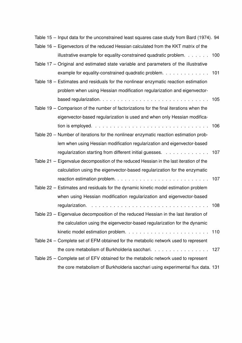
Table 15 – Input data for the unconstrained least squares case study from Bard (1974). 94

Table 16 – Eigenvectors of the reduced Hessian calculated from the KKT matrix of the

illustrative example for equality-constrained quadratic problem. . . . . . . 100

Table 17 – Original and estimated state variable and parameters of the illustrative

example for equality-constrained quadratic problem. . . . . . . . . . . . . 101

Table 18 – Estimates and residuals for the nonlinear enzymatic reaction estimation

problem when using Hessian modification regularization and eigenvector-

based regularization. . . . . . . . . . . . . . . . . . . . . . . . . . . . . . 105

Table 19 – Comparison of the number of factorizations for the final iterations when the

eigenvector-based regularization is used and when only Hessian modifica-

tion is employed. . . . . . . . . . . . . . . . . . . . . . . . . . . . . . . . 106

Table 20 – Number of iterations for the nonlinear enzymatic reaction estimation prob-

lem when using Hessian modification regularization and eigenvector-based

regularization starting from different initial guesses. . . . . . . . . . . . . 107

Table 21 – Eigenvalue decomposition of the reduced Hessian in the last iteration of the

calculation using the eigenvector-based regularization for the enzymatic

reaction estimation problem. . . . . . . . . . . . . . . . . . . . . . . . . . 107

Table 22 – Estimates and residuals for the dynamic kinetic model estimation problem

when using Hessian modification regularization and eigenvector-based

regularization. . . . . . . . . . . . . . . . . . . . . . . . . . . . . . . . . 108

Table 23 – Eigenvalue decomposition of the reduced Hessian in the last iteration of

the calculation using the eigenvector-based regularization for the dynamic

kinetic model estimation problem. . . . . . . . . . . . . . . . . . . . . . . 110

Table 24 – Complete set of EFM obtained for the metabolic network used to represent

the core metabolism of Burkholderia sacchari. . . . . . . . . . . . . . . . 127

Table 25 – Complete set of EFV obtained for the metabolic network used to represent

the core metabolism of Burkholderia sacchari using experimental flux data. 131

List of abbreviations and acronyms

3HB 3-hydroxybutyrate

3HHx 3-hydroxyhexanoate

AcCoA Acetyl coenzyme A

ADP Adenosine diphosphate

AIC Akaike information criteria

ATP Adenosine triphosphate

BIC Bayesian information criteria

BPG13 1,3-Bisphosphoglycerate

Br Bromine (atom)

Br2 Bromine

ButCoA Butanoyl-CoA

ButenCoA Butenoyl-CoA

Cat Catalyst

CButCoA Keto-butyryl-CoA

CHexCoA Keto-hexanoyl-CoA

Cit Citrate

CO2 Carbon dioxide

DHP Dihydroxyacetone

DMFA Dynamic metabolic flux analysis

E Enzyme

E4P Erythrose-4-phosphate

ED Entner–Doudoroff (pathway)

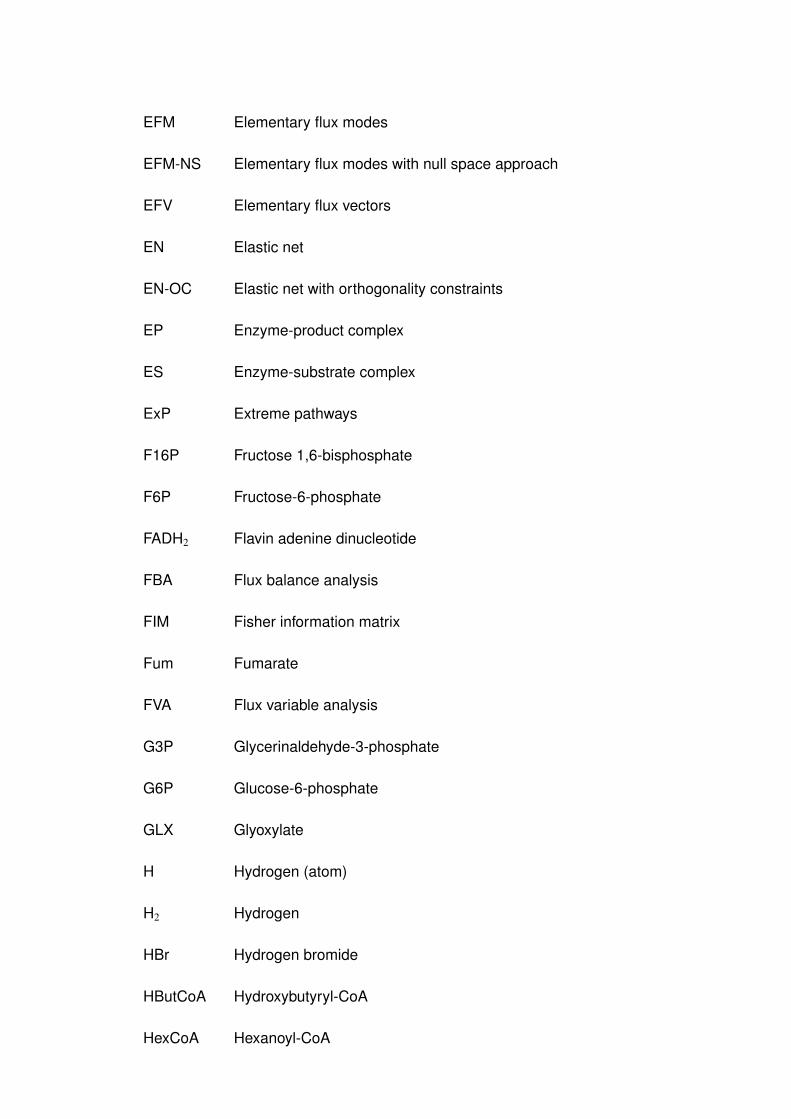
EFM Elementary flux modes

EFM-NS Elementary flux modes with null space approach

EFV Elementary flux vectors

EN Elastic net

EN-OC Elastic net with orthogonality constraints

EP Enzyme-product complex

ES Enzyme-substrate complex

ExP Extreme pathways

F16P Fructose 1,6-bisphosphate

F6P Fructose-6-phosphate

FADH2 Flavin adenine dinucleotide

FBA Flux balance analysis

FIM Fisher information matrix

Fum Fumarate

FVA Flux variable analysis

G3P Glycerinaldehyde-3-phosphate

G6P Glucose-6-phosphate

GLX Glyoxylate

H Hydrogen (atom)

H2 Hydrogen

HBr Hydrogen bromide

HButCoA Hydroxybutyryl-CoA

HexCoA Hexanoyl-CoA

HexenCoA Hexenoyl-CoA

HHexCoA Hydroxyhexanoyl-CoA

I Inactive enzyme

IsoCit Isocitrate

KDPG2 2-Keto-3-deoxy-6-phosphogluconate

KG2 α-ketoglutarate

KKT Karush-Kuhn-Tucker

LP Linear programming

M Modifier

Mal Malate

MFA Metabolic flux analysis

MLE Maximum likelihood estimation

NADH Nicotinamide adenine dinucleotide

NADPH Nicotinamide adenine dinucleotide phosphate

NLP Nonlinear Programming

NNZ Number of nonzero entries

O2 Oxygen

OAA Oxaloacetate

ODE Ordinary differential equations

P Product

P3HB Poly-3-hydroxybutyrate

P3HB-co-3HHx Poly(3-hydroxybutyrate-co-3-hydroxyhexanoate)

PCA Principal component analysis

PCR Principal component regression

PEP Phosphoenolpyruvate

PG2 2-phosphoglycerate

PG3 3-phosphoglycerate

PG6 6-phosphogluconate

PHA Polyhydroxyalkanoate

PIR Pyruvate

PP Pentose phosphate (pathway)

QP Quadratic programming

Rb5P Ribose-5-phosphate

Rbl5P Ribulose-5-phosphate

S Substrate

S7P Sedoheptulose-7-phosphate

SQP Sequential quadratic programming

SSE Sum of squared errors

Suc Succinate

SucCoA Succinyl-CoA

UML Unified modeling language

X5P Xylulose-5-phosphate

List of Symbols

Part I - Stoichiometric models for metabolic networks

N Stoichiometry matrix

m Total number of internal metabolites

r Total number of reactions

K Null space of the the stoichiometry matrix

Xm Concentration vector for internal metabolites

rm Vector of formation rates of internal metabolites

µ Biomass specific growth rate

v Flux vector

Ne Stoichiometry matrix with experimentally measured reaction rates

ve Vector with experimentally measured reaction rates

Nu Stoichiometry matrix with unknown reaction rates

vu Vector with unknown reaction rates

rexp Number of reactions with experimentally measured flux rate

T ( j) jth tableau for elementary flux mode/vector calculation

Nrev Stoichiometry matrix with reversible reactions

Nirr Stoichiometry matrix with irreversible reactions

I Identity matrix

t( j)i, j+1 jth tableau entry of row i and column j + 1

S (i) Set with column indices of zero elements in row i right hand side in T ( j)

vext Vector with external flux rates

ε Vector of random errors

Σ Covariance matrix of external flux rates

A Matrix with balancing equations for the external fluxes

W Weight matrix

nbal Number of balancing equations

rext Number of external reactions

v Vector with estimated flux rates

f Vector representing a EFM

G Linear equality constraints

neq Number of equality constraints

b Vector with the right had side of the equality constraints

λ Auxiliary scalar variable

H Inequality constraints

nineq Number of inequality constraints

c Vector with bound values for inequality constraints

s Slack variables

α A scalar

nEFV Number of elementary flux vectors

y A vector of dimension n

Part II - Regularization of parameter estimation problems

f Objective function

w Vector of unknown variables

n Total number of unknown variables

Q Square symmetric matrix / Hessian matrix

c A known vector

A Coefficients for linear constraints (for state variables)

b Right-hand side of linear constraints

p Total number of equality constraints / state variables

L Lagrange function

λ Vector with Lagrange multipliers

d Step / Search direction

Z Null space matrix

α A scalar that determines the step length in line search algorithms

mk Quadratic function approximation of the kth iteration

c1 Parameter for the first Wolfe condition

c2 Parameter for the second Wolfe condition

h Vector function of equality constraints

µ Barrier parameter

z Vector with Lagrange multipliers for variable bounds

W Diagonal matrix with variables w in the main diagonal

Z Diagonal matrix with Lagrange multipliers z in the main diagonal

e Vector of ones

Hk Hessian of the Lagrange function at the kth iteration

I Identity matrix

Σk Term added to Hk in a interior point algorithm

ϕ Objective function with the barrier term

τ Parameter that limits how close to the bound variables w gets

ρ Constraint violation

γρ Parameter for the expression to assess constraint violation improvement

γρ Parameter for the expression to assess objective value improvement

x Vector of state variables

θ Vector of parameters

m Total number of parameters

Dw Unknown variables for reduced Hessian calculation

η Vector of output observations / experiments

L Total number of observations / experiments

ε` Noise of the `th observation / experiment

σ2 Variance

X Matrix with state variables for all observations / experiments

ε Vector of independent and identically distributed noise

K Kernel / Hessian matrix

V Covariance matrix

V Matrix of eigenvectors

Λ Diagonal matrix with eigenvalues in the main diagonal

λ j Eigenvalue associated with the jth eigenvector

v j Eigenvector associated with the jth eigenvalue

R Coefficients of linear constraints

r Right-hand side of linear constraints

q Number of small eigenvalues

γ Reduced set of parameters

κ1 Tuning parameter for the `1 norm

κ2 Tuning parameter for the `2 norm

k j Kinetic constant of the jth reaction

F Volume flow rate

s Number of output observations for each experiment

φ Mapping function between problem variables and output observations

LH Likelihood function

δH Multiple of the identity matrix that modifies the Hessian of the Lagrange function

δh Multiple of the identity used when ∇h is linearly dependent

β Threshold for splitting Λ into small and large eigenvalues

t Time

T Temperature

C Coefficients of linear φ for the state variables

D Coefficients of linear φ for the parameters

B Coefficients for linear constraints for the parameters

ð Columns of matrix D

βε Threshold for considering an eigenvalue zero

βµ Limiting value of the barrier parameter for using eigenvalue-based regularization

M Set of measured species

S Complete set of species

T Set of measurement time points

Contents

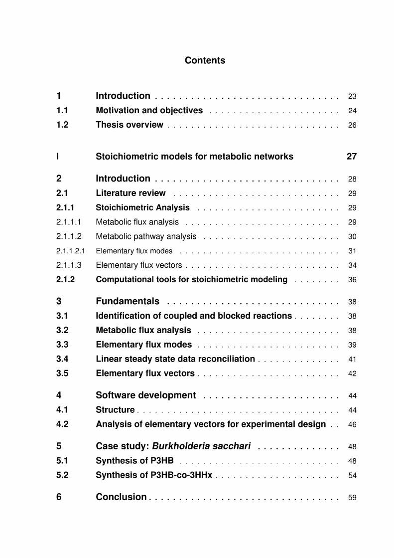
1 Introduction . . . . . . . . . . . . . . . . . . . . . . . . . . . . . . . 23

1.1 Motivation and objectives . . . . . . . . . . . . . . . . . . . . . . 24

1.2 Thesis overview . . . . . . . . . . . . . . . . . . . . . . . . . . . . . 26

I Stoichiometric models for metabolic networks 27

2 Introduction . . . . . . . . . . . . . . . . . . . . . . . . . . . . . . . 28

2.1 Literature review . . . . . . . . . . . . . . . . . . . . . . . . . . . . 29

2.1.1 Stoichiometric Analysis . . . . . . . . . . . . . . . . . . . . . . . . 29

2.1.1.1 Metabolic flux analysis . . . . . . . . . . . . . . . . . . . . . . . . . . 29

2.1.1.2 Metabolic pathway analysis . . . . . . . . . . . . . . . . . . . . . . . 30

2.1.1.2.1 Elementary flux modes . . . . . . . . . . . . . . . . . . . . . . . . . . . 31

2.1.1.3 Elementary flux vectors . . . . . . . . . . . . . . . . . . . . . . . . . . 34

2.1.2 Computational tools for stoichiometric modeling . . . . . . . . 36

3 Fundamentals . . . . . . . . . . . . . . . . . . . . . . . . . . . . . 38

3.1 Identification of coupled and blocked reactions . . . . . . . . 38

3.2 Metabolic flux analysis . . . . . . . . . . . . . . . . . . . . . . . . 38

3.3 Elementary flux modes . . . . . . . . . . . . . . . . . . . . . . . . 39

3.4 Linear steady state data reconciliation . . . . . . . . . . . . . . 41

3.5 Elementary flux vectors . . . . . . . . . . . . . . . . . . . . . . . . 42

4 Software development . . . . . . . . . . . . . . . . . . . . . . . 44

4.1 Structure . . . . . . . . . . . . . . . . . . . . . . . . . . . . . . . . . . 44

4.2 Analysis of elementary vectors for experimental design . . 46

5 Case study: Burkholderia sacchari . . . . . . . . . . . . . . 48

5.1 Synthesis of P3HB . . . . . . . . . . . . . . . . . . . . . . . . . . . 48

5.2 Synthesis of P3HB-co-3HHx . . . . . . . . . . . . . . . . . . . . . 54

6 Conclusion . . . . . . . . . . . . . . . . . . . . . . . . . . . . . . . . 59

II Regularization of parameter estimation problems 60

7 Introduction . . . . . . . . . . . . . . . . . . . . . . . . . . . . . . . 61

7.1 Literature review . . . . . . . . . . . . . . . . . . . . . . . . . . . . 62

7.1.1 Regularization of linear parameter estimation . . . . . . . . . . . 62

7.1.2 Ill-conditioned nonlinear parameter estimation . . . . . . . . . . 64

7.1.3 Regularization in nonlinear solvers . . . . . . . . . . . . . . . . . 66

8 Fundamentals . . . . . . . . . . . . . . . . . . . . . . . . . . . . . 68

8.1 Quadratic programming . . . . . . . . . . . . . . . . . . . . . . . 68

8.2 Line search methods for nonlinear optimization . . . . . . . 69

8.2.1 Unconstrained problems . . . . . . . . . . . . . . . . . . . . . . . . 69

8.2.2 Constrained problems . . . . . . . . . . . . . . . . . . . . . . . . . 71

8.2.2.1 Interior point methods . . . . . . . . . . . . . . . . . . . . . . . . . . . 72

8.3 Reduced Hessian . . . . . . . . . . . . . . . . . . . . . . . . . . . . 74

9 Linear parameter estimation . . . . . . . . . . . . . . . . . . . 75

9.1 Constraint-based regularization . . . . . . . . . . . . . . . . . . 76

9.1.1 Regularization using eigenvector constraints . . . . . . . . . . . 77

9.1.2 Principal component regression . . . . . . . . . . . . . . . . . . . 78

9.1.3 Sparse principal component regression . . . . . . . . . . . . . . 79

9.2 Illustrative examples . . . . . . . . . . . . . . . . . . . . . . . . . . 81

9.2.1 Collineatities in the input data . . . . . . . . . . . . . . . . . . . . 81

9.2.2 Fewer input observations than parameters . . . . . . . . . . . . 84

9.3 Case study: Enzymatic reactions . . . . . . . . . . . . . . . . . 85

9.4 Conclusion . . . . . . . . . . . . . . . . . . . . . . . . . . . . . . . . 88

10 Nonlinear parameter estimation . . . . . . . . . . . . . . . . . 90

10.1 Hessian modification . . . . . . . . . . . . . . . . . . . . . . . . . 91

10.2 Eigenvector-based regularization . . . . . . . . . . . . . . . . . 92

10.2.1 Unconstrained problems . . . . . . . . . . . . . . . . . . . . . . . . 92

10.2.1.1 Case study . . . . . . . . . . . . . . . . . . . . . . . . . . . . . . . . . 93

10.2.2 Constrained problems . . . . . . . . . . . . . . . . . . . . . . . . . 96

10.2.2.1 Equality-constrained quadratic problems . . . . . . . . . . . . . . . . 97

10.2.2.1.1 Illustrative example . . . . . . . . . . . . . . . . . . . . . . . . . . . . . 100

10.2.2.2 Interior point implementation . . . . . . . . . . . . . . . . . . . . . . . 101

10.3 Case studies . . . . . . . . . . . . . . . . . . . . . . . . . . . . . . . 104

10.3.1 Enzymatic reaction . . . . . . . . . . . . . . . . . . . . . . . . . . . 104

10.3.2 Dynamic kinetic model . . . . . . . . . . . . . . . . . . . . . . . . . 107

10.4 Conclusion . . . . . . . . . . . . . . . . . . . . . . . . . . . . . . . . 110

11 Concluding remarks . . . . . . . . . . . . . . . . . . . . . . . . . 112

11.1 Recommendations for future work . . . . . . . . . . . . . . . . 112

Bibliography . . . . . . . . . . . . . . . . . . . . . . . . . . . . . . . 114

Appendix A – Case Study: Burkholderia sacchari . . . . 124

A.1 Input file and list of reactions . . . . . . . . . . . . . . . . . . . . 124

A.2 Elementary flux modes and elementary flux vectors . . . . 126

23

1 Introduction

Due to environmental constraints and uncertainties regarding the availability of natural

resources, the usage of renewable resources has been of great interest for the industry

for the past decades. Alternative routes, such as biochemical, have been widely studied.

However, there are still barriers that prevent its vast utilization. The main reason is the need

to increase their economic rentability, since there are very few cases in which they can

compete with traditional chemical processes. One possible way to overcome this problem is

by improving the product yield of microorganisms.

Extensive research is still necessary to increase the efficiency of biochemical routes.

Multi-level biological information and technological capacity for genetic manipulation can

contribute to this end. In this scenario, several research areas have arisen. System biology

and metabolic engineering are examples of such areas. The former treats organisms as a

collection of functional modules just as chemical processes are represented by unit opera-

tions (ROLLIÉ et al., 2012). Whereas the latter is defined as the enhancement of biochemical

products or cellular properties through modifications or addition of metabolic reactions

using the recombinant DNA technique guided by the quantitative knowledge of metabolic

fluxes (STEPHANOPOULOS, 1999). Applying these areas of knowledge requires computational

tools to analyze and interpret how microorganisms work in order to predict the effects of

modifications in their metabolism and how they will behave (NIELSEN et al., 2014).

Advances in this field have only been possible due to multidisciplinary groups that

were formed worldwide, as it requires solid knowledge of concepts from distinct areas.

Chemical engineers are particularly interested in this field, as it requires similar concepts

and mathematical tools, such as chemical reactions, optimization and parameter estimation.

Molecular biologists have a vast knowledge of biochemistry and genetics, but they tend

to have difficulties when dealing with material balance and large amount of data. Hence,

researchers from both areas developed techniques, such as metabolic fluxes analysis and

flux balance analysis, that require a deep understanding on cellular metabolism and are

based on tools already used in process engineering.

Mathematical modeling and simulation of biological systems are the basis of metabolic

engineering, playing a fundamental role in characterizing and improving the metabolism

of important industrial microorganisms. Understanding how the metabolic fluxes can be

distributed inside a microorganism, for example, is a key factor for genetic modification and

24

adjusting bioprocess conditions in order to increase production efficiency. There are several

different types of mathematical models that can be used to represent the metabolism of a

microorganism. These models can be categorized into groups according to the level of detail

required.

Wiechert (2002) reviewed different metabolic modeling approaches and subdivided

them into structural models, stoichiometric models, carbon flux models, mechanistic (kinetic)

models and models with gene regulation. According to the author, structural models are

merely the graphic representation of a metabolic network with two kinds of nodes: metabolites

and fluxes. Stoichiometric models use only the stoichiometry matrix of metabolites and

enzymatic reactions. Metabolic flux analysis (MFA) and elementary flux modes (EFM) are

common examples of application of such models. Carbon flux models are a special form of

MFA using atom transitions to estimate internal flux distribution by experimentally measuring13C patterns in key metabolites (GUO et al., 2015). Mechanistic models are also based on

the stoichiometry matrix, but they use mathematical expressions to describe reaction rates.

Models with gene regulation require the most information about the microorganism, as they

consider gene expression, which determines enzymatic activity in the metabolic network

(WIECHERT, 2002).

Techniques used for modifying genetic material have improved greatly in the past few

years (CONG et al., 2013), but system technology has not developed in the same pace when

limited data is available. There are several tools available to address problems related to

system biology and metabolic engineering; however, due to its complexity and limitation in

data availability, it is still not possible to predict the consequences of manipulation of cellular

metabolism with high accuracy in any microbial platform; successful cases are still expensive

and demand great experimental effort. Despite the remarkable advances in the experimental

area, there is room for improvement in the modeling and the data collection fields (NIELSEN

et al., 2014).

1.1 Motivation and objectives

Considering the important role that mathematical modeling and simulation play in

metabolic engineering, the main motivation of this project lies on developing mathematical

tools for studying biological platforms, especially non-model microorganisms. Non-model

organisms are those that, for historical or practical reason, have not been selected by

25

the research community to be extensively studied and, therefore, very few information at

molecular and biological level is available. However, non-model organisms may have distinct

properties that are worth exploring (RUSSELL et al., 2017). For instance, Burkholderia sacchari

is a non-model bacteria isolated from sugarcane crops in Brazil that has the potential for

producing high-value molecules from renewable carbon sources with five or six carbon atoms

(GUAMÁN et al., 2018).

In this context, besides being used to analyze and elucidate properties and behavior

of microorganisms, mathematical modeling and simulation are also useful for guiding experi-

mental efforts to collect more information. Stoichiometric modeling is a good starting point;

due to its simplicity and consolidated mathematical theory, it can be used to explore different

assumptions and scenarios, being able to analyze the flexibility of metabolic networks and

identify possibilities of environmental and genetic modification in a macro level. Therefore,

some stoichiometric modeling techniques are implemented in this project and their choice

is based on the need of better understanding and mastering how models can be used to

identify optimal product yield, detect pathways and their importance, and guide experimental

design. Although these features might appear simple to a user with mathematical modeling

background, they may have some singularities and also help users with experimental leaning

background interpret the results.

Even though stoichiometric models have many applications and are useful for

metabolic engineering, they are not able to capture nonlinear dynamics to which metabolisms

are subjected, which compromises their prediction capabilities. Mechanistic models are ap-

pealing in this sense as they can describe more complex behaviors and, thus, provide better

predictions. Several approaches to build kinetic models have been proposed, being the

ensemble modeling technique probably the most popular, as it requires minimal data (TRAN

et al., 2008). However, every framework for kinetic modeling of metabolic fluxes have the

limitation of data availability that directly affects parameter identification (STRUTZ et al., 2019).

Motivated by this limitation, regularization of ill-conditioned estimation problems is

investigated in this project. Instead of studying frameworks for kinetic modeling, the focus is

directed towards understanding how regularization methods work and their application in

handling problems with identifiability issues. In addition, extracting and interpreting informa-

tion that can be obtained with regularization methods based on eigenvalue decomposition is

addressed.

26

1.2 Thesis overview

This doctoral thesis is divided in two parts, the first corresponding to the study of

stoichiometric models for metabolic networks, and the second part addresses regularization

methods for ill-conditioned parameter estimation problems. In Part I, Chapter 2 introduces

the study of stoichiometric models and presents a brief literature review. In Chapter 3, the

consolidated modeling techniques and algorithms that are implemented in this project are

presented. Chapter 4 describes some key aspects of the development of the software that

comprises the stoichiometric models, and a case study analyzing the core metabolism of a

non-model microorganism of interest using this software is described in Chapter 5. Chapter

6 concludes the topic.

Part II comprises the investigation of regularization methods, with an introduction

and a brief literature review on handling ill-conditioned parameter estimation problems and

regularization approaches in Chapter 7. Chapter 8 presents an overview on quadratic and

nonlinear optimization, which is a mathematical basis for parameter estimation. Chapter

9 examines linear parameter estimation and discuss constrained-based regularization ap-

proaches that minimizes parameter variance. Nonlinear parameter estimation is the topic in

Chapter 10, focusing on the implementation of an eigenvalue decomposition based regu-

larization method for line search interior point algorithms that can be used for dealing with

ill-conditioned parameter estimation problems. Finally, Chapter 11 concludes this thesis with

recommendations for possible future work.

Part I

Stoichiometric models for metabolic

networks

28

2 Introduction

Complex models of microorganisms that can successfully simulate genome-scale

representation of metabolisms have been developed and continuously enhanced for model

organisms, such as Escherichia coli and Saccharomyces cerevisiae. However, when working

with non-model organisms, those that have not been extensively studied, there is usually

not sufficient information to apply these highly detailed models based on the complete

genome. Despite that obstacle, non-model organisms are worth investigating, as they can

reveal unique properties and have potential economical interest for industrial processes

(GUAMÁN et al., 2018; ARMENGAUD et al., 2014). Taking it into consideration, the first part of

this thesis describes the implementation of stoichiometric modeling techniques for small and

medium metabolic networks that can help elucidate the physiological state of microorganisms

and identify means to improve their metabolism to hopefully make their application in

biotechnological processes viable.

The selected models implemented in this project are metabolic flux analysis (MFA),

elementary flux modes (EFM) and elementary flux vectors (EFV). Metabolic flux analysis is

a modeling approach that can only be effective in very few cases, since there are usually

many degrees of freedom in the MFA formulation. Nevertheless, it can still be an interesting

calculation for preliminary analysis of small networks representing parts of the metabolism

or adopting theoretical assumptions (BONARIUS et al., 1996). Elementary flux modes and

elementary flux vectors are modeling approaches that can explore all possible minimal

pathways of metabolic networks in steady state; with the latter being able to incorporate

existing flux information, such as bounds or measurements. The computation of complete

sets of EFM and EFV is prohibitively expensive for genome-scale networks and, even for

relatively large networks, there can be thousands of EFM or EFV, which can make an

objective analysis challenging (QUEK; NIELSEN, 2014). However, for dealing with small or

medium metabolic networks, they are an important tool for characterizing the complete set

of possible pathways of a network, including the identification of all pathways that lead to the

optimal yield, and identifying targets for genetic modification (ZANGHELLINI et al., 2013).

In this part, the theory and description of implementation of the selected stoichio-

metric models are presented. In addition, a case study focused on the core metabolism of

Burkholderia sacchari producing polyhydroxyalkanoate (PHA) using this computational tool

is discussed. PHA is a group of polyesters that are of interest as bio-derived and biodegrad-

29

able plastics (DIETRICH et al., 2017). This microorganism is a bacteria that is currently being

investigated by our collaborators, so these results are important for a better understanding

of its metabolism and for guiding experiments to be performed that can help elucidate

the physiological state being analyzed. The case study is also used as an example of the

applicability of this software in helping the study of core metabolisms.

2.1 Literature review

2.1.1 Stoichiometric Analysis

Depending on the question being asked, either a simpler or a more complex model

can be used to find the answer or at least gain deeper insight. Stoichiometric models are

relatively simple and can provide valuable information about the metabolism of a microor-

ganism. They generally require relatively simple information, such as the stoichiometry of

the metabolic network and reversibility of each reaction. From the stoichiometry matrix of

a metabolic network, it is possible to identify biomass or product theoretical yield, detect

pathways and their importance, and analyze the network flexibility. One can also characterize

and quantify flux distribution in central metabolisms using experimental data of external

metabolites (KLAMT et al., 2014). Stoichiometric analyses are mostly performed under the

steady state assumption so, in this case, the system becomes linear, which is an advantage,

as methods from linear algebra and convex analysis can be readily applied.

2.1.1.1 Metabolic flux analysis

Metabolic flux analysis is the determination of the metabolic fluxes in vivo and plays

a fundamental role in metabolic engineering (STEPHANOPOULOS, 1999). When this research

area first arose, MFA was conducted by splitting the stoichiometry matrix into a matrix with

internal reactions and another with external reactions, whose flux values were experimentally

obtained (ANTONIEWICZ, 2015). This approach leads to a linear system where the vector to

be calculated normally corresponds to the internal metabolic fluxes. When the stoichiometry

matrix has full rank and the number of metabolite balances is equal to the number of these

fluxes, the system is said to be determined and has a unique solution; if there are more

metabolites, the system is overdetermined and a more rigorous solution is obtained; and

30

if there are not enough flux measurements and there are fewer metabolite balances, the

system is underdetermined and infinite solutions are possible (KLAMT et al., 2014).

When working with a steady state linear stoichiometric model for a metabolic network,

almost every case falls into the underdetermined category. However, if a small and simple

network can be used to represent a part of interest of the metabolism, MFA can be suc-

cessfully used. Sridhar and Eiteman (2001) used MFA to analyze the effect of pH and redox

potential on the batch fermentation of C. thermosuccinogenes. They considered a simplified

metabolic network of the fermentation process and were able to build an overdetermined

system, which was solved using the least-square method. Metabolic flux analysis of a strain

of E. coli with amplified malic enzyme activity was also conducted on a simplified metabolic

network for anaerobic culture (HONG; LEE, 2001).

A possible way of dealing with underdetermined system is to make a further as-

sumption and treat the model as a linear programming problem; this approach is called

flux balance analysis (FBA) (ORTH et al., 2010). Normally, maximizing biomass synthesis is

defined as the objective function and measured fluxes are set as restrictions to the model;

this way, a mathematical flux distribution is always obtained. FBA has been successfully

employed with different purposes, such as the elucidation of cellular regulatory networks

(COVERT et al., 2004), the analysis of the metabolic capabilities of a microorganism (FORSTER

et al., 2003), and the prediction of the influence of gene knockouts in a cell metabolism

(YOSHIKAWA et al., 2017).

2.1.1.2 Metabolic pathway analysis

Metabolic pathway analysis studies the right null space of stoichiometry matrices of

metabolic networks, which contains all flux vectors, or pathways, that keep the system in a

steady state. The two most consolidated concepts are elementary flux modes (EFM) and

extreme pathways (ExP); they are very similar, as both derive from the stoichiometry matrix

of internal metabolites and use methods developed in convex analysis, due to the positive

constraints imposed by irreversible fluxes. The set of vectors that characterize them needs

to have three properties, being the first two common for both approaches: this set is unique

up to multiplication by positive scalars for each metabolic network, and each flux vector

has the minimal number of reactions necessary to function, if one reaction is removed, the

complete pathway ceases to exist. For EFM, the third property states that the set comprises

31

Figure 1 – A simple metabolic network with internal metabolites A, B and C, and the repre-sentation of its elementary flux modes and extreme pathways.

all flux vectors that are consistent with the second property; while ExP are independent

convex vectors, i.e., each extreme pathway cannot be expressed as a non-negative linear

combination of other extreme pathways (PAPIN et al., 2004). Figure 1 shows an example

of a simple metabolic network with 3 internal metabolites and 6 reactions; note that this

network has 3 ExP and 4 EFM, the fourth EFM can be described as a combination of the

first and second EFM. By comparing the third property of both EFM and ExP, it is possible

to conclude that extreme pathways are actually a subset of EFM. Since there normally are

fewer vectors, calculating ExP tends to be less computationally demanding. Nonetheless,

by not providing all possible pathways, it can be difficult to check, for example, the network

robustness, since later analysis of extreme pathway combinations can be often very complex

(KLAMT; STELLING, 2003).

2.1.1.2.1 Elementary flux modes

The term elementary flux modes was first defined by Schuster and Hilgetag (1994),

referring to vectors that satisfy all three properties presented earlier. When all reactions in the

metabolic network are irreversible, EFM equals ExP. However, in the presence of reversible

reactions, the corresponding fluxes do not have sign restriction and the cone is flat, i.e., it

contains a vector bi and its opposite, −bi, also belongs to the cone. Thus, the vectors that

span it are not independent, as not all of them lie on an edge of the cone. Figure 2 shows a

graphic representation of the EFM for a simple metabolic network with three fluxes; note that

the three EFM lie in the plane corresponding to the null space of the stoichiometry matrix and

32

Figure 2 – Graphic representation of the EFM (thick lines) of a simple metabolic networkwith one internal metabolite and three fluxes.

that, due to the presence of a reversible reaction, they are not independent. Nevertheless,

this set of generating vectors representing the elementary flux modes can still be considered

unique by defining them as the simplest flux vectors satisfying sign restriction that keep the

system in steady state. Here, the word simple is related to the number of coefficients that

are zero, each flux vector in the set cannot be described by non-negative combinations of

other vectors that have more zeros. (SCHUSTER et al., 2002; SCHUSTER; HILGETAG, 1994).

Schuster and Hilgetag (1994) proposed the first algorithm for calculating EFM of

metabolic networks. It is based on the double description method from convex analysis

(MOTZKIN et al., 1953) used for calculating extreme rays of polyhedral cones. This method

starts with a cone that initially has some constraints of the network and iteratively adds the

remaining ones by using Gaussian elimination on pairs of already calculated extreme rays to

create new flux vectors that are then tested to check if they are indeed elementary modes

(TERZER; STELLING, 2008). It is very computationally demanding, resulting in an algorithm

originally capable of obtaining EFM only for small networks as the number of iterations and

memory requirement greatly increase with the size of the network.

Over the years, several improvements have been proposed that enabled the calcula-

tion of EFM for larger metabolic networks. The null space approach was the first important

modification proposed; it uses a special basis of the null space as the initial cone. This

way, more constraints are satisfied at the beginning, leaving less restrictions to be fulfilled

iteratively, which considerably reduces computational time (WAGNER, 2004). In addition,

33

other improvements concerning memory management and algorithm implementation have

been incorporated to speed up calculation of EFM (GAGNEUR; KLAMT, 2004; KLAMT et al.,

2005; TERZER; STELLING, 2006; TERZER; STELLING, 2008; VAN KLINKEN; VAN DIJK, 2016). Other

algorithms have also been proposed, such as one that uses thermodynamic information to

limit the number of EFM (GERSTL et al., 2015; PERES et al., 2017) and another that formulates

linear programming (LP) optimization problems (GUIL et al., 2020; QUEK; NIELSEN, 2014). With

all these enhancements, it is now possible to obtain all EFM for relatively large networks,

and identify a subset of EFM for genome-scale metabolic networks.

Despite of their limitation, elementary flux modes are an extremely relevant analysis

and have several important applications in systems biology, biotechnology and metabolic

engineering. They can be used to identify pathways, i.e., routes that transform substrates into

products; assess the network’s structural robustness (redundancy); identify the pathways

with optimal product yield; check the importance of reactions, usually by the number of

EFM they participate in and their flux values; identify correlations among reactions, such

as an enzyme subset, when all reactions must operate together; and compute minimal cut

sets, which are a minimal set of reactions that must be removed to guarantee that a desired

function will fail (GAGNEUR; KLAMT, 2004).

Considering all these applications, EFM are an important tool to aid determining

genetic engineering targets. EFM are considered an unbiased method, since it can describe

the complete space of possible pathways. This characteristic can be seen as an advantage

when compared to biased methods, like flux balance analysis (FBA). Biased methods require

a biological optimization objective, usually the maximization of growth, which works well

with wild types, but it is not the case when dealing with mutants, as they need time to adapt

and often work with suboptimal flux distributions (RUCKERBAUER et al., 2015). Carlson and

Srienc (2004) were the first to propose using EFM for identifying gene deletions to minimize

the functionality of the cell metabolism, allowing to direct the fluxes to the production of

the desired metabolite, for example. Trinh and Srienc (2009) designed an E. coli mutant

strain to convert glycerol into ethanol efficiently by employing this approach. EFM analysis

has also been used to design a Pseudomonas putida mutant to increase the production of

polyhydroxyalkanoate (PHA) on glucose (POBLETE-CASTRO et al., 2013). Other authors have

also successfully used this technique for targeting genetic modification (UNREAN et al., 2010;

TRINH et al., 2011).

34

As already mentioned, a metabolic network can have a large number of EFM, e.g.

medium networks may even contain millions of EFM, which confirms the robustness and

adaptability of cellular metabolisms. However, not all of them are thermodynamically feasible

or physiologically reachable (FERREIRA et al., 2011). Besides, any flux distribution in steady

state can be expressed as a non negative linear combination of its EFM and, for a given

distribution, only some elementary modes are active. Identifying only the EFM that explain

a flux distribution can be an important asset to help focusing the pathway analysis on

physiologically active processes, especially for large networks (VON STOSCH et al., 2016;

ODDSDÓTTIR et al., 2016).

Several methods have been proposed for determining the weights of each EFM of

a metabolic network that reconstruct a flux distribution. The first one, named α-spectrum,

uses a LP formulation to calculate the lowest and highest value for each coefficient αi,

which represents the weight of each EFM (WIBACK et al., 2003). Some authors proposed

approaches that select one solution by using external flux measurements and adopting

a hypothesis, such as minimum norm (POOLMAN et al., 2004), minimum number of active

EFM (SCHWARTZ; KANEHISA, 2005), maximum number of active EFM (NOOKAEW et al., 2007),

assuming EFM are random events and maximizing Shanon’s entropy (ZHAO; KURATA, 2009),

and assuming EFM are latent variables, like in principal component analysis (PCA), and

maximizing the variance in flux data (VON STOSCH et al., 2016). These are all mathematical

assumptions and there is no way to be sure if they have biological meaning. Some authors

also group the EFM according to their overall stoichiometry, since external flux data alone is

usually not capable of differentiating redundant paths. This approach narrows the number of

possible pathways, but the problem is usually still underdetermined and more information or

assumptions are needed (WLASCHIN et al., 2006; VON STOSCH et al., 2016).

2.1.1.3 Elementary flux vectors

Elementary flux vectors (EFV), first proposed by Urbanczik (2007), are very similar

to EFM, but they are capable of incorporating flux information, such as measurements and

bounds. In geometrical terms, differently from EFM that only enumerate edges and other

important rays of the flux cone, the addition of constraints results in a general polyhedron

which vertices are EFV, as illustrated in Figure 3. FBA searches the same polyhedron using

a LP algorithm to find one solution that lies in one vertex; however, for metabolic models, the

35

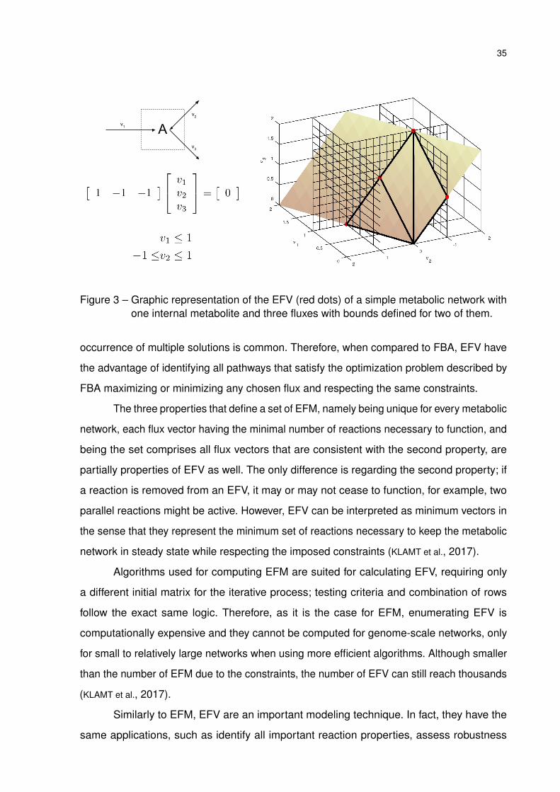
Figure 3 – Graphic representation of the EFV (red dots) of a simple metabolic network withone internal metabolite and three fluxes with bounds defined for two of them.

occurrence of multiple solutions is common. Therefore, when compared to FBA, EFV have

the advantage of identifying all pathways that satisfy the optimization problem described by

FBA maximizing or minimizing any chosen flux and respecting the same constraints.

The three properties that define a set of EFM, namely being unique for every metabolic

network, each flux vector having the minimal number of reactions necessary to function, and

being the set comprises all flux vectors that are consistent with the second property, are

partially properties of EFV as well. The only difference is regarding the second property; if

a reaction is removed from an EFV, it may or may not cease to function, for example, two

parallel reactions might be active. However, EFV can be interpreted as minimum vectors in

the sense that they represent the minimum set of reactions necessary to keep the metabolic

network in steady state while respecting the imposed constraints (KLAMT et al., 2017).

Algorithms used for computing EFM are suited for calculating EFV, requiring only

a different initial matrix for the iterative process; testing criteria and combination of rows

follow the exact same logic. Therefore, as it is the case for EFM, enumerating EFV is

computationally expensive and they cannot be computed for genome-scale networks, only

for small to relatively large networks when using more efficient algorithms. Although smaller

than the number of EFM due to the constraints, the number of EFV can still reach thousands

(KLAMT et al., 2017).

Similarly to EFM, EFV are an important modeling technique. In fact, they have the

same applications, such as identify all important reaction properties, assess robustness

36

of a metabolic network, and identify genetic targets, and identify pathways with maximum

yield. However, because flux information can be incorporated, EFV is able to identify the

maximum and minimum flux values in each reaction, which is the goal of flux variability

analysis (FVA), a technique based on FBA (KLAMT et al., 2017). This information can be

helpful, for example, for assessing network robustness under some fixed conditions (THIELE;

GUDMUNDSSON, 2010).

Now, oppositely to EFM, EFV have not become so popular yet and there are only

few works in literature using this modeling approach. Kamp and Klamt (2017) use EFV to

test the feasibility of growth-coupled production of five metabolites for a small network of the

core metabolism of E. coli. EFV has also been used to determine bounds for internal fluxes

in a dynamic metabolic flux analysis (DMFA) that approximated time intervals to a pseudo

steady state (FERNANDES et al., 2016). De Groot et al. (2019) show that, for metabolisms

aiming optimal growth in growth-limiting situations, only a small number of EFM are active

pathways or, equivalently, only one EFV.

2.1.2 Computational tools for stoichiometric modeling

Several computational tools have been developed, especially during the last 15 years,

in the context of metabolic engineering. The COBRA Toolbox is probably one of the most

popular tools for constraint-based modeling and analysis of metabolic network focusing

on FBA. It started as a MATLAB R© package (BECKER et al., 2007; SCHELLENBERGER et al.,

2011), but has recently been turned into an open source project, with versions for MATLAB R©,

Python and Julia (HEIRENDT et al., 2019). Optflux is a standalone software developed in Java

also for constrained-based modeling (ROCHA et al., 2010).

Metatool is the most popular tool for calculating elementary flux modes. Its first

version was developed in C/C ++ as a standalone software, while Metatool 5.0, and later

version 5.1, was implemented with a more efficient algorithm in MATLAB and Octave to

facilitate the analysis of the results (PFEIFFER et al., 1999; VON KAMP; SCHUSTER, 2006).

FluxModeCalculator is another tool that can calculate EFM written in MATLAB R© which

incorporates several solutions for improving performance (KLINKEN; DIJK, 2016).

CellNetAnalyzer is a MATLAB toolbox that performs several stoichiometric analysis,

including MFA, FBA, EFM, and EFV. It is also possible to explore scenarios for minimal

cut sets. This tool can be used from the command line or within an interface capable of

37

displaying a graphic representation of the metabolic network analyzed (KLAMT et al., 2007;

KLAMT; VON KAMP, 2011; KAMP et al., 2017). COPASI is a complete tool developed for the study

of metabolic fluxes capable of performing various types of analyses, including stoichiometric

analysis of networks, like mass conservation and EFM, optimization of a metabolic model,

and sensitivity analysis. (HOOPS et al., 2006).

38

3 Fundamentals

3.1 Identification of coupled and blocked reactions

Identifying coupled and block reactions is an important analysis to perform when

dealing with stoichiometric models in steady state. Coupled reactions have a fixed flux ratio

and are controlled by an enzyme subset, which is a group of enzymes that operate as a

unit. Since they always work together with the same proportion, a single reaction can be

used to represent them all. Blocked reaction have zero fluxes and can be removed from the

network when working in steady state. This way, metabolic networks can be reduced before

performing expensive analysis, such as EFM.

Assuming the stoichiometry matrix of internal metabolites N ∈ Rm×r has full rank,

matrix K ∈ Rr×r−m, which columns form a basis of the null space of N, also represents the

space of all fluxes that keep the system at steady state, since

NK = 0 (3.1)

by definition. This means that every flux distribution that can keep the system at steady state

can be described as a combination of the columns of K. Each row of K corresponds to a

reaction described by the columns of N. Blocked reactions can be identified by rows of K

that are null vectors because for any combination of the columns of N, their coefficients are

always zero. If every row K is divided by its largest coefficient, then equal rows indicate that

the corresponding reactions are coupled (PFEIFFER et al., 1999).

3.2 Metabolic flux analysis

The idea of MFA is to calculate unknown intracellular fluxes from measured external

fluxes. It does so by splitting the stoichiometry matrix and formulating a system of linear

equations that represents the mass balances of each metabolite. Using only basic linear

algebra concepts, two cases can be modeled with MFA: determined and overdetermined

systems. One starts with the mass balance equations given by

dXm

dt= rm − µXm (3.2)

where Xm ∈ Rm+ is the concentration vector for the internal metabolites, rm ∈ R

m+ is the vector

of formation rates of internal metabolites, and µ ∈ R+ is the biomass specific growth rate. At

39

this point, two hypotheses can be assumed. The first one considers intracellular metabolites

to be at steady state. The other neglects the second term of equation 3.2, which represents

the dilution of the metabolite pool due to growth, as it can be proved its effect is very small

compared to other fluxes that affect the metabolites (STEPHANOPOULOS et al., 1998).

This way, mass balance equations are simplified to

rm = 0 = Nv (3.3)

and the formation rates of intracellular metabolites can be expressed by the product of the

stoichiometry matrix, N ∈ Rm×r, and the flux vector with the rate of all reactions involved,

v ∈ Rr. This product can be split into two terms

Nv = Neve + Nuvu = 0 (3.4)

Ne ∈ Rm×rexp and ve ∈ R

rexp comprise only the reactions with experimentally measured flux

rates, Nu ∈ Rm×r−rexp and vu ∈ R

r−rexp consist of the stoichiometry matrix and flux vector with

the unknown reactions to be determined. If the number of unknown fluxes is the same as

the number of internal metabolites and Nu is invertible, the linear system is determined and

the unknown flux vector can be obtained by

vu = −N−1u Neve (3.5)

In cases where Nu is full rank and there are more measured fluxes than degrees of freedom

in system 3.3, an estimate of the unknown flux vector can be obtained by applying the least

squares method in the overdetermined system, i.e., the pseudo-inverse of Nu should be

used in (3.5) instead of Nu−1.

3.3 Elementary flux modes

The algorithm presented by Schuster and Hilgetag (1994) derives from an algorithm

developed in convex analysis for finding generating vectors. It starts by creating an initial

tableau formed by the stoichiometriy matrix N ∈ Rm×r augmented with an identity matrix of

appropriate size; with the reactions grouped in two blocks, one comprising the reversible

reactions and the other with the irreversible reactions

T (0) =

NTrev I 0

NTirr 0 I

; (3.6)

40

note that the transpose of N must be used. This is an iterative process and the number of

tableaux used is equal to the number of rows in N. In the end, the elementary flux modes are

represented by the rows of the right-hand part, while the left-hand part, initially N, becomes

the null matrix. A new tableau, T ( j+1), is built by combining the rows in T ( j) with each other in

a way that all new rows have zero entry at position j + 1 in the left-hand part. If both rows

are in the irreversible flux block, then

t( j)i, j+1 × t( j)

k, j+1 < 0, (3.7)

since they can only be multiplied by positive coefficients when combined. However, when

a row from the reversible flux block is involved, this row can be multiplied by a negative

coefficient and inequality (3.7) does not need to hold. When adding a new row to tableau

T ( j+1), reversibility of the rows must be respected; only if both rows are reversible the new

row must be added to the reversible flux block. However, only a subset of the new rows

can be added to the next tableau. For each row i of the right-hand part of each T ( j), S (i) is

defined as the set comprising the column indices of elements that are zero. The new rows

generated from combinations and the rows that already have zero entry at j + 1 position

must fulfill the condition

S (i) ∩ S (k) * S (l) with l , i, k, (3.8)

to be added to T ( j+1).

To illustrate the algorithm just presented, consider the simple metabolic network

in Figure 2 with one internal metabolite and three reactions, being the second reaction

reversible. The stoichiometry matrix of this metabolic network is

N =

[1 −1 −1

], (3.9)

so the initial tableau is given by

T (0) =

−1 1 0 0

1 0 1 0

−1 0 0 1

, (3.10)

with the first column in the right-hand side corresponding to v2, the second column to v1 and

the last column to v3. To create the next tableau, rows 1 and 2 can be summed to create a

row with zero entry in the first position of the right-hand side and S (1) ∩ S (2) = {3} in the

left-hand side. It can be added to T (1) since index 3 is not present in S (3) = {1, 2}. Because

41

the first row corresponds to a reversible reaction, it can be multiplied by -1 and added to row

3. This new row can also be added to the next tableau as is also satisfies 3.8. Finally, rows 2

and 3 can be combined and added to T (1) since they satisfy both 3.7 and 3.8, resulting in

T (1) =

0 1 1 0

0 −1 0 1

0 0 1 1

. (3.11)

Since the left-hand side of 3.11 is the zero matrix, calculation is complete and the right-hand

side corresponds to the set of EFM of 3.9. Because of all the EFM involve at least one

irreversible reaction, they were all irreversible.

The original methodology (SCHUSTER; HILGETAG, 1994) is important for understanding

in depth how the calculation of elementary flux modes works. However, ten years after it

was published, Wagner (2004) proposed a different algorithm that considerably reduced

computational time, called the null space approach. In this algorithm, the initial tableau is

matrix KT ∈ Rr−m×r, the transpose of the null space of N ∈ Rm×r, written in the form

T (0) = KT = [K′ I], (3.12)

where K′ ∈ Rr−m×m and I ∈ Rr−m×r−m. This algorithm works based on the fact that an EFM can

only have m + 1 non zero entries at most. With this method only m tableaux are generated.

A new tableau T ( j+1) starts as a copy of the previous one, and new rows are created by

combining all rows of T ( j) that have non zero entries in position j + 1 so there is a zero entry

in that position. Similarly to the original algorithm, a row can only be multiplied by a negative

coefficient if all reactions in that row are reversible and a new row can be added if it satisfies

(3.8). In the end of a new tableau iteration, column j + 1 in T ( j+1) must be the null vector.

After the last tableau is computed, all rows with fluxes violating reversibility constraints must

be removed.

3.4 Linear steady state data reconciliation

From a mathematical point of view, data reconciliation is a parameter estimation

problem. If, for example, all external fluxes are measured, they can be modeled as

vext = v + ε (3.13)

42

where vext is the vector of external fluxes, v ∈ Rrexp is a flux vector representing their true

values and ε ∼ N(0,Σ) is vector of random errors assumed to follow a normal distribution with

covariance matrix Σ ∈ Rrexp×rexp . Vector v is the parameters to be estimated, and formulating

a least squares problem for the estimation leads to the objective function

v ∈ arg minv

(vext − v)T W(vext − v). (3.14)

where W ∈ Rrexp×rexp is a weight matrix. Constraints for v are given by

Av = 0, (3.15)

where A ∈ Rnbal×rext is a matrix with nbal rows corresponding to balancing equations that

represent conservation. Based on a single global equation involving all substrates and

products, the rows of A can correspond to the number of carbon atoms in each metabolite

and the oxidation state, for example.

For a linear system in steady state, (3.14) has an analytical solution

v = vext −W−1AT (AW−1AT )−1Avext, (3.16)

where v ∈ Rrext is a vector with estimates for the true value of the external fluxes. When the

errors follow a normal distribution with zero mean, as it was assumed here, matrix W can be

defined as the inverse of their covariance matrix. If the fluxes are considered independent

from each other, Σ is a diagonal matrix with the variance of each measured flux in the

corresponding entry of the diagonal. If a weight matrix is not used, W can be defined as an

identity matrix of appropriate size (NARASIMHAN; JORDACHE, 1999).

3.5 Elementary flux vectors

Elementary flux vectors can be computed applying the same algorithms used for

calculating elementary flux modes (KLAMT et al., 2017). The initial tableau still has the same

form as Equation (3.6); however, instead of using the stoichiometry matrix N, a matrix that

also takes into consideration the constraints must be used. All EFM keep the metabolic

network in steady state, therefore they satisfy the equation

N f = 0 (3.17)

where f ∈ Rr is a flux vector representing an EFM.

43

When dealing with equality constraints, for example fixing values for external fluxes, f

represents an EFV and, besides satisfying (3.17), it must also satisfy the constraints. These

conditions can be written as N 0

G −b

f

λ

= 0 (3.18)

where G ∈ Rneq×r is a matrix with neq rows corresponding to equality constraints, λ ∈ R is an

auxiliary scalar variable and b ∈ Rneq is the right-hand side of the equality constraints, and

the matrix in the left-hand side of (3.18) is defined as D ∈ Rm+neq×r+1. For computing EFV,

D can replace N to form the initial tableau; if, for example, the original algorithm is used,

T (0) = [D I]. After EFV are computed, if λ = 0 the corresponding EFV is unbounded, like an

EFM, and if > 0, the bounded EFV is given by f /λ.

When flux bounds are added as constraints, D is slightly different. Inequalities must

first be converted to equality constraints by using slack variables, which are free variables

that determine how far from the bounds the fluxes are. So, the conditions that an EFV must

fulfill are represented by N 0 0

G 0 −b

H I −c

f

s

λ

= 0 (3.19)

where H ∈ Rnineq×r is a matrix with nineq rows corresponding to inequality constraints, s ∈ Rnineq

is a vector with the slack variables and c ∈ Rnineq is a vector with bound values.

44

4 Software development

A computational tool for stoichiometry analysis of metabolic networks was developed

using the C++ language. This language was chosen for being free, fast, one of the most

popular languages currently in use, which consequently implies availability of many resources

and community support; and object oriented, which is an important asset for structuring

software. Eigen, which is a template library for C++, was used for linear algebra calculation

(GUENNEBAUD et al., 2010).

4.1 Structure

This software was built using the object oriented programming paradigm, based on

hierarchy, composition concepts, and polymorphism, to facilitate maintenance and addition of

new functionalities. Design patterns (GAMMA et al., 1995), which are well-established solutions

for common problems in software design, were implemented where applicable. This way,

every feature of this software can be easily connected to the metabolic network and each

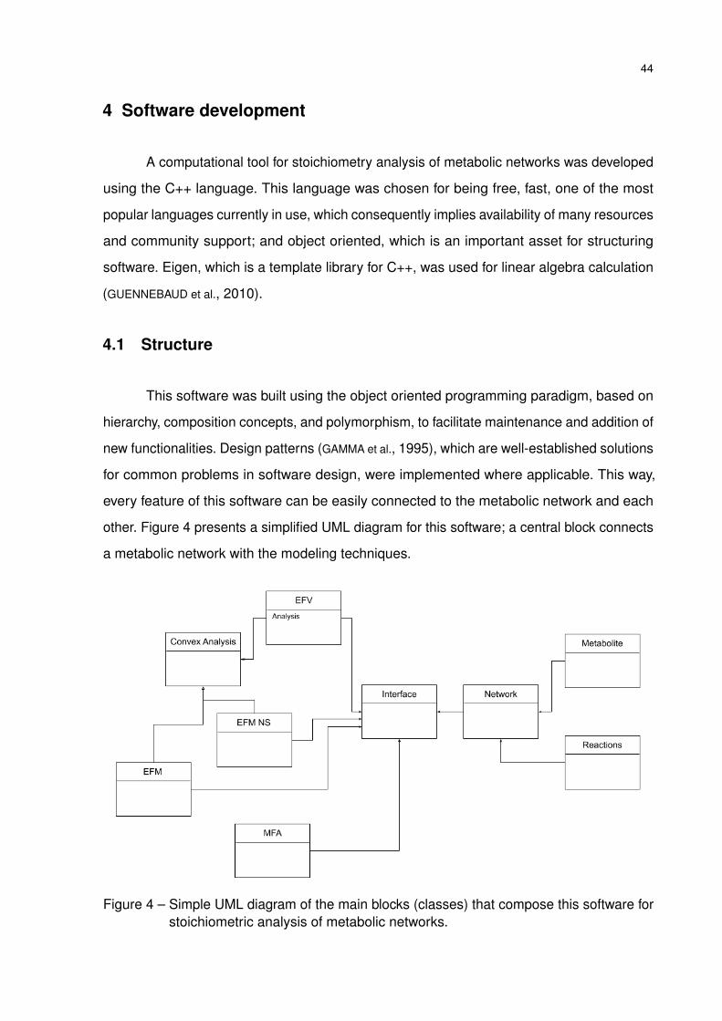
other. Figure 4 presents a simplified UML diagram for this software; a central block connects

a metabolic network with the modeling techniques.

Figure 4 – Simple UML diagram of the main blocks (classes) that compose this software forstoichiometric analysis of metabolic networks.

45

The stoichiometric models and main supporting features implemented in this compu-

tational tool are:

• metabolic flux analysis,

• elementary flux modes,

• elementary flux vectors,

• analysis of elementary flux vectors for experimental design.

MFA was applied as described in Section 3.2 using linear algebra functions. Two algorithms

were implemented for calculating EFM and EFV, the original routine (EFM) and the null space

approach (EFM-NS) (SCHUSTER; HILGETAG, 1994; WAGNER, 2004). Analysis of elementary

flux vectors for experimental design comprises the calculation of some properties from EFV,

including a similarity measure for the flux pattern that each reaction present in the set of

EFV. These properties are described with more details in the next section.

Other supporting features include

• processing the input metabolic network to verify its consistency,

• treatment of elementary flux modes to help categorize and go through the large number

of EFM that metabolic networks usually have,

• identifying coupled and blocked reactions, as presented in Section 3.1, to reduce the

metabolic network and, consequently, improve the computation of EFM and EFV,

• performing data reconciliation on experimental measurements used as constraints for

calculating EFV as described in Section 3.4.

This last feature is necessary because EFV are a deterministic model, therefore errors in flux

measurements can hamper their computation when equality constraints are used, i.e., fixed

values for some fluxes. There are basically two ways to readily deal with this issue: relaxing

the tolerance during EFV calculation or perform data reconciliation on flux measurements.

Because some fluxes are easier to determine than others and they can present different

variances, data reconciliation was implemented using carbon and redox balances. Treatment

of EFM consists of removing thermodynamically infeasible EFM with no substrate uptake,

calculating each EFM yield by dividing the EFM by the flux of the main substrate (defined

as the first substrate listed at input), and grouping EFM with the same overall stoichiometry,

which helps to identify redundant pathways of the metabolic network.

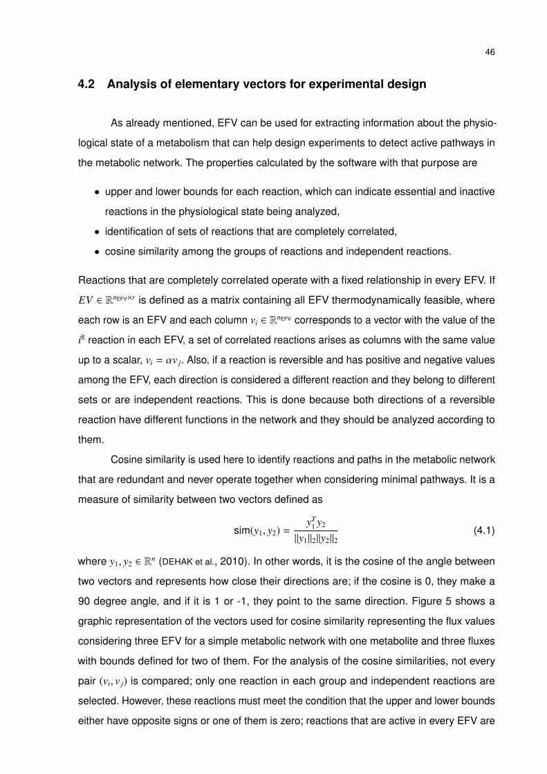
46

4.2 Analysis of elementary vectors for experimental design

As already mentioned, EFV can be used for extracting information about the physio-

logical state of a metabolism that can help design experiments to detect active pathways in

the metabolic network. The properties calculated by the software with that purpose are

• upper and lower bounds for each reaction, which can indicate essential and inactive

reactions in the physiological state being analyzed,

• identification of sets of reactions that are completely correlated,

• cosine similarity among the groups of reactions and independent reactions.

Reactions that are completely correlated operate with a fixed relationship in every EFV. If

EV ∈ RnEFV×r is defined as a matrix containing all EFV thermodynamically feasible, where

each row is an EFV and each column vi ∈ RnEFV corresponds to a vector with the value of the

iit reaction in each EFV, a set of correlated reactions arises as columns with the same value

up to a scalar, vi = αv j. Also, if a reaction is reversible and has positive and negative values

among the EFV, each direction is considered a different reaction and they belong to different

sets or are independent reactions. This is done because both directions of a reversible

reaction have different functions in the network and they should be analyzed according to

them.

Cosine similarity is used here to identify reactions and paths in the metabolic network

that are redundant and never operate together when considering minimal pathways. It is a

measure of similarity between two vectors defined as

sim(y1, y2) =yT

1 y2

‖y1‖2‖y2‖2(4.1)

where y1, y2 ∈ Rn (DEHAK et al., 2010). In other words, it is the cosine of the angle between

two vectors and represents how close their directions are; if the cosine is 0, they make a

90 degree angle, and if it is 1 or -1, they point to the same direction. Figure 5 shows a

graphic representation of the vectors used for cosine similarity representing the flux values

considering three EFV for a simple metabolic network with one metabolite and three fluxes

with bounds defined for two of them. For the analysis of the cosine similarities, not every

pair (vi, v j) is compared; only one reaction in each group and independent reactions are

selected. However, these reactions must meet the condition that the upper and lower bounds

either have opposite signs or one of them is zero; reactions that are active in every EFV are

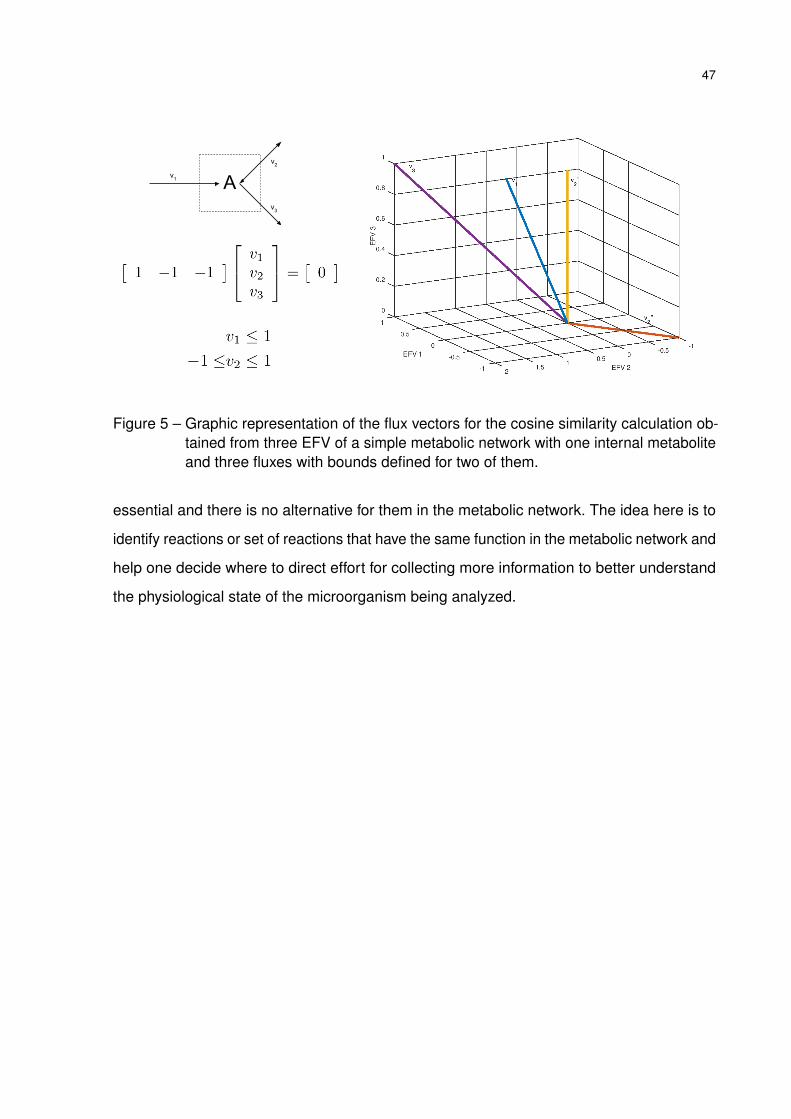
47

Figure 5 – Graphic representation of the flux vectors for the cosine similarity calculation ob-tained from three EFV of a simple metabolic network with one internal metaboliteand three fluxes with bounds defined for two of them.

essential and there is no alternative for them in the metabolic network. The idea here is to

identify reactions or set of reactions that have the same function in the metabolic network and

help one decide where to direct effort for collecting more information to better understand

the physiological state of the microorganism being analyzed.

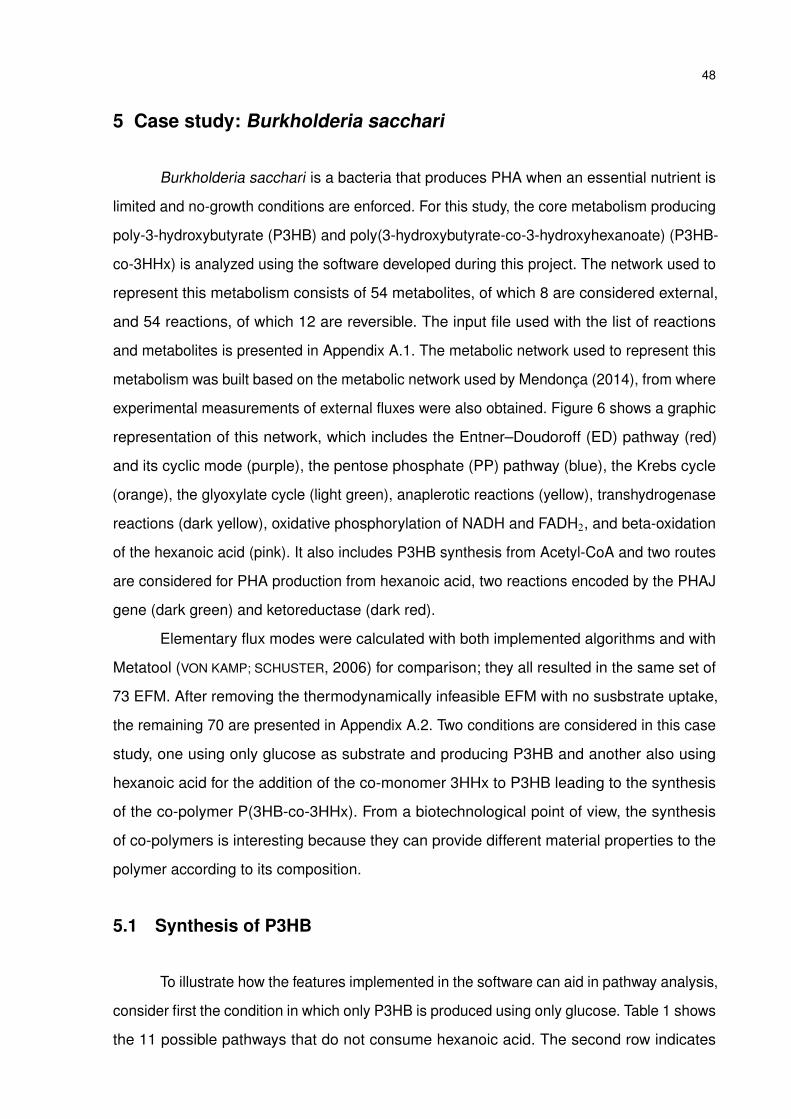
48

5 Case study: Burkholderia sacchari

Burkholderia sacchari is a bacteria that produces PHA when an essential nutrient is

limited and no-growth conditions are enforced. For this study, the core metabolism producing

poly-3-hydroxybutyrate (P3HB) and poly(3-hydroxybutyrate-co-3-hydroxyhexanoate) (P3HB-

co-3HHx) is analyzed using the software developed during this project. The network used to

represent this metabolism consists of 54 metabolites, of which 8 are considered external,

and 54 reactions, of which 12 are reversible. The input file used with the list of reactions

and metabolites is presented in Appendix A.1. The metabolic network used to represent this

metabolism was built based on the metabolic network used by Mendonça (2014), from where

experimental measurements of external fluxes were also obtained. Figure 6 shows a graphic

representation of this network, which includes the Entner–Doudoroff (ED) pathway (red)

and its cyclic mode (purple), the pentose phosphate (PP) pathway (blue), the Krebs cycle

(orange), the glyoxylate cycle (light green), anaplerotic reactions (yellow), transhydrogenase

reactions (dark yellow), oxidative phosphorylation of NADH and FADH2, and beta-oxidation

of the hexanoic acid (pink). It also includes P3HB synthesis from Acetyl-CoA and two routes

are considered for PHA production from hexanoic acid, two reactions encoded by the PHAJ

gene (dark green) and ketoreductase (dark red).

Elementary flux modes were calculated with both implemented algorithms and with

Metatool (VON KAMP; SCHUSTER, 2006) for comparison; they all resulted in the same set of

73 EFM. After removing the thermodynamically infeasible EFM with no susbstrate uptake,

the remaining 70 are presented in Appendix A.2. Two conditions are considered in this case

study, one using only glucose as substrate and producing P3HB and another also using

hexanoic acid for the addition of the co-monomer 3HHx to P3HB leading to the synthesis

of the co-polymer P(3HB-co-3HHx). From a biotechnological point of view, the synthesis

of co-polymers is interesting because they can provide different material properties to the

polymer according to its composition.

5.1 Synthesis of P3HB

To illustrate how the features implemented in the software can aid in pathway analysis,

consider first the condition in which only P3HB is produced using only glucose. Table 1 shows

the 11 possible pathways that do not consume hexanoic acid. The second row indicates

49

Figure 6 – Metabolic network used to represent the central metabolism of B. sacchari pro-ducing P3HB and P3HB-co-3HHx.

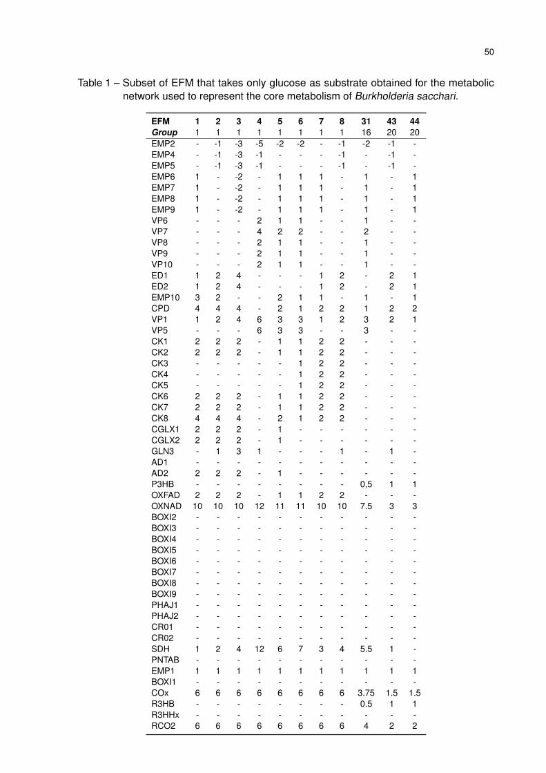
50

Table 1 – Subset of EFM that takes only glucose as substrate obtained for the metabolicnetwork used to represent the core metabolism of Burkholderia sacchari.

EFM 1 2 3 4 5 6 7 8 31 43 44Group 1 1 1 1 1 1 1 1 16 20 20EMP2 - -1 -3 -5 -2 -2 - -1 -2 -1 -EMP4 - -1 -3 -1 - - - -1 - -1 -EMP5 - -1 -3 -1 - - - -1 - -1 -EMP6 1 - -2 - 1 1 1 - 1 - 1EMP7 1 - -2 - 1 1 1 - 1 - 1EMP8 1 - -2 - 1 1 1 - 1 - 1EMP9 1 - -2 - 1 1 1 - 1 - 1VP6 - - - 2 1 1 - - 1 - -VP7 - - - 4 2 2 - - 2 - -VP8 - - - 2 1 1 - - 1 - -VP9 - - - 2 1 1 - - 1 - -VP10 - - - 2 1 1 - - 1 - -ED1 1 2 4 - - - 1 2 - 2 1ED2 1 2 4 - - - 1 2 - 2 1EMP10 3 2 - - 2 1 1 - 1 - 1CPD 4 4 4 - 2 1 2 2 1 2 2VP1 1 2 4 6 3 3 1 2 3 2 1VP5 - - - 6 3 3 - - 3 - -CK1 2 2 2 - 1 1 2 2 - - -CK2 2 2 2 - 1 1 2 2 - - -CK3 - - - - - 1 2 2 - - -CK4 - - - - - 1 2 2 - - -CK5 - - - - - 1 2 2 - - -CK6 2 2 2 - 1 1 2 2 - - -CK7 2 2 2 - 1 1 2 2 - - -CK8 4 4 4 - 2 1 2 2 - - -CGLX1 2 2 2 - 1 - - - - - -CGLX2 2 2 2 - 1 - - - - - -GLN3 - 1 3 1 - - - 1 - 1 -AD1 - - - - - - - - - - -AD2 2 2 2 - 1 - - - - - -P3HB - - - - - - - - 0,5 1 1OXFAD 2 2 2 - 1 1 2 2 - - -OXNAD 10 10 10 12 11 11 10 10 7.5 3 3BOXI2 - - - - - - - - - - -BOXI3 - - - - - - - - - - -BOXI4 - - - - - - - - - - -BOXI5 - - - - - - - - - - -BOXI6 - - - - - - - - - - -BOXI7 - - - - - - - - - - -BOXI8 - - - - - - - - - - -BOXI9 - - - - - - - - - - -PHAJ1 - - - - - - - - - - -PHAJ2 - - - - - - - - - - -CR01 - - - - - - - - - - -CR02 - - - - - - - - - - -SDH 1 2 4 12 6 7 3 4 5.5 1 -PNTAB - - - - - - - - - - -EMP1 1 1 1 1 1 1 1 1 1 1 1BOXI1 - - - - - - - - - - -COx 6 6 6 6 6 6 6 6 3.75 1.5 1.5R3HB - - - - - - - - 0.5 1 1R3HHx - - - - - - - - - - -RCO2 6 6 6 6 6 6 6 6 4 2 2

51

EFM with the same overall stoichiometry; they have the same group number. There are 3

EFM corresponding to pathways for 3HB synthesis, but only 2 different overall stoichiometry

proportions, and 8 EFM that only release CO2, all belonging to the same stoichiometry group.

The pathways that produce 3HB use the PP or the ED pathway; the latter being either the

linear or the cyclic mode. As for the EFM that release CO2, other redundant paths arise, like

the glyoxylate and Krebs cycle, and combinations among them are possible. For example,

EFM 4 releases all 6 moles of CO2 through the PP pathway, while EFM 7 uses the ED

pathway and Krebs cycle.

Since the polymer is the product of interest, EFM that use the ED pathway (group

20) are the ones with optimal yield for metabolic network considered; for one mole of

glucose consumed, one mole of 3HB is produced with the release of 2 moles of CO2.

Experimental data for this condition (see Table 2) show that the ratio between CO2 and

3HB is 2.66:1; 90.2% of the glucose is used for synthesis of P3HB with maximum yield,

while 9.8% is just used for respiration, which means there still is room for improvement.

Understanding how a physiological state of a microorganism operates can help planning

strategies that can increase product yield. One way to analyze active pathways would be

performing a MFA calculation using the overall stoichiometry of each group of EFM as the

unknown stoichiometry matrix and estimate the flux through each group. Since there are 4

measurements (glucose, O2, 3HB and CO2) and 3 groups, the problem is overdetermined

and the least squares method can be applied. Table 2 shows the estimated contribution

of each group of EFM. Group 16, which comprises one EFM using the PP pathway, has

zero flux, implying that the production of 3HB relies on the ED pathway, either the linear or

cyclic mode. The excess CO2 is produced by one or a combination of EFM in group 1; to

distinguish which pathways are being used, more information needs to be experimentally

collected.

Table 2 – Overall stoichiometry of the three groups of EFM involved in metabolize glucose inthe studied metabolic network. vg is the estimated flux through each group and ve

is the experimental measured flux corresponding to consumption or production ofthe external metabolites (MENDONÇA, 2014).

Group 1 Group 16 Group 20 ve (mmol/g.h)Glucose -1 -1 -1 -1.97O2 -6 -3.75 -1.5 -3.573HB 0 0.5 1 1.6CO2 6 4 2 4.26vg (mmol/g.h) 0.179 0 1.65

52

At first glance, one could think there are 16 minimal pathways in this metabolic

network that can explain the measured fluxes, as group 1 has 8 EFM and group 8 has 2 EFM.

However, when EFV are calculated fixing the values of external fluxes, 7 minimal pathways

are obtained. Table 3 shows the EFV obtained from the metabolic network in Figure 6 and

the experimental data in Table 2. Note that the external fluxes in the EFV, the last 6 reactions

in Table 3 differ from the ones in Table 2; due to experimental errors, data reconciliation was

performed and a weight matrix was not used because variance on the measurements was

not available. An interesting observation is that there are two EFM that use the PP pathway

and either the glyoxylate or the Krebs cycle at the same time. Those EFM are not present in

the EFV set, indicating that, for this flux distribution, they all have the same function. Also,

note that when the cyclic mode of the ED pathway is active, the flux through the membrane

transhydrogenase (SDH) is higher to oxidize the excess NADPH produced.

Table 3 also shows independent reactions and sets of completely correlated reactions

identified from EFV, as well as the maximum and minimum values of each reaction. Using this

information, cosine similarity was calculated for every pair of selected reactions according to

Section 4.2, which is presented in Table 4. A similarity value equal to zero, indicate that the

involved reactions are redundant, i.e., have equivalent functions in the metabolic network.

For example, corroborating the observation above, the PP pathway (PPP) have zero cosine

similarity with the Krebs cycle (CKc) and the glyoxylate cycle (GLXc) with or without the

anaplerotic reactions, which shows that their function, for the considered physiological state

based on this metabolic network, is to release the remainder of the CO2 accounted for

that was not produced in the CPD reaction. Therefore, in this case, the PP pathway is not

necessary for generating the co-factor NADPH used for producing 3HB; other reactions in

the metabolism have enough flux to meet that demand. Other redundancies that the cosine

similarity identified for this metabolic network are, for instance, the linear (EDPl) and cyclic

(EDPC) modes of the ED pathway, and the Krebs and the glyoxylate cycles.

When deciding what new information should be collected, a possible reasoning would

be assuming, for example, that the PP pathway, the glyoxylate cycle and the anaplerotic

reactions are not active or have very little flux through them since there is no growth in

the experiment from which data is being considered. Thus, excess CO2 is assumed to be

produced by the Krebs cycle and the ED pathway to be active, either the cyclic or the linear

mode. How the flux is divided between them depends on co-factor and energy balances and,

in this case, this can be verified by analyzing the fluxes through the ED pathway and/or the

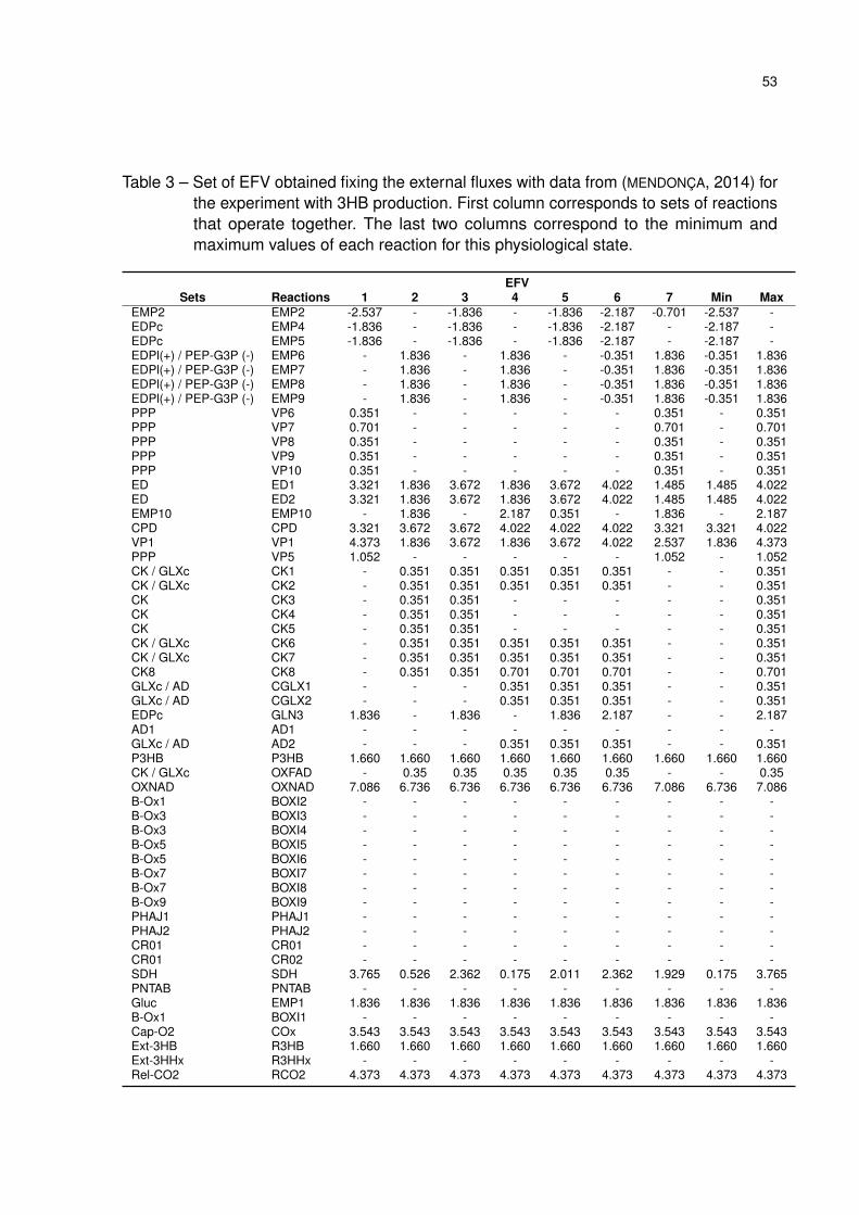
53

Table 3 – Set of EFV obtained fixing the external fluxes with data from (MENDONÇA, 2014) forthe experiment with 3HB production. First column corresponds to sets of reactionsthat operate together. The last two columns correspond to the minimum andmaximum values of each reaction for this physiological state.

EFVSets Reactions 1 2 3 4 5 6 7 Min Max

EMP2 EMP2 -2.537 - -1.836 - -1.836 -2.187 -0.701 -2.537 -EDPc EMP4 -1.836 - -1.836 - -1.836 -2.187 - -2.187 -EDPc EMP5 -1.836 - -1.836 - -1.836 -2.187 - -2.187 -EDPl(+) / PEP-G3P (-) EMP6 - 1.836 - 1.836 - -0.351 1.836 -0.351 1.836EDPl(+) / PEP-G3P (-) EMP7 - 1.836 - 1.836 - -0.351 1.836 -0.351 1.836EDPl(+) / PEP-G3P (-) EMP8 - 1.836 - 1.836 - -0.351 1.836 -0.351 1.836EDPl(+) / PEP-G3P (-) EMP9 - 1.836 - 1.836 - -0.351 1.836 -0.351 1.836PPP VP6 0.351 - - - - - 0.351 - 0.351PPP VP7 0.701 - - - - - 0.701 - 0.701PPP VP8 0.351 - - - - - 0.351 - 0.351PPP VP9 0.351 - - - - - 0.351 - 0.351PPP VP10 0.351 - - - - - 0.351 - 0.351ED ED1 3.321 1.836 3.672 1.836 3.672 4.022 1.485 1.485 4.022ED ED2 3.321 1.836 3.672 1.836 3.672 4.022 1.485 1.485 4.022EMP10 EMP10 - 1.836 - 2.187 0.351 - 1.836 - 2.187CPD CPD 3.321 3.672 3.672 4.022 4.022 4.022 3.321 3.321 4.022VP1 VP1 4.373 1.836 3.672 1.836 3.672 4.022 2.537 1.836 4.373PPP VP5 1.052 - - - - - 1.052 - 1.052CK / GLXc CK1 - 0.351 0.351 0.351 0.351 0.351 - - 0.351CK / GLXc CK2 - 0.351 0.351 0.351 0.351 0.351 - - 0.351CK CK3 - 0.351 0.351 - - - - - 0.351CK CK4 - 0.351 0.351 - - - - - 0.351CK CK5 - 0.351 0.351 - - - - - 0.351CK / GLXc CK6 - 0.351 0.351 0.351 0.351 0.351 - - 0.351CK / GLXc CK7 - 0.351 0.351 0.351 0.351 0.351 - - 0.351CK8 CK8 - 0.351 0.351 0.701 0.701 0.701 - - 0.701GLXc / AD CGLX1 - - - 0.351 0.351 0.351 - - 0.351GLXc / AD CGLX2 - - - 0.351 0.351 0.351 - - 0.351EDPc GLN3 1.836 - 1.836 - 1.836 2.187 - - 2.187AD1 AD1 - - - - - - - - -GLXc / AD AD2 - - - 0.351 0.351 0.351 - - 0.351P3HB P3HB 1.660 1.660 1.660 1.660 1.660 1.660 1.660 1.660 1.660CK / GLXc OXFAD - 0.35 0.35 0.35 0.35 0.35 - - 0.35OXNAD OXNAD 7.086 6.736 6.736 6.736 6.736 6.736 7.086 6.736 7.086B-Ox1 BOXI2 - - - - - - - - -B-Ox3 BOXI3 - - - - - - - - -B-Ox3 BOXI4 - - - - - - - - -B-Ox5 BOXI5 - - - - - - - - -B-Ox5 BOXI6 - - - - - - - - -B-Ox7 BOXI7 - - - - - - - - -B-Ox7 BOXI8 - - - - - - - - -B-Ox9 BOXI9 - - - - - - - - -PHAJ1 PHAJ1 - - - - - - - - -PHAJ2 PHAJ2 - - - - - - - - -CR01 CR01 - - - - - - - - -CR01 CR02 - - - - - - - - -SDH SDH 3.765 0.526 2.362 0.175 2.011 2.362 1.929 0.175 3.765PNTAB PNTAB - - - - - - - - -Gluc EMP1 1.836 1.836 1.836 1.836 1.836 1.836 1.836 1.836 1.836B-Ox1 BOXI1 - - - - - - - - -Cap-O2 COx 3.543 3.543 3.543 3.543 3.543 3.543 3.543 3.543 3.543Ext-3HB R3HB 1.660 1.660 1.660 1.660 1.660 1.660 1.660 1.660 1.660Ext-3HHx R3HHx - - - - - - - - -Rel-CO2 RCO2 4.373 4.373 4.373 4.373 4.373 4.373 4.373 4.373 4.373

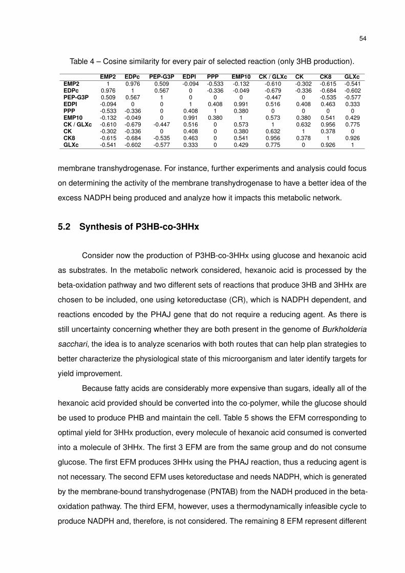
54

Table 4 – Cosine similarity for every pair of selected reaction (only 3HB production).

EMP2 EDPc PEP-G3P EDPl PPP EMP10 CK / GLXc CK CK8 GLXcEMP2 1 0.976 0.509 -0.094 -0.533 -0.132 -0.610 -0.302 -0.615 -0.541EDPc 0.976 1 0.567 0 -0.336 -0.049 -0.679 -0.336 -0.684 -0.602PEP-G3P 0.509 0.567 1 0 0 0 -0.447 0 -0.535 -0.577EDPl -0.094 0 0 1 0.408 0.991 0.516 0.408 0.463 0.333PPP -0.533 -0.336 0 0.408 1 0.380 0 0 0 0EMP10 -0.132 -0.049 0 0.991 0.380 1 0.573 0.380 0.541 0.429CK / GLXc -0.610 -0.679 -0.447 0.516 0 0.573 1 0.632 0.956 0.775CK -0.302 -0.336 0 0.408 0 0.380 0.632 1 0.378 0CK8 -0.615 -0.684 -0.535 0.463 0 0.541 0.956 0.378 1 0.926GLXc -0.541 -0.602 -0.577 0.333 0 0.429 0.775 0 0.926 1

membrane transhydrogenase. For instance, further experiments and analysis could focus

on determining the activity of the membrane transhydrogenase to have a better idea of the

excess NADPH being produced and analyze how it impacts this metabolic network.

5.2 Synthesis of P3HB-co-3HHx

Consider now the production of P3HB-co-3HHx using glucose and hexanoic acid

as substrates. In the metabolic network considered, hexanoic acid is processed by the

beta-oxidation pathway and two different sets of reactions that produce 3HB and 3HHx are

chosen to be included, one using ketoreductase (CR), which is NADPH dependent, and

reactions encoded by the PHAJ gene that do not require a reducing agent. As there is

still uncertainty concerning whether they are both present in the genome of Burkholderia

sacchari, the idea is to analyze scenarios with both routes that can help plan strategies to

better characterize the physiological state of this microorganism and later identify targets for

yield improvement.

Because fatty acids are considerably more expensive than sugars, ideally all of the

hexanoic acid provided should be converted into the co-polymer, while the glucose should

be used to produce PHB and maintain the cell. Table 5 shows the EFM corresponding to

optimal yield for 3HHx production, every molecule of hexanoic acid consumed is converted

into a molecule of 3HHx. The first 3 EFM are from the same group and do not consume

glucose. The first EFM produces 3HHx using the PHAJ reaction, thus a reducing agent is

not necessary. The second EFM uses ketoreductase and needs NADPH, which is generated

by the membrane-bound transhydrogenase (PNTAB) from the NADH produced in the beta-

oxidation pathway. The third EFM, however, uses a thermodynamically infeasible cycle to

produce NADPH and, therefore, is not considered. The remaining 8 EFM represent different

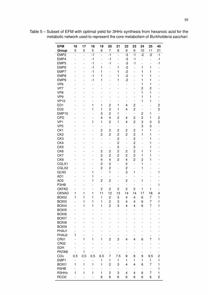
55

Table 5 – Subset of EFM with optimal yield for 3HHx synthesis from hexanoic acid for themetabolic network used to represent the core metabolism of Burkholderia sacchari.

EFM 16 17 18 19 20 21 22 23 24 25 45Group 5 5 5 6 7 8 9 9 10 11 21EMP2 - - -1 - -1 - -3 -1 -2 -2 -1EMP4 - - -1 - -1 - -3 -1 - - -1EMP5 - - -1 - -1 - -3 -1 - - -1EMP6 - - -1 1 - 1 -2 - 1 1 -EMP7 - - -1 1 - 1 -2 - 1 1 -EMP8 - - -1 1 - 1 -2 - 1 1 -EMP9 - - -1 1 - 1 -2 - 1 1 -VP6 - - - - - - - - 1 1 -VP7 - - - - - - - - 2 2 -VP8 - - - - - - - - 1 1 -VP9 - - - - - - - - 1 1 -VP10 - - - - - - - - 1 1 -ED1 - - 1 1 2 1 4 2 - - 2ED2 - - 1 1 2 1 4 2 - - 2EMP10 - - - 3 2 1 - - 2 1 -CPD - - - 4 4 2 4 2 2 1 2VP1 - - 1 1 2 1 4 2 3 3 2VP5 - - - - - - - - 3 3 -CK1 - - - 2 2 2 2 2 1 1 -CK2 - - - 2 2 2 2 2 1 1 -CK3 - - - - - 2 - 2 - 1 -CK4 - - - - - 2 - 2 - 1 -CK5 - - - - - 2 - 2 - 1 -CK6 - - - 2 2 2 2 2 1 1 -CK7 - - - 2 2 2 2 2 1 1 -CK8 - - - 4 4 2 4 2 2 1 -CGLX1 - - - 2 2 - 2 - 1 - -CGLX2 - - - 2 2 - 2 - 1 - -GLN3 - - 1 - 1 - 3 1 - - 1AD1 - - 1 - - - - - - - -AD2 - - 1 2 2 - 2 - 1 - -P3HB - - - - - - - - - - 1OXFAD - - - 2 2 2 2 2 1 1 -OXNAD 1 1 1 11 12 13 14 14 17 18 4BOXI2 1 1 1 1 2 3 4 4 6 7 1BOXI3 - 1 1 1 2 3 4 4 6 7 1BOXI4 - 1 1 1 2 3 4 4 6 7 1BOXI5 - - - - - - - - - - -BOXI6 - - - - - - - - - - -BOXI7 - - - - - - - - - - -BOXI8 - - - - - - - - - - -BOXI9 - - - - - - - - - - -PHAJ1 - - - - - - - - - - -PHAJ2 1 - - - - - - - - - -CR01 - 1 1 1 2 3 4 4 6 7 1CR02 - - - - - - - - - - -SDH - - - - - - - - - - -PNTAB - 1 - - - - - - - - -COx 0.5 0.5 0.5 6.5 7 7.5 8 8 9 9.5 2EMP1 - - - 1 1 1 1 1 1 1 1BOXI1 1 1 1 1 2 3 4 4 6 7 1R3HB - - - - - - - - - - 1R3HHx 1 1 1 1 2 3 4 4 6 7 1RCO2 - - - 6 6 6 6 6 6 6 2

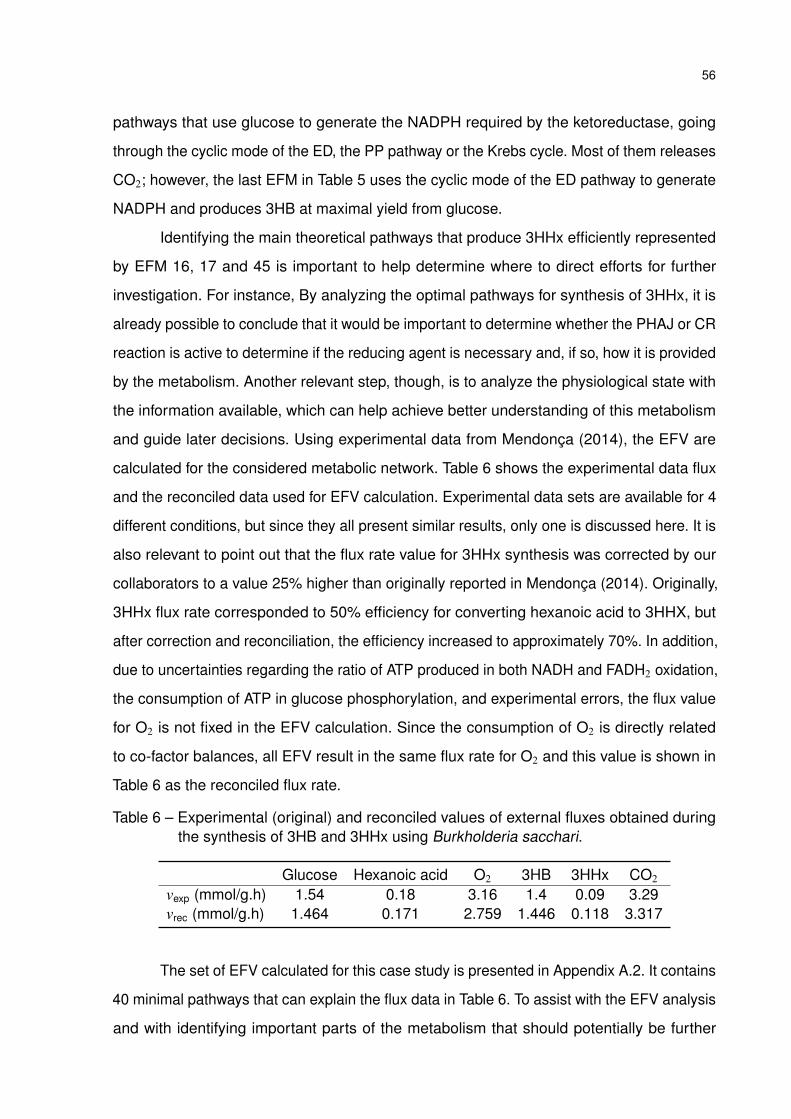
56

pathways that use glucose to generate the NADPH required by the ketoreductase, going

through the cyclic mode of the ED, the PP pathway or the Krebs cycle. Most of them releases

CO2; however, the last EFM in Table 5 uses the cyclic mode of the ED pathway to generate

NADPH and produces 3HB at maximal yield from glucose.

Identifying the main theoretical pathways that produce 3HHx efficiently represented

by EFM 16, 17 and 45 is important to help determine where to direct efforts for further

investigation. For instance, By analyzing the optimal pathways for synthesis of 3HHx, it is

already possible to conclude that it would be important to determine whether the PHAJ or CR

reaction is active to determine if the reducing agent is necessary and, if so, how it is provided

by the metabolism. Another relevant step, though, is to analyze the physiological state with

the information available, which can help achieve better understanding of this metabolism

and guide later decisions. Using experimental data from Mendonça (2014), the EFV are

calculated for the considered metabolic network. Table 6 shows the experimental data flux

and the reconciled data used for EFV calculation. Experimental data sets are available for 4

different conditions, but since they all present similar results, only one is discussed here. It is

also relevant to point out that the flux rate value for 3HHx synthesis was corrected by our

collaborators to a value 25% higher than originally reported in Mendonça (2014). Originally,

3HHx flux rate corresponded to 50% efficiency for converting hexanoic acid to 3HHX, but

after correction and reconciliation, the efficiency increased to approximately 70%. In addition,

due to uncertainties regarding the ratio of ATP produced in both NADH and FADH2 oxidation,

the consumption of ATP in glucose phosphorylation, and experimental errors, the flux value

for O2 is not fixed in the EFV calculation. Since the consumption of O2 is directly related

to co-factor balances, all EFV result in the same flux rate for O2 and this value is shown in

Table 6 as the reconciled flux rate.

Table 6 – Experimental (original) and reconciled values of external fluxes obtained duringthe synthesis of 3HB and 3HHx using Burkholderia sacchari.

Glucose Hexanoic acid O2 3HB 3HHx CO2

vexp (mmol/g.h) 1.54 0.18 3.16 1.4 0.09 3.29vrec (mmol/g.h) 1.464 0.171 2.759 1.446 0.118 3.317

The set of EFV calculated for this case study is presented in Appendix A.2. It contains

40 minimal pathways that can explain the flux data in Table 6. To assist with the EFV analysis

and with identifying important parts of the metabolism that should potentially be further

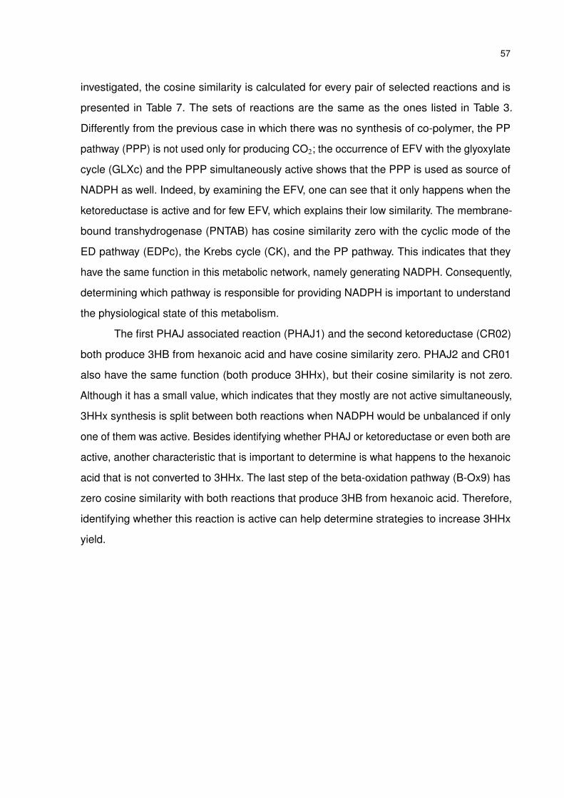
57

investigated, the cosine similarity is calculated for every pair of selected reactions and is

presented in Table 7. The sets of reactions are the same as the ones listed in Table 3.

Differently from the previous case in which there was no synthesis of co-polymer, the PP

pathway (PPP) is not used only for producing CO2; the occurrence of EFV with the glyoxylate

cycle (GLXc) and the PPP simultaneously active shows that the PPP is used as source of

NADPH as well. Indeed, by examining the EFV, one can see that it only happens when the

ketoreductase is active and for few EFV, which explains their low similarity. The membrane-

bound transhydrogenase (PNTAB) has cosine similarity zero with the cyclic mode of the

ED pathway (EDPc), the Krebs cycle (CK), and the PP pathway. This indicates that they

have the same function in this metabolic network, namely generating NADPH. Consequently,

determining which pathway is responsible for providing NADPH is important to understand

the physiological state of this metabolism.

The first PHAJ associated reaction (PHAJ1) and the second ketoreductase (CR02)

both produce 3HB from hexanoic acid and have cosine similarity zero. PHAJ2 and CR01

also have the same function (both produce 3HHx), but their cosine similarity is not zero.

Although it has a small value, which indicates that they mostly are not active simultaneously,

3HHx synthesis is split between both reactions when NADPH would be unbalanced if only

one of them was active. Besides identifying whether PHAJ or ketoreductase or even both are

active, another characteristic that is important to determine is what happens to the hexanoic

acid that is not converted to 3HHx. The last step of the beta-oxidation pathway (B-Ox9) has

zero cosine similarity with both reactions that produce 3HB from hexanoic acid. Therefore,

identifying whether this reaction is active can help determine strategies to increase 3HHx

yield.

58

Table 7 – Cosine similarity for every pair of selected reaction (3HB and 3HHx production).

EMP2 EDPc PEP-G3P EDPl PPP EMP10 CK / GLXc CK CK8 GLXc B-Ox7 B-Ox9 PHAJ1 PHAJ2 CR01 CR02 SDH PNTABEMP2 1 0.979 0.523 -0.091 -0.479 -0.104 -0.416 -0.182 -0.420 -0.389 -0.556 -0.527 -0.229 -0.295 -0.523 -0.232 -0.970 0EDPc 0.979 1 0.570 -0.009 -0.290 -0.029 -0.450 -0.198 -0.454 -0.421 -0.516 -0.517 -0.181 -0.256 -0.477 -0.181 -0.904 0PEP-G3P 0.523 0.570 1 0 0 0 -0.314 0 -0.358 -0.382 -0.218 -0.280 -0.167 -0.163 -0.225 0 -0.436 0EDPl -0.091 -0.009 0 1 0.389 0.997 0.763 0.463 0.731 0.630 0.666 0.450 0.537 0.531 0.681 0.503 0.198 0.310PPP -0.479 -0.290 0 0.389 1 0.364 0.014 0 0.016 0.017 0.390 0.251 0.293 0.281 0.405 0.311 0.661 0EMP10 -0.104 -0.029 0 0.997 0.364 1 0.787 0.437 0.767 0.677 0.676 0.460 0.539 0.528 0.694 0.506 0.200 0.327CK / GLXc -0.416 -0.450 -0.314 0.763 0.014 0.787 1 0.573 0.969 0.848 0.746 0.610 0.468 0.515 0.727 0.431 0.378 0.300CK -0.182 -0.198 0 0.463 0 0.437 0.573 1 0.351 0.051 0.453 0.374 0.221 0.384 0.350 0.259 0.226 0CK8 -0.420 -0.454 -0.358 0.731 0.016 0.767 0.969 0.351 1 0.953 0.714 0.584 0.467 0.472 0.725 0.414 0.363 0.343GLXc -0.389 -0.421 -0.382 0.630 0.017 0.677 0.848 0.051 0.953 1 0.615 0.502 0.427 0.379 0.660 0.358 0.314 0.366B-Ox7 -0.556 -0.516 -0.218 0.666 0.390 0.676 0.746 0.453 0.714 0.615 1 0.779 0 0.516 0.673 0.627 0.580 0.254B-Ox9 -0.527 -0.517 -0.280 0.450 0.251 0.460 0.610 0.374 0.584 0.502 0.779 1 0 0.468 0.479 0 0.523 0.163PHAJ1 -0.229 -0.181 -0.167 0.537 0.293 0.539 0.468 0.221 0.467 0.427 0 0 1 0.276 0.483 0 0.290 0.091PHAJ2 -0.295 -0.256 -0.163 0.531 0.281 0.528 0.515 0.384 0.472 0.379 0.516 0.468 0.276 1 0.027 0.242 0.379 0CR01 -0.523 -0.477 -0.225 0.681 0.405 0.694 0.727 0.350 0.725 0.660 0.673 0.479 0.483 0.027 1 0.478 0.531 0.323CR02 -0.232 -0.181 0 0.503 0.311 0.506 0.431 0.259 0.414 0.358 0.627 0 0 0.242 0.478 1 0.276 0.202SDH -0.970 -0.904 -0.436 0.198 0.661 0.200 0.378 0.226 0.363 0.314 0.580 0.523 0.290 0.379 0.531 0.276 1 0PNTAB 0 0 0 0.310 0 0.327 0.300 0 0.343 0.366 0.254 0.163 0.091 0 0.323 0.202 0 1

59

6 Conclusion

In this part, stoichiometric models and their application in studying non-model mi-

croorganism and performing preliminary analysis is presented. The case studied presented

here showed that, given a metabolic network representing key parts of a cellular metabolism,

these models can elucidate important properties and provide information that helps guiding

future experiments. Although they cannot capture non-linear behaviors intrinsic to cellular

functioning, being relatively simple allows for exploring possible scenarios easily and testing

different assumptions adopted for properties involving uncertainties. The case studies also

illustrated that the cosine similarity can be used to inspect the elementary flux vectors and

assist in the identification of redundant pathways and the corresponding functionalities that

can be missed if they are manually analyzed.

Part II

Regularization of parameter estimation

problems

61

7 Introduction

Mathematical modeling of processes is important for understanding how they operate

as a unit and how each component works and interacts with each other, with the ultimate

goal of making reliable predictions. In theory, one gets better representation and, conse-

quently, predictions of a process when working with more complex and mechanistic models

(GRACIANO et al., 2014). But estimating the required parameters can be challenging, if not

impossible, due to the necessary amount and quality of information. When it is not possible

to estimate the parameters with the information available with the desired confidence, it is

said that the estimation problem is ill-conditioned or that the model is unidentifiable.

Every parameter estimation problem can be often postulated as an optimization

problem with an objective function that usually aims to minimize the difference between

measured and modeled data. Formally, a model is said to be identifiable if this objective

function has an isolated minimum; more specifically, it is locally identifiable if this minimum is

local and globally if the minimum is global (NGUYEN; WOOD, 1982). Model identifiability can

be classified into two types: structural and practical. The former evaluates whether a unique

parameter set can be estimated based on the model structure, regardless of measured

data; the latter takes into account the quantity and quality of measured data, assessing if

the available information is enough for estimating the parameters with a desired confidence

(RAUE et al., 2009).

There are essentially two ways of dealing with practical unidentifiability issues. One

would be collecting more data and/or decrease the uncertainty of the measurements; this

approach, however, is usually expensive, in terms of labor and finance, and not always

possible. The other one would be applying a mathematical strategy that can help reduce

the parameter uncertainty, ideally combined with a priori information about the physical

process, parameters or estimator. Regularization approaches are one of those mathematical

strategies for dealing with ill-conditioning.

In this part, a study on how to use eigenvectors of the (reduced) Hessian as con-

straints of ill-conditioned parameter estimation problems is presented. This approach is

first applied to parameter estimation problems of linear models, showing that eigenvector

constraints effectively reduce parameter variance and can be used to identify clusters of

correlated parameters. A modified elastic net formulation for sparsifying the eigenvectors is

also presented; the idea is to make combinations of parameters identified by the eigenvectors

62

more interpretable while keeping optimal variance. The application of this regularization for

linear models is demonstrated in a case study estimating kinetic parameters of enzymatic

reactions in steady state. This study, presented in Chapter 9, has been published in the

journal Computers & Chemical Engineering (NAKAMA et al., 2020). This regularization ap-

proach is also implemented for nonlinear parameter estimation. The implementation is first

discussed in the unconstrained optimization context and a simple case study using a basic

Newton’s method implementation is presented. Then, the eigenvector-based regularization

is implemented in a line search interior-point solver for dealing with constrained nonlinear

problems with the goal of hopefully improving the quality of the search step, when compared

to the most commonly used approach that adds a multiple of the identity matrix to the

Hessian, and also recognize groups of correlated parameters while obtaining a solution that

can describe the experimental data.

7.1 Literature review

Parameter estimation problems are often ill-conditioned due to insufficient exper-

imental data, model overparameterization, or large measurement errors. Ill-conditioning

manifests itself as high sensitivity of the parameter estimates to the observation data and

high parameter variance. Several approaches have been proposed for tackling this issue for

both linear and nonlinear parameter estimation problems.

7.1.1 Regularization of linear parameter estimation

Linear regression and regularization were extensively studied around 50 years ago

(HELMS, 1974; LIEW, 1976; GUNST; MASON, 1979). However, with the advance of machine

learning, these topics have been revisited since the 00s (FRIEDMAN et al., 2010b; LIU et al.,

2011; THRAMPOULIDIS et al., 2015). Examples of applications where ill-conditioning arises in

linear models include image restoration (ZHANG et al., 2015), gene selection (ANG et al., 2015),

gas emission source identification (MA et al., 2017), and seasonal forecasting (DELSOLE;

BANERJEE, 2017). Ill-conditioning can be addressed by using regularization strategies, of

which the two main approaches are using objective penalization terms and adding constraints

to the optimization model.

63

The three most popular regularization methods that add a penalization term to the

objective function are ridge, lasso and elastic net. Ridge regression uses a term in the form

of an `2 norm of the parameters to stabilize them; the squared `2 norm has the same effect

as displacing the eigenvalues of the Hessian to increase the small eigenvalues responsible

for large variance (HANSEN, 2005; WIERINGEN, 2015). Ridge regression is a special case of

Tikhonov regularization, in which the `2 term is of a matrix L times the parameter vector;

in ridge regression, L is the identity matrix (KARL, 2005). When some properties of the

estimated parameters are known, it might be beneficial to use a custom matrix L (FUHRY;

REICHEL, 2012).

Lasso regularization was first introduced by Santosa and Symes (1986) and later

popularized by Tibshirani (1996) with the intent of reducing the estimates variance and, at

the same time, improving interpretation of the parameters. The idea behind this approach is

to combine these features from ridge regression and parameter subset selection. To achieve

that, lasso uses an `1 norm of the parameters, which promotes continuous shrinkage of the

estimates that can lead to a subset of them being zero. The number of nonzero estimates

is controlled by the value of a weight parameter associated with the `1 norm penalization

term. Since then, variations of the lasso method have been proposed. Group lasso selects

groups of parameters or drops them out all together, and sparse group lasso also sparsifies

the selected groups (YUAN; LIN, 2006; FRIEDMAN et al., 2010a). In adaptive lasso, weights

are used for penalizing different coefficients in the `1 norm of the parameters penalty term

(ZOU, 2006). More recently, a lasso modification that takes prior information was proposed,

prior lasso adds an extra term to the objective function corresponding to a measure of the

discrepancy between the prior information and the model (JIANG et al., 2016).

The elastic net regularization is similar to the lasso as it performs parameter selection

and continuous shrinkage simultaneously. However, in lasso, when the number of parameters

is much larger than the number of observations, the number of nonzero parameters is limited

to the number of observations and, when there are sets of correlated parameters, only one of

them is selected. To overcome those limitations, the elastic net adds a weighted combination

of the `1 and `2 norms to the objective function (ZOU; HASTIE, 2005).

An issue associated with objective penalization is that tuning the regularization

parameter is usually non-trivial (BAUER; LUKAS, 2011). Another approach that can be used to

regularize an ill-conditioned problem is enforcing constraints on the parameters. Constraints

have the effect of reducing the allowable parameter space to be explored. A straightforward

64

approach to reduce the parameter space is simply to fix a subset of parameters, which

is known as parameter subset selection. However, finding an optimal set of parameters

is challenging, subset selection is a combinatorial problem and an exhaustive search is

expensive. Several algorithms for searching for subsets, such as greedy, branch and bound

and Monte Carlo, and criteria for evaluating models, such as the Akaike information criteria

(AIC) and the Bayesian information criteria (BIC), have been applied to deal with this type of

problems (GEORGE, 2000).

Another popular strategy consists in using trust-region constraints, which defines a

region in the parameter space by adding an inequality constraint that bounds the norm of

the parameters. This region limits the space over which the parameters can be searched for

(ARORA; BIEGLER, 2004). This approach, however, results in a similar behavior as regulariza-

tion methods that add a penalization term to the objective function (MORÉ, 1983; CARTIS et

al., 2009). For example, adding an `2 norm constraint has similar behavior as Tikhonov and

ridge regression (GANDER, 1980; HANSEN, 2005).

To reduce the allowable parameter space, it is also possible to use the eigenvalue

decomposition of the Hessian matrix. Park (1981) showed that one can build constraints that

are optimal in the sense that they minimize the parameter covariance by using eigenvectors

of the Hessian matrix. Principal component regression (JOLLIFFE, 1982) is another powerful

approach that reduces the parameter subspace by using eigenvectors of the Hessian

matrix. PCR selects the eigenvectors with largest eigenvalues (principal components),

which correspond to directions that can explain most of the data variance, and drops the

eigenvectors with associated small eigenvalues. The input data is then projected into the

principal components and a reduced set of the parameters is estimated. An important feature

of the principal components is that they have embedded information on correlated input data

and can be used to identify these correlations (JOLLIFFE; CADIMA, 2016).

7.1.2 Ill-conditioned nonlinear parameter estimation

Instead of modifying the optimization problem directly, one way to deal with ill-

conditioned problems is to use known information about the process, parameters or esti-

mators and modify the model itself (GRACIANO et al., 2014). Model reduction is commonly

used in kinetic models (NIKEREL et al., 2009; FAN et al., 2016) and it consists in using a priori

information to simplify the model and reduce the number of equations. A classic example

65

is the Michaelis-Menten equation that describes enzymatic reactions (CHEN et al., 2010).

From the mass balance equations of the present compounds and considering mass action

kinetics, assuming that the complex enzyme-substrate is in quasi-steady-state reduces

the model to one equation that depends only on the concentration of the substrate and

two parameters, maximum velocity and a constant known as Michaelis constant. However,

an issue associated with model reduction is that the simplification might limit the model’s

applicability (GRACIANO et al., 2014).

Sensitivity-based methods use the sensitivity matrix to evaluate identifiability of the

parameters and identify strong correlation among parameters. A parameter is more likely

to be identifiable if the model output is sensitive to small perturbation of this parameter

and correlation among parameters can be assessed by analyzing linear dependency in

the sensitivity matrix (MIAO et al., 2011). For instance, the eigenvalue decomposition of the

sensitivity matrix can be used to detect those correlations that can identify parts of the model

where reduction can be applied without compromising the performance of the model (VAJDA

et al., 1985; TURANYI et al., 1989).

Automatic selection of parameters focuses on finding unidentifiable parameters to fix

their values and estimate the identifiable ones. It is an iterative process that test different sets

of selected parameters that are fixed at an initial value until some criteria are met. The most

popular methods use sensitivity information and the Fisher information matrix (FIM) to select

the parameters to be fixed and compare the performance of the model with the estimated

sets of parameters. An earlier approach evaluated every possible combination from a

subset of selected parameters (WEIJERS; VANROLLEGHEM, 1997). Later, other methodologies

were proposed that perform eigenvalue decomposition of the sensitivity matrix to rank the

parameters and avoid the combinatorial problem (LI et al., 2004; SECCHI et al., 2006). More

recently, an algorithm that selects sets at a time instead of individual parameters was

proposed to save computational time but the solution is not unique (ALBERTON et al., 2013).

Reparameterization is an approach similar to automatic selection of parameters as

some parameters that are considered unidentifiable are fixed. However, this method deals

with combinations and relations of the parameters. The idea is to perform a coordinate

transformation and partition the parameter space into two parts, estimable and inestimable,

in a way that they are independent. This way, the estimable parameters are not sensitive to

the nominal values defined for the inestimable parameters. This coordinate transformation

can be linear based on the SVD decomposition of the sensitivity matrix (SURISETTY et al.,

66

2010) or nonlinear using a priori information (BEN-ZVI, 2008). A geometric approach that

does not solely rely on known information has recently been proposed (TRANSTRUM et al.,

2018).

7.1.3 Regularization in nonlinear solvers

The approaches described in the previous section either require expertise to reduce

or regroup parameters or are computationally expensive for large-scale problems. Thus,

another option to deal with ill-conditioned parameter estimation problems is to rely on the

chosen nonlinear optimization solver and their built-in functions to deal with ill-conditioning.

There are two main classes of algorithms designed to solve large-scale nonlinear optimization

problems: line-search and trust-region. Trust-region algorithms define a quadratic region

around an initial point in the solution space and solve a quadratic subproblem in that region

to determine the step and complete the iteration. When defining this quadratic region, trust-

region algorithms implicitly regularize ill-conditioned problems (YUAN, 2000). FilterSQP is a

solver that uses a sequential quadratic programming (SQP) trust-region algorithm (FLETCHER;

LEYFFER, 1998), and other trust-region methods can be found in MATLAB R© optimization

toolbox (MATHWORKS, R2020a).

Line-search algorithms, on the other hand, first find a descent direction and then

define the step size. In this case, regularization might be necessary to guarantee that the

search direction is descent, even though regularization tends to decrease the quality of the

step and increase the number of trial step computations. However, an advantage is that

line-search algorithms can use any linear algebra technique to calculate the step, if this step

is a descent direction, which provides flexibility to handle a variety of large-scale problems

with different structures, while trust-region algorithms depend on linear solvers with some

specific properties and on preconditioners that project each iterate onto the Jacobian of the

constraints (CHIANG; ZAVALA, 2016).

To ensure convergence, line-search methods need a descent search direction at

each iteration, which is attained by guaranteeing positive definiteness of the (reduced)

Hessian matrix. SQP line-search algorithms, such as SNOPT, usually use an initial positive

approximation of the Hessian and maintain positive definiteness by refraining from updating

the Hessian approximation if the update has negative curvature (GILL et al., 2005). Ipopt is

an interior-point line search optimization solver that regularizes ill-conditioned Hessian by

67

adding a sufficiently large multiple of the identity matrix so that the problem is no longer ill-

conditioned. This solver uses heuristics to update this multiple efficiently whenever necessary

(WÄCHTER; BIEGLER, 2006). This approach is also implemented in LOQO, which is also a

barrier method solver (VANDERBEI, 1999). However, as the multiple of the identity matrix

increases, the search direction tends to the steepest descent direction, which is known to be

inefficient with very slow convergence rate (YUAN, 2006).

KNITRO is a package with different algorithms for nonlinear optimization, including

line search and trust-region methods. The line search interior-point implementation does

not modify the Hessian when it has negative curvature or is rank deficient; instead, when

the algorithm detects that the Hessian is ill-conditioned, it switches to the calculation of a

trust-region step that is guaranteed to make progress. The idea is to combine the efficiency

of line search methods with the robustness of trust-region algorithms (BYRD et al., 2006;

WALTZ et al., 2006).

Primal-dual interior point methods, i.e., those that update both the original variables

and multipliers (like Ipopt), require the gradient of the constraints to be linearly independent.

When this condition is not met, some specific regularization approaches can be implemented.

Wan and Biegler (2017) propose a regularization method and compare it to two alternatives

that change the structure of the problem by removing the dependent constraints. The

proposed approach identifies and removes the dependent constraints during the calculation

of the Newton step, which is more computationally efficient since the structure of the problem

is kept and a new factorization of the system is not necessary.

Rotational or directional discrimination is a regularization approach that has not been

considerably explored in literature, but could potentially be more effective for some types

of problems when compared to the most common regularization method which consists

in adding a multiple of the identity matrix to the Hessian. By performing the eigenvalue

decomposition of the (reduced) Hessian, negative and null eigenvalues can be replaced

by positive values and a new (reduced) Hessian is obtained with modifications only in the

degenerating directions, leaving the original positive curvature unchanged (BARD, 1974;

FARISS; LAW, 1979). However, due to the spectral decomposition, this approach is suitable

for problems with relatively small degrees of freedom (WANG et al., 2013).

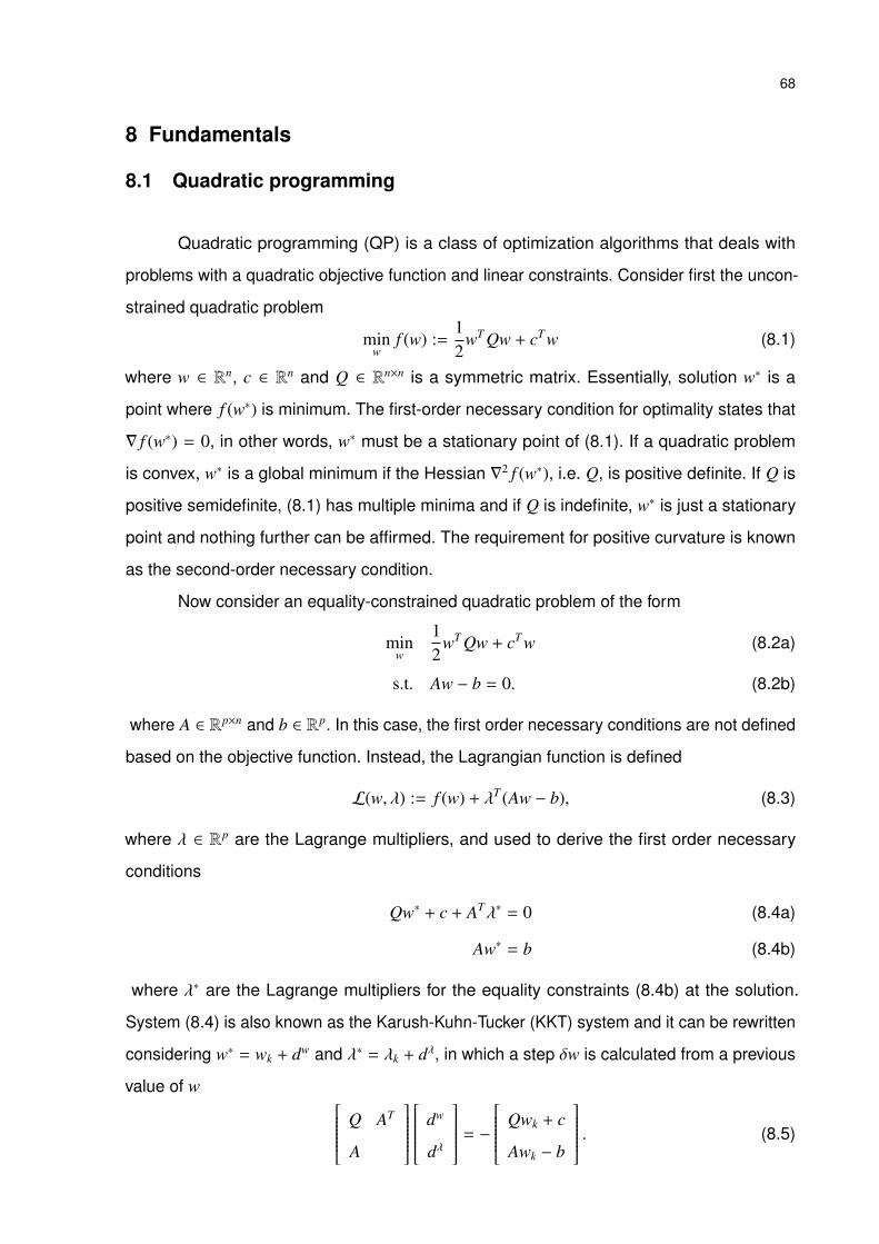
68

8 Fundamentals

8.1 Quadratic programming

Quadratic programming (QP) is a class of optimization algorithms that deals with

problems with a quadratic objective function and linear constraints. Consider first the uncon-

strained quadratic problem

minw

f (w) :=12

wT Qw + cT w (8.1)

where w ∈ Rn, c ∈ Rn and Q ∈ Rn×n is a symmetric matrix. Essentially, solution w∗ is a

point where f (w∗) is minimum. The first-order necessary condition for optimality states that

∇ f (w∗) = 0, in other words, w∗ must be a stationary point of (8.1). If a quadratic problem

is convex, w∗ is a global minimum if the Hessian ∇2 f (w∗), i.e. Q, is positive definite. If Q is

positive semidefinite, (8.1) has multiple minima and if Q is indefinite, w∗ is just a stationary

point and nothing further can be affirmed. The requirement for positive curvature is known

as the second-order necessary condition.

Now consider an equality-constrained quadratic problem of the form

minw

12

wT Qw + cT w (8.2a)

s.t. Aw − b = 0. (8.2b)

where A ∈ Rp×n and b ∈ Rp. In this case, the first order necessary conditions are not defined

based on the objective function. Instead, the Lagrangian function is defined

L(w, λ) := f (w) + λT (Aw − b), (8.3)

where λ ∈ Rp are the Lagrange multipliers, and used to derive the first order necessary

conditions

Qw∗ + c + ATλ∗ = 0 (8.4a)

Aw∗ = b (8.4b)

where λ∗ are the Lagrange multipliers for the equality constraints (8.4b) at the solution.

System (8.4) is also known as the Karush-Kuhn-Tucker (KKT) system and it can be rewritten

considering w∗ = wk + dw and λ∗ = λk + dλ, in which a step δw is calculated from a previous

value of w Q AT

A

dw

dλ

= −

Qwk + c

Awk − b

. (8.5)

69

For a quadratic programming problem, a solution is reached in one iteration; since only one

step needs to be calculated, wk = w0.

Differently from unconstrained optimization, solution w∗ is not located at a minimum

point of the Lagrangian function. Therefore, the second-order necessary conditions evaluate

the the projection of the Hessian Q onto the null space of the gradient of the constraints A,

represented by Z ∈ Rn×n−p. The conditions state that w∗ is a global minimum if this projection,

ZT QZ, which is called the reduced Hessian, is positive definite.

8.2 Line search methods for nonlinear optimization

Line search methods are an iterative strategy for solving optimization problems. In

nonlinear optimization, algorithms start with an initial guess w0 in the variable space Rn and

generate a sequence of {wk}w∈N until it can no longer make progress or it reaches a solution

with sufficient accuracy. This type of methods first calculates a search direction and then

a step size at each iteration k, which results in a new point wk+1 that shows some kind of

improvement, e.g., reduction of the objective function.

8.2.1 Unconstrained problems

Consider the nonlinear unconstrained optimization problem

minw

f (w) (8.6)

where w ∈ Rn and f : Rn → R is the nonlinear function to be minimized. Because nonlinear

problems are often non convex, most methods can only guarantee to find a local minimizer,

meaning that w∗ is a local minimum if, in a neighborhood N of w∗, f (w∗) < f (w) for all w ∈ N .

For a smooth and twice continuously differentiable f (w), one can verify if a point w∗ is a local

minimum by checking the first and second order conditions as it was shown for QP. The

gradient, ∇ f (w∗), and the Hessian, ∇2 f (w∗) of the objective function must be, respectively,

zero and positive (semi)definite.

An iterate wk+1 is calculated by

wk+1 = wk + αd (8.7)

70

where α is a scalar that determines the step length and d is the search direction. Newton’s

method can be used to determine a search direction by approximating a neighborhood of

f (wk) to a quadratic function using Taylor’s expansion as follows

mk(p) := f (wk) + dT∇ f (wk) +12

dT∇2 f (wk)d ≈ f (wk + d). (8.8)

Taking the first derivative of (8.8) with respect to d and setting it to zero leads to

∇ f (wk) + ∇2 f (wk)d = 0, (8.9)

which results in

dk = −[∇2 f (wk)]−1∇ f (wk). (8.10)

It is important to note that to ensure that the algorithm makes progress, this direction must

be descent, i.e. f (wk +αd) < f (wk), and, for that, ∇2 f (wk) needs to be positive definite (BARD,

1974).

Ideally, the step length parameter α would be determined by

minα

f (wk + αdk) (8.11a)

s.t. α > 0. (8.11b)

However, solving an optimization subproblem at each step can be expensive; thus, there

are several strategies that can be followed to find a value for α that is a good trade-off

between the actual optimized step and computational cost (NOCEDAL; WRIGHT, 2006). A

simple backtracking method, for instance, starts with the full step length, α = 1, and α is

iteratively updated to 0.5α until the step is accepted.

For a step to be accepted, it has to meet certain criteria. In addition to having a

descent search direction, two conditions need to be satisfied

f (wk + αkdk) ≤ f (wk) + c1αk∇ f (wk)T dk (8.12a)

∇ f (wk + αkdk)T dk ≥ c2∇ f (wk)T dk, (8.12b)

for c1 ∈ (0, 1) and c2 ∈ (c1, 1). These conditions are known as the Wolfe conditions, and

typical values for c1 and c2 are, respectively, 10−4 and 0.9 (NOCEDAL; WRIGHT, 2006). The first

condition defines a sufficient decrease for the objective function when choosing α and the

latter ensures that the slope of the objective function in the current search direction at α = αk

is greater than at α = 0; otherwise f could still be significantly reduced moving further along

the search direction.

71

8.2.2 Constrained problems

Now consider the constrained problem

minw

f (w) (8.13a)

s.t. h(w) = 0 (8.13b)

where f : Rn → R is again the nonlinear function to be minimized and h : Rn → Rp is a

vector function corresponding to equality constraints. Here f and h are also assumed to be

smooth and twice continuously differentiable. Because inequalities constraints can be written

as equality constraints using slack variables, the theory presented here can be adapted to

include inequality constraints as well. Similarly to unconstrained optimization, algorithms

only find local minimizers; the difference now is that the neighborhood of w∗ is now limited to

the feasible region, i.e., values of w that satisfy the constraints h(w) = 0.

Similarly to QP, the Lagrange function is defined as

L(w, λ) := f (w) +

p∑i=1

λihi(w), (8.14)

where λi is the Langrange multiplier for the ith constraint. The first-order necessary conditions

states that, if the gradient of the constraints at w∗ are linearly independent, there exists a

vector λ∗ such that

∇wL(w∗, λ∗) = 0 (8.15a)

hi(w∗) = 0 for all i ∈ {1, . . . , p}. (8.15b)

A stationary point w∗ of f (w) subject to h(w) is a stationary point of L(w, λ). To guarantee

that w∗ is a local minimizer, one needs to check the reduced Hessian of the Lagrange function

at w∗, that is, the projection of ∇2wwL(w∗, λ∗) onto the null space of ∇h(w∗)T , Z. The point

(w∗, λ∗) is a local minimum if it satisfies (8.15) and the reduced Hessian, ZT∇2wwL(w∗, λ∗)Z,

is positive (semi)definite.

To calculate a search direction, Newton-based algorithms use Newton’s method

for nonlinear equations, which approximates the neighborhood region to a linear model.

Applying it to (8.15) gives

∇2wwL(wk, λk)dw

k +

p∑i=1

λi∇hi(wk)dλk + ∇wL(wk, λk) = 0 (8.16a)

∇hi(wk)dwk + hi(wk) = 0 for all i ∈ 1, . . . , p, (8.16b)

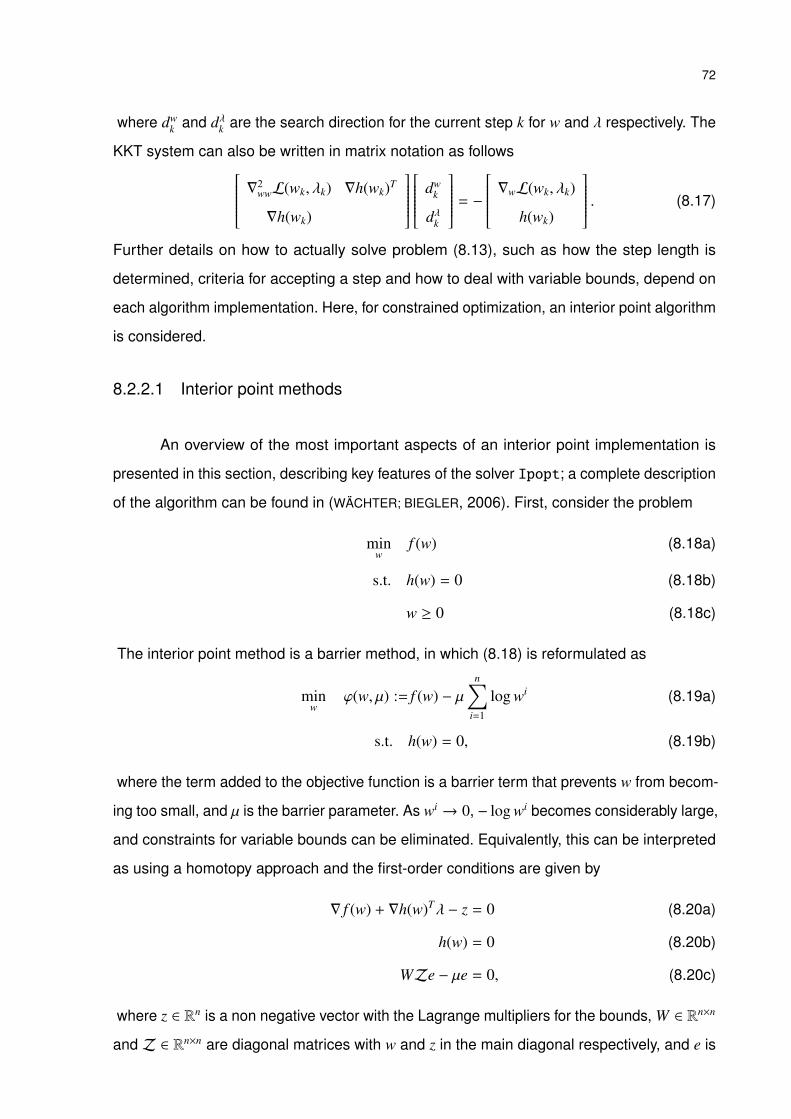
72

where dwk and dλk are the search direction for the current step k for w and λ respectively. The

KKT system can also be written in matrix notation as follows ∇2wwL(wk, λk) ∇h(wk)T

∇h(wk)

dw

k

dλk

= −

∇wL(wk, λk)

h(wk)

. (8.17)

Further details on how to actually solve problem (8.13), such as how the step length is

determined, criteria for accepting a step and how to deal with variable bounds, depend on

each algorithm implementation. Here, for constrained optimization, an interior point algorithm

is considered.

8.2.2.1 Interior point methods

An overview of the most important aspects of an interior point implementation is

presented in this section, describing key features of the solver Ipopt; a complete description

of the algorithm can be found in (WÄCHTER; BIEGLER, 2006). First, consider the problem

minw

f (w) (8.18a)

s.t. h(w) = 0 (8.18b)

w ≥ 0 (8.18c)

The interior point method is a barrier method, in which (8.18) is reformulated as

minw

ϕ(w, µ) := f (w) − µn∑

i=1

log wi (8.19a)

s.t. h(w) = 0, (8.19b)

where the term added to the objective function is a barrier term that prevents w from becom-

ing too small, and µ is the barrier parameter. As wi → 0, − log wi becomes considerably large,

and constraints for variable bounds can be eliminated. Equivalently, this can be interpreted

as using a homotopy approach and the first-order conditions are given by

∇ f (w) + ∇h(w)Tλ − z = 0 (8.20a)

h(w) = 0 (8.20b)

WZe − µe = 0, (8.20c)

where z ∈ Rn is a non negative vector with the Lagrange multipliers for the bounds, W ∈ Rn×n

and Z ∈ Rn×n are diagonal matrices with w and z in the main diagonal respectively, and e is

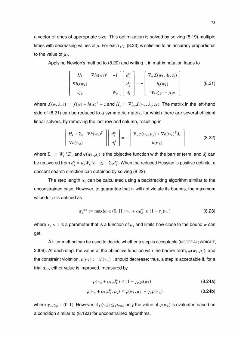
73

a vector of ones of appropriate size. This optimization is solved by solving (8.19) multiple

times with decreasing values of µ. For each µ j, (8.20) is satisfied to an accuracy proportional

to the value of µ j.

Applying Newton’s method to (8.20) and writing it in matrix notation leads toHk ∇hi(wk)T −I

∇hi(wk)

Zk Wk

dwk

dλk

dzk

= −

∇wL(wk, λk, zk)

hi(wk)

WkZke − µ je

(8.21)

where L(w, λ, z) := f (w) + h(w)T − z and Hk := ∇2wwL(wk, λk, zk). The matrix in the left-hand

side of (8.21) can be reduced to a symmetric matrix, for which there are several efficient

linear solvers, by removing the last row and column, resulting in Hk + Σk ∇h(wk)T

∇h(wk)

dw

k

dλk

= −

∇wϕ(wk, µ j) + ∇h(wk)Tλk

h(wk)

(8.22)

where Σk := W−1k Zk and ϕ(wk, µ j) is the objective function with the barrier term, and dz

k can

be recovered from dzk = µ jW−1

k e − zk − Σkdwk . When the reduced Hessian is positive definite, a

descent search direction can obtained by solving (8.22).

The step length αk can be calculated using a backtracking algorithm similar to the

unconstrained case. However, to guarantee that w will not violate its bounds, the maximum

value for α is defined as

αmaxk := max{α ∈ (0, 1] : wk + αdw

k ≥ (1 − τ j)wk} (8.23)

where τ j < 1 is a parameter that is a function of µ j and limits how close to the bound w can

get.

A filter method can be used to decide whether a step is acceptable (NOCEDAL; WRIGHT,

2006). At each step, the value of the objective function with the barrier term, ϕ(wk, µ j), and

the constraint violation, ρ(wk) := ‖h(wk)‖, should decrease; thus, a step is acceptable if, for a

trial αk,l, either value is improved, measured by

ρ(wk + αk,ldwk ) ≤ (1 − γρ)ρ(wk) (8.24a)

ϕ(wk + αk,ldwk , µ j) ≤ ϕ(wk, µ j) − γϕρ(wk) (8.24b)

where γρ, γϕ ∈ (0, 1). However, if ρ(wk) ≤ ρmin, only the value of ϕ(wk) is evaluated based on

a condition similar to (8.12a) for unconstrained algorithms.

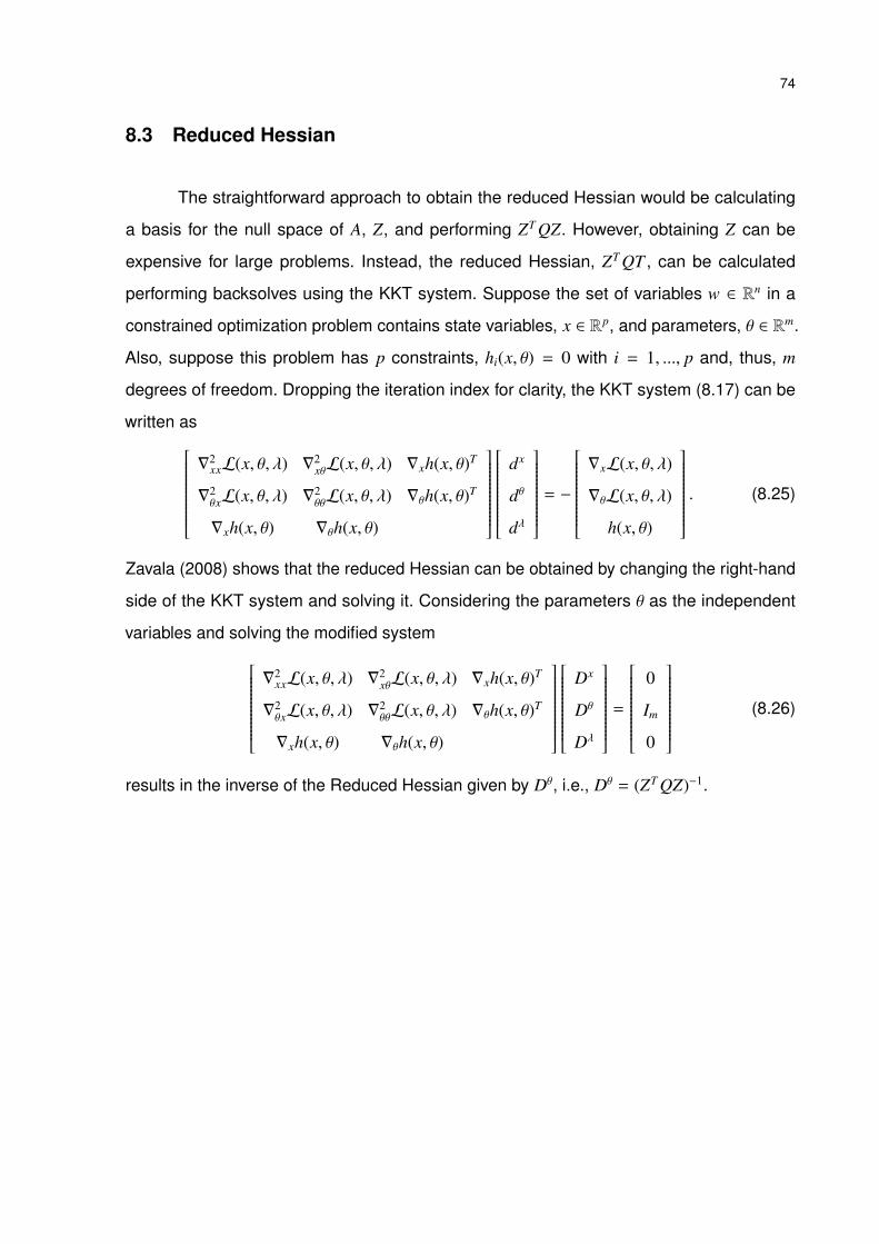
74

8.3 Reduced Hessian

The straightforward approach to obtain the reduced Hessian would be calculating

a basis for the null space of A, Z, and performing ZT QZ. However, obtaining Z can be

expensive for large problems. Instead, the reduced Hessian, ZT QT , can be calculated

performing backsolves using the KKT system. Suppose the set of variables w ∈ Rn in a

constrained optimization problem contains state variables, x ∈ Rp, and parameters, θ ∈ Rm.

Also, suppose this problem has p constraints, hi(x, θ) = 0 with i = 1, ..., p and, thus, m

degrees of freedom. Dropping the iteration index for clarity, the KKT system (8.17) can be

written as∇2

xxL(x, θ, λ) ∇2xθL(x, θ, λ) ∇xh(x, θ)T

∇2θxL(x, θ, λ) ∇2

θθL(x, θ, λ) ∇θh(x, θ)T

∇xh(x, θ) ∇θh(x, θ)

dx

dθ

dλ

= −

∇xL(x, θ, λ)

∇θL(x, θ, λ)

h(x, θ)

. (8.25)

Zavala (2008) shows that the reduced Hessian can be obtained by changing the right-hand

side of the KKT system and solving it. Considering the parameters θ as the independent

variables and solving the modified system∇2

xxL(x, θ, λ) ∇2xθL(x, θ, λ) ∇xh(x, θ)T

∇2θxL(x, θ, λ) ∇2

θθL(x, θ, λ) ∇θh(x, θ)T

∇xh(x, θ) ∇θh(x, θ)

Dx

Dθ

Dλ

=

0

Im

0

(8.26)

results in the inverse of the Reduced Hessian given by Dθ, i.e., Dθ = (ZT QZ)−1.

75

9 Linear parameter estimation

Consider a set of input observations x` ∈ Rm and output observations η` ∈ R, where

the observation index is given by ` = 1, ..., L. Suppose the correspondence between them

follows a linear model response

η` = θT x` + ε` (9.1)

where θ ∈ Rm is a set of parameters to be estimated and ε` ∼ N(0, σ2) are independent

and identically distributed random variables representing noise. In matrix notation, 9.1 is

η = Xθ + ε, where X ∈ Rs×m is the input data matrix, η ∈ RL is the response data vector, and

ε ∼ N(0, σ2I).

Applying the least squares method leads to a quadratic programming problem defined

by

θ ∈ arg minθ

12

(η − Xθ)T (η − Xθ). (9.2)

The first-order optimality conditions result in

θ = K−1XTη. (9.3)

where θ ∈ Rm is known as the least squares estimator and K := XT X ∈ Rm×m is the

Hessian matrix that here is also called kernel matrix and encodes all information from X and

associated impact on the estimated parameters. Since η are Gaussian variables and the

estimated parameters θ are a linear transformation of η, they are also normally distributed

with covariance matrix

V[θ] = σ2K−1. (9.4)

Note from (9.3) that θ exist, are unique, and a minimum of 9.2 if and only if the

input data matrix X has full rank, which implies that K is nonsingular and positive definite.

Also, from (9.4) it is possible to observe that the inverse of K has direct effect on the

covariance matrix V[θ]. If the inverse of K is rewritten as K−1 = VΛ−1VT , with V ∈ Rm×m

being the matrix with the eigenvectors of K and Λ ∈ Rm×m the diagonal matrix with its

eigenvalues, the kernel matrix can be expressed as K =∑m

j=1 λ jv jvTj and its Frobenius norm

as ‖K‖F = ‖Λ‖F =√∑m

j=1 λ2j . Since the eigenvalues of V[θ] indicate the level of confidence

in the parameters, as the eigenvalues of K decrease, the parameters become less reliable

and, when variance is high, the problem is said to be ill-conditioned.

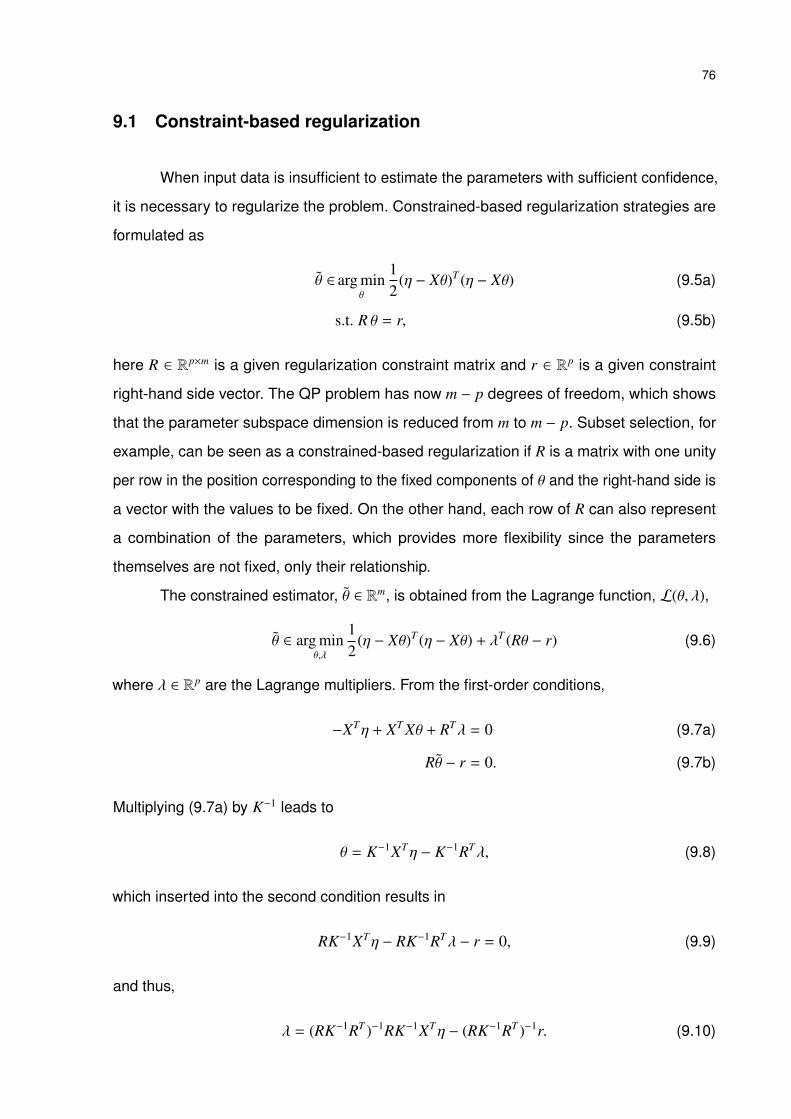
76

9.1 Constraint-based regularization

When input data is insufficient to estimate the parameters with sufficient confidence,

it is necessary to regularize the problem. Constrained-based regularization strategies are

formulated as

θ ∈ arg minθ

12

(η − Xθ)T (η − Xθ) (9.5a)

s.t. R θ = r, (9.5b)

here R ∈ Rp×m is a given regularization constraint matrix and r ∈ Rp is a given constraint

right-hand side vector. The QP problem has now m − p degrees of freedom, which shows

that the parameter subspace dimension is reduced from m to m − p. Subset selection, for

example, can be seen as a constrained-based regularization if R is a matrix with one unity

per row in the position corresponding to the fixed components of θ and the right-hand side is

a vector with the values to be fixed. On the other hand, each row of R can also represent

a combination of the parameters, which provides more flexibility since the parameters

themselves are not fixed, only their relationship.

The constrained estimator, θ ∈ Rm, is obtained from the Lagrange function, L(θ, λ),

θ ∈ arg minθ,λ

12

(η − Xθ)T (η − Xθ) + λT (Rθ − r) (9.6)

where λ ∈ Rp are the Lagrange multipliers. From the first-order conditions,

−XTη + XT Xθ + RTλ = 0 (9.7a)

Rθ − r = 0. (9.7b)

Multiplying (9.7a) by K−1 leads to

θ = K−1XTη − K−1RTλ, (9.8)

which inserted into the second condition results in

RK−1XTη − RK−1RTλ − r = 0, (9.9)

and thus,

λ = (RK−1RT )−1RK−1XTη − (RK−1RT )−1r. (9.10)

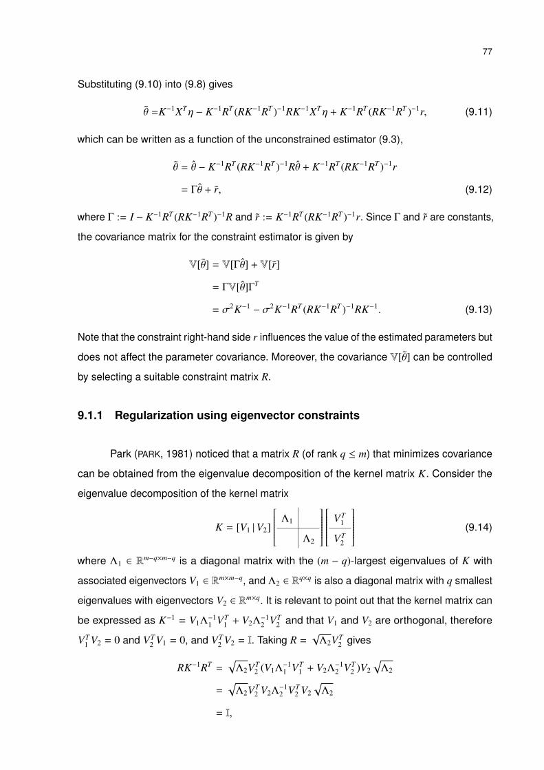
77

Substituting (9.10) into (9.8) gives

θ =K−1XTη − K−1RT (RK−1RT )−1RK−1XTη + K−1RT (RK−1RT )−1r, (9.11)

which can be written as a function of the unconstrained estimator (9.3),

θ = θ − K−1RT (RK−1RT )−1Rθ + K−1RT (RK−1RT )−1r

= Γθ + r, (9.12)

where Γ := I − K−1RT (RK−1RT )−1R and r := K−1RT (RK−1RT )−1r. Since Γ and r are constants,

the covariance matrix for the constraint estimator is given by

V[θ] = V[Γθ] + V[r]

= ΓV[θ]ΓT

= σ2K−1 − σ2K−1RT (RK−1RT )−1RK−1. (9.13)

Note that the constraint right-hand side r influences the value of the estimated parameters but

does not affect the parameter covariance. Moreover, the covariance V[θ] can be controlled

by selecting a suitable constraint matrix R.

9.1.1 Regularization using eigenvector constraints

Park (PARK, 1981) noticed that a matrix R (of rank q ≤ m) that minimizes covariance

can be obtained from the eigenvalue decomposition of the kernel matrix K. Consider the

eigenvalue decomposition of the kernel matrix

K = [V1 |V2]

Λ1

Λ2

VT

1

VT2

(9.14)

where Λ1 ∈ Rm−q×m−q is a diagonal matrix with the (m − q)-largest eigenvalues of K with

associated eigenvectors V1 ∈ Rm×m−q, and Λ2 ∈ R

q×q is also a diagonal matrix with q smallest

eigenvalues with eigenvectors V2 ∈ Rm×q. It is relevant to point out that the kernel matrix can

be expressed as K−1 = V1Λ−11 VT

1 + V2Λ−12 VT

2 and that V1 and V2 are orthogonal, therefore

VT1 V2 = 0 and VT

2 V1 = 0, and VT2 V2 = I. Taking R =

√Λ2VT

2 gives

RK−1RT =√

Λ2VT2 (V1Λ

−11 VT

1 + V2Λ−12 VT

2 )V2

√Λ2

=√

Λ2VT2 V2Λ

−12 VT

2 V2

√Λ2

= I,

78

which in turn leads to

K−1RT (RK−1RT )−1RK = (V1Λ−11 VT

1 + V2Λ−12 VT

2 )V2

√Λ2I

√Λ2VT

2 (V1Λ−11 VT

1 + V2Λ−12 VT

2 )

= (V1Λ−11 VT

1 + V2Λ−12 VT

2 )V2Λ2VT2 (V1Λ

−11 VT

1 + V2Λ−12 VT

2 )

= V2VT2 (V1Λ

−11 VT

1 + V2Λ−12 VT

2 )

= V2Λ−12 VT

2 .

Upon substitution in (9.13), the covariance matrix of estimator calculated with eigenvector

constraints is given by

V[θ] = σ2(V1Λ−11 VT

1 + V2Λ−12 VT

2 ) − σ2V2Λ−12 VT

2

= σ2(V1Λ−11 VT

1 ). (9.15)

Consequently, enforcing the constraint Rθ = r (with R =√

Λ2VT2 ) minimizes the effect of the

damaging (small) eigenvalues of K on the covariance matrix since only their components

are removed in (9.15); in particular, note that ‖V[θ]‖F = σ2 ∑m−qj=1 λ

−2j .

9.1.2 Principal component regression

Originally, principal component regression projects the input data matrix X onto the

space of the (m−q) largest eigenvectors as XV1 ∈ Rn×m−q and estimates a reduced parameter

set γ ∈ Rm−q by solving

γ ∈ arg minγ

12

(η − XV1γ)T (η − XV1γ). (9.16)

Therefore, an estimator for the reduced parameter set is given by γ = (VT1 XT XV1)−1VT

1 XTη

and a solution in the original parameter space is recovered from θ = V1γ. However, PCR can

also be seen as a constrained QP defined by

(θ, γ) ∈ arg minγ,θ

12

(η − Xθ)T (η − Xθ) (9.17a)

s.t. VT1 θ = γ (9.17b)

Note that the coefficient matrix is R = VT1 and r = γ.

The covariance of γ is given by

V[γ] = σ2(VT1 XT XV1)−1

= σ2(VT1 (V1Λ1VT

1 + V2Λ2VT2 )V1)−1

= σ2Λ−11 . (9.18)

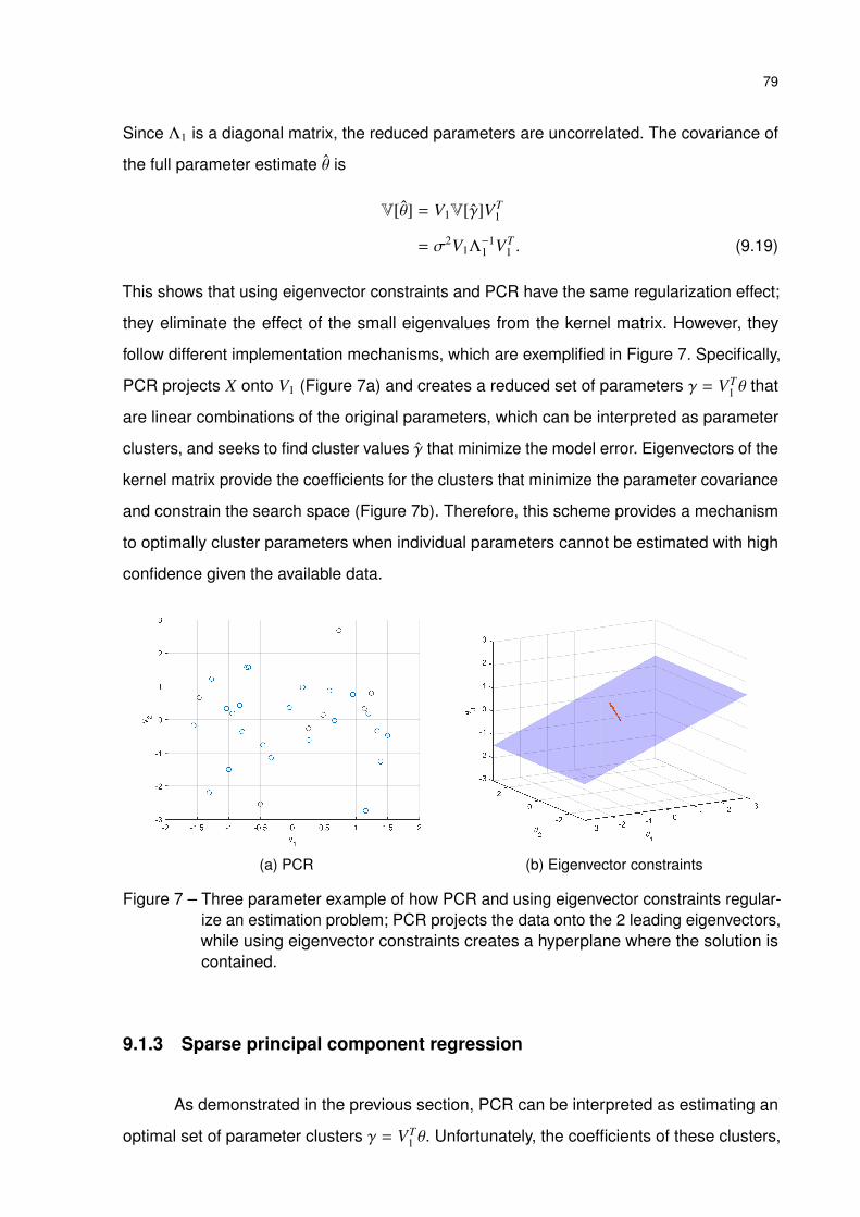
79

Since Λ1 is a diagonal matrix, the reduced parameters are uncorrelated. The covariance of

the full parameter estimate θ is

V[θ] = V1V[γ]VT1

= σ2V1Λ−11 VT

1 . (9.19)

This shows that using eigenvector constraints and PCR have the same regularization effect;

they eliminate the effect of the small eigenvalues from the kernel matrix. However, they

follow different implementation mechanisms, which are exemplified in Figure 7. Specifically,

PCR projects X onto V1 (Figure 7a) and creates a reduced set of parameters γ = VT1 θ that

are linear combinations of the original parameters, which can be interpreted as parameter

clusters, and seeks to find cluster values γ that minimize the model error. Eigenvectors of the

kernel matrix provide the coefficients for the clusters that minimize the parameter covariance

and constrain the search space (Figure 7b). Therefore, this scheme provides a mechanism

to optimally cluster parameters when individual parameters cannot be estimated with high

confidence given the available data.

(a) PCR (b) Eigenvector constraints

Figure 7 – Three parameter example of how PCR and using eigenvector constraints regular-ize an estimation problem; PCR projects the data onto the 2 leading eigenvectors,while using eigenvector constraints creates a hyperplane where the solution iscontained.

9.1.3 Sparse principal component regression

As demonstrated in the previous section, PCR can be interpreted as estimating an

optimal set of parameter clusters γ = VT1 θ. Unfortunately, the coefficients of these clusters,

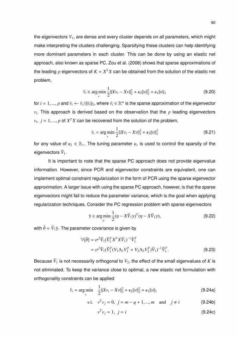
80

the eigenvectors V1, are dense and every cluster depends on all parameters, which might

make interpreting the clusters challenging. Sparsifying these clusters can help identifying

more dominant parameters in each cluster. This can be done by using an elastic net

approach, also known as sparse PC. Zou et al. (2006) shows that sparse approximations of

the leading p eigenvectors of K = XT X can be obtained from the solution of the elastic net

problem,

vi ∈ arg minv

12‖Xvi − Xv‖22 + κ2‖v‖22 + κ1‖v‖1 (9.20)

for i = 1, ..., p and vi ← vi/‖vi‖2, where vi ∈ Rm is the sparse approximation of the eigenvector

vi. This approach is derived based on the observation that the p leading eigenvectors

vi, j = 1, ..., p of XT X can be recovered from the solution of the problem,

vi = arg minv

12‖Xvi − Xv‖22 + κ2‖v‖22 (9.21)

for any value of κ2 ∈ R+. The tuning parameter κ1 is used to control the sparsity of the

eigenvectors V1.

It is important to note that the sparse PC approach does not provide eigenvalue

information. However, since PCR and eigenvector constraints are equivalent, one can

implement optimal constraint regularization in the form of PCR using the sparse eigenvector

approximation. A larger issue with using the sparse PC approach, however, is that the sparse

eigenvectors might fail to reduce the parameter variance, which is the goal when applying

regularization techniques. Consider the PC regression problem with sparse eigenvectors

γ ∈ arg minγ

12

(η − XV1γ)T (η − XV1γ), (9.22)

with θ = V1γ. The parameter covariance is given by

V[θ] = σ2V1(VT1 XT XV1)−1VT

1

= σ2V1(VT1 (V1Λ1VT

1 + V2Λ2VT2 )V1)−1VT

1 . (9.23)

Because V1 is not necessarily orthogonal to V2, the effect of the small eigenvalues of K is

not eliminated. To keep the variance close to optimal, a new elastic net formulation with

orthogonality constraints can be applied

vi = arg minv

12‖Xvi − Xv‖22 + κ2‖v‖22 + κ1‖v‖1 (9.24a)

s.t. vT v j = 0, j = m − q + 1, ...,m and j , i (9.24b)

vT v j = 1, j = i (9.24c)

81

which is solved for i = 1, ...,m − q and with vi ← vi/‖vi‖2 to construct the sparse eigenvector

matrix V1.

9.2 Illustrative examples

9.2.1 Collineatities in the input data

The studied eigenvector regularization approach is applied to an ill-conditioned linear

model in which the input data present near collinearities. A synthetic model is built with m = 6

parameters and L = 15 data points. To induce collinearities, the input data is generated as

follows

x1 ∼ N(0, 1) (9.25a)

x2 ∼ N(0, 1) (9.25b)

x3 ∼ N(0, 1) (9.25c)

x4 = x1 (9.25d)

x5 = x2 (9.25e)

x6 = x1 + x2, (9.25f)

implying dependencies between parameters θ1, θ4, θ6 and between parameters θ2, θ5, θ6. No

collinearities are induced by the third input. The kernel matrix is shown in Table 8 and Table

9 presents the eigenvectors and eigenvalues of XT X.

Table 8 – Kernel matrix corresponding to the first example.

K = XT X15.02 -1.69 6.09 15.02 -1.69 13.33-1.69 11.16 -3.2 -1.68 11.16 9.486.09 -3.2 17.33 6.08 -3.2 2.8815.02 -1.68 6.08 15.03 -1.68 13.33-1.69 11.16 -3.2 -1.68 11.15 9.4713.33 9.48 2.88 13.33 9.47 22.8

Inspecting the eigenvalues of K, one can conclude that most of the variance of

the inputs can be captured by the m − q = 3 leading eigenvalues. This highlights, as

expected, that only three parameters can be estimated, e.g., the two clusters and an

additional parameter. The eigenvector matrix V1 is shown in Table 10, which also presents the

82

Table 9 – Eigenvectors and corresponding eigenvalues of XT X from the first example.

X1 -0.502 -0.253 0.244 0.051 -0.587 0.527X2 -0.138 0.554 -0.222 -0.346 0.324 0.633X3 -0.224 -0.409 -0.884 0 0 0X4 -0.502 -0.252 0.244 -0.661 0.298 -0.316X5 -0.138 0.554 -0.222 -0.264 -0.614 -0.422X6 -0.639 0.302 0.023 0.610 0.290 -0.211Λ 48.8 31.4 12.3 1.6e-5 5.8e-6 1.9e-6

sparse eigenvectors obtained with both the elastic net and the elastic net with orthogonality

constraints approaches. Figure 8 shows the parameter covariance when using unregularized

estimation and PCR. It is clear that the problem is ill-conditioned, due to the large entries

in the covariance matrix of the unregularized estimation, and regularization is needed to

stabilize the estimates.

1 2 3 4 5 6

1

2

3

4

5

6

2065.9

1423.3

-0.6

-1204.3

-561.8

-861.2

1423.3

2374.5

-0.3

-748.0

-1700.0

-675.0

-0.6

-0.3

0.0

0.3

0.0

0.3

-1204.3

-748.0

0.3

955.8

499.6

248.2

-561.8

-1700.0

0.0

499.6

1638.6

61.9

-861.2

-675.0

0.3

248.2

61.9

613.0-1500

-1000

-500

0

500

1000

1500

2000

(a) Unregularized1 2 3 4 5 6

1

2

3

4

5

6

0.012

-0.007

-0.012

0.012

-0.007

0.005

-0.007

0.014

0.009

-0.007

0.014

0.007

-0.012

0.009

0.070

-0.012

0.009

-0.003

0.012

-0.007

-0.012

0.012

-0.007

0.005

-0.007

0.014

0.009

-0.007

0.014

0.007

0.005

0.007

-0.003

0.005

0.007

0.011 -0.01

0

0.01

0.02

0.03

0.04

0.05

0.06

0.07

0.08

0.09

(b) PCR

Figure 8 – Covariance matrix for estimated parameters V[θ] from the first example.

Table 10 – Eigenvectors V1 and sparse eigenvectors V1 obtained with elastic net (EN) andelastic net with orthogonality constraints (EN-OC) (First example).

V1 V1 (EN) V1 (EN-OC)v1 v2 v3 v1 v2 v3 v1 v2 v3

X1 -0.502 -0.253 0.244 0 0 0 -0.577 0 0X2 -0.138 0.554 -0.222 0 0.950 -0.354 0 0.577 0X3 -0.224 -0.409 -0.884 -0.009 -0.285 -0.820 0 0 -1.0X4 -0.502 -0.252 0.244 -0.577 0 0.451 -0.577 0 0X5 -0.138 0.554 -0.222 0 0.127 0 0 0.577 0X6 -0.639 0.302 0.023 -0.817 0 0 -0.577 0.577 0

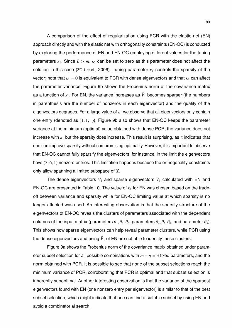
83

A comparison of the effect of regularization using PCR with the elastic net (EN)

approach directly and with the elastic net with orthogonality constraints (EN-OC) is conducted

by exploring the performance of EN and EN-OC employing different values for the tuning

parameters κ1. Since L > m, κ2 can be set to zero as this parameter does not affect the

solution in this case (ZOU et al., 2006). Tuning parameter κ1 controls the sparsity of the

vector; note that κ1 = 0 is equivalent to PCR with dense eigenvectors and that κ1 can affect

the parameter variance. Figure 9b shows the Frobenius norm of the covariance matrix

as a function of κ1. For EN, the variance increases as V1 becomes sparser (the numbers

in parenthesis are the number of nonzeros in each eigenvector) and the quality of the

eigenvectors degrades. For a large value of κ1 we observe that all eigenvectors only contain

one entry (denoted as (1, 1, 1)). Figure 9b also shows that EN-OC keeps the parameter

variance at the minimum (optimal) value obtained with dense PCR; the variance does not

increase with κ1 but the sparsity does increase. This result is surprising, as it indicates that

one can improve sparsity without compromising optimality. However, it is important to observe

that EN-OC cannot fully sparsify the eigenvectors; for instance, in the limit the eigenvectors

have (3, 6, 1) nonzero entries. This limitation happens because the orthogonality constraints

only allow spanning a limited subspace of X.

The dense eigenvectors V1 and sparse eigenvectors V1 calculated with EN and

EN-OC are presented in Table 10. The value of κ1 for EN was chosen based on the trade-

off between variance and sparsity while for EN-OC limiting value at which sparsity is no

longer affected was used. An interesting observation is that the sparsity structure of the

eigenvectors of EN-OC reveals the clusters of parameters associated with the dependent

columns of the input matrix (parameters θ1, θ4, θ6, parameters θ2, θ5, θ6, and parameter θ3).

This shows how sparse eigenvectors can help reveal parameter clusters, while PCR using

the dense eigenvectors and using V1 of EN are not able to identify these clusters.

Figure 9a shows the Frobenius norm of the covariance matrix obtained under param-

eter subset selection for all possible combinations with m − q = 3 fixed parameters, and the

norm obtained with PCR. It is possible to see that none of the subset selections reach the

minimum variance of PCR, corroborating that PCR is optimal and that subset selection is

inherently suboptimal. Another interesting observation is that the variance of the sparsest

eigenvectors found with EN (one nonzero entry per eigenvector) is similar to that of the best

subset selection, which might indicate that one can find a suitable subset by using EN and

avoid a combinatorial search.

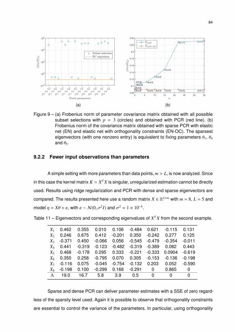
84

Fixed parameters

(θ 1, θ

2, θ 3

)

(θ 1, θ

2, θ 5

)

(θ 1, θ

3, θ 4

)

(θ 1, θ

3, θ 6

)

(θ 1, θ

4, θ 6

)

(θ 2, θ

3, θ 4

)

(θ 2, θ

3, θ 6

)

(θ 2, θ

4, θ 6

)

(θ 3, θ

4, θ 5

)

(θ 3, θ

5, θ 6

)

||Var(θ)|| F

10-2

100

102

104

106

Subset selection

PC regression

(a)

κ1

0 5 10 15 20 25 30 35

||Var(θ)|| F

0.08

0.1

0.12

0.14

0.16

0.18

0.2

0.22

0.24

(6,6,6)

(6,6,4)

(4,5,3) (4,4,3)

(3,3,2)

(2,2,2)

(2,1,1) (1,1,1)

(6,6,6) (6,6,6) (5,6,5) (3,6,5) (3,6,5) (3,6,1)

V1,EN

V1,EN−OC

(b)

Figure 9 – (a) Frobenius norm of parameter covariance matrix obtained with all possiblesubset selections with p = 3 (circles) and obtained with PCR (red line). (b)Frobenius norm of the covariance matrix obtained with sparse PCR with elasticnet (EN) and elastic net with orthogonality constraints (EN-OC). The sparsesteigenvectors (with one nonzero entry) is equivalent to fixing parameters θ1, θ4

and θ5.

9.2.2 Fewer input observations than parameters

A simple setting with more parameters than data points, m > L, is now analyzed. Since

in this case the kernel matrix K = XT X is singular, unregularized estimation cannot be directly

used. Results using ridge regularization and PCR with dense and sparse eigenvectors are

compared. The results presented here use a random matrix X ∈ RL×m with m = 8, L = 5 and

model η = Xθ + ε, with ε ∼ N(0, σ2I) and σ2 = 1 × 10−4.

Table 11 – Eigenvectors and corresponding eigenvalues of XT X from the second example.

X1 0.462 0.355 0.010 0.106 -0.484 0.621 -0.115 0.131X2 0.246 0.675 0.412 -0.201 0.350 -0.242 0.277 0.125X3 -0.371 0.450 -0.066 0.056 -0.545 -0.479 -0.354 -0.011X4 0.441 -0.319 -0.123 -0.482 -0.319 -0.389 0.082 0.443X5 0.468 -0.178 0.295 0.333 -0.221 -0.333 0.0904 -0.619X6 0.350 0.258 -0.795 0.070 0.305 -0.153 -0.136 -0.198X7 -0.116 0.075 -0.045 -0.754 -0.132 0.203 0.052 -0.590X8 -0.198 0.100 -0.299 0.168 -0.291 0 0.865 0Λ 19.0 16.7 5.8 3.9 0.5 0 0 0

Sparse and dense PCR can deliver parameter estimates with a SSE of zero regard-

less of the sparsity level used. Again it is possible to observe that orthogonality constraints

are essential to control the variance of the parameters. In particular, using orthogonality

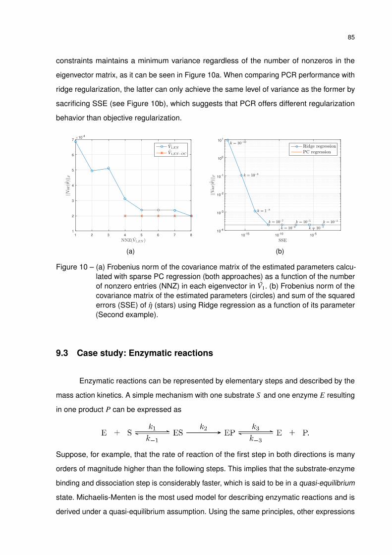
85

constraints maintains a minimum variance regardless of the number of nonzeros in the

eigenvector matrix, as it can be seen in Figure 10a. When comparing PCR performance with

ridge regularization, the latter can only achieve the same level of variance as the former by

sacrificing SSE (see Figure 10b), which suggests that PCR offers different regularization

behavior than objective regularization.

NNZ(V1,EN )1 2 3 4 5 6 7 8

||Var(θ)|| F

×10-4

1

2

3

4

5

6

7

V1,EN

V1,EN−OC

(a)

SSE10

-1510

-1010

-5

||Var(θ)|| F

10-4

10-3

10-2

10-1

100

101

k = 10−10

k = 10−9

k = 1−8

k = 10−7

k = 10−6

k = 10−5

k = 10−4

k = 10−3

Ridge regression

PC regression

(b)

Figure 10 – (a) Frobenius norm of the covariance matrix of the estimated parameters calcu-lated with sparse PC regression (both approaches) as a function of the numberof nonzero entries (NNZ) in each eigenvector in V1. (b) Frobenius norm of thecovariance matrix of the estimated parameters (circles) and sum of the squarederrors (SSE) of η (stars) using Ridge regression as a function of its parameter(Second example).

9.3 Case study: Enzymatic reactions

Enzymatic reactions can be represented by elementary steps and described by the

mass action kinetics. A simple mechanism with one substrate S and one enzyme E resulting

in one product P can be expressed as

Suppose, for example, that the rate of reaction of the first step in both directions is many

orders of magnitude higher than the following steps. This implies that the substrate-enzyme

binding and dissociation step is considerably faster, which is said to be in a quasi-equilibrium

state. Michaelis-Menten is the most used model for describing enzymatic reactions and is

derived under a quasi-equilibrium assumption. Using the same principles, other expressions

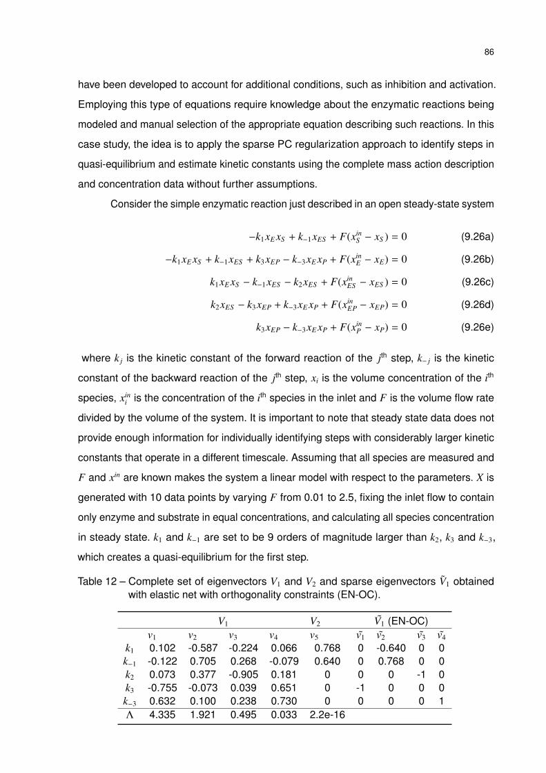
86

have been developed to account for additional conditions, such as inhibition and activation.

Employing this type of equations require knowledge about the enzymatic reactions being

modeled and manual selection of the appropriate equation describing such reactions. In this

case study, the idea is to apply the sparse PC regularization approach to identify steps in

quasi-equilibrium and estimate kinetic constants using the complete mass action description

and concentration data without further assumptions.

Consider the simple enzymatic reaction just described in an open steady-state system

−k1xE xS + k−1xES + F(xinS − xS ) = 0 (9.26a)

−k1xE xS + k−1xES + k3xEP − k−3xE xP + F(xinE − xE) = 0 (9.26b)

k1xE xS − k−1xES − k2xES + F(xinES − xES ) = 0 (9.26c)

k2xES − k3xEP + k−3xE xP + F(xinEP − xEP) = 0 (9.26d)

k3xEP − k−3xE xP + F(xinP − xP) = 0 (9.26e)

where k j is the kinetic constant of the forward reaction of the jth step, k− j is the kinetic

constant of the backward reaction of the jth step, xi is the volume concentration of the ith

species, xini is the concentration of the ith species in the inlet and F is the volume flow rate

divided by the volume of the system. It is important to note that steady state data does not

provide enough information for individually identifying steps with considerably larger kinetic

constants that operate in a different timescale. Assuming that all species are measured and

F and xin are known makes the system a linear model with respect to the parameters. X is

generated with 10 data points by varying F from 0.01 to 2.5, fixing the inlet flow to contain

only enzyme and substrate in equal concentrations, and calculating all species concentration

in steady state. k1 and k−1 are set to be 9 orders of magnitude larger than k2, k3 and k−3,

which creates a quasi-equilibrium for the first step.

Table 12 – Complete set of eigenvectors V1 and V2 and sparse eigenvectors V1 obtainedwith elastic net with orthogonality constraints (EN-OC).

V1 V2 V1 (EN-OC)v1 v2 v3 v4 v5 v1 v2 v3 v4

k1 0.102 -0.587 -0.224 0.066 0.768 0 -0.640 0 0k−1 -0.122 0.705 0.268 -0.079 0.640 0 0.768 0 0k2 0.073 0.377 -0.905 0.181 0 0 0 -1 0k3 -0.755 -0.073 0.039 0.651 0 -1 0 0 0k−3 0.632 0.100 0.238 0.730 0 0 0 0 1Λ 4.335 1.921 0.495 0.033 2.2e-16

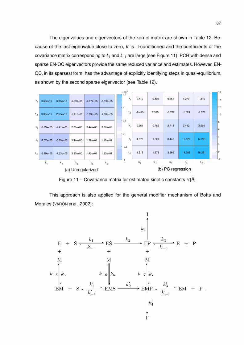
87

The eigenvalues and eigenvectors of the kernel matrix are shown in Table 12. Be-

cause of the last eigenvalue close to zero, K is ill-conditioned and the coefficients of the

covariance matrix corresponding to k1 and k−1 are large (see Figure 11). PCR with dense and

sparse EN-OC eigenvectors provide the same reduced variance and estimates. However, EN-

OC, in its sparsest form, has the advantage of explicitly identifying steps in quasi-equilibrium,

as shown by the second sparse eigenvector (see Table 12).

k1

k-1

k2

k3

k-3

k1

k-1

k2

k3

k-3

3.60e+15

3.00e+15

-2.89e+05

-7.07e+05

-5.19e+05

3.00e+15

2.50e+15

-2.41e+05

-5.89e+05

-4.33e+05

-2.89e+05

-2.41e+05

2.71e+00

3.44e+00

3.57e+00

-7.07e+05

-5.89e+05

3.44e+00

1.29e+01

1.42e+01

-5.19e+05

-4.33e+05

3.57e+00

1.42e+01

1.63e+01

-1

-0.5

0

0.5

1

1.5

106

(a) Unregularized

k1

k-1

k2

k3

k-3

k1

k-1

k2

k3

k-3

0.412

-0.495

0.651

1.270

1.315

-0.495

0.593

-0.782

-1.523

-1.578

0.651

-0.782

2.713

3.442

3.566

1.270

-1.523

3.442

12.879

14.201

1.315

-1.578

3.566

14.201

16.251

-2

0

2

4

6

8

10

12

14

16

(b) PC regression

Figure 11 – Covariance matrix for estimated kinetic constants V[θ].

This approach is also applied for the general modifier mechanism of Botts and

Morales (VARÓN et al., 2002):

88

Table 13 – Dense eigenvectors V1 for Botts-Morales example.

V1

k1 0.294 -0.544 -0.084 -0.152 0.001 -0.064 0.03 -0.084 0.264 0.0 0.076k−1 -0.294 0.544 0.084 0.152 -0.001 0.064 -0.03 0.084 -0.264 0.0 -0.076k2 -0.054 0.304 -0.227 -0.829 0.036 -0.216 0.209 -0.222 -0.037 0.115 0.1k3 -0.066 0.011 0.032 0.296 -0.056 -0.602 -0.078 -0.658 -0.111 -0.264 0.146k−3 0.017 -0.002 -0.008 -0.077 0.012 0.208 0.007 0.189 -0.182 -0.54 0.768k4 0.001 -0.015 0.021 0.224 -0.089 -0.077 0.964 0.075 0.001 -0.026 -0.0k′1 -0.069 -0.201 -0.495 0.042 -0.13 -0.017 -0.021 0.075 -0.413 -0.013 -0.119k′−1 0.069 0.201 0.495 -0.042 0.13 0.017 0.021 -0.075 0.413 0.013 0.119k′2 0.001 -0.009 0.267 -0.194 -0.836 -0.225 -0.082 0.259 0.037 -0.213 -0.148k′3 0.0 0.0 0.0 0.0 0.0 0.0 0.0 0.0 0.0 0.0 0.0k′−3 0.001 0.0 0.011 -0.038 -0.332 0.695 0.078 -0.616 -0.024 -0.091 -0.105k′4 0.0 0.0 0.0 0.0 0.0 0.0 0.0 0.0 0.0 0.0 0.0k5 0.632 0.217 0.021 0.035 0.007 -0.015 -0.007 -0.001 -0.215 -0.013 -0.066k−5 -0.632 -0.217 -0.021 -0.035 -0.007 0.015 0.007 0.001 0.215 0.013 0.066k6 0.065 0.264 -0.43 0.158 -0.126 0.001 -0.041 0.036 0.432 -0.093 0.041k−6 -0.065 -0.264 0.43 -0.158 0.126 -0.001 0.041 -0.036 -0.432 0.093 -0.041k7 0.034 0.019 -0.005 0.168 -0.336 -0.012 -0.046 -0.048 -0.073 0.744 0.542k−7 0.0 0.0 0.0 0.0 0.0 0.0 0.0 0.0 0.0 0.0 0.0

Depending on the values of the parameters, species M can act as an inhibitor or

as an activator. Usually, quasi-equilibrium is assumed for the reversible reactions so that

Michaelis-Menten type of equations can be used. The goal is to use concentration data for all

species to identify quasi-equilibrium steps and the actual role of M. Considering a reaction

with non-competitive linear inhibition, zero rate of reaction for steps 1’, 2’, 3’, 4’ and 7 is set,

and kinetic constants for steps 1, 5 and 6 are defined to be much larger than for steps 2, 4

and 3. This time, 250 points for F ranging from 0.01 to 2.5 are used, which generate a data

matrix X with 2500 rows. Note that the sparse eigenvectors of EN-OC identify steps 1, 1’, 5,

and 6 to be in quasi-equilibrium (see Table 14). In contrast, PCR correctly estimates reaction

steps with zero rate but does not reveal quasi-equilibrium states (see Table 13). Other

configurations were also tested, such as cases with essential activation and competitive

inhibition, and EN-OC correctly identified steps that are in a different timescale and those

with zero rate of reaction.

9.4 Conclusion

In this study, strategies to regularize ill-posed parameter estimation problems of linear

models by using constraints were explored, showing that optimal constraints that minimize

parameter covariance can be constructed by exploiting information from the kernel matrix. A

modified elastic net strategy to sparsify the constraints and facilitate their interpretability is

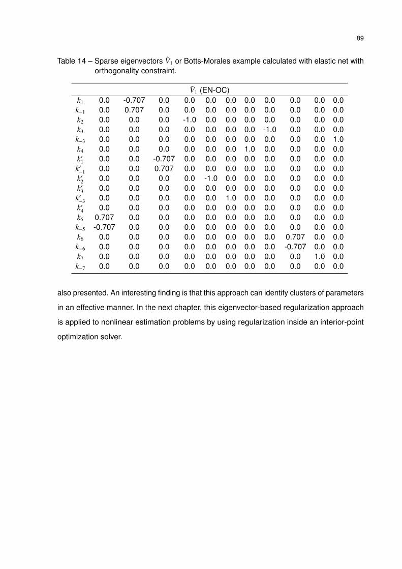
89

Table 14 – Sparse eigenvectors V1 or Botts-Morales example calculated with elastic net withorthogonality constraint.

V1 (EN-OC)k1 0.0 -0.707 0.0 0.0 0.0 0.0 0.0 0.0 0.0 0.0 0.0k−1 0.0 0.707 0.0 0.0 0.0 0.0 0.0 0.0 0.0 0.0 0.0k2 0.0 0.0 0.0 -1.0 0.0 0.0 0.0 0.0 0.0 0.0 0.0k3 0.0 0.0 0.0 0.0 0.0 0.0 0.0 -1.0 0.0 0.0 0.0k−3 0.0 0.0 0.0 0.0 0.0 0.0 0.0 0.0 0.0 0.0 1.0k4 0.0 0.0 0.0 0.0 0.0 0.0 1.0 0.0 0.0 0.0 0.0k′1 0.0 0.0 -0.707 0.0 0.0 0.0 0.0 0.0 0.0 0.0 0.0k′−1 0.0 0.0 0.707 0.0 0.0 0.0 0.0 0.0 0.0 0.0 0.0k′2 0.0 0.0 0.0 0.0 -1.0 0.0 0.0 0.0 0.0 0.0 0.0k′3 0.0 0.0 0.0 0.0 0.0 0.0 0.0 0.0 0.0 0.0 0.0k′−3 0.0 0.0 0.0 0.0 0.0 1.0 0.0 0.0 0.0 0.0 0.0k′4 0.0 0.0 0.0 0.0 0.0 0.0 0.0 0.0 0.0 0.0 0.0k5 0.707 0.0 0.0 0.0 0.0 0.0 0.0 0.0 0.0 0.0 0.0k−5 -0.707 0.0 0.0 0.0 0.0 0.0 0.0 0.0 0.0 0.0 0.0k6 0.0 0.0 0.0 0.0 0.0 0.0 0.0 0.0 0.707 0.0 0.0k−6 0.0 0.0 0.0 0.0 0.0 0.0 0.0 0.0 -0.707 0.0 0.0k7 0.0 0.0 0.0 0.0 0.0 0.0 0.0 0.0 0.0 1.0 0.0k−7 0.0 0.0 0.0 0.0 0.0 0.0 0.0 0.0 0.0 0.0 0.0

also presented. An interesting finding is that this approach can identify clusters of parameters

in an effective manner. In the next chapter, this eigenvector-based regularization approach

is applied to nonlinear estimation problems by using regularization inside an interior-point

optimization solver.

90

10 Nonlinear parameter estimation

Consider a set of state variables x` ∈ Rp and output observations η` ∈ Rs with

` = 1, . . . , L experiments. Suppose the output observations can be modeled as η` = φ(x`, θ)

where η` ∈ Rs are the modeled observations and θ ∈ Rm are unknown parameters. Assuming

that the error ε` = η` − η` is a Gaussian variable ε` ∼ N(0,V`) with covariance V` ∈ Rs×s, the

likelihood function is given by

LH(θ) := (2π)−sL/2L∏`=1

(detV`)(−1/2) exp(−

12

L∑`=1

εT` V−1` ε`

). (10.1)

In maximum likelihood estimation (MLE), the idea is to find an estimate θ for the parameters

that maximize the likelihood function. Because the natural logarithm is a monotone function,

maximizing the likelihood function is equivalent to maximizing the log likelihood function.

Assuming that errors from different experiments are independent and that every experiment

` has the same covariance matrix V, the log likelihood function is

log LH(θ) = −sL2

log 2π −L2

log detV −12

L∑`=1

εT` V−1` ε`. (10.2)

Maximizing log LH(θ) is equivalent to minimizing − log LH(θ) and, since only ε` depends on

the parameters, the MLE estimate is given by

θ ∈ arg minθ

12

L∑`=1

(η` − η`)TV−1(η` − η`). (10.3)

If the errors within each experiment are also independent, V is diagonal and MLE is equiva-

lent to the weighted least squares estimation with the V as the weight matrix. Bard (1974)

shows that for a single equation model, MLE is equivalent to the unweighted least squares

method.

When the state variables x are known exactly and there are no constraints on the

parameters, the estimation problem can be formulated as an unconstrained optimization

problem

θ ∈ arg minθ

12

L∑`=1

(η` − φ(x`, θ)

)TV−1(η` − φ(x`, θ)

)(10.4)

where φ(x`, θ) is a nonlinear mapping function between the problem variables and the output

observation, and solved according to Section 8.2.1. However, if the states variables are not

directly measured or are subjected to errors, they can also be treated as random variables

91

to be estimated. Models that represent their behavior can be used as constraints in the

formulated optimization problem as follows

(θ, x) ∈ arg minθ,x

12

L∑`=1

(η` − φ(x`, θ)

)TV−1(η` − φ(x`, θ)

)(10.5a)

s.t. h`(x`, θ) = 0 for ` = 1, . . . , L (10.5b)

where φ(x`, θ) is a mapping function between the problem variables and the output observa-

tion and h`(x`, θ) corresponds to the p model equations for the `th experiment.

Whether the estimation problem is an unconstrained or a constrained optimization,

positive definiteness of the Hessian or the reduced Hessian, respectively, is a required

condition for convergence to a local minimum, if the problem is non-convex. If, for example,

during the iterative solution using a line search interior point algorithm, they are singular or

indefinite, a regularization approach is necessary.

10.1 Hessian modification

A common strategy for regularizing ill-conditioned (reduced) Hessian in line search

interior point algorithms is modifying the Hessian of the Lagrange function by adding a

multiple of the identity matrix. Ipopt and LOQO, for example, are two solvers that implement

this approach (WÄCHTER; BIEGLER, 2006; VANDERBEI, 1999).

Consider the KKT system (8.22) for iteration k in a line search interior point algorithm.

If the reduced Hessian is not positive definite, the KKT matrix is modified as follows Hk + Σk + δHI ∇h(wk)T

∇h(wk) −δhI

dw

k

dλk

= −

∇wϕ(wk, µ j) + ∇h(wk)Tλk

h(wk)

(10.6)

where δH ≥ 0 is a scalar chosen in a way that the reduced Hessian becomes positive definite

and δh ≥ 0 is used when ∇h(wk) are linearly dependent, which implies that the KKT matrix is

singular. In each iteration, Ipopt uses a heuristic for choosing δH that increases δH gradually

so that it can be approximately the smallest necessary value. A nonzero value is also set to

δh whenever the KKT matrix is singular; it is always assumed that, in this case, ill-conditioning

is due to rank-deficient constraint gradients, the occurrence of singularity in reduced Hessian

is not verified (WÄCHTER; BIEGLER, 2006).

92

10.2 Eigenvector-based regularization

An eigenvector-based regularization inspired by rotational discrimination (FARISS;

LAW, 1979) and PCR (JOLLIFFE, 1982) is presented. The idea is to decompose the (reduced)

Hessian into eigenvalues and eigenvectors, and to remove directions from the solution space

associated with near zero eigenvalues, i.e., directions with small curvature, at iterations

that require regularization due to (near) singularity in the reduced Hessian. The advantage

of this approach is that convex directions are kept unchanged, while directions that do

not significantly influence the objective value in the iterate neighborhood are removed. In

addition, groups of correlated parameters can be identified by inspecting the eigenvectors of

the reduced Hessian.

10.2.1 Unconstrained problems

Consider the unconstrained estimation problem

minθ

f (θ) :=12

L∑`=1

(η` − φ(x`, θ)

)T (η` − φ(x`, θ)

)(10.7)

where η` ∈ R is an output observation and x` ∈ Rp is a known state variable for the Lth

experiment, θ ∈ Rm are the unknown parameters and φ(x`, θ) is a nonlinear mapping function

between the state variable and parameters and the output observation. Here the focus is on

the calculation of the search direction, since it is the step of the iteration calculation that is

directly influenced by ill-conditioning of the Hessian. Equation 8.10 can be rewritten using

the eigenvalue decomposition of ∇2 f (θk) as

(VΛVT )dk = −∇ f (θk), (10.8)

where V ∈ Rm×m is the eigenvectors and Λ ∈ Rm×m is a diagonal matrix with the eigenvalues

of the Hessian. VΛVT can be split into a term with large eigenvalues Λ1 ∈ Rm−q×m−q and their

associated eigenvectors V1 ∈ Rm×m−q and a term with (near) zero eigenvalues Λ2 ∈ R

q×q,

defined by a threshold β, and their associated eigenvectors V2 ∈ Rm×q, resulting in

(V1Λ1VT1 + V2Λ2VT

2 )dk = −∇ f (θk). (10.9)

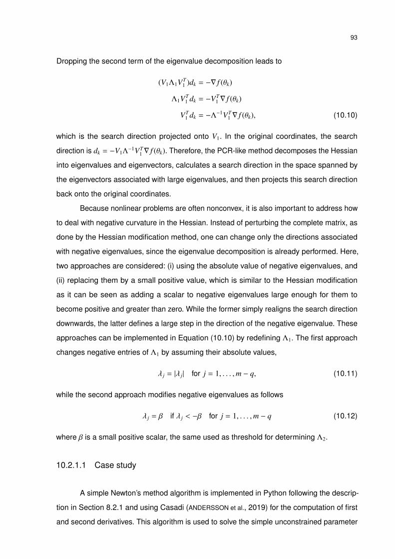
93

Dropping the second term of the eigenvalue decomposition leads to

(V1Λ1VT1 )dk = −∇ f (θk)

Λ1VT1 dk = −VT

1 ∇ f (θk)

VT1 dk = −Λ−1VT

1 ∇ f (θk), (10.10)

which is the search direction projected onto V1. In the original coordinates, the search

direction is dk = −V1Λ−1VT

1 ∇ f (θk). Therefore, the PCR-like method decomposes the Hessian

into eigenvalues and eigenvectors, calculates a search direction in the space spanned by

the eigenvectors associated with large eigenvalues, and then projects this search direction

back onto the original coordinates.

Because nonlinear problems are often nonconvex, it is also important to address how

to deal with negative curvature in the Hessian. Instead of perturbing the complete matrix, as

done by the Hessian modification method, one can change only the directions associated

with negative eigenvalues, since the eigenvalue decomposition is already performed. Here,

two approaches are considered: (i) using the absolute value of negative eigenvalues, and

(ii) replacing them by a small positive value, which is similar to the Hessian modification

as it can be seen as adding a scalar to negative eigenvalues large enough for them to

become positive and greater than zero. While the former simply realigns the search direction

downwards, the latter defines a large step in the direction of the negative eigenvalue. These

approaches can be implemented in Equation (10.10) by redefining Λ1. The first approach

changes negative entries of Λ1 by assuming their absolute values,

λ j = |λ j| for j = 1, . . . ,m − q, (10.11)

while the second approach modifies negative eigenvalues as follows

λ j = β if λ j < −β for j = 1, . . . ,m − q (10.12)

where β is a small positive scalar, the same used as threshold for determining Λ2.

10.2.1.1 Case study

A simple Newton’s method algorithm is implemented in Python following the descrip-

tion in Section 8.2.1 and using Casadi (ANDERSSON et al., 2019) for the computation of first

and second derivatives. This algorithm is used to solve the simple unconstrained parameter

94

estimation problem presented here. The problem, obtained from Bard (1974), consists of

a least squares estimation of two parameters from a single compound chemical reaction

model starting from initial conditions η0 = 1 and t0 = 0, which is given by

η = exp(− θ1t exp

(−θ2

T

))(10.13)

where η ∈ R is the modeled remaining fraction of the reacting compound, θ ∈ R2 are the

parameters, t ∈ R is time ellapsed (s) and T ∈ R is temperature (K). The input data used for

this estimation problem are listed in Table 15. This problem is not actually ill-conditioned,

but it is a good example to analyze how the regularization approach based on eigenvalue

decomposition deals with non convexity in the solution space.

Table 15 – Input data for the unconstrained least squares case study from Bard (1974).

Experiment ` t (s) T (K) η

1 0.1 100 0.9802 0.2 100 0.9833 0.3 100 0.9554 0.4 100 0.9795 0.5 100 0.9936 0.05 200 0.6267 0.1 200 0.5448 0.15 200 0.4559 0.2 200 0.22510 0.25 200 0.16711 0.02 300 0.56612 0.04 300 0.31713 0.06 300 0.03414 0.08 300 0.01615 0.1 300 0.066

A three dimensional graph and a contour plot of the solution space are presented

in Figure 12, which shows that the problem is not convex and has small curvature mostly

along axis θ1. The eigenvector-based regularization approach is compared with the Hessian

modification method. The former is combined with both approaches described in Section

(10.2.1) to deal with negative eigenvalues, namely (i) using the absolute value of negative

eigenvalues to rewrite the Hessian, and (ii) setting a small positive value equal to the

threshold β to replace negative eigenvalues.

For the eigenvector-based regularization approach, a threshold β = 10−6 is used and,

for the Hessian modification, constant δ is calculated in a way that the smallest eigenvalue

bellow this threshold has the same value as β. 20 different initial points for θ are used to

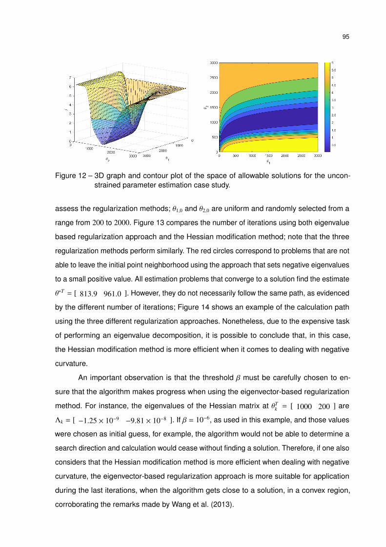
95

Figure 12 – 3D graph and contour plot of the space of allowable solutions for the uncon-strained parameter estimation case study.

assess the regularization methods; θ1,0 and θ2,0 are uniform and randomly selected from a

range from 200 to 2000. Figure 13 compares the number of iterations using both eigenvalue

based regularization approach and the Hessian modification method; note that the three

regularization methods perform similarly. The red circles correspond to problems that are not

able to leave the initial point neighborhood using the approach that sets negative eigenvalues

to a small positive value. All estimation problems that converge to a solution find the estimate

θ∗T = [ 813.9 961.0 ]. However, they do not necessarily follow the same path, as evidenced

by the different number of iterations; Figure 14 shows an example of the calculation path

using the three different regularization approaches. Nonetheless, due to the expensive task

of performing an eigenvalue decomposition, it is possible to conclude that, in this case,

the Hessian modification method is more efficient when it comes to dealing with negative

curvature.

An important observation is that the threshold β must be carefully chosen to en-

sure that the algorithm makes progress when using the eigenvector-based regularization

method. For instance, the eigenvalues of the Hessian matrix at θTk = [ 1000 200 ] are

Λk = [ −1.25 × 10−9 −9.81 × 10−8 ]. If β = 10−6, as used in this example, and those values

were chosen as initial guess, for example, the algorithm would not be able to determine a

search direction and calculation would cease without finding a solution. Therefore, if one also

considers that the Hessian modification method is more efficient when dealing with negative

curvature, the eigenvector-based regularization approach is more suitable for application

during the last iterations, when the algorithm gets close to a solution, in a convex region,

corroborating the remarks made by Wang et al. (2013).

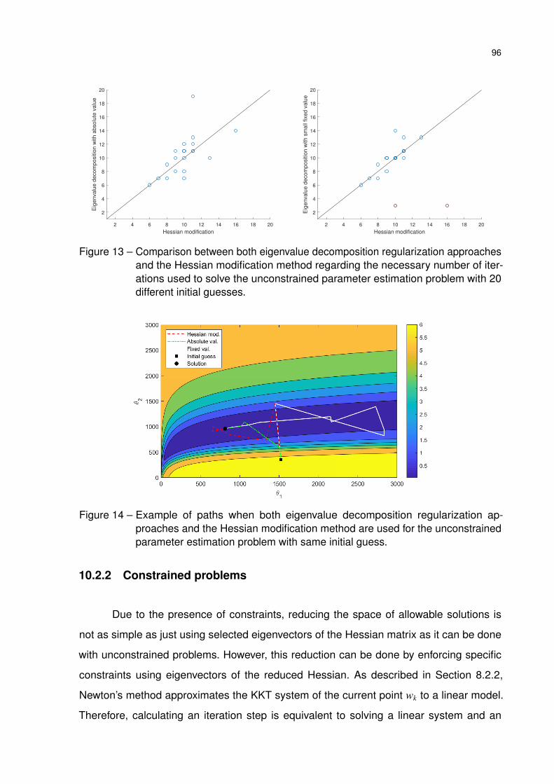
96

2 4 6 8 10 12 14 16 18 20

Hessian modification

2

4

6

8

10

12

14

16

18

20E

igenvalu

e d

ecom

positio

n w

ith a

bsolu

te v

alu

e

2 4 6 8 10 12 14 16 18 20

Hessian modification

2

4

6

8

10

12

14

16

18

20

Eig

envalu

e d

ecom

positio

n w

ith s

mall

fixed v

alu

e

Figure 13 – Comparison between both eigenvalue decomposition regularization approachesand the Hessian modification method regarding the necessary number of iter-ations used to solve the unconstrained parameter estimation problem with 20different initial guesses.

Figure 14 – Example of paths when both eigenvalue decomposition regularization ap-proaches and the Hessian modification method are used for the unconstrainedparameter estimation problem with same initial guess.

10.2.2 Constrained problems

Due to the presence of constraints, reducing the space of allowable solutions is

not as simple as just using selected eigenvectors of the Hessian matrix as it can be done

with unconstrained problems. However, this reduction can be done by enforcing specific

constraints using eigenvectors of the reduced Hessian. As described in Section 8.2.2,

Newton’s method approximates the KKT system of the current point wk to a linear model.

Therefore, calculating an iteration step is equivalent to solving a linear system and an

97

analogy can be made between QP and calculating an iteration in nonlinear programming

(NLP) by comparing Equations (8.5) and (8.17). In this section, it is first demonstrated that

adding a constraint of the form VT2 θ = 0 in an equality-constrained quadratic problem is

equivalent to performing the eigenvalue decomposition of the reduced Hessian and removing

the directions corresponding to V2. Then, based on this observation and on the results from

unconstrained parameter estimation, the implementation of this regularization approach in

an interior point solver for nonlinear optimization is described. The main advantage of this

regularization method is that, besides dealing with nearly flat regions in the neighborhood of

the solution, the eigenvectors can be used to recognize groups of correlated parameters

providing valuable information for identifiability analysis.

10.2.2.1 Equality-constrained quadratic problems

Consider the QP problem for one experiment

minx,θ

12(η − (Cx + Dθ)

)T (η − (Cx + Dθ)

)(10.14a)

s.t. h(x, θ) := Ax + Bθ = 0 (10.14b)

where η ∈ Rs are output observations, x ∈ Rp are state variables and θ ∈ Rm are parameters.

The expression Cx + Dθ is a linear mapping between the state variables and parameters,

and the output observations with C ∈ Rs×p and D ∈ Rs×m, and h(x, θ) are equality constraints

where A ∈ Rp×p is a nonsingular square matrix and B ∈ Rp×m. Note that this problem has m

degrees of freedom, as there are the same number of constraints and state variables. From

equation (8.5), the KKT system for this optimization problem is given byCTC CT D AT

DTC DT D BT

A B

dx

dθ

λ

= −

CTCx0 + CT Dθ0 + cx

DTCx0 + DT Dθ0 + cθ

Ax0 + Bθ0

. (10.15)

where λ ∈ Rp are the Lagrange multipliers, d are the steps for the state variables and

parameters, x0 and θ0 are the initial value for the state variables and the parameters, and

cx := ηTC and cθ := ηT D.

The reduced Hessian can be obtained by calculating the null space of ∇h(x, θ),

Z ∈ Rn×m with n = m + p, and performing ZT QZ, where Q ∈ Rn×n is the Hessian matrix. Matrix

Z is not unique; however, a pertinent way of calculating it is to consider the state variables x

98

as dependent variables and the parameters θ as independent variables, as shown in Section

8.3, and calculate

Z =

−A−1B

Ip

(10.16)

where Ip is the identity matrix of dimension p. The Hessian matrix, Q, is the 2 × 2 top right

block in the KKT matrix in (10.15). By calculating ZT QZ, the reduced Hessian is given by

ZT QZ = DT D − DTCA−1B − BT (A−1)TCT D + BT (A−1)TCTCA−1B. (10.17)

The KKT system (10.15) can be analytically solved. Rearranging the third equation

leads to

dx = −A−1(Bdθ + Bθ0 + Ax0), (10.18)

and substituting it into the first equation gives

λ = −A−T (CT D −CTCA−1B)dθ + A−TCTCA−1(Bθ0 + Ax0)− A−T (CT Dθ0 + CTCx0) − A−T cx.

(10.19)

Substituting λ and dx into the second equation and rearranging all terms result in

ZT QZdθ = −ZT QZθ0 + BT A−T cx − cθ. (10.20)

Once dθ is obtained, the dependent variable step dx and the Lagrange multipliers λ can be

then calculated.

If the reduced Hessian is (near) singular, this problem can be regularized in a PCR-like

approach. The eigenvalue decomposition of the reduced Hessian can be used for that end.

After defining a threshold β, ZT QZ can be split into two terms according to its eigenvalues

as follows

ZT QZ = V1Λ1VT1 + V2Λ2VT

2 , (10.21)

where V2 are the q eigenvectors associated with the (near) zero eigenvalues Λ2 and V1 are

the m − q eigenvectors associated with the large eigenvalues Λ1. Then, dropping the term

with Λ2 in the left-hand side, equation (10.20) becomes

V1Λ1VT1 dθ = −ZT QZθ0 + BT A−T cx − cθ. (10.22)

99

Multiplying both sides by VT1 and then by Λ−1

1 respectively leads to

VT1 dθ = −Λ−1

1 VT1 (ZT QZθ0 + BT A−T cx − cθ), (10.23)

which is the reduced set of variables corresponding to the step of the independent variables

dθ in V1 coordinates. Projecting it back to the original coordinates gives the expression

dθ = −V1Λ−11 VT

1 (ZT QZθ0 + BT A−T cx − cθ). (10.24)

Alternatively, an ill-conditioned problem of the form (10.14) can be solved by adding

new constraints that fix the parameter relationships present in V2, the eigenvectors associated

with the damaging eigenvalues from the reduced Hessian. Modifying the KKT system (10.15)

and enforcing the constraint VT2 dθ = 0 result in

CTC CT D AT

DTC DT D BT V2

A B

VT2

dx

dθ

λ

ν

= −

CTCx0 + CT Dθ0 + cx

DTCx0 + DT Dθ0 + cθ

Ax0 + Bθ0

0

, (10.25)

where ν are the Lagrange multipliers corresponding to the new constraints. Comparing

(10.25) to (10.15), it is possible to see that equations one and three are both unchanged,

so dx and λ are also described by the same expressions (10.18) and (10.19). The second

equation from (10.25), however, has a new term when compared to (10.20), and when

(10.18) and (10.19) are substituted into it, the new expression is

ZT QZdθ + V2ν = −ZT QZθ0 + BT A−T cx − cθ. (10.26)

Again, splitting ZT QZ into two terms according to its eigenvalues, as in (10.21), and multiply-

ing by VT1 leads to

VT1 (V1Λ1VT

1 + V2Λ2VT2 )dθ + VT

1 V2ν = −VT1 (ZT QZθ0 + BT A−T cx − cθ). (10.27)

Because V1 and V2 are orthogonal, VT1 V2Λ2VT

2 dθ and the second term on the letf-hand

side are both zero, which results in (10.23). This shows that adding the set of constraints

VT2 dθ = 0 with eigenvectors of the reduced Hessian is equivalent to reducing the space of

allowable solutions in a PCR-like approach.

100

10.2.2.1.1 Illustrative example

An example is now presented to illustrate that adding new constraints using the

eigenvectors of the reduced Hessian, and performing a principal component reduction in the

space of solution are equivalent. The results are also compared to the Hessian modification

approach, which adds a diagonal matrix to the top left block of the KKT matrix. A simple

synthetic ill-conditioned QP problem in the same form as (10.14) is created. The model is

built with m = 5 parameters θ and p = 1 state variable . To induce correlations among the

parameters, the columns of D are generated as follows

ð1 ∼ N(0, 1)

ð2 ∼ N(0, 1)

ð3 ∼ N(0, 1)

ð4 = ð1 + ε

ð5 = 2ð2 + ε

where ði ∈ Rs is the ith column of D and ε ∼ N(0, I ·10−12) is a small perturbation. In this case,

C ∼ N(0, I) is a column vector, and η is generated from the mapping function, with the original

parameters and state variable in Table 17 and the addition of an error ε ∼ N(0, I · 10−2). The

equality constraint h(x, θ) is defined by A = [−1] and B = [ 1.3 1 1 1 1 ].

The reduced Hessian is calculated following the methodology described in Section

8.3. The eigenvalue decomposition is presented in Table 16. The presence of a small

eigenvalue indicates that the equality constraint is not able to provide all the information

necessary to uniquely determine the parameters with high confidence, as shown in the

previous chapter; there is still one direction V2 that keeps the problem ill-conditioned.

Table 16 – Eigenvectors of the reduced Hessian calculated from the KKT matrix of theillustrative example for equality-constrained quadratic problem.

V2 V1

θ1 -0.639 0.206 0.251 -0.686 0.129θ2 0.383 0.773 0.043 -0.015 0.504θ3 0.000 -0.101 -0.914 -0.323 0.223θ4 0.639 -0.391 0.273 -0.599 0.073θ5 -0.192 -0.444 0.158 0.258 0.822Λ 2.24e-12 0.91 10.95 30.92 116.64

101

Table 17 shows the original parameters and state variable, as well as estimations

computed with the PCR-like approach (10.24), by adding the new constraint VT2 θ = 0, and

by adding δHI to the Hessian with δH = 10−6. The same initial values for x and θ is used. It is

possible to see that reducing the space of allowable solution according to the eigenvalue

decomposition and adding new constraint built with the eigenvectors associated with the

smallest eigenvalues generate equivalent steps. Also, the Hessian modification method

resulted in a different estimate for θ, which shows that this regularization approach provides

a different search direction than regularization based on the eigenvalue decomposition of

the reduced Hessian. An advantage of the latter approach is that parameters that cannot be

individually estimated and are, therefore, correlated can be singled out by the entries of the

eigenvectors in V2.

Table 17 – Original and estimated state variable and parameters of the illustrative examplefor equality-constrained quadratic problem.

x θ1 θ2 θ3 θ4 θ5

Original variables 2 1 1.5 -0.5 0.7 -1PCR-like 1.999 0.980 1.462 -0.471 0.710 -0.975Constraint V2 1.998 0.979 1.463 -0.471 0.709 -0.975Hessian modification 1.998 1.812 0.963 -0.471 -0.125 -0.725

10.2.2.2 Interior point implementation

The eigenvector-based regularization method is implemented in an existing interior

point solver developed with Pynumero (RODRIGUEZ et al., 2018), which is a framework for

developing NLP optimization algorithms in Python. Pyomo (HART et al., 2017; HART et al.,

2011) is used as the mathematical modeling language. Since it has interfaces with tools for

automatic differentiation, Pyomo provides exact first and second derivatives. This interior

point implementation is based on the Ipopt algorithm and, thus, follows the same steps as

described in Section 8.2.2.1. For later reference, the KKT system (8.22) can be rewritten

102

defining Wk := Hk + Σk and splitting the complete vector of variables into state variables and

parameters as followsW xx

k W xθk ∇xh(xk, θk)T

Wθxk Wθθ

k ∇θh(xk, θk)T

∇hx(xk, θk) ∇hθ(xk, θk)

dxk

dθk

dλk

= −

∇xϕ(xk, θk, µ j) + ∇xh(xk, θk)Tλk

∇θϕ(xk, θk, µ j) + ∇θh(xk, θk)Tλk

h(xk, θk)

.(10.29)

To calculate a step, the interior point algorithm provides the KKT system to a linear

solver. First, the linear solver factorizes the KKT matrix and, then, performs backsolves using

the right-hand side. After the factorization step, some solvers, such as MA27, MA57 and

MUMPS (AMESTOY et al., 2001; STFC, 2020), return the inertia of the factorized matrix, i.e, the

number of positive, negative and zero eigenvalues. For the reduced Hessian to be positive

definite, the KKT matrix must have n positive, p negative, and no zero eigenvalues (CHIANG;

ZAVALA, 2016), where n is the total number of variables and p is the number of constraints.

Therefore, when there are more than p negative eigenvalues, the reduced Hessian is not

positive definite, and when there are zero eigenvalues, the matrix is not invertible and there

are infinite possible values for the step. In both cases, regularization is needed. The interior

point algorithm used relies on the inertia information to decide when to regularize the KKT

matrix.

The default precision to determine if an eigenvalue is zero is machine precision,

but a different value can be provided to the linear solver. To implement the eigenvector-

based regularization method, a threshold βε is defined to identify iterations at which the

reduced Hessian might have nearly flat directions. However, based on the results from

Section 10.2.1.1, this regularization approach is ideally applied close to the solution, thus

the threshold βε is only defined when the barrier parameter µ j is smaller than a specified

value βµ.

The eigenvector-based regularization uses the KKT matrix to calculate the reduced

Hessian using the approach described in Section 8.3 and performs its eigenvalue decompo-

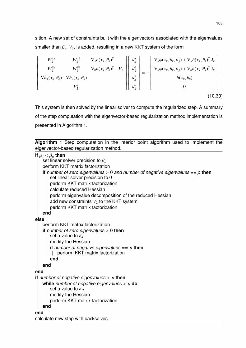
103

sition. A new set of constraints built with the eigenvectors associated with the eigenvalues

smaller than βε, V2, is added, resulting in a new KKT system of the form

W xxk W xθ

k ∇xh(xk, θk)T

Wθxk Wθθ

k ∇θh(xk, θk)T V2

∇hx(xk, θk) ∇hθ(xk, θk)

VT2

dxk

dθk

dλk

dνk

= −

∇xϕ(xk, θk, µ j) + ∇xh(xk, θk)Tλk

∇θϕ(xk, θk, µ j) + ∇θh(xk, θk)Tλk

h(xk, θk)

0

.

(10.30)

This system is then solved by the linear solver to compute the regularized step. A summary

of the step computation with the eigenvector-based regularization method implementation is

presented in Algorithm 1.

Algorithm 1 Step computation in the interior point algorithm used to implement theeigenvector-based regularization method.if µ j < βµ then

set linear solver precision to βεperform KKT matrix factorizationif number of zero eigenvalues > 0 and number of negative eigenvalues == p then

set linear solver precision to 0perform KKT matrix factorizationcalculate reduced Hessianperform eigenvalue decomposition of the reduced Hessianadd new constraints V2 to the KKT systemperform KKT matrix factorization

endelse

perform KKT matrix factorizationif number of zero eigenvalues > 0 then

set a value to δh

modify the Hessianif number of negative eigenvalues == p then

perform KKT matrix factorizationend

endendif number of negative eigenvalues > p then

while number of negative eigenvalues > p doset a value to δH

modify the Hessianperform KKT matrix factorization

endendcalculate new step with backsolves

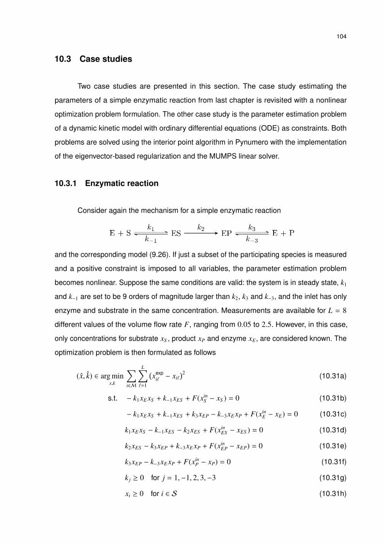
104

10.3 Case studies

Two case studies are presented in this section. The case study estimating the

parameters of a simple enzymatic reaction from last chapter is revisited with a nonlinear

optimization problem formulation. The other case study is the parameter estimation problem

of a dynamic kinetic model with ordinary differential equations (ODE) as constraints. Both

problems are solved using the interior point algorithm in Pynumero with the implementation

of the eigenvector-based regularization and the MUMPS linear solver.

10.3.1 Enzymatic reaction

Consider again the mechanism for a simple enzymatic reaction

and the corresponding model (9.26). If just a subset of the participating species is measured

and a positive constraint is imposed to all variables, the parameter estimation problem

becomes nonlinear. Suppose the same conditions are valid: the system is in steady state, k1

and k−1 are set to be 9 orders of magnitude larger than k2, k3 and k−3, and the inlet has only

enzyme and substrate in the same concentration. Measurements are available for L = 8

different values of the volume flow rate F, ranging from 0.05 to 2.5. However, in this case,

only concentrations for substrate xS , product xP and enzyme xE, are considered known. The

optimization problem is then formulated as follows

(x, k) ∈ arg minx,k

∑i∈M

L∑`=1

(xexp

i` − xi`)2 (10.31a)

s.t. − k1xE xS + k−1xES + F(xinS − xS ) = 0 (10.31b)

− k1xE xS + k−1xES + k3xEP − k−3xE xP + F(xinE − xE) = 0 (10.31c)

k1xE xS − k−1xES − k2xES + F(xinES − xES ) = 0 (10.31d)

k2xES − k3xEP + k−3xE xP + F(xinEP − xEP) = 0 (10.31e)

k3xEP − k−3xE xP + F(xinP − xP) = 0 (10.31f)

k j ≥ 0 for j = 1,−1, 2, 3,−3 (10.31g)

xi ≥ 0 for i ∈ S (10.31h)

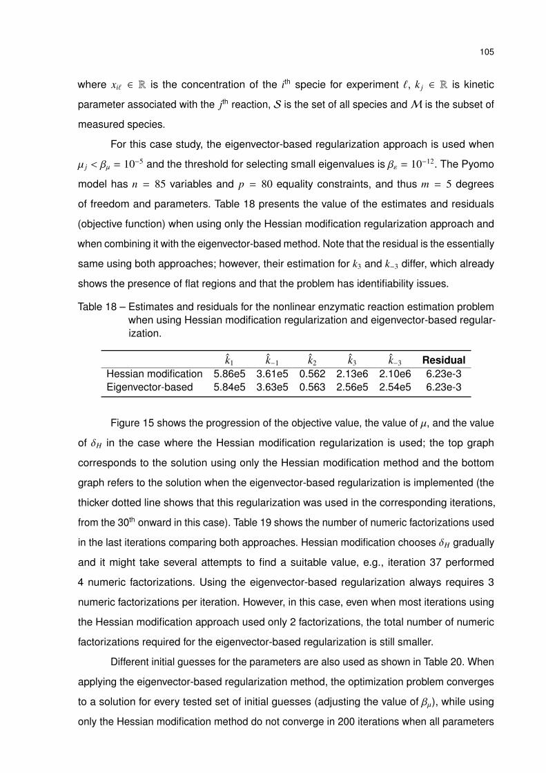
105

where xi` ∈ R is the concentration of the ith specie for experiment `, k j ∈ R is kinetic

parameter associated with the jth reaction, S is the set of all species andM is the subset of

measured species.

For this case study, the eigenvector-based regularization approach is used when

µ j < βµ = 10−5 and the threshold for selecting small eigenvalues is βε = 10−12. The Pyomo

model has n = 85 variables and p = 80 equality constraints, and thus m = 5 degrees

of freedom and parameters. Table 18 presents the value of the estimates and residuals

(objective function) when using only the Hessian modification regularization approach and

when combining it with the eigenvector-based method. Note that the residual is the essentially

same using both approaches; however, their estimation for k3 and k−3 differ, which already

shows the presence of flat regions and that the problem has identifiability issues.

Table 18 – Estimates and residuals for the nonlinear enzymatic reaction estimation problemwhen using Hessian modification regularization and eigenvector-based regular-ization.

k1 k−1 k2 k3 k−3 ResidualHessian modification 5.86e5 3.61e5 0.562 2.13e6 2.10e6 6.23e-3Eigenvector-based 5.84e5 3.63e5 0.563 2.56e5 2.54e5 6.23e-3

Figure 15 shows the progression of the objective value, the value of µ, and the value

of δH in the case where the Hessian modification regularization is used; the top graph

corresponds to the solution using only the Hessian modification method and the bottom

graph refers to the solution when the eigenvector-based regularization is implemented (the

thicker dotted line shows that this regularization was used in the corresponding iterations,

from the 30th onward in this case). Table 19 shows the number of numeric factorizations used

in the last iterations comparing both approaches. Hessian modification chooses δH gradually

and it might take several attempts to find a suitable value, e.g., iteration 37 performed

4 numeric factorizations. Using the eigenvector-based regularization always requires 3

numeric factorizations per iteration. However, in this case, even when most iterations using

the Hessian modification approach used only 2 factorizations, the total number of numeric

factorizations required for the eigenvector-based regularization is still smaller.

Different initial guesses for the parameters are also used as shown in Table 20. When

applying the eigenvector-based regularization method, the optimization problem converges

to a solution for every tested set of initial guesses (adjusting the value of βµ), while using

only the Hessian modification method do not converge in 200 iterations when all parameters

106

started with value 0.25 and, when three other initial guesses are used, it is not able to satisfy

the optimization tolerance set to 10−8 (indicated by a dash). Note that, in this case, reducing

the solution space using the eigenvectors of the reduced Hessian resulted in a smaller

number of iterations necessary for convergence, indicating that enforcing these constraints

can help the algorithm achieve convergence when the neighborhood around the solution is

nearly flat.

0 5 10 15 20 25 30 35 40 45

iteration

-2.5

-2

-1.5

-1

-0.5

0

-10

-5

0Hessian modification

log(res)

log( )

log(H

)

0 5 10 15 20 25 30 35 40 45

iteration

-2.5

-2

-1.5

-1

-0.5

0

-10

-5

0Eigenvector-based

log(res)

log( )

log(H

)

Figure 15 – Progression of the nonlinear enzymatic reaction estimation problem employingthe Hessian modification and the eigenvector-based regularization approaches.

Table 19 – Comparison of the number of factorizations for the final iterations when theeigenvector-based regularization is used and when only Hessian modification isemployed.

Iteration 29 30 31 32 33 34 35 36 37 38 39 40 41 42 TotalHessian modification 1 2 2 1 2 2 2 1 4 2 1 1 3 2 26Eigenvector-based 1 3 3 3 3 3 3 3 22

Another advantage of using the eigenvector-based regularization approach is that

the eigenvalue decomposition of the reduced Hessian can indicate correlated parameters.

Table 21 shows the eigenvectors and eigenvalues obtained in the last iteration during the

calculation of the estimates. Note that each vector in V2 shows a pair of kinetic constants

that are correlated, namely k1 and k−1, and k3 and k−3. As evidenced by the eigenvalues Λ2,

changing the values of these parameters while keeping their ratio fixed does not significantly

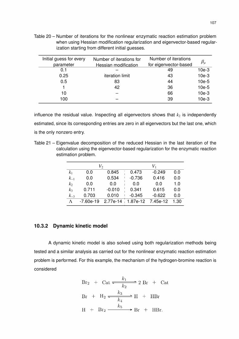
107

Table 20 – Number of iterations for the nonlinear enzymatic reaction estimation problemwhen using Hessian modification regularization and eigenvector-based regular-ization starting from different initial guesses.

Initial guess for everyparameter

Number of iterations forHessian modification

Number of iterationsfor eigenvector-based

βµ

0.1 – 49 10e-30.25 iteration limit 43 10e-30.5 83 44 10e-51 42 36 10e-5

10 – 66 10e-3100 – 39 10e-3

influence the residual value. Inspecting all eigenvectors shows that k2 is independently

estimated, since its corresponding entries are zero in all eigenvectors but the last one, which

is the only nonzero entry.

Table 21 – Eigenvalue decomposition of the reduced Hessian in the last iteration of thecalculation using the eigenvector-based regularization for the enzymatic reactionestimation problem.

V2 V1

k1 0.0 0.845 0.473 -0.249 0.0k−1 0.0 0.534 -0.736 0.416 0.0k2 0.0 0.0 0.0 0.0 1.0k3 0.711 -0.010 0.341 0.615 0.0k−3 0.703 0.010 -0.345 -0.622 0.0Λ -7.60e-19 2.77e-14 1.87e-12 7.45e-12 1.30

10.3.2 Dynamic kinetic model

A dynamic kinetic model is also solved using both regularization methods being

tested and a similar analysis as carried out for the nonlinear enzymatic reaction estimation

problem is performed. For this example, the mechanism of the hydrogen-bromine reaction is

considered

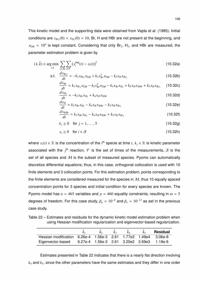
108

This kinetic model and the supporting data were obtained from Vajda et al. (1985). Initial

conditions are xBr2(0) = xH2(0) = 10, Br, H and HBr are not present at the beginning, and

xCat = 104 is kept constant. Considering that only Br2, H2, and HBr are measured, the

parameter estimation problem is given by

(x, k) ∈ arg minx,k

∑i∈M

∑t∈T

(xexp

i (t) − xi(t))2 (10.32a)

s.t.dxBr2

dt= −k1xBr2 xCat + k2x2

Br xCat − k5xH xBr2 (10.32b)

dxBr

dt= k1xBr2 xCat − k2x2

Br xCat − k3xBr xH2 + k4xH xHBr + k5xH xBr2 (10.32c)

dxH2

dt= −k3xBr xH2 + k4xH xHBr (10.32d)

dxH

dt= k3xBr xH2 − k4xH xHBr − k5xH xBr2 (10.32e)

dxHBr

dt= k3xBr xH2 − k4xH xHBr + k5xH xBr2 (10.32f)

k j ≥ 0 for j = 1, . . . , 5 (10.32g)

xi ≥ 0 for i ∈ S (10.32h)

where xi(t) ∈ R is the concentration of the ith specie at time t, k j ∈ R is kinetic parameter

associated with the jth reaction, T is the set of times of the measurements, S is the

set of all species and M is the subset of measured species. Pyomo can automatically

discretize differential equations; thus, in this case, orthogonal collocation is used with 10

finite elements and 3 collocation points. For this estimation problem, points corresponding to

the finite elements are considered measured for the species inM, thus 10 equally spaced

concentration points for 3 species and initial condition for every species are known. The

Pyomo model has n = 465 variables and p = 460 equality constraints, resulting in m = 5

degrees of freedom. For this case study, βµ = 10−8 and βε = 10−12 as set in the previous

case study.

Table 22 – Estimates and residuals for the dynamic kinetic model estimation problem whenusing Hessian modification regularization and eigenvector-based regularization.

k1 k2 k3 k4 k5 ResidualHessian modification 6.26e-4 1.56e-3 2.61 1.77e3 1.49e4 3.06e-8Eigenvector-based 6.27e-4 1.56e-3 2.61 3.20e2 2.69e3 1.18e-6

Estimates presented in Table 22 indicates that there is a nearly flat direction involving

k4 and k5, since the other parameters have the same estimates and they differ in one order

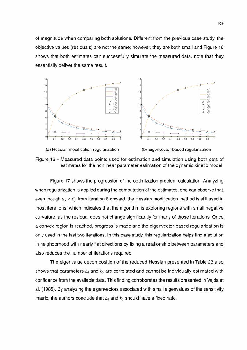
109

of magnitude when comparing both solutions. Different from the previous case study, the

objective values (residuals) are not the same; however, they are both small and Figure 16

shows that both estimates can successfully simulate the measured data, note that they

essentially deliver the same result.

0 0.1 0.2 0.3 0.4 0.5 0.6 0.7 0.8 0.9 1

0

2

4

6

8

10

12

14

16

18

(a) Hessian modification regularization

0 0.1 0.2 0.3 0.4 0.5 0.6 0.7 0.8 0.9 1

0

2

4

6

8

10

12

14

16

18

(b) Eigenvector-based regularization

Figure 16 – Measured data points used for estimation and simulation using both sets ofestimates for the nonlinear parameter estimation of the dynamic kinetic model.

Figure 17 shows the progression of the optimization problem calculation. Analyzing

when regularization is applied during the computation of the estimates, one can observe that,

even though µ j < βµ from iteration 6 onward, the Hessian modification method is still used in

most iterations, which indicates that the algorithm is exploring regions with small negative

curvature, as the residual does not change significantly for many of those iterations. Once

a convex region is reached, progress is made and the eigenvector-based regularization is

only used in the last two iterations. In this case study, this regularization helps find a solution

in neighborhood with nearly flat directions by fixing a relationship between parameters and

also reduces the number of iterations required.

The eigenvalue decomposition of the reduced Hessian presented in Table 23 also

shows that parameters k4 and k5 are correlated and cannot be individually estimated with

confidence from the available data. This finding corroborates the results presented in Vajda et

al. (1985). By analyzing the eigenvectors associated with small eigenvalues of the sensitivity

matrix, the authors conclude that k4 and k5 should have a fixed ratio.

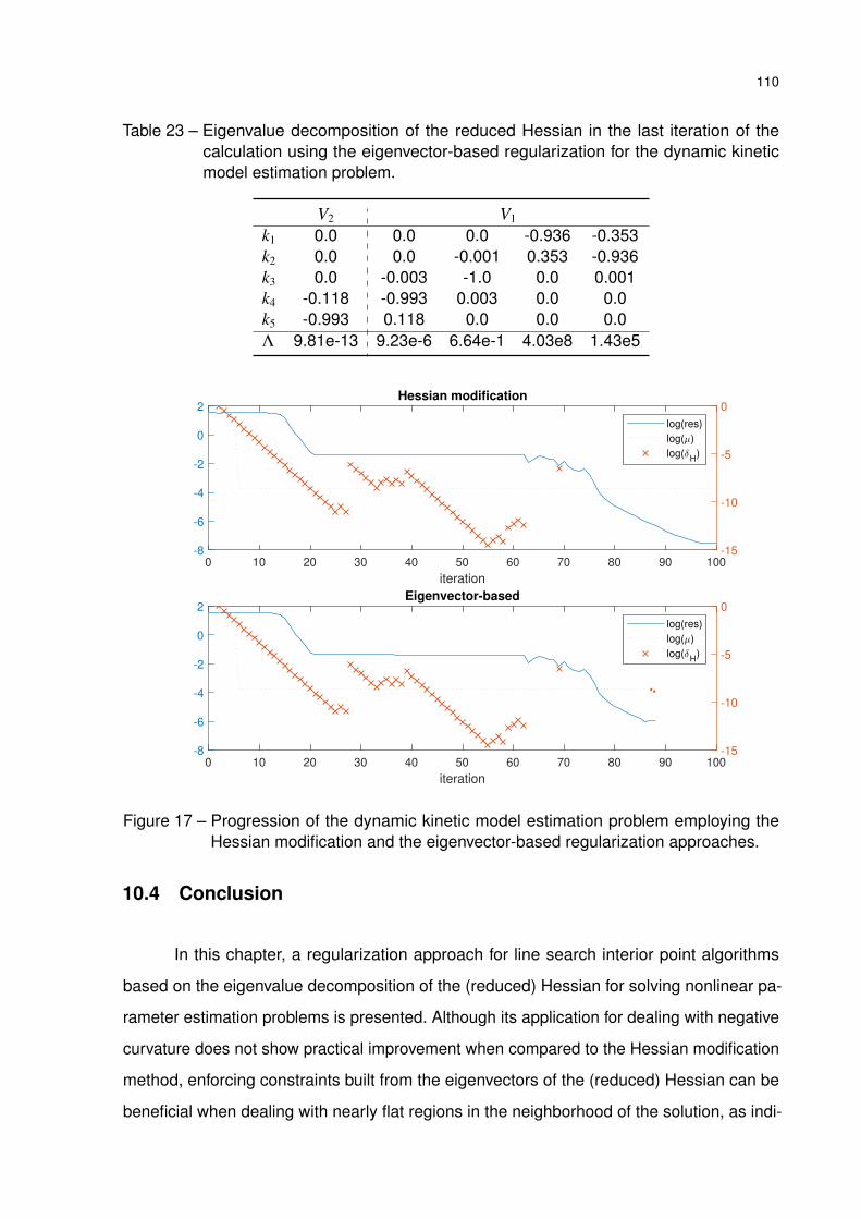
110

Table 23 – Eigenvalue decomposition of the reduced Hessian in the last iteration of thecalculation using the eigenvector-based regularization for the dynamic kineticmodel estimation problem.

V2 V1

k1 0.0 0.0 0.0 -0.936 -0.353k2 0.0 0.0 -0.001 0.353 -0.936k3 0.0 -0.003 -1.0 0.0 0.001k4 -0.118 -0.993 0.003 0.0 0.0k5 -0.993 0.118 0.0 0.0 0.0Λ 9.81e-13 9.23e-6 6.64e-1 4.03e8 1.43e5

0 10 20 30 40 50 60 70 80 90 100

iteration

-8

-6

-4

-2

0

2

-15

-10

-5

0Hessian modification

log(res)

log( )

log(H

)

0 10 20 30 40 50 60 70 80 90 100

iteration

-8

-6

-4

-2

0

2

-15

-10

-5

0Eigenvector-based

log(res)

log( )

log(H

)

Figure 17 – Progression of the dynamic kinetic model estimation problem employing theHessian modification and the eigenvector-based regularization approaches.

10.4 Conclusion

In this chapter, a regularization approach for line search interior point algorithms

based on the eigenvalue decomposition of the (reduced) Hessian for solving nonlinear pa-

rameter estimation problems is presented. Although its application for dealing with negative

curvature does not show practical improvement when compared to the Hessian modification

method, enforcing constraints built from the eigenvectors of the (reduced) Hessian can be

beneficial when dealing with nearly flat regions in the neighborhood of the solution, as indi-

111

cated by the results from the case studies. Another advantage of using the eigenvector-based

regularization is that the constraints actually represent sets of correlated parameters, which

is important information for identifiability analysis and for suggesting some phenomenological

simplifications in the model.

112

11 Concluding remarks

Stoichiometric modeling has been an important tool for metabolic engineering since

this field has emerged in the 1990s based on metabolic flux analysis. Over the past 30 years,

improvement in computational power and development of different modeling techniques have

enabled highly detailed in silico models, especially for extensively investigated organisms.

However, non-model organisms, such as Burkholderia sacchari, still need effort towards

experimental work to develop more complex models that could potentially simulate their

metabolism. Part I of this thesis illustrates that stoichiometric models based on small to

medium metabolic networks are still a valuable tool that can help elucidate properties of

microorganisms and guide the design of experiments. In addition, they are a good starting

point for metabolic engineering; since stoichiometric models are linear, they can be relatively

simple (especially for small networks), which helps build the connection between biology

and mathematical modeling concepts more clearly.

Mechanistic models for describing cellular metabolism are challenging mainly due to

the amount and quality of data required, which are difficult to collect (if not impossible). This

obstacle gives rise to identifiability issues, which are evidenced by the high uncertainty of the

estimates. Regularization is a mathematical strategy that can successfully reduce parameter

variance, as discussed in Part II. Moreover, designing regularization methods based on the

eigenvalue decomposition of the (reduced) Hessian matrix is optimal for linear problems and

helpful for nonlinear problems with nearly flat neighborhood around the solution. However,

an important and valuable property of eigenvector-based regularization in both cases is that

these approaches also recognize correlated parameters, allowing for better understanding

the identifiability sources.

11.1 Recommendations for future work

• An interesting work for the near future is to continue with the analysis of the Burkholde-

ria sacchari metabolism and perform experiments that can elucidate the co-factor

balance to help plan for strategies that increase the conversion of fatty acid into

co-polymer, ideally to 100%.

• A recommendation of work related to modeling of metabolic networks is studying

kinetic model frameworks and their inherent identifiability issues. How regularization

113

methods based on eigenvalue decomposition would impact these frameworks is worth

investigating. Starting with the ensemble modeling technique would be a good strategy

since it is a popular more consolidated framework.

• The implementation of the eigenvector-based regularization method in a linear search

interior point algorithm can continue; some details of implementation can be further

investigated to require less manual input. For instance, the definition of the threshold

for deciding when a direction is considered flat and the algorithm for deciding whether

the eigenvector-based regularization should be used are two points that have room for

improvement.

• It would also be interesting to use the eigenvector-based regularization method in

larger nonlinear problems and verify whether the sparse principal components with

orthogonality constraints can also group sets of parameters with larger correlation.

• Another interesting idea that could be investigated is whether this eigenvector-based

regularization method could be extended to general optimization problems and if

it would be relevant doing so. A straightforward obstacle is how to define a good

set of independent variables. For parameter estimation problems, the choice of the

parameters is obvious, but they still have to be selected by the user.

114

Bibliography

ALBERTON, K. P. et al. Accelerating the parameters identifiability procedure: set by setselection. Computers & chemical engineering, Elsevier, v. 55, p. 181–197, 2013.

AMESTOY, P. et al. A fully asynchronous multifrontal solver using distributed dynamicscheduling. SIAM Journal on Matrix Analysis and Applications, v. 23, n. 1, p. 15–41, 2001.

ANDERSSON, J. A. E. et al. CasADi – A software framework for nonlinear optimization andoptimal control. Mathematical Programming Computation, Springer, v. 11, n. 1, p. 1–36,2019.

ANG, J. C. et al. Supervised, unsupervised, and semi-supervised feature selection: a reviewon gene selection. IEEE/ACM transactions on computational biology and bioinformatics,IEEE, v. 13, n. 5, p. 971–989, 2015.

ANTONIEWICZ, M. R. Methods and advances in metabolic flux analysis: a mini-review.Journal of Industrial Microbiology and Biotechnology, v. 42, n. 3, p. 317–325, 2015.

ARMENGAUD, J. et al. Non-model organisms, a species endangered by proteogenomics.Journal of proteomics, Elsevier, v. 105, p. 5–18, 2014.

ARORA, N.; BIEGLER, L. T. Parameter estimation for a polymerization reactor model with acomposite-step trust-region nlp algorithm. Industrial & engineering chemistry research, ACSPublications, v. 43, n. 14, p. 3616–3631, 2004.

BARD, Y. Nonlinear Parameter Estimation. [S.l.]: Academic Press, 1974.

BAUER, F.; LUKAS, M. A. Comparing parameter choice methods for regularization ofill-posed problems. Mathematics and Computers in Simulation, Elsevier, v. 81, n. 9, p.1795–1841, 2011.

BECKER, S. A. et al. Quantitative prediction of cellular metabolism with constraint-basedmodels: the cobra toolbox. Nature protocols, Nature Publishing Group, v. 2, n. 3, p. 727–738,2007.

BEN-ZVI, A. Reparameterization of inestimable systems with applications to chemical andbiochemical reactor systems. AIChE journal, Wiley Online Library, v. 54, n. 5, p. 1270–1281,2008.

BONARIUS, H. P. et al. Metabolic flux analysis of hybridoma cells in different culture mediausing mass balances. Biotechnology and bioengineering, Wiley Online Library, v. 50, n. 3, p.299–318, 1996.

BYRD, R. H.; NOCEDAL, J.; WALTZ, R. A. Knitro: An integrated package for nonlinearoptimization. In: Large-scale nonlinear optimization. [S.l.]: Springer, 2006. p. 35–59.

CARLSON, R.; SRIENC, F. Fundamental Escherichia coli Biochemical Pathways for Biomassand Energy Production: Identification of Reactions. Biotechnology and Bioengineering, v. 85,n. 1, p. 1–19, 2004.

CARTIS, C.; GOULD, N. I.; TOINT, P. L. Trust-region and other regularisations of linearleast-squares problems. BIT Numerical Mathematics, Springer, v. 49, n. 1, p. 21–53, 2009.

115

CHEN, W. W.; NIEPEL, M.; SORGER, P. K. Classic and contemporary approaches tomodeling biochemical reactions. Genes & development, Cold Spring Harbor Lab, v. 24,n. 17, p. 1861–1875, 2010.

CHIANG, N.-Y.; ZAVALA, V. M. An inertia-free filter line-search algorithm for large-scalenonlinear programming. Computational Optimization and Applications, Springer, v. 64, n. 2,p. 327–354, 2016.

CONG, L. et al. Multiplex Genome Engineering Using CRISPR/VCas Systems. Science,v. 339, n. 6121, p. 819–823, 2013.

COVERT, M. W. et al. Integrating high-throughput and computational data elucidatesbacterial networks. Nature, v. 429, n. 6987, p. 92–96, 2004.

DE GROOT, D. H. et al. The number of active metabolic pathways is bounded by the numberof cellular constraints at maximal metabolic rates. PLoS computational biology, PublicLibrary of Science, v. 15, n. 3, p. e1006858, 2019.

DEHAK, N. et al. Cosine similarity scoring without score normalization techniques. In:Odyssey. [S.l.: s.n.], 2010. p. 15.

DELSOLE, T.; BANERJEE, A. Statistical seasonal prediction based on regularizedregression. Journal of Climate, v. 30, n. 4, p. 1345–1361, 2017.

DIETRICH, K. et al. Producing phas in the bioeconomy—towards a sustainable bioplastic.Sustainable production and consumption, Elsevier, v. 9, p. 58–70, 2017.

FAN, Y. et al. Model reduction of kinetic equations by operator projection. Journal ofStatistical Physics, Springer, v. 162, n. 2, p. 457–486, 2016.

FARISS, R.; LAW, V. An efficient computational technique for generalized application ofmaximum likelihood to improve correlation of experimental data. Computers & ChemicalEngineering, Elsevier, v. 3, n. 1-4, p. 95–104, 1979.

FERNANDES, S. et al. Application of dynamic metabolic flux convex analysis to cho-dxb11cell fed-batch cultures. IFAC-PapersOnLine, Elsevier, v. 49, n. 7, p. 466–471, 2016.

FERREIRA, A. R. et al. Projection to latent pathways (PLP): a constrained projection tolatent variables (PLS) method for elementary flux modes discrimination. BMC systemsbiology, v. 5, n. 1, p. 181, 2011.

FLETCHER, R.; LEYFFER, S. User manual for filtersqp. Numerical Analysis Report NA/181,Department of Mathematics, University of Dundee, Dundee, Scotland, v. 35, 1998.

FORSTER, J. et al. Genome-scale reconstruction of the <i>Saccharomyces cerevisiae</i>metabolic network. Genome Research, n. 13, p. 244–253, 2003.

FRIEDMAN, J.; HASTIE, T.; TIBSHIRANI, R. A note on the group lasso and a sparse grouplasso. arXiv preprint arXiv:1001.0736, 2010.

FRIEDMAN, J.; HASTIE, T.; TIBSHIRANI, R. Regularization paths for generalized linearmodels via coordinate descent. Journal of statistical software, NIH Public Access, v. 33, n. 1,p. 1, 2010.

116

FUHRY, M.; REICHEL, L. A new tikhonov regularization method. Numerical Algorithms,Springer, v. 59, n. 3, p. 433–445, 2012.

GAGNEUR, J.; KLAMT, S. Computation of elementary modes: a unifying framework and thenew binary approach. BMC bioinformatics, v. 5, n. 1, p. 175, 2004.

GAMMA, E. et al. Design Patterns: Elements of Reusable Object-oriented Software. [S.l.]:Addison-Wesley Longman Publishing Co., Inc., 1995. ISBN 0-201-63361-2.

GANDER, W. Least squares with a quadratic constraint. Numerische Mathematik, Springer,v. 36, n. 3, p. 291–307, 1980.

GEORGE, E. I. The variable selection problem. Journal of the American StatisticalAssociation, Taylor & Francis Group, v. 95, n. 452, p. 1304–1308, 2000.

GERSTL, M. P.; JUNGREUTHMAYER, C.; ZANGHELLINI, J. TEFMA: Computingthermodynamically feasible elementary flux modes in metabolic networks. Bioinformatics,v. 31, n. 13, p. 2232–2234, 2015.

GILL, P. E.; MURRAY, W.; SAUNDERS, M. A. Snopt: An sqp algorithm for large-scaleconstrained optimization. SIAM review, SIAM, v. 47, n. 1, p. 99–131, 2005.

GRACIANO, J.; MENDOZA, D.; ROUX, G. A. L. Performance comparison of parameterestimation techniques for unidentifiable models. Computers & Chemical Engineering,Elsevier, v. 64, p. 24–40, 2014.

GUAMÁN, L. P. et al. Engineering xylose metabolism for production of polyhydroxybutyratein the non-model bacterium burkholderia sacchari. Microbial cell factories, BioMed Central,v. 17, n. 1, p. 74, 2018.

GUENNEBAUD, G.; JACOB, B. et al. Eigen v3. 2010. Disponível em: <http://eigen.tuxfamily-.org>.

GUIL, F.; HIDALGO, J. F.; GARCÍA, J. M. Boosting the extraction of elementary flux modesin genome-scale metabolic networks using the linear programming approach. Bioinformatics,2020.

GUNST, R. F.; MASON, R. L. Some considerations in the evaluation of alternate predictionequations. Technometrics, Taylor & Francis, v. 21, n. 1, p. 55–63, 1979.

GUO, W.; SHENG, J.; FENG, X. 13C-Metabolic Flux Analysis: An Accurate Approach toDemystify Microbial Metabolism for Biochemical Production. Bioengineering, v. 3, n. 1, p. 3,2015.

HANSEN, P. C. Rank-deficient and discrete ill-posed problems: numerical aspects of linearinversion. [S.l.]: Siam, 2005. v. 4.

HART, W. E. et al. Pyomo–optimization modeling in python. Second. [S.l.]: Springer Science& Business Media, 2017. v. 67.

HART, W. E.; WATSON, J.-P.; WOODRUFF, D. L. Pyomo: modeling and solving mathematicalprograms in python. Mathematical Programming Computation, Springer, v. 3, n. 3, p.219–260, 2011.

117

HEIRENDT, L. et al. Creation and analysis of biochemical constraint-based models usingthe cobra toolbox v. 3.0. Nature protocols, Nature Publishing Group, v. 14, n. 3, p. 639–702,2019.

HELMS, R. W. The average estimated variance criterion for the selection-of-variablesproblem in general linear models. Technometrics, Taylor & Francis Group, v. 16, n. 2, p.261–273, 1974.

HONG, S. H.; LEE, S. Y. Metabolic flux analysis for succinic acid production by recombinantEscherichia coli with amplified malic enzyme activity. Biotechnology and bioengineering,v. 74, n. 2, p. 89–95, 2001.

HOOPS, S. et al. COPASI - A COmplex PAthway SImulator. Bioinformatics, v. 22, n. 24, p.3067–3074, 2006.

JIANG, Y.; HE, Y.; ZHANG, H. Variable selection with prior information for generalized linearmodels via the prior lasso method. Journal of the American Statistical Association, Taylor &Francis, v. 111, n. 513, p. 355–376, 2016.

JOLLIFFE, I. T. A note on the use of principal components in regression. Journal of theRoyal Statistical Society: Series C (Applied Statistics), Wiley Online Library, v. 31, n. 3, p.300–303, 1982.

JOLLIFFE, I. T.; CADIMA, J. Principal component analysis: a review and recentdevelopments. Philosophical Transactions of the Royal Society A: Mathematical, Physicaland Engineering Sciences, The Royal Society Publishing, v. 374, n. 2065, p. 20150202,2016.

KAMP, A. von; KLAMT, S. Growth-coupled overproduction is feasible for almost allmetabolites in five major production organisms. Nature communications, Nature PublishingGroup, v. 8, n. 1, p. 1–10, 2017.

KAMP, A. von et al. Use of cellnetanalyzer in biotechnology and metabolic engineering.Journal of biotechnology, Elsevier, v. 261, p. 221–228, 2017.

KARL, W. C. Regularization in image restoration and reconstruction. In: BOVIK, A. (Ed.).Handbook of Image and Video Processing. Second edition. [S.l.]: Academic Press, 2005,(Communications, Networking and Multimedia). p. 183 – V.

KLAMT, S.; GAGNEUR, J.; KAMP, A. von. Algorithmic approaches for computing elementarymodes in large biochemical reaction networks. IEE Proceedings-Systems Biology, v. 152,n. 4, p. 249–255, 2005.

KLAMT, S.; HÄDICKE, O.; KAMP, A. von. Stoichiometric and constraint-based analysis ofbiochemical reaction networks. In: Large-Scale Networks in Engineering and Life Sciences.[S.l.]: Springer, 2014. p. 263–316.

KLAMT, S. et al. From elementary flux modes to elementary flux vectors: Metabolic pathwayanalysis with arbitrary linear flux constraints. PLoS computational biology, Public Library ofScience, v. 13, n. 4, 2017.

KLAMT, S.; SAEZ-RODRIGUEZ, J.; GILLES, E. D. Structural and functional analysis ofcellular networks with cellnetanalyzer. BMC systems biology, v. 1, n. 1, p. 2, 2007.

118

KLAMT, S.; STELLING, J. Two approaches for metabolic pathway analysis? Trends inbiotechnology, v. 21, n. 2, p. 64–69, 2003.

KLAMT, S.; VON KAMP, A. An application programming interface for cellnetanalyzer.Biosystems, v. 105, n. 2, p. 162–168, 2011.

KLINKEN, J. B. V.; DIJK, K. Willems van. Fluxmodecalculator: an efficient tool for large-scaleflux mode computation. Bioinformatics, Oxford University Press, v. 32, n. 8, p. 1265–1266,2016.

LI, R.; HENSON, M. A.; KURTZ, M. J. Selection of model parameters for off-line parameterestimation. IEEE Transactions on control systems technology, IEEE, v. 12, n. 3, p. 402–412,2004.

LIEW, C. K. Inequality constrained least-squares estimation. Journal of the AmericanStatistical Association, Taylor & Francis, v. 71, n. 355, p. 746–751, 1976.

LIU, X. et al. Image interpolation via regularized local linear regression. IEEE Transactionson Image Processing, IEEE, v. 20, n. 12, p. 3455–3469, 2011.

MA, D. et al. Parameter identification for continuous point emission source based ontikhonov regularization method coupled with particle swarm optimization algorithm. Journalof hazardous materials, Elsevier, v. 325, p. 239–250, 2017.

MATHWORKS. Constrained Nonlinear Optimization Algorithms. R2020a. Disponívelem: <https://www.mathworks.com/help/optim/ug/constrained-nonlinear-optimization-algorithms.html>.

MENDONÇA, T. T. Estudo de bactérias recombinantes e análise de fluxosmetabólicos para a biossíntese do copolímero biodegradável poli(3-hidroxibutirato-co-3-hidroxihexanoato)[p(3hb-co-3hhx)]. Tese (Doutorado) — Universidade de São Paulo,2014.

MIAO, H. et al. On identifiability of nonlinear ode models and applications in viral dynamics.SIAM review, SIAM, v. 53, n. 1, p. 3–39, 2011.

MORÉ, J. J. Recent developments in algorithms and software for trust region methods. In:Mathematical programming The state of the art. [S.l.]: Springer, 1983. p. 258–287.

MOTZKIN, T. S. et al. The double desciption method. In: KUHN, H. W.; TUCKER, A. W. (Ed.).Contributions to theory of games. [S.l.]: Princeton University Press, 1953. v. 2, p. 51–73.

NAKAMA, C. S.; ROUX, G. A. L.; ZAVALA, V. M. Optimal constraint-based regularization forparameter estimation problems. Computers & Chemical Engineering, Elsevier, v. 139, p.106873, 2020.

NARASIMHAN, S.; JORDACHE, C. Data reconciliation and gross error detection: Anintelligent use of process data. [S.l.]: Elsevier, 1999.

NGUYEN, V.; WOOD, E. Review and unification of linear identifiability concepts. SIAMreview, SIAM, v. 24, n. 1, p. 34–51, 1982.

NIELSEN, J. et al. Engineering synergy in biotechnology. Nature Chemical Biology, v. 10,n. 5, p. 319–322, 2014.

119

NIKEREL, I. E. et al. Model reduction and a priori kinetic parameter identifiability analysisusing metabolome time series for metabolic reaction networks with linlog kinetics. Metabolicengineering, Elsevier, v. 11, n. 1, p. 20–30, 2009.

NOCEDAL, J.; WRIGHT, S. Numerical optimization. [S.l.]: Springer Science & BusinessMedia, 2006.

NOOKAEW, I. et al. Identification of flux regulation coefficients from elementary flux modes:A systems biology tool for analysis of metabolic networks. Biotechnology and bioengineering,v. 97, n. 6, p. 1535–1549, 2007.

ODDSDÓTTIR, H. Æ. et al. Robustness analysis of elementary flux modes generated bycolumn generation. Mathematical biosciences, Elsevier, v. 273, p. 45–56, 2016.

ORTH, J. D.; THIELE, I.; PALSSON, B. Ø. O. What is flux balance analysis? Naturebiotechnology, v. 28, n. 3, p. 245–248, 2010.

PAPIN, J. A. et al. Comparison of network-based pathway analysis methods. Trends inBiotechnology, v. 22, n. 8, p. 400–405, 2004.

PARK, S. H. Collinearity and optimal restrictions on regression parameters for estimatingresponses. Technometrics, Taylor & Francis Group, v. 23, n. 3, p. 289–295, 1981.

PERES, S. et al. How important is thermodynamics for identifying elementary flux modes?PloS one, Public Library of Science, v. 12, n. 2, 2017.

PFEIFFER, T. et al. METATOOL: For studying metabolic networks. Bioinformatics, v. 15,n. 3, p. 251–257, 1999.

POBLETE-CASTRO, I. et al. In-silico-driven metabolic engineering of Pseudomonas putidafor enhanced production of poly-hydroxyalkanoates. Metabolic Engineering, Elsevier, v. 15,n. 1, p. 113–123, 2013.

POOLMAN, M. G. et al. A method for the determination of flux in elementary modes, and itsapplication to Lactobacillus rhamnosus. Biotechnology and Bioengineering, v. 88, n. 5, p.601–612, 2004.

QUEK, L.-E.; NIELSEN, L. K. A depth-first search algorithm to compute elementary fluxmodes by linear programming. BMC systems biology, BioMed Central, v. 8, n. 1, p. 94, 2014.

RAUE, A. et al. Structural and practical identifiability analysis of partially observed dynamicalmodels by exploiting the profile likelihood. Bioinformatics, Oxford University Press, v. 25,n. 15, p. 1923–1929, 2009.

ROCHA, I. et al. Optflux: an open-source software platform for in silico metabolicengineering. BMC systems biology, v. 4, n. 1, p. 45, 2010.

RODRIGUEZ, J. S. et al. PyNumero: Python Numerical Optimization. [S.l.], 2018.

ROLLIÉ, S.; MANGOLD, M.; SUNDMACHER, K. Designing biological systems: SystemsEngineering meets Synthetic Biology. Chemical Engineering Science, v. 69, n. 1, p. 1–29,2012.

120

RUCKERBAUER, D. E.; JUNGREUTHMAYER, C.; ZANGHELLINI, J. Predicting geneticengineering targets with Elementary Flux Mode Analysis: A review of four current methods.New Biotechnology, v. 32, n. 6, p. 534–546, 2015.

RUSSELL, J. J. et al. Non-model model organisms. BMC biology, BioMed Central, v. 15,n. 1, p. 1–31, 2017.

SANTOSA, F.; SYMES, W. W. Linear inversion of band-limited reflection seismograms. SIAMJournal on Scientific and Statistical Computing, v. 7, n. 4, p. 1307–1330, 1986.

SCHELLENBERGER, J. et al. Quantitative prediction of cellular metabolism withconstraint-based models: the cobra toolbox v2. 0. Nature protocols, v. 6, n. 9, p. 1290–1307,2011.

SCHUSTER, S.; HILGETAG, C. on Elementary Flux Modes in Biochemical ReactionSystems At Steady State. Journal of Biological Systems, v. 02, n. 02, p. 165–182, 1994.

SCHUSTER, S. et al. Reaction routes in biochemical reaction systems: Algebraic properties,validated calculation procedure and example from nucleotide metabolism. Journal ofMathematical Biology, v. 45, n. 2, p. 153–181, 2002.

SCHWARTZ, J. M.; KANEHISA, M. A quadratic programming approach for decomposingsteady-state metabolic flux distributions onto elementary modes. Bioinformatics, v. 21, n.SUPPL. 2, p. 204–205, 2005.

SECCHI, A. R. et al. An algorithm for automatic selection and estimation of modelparameters. IFAC Proceedings Volumes, Elsevier, v. 39, n. 2, p. 789–794, 2006.

SRIDHAR, J.; EITEMAN, M. A. Metabolic flux analysis of Clostridium thermosuccinogenes:effects of pH and culture redox potential. Applied biochemistry and biotechnology, v. 94,n. 1, p. 51–69, 2001.

STEPHANOPOULOS, G. Metabolic fluxes and metabolic engineering. Metabolicengineering, v. 1, n. 1, p. 1–11, 1999.

STEPHANOPOULOS, G.; ARISTIDOU, A. A.; NIELSEN, J. Metabolic engineering:principles and methodologies. [S.l.]: Academic press, 1998.

STFC, S. HSL. A collection of Fortran codes for large scale scientific computation. 2020.Disponível em: <http://www.hsl.rl.ac.uk/>.

STRUTZ, J. et al. Metabolic kinetic modeling provides insight into complex biologicalquestions, but hurdles remain. Current opinion in biotechnology, Elsevier, v. 59, p. 24–30,2019.

SURISETTY, K. et al. Model re-parameterization and output prediction for a bioreactorsystem. Chemical Engineering Science, Elsevier, v. 65, n. 16, p. 4535–4547, 2010.

TERZER, M.; STELLING, J. Accelerating the computation of elementary modes usingpattern trees. Wabi, v. 2006, n. 1, p. 333–343, 2006.

TERZER, M.; STELLING, J. Large-scale computation of elementary flux modes with bitpattern trees. Bioinformatics, v. 24, n. 19, p. 2229–2235, 2008.

121

THIELE, I.; GUDMUNDSSON, S. Computationally efficient flux variability analysis. BMCBioninformatics, v. 11, n. 489, p. 1–3, 2010.

THRAMPOULIDIS, C.; OYMAK, S.; HASSIBI, B. Regularized linear regression: A preciseanalysis of the estimation error. Proceedings of Machine Learning Research, PMLR, v. 40, p.1683–1709, 2015.

TIBSHIRANI, R. Regression shrinkage and selection via the lasso. Journal of the RoyalStatistical Society: Series B (Methodological), Wiley Online Library, v. 58, n. 1, p. 267–288,1996.

TRAN, L. M.; RIZK, M. L.; LIAO, J. C. Ensemble Modeling of Metabolic Networks.Biophysical Journal, v. 95, n. 12, p. 5606–5617, 2008.

TRANSTRUM, M. K. et al. Geometrically motivated reparameterization for identifiabilityanalysis in power systems models. In: IEEE. 2018 North American Power Symposium(NAPS). [S.l.], 2018. p. 1–6.

TRINH, C. T. et al. Redesigning escherichia coli metabolism for anaerobic production ofisobutanol. Applied and environmental microbiology, v. 77, n. 14, p. 4894–4904, 2011.

TRINH, C. T.; SRIENC, F. Metabolic engineering of Escherichia coli for efficient conversionof glycerol to ethanol. Applied and Environmental Microbiology, v. 75, n. 21, p. 6696–6705,2009. ISSN 00992240.

TURANYI, T.; BERCES, T.; VAJDA, S. Reaction rate analysis of complex kinetic systems.International Journal of Chemical Kinetics, Wiley Online Library, v. 21, n. 2, p. 83–99, 1989.

UNREAN, P.; TRINH, C. T.; SRIENC, F. Rational design and construction of an efficient e.coli for production of diapolycopendioic acid. Metabolic engineering, v. 12, n. 2, p. 112–122,2010.

URBANCZIK, R. Enumerating constrained elementary flux vectors of metabolic networks.IET systems biology, IET, v. 1, n. 5, p. 274–279, 2007.

VAJDA, S.; VALKO, P.; TURANYI, T. Principal component analysis of kinetic models.International Journal of Chemical Kinetics, Wiley Online Library, v. 17, n. 1, p. 55–81, 1985.

VAN KLINKEN, J. B.; VAN DIJK, K. W. FluxModeCalculator: An efficient tool for large-scaleflux mode computation. Bioinformatics, v. 32, n. 8, p. 1265–1266, 2016.

VANDERBEI, R. J. Loqo: An interior point code for quadratic programming. Optimizationmethods and software, Taylor & Francis, v. 11, n. 1-4, p. 451–484, 1999.

VARÓN, R. et al. Kinetic analysis of the general modifier mechanism of botts and moralesinvolving a suicide substrate. Journal of theoretical biology, Elsevier, v. 218, n. 3, p. 355–374,2002.

VON KAMP, A.; SCHUSTER, S. Metatool 5.0: Fast and flexible elementary modes analysis.Bioinformatics, v. 22, n. 15, p. 1930–1931, 2006.

VON STOSCH, M. et al. A principal components method constrained by elementary fluxmodes: analysis of flux data sets. BMC Bioinformatics, BMC Bioinformatics, v. 17, n. 1, p.200–218, 2016.

122

WÄCHTER, A.; BIEGLER, L. T. On the implementation of an interior-point filter line-searchalgorithm for large-scale nonlinear programming. Mathematical programming, Springer,v. 106, n. 1, p. 25–57, 2006.

WAGNER, C. Nullspace Approach to Determine the Elementary Modes of ChemicalReaction Systems. The Journal of Physical Chemistry B, v. 108, n. 7, p. 2425–2431, 2004.

WALTZ, R. A. et al. An interior algorithm for nonlinear optimization that combines line searchand trust region steps. Mathematical programming, Springer, v. 107, n. 3, p. 391–408, 2006.

WAN, W.; BIEGLER, L. T. Structured regularization for barrier nlp solvers. ComputationalOptimization and Applications, Springer, v. 66, n. 3, p. 401–424, 2017.

WANG, K. et al. Barrier nlp methods with structured regularization for optimization ofdegenerate optimization problems. Computers & chemical engineering, Elsevier, v. 57, p.24–29, 2013.

WEIJERS, S. R.; VANROLLEGHEM, P. A. A procedure for selecting best identifiableparameters in calibrating activated sludge model no. 1 to full-scale plant data. Water scienceand technology, Elsevier, v. 36, n. 5, p. 69–79, 1997.

WIBACK, S. J.; MAHADEVAN, R.; PALSSON, B. Reconstructing metabolic flux vectors fromextreme pathways: Defining the α-spectrum. Journal of Theoretical Biology, v. 224, n. 3, p.313–324, 2003.

WIECHERT, W. Modeling and simulation: Tools for metabolic engineering. Journal ofBiotechnology, v. 94, n. 1, p. 37–63, 2002.

WIERINGEN, W. N. van. Lecture notes on ridge regression. arXiv preprint arXiv:1509.09169,2015.

WLASCHIN, A. P. et al. The fractional contributions of elementary modes to the metabolismof Escherichia coli and their estimation from reaction entropies. Metabolic Engineering, v. 8,n. 4, p. 338–352, 2006.

YOSHIKAWA, K.; TOYA, Y.; SHIMIZU, H. Metabolic engineering of Synechocystis sp. PCC6803 for enhanced ethanol production based on flux balance analysis. Bioprocess andBiosystems Engineering, v. 40, n. 5, p. 791–796, 2017.

YUAN, M.; LIN, Y. Model selection and estimation in regression with grouped variables.Journal of the Royal Statistical Society: Series B (Statistical Methodology), Wiley OnlineLibrary, v. 68, n. 1, p. 49–67, 2006.

YUAN, Y. A review of trust region algorithms for optimization. In: CITESEER. Iciam. [S.l.],2000. v. 99, n. 1, p. 271–282.

YUAN, Y. A new stepsize for the steepest descent method. Journal of ComputationalMathematics, JSTOR, p. 149–156, 2006.

ZANGHELLINI, J. et al. Elementary flux modes in a nutshell: properties, calculation andapplications. Biotechnology journal, Wiley Online Library, v. 8, n. 9, p. 1009–1016, 2013.

ZAVALA, V. M. Computational Strategies for the Optimal Operation of Large-Scale ChemicalProcesses. Tese (Doutorado) — Carnegie Mellon University, 2008.

123

ZHANG, K. et al. Learning multiple linear mappings for efficient single image super-resolution.IEEE Transactions on Image Processing, IEEE, v. 24, n. 3, p. 846–861, 2015.

ZHAO, Q.; KURATA, H. Maximum entropy decomposition of flux distribution at steady stateto elementary modes. Journal of Bioscience and Bioengineering, v. 107, n. 1, p. 84–89,2009.

ZOU, H. The adaptive lasso and its oracle properties. Journal of the American statisticalassociation, Taylor & Francis, v. 101, n. 476, p. 1418–1429, 2006.

ZOU, H.; HASTIE, T. Regularization and variable selection via the elastic net. Journal of theroyal statistical society: series B (statistical methodology), Wiley Online Library, v. 67, n. 2, p.301–320, 2005.

ZOU, H.; HASTIE, T.; TIBSHIRANI, R. Sparse principal component analysis. Journal ofcomputational and graphical statistics, Taylor & Francis, v. 15, n. 2, p. 265–286, 2006.

124

Appendix A – Case Study: Burkholderia sacchari

A.1 Input file and list of reactions

The software reads and processes metabolic networks written in the same format

the input files used by Metatool with some modifications to include the number of carbon

atoms in each metabolite, external metabolites atomic composition, and flux rate values

for boundary reactions. The first two are used for carbon and redox balances, and data

reconciliation of the flux rates. The input file used for the case study of the Burkholderia

sacchari is presented here, and it includes a list of the reactions considered for the metabolic

network used to represent the core metabolism.

# Biossíntese de P3HB-co-3HHx a partir de glicose e ácido hexanóico considerando também

a biossíntese de biomassa

# considera vias ED, PPP, CK, Glioxilato, anapleróticas e respiração aeróbia de coenzimas

Considerando phaJ como única saída b-oxidação para PHA.

#

#

-ENZREV

EMP2 EMP4 EMP5 EMP6 EMP7 EMP8 EMP9 VP6 VP7 VP8 VP9 VP10

-ENZIRREV

ED1 ED2 EMP10 CPD VP1 VP5 CK1 CK2 CK3 CK4 CK5 CK6 CK7 CK8 CGLX1 CGLX2

GLN3 AD1 AD2 P3HB OXFAD OXNAD BOXI2 BOXI3 BOXI4 BOXI5 BOXI6 BOXI7 BOXI8

BOXI9 PHAJ1 PHAJ2 CR01 CR02 SDH PNTAB COx

-ENZMEAS

EMP1 BOXI1 R3HB R3HHx RCO2

1.54 0.18 1.4 0.1125 3.29

-METINT [C]

G6P [6] KDPG2 [6] NADP [0] NADPH [0] PG6 [6] PIR [3] G3P [3] BPG13 [3] PG3 [3] PG2

[3] PEP [3] AcCoA [2] Rbl5P [5] Rb5P [5] X5P [5] S7P [7] E4P [4] F6P [6] DHP [3] F16P

[6] OAA [4] Cit [6] KG2 [5] IsoCit [6] SucCoA [4] Suc [4] Fum [4] Mal [4] GLX [2] FAD [0]

FADH2 [0] NAD [0] NADH [0] CoASH [0] HexCoA [6] HexenCoA [6] HHexCOA [6] CHexCoA

[6] ButCoA [4] ButenCoA [4] HButCoA [4] CButCoA [4] CO2 [1] O [0] 3HB [4] 3HHx [6]

-METEXT [C]

ADP [0] ATP [0] Gliex [6] Hexext [6] Oext [0] CO2ext [1] 3HBext [4] 3HHxext [6]

125

0 0 1 1 1 1 1 1

-CAT

EMP1 : Gliex + ATP = G6P + ADP .

EMP2 : G6P = F6P .

VP1 : G6P + NADP = PG6 + NADPH .

ED1 : PG6 = KDPG2 .

ED2 : KDPG2 = PIR + G3P .

EMP4 : F16P = G3P + DHP .

EMP5 : DHP = G3P .

EMP6 : G3P + NAD = BPG13 + NADH .

EMP7 : BPG13 + ADP = PG3 + ATP .

EMP8 : PG3 = PG2 .

EMP9 : PG2 = PEP .

EMP10 : PEP + ADP = PIR + ATP .

CPD : PIR + NAD + CoASH = AcCoA + NADH + CO2 .

VP5 : PG6 + NADP = NADPH + Rbl5P + CO2 .

VP6 : Rbl5P = Rb5P .

VP7 : Rbl5P = X5P .

VP8 : Rb5P + X5P = S7P + G3P .

VP9 : G3P + S7P = E4P + F6P .

VP10 : X5P + E4P = F6P + G3P .

CK1 : OAA + AcCoA = Cit + CoASH .

CK2 : Cit = IsoCit .

CK3 : IsoCit + NADP = KG2 + NADPH + CO2 .

CK4 : KG2 + NAD + CoASH = SucCoA + NADH + CO2 .

CK5 : SucCoA + ADP = Suc + ATP + CoASH .

CK6 : Suc + FAD = Fum + FADH2 .

CK7 : Fum = Mal .

CK8 : Mal + NAD = OAA + NADH .

CGLX1 : IsoCit = GLX + Suc .

CGLX2 : GLX + AcCoA = Mal + CoASH .

GLN3 : F16P = F6P .

AD1 : PIR + CO2 + ATP = OAA + ADP .

AD2 : OAA + ATP = PEP + ADP + CO2 .

P3HB : 2 AcCoA + 1 NADPH = 3HB + 2 CoASH + 1 NADP .

OXFAD : FADH2 + 2 ADP + O = FAD + 2 ATP .

OXNAD : NADH + 3 ADP + O = NAD + 3 ATP .

BOXI1 : Hexext + 2 ATP + CoASH = HexCoA + 2 ADP .

126

BOXI2 : HexCoA + NAD = HexenCoA + NADH .

BOXI3 : HexenCoA = HHexCOA .

BOXI4 : HHexCOA + NAD = CHexCoA + NADH .

BOXI5 : CHexCoA + CoASH = ButCoA + AcCoA .

BOXI6 : ButCoA + NAD = ButenCoA + NADH .

BOXI7 : ButenCoA = HButCoA .

BOXI8 : HButCoA + NAD = CButCoA + NADH .

BOXI9 : CButCoA + CoASH = 2 AcCoA .

CR01 : CHexCoA + NADPH = 3HHx + NADP + CoASH .

CR02 : CButCoA + NADPH = 3HB + NADP + CoASH .

PHAJ1 : ButenCoA = 3HB + CoASH .

PHAJ2 : HexenCoA = 3HHx + CoASH .

SDH : NADPH + NAD = NADP + NADH .

PNTAB : NADH + ATP + NADP = NAD + ADP + NADPH .

R3HB : 3HB = 3HBext .

R3HHx : 3HHx = 3HHxext .

RCO2 : CO2 = CO2ext .

COx : Oext = O .

-COMP

Gliex : 6 C + 12 H + 6 O .

Hexext : 6 C + 12 H + 2 O .

Oext : O .

CO2ext : C + 2 O .

3HBext : 4 C + 8 H + 3 O .

3HHxext : 6 C + 12 H + 3 O .

A.2 Elementary flux modes and elementary flux vectors

Table 24 shows the complete set of EFM obtained for the metabolic network used to

represent the core metabolism of Burkholderia sacchari after removing 3 infeasible EFM

without substrate uptake. Table 25 shows the complete set of EFV obtained for the second

part of the case study that use experimental data with 3HHx synthesis.

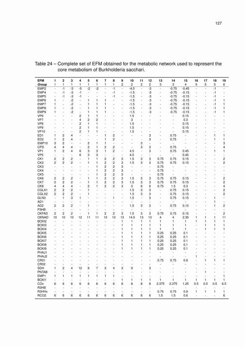
127

Table 24 – Complete set of EFM obtained for the metabolic network used to represent thecore metabolism of Burkholderia sacchari.

EFM 1 2 3 4 5 6 7 8 9 10 11 12 13 14 15 16 17 18 19Group 1 1 1 1 1 1 1 1 2 2 2 2 3 3 4 5 5 5 6EMP2 - -1 -3 -5 -2 -2 - -1 - -4.5 - -3 - -0.75 -0.45 - - -1 -EMP4 - -1 -3 -1 - - - -1 - -1.5 - -3 - -0.75 -0.15 - - -1 -EMP5 - -1 -3 -1 - - - -1 - -1.5 - -3 - -0.75 -0.15 - - -1 -EMP6 1 - -2 - 1 1 1 - - -1.5 - -3 - -0.75 -0.15 - - -1 1EMP7 1 - -2 - 1 1 1 - - -1.5 - -3 - -0.75 -0.15 - - -1 1EMP8 1 - -2 - 1 1 1 - - -1.5 - -3 - -0.75 -0.15 - - -1 1EMP9 1 - -2 - 1 1 1 - - -1.5 - -3 - -0.75 -0.15 - - -1 1VP6 - - - 2 1 1 - - - 1.5 - - - - 0.15 - - - -VP7 - - - 4 2 2 - - - 3 - - - - 0.3 - - - -VP8 - - - 2 1 1 - - - 1.5 - - - - 0.15 - - - -VP9 - - - 2 1 1 - - - 1.5 - - - - 0.15 - - - -VP10 - - - 2 1 1 - - - 1.5 - - - - 0.15 - - - -ED1 1 2 4 - - - 1 2 - - - 3 - 0.75 - - - 1 1ED2 1 2 4 - - - 1 2 - - - 3 - 0.75 - - - 1 1EMP10 3 2 - - 2 1 1 - - - 3 - - - - - - - 3CPD 4 4 4 - 2 1 2 2 - - 3 3 - 0.75 - - - - 4VP1 1 2 4 6 3 3 1 2 - 4.5 - 3 - 0.75 0.45 - - 1 1VP5 - - - 6 3 3 - - - 4.5 - - - - 0.45 - - - -CK1 2 2 2 - 1 1 2 2 3 1.5 3 3 0.75 0.75 0.15 - - - 2CK2 2 2 2 - 1 1 2 2 3 1.5 3 3 0.75 0.75 0.15 - - - 2CK3 - - - - - 1 2 2 3 - - - 0.75 - - - - - -CK4 - - - - - 1 2 2 3 - - - 0.75 - - - - - -CK5 - - - - - 1 2 2 3 - - - 0.75 - - - - - -CK6 2 2 2 - 1 1 2 2 3 1.5 3 3 0.75 0.75 0.15 - - - 2CK7 2 2 2 - 1 1 2 2 3 1.5 3 3 0.75 0.75 0.15 - - - 2CK8 4 4 4 - 2 1 2 2 3 3 6 6 0.75 1.5 0.3 - - - 4CGLX1 2 2 2 - 1 - - - - 1.5 3 3 - 0.75 0.15 - - - 2CGLX2 2 2 2 - 1 - - - - 1.5 3 3 - 0.75 0.15 - - - 2GLN3 - 1 3 1 - - - 1 - 1.5 - 3 - 0.75 0.15 - - 1 -AD1 - - - - - - - - - - - - - - - - - 1 -AD2 2 2 2 - 1 - - - - 1.5 3 3 - 0.75 0.15 - - 1 2P3HB - - - - - - - - - - - - - - - - - - -OXFAD 2 2 2 - 1 1 2 2 3 1.5 3 3 0.75 0.75 0.15 - - - 2OXNAD 10 10 10 12 11 11 10 10 13 14.5 13 13 4 4 2.35 1 1 1 11BOXI2 - - - - - - - - 1 1 1 1 1 1 1 1 1 1 1BOXI3 - - - - - - - - 1 1 1 1 1 1 1 - 1 1 1BOXI4 - - - - - - - - 1 1 1 1 1 1 1 - 1 1 1BOXI5 - - - - - - - - 1 1 1 1 0.25 0.25 0.1 - - - -BOXI6 - - - - - - - - 1 1 1 1 0.25 0.25 0.1 - - - -BOXI7 - - - - - - - - 1 1 1 1 0.25 0.25 0.1 - - - -BOXI8 - - - - - - - - 1 1 1 1 0.25 0.25 0.1 - - - -BOXI9 - - - - - - - - 1 1 1 1 0.25 0.25 0.1 - - - -PHAJ1 - - - - - - - - - - - - - - - - - - -PHAJ2 - - - - - - - - - - - - - - - 1 - - -CR01 - - - - - - - - - - - - 0.75 0.75 0.9 - 1 1 1CR02 - - - - - - - - - - - - - - - - - - -SDH 1 2 4 12 6 7 3 4 3 9 - 3 - - - - - - -PNTAB - - - - - - - - - - - - - - - - 1 - -EMP1 1 1 1 1 1 1 1 1 - - - - - - - - - - 1BOXI1 - - - - - - - - 1 1 1 1 1 1 1 1 1 1 1COx 6 6 6 6 6 6 6 6 8 8 8 8 2.375 2.375 1.25 0.5 0.5 0.5 6.5R3HB - - - - - - - - - - - - - - - - - - -R3HHx - - - - - - - - - - - - 0.75 0.75 0.9 1 1 1 1RCO2 6 6 6 6 6 6 6 6 6 6 6 6 1.5 1.5 0.6 - - - 6

128

Table 24 continued – Complete set of EFM obtained for the metabolic network used torepresent the core metabolism of Burkholderia sacchari.

EFM 20 21 22 23 24 25 26 27 28 29 30 31 32 33 34 35 36 37Group 7 8 9 9 10 11 12 13 14 15 15 16 17 18 18 18 18 18EMP2 -1 - -3 -1 -2 -2 -5 -0.375 -0.5 -0.5 - -2 -2 - -1 - -1 -EMP4 -1 - -3 -1 - - -1 -0.125 -0.167 -0.5 - - - - -1 - -1 -EMP5 -1 - -3 -1 - - -1 -0.125 -0.167 -0.5 - - - - -1 - -1 -EMP6 - 1 -2 - 1 1 - -0.125 -0.167 -0.5 - 1 1 - -1 - -1 -EMP7 - 1 -2 - 1 1 - -0.125 -0.167 -0.5 - 1 1 - -1 - -1 -EMP8 - 1 -2 - 1 1 - -0.125 -0.167 -0.5 - 1 1 - -1 - -1 -EMP9 - 1 -2 - 1 1 - -0.125 -0.167 -0.5 - 1 1 - -1 - -1 -VP6 - - - - 1 1 2 0.125 0.167 - - 1 1 - - - - -VP7 - - - - 2 2 4 0.25 0.333 - - 2 2 - - - - -VP8 - - - - 1 1 2 0.125 0.167 - - 1 1 - - - - -VP9 - - - - 1 1 2 0.125 0.167 - - 1 1 - - - - -VP10 - - - - 1 1 2 0.125 0.167 - - 1 1 - - - - -ED1 2 1 4 2 - - - - - 0.5 - - - - 1 - 1 -ED2 2 1 4 2 - - - - - 0.5 - - - - 1 - 1 -EMP10 2 1 - - 2 1 - - - - - 1 1 - - 1 - 1CPD 4 2 4 2 2 1 - - - 0.5 - 1 1 - 1 1 1 1VP1 2 1 4 2 3 3 6 0.375 0.5 0.5 - 3 3 - 1 - 1 -VP5 - - - - 3 3 6 0.375 0.5 - - 3 3 - - - - -CK1 2 2 2 2 1 1 - 0.125 0.167 0.5 0.5 - - 1 1 1 1 1CK2 2 2 2 2 1 1 - 0.125 0.167 0.5 0.5 - - 1 1 1 1 1CK3 - 2 - 2 - 1 - - - - 0.5 - - 1 - - - -CK4 - 2 - 2 - 1 - - - - 0.5 - - 1 - - - -CK5 - 2 - 2 - 1 - - - - 0.5 - - 1 - - - -CK6 2 2 2 2 1 1 - 0.125 0.167 0.5 0.5 - - 1 1 1 1 1CK7 2 2 2 2 1 1 - 0.125 0.167 0.5 0.5 - - 1 1 1 1 1CK8 4 2 4 2 2 1 - 0.25 0.333 1 0.5 - - 1 2 2 2 2CGLX1 2 - 2 - 1 - - 0.125 0.167 0.5 - - - - 1 1 1 1CGLX2 2 - 2 - 1 - - 0.125 0.167 0.5 - - - - 1 1 1 1GLN3 1 - 3 1 - - 1 0.125 0.167 0.5 - - - - 1 - 1 -AD1 - - - - - - - - - - - - - - - - - -AD2 2 - 2 - 1 - - 0.125 0.167 0.5 - - - - 1 1 1 1P3HB - - - - - - - - - - - 0.5 0.5 - - - - -OXFAD 2 2 2 2 1 1 - 0.125 0.167 0.5 0.5 - - 1 1 1 1 1OXNAD 12 13 14 14 17 18 24 2.375 2.833 3.5 3.5 7.5 13 6 6 6 6 6BOXI2 2 3 4 4 6 7 12 1 1 1 1 - 5.5 1 1 1 1 1BOXI3 2 3 4 4 6 7 12 1 1 1 1 - 5.5 1 1 1 1 1BOXI4 2 3 4 4 6 7 12 1 1 1 1 - 5.5 1 1 1 1 1BOXI5 - - - - - - - 0.25 0.333 0.5 0.5 - - 1 1 1 1 1BOXI6 - - - - - - - 0.25 0.333 0.5 0.5 - - 1 1 1 1 1BOXI7 - - - - - - - - 0.333 - - - - 1 - - 1 1BOXI8 - - - - - - - - 0.333 - - - - 1 - - 1 1BOXI9 - - - - - - - - - - - - - - - - - -PHAJ1 - - - - - - - 0.25 - 0.5 0.5 - - - 1 1 - -PHAJ2 - - - - - - - - - - - - - - - - - -CR01 2 3 4 4 6 7 12 0.75 0.667 0.5 0.5 - 5.5 - - - - -CR02 - - - - - - - - 0.333 - - - - 1 - - 1 1SDH - - - - - - - - - - - 5.5 - - 1 - - -PNTAB - - - - - - - - - - - - - - - - - 1EMP1 1 1 1 1 1 1 1 - - - - 1 1 - - - - -BOXI1 2 3 4 4 6 7 12 1 1 1 1 - 5.5 1 1 1 1 1COx 7 7.5 8 8 9 9.5 12 1.25 1.5 2 2 3.75 6.5 3.5 3.5 3.5 3.5 3.5R3HB - - - - - - - 0.25 0.333 0.5 0.5 0.5 0.5 1 1 1 1 1R3HHx 2 3 4 4 6 7 12 0.75 0.667 0.5 0.5 - 5.5 - - - - -RCO2 6 6 6 6 6 6 6 0.5 0.667 1 1 4 4 2 2 2 2 2

129

Table 24 continued – Complete set of EFM obtained for the metabolic network used torepresent the core metabolism of Burkholderia sacchari.

EFM 38 39 40 41 42 43 44 45 46 47 48 49 50 51 52 53Group 18 18 18 19 18 20 20 21 18 18 22 22 23 23 24 25EMP2 -1.5 -1.5 - - -0.5 -1 - -1 - -1 -0.643 -0.643 - -0.333 -0.214 -0.5EMP4 -0.5 -0.5 - - -0.167 -1 - -1 - -1 -0.214 -0.214 - -0.333 -0.071 -0.5EMP5 -0.5 -0.5 - - -0.167 -1 - -1 - -1 -0.214 -0.214 - -0.333 -0.071 -0.5EMP6 -0.5 -0.5 - 1 -0.167 - 1 - - -1 -0.214 -0.214 - -0.333 -0.071 -0.5EMP7 -0.5 -0.5 - 1 -0.167 - 1 - - -1 -0.214 -0.214 - -0.333 -0.071 -0.5EMP8 -0.5 -0.5 - 1 -0.167 - 1 - - -1 -0.214 -0.214 - -0.333 -0.071 -0.5EMP9 -0.5 -0.5 - 1 -0.167 - 1 - - -1 -0.214 -0.214 - -0.333 -0.071 -0.5VP6 0.5 0.5 - - 0.167 - - - - - 0.214 0.214 - - 0.071 -VP7 1 1 - - 0.333 - - - - - 0.429 0.429 - - 0.143 -VP8 0.5 0.5 - - 0.167 - - - - - 0.214 0.214 - - 0.071 -VP9 0.5 0.5 - - 0.167 - - - - - 0.214 0.214 - - 0.071 -VP10 0.5 0.5 - - 0.167 - - - - - 0.214 0.214 - - 0.071 -ED1 - - - 1 - 2 1 2 - 1 - - - 0.333 - 0.5ED2 - - - 1 - 2 1 2 - 1 - - - 0.333 - 0.5EMP10 - - - 4 0.667 - 1 - - - - - - - - -CPD - - - 5 0.667 2 2 2 - 1 - - - 0.333 - -VP1 1.5 1.5 - 1 0.5 2 1 2 - 1 0.643 0.643 - 0.333 0.214 0.5VP5 1.5 1.5 - - 0.5 - - - - - 0.643 0.643 - - 0.214 -CK1 0.5 0.5 1 3 0.833 - - - 1 1 0.214 0.214 0.333 0.333 0.071 -CK2 0.5 0.5 1 3 0.833 - - - 1 1 0.214 0.214 0.333 0.333 0.071 -CK3 - - 1 - - - - - 1 - - - 0.333 - - -CK4 - - 1 - - - - - 1 - - - 0.333 - - -CK5 - - 1 - - - - - 1 - - - 0.333 - - -CK6 0.5 0.5 1 3 0.833 - - - 1 1 0.214 0.214 0.333 0.333 0.071 -CK7 0.5 0.5 1 3 0.833 - - - 1 1 0.214 0.214 0.333 0.333 0.071 -CK8 1 1 1 6 1.667 - - - 1 2 0.429 0.429 0.333 0.667 0.143 -CGLX1 0.5 0.5 - 3 0.833 - - - - 1 0.214 0.214 - 0.333 0.071 -CGLX2 0.5 0.5 - 3 0.833 - - - - 1 0.214 0.214 - 0.333 0.071 -GLN3 0.5 0.5 - - 0.167 1 - 1 - 1 0.214 0.214 - 0.333 0.071 0.5AD1 - - - - - - - - - - - - - - - 0.5AD2 0.5 0.5 - 3 0.833 - - - - 1 0.214 0.214 - 0.333 0.071 0.5P3HB - - - - - 1 1 1 1 1 1.286 0.286 0.333 0.333 0.429 0.5OXFAD 0.5 0.5 1 3 0.833 - - - 1 1 0.214 0.214 0.333 0.333 0.071 -OXNAD 6.5 6.5 6 16 6.167 3 3 4 6 6 4.214 4.214 3.667 3.667 3.071 2.5BOXI2 1 1 1 1 1 - - 1 1 1 1 1 1 1 1 1BOXI3 1 1 1 1 1 - - 1 1 1 1 1 1 1 1 1BOXI4 1 1 1 1 1 - - 1 1 1 1 1 1 1 1 1BOXI5 1 1 1 1 1 - - - 1 1 1 1 1 1 1 1BOXI6 1 1 1 1 1 - - - 1 1 1 1 1 1 1 1BOXI7 - 1 - 1 1 - - - 1 1 1 1 - - - -BOXI8 - 1 - 1 1 - - - 1 1 1 1 - - - -BOXI9 - - - - - - - - 1 1 1 - - - - -PHAJ1 1 - 1 - - - - - - - - - 1 1 1 1PHAJ2 - - - - - - - - - - - - - - - -CR01 - - - - - - - 1 - - - - - - - -CR02 - 1 - 1 1 - - - - - - 1 - - - -SDH 3 2 1 - - 1 - - - - - - - - - -PNTAB - - - - - - - - - - - - - - - -EMP1 - - - 1 - 1 1 1 - - - - - - - -BOXI1 1 1 1 1 1 - - 1 1 1 1 1 1 1 1 1COx 3.5 3.5 3.5 9.5 3.5 1.5 1.5 2 3.5 3.5 2.214 2.214 2 2 1.571 1.25R3HB 1 1 1 1 1 1 1 1 1 1 1.286 1.286 1.333 1.333 1.429 1.5R3HHx - - - - - - - 1 - - - - - - - -RCO2 2 2 2 8 2 2 2 2 2 2 0.857 0.857 0.667 0.667 0.286 -

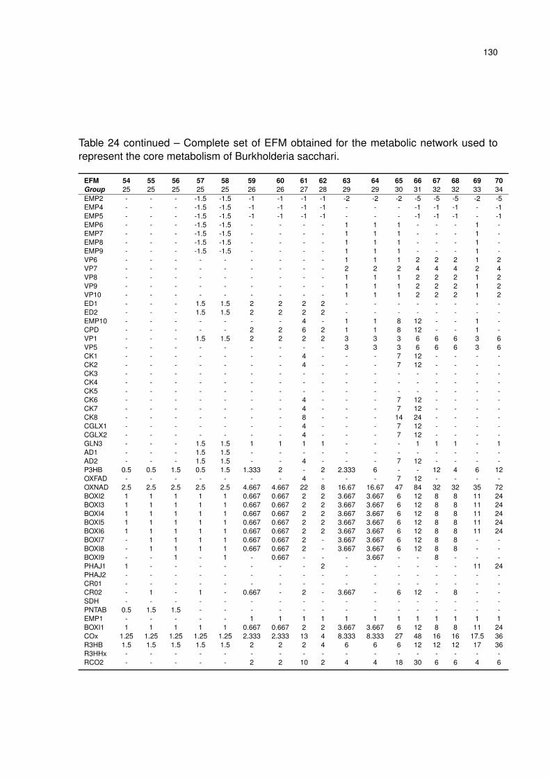
130

Table 24 continued – Complete set of EFM obtained for the metabolic network used torepresent the core metabolism of Burkholderia sacchari.

EFM 54 55 56 57 58 59 60 61 62 63 64 65 66 67 68 69 70Group 25 25 25 25 25 26 26 27 28 29 29 30 31 32 32 33 34EMP2 - - - -1.5 -1.5 -1 -1 -1 -1 -2 -2 -2 -5 -5 -5 -2 -5EMP4 - - - -1.5 -1.5 -1 -1 -1 -1 - - - -1 -1 -1 - -1EMP5 - - - -1.5 -1.5 -1 -1 -1 -1 - - - -1 -1 -1 - -1EMP6 - - - -1.5 -1.5 - - - - 1 1 1 - - - 1 -EMP7 - - - -1.5 -1.5 - - - - 1 1 1 - - - 1 -EMP8 - - - -1.5 -1.5 - - - - 1 1 1 - - - 1 -EMP9 - - - -1.5 -1.5 - - - - 1 1 1 - - - 1 -VP6 - - - - - - - - - 1 1 1 2 2 2 1 2VP7 - - - - - - - - - 2 2 2 4 4 4 2 4VP8 - - - - - - - - - 1 1 1 2 2 2 1 2VP9 - - - - - - - - - 1 1 1 2 2 2 1 2VP10 - - - - - - - - - 1 1 1 2 2 2 1 2ED1 - - - 1.5 1.5 2 2 2 2 - - - - - - - -ED2 - - - 1.5 1.5 2 2 2 2 - - - - - - - -EMP10 - - - - - - - 4 - 1 1 8 12 - - 1 -CPD - - - - - 2 2 6 2 1 1 8 12 - - 1 -VP1 - - - 1.5 1.5 2 2 2 2 3 3 3 6 6 6 3 6VP5 - - - - - - - - - 3 3 3 6 6 6 3 6CK1 - - - - - - - 4 - - - 7 12 - - - -CK2 - - - - - - - 4 - - - 7 12 - - - -CK3 - - - - - - - - - - - - - - - - -CK4 - - - - - - - - - - - - - - - - -CK5 - - - - - - - - - - - - - - - - -CK6 - - - - - - - 4 - - - 7 12 - - - -CK7 - - - - - - - 4 - - - 7 12 - - - -CK8 - - - - - - - 8 - - - 14 24 - - - -CGLX1 - - - - - - - 4 - - - 7 12 - - - -CGLX2 - - - - - - - 4 - - - 7 12 - - - -GLN3 - - - 1.5 1.5 1 1 1 1 - - - 1 1 1 - 1AD1 - - - 1.5 1.5 - - - - - - - - - - - -AD2 - - - 1.5 1.5 - - 4 - - - 7 12 - - - -P3HB 0.5 0.5 1.5 0.5 1.5 1.333 2 - 2 2.333 6 - - 12 4 6 12OXFAD - - - - - - - 4 - - - 7 12 - - - -OXNAD 2.5 2.5 2.5 2.5 2.5 4.667 4.667 22 8 16.67 16.67 47 84 32 32 35 72BOXI2 1 1 1 1 1 0.667 0.667 2 2 3.667 3.667 6 12 8 8 11 24BOXI3 1 1 1 1 1 0.667 0.667 2 2 3.667 3.667 6 12 8 8 11 24BOXI4 1 1 1 1 1 0.667 0.667 2 2 3.667 3.667 6 12 8 8 11 24BOXI5 1 1 1 1 1 0.667 0.667 2 2 3.667 3.667 6 12 8 8 11 24BOXI6 1 1 1 1 1 0.667 0.667 2 2 3.667 3.667 6 12 8 8 11 24BOXI7 - 1 1 1 1 0.667 0.667 2 - 3.667 3.667 6 12 8 8 - -BOXI8 - 1 1 1 1 0.667 0.667 2 - 3.667 3.667 6 12 8 8 - -BOXI9 - - 1 - 1 - 0.667 - - - 3.667 - - 8 - - -PHAJ1 1 - - - - - - - 2 - - - - - - 11 24PHAJ2 - - - - - - - - - - - - - - - - -CR01 - - - - - - - - - - - - - - - - -CR02 - 1 - 1 - 0.667 - 2 - 3.667 - 6 12 - 8 - -SDH - - - - - - - - - - - - - - - - -PNTAB 0.5 1.5 1.5 - - - - - - - - - - - - - -EMP1 - - - - - 1 1 1 1 1 1 1 1 1 1 1 1BOXI1 1 1 1 1 1 0.667 0.667 2 2 3.667 3.667 6 12 8 8 11 24COx 1.25 1.25 1.25 1.25 1.25 2.333 2.333 13 4 8.333 8.333 27 48 16 16 17.5 36R3HB 1.5 1.5 1.5 1.5 1.5 2 2 2 4 6 6 6 12 12 12 17 36R3HHx - - - - - - - - - - - - - - - - -RCO2 - - - - - 2 2 10 2 4 4 18 30 6 6 4 6

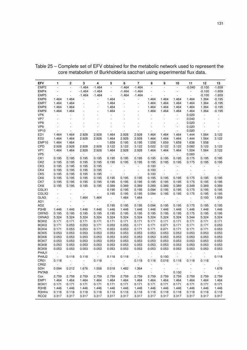
131

Table 25 – Complete set of EFV obtained for the metabolic network used to represent thecore metabolism of Burkholderia sacchari using experimental flux data.

EFV 1 2 3 4 5 6 7 8 9 10 11 12 13EMP2 - - -1.464 -1.464 - -1.464 -1.464 - - - -0.040 -0.100 -1.659EMP4 - - -1.464 -1.464 - -1.464 -1.464 - - - - -0.100 -1.659EMP5 - - -1.464 -1.464 - -1.464 -1.464 - - - - -0.100 -1.659EMP6 1.464 1.464 - - 1.464 - - 1.464 1.464 1.464 1.464 1.364 -0.195EMP7 1.464 1.464 - - 1.464 - - 1.464 1.464 1.464 1.464 1.364 -0.195EMP8 1.464 1.464 - - 1.464 - - 1.464 1.464 1.464 1.464 1.364 -0.195EMP9 1.464 1.464 - - 1.464 - - 1.464 1.464 1.464 1.464 1.364 -0.195VP6 - - - - - - - - - - 0.020 - -VP7 - - - - - - - - - - 0.040 - -VP8 - - - - - - - - - - 0.020 - -VP9 - - - - - - - - - - 0.020 - -VP10 - - - - - - - - - - 0.020 - -ED1 1.464 1.464 2.928 2.928 1.464 2.928 2.928 1.464 1.464 1.464 1.444 1.564 3.122ED2 1.464 1.464 2.928 2.928 1.464 2.928 2.928 1.464 1.464 1.464 1.444 1.564 3.122EMP10 1.464 1.464 - - 1.659 0.195 0.195 1.558 1.659 1.659 1.638 1.558 -CPD 2.928 2.928 2.928 2.928 3.122 3.122 3.122 3.022 3.122 3.122 3.082 3.122 3.122VP1 1.464 1.464 2.928 2.928 1.464 2.928 2.928 1.464 1.464 1.464 1.504 1.564 3.122VP5 - - - - - - - - - - 0.060 - -CK1 0.195 0.195 0.195 0.195 0.195 0.195 0.195 0.195 0.195 0.195 0.175 0.195 0.195CK2 0.195 0.195 0.195 0.195 0.195 0.195 0.195 0.195 0.195 0.195 0.175 0.195 0.195CK3 0.195 0.195 0.195 0.195 - - - 0.100 - - - - -CK4 0.195 0.195 0.195 0.195 - - - 0.100 - - - - -CK5 0.195 0.195 0.195 0.195 - - - 0.100 - - - - -CK6 0.195 0.195 0.195 0.195 0.195 0.195 0.195 0.195 0.195 0.195 0.175 0.195 0.195CK7 0.195 0.195 0.195 0.195 0.195 0.195 0.195 0.195 0.195 0.195 0.175 0.195 0.195CK8 0.195 0.195 0.195 0.195 0.389 0.389 0.389 0.289 0.389 0.389 0.349 0.389 0.389CGLX1 - - - - 0.195 0.195 0.195 0.094 0.195 0.195 0.175 0.195 0.195CGLX2 - - - - 0.195 0.195 0.195 0.094 0.195 0.195 0.175 0.195 0.195GLN3 - - 1.464 1.464 - 1.464 1.464 - - - - 0.100 1.659AD1 - - - - - - - - - - - - -AD2 - - - - 0.195 0.195 0.195 0.094 0.195 0.195 0.175 0.195 0.195P3HB 1.446 1.446 1.446 1.446 1.446 1.446 1.446 1.446 1.446 1.446 1.446 1.446 1.446OXFAD 0.195 0.195 0.195 0.195 0.195 0.195 0.195 0.195 0.195 0.195 0.175 0.195 0.195OXNAD 5.324 5.324 5.324 5.324 5.324 5.324 5.324 5.324 5.324 5.324 5.344 5.324 5.324BOXI2 0.171 0.171 0.171 0.171 0.171 0.171 0.171 0.171 0.171 0.171 0.171 0.171 0.171BOXI3 0.171 0.053 0.053 0.171 0.053 0.053 0.171 0.171 0.071 0.171 0.171 0.171 0.053BOXI4 0.171 0.053 0.053 0.171 0.053 0.053 0.171 0.171 0.071 0.171 0.171 0.171 0.053BOXI5 0.053 0.053 0.053 0.053 0.053 0.053 0.053 0.053 0.053 0.053 0.053 0.053 0.053BOXI6 0.053 0.053 0.053 0.053 0.053 0.053 0.053 0.053 0.053 0.053 0.053 0.053 0.053BOXI7 0.053 0.053 0.053 0.053 0.053 0.053 0.053 0.053 0.053 0.053 0.053 0.053 0.053BOXI8 0.053 0.053 0.053 0.053 0.053 0.053 0.053 0.053 0.053 0.053 0.053 0.053 0.053BOXI9 0.053 0.053 0.053 0.053 0.053 0.053 0.053 0.053 0.053 0.053 0.053 0.053 0.053PHAJ1 - - - - - - - - - - - - -PHAJ2 - 0.118 0.118 - 0.118 0.118 - - 0.100 - - - 0.118CR01 0.118 - - 0.118 - - 0.118 0.118 0.018 0.118 0.118 0.118 -CR02 - - - - - - - - - - - - -SDH 0.094 0.212 1.676 1.558 0.018 1.482 1.364 - - - - - 1.676PNTAB - - - - - - - - - 0.100 - - -Cox 2.759 2.759 2.759 2.759 2.759 2.759 2.759 2.759 2.759 2.759 2.759 2.759 2.759EMP1 1.464 1.464 1.464 1.464 1.464 1.464 1.464 1.464 1.464 1.464 1.464 1.464 1.464BOXI1 0.171 0.171 0.171 0.171 0.171 0.171 0.171 0.171 0.171 0.171 0.171 0.171 0.171R3HB 1.446 1.446 1.446 1.446 1.446 1.446 1.446 1.446 1.446 1.446 1.446 1.446 1.446R3HHx 0.118 0.118 0.118 0.118 0.118 0.118 0.118 0.118 0.118 0.118 0.118 0.118 0.118RCO2 3.317 3.317 3.317 3.317 3.317 3.317 3.317 3.317 3.317 3.317 3.317 3.317 3.317

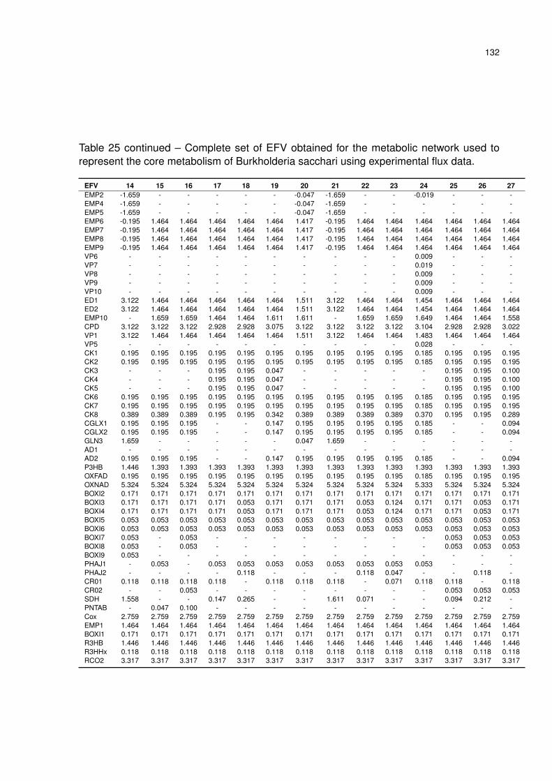
132

Table 25 continued – Complete set of EFV obtained for the metabolic network used torepresent the core metabolism of Burkholderia sacchari using experimental flux data.

EFV 14 15 16 17 18 19 20 21 22 23 24 25 26 27EMP2 -1.659 - - - - - -0.047 -1.659 - - -0.019 - - -EMP4 -1.659 - - - - - -0.047 -1.659 - - - - - -EMP5 -1.659 - - - - - -0.047 -1.659 - - - - - -EMP6 -0.195 1.464 1.464 1.464 1.464 1.464 1.417 -0.195 1.464 1.464 1.464 1.464 1.464 1.464EMP7 -0.195 1.464 1.464 1.464 1.464 1.464 1.417 -0.195 1.464 1.464 1.464 1.464 1.464 1.464EMP8 -0.195 1.464 1.464 1.464 1.464 1.464 1.417 -0.195 1.464 1.464 1.464 1.464 1.464 1.464EMP9 -0.195 1.464 1.464 1.464 1.464 1.464 1.417 -0.195 1.464 1.464 1.464 1.464 1.464 1.464VP6 - - - - - - - - - - 0.009 - - -VP7 - - - - - - - - - - 0.019 - - -VP8 - - - - - - - - - - 0.009 - - -VP9 - - - - - - - - - - 0.009 - - -VP10 - - - - - - - - - - 0.009 - - -ED1 3.122 1.464 1.464 1.464 1.464 1.464 1.511 3.122 1.464 1.464 1.454 1.464 1.464 1.464ED2 3.122 1.464 1.464 1.464 1.464 1.464 1.511 3.122 1.464 1.464 1.454 1.464 1.464 1.464EMP10 - 1.659 1.659 1.464 1.464 1.611 1.611 - 1.659 1.659 1.649 1.464 1.464 1.558CPD 3.122 3.122 3.122 2.928 2.928 3.075 3.122 3.122 3.122 3.122 3.104 2.928 2.928 3.022VP1 3.122 1.464 1.464 1.464 1.464 1.464 1.511 3.122 1.464 1.464 1.483 1.464 1.464 1.464VP5 - - - - - - - - - - 0.028 - - -CK1 0.195 0.195 0.195 0.195 0.195 0.195 0.195 0.195 0.195 0.195 0.185 0.195 0.195 0.195CK2 0.195 0.195 0.195 0.195 0.195 0.195 0.195 0.195 0.195 0.195 0.185 0.195 0.195 0.195CK3 - - - 0.195 0.195 0.047 - - - - - 0.195 0.195 0.100CK4 - - - 0.195 0.195 0.047 - - - - - 0.195 0.195 0.100CK5 - - - 0.195 0.195 0.047 - - - - - 0.195 0.195 0.100CK6 0.195 0.195 0.195 0.195 0.195 0.195 0.195 0.195 0.195 0.195 0.185 0.195 0.195 0.195CK7 0.195 0.195 0.195 0.195 0.195 0.195 0.195 0.195 0.195 0.195 0.185 0.195 0.195 0.195CK8 0.389 0.389 0.389 0.195 0.195 0.342 0.389 0.389 0.389 0.389 0.370 0.195 0.195 0.289CGLX1 0.195 0.195 0.195 - - 0.147 0.195 0.195 0.195 0.195 0.185 - - 0.094CGLX2 0.195 0.195 0.195 - - 0.147 0.195 0.195 0.195 0.195 0.185 - - 0.094GLN3 1.659 - - - - - 0.047 1.659 - - - - - -AD1 - - - - - - - - - - - - - -AD2 0.195 0.195 0.195 - - 0.147 0.195 0.195 0.195 0.195 0.185 - - 0.094P3HB 1.446 1.393 1.393 1.393 1.393 1.393 1.393 1.393 1.393 1.393 1.393 1.393 1.393 1.393OXFAD 0.195 0.195 0.195 0.195 0.195 0.195 0.195 0.195 0.195 0.195 0.185 0.195 0.195 0.195OXNAD 5.324 5.324 5.324 5.324 5.324 5.324 5.324 5.324 5.324 5.324 5.333 5.324 5.324 5.324BOXI2 0.171 0.171 0.171 0.171 0.171 0.171 0.171 0.171 0.171 0.171 0.171 0.171 0.171 0.171BOXI3 0.171 0.171 0.171 0.171 0.053 0.171 0.171 0.171 0.053 0.124 0.171 0.171 0.053 0.171BOXI4 0.171 0.171 0.171 0.171 0.053 0.171 0.171 0.171 0.053 0.124 0.171 0.171 0.053 0.171BOXI5 0.053 0.053 0.053 0.053 0.053 0.053 0.053 0.053 0.053 0.053 0.053 0.053 0.053 0.053BOXI6 0.053 0.053 0.053 0.053 0.053 0.053 0.053 0.053 0.053 0.053 0.053 0.053 0.053 0.053BOXI7 0.053 - 0.053 - - - - - - - - 0.053 0.053 0.053BOXI8 0.053 - 0.053 - - - - - - - - 0.053 0.053 0.053BOXI9 0.053 - - - - - - - - - - - - -PHAJ1 - 0.053 - 0.053 0.053 0.053 0.053 0.053 0.053 0.053 0.053 - - -PHAJ2 - - - - 0.118 - - - 0.118 0.047 - - 0.118 -CR01 0.118 0.118 0.118 0.118 - 0.118 0.118 0.118 - 0.071 0.118 0.118 - 0.118CR02 - - 0.053 - - - - - - - - 0.053 0.053 0.053SDH 1.558 - - 0.147 0.265 - - 1.611 0.071 - - 0.094 0.212 -PNTAB - 0.047 0.100 - - - - - - - - - - -Cox 2.759 2.759 2.759 2.759 2.759 2.759 2.759 2.759 2.759 2.759 2.759 2.759 2.759 2.759EMP1 1.464 1.464 1.464 1.464 1.464 1.464 1.464 1.464 1.464 1.464 1.464 1.464 1.464 1.464BOXI1 0.171 0.171 0.171 0.171 0.171 0.171 0.171 0.171 0.171 0.171 0.171 0.171 0.171 0.171R3HB 1.446 1.446 1.446 1.446 1.446 1.446 1.446 1.446 1.446 1.446 1.446 1.446 1.446 1.446R3HHx 0.118 0.118 0.118 0.118 0.118 0.118 0.118 0.118 0.118 0.118 0.118 0.118 0.118 0.118RCO2 3.317 3.317 3.317 3.317 3.317 3.317 3.317 3.317 3.317 3.317 3.317 3.317 3.317 3.317

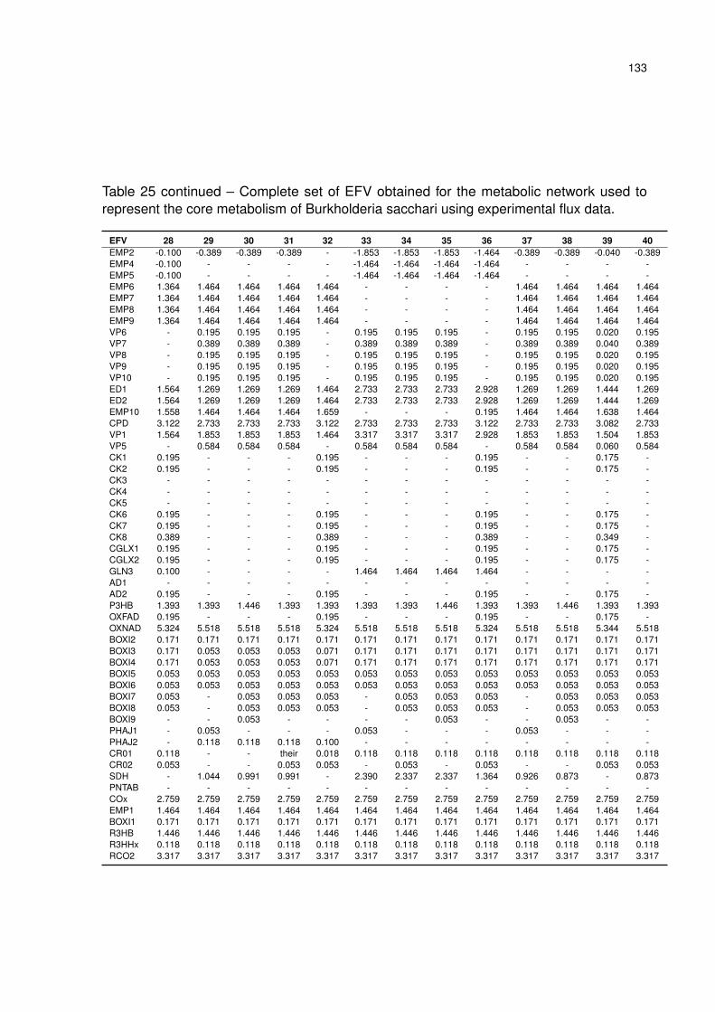
133

Table 25 continued – Complete set of EFV obtained for the metabolic network used torepresent the core metabolism of Burkholderia sacchari using experimental flux data.

EFV 28 29 30 31 32 33 34 35 36 37 38 39 40EMP2 -0.100 -0.389 -0.389 -0.389 - -1.853 -1.853 -1.853 -1.464 -0.389 -0.389 -0.040 -0.389EMP4 -0.100 - - - - -1.464 -1.464 -1.464 -1.464 - - - -EMP5 -0.100 - - - - -1.464 -1.464 -1.464 -1.464 - - - -EMP6 1.364 1.464 1.464 1.464 1.464 - - - - 1.464 1.464 1.464 1.464EMP7 1.364 1.464 1.464 1.464 1.464 - - - - 1.464 1.464 1.464 1.464EMP8 1.364 1.464 1.464 1.464 1.464 - - - - 1.464 1.464 1.464 1.464EMP9 1.364 1.464 1.464 1.464 1.464 - - - - 1.464 1.464 1.464 1.464VP6 - 0.195 0.195 0.195 - 0.195 0.195 0.195 - 0.195 0.195 0.020 0.195VP7 - 0.389 0.389 0.389 - 0.389 0.389 0.389 - 0.389 0.389 0.040 0.389VP8 - 0.195 0.195 0.195 - 0.195 0.195 0.195 - 0.195 0.195 0.020 0.195VP9 - 0.195 0.195 0.195 - 0.195 0.195 0.195 - 0.195 0.195 0.020 0.195VP10 - 0.195 0.195 0.195 - 0.195 0.195 0.195 - 0.195 0.195 0.020 0.195ED1 1.564 1.269 1.269 1.269 1.464 2.733 2.733 2.733 2.928 1.269 1.269 1.444 1.269ED2 1.564 1.269 1.269 1.269 1.464 2.733 2.733 2.733 2.928 1.269 1.269 1.444 1.269EMP10 1.558 1.464 1.464 1.464 1.659 - - - 0.195 1.464 1.464 1.638 1.464CPD 3.122 2.733 2.733 2.733 3.122 2.733 2.733 2.733 3.122 2.733 2.733 3.082 2.733VP1 1.564 1.853 1.853 1.853 1.464 3.317 3.317 3.317 2.928 1.853 1.853 1.504 1.853VP5 - 0.584 0.584 0.584 - 0.584 0.584 0.584 - 0.584 0.584 0.060 0.584CK1 0.195 - - - 0.195 - - - 0.195 - - 0.175 -CK2 0.195 - - - 0.195 - - - 0.195 - - 0.175 -CK3 - - - - - - - - - - - - -CK4 - - - - - - - - - - - - -CK5 - - - - - - - - - - - - -CK6 0.195 - - - 0.195 - - - 0.195 - - 0.175 -CK7 0.195 - - - 0.195 - - - 0.195 - - 0.175 -CK8 0.389 - - - 0.389 - - - 0.389 - - 0.349 -CGLX1 0.195 - - - 0.195 - - - 0.195 - - 0.175 -CGLX2 0.195 - - - 0.195 - - - 0.195 - - 0.175 -GLN3 0.100 - - - - 1.464 1.464 1.464 1.464 - - - -AD1 - - - - - - - - - - - - -AD2 0.195 - - - 0.195 - - - 0.195 - - 0.175 -P3HB 1.393 1.393 1.446 1.393 1.393 1.393 1.393 1.446 1.393 1.393 1.446 1.393 1.393OXFAD 0.195 - - - 0.195 - - - 0.195 - - 0.175 -OXNAD 5.324 5.518 5.518 5.518 5.324 5.518 5.518 5.518 5.324 5.518 5.518 5.344 5.518BOXI2 0.171 0.171 0.171 0.171 0.171 0.171 0.171 0.171 0.171 0.171 0.171 0.171 0.171BOXI3 0.171 0.053 0.053 0.053 0.071 0.171 0.171 0.171 0.171 0.171 0.171 0.171 0.171BOXI4 0.171 0.053 0.053 0.053 0.071 0.171 0.171 0.171 0.171 0.171 0.171 0.171 0.171BOXI5 0.053 0.053 0.053 0.053 0.053 0.053 0.053 0.053 0.053 0.053 0.053 0.053 0.053BOXI6 0.053 0.053 0.053 0.053 0.053 0.053 0.053 0.053 0.053 0.053 0.053 0.053 0.053BOXI7 0.053 - 0.053 0.053 0.053 - 0.053 0.053 0.053 - 0.053 0.053 0.053BOXI8 0.053 - 0.053 0.053 0.053 - 0.053 0.053 0.053 - 0.053 0.053 0.053BOXI9 - - 0.053 - - - - 0.053 - - 0.053 - -PHAJ1 - 0.053 - - - 0.053 - - - 0.053 - - -PHAJ2 - 0.118 0.118 0.118 0.100 - - - - - - - -CR01 0.118 - - their 0.018 0.118 0.118 0.118 0.118 0.118 0.118 0.118 0.118CR02 0.053 - - 0.053 0.053 - 0.053 - 0.053 - - 0.053 0.053SDH - 1.044 0.991 0.991 - 2.390 2.337 2.337 1.364 0.926 0.873 - 0.873PNTAB - - - - - - - - - - - - -COx 2.759 2.759 2.759 2.759 2.759 2.759 2.759 2.759 2.759 2.759 2.759 2.759 2.759EMP1 1.464 1.464 1.464 1.464 1.464 1.464 1.464 1.464 1.464 1.464 1.464 1.464 1.464BOXI1 0.171 0.171 0.171 0.171 0.171 0.171 0.171 0.171 0.171 0.171 0.171 0.171 0.171R3HB 1.446 1.446 1.446 1.446 1.446 1.446 1.446 1.446 1.446 1.446 1.446 1.446 1.446R3HHx 0.118 0.118 0.118 0.118 0.118 0.118 0.118 0.118 0.118 0.118 0.118 0.118 0.118RCO2 3.317 3.317 3.317 3.317 3.317 3.317 3.317 3.317 3.317 3.317 3.317 3.317 3.317