2013 Editors: Patrizia Tenerelli and Helen Crowley Reviewers: Amir M. Kaynia Publishing Editors: Fabio Taucer and Ufuk Hancilar SYNER-G Reference Report 3 Development of inventory datasets through remote sensing and direct observation data for earthquake loss estimation Report EUR 25890 EN

Welcome message from author
This document is posted to help you gain knowledge. Please leave a comment to let me know what you think about it! Share it to your friends and learn new things together.
Transcript
2 0 1 3
Editors: Patrizia Tenerelli and Helen Crowley Reviewers: Amir M. Kaynia
Publishing Editors: Fabio Taucer and Ufuk Hancilar
SYNER-G Reference Report 3
Development of inventory datasets
through remote sensing and direct
observation data for earthquake loss
estimation
Report EUR 25890 EN

European Commission
Joint Research Centre
Institute for the Protection and Security of the Citizen
Contact information
Fabio Taucer
Address: Joint Research Centre, Via Enrico Fermi 2749, TP 480, 21027 Ispra (VA), Italy
E-mail: [email protected]
Tel.: +39 0332 78 5886
Fax: +39 0332 78 9049
http://elsa.jrc.ec.europa.eu/
http://www.jrc.ec.europa.eu/
This publication is a Reference Report by the Joint Research Centre of the European Commission.
Legal Notice
Neither the European Commission nor any person acting on behalf of the Commission
is responsible for the use which might be made of this publication.
Europe Direct is a service to help you find answers to your questions about the European Union
Freephone number (*): 00 800 6 7 8 9 10 11
(*) Certain mobile telephone operators do not allow access to 00 800 numbers or these calls may be billed.
A great deal of additional information on the European Union is available on the Internet.
It can be accessed through the Europa server http://europa.eu/.
JRC80662
EUR 25890 EN
ISBN 978-92-79-29017-6
ISSN 1831-9424
doi:10.2788/86322
Luxembourg: Publications Office of the European Union, 2013
© European Union, 2013
Reproduction is authorised provided the source is acknowledged.
Printed in Ispra (Va) - Italy
D 8.9
DELIVERABLE
PROJECT INFORMATION
Project Title: Systemic Seismic Vulnerability and Risk Analysis for
Buildings, Lifeline Networks and Infrastructures Safety Gain
Acronym: SYNER-G
Project N°: 244061
Call N°: FP7-ENV-2009-1
Project start: 01 November 2009
Duration: 36 months
DELIVERABLE INFORMATION
Deliverable Title:
D8.9 - Development of inventory datasets through remote
sensing and direct observation data for earthquake loss
estimation
Date of issue: 31 March 2013
Work Package: WP8 – Guidelines, recommendations and dissemination
Deliverable/Task Leader: Joint Research Centre
Editors: Patrizia Tenerelli (JRC) and Helen Crowley (UPAV)
Reviewer: Amir M. Kaynia (NGI)
REVISION: Final
Project Coordinator:
Institution:
e-mail:
fax:
telephone:
Prof. Kyriazis Pitilakis
Aristotle University of Thessaloniki
+ 30 2310 995619
+ 30 2310 995693

The SYNER-G Consortium
Aristotle University of Thessaloniki (Co-ordinator) (AUTH)
Vienna Consulting Engineers (VCE)
Bureau de Recherches Geologiques et Minieres (BRGM)
European Commission – Joint Research Centre (JRC)
Norwegian Geotechnical Institute (NGI)
University of Pavia (UPAV)
University of Roma “La Sapienza” (UROMA)
Middle East Technical University (METU)
Analysis and Monitoring of Environmental Risks (AMRA)
University of Karlsruhe (KIT-U)
University of Patras (UPAT)
Willis Group Holdings (WILLIS)
Mid-America Earthquake Center, University of Illinois (UILLINOIS)
Kobe University (UKOBE)
i
Foreword
SYNER-G is a European collaborative research project funded by European Commission
(Seventh Framework Program, Theme 6: Environment) under Grant Agreement no. 244061.
The primary purpose of SYNER-G is to develop an integrated methodology for the systemic
seismic vulnerability and risk analysis of buildings, transportation and utility networks and
critical facilities, considering for the interactions between different components and systems.
The whole methodology is implemented in an open source software tool and is validated in
selected case studies. The research consortium relies on the active participation of twelve
entities from Europe, one from USA and one from Japan. The consortium includes partners
from the consulting and the insurance industry.
SYNER-G developed an innovative methodological framework for the assessment of
physical as well as socio-economic seismic vulnerability and risk at the urban/regional level.
The built environment is modelled according to a detailed taxonomy, grouped into the
following categories: buildings, transportation and utility networks, and critical facilities. Each
category may have several types of components and systems. The framework encompasses
in an integrated fashion all aspects in the chain, from hazard to the vulnerability assessment
of components and systems and to the socio-economic impacts of an earthquake,
accounting for all relevant uncertainties within an efficient quantitative simulation scheme,
and modelling interactions between the multiple component systems.
The methodology and software tools are validated in selected sites and systems in urban
and regional scale: city of Thessaloniki (Greece), city of Vienna (Austria), harbour of
Thessaloniki, gas system of L’Aquila in Italy, electric power network, roadway network and
hospital facility again in Italy.
The scope of the present series of Reference Reports is to document the methods,
procedures, tools and applications that have been developed in SYNER-G. The reports are
intended to researchers, professionals, stakeholders as well as representatives from civil
protection, insurance and industry areas involved in seismic risk assessment and
management.
Prof. Kyriazis Pitilakis
Aristotle University of Thessaloniki, Greece
Project Coordinator of SYNER-G
Fabio Taucer and Ufuk Hancilar
Joint Research Centre
Publishing Editors of the SYNER-G Reference Reports

iii
Abstract
This report summarizes the lessons learnt in extracting exposure information for the three
study sites, Thessaloniki, Vienna and Messina that were addressed in SYNER-G. Fine scale
information on exposed elements that for SYNER-G include buildings, civil engineering
works and population, is one of the variables used to quantify risk. Collecting data and
creating exposure inventories is a very time-demanding job and all possible data-gathering
techniques should be used to address the data shortcoming problem. This report focuses on
combining direct observation and remote sensing data for the development of exposure
models for seismic risk assessment. In this report a summary of the methods for collecting,
processing and archiving inventory datasets is provided in Chapter 2. Chapter 3 deals with
the integration of different data sources for optimum inventory datasets, whilst Chapters 4, 5
and 6 provide some case studies where combinations between direct observation and
remote sensing have been used. The cities of Vienna (Austria), Thessaloniki (Greece) and
Messina (Italy) have been chosen to test the proposed approaches.
Keywords: inventory data, remote sensing, direct observation, census, risk assessment


v
Acknowledgments
The research leading to these results has received funding from the European Community's
Seventh Framework Programme [FP7/2007-2013] under grant agreement n° 244061

vii
Deliverable Contributors
Joint Research Centre (JRC) Patrizia Tenerelli Sections 2.1.1, 2.1.2, 2.1.3,
2.1.4, 2.1.5, 2.1.6, 2.1.7,
2.1.8, 2.2.1, 2.3, 5.2, 7
Ufuk Hancilar
Fabio Taucer
Daniele Ehrlich
University of Pavia (UPAV) Diego Polli Sections 1, 2.1.9, 4.2, 6, 7
Fabio Dell’Acqua
Gianni Lisini
Helen Crowley
Miriam Colombi
Aristotle University of
Thessaloniki (AUTH)
Sotiris Argyroudis
Kalliopi Kakderi
Section 5.1
Bureau de Recherches
Geologiques et Minieres
(BRGM)
Daniel Raucoules
Pierre Gehl
Section 2.2.2
Vienna Consulting Engineers
(VCE)
Helmut Wenzel
David Schäfer
Section 4.1

ix
Table of Contents
Foreword .................................................................................................................................... i
Abstract .................................................................................................................................... iii
Acknowledgments .................................................................................................................... v
Deliverable Contributors ........................................................................................................ vii
Table of Contents ..................................................................................................................... ix
List of Figures .......................................................................................................................... xi
List of Tables .......................................................................................................................... xiii
1 Introduction ....................................................................................................................... 1
2 Summary of methods for collecting, processing and archiving inventory datasets ... 3
2.1 REMOTE SENSING ................................................................................................... 3
2.1.1 Very High Resolution optical........................................................................... 5
2.1.2 Stereo High and Very High Resolution (i.e. aerial, satellite) ............................ 6
2.1.3 Hyperspectral ................................................................................................. 6
2.1.4 High Resolution optical ................................................................................... 7
2.1.5 Medium Resolution optical ............................................................................. 7
2.1.6 Low Resolution optical .................................................................................... 8
2.1.7 Oblique Aerial Imagery ................................................................................... 8
2.1.8 LIDAR ............................................................................................................ 8
2.1.9 RADAR .......................................................................................................... 8
2.2 CENSUS DATA .......................................................................................................... 9
2.2.1 Demographic data ........................................................................................ 10
2.2.2 Housing census data .................................................................................... 11
2.3 GROUND SURVEYS AND FIELD DATA.................................................................. 13
2.3.1 Paper forms .................................................................................................. 13
2.3.2 Hand-held equipment ................................................................................... 16
2.3.3 Digital cameras............................................................................................. 17
2.3.4 GPS receivers .............................................................................................. 17
2.3.5 Palm tops ..................................................................................................... 18
3 Integration of data sources for optimum inventory datasets ...................................... 19
3.1 INTEGRATION OF DATA EXTRACTED FROM REMOTE SENSING IN A GIS
ENVIRONMENT ....................................................................................................... 19
x
3.1.1 Built-up spatial metrics ................................................................................. 19
3.2 METHODS FOR COMBINING REMOTE SENSING, CENSUS AND FIELD DATA .. 19
3.2.1 GIS modelling for population downscaling .................................................... 20
3.2.2 Contribution of remote sensing in population downscaling models ............... 20
4 Case Study: Vienna ........................................................................................................ 23
4.1 DATABASE OF VIENNA CITY ................................................................................. 23
4.1.1 Building identification procedure (BIP) .......................................................... 24
4.2 REMOTE SENSING DATA....................................................................................... 27
4.2.1 Building and road parameters extraction ...................................................... 27
4.2.2 Building vulnerability assessment ................................................................. 28
4.3 COMBINING REMOTE SENSING AND POPULATION CENSUS DATA ................. 31
4.3.1 Sampling of population density classes ........................................................ 33
4.3.2 Fixed ratio method ........................................................................................ 34
4.3.3 Limiting variable method ............................................................................... 35
4.3.4 Selection and application of the model ......................................................... 35
4.3.5 Results ......................................................................................................... 36
5 Case Study: Thessaloniki ............................................................................................... 37
5.1 DATABASE OF THESSALONIKI CITY .................................................................... 37
5.1.1 Buildings....................................................................................................... 37
5.1.2 Roadway bridges .......................................................................................... 38
5.2 REMOTE SENSING DATA....................................................................................... 41
5.2.1 Building count ............................................................................................... 42
5.2.2 Building area extraction ................................................................................ 43
5.2.3 Building height extraction ............................................................................. 45
5.3 GEOMETRIC ATTRIBUTES AND SPATIAL METRICS ............................................ 47
6 Case Study: Messina ...................................................................................................... 51
7 Closing Remarks ............................................................................................................. 53
References .............................................................................................................................. 55
xi
List of Figures
Fig. 2.1 Extraction of a road network with rapid mapping procedure from SAR data ............. 9
Fig. 2.2 Population density grid of EU-27+ for the city of Thessaloniki ................................ 11
Fig. 2.3 AeDES survey form (Baggio et al. 2007) ................................................................ 15
Fig. 2.4 Data collection forms by FEMA 154 (FEMA, 2002)................................................. 16
Fig. 2.5 A Windows Mobile Smartphone and a Bluetooth GPS device, and screen shots of
the installed ROVER software for data collection ............................................. 18
Fig. 4.1 Study area of Vienna city: the 20th district ............................................................... 23
Fig. 4.2 Example of building database in Vienna ................................................................. 24
Fig. 4.3 Example of bridge database in Vienna .................................................................. 24
Fig. 4.4 Data collection form for buildings in Vienna city ..................................................... 26
Fig. 4.5 Radar data of the Vienna study area ...................................................................... 27
Fig. 4.6 Shape file layer of the building stock in the study area of Vienna ........................... 28
Fig. 4.7 Road network extraction in Vienna ......................................................................... 28
Fig. 4.8 a) The optical image from Google Earth; b) The SAR image of the selected building;
c) Segments extracted from North-West façade; d) Segments extracted from
North façade .................................................................................................... 29
Fig. 4.9 Example of vulnerability study: the building under study marked by green rectangle
(left) and its fragility curves (right) .................................................................... 30
Fig. 4.10 Example of building vulnerability mapping for the Vienna case study. Each colour
corresponds to different levels of estimated vulnerabilities ............................... 31
Fig. 4.11 Population census data for the Large Urban Zone of Vienna: local population
census (left side), country level population census (right side) ......................... 32
Fig. 4.12 Population zones for the study area in Vienna ...................................................... 33
Fig. 4.13 Disaggregated population density map for the Vienna Large Urban Zone ............ 36
Fig. 5.1 Study area of Thessaloniki including the “block-by-block” analyses of 1984-86 and
2003................................................................................................................. 38
Fig. 5.2 Roadway bridges of Thessaloniki ........................................................................... 39
Fig. 5.3 Inventory sheet used for the collection of data for roadway bridges in Thessaloniki 40
Fig. 5.4 VHR multispectral image of Thessaloniki city and its hinterland from GeoEye. The
panchromatic band was used to enhance the spatial resolution of the multi-
spectral bands using the Gran Smith pan-sharpening technique. ..................... 41
Fig. 5.5 Snapshots from the GeoEye image on the central area of the city. The red spots
represent the photo-interpreted building centroids ........................................... 43
xii
Fig. 5.6 Building count map showing the estimated number of buildings in the study area of
Thessaloniki ..................................................................................................... 43
Fig. 5.7 Map showing the identified built-up areas in Thessaloniki ...................................... 44
Fig. 5.8 Map showing the estimated number of storeys in the study area of Thessaloniki ... 46
Fig. 5.9 Map showing the Building SHAPE index in the study area of Thessaloniki ............. 48
Fig. 5.10 Map showing the NEAR index for Building to Building proximity analysis in the
study area of Thessaloniki ............................................................................... 48
Fig. 5.11 Map showing the NEAR index for Building to Main Road proximity analysis in the
study area of Thessaloniki ............................................................................... 49
Fig. 5.12 Map showing NEAR index for Building to Transportation Network proximity analysis
in the study area of Thessalonik ....................................................................... 49
Fig. 6.1 Optical (left) and radar (right) data of the case study area ...................................... 51
Fig. 6.2 An example of vulnerability study: The building under study (left), and its
vulnerability curves (right) ................................................................................ 52
Fig. 6.3 Example of vulnerability map for Messina .............................................................. 52
xiii
List of Tables
Table 2.1 Remote sensing data types and detectable physical parameters for each typical
European element at risk ................................................................................... 4
Table 4.1 SAR Data Features ............................................................................................. 27
Table 4.2 Population density values for each urban land use class and each stratum......... 34
Table 4.3 Statistic indicators for each model output comparison with the reference population
data.................................................................................................................. 35
Table 5.1 Building area confusion matrix parameters .......................................................... 44
Table 5.2 Regression statistics on the estimated number of storeys ................................... 46

Introduction
1
1 Introduction
Seismic disaster risk modelling requires exposure information that in SYNER-G includes the
building stock, civil engineering works and population. Exposure information is rarely readily
available with the characteristics required for risk modelling. Where data is available, its
format, resolution and level of information are often not standardized. Furthermore, a
considerable amount of fine detailed data – typically available with local authorities - are not
accessible due to confidentiality issues.
Collecting data and creating exposure inventories is a time-consuming and expensive
activity. Different techniques should thus be used and combined to address the data
shortcoming. Depending on a number of factors such as the necessary temporal and spatial
resolution, different remote sensing systems can be used to collect images and data, and
different methodologies can then be implemented to manage and post-process them to
develop the required inventory. Census and street survey data can be used to support and
further classify data collected by remote sensing. This is of particular importance for seismic
risk assessment, where a number of structural characteristics are not visible from remotely
sensed images.
In this report a summary of the methods for collecting, processing and archiving inventory
datasets is provided in Chapter 2. Chapter 3 deals with the integration of different data
sources for the development of optimum inventory datasets, whilst Chapters 4, 5 and 6
provide some case studies where a combination of both direct observation and remote
sensing has been used. The cities of Vienna (Austria), Thessaloniki (Greece) and Messina
(Italy) have been chosen to test the proposed approaches.

Summary of methods for collecting, processing and archiving inventory datasets
3
2 Summary of methods for collecting,
processing and archiving inventory datasets
2.1 REMOTE SENSING
Satellite and airborne remote sensing data may provide exposure information in a timely and
cost effective manner. In fact, remote sensing data have been used in numerous case
studies for spatial approaches to characterize the physical exposure and vulnerability for risk
assessment (Mueller et al. 2006, Ehrlich and Tenerelli 2012).
The different types of remote sensing systems are sensitive to specific wavelengths of the
electromagnetic spectrum and have different advantages and disadvantages for specific
applications. Satellite and airborne remote sensing typically collect information in the Optical
part of the Electro Magnetic Radiation (EMR) Spectrum and in the Radar part of the EMR
spectrum. Optical sensors are sensitive to visible and infrared wavelengths; optical
hyperspectral sensors, in particular, collect information in a high number of spectral bands.
Radar, or SAR (Synthetic Aperture Radar), sensors use microwaves that detect the signal
scattered back from objects on the ground. Optical and radar data can produce stereo
models which allow for the processing of 3D surfaces.
Spatial resolution is critical for mapping physical exposure (buildings and civil engineering
works). When conducting studies at the local scale, and considering a medium building size
of 10m2, a spatial resolution of 5x5m or less is needed. Data with a minimum resolution of
1x1m are normally defined as Very High Resolution (VHR). High Resolution (HR) data are
typically characterized by a spatial resolution between 1x1 and 10x10m. Medium Resolution
(MR) data - with a spatial detail between 10x10 and 100x100m - can be used to detect
building aggregates for larger study areas (Taubenböck et al 2012). Resolution coarser than
100 x 100 m (Low Resolution – LR) is considered for the global analysis of the built-up areas
and is typically of little use for local studies.
Temporal resolution becomes relevant when a specific time scale is required and when
multi-temporal analysis is needed for monitoring building stock and urban area changes.
Multi-temporal data can also be exploited to detect the building age.
VHR and HR data accessibility from remote sensing largely depends on the available
funding. Aerial photography, which allows for a higher spatial resolution, is more expensive
than satellite data. On the other hand, satellite imagery provides a synoptic view of large
areas, and a nearly global coverage is available from different data providers. Satellite data
also allows for the collection of datasets with spatial resolutions that are comparable to those
of aerial photography. The interest in satellite data applications for physical exposure
analysis is therefore rapidly increasing.
Only the above-ground physical infrastructure, including buildings, utility networks, and
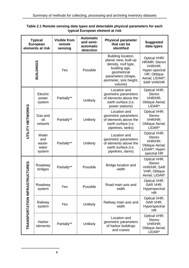
transport corridors, can be observed by remote sensing. Table 2.1 lists the most suitable
types of satellite imagery that can be used to gather information on the European elements
at risk. Descriptions for the suggested remote sensing imagery are given in the following
sections.
Summary of methods for collecting, processing and archiving inventory datasets
4
Table 2.1 Remote sensing data types and detectable physical parameters for each
typical European element at risk
Typical European
elements at risk
Visible from remote sensing
Automatic and semi-automatic detection
Physical parameter that can be identified
Suggested data types
BU
ILD
ING
S
Yes Possible
Building location, planar view, built-up density, roof type,
building age, geometrical
parameters (shape, perimeter, size height,
volume)
Optical VHR/ HR/MR; Stereo
VHR/HR; Hyper-spectral HR; Oblique
Aerial; LIDAR*; SAR VHR/HR
UT
ILIT
Y N
ET
WO
RK
S
Electric power system
Partially**
Unlikely
Location and geometric parameters of elements above the
earth surface (i.e. power stations)
Optical VHR; Stereo
VHR/HR; Oblique Aerial;
LIDAR*
Gas and oil
network Partially** Unlikely
Location and geometric parameters of elements above the
earth surface (i.e. pipelines, tanks)
Optical VHR; Stereo
VHR/HR; Oblique Aerial;
LIDAR*
Water and
waste-water
system
Partially** Unlikely
Location and geometric parameters of elements above the
earth surface (i.e. pipelines, dams)
Optical VHR; Stereo
VHR/HR; Oblique Aerial; LIDAR*; Hyper-
spectral HR
TR
AN
SP
OR
TA
TIO
N I
NF
RA
ST
RU
CT
UR
ES
Roadway bridges
Partially** Possible Bridge location and
width
Optical VHR; Stereo
VHR/HR; SAR VHR; Oblique Aerial; LIDAR*
Roadway system
Yes Possible Road main axis and
width
Optical VHR; SAR VHR;
Hyperspectral HR
Railway system
Yes Unlikely Railway main axis and
width
Optical VHR; SAR VHR;
Hyperspectral HR
Harbor elements
Partially** Unlikely
Location and geometric parameters
of harbor buildings and cranes
Optical VHR; Stereo
VHR/HR; Oblique Aerial;
LIDAR*
Summary of methods for collecting, processing and archiving inventory datasets
5
Typical European
elements at risk
Visible from remote sensing
Automatic and semi-automatic detection
Physical parameter that can be identified
Suggested data types
CR
ITIC
AL
FA
CIL
ITIE
S
Health-care
facilities Partially** Unlikely
Location and geometric parameters
of facility buildings
Optical VHR; Stereo
VHR/HR; Oblique Aerial;
LIDAR*
Fire-fighting system
Partially** Unlikely Location and
geometric parameters of facility buildings
Optical VHR; Stereo
VHR/HR; Oblique Aerial;
LIDAR*
*LIDAR=Laser Imaging Detection and Ranging
** secondary information are necessary
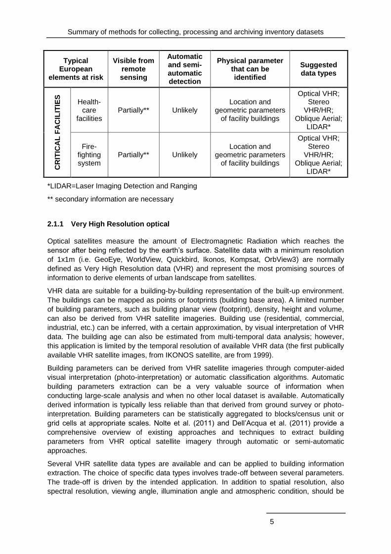
2.1.1 Very High Resolution optical
Optical satellites measure the amount of Electromagnetic Radiation which reaches the
sensor after being reflected by the earth’s surface. Satellite data with a minimum resolution
of 1x1m (i.e. GeoEye, WorldView, Quickbird, Ikonos, Kompsat, OrbView3) are normally
defined as Very High Resolution data (VHR) and represent the most promising sources of
information to derive elements of urban landscape from satellites.
VHR data are suitable for a building-by-building representation of the built-up environment.
The buildings can be mapped as points or footprints (building base area). A limited number
of building parameters, such as building planar view (footprint), density, height and volume,
can also be derived from VHR satellite imageries. Building use (residential, commercial,
industrial, etc.) can be inferred, with a certain approximation, by visual interpretation of VHR
data. The building age can also be estimated from multi-temporal data analysis; however,
this application is limited by the temporal resolution of available VHR data (the first publically
available VHR satellite images, from IKONOS satellite, are from 1999).
Building parameters can be derived from VHR satellite imageries through computer-aided
visual interpretation (photo-interpretation) or automatic classification algorithms. Automatic
building parameters extraction can be a very valuable source of information when
conducting large-scale analysis and when no other local dataset is available. Automatically
derived information is typically less reliable than that derived from ground survey or photo-
interpretation. Building parameters can be statistically aggregated to blocks/census unit or
grid cells at appropriate scales. Nolte et al. (2011) and Dell’Acqua et al. (2011) provide a
comprehensive overview of existing approaches and techniques to extract building
parameters from VHR optical satellite imagery through automatic or semi-automatic
approaches.
Several VHR satellite data types are available and can be applied to building information
extraction. The choice of specific data types involves trade-off between several parameters.
The trade-off is driven by the intended application. In addition to spatial resolution, also
spectral resolution, viewing angle, illumination angle and atmospheric condition, should be
Summary of methods for collecting, processing and archiving inventory datasets
6
considered when selecting a satellite image for a specific purpose and processing technique.
Some of these parameters may influence the quality of the imagery (i.e. atmospheric
conditions) and thus the precision of object extraction, while some other parameters can
determine the possibility to extract specific parameters - i.e. the acquisition angle and sun
elevation angle influence the shadow and the view angle of high objects, which are exploited
to extract buildings and object height.
Critical facilities (i.e. fire stations, dams and water supply facilities) and some above ground
elements belonging to utility networks (i.e. pipelines, power stations, tanks), can be manually
extracted, with a certain approximation, by visual interpretation of VHR data.
VHR data can also be applied to extract transportation infrastructures (roads, railways and
bridges). An overview of existing techniques to extract transportation infrastructures from
optical remote sensing can be found in Nolte et al. (2011).
2.1.2 Stereo High and Very High Resolution (i.e. aerial, satellite)
Stereo products consist of two images of the same location on Earth, taken at two different
angles, which can be processed to obtain 3D surface models. Stereo HR and VHR imagery
can be processed to generate very valuable building stock information, such as planar and
height attributes of buildings. The precision of the measurement depends on the resolution
of the input imagery and the type of processing.
Typically, stereo images are processed using photogrammetric stations with procedures that
are not automated. Newly available software allow imagery to be processed in an automatic
way which is, however, more prone to error. Stereo imagery’s first output, the Digital Surface
Model (DSM), can be refined based on ancillary information- i.e. street level elevation - to
obtain a Digital Elevation model (DEM) and extract building heights. References related to
DSM footprint extraction from VHR imagery include Toutin (2004a, 2004b, 2006a, 2006b)
and Poli et al. (2010).
VHR Stereo imagery is among the best suited data to address the typical European
elements at risk. Stereo aerial photography has been collected for decades to provide fine
scale information on the built environment. Most of the VHR satellites can also acquire
stereo pair imageries, with a resolution which is about two to three times lower than normal
sensor acquisition. Satellite-based stereo imagery is, however, often limited by imaging
angles that may not always be adequate for 3D processing.
2.1.3 Hyperspectral
Hyperspectral Imagery (HSI), or Imaging Spectrometry data, measure the Electromagnetic
Radiation reflected by the earth’s surface in a very high number of spectral bands (more
than 200 bands), providing a contiguous spectral coverage over selected spectral ranges.
Detailed spectral information can be exploited to detect Earth-surface minerals and to
characterize surface materials. Spectrometers are generally transported on aerial platforms
that also allow high spatial ground resolution (few meters).
Different airborne Hyperspectral data have been used for urban application, i.e. Airborne
Visible InfraRed Imaging Spectrometer (AVIRIS), Multispectral Infrared and Visible Imaging
Spectrometer (MIVIS), Digital Airborne Imaging Spectrometer (DAIS) and Reflective Optics
System Imaging Spectrometer (ROSIS). The applications include the detection of roof
Summary of methods for collecting, processing and archiving inventory datasets
7
materials (brick, metallic, gravel, asphalt, shingles, tiles, wood and roof tops covered by toxic
material, e.g. asbestos), urban land cover classes and sealing materials such as asphalt,
bitumen, parking special cover, gravel and concrete (Herold et al. 2003, Dell’Acqua et al.
2005, Marino et al. 2001). The roof material can be used to infer, with a certain
approximation, the building type. The sealing material classification can also be used to
extract roadways, railways and built-up area.
2.1.4 High Resolution optical
Data from optical High Resolution (HR) satellites (i.e. SPOT, Formosat, ALOS, CBERS,
RapidEye) are typically characterized by a spatial resolution ranging between 1x1m and
10x10m (Taubenböck et al 2012). HR data can be used to derive built-up binary masks
(maps of built-up/non built-up) or built-up density maps. The built-up map represents
buildings in spatial units with a variable area corresponding to building aggregates. The
resolution of HR data does not normally allow mapping the planar view of single buildings.
Built-up maps are typically extracted through automatic or semi-automatic algorithms and
can be used to approximate information on physical elements exposed to risk. Different
classification procedures can be based on statistical or logical decision rules in the
multispectral or spatial domain - the spatial domain includes shape, size, texture, and
patterns of pixels or group of pixels - (Gao 2009). Nolte et al. (2011) and Dell’Acqua et al.
(2011) provide a comprehensive overview of existing techniques to extract built-up areas
applying different image classification algorithms.
Built-up maps are particularly useful to rapidly cover large areas, such as country level
mapping.
2.1.5 Medium Resolution optical
Medium Resolution (MR) satellite imagery has a spatial resolution between 10x10m and
100x100m (Taubenböck et al 2012) and includes what is typically referred to as imagery
collected for environmental purposes. Such datum allows built-up areas to be identified but
is not able to resolve single elements of an urban landscape – building units and civil
engineering works.
Large volume archives of MR satellite data covering the globe between 1982 and 2000 are
now available. The data are available mostly free of charge. One of the richest repositories is
that of Landsat imagery available from NASA. Landsat data has been, by and large, used to
analyse environmental issues in urban settings or to map “urban” type of classes in national
and continental land cover products. The most notable products are the CORINE Land
Cover (EEA 1999), Afri-Cover and the North America Landscape Characterization
(Vogelmann 2001). Landsat data has found large application for hydrological studies where
the urban areas are outlined to identify impervious or artificial surfaces, and the heat island
effect of cities.
MR data is not suited to characterize single units of the European elements at risk; the
spatial resolution is just not sufficient to resolve such elements.
Summary of methods for collecting, processing and archiving inventory datasets
8
2.1.6 Low Resolution optical
One set of environmental satellites image the entire Earth every day at coarse resolution
(100x100m or coarser). Yet, this imagery has been used to derive global land cover products
which include one or more “urban” classes. Few of these global datasets have been actually
validated. When urban classes are compared across land-cover datasets, discrepancies
have resulted largely due to a non-standardized semantic (Potere et al. 2009).
The MODIS-Urban layer (Schnedier et al. 2009) maps major urban agglomerations with a
resolution of 500x500m. This product has been validated, displaying unexpected
consistency across continents.
Global scale built-up layers may not be of use in a local application such as that addressed
in SYNER-G; in fact its use lies largely across regional comparison and continental to global
land cover applications.
2.1.7 Oblique Aerial Imagery
Oblique Aerial data provide VHR Imagery from multiple angles with oblique perspectives.
For example, Pictometry technology acquires images simultaneously from an aircraft at 40°
angles (North, South, East, West and vertical) for every feature within the urban
environment. Thanks to the oblique views, some specific parameters of buildings,
infrastructures and facilities, that would be normally collected from ground survey, can be
extracted - i.e. existence of soft stories, added attic spaces, openings and façade elements.
Moreover, ground elevations, building heights, roof height and shape can be extracted with
high resolution.
Oblique Aerial Imagery is among the best-suited data to address the typical European
elements at risk.
2.1.8 LIDAR
LASER (Light Amplification by Stimulated Emission of Radiation) systems represent a
source of high-accuracy elevation data. The LASER technology is also known as LIDAR
(Laser Imaging Detection and Ranging), LADAR (LAser Detection And Ranging) or Laser
Radar. LASER scanners can be mounted on an aircraft platform and applied for
measurements of surface elevation profiles with sub-meter accuracy, at reduced cost
compared to traditional survey methods. These measures are relevant for collecting the
height and other geometric parameters of building and civil engineering works such as
bridges, power lines, pipelines and dams.
2.1.9 RADAR
Synthetic Aperture Radar (SAR) systems emit radio waves and detect the signal that is
scattered back from objects on the ground. The advantages of SAR compared to optical
systems are that they can collect information through dense cloud cover, and they can
directly provide precise information on ground elevation. The measurement of elevation is
useful for terrain modelling, an important task for many hazard applications, and for
monitoring changes in land surface, for example, from subsidence or landslides.
Summary of methods for collecting, processing and archiving inventory datasets
9
SAR sensors had been considered as unsuitable for precise characterization of the urban
environment. This however has now changed. In fact the availability of VHR SAR imagery
from TerraSAR-X and COSMO-SkyMed provides new data to exploit the fine scale spatial
patterns characterized by human settlements (Dell’Acqua et al. 2008).
SAR data processing requires specialized training in image processing. The datum cannot
intuitively be analysed as optical datum. In addition, since the signal records the dialectric
properties of objects, the datum cannot uniquely be converted in a categorical class
associated to an urban object. At present, a huge repository of fine resolution COSMO-
SkyMed and TerraSAR-X is being built and disclosed to the research community. SAR has
shown to be suitable for detecting settlements and roads and is very efficient in monitoring
earth displacements when a number of images covering the same area can be processed
with interferometry techniques. SAR may also be used for damage assessment, in
combination with other data (Dell’Acqua et al. 2011). However, comprehensive and validated
products are still not available.
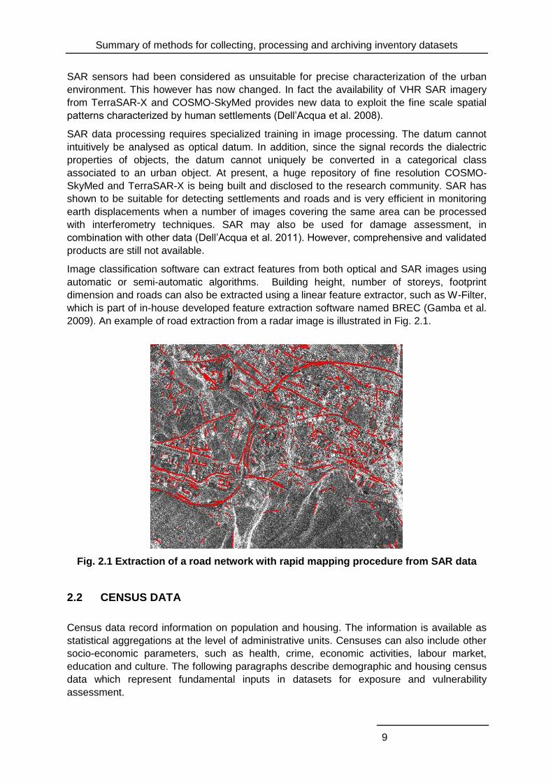
Image classification software can extract features from both optical and SAR images using
automatic or semi-automatic algorithms. Building height, number of storeys, footprint
dimension and roads can also be extracted using a linear feature extractor, such as W-Filter,
which is part of in-house developed feature extraction software named BREC (Gamba et al.
2009). An example of road extraction from a radar image is illustrated in Fig. 2.1.
Fig. 2.1 Extraction of a road network with rapid mapping procedure from SAR data
2.2 CENSUS DATA
Census data record information on population and housing. The information is available as
statistical aggregations at the level of administrative units. Censuses can also include other
socio-economic parameters, such as health, crime, economic activities, labour market,
education and culture. The following paragraphs describe demographic and housing census
data which represent fundamental inputs in datasets for exposure and vulnerability
assessment.
Summary of methods for collecting, processing and archiving inventory datasets
10
2.2.1 Demographic data
Population data at sub-national level are normally collected in Europe through population
census every 5 to 10 years. Census units have a spatial dimension which commonly
corresponds to building aggregates matching administrative districts at different scales (i.e.
Nomenclature of Territorial Units for Statistics – NUTS - regions). In many cases census
data are only available at the commune level. In some cases demographic and socio-
economic census are conducted using grid cell spatial units. Grid-based representations of
population offer several advantages when population data must be integrated with a
representation of settlements or environmental phenomena (Martin 2009). More precise
demographic data are collected in local administrative offices, but are normally not
accessible or not available as geo-referenced digital data format.
When studying exposure, the spatial detail of elements exposed to risk affects the scale of
analysis and allows scenarios to be performed with different levels of approximation. The
census spatial units therefore affect the detail at which the information on human exposure
can be provided. When it is not possible to collect ad hoc demographic data from the field,
downscaling or spatial disaggregation techniques can be used to address heterogeneity
within census units, displacing the population density to smaller and more homogeneous
spatial units. The disaggregation techniques may be based on ancillary data which are
normally related to the land use.
Downscaling techniques can map three types of population distribution: residential, ambient
and time-specific. Time-specific and ambient population maps are based on spatio-temporal
models, which take into account the movements of population during different times of the
day, through a given area (Martin 2009, Ahola et al. 2007). Ambient population refers to an
average distribution of population over 24 hours (Dobson et al. 2000). When mapping
ambient or temporal distribution of the population, the input data collection is much more
challenging. Two datasets are in fact needed in this case: the map of the activity location, or
physical features where they take place, and the census of the mobile population, which
include statistics on tourism, all work related travels, temporary accommodations, education
and traffic (Bhaduri 2007, Martin 2009, Ahola et al. 2007).
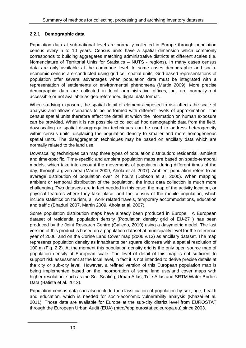
Some population distribution maps have already been produced in Europe. A European
dataset of residential population density (Population density grid of EU-27+) has been
produced by the Joint Research Centre (Gallego, 2010) using a dasymetric model. The last
version of this product is based on a population dataset at municipality level for the reference
year of 2006, and on the Corine Land Cover map (2006 v.13) as ancillary dataset. The map
represents population density as inhabitants per square kilometre with a spatial resolution of
100 m (Fig. 2.2). At the moment this population density grid is the only open source map of
population density at European scale. The level of detail of this map is not sufficient to
support risk assessment at the local level, in fact it is not intended to derive precise details at
the city or sub-city level. However, a refined version of this European population map is
being implemented based on the incorporation of some land use/land cover maps with
higher resolution, such as the Soil Sealing, Urban Atlas, Tele Atlas and SRTM Water Bodies
Data (Batista et al. 2012).
Population census data can also include the classification of population by sex, age, health
and education, which is needed for socio-economic vulnerability analysis (Khazai et al.
2011). Those data are available for Europe at the sub-city district level from EUROSTAT
through the European Urban Audit (EUA) (http://epp.eurostat.ec.europa.eu) since 2003.
Summary of methods for collecting, processing and archiving inventory datasets
11
Fig. 2.2 Population density grid of EU-27+ for the city of Thessaloniki
2.2.2 Housing census data
Housing census data record the characteristics of housing for the entire population and
entire geographic extent of a country. Although the level of detail and procedures involved in
compiling such information is quite exhaustive, the housing census surveys are not intended
for database development in earthquake loss estimation studies. The housing census
compilations are commonly not carried out by engineering professionals and hence the data
provide only a limited contribution for the engineering characterization of building
construction types. The housing types might be deduced from the material used for
constructing the roof, floors, and external walls and by the help of photos, if available, as it
has been done in the compilation of the PAGER database (Jaiswal and Wald 2008). In the
2000 census (1995-2004 decade), about 173 countries conducted housing censuses. Still,
many countries in the world either have not planned to conduct housing census or have not
shared the information with the United Nations Statistics Division. Among the 131 countries
for which the housing census data were available at the United Nations office, only 73
countries have data related to the construction material of the outer walls of buildings
(Jaiswal and Wald 2008).
The EUA (http://www.urbanaudit.org/) provides European urban statistics for 258 cities
across 27 European countries. It contains almost 300 statistical indicators presenting
information on matters such as demography, society, economy, environment, transport,
information society and leisure. The EUA was conducted at the initiative of the Directorate-
General for Regional Policy at the European Commission, in cooperation with EUROSTAT
and the national statistical offices of the 25 Member States at the time plus Bulgaria and
Romania. EUROSTAT adopts a classification on the basis of the provisional Central Product
Summary of methods for collecting, processing and archiving inventory datasets
12
Classification (CPC) published in 1991 by the United Nations and considers two main
categories of constructions: "Buildings" and "Civil engineering works" (Eurostat 1997).
Classification of types of constructions (CC) distinguishes between technical design, which
results from the special use of the structure (e.g. commercial buildings, road structures,
waterworks, pipelines), from the main use of a building (e.g. residential, non-residential). If
less than half of the overall useful floor area is used for residential purposes, the building is
classified under non-residential buildings in accordance with its purpose-oriented design. If
at least half of the overall useful floor area is used for residential purposes, the building is
classified as residential. Civil engineering works include all constructions not classified under
buildings: railways, roads, bridges, highways, airport runways, dams, etc. Civil engineering
works are classified mainly according to the engineering design which is determined by the
purpose of the structure. Residential building stock is further divided into three classes: one-
dwelling buildings, two- and more dwelling buildings and residences for communities. Single-
family houses include individual houses that are inhabited by one or two families including
terraced houses. Multi-family houses contain more than two dwellings in the house, up to 9
storeys. High-rise buildings are defined as buildings that are higher than 8 storeys. A special
building type, corresponding to panelised structure buildings, is found in most Eastern
European countries. In literature and statistics, these buildings are considered as being high-
rise or multi-family buildings. In the EU-25, 34 million dwellings, or 17% of the whole building
stock, are panelised buildings. In each country where these buildings exist, one to three
different building types are defined.
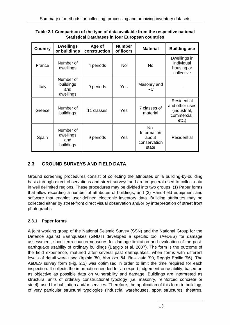
At national scale, within Europe, each national Statistical Data Institute has its own table
format, linked to different methods for information collection. Table 2.1 presents the kind of
data concerning the building stock which can be found in four European countries.
More detailed data is found in cadastral plans. Differently from census data, cadastral data is
taken individually for each construction. This data is not always distributed by authorities
because it often contains confidential information. Attributes usually included in these
databases are: wall and roof material, age of construction, conservation state, number of
floors, and number of households per building.
Finally, other data sources are provided by some databases based on Geographical
Information System (GIS) which contain building delimitations (footprints) and some
geometrical characteristics (height, surface). However, information about construction type
or age is not always provided. These databases sometimes delimit building aggregates and
not individual buildings.
The SYNER-G methodology accounts for the type and format of information in the available
databases (Franchin et al 2011). Socio-economic data, as well as data on building type and
distribution for European cities which are available from EUROSTAT, respectively, through
the EUA and the Building Census (BC), are used. Data on land use are available on a local
basis in the form of a Land Use Plan (LUP), usually maintained from a local source (e.g. the
Municipality). However, each of these data sources adopts a different meshing of the urban
territory, according to its own criteria. For example, the urban territory is subdivided in the
EUA into sub-city districts (SCD), which are areas sufficiently homogeneous in terms of
some socio-economic indicators (e.g. income). On the other hand the Land Use Plan, by its
very nature, subdivides the territory in areas that are homogenous per use type (green,
industrial, commercial, residential).
Summary of methods for collecting, processing and archiving inventory datasets
13
Table 2.1 Comparison of the type of data available from the respective national
Statistical Databases in four European countries
Country Dwellings
or buildings Age of
construction Number of floors
Material Building use
France Number of dwellings
4 periods No No
Dwellings in individual housing or collective
Italy
Number of buildings
and dwellings
9 periods Yes Masonry and
RC -
Greece Number of buildings
11 classes Yes 7 classes of
material
Residential and other uses
(industrial, commercial,
etc.)
Spain
Number of dwellings
and buildings
9 periods Yes
No. Information
about conservation
state
Residential
2.3 GROUND SURVEYS AND FIELD DATA
Ground screening procedures consist of collecting the attributes on a building-by-building
basis through direct observations and street surveys and are in general used to collect data
in well delimited regions. These procedures may be divided into two groups: (1) Paper forms
that allow recording a number of attributes of buildings, and (2) Hand-held equipment and
software that enables user-defined electronic inventory data. Building attributes may be
collected either by street-front direct visual observation and/or by interpretation of street front
photographs.
2.3.1 Paper forms
A joint working group of the National Seismic Survey (SSN) and the National Group for the
Defence against Earthquakes (GNDT) developed a specific tool (AeDES) for damage
assessment, short term countermeasures for damage limitation and evaluation of the post-
earthquake usability of ordinary buildings (Baggio et al. 2007). The form is the outcome of
the field experience, matured after several past earthquakes, when forms with different
levels of detail were used (Irpinia ’80, Abruzzo ’84, Basilicata ’90, Reggio Emilia ’96). The
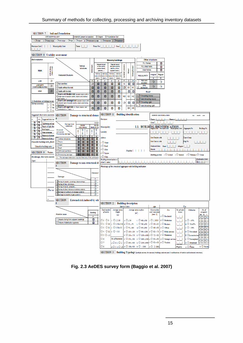
AeDES survey form (Fig. 2.3) was optimised in order to limit the time required for each
inspection. It collects the information needed for an expert judgement on usability, based on
as objective as possible data on vulnerability and damage. Buildings are interpreted as
structural units of ordinary constructional typology (i.e. masonry, reinforced concrete or
steel), used for habitation and/or services. Therefore, the application of this form to buildings
of very particular structural typologies (industrial warehouses, sport structures, theatres,
Summary of methods for collecting, processing and archiving inventory datasets
14
churches etc.), or to monuments, is excluded. The form allows a quick survey and a first
identification of the building stock, with the collection of metrical and typological data of the
buildings.
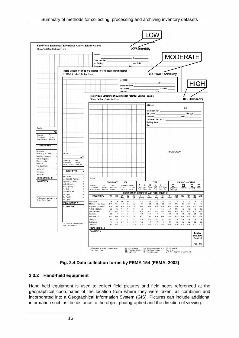
Another example of detailed paper forms for recording building attributes is provided by
FEMA 154 - “Rapid visual screening of buildings for potential seismic hazards: A handbook”.
The rapid visual screening (RVS) procedure uses a methodology based on a ‘sidewalk
survey’ of a building and a Data Collection Form, which is completed by the person
conducting the survey (the screener), based on visual observation of the building from the
exterior, and if possible, the interior (FEMA 2002). The Data Collection Form includes space
for documenting information on the building identification, including its use and size, a
photograph of the building, sketches, and documentation of pertinent data related to seismic
performance, including the development of a numeric seismic hazard score (Fig. 2.4).
Completion of the Data Collection Form starts by identifying the primary structural lateral-
load-resisting system and structural materials of the building. Basic Structural Hazard Scores
for various building types are provided on the form where the screener circles the
appropriate one. For many buildings, viewed only from the exterior, this important decision
requires the screener to be trained and experienced in building construction and design. The
screener modifies the Basic Structural Hazard Score by identifying and circling Score
Modifiers related to observed performance attributes, which are then added (or subtracted)
to the Basic Structural Hazard Score to get a final Structural Score (S). The Basic Structural
Hazard Score, Score Modifiers, and final Structural Score are all related to the probability of
building collapse should severe ground shaking occur (that is, a ground shaking level
equivalent to that currently used in the seismic design of new buildings). Final S scores
typically range from 0 to 7, with higher S scores corresponding to better expected seismic
performance.
Summary of methods for collecting, processing and archiving inventory datasets
15
Fig. 2.3 AeDES survey form (Baggio et al. 2007)
Summary of methods for collecting, processing and archiving inventory datasets
16
Fig. 2.4 Data collection forms by FEMA 154 (FEMA, 2002)
2.3.2 Hand-held equipment
Hand held equipment is used to collect field pictures and field notes referenced at the
geographical coordinates of the location from where they were taken, all combined and
incorporated into a Geographical Information System (GIS). Pictures can include additional
information such as the distance to the object photographed and the direction of viewing.
Summary of methods for collecting, processing and archiving inventory datasets
17
Once structured into a GIS, the civil engineer is able to view the collected information and to
tag the buildings with the appropriate attributes. This last step allows transforming the
assembly of GIS data into an exposure database.
Some of these hand held equipment are now mounted on moving vehicles: i.e. cars,
motorbikes or even bicycles. Their development was spurred by the need to rapidly collect
damage information after a disaster. This has proven to be extremely effective, as it allows a
few people with minimal time investment to collect large amounts of data that is then
interpreted by specialists in the office.
Imaging with video and high through-put imaging cameras allows models of urban areas to
be created that include the facades of all buildings. The technology at present is not mature
enough to include full processing in an automatic way. However, the demand for such
systems goes beyond crisis management applications. Before not too long entire streets will
be imaged and reconstructed in 3D. Nevertheless, imaging the full extent of a city from the
ground may not be justifiable for crisis management applications, owing to the following
three reasons: 1) cost of acquiring field images, 2) inaccessibility of given parts of a city (i.e.
informal settlements), and 3) cost of processing the imagery. At present, the combination of
field pictures and remote sensing data may be considered as an acceptable compromise
between the precision of the collected information and the extent of the area to be covered
(Wieland et al 2012). A brief discussion of digital cameras, Geographical Position Systems
(GPS) receivers and palmtops for collecting ground information is provided bellow.
2.3.3 Digital cameras
Pictures from digital cameras provide general information for image interpretation and risk
assessment. Collecting the location of each image facilitates its integration with other
spatially referenced information. The process of attaching location (e.g., latitude/longitude)
information to pictures is also referred to as geo-tagging. Some digital cameras are equipped
with GPS receivers that generate geo-tagged digital pictures. The most suitable equipment
available in the market for fieldwork has a GPS receiver integrated in the camera with a
positional accuracy of 1-5 meters. When the camera is switched on the GPS receiver
searches for GPS signals, and when at least three satellites communicate with the GPS
receiver the exact position is shown in the camera display. When the picture is taken, the
GPS coordinates are saved within the image’s Exchangeable Image File Format (Exif) file.
Together with further metadata, such as date, time, focal length, shutter speed, and so on,
the latitude and longitude (sometimes also altitude) coordinates are saved and can be later
accessed using image processing or GIS tools.
Specialized software is available for processing field collected imagery and outputs to a full
scale 3D building, inclusive of façade reconstruction. This software relies on a large
collection of building pictures taken at different angles. Although the collection of images is
not always possible and the reconstruction of the facade is time consuming, the output is of
particular value since this allows for the geometric parameters of the typical European
elements at risk to be interpreted.
2.3.4 GPS receivers
Positioning devices are used for locating the information collected in the field. GPS
coordinates are linked to photographs using post-processing when pictures and location
Summary of methods for collecting, processing and archiving inventory datasets
18
information are collected independently. Location information needs to be collected with an
external GPS device: by synchronizing the timestamps of coordinates and digital photos,
every picture can be linked to a geographic position. When location information cannot be
captured with the digital picture automatically, photos can still be geo-tagged by identifying
the location of pictures from digital maps. For this method several software tools are
available (e.g. Geosetter, which integrates Google Maps).
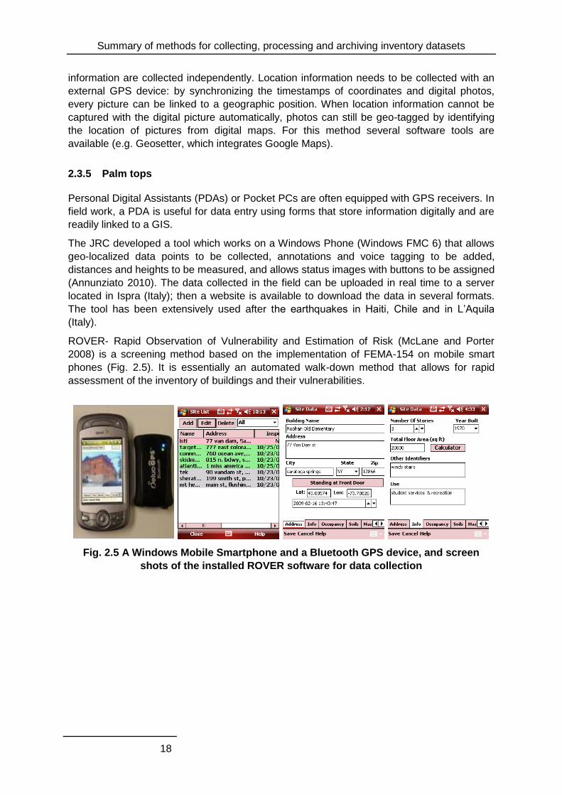
2.3.5 Palm tops
Personal Digital Assistants (PDAs) or Pocket PCs are often equipped with GPS receivers. In
field work, a PDA is useful for data entry using forms that store information digitally and are
readily linked to a GIS.
The JRC developed a tool which works on a Windows Phone (Windows FMC 6) that allows
geo-localized data points to be collected, annotations and voice tagging to be added,
distances and heights to be measured, and allows status images with buttons to be assigned
(Annunziato 2010). The data collected in the field can be uploaded in real time to a server
located in Ispra (Italy); then a website is available to download the data in several formats.
The tool has been extensively used after the earthquakes in Haiti, Chile and in L’Aquila
(Italy).
ROVER- Rapid Observation of Vulnerability and Estimation of Risk (McLane and Porter
2008) is a screening method based on the implementation of FEMA-154 on mobile smart
phones (Fig. 2.5). It is essentially an automated walk-down method that allows for rapid
assessment of the inventory of buildings and their vulnerabilities.
Fig. 2.5 A Windows Mobile Smartphone and a Bluetooth GPS device, and screen
shots of the installed ROVER software for data collection
Integration of data sources for optimum inventory datasets
19
3 Integration of data sources for optimum
inventory datasets
3.1 INTEGRATION OF DATA EXTRACTED FROM REMOTE SENSING IN A GIS
ENVIRONMENT
Data integration involves the processing of different data layers in order to make them
compatible with respect to spatial system (extent, projection system), data format and
information content consistency. Once all the data are stored in a GIS database
(geodatabase); they can be overlaid, queried, and analysed, obtaining statistical aggregation
and spatial indicators that can be exploited in vulnerability analysis.
3.1.1 Built-up spatial metrics
Spatial metrics have been defined and applied in landscape patterns analysis to describe
habitat configurations, functional connectivity and process-based relationships (O’Neil et al.
1988; McGarigaland Marks 1995; Alberti and Waddell 2000). In more general applications,
these metrics can be used for spatially explicit analysis to assess the patterns of physical
features, and to describe their geometry.
Spatial metrics have been used to characterize urban patterns in built-up and building stock
analysis (Tenerelli and Ehrlich 2010, Xi et al. 2009).
Several spatial metrics can be applied for assessing the building exposure to risk, and can
characterize the geometry and spatial pattern of buildings or building aggregates. These
metrics can be grouped in three main categories: area/density, shape and proximity. The
first two categories characterize single buildings or built-up units, while the last category of
metrics can also characterizes the spatial relation between different built-up categories such
as buildings and roads or open spaces. Area density indexes represent the number of
buildings in the land unit. Shape indexes measure the building shape complexity. Proximity
indexes measure the isolation of a building or the distance between each building and the
nearest open space, road or critical infrastructure.
3.2 METHODS FOR COMBINING REMOTE SENSING, CENSUS AND FIELD DATA
Socio-economic data characterizes fundamental variables in vulnerability assessment;
population data, in particular, are needed when performing estimates of casualties in natural
disaster scenarios. The data are normally available from censuses, which account specific
entities (i.e. people, household) as statistic aggregations at the level of arbitrary areal units.
These units commonly correspond to administrative boundaries and do not have an intrinsic
geographical meaning. Thematic maps which are based on such predefined areal units are
also called cloropleth maps.
Socio-economic census data can be mapped using spatial disaggregation techniques
(Eicher and Brewer 2001, Mrozinski and Cromley 1999, Chen 2002) which realistically place
Integration of data sources for optimum inventory datasets
20
non-spatially explicit attributes over geographical units (reporting zones). This is needed
when performing analyses which integrate the census data with physical parameters (i.e.
environmental data, built-up maps, topography) which follow natural boundaries or regular
grid cells. The disaggregation techniques may be based on ancillary data which are normally
related to the land use. These ancillary data can be extracted from remote sensing data.
In the following the methods that are used to map population density are described, focusing
on the main downscaling techniques used in GIS modelling and the contribution of remote
sensing in population density displacement models.
3.2.1 GIS modelling for population downscaling
The downscaling methods based on GIS can be classified as geostatistical methods and
areal interpolation methods (Wu et al. 2006). In geostatistical models continuous density
surfaces (isopleth maps) are produced using control points, which represent census values
(Tobler 1979, Wu et al 2006, Wu et al. 2008). In addition to the population dataset,
geostatistical models can be applied with or without ancillary information.
Areal interpolation methods are commonly used in population downscaling, they apply a
homogeneous zone approach where the census units are disaggregated into smaller
enumeration zones. Areal methods, which interpolate census data using ancillary
information, are generally referred to as dasymetric, or “intelligent areal interpolations”.
Different techniques for dasymetric modelling exist. The dasymetric models normally apply
one downscaling parameter. Dobson et al. (2000) applied a multi-dimensional dasymetric
model which includes multiple physical parameters to map ambient population in 1km grid
cells at the global scale (ORNL's LandScanTM). In dasymetric models, the categorical or
continuous proxies are related to population through sampling techniques (Wu et al. 2008,
Mennis 2003, Mennis and Hultgren 2006), regression analysis (Yuan et al. 1997, Wu et al.
2006, Chen 2002, Lu et al. 2010, Briggs et al. 2007) or expert knowledge (Eicher and
Brewer 2001).
Another important distinction must be made between volume preserving methods and non-
volume preserving methods. In volume preserving methods the pycnophylactic constraint is
applied, which means that the sum of population from all zones coincide with the known
population (Tobler, 1979, Gallego et al. 2011).
The criteria for the choice of method for population interpolation are the data availability and
quality (accuracy, scale), together with the purpose of investigation. Dasymetric downscaling
is particularly suitable for discrete variables with approximately homogeneous intra-zone
distribution and inter-zones with actual changes, as is the case of many socioeconomic
variables (Cai, 2006).
3.2.2 Contribution of remote sensing in population downscaling models
When disaggregating population distribution, remote sensing data can provide input proxies
in three different approaches:
i. Extract the physical features that are then related to the population distribution. The
most typically used features are the buildings and the built-up area. Physical feature
classes can be extracted by manual digitalization and automatic or semiautomatic
image classifications, based on spectral or textural parameters (Liu and Clarke 2002,

Integration of data sources for optimum inventory datasets
21
Yuan et al. 1997, Schneiderbauer and Ehrlich 2005, Holt et al. 2004, Dong et al.
2010, Lu et al. 2006).
ii. Extract textural or spectral parameters that are not classified in features classes, but
are used as predictor variables in regression models at the pixel level (pixel-based
approaches) (Azar et al. 2010, Li and Weng 2005, Lu et al. 2010, Lo 1995, Wu and
Murray 2007).
iii. Combination of aerial interpolations at zones, blocks or land use class levels and
regression models at the pixel or object level to obtain sub-zones population
distributions (Chen 2002, Wu et al 2008, Wu et al 2006, Briggs et al. 2007, Harvey
2002).

Case Study: Vienna
23
4 Case Study: Vienna
4.1 DATABASE OF VIENNA CITY
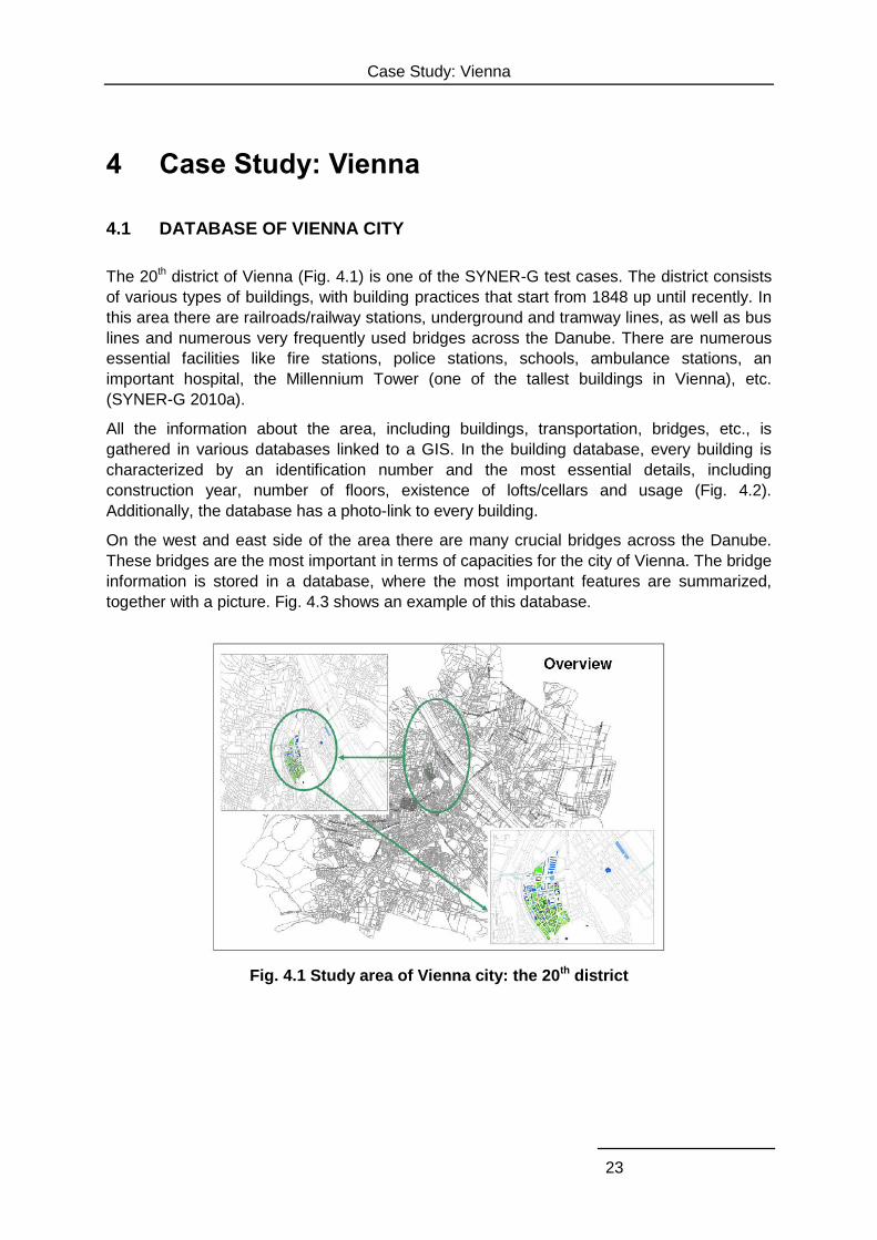
The 20th district of Vienna (Fig. 4.1) is one of the SYNER-G test cases. The district consists
of various types of buildings, with building practices that start from 1848 up until recently. In
this area there are railroads/railway stations, underground and tramway lines, as well as bus
lines and numerous very frequently used bridges across the Danube. There are numerous
essential facilities like fire stations, police stations, schools, ambulance stations, an
important hospital, the Millennium Tower (one of the tallest buildings in Vienna), etc.
(SYNER-G 2010a).
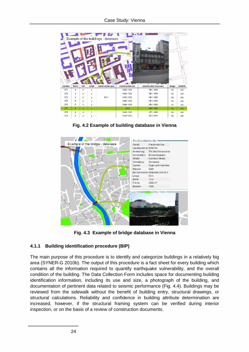
All the information about the area, including buildings, transportation, bridges, etc., is
gathered in various databases linked to a GIS. In the building database, every building is
characterized by an identification number and the most essential details, including
construction year, number of floors, existence of lofts/cellars and usage (Fig. 4.2).
Additionally, the database has a photo-link to every building.
On the west and east side of the area there are many crucial bridges across the Danube.
These bridges are the most important in terms of capacities for the city of Vienna. The bridge
information is stored in a database, where the most important features are summarized,
together with a picture. Fig. 4.3 shows an example of this database.
Fig. 4.1 Study area of Vienna city: the 20th district
Case Study: Vienna
24
Fig. 4.2 Example of building database in Vienna
Fig. 4.3 Example of bridge database in Vienna
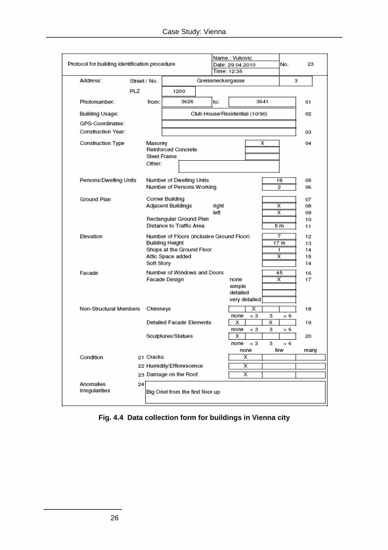
4.1.1 Building identification procedure (BIP)
The main purpose of this procedure is to identify and categorize buildings in a relatively big
area (SYNER-G 2010b). The output of this procedure is a fact sheet for every building which
contains all the information required to quantify earthquake vulnerability, and the overall
condition of the building. The Data Collection Form includes space for documenting building
identification information, including its use and size, a photograph of the building, and
documentation of pertinent data related to seismic performance (Fig. 4.4). Buildings may be
reviewed from the sidewalk without the benefit of building entry, structural drawings, or
structural calculations. Reliability and confidence in building attribute determination are
increased, however, if the structural framing system can be verified during interior
inspection, or on the basis of a review of construction documents.

Case Study: Vienna
25
The BIP is completed for each building screened through execution of the following steps:
o verifying and updating the building identification information;
o walking around the building to identify its size and shape and looking for signs that
identify the construction year;
o determining and documenting the occupancy;
o determining the construction type;
o identifying the number of persons living/working in the building;
o characterizing the building through the ground plan and determining the distance to
traffic area;
o characterizing the building elevation, using the laser telemeter to define building
height;
o identifying soft stories or added attic space;
o identifying façade elements including the number of windows and doors;
o determining non-structural members;
o determining the overall condition of the building;
o noting any irregularities/anomalies;
o taking pictures with the digital camera.
Case Study: Vienna
26
Fig. 4.4 Data collection form for buildings in Vienna city
Case Study: Vienna
27
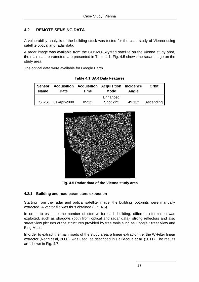
4.2 REMOTE SENSING DATA
A vulnerability analysis of the building stock was tested for the case study of Vienna using
satellite optical and radar data.
A radar image was available from the COSMO-SkyMed satellite on the Vienna study area,
the main data parameters are presented in Table 4.1. Fig. 4.5 shows the radar image on the
study area.
The optical data were available for Google Earth.
Table 4.1 SAR Data Features
Sensor
Name
Acquisition
Date
Acquisition
Time
Acquisition
Mode
Incidence
Angle
Orbit
CSK-S1
01-Apr-2008
05:12
Enhanced
Spotlight
49.13°
Ascending
Fig. 4.5 Radar data of the Vienna study area
4.2.1 Building and road parameters extraction
Starting from the radar and optical satellite image, the building footprints were manually
extracted. A vector file was thus obtained (Fig. 4.6).
In order to estimate the number of storeys for each building, different information was
exploited, such as shadows (both from optical and radar data), strong reflectors and also
street view pictures of the structures provided by free tools such as Google Street View and
Bing Maps.
In order to extract the main roads of the study area, a linear extractor, i.e. the W-Filter linear
extractor (Negri et al, 2006), was used, as described in Dell’Acqua et al. (2011). The results
are shown in Fig. 4.7.
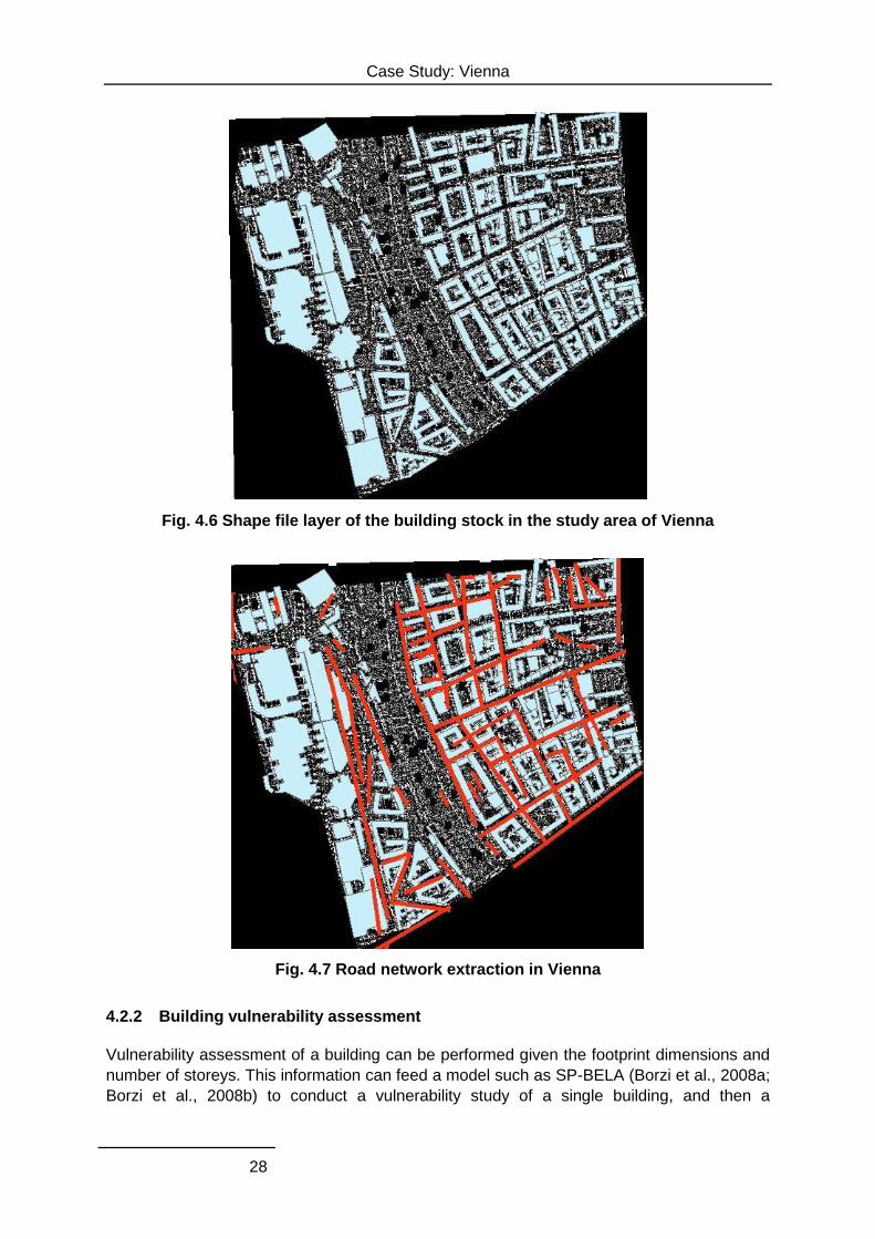
Case Study: Vienna
28
Fig. 4.6 Shape file layer of the building stock in the study area of Vienna
Fig. 4.7 Road network extraction in Vienna
4.2.2 Building vulnerability assessment
Vulnerability assessment of a building can be performed given the footprint dimensions and
number of storeys. This information can feed a model such as SP-BELA (Borzi et al., 2008a;
Borzi et al., 2008b) to conduct a vulnerability study of a single building, and then a
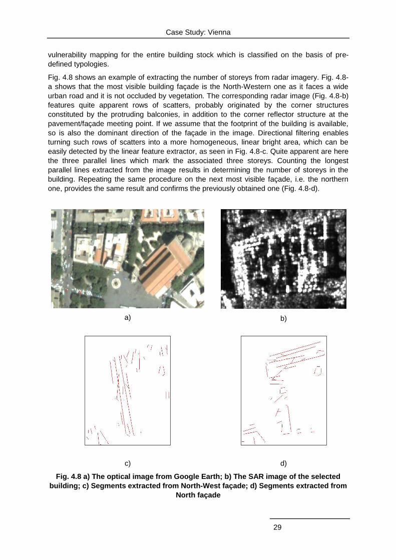
Case Study: Vienna
29
vulnerability mapping for the entire building stock which is classified on the basis of pre-
defined typologies.
Fig. 4.8 shows an example of extracting the number of storeys from radar imagery. Fig. 4.8-
a shows that the most visible building façade is the North-Western one as it faces a wide
urban road and it is not occluded by vegetation. The corresponding radar image (Fig. 4.8-b)
features quite apparent rows of scatters, probably originated by the corner structures
constituted by the protruding balconies, in addition to the corner reflector structure at the
pavement/façade meeting point. If we assume that the footprint of the building is available,
so is also the dominant direction of the façade in the image. Directional filtering enables
turning such rows of scatters into a more homogeneous, linear bright area, which can be
easily detected by the linear feature extractor, as seen in Fig. 4.8-c. Quite apparent are here
the three parallel lines which mark the associated three storeys. Counting the longest
parallel lines extracted from the image results in determining the number of storeys in the
building. Repeating the same procedure on the next most visible façade, i.e. the northern
one, provides the same result and confirms the previously obtained one (Fig. 4.8-d).
a)
b)
c)
d)
Fig. 4.8 a) The optical image from Google Earth; b) The SAR image of the selected
building; c) Segments extracted from North-West façade; d) Segments extracted from
North façade
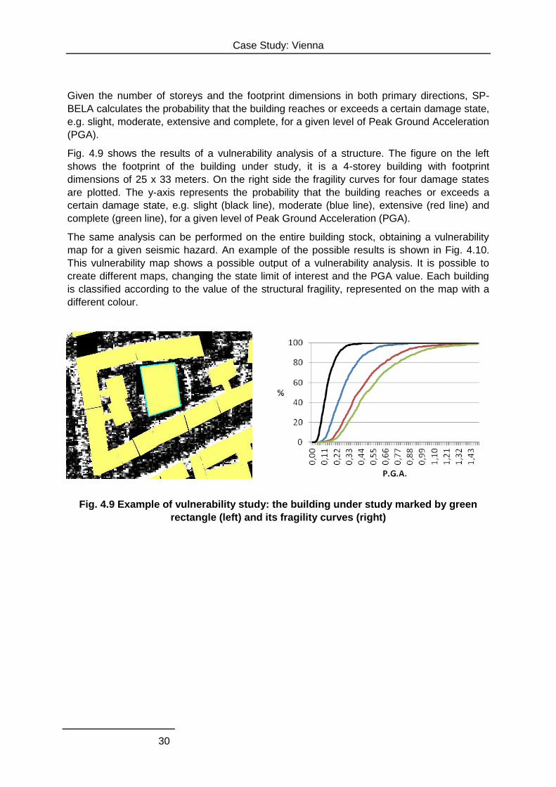
Case Study: Vienna
30
Given the number of storeys and the footprint dimensions in both primary directions, SP-
BELA calculates the probability that the building reaches or exceeds a certain damage state,
e.g. slight, moderate, extensive and complete, for a given level of Peak Ground Acceleration
(PGA).
Fig. 4.9 shows the results of a vulnerability analysis of a structure. The figure on the left
shows the footprint of the building under study, it is a 4-storey building with footprint
dimensions of 25 x 33 meters. On the right side the fragility curves for four damage states
are plotted. The y-axis represents the probability that the building reaches or exceeds a
certain damage state, e.g. slight (black line), moderate (blue line), extensive (red line) and
complete (green line), for a given level of Peak Ground Acceleration (PGA).
The same analysis can be performed on the entire building stock, obtaining a vulnerability
map for a given seismic hazard. An example of the possible results is shown in Fig. 4.10.
This vulnerability map shows a possible output of a vulnerability analysis. It is possible to
create different maps, changing the state limit of interest and the PGA value. Each building
is classified according to the value of the structural fragility, represented on the map with a
different colour.
Fig. 4.9 Example of vulnerability study: the building under study marked by green
rectangle (left) and its fragility curves (right)
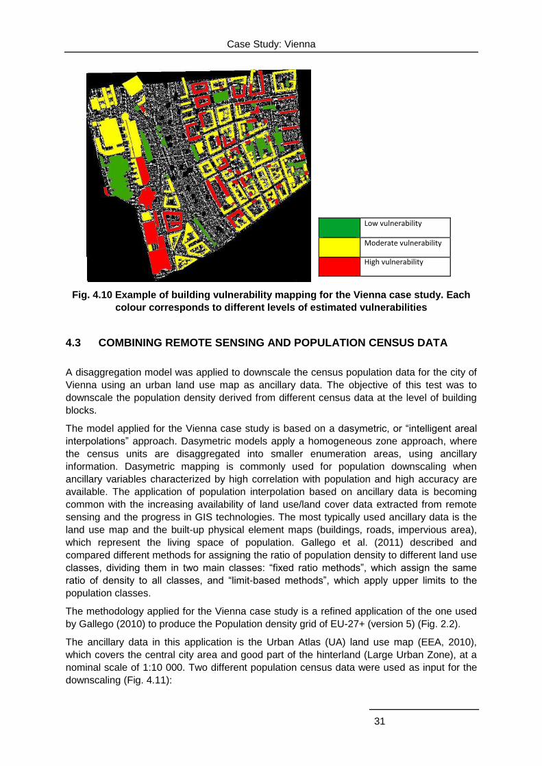
Case Study: Vienna
31
Fig. 4.10 Example of building vulnerability mapping for the Vienna case study. Each
colour corresponds to different levels of estimated vulnerabilities
4.3 COMBINING REMOTE SENSING AND POPULATION CENSUS DATA
A disaggregation model was applied to downscale the census population data for the city of
Vienna using an urban land use map as ancillary data. The objective of this test was to
downscale the population density derived from different census data at the level of building
blocks.
The model applied for the Vienna case study is based on a dasymetric, or “intelligent areal
interpolations” approach. Dasymetric models apply a homogeneous zone approach, where
the census units are disaggregated into smaller enumeration areas, using ancillary
information. Dasymetric mapping is commonly used for population downscaling when
ancillary variables characterized by high correlation with population and high accuracy are
available. The application of population interpolation based on ancillary data is becoming
common with the increasing availability of land use/land cover data extracted from remote
sensing and the progress in GIS technologies. The most typically used ancillary data is the
land use map and the built-up physical element maps (buildings, roads, impervious area),
which represent the living space of population. Gallego et al. (2011) described and
compared different methods for assigning the ratio of population density to different land use
classes, dividing them in two main classes: “fixed ratio methods”, which assign the same
ratio of density to all classes, and “limit-based methods”, which apply upper limits to the
population classes.
The methodology applied for the Vienna case study is a refined application of the one used
by Gallego (2010) to produce the Population density grid of EU-27+ (version 5) (Fig. 2.2).
The ancillary data in this application is the Urban Atlas (UA) land use map (EEA, 2010),
which covers the central city area and good part of the hinterland (Large Urban Zone), at a
nominal scale of 1:10 000. Two different population census data were used as input for the
downscaling (Fig. 4.11):
Lowvulnerability
Moderatevulnerability
Highvulnerability
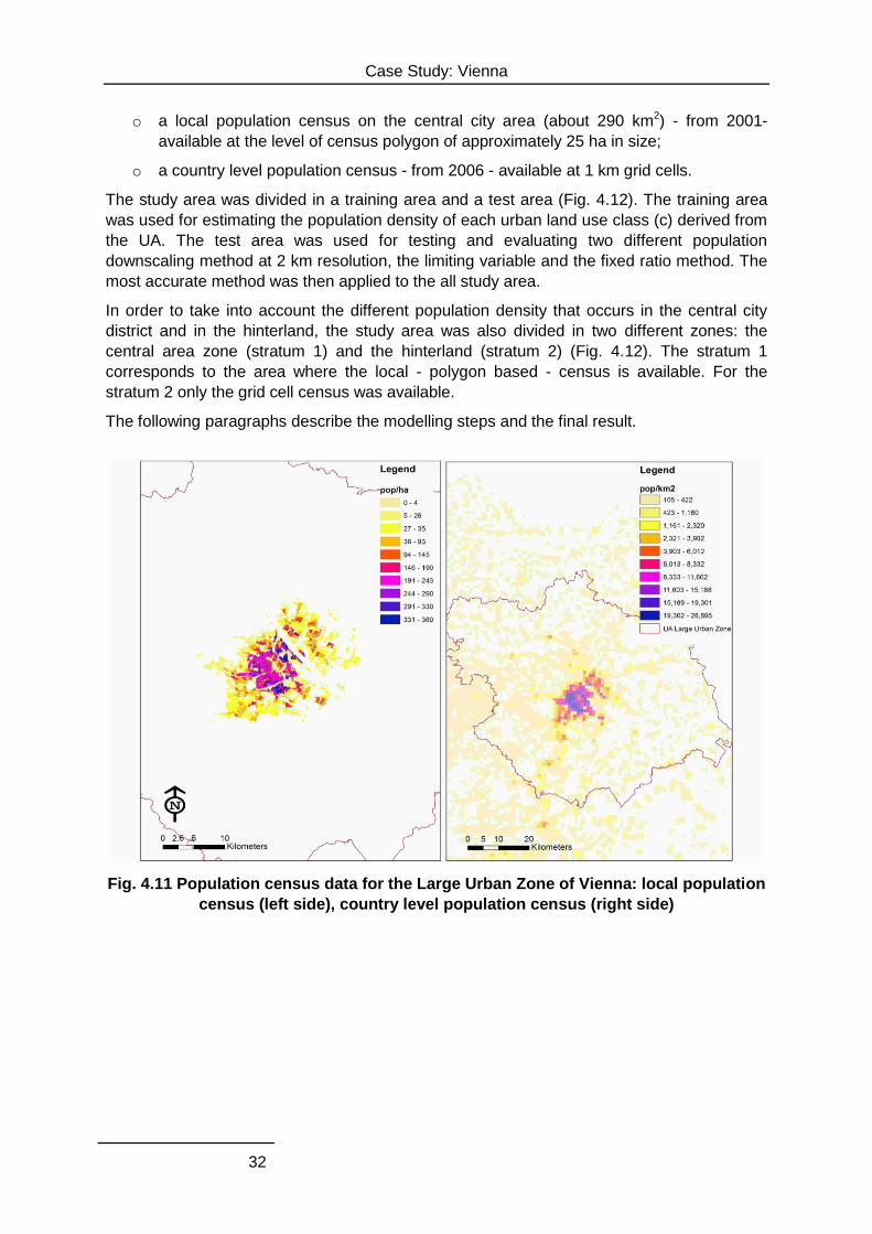
Case Study: Vienna
32
o a local population census on the central city area (about 290 km2) - from 2001-
available at the level of census polygon of approximately 25 ha in size;
o a country level population census - from 2006 - available at 1 km grid cells.
The study area was divided in a training area and a test area (Fig. 4.12). The training area
was used for estimating the population density of each urban land use class (c) derived from
the UA. The test area was used for testing and evaluating two different population
downscaling method at 2 km resolution, the limiting variable and the fixed ratio method. The
most accurate method was then applied to the all study area.
In order to take into account the different population density that occurs in the central city
district and in the hinterland, the study area was also divided in two different zones: the
central area zone (stratum 1) and the hinterland (stratum 2) (Fig. 4.12). The stratum 1
corresponds to the area where the local - polygon based - census is available. For the
stratum 2 only the grid cell census was available.
The following paragraphs describe the modelling steps and the final result.
Fig. 4.11 Population census data for the Large Urban Zone of Vienna: local population
census (left side), country level population census (right side)
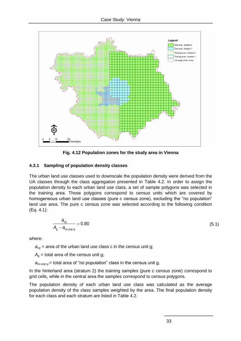
Case Study: Vienna
33
Fig. 4.12 Population zones for the study area in Vienna
4.3.1 Sampling of population density classes
The urban land use classes used to downscale the population density were derived from the
UA classes through the class aggregation presented in Table 4.2. In order to assign the
population density to each urban land use class, a set of sample polygons was selected in
the training area. Those polygons correspond to census units which are covered by
homogeneous urban land use classes (pure c census zone), excluding the “no population”
land use area. The pure c census zone was selected according to the following condition
(Eq. 4.1):
0.80cg
g no pop g
a
A a (5.1)
where:
acg = area of the urban land use class c in the census unit g;
Ag = total area of the census unit g;
ano pop g = total area of “no population” class in the census unit g.
In the hinterland area (stratum 2) the training samples (pure c census zone) correspond to
grid cells, while in the central area the samples correspond to census polygons.
The population density of each urban land use class was calculated as the average
population density of the class samples weighted by the area. The final population density
for each class and each stratum are listed in Table 4.2.
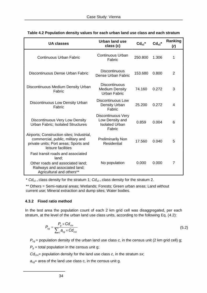
Case Study: Vienna
34
Table 4.2 Population density values for each urban land use class and each stratum
UA classes Urban land use
class (c) Cds1* Cds2*
Ranking
(r)
Continuous Urban Fabric Continuous Urban
Fabric 250.800 1.306 1
Discontinuous Dense Urban Fabric Discontinuous
Dense Urban Fabric 153.680 0.800 2
Discontinuous Medium Density Urban Fabric
Discontinuous Medium Density
Urban Fabric 74.160 0.272 3
Discontinuous Low Density Urban Fabric
Discontinuous Low Density Urban
Fabric 25.200 0.272 4
Discontinuous Very Low Density Urban Fabric; Isolated Structures
Discontinuous Very Low Density and Isolated Urban
Fabric
0.859 0.004 6
Airports; Construction sites; Industrial, commercial, public, military and
private units; Port areas; Sports and leisure facilities
Preliminarily Non Residential
17.560 0.040 5
Fast transit roads and associated land;
Other roads and associated land; Railways and associated land;
Agricultural and others**
No population 0.000 0.000 7
* Cds1 = class density for the stratum 1; Cds2 = class density for the stratum 2.
** Others = Semi-natural areas; Wetlands; Forests; Green urban areas; Land without current use; Mineral extraction and dump sites; Water bodies.
4.3.2 Fixed ratio method
In the test area the population count of each 2 km grid cell was disaggregated, per each
stratum, at the level of the urban land use class units, according to the following Eq. (4.2):
g csx
cg
cg csxc
P CdP
a Cd (5.2)
Pcg = population density of the urban land use class c, in the census unit (2 km grid cell) g;
Pg = total population in the census unit g;
Cdcsx= population density for the land use class c, in the stratum sx;
acg= area of the land use class c, in the census unit g.
Case Study: Vienna
35
4.3.3 Limiting variable method
The limiting variable method is described through the following steps (Gallego et al., 2011):
o a uniform population density value derived from the original census dataset is
assigned to all the land use polygons in each 2 km grid cell (Dg);
o the land use classes are ranked and an index (r) is assigned from the lowest to the
highest population density value (from “Continuous Urban Fabric”- r=1 – to ”No
population” - r=7) (Table 1);
o If the Dg is above the population class density of the given stratum, the density value
is modified: the population density become equal to Cds1 or Cds2 , and the population
in excess is redistributed among the more dense classes according to the following
Eq. (4.3) (Gallego et al., 2011):
'
''
r
cg g csxr
cg g r
cgr r
a D CdP D
a (5.3)
this step is iterated for each r’ > r : 7 iterations in total, one for each land use class,
were performed;
o at the end of the process if there is still some excess population it is redistributed to
all the land use classes proportionally to the class density (Cds1 or Cds2).
4.3.4 Selection and application of the model
The disaggregated population map resulting from the two tests were re-aggregated at 1 km
grid and compared with the original 1 km census population grid. This was done for
evaluating the two models, in absence of reference data.
The correlation analysis between the observed and the model-simulated data indicated a
similar performance for the two models, showing a coefficient of determination (r2) of about
0.93 for both the model outputs (Table 4.3).
The agreement with the reference population grid was estimated, for each model output, in
terms of Total Absolute Error (TAE), which is calculated as the sum of the residual absolute
value. The TAE measures the average model-performance error in a way which is less
ambiguous (Willmott and Matsuura 2005) and more robust in the presence of outliers
(Gallego et al. 2011, Legates and McCabe 1999) than the commonly used Root Mean
Square Error (RMSE). The TAE of the fixed ratio model was slightly lower than that of the
limiting variable model (Table 4.3). The fixed ratio method was therefore applied to the whole
study area (test area plus training area), for each 1km grid cell.
Table 4.3 Statistic indicators for each model output comparison with the reference
population data
Statistic indicator Limiting variable model Fixed ratio model
r2 0.931 0.936
TAE 260241 242334
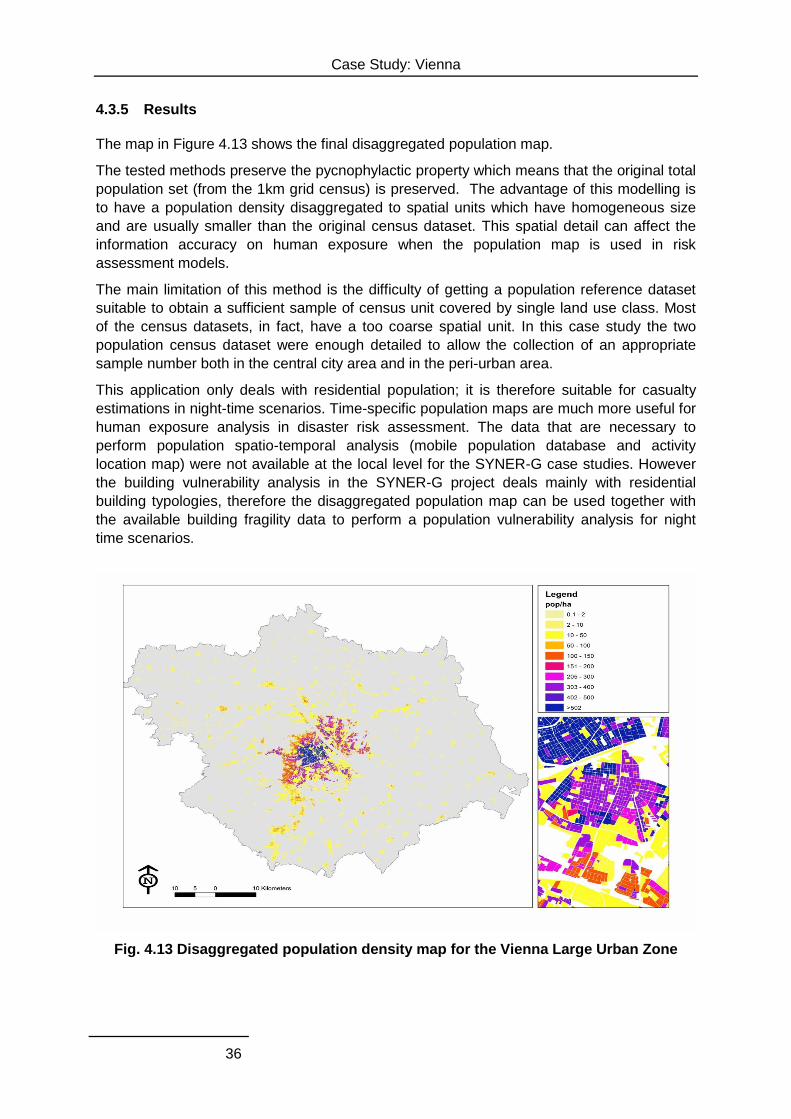
Case Study: Vienna
36
4.3.5 Results
The map in Figure 4.13 shows the final disaggregated population map.
The tested methods preserve the pycnophylactic property which means that the original total
population set (from the 1km grid census) is preserved. The advantage of this modelling is
to have a population density disaggregated to spatial units which have homogeneous size
and are usually smaller than the original census dataset. This spatial detail can affect the
information accuracy on human exposure when the population map is used in risk
assessment models.
The main limitation of this method is the difficulty of getting a population reference dataset
suitable to obtain a sufficient sample of census unit covered by single land use class. Most
of the census datasets, in fact, have a too coarse spatial unit. In this case study the two
population census dataset were enough detailed to allow the collection of an appropriate
sample number both in the central city area and in the peri-urban area.
This application only deals with residential population; it is therefore suitable for casualty
estimations in night-time scenarios. Time-specific population maps are much more useful for
human exposure analysis in disaster risk assessment. The data that are necessary to
perform population spatio-temporal analysis (mobile population database and activity
location map) were not available at the local level for the SYNER-G case studies. However
the building vulnerability analysis in the SYNER-G project deals mainly with residential
building typologies, therefore the disaggregated population map can be used together with
the available building fragility data to perform a population vulnerability analysis for night
time scenarios.
Fig. 4.13 Disaggregated population density map for the Vienna Large Urban Zone
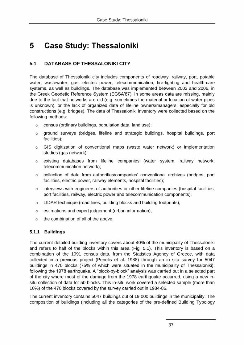
Case Study: Thessaloniki
37
5 Case Study: Thessaloniki
5.1 DATABASE OF THESSALONIKI CITY
The database of Thessaloniki city includes components of roadway, railway, port, potable
water, wastewater, gas, electric power, telecommunication, fire-fighting and health-care
systems, as well as buildings. The database was implemented between 2003 and 2006, in
the Greek Geodetic Reference System (EGSA’87). In some areas data are missing, mainly
due to the fact that networks are old (e.g. sometimes the material or location of water pipes
is unknown), or the lack of organized data of lifeline owners/managers, especially for old
constructions (e.g. bridges). The data of Thessaloniki inventory were collected based on the
following methods:
o census (ordinary buildings, population data, land use);
o ground surveys (bridges, lifeline and strategic buildings, hospital buildings, port
facilities);
o GIS digitization of conventional maps (waste water network) or implementation
studies (gas network);
o existing databases from lifeline companies (water system, railway network,
telecommunication network);
o collection of data from authorities/companies’ conventional archives (bridges, port
facilities, electric power, railway elements, hospital facilities);
o interviews with engineers of authorities or other lifeline companies (hospital facilities,
port facilities, railway, electric power and telecommunication components);
o LIDAR technique (road lines, building blocks and building footprints);
o estimations and expert judgement (urban information);
o the combination of all of the above.
5.1.1 Buildings
The current detailed building inventory covers about 40% of the municipality of Thessaloniki
and refers to half of the blocks within this area (Fig. 5.1). This inventory is based on a
combination of the 1991 census data, from the Statistics Agency of Greece, with data
collected in a previous project (Penelis et al. 1988) through an in situ survey for 5047
buildings in 470 blocks (75% of which were situated in the municipality of Thessaloniki),
following the 1978 earthquake. A “block-by-block” analysis was carried out in a selected part
of the city where most of the damage from the 1978 earthquake occurred, using a new in-
situ collection of data for 50 blocks. This in-situ work covered a selected sample (more than
10%) of the 470 blocks covered by the survey carried out in 1984-86.
The current inventory contains 5047 buildings out of 19 000 buildings in the municipality. The
composition of buildings (including all the categories of the pre-defined Building Typology
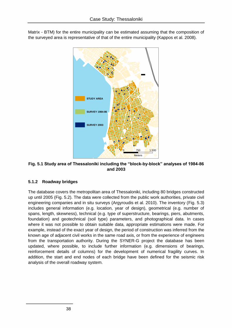
Case Study: Thessaloniki
38
Matrix - BTM) for the entire municipality can be estimated assuming that the composition of
the surveyed area is representative of that of the entire municipality (Kappos et al. 2008).
Fig. 5.1 Study area of Thessaloniki including the “block-by-block” analyses of 1984-86
and 2003
5.1.2 Roadway bridges
The database covers the metropolitan area of Thessaloniki, including 80 bridges constructed
up until 2005 (Fig. 5.2). The data were collected from the public work authorities, private civil
engineering companies and in situ surveys (Argyroudis et al. 2010). The inventory (Fig. 5.3)
includes general information (e.g. location, year of design), geometrical (e.g. number of
spans, length, skewness), technical (e.g. type of superstructure, bearings, piers, abutments,
foundation) and geotechnical (soil type) parameters, and photographical data. In cases
where it was not possible to obtain suitable data, appropriate estimations were made. For
example, instead of the exact year of design, the period of construction was inferred from the
known age of adjacent civil works in the same road axis, or from the experience of engineers
from the transportation authority. During the SYNER-G project the database has been
updated, where possible, to include further information (e.g. dimensions of bearings,
reinforcement details of columns) for the development of numerical fragility curves. In
addition, the start and end nodes of each bridge have been defined for the seismic risk
analysis of the overall roadway system.
0 1.500750
Meters
STUDY AREA
SURVEY 1984-86
SURVEY 2003
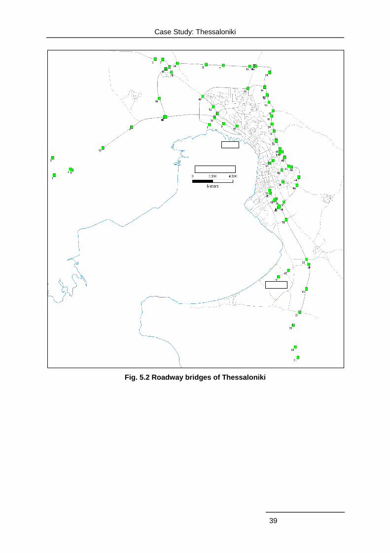
Case Study: Thessaloniki
39
Fig. 5.2 Roadway bridges of Thessaloniki
Case Study: Thessaloniki
40
Fig. 5.3 Inventory sheet used for the collection of data for roadway bridges in
Thessaloniki
INVENTORY SHEET FOR ROADWAY BRIDGE
Date: Bridge ID:
GENERAL INFORMATION
Name/Location of bridge:
Year of construction:
Contractor - Designer:
GEOMETRICAL CHARACTERISTICS
Number of spans:
Length of spans (m):
Total length (m): Width (m):
Different pier heights: Regular Irregular
Alignment of bridge: Skewed Straight
Skewness (0):
Comments:
TECHNICAL CHARACTERISTICS
SUPERSTRUCTURE
Type-Material:
Pier-Deck connection:
Continuous superstructure: Yes No
Number of intermediate joints:
Comments:
BEARINGS
Bearings type:
Support length:
Comments:
PIERS
Pier type: Single column Multi column Wall
Maximum height (m):
Foundation type:
Comments:
ABUTMENTS
Abutment type:
Foundation type:
Comments:
SOIL
Description:
Soil class:
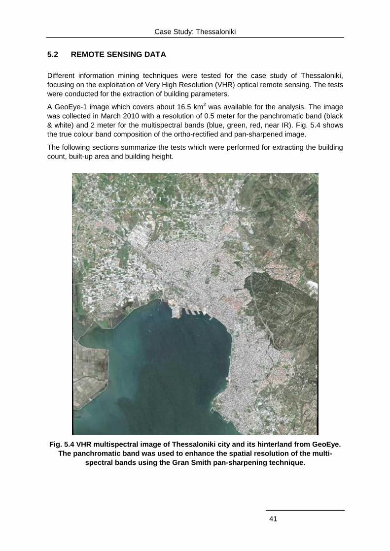
Case Study: Thessaloniki
41
5.2 REMOTE SENSING DATA
Different information mining techniques were tested for the case study of Thessaloniki,
focusing on the exploitation of Very High Resolution (VHR) optical remote sensing. The tests
were conducted for the extraction of building parameters.
A GeoEye-1 image which covers about 16.5 km2 was available for the analysis. The image
was collected in March 2010 with a resolution of 0.5 meter for the panchromatic band (black
& white) and 2 meter for the multispectral bands (blue, green, red, near IR). Fig. 5.4 shows
the true colour band composition of the ortho-rectified and pan-sharpened image.
The following sections summarize the tests which were performed for extracting the building
count, built-up area and building height.
Fig. 5.4 VHR multispectral image of Thessaloniki city and its hinterland from GeoEye.
The panchromatic band was used to enhance the spatial resolution of the multi-
spectral bands using the Gran Smith pan-sharpening technique.
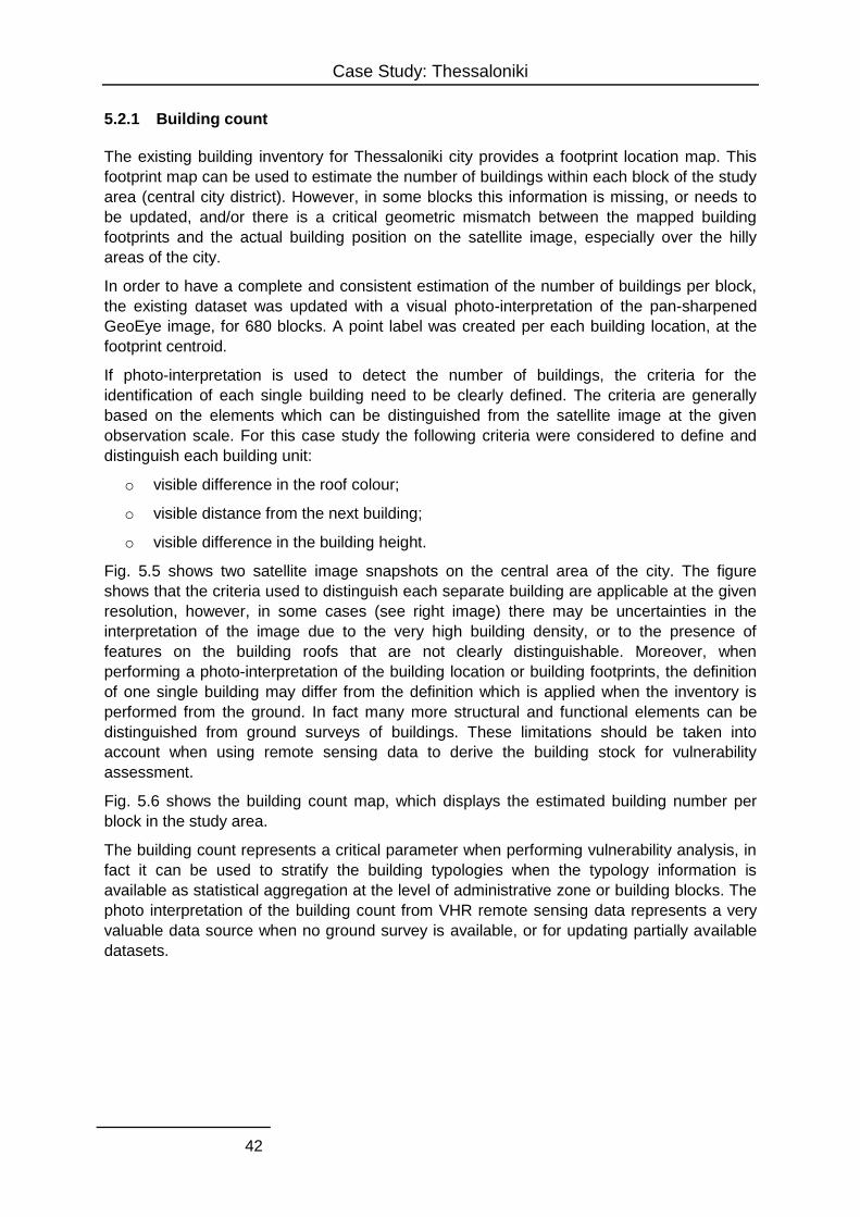
Case Study: Thessaloniki
42
5.2.1 Building count
The existing building inventory for Thessaloniki city provides a footprint location map. This
footprint map can be used to estimate the number of buildings within each block of the study
area (central city district). However, in some blocks this information is missing, or needs to
be updated, and/or there is a critical geometric mismatch between the mapped building
footprints and the actual building position on the satellite image, especially over the hilly
areas of the city.
In order to have a complete and consistent estimation of the number of buildings per block,
the existing dataset was updated with a visual photo-interpretation of the pan-sharpened
GeoEye image, for 680 blocks. A point label was created per each building location, at the
footprint centroid.
If photo-interpretation is used to detect the number of buildings, the criteria for the
identification of each single building need to be clearly defined. The criteria are generally
based on the elements which can be distinguished from the satellite image at the given
observation scale. For this case study the following criteria were considered to define and
distinguish each building unit:
o visible difference in the roof colour;
o visible distance from the next building;
o visible difference in the building height.
Fig. 5.5 shows two satellite image snapshots on the central area of the city. The figure
shows that the criteria used to distinguish each separate building are applicable at the given
resolution, however, in some cases (see right image) there may be uncertainties in the
interpretation of the image due to the very high building density, or to the presence of
features on the building roofs that are not clearly distinguishable. Moreover, when
performing a photo-interpretation of the building location or building footprints, the definition
of one single building may differ from the definition which is applied when the inventory is
performed from the ground. In fact many more structural and functional elements can be
distinguished from ground surveys of buildings. These limitations should be taken into
account when using remote sensing data to derive the building stock for vulnerability
assessment.
Fig. 5.6 shows the building count map, which displays the estimated building number per
block in the study area.
The building count represents a critical parameter when performing vulnerability analysis, in
fact it can be used to stratify the building typologies when the typology information is
available as statistical aggregation at the level of administrative zone or building blocks. The
photo interpretation of the building count from VHR remote sensing data represents a very
valuable data source when no ground survey is available, or for updating partially available
datasets.
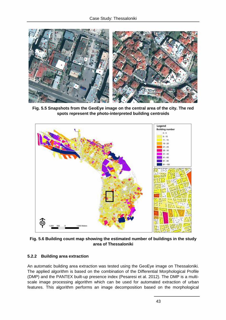
Case Study: Thessaloniki
43
Fig. 5.5 Snapshots from the GeoEye image on the central area of the city. The red
spots represent the photo-interpreted building centroids
Fig. 5.6 Building count map showing the estimated number of buildings in the study
area of Thessaloniki
5.2.2 Building area extraction
An automatic building area extraction was tested using the GeoEye image on Thessaloniki.
The applied algorithm is based on the combination of the Differential Morphological Profile
(DMP) and the PANTEX built-up presence index (Pesaresi et al. 2012). The DMP is a multi-
scale image processing algorithm which can be used for automated extraction of urban
features. This algorithm performs an image decomposition based on the morphological
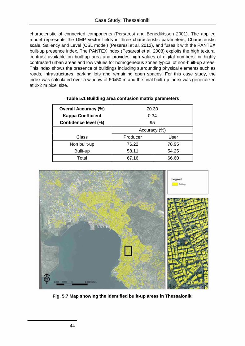
Case Study: Thessaloniki
44
characteristic of connected components (Persaresi and Benediktsson 2001). The applied
model represents the DMP vector fields in three characteristic parameters, Characteristic
scale, Saliency and Level (CSL model) (Pesaresi et al. 2012), and fuses it with the PANTEX
built-up presence index. The PANTEX index (Pesaresi et al. 2008) exploits the high textural
contrast available on built-up area and provides high values of digital numbers for highly
contrasted urban areas and low values for homogeneous zones typical of non-built-up areas.
This index shows the presence of buildings including surrounding physical elements such as
roads, infrastructures, parking lots and remaining open spaces. For this case study, the
index was calculated over a window of 50x50 m and the final built-up index was generalized
at 2x2 m pixel size.
Table 5.1 Building area confusion matrix parameters
Overall Accuracy (%) 70.30
Kappa Coefficient 0.34
Confidence level (%) 95
Class
Accuracy (%)
Producer User
Non built-up 76.22 78.95
Built-up 58.11 54.25
Total 67.16 66.60
Fig. 5.7 Map showing the identified built-up areas in Thessaloniki
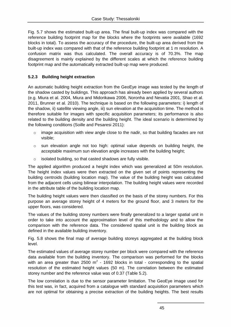
Case Study: Thessaloniki
45
Fig. 5.7 shows the estimated built-up area. The final built-up index was compared with the
reference building footprint map for the blocks where the footprints were available (1692
blocks in total). To assess the accuracy of the procedure, the built-up area derived from the
built-up index was compared with that of the reference building footprint at 1 m resolution. A
confusion matrix was thus calculated. The overall accuracy is of 70.3%. The map
disagreement is mainly explained by the different scales at which the reference building
footprint map and the automatically extracted built-up map were produced.
5.2.3 Building height extraction
An automatic building height extraction from the GeoEye image was tested by the length of
the shadow casted by buildings. This approach has already been applied by several authors
(e.g. Miura et al. 2004, Miura and Midorikawa 2006, Noronha and Nevatia 2001, Shao et al.
2011, Brunner et al. 2010). The technique is based on the following parameters: i) length of
the shadow, ii) satellite viewing angle, iii) sun elevation at the acquisition time. The method is
therefore suitable for images with specific acquisition parameters; its performance is also
related to the building density and the building height. The ideal scenario is determined by
the following conditions (Soille and Pesaresi 2011):
o image acquisition with view angle close to the nadir, so that building facades are not
visible;
o sun elevation angle not too high: optimal value depends on building height, the
acceptable maximum sun elevation angle increases with the building height;
o isolated building, so that casted shadows are fully visible.
The applied algorithm produced a height index which was generalized at 50m resolution.
The height index values were then extracted on the given set of points representing the
building centroids (building location map). The value of the building height was calculated
from the adjacent cells using bilinear interpolation. The building height values were recorded
in the attribute table of the building location map.
The building height values were then classified on the basis of the storey numbers. For this
purpose an average storey height of 4 meters for the ground floor, and 3 meters for the
upper floors, was considered.
The values of the building storey numbers were finally generalized to a larger spatial unit in
order to take into account the approximation level of this methodology and to allow the
comparison with the reference data. The considered spatial unit is the building block as
defined in the available building inventory.
Fig. 5.8 shows the final map of average building storeys aggregated at the building block
level.
The estimated values of average storey number per block were compared with the reference
data available from the building inventory. The comparison was performed for the blocks
with an area greater than 2500 m2 - 1692 blocks in total - corresponding to the spatial
resolution of the estimated height values (50 m). The correlation between the estimated
storey number and the reference value was of 0.37 (Table 5.2).
The low correlation is due to the sensor parameter limitation. The GeoEye image used for
this test was, in fact, acquired from a catalogue with standard acquisition parameters which
are not optimal for obtaining a precise extraction of the building heights. The best results
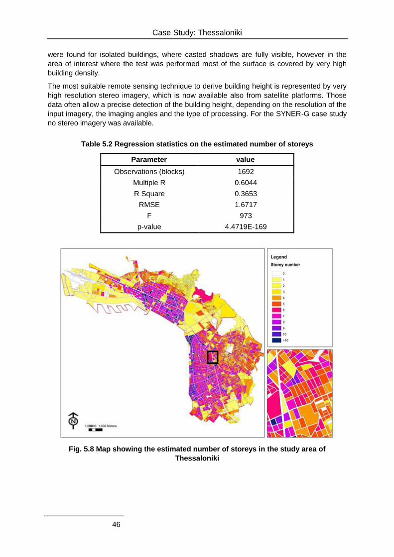
Case Study: Thessaloniki
46
were found for isolated buildings, where casted shadows are fully visible, however in the
area of interest where the test was performed most of the surface is covered by very high
building density.
The most suitable remote sensing technique to derive building height is represented by very
high resolution stereo imagery, which is now available also from satellite platforms. Those
data often allow a precise detection of the building height, depending on the resolution of the
input imagery, the imaging angles and the type of processing. For the SYNER-G case study
no stereo imagery was available.
Table 5.2 Regression statistics on the estimated number of storeys
Parameter value
Observations (blocks) 1692
Multiple R 0.6044
R Square 0.3653
RMSE 1.6717
F 973
p-value 4.4719E-169
Fig. 5.8 Map showing the estimated number of storeys in the study area of
Thessaloniki
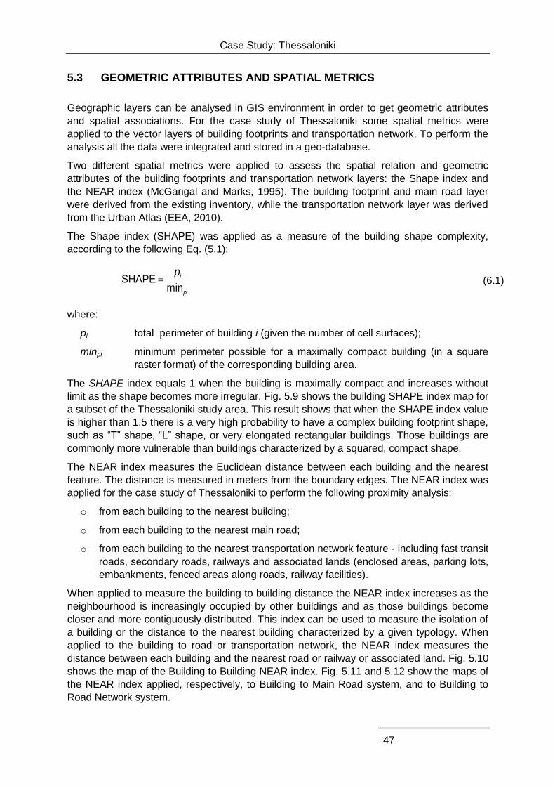
Case Study: Thessaloniki
47
5.3 GEOMETRIC ATTRIBUTES AND SPATIAL METRICS
Geographic layers can be analysed in GIS environment in order to get geometric attributes
and spatial associations. For the case study of Thessaloniki some spatial metrics were
applied to the vector layers of building footprints and transportation network. To perform the
analysis all the data were integrated and stored in a geo-database.
Two different spatial metrics were applied to assess the spatial relation and geometric
attributes of the building footprints and transportation network layers: the Shape index and
the NEAR index (McGarigal and Marks, 1995). The building footprint and main road layer
were derived from the existing inventory, while the transportation network layer was derived
from the Urban Atlas (EEA, 2010).
The Shape index (SHAPE) was applied as a measure of the building shape complexity,
according to the following Eq. (5.1):
SHAPEmin
i
i
p
p (6.1)
where:
pi total perimeter of building i (given the number of cell surfaces);
minpi minimum perimeter possible for a maximally compact building (in a square
raster format) of the corresponding building area.
The SHAPE index equals 1 when the building is maximally compact and increases without
limit as the shape becomes more irregular. Fig. 5.9 shows the building SHAPE index map for
a subset of the Thessaloniki study area. This result shows that when the SHAPE index value
is higher than 1.5 there is a very high probability to have a complex building footprint shape,
such as “T” shape, “L” shape, or very elongated rectangular buildings. Those buildings are
commonly more vulnerable than buildings characterized by a squared, compact shape.
The NEAR index measures the Euclidean distance between each building and the nearest
feature. The distance is measured in meters from the boundary edges. The NEAR index was
applied for the case study of Thessaloniki to perform the following proximity analysis:
o from each building to the nearest building;
o from each building to the nearest main road;
o from each building to the nearest transportation network feature - including fast transit
roads, secondary roads, railways and associated lands (enclosed areas, parking lots,
embankments, fenced areas along roads, railway facilities).
When applied to measure the building to building distance the NEAR index increases as the
neighbourhood is increasingly occupied by other buildings and as those buildings become
closer and more contiguously distributed. This index can be used to measure the isolation of
a building or the distance to the nearest building characterized by a given typology. When
applied to the building to road or transportation network, the NEAR index measures the
distance between each building and the nearest road or railway or associated land. Fig. 5.10
shows the map of the Building to Building NEAR index. Fig. 5.11 and 5.12 show the maps of
the NEAR index applied, respectively, to Building to Main Road system, and to Building to
Road Network system.
Case Study: Thessaloniki
48
Fig. 5.9 Map showing the Building SHAPE index in the study area of Thessaloniki
Fig. 5.10 Map showing the NEAR index for Building to Building proximity analysis in
the study area of Thessaloniki
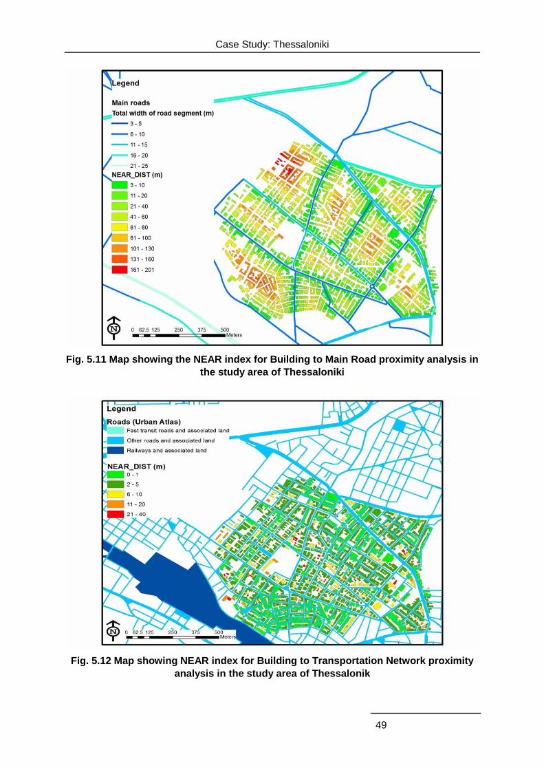
Case Study: Thessaloniki
49
Fig. 5.11 Map showing the NEAR index for Building to Main Road proximity analysis in
the study area of Thessaloniki
Fig. 5.12 Map showing NEAR index for Building to Transportation Network proximity
analysis in the study area of Thessalonik

Case Study: Thessaloniki
50
Spatial metrics, such as the SHAPE and the NEAR indexes, can be stored as attributes in a
vector file and then used in risk assessment applications or emergency evacuation plans.
For example the NEAR index can be applied to evaluate the road closure risk due to the
collapse of a near building of a given typology. This index can also be applied to assess the
distance of a given point or building to the nearest utility network (electric power system, gas
and oil network, water system), or critical infrastructure (healthcare facilities, fire fighting
system).
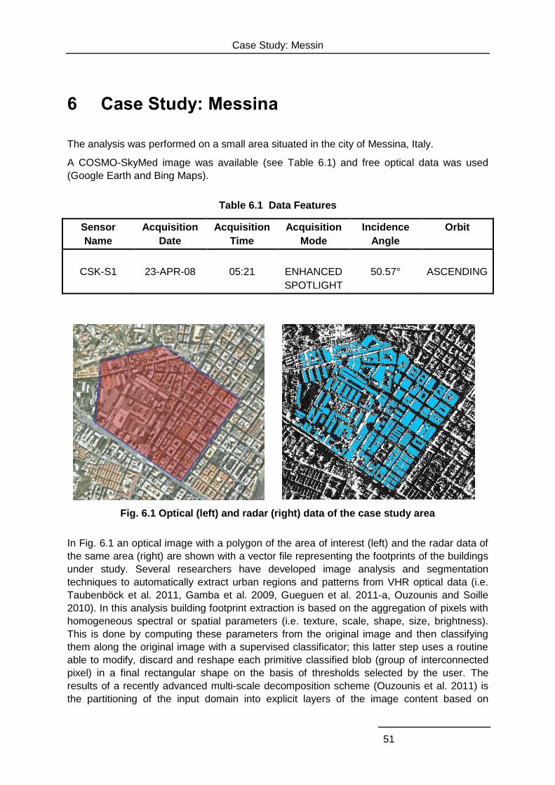
Case Study: Messin
51
6 Case Study: Messina
The analysis was performed on a small area situated in the city of Messina, Italy.
A COSMO-SkyMed image was available (see Table 6.1) and free optical data was used
(Google Earth and Bing Maps).
Table 6.1 Data Features
Sensor
Name
Acquisition
Date
Acquisition
Time
Acquisition
Mode
Incidence
Angle
Orbit
CSK-S1
23-APR-08
05:21
ENHANCED
SPOTLIGHT
50.57°
ASCENDING
Fig. 6.1 Optical (left) and radar (right) data of the case study area
In Fig. 6.1 an optical image with a polygon of the area of interest (left) and the radar data of
the same area (right) are shown with a vector file representing the footprints of the buildings
under study. Several researchers have developed image analysis and segmentation
techniques to automatically extract urban regions and patterns from VHR optical data (i.e.
Taubenböck et al. 2011, Gamba et al. 2009, Gueguen et al. 2011-a, Ouzounis and Soille
2010). In this analysis building footprint extraction is based on the aggregation of pixels with
homogeneous spectral or spatial parameters (i.e. texture, scale, shape, size, brightness).
This is done by computing these parameters from the original image and then classifying
them along the original image with a supervised classificator; this latter step uses a routine
able to modify, discard and reshape each primitive classified blob (group of interconnected
pixel) in a final rectangular shape on the basis of thresholds selected by the user. The
results of a recently advanced multi-scale decomposition scheme (Ouzounis et al. 2011) is
the partitioning of the input domain into explicit layers of the image content based on
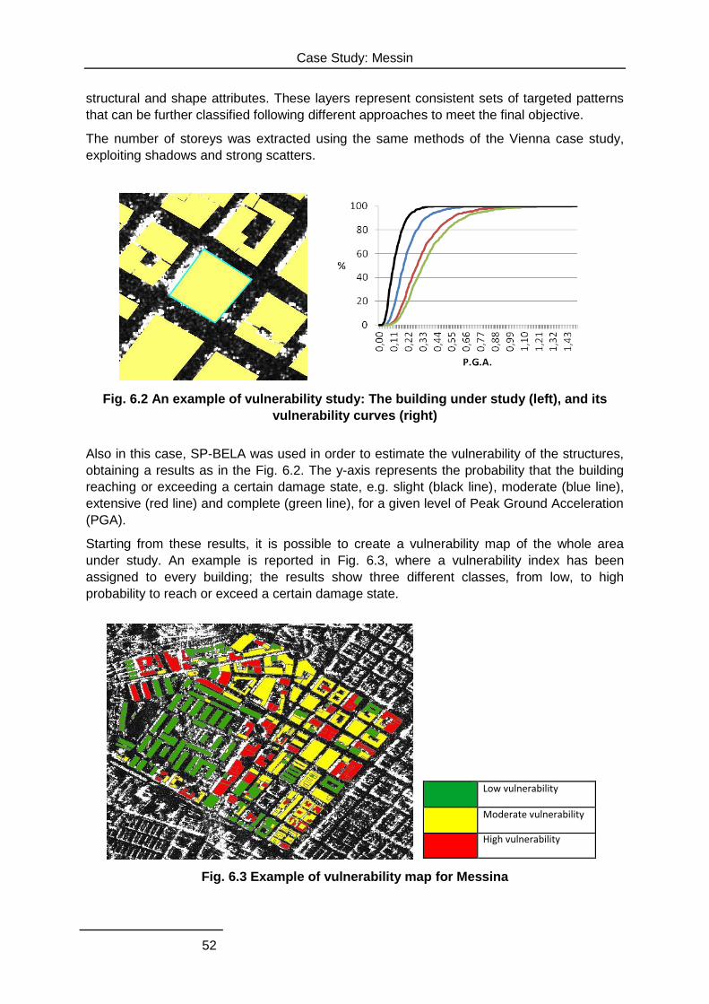
Case Study: Messin
52
structural and shape attributes. These layers represent consistent sets of targeted patterns
that can be further classified following different approaches to meet the final objective.
The number of storeys was extracted using the same methods of the Vienna case study,
exploiting shadows and strong scatters.
Fig. 6.2 An example of vulnerability study: The building under study (left), and its
vulnerability curves (right)
Also in this case, SP-BELA was used in order to estimate the vulnerability of the structures,
obtaining a results as in the Fig. 6.2. The y-axis represents the probability that the building
reaching or exceeding a certain damage state, e.g. slight (black line), moderate (blue line),
extensive (red line) and complete (green line), for a given level of Peak Ground Acceleration
(PGA).
Starting from these results, it is possible to create a vulnerability map of the whole area
under study. An example is reported in Fig. 6.3, where a vulnerability index has been
assigned to every building; the results show three different classes, from low, to high
probability to reach or exceed a certain damage state.
Fig. 6.3 Example of vulnerability map for Messina
Lowvulnerability
Moderatevulnerability
Highvulnerability
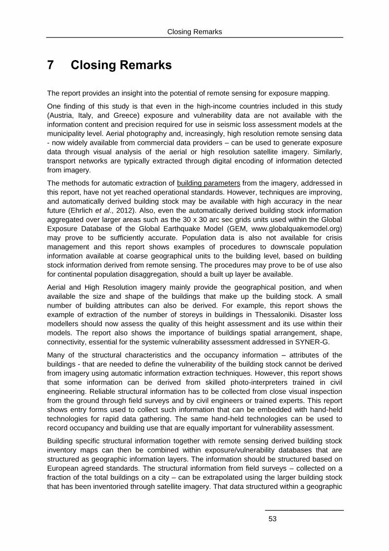
Closing Remarks
53
7 Closing Remarks
The report provides an insight into the potential of remote sensing for exposure mapping.
One finding of this study is that even in the high-income countries included in this study
(Austria, Italy, and Greece) exposure and vulnerability data are not available with the
information content and precision required for use in seismic loss assessment models at the
municipality level. Aerial photography and, increasingly, high resolution remote sensing data
- now widely available from commercial data providers – can be used to generate exposure
data through visual analysis of the aerial or high resolution satellite imagery. Similarly,
transport networks are typically extracted through digital encoding of information detected
from imagery.
The methods for automatic extraction of building parameters from the imagery, addressed in
this report, have not yet reached operational standards. However, techniques are improving,
and automatically derived building stock may be available with high accuracy in the near
future (Ehrlich et al., 2012). Also, even the automatically derived building stock information
aggregated over larger areas such as the 30 x 30 arc sec grids units used within the Global
Exposure Database of the Global Earthquake Model (GEM, www.globalquakemodel.org)
may prove to be sufficiently accurate. Population data is also not available for crisis
management and this report shows examples of procedures to downscale population
information available at coarse geographical units to the building level, based on building
stock information derived from remote sensing. The procedures may prove to be of use also
for continental population disaggregation, should a built up layer be available.
Aerial and High Resolution imagery mainly provide the geographical position, and when
available the size and shape of the buildings that make up the building stock. A small
number of building attributes can also be derived. For example, this report shows the
example of extraction of the number of storeys in buildings in Thessaloniki. Disaster loss
modellers should now assess the quality of this height assessment and its use within their
models. The report also shows the importance of buildings spatial arrangement, shape,
connectivity, essential for the systemic vulnerability assessment addressed in SYNER-G.
Many of the structural characteristics and the occupancy information – attributes of the
buildings - that are needed to define the vulnerability of the building stock cannot be derived
from imagery using automatic information extraction techniques. However, this report shows
that some information can be derived from skilled photo-interpreters trained in civil
engineering. Reliable structural information has to be collected from close visual inspection
from the ground through field surveys and by civil engineers or trained experts. This report
shows entry forms used to collect such information that can be embedded with hand-held
technologies for rapid data gathering. The same hand-held technologies can be used to
record occupancy and building use that are equally important for vulnerability assessment.
Building specific structural information together with remote sensing derived building stock
inventory maps can then be combined within exposure/vulnerability databases that are
structured as geographic information layers. The information should be structured based on
European agreed standards. The structural information from field surveys – collected on a
fraction of the total buildings on a city – can be extrapolated using the larger building stock
that has been inventoried through satellite imagery. That data structured within a geographic

Closing Remarks
54
information layer can then become the data infrastructure from which disaster loss models
can be executed.
The work of this report contributes to define the state-of-the-art in exposure and, to some
extent, vulnerability assessment in Europe. Two important findings are the lack of available
exposure and vulnerability, data and the lack of standardization/procedures for collection of
exposure and vulnerability information for the three countries. This report shows examples
on how remote sensing can be used to address the shortcomings. The report also
contributes to define guidelines for use in the aforementioned Global Exposure Database
(GED) of the Global Earthquake Model (GEM).
References
55
References
Ahola, T., K. Virrantaus, J. M. Krisp and G. J. Hunter, 2007. A spatio-temporal population
model to support risk assessment and damage analysis for decision-making.
International Journal of Geographical Information Science 21, 935-953.
Alberti, M., and P. Waddell. 2000. An integrated urban development and ecological
simulation model. Integrated Assessment 1 (3): 215-227
Annunziato, A., S. Gadenz, D. Galliano, R. Guana and F. Igualada, 2010. Field tracking tool:
a collaborative framework from the field to the decision makers, In: Konecny M., S.
Zlatanova, T. L. Bandrova (Eds.),, Geographic Information and Cartography for Risk and
Crisis Management, Lecture Notes in Geoinformation and Cartography, Springer Berlin
Heidelberg, pp. 287-303.
Argyroudis, S., 2010. Contribution to Seismic Vulnerability and Risk of Transportation
Networks in Urban Environment, PhD Thesis (in Greek), Dept. of Civil Engineering,
Aristotle University of Thessaloniki, Greece.
Azar,D., J. Graesser, R. Engstrom, J. Comenetz, R.M. LeddyJr, N.G. Schechtman, T.
Andrews. 2010.Spatial refinement of census population distribution using remotely
sensed estimates of impervious surfaces in Haiti. International Journal of Remote
Sensing, 31 (21): 5635–5655.
Baggio, C, A. Bernardini, R. Colozza, R. Corazza, M. Della Bella, G. Di Pasquale, M. Dolce,
A. Goretti, A. Martinelli, G. Orsini, F. Papa and G. Zuccaro, 2007. Field Manual for post-
earthquake damage and safety assessment and short term countermeasures (AeDES),
Ed.s Pinto AV, Taucer F, Translation from Italian: Rota, M. and A. Goretti, European
Communities.
Batista e Silva, F., F.J. Gallego. 2010. European Population Density Map 2006. Copenhagen
(Denmark): European Environment Agency. JRC61399
Batista e Silva, F., C. Lavalle, and E. Koomen, 2012. A procedure to obtain a refined
European land use/cover map. Journal of Land Use Science, in press.
Bhaduri, B., E. Bright, P. Coleman and M. Urban. 2007.LandScan USA: A High Resolution
Geospatial and Temporal Modeling Approach for Population Distribution and Dynamics.
GeoJournal 69: 103-117.
Borzi, B., H. Crowley, and R. Pinho, 2008 (a). Simplified Pushover-Based Vulnerability
Analysis for Large Scale Assessment of RC Buildings. Engineering Structures. 30 (3):
804-820.
Borzi, B., H. Crowley and R. Pinho, 2008(b). Simplified Pushover-Based Earthquake Loss
Assessment (SP-BELA) Method for Masonry Buildings. International Journal of
Architectural Heritage, 2(4): 353 — 376.
Briggs, D. J., J. Gulliver, D. Fecht, D. M. Vienneau. 2007. Dasymetric modelling of small-
area population distribution using land cover and light emissions data. Remote Sensing
of Environment 108 (2007): 451–466.
Brunner, D., G. Lemoine, and L. Bruzzone. 2010. Earthquake Damage Assessment of
Buildings Using VHR Optical and SAR Imagery. IEEE Transactions On Geoscience And
Remote Sensing 48 (5).
References
56
Cai, Q., G.Rushton, B.Bhaduri, E. Bright, and P. Coleman. 2006. Estimating Small-Area
Populations by Age and Sex Using Spatial Interpolation and Statistical Inference
Methods. Transactions in GIS, 10(4): 577–598.
Chen, K., 2002. An approach to linking remotely sensed data and areal census data.
International Journal of Remote Sensing,23(1): 37–48.
Dell’Acqua, F, P. Gamba, and G. Lisini, 2005. Urban land cover mapping using
hyperspectral and multispectral vhr Sensors: spatial versus spectral resolution. In:
Proceedings of the ISPRS Joint Symposium URBAN05 and URS05, Tempe, AZ, USA,
March 14-16 2005.
Dell’Acqua, F, 2008. The role of SAR Sensors. In Global Mapping of Human Settlement. In:
P. Gamba and M. Herlod Eds. Taylor and Fracis Series, Remote Sensing Applications,
CRC Press, pp. 309-319.
Dell’Acqua, F., P. Gamba, and D. A. Polli, 2011. Earthquake damage assessment from
post-event VHR radar data: from Sichuan, 2008 to Haiti, 2010. In: STilla, U. Gamba,
Jurgens C., Maktav D (eds), JURSE 2011 – Joint Urban Remote Sensing Event, Munich,
Germany, April 11-13, 2011.
Dell’Acqua, F., D. A. Polli, P. Tenerelli and D. Ehrlich., 2011. D2.14 - Methods to extract
building and road infrastructures from remote sensing and integration with ancillary
information. SYNER-G Deliverable Report.
Dobson, J., E. Bright, P. Coleman, R. Durfee and B. Worley. 2000. LandScan: A global
population database for estimating populations at risk. Photogrammetric Engineering
and Remote Sensing, Volume: 66, Issue: 7, Publisher: Taylor & Francis, Pages: 849-857
Dong, P., S. Ramesh, and A. Nepali. 2010.Evaluation of small-area population estimation
using LiDAR, Landsat TM and parcel data. International Journal of Remote Sensing 31
(21): 5571–5586.
EEA, 1999. CORINE Land Cover. Brussels, Belgium.
EEA, 2010. GMES Urban Atlas. http://www.eea.europa.eu/data-and-maps/data/urban-atlas/
Last accessed on 10 Jan 2012.
Ehrlich D. and P. Tenerelli, 2012. Optical satellite imagery for quantifying spatio-temporal
dimension of physical exposure in disaster risk assessments. Natural Hazards.
Submitted.
Eicher, C., and C. Brewer. 2001. Dasymetric mapping and areal interpolation:
implementation and evaluation. Cartography and Geographic Information Science 28:
125–138.
EUROSTAT, 1997. Classification of Types of Constructions (CC).
FEMA, 2002. Rapid visual screening of buildings for potential seismic hazards: a handbook.
Washington, DC: Federal Emergency Management Agency; FEMA-154.
Franchin, P., F. Cavalieri, P.E. Pinto, et al., 2011. Deliverable 2.1-General methodology for
systemic seismic vulnerability assessment, SYNER-G Project.
Gallego, F.J., 2010. A population density grid of the European Union. Population and
Environment. 31: 460-473.
Gallego, F.J., F. Batista, C.Rocha, and S. Mubareka.2011. Disaggregating population
density of the European Union with CORINE Land Cover. International Journal of
Geographical Information Science, in press.
Gamba, P., F. Dell’Acqua and G. Lisini, 2009. BREC: the Built-up area RECognition tool.
Joint Urban Remote Sensing Event, 22-24 May 2009, Shanghai.
Gao, J., 2009. Digital Analysis of Remotely Sensed Imagery. McGraw-Hill, New York, 2009,
645.
References
57
Gueguen L., M. Pesaresi, A. Gerhardinger, P. Soille, 2011. Characterizing and Counting
Roofless Buildings in Very High Resolution Optical Images journal IEEE Geoscience
and Remote Sensing Letters November 27, 2011
Harvey,J. T. 2002. Estimating census district populations from satellite imagery: Some
approaches and limitations. International Journal of Remote Sensing 23 (10): 2071-2095.
Herold, M., M.E. Gardner and D.A. Roberts, 2003. Spectral resolution requirements for
mapping urban areas. IEEE Trans. Geosc. Remote Sens, 41(9): 1907-1919.
Holt, J., C.P. Lo, T. W. Hodler.2004. Dasymetric estimation of population density and areal
interpolation of census data. Cartography and Geographic Information Science, 31: 103–
121.
Jaiswal, K.S. and DJ. Wald, 2008. Creating a global building inventory for earthquake loss
assessment and risk management. U.S. Geological Survey, Open File Report 2008-
1160, USGS. p. 109.
Kappos, A.J., G. Panagopoulos and G. Penelis, 2008. Development of a Seismic Damage
and Loss Scenario for Contemporary and Historical Buildings in Thessaloniki, Greece.
Soil Dynamics and Earthquake Engineering, 28(10-11): 836-850.
Khazai, B., J. Braun, B. V. Vangelsten and S. Duzgun, 2011. D2.10 Development of an
innovative methodology to assess socio-economic losses based on indicators , SYNER-
G Project.
Legates, D. R., and G. J. Mccabe Jr., 1999. Evaluating the Use of “Goodness-of-Fit”
Measures in Hydrologic and Hydroclimatic Model Validation, Water Resources
Research, 35(1), 233–241.
Li,G., and Q. Weng. 2005. Using Landsat ETM Imagery to Measure Population Density in
Indianapolis, Indiana, USA. Photogrammetric Engineering & Remote Sensing, 71 (8):
947–958.
Liu, X. and K. C. Clarke. 2002. Estimation of residential population using high resolution
satellite imagery. In: Proceedings, Third International Symposium on Remote Sensing of
Urban Areas, June 2002, Istanbul, Turkey, pp. 153-160.
Lu, D., Q. Weng, and G. Li. 2006. Residential population estimation using a remote sensing
derived impervious surface approach. International Journal of Remote Sensing, 27 (16):
3553–3570.
Lu, Z. ,J. Im, L. Quackenbush, K. Halligan. 2010.Population estimation based on multi-
sensor data fusion. International Journal of Remote Sensing, 31 (21): 5587–5604.
Marino, C.M., C. Panigada and L. Busetto, 2001. Airborne hyperspectral remote sensing
applications in urban areas: asbestos concrete sheeting identification and mapping. In:
Proc. of the 1st IEEE/ISPRS Joint Workshop on Remote Sensing and Data Fusion over
Urban Areas, Rome, Italy, 8-9 Nov. 2001, pp. 212-216.
Martin, D., S. Cockings, and S. Leung. 2009. Population 24/7: building time-specific
population grid models. In European Forum for Geostatistics Conference 2009, The
Hague, Netherlands, 5-7 October 2009.
McGarigal, K., and B.J. Marks., 1995. FRAGSTATS: Spatial pattern analysis program for
quantifying landscape structure. Corvallis: Forest Science Department, Oregon State
University.
Mennis, J., 2003. Generating surface models of population using dasymetric mapping. The
Professional Geographer, 55: 31–42.
Mennis, J. and Hultgren, T., 2006. Intelligent dasymetric mapping and its application to areal
interpolation. Cartography and Geographic Information Science, 33(3): 179-194.
References
58
Miura, H., S. Midorikawa, and FujimotoK., 2004. Automated building detection from High-
resolution satellite image for updating GIS building inventory data. In: 13th World
Conference on Earthquake Engineering Vancouver, B.C., Canada, August 1-6, 2004.
Miura, H., and S. Midorikawa. 2006. Updating GIS Building Inventory Data Using High-
Resolution Satellite Images for Earthquake Damage Assessment: Application to Metro
Manila, Philippines. Earthquake Spectra, 22 (1): 151-168.
Mueller, M, K, Segl, U, Heiden, H. Kaufmann, 2006. Potential of High-Resolution Satellite
Data in the Context of Vulnerability of Buildings. Natural Hazards 38:247-258.
McLane, T. R. and K. and A. Porter, 2008. ROVER - Rapid Observation of Vulnerability and
Estimation of Risk. http:// www.sparisk.com/pubs/McLane-Porter-02-Aug-2008-ROVER-
overview.pdf.
Mrozinski, R.D., and R. Cromley. 1999. Singly-and doubly-constrained methods of areal
interpolation for vector-based GIS. Transactions in Geographical Information Systems, 3:
285–301.
Nolte, E.M., B. Khazi and F. Wenzel. 2011. D2.16 Vulnerability assessment by optical
satellite Imagery. SYNER-G Deliverable Report.
Noronha, S., and R. Nevatia. 2001. Detection and Modeling of Buildings from Multiple Aerial
Images. IEEE Transactions On Pattern Analysis And Machine Intelligence, 23 (5).
O’Neil, R.V., B.T Milne., M.G. Turner, R.H. Gadner. 1988. Resource utilization scales and
landscape pattern. Landscape Ecology. 2, pp 63-69.
Ouzounis, G.K., and P. Soille, 2010. Differential Area Profiles. In: 20th International
Conference on Pattern Recognition, 23-26 august 2010, Istanbul, Turkey
Ouzounis, G.K., and P. Soille, 2011. Attribute Constrained Connectivity and Alpha Tree
Representation. IEEE Trans. Image Analysis. Submitted.
Penelis, G.G., D. Sarigiannis, E. Stavrakakis and KC. Stylianidis, 1988. A statistical
evaluation of damage to buildings in the Thessaloniki, Greece, earthquake of June, 20,
1978, Proceedings of the 9th World Conf. on Earthq. Engng., Tokyo-Kyoto, Japan, Aug.
1988, Tokyo: Maruzen, VII:187-192.
Persaresi, M. and J. A. Benediktsson, 2001. A new approach for the morphological
segmentation of high resolution satellite imagery. IEEE Transactions on Geoscience and
Remote Sensing, 39(2):309–320.
Pesaresi, M., A. Gerhardinger, and F. Kayitakire. 2008. A robust built-up area presence
index by anisotropic rotation-invariant textural measure. IEEE Journal of Selected Topics
in Applied Earth Observations and Remote Sensing, 1 (3): 180-192.
Pesaresi M, G.K. Ouzounis, and L. Gueguen. 2012. A new compact representation of
morphological profiles: report on first massive VHR image processing at the JRC. Proc.
SPIE 8390, 839025.
Poli, D., Angiuli E. and Remondino F., 2010. Radiometric and geometric analysis of
WorldView-2 stereo scenes. International Archives of Photogrammetry and Remote
Sensing and Spatial Information Sciences, Vol. XXXVIII, Part 1, 15-18 June 2010,
Calgary, Canada.
Potere, D. and A. Schneider, 2009. Comparison of global urban maps. In: Global Mapping of
Human Settlements, Ed. P. Gamba and M Herlod, CRC Press, 2009, pp. 269-308.
Schneiderbauer, S., and D. Ehrlich. 2005. Population density estimations for disaster
management. Case study rural Zimbabwe. In: van Oosterom, P., S.Zlatanova, E.M.
Fendel.Geo-information for Disaster Management. Proc. of the 1st International
Symposium on Geo-information for Disaster Management', Delft, The Netherlands,
March 21-23, 2005. Eds. Springer, 901-922.
References
59
Shao, Y., G.N. Taff, S.J. Walsh, 2011. Shadow detection and building height estimation
using IKONOS data. International Journal of Remote Sensing, 32 (22): 6929-6944.
Schnedier, A., M. Friedl, and D. Potere, 2009. A new map of global urban extent from
MODIS remote sensing data based on an urban ecoregion approach. In: Global Mapping
of Human Settlements, Ed. P. Gamba and M Herlod, CRC Press, 2009, pp. 107-125.
Silván-Cárdenas, J. L., L. Wang, P.Rogerson, C.Wu, T.Feng and B.D.Kamphaus, 2010.
Assessing fine-spatial-resolution remote sensing for small-area population estimation.
International Journal of Remote Sensing, 31 (21): 5605–5634.
Soille, P. and M. Pesaresi, 2011. Morphological Image Analysis for Remote Sensing City
Analysis. In: Remote Sensing City Analysis Workshop, Joint Research Centre, Ispra, 15-
17 February, 2011.
Steinnocher, K., M. Köstl, J. Weichselbaum. 2011. Grid-based population and land take
trend indicators. In Conference New Techniques and Technologies for Statistics –NTTS,
2011 Brussels, February 22-24.
SYNER-G, 2010a. Working Document WD24,SYNER-G project.
SYNER-G, 2010b. Working Document WD21, SYNER-G project.
Taubenböck, H., T. Esch, M. Wurm, A. Roth, and S. Dech. 2011. Object-based feature
extraction using high spatial resolution satellite data of urban areas. Journal of Spatial
Science, 55 (1): 117–132.
Taubenböck, H., T. Esch, A. Felbier, M. Wiesner, A. Roth, S. Dech, 2012. Monitoring
urbanization in mega cities from space. Remote Sensing of Environment, 117 (15): 162-
176.
Tenerelli, P., and D. Ehrlich. 2010. Analysis of built-up spatial pattern at different scales: can
scattering affect map accuracy? International Journal of Digital Earth, in press, DOI:
10.1080/17538947.2010.512431
Tobler, W. R. 1979. Smooth pycnophylactic interpolation for geographical regions. Journal of
the American Statistical Association, 74,367:519-530.
Toutin, TH, 2004a. DSM generation and evaluation from QuickBird stereo imagery with 3D
physical modelling. International Journal of Remote Sensing, 25(22): 5181-5193.
Toutin, T.H., 2004b. Comparison of Stereo-Extracted DTM from Different High-Resolution
Sensors: SPOT-5, EROS-A, IKONOS-II, and QuickBird. IEEE Transactions on
Geoscience and Remote Sensing, 42(10): 2121-2129.
Toutin, T.H., 2006a. Comparison of DSMs Generated from Stereo HR Images Using 3D
Physical or Empirical Models. Photogrammetric Engineering and Remote Sensing, 72
(5): 597-60.
Toutin, T.H., 2006b. Generation of DSM from SPOT-5 in-track HRS and across-track HRG
stereo data using spatiotriangulation and autocalibration. ISPRS Journal of
Photogrammetry and Remote Sensing, 60 (3): 170-181.
Vogelmann, J.E., S.M. Howard, L. Yang, C.R. Larson, B.K. Wylie, and J.N. Van Driel, 2001.
Completion of the 1990’s National Land Cover Data Set for the conterminous United
States. Photogrammetric Engineering and Remote Sensing, 67:650-662.
Wieland, M., M. Pittore, S. Parolai, J. Szchau, B. Moldobekov and U. Begaliev, 2012.
Estimating building inventory for rapid seismic vulnerability assessment: Towards an
integrated approach based on multi-source imaging. Soil Dynamics and Earthquake
Engineering 36:78-83.
Willmott, C. J., and Matsuura, K., 2005. Advantages of the mean absolute error (MAE) over
the root mean square error (RMSE) in assessing average model performance. Climate
Research, 30(1), 79-82.
References
60
Wu,C., and A.T. Murray. 2007. Population Estimation Using Landsat Enhanced Thematic
Mapper Imagery. Geographical Analysis 39: 26–43.
Wu,S.S., Qiu,X., and Wang,L.. 2006. Using Semi-variance Image Texture Statistics to Model
Population Densities. Cartography and Geographic Information Science (33) 2: 127-140.
Wu,S.S., L. Wang, and X. Qiu. 2008.Incorporating GIS Building Data and Census Housing
Statistics for Sub-Block-Level Population Estimation. The Professional Geographer, 6(1):
121–135
Xi,F., H.S. He, Y. Hu, X. Wu, R. Bu, Y. Chang, M. Liu, and J. Yu. 2009. Simulate urban
growth based on RS, GIS, and SLEUTH model in Shenyang-Fushun metropolitan area
northeaster China. In: Urban Remote Sensing Event, 2009 Joint,20-22 May 2009,
Shanghai.
Yuan, Y., R. Smith, and W. Limp. 1997. Remodelling census population with spatial
information from LandsatTM imagery. Computers Environment and Urban Systems, 21:
245–258.


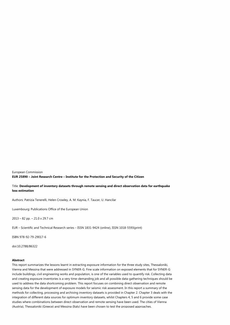
European Commission
EUR 25890 – Joint Research Centre – Institute for the Protection and Security of the Citizen
Title: Development of inventory datasets through remote sensing and direct observation data for earthquake
loss estimation
Authors: Patrizia Tenerelli, Helen Crowley, A. M. Kaynia, F. Taucer, U. Hancilar
Luxembourg: Publications Office of the European Union
2013 – 82 pp. – 21.0 x 29.7 cm
EUR – Scientific and Technical Research series – ISSN 1831-9424 (online), ISSN 1018-5593(print)
ISBN 978-92-79-29017-6
doi:10.2788/86322
Abstract
This report summarizes the lessons learnt in extracting exposure information for the three study sites, Thessaloniki,
Vienna and Messina that were addressed in SYNER-G. Fine scale information on exposed elements that for SYNER-G
include buildings, civil engineering works and population, is one of the variables used to quantify risk. Collecting data
and creating exposure inventories is a very time-demanding job and all possible data-gathering techniques should be
used to address the data shortcoming problem. This report focuses on combining direct observation and remote
sensing data for the development of exposure models for seismic risk assessment. In this report a summary of the
methods for collecting, processing and archiving inventory datasets is provided in Chapter 2. Chapter 3 deals with the
integration of different data sources for optimum inventory datasets, whilst Chapters 4, 5 and 6 provide some case
studies where combinations between direct observation and remote sensing have been used. The cities of Vienna
(Austria), Thessaloniki (Greece) and Messina (Italy) have been chosen to test the proposed approaches.

z
As the Commission’s in-house science service, the Joint Research Centre’s mission is to provide
EU policies with independent, evidence-based scientific and technical support throughout the
whole policy cycle.
Working in close cooperation with policy Directorates-General, the JRC addresses key societal
challenges while stimulating innovation through developing new standards, methods and tools,
and sharing and transferring its know-how to the Member States and international community.
Key policy areas include: environment and climate change; energy and transport; agriculture
and food security; health and consumer protection; information society and digital agenda;
safety and security including nuclear; all supported through a cross-cutting and multi-
disciplinary approach.
LB
-NA
-25890-E
N-C
Related Documents