Development of HF radar inversion algorithm for spectrum ...w3.u-ryukyu.ac.jp/yhisaki/manuscript/2015-Journal...RESEARCH ARTICLE 10.1002/2014JC010548 Development of HF radar inversion

RESEARCH ARTICLE10.1002/2014JC010548

Development of HF radar inversion algorithm for spectrumestimation (HIAS)Yukiharu Hisaki1

1Department of Physics and Earth Sciences, University of the Ryukyus, Okinawa, Japan

Abstract A method for estimating ocean wave directional spectra using an HF (high-frequency)ocean radar was developed. This method represents the development of work conducted in previousstudies. In the present method, ocean wave directional spectra are estimated on polar coordinateswhose center is the radar position, while spectra are estimated on regular grids. This method can beapplied to both single and multiple radar cases. The area for wave estimation is more flexible than thatof the previous method. As the signal to noise (SN) ratios of Doppler spectra are critical for waveestimation, we develop a method to exclude low SN ratio Doppler spectra. The validity of the methodis demonstrated by comparing results with in situ observed wave data that it would be impossible toestimate by the methods of other groups.

1. Introduction

An HF ocean radar observes surface currents and ocean waves by radiating HF radio waves to the sea sur-face. Surface currents are estimated by identifying the first-order Doppler peaks in the Doppler spectrumfrom HF ocean radar. The wave spectrum is estimated not only from the first-order, but also from thesecond-order scattering. Although estimating ocean wave spectra is important for both scientific and practi-cal applications, few studies have sought to estimate ocean wave spectra from HF radar [e.g., Lipa and Bar-rick, 1986; Wyatt, 1990; Howell and Walsh, 1993; Hisaki, 1996; Hashimoto et al., 2003]. Here we developed amethod for estimating ocean wave spectra from HF radar.

The relationship between the ocean wave spectrum and the second-order radar cross section is written interms of the integral equation. The wave spectrum is inverted from the integral equation.

Methods have previously been developed for estimating ocean wave spectra. Wyatt [1990] and Howell andWalsh [1993] developed the inversion method, in which the integral equation is linearized by assuming thespectral form at higher frequencies. Hisaki [1996] and Hashimoto et al. [2003] developed a method of theinversion without linearization. An ocean wave directional spectrum at a given location can be estimatedfrom two or more radars in these methods. The SN ratios in the Doppler spectra at the position in all radarsmust be high enough to estimate a wave spectrum. The area for wave estimation is thus limited in thesemethods.

A method to estimate ocean wave spectra using a single radar has also been developed [e.g., de Valk et al.,1999; Hisaki, 2005, 2006, 2009, 2014]. In this method, constraints such as the energy balance equation areused along with the relationship between the wave spectra and Doppler spectra. Wave spectra are esti-mated on radial grid points with the origin at the radar position in the method. Hisaki [2005] compared sin-gle radar-estimated wave data with in situ observed wave data; he then [Hisaki, 2006] described andverified the method from simulated Doppler spectra. The radar-wave data were significantly affected by thecontamination of Doppler spectra, and so Hisaki [2009] developed a method of quality control for singleradar-estimated wave data. He then [Hisaki, 2014] compared radar-estimated wave data with model-predicted wave data.

These methods are for a phase array system. Wave parameters are also estimated by the Coastal OceanDynamics Applications Radar (CODAR)-type HF radars, which is a compact antenna system. The CODAR-type HF radar systems, however, can only isolate the Doppler spectrum in range, not in azimuth. The waveparameters are estimated by applying the Pierson-Moskowitz model to second-order Doppler spectra in theCODAR radar system [Long et al., 2011].

Key Points:� A method to estimate ocean wave

directional spectrum from HF radar isdeveloped� Estimate wave spectrum even at

single radar Doppler spectrum cells� This method is verified by comparing

with in situ wave data

Correspondence to:Y. Hisaki,[email protected]

Citation:Hisaki, Y. (2015), Development of HFradar inversion algorithm for spectrumestimation (HIAS), J. Geophys. Res.Oceans, 120, doi:10.1002/2014JC010548.

Received 27 OCT 2014

Accepted 30 JAN 2015

Accepted article online 6 FEB 2015

HISAKI VC 2015. American Geophysical Union. All Rights Reserved. 1

Journal of Geophysical Research: Oceans

PUBLICATIONS

http://dx.doi.org/10.1002/2014JC010548

http://onlinelibrary.wiley.com/journal/10.1002/(ISSN)2169-9291/

http://publications.agu.org/

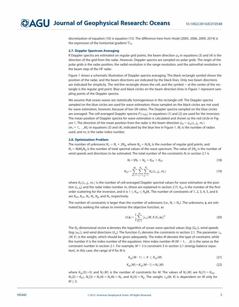
We extend the method in the present work, thewave spectra are estimated on the regular grid,and this method can be applied to both singleand multiple radar array cases. The area for waveestimation is flexible, because wave spectra atpositions where the Doppler spectra are notobserved can be estimated in this method. Themethod is named HIAS (HF radar Inversion Algo-rithm for Spectrum estimation).

The objectives of this paper are as follows: (1) todescribe the HIAS; (2) to describe the method forexcluding low SN Doppler spectra; and (3) to vali-date the HIAS by comparing results with in situobservations.

This paper is organized as follows. The inversionmethod is described in section 2. In section 3, wepresent the observations by HF radar and themethod to select Doppler spectra for wave esti-mation. The results of the selection of Dopplerspectra and wave estimation are presented insection 4, and discussed in section 5. We summa-rize our conclusions in section 5.

2. Inversion Method

2.1. ConstraintsThe inversion method is almost the same as that described in Hisaki [2005, 2006]. The details are presentedin Hisaki [2005, 2006, 2009]. The constraints for estimating wave spectra are as follows:

1. The relationship between the first-order Doppler spectrum and ocean wave directional spectrum.

2. The relationship between the second-order Doppler spectrum and ocean wave directional spectrum.

3. The energy balance equation under the assumption of stationarity.

4. Regularization constraints for spectral values in the wave frequency-wave direction plane.

5. The continuity equation of surface winds.

6. Regularization constraints for spectral values in the x-y plane.

2.2. Relationship Between the First and Second-Order Doppler Spectrum and Wave SpectrumAn observed Doppler spectral density PðxDNÞ at a normalized Doppler frequency xDN5xD=xB is decom-posed into

P1ðxDNÞ5PðxDNÞ xdlNðmÞ � xDN � xduNðmÞ (1)

P2ðxDNÞ5PðxDNÞ xDN < xdlNðmÞ; xDN > xduNðmÞ (2)

where P1ðxDNÞ and P2ðxDNÞ are the first and second-order Doppler spectral densities, respectively.Parameters xD and xB are a radian Doppler frequency and the radian Bragg frequency, respectively.The normalized Doppler frequency ranges xdlNðmÞ and xduNðmÞ are lower and upper Doppler frequen-cies of the first-order scattering for the negative (m 5 1) and positive (m 5 2) Doppler frequency regions,respectively. They satisfy xdlNðmÞ< 2m23<xduNðmÞ, and are determined by identifying local minimaaround the two first-order scattering peaks [e.g., Hisaki, 2006, Figure 1]. The effect of the surface currenton the Doppler spectrum is corrected. The Doppler spectra are shifted so that the first-order peaks areat the Bragg frequency.

The first and second-order Doppler spectral densities are written in terms of a normalized wave directionalspectrum GNðxN; hÞ5xBð2k0Þ2Gðx; hÞ, in which k0 is the radio wave number, x is the radian wave

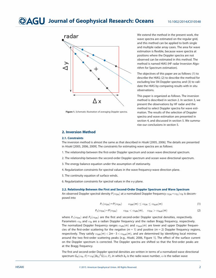
Figure 1. Schematic illustration of averaging Doppler spectra.

Journal of Geophysical Research: Oceans 10.1002/2014JC010548


frequency, h is the wave direction, and xN 5 x=xB is the normalized frequency. The radian Bragg wave fre-quency is xB 5 ð2gk0Þ1=2 for deep water, where g is the gravitational acceleration. The subscript ‘‘N’’ denotesthe normalized form by the Bragg parameters, such as xB and Bragg wave number 2k0.

The relationship between the first-order Doppler spectral density P1ðxDNÞ and the normalized first-orderradar cross section r1NðxDNÞ is written in equations (2), (4), (5), and (6) in Hisaki [2006]; the relationshipbetween the second-order Doppler spectral density P2ðxDNÞ and the normalized second-order radar crosssection r2NðxDNÞ is written in equations (3), (4), (5), and (7) of that same study. The integrated first-orderradar cross section is written asð1

0r1Nðð2m23ÞxDNÞdxDN52pGNð1;wB1ðm21ÞpÞ; ðm51; 2Þ (3)

for deep water, where wB is the radar beam direction. The second-order radar cross section is written interms of GNðxN; hÞ, as

r2NðxDNÞ5ðhL1wB

2hL1wB

KlðxDN; hbÞGNðx1N; h1ÞGNðx2N; h2Þdh (4)

where hb 5h2wB [Hisaki, 2006]. Meanwhile, the kernel function KlðxDN; hbÞ may be found in equation (29)in Hisaki [1996]. The integration range hL in equation (4) is p for x2

D � 2 for deep water, or equations (19),(20), and (21) in Hisaki [1996] for shallow water. The normalized wave frequencies and directions, ðx1N; h1Þand ðx2N; h2Þ, are those of wave components contributing to the second-order scattering. Details regardingthe calculation of equation (4) are described in Hisaki [1996].

2.3. Energy Balance EquationThe energy balance equation under the assumption of the stationarity of wavefields is written as

CgN � rNGNðxN; hÞ2StN50 (5)

where CgN5@xN=@kN is the normalized group velocity vector of waves for wave frequency xN andwave number vector kN;rN denotes the normalized horizontal gradient by 1=ð2k0Þ, and StN denotesthe total wave energy input [Hisaki, 2006]. The parameterization of the source function StN is thesame as that in Hisaki [2006]. The propagation term in equation (5) is written in the regular coordi-nates (xN, yN) 5 2k0ðx; yÞ as

CgN � rNGNðxN; hÞ5CgxN@GNðxN; hÞ

@xN1CgyN

@GNðxN; hÞ@yN

(6)

where CgxN and CgyN are the x and y components of the group velocity vector CgN . They are written as

ðCgxN; CgyNÞ5CgNðcos h; sin hÞ (7)

where h is the wave direction with respect to the x direction, and the counterclockwise is positive.

2.4. Other ConstraintsThe source function StN in equation (5) is not only dependent on the wave spectrum but also on the windvector. The unknowns to be estimated are spectral values and wind vectors. The continuity equation of thenondivergent sea surface wind vector uN5ðuxN; uyNÞ5ðuNcos hw ; uNsin hwÞ is written as

rN � uN50 (8)

or

@ðuNcos hwÞ@xN

1@ðuNsin hwÞ

@yN50 (9)

Equation (8) is the same as equation (15) in Hisaki [2006]. Equation (9) is written in the regular coordinate,while equation (16) in Hisaki [2006] is written in the polar coordinate.



The constraint written as

CgN � rNGNðxN; hÞ50 (10)

is used as a regularization constraint in the horizontal plane. This is in order to reduce the computationtime [Hisaki, 2006].

2.5. DiscretizationThe wave spectral values GNðxN; hÞ5GNðxN; h; xN; yNÞ are estimated on the xN – h – xN – yN space at

log xN5log ðxNðkf ÞÞ5log ðxminNÞ1ðkf 21Þlog ðDxÞ; ðkf 51; :::::;Mf Þ (11)

h5hðldÞ52p12pMdðld21Þ; ðld51; ::::;MdÞ (12)

xN5xNðixÞ5DxNðix21Þ ðix51; ::::;NxÞ (13)

and

yN5yNðjyÞ5DyNðjy21Þ ðjy51; ::::;NyÞ (14)

where kf is the wave frequency index number, Mf is the number of frequencies, Dx > 1 is the increment ofthe frequency, ld is the wave direction index number, and Md is the number of directions. The normalizedspatial resolutions in the x and y directions are DxN52k0Dx and DyN52k0Dy, respectively, where ðDx;DyÞ isthe dimensional horizontal resolution. The number of grids in the x and y directions are Nx and Ny, respec-tively. Meanwhile, the index number of the grids in the x and y directions are ix and jy, respectively.

The discretized propagation term CgN � rNGNðxN; hÞ in equations (5) and (10) is Adðkf ; ld; ix ; jyÞ, which is writ-ten as

Adðkf ; ld; ix ; jyÞ5CgN � rNGNðxN; hÞ

5CgxNðkf ; ldÞGNðkf ; ld; ix1mx1; jyÞ2GNðkf ; ld; ix2mx2; jyÞ

ðmx11mx2ÞDxN

1CgyNðkf ; ldÞGNðkf ; ld; ix ; jy1my1Þ2GNðkf ; ld; ix ; jy2my2Þ

ðmy11my2ÞDyN

(15)

The continuity equation (equation (8)) is discretized as

uxNðix1mx1; jyÞ2uxNðix2mx2; jyÞðmx11mx2ÞDxN

1uyNðix; jy1my1Þ2uyNðix ; jy2my2Þ

ðmy11my2ÞDyN50 (16)

where mx1;mx2;my1, and my2 in equations (15) and (16) are 0 or 1. The value mx150 for ix 5 Nx, mx250 forix 5 1, my150 for jy 5 Ny, and my250 for jy 5 1. Otherwise, they are 1.

The regularization constraint is expressed as

log ðGNðkf 11; ldÞÞ1log ðGNðkf 21; ldÞÞ

1log ðGNðkf ; ld21ÞÞ1log ðGNðkf ; ld11ÞÞ

24log ðGNðkf ; ldÞÞ50 for 1 < kf < Mf and 1 � ld � Md

or log ðGNðkf ; ld21ÞÞ1log ðGNðkf ; ld11ÞÞ

22log ðGNðkf ; ldÞÞ50 for kf 51;Mf

(17)

where GNðkf ; 0Þ5GNðkf ;MdÞ and GNðkf ;Md11Þ5GNðkf ; 1Þ.

2.6. Summary of ConstraintsConstraints 1 in section 2.1 are equations (2), (4), (5), and (6) in Hisaki [2006] and equation (3); constraints 2in section 2.1 are equations (3–5) and (7) in Hisaki [2006] and equation (4). The discretization of equation (4)is described in Hisaki [1996]. Constraint 3 in section 2.1 is equation (5). The source function, including thenonlinear source function, is discretized as section 3b in Hisaki [2006], and the propagation term is discre-tized as equation (15). Constraint 4 is discretized as equation (17), and constraint 5 in section 2.1 is equation(8). The discretization of equation (8) is equation (16). Constraint 6 in section 2.1 is equation (10), and the



discretization of equation (10) is equation (15). The difference here from Hisaki [2005, 2006, 2009, 2014] isthe expression of the horizontal gradient rN .

2.7. Doppler Spectrum AveragingIf Doppler spectra are estimated on regular grid points, the beam direction wB in equations (3) and (4) is thedirection of the grid from the radar. However, Doppler spectra are sampled on polar grids. The origin of thepolar grids is the radar position, the radial resolution is the range resolution, and the azimuthal resolution isthe beam step of the HF radar.

Figure 1 shows a schematic illustration of Doppler spectra averaging. The black rectangle symbol shows theposition of the radar, and the beam directions are indicated by the black lines. Only two beam directionsare indicated for simplicity. The red-line rectangle shows the cell, and the symbol 1 at the center of the rec-tangle is the regular grid point. Blue and black circles on the beam direction lines in Figure 1 represent sam-pling points of the Doppler spectra.

We assume that ocean waves are statistically homogeneous in the rectangle cell. The Doppler spectrasampled on the blue circles are used for wave estimation; those sampled on the black circles are not usedfor wave estimation, however, because of low SN ratios. The Doppler spectra sampled on the blue circlesare averaged. The cell-averaged Doppler spectra PðxDNÞ in equations (1) and (2) are used for the inversion.The mean position of Doppler spectra for wave estimation is calculated and shown as the red circle in Fig-ure 1. The direction of the mean position from the radar is the beam direction wB 5 wBðix ; jy ;mrÞ(mr 5 1,. . .,Mr) in equations (3) and (4), indicated by the blue line in Figure 1. Mr is the number of radarsused, and mr is the radar index number.

2.8. Optimization ProblemThe number of unknowns Nu 5 Ns 1 2Ng, where Ng 5 NxNy is the number of regular grid points, andNs 5 MfMdNg is the number of total spectral values of the wave spectrum. The value of 2Ng is the number ofwind speeds and directions to be estimated. The total number of the constraints Nt in section 2.1 is

Nt53Ns 1 Ng 1 KDF 1 KDT (18)

KDT 5XMr

mr 51

XNx

ix 51

XNy

jy 51

KDðix; jy ;mrÞ (19)

where KDðix ; jy ;mrÞ is the number of cell-averaged Doppler spectral values for wave estimation at the posi-tion (ix, jy) and the radar index number mr (these are explained in section 2.7). KDF is the number of the first-order scattering for the inversion, and it is 1� KDF�NgMr. The number of constraints of 1, 2, 3, 4, 5, and 6are KDF, KDT, Ns, Ns, Ng, and Ns, respectively.

The number of constraints is larger than the number of unknowns (i.e., Nt>Nu). The unknowns, s, are esti-mated by seeking the values to minimize the objective function, as

UðsÞ5 12

XNt

K51

½kwðM; KÞFkðsÞ�2 (20)

The Nu-dimensional vector s denotes the logarithm of ocean wave spectral values (log ðGNÞ), wind speeds(log ðuNÞ), and wind directions (hw). The function FK denotes the constraints in section 2.1. The parameter kw

ðM; KÞ is the weight, which should be given adequately. The index M denotes the type of constraint, whilethe number K is the index number of the equations. Here index number M (M 5 1,. . .,6) is the same as theconstraint number in section 2.1. For example, M 5 3 is constraint 3 in section 2.1 (energy balance equa-tion). In this case, the range of K for M is

KrgðM21Þ < K � KrgðMÞ (21)

KrgðMÞ5KrgðM21Þ1NcðMÞ (22)

where Krgð0Þ50, and NcðMÞ is the number of constraints for M. The values of NcðMÞ are Nc(1) 5 KDF,Nc(2) 5 KDT, Nc(3) 5 Nc(4) 5 Nc(6) 5 Ns, and Nc(5) 5 Ng. The weight kw(M, K) is dependent on M only forM� 3.



The contribution to the solution of the cell-averaged Doppler spectrum from many Doppler spectra is large,while the contribution of averaged Doppler spectrum from a few Doppler spectra is small. The weightkw(M,K) for M 5 1 and 2 is dependent on the number of Doppler spectra for averaging, explained in section2.7. The weight is written as

kwðM; KÞ5kwMNdðix ; jy ;mrÞ ðM51; 2Þ (23)

where Nd(ix,jy,mr) is the number of Doppler spectra for averaging in the cell (ix, jy) and the radar index num-ber mr. The parameters kwM (M 5 1, 2) are adequately given. The number of Doppler spectra for constraints1 and 2 in section 2.1 are the same here. The algorithm to solve the optimization problem of equation (20)is the same as in Hisaki [2006, 2009].

3. Data Analysis

3.1. ObservationThe Doppler spectra from 17 April 1998to 13 May 1998, observed to the east of Okinawa Island,Japan, were used for analysis. Observations are described in Hisaki et al. [2001] and Hisaki [2002].Radio frequency was 24.5 MHz, and Bragg frequency fB 5 xB=(2p) was 0.506 Hz. The sampling inter-val of radar signals was 0.5 s, which gave a Nyquist frequency of 1 Hz. Resolution in the Dopplerfrequency was 1/128 Hz.

Figure 2 shows the HF radar observation area. In the figure, the radar locations are A (26:12� N; 127:76� E)and B (26:31�N; 127:84�E). Beam directions of radar A are from 43:5�T to 126�T. Those of radar B are from118:5�T to 201�T. Beam step is 7:5�, number of beam directions for each radar is 12, and range resolution is1.5 km. The black triangles and squares in Figure 2 are sampling points of Doppler spectra from radars Aand B, respectively. The temporal resolution of observed Doppler spectra was 2 h. The period of analysiswas from 0 LST (Local Standard Time) 17 April 1998to 22 LST 13 May 1998.

Waves were measured at position N in Figure 2 using the Ultrasonic Wave Gauge (USW) (Port and HarbourResearch Institute, Japan). The USW measures surface waves at 0.5 s intervals. Significant wave heights wereestimated using the zero-up-cross method based on 20 min of observation of surface displacements at 2 hintervals [e.g., Hisaki, 2007]. The water depth at N in Figure 2 was 46 m.

The regular grids for wave estimation are indicated in Figure 2. The x direction is eastward and the y direc-tion northward. Number of grid points is Nx 5 Ny 5 4 for both x and y directions; grid size is Dx5Dy59 km.Symbols 1 in Figure 2 designate the centers of the regular cells processed from radial grids. The grid centerposition for ix 5 jy 5 1 is (25:95�N; 127:9�E).

The wave parameters estimated by the HF radar were the same as those in Hisaki [2009]. The wave fre-quency parameters in equation (11) were Dx 5 1.15, xmin=(2p) 5 0.049 Hz, and Mf 5 21. The maximumwave frequency was xmax=(2p) 5 0.813 Hz; the wave direction parameter in equation (12) was Md 5 18; andthe number of unknowns was Nu 5 6080.

The Doppler frequency ranges of the second-order scattering for wave estimation were 0.61� |xDN|� 0.94and 1.06� |xDN|� 1.39 at the 0.03 interval, and KDðix ; jy ;mrÞ548 for Ndðix ; jy ;mrÞ > 0. The normalizedDoppler frequency interval 0.03 is different from that of measured Doppler spectra (1=ð128fBÞ). The value P2

ðxDNÞ for the cell-averaged Doppler spectrum was interpolated with respect to the Doppler frequency.

The noise floor was subtracted from the cell-averaged Doppler spectrum, and evaluated by averagingthe lowest quarter of the Doppler spectral values. The evaluated noise floor was much smaller than thesecond-order Doppler peak values. The mean ratio of the second-order Doppler peak to the noise floorwas 13 dB.

The weight in equations (20) and (23) was kw1=kw25ðm1=m2Þ1=2, where m1 is the degree of freedom of the

integrated first-order Doppler spectrum, and m2 is the degree of freedom of the second-order Doppler spec-

trum. Sampling variability in the spectral estimate is inversely proportional to the square of the degree of

freedom. Here the values were m1572 and m2511 [e.g., Hisaki, 2005, 2009]. Other weights were kw2510, and

kwðM; KÞ51 for M � 3. We calculated for different values of the weights, and wave estimation results were

similar to those presented in this paper.



3.2. Selection of Doppler SpectraIf a Doppler spectrum is significantly contaminated by noise, radar-estimate wave data will not be good.The selection of Doppler spectra is critical for wave estimation. The methods and criteria for selecting Dopp-ler spectra are as follows:

1. Manual selection.

2. Identification of first-order scattering.

3. Classification of Doppler spectra by the self-organizing map (SOM) analysis.

4. Ratio of the second-order scattering to the first-order scattering.

A manual selection of Doppler spectra may be useful. However, it is impossible to select manually from toomany Doppler spectra. This method was applied only for Doppler spectra averaged over the observationperiod. Figure 3 shows examples of averaged Doppler spectra from radar A and beam direction 96�T. Thecorresponding distances of Doppler spectra from radar A are from 3 to 51 km in Figure 3.

The second-order scattering is not so clear in averaged Doppler spectra from 3 km (red line) to 9 km (redline) in Figure 3. The Doppler peaks at xDN ’ 20.4 for longer distance are spurious, because this Dopplerpeak becomes larger as distance increases. The Doppler peaks at xDN ’ 21.7 for longer distances are alsospurious. The distance of the Doppler spectra passed criteria 1 for this radar A and beam direction 96� Twas from 10.5 to 30 km. This selection was performed for both radars (A and B), and for 12 beam directionsfor each radar manually. The ranges of the distance of Doppler spectra from the radar were decided foreach radar and beam direction manually from Doppler spectra averaged over the observation period. Out-of-range Doppler spectra were not used for wave estimation. Some other spectra within the range werealso not used for wave estimation.

Figure 2. Map of HF radar observation area.



At the least, the first-order scatter-ing peaks must be identified forwave estimation. In addition, thefirst-order scattering Doppler fre-quency rangesxdlNðmÞ< 2m23<xduNðmÞ,(m 5 1, 2) must be identified. Theyare identified by seeking the localminima of the running averageDoppler spectrum. Doppler spectraare running averaged with respectto Doppler frequencies. If theDoppler frequencies of local min-ima are sensitive to the runningaverage number, we consider thatthe first-order scattering Dopplerfrequency ranges(xdlNðmÞ;xduNðmÞ) are notidentified.

The SOM method described in Liuand Weisberg [2005] and Hisaki[2013] was used to classify theDoppler spectra. The purpose ofclassifying the Doppler spectra is toisolate those spectra contaminatedby noise.

SOM analysis evaluates the weightvectors and the best-matchingunit (BMU). The BMU is the group

number, and the weight vector shows the pattern of the group. The SOM array is the array of weightvectors. The distance between two units in the SOM array indicates the similarity of the groups. Forexample, in the case of the KS3KS SOM array, the BMU is from 1 to K 2

S . The distance between BMU 5 1and BMU 5 2 is 1, and the distance between BMU 5 1 and BMU 5 KS 1 1 is also 1, this shows that thegroups of BMU 5 2 and BMU 5 KS 1 1 are the most similar to the group of BMU 5 1. The distancebetween BMU 5 1 and BMU 5 K 2

S is ðKS21Þffiffiffi2p

, which shows that the groups of BMU 5 1 and BMU 5 K 2S

are the most dissimilar to each other.

A Doppler spectrum is converted to

QðxDNÞ510log 10

�Pðð2m23ÞxDNÞ

Pð2m23Þ

�ðm51 or 2Þ (24)

where m 5 1 for Pð21Þ> P(1), and m 5 2 for P(21)� P(1). The maximum value of QðxDNÞ is 0 dB at xDN 5 1.This conversion aims to avoid to classify the Doppler spectra of P(21)> P(1) and those of Pð21Þ< P(1) intodifferent groups. The Doppler spectrum is normalized by the peak value of the Doppler spectrum, and thenconverted into decibels. The Doppler frequency range for the classification is xpdN� |xDN|�xqdN, wherexpdN and xqdN are given parameters.

The first 1000 Doppler spectra that satisfied criteria 1 and 2 were used for classification. They were classifiedinto KS 3 KS groups. We selected the groups that included the Doppler spectra contaminated by noise. The1000 Doppler spectra were used to establish group numbers (BMU) and typical patterns (weight vectors) ofDoppler spectra for each group. Other Doppler spectra that satisfied criteria 1 and 2 were classified into anygroup of KS 3 KS groups. If the Doppler spectrum belonged to the noisy Doppler spectrum groups, it wasnot used for wave estimation.

Figure 3. Averaged Doppler spectra for various ranges (distances from the radar). Theradar is A in Figure 2, and the beam direction is 96�T. The left vertical axis indicates thedistance of each Doppler spectrum from the radar. The right vertical axis indicates therelative signal intensity in decibels.



The parameter

R125

"8

Ð121 P2ðxDNÞ=wðxDNÞdxDNÐ1

21 P1ðxDNÞdxDN

#1=2

’" 8X2

m51

ÐxqdN

xpdNP2ðð2m23ÞxDNÞ=wðxDNÞdxDN

X2

m51

ÐxduNðmÞxdlNðmÞ P1ðxDNÞdxDN

#1=2(25)

where w(xDN) is the weighting function for normalized Doppler frequency xDN defined in Barrick [1977] wasevaluated for the Doppler spectra that passed criteria 1–3. The value of R12 can be seen as a rough approxima-

tion of the wave height [Barrick, 1977]. Ifthe value of R12 for a Doppler spectrumwas much larger than those of otherDoppler spectra, that spectrum wasexcluded from wave estimation.

4. Results

4.1. Doppler SpectrumThe SOM was applied for QðxDNÞ in equa-tion (24). The parameters were MS 5 5,xpdN 5 0.5, and xqdN 5 1.5.

Figure 4 shows the weight vectors ofSOM classification of QðxDNÞ in equation(24) for BMU 5 1 and BMU 5 25. Theweight vector shows the classificationpattern for each BMU. The examples inFigure 4 are frequent patterns. The dis-tance between the BMU 5 1 andBMU 5 25 was the longest in the SOMarray, which means that these patternswere opposite to each other. The fre-quency for BMU 5 1 was 9.4% (Figure 4a),which means that 1000 3 0.094 5 94Doppler spectra belonged to this group.The frequency for BMU 5 25 was 9.1%.The second-order scattering peaks areclear in Figure 4a, and not in Figure 4b.The noise floor was about 235 dB in Fig-ure 4a, and about 219 dB in Figure 4b.Thus, the group BMU 5 25, and groupsclose to it, such as BMU 5 19, 20, and 24,were the noisy Doppler spectra groups.

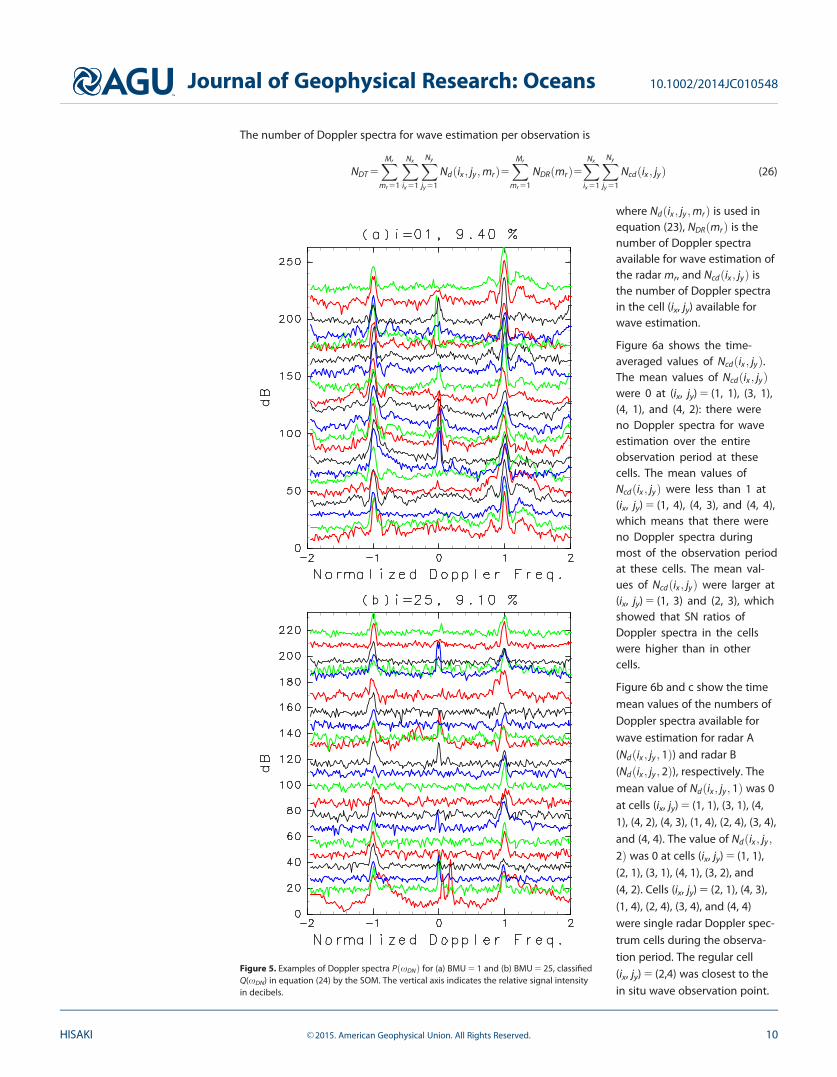
Figure 5 shows examples of Dopplerspectra PðxDNÞ for BMU 5 1 and 25. Thesecond-order Doppler peaks can be seenin most of the Doppler spectra forBMU 5 1 (Figure 5a). They are quasiab-sent for BMU 5 25 (Figure 5b). The SOMis useful for isolating the noisy Dopplerspectra. However, it is better to use theSOM in combination with other methods,such as a method of criteria 4, to selectDoppler spectra for wave estimation.

Figure 4. Weight vectors, which are explained in section 3.2, for (a) BMU 5 1and (b) BMU 5 25, classified QðxDNÞ in equation (24) by the SOM.



The number of Doppler spectra for wave estimation per observation is

NDT 5XMr

mr 51

XNx

ix 51

XNy

jy 51

Ndðix ; jy;mrÞ5XMr

mr 51

NDRðmrÞ5XNx

ix 51

XNy

jy 51

Ncdðix ; jyÞ (26)

where Ndðix ; jy ;mrÞ is used inequation (23), NDRðmrÞ is thenumber of Doppler spectraavailable for wave estimation ofthe radar mr, and Ncdðix; jyÞ isthe number of Doppler spectrain the cell (ix, jy) available forwave estimation.

Figure 6a shows the time-averaged values of Ncdðix ; jyÞ.The mean values of Ncdðix ; jyÞwere 0 at (ix, jy) 5 (1, 1), (3, 1),(4, 1), and (4, 2): there wereno Doppler spectra for waveestimation over the entireobservation period at thesecells. The mean values ofNcdðix ; jyÞ were less than 1 at(ix, jy) 5 (1, 4), (4, 3), and (4, 4),which means that there wereno Doppler spectra duringmost of the observation periodat these cells. The mean val-ues of Ncdðix ; jyÞ were larger at(ix, jy) 5 (1, 3) and (2, 3), whichshowed that SN ratios ofDoppler spectra in the cellswere higher than in othercells.

Figure 6b and c show the time

mean values of the numbers ofDoppler spectra available for

wave estimation for radar A

(Ndðix ; jy ; 1Þ) and radar B(Ndðix ; jy ; 2Þ), respectively. The

mean value of Ndðix ; jy ; 1Þ was 0

at cells (ix, jy) 5 (1, 1), (3, 1), (4,1), (4, 2), (4, 3), (1, 4), (2, 4), (3, 4),

and (4, 4). The value of Ndðix ; jy ;

2Þ was 0 at cells (ix, jy) 5 (1, 1),(2, 1), (3, 1), (4, 1), (3, 2), and

(4, 2). Cells (ix, jy) 5 (2, 1), (4, 3),

(1, 4), (2, 4), (3, 4), and (4, 4)were single radar Doppler spec-

trum cells during the observa-

tion period. The regular cell(ix, jy) 5 (2,4) was closest to the

in situ wave observation point.

Figure 5. Examples of Doppler spectra PðxDNÞ for (a) BMU 5 1 and (b) BMU 5 25, classifiedQ(xDN) in equation (24) by the SOM. The vertical axis indicates the relative signal intensityin decibels.



Figure 7a shows the time series of the numberof total Doppler spectra for both radars (NDT),radar A ðNDRð1ÞÞ and radar B ðNDRð2ÞÞ, in equa-tion (26) for wave estimation. Figure 7b showsthe time series of the number of Doppler spec-tra Ncdðix ; jyÞ for wave estimation in the regularcell at (ix, jy) 5 (2,4). There were no Dopplerspectra for wave estimation from 18 LST to 22LST 20 April 1998 (Figure 7a). Ocean wave spec-tra were therefore not estimated at that time.The time-averaged value of NDT was 106 forNDT> 0, which means that 106 Doppler spectra,on average, were used for wave estimation. Thetime-averaged value of Ncd(2,4) was 12, whichmeans that, on average, 12 Doppler spectra inthe regular cell (ix, jy) 5 (2,4) were used forwave estimation. The value of NDT varied withtime. The maximum was 144, and the minimumwas 40 for NDT> 0. The maximum of Ncd(2,4)was 18 and the minimum was 0 for NDT> 0.The beam direction wBðix ; jy;mrÞ also variedwith time.

4.2. Wave EstimationFigure 8 shows examples of ocean wave direc-tional spectra 2pGð2pf ; hÞðf 5x=ð2pÞÞ in cell(ix, jy) 5 (2,4), which was closest to the in situwave observation point. Although the Dopplerspectra of radar B only were included in thecell, the wave directional spectrum could beestimated. The estimated wave height is 1.76 min Figure 8a, while the in situ measured waveheight was 1.42 m, relatively high for the obser-vation period. The estimated wave height is0.96 m in Figure 8b, while the in situ measuredwave height was 0.97 m.

The peak wave direction is about h 5 120� inFigure 8a, which means that the dominantwave propagated northwestward. The peakwave direction is about h 5 2160� in Figure 8b,which means that the dominant wave propa-gated west-south westward. The waves arepropagated from offshore.

The hindcast dominant wave direction at(26�N; 128�E) by JMA (Japan MeteologicalAgency) was east-southeast at 9 LST (0 UTC)21 April, and the wind at the location wassoutheasterly. The hindcast dominant wavedirections were east at 9 LST 7 and 8 May,and winds were southerly [Japan Meteologi-cal Agency, 1999]. Dominant wave directionsof radar-estimated wave spectra agreed withthose predicted by JMA.

Figure 6. (a) Time-averaged value of the number of available Dopplerspectra for wave estimation per observation, Ncdðix ; jyÞ in equation (26);(b) same as Figure 6a but for radar A (Ndðix ; jy ; 1Þ); (c) same as Figure 6abut for radar B (Ndðix ; jy ; 2Þ).



Figure 9 shows the comparisonbetween USW wave heights (Hs) andradar-estimated wave heights (Hr) inthe cell closest to the in situ observa-tion point. The maximum in situ waveheight Hs was 1.57 m at 8 LST 21 April.The wave conditions were calm duringthe observation period. There were 321comparisons. The correlation coeffi-cient between Hs and Hr was 0.82 withan rms difference of 0.22 m. There wasgood agreement between USW waveheights and radar-estimated waveheights. The linear regression line inFigure 9b is Hr 5 1.14 Hs 1 0.045, indi-cating that radar-estimated waveheights were slightly higher than USWwave heights.

Figure 10 shows the mean radar-estimated wave heights during theobservation period. Mean wave heightsranged from 1 to 1.2 m. Mean waveheight was higher further offshore.

5. Discussion and Conclusions

We developed a method for estimatingocean wave spectra from HF radar, called the HIAS (HF radar Inversion Algorithm for Spectrum estimation).Doppler spectra used for estimating ocean wave spectra must not be contaminated by noise. However,many Doppler spectra are noise contaminated. We used the SOM, along with the other criteria listed in sec-tion 3.2 to select Doppler spectra.

We assumed that the wavefield was statistically homogeneous in the regular grid cell of Dx 3 Dy. The Dopplerspectra available for wave estimation change over time. The Doppler spectrum data are tractable due to theassumption, however, because we only averaged Doppler spectra for wave estimation and positions. If homoge-neity in the cell is not assumed, the cell-averaged Doppler spectrum would be expressed in terms of the wavespectra at the four grid points surrounding the cell. The inversion then becomes more complicated than thatused in the present method.

Six kinds of constrains were used in the present method. It may be possible to estimate wave spectra with-out the energy balance equation (constraint 3). We also estimated wave spectra for the same weightskw(M,K) as in section 3.1, except for kw(3,K) 5 0, which means that the energy balance equation was notincorporated into the inversion. The correlation coefficient between in situ measured wave heights (Hs) andthe radar-estimated wave heights (Hr) was 0.71 with an rms difference of 0.35 m. This result was poorerthan that in section 4.2. Therefore, we conclude that it is necessary to incorporate the energy balance equa-tion into the inversion.

The regular cells were classified into three groups. The first was the dual radar Doppler spectrum cell, in whichNdðix ; jy ; 1Þ 6¼ 0 and Ndðix ; jy ; 2Þ 6¼ 0. The second the no-radar Doppler spectrum cell, in whichNdðix ; jy ; 1Þ5Ndðix ; jy ; 2Þ50. Finally, the third was the single radar Doppler spectrum cell, which is onlyNdðix ; jy ; 1Þ50, or Ndðix ; jy ; 2Þ50. These cell types vary with time. The regular cell at (ix, jy) 5 (2,4) was a single radarDoppler spectrum cell for most of the observation period; this cell (ix, jy) 5 (2,4) was never a dual radar Dopplerspectrum cell.

The agreement between in situ measured wave heights and radar-estimated wave heights was good at thiscell. Previous methods for estimating wave spectra from HF radar developed by other groups [Wyatt, 1990;

Figure 7. (a) Time series of the number of Doppler spectra for wave estimation.Green: NDT in equation (26). Red: Radar A (NDR(1)). Blue: Radar B (NDR(2)). (b) Timeseries of the number of Doppler spectra for wave estimation in the cell closest tothe wave observation point. Ncdðix ; jyÞ at (ix, jy) 5 (2, 4).



Figure 8. Examples of ocean wave spectra 2pGð2pf ; hÞðf 5x=ð2pÞÞ in the cell (ix, jy) 5 (2,4) at (a) 6 LST 21 April 1998 and (b) 22 LST 7 May 1998.



Hashimoto et al., 2003; Wyatt et al., 2011] canonly estimate wave spectra for dual radarDoppler spectrum cells. This study demon-strates the advantages of the present method.

The wave spectra in the no-radar Dopplerspectrum cell were estimated by interpolationor extrapolation from constraints 3 and 6 insection 2.1. The grid cell (ix, jy) 5 (2, 4) was ano-radar Doppler spectrum cell only at 18 LST12 May (Figure 7b), as well as from 18 LST to22 LST 20 April. The radar-estimated waveheight in the cell was 1.32 m, while the USWwave height was 0.79 m at 18 LST 12 May. Theradar-estimated wave heights in the cell at 16LST 12 May and 20 LST 12 May were both0.99 m. The wave height at 18 LST 12 May wasthus overestimated, probably due to the noise-contaminated Doppler spectra, because theradar-estimated wave height in the cell(ix, jy) 5 (2, 2) was much larger than those inthe surrounding cells at the time. Furtherimprovement of the method for selectingDoppler spectra is necessary. The validity ofwave estimation for no-radar Doppler spec-trum cell should be explored further. The rela-tionship between the accuracy of the radar-estimated wave height and Ncdðix ; jyÞ remainsunclear.

The Doppler spectra for constraints 1 and 2 in section 2.1 are the same in the present estimation, as indi-cated in equation (23). However, the first-order Doppler spectrum for constraint 1 in section 2.1 can be usedeven though the second-order scattering is contaminated by noise. This improvement will be explored.

The advantage of the method is that wave spectra can be estimated in both single and dual radar Dopplerspectrum cells. In addition, the area for wave estimation can be set flexibly. The wave estimation area is setso that most of the cells are dual and single radar Doppler spectrum cells. The conditions for selecting thewave estimation area are less restrictive than those of other methods.

The advantage of the present method over the single radar method is that the area of wave estimation isalso more flexible than that in the single radar method. If two radars are used, and the wave spectra are esti-mated by the single radar method for each radar, the area of wave estimation is wider. However, attempt-ing to combine wave data from two radars is problematic. The wave data from each radar differ from eachother, even in the radar overlapping coverage area. If the wave data in the overlapping coverage are cor-rected, wave data in the nonoverlapping coverage must be also corrected. The present method combinesthe wave data from multiple radars.

In addition, the method of quality control is improved compared with that in Hisaki [2009]. Control is per-formed for radar-estimated wave data in Hisaki [2009]. As a result, many radar-estimated wave data werediscarded. Quality control was performed for the Doppler spectra in the present study. Even if only a fewDoppler spectra for wave estimation are not good quality, the radar-estimated wave data will not be goodquality. Therefore, the number of rejected wave data by the present method is smaller than that of the pre-vious method [Hisaki, 2009].

The drawback of the current method is that it requires substantial computer memory, and, as a result, spa-tial and spectral resolutions are coarse. If we want to estimate wave spectra at higher spatial resolution, thewave estimation area must be narrower. This drawback can be resolved by advances in computer perform-ance and memory.

Figure 9. Comparison of radar-estimated wave heights (Hr) at the cell(ix, jy) 5 (2, 4) and USW significant wave heights (Hs). (a) Time series(Blue: Hs, red: Hr); and (b) scatterplot between Hs and Hr. The linear lineis the regression line.



Our conclusions can be summarized as follows. We developed a method for estimating ocean wave spectrafrom HF radar by extending the method of Hisaki [2005, 2006, 2009, 2014] to multiple radar cases and regu-lar wave estimation grids. A method for selecting Doppler spectra for wave estimation was also developed.The method was verified by comparing in situ observed wave height with the radar-estimated wave heightsin a single radar Doppler spectrum cell in which the wave directional spectrum could not be estimated bythe previous methods of other groups.

ReferencesBarrick, D. E. (1977), The ocean wave height nondirectional spectrum from inversion of the HF sea-echo Doppler spectrum, Remote Sens.

Environ., 6, 201–227, doi:10.1016/0034-4257(77)90004-9.de Valk, C., A. Reniers, J. Atanga, A. Vizinho, and J. Vogelzang (1999), Monitoring surface waves in coastal waters by integrating HF radar

measurement and modelling, Coastal Eng., 37, 431–453, doi:10.1016/S0378-3839(99)00037-X.Hashimoto, N., L. R. Wyatt, and S. Kojima (2003), Verification of a Bayesian method for estimating directional spectra from HF radar surface

backscatter, Coastal Eng. J., 45, 255–274, doi:10.1142/S0578563403000725.Hisaki, Y. (1996), Nonlinear inversion of the integral equation to estimate ocean wave spectra from HF radar, Radio Sci., 31, 25–39, doi:

10.1029/95RS02439.Hisaki, Y. (2002), Short-wave directional properties in the vicinity of atmospheric and oceanic fronts, J. Geophys. Res., 107(C11), 3188, doi:

10.1029/2001JC000912.Hisaki, Y. (2005), Ocean wave directional spectra estimation from an HF ocean radar with a single antenna array: Observation, J. Geophys.

Res., 110, C11004, doi:10.1029/2005JC002881.Hisaki, Y. (2006), Ocean wave directional spectra estimation from an HF ocean radar with a single antenna array: Methodology, J. Atmos.

Oceanic Technol., 23, 268–286, doi:10.1175/JTECH1836.1.Hisaki, Y. (2007), Directional distribution of the short wave estimated from HF ocean radars, J. Geophys. Res., 112, C10014, doi:10.1029/

2007JC004296.Hisaki, Y., (2009), Quality control of surface wave data estimated from low signal-to-noise ratio HF radar Doppler spectra, J. Atmos. Oceanic

Technol., 26, 2444–2461, doi:10.1175/2009JTECHO653.1.Hisaki, Y. (2013), Classification of surface current maps, Deep Sea Res., Part I, 73, 117–126, doi:10.1016/j.dsr.2012.12.001.

Figure 10. Mean radar-estimated wave heights during the observation period.

AcknowledgmentsThis study was supported by a grant-in-aid for scientific research (C-2) fromthe Ministry of Education, Culture,Sports, Science, and Technology ofJapan (26420504). The GFD DENNOULibrary (http://dennou.gaia.h.kyoto-u.ac.jp/arch/dcl/) was used for drawingfigures. The Doppler spectra wereprovided from OkinawaElectromagnetic Technology Center,National Institute of Information andCommunications Technology, Japan(http://okinawa.nict.go.jp/EN/). Thewave data were provided from CoastalDevelopment Institute of Technology,Japan (http://www.cdit.or.jp/).Comments from anonymous reviewerswere helpful in improving themanuscript.



http://dennou.gaia.h.kyoto-u.ac.jp/arch/dcl/

http://okinawa.nict.go.jp/EN/

http://www.cdit.or.jp/

http://dx.doi.org/10.1029/95RS02439

http://dx.doi.org/10.1029/2001JC000912

http://dx.doi.org/10.1029/2005JC002881

http://dx.doi.org/10.1175/JTECH1836.1

http://dx.doi.org/10.1029/2007JC004296

http://dx.doi.org/10.1029/2007JC004296

http://dx.doi.org/10.1175/2009JTECHO653.1

http://dx.doi.org/10.1016/j.dsr.2012.12.001



http://okinawa.nict.go.jp/EN/

http://www.cdit.or.jp/

Hisaki, Y. (2014), Intercomparison of wave data obtained from single high-frequency radar, in-situ observation and model prediction, Int. J.Remote Sens., 35, 3459–3481, doi:10.1080/01431161.2014.904971.

Hisaki, Y., W. Fujiie, T. Tokeshi, K. Sato, and S. Fujii (2001), Surface current variability east of Okinawa Island obtained from remotely sensedand in-situ observational data, J. Geophys. Res., 106, 31,057–31,073, doi:10.1029/2000JC000784.

Howell, R., and J. Walsh (1993), Measurement of ocean wave spectra using narrow-beam HF radar, IEEE. J. Oceanic Eng., 18, 296–305, doi:10.1109/JOE.1993.236368.

Japan Meteological Agency (1999), Annual report on ocean waves 1998, Rep. 3, Tokyo.Lipa, B. J., and D. E. Barrick (1986), Extraction of sea state from HF radar sea echo: Mathematical theory and modeling, Radio Sci., 21, 81–

100, doi:10.1029/RS021i001p00081.Liu, Y., and R. H. Weisberg, (2005), Patterns of ocean current variability on the West Florida Shelf using the self organizing map, J. Geophys.

Res., 110, C06003, doi:10.1029/2004JC002786.Long, R., D. E. Barrick, J. L. Largier, and N. Garfield (2011), Wave observations from Central California: SeaSonde systems and in situ wave

buoys, J. Sensors, 0112, 1–18, doi:10.1155/2011/728936.Wyatt, L. R. (1990), A relaxation method for integral inversion applied to HF radar measurement of the ocean wave directional spectra,

Int. J. Remote Sens., 11, 1481–1494, doi:10.1080/01431169008955106.Wyatt, L. R., J. J. Green, and A. Middleditch (2011), HF radar data quality requirements for wave measurement, Coastal Eng., 58, 327–336,

doi:10.1016/j.coastaleng.2010.11.005.



http://dx.doi.org/10.1080/01431161.2014.904971

http://dx.doi.org/10.1029/2000JC000784

http://dx.doi.org/10.1109/JOE.1993.236368

http://dx.doi.org/10.1029/RS021i001p00081

http://dx.doi.org/10.1029/2004JC002786

http://dx.doi.org/10.1155/2011/728936

http://dx.doi.org/10.1080/01431169008955106

http://dx.doi.org/10.1016/j.coastaleng.2010.11.005

Development of HF radar inversion algorithm for spectrum ...w3.u-ryukyu.ac.jp/yhisaki/manuscript/2015-Journal...RESEARCH ARTICLE 10.1002/2014JC010548 Development of HF radar inversion

Documents