Development of Fast, Distributed Computational Schemes for ...

Old Dominion University Old Dominion University

ODU Digital Commons ODU Digital Commons

Electrical & Computer Engineering Theses & Dissertations Electrical & Computer Engineering

Winter 2007

Development of Fast, Distributed Computational Schemes for Full Development of Fast, Distributed Computational Schemes for Full

Body Bio-Models and Their Application to Novel Action Potential Body Bio-Models and Their Application to Novel Action Potential

Block in Nerves Using Ultra-Short, High Intensity Electric Pulses Block in Nerves Using Ultra-Short, High Intensity Electric Pulses

Ashutosh Mishra Old Dominion University

Follow this and additional works at: https://digitalcommons.odu.edu/ece_etds

Part of the Biomedical Engineering and Bioengineering Commons, and the Electrical and Computer

Engineering Commons

Recommended Citation Recommended Citation Mishra, Ashutosh. "Development of Fast, Distributed Computational Schemes for Full Body Bio-Models and Their Application to Novel Action Potential Block in Nerves Using Ultra-Short, High Intensity Electric Pulses" (2007). Doctor of Philosophy (PhD), Dissertation, Electrical & Computer Engineering, Old Dominion University, DOI: 10.25777/vegt-r564 https://digitalcommons.odu.edu/ece_etds/112

This Dissertation is brought to you for free and open access by the Electrical & Computer Engineering at ODU Digital Commons. It has been accepted for inclusion in Electrical & Computer Engineering Theses & Dissertations by an authorized administrator of ODU Digital Commons. For more information, please contact [email protected].

https://digitalcommons.odu.edu/

https://digitalcommons.odu.edu/ece_etds

https://digitalcommons.odu.edu/ece_etds

https://digitalcommons.odu.edu/ece

https://digitalcommons.odu.edu/ece_etds?utm_source=digitalcommons.odu.edu%2Fece_etds%2F112&utm_medium=PDF&utm_campaign=PDFCoverPages

http://network.bepress.com/hgg/discipline/229?utm_source=digitalcommons.odu.edu%2Fece_etds%2F112&utm_medium=PDF&utm_campaign=PDFCoverPages



https://digitalcommons.odu.edu/ece_etds/112?utm_source=digitalcommons.odu.edu%2Fece_etds%2F112&utm_medium=PDF&utm_campaign=PDFCoverPages

mailto:[email protected]

DEVELOPMENT OF FAST, DISTRIBUTED COMPUTATIONAL

SCHEMES FOR FULL BODY BIO-MODELS AND THEIR

APPLICATION TO NOVEL ACTION POTENTIAL BLOCK IN

NERVES USING ULTRA-SHORT, HIGH INTENSITY ELECTRIC

PULSES

by

Ashutosh M ishra M.S. M ay 2003, Old Dominion University

A Dissertation Submitted to the Faculty o f Old Dominion University in Partial Fulfillment o f the Requirements for the Degree o f

DOCTOR OF PHILOSOPHY

ELECTRICAL AND COMPUTER ENGINEERING

OLD DOMINION UNIVERSITY December 2007

Approved by:

Ravindra P. Joshi (Director)

Linda Vahala (Member)

^Frederic D. M ckenae (Member)

Mujere Erten-Unal (Member)

Reproduced with permission of the copyright owner. Further reproduction prohibited without permission.

Abstract

DEVELOPMENT OF FAST, DISTRIBUTED COMPUTATIONAL SCHEMES FOR FULL BODY BIO-MODELS AND THEIR APPLICATION TO NOVEL ACTION POTENTIAL BLOCK IN NERVES USING ULTRA-SHORT, HIGH INTENSITY ELECTRIC PULSES

Ashutosh Mishra Old Dominion University, 2007

Director: Dr. R.P. Joshi

An extremely robust and novel scheme for computing three-dimensional, time-

dependent potential distributions in full body bio-models is proposed, which, to the best of our

knowledge, is the first of its kind. This simulation scheme has been developed to employ

distributed computation resources, to achieve a parallelized numerical implementation for

enhanced speed and memory capability. The other features of the numerical bio-model included

in this dissertation research, are the ability to incorporate multiple electrodes of varying shapes

and arbitrary locations. The parallel numerical tool also allows for user defined, current or

potential stimuli as the excitation input. Using the available computation resources at the

university, a strong capability for extremely large bio-models was developed. So far a

maximum simulation comprised of 6.7 million nodes has been achieved for a “full rat bio

model” with a 1 mm spatial resolution at an average of 30 seconds per iteration.

The ability to compute the resulting potential distribution in a full animal body allows

for realistic and accurate studies of bio-responses to electrical stimuli. For example, the voltages

computed from the full-body models at various sites and tissue locations could be used to

examine the potential for using nanosecond, high-intensity, pulsed electric fields for blocking

neural action or action potential (AP) propagation. This would be a novel, localized, and

reversible method of controlling neural function without tissue damage. It could potentially be

used in “electrically managed pain relief,” non-lethal incapacitation, and neural/muscular

therapy.

The above concept has quantitatively been evaluated in this dissertation. Specifically,

the effects of high-intensity (kilo-Volt), ultra-short (-100 nanosecond) electrical pulses have

been evaluated, and compared with available experimental data. Good agreement with available

data is demonstrated. It is also shown that nerve membrane electroporation, brought about by

the high-intensity, external pulsing, could indeed be instrumental in halting AP propagation.

Simulations based on a modified distributed cable model to represent nerve segments have been

used to demonstrate a numerical “proof-of-concept.”


iv

This dissertation is humbly dedicated to my parents - Asha & Anjani. You are the

world I know, the name I worship and all the love I need. My darling sister - Anubha,

who means the life to me and has shown resilience and personal strength rarely found in

mere mortals! I thank you for your unconditional acceptance, patience and my being.

-Ashutosh, 2007


V

ACKNOWLEDGEMENTS

This dissertation would not be complete without the acknowledgement of significantly

superior individuals that have given me their time. The first and foremost of this group is my

advisor - Dr. R.P. Joshi. His faith in my abilities, generosity and the relentless drive that helped

me push my own envelop are the prime-movers of this dissertation. Nothing would have been

possible without his patience, understanding and the sense of humor. I shall remain forever in

awe of his stature.

I would also like to express my profuse gratitude to Dr. L. Vahala, Dr. R. McKenzie,

and Dr. M. Erten-Unal, for consenting to be on my dissertation advisory committee. This is also

an opportune moment to thank Dr. V. Lakdawala for his words of encouragement and guidance

and members of the staff - Linda and Hero - for all their support help and the food!

Outside the environs of the campus there is an active group of people who kept me

laughing and driven. They are: Steve Corson, Tim Goodale, Jack Bloom, Noreen, Vissu and

Rebekka Althouse and all the regulars at O’Sullivans. Ladies and gentlemen, you are my friends

for life and I am a better man due to you.

Finally, I bow my head to Dr. D. K Pandey and Mrs. Snehlata Pandey, who have been

my family away from home.

Thank you everyone!


TABLE OF CONTENTS

LIST OF FIGURES.............................................................................................................................ix

LIST OF TABLES............................................................................................................................. xii

CHAPTER 1...........................................................................................................................................1

INTRODUCTION................................................................................................................................ 1

1.1 B io e l e c t r ic s - a n o v e r v ie w ................................................................................................................1

1.2 T h e r o l e a n d a d v a n t a g e s o f b io -m o d e l in g ..............................................................................2

1.3 O v e r a l l s c o p e a n d s p e c if ic g o a l s o f t h is r e s e a r c h w o r k .............................................. 2

CHAPTER I I .........................................................................................................................................5

LITERATURE REVIEW AND PERTINENT BACKGROUND....................................................5

2.1 O v e r v ie w ...................................................................................................................................................... 5

2.2 F u l l b o d y m o d e l in g s c h e m e ..............................................................................................................6

2.2.1 Intrinsic hurdles in full body modeling............................................................................ 9

2.2.1.1 Model resolution.......................................................................................................11

2.2.1.2 Tissue parameters.....................................................................................................11

2.2.1.3 Excitation (stimulus) locations and form................................................................11

2.3 N e u r a l S ig n a l s a n d b l o c k s c h e m e s ............................................................................................ 14

2.3.1 Nerve segment structure and key terms......................................................................... 15

2.3.1 Action Potential............................................................................................................... 16

2.3.2 Action Potential conduction block..................................................................................18

2.3.2.1 Electroporation.........................................................................................................21

2.3.3 Proposed Action Potential conduction block scheme...................................................22

2.3.4 Synaptic process and possible AP block site................................................................ 24

2.3.5 More recent modes and studies.......................................................................................25

CHAPTER III..................................................................................................................................... 27

MODELING DETAILS AND NUMERICAL IMPLEMENTATION.........................................27

3.1 F u l l -b o d y M o d e l in g Sc h e m e ....................................................................................................... 27

3.1.1 Input Format Details........................................................................................................27

3.1.2 Proposed Modeling Scheme............................................................................................31

3.1.2.1 Matrix Sparsity and its Significance.......................................................................37

3.1.2.2 Solution Scheme Overview for the Full Body Models......................................... 39

3.1.3 Distributed Algorithm Details.........................................................................................42


3.1.3.1 Algorithm Process Flow Diagram..........................................................................43

3.1.3.2 Coefficient Matrix Setup in Compressed Row Storage Scheme.........................43

3.2 Modeling N eural Traffic Interruption M ethods..................................................47

3.2.1 Distributed Cable Model for Representing the Unmyelinated Nerve Segment.........47

3.2.2 Distributed Cable Model for Representing the Myelinated Nerve Segment............. 49

3.2.2 Modified HH Model for Membrane Conductance Modulation...................................53

3.2.3 Membrane Electroporation Effects................................................................................ 54

CHAPTER IV ..................................................................................................................................... 58

RESULTS AND DISCUSSION........................................................................................................58

4.1 D istributed modeling schem e..........................................................................................58

4.1.1 Input data visualization methods.................................................................................... 58

4.1.2 Validating the full-body modeling scheme....................................................................61

4.1.2.1 Saline sphere with two parallel planar disc electrodes..........................................61

4.1.2.2 Saline sphere with symmetric axially located electrodes......................................63

4.1.2.3 Saline brick with an air pocket................................................................................64

4.1.3 Preliminary results highlighting current density computations....................................65

4.1.4 Distributed process grid size and cluster load impact...................................................68

4.1.5 Reducing fill-in during coefficient matrix factorization...............................................70

4.1.6 Simulation results for a complex multi-tissue whole body model...............................71

4.1.6.1 Rat model with cross-diagonally grounded paws................................................. 72

4.1.6.2 Monkey head with planar electrodes...................................................................... 78

4.1.6.3 Significantly larger rat model..................................................................................80

4.1.7 Comparing the symmetric and asymmetric modeling schemes................................... 81

4.2 N erve segment modeling and action potential (AP) block ................................... 84

4.2.1 Visualizing the action potential.......................................................................................84

4.2.2 AP propagation velocity.................................................................................................. 86

4.2.3 Conduction block using continuous electric stimuli (DC/AC).................................... 87

4.2.4 Modifying the shunt conductance...................................................................................90

4.2.5 Application to multi-branch nerve segments................................................................ 94

4.2.6 Experimental AP inhibition and validation....................................................................95

4.2.7 More recent observations that may support alternative AP block mechanisms 98

CHAPTER V ...................................................................................................................................... 99

CONCLUSIONS AND SUGGESTIONS FOR FUTURE WORK............................................... 99

5.1 Intro ductio n .........................................................................................................................99


5.2 FULL BODY MODELING.............................................................................................................................99

5.3 MODELING ACTION POTENTIAL AND CONDUCTION BLOCK.....................................................102

5.4 Sc o p e f o r f u t u r e w o r k a n d e x t e n s io n ................................................................................... 104

5.5 E x t e n d in g t o m ic r o -l e v e l s y s t e m s (e .g ., c e l l c l u s t e r s ) ............................................. 107

5.5.1 Low intensity electric field cases..................................................................................109

5.5.2 High intensity electric field cases.................................................................................I l l

5.5.2 Summarizing the cell cluster......................................................................................... 112

REFERENCES................................................................................................................................. 114

APPENDIX.......................................................................................................................................122

A. 1 CONVERTING INDEX TO COORDINATES:............................................................................. 122

A .2 Sy m m e t r ic m o d e l in g s c h e m e : ......................................................................................................123

A.3 Sp a r s e M a t r ix St o r a g e (C o m p r e s s e d R o w F o r m a t ) ...................................................... 125

A .4 T h e C o e f f ic ie n t M a t r ix in C o m p r e s s e d R o w Fo r m a t ....................................................126

CURRICULUM VITA.....................................................................................................................128


LIST OF FIGURES

1. Illustration showing the entry of PI into the PN M ...............................................................8

2. Cross-sectional representation of human skin tissue..........................................................10

3. Typical Mammalian neuron (myelinated)...........................................................................16

4. Typical Mammalian neuron (unmyelinated)...................................................................... 16

5. Representation of a cell membrane section......................................................................... 22

6. Snapshots of pore formation in the DOPC bilayer..............................................................23

7. Major elements in prototypical synaptic process................................................................24

8. Sample volumetric data set with the tissue cell indexing scheme......................................28

9. Visualization of a sample raw data file of a rat...................................................................29

10. Cross-sections of the rat at different depths........................................................................ 31

11. Schematic of the discretized electrical model..................................................................... 32

12. Simplified schematic to highlight the nodal links and node indexing.............................. 34

13. Non-zero entries in case of a 1000 node, saline brick model............................................37

14. Example of fill-in with and without reordering.................................................................41

15. Process flow diagram for the distributed scheme of full body modeling........................45

16. Equivalent circuit representing the cable line model for the

unmyelinated nerve segment............................................................................................. 48

17. Physical structure and Equivalent circuit of a myelinated nerve segment.......................50

18. Action potential propagation in a 23.8pm diameter nerve segment................................. 52

19. Schematic for the modified cable m odel.............................................................................54

20. Action potential propagation block a 23.8pm diameter nerve segment........................... 55

21. Sketch of pores created on the nerve membrane by the external voltage......................... 56

22. Two forms of volumetric representation of the data.......................................................... 58

23. Tissue layout present at different depths..............................................................................59

24. Tissue layout in a human head as visible in three orientations..........................................60

25. Two-Dimensional projection for the geometry

used in the second validation case ...................................................................................... 61

26. Current response and Potential profile to the FIRST validation test case ........................62

27. Solid rendered saline sphere.................................................................................................63

28. Potential profile & current response for the second validation case................................ 64

29. Saline Brick with air slab and the its response................................................................... 64

30. Potential profile for layer 11 in the x-y orientation for saline sphere..............................65


X

31. Potential profile for layer 11 in the Y-Z orientation for saline sphere......................... 66

32. Current density components for saline sphere...................................................................67

33. Timing diagram for the rat model for different

process grid sizes during peak load hour........................................................................... 68

34. Timing diagram for the rat model for different

process grid sizes during off peak hour..............................................................................69

35. Profile for the applied potential pulse for the rat model....................................................72

36. Wire mesh rendered rat model............................................................................................. 73

37. Simulated potential profile at two slices for small rat model.............................................75

38. Computed conduction current density for small rat model................................................76

39. Central slice conduction current density in each orientation.............................................77

40. A semi-transparent solid rendered plot showing the

outer geometry in the monkey head model........................................................................ 78

41. Potential contours for the monkey head model...................................................................79

42. Potential contours for the LARGE rat model......................................................................80

43. Average computation time per time iteration with symmetric method..............................81

44. Three forms of visual representation of the action potential.............................................84

45. Computed velocity dependence upon the axon

diameter for unmyelinated nerves....................................................................................... 85

46. AP block with DC pulse.......................................................................................................87

47. AP block with AC interrupt signal......................................................................................88

48. Minimum shunt conductance required for AP block in unmyelinated nerve segments

as a function of number of nodes where the conductance was modulated......................89

49. Minimum shunt conductance required for AP block in myelinated nerve segments

as a function of number of nodes where the conductance was modulated......................90

50. Angular pore density variation to e-fields...........................................................................91

51. Strength-duration curves for axon of different diameters for achieving minimum Gshunt

................................................................................................................................................ 92

52. A sample multi-branch layout.............................................................................................. 93

53. AP initiation and block using electroporation in a multi-segment unmyelinated nerve

................................................................................................................................................ 94

54. Schematic of experimental rat setup that was simulated................................................... 95

55. Computed electric field along the spinal

region along the entire length of the rat m odel.................................................................96


xi

56. Alternative physical model for Na+ channels...................................................................102

51. Voronoi networks with different disorder parameter........................................................107

58. Distributed representation for the electrical analysis at cellular level.............................107

59. Simulation schematic showing an all-tissue and cell clusters........................................ 108

60. Membrane Potential and Electric field for homogenous tissue system...........................109

61. A 550 ns snapshot of the cell cluster indicating porated cells ....................................... 109

62. S-D curves for cell clusters with various

distortion parameters and that for a single spherical cell.................................................111


LIST OF TABLES

1. AC block frequency range for good and fail AP block in an unmyelinated nerve

segment................................................................................................................................ 20

2. Electrical parameters for various constituent tissues.......................................................33

3. Comparative figures for fill-in with and without reordering.................................... 70

4. Computational statistics for the symmetric solution scheme.....................................82

5. Shunt conductance with standard electric field and

pulse width combinations....................................................................................................92


1

Chapter I

Introduction

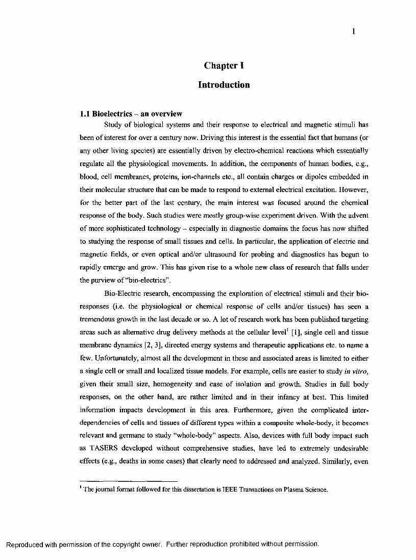
1.1 Bioelectrics - an overviewStudy of biological systems and their response to electrical and magnetic stimuli has

been of interest for over a century now. Driving this interest is the essential fact that humans (or

any other living species) are essentially driven by electro-chemical reactions which essentially

regulate all the physiological movements. In addition, the components of human bodies, e.g.,

blood, cell membranes, proteins, ion-channels etc., all contain charges or dipoles embedded in

their molecular structure that can be made to respond to external electrical excitation. However,

for the better part of the last century, the main interest was focused around the chemical

response of the body. Such studies were mostly group-wise experiment driven. With the advent

of more sophisticated technology - especially in diagnostic domains the focus has now shifted

to studying the response of small tissues and cells. In particular, the application of electric and

magnetic fields, or even optical and/or ultrasound for probing and diagnostics has begun to

rapidly emerge and grow. This has given rise to a whole new class of research that falls under

the purview of “bio-electrics”.

Bio-Electric research, encompassing the exploration of electrical stimuli and their bio

responses (i.e. the physiological or chemical response of cells and/or tissues) has seen a

tremendous growth in the last decade or so. A lot of research work has been published targeting

areas such as alternative drug delivery methods at the cellular level1 [1], single cell and tissue

membrane dynamics [2, 3], directed energy systems and therapeutic applications etc. to name a

few. Unfortunately, almost all the development in these and associated areas is limited to either

a single cell or small and localized tissue models. For example, cells are easier to study in vitro,

given their small size, homogeneity and ease of isolation and growth. Studies in full body

responses, on the other hand, are rather limited and in their infancy at best. This limited

information impacts development in this area. Furthermore, given the complicated inter

dependencies of cells and tissues of different types within a composite whole-body, it becomes

relevant and germane to study “whole-body” aspects. Also, devices with full body impact such

as TASERS developed without comprehensive studies, have led to extremely undesirable

effects (e.g., deaths in some cases) that clearly need to addressed and analyzed. Similarly, even

1 The journal format followed for this dissertation is IEEE Transactions on Plasma Science.


2

though studies of nerve segments [4-6] and the conduction block of electrical action potentials

(AP) in nerves have been probed for several decades [7-10], there is currently no viable solution

for achieving AP blocks in a robust, controlled and consistent manner. Some of the methods

that have been proposed involve AC interruption signals [7, 11], while other work has explored

DC current injection [12-14]. Other methods that have been examined include temperature

alterations [15, 16] and injection of chemicals. However, in all of these proposed methods, there

is a high degree of variability; there are often deleterious side-effects such as tissue damage; the

effects can be non-localized, slow, or not very robust. Consequently, a robust AP block method

is the other aspect that the present dissertation will explore.

1.2 The role and advantages of bio-modeling

Over the past decade, simulation capabilities have grown tremendously in ways of

scope as well as the level of detail, in every aspect of life. The most important reason driving

this surge in modeling and simulation schemes is that given sufficient level of detail, these

systems are able to provide an acceptable level of accuracy in making realistic predictions,

while being completely non-invasive. Whether it is modeling tissue necrosis during

radiofrequency ablation [17], optimal biopsy pathways [18], or tumor progression paths [19],

extremely sophisticated and powerful schemes exist that allow such models to deliver high

precision estimates and results. The other advantage of any modeling based approach is that it

significantly reduces the prototyping collateral, making it a cheaper and faster process. It also

allows for the quick evaluation of a wide parameter range without having to experiment and

physically evaluate a range of scenarios and possibilities. A study for validation data involving

live subjects, even though vital for end validation, is expensive and requires various

arrangements and protocols and some inherent delays. Simulations, on the other hand, are faster

and provide fundamental understanding of the underlying basic processes and phenomena.

Besides, both deterministic processes (such as propagation of information in nerve fibers) and

non-deterministic systems such the use of heuristic machine learning to study vocal pitch tracks

can be studied and estimated.

1.3 Overall scope and specific goals of this research work

In order to be able to perform a systematic analysis or development, it is necessary that

there exist a clear body of work that needs to be performed, since neither unlimited time nor


3

resources exist. Towards this end, this chapter provides the overall scope and a list of more

specific targets and tasks that this research expects to meet and accomplish.

• Develop a full body mathematical model that will allow for computation of potential

values in the 3-D discretized tissue volume.

• The underlying algorithms will then be validated using analytical computations for

simple cases of geometry and complexity.

• The system will be further developed to incorporate tissue complexity and body contour

variability.

• Provisions will be provided for simulating multiple electrodes.

• These electrodes can be defined as arbitrary shapes depending on user specification.

• The overall system will be applied stimulus independent, which could be potential or

current waveforms.

• For the purposes of development, binary model files provided by Brooks Air Force

Base, San Antonio, TX will be used.

• This system will employ distributed algorithm and distributed (parallel) computing. It

will be scalable by the number of processors, and consequently, the problem size.

• The output form of this system will also allow for computation of current, current

density in each of the three orientations.

Upon successful completion of the above goals, the resulting computed data for potential

values within a tissue model would facilitate and allow for studies of possible activation of

nerves and potential action potential block. The following tasks are therefore proposed for

implementation.

• Existing nerve models for myelinated and unmyelinated nerve segments will be

validated.

• Potential problems with the AP blockage schemes that exist, involving AC and DC

current injection will be explored and analyzed.

• Electroporative effects of ultra-short, high intensity pulses to nerve membranes will be

studied from existing literature [20-25].

• The resulting changes in membrane conductivity due to formation of nano-pores in

membranes will then be incorporated into a modified model of nerve segments. This

will be done to study whether action potentials can be interrupted by modulating the

membrane conductivity in unmyelinated nerve segments.


4

• Upon systematic examination of the above, this will also be explored and expanded for

application in myelinated nerve segments.

• The numerical models will eventually result in “strength-duration (SD)” curves relating

the applied electric potential and the pulse duration required for successful AP block in

nerve segment (myelinated and unmyelinated) of some selected diameters.

• Given the sparsity of modeling schemes that incorporate branching of the nerve

segments, the above concepts will also be probed for their applicability to multi-branch

segments, myelinated as well as unmyelinated.

• Finally, some recent experimental observations on ion-channel blockage (e.g., the

Sodium channels) will be examined with the intension to put forth plausible

explanations and scenarios. Here the emphasis will be more on qualitative features and

the underlying physics rather than rigorous bio-computational analyses.

The above overview was meant to present an extremely abbreviated idea of an extremely

detailed research area encompassing significant work that is to follow. It is hoped that by way

of this research work, multiple levels of tissue resolutions could be studied upon being stressed

by electric fields. At the conclusion phase of this dissertation work, a brief over view of the

latest work that targets electric field effects on cell clusters will be presented. Even though

single cell response has been studied extensively [24, 26-29], very few attempts have actually

targeted cell clusters [30, 31]. Even fewer time dependent analyses exist, as will be presented in

this dissertation research.

This dissertation is structured in the following manner. Chapter 2 is devoted to an in-

depth background study of the current research area and related aspects. This is followed in

chapter 3 by a detailed presentation of the numerical and algorithmic details of all the modeling

schemes that this dissertation targets. Subsequently, all the results and analyses appear in

chapter 4. This chapter also includes discussions of the results. The final chapter is used to

summarize results from this dissertation. It also lists possible future work or extensions to the

work already done in this research. Some miscellaneous algorithms and concepts (which have

been identified as important) are collated in an appendix that follows the references.


5

Chapter II

Literature Review and Pertinent Background

Proteins are the machinery o f living tissue that builds the structures and carries out the

chemical reactions necessary fo r life. - M ichael Behe

2.1 Overview

The biochemist, Michael Behe, may or may not find universal acceptance for his beliefs

owing to his advocacy of Intelligent Design. However, the above statement does highlight a

key truth - that every mammal body is driven (at the fundamental level) by chemical reactions.

Over the last two centuries, human interest in the inherent biological functioning of the body

has lead to several discoveries. The founding facts, all point towards a chemical basis, or, more

accurately, an electro-chemical basis for biological action. Mammalian anatomy, in general, is

comprised of organic tissue down to the cellular level. Consequently, every behavior exhibited

when examined at the cellular level, shows the distinct signature of its chemical nature and

inherent ionic movement.

For example, one can consider the simple act of breathing. It involves systematic

stimuli from the brain stem whether voluntary or involuntary. At a very coarse level this can be

viewed as the contraction of the diaphragm caused by the systematic stimuli, followed by its

elastic recoil. However, at the micro level, this is a reasonably complex process driven by

chemo-receptors. These are a special type of cells that perform transduction of a chemical signal

into an action potential (AP). The AP is a voltage driven electrical signal and the bio-response

form along neural pathways. These chemo-receptors detect levels of C 0 2 in the blood-steam by

monitoring the H+ (hydrogen ion) concentration. A higher concentration leads to a drop in the

pH. In response, the inspiratory centre in the medulla sends nervous impulses down the phrenic

nerve to activate the intercostal muscles. This, in turn, regulates the breathing rate as well as the

volume of the lungs. Thus, an electrically-driven, continuous feedback processes based on

distributed sensors is at work within the mammalian body.

The above example is meant to highlight the chemical interactions at the most fundamental

level o f the mammalian anatomy. It also shows the intricate and fundamental role o f electrical

signaling. The implication is that all mammalian tissue is extremely susceptible to any

electric/electromagnetic stimulus. This is very important since it means that through external


6

application, electrical stimuli, could possibly be made to have an effect on the nervous system

and the electrical signaling within mammalian bodies. A modeling study to examine and make

predictions of the biological behavior or tissue response could be geared towards the

functioning and neural activation and effects of external electrical stimuli. Previous studies have

explored the intrinsic anatomical stimulation based on natural nervous signaling. However, the

gap that exists in the bio-electric/bio-medical community is in the area of physiological

response to artificial (external) stimuli (such as direct contact electrical impulse) or

electromagnetic radiation.

Studies of such electrically induced bio-responses are driven by several considerations.

First, external electrical stimulation could be a useful therapeutic tool to re-activate nerves and

spinal tissue in injuries to the nervous system. Second, concrete thresholds relating to safety

levels and potentially hazardous limits of electrical stimulation need to be ascertained. This is

particularly important in the context of pace-makers and electrically driven medical instruments

and sensors. The safety aspect is also important in specific modern-day environments such as

high-power transmitters, microwave stations, and military radars. Currently, there exist schemes

that allow for the study of “small tissue volume” response to external excitation such as

ablation. However, prediction of possible outcomes such as fibrillation in response to a directed

energy source (such as the TASER® gun or high-power microwaves) requires the inclusion and

careful analysis of a full body response. In particular, the various nervous pathways that could

get activated need to be examined. This is a complex task and involves the electrical details,

bio-electric interactions, whole body bio-responses associated with the complex bio

components and their inter-dependent interactions. However, here we attempt to study a small

aspect of this overall issue through appropriate simulations as a pioneering step. Therefore, one

of the key objectives of this research is to address the void in modeling schemes that would help

predict and quantify the full body response of mammals to external, direct-contact electrical

stimuli. Apart from the numerical model development, this dissertation research also attempts to

explore electrically driven means of controlling the neural pathways through the use of ultra-

short voltage pulses. The analysis is based on time-dependent, spatially distributed neural bio

models.

2.2 Full body modeling schemeElectrical excitation, which has been used to stimulate both the central and the

peripheral nervous system, has a variety of potential diagnostic and therapeutic applications


7

[32-34], For example, electrically stimulated neurogenesis is a potential tool for enabling the

production of new nerve cells from neuronal stem cells [35, 36], It is used in implantable

devices for neuromuscular stimulation; these devices are designed to control the contraction of

paralyzed skeletal muscles, thereby producing functional movements in patients with stroke and

spinal cord injuries [5, 37], Electrical excitation is also a useful tool for studying the properties

and functions of nerves (including the brain) and muscles (including the heart). It also provides

information on strength-duration characteristics including the inherent time constants.

Strength-duration curves yield the critical electric pulse duration thresholds for a given

electrical signal intensity. These are important for determining the safety levels for electrical

excitation for a given voltage pulse or, conversely, the electrical intensity that can be applied for

a chosen pulse duration.

Excitation with ultra-short pulses is also an important issue for the health and safety

assessment of ultra-wideband (UWB) sources that produce nanosecond pulses. This issue has

been discussed at length elsewhere [3], In general, muscle excitation can be achieved either

remotely through the principle of electromagnetic induction [38-40] or directly through

electrical contact [41]. UWB pulses have not, to date, shown significant, robust, and reliable

biological effects. Such UWB studies using rats examined behavioral teratology, heart rate,

blood pressure, brain histology, and genetic alterations [42-45]. This contribution focuses on

pulsed excitation delivered to biological tissues (and whole bodies) through direct electrical

contacts. Thus, it is assumed that electrodes can be directly applied on the muscle/tissue surface.

Motor nerve fibers within the muscle are then excited by the potential created within the muscle

by the external source. In general, the potential can also be applied through a conductive

medium surrounding the biomass as discussed in a previous report [46], The use of ultra-short

electrical pulses in this context is an emerging topic of interest [27]. Such pulses of nanosecond

duration have been shown to penetrate the outer (plasma) membrane to create large trans

membrane potentials across sub-cellular organelles [47], Thus, for example, neurotransmitter

triggering or calcium release (from the Endoplasmic Reticulum) is possible through the use of

ultra-short pulses [1, 26, 48]. These ultra-short pulses have also been shown to porate the outer

plasma membrane reversibly, and this can be an important technique of artificially tailoring a

pathway into the cell for drug delivery. Use of this new technology to study sub-microsecond

pulse widths might reveal new biological phenomena as well. To highlight the plasma

membrane poration and its reversibility, upon the application of nano-second Pulsed Electric

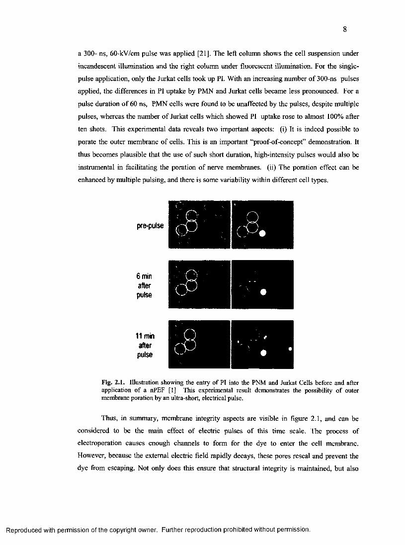
Field (nPEF), consider figure 2.1. It shows the PI uptake in a cell suspension containing both

PMN (poly-morpho-nuclear leuckcyte) cells (yellow circles) and Jurkat cells (blue circles) after


8

a 300- ns, 60-kV/cm pulse was applied [21]. The left column shows the cell suspension under

incandescent illumination and the right column under fluorescent illumination. For the single

pulse application, only the Jurkat cells took up PI. With an increasing number of 300-ns pulses

applied, the differences in PI uptake by PMN and Jurkat cells became less pronounced. For a

pulse duration of 60 ns, PMN cells were found to be unaffected by the pulses, despite multiple

pulses, whereas the number of Jurkat cells which showed PI uptake rose to almost 100% after

ten shots. This experimental data reveals two important aspects: (i) It is indeed possible to

porate the outer membrane of cells. This is an important “proof-of-concept” demonstration. It

thus becomes plausible that the use of such short duration, high-intensity pulses would also be

instrumental in facilitating the poration of nerve membranes, (ii) The poration effect can be

enhanced by multiple pulsing, and there is some variability within different cell types.

pre*pulse

6 min after pulse

11 min after pulse

Fig. 2.1. Illustration showing the entry of PI into the PNM and Jurkat Cells before and after application of a nPEF [1] This experimental result demonstrates the possibility of outer membrane poration by an ultra-short, electrical pulse.

Thus, in summary, membrane integrity aspects are visible in figure 2.1, and can be

considered to be the main effect of electric pulses of this time scale. The process of

electroporation causes enough channels to form for the dye to enter the cell membrane.

However, because the external electric field rapidly decays, these pores reseal and prevent the

dye from escaping. Not only does this ensure that structural integrity is maintained, but also


9

that this is a repeatable process. Therefore, the chemical (and consequently the electric)

property of the intracellular regions can momentarily be altered and then recovered fairly

rapidly (considering the time scale of operation) using the application of these nanosecond

pulsed electric fields. The importance of this will become apparent when we discuss the

possibility of using electroporation for neural traffic interruption.

The other key area in which the lack of full body electrical modeling is acutely felt is in

non-lethal weapons development. Over the last few years, there have been several news reports

of fatalities involving TASERS [49]. The underlying reasons range from cardiac fibrillation or

destruction of neural pathways from the electrical energy. A robust scheme to study the impact

of such directed energy devices at different areas of the body that may be dependent on other

bio-factors will certainly help to improve designs of such devices.

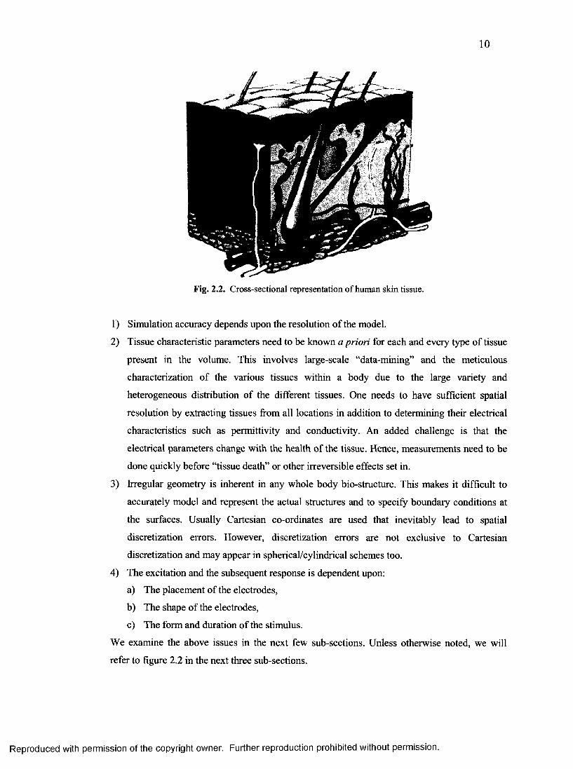
2.2.1 Intrinsic hurdles in full body modeling.One of the primary reasons that full body modeling schemes are not so common is

tissue complexity. So far, the most that has been done involves small tissue volume modeling

for thermal ablation [17] or lesion growth modeling [50]. The above is perhaps better

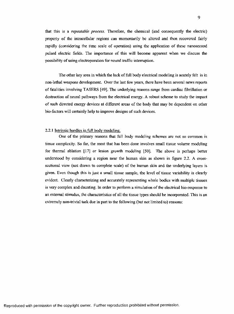
understood by considering a region near the human skin as shown in figure 2.2. A cross-

sectional view (not drawn to complete scale) of the human skin and the underlying layers is

given. Even though this is just a small tissue sample, the level of tissue variability is clearly

evident. Clearly characterizing and accurately representing whole bodies with multiple tissues

is very complex and daunting. In order to perform a simulation of the electrical bio-response to

an external stimulus, the characteristics of all the tissue types should be incorporated. This is an

extremely non-trivial task due in part to the following (but not limited to) reasons:


10

Fig. 2.2. Cross-sectional representation of human skin tissue.

1) Simulation accuracy depends upon the resolution of the model.

2) Tissue characteristic parameters need to be known a priori for each and every type of tissue

present in the volume. This involves large-scale “data-mining” and the meticulous

characterization of the various tissues within a body due to the large variety and

heterogeneous distribution of the different tissues. One needs to have sufficient spatial

resolution by extracting tissues from all locations in addition to determining their electrical

characteristics such as permittivity and conductivity. An added challenge is that the

electrical parameters change with the health of the tissue. Hence, measurements need to be

done quickly before “tissue death” or other irreversible effects set in.

3) Irregular geometry is inherent in any whole body bio-structure. This makes it difficult to

accurately model and represent the actual structures and to specify boundary conditions at

the surfaces. Usually Cartesian co-ordinates are used that inevitably lead to spatial

discretization errors. However, discretization errors are not exclusive to Cartesian

discretization and may appear in spherical/cylindrical schemes too.

4) The excitation and the subsequent response is dependent upon:

a) The placement of the electrodes,

b) The shape of the electrodes,

c) The form and duration of the stimulus.

We examine the above issues in the next few sub-sections. Unless otherwise noted, we will

refer to figure 2.2 in the next three sub-sections.


11

2.2.1.1 Model resolutionConsider that the tissue block given in figure 2.2 spans 10 cm by 5 cm by 1 cm. Since

any digitization of this tissue volume will involve some form of scanning operation, let us

assume that the tissue section is discretized at 1 cm. This means that the tissue volume is

scanned in 1cm sections in each dimension (direction). The resulting section will then consist of

(10*5*1) cm3 blocks. These elemental volumes are called nodes and make up the building block

of the underlying modeling scheme. Using such a low (coarse) resolution leads to 50 nodes but

at the cost of loss of tissue complexity detail. What that means is that given that most of the

embedded regions that are significantly smaller than 1 cm, such as vesicles and follicles will be

lost in such a discretization scheme. However, if the scanning is done at say - 1 mm resolution,

the total number of nodes rises to 100*50*10=50000. This leads to a dramatic rise in

computational price but yields the advantage of extremely fine-grained results. To highlight

this, typical myelinated nerves have a 2 mm inter-nodal span.

2.2.1.2 Tissue parametersAs mentioned previously, bio-models are, without exception, obtained using some form

of volumetric scanning method. However, these methods (MRI, CAT, etc.) are imaging

methods. That means the tissue density or its response to a particular excitation method is used

to “draw” its shape. It is relatively easy, though incomplete, to generate the volumetric image

data of a particular data type; however, in order to be able to use such information in

mathematical models, it is imperative that their characteristics and parameter values also be

known. For example, in the electrical domain, the specific conductivity and permittivity is

needed for mathematical modeling and quantification. Fortunately, over the years, almost all the

normal tissue types present in common animals and humans have been mapped and

characterized. Nevertheless, this does not preclude the possibility that a particular tissue volume

might consist of an abnormal growth that displays characteristics different from those in the

surrounding regions. This can also be understood by considering the case where a bone has been

replaced, grafted, or in extreme cases, replaced with an artificial limb. In any event, in order to

successfully model and compute the response of a bio-model, all the underlying tissue models

need to be identified and characterized using known, quantifiable parameters.

2.2.1.3 Excitation (stimulus) locations and form.As mentioned in section 2.1, since short term UWB radiation has to date, not shown

significant biological effects, this research focuses on pulsed electrical stimulus delivered

through direct contact pathways (electrodes). Referring again to figure 2.2, assume that a


12

rectangular electrode spanning the entire top surface is used as the “Anode”. Given such a

setup, barring a few minor areas at the follicle and other similar irregular regions, the electric

field lines would mostly be linear and vertical. If the orientation of the electrode plates were to

be changed, the average electric field would be different from the previous case. Furthermore, if

the cathode was reduced to a small circular region, with the anode being kept the same, the

electric field would not only be different, but would also no longer be uniform. These different

examples all indicate the fact that electrode regions’ size, shape and placement play a vital role

in setting up the electrical driving forces that ultimate affect the behavioral response of the

tissue upon stimulation. This is worth mentioning because this response can range from

activation of nerves (if any, as embedded in a particular region), to cell death (tissue necrosis

and apoptosis).

On the topic of applied stimulus, it should be mentioned that even the duration of the

applied potential pulse is a variable that needs to be accounted for and studied. For example, let

us assume that the entire tissue volume represented in figure 2.2 is comprised of only the

dermis. If the applied stimulus is a DC pulse with a finite ON time, then this ON time MUST be

such that the dermis sub-volumes are sufficiently charged. Otherwise, the observed current flow

and potentials would be lower than the maximum that could be achieved owing to the finite

electrical charging time of the system. In the next chapter, a brief table highlighting the

effective conductivity and permittivity of some of these tissues is listed. These can be used to

compute the effective time constants and the charging durations for various tissues in the

context of electrical pulsing.

The above essentially highlights the hurdles that make it virtually impossible to perform

accurate simulation studies. Consequently, research groups have tended to focus on tissue sub

sections and localized effects within such regions. Localized tissue uniformity (e.g. liver block

or skin section) definitely helps. Micro level non-uniformity in cases such as capillaries, is

typically ignored without loss of any appreciable accuracy. Flowever, to develop a more

physical and accurate bio-model and to address this void in the area of bio-medical modeling,

this dissertation aims to create a robust and scalable simulation scheme that will allow for whole

body modeling.

As mentioned earlier, to obtain any practical, usable information the discretization

resolution of the tissue model needs to be sufficiently high. However, this leads to a dramatic

increase in the computation cost. Stand alone computational systems cannot fulfill the resource

requirement for such a large order system. Additionally, the commercial restrictions that are


13

often imposed on commercial simulation packages such as those used in [17], can be

prohibitive. In this context, parallel algorithms have the potential to alleviate most of these

computational restrictions by providing resources that span more than one physical system.

These resources include memory capacity and processing capability. However, distributed

(parallel) algorithms are essentially more complex than their serial counterparts because apart

from numerical model component, they also need to incorporate data and synchronization

communication schemes. Furthermore, to be really efficient in handling large-scale problems

based on a given resource/processor limit, even the data storage scheme needs to be altered. A

more detailed example of this is given in chapter three, where the entire process flow diagram

of the proposed distributed modeling scheme is presented. To preface that however, consider

the following hypothetical scenario where two data sets A, B are operated upon. This operation

could be anything from simple data match to solution of a system of equations. In a serial

system the entire operation could be summarized using the following steps.

1. Load the datasets.

2. For each element in dataset A:

a. Perform operation with element in dataset B.

b. Echo the result.

3. Exit.

Comparing this to a parallel scheme of operation, and using the shared data scheme, the

algorithm would end up with a possible form such as:

1. Identify a control processor.

2. Send appropriate sized datasets to each slave processor.

3. Wait fo r results from each slave.

a. At each slave node for each element in sub-dataset A:

i. Perform operation with sub-dataset of Element B

ii. Send result to Control processor.

4. Reorder each result as received from the slaves.

5. Echo result of each operation.

This is an extremely simplified and generic example, yet one can clearly identify the

communication and synchronization overhead that would be involved with a distributed

solution scheme. The extra steps have been italicized. However, the underlying advantage that


14

is perhaps not very apparent is that significantly large datasets can be operated upon with a

distributed solution scheme.

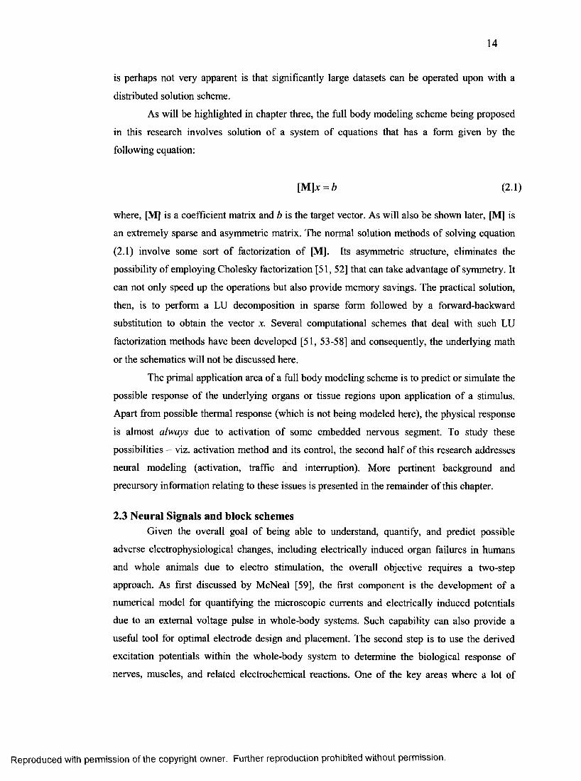
As will be highlighted in chapter three, the full body modeling scheme being proposed

in this research involves solution of a system of equations that has a form given by the

following equation:

[M]x = 6 (2.1)

where, [M] is a coefficient matrix and b is the target vector. As will also be shown later, [M] is

an extremely sparse and asymmetric matrix. The normal solution methods of solving equation

(2.1) involve some sort of factorization of [M]. Its asymmetric structure, eliminates the

possibility of employing Cholesky factorization [51, 52] that can take advantage of symmetry. It

can not only speed up the operations but also provide memory savings. The practical solution,

then, is to perform a LU decomposition in sparse form followed by a forward-backward

substitution to obtain the vector x. Several computational schemes that deal with such LU

factorization methods have been developed [51, 53-58] and consequently, the underlying math

or the schematics will not be discussed here.

The primal application area of a full body modeling scheme is to predict or simulate the

possible response of the underlying organs or tissue regions upon application of a stimulus.

Apart from possible thermal response (which is not being modeled here), the physical response

is almost always due to activation of some embedded nervous segment. To study these

possibilities - viz. activation method and its control, the second half of this research addresses

neural modeling (activation, traffic and interruption). More pertinent background and

precursory information relating to these issues is presented in the remainder of this chapter.

2.3 Neural Signals and block schemesGiven the overall goal of being able to understand, quantify, and predict possible

adverse electrophysiological changes, including electrically induced organ failures in humans

and whole animals due to electro stimulation, the overall objective requires a two-step

approach. As first discussed by McNeal [59], the first component is the development of a

numerical model for quantifying the microscopic currents and electrically induced potentials

due to an external voltage pulse in whole-body systems. Such capability can also provide a

useful tool for optimal electrode design and placement. The second step is to use the derived

excitation potentials within the whole-body system to determine the biological response of

nerves, muscles, and related electrochemical reactions. One of the key areas where a lot of


15

research and study has been done is that of nerve segments and the action potential propagation

and block mechanism. However, before we investigate any of this, it is prudent and logical to

examine the basic structure of a nerve segment and this is given in the next sub-section.

2.3.1 Nerve segment structure and kev termsAs is well known in the field of physiology, the basic information/signal pathway in

any mammal is comprised of a complex network made up of neurons. Neurons are electrically

excitable cells that process and transmit information and in vertebrate animals, they are the core

components of the brain, spinal cord and peripheral nerves. A schematic figure of a neuron is

shown in figure 2.3 [60],

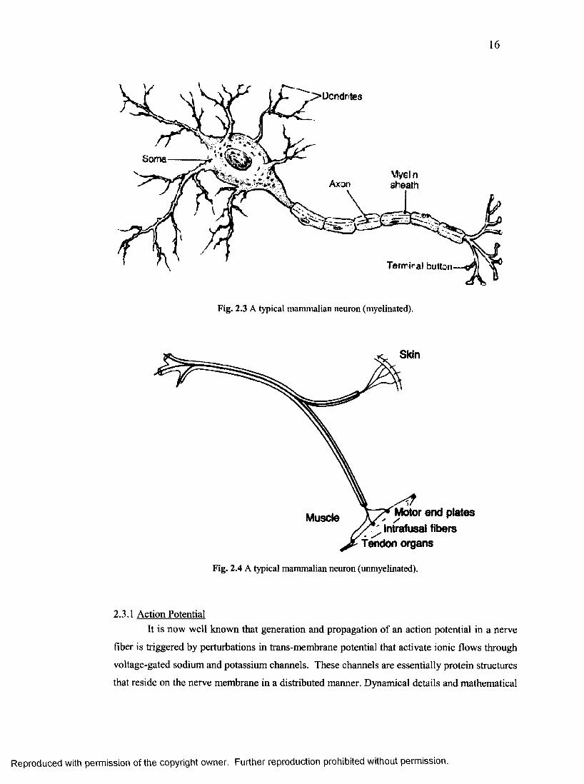
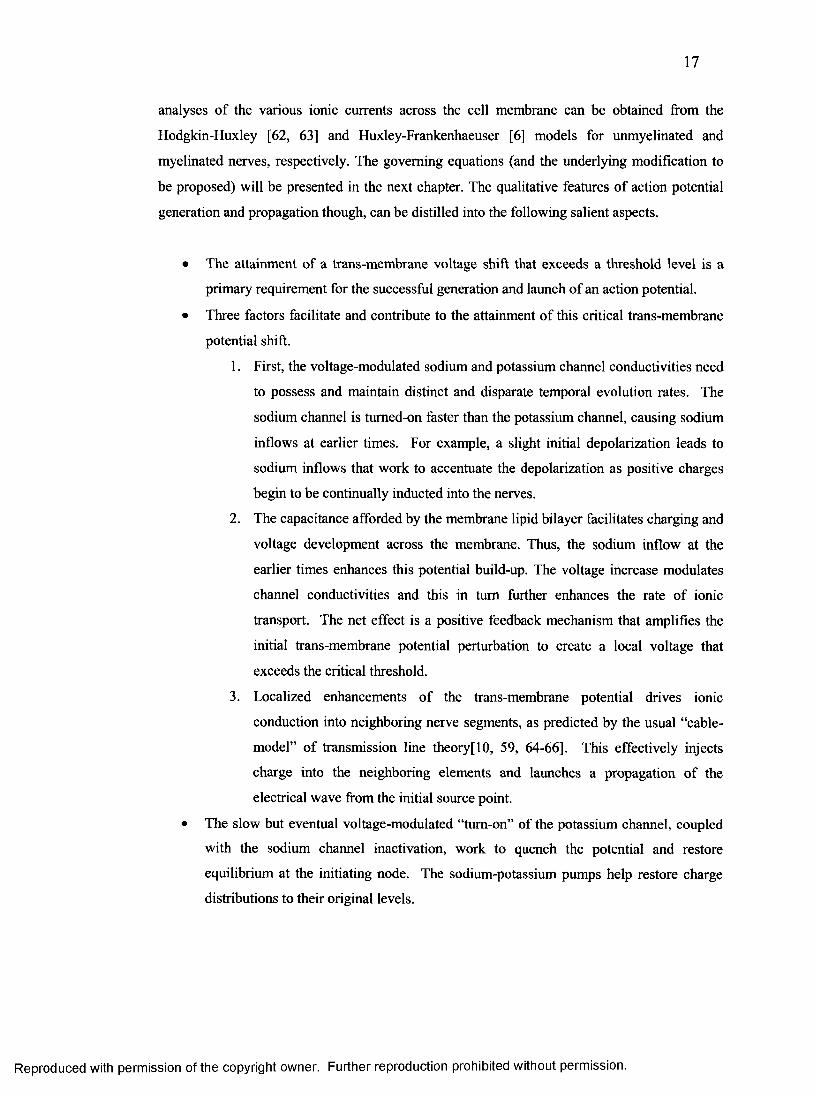
It should be noted that figure 2.3 represents a myelinated neuron in contrast to an

unmyelinated one which is shown in figure 2.4. The differentiating element is the myelin sheath

that is shown covering the axon. Also to be noted is the segmented form of this myelin sheath.

The region between each such myelin covered axon (myelinated axon) segment is known as the

“Node of Ranvier.” For the most part, the primary conduction pathways are comprised of

myelinated neurons. This is due to the fact that myelinated neurons provide a faster conduction

velocity of information due to salutatory effect induced by the extremely high resistance myelin

sheath between consecutive nodes [6, 59, 61]. It should also be noted that any “information” or

a signal that is propagated via the neural channels is in the form of a temporally varying

potential wave known as the Action Potential (AP). For the sake of thoroughness, prior to any

discussion of significance and methods of AP arrest, a brief discussion of the underlying

mechanism involving the rise and propagation of AP is presented and discussed.


16

SomaMyel n sheathAxon

Terrriral button

Fig. 2.3 A typical mammalian neuron (myelinated).

Skin

Motor end plates A S ' /

Intrafusal fiberstendon organs

Muscle

Fig. 2.4 A typical mammalian neuron (unmyelinated).

2.3.1 Action PotentialIt is now well known that generation and propagation of an action potential in a nerve

fiber is triggered by perturbations in trans-membrane potential that activate ionic flows through

voltage-gated sodium and potassium channels. These channels are essentially protein structures

that reside on the nerve membrane in a distributed manner. Dynamical details and mathematical


17

analyses of the various ionic currents across the cell membrane can be obtained from the

Hodgkin-Huxley [62, 63] and Huxley-Frankenhaeuser [6 ] models for unmyelinated and

myelinated nerves, respectively. The governing equations (and the underlying modification to

be proposed) will be presented in the next chapter. The qualitative features of action potential

generation and propagation though, can be distilled into the following salient aspects.

• The attainment of a trans-membrane voltage shift that exceeds a threshold level is a

primary requirement for the successful generation and launch of an action potential.

• Three factors facilitate and contribute to the attainment of this critical trans-membrane

potential shift.

1. First, the voltage-modulated sodium and potassium channel conductivities need

to possess and maintain distinct and disparate temporal evolution rates. The

sodium channel is tumed-on faster than the potassium channel, causing sodium

inflows at earlier times. For example, a slight initial depolarization leads to

sodium inflows that work to accentuate the depolarization as positive charges

begin to be continually inducted into the nerves.

2. The capacitance afforded by the membrane lipid bilayer facilitates charging and

voltage development across the membrane. Thus, the sodium inflow at the

earlier times enhances this potential build-up. The voltage increase modulates

channel conductivities and this in turn further enhances the rate of ionic

transport. The net effect is a positive feedback mechanism that amplifies the

initial trans-membrane potential perturbation to create a local voltage that

exceeds the critical threshold.

3. Localized enhancements of the trans-membrane potential drives ionic

conduction into neighboring nerve segments, as predicted by the usual “cable-

model” of transmission line theory[10, 59, 64-66]. This effectively injects

charge into the neighboring elements and launches a propagation of the

electrical wave from the initial source point.

• The slow but eventual voltage-modulated “tum-on” of the potassium channel, coupled

with the sodium channel inactivation, work to quench the potential and restore

equilibrium at the initiating node. The sodium-potassium pumps help restore charge

distributions to their original levels.


18

It should be noted that the neuron model proposed in [62] which has been adopted as the de-

facto standard in almost all subsequent studies in this area, was based on a giant squid axon. In

more recent studies [67, 6 8 ], it has been shown that the neurons in humans and other mammals

tend to have a significantly higher number of ionic channels that contributed to the activation of

the nodes. Some recent researchers [69, 70], have employed a slightly different model wherein

it has been assumed, in contrast to the classic model, that the sodium channel does not have any

inactivation variable. They also incorporate the dynamics of an additional calcium channel

current in the membrane activation/deactivation process along with a calcium assisted

potassium hyper-polarizing current.

It should also be mentioned that the original Hodgkin-Huxley (HH) model was for an

unmyelinated axon. One of the first studies for the myelinated case involved incorporation of

the molar concentration of sodium and potassium ions in the medium surrounding the axon.

However, in quite a few other reports such as [61, 71], the original HH equations defining the

nodes were retained. Changes were incorporated by treating the “Node-of-Ranvier” as having

significantly higher densities of sodium, potassium and leakage channels. The inter-nodal

distance (myelinated part) is usually modeled as extremely high resistance, coupled with an

extremely low capacitance value. This gives rise to an extremely low time constant for the

myelinated segment of the axon and consequently allows for the modeling of the salutatory

conduction and leads to a fast response. This form of treatment of the myelinated segments

allows for a unified scheme of modeling the complete neural spectrum while keeping the

equations consistent. It is the apparent lack of incorporating the myelinated segment in studies

such as [69, 70], that seems to contradict those of other researchers in this area [72-74]. The

possibility of interrupting AP propagation, as already mentioned in section 2.2, is the primary

motive behind this dissertation. Hence, concepts and issues relating to AP signal blockage are

examined next.

2.3.2 Action Potential conduction blockSince a shift in electrical potential is a necessary requirement to initiate and maintain electrical

propagation through a nerve fiber, any event that disrupts the trans-membrane voltage can

potentially impede action potential propagation. One possibility is through the application of

an external DC bias near a nerve. For a propagating action potential (initiated, for example, by

a depolarizing voltage), the application of a positive bias on the outer region of the nerve would

prevent the local potential from reaching the requisite negative value. This would effectively

arrest AP propagation, and hence, in theory block nerve conduction. However, a number of


19

potential and practical problems arise from the application of an external DC bias for purposes

of a conduction block.

(i) First, the prolonged application of the DC bias can itself inject localized currents

and charge the axonal membranes, thereby launching its own AP. The duration and

amplitude of the external DC has to be sufficiently low to circumvent such “self

launch” phenomena.

(ii) In addition, since the timing and sequence of propagating action potentials are not

known a priori, it is practically very difficult to achieve reliable conduction

blockages for all possible propagating APs.

(iii) Any sharp rise times for the DC biasing voltages can lead to large capacitive

charging currents that have a similar undesirable effect of self-launching an AP.

Hence, the rise and fall times of any applied DC bias need to be sufficiently large.

(iv) Long durations or repetitive DC biasing can potentially cause tissue damage due to

internal heating [75]. For effective suppression of this deleterious effect, the net

energy needs to be sufficiently small.

All the above problems notwithstanding, a good deal of research involving application

of AC/DC interrupting signals to achieve AP block [8 , 12, 13, 76-78], has been carried out.

Though other methods of achieving nerve conduction blockage such as pressure application

[79], temperature lowering [15], chemical and pharmacological means[77] exist, none can be as

quick-acting, localized and yet reversible as electrical stimulation. Cessation of biological

electrical signaling pathways can have a variety of applications in neurophysiology, clinical

research, neuromuscular stimulation therapies, and even non-lethal bio-weapons development.

For example, pudendal nerve conduction block during micturition can reduce urethral pressure

[16, 80], or help relieve chronic pain from a site of peripheral nerve injury [81]. It is well

known that the nerve blocking ability of electrical stimulation is progressive from larger to

smaller fibers [82, 83] and has been used to activate muscles in a physiological recruitment

order and to reduce muscle fatigue. The concept of arresting action potential (AP) propagation

on command through external electrical stimulation could open the possibility of temporary

incapacitation with applications to crowd-control.

The application of high frequency blocking signals alleviates some of the problems with

DC biasing. The heat generation can be reduced and the biphasic signals make it somewhat

more difficult to self-launch action potentials. However, the overall difficulties are not


20

eliminated, and the fundamental issues remain. In addition, the frequency of operation begins

to play an important role in the blocking effectiveness. A frequency bandwidth limitation for

AP extinction exists, and excitation that is either too fast or too slow cannot provide a

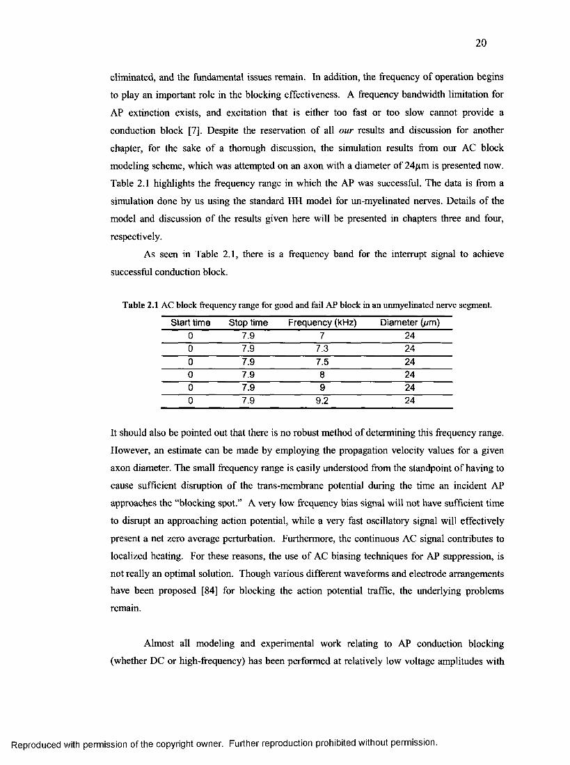
conduction block [7], Despite the reservation of all our results and discussion for another

chapter, for the sake of a thorough discussion, the simulation results from our AC block

modeling scheme, which was attempted on an axon with a diameter of 24/xm is presented now.

Table 2.1 highlights the frequency range in which the AP was successful. The data is from a

simulation done by us using the standard HH model for un-myelinated nerves. Details of the

model and discussion of the results given here will be presented in chapters three and four,

respectively.

As seen in Table 2.1, there is a frequency band for the interrupt signal to achieve

successful conduction block.

Table 2.1 AC block frequency range for good and fail AP block in an unmyelinated nerve segment.

Start time Stop time Frequency (kHz) Diameter (//m)0 7.9 7 240 7.9 7.3 240 7.9 7.5 240 7.9 8 240 7.9 9 240 7.9 9.2 24

It should also be pointed out that there is no robust method of determining this frequency range.

However, an estimate can be made by employing the propagation velocity values for a given

axon diameter. The small frequency range is easily understood from the standpoint of having to

cause sufficient disruption of the trans-membrane potential during the time an incident AP

approaches the “blocking spot.” A very low frequency bias signal will not have sufficient time

to disrupt an approaching action potential, while a very fast oscillatory signal will effectively

present a net zero average perturbation. Furthermore, the continuous AC signal contributes to

localized heating. For these reasons, the use of AC biasing techniques for AP suppression, is

not really an optimal solution. Though various different waveforms and electrode arrangements

have been proposed [84] for blocking the action potential traffic, the underlying problems

remain.

Almost all modeling and experimental work relating to AP conduction blocking

(whether DC or high-frequency) has been performed at relatively low voltage amplitudes with


21

temporal durations in the micro-second range or higher. However, the development and use of

electric pulses with very high fields (~ lOOkV/cm or higher) and pulse durations in the

nanosecond range [24, 85] has been a very recent development in bio-electrics. From a

practical standpoint, such high-intensity, short-duration electrical pulses (HISDEPs) or nPEFs

have been shown to be useful for various biological applications including cellular

electroporation [1], electrically-triggered intra-cellular calcium release [25, 26], the non-thermal

destruction of micro-organisms [1, 8 6 , 87], killing of tumor cells [1, 8 8 ], DNA damage [89],

and possibly wound healing [90, 91]. The hallmark of such a HISDEP is the creation of a high

density of nanometer-sized pores on the cellular membrane, followed by their relatively rapid

recovery through re-sealing. This has been confirmed by analytical calculations [85, 92-94] as

well as molecular dynamic simulations [95-97] and verified by tracking fluorescent dyes in flow

cytometry experiments [1], Since the process of electroporation in cell membrane has

potentially far reaching possibilities (not to mention application in the AP block schema being

proposed), it warrants a slightly detailed examination. Some of the pertinent and salient aspects

of electroporation are briefly discussed in the next section.

2.3.2.1 ElectroporationIt is fairly well known that cell membranes are composed of lipids and proteins.

Differences between cell membranes arise from the relative composition of these two

constitutive elements and their structural arrangement. For example, proteins make up only 18%

of the myelin membrane of nerve cells, while the rest of it is lipids. On the other hand, the inner

mitochondrial membrane is 76% proteins [98]. A schematic representation of the cell

membrane is shown in figure 2.5. Note that the cell membrane represented in figure 2.5 shows a

significantly higher presence of lipids compared to proteins and may be considered to be

representative of the myelin sheath. The other aspect is the variability in the lipid composition

itself. A large fraction of mammalian plasma membrane is constituted of cholesterol and

carbohydrates, etc. In any event, the above simply implies that a membrane has a very complex

structure.

The central idea o f “electroporation” is that it is a progressive and systematic re

organization without any molecular breakup or detachment [99] brought about by an electric

field. Thus, the application o f external electric fields to cells or tissues permeabilizes the cell

membrane producing aqueous pathways (called filled pores) in the bilayer system. This process

is referred to as electropermeabilization or membrane breakdown.


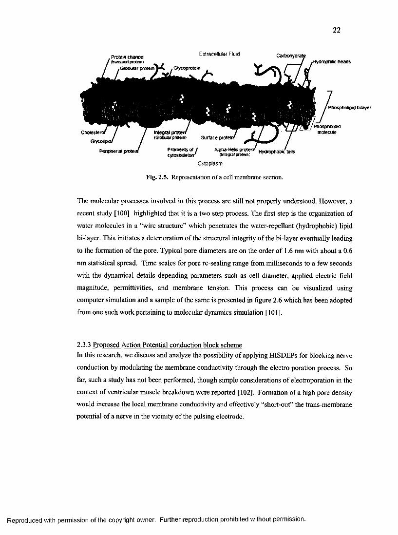
22

Hydropnilic heads

|^^^W iospho lip id brlayer

Phospholipidmolecule

The molecular processes involved in this process are still not properly understood. However, a

recent study [100] highlighted that it is a two step process. The first step is the organization of

water molecules in a “wire structure” which penetrates the water-repellant (hydrophobic) lipid

bi-layer. This initiates a deterioration of the structural integrity of the bi-layer eventually leading

to the formation of the pore. Typical pore diameters are on the order of 1. 6 nm with about a 0.6

nm statistical spread. Time scales for pore re-sealing range from milliseconds to a few seconds

with the dynamical details depending parameters such as cell diameter, applied electric field

magnitude, permittivities, and membrane tension. This process can be visualized using

computer simulation and a sample of the same is presented in figure 2 . 6 which has been adopted

from one such work pertaining to molecular dynamics simulation [ 1 0 1 ].

2.3.3 Proposed Action Potential conduction block schemeIn this research, we discuss and analyze the possibility of applying HISDEPs for blocking nerve

conduction by modulating the membrane conductivity through the electro poration process. So

far, such a study has not been performed, though simple considerations of electroporation in the

context of ventricular muscle breakdown were reported [102]. Formation of a high pore density

would increase the local membrane conductivity and effectively “short-out” the trans-membrane

potential of a nerve in the vicinity of the pulsing electrode.

, Protein channel

, Gtobolar protein

Extracellular Fluid Carbohydrat

Glycoprotein

integral (Globular protein;

Chotesti

Giya

Penphenal |

Surface proteir

*’ Hydrophobic tads

Cytoplasm

Fig. 2.5. Representation of a cell membrane section.

Filaments of / eytoskeieton


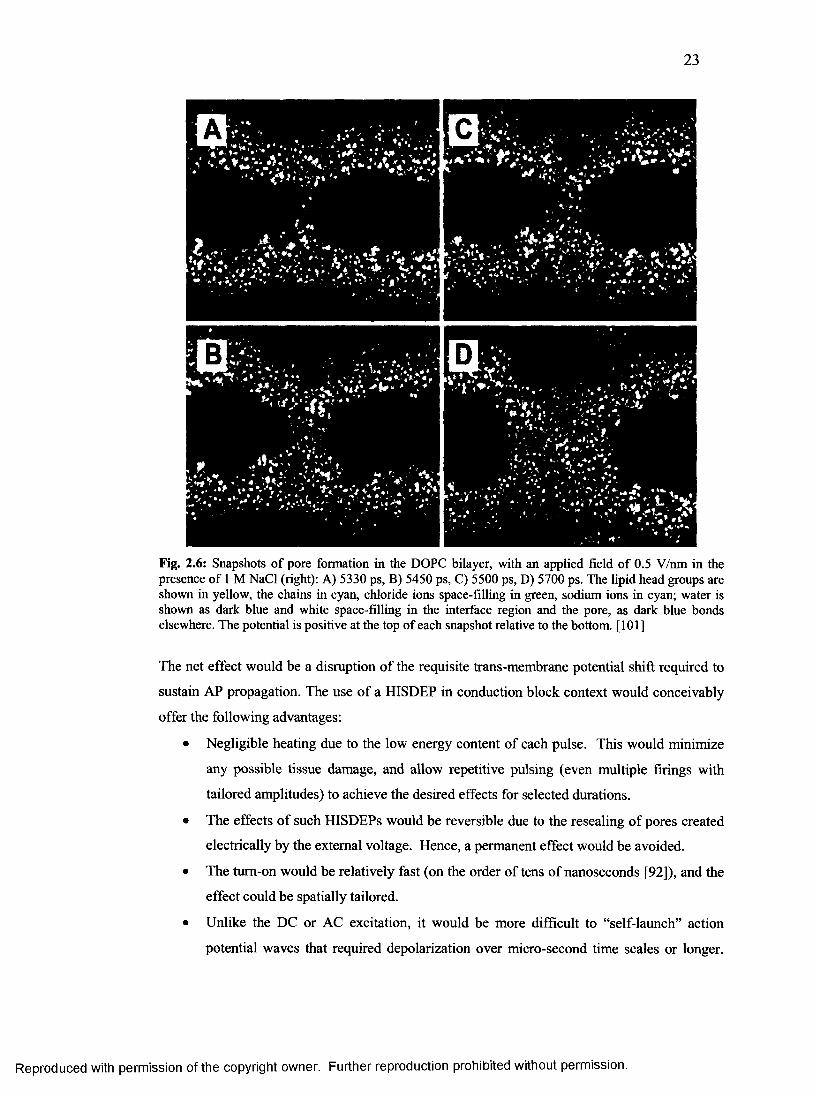
23

Fig. 2.6: Snapshots of pore formation in the DOPC bilayer, with an applied field of 0.5 V/nm in the presence of 1 M NaCl (right): A) 5330 ps, B) 5450 ps, C) 5500 ps, D) 5700 ps. The lipid head groups are shown in yellow, the chains in cyan, chloride ions space-filling in green, sodium ions in cyan; water is shown as dark blue and white space-filling in the interface region and the pore, as dark blue bonds elsewhere. The potential is positive at the top of each snapshot relative to the bottom. [101]

The net effect would be a disruption of the requisite trans-membrane potential shift required to

sustain AP propagation. The use of a HISDEP in conduction block context would conceivably

offer the following advantages;

• Negligible heating due to the low energy content of each pulse. This would minimize

any possible tissue damage, and allow repetitive pulsing (even multiple firings with

tailored amplitudes) to achieve the desired effects for selected durations.

• The effects of such HISDEPs would be reversible due to the resealing of pores created

electrically by the external voltage. Hence, a permanent effect would be avoided.

• The turn-on would be relatively fast (on the order of tens of nanoseconds [92]), and the

effect could be spatially tailored.

• Unlike the DC or AC excitation, it would be more difficult to “self-launch” action

potential waves that required depolarization over micro-second time scales or longer.


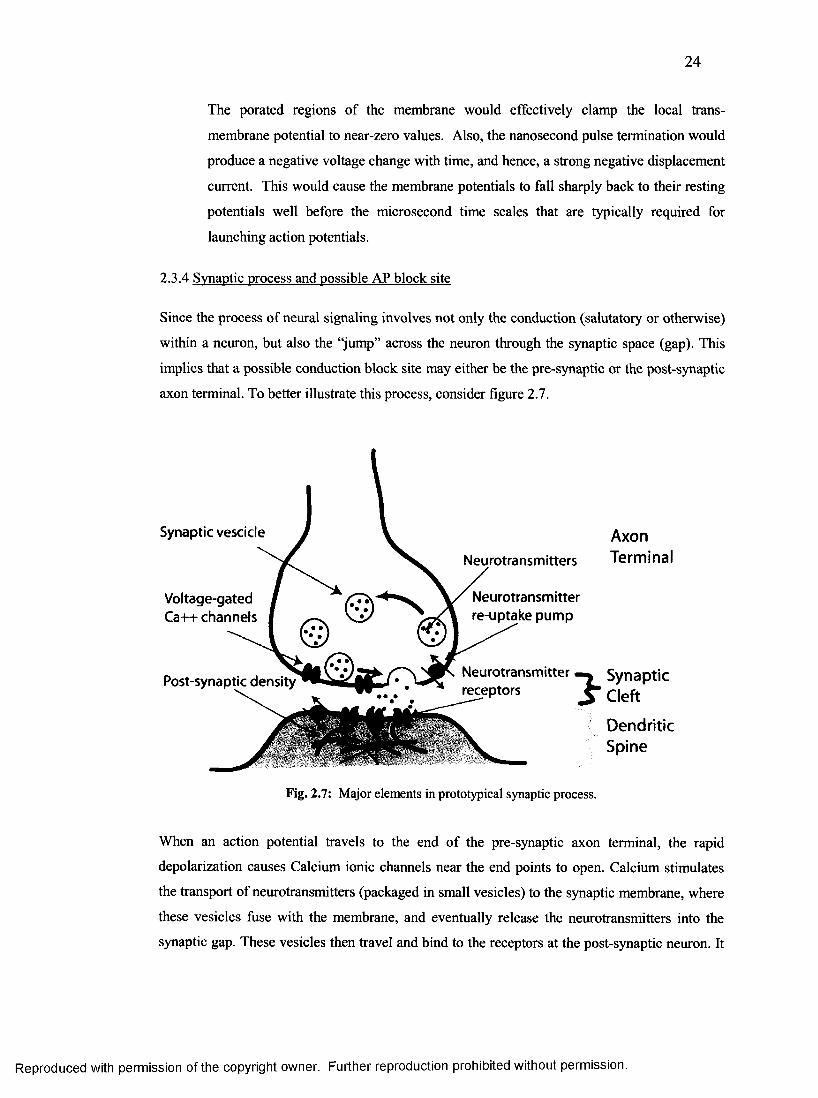
24

The porated regions of the membrane would effectively clamp the local trans

membrane potential to near-zero values. Also, the nanosecond pulse termination would

produce a negative voltage change with time, and hence, a strong negative displacement

current. This would cause the membrane potentials to fall sharply back to their resting

potentials well before the microsecond time scales that are typically required for

launching action potentials.

2.3.4 Synaptic process and possible AP block site

Since the process of neural signaling involves not only the conduction (salutatory or otherwise)

within a neuron, but also the “jump” across the neuron through the synaptic space (gap). This

implies that a possible conduction block site may either be the pre-synaptic or the post-synaptic

axon terminal. To better illustrate this process, consider figure 2.7.

When an action potential travels to the end of the pre-synaptic axon terminal, the rapid

depolarization causes Calcium ionic channels near the end points to open. Calcium stimulates

the transport of neurotransmitters (packaged in small vesicles) to the synaptic membrane, where

these vesicles fuse with the membrane, and eventually release the neurotransmitters into the

synaptic gap. These vesicles then travel and bind to the receptors at the post-synaptic neuron. It

Synaptic vescide

Neurotransmitters

Neurotransmitter re-uptake pum p

Voltage-gated Ca++ channels

NeurotransmitterreceptorsPost-synaptic density S yn ap tic

C left

D en d riticS p in e

A xonT erm inal

Fig. 2.7: Major elements in prototypical synaptic process.


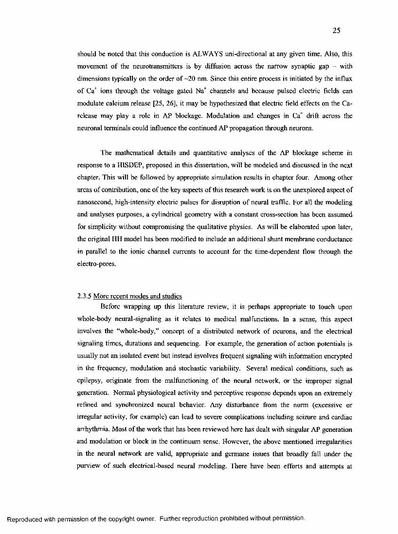
25

should be noted that this conduction is ALWAYS uni-directional at any given time. Also, this

movement of the neurotransmitters is by diffusion across the narrow synaptic gap - with

dimensions typically on the order of ~20 nm. Since this entire process is initiated by the influx

of Ca+ ions through the voltage gated Na+ channels and because pulsed electric fields can

modulate calcium release [25, 26], it may be hypothesized that electric field effects on the Ca-

release may play a role in AP blockage. Modulation and changes in Ca+ drift across the

neuronal terminals could influence the continued AP propagation through neurons.

The mathematical details and quantitative analyses of the AP blockage scheme in

response to a HISDEP, proposed in this dissertation, will be modeled and discussed in the next

chapter. This will be followed by appropriate simulation results in chapter four. Among other

areas of contribution, one of the key aspects of this research work is on the unexplored aspect of

nanosecond, high-intensity electric pulses for disruption of neural traffic. For all the modeling

and analyses purposes, a cylindrical geometry with a constant cross-section has been assumed

for simplicity without compromising the qualitative physics. As will be elaborated upon later,

the original HH model has been modified to include an additional shunt membrane conductance

in parallel to the ionic channel currents to account for the time-dependent flow through the

electro-pores.

2.3.5 More recent modes and studiesBefore wrapping up this literature review, it is perhaps appropriate to touch upon

whole-body neural-signaling as it relates to medical malfunctions. In a sense, this aspect

involves the “whole-body,” concept of a distributed network of neurons, and the electrical

signaling times, durations and sequencing. For example, the generation of action potentials is

usually not an isolated event but instead involves frequent signaling with information encrypted

in the frequency, modulation and stochastic variability. Several medical conditions, such as

epilepsy, originate from the malfunctioning of the neural network, or the improper signal

generation. Normal physiological activity and perceptive response depends upon an extremely

refined and synchronized neural behavior. Any disturbance from the norm (excessive or

irregular activity, for example) can lead to severe complications including seizure and cardiac

arrhythmia. Most of the work that has been reviewed here has dealt with singular AP generation

and modulation or block in the continuum sense. However, the above mentioned irregularities

in the neural network are valid, appropriate and germane issues that broadly fall under the

purview of such electrical-based neural modeling. There have been efforts and attempts at


26

addressing problems and issues associated with such whole-body, neural signaling and its

failures. The study of such instances that may be perceived as failure of neural stability or

synchronization have incorporated multi-neural models in some form or multi-state

environments where the activity level of one group of neural segment may or may not be causal.

In some reports, this has been done as a focus on seizure dynamics using a nonlinear network

[70], or employing chaos theory for the same [103] or cardiac activity [104]. All this points to

the possibility that focused electrical stimulation can be used to alleviate some of these

problems, akin to the transcutaneous electric nerve stimulator. Just as electrical stimulation

proves to be an effective treatment for controlling heart disorders (such as arrhythmia) via

“pacemakers,” it would seem natural to look to similar electrical stimulation for regulating and

controlling neural disorders such as epilepsy. However, the above aspect through interesting

remains outside the present scope of this dissertation research. It has been mentioned here,

simply from the standpoint of completeness.

In this chapter, all relevant background research that related directly to this research

work has been highlighted. The preface to the actual modeling details and simulation results,

which follow in the subsequent chapters, has also been incorporated. The remainder of this

dissertation will present the proposed simulation schemes for full body modeling, nerve

segment model with action potential block methods, followed by simulation results in both

these areas. The final chapter includes concluding remarks along with the road map of possible

extension to this work.


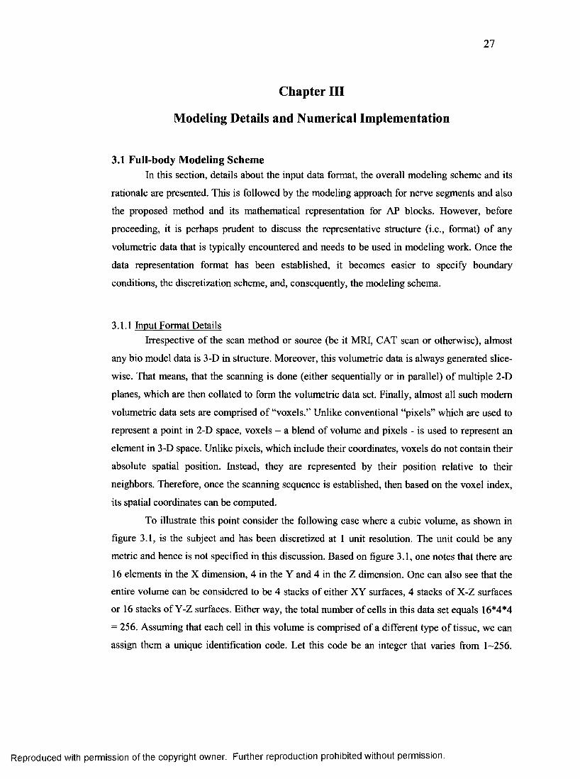
27

Chapter III

Modeling Details and Numerical Implementation

3.1 Full-body Modeling SchemeIn this section, details about the input data format, the overall modeling scheme and its

rationale are presented. This is followed by the modeling approach for nerve segments and also

the proposed method and its mathematical representation for AP blocks. However, before

proceeding, it is perhaps prudent to discuss the representative structure (i.e., format) of any

volumetric data that is typically encountered and needs to be used in modeling work. Once the

data representation format has been established, it becomes easier to specify boundary

conditions, the discretization scheme, and, consequently, the modeling schema.

3.1.1 Input Format DetailsIrrespective of the scan method or source (be it MRI, CAT scan or otherwise), almost

any bio model data is 3-D in structure. Moreover, this volumetric data is always generated slice-

wise. That means, that the scanning is done (either sequentially or in parallel) of multiple 2-D

planes, which are then collated to form the volumetric data set. Finally, almost all such modem

volumetric data sets are comprised of “voxels.” Unlike conventional “pixels” which are used to

represent a point in 2-D space, voxels - a blend of volume and pixels - is used to represent an

element in 3-D space. Unlike pixels, which include their coordinates, voxels do not contain their

absolute spatial position. Instead, they are represented by their position relative to their

neighbors. Therefore, once the scanning sequence is established, then based on the voxel index,

its spatial coordinates can be computed.

To illustrate this point consider the following case where a cubic volume, as shown in

figure 3.1, is the subject and has been discretized at 1 unit resolution. The unit could be any

metric and hence is not specified in this discussion. Based on figure 3.1, one notes that there are

16 elements in the X dimension, 4 in the Y and 4 in the Z dimension. One can also see that the

entire volume can be considered to be 4 stacks of either XY surfaces, 4 stacks of X-Z surfaces

or 16 stacks of Y-Z surfaces. Either way, the total number of cells in this data set equals 16*4*4

= 256. Assuming that each cell in this volume is comprised of a different type of tissue, we can

assign them a unique identification code. Let this code be an integer that varies from 1~256.


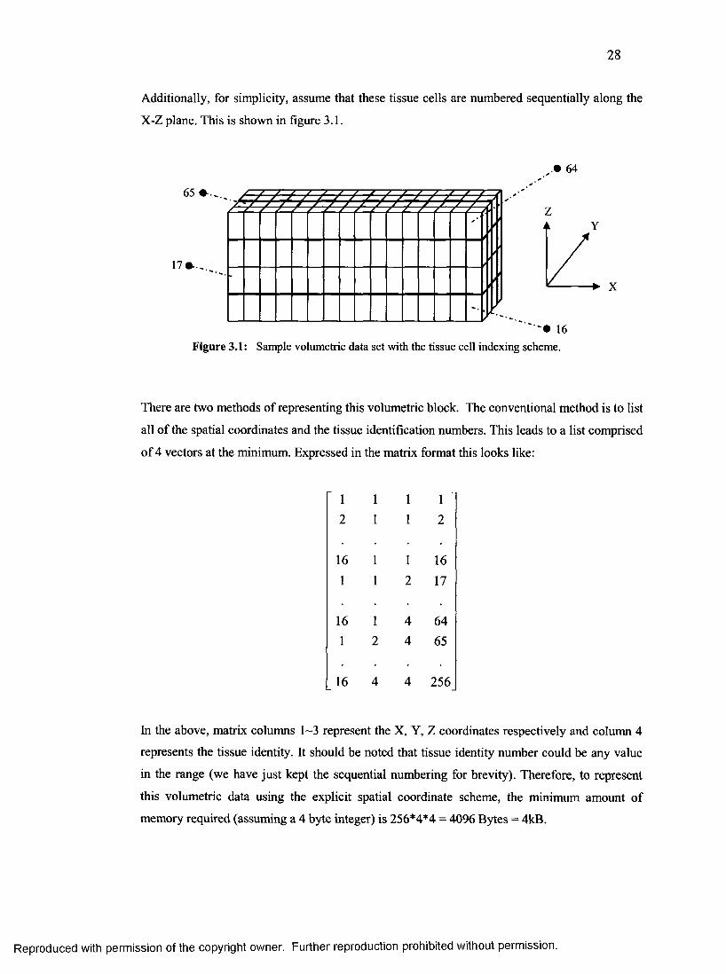
28

Additionally, for simplicity, assume that these tissue cells are numbered sequentially along the

X-Z plane. This is shown in figure 3.1.

, • 64

65

17 <

iSSf 52SSe s

Tmm-

•/

/ ' "

' • 16Figure 3.1: Sample volumetric data set with the tissue cell indexing scheme.

There are two methods of representing this volumetric block. The conventional method is to list

all of the spatial coordinates and the tissue identification numbers. This leads to a list comprised

of 4 vectors at the minimum. Expressed in the matrix format this looks like:

i 1 1 1

2 1 1 2

16 1 1 161 1 2 17

16 1 4 641 2 4 65

16 4 4 256

In the above, matrix columns 1-3 represent the X, Y, Z coordinates respectively and column 4

represents the tissue identity. It should be noted that tissue identity number could be any value

in the range (we have just kept the sequential numbering for brevity). Therefore, to represent

this volumetric data using the explicit spatial coordinate scheme, the minimum amount of

memory required (assuming a 4 byte integer) is 256*4*4 = 4096 Bytes = 4kB.


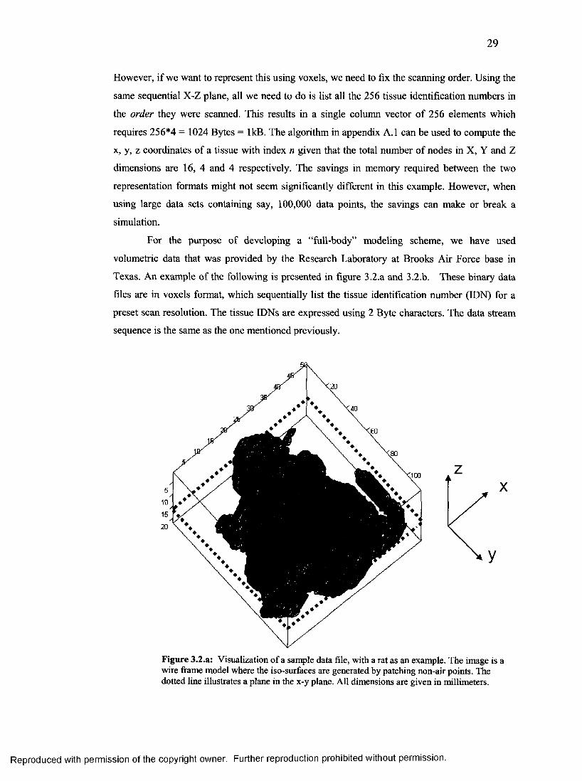
29

However, if we want to represent this using voxels, we need to fix the scanning order. Using the

same sequential X-Z plane, all we need to do is list all the 256 tissue identification numbers in

the order they were scanned. This results in a single column vector of 256 elements which

requires 256*4 = 1024 Bytes = lkB. The algorithm in appendix A.l can be used to compute the

x, y, z coordinates of a tissue with index n given that the total number of nodes in X, Y and Z

dimensions are 16, 4 and 4 respectively. The savings in memory required between the two

representation formats might not seem significantly different in this example. However, when

using large data sets containing say, 1 0 0 , 0 0 0 data points, the savings can make or break a

simulation.

For the purpose of developing a “full-body” modeling scheme, we have used

volumetric data that was provided by the Research Laboratory at Brooks Air Force base in

Texas. An example of the following is presented in figure 3.2.a and 3.2.b. These binary data

files are in voxels format, which sequentially list the tissue identification number (DDN) for a

preset scan resolution. The tissue IDNs are expressed using 2 Byte characters. The data stream

sequence is the same as the one mentioned previously.

Figure 3.2.a: Visualization of a sample data file, with a rat as an example. The image is a wire frame model where the iso-surfaces are generated by patching non-air points. The dotted line illustrates a plane in the x-y plane. All dimensions are given in millimeters.


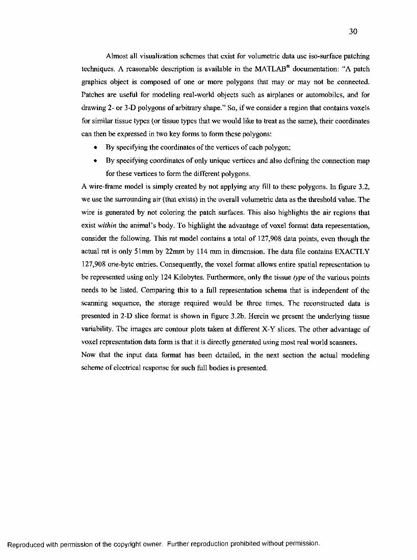
30

Almost all visualization schemes that exist for volumetric data use iso-surface patching

techniques. A reasonable description is available in the MATLAB® documentation: “A patch

graphics object is composed of one or more polygons that may or may not be connected.

Patches are useful for modeling real-world objects such as airplanes or automobiles, and for

drawing 2- or 3-D polygons of arbitrary shape.” So, if we consider a region that contains voxels

for similar tissue types (or tissue types that we would like to treat as the same), their coordinates

can then be expressed in two key forms to form these polygons:

• By specifying the coordinates of the vertices of each polygon;

• By specifying coordinates of only unique vertices and also defining the connection map

for these vertices to form the different polygons.

A wire-frame model is simply created by not applying any fill to these polygons. In figure 3.2,

we use the surrounding air (that exists) in the overall volumetric data as the threshold value. The

wire is generated by not coloring the patch surfaces. This also highlights the air regions that

exist within the animal’s body. To highlight the advantage of voxel format data representation,

consider the following. This rat model contains a total of 127,908 data points, even though the

actual rat is only 51mm by 22mm by 114 mm in dimension. The data file contains EXACTLY

127,908 one-byte entries. Consequently, the voxel format allows entire spatial representation to

be represented using only 124 Kilobytes. Furthermore, only the tissue type of the various points

needs to be listed. Comparing this to a full representation schema that is independent of the

scanning sequence, the storage required would be three times. The reconstructed data is

presented in 2-D slice format is shown in figure 3.2b. Herein we present the underlying tissue

variability. The images are contour plots taken at different X-Y slices. The other advantage of

voxel representation data form is that it is directly generated using most real world scanners.

Now that the input data format has been detailed, in the next section the actual modeling

scheme of electrical response for such full bodies is presented.


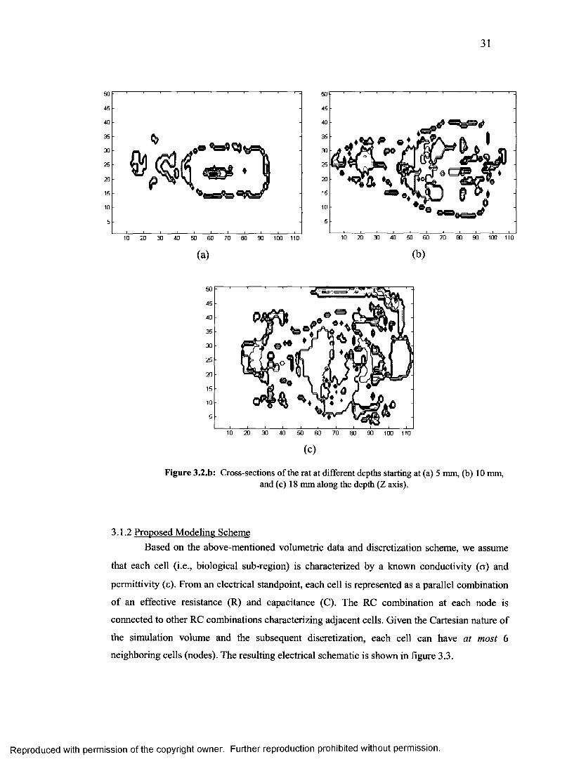
Figure 3.2.b: Cross-sections of the rat at different depths starting at (a) 5 mm, (b) 10 mm, and (c) 18 mm along the depth (Z axis).

3.1.2 Proposed Modeling SchemeBased on the above-mentioned volumetric data and discretization scheme, we assume

that each cell (i.e., biological sub-region) is characterized by a known conductivity (a) and

permittivity (e). From an electrical standpoint, each cell is represented as a parallel combination

of an effective resistance (R) and capacitance (C). The RC combination at each node is

connected to other RC combinations characterizing adjacent cells. Given the Cartesian nature of

the simulation volume and the subsequent discretization, each cell can have at most 6

neighboring cells (nodes). The resulting electrical schematic is shown in figure 3.3.


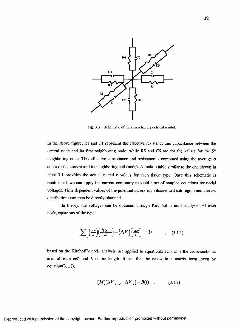
32

Fig. 3.3. Schematic of the discretized electrical model.

In the above figure, R1 and C l represent the effective resistance and capacitance between the

central node and its first neighboring node, while R5 and C5 are for the values for the 5th

neighboring node. This effective capacitance and resistance is computed using the average a

and e of the current and its neighboring cell (node). A lookup table similar to the one shown in

table 3.1 provides the actual a and 8 values for each tissue type. Once this schematic is

established, we can apply the current continuity to yield a set of coupled equations for nodal

voltages. Time dependent values of the potential across each discretized sub-region and current

distributions can then be directly obtained.

In theory, the voltages can be obtained through KirchhofFs node analysis. At each

node, equations of the type:

based on the Kirchoff s node analysis, are applied In equation(3.1.1), A is the cross-sectional

area of each cell and L is the length. It can then be recast in a matrix form given by

equation(3.1.2).

(3.1.1)


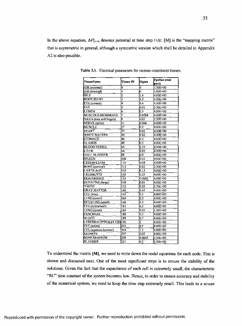
33

In the above equation, AF|,+At denotes potential at time step t+At. [M] is the “mapping matrix”

that is asymmetric in general, although a symmetric version which shall be detailed in Appendix

A2 is also possible.

Table 3.1. Electrical parameters for various constituent tissues.

TissueName Tissue ID Sigma Epsilon (real part)

AIR.(extemal) 0 0 1.00E+00AIR.(intemal) 1 0 1.00E+00BILE 2 1.4 4.00E+00BODY.FLUID 3 1.5 4.00E+00EYE.(comea) 4 0.4 4.00E+00FAT 5 0.01 2.50E+00LYMPH 6 0.5 4.00E+00MUSCOUS.MEMBRANE 7 0.0004 4.00E+00NAILS.(toes.and.fingers) 8 0.02 2.50E+00NERVE.(spine) 11 0.006 4.00E+00MUSCLE. 17 0.2 4.00E+00HEART 25 0.05 4.00E+00WHITE.MATTER 30 0.02 4.00E+00STOMACH 48 0.5 4.00E+00GLANDS 49 0.5 4.00E+00BLOOD.VESSEL 65 0.25 4.00E+00LIVER 68 0.02 4.00E+00GALLBLADDER 88 0.9 4.00E+00SPLEEN 108 0.03 4.00E+00CEREBELLUM 110 0.04 4.00E+00BONE.(cortical) 111 0.02 2.50E+00CARTILAGE. 133 0.15 4.00E+00LIGAMENTS 142 0.25 4.00E+00SKIN/DERMIS 143 0.0002 4.00E400INTESTINE.(large) 148 0.01 4.00E+00TOOTH 152 0.02 2.50E+00GRAY.MATTER 160 0.02 4.00E+00EYE.(lens) 163 0.3 4.00E+00LUNG.(outer) 164 0.2 4.00E+00INTESTINE.(small) 168 0.5 4.00E+00EYE.(sclera/wall) 183 0.5 4.00E+00LUNG.(inner) 184 0.03 2.50E+00PANCREAS 188 0.5 4.00E+00BLOOD 189 0.7 4.00E+00CEREBRALSPINALFLUID 190 2 4.00E+00EYE.(retina) 203 0.5 4.00E+00EYE.(aqueous.humour) 204 1.5 4.00E+00KIDNEYS 207 0.05 4.00E+00BONE.MARROW 209 0.0005 2.50E+00BLADDER 227 0.2 2.50E+00

To understand the matrix [M], we need to write down the nodal equations for each node. This is

shown and discussed next. One of the most significant steps is to ensure the stability of the

solutions. Given the fact that the capacitance of each cell is extremely small, the characteristic

“RC” time constant of the system becomes low. Hence, in order to ensure accuracy and stability

of the numerical system, we need to keep the time step extremely small. This leads to a severe


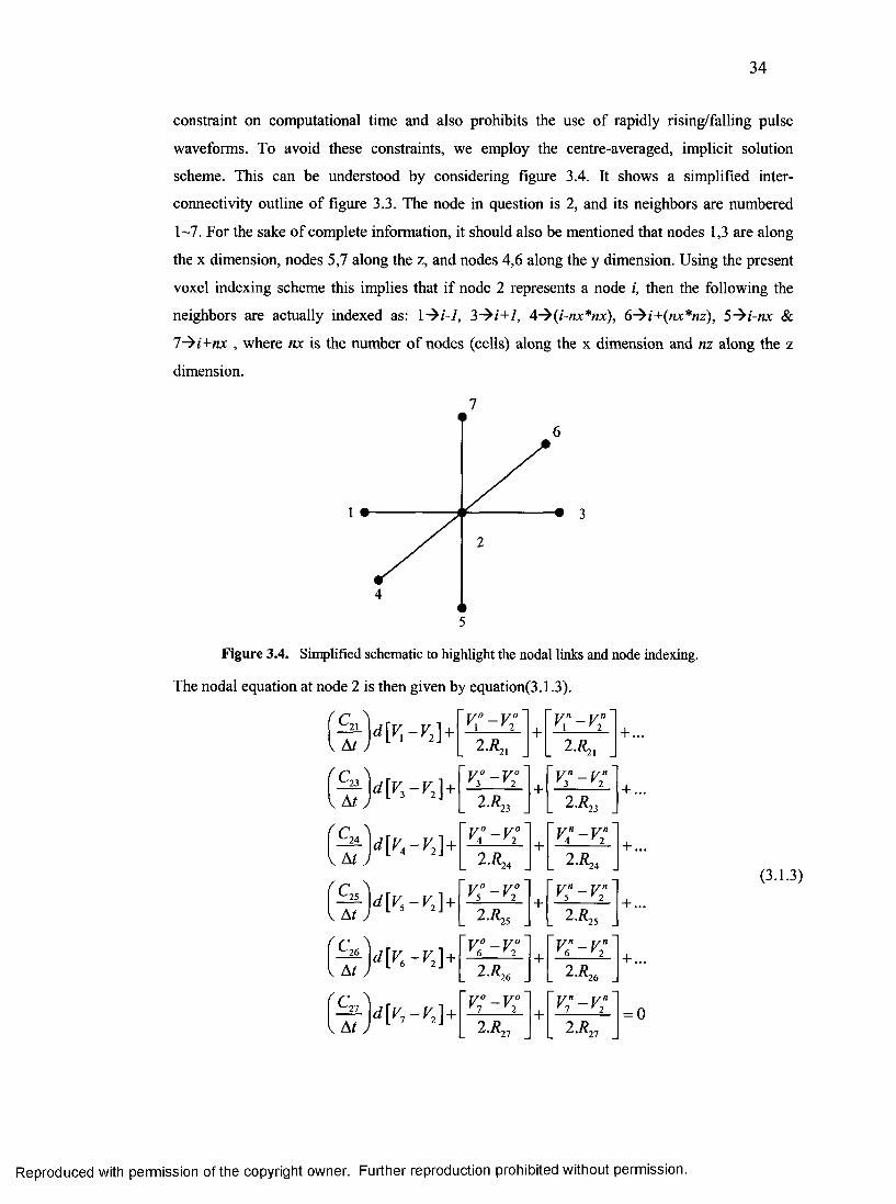
34

constraint on computational time and also prohibits the use of rapidly rising/falling pulse

waveforms. To avoid these constraints, we employ the centre-averaged, implicit solution

scheme. This can be understood by considering figure 3.4. It shows a simplified inter

connectivity outline of figure 3.3. The node in question is 2, and its neighbors are numbered

1-7. For the sake of complete information, it should also be mentioned that nodes 1,3 are along

the x dimension, nodes 5,7 along the z, and nodes 4,6 along the y dimension. Using the present

voxel indexing scheme this implies that if node 2 represents a node i, then the following the

neighbors are actually indexed as: l-î-1, 3-î+1, 4~^(i-nx*nx), 6~î+(nx*nz), 5~$i-nx &

l-î+ nx , where nx is the number of nodes (cells) along the x dimension and nz along the z

dimension.

7

1

Figure 3.4. Simplified schematic to highlight the nodal links and node indexing.

The nodal equation at node 2 is then given by equation(3.1.3).

At

C ^23

At j< r [ n - r 2]+

c, \25

\ At j

C26

At

r 27

At

d [ r , - v , ] +

4 n - K ] +

4 r,-v2]+

1 1

L"

-cs1

1 1

+v n - V " r \ ' 2

. 2 - ^ 2 . .+ ...

V° — V°r 3 v 2

2.R23+

v n — V n3 2

2 .7?23+ ...

v° — v°' 4 2L 2 ^ 4 .

+Vn - V' 4 2L 2 ^ 4 .

+ . ..

v° — v°5 2L 2 ^ 5 J+

1 1

ikr ^

i

1 1

+ ...

1 1

* i i

+V n — V n

6 r 2

[ 2 -^ 2 6

+ ...

r i

>3

1

I i

+v n - v n r 1 v 2

2.R27= 0

(3.1.3)


35

In the above equation, V° implies potential at node i, at the old time step and C2 5 , R25 represent

the effective capacitance of the link between nodes 2 and 5 respectively. Further expanding the

above equation yields:

S u - j O ; - r ; - k " + k ; ] + ^ \[v; - v; - v; + > ? ]+ ...

^ )[v ;-V ! ~v;+v? ]+ \^ jy l- -v; -v;+v2']+...

^ ) l n - y ; - k + k ] + ( ^ - ) [ k - r; - v ; +*?]+...

Iti

*skT

+~v*-vf

+

■ i a i

I

+

i

i

2.^21 J [ 2 .^ 3 __ 2 .^ 4 . . i

oTCN

k"1

+

1

I

i 1 o1

0 1-'

I 1

2 . ^ 6 J L 2 .R21 _ L 2-^ i _2.i?23

y ° — V °¥ 4 V 2

1

1

i

1 i

i

I

2-^24 J 1

VI<Nri

1 2 - ^ 6 J 2 ,R21

(3.1.4)

Separating the old and new terms to either side of the equation results in:

V2

K

a . iAt 2 R

-v;

c.24+ -

1

( K - y ; )

(v;-v;)

At 2R1,

1

2 R

2i J

- K

c21

At

C21+ -

1

At 2 R-v"

c25+ -

1

At 2 R 25

2 1

1 c.2 ^ 5

25

At

+(v;-v‘)

(v;-v;)

21

K

l

c.23+ -

1

c 26

At 2RZ3

1

+ -At 2R26

C,

-v; c 27+ -

1

2 R23

At

+

23

1 c.2R■26

26

At

+ ( K - v ? )

+(y; -y?)

At 2 R2

1 C24

1 C27

2 / ? 2 7 At

(3.1.5)

For notational simplicity, we assign the following variables to terms on the left hand side

(LHS):


36

K =

kA =

a iAt 2R^X

c 24+ -

1

At 2 R 24

c„ 1

Aif 2/?.26

H- 11 c23 1 — + —

1C<1

orC4-**4

<11•44?

r ]

+

1

At 2 R251H* 11

1

1 -0 +

1

At 2 R21

and the following for those on the right hand side( RHS):

ml =

m4 -

m6 =

1 C

2 R 2 1

21

At

C,24

2R24 At

J C*At2 R.

;m3 =

;m5 =

;m7 =

1 C2 R23

2 ^ 5

__ 23_

At

r25

At

26

1 c.27

2/?27 A/

Equation (3.1.5) can then be recast as:

V2 [fc, + k3 + k4 + k5 + k6 + k7 ] - . . ._ V fK _ V :K _ V n ^ _ ynK _ ynki =

V: iyix + V3 nt3 + V4 tn4 + V4 m4 + V$m5 + V6°m6 + V°m1 —...

VI [m, + m3 + m4 + m5 + m6 + m7 ]

(3.1.6)

The left hand side of equation (3.1.6) contains terms involving the current node of interest (V2 )

and its neighboring nodes. Given that there are N nodes, the resulting N coupled equations when

cast in matrix form, yield a system of simultaneous equations that has just the same form as

equation (3.1.2). Now we are in a better position to discuss the structure of the matrix [M].

Since each row of this matrix can contain at the utmost 1 non-zero entries (including the

diagonal), this matrix is extremely sparse. If the applied stimulus is a potential pulse train, then,

those nodes that serve as electrode locations (i.e. connected to an Anode or Cathode) contain

only one element (at the diagonal). However, if the applied stimulus is a current pulse train,

then only cathode location nodes contain one diagonal element. This is simply due to the fact

that application of KCL at the anode location in a current stimulated system does not provide a-

priori knowledge of the potential at the anode location. However, since Cathode is always

grounded (the chosen reference potential), consequently V” = V" = 0.


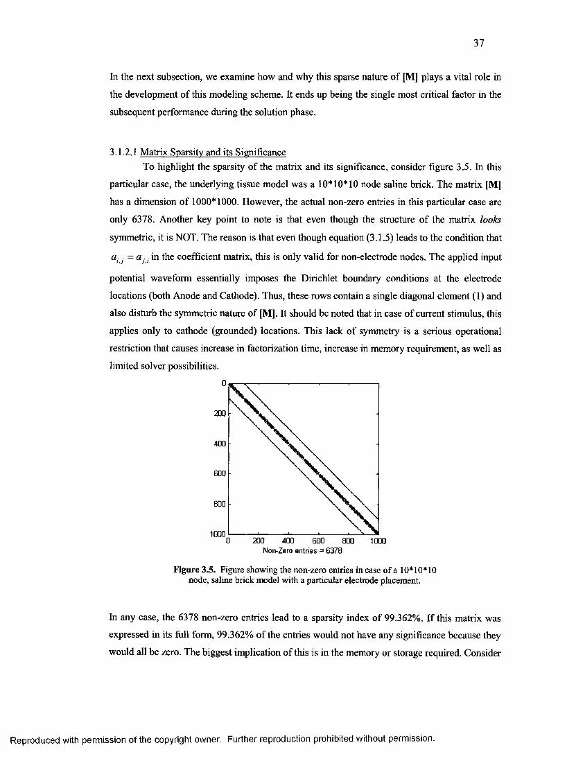
37

In the next subsection, we examine how and why this sparse nature of [M] plays a vital role in

the development of this modeling scheme. It ends up being the single most critical factor in the

subsequent performance during the solution phase.

3.1.2.1 Matrix Sparsity and its SignificanceTo highlight the sparsity of the matrix and its significance, consider figure 3.5. In this

particular case, the underlying tissue model was a 10*10*10 node saline brick. The matrix [M]

has a dimension of 1000*1000. However, the actual non-zero entries in this particular case are

only 6378. Another key point to note is that even though the structure of the matrix looks

symmetric, it is NOT. The reason is that even though equation (3.1.5) leads to the condition that

ai j = d j , in the coefficient matrix, this is only valid for non-electrode nodes. The applied input

potential waveform essentially imposes the Dirichlet boundary conditions at the electrode

locations (both Anode and Cathode). Thus, these rows contain a single diagonal element (1) and

also disturb the symmetric nature of [MJ. It should be noted that in case of current stimulus, this

applies only to cathode (grounded) locations. This lack of symmetry is a serious operational

restriction that causes increase in factorization time, increase in memory requirement, as well as

limited solver possibilities.

0

200

400

600

800

10000 200 400 600 800 1000

Non-Zero entries = 6378

Figure 3.5. Figure showing the non-zero entries in case of a 10*10*10 node, saline brick model with a particular electrode placement.

In any case, the 6378 non-zero entries lead to a sparsity index of 99.362%. If this matrix was

expressed in its full form, 99.362% of the entries would not have any significance because they

would all be zero. The biggest implication of this is in the memory or storage required. Consider


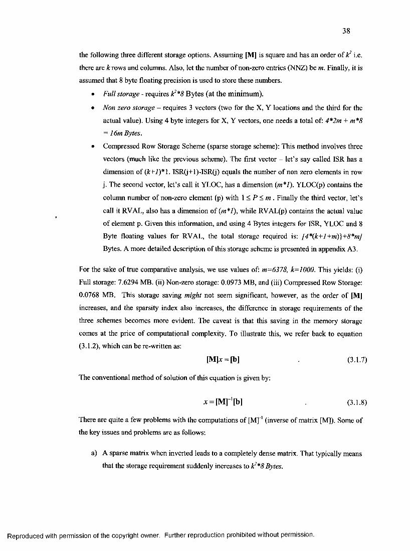
38

the following three different storage options. Assuming [M] is square and has an order of k2 i.e.

there are k rows and columns. Also, let the number of non-zero entries (NNZ) be m. Finally, it is

assumed that 8 byte floating precision is used to store these numbers.

• Full storage - requires k2*8 Bytes (at the minimum).

• Non zero storage - requires 3 vectors (two for the X, Y locations and the third for the

actual value). Using 4 byte integers for X, Y vectors, one needs a total of: 4*2m + m*8

= 16m Bytes.

• Compressed Row Storage Scheme (sparse storage scheme): This method involves three

vectors (much like the previous scheme). The first vector - let’s say called ISR has a

dimension of (k+7)*l. ISR(j+l)-ISR(j) equals the number of non zero elements in row

j. The second vector, let’s call it YLOC, has a dimension (m *l). YLOC(p) contains the

column number of non-zero element (p) with 1 < P < m . Finally the third vector, let’s

call it RVAL, also has a dimension of (m *l), while RVAL(p) contains the actual value

of element p. Given this information, and using 4 Bytes integers for ISR, YLOC and 8

Byte floating values for RVAL, the total storage required is: [4*(k+l +m)}+8*m]

Bytes. A more detailed description of this storage scheme is presented in appendix A3.

For the sake of true comparative analysis, we use values of: m=6378, k=1000. This yields: (i)

Full storage: 7.6294 MB. (ii) Non-zero storage: 0.0973 MB, and (iii) Compressed Row Storage:

0.0768 MB. This storage saving might not seem significant, however, as the order of [M]

increases, and the sparsity index also increases, the difference in storage requirements of the

three schemes becomes more evident. The caveat is that this saving in the memory storage

comes at the price of computational complexity. To illustrate this, we refer back to equation

(3.1.2), which can be re-written as:

[M]x = [b] (3.1.7)

The conventional method of solution of this equation is given by:

* = [M r'[b ] (3.1.8)

There are quite a few problems with the computations of [M] ' 1 (inverse of matrix [M]). Some of

the key issues and problems are as follows:

a) A sparse matrix when inverted leads to a completely dense matrix. That typically means

that the storage requirement suddenly increases to k?*8 Bytes.


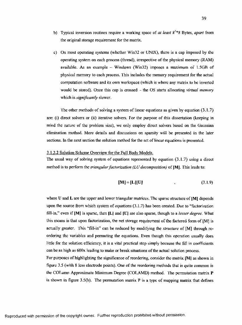
39

b) Typical inversion routines require a working space of at least k?*8 Bytes, apart from

the original storage requirement for the matrix.

c) On most operating systems (whether Win32 or UNIX), there is a cap imposed by the

operating system on each process (thread), irrespective of the physical memory (RAM)

available. As an example - Windows (Win32) imposes a maximum of 1.5GB of

physical memory to each process. This includes the memory requirement for the actual

computation software and its own workspace (which is where any matrix to be inverted

would be stored). Once this cap is crossed - the OS starts allocating virtual memory

which is significantly slower.

The other methods of solving a system of linear equations as given by equation (3.1.7)

are: (i) direct solvers or (ii) iterative solvers. For the purpose of this dissertation (keeping in

mind the nature of the problem size), we only employ direct solvers based on the Gaussian

elimination method. More details and discussions on sparsity will be presented in the later

sections. In the next section the solution method for the set of linear equations is presented.

3.1.2.2 Solution Scheme Overview for the Full Body Models.The usual way of solving system of equations represented by equation (3.1.7) using a direct

method is to perform the triangular factorization (LU decomposition) of [M], This leads to:

[M] = [L][U] , (3.1.9)

where U and L are the upper and lower triangular matrices. The sparse structure of [M] depends

upon the source from which system of equations (3.1.7) has been created. Due to “factorization

fill-in,” even if [M] is sparse, then [L] and [U] are also sparse, though to a lesser degree. What

this means is that upon factorization, the net storage requirement of the factored form of [M] is

actually greater. This “fill-in” can be reduced by modifying the structure of [M] through re

ordering the variables and permuting the equations. Even though this operation usually does

little for the solution efficiency, it is a vital practical step simply because the fill in coefficients

can be as high as 600x leading to make or break situations of the actual solution process.

For purposes of highlighting the significance of reordering, consider the matrix [M] as shown in

figure 3.5 (with 8 less electrode points). One of the reordering methods that is quite common is

the COLumn Approximate Minimum Degree (COLAMD) method. The permutation matrix P

is shown in figure 3.5(b). The permutation matrix P is a type of mapping matrix that defines


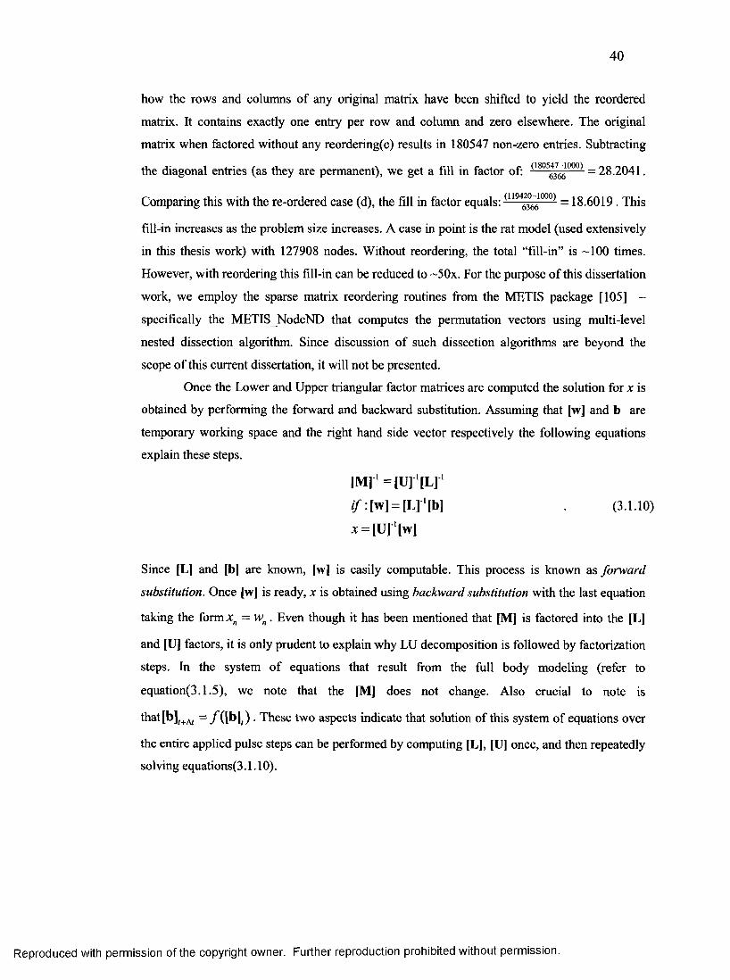
40

how the rows and columns of any original matrix have been shifted to yield the reordered

matrix. It contains exactly one entry per row and column and zero elsewhere. The original

matrix when factored without any reordering(c) results in 180547 non-zero entries. Subtracting

the diagonal entries (as they are permanent), we get a fill in factor of: (1 8 0 S3 661000) = 28.2041.

Comparing this with the re-ordered case (d), the fill in factor equals: (1194 30661000) =18.6019. This

fill-in increases as the problem size increases. A case in point is the rat model (used extensively

in this thesis work) with 127908 nodes. Without reordering, the total “fill-in” is -100 times.

However, with reordering this fill-in can be reduced to ~50x. For the purpose of this dissertation

work, we employ the sparse matrix reordering routines from the METIS package [105] -

specifically the METIS NodeND that computes the permutation vectors using multi-level

nested dissection algorithm. Since discussion of such dissection algorithms are beyond the

scope of this current dissertation, it will not be presented.

Once the Lower and Upper triangular factor matrices are computed the solution for x is

obtained by performing the forward and backward substitution. Assuming that [w] and b are

temporary working space and the right hand side vector respectively the following equations

explain these steps.

[ M r ^ i u r u r 1

i f :[w] = [L]1[b] (3.1.10)

x = [U] [w]

Since [L] and [b] are known, [w] is easily computable. This process is known as forward

substitution. Once [w] is ready, x is obtained using backward substitution with the last equation

taking the form = wn . Even though it has been mentioned that [M] is factored into the [L]

and [U] factors, it is only prudent to explain why LU decomposition is followed by factorization

steps. In the system of equations that result from the full body modeling (refer to

equation(3.1.5), we note that the [M] does not change. Also crucial to note is

that [b];+A/ = /([b ]() . These two aspects indicate that solution of this system of equations over

the entire applied pulse steps can be performed by computing [L], [U] once, and then repeatedly

solving equations(3.1 .1 0 ).


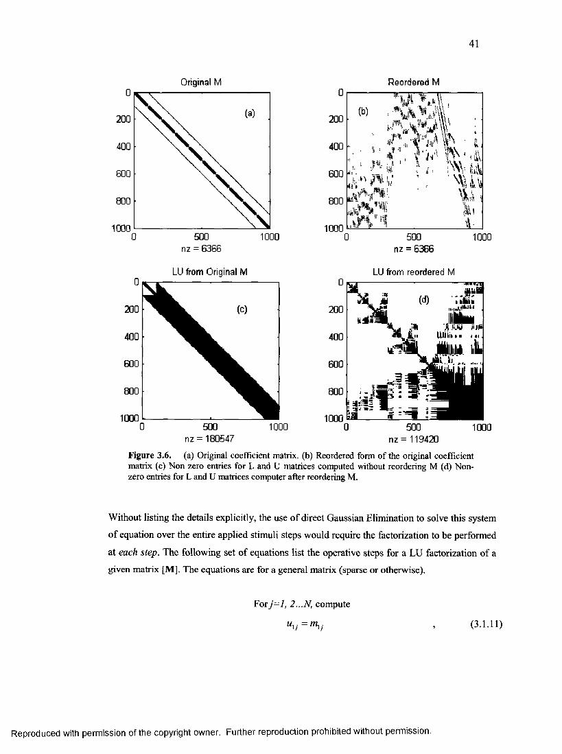
41

Original M Reordered M

200

400

600

800

10000 500 1000

nz = 6366

LU from Original M

200

400

600

800

10000 500 1000

nz = 180547

0

200

400

600

800

1000

.V'"..

L ■ k'i

a w

. f V i ib

j L0 500

nz = 6366

LU from reordered M

1000

■■i.iJiiili

likk

S Ji.kj >>IP ............

500 nz = 119420

1000

Figure 3.6. (a) Original coefficient matrix, (b) Reordered form of the original coefficientmatrix (c) Non zero entries for L and U matrices computed without reordering M (d) Nonzero entries for L and U matrices computer after reordering M.

Without listing the details explicitly, the use of direct Gaussian Elimination to solve this system

of equation over the entire applied stimuli steps would require the factorization to be performed

at each step. The following set of equations list the operative steps for a LU factorization of a

given matrix [M], The equations are for a general matrix (sparse or otherwise).

For j= l, 2...N, compute

U\j ~ m^j (3.1.11)


42

i-i11 v = m ‘j ~ T , l.k-ukj ; i=2- j (3.1.12)

k=\

1 f jA \and, /.. = — ;i= j+ l...N

U ]j v *=i )

(3.1.13)

One of the peripheral advantages of LU decomposition is that we can compute the determinant

The equations above also highlight the advantages of solution using LU decomposition versus

the Gaussian elimination method, in this particular modeling scheme. Since equations (3.1.11)

~ (3.1.13) do not involve the [b] vector, we need to perform this factorization step only once.

sequential stimulus pulse with multiple time steps. With the simulation scheme and the principal

solution methodology laid out, the next two of sections list the need and details of converting

this to a distributed solution scheme.

3.1.3 Distributed Algorithm DetailsFull body modeling involves quite a large number of discrete points (nodes), and

consequently, memory available for solution becomes a critical factor. Direct inversion is

clearly not viable and using other solution schemes such as LU decomposition, which definitely

allow for a larger simulation size to be solved for a given memory capacity, would benefit

greatly, if the most memory and computation intensive operation of the entire solution scheme

was distributed. However, before a distributed scheme of solution is implemented, the following

key characteristics intrinsic to the proposed modeling scheme need to be borne in mind.

1. The system of equations gives rise to an asymmetric [M] or an asymmetric coefficient

matrix.

2. [Ml is extremely sparse, and yet, the factors are not quite as much.

3. Sparsity in factors can be improved with re-ordering of [M].

4. Since [b](+A/ = f ([b]() , this implies that the equations are coupled in time, and

consequently, such systems cannot be parallelized in time.

of [M]:

(3.1.14)

Needless to say, this gives a definite advantage when solving the system of equations for a


43

5. From a deployment perspective, it’s better if the solver employs distributed memory

architecture - especially given that shared memory systems are typically limited in the

number of CPUs that are available.

Based on the above points, the optimal solver would be one that can solve sparse systems that

are asymmetric and also allow for different reordering methods prior to factorization. A rather

detailed survey of the available solver packages available in the open source community finally

leads to “SuperLU DIST” [106]. This is a distributed version of a “general purpose library for

the direct solution of large, sparse, nonsymmetric system of linear equations on high

performance machines.” The other advantage of this package is that apart from providing

internal reordering routines, it supports external reordering packages. However, the one limiting

aspect is that during factorization phase, if the default memory allocation for factorization is not

sufficient, then this factor needs to be modified and the subroutine re-linked through re

compilation. Like any other sparse solver, the onus lies on the user to provide the matrix [M] in

a sparse format that must be ordered. Also, if an external reordering routine is being used, then

the user must provide either the permutation vector or [M] in the reordered and sparse format.

3.1.3.1 Algorithm Process Flow DiagramThe process flow of the distributed version of the solution scheme is now presented.

Since Message Passing Interface (MPI) is also used, a process grid is classified, comprised of n

processors, with the master being identified with 1DN 0, and n-1 slave processors with IDNs

l~n-l. In the flow diagram, the critical processes of setting up the [M] in the sparse format

have been highlighted. For the sake of thoroughness, this section is also presented as pseudo

code in section 3.1.3.2.

The other key point regarding the following flow-diagram is that, in case the simulation

size is not big enough, the memory saving achieved by reordering is not offset by the additional

computation time required. Consequently, there are decision blocks that account for whether or

not METIS is being called for reordering.

3.1.3.2 Coefficient Matrix Setup in Compressed Row Storage SchemeThe following is the pseudo-code for the steps involved in setting up the [M] in the

compressed row storage scheme. It is assumed that bio model has n nodes. Equation (3.1.6) is

also referenced.

allocate ISR(n+l), ICOLTEMP(7*n) and RVTEMP(7*n) initialize ISR(1) to 1initialize ISRCOUNTER to 2, COLCOUNTER to 1, nodecounter to 1


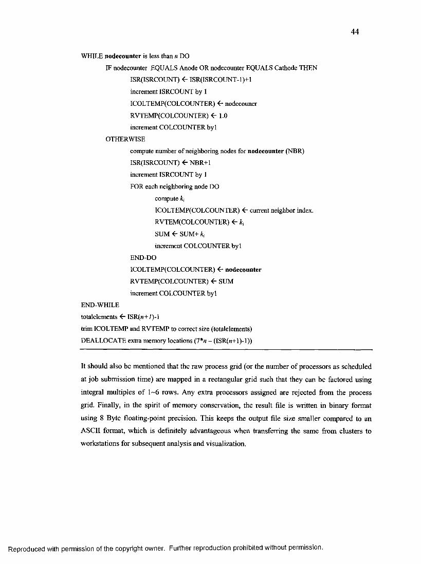
44

WHILE nodecounter is less than n DO

IF nodecounter EQUALS Anode OR nodecounter EQUALS Cathode THEN

ISR(ISRCOUNT) <- ISR(ISRCOUNT-1)+1

increment ISRCOUNT by 1

ICOLTEMP(COLCOUNTER) <r nodecouner

RVTEMP(COLCOUNTER) 1.0

increment COLCOUNTER byl

OTHERWISE

compute number of neighboring nodes for nodecounter (NBR)

ISR(ISRCOUNT) <- NBR+1

increment ISRCOUNT by 1

FOR each neighboring node DO

compute ki

ICOLTEMP(COLCOUNTER) <- current neighbor index.

RVTEM(COLCOUNTER) <r kt

SUM <- SUM+ kf


END-DO

ICOLTEMP(COLCOUNTER) nodecounter

RVTEMP(COLCOUNTER) <- SUM


END-WHILE

totalelements <- ISR(n+7)-l

trim ICOLTEMP and RVTEMP to correct size (totalelements)

DEALLOCATE extra memory locations (7*n - (ISR(«+1)-1))

It should also be mentioned that the raw process grid (or the number of processors as scheduled

at job submission time) are mapped in a rectangular grid such that they can be factored using

integral multiples of 1~6 rows. Any extra processors assigned are rejected from the process

grid. Finally, in the spirit of memory conservation, the result file is written in binary format

using 8 Byte floating-point precision. This keeps the output file size smaller compared to an

ASCII format, which is definitely advantageous when transferring the same from clusters to

workstations for subsequent analysis and visualization.


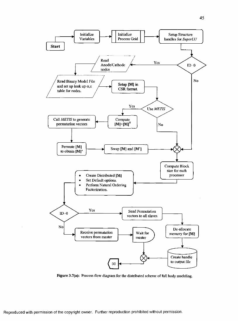
45

Initialize Initialize Setup Structurew Variables Process Grid handles for Super LU

Start

ReadAnode/Cathode A nodes

Read Binary Model File and set up look up a,e table for nodes. /

/ , Setup [M] inCSR format.

'

No

Call METIS to generate permutation vectors

Permute [M] to obtain [M]’

Use METIS

Compute[M1+1M]

Swap [M] and [M’]

Create Distributed [M] Set Default options. Perform Natural Ordering Factorization.

Compute Block size for each

processor

Yes Send Permutation vectors to all slaves

Receive permutation vectors from master

Wait for master

De-allocate memory for [M]

0Create handle to output file

Figure 3.7(a): Process flow diagram for the distributed scheme of full body modeling.


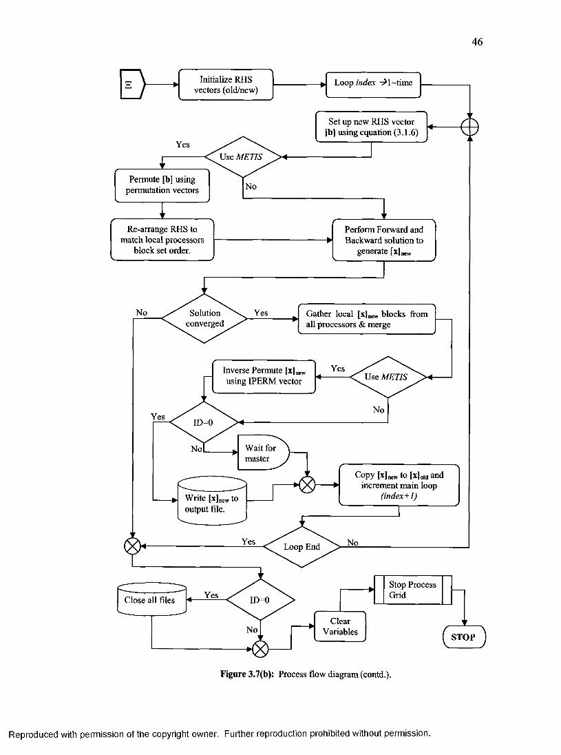
46

E> Initialize RHS vectors (old/new)

Loop index -^l~time

Use METIS > «

Set up new RHS vector [b] using equation (3.1.6)

Permute [b] using permutation vectors No

' r yr

Re-arrange RHS to match local processors

block set order.

f \Perform Forward and Backward solution to

generate [x]neww

No .— Solutionconverged

Gather local [x]new blocks from all processors & merge

1 r

■0

Yes

Inverse Permute [x]new using IPERM vector

YesN <T Use METIS

No

Wait for master

Write [x]new to output file.

Copy [x] new to [xloid and increment main loop

(index+I)

Yes ^ Loop End ^ No

Close all files

ClearVariables

Stop ProcessGrid

Figure 3.7(b): Process flow diagram (contd.).


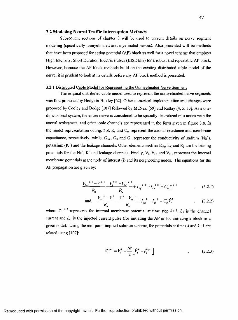
47

3.2 Modeling Neural Traffic Interruption MethodsSubsequent sections of chapter 3 will be used to present details on nerve segment

modeling (specifically unmyelinated and myelinated nerves). Also presented will be methods

that have been proposed for action potential (AP) block as well for a novel scheme that employs

High Intensity, Short Duration Electric Pulses (HISDEPs) for a robust and repeatable AP block.

However, because the AP block methods build on the existing distributed cable model of the

nerve, it is prudent to look at its details before any AP block method is presented.

3.2.1 Distributed Cable Model for Representing the Unmyelinated Nerve SegmentThe original distributed cable model used to represent the unmyelinated nerve segments

was first proposed by Hodgkin-Huxley [62], Other numerical implementation and changes were

proposed by Cooley and Dodge [107] followed by McNeal [59] and Rattay [4, 5, 33]. As a one

dimensional system, the entire nerve is considered to be spatially discretized into nodes with the

axonal resistances, and other ionic channels are represented in the form given in figure 3.8. In

the model representation of Fig. 3.8, Ra and Cm represent the axonal resistance and membrane

capacitance, respectively, while, GNa, GK and GL represent the conductivity of sodium (Na+),

potassium (K+) and the leakage channels. Other elements such as ENa, EK and EL are the biasing

potentials for the Na+, K+ and leakage channels. Finally, V;, Vn and Vj+i represent the internal

membrane potentials at the node of interest (i) and its neighboring nodes. The equations for the

AP propagation are given by:

k + 1 j / k + \ j / k + \ j / - k + 1i+1 . T k + 1 _ t k + 1 _ ✓-! j / k + l « ^

'T 1 m j 1 ch m i >

V k+l — Vk+1 Vk+1 - V yi-1 r i _ G ' 1R,, R.

v k - V k v k - V k and, - ^ ■ J^ + I inj ~ I chk = C mVlk , (3.2.2)

a a

where V,.,kil represents the internal membrane potential at time step k+1, Ich is the channel

current and Iinj is the injected current pulse (for initiating the AP or for initiating a block or a

given node). Using the mid-point implicit solution scheme, the potentials at times k and k+1 are

related using [107]:

vk+l =vk+—\ v k+Vk+'] . (3 .2 .3)


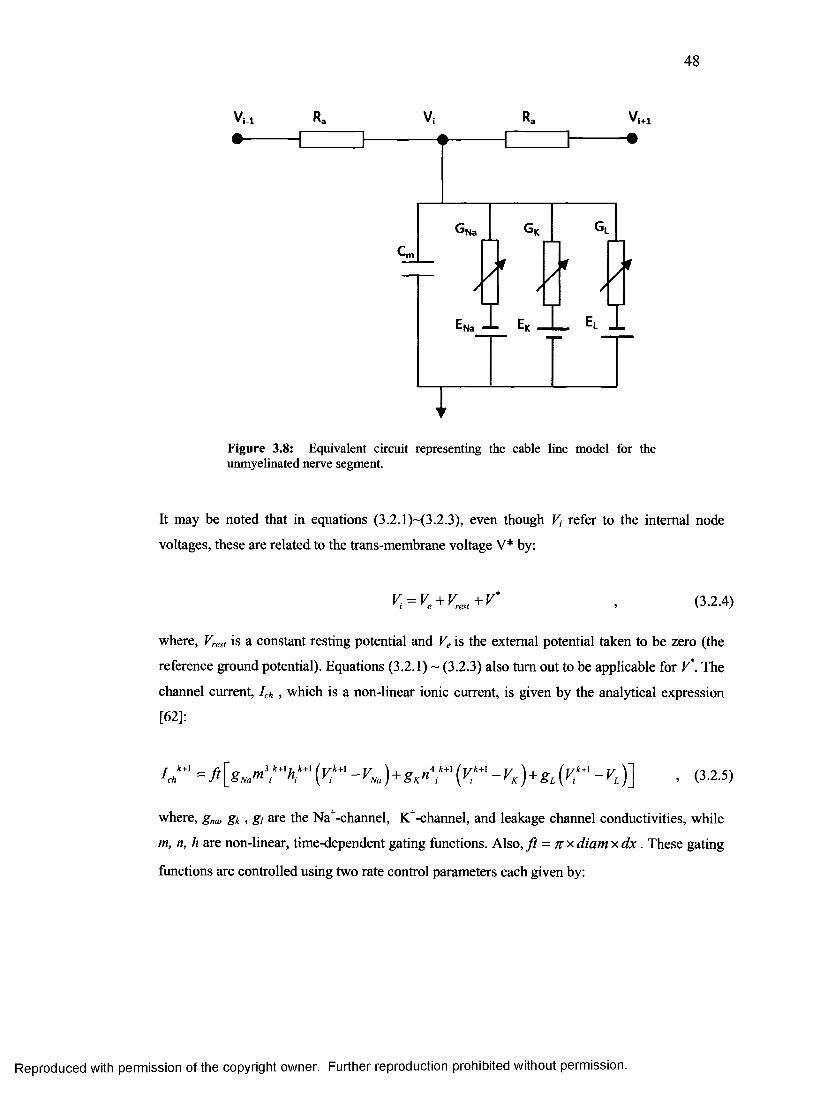
48

Vm Ra V, Ra Vl+1

'Na

Na

Figure 3.8: Equivalent circuit representing the cable line model for theunmyelinated nerve segment.

It may be noted that in equations (3.2.1)~(3.2.3), even though V, refer to the internal node

voltages, these are related to the trans-membrane voltage V* by:

V i ^ K + V ^ + V , (3.2.4)

where, Vrest is a constant resting potential and Ve is the external potential taken to be zero (the

reference ground potential). Equations (3.2.1) ~ (3.2.3) also turn out to be applicable for V*. The

channel current, lCh , which is a non-linear ionic current, is given by the analytical expression

[62]:

ij"=fi[g^*\M{v -vNa)+gKn'r{vr-v,:)+gL{vr-rS\ , <3.2.5)

where, gna, gk , gi are the Na+-channel, K+-channel, and leakage channel conductivities, while

m, n, h are non-linear, time-dependent gating functions. Also, f t = n x diam x d x . These gating

functions are controlled using two rate control parameters each given by:


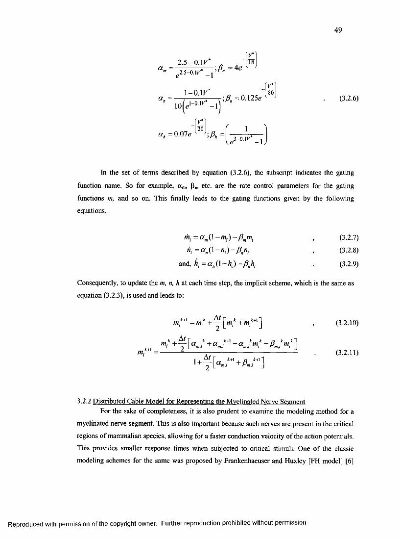
In the set of terms described by equation (3.2.6), the subscript indicates the gating

function name. So for example, a m, pm etc. are the rate control parameters for the gating

functions m, and so on. This finally leads to the gating functions given by the following

equations.

Consequently, to update the m, n, h at each time step, the implicit scheme, which is the same as

equation (3.2.3), is used and leads to:

3.2.2 Distributed Cable Model for Representing the Myelinated Nerve SegmentFor the sake of completeness, it is also prudent to examine the modeling method for a

myelinated nerve segment. This is also important because such nerves are present in the critical

regions of mammalian species, allowing for a faster conduction velocity of the action potentials.

This provides smaller response times when subjected to critical stimuli. One of the classic

modeling schemes for the same was proposed by Frankenhaeuser and Huxley [FH model] [6]

m. ~ a m{ \ - m i) - f i mmi

hi = a ll( l - n l) - 0 nni

and, hi = a h( l - h i) - / 3 lthi

(3.2.7)

(3.2.8)

(3.2.9)

(3.2.10)

(3.2.11)


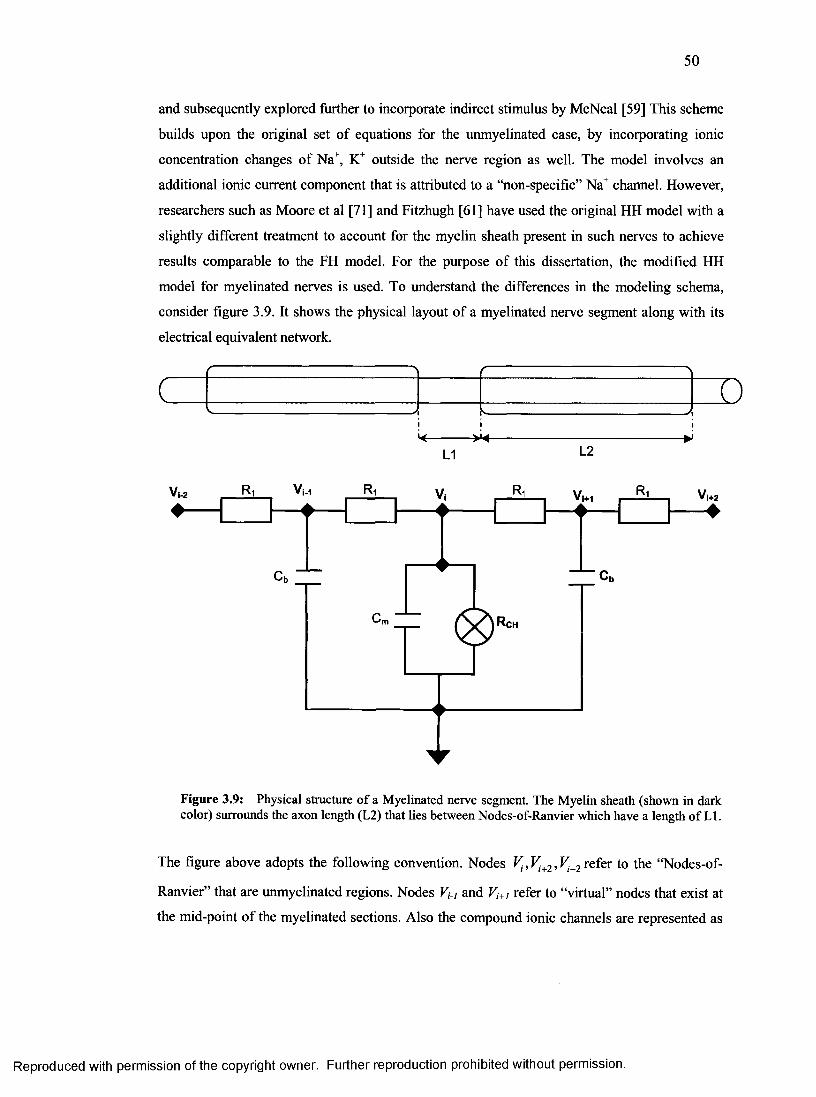
50

and subsequently explored further to incorporate indirect stimulus by McNeal [59] This scheme

builds upon the original set of equations for the unmyelinated case, by incorporating ionic

concentration changes of Na+, K+ outside the nerve region as well. The model involves an

additional ionic current component that is attributed to a “non-specific” Na+ channel. However,

researchers such as Moore et al [71] and Fitzhugh [61] have used the original HH model with a

slightly different treatment to account for the myelin sheath present in such nerves to achieve

results comparable to the FH model. For the purpose of this dissertation, the modified HH

model for myelinated nerves is used. To understand the differences in the modeling schema,

consider figure 3.9. It shows the physical layout of a myelinated nerve segment along with its

electrical equivalent network.

i i i ►>

L1 12

i-2 i+1

CH

Figure 3.9: Physical structure of a Myelinated nerve segment. The Myelin sheath (shown in dark color) surrounds the axon length (L2) that lies between Nodes-of-Ranvier which have a length of LI.

The figure above adopts the following convention. Nodes V(, Vi+2, Vi2 refer to the “Nodes-of-

Ranvier” that are unmyelinated regions. Nodes F,_/ and Vi+, refer to “virtual” nodes that exist at

the mid-point of the myelinated sections. Also the compound ionic channels are represented as


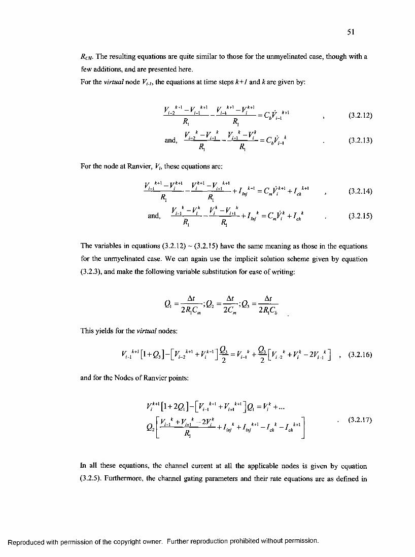
51

RCh- The resulting equations are quite similar to those for the unmyelinated case, though with a

few additions, and are presented here.

For the virtual node V^,, the equations at time steps k+1 and k are given by:

TT k+l TT £ + 1 TT £ + 1 T f k + lV i - 2 ~ y i - \ V i - 1 ~ y i _ t> *+1

R R= C V^ b ' i - l

V k - V k V k —V k and, ^ ^ J ~ = CbVi l k

R j R, b M

For the node at Ranvier, V,-, these equations are:

fc + 1 J/r^+ Jfi - 1 i i i+ l

R R_l_ j k + \ y k + \ j i + l

I n j m i c h

y k _ v k Vk —V k _ t l i i <+!_ + / k = C V k +1 kand,

RxI n j m i ch

(3.2.12)

(3.2.13)

(3.2.14)

(3.2.15)

The variables in equations (3.2.12) ~ (3.2.15) have the same meaning as those in the equations

for the unmyelinated case. We can again use the implicit solution scheme given by equation

(3.2.3), and make the following variable substitution for ease of writing:

01 ; 0 2 = — ;03 = - ^ —2R\Cm ^ 2Cm ^ 2RxCb

This yields for the virtual nodes:

+ & ]"[> ,-2*“ + K‘" ] ^ = K- ,* + & [ V , J + V ‘ - 2 V J ] , (3.2.16)

and for the Nodes of Ranvier points:

^*‘[1+22, FIX,**1 =V,‘ +...

ay K + y *— ------- ^ --------- - + I ini + I inik+l - h h ~ 7 c / +'i n j i n j ch chR

. (3.2.17)

In all these equations, the channel current at all the applicable nodes is given by equation

(3.2.5). Furthermore, the channel gating parameters and their rate equations are as defined in


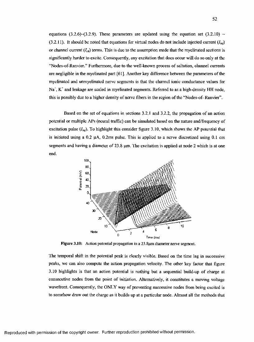
52

equations (3.2.6)~(3.2.9). These parameters are updated using the equation set (3.2.10) ~

(3.2.11). It should be noted that equations for virtual nodes do not include injected current (/,„,)

or channel current (Ich) terms. This is due to the assumption made that the myelinated sections is

significantly harder to excite. Consequently, any excitation that does occur will do so only at the

“Nodes-of-Ranvier.” Furthermore, due to the well-known process of saltation, channel currents

are negligible in the myelinated part [61], Another key difference between the parameters of the

myelinated and unmyelinated nerve segments is that the channel ionic conductance values for

Na+, K+ and leakage are scaled in myelinated segments. Referred to as a high-density HH node,

this is possibly due to a higher density of nerve fibers in the region of the “Nodes-of- Ranvier”.

Based on the set of equations in sections 3.2.1 and 3.2.2, the propagation of an action

potential or multiple APs (neural traffic) can be simulated based on the nature and/frequency of

excitation pulse (/,„,). To highlight this consider figure 3.10, which shows the AP potential that

is initiated using a 0.2 pA, 0.2ms pulse. This is applied to a nerve discretized using 0.1 cm

segments and having a diameter of 23.8 pm. The excitation is applied at node 2 which is at one

end.

Time (ms)

Figure 3.10: Action potential propagation in a 23.8pm diameter nerve segment.

The temporal shift in the potential peak is clearly visible. Based on the time lag in successive

peaks, we can also compute the action propagation velocity. The other key factor that figure

3.10 highlights is that an action potential is nothing but a sequential build-up of charge at

consecutive nodes from the point of initiation. Alternatively, it constitutes a moving voltage

wavefront. Consequently, the ONLY way of preventing successive nodes from being excited is

to somehow draw out the charge as it builds up at a particular node. Almost all the methods that


53

have been proposed so far involve either injection of an “Interrupt Signal,” which could be a

suitably polarized DC current [8] at a node downstream and/or AC current injection of suitable

frequency [7]. In all these cases, the basic nerve model is not disturbed. Apart from problems

such as permanent nerve damage due to heating (which is clearly undesirable) these methods

also do not guarantee a robust block owing to their narrow frequency range. The fact that this

frequency range is variable as a function of the nerve diameter does not help either. In the next

section a new scheme is presented that allows for modulation of the trans-membrane

conductivity, which in turn can facilitate the extraction of the charge required for AP

propagation. The problems and disadvantages associated with the possible AC/DC block

schemes have already been discussed in chapter 2.

3.2.2 Modified HH Model for Membrane Conductance ModulationAs shown earlier, the AP propagation mandates a sequential charge build up at

successive nodes. It is also known that the external surface of the axon surrounded by some

medium (body fluid, cerebral fluid, etc.) can be considered as grounded for all practical reasons.

This leads to a possibility that if the stimulating charge propagating from a neighboring node

can be shunted around the membrane capacitance, it will prevent the capacitance from charging.

Consequently, the channel ionic gates would be prevented from switching from their default

states. To test this scheme, a slightly modified electrical schematic is now presented. Only the

unmyelinated equivalent circuit is shown, but it is applicable to the myelinated case as well,

owing to the similarities between the two models.

Looking at figure 3.11, the pathway for channeling the charge is represented by a

variable conductance GSH. Before examining or discussing the possible ways by which this

shunt conductance can be practically achieved, the modified equations are first presented. For

the sake of brevity only the two key nodal equations are given.

The resulting nodal equation for Vt at time steps k, k+1 are:

tz £+1 _/ ' - l i i i + l _ _ _ _ _ _ , t k+ l _ _ j £ + 1 _ _ T / k + l , t k+ \ ('X 1 1 Q \

~r i inj ch m i 1 sh >

v k - V k V k - V ki - 1 i i i + l a j k T k /-* j r k . j k

K Ra

where, I shk = V k .Gsh. Since the nodal equations for the “Nodes-of-Ranvier” in the myelinated

model are quite similar to those in equation (3.2.1), equation (3.2.19) applies there as well.


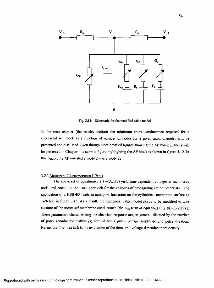
54

Vi-! Ra V, Ra v i+1

'Na

■m

Na

Fig. 3.11: Schematic for the modified cable model.

In the next chapter (the results section) the minimum shunt conductance required for a

successful AP block as a function of number of nodes for a given axon diameter will be

presented and discussed. Even though more detailed figures showing the AP block nuances will

be presented in Chapter 4, a sample figure highlighting the AP block is shown in figure 3.12. In

this figure, the AP initiated at node 2 was at node 28.

3.2.3 Membrane Electroporation EffectsThe above set of equations(3.2.1)~(3.2.17) yield time-dependent voltages at each nerve

node, and constitute the usual approach for the analyses of propagating action potentials. The

application of a HISDEP leads to nanopore formation on the cylindrical membrane surface as

sketched in figure 3.13. As a result, the traditional cable model needs to be modified to take

account of the increased membrane conductance (the GSh term of equations (3.2.18)~(3.2.19) ).

These parameters characterizing the electrical response are, in general, dictated by the number

of pores (conduction pathways) formed for a given voltage amplitude and pulse duration.

Hence, the foremost task is the evaluation of the time- and voltage-dependent pore density.


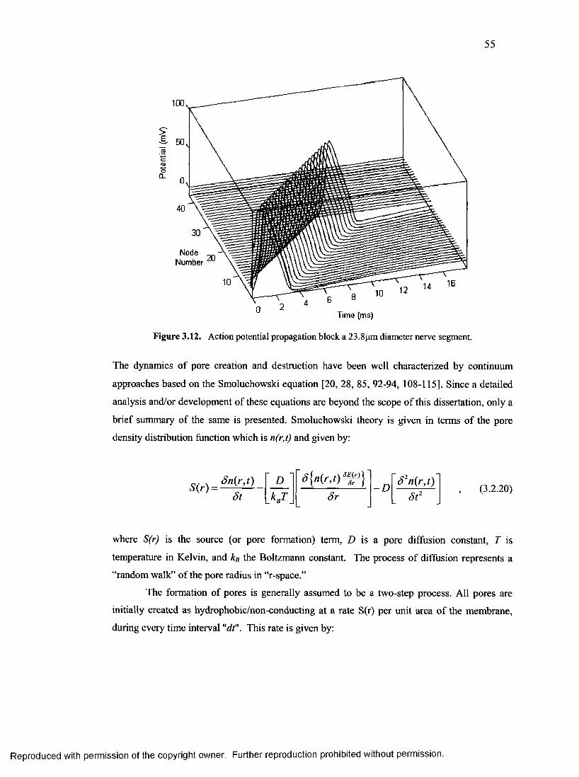
Figure 3.12. Action potential propagation block a 23.8pm diameter nerve segment.

The dynamics of pore creation and destruction have been well characterized by continuum

approaches based on the Smoluchowski equation [20, 28, 85, 92-94, 108-115]. Since a detailed

analysis and/or development of these equations are beyond the scope of this dissertation, only a

brief summary of the same is presented. Smoluchowski theory is given in terms of the pore

density distribution function which is n(r,t) and given by:

where S(r) is the source (or pore formation) term, D is a pore diffusion constant, T is

temperature in Kelvin, and kB the Boltzmann constant. The process of diffusion represents a

“random walk” of the pore radius in “r-space.”

The formation of pores is generally assumed to be a two-step process. All pores are

initially created as hydrophobic/non-conducting at a rate S(r) per unit area of the membrane,

during every time interval "dt". This rate is given by:

(3.2.20)


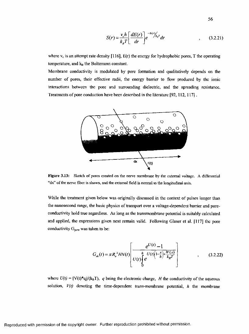
56

S{r) = (3.2.21)kgT L dr

where vc is an attempt rate density [116], E(r) the energy for hydrophobic pores, T the operating

temperature, and kB the Boltzmann constant.

Membrane conductivity is modulated by pore formation and qualitatively depends on the

number of pores, their effective radii, the energy barrier to flow produced by the ionic

interactions between the pore and surrounding dielectric, and the spreading resistance.

Treatments of pore conduction have been described in the literature [92, 112, 117].

While the treatment given below was originally discussed in the context of pulses longer than

the nanosecond range, the basic physics of transport over a voltage-dependent barrier and pore-

conductivity hold true regardless. As long as the transmembrane potential is suitably calculated

and applied, the expressions given next remain valid. Following Glaser et al. [117] the pore

conductivity Gpore was taken to be:

where U(t) = [V(t)*q]/(kBT), q being the electronic charge, H the conductivity of the aqueous

solution, V(t) denoting the time-dependent trans-membrane potential, h the membrane

Figure 3.13: Sketch of pores created on the nerve membrane by the external voltage. A differential

“dx” of the nerve fiber is shown, and the external field is normal to the longitudinal axis.

(3.2.22)

0


57

thickness, N(t) are the number of pores, and W(x) is the energy barrier for an ion inside the pore.

The W(x) profile has a trapezoidal shape [117, 118] with a linearly varying regions of thickness

d at the two ends of the pore, and a constant value of W0 over the central pore region.

Thus - the expression for W(x) profile is:

Typically W0 is much larger than the thermal energy kBT, and under these conditions, the pore

conductivity simplifies to:

diameter of the nerve fiber and Lz is the inter-nodal segment length. In equation (3.2.24),

n(r,0,t) is the pore density function as defined in equation (3.2.20). Since the number of pores is

non-uniform with an angular dependence, the pore resistance needs to be evaluated across

differential stripes of width Rd0 (R = nerve fiber radius) and longitudinal length Lz across the

nerve membrane. The overall shunt conductivity Gsh is obtained by adding the spreading

resistance at the pore entrance to the effective pore resistivity. Thus: Gsh = [l/GSh + Rsp] 1 where

the pore spreading resistance RsP = p/2r, and is the resistivity of the aqueous medium. This

latter characteristic is also referred to as the access resistance [119, 120].

This chapter detailed all the modeling methods and aspects thereof that this dissertation

targets. In the next chapter, results from these schemes are presented along with relevant

discussions and a few highlights of problems that were encountered in the development process.

In the last chapter, a summary of this entire dissertation along with suggestions for future work

in this area will be presented.

W(x) = W0; d < x < ( h - d )

W(x) = Wo— ; 0 < x < dd

(3.2.23)

W(x) = WQ- —- \ { h - d ) < x < hd

G A O -d d J n (r ,0 ,t) r 2HDdr

(3.2.24)

T] = d /h is a measure of the relative size of the pore, D is thewhere, P (t)


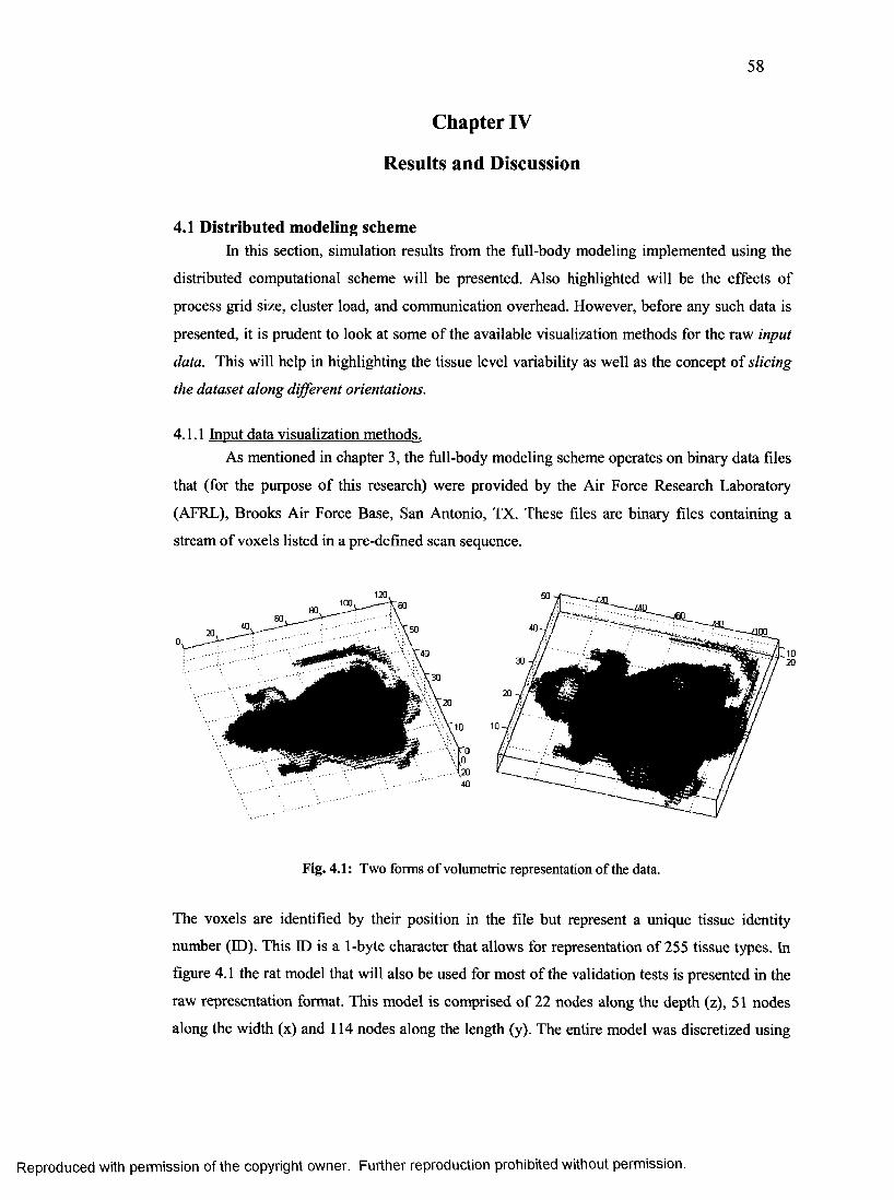
58

Chapter IV

Results and Discussion

4.1 Distributed modeling schemeIn this section, simulation results from the full-body modeling implemented using the

distributed computational scheme will be presented. Also highlighted will be the effects of

process grid size, cluster load, and communication overhead. However, before any such data is

presented, it is prudent to look at some of the available visualization methods for the raw input

data. This will help in highlighting the tissue level variability as well as the concept of slicing

the dataset along different orientations.

4.1.1 Input data visualization methods.As mentioned in chapter 3, the full-body modeling scheme operates on binary data files

that (for the purpose of this research) were provided by the Air Force Research Laboratory

(AFRL), Brooks Air Force Base, San Antonio, TX. These files are binary files containing a

stream of voxels listed in a pre-defined scan sequence.

Fig. 4.1: Two forms of volumetric representation of the data.

The voxels are identified by their position in the file but represent a unique tissue identity

number (ID). This ID is a 1-byte character that allows for representation of 255 tissue types. In

figure 4.1 the rat model that will also be used for most of the validation tests is presented in the

raw representation format. This model is comprised of 22 nodes along the depth (z), 51 nodes

along the width (x) and 114 nodes along the length (y). The entire model was discretized using


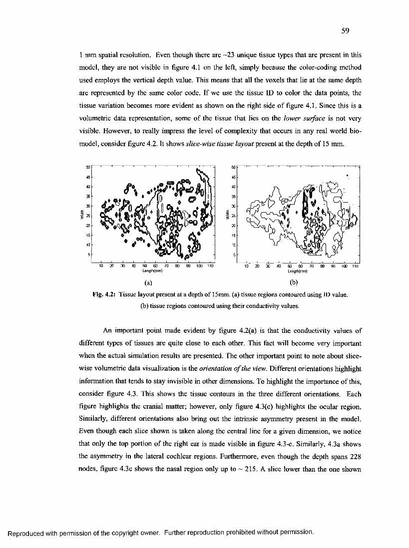
59

1 mm spatial resolution. Even though there are ~23 unique tissue types that are present in this

model, they are not visible in figure 4.1 on the left, simply because the color-coding method

used employs the vertical depth value. This means that all the voxels that lie at the same depth

are represented by the same color code. If we use the tissue ID to color the data points, the

tissue variation becomes more evident as shown on the right side of figure 4.1. Since this is a

volumetric data representation, some of the tissue that lies on the lower surface is not very

visible. However, to really impress the level of complexity that occurs in any real world bio

model, consider figure 4.2. It shows slice-wise tissue layout present at the depth of 15 mm.

5045403530

I 2520

1510

610 20 30 40 50 60 70 80 90 100 110

L e n g th (m m )

6045403530

| 2520

1510

510 20 30 40 50 60 70 80 90 100 110

L en g th (m m )

(a) (b)

Fig. 4.2: Tissue layout present at a depth of 15mm. (a) tissue regions contoured using ID value,

(b) tissue regions contoured using their conductivity values.

An important point made evident by figure 4.2(a) is that the conductivity values of

different types of tissues are quite close to each other. This fact will become very important

when the actual simulation results are presented. The other important point to note about slice-

wise volumetric data visualization is the orientation o f the view. Different orientations highlight

information that tends to stay invisible in other dimensions. To highlight the importance of this,

consider figure 4.3. This shows the tissue contours in the three different orientations. Each

figure highlights the cranial matter; however, only figure 4.3(c) highlights the ocular region.

Similarly, different orientations also bring out the intrinsic asymmetry present in the model.

Even though each slice shown is taken along the central line for a given dimension, we notice

that only the top portion of the right ear is made visible in figure 4.3-c. Similarly, 4.3a shows

the asymmetry in the lateral cochlear regions. Furthermore, even though the depth spans 228

nodes, figure 4.3c shows the nasal region only up to ~ 215. A slice lower than the one shown


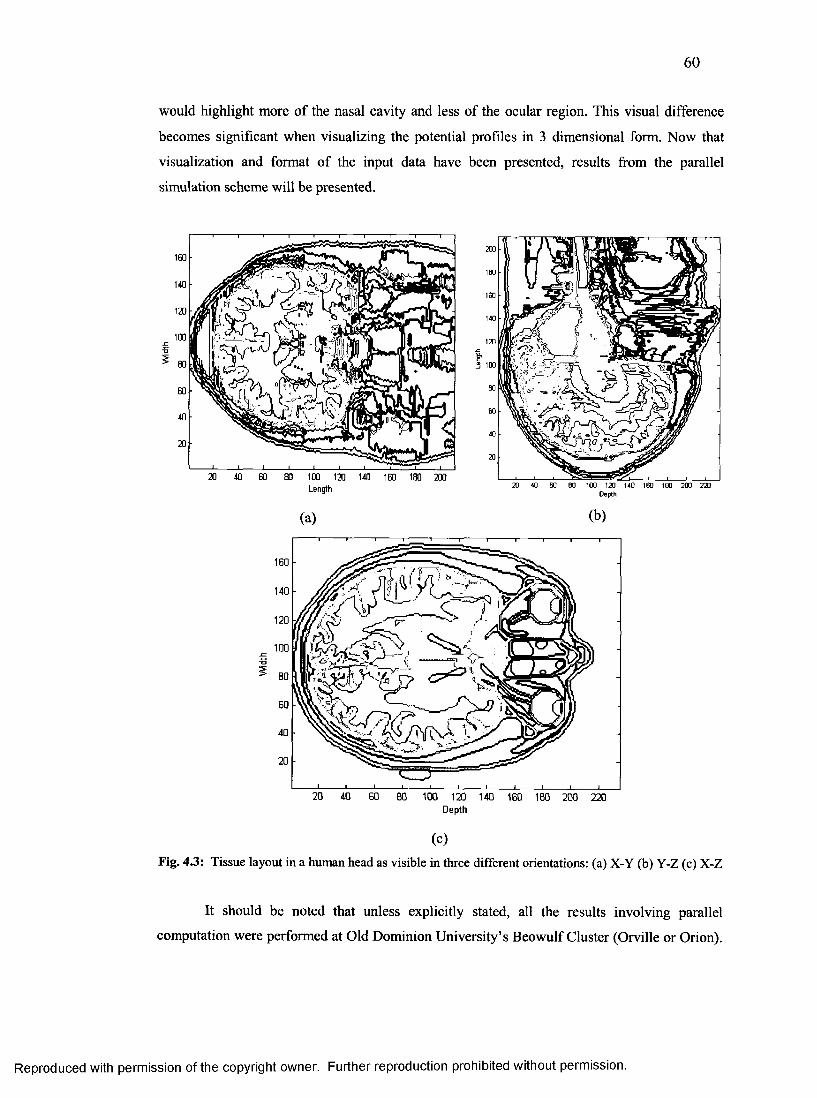
60

would highlight more of the nasal cavity and less of the ocular region. This visual difference

becomes significant when visualizing the potential profiles in 3 dimensional form. Now that

visualization and format of the input data have been presented, results from the parallel

simulation scheme will be presented.

5 100

20 40 60 80 100 120 140 160 180 200Length 20 40 60 80 100 120 140 160 180 200 220

Depth

(a) (b)

20 40 60 80 1 CD 120 140 160 180 200 220Depth

(C)Fig. 4.3: Tissue layout in a human head as visible in three different orientations: (a) X-Y (b) Y-Z (c) X-Z

It should be noted that unless explicitly stated, all the results involving parallel

computation were performed at Old Dominion University’s Beowulf Cluster (Orville or Orion).


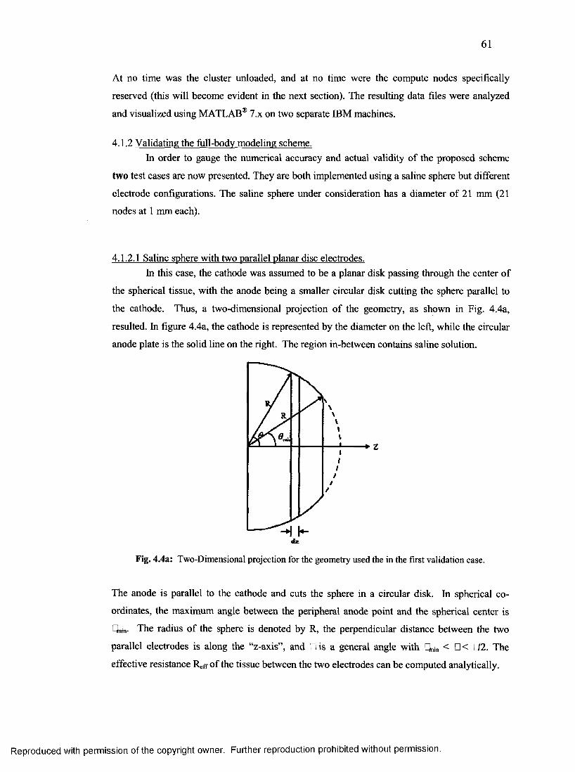
6 1

At no time was the cluster unloaded, and at no time were the compute nodes specifically

reserved (this will become evident in the next section). The resulting data files were analyzed

and visualized using MATLAB® 7.x on two separate IBM machines.

4.1.2 Validating the full-bodv modeling scheme.In order to gauge the numerical accuracy and actual validity of the proposed scheme

two test cases are now presented. They are both implemented using a saline sphere but different

electrode configurations. The saline sphere under consideration has a diameter of 21 mm (21

nodes at 1 mm each).

4.1.2.1 Saline sphere with two parallel planar disc electrodes.In this case, the cathode was assumed to be a planar disk passing through the center of

the spherical tissue, with the anode being a smaller circular disk cutting the sphere parallel to

the cathode. Thus, a two-dimensional projection of the geometry, as shown in Fig. 4.4a,

resulted. In figure 4.4a, the cathode is represented by the diameter on the left, while the circular

anode plate is the solid line on the right. The region in-between contains saline solution.

dz

Fig. 4.4a: Two-Dimensional projection for the geometry used the in the first validation case.

The anode is parallel to the cathode and cuts the sphere in a circular disk. In spherical co

ordinates, the maximum angle between the peripheral anode point and the spherical center is

Tnin. The radius of the sphere is denoted by R, the perpendicular distance between the two

parallel electrodes is along the “z-axis”, and mis a general angle with CLi < □< J2 . The

effective resistance Reff of the tissue between the two electrodes can be computed analytically.

/


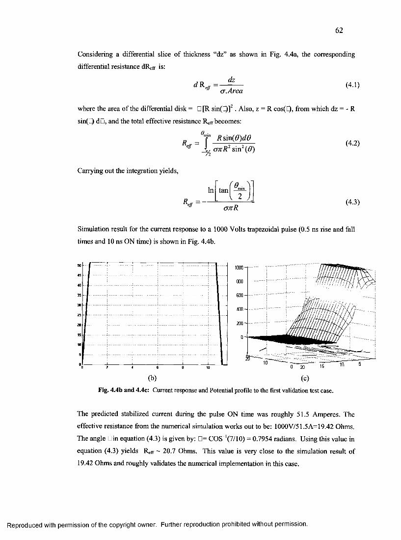
6 2

Considering a differential slice of thickness “dz” as shown in Fig. 4.4a, the corresponding

differential resistance dReff is:

dzeff cr.Area

(4.1)

where the area of the differential disk = D[R sin(t)]2 . Also, z = R cos(Q, from which dz = - R

sin(t) dm, and the total effective resistance R rr becomes:

8mjn Rsm {G )ddeff J y craR2 sin2($)

(4.2)

Carrying out the integration yields,

In

Reff =

( 9 . VItan I 2 )\

crnR(4.3)

Simulation result for the current response to a 1000 Volts trapezoidal pulse (0.5 ns rise and fall

times and 10 ns ON time) is shown in Fig. 4.4b.

1000-1

000

GOO-

30

(b) (c)

Fig. 4.4b and 4.4c: Current response and Potential profile to the first validation test case.

The predicted stabilized current during the pulse ON time was roughly 51.5 Amperes. The

effective resistance from the numerical simulation works out to be: 1000V/51.5A=19.42 Ohms.

The angle Din equation (4.3) is given by: □= COS_1(7/10) = 0.7954 radians. Using this value in

equation (4.3) yields Reff ~ 20.7 Ohms. This value is very close to the simulation result of

19.42 Ohms and roughly validates the numerical implementation in this case.


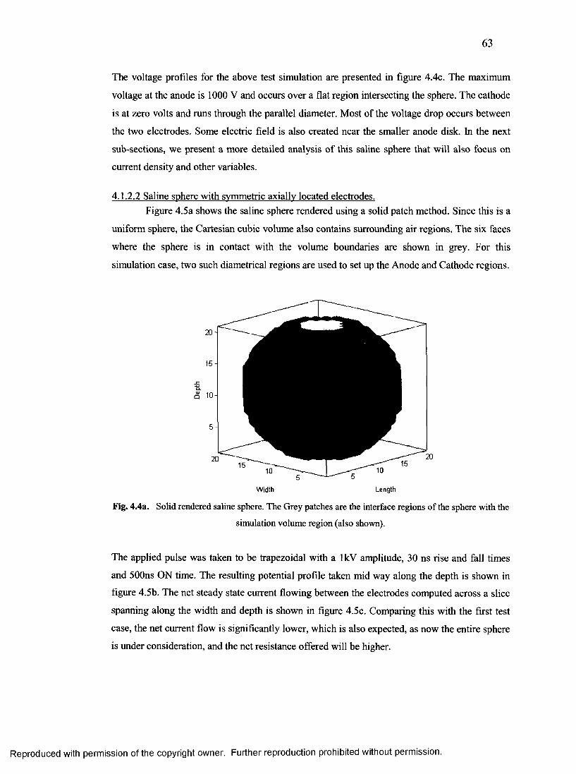
63

The voltage profiles for the above test simulation are presented in figure 4.4c. The maximum

voltage at the anode is 1000 V and occurs over a flat region intersecting the sphere. The cathode

is at zero volts and runs through the parallel diameter. Most of the voltage drop occurs between

the two electrodes. Some electric field is also created near the smaller anode disk. In the next

sub-sections, we present a more detailed analysis of this saline sphere that will also focus on

current density and other variables.

4.1.2.2 Saline sphere with symmetric axially located electrodes.Figure 4.5a shows the saline sphere rendered using a solid patch method. Since this is a

uniform sphere, the Cartesian cubic volume also contains surrounding air regions. The six faces

where the sphere is in contact with the volume boundaries are shown in grey. For this

simulation case, two such diametrical regions are used to set up the Anode and Cathode regions.

Width Length

Fig. 4.4a. Solid rendered saline sphere. The Grey patches are the interface regions of the sphere with the

simulation volume region (also shown).

The applied pulse was taken to be trapezoidal with a lkV amplitude, 30 ns rise and fall times

and 500ns ON time. The resulting potential profile taken mid way along the depth is shown in

figure 4.5b. The net steady state current flowing between the electrodes computed across a slice

spanning along the width and depth is shown in figure 4.5c. Comparing this with the first test

case, the net current flow is significantly lower, which is also expected, as now the entire sphere

is under consideration, and the net resistance offered will be higher.


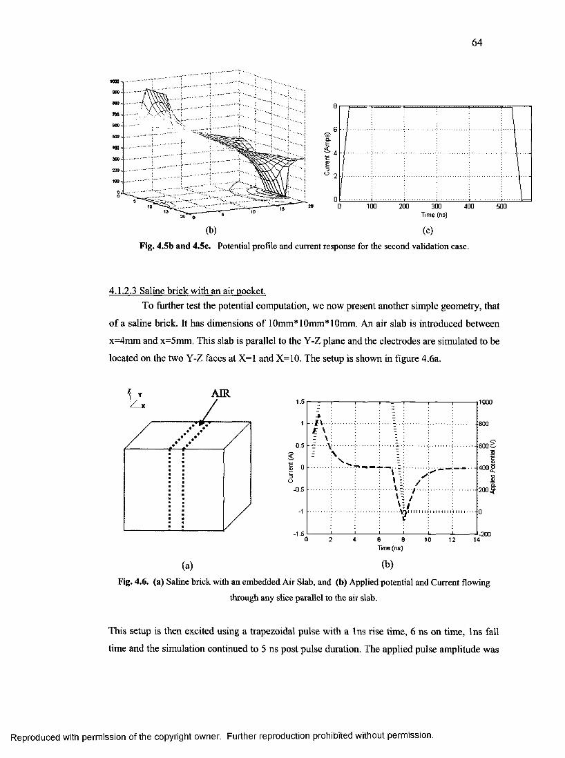
64

. . . . . I

20 0

(b)

8

2

00 100 200 300 400 500

Time (ns)

(c)

Fig. 4.5b and 4.5c. Potential profile and current response for the second validation case.

4.1.2.3 Saline brick with an air pocket.To further test the potential computation, we now present another simple geometry, that

of a saline brick. It has dimensions of 10mm* 10mm* 10mm. An air slab is introduced between

x=4mm and x=5mm. This slab is parallel to the Y-Z plane and the electrodes are simulated to be

located on the two Y-Z faces at X=1 and X=10. The setup is shown in figure 4.6a.

AIR|1000

1\ - 800

- 600 £0.5

■ - 400

- 0.5 - 200

- 1.5 '-200

Time (ns)

(a) (b)

Fig. 4.6. (a) Saline brick with an embedded Air Slab, and (b) Applied potential and Current flowing

through any slice parallel to the air slab.

This setup is then excited using a trapezoidal pulse with a Ins rise time, 6 ns on time, Ins fall

time and the simulation continued to 5 ns post pulse duration. The applied pulse amplitude was


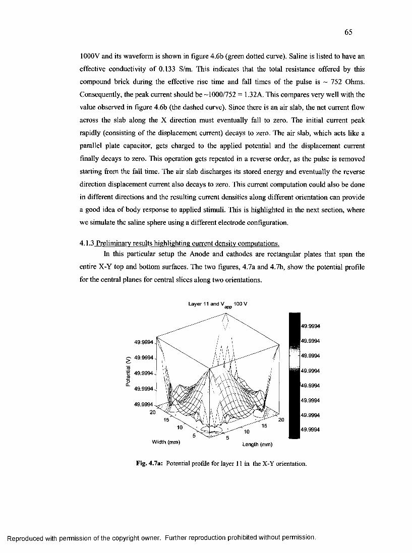
65

1000V and its waveform is shown in figure 4.6b (green dotted curve). Saline is listed to have an

effective conductivity of 0.133 S/m. This indicates that the total resistance offered by this

compound brick during the effective rise time and fall times of the pulse is ~ 752 Ohms.

Consequently, the peak current should be ~1000/752 = 1.32A. This compares very well with the

value observed in figure 4.6b (the dashed curve). Since there is an air slab, the net current flow

across the slab along the X direction must eventually fall to zero. The initial current peak

rapidly (consisting of the displacement current) decays to zero. The air slab, which acts like a

parallel plate capacitor, gets charged to the applied potential and the displacement current

finally decays to zero. This operation gets repeated in a reverse order, as the pulse is removed

starting from the fall time. The air slab discharges its stored energy and eventually the reverse

direction displacement current also decays to zero. This current computation could also be done

in different directions and the resulting current densities along different orientation can provide

a good idea of body response to applied stimuli. This is highlighted in the next section, where

we simulate the saline sphere using a different electrode configuration.

4.1.3 Preliminary results highlighting current density computations.In this particular setup the Anode and cathodes are rectangular plates that span the

entire X-Y top and bottom surfaces. The two figures, 4.7a and 4.7b, show the potential profile

for the central planes for central slices along two orientations.

Layer 11 and V 100 V7 a n napp

Width (mm) Length (mm)

Fig. 4.7a: Potential profile for layer 11 in the X-Y orientation.


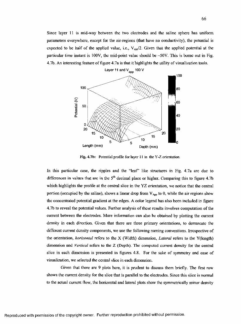
66

Since layer 11 is mid-way between the two electrodes and the saline sphere has uniform

parameters everywhere, except for the air-regions (that have no conductivity), the potential is

expected to be half of the applied value, i.e., Yapp/2. Given that the applied potential at the

particular time instant is 100V, the mid-point value should be ~50V. This is borne out in Fig.

4.7b. An interesting feature of figure 4.7a is that it highlights the utility of visualization tools.Layer 11 and V 100 V 1 app

100

3 50-cCDO

CL

Length (mm) Depth (mm)

i100

180

60

140

120

Fig. 4.7b: Potential profile for layer 11 in the Y-Z orientation.

In this particular case, the ripples and the “leaf’ like structures in Fig. 4.7a are due to

differences in values that are in the 5th decimal place or higher. Comparing this to figure 4.7b

which highlights the profile at the central slice in the YZ orientation, we notice that the central

portion (occupied by the saline), shows a linear drop from VApp to 0, while the air regions show

the concentrated potential gradient at the edges. A color legend has also been included in figure

4.7b to reveal the potential values. Further analysis of these results involves computation of the

current between the electrodes. More information can also be obtained by plotting the current

density in each direction. Given that there are three primary orientations, to demarcate the

different current density components, we use the following naming conventions. Irrespective of

the orientation, horizontal refers to the X (Width) dimension, Lateral refers to the Y(length)

dimension and Vertical refers to the Z (Depth). The computed current density for the central

slice in each dimension is presented in figures 4.8. For the sake of symmetry and ease of

visualization, we selected the central slice in each dimension.

Given that there are 9 plots here, it is prudent to discuss them briefly. The first row

shows the current density for the slice that is parallel to the electrodes. Since this slice is normal

to the actual current flow, the horizontal and lateral plots show the symmetrically minor density


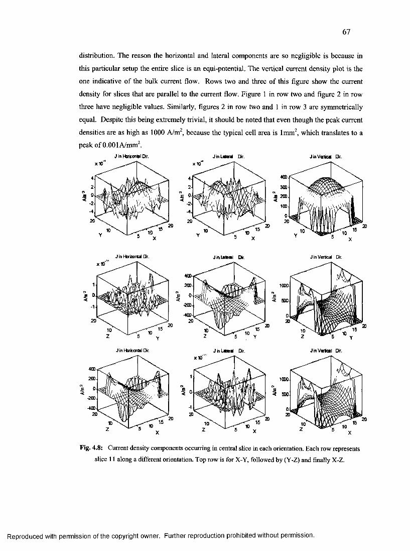
67

distribution. The reason the horizontal and lateral components are so negligible is because in

this particular setup the entire slice is an equi-potential. The vertical current density plot is the

one indicative of the bulk current flow. Rows two and three of this figure show the current

density for slices that are parallel to the current flow. Figure 1 in row two and figure 2 in row

three have negligible values. Similarly, figures 2 in row two and 1 in row 3 are symmetrically

equal. Despite this being extremely trivial, it should be noted that even though the peak current

densities are as high as 1000 A/m2, because the typical cell area is 1mm2, which translates to a

peak of 0.001 A/mm2.J in Lateral Dir.J in Hbrecntal Dir. J in V e r ie r Or.

*10

20

£ 200

V'

J in Hbrizortal Dr. J in Lateral Dir. J in Vertical Dir.

< 500

J in htorg-cnta l Dir. J h Lateral Dir. J in Vertical Dir.

200.

20

< 500

20

Fig. 4.8: Current density components occurring in central slice in each orientation. Each row represents

slice 11 along a different orientation. Top row is for X-Y, followed by (Y-Z) and finally X-Z.


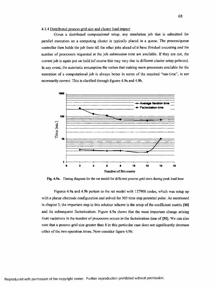
68

4.1.4 Distributed process grid size and cluster load impactGiven a distributed computational setup, any simulation job that is submitted for

parallel execution on a computing cluster is typically placed in a queue. The process/queue

controller then holds the job there till the other jobs ahead of it have finished executing and the

number of processors requested at the job submission time are available. If they are not, the

current job is again put on hold (of course this may vary due to different cluster setup policies).

In any event, the automatic assumption the notion that making more processors available for the

execution of a computational job is always better in terms of the required “run-time”, is not

necessarily correct. This is clarified through figures 4.9a and 4.9b.

1000

Avorogo Iteration lima Factorization ftma

100

0 2 4 6 10 1012 14

Number o f Processors

Fig. 4.9a. Timing diagram for the rat model for different process grid sizes during peak load hour

Figures 4.9a and 4.9b pertain to the rat model with 127908 nodes, which was setup up

with a planar electrode configuration and solved for 503 time step potential pulse. As mentioned

in chapter 3, the important step in this solution scheme is the setup of the coefficient matrix [M]

and its subsequent factorization. Figure 4.9a shows that the most important change arising

from variations in the number of processors occurs in the factorization time of [M]. We can also

note that a process grid size greater than 8 in this particular case does not significantly decrease

either of the two operation times. Now consider figure 4.9b.


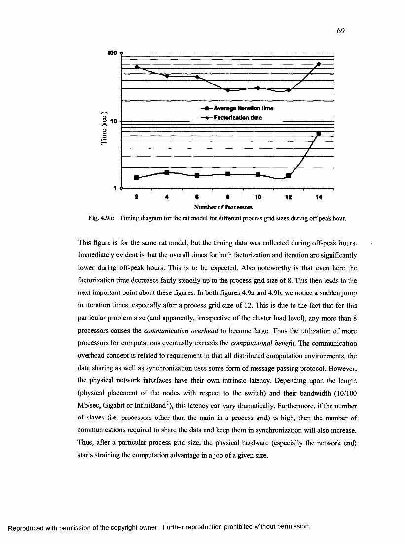
69

100 «— *.

Average Iteration time Factorization time

2 04 10 12 14Number o f Processors

Fig. 4.9b: Timing diagram for the rat model for different process grid sizes during off peak hour.

This figure is for the same rat model, but the timing data was collected during off-peak hours.

Immediately evident is that the overall times for both factorization and iteration are significantly

lower during off-peak hours. This is to be expected. Also noteworthy is that even here the

factorization time decreases fairly steadily up to the process grid size of 8. This then leads to the

next important point about these figures. In both figures 4.9a and 4.9b, we notice a sudden jump

in iteration times, especially after a process grid size of 12. This is due to the fact that for this

particular problem size (and apparently, irrespective of the cluster load level), any more than 8

processors causes the communication overhead to become large. Thus the utilization of more

processors for computations eventually exceeds the computational benefit. The communication

overhead concept is related to requirement in that all distributed computation environments, the

data sharing as well as synchronization uses some form of message passing protocol. However,

the physical network interfaces have their own intrinsic latency. Depending upon the length

(physical placement of the nodes with respect to the switch) and their bandwidth (10/100

Mb/sec, Gigabit or InfiniBand®), this latency can vary dramatically. Furthermore, if the number

of slaves (i.e. processors other than the main in a process grid) is high, then the number of

communications required to share the data and keep them in synchronization will also increase.

Thus, after a particular process grid size, the physical hardware (especially the network end)

starts straining the computation advantage in a job of a given size.


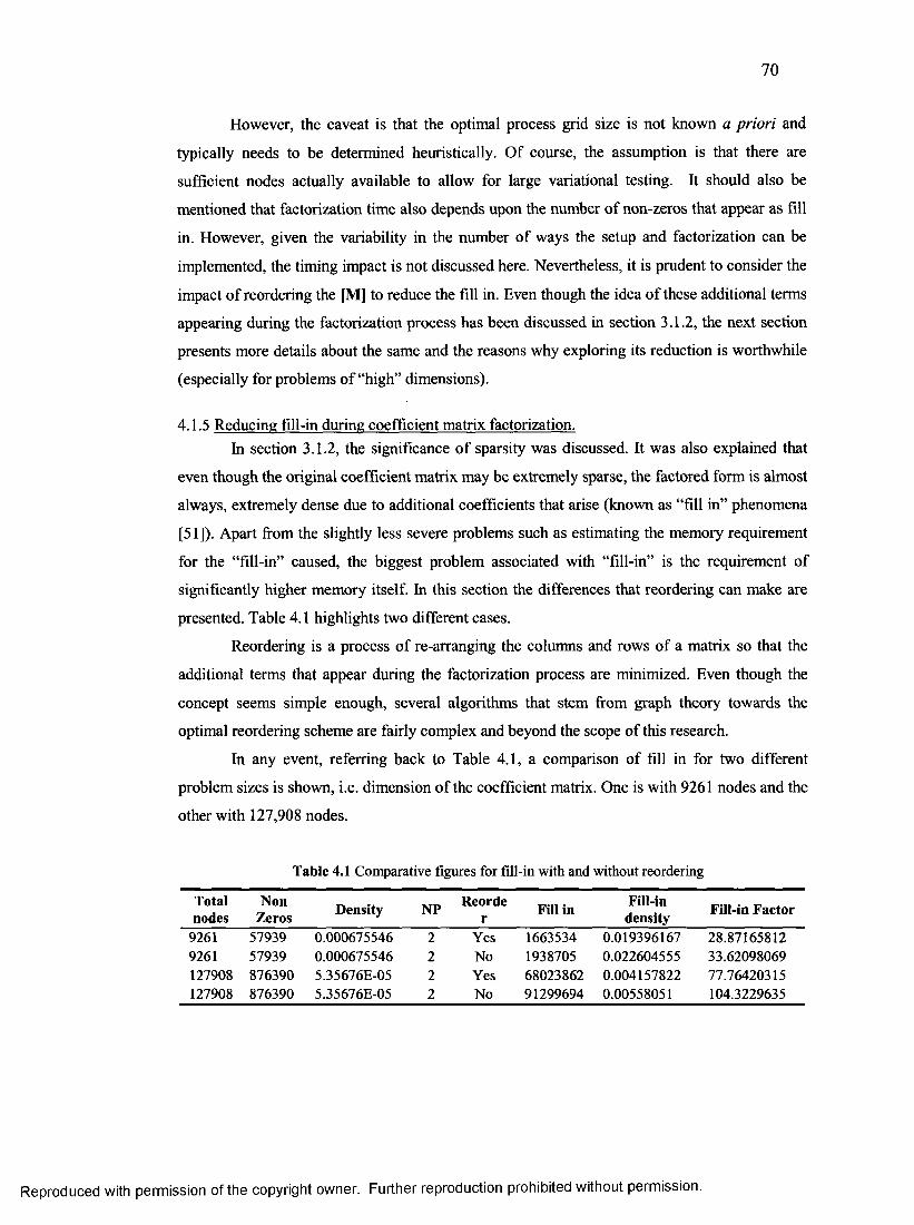
70

However, the caveat is that the optimal process grid size is not known a priori and

typically needs to be determined heuristically. Of course, the assumption is that there are

sufficient nodes actually available to allow for large variational testing. It should also be

mentioned that factorization time also depends upon the number of non-zeros that appear as fill

in. However, given the variability in the number of ways the setup and factorization can be

implemented, the timing impact is not discussed here. Nevertheless, it is prudent to consider the

impact of reordering the [M] to reduce the fill in. Even though the idea of these additional terms

appearing during the factorization process has been discussed in section 3.1.2, the next section

presents more details about the same and the reasons why exploring its reduction is worthwhile

(especially for problems of “high” dimensions).

4.1.5 Reducing fill-in during coefficient matrix factorization.In section 3.1.2, the significance of sparsity was discussed. It was also explained that

even though the original coefficient matrix may be extremely sparse, the factored form is almost

always, extremely dense due to additional coefficients that arise (known as “fill in” phenomena

[51]). Apart from the slightly less severe problems such as estimating the memory requirement

for the “fill-in” caused, the biggest problem associated with “fill-in” is the requirement of

significantly higher memory itself. In this section the differences that reordering can make are

presented. Table 4.1 highlights two different cases.

Reordering is a process of re-arranging the columns and rows of a matrix so that the

additional terms that appear during the factorization process are minimized. Even though the

concept seems simple enough, several algorithms that stem from graph theory towards the

optimal reordering scheme are fairly complex and beyond the scope of this research.

In any event, referring back to Table 4.1, a comparison of fill in for two different

problem sizes is shown, i.e. dimension of the coefficient matrix. One is with 9261 nodes and the

other with 127,908 nodes.

Table 4.1 Comparative figures for fill-in with and without reordering

Totalnodes

NonZeros Density NP Reorde

r Fill in Fill-indensity Fill-in Factor

9261 57939 0.000675546 2 Yes 1663534 0.019396167 28.871658129261 57939 0.000675546 2 No 1938705 0.022604555 33.62098069127908 876390 5.35676E-05 2 Yes 68023862 0.004157822 77.76420315127908 876390 5.35676E-05 2 No 91299694 0.00558051 104.3229635


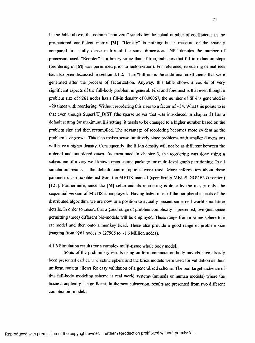
71

In the table above, the column “non-zero” stands for the actual number of coefficients in the

pre-factored coefficient matrix [MJ. “Density” is nothing but a measure of the sparsity

compared to a fully dense matrix of the same dimension. “NP” denotes the number of

processors used. “Reorder” is a binary value that, if true, indicates that fill in reduction steps

(reordering of [M] was performed prior to factorization). For reference, reordering of matrices

has also been discussed in section 3.1.2. The “Fill-in” is the additional coefficients that were

generated after the process of factorization. Anyway, this table shows a couple of very

significant aspects of the full-body problem in general. First and foremost is that even though a

problem size of 9261 nodes has a fill-in density of 0.00067, the number of fill-ins generated is

~29 times with reordering. Without reordering this rises to a factor of -34. What this points to is

that even though SuperLU DIST (the sparse solver that was introduced in chapter 3) has a

default setting for maximum fill setting, it needs to be changed to a higher number based on the

problem size and then recompiled. The advantage of reordering becomes more evident as the

problem size grows. This also makes sense intuitively since problems with smaller dimensions

will have a higher density. Consequently, the fill-in density will not be as different between the

ordered and unordered cases. As mentioned in chapter 3, the reordering was done using a

subroutine of a very well known open source package for multi-level graph partitioning. In all

simulation results - the default control options were used. More information about these

parameters can be obtained from the METIS manual (specifically METISNODEND section)

[121]. Furthermore, since the [M] setup and its reordering is done by the master only, the

sequential version of METIS is employed. Having listed most of the peripheral aspects of the

distributed algorithm, we are now in a position to actually present some real world simulation

details. In order to ensure that a good range of problem complexity is presented, two (and space

permitting three) different bio-models will be employed. These range from a saline sphere to a

rat model and then onto a monkey head. These also provide a good range of problem size

(ranging from 9261 nodes to 127908 to -1.6 Million nodes).

4.1.6 Simulation results for a complex multi-tissue whole body model.Some of the preliminary results using uniform composition body models have already

been presented earlier. The saline sphere and the brick models were used for validation as their

uniform content allows for easy validation of a generalized scheme. The real target audience of

this full-body modeling scheme is real world systems (animals or human models) where the

tissue complexity is significant. In the next subsection, results are presented from two different

complex bio-models.


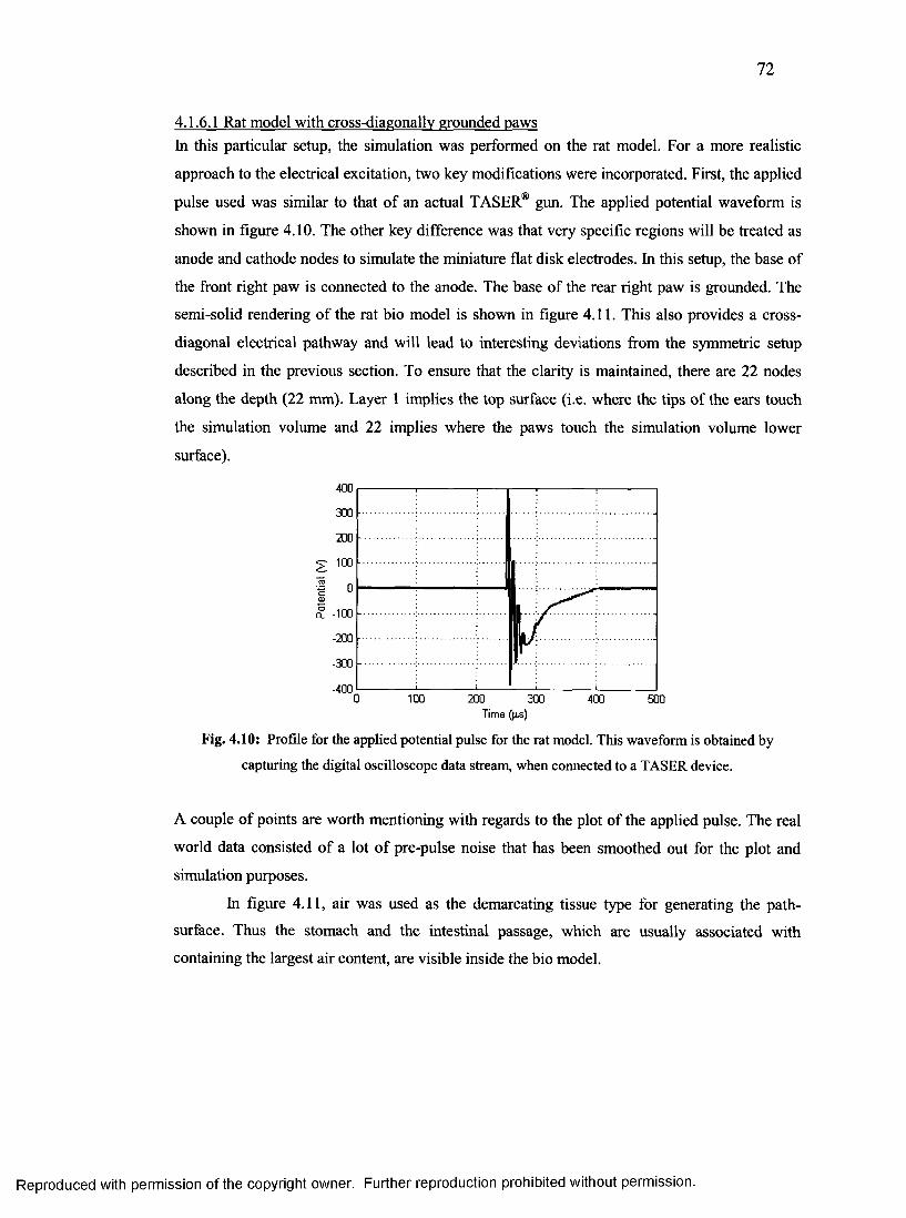
72

4.1.6.1 Rat model with cross-diagonally grounded pawsIn this particular setup, the simulation was performed on the rat model. For a more realistic

approach to the electrical excitation, two key modifications were incorporated. First, the applied

pulse used was similar to that of an actual TASER® gun. The applied potential waveform is

shown in figure 4.10. The other key difference was that very specific regions will be treated as

anode and cathode nodes to simulate the miniature flat disk electrodes. In this setup, the base of

the front right paw is connected to the anode. The base of the rear right paw is grounded. The

semi-solid rendering of the rat bio model is shown in figure 4.11. This also provides a cross

diagonal electrical pathway and will lead to interesting deviations from the symmetric setup

described in the previous section. To ensure that the clarity is maintained, there are 22 nodes

along the depth (22 mm). Layer 1 implies the top surface (i.e. where the tips of the ears touch

the simulation volume and 22 implies where the paws touch the simulation volume lower

surface).

400

300

200

100

S. -100

-200

-300

-400100 200 300 400 500

Time (fis)

Fig. 4.10: Profile for the applied potential pulse for the rat model. This waveform is obtained by

capturing the digital oscilloscope data stream, when connected to a TASER device.

A couple of points are worth mentioning with regards to the plot of the applied pulse. The real

world data consisted of a lot of pre-pulse noise that has been smoothed out for the plot and

simulation purposes.

In figure 4.11, air was used as the demarcating tissue type for generating the path-

surface. Thus the stomach and the intestinal passage, which are usually associated with

containing the largest air content, are visible inside the bio model.


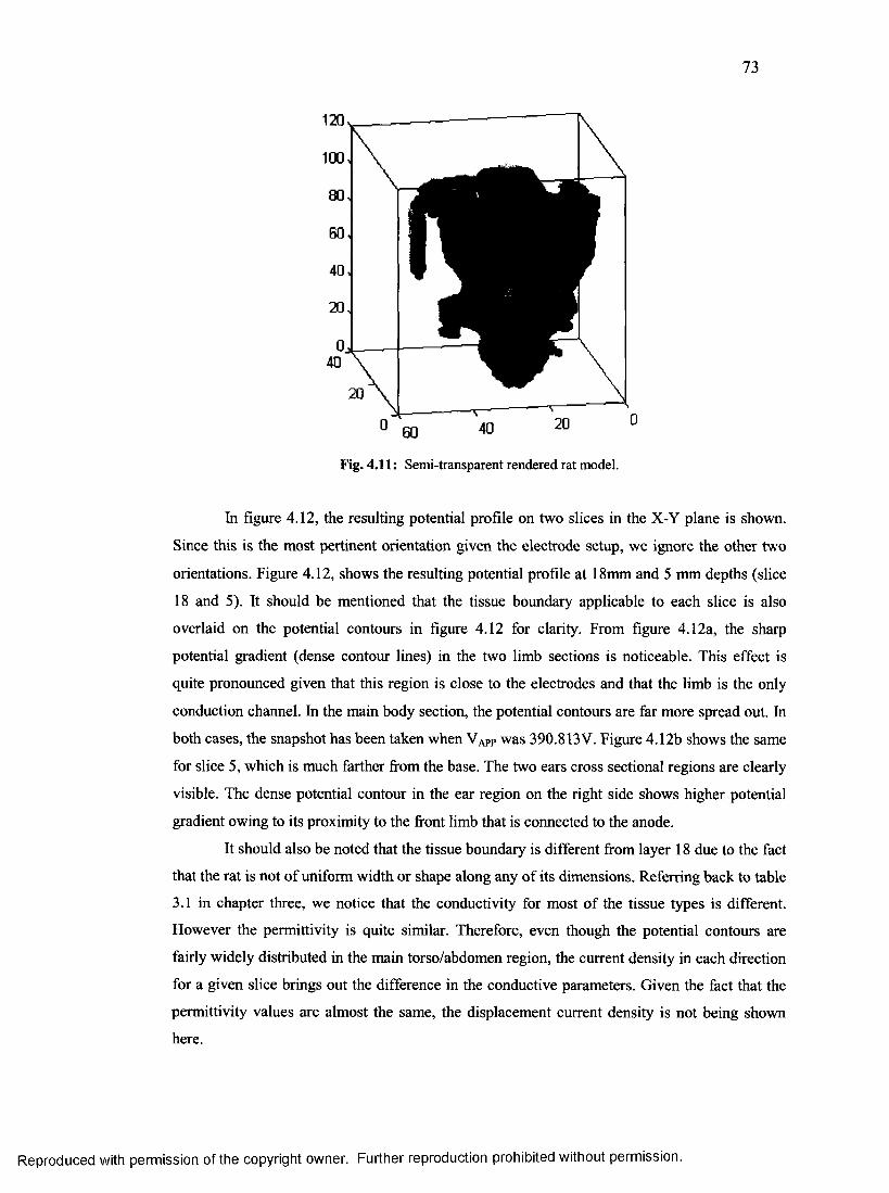
Fig. 4.11: Semi-transparent rendered rat model.

In figure 4.12, the resulting potential profile on two slices in the X-Y plane is shown.

Since this is the most pertinent orientation given the electrode setup, we ignore the other two

orientations. Figure 4.12, shows the resulting potential profile at 18mm and 5 mm depths (slice

18 and 5). It should be mentioned that the tissue boundary applicable to each slice is also

overlaid on the potential contours in figure 4.12 for clarity. From figure 4.12a, the sharp

potential gradient (dense contour lines) in the two limb sections is noticeable. This effect is

quite pronounced given that this region is close to the electrodes and that the limb is the only

conduction channel. In the main body section, the potential contours are far more spread out. In

both cases, the snapshot has been taken when VapP was 390.813V. Figure 4.12b shows the same

for slice 5, which is much farther from the base. The two ears cross sectional regions are clearly

visible. The dense potential contour in the ear region on the right side shows higher potential

gradient owing to its proximity to the front limb that is connected to the anode.

It should also be noted that the tissue boundary is different from layer 18 due to the fact

that the rat is not of uniform width or shape along any of its dimensions. Referring back to table

3.1 in chapter three, we notice that the conductivity for most of the tissue types is different.

However the permittivity is quite similar. Therefore, even though the potential contours are

fairly widely distributed in the main torso/abdomen region, the current density in each direction

for a given slice brings out the difference in the conductive parameters. Given the fact that the

permittivity values are almost the same, the displacement current density is not being shown

here.


74

Figure 4.13 shows the conductive current density in A/m2 in the XY slice at 11 mm depth.

Unlike the symmetric spherical case, since the electrical pathway from the anode to cathode has

clear vertical, horizontal and lateral components, the current densities reflect these as well. The

left column in figure 4.13 employs contours to highlight regions that have similar current

density values (owing to similar tissue regions) while the right column is a standard 3-d surface

plot. A negative current density means that the current flow is opposite to the direction assigned

for the computation. As expected, the region of air that has negligible conductivity displays no

current flow (density). Yet another significant result is visible from the vertical current density

plot in figure 4.13. The three high current density regions (visible as circular regions) near the

central part are coincidental with the spine placement. Given the fact that the spine curvature

spans multiple regions along the depth, this shows that a part of the spinal region is under an

unusually high electric stress. The significance of this result will become evident in the later

sections when we discuss the hypothesis of high intensity electric pulses for the purposes of

action potential block in nerve segments. We will also revisit this particular result when

discussing an experimental result that will be used to support this hypothesis. For the sake of

completeness, the total current flow across the central slices in each dimension is also shown in

figure 4.14. In each subfigure of 4.14, the current magnitudes are in fiA. Perhaps the most

interesting result is that for the longitudinal current flow. It shows that the most of the current

variation and flow is occurring not through the bulk but through the region near the edges. The

proximity effect of the anode is also visible in the vertical current flow. It should also be

mentioned that the visualization in figure 4.14 b and 4.14c are shown with angular rotation of

90 and 180 degrees, respectively.


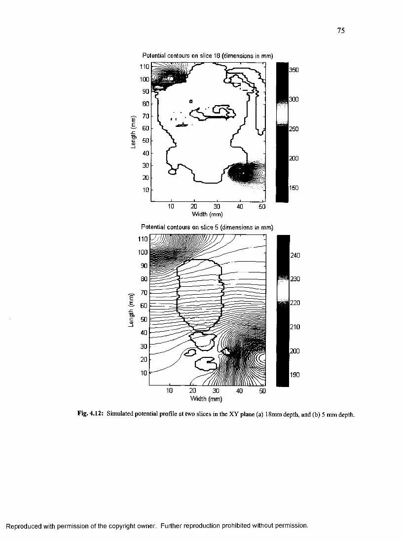
75

Potential contours on slice 18 (dimensions in mm)

20 30Width (mm)

Potential contours on slice 5 (dimensions in mm)

110

20 30Width (mm)

Fig. 4.12: Simulated potential profile at two slices in the XY plane (a) 18mm depth, and (b) 5 mm depth.


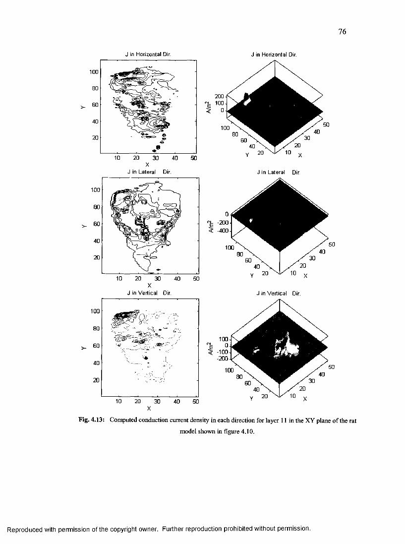
76

J in Horizontal Dir. J in Horizontal Dir.

100

80

60

40

10 20 30 40 50X

J in Lateral Dir.

XJ in Vertical Dir.

100

5 -

40

10 20 30 40 50

~ 100 -

J in Lateral Dir.

"E - 2 0 0 -

5 -400-

J in Vertical Dir.

100

10 20 30 40 50

5 -100 -200

Fig. 4.13: Computed conduction current density in each direction for layer 11 in the XY plane of the rat

model shown in figure 4.10.


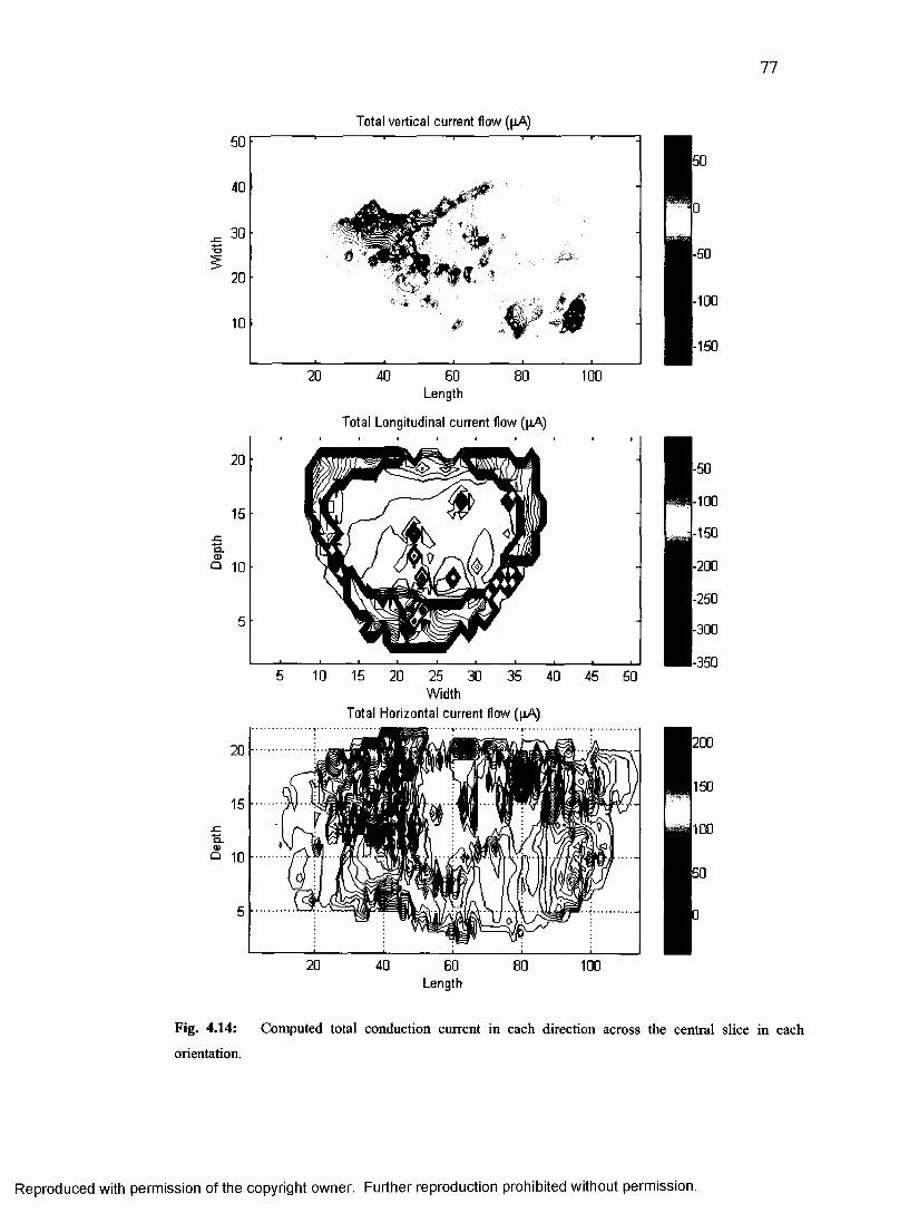
77

Total vertical current flow ((xA)

Length

Total Longitudinal current flow (|jA)

WidthTotal Horizontal current flow (pA)

20 40 60 80 100Length

Fig. 4.14: Computed total conduction current in each direction across the central slice in each

orientation.


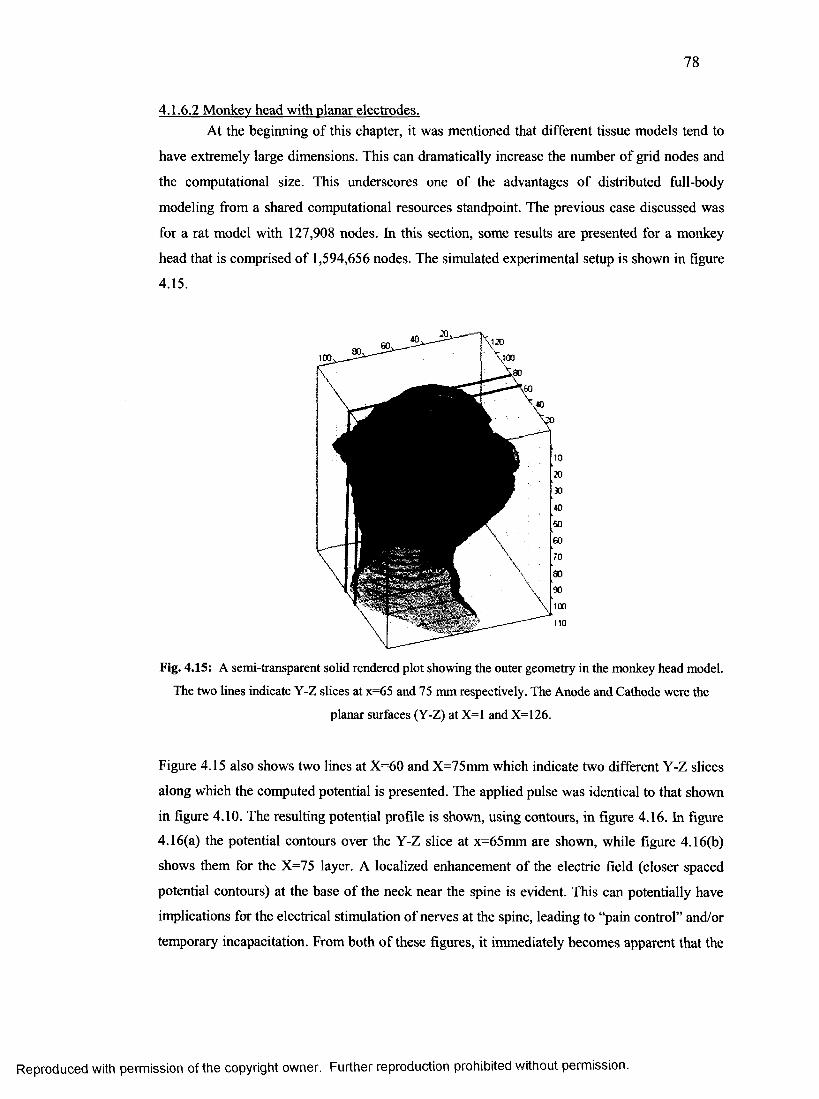
78

4.1.6.2 Monkey head with planar electrodes.At the beginning of this chapter, it was mentioned that different tissue models tend to

have extremely large dimensions. This can dramatically increase the number of grid nodes and

the computational size. This underscores one of the advantages of distributed full-body

modeling from a shared computational resources standpoint. The previous case discussed was

for a rat model with 127,908 nodes. In this section, some results are presented for a monkey

head that is comprised of 1,594,656 nodes. The simulated experimental setup is shown in figure

4.15.

Fig. 4.15: A semi-transparent solid rendered plot showing the outer geometry in the monkey head model.

The two lines indicate Y-Z slices at x=65 and 75 mm respectively. The Anode and Cathode were the

planar surfaces (Y-Z) at X=1 and X=126.

Figure 4.15 also shows two lines at X=60 and X=75mm which indicate two different Y-Z slices

along which the computed potential is presented. The applied pulse was identical to that shown

in figure 4.10. The resulting potential profile is shown, using contours, in figure 4.16. In figure

4.16(a) the potential contours over the Y-Z slice at x=65mm are shown, while figure 4.16(b)

shows them for the X=75 layer. A localized enhancement of the electric field (closer spaced

potential contours) at the base of the neck near the spine is evident. This can potentially have

implications for the electrical stimulation of nerves at the spine, leading to “pain control” and/or

temporary incapacitation. From both of these figures, it immediately becomes apparent that the


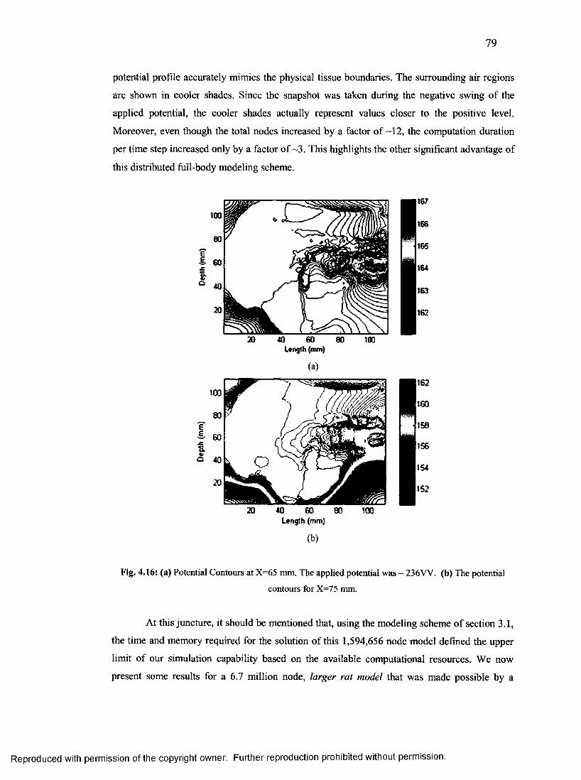
79

potential profile accurately mimics the physical tissue boundaries. The surrounding air regions

are shown in cooler shades. Since the snapshot was taken during the negative swing of the

applied potential, the cooler shades actually represent values closer to the positive level.

Moreover, even though the total nodes increased by a factor of -12, the computation duration

per time step increased only by a factor of -3 . This highlights the other significant advantage of

this distributed full-body modeling scheme.

20 40 60 80 100lengih (mm)

(a)

20 <0 60 80 100 Length (mm)

(b)

Fig. 4.16: (a) Potential Contours at X=65 mm. The applied potential was - 236W . (b) The potential

contours for X=75 mm.

At this juncture, it should be mentioned that, using the modeling scheme of section 3.1,

the time and memory required for the solution of this 1,594,656 node model defined the upper

limit of our simulation capability based on the available computational resources. We now

present some results for a 6.7 million node, larger rat model that was made possible by a


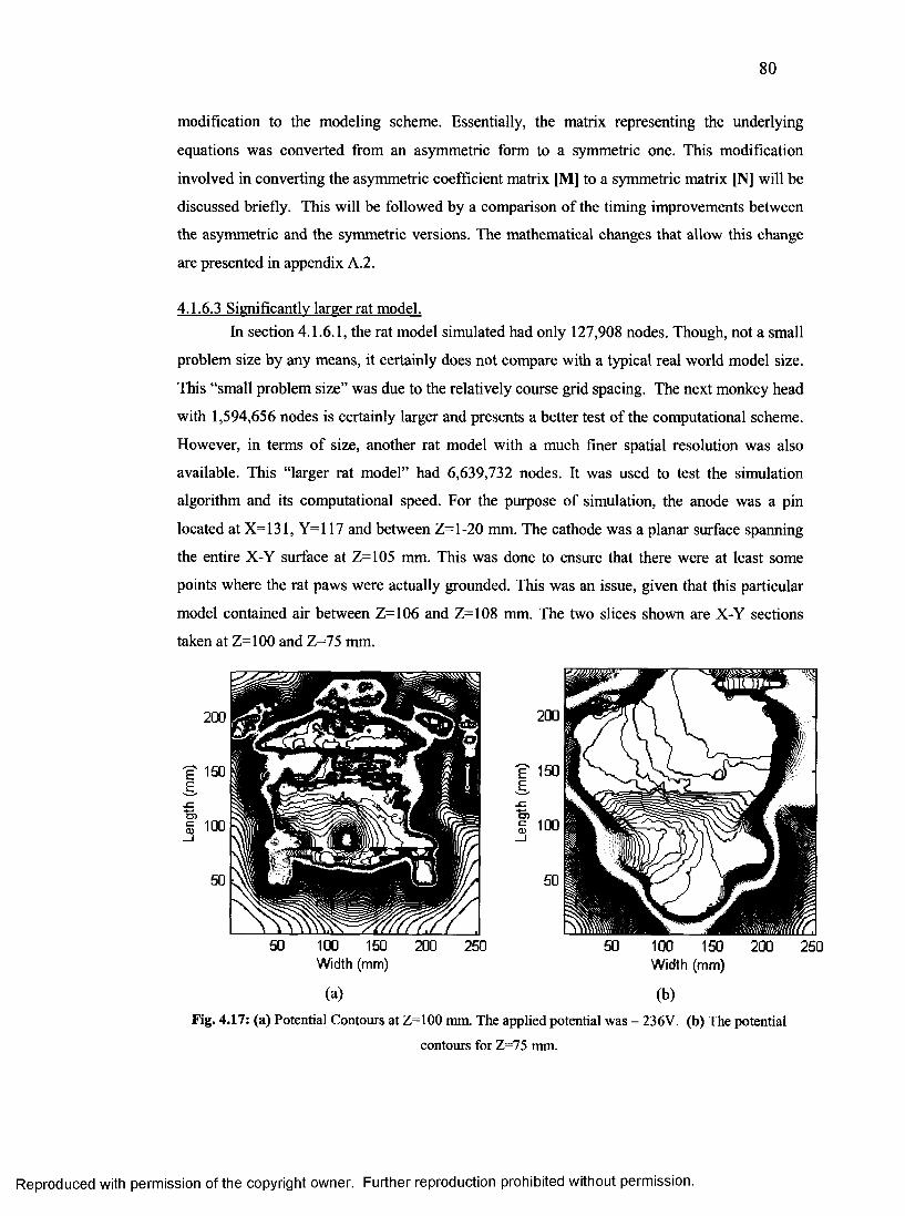
80

modification to the modeling scheme. Essentially, the matrix representing the underlying

equations was converted from an asymmetric form to a symmetric one. This modification

involved in converting the asymmetric coefficient matrix [M] to a symmetric matrix [N] will be

discussed briefly. This will be followed by a comparison of the timing improvements between

the asymmetric and the symmetric versions. The mathematical changes that allow this change

are presented in appendix A.2.

4.1.6.3 Significantly larger rat model.In section 4.1.6.1, the rat model simulated had only 127,908 nodes. Though, not a small

problem size by any means, it certainly does not compare with a typical real world model size.

This “small problem size” was due to the relatively course grid spacing. The next monkey head

with 1,594,656 nodes is certainly larger and presents a better test of the computational scheme.

However, in terms of size, another rat model with a much finer spatial resolution was also

available. This “larger rat model” had 6,639,732 nodes. It was used to test the simulation

algorithm and its computational speed. For the purpose of simulation, the anode was a pin

located at X= 131, Y=117 and between Z=l-20 mm. The cathode was a planar surface spanning

the entire X-Y surface at Z=105 mm. This was done to ensure that there were at least some

points where the rat paws were actually grounded. This was an issue, given that this particular

model contained air between Z=106 and Z=108 mm. The two slices shown are X-Y sections

taken at Z=100 and Z=75 mm.

Fig. 4.17: (a) Potential Contours at Z=100 mm. The applied potential was - 236V. (b) The potential

contours for Z=75 mm.

50 100 150 200 250Width (mm)

(a)

50 100 150 200 250Width (mm)

(b)


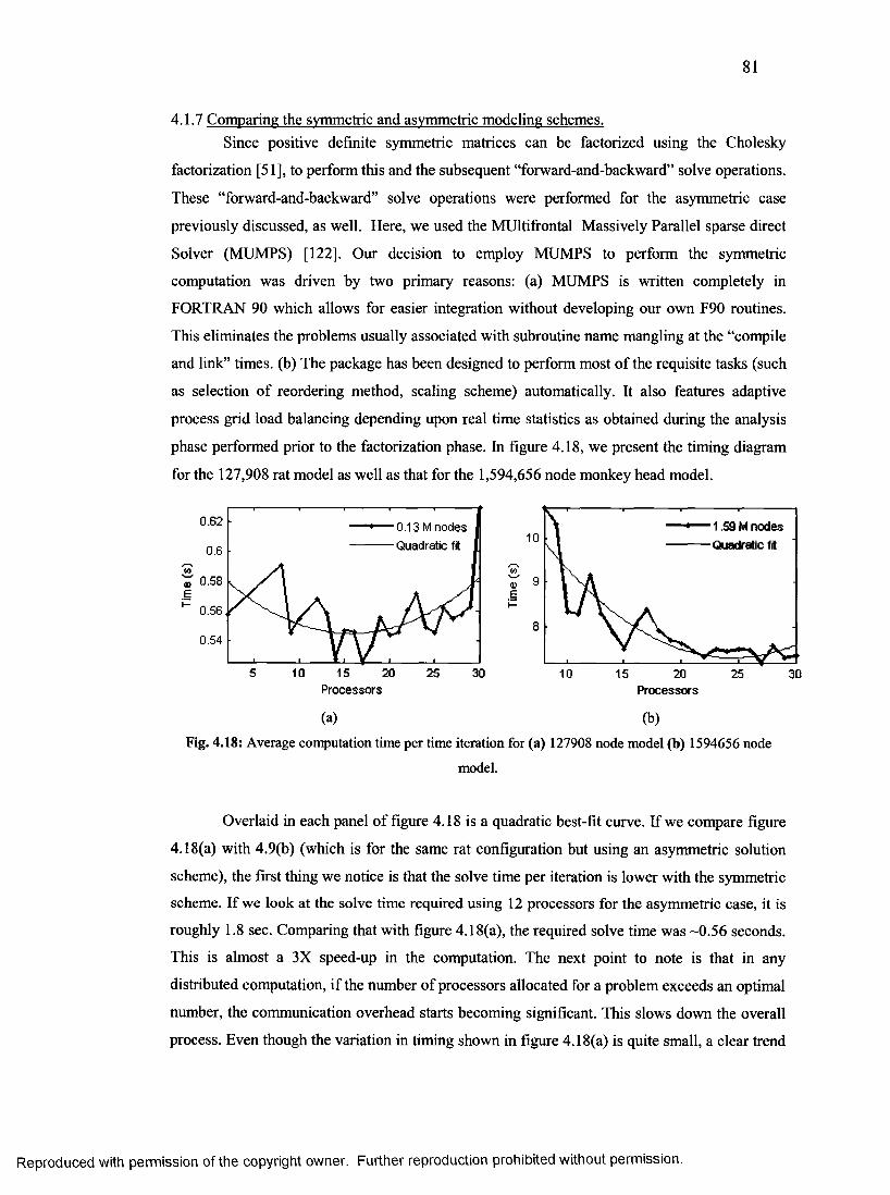
81

4.1.7 Comparing the symmetric and asymmetric modeling schemes.Since positive definite symmetric matrices can be factorized using the Cholesky

factorization [51], to perform this and the subsequent “forward-and-backward” solve operations.

These “forward-and-backward” solve operations were performed for the asymmetric case

previously discussed, as well. Here, we used the MUltifrontal Massively Parallel sparse direct

Solver (MUMPS) [122]. Our decision to employ MUMPS to perform the symmetric

computation was driven by two primary reasons: (a) MUMPS is written completely in

FORTRAN 90 which allows for easier integration without developing our own F90 routines.

This eliminates the problems usually associated with subroutine name mangling at the “compile

and link” times, (b) The package has been designed to perform most of the requisite tasks (such

as selection of reordering method, scaling scheme) automatically. It also features adaptive

process grid load balancing depending upon real time statistics as obtained during the analysis

phase performed prior to the factorization phase. In figure 4.18, we present the timing diagram

for the 127,908 rat model as well as that for the 1,594,656 node monkey head model.

0.62 0.13 M nodes Quadratic fit0.6

V)U 0-58 E

0.56

0.54

5 10 15 20 25 30

1.59 M nodes Quadratic fit10

9

8

10 2515 20 30Processors P rocessors

(a) (b)Fig. 4.18: Average computation time per time iteration for (a) 127908 node model (b) 1594656 node

model.

Overlaid in each panel of figure 4.18 is a quadratic best-fit curve. If we compare figure

4.18(a) with 4.9(b) (which is for the same rat configuration but using an asymmetric solution

scheme), the first thing we notice is that the solve time per iteration is lower with the symmetric

scheme. If we look at the solve time required using 12 processors for the asymmetric case, it is

roughly 1.8 sec. Comparing that with figure 4.18(a), the required solve time was -0.56 seconds.

This is almost a 3X speed-up in the computation. The next point to note is that in any

distributed computation, if the number of processors allocated for a problem exceeds an optimal

number, the communication overhead starts becoming significant. This slows down the overall

process. Even though the variation in timing shown in figure 4.18(a) is quite small, a clear trend


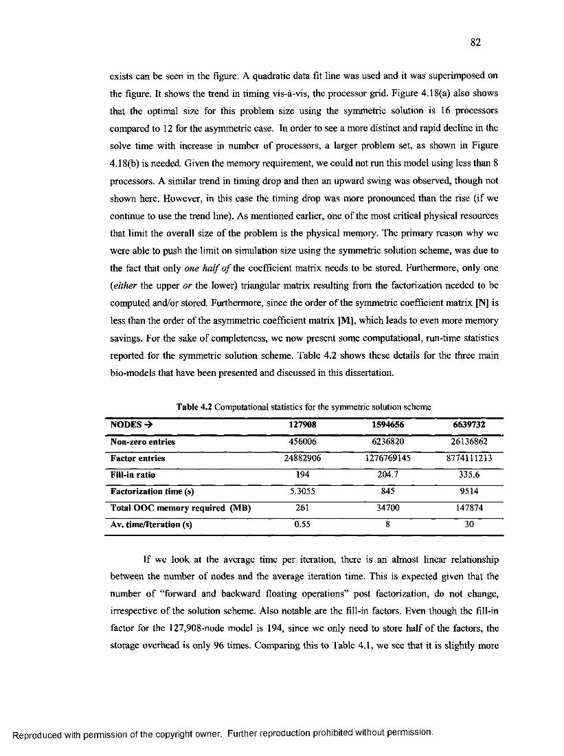
82

exists can be seen in the figure. A quadratic data fit line was used and it was superimposed on

the figure. It shows the trend in timing vis-a-vis, the processor grid. Figure 4.18(a) also shows

that the optimal size for this problem size using the symmetric solution is 16 processors

compared to 12 for the asymmetric case. In order to see a more distinct and rapid decline in the

solve time with increase in number of processors, a larger problem set, as shown in Figure

4.18(b) is needed. Given the memory requirement, we could not run this model using less than 8

processors. A similar trend in timing drop and then an upward swing was observed, though not

shown here. However, in this case the timing drop was more pronounced than the rise (if we

continue to use the trend line). As mentioned earlier, one of the most critical physical resources

that limit the overall size of the problem is the physical memory. The primary reason why we

were able to push the limit on simulation size using the symmetric solution scheme, was due to

the fact that only one half o f the coefficient matrix needs to be stored. Furthermore, only one

{either the upper or the lower) triangular matrix resulting from the factorization needed to be

computed and/or stored. Furthermore, since the order of the symmetric coefficient matrix [N] is

less than the order of the asymmetric coefficient matrix [M], which leads to even more memory

savings. For the sake of completeness, we now present some computational, run-time statistics

reported for the symmetric solution scheme. Table 4.2 shows these details for the three main

bio-models that have been presented and discussed in this dissertation.

Table 4.2 Computational statistics for the symmetric solution scheme

NODES -> 127908 1594656 6639732

Non-zero entries 456006 6236820 26136862

Factor entries 24882906 1276769145 8774111213

Fill-in ratio 194 204.7 335.6

Factorization time (s) 5.3055 845 9514

Total OOC memory required (MB) 261 34700 147874

Av. time/iteration (s) 0.55 8 30

If we look at the average time per iteration, there is an almost linear relationship

between the number of nodes and the average iteration time. This is expected given that the

number o f “forward and backward floating operations” post factorization, do not change,

irrespective of the solution scheme. Also notable are the fill-in factors. Even though the fill-in

factor for the 127,908-node model is 194, since we only need to store half of the factors, the

storage overhead is only 96 times. Comparing this to Table 4.1, we see that it is slightly more


83

than when reordering is used. This slight increase is most probably due to the difference in

ordering schemes (METIS versus the default option used in MUMPS). Finally, the transition

from the 127,908-node model to the 6,639,732-node model represents an increase by a factor of

-52. A comparison between the average time per iteration for these two models yields a ratio of

roughly 30/0.55 = 54.5. Thus, the computational problem seems to scale with the number, “N”,

of nodes. This is a significant advantage and of a practical utility.


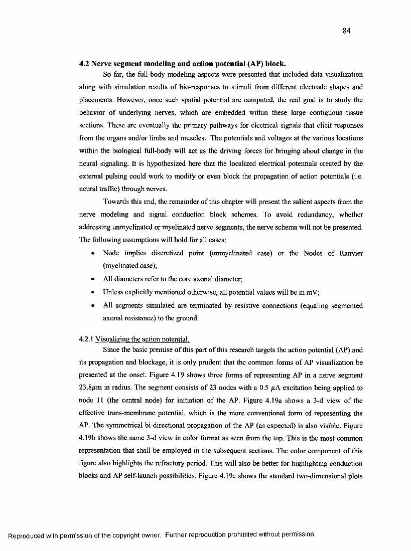
84

4.2 Nerve segment modeling and action potential (AP) block.So far, the full-body modeling aspects were presented that included data visualization

along with simulation results of bio-responses to stimuli from different electrode shapes and

placements. However, once such spatial potential are computed, the real goal is to study the

behavior of underlying nerves, which are embedded within these large contiguous tissue

sections. These are eventually the primary pathways for electrical signals that elicit responses

from the organs and/or limbs and muscles. The potentials and voltages at the various locations

within the biological full-body will act as the driving forces for bringing about change in the

neural signaling. It is hypothesized here that the localized electrical potentials created by the

external pulsing could work to modify or even block the propagation of action potentials (i.e.

neural traffic) through nerves.

Towards this end, the remainder of this chapter will present the salient aspects from the

nerve modeling and signal conduction block schemes. To avoid redundancy, whether

addressing unmyelinated or myelinated nerve segments, the nerve schema will not be presented.

The following assumptions will hold for all cases:

• Node implies discretized point (unmyelinated case) or the Nodes of Ranvier

(myelinated case);

• All diameters refer to the core axonal diameter;

• Unless explicitly mentioned otherwise, all potential values will be in mV;

• All segments simulated are terminated by resistive connections (equaling segmented

axonal resistance) to the ground.

4.2.1 Visualizing the action potential.Since the basic premise of this part of this research targets the action potential (AP) and

its propagation and blockage, it is only prudent that the common forms of AP visualization be

presented at the onset. Figure 4.19 shows three forms of representing AP in a nerve segment

23.8/rm in radius. The segment consists of 23 nodes with a 0.5 fiA excitation being applied to

node 11 (the central node) for initiation of the AP. Figure 4.19a shows a 3-d view of the

effective trans-membrane potential, which is the more conventional form of representing the

AP. The symmetrical bi-directional propagation of the AP (as expected) is also visible. Figure

4.19b shows the same 3-d view in color format as seen from the top. This is the most common

representation that shall be employed in the subsequent sections. The color component of this

figure also highlights the refractory period. This will also be better for highlighting conduction

blocks and AP self-launch possibilities. Figure 4.19c shows the standard two-dimensional plots


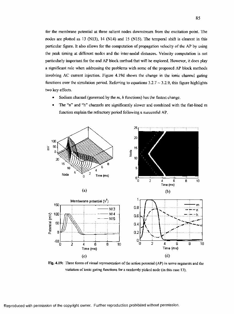
85

for the membrane potential at three salient nodes downstream from the excitation point. The

nodes are plotted as 13 (N13), 14 (N14) and 15 (N15). The temporal shift is clearest in this

particular figure. It also allows for the computation of propagation velocity of the AP by using

the peak timing at different nodes and the inter-nodal distances. Velocity computation is not

particularly important for the end AP block method that will be explored. However, it does play

a significant role when addressing the problems with some of the proposed AP block methods

involving AC current injection. Figure 4.19d shows the change in the ionic channel gating

functions over the simulation period. Referring to equations 3.2.7 ~ 3.2.9, this figure highlights

two key effects.

• Sodium channel (governed by the m, h functions) has the fastest change.

• The “n” and “h” channels are significantly slower and combined with the flat-lined m

function explain the refractory period following a successful AP.

Time (ms)

(a)

Memberane potential ( / )150

N13N14N15

;>■ 100

-50

Time (ms)

(c)

2 4 6Time (ms)

(b)

1

0.8

0.6

0.4

0.2

0

/ m

1 /~ 1 . / .

1 N■- — n- : : .hS J / . . . . ^

----------

I \i*'"

0 4 6Time (ms)

(d)

10

Fig. 4.19: Three forms of visual representation of the action potential (AP) in nerve segments and the

variation of ionic gating functions for a randomly picked node (in this case 13).


86

4.2.2 AP propagation velocity.As mentioned in the previous sub-section, computation of AP propagation velocity,

though not vital, is necessary for the following reasons:

1. As a validity check of the intrinsic modeling scheme for the nerve segments.

2. It is an important element for explaining the inherent problems with AC current based

conduction block interruption schemes.

Figure 4.20 shows the variation of the propagation velocity as a function of the unmyelinated

axon diameter. The figure also shows the superimposed power fit using the axon diameter as the

variable. The resulting best-fit relationship is given by equation(4.1).

v = 0.5r/° 5279 , (4.1)where, v is the velocity (m/s) and d is the axon diameter (/urn). This agrees very well with the

established relationship of v <x -Jd [123] for the unmyelinated nerve segments. The computed

velocity relationship (not shown in the figure) for the myelinated nerve segments is given by

equation (4.2) which also agrees very well with the known v oc d relationship [71].

v = 2243c?1'0879 . (4.2)

Velocity v/s Diameter.

14

12

10

8

6

4

2

00 100 200 300 400 500

Diameter (pm)

Fig. 4.20: Computed velocity dependence upon the axon diameter for unmyelinated nerves.


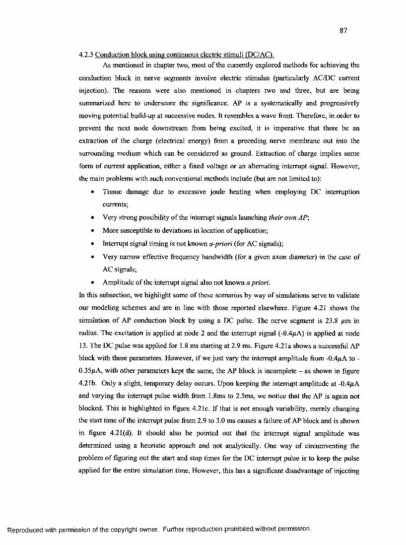
87

4.2.3 Conduction block using continuous electric stimuli (DC/AC).As mentioned in chapter two, most of the currently explored methods for achieving the

conduction block in nerve segments involve electric stimulus (particularly AC/DC current

injection). The reasons were also mentioned in chapters two and three, but are being

summarized here to underscore the significance. AP is a systematically and progressively

moving potential build-up at successive nodes. It resembles a wave front. Therefore, in order to

prevent the next node downstream from being excited, it is imperative that there be an

extraction of the charge (electrical energy) from a preceding nerve membrane out into the

surrounding medium which can be considered as ground. Extraction of charge implies some

form of current application, either a fixed voltage or an alternating interrupt signal. However,

the main problems with such conventional methods include (but are not limited to):

• Tissue damage due to excessive joule heating when employing DC interruption

currents;

• Very strong possibility of the interrupt signals launching their own AP;

• More susceptible to deviations in location of application;

• Interrupt signal timing is not known a-priori (for AC signals);

• Very narrow effective frequency bandwidth (for a given axon diameter) in the case of

AC signals;

• Amplitude of the interrupt signal also not known a priori.

In this subsection, we highlight some of these scenarios by way of simulations serve to validate

our modeling schemes and are in line with those reported elsewhere. Figure 4.21 shows the

simulation of AP conduction block by using a DC pulse. The nerve segment is 23.8 pm in

radius. The excitation is applied at node 2 and the interrupt signal (-0.4juA) is applied at node

13. The DC pulse was applied for 1.8 ms starting at 2.9 ms. Figure 4.21a shows a successful AP

block with these parameters. However, if we just vary the interrupt amplitude from -OApA to -

0.35/iA, with other parameters kept the same, the AP block is incomplete - as shown in figure

4.21b. Only a slight, temporary delay occurs. Upon keeping the interrupt amplitude at -OApA

and varying the interrupt pulse width from 1.8ms to 2.5ms, we notice that the AP is again not

blocked. This is highlighted in figure 4.21c. If that is not enough variability, merely changing

the start time of the interrupt pulse from 2.9 to 3.0 ms causes a failure of AP block and is shown

in figure 4.21(d). It should also be pointed out that the interrupt signal amplitude was

determined using a heuristic approach and not analytically. One way of circumventing the

problem of figuring out the start and stop times for the DC interrupt pulse is to keep the pulse

applied for the entire simulation time. However, this has a significant disadvantage of injecting


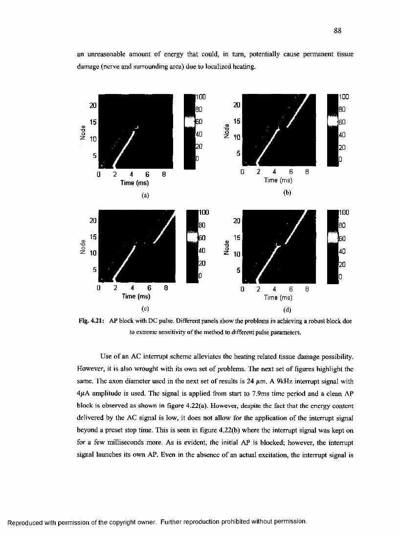
88

an unreasonable amount of energy that could, in turn, potentially cause permanent tissue

damage (nerve and surrounding area) due to localized heating.

a>T 3o

a)-ao

Time (ms)

Time (ms)

a]■ao

Time (ms)

Time (ms)

Fig. 4.21: AP block with DC pulse. Different panels show the problems in achieving a robust block due to extreme sensitivity of the method to different pulse parameters.

Use of an AC interrupt scheme alleviates the heating related tissue damage possibility.

However, it is also wrought with its own set of problems. The next set of figures highlight the

same. The axon diameter used in the next set of results is 24 /xm. A 9kHz interrupt signal with

4/xA amplitude is used. The signal is applied from start to 7.9ms time period and a clean AP

block is observed as shown in figure 4.22(a). However, despite the fact that the energy content

delivered by the AC signal is low, it does not allow for the application of the interrupt signal

beyond a preset stop time. This is seen in figure 4.22(b) where the interrupt signal was kept on

for a few milliseconds more. As is evident, the initial AP is blocked; however, the interrupt

signal launches its own AP. Even in the absence of an actual excitation, the interrupt signal is


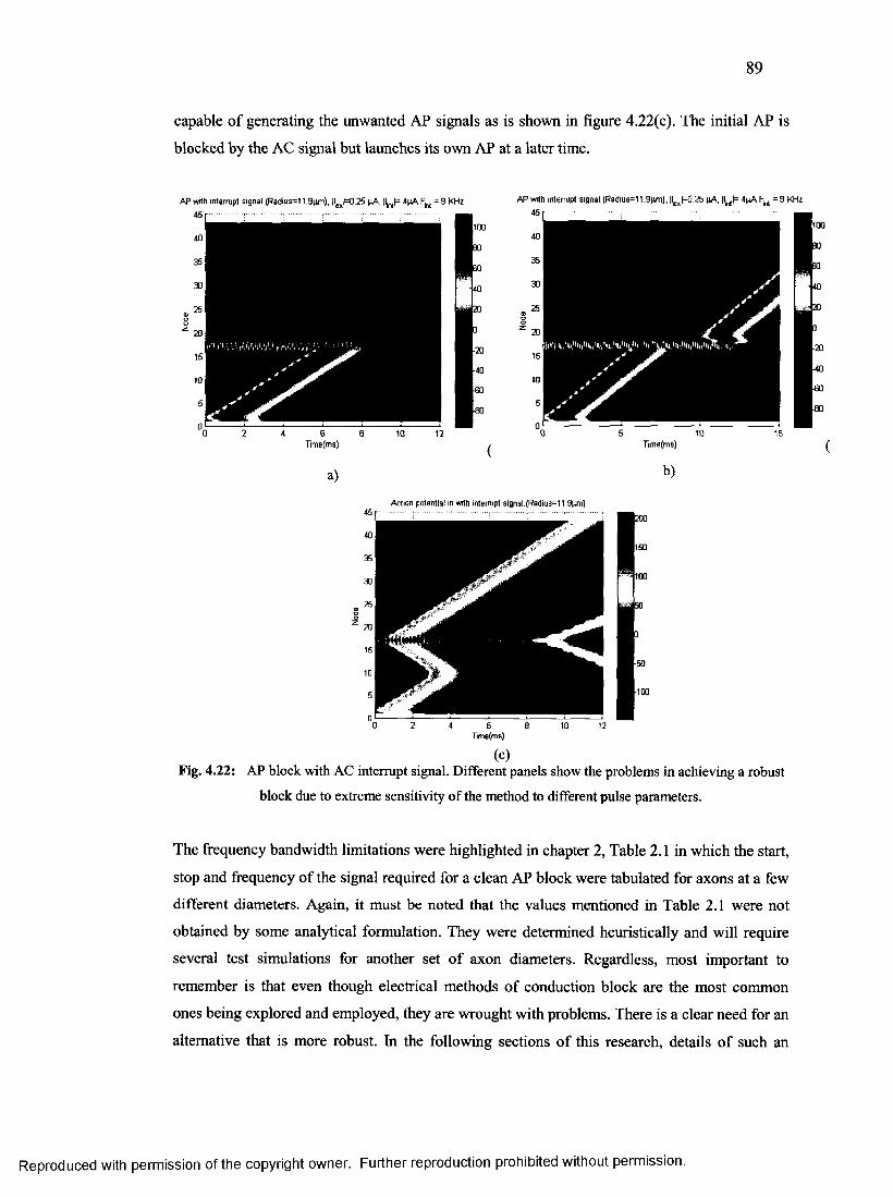
89

capable of generating the unwanted AP signals as is shown in figure 4.22(c). The initial AP is

blocked by the AC signal but launches its own AP at a later time.

AP w ilh in te rru p t s ig n a l .(R a d iu s = 1 1 .9 p m ) , |l„x l= 0 .2 5 p A , |tr t |= 4 p A Fw = 9 K H z A P w ith in te rrup t s ig n a l. (R a d iu s = 1 1 .9 p m ) , |le x l = 0 2 5 p A , |lr t l= 4 p A Fr t = 9 K H z

T im e(m s) T im e (m s)

a) b)

A ction p o ten tia l in w ith in te rrup t s igna l. (R a d iu s= 1 1 ,9pim)

Time(ms)

(c)Fig. 4.22: AP block with AC interrupt signal. Different panels show the problems in achieving a robust

block due to extreme sensitivity of the method to different pulse parameters.

The frequency bandwidth limitations were highlighted in chapter 2, Table 2.1 in which the start,

stop and frequency of the signal required for a clean AP block were tabulated for axons at a few

different diameters. Again, it must be noted that the values mentioned in Table 2.1 were not

obtained by some analytical formulation. They were determined heuristically and will require

several test simulations for another set of axon diameters. Regardless, most important to

remember is that even though electrical methods of conduction block are the most common

ones being explored and employed, they are wrought with problems. There is a clear need for an

alternative that is more robust. In the following sections of this research, details of such an


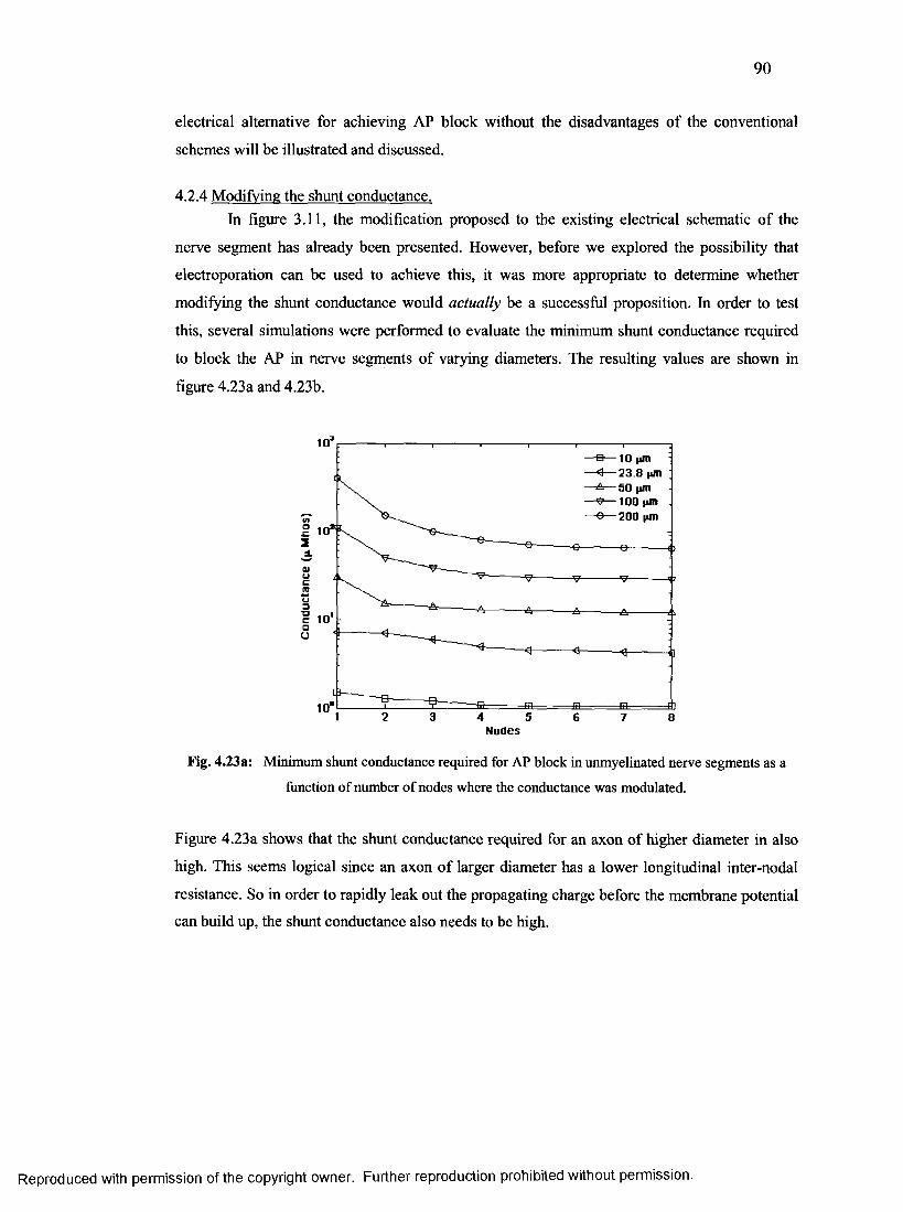
90

electrical alternative for achieving AP block without the disadvantages of the conventional

schemes will be illustrated and discussed.

4.2.4 Modifying the shunt conductance.In figure 3.11, the modification proposed to the existing electrical schematic of the

nerve segment has already been presented. However, before we explored the possibility that

electroporation can be used to achieve this, it was more appropriate to determine whether

modifying the shunt conductance would actually be a successful proposition. In order to test

this, several simulations were performed to evaluate the minimum shunt conductance required

to block the AP in nerve segments of varying diameters. The resulting values are shown in

figure 4.23a and 4.23b.

10'■e— io |im

N odes

Fig. 4.23a: Minimum shunt conductance required for AP block in unmyelinated nerve segments as a

function of number of nodes where the conductance was modulated.

Figure 4.23a shows that the shunt conductance required for an axon of higher diameter in also

high. This seems logical since an axon of larger diameter has a lower longitudinal inter-nodal

resistance. So in order to rapidly leak out the propagating charge before the membrane potential

can build up, the shunt conductance also needs to be high.


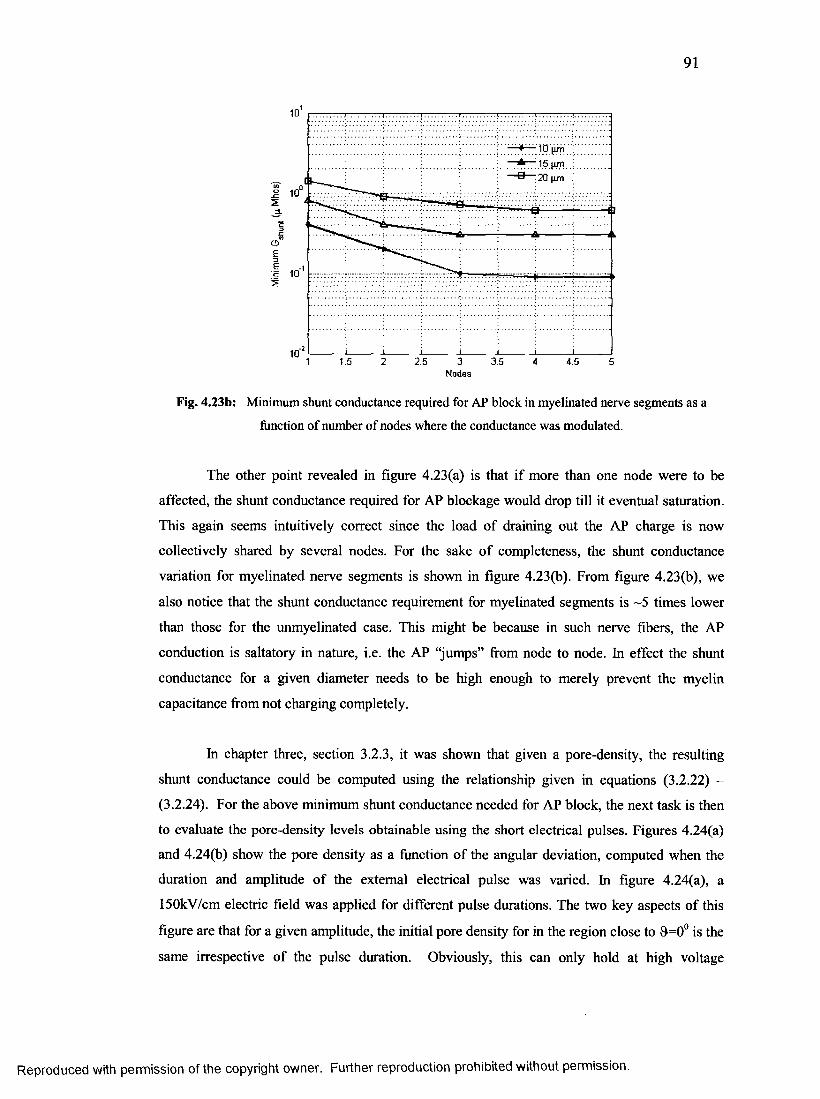
91

Io

2.5 3.5 4.5Nodes

Fig. 4.23b: Minimum shunt conductance required for AP block in myelinated nerve segments as a

function of number of nodes where the conductance was modulated.

The other point revealed in figure 4.23(a) is that if more than one node were to be

affected, the shunt conductance required for AP blockage would drop till it eventual saturation.

This again seems intuitively correct since the load of draining out the AP charge is now

collectively shared by several nodes. For the sake of completeness, the shunt conductance

variation for myelinated nerve segments is shown in figure 4.23(b). From figure 4.23(b), we

also notice that the shunt conductance requirement for myelinated segments is ~5 times lower

than those for the unmyelinated case. This might be because in such nerve fibers, the AP

conduction is saltatory in nature, i.e. the AP “jumps” from node to node. In effect the shunt

conductance for a given diameter needs to be high enough to merely prevent the myelin

capacitance from not charging completely.

In chapter three, section 3.2.3, it was shown that given a pore-density, the resulting

shunt conductance could be computed using the relationship given in equations (3.2.22) -

(3.2.24). For the above minimum shunt conductance needed for AP block, the next task is then

to evaluate the pore-density levels obtainable using the short electrical pulses. Figures 4.24(a)

and 4.24(b) show the pore density as a function of the angular deviation, computed when the

duration and amplitude of the external electrical pulse was varied. In figure 4.24(a), a

150kV/cm electric field was applied for different pulse durations. The two key aspects of this

figure are that for a given amplitude, the initial pore density for in the region close to &=0° is the

same irrespective of the pulse duration. Obviously, this can only hold at high voltage


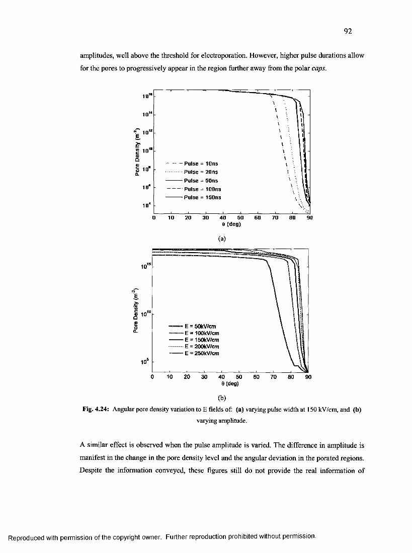
92

amplitudes, well above the threshold for electroporation. However, higher pulse durations allow

for the pores to progressively appear in the region further away from the polar caps.

« 1 0

— P u lse = io n s

P u lse = 2 0 n s

P u lse = 5 0 n s

P u lse = 100ns P u lse = 150ns

10*

200 10 30 4 0 SO 60 70 80 900 ((leg)

(a)

.1510 '

E = 5okV/cm E = 100kV/cm E = 150kV/cm E = 200kV/cm E = 250kV/cm

.510‘

0 10 20 30 40 50 60 70 80 906 (deg)

(b)

Fig. 4.24: Angular pore density variation to E fields of: (a) varying pulse width at 150 kV/cm, and (b)

varying amplitude.

A similar effect is observed when the pulse amplitude is varied. The difference in amplitude is

manifest in the change in the pore density level and the angular deviation in the porated regions.

Despite the information conveyed, these figures still do not provide the real information of


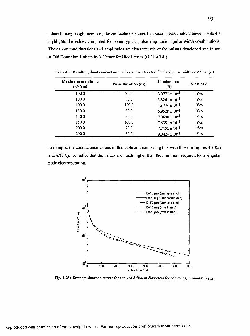
93

interest being sought here, i.e., the conductance values that such pulses could achieve. Table 4.3

highlights the values computed for some typical pulse amplitude - pulse width combinations.

The nanosecond durations and amplitudes are characteristic of the pulsars developed and in use

at Old Dominion University’s Center for Bioelectrics (ODU-CBE).

Table 4.3: Resulting shunt conductance with standard Electric field and pulse width combinations

Maximum amplitude (kV/cm) Pulse duration (ns) Conductance

(S)AP Block?

100.0 20.0 3.0777 x 10-4 Yes100.0 50.0 3.8265 x lO-4 Yes100.0 100.0 4.3744 x lO’4 Yes150.0 20.0 5.9528 x lO*4 Yes150.0 50.0 7.0608 x lO'4 Yes150.0 100.0 7.8385 x lO’4 Yes200.0 20.0 7.7152x10-4 Yes200.0 50.0 9.0424 x lO’4 Yes

Looking at the conductance values in this table and comparing this with those in figures 4.23(a)

and 4.23(b), we notice that the values are much higher than the minimum required for a singular

node electroporation.

10'

D=10 nm (unmyelinated) D=23.8 |i.m (unmyelinated) D=50 jim (unmyelinated) D=10 nm (myelinated)

D=20 jrm (myelinated)

.210

,110 '

,o10 0 100 200 300 400 500 600 700Pulse time (ns)

Fig. 4.25: Strength-duration curves for axon of different diameters for achieving minimum GShunt-


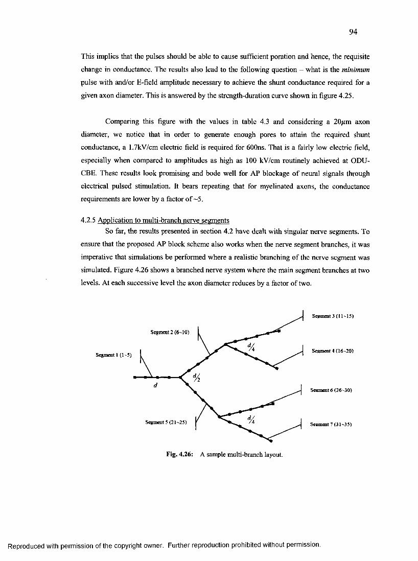
94

This implies that the pulses should be able to cause sufficient poration and hence, the requisite

change in conductance. The results also lead to the following question - what is the minimum

pulse with and/or E-field amplitude necessary to achieve the shunt conductance required for a

given axon diameter. This is answered by the strength-duration curve shown in figure 4.25.

Comparing this figure with the values in table 4.3 and considering a 20/xm axon

diameter, we notice that in order to generate enough pores to attain the required shunt

conductance, a 1,7kV/cm electric field is required for 600ns. That is a fairly low electric field,

especially when compared to amplitudes as high as 100 kV/cm routinely achieved at ODU-

CBE. These results look promising and bode well for AP blockage of neural signals through

electrical pulsed stimulation. It bears repeating that for myelinated axons, the conductance

requirements are lower by a factor of ~5.

4.2.5 Application to multi-branch nerve segmentsSo far, the results presented in section 4.2 have dealt with singular nerve segments. To

ensure that the proposed AP block scheme also works when the nerve segment branches, it was

imperative that simulations be performed where a realistic branching of the nerve segment was

simulated. Figure 4.26 shows a branched nerve system where the main segment branches at two

levels. At each successive level the axon diameter reduces by a factor of two.

S eam en t3 (ll-15 )

Segment 2 (6 '10)

Seament 4 (16-20)Segment 1 (1-5)

Sesment 6 (26-30)

Segment 5 (21-25) Seament 7 (31-35)

Fig. 4.26: A sample multi-branch layout.


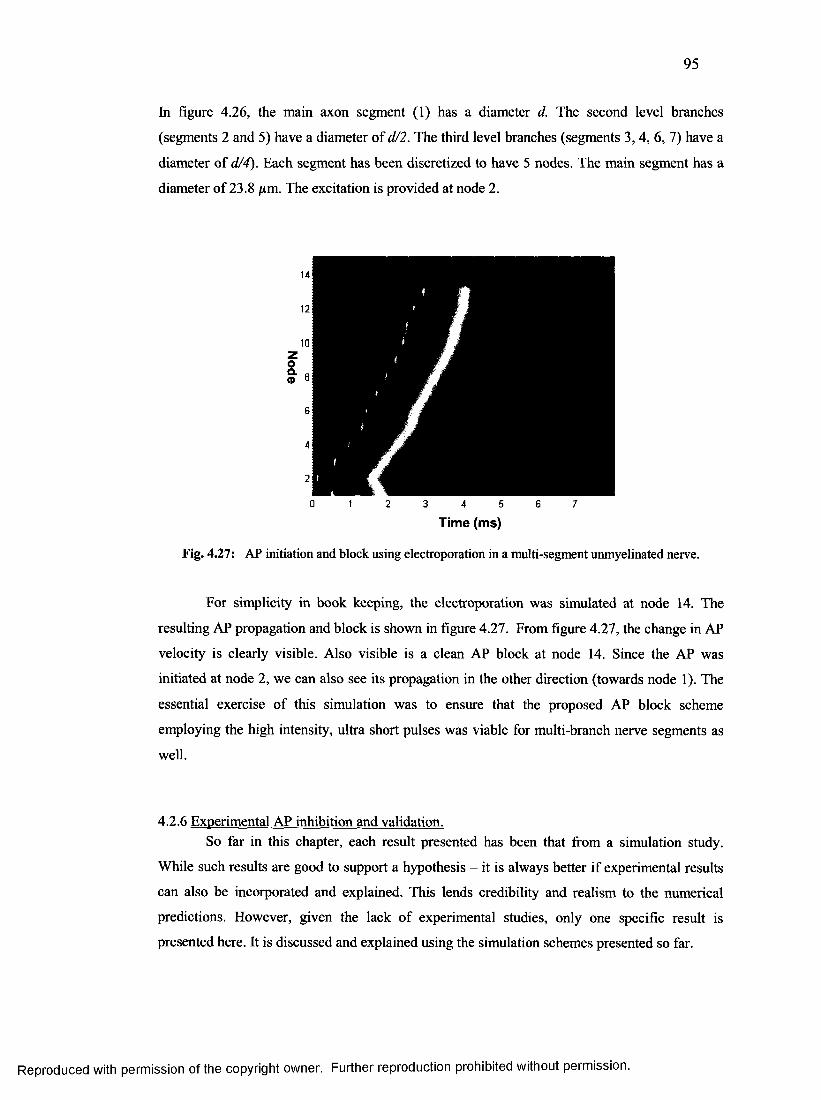
95

In figure 4.26, the main axon segment (1) has a diameter d. The second level branches

(segments 2 and 5) have a diameter of d/2. The third level branches (segments 3,4 , 6, 7) have a

diameter of d/4). Each segment has been discretized to have 5 nodes. The main segment has a

diameter of 23.8 jum. The excitation is provided at node 2.

0 1 2 3 4 5 6 7

Tim e (ms)

Fig. 4.27: AP initiation and block using electroporation in a multi-segment unmyelinated nerve.

For simplicity in book keeping, the electroporation was simulated at node 14. The

resulting AP propagation and block is shown in figure 4.27. From figure 4.27, the change in AP

velocity is clearly visible. Also visible is a clean AP block at node 14. Since the AP was

initiated at node 2, we can also see its propagation in the other direction (towards node 1). The

essential exercise of this simulation was to ensure that the proposed AP block scheme

employing the high intensity, ultra short pulses was viable for multi-branch nerve segments as

well.

4.2.6 Experimental AP inhibition and validation.So far in this chapter, each result presented has been that from a simulation study.

While such results are good to support a hypothesis - it is always better if experimental results

can also be incorporated and explained. This lends credibility and realism to the numerical

predictions. However, given the lack of experimental studies, only one specific result is

presented here. It is discussed and explained using the simulation schemes presented so far.


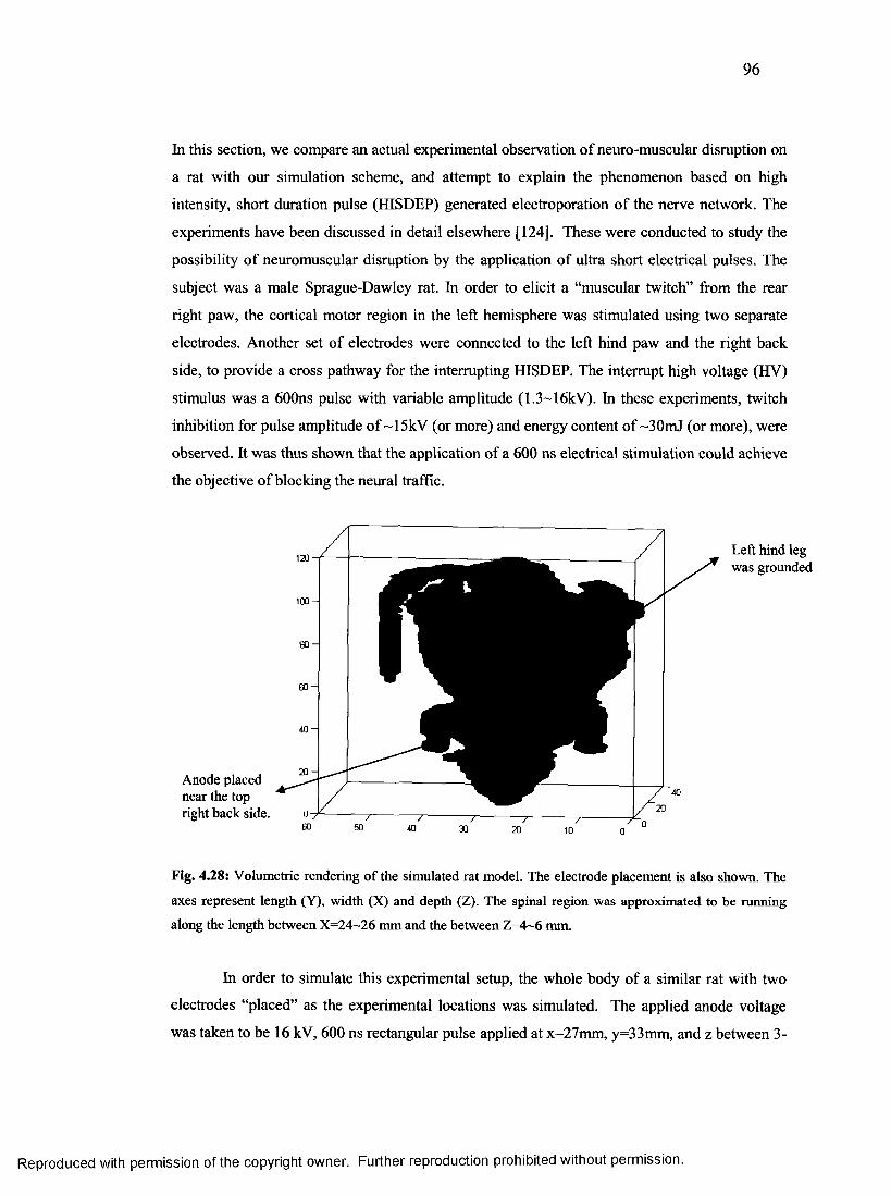
96

In this section, we compare an actual experimental observation of neuro-muscular disruption on

a rat with our simulation scheme, and attempt to explain the phenomenon based on high

intensity, short duration pulse (HISDEP) generated electroporation of the nerve network. The

experiments have been discussed in detail elsewhere [124], These were conducted to study the

possibility of neuromuscular disruption by the application of ultra short electrical pulses. The

subject was a male Sprague-Dawley rat. In order to elicit a “muscular twitch” from the rear

right paw, the cortical motor region in the left hemisphere was stimulated using two separate

electrodes. Another set of electrodes were connected to the left hind paw and the right back

side, to provide a cross pathway for the interrupting HISDEP. The interrupt high voltage (HV)

stimulus was a 600ns pulse with variable amplitude (1.3~16kV). In these experiments, twitch

inhibition for pulse amplitude of ~15kV (or more) and energy content of ~30mJ (or more), were

observed. It was thus shown that the application of a 600 ns electrical stimulation could achieve

the objective of blocking the neural traffic.

Anode placed near the top right back side.

60 50 40 30 20' 10 o ' U

Fig. 4.28: Volumetric rendering of the simulated rat model. The electrode placement is also shown. The

axes represent length (Y), width (X) and depth (Z). The spinal region was approximated to be running

along the length between X=24~26 mm and the between Z=4~6 mm.

In order to simulate this experimental setup, the whole body of a similar rat with two

electrodes “placed” as the experimental locations was simulated. The applied anode voltage

was taken to be 16 kV, 600 ns rectangular pulse applied at x=27mm, y=33mm, and z between 3-

Left hind leg was grounded


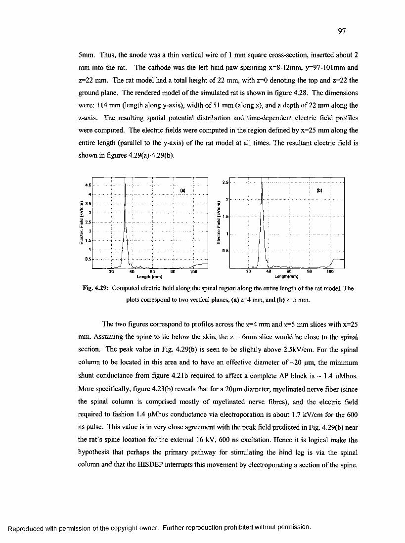
97

5mm. Thus, the anode was a thin vertical wire of 1 mm square cross-section, inserted about 2

mm into the rat. The cathode was the left hind paw spanning x=8-12mm, y=97-101mm and

z=22 mm. The rat model had a total height of 22 mm, with z=0 denoting the top and z=22 the

ground plane. The rendered model of the simulated rat is shown in figure 4.28. The dimensions

were: 114 mm (length along y-axis), width of 51 mm (along x), and a depth of 22 mm along the

z-axis. The resulting spatial potential distribution and time-dependent electric field profiles

were computed. The electric fields were computed in the region defined by x=25 mm along the

entire length (parallel to the y-axis) of the rat model at all times. The resultant electric field is

shown in figures 4.29(a)-4.29(b).

4 5

f 3.5

s 2 5

0 5

20 40 00 80 100Length (m m )

2.5

?o>

■aa)u .u5CJ£LU

0 5

20 40 60 80 100Length(m m )

Fig. 4.29: Computed electric field along the spinal region along the entire length of the rat model. The

plots correspond to two vertical planes, (a) z=4 mm, and (b) z=5 mm.

The two figures correspond to profiles across the z=4 mm and z=5 mm slices with x=25

mm. Assuming the spine to lie below the skin, the z = 6mm slice would be close to the spinal

section. The peak value in Fig. 4.29(b) is seen to be slightly above 2.5kV/cm. For the spinal

column to be located in this area and to have an effective diameter of ~20 pm, the minimum

shunt conductance from figure 4.21b required to affect a complete AP block is ~ 1.4 pMhos.

More specifically, figure 4.23(b) reveals that for a 20pm diameter, myelinated nerve fiber (since

the spinal column is comprised mostly of myelinated nerve fibres), and the electric field

required to fashion 1.4 pMhos conductance via electroporation is about 1.7 kV/cm for the 600

ns pulse. This value is in very close agreement with the peak field predicted in Fig. 4.29(b) near

the rat’s spine location for the external 16 kV, 600 ns excitation. Hence it is logical make the

hypothesis that perhaps the primary pathway for stimulating the hind leg is via the spinal

column and that the HISDEP interrupts this movement by electroporating a section of the spine.


98

This membrane breakdown due to formation of localized nano-pores is temporary, but it

effectively results in a complete leakage of the stimulating energy propagating from the cortex.

It should also be pointed out that in the very likely scenario that more than one “node” or region

of the spine being affected from this breakdown, the required shunt conductance for “twitch

inhibition” would be lower and consequently could be achieved by a shorter HV pulse, or one

of slightly lower amplitude.

4.2.7 More recent observations that may support alternative AP block mechanismsThe present simulations and associated theory supports the above hypothesis of nerve

electroporation. However, given the complexity of the biological system and the plurality of

underlying mechanisms and processes, other explanations of the nerve conduction block arising

from application of Ultra-short High Intensity pulses are possible. In this context, it must be

mentioned that experimental work relating to HISDEP based bio-responses has been on-going

at the Center for Bioelectrics within Old Dominion University (CBE-ODU) using patch-clamp

methods. One of the phenomenon that have been observed in such patch-clamp experiments [A.

G. Pakhomov, Private Communication] is that HISDEP application tends to severely inhibit the

Na+ ion channel uptake across membranes. Since Na+ ion channels are also present in nerve

segments, it is then possible that the observed AP blockage may arise from HISDEP effects on

Na+ ion channels. Since AP launches and their propagation depend on the timed-triggering of

both Na- and K-channels, any process that works to alter or disrupt such channels could be a

pathway for signal blockage. Specifically, since AP generation is intimately connected to Na-

channel activity, any adverse effect or destruction of this ion pathway would impede AP

generation. It should also be mentioned that this recent finding becomes more pertinent in light

of works published earlier by some researchers [125, 126], They have tried to explain the

Sodium gating function (i.e. m) in the original HH model by attempting a more physically

realistic representation. Some qualitative discussion of this aspect is included in possibilities for

future research in the next chapter.


99

Chapter V

Conclusions and Suggestions for Future Work

5.1 IntroductionHaving presented all the aspects of this research work (as enumerated in the first

chapter), this chapter presents a brief summary of this entire dissertation research effort, the

overall implications and salient features, our unique contributions in this field, and finally some

relevant and germane suggestions on how this work can be extended to broaden the present

application and scope. Ideas relating to the proposed modeling schemes, action potential block

methods and their analyses are also presented. Given that this dissertation so far has followed

the structured approach of full body modeling, followed by neural segments and AP block

schemes, the same format will be used for this concluding chapter.

The summarizing conclusions have been broken down, for convenience, into two broad

categories that effectively address the various aspects of this dissertation research. These are:

(a) Full body modeling, and (b) Modeling Action Potential propagation and the conduction

block in nerves. These discussions are followed by scope for future work and extensions to

micro-level systems such as cell clusters and tissues.

5.2 Full body modelingThere were two key reasons why this part of the current research work came to be: (1)

despite the dramatic surge in using simulation techniques - full body analysis is quite primitive

at best; (2) in order to study macro (physiological response) or micro level (activation of neural

pathways), it is necessary to compute the electric potentials in the surrounding tissues. As has

been mentioned, full body imaging and examination methods such as MRI, CAT, etc. have

existed for over two decades. However, these methods are no more than devices to peek into the

living body. While practical application of such devices in order to “capture visual/ imaging”

data is useful, it is more important to be able to perform analysis, perform computations for

meaningful predictions, and draw meaningful conclusions from the raw data. Computations to

perform any viable analysis involve:

a) A robust algorithm

b) Computation resources.


100

Though these two might not seem significant, issues such as physical memory and computation

nodes become severe bottlenecks (as was discussed in chapters 3 and 4) when performing

almost any numerical analyses.

Only with recent advances in computational science and the availability of electronic

hardware, have some researchers started venturing into simulation analysis on small bio

volumes and localized tissues. The other reason for the relative scarcity of schemes for full body

modeling and analysis is that tissue level complexity is extremely hard to capture (incorporate)

in the computational process. Adequate incorporation also requires accurate and microscopic

data mining, e.g., the electrical characteristics of the various tissues and organs that comprise

the whole body. As mentioned earlier, volumetric imaging data does exist. However, that does

not directly translate to usable electrical properties. When the attempt to develop a system to

perform the full body analysis was initiated in this research, it was originally assumed that a

sequential computational system would suffice. Given that the mathematical model for the bio

system in this research involved solution of linear, simultaneous equations that were coupled in

time, some very critical lessons and requirements came to be recognized very rapidly. They

were:

1. Decoupling these equations in time would not be feasible for any intent and purpose.

2. Deployment (applicability) of the simulation scheme would require a very large system

of equations to be solved, associated with the fine spatial resolution of a three-

dimensional volume into microscopic details.

3. The only way to perform such large scale computation was to develop a distributed

approach for the numerical solution.

4. Furthermore, tissue model data has to be combed prior to being fed to the computation

engine to prevent computation phase errors. To put this in perspective, one of the raw

model files that were received consisted of tissue types that were listed to have negative

conductivity.

5. Standard pulse shapes such as trapezoidal, rectangular, etc. were too restrictive. The

ability to incorporate excitation from arbitrarily shaped potential pulses was essential.

6. In order to address real world processes such as ablation, the ability to provide current

stimuli, in addition to external voltage driving responses, had to be provided.

7. Different electrodes (size and shape) present a completely different response, as does

their placement. Consequently, generalization pertaining to electrode placements,

geometry had to be adequately incorporated.


101

8. Real world volumetric datasets can have different discretization lengths in each

dimension in order to eliminate unnecessary resolution in a particular plane. This meant

that the numerical system also needed to be flexible enough to accommodate such

events.

9. Last but not least, there is a need to perform visualization of the computational results

both during and after the entire computations are complete. For example, visualization

of the applied pulse and the responses during a specific time interval may be desired.

This means that the output form of this system would need to allow in-situ visualization

and post-analysis.

The full body modeling scheme that was developed in this research addressed all the above

listed issues. Additionally, the following aspects were also included:

• The results were validated using different bio-model shaped and electrode

geometries.

• The nuances involving visualization of results were also highlighted.

• The system allowed for arbitrarily shaped bio-models (bodies) to be simulated

without loss of edge points by maintaining a systematic Cartesian simulation

volume. The additional overhead of incorporating the air region was definitely

worthwhile in view of the following advantages offered:

i. Applicability to any model shape, and

ii. Avoidance of unnecessary complexity in the algorithm which makes it

faster than the alternative schema.

• This modeling scheme did not make any assumptions about the shape of the

input data set. Hence, just a part of the whole body could also be simulated, if

present as a separate bio-model file.

• Since the resulting output contained the computed potential values for each

discretized point over EVERY time step, post analysis including those listed

below (but not limited to) could be performed:

i. Different orientation potential visualization.

ii. E-Field calculation (over different slices in each orientation).

iii. Current density along a slice or a line

We have published a few salient points of our distributed full body modeling scheme [127] and

its experimental application [128], However, there is definitely room for extending the


102

capabilities of this system, and these will be listed in the last section of this chapter. That said,

it is certainly hoped that this research work will serve to address a void that currently exists in

the simulation community. This work should also find application in: (a) clinical studies, and

(b) development and design of better, non-lethal directed energy devices and several other

applications as listed in chapter 2.

5.3 Modeling Action Potential and Conduction BlockStarting with the original HH model, many researchers have been exploring possible

methods for action potential conduction block. This is of importance given the vast number of

potential applications in therapeutic, physiological and other areas. However, as discussed in the

background review in chapter 2, almost all the methods that have been proposed involve either

some form of relatively long current injection and/or chemical introduction. There are distinct

drawbacks with each method. This research work has attempted to address the existing

deficiencies by contributing to the development and understanding of a novel approach to

electrically-activated conduction blockage. In particular, our proposed method alleviates the

following problems that are intrinsic to other proposed methods:

• Possibility for tissue damage due to excessive energy injection - as could happen with

continuous DC and AC pulse based methods;

• Variability in successful conduction block by AC pulses arising from frequency and

timing issues

The method discussed in this dissertation provides robust conduction blocks through the

application of nano-second pulses. In addition, the refractive period intrinsic to each AP passage

would seem to allow for the application of these interrupt pulses in a discrete manner. This

further enhances the viability of their usage.

A modified lumped parameter cable model was proposed to account for electroporative

effects. Application of high intensity pulses has been explored fairly extensively, especially

with regards to their effects on membranes. Therefore, it seemed only logical to explore the

possibility of modulating the trans-membrane conductance by applying ultra-short electrical

pulses. The main mechanism was shown to be membrane conduction modulation arising from

electroporation. Despite the novel simulation work and concepts developed here, there is

however, room for further improvements and the consideration of other mechanisms. These

possible aspects and mechanisms are briefly discussed here under scope for future work.

Despite the extremely common adoption of the HH model by many researchers, there

has been some progress [125, 126, 129, 130] towards creating more physically plausible models


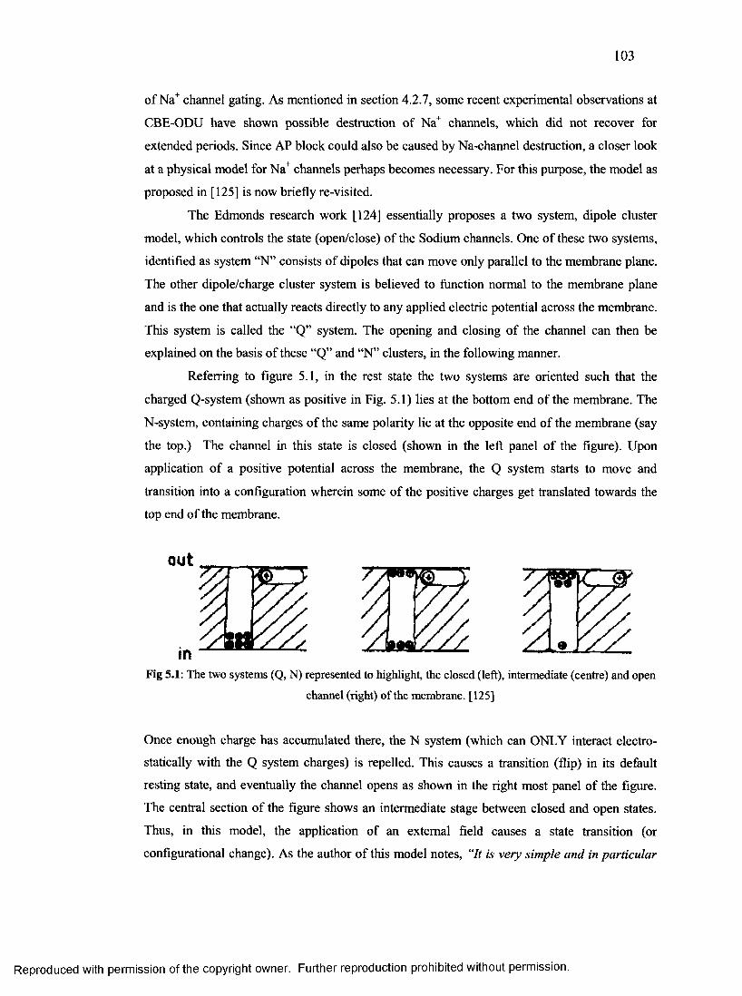
103

of Na+ channel gating. As mentioned in section 4.2.7, some recent experimental observations at

CBE-ODU have shown possible destruction of Na+ channels, which did not recover for

extended periods. Since AP block could also be caused by Na-channel destruction, a closer look

at a physical model for Na+ channels perhaps becomes necessary. For this purpose, the model as

proposed in [125] is now briefly re-visited.

The Edmonds research work [124] essentially proposes a two system, dipole cluster

model, which controls the state (open/close) of the Sodium channels. One of these two systems,

identified as system “N” consists of dipoles that can move only parallel to the membrane plane.

The other dipole/charge cluster system is believed to function normal to the membrane plane

and is the one that actually reacts directly to any applied electric potential across the membrane.

This system is called the “Q” system. The opening and closing of the channel can then be

explained on the basis of these “Q” and “N” clusters, in the following manner.

Referring to figure 5.1, in the rest state the two systems are oriented such that the

charged Q-system (shown as positive in Fig. 5.1) lies at the bottom end of the membrane. The

N-system, containing charges of the same polarity lie at the opposite end of the membrane (say

the top.) The channel in this state is closed (shown in the left panel of the figure). Upon

application of a positive potential across the membrane, the Q system starts to move and

transition into a configuration wherein some of the positive charges get translated towards the

top end of the membrane.

zFig 5.1: The two systems (Q, N) represented to highlight, the closed (left), intermediate (centre) and open

channel (right) of the membrane. [125]

Once enough charge has accumulated there, the N system (which can ONLY interact electro

statically with the Q system charges) is repelled. This causes a transition (flip) in its default

resting state, and eventually the channel opens as shown in the right most panel of the figure.

The central section of the figure shows an intermediate stage between closed and open states.

Thus, in this model, the application of an external field causes a state transition (or

configurational change). As the author of this model notes, “It is very simple and in particular


104

much simpler than the m3 model usually employed. ” Obviously, this mechanism does not

require the initial bottom membrane Q-charge to be positive. Negative charges at both the Q and

N-sites would work equally well. In practice, the existence of molecules such as phosphatidyl-

serine (PS) naturally imparts a net negative charge to the inner membrane.

The reason for highlighting this model was to show the role of electrically driven

conformational changes in driving the transitions in a voltage-gated channel through charge

displacement. However, the above model does not consider the possible role of electroporation.

In principle, though, the use of high-intensity electric fields could not only create pores at sites

close to such protein-based Na+ channels, but also widen the inner diameter of existing protein

structures. The next result would then be the possibility for “mobile charge” outfluxes from

within the inner side of the membrane to the exterior portion. Such “extemalization” through

electro pores, has been demonstrated both experimentally [26] and through theoretical

Molecular Dynamics simulations [27, 85, 94, 131] recently, in response to large externally

applied fields. A similar process of charge migration could occur through the protein channels.

In any event, the process of applying high-voltage pulses then opens up the possibility

to drag charge and alter its relative placement on the overall membrane structure. Thus, the

protein channels located near such charge translocation would be affected and change their

state, as outlined in Fig. 5.1 of the Edmonds model. The more mobile charges (e.g., PS) present

initially at the inner membrane could even diffuse out and strongly populate sites on the outer

membrane. Due to the electrostatic repulsion between charges, such charge translocation would

require energy and take a long time to recover to its original state. During such time, the state of

the protein channels would stay in their altered state. Hence, conceivably, this would be a

physical mechanism of altering the channel “destruction” and preventing it from “normal”

operation following strong voltage-pulsing.

The above mechanism might be an alternative response pathway. It would explain AP

blockage and also the observed deviation from voltage-controlled behavior in patch-clamp

experiments.

5.4 Scope for future work and extensionSo far some summarizing observations about the current research work have been

presented. These essentially highlight the current capabilities and novel features of this research.

However, there is definitely scope for improvement and extension of this overall technique.

Some of these ideas include:


105

• A symmetric version of the algorithm (which is presented in the appendix) has been

implemented on a distributed system. Even though a lot of code optimization has been

performed, there still exists room for more.

• For the purpose of this research, the full body modeling scheme was developed using a

very specific format of volumetric data provided by the Brooks Air Force Base.

However, it could be modified (with minimal overhead) to use other forms of

volumetric data sets such as those from MRI, etc. The caveat is that tissue

characteristics would need to be mapped out based on imagery analysis. That would not

only extend this system to be truly bio-model independent but could also conceivably

allow for studying the possible electro-chemical response of bio-subjects in real time.

• It is also possible to perform the full body modeling using a “segmented approach”

wherein each anatomical section is simulated independently. However, this is not as

trivial as it seems, given that nodes are coupled to each other spatially as well as in

time. Nevertheless, it will definitely extend the simulation capability of this work

several fold for the same given computation resources.

• The distributed computation model for the full body modeling scheme could be made

more interactive by providing a GUI front-end that would allow the end user to

dynamically specify the electrode points, define input pulse shapes, specify other

geometric entities, and output file format. Currently, all this is done at the command

line using several scripts written in MATLAB® and F90.

• In the process of this research work, both the myelinated and unmyelinated nerve

segment systems were validated. It was mentioned earlier that discrete pulses for the

purpose of AP block could be employed. However, a more detailed study needs to be

undertaken to clearly identify the refractory period in different nerve segment

configurations.

• Even though modeling studies have been performed on myelinated nerve segments, the

basic assumption made was that the shunt conductance modulation occurs only at the

Nodes-of-Ranvier - i.e. the unmyelinated segments. Though such an assumption does

not violate or critically compromise the end result, a more realistic system would also

allow for the possibility of myelin sheath electroporation.

• Based on the simulation studies and background studies, it has been shown that

refractory periods for single nerve segments can be as long as ~50 ms. However, it

should be mentioned that this value does vary for branched systems and also for those


106

segments that may have variable diameters. A more detailed study is in order to explore

these aspects.

• Focused application of electroporating pulses at the nerve locations is an assumption

that was made for the sake of partial simplicity. However, in real-world applications, it

may be more prudent to also incorporate modulation/attenuation of the applied pulse

owing to the surrounding tissue where the nerve is embedded.

• Electroporation of a nerve membrane was shown to be a plausible basis for AP

blockage. However, there could be other explanations and intrinsic processes that could

conceivably be responsible for the AP block. For example, sodium channels embedded

within nerve membranes could be destroyed or inactivated by a sudden electrical jolt

arising from the application of a high-intensity, nanosecond pulse. Preliminary

experimental data obtained at CBE-ODU is indicative of such sodium-channel effects.

Since AP launch and propagation is intimately linked to sodium-channel activity, it is

quite likely that any detrimental effect of voltages on such channels would lead to AP

blockage. Such phenomena merit detailed study, and should be modeled to evaluate

alternative pathways and mechanisms. It is very likely that multiple processes are at

work, each dominant and operative over different regimes. In the interest of

quantification and for clarifying the relative role of such competing mechanisms, a

more detailed study of the voltage-induced, channel related bio-electric phenomena is

warranted in the near future.

One of the more latent objectives of this research work was to provide a “suite” of

models that would address the entire spectrum of tissue systems. The full body modeling system

was designed to provide a “macro” level analyses capability of the tissue response. The nerve

segments and branches were studied because they are the primary pathways of consequent

physiological changes. While the focus was on voltage-induced nerve membrane phenomena,

the numerical simulation methods developed could easily be extended for the analysis of micro

level tissue systems and cell clusters. For instance, membrane poration and the time dependent

voltage changes in cell clusters placed within a suspension medium, due to pulses of varying

strengths could be examined. A brief description of an application of the current modeling

scheme to probe the response of cell clusters is therefore presented for completeness. It is a

topical extension of the same general theme.


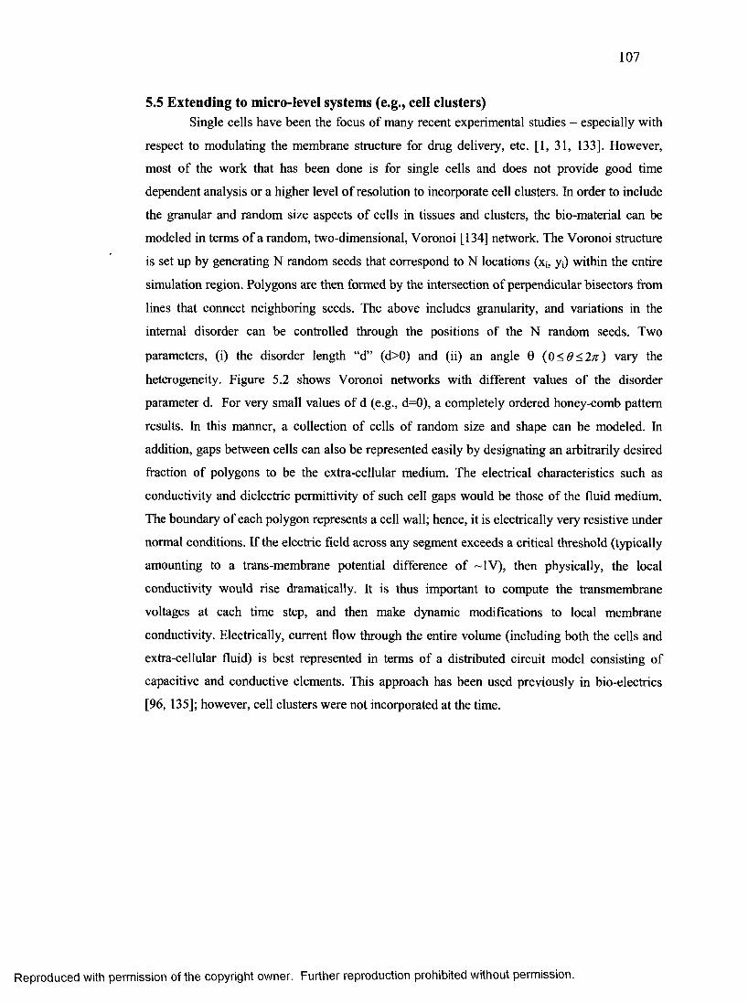
107

5.5 Extending to micro-level systems (e.g., cell clusters)Single cells have been the focus of many recent experimental studies - especially with

respect to modulating the membrane structure for drug delivery, etc. [1, 31, 133]. However,

most of the work that has been done is for single cells and does not provide good time

dependent analysis or a higher level of resolution to incorporate cell clusters. In order to include

the granular and random size aspects of cells in tissues and clusters, the bio-material can be

modeled in terms of a random, two-dimensional, Voronoi [134] network. The Voronoi structure

is set up by generating N random seeds that correspond to N locations (xj; y() within the entire

simulation region. Polygons are then formed by the intersection of perpendicular bisectors from

lines that connect neighboring seeds. The above includes granularity, and variations in the

internal disorder can be controlled through the positions of the N random seeds. Two

parameters, (i) the disorder length “d” (d>0) and (ii) an angle 0 (0< d<2/r) vary the

heterogeneity. Figure 5.2 shows Voronoi networks with different values of the disorder

parameter d. For very small values of d (e.g., d=0), a completely ordered honey-comb pattern

results. In this manner, a collection of cells of random size and shape can be modeled. In

addition, gaps between cells can also be represented easily by designating an arbitrarily desired

fraction of polygons to be the extra-cellular medium. The electrical characteristics such as

conductivity and dielectric permittivity of such cell gaps would be those of the fluid medium.

The boundary of each polygon represents a cell wall; hence, it is electrically very resistive under

normal conditions. If the electric field across any segment exceeds a critical threshold (typically

amounting to a trans-membrane potential difference of ~1V), then physically, the local

conductivity would rise dramatically. It is thus important to compute the transmembrane

voltages at each time step, and then make dynamic modifications to local membrane

conductivity. Electrically, current flow through the entire volume (including both the cells and

extra-cellular fluid) is best represented in terms of a distributed circuit model consisting of

capacitive and conductive elements. This approach has been used previously in bio-electrics

[96, 135]; however, cell clusters were not incorporated at the time.


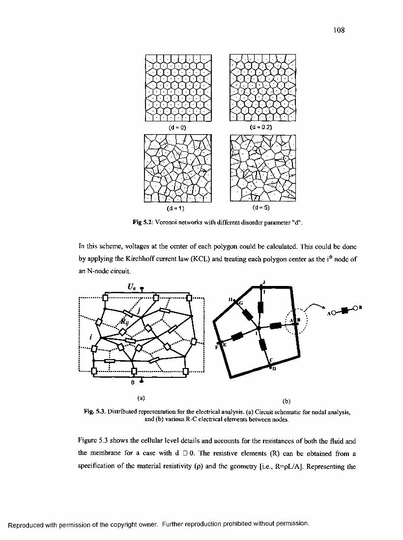
108

(d = 0) (d = 0.2)

(d = 1) (d = 5)

Fig 5.2: Voronoi networks with different disorder parameter "d".

In this scheme, voltages at the center of each polygon could be calculated. This could be done

by applying the Kirchhoff current law (KCL) and treating each polygon center as the ith node of

an N-node circuit.j

(a) (b)Fig. 5.3. Distributed representation for the electrical analysis, (a) Circuit schematic for nodal analysis,

and (b) various R-C electrical elements between nodes.

Figure 5.3 shows the cellular level details and accounts for the resistances of both the fluid and

the membrane for a case with d □ 0. The resistive elements (R) can be obtained from a

specification of the material resistivity (p) and the geometry [i.e., R=pL/A], Representing the


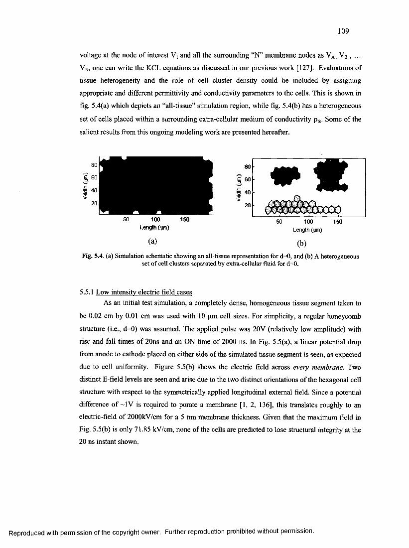
109

voltage at the node of interest Vi and all the surrounding “N” membrane nodes as VA, VB ,

VN, one can write the KCL equations as discussed in our previous work [127], Evaluations of

tissue heterogeneity and the role of cell cluster density could be included by assigning

appropriate and different permittivity and conductivity parameters to the cells. This is shown in

fig. 5.4(a) which depicts an “all-tissue” simulation region, while fig. 5.4(b) has a heterogeneous

set of cells placed within a surrounding extra-cellular medium of conductivity pfe. Some of the

salient results from this ongoing modeling work are presented hereafter.

100 Length (tim)

(a)

20 -

W f t

100 Length (pm)

150

(b)Fig. 5.4. (a) Simulation schematic showing an all-tissue representation for d=0, and (b) A heterogeneous

set of cell clusters separated by extra-cellular fluid for d=0.

5.5.1 Low intensity electric field casesAs an initial test simulation, a completely dense, homogeneous tissue segment taken to

be 0.02 cm by 0.01 cm was used with 10 pm cell sizes. For simplicity, a regular honeycomb

structure (i.e., d=0) was assumed. The applied pulse was 20V (relatively low amplitude) with

rise and fall times of 20ns and an ON time of 2000 ns. In Fig. 5.5(a), a linear potential drop

from anode to cathode placed on either side of the simulated tissue segment is seen, as expected

due to cell uniformity. Figure 5.5(b) shows the electric field across every membrane. Two

distinct E-field levels are seen and arise due to the two distinct orientations of the hexagonal cell

structure with respect to the symmetrically applied longitudinal external field. Since a potential

difference of ~1V is required to porate a membrane [1, 2, 136], this translates roughly to an

electric-field of 2000kV/cm for a 5 nm membrane thickness. Given that the maximum field in

Fig. 5.5(b) is only 71.85 kV/cm, none of the cells are predicted to lose structural integrity at the

20 ns instant shown.


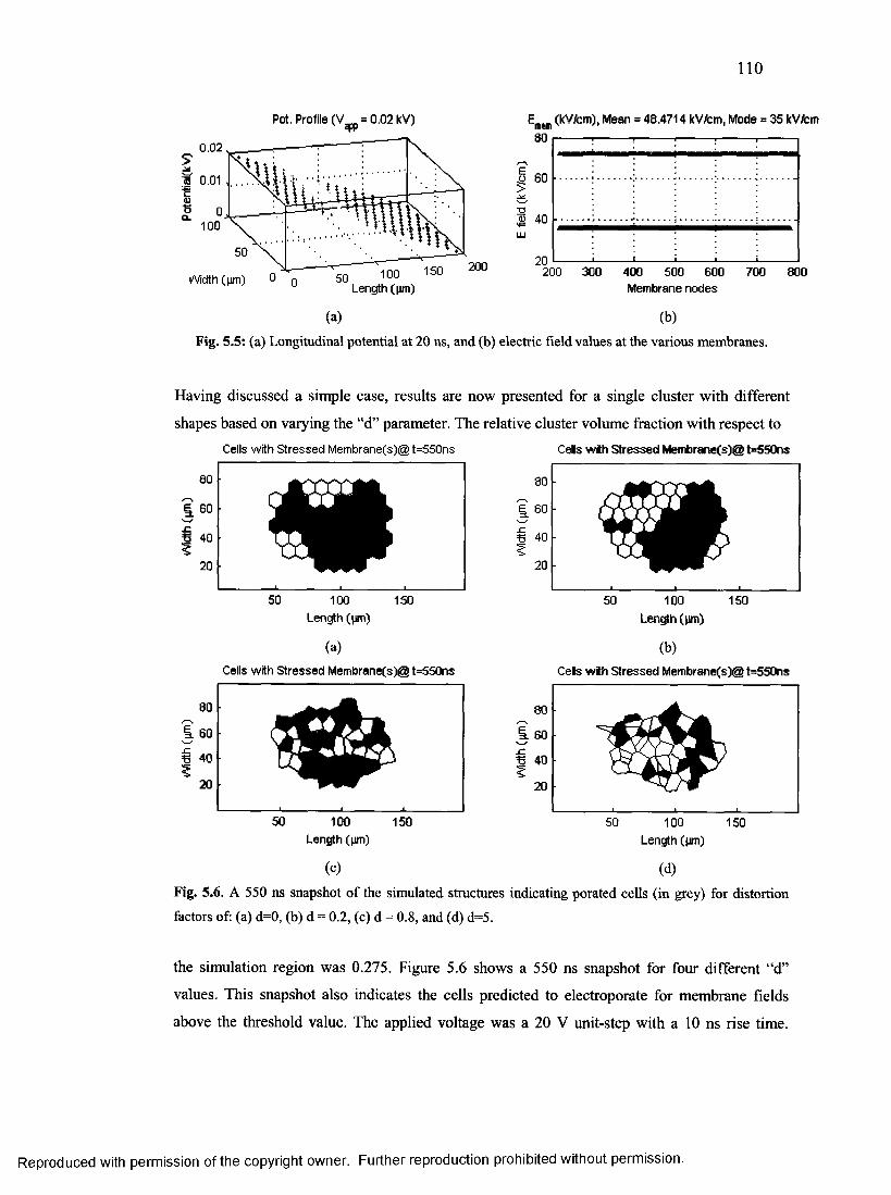
110

Pot. Profile (V =0.02 kV)

0.02

ra 0.01

100

200100 150 Length (pm)

Wdth (pm)

E ™ (kV/cm), Mean = 48.4714 kV/cm, Mode = 35 kV/cm memx f% 180

I 60 > w5M 40

20200 300 400 500 600 700 800

Membrane nodes

(a) (b)Fig. 5.5: (a) Longitudinal potential at 20 ns, and (b) electric field values at the various membranes.

Having discussed a simple case, results are now presented for a single cluster with different

shapes based on varying the “d” parameter. The relative cluster volume fraction with respect to

60

=6 40

Cells with S tressed Membrane(s)@ t=550ns

100 150Length (pm)

(a)Cells with S tressed Membrane(s)@ t=550ns

=6 40

100 Length (pm)

(c)

Cells with S tressed Membrane(s)@ t=550ns

100 Length (pm)

(b)Cells with S tressed Membrane(s)@ t=550ns

=6 40

100 Length (pm)

(d)

150

Fig. 5.6. A 550 ns snapshot of the simulated structures indicating porated cells (in grey) for distortion

factors of: (a) d=0, (b) d = 0.2, (c) d = 0.8, and (d) d=5.

the simulation region was 0.275. Figure 5.6 shows a 550 ns snapshot for four different “d”

values. This snapshot also indicates the cells predicted to electroporate for membrane fields

above the threshold value. The applied voltage was a 20 V unit-step with a 10 ns rise time.


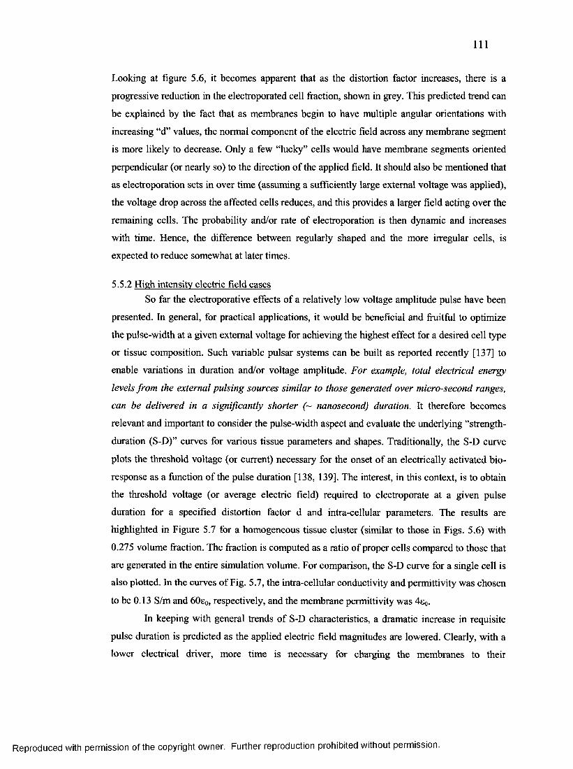
I l l

Looking at figure 5.6, it becomes apparent that as the distortion factor increases, there is a

progressive reduction in the electroporated cell fraction, shown in grey. This predicted trend can

be explained by the fact that as membranes begin to have multiple angular orientations with

increasing “d” values, the normal component of the electric field across any membrane segment

is more likely to decrease. Only a few “lucky” cells would have membrane segments oriented

perpendicular (or nearly so) to the direction of the applied field. It should also be mentioned that

as electroporation sets in over time (assuming a sufficiently large external voltage was applied),

the voltage drop across the affected cells reduces, and this provides a larger field acting over the

remaining cells. The probability and/or rate of electroporation is then dynamic and increases

with time. Hence, the difference between regularly shaped and the more irregular cells, is

expected to reduce somewhat at later times.

5.5.2 High intensity electric field casesSo far the electroporative effects of a relatively low voltage amplitude pulse have been

presented. In general, for practical applications, it would be beneficial and fruitful to optimize

the pulse-width at a given external voltage for achieving the highest effect for a desired cell type

or tissue composition. Such variable pulsar systems can be built as reported recently [137] to

enable variations in duration and/or voltage amplitude. For example, total electrical energy

levels from the external pulsing sources similar to those generated over micro-second ranges,

can be delivered in a significantly shorter (~ nanosecond) duration. It therefore becomes

relevant and important to consider the pulse-width aspect and evaluate the underlying “strength-

duration (S-D)” curves for various tissue parameters and shapes. Traditionally, the S-D curve

plots the threshold voltage (or current) necessary for the onset of an electrically activated bio

response as a function of the pulse duration [138, 139]. The interest, in this context, is to obtain

the threshold voltage (or average electric field) required to electroporate at a given pulse

duration for a specified distortion factor d and intra-cellular parameters. The results are

highlighted in Figure 5.7 for a homogeneous tissue cluster (similar to those in Figs. 5.6) with

0.275 volume fraction. The fraction is computed as a ratio of proper cells compared to those that

are generated in the entire simulation volume. For comparison, the S-D curve for a single cell is

also plotted. In the curves of Fig. 5.7, the intra-cellular conductivity and permittivity was chosen

to be 0.13 S/m and 60e0, respectively, and the membrane permittivity was 4e0.

In keeping with general trends of S-D characteristics, a dramatic increase in requisite

pulse duration is predicted as the applied electric field magnitudes are lowered. Clearly, with a

lower electrical driver, more time is necessary for charging the membranes to their


112

electroporative threshold. Furthermore, with increasing random orientations of the membrane

segments with respect to a given axis (i.e., the applied field direction; for instance), there is a

lower probability of reaching the threshold for the collective population. Hence, the threshold

field increases with cell irregularity (i.e. the d parameter).

-*----d=0H d=0.2A — d=0.8

45

Single Cell ‘

£ 30

Time (ns)

Fig. 5.6. S-D curves for cell clusters with various distortion parameters and that for a single spherical

cell.

5.5.2 Summarizing the cell clusterIt should be mentioned that an extremely brief presentation of the details pertaining to the

micro-level simulations, in particular, for cell clusters has been presented here. Nevertheless,

the results do demonstrate the following aspects.

• First, clusters typically would need larger voltage amplitudes than a single cell,

especially for the ultra-short nanosecond regime.

• For a given extra-cellular conductivity parameter, the disparity between single cell and

clusters is predicted to increase as the intracellular conductivity reduces.

• A strong selectivity for membrane poration is indicated within heterogeneous tissues.

Hence, it should be possible to set the voltage amplitude for chosen pulse duration for

preferentially porating only the higher internal conductivity clusters, without any

damage to the remaining tissue.

• This selectivity would be stronger within tissues having more irregularly shaped cells.

Section 5.5 and its sub-sections were meant to provide a preview of how the proposed modeling

schema of this research contribution could be extended to micro-level systems. It should also be


113

pointed out that given the similarity of the underlying mathematics involved, these models can

be trivially extended to utilize distributed computation resources, thus extending the population

and diversity of these cell clusters.


114

References

[1] K. H. Schoenbach, R. P. Joshi, J. F. Kolb, N. Chen, M. Stacey, P. F. Blackmore, E. S. Buescher, and S. J. Beebe, "Ultrashort electrical pulses open a new gateway into biological cells," Proceedings o f the IEEE, vol. 92, pp. 1122-1137, 2004.

[2] U. Pliquett, R. Elez, A. Piiper, and E. Neumann, "Electroporation of subcutaneous mouse tumors by rectangular and trapezium high voltage pulses," Bioelectrochemistry, vol. 62, pp. 83-93, Apr 2004.

[3] M. P. Rogers, J. H. Merritt, J. C. Comeaux, C. T. JKuhnel Jr., D. F. Moreland, D. G. Teltschik, J. H. Lucas, and M. R. Murphy, "Strength-duration curve for an electrically excitable tissue extended down to near 1 nanosecond," IEEE Trans Plasma Sci., vol. 32, p p .1587-1599, 2003.

[4] F. Rattay, "Analysis of models for external stimulation of axons," IEEE Trans Biomed Eng, vol. 33, pp. 974-7, Oct 1986.

[5] F. Rattay, Electrical Nerve Stimulation: Theory, Experiments and Applications. New York: Springer-Verlag, 1990.

[6] B. Frankenhaeuser and A. F. Huxley, "The Action Potential in the Myelinated Nerve Fiber of Xenopus Laevis as Computed on the Basis of Voltage Clamp Data," J Physiol, vol. 171, pp. 302-15, Jun 1964.

[7] C. Tai, W. C. de Groat, and J. R. Roppolo, "Simulation of nerve block by high- frequency sinusoidal electrical current based on the Hodgkin-Huxley model," IEEE Trans Neural Syst Rehabil Eng, vol. 13, pp. 415-22, Sep 2005.

[8] C. Tai, W. C. de Groat, and J. R. Roppolo, "Simulation analysis of conduction block in unmyelinated axons induced by high-frequency biphasic electrical currents," IEEE Trans Biomed Eng, vol. 52, pp. 1323-32, Jul 2005.

[9] R. Stampfli, "Reversible electrical breakdown of the excitable membrane of a Ranvier node.," An. Acad. Brasil. Ciens., vol. 30, pp. 57-63, 1958.

[10] P. H. Veltink, J. A. van Alste, and H. B. Boom, "Simulation of intrafascicular and extraneural nerve stimulation," IEEE Trans Biomed Eng, vol. 35, pp. 69-75, Jan 1988.

[11] N. Bhadra, E. A. Lahowetz, S. T. Foldes, and K. L. Kilgore, "Simulation of high- frequency sinusoidal electrical block of mammalian myelinated axons," J Comput Neurosci, Jan 3 2007.

[12] N. Bhadra and K. L. Kilgore, "Direct current electrical conduction block of peripheral nerve," IEEE Trans Neural Syst Rehabil Eng, vol. 12, pp. 313-24, Sep 2004.

[13] M. Manfredi, "Differential block of conduction of larger fibers in peripheral nerve by direct current," Arch Ital Biol, vol. 108, pp. 52-71, Jan 1970.

[14] A. G. Brown and W. C. Hamann, "DC-polarization and impulse conduction failure in mammalian nerve fibres," J Physiol, vol. 222, pp. 66P-67P, Apr 1972.

[15] A. S. Paintal, "Block of conduction in mammalian myelinated nerve fibres by low temperatures," J Physiol, vol. 180, pp. 1-19, Sep 1965.

[16] S. Schumacher, S. Bross, J. R. Scheepe, C. Seif, K. P. Junemann, and P. Aiken, "Extradural cold block for selective neurostimulation of the bladder: development of a new technique," J Urol, vol. 161, pp. 950-4, Mar 1999.

[17] I. A. Chang and U. D. Nguyen, "Thermal modeling of lesion growth with radiofrequency ablation devices," Biomed Eng Online, vol. 3, p. 27, Aug 6 2004.

[18] W. M. Wells and A. C. F. Colchester, Medical image computing and computer-assisted intervention—MICCAI '98 : first international conference, Cambridge, MA, USA, October 11-13, 1998 proceedings. Berlin; New York: Springer, 1998.


115

[19] L. Sontag and D. E. Axelrod, "Evaluation of pathways for progression of heterogeneous breast tumors," Journal o f Theoretical Biology, vol. 232, pp. 179-189, 2005.

[20] E. Neumann and K. Rosenheck, "Permeability changes induced by electric impulses in vesicular membranes," JM embr Biol, vol. 10, pp. 279-90, Dec 29 1972.

[21] E. Neumann and J. Bernhardt, "Physical chemistry of excitable biomembranes," Annu Rev Biochem, vol. 46, pp. 117-41, 1977.

[22] I. P. Sugar, W. Forster, and E. Neumann, "Model of cell electrofusion. Membrane electroporation, pore coalescence and percolation," Biophys Chem, vol. 26, pp. 321-35, May 9 1987.

[23] E. Neumann, S. Kakorin, and K. Toensing, "Membrane electroporation and electromechanical deformation of vesicles and cells," Faraday Discuss, pp. 111-25; discussion 137-57, 1998.

[24] K. H. Schoenbach, S. J. Beebe, and E. S. Buescher, "Intracellular effect of ultrashort electrical pulses," Bioelectromagnetics, vol. 22, pp. 440-8, Sep 2001.

[25] S. J. Beebe, P. F. Blackmore, J. White, R. P. Joshi, and K. H. Schoenbach, "Nanosecond pulsed electric fields modulate cell function through intracellular signal transduction mechanisms," Physiol Meas, vol. 25, pp. 1077-93, Aug 2004.

[26] P. T. Vernier, Y. Sun, L. Marcu, S. Salemi, C. M. Craft, and M. A. Gundersen,"Calcium bursts induced by nanosecond electric pulses," Biochem Biophys ResCommun, vol. 310, pp. 286-95, Oct 17 2003.

[27] R. P. Joshi, Q. Hu, R. Aly, K. H. Schoenbach, and H. P. Hjalmarson, "Self-consistent simulations of electroporation dynamics in biological cells subjected to ultrashortelectrical pulses," Phys Rev E Stat Nonlin Soft Matter Phys, vol. 64, p. 011913, Jul2001.

[28] T. Y. Tsong, "Electroporation of cell membranes," Biophys J, vol. 60, pp. 297-306, Aug 1991.

[29] M. Pavlin, T. Slivnik, and D. Miklavcic, "Effective conductivity of cell suspensions," IEEE Trans Biomed Eng, vol. 49, pp. 77-80, Jan 2002.

[30] M. Pavlin, N. Pavselj, and D. Miklavcic, "Dependence of induced transmembrane potential on cell density, arrangement, and cell position inside a cell system," IEEE Trans Biomed Eng, vol. 49, pp. 605-12, Jun 2002.

[31] M. Pavlin, V. Leben, and D. Miklavcic, "Electroporation in dense cell suspension-theoretical and experimental analysis of ion diffusion and cell permeabilization,"Biochim Biophys Acta, vol. 1770, pp. 12-23, Jan 2007.

[32] P. J. Basser and B. J. Roth, "New currents in electrical stimulation of excitable tissues," Annu Rev Biomed Eng, vol. 2, pp. 377-97, 2000.

[33] J. P. Reilly, Electrical Stimulation and Electropathology. Cambridge: Cambridge Press, UK, 1992.

[34] B. J. Roth, "Mechanisms for electrical stimulation of excitable tissue," Crit Rev Biomed Eng, vol. 22, pp. 253-305, 1994.

[35] P. S. Eriksson, E. Perfilieva, T. Bjork-Eriksson, A. M. Albom, C. Nordborg, D. A. Peterson, and F. H. Gage, "Neurogenesis in the adult human hippocampus," Nat Med, vol. 4, pp. 1313-7, Nov 1998.

[36] E. Gould, A. J. Reeves, M. S. Graziano, and C. G. Gross, "Neurogenesis in the neocortex of adult primates," Science, vol. 286, pp. 548-52, Oct 15 1999.

[37] D. M. Durand, "Electrical Stimulation of Excitable Tissue," in Biomedical Engineering Handbook, J. D. Bronzino, Ed. Boca Raton: CRC Press, 1995.

[38] K. P. Esselle and M. A. Stuchly, "Neural stimulation with magnetic fields: analysis of induced electric fields," IEEE Trans Biomed Eng, vol. 39, pp. 693-700, Jul 1992.

[39] L. Heller and D. B. van Hulsteyn, "Brain stimulation using electromagnetic sources: theoretical aspects," Biophys J, vol. 63, pp. 129-38, Jul 1992.


116

[40] P. J. Basser and B. J. Roth, "Stimulation of a myelinated nerve axon by electromagnetic induction," Med Biol Eng Comput, vol. 29, pp. 261-8, May 1991.

[41] J. H. Meier, W. L. Rutten, A. E. Zoutman, H. B. Boom, and P. Bergveld, "Simulation of multipolar fiber selective neural stimulation using intrafascicular electrodes," IEEE Trans Biomed Eng, vol. 39, pp. 122-34, Feb 1992.

[42] B. L. Cobb, J. R. Jauchem, P. A. Mason, M. P. Dooley, S. A. Miller, J. M. Ziriax, and M. R. Murphy, "Neural and behavioral teratological evaluation of rats exposed to ultra- wideband electromagnetic fields," Bioelectromagnetics, vol. 21, pp. 524-37, Oct 2000.

[43] J. R. Jauchem, M. R. Frei, K. L. Ryan, J. H. Merritt, and M. R. Murphy, "Lack of effects on heart rate and blood pressure in ketamine-anesthetized rats briefly exposed to ultra-wideband electromagnetic pulses," IEEE Trans Biomed Eng, vol. 46, pp. 117-20, Jan 1999.

[44] Vijayalaxmi, R. L. Seaman, M. L. Belt, J. M. Doyle, S. P. Mathur, and T. J. Prihoda, "Frequency of micronuclei in the blood and bone marrow cells of mice exposed to ultra- wideband electromagnetic radiation," IntJRadiat Biol, vol. 75, pp. 115-20, Jan 1999.

[45] S. A. Miller, M. E. Bronson, and M. R. Murphy, "Ultrawideband radiation and pentylenetetrazol-induced convulsions in rats," Bioelectromagnetics, vol. 20, pp. 327-9,1999.

[46] R. P. Joshi, F. Chen, and W. R. Rogers, "Modeling Electrode-Based Stimulation of Muscle and Nerve by Ultra-Short Electric Pulses," IEEE Trans Plasma Sci., vol. 32, pp. 1687-1695, 2004.

[47] R. P. Joshi, Q. Hu, and K. Schoenbach, "Modeling Studies of Cell Response to Ultrashort, High-Intensity Electric Fields - Implications for Intracellular Manipulation," IEEE Trans Plasma Sci., vol. 32, pp. 1677-1686, 2004.

[48] K. H. Schoenbach, F. E. Peterkin, R. W. Alden, III, and S. J. Beebe, " The effect of pulsed electric fields on biological cells:experiments and applications," IEEE Trans. Plasma Sci., vol. 25, pp. 284-292, 1997.

[49] E. Murray, "OKC police release video in Taser death case," in The Wichita Eagle, 2007.[50] D. B. Dunson, C. Holloman, C. Calder, and L. H. Gunn, "Bayesian modeling of

multiple lesion onset and growth from interval-censored data," Biometrics, vol. 60, pp. 676-83, Sep 2004.

[51] S. Pissanetzky, Sparse Matrix Technology. Orlando, FL: Academic Press Inc., 1984.[52] A. George, J. W. H. Liu, and E. Ng, "Communication results for parallel sparse

Cholesky factorization on a hypercube," Parallel Computing, vol. 10, pp. 287-298, 1989.

[53] T. Imamura, "An estimation of complexity and computational costs for vertical block- cyclic distributed parallel LU factorization," The Journal o f Supercomputing, vol. 15, pp. 95-110, 2000.

[54] D. Kaya and K. Wright, "Parallel algorithms for LU decomposition on a shared memory multiprocessor," Applied Mathematics and Computation, vol. 163, pp. 179-192, 2005.

[55] J. M. Conroy, S. G. Kratzer, R. F. Lucas, and A. E. Aaron, "Parallel sparse LU factorization," SIAM Journal on Scientific Computing, vol. 19, pp. 584-604, 1998.

[56] K. Shen, T. Yang, and X. Jiao, "Efficient 2D sparse LU factorization on parallel machines," SIAM Journal on Matrix Analysis and Applications, vol. 22, pp. 282-305, 2001 .

[57] M. Hahad, "A parallel sparse LU Decomposition with Application to Semiconductor Device Simulation," Lecture Notes in Ccomputer Science, vol. 1300, pp. 848-872, 1997.

[58] P. Chen, H. Runesha, D. T. Nguyen, P. Tong, and T. Y. P. Chang, "Sparse algorithms for indefinite system of linear equations," Computational Mechanics, vol. 25, pp. 33-42,2000.


117

[59] D. R. McNeal, "Analysis of a model for excitation of myelinated nerve," IEEE Trans Biomed Eng, vol. 23, pp. 329-37, Jul 1976.

[60] N. A. Carlson, Foundations o f Physiological Psychology. Needham Heights, MA.: Simon & Schuster, 1992.

[61] R. Fitzhugh, "Computation of impulse initiation and saltatory conduction in a myelinated nerve fiber," Biophys J, vol. 2, pp. 11-21, Jan 1962.

[62] A. L. Hodgkin and A. F. Huxley, "A quantitative description of membrane current and its application to conduction and excitation in nerve," J Physiol, vol. 117, pp. 500-544, Aug 1952.

[63] A. L. Hodgkin and A. F. Huxley, "A quantitative description of membrane current and its application to conduction and excitation in nerve," J Physiol, vol. 117, pp. 500-44, Aug 1952.

[64] J. P. Reilly, V. T. Freeman, and W. D. Larkin, "Sensory effects of transient electrical stimulation—evaluation with a neuroelectric model," IEEE Trans Biomed Eng, vol. 32, pp. 1001-11, Dec 1985.

[65] F. Rattay, "High frequency electrostimulation of excitable cells," J Theor Biol, vol. 123, pp. 45-54, Nov 7 1986.

[66] K. W. Altman and R. Plonsey, "Point source nerve bundle stimulation: effects of fiber diameter and depth on simulated excitation," IEEE Trans Biomed Eng, vol. 37, pp. 688- 98, Jul 1990.

[67] M. J. Gutnick and W. E. Crill, The Cortical Neuron as an electrophysiological unit. New York: Oxford University Press, 1995.

[68] G. M. Shepherd, The synaptic organization o f the brain, 4th ed. New York: Oxford University Press, 1998.

[69] H. R. Wilson, "Simplified dynamics of human and mammalian neocortical neurons," J Theor Biol, vol. 200, pp. 375-88, Oct 21 1999.

[70] D. Takeshita, Y. D. Sato, and S. Bahar, "Transitions between multistable states as a model of epileptic seizure dynamics," Phys Rev E, vol. 75, pp. 051925-1 2007.

[71] J. W. Moore, R. W. Joyner, M. H. Brill, S. D. Waxman, and M. Najar-Joa, "Simulations of conduction in uniform myelinated fibers. Relative sensitivity to changes in nodal and intemodal parameters," Biophys J, vol. 21, pp. 147-60, Feb 1978.

[72] R. J. MacGregor and R. M. Oliver, "A model for repetitive firing in neurons," Kybernetik, vol. 16, pp. 53-64, 1974.

[73] M. Huss, A. Lansner, P. Wallen, A. El Manira, S. Grillner, and J. H. Kotaleski, "Roles of ionic currents in lamprey CpG neurons: a modeling study," J Neurophysiol, vol. 97, pp. 2696-711, Apr 2007.

[74] J. H. Caldwell, K. L. Schaller, R. S. Lasher, E. Peles, and S. R. Levinson, "Sodium channel Na(v)1.6 is localized at nodes of ranvier, dendrites, and synapses," Proc Natl Acad Sci U SA , vol. 97, pp. 5616-20, May 9 2000.

[75] W. F. Agnew and D. B. McCreery, Neural Prosthesis: Fundamental Studies. Englewood Cliffs: Prentice Hall, 1990.

[76] J. C. Petruska, C. H. Hubscher, and R. D. Johnson, "Anodally focused polarization of peripheral nerve allows discrimination of myelinated and unmyelinated fiber input to brainstem nuclei," Exp Brain Res, vol. 121, pp. 379-90, Aug 1998.

[77] J. G. Whitwam and C. Kidd, "The use of direct current to cause selective block of large fibres in peripheral nerves," Br JAnaesth, vol. 47, pp. 1123-33, Nov 1975.

[78] M. Cattell and R. W. Gerard, "The "inhibitory" effect of high-frequency stimulation and the excitation state of nerve," J Physiol, vol. 83, pp. 407-15, Mar 15 1935.

[79] S. W. Kuffler and R. W. Gerard, "The small-nerve motor system to skeletal muscle," J. Neurophysiol., vol. 10, pp. 383-394, 1947.


118

[80]

[81]

[82]

[83]

[84]

[85]

[86]

Effects

[87]

[88]

[89]

[90]

[91]

[92]

[93]

[94]

[95]

M. Ishigooka, T. Hashimoto, I. Sasagawa, K. Izumiya, and T. Nakada, "Modulation of the urethral pressure by high-frequency block stimulus in dogs," Eur Urol, vol. 25, pp. 334-7, 1994.S. J. Tsai, H. L. Lew, E. Date, and L. I. Bih, "Treatment of detrusor-sphincter dyssynergia by pudendal nerve block in patients with spinal cord injury," Arch Phys Med Rehabil, vol. 83, pp. 714-7, May 2002.R. Baratta, M. Ichie, S. K. Hwang, and M. Solomonow, "Orderly stimulation of skeletal muscle motor units with tripolar nerve cuff electrode," IEEE Trans Biomed Eng, vol. 36, pp. 836-43, Aug 1989.Z. P. Fang and J. T. Mortimer, "A method to effect physiological recruitment order in electrically activated muscle," IEEE Trans Biomed Eng, vol. 38, pp. 175-9, Feb 1991.N. Accomero, G. Bini, G. L. Lenzi, and M. Manfredi, "Selective Activation of peripheral nerve fibre groups of different diameter by triangular shaped stimulus pulses," J Physiol, vol. 273, pp. 539-60, Dec 1977.R. P. Joshi, Q. Hu, K. H. Schoenbach, and H. P. Hjalmarson, "Improved energy model for membrane electroporation in biological cells subjected to electrical pulses," Phys Rev E Stat Nonlin Soft Matter Phys, vol. 65, p. 041920, Apr 2002.A. J. H. Sale and W. A. Hamilton, "Effects of high electric fields on micro-organisms: I. Killing of bacteria and yeast.of high electric fields on microorganisms : II. Mechanism of action of the lethal effect.," Biochimica et Biophysica Acta., vol. 148, pp. 781-800, 1967.K. Schoenbach, R. P. Joshi, R. H. Stark, F. C. Dobbs, and S. J. Beebe, "Bacterial decontamination of liquids with pulsed electric fields," IEEE Trans. Dielectrics & Electrical Insulation, vol. 7, pp. 637-645, 2000.R. Nuccitelli, U. Pliquett, X. Chen, W. Ford, R. James Swanson, S. J. Beebe, J. F. Kolb, and K. H. Schoenbach, "Nanosecond pulsed electric fields cause melanomas to self- destruct," Biochem Biophys Res Commun, vol. 343, pp. 351-60, May 5 2006.M. Stacey, J. Stickley, P. Fox, V. Statler, K. Schoenbach, S. J. Beebe, and S. Buescher, "Differential effects in cells exposed to ultra-short, high intensity electric fields: cell survival, DNA damage, and cell cycle analysis," Mutat Res, vol. 542, pp. 65-75, Dec 9 2003.R. Nuccitelli, "Endogenous electric fields in embryos during development, regeneration and wound healing," Radiat Prot Dosimetry, vol. 106, pp. 375-83, 2003.M. Zhao, B. Song, J. Pu, T. Wada, B. Reid, G. Tai, F. Wang, A. Guo, P. Walczysko, Y. Gu, T. Sasaki, A. Suzuki, J. V. Forrester, H. R. Bourne, P. N. Devreotes, C. D. McCaig, and J. M. Penninger, "Electrical signals control wound healing through phosphatidylinositol-3-OH kinase-gamma and PTEN," Nature, vol. 442, pp. 457-60, Jul 27 2006.Z. Vasilkoski, A. T. Esser, T. R. Gowrishankar, and J. C. Weaver, "Membrane electroporation: The absolute rate equation and nanosecond time scale pore creation," Phys Rev E Stat Nonlin Soft Matter Phys, vol. 74, p. 021904, Aug 2006.J. C. Neu and W. Krassowska, "Modeling postshock evolution of large electropores," Phys Rev E Stat Nonlin Soft Matter Phys, vol. 67, p. 021915, Feb 2003.R. P. Joshi, Q. Hu, and K. Schoenbach, "Dynamical Modeling of Cellular Response to Short-Duration, High-Intensity Electric Fields," IEEE Trans. Dielectrics & Electrical Insulation, vol. 10, pp. 778-787, 2003.Q. Hu, R. P. Joshi, and K. H. Schoenbach, "Simulations of nanopore formation and phosphatidylserine extemalization in lipid membranes subjected to a high-intensity, ultrashort electric pulse," Phys Rev E Stat Nonlin Soft Matter Phys, vol. 72, p. 031902, Sep 2005.


119

96] Q. Hu, S. Viswanadham, R. P. Joshi, K. H. Schoenbach, S. J. Beebe, and P. F. Blackmore, "Simulations of transient membrane behavior in cells subjected to a high- intensity ultrashort electric pulse," Phys Rev E Stat Nonlin Soft Matter Phys, vol. 71, p. 031914, Mar 2005.

97] D. P. Tieleman, H. Leontiadou, A. E. Mark, and S. J. Marrink, "Simulation of pore formation in lipid bilayers by mechanical stress and electric fields," J Am Chem Soc, vol. 125, pp. 6382-3, May 28 2003.

98] G. Guidotti, "Membrane proteins," Annu Rev Biochem, vol. 41, pp. 731-52, 1972.99] E. Neumann, M. Schaefer-Ridder, Y. Wang, and P. H. Hofschneider, "Gene transfer

into mouse lyoma cells by electroporation in high electric fields," Embo J, vol. 1, pp. 841-5, 1982.

100] D. P. Tieleman, "The molecular basis of electroporation," BMC Biochem, vol. 5, p. 10, Jul 19 2004.

101] L. Monticelli, K. M. Robertson, J. L. MacCallum, and D. P. Tieleman, "Computer simulation of the KvAP voltage-gated potassium channel: steered molecular dynamics of the voltage sensor," FEBSLett, vol. 564, pp. 325-32, Apr 30 2004.

102] K. Ohuchi, Y. Fukui, I. Sakuma, N. Shibata, H. Honjo, and I. Kodama, "A dynamic action potential model analysis of shock-induced aftereffects in ventricular muscle by reversible breakdown of cell membrane," IEEE Trans Biomed Eng, vol. 49, pp. 18-30, Jan 2002.

103] Y. Suemitsu and S. Nara, "A solution for two-dimensional mazes with use of chaotic dynamics in a recurrent neural network model," Neural Comput, vol. 16, pp. 1943-57, Sep 2004.

104] M. E. Brandt and C. Guanrong, "Feedback control of pathological rhythms in two models of cardiac activity," 1997, pp. 219-223 vol.2.

105] G. Karypsis and V. Kumar, "METIS - A Software Package for PartitioningUnstructured Graphs, Partitioning Meshes, and Computing Fill-Reducing Orderings ofSparse Matrices.," Minneapolis, MN, 1998.

106] X. S. Li and J. W. Demmel, "SuperLU-DIST: A scalable distributed memory sparsedirect solver for unsymmetric linear systems," ACM Trans, on Mathematical Software,vol. 29, pp. 110-140, 2003.

107] J. W. Cooley and F. A. Dodge, Jr., "Digital computer solutions for excitation and propagation of the nerve impulse," Biophys J, vol. 6, pp. 583-99, Sep 1966.

108] J. C. Weaver, "Electroporation theory. Concepts and mechanisms," Methods Mol Biol, vol. 55, pp. 3-28, 1995.

109] J. C. Weaver, "Molecular basis for cell membrane electroporation," Ann N Y Acad Sci, vol. 720, pp. 141-52, May 31 1994.

110] V. F. Pastushenko and A. Chizmadzhev Iu, "[Theory of electric clamp of lipid bilayer membranes. Splitting of the energy barrier]," Biofizika, vol. 27, pp. 475-9, May-Jun 1982.

111] V. F. Pastushenko and A. Chizmadzhiev Iu, "[Electric breakdown of lipid vesicles]," Biofizika, vol. 28, pp. 1036-9, Nov-Dee 1983.

112] A. Barnett, "The current-voltage relation of an aqueous pore in a lipid bilayer membrane," Biochim Biophys Acta, vol. 1025, pp. 10-4, Jun 11 1990.

113] S. A. Freeman, M. A. Wang, and J. C. Weaver, "Theory of electroporation of planar bilayer membranes: predictions of the aqueous area, change in capacitance, and pore- pore separation," Biophys J, vol. 67, pp. 42-56, Jul 1994.

114] M. Winterhalter and W. Helffich, "Effect of voltage on pores in membranes," Physical Review. A, vol. 36, pp. 5874-5876, Dec 15 1987.

115] E. Neumann, A. E. Sowers, and C. A. Jordan, Electroporation and electrofusion in cell biology. New York: Plenum Press, 1989.


120

116] J. T. Rubinstein, "Threshold fluctuations in an N sodium channel model of the node of Ranvier," Biophys J, vol. 68, pp. 779-85, Mar 1995.

117] R. W. Glaser, S. L. Leikin, L. V. Chemomordik, V. F. Pastushenko, and A. I. Sokirko, "Reversible electrical breakdown of lipid bilayers: formation and evolution of pores," Biochim Biophys Acta, vol. 940, pp. 275-87, May 24 1988.

118] L. V. Chemomordik, S. I. Sukharev, S. V. Popov, V. F. Pastushenko, A. V. Sokirko, I.G. Abidor, and Y. A. Chizmadzhev, "The electrical breakdown of cell and lipid membranes: the similarity of phenomenologies," Biochim Biophys Acta, vol. 902, pp. 360-73, Sep 3 1987.

119] J. E. Hall, "Access resistance of a small circular pore," J Gen Physiol, vol. 66, pp. 531 - 2, Oct 1975.

120] B. Hille, "Pharmacological modifications of the sodium channels of frog nerve," J Gen Physiol, vol. 51, pp. 199-219, Feb 1968.

121] G. Karypsis and V. Kumar, "A Software Package for Partitioning Unstructured Graphs, Partitioning Meshes, and Computing Fill-Reducing Orderings of Sparse Matrices," University of Minnesota/Army HPC Centre, Minneapolis, MN, 1998.

122] P. R. Amestoy, I. S. Duff, and J.-Y. L’Excellent, "Multifrontal parallel distributed symmetric and unsymmetric solvers.," Computational Methods in Applied Mechanical Mechanical Engineering., vol. 184, pp. 501-520, 2000.

123] C. B. Muratov, "A quantitative approximation scheme for the traveling wave solutions in the Hodgkin-Huxley model," Biophys J, vol. 79, pp. 2893-901, Dec 2000.

124] A. G. Pakhomov, J. F. Kolb, R. P. Joshi, K. H. Schoenbach, T. Dayton, J. C. Comeaux, J. Ashmore, and C. Beason, "Neuromuscular disruption with ultrashort electrical pulses," Proceedings o f SPIE - The International Society fo r Optical Engineering, vol. 6219, pp. 621903-621910, 2006.

125] D. T. Edmonds, "A physical model of sodium channel gating," Eur Biophys J, vol. 14, pp. 195-201, 1987.

126] D. T. Edmonds, "Electrostatic models for ion channels and pumps," Biochem Soc Symp, vol. 50, pp. 1-10, 1985.

127] A. Mishra, R. P. Joshi, K. H. Schoenbach, and C. D. Clarke III, "Parallelized Computational Approach Based on Sparse LU Factorization for Predictions of Spatial and Time-Dependent Currents and Voltages in Full-Body Bio-Models," IEEE Trans Plasma Sci., vol. 34, pp. 1431-1440, 2006.

128] R. P. Joshi, A. Mishra, Q. Hu, K. H. Schoenbach, and A. G. Pakhomov, "Self-consistent analyses for potential conduction block in nerves by an ultrashort high-intensity electric pulse," Phys Rev E, vol. 75, pp. 061906-17, June, 2007 2007.

129] D. T. Edmonds, "The alpha-helix dipole in membranes: a new gating mechanism for ion channels," Eur Biophys J, vol. 13, pp. 31-5,1985.

130] C. M. Armstrong, "Sodium channels and gating currents," Physiol Rev, vol. 61, pp. 644- 83,Jul 1981.

131] R. P. Joshi, Q. Hu, and K. H. Schoenbach, "Dynamical modeling of cellular response to short-duration, high-intensity electric fields.," IEEE Trans Dielectrics and Electrical Insulation, vol. 10, pp. 778- 787, 2003.

132] J. A. George and W. H. Liu, Computer Solution o f Large Sparse Positive Definite Systems. Englewood Cliffs, NJ: Prentice-Hall, USA, 1981.

133] M. Pavlin, M. Kanduser, M. Rebersek, G. Pucihar, F. X. Hart, R. Magjarevic, and D. Miklavcic, "Effect of cell electroporation on the conductivity of a cell suspension," Biophys J, vol. 88, pp. 4378-90, Jun 2005.

134] D. Weaire and N. Rivier, "Soap, cells and statistics - random patterns in two- dimensions," Contemp. Phys., vol. 25, pp. 59-99, 1984.


121

[135]

[136]

[137]

[138]

[139]

K. C. Smith, T. R. Gowrishankar, A. T. Esser, D. A. Stewart, and J. C. Weaver, "The spatially distributed transmembrane voltage of cells and organelles due to 10-ns pulses: meshed transport networks.," IEEE Trans Plasma Sci., vol. 34, pp. 1394-1404, 2006.D. P. Tieleman, "Computer simulations of transport through membranes: passive diffusion, pores, channels and transporters," Clin Exp Pharmacol Physiol, vol. 33, pp. 893-903, Oct 2006.K. H. Schoenbach, R. P. Joshi, R. H. Stark, F. C. Dobbs, and S. J. Beebe, "Bacterial decontamination of liquids with pulsed electric fields " IEEE Trans Dielectrics and Electrical Insulation, vol. 7, pp. 637-645, 2000.H. A. Blair, "On the intensity-time relations for stimulation by electric currents, I.," J. Gen. Physiol., vol. 15, pp. 709-721, 1932.H. A. Blair, "On the intensity-time relations for stimulation by electric currents, II," J. Gen. Physiol., vol. 15, pp. 731-755, 1932.


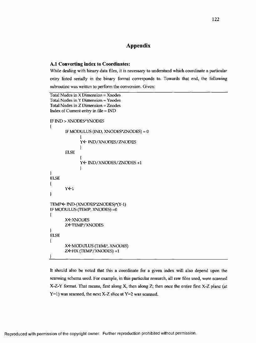
122

Appendix

A.1 Converting index to Coordinates:While dealing with binary data files, it is necessary to understand which coordinate a particular

entry listed serially in the binary format corresponds to. Towards that end, the following

subroutine was written to perform the conversion. Given:

Total Nodes in X Dimension = Xnodes Total Nodes in Y Dimension - Ynodes Total Nodes in Z Dimension = Znodes Index of Current entry in file = IND

IF IND > XNODES*YNODES {

IF MODULUS (IND, XNODES*ZNODES) = 0 {Y«- IND/XNODES/ZNODES }

ELSE{Y<- IND/XNODES/ZNODES +1 }

ELSE

Y«-l

TEMP<- IND-(XNODES*ZNODES)*(Y-l) IF MODULUS (TEMP, XNODES) =0

X<-XNODESZ^TEMP/XNODES

ELSE

X<-MODULUS (TEMP, XNODES) Z4-FIX (TEMP/XNODES) +1

It should also be noted that this a coordinate for a given index will also depend upon the

scanning schema used. For example, in this particular research, all raw files used, were scanned

X-Z-Y format. That means, first along X, then along Z; then once the entire first X-Z plane (at

Y=l) was scanned, the next X-Z slice at Y=2 was scanned.


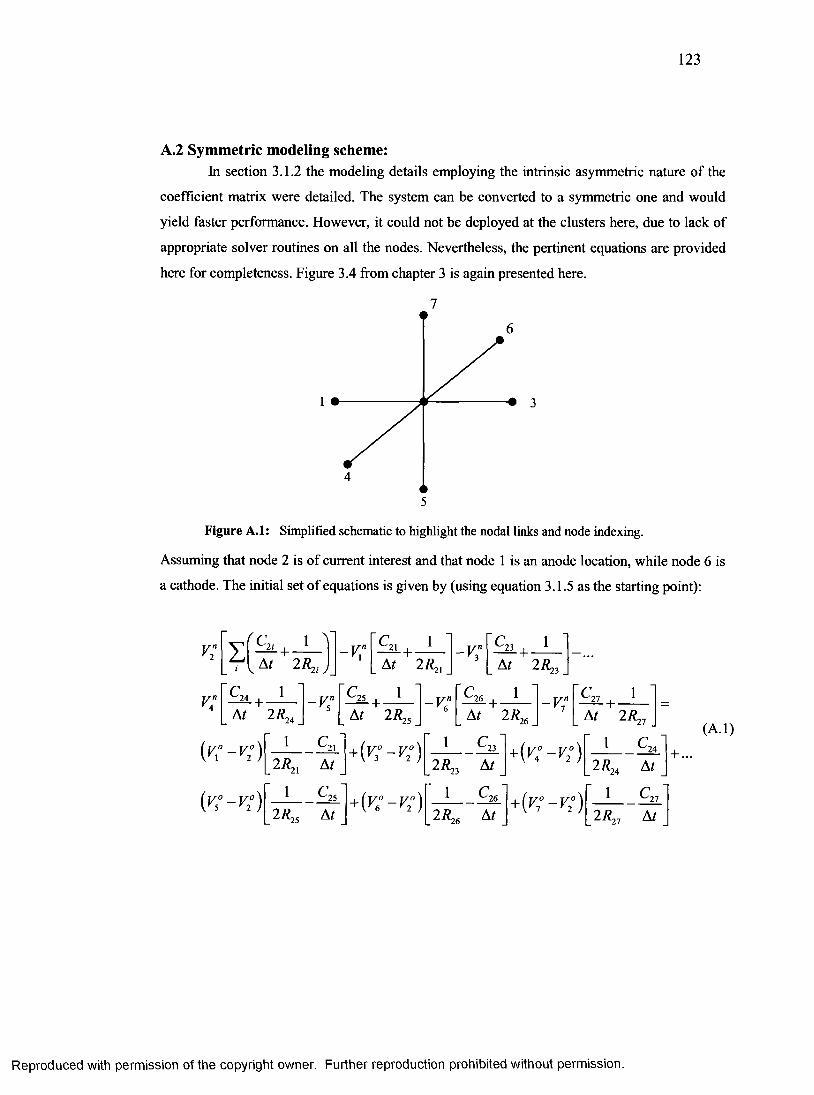
123

A.2 Symmetric modeling scheme:In section 3.1.2 the modeling details employing the intrinsic asymmetric nature of the

coefficient matrix were detailed. The system can be converted to a symmetric one and would

yield faster performance. However, it could not be deployed at the clusters here, due to lack of

appropriate solver routines on all the nodes. Nevertheless, the pertinent equations are provided

here for completeness. Figure 3.4 from chapter 3 is again presented here.

7

1

5

Figure A.1: Simplified schematic to highlight the nodal links and node indexing.

Assuming that node 2 is of current interest and that node 1 is an anode location, while node 6 is

a cathode. The initial set of equations is given by (using equation 3.1.5 as the starting point):

V n '2

v :

At 21L

\- V "

1It

p+

1

-v; r c 2 3 , i i

J _ At 2 /^ , At 2^23

c.24 + -1

At 2 ^-V s

' 2 5+ -

1At 2 R,25

-v: c 2 6+ -

1At 2i?26

■v;c.27

+ -1

At 2 R2 7

( v ° - v 2°)

( K - K )

1 r 21 + ( v ° - v ° )1 r 23 + ( r ,” - r / )

1 C 124L2*21 At 2R23 At . 2 ^ 4 At

1 r 25 + ( v ° - v 2°)1 r 26 + (v1° - v ° )

1 r 27L ^ s At L2^26 At \ / L /

[_ 2*27 At

(A.1)


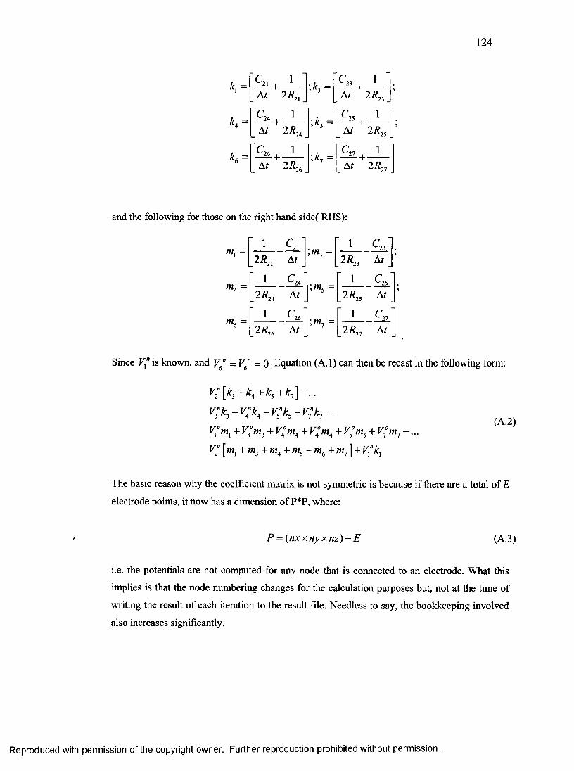
124

kx =

k£ =

^ l + _ LAt 2 R21

IIr•a

1

ml1

At 27?23

c .24+ -

1

At 2R,■24

c .26+ -

1A/ 2tf26

;k5 =

,kj

C25+ -

1A/ 2tf25

c 27+ -

1A/ 2/?■27

and the following for those on the right hand side( RHS):

m. =

1 c 121 ;m3 =1

r ..mlOH

2 R2l At 2 R23 At J1 r 24 ;m5 =

1 C25

L2*24 At 2 R25 At

1

I50\ ;m7 =

1 r 27At 2i?i7 At

Since V" is known, and y n = y ° = q . Equation (A.1) can then be recast in the following form:

V" [ft3 + k4 + k5 + k7 ] - . . .

V3'k3 - V 4% - V s'k5 - V 1' k l =

V°mx + V°m^ + V°m4 + V°m4 + V5°m5 + V1°m1 - . . .

V° \m x + m3 + m4 + m5 - m6 + m1 ] + V"kx

(A.2)

The basic reason why the coefficient matrix is not symmetric is because if there are a total of E

electrode points, it now has a dimension of P*P, where:

P = ( n x x n y x n z ) - E (A.3)

i.e. the potentials are not computed for any node that is connected to an electrode. What this

implies is that the node numbering changes for the calculation purposes but, not at the time of

writing the result of each iteration to the result file. Needless to say, the bookkeeping involved

also increases significantly.


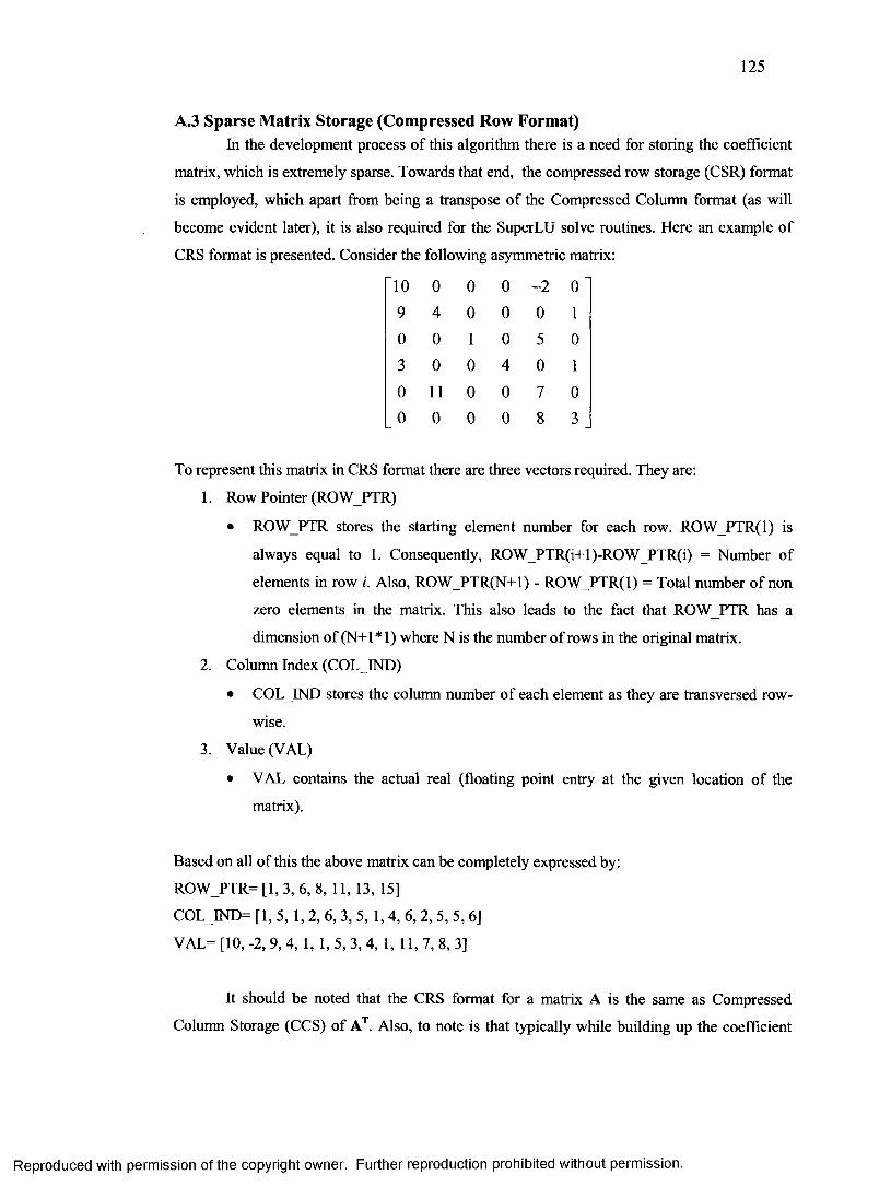
125

A.3 Sparse Matrix Storage (Compressed Row Format)In the development process of this algorithm there is a need for storing the coefficient

matrix, which is extremely sparse. Towards that end, the compressed row storage (CSR) format

is employed, which apart from being a transpose of the Compressed Column format (as will

become evident later), it is also required for the SuperLU solve routines. Here an example of

CRS format is presented. Consider the following asymmetric matrix:

10 0 0 0 -2 0

9 4 0 0 0 1

0 0 1 0 5 0

3 0 0 4 0 1

0 11 0 0 7 0

0 0 0 0 8 3

To represent this matrix in CRS format there are three vectors required. They are:

1. Row Pointer (ROW PTR)

• ROW PTR stores the starting element number for each row. RO W PTR (l) is

always equal to 1. Consequently, ROW_PTR(i+l)-ROW_PTR(i) = Number of

elements in row i. Also, ROW_PTR(N+l) - RO W PTR (l) = Total number of non

zero elements in the matrix. This also leads to the fact that ROW PTR has a

dimension of (N +l*l) where N is the number of rows in the original matrix.

2. Column Index (COLIND)

• COL IND stores the column number of each element as they are transversed row

wise.

3. Value (VAL)

• VAL contains the actual real (floating point entry at the given location of the

matrix).

Based on all of this the above matrix can be completely expressed by:

ROW_PTR= [1, 3, 6, 8, 11, 13, 15]

COLJND= [1, 5, 1, 2, 6, 3, 5, 1, 4, 6, 2, 5, 5, 6]

VAL= [10, -2, 9,4, 1, 1, 5, 3, 4, 1, 11, 7, 8, 3]

It should be noted that the CRS format for a matrix A is the same as Compressed

Column Storage (CCS) of AT. Also, to note is that typically while building up the coefficient


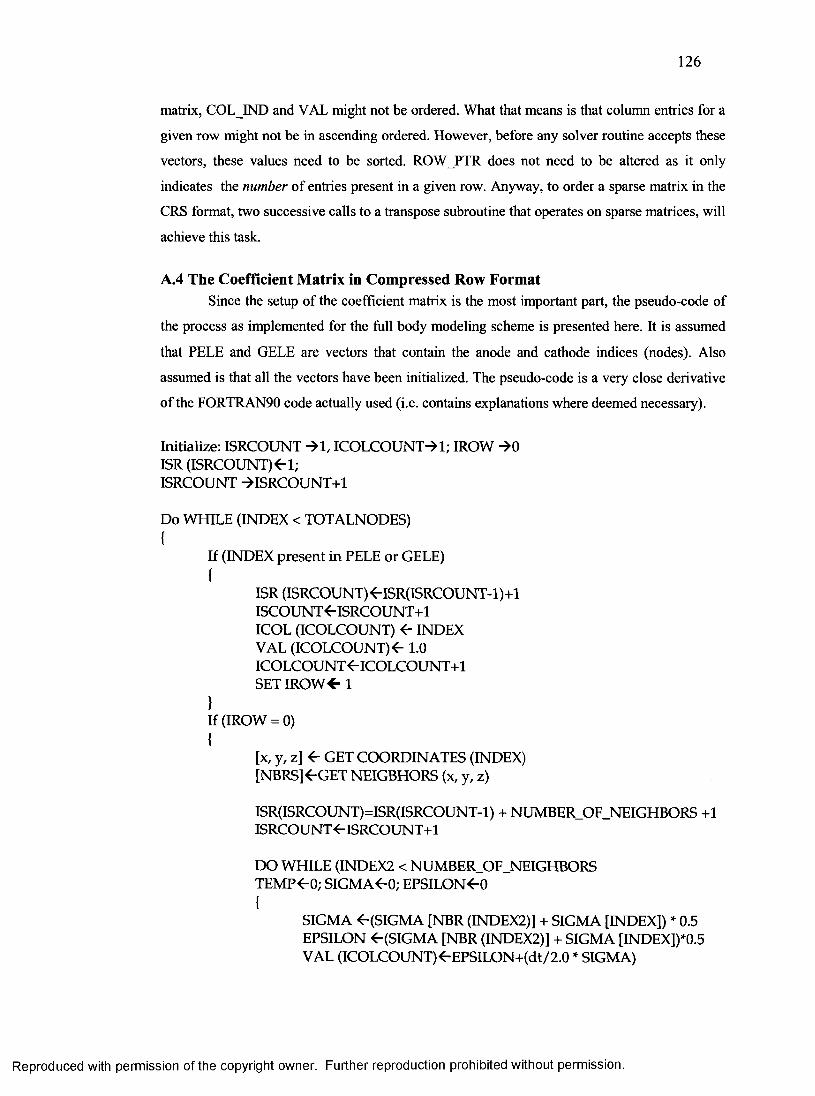
126

matrix, COL IND and VAL might not be ordered. What that means is that column entries for a

given row might not be in ascending ordered. However, before any solver routine accepts these

vectors, these values need to be sorted. ROW PTR does not need to be altered as it only

indicates the number of entries present in a given row. Anyway, to order a sparse matrix in the

CRS format, two successive calls to a transpose subroutine that operates on sparse matrices, will

achieve this task.

A.4 The Coefficient Matrix in Compressed Row FormatSince the setup of the coefficient matrix is the most important part, the pseudo-code of

the process as implemented for the full body modeling scheme is presented here. It is assumed

that PELE and GELE are vectors that contain the anode and cathode indices (nodes). Also

assumed is that all the vectors have been initialized. The pseudo-code is a very close derivative

of the FORTRAN90 code actually used (i.e. contains explanations where deemed necessary).

Initialize: ISRCOUNT -*1, IC O L C O U N T ^l; IROW -*0 ISR (ISRCOUNT) 1;ISRCOUNT ->ISRCOUNT+l

Do WHILE (INDEX < TOTALNODES){

If (INDEX present in PELE or GELE){

ISR (ISRCOUNT) <r ISR(ISRCOUNT-l)+1 ISCOUNT <-ISRCOUNT+l ICOL (ICOLCOUNT) < r INDEX VAL (ICOLCOUNT) <-1.0 ICOLCOUNT <-ICOLCOUNT+l SET IROW 4 -1

}If (IROW = 0){

[x, y, z] <- GET COORDINATES (INDEX)[NBRS]<-GET NEIGBHORS (x, y, z)

ISR(ISRCOUNT)=ISR(ISRCOUNT-l) + NUMBER_OF_NEIGHBORS +1 ISRCOUNT 4-ISRCOUNT+l

DO WHILE (INDEX2 < NUMBER_OF_NEIGHBORS TEMPÔ; SIGMA^-0; EPSILON<-0 {

SIGMA (SIGMA [NBR (INDEX2)] + SIGMA [INDEX]) * 0.5 EPSILON (SIGMA [NBR (INDEX2)] + SIGMA [INDEX])*0.5 VAL (ICOLCOUNT)«-EPSILON+(dt/2.0 * SIGMA)


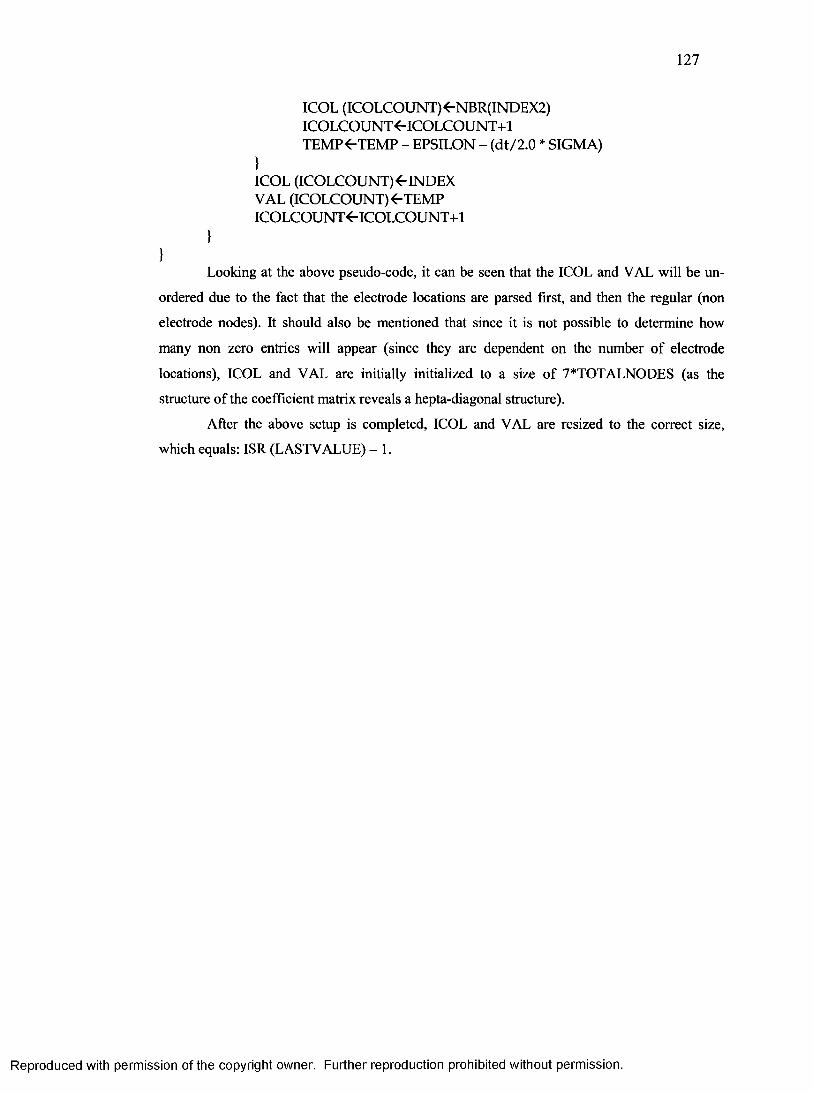
127

ICOL (ICOLCOUNT) 4-NBR(INDEX2)ICOLCOUNT4-ICOLCOUNT+1TEMP4-TEMP - EPSILON - (d t/2 .0 * SIGMA)

}ICOL (ICOLCOUNT) 4-INDEX VAL (ICOLCOUNT) 4-TEMP ICOLCOUNT <-ICOLCOUNT+l

}}

Looking at the above pseudo-code, it can be seen that the ICOL and VAL will be un

ordered due to the fact that the electrode locations are parsed first, and then the regular (non

electrode nodes). It should also be mentioned that since it is not possible to determine how

many non zero entries will appear (since they are dependent on the number of electrode

locations), ICOL and VAL are initially initialized to a size of 7*TOTALNODES (as the

structure of the coefficient matrix reveals a hepta-diagonal structure).

After the above setup is completed, ICOL and VAL are resized to the correct size,

which equals: ISR (LASTVALUE) - 1.


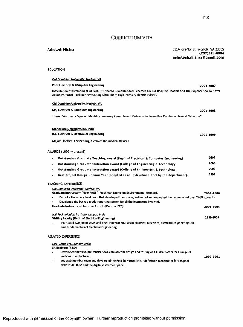
128

C u r r i c u l u m v i t a

Ashutosh Mishra 6114, Granby St., Norfolk, VA 23505(757)515-4804

ashutosh .m ishra@ am ail.com

EDUCATION

Old Dominion University. Norfolk. VA

PhD, Electrical & C o m p u te r Engineering 2 0 0 3 - 2 0 0 7

Dissertation: "D eve lopm en t Of Fast, Dis tr ibuted Com puta t iona l S chem es For Full Body Bio-Models And Their Application To Novel Action Potentia l Block In Nerves Using Ultra-Short, High Intensity Electric Pulses".

Old D om inion Univers ity. Norfolk. VA

MS, Electrical & C o m p u te r Engineering 2 0 0 1 - 2 0 0 3

Thesis: "Automatic Speaker Identificat ion using Reusable and Re-trainable Binary Pair Part i tioned Neural Netw orks"

M a n g a lo re Univers ity . KA. India

B.E. Electrical & Electronics Engineering 1 9 9 5 - 1 9 9 9

Major: Electrical Engineering; E l e c t i v e : Bio-medical Devices

AWARDS (1999 ~ present)

• O u t s t a n d i n g G r a d u a t e T e a c h i n g a w a r d ( D e p t , o f E l e c t r i c a l & C o m p u t e r E n g i n e e r i n g ) 2007

• O u t s t a n d i n g G r a d u a t e I n s t r u c t i o n a w a r d ( C o l le g e o f E n g i n e e r i n g & T e c h n o l o g y ) 2006

• O u t s t a n d i n g G r a d u a t e I n s t r u c t i o n a w a r d ( C o l le g e o f E n g i n e e r i n g & T e c h n o l o g y ) 2003

B e s t P r o j e c t D e s i g n - S e n i o r Y e a r ( a d o p t e d a s a n i n s t r u c t i o n a l t o o l by t h e d e p a r t m e n t ) . 1999

TEACHING EXPERIENCEO l d D o m i n i o n U n i v e r s i t y . N o r f o l k . V AG ra d u a te In s t ruc to r - "New PAGE" (F reshman course on Environmenta l Aspects) . 2 0 0 4 - 2 0 0 6

Part of a University level t e a m t h a t de ve loped t h e course , ins truc ted a nd eva lua ted t h e re s p o n se s of ove r 2200 s tuden ts .

Developed t h e backup g rade -repo r t ing system for all t h e ins truc tors involved.

G ra d u a te In s t ruc to r - Electronic Circuits (Dept, o f ECE). 2 0 0 1 - 2 0 0 4

H .B T e c h n o l o g i c a l I n s t i t u t e . K a n p u r . I n d iaVisiting Faculty (Dept, o f Electrical Engineering) 1999-2001

Instructed t w o jun io r Level and o n e Final Year cou rses in Electrical Machines, Electrical Engineering Lab

an d F undam en ta ls o f Electrical Engineering.

RELATED EXPERIENCE

L M L - V e s o a L td . . K a n p u r . I n d io Sr. Engineer (R&D)

• Developed t h e fi rst (pre- fabricat ion) s im ula to r fo r design a n d te s t ing of A.C a l te rna to rs fo r a range of

vehic les m anufac tu red . 1 9 9 9 - 2 0 0 1

• Led a SO m e m b e r t e a m a n d developed th e first, in -house , linear deflection t a c h o m e te r fo r range of

100~11500 RPM and t h e digital i n s t ru m e n t panel .


mailto:[email protected]

129

PUBLICATIONS AND PRESENTATIONS

Journal Publications

" M o d e l A s s e s s m e n t o f Cel l M e m b r a n e B r e a k d o w n in C l u s t e r s a n d T i s s u e s u n d e r H i g h - i n t e n s i t y E lec t r i c P u ls in g "

( a c c e p t e d f o r p u b l i c a t i o n , IEEE T r a n s , o n P l a s m a S c i e n c e s - s p e c i a l i s s u e A ug . 2 0 0 8 )

• “S i m u l a t i o n S t u d i e s o f U l t r a - S h o r t , H i g h - i n t e n s i t y E lec t r i c P u l s e I n d u c e d A c t io n P o t e n t i a l B lock in W h o l e - A n i m a l

N e r v e S e g m e n t s " , ( A c c e p t e d f o r p u b l i c a t i o n , O c t . 2 0 0 7 in IEEE T r a n s . O n B i o m e d ic a l E n g i n e e r i n g ) , Vol. 5 5 , No.

4 , 2 0 0 8 .

• " S e l f - C o n s i s t e n t A n a l y s e s f o r P o t e n t i a l C o n d u c t i o n B lock in N e r v e s b y a n U l t r a - S h o r t , H i g h - i n t e n s i t y E lec t r i c

P u l s e " , P h y s ic a l R e v i e w (E), Vol. 7 5 , 0 6 1 9 0 6 , J u n e , 2 0 0 7 .

"A F a s t , P a r a l l e l i z e d C o m p u t a t i o n a l A p p r o a c h B a s e d o n S p a r s e LU F a c t o r i z a t i o n f o r P r e d i c t i o n s o f S p a t i a l a n d

T i m e - O e p e n d e n t C u r r e n t s a n d V o l t a g e s in F u l l -B o d y B i o - M o d e l s " ( I n v i t e d P a p e r ) , IEEE T r a n s , o n P l a s m a Sc. ,

Vol. 3 4 , 1 4 3 1 - 1 4 4 0 , 2 0 0 6 .

• " S i m u l a t i o n s o f D i s t r i b u t e d V o l t a g e s i n F u l l - B o d y B i o - M o d e l s U s i n g S y m m e t r i c F a c t o r i z a t i o n w i t h M a s s i v e l y

P a r a l l e l S o l v e r s i n R e s p o n s e t o E x t e r n a l P u l s i n g " , - i n r e v i e w , s t a g e 2 , I E E E T r a n s , o n P l a s m a S c i e n c e s .

C onference and Poster p resen ta tio n s

• “S e l f C o n s i s t e n t A n a ly s e s f o r P o t e n t i a l C o n d u c t i o n B lock in N e r v e s by U l t r a S h o r t , High I n t e n s i t y P u l s e s " ,

PPPS 2 0 0 7 , J u n e 1 7 ~ 2 1 , A l b u q u e r q u e , NM.

• " S t a t u s o f F ie ld M a r s h a l P r o j e c t " , IVEC, M a y 2 0 0 7 , K i t a k y u s h u , J a p a n .

• " B io S im " - A g r id e n a b l e d a p p l i c a t i o n . Fall I n t e r n e t 2 M e m b e r M e e t i n g , Dec 2 0 0 6 , C h ic a g o , IL - 6 0 6 1 6

• "F ie ld M a r s h a l S i m u l a t i o n E n v i r o n m e n t " , ICOPS 2 0 0 6 , T r a v e r s e City, Ml, 2 0 0 6 .

• “T e x t I n d e p e n d e n t S p e a k e r I d e n t i f i c a t i o n u s i n g r e - t r a i n a b l e a n d r e u s a b l e BPP n e u r a l n e t w o r k s " , ICASSP 2 0 0 2

OTHER PROJECTS

• H u m a n F a t ig u e M o d e l s c h e m e . D e v e l o p e d a n A N N b a s e d s y s t e m t o p r e d i c t t h e f a t i g u e l e v e l b a s e d o n

e x p e c t e d " w a k e " h o u r s . N o w b e i n g u s e d a s a m o d u l e i n a l a r g e r s i m u l a t i o n e n v i r o n m e n t . ( C o m p l e t e )

P a r t o f t h e c o l l a b o r a t i v e c o m p u t a t i o n F ie ld M a r s h a l p r o j e c t .

• A u t o m a t i c C o n f i g u r a t i o n s y s t e m f o r c o n t r o l l i n g P a r t i c l e in Cel l (PIC) s i m u l a t i o n s .

INTERESTS

. High P e r f o r m a n c e C o m p u t a t i o n , A r t i f ic ia l N e u r a l N e t w o r k s , SVM, C o m p u t a t i o n a l M e t h o d s , S ig n a l P r o c e s s i n g ,

A l g o r i t h m d e v e l o p m e n t .

• A c t iv e c o n t r i b u t o r o n t h e o n l i n e MATLAB/FORTRAN h e l p f o r u m s .

• R e a d i n g , w r i t i n g .

PROFICIENCY

MATLAB', FORTRAN, C/C ++, P y t h o n , VB, MPI

• Long t e r m e x p e r i e n c e w i t h W in 3 2 / L i n u x


Development of Fast, Distributed Computational Schemes for ...

Documents