Final Report May 28, 2019 May 28, 2019 Development of Design Wind Speed Maps for the Caribbean for Application with the Wind Load Provisions of ASCE 7-16 and Later Prepared for: Pan American Health Organization Regional Office for The Americas World Health Organization 525 23 rd Street NW Washington, DC 20037-2875 Prepared by: L. A. Mudd, A. Liu and P. J. Vickery Applied Research Associates, Inc. 8537 Six Forks Rd, Suite 600 Raleigh NC 27615 ARA Project # 003449

Welcome message from author
This document is posted to help you gain knowledge. Please leave a comment to let me know what you think about it! Share it to your friends and learn new things together.
Transcript
Final Report May 28, 2019
May 28, 2019
Development of Design Wind Speed Maps for the Caribbean for Application with the Wind Load
Provisions of ASCE 7-16 and Later
Prepared for:
Pan American Health Organization Regional Office for The Americas World Health Organization
525 23rd Street NW Washington, DC 20037-2875
Prepared by:
L. A. Mudd, A. Liu and P. J. Vickery Applied Research Associates, Inc.
8537 Six Forks Rd, Suite 600 Raleigh NC 27615
ARA Project # 003449
1 Final Report May 28, 2019
1. INTRODUCTION
The objective of this study is to develop estimates of wind speeds as a function of return period for locations in the Caribbean Basin that can be used in conjunction with the design wind provisions used in the US wind loading standards that reference ASCE 7-16 and later. Maps of hurricane induced wind speeds are developed using a peer reviewed hurricane simulation model as described in Vickery et al. (2000a, 2000b, 2006, 2009a, 2009b), and Vickery and Wadhera (2008). The hurricane simulation model used here is an updated version of that described in Vickery et al. (2009a, 2009b) and Vickery and Wadhera (2008) which was used to produce the design wind speeds used in ASCE 7-10 and ASCE 7-16, the current version.
Section 2 of the report describes the simulation methodology and model validation results, and section 3 presents the wind speed results. A summary is presented in section 4.
With financial support from Global Affairs Canada
2 Final Report May 28, 2019
2. METHODOLOGY
The hurricane simulation approach used to define the hurricane hazard in the Caribbean consists of two major components. The first component comprises a hurricane track model that reproduces the frequency and geometric characteristics of hurricane tracks as well as the variation of hurricane size and intensity as they move along the tracks. The second portion of the model is the hurricane wind field model, where given key hurricane parameters at any point in time from the track model, the wind field model provides estimates of the wind speed and wind direction at an arbitrary position. The meteorological inputs to the wind field model include the central pressure difference, Δp, translation speed, c, radius to maximum winds (RMW) and the Holland B parameter. (For computing Δp, the far field pressure is taken as 1013 mbar, and thus Δp is defined as 1013 minus the central pressure, pc.) The geometric inputs include storm position, heading and the location of the site where wind speeds are required. The following sections describe the verification of the track model for the Caribbean and a summary of the wind field model is also presented. 2.1.Track and Intensity Modelling
The hurricane track and intensity simulation methodology used to define the hurricane hazard in the Caribbean follows that described in Vickery et al. (2000, 2008), but the coefficients used in the statistical models have been calibrated to model the variation in storm characteristics throughout the Caribbean basin.
Track and Relative Intensity Modelling The over water hurricane track simulation
is performed in two steps. In the first step, the hurricane position at any point in time is modelled using the approach given in Vickery et al. (2000a). In the second step, the relative intensity, I, of the hurricane is modelled using a modified version of the approach given in Vickery et al. (2000a) as described in Vickery et al. (2008a) The relative intensity is then used to compute the central pressure, as described in Vickery et al (2000a). Then, using this central pressure, the RMW and B are computed as described in Vickery and Wadhera (2008) and Vickery et al (2008a). A simple one dimensional ocean mixing model, described in Emanuel et al. (2006), is used to simulate the effect of ocean feedback on the relative intensity calculations. The ocean mixing model returns an estimate of a mixed layer depth which is used to compute the reduction in sea surface temperature caused by the passage of a hurricane. This reduced sea surface temperature is used to convert historical pressures to relative intensity values. The historical relative intensity values are then used to develop regional statistical models of the form of Equation 2-1, where the relative intensity at any time is modelled as a function of relative intensity at last three steps and the scaled vertical wind shear, Vs, (DeMaria and Kaplan, 1999).
ε++++= −−+ siiii VcIcIcIcI 4231211 )ln()ln()ln()ln( (2-1)
where c1, c2, etc. are constants that vary with region in the Atlantic Basin, and ε is a random error term. If a storm crosses land, the central pressure is computed using a filling model, where the central pressure t hours after landfall is dependent on the storm pressure at the time of landfall and the number of hours that the storm has been over land.
3 Final Report May 28, 2019
Storm Filling New filling models have been developed to better model the intensity of storms making landfall in Cuba, Hispaniola, and the Yucatan Peninsula. The new filling models were developed using HURDAT2 and H*WIND data. The landfall pressure was computed from the HURDAT2 database by extrapolating the central pressures using the last two central pressures before landfall. Using this approach, the pressure tendency of the hurricane before landfall was maintained, such that weakening storms continue to weaken and strengthening storms continue to intensify until landfall. The RMW at landfall were extracted from the H*WIND database. The RMW of the last over water point was used as the land falling RMW when the RMW at the time of landfall was not found in the H*WIND database. Weakening of the hurricane after landfall was modelled using an exponential decay (filling) function in the form of Equation (2-2).
∆𝑝𝑝 𝑡𝑡 = ∆ 𝑝𝑝𝑜𝑜𝑒𝑒𝑒𝑒𝑝𝑝 − 𝑎𝑎𝑡𝑡 (2-2) where ∆𝑝𝑝 𝑡𝑡 is the central pressure difference t hours after landfall, ∆𝑝𝑝0 is the central pressure difference at the time of landfall and a is an empirically derived filling coefficient. One model was developed for the Yucatan Peninsula using central pressure difference, translation speed, and RMW. Two models were developed for the region encompassing Cuba, Jamaica, and Hispaniola: one with storms having central pressures less than 980 mb and the other with storms having central pressures greater than 980 mb. The filling coefficient was found to be a function of the longitude of the landfall location for storms having central pressure less than 980 mb. The filling coefficients tended to decrease for this pressure category with increasing longitude. In this region, Hispaniola, Jamaica, and the eastern part of Cuba have some mountainous terrain, which helps in the weakening of storms passing east to west. The terrain in the western part of Cuba is not as mountainous as the eastern part of the island, and therefore the storms tend to weaken less in the western part of Cuba. No correlation was found for weaker storms making landfall in the same region. Therefore, a constant mean value and standard deviation of error were used for the filling model for weaker land falling storms in this region. A separate filling model was developed for Puerto Rico based on the fact that storms that are larger than the width of the island will be less affected by the mountainous terrain.
There are cases for some weaker storms (i.e., 1998 Georges, 2010 Alex, 2012 Emily), that actually intensified while passing over Cuba and the Yucatan Peninsula. A separate negative-filling model was developed to simulate the increase in intensity in the region for weaker storms (Pc > 980 mb) only. The filling models were developed using 17 years (1996-2012) of historic data due to limited H*WIND data. It was observed that the probability of the intensity to increase while passing over the island is 7.5% in this region during the 17-year period. The filling model was developed in such a way that the probability of executing the negative-filling model is 7.5%.
4 Final Report May 28, 2019
2.1.1. Model Validation
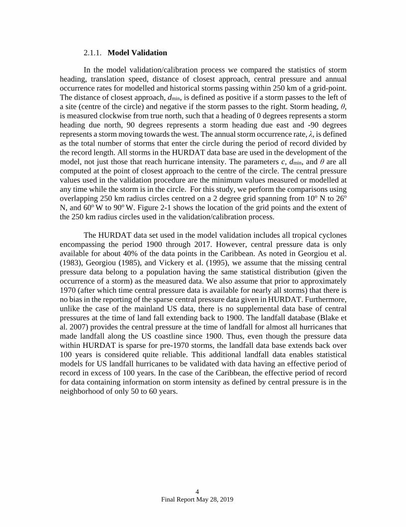
In the model validation/calibration process we compared the statistics of storm heading, translation speed, distance of closest approach, central pressure and annual occurrence rates for modelled and historical storms passing within 250 km of a grid-point. The distance of closest approach, dmin, is defined as positive if a storm passes to the left of a site (centre of the circle) and negative if the storm passes to the right. Storm heading, θ, is measured clockwise from true north, such that a heading of 0 degrees represents a storm heading due north, 90 degrees represents a storm heading due east and -90 degrees represents a storm moving towards the west. The annual storm occurrence rate, λ, is defined as the total number of storms that enter the circle during the period of record divided by the record length. All storms in the HURDAT data base are used in the development of the model, not just those that reach hurricane intensity. The parameters c, dmin, and θ are all computed at the point of closest approach to the centre of the circle. The central pressure values used in the validation procedure are the minimum values measured or modelled at any time while the storm is in the circle. For this study, we perform the comparisons using overlapping 250 km radius circles centred on a 2 degree grid spanning from 10o N to 26o N, and 60o W to 90o W. Figure 2-1 shows the location of the grid points and the extent of the 250 km radius circles used in the validation/calibration process.
The HURDAT data set used in the model validation includes all tropical cyclones encompassing the period 1900 through 2017. However, central pressure data is only available for about 40% of the data points in the Caribbean. As noted in Georgiou et al. (1983), Georgiou (1985), and Vickery et al. (1995), we assume that the missing central pressure data belong to a population having the same statistical distribution (given the occurrence of a storm) as the measured data. We also assume that prior to approximately 1970 (after which time central pressure data is available for nearly all storms) that there is no bias in the reporting of the sparse central pressure data given in HURDAT. Furthermore, unlike the case of the mainland US data, there is no supplemental data base of central pressures at the time of land fall extending back to 1900. The landfall database (Blake et al. 2007) provides the central pressure at the time of landfall for almost all hurricanes that made landfall along the US coastline since 1900. Thus, even though the pressure data within HURDAT is sparse for pre-1970 storms, the landfall data base extends back over 100 years is considered quite reliable. This additional landfall data enables statistical models for US landfall hurricanes to be validated with data having an effective period of record in excess of 100 years. In the case of the Caribbean, the effective period of record for data containing information on storm intensity as defined by central pressure is in the neighborhood of only 50 to 60 years.
5 Final Report May 28, 2019
Figure 2-1. Locations of simulation circle centres showing extent of 250 km sample circles.
In order to verify the ability of the model to reproduce the characteristics of historical storms we perform statistical tests comparing the characteristics of model and observed hurricane parameters. The statistical tests include t-tests for equivalence of means, F-tests for equivalence of variance and the Kolmogorov-Smirnov (K-S) tests for equivalence of the Cumulative Distribution Functions (CDF). In the case of central pressures we also used a statistical test method described in James and Mason (2005) for testing equivalence of the modelled and observed central pressure conditional distributions of pressure, and as a function of annual exceedance probability. No consideration is given to the measurement errors inherent in the HURDAT data in the computation of translation speed, heading, central pressure, etc., in any of the statistical tests.
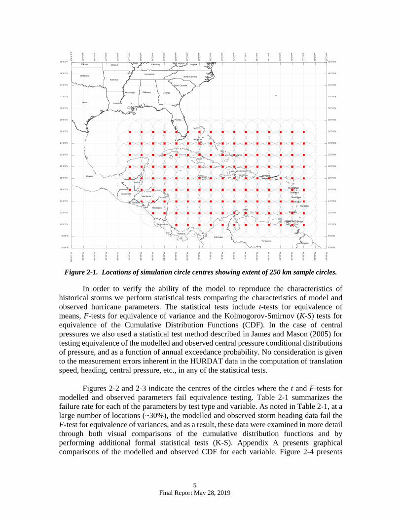
Figures 2-2 and 2-3 indicate the centres of the circles where the t and F-tests for modelled and observed parameters fail equivalence testing. Table 2-1 summarizes the failure rate for each of the parameters by test type and variable. As noted in Table 2-1, at a large number of locations (~30%), the modelled and observed storm heading data fail the F-test for equivalence of variances, and as a result, these data were examined in more detail through both visual comparisons of the cumulative distribution functions and by performing additional formal statistical tests (K-S). Appendix A presents graphical comparisons of the modelled and observed CDF for each variable. Figure 2-4 presents
100°
0'0"
W
98°0
'0"W
96°0
'0"W
94°0
'0"W
92°0
'0"W
90°0
'0"W
88°0
'0"W
86°0
'0"W
84°0
'0"W
82°0
'0"W
80°0
'0"W
78°0
'0"W
76°0
'0"W
74°0
'0"W
72°0
'0"W
70°0
'0"W
68°0
'0"W
66°0
'0"W
64°0
'0"W
62°0
'0"W
60°0
'0"W
58°0
'0"W
56°0
'0"W
6°0'0"N
8°0'0"N
10°0'0"N
12°0'0"N
14°0'0"N
16°0'0"N
18°0'0"N
20°0'0"N
22°0'0"N
24°0'0"N
26°0'0"N
28°0'0"N
30°0'0"N
32°0'0"N
34°0'0"N
36°0'0"N
38°0'0"N
Barbados
Bahamas
Belize
Colombia
Costa Rica
Cuba
Dominica
Dominican
Republic
El Salvador
Guatemala
Haiti
Honduras
Jamaica
Martinique
ArubaNicaragua
Panama
Puerto Rico
Saint Lucia
Trinidad and Tobago
Venezuela
Guadeloupe
Turks and Caicos Islands
Arkansas
Georgia
Louisiana
Oklahoma
South Carolina
Tennessee
Florida
Virginia
Alabama
Kentucky
Mississippi
Texas
North Carolina
Grenada
Guyana
Mexico
Kansas MissouriIllinois West Virginia Maryland
6 Final Report May 28, 2019
graphical comparisons of the CDFs for some locations where the t, F, or K-S tests for storm heading failed.
Table 2-1. Percent of locations failing the indicated statistical equivalence tests at the 95% confidence level. Number of points failing equivalency is given in parentheses.
Variable t-test F-test K-S test dmin 10.9% (15) 2.9% (4) 12.4 (17) Translation speed 27.7% (38) 31.3% (43 25.5% (35) Heading 13.9% (19) 29.9% (41) 20.4% (28) Central Pressure 7.3 (10) 2.9% (4) 8.8% (12)
Figure 2-2. Locations where t-tests fail at the 95% confidence level.
F
F
F
F F
F
F
F
F
F
F
F
F
F
F
Minimum Distance of Approach
F
F
F
F
F
F
F
F
F
F
F
F
F
F
F
F
F
F
F
F
F F
F
F
F
F
F
F
F
F
F
F
F
F
F
F
F
F
Translation Speed
F
F
F
F
F
F
F
F
F
F
F
F F
F
F
F
F
F
F
F
Storm Heading
F F
F
F F
F
F
F
F
F
Central Pressure Difference
7 Final Report May 28, 2019
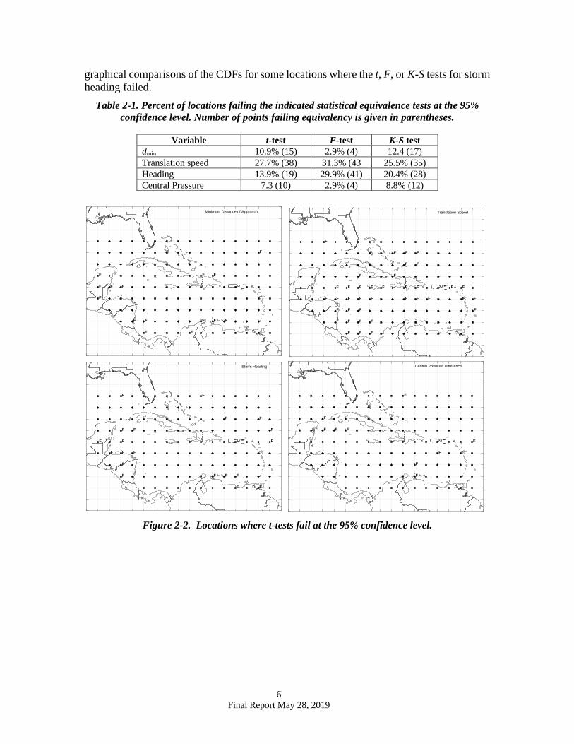
Figure 2-3. Locations where F-tests fail at the 95% confidence level.
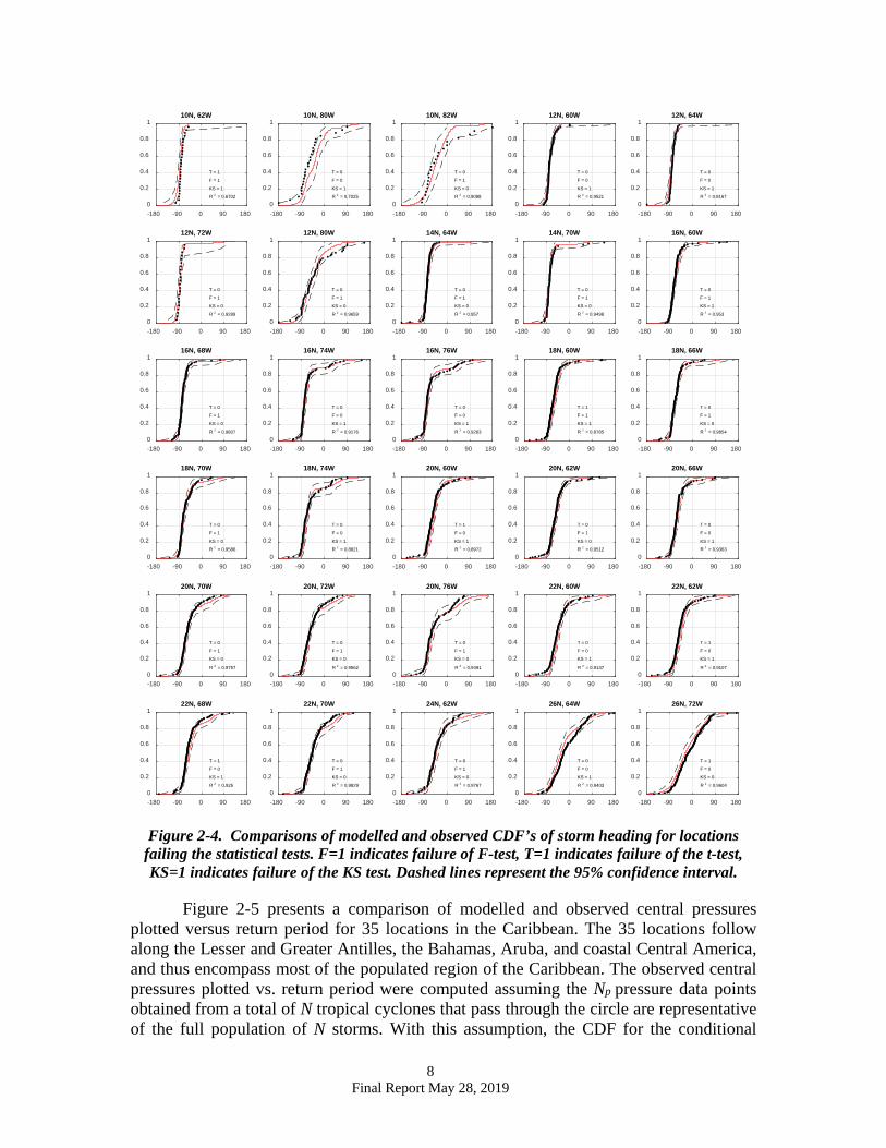
For those locations where the model fails the F-test for heading equivalence, a visual comparison of the modelled and observed CDF data given in Appendix A and Figure 2-4 indicates that overall the model reproduces the observed heading data very well, and the variance of the observed data is strongly dependent on a few outliers. In most cases, these outliers are associated with the infrequent occurrence of one, or at most two, storms heading in an easterly direction in the southern portion of the Caribbean. In the southern portion of the Caribbean, the model produces eastward moving storms, but the occurrence of these eastward moving storms is distributed over a wider range of sample/validation circles than the historical storms, yielding both overestimates and underestimates of the variance, depending upon which circle the few historical storms happen to pass through. For those locations that fail the F-tests for heading equivalence in the Western Caribbean the model results tend to have a broader distribution.
F
F
F
F
Minimum Distance of Approach
F
F
F
F
F
F F
F
F
F
F
F
F
F
F
F
F
F
F
F
F
F
F
F
F
F
F
F
F
F
F
F
F
F
F
F
F
F
F
F
F
F
F
Translation Speed
F
F
F
F
F
F
F
F
F
F
F
F F F
F
F
F
F
F
F
F
F
F
F
F
F
F
F
F
F
F
F
F
F
F
F
F
F
F
F
F
Storm Heading
F
F
F
F
Central Pressure Difference
8 Final Report May 28, 2019
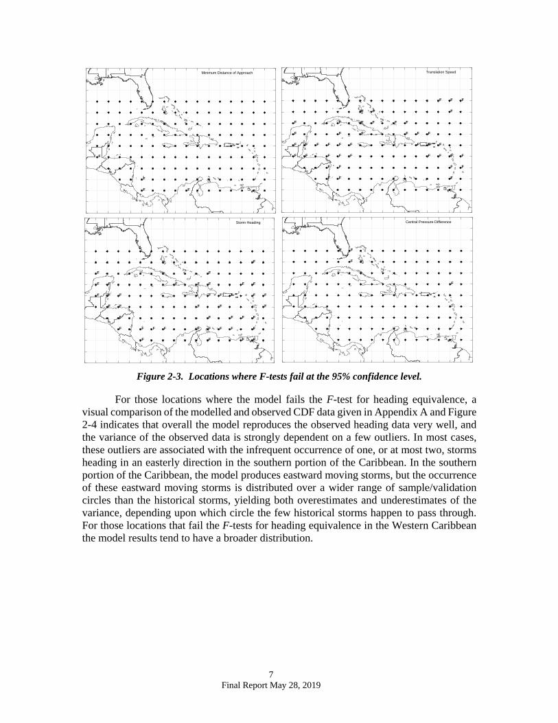
Figure 2-4. Comparisons of modelled and observed CDF’s of storm heading for locations
failing the statistical tests. F=1 indicates failure of F-test, T=1 indicates failure of the t-test, KS=1 indicates failure of the KS test. Dashed lines represent the 95% confidence interval.
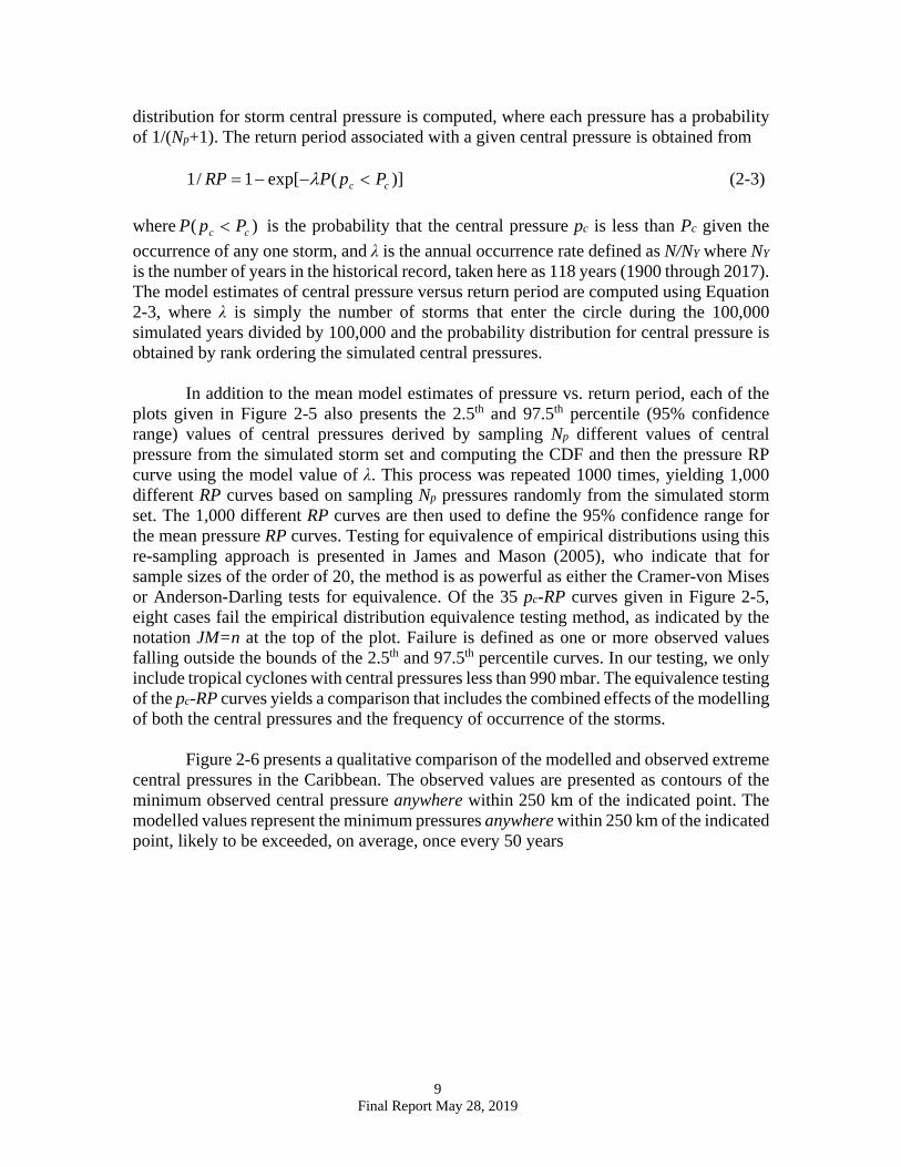
Figure 2-5 presents a comparison of modelled and observed central pressures plotted versus return period for 35 locations in the Caribbean. The 35 locations follow along the Lesser and Greater Antilles, the Bahamas, Aruba, and coastal Central America, and thus encompass most of the populated region of the Caribbean. The observed central pressures plotted vs. return period were computed assuming the Np pressure data points obtained from a total of N tropical cyclones that pass through the circle are representative of the full population of N storms. With this assumption, the CDF for the conditional
-180 -90 0 90 1800
0.2
0.4
0.6
0.8
110N, 62W
R 2 = 0.6702
KS = 1
F = 1
T = 1
-180 -90 0 90 1800
0.2
0.4
0.6
0.8
110N, 80W
R 2 = 0.7025
KS = 1
F = 0
T = 0
-180 -90 0 90 1800
0.2
0.4
0.6
0.8
110N, 82W
R 2 = 0.9088
KS = 0
F = 1
T = 0
-180 -90 0 90 1800
0.2
0.4
0.6
0.8
112N, 60W
R 2 = 0.9521
KS = 1
F = 0
T = 0
-180 -90 0 90 1800
0.2
0.4
0.6
0.8
112N, 64W
R 2 = 0.8167
KS = 1
F = 0
T = 0
-180 -90 0 90 1800
0.2
0.4
0.6
0.8
112N, 72W
R 2 = 0.9289
KS = 0
F = 1
T = 0
-180 -90 0 90 1800
0.2
0.4
0.6
0.8
112N, 80W
R 2 = 0.9659
KS = 0
F = 1
T = 0
-180 -90 0 90 1800
0.2
0.4
0.6
0.8
114N, 64W
R 2 = 0.957
KS = 0
F = 1
T = 0
-180 -90 0 90 1800
0.2
0.4
0.6
0.8
114N, 70W
R 2 = 0.9498
KS = 0
F = 1
T = 0
-180 -90 0 90 1800
0.2
0.4
0.6
0.8
116N, 60W
R 2 = 0.953
KS = 1
F = 1
T = 0
-180 -90 0 90 1800
0.2
0.4
0.6
0.8
116N, 68W
R 2 = 0.9807
KS = 0
F = 1
T = 0
-180 -90 0 90 1800
0.2
0.4
0.6
0.8
116N, 74W
R 2 = 0.9176
KS = 1
F = 0
T = 0
-180 -90 0 90 1800
0.2
0.4
0.6
0.8
116N, 76W
R 2 = 0.9263
KS = 1
F = 0
T = 0
-180 -90 0 90 1800
0.2
0.4
0.6
0.8
118N, 60W
R 2 = 0.8785
KS = 1
F = 1
T = 1
-180 -90 0 90 1800
0.2
0.4
0.6
0.8
118N, 66W
R 2 = 0.9854
KS = 0
F = 1
T = 0
-180 -90 0 90 1800
0.2
0.4
0.6
0.8
118N, 70W
R 2 = 0.9586
KS = 0
F = 1
T = 0
-180 -90 0 90 1800
0.2
0.4
0.6
0.8
118N, 74W
R 2 = 0.8821
KS = 1
F = 0
T = 0
-180 -90 0 90 1800
0.2
0.4
0.6
0.8
120N, 60W
R 2 = 0.8972
KS = 1
F = 0
T = 1
-180 -90 0 90 1800
0.2
0.4
0.6
0.8
120N, 62W
R 2 = 0.9512
KS = 0
F = 1
T = 0
-180 -90 0 90 1800
0.2
0.4
0.6
0.8
120N, 66W
R 2 = 0.9363
KS = 1
F = 0
T = 0
-180 -90 0 90 1800
0.2
0.4
0.6
0.8
120N, 70W
R 2 = 0.9757
KS = 0
F = 1
T = 0
-180 -90 0 90 1800
0.2
0.4
0.6
0.8
120N, 72W
R 2 = 0.9562
KS = 0
F = 1
T = 0
-180 -90 0 90 1800
0.2
0.4
0.6
0.8
120N, 76W
R 2 = 0.9491
KS = 0
F = 1
T = 0
-180 -90 0 90 1800
0.2
0.4
0.6
0.8
122N, 60W
R 2 = 0.9137
KS = 1
F = 0
T = 0
-180 -90 0 90 1800
0.2
0.4
0.6
0.8
122N, 62W
R 2 = 0.9107
KS = 1
F = 0
T = 1
-180 -90 0 90 1800
0.2
0.4
0.6
0.8
122N, 68W
R 2 = 0.925
KS = 1
F = 0
T = 1
-180 -90 0 90 1800
0.2
0.4
0.6
0.8
122N, 70W
R 2 = 0.9829
KS = 0
F = 1
T = 0
-180 -90 0 90 1800
0.2
0.4
0.6
0.8
124N, 62W
R 2 = 0.9767
KS = 0
F = 1
T = 0
-180 -90 0 90 1800
0.2
0.4
0.6
0.8
126N, 64W
R 2 = 0.9403
KS = 1
F = 0
T = 0
-180 -90 0 90 1800
0.2
0.4
0.6
0.8
126N, 72W
R 2 = 0.9604
KS = 0
F = 0
T = 1
9 Final Report May 28, 2019
distribution for storm central pressure is computed, where each pressure has a probability of 1/(Np+1). The return period associated with a given central pressure is obtained from
)](exp[1/1 cc PpPRP <−−= λ (2-3) where )( cc PpP < is the probability that the central pressure pc is less than Pc given the occurrence of any one storm, and λ is the annual occurrence rate defined as N/NY where NY is the number of years in the historical record, taken here as 118 years (1900 through 2017). The model estimates of central pressure versus return period are computed using Equation 2-3, where λ is simply the number of storms that enter the circle during the 100,000 simulated years divided by 100,000 and the probability distribution for central pressure is obtained by rank ordering the simulated central pressures.
In addition to the mean model estimates of pressure vs. return period, each of the plots given in Figure 2-5 also presents the 2.5th and 97.5th percentile (95% confidence range) values of central pressures derived by sampling Np different values of central pressure from the simulated storm set and computing the CDF and then the pressure RP curve using the model value of λ. This process was repeated 1000 times, yielding 1,000 different RP curves based on sampling Np pressures randomly from the simulated storm set. The 1,000 different RP curves are then used to define the 95% confidence range for the mean pressure RP curves. Testing for equivalence of empirical distributions using this re-sampling approach is presented in James and Mason (2005), who indicate that for sample sizes of the order of 20, the method is as powerful as either the Cramer-von Mises or Anderson-Darling tests for equivalence. Of the 35 pc-RP curves given in Figure 2-5, eight cases fail the empirical distribution equivalence testing method, as indicated by the notation JM=n at the top of the plot. Failure is defined as one or more observed values falling outside the bounds of the 2.5th and 97.5th percentile curves. In our testing, we only include tropical cyclones with central pressures less than 990 mbar. The equivalence testing of the pc-RP curves yields a comparison that includes the combined effects of the modelling of both the central pressures and the frequency of occurrence of the storms.
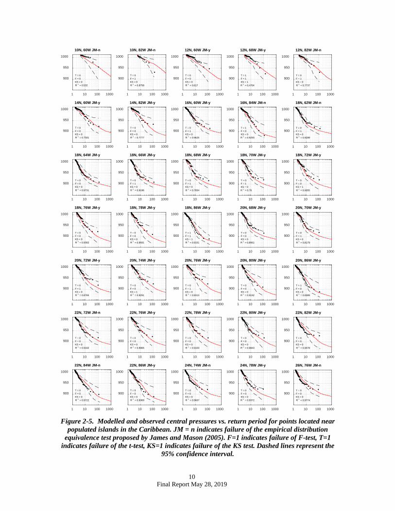
Figure 2-6 presents a qualitative comparison of the modelled and observed extreme
central pressures in the Caribbean. The observed values are presented as contours of the minimum observed central pressure anywhere within 250 km of the indicated point. The modelled values represent the minimum pressures anywhere within 250 km of the indicated point, likely to be exceeded, on average, once every 50 years
10 Final Report May 28, 2019
Figure 2-5. Modelled and observed central pressures vs. return period for points located near
populated islands in the Caribbean. JM = n indicates failure of the empirical distribution equivalence test proposed by James and Mason (2005). F=1 indicates failure of F-test, T=1
indicates failure of the t-test, KS=1 indicates failure of the KS test. Dashed lines represent the 95% confidence interval.
1 10 100 1000
900
950
1000
10N, 60W JM-n
R 2 = 0.532KS = 0F = 0T = 0
1 10 100 1000
900
950
1000
10N, 82W JM-n
R 2 = 0.8758KS = 0F = 1T = 0
1 10 100 1000
900
950
1000
12N, 60W JM-y
R 2 = 0.617KS = 0F = 0T = 0
1 10 100 1000
900
950
1000
12N, 68W JM-y
R 2 = 0.4764KS = 1F = 1T = 1
1 10 100 1000
900
950
1000
12N, 82W JM-n
R 2 = 0.7737KS = 0F = 1T = 0
1 10 100 1000
900
950
1000
14N, 60W JM-y
R 2 = 0.7501KS = 0F = 0T = 0
1 10 100 1000
900
950
1000
14N, 82W JM-y
R 2 = 0.7777KS = 0F = 0T = 0
1 10 100 1000
900
950
1000
16N, 60W JM-y
R 2 = 0.9625KS = 0F = 1T = 0
1 10 100 1000
900
950
1000
16N, 84W JM-n
R 2 = 0.9293KS = 0F = 0T = 1
1 10 100 1000
900
950
1000
18N, 62W JM-n
R 2 = 0.9289KS = 0F = 1T = 0
1 10 100 1000
900
950
1000
18N, 64W JM-y
R 2 = 0.9731KS = 0F = 0T = 0
1 10 100 1000
900
950
1000
18N, 66W JM-y
R 2 = 0.9196KS = 0F = 1T = 0
1 10 100 1000
900
950
1000
18N, 68W JM-y
R 2 = 0.7654KS = 0F = 1T = 0
1 10 100 1000
900
950
1000
18N, 70W JM-y
R 2 = 0.76KS = 0F = 1T = 0
1 10 100 1000
900
950
1000
18N, 72W JM-y
R 2 = 0.9355KS = 1F = 0T = 0
1 10 100 1000
900
950
1000
18N, 76W JM-y
R 2 = 0.9302KS = 0F = 0T = 0
1 10 100 1000
900
950
1000
18N, 78W JM-y
R 2 = 0.9591KS = 0F = 0T = 0
1 10 100 1000
900
950
1000
18N, 86W JM-y
R 2 = 0.9151KS = 1F = 1T = 1
1 10 100 1000
900
950
1000
20N, 68W JM-y
R 2 = 0.8561KS = 0F = 0T = 0
1 10 100 1000
900
950
1000
20N, 70W JM-y
R 2 = 0.8179KS = 0F = 1T = 0
1 10 100 1000
900
950
1000
20N, 72W JM-y
R 2 = 0.8765KS = 0F = 1T = 0
1 10 100 1000
900
950
1000
20N, 74W JM-y
R 2 = 0.9291KS = 1F = 0T = 0
1 10 100 1000
900
950
1000
20N, 76W JM-y
R 2 = 0.8313KS = 0F = 1T = 0
1 10 100 1000
900
950
1000
20N, 80W JM-y
R 2 = 0.9192KS = 0F = 0T = 0
1 10 100 1000
900
950
1000
20N, 86W JM-y
R 2 = 0.8389KS = 0F = 0T = 1
1 10 100 1000
900
950
1000
22N, 72W JM-n
R 2 = 0.9102KS = 0F = 0T = 0
1 10 100 1000
900
950
1000
22N, 76W JM-y
R 2 = 0.8966KS = 0F = 0T = 0
1 10 100 1000
900
950
1000
22N, 78W JM-y
R 2 = 0.9103KS = 0F = 0T = 0
1 10 100 1000
900
950
1000
22N, 80W JM-y
R 2 = 0.9843KS = 0F = 0T = 0
1 10 100 1000
900
950
1000
22N, 82W JM-y
R 2 = 0.9478KS = 0F = 0T = 0
1 10 100 1000
900
950
1000
22N, 84W JM-n
R 2 = 0.9722KS = 0F = 0T = 0
1 10 100 1000
900
950
1000
22N, 86W JM-y
R 2 = 0.8369KS = 0F = 0T = 0
1 10 100 1000
900
950
1000
24N, 74W JM-n
R 2 = 0.9607KS = 0F = 0T = 0
1 10 100 1000
900
950
1000
24N, 78W JM-y
R 2 = 0.9372KS = 0F = 0T = 0
1 10 100 1000
900
950
1000
26N, 76W JM-n
R 2 = 0.9774KS = 0F = 0T = 0
11 Final Report May 28, 2019
The effective period of record for the historical data is not known since there are relatively few pressure measurements in the Caribbean basin prior to the ~1970’s, and at any given location the minimum pressure represents the minimum value obtained during a period varying from perhaps 30 or 40 years long to, at most, about 100 years long. Qualitatively, the comparison shows that the model reproduces the region of intense hurricanes passing to the south of the Greater Antilles and up through the Yucatan Channel. The magnitude of the modelled 50 year return period pressures are similar to the observed values, but reflect the smoothing expected for predicted mean values rather than single point observations from a ~50 year record. The increase in hurricane central pressure near the south east end of Cuba is not as pronounced in the model estimates suggesting that south-east Cuba has been lucky during the short period of record, or the model may be overestimating the intensity of hurricanes in this area.
Figure 2-6. Contour plots of observed (upper plot) minimum central pressures and modelled
50 year return period pressures (lower plot). Contours represent the minimum pressure (mbar) anywhere within 250 km of a point.
890
890
890
900
900
900
900
900910
910
910
910
910
910 910
920
920
920
920
920
920
920
920
920 920
920930
930
930
930
930
930
940
940
940
940
940
950
950 950
950950960
960960
970970
970
970
980
980
980
990
990
9901000
890
890
890
900
900
900
900
910
910
910
910
910
910
910
910
910
920
920920
920
920 920
920
930
930930
930
940
940940 940
950
950 950 950
960
960 960960
970970
970
980
980 980990
990
12 Final Report May 28, 2019
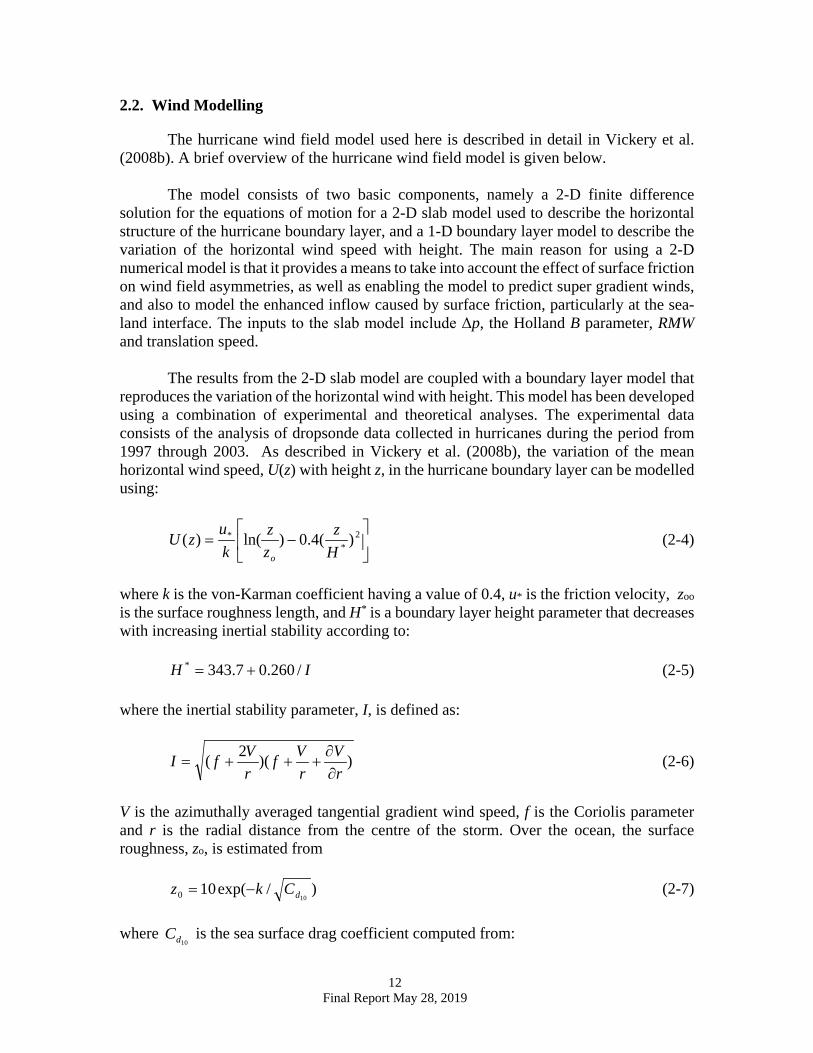
2.2. Wind Modelling
The hurricane wind field model used here is described in detail in Vickery et al. (2008b). A brief overview of the hurricane wind field model is given below.
The model consists of two basic components, namely a 2-D finite difference
solution for the equations of motion for a 2-D slab model used to describe the horizontal structure of the hurricane boundary layer, and a 1-D boundary layer model to describe the variation of the horizontal wind speed with height. The main reason for using a 2-D numerical model is that it provides a means to take into account the effect of surface friction on wind field asymmetries, as well as enabling the model to predict super gradient winds, and also to model the enhanced inflow caused by surface friction, particularly at the sea-land interface. The inputs to the slab model include Δp, the Holland B parameter, RMW and translation speed.
The results from the 2-D slab model are coupled with a boundary layer model that
reproduces the variation of the horizontal wind with height. This model has been developed using a combination of experimental and theoretical analyses. The experimental data consists of the analysis of dropsonde data collected in hurricanes during the period from 1997 through 2003. As described in Vickery et al. (2008b), the variation of the mean horizontal wind speed, U(z) with height z, in the hurricane boundary layer can be modelled using:
−= 2
** )(4.0)ln()(
Hz
zz
kuzU
o
(2-4)
where k is the von-Karman coefficient having a value of 0.4, u* is the friction velocity, zoo is the surface roughness length, and H* is a boundary layer height parameter that decreases with increasing inertial stability according to:
IH /260.07.343* += (2-5) where the inertial stability parameter, I, is defined as:
))(2(rV
rVf
rVfI
∂∂
+++= (2-6)
V is the azimuthally averaged tangential gradient wind speed, f is the Coriolis parameter and r is the radial distance from the centre of the storm. Over the ocean, the surface roughness, zo, is estimated from
)/exp(10100 dCkz −= (2-7)
where
10dC is the sea surface drag coefficient computed from:
13 Final Report May 28, 2019
310))10(065.049.0(10
−+= UCd ; max10 dd CC ≤ (2-8a)
410)66.170881.0(
max
−+= rCd ; 0025.00019.0max
≤≤ dC (2-8b) where r is the radial distance from the storm centre (km), but r is constrained to have a minimum value equal to the RMW. The limiting value of the sea surface drag coefficient used in the wind field model differs from that used in Vickery et al. (2000b) and Vickery and Skerlj (2000), where Cd continues to increase with wind speed. The effect of limiting Cd is to place a limit on the aerodynamic roughness of the ocean, and thus unlike the wind field model described in Vickery et al. (2000b), the model used here does not yield aerodynamic roughness values over the open ocean that approach those of open terrain values in high winds. This limiting, or capping, of the sea surface drag coefficient is discussed further in Powell et al. (2003) and Donelan et al. (2004). The consequences of the reduced, or limited, drag coefficient with respect to the calculation of wind loads using ASCE 7 is discussed in Simiu et al. (2007), where it is indicated that the use of exposure D for the design of structures near the hurricane coastline is appropriate.
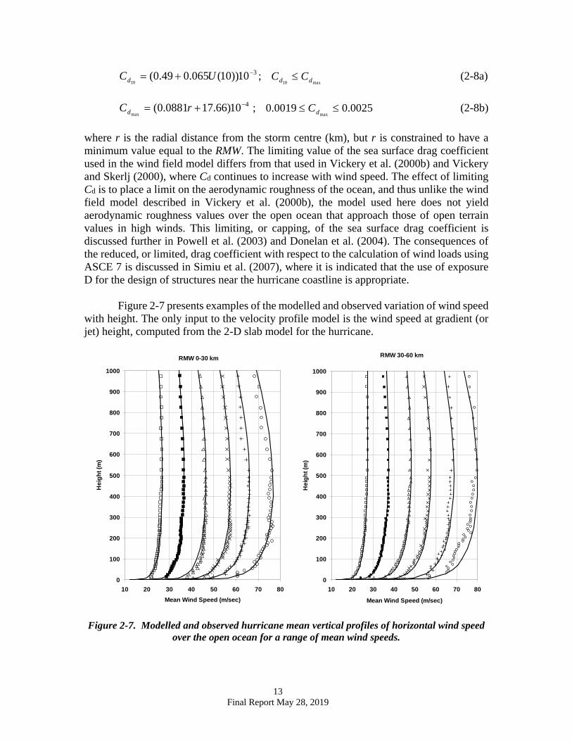
Figure 2-7 presents examples of the modelled and observed variation of wind speed
with height. The only input to the velocity profile model is the wind speed at gradient (or jet) height, computed from the 2-D slab model for the hurricane.
Figure 2-7. Modelled and observed hurricane mean vertical profiles of horizontal wind speed
over the open ocean for a range of mean wind speeds.
RMW 30-60 km
0
100
200
300
400
500
600
700
800
900
1000
10 20 30 40 50 60 70 80
Mean Wind Speed (m/sec)
Hei
ght (
m)
RMW 0-30 km
0
100
200
300
400
500
600
700
800
900
1000
10 20 30 40 50 60 70 80Mean Wind Speed (m/sec)
Hei
ght (
m)
14 Final Report May 28, 2019
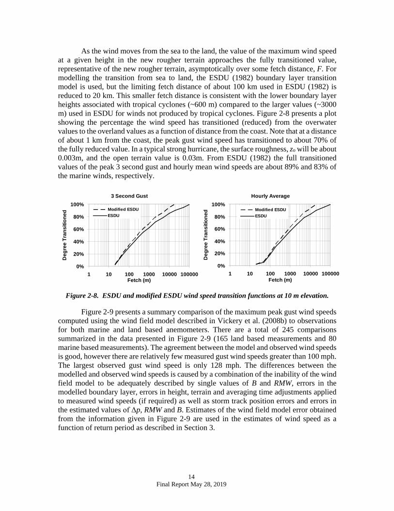
As the wind moves from the sea to the land, the value of the maximum wind speed at a given height in the new rougher terrain approaches the fully transitioned value, representative of the new rougher terrain, asymptotically over some fetch distance, F. For modelling the transition from sea to land, the ESDU (1982) boundary layer transition model is used, but the limiting fetch distance of about 100 km used in ESDU (1982) is reduced to 20 km. This smaller fetch distance is consistent with the lower boundary layer heights associated with tropical cyclones (~600 m) compared to the larger values (~3000 m) used in ESDU for winds not produced by tropical cyclones. Figure 2-8 presents a plot showing the percentage the wind speed has transitioned (reduced) from the overwater values to the overland values as a function of distance from the coast. Note that at a distance of about 1 km from the coast, the peak gust wind speed has transitioned to about 70% of the fully reduced value. In a typical strong hurricane, the surface roughness, zo will be about 0.003m, and the open terrain value is 0.03m. From ESDU (1982) the full transitioned values of the peak 3 second gust and hourly mean wind speeds are about 89% and 83% of the marine winds, respectively.
Figure 2-8. ESDU and modified ESDU wind speed transition functions at 10 m elevation.
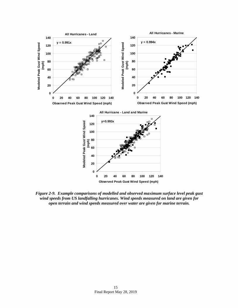
Figure 2-9 presents a summary comparison of the maximum peak gust wind speeds computed using the wind field model described in Vickery et al. (2008b) to observations for both marine and land based anemometers. There are a total of 245 comparisons summarized in the data presented in Figure 2-9 (165 land based measurements and 80 marine based measurements). The agreement between the model and observed wind speeds is good, however there are relatively few measured gust wind speeds greater than 100 mph. The largest observed gust wind speed is only 128 mph. The differences between the modelled and observed wind speeds is caused by a combination of the inability of the wind field model to be adequately described by single values of B and RMW, errors in the modelled boundary layer, errors in height, terrain and averaging time adjustments applied to measured wind speeds (if required) as well as storm track position errors and errors in the estimated values of Δp, RMW and B. Estimates of the wind field model error obtained from the information given in Figure 2-9 are used in the estimates of wind speed as a function of return period as described in Section 3.
Hourly Average
0%
20%
40%
60%
80%
100%
1 10 100 1000 10000 100000Fetch (m)
Deg
ree
Tran
sitio
ned Modified ESDU
ESDU
3 Second Gust
0%
20%
40%
60%
80%
100%
1 10 100 1000 10000 100000Fetch (m)
Deg
ree
Tran
sitio
ned Modified ESDU
ESDU
15 Final Report May 28, 2019
Figure 2-9. Example comparisons of modelled and observed maximum surface level peak gust
wind speeds from US landfalling hurricanes. Wind speeds measured on land are given for open terrain and wind speeds measured over water are given for marine terrain.
All Hurricanes - Marine
y = 0.994x
0
20
40
60
80
100
120
140
0 20 40 60 80 100 120 140Observed Peak Gust Wind Speed (mph)
Mod
eled
Pea
k G
ust W
ind
Spee
d (m
ph)
All Hurricanes - Land
y = 0.991x
0
20
40
60
80
100
120
140
0 20 40 60 80 100 120 140Observed Peak Gust Wind Speed (mph)
Mod
eled
Pea
k G
ust W
ind
Spee
d (m
ph)
All Hurricane - Land and Marine
y=0.993x
0
20
40
60
80
100
120
140
0 20 40 60 80 100 120 140Observed Peak Gust Wind Speed (mph)
Mod
eled
Pea
k G
ust W
ind
Spee
d (m
ph)
16 Final Report May 28, 2019
3. DESIGN WIND SPEEDS
The hurricane simulation model described in Section 2 was used to develop estimates of peak gust wind speeds as a function of return period in the Caribbean. All speeds are produced as values associated with a 3 second gust wind speed at a height of 10 m in flat open terrain. For buildings located near the coast, the wind speeds presented herein should be used with the procedures given in ASCE 7 including the use of Exposure D. The use of exposure D is required because of the limit in the sea surface drag coefficient. The following sections discuss the development of the wind speed maps and the use of the resulting wind speeds in conjunction with the wind load provisions as given in ASCE 7-10 and later. 3.1 Design Wind Speed Maps
Predictions of wind speed as a function of return period at any point in the Caribbean are obtained using the hurricane simulation model described in Section 2 using a 100,000 year simulation of hurricanes. Upon completion of the 100,000-year simulation, the wind speed data are rank ordered and then used to define the wind speed probability distribution, P(v>V), conditional on a storm having passed within 250 km of the site and producing a peak gust wind speed of at least 20 mph. The wind speed associated with a given exceedance probability is obtained by interpolating from the rank ordered wind speed data. The probability that the tropical cyclone wind speed (independent of direction) is exceeded during time period t is,
∑∞
=
<−=>0
)()|(1)(x
tt xpxVvPVvP (3-1)
where )|( xVvP < is the probability that the velocity v is less than V given that x storms occur, and pt(x) is the probability of x storms occurring during time period t. From Equation 3-1, with pt(x) defined as having a Poisson distribution and defining t as one year, the annual probability of exceeding a given wind speed is,
)](exp[1)( VvPVvPa >−−=> λ (3-2)
where λ (annual occurrence rate) represents the average annual number of storms approaching within 250 km of the site and producing a minimum 20 mph peak gust wind speed, and )( VvP > is the probability that the velocity v is greater than V given the occurrence of any one storm.
In order to develop wind speed contours for use in the Caribbean basin, we developed contour maps of wind speeds using a nominal 1 km grid. For the large Islands, the grid resolution was reduced for distances greater than 5 km form the coast. The coarsest inland grid was 10 km. Each grid point contains information on the distance to the coast for all (36) directions.
17 Final Report May 28, 2019
Wind speeds were predicted for return periods of 300, 700 1,700 and 3,000 years. At each location the effect of wind field modelling uncertainty was included, as is the case with the ASCE 7-10 and ASCE 7-16 winds. The inclusion of the wind field modelling uncertainty results in an increase in the predicted wind speeds compared to the case where wind field model uncertainty is not included. The magnitude of the increased wind speeds increases with increasing return period, where the 50-, 100-, 700- and 1,700-year return period wind speeds are, on average about 1%, 2%, 4% and 5%, respectively, higher than those obtained without considering uncertainty.
The resulting hurricane hazard maps are presented in Figure 3-1 through Figure
3-48. The Figures present contour maps of 3-second gust wind speeds at a height of 10 m over flat open terrain, consistent with those presented in ASCE 7-10 and ASCE 7-16 and the upcoming ASCE 7-22.
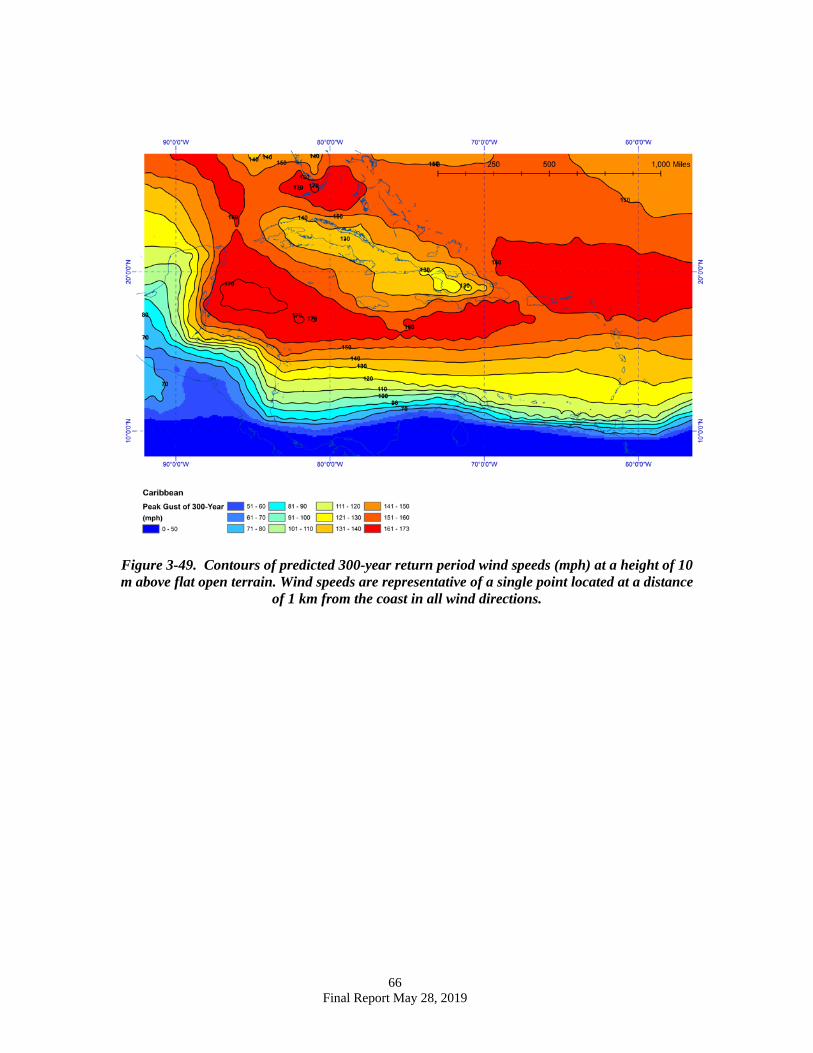
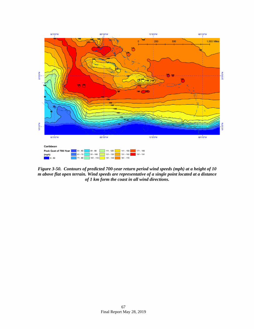
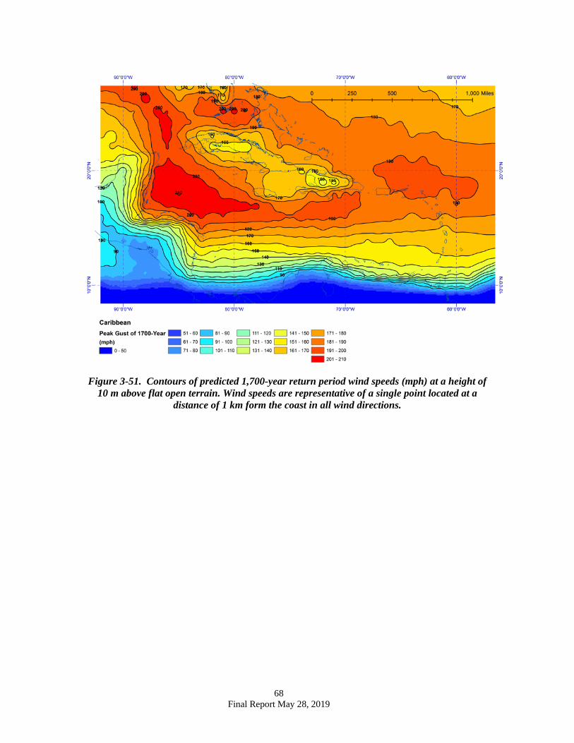
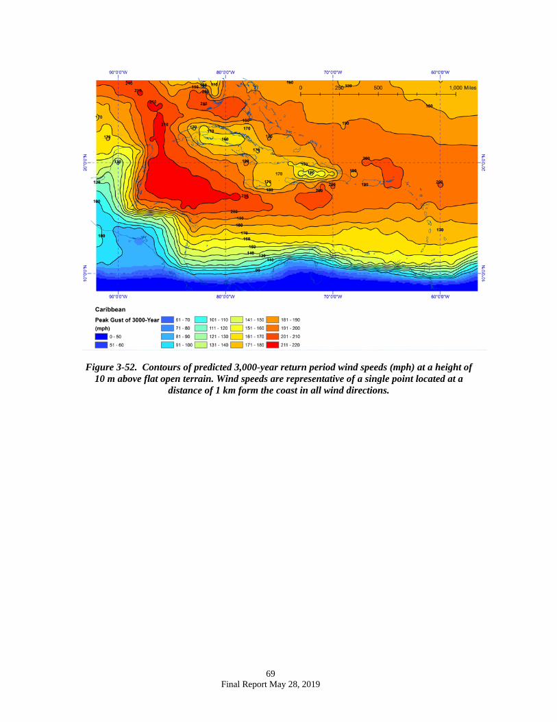
An overall depiction of the variation in the tropical cyclone wind speed hazard over
the Caribbean is presented in Figure 3-49 through Figure 3-52. The wind speed contours depicted in Figure 3-49 through Figure 3-52 were developed using a 1 degree by 1-degree grid of points, with each point representative of the centre of a small circular island with a distance of 1 km from the coast in all directions, even if the actual point is located on a larger island. Decreases in wind speeds seen on some of the larger islands are due to the weakening of the hurricanes as they travel over the islands.
18 Final Report May 28, 2019
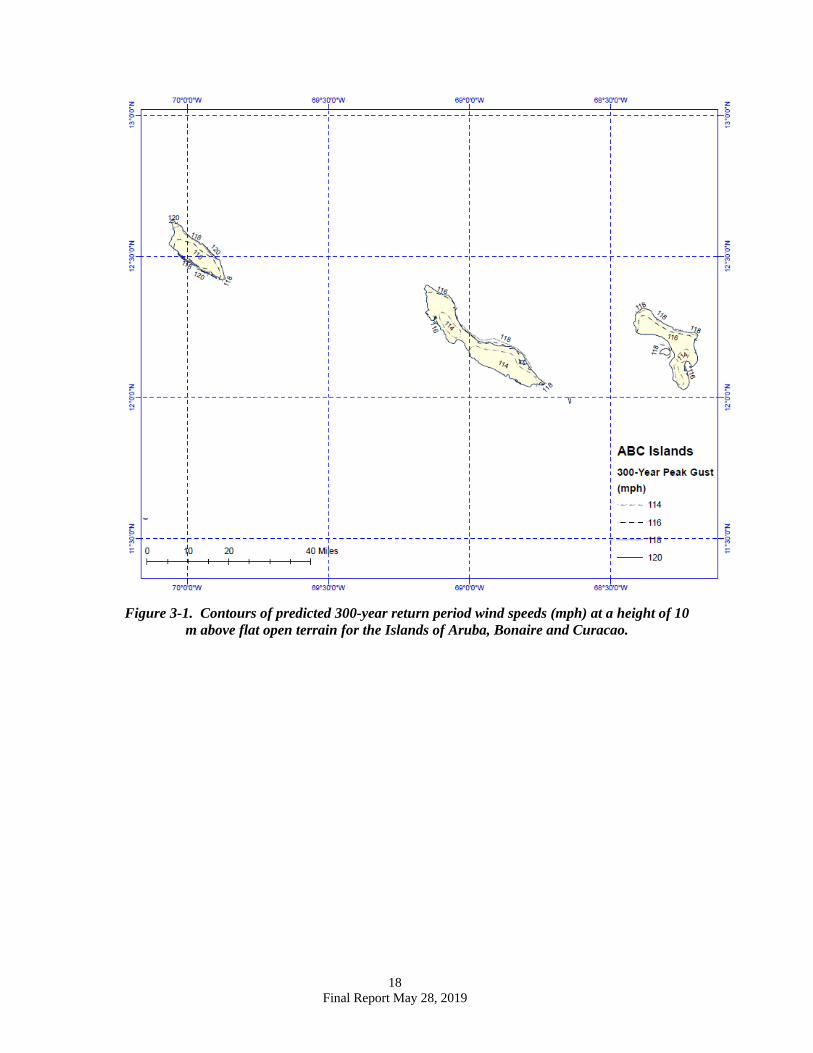
Figure 3-1. Contours of predicted 300-year return period wind speeds (mph) at a height of 10
m above flat open terrain for the Islands of Aruba, Bonaire and Curacao.
19 Final Report May 28, 2019
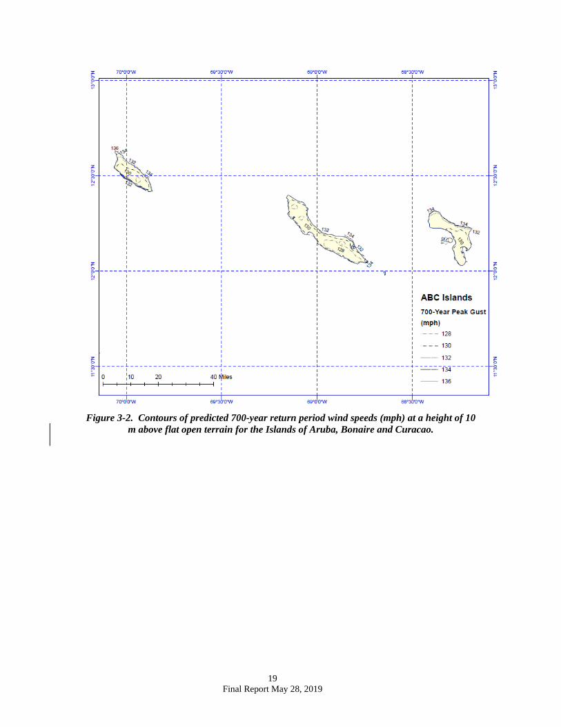
Figure 3-2. Contours of predicted 700-year return period wind speeds (mph) at a height of 10
m above flat open terrain for the Islands of Aruba, Bonaire and Curacao.
20 Final Report May 28, 2019
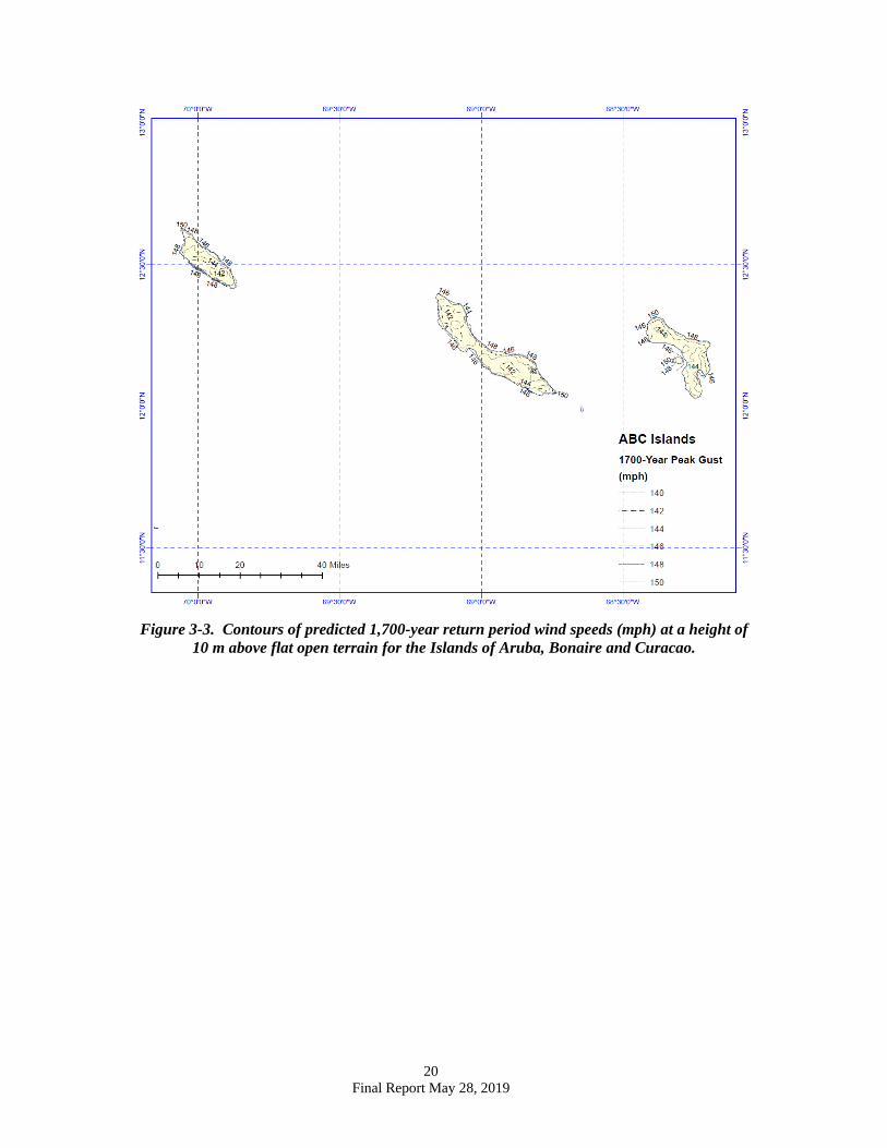
Figure 3-3. Contours of predicted 1,700-year return period wind speeds (mph) at a height of
10 m above flat open terrain for the Islands of Aruba, Bonaire and Curacao.
21 Final Report May 28, 2019
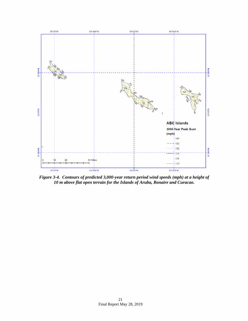
Figure 3-4. Contours of predicted 3,000-year return period wind speeds (mph) at a height of
10 m above flat open terrain for the Islands of Aruba, Bonaire and Curacao.
22 Final Report May 28, 2019
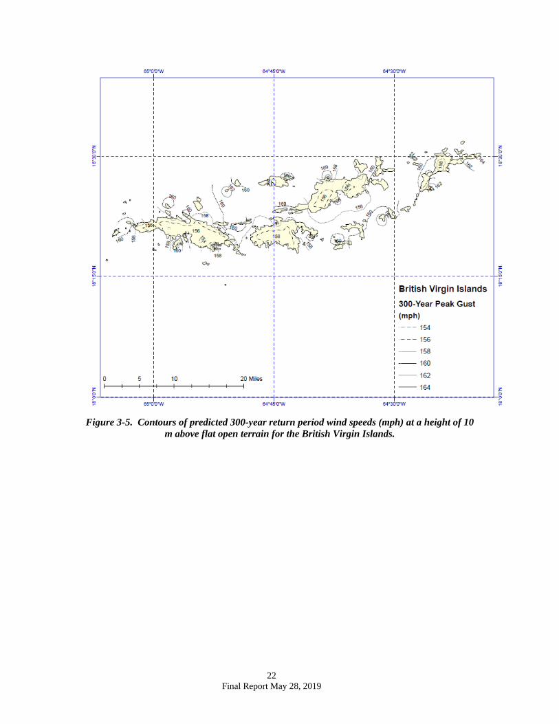
Figure 3-5. Contours of predicted 300-year return period wind speeds (mph) at a height of 10
m above flat open terrain for the British Virgin Islands.
23 Final Report May 28, 2019
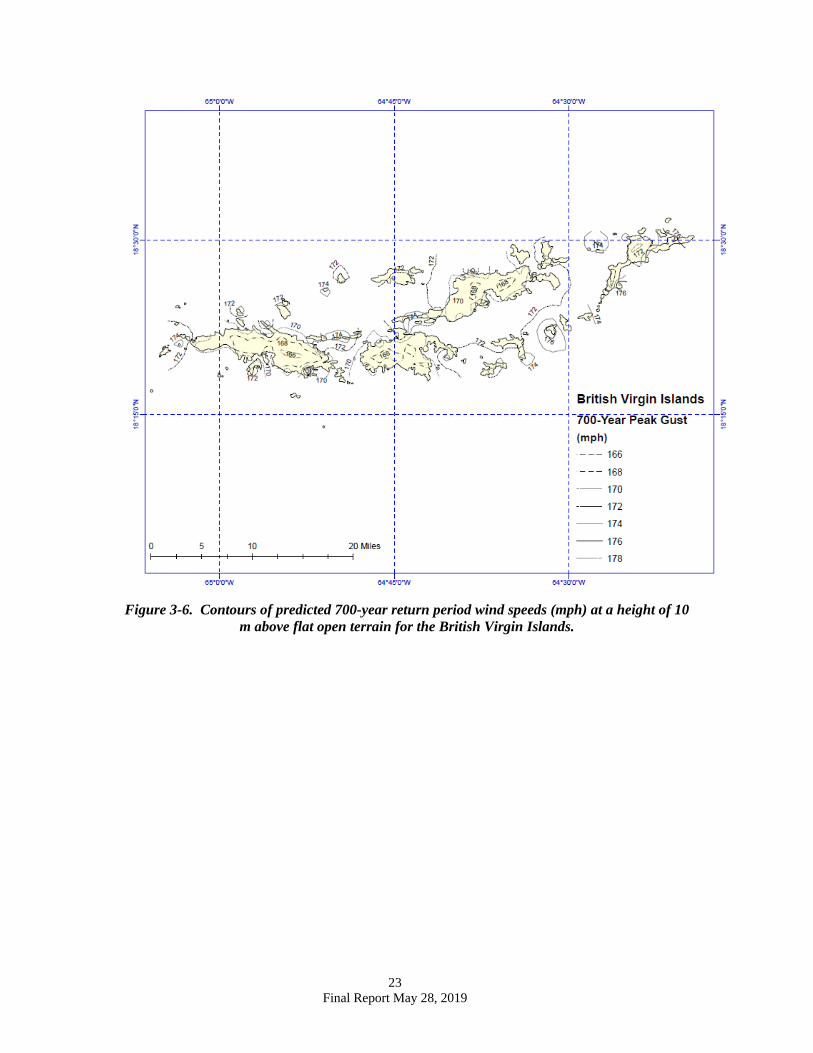
Figure 3-6. Contours of predicted 700-year return period wind speeds (mph) at a height of 10
m above flat open terrain for the British Virgin Islands.
24 Final Report May 28, 2019
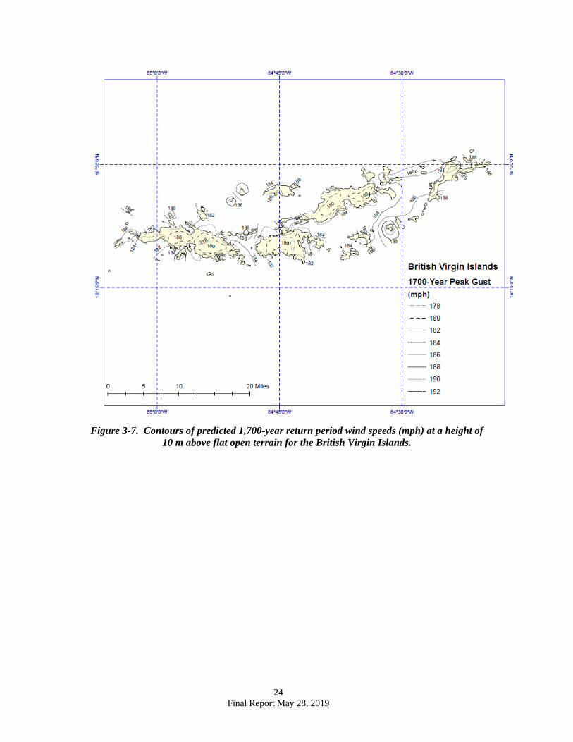
Figure 3-7. Contours of predicted 1,700-year return period wind speeds (mph) at a height of
10 m above flat open terrain for the British Virgin Islands.
25 Final Report May 28, 2019
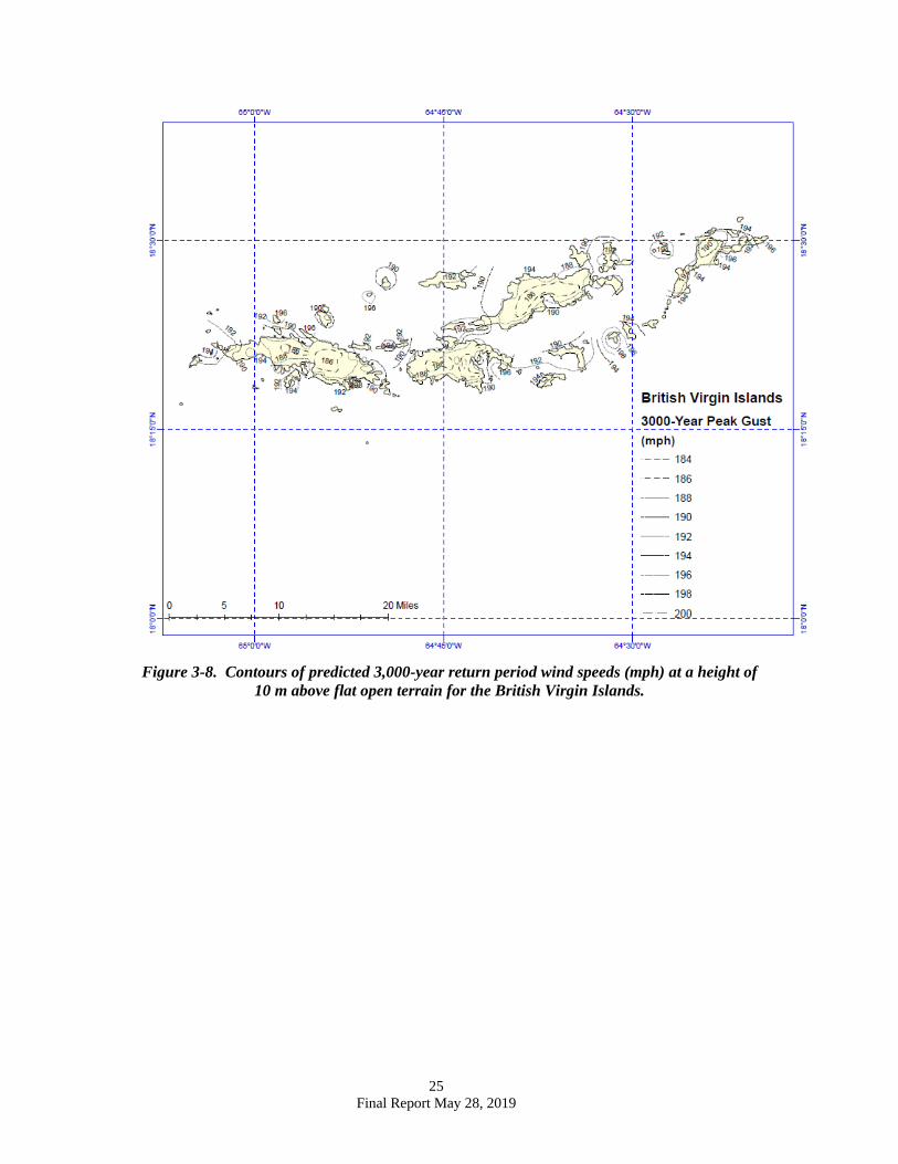
Figure 3-8. Contours of predicted 3,000-year return period wind speeds (mph) at a height of
10 m above flat open terrain for the British Virgin Islands.
26 Final Report May 28, 2019
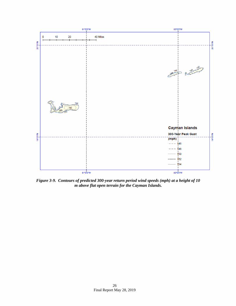
Figure 3-9. Contours of predicted 300-year return period wind speeds (mph) at a height of 10
m above flat open terrain for the Cayman Islands.
27 Final Report May 28, 2019
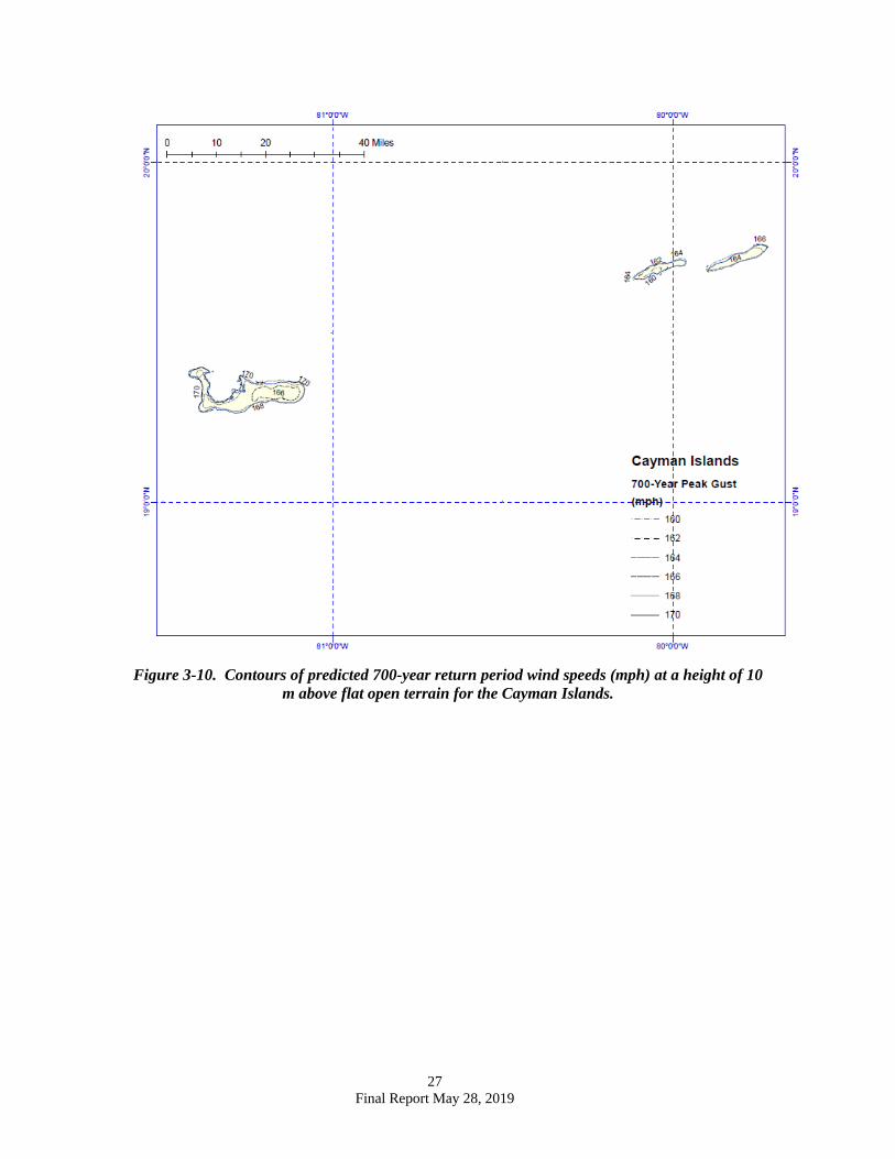
Figure 3-10. Contours of predicted 700-year return period wind speeds (mph) at a height of 10
m above flat open terrain for the Cayman Islands.
28 Final Report May 28, 2019
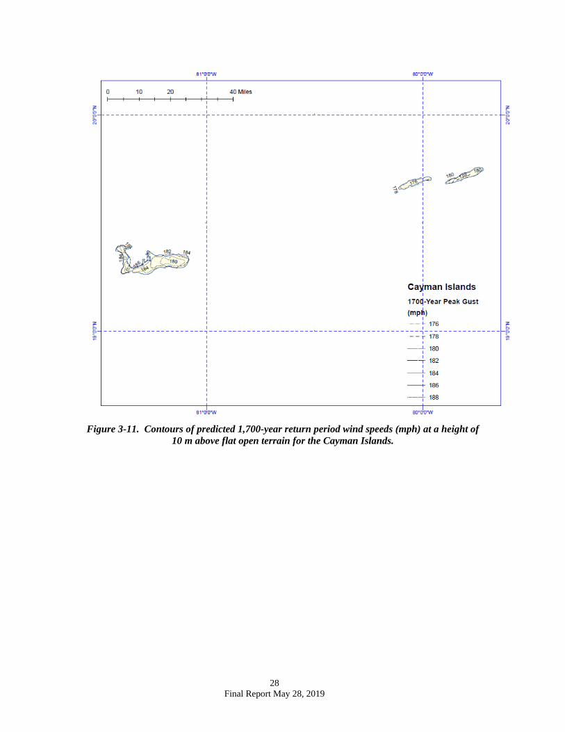
Figure 3-11. Contours of predicted 1,700-year return period wind speeds (mph) at a height of
10 m above flat open terrain for the Cayman Islands.
29 Final Report May 28, 2019
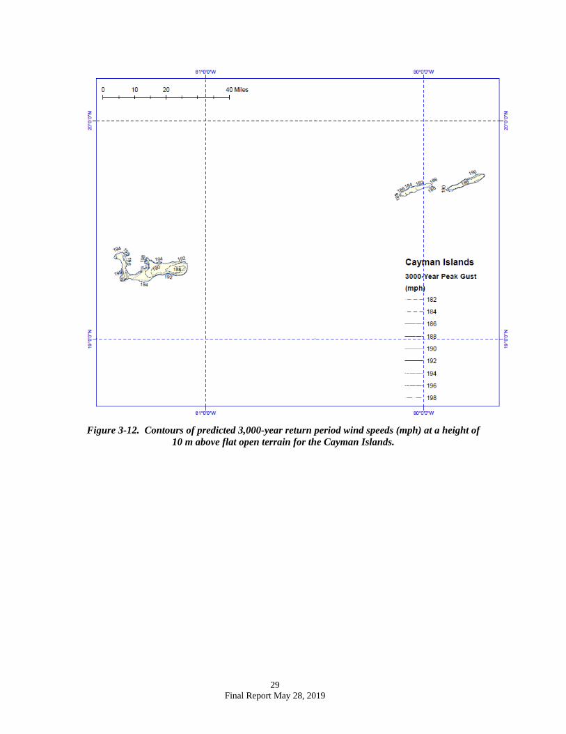
Figure 3-12. Contours of predicted 3,000-year return period wind speeds (mph) at a height of
10 m above flat open terrain for the Cayman Islands.
30 Final Report May 28, 2019
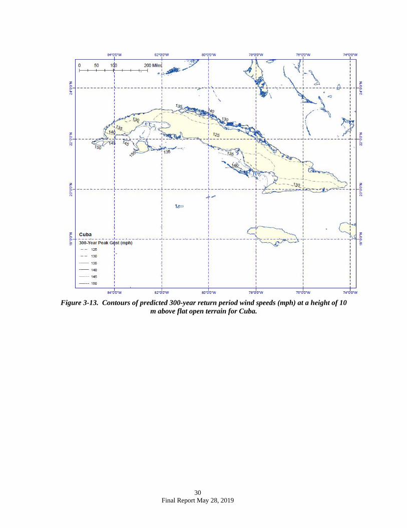
Figure 3-13. Contours of predicted 300-year return period wind speeds (mph) at a height of 10
m above flat open terrain for Cuba.
31 Final Report May 28, 2019
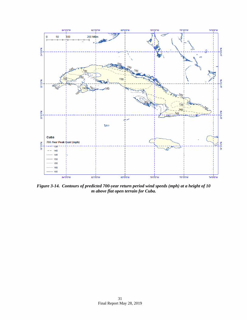
Figure 3-14. Contours of predicted 700-year return period wind speeds (mph) at a height of 10
m above flat open terrain for Cuba.
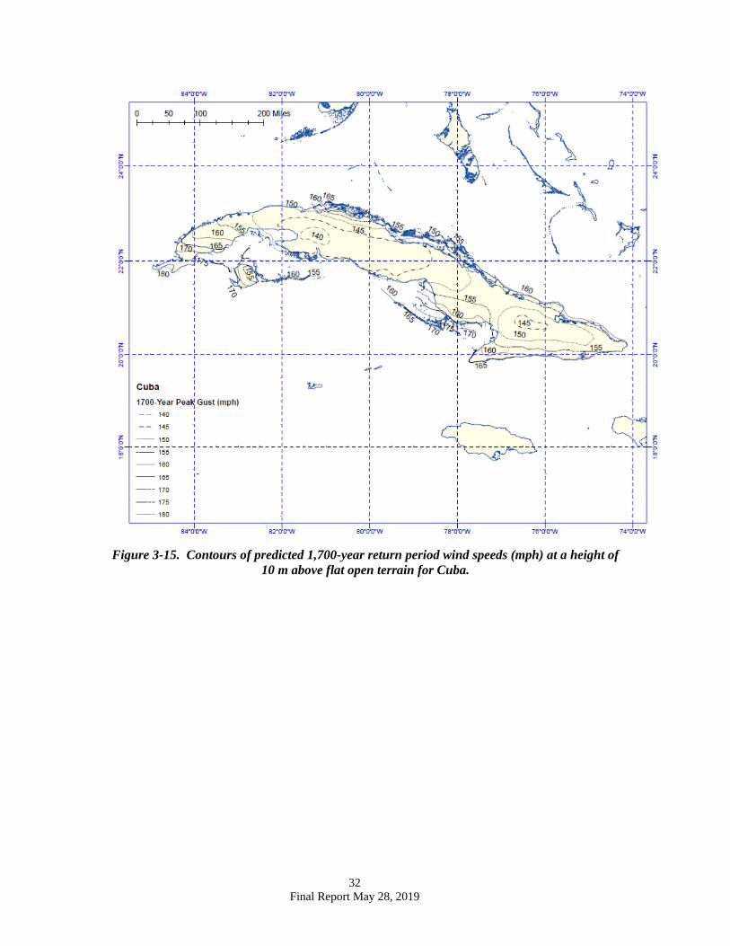
32 Final Report May 28, 2019
Figure 3-15. Contours of predicted 1,700-year return period wind speeds (mph) at a height of
10 m above flat open terrain for Cuba.
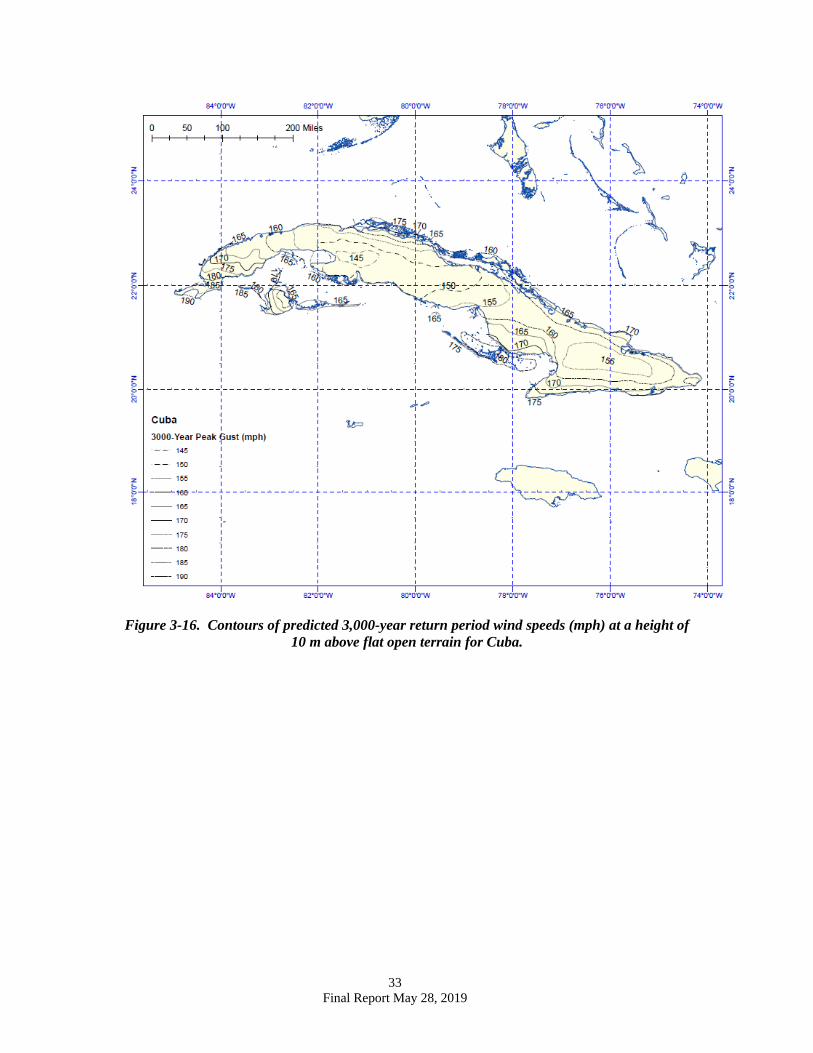
33 Final Report May 28, 2019
Figure 3-16. Contours of predicted 3,000-year return period wind speeds (mph) at a height of
10 m above flat open terrain for Cuba.
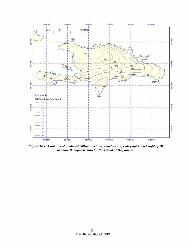
34 Final Report May 28, 2019
Figure 3-17. Contours of predicted 300-year return period wind speeds (mph) at a height of 10
m above flat open terrain for the Island of Hispaniola.

35 Final Report May 28, 2019
Figure 3-18. Contours of predicted 700-year return period wind speeds (mph) at a height of 10
m above flat open terrain for the Island of Hispaniola.
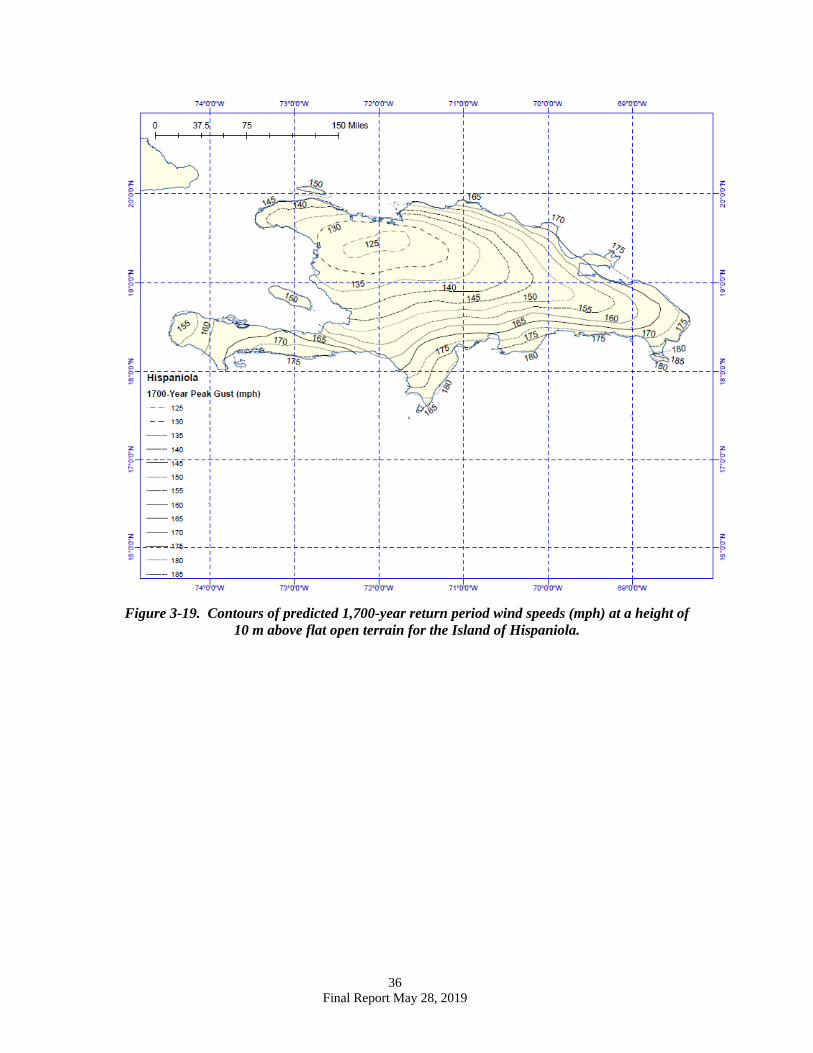
36 Final Report May 28, 2019
Figure 3-19. Contours of predicted 1,700-year return period wind speeds (mph) at a height of
10 m above flat open terrain for the Island of Hispaniola.
37 Final Report May 28, 2019
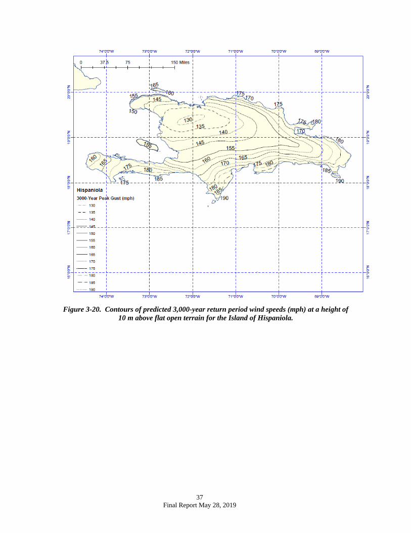
Figure 3-20. Contours of predicted 3,000-year return period wind speeds (mph) at a height of
10 m above flat open terrain for the Island of Hispaniola.
38 Final Report May 28, 2019
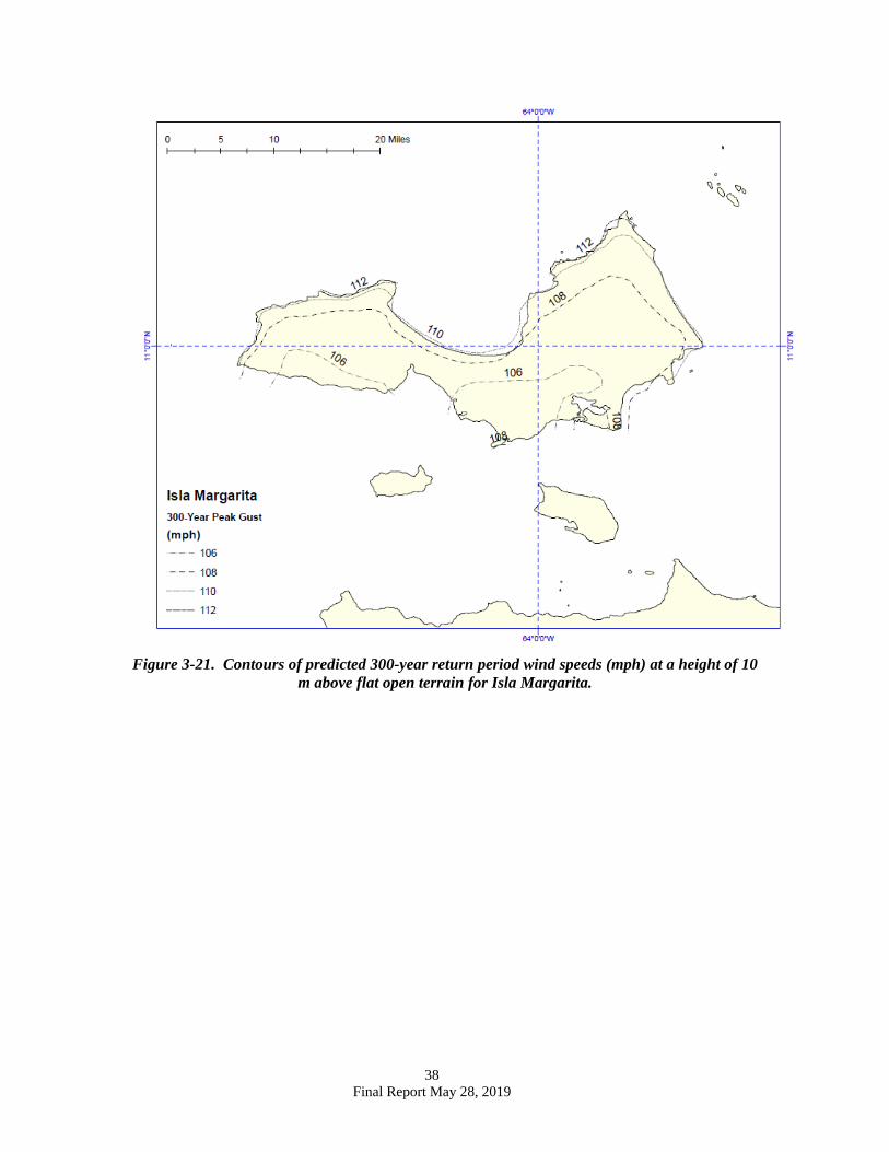
Figure 3-21. Contours of predicted 300-year return period wind speeds (mph) at a height of 10
m above flat open terrain for Isla Margarita.
39 Final Report May 28, 2019
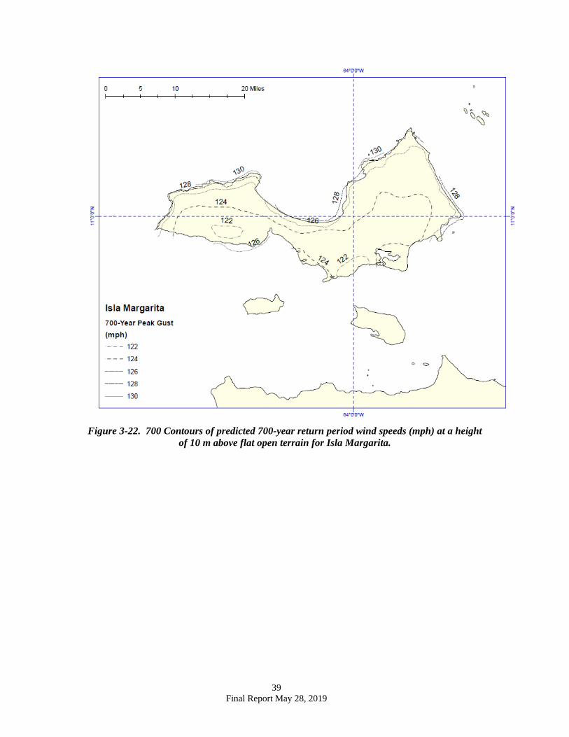
Figure 3-22. 700 Contours of predicted 700-year return period wind speeds (mph) at a height
of 10 m above flat open terrain for Isla Margarita.
40 Final Report May 28, 2019
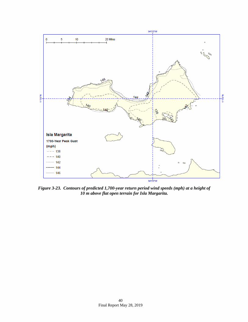
Figure 3-23. Contours of predicted 1,700-year return period wind speeds (mph) at a height of
10 m above flat open terrain for Isla Margarita.
41 Final Report May 28, 2019
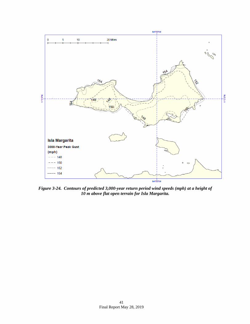
Figure 3-24. Contours of predicted 3,000-year return period wind speeds (mph) at a height of
10 m above flat open terrain for Isla Margarita.
42 Final Report May 28, 2019
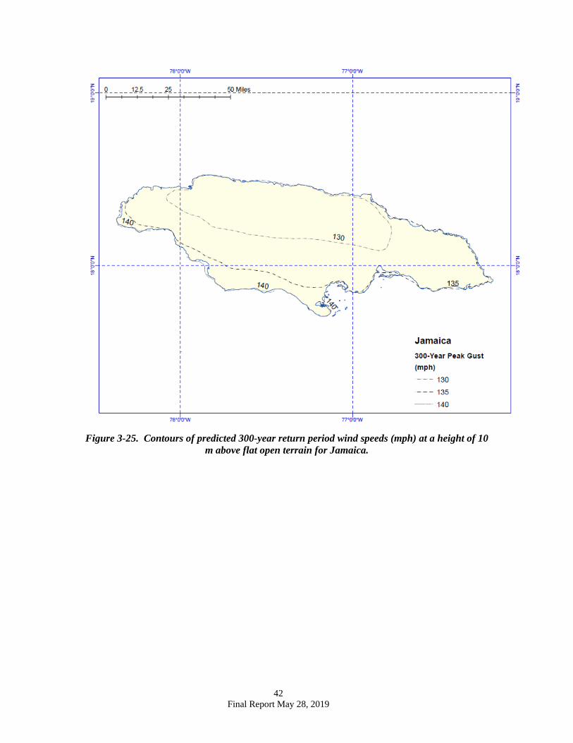
Figure 3-25. Contours of predicted 300-year return period wind speeds (mph) at a height of 10
m above flat open terrain for Jamaica.
43 Final Report May 28, 2019
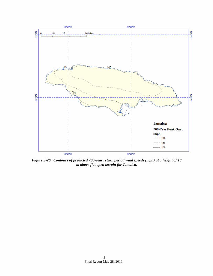
Figure 3-26. Contours of predicted 700-year return period wind speeds (mph) at a height of 10
m above flat open terrain for Jamaica.
44 Final Report May 28, 2019
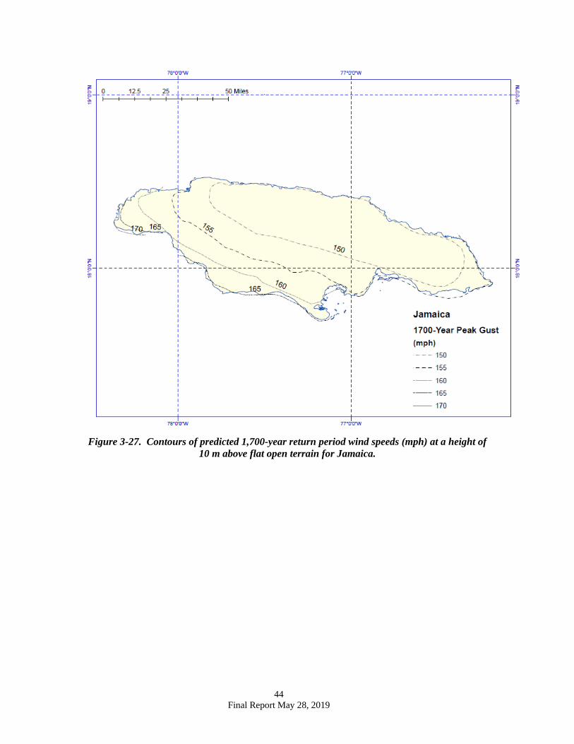
Figure 3-27. Contours of predicted 1,700-year return period wind speeds (mph) at a height of
10 m above flat open terrain for Jamaica.
45 Final Report May 28, 2019
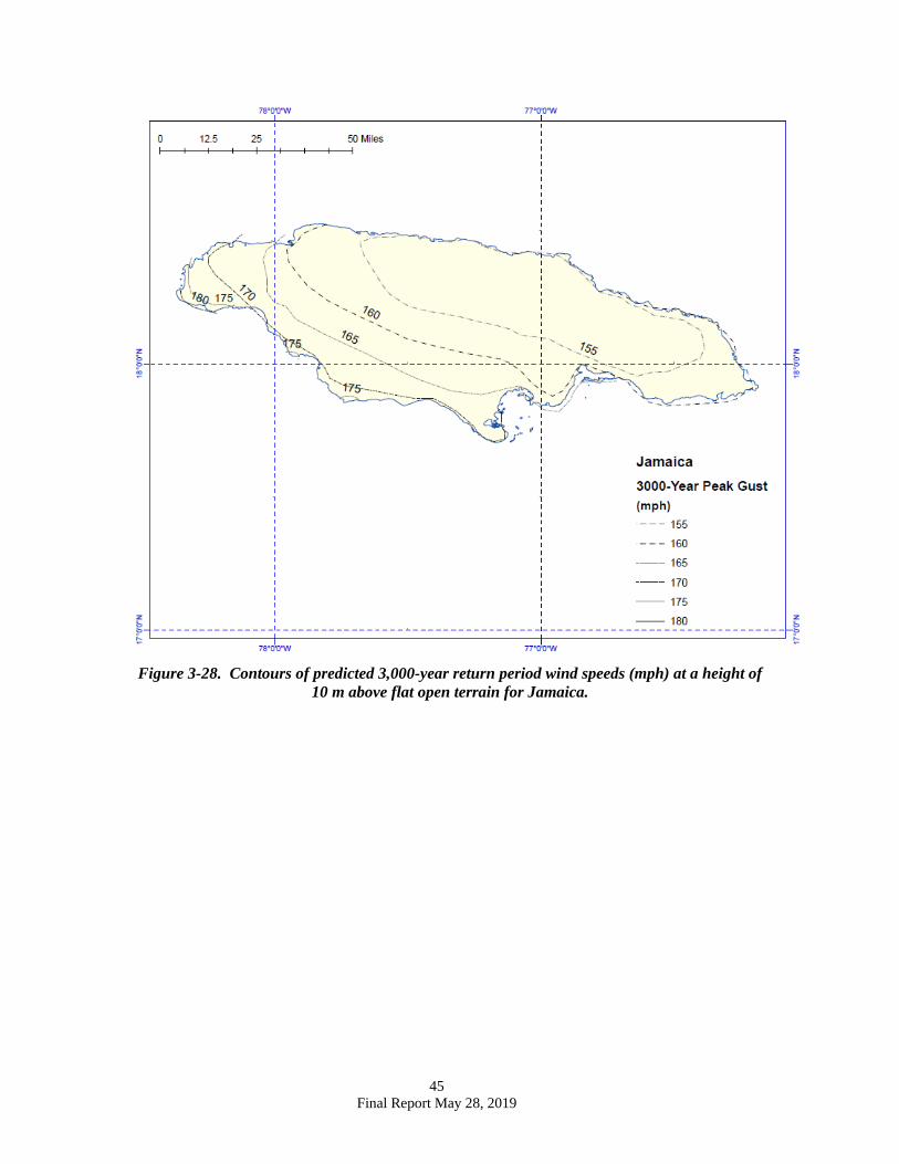
Figure 3-28. Contours of predicted 3,000-year return period wind speeds (mph) at a height of
10 m above flat open terrain for Jamaica.
46 Final Report May 28, 2019
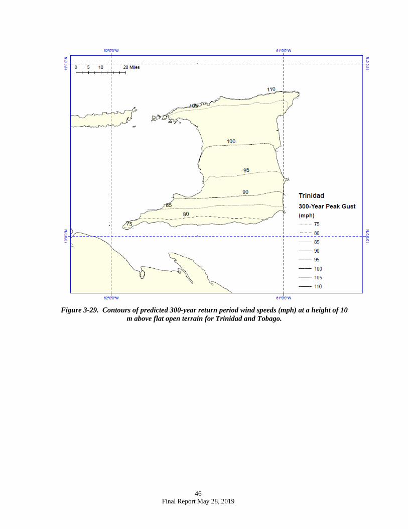
Figure 3-29. Contours of predicted 300-year return period wind speeds (mph) at a height of 10
m above flat open terrain for Trinidad and Tobago.
47 Final Report May 28, 2019
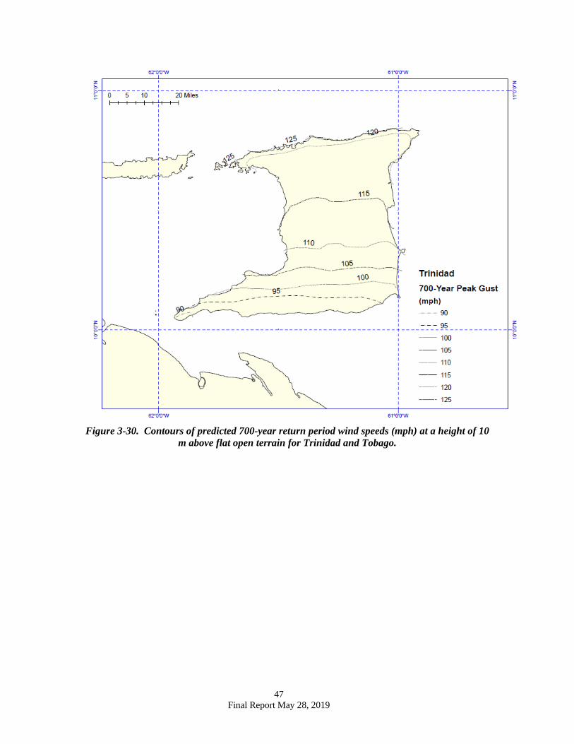
Figure 3-30. Contours of predicted 700-year return period wind speeds (mph) at a height of 10
m above flat open terrain for Trinidad and Tobago.
48 Final Report May 28, 2019
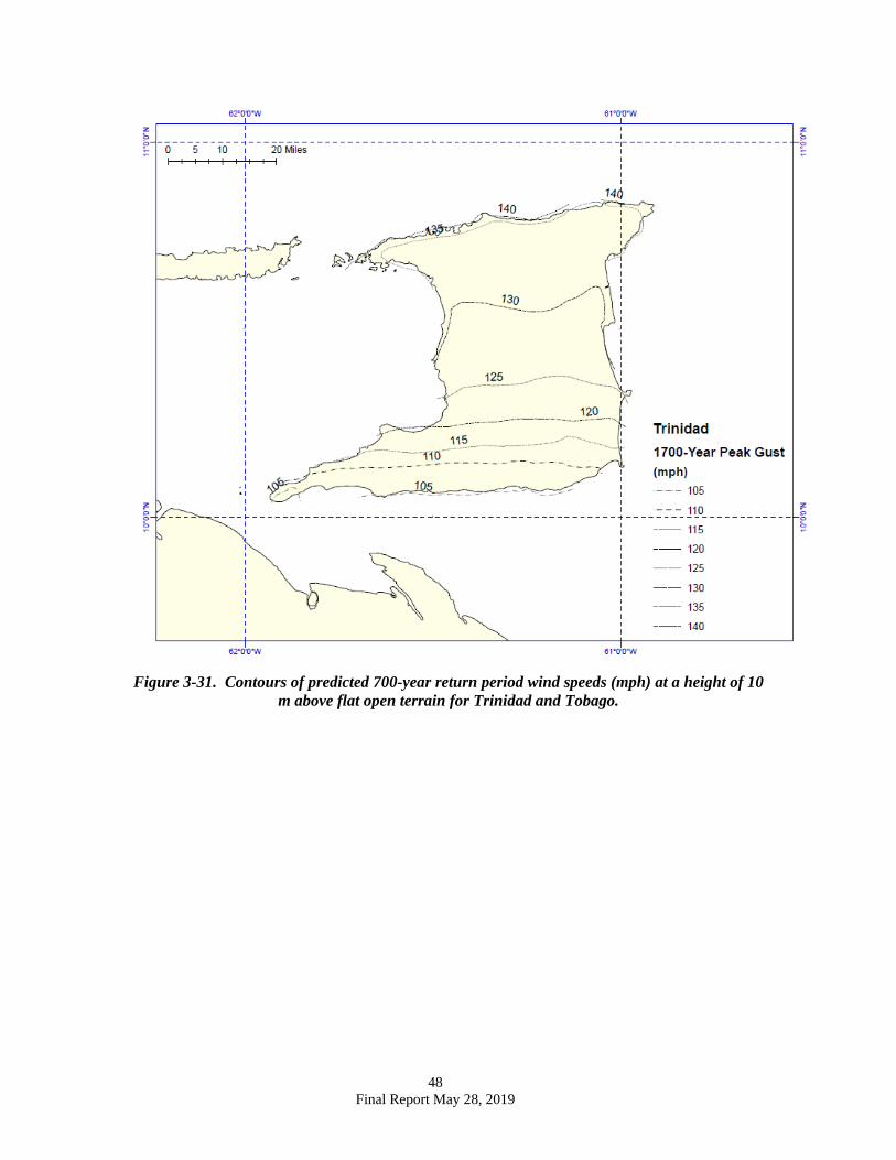
Figure 3-31. Contours of predicted 700-year return period wind speeds (mph) at a height of 10
m above flat open terrain for Trinidad and Tobago.
49 Final Report May 28, 2019
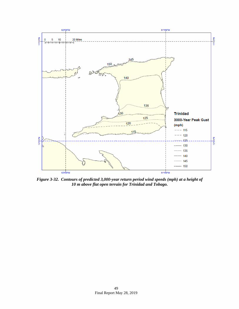
Figure 3-32. Contours of predicted 3,000-year return period wind speeds (mph) at a height of
10 m above flat open terrain for Trinidad and Tobago.
50 Final Report May 28, 2019
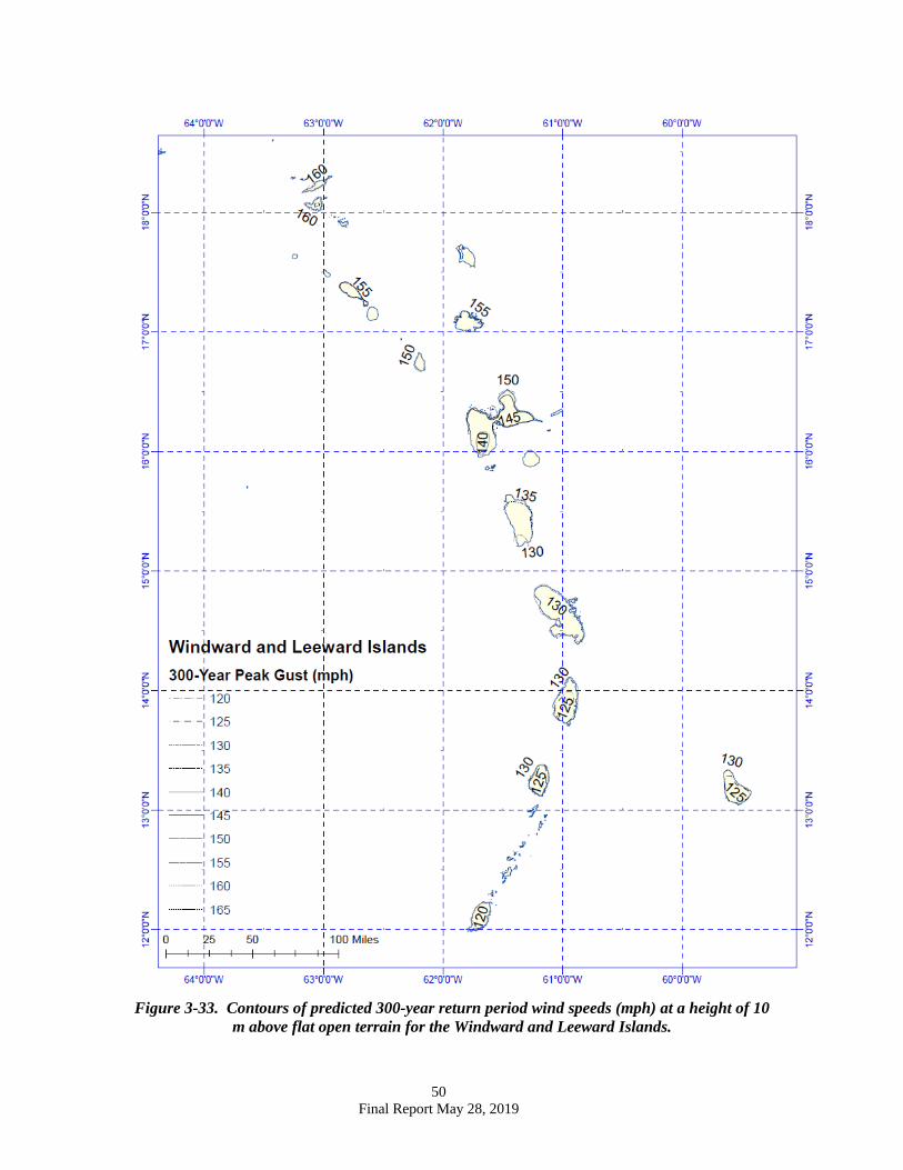
Figure 3-33. Contours of predicted 300-year return period wind speeds (mph) at a height of 10
m above flat open terrain for the Windward and Leeward Islands.
51 Final Report May 28, 2019
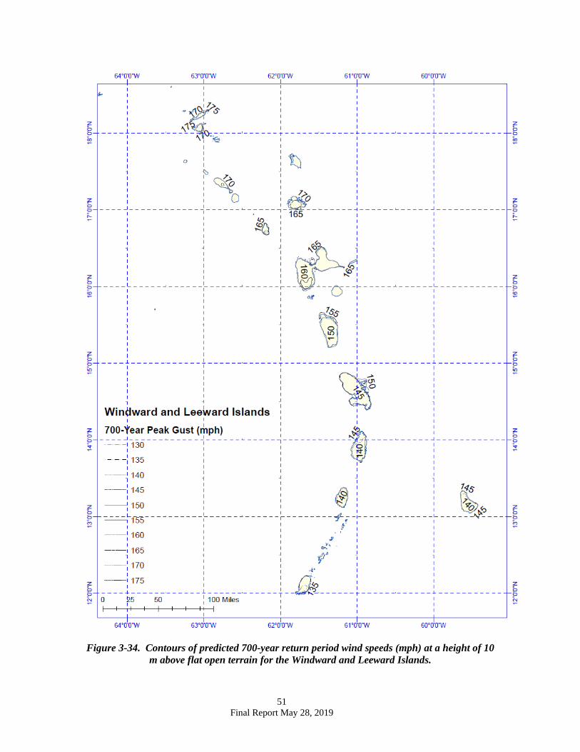
Figure 3-34. Contours of predicted 700-year return period wind speeds (mph) at a height of 10
m above flat open terrain for the Windward and Leeward Islands.
52 Final Report May 28, 2019
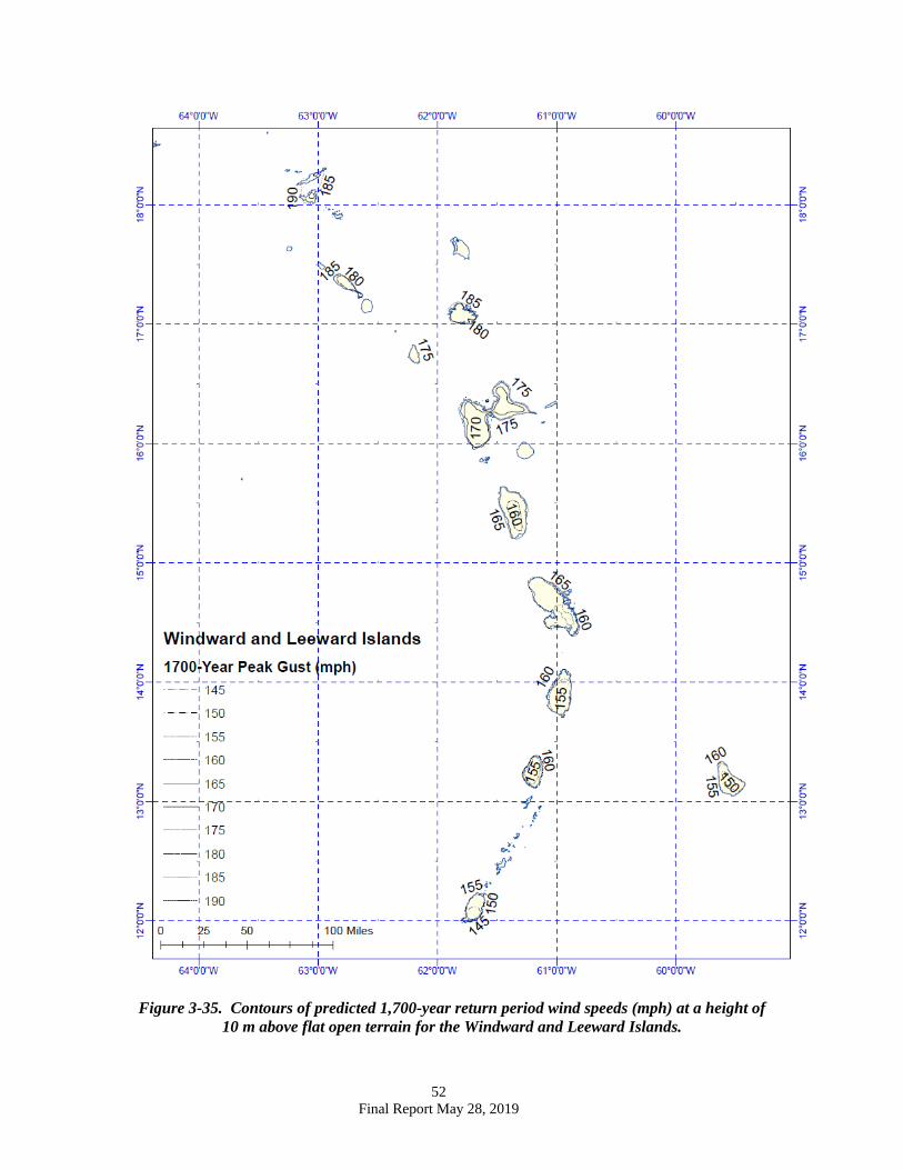
Figure 3-35. Contours of predicted 1,700-year return period wind speeds (mph) at a height of
10 m above flat open terrain for the Windward and Leeward Islands.
53 Final Report May 28, 2019
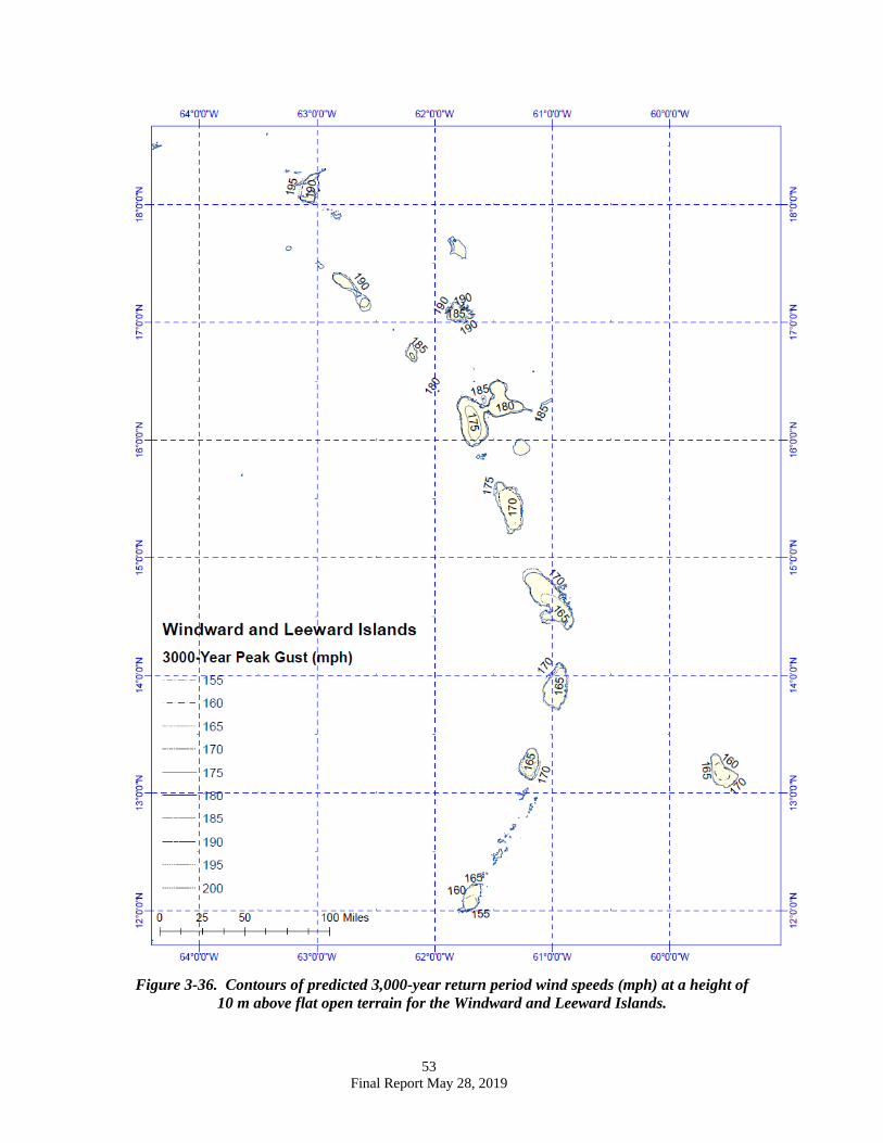
Figure 3-36. Contours of predicted 3,000-year return period wind speeds (mph) at a height of
10 m above flat open terrain for the Windward and Leeward Islands.
54 Final Report May 28, 2019
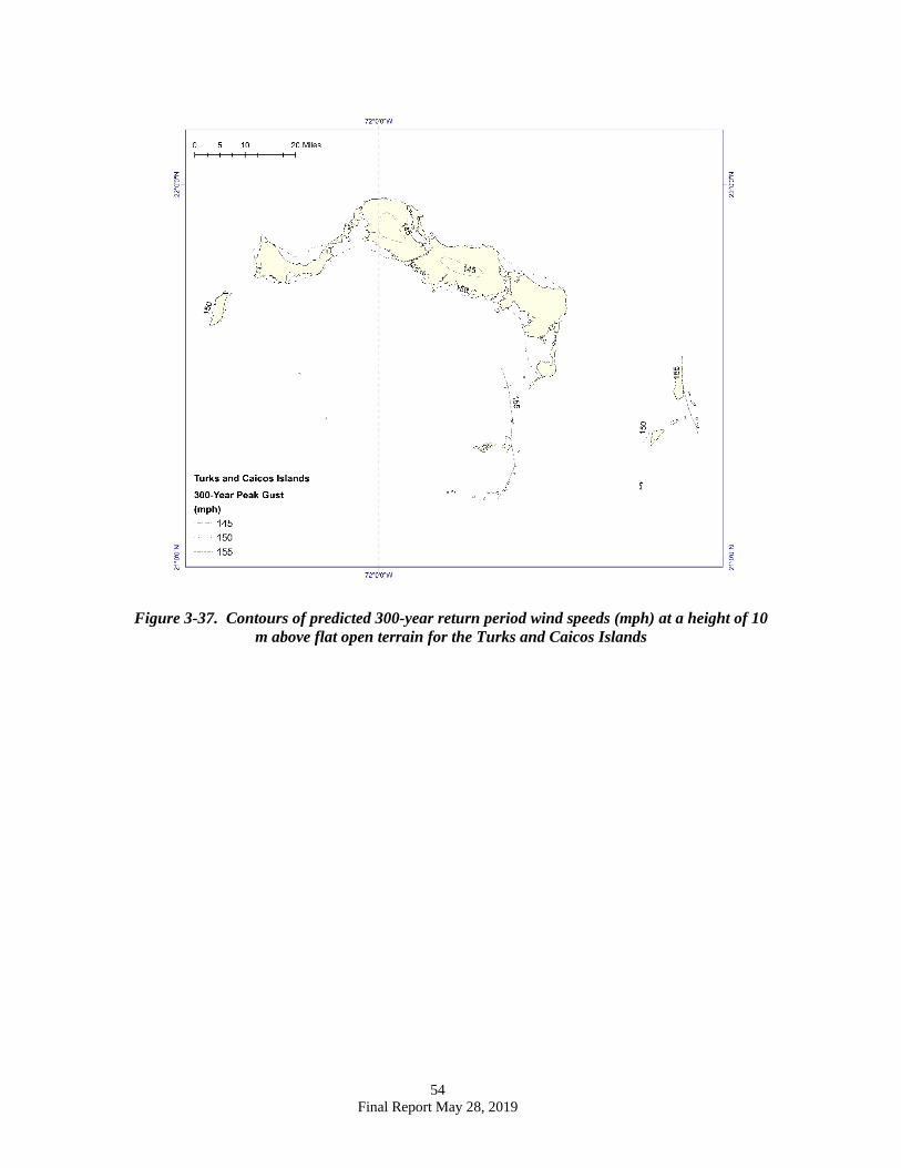
Figure 3-37. Contours of predicted 300-year return period wind speeds (mph) at a height of 10
m above flat open terrain for the Turks and Caicos Islands

55 Final Report May 28, 2019
Figure 3-38. Contours of predicted 700-year return period wind speeds (mph) at a height of 10 m above flat open terrain for the Turks and Caicos Islands
56 Final Report May 28, 2019
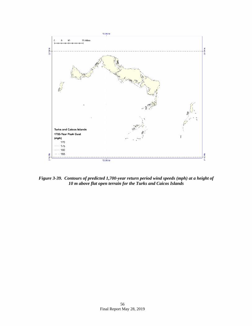
Figure 3-39. Contours of predicted 1,700-year return period wind speeds (mph) at a height of
10 m above flat open terrain for the Turks and Caicos Islands
57 Final Report May 28, 2019
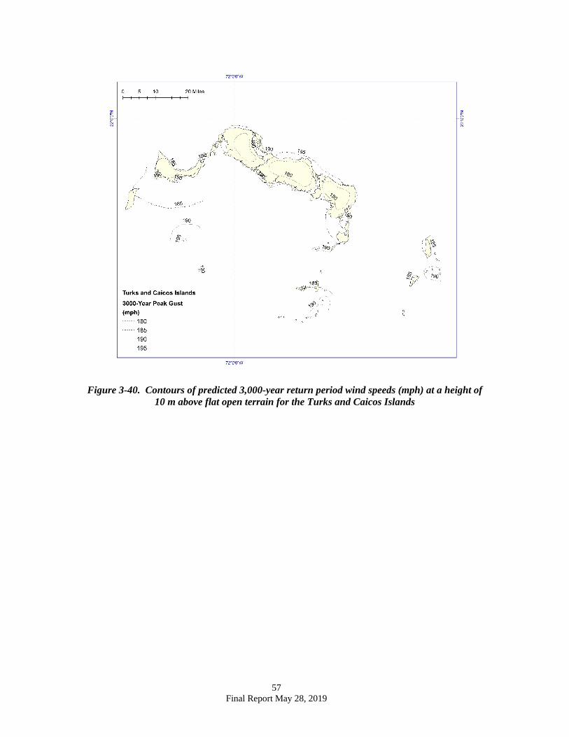
Figure 3-40. Contours of predicted 3,000-year return period wind speeds (mph) at a height of
10 m above flat open terrain for the Turks and Caicos Islands
58 Final Report May 28, 2019
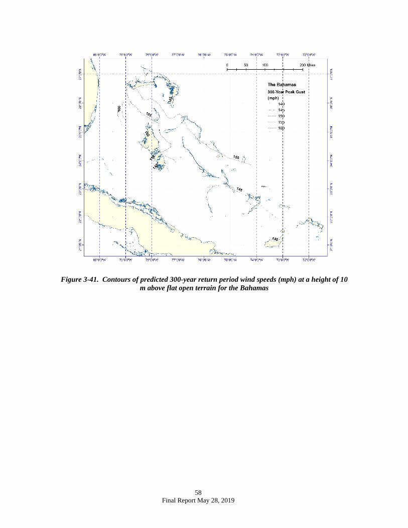
Figure 3-41. Contours of predicted 300-year return period wind speeds (mph) at a height of 10
m above flat open terrain for the Bahamas
59 Final Report May 28, 2019
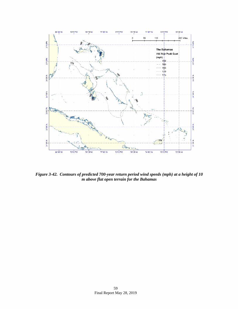
Figure 3-42. Contours of predicted 700-year return period wind speeds (mph) at a height of 10
m above flat open terrain for the Bahamas
60 Final Report May 28, 2019
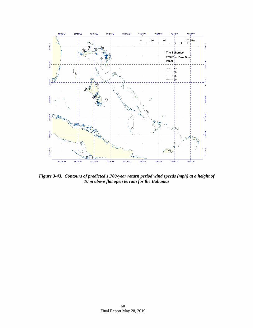
Figure 3-43. Contours of predicted 1,700-year return period wind speeds (mph) at a height of 10 m above flat open terrain for the Bahamas
61 Final Report May 28, 2019
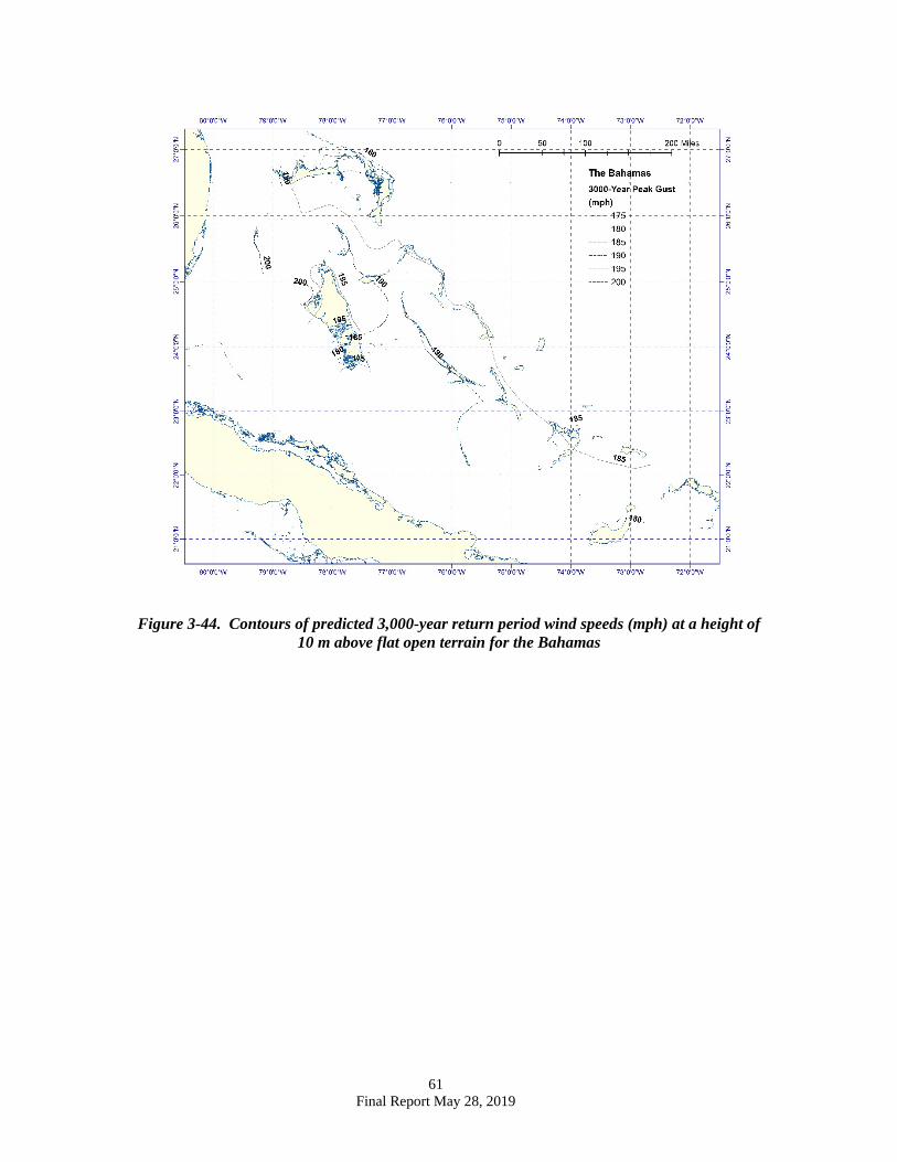
Figure 3-44. Contours of predicted 3,000-year return period wind speeds (mph) at a height of 10 m above flat open terrain for the Bahamas
62 Final Report May 28, 2019
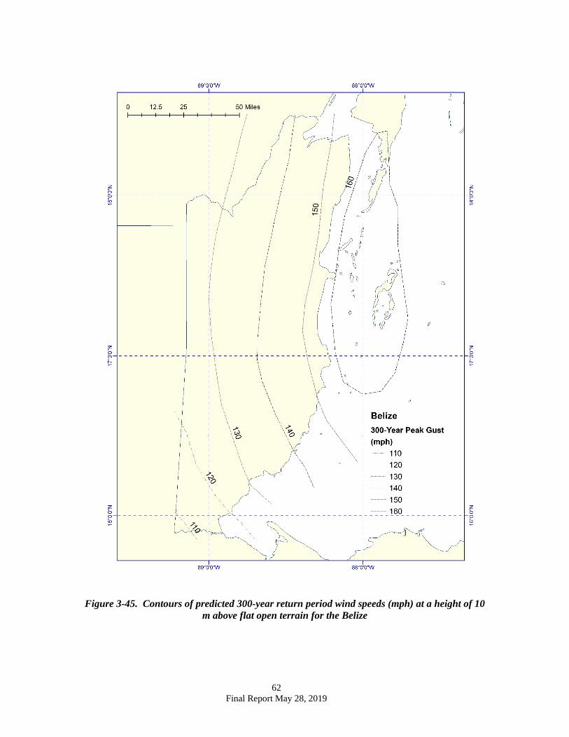
Figure 3-45. Contours of predicted 300-year return period wind speeds (mph) at a height of 10 m above flat open terrain for the Belize
63 Final Report May 28, 2019
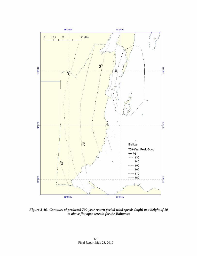
Figure 3-46. Contours of predicted 700-year return period wind speeds (mph) at a height of 10 m above flat open terrain for the Bahamas

64 Final Report May 28, 2019
Figure 3-47. Contours of predicted 1,700-year return period wind speeds (mph) at a height of 10 m above flat open terrain for the Bahamas
65 Final Report May 28, 2019
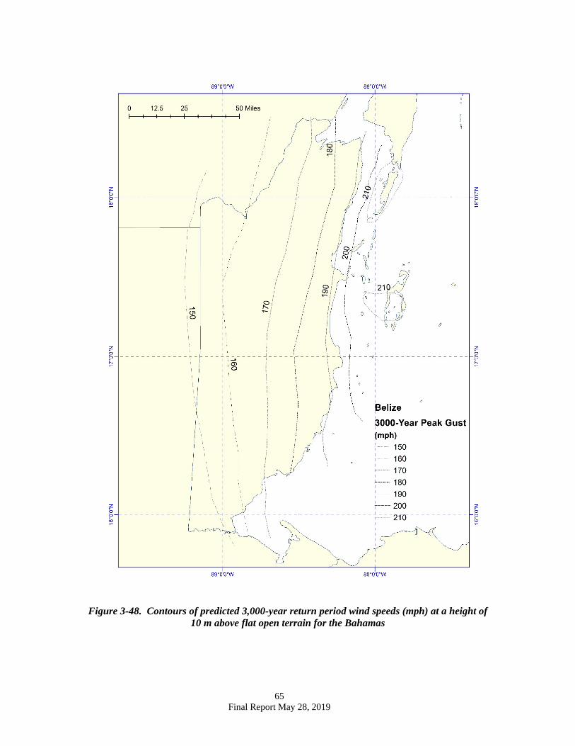
Figure 3-48. Contours of predicted 3,000-year return period wind speeds (mph) at a height of 10 m above flat open terrain for the Bahamas
66 Final Report May 28, 2019
Figure 3-49. Contours of predicted 300-year return period wind speeds (mph) at a height of 10 m above flat open terrain. Wind speeds are representative of a single point located at a distance
of 1 km from the coast in all wind directions.
67 Final Report May 28, 2019
Figure 3-50. Contours of predicted 700-year return period wind speeds (mph) at a height of 10 m above flat open terrain. Wind speeds are representative of a single point located at a distance
of 1 km form the coast in all wind directions.
68 Final Report May 28, 2019
Figure 3-51. Contours of predicted 1,700-year return period wind speeds (mph) at a height of 10 m above flat open terrain. Wind speeds are representative of a single point located at a
distance of 1 km form the coast in all wind directions.
69 Final Report May 28, 2019
Figure 3-52. Contours of predicted 3,000-year return period wind speeds (mph) at a height of 10 m above flat open terrain. Wind speeds are representative of a single point located at a
distance of 1 km form the coast in all wind directions.
70 Final Report May 28, 2019
SUMMARY
Estimates of wind speeds as a function of return period for locations in the Caribbean basin were developed using a peer reviewed hurricane simulation model as described in Vickery et al. (2000a, 2000b, 2009a, 2009b), Vickery and Wadhera, (2008). The hurricane model has been updated to include historical storms through 2017. Using the results of a 100,000-year simulation of tropical cyclones, wind speeds were obtained at grid points in each country being studied. Predictions of hurricane wind speeds as a function of return period were used to produce maps of hurricane wind speeds for return periods of 300-, 700-, 1,700- and 3,000-years. The hurricane simulation model used here is an updated version of that described in Vickery et al. (2009a, 2009b) and Vickery and Wadhera (2008) which was used to produce the design wind speeds used in the ASCE 7-98 through to the ASCE 7-16, the most current version. The wind speeds presented here can be used without modification with the wind loading provisions of ASCE 7-16 and later editions.
All wind speeds presented herein are 3 second gust wind speeds at a height of 10 m in flat open terrain. For buildings located near the coast, the wind speeds presented herein should be used with the procedures given in ASCE 7 including the use of exposure D. The use of exposure D is required because of the limit in the sea surface drag coefficient.
71 Final Report May 28, 2019
5. REFERENCES
Donelan, M.A., B.K. Haus, N. Reul, W.J. Plant, M. Stiassnie, H.C. Graber, O.B. Brown, and E.S. Saltzman, (2004). “On the limiting aerodynamic roughness in the ocean in very strong winds” Geophys. Res. Lett., 31, L18306
Emanuel, K.A, S. Ravela, E. Vivant and C. Risi, (2006), “A statistical–deterministic approach to hurricane risk assessment”, Bull. Amer. Meteor. Soc., 19, 299-314.
ESDU, (1982), “Strong Winds in the Atmospheric Boundary Layer, Part 1: Mean Hourly Wind Speed”, Engineering Sciences Data Unit Item No. 82026, London, England, 1982.
Georgiou, P.N., (1985), “Design Windspeeds in Tropical Cyclone-Prone Regions”, Ph.D. Thesis, Faculty of Engineering Science, University of Western Ontario, London, Ontario, Canada, 1985.
Georgiou, P.N., A.G. Davenport and B.J. Vickery, (1983) “Design wind speeds in regions dominated by tropical cyclones”, 6th International Conference on Wind Engineering, Gold Coast, Australia, 21-25 March and Auckland, New Zealand, 6-7 April.
Holland, G.J., (1980), “An analytic model of the wind and pressure profiles in hurricanes, Mon. Wea. Rev., 108 (1980) 1212-1218.
James, M. K. and L.B. Mason, (2005), “Synthetic tropical cyclone database”, J. Wtrwy, Port, Coast and Oc. Engrg., 131, 181-192
Jarvinen, B.R., C.J. Neumann, and M.A.S. Davis, (1984), “A Tropical Cyclone Data Tape for the North Atlantic Basin 1886-1983: Contents, Limitations and Uses”, NOAA Technical Memorandum NWS NHC 22, U.S. Department of Commerce, March, 1984. DeMaria, M., and J. Kaplan (1999), “An updated Statistical Hurricane Intensity Prediction Scheme (SHIPS) for the Atlantic and Eastern North Pacific Basins”, Weather and Forecasting, 14, 326–337. Powell, M.D., P.J. Vickery, and T.A. Reinhold, (2003), “Reduced drag coefficient for high wind speeds in tropical cyclones”, Nature, 422, 279-283. Simiu, E., P. J. Vickery, and A Kareem, (2007), “Relations between Saffir-Simpson hurricane scale wind speeds and peak 3-s gust speeds over open terrain”, J. Struct. Eng, 133, 1043-1045 Vickery, P.J. and D. Wadhera, (2008), “Statistical models of the Holland pressure profile parameter and radius to maximum winds of hurricanes from flight level pressure and H*wind data.” J. Appl. Meteor., 47, 2497-2517 Vickery, P.J.; D. Wadhera, L.A. Twisdale Jr. and F. M. Lavelle, (2009a). “United States Hurricane Wind Speed Risk and Uncertainty.”. J. Struct. Engrg. 135, 301-320
72 Final Report May 28, 2019
Vickery, P.J., D. Wadhera, M.D. Powell and Y. Chen, (2009b) “A Hurricane Boundary Layer and Wind Field Model for Use in Engineering Applications.” J. Appl. Meteor., 48, 381-405 Vickery, P.J., J. X. Lin, P. F. Skerlj, and L. A. Twisdale Jr., (2006), “The HAZUS-MH hurricane model methodology part I: Hurricane hazard, terrain and wind load modelling”, Nat. Hazards Rev., 7, 82-93 Vickery, P.J., (2005), “Simple empirical models for estimating the increase in the central pressure of tropical cyclones after landfall along the coastline of the United States”, J. Appl. Meteor., 44, 1807-1826. Vickery, P.J., P.F. Skerlj and L.A. Twisdale Jr., (2000a) “Simulation of hurricane risk in the U.S. using an empirical track model,” J. Struct. Eng., 126, 1222-1237 Vickery, P.J., P.F. Skerlj, A.C. Steckley and L.A. Twisdale Jr., (2000b) Hurricane wind field model for use in hurricane simulations, J. Struct. Eng., 126. 1203-1221 Vickery, P.J. and P.F. Skerlj, (2000), “Elimination of exposure D along hurricane coastline in ASCE 7”, J. Struct. Eng.. 126, 545-549 Vickery, P.J., and L.A. Twisdale, (1995), “Prediction of hurricane wind speeds in the U.S.,” J. Struct. Eng., 121, 1691-1699
A-1
Appendix A
Comparisons of modelled and observed cumulative frequency distributions of central pressure, heading, and translational speed
A-2
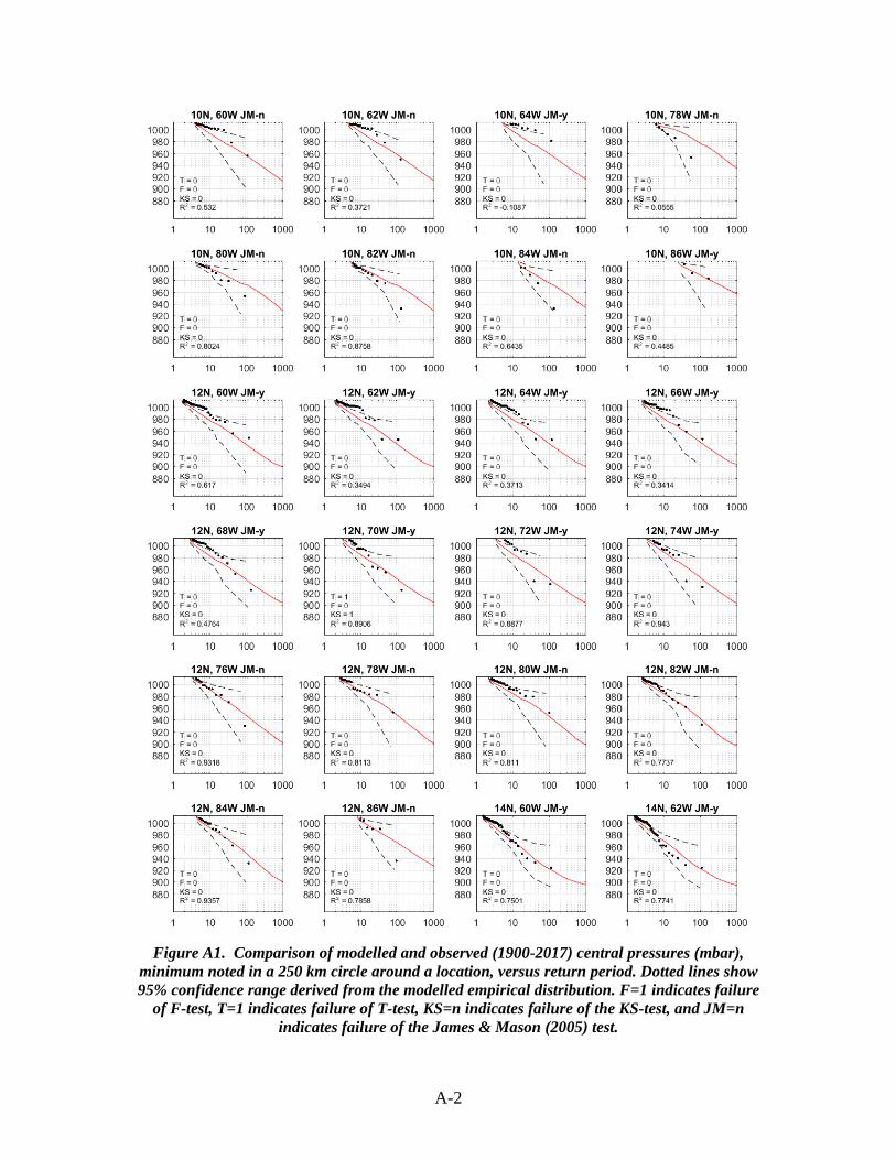
Figure A1. Comparison of modelled and observed (1900-2017) central pressures (mbar),
minimum noted in a 250 km circle around a location, versus return period. Dotted lines show 95% confidence range derived from the modelled empirical distribution. F=1 indicates failure
of F-test, T=1 indicates failure of T-test, KS=n indicates failure of the KS-test, and JM=n indicates failure of the James & Mason (2005) test.
A-3
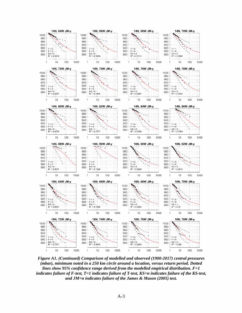
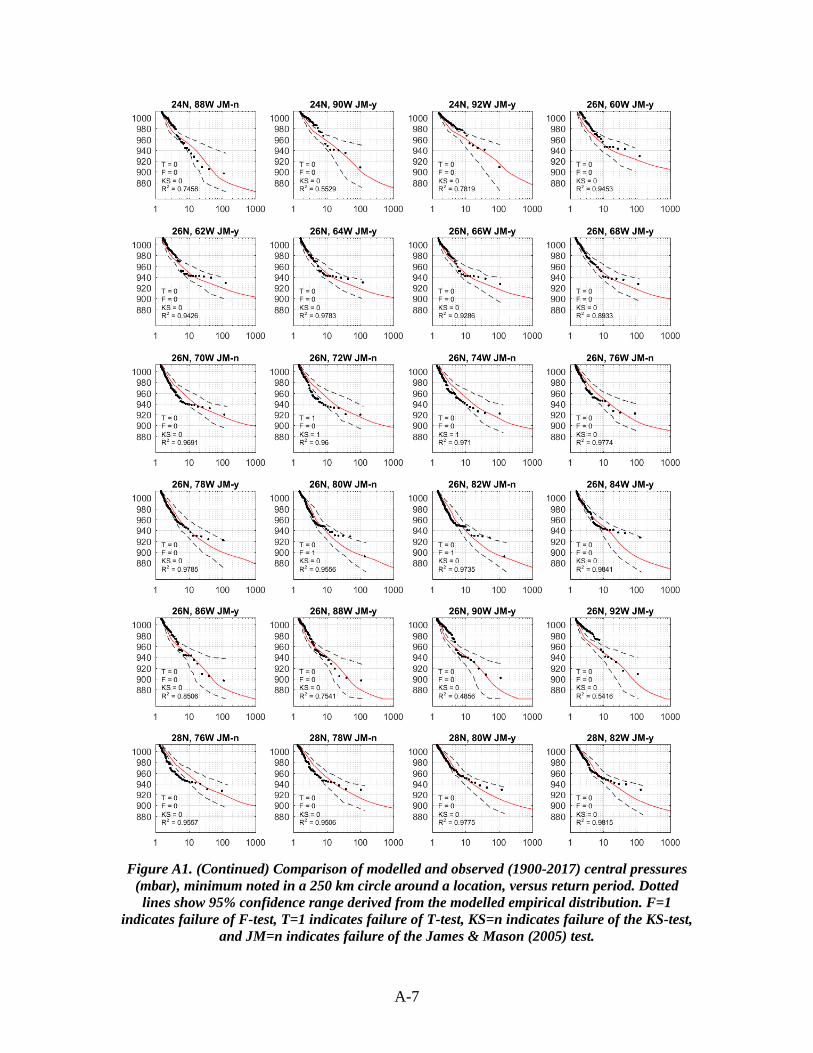
Figure A1. (Continued) Comparison of modelled and observed (1900-2017) central pressures
(mbar), minimum noted in a 250 km circle around a location, versus return period. Dotted lines show 95% confidence range derived from the modelled empirical distribution. F=1
indicates failure of F-test, T=1 indicates failure of T-test, KS=n indicates failure of the KS-test, and JM=n indicates failure of the James & Mason (2005) test.
A-4
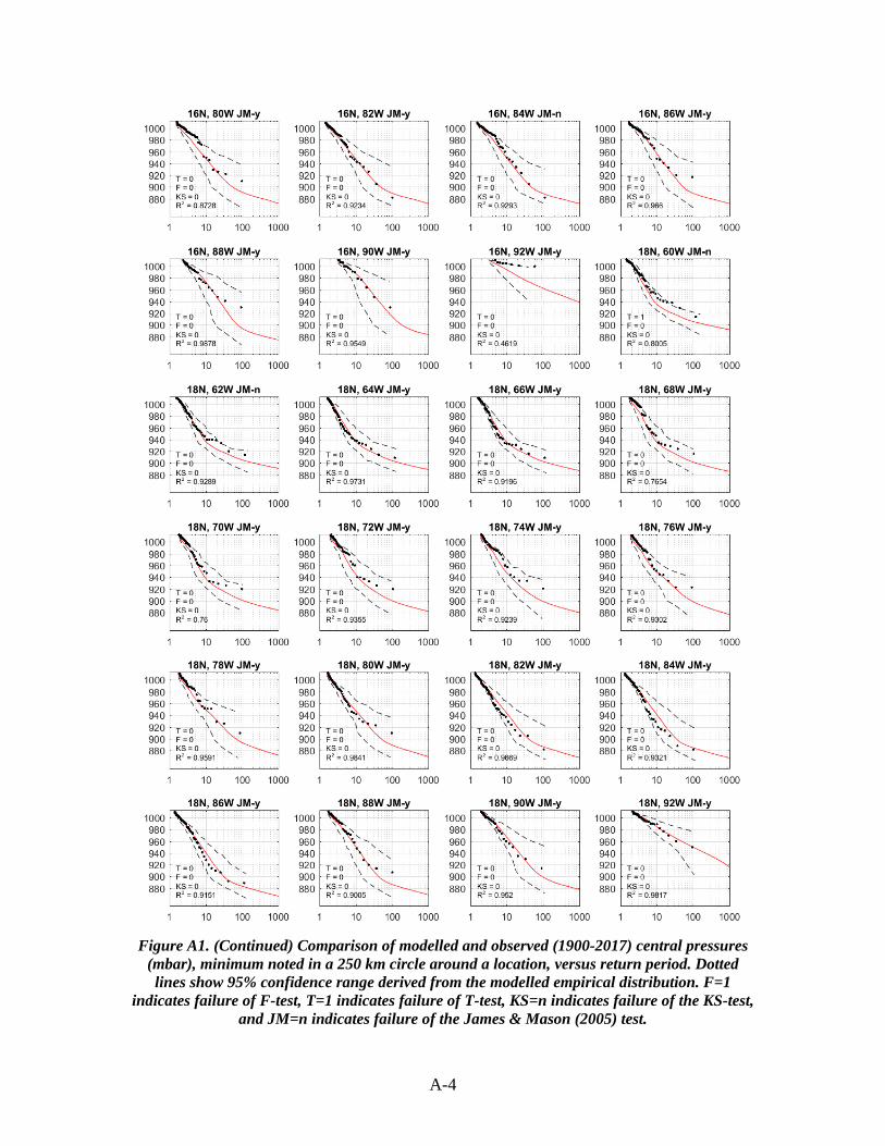
Figure A1. (Continued) Comparison of modelled and observed (1900-2017) central pressures
(mbar), minimum noted in a 250 km circle around a location, versus return period. Dotted lines show 95% confidence range derived from the modelled empirical distribution. F=1
indicates failure of F-test, T=1 indicates failure of T-test, KS=n indicates failure of the KS-test, and JM=n indicates failure of the James & Mason (2005) test.
A-5
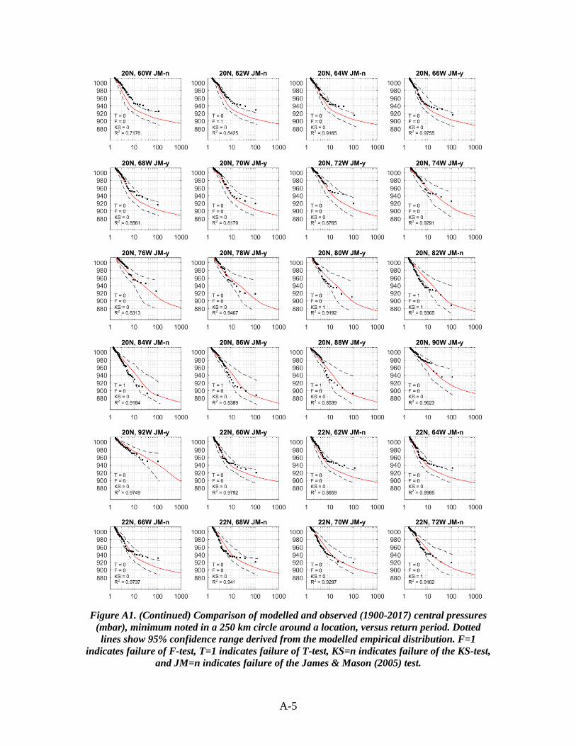
Figure A1. (Continued) Comparison of modelled and observed (1900-2017) central pressures
(mbar), minimum noted in a 250 km circle around a location, versus return period. Dotted lines show 95% confidence range derived from the modelled empirical distribution. F=1
indicates failure of F-test, T=1 indicates failure of T-test, KS=n indicates failure of the KS-test, and JM=n indicates failure of the James & Mason (2005) test.
A-6
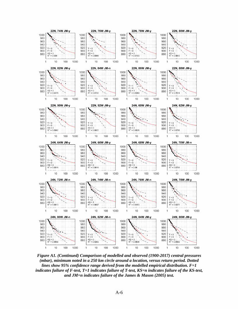
Figure A1. (Continued) Comparison of modelled and observed (1900-2017) central pressures
(mbar), minimum noted in a 250 km circle around a location, versus return period. Dotted lines show 95% confidence range derived from the modelled empirical distribution. F=1
indicates failure of F-test, T=1 indicates failure of T-test, KS=n indicates failure of the KS-test, and JM=n indicates failure of the James & Mason (2005) test.
A-7
Figure A1. (Continued) Comparison of modelled and observed (1900-2017) central pressures
(mbar), minimum noted in a 250 km circle around a location, versus return period. Dotted lines show 95% confidence range derived from the modelled empirical distribution. F=1
indicates failure of F-test, T=1 indicates failure of T-test, KS=n indicates failure of the KS-test, and JM=n indicates failure of the James & Mason (2005) test.
A-8
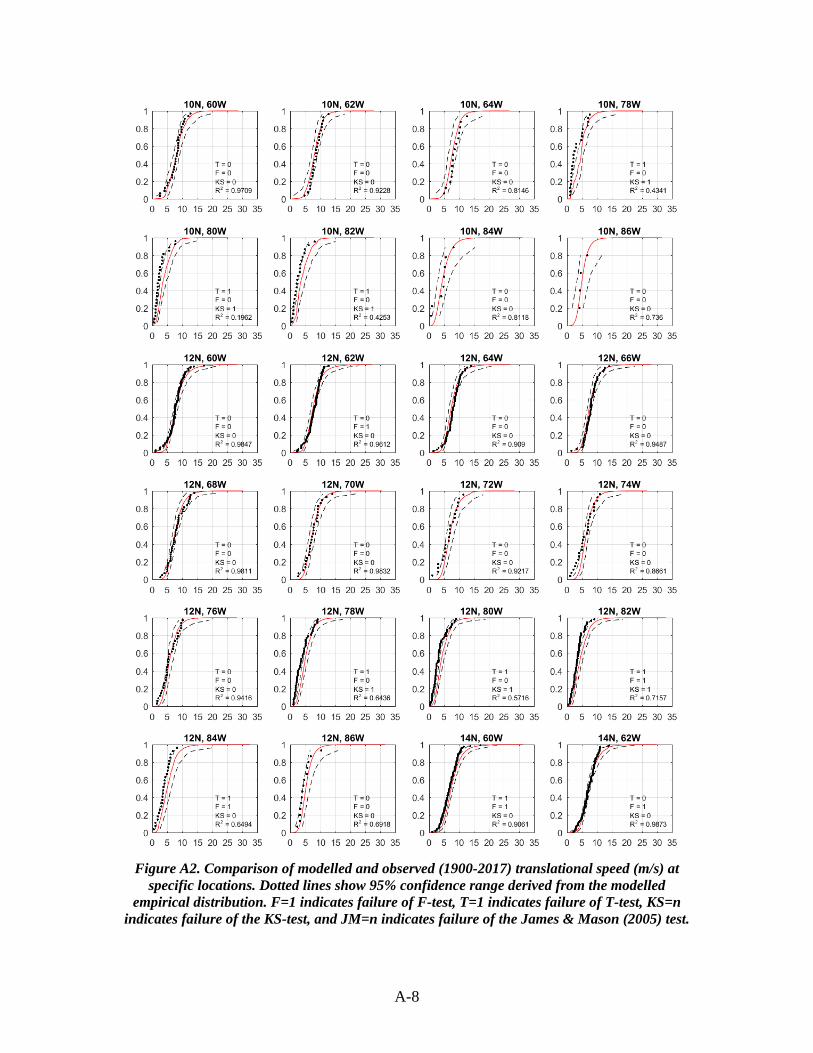
Figure A2. Comparison of modelled and observed (1900-2017) translational speed (m/s) at
specific locations. Dotted lines show 95% confidence range derived from the modelled empirical distribution. F=1 indicates failure of F-test, T=1 indicates failure of T-test, KS=n
indicates failure of the KS-test, and JM=n indicates failure of the James & Mason (2005) test.
A-9
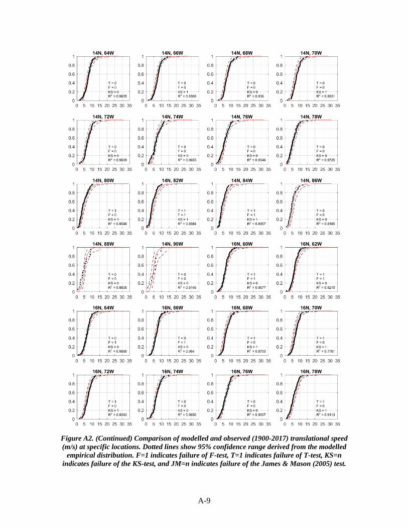
Figure A2. (Continued) Comparison of modelled and observed (1900-2017) translational speed (m/s) at specific locations. Dotted lines show 95% confidence range derived from the modelled
empirical distribution. F=1 indicates failure of F-test, T=1 indicates failure of T-test, KS=n indicates failure of the KS-test, and JM=n indicates failure of the James & Mason (2005) test.
A-10
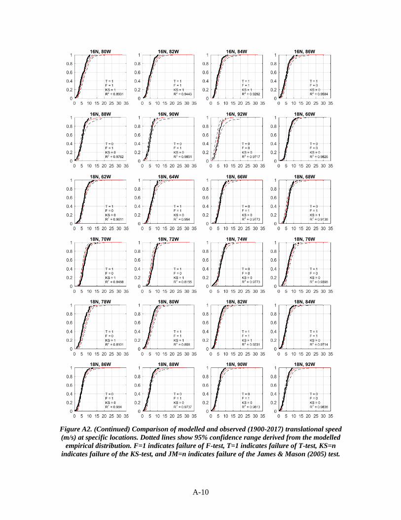
Figure A2. (Continued) Comparison of modelled and observed (1900-2017) translational speed (m/s) at specific locations. Dotted lines show 95% confidence range derived from the modelled
empirical distribution. F=1 indicates failure of F-test, T=1 indicates failure of T-test, KS=n indicates failure of the KS-test, and JM=n indicates failure of the James & Mason (2005) test.
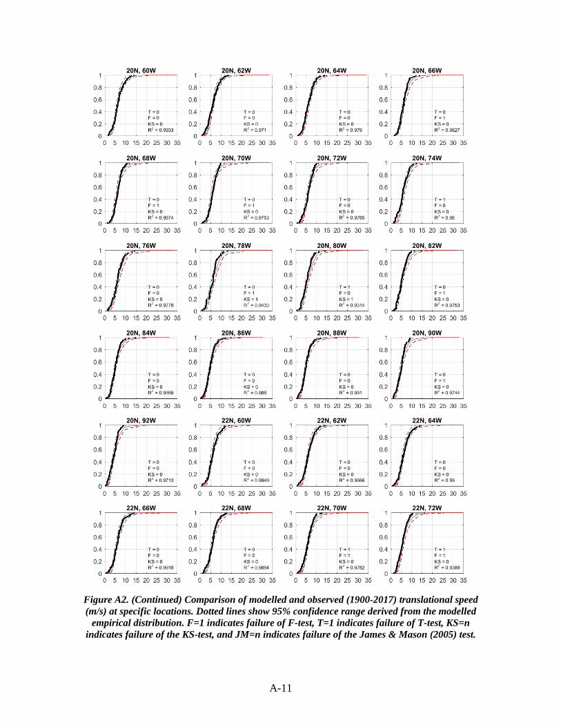
A-11
Figure A2. (Continued) Comparison of modelled and observed (1900-2017) translational speed (m/s) at specific locations. Dotted lines show 95% confidence range derived from the modelled
empirical distribution. F=1 indicates failure of F-test, T=1 indicates failure of T-test, KS=n indicates failure of the KS-test, and JM=n indicates failure of the James & Mason (2005) test.
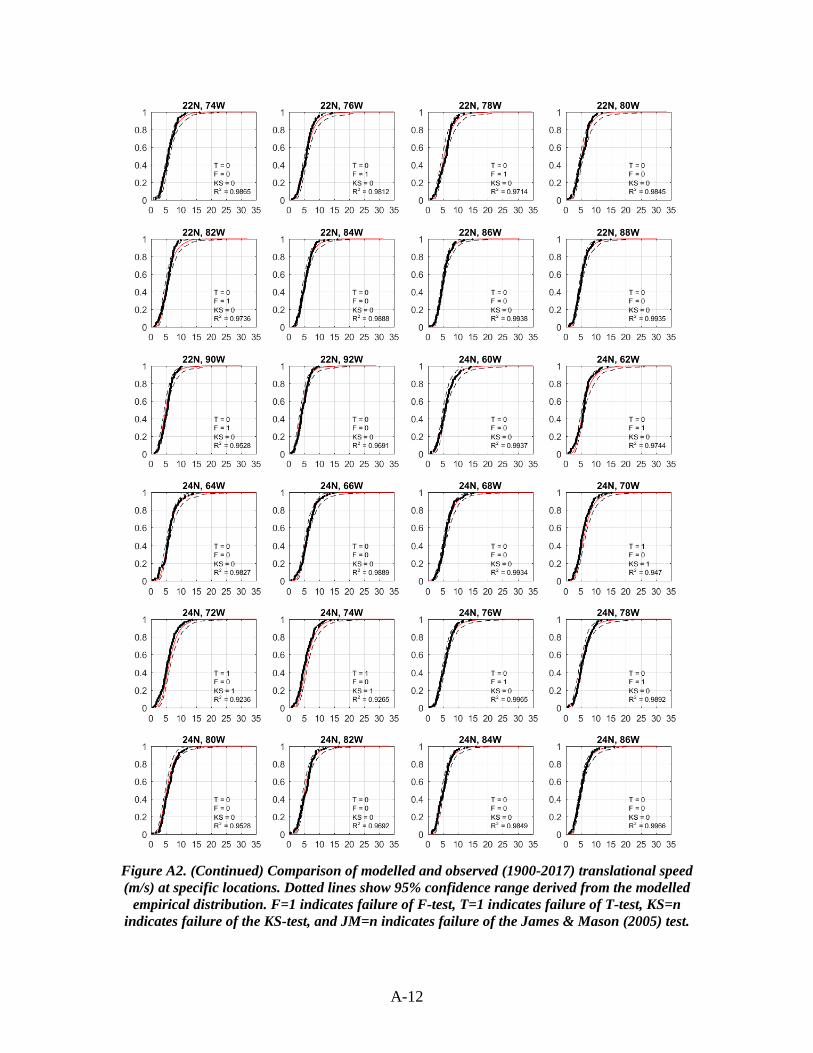
A-12
Figure A2. (Continued) Comparison of modelled and observed (1900-2017) translational speed (m/s) at specific locations. Dotted lines show 95% confidence range derived from the modelled
empirical distribution. F=1 indicates failure of F-test, T=1 indicates failure of T-test, KS=n indicates failure of the KS-test, and JM=n indicates failure of the James & Mason (2005) test.
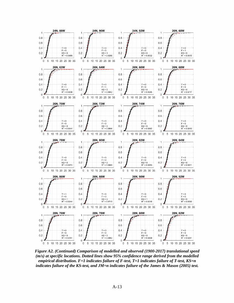
A-13
Figure A2. (Continued) Comparison of modelled and observed (1900-2017) translational speed (m/s) at specific locations. Dotted lines show 95% confidence range derived from the modelled
empirical distribution. F=1 indicates failure of F-test, T=1 indicates failure of T-test, KS=n indicates failure of the KS-test, and JM=n indicates failure of the James & Mason (2005) test.
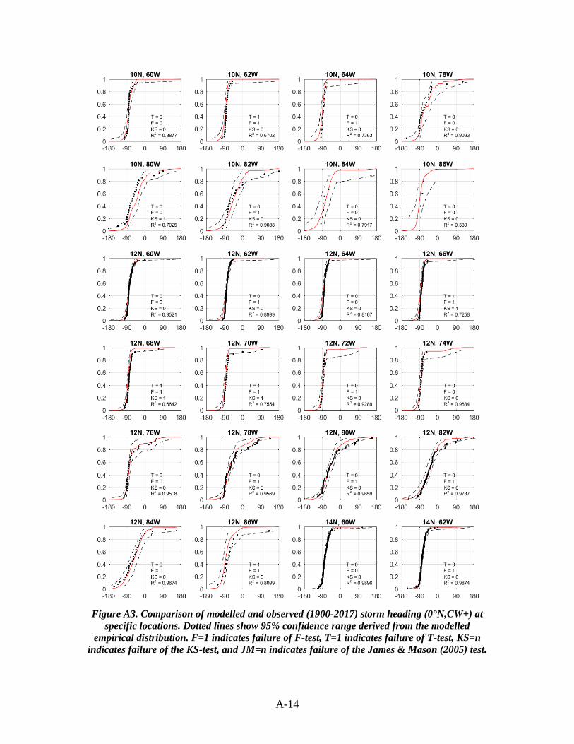
A-14
Figure A3. Comparison of modelled and observed (1900-2017) storm heading (0°N,CW+) at
specific locations. Dotted lines show 95% confidence range derived from the modelled empirical distribution. F=1 indicates failure of F-test, T=1 indicates failure of T-test, KS=n
indicates failure of the KS-test, and JM=n indicates failure of the James & Mason (2005) test.
A-15
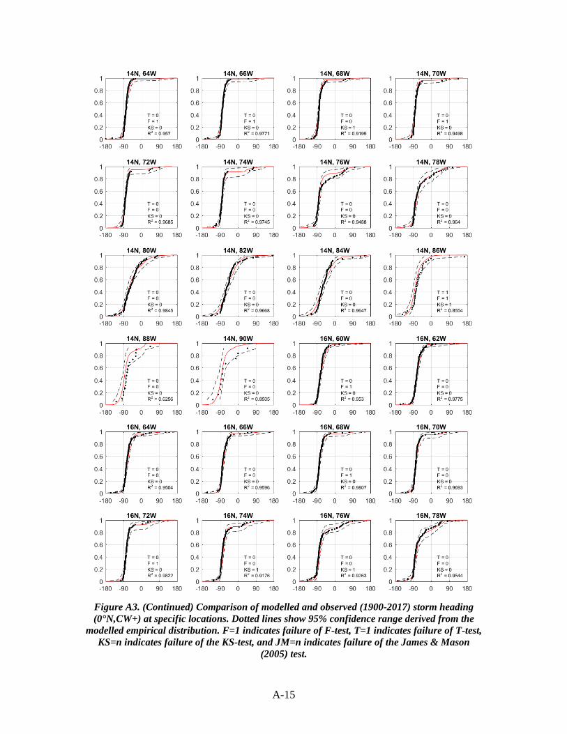
Figure A3. (Continued) Comparison of modelled and observed (1900-2017) storm heading (0°N,CW+) at specific locations. Dotted lines show 95% confidence range derived from the
modelled empirical distribution. F=1 indicates failure of F-test, T=1 indicates failure of T-test, KS=n indicates failure of the KS-test, and JM=n indicates failure of the James & Mason
(2005) test.
A-16
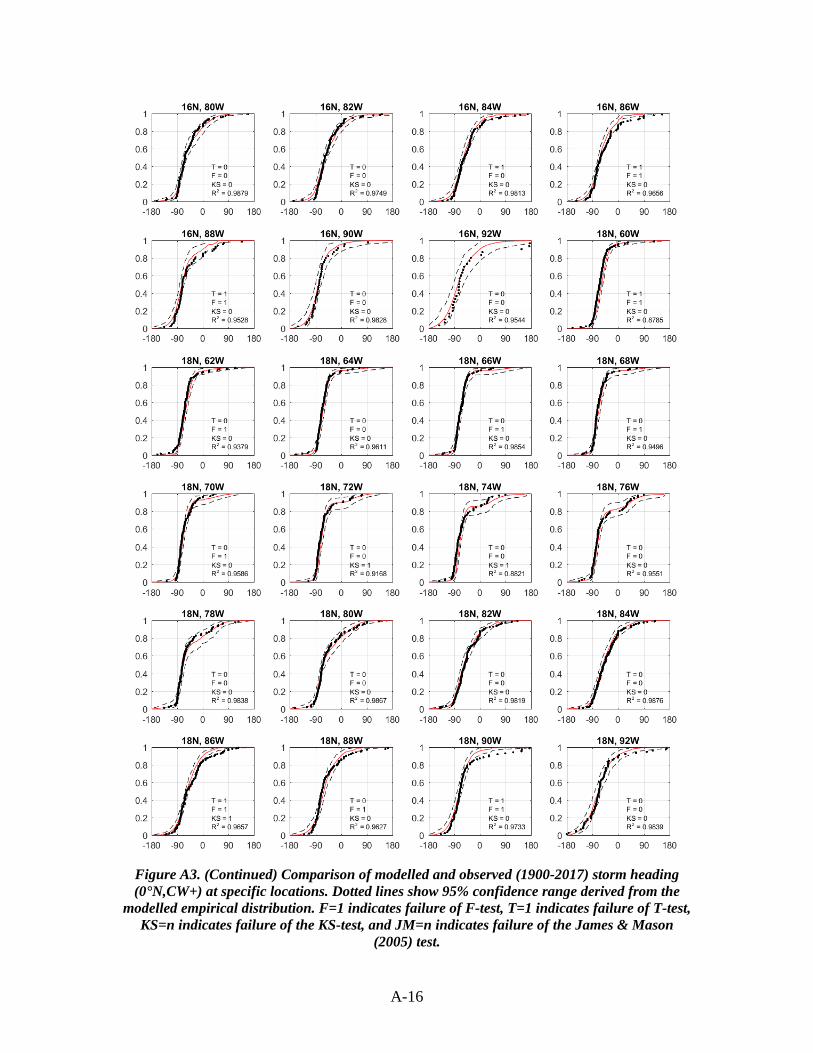
Figure A3. (Continued) Comparison of modelled and observed (1900-2017) storm heading (0°N,CW+) at specific locations. Dotted lines show 95% confidence range derived from the
modelled empirical distribution. F=1 indicates failure of F-test, T=1 indicates failure of T-test, KS=n indicates failure of the KS-test, and JM=n indicates failure of the James & Mason
(2005) test.
A-17
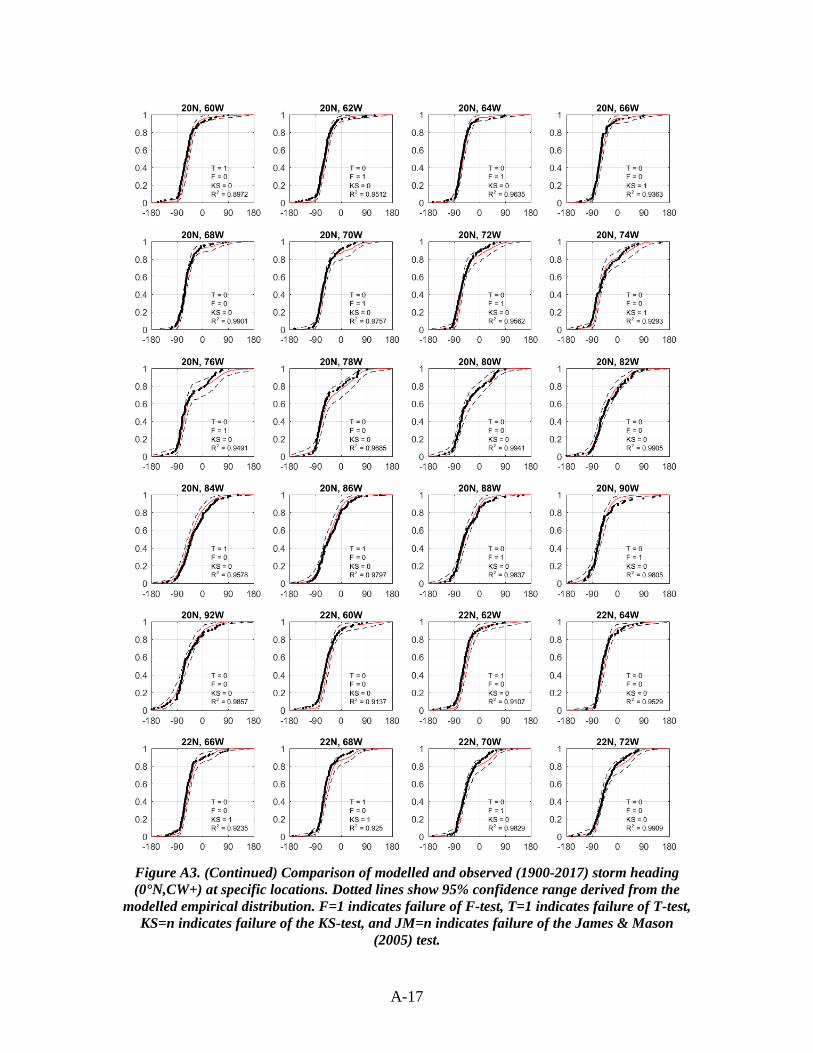
Figure A3. (Continued) Comparison of modelled and observed (1900-2017) storm heading (0°N,CW+) at specific locations. Dotted lines show 95% confidence range derived from the
modelled empirical distribution. F=1 indicates failure of F-test, T=1 indicates failure of T-test, KS=n indicates failure of the KS-test, and JM=n indicates failure of the James & Mason
(2005) test.
A-18
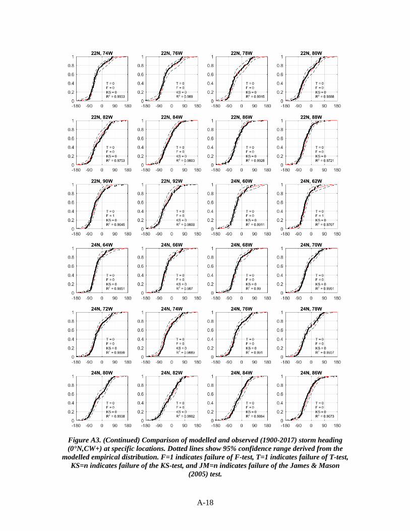
Figure A3. (Continued) Comparison of modelled and observed (1900-2017) storm heading (0°N,CW+) at specific locations. Dotted lines show 95% confidence range derived from the
modelled empirical distribution. F=1 indicates failure of F-test, T=1 indicates failure of T-test, KS=n indicates failure of the KS-test, and JM=n indicates failure of the James & Mason
(2005) test.
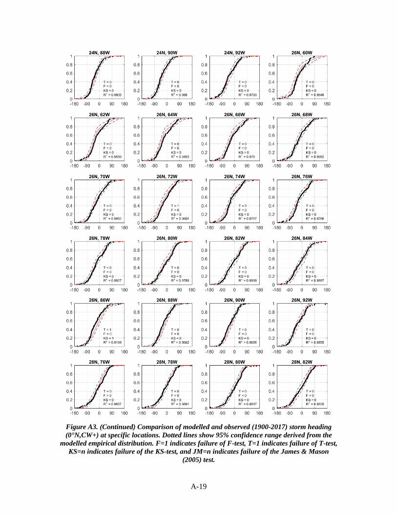
A-19
Figure A3. (Continued) Comparison of modelled and observed (1900-2017) storm heading (0°N,CW+) at specific locations. Dotted lines show 95% confidence range derived from the
modelled empirical distribution. F=1 indicates failure of F-test, T=1 indicates failure of T-test, KS=n indicates failure of the KS-test, and JM=n indicates failure of the James & Mason
(2005) test.
Related Documents