1 School of Chemical Sciences Dublin City University Glasnevin, Dublin 9. Development of Chiral and Achiral Supercritical Fluid Chromatographic methods for the characterisation of ophthalmic drug substances and drug products. Adrian Michael Marley, B.Sc. Under the supervision of: Dr. Damian Connolly, Pharmaceutical and Molecular Biotechnology Research Centre (PMBRC), Department of Science, Waterford Institute of Technology. Prof. Apryll M. Stalcup, Irish Separation Science Cluster (ISSC), National Centre for Sensor Research, Dublin City University, Glasnevin, Dublin 9, Ireland. A thesis submitted to Dublin City University for consideration for the degree of: Master of Science. September 2016

Welcome message from author
This document is posted to help you gain knowledge. Please leave a comment to let me know what you think about it! Share it to your friends and learn new things together.
Transcript
1
School of Chemical Sciences
Dublin City University
Glasnevin, Dublin 9.
Development of Chiral and Achiral Supercritical Fluid
Chromatographic methods for the characterisation of ophthalmic
drug substances and drug products.
Adrian Michael Marley, B.Sc.
Under the supervision of:
Dr. Damian Connolly, Pharmaceutical and Molecular Biotechnology Research Centre
(PMBRC), Department of Science, Waterford Institute of Technology.
Prof. Apryll M. Stalcup, Irish Separation Science Cluster (ISSC), National Centre for
Sensor Research, Dublin City University, Glasnevin, Dublin 9, Ireland.
A thesis submitted to Dublin City University for consideration for the degree of:
Master of Science.
September 2016

3
Table of Contents
List of Publications .................................................................................................................. 7
List of Tables ............................................................................................................................ 9
List of Figures ......................................................................................................................... 10
Acknowledgments .................................................................................................................. 13
Abstract ................................................................................................................................... 14
1.0 Chapter 1: Introduction to Supercritical Fluid Chromatography ......................... 15
1.1 What is Supercritical Fluid Chromatography (SFC)? ........................................... 15
1.2 Supercritical Fluids (SFs) ...................................................................................... 15
1.3 Properties of SFs .................................................................................................... 18
1.4 Historical development of SFC ............................................................................. 20
1.5 pSFC Applications ................................................................................................. 24
1.6 pSFC Instrumentation ............................................................................................ 24
1.6.1 Gas supply .......................................................................................................... 24
1.6.2 Pumps ................................................................................................................. 25
1.6.2.1 Compressible fluid pump .................................................................................... 25
1.6.3 Mobile Phases used in pSFC .............................................................................. 28
1.6.4 pSFC Injector ...................................................................................................... 29
1.6.5 pSFC Columns and Stationary Phases ................................................................ 30
1.6.6 Column oven ....................................................................................................... 31
1.6.7 Detectors ............................................................................................................. 32
1.6.8 Backpressure Regulator (BPR) ........................................................................... 33
1.7 SFC versus LC ....................................................................................................... 35
1.8 Green Chromatography ......................................................................................... 36
1.9 Project outline ........................................................................................................ 38

4
2.0 Chapter 2: Determination of (R)-timolol in (S)-timolol maleate active
pharmaceutical ingredient: Validation of a new pSFC method with an established
NP-HPLC method. ................................................................................................................. 40
2.1 Introduction ........................................................................................................... 40
2.1.1 Properties of Timolol Maleate ............................................................................ 40
2.1.2 Analysis of Timolol Maleate by HPLC .............................................................. 41
2.1.3 Analysis of Timolol Maleate by Capillary Electrophoresis (CE) ....................... 46
2.1.4 Chiral analysis by SFC ....................................................................................... 50
2.2 Experimental .......................................................................................................... 53
2.2.1 Instrumentation and Software ............................................................................. 53
2.2.2 Materials and Reagents ....................................................................................... 54
2.2.3 Solution preparation for Timolol NP-HPLC analysis ........................................ 54
2.2.4 Solution preparation for Timolol pSFC analysis ................................................ 55
2.2.5 Solution preparation for evaluation of Timolol pSFC Specificity ..................... 55
2.3 Results and discussion ........................................................................................... 55
2.3.1 Timolol pSFC Method Development ................................................................. 55
2.3.2 Timolol pSFC Method Validation ...................................................................... 62
2.3.2.1 Validation of Timolol pSFC Method as a Limit Test – Specificity and LOD ... 62
2.3.2.2 Investigation of Timolol pSFC Method as a potential Quantitative Impurities
Assay .................................................................................................................. 63
2.3.2.3 Timolol pSFC Precision studies: Repeatability and Intermediate Precision ...... 63
2.3.2.4 Timolol pSFC Robustness .................................................................................. 64
2.3.2.5 Timolol pSFC Accuracy ..................................................................................... 65
2.3.3 Analytical Performance Comparison: pSFC versus NP-HPLC ........................ 66
2.4 Conclusion ............................................................................................................. 70
3.0 Chapter 3: Development and Validation of a new stability indicating Reversed
Phase liquid chromatographic method for the determination of Prednisolone acetate
and impurities in an ophthalmic suspension. ...................................................................... 71
5
3.1 Introduction ........................................................................................................... 71
3.2 Experimental .......................................................................................................... 74
3.2.1 Instrumentation and Software ............................................................................. 74
3.2.2 Materials and Reagents ....................................................................................... 74
3.2.3 Solution preparation for PAC RP-HPLC analysis .............................................. 75
3.3 Results and discussion ........................................................................................... 77
3.3.1 PAC RP-HPLC Method Development ............................................................... 77
3.3.2 PAC RP-HPLC Method Validation .................................................................... 80
3.3.2.1 PAC RP-HPLC Accuracy/Linearity studies ....................................................... 80
3.3.2.2 PAC RP-HPLC Precision ................................................................................... 84
3.3.2.3 PAC RP-HPLC Specificity and Solution Stability ............................................. 85
3.3.2.4 PAC RP-HPLC Method Detection Limits and Acceptance Criteria .................. 86
3.3.2.5 PAC RP-HPLC Robustness ................................................................................ 87
3.4 Conclusion ............................................................................................................. 92
4.0 Chapter 4: Development of an orthogonal method for the determination of
Prednisolone acetate and impurities in an ophthalmic suspension using supercritical
fluid chromatography: Validation based on the Total Error Approach with Accuracy
Profiles. ................................................................................................................................... 93
4.1 Introduction ........................................................................................................... 93
4.1.1 Analysis of Steroids by SFC ............................................................................... 93
4.1.2 Method Validation using the Total Error Approach ........................................... 97
4.2 Experimental ........................................................................................................ 113
4.2.1 Instrumentation and Software ........................................................................... 113
4.2.2 Materials and Reagents ..................................................................................... 114
4.2.3 Solution preparation for PAC pSFC analysis ................................................... 114
4.2.3.1 pSFC PAC Matrix Placebo solution preparation .............................................. 114
4.2.3.2 pSFC PAC Column Screening Study Standard Preparation ............................ 114
4.2.3.3 pSFC PAC Calibration and Validation Standard Preparations ........................ 114
6
4.2.3.4 pSFC PAC Impurity Calibration and Validation Standard Preparations ......... 115
4.2.3.5 pSFC PAC Real Sample Preparation ................................................................ 115
4.3 Results and discussion ......................................................................................... 115
4.3.1 PAC pSFC Method Development .................................................................... 115
4.3.2 Method Transfer onto an Ultra Performance SFC (UPSFC) system ................ 124
4.3.3 PAC Method Development on UPSFC system ................................................ 130
4.3.4 PAC UPSFC Robustness .................................................................................. 134
4.3.5 PAC UPSFC Method Validation ...................................................................... 138
4.3.5.1 PAC UPSFC Specificity/Stability Indication and Solution Stability ............... 139
4.3.5.2 PAC UPSFC Trueness and Precision ............................................................... 141
4.3.5.3 PAC UPSFC Accuracy ..................................................................................... 141
4.3.5.4 PAC UPSFC Impurity Accuracy and LOQ/LOD limits .................................. 142
4.3.5.5 PAC UPSFC Linearity ...................................................................................... 144
4.3.6 Selection of Appropriate Response Function for PAC UPSFC Quantitative
Analysis ............................................................................................................ 145
4.3.7 Analytical Performance Comparison; UPSFC versus RP-HPLC ..................... 146
4.4 Conclusion ........................................................................................................... 149
5.0 Conclusions and future work ................................................................................... 150
6.0 References .................................................................................................................. 152
7
List of Publications • A. Marley, D. Connolly, Determination of (R)-timolol in (S)-timolol maleate active
pharmaceutical ingredient: Validation of a new supercritical fluid chromatography
method with an established normal phase liquid chromatography method, Journal of
Chromatography A, Volume 1325, 17 January 2014, Pages 213-220. (Chapter 2)
8
• A. Marley, A.M. Stalcup, D. Connolly, Development and validation of a new stability
indicating reversed phase liquid chromatographic method for the determination of
prednisolone acetate and impurities in an ophthalmic suspension, Journal of
Pharmaceutical and Biomedical Analysis, Volume 102, 5 January 2015, Pages 261-
266. (Chapter 3)

9
List of Tables
Table 1.1: Comparison of Gases, Supercritical Fluids and Liquids…………………… 20
Table 1.2: The twelve principles of green chemistry…………………………………... 37
Table 2.1: Solution preparation for NP-HPLC and pSFC analysis…………………… 58
Table 2.2: Analytical performance for determination of R-timolol impurity in
S-timolol maleate…………………………………………………………… 68
Table 2.3: Comparison between HPLC and pSFC analytical conditions and
performance………..……………………………………………………….. 69
Table 3.1: Solution preparation for validation of RP-HPLC method………………….. 76
Table 3.2: RP-HPLC PAC method optimisation………………………………………. 82
Table 3.3: Analytical performance for determination of PAC and selected impurities
in a spiked ophthalmic suspension……………..…………………………… 89
Table 3.4: Comparison between HPLC analytical conditions and
performance……………………………………...…………………………. 92
Table 4.1: Solution preparation for validation of UPSFC method…………………….. 117
Table 4.2: Summary of column screening results from the Thar Method Station…….. 119
Table 4.3: Impurity level accuracy and LOQ/LOD limits based on accuracy profiles... 142
Table 4.4: Comparison between RP-HPLC and UPSFC analytical conditions and
performance……………………………………………………….……...... 148
10
List of Figures
Figure 1.1: Phase diagram for a pure substance .................................................................... 16
Figure 1.2: Demonstration of the formation of supercritical CO2 ......................................... 18
Figure 1.3: Left: Giddings eluotropic series ........................................................................... 21
Figure 1.4: Schematic overview of typical pSFC system ........................................................ 22
Figure 1.5: Diagram demonstrating the operation of the compressible fluid pump............... 27
Figure1.6: Relationship between the calculated critical temperature, pressure and
concentration of the organic modifier ..................................................................................... 29
Figure 2.1: Molecular structure of S-timolol maleate ............................................................ 42
Figure 2.2: Molecular structure of the Chiracel OD chiral stationary phase ........................ 43
Figure 2.3: HPLC separation of timolol maleate enantiomers ............................................... 44
Figure 2.4: Typical chromatograms of a solution containing S-timolol, R-timolol ................ 47
Figure 2.5: Enantio-separation of a reconstituted racemic mixture of timolol maleate ......... 48
Figure2.6: Typical electropherogram of a mixture solution containing the main timolol
impurities ................................................................................................................................. 49
Figure 2.7: Peak sharpening of S-timolol ............................................................................... 51
Figure 2.8: Separation of R-timolol and S-timolol via pSFC ................................................ 59
Figure 2.9: Plot of retention factor (k) of R-timolol (red) and S-timolol (green) along with
resolution (Rs) between R-timolol and S-timolol (purple) ....................................................... 60
Figure 2.10: Comparison of optimised pSFC separation (a) and normal phase separation (b)
of timolol enantiomers ............................................................................................................. 61
Figure 2.11: Chromatograms of (a), pSFC sample containing R-timolol at the LOD ........... 63
Figure 2.12: Chromatograms of (a) EP timolol for system suitability CRS ........................... 64
Figure 2.13: Typical chromatograms of the CRM containing R-timolol and S-timolol ........ 65
Figure 2.14: Typical chromatograms comparing pSFC (a,b) and NP-HPLC (c,d) ............... 67
Figure 3.1: Molecular structure of prednisolone acetate (PAC) and impurities .................... 72
Figure 3.2: (a): Separation of eight selected PAC impurities................................................. 78
Figure 3.3: Representative chromatograms of development injections .................................. 81
Figure 3.4: Chromatogram of PAC impurity standard mixture containing the eight selected
PAC impurities ......................................................................................................................... 85
Figure 3.5: Top: (a) Chromatogram of 0.20 mg.mL-1 PAC spiked with eight selected PAC
impurities ................................................................................................................................. 87
11
Figure 3.6: Overlaid chromatograms of 0.20 mg.mL-1 PAC spiked with eight selected PAC
impurities. ................................................................................................................................ 88
Figure 4.1: Lifecycle of an analytical method ......................................................................... 98
Figure 4.2: Example of an accuracy profile ........................................................................... 99
Figure 4.3: Accuracy profile obtained for the validation of the quantification amoxicilline in
pharmaceutical formulation................................................................................................... 112
Figure 4.4: Representative chromatograms of development injections conducted on the Thar
method station ........................................................................................................................ 121
Figure 4.5: (a) Overlaid chromatograms of PAC standard at 200 mg.L-1 and impurity stock
standards at 40 mg.L-1). ......................................................................................................... 122
Figure 4.6: Overlaid chromatograms (expanded view to show baseline detail) of spiked
sample containing PAC at 600 mg.L-1 and impurities 3 mg.L-1............................................. 123
Figure 4.7: Expanded chromatogram of spiked sample containing PAC at 600 mg.L-1 and
impurities 12 mg.L-1conducted on the Waters UPC2 system ................................................. 125
Figure 4.8: Expanded chromatogram of spiked sample under the geometric transfer
conditions. .............................................................................................................................. 127
Figure 4.9: Expanded chromatogram of spiked sample under the geometric transfer
conditions described in Figure 4.7 with the following exceptions; Back-pressure regulation:
220 bar ................................................................................................................................... 127
Figure 4.10: Expanded chromatogram of spiked sample under the geometric transfer
conditions described in Figure 4.7 with the following exceptions; Column temperature:
45 °C. ..................................................................................................................................... 128
Figure 4.11: Expanded chromatogram of spiked sample under the geometric transfer
conditions described in Figure 4.7 with the following exceptions; Column temperature:
55 °C ...................................................................................................................................... 129
Figure 4.12: Expanded chromatogram of spiked sample under conditions described in
Figure 4.7 with the following exceptions Mobile phase: 10 to 20 % MeOH over 15 min. ... 130
Figure 4.13: Expanded overlaid chromatograms of spiked sample containing PAC at
600 mg.L-1 and impurities 6 mg.L-1(black) ............................................................................ 132
Figure 4.14: Chromatogram of spiked sample containing PAC at 600 mg.L-1 and impurities
6 mg.L-1. Chromatographic conditions; Column: DEA ......................................................... 133
Figure 4.15: Expanded overlaid chromatograms of spiked sample containing PAC at
600 mg.L-1 and impurities 6 mg.L-1 ........................................................................................ 134

12
Figure 4.16: Plot of retention time (Rt) and resolution (Rs) versus column temperature.
Chromatographic conditions as per Figure 4.14 with temperatures of 40, 45, 50, 55 and
60 °C. ..................................................................................................................................... 136
Figure 4.17: Plot of retention time (Rt) and resolution (Rs) versus back pressure (bar).
Chromatographic conditions as per Figure 4.14 with back pressures of 110, 120, 138, 150
and 160 bar. ........................................................................................................................... 137
Figure 4.18: Plot of retention time (Rt) and resolution (Rs) versus flow rate (mL.min-1).
Chromatographic conditions as per Figure 4.14 with flow rates of 2.3, 2.4, 2.5, 2.6 and
2.7 mL.min-1. .......................................................................................................................... 138
Figure 4.19: Overlaid chromatograms of MeOH blank (blue), placebo blank (red), PAC
standard at 600 mg.L-1 (green) and spiked sample ................................................................ 140
Figure 4.20: Plots of relative bias (%) and repeatability RSD (%) for PAC and impurity
results generated using the L and Lo response functions ...................................................... 143
Figure 4.21: Overlaid chromatograms of MeOH blank (blue), placebo blank (red) and spiked
placebo containing PAC and impurities at 0.3 mg.L-1(black) ............................................... 144
Figure 4.22: (a) Chromatogram of spiked sample containing PAC at 200 mg.L-1 and
impurities 1.2 mg.L-1under RP-HPLC conditions ................................................................. 147
Figure 4.23: Comparison of relative retention times (vs matrix peak) in UPSFC method and
in RP-HPLC method. ............................................................................................................. 148

13
Acknowledgments
I would like to take this opportunity to thank Professor Apryll Stalcup (DCU/ISSC),
Dr. Damian Connolly (WIT) and Dr. Aoife Hennessy (WIT) for their guidance and advice
over the duration of this Masters project. I would also like to thank the management of
Allergan Pharmaceuticals Westport for giving me the opportunity to undertake this Masters
project and for their continuous support and financial sponsorship throughout. Many thanks
also go to the technical staff of the School of Chemical Sciences in DCU, particularly to
Stephen Fuller for his invaluable assistance. To the members of the Waters Corporation who
assisted in this project by securing the loan of instrumentation which enabled the completion
of the work detailed in Chapter 4. Without their willingness to assist in this project, the
completion of this work would not have been possible. Finally, I would like to thank my
work colleagues, friends and most of all, my family, for their constant support and
encouragement throughout this journey.
14
Abstract
Development of Chiral and Achiral Supercritical Fluid Chromatographic methods for the characterisation of ophthalmic drug substances and drug products.
Adrian Michael Marley, B.Sc.
With the global drive for faster, more environmentally friendly separation techniques, the aim
of this research was to demonstrate the potential of Supercritical Fluid Chromatography
(SFC) as a viable alternative or complementary technique to High Performance Liquid
Chromatography (HPLC) in the highly regulated world of the Quality Control (QC)
laboratory. SFC methods capable of meeting QC method performance expectations in
accordance with current guidance were therefore developed and validated under current
International Conference of Harmonisation (ICH) guidance.
Firstly, an enantioselective pSFC method was developed and validated to meet the
current European Pharmacopoeia requirements of a limit test for the determination of
S-timolol maleate enantiomeric purity in timolol maleate drug substance. The newly
developed pSFC method achieved a resolution of 2.0 within 5 min, representing a 3-fold
reduction in run-time and an 11-fold reduction in solvent consumption relative to the normal
phase HPLC method described in the European Pharmacopoeia.
Secondly, a stability-indicating Reversed Phase (RP-HPLC) method was developed
and validated for the determination of prednisolone acetate (PAC) and eight selected PAC
impurities and degradation products in an ophthalmic suspension using a superficially porous
“core-shell” stationary phase. Using an Agilent Poroshell column with step gradient elution,
all peaks of interest were eluted in 33 min with resolution of 1.5 between the critical pairs.
With core-shell stationary phases being considered the most efficient technology currently
available for packed column HPLC applications, this RP-HPLC method was developed to
enable a direct comparison to be made between RP-HPLC and SFC in terms of orthogonality,
efficiency, selectivity, sensitivity and reproducibility.
Finally, an orthogonal achiral pSFC method was developed and validated for the same
PAC sample described above. For the pSFC method, validation was carried out using the
total error approach to generate accuracy profiles for two regression models, based on
β-expectation tolerance intervals. Successful completion of the method validation
demonstrated that the new pSFC method was a viable complementary or alternative to the
previously developed RP-HPLC method for use in the highly regulated QC laboratory
environment.
15
1.0 Chapter 1: Introduction to Supercritical Fluid Chromatography
1.1 What is Supercritical Fluid Chromatography (SFC)?
Supercritical fluid chromatography (SFC) has been described by Berger as a chromatographic
technique with properties that place it somewhere between liquid chromatography (LC) and
gas chromatography (GC) [1]. As with LC and GC, separation of solutes is achieved in SFC
through physiochemical interactions of solute molecules with a stationary phase and a mobile
phase. In SFC, the mobile phase primarily consists of a highly compressible dense fluid
which is often in the supercritical state. However, for many applications involving binary or
tertiary mobile phases, the mobile phase is not maintained in the supercritical state but rather
at “near-critical” or so called “subcritical” states. Over the course of its development as a
separations technique, this fact has led to some confusion over the correct naming of this
technique, with alternative names such as “dense gas chromatography” and in more recent
times “convergence chromatography” being proposed. However, to date, SFC remains the
popular description regardless of the defined state of the mobile phase. Probably the most
practical description of the mobile phase used in SFC would be as a dense compressed fluid
which due to the lack of intermolecular forces, will dramatically expand if the external
pressure is removed [1].
1.2 Supercritical Fluids (SFs)
Before one begins any discussion of SFC, it is important to gain some appreciation of the
properties of supercritical fluids (SFs). To put SFs in context one must first consider the three
possible states of matter; i.e. solids, liquids and gases. Pressure and temperature are the
parameters that determine the thermodynamically distinct phase in which matter will exist.
Transitioning from one phase to another is known as phase transition and can take place
when the conditions of pressure and temperature are altered so that the conditions favour the
existence of a particular phase, e.g. when a solid is heated it may become a liquid or when a
gas is compressed it may become a liquid.
Phase diagrams are a type of two-dimensional graph used to show the conditions in
which thermodynamically distinct phases can occur and can be used to demonstrate
supercritical conditions for a given substance. In Figure 1.1, the x-axis of the phase diagram
corresponds to temperature, while the y-axis corresponds to pressure. The phase diagram

16
shows, in pressure-temperature space, the lines of equilibrium, known as phase boundaries
between the three phases of matter for a given substance [1].
Figure 1.1: Phase diagram for a pure substance. Reproduced from [2].
Figure 1.1 illustrates a typical phase diagram for a pure substance. The red line
emerging from the lower left-hand corner separates the solid phase from the gaseous phase.
Crossing this line from left to right represents sublimation of the solid to the gas [3]. The
“triple point” is the point in the diagram where all three phases; i.e. solid, liquid and gas,
exist in equilibrium. The solid green vertical line emerging from the triple point separates the
solid phase from the liquid phase. The line itself represents a phase boundary and defines the
conditions where equilibrium exists between solid and liquid. The blue line that continues
diagonally from the triple point towards the upper right of the diagram separates the liquid
phase from the gaseous phase. Above and to the left of the line only liquid exists, while
below and to the right, only gas exists. As is the case for the solid/liquid boundary, this line
represents the phase boundary between the liquid and gaseous phases. Directly on the
liquid/gas boundary, both liquid and gases exists in equilibrium. This line is sometimes called
17
the boiling line or the vapour-liquid equilibrium line (VLE) [1]. This VLE line continues to a
point on the diagram known as the “critical point”.
The idea of a critical point was developed by Andrews in 1896 [3]. It was proposed
that for all substances, there is a temperature above which it can no longer exist as a liquid,
no matter how much pressure is applied. This temperature is called the critical temperature
(Tc) of the substance. Likewise, there is a pressure above which the substance can no longer
exist as a gas no matter how high the temperature is increased. This pressure value is called
the critical pressure (Pc) of the substance. Therefore, the critical point can be described as the
point where both the Tc and the Pc of the substance in question are reached. Thus, Tc and Pc
are the defining boundaries on a phase diagram for the critical point for a pure
substance. Above both Tc and Pc, no increase in temperature or pressure can cause two
phases to form and the substance is said to exist in the supercritical state or as a SF. However,
below either Tc or Pc or both, the substance is said to be in a subcritical state.
The most important point to note with respect to phase diagrams is that while
moving from one phase to another; i.e. crossing a phase boundary represents a phase
transition, moving from so called subcritical conditions to supercritical conditions, does not
constitute a phase transition. The dashed lines emerging horizontally and vertically from the
critical point in the phase diagram shown in Figure 1.1 are only included for illustrative
purposes to highlight the supercritical region. Some would argue that these lines should not
be included as there is no phase transition between a liquid and a SF or between a gas and a
SF and the inclusion of such lines only results in confusion [1]. SFs are not a separate state of
matter and should never be considered as such as they do not possess any unique physical
characteristics that would deem them to be a distinct phase [1]. Therefore, being supercritical
is about being in a defined state; i.e. defining the conditions of pressure and temperature in
which a substance finds itself, rather than being a distinct phase. It should be emphasised that
for a substance to be truly in the supercritical state, it must be maintained in conditions above
both its Pc and Tc. Thus, for SFs with the word “super” only intended to indicate “above”.
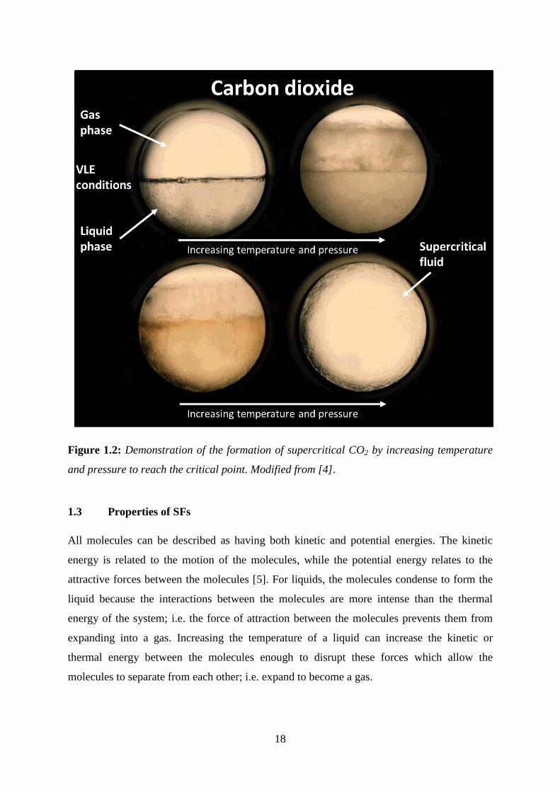
Figure 1.2 demonstrates the formation of supercritical CO2 where the conditions of pressure
and temperature are increased to a point where the substance becomes supercritical. Note that
below the critical point, two phases can exist in equilibrium; i.e. on the VLE line of a phase
diagram.
18
Figure 1.2: Demonstration of the formation of supercritical CO2 by increasing temperature
and pressure to reach the critical point. Modified from [4].
1.3 Properties of SFs
All molecules can be described as having both kinetic and potential energies. The kinetic
energy is related to the motion of the molecules, while the potential energy relates to the
attractive forces between the molecules [5]. For liquids, the molecules condense to form the
liquid because the interactions between the molecules are more intense than the thermal
energy of the system; i.e. the force of attraction between the molecules prevents them from
expanding into a gas. Increasing the temperature of a liquid can increase the kinetic or
thermal energy between the molecules enough to disrupt these forces which allow the
molecules to separate from each other; i.e. expand to become a gas.

19
SFs lack the adequate intermolecular interactions to allow them to condense into
liquids [1] and are maintained in the fluid state due to the presence of an external pressure
source. With SFs, this pressure can be increased, forcing the molecules as close together as
the molecules in a condensed liquid; thus increasing the density of the fluid. This enforced
molecular closeness results in high collision frequency between molecules which makes the
fluids reasonable solvents for many solutes [1]. This property of SFs was first demonstrated
by Hannay and Hogarth in 1879 when they successfully dissolved inorganic salts in
supercritical ethanol and re-precipitated them by decreasing the temperature [3]. This ability
of SFs to solvate solute molecules is the key to SFs being used in chromatographic
separations.
Altering the amount of pressure applied to the fluid has the effect of changing the
density of the fluid and hence its ability to dissolve solutes by making the fluid either more
gas like or more liquid like. Temperature also has an effect on the density of the SF.
Increasing temperature at a constant pressure has the effect of reducing the density of the SF
and hence the solvent strength of the SF. These properties of SFs enables the solvent strength
of the fluid to be manipulated by altering physical parameters; i.e. temperature and pressure
which, as will be discussed later, can be exploited to fine tune chromatographic separations
involving the use of SFs as the mobile phase.
It should be noted that the forcing together of molecules in SFs results in more
extensive molecular interactions, but does not force more intense molecular interactions [1].
Having low inherent intermolecular interactions, SFs have lower viscosities and higher
diffusivity of solutes in the fluids compared to normal liquids. The intermolecular forces that
cause liquid molecules to “stick” together give rise to surface tension, higher viscosity, and
slower diffusion for normal liquids compared to supercritical fluids. Such properties can
hinder the solvation because the molecules do not mix or diffuse well. In the case of SFs,
when above a solvent’s Tc, the kinetic energy overcomes the potential energy effect and the
molecules no longer “stick” together. As a consequence, surface tension and viscosity are
lower, and diffusion rates increase for supercritical fluids compared to normal liquids [5].
Thus, SFs have properties that lie between those of gases and liquids. Table 1.1 compares the
properties of gases, SFs and liquids in terms of density, viscosity and diffusivity.

20
Table 1.1: Comparison of Gases, Supercritical Fluids and Liquids. Reproduced from [6].
Density (kg/m3) Viscosity (µPa∙s) Diffusivity (mm²/s) Gases 1 10 1–10
Supercritical Fluids 100–1000 50–100 0.01–0.1 Liquids 1000 500–1000 0.001
1.4 Historical development of SFC
A number of articles have been published charting the development and theory of SFC from
its beginnings up to the present day [3,7-9]. Klesper et al. are credited with discovering SFC
in 1962 when they described the separation of thermo-labile porphyrin derivatives on a
packed column using supercritical chlorofluorocarbon as the mobile phase [10]. From that
first reported separation, many separation scientists recognised the potential of SFC and
attempted to exploit the properties of SFs as mobile phases to generate faster, more efficient
chromatographic separations. Throughout the late 1960’s, Calvin Giddings dominated the
theoretical development of SFC. His work focused on using pure SFs as mobile phases
including various gases such as He, N2, CO2 and NH3 [8]. However, over the course of time,
CO2 was to become the default choice of fluid for use as SFC mobile phases due to its low
critical temperature (31.1 °C) and pressure (74 bar) respectively along with being non-toxic,
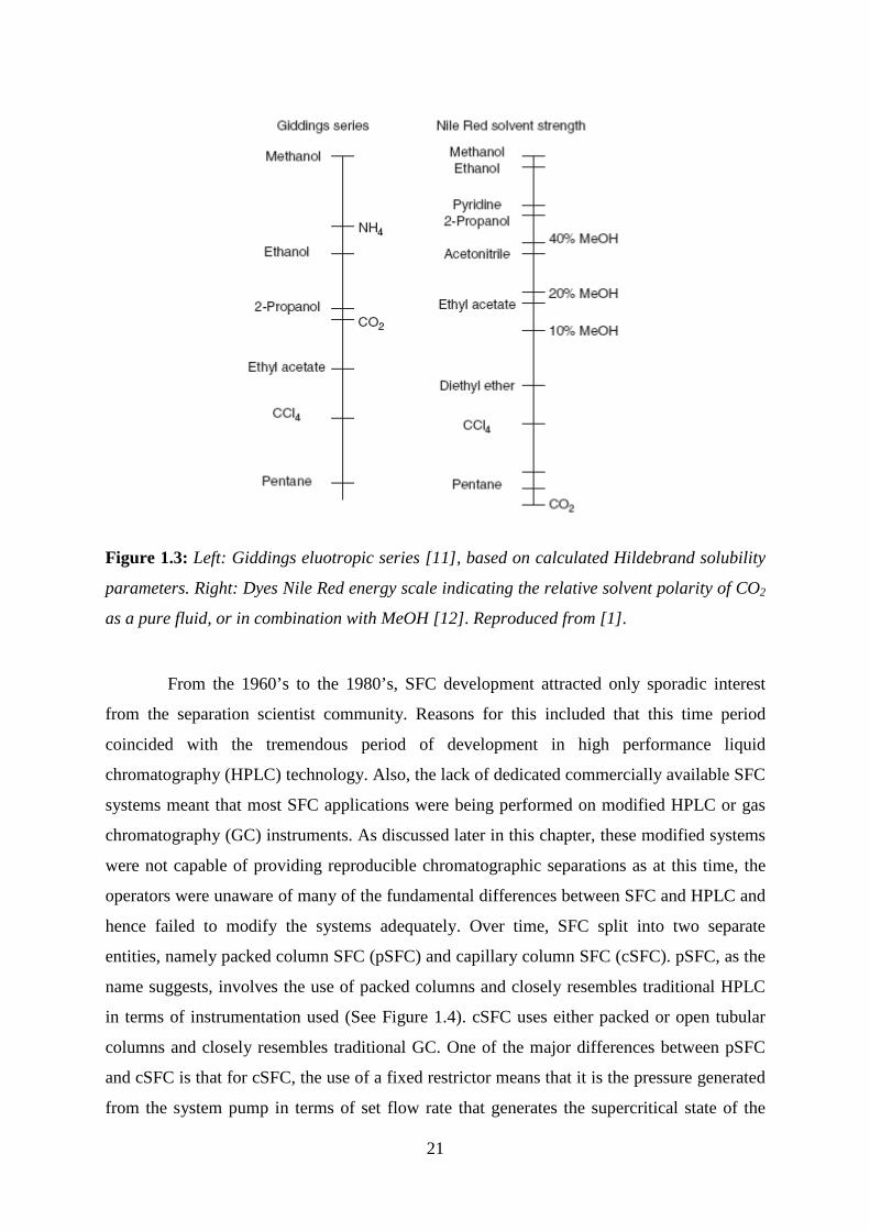
non-flammable and inexpensive [8]. In 1968, Giddings proposed an eluotropic series in
which supercritical CO2 was placed next to isopropanol in terms of solvent polarity [11].
According to Giddings’ series, the polarity of CO2 could be changed from hydrocarbon-like
to alcohol-like simply by altering the density of the fluid; i.e. by adjusting a physical
parameter such as pressure. This wide range of polarity would have eliminated the need for
binary mobile phases and allowed the separation of solutes with wide ranging polarities using
pure SF CO2 as the mobile phase coupled with density programming. Unfortunately,
Giddings eluotropic series turned out not to be correct and it was later shown that the polarity
of SF CO2 was actually closer to that of pentane rather than isopropanol [12]. However,
Giddings series was left unchallenged for almost 30 years and greatly influenced the course
of SFC development as separation technique during this time.
21
Figure 1.3: Left: Giddings eluotropic series [11], based on calculated Hildebrand solubility
parameters. Right: Dyes Nile Red energy scale indicating the relative solvent polarity of CO2
as a pure fluid, or in combination with MeOH [12]. Reproduced from [1].
From the 1960’s to the 1980’s, SFC development attracted only sporadic interest
from the separation scientist community. Reasons for this included that this time period
coincided with the tremendous period of development in high performance liquid
chromatography (HPLC) technology. Also, the lack of dedicated commercially available SFC
systems meant that most SFC applications were being performed on modified HPLC or gas
chromatography (GC) instruments. As discussed later in this chapter, these modified systems
were not capable of providing reproducible chromatographic separations as at this time, the
operators were unaware of many of the fundamental differences between SFC and HPLC and
hence failed to modify the systems adequately. Over time, SFC split into two separate
entities, namely packed column SFC (pSFC) and capillary column SFC (cSFC). pSFC, as the
name suggests, involves the use of packed columns and closely resembles traditional HPLC
in terms of instrumentation used (See Figure 1.4). cSFC uses either packed or open tubular
columns and closely resembles traditional GC. One of the major differences between pSFC
and cSFC is that for cSFC, the use of a fixed restrictor means that it is the pressure generated
from the system pump in terms of set flow rate that generates the supercritical state of the
22
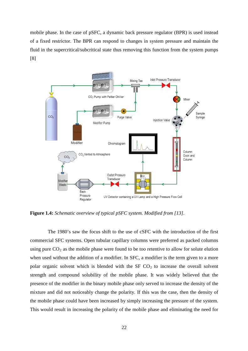
mobile phase. In the case of pSFC, a dynamic back pressure regulator (BPR) is used instead
of a fixed restrictor. The BPR can respond to changes in system pressure and maintain the
fluid in the supercritical/subcritical state thus removing this function from the system pumps
[8]
Figure 1.4: Schematic overview of typical pSFC system. Modified from [13].
The 1980’s saw the focus shift to the use of cSFC with the introduction of the first
commercial SFC systems. Open tubular capillary columns were preferred as packed columns
using pure CO2 as the mobile phase were found to be too retentive to allow for solute elution
when used without the addition of a modifier. In SFC, a modifier is the term given to a more
polar organic solvent which is blended with the SF CO2 to increase the overall solvent
strength and compound solubility of the mobile phase. It was widely believed that the
presence of the modifier in the binary mobile phase only served to increase the density of the
mixture and did not noticeably change the polarity. If this was the case, then the density of
the mobile phase could have been increased by simply increasing the pressure of the system.
This would result in increasing the polarity of the mobile phase and eliminating the need for
23
the modifier thus reducing the need for a second modifier pump. This unchallenged belief,
based on Giddings eluotropic series, that the polarity of CO2 could be altered to that close to
isopropanol simply by increasing the pressure of the system led to practitioners persisting
with the use of pure fluids in the supercritical state on packed columns. This resulted in a
very limited success rate for packed column separations with most applications being
confined to very non-polar solutes [3].
Berger and Deye [12] went on to disprove the theory that the function of the
modifier in the binary mixture acting solely as a means to increase the density of the mixture.
They did this by measuring the density of CO2-methanol mixtures and proved that even at a
constant density, altering the concentration of the modifier had a major effect on solute
retention. They later went on to prove that Giddings eluotropic series was incorrect and that
CO2 was in fact non-polar and more closely related to pentane in terms of solvent polarity.
Their findings along with the fact that the addition of modifiers can greatly increase the
polarity of binary mixtures led to a renewed interest in the 1990’s for pSFC coupled with
composition programming rather that pressure programming [3]. Over time, alcohols were
found to be the most universal modifiers being able to provide good overall efficiency
[14,15] with methanol now being considered the first choice for the elution of polar
compounds in pSFC [16].
Due to the type and quality of packed column stationary phases that were available
in the late 1980’s, many polar solutes still failed to elute, or eluted with poor peak shapes
when pSFC was employed with binary mobile phases. This prompted investigation into the
use of additives as part of the mobile phase. Berger, Deye and Taylor were among the first
publish work on the role of additives in pSFC [17]. Additives can be described as very polar
substances, usually strong acids or bases, which are added to the modifier in small
concentrations and can greatly improve peak shape and resolution. The addition of additives
shifted the emphasis of pSFC towards the analysis of small drug-like molecules during the
1990’s. Additives and modifiers had the effect of changing pSFC from a largely lipophilic
technique to a small, polar molecule technique [3]. This new found potential range of
application shifted the focus of SFC development towards pSFC applications and signalled
the decline in interest for cSFC.
24
1.5 pSFC Applications
One of the first major areas of success for pSFC application was in the separation of chiral
compounds. A key factor in this success was the development of a number of highly efficient
and versatile chiral stationary phases (CSPs) in the 1980’s by Okamoto et al. [18,19] which
were later commercialised by the Daicel Corporation, Osaka, Japan. The availability of such
stationary phases combined with the practical advantages of pSFC over liquid
chromatography (LC) in terms of fast method development times, high sample throughput
and ease of solute recovery resulted in many successful pSFC chiral applications being
reported [20,21]. This success has made pSFC the preferred option for chiral separations at
both the analytical and preparative scale.
pSFC has also been successfully employed for both chiral and achiral applications in
different fields including; pharmaceutical [22,23], bioanalysis [24,25] and biomolecules
[26,27], agrochemicals and environmental applications [28,29], polymer additives [30,31],
food science [32,33] and natural products [34,35]. This ever increasing range of application
demonstrates that all applications that are relevant to HPLC analysis of small molecules
should also be applicable to SFC.
1.6 pSFC Instrumentation
Figure 1.4 shows a schematic overview of a typical pSFC system. While the overall picture
may closely resemble that of a traditional HPLC system, there are a number of modifications
that must be made in order to achieve reproducible chromatography using pSFC. Berger, who
has been described by as the father of modern SFC [7], based on his contribution to SFC
instrumental design, provided a detailed description of the practical aspects of SFC hardware
[1]. Due to the important role instrumentation plays in generating reproducible
chromatography in SFC applications, the following sections provide detail on some of the
functional requirements of SFC hardware and the challenges that must be overcome
compared to conventional HPLC.
1.6.1 Gas supply
For most pSFC applications, food grade CO2 is of sufficient purity to give acceptable
chromatographic performance. pSFC systems require that CO2 be supplied to the pump in
liquid form. To achieve this, high pressure gas cylinders are used in which the majority of the
CO2 in the cylinder exists as a liquid with the remaining head space being filled with CO2
25
gas. The liquid CO2 is supplied to the pSFC pump using a dip-tube feed which takes the
liquid CO2 from the bottom of the cylinder where it is under greatest pressure. The headspace
pressure within the cylinder is used to force the liquid CO2 up through the dip tube and into
the pSFC pump. To achieve consistent and reproducible chromatography in pSFC, the
relationship between cylinder temperature and cylinder pressure is extremely important. Any
fluctuations in temperature between the gas supply and the pump head can have detrimental
effects on chromatographic performance [1]. The best option to avoid problems associated
with the CO2 supply to the pSFC system is to have the cylinder as close to the pSFC system
as possible. This will ensure that there are no temperature fluctuations during the transport of
the CO2 from the cylinder to the pSFC system, while ensuring that the supply line is short
enough to avoid any large pressure differences between the cylinder and the pump heads. For
these reasons, it is always best to have the CO2 cylinder in the same room and as close as
possible to the pSFC system.
1.6.2 Pumps
The pumps used in modern pSFC systems are similar to those used in HPLC systems in that
they are both positive displacement reciprocating piston pumps which can operate up to
600 bar pressure and flow rates up to 10 mL.min-1. As pSFC often requires a modifier to
ensure solute elution from the column, pSFC systems contain two separate reciprocating
pumps, one to deliver the pressurized CO2, which is known as the compressible fluid pump
and the other to deliver the liquid modifier, which is known as the modifier pump. The
modifier pump used is identical to those used in traditional HPLC systems. However, a
number of modifications are required for the compressible fluid pump to ensure a consistent
flow rate is maintained.
1.6.2.1 Compressible fluid pump
The compressible fluid pump is probably the most important component of the pSFC system.
It must be able to deliver a precise amount of a compressible fluid independently of the
column temperature or pressure, to ensure consistent and reproducible chromatography. The
first issue this pump has to deal with is that although the CO2 supplied from the cylinder is
defined as a liquid, it will readily expand to form a low density gas if the external pressure
source is removed. Therefore, the pump must be capable of maintaining pressure at all times,
even during the filling stroke. This is to ensure that the CO2 doesn’t expand and separate into
two phases due to the pressure drop when the CO2 enters the pump cylinder [1].

26
The first major modification of the compressible fluid pump compared to the
modifier pump is the presence of a chilling unit attached to the pump head. Chilling the CO2
as it enters the pump ensures that it remains in the liquid form and reduces the possibility of
phase separation due to an increase in temperature within the pump head. To ensure adequate
heat transfer, most modern pSFC systems are fitted with electronically controlled Peltier
coolers which are directly attached to the pump head. This type of cooling system allows
accurate temperature control of the pump and reduces the risk of phase separation within the
pump due to inadequate heat transfer. However, chilling the CO2 to ensure that it remains in
the liquid form as it enters the pump is only part of the solution to providing an accurate flow
from the compressible fluid pump. Even in its liquid form, CO2 remains relatively
compressible. Therefore, this compressibility factor must be taken into account by the pump
to ensure that the correct flow from the pump is achieved at all times.
On completion of the fill stroke, the pump is filled with the liquid CO2 at the same
pressure as the supply cylinder. It is at this point that compressibility compensation comes
into play to ensure accurate and precise CO2 delivery from the pump. As the pump piston
moves forward it will continue to compress the fluid within the pump. However, the outlet
check valve will not open and hence there will be no flow to the column until the pressure
within the pump exceeds that of the column pressure. As the CO2 is compressible, it may
take up to 12% of the pump delivery stroke just to increase the pump pressure enough to open
the outlet check valve [1]. Without compressibility compensation, this would result in a 12%
loss of flow from the pump compared to the set flow rate which could have a dramatic effect
on the chromatographic results especially when binary mobile phases are used. Therefore, so
called compressibility factors must be calculated and included in each delivery stroke in order
to accurately achieve the desired flow rate. The distance the piston must travel in order to
achieve adequate compression is dependent on the pressure at the head of the column.
Greater compression is required with higher column pressure which results in greater loss of
the delivery stroke.
Calculation of compressibility factors is dependent on factors including the volume
of the pump head cylinder, the temperature and the pressure both in the piston and at the head
of the column [1]. Pump control algorithms were developed to empirically optimise nominal
compressibility compensation for any fluid and also to compensate for pump leaks. Such
compensation also helped minimize baseline noise which improved the sensitivity of pSFC
[36].
27
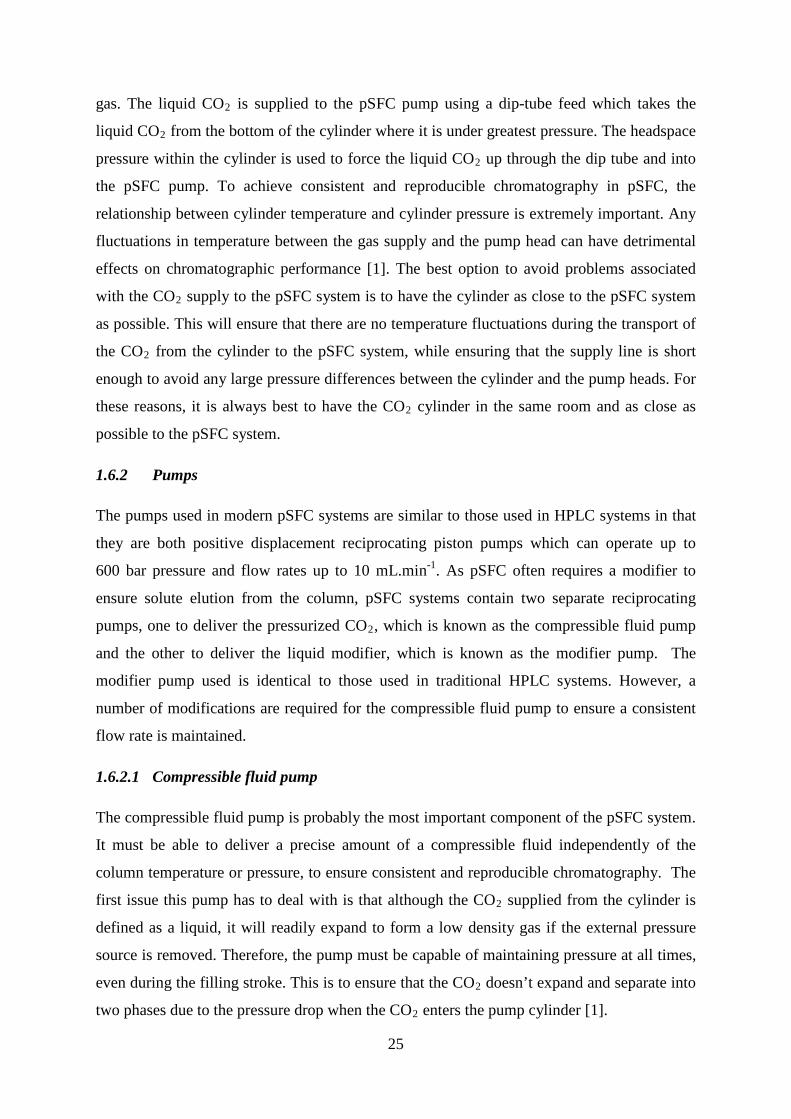
Figure 1.5: Diagram demonstrating the operation of the compressible fluid pump including
compression compensation.
However, even if one knows the precise values required for accurate generation of
the compressibility factor, there is still a further issue that can affect the fluid delivery from
the pump. The factor in question is a rise in temperature during the compression stroke of the
pump cycle; i.e. when liquids are compressed, there is an increase in temperature due to
adiabatic heating [1]. The temperature of the fluid in the pump cylinder is at its highest just
after the completion of the compression stroke. As there is no time for this heat to dissipate
into the cylinder walls prior to delivery, this increase in temperature causes a net increase in
the pressure within the pump cylinder which in turn can result in the premature opening of
the outlet check valve. The premature opening of the outlet check valve results in more mass
leaving the pump than expected. However, as the fluid cools, its density increases and the
shrinking volume of the fluid negates part of the forward motion of the piston during the
delivery stroke. This results in less mass than expected leaving the pump. Therefore, during
each pump cycle, the delivery stroke repeats a cycle of first excessive flow followed by
inadequate flow as a result of adiabatic heating. As there is no way of keeping the fluid
isothermal during the compression stroke, the only way to ensure consistent flow is to vary
the piston speed to compensate for the changing fluid densities. This has been made possible
28
as heat generation during compression can be accurately modelled so an algorithm can be
written to vary the piston speed during delivery.
In summary, to ensure accurate and precise flow from the compressible fluid pump
requires not only that the pump head be chilled to help maintain the CO2 in the liquid form
but also accurate calculation of the compressibility factor. In turn, further compensation
factors must be generated by the system software to regulate the piston speed in order to
negate the effects of adiabatic heating and to compensate for seal and check valve leaks. The
sum of all these factors result in a complex challenge for the compressible fluid pump to
ensure accurate flow and if any factor is over looked or underestimated; the results can be
noisy chromatography with poor reproducibility.
1.6.3 Mobile Phases used in pSFC
Due to the low polarity of CO2, most mobile phases used in pSFC applications are binary
mixtures of CO2 and an organic modifier. It has been demonstrated that the composition of
these binary mixtures is the most important factor in controlling SFC separations [37] with
temperature and pressure being used for fine tuning separations. Methanol has emerged as the
first choice when trying to elute polar compounds as it is completely miscible with CO2 over
a wide range of temperatures and pressures [16]. Saito and Nitta investigated the relationship
between critical values of CO2/methanol mixtures and found that the addition of an organic
modifier to the mobile phase can have a substantial effect on the critical point of the mobile
phase with both Tc and Pc increasing proportionally to the amount of modifier present [8]
(see Figure 1.6). However, the important point to note when using binary or tertiary mobile
phases in pSFC is not whether or not the mobile phase is strictly maintained in the
supercritical state, but rather that a single phase is maintained; i.e. that the mobile phase
doesn’t phase separate. It has been reported that all binary CO2/methanol mixtures form a
single phase at 40 °C and with pressure set to 80 bar [38]. However, if the pressure is reduced
below 80 bar, the mobile phase will separate into two phases. To ensure that this doesn’t
happen, it is recommended that the pressure be maintained above 100 bar when using CO2
based binary mobile phases with pSFC.

29
Figure 1.6: Relationship between the calculated critical temperature, pressure and
concentration of the organic modifier. Reproduced from [8].
1.6.4 pSFC Injector
Traditional external loop autosamplers are the best option to ensure accurate and reproducible
injections in pSFC applications. The size of the injection loop used is extremely important in
ensuring reproducible results are obtained. In HPLC, it can be common place to use large
sample loops and vary the injection volumes. This results in what is known as partial loop
injections in which part of the loop can remain filled with mobile phase. This does not work
with pSFC as any mobile phase left in the sample loop will expand back into the syringe once
the system pressure is removed. For this reason, it was always better to use small sample
loops and carryout full loop injections in pSFC where the sample loop will be completely
filled with sample. However, more recent advances in injector design now allow for partial
loop injections to be carried out with pSFC; i.e. on the Waters Acquity UPC2 system.
Along with the injection mode, the sample solvent composition and injection volume
are also important factors in pSFC. Recent studies [39,40] detailing the influence of sample
solvent composition in analytical SFC demonstrate that non-polar solvents such as heptane or
hexane are best to deliver good peak shapes. The reason for this is due to the similar polarity
30
of these solvents is similar to that of CO2. However, there are drawbacks to using such
solvents; firstly, due to their volatile nature they can evaporate quickly which could result in
the sample being continually concentrated over the course of analysis. This has a detrimental
effect on quantitative analysis. Secondly, they have limited dissolving power, particularly for
ionisable compounds. Therefore, to achieve good solubility and acceptable peak shapes it is
recommended to blend miscible polar and apolar solvents [39]. It is also recommended that
the injection volume be kept as small as possible; i.e. without compromising injection
repeatability or detection limits. In HPLC, the rule of thumb is that the injection volume be
approximately 1% of the column volume [16]. However, in pSFC it is recommended that this
be reduced to 0.1 – 0.5% of the column volume [16].
1.6.5 pSFC Columns and Stationary Phases
In the past, the most common column dimension used in pSFC were 4.6 mm i.d x 250 mm
column packed with 5 µm or 3 µm particle size. Due to the lower viscosity of the pSFC
mobile phase compared to normal liquids, the columns could be used at 3 to 5 times the
maximum flow rate recommended by the column manufacturer without impacting the
performance or lifetime of the column. It is this ability to operate at much higher flow rates
that gives pSFC its advantage over HPLC in terms of speed of analysis. pSFC has also
benefited from the development of stationary phases with smaller particle sizes; i.e. sub
2 µm, which were designed to improve efficiency and performance in LC separations.
However, a study carried out to assess column performance on two modern pSFC systems,
namely, the Waters Acquity UPC2 and Agilent 1260 Infinity Analytical SFC systems, versus
HPLC/ Ultra High Performance LC (UPLC) systems suggests that not all sub 2 µm columns
will provide improved performance on pSFC systems [16]. The study was based on the
measurement of efficiency loss arising from instrumental contributions and found that when a
standard column dimension for UHPLC, namely, 50 x 2.1 mm, 1.7µm. It was found that
when such a column was used with modern SFC systems, the intrinsic column efficiency
could be reduced by as much as 45%. Therefore, to keep the efficiency loss below the
recommend 10% [41] level, the best compromise proposed is to use a 100 x 3.0 mm, 1.7µm
column as this would only result in a 9% loss on the modern SFC systems studied.
SFC is described as a unified separation method as, due to the lack of water in the
mobile phase, it allows the use of both polar and non-polar stationary phases with the same
mobile phase [42,43]. Therefore, virtually all HPLC stationary phases can be used with SFC

31
from pure silica to octadecylsilyl-bonded silica (ODS) [16]. While these columns can also be
used for pSFC applications, in recent years, manufacturers have started to develop and
produce stationary phases specifically designed for pSFC applications. One of the first
stationary phases to be specifically designed for pSFC achiral applications was the
2-ethylpyridine phase. This stationary phase was often recommended as the first choice for
pSFC column screening because it offers good selectivity between acidic, neutral and basic
compounds and offers reduced tailing for basic compounds [43-47]. With the addition of the
pSFC specifically designed stationary phases, the analyst now has a wide array of
possibilities when it comes to choosing the best one for a particular application. While having
such an array of stationary phases to choose from provides pSFC with countless options for
achiral applications, for the same reason it can make the method development process tricky
in terms of choosing the best suited stationary for a given application. For this reason, a
number of studies have been carried out to develop a classification system for stationary
phases used in pSFC. Using the solvation parameter model and studying over 70 varied
stationary phases, West et al. [48-55] graphically illustrated the functional distribution of the
various stationary phases in the form of a spidergram. Such diagrams allow the analyst to
select the most appropriate stationary phase options when it comes to method development,
thus speeding up the process.
1.6.6 Column oven
In pSFC, changes in temperature can have a greater effect on selectivity among closely
related compounds than on solute retention [56]. Therefore, in pSFC, ensuring precise
temperature control is important for maintaining the quality and reproducibility of the
separation. Column ovens used in pSFC are similar to those used in HPLC with most
consisting of a temperature controlled metal block which is held in contact with the column.
To insure adequate heat transfer to the column, most modern column ovens contain a
pre-column heater, which consists of metal block with tubing passing through it. The block is
set to the desired temperature and as the mobile phase passes through the tubing, it is heated
to the desired temperature before it reaches the head of the column.
While pre-column heaters can help solve part of the problem of poor heat transfer
from the column heating block to the column, there is another factor at play in pSFC that
must be considered. The mobile phase passing through the column in pSFC is subject to a
certain amount of pressure drop. As the pressure drops, the compressed fluid is able to

32
expand slightly on its journey through the column. This expansion results in localized
adiabatic cooling within the column. Therefore, in pSFC, the column oven has to be capable
of overcoming not only thermal contact and heat transfer issues, but also the fact that the
column is being slightly cooled internally as the mobile phase is flowing through the column.
Both of these effects can result in the temperature of the fluid being as much as 5 °C different
from the set temperature. This could have a major effect on solute selectivity and depending
on the column oven type used, could result in issues with method transfer. Therefore, some
manufacturers recommend programming a temperature gradient within the column heater,
with a higher temperature at the column outlet. This helps offset any temperature variations
within the column, ensuring precise and accurate column temperature control. One drawback
of column ovens which are used on modern SFC systems is that they are unable to perform
column cooling. This results in a limited temperature range and prevents applications being
carried out under sub-ambient conditions.
1.6.7 Detectors
SFC is compatible with a wide range of detector types including evaporative light-scattering
(ELSD), corona charged aerosol detectors (CAD), Uv-vis and diode array detectors (PDA),
mass spectrometry and flame ionization detectors (FID) detectors. However, as binary mobile
phases are required for many pSFC applications, FID are not suitable due to the presence of
carbon containing modifiers in the binary mobile phase which contributes to excessive
baseline noise [1]. Therefore, the UV-Vis and PDA detectors are the most common type of
detectors used in pSFC applications involving binary mobile phases.
The major difference between the UV detector used in HPLC and pSFC systems is
that in pSFC, the detector cell must be capable of withstanding the high pressures resulting
from the mobile phase being a compressed fluid. In some cases, the pressure can be as high
as 400 bar. To prevent the cell form shattering under such pressures, a special design was
developed in which the windows of the cell are bevelled at a 45 ° angle on both the front and
back [1]. The design means that only small parts of the window surfaces remain parallel to
each other and also that only a small portion of the window remains perpendicular to the cell
axis. This unusual shape results in all of the forces within the cell being distributed towards
the centre with the net result being that the forces cancel each other out. This design is similar
to that used in the windows of submarines [56] and results in the detector cell being able to
withstand the large forces experienced in pSFC.
33
Historically, pSFC with UV detection has suffered from a lack of sensitivity
compared to HPLC due to the higher baseline noise observed in pSFC. Variations in mobile
phase refractive index (RI) within the detector flow cell greatly impact the level of baseline
noise observed in pSFC [57]. Such variations can be caused by fluctuations in the pumping
system or the BPR, along with temperature changes in the detector cell which may arise from
fluctuations in room temperature, or through heat generated from the detector itself which if
intermittently transferred to the mobile phase before entering the cell. The RI is relative to the
density of the fluid within the cell; i.e. The RI increases with increasing fluid density.
Therefore, an increase in temperature within the detector cell will result in a decrease in the
fluid density and thus a decrease in the RI of the fluid [58,59]. Keeping the detector
temperature below the Tc helps minimise any density changes and thus RI variations within
the cell [60]. It has also been reported that with back-pressures above 100 bar, fluctuations in
RI are very similar whether operating at 40 °C or 90 °C [59]. This suggests that maintaining
the back pressure well above Pc can help reduce RI effects as a result of temperature
variations. The presence of a modifier in the mobile phase can also help reduce RI
fluctuations and hence RI induced noise. Therefore, a combination of back pressures above
100 bar coupled with modifier composition of greater than 5% has been reported as an
effective way to reduce detector noise and allow pSFC to be applied to low-level impurity
analysis [57].
Another factor that must be considered in pSFC detectors has to do with the detector
sampling rate. Due to the higher flow rates and faster analysis times found in pSFC compared
to HPLC, the peak widths of pSFC peaks are often 1/3rd to 1/5th of those found in HPLC. This
meant that in the past detectors designed for standard HPLC applications were simply not fast
enough to detect the peaks in pSFC. This was also the major reason why smaller particle
sized columns were not suitable for pSFC as their greater efficiency was lost in pSFC
detection [1]. For this reason, the columns used in pSFC tend to be longer columns with
larger particle sizes. However, with the development of UPLC, there are now detectors
available with sample bandwidths up to 80 Hz which should make the advantages of smaller
particle sizes available for exploitation in pSFC.
1.6.8 Backpressure Regulator (BPR)
As mentioned previously, pSFC requires that the entire system be maintained at a particular
pressure in order to maintain the integrity of the mobile phase as a fluid, from the supply

34
cylinder to the detector cell. This pressure control is achieved by a BPR, which is situated
downstream from the detector cell. In the early days of pSFC, back pressure regulators were
more akin to fixed restrictors in that they were passive mechanical devices which had to be
adjusted manually. Such devices were cumbersome to use and required constant monitoring
during the course of an analysis. However, fixed restrictors can still be a useful option to
allow for example simple hyphenation of SFC with mass spectrometry (MS) [61]. The
development of dynamic electronically controlled BPRs allowed for automatic dynamic
control of system pressure which, coupled with inlet and outlet pressure transducers, enables
the pSFC system to deliver a constant flow of mobile phase with constant pressure control
which is unaffected by changes in fluid viscosity.
BPRs allow for the controlled expansion of the compressed mobile phase to waste.
When using pure CO2 as the mobile phase, this expansion can lead to the formation of dry ice
due to adiabatic cooling of the gas as it expands. This dry ice can transiently plug the back
pressure regulator outlet which can result in system pressure fluctuations resulting from
erratic flow. The particles can also lead to a noisy baseline which in turn will affect the
chromatography obtained. While binary mobile phases are less likely to form dry ice, the
cooling on expansion can also cause pressure fluctuations. Such adiabatic cooling with
subsequent dry ice formation and melting can also lead to issues with corrosion of the back
pressure regulator. To prevent the issues of plugging and corrosion, the back pressure
regulator should be heated. Just enough heat needs to be applied to prevent the formation of
dry ice with temperatures of 40 oC to 80 oC being common. This ensures the prevention of
dry ice formation while preventing the thermal destruction of solutes if peak collection is
important. The dead volume of the regulator is also important for peak collection as low dead
volumes ensure that excessive peak broadening is avoided.
In pSFC, once the binary mobile phase exits the back pressure regulator it breaks
down into two phase. The majority of waste produced will be CO2 gas with a small
proportion being the modifier. Thus, the modifier waste volumes will be low compared to
HPLC. This also offers SFC an advantage in terms of sample collection or fraction collection
as the solute can be collected dissolved in the modifier solution.

35
1.7 SFC versus LC
Despite being compatible with a wide range of stationary phase types, unlike LC which can
be described under a number of different modes, SFC is virtually always considered by
definition to be a normal phase technique [1]. By simplest definition, normal phase
chromatography occurs with a combination of a polar stationary phase with a non-polar
mobile phase. In pSFC, when CO2 is used as the mobile phase, adsorption of CO2 onto the
stationary phase occurs regardless of the type of stationary phase used. The adsorbed CO2 is
essentially a condensed fluid which has a density in the region of 1.0 g.cm-3, even when the
density of the CO2 in the mobile phase is in the region of 0.3 g.cm-3 [1]. Therefore, for pSFC
separations using pure CO2 as the mobile phase, the absorbed CO2 layer on the stationary
phase will always have a higher density than that of the CO2 in the mobile phase. As solvent
strength is proportional to the density of the fluid, the denser adsorbed layer should have a
higher solvent strength than the less dense mobile phase. Therefore, the adsorbed layer not
only modifies the volume of the stationary but also its polarity. This gives rise to the situation
where the stationary phase becomes more polar than the mobile phase and thus, by definition
pSFC with pure CO2 is considered to be a normal phase technique. Therefore, SFC has the
potential to replace many NP-HPLC methods and reduce the amount of harsh chemicals
associated with this technique. Also, SFC can offer orthogonal selective compared to the
widely used reversed phase HPLC (RP-HPLC) technique. Having such orthogonality can be
useful in the drug development context or as a confirmation of method specificity of
established RP-HPLC applications.
The kinetic advantages of SFC over LC are primarily due to the properties of the
mobile phase used in SFC, the majority of which being composed of a sub or supercritical
fluids which have higher diffusivity and lower viscosity compared to normal liquids. These
advantages can be illustrated by plotting Van Deemter curves and pressure plots for SFC and
LC applications to compare both techniques. Grand-Guillaume Perrenoud et al. [62]
generated four such Van Deemter curves corresponding to HPLC, UPLC, SFC and Ultra
High Performance SFC (UPSFC) to compare the kinetic performances of each technique. As
one would expect, conventional HPLC was found to be the least efficient strategy with a low
optimal liner velocity being reported. Compared to HPLC, SFC recorded a comparable Hmin
value but with 5 times higher optimal liner velocity. UPLC gave the lowest Hmin value; three
times lower than HPLC but only 1.2 times lower compared to UPSFC. However, UPSFC was
able to operate at 4.6 times the optimal linear velocity of UPLC. It is this ability of SFC to

36
operate at much higher optimal liner velocities that gives it advantages in terms of sample
throughput and reduced analysis times over LC. The authors also examined pressure drops
across the column for the four different configurations listed above. The reported pressure
drop for UPSFC was 1.7 times less than for UPLC (185 bar versus 322 bar) when operating
at optimum linear velocities on columns packed with sub 2 µm particles. Thus, the ability to
operate at higher optimum linear velocities while generating lower column pressure drops
gives UPSFC further potential advantages over conventional UPLC.
However, despite kinetic advantages of using sub or supercritical fluids as mobile
phases, working with such compressible fluids results in SFC being far more complex than
traditional LC. These issues have led to SFC being described by some as a “rubber variant”
of LC where everything that can be considered as constant in LC, varies in SFC [63-65]. In
pSFC, as the mobile phase travels through the column it is subject to a certain amount of
pressure drop. This drop in pressure allows the fluid to expand somewhat which in turn
allows for adiabatic cooling to take place within the column. The cooling results in both
radial and axial density and temperature gradients within the column which in turn affects the
thermodynamics of adsorption and cause a volumetric flow rate gradient through the column
[66-68]. The practical consequences of this are that one cannot guarantee that the set
operational conditions reflect the true conditions over the column like one can in LC
separations [63], which has resulted in poor system-to-system reproducibility and method
transfer to alternative systems for SFC applications. However, with modern holistically
designed SFC instruments, the issues of poor system-to-system reproducibility could be
reduced somewhat as these systems are manufactured and maintained to ensure that
differences in system dwell volumes are kept to a minimum. Therefore, one would expect to
see more successful SFC method transfers in the future and open the door to increased
application of SFC in the analytical laboratory.
1.8 Green Chromatography
Since the early 1990’s there has been a focused attempt by a number of chemists to promote
so-called “green chemistry” within academia and industry, in an attempt to reduce the risks of
chemical exposure to both humans and the environment [69]. Green chemistry is based on
12 founding principles which are set out to improve upon all types of chemical products and
processes by reducing impacts on human health and the environment relative to competing
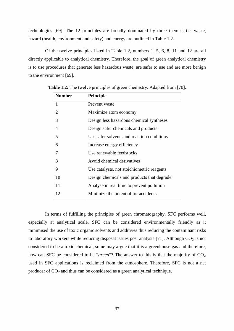
37
technologies [69]. The 12 principles are broadly dominated by three themes; i.e. waste,
hazard (health, environment and safety) and energy are outlined in Table 1.2.
Of the twelve principles listed in Table 1.2, numbers 1, 5, 6, 8, 11 and 12 are all
directly applicable to analytical chemistry. Therefore, the goal of green analytical chemistry
is to use procedures that generate less hazardous waste, are safer to use and are more benign
to the environment [69].
Table 1.2: The twelve principles of green chemistry. Adapted from [70].
Number Principle
1 Prevent waste
2 Maximize atom economy
3 Design less hazardous chemical syntheses
4 Design safer chemicals and products
5 Use safer solvents and reaction conditions
6 Increase energy efficiency
7 Use renewable feedstocks
8 Avoid chemical derivatives
9 Use catalysts, not stoichiometric reagents
10 Design chemicals and products that degrade
11 Analyse in real time to prevent pollution
12 Minimize the potential for accidents
In terms of fulfilling the principles of green chromatography, SFC performs well,
especially at analytical scale. SFC can be considered environmentally friendly as it
minimised the use of toxic organic solvents and additives thus reducing the contaminant risks
to laboratory workers while reducing disposal issues post analysis [71]. Although CO2 is not
considered to be a toxic chemical, some may argue that it is a greenhouse gas and therefore,
how can SFC be considered to be “green”? The answer to this is that the majority of CO2
used in SFC applications is reclaimed from the atmosphere. Therefore, SFC is not a net
producer of CO2 and thus can be considered as a green analytical technique.
38
1.9 Project outline
With the global drive for faster, more environmentally friendly separation techniques, the aim
of this research was to demonstrate the potential of SFC to be used as a viable alternative or
complementary technique to HPLC in the highly regulated world of the Pharma Quality
Control (QC) laboratory. This was achieved in the present work through the development and
more importantly, the validation of selected applications to showcase the strengths, while at
the same time dispelling some of the historically perceived weaknesses (e.g. poor sensitivity,
reproducibility), associated with analytical SFC. To do this, any SFC application had to be
capable of meeting, if not exceeding the performance levels of the current established LC
applications for QC testing of pharmaceutical drug substance (DS) and drug product (DP)
formulations.
Chapter 2 focuses on exploiting one of the recognised and established strengths of
SFC (i.e. chiral separations). In this chapter, a new enantioselective pSFC method was
developed and validated under International Conference of Harmonisation (ICH) guidance to
meet the current European Pharmacopoeia requirements of a limit test for the determination
of S-timolol enantiomeric purity in timolol maleate DS. The developed pSFC method is
presented as an alternative to the current NP-HPLC method described in the European
Pharmacopoeia (Timolol Maleate Monograph). The newly developed pSFC method achieved
a resolution of 2.0 within 5 min, representing a 3-fold reduction in run-time and an 11-fold
reduction in solvent consumption relative to the NP-HPLC method.
Chapter 3 details the development of an improved HPLC application using the most
up-to-date stationary phase technology available. This chapter focuses on the use of
superficially porous particles or so called “coreshell” stationary phase technology which has
seen resurgence in recent years particularly in HPLC applications due performance
improvements over more traditional fully porous HPLC stationary phases. A new stability
indicating reversed phase HPLC (RP-HPLC) method was developed and validated under
current ICH guidance for the determination of prednisolone acetate (PAC) and impurities in
an ophthalmic suspension. The developed method is presented as an alternative to a modified
version of the current RP-HPLC method described in the USP monograph for the assay of
PAC in an ophthalmic suspension and is capable of identifying and quantifying PAC and
eight selected PAC impurities and degradation products in an ophthalmic suspension. Using
an Agilent Poroshell column with step gradient elution, all peaks of interest are eluted in
39
33 min with resolution of 1.5 between the critical pairs. This method represents optimal
HPLC performance for the selected separation and was used as yardstick for comparison
purposes between the HPLC and SFC applications.
Chapter 4 focuses on demonstrating the potential of SFC to complement HPLC in
the QC laboratory by developing and validating an orthogonal achiral separation for the same
PAC sample described in Chapter 3. To be deemed viable, the new pSFC method had to be
capable of meeting the ICH requirements for a stability indicating method for trace impurity
analysis of the PAC sample, whilst providing an equivalent if not better separation to the
RP-HPLC method described in Chapter 3. The validation strategy employed was more
statistically based compared to the more traditional method characterisation based strategies
employed for the validation of methods in Chapters 2 and 3. The statistical approach selected
for the method validation was the total error approach with accuracy profiles for two
regression models, based on β-expectation tolerance intervals. The accuracy profiles
demonstrate that the new pSFC method is indeed fit for purpose and is capable of meeting the
QC requirements for each compound of interest and can be presented as a viable alternative
to the previously developed RP-HPLC method.
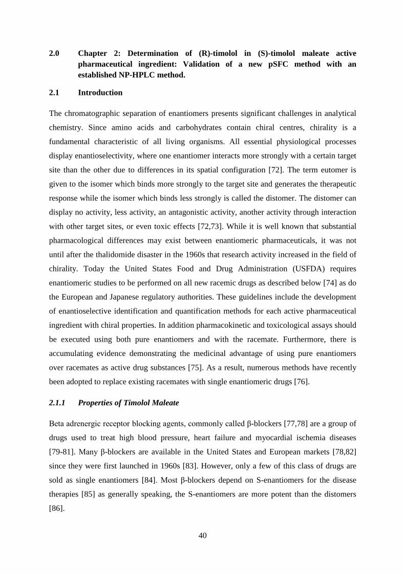
40
2.0 Chapter 2: Determination of (R)-timolol in (S)-timolol maleate active pharmaceutical ingredient: Validation of a new pSFC method with an established NP-HPLC method.
2.1 Introduction
The chromatographic separation of enantiomers presents significant challenges in analytical
chemistry. Since amino acids and carbohydrates contain chiral centres, chirality is a
fundamental characteristic of all living organisms. All essential physiological processes
display enantioselectivity, where one enantiomer interacts more strongly with a certain target
site than the other due to differences in its spatial configuration [72]. The term eutomer is
given to the isomer which binds more strongly to the target site and generates the therapeutic
response while the isomer which binds less strongly is called the distomer. The distomer can
display no activity, less activity, an antagonistic activity, another activity through interaction
with other target sites, or even toxic effects [72,73]. While it is well known that substantial
pharmacological differences may exist between enantiomeric pharmaceuticals, it was not
until after the thalidomide disaster in the 1960s that research activity increased in the field of
chirality. Today the United States Food and Drug Administration (USFDA) requires
enantiomeric studies to be performed on all new racemic drugs as described below [74] as do
the European and Japanese regulatory authorities. These guidelines include the development
of enantioselective identification and quantification methods for each active pharmaceutical
ingredient with chiral properties. In addition pharmacokinetic and toxicological assays should
be executed using both pure enantiomers and with the racemate. Furthermore, there is
accumulating evidence demonstrating the medicinal advantage of using pure enantiomers
over racemates as active drug substances [75]. As a result, numerous methods have recently
been adopted to replace existing racemates with single enantiomeric drugs [76].
2.1.1 Properties of Timolol Maleate
Beta adrenergic receptor blocking agents, commonly called β-blockers [77,78] are a group of
drugs used to treat high blood pressure, heart failure and myocardial ischemia diseases
[79-81]. Many β-blockers are available in the United States and European markets [78,82]
since they were first launched in 1960s [83]. However, only a few of this class of drugs are
sold as single enantiomers [84]. Most β-blockers depend on S-enantiomers for the disease
therapies [85] as generally speaking, the S-enantiomers are more potent than the distomers
[86].

41
Timolol maleate (s)-(-)-1-(tert.-butylamino)-3-[(4-morpholino-1,2,5-thiadiazol-3-
yl)oxy]-2-propanol maleate (shown below in Figure 2.1) belongs to the thiadiazole class of
compounds and is a non-selective β-adrenergic blocker which is used as a single enantiomer
(S-timolol) for the treatment of hypertension, arrhythmias, angina pectoris, and for the
secondary prevention of myocardial infarctions [87-92]. It is also used for the topical
treatment of increasing intraocular pressure in patients with chronic open angle glaucoma and
aphakia [93-97]. Like all β-adrenoceptor antagonists, timolol is contraindicated in patients
with asthma and its inadvertent administration as eye drops to such patients continues to have
severe and even fatal consequences [98]. Richards and Tattersfield [99] reported that the
R-timolol enantiomer was considerably less potent as a β-adrenoceptor antagonist in animals
than the clinically used S-timolol enantiomer, but only slightly less potent in reducing
intraocular pressure [100]. The R-timolol enantiomer was reported to be 49 times less potent
than S-timolol on β-adrenoceptor in animals and thirteen times less potent in constricting the
airways of normal subjects, yet it is only four times less potent in reducing intraocular
pressure in man [100]. These findings suggested that R-timolol might be a safer alternative
for the treatment of glaucoma with less systemic side-effects than the S-enantiomer when
applied as eye drops (in concentrations ranging between 0.25 and 4.0% (w/v)), as it has a
smaller broncho-constricting effect [100]. However, despite this, the S-enantiomer is still the
choice of drug substance used in the manufacture of timolol-containing products for the
treatment of glaucoma.
Timolol maleate was first synthesized in the Merck-Frosst laboratories in Montreal,
Canada. Timolol maleate is soluble in water, methanol (MeOH) and ethanol. The pKa of
timolol base obtained by potentiometric titration in water at 25 °C is approximately 9.2 [92]
and the native pH of a saturated aqueous solution of timolol maleate is approximately 4.0
[92]. The first non-patent literature reference to timolol maleate appeared in 1972 [94,101].
2.1.2 Analysis of Timolol Maleate by HPLC
A 2008 review by Wang et al. discusses recent developments in enantio-separations of
adrenergic pharmaceuticals [102]. Specifically, enantio-separation of timolol maleate has
been previously reported using capillary electrophoresis (CE) and NP-HPLC.
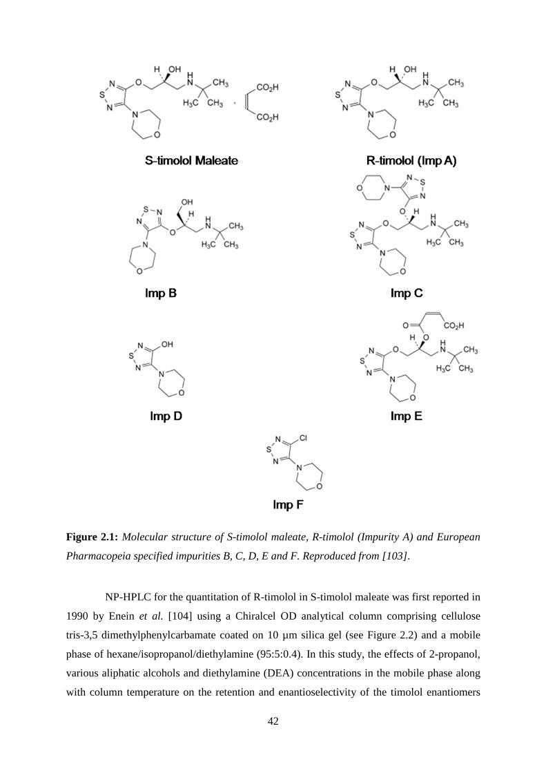
42
Figure 2.1: Molecular structure of S-timolol maleate, R-timolol (Impurity A) and European
Pharmacopeia specified impurities B, C, D, E and F. Reproduced from [103].
NP-HPLC for the quantitation of R-timolol in S-timolol maleate was first reported in
1990 by Enein et al. [104] using a Chiralcel OD analytical column comprising cellulose
tris-3,5 dimethylphenylcarbamate coated on 10 µm silica gel (see Figure 2.2) and a mobile
phase of hexane/isopropanol/diethylamine (95:5:0.4). In this study, the effects of 2-propanol,
various aliphatic alcohols and diethylamine (DEA) concentrations in the mobile phase along
with column temperature on the retention and enantioselectivity of the timolol enantiomers
43
were investigated. It was noted that the enantiomers failed to elute without an alcohol present
in the mobile phase with branched-chain alcohols (particularly 2-propanol) exhibiting the
best resolution (Rs). Retention factor (k), selectivity and Rs all decreased with increasing
2-propanol concentration, with the best Rs being obtained with 5% (v/v) 2-propanol.
Figure 2.2: Molecular structure of the Chiracel OD chiral stationary phase (CSP).
Reproduced from [103].
The effect of DEA concentration ranging from 0.0% to 1.0% (v/v) was also
investigated. It was noted that no separation was obtained in the absence of DEA. The
1.0% (v/v) concentration gave the best enantioresolution of 4.32. However, in order to
prevent the detrimental effect of the basic mobile phase on the stationary phase due to
saponification, as ester groups were present in the packing material, only 0.4% (v/v) DEA
was used, resulting in an R of 4.0 [104]. It was found that the Chiracel OD column was
sensitive to small changes in column temperature. The Rs increased about 1.6-fold when the
temperature was decreased from 30 °C to 5 °C. This increase in Rs with decreasing
temperature supports the existence of both a simultaneous and stepwise binding chiral
recognition mechanism on the CSP as proposed by Wainer et al. [105] in which the chiral
recognition mechanism for the enantiomeric aromatic alcohols were studied. The proposed
mechanism involves: (1) the formation of diastereomeric solute-CSP complexes through a
hydrogen bonding interaction between the solute’s alcoholic hydrogen and an ester carbonyl
on the CSP; (2) the stabilisation of this complex through the insertion of the aromatic portion
of the solute into a chiral cavity (or ravine) of the CSP; and (3) chiral discrimination between
enantiomeric solutes due to difference in their steric fit in the chiral cavity. Therefore, an
increase in temperature resulted in a corresponding increase in the conformational mobility of
the solute, which destabilised the solute-CSP complex and reduced the stereoselectivity. The
final optimised conditions were obtained when using the solvent system hexane: 2-propanol
(95:5) contains 0.4% (v/v) DEA at 5 °C as illustrated in Figure 2.3 [104].

44
Figure 2.3: HPLC separation of timolol maleate enantiomers. Column: Chiralcel OD (250
mm x 4.6 mm I.D.); mobile phase, hexane-2-propanol-DEA (95:5:0.4); flow-rate,
0.7 mL.min-1 ; chart-speed, 0.5 cm/mm; temperature, 5 °C; pressure, 250 p.s.i.; sample
amount, 10 nmol; detector: UV (224 nm); sensitivity, 0.01 a.u.f.s. Reproduced from [104].
In 1994, Lacroix et al. [106] developed and validated NP-HPLC and proton nuclear
magnetic resonance (1H-NMR) methods for the quantitation of the R-enantiomer in S-timolol
maleate. The NP-HPLC method was based on the method previously developed by
Enein et al. [104] which had been optimised for the separation of the R- and S-enantiomers.
However, no data were provided in the Enein method on the selectivity of the method in the
presence of other potential timolol impurities or on the limit of quantitation (LOQ) for the
R-enantiomer in S-timolol maleate raw material. Therefore, Lacroix et al. set out to optimise
the method on the newly available 5 µm particle size column (Chiracel OD-H) which
potentially offered higher efficiencies and the possibility that the Enein method could be
modified and validated for the quantitation of the R-enantiomer in S-timolol maleate drug
substance. Detection at 297 nm was used instead of 224 nm because this corresponds to a
maximum in UV absorbance for the drug in MeOH. Also, several of the related compounds
do not absorb at 297 nm, which minimised interference from these compounds. The
composition of the mobile phase was changed to optimise the separation of the two
enantiomers and other closely eluting compounds, particularly for (S)-l-[l,l-dimethylethyl)

45
amino]-2-[[4-(4-morpholinyl)-l,2,5-thiadiazol-3-yl]oxy]-3-propanol, a structural isomer of
timolol. The final optimised conditions were; mobile phase of 0.2% (v/v) DEA and 4% (v/v)
isopropanol in hexane (1 mL.min-1) for 15 min and UV detection at 297 nm on a Chiracel
OD-H (cellulose tris-3,5-dimethylphenylcarbamate) column (5 µm). Under the conditions
described in this method, typical values for retention factors were k1 = 1.64 and k2 = 2.80, for
the R- and S-enantiomers, respectively; the separation factor (α) was 1.70 and Rs, 4.81 [106].
The effect of temperature on the separation was studied and it was found that an
increase in temperature from ambient to 40 °C caused a decrease in the retention times of the
R- and S-enantiomers and also the structural isomer. Generally the Rs between the R- and
S-enantiomers decreased while the Rs between R- and the structural isomer was only slightly
affected. Rs between the R- and S-enantiomers of timolol increased when the proportion of
isopropanol in the mobile phase was reduced from 5% to 1% (v/v). However, the Rs between
R-timolol and the isomer decreased over the same range and these latter compounds were
unresolved when the proportion of isopropanol was 1% (v/v) [106]. The relative standard
deviation (RSD) of peak area responses for six replicate injections of a solution of R-timolol
maleate at the 0.05% mass/mass (m/m) level was 17.8%. The LOQ for this method was
0.05% (m/m) R-timolol maleate [106].
In 2003, Marini et al. [107] developed a NP-HPLC method on a cellulose tris(3,5-
dimethylphenylcarbamate) (5 µm) CSP and a mixture of hexane, 2-propanol, and DEA as
mobile phase for the simultaneous determination of R-timolol and other potential related
substances in S-timolol maleate. The method was based on the NP-HPLC method described
in the monograph of timolol maleate presented in the European Pharmacopeia (EP) [108]. An
experimental design was elaborated in order to test the effects of three different selected
factors, namely column temperature, the concentrations of 2-propanol and DEA. The three
factors were studied simultaneously, with the effects being evaluated statistically to
determine the optimum LC conditions. The developed LC method was then compared to the
EP method [108] and was applied to the determination of R-timolol and other related
substances in several samples of S-timolol maleate from different sources.
The EP method [108] used mobile phase consisting of hexane/isopropanol/DEA
(95.8:4.0:0.2) (v/v/v). For system suitability purposes, a Rs of 4.0 between the enantiomers
was specified. The optimised method developed by Marini et al. [107-110] permitted the
separation of both enantiomers in the presence of other potential S-timolol impurities;
46
isotimolol, a degradation product, dimer maleate and dimorpholinothiadiazole (DMTDZ)
which are potential synthesis impurities. The separation was achieved within 20 min by
modifying the mobile phase to hexane/isopropanol/DEA (96.5:3.5:0.1) (v/v/v) and the
column temperature (previously unspecified in the EP monograph) to 23 oC. Figure 2.4
illustrates representative chromatograms comparing the EP and optimised methods [107]. For
the EP method, Rs was 1.3 between the critical peak pair (R-timolol and isotimolol) whereas
with Marini’s optimised method Rs was 1.7. Therefore, the developed LC method was
proposed to be used for the simultaneous determination of S-timolol enantiomeric purity and
for the determination of related substances in the revised version of the monograph of
S-timolol maleate. However, this method was not adopted into later versions of the EP
monograph and separate methods for the determination of enantiomeric purity and related
substances still exist in the monograph of S-timolol maleate [103].
2.1.3 Analysis of Timolol Maleate by Capillary Electrophoresis (CE)
In the case of electrophoretic separations, as a result of the higher separation efficiency of CE
compared to conventional HPLC, it is theoretically possible to improve Rs and shorten the
analysis times with CE compared to LC. However, one of the drawbacks is that the limit of
detection (LOD) is often higher for CE than for LC due to the lower loading capacity of CE
and the use of on-column detection. This high detection limit can result in issues for impurity
analysis when using CE [111]. In 2004, Servais et al. investigated the use of non-aqueous
capillary electrophoresis (NACE) with heptakis (2,3-di-O-methyl-6-O-sulfo)-β-cyclodextrin
(HDMS-b-CD) as chiral selector in combination with potassium camphorsulfonate [112]. The
best timolol enantio-separation was observed with 30 mM HDMS-b-CD and 30 mM
potassium camphorsulfonate, all in MeOH containing 0.75 M formic acid which gave a Rs of
8.5 within 12.5 min as shown in Figure 2.5.
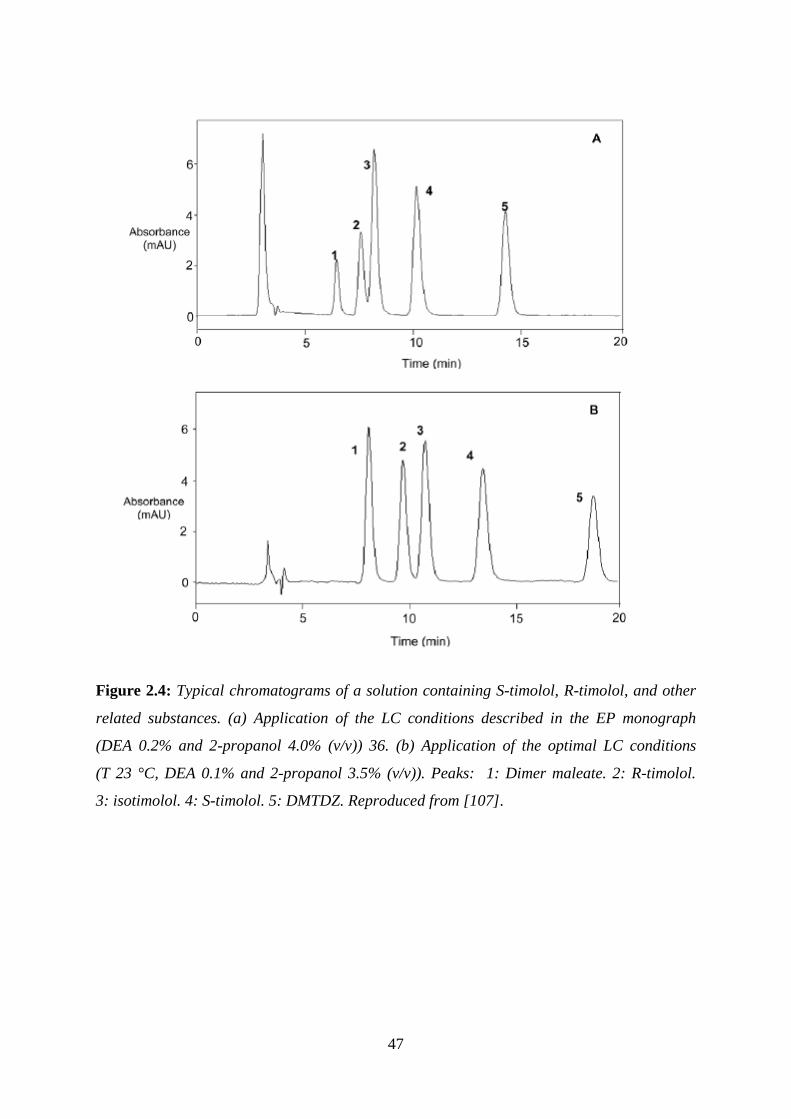
47
Figure 2.4: Typical chromatograms of a solution containing S-timolol, R-timolol, and other
related substances. (a) Application of the LC conditions described in the EP monograph
(DEA 0.2% and 2-propanol 4.0% (v/v)) 36. (b) Application of the optimal LC conditions
(T 23 °C, DEA 0.1% and 2-propanol 3.5% (v/v)). Peaks: 1: Dimer maleate. 2: R-timolol.
3: isotimolol. 4: S-timolol. 5: DMTDZ. Reproduced from [107].

48
Figure 2.5: Enantio-separation of a reconstituted racemic mixture of timolol maleate.
Buffers: 30 mM HDMS-b-CD, 30 mM potassium camphorsulfonate and 0.75 M formic acid
in MeOH. Capillary: 50 um, total length: 48.5 cm, effective length: 40 cm. Voltage: 25 kV.
Injection: 50 mbar, 5 sec. Capillary temperature: 15 oC. Detection: UV @ 295 nm. Peak
concentrations 50 µg.mL-1 in MeOH. Reproduced from [112].
In 2006, Marini et al. investigated the use of NACE to determine the enantiomeric
purity of timolol maleate [113]. The main goal of this work was to achieve adequate
separation while maintaining a LOD of 0.1% for the R-timolol and other impurities
investigated using the NACE method developed by Servais et al. [112]. Another goal of this
study was to confirm the specificity of the LC method previously developed for the
determination of timolol maleate enantiomeric purity [107-110] by using the NACE method
as an orthogonal method to the NP-HPLC method. Once the equivalence of the two methods
was demonstrated, the NACE method could be proposed as an alternative to the NP-HPLC
method.
The final optimised method used for the study included the use of an internal
standard for quantification to compensate for the injection variability due to the low volume
of sample solutions introduced in the capillary and by the possible solvent evaporation from
sample solutions [114]. Pyridoxine at a concentration of 5 µg.mL-1 was selected as internal
standard with the best resolution results (Rs 9.2) being obtained by using a S-timolol solution
at a concentration of 2 mg.mL-1 and by introducing this solution in the capillary under a
pressure of 5 kPa during 8 sec. The applied voltage was 25 kV and UV detection was set at

49
295 nm for data acquisition. Figure 2.6 shows a typical electropherogram of an S-timolol
maleate solution spiked with R-enantiomer (0.1%) and containing the internal standard [113].
Figure 2.6: Typical electropherogram of a mixture solution containing the main timolol
impurities and the pyridoxine used as internal standard. Chromatographic conditions;
Column: uncoated fused silica capillaries having 50 µm internal diameter and 48.5 cm
length (40 cm to the detector). Applied voltage: 25 kV. Selected BGE-CD: 30mM potassium
camphorSO3− and 30mM HDMS-β-CD in methanol acidified with 0.75M formic acid.
Injection: made by pressure (50 mbar) for a period of 8 s (corresponding to 23.4 nL, i.e.
2.5% of the total volume of the capillary). Capillary temperature: 15 °C. Peaks and
concentrations: (1) pyridoxine (10 g.mL-1), (2) S-timolol (2 mg.mL-1), (3) R-timolol (1.0% or
20 g.mL-1), (4) isotimolol (1.09% or 21.8 g/mL) and (5) dimer maleate (0.51% or
10.3 g.mL-1). Reproduced from [113].
A comparison was made between the NACE and NP-HPLC methods by analysing
the same S-timolol samples with both methods. It was concluded that the two analytical
methods were equivalent because the difference of the means observed were comprised
within the 95% agreement limits [113].
In 2007 Hedeland et al. demonstrated the enantioresolution of timolol using 1S,4R-
(+) ketopinic acid [(+)-KPA] as chiral selector in NACE [111]. The method was applied to
determine the enantiomeric impurity R-timolol in the presence of S-timolol with a LOD
requirement of 1% to satisfy the EP specification [115]. During method development, the

50
detection wavelength was set at 220 nm for all experiments. The background electrolyte
(BGE) containing the chiral selector selector [100 mM (+)-KPA] and 40 mM KOH in
MeOH:ethanol [(40:60), (v/v)] was selected for the enantiomeric purity determination of
S-timolol. Under these conditions, the R-timolol impurity was observed to be the fastest
migrating enantiomer, with the enantioresolution of Rs = 4.2 obtained for a racemic mixture
of 0.2 mM timolol. However, in the absence of a stacking technique, a maximum of 1 mM
S-timolol could be injected (35 mbar over 5 sec). In an attempt to decrease the LOD of the
method, the possibility of pre-concentration by Field amplified sample stacking (FASS) and
transient Isotachophoresis (tITP) were evaluated. Through the use of FASS, the LOD was
improved to 1% R-timolol.
However, it was observed that the use of tITP seemed to be a more efficient pre-
concentration technique in this study as illustrated in Figure 2.7. The tITP conditions used in
this study were based on the work by Shihabi [116]. The capillary was first flushed with the
BGE containing the chiral selector. A plug of 100 mM NaAc in MeOH (the leading
electrolyte) was injected by pressure (25 mbar over 1 second) after the chiral BGE and before
the sample injection (S-timolol 2 mM, 35 mbar over 5 sec). Triethanolamine (200 mM in
MeOH) was used as the anodic solution (i.e., the terminating electrolyte), and the chiral BGE
was used as the cathodic solution [111]. By injection of a sample with high concentration, the
LOD could be decreased from 2.5 to 0.2% for the R-enantiomer using tITP. A typical
electropherogram at the LOD are shown in Figure 2.7(c). Furthermore, it was noted that the
migration time decreased from 23 to 10.5 min in the tITP system. This decrease in migration
time was due to the cathodic EOF (1.1×10⁻⁵ cm2 V−1 s−1), caused by the tailing electrolyte.
Only in the selector BGE, the EOF was anodic (−1.9×10⁻⁵ cm2 V−1 s−1) [111].
2.1.4 Chiral analysis by SFC
To date, HPLC utilising polysaccharide CSPs remains the most widely used technique for
enantioseparations in the pharmaceutical industry [116,117]. However, despite its popularity
there are a number of disadvantages associated with this separation technique including;
(1) relatively long analysis times, (2) limited sample throughput and (3) the high consumption
of toxic and flammable solvents. Also, there can be issues in terms of up-scaling of the chiral
separation method to a preparative level, especially with reversed-phase liquid
chromatography [118]. Therefore, SFC is currently experiencing a renaissance (particularly
within the pharmaceutical industry) as a valuable alternative chromatographic technique for

51
chiral separations due to its relative environmental benignity [119,120]. Evidence of this is
seen from the increased publication of review papers relating to SFC applications [121-124].
Figure 2.7: Peak sharpening of S-timolol. BGE: 100 mM (+)-KPA and 40 mM KOH in
MeOH:EtOH (3:2, v/v). 30 kV, Ldet 23 cm Sample: 2 mM S-timolol and 0.05 mM R-timolol
(2.4%) dissolved in MeOH. (a) Normal injection pressure injection at 35 mbar over 5 s, (b)
transient ITP, leading electrolyte: 100 mM NaAc in MeOH (25 mbar over 1 s). Terminating
electrolyte: 200 mM triethanolamine in MeOH (anodic vial). (c) Transient ITP at LOD (0.2%
R-timolol). Conditions as in (B). The arrow in the electropherograms (a–c) points out the
position of the R-timolol peak. Reproduced from [111].
There has also been an increase in the number of industrial users driven in part by the
increased investment of major instrument manufacturers in the production of commercial
52
availability of SFC instrumentation which exhibits significantly improved performance
characteristics relative to the instrumentation of the early 1990’s [125,126] as noted in
Chapter 1. Also, the potential benefits over conventional HPLC in terms of solvent cost
reduction and waste removal are becoming ever more important to satisfy the need for more
environmentally friendly modes of analysis. As a result, packed column SFC is becoming
more widely used for chiral separations and has the potential to replace HPLC as a first
choice technique for enantioseparations and purifications in drug discovery and development
processes.
However, SFC has historically suffered from a serious lack of sensitivity and has
rarely found a place in trace analysis or regulated environments [57,127]. One of the major
obstacles is that (until recently) SFC instruments employing UV detection were less sensitive
compared to HPLC-UV instruments making the detection of trace level impurities very
challenging [128]. A recent review by De Klerk et al. reveals that SFC is becoming ever
more popular for enantioseparation of pharmaceuticals [129]. Gyllenhaal et al. demonstrated
the use of a Hypercarb packed column using L-(+)-tartaric acid as chiral selector to resolve
enantiomers of selected β-blockers [130]. Medvedovici et al. used polysaccharide stationary
phases to separate β-agonists [131]. Lui et al. used three macrocyclic glycopeptide chiral
selectors and compared their performance in the separation of a range of β-blockers [132].
However, at the time our work was undertaken, to the best of our knowledge, no report has
appeared in the literature describing the use of SFC for the enantioseparation of timolol
maleate or indeed any active pharmaceutical ingredient used in ophthalmic medications.
During the last decades, a large number of CSPs have been developed to achieve
chiral separation of a wide variety of racemic compounds and enantio-separations on CSPs
has thus far been one of the most popular applications of SFC [129,133,134]. A wide range of
CSPs have been used in SFC including Pirkle type, cyclodextrins and derivatized
polysaccharide-based CSPs. The polysaccharide-based stationary phases, mainly the tris(3,5-
dimethylphenylcarbamate) of amylose (Chiralpak AD) and cellulose (Chiralcel OD), have
proven to be two of the most successful and widely applied CSPs due to the high number of
compounds resolved in normal phase mode. Fortuitously, these polysaccharide-based
stationary phases are also among the most successful in chiral SFC applications. The
derivatized polysaccharide phase, Chiralcel OD-H, incorporates a cellulose carbamate
derivative coated on silica gel as the chiral selector and has been used to separate R-timolol
and S-timolol as described above.
53
Although fundamental studies of the chiral recognition mechanisms on
polysaccharide CSPs have been reported, [135-137] a clear description of the
chromatographic processes operating on these CSPs is still missing. However, a clear
difference in enantioselectivity has been observed between SFC and LC modes with
hydrogen bonding being found to play an important role in the differential binding of the
enantiomers to the CSPs in SFC applications [134]. Consequently, method development in
chiral SFC, as in chiral NP-HPLC, generally relies on a systematic screening of CSPs and
mobile phases, in a preferential order or in parallel based on personal experience of the
analyst. However, with shorter retention times compared to conventional NP-HPLC, method
development with chiral SFC is faster without sacrificing efficiency [129]. The mobile phase
components to be optimised are relatively limited, with only a few organic modifiers
commonly used and investigations into the effect of pH generally omitted with CO2-based
mobile phases. As with NP-HPLC, temperature can play a significant role in SFC method
development particularly in chiral separations [138].
With this in mind, the aim of this study was to develop an alternative pSFC limit test
assay for the determination of S-timolol maleate enantiomeric purity and compare it to the
current EP NP-HPLC compendial method of analysis which uses a cellulose tris(3,5-
dimethylphenylcarbamate) coated silica stationary phase [104,107,109,110] under normal
phase conditions [103]. The developed method was compared with the existing normal phase
method using standard analytical performance criteria.
2.2 Experimental
2.2.1 Instrumentation and Software
Both NP-HPLC and pSFC assays were carried out on a 4.6 mm x 250 mm Chiralcel OD-H
column packed with 5 µm silica particles coated with cellulose tris(3,5-
dimethylphenylcarbamate) from Daicel Limited Industries (Tokyo, Japan). The NP-HPLC
assay was performed on a Waters Alliance 2695 HPLC system coupled with Waters 2487
Dual Wavelength Absorbance Detector (Waters, Milford, MA, USA). Chromatographic data
was acquired and processed using Waters EmpowerTM 2 software. For the optimised
NP-HPLC assay the mobile phase of hexane/2-propanol/DEA (960:40:2) was delivered at
1.0 mL.min-1 at ambient column temperature [103]. Injection volume was 5 µL and detection
was by UV at 297 nm with data acquisition at 5 Hz. The pSFC method development and
validation was performed on an Agilent 1260 Infinity Analytical SFC system coupled with an
54
Aurora SFC Fusion A5 CO2 delivery system equipped with a DAD detector (Agilent
Technologies, Santa Clara, CA, USA). Chromatographic data was acquired and processed
using Agilent Chemstation Rev B.04.03 software. For the optimised pSFC assay, the mobile
phase of (93:7) CO2/0.1% (v/v) triethylamine (TEA) in MeOH was delivered isocratically at
a flow rate of 4.0 mL.min-1. Column temperature was set to 40 oC with backpressure
regulation set to 130 bar. An injection loop of 5 µL was over-filled with 15 µL of sample
and peaks were detected at 297 nm with data acquisition at 20 Hz.
2.2.2 Materials and Reagents
Samples of S-timolol maleate and R-timolol base and impurities B, C, D and F were obtained
from the EP Secretariat (Strasbourg, France). (Note: R-timolol is also known as Impurity A).
N-hexane of LC grade was purchased from Romil (Waterbeach, Cambridge, UK). Methylene
chloride, HPLC grade MeOH and 2-propanol was from Merck (Darmstadt, Germany), and
reagent grade DEA and reagent grade TEA from Sigma Aldrich (Dublin, Ireland). Food
grade CO2 (99.9% v/v minimum) was purchased from BOC Ltd. (Dublin, Ireland).
2.2.3 Solution preparation for Timolol NP-HPLC analysis
Note: Solution preparation for the NP-HPLC assay and the SFC assay (below) is also detailed
in Table 2.1 for the sake of clarity.
All standard solutions were prepared (and diluted as appropriate) in methylene chloride/2-
propanol (10:30) using actinic glassware to protect from light. Two stock standards of
S-timolol maleate and one stock standard of R-timolol were prepared based on timolol free
base at 9.5 mM and 7.6 x 10⁻² mM respectively. Both S-timolol maleate stock standards were
diluted to 9.5 x 10⁻² mM for recovery and method precision studies. A racemic mixture
containing S-timolol maleate and R-timolol at a concentration of 4.7 x 10⁻² mM was prepared
from stock standard dilutions and used as a control resolution mixture (CRM) to assess Rs and
to calculate a relative response factor (RRF) for R-timolol relative to S-timolol maleate.
Finally, a solution of S-timolol maleate and R-timolol was prepared at 9.5 x 10⁻² mM and
9.5 x 10⁻⁴ mM respectively (R-timolol concentration being equivalent to 1.0 % of the
S-timolol maleate concentration). This solution was used to generate data for comparative
purposes with the pSFC method.

55
2.2.4 Solution preparation for Timolol pSFC analysis
All standard solutions were prepared in 100% MeOH using actinic glassware. Four stock
standards of S-timolol maleate and three stock standards of R-timolol were prepared based on
timolol free base at 28 mM and 2.3 x 10⁻¹ mM respectively. Two of the S-timolol maleate
stock standards were diluted to 2.8 x 10⁻¹ mM for recovery and method precision studies.
Standards were prepared containing S-timolol maleate at 2.8 x 10⁻¹ mM and R-timolol at
5.7 x 10⁻³ mM, 2.8 x 10⁻³ mM, 1.4 x 10⁻³ mM, 2.8 x 10⁻⁴ mM, 1.4 x 10⁻⁴ mM, equivalent to 2.0,
1.0, 0.5, 0.1 and 0.05 % of the S-timolol maleate concentration. These standards were used for
validation of the SFC method. A solution containing S-timolol maleate and R-timolol at
1.4 x 10⁻¹ mM was prepared as a CRM to assess Rs and to calculate an RRF for R-timolol
maleate relative to S-timolol maleate.
2.2.5 Solution preparation for evaluation of Timolol pSFC Specificity
A solution was prepared containing all of the EP timolol specified impurities i.e. B ((2RS)-3-
[(1,1-dimethylethyl)amino]-2-[[4-(morpholin-4-yl)-1,2,5-thiadiazol-3-yl]oxy]propan-1-ol),
C((2RS)-N-(1,1-dimethylethyl)-2,3-bis[[4-(morpholin-4-yl)-1,2,5-thiadiazol-3-yl]oxy]propan-
1-amine),D(4-(morpholin-4-yl)-1,2,5-thiadiazol-3-ol), E ((2Z)-4-[(1S)-1-[[(1,1-dimethylethyl)
amino]methyl]-2-[[4-(morpholin-4-yl)-1,2,5-thiadiazol-3-yl]oxy]ethoxy]-4-oxobut-2-enoic
acid) and F (4-(4-chloro-1,2,5-thiadiazol-3-yl)morpholine) by dissolving 5 mg of the timolol
for system suitability standard obtained from the EP Secretariat (Strasbourg, France) in 1 mL
of MeOH. Impurity E was generated as described in the EP [103] by reacting timolol maleate
(2 mg) with maleic acid (20 mg) in acetonitrile (10 mL). 1 mL of this solution was then
evaporated under nitrogen before being dried at 105 °C for 1 hour. The reagent was then
reconstituted with 1 mL of MeOH. 200 µL of the Impurity E solution was added to a vial of
EP system suitability mix (containing impurity B, C, D and F) containing 800 µL of MeOH to
generate an impurity mix solution containing all of the specified timolol impurities.
2.3 Results and discussion
2.3.1 Timolol pSFC Method Development
All pSFC development work was carried out on same Chiralcel OD-H cellulose tris(3,5-
dimethylphenylcarbamate) stationary phase as was used for the NP-HPLC assay [103,108].
This stationary phase was selected primarily so that a direct comparison could be made
between the pSFC method described here, and the previously developed NP-HPLC assay.
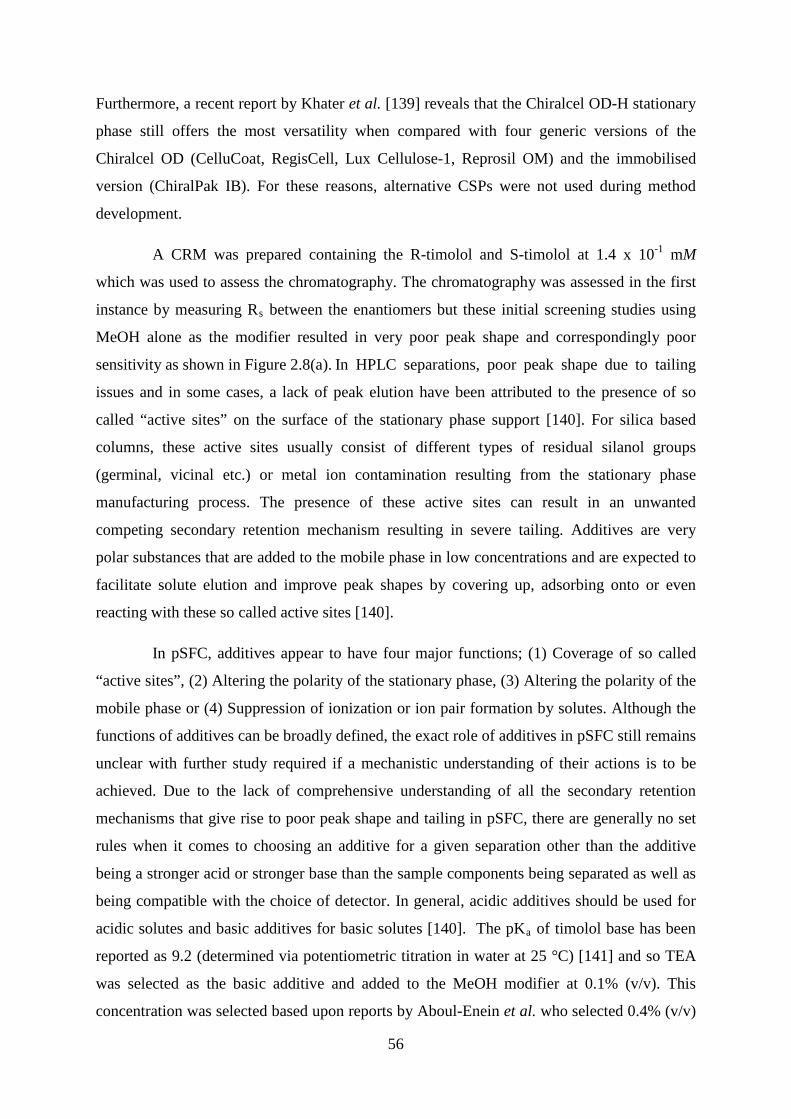
56
Furthermore, a recent report by Khater et al. [139] reveals that the Chiralcel OD-H stationary
phase still offers the most versatility when compared with four generic versions of the
Chiralcel OD (CelluCoat, RegisCell, Lux Cellulose-1, Reprosil OM) and the immobilised
version (ChiralPak IB). For these reasons, alternative CSPs were not used during method
development.
A CRM was prepared containing the R-timolol and S-timolol at 1.4 x 10⁻¹ mM
which was used to assess the chromatography. The chromatography was assessed in the first
instance by measuring Rs between the enantiomers but these initial screening studies using
MeOH alone as the modifier resulted in very poor peak shape and correspondingly poor
sensitivity as shown in Figure 2.8(a). In HPLC separations, poor peak shape due to tailing
issues and in some cases, a lack of peak elution have been attributed to the presence of so
called “active sites” on the surface of the stationary phase support [140]. For silica based
columns, these active sites usually consist of different types of residual silanol groups
(germinal, vicinal etc.) or metal ion contamination resulting from the stationary phase
manufacturing process. The presence of these active sites can result in an unwanted
competing secondary retention mechanism resulting in severe tailing. Additives are very
polar substances that are added to the mobile phase in low concentrations and are expected to
facilitate solute elution and improve peak shapes by covering up, adsorbing onto or even
reacting with these so called active sites [140].
In pSFC, additives appear to have four major functions; (1) Coverage of so called
“active sites”, (2) Altering the polarity of the stationary phase, (3) Altering the polarity of the
mobile phase or (4) Suppression of ionization or ion pair formation by solutes. Although the
functions of additives can be broadly defined, the exact role of additives in pSFC still remains
unclear with further study required if a mechanistic understanding of their actions is to be
achieved. Due to the lack of comprehensive understanding of all the secondary retention
mechanisms that give rise to poor peak shape and tailing in pSFC, there are generally no set
rules when it comes to choosing an additive for a given separation other than the additive
being a stronger acid or stronger base than the sample components being separated as well as
being compatible with the choice of detector. In general, acidic additives should be used for
acidic solutes and basic additives for basic solutes [140]. The pKa of timolol base has been
reported as 9.2 (determined via potentiometric titration in water at 25 °C) [141] and so TEA
was selected as the basic additive and added to the MeOH modifier at 0.1% (v/v). This
concentration was selected based upon reports by Aboul-Enein et al. who selected 0.4% (v/v)

57
DEA in their NP-HPLC assay, observing that the absence of base on the mobile phase
resulted in no separation, whereas higher levels (1% v/v) could result in damage to the silica
support particle [104].
The effect of the additive was immediate, with peak shape and sensitivity being
dramatically improved as shown in Figure 2.8(b). Elution order remained unaffected but Rs
of 2.82 and peak asymmetries of 0.82 for both R-timolol and S-timolol was achieved by the
inclusion of the additive to the mobile phase. Although other workers [109,110] and the EP
monograph [103] have indicated the use of DEA as the basic additive in NP-HPLC assays, in
the work presented herein, no further efforts were made to investigate the effect of alternative
basic additives or the effect of TEA concentration, since adequate Rs was achieved for the
purposes of a limit test.

58
Table 2.1: Solution preparation for NP-HPLC and pSFC analysis Solutions for NP-HPLC Diluent Solution Analyte Concentration (mM)a % R-timolol w.r.t S-timolol
Methylene chloride/2-
propanol (10:30)
R-timolol Stock standard R-timolol 7.6 x 10⁻² mM
n/a
S-timolol Stock standard S-timolol 9.5 mM Recovery/method
precision standards S-timolol 9.5 x 10⁻² mM
CRM mixture R-timolol
4.7 x 10⁻² mM S-timolol
S-timolol/R-timolol spiked standards
R-timolol 9.5 x 10⁻⁴ mM 1.0%
S-timolol Solutions for pSFC Diluent Solution Analyte Concentration (mM)a % R-timolol w.r.t S-timolol
MeOH
R-timolol Stock standard R-timolol 2.3 x 10⁻¹ mM S-timolol Stock standard S-timolol 28 mM n/a
Precision studies S-timolol 2.8 x 10⁻¹ mM
S-timolol/R-timolol spiked standards
R-timolol 5.7 x 10⁻³ mM, 2.8 x 10⁻³ mM, 1.4 x 10⁻³ mM,
2.8 x 10⁻⁴ mM, 1.4 x 10⁻⁴ mM, 2.0%, 1.0%, 0.5%, 0.1%, 0.05%
S-timolol 2.8 x 10⁻¹ mM
CRM mixture R-timolol
1.4 x 10⁻¹ mM 50% S-timolol
a Based on timolol free base M.W. 316.4 g

59
Figure 2.8: Separation of R-timolol and S-timolol via pSFC using a mobile phase without
(a) and with (b) the presence of 0.1% (v/v) TEA of the MeOH modifier. Chromatographic
conditions; Column: 4.6 mm x 250 mm Chiralcel OD-H, 5 µm. Flow rate: 4.0 mL.min-1.
Injection volume: 15 µL. Column temperature: 40 oC. Back-pressure regulation: 130 bar.
Detection: 297 nm. Mobile phase: (93:7) CO2/MeOH for chromatogram (a) and (93:7)
CO2/0.1% (v/v) TEA in MeOH for chromatogram (b). Peak assignment and concentration:
(R): R-timolol at 1.4 x 10⁻¹ mM and (S): S-timolol at 1.4 x 10⁻¹ mM.
The remainder of the development work involved performing optimisation
experiments in which flow rate and mobile phase composition were adjusted to reduce
runtimes for increased sample throughput, while maintaining USP Rs > 2 and peak tailing
< 1.5 for both enantiomers in the CRM. Isocratic methods were favoured over gradient
methods to eliminate the necessary system equilibration time after each run. A series of
chromatograms were generated with varying amounts of modifier. The selected optimised
conditions described above were used with modifier concentrations of 3, 5, 7, 9, 11, 15, and
20% (v/v) respectively. For this investigation, the CRM contained both R- and S-timolol at a
concentration of 1.4 x 10⁻¹ mM. A plot of k and Rs values versus % modifier concentration is
shown in Figure 2.10 where the non-linear effect of modifier concentrations on the retention
factors of R-timolol and S-timolol is demonstrated. As expected, retention decreased steadily
as % MeOH increased with a corresponding decrease in resolution at higher modifier
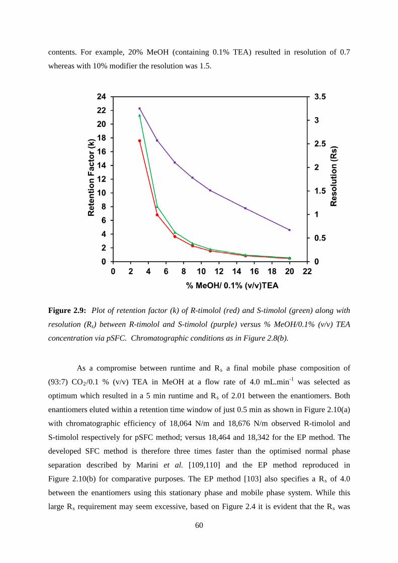
60
contents. For example, 20% MeOH (containing 0.1% TEA) resulted in resolution of 0.7
whereas with 10% modifier the resolution was 1.5.
Figure 2.9: Plot of retention factor (k) of R-timolol (red) and S-timolol (green) along with
resolution (Rs) between R-timolol and S-timolol (purple) versus % MeOH/0.1% (v/v) TEA
concentration via pSFC. Chromatographic conditions as in Figure 2.8(b).
As a compromise between runtime and Rs a final mobile phase composition of
(93:7) CO2/0.1 % (v/v) TEA in MeOH at a flow rate of 4.0 mL.min-1 was selected as
optimum which resulted in a 5 min runtime and Rs of 2.01 between the enantiomers. Both
enantiomers eluted within a retention time window of just 0.5 min as shown in Figure 2.10(a)
with chromatographic efficiency of 18,064 N/m and 18,676 N/m observed R-timolol and
S-timolol respectively for pSFC method; versus 18,464 and 18,342 for the EP method. The
developed SFC method is therefore three times faster than the optimised normal phase
separation described by Marini et al. [109,110] and the EP method reproduced in
Figure 2.10(b) for comparative purposes. The EP method [103] also specifies a Rs of 4.0
between the enantiomers using this stationary phase and mobile phase system. While this
large Rs requirement may seem excessive, based on Figure 2.4 it is evident that the Rs was
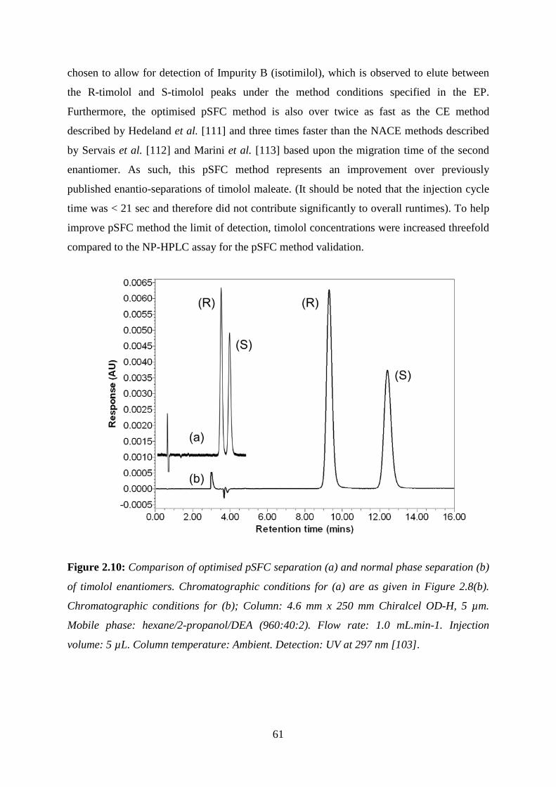
61
chosen to allow for detection of Impurity B (isotimilol), which is observed to elute between
the R-timolol and S-timolol peaks under the method conditions specified in the EP.
Furthermore, the optimised pSFC method is also over twice as fast as the CE method
described by Hedeland et al. [111] and three times faster than the NACE methods described
by Servais et al. [112] and Marini et al. [113] based upon the migration time of the second
enantiomer. As such, this pSFC method represents an improvement over previously
published enantio-separations of timolol maleate. (It should be noted that the injection cycle
time was < 21 sec and therefore did not contribute significantly to overall runtimes). To help
improve pSFC method the limit of detection, timolol concentrations were increased threefold
compared to the NP-HPLC assay for the pSFC method validation.
Figure 2.10: Comparison of optimised pSFC separation (a) and normal phase separation (b)
of timolol enantiomers. Chromatographic conditions for (a) are as given in Figure 2.8(b).
Chromatographic conditions for (b); Column: 4.6 mm x 250 mm Chiralcel OD-H, 5 µm.
Mobile phase: hexane/2-propanol/DEA (960:40:2). Flow rate: 1.0 mL.min-1. Injection
volume: 5 µL. Column temperature: Ambient. Detection: UV at 297 nm [103].

62
2.3.2 Timolol pSFC Method Validation
The pSFC method was developed to offer an alternative to the existing NP-HPLC assay
currently in use within industry (Allergan Pharmaceuticals) and reported by Marini et al.
[109,110]. R-timolol is an unwanted impurity in S-timolol drug substance and in the
pharmaceutical industry, the purity of an active pharmaceutical ingredient can be determined
using either a limit test or a quantitative test. The NP-HPLC assay is described in the EP
[103] as a limit test based upon a specification of not more than (NMT) 1.0% of R-timolol in
the presence of S-timolol. The ICH requirements for the validation of a limit test are
specificity and LOD [142]. Therefore, in the first instance, these two analytical performance
criteria were initially evaluated to demonstrate the applicability of the developed SFC method
as a limit test and the results are evaluated below. For a quantitative test relative to a “limit
test”, additional analytical performance characteristics must be evaluated, namely: accuracy,
precision, LOQ, linearity, range and robustness [142,143]. Therefore, further selected
validation criteria were then studied to demonstrate the additional potential of this method as
a quantitative test for R-timolol impurity in S-timolol and the results presented hereafter.
2.3.2.1 Validation of Timolol pSFC Method as a Limit Test – Specificity and LOD
The LOD is defined as the smallest quantity of the target substance (in this case, R-timolol)
that can be detected relative to baseline noise, but not accurately quantified in the sample
[142]. Baseline noise was compared with the peak height of a standard containing 0.5%
R-timolol in the presence of S-timolol as seen in Figure 2.11 below. The magnitude of
baseline noise was measured in a blank chromatogram over a distance equivalent to 5 times
the peak width at half height of the R-timolol peak, centred around its expected retention time
(noise window: 3.8 min). The LOD results are summarised in Table 2.2 and indicate that the
LOD was found to be 0.5% for R-timolol in the presence of S-timolol maleate, satisfying the
requirement for the limit test method [103] to be able to detect R-timolol at the 1.0% level of
the S-timolol maleate peak.
The specificity of a method is defined as the ability to assess unequivocally the
analyte in the presence of components which may be expected to be present [142]. The EP
specifies five impurities shown in Figure 2.1 which can potentially be present in S-timolol
drug substance; Impurity A (R-timolol), Impurity B (isotimolol), Impurity C, Impurity D,
Impurity E and Impurity F [103]. A commercially available EP impurity system suitability
mixture comprising S-timolol spiked with all known impurities was used to assess the
63
specificity of the method (Impurity E was added separately to this mixture). However, only
Impurity A (R-timolol) and Impurity E could be individually identified by retention time.
Nevertheless Figure 2.12 clearly indicates that all five impurity peaks are baseline separated
from R- and S-timolol, demonstrating the specificity of the method for the determination of
R-timolol in S-timolol drug substance.
Figure 2.11: Chromatograms of (a), pSFC sample containing R-timolol at the LOD of 0.5%
in the presence of S-timolol maleate demonstrating the USP signal-to-noise (SN) calculation
2(H)/h [143]. (b), MeOH blank demonstrating specificity and the low baseline noise.
Chromatographic conditions are as given in Figure 2.8(b).
2.3.2.2 Investigation of Timolol pSFC Method as a potential Quantitative Impurities
Assay
The additional analytical performance characteristics evaluated to demonstrate the potential
of the method for quantitative analysis for R-timolol impurity in S-timolol were; precision,
robustness and accuracy.
2.3.2.3 Timolol pSFC Precision studies: Repeatability and Intermediate Precision
The repeatability of the pSFC method was evaluated by preparing a standard containing
R-timolol at 1.0% relative to S-timolol maleate concentration and injecting six times on
Day #1. Intermediate precision was determined by preparing two separate fresh preparations
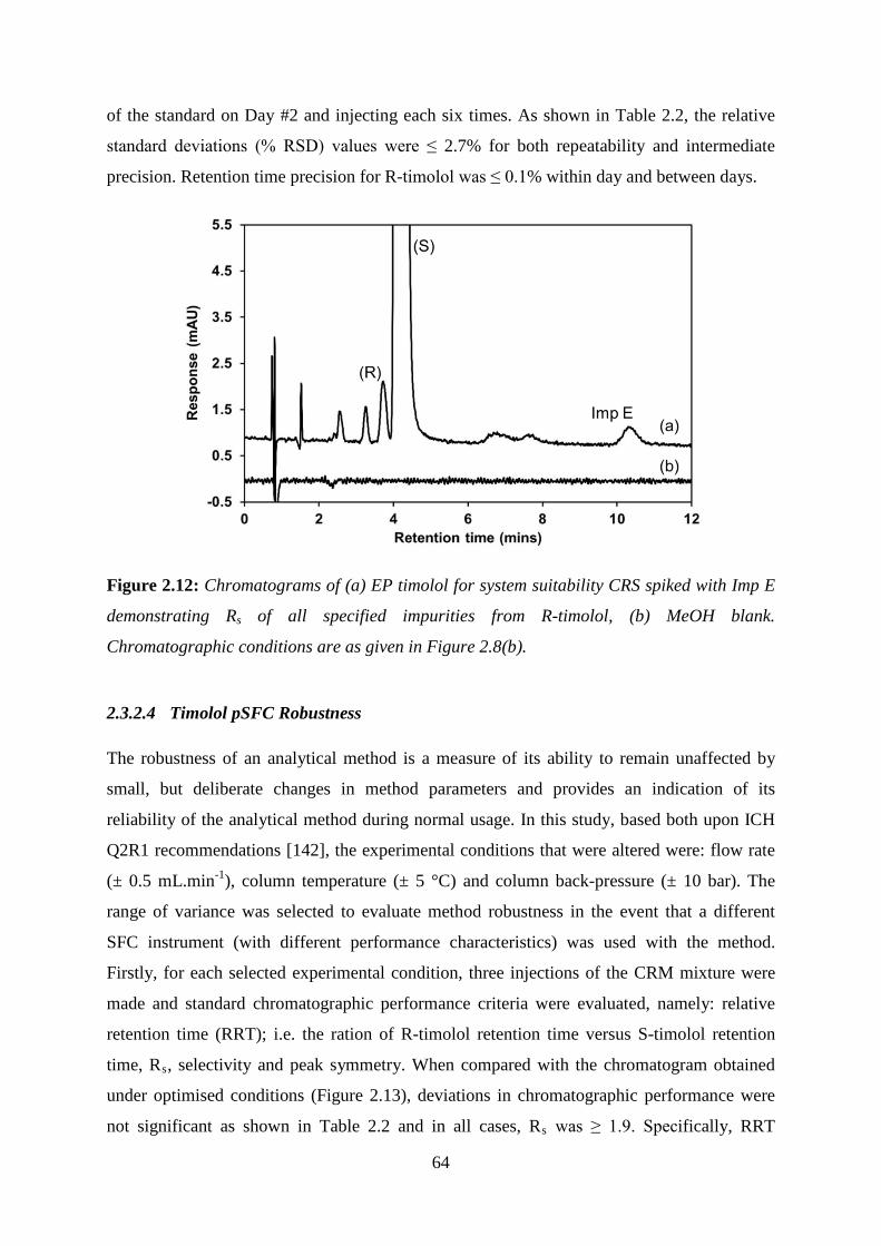
64
of the standard on Day #2 and injecting each six times. As shown in Table 2.2, the relative
standard deviations (% RSD) values were ≤ 2.7% for both repeatability and intermediate
precision. Retention time precision for R-timolol was ≤ 0.1% within day and between days.
Figure 2.12: Chromatograms of (a) EP timolol for system suitability CRS spiked with Imp E
demonstrating Rs of all specified impurities from R-timolol, (b) MeOH blank.
Chromatographic conditions are as given in Figure 2.8(b).
2.3.2.4 Timolol pSFC Robustness
The robustness of an analytical method is a measure of its ability to remain unaffected by
small, but deliberate changes in method parameters and provides an indication of its
reliability of the analytical method during normal usage. In this study, based both upon ICH
Q2R1 recommendations [142], the experimental conditions that were altered were: flow rate
(± 0.5 mL.min-1), column temperature (± 5 °C) and column back-pressure (± 10 bar). The
range of variance was selected to evaluate method robustness in the event that a different
SFC instrument (with different performance characteristics) was used with the method.
Firstly, for each selected experimental condition, three injections of the CRM mixture were
made and standard chromatographic performance criteria were evaluated, namely: relative
retention time (RRT); i.e. the ration of R-timolol retention time versus S-timolol retention
time, Rs, selectivity and peak symmetry. When compared with the chromatogram obtained
under optimised conditions (Figure 2.13), deviations in chromatographic performance were
not significant as shown in Table 2.2 and in all cases, Rs was ≥ 1.9. Specifically, RRT
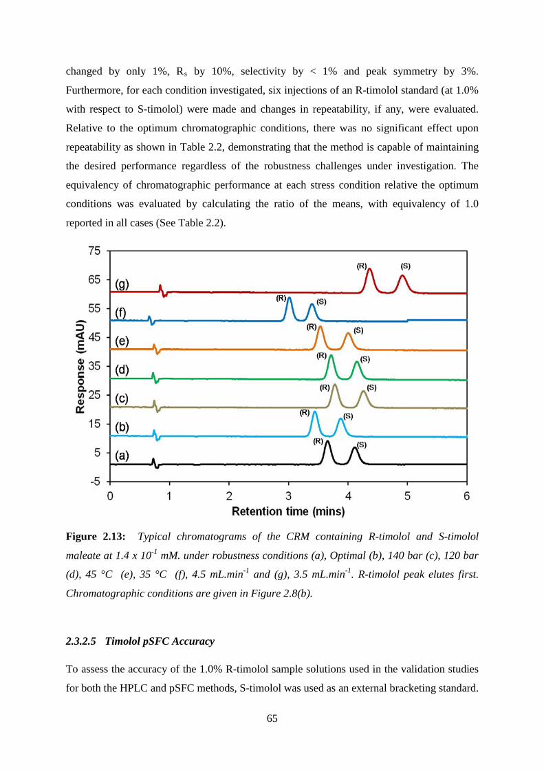
65
changed by only 1%, Rs by 10%, selectivity by < 1% and peak symmetry by 3%.
Furthermore, for each condition investigated, six injections of an R-timolol standard (at 1.0%
with respect to S-timolol) were made and changes in repeatability, if any, were evaluated.
Relative to the optimum chromatographic conditions, there was no significant effect upon
repeatability as shown in Table 2.2, demonstrating that the method is capable of maintaining
the desired performance regardless of the robustness challenges under investigation. The
equivalency of chromatographic performance at each stress condition relative the optimum
conditions was evaluated by calculating the ratio of the means, with equivalency of 1.0
reported in all cases (See Table 2.2).
Figure 2.13: Typical chromatograms of the CRM containing R-timolol and S-timolol
maleate at 1.4 x 10⁻¹ mM. under robustness conditions (a), Optimal (b), 140 bar (c), 120 bar
(d), 45 °C (e), 35 °C (f), 4.5 mL.min-1 and (g), 3.5 mL.min-1. R-timolol peak elutes first.
Chromatographic conditions are given in Figure 2.8(b).
2.3.2.5 Timolol pSFC Accuracy
To assess the accuracy of the 1.0% R-timolol sample solutions used in the validation studies
for both the HPLC and pSFC methods, S-timolol was used as an external bracketing standard.
66
To eliminate differences in UV response between R-timolol and S-timolol, relative response
factors (RRF) were generated by calculating the differences in peak area versus concentration
for the CRM solution, since both enantiomers were present at the same concentration. The
RRF values for both the HPLC and pSFC methods are shown in Table 2.2. Recovery values
of 98% and 101% are reported for R-timolol in the NP-HPLC and pSFC methods
respectively.
2.3.3 Analytical Performance Comparison: pSFC versus NP-HPLC
The pSFC method offered comparable performance to the NP-HPLC method in terms of peak
response, precision and detection limit (with increased sample concentration). A comparison
of the pSFC and NP-HPLC methods is outlined in Table 2.3. For comparative purposes,
Figure 2.14 illustrates chromatograms from both methods in which the benefits of pSFC over
NP-HPLC in terms of analysis time and solvent consumption are obvious. To our knowledge
Figure 2.14 represents the fastest enantiomeric separation of timolol enantiomers reported to
date.
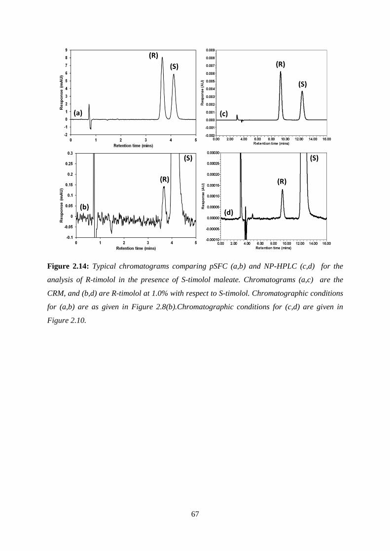
67
Figure 2.14: Typical chromatograms comparing pSFC (a,b) and NP-HPLC (c,d) for the
analysis of R-timolol in the presence of S-timolol maleate. Chromatograms (a,c) are the
CRM, and (b,d) are R-timolol at 1.0% with respect to S-timolol. Chromatographic conditions
for (a,b) are as given in Figure 2.8(b).Chromatographic conditions for (c,d) are given in
Figure 2.10.
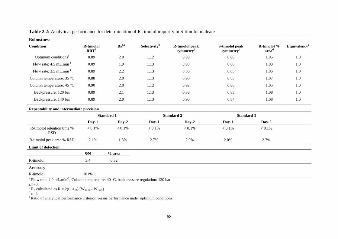
68
Table 2.2: Analytical performance for determination of R-timolol impurity in S-timolol maleate Robustness
Condition R-timolol RRTb
Rsb,c Selectivityb R-timolol peak symmetryb
S-timolol peak symmetryb
R-timolol % aread
Equivalencye
Optimum conditionsa 0.89 2.0 1.12 0.89 0.86 1.05 1.0
Flow rate: 4.5 mL.min-1 0.89 1.9 1.13 0.90 0.86 1.03 1.0
Flow rate: 3.5 mL.min-1 0.89 2.2 1.13 0.86 0.85 1.05 1.0
Column temperature: 35 °C 0.88 2.0 1.13 0.90 0.83 1.07 1.0
Column temperature: 45 °C 0.90 2.0 1.12 0.92 0.86 1.05 1.0
Backpressure: 120 bar 0.89 2.1 1.13 0.88 0.85 1.08 1.0
Backpressure: 140 bar 0.89 2.0 1.13 0.90 0.84 1.08 1.0
Repeatability and intermediate precision Standard 1 Standard 2 Standard 3
Day-1 Day-2 Day-1 Day-2 Day-1 Day-2 R-timolol retention time %
RSD < 0.1% < 0.1% < 0.1% < 0.1% < 0.1% < 0.1%
R-timolol peak area % RSD 2.1% 1.8% 2.7% 2.0% 2.0% 2.7%
Limit of detection S/N % area
R-timolol 3.4 0.52
Accuracy R-timolol 101% a Flow rate: 4.0 mL.min-1, Column temperature: 40 oC, backpressure regulation: 130 bar. b n=3. c Rs calculated as R = 2(tr1-tr2)/(WB(1) – WB(2)) d n=6 e Ratio of analytical performance criterion versus performance under optimum conditions

69
Table 2.3: Comparison between HPLC and pSFC analytical conditions and performance Parameters NP-HPLC pSFC Column Chiracel OD-H® Cellulose tris (3,5-dimethylphenylcarbamate) 5μm, 250 x 4.6 mm i.d. Column temperature Ambient 40 °C Flow rate 1.0 mL.min-1 4.0 mL.min-1 Detection 297 nm 5Hz acquisition rate 297 nm 20Hz acquisition rate Flow cell 10 mm path length, 10 µL volume flow cell 10 mm path length, 13 µL volume high
pressure flow cell Injection volume 5 µL on a 100 µL loop 15 µL on a 5 µL loop Back pressure - 130 bar Analysis type Isocratic Isocratic Run time 16 min 5 min Mobile phase Mixture of DEA, 2-propanol and hexane
(2:40:960) 93 % supercritical fluid CO2, 7 % MeOH containing 0.1% (v/v) TEA
Sample diluent Mixture of methylene chloride and 2-propanol a (10:30)
MeOH
R-timolol RRF CRM 0.80 0.83
R-timolol RRT CRM 0.75 0.89
R-timolol, S-timolol tailing
factors
1.2, 1.3 1.1, 1.1
R-timolol, S-timolol plate
count
18,064 N/m, 18,676 N/m 18,464 N/m, 18,342 N/m
Resolution CRM 4.8 2.0
S-timolol peak area
repeatabilitya
0.4% 0.2%
R-timolol peak area
repeatabilityb
2.5% 2.1%
% recovery of R-timolol 98%c 101%c
S-timolol working standard
concentration
9.5 x 10⁻² mM 1.4 x 10⁻¹ mM
Analysis time per sample 16 min 5 min
Solvent usage per sample 16 mL 1.4 mL a (n = 6) b 1.0% R-timolol in S-timolol, (n=6) c 1.0% R-timolol in S-timolol
70
2.4 Conclusion
A pSFC method has been described in which the R- and S-enantiomers of timolol have been
separated on a Chiralcel OD-H stationary phase within 5 min, representing a 3-fold decrease
in runtime and an 11-fold decrease in solvent consumption relative to the industry standard,
EP method based upon NP-HPLC [103]. The reduction in runtime is due in part to the
restrictive Rs requirement between the R- and S-enantiomers placed on the EP method to
allow for the detection if Impurity B (isotimolol). Based on the chromatographic evidence
observed in Figure 2.12, Impurity B (isotimolol) does not elute between the R- and
S-enantiomers under the pSFC conditions, hence the runtime could be reduced as only
baseline Rs between the R- and S-enantiomers was required. Also, due to the low viscosity
and high diffusivity of the pSFC mobile phase, a 4-fold increase in flow rate was possible,
thus reducing the runtime for the pSFC method. The method validation parameters required
for a limit test for R-timolol in S-timolol (specificity and detection limit) were established for
the pSFC method. In addition, the potential of this method to be used for quantitation of
R-timolol impurity was investigated by evaluation of further analytical performance criteria
(robustness, precision, accuracy). Clearly the developed pSFC assay demonstrates potential
as a full quantitative assay, and represents the fastest separation of timolol enantiomers to
date, relative to previously reported NP-HPLC or NACE-based methods. Future work will
involve the use of shorter chiral columns packed with smaller particles (3 µm) in order to
further decrease runtimes in chiral pSFC. Dissolution of the samples in a more non-polar
solvent such as heptane or heptane/isopropanol mixtures compared with MeOH may also
result in improved chromatographic efficiency.

71
3.0 Chapter 3: Development and Validation of a new stability indicating Reversed Phase liquid chromatographic method for the determination of Prednisolone acetate and impurities in an ophthalmic suspension.
3.1 Introduction
It is a technical requirement of the International Conference on Harmonization (ICH) for
registration of pharmaceuticals for human use [144] that impurities present in an active
pharmaceutical ingredient (API) as well as the final drug product be quantified and/or
identified. Impurities may be derived from the API and/or final drug product manufacturing
process or may be generated over time due to poor stability of either the API or drug product.
Many process-related impurities have similar chemical structures as the API or can often
co-elute with components of the drug product sample matrix, such that method specificity is a
key analytical performance criterion for any chromatographic method used for drug product
release testing or stability indicating assays.
Prednisolone acetate (PAC) is a synthetic glucocorticoid steroid which is used as the
API either alone or in combination with an additional API in several commercial ophthalmic
suspensions used for the treatment of a wide range of inflammatory conditions of the eye.
PAC is produced by the esterification of prednisolone and is defined as a pro-drug with
modified pharmacokinetic properties compared to prednisolone [145,146]. The usefulness of
pro-drugs in ophthalmic drug delivery has been comprehensively discussed in a number of
reviews [147,148]. Acetate ester pro-drugs such as PAC have been designed to increase the
lipophilicity and the cornea1 absorption of the parent steroid [149-152]. Enzymatic
transformation of pro-drugs in ocular tissues is often utilised for releasing the active drug. In
fact, PAC hydrolyses completely to prednisolone in vitro and in vivo, and the enzymatic
conversion is assumed to occur in the cornea [153,154]. Although ester pro-drugs are usually
more stable in vitro than in vivo, they may exhibit chemical instability in aqueous eye-drop
formulations [155]. Since PAC is vulnerable to enzymatic and chemical hydrolysis [156] it is
important to monitor the concentration of PAC and related substances over time in such
suspensions. Figure 3.1 illustrates the molecular structure of PAC along with its eight known
impurities (and potential degradants).
There have been numerous publications reporting on the chromatographic
determination of either prednisolone or PAC in tissue culture media [156] and various

72
biological fluids [157-163] including aqueous humour [157], human serum [158], plasma
[159], urine [159,161,162] and swine plasma [160,163].
Figure 3.1: Molecular structure of Prednisolone Acetate (PAC) and impurities 20(S), 20(R),
PN, P, HC, P-17A, HCA, P-11,21D reproduced from [173].
Fewer studies have been reported on the determination of PAC and related impurities
(originating either from the manufacturing process or due to drug product/drug substance
stability issues) in ophthalmic suspensions. Barot et al. reported on the determination of PAC
and ofloxacin in eye drops using a spectrophotometric method, but the method did not permit
quantitation of PAC impurities [164]. Musharraf et al. developed a stability indicating
thin-layer chromatography method for PAC in the presence of its degraded products,
generated by either acidic, alkaline or neutral hydrolysis, or oxidation and wet heating
degradation [165]. The authors subsequently applied the method to “ophthalmic samples”.
A number of micellar electrokinetic capillary chromatographic methods have been reported
by Gallego et al. [166-168] for the determination of either prednisolone [166] or prednisolone
acetate [167] in pharmaceutical products, but only reported one method [168] for the

73
simultaneous determination of both pharmaceuticals in the presence of other compounds
(naphazoline, Zn-bacitracin, sulfacetamide and phenylephrine) in pharmaceutical products.
The runtime was 8 min and limits of quantification were 1.0 mg.L-1 for all components, but
again, the method was not applicable to the determination of PAC in the presence of all
known impurities.
Reversed phase HPLC (RP-HPLC) assays have appeared in the literature [169-171]
most notably the work of Razzaq et al. who developed and validated an isocratic separation
of moxifloxacin and prednisolone on a BDS Hypersil C8 column using a methanol/phosphate
buffer mobile phase [171]. The authors used the method as a stability indicating assay for
both drug substances in selected pharmaceutical formulations which had been subjected to
oxidative, thermal and other stress conditions. Nevertheless, impurities were neither
identified nor quantified. The current USP monograph describes an isocratic RP-HPLC
method for the assay of PAC in an ophthalmic suspension using a water/acetonitrile mobile
phase (60:40) and a C18 (USP designation: L1) column [172]. While the method identifies the
impurity prednisolone P, it is not quantitative for impurities. The European Pharmacopoeia
describes a RP-HPLC method for the assay of PAC related substance in PAC drug substance
[173]. The method is capable of identifying and quantifying PAC and three specified
impurities; hydrocortisone acetate (HCA), P and prednisolone 11,21-diacetate (P-11,21D)
which are quantified as a percentage of the PAC peak. However, despite an extensive review
of the literature, no method has been reported for the quantitation of prednisolone acetate and
all known impurities shown in Figure 3.1 in an ophthalmic suspension. With this in mind, we
set out to develop and validate a stability indicating RP-HPLC method for the analysis of
prednisolone acetate (PAC) and eight potential impurities in a drug product ophthalmic
suspension. Note: P and prednisolone 17-acetate (P-17A) are degradants of PAC whereas
HCA and P-11,21D are process impurities [173]. The European Pharmacopoeia specifies that
hydrocortisone (HC), prednisone (PN), (20S)-hydroxyprednisolone (20(S)) and (20R)-
hydroxyprednisolone (20(R)) are potential impurities of P; i.e. the main degradant of PAC.
The ophthalmic suspension chosen for this work was proprietary formulation containing PAC
at 1%. The developed method has potential as a stability indicating assay for PAC in
ophthalmic suspension, capable of identifying and quantifying PAC impurities as well as
potential P impurities. Method development, validation and preliminary accelerated stability
studies is described herein.

74
3.2 Experimental
3.2.1 Instrumentation and Software
All assays were performed on a Waters Alliance 2695 HPLC system equipped with a Waters
2487 dual wavelength absorbance detector and a Waters 2996 photodiode array (PDA)
detector (Waters, Milford, MA, USA). The detection wavelength was 254 nm with data
acquisition at 5 Hz. The column for the modified version of the USP RP-HPLC method [174]
was a Waters µBondapak C18 (10 µm) 3.9 mm x 300 mm column (Waters, Milford, MA,
USA). The injection volume was 30 µL and the mobile phase of acetonitrile/water (40:60) was
delivered at 2.0 mL.min-1 at ambient column temperature. The gradient RP-HPLC method
was developed and validated on an Agilent Poroshell 120 EC-C18 100 mm x 4.6 mm, 2.7 µm
column (Agilent Technologies, Santa Clara, CA, USA). Mobile phase A consisted of
acetonitrile/water (10:90), while mobile phase B was acetonitrile, using a flow rate of
1.2 mL.min-1. The optimised gradient programme was as follows: 0.0-15.0 min (8.9% B),
15.0-15.1 min (8.9% to 16.7% B), 15.1-26.0 min (16.7% B), 26.0-26.1 min (16.7% to 33.4%
B), 26.1-30.0 min (33.4% B) and 30.0-30.1 min (33.4% to 8.9% B). The column temperature
was 60 °C and the injection volume was 10 µL. Chromatographic data were acquired and
processed using Waters EmpowerTM 2 software. Regression analysis for PAC and impurities
was carried out using SigmaPlot version 9.0 software and Microsoft Excel 2010.
3.2.2 Materials and Reagents
Prednisolone acetate (PAC) was obtained from Sanofi Aventis (Paris, France). Prednisolone-
11,21 diacetate (P-11,21D) was obtained from Steraloids Inc. (Newport, RI, USA).
Hydrocortisone (HC) and hydrocortisone acetate (HCA) were obtained from US
Pharmacopoeia (USP) (Rockville, Maryland, USA). Prednisolone 17-acetate (P-17A),
(20S)-hydroxyprednisolone (20S), (20R)-hydroxyprednisolone (20R) and prednisone (PN)
were obtained from LGC Standards (Teddington, Middlesex, UK). Prednisolone (P) was
from Sigma Aldrich (St Louis, Missouri, USA). Reagent grade sodium acetate, glacial acetic
acid (100%), HPLC grade acetonitrile (ACN) and methanol (MeOH) were purchased from
Merck (Darmstadt, Germany). Deionised water was produced from a Millipore Milli-Q Plus
Purifier system (Molsheim, France).

75
3.2.3 Solution preparation for PAC RP-HPLC analysis
All solutions were prepared in low actinic glassware to protect from light. (Note: Solutions
described in this work belong to one of two subclasses. “Working standards” were used for
quantitative purposes as external calibrators and did not contain matrix components.
“Working samples” are simulated samples, containing PAC at 100% label strength plus
spiked matrix components at label strength and spiked impurities at appropriate spike levels).
Stock standard solutions of PAC and individual impurities were prepared in MeOH as
described in Table 3.1. External PAC standard curves for quantification of both impurity
levels and PAC in working samples involved the use of Calibration Set #1 or Calibration
Set #2 respectively, prepared as shown in Table 3.1 using 0.1 M sodium acetate
pH 4.0/MeOH (50:50) as diluent. For the preparation of working samples, an additional
matrix spiking solution containing the matrix components of the ophthalmic suspension was
prepared in deionised water. In this work, the exact formulation of the matrix is proprietary
but included compounds which act as preservatives, ophthalmic lubricants (“artificial tears”),
antipyretics, vasoconstrictors and mydriatics. All other solutions described hereafter (except
the above external PAC standards for quantification) were spiked at 1:50 with the stock
matrix spiking solution to ensure that matrix components were present at label strength after
dilution. For PAC accuracy and linearity studies, a series of working samples were prepared
(n=5) containing PAC at 40% to 160% (w/w) of product LS after dilution (including a 1:50
matrix solution spike). Method detection limits were determined using serial dilutions of a
0.1 mg.L-1 mixed PAC/impurities standard. For impurity accuracy and linearity studies,
impurity solutions were prepared at 5 concentrations ranging from 0.1 mg.L-1 to 4.0 mg.L-1,
equivalent to 0.05% to 2.0% of PAC working standard concentration. Each solution also
contained a fixed concentration of PAC at 0.2 mg.mL-1. For precision, specificity and
robustness studies a 0.2 mg.mL-1 PAC working standard was spiked with each. For the
comparison study between both HPLC methods, a 0.2 mg.mL-1 PAC working standard was
prepared in the appropriate diluent as well as a separate impurity standard mixture containing
each impurity at a concentration of 2.0 mg.L-1 equivalent to 1.0% of PAC concentration after
dilution. (Note: For the sake of clarity, solution preparation is also detailed in Table 3.1).

76
Table 3.1: Solution preparation for validation of RP-HPLC method Diluent Solution Analyte Concentration % w.r.t PAC Label Strength
MeOH PAC stock standard PAC 2.0 mg.mL-1 n/a
Impurity stock standards Individual impurities 0.20 mg.mL-1 n/a
MeOH/100 mM sodium acetate buffer pH 4.0 (50:50)
Solution A Precision/specificity/robustness spiked sample
PAC 0.20 mg.mL-1 100.0%
Impurities 1.2 mg.L-1 0.60%
MeOH/100 mM sodium acetate buffer pH 4.0 (50:50) plus stock matrix spiking solution at 1:50
External PAC working standard (Calibration Set #1)
PAC 0.1 mg.L-1, 0.2 mg.L-1, 1.0 mg.L-1, 2.0 mg.L-1, 4.0 mg.L-1 0.05%, 0.10%, 0.50%, 1.0%, 2.0%
External PAC working standard (Calibration Set #2)
PAC 80.0 mg.L-1, 0.16 mg.mL-1 , 0.20 mg.mL-1, 0.24 mg.mL-1, 0.32 mg.mL-1
40.0%, 80.0%, 100.0%, 120.0%, 160.0%
LOD/LOQ studies. PAC/Impurities 0.1 mg.L-1 0.05%
PAC accuracy/linearity studies PAC 0.1 mg.L-1, 0.2 mg.L-1, 1.0 mg.L-1, 2.0 mg.L-1, 4.0 mg.L-1 0.05%, 0.10%, 0.50%, 1.0%, 2.0%
PAC accuracy/linearity studies PAC 80.0 mg.L-1, 0.16 mg.mL-1 , 0.20 mg.mL-1, 0.24 mg.mL-1, 0.32 mg.mL-1
40.0%, 80.0%, 100.0%, 120.0%, 160.0%
Impurity accuracy/linearity studies
PACa (Impurities) 0.20 mg.mL-1 (0.1 mg.L-1, 0.2 mg.L-1, 1.0 mg.L-1, 2.0 mg.L-1, 4.0 mg.L-1)
100.0% (0.05%, 0.10%, 0.50%, 1.0%, 2.0%)
MeOH/40 mM phosphate buffer pH 3.4 (70:30)
Method comparison sample PAC 0.20 mg.mL-1 100.0%
Method comparison impurity solution
Impurities 2.0 mg.L-1 1.00%
a PAC omitted from P and HCA impurity accuracy/linearity studies due presence of these impurities in PAC standard material
77
3.3 Results and discussion
3.3.1 PAC RP-HPLC Method Development
A method capable of the identification and quantitation of PAC and selected process
impurities/degradants in ophthalmic suspensions is essential in ensuring that the method is
suitable for drug product release testing and routine drug product stability studies. As a
starting point, the initial phase of the development work therefore focused on the USP
monograph method for the analysis of PAC in ophthalmic suspensions [174] with certain
modifications made to improve method performance. Specifically, a diluent of 40 mM
phosphate buffer pH 3.4/MeOH (30:70) was used instead of 50% ACN. MeOH was selected
due to its protic nature to improve working sample stability by minimizing base catalyzed
hydrolysis of PAC to P. The working standard and working sample concentrations were
increased from 0.1 mg.mL-1 to 0.2 mg.mL-1 and the injection volume increased from 10 µL to
30 µL in order to improve limits of detection and method accuracy. It should be noted that
the USP monograph method is capable of identifying (but not quantifying) the impurity P in
ophthalmic suspensions where PAC is the main active pharmaceutical ingredient (API).
A mixture of PAC and impurities (PN, P, 20(S), 20(R), HC, P-17A, HCA, P-11,21D) each at
2.0 mg.L-1 or 1% (w/w) of PAC label strength was injected and as illustrated in Figure 3.2(a),
several co-elutions were evident with the given chromatographic conditions, namely:
20(S)/20(R), PN/P/HC and PAC/HCA. Furthermore, a 1:50 dilution of solution PAC sample
was prepared and assayed to determine if there was any additional co-elution with matrix
components; a significant matrix peak at ~ 2.2 min had the same retention time as the co-
eluting 20(S) and 20(R) peaks as illustrated in Figure 3.2(b). Clearly, the modified USP
method was incapable of quantifying all remaining seven known PAC-related impurities
(besides P) in ophthalmic solutions.
An opportunity therefore presented itself to significantly improve the utility of the
method by adopting more modern column technologies (a C18 core-shell stationary phase), to
improve the efficiency of the chromatographic separation. To exploit the benefits of
core-shell column technology, a 100 mm x 4.6 mm Agilent Poroshell 120 EC-C18 2.7 µm
column was selected which, in contrast with the 10 µm fully porous support particle exhibited
by the Waters µBondapak stationary phase, comprises a 2.7-µm superficially porous particle
with a 1.7-µm solid core and a 0.5-µm porous shell. Core-shell (or “superficially porous”)

78
particles have high loading capacities because 75% of the volume of these particles is porous
[175].
Figure 3.2: (a): Separation of eight selected PAC impurities at 2.0 mg.L-1 or 1% (w/w) of
PAC LS. (b): chromatogram of 0.20 mg.mL-1 PAC sample. Chromatographic conditions:
Column: Waters µBondapak C18 (10 µm) 3.9 mm x 300 mm. Mobile phase:
acetonitrile/water (40:60). Injection volume: 30 µL. Column temperature: ambient.
Detection: 254 nm.
Most importantly, 4.6 mm i.d. columns packed with these particles provide
efficiencies equivalent to those of columns packed with 1.7-µm fully porous particles, with
the additional advantage of operating at back pressures that are 2-3 times lower [176,177].
79
Therefore, these particles make it possible to achieve ultra-high performance liquid
chromatography (UPLC)-like performance when the HPLC connecting tubing is modified to
minimise extra-column volumes and the detector flow-cell volume is reduced appropriately
[178]. The pore size of the two particle types was broadly similar at 125 Ǻ and 120 Ǻ for the
µBondapak and Poroshell materials respectively but as expected, both stationary phases
exhibit very different surface areas of 330 m2.g-1 and 130 m2.g-1 respectively. The decrease in
surface area for the Poroshell phase can be expected to be offset by the increased efficiency
due to improved packing quality (spherical rather than irregular particle shape), reduced
particle size and reduced diffusion path lengths.
The Agilent Poroshell stationary phase also fulfils the USP requirement for an L1
stationary phase (octadecyl saline (ODS or C18) chemically bounded to porous silica or
ceramic particles – 1.5 to 10 µm in diameter) but offers significantly different C18 selectivity
relative to the Waters µBondapak phase. Although the carbon load for both stationary phases
was 10%, nevertheless the column comparison function (Fs) value describing the similarity
(or difference) in selectivity between both stationary phases was 13.4, based on the
Hydrophobic Subtraction Model first described by Snyder et al. [179]. Initial method
development was performed using the same working standard/sample concentrations as the
modified USP method described above, but using a diluent of 100 mM sodium acetate
pH 4.0/MeOH (50:50). A mobile phase flow rate of 1.2 mL.min-1 was used along with an
injection volume of 10 µL and a detection wavelength of 254 nm. However, a number of
different gradient programs and column temperatures were used during method optimisation
(with a water/acetonitrile mobile phase) as illustrated in Table 3.2. The goal was to separate
all critical peak pairs with a resolution of at least 1.5. Figure 3.3 provides representative
chromatograms of the development conditions outlined in Table 3.2. The elution order was
confirmed by running individual standard injections of PAC [179] and the selected impurities
under the optimised conditions.
The polarity of the selected analytes (log P values) varied widely from 0.26 ± 0.51
for 20(S) to 3.04 ± 0.60 for P11,21D [180]. Therefore, the final developed gradient (Test 11
from Table 3.2) incorporated an initial isocratic hold to resolve early eluting peaks followed
by a two-step gradient in order to resolve mid-gradient peaks and elute the strongly retained
analytes within a reasonable timeframe. Column temperature was observed to be critical for
the separation of PN, P and HC. It was not possible to separate PN and P under any gradient
conditions below 40 °C and it was not until the column temperature was increased to 60 °C
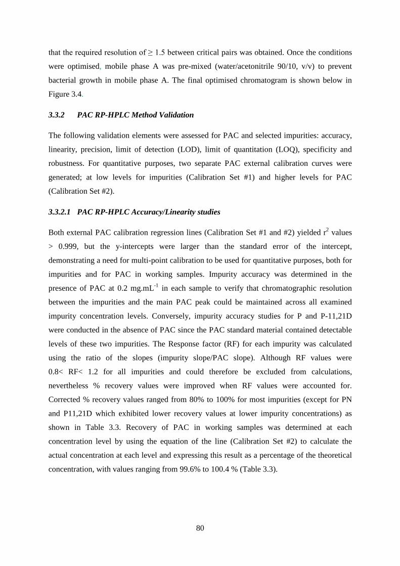
80
that the required resolution of ≥ 1.5 between critical pairs was obtained. Once the conditions
were optimised, mobile phase A was pre-mixed (water/acetonitrile 90/10, v/v) to prevent
bacterial growth in mobile phase A. The final optimised chromatogram is shown below in
Figure 3.4.
3.3.2 PAC RP-HPLC Method Validation
The following validation elements were assessed for PAC and selected impurities: accuracy,
linearity, precision, limit of detection (LOD), limit of quantitation (LOQ), specificity and
robustness. For quantitative purposes, two separate PAC external calibration curves were
generated; at low levels for impurities (Calibration Set #1) and higher levels for PAC
(Calibration Set #2).
3.3.2.1 PAC RP-HPLC Accuracy/Linearity studies
Both external PAC calibration regression lines (Calibration Set #1 and #2) yielded r2 values
> 0.999, but the y-intercepts were larger than the standard error of the intercept,
demonstrating a need for multi-point calibration to be used for quantitative purposes, both for
impurities and for PAC in working samples. Impurity accuracy was determined in the
presence of PAC at 0.2 mg.mL-1 in each sample to verify that chromatographic resolution
between the impurities and the main PAC peak could be maintained across all examined
impurity concentration levels. Conversely, impurity accuracy studies for P and P-11,21D
were conducted in the absence of PAC since the PAC standard material contained detectable
levels of these two impurities. The Response factor (RF) for each impurity was calculated
using the ratio of the slopes (impurity slope/PAC slope). Although RF values were
0.8< RF< 1.2 for all impurities and could therefore be excluded from calculations,
nevertheless % recovery values were improved when RF values were accounted for.
Corrected % recovery values ranged from 80% to 100% for most impurities (except for PN
and P11,21D which exhibited lower recovery values at lower impurity concentrations) as
shown in Table 3.3. Recovery of PAC in working samples was determined at each
concentration level by using the equation of the line (Calibration Set #2) to calculate the
actual concentration at each level and expressing this result as a percentage of the theoretical
concentration, with values ranging from 99.6% to 100.4 % (Table 3.3).

81
Figure 3.3: Representative chromatograms of development injections under development
conditions outlined in Table 3.2 below Test 1 (a), Test 2 (b), Test 3 (c), Test 4 (d), Test 5 (e),
Test 6 (f), Test 7 (g),Test 8 (h), Test 10 (i) and Test 11 (j). Top: Chromatograms of PAC
impurity mix. Test 1 to Test 6 impurity mix contained PAC impurities at 20.0 mg.L-1 or 10.0%
(w/w) of PAC after dilution. Bottom: Chromatograms of PAC samples spiked with impurities.
Test 7 to Test 10 contained PAC sample spiked with impurities at 20.0 mg.L-1 or 10.0% (w/w)
of PAC after dilution. Test 11 contained PAC sample spiked with impurities at 4.0 mg.L-1 or
2.0% (w/w) of PAC after dilution.

82
Table 3.2: RP-HPLC PAC method optimisation
Test Flow rate mL.min-1
Run time
Column temperature
(oC)
Mobile Phase Components
Gradient composition Rs
PN/P
Rs
P/HC
Time % A % B
Test 1 1.2 30 min 40 A = 25% ACN
B = 100% ACN
0.0 100.0 0.0 - 1.70 20.0 100.0 0.0
20.1 80.0 20.0
26.0 80.0 20.0
26.1 100.0 0.0
30.0 100.0 0.0
Test 2 1.2 34 min 50 A = 100% H2O
B = 100% ACN
0.0 82.0 18.0 1.36 1.27 16.0 82.0 18.0
16.1 75.0 25.0
26.0 75.0 25.0
26.1 60.0 40.0
31.0 60.0 40.0
31.1 82.0 18.0
34.0 82.0 18.0
Test 3 1.2 42 min 55 A = 100% H2O
B = 100% ACN
0.0 85.0 15.0 1.13 1.23 17.0 85.0 15.0
17.1 75.0 25.0
35.0 75.0 25.0
35.1 60.0 40.0
40.0 60.0 40.0
40.1 85.0 15.0
42.0 85.0 15.0
Test 4 1.2 52 min 55 A = 100% H2O
B = 100% ACN
0.0 85.0 15.0 2.15 - 30.0 85.0 15.0
30.1 70.0 30.0
45.0 70.0 30.0
45.1 60.0 40.0
50.0 60.0 40.0
50.1 85.0 15.0
52.0 85.0 15.0
Test 5 1.2 34 min 60 A = 100% H2O
B = 100% ACN
0.0 82.0 18.0 1.28 1.15 17.0 82.0 18.0
17.1 75.0 25.0
27.0 75.0 25.0
27.1 60.0 40.0
32.0 60.0 40.0
32.1 82.0 18.0
34.0 82.0 18.0
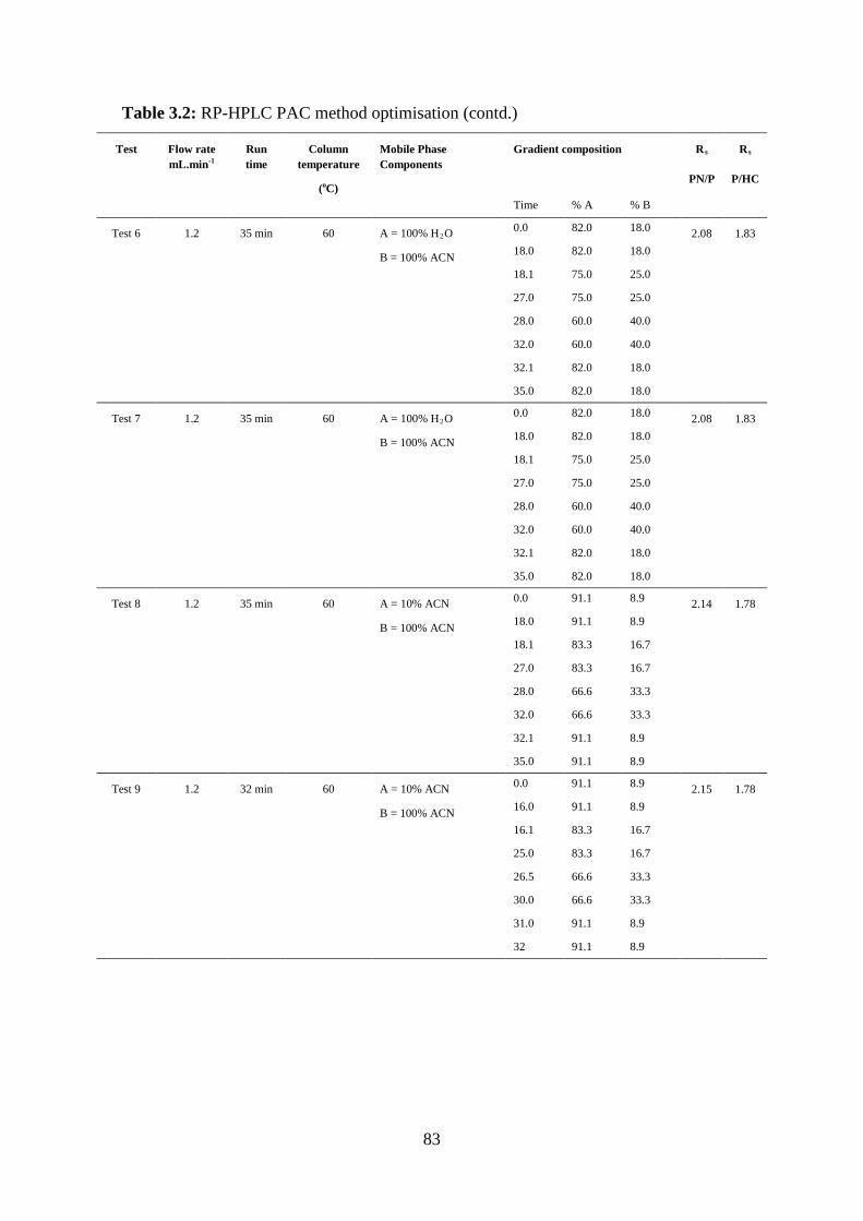
83
Table 3.2: RP-HPLC PAC method optimisation (contd.)
Test Flow rate mL.min-1
Run time
Column temperature
(oC)
Mobile Phase Components
Gradient composition Rs
PN/P
Rs
P/HC
Time % A % B
Test 6 1.2 35 min 60 A = 100% H2O
B = 100% ACN
0.0 82.0 18.0 2.08 1.83 18.0 82.0 18.0
18.1 75.0 25.0
27.0 75.0 25.0
28.0 60.0 40.0
32.0 60.0 40.0
32.1 82.0 18.0
35.0 82.0 18.0
Test 7 1.2 35 min 60 A = 100% H2O
B = 100% ACN
0.0 82.0 18.0 2.08 1.83 18.0 82.0 18.0
18.1 75.0 25.0
27.0 75.0 25.0
28.0 60.0 40.0
32.0 60.0 40.0
32.1 82.0 18.0
35.0 82.0 18.0
Test 8 1.2 35 min 60 A = 10% ACN
B = 100% ACN
0.0 91.1 8.9 2.14 1.78 18.0 91.1 8.9
18.1 83.3 16.7
27.0 83.3 16.7
28.0 66.6 33.3
32.0 66.6 33.3
32.1 91.1 8.9
35.0 91.1 8.9
Test 9 1.2 32 min 60 A = 10% ACN
B = 100% ACN
0.0 91.1 8.9 2.15 1.78 16.0 91.1 8.9
16.1 83.3 16.7
25.0 83.3 16.7
26.5 66.6 33.3
30.0 66.6 33.3
31.0 91.1 8.9
32 91.1 8.9
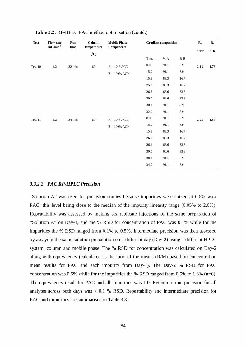
84
Table 3.2: RP-HPLC PAC method optimisation (contd.)
Test Flow rate mL.min-1
Run time
Column temperature
(oC)
Mobile Phase Components
Gradient composition Rs
PN/P
Rs
P/HC
Time % A % B
Test 10 1.2 32 min 60 A = 10% ACN
B = 100% ACN
0.0 91.1 8.9 2.18 1.78 15.0 91.1 8.9
15.1 83.3 16.7
25.0 83.3 16.7
26.5 66.6 33.3
30.0 66.6 33.3
30.1 91.1 8.9
32.0 91.1 8.9
Test 11 1.2 34 min 60 A = 10% ACN
B = 100% ACN
0.0 91.1 8.9 2.22 1.89 15.0 91.1 8.9
15.1 83.3 16.7
26.0 83.3 16.7
26.1 66.6 33.3
30.0 66.6 33.3
30.1 91.1 8.9
34.0 91.1 8.9
3.3.2.2 PAC RP-HPLC Precision
“Solution A” was used for precision studies because impurities were spiked at 0.6% w.r.t
PAC; this level being close to the median of the impurity linearity range (0.05% to 2.0%).
Repeatability was assessed by making six replicate injections of the same preparation of
“Solution A” on Day-1, and the % RSD for concentration of PAC was 0.1% while for the
impurities the % RSD ranged from 0.1% to 0.5%. Intermediate precision was then assessed
by assaying the same solution preparation on a different day (Day-2) using a different HPLC
system, column and mobile phase. The % RSD for concentration was calculated on Day-2
along with equivalency (calculated as the ratio of the means (R/M) based on concentration
mean results for PAC and each impurity from Day-1). The Day-2 % RSD for PAC
concentration was 0.5% while for the impurities the % RSD ranged from 0.5% to 1.6% (n=6).
The equivalency result for PAC and all impurities was 1.0. Retention time precision for all
analytes across both days was < 0.1 % RSD. Repeatability and intermediate precision for
PAC and impurities are summarised in Table 3.3.
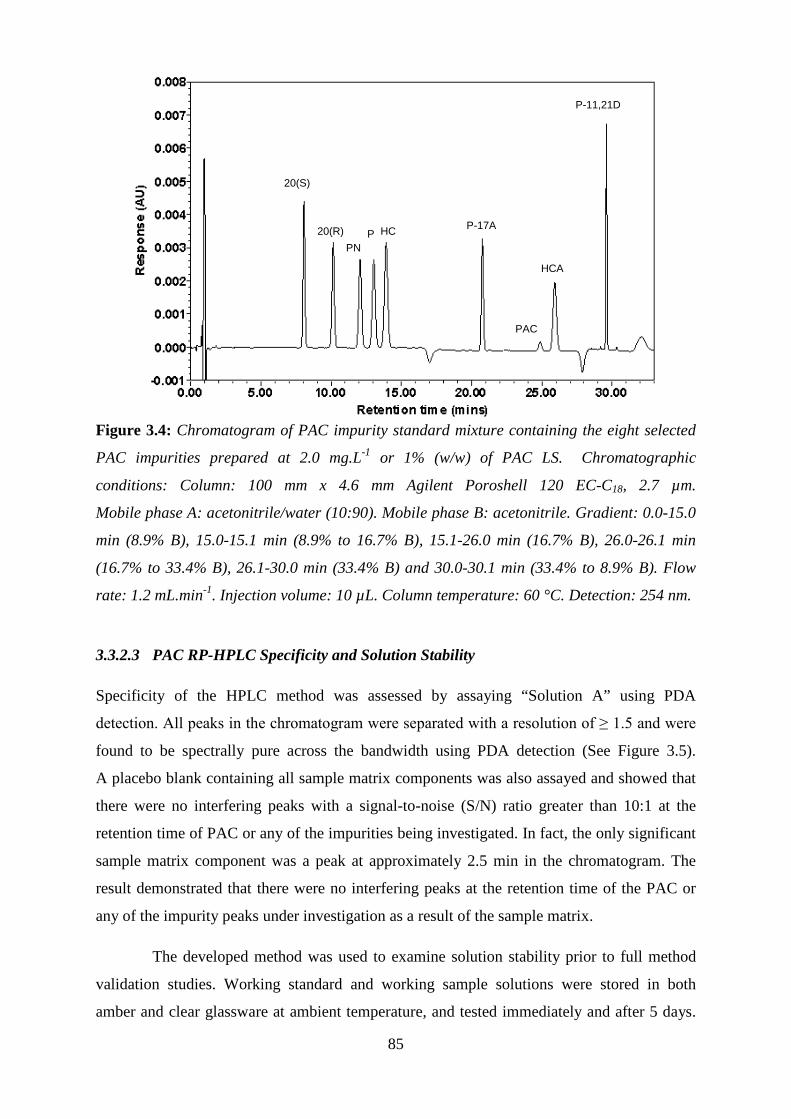
85
Figure 3.4: Chromatogram of PAC impurity standard mixture containing the eight selected
PAC impurities prepared at 2.0 mg.L-1 or 1% (w/w) of PAC LS. Chromatographic
conditions: Column: 100 mm x 4.6 mm Agilent Poroshell 120 EC-C18, 2.7 µm.
Mobile phase A: acetonitrile/water (10:90). Mobile phase B: acetonitrile. Gradient: 0.0-15.0
min (8.9% B), 15.0-15.1 min (8.9% to 16.7% B), 15.1-26.0 min (16.7% B), 26.0-26.1 min
(16.7% to 33.4% B), 26.1-30.0 min (33.4% B) and 30.0-30.1 min (33.4% to 8.9% B). Flow
rate: 1.2 mL.min-1. Injection volume: 10 µL. Column temperature: 60 °C. Detection: 254 nm.
3.3.2.3 PAC RP-HPLC Specificity and Solution Stability
Specificity of the HPLC method was assessed by assaying “Solution A” using PDA
detection. All peaks in the chromatogram were separated with a resolution of ≥ 1.5 and were
found to be spectrally pure across the bandwidth using PDA detection (See Figure 3.5).
A placebo blank containing all sample matrix components was also assayed and showed that
there were no interfering peaks with a signal-to-noise (S/N) ratio greater than 10:1 at the
retention time of PAC or any of the impurities being investigated. In fact, the only significant
sample matrix component was a peak at approximately 2.5 min in the chromatogram. The
result demonstrated that there were no interfering peaks at the retention time of the PAC or
any of the impurity peaks under investigation as a result of the sample matrix.
The developed method was used to examine solution stability prior to full method
validation studies. Working standard and working sample solutions were stored in both
amber and clear glassware at ambient temperature, and tested immediately and after 5 days.
20(S)
20(R) P PN
HC
P-11,21D
PAC
HCA
P-17A
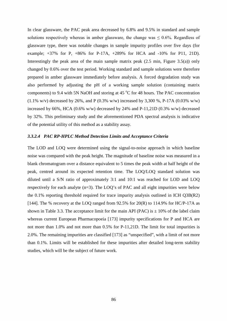
86
In clear glassware, the PAC peak area decreased by 6.8% and 9.5% in standard and sample
solutions respectively whereas in amber glassware, the change was ≤ 0.6%. Regardless of
glassware type, there was notable changes in sample impurity profiles over five days (for
example; +37% for P, +86% for P-17A, +289% for HCA and -10% for P11, 21D).
Interestingly the peak area of the main sample matrix peak (2.5 min, Figure 3.5(a)) only
changed by 0.6% over the test period. Working standard and sample solutions were therefore
prepared in amber glassware immediately before analysis. A forced degradation study was
also performed by adjusting the pH of a working sample solution (containing matrix
components) to 9.4 with 5N NaOH and storing at 45 oC for 48 hours. The PAC concentration
(1.1% w/v) decreased by 26%, and P (0.3% w/w) increased by 3,300 %, P-17A (0.03% w/w)
increased by 66%, HCA (0.6% w/w) decreased by 24% and P-11,21D (0.3% w/w) decreased
by 32%. This preliminary study and the aforementioned PDA spectral analysis is indicative
of the potential utility of this method as a stability assay.
3.3.2.4 PAC RP-HPLC Method Detection Limits and Acceptance Criteria
The LOD and LOQ were determined using the signal-to-noise approach in which baseline
noise was compared with the peak height. The magnitude of baseline noise was measured in a
blank chromatogram over a distance equivalent to 5 times the peak width at half height of the
peak, centred around its expected retention time. The LOQ/LOQ standard solution was
diluted until a S/N ratio of approximately 3:1 and 10:1 was reached for LOD and LOQ
respectively for each analyte (n=3). The LOQ’s of PAC and all eight impurities were below
the 0.1% reporting threshold required for trace impurity analysis outlined in ICH Q3B(R2)
[144]. The % recovery at the LOQ ranged from 92.5% for 20(R) to 114.9% for HC/P-17A as
shown in Table 3.3. The acceptance limit for the main API (PAC) is ± 10% of the label claim
whereas current European Pharmacopoeia [173] impurity specifications for P and HCA are
not more than 1.0% and not more than 0.5% for P-11,21D. The limit for total impurities is
2.0%. The remaining impurities are classified [173] as “unspecified”, with a limit of not more
than 0.1%. Limits will be established for these impurities after detailed long-term stability
studies, which will be the subject of future work.
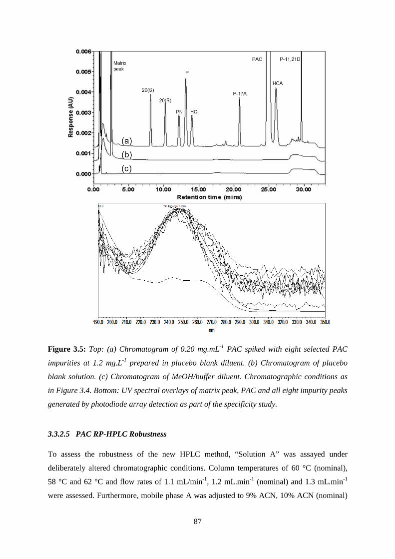
87
Figure 3.5: Top: (a) Chromatogram of 0.20 mg.mL-1 PAC spiked with eight selected PAC
impurities at 1.2 mg.L-1 prepared in placebo blank diluent. (b) Chromatogram of placebo
blank solution. (c) Chromatogram of MeOH/buffer diluent. Chromatographic conditions as
in Figure 3.4. Bottom: UV spectral overlays of matrix peak, PAC and all eight impurity peaks
generated by photodiode array detection as part of the specificity study.
3.3.2.5 PAC RP-HPLC Robustness
To assess the robustness of the new HPLC method, “Solution A” was assayed under
deliberately altered chromatographic conditions. Column temperatures of 60 °C (nominal),
58 °C and 62 °C and flow rates of 1.1 mL/min-1, 1.2 mL.min-1 (nominal) and 1.3 mL.min-1
were assessed. Furthermore, mobile phase A was adjusted to 9% ACN, 10% ACN (nominal)
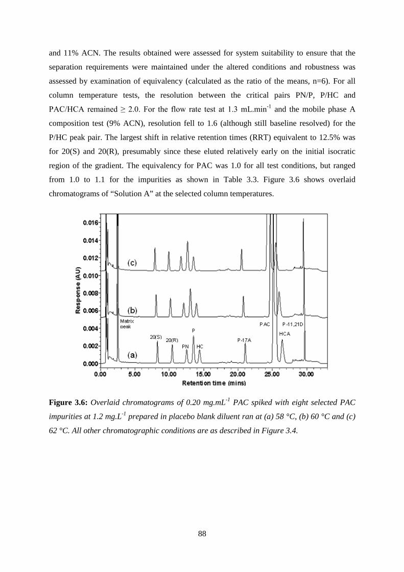
88
and 11% ACN. The results obtained were assessed for system suitability to ensure that the
separation requirements were maintained under the altered conditions and robustness was
assessed by examination of equivalency (calculated as the ratio of the means, n=6). For all
column temperature tests, the resolution between the critical pairs PN/P, P/HC and
PAC/HCA remained ≥ 2.0. For the flow rate test at 1.3 mL.min-1 and the mobile phase A
composition test (9% ACN), resolution fell to 1.6 (although still baseline resolved) for the
P/HC peak pair. The largest shift in relative retention times (RRT) equivalent to 12.5% was
for 20(S) and 20(R), presumably since these eluted relatively early on the initial isocratic
region of the gradient. The equivalency for PAC was 1.0 for all test conditions, but ranged
from 1.0 to 1.1 for the impurities as shown in Table 3.3. Figure 3.6 shows overlaid
chromatograms of “Solution A” at the selected column temperatures.
Figure 3.6: Overlaid chromatograms of 0.20 mg.mL-1 PAC spiked with eight selected PAC
impurities at 1.2 mg.L-1 prepared in placebo blank diluent ran at (a) 58 °C, (b) 60 °C and (c)
62 °C. All other chromatographic conditions are as described in Figure 3.4.

89
Table 3.3: Analytical performance for determination of PAC and selected impurities in a spiked ophthalmic suspension Accuracy PAC 20(S) 20(R) PN P HC P-17A HCA P-11,21D
0.05% 96.3 ± 16.0 79.6 ± 2.2 80.2 ± 1.8 74.6 ± 6.3 87.3 ±13.1 86.0 ± 12.3 65.5 ± 6.1 80.6 ± 5.4 64.7 ± 5.3
0.10% 106.7 ± 8.4 86.9 ± 5.1 99.3 ± 3.9 86.2 ± 5.8 95.9 ± 6.2 84.0 ± 3.1 79.9 ± 1.2 89.1 ± 10.1 78.8 ± 1.1
0.50% 99.7 ± 2.4 99.2 ± 1.2 99.2 ± 1.4 97.6 ± 1.4 98.6 ± 0.6 98.5 ± 1.1 96.7 ± 0.6 98.7 ± 4.2 91.7 ± 0.9
1.00% 99.3 ± 2.4 98.8 ± 0.2 99.0 ± 0.3 98.9 ± 0.5 99.4 ± 1.3 98.2 ± 1.5 97.6 ± 1.0 97.8 ± 0.5 100.1 ± 1.1
2.00% 100.2 ± 0.2 99.5 ± 0.2 99.8 ± 0.5 99.3 ± 0.5 99.7 ± 0.4 99.5 ± 0.8 99.1 ± 0.7 99.6 ± 0.7 98.6 ± 0.2
40.00% 100.2 ± 0.4 --- --- --- --- --- --- --- ---
80.00% 100.2 ± 0.5 --- --- --- --- --- --- --- ---
100.00% 99.6 ± 0.4 --- --- --- --- --- --- --- ---
120.00% 100.4 ± 0.2 --- --- --- --- --- --- --- ---
160.00% 100.0 ± 0.4 --- --- --- --- --- --- --- ---
RFa n/a 1.12 1.13 1.09 1.09 1.19 0.95 0.99 0.87
Linearity r2(n=5)
> 0.999 > 0.999 > 0.999 > 0.999 > 0.999 > 0.999 > 0.999 > 0.999 > 0.999
Precision (% RSD)
Day-1 Day-2 Day-1 Day-2 Day-1 Day-2 Day-1 Day-2 Day-1 Day-2 Day-1 Day-2 Day-1 Day-2 Day-1 Day-2 Day-1 Day-2
Retention time <0.1 <0.1 <0.1 <0.1 <0.1 <0.1 <0.1 <0.1 <0.1 <0.1 <0.1 <0.1 <0.1 <0.1 <0.1 <0.1 <0.1 <0.1
Concentration 0.1 0.5 0.3 0.9 0.3 1.6 0.3 2.2 0.1 2.2 0.4 1.3 0.5 0.6 0.3 0.5 0.1 0.5
Equivalencyb 1.0 1.0 1.0 1.0 1.0 1.0 1.0 1.0 1.0

90
Table 3.3: Analytical performance for determination of PAC and selected impurities in a spiked ophthalmic suspension (contd.)
Detection limitsc PAC 20(S) 20(R) PN P HC P-17A HCA P-11,21D
LOD % (w/w) 0.004 0.002 0.003 0.004 0.004 0.004 0.003 0.005 0.002
LOQ % (w/w) 0.015 0.007 0.010 0.014 0.014 0.013 0.010 0.018 0.008
% Recovery (at LOQ) 112.9 106.2 92.5 101.7 98.0 114.9 114.9 105.7 112.2
Robustnessd PAC 20(S) 20(R) PN P HC P-17A HCA P-11,21D
Temperature: 60 oC RRT(Resolution) 1.00(2.1e) 0.32 0.40 0.48(2.4f) 0.52(2.0g) 0.56 0.83 1.04 1.18
Temperature: 58 oC RRT(Resolution) 1.00(2.1e) 0.33 0.41 0.49(2.4f) 0.53(2.0g) 0.57 0.83 1.04 1.17
Equivalencyh 1.0 1.0 1.0 1.0 1.0 1.0 1.0 1.0 1.0
Temperature: 62 °C RRT(Resolution) 1.00(2.3e) 0.33 0.41 0.48(2.5f) 0.52(2.1g) 0.55 0.84 1.04 1.21
Equivalencyh 1.0 1.0 1.0 1.0 1.0 1.0 1.0 1.0 1.0
Flow: 1.1 mL.min-
1RRT(Resolution) 1.00(2.4e) 0.33 0.41 0.50(2.4f) 0.53(2.0g) 0.57 0.83 1.04 1.18
Equivalencyh 1.0 1.0 1.0 1.0 1.0 1.0 1.0 1.0 1.0
Flow: 1.3 mL.min-
1RRT(Resolution) 1.00(1.9e) 0.31 0.39 0.46(2.0f) 0.50(1.6g) 0.53 0.84 1.04 1.24
Equivalencyh 1.0 1.0 1.0 1.0 1.1 1.0 1.0 1.0 1.0
Mobile Phase A: 9% RRT(Resolution)
1.00(2.0e) 0.35 0.45 0.53(2.1f) 0.58(1.6g) 0.61 0.83 1.04 1.13
Equivalencyh 1.0 1.0 1.0 1.0 1.1 1.0 1.0 0.9 1.0
Mobile Phase A: 11% RRT(Resolution)
1.00(2.0e) 0.28 0.35 0.43(1.9f) 0.47(1.7g) 0.50 0.85 1.04 1.29
Equivalencyh 1.0 1.0 1.0 1.0 1.1 1.0 1.0 1.0 1.0
91
a Calculated on ratio of the slopes (IMP slope/PAC slope) over 0.05% to 2.00% b Ratio of analyte concentration Day 2 versus analyte concentration Day 1 c
n=3. d n=6. e Rs calculated as Rs = 1.18(tr2-tr1)/(W1 h/2– W2 h/2) for critical pair PAC/HCA f Rs calculated as Rs = 1.18(tr2-tr1)/(W1 h/2– W2 h/2) for critical pair PN/P g Rs calculated as Rs = 1.18(tr2-tr1)/(W1 h/2– W2 h/2) for critical pair P/HC h Ratio of analyte concentration versus analyte concentration under optimum (nominal) conditions
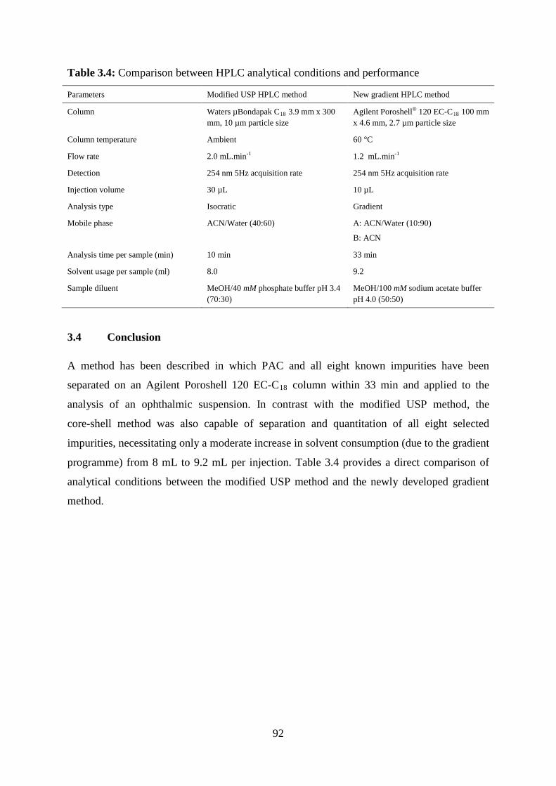
92
Table 3.4: Comparison between HPLC analytical conditions and performance
Parameters Modified USP HPLC method New gradient HPLC method
Column Waters µBondapak C18 3.9 mm x 300 mm, 10 µm particle size
Agilent Poroshell® 120 EC-C18 100 mm x 4.6 mm, 2.7 µm particle size
Column temperature Ambient 60 °C
Flow rate 2.0 mL.min-1 1.2 mL.min-1
Detection 254 nm 5Hz acquisition rate 254 nm 5Hz acquisition rate
Injection volume 30 µL 10 µL
Analysis type Isocratic Gradient
Mobile phase ACN/Water (40:60) A: ACN/Water (10:90)
B: ACN
Analysis time per sample (min) 10 min 33 min
Solvent usage per sample (ml) 8.0 9.2
Sample diluent MeOH/40 mM phosphate buffer pH 3.4 (70:30)
MeOH/100 mM sodium acetate buffer pH 4.0 (50:50)
3.4 Conclusion
A method has been described in which PAC and all eight known impurities have been
separated on an Agilent Poroshell 120 EC-C18 column within 33 min and applied to the
analysis of an ophthalmic suspension. In contrast with the modified USP method, the
core-shell method was also capable of separation and quantitation of all eight selected
impurities, necessitating only a moderate increase in solvent consumption (due to the gradient
programme) from 8 mL to 9.2 mL per injection. Table 3.4 provides a direct comparison of
analytical conditions between the modified USP method and the newly developed gradient
method.
93
4.0 Chapter 4: Development of an orthogonal method for the determination of Prednisolone acetate and impurities in an ophthalmic suspension using supercritical fluid chromatography: Validation based on the Total Error Approach with Accuracy Profiles.
4.1 Introduction
With the global drive for faster more environmentally friendly separation techniques, the aim
of this chapter was to demonstrate the potential of pSFC as a viable alternative, or
complementary technique to the established technique of HPLC, in the highly regulated
world of the Quality Control (QC) laboratory. To achieve this aim, any new pSFC method
has to be shown to be able to provide equivalent, if not exceed the analytical performance of
the established HPLC method for a given application. For this body of work, it was decided
to attempt to develop and validate a pSFC method as an alternative to the RP-HPLC method
for the determination of PAC and its related impurities in an ophthalmic suspension described
in Chapter 3 above. For a pSFC method of this type to be accepted into the QC laboratory, it
has to be capable of meeting the requirements for the quantitation of trace level impurities
and be accompanied by a detailed validation report that proves that the method is indeed fit
for its intended purpose.
4.1.1 Analysis of Steroids by SFC
A review of the literature revealed that a number of steroid based applications using SFC
have been reported. Baiocch et al. [181] attempted to develop a capillary supercritical
chromatography (cSFC) method using pure CO2 as the mobile phase for several steroidal
substances including prednisolone (P) and prednisolone acetate (PAC). The goal was to
optimise the separation and to study the underlying separation mechanism. The test
compounds selected were separated on diverse stationary phases using supercritical CO2 as
the mobile phase along with flame-ionization (FID) and electron-capture detectors (ECD) to
compare chromatographic results and to optimise resolution. However, some substances
including PAC were found to have long retention times and were poorly detected (low
sensitivity) using FID. The authors attributed such behaviour in part to the slight solubility of
these compounds in supercritical CO2 due to their polar nature. It was noted that an increase
in the polarity of the compounds corresponded to a diminution of sensitivity that was
particularly dramatic for PAC compared to P given that the only difference was the presence
of the acetate group, which doesn’t imply a great difference in polarity. Therefore, the
authors employed more specific chromatographic conditions with a more sensitive detection
94
system (ECD), which exploited the presence of several keto and free hydroxy groups, in an
attempt to improve the quality of the results. A chromatographic separation with ECD
detection on an OV-1701 stationary phase was developed which provided shorter retention
time, better peak shape and sensitivity for PAC. The reproducibility of qualitative and
quantitative determinations was close to 1.0% for retention time with an RSD close to ± 5.0%
for peak area. The detection limit ranged from 1.0 to 5.0 ppm.
Several publications of rapid separations of polyfunctional corticosteroids have been
reported. Berry et al. [182] separated eight steroids in less than 6 min using 20%
methoxyethanol in carbon dioxide with a (5 µm) 4.6 mm x 100 mm silica column. Lesellier
et al. [183] separated eleven steroids, including hydrocortisone (HC), in less than 2 min using
6.1% methanol in CO2 and a (3 µm) 4.6 mm x 75 mm cyanopropyl column. Berger et al. [1]
reported the separation of four hydroxysteroids in less than 10 sec using a 1.5 µm pellicular
diol packing in a 30 mm column. Yaku et al. [184] investigated the retention behaviour of
synthetic corticosteroids in pSFC. The authors used seven polar synthetic corticosteroids,
(including HC) which contained 1 to 4 hydroxyl groups as test compounds to systematically
study the influence of stationary phase, modifiers, column pressure and temperature on pSFC
retention and compare the retention mechanism to both normal and reversed-phase retention
mechanisms respectively. Four stationary phases of varying polarity were screened using the
test compounds under SFC operating conditions of; mean pressure 209 bar, flow-rate of CO2
3.0 mL.min-1, flow-rate of methanol 0.4 mL.min-1 and column temperature of 40 °C. The four
stationary phases included; Cosmosil 5 NH2 modified with aminopropyl, Ultoron VX-SIL,
Inertsil ODS-2 and Zorbax phenyl. All column dimensions were (5 µm) 4.6 mm x 150 mm.
Under the above conditions, the authors concluded that the NH2 column exhibited the best
selectivity and peak shape along with reasonable retention time compared to the other
columns.
To assess the effect of modifiers, the authors selected several modifiers of varying
polarity including; tetrahydrofuran (THF), 95% ethanol, 99.5% ethanol, 1-propanol,
2-propanol and methanol (MeOH). No peaks eluted from the NH2 stationary phase when
pure CO2 was used as the mobile phase, which demonstrated the need for a modifier. Of the
modifiers studied, MeOH was found to give the best resolution and peak shape. Based on
previous studies carried out on the effect of column and mobile phase polarity on the
separation of steroids, Berger et al. [185] had concluded that the role of the modifier was to
decrease the intensity of the solute-silanol interactions. Further work by Blilie and Greibrokk
95
[186] suggested that the modifier functioned as a deactivating agent by direct interaction with
residual silanols, and also to increase the eluting power of the mobile phase. Janssen et al.
[187] confirmed that only a few % of modifier was necessary for the deactivation of residual
silanol groups on the silica support and demonstrated that almost the same % of THF and
MeOH was required to cover 95% of the surface of the stationary phase. However, based on
their observations, Yaku et al. [184] concluded that in the case of the separation of synthetic
corticosteroids, the effect of the modifier is to enhance the solvent strength of the mobile
phase rather than the deactivation of active sites on the silica support. This was born out by
the fact that when MeOH was replaced with THF, no peaks eluted from the NH2 stationary
phase. Also, the retention factor of the selected test compounds decreased 2 to 4-fold with a
1.8-fold increase in MeOH concentration. The optimum separation was achieved using 16.7%
MeOH as the modifier, with all test compounds eluted within 5 min with a minimum
resolution of 1.6 between peaks.
The authors also investigated the effect of system back pressure at constant
temperature on the separation. Retention factor was shown to reduce by a factor of 2 with an
increase in the range of 105 – 219 bar. Theoretical plate counts showed maximum values at
124 and 141 bar while maximum resolution was observed from 124 – 159 bar. Above
159 bar, both plate count and resolution decreased demonstrating that pressure is a significant
parameter when it comes to optimising pSFC operating conditions. Upon investigating the
effects of temperature, from 22 – 58 °C, at constant pressure, the authors noted that the
retention of all solutes increased with increasing temperature, due to the decrease in mobile
phase density. It was noted that the separation factor (α) between neighbouring peaks
changed very little with increasing temperature. Based on previous work carried out by
Berger [38], the authors estimated that the critical temperature for the binary mobile phase
used in their separation was in the range of 40 to 50 °C. Both plate count and resolution
reached their maximums at 39 – 49 °C which led the authors to conclude that the optimum
separation was achieved around the critical temperature of the mobile phase used in the
separation.
For the comparison of retention mechanisms, both the NP-HPLC and pSFC
separations were run on the NH2 column, while the RP-HPLC separation was run on an ODS
column. The elution orders of the NP-HPLC and pSFC separations were the same (as
expected) while for the RP-HPLC separation, the elution order was almost the reverse,
demonstrating the orthogonal nature of SFC compared to RP-HPLC. For the NP-HPLC and
96
pSFC separations, the authors concluded that the elution order was mainly governed by the
number of hydroxyl groups possessed by the solute; i.e. those with one hydroxyl group
eluting first followed by those with two hydroxyl groups etc. The second factor governing
elution order in the NP-HPLC and pSFC separations was the size of the solutes dipole
moment. The authors estimated the dipole moments for four of the corticosteroids using the
molecular orbital method and found correlation between retention and the size of the
calculated dipole moment for solutes containing the same number of hydroxyl groups; i.e.
those with larger dipole moments being retained longer on the column. All three separations
were shown to be comparable in terms of efficiency and resolution. However, the pSFC
method was 4 times faster than the NP-HPLC method and 1.5 times faster than the RP-HPLC
method demonstrating the potential advantages for the application of pSFC as a rapid method
for quality control and routine analysis.
Wang et al. [128] developed an orthogonal pSFC method to an RP-HPLC method
for mometasone furonate impurity analysis. On review of the literature, the authors noted that
there had been very few publications involving the application of SFC for impurity analysis
[188,189]. They attributed this to the lower sensitivity of SFC compared to HPLC.
The authors evaluated three polar stationary phases including; 2-ethylpyridine, cyano, and
silica. The best separation was achieved on a (5 µm) 4.6 mm x 250 mm silica column with
optimum operating conditions using a shallow gradient of 5 to 15% MeOH in CO2 over 15
min delivered at a flow rate of 4.0 mL.min-1. Mometasone furonate linearity was established
form 0.1% to 120.0% of the nominal concentration, yielding an r2 value > 0.999. Accuracy at
the assay level ranged from 99.8% to 101.6% while at the impurity level it ranged from
88.3% to 104.7%. Precision % RSD results of 0.7% (n=6) were obtained at the assay level
while the recovery precision % RSD of each impurity was in the range of 1.4 to 5.4%. The
LOQ of the method was determined to be 0.05% (relative to the active) for the impurities.
The developed pSFC method was compared to the established RP-HPLC method which was
run on a (5 µm) 4.6 mm x 250 mm ODS column. Both methods gave comparable results for
linearity, accuracy, precision (repeatability) and LOQ. However, the pSFC method provided
baseline separation for all components with an analysis time less than one third of that
required by the RP-HPLC method. This study demonstrated that if measures were taken to
compensate for the lower inherent sensitivity of pSFC, it can be used as an alternative or
complementary technique to HPLC for trace impurity analysis in the QC environment.

97
Lateef et al. [190] developed a pSFC method to replace the USP NP-HPLC method
for the assay of P raw material. The developed method was run on an Agilent ZORBAX
Rx-SIL (5 μm) 4.6 mm × 250 mm column with optimum operating conditions obtained with
a mobile phase of (85:15) CO2/MeOH delivered isocratically at a flow rate of 2.9 mL.min-1.
Column temperature was set to 40 °C with the back pressure regulator set to 150 bar. An
injection loop of 5 µL was over-filled with 15 µL of sample and peaks were detected at
254 nm. The developed method was assessed for linearity, LOD, LOQ and robustness. The
method was found to be linear over a range of 7 to 480 µg.mL-1 with an LOD and LOQ for
PAC of 2 µg.mL-1 and 7 µg.mL-1 respectively. Robustness was assessed for flow rate (± 2%),
column temperature (± 2.5%), injection volume (± 3%), absorption wavelength (± 1 nm) and
modifier concentration (± 1%). Of the conditions investigated, the method was found to be
tolerant of changes to flow rate, column temperature and injection volume, while alterations
to absorption wavelength and modifier concentration were not tolerated. The peak area
repeatability % RSD for P at 100 ppm was 0.1% for (n = 4), while for retention time % RSD
was less than 0.2%, thus demonstrating the precision of the developed method. The
developed method was then compared to the established NP-HPLC method for the assay of P
in real samples. Both methods gave equivalent results for the sample tested with the pSFC
method being approximately 4 times faster (5.5 min compared to 20 min) and approximately
17 times less expensive (per sample assayed) than the established NP-HPLC method.
4.1.2 Method Validation using the Total Error Approach
Figure 4.1 demonstrates that validation is one of the main steps in the life cycle of
any analytical method; with the purpose of performing validation is to demonstrate that the
analytical method is fit for its intended use. Given its importance, many official guidance
documents have been published (ISO, GMP, FAD, ICH, etc.) which describe the criteria of
validation to be tested depending on the type of analytical method being validated. However,
despite the volume of such guidance documents, confusion can still remain as to whether or
not the analytical method is indeed validated [191]. The main reason for this is that; although
these guidance documents define validation criteria to be tested, they do not propose
experimental approaches and are therefore most often limited to general concept [191].
To overcome this confusion, the commission of the Societe Francaise des Sciences et
Techniques Pharmaceutiques (SFSTP) generated a report detailing the harmonization of
approaches for the validation of quantitative analytical methods [192] in order to help the
pharmaceutical industry to fully validate their analytical methods.

98
Figure 4.1: Lifecycle of an analytical method. Reproduced from [197].
The SFSTP report recommended a statistical based approach to validation of
analytical methods based on two sided β-expectation tolerance intervals for total error. Using
the total error approach, a predetermined number of experiments are carried out using the
analytical method in order to generate estimations of method bias and method variance.
These estimates are then used to compute tolerance interval which represents a region where,
on average it is expected to find a defined proportion of the population of the results, i.e. β
[193]. The calculated tolerance intervals are used to construct what is known as an “accuracy
profile” which is a graphical representation, combining the calculated tolerance intervals,
(based on the total error (method bias + standard deviation)), bias and the predefined method
acceptance limits (λ). An example of an accuracy profile is shown in Figure 4.2.
Using this validation approach, it is possible to unambiguously demonstrate the
fitness-for-purpose of the new analytical method as stated in all regulatory documents [191].
To aid with the implementation of this novel validation strategy, Hubert et al. produced a
series of papers detailing the rationale behind the approach [191], experimental design
necessary to implement the approach [194], a practical worked example for reference [195]
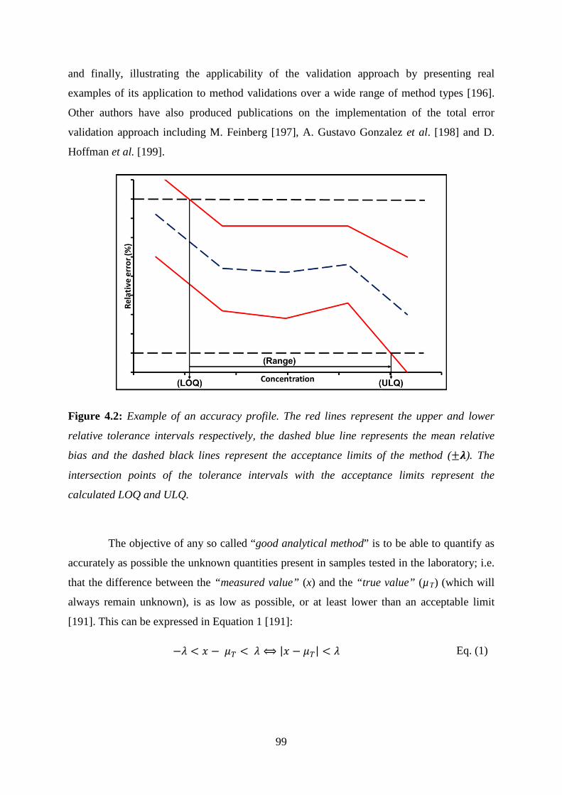
99
and finally, illustrating the applicability of the validation approach by presenting real
examples of its application to method validations over a wide range of method types [196].
Other authors have also produced publications on the implementation of the total error
validation approach including M. Feinberg [197], A. Gustavo Gonzalez et al. [198] and D.
Hoffman et al. [199].
Figure 4.2: Example of an accuracy profile. The red lines represent the upper and lower
relative tolerance intervals respectively, the dashed blue line represents the mean relative
bias and the dashed black lines represent the acceptance limits of the method (±𝝀). The
intersection points of the tolerance intervals with the acceptance limits represent the
calculated LOQ and ULQ.
The objective of any so called “good analytical method” is to be able to quantify as
accurately as possible the unknown quantities present in samples tested in the laboratory; i.e.
that the difference between the “measured value” (x) and the “true value” (µT) (which will
always remain unknown), is as low as possible, or at least lower than an acceptable limit
[191]. This can be expressed in Equation 1 [191]:
−𝜆 < 𝑥 − 𝜇𝑇 < 𝜆 ⟺ |𝑥 − 𝜇𝑇| < 𝜆
Eq. (1)
100
Where λ, the acceptance limit which is set depending on the requirements or objective of the
analytical method. Thus, two important concepts are introduced for this approach to method
validation, namely (i) acceptance limits (λ) for the performance of the method must be
defined and (ii), the analyst must take responsibility in the decision of accepting the
performance of the method with respect to its intended use [191].
Every analytical method used for quantitative analysis is subject to inherent errors
[200]. Therefore, one of the guiding principles in statistical analysis is that no quantitative
results are of any value unless they are accompanied by some measure of the errors inherent
within them [200]. The types of inherent errors of most importance in a quantitative
analytical method can be categorised as “random errors” and “systematic errors”. Random
errors affect the precision or reproducibility of an experiment and are associated more with
analyst input, but may also arise from instrumentation imprecision or environmental factors
e.g. temperature fluctuations. Systematic errors, also called “bias”, affect the accuracy of the
experiment and are associated more with the equipment used in the experiment. Random
errors, known as the “true variance” (𝜎𝑀2 ) is measured by standard deviation whereas
systematic errors (𝜇𝑀) is measured as “true bias” of the analytical method. As with the true
value (µT), the actual value for both (𝜎𝑀2 ) and (𝜇𝑀) will always remain unknown for a given
analytical method. However, estimations for (𝜎𝑀2 ) and (𝜇𝑀) can be made from the
experiments carried out during the validation of the analytical method [191]. The reliability
of these estimates depends on the adequacy of the measurements performed on samples of
known concentration, experimental design and the number of replicates performed during the
validation phase [191]. Once these estimates for (𝜎𝑀2 ) and (𝜇𝑀) have been obtained, they can
be used to evaluate the ability of the analytical method to quantify with sufficient accuracy
each of the unknown quantities the method will be subject to in its future application; i.e. to
determine if the method is a “good analytical method” [201,202].
Deciding on what the acceptance limits (λ) of the analytical method will be depends
on its intended use, e.g. the analysis of bulk pharmaceutical compounds, dosage forms or
bioanalysis. However, as all analytical methods have inherent errors, it is next to impossible
to be able to state that every future result generated will lie within the selected acceptance
limits (λ). To overcome this dilemma, the analyst has to try to control the risk associated with
the analytical method by starting with the assumption that only an acceptable maximum
proportion of future measurements will fall outside the defined acceptance limits (λ), e.g. 5%
101
of all future results will fall outside λ. Therefore, a method can be qualified as acceptable if it
is very likely (i.e. with a guarantee) that the difference between every measurement (x) and
the true value (𝜇𝑇) is inside the predefined acceptance limits (λ) [191]. Equation 2 describes
this concept which lies at the heart of this validation approach [191]:
𝑃(|𝑥 − 𝜇𝑇| < λ) ≥ β
Eq. (2)
Where β is the proportion of measurements lying within the acceptance limits (λ) fix a priori
according to the objectives of the method. Therefore, the expected proportion of
measurements (P) expressed as a percentage, which fall outside the acceptance limits (λ)
represents the risk of the analytical method [191].
In this context, the purpose of method validation is, via a selectively designed set of
experiments, to provide the analyst with good estimates of the standard deviation of the
intermediate precision of the method (𝜎�𝑀), along with estimates of method bias (�̂�𝑀). These
estimates will be more reliable if the experimental design and the number of experiments
performed in method validation are appropriate [195,203,204]. Details of the experimental
design required to achieve good estimates for both (𝜎�𝑀) and (�̂�𝑀); i.e. validation protocols,
are outlined in Part II of the summary report produced by Hubert et al. [195]. In this report, it
is emphasised that it is necessary to perform these validation studies in the same way that the
analytical method will be run during routine use; i.e. that the samples used should be
prepared in the same sample matrix as the samples tested in routine use. These estimates of
both (𝜎�𝑀) and (�̂�𝑀) are then used to calculate the confidence interval that allows the
evaluation of the proportion of the measurements that will lie inside the acceptance limit (λ).
The confidence interval used is the so-called “two-sided β-expectation tolerance interval”
proposed by Mee [205], which defines an interval where the expected proportion of future
results will fall in β [191] and obeys the following property;
𝐸𝜇� ,𝜎� {𝑃[|𝑥𝑖 − 𝜇𝑇| < 𝜆]/�̂�𝑀,𝜎�𝑀 } ≥ 𝛽
Eq. (3)
With (E) meaning the “expected value” of the result and (𝑥𝑖) the overall mean result
for series i.
Although the estimations of method bias (�̂�𝑀) and method variance (𝜎�𝑀) are
essential elements to compute the evaluation of the expected proportion of measurements
102
within the acceptance limits (i.e. the calculated tolerance intervals), the decision of whether a
method is indeed a “good method” is not based on these estimates [191]. Instead, the
calculated tolerance intervals are used to construct what is known as an accuracy profile
which is a graphical representation, combining the calculated tolerance intervals, (based on
the total error (bias + standard deviation)), bias and acceptance limits (λ). Therefore, the
accuracy profile can be used as the decision making tool which not only brings together the
objectives of the procedure with those of validation, but also allows the analyst to visually
evaluate the capacity of the procedure to fulfil its objectives and to control the risk associated
with its routine use [191,206].
The main steps involved in the generation of an accuracy profile are summarised as follows;
Step 1: Design of Experiments
The validation protocols must outline a sufficient but realistic number of experiments to
ensure the data generated is of high enough quality to give good estimation of method bias
(�̂�𝑀) and method variance (𝜎�𝑀). Two types of solutions must be prepared for use in the
validation experiments namely (i) calibration standards (CSs) and (ii) validation standards
(VSs). CSs are solutions containing reference standard material at a known concentration
which are prepared in sample diluent without any sample matrix components being present.
VSs which are solutions containing reference standard material at a known concentration
which are prepared in sample diluent, which also includes all of the sample matrix
components and are designed to mimic “real samples”. A typical validation experimental
design involves replicate preparations of CSs and VSs, (at several concentrations over the
selected concentration range) which are then analysed in series under the specified analytical
conditions. Several such series are performed with fresh CSs and VSs being prepared (from
common stocks) for each individual series. Typically, different series are prepared and run on
different days. For ease of calculation, it is important that the study design is balanced, i.e.
the repetition number is identical in every series for each concentration level [195].
Step 2: Determination of the Response Function
CSs are used to determine what is termed the “response function” of the method. The
response function is the relationship between the response (signal or response of the
apparatus) Y and the quantity (concentration) X [195]. This relationship is characterised by a
function that must be strictly monotonic (i.e. strictly increasing or decreasing) over the
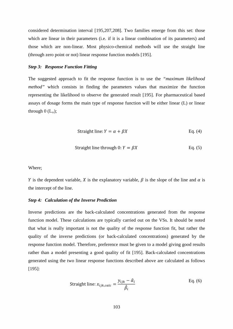
103
considered determination interval [195,207,208]. Two families emerge from this set: those
which are linear in their parameters (i.e. if it is a linear combination of its parameters) and
those which are non-linear. Most physico-chemical methods will use the straight line
(through zero point or not) linear response function models [195].
Step 3: Response Function Fitting
The suggested approach to fit the response function is to use the “maximum likelihood
method” which consists in finding the parameters values that maximize the function
representing the likelihood to observe the generated result [195]. For pharmaceutical based
assays of dosage forms the main type of response function will be either linear (L) or linear
through 0 (Lo);
Straight line:𝑌 = 𝛼 + 𝛽𝛽
Eq. (4)
Straight line through 0: 𝑌 = 𝛽𝛽 Eq. (5)
Where;
𝑌 is the dependent variable, 𝛽 is the explanatory variable, 𝛽 is the slope of the line and 𝛼 is
the intercept of the line.
Step 4: Calculation of the Inverse Prediction
Inverse predictions are the back-calculated concentrations generated from the response
function model. These calculations are typically carried out on the VSs. It should be noted
that what is really important is not the quality of the response function fit, but rather the
quality of the inverse predictions (or back-calculated concentrations) generated by the
response function model. Therefore, preference must be given to a model giving good results
rather than a model presenting a good quality of fit [195]. Back-calculated concentrations
generated using the two linear response functions described above are calculated as follows
[195]:
Straight line: 𝑥𝑖𝑖𝑖,𝑐𝑐𝑐𝑐 =𝑦𝑖𝑖𝑖 − 𝛼�𝑖
�̂�𝑖
Eq. (6)
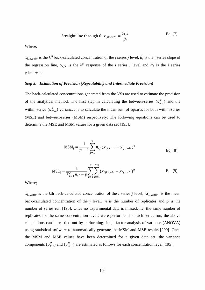
104
Straight line through 0: 𝑥𝑖𝑖𝑖,𝑐𝑐𝑐𝑐 =𝑦𝑖𝑖𝑖�̂�𝑖
Eq. (7)
Where;
𝑥𝑖𝑖𝑖,𝑐𝑐𝑐𝑐 is the kth back-calculated concentration of the i series j level, �̂�𝑖 is the i series slope of
the regression line, 𝑦𝑖𝑖𝑖 is the kth response of the i series j level and 𝛼�𝑖 is the i series
y-intercept.
Step 5: Estimation of Precision (Repeatability and Intermediate Precision)
The back-calculated concentrations generated from the VSs are used to estimate the precision
of the analytical method. The first step in calculating the between-series (𝜎𝐵,𝑖2 ) and the
within-series (𝜎𝑊,𝑖2 ) variances is to calculate the mean sum of squares for both within-series
(MSE) and between-series (MSM) respectively. The following equations can be used to
determine the MSE and MSM values for a given data set [195]:
MSMj =1
𝑝 − 1�𝑛𝑖𝑖
𝑝
𝑖=1
(�̅�𝑖𝑖.,𝑐𝑐𝑐𝑐 − �̅�.𝑖.,𝑐𝑐𝑐𝑐)2
Eq. (8)
MSEj =1
∑ 𝑛𝑖𝑖𝑝𝑖=1 − 𝑝
��(�̅�𝑖𝑖𝑖,𝑐𝑐𝑐𝑐 − �̅�𝑖𝑖.,𝑐𝑐𝑐𝑐)2𝑛𝑖𝑖
𝑖=1
𝑝
𝑖=1
Eq. (9)
Where;
�̅�𝑖𝑖.,𝑐𝑐𝑐𝑐 is the kth back-calculated concentration of the i series j level, �̅�.𝑖.,𝑐𝑐𝑐𝑐 is the mean
back-calculated concentration of the j level, 𝑛 is the number of replicates and 𝑝 is the
number of series run [195]. Once no experimental data is missed; i.e. the same number of
replicates for the same concentration levels were performed for each series run, the above
calculations can be carried out by performing single factor analysis of variance (ANOVA)
using statistical software to automatically generate the MSM and MSE results [209]. Once
the MSM and MSE values have been determined for a given data set, the variance
components (𝜎𝐵,𝑖2 ) and (𝜎𝑊,𝑖
2 ) are estimated as follows for each concentration level [195]:
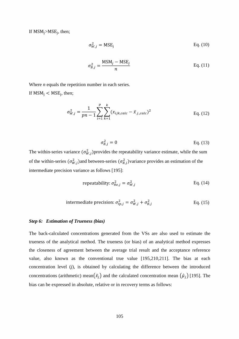
105
If MSMj>MSEj, then;
𝜎𝑊,𝑖2 = MSEj
Eq. (10)
𝜎𝐵,𝑖2 =
MSM𝑖 − MSE𝑖𝑛
Eq. (11)
Where n equals the repetition number in each series.
If MSMj < MSEj, then;
𝜎𝑊,𝑖2 =
1𝑝𝑛 − 1
��(𝑥𝑖𝑖𝑖,𝑐𝑐𝑐𝑐 − �̅�.𝑖.,𝑐𝑐𝑐𝑐)2𝑖
𝑖=1
𝑝
𝑖=1
Eq. (12)
𝜎𝐵,𝑖2 = 0 Eq. (13)
The within-series variance (𝜎𝑊,𝑖2 )provides the repeatability variance estimate, while the sum
of the within-series (𝜎𝑊,𝑖2 )and between-series (𝜎𝐵,𝑖
2 )variance provides an estimation of the
intermediate precision variance as follows [195]:
repeatability: 𝜎𝑅𝑅,𝑖2 = 𝜎𝑊,𝑖
2
Eq. (14)
intermediate precision: 𝜎𝐼𝑝,𝑖2 = 𝜎𝑊,𝑖
2 + 𝜎𝐵,𝑖2 Eq. (15)
Step 6: Estimation of Trueness (bias)
The back-calculated concentrations generated from the VSs are also used to estimate the
trueness of the analytical method. The trueness (or bias) of an analytical method expresses
the closeness of agreement between the average trial result and the acceptance reference
value, also known as the conventional true value [195,210,211]. The bias at each
concentration level (j), is obtained by calculating the difference between the introduced
concentrations (arithmetic) mean��̅�𝑖� and the calculated concentration mean ��̂�𝑖� [195]. The
bias can be expressed in absolute, relative or in recovery terms as follows:
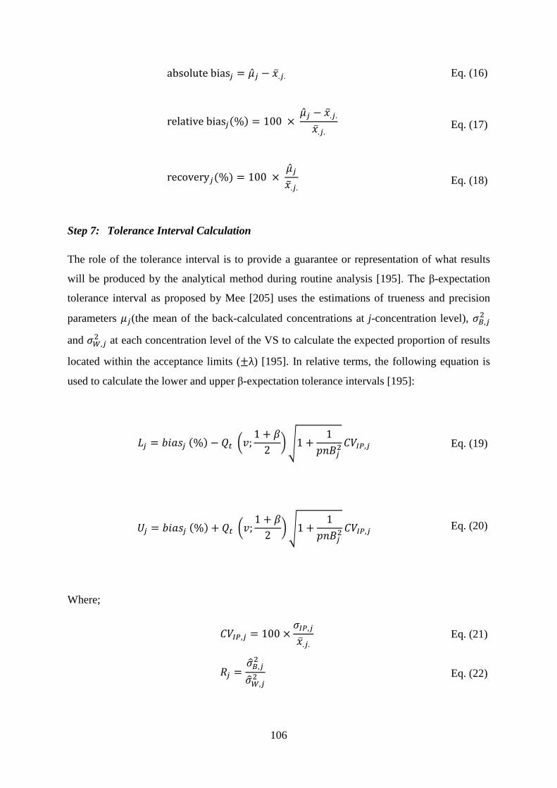
106
absolute bias𝑖 = �̂�𝑖 − �̅�.𝑖.
Eq. (16)
relative bias𝑖(%) = 100 × �̂�𝑖 − �̅�.𝑖.
�̅�.𝑖.
Eq. (17)
recovery𝑖(%) = 100 × �̂�𝑖�̅�.𝑖.
Eq. (18)
Step 7: Tolerance Interval Calculation
The role of the tolerance interval is to provide a guarantee or representation of what results
will be produced by the analytical method during routine analysis [195]. The β-expectation
tolerance interval as proposed by Mee [205] uses the estimations of trueness and precision
parameters 𝜇𝑖(the mean of the back-calculated concentrations at j-concentration level), 𝜎𝐵,𝑖2
and 𝜎𝑊,𝑖2 at each concentration level of the VS to calculate the expected proportion of results
located within the acceptance limits (±λ) [195]. In relative terms, the following equation is
used to calculate the lower and upper β-expectation tolerance intervals [195]:
𝐿𝑖 = 𝑏𝑏𝑏𝑏𝑖 (%) − 𝑄𝑡 �𝑣;1 + 𝛽
2��1 +
1𝑝𝑛𝑝𝑖2
𝐶𝐶𝐼𝐼,𝑖
Eq. (19)
𝑈𝑖 = 𝑏𝑏𝑏𝑏𝑖 (%) + 𝑄𝑡 �𝑣;1 + 𝛽
2��1 +
1𝑝𝑛𝑝𝑖2
𝐶𝐶𝐼𝐼,𝑖
Eq. (20)
Where;
𝐶𝐶𝐼𝐼,𝑖 = 100 ×𝜎𝐼𝐼,𝑖
�̅�.𝑖. Eq. (21)
𝑅𝑖 =𝜎�𝐵,𝑖2
𝜎�𝑊,𝑖2
Eq. (22)

107
𝑝𝑖 = �𝑅𝑖 + 1𝑛𝑅𝑖 + 1
Eq. (23)
𝑣 =(𝑅𝑖 + 1)2
(𝑅𝑖 + 1 𝑛⁄ ))2 (𝑝 − 1)⁄ + (1 − (1 𝑛⁄ )) 𝑝𝑛⁄
Eq. (24)
𝑄𝑡 �𝑣;1 + 𝛽
2� = the β quantile of the Student t distribution with v degrees of freedom
Eq. (25)
Two terms are contained in the tolerance interval: (i) trueness and (ii) up to a factor,
the intermediate precision coefficient variation. Therefore, the tolerance interval may be
considered as an expression of the results accuracy. However, the tolerance interval
incorporates an additional dimension; i.e. the chance or risk of future results, conditional to
past results (i.e. the results generated during the method validation), to fall within (or outside)
the acceptance limits. Therefore, the method can be considered accurate, at β chance level,
for the concentration level in question, if the tolerance interval is included within the
acceptance limits (±λ) defined a priori, according to the method objectives [195].
Step 8: Construction of the Accuracy Profile and decision making
The accuracy profile is a 2D-graphical representation of the calculated results, with the x-axis
comprised of the concentration levels and the y-axis comprised of the tolerance interval limits
and accuracy expressed as either concentration or percent. The accuracy profile contains four
main elements namely; (i) the upper and lower tolerance limits (which are achieved by
joining on one hand the lower limits between themselves, and, on the other hand, the upper
limits between themselves), (ii) the individual bias results, (iii) the mean bias (which are
achieved by joining the mean bias results at each concentration level) and (iv) the acceptance
limits (±λ). Figure 4.2 represents an example accuracy profile (calculated in relative terms)
for analytical results observed during method validation. From the accuracy profile a number
of key validation elements can be determined which can be used to support the claim that the
analytical method is indeed validated and fit for its intended use. The first of these is to
demonstrate that the correct response function has been selected in order to achieve the
objectives of the analytical method which are defined a priori. In Figure 4.2 it can be seen
that the tolerance intervals (red lines) exceed the method acceptance limits (dashed black
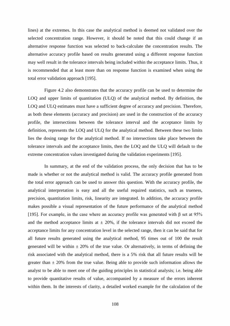
108
lines) at the extremes. In this case the analytical method is deemed not validated over the
selected concentration range. However, it should be noted that this could change if an
alternative response function was selected to back-calculate the concentration results. The
alternative accuracy profile based on results generated using a different response function
may well result in the tolerance intervals being included within the acceptance limits. Thus, it
is recommended that at least more than on response function is examined when using the
total error validation approach [195].
Figure 4.2 also demonstrates that the accuracy profile can be used to determine the
LOQ and upper limits of quantitation (ULQ) of the analytical method. By definition, the
LOQ and ULQ estimates must have a sufficient degree of accuracy and precision. Therefore,
as both these elements (accuracy and precision) are used in the construction of the accuracy
profile, the intersections between the tolerance interval and the acceptance limits by
definition, represents the LOQ and ULQ for the analytical method. Between these two limits
lies the dosing range for the analytical method. If no intersections take place between the
tolerance intervals and the acceptance limits, then the LOQ and the ULQ will default to the
extreme concentration values investigated during the validation experiments [195].
In summary, at the end of the validation process, the only decision that has to be
made is whether or not the analytical method is valid. The accuracy profile generated from
the total error approach can be used to answer this question. With the accuracy profile, the
analytical interpretation is easy and all the useful required statistics, such as trueness,
precision, quantitation limits, risk, linearity are integrated. In addition, the accuracy profile
makes possible a visual representation of the future performance of the analytical method
[195]. For example, in the case where an accuracy profile was generated with β set at 95%
and the method acceptance limits at ± 20%, if the tolerance intervals did not exceed the
acceptance limits for any concentration level in the selected range, then it can be said that for
all future results generated using the analytical method, 95 times out of 100 the result
generated will be within ± 20% of the true value. Or alternatively, in terms of defining the
risk associated with the analytical method, there is a 5% risk that all future results will be
greater than ± 20% from the true value. Being able to provide such information allows the
analyst to be able to meet one of the guiding principles in statistical analysis; i.e. being able
to provide quantitative results of value, accompanied by a measure of the errors inherent
within them. In the interests of clarity, a detailed worked example for the calculation of the
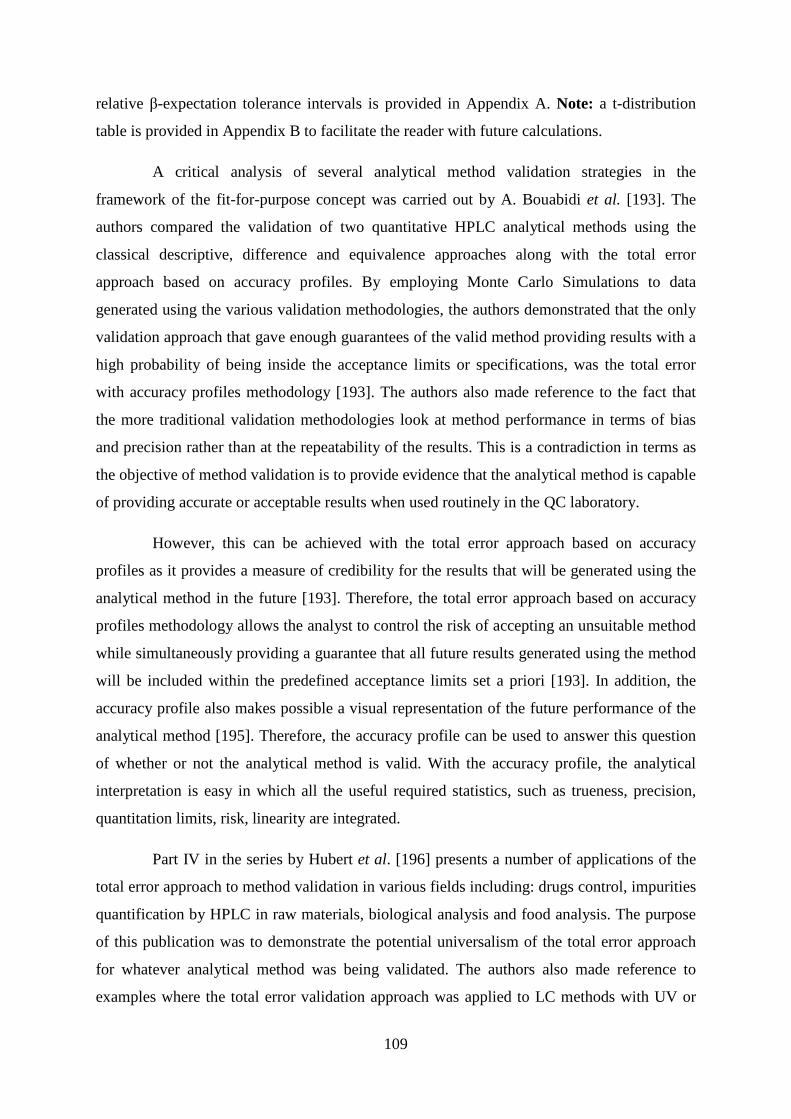
109
relative β-expectation tolerance intervals is provided in Appendix A. Note: a t-distribution
table is provided in Appendix B to facilitate the reader with future calculations.
A critical analysis of several analytical method validation strategies in the
framework of the fit-for-purpose concept was carried out by A. Bouabidi et al. [193]. The
authors compared the validation of two quantitative HPLC analytical methods using the
classical descriptive, difference and equivalence approaches along with the total error
approach based on accuracy profiles. By employing Monte Carlo Simulations to data
generated using the various validation methodologies, the authors demonstrated that the only
validation approach that gave enough guarantees of the valid method providing results with a
high probability of being inside the acceptance limits or specifications, was the total error
with accuracy profiles methodology [193]. The authors also made reference to the fact that
the more traditional validation methodologies look at method performance in terms of bias
and precision rather than at the repeatability of the results. This is a contradiction in terms as
the objective of method validation is to provide evidence that the analytical method is capable
of providing accurate or acceptable results when used routinely in the QC laboratory.
However, this can be achieved with the total error approach based on accuracy
profiles as it provides a measure of credibility for the results that will be generated using the
analytical method in the future [193]. Therefore, the total error approach based on accuracy
profiles methodology allows the analyst to control the risk of accepting an unsuitable method
while simultaneously providing a guarantee that all future results generated using the method
will be included within the predefined acceptance limits set a priori [193]. In addition, the
accuracy profile also makes possible a visual representation of the future performance of the
analytical method [195]. Therefore, the accuracy profile can be used to answer this question
of whether or not the analytical method is valid. With the accuracy profile, the analytical
interpretation is easy in which all the useful required statistics, such as trueness, precision,
quantitation limits, risk, linearity are integrated.
Part IV in the series by Hubert et al. [196] presents a number of applications of the
total error approach to method validation in various fields including: drugs control, impurities
quantification by HPLC in raw materials, biological analysis and food analysis. The purpose
of this publication was to demonstrate the potential universalism of the total error approach
for whatever analytical method was being validated. The authors also made reference to
examples where the total error validation approach was applied to LC methods with UV or
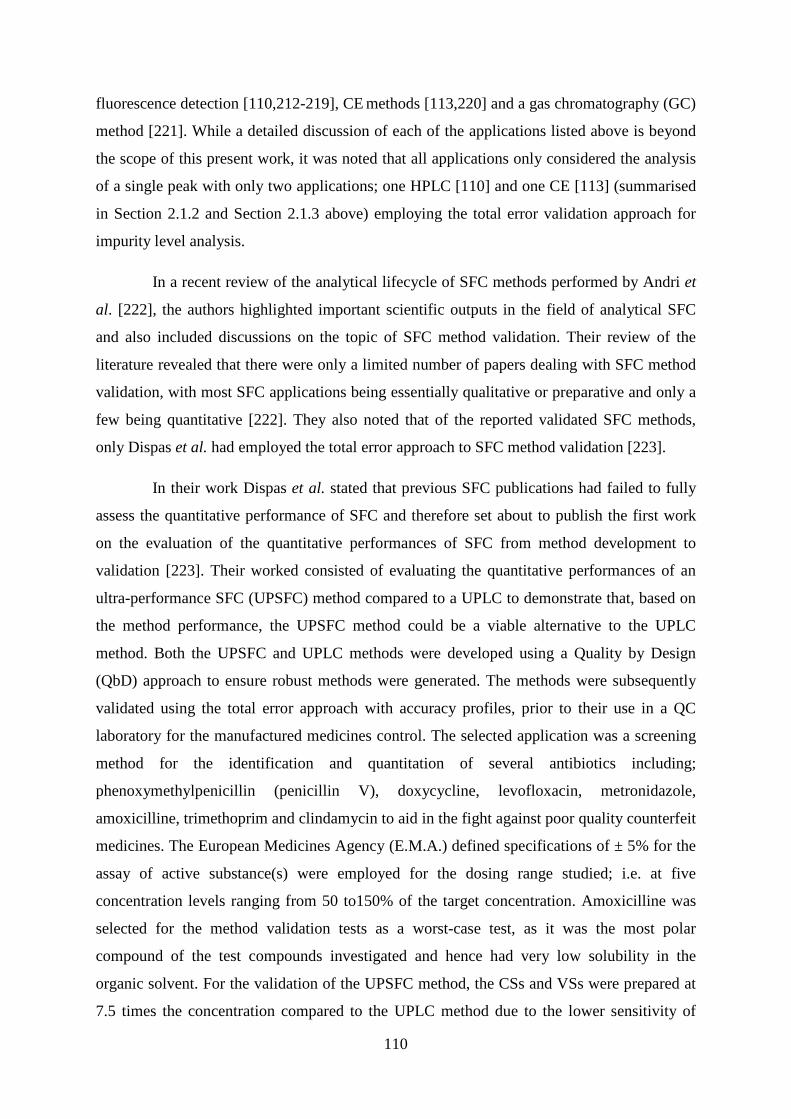
110
fluorescence detection [110,212-219], CE methods [113,220] and a gas chromatography (GC)
method [221]. While a detailed discussion of each of the applications listed above is beyond
the scope of this present work, it was noted that all applications only considered the analysis
of a single peak with only two applications; one HPLC [110] and one CE [113] (summarised
in Section 2.1.2 and Section 2.1.3 above) employing the total error validation approach for
impurity level analysis.
In a recent review of the analytical lifecycle of SFC methods performed by Andri et
al. [222], the authors highlighted important scientific outputs in the field of analytical SFC
and also included discussions on the topic of SFC method validation. Their review of the
literature revealed that there were only a limited number of papers dealing with SFC method
validation, with most SFC applications being essentially qualitative or preparative and only a
few being quantitative [222]. They also noted that of the reported validated SFC methods,
only Dispas et al. had employed the total error approach to SFC method validation [223].
In their work Dispas et al. stated that previous SFC publications had failed to fully
assess the quantitative performance of SFC and therefore set about to publish the first work
on the evaluation of the quantitative performances of SFC from method development to
validation [223]. Their worked consisted of evaluating the quantitative performances of an
ultra-performance SFC (UPSFC) method compared to a UPLC to demonstrate that, based on
the method performance, the UPSFC method could be a viable alternative to the UPLC
method. Both the UPSFC and UPLC methods were developed using a Quality by Design
(QbD) approach to ensure robust methods were generated. The methods were subsequently
validated using the total error approach with accuracy profiles, prior to their use in a QC
laboratory for the manufactured medicines control. The selected application was a screening
method for the identification and quantitation of several antibiotics including;
phenoxymethylpenicillin (penicillin V), doxycycline, levofloxacin, metronidazole,
amoxicilline, trimethoprim and clindamycin to aid in the fight against poor quality counterfeit
medicines. The European Medicines Agency (E.M.A.) defined specifications of ± 5% for the
assay of active substance(s) were employed for the dosing range studied; i.e. at five
concentration levels ranging from 50 to150% of the target concentration. Amoxicilline was
selected for the method validation tests as a worst-case test, as it was the most polar
compound of the test compounds investigated and hence had very low solubility in the
organic solvent. For the validation of the UPSFC method, the CSs and VSs were prepared at
7.5 times the concentration compared to the UPLC method due to the lower sensitivity of

111
UPSFC–UV than UPLC–UV, which the authors attributed to the difference of solvating
power between supercritical fluids and liquids.
In terms of the precision criterion, it was observed that while the UPLC method
showed lower RSD values (< 1% for repeatability and intermediate precision) across the
entire concentration range studied, the UPSFC method RSD values are close to 1 (highest
value: 1.22% for level 2); over the three median concentration levels which correspond to
80– 120% of the targeted concentration. However, these UPSFC precision results meet the
E.M.A. and ICH requirements and therefore, despite the lower precision than the UPLC
method, the UPSFC method was acceptable to meet the precision specifications for
pharmaceutical finish product.
Figure 4.3 illustrates the accuracy profiles generated for both the UPSFC and UPLC
methods. As illustrated, the UPSFC method upper and lower 95% β-expectation tolerance
limits (%) exceeded the acceptance limits set at ± 5% for the extremities of the concentration
range investigated. Therefore, the UPSFC method was only able to provide accurate results
over the concentration range corresponding from 65.8 to 129.1% of the target concentration,
whereas the UPLC method was considered valid over the complete concentration range tested
(i.e. from 50 to150% of the target concentration). However, despite this, the UPSFC method
was valid at least in the 80–120% of the target concentration interval with acceptance limits
set at ± 5%, which demonstrated its suitability for the quality control of manufactured
medicines [223].
Finally, the authors applied both the UPSFC and UPLC methods to test real samples
(n=3). The results obtained were similar for both methods with; 105.9 ± 1.6% (mean ± RSD)
obtained for the UPSFC method and 106.6 ± 1.9% (mean ± RSD) for UPLC method. Thus,
the authors concluded that compared to the well-established UPLC technique, UPSFC
showed real promise in the field of QC quantitative analysis. Their study was the first
demonstration of a successful total error approach validation of UPSFC method, thus opening
the door of pharmaceutical industry QC lab [223]. Their work also demonstrated the
application of UPSFC outside the academia research context and provided QC laboratories of
the pharmaceutical industry with a new eco-friendly tool for the quantitative analysis [223].
Therefore, despite an extensive review of the literature, to the best of our knowledge
no SFC method has been reported for the quantitation of PAC and its related impurities
(shown in Figure 3.1) in an ophthalmic suspension. We were also unable to find any
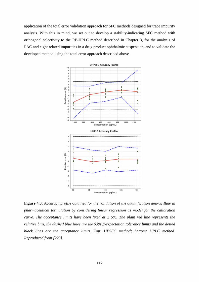
112
application of the total error validation approach for SFC methods designed for trace impurity
analysis. With this in mind, we set out to develop a stability-indicating SFC method with
orthogonal selectivity to the RP-HPLC method described in Chapter 3, for the analysis of
PAC and eight related impurities in a drug product ophthalmic suspension, and to validate the
developed method using the total error approach described above.
Figure 4.3: Accuracy profile obtained for the validation of the quantification amoxicilline in
pharmaceutical formulation by considering linear regression as model for the calibration
curve. The acceptance limits have been fixed at ± 5%. The plain red line represents the
relative bias, the dashed blue lines are the 95% β-expectation tolerance limits and the dotted
black lines are the acceptance limits. Top: UPSFC method; bottom: UPLC method.
Reproduced from [223].
113
4.2 Experimental
4.2.1 Instrumentation and Software
The Thar SFC Method Station Analytical System (Thar SFC /Waters), Pittsburgh,
PA) was equipped with a Fluid Delivery Module (CO2 pump and solvent pump), Analytical-
2-Prep column oven capable of holding ten analytical columns up to 250 mm in length, Alias
autosampler, automated back pressure regulator and a Waters 2998 photodiode array (PDA)
detector (Waters, Milford, MA, USA). Injection loops of 10 µL and 100 µL were used during
initial method development. The maximum flow rate, pressure and column temperature were
10 mL.min-1, 400 bar and 90 oC respectively. The instrument control data collection was
conducted using Waters EmpowerTM 2 software.
The Agilent 1260 Infinity Analytical SFC system was equipped with a PDA detector
and coupled to an Aurora SFC Fusion A5 CO2 delivery system (Agilent Technologies, Santa
Clara, CA, USA). A 5 µL injection loop was fitted which operated in the full loop mode with
needle overfill and methanol was used as the solvent wash. The column oven was capable of
holding two analytical columns up to 250 mm in length. The maximum flow rate, pressure
and column temperature of the instrument are 5 mL.min-1, 600 bar and 70 oC respectively.
Peaks were integrated at a wavelength of 254 nm using Agilent Chemstation software Rev
B.04.03.
The Waters Acquity UPC2 system (Waters, Milford, MA, USA) was equipped with
a PDA detector. A 10 µL loop was fitted which operated in the partial loop mode with needle
overfill, with methanol used as the wash solvent. The column oven was capable of holding
two analytical columns up to 150 mm in length. The maximum flow rate and pressure of the
instrument are 4 mL.min-1 and 413 bar respectively, while the column oven is compatible
with temperatures of up to 90 °C. Peaks were integrated at a wavelength of 254 nm using
Waters EmpowerTM 3 software.
Columns used included: Phenomenex Luna Silica, Phenomenex Luna CN,
Phenomenex Luna NH2, Phenomenex Luna HILIC (Phenomenex, Madrid Avenue, Torrance,
CA, USA) and Waters Viridis SFC 2-Ethylpyridine (Waters, Milford, MA, USA) all with
dimensions of 100 Å (5 µm) 4.6 mm x 250 mm. Also, Waters Torus DEA and Torus PIC
130 Å (1.7 µm) 3.0 mm x 100 mm columns were used.

114
4.2.2 Materials and Reagents
Materials and reagents were as described in Chapter 3 Section 3.2.2 with the following
exception; CO2 was food grade purchased from BOC Ltd. (Dublin, Ireland). The final drug
product Samples of the PAC 1.0% (w/v) ophthalmic suspension were obtained from Allergan
Pharmaceuticals Ltd. (Westport, Ireland).
4.2.3 Solution preparation for PAC pSFC analysis
Note: All solutions were prepared in low actinic glassware to protect from light.
4.2.3.1 pSFC PAC Matrix Placebo solution preparation
For the preparation of the validation standards (VS) and impurity validation standards (IVS)
described below, an additional matrix spiking solution containing the matrix components of
the ophthalmic suspension was prepared as described in Chapter 3 Section 3.2.3 All VS and
IVS described hereafter were spiked (3:50) with the stock matrix spiking solution to ensure
that matrix components were present at label strength after dilution.
4.2.3.2 pSFC PAC Column Screening Study Standard Preparation
For the initial column screening study, a stock standard solution of PAC was prepared in
MeOH at a concentration of 2 g.L-1. Impurity stock standards of P-11,21D, HCA, P-17A, HC,
P, 20(R) and 20(S) were prepared in MeOH at a concentration of 40 mg.L-1. From the stock
solutions, a working solution was prepared in MeOH containing PAC at 200 mg.L-1 and
impurities at 4 mg.L-1; i.e. at approximately 2% of the PAC concentration.
4.2.3.3 pSFC PAC Calibration and Validation Standard Preparations
For the PAC calibration standards (CS) preparation, a stock solution was prepared at
approximately 6 mg.mL-1 in MeOH. The solution was then diluted with MeOH in order to
obtain final concentrations of 480, 540, 600, 660 and 720 mg.L-1, equivalent to approximately
80%, 90%, 100%, 110% and 120% of nominal PAC concentration. For the PAC VS
preparation, the same stock solution used for the PAC CS was diluted with MeOH across the
same concentration range as above, but spiked with matrix solution as described in
Section 3.2.3. The VS were independently prepared for each series to mimic as much as
possible its corresponding PAC formulation in routine analysis. The validation experiments
were conducted by means of running four sequences (with freshly prepared CS and VS) over

115
four separate days on the same UPSFC system. Triplicate injections of each concentration
level were made for both the CS and VS.
4.2.3.4 pSFC PAC Impurity Calibration and Validation Standard Preparations
For the impurity level calibration standards (ICS) preparation, the same stock solution used
for the PAC CS was used. For each of the eight selected impurities, stock solutions were
prepared at 0.2 mg.mL-1 in MeOH. A PAC and impurity ICS was then prepared by diluting
with MeOH in order to obtain final concentrations for PAC and impurities of 0.30, 0.60, 3.00,
6.00 and 12.00 mg.L-1, equivalent to approximately 0.05%, 0.10%, 0.50%, 1.00% and 2.00%
of nominal PAC concentration. For the impurity level IVS preparation, the same stock
solutions of PAC and the eight selected impurities used for the ICS were diluted with MeOH
across the same concentration range as above, but spiked with matrix solution as described in
Section 2.3.1 The IVS were independently prepared for each series to mimic as much as
possible its corresponding PAC formulation in routine analysis.
Note: Due to a limited supply of impurity reference standard material, the impurity level
validation experiments were conducted by means of running four series (two ICS and two
IVS) over four separate days on the same UPSFC system. Triplicate injections of each
concentration level were made for both the ICS and IVS. Response function and back-
calculated amounts were obtained from all four series and used in the various calculations
required to employ the total error validation approach.
4.2.3.5 pSFC PAC Real Sample Preparation
For the preparation of real samples, the PAC-containing formulation was diluted 3 mL into a
50 mL amber volumetric flask with MeOH to give a nominal PAC concentration of
600 mg.L-1.
4.3 Results and discussion
4.3.1 PAC pSFC Method Development
The main objective of this work was to develop and validate a pSFC method, which could
provide orthogonal selectivity along with comparable quantitative performance to that of the
established RP-HPLC method, for the analysis of PAC and its eight selected impurities in an
ophthalmic suspension. Initial method development was carried out on a Thar method station
and consisted of performing a column screening study to select the most appropriate

116
stationary phase for the separation. Four traditional NP-HPLC polar stationary phases were
selected, namely; Phenomenex Luna silica gel (Si), cyanopropyl-bonded silica (CN),
propanediol-bonded silica (Diol) and aminopropyl-bonded silica (NH2) columns along with
the Waters Viridis SFC 2-Ethylpyridine (2-EP) column which was developed more
specifically for pSFC applications. All column dimensions were (5 µm) 4.6 mm x 250 mm.
For the initial screening, neat MeOH which is considered to be the first choice for the elution
of polar compounds in pSFC was used as the modifier [16]. Initial screening was carried out
using the standard solutions described in Section 4.2.3.2 employing a shallow gradient of
14 to 18% modifier over 8.5 min with a 1 min equilibration. The chromatographic conditions
employed in the initial screening study are detailed in Figure 4.4 along with representative
chromatograms. Table 4.2 summarises separation performance in terms of retention time
window, peak asymmetry at 10% and resolution at half height (0.5). The normalised
resolution product (NRP) which is a measure of how evenly spaced the peaks are in a
chromatogram was calculated as described by K.L. Ng et al. [224].
As shown in Figure 4.4 (a), on the Si column, only six peaks (of a total of eight peaks
including PAC) were visible in the chromatogram. Although the Rs values at half height of
the visible peaks were acceptable; i.e. > 1.5, the fact that only six peaks were observed
indicates that there were some co-elutions occurring. Also, peak asymmetry of the PAC peak
was poor (< 0.8). On the CN column Figure 4.4 (b), all peaks eluted very early in the
chromatogram indicating less retention compared to the Si column. Once again, only six of
the eight expected peaks were observed which also indicates that there were some co-elutions
occurring. Rs values for three of the visible peak pairs were less than the required value of 1.5
and the peak asymmetry for peak 2 was poor (< 0.8).
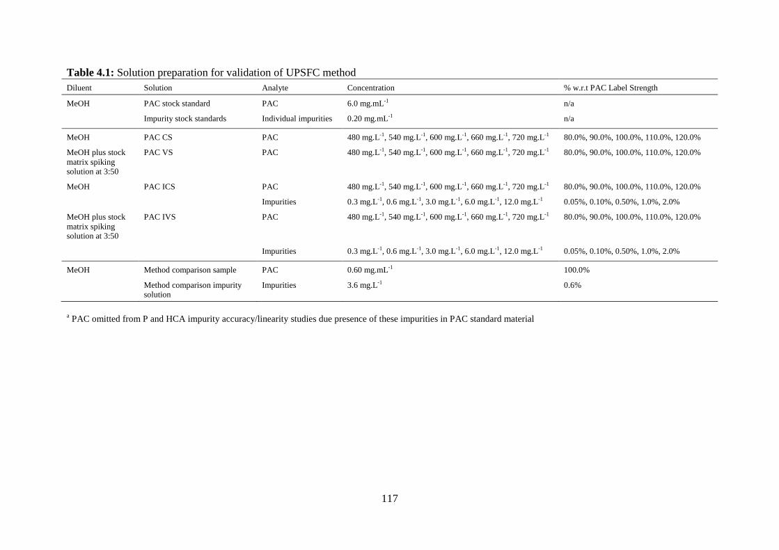
117
Table 4.1: Solution preparation for validation of UPSFC method Diluent Solution Analyte Concentration % w.r.t PAC Label Strength
MeOH PAC stock standard PAC 6.0 mg.mL-1 n/a Impurity stock standards Individual impurities 0.20 mg.mL-1 n/a
MeOH PAC CS PAC 480 mg.L-1, 540 mg.L-1, 600 mg.L-1, 660 mg.L-1, 720 mg.L-1 80.0%, 90.0%, 100.0%, 110.0%, 120.0%
MeOH plus stock matrix spiking solution at 3:50
PAC VS PAC 480 mg.L-1, 540 mg.L-1, 600 mg.L-1, 660 mg.L-1, 720 mg.L-1 80.0%, 90.0%, 100.0%, 110.0%, 120.0%
MeOH PAC ICS PAC 480 mg.L-1, 540 mg.L-1, 600 mg.L-1, 660 mg.L-1, 720 mg.L-1 80.0%, 90.0%, 100.0%, 110.0%, 120.0%
Impurities 0.3 mg.L-1, 0.6 mg.L-1, 3.0 mg.L-1, 6.0 mg.L-1, 12.0 mg.L-1 0.05%, 0.10%, 0.50%, 1.0%, 2.0%
MeOH plus stock matrix spiking solution at 3:50
PAC IVS PAC 480 mg.L-1, 540 mg.L-1, 600 mg.L-1, 660 mg.L-1, 720 mg.L-1 80.0%, 90.0%, 100.0%, 110.0%, 120.0%
Impurities 0.3 mg.L-1, 0.6 mg.L-1, 3.0 mg.L-1, 6.0 mg.L-1, 12.0 mg.L-1 0.05%, 0.10%, 0.50%, 1.0%, 2.0%
MeOH Method comparison sample PAC 0.60 mg.mL-1 100.0%
Method comparison impurity solution
Impurities 3.6 mg.L-1 0.6%
a PAC omitted from P and HCA impurity accuracy/linearity studies due presence of these impurities in PAC standard material

118
A similar situation was noted on the Diol column Figure 4.4 (c). Only six peaks of
the eight expected peaks were observed which also indicates that there were some co-elutions
occurring. Of the visible peaks, Rs values for peaks 5 and 6 was less than the required value
of 1.5 and the peak asymmetry for peaks 2 and 5 were poor (< 0.8). On the NH2 column
Figure 4.4 (d), only five peaks of the eight expected peaks were noted in the initial injection.
However, with replicate injections additional peaks were observed at the beginning of the
chromatogram which indicated that not all peaks were eluting from the column under the
given conditions. Rs values for the visible peak pairs were far greater than the required value
of 1.5 and the peak asymmetry for the visible peaks were good (0.8-1.2). This observation; i.e.
good peak asymmetry and resolution between the peaks that were observed, suggested that
the NH2 column provided the greatest retention for the selected analytes. Finally, on the 2-EP
column Figure 4.4 (e), only six peaks of the eight expected peaks were observed which also
indicates that there were some co-elutions occurring. Rs values for two of the peak pairs were
less than the required value of 1.5 and the peak asymmetry for peaks 2 and 5 were poor
(< 0.8).
The results of the screening study demonstrated that maximum retention was
obtained on the NH2 column while minimum retention was obtained on the CN column.
Although most columns gave promising results in terms of peak asymmetry (demonstrating
that an additive wasn’t necessary component of the mobile phase composition), given the
co-elution and poor resolution observed under the given conditions for the Si, CN, Diol and
2-EP columns, it was decided to investigate optimising this gradient further on the NH2
column in order to obtain the desired separation.
As not all peaks in the mix were eluted from the NH2 column under the original
gradient conditions, it was decided to increase the flow rate to 4.0 mL.min-1 and the gradient
from 15 to 23% modifier over 7 min with a 1 min equilibration step. To determine the elution
order of the impurity peaks, the individual impurity stock standards were run under the new
conditions. Figure 4.5 shows that all eight peaks were baseline resolved with good peak
asymmetry, (at 10% ranging from 0.91 for HCA to 1.19 for P-11,21D), in less than eight min
under the altered gradient conditions. The NRP under the selected conditions was calculated
as 0.41. The elution order was found to be in agreement with that observed by Yaku et al.
[184] for corticosteroids containing 1 to 4 hydroxyl groups using an NH2 stationary phase in
that the analytes were eluted in order of increasing number of hydroxyl groups.

119
Table 4.2: Summary of column screening results from the Thar Method Station
Column Si CN Diol NH2 2-EP
Parameter
Peaks observed 6 6 6 5 6
RT Window 5.17 1.16 5.23 6.05 4.07
Rs @ 0.5/(Asym @ 10%)
Peak 1 N/A/(0.81) N/A/(0.85) N/A/(0.86) N/A/(0.90) N/A/(0.90)
Peak 2 2.7/(0.85) 1.4/(0.67) 4.9/(0.74) 7.7/(1.03) 3.9/(0.51)
PAC 1.5/(0.77) 1.2/(1.02) 1.6/(1.07) 2.8/(1.00) 1.3/(0.94)
Peak 4 2.7/(0.87) 3.3/(0.85) 8.3/(0.97) 4.4/(0.94) 7.0/(0.95)
Peak 5 3.4/(0.87) 1.2/(0.91) 10.7/(0.62) 11.9/(1.18) 6.1/(0.74)
Peak 6 12.9/(0.98) 1.2/(1.03) 1.0/(1.17) N/D/(N/D) 1.2/(1.16)
NRP 0 0 0 N/A1 0 1 = Not all peaks eluted at the selected runtime
Upon the completion of the initial column screening study and selection of the NH2
stationary phase, it was decided to further optimise the separation on an Agilent 1260 Infinity
Analytical SFC system coupled with an Aurora SFC Fusion A5 CO2 delivery system. The
system was selected to provide greater sensitivity than the Thar system which was required
for the analysis of PAC potential impurities at trace levels in the final product. As the column
dimensions remained the same, it was envisioned that the transfer onto the Agilent system
would be straight forward. However, system differences coupled with the fact that an
additional impurity, prednisone (PN), (which had been omitted from the original screening
study due to the unavailability of reference standard material at the time the study was
undertaken) was included in the mix meant that the method parameters had to be re-optimised
on the Agilent system. As the method was to be used for real samples, a placebo solution
containing the matrix components of the ophthalmic suspension was prepared in deionised
water and included during the method optimisation to ensure method specificity. The initial
method requirements were set to be the same as for the previously developed RP-HPLC assay
described in Chapter 3 above. All peaks had to be baseline resolved with Rs > 1.5 and a
detection limit of 0.05% of the nominal PAC concentration for the selected impurities. The
final optimised pSFC method conditions on the Agilent system are described in Figure 4.6
which demonstrates all peaks being separated in less than 11 min. Due to the addition of the
PN impurity, stock standards of PAC and each impurity were run on the final optimised
conditions to determine the elution order. No selectivity changes for the PAC impurities were
noted between the Thar and Agilent systems with the PN peak eluting between PAC and
P-17A. However, on the Agilent system, the newly optimised conditions did result in a

120
selectivity change for the matrix peak. Using the newly optimised conditions, the matrix peak
was seen to elute at the beginning of the chromatogram, prior to any peaks of interest, thus
demonstrating the specificity of the method (See Figure 4.6). The cause of this selectivity
change was not investigated at the time as it had no negative impact on the separation.
However, given the differences in the operating conditions between the two systems; i.e. the
higher column temperature on the Agilent system; a possible cause may be that the matrix
peak was more susceptible to temperature changes than the other peaks in the separation. The
retention time window for the Agilent separation was approximately 7 min, while peak
symmetry ranged from 0.87 for the PN peak to 1.21 for the PAC peak. The NRP was for the
separation was 0.34.
While the above method conditions satisfied the separation goal for the new method,
(i.e. all peaks were baseline resolved) it was noted that the sensitivity was much lower on the
pSFC method compared to that of the RP-HPLC method. Therefore, the criterion of being
able to detect impurities at 0.05% of the nominal PAC concentration was not achievable with
the proposed nominal PAC concentration of 200 mg.L-1. To compensate for this lack of
sensitivity, the nominal concentration of working solutions was increased three fold
compared to that of the RP-HPLC method, giving a PAC nominal working concentration of
600 mg.L-1. This increase in concentration allowed for impurity peaks to be detected at the
0.10% level relative to the PAC main peak. Although a sensitivity level of 0.05% was not
met for the pSFC method, the 0.10% value was deemed acceptable based on the fact that for
the selected ophthalmic suspension used in this work, the maximum recommended daily dose
equates to approximately 624 µL (based on in-house drop size studies). This in turn equates
to 6.2 µg (based on a label claim of 1%). Therefore, according to Attachment 1 of ICH
Q3B(R2) [144], the reporting threshold for degradation products of PAC in the selected
ophthalmic suspension was 0.1%, with an identification threshold and the quantification
threshold of 1.0%.

121
Figure 4.4: Representative chromatograms of development injections conducted on the Thar method station using Si (a), CN (b), Diol (c), NH2
(d) and 2-EP (e) stationary phases. Sample contained PAC at 200 mg.L-1 and impurities at 4 mg.L-1, i.e. at approximately 2% of the PAC
concentration. Chromatograms (a) to (e) expanded view to show baseline detail. Chromatographic conditions; Columns: (5 µm) 4.6 mm x 250
mm. Flow rate: 3.5 mL.min-1. Injection volume: 10 µL. Column temperature: 40 °C. Back-pressure regulation: 120 bar. Detection: 254 nm.
Mobile phase: 14 to 18% MeOH over 8.5 min with a 1 min equilibration step. Note: individual injections of impurities were not made for peak
assignment purposes.

122
Figure 4.5: (a) Overlaid chromatograms of PAC standard at 200 mg.L-1 and impurity stock
standards at 40 mg.L-1 conducted on the Thar method station using the NH2 stationary phase
to determine the elution order sequence of the separation. (b) Chromatogram of PAC sample
at 200 mg.L-1 spiked with impurities at 4 mg.L-1. Chromatographic conditions; as per
Figure 4.3 with the following exceptions; Flow rate: 4.0 mL.min-1. Mobile phase: 15 to 23%
MeOH over 7 min with a 1 min equilibration step. Peak elution order; P-11,21D (1), HCA
(2), PAC (3), P-17A (4), HC (5), P (6), 20(R) (7) and 20(S) (8).
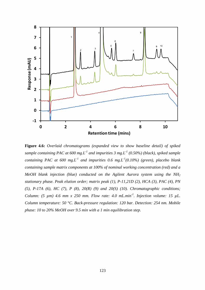
123
Figure 4.6: Overlaid chromatograms (expanded view to show baseline detail) of spiked
sample containing PAC at 600 mg.L-1 and impurities 3 mg.L-1 (0.50%) (black), spiked sample
containing PAC at 600 mg.L-1 and impurities 0.6 mg.L-1(0.10%) (green), placebo blank
containing sample matrix components at 100% of nominal working concentration (red) and a
MeOH blank injection (blue) conducted on the Agilent Aurora system using the NH2
stationary phase. Peak elution order; matrix peak (1), P-11,21D (2), HCA (3), PAC (4), PN
(5), P-17A (6), HC (7), P (8), 20(R) (9) and 20(S) (10). Chromatographic conditions;
Column: (5 µm) 4.6 mm x 250 mm. Flow rate: 4.0 mL.min-1. Injection volume: 15 µL.
Column temperature: 50 °C. Back-pressure regulation: 120 bar. Detection: 254 nm. Mobile
phase: 10 to 20% MeOH over 9.5 min with a 1 min equilibration step.
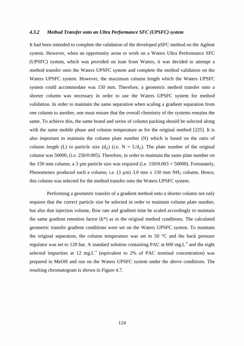
124
4.3.2 Method Transfer onto an Ultra Performance SFC (UPSFC) system
It had been intended to complete the validation of the developed pSFC method on the Agilent
system. However, when an opportunity arose to work on a Waters Ultra Performance SFC
(UPSFC) system, which was provided on loan from Waters, it was decided to attempt a
method transfer onto the Waters UPSFC system and complete the method validation on the
Waters UPSFC system. However, the maximum column length which the Waters UPSFC
system could accommodate was 150 mm. Therefore, a geometric method transfer onto a
shorter column was necessary in order to use the Waters UPSFC system for method
validation. In order to maintain the same separation when scaling a gradient separation from
one column to another, one must ensure that the overall chemistry of the systems remains the
same. To achieve this, the same brand and series of column packing should be selected along
with the same mobile phase and column temperature as for the original method [225]. It is
also important to maintain the column plate number (N) which is based on the ratio of
column length (L) to particle size (dp) (i.e. N = L/dp). The plate number of the original
column was 50000, (i.e. 250/0.005). Therefore, in order to maintain the same plate number on
the 150 mm column, a 3 µm particle size was required (i.e. 150/0.003 = 50000). Fortunately,
Phenomenex produced such a column; i.e. (3 µm) 3.0 mm x 150 mm NH2 column. Hence,
this column was selected for the method transfer onto the Waters UPSFC system.
Performing a geometric transfer of a gradient method onto a shorter column not only
requires that the correct particle size be selected in order to maintain column plate number,
but also that injection volume, flow rate and gradient time be scaled accordingly to maintain
the same gradient retention factor (k*) as in the original method conditions. The calculated
geometric transfer gradient conditions were set on the Waters UPSFC system. To maintain
the original separation, the column temperature was set to 50 °C and the back pressure
regulator was set to 120 bar. A standard solution containing PAC at 600 mg.L-1 and the eight
selected impurities at 12 mg.L-1 (equivalent to 2% of PAC nominal concentration) was
prepared in MeOH and run on the Waters UPSFC system under the above conditions. The
resulting chromatogram is shown in Figure 4.7.

125
Figure 4.7: Expanded chromatogram of spiked sample containing PAC at 600 mg.L-1 and
impurities 12 mg.L-1conducted on the Waters UPC2 system under the geometric transfer
conditions. Chromatographic conditions; Column: NH2 (3 µm) 3.0 mm x 150 mm. Flow rate:
2.84 mL.min-1. Injection volume: 1.27 µL. Column temperature: 50 °C. Back-pressure
regulation: 120 bar. Detection: 254 nm. Mobile phase: 10 to 20 % MeOH over 3.41 min with
a 0.5 min equilibration step. Peak elution order; P-11,21D (1), HCA (2), PAC (3), PN (4),
P-17A (5), HC (6) and P (7).
As shown in Figure 4.7 only seven peaks (of a total of nine peaks including PAC)
were observed under the geometric transfer conditions. Also, peaks 4 and 5 were not totally
resolved (Rs = 0.3). This result was surprising given the fact the Waters UPSFC system has a
smaller reported dwell volume, 440 µL [226] versus 700 µL [16] for the Agilent system.
Therefore, it would be expected that under similar operating conditions, all peaks would elute
slightly earlier on the Waters UPSFC system given that no compensation was made in the
gradient table for the slight dwell volume differences between the two systems. Also,
efficiency loss due to the influence of extra-column band broadening (arising from
instrumental contributions) could also be ruled out given that the extra-column band
broadening (σ2ext) for both systems has been experimentally characterised and found to be
identical for both systems i.e. 85 µL2 [227].
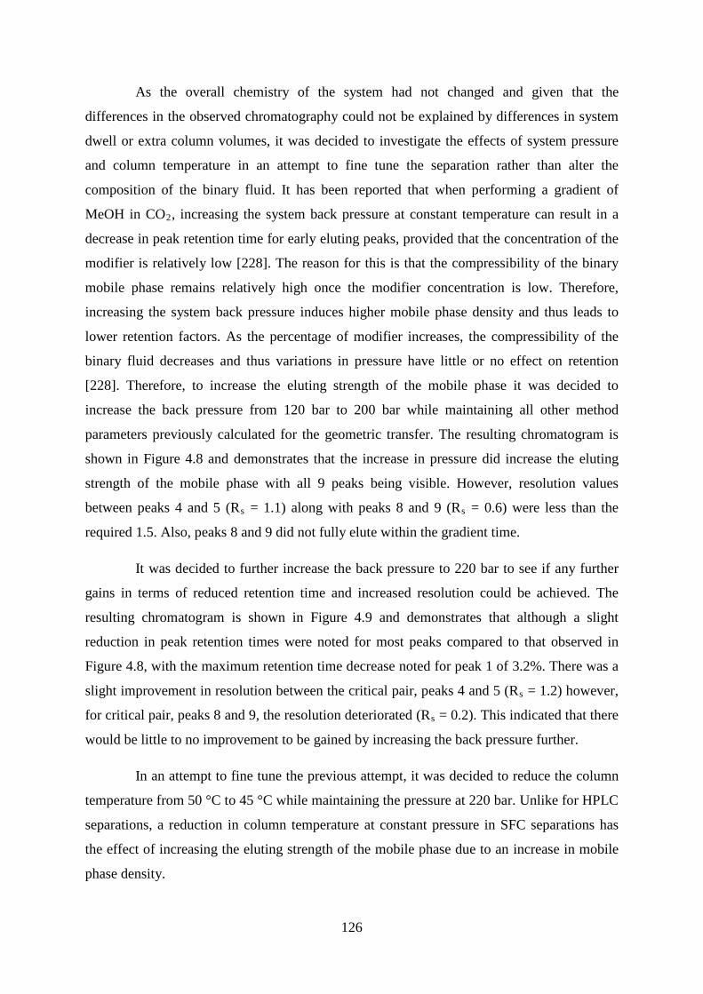
126
As the overall chemistry of the system had not changed and given that the
differences in the observed chromatography could not be explained by differences in system
dwell or extra column volumes, it was decided to investigate the effects of system pressure
and column temperature in an attempt to fine tune the separation rather than alter the
composition of the binary fluid. It has been reported that when performing a gradient of
MeOH in CO2, increasing the system back pressure at constant temperature can result in a
decrease in peak retention time for early eluting peaks, provided that the concentration of the
modifier is relatively low [228]. The reason for this is that the compressibility of the binary
mobile phase remains relatively high once the modifier concentration is low. Therefore,
increasing the system back pressure induces higher mobile phase density and thus leads to
lower retention factors. As the percentage of modifier increases, the compressibility of the
binary fluid decreases and thus variations in pressure have little or no effect on retention
[228]. Therefore, to increase the eluting strength of the mobile phase it was decided to
increase the back pressure from 120 bar to 200 bar while maintaining all other method
parameters previously calculated for the geometric transfer. The resulting chromatogram is
shown in Figure 4.8 and demonstrates that the increase in pressure did increase the eluting
strength of the mobile phase with all 9 peaks being visible. However, resolution values
between peaks 4 and 5 (Rs = 1.1) along with peaks 8 and 9 (Rs = 0.6) were less than the
required 1.5. Also, peaks 8 and 9 did not fully elute within the gradient time.
It was decided to further increase the back pressure to 220 bar to see if any further
gains in terms of reduced retention time and increased resolution could be achieved. The
resulting chromatogram is shown in Figure 4.9 and demonstrates that although a slight
reduction in peak retention times were noted for most peaks compared to that observed in
Figure 4.8, with the maximum retention time decrease noted for peak 1 of 3.2%. There was a
slight improvement in resolution between the critical pair, peaks 4 and 5 (Rs = 1.2) however,
for critical pair, peaks 8 and 9, the resolution deteriorated (Rs = 0.2). This indicated that there
would be little to no improvement to be gained by increasing the back pressure further.
In an attempt to fine tune the previous attempt, it was decided to reduce the column
temperature from 50 °C to 45 °C while maintaining the pressure at 220 bar. Unlike for HPLC
separations, a reduction in column temperature at constant pressure in SFC separations has
the effect of increasing the eluting strength of the mobile phase due to an increase in mobile
phase density.
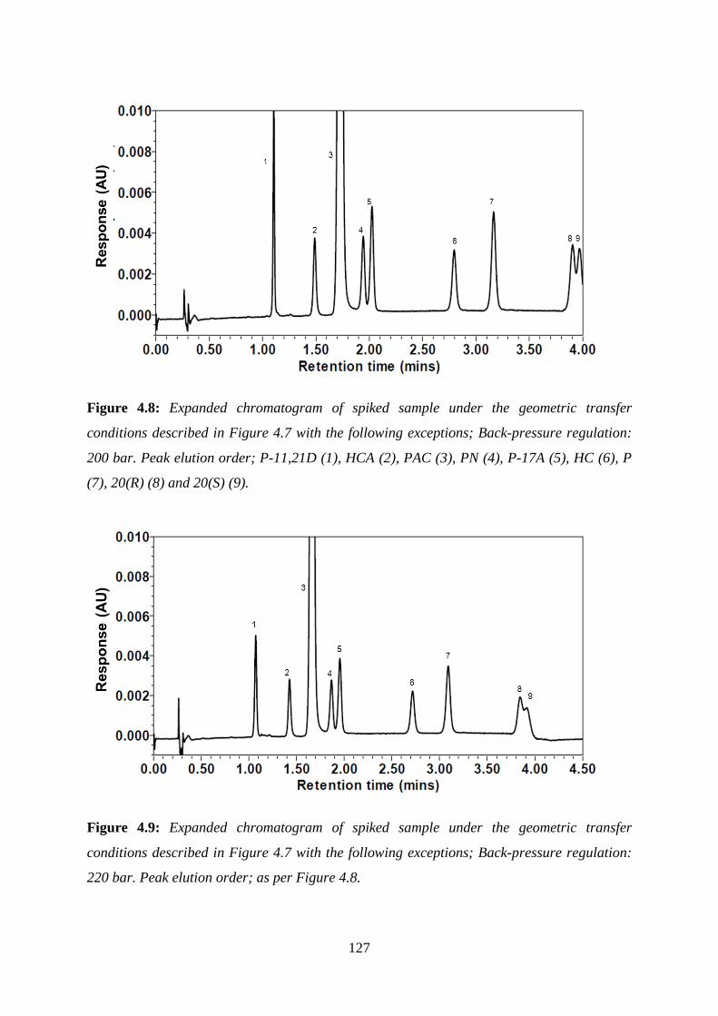
127
Figure 4.8: Expanded chromatogram of spiked sample under the geometric transfer
conditions described in Figure 4.7 with the following exceptions; Back-pressure regulation:
200 bar. Peak elution order; P-11,21D (1), HCA (2), PAC (3), PN (4), P-17A (5), HC (6), P
(7), 20(R) (8) and 20(S) (9).
Figure 4.9: Expanded chromatogram of spiked sample under the geometric transfer
conditions described in Figure 4.7 with the following exceptions; Back-pressure regulation:
220 bar. Peak elution order; as per Figure 4.8.
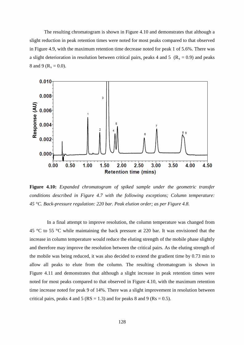
128
The resulting chromatogram is shown in Figure 4.10 and demonstrates that although a
slight reduction in peak retention times were noted for most peaks compared to that observed
in Figure 4.9, with the maximum retention time decrease noted for peak 1 of 5.6%. There was
a slight deterioration in resolution between critical pairs, peaks 4 and 5 (Rs = 0.9) and peaks
8 and 9 (Rs = 0.0).
Figure 4.10: Expanded chromatogram of spiked sample under the geometric transfer
conditions described in Figure 4.7 with the following exceptions; Column temperature:
45 °C. Back-pressure regulation: 220 bar. Peak elution order; as per Figure 4.8.
In a final attempt to improve resolution, the column temperature was changed from
45 °C to 55 °C while maintaining the back pressure at 220 bar. It was envisioned that the
increase in column temperature would reduce the eluting strength of the mobile phase slightly
and therefore may improve the resolution between the critical pairs. As the eluting strength of
the mobile was being reduced, it was also decided to extend the gradient time by 0.73 min to
allow all peaks to elute from the column. The resulting chromatogram is shown in
Figure 4.11 and demonstrates that although a slight increase in peak retention times were
noted for most peaks compared to that observed in Figure 4.10, with the maximum retention
time increase noted for peak 9 of 14%. There was a slight improvement in resolution between
critical pairs, peaks 4 and 5 (RS = 1.3) and for peaks 8 and 9 (Rs = 0.5).
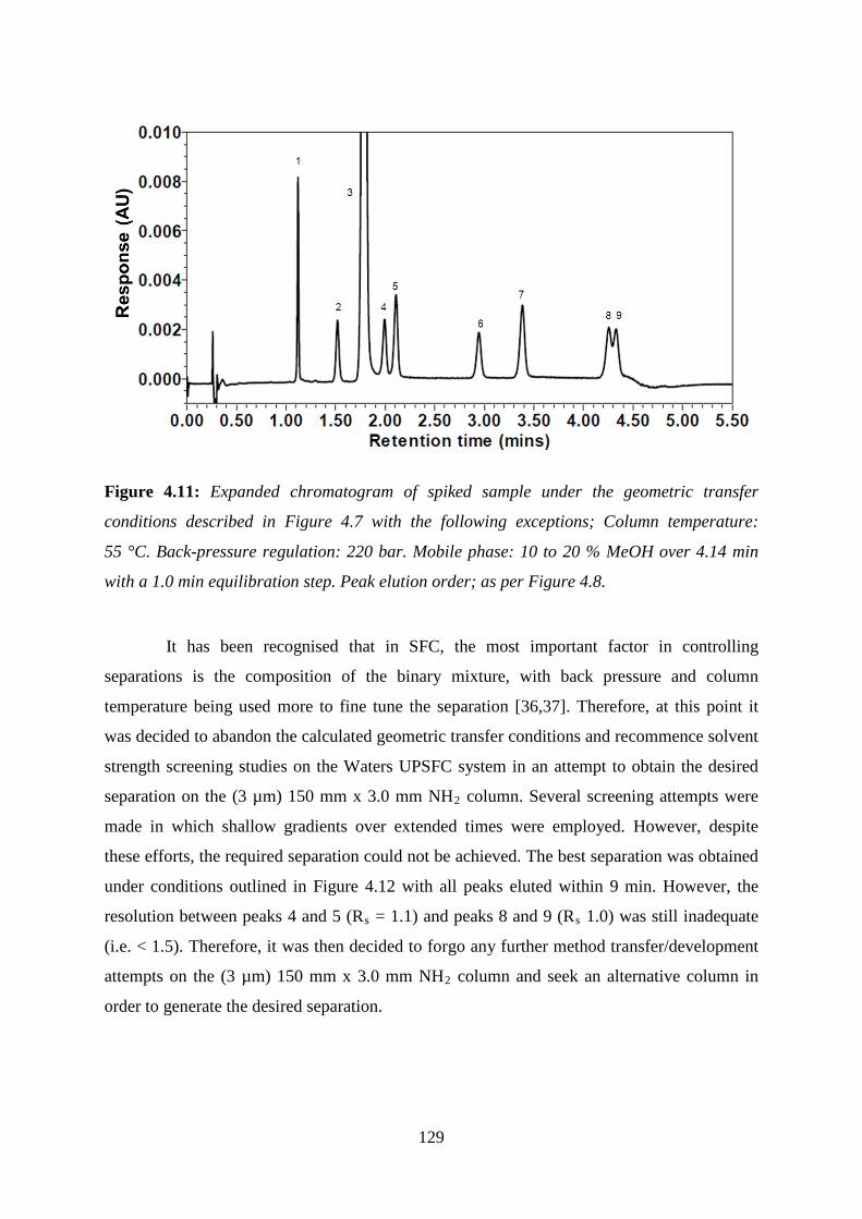
129
Figure 4.11: Expanded chromatogram of spiked sample under the geometric transfer
conditions described in Figure 4.7 with the following exceptions; Column temperature:
55 °C. Back-pressure regulation: 220 bar. Mobile phase: 10 to 20 % MeOH over 4.14 min
with a 1.0 min equilibration step. Peak elution order; as per Figure 4.8.
It has been recognised that in SFC, the most important factor in controlling
separations is the composition of the binary mixture, with back pressure and column
temperature being used more to fine tune the separation [36,37]. Therefore, at this point it
was decided to abandon the calculated geometric transfer conditions and recommence solvent
strength screening studies on the Waters UPSFC system in an attempt to obtain the desired
separation on the (3 µm) 150 mm x 3.0 mm NH2 column. Several screening attempts were
made in which shallow gradients over extended times were employed. However, despite
these efforts, the required separation could not be achieved. The best separation was obtained
under conditions outlined in Figure 4.12 with all peaks eluted within 9 min. However, the
resolution between peaks 4 and 5 (Rs = 1.1) and peaks 8 and 9 (Rs 1.0) was still inadequate
(i.e. < 1.5). Therefore, it was then decided to forgo any further method transfer/development
attempts on the (3 µm) 150 mm x 3.0 mm NH2 column and seek an alternative column in
order to generate the desired separation.
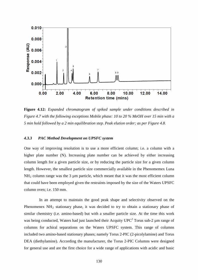
130
Figure 4.12: Expanded chromatogram of spiked sample under conditions described in
Figure 4.7 with the following exceptions Mobile phase: 10 to 20 % MeOH over 15 min with a
5 min hold followed by a 2 min equilibration step. Peak elution order; as per Figure 4.8.
4.3.3 PAC Method Development on UPSFC system
One way of improving resolution is to use a more efficient column; i.e. a column with a
higher plate number (N). Increasing plate number can be achieved by either increasing
column length for a given particle size, or by reducing the particle size for a given column
length. However, the smallest particle size commercially available in the Phenomemex Luna
NH2 column range was the 3 µm particle, which meant that it was the most efficient column
that could have been employed given the restraints imposed by the size of the Waters UPSFC
column oven; i.e. 150 mm.
In an attempt to maintain the good peak shape and selectivity observed on the
Phenomenex NH2 stationary phase, it was decided to try to obtain a stationary phase of
similar chemistry (i.e. amino-based) but with a smaller particle size. At the time this work
was being conducted, Waters had just launched their Acquity UPC2 Torus sub-2 µm range of
columns for achiral separations on the Waters UPSFC system. This range of columns
included two amino-based stationary phases; namely Torus 2-PIC (2-picolylamine) and Torus
DEA (diethylamine). According the manufacturer, the Torus 2-PIC Columns were designed
for general use and are the first choice for a wide range of applications with acidic and basic
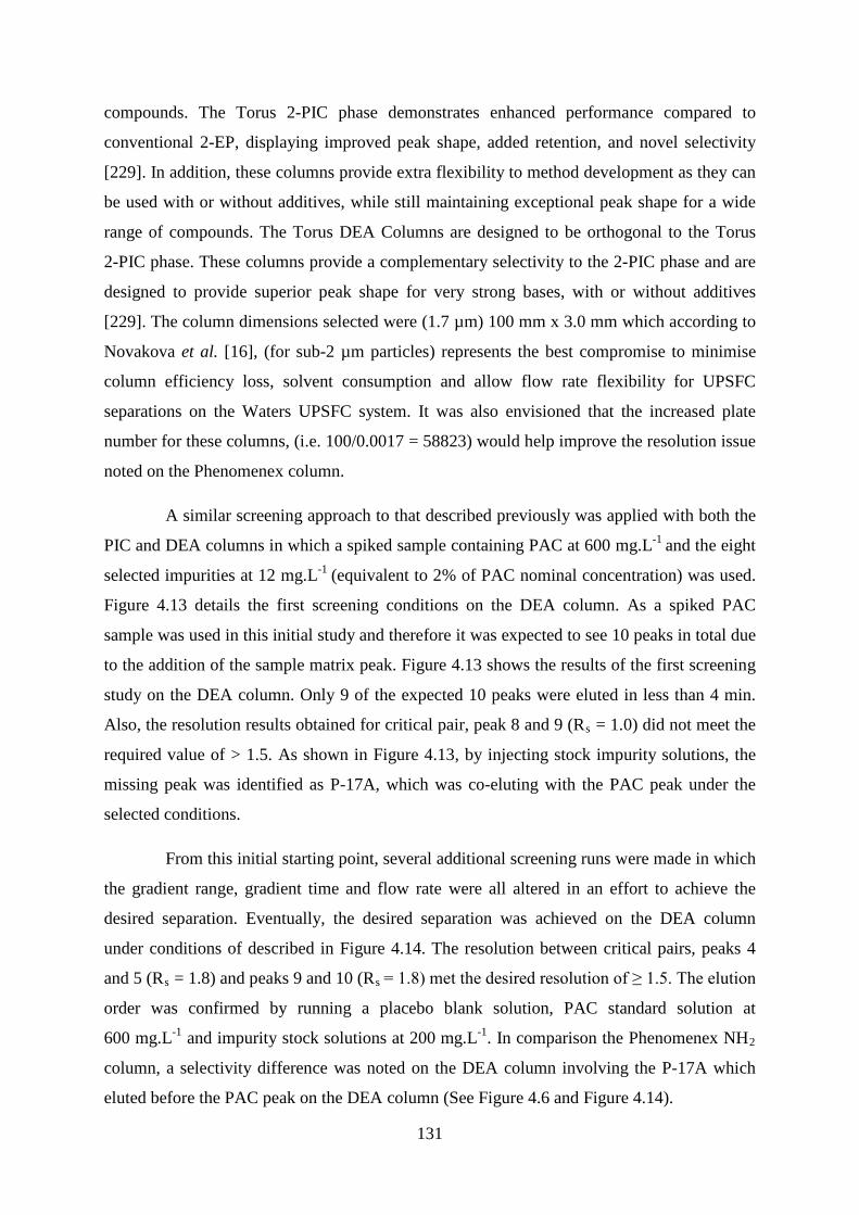
131
compounds. The Torus 2-PIC phase demonstrates enhanced performance compared to
conventional 2-EP, displaying improved peak shape, added retention, and novel selectivity
[229]. In addition, these columns provide extra flexibility to method development as they can
be used with or without additives, while still maintaining exceptional peak shape for a wide
range of compounds. The Torus DEA Columns are designed to be orthogonal to the Torus
2-PIC phase. These columns provide a complementary selectivity to the 2-PIC phase and are
designed to provide superior peak shape for very strong bases, with or without additives
[229]. The column dimensions selected were (1.7 µm) 100 mm x 3.0 mm which according to
Novakova et al. [16], (for sub-2 µm particles) represents the best compromise to minimise
column efficiency loss, solvent consumption and allow flow rate flexibility for UPSFC
separations on the Waters UPSFC system. It was also envisioned that the increased plate
number for these columns, (i.e. 100/0.0017 = 58823) would help improve the resolution issue
noted on the Phenomenex column.
A similar screening approach to that described previously was applied with both the
PIC and DEA columns in which a spiked sample containing PAC at 600 mg.L-1 and the eight
selected impurities at 12 mg.L-1 (equivalent to 2% of PAC nominal concentration) was used.
Figure 4.13 details the first screening conditions on the DEA column. As a spiked PAC
sample was used in this initial study and therefore it was expected to see 10 peaks in total due
to the addition of the sample matrix peak. Figure 4.13 shows the results of the first screening
study on the DEA column. Only 9 of the expected 10 peaks were eluted in less than 4 min.
Also, the resolution results obtained for critical pair, peak 8 and 9 (Rs = 1.0) did not meet the
required value of > 1.5. As shown in Figure 4.13, by injecting stock impurity solutions, the
missing peak was identified as P-17A, which was co-eluting with the PAC peak under the
selected conditions.
From this initial starting point, several additional screening runs were made in which
the gradient range, gradient time and flow rate were all altered in an effort to achieve the
desired separation. Eventually, the desired separation was achieved on the DEA column
under conditions of described in Figure 4.14. The resolution between critical pairs, peaks 4
and 5 (Rs = 1.8) and peaks 9 and 10 (Rs = 1.8) met the desired resolution of ≥ 1.5. The elution
order was confirmed by running a placebo blank solution, PAC standard solution at
600 mg.L-1 and impurity stock solutions at 200 mg.L-1. In comparison the Phenomenex NH2
column, a selectivity difference was noted on the DEA column involving the P-17A which
eluted before the PAC peak on the DEA column (See Figure 4.6 and Figure 4.14).
132
Figure 4.13: Expanded overlaid chromatograms of spiked sample containing PAC at
600 mg.L-1 and impurities 6 mg.L-1(black), P-17A impurity stock at 200 mg.L-1 (blue) and PN
impurity stock at 200 mg.L-1(red) conducted on the Waters UPC2 system under initial
screening conditions. Chromatographic conditions; Column: DEA (1.7 µm) 3.0 mm x 100
mm. Flow rate: 2.0 mL.min-1. Injection volume: 1.0 µL. Column temperature: 50 °C. Back-
pressure regulation: 138 bar. Detection: 254 nm. Mobile phase: 2 to 30 % MeOH over 5 min
with a followed by a 1 min equilibration step. Peak elution order; matrix peak (1), P-11,21D
(2), HCA (3), PAC/ P-17A (4/5), PN (6), HC (7), P (8), 20(R) (9) and 20(S) (10).
As HCA, P-17A, PAC and PN all contain the same number of hydroxyl groups
along with estimated LogP values of 1.41 for PN and 2.30 for HCA, P-17A and PAC; the
selectivity change noted on the DEA column versus the NH2 column may be as a result of
differences in the steric interactions of the solutes with the different stationary phases. In fact,
steric effects have been reported to appear more dramatic in SFC than in LC [230].
For the sake of completion, it was decided to screen the PIC column to see if any
additional improvements could be made in terms of resolution or reduction of analysis time
over the DEA column. It was also envisioned that if successful, the PIC column could be
offered as an alternative to the DEA column or vice versa for the proposed application. Based
on the initial screening conditions employed with the DEA column, it was decided to reduce
the gradient for the PIC column screening. Therefore, the first screening attempt on the PIC

133
column employed conditions described in Figure 4.15 which shows that only 9 of the
expected 10 peaks eluted in less than 9 min.
Figure 4.14: Chromatogram of spiked sample containing PAC at 600 mg.L-1 and impurities
6 mg.L-1. Chromatographic conditions; Column: DEA (1.7 µm) 3.0 mm x 100 mm. Flow rate:
2.5 mL.min-1. Injection volume: 1.0 µL. Column temperature: 50 °C. Back-pressure
regulation: 138 bar. Detection: 254 nm. Mobile phase: 2 to 13.6 % MeOH over 6.2 min with
a 1.8 min equilibration step. Peak elution order; matrix peak (1), P-11,21D (2), HCA (3),
P-17A (4), PAC (5), PN (6), HC (7), P (8), 20(R) (9) and 20(S) (10).
However, the resolution results obtained for critical pair, peak 9 and 10 was ≥ 1.5
(Rs = 2.5), indicating that the PIC column may be a suitable candidate for the separation. In
an attempt to identify the missing peak, both the P-17A and PN stock impurity standards
were run under the same conditions. As shown in Figure 4.15 the missing peak was identified
as PN, which was co-eluting with the PAC peak. However, despite several attempts to
modify the gradient conditions, we were unable to resolve the PAC and PN peaks on the PIC
column. Therefore, the DEA column was selected as the alternative column to the NH2
column and was used in the validation of the new UPSFC method.
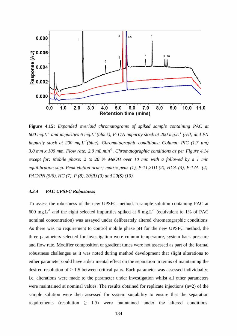
134
Figure 4.15: Expanded overlaid chromatograms of spiked sample containing PAC at
600 mg.L-1 and impurities 6 mg.L-1(black), P-17A impurity stock at 200 mg.L-1 (red) and PN
impurity stock at 200 mg.L-1(blue). Chromatographic conditions; Column: PIC (1.7 µm)
3.0 mm x 100 mm. Flow rate: 2.0 mL.min-1. Chromatographic conditions as per Figure 4.14
except for: Mobile phase: 2 to 20 % MeOH over 10 min with a followed by a 1 min
equilibration step. Peak elution order; matrix peak (1), P-11,21D (2), HCA (3), P-17A (4),
PAC/PN (5/6), HC (7), P (8), 20(R) (9) and 20(S) (10).
4.3.4 PAC UPSFC Robustness
To assess the robustness of the new UPSFC method, a sample solution containing PAC at
600 mg.L-1 and the eight selected impurities spiked at 6 mg.L-1 (equivalent to 1% of PAC
nominal concentration) was assayed under deliberately altered chromatographic conditions.
As there was no requirement to control mobile phase pH for the new UPSFC method, the
three parameters selected for investigation were column temperature, system back pressure
and flow rate. Modifier composition or gradient times were not assessed as part of the formal
robustness challenges as it was noted during method development that slight alterations to
either parameter could have a detrimental effect on the separation in terms of maintaining the
desired resolution of > 1.5 between critical pairs. Each parameter was assessed individually;
i.e. alterations were made to the parameter under investigation whilst all other parameters
were maintained at nominal values. The results obtained for replicate injections (n=2) of the
sample solution were then assessed for system suitability to ensure that the separation
requirements (resolution ≥ 1.5) were maintained under the altered conditions.

135
Column temperature was assessed at 40 °C, 45 °C, 50 °C (nominal), 55 °C and 60 °C. Back
pressure was assessed at 110 bar, 120 bar, 138 bar (nominal), 150 bar and 160 bar. Flow rate
was assessed at 2.3 mL.min-1, 2.4 mL.min-1, 2.5 mL.min-1 (nominal), 2.6 mL.min-1 and
2.7 mL.min-1. Plots of retention time and resolution (for critical pairs PAC/P-17A and
20(R)/20(S)) versus the selected parameter are shown in Figure 4.16 to Figure 4.18. The
slopes of the lines generated for each peak under the various robustness challenges are also
included in the plots. Significant differences (> 10%) between the peak slopes under a given
condition can be an indication that the condition is likely to have a significant influence on
the separation in terms of selectivity and elution order.
Figure 4.16 demonstrates that for column temperature the retention time of all peaks
increased with increasing temperature, with a maximum increase of 26.8% exhibited for the
P-11,21D peak. This correlates with the fact that increasing column temperature results in a
decrease in mobile phase density and hence the eluting strength of the mobile phase. While
no elution order change was noted for any of the temperatures investigated, it can be seen that
for the temperatures studied < 50 °C, resolution fell below 1.5 between the 20(R)/20(S)
critical pair. This observation coupled with the fact that the difference between the
20(R)/20(S) slopes is approximately 9.1%, confirms that temperature has a significant
influence in the separation of these two peaks. Also, it should be noted that the slope of the
matrix peak was significantly different (62% on average) from the slopes of the other peaks
in the separation. This indicates that temperature has a significant influence over the elution
of the matrix peak relative to the other peaks. This observation may be the reason for the
elution order change noted for the matrix peak and P-11,21D in Section 4.3.1 above when the
method was run on the Agilent system and the column temperature was increased by 10 °C.
Figure 4.17 demonstrates that for back pressure the retention time of all peaks
decreased with increasing pressure, with a maximum decrease of 13.6% exhibited for the
matrix peak. This correlates with the fact that increasing back pressure results in an increase
in mobile phase density and hence the eluting strength of the mobile phase and explains why
the analytes eluted faster from the column. Interestingly, while no elution order change was
noted for any of the pressures investigated, resolution was seen to increase sharply between
P17 and PAC above 138 bar, which correlates with the difference between the slopes of these
two peaks being 16.7%. It was also interesting to note that between the pressure of 110 bar to
120 bar, and 138 bar to 150 bar, baseline resolution is lost between the 20(R)/20(S) critical
pair even though there was no difference noted in the slopes of these two peaks.

136
Figure 4.16: Plot of retention time (Rt) and resolution (Rs) versus column temperature.
Chromatographic conditions as per Figure 4.14 with temperatures of 40, 45, 50, 55 and
60 °C. Dashed line indicates the minimum resolution requirements between critical peak
pairs.
Figure 4.18 demonstrates that for flow rate, the retention time of all peaks decreased
with increasing flow rate, with a maximum decrease of 18.7% exhibited for the matrix peak.
This correlates with the fact that by increasing the flow rate, the analytes eluted faster from
the column. While no elution order change was noted for any of the flow rates investigated, it
can be seen that at flow rates below 2.5 mL.min-1, baseline resolution is lost between the
P17/PAC critical pair even though the difference between the slopes of these two peaks was
only 4.5%.
Based on the results of this robustness study, it was concluded that to maintain the
system suitability requirement of maintaining resolution > 1.5 between critical pairs; the
separation was able to withstand a 10% increase in column temperature from nominal, a 10%
decrease in system back pressure from nominal and an 8% increase in flow rate form
nominal. However, the separation cannot withstand a 10% decrease in column temperature

137
from nominal, a 10% increase in system back pressure from nominal or an 8% decrease in
flow rate form nominal.
Figure 4.17: Plot of retention time (Rt) and resolution (Rs) versus back pressure (bar).
Chromatographic conditions as per Figure 4.14 with back pressures of 110, 120, 138, 150
and 160 bar. Dashed line indicates the minimum resolution requirements between critical
peak pairs.
While there may be some argument for increasing the flow rate to 2.6 mL.min-1 (In
order to increase resolution of P-17A and PAC at 2.5 mL.min-1 from Rs = 1.6 to Rs = 1.8 at
2.6 mL.min-1, it was decided to stay with 2.5 mL.min-1 to ensure that the overall system
pressure was maintained below the 400 bar limit of the Waters UPSFC system. Based on
Figure 1.6 which describes the relationship between the calculated critical temperature,
pressure and concentration of organic modifier, it can be stated that for operating conditions
of the new UPSFC method, conditions transition from supercritical to subcritical over the
course of the gradient; i.e. from the point in the gradient where the % MeOH exceeds
approximately 5%. However, despite this transition there was no adverse effect observed on

138
the chromatographic performance of the UPSFC method indicating that strict supercritical
conditions were not necessary to obtain a satisfactory separation.
Figure 4.18: Plot of retention time (Rt) and resolution (Rs) versus flow rate (mL.min-1).
Chromatographic conditions as per Figure 4.14 with flow rates of 2.3, 2.4, 2.5, 2.6 and
2.7 mL.min-1. Dashed line indicates the minimum resolution requirements between critical
peak pairs.
4.3.5 PAC UPSFC Method Validation
The validation of the new UPSFC method was carried out for PAC and the eight selected
impurities using the total error approach to generate accuracy profiles based on β-expectation
tolerance intervals. As stated in Section 4.1.2 above, the β-expectation tolerance interval
defines an interval where it is expected that a defined proportion (i.e. β) of future results will
fall. For PAC at the assay concentration, the β-expectation tolerance limits was set at 95%
with the acceptance limits set at ± 10% which was in agreement with the product
specifications of the selected ophthalmic suspension. For PAC and selected impurities at the
impurity concentration, the β-expectation tolerance limits was set at 90% with the acceptance
139
limits set at ± 20%, due to the greater degree of variance expected for trace level analysis.
The developed UPSFC method was validated for PAC and impurities to ICH
recommendations using the total error approach for trueness and precision, accuracy, limit of
detection (LOD), limit of quantitation (LOQ) and linearity. Method specificity/stability
indication along with solution stability was also assessed as per ICH Q2R1 guidance [142].
4.3.5.1 PAC UPSFC Specificity/Stability Indication and Solution Stability
Method specificity was demonstrated by the analysis of a placebo blank solution containing
only the pharmaceutical excipients, a MeOH blank solution and a sample solution spiked
with each of the selected impurities at a concentration of 3.6 mg.L-1 (equivalent to 0.6% of
nominal PAC concentration) using PDA detection. All peaks in the spiked sample
chromatogram were separated with a resolution of ≥ 1.5 and found to be spectrally pure
across the bandwidth using PDA detection. Figure 4.19 shows overlaid chromatograms of the
MeOH blank, placebo blank, a PAC sample spiked with impurities equivalent to 0.1% of
PCA concentration and a PAC standard. Figure 4.19 demonstrates that there were no
interfering peaks with a signal-to-noise (S/N) ratio greater than 10:1 at the retention time of
PAC or any of the impurities being investigated in the placebo blank or MeOH blank
injections. In fact, the only significant sample matrix component was a peak at approximately
1.3 min in the placebo blank chromatogram. Therefore, the new UPSFC method can be
considered specific for PAC and the eight selected impurities.
A forced degradation study was also performed on a PAC sample solution as
described in Section 3.3.2.3 to promote the base hydrolysis of PAC. The stressed PAC
sample was then analysed using the UPSFC method along with an un-stressed sample as a
control to determine the amount of PAC degradation. Under the stress conditions, the PAC
concentration decreased by 11.5%. In terms of impurities, the P concentration increased by
2,066%, P-17A decreased by 100%, HCA decreased by 13%, P-11,21D decreased by 32%,
PN decreased by 18%, HC increased by 19% and 20(S) increased by 293%. 20(R) was not
detected in either the control or stressed sample preparations. This preliminary study and the
aforementioned PDA spectral analysis are indicative of the potential utility of this UPSFC
method as a stability assay for routine stability monitoring.
The developed UPSFC method was used to examine solution stability prior to full
method validation studies. PAC working standards and working sample solutions were
prepared and stored in amber glassware at ambient laboratory temperature. The working

140
standards were prepared at two concentration levels, namely 100% and 1% of nominal to
accommodate for both assay and trace impurity analysis using PAC as the reference standard.
The prepared standards and sample solutions were tested immediately and again after 6 and 7
days respectively using the developed UPSFC method.
Figure 4.19: Overlaid chromatograms of MeOH blank (blue), placebo blank (red), PAC
standard at 600 mg.L-1 (green) and spiked sample containing PAC at 600 mg.L-1 and
impurities 0.6 mg.L-1(black) expanded view to show detail. Chromatographic conditions and
peak elution order as per Figure 4.14.
For standard stability, the 1% standard showed a decrease in PAC peak area of
0.44% whereas the 100% standard showed a decrease of 0.06% after 6 days storage. For the
sample stability, the PAC peak area showed a decrease of 1.72% after 7 days storage.
However, there was a notable change in the sample impurity profile after 7 days (for
example; +628% for P, +1229% for P-17A, -0.54% for HCA, -9.14% for P11,21D,
+211.54% for PN , +12.16% for HC and, +7.37% for 20(S)). Therefore, it was concluded that
working standards at 1% and 100% of nominal could be prepared in amber glass and stored at
ambient room temperature for up to 6 days. However, working sample solutions were
prepared in amber glassware immediately before performing routine analysis.

141
4.3.5.2 PAC UPSFC Trueness and Precision
The trueness and precision of the UPSFC method were estimated from the back-calculated
amounts of the VS and IVS preparations (See Table 4.1). The back-calculated amounts were
calculated from the CS and ICS using both L and Lo response functions. Impurity response
factors (RFs) were calculated for each of the selected impurities using the ratio of the slopes
versus PAC (i.e. impurity slope/PAC slope) for both the L and Lo response functions (See
Table C.1 and Table C.2). Some RF values were found to be outside 0.8< RF< 1.2 range,
which according to the current European Pharmacopoeia [231] meant they were required to
be included in quantitative calculations when PAC was used as the external reference
standard. However, as was the case for the RP-HPLC method described in Chapter 3, it was
noted that the % recovery values for all impurities improved when RF values were included
in the quantitative calculation; i.e. even for those whose RFs were within the 0.8< RF< 1.2
range. Therefore, it was decided to include RFs for all impurity quantitative calculations.
Trueness was expressed in term of relative bias (%) whereas the precision was
determined by computing the relative standard deviation (RSD (%)) for repeatability and
between-series intermediate precision at each concentration level of VS and IVS respectively.
The relative bias (%) and RSD (%) results for PAC and the eight selected impurities based on
both response functions studied are presented in Table C.3 to Table C.22 of Appendix C and
graphically in Figure 4.20. For PAC at nominal concentration, the relative bias (%) and RSD
(%) for repeatability and between-series intermediate precision were all equivalent when
either the L or Lo model was selected as the response function (See Table C.3 and Table C.4).
However, at the impurity concentration levels, there was significant improvement in the
relative bias (%), particularly at the lowest concentration levels, when the Lo model was
selected as the response function (See Table C.5 and Table C.6). This trend was repeated for
all selected impurities as shown in Table C.7 to Table C.22 and graphically in Figure 4.20.
4.3.5.3 PAC UPSFC Accuracy
The accuracy profile, which takes into account the total error (i.e. systematic and random
errors) can be used as a decision tool in deciding whether or not a method can be considered
accurate over a given concentration range. For PAC at assay concentration level, the upper
and lower 95% β-expectation tolerance limits (%) did not exceed the acceptance limits set a
priori at ± 10% for the concentration range investigated, when either the L or Lo response
functions were used (See Figure D.1). Consequently, the UPSFC method was able to provide

142
accurate results for PAC from 80 to 120% of the target assay concentration when either the L
or Lo response function were used to calculate results. Recovery values (%) ranged from
99.81 to 100.18% for the L response function and from 98.70 to 100.25% for the Lo response
function (See Table C.3 and Table C.4).
4.3.5.4 PAC UPSFC Impurity Accuracy and LOQ/LOD limits
For PAC and the selected impurities at the impurity concentration level, the acceptance limits
were set a priori at ± 20% for the upper and lower 90% β-expectation tolerance limits (%). As
stated previously in Section 4.1.2, the intersections between the tolerance interval and the
acceptance limits by definition represents the LOQ and ULQ of the analyte under the
analytical method conditions. Conventionally, a conservative method of LOD determination
consists of calculation of the LOD as approximately three times less than the LOQ. Table 4.3
summarises the LOQ results for PAC and the selected impurities based on the accuracy
profiles generated using the L and Lo response functions as illustrated in Figures D.2 to D.10.
Table 4.3 also summarises the estimated LOD concentrations based on the observed LOQ
values (i.e. LOD = LOQ/3) along with the % recovery ranges for PAC and the selected
impurities as detailed in Tables C.5 to C.22 for both the L and Lo response functions.
However, based on the signal-to-noise approach (peak height versus baseline noise), it was
decided to conservatively set the LOD for both the L and Lo response functions at 0.05% for
PAC and the selected impurities as illustrated in Figure 4.21 due to the level of detector noise
associated with SFC.
Table 4.3: Impurity level accuracy and LOQ/LOD limits based on accuracy profiles LOQa Estimated LODa Recovery range (%)
Response function L Lo L Lo L Lo
PAC 0.17 0.05 0.057 0.017 97.8 - 116.9 96.2 – 100.6
P-11,21D 0.43 0.15 0.143 0.050 100.5 – 125.6 100.5 – 104.3
HCA 0.62 0.20 0.207 0.067 100.9 – 136.5 99.9 – 105.6
P-17A 0.45 0.05 0.150 0.017 99.5 – 122.5 99.8 – 103.5
PN 0.28 0.10 0.093 0.033 100.6 – 119.3 100.1 – 105.2
HC 0.52 0.08 0.173 0.026 99.5 – 118.7 99.1 – 101.1
P 0.43 0.20 0.143 0.067 100.5 – 118.0 99.7 – 102.8
20(R) 0.37 0.05 0.123 0.017 100.1 – 113.9 99.5 – 101.1
20(S) 0.37 0.22 0.123 0.073 100.2 – 116.3 99.4 – 103.5 a = % w.r.t PAC Label Claim

143
Figure 4.20: Plots of relative bias (%) and repeatability RSD (%) for PAC and impurity
results generated using the L and Lo response functions over the selected concentration
ranges. Blue = relative bias (%) for the L response function; red = relative bias (%) for the
Lo response function; green = repeatability RSD (%) for the L response function and
purple = repeatability RSD (%) for the Lo response function.
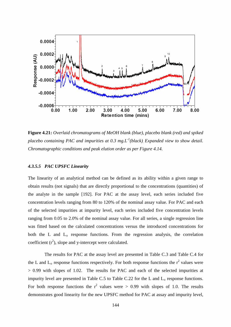
144
Figure 4.21: Overlaid chromatograms of MeOH blank (blue), placebo blank (red) and spiked
placebo containing PAC and impurities at 0.3 mg.L-1(black). Expanded view to show detail.
Chromatographic conditions and peak elution order as per Figure 4.14.
4.3.5.5 PAC UPSFC Linearity
The linearity of an analytical method can be defined as its ability within a given range to
obtain results (not signals) that are directly proportional to the concentrations (quantities) of
the analyte in the sample [192]. For PAC at the assay level, each series included five
concentration levels ranging from 80 to 120% of the nominal assay value. For PAC and each
of the selected impurities at impurity level, each series included five concentration levels
ranging from 0.05 to 2.0% of the nominal assay value. For all series, a single regression line
was fitted based on the calculated concentrations versus the introduced concentrations for
both the L and Lo response functions. From the regression analysis, the correlation
coefficient (r2), slope and y-intercept were calculated.
The results for PAC at the assay level are presented in Table C.3 and Table C.4 for
the L and Lo response functions respectively. For both response functions the r2 values were
> 0.99 with slopes of 1.02. The results for PAC and each of the selected impurities at
impurity level are presented in Table C.5 to Table C.22 for the L and Lo response functions.
For both response functions the r2 values were > 0.99 with slopes of 1.0. The results
demonstrates good linearity for the new UPSFC method for PAC at assay and impurity level,
145
along with each of the selected impurities at impurity level, whether the L and Lo response
function was used to back-calculate the sample results.
4.3.6 Selection of Appropriate Response Function for PAC UPSFC Quantitative
Analysis
Having calculated the two sided β-expectation tolerance intervals of the validation samples
and subsequent generation of accuracy profiles for PAC and selected impurities, all that
remained was to select the most appropriate response function; i.e. either L or Lo, for use
with the new UPSFC method during routine quantitative analysis. As stated previously, when
it comes to selecting the most appropriate response function preference must be given to a
model giving good results rather than a model presenting a good quality of fit [195].
Therefore, it is important to keep in mind the requirements of the method when it comes to
making this decision. For the new UPSFC method, one of the main goals was to develop a
method that could provide comparable or sufficient sensitivity to that of the RP-HPLC
method for the trace analysis of the select impurities in an ophthalmic suspension. Therefore,
when comparing the two selected response functions, preference was given to the model that
could provide the lower LOQ values for PAC and selected impurities.
On review of Tables C.3 to Table C.22 (Appendix C) along with the accuracy
profiles in Figure D.1 to Figure D.10 (Appendix D) it is clear that the response function that
best satisfied the main goal of the method was the Lo response function. Estimated LOQ
values were significantly lower for the Lo model (≤ 0.22%) compared to those of the linear
model (≤ 0.62%) for the selected impurities. This enabled the new UPSFC method to meet
the identification threshold and quantification threshold of 1.0% for degradation products of
PAC as per Attachment 1 of ICH Q3B(R2) [144] which were defined a priori for the
ophthalmic suspension in question. Also, the Lo model provided equivalent linearity to that
of the L model whilst recovery (%), repeatability % RSD and intermediate precision % RSD
were all equivalent if not better, (particularly at the lowest concentrations) for the Lo model.
Thus, there was no impact on the quality of fit by selecting the Lo model. Finally, as shown
in Table C.1, based on the regression analysis of PAC at assay and impurity level for all the
ICS series, and all bar series 4 of the CS, the y- intercept was less than the standard error of
the y-intercept, which gives strong support for the use of a single point calibration curve
during routine analysis [232]. Therefore, the proposed PAC standard concentration levels for

146
such single point calibration curves during routine quantitative analysis were 100% and 1%
for assay and impurity level calculations respectively.
4.3.7 Analytical Performance Comparison; UPSFC versus RP-HPLC
The other goal of this method development was to provide orthogonal selectivity to that of
the previously developed RP-HPLC method described in Chapter 3. Figure 4.22 demonstrates
the dramatically different elution order of the new UPSFC method compared to the
RP-HPLC method. This can be attributed to the normal phase-like retention mechanism of
SFC. The orthogonality of two chromatographic separations was also quantitatively described
by calculating the coefficient of determination (r2) of relative retention times from both
methods. In order to provide a direct comparison between the two methods, the matrix peak
was selected as the reference peak when calculating the relative retention times as it was the
first peak to elute in both separations. As shown in Figure 4.23, the r2 is only about 0.06,
which indicates a significant selectivity difference between two separation methods [128].
Having such an orthogonal UPSFC method also aids in confirming the selectivity of the
original RP-HPLC method for the separation of PAC and the selected impurities [233].
In terms of analytical performance, the UPSFC method represents a 4 fold decrease
in analysis time compared to the RP-HPLC method. There was also a significant 6.5 fold
reduction in solvent consumption per injection with the UPSFC method, which demonstrated
the potential of the UPSFC method for higher sample throughput and reduced solvent
purchase/disposal costs if implemented into routine analysis. Both methods demonstrated
good linearity for PAC and selected impurity peaks (r2 > 0.99) over a wide sample
concentration range. Both methods were fully validated to meet current ICH requirements for
specificity, trueness and precision, accuracy, LOD, LOQ, linearity and robustness. The
accuracy results were comparable between the two methods at both assay and impurity levels.
However, as expected the UPSFC method was found to be less sensitive than the RP-HPLC
method. Even when measures such as increased sample concentration and the use of
reference wavelength compensation function were employed, the LOQs of all peaks were
higher in the UPSFC method (< 0.22% for Lo response function) than for the RP-HPLC
method (< 0.05%). However, despite the higher LOQs of the UPSFC method compared to the
RP-HPLC method, they were sufficient to meet the identification threshold and quantification
threshold of 1.0% for degradation products of PAC as per Attachment 1 of ICH Q3B(R2)
[144] for the ophthalmic suspension in question. The UPSFC also meets the current European

147
Pharmacopoeia [234] impurity specifications for P and HCA are not more than 1.0% and not
more than 0.5% for P-11,21D thus demonstrating the potential for the method to be used in
routine stability studies. A comparison of the UPSFC and RP-HPLC analytical conditions
and performance is outlined in Table 4.4.
Figure 4.22: (a) Chromatogram of spiked sample containing PAC at 200 mg.L-1 and
impurities 1.2 mg.L-1under RP-HPLC conditions. Chromatographic conditions as per
Figure 3.4. (b) Chromatogram of spiked sample containing PAC at 600 mg.L-1 and impurities
3.6 mg.L-1under UPSFC conditions. Chromatographic conditions as per Figure 4.14. Peak
elution order; matrix peak (1), 20(S) (2), 20(R) (3), PN (4), P (5), HC (6), P-17A (7), PAC
(8), HCA (9) and P-11,21D (10).
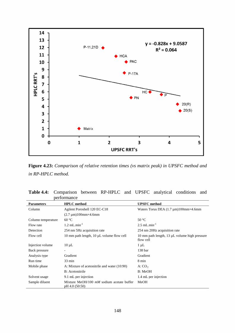
148
Figure 4.23: Comparison of relative retention times (vs matrix peak) in UPSFC method and
in RP-HPLC method.
Table 4.4: Comparison between RP-HPLC and UPSFC analytical conditions and performance
Parameters HPLC method UPSFC method Column Agilent Poroshell 120 EC-C18
(2.7 µm)100mm×4.6mm Waters Torus DEA (1.7 µm)100mm×4.6mm
Column temperature 60 °C 50 °C Flow rate 1.2 mL.min-1 2.5 mL.min-1 Detection 254 nm 5Hz acquisition rate 254 nm 20Hz acquisition rate Flow cell 10 mm path length, 10 µL volume flow cell 10 mm path length, 13 µL volume high pressure
flow cell Injection volume 10 µL 1 µL Back pressure - 138 bar Analysis type Gradient Gradient Run time 33 min 8 min Mobile phase A: Mixture of acetonitrile and water (10:90)
B: Acetonitrile A: CO2 B: MeOH
Solvent usage 9.1 mL per injection 1.4 mL per injection Sample diluent Mixture MeOH/100 mM sodium acetate buffer
pH 4.0 (50:50) MeOH
149
4.4 Conclusion
The new UPSFC method was shown to be a truly orthogonal chromatographic method to that
of the established RP-HPLC method for the analysis of PAC and its selected impurities in an
ophthalmic suspension. The new UPSFC method also operates with higher separation
efficiency, providing faster analyses time and with less consumption of organic solvent
compared to the RP-HPLC method. The use of the total error validation approach and
generation of accuracy profiles not only meets all the ICH requirements for method
validation, but also demonstrated the repeatability of the method (often an issue for SFC
separations in the past) and provided a degree of confidence in the selection of the best
response function (i.e. Lo) for use during routine quantitative analysis. The new UPSFC
method was found to be capable of meeting the impurity identification and quantitation
thresholds defined by both the ICH Q3B(R2) and current EP for the selected PAC impurities.
Therefore, based on the total error validation approach, the new UPSFC method can be
considered validated for the determination of PAC and selected impurities in an ophthalmic
suspension.

150
5.0 Conclusions and future work
The aim of this research project was to demonstrate the potential of SFC to be used as a
viable alternative or complementary technique to HPLC in the highly regulated world of the
Pharma QC laboratory. To do this, the historical weaknesses of poor reproducibility and low
sensitivity associated with SFC had to be overcome, to allow the application of SFC for
routine trace level analysis on selected pharmaceutical ingredients/products.
This aim had been achieved by the development and validation of both chiral and
achiral SPC applications described in Chapters 2 and 4 above. The chiral application
described in Chapter 2 was shown to be capable of providing an alternative to the EP method
based upon NP-HPLC for determining the enantiomeric purity of timolol maleate raw
material. The achiral application described in Chapter 4 was also shown to be an acceptable
alternative to the established RP-HPLC method for the trace impurity analysis of PAC in an
aqueous ophthalmic suspension. Both SFC methods demonstrated significant improvements
in terms of reduced analysis times and solvent consumption compared to their LC
counterparts.
The success of these applications was due in no small part to the availability of
holistically designed SFC instrumentation and stationary phases. This renewed focus by
instrument manufacturers such as Agilent and Waters have resulted many of the historically
challenges of poor reproducibility and low sensitivity becoming less of an issue for SFC
applications.
From an environmental perspective, initiatives such as the Registration, Evaluation,
Authorisation and Restriction of Chemicals (REACH) directive [235] are continuing to focus
on reducing the use of environmentally harmful chemicals. In this context, by adopting the
principals of green chemistry, SFC offers an attractive alternative to the established LC
techniques (particularly NP-HPLC) in helping QC laboratories achieve these goals.
From a regulatory perspective, industry guidance such as the new FDA guidance
entitled "Analytical Procedures and Methods Validation for Drugs and Biologics" [236] are
now placing greater focus on employing appropriate statistical methods when; developing
new test methods, evaluating existing test methods, evaluating measurement system
performance and interpreting or treating of analytical data like determining equivalence of
two test methods. This guidance also suggests that to fully understand the effect of changes in

151
method parameters on an analytical procedure, a systematic approach for a method
robustness study (e.g., a design of experiments with method parameters) should be used. This
approach involves an initial risk assessment and follow with multivariate experiments. Such
approaches allow the analyst to understand factorial parameter effects on method
performance.
The FDA guidance states that to fully understand the effect of changes in method
parameters on an analytical procedure, one should adopt a systematic approach for a method
robustness study (e.g., a design of experiments with method parameters). One should begin
with an initial risk assessment and follow with multivariate experiments. Such approaches
allow one to understand factorial parameter effects on method performance. Evaluation of a
method’s performance may include analyses of samples obtained from various stages of the
manufacturing process from in-process to the finished product. Knowledge gained during
these studies on the sources of method variation can help you assess the method performance.
The guidance also states that statistical analysis of validation data can be used to evaluate
validation characteristics against predetermined acceptance criteria and that all statistical
procedures and parameters used in the analysis of the data should be based on sound
principles and appropriate for the intended evaluation. In this context, the work carried out by
the likes of Dispas et al. [223], where DOE principals were employed at the method
development stage, along with the use of the total error approach for method validation stage
(also employed in Chapter 4), demonstrate the ability of SFC to satisfy this new regulatory
guidance.
Therefore, in the context of both the updated environmental and regulatory
guidance, the work presented in Chapters 2 and 4 above demonstrate the now real potential
for SFC to move beyond the realm of academic research or chiral preparative applications.
Thus, with the continuous improvements being made in the design of SFC instrumentation,
along with the ever expanding range of published SFC analytical applications; SFC is finally
showing real potential in offering the QC analyst an alternative/complementary technique to
that of the established techniques (i.e. LC, GC and CE) in the QC laboratory.
152
6.0 References
[1] T.A. Berger, Packed Column SFC, The Royal Society of Chemistry Chromatography Monograph Series, R.M. Smith ed., Cambridge, UK, 1995.
[2] http://chemwiki.ucdavis.edu/Core/Physical_Chemistry/Physical_Properties_of_Matter/States_ of_Matter/Phase_Transitions/Phase_Diagrams.
[3] T.A. Berger, Chromatography: Supercritical Fluid, Historical Development, in: I.D. Wilson, C. Pool (Eds.), Handbook of Methods and Instrumentation in Separation Science Vol. 1, Academic Press, 2009, pp: 653.
[4] http://www1.chem.leeds.ac.uk//People/CMR/criticalpics.html
[5] http://www.enen.co.kr/index2.html
[6] “What is a supercritical fluid”, Budapest University of Technology and Economics, 2013.
[7] L.T. Taylor, J. Supercritical Fluids, 47, (2009) 566.
[8] M. Saito, J. Biosci and Boioeng, 115, 6 (2013) 590.
[9] E. Lesellier, C. West, J. Chromatogr. A1382 (2015) 2.
[10] E. Klesper, A.H. Corwin, D.A. Turner, J. Org. Chem. 27 (1962) 700.
[11] J.C. Giddings, M.N. Myers, L.M. McLarne, R.A. Keller, Sci. 162 (1968) 67.
[12] J.F.Deye, T.A. Berger, A.G. Anderson, Anan. Chem. 62 (1990) 615.
[13] T.A. Berger, Chemical basis for the instrumentation used in packed column supercritical fluid chromatography, in: K. Anton, C. Berger, Supercritical Fluid Chromatography with Packed Columns, Marcel Dekker Inc., New York, Basel, Hong Kong, 1998, pp. 19.
[14] G.O. Cantrell, R.W. Stringham, J.A. Blackwell, J.D. Weckwerth, P.W. Carr, Anal. Chem. 68 (1996) 3645.
[15] J.A. Blackwell, R.W. Stringham, J.D. Weckwerth, Anal. Chem. 69 (1997) 409.
[16] L. Nováková, A. Grand-Guillaume Perrenoud, I. Francois, C. West, E. Lesellier, D. Guillarme, Anal. Chim. Acta 824 (2014) 18.
[17] T.A. Berger, J.F. Deye, J. Chromatogr. A 547 (1991) 377.
[18] Y. Okamoto, M. Kawashima, K. Hatada, K, J. Am. Chem. Soc. 106 (1984) 5357.
[19] Y. Okamoto, M. Kawashima, K. Hatada, K, J. Chromatogr. 363 (1986) 173.
[20] K. W. Phinney, Anal. Bioanal. Chem. 382 (2005) 639.
[21] D. Mangelings, Y. V. Heyden, J. Sep. Sci. 31 (2008) 1252.
[22] A.M.V. Schou-Pedersen, J. Østergaard, M. Johansson, S. Dubant, R.B. Fred-eriksen, S.H. Hansen, J. Pharm. Biomed. Anal. 88 (2014) 256.
[23] A.J. Alexander, L. Zhang, T.F. Hooker, F.P. Tomasella, J. Pharm. Biomed. Anal. 78–79 (2013) 243.

153
[24] E. Lesellier, K. Gaudin, P. Chaminade, A. Tchapla, A. Baillet, J. Chromatogr. A 1016 (2003) 111.
[25] V. Goss, A. Cazenave-Gassiot, A. Pringle, A. Postle, Curr. Anal. Chem. 10 (2014) 121.
[26] D. Tognarelli, A. Tsukamoto, J. Caldwell, W. Caldwell, Bioana. 2 (2010) 5.
[27] J. Zheng, J.D. Pinkston, P.H. Zoutendam, L.T. Taylor, Anal. Chem. 78 (2006) 1535.
[28] M. Ishibashi, T. Ando, M. Sakai, A. Matsubara, T. Uchikata, E. Fukusaki, J. Chromatogr. A 1266 (2012)143.
[29] X. Yang, B. Ma, X. Zheng, C. Lin, Anal. Methods 6 (2014) 4769.
[30] D. Johnston, M. Ashraf-Khorassani, L.T. Taylor, Chromatographia 57 (2003) 533.
[31] J.P. Kithinji, K.D. Bartle, M.W. Raynor, A.A. Clifford, Analyst 115 (1990) 125.
[32] S. Bijttebier, E. D’Hondt, B. Noten, N. Hermans, S. Apers, V. Exarchou, Food Chem. 165 (2014) 371.
[33] T.A. Berger, B.K. Berger, Chromatographia 76 (2013) 393.
[34] V. Abrahamsson, I. Rodriguez-Meizoso, C. Turner, J. Chromatogr. A 1250 (2012) 63.
[35] C. Desmortreux, M. Rothaupt, C. West, E. Lesellier, J. Chromatogr. A 1216 (2009) 7088.
[36] T.A. Berger, J. Chromatogr. A 785 (1997) 3.
[37] T.A. Berger, Anal. Chem. 62 (1990) 1181.
[38] T.A. Berger, J. of H. Res. Chromatogr. 14 (1991) 312.
[39] J.N. Fairchild, J.F. Hill, P.C. Iraneta, LC-GC N. Am. 31 (2013) 326.
[40] V. Abrahamsson, M. Sandahl, J. Chromatogr. A 1306 (2013) 80.
[41] S. Fekete, I. Kohler, S. Rudaz, J.L. Veuthey, J. Pharm. Biomed. Anal. 87 (2014) 105.
[42] E. Lesellier, J. Chromatogr. A 1216 (2009) 1881.
[43] E. Lesellier, J. Sep. Sci. 31 (2008) 1238.
[44] H.S.H. Yip, M. Ashraf-Khorassani, L.T. Taylor, Chromatographia 65 (2007) 655.
[45] A. Cazenve-Gassiot, R. Boughtflower, J. Caldwell, R. Coxhead, L. Hitzel, S. Lane,
P. Oakley, C. Holyoak, F. Pullen, G.J. Langley, J. Chromatogr. A 1189 (2008) 254.
[46] A.J. Alexander, T.F. Hooker, F.P. Tomasella, J. Pharm. Biomed. Anal. 70 (2012) 77.
[47] J. Lundgreen, J. Salomonsson, O. Gyllenhaal, E. Johansson, J. Chromatogr. A 1154 (2007) 360.
[48] C. West, E. Lesellier, J. Chromatogr. A 1110 (2006) 181.
[49] C.West, E. Lesellier, A. Tchapla, J. Chromatogr. A 1048 (2004) 99.
[50] C. West, E. Lesellier, J. Chromatogr. A 1087 (2005) 64.
[51] C. West, E. Lesellier, J. Chromatogr. A 1110 (2006) 200.

154
[52] C.West, S. Khater, E. Lesellier, J. Chromatogr. A 1250 (2012) 182.
[53] C. West, E. Lesellier, J. Chromatogr. A 1110 (2006) 191.
[54] C. West, E. Lesellier, J. Chromatogr. A 1169 (2007) 205.
[55] C. West, E. Lesellier, J. Chromatogr. A 1115 (2006) 233.
[56] T.A. Berger, Chromatography: Supercritical Fluid, Instrumentation, in: I.D. Wilson, C. Pool (Eds.), Handbook of Methods and Instrumentation in Separation Science Vol. 1, Academic Press, 2009, pp: 659.
[57] T.A. Berger, B.K. Berger, J. Chromatogr. A 1218 (2011) 2320.
[58] Y. Hirata, Y. Kawaguchi, Y. Funada, J. Chromatogr. Sci. 34 (1996) 58.
[59] Y. Sun, B.Y. Shekunov, P. York, Chem. Eng. Commun. 190 (2003) 1.
[60] J.E. France, K.J. Voorhees, J. High Resolut. Chromatogr. 11 (1988) 692.
[61] A. Pereira, F. David, G. Vanhoenacker, C. Brunelli, P. Sandra, LC–GC N. Am. 29 (2011).
[62] A. Grand-Guillaume Perrenoud, J.L. Veuthey, D. Guillarme, J. Chromatogr. A 1266 (2012) 158.
[63] T. Fornstedt, R. E. Majors, LC-GC E. 28 (2015).
[64] A. Tarafder, K. Kaczmarski, D. P. Poe, G. Guiochon, J. Chromatogr. A 1258 (2012) 124.
[65] K. Kaczmarski, D. P. Poe, G. Guiochon, J. Chromatogr. A 1218 (2011) 6531.
[66] M. Enmark, P. Forssen, J. Samuelsson, T. Fornstedt, J. Chromatogr. A 1312 (2013) 124.
[67] F. Kamarei, F. Gritti, G. Guiochon, J. Chromatogr. A 1306 (2013) 89.
[68] M. Enmark, J. Samuelsson, E. Forss, P. Forssen, T. Fornstedt, J. Chromatogr. A 1354 (2014) 129.
[69] R. Majors, D. Raynie, LC-GC E. 24 (2011).
[70] P.T. Anastas and J.C. Warner, Green Chemistry: Theory and practice, Oxford University Press, New York, 1988.
[71] P. Sandra, A. Pereira, M. Dunkle, C. Brunell, F. David, LC-GC E. 23 (2010).
[72] W.A. Bonner, Chirality 12 (2000) 114.
[73] N.M. Maier, P. Franco, W. Lindner, J. Chromatogr. A 906 (2001) 3.
[74] Food & Drug Administration. FDA’s policy statement for the development of new stereoisomeric drugs. 57 Fed. (1992) Reg. 22249.
[75] B.S. Sekhon, J. Mod. Med. Chem., 1 (2013) 10.
[76] J. Agustian, A.H. Kamaruddin, S. Bhatia, Process Biochem. 45 (10) (2010) 1587.
[77] W.H. Frishman, Circulation 107 (2003) 117.
[78] M.J. Reiter, Prog. Cardiovasc. Dis. 47 (2004) 11.
[79] J. Agustian, A.H. Kamaruddin, S. Bhatia, Process Biochem. 45 (2010) 1587.

155
[80] H.L. Kennedy, Am. J. Med. 110 (2001) 2.
[81] R. Mehvar, D. R. Brocks, J. Pharm. Pharm. Sci. 4 (2001) 185.
[82] W.H. Frisman, Circulation 107 (2003) 117.
[83] Bryan, J. Pharmacogen J. 279 (2007) 538.
[84] D.J. Cordato, L.E. Mather, G.K. Herkes, J. Clin. Neurosci. 10 (2003) 649.
[85] J.A. Nathanson, J. Pharmac. Exp. Ther. 245 (1998) 94.
[86] T. Walle, J.G. Web, E.E. Bagwel, U.K. Wale, H.B. Daniel, T.E. Gaffney, Biochem. Pharmac. 37 (1998) 115.
[87] A.B. Rofman, F.K. Stanley. A.G.Munir, B. Thiyagarajan, F.J. Nancarrow, B.W. Abrams, Hypertension, 2 (1980) 643.
[88] A.J. Franciosa, D.E. Freis, J. Conway, Circulation 48 (1973) 118.
[89] H.W. Frishman, D.C. Furberg, T.W. Friedewald, N. Engl. J. Med. 310 (1984) 830.
[90] The International Collaborative Study Group. N. Engl. J. Med. 310 (1984) 9.
[91] The Norwegian Multicenter Study Group. N. Engl. J. Med. 304 (1981) 801.
[92] D.J. Mazzo, A.E. Loper, Timolol Maleate in: K. Florey (Eds.), Analytical Profiles of Drug Substances, Vol. 16, Academic Press, 1987 pp. 641.
[93] T.J. Zimmerman, Invest. Ophth. Vis. Sci. 16 (1977) 687.
[94] K. Dickstein, R. Hapnes, T. Aarsland, Am. J. Ophth. 132 (2001) 626.
[95] W.H. Frishman, N. Engl. J. Med. 306 (1982) 1456.
[96] R.C. Heel, R.N. Brogden, T.M. Speight, G.S. Avery, Drugs 17 (1979) 38.
[97] W.P. Boger, Drugs 18 (1979) 25.
[98] F.T. Fraunfelder, A.F. Barker, N. Engl. J. Med. 311 (1984) 1441.
[99] R. Richards, A. Tattersfield, Br. J. Clin. Pharmacol. 20 (1985) 459.
[100] R. Richards, A. Tattersfield, Br. J. Clin. Pharmacol. 24 (1987) 485.
[101] B.K Wasson, W.K. Gibson, R.S. Stuart, H.W.R. Williams, C.H. Yates, J. Med. Chem. 15 (1972) 651.
[102] Z. Wang, J. Ouyang, W.R.G. Baeyens, J. Chromatogr. B 862 (2008) 1.
[103] Eur. Pharmacop.(Version 7.5): Timolol Maleate monograph.
[104] H.Y. Aboul-Enein, M.R. Islam, J. Chromatogr. A 511 (1990) 109.
[105] I.W. Wainer, R.M. Stiffin, T. Shibata, J. Chromatogr. A 411 (1987) 139.
[106] P.M. Lacroix, B.A. Dawson, R.W. Sears, D.B. Black, Chirality 6 (1994) 484.
[107] R.D. Marini, P. Chiap, B. Boulanger, W. Dewe, P. Hubert, J. Crommen, J. Sep. Sci. 26 (2003) 809.
[108] Eur. Pharmcop. 4th Edition, Addendum 2002, Council of Europe, Strasbourg.
156
[109] R.D. Marini, B. Boulanger, Y. Vander Heyden, P. Chiap, J. Crommen, P. Hubert, Anal. Chim. Acta 531 (2005) 131.
[110] R.D. Marini, P. Chiap, B. Boulanger, S. Rudaz , E. Rozet, J. Crommen, Ph. Hubert,Talant. 68 (2006) 1166.
[111] Y. Hedeland, J. Lehtinen, C. Pettersson, J. Chromatogr. A 1141 (2007) 287.
[112] A.C. Servais, M. Fillet, P. Chiap, W. Dewé, P. Hubert, J. Crommen, Electrophoresis 25 (2004) 2701.
[113] R.D. Marini, A-C. Servais , E. Roze, P. Chiap, B. Boulanger, S. Rudaz, J. Crommen, Ph. Hubert, M. Fillet, J. Chromatogr. A 1120 (2006) 102.
[114] K.D. Altria, LC–GC E. September 2002.
[115] Eur. Pharmcop. European Directorate for the Quality of Medicines, Nordlingen, 2005.
[116] Z.K. Shihabi, Electrophoresis 23 (2002) 1628.
[117] T.J. Ward, K.D. Ward, Ana. Chem. 82 (2010) 4712.
[118] K. De Klerck, D. Mangelings, D. Clicq, F. De Boever, Y. Vander Heyden, J. Chromatogr. A 1234 (2012) 72.
[119] L. Miller, M. Potter, J. Chromatogr. B 875 (2008) 230.
[120] W.R. Leonard, D.W. Henderson, R.A Miller, G.A. Spencer, O.S.Sudah, M. Biba, C.J. Welch, Chirality 19 (2007) 693.
[121] L.T. Taylor, J. Super. Flu. 47 (2009) 566.
[122] W. Ren-Qi, O. Teng-Teng, N. Siu-Choon, T. Weihua, Trends in Analytical Chemistry 37 (2012) 83.
[123] B. Chankvetadze, J. Chromatogr. A 1269 (2012) 26.
[124] L.T. Taylor, Anal. Chem. 82 (2010) 4925.
[125] K. De Klerck, D. Mangelings, Y. Vander Heyden, LC-GC E. Supp: May (2013) 24.
[126] R.L. Stevenson, Am. Lab. 45 (2013) 36.
[127] R. Helmy, M. Biba, J. Zang, B. Mao, K. Fogelman, V. Vlacho, P. Hosek, C.J. Welch, Chirality 19 (2007) 787.
[128] Z. Wang, H. Zhang, O. Liu, B. Donovan, J. Chromatogr. A 1218 (2011) 2311.
[129] K. De Klerck, D. Mangelings, Y.Vander Heyden, J. Pharm. Biomed. Anal. 69 (2012) 77.
[130] O. Gyllenhaal, A. Karlsson, J. Biomed. Biophys. Methods 54 (2002) 169.
[131] A. Medvedovici, P. Sandra, L. Toribio, F. David, J. Chromatogr. A 785 (1997) 159.
[132] Y. Liu, A. Berthod, C.R. Mitchell, T.L. Xiao, B. Zhang, D.W. Armstrong, J. Chromatogr. A 978 (2002) 185.
[133] K.L. Williams, L.C. Sander, J. Chromatogr. A 785 (1997) 149.
[134] H. Nelander, S. Andersson, K. Öhlén, J. Chromatogr. A1218 (2011) 9397.

157
[135] C. Roussel, B. Bonnet, A. Piederriere, C. Suteu, Chirality 13 (2001) 56.
[136] R.B. Kasat, N.H.L. Wang, E.I. Franses, J. Chromatogr. A 1190 (2008) 110.
[137] S. Ma, S. Shen, H. Lee, M. Eriksson, X. Zeng, J. Xu, K. Fandrick, N. Yee, C. Senanayake, N. Grinberg, J. Chromatogr. A 1216 (2009) 3784.
[138] R.W. Stringham, J.A. Blackwell, Anal. Chem. 68 (1996) 2179.
[139] S. Khater, Y. Zhang, C. West, J. Chromatogr. A 1303 (2013) 83.
[140] M. Ventura, B. Murphy, W. Goetzinger, J. Chromatogr. A 1220 (2012) 147.
[141] K. Kontturi, L. Murtomaki, J. Pharm. Sci-US. 81 (1992) 970.
[142] ICH [Validation of Analytical Procedures: Methodology (Q2R1)], International Conference on Harmonization, November 1996.
[143] United States Pharmacop. No. 31-NF- 26, (2008), ch. 621.
[144] International Conference on Harmonisation of Technical Requirements for Registration of Pharmaceuticals for Human Use: Impurities in New Drug Products Q3B(R2), (2006).
[145] H. Derendorf, H. Mollmann, A. Griiner, D. Haack and G. Gyselby, Clin. Pharmacol. Ther. 39 (1986) 313.
[146] H. Derendorf, E Rohdewald, G. Hochhaus and H. Mollmann, J. Pharm. Biomed. Anal. 4 (1986) 197.
[147] VH.L. Lee, V.H.K. Li, Adv. Drug. Deliv. Rev. 3 (1989) l.
[148] V.H.L. Lee, H. Bundgaard, Improved ocular drug delivery with prodrugs. In: K.B. Sloan (Ed.), Drugs and the Pharmaceutical Sciences, Vol. 53: Prodrugs, Topical and Ocular Drug Delivery, Marcel Dekker, Inc., New York, (1992) pp. 221.
[149] R.D. Schoenwald, R.L. Ward, J. Pharm. Sci. 67 (1978) 787.
[150] A. Kupferman, A.R. Berrospi, H.M. Leipowitz. Arch. Ophthalmol. 100 (1982) 640.
[151] H.M. Leibowitz, A.R. Berrospi, A. Kupferman, G.V. Restropo, V. Galvis, J.A. Alvarez, Am. J. Ophthalmol. 83 (1977) 402.
[152] A. Kupferman, M.V. Pratt, K. Suckewer, H.M. Leibowitz, Arch. Ophthalmol. 91 (1974) 373.
[153] D. Musson, A. Bidgood, 0. Olejnik, Pharm. Res. (Suppl.) 6 (1989) 1.
[154] D. Musson, A. Bidgood, 0. Olejnik, J. Ocul. Pharmacol. 7 (1991) 175.
[155] T. Jarvinen, K. Jarvinen, Advanced Drug Delivery Reviews, 19 (1996) 203.
[156] G.R. Cannell, R.H. Mortimer, D.J. Maguire, R.S. Addison, J. Chromatogr. 563 (1991) 341.
[157] D.G. Musson, A.M. Bidgood, O. OLejnik, J. Chromatogr. 565 (1991) 89.
[158] S.A. Doppenschmitt, B. Scheidel, F. Harrison, J.P. Surmann, J. Chromatogr. B 674 (1995) 237.
[159] N. Shibata, T. Hayakawa, K. Takada, N. Hoshino, T. Minouchi, A. Yamaji, J. Chromatogr. B 706 (1998) 191.
158
[160] A.S. Carlin, V.K. Prasad, J. Chromatogr. 425 (1988) 162.
[161] A. Santos-Montes, R. Izquierdo-Hornillos, J.Chromatogr. B 724 (1999) 53.
[162] V. Garg, W.J. Jusko, J.Chromatogr. 567 (1991) 3947.
[163] V.K. Prasad, B. HO, C. Haneke, J. Chromatogr. 378 (1986) 305.
[164] H.N. Barot, J.B. Dave, C.N. Patel, IJPSR, Vol. 3(6) (2012) 1817.
[165] S.G. Musharraf, U. Fatima, R. Sultana, Chem. Centr. J. 6 (2012) 7.
[166] J.M.L. Gallego, J. Perez Arroyo, J. Sep. Sci. 26 (2003) 947.
[167] J.M. Lemus Gallego, J. Perez Arroyo, J. Pharm. Biomed. Ana. 31 (2003) 873.
[168] J.M. Lemus Gallego, J. Perez Arroyo, J. Chromatogr. B 784 (2003) 39.
[169] M.L. Rocci Jr., W.J. Jusko, J. Chromatogr. 224 (1981) 221.
[170] A. Shalaby, M. Shahjahan, J. Liq. Chromatogr. 14 (1991) 1267.
[171] S. N. Razzaq, Chem. Centr. J. 6 (2012) 94.
[172] United States Pharmacop.No. 36-NF1, prednisolone acetate in ophthalmic suspension monograph, (2014).
[173] Eur. Pharmacop.8th edition, prednisolone acetate monograph, (2014).
[174] United States Pharmacop. No. 36-NF1, prednisolone acetate in ophthalmic suspension monograph, (2014).
[175] J. Kirkland, T. Langlois, J. DeStefano, Am. Lab. 39 (2007) 18.
[176] F. Gritti, G. Guiochon, LC-GC N. Am. 7(30) (July 2012) 586.
[177] F. Gritti, A. Cavazzini, N. Marchetti, G. Guiochon, J. Chromatogr. A 1157 (2007) 289.
[178] F. Gritti, C. Sanchez, T. Farkas, G. Guiochon, J. Chromatogr. A 1217 (2010) 3000.
[179] N.S. Wilson, M.D. Nelson, J.W. Dolan, L.R. Snyder, R.G. Wolcott, P.W. Carr, J. Chromatogr. A 961 (2002) 171.
[180] ACD ChemSketch, Version 12.01 (www.acdlabs.com).
[181] C. Baiocchi, D. Giacosa, M.A. Roggero, E. Marengo J. Chromatogr Sci, 34, (1996) 399.
[182] A.J. Berry, D.E. Games, J.A. Perkins, J. Chromatogr. 363 (1986) 147.
[183] E. Lesellier, A. Tchapla, C. Marty, A. Lebert, J. Chromatogr. 633 (1993) 9.
[184] Koji Yaku, Keiichi Aoe, Noriyuki Nishimura, Tadashi Sato, Fujio Morishita, J.Chromatogr. A, 773 (1997) 277.
[185] T.A. Berger, J.F. Deye, J. Chromatogr. Sci. 29 (1991) 280.
[186] A.L. Blilie, T. Greibrokk, Anal. Chem. 57 (1985) 2239.
[187] J.G.M. Janssen, P.J. Schoenmakers, C.A. Cramers, J. High Resolut. Chromatogr. 12 (1989) 645.
[188] N.K. Jagota, J.B. Nair, R. Frazer, M. Klee, M.Z. Wang, J. Chromatogr. A 721 (1996) 315.
159
[189] J.L. Bernal, M.J. del Nozal, H. Velasco, L. Toribio, J. Liq. Chromatogr. Related Technol. 19 (1996) 1579.
[190] S. Salman Lateef, Vinayak AK . www.agilent.com/chem © Agilent Technologies, Inc., 2012 Published in the USA, May 1, 2012 5991-0277EN.
[191] Ph. Hubert, J.J. Nguyen-Huu, B. Boulanger, E. Chapuzet, P. Chiap, N. Cohen, P.A.Compagnon, W. Dewé, M. Feinberg, M. Lallier, M. Laurentie, N. Mercier, G.Muzard, C. Nivet, L. Valat, J. Pharm. Biomed. Anal. 36 (2004) 579.
[192] Ph. Hubert, J.J. Nguyen-Huu, B. Boulanger, E. Chapuzet, P. Chiap, N. Cohen, P.A. Compagnon, W. Dewé, M. Feinberg, M. Lallier, M. Laurentie, N. Mercier, G. Muzard, C. Nivet, L. Valat, S.T.P. Pharma Pratiques 13 (3) (2003) 101.
[193] A. Bouabidi, E. Rozet, M. Fillet, E. Ziemons, E. Chapuzet, B. Mertens, R. Klinkenberg, A. Ceccato, M. Talbi, B. Streel, A. Bouklouze, B. Boulanger, Ph. Hubert, J. Chromatogr. A 1217 (2010) 3180.
[194] Ph. Hubert, J.J. Nguyen-Huu, B. Boulanger, E. Chapuzet, P. Chiap, N. Cohen,P.A. Compagnon, W. Dewé, M. Feinberg, M. Lallier, M. Laurentie, N. Mercier,G. Muzard, C. Nivet, L. Valat, E. Rozet, J. Pharm. Biomed. Anal. 45 (2007) 70.
[195] Ph. Hubert, J.-J. Nguyen-Huu, B. Boulanger, E. Chapuzet, N. Cohen, P.-A. Com-pagnon, W. Dewé, M. Feinberg, M. Laurentie, N. Mercier, G. Muzard, L. Valat, E.Rozet, J. Pharm. Biomed. Anal. 45 (2007) 82.
[196] Ph. Hubert, J.-J. Nguyen-Huu, B. Boulanger, E. Chapuzet, N. Cohen, P.-A. Com-pagnon, W. Dewé, M. Feinberg, M. Laurentie, N. Mercier, G. Muzard, L. Valat, E.Rozet, J. Pharm. Biomed. Anal. 48 (2008) 760.
[197] M. Feinberg, J. Chromatogr. A 1158 (2007) 174.
[198] A. Gustavo Gonzalez, M. Angeles Herrador, Tren. Anal. Chem. 26 (3) (2007) 227.
[199] D. Hoffman, R. Kringle, Pharma. Res. 24 (6) (2007) 1157.
[200] J. C. Miller, J. N. Miller, statistics for analytical chemistry, 3rd edition, chapter 1 (1993).
[201] B. Boulanger, Ph. Hubert, P. Chiap, W. Dewé, Objectives of pre-study validation and decision rules, AAPS APQ Open forum, Washington, 2000.
[202] B. Boulanger, Ph. Hubert, P. Chiap, W. Dewé, J. Crommen, Statistical analysis of the validation results, in: GMP, 2000.
[203] J. Ermer, J. Pharm. Biomed. Anal. 24 (2001) 755.
[204] J. Ermer, H.J. Ploss, J. Pharm. Biomed. Anal. 37 (2005) 859.
[205] R.W. Mee, Technometrics 26 (1984) 251.
[206] Food and Drug Administration, Process Analytical Technology (PAT) Initiative, 2002, http://www.fda.gov/cder/OPS/PAT.html.
[207] B. Boulanger, W. Dewé, P. Chiap, J. Crommen, P.H. Hubert, J. Pharm. Biomed. Anal. 32 (2003) 753.

160
[208] SANCO – Commission of the European Communities, Off. J. Eur. Commun. L221 (2002) 8.
[209] I. Bouchaib, S.I Mohamed, E.H.E. Mestafa, A. Sanae, S. Taoufiq. Int J Pharm Pharm Sci, 6, 11 (2014), 413.
[210] ISO 5725, Accuracy (trueness and precision) of measurement methods and results—Parts1–4, Part 6, ISO, Geneva, Switzerland, 1994.
[211] S. Huet, E. Jolivet, A.Messean, La regression non lineaire, Editions INRA, Paris, 1992.
[212] M.A. Bimazubute, E. Rozet , I. Dizier , P. Gustin , Ph. Hubert , J. Crommenc, P. Chiap ,J. Chromatogr. A 1189 (2008) 456.
[213] O. Rbeida, B. Christiaens, Ph. Hubert, D. Lubda, K.-S. Boos, J. Crommen, P. Chiap, J. Pharm. Biomed. Anal.36 (2005) 947.
[214] S. Henry de Hassonville, P. Chiap, J.F. Liégeois B. Evrard, L. Delattre, J. Crommen, G. Piel, Ph. Hubert, J. Pharm. Biomed. Anal.36 (2004) 133.
[215] B. Christiaens, P. Chiap, O. Rbeida, D. Cello, J. Crommen, Ph. Hubert, J. Chromatogr. B 795 (2003) 73.
[216] O. Rbeida, B. Christiaens, P. Chiap, Ph. Hubert, D. Lubda, K.-S. Boos, J. Crommen, J. Pharm. Biomed. Anal. 32 (2003) 829.
[217] O. Rbeida, P. Chiap, D. Lubda, K.-S. Boos, J. Crommen, Ph. Hubert, J. Pharm. Biomed. Anal.36 (2005) 961.
[218] P. Chiap, M. Piette, B. Evrard, F. Frankenne, B. Christiaens, G. Piel, D. Cataldo, J.-M. Foidart, L. Delattre, J. Crommen,, Ph. Hubert, J. Chromatogr. B 817 (2005) 109.
[219] E. Rozet, C. Hubert, A. Ceccato, W. Dewe, E. Ziemons, F.Moonen, K. Michail, R. Wintersteiger, B. Streel, B. Boulanger, Ph. Hubert, J. Chromatogr. A 1158 (2007) 126.
[220] A.-C. Servais, M. Fille, R. Mol, G. W. Somsen, P. Chiap, G. J. de Jong, J. Crommen, J. Pharm. Biomed. Anal. 40 (2006) 752.
[221] P. Jacobs, W. Dew, A. Flament, M. Gibella, A. Ceccato, J. Pharm. Biomed. Anal. 40 (2006) 294.
[222] B. Andri, A. Dispas, R.D. Marini, P. Hubert, Americ. J. Anal. Chem. 7 (2016) 75.
[223] A. Dispas, P. Lebruna,, E. Ziemonsa, R. Marinia, E. Rozeta, Ph. Hubert, J. Chromatogr. A 1353 (2014) 78.
[224] K. L. Ng, B. Paull, P. R. Haddad , Ka. Tanaka J. Chromatogr. A 850 (1999) 17.
[225] J.W. Dolan, LCGC Europe 27(1) (2014) 138.
[226] A. Grand-Guillaume Perrenoud, J.L. Veuthey, D. Guillarme, J. Chromatogr. A 1266 (2012) 158.
[227] A. Grand-Guillaume Perrenoud, C. Hamman, M. Goel, J.L. Veuthey, D. Guillarme, S. Fekete, J. Chromatogr. A 1314 (2013) 288.
[228] C. Brunelli, Y. Zhao, M.-H. Brown, P. Sandra, J. Chromatogr. A 1185 (2008) 1299.

161
[229] http://www.waters.com/waters/en_IE/ACQUITY-UPC2-Trefoil-and-Torus-Columns.
[230] T.A. Berger, W.H. Wilson, J. Chromatogr. Sci. 31 (1993) 127.
[231] European Pharmacopoeia 8th edition, Chromatographic separation techniques, 2015.
[232] L. R. Snyder, J. J. Kirkland, J. W. Dolan, Introduction to modern liquid chromatography 3rd edition, (2010) Ch. 11, 511.
[233] J. Pellett, P. Lukulay, Y. Mao, W. Bowen, R. Reed, M. Ma, R.C. Munger, J.W. Dolan, L. Wrisley, K. Medwid, N.P. Toltl, C.C. Chan, M. Skibic, K. Biswas, K.A. Wells, L.R. Snyder, J. Chromatogr. A. 1101 (2006) 122.
[234] European Pharmacopoeia 8th edition, prednisolone acetate monograph, 2015.
[235] Regulation (EC) No 1907/2006 of the European Parliament and of the Council of 18 December 2006 concerning the Registration, Evaluation, Authorisation and Restriction of Chemicals (REACH), establishing a European Chemicals Agency.
[236] Analytical Procedures and Methods Validation for Drugs and Biologics Guidance for Industry, FDA. 27 July2015.
http://www.fda.gov/downloads/drugs/guidancecomplianceregulatoryinformation/guidances/ucm386366.pdf
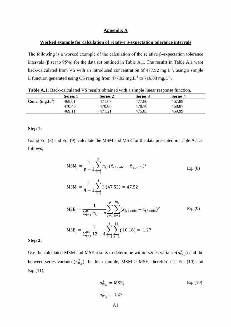
A1
Appendix A
Worked example for calculation of relative β-expectation tolerance intervals
The following is a worked example of the calculation of the relative β-expectation tolerance
intervals (β set to 95%) for the data set outlined in Table A.1. The results in Table A.1 were
back-calculated from VS with an introduced concentration of 477.92 mg.L-1, using a simple
L function generated using CS ranging from 477.92 mg.L-1 to 716.88 mg.L-1.
Table A.1: Back-calculated VS results obtained with a simple linear response function. Series 1 Series 2 Series 3 Series 4 Conc. (mg.L-1) 468.01 471.67 477.80 467.88 470.48 470.86 478.78 468.87 469.11 471.21 475.83 469.99
Step 1:
Using Eq. (8) and Eq. (9), calculate the MSM and MSE for the data presented in Table A.1 as
follows;
MSMj =1
𝑝 − 1�𝑛𝑖𝑖
𝑝
𝑖=1
(�̅�𝑖𝑖.,𝑐𝑐𝑐𝑐 − �̅�.𝑖.,𝑐𝑐𝑐𝑐)2
Eq. (8)
MSMj =1
4 − 1�34
𝑖=1
(47.52) = 47.52
MSEj =1
∑ 𝑛𝑖𝑖𝑝𝑖=1 − 𝑝
��(�̅�𝑖𝑖𝑖,𝑐𝑐𝑐𝑐 − �̅�𝑖𝑖.,𝑐𝑐𝑐𝑐)2𝑛𝑖𝑖
𝑖=1
𝑝
𝑖=1
Eq. (9)
MSEj =1
∑ 12𝑝4𝑖=1 − 4
��(12
𝑖=1
4
𝑖=1
10.16) = 1.27
Step 2:
Use the calculated MSM and MSE results to determine within-series variance(𝜎𝑊,𝑖2 ) and the
between-series variance(𝜎𝐵,𝑖2 ). In this example, MSM > MSE, therefore use Eq. (10) and
Eq. (11);
𝜎𝑊,𝑖2 = MSEj
Eq. (10)
𝜎𝑊,𝑖2 = 1.27
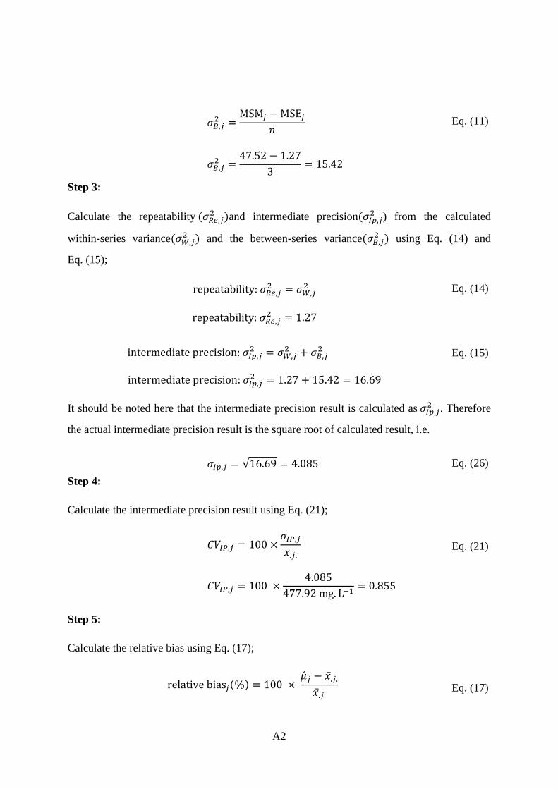
A2
𝜎𝐵,𝑖2 =
MSM𝑖 − MSE𝑖𝑛
Eq. (11)
𝜎𝐵,𝑖2 =
47.52 − 1.273
= 15.42
Step 3:
Calculate the repeatability (𝜎𝑅𝑅,𝑖2 )and intermediate precision(𝜎𝐼𝑝,𝑖
2 ) from the calculated
within-series variance(𝜎𝑊,𝑖2 ) and the between-series variance(𝜎𝐵,𝑖
2 ) using Eq. (14) and
Eq. (15);
repeatability: 𝜎𝑅𝑅,𝑖2 = 𝜎𝑊,𝑖
2
Eq. (14)
repeatability: 𝜎𝑅𝑅,𝑖2 = 1.27
intermediate precision: 𝜎𝐼𝑝,𝑖2 = 𝜎𝑊,𝑖
2 + 𝜎𝐵,𝑖2 Eq. (15)
intermediate precision: 𝜎𝐼𝑝,𝑖2 = 1.27 + 15.42 = 16.69
It should be noted here that the intermediate precision result is calculated as 𝜎𝐼𝑝,𝑖2 . Therefore
the actual intermediate precision result is the square root of calculated result, i.e.
𝜎𝐼𝑝,𝑖 = √16.69 = 4.085 Eq. (26) Step 4:
Calculate the intermediate precision result using Eq. (21);
𝐶𝐶𝐼𝐼,𝑖 = 100 ×𝜎𝐼𝐼,𝑖
�̅�.𝑖. Eq. (21)
𝐶𝐶𝐼𝐼,𝑖 = 100 ×4.085
477.92 mg. L−1= 0.855
Step 5:
Calculate the relative bias using Eq. (17);
relative bias𝑖(%) = 100 × �̂�𝑖 − �̅�.𝑖.
�̅�.𝑖.
Eq. (17)

A3
relative bias𝑖(%) = 100 × 471.71 − 477.92
477.92= −1.30
Step 6:
At this point, most of the elements necessary to calculate the relative β-tolerance intervals
have been generated. However, before completing the calculation of the relative β-tolerance
intervals, calculate 𝑅𝑖 , 𝐵𝑖 and 𝑣 using Eq. (22), Eq. (23) and Eq. (24) respectively;
𝑅𝑖 =𝜎�𝐵,𝑖2
𝜎�𝑊,𝑖2
Eq. (22)
𝑅𝑖 =15.421.27
= 12.14
𝐵𝑖 = �𝑅𝑖 + 1𝑛𝑅𝑖 + 1
Eq. (23)
𝐵𝑖 = �12.14 + 1
(3)(12.14) + 1= 0.59
𝑣 =(𝑅𝑖 + 1)2
(𝑅𝑖 + 1 𝑛⁄ ))2 (𝑝 − 1)⁄ + (1 − (1 𝑛⁄ )) 𝑝𝑛⁄
Eq. (24)
𝑣 =(12.14 + 1)2
(12.14 + 1 3⁄ ))2 (4 − 1)⁄ + (1 − (1 3⁄ )) (4)(3)⁄ = 3.33 ≅ 3
Step 7:
From Eq.(25), use the t-distribution table (See Attachment B) to obtain 𝑄𝑡 �𝑣; 1+𝛽2�, the
β quantile with 𝑣 degrees of freedom. In this example, β = 95% confidence interval.
Therefore, the value at 95% with 3 degrees is 3.182.
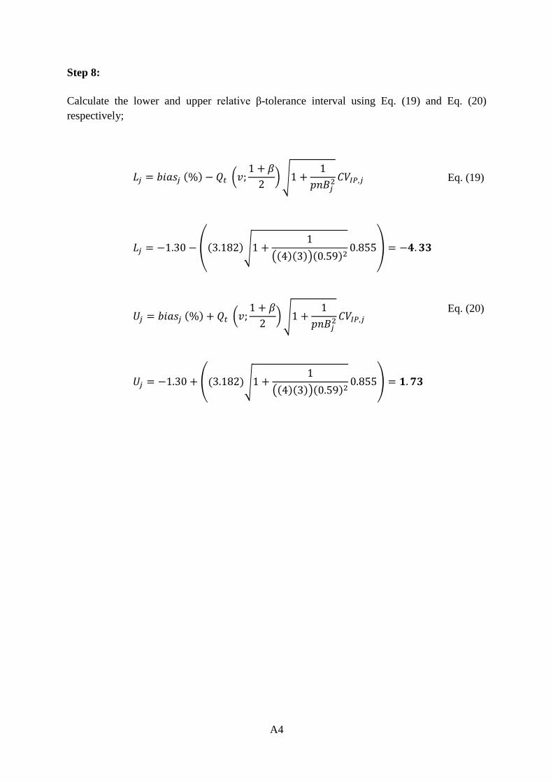
A4
Step 8:
Calculate the lower and upper relative β-tolerance interval using Eq. (19) and Eq. (20) respectively;
𝐿𝑖 = 𝑏𝑏𝑏𝑏𝑖 (%) − 𝑄𝑡 �𝑣;1 + 𝛽
2��1 +
1𝑝𝑛𝐵𝑖2
𝐶𝐶𝐼𝐼,𝑖
Eq. (19)
𝐿𝑖 = −1.30 − �(3.182)�1 +1
�(4)(3)�(0.59)20.855� = −𝟒.𝟑𝟑
𝑈𝑖 = 𝑏𝑏𝑏𝑏𝑖 (%) + 𝑄𝑡 �𝑣;1 + 𝛽
2��1 +
1𝑝𝑛𝐵𝑖2
𝐶𝐶𝐼𝐼,𝑖
Eq. (20)
𝑈𝑖 = −1.30 + �(3.182)�1 +1
�(4)(3)�(0.59)20.855� = 𝟏.𝟕𝟑
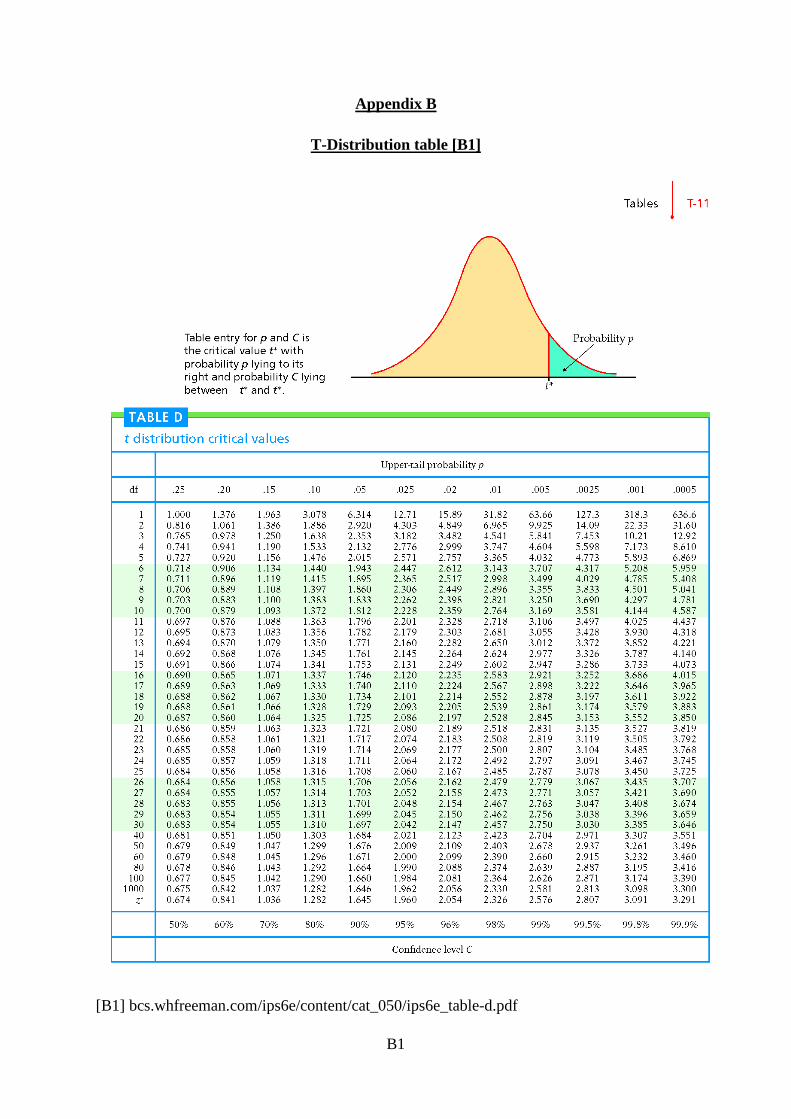
B1
Appendix B
T-Distribution table [B1]
[B1] bcs.whfreeman.com/ips6e/content/cat_050/ips6e_table-d.pdf

C1
Appendix C UPSFC method validation data tables
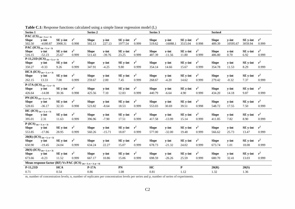
C2
Table C.1: Response functions calculated using a simple linear regression model (L) Series 1 Series 2 Series 3 Series4 PAC (CS) (m = 5; n = 3) Slope y-int SE y-int r2 Slope y-int SE y-int r2 Slope y-int SE y-int r2 Slope y-int SE y-int r2 502.50 -4180.87 3908.31 0.998 502.13 227.13 1977.54 0.999 519.62 -16088.1 3515.04 0.998 489.39 10595.67 3059.94 0.999 PAC (ICS) (m = 5; n = 3) Slope y-int SE y-int r2 Slope y-int SE y-int r2 Slope y-int SE y-int r2 Slope y-int SE y-int r2 516.15 -52.23 25.67 0.999 511.43 -39.76 23.25 0.999 487.39 -11.56 11.80 0.999 486.80 0.70 6.92 0.999 P-11,21D (ICS) (m = 5; n = 3) Slope y-int SE y-int r2 Slope y-int SE y-int r2 Slope y-int SE y-int r2 Slope y-int SE y-int r2 350.27 -0.33 9.26 0.999 347.91 -4.25 9.80 0.999 354.14 14.66 15.67 0.999 354.78 11.53 8.29 0.999 HCA (ICS) (m = 5; n = 3) Slope y-int SE y-int r2 Slope y-int SE y-int r2 Slope y-int SE y-int r2 Slope y-int SE y-int r2 262.15 13.33 7.00 0.999 259.67 2.00 7.45 0.999 268.67 -4.20 14.62 0.999 279.42 -0.32 7.37 0.999 P-17A (ICS) (m = 5; n = 3) Slope y-int SE y-int r2 Slope y-int SE y-int r2 Slope y-int SE y-int r2 Slope y-int SE y-int r2 426.64 -14.08 30.36 0.998 425.56 7.10 12.83 0.999 440.79 -6.64 4.90 0.999 434.20 14.18 9.87 0.999 PN (ICS) (m = 5; n = 3) Slope y-int SE y-int r2 Slope y-int SE y-int r2 Slope y-int SE y-int r2 Slope y-int SE y-int r2 528.65 -36.17 32.33 0.998 523.82 -8.64 18.53 0.999 553.03 30.69 39.51 0.998 548.72 17.55 7.50 0.999 HC (ICS) (m = 5; n = 3) Slope y-int SE y-int r2 Slope y-int SE y-int r2 Slope y-int SE y-int r2 Slope y-int SE y-int r2 395.01 2.31 11.63 0.999 396.96 -7.90 17.51 0.999 417.58 -13.99 15.14 0.999 411.85 7.82 8.90 0.999 P (ICS) (m = 5; n = 3) Slope y-int SE y-int r2 Slope y-int SE y-int r2 Slope y-int SE y-int r2 Slope y-int SE y-int r2 553.85 -17.86 28.95 0.999 560.26 -15.71 18.87 0.999 577.00 -32.00 19.48 0.999 566.62 25.73 13.47 0.999 20(R) (ICS) (m = 5; n = 3) Slope y-int SE y-int r2 Slope y-int SE y-int r2 Slope y-int SE y-int r2 Slope y-int SE y-int r2 650.90 -19.45 24.04 0.999 634.24 22.27 15.07 0.999 678.73 -21.32 24.02 0.999 673.74 1.01 18.08 0.999 20(S) (ICS) (m = 5; n = 3) Slope y-int SE y-int r2 Slope y-int SE y-int r2 Slope y-int SE y-int r2 Slope y-int SE y-int r2 673.66 -0.23 11.52 0.999 667.17 10.86 15.06 0.999 698.59 -26.26 25.59 0.999 680.70 32.41 13.03 0.999 Mean response factor (RF) Vs PAC (ICS) (m = 5; n = 3; p = 4) P-11,21D HCA P-17A PN HC P 20(R) 20(S) 0.71 0.54 0.86 1.08 0.81 1.12 1.32 1.36 m, number of concentration levels; n, number of replicates per concentration levels per series and p, number of series of experiments.
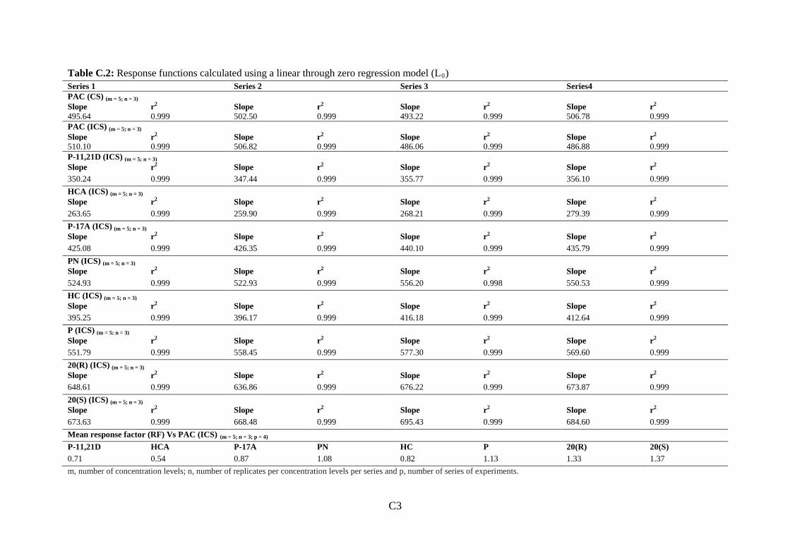
C3
Table C.2: Response functions calculated using a linear through zero regression model (L0) Series 1 Series 2 Series 3 Series4 PAC (CS) (m = 5; n = 3) Slope r2 Slope r2 Slope r2 Slope r2 495.64 0.999 502.50 0.999 493.22 0.999 506.78 0.999 PAC (ICS) (m = 5; n = 3) Slope r2 Slope r2 Slope r2 Slope r2 510.10 0.999 506.82 0.999 486.06 0.999 486.88 0.999 P-11,21D (ICS) (m = 5; n = 3) Slope r2 Slope r2 Slope r2 Slope r2 350.24 0.999 347.44 0.999 355.77 0.999 356.10 0.999 HCA (ICS) (m = 5; n = 3) Slope r2 Slope r2 Slope r2 Slope r2 263.65 0.999 259.90 0.999 268.21 0.999 279.39 0.999 P-17A (ICS) (m = 5; n = 3) Slope r2 Slope r2 Slope r2 Slope r2 425.08 0.999 426.35 0.999 440.10 0.999 435.79 0.999 PN (ICS) (m = 5; n = 3) Slope r2 Slope r2 Slope r2 Slope r2 524.93 0.999 522.93 0.999 556.20 0.998 550.53 0.999 HC (ICS) (m = 5; n = 3) Slope r2 Slope r2 Slope r2 Slope r2 395.25 0.999 396.17 0.999 416.18 0.999 412.64 0.999 P (ICS) (m = 5; n = 3) Slope r2 Slope r2 Slope r2 Slope r2 551.79 0.999 558.45 0.999 577.30 0.999 569.60 0.999 20(R) (ICS) (m = 5; n = 3) Slope r2 Slope r2 Slope r2 Slope r2 648.61 0.999 636.86 0.999 676.22 0.999 673.87 0.999 20(S) (ICS) (m = 5; n = 3) Slope r2 Slope r2 Slope r2 Slope r2 673.63 0.999 668.48 0.999 695.43 0.999 684.60 0.999 Mean response factor (RF) Vs PAC (ICS) (m = 5; n = 3; p = 4) P-11,21D HCA P-17A PN HC P 20(R) 20(S) 0.71 0.54 0.87 1.08 0.82 1.13 1.33 1.37 m, number of concentration levels; n, number of replicates per concentration levels per series and p, number of series of experiments.

C4
Table C.3: Validation results for PAC using the L response function to back-calculate VS amounts Validation criteria (n = 3; p = 4) Level 1 Level 2 Level 3 Level 4 Level 5
Level (%) 80 90 100 110 120 Mean introduced concentration (mg.L-1) 477.92 537.66 597.40 657.14 716.88 Mean predicted concentration (mg.L-1) 472.59 536.88 598.17 658.32 715.55 Relative bias (%) -1.12 -0.15 0.13 0.18 -0.19 Recovery (%) 98.88 99.85 100.13 100.18 99.81 Repeatability standard deviation 1.106 1.128 0.586 1.429 1.744 Intermediate precision standard deviation 8.484 7.459 7.785 6.370 4.939 Repeatability RSD (%) 0.23 0.21 0.10 0.22 0.24 Intermediate precision RSD (%) 1.78 1.39 1.30 0.97 0.69 Relative tolerance interval at 95% (%) 6.31 4.93 4.63 3.44 2.12 Lower relative β tolerance limit (%) -7.42 -5.07 -4.51 -3.26 -2.31 Upper relative β tolerance limit (%) 5.19 4.78 4.76 3.62 1.93
Linearity (m = 5; n = 3; p = 4) Slope 1.0167 y-intercept -11.055 r2 0.994 m, number of concentration levels; n, number of replicates per concentration levels per series and p, number of series of experiments.
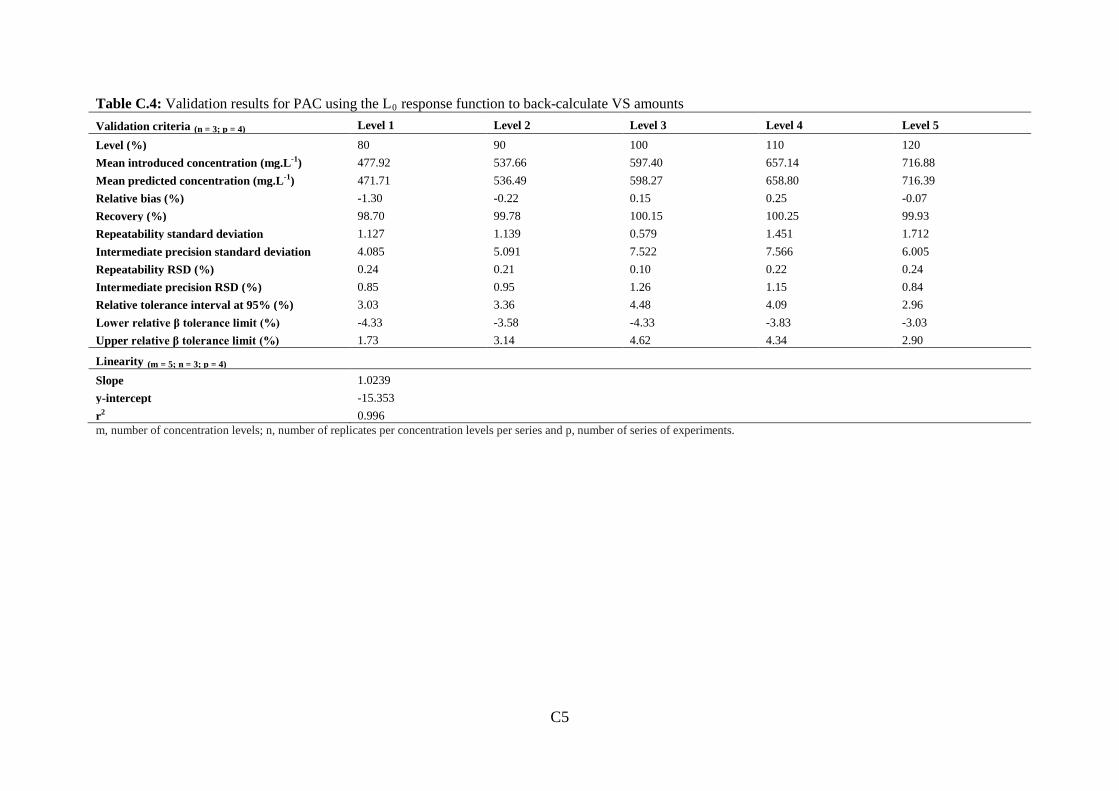
C5
Table C.4: Validation results for PAC using the L0 response function to back-calculate VS amounts Validation criteria (n = 3; p = 4) Level 1 Level 2 Level 3 Level 4 Level 5
Level (%) 80 90 100 110 120 Mean introduced concentration (mg.L-1) 477.92 537.66 597.40 657.14 716.88 Mean predicted concentration (mg.L-1) 471.71 536.49 598.27 658.80 716.39 Relative bias (%) -1.30 -0.22 0.15 0.25 -0.07 Recovery (%) 98.70 99.78 100.15 100.25 99.93 Repeatability standard deviation 1.127 1.139 0.579 1.451 1.712 Intermediate precision standard deviation 4.085 5.091 7.522 7.566 6.005 Repeatability RSD (%) 0.24 0.21 0.10 0.22 0.24 Intermediate precision RSD (%) 0.85 0.95 1.26 1.15 0.84 Relative tolerance interval at 95% (%) 3.03 3.36 4.48 4.09 2.96 Lower relative β tolerance limit (%) -4.33 -3.58 -4.33 -3.83 -3.03 Upper relative β tolerance limit (%) 1.73 3.14 4.62 4.34 2.90
Linearity (m = 5; n = 3; p = 4) Slope 1.0239 y-intercept -15.353 r2 0.996 m, number of concentration levels; n, number of replicates per concentration levels per series and p, number of series of experiments.
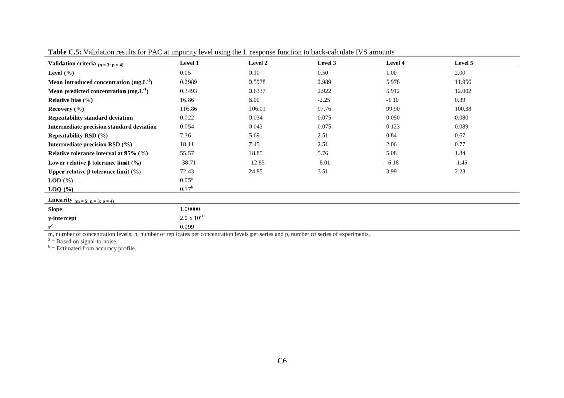
C6
Table C.5: Validation results for PAC at impurity level using the L response function to back-calculate IVS amounts Validation criteria (n = 3; p = 4) Level 1 Level 2 Level 3 Level 4 Level 5
Level (%) 0.05 0.10 0.50 1.00 2.00 Mean introduced concentration (mg.L-1) 0.2989 0.5978 2.989 5.978 11.956 Mean predicted concentration (mg.L-1) 0.3493 0.6337 2.922 5.912 12.002 Relative bias (%) 16.86 6.00 -2.25 -1.10 0.39 Recovery (%) 116.86 106.01 97.76 99.90 100.38 Repeatability standard deviation 0.022 0.034 0.075 0.050 0.080 Intermediate precision standard deviation 0.054 0.043 0.075 0.123 0.089 Repeatability RSD (%) 7.36 5.69 2.51 0.84 0.67 Intermediate precision RSD (%) 18.11 7.45 2.51 2.06 0.77 Relative tolerance interval at 95% (%) 55.57 18.85 5.76 5.08 1.84 Lower relative β tolerance limit (%) -38.71 -12.85 -8.01 -6.18 -1.45 Upper relative β tolerance limit (%) 72.43 24.85 3.51 3.99 2.23 LOD (%) 0.05a LOQ (%) 0.17b
Linearity (m = 5; n = 3; p = 4) Slope 1.00000 y-intercept 2.0 x 10⁻¹² r2 0.999 m, number of concentration levels; n, number of replicates per concentration levels per series and p, number of series of experiments. a = Based on signal-to-noise. b = Estimated from accuracy profile.

C7
Table C.6: Validation results for PAC at impurity level using the L0 response function to back-calculate IVS amounts Validation criteria (n = 3; p = 4) Level 1 Level 2 Level 3 Level 4 Level 5
Level (%) 0.05 0.10 0.50 1.00 2.00 Mean introduced concentration (mg.L-1) 0.2989 0.5978 2.989 5.978 11.956 Mean predicted concentration (mg.L-1) 0.3008 0.5867 2.888 5.896 12.023 Relative bias (%) 0.62 -1.91 -3.38 -1.37 0.56 Recovery (%) 100.64 98.14 96.62 98.62 100.56 Repeatability standard deviation 0.020 0.034 0.077 0.050 0.081 Intermediate precision standard deviation 0.020 0.038 0.091 0.138 0.104 Repeatability RSD (%) 6.66 5.75 2.58 0.84 0.68 Intermediate precision RSD (%) 6.66 6.37 3.06 2.31 0.87 Relative tolerance interval at 95% (%) 15.26 15.20 7.50 7.09 2.19 Lower relative β tolerance limit (%) -14.64 -17.11 -10.87 -8.47 -1.64 Upper relative β tolerance limit (%) 15.89 13.30 4.12 5.72 2.75 LOD (%) 0.05a LOQ (%) 0.05b
Linearity (m = 5; n = 3; p = 4) Slope 1.0059 y-intercept 0.0508 r2 0.999 m, number of concentration levels; n, number of replicates per concentration levels per series and p, number of series of experiments. a = Based on signal-to-noise. b = Estimated from accuracy profile.

C8
Table C.7: Validation results for P-11,21D at impurity level using the L response function to back-calculate IVS amounts Validation criteria (n = 3; p = 4) Level 1 Level 2 Level 3 Level 4 Level 5
Level (%) 0.05 0.10 0.50 1.00 2.00 Mean introduced concentration (mg.L-1) 0.3119 0.6239 3.119 6.239 12.477 Mean predicted concentration (mg.L-1) 0.3916 0.7206 3.208 6.304 12.545 Relative bias (%) 25.55 15.51 2.84 1.05 0.54 Recovery (%) 125.55 115.50 102.85 101.04 100.54 Repeatability standard deviation 0.027 0.025 0.037 0.121 0.107 Intermediate precision standard deviation 0.069 0.062 0.100 0.121 0.128 Repeatability RSD (%) 8.66 4.01 1.19 1.94 0.86 Intermediate precision RSD (%) 22.03 9.97 3.19 1.94 1.03 Relative tolerance interval at 95% (%) 67.63 30.61 9.82 4.44 2.52 Lower relative β tolerance limit (%) -42.09 -15.10 -6.99 -3.39 -1.98 Upper relative β tolerance limit (%) 93.18 46.12 12.66 5.49 3.07 LOD (%) 0.05a LOQ (%) 0.43b
Linearity (m = 5; n = 3; p = 4) Slope 0.9980 y-intercept 0.0886 r2 0.999 m, number of concentration levels; n, number of replicates per concentration levels per series and p, number of series of experiments. a = Based on signal-to-noise. b = Estimated from accuracy profile.

C9
Table C.8: Validation results for P-11,21D at impurity level using the L0 response function to back-calculate IVS amounts Validation criteria (n = 3; p = 4) Level 1 Level 2 Level 3 Level 4 Level 5
Level (%) 0.05 0.10 0.50 1.00 2.00 Mean introduced concentration (mg.L-1) 0.3119 0.6239 3.119 6.239 12.477 Mean predicted concentration (mg.L-1) 0.3200 0.6509 3.153 6.267 12.545 Relative bias (%) 2.60 4.34 1.07 0.45 0.54 Recovery (%) 102.60 104.33 101.09 100.45 100.55 Repeatability standard deviation 0.025 0.025 0.037 0.123 0.107 Intermediate precision standard deviation 0.05 0.040 0.070 0.132 0.128 Repeatability RSD (%) 7.95 4.01 1.19 1.97 0.86 Intermediate precision RSD (%) 7.95 6.42 2.25 2.11 1.02 Relative tolerance interval at 95% (%) 18.22 17.96 6.85 4.95 2.51 Lower relative β tolerance limit (%) -15.62 -13.62 -5.78 -4.49 -1.97 Upper relative β tolerance limit (%) 20.82 22.29 7.92 5.40 3.06 LOD (%) 0.05a LOQ (%) 0.15b
Linearity (m = 5; n = 3; p = 4) Slope 1.0039 y-intercept 0.0151 r2 0.999 m, number of concentration levels; n, number of replicates per concentration levels per series and p, number of series of experiments. a = Based on signal-to-noise. b = Estimated from accuracy profile.

C10
Table C.9: Validation results for HCA at impurity level using the L response function to back-calculate IVS amounts Validation criteria (n = 3; p = 4) Level 1 Level 2 Level 3 Level 4 Level 5
Level (%) 0.05 0.10 0.50 1.00 2.00 Mean introduced concentration (mg.L-1) 0.3096 0.6191 3.096 6.191 12.383 Mean predicted concentration (mg.L-1) 0.4226 0.7370 3.173 6.321 12.491 Relative bias (%) 36.52 19.03 2.50 2.09 0.87 Recovery (%) 136.50 119.04 102.49 102.10 100.87 Repeatability standard deviation 0.052 0.041 0.070 0.401 0.095 Intermediate precision standard deviation 0.134 0.107 0.194 0.407 0.108 Repeatability RSD (%) 16.80 6.62 2.26 6.48 0.77 Intermediate precision RSD (%) 43.44 17.30 6.28 6.57 0.87 Relative tolerance interval at 95% (%) 133.49 53.16 19.32 15.50 2.12 Lower relative β tolerance limit (%) -96.97 -34.13 -16.82 -13.41 -1.25 Upper relative β tolerance limit (%) 170.01 72.19 21.81 17.59 3.00 LOD (%) 0.05a LOQ (%) 0.62b
Linearity (m = 5; n = 3; p = 4) Slope 1.0002 y-intercept 0.1083 r2 0.999 m, number of concentration levels; n, number of replicates per concentration levels per series and p, number of series of experiments. a = Based on signal-to-noise. b = Estimated from accuracy profile.

C11
Table C.10: Validation results for HCA at impurity level using the L0 response function to back-calculate IVS amounts Validation criteria (n = 3; p = 4) Level 1 Level 2 Level 3 Level 4 Level 5
Level (%) 0.05 0.10 0.50 1.00 2.00 Mean introduced concentration (mg.L-1) 0.3096 0.6191 3.096 6.191 12.383 Mean predicted concentration (mg.L-1) 0.3268 0.6429 3.093 6.259 12.466 Relative bias (%) 5.57 3.83 -0.07 1.10 0.67 Recovery (%) 105.56 103.84 99.90 101.10 100.67 Repeatability standard deviation 0.052 0.041 0.070 0.110 0.094 Intermediate precision standard deviation 0.056 0.048 0.146 0.133 0.094 Repeatability RSD (%) 16.80 6.62 2.26 1.78 0.76 Intermediate precision RSD (%) 18.21 7.80 4.71 2.16 0.76 Relative tolerance interval at 95% (%) 42.70 18.72 14.40 5.30 1.74 Lower relative β tolerance limit (%) -37.13 -14.89 -14.45 -4.20 -1.07 Upper relative β tolerance limit (%) 48.27 22.56 14.32 6.40 2.41 LOD (%) 0.05a LOQ (%) 0.20b
Linearity (m = 5; n = 3; p = 4) Slope 1.0061 y-intercept 0.0105 r2 0.999 m, number of concentration levels; n, number of replicates per concentration levels per series and p, number of series of experiments. a = Based on signal-to-noise. b = Estimated from accuracy profile.

C12
Table C.11: Validation results for P-17A at impurity level using the L response function to back-calculate IVS amounts Validation criteria (n = 3; p = 4) Level 1 Level 2 Level 3 Level 4 Level 5
Level (%) 0.05 0.10 0.50 1.00 2.00 Mean introduced concentration (mg.L-1) 0.3109 0.6217 3.109 6.217 12.434 Mean predicted concentration (mg.L-1) 0.3808 0.6857 3.224 6.188 12.548 Relative bias (%) 22.49 10.29 3.71 -0.48 0.92 Recovery (%) 122.48 110.29 103.70 99.53 100.92 Repeatability standard deviation 0.016 0.033 0.030 0.097 0.071 Intermediate precision standard deviation 0.064 0.057 0.106 0.178 0.088 Repeatability RSD (%) 5.15 5.31 0.96 1.56 0.57 Intermediate precision RSD (%) 20.46 9.11 3.42 2.86 0.71 Relative tolerance interval at 95% (%) 72.50 25.58 12.09 6.99 1.75 Lower relative β tolerance limit (%) -50.01 -15.29 -8.38 -7.46 -0.83 Upper relative β tolerance limit (%) 95.00 35.87 15.81 6.51 2.66 LOD (%) 0.05a LOQ (%) 0.45b
Linearity (m = 5; n = 3; p = 4) Slope 1.0014 y-intercept 0.0605 r2 0.999 m, number of concentration levels; n, number of replicates per concentration levels per series and p, number of series of experiments. a = Based on signal-to-noise. b = Estimated from accuracy profile.

C13
Table C.12: Validation results for P-17A at impurity level using the L0 response function to back-calculate IVS amounts Validation criteria (n = 3; p = 4) Level 1 Level 2 Level 3 Level 4 Level 5
Level (%) 0.05 0.10 0.50 1.00 2.00 Mean introduced concentration (mg.L-1) 0.3109 0.6217 3.109 6.217 12.434 Mean predicted concentration (mg.L-1) 0.3217 0.6275 3.174 6.145 12.527 Relative bias (%) 3.48 0.92 2.10 -1.15 0.75 Recovery (%) 103.47 100.93 102.09 98.84 100.75 Repeatability standard deviation 0.016 0.030 0.030 0.097 0.072 Intermediate precision standard deviation 0.019 0.030 0.080 0.185 0.149 Repeatability RSD (%) 5.15 4.83 0.96 1.56 0.58 Intermediate precision RSD (%) 5.97 4.83 2.56 2.97 1.20 Relative tolerance interval at 95% (%) 14.66 11.07 7.88 9.06 3.67 Lower relative β tolerance limit (%) -11.18 -10.14 -5.78 -10.21 -2.92 Upper relative β tolerance limit (%) 18.13 11.99 9.98 7.90 4.41 LOD (%) 0.05a LOQ (%) 0.05b
Linearity (m = 5; n = 3; p = 4) Slope 1.0045 y-intercept 0.0002 r2 0.999 m, number of concentration levels; n, number of replicates per concentration levels per series and p, number of series of experiments. a = Based on signal-to-noise. b = Estimated from accuracy profile.

C14
Table C.13: Validation results for PN at impurity level using the L response function to back-calculate IVS amounts Validation criteria (n = 3; p = 4) Level 1 Level 2 Level 3 Level 4 Level 5
Level (%) 0.05 0.10 0.50 1.00 2.00 Mean introduced concentration (mg.L-1) 0.3369 0.6737 3.369 6.737 13.474 Mean predicted concentration (mg.L-1) 0.4019 0.7369 3.409 6.777 13.574 Relative bias (%) 19.30 9.39 1.21 0.59 0.74 Recovery (%) 119.29 109.38 101.19 100.59 100.74 Repeatability standard deviation 0.019 0.030 0.058 0.062 0.051 Intermediate precision standard deviation 0.047 0.040 0.124 0.282 0.122 Repeatability RSD (%) 5.64 4.45 1.72 0.92 0.38 Intermediate precision RSD (%) 13.82 5.90 3.68 4.19 0.90 Relative tolerance interval at 95% (%) 42.42 14.98 11.24 10.76 2.78 Lower relative β tolerance limit (%) -23.13 -5.59 -10.04 -10.17 -2.04 Upper relative β tolerance limit (%) 61.72 24.36 12.45 11.35 3.51 LOD (%) 0.05a LOQ (%) 0.28b
Linearity (m = 5; n = 3; p = 4) Slope 1.0025 y-intercept 0.0494 r2 0.999 m, number of concentration levels; n, number of replicates per concentration levels per series and p, number of series of experiments. a = Based on signal-to-noise. b = Estimated from accuracy profile.
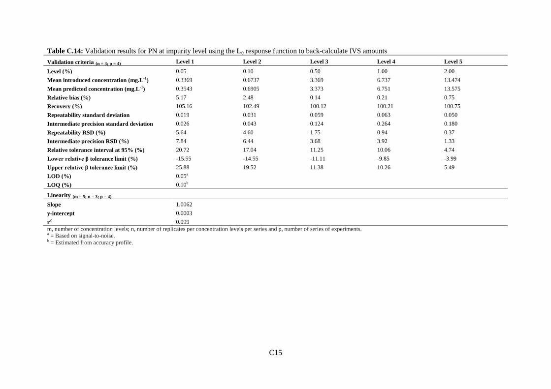
C15
Table C.14: Validation results for PN at impurity level using the L0 response function to back-calculate IVS amounts Validation criteria (n = 3; p = 4) Level 1 Level 2 Level 3 Level 4 Level 5
Level (%) 0.05 0.10 0.50 1.00 2.00 Mean introduced concentration (mg.L-1) 0.3369 0.6737 3.369 6.737 13.474 Mean predicted concentration (mg.L-1) 0.3543 0.6905 3.373 6.751 13.575 Relative bias (%) 5.17 2.48 0.14 0.21 0.75 Recovery (%) 105.16 102.49 100.12 100.21 100.75 Repeatability standard deviation 0.019 0.031 0.059 0.063 0.050 Intermediate precision standard deviation 0.026 0.043 0.124 0.264 0.180 Repeatability RSD (%) 5.64 4.60 1.75 0.94 0.37 Intermediate precision RSD (%) 7.84 6.44 3.68 3.92 1.33 Relative tolerance interval at 95% (%) 20.72 17.04 11.25 10.06 4.74 Lower relative β tolerance limit (%) -15.55 -14.55 -11.11 -9.85 -3.99 Upper relative β tolerance limit (%) 25.88 19.52 11.38 10.26 5.49 LOD (%) 0.05a LOQ (%) 0.10b
Linearity (m = 5; n = 3; p = 4) Slope 1.0062 y-intercept 0.0003 r2 0.999 m, number of concentration levels; n, number of replicates per concentration levels per series and p, number of series of experiments. a = Based on signal-to-noise. b = Estimated from accuracy profile.

C16
Table C.15: Validation results for HC at impurity level using the L response function to back-calculate IVS amounts Validation criteria (n = 3; p = 4) Level 1 Level 2 Level 3 Level 4 Level 5
Level (%) 0.05 0.10 0.50 1.00 2.00 Mean introduced concentration (mg.L-1) 0.3453 0.6906 3.453 6.906 13.812 Mean predicted concentration (mg.L-1) 0.4097 0.7576 3.536 6.870 13.880 Relative bias (%) 18.66 9.70 2.41 -0.52 0.49 Recovery (%) 118.65 109.69 102.40 99.48 100.49 Repeatability standard deviation 0.023 0.045 0.091 0.075 0.101 Intermediate precision standard deviation 0.050 0.086 0.157 0.075 0.158 Repeatability RSD (%) 6.66 6.51 2.64 1.08 0.73 Intermediate precision RSD (%) 14.39 12.43 4.55 1.08 1.14 Relative tolerance interval at 95% (%) 44.05 37.85 12.79 2.48 3.19 Lower relative β tolerance limit (%) -25.39 -28.15 -10.39 -3.00 -2.70 Upper relative β tolerance limit (%) 62.71 47.56 15.20 1.96 3.68 LOD (%) 0.05a LOQ (%) 0.52b
Linearity (m = 5; n = 3; p = 4) Slope 0.9984 y-intercept 0.0574 r2 0.999 m, number of concentration levels; n, number of replicates per concentration levels per series and p, number of series of experiments. a = Based on signal-to-noise. b = Estimated from accuracy profile.
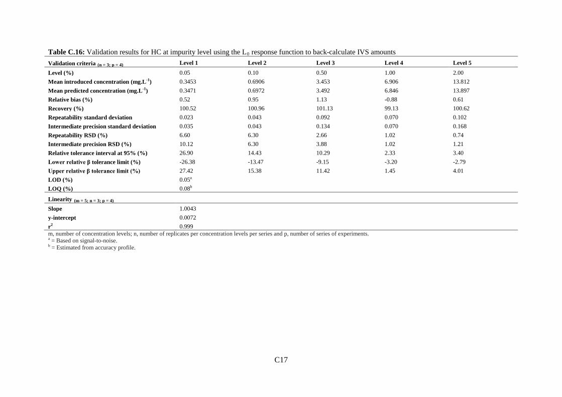
C17
Table C.16: Validation results for HC at impurity level using the L0 response function to back-calculate IVS amounts Validation criteria (n = 3; p = 4) Level 1 Level 2 Level 3 Level 4 Level 5
Level (%) 0.05 0.10 0.50 1.00 2.00 Mean introduced concentration (mg.L-1) 0.3453 0.6906 3.453 6.906 13.812 Mean predicted concentration (mg.L-1) 0.3471 0.6972 3.492 6.846 13.897 Relative bias (%) 0.52 0.95 1.13 -0.88 0.61 Recovery (%) 100.52 100.96 101.13 99.13 100.62 Repeatability standard deviation 0.023 0.043 0.092 0.070 0.102 Intermediate precision standard deviation 0.035 0.043 0.134 0.070 0.168 Repeatability RSD (%) 6.60 6.30 2.66 1.02 0.74 Intermediate precision RSD (%) 10.12 6.30 3.88 1.02 1.21 Relative tolerance interval at 95% (%) 26.90 14.43 10.29 2.33 3.40 Lower relative β tolerance limit (%) -26.38 -13.47 -9.15 -3.20 -2.79 Upper relative β tolerance limit (%) 27.42 15.38 11.42 1.45 4.01 LOD (%) 0.05a LOQ (%) 0.08b
Linearity (m = 5; n = 3; p = 4) Slope 1.0043 y-intercept 0.0072 r2 0.999 m, number of concentration levels; n, number of replicates per concentration levels per series and p, number of series of experiments. a = Based on signal-to-noise. b = Estimated from accuracy profile.

C18
Table C.17: Validation results for P at impurity level using the L response function to back-calculate IVS amounts Validation criteria (n = 3; p = 4) Level 1 Level 2 Level 3 Level 4 Level 5
Level (%) 0.05 0.10 0.50 1.00 2.00 Mean introduced concentration (mg.L-1) 0.2997 0.5993 2.997 5.993 11.986 Mean predicted concentration (mg.L-1) 0.3536 0.6419 3.043 6.022 12.141 Relative bias (%) 18.01 7.10 1.55 0.48 1.29 Recovery (%) 117.98 107.11 101.53 100.48 101.29 Repeatability standard deviation 0.011 0.022 0.100 0.071 0.062 Intermediate precision standard deviation 0.053 0.071 0.135 0.152 0.190 Repeatability RSD (%) 3.67 3.67 3.34 1.18 0.52 Intermediate precision RSD (%) 17.82 11.87 4.50 2.54 1.58 Relative tolerance interval at 95% (%) 63.20 41.97 11.45 6.22 5.59 Lower relative β tolerance limit (%) -45.19 -34.87 -9.90 -5.75 -4.30 Upper relative β tolerance limit (%) 81.21 49.07 13.00 6.70 6.88 LOD (%) 0.05a LOQ (%) 0.43b
Linearity (m = 5; n = 3; p = 4) Slope 1.0083 y-intercept 0.0287 r2 0.999 m, number of concentration levels; n, number of replicates per concentration levels per series and p, number of series of experiments. a = Based on signal-to-noise. b = Estimated from accuracy profile.
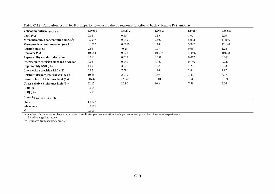
C19
Table C.18: Validation results for P at impurity level using the L0 response function to back-calculate IVS amounts Validation criteria (n = 3; p = 4) Level 1 Level 2 Level 3 Level 4 Level 5
Level (%) 0.05 0.10 0.50 1.00 2.00 Mean introduced concentration (mg.L-1) 0.2997 0.5993 2.997 5.993 11.986 Mean predicted concentration (mg.L-1) 0.3082 0.5976 3.008 5.997 12.140 Relative bias (%) 2.86 -0.29 0.37 0.06 1.28 Recovery (%) 102.84 99.72 100.37 100.07 101.28 Repeatability standard deviation 0.012 0.022 0.101 0.072 0.063 Intermediate precision standard deviation 0.021 0.045 0.122 0.146 0.236 Repeatability RSD (%) 4.00 3.67 3.37 1.20 0.53 Intermediate precision RSD (%) 6.85 7.59 4.06 2.44 1.97 Relative tolerance interval at 95% (%) 19.28 23.19 9.97 7.46 6.97 Lower relative β tolerance limit (%) -16.42 -23.48 -9.60 -7.40 -5.69 Upper relative β tolerance limit (%) 22.15 22.90 10.34 7.51 8.26 LOD (%) 0.05a LOQ (%) 0.20b
Linearity (m = 5; n = 3; p = 4) Slope 1.0122 y-intercept 0.0181 r2 0.999 m, number of concentration levels; n, number of replicates per concentration levels per series and p, number of series of experiments. a = Based on signal-to-noise. b = Estimated from accuracy profile.
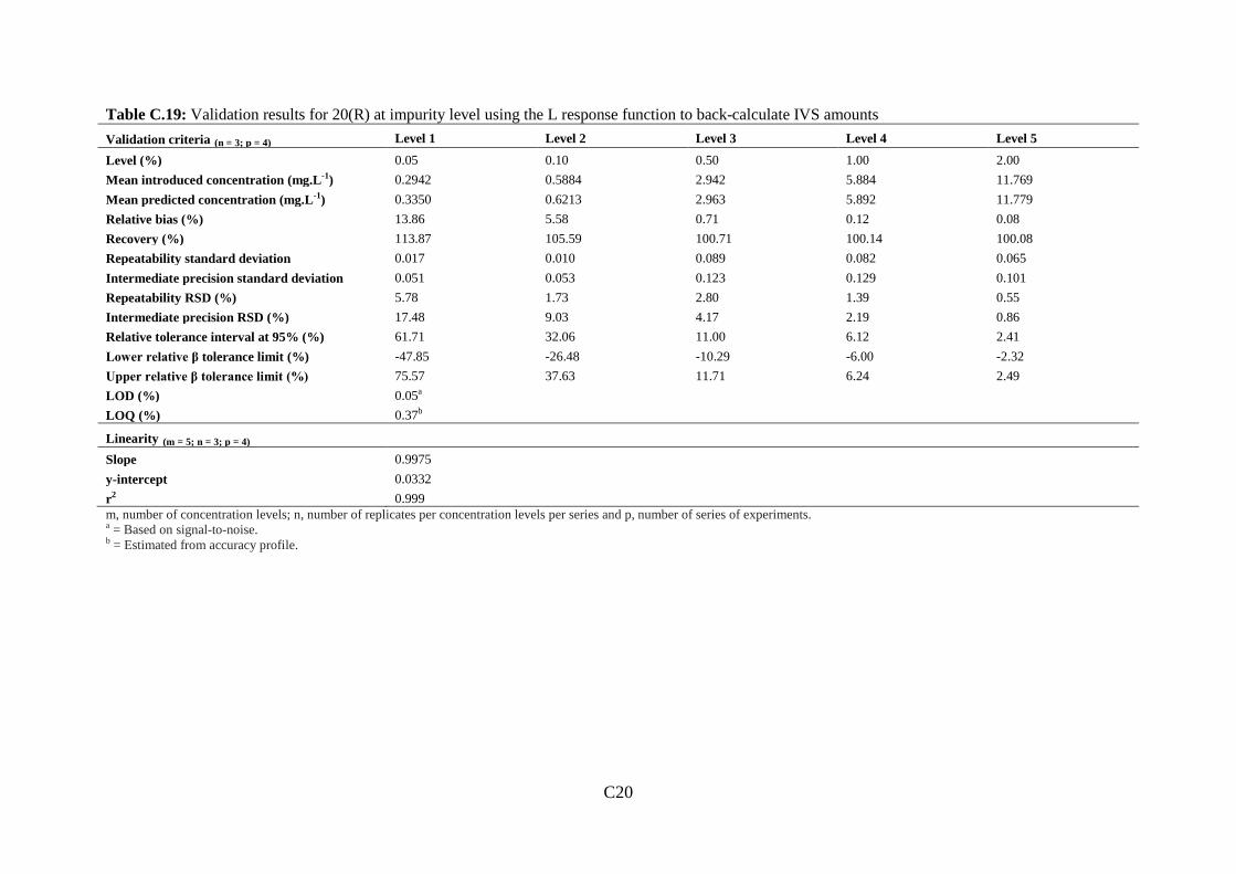
C20
Table C.19: Validation results for 20(R) at impurity level using the L response function to back-calculate IVS amounts Validation criteria (n = 3; p = 4) Level 1 Level 2 Level 3 Level 4 Level 5
Level (%) 0.05 0.10 0.50 1.00 2.00 Mean introduced concentration (mg.L-1) 0.2942 0.5884 2.942 5.884 11.769 Mean predicted concentration (mg.L-1) 0.3350 0.6213 2.963 5.892 11.779 Relative bias (%) 13.86 5.58 0.71 0.12 0.08 Recovery (%) 113.87 105.59 100.71 100.14 100.08 Repeatability standard deviation 0.017 0.010 0.089 0.082 0.065 Intermediate precision standard deviation 0.051 0.053 0.123 0.129 0.101 Repeatability RSD (%) 5.78 1.73 2.80 1.39 0.55 Intermediate precision RSD (%) 17.48 9.03 4.17 2.19 0.86 Relative tolerance interval at 95% (%) 61.71 32.06 11.00 6.12 2.41 Lower relative β tolerance limit (%) -47.85 -26.48 -10.29 -6.00 -2.32 Upper relative β tolerance limit (%) 75.57 37.63 11.71 6.24 2.49 LOD (%) 0.05a LOQ (%) 0.37b
Linearity (m = 5; n = 3; p = 4) Slope 0.9975 y-intercept 0.0332 r2 0.999 m, number of concentration levels; n, number of replicates per concentration levels per series and p, number of series of experiments. a = Based on signal-to-noise. b = Estimated from accuracy profile.
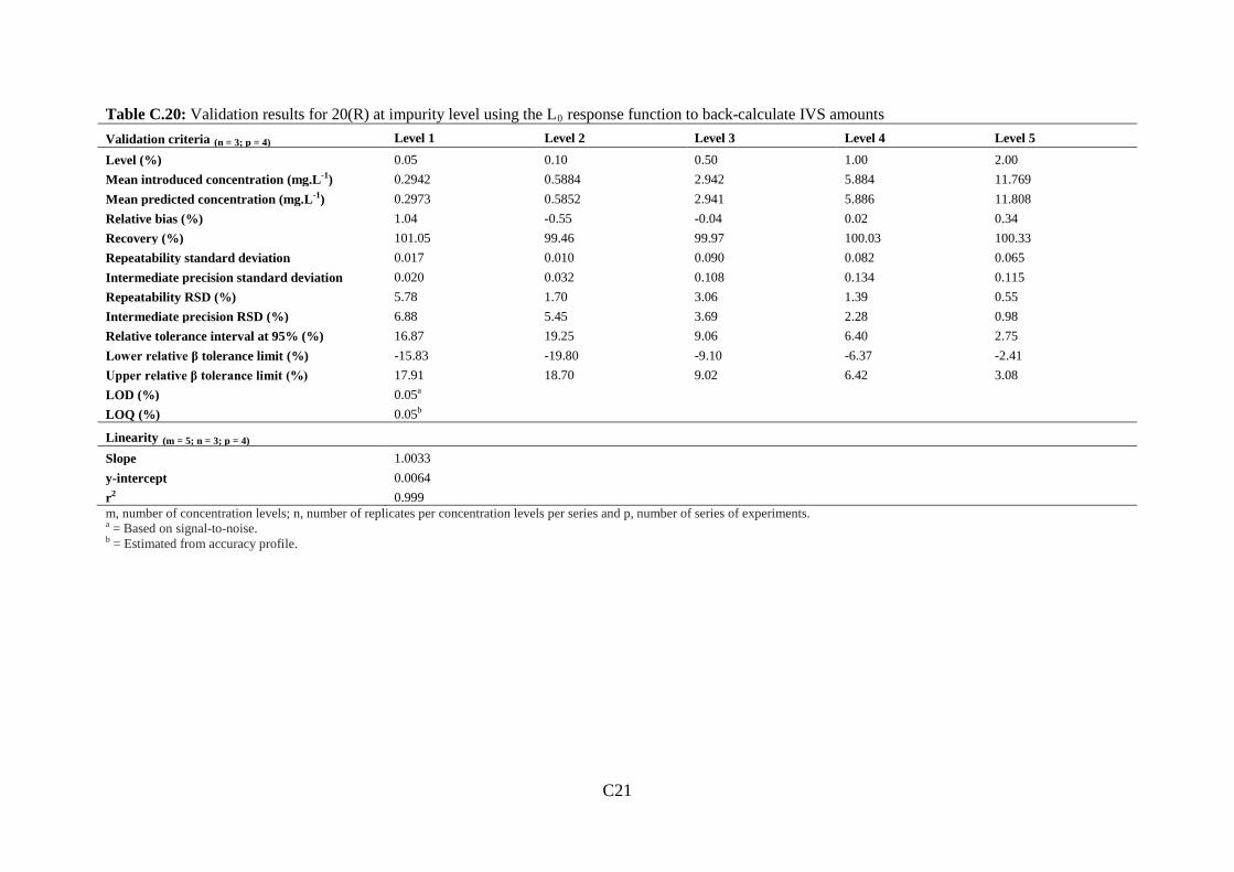
C21
Table C.20: Validation results for 20(R) at impurity level using the L0 response function to back-calculate IVS amounts Validation criteria (n = 3; p = 4) Level 1 Level 2 Level 3 Level 4 Level 5
Level (%) 0.05 0.10 0.50 1.00 2.00 Mean introduced concentration (mg.L-1) 0.2942 0.5884 2.942 5.884 11.769 Mean predicted concentration (mg.L-1) 0.2973 0.5852 2.941 5.886 11.808 Relative bias (%) 1.04 -0.55 -0.04 0.02 0.34 Recovery (%) 101.05 99.46 99.97 100.03 100.33 Repeatability standard deviation 0.017 0.010 0.090 0.082 0.065 Intermediate precision standard deviation 0.020 0.032 0.108 0.134 0.115 Repeatability RSD (%) 5.78 1.70 3.06 1.39 0.55 Intermediate precision RSD (%) 6.88 5.45 3.69 2.28 0.98 Relative tolerance interval at 95% (%) 16.87 19.25 9.06 6.40 2.75 Lower relative β tolerance limit (%) -15.83 -19.80 -9.10 -6.37 -2.41 Upper relative β tolerance limit (%) 17.91 18.70 9.02 6.42 3.08 LOD (%) 0.05a LOQ (%) 0.05b
Linearity (m = 5; n = 3; p = 4) Slope 1.0033 y-intercept 0.0064 r2 0.999 m, number of concentration levels; n, number of replicates per concentration levels per series and p, number of series of experiments. a = Based on signal-to-noise. b = Estimated from accuracy profile.

C22
Table C.21: Validation results for 20(S) at impurity level using the L response function to back-calculate IVS amounts Validation criteria (n = 3; p = 4) Level 1 Level 2 Level 3 Level 4 Level 5
Level (%) 0.05 0.10 0.50 1.00 2.00 Mean introduced concentration (mg.L-1) 0.2882 0.5763 2.882 5.763 11.526 Mean predicted concentration (mg.L-1) 0.3352 0.6083 2.931 5.799 11.549 Relative bias (%) 16.32 5.55 1.72 0.62 0.20 Recovery (%) 116.31 105.55 101.70 100.62 100.20 Repeatability standard deviation 0.018 0.013 0.092 0.072 0.063 Intermediate precision standard deviation 0.048 0.058 0.104 0.089 0.066 Repeatability RSD (%) 6.28 2.26 3.19 1.25 0.55 Intermediate precision RSD (%) 16.81 10.08 3.62 1.54 0.58 Relative tolerance interval at 95% (%) 51.68 36.75 8.67 3.81 1.34 Lower relative β tolerance limit (%) -35.36 -30.19 -6.95 -3.19 -1.15 Upper relative β tolerance limit (%) 67.99 41.30 10.40 4.42 1.54 LOD (%) 0.05a LOQ (%) 0.37b
Linearity (m = 5; n = 3; p = 4) Slope 0.9983 y-intercept 0.0445 r2 0.999 m, number of concentration levels; n, number of replicates per concentration levels per series and p, number of series of experiments. a = Based on signal-to-noise. b = Estimated from accuracy profile.

C23
Table C.22: Validation results for 20(S) at impurity level using the L0 response function to back-calculate IVS amounts Validation criteria (n = 3; p = 4) Level 1 Level 2 Level 3 Level 4 Level 5
Level (%) 0.05 0.10 0.50 1.00 2.00 Mean introduced concentration (mg.L-1) 0.2882 0.5763 2.882 5.763 11.526 Mean predicted concentration (mg.L-1) 0.2984 0.5726 2.905 5.784 11.558 Relative bias (%) 3.54 -0.65 0.82 0.36 0.28 Recovery (%) 103.54 99.36 100.80 100.36 100.28 Repeatability standard deviation 0.018 0.013 0.092 0.072 0.063 Intermediate precision standard deviation 0.023 0.042 0.096 0.082 0.111 Repeatability RSD (%) 6.25 2.26 3.19 1.25 0.55 Intermediate precision RSD (%) 8.05 7.36 3.34 1.41 0.96 Relative tolerance interval at 95% (%) 20.39 26.00 7.79 3.39 2.70 Lower relative β tolerance limit (%) -16.84 -26.65 -6.97 -3.03 -2.42 Upper relative β tolerance limit (%) 23.93 25.35 8.61 3.75 2.97 LOD (%) 0.05a LOQ (%) 0.22b
Linearity (m = 5; n = 3; p = 4) Slope 1.0024 y-intercept 0.0064 r2 0.999 m, number of concentration levels; n, number of replicates per concentration levels per series and p, number of series of experiments. a = Based on signal-to-noise. b = Estimated from accuracy profile.
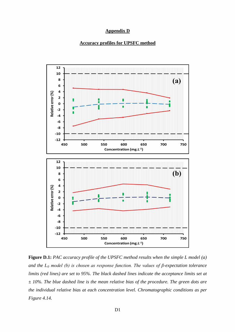
D1
Appendix D
Accuracy profiles for UPSFC method
Figure D.1: PAC accuracy profile of the UPSFC method results when the simple L model (a)
and the L0 model (b) is chosen as response function. The values of β-expectation tolerance
limits (red lines) are set to 95%. The black dashed lines indicate the acceptance limits set at
± 10%. The blue dashed line is the mean relative bias of the procedure. The green dots are
the individual relative bias at each concentration level. Chromatographic conditions as per
Figure 4.14.
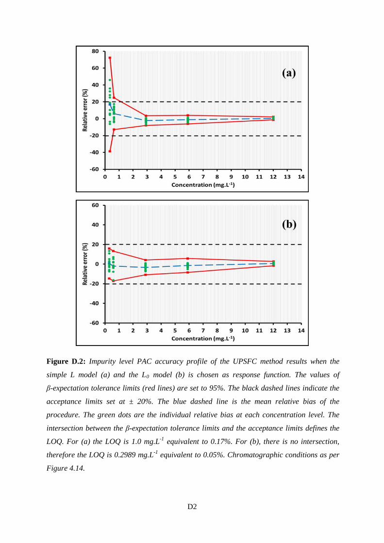
D2
Figure D.2: Impurity level PAC accuracy profile of the UPSFC method results when the
simple L model (a) and the L0 model (b) is chosen as response function. The values of
β-expectation tolerance limits (red lines) are set to 95%. The black dashed lines indicate the
acceptance limits set at ± 20%. The blue dashed line is the mean relative bias of the
procedure. The green dots are the individual relative bias at each concentration level. The
intersection between the β-expectation tolerance limits and the acceptance limits defines the
LOQ. For (a) the LOQ is 1.0 mg.L-1 equivalent to 0.17%. For (b), there is no intersection,
therefore the LOQ is 0.2989 mg.L-1 equivalent to 0.05%. Chromatographic conditions as per
Figure 4.14.
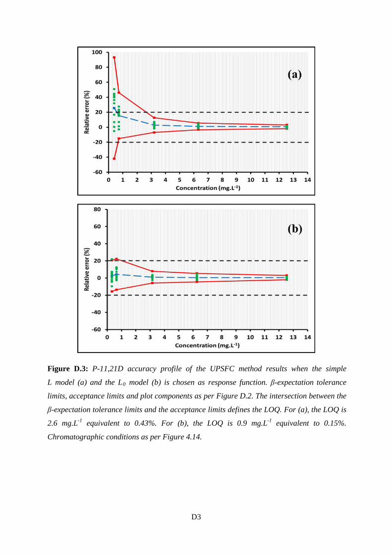
D3
Figure D.3: P-11,21D accuracy profile of the UPSFC method results when the simple
L model (a) and the L0 model (b) is chosen as response function. β-expectation tolerance
limits, acceptance limits and plot components as per Figure D.2. The intersection between the
β-expectation tolerance limits and the acceptance limits defines the LOQ. For (a), the LOQ is
2.6 mg.L-1 equivalent to 0.43%. For (b), the LOQ is 0.9 mg.L-1 equivalent to 0.15%.
Chromatographic conditions as per Figure 4.14.

D4
Figure D.4: HCA accuracy profile of the UPSFC method results when the simple L model (a)
and the L0 model (b) is chosen as response function. β-expectation tolerance limits,
acceptance limits and plot components as per Figure D.2. The intersection between the
β-expectation tolerance limits and the acceptance limits defines the LOQ. For (a), the LOQ is
3.7 mg.L-1 equivalent to 0.62%. For (b), the LOQ is 1.2 mg.L-1 equivalent to 0.20%.
Chromatographic conditions as per Figure 4.14.

D5
Figure D.5: P-17A accuracy profile of the UPSFC method results when the simple L model
(a) and the L0 model (b) is chosen as response function. β-expectation tolerance limits,
acceptance limits and plot components as per Figure D.2. The intersection between the
β-expectation tolerance limits and the acceptance limits defines the LOQ. For (a), the LOQ is
2.7 mg.L-1 equivalent to 0.45%. For (b), there is no intersection; therefore the LOQ is
0.310 mg.L-1 equivalent to 0.05%. Chromatographic conditions as per Figure 4.14.
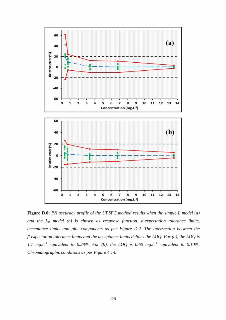
D6
Figure D.6: PN accuracy profile of the UPSFC method results when the simple L model (a)
and the L0 model (b) is chosen as response function. β-expectation tolerance limits,
acceptance limits and plot components as per Figure D.2. The intersection between the
β-expectation tolerance limits and the acceptance limits defines the LOQ. For (a), the LOQ is
1.7 mg.L-1 equivalent to 0.28%. For (b), the LOQ is 0.60 mg.L-1 equivalent to 0.10%.
Chromatographic conditions as per Figure 4.14.

D7
Figure D.7: HC accuracy profile of the UPSFC method results when the simple L model (a)
and the L0 model (b) is chosen as response function. β-expectation tolerance limits,
acceptance limits and plot components as per Figure D.2. The intersection between the
β-expectation tolerance limits and the acceptance limits defines the LOQ. For (a), the LOQ is
3.1 mg.L-1 equivalent to 0.52%. For (b), the LOQ is 0.50 mg.L-1 equivalent to 0.08%.
Chromatographic conditions as per Figure 4.14.
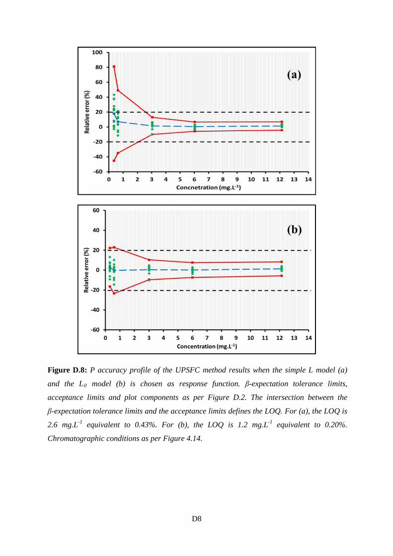
D8
Figure D.8: P accuracy profile of the UPSFC method results when the simple L model (a)
and the L0 model (b) is chosen as response function. β-expectation tolerance limits,
acceptance limits and plot components as per Figure D.2. The intersection between the
β-expectation tolerance limits and the acceptance limits defines the LOQ. For (a), the LOQ is
2.6 mg.L-1 equivalent to 0.43%. For (b), the LOQ is 1.2 mg.L-1 equivalent to 0.20%.
Chromatographic conditions as per Figure 4.14.
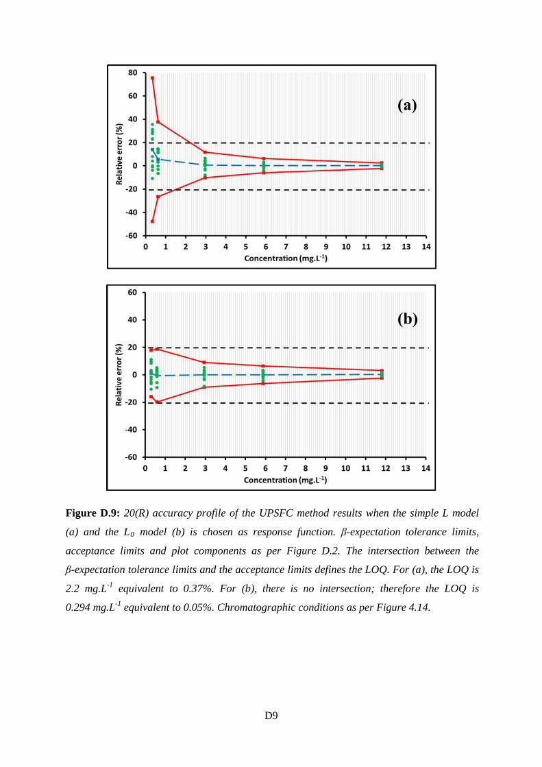
D9
Figure D.9: 20(R) accuracy profile of the UPSFC method results when the simple L model
(a) and the L0 model (b) is chosen as response function. β-expectation tolerance limits,
acceptance limits and plot components as per Figure D.2. The intersection between the
β-expectation tolerance limits and the acceptance limits defines the LOQ. For (a), the LOQ is
2.2 mg.L-1 equivalent to 0.37%. For (b), there is no intersection; therefore the LOQ is
0.294 mg.L-1 equivalent to 0.05%. Chromatographic conditions as per Figure 4.14.
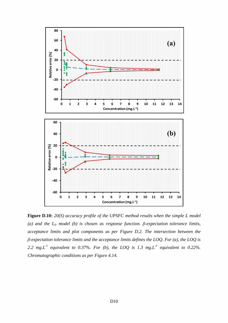
D10
Figure D.10: 20(S) accuracy profile of the UPSFC method results when the simple L model
(a) and the L0 model (b) is chosen as response function. β-expectation tolerance limits,
acceptance limits and plot components as per Figure D.2. The intersection between the
β-expectation tolerance limits and the acceptance limits defines the LOQ. For (a), the LOQ is
2.2 mg.L-1 equivalent to 0.37%. For (b), the LOQ is 1.3 mg.L-1 equivalent to 0.22%.
Chromatographic conditions as per Figure 4.14.
Related Documents

![Achiral and chiral, C2-symmetric bicyclic guanidinates ... · achiral and chiral, c2-symmetric bicyclic guanidinates based on 1,5,7-triazabicyclo[4.4.0.]dec-5-ene as ligands in high-](https://static.cupdf.com/doc/110x72/5b4240027f8b9a2e058b770b/achiral-and-chiral-c2-symmetric-bicyclic-guanidinates-achiral-and-chiral.jpg)