i Development of an Inventory Policy Based on EOQ Model in a Dyeing Unit: A Case Study By Mst. Morium Perveen A thesis work submitted to the Department of Industrial and Production Engineering, Bangladesh University of Engineering and Technology (BUET), in partial fulfillment of the requirements for the degree Master of Engineering in Advanced Engineering Management (AEM). DEPARTMENT OF INDUSTRIAL AND PRODUCTION ENGINEERING BANGLADESH UNIVERSITY OF ENGINEERING AND TECHNOLOGY DHAKA-1000, BANGLADESH JUNE, 2015

Welcome message from author
This document is posted to help you gain knowledge. Please leave a comment to let me know what you think about it! Share it to your friends and learn new things together.
Transcript

i
Development of an Inventory Policy Based on EOQ Model in a Dyeing Unit:
A Case Study
By
Mst. Morium Perveen
A thesis work submitted to the Department of Industrial and Production Engineering,
Bangladesh University of Engineering and Technology (BUET), in partial fulfillment of the
requirements for the degree Master of Engineering in Advanced Engineering Management
(AEM).
DEPARTMENT OF INDUSTRIAL AND PRODUCTION ENGINEERING BANGLADESH UNIVERSITY OF ENGINEERING AND TECHNOLOGY
DHAKA-1000, BANGLADESH
JUNE, 2015

ii
CERTIFICATE OF APPROVAL
The thesis titled Development of an Inventory Policy based on EOQ Model in a Dyeing
Unit: A Case Study submitted by Mst. Morium Perveen, Roll No. 0409082108, Session-
April, 2009 has been accepted as satisfactory in partial fulfillment of the requirements for
the degree of Master of Engineering in Advanced Engineering Management (AEM) on June,
2015.
BOARD OF EXAMINERS
1.___________________________ Dr. Shuva Ghosh Chairman Assistant Professor (Supervisor) Department of Industrial and Production Engineering Bangladesh University of Engineering and Technology Dhaka-1000, Bangladesh
2.___________________________ Dr. Sultana Parveen Member Professor and Head Department of Industrial and Production Engineering Bangladesh University of Engineering and Technology Dhaka-1000, Bangladesh
3.___________________________ Dr. Ferdous Sarwar Member Assistant Professor Department of Industrial and Production Engineering Bangladesh University of Engineering and Technology Dhaka-1000, Bangladesh

iii
CANDIDATE’S DECLARATION It is hereby declared that this thesis or any part of this has not been submitted elsewhere for the award of any degree or diploma except for publication.
_________________ Mst. Morium Perveen

iv
ACKNOWLEDGEMENT My gratitude earnestly goes first to almighty Allah Taala, the most merciful, and the most beneficent. Without the help from Allah nothing can come true.
I acknowledge my profound indebtedness and express sincere gratitude to my supervisor Dr. Shuva Ghosh, Assistant Professor, Department of Industrial and Production Engineering (IPE), BUET, Dhaka. He provided proper guidance, supervision and valuable suggestions at all stages to carry out this research work. I am proud to have him as my supervisor for Master’s thesis. I also express my gratitude to Dr. Sultana Parveen, Head of the Dept. for her valuable suggestions and guidelines time to time.
I would also like to thank employee of Reedisha Knitex Ltd. for providing necessary support, information and data for the analysis part of my project.
Finally, I wish to express my heartiest gratitude to my teachers at the Department of Industrial & Production Engineering (IPE), BUET and to all my colleagues, friends and family members who helped me directly or indirectly in this work.
v
ABSTRACT
Many firms/industries, whether manufacturing or purchasing, face great challenges in
managing inventories. Poor inventory management may result in under-stocking, over-
stocking as well as high inventory total cost. The study examines inventory situation at
Dyeing unit of Reedisha Knittex Ltd. Gazipur, Bangladesh. For Reedisha two inventory
problems, stock-out and overstock occur frequently. The company wants to improve its
efficiency and is considering a change in the inventory management. The objectives of this
thesis work is to develop inventory management system of Dyeing section by using
Economic Order Quantity (EOQ) model that will determine number of units of an item to
order at a time and the re-order point (r), that is the level to which stocks of items are
allowed to fall before ordering other items, for raw materials. The resulting EOQ for each
raw material is compared to the actual ordered quantities so as to see whether there is any
relationship between them in operational cost reduction. For variable demand over the
period Wagner-Whitin Algorithm is used to determine ordering schedule of the items. By
comparing ordering cost and holding cost for each item it is determined when to order and
how much to order at a time. The study used cross sectional secondary data from Reedisha
Knitex. Excel was used to find EOQ and the re-order point. After doing analysis and
calculation of the data, it was concluded that the ordered quantities at Reedisha Knitex Ltd.
were not optimal. Therefore, it is recommended that in order to manage inventory
effectively, Reedisha needs to employ inventory control methods such as the EOQ model to
obtain reasonable ordered quantities for its raw materials.

vi
TABLE OF CONTENTS
Topics Page
Certificate of Approval ii
Candidates Declaration iii
Acknowledgement iv
Abstract v
Table of Contents vi
List of Tables ix
List of Figures x
Chapter 1: Introduction 1-3
1.1 Introduction 1
1.2 Background of the study 2
1.3 Objectives of the study 3
1.4 Disposition 3
Chapter 2: Literature Review 4-28
2.1 Supply Chain Management 4
2.2 Inventory Management 5
2.2.1 Functions of Inventory 6
2.2.2 Types of Inventory 6
2.2.3 Demand Management 7
2.2.4 Demand Forecast 8
2.2.5 Stock Out 9
2.2.6 Safety Stock 9
2.2.7 Inventory Turnover Ratio 10
vii
Topics Page
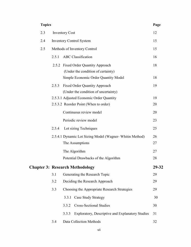
2.3 Inventory Cost 12
2.4 Inventory Control System 15
2.5 Methods of Inventory Control 15
2.5.1 ABC Classification 16
2.5.2 Fixed Order Quantity Approach 18
(Under the condition of certainty)
Simple Economic Order Quantity Model 18
2.5.3 Fixed Order Quantity Approach 19
(Under the condition of uncertainty)
2.5.3.1 Adjusted Economic Order Quantity 19
2.5.3.2 Reorder Point (When to order) 20
Continuous review model 20
Periodic review model 23
2.5.4 Lot sizing Techniques 25
2.5.4.1 Dynamic Lot Sizing Model (Wagner- Whitin Method) 26
The Assumptions 27
The Algorithm 27
Potential Drawbacks of the Algorithm 28
Chapter 3: Research Methodology 29-32 3.1 Generating the Research Topic 29
3.2 Deciding the Research Approach 29
3.3 Choosing the Appropriate Research Strategies 29
3.3.1 Case Study Strategy 30
3.3.2 Cross-Sectional Studies 30
3.3.3 Exploratory, Descriptive and Explanatory Studies 31
3.4 Data Collection Methods 32

viii
Topics Page
Chapter 4: Case Study 33-37
4.1 Company Profile 33
4.2 Production Zone 34
4.3 Dyes and Chemicals Receiving Process 37
Chapter 5: Analysis and Findings 40-67
5.1 Classifying Inventory (ABC Analysis) 40
Calculation on ABC analysis 44
5.2 Selecting Inventory Methods 46
5.2.1 Economic Order Quantity (EOQ) Model 46
Calculation on EOQ 47
5.2.2 The Total Cost Function 49
Calculation on Total cost for EOQ 50
Calculation on Total cost for non EOQ 53
5.2.3 Reorder Points: (How much to Order) 54
Calculation on Reorder point 56
5.2.4 Dynamic Lot Sizing Technique (Wagner-Whitin Method) 57
Calculation on Wagner-Whitin method 67
Chapter 6: Conclusion and Recommendation 71-72
6.1 Conclusion 71
6.2 Recommendation 72
6.3 Limitation of the Study 72
References 77
Appendices 79-83
Appendix 1 Annual consumption report for twenty items in 2013 79
Appendix 2 Questionnaires 83
ix
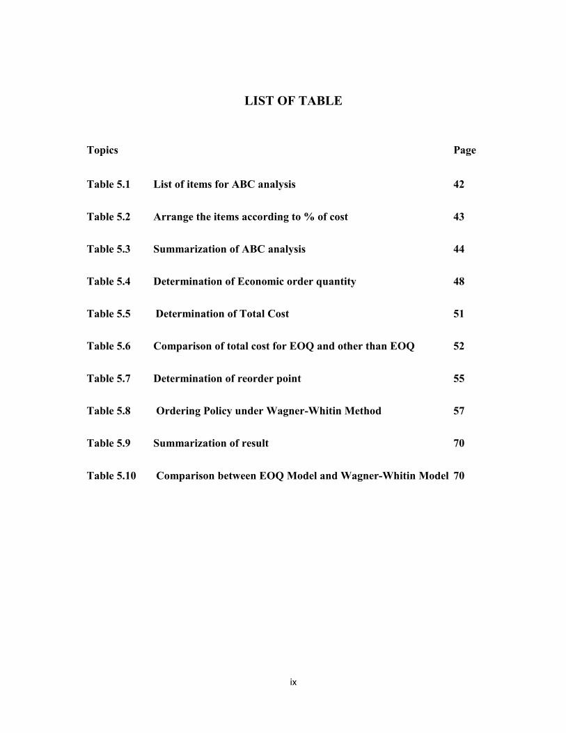
LIST OF TABLE
Topics Page
Table 5.1 List of items for ABC analysis 42
Table 5.2 Arrange the items according to % of cost 43
Table 5.3 Summarization of ABC analysis 44
Table 5.4 Determination of Economic order quantity 48
Table 5.5 Determination of Total Cost 51
Table 5.6 Comparison of total cost for EOQ and other than EOQ 52
Table 5.7 Determination of reorder point 55
Table 5.8 Ordering Policy under Wagner-Whitin Method 57
Table 5.9 Summarization of result 70
Table 5.10 Comparison between EOQ Model and Wagner-Whitin Model 70

x
LIST OF FIGURES
Topics Page
Figure 2.1 Saving inventory dollar by increasing inventory turns 11
Figure 2.2 What costs go into inventory carrying cost? 14
Figure 2.3 Graphical representation of ABC analysis 17
Figure 2.4 Inventory level in a continuous review model 21
Figure 2.5 ROP with safety stock 22
Figure 2.6 Inventory level in a periodic review model 24
Figure 4.1 Process flow chart of Dyeing Unit 38
Figure 4.2 Organ gram of Dyeing Unit 39
Figure 5.1 Graphic representation of ABC analysis 45
Figure 5.2 Typical representation of ABC analysis 45
Figure 5.3 Inventory usage over time 46
Figure 5.4 Total cost as a function of order quantity 50
Figure 5.5 Reorder point 54
Figure 6 Main Chemical Store of Reedisha Knittex Ltd 73
Figure 7 Stock of Chemical of Felosan NOF 74
Figure 8 Stock of Chemical of Crosoft NBC 75
Figure 9 Stock of Chemical of Leucophor BMB 76
1

1
CHAPTER ONE INTRODUCTION
1.1 Introduction Inventory management is pivotal in effective and efficient organization. It is also vital in the
control of materials and goods that have to be held (or stored) for later use in the case of
production or later exchange activities in the case of services. The principal goal of
inventory management involves having to balance the conflicting economics of not wanting
to hold too much stock. Thereby having to tie up capital so as to guide against the incurring
of costs such as storage, spoilage, pilferage and obsolescence and, the desire to make items
or goods available when and where required (quality and quantity wise) so as to avert the
cost of not meeting such requirement. Inventory problems of too great or too small
quantities on hand can cause business failures. If a manufacturer experiences stock-out of a
critical inventory item, production halts could result. Moreover, a shopper expects the
retailer to carry the item wanted. If an item is not stocked when the customer thinks it should
be, the retailer loses a customer not only on that item but also on many other items in the
future. The conclusion one might draw is that effective inventory management can make a
significant contribution to a company’s profit as well as increase its return on total assets. It
is thus the management of this economics of stockholding, that is appropriately being refers
to as inventory management. The reason for greater attention to inventory management is
that this figure, for many firms, is the largest item appearing on the asset side of the balance
sheet. Essentially, inventory management, within the context of the foregoing features
involves planning and control. The planning aspect involves looking ahead in terms of the
determination in advance:
What quantity of items to order;
How often (periodicity) do we order for them to maintain the overall source-store
sink coordination in an economically efficient way?
The control aspect, which is often described as stock control involves following the
procedure, set up at the planning stage to achieve the above objective. This may include
monitoring stock levels periodically or continuously and deciding what to do on the basis of
information that is gathered and adequately processed. Effort must be made by the

2
management of any organization to strike an optimum investment in inventory since it costs
much money to tie down capital in excess inventory.
1.2 Background of the Study The readymade garment (RMG) industry, a very important segment in Bangladesh’s
manufacturing industry, is playing a critical role in its economic development. The RMG
industry plays an important role in satisfying our local demand and also contributes a huge
part in our overall export. In 2011-12, amount of export earnings from RMG sector is over
USD17.9 billion which is about 77% of total export earnings of this country and it
contributes 13% of our total GDP. The RMG industry has played an important role in
Bangladesh’s economy for a long time. Currently, the RMG industry in Bangladesh
accounts for 45 percent of all industrial employment and contributes 5 percent to the total
national income. The industry employs nearly 4 million people, mostly women.
The RMG industries have difficulties in matching its supply with production requirements.
There are both stock-out of inventoriable items and excess inventory. Both situations impact
the profitability negatively. It is considered that the problem results from insufficient control
over inventory and volatile demand of some product and another reason is that the lead-time
of most products is long about three months at the longest. The root cause of this problem is
that industry does not use optimum inventory policy. Optimum order quantity and re-order
point need to be determined.
In a composite RMG unit there are six major sections: spinning, weaving/knitting, dyeing,
cutting, sewing and finishing. Our focus will be in dyeing unit only as there are all the raw
materials are imported from abroad. So, huge amount of dollar value is associated with it.
The purpose of this thesis project is to investigate and identify the reasons behind the
inefficient inventory management in a Dyeing unit. To do this at first we categorized the
item on priority basis and then perform cost analysis of the items. Then we would develop
an inventory policy to improve the unit’s inventory management based on EOQ model, after
examining the relevant theories and understanding the business operational practices.

3
1.3 Objectives of the Study
The specific objectives of the present research work are as follows:
To develop an inventory system.
To find an optimal re-order level to decide when items should be ordered.
To compare existing inventory cost with the expected inventory cost for the proposed
model.
1.4 Disposition
Chapter 1: The first chapter gives an introduction and background of this study.
Furthermore it gives an explanation of company’s problems. Then the research questions
and purpose of this thesis are presented.
Chapter 2: This chapter will explore the different theories and models that are related to the
subject of this thesis and can be used for the analysis.
Chapter 3: This chapter will examine different research methods and present what methods
are applied to this thesis.
Chapter 4: The authors will present their empirical findings about business practice of the
studied company and the major issues that needs to be addressed in their inventory
management.
Chapter 5: This chapter will conduct the analysis guided by theoretical framework. The
analysis part is based on our empirical findings. Furthermore, the authors will present their
suggestions upon the problems identified.
Chapter 6: This chapter carries out the conclusion about the whole thesis and summarizes
the implications of the research.

4
CHAPTER 2 LITERATURE REVIEW
2.1 Supply Chain Management (SCM)
Many theorists have given the definitions for the term supply chain management. One of
them that can describe the term supply chain management really well and it seems to cover
all related activities is that; Supply chain management is a set of approaches utilized to
efficiently integrate suppliers, manufacturers, warehouses and stores, so that merchandise is
produced and distributed at the right quantities, to the right locations, and at the right time,
in order to minimize system-wise costs while satisfying service level requirements.
As the definition implies, supply chain management has been developed for customers who
play the most important role in businesses. Especially in this globalization era, customers,
ever more demanding and powerful than before, are seeking for products and services with
higher criteria. In order to meet customers’ requirements and satisfactions, companies have
to be proactive against globalized markets which can be changed and influenced by several
factors. With an increase of use of technology like internet, some claim that there is no more
geography in business nowadays. Offshore production, collaboration between international
companies, and openness of the global market are the significance of the global
environment. Supply chain management can therefore be labeled as global supply chain
management in today’s environment.
Based on the concept of supply chain management, it requires integration of many business
components. In 1985, Michael Porter introduced and described his new concept for business
management, the value chain. The concept of value chain has developed as a tool for
competitive analysis and strategy. It is comprised of inbound and outbound logistics which
are the primary components of this business model. The more integrated marketing, sales
and production are also the important jigsaws that contribute value to firm’s customers.
2.1.1 Push System Push system is referred when raw materials are stored before production and products are
produced to stock before orders are placed. The action is stimulated by demand estimation
or demand forecast. Products and information flow the same way, from seller to buyer.

5
Communication carried out in the supply chain of this approach can be either interactive or
non-interactive since customers or buyers do not always response to messages sent by
producer or sellers. For example, there is no direct feedback from customers after message
in advertisement was sent by vendors through media channels. Push system, typical and
traditional, is still widely utilized by many firms in different industries.
2.1.2 Pull System Pull system, on the other hand, is used in response to confirmed orders. Products are
produced after or at production planning stage. Therefore, stock does not contain finished
goods, but semi-finished materials. Customers send their requirements and place orders to
producers or sellers. The requested product is pulled through the delivery channel.
Communication carried out in pull system is usually interactive. Pull model is also widely
used inside the same firm, for instance, a department sends an internal order to the other
department to manufacturer an item that is needed in their work process.
Pull system includes just-in-time (JIT) which is an inventory strategy to improve business
‟inventory turnover” by bringing inventory to a minimum. JIT strategy considers inventory
as waste, its emphasis therefore is ensure that supplies are delivered at when and to where
they are needed.
2.2 Inventory Management Inventory management is a science primarily about specifying the shape and percentage of
stocked goods. It is required at different locations within a facility or within many locations
of a supply network to precede the regular and planned course of production and stock of
materials. The scope of inventory management concerns the fine lines between
replenishment lead time, carrying costs of inventory, asset management, inventory
forecasting, inventory valuation, inventory visibility, future inventory price forecasting,
physical inventory, available physical space for inventory, quality management,
replenishment, returns and defective goods, and demand forecasting. Balancing these
competing requirements leads to optimal inventory levels, which is an on-going process as
the business needs shift and react to the wider environment.
Inventory control is challenging in business. Managing inventory control can directly affect
business performance. The reason for having inventories or stocks is to buffer against
6
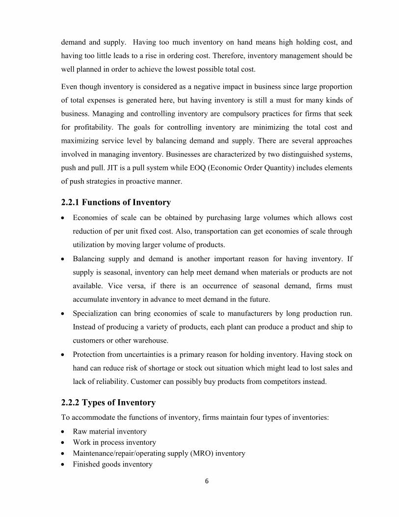
demand and supply. Having too much inventory on hand means high holding cost, and
having too little leads to a rise in ordering cost. Therefore, inventory management should be
well planned in order to achieve the lowest possible total cost.
Even though inventory is considered as a negative impact in business since large proportion
of total expenses is generated here, but having inventory is still a must for many kinds of
business. Managing and controlling inventory are compulsory practices for firms that seek
for profitability. The goals for controlling inventory are minimizing the total cost and
maximizing service level by balancing demand and supply. There are several approaches
involved in managing inventory. Businesses are characterized by two distinguished systems,
push and pull. JIT is a pull system while EOQ (Economic Order Quantity) includes elements
of push strategies in proactive manner.
2.2.1 Functions of Inventory
Economies of scale can be obtained by purchasing large volumes which allows cost
reduction of per unit fixed cost. Also, transportation can get economies of scale through
utilization by moving larger volume of products.
Balancing supply and demand is another important reason for having inventory. If
supply is seasonal, inventory can help meet demand when materials or products are not
available. Vice versa, if there is an occurrence of seasonal demand, firms must
accumulate inventory in advance to meet demand in the future.
Specialization can bring economies of scale to manufacturers by long production run.
Instead of producing a variety of products, each plant can produce a product and ship to
customers or other warehouse.
Protection from uncertainties is a primary reason for holding inventory. Having stock on
hand can reduce risk of shortage or stock out situation which might lead to lost sales and
lack of reliability. Customer can possibly buy products from competitors instead.
2.2.2 Types of Inventory To accommodate the functions of inventory, firms maintain four types of inventories:
Raw material inventory Work in process inventory Maintenance/repair/operating supply (MRO) inventory Finished goods inventory

7
Raw material inventory
Raw material is the basic material that is processed and converted into finished goods. The
cost incurred to obtain raw materials that have not yet been placed into production is
reported as raw materials inventory in the current assets section of the balance sheet.
Examples of raw materials include wood for the manufacturers of cricket bat and steel for
the manufacturers of cars.
Work-in-process inventory:
The units that remain incomplete at the end of a period are known as work-in-process
inventory. These units need the addition of more materials, labor or manufacturing overhead
to be completed in the coming period. Like raw materials, work-in-process inventory is
reported in the current assets section of the balance sheet.
Maintenance/repair/operating supply (MRO) inventory:
MRO supplies are necessary to keep machinery and processes productive. They exist
because the need and timing for maintenance and repair of some equipment are unknown.
Although the demand for MRO inventory is often a function of maintenance schedules,
other unscheduled MRO demands must be anticipated.
Finished goods inventory:
Finished goods are completed but unsold goods. The total cost incurred to complete these
unsold goods are reported as finished goods inventory along with raw materials and work-
in-process inventory in the current assets section of the balance sheet.
2.2.3 Demand Management Demand management may be thought of as “focused efforts to estimate and manage
customers’ demand, with the intention of using this information to shape operating
decision.” Inventory Management deals essentially with balancing the inventory levels.
Inventory is categorized into two types based on the demand pattern, which creates the need
for inventory. The two types of demand are Independent Demand and Dependent Demand
for inventories.
Independent Demand
An inventory of an item is said to be falling into the category of independent demand when
the demand for such an item is not dependent upon the demand for another item. Finished

8
goods Items, which are ordered by External Customers or manufactured for stock and sale,
are called independent demand items. Independent demands for inventories are based on
confirmed Customer orders, forecasts, estimates and past historical data.
Dependent Demand
If the demand for inventory of an item is dependent upon another item, such demands are
categorized as dependent demand. Raw materials and component inventories are dependent
upon the demand for Finished Goods and hence can be called as Dependent demand
inventories.
2.2.4 Demand Forecast The sales forecast is particularly important as it is the foundation upon which all company
plans are built in terms of markets and revenue. Management would be a simple matter if
business was not in a continual state of change, the pace of which has quickened in recent
years. It is becoming increasingly important and necessary for business to predict their
future prospects in terms of sales, cost and profits. The value of future sales is crucial as it
affects costs profits, so the prediction of future sales is the logical starting point of all
business planning.
Sufficient data result in more effective forecasts. The traditional way to forecast demand is
to refer to the historical record of demand. All forecasting techniques are characterized by
the fact that the more data are observed, the more we modify the estimates of the average
demand and demand variability, and the more accurate these predictions can be (Simchi-
Levi et al., 2004). Of course, forecasts are never completely accurate. Indeed, the following
rules of forecasting hold:
The forecast is always wrong. It is very unlikely that actual demand will exactly equal
forecast demand.
The longer the forecast horizon, the worse is the forecast. A forecast of demand far in
the future is likely to be less accurate than a forecast of near-future demand.
Aggregate forecasts are more accurate.

9
2.2.5 Stock-out A stock out or out-of-stock (OOS) event is an event that causes inventory to be exhausted.
While out-of stocks can occur along the entire supply chain, the most visible kinds are retail
out-of-stocks in the fast moving consumer goods industry (e.g., sweets, diapers, fruits).
Stock outs are the opposite of overstocks, where too much inventory is retained. Out-of-
stock inventory does not necessarily indicate that a seller is doing poorly, and in fact, it can
be a good sign for the business if inventory is managed well. Out-of-stock inventory is
sometimes called backordered inventory if orders are placed for an item before the new
inventory supply arrives. Out-of-stock inventory also sometimes happens because of
business or manufacturing problems regardless of the market. For instance, a bad snow
storm might delay a shipment or a robot on an assembly line might break down.
Advantages
An advantage of out-of-stock inventory is that it allows the seller to continue doing business
even if he physically does not have the item he is selling. For instance, he can alert buyers of
the out-of-stock status and then let them purchase the item on backorder, provided he knows
he can get more of the item. This can save seller money, because he does not need to reprint
advertisements; instead of removing and adding every out-of-stock inventory item on a
website, he can just note the change in status. Having out-of-stock inventory sometimes
means that a seller is doing well, as he is able to sell the entire inventory he has on hand.
Disadvantages
Handling out-of-stock inventory can complicate the inventory tracking process, as customers
may continue to place orders for items the seller has yet to receive. The seller also has to
deal with inquiries about the out-of-stock items, such as when the seller expects to have
more of the item. Additionally, listing an item as out of stock sometimes costs a seller a sale,
as buyers opt not to backorder and simply go to another vendor who does have the item
readily available.
2.2.6 Safety Stock Safety stock is the stock held by a company in excess of its requirement for the lead time.
Companies hold safety stock to guard against stock-out. The term Safety stock (also called
buffer stock) is used by logisticians to describe a level of extra stock that is maintained to
mitigate risk of stock outs (shortfall in raw material or packaging) due to uncertainties in
10
supply and demand. Adequate safety stock levels permit business operations to proceed
according to their plans. Safety stock is held when there is uncertainty in demand, supply, or
manufacturing yield; it serves as an insurance against stock outs. The amount of safety stock
an organization chooses to keep on hand can dramatically affect their business. Too much
safety stock can result in high holding costs of inventory. In addition, products which are
stored for too long a time can spoil, expire, or break during the warehousing process. Too
little safety stock can result in lost sales and, thus, a higher rate of customer turnover. As a
result, finding the right balance between too much and too little safety stock is essential.
Safety stock is calculated using the following formula:
Safety Stock = (Maximum Daily Usage − Average Daily Usage) × Lead Time Lead time is the time which supplier takes in ordering the items.
Safety stock may be calculated in another way. Safety Stock, SS = z𝝈𝑳 Where, z = Number of standard deviations for a specified service probability 𝜎𝐿 = Standard deviation of usage during lead time
2.2.7 Inventory Turnover Ratio The inventory turnover ratio is an efficiency ratio that shows how effectively inventory is
managed by comparing cost of goods sold with average inventory for a period. This
measures how many times average inventory is "turned" or sold during a period. In other
words, it measures how many times a company sold its total average inventory dollar
amount during the year. A company with $1,000 of average inventory and sales of $10,000
effectively sold its 10 times over.
This ratio is important because total turnover depends on two main components of
performance. The first component is stock purchasing. If larger amounts of inventory are
purchased during the year, the company will have to sell greater amounts of inventory to
improve its turnover. If the company can't sell these greater amounts of inventory, it will
incur storage costs and other holding costs. The second component is sales. Sales have to
match inventory purchases otherwise the inventory will not turn effectively. That's why the
purchasing and sales departments must be in tune with each other. The inventory turnover
ratio is calculated by dividing the cost of goods sold for a period by the average inventory
for that period.
Inventory Turnover =Cost of Goods Sold/Average Inventory
11
Cost of goods sold figure is obtained from the income of a business whereas average
inventory is calculated as the sum of the inventory at the beginning and at the end of the
period divided by 2. The values of beginning and ending inventory are obtained from the
sheets at the start and at the end of the accounting period.
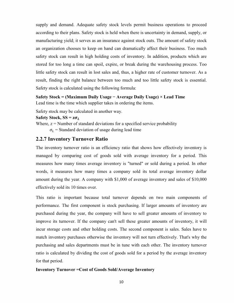
Inventory turnover ratio is used to measure the inventory management efficiency of a
business. In general, a higher value of inventory turnover indicates better performance and
lower value means inefficiency in controlling inventory levels. A lower inventory turnover
ratio may be an indication of over-stocking which may pose risk of obsolescence and
increased inventory holding costs. However, a very high value of this ratio may be
accompanied by loss of sales due to inventory shortage. Inventory turnover is different for
different industries. Businesses which trade perishable goods have very higher turnover
compared to those dealing in durables. Hence a comparison would only be fair if made
between businesses of same industry.
Fig: 2.1: Saving inventory dollar by increasing inventory turns

12
2.3 Inventory Costs Inventory costs are the costs related to storing and maintaining its inventory over a certain
period of time. Typically, inventory costs are described as a percentage of the inventory
value (annual average inventory, i.e. for a retailer the average of the goods bought to its
suppliers during a year) on an annualized basis. They vary strongly depending on the
business field, but they are always quite high. It is commonly accepted that the carrying
costs alone represent generally 25% of inventory value on hand. Inventory is associated with
three major costs as follows.
Ordering Cost (also called setup cost):
Holding Cost (also called carrying cost) Stock out (also called shortage cost)
Ordering Cost:
The ordering cost (also called setup costs, especially when producers are concerned), or cost
of replenishing inventory, covers the friction created by orders themselves, that is, the costs
incurred every time you place an order. These costs can be split in two parts:
The cost of the ordering process itself: it can be considered as a fixed cost,
independent of the number of units ordered. It typically includes fees for placing the
order, and all kinds of clerical costs related to invoice processing, accounting, or
communication.
The inbound logistics costs, related to transportation and reception (unloading and
inspecting). Those costs are variable. Then, the supplier’s shipping cost is dependent on
the total volume ordered, thus producing sometimes strong variations on the cost per unit
of order.
There are ways to try to minimize those costs, more precisely to determine the right trade-
off of carrying costs vs. volume discounts, thus essentially balancing the cost of ordering too
much and the cost of ordering too less (basically, a smaller inventory typically leads to more
orders, which means higher ordering costs, but is also implies lower carrying costs).

13
Holding or Carrying Cost: There are costs associated with holding all inventories, and the costs go beyond the
expenditure of the inventory investment, inventory carrying costs form an interesting
concept, representing both accounting costs and economic costs. Accounting costs are
explicit and call for a cash payment. Economic costs are implicit, not necessarily involving
an outlay but rather an opportunity cost.
Inventory Carrying Cost in Summary Total inventory carrying cost can be estimated at …..
Types of Cost Percentage Cost of money 6% - 12%
Taxes 2% - 6% Insurance 1% - 3%
Warehouse Expenses 2% - 5% Physical Handling 2% - 5%
Clerical & Inventory Control 3% - 6% Obsolescence 6% - 12%
Deterioration & Pilferage 3% - 6% Total 25% - 55%

14
Figure 2.2: Components of inventory carrying cost Source: Goldsby t al., 2005

15
2.4 Inventory Control System
An inventory system is a structure for controlling the level of inventory by determining how
much to order (the level of replenishment) and when to order. There are two basic types of
inventory system:
1. Continuous or fixed order quantity system (Q system)
2. Periodic or fixed time period system (P system)
Continuous inventory system:
In a continuous inventory system (alternatively referred as a perpetual system or fixed
order quantity system) a constant amount is ordered when inventory declines to a
predetermined level, referred to as the reorder point.
This fixed order quantity is called the economic order quantity.
The inventory level is closely and continuously monitored so that management always
knows the inventory status.
However, the cost of maintaining a continual record of the amount of inventory on hand
can also be a disadvantage of this type of system.
Periodic Inventory System
Fixed time period system. An order is placed for a variable amount.
The inventory level is not monitored at all during the time interval between orders.
It has the advantage of requiring little or no record keeping.
It has the disadvantage of less direct control after a fixed passage of time
2.5 Methods of Inventory Control
Many approaches are used in order to control inventory. Choosing a method to use in
business must be carefully considered and analyzed based on its comprehensiveness. In a
textile industry, there are several methods employed to control inventory and to facilitate
procurement’s policy. Each method has different objectives and procedures. Selecting and
utilizing methods of inventory control depends on feasibility and suitability. Several factors
are involved in making decision regarding utilization of inventory methods such as, budget,
technology and personnel. Methods of inventory control are summarized as follows:

16
2.5.1 ABC Classification
ABC analysis is one the most widely used tool for materials management. It is also known
as Paretos Law or “80–20 Rule”. This classification has been conducted and developed by
Vilfredo Pareto, an Italian philosopher and economist. He observed that a very large
percentage of total national income and wealth was concentrated on a small percentage of
population. This rule of thumb expresses that 80 % of total value is accounted by 20 % of
items. This analysis is considered a universal principle. It is therefore widely used in many
situations of businesses.
Class A represents 20 % of materials in inventory and 70 % of the inventory value.
Class B represents 30 % of materials in inventory and 20 % of the inventory value.
Class C represents 50 % of material in inventory and only 10 % of inventory value.
According to ABC classification, it suggests that the more analysis should be applied to
materials with high inventory value. Class A should be most extensively handled and Class
C is analyzed little. Advantage of ABC classification is that controlling small numbers of
items amounting to 10-20 % will result in the control of 75-80 % of the monetary value of
the inventory held.
If items in the inventory are not classified, managing and handling materials would be very
expensive since equal attention is given to all items. Having classified the inventory,
different levels of control can be assigned to items in the different classes.
Very strict control procedures should be used with A items and the controller should have
great authority. Inventory held in safety stock should be very low or none compensated with
more frequent order placements. Consumption control and product movement should be
reviewed regularly – weekly or daily. Number of sources for high valued items should be
increase in order to ensure good supplier performance and reduction in lead time. Purchases
of items should be centralized.
Class B can be controlled by middle management. Low safety stock policy is applied to this
class with quarterly or monthly orders. Past consumption can be used a basis for calculating
order quantity. There should be two or four reliable suppliers to ensure that lead time is
reduced.

17
Power can be delegated to user department to determine stock level. Class C items do not
need to be highly controlled. Since the items have the lowest value compared to the class A
and B, orders can be placed at a greater volume to take advantage of quantity discount.
Rough estimates are sufficient to manage class C materials.
Figure 2.3: Graphical representation of ABC Analysis Source: Own prepared
Benefits and Pitfalls of ABC Analysis:
Onwubolu et al. stated that the advantage of dividing inventory items into classes allows
policies and controls to be established for each class. Policies that may be based on ABC
analysis include the following:
The purchasing resources expended on supplier development should be much higher for
individual A items than C items.
A items should have tighter physical inventory control; perhaps they belong in a more
secure area, and perhaps the accuracy of inventory records for A items should be verified
more frequently.
Forecasting A items may warrant more care than forecasting other items.
Better forecasting, physical control, supplier reliability, and an ultimate reduction in safety
stock can all result from inventory management techniques such as ABC analysis.

18
But Fuerst argued that there are also some pitfalls of ABC analysis:
Although an item is classified as a C item, this does not necessarily mean that this item
can (or should) be eliminated from the product mix. For example, a retail establishment
may not be able to eliminate a particular item even though it is a C item because
customers expect to be able to purchase that item in that store.
In manufacturing endeavors, a stock-out of a C item may cause serious delays in the
completion for a finished product.
Some inventory situations do not lend themselves to classification. If the inventory
situation does not reasonably reflect the underlying basis of the ABC technique-the
“important few” and the “trivial many”-then such a technique should not be employed.
2.5.2 Fixed Order Quantity Approach (Under the Condition of Certainty)
Under the condition of certainty when lead time and demand are certain, fixed order quantity
approach can be applied to determine order quantity. As the name implies, order is placed at
a fixed quantity which is calculated based on product cost and its demand characteristics.
Inventory carrying and ordering costs are the main components of this equation.
Simple Economic Order Quantity Model (How much to order) Economic Order Quantity (EOQ) is one of the most popular formulas used for calculating
quantity of order placement. EOQ is formulated to get trade-off point on basis of regular
relationship between ordering cost and carrying cost. Before employing this method to
determine an order quantity, there are several assumptions that should be taken into account
as follows:
There is a continuous, constant, and known demand rate.
The lead time cycle is known and constant.
The constant purchase price is independent of the amount ordered.
Transportation costs are constant no matter the amount moved or the distance traveled.
There is no inventory in transit.
All inventory parts are independent of each other.
The planning horizon is infinite.
There is no limit of the amount of capital available.

19
The formula for basic EOQ is given as
EOQ = √2𝑅𝐴
𝑣𝑤
Where: EOQ= Economic order quantity
R= Ordering cost per order
A= Annual demand for the product
w= Annual inventory carrying cost expressed as a %age of the product’s cost
v= Average cost or value of one unit of inventory
According to Coyle, Bari & Langley, some may feel that simple EOQ model is too simplistic and it might lead to consequent inaccurate result. However, they have mentioned that the simple EOQ method is chosen to use instead of the complex one for several reasons: Adopting more complex analysis would cost more since demand variation is so small. Data is too limited to formulate sophisticated methods for firm that just develops
inventory models. Changes in input variables will not significantly affect simple EOQ‟s result. It is also suitable for products with constant price or discount is not offered.
2.5.3 Fixed Order Quantity Approach (Under the Condition of Uncertainty)
An existence of uncertainties seems to be a very common and regular situation in business. Uncertainty includes change in demand, damage during transportation and delay delivery, for example. If there is an uncertainty of demand, EOQ therefore has to be adjusted to buffer against uncertain business atmosphere. Reorder point (ROP) also needs to be taken into account when both demand and lead time vary. ROP calculation is not anymore straightforward when there is an occurrence of delay in delivery and fluctuation in demand.
2.5.3.1 Adjusted Economic Order Quantity
In a business environment, fluctuation in demand is a common situation. Since uncertainty in demand seems to be the situation encountered the most, EOQ model should be fixed to cope with this uncertainty. As the emphasis of this adjusted formula is demand, the other assumptions applied to simple EOQ therefore still exist.
Q = √2𝑅𝐴𝐺
𝑣𝑤

20
Where: Q= Order quantity
R= Ordering cost per order
G= Expected stock out cost per cycle (expected shorts in units*stockout cost per unit)
A= Annual demand for the product
w= Annual inventory carrying cost expressed as a %age of the product’s cost
v= Average cost or value of one unit of inventory
2.5.3.2 Reorder Point (When to order)
The reorder point (ROP) is the level of inventory which triggers an action to replenish that
particular inventory stock. It is normally calculated as the forecast usage during the
replenishment lead time plus safety stock. In the EOQ (Economic Order Quantity) model, it
was assumed that there is no time lag between ordering and procuring of materials.
Therefore the reorder point for replenishing the stocks occurs at that level when the
inventory level drops to zero and because instant delivery by suppliers, the stock level
bounce back. Continuous review and periodic review are two main types of models for
companies to decide when to order. In continuous review model inventory should be
reviewed every day. Then management makes the decision whether the company needs to
order more. And different from the continuous review policy, the periodic review is the
policy in which the inventory is reviewed at regular intervals, and an appropriate quantity is
ordered after each review. Simchi-Levi et al. (2004) also mention that both of the above two
models have a common basis, which is the concept of inventory position. The inventory
position in real time is the actual inventory at the facility plus items ordered by the company
but not yet arrived minus items that are back ordered.
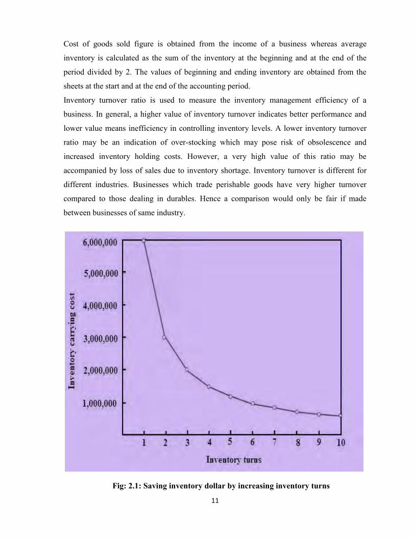
Continuous Review Model This inventory review model is characterized by two parameters-the reorder point (ROP) “s”
and the order-up-to level “S”. Whenever the inventory position is at or below the reorder
point “s”, an order should be placed to increase the inventory level to the order-up-to level
“S” (Simchi-Levi et al., 2004). Figure 2.4 shows the inventory level in a continuous review
model.
21
Figure 2.4: Inventory level in a continuous review model Source: Simchi-Levi et al., 2004
The reorder point (ROP) system determines when to place orders based on the number of
component units on hand. The reorder point consists of two components. The first is the
average demand during lead time, and the second is the safety stock. The safety stock is the
amount of inventory that the company needs to keep at the warehouse and in the pipeline to
protect against deviations from average demand during lead time. ROP is calculated using
lead time, average demand, and safety stock. Lin (1980) suggested if demand has no
seasonal fluctuation, and the supplier’s lead time is reliable, the reorder point is just the
demand during lead time (DDLT) plus a small amount of safety stock. Following above
mentioned, the formula can be described as:
ROP = Cycle Stock + Safety Stock
= Demand during lead time + Safety Stock

22
Fig 2.5: ROP with Safety Stock Source: Http://www.usfca.edu/villegas/classes/984-307/307ch12/sld024.htm
Cycle Stock
Cycle stock is the estimate quantity of an item that will be sold or used during the time that
takes until the new order arrives from the supplier (lead time). When lead time and demand
are known and constant, firms can simply calculate cycle stock by multiplying daily demand
by lead time in days.
Cycle stock = (Annual demand/ no of working days in a year) × Lead time in days
= 𝐴
𝑁× 𝐿
Where
A= Annual demand of the Product
N= No. of working days in a year
L= Lead time
Safety Stock
Safety stock is added to the method of ROP to reduce risk when a delay in delivery and
fluctuation in demand during lead time take place. When comparing to cycle stock, safety
stock is a bit trickier to calculate since there are several methods to determine safety stock.

23
Results from different methods can vary. It therefore depends on how much we would want
to have on hand during the replenishment cycle.
A simple method is used to determine safety stock is:
Safety stock = (Maximum usage – Average usage)* Lead time.
However, this method might give an exaggerating result if there is a big gap between
maximum usage and average usage. One can end up holding too much inventory on hand
more than required. This formula is thus suitable for items whose demand rate is more
constant. Another way to determine safety stock which is a bit more sophisticated than the
previous one is standard deviation method. The equation of determining safety stock is as
follow:
Safety Stock = 𝒛𝜶×STD×L
Where
= service level
z = No. of std. deviation for a given cycle service level
STD = standard deviation of daily demand
L= lead time
ROP = Cycle Stock + Safety Stock
ROP = 𝑨
𝑵× 𝑳 + 𝒛𝜶 × 𝑺𝑻𝑫 × √𝑳
Periodic Review Model
In many real situations, the continuous review is generally not practical. The more popular
way is that the inventory is reviewed periodically, at regular interval. For example, the
inventory level may be reviewed at the end of each month and an order may be placed at the
same time. The review period can be set according to the company’s actual situation. Since
the inventory levels are reviewed at a periodic interval, the fixed cost of placing an order is a
sunk cost and hence can be ignored.
Since fixed cost does not play a role in this review model, one parameter for inventory is the
base-stock level. The company determines a target inventory level, the base-stock level, and
each review interval point the inventory position is reviewed, and the replenishment order is
placed for an amount large enough to bring the inventory level back to the base-stock level.
Figure 2.6 illustrates the inventory level in a periodic review model.

24
Figure 2.6 Inventory level in a priodic review model Source: Simchi Levi et al., 2004
The base-stock level consists of two components: (1) average demand during an interval of
time equal to the review period plus the lead time and (2) safety stock, which is the amount
of inventory that the company needs to cover deviations from average demand during the
same period (Simchi-Levi et al., 2004). It is difficult to determine the appropriate safety
stock level, as it is affected by a variety of characteristics, like the service level. The service
level is a critical factor in relation to safety stock determination. If a higher service level is
desired, more safety stock will be required. Also, if demand is highly variable (frequently
much higher or lower than average), it is also important to hold more safety stock. Similarly,
if lead time is long, more safety stock is needed to guard against possible stock-outs during
lead time.For periodic review model, reorder point
ROP = 𝐴
𝑁× (𝑟 + 𝐿) + 𝑧𝛼 × 𝑆𝑇𝐷 × √𝑟 + 𝐿
Where, A/N=Demand per day L= Lead time
r = length of review period STD= Standard deviation

25
2.5.4 Lot Sizing Techniques:
The techniques used for determine lot size to minimize total holding and setup costs when demands are not equal in each period. There are a variety of ways to determine lot sizes. Methods include:
1. Economic Order Quantity (EOQ)
2. Periodic Order Quantity (POQ)
3. Lot for Lot
4. Part period Balancing (PPB)
5. Wagner- Whitin Algorithm (WWA)
1. Economic Order Quantity (EOQ): The method computes the EOQ based on the
average demand over the period and orders in lots of this size. Enough lots are ordered to
cover the demand.
2. Periodic Order Quantity (POQ): It translates the EOQ into time units (number of
periods) rather than an order quantity. The POQ is the length of time an EOQ order will
cover rounded off to an integer. For example, if the demand rate averages 100 units per
period and EOQ is 20 units per order then POQ is 100/20 = 5 periods.
3. Lot for Lot: It is the traditional way of ordering exactly what is needed in every period.
This is optimal if set up costs are zero.
4. Part Period Balancing (PPB): It is a more dynamic approach to balance setup and
holding cost. PPB uses additional information by changing the lot size to reflect
requirements of the next lot size in the future. PPB attempts to balance setup and holding
cost for known demand.PPB develops an Economic part period (EPP), which is the ratio of
setup cost to holding cost.
5. Wagner-Whitin Algorithm (WWA): It is a dynamic programming model that adds
some complexity to the lot size computation. It assumes a finite time horizon beyond which
there are no additional net requirements. Wagner-Whitin finds the production schedule
which minimizes the total costs (holding +setup).
26
2.5.4.1 Dynamic Lot Sizing Technique– WAGNER-WHITIN METHOD
The dynamic lot-size model in inventory theory is a generalization of the economic order
quantity model that takes into account that demand for the product varies over time. The
model was introduced by Harvey M. Wagner and Thomson M. Whitin in 1958. Dissatisfied
with the “square root formula” to find the economic lot size under the assumption of steady-
state (constant) demand, Wagner and Whitin (1958) developed an elegant forward algorithm
based on dynamic programming principles to make optimal lot size decisions.
The problem considered by Wagner and Whitin is the N periods problem with no backorders
when the assumption of constant demand is dropped i.e. when the amounts demanded in
each period are known but are different– and furthermore, when inventory costs vary from
period to period. Their 1958 paper is considered a classical and had been cited innumerable
times in the lot-sizing literature. Their model formulation permits the determination of
optimal lot sizes for a single item when demand, inventory holding charges and setup costs
vary over N periods of time.
The solution provided by the Wagner and Whitin algorithm (WWA) is considered the
benchmark or standard against which other lot-sizing rules or heuristics are judged.
Notwithstanding the fact of providing an optimal solution to the discrete lot-sizing problem,
the WWA has been considered by many as an impractical approach. Many researchers
indicate that the algorithm is difficult to use due to the dynamic programming nature of the
procedure and other limitations such as computational time, computer memory and
misunderstanding of its complexity (Evans 1985; Heady and Zhu 1994; Jacobs and
Khumawala 1987; Saydam and McKnew 1987; Boe and Yilmaz 1983).For practitioners in
general, the WWA is considered more as a philosophy of problem solving than as a
technique for lot-sizing decisions.
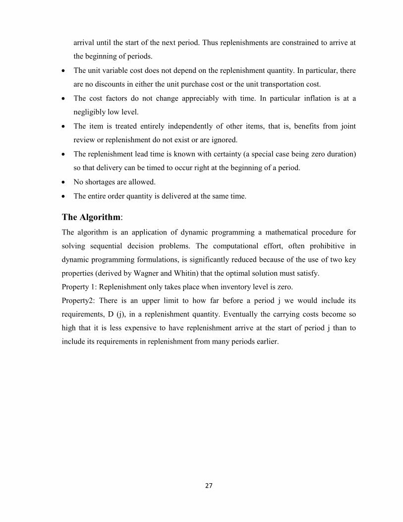
The Assumptions:
The demand rate is given in the form of D(j) to be satisfied in period j (j = 1,2, --------N)
where the planning horizon is at the end of period N. Of course demand rate may vary
from one period to the next, but it is assumed known.
The entire requirements of each period must be available at the beginning of that period.
Therefore a replenishment arriving part -way through a period cannot be used to satisfy
that periods requirements. It is cheaper, in terms of reduced carrying costs, to delay its
27
arrival until the start of the next period. Thus replenishments are constrained to arrive at
the beginning of periods.
The unit variable cost does not depend on the replenishment quantity. In particular, there
are no discounts in either the unit purchase cost or the unit transportation cost.
The cost factors do not change appreciably with time. In particular inflation is at a
negligibly low level.
The item is treated entirely independently of other items, that is, benefits from joint
review or replenishment do not exist or are ignored.
The replenishment lead time is known with certainty (a special case being zero duration)
so that delivery can be timed to occur right at the beginning of a period.
No shortages are allowed.
The entire order quantity is delivered at the same time.
The Algorithm: The algorithm is an application of dynamic programming a mathematical procedure for
solving sequential decision problems. The computational effort, often prohibitive in
dynamic programming formulations, is significantly reduced because of the use of two key
properties (derived by Wagner and Whitin) that the optimal solution must satisfy.
Property 1: Replenishment only takes place when inventory level is zero.
Property2: There is an upper limit to how far before a period j we would include its
requirements, D (j), in a replenishment quantity. Eventually the carrying costs become so
high that it is less expensive to have replenishment arrive at the start of period j than to
include its requirements in replenishment from many periods earlier.

28
Potential Drawbacks of the Algorithm:
As mentioned earlier, the Wagner-Whitin algorithms guaranteed to provide a set of
replenishment quantities that minimize the sum of replenishment plus carrying cost out to a
specified horizon. In general, the algorithm has received extremely limited acceptance in
practice. The primary reasons for this lack of acceptance are as follows:
The relatively complex nature of the algorithm makes it more difficult for the
practitioner to understand than other approaches.
There is a possible need for a well defined ending point for the demand pattern. Such an
ending point is not needed when there is at least one period whose requirements exceed
A/vr.
A related issue is the fact that the algorithm is often used in conjunction with MRP
software. Because MRP typically operates on a rolling schedule, the replenishment
quantities chosen should not change when new information about future demands
become available. Unfortunately the Wagner-Whitin approach does not necessarily have
this property
The necessary assumption is that replenishment can be made only at discrete intervals. This
assumption can be relaxed by subdividing the periods. However, the computational
requirements of the algorithm go up rapidly with the number of periods considered.
29
CHAPTER 3 RESEARCH METHODOLOGY
[In this chapter, the authors will examine different research methods and present what
methods are applied to this thesis.] The research process usually includes formulating and clarifying a topic, reviewing the
literature, choosing a strategy, collecting data, analyzing data and writing up. The research
process is not strictly sequential in reality; the researcher often needs to revisit each stage
many times in order to refine the ideas.
3.1 Generating the Research Topic The authors decided to make the thesis a research project based on practical work, and a
specific company needed to be accessed to collect empirical data for the research project.
Somehow the authors managed to find a company that showed their initial interest in
supporting the business management research project. The research project, given this topic,
is particularly of practical relevance for the company.
3.2 Deciding the Research Approach According to Saunders et al. (2003) there exist two types of research approach: one is the
deductive approach, in which the researcher develops certain theories and/or hypotheses and
design a research strategy to verify the hypotheses; the other is inductive approach, in which
the researcher collects data and develops theories as a result of the data analysis.
Considering the research questions and purpose of the thesis the authors choose the
deductive approach as the legitimate approach to be used. The authors conducted a range of
relevant theories review, proposed some hypotheses, such as the implications gained from
the relevant theories would help to improve the management of the researched company and
how to improve, and tested the hypotheses by concluding that they really worked.
3.3 Choosing the Appropriate Research Strategies Saunders et al. (2003) present that eight strategies can be used in the research work: ex-
periment; survey; case study; grounded theory; ethnography; action research; cross-sectional
and longitudinal studies; exploratory, descriptive and explanatory studies.

30
3.3.1 Case Study Strategy Robson defines case study as ‘a strategy for doing research which involves an empirical
investigation of a particular contemporary phenomenon within its real life context using
multiple sources of evidence’. The researcher must be alert to the need for multiple sources
of evidence. ‘All evidence is of some use to the case study researcher: nothing is turned
away.’ (Gillham (2000) gave us the following list of six main evidences.
1. Documents. These can be letters, policy statements, regulations and guidelines. They
provide a formal framework to which a researcher may relate the informal reality.
2. Records. These are the evidences that go back in time but may provide a useful
longitudinal fix on the present situation. These may well be stored in computer files.
3. Interviews. This is an inadequate term for the range of ways in which people can give you
information.
4. Direct observation. It is used mainly when a researcher needs to be more systematic in
how he or she observes.
5. Participant observation. This is the more usual sort in a case study-where a researcher is
‘in’ the setting in some active sense-perhaps even working there but keeping the ears and
eyes open, noticing things that they might normally overlook.
6. Physical artifacts. These are things made or produced. Sometimes this kind of evidence is
most important when a researcher is doing a multiple case study.
As to our research project, we investigated the current situation of inventory management in
Reedisha Knitex by using multiple sources of evidence, for instance, the interviews with the
top manager and other related staff at dyeing section of Reedisha, and monthly consumption
report for twenty sample items. When we were visiting at Reedisha, we conducted direct
observation on warehousing operation and the information system.
3.3.2 Cross-Sectional Studies Cross-sectional research can be interpreted as the study of a particular phenomenon at a
particular time. In this sense our thesis project is a cross-sectional research as the case study
conducted in Reedisha knitex Ltd. was based on interviews and observations over a short
period of time less than three months.
31
3.3.3 Exploratory, Descriptive and Explanatory Studies (1) Exploratory studies
An exploratory study is conducted when not much is known about the current situation, or
no information is available on how similar problems or research issues have been solved in
the past that exploratory studies are particularly useful if the researcher seeks to clarify his
understanding of a problem. There are three major ways of conducting exploratory research:
A search of the literature;
Talking to experts in the subject;
Conducting focus group interviews.
Our thesis research is obviously not an exploratory study according to the above explanation
of exploratory studies.
(2) Descriptive studies
A descriptive study is undertaken in order to ascertain and be able to describe the
characteristics of the variables in certain situation, and to understand the characteristics of
organizations that follow certain routine practice. The aim of a descriptive study, therefore,
is to provide the researcher with a profile or to describe the relevant aspects of the
phenomenon from an individual, organizational, industry-oriented, or other perspective.
The descriptive study strategy was used in the chapter of empirical findings to clarify and
elaborate the case study context, which included the company organizational structure, the
functions performed in-house, the outsourcing functions, the business operational process,
and the physical facilities.
(3) Explanatory studies
According to Saunders et al. (2003) a study that establishes causal relationships between
variables may be termed explanatory study; the key issue here is to study a situation or a
problem in order to explain the relationships between variables.
As the authors recognized there are a number of issues associated with the inventory control
problem in Reedisha Knitex Ltd. that are actually affecting each other, we did not pursue a
simple cause-and-effect approach to the problem discussion and the suggested solutions to
the problem.

32
3.4 Data Collection Methods We collected primary data mainly through in-depth interviews with the head of the dyeing
unit of the company and through non-participant observations in the fieldwork, such as
looking into the information system, visiting the warehouses, and observing the operational
process of warehouse activities. E-mails also were used to send out questions and get
responses and other data from the same interviewees. We prepared the interview questions
in advance and also raised unprepared questions of relevance when interacting with the
interviewees during the conversations. We used semi-structured and unstructured interviews
approach to all the interviews that were conducted. Using unstructured interview approach
gave the authors greatest flexibility in picking up as many clues as we could to draw a clear
picture of the facts. While semi-structured interview approach was applied to the later stage
of data collection actions, which assisted us in keeping focus on identified questions and
digging deeper into the questions, however, concurrently, allowed a certain degree of
flexibility during the interview.
We also gathered the product catalogue of the company as the secondary data for the thesis
project. But we decided not to collect the historical commercial documents, for instance, the
invoices that are most frequently used in the company’s business activity, since we
considered these documents as small pieces of a puzzle and they were too many to collect
and form the whole picture for outside researchers. Instead we acquired the relevant
information from the manager through in-depth interviews.
Purposive sampling is very useful for researchers. We collect 2013 daily chemical
consumption report for twenty sample items, which were selected through purposive
sampling. The consumption report also is the secondary data and was retrieved from the
company’s information system. We set the criteria for sampling as listed: they should be
“alive” which means they are ordered frequently, and they should have different unit price-
low, medium, and high. All the primary and secondary data collection in the company was
under the permission of the manager and without any offence in ethical rules during the
whole research process.

33
CHAPTER 4
CASE STUDY
4.1 Company Profile Reedisha Knitex Ltd. a 100% export oriented composite knit textile unit established with the
commitment to cater the global needs for knit and casual clothing. The project has employed
the State -of –A technology in its every piece of investments. Aiming at the context of the
changing global demand pattern, international environment on trade specially the
withdrawal of quota system and GSP and the availability of craftsmanship in the country,
the project encompassed the knitting, dyeing and processing of fabrics and readymade
garments production to be available from one stop service. The project ensures sampling to
supply of finished RMG all from one source, ensuring in time delivery and complying
quality. The machines and equipment’s setup for these projects are procured from world
class brand, names renowned for their high quality, product integrity and dependable
production.
The project is established in 2003, but the manpower engaged in the projects to carry out the
day to day business are all highly skilled, purely professional, vastly experienced, The
unique combination of organized Managerial and technical team in one hand and latest,
advanced and balanced technology on the other hand made the project one of the top to be
referred in this field in the country. The best use of continuous development of human
resources by providing them International Standard Environment and equal opportunity is
the keys for achieving comprehensive competence in all the level of the Organizational
Hierarchy.
Reedisha Knitex Ltd. has been established with the objective and vision to cater the needs of
21st century of worldwide knit apparels market from one stop service being committed to on
time delivery, short lead time, quality assurance, price affordability and social
accountability. RKL already achieved Worldwide Responsible Apparels Production
(WRAP) certificate in April 2007.
34
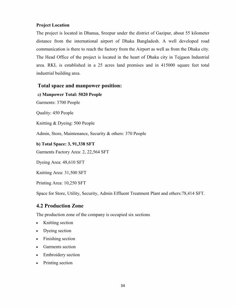
Project Location
The project is located in Dhanua, Sreepur under the district of Gazipur, about 55 kilometer
distance from the international airport of Dhaka Bangladesh. A well developed road
communication is there to reach the factory from the Airport as well as from the Dhaka city.
The Head Office of the project is located in the heart of Dhaka city in Tejgaon Industrial
area. RKL is established in a 25 acres land premises and in 415000 square feet total
industrial building area.
Total space and manpower position: a) Manpower Total: 5020 People
Garments: 3700 People
Quality: 450 People
Knitting & Dyeing: 500 People
Admin, Store, Maintenance, Security & others: 370 People
b) Total Space: 3, 91,338 SFT
Garments Factory Area: 2, 22,564 SFT
Dyeing Area: 48,610 SFT
Knitting Area: 31,500 SFT
Printing Area: 10,250 SFT
Space for Store, Utility, Security, Admin Effluent Treatment Plant and others:78,414 SFT.
4.2 Production Zone
The production zone of the company is occupied six sections
Knitting section
Dyeing section
Finishing section
Garments section
Embroidery section
Printing section

35
Knitting Section:
Reedisha Knitex Ltd. is one of the world-class pioneers in the knitting and processing of
stretch fabrics for use in manufacturing sportswear, active wear, performance wear, body
wear, intimate apparel and swim wear. Reddish’s Fabrics and RMG are performed on
specialized and highly technologically advanced Knitting, Dyeing and Finishing
machineries. The processing of fabrics that contains stretch yarns require precision
technology, special conditioning and consistently clean machinery and constant maintenance
over and above the standards of the units.
The Unit has the strength to produce various types of Fabrics, like: Single Jersey, Pique and
Double Pique, Lacoste, Waffle, Rib, Inter Lock, Fleece, Design Interlock, Feeder Stripe,
Engineering Stripe, Lycra attachment, Flat Knit Collar & Cuff making with half jacquard
design. All above fabric are lycra Knitting.
Knitting Production capacity: 16,000 kg of Gray Fabrics per Day
Dyeing Section:
The process of dyeing to produce the most reliable color quality and steadfastness is a very
sensitive and sophisticated process on any fabrics. Especially the stretch fabrics require the
level require the level of sophistication in the dyeing process. The quality of our dyeing
equipment coupled with the high precision skill of our dyeing plant operators have enabled
us to excel in this very complex process. To meet the worldwide demand trend the unit has
the combination of Tubular and Open Width fabrics processing.
Fabric Product Range:
The plant has the facilities to process 100 % Cotton, Cotton Blend, T/C, Viscose, Acrylic,
elastic etc. fabrics. The Dyeing and finishing machines are of Computer controlled having
highly sophisticated and advanced Technology of German, USA and UK.
Dyeing Production capacity: 16,000 kg of Fabrics per Day
Finishing Section:
Reedisha Knitex Ltd. has amassed a highly successful prows of finishing based on process
scientific methods, collective experience and accumulated expertise, because finishing is not
only by its notional implications, but is also of crucial importance. Finishing is one of the
most critical stages in the final performance of fabrics. Our most latest and state-of-the-art
36
finishing technology is constantly updated to meet our fabric-specific requirements for
quality, standardization and performance.
Garments Section:
Reedisha’s acquired mileage is ensured from the fact that its consumption of fabrics comes
entirely from its own making. Good fabrics help tailoring good apparel for the demanding
buyers of the world. Our range of apparel includes T-shirt, Polo shirt, Ladies-wear, Sports-
wear, Tank-Tops and Children’s wear, Sacket, Trousers etc. The support for printing,
embroidery and washing are organized from associated projects.
Present Garments Production capacity:
Garments Production Per Month: 1,800,000 pieces
Garments Production Lines: 59 Lines.
Garments Factory Area : 2, 22,564 SFT
Embroidery Section
The Embroidery section of Reedisha Knitex Limited has two sets of 9 colors Embroidery
machine within 20 heads each.
Production Capacity : 10,000 pcs per day.
Manpower : 40 People
Embroidery Plant Area : 1200 sft
Printing Section
The Printing Unit of Reedisha Knitex Limited has the strength to produce various types of
Garment Printings like Pigment Print, Rubber Print, Discharge Print, Plastisol Print, High
Density Print, Flock Print, Foil Print, Puff Print, Crack Print, Gel Print, Glitter Print, Sticker
Print, Stone Setting, Metalic Print etc.
Printing Plant Area: 12000 sft.
Manpower: 212 people
Production Capacity: 50,000 pcs per day
37
4.3 Dyes and Chemicals Receiving Process of Reedisha Knitex :
Reedisha Knitex Ltd is a 100% export oriented fully knit composite factory & one of the
leading textile & garments factory of the country. It has all the unit of textiles under one
roof. It only imports raw cotton & Dyes & Chemicals from foreign countries. It has all the
units for processing from raw cotton to finished garments. Dyeing unit is back process of
garments. Here fabrics are dyed at different shades & finished & delivery to garments. For
processing fabrics different types of dyes & chemicals are used in dyeing.
There are almost 30 chemicals and 20 dyes are used in dyeing section. Almost all of the
chemicals are imported from abroad. The chemicals are mainly imported from India, China,
Singapore, Germany, Thailand, Belgium, Srilanka. Lead time for all the chemicals is 90
days. The materials are ordered through L/C opened. Safety stock for every chemical for 3-
4 months is maintained here. Here chemicals are imported for 3-6 months projection basis.
Chemicals required for 3-4 months calculated first, then per day average requirement is
calculated. The chemicals required for 3-6 months calculated & inform the purchase
manager. He then contacts with local agent, negotiates about current price & open L/C
against the respective supplier. As per L/C rule supplier reaches the chemical through ship to
Chittagong sea port. Then Reedisha authority sends C & F agent to Chittagong sea port. He
contacts with custom authority & finishes all the formalities chemicals are imported to
factory by truck or cavered van.
When the truck enters into factory gate, security authority receive products & give a number
that is Gate Receive No(GRN).Then security & store authority counts the drum & quantity
& unload by loader. The loaders transport chemicals to main godown or ware house. Then
the listed chemicals are registered in a book that is called Material Receive Report(MRR) &
put entry into computer. Batch card is maintained for every types of chemicals & lot wise
receiving date is recorded there. Here FIFO is maintained for well management of chemicals
that is First In First Out.
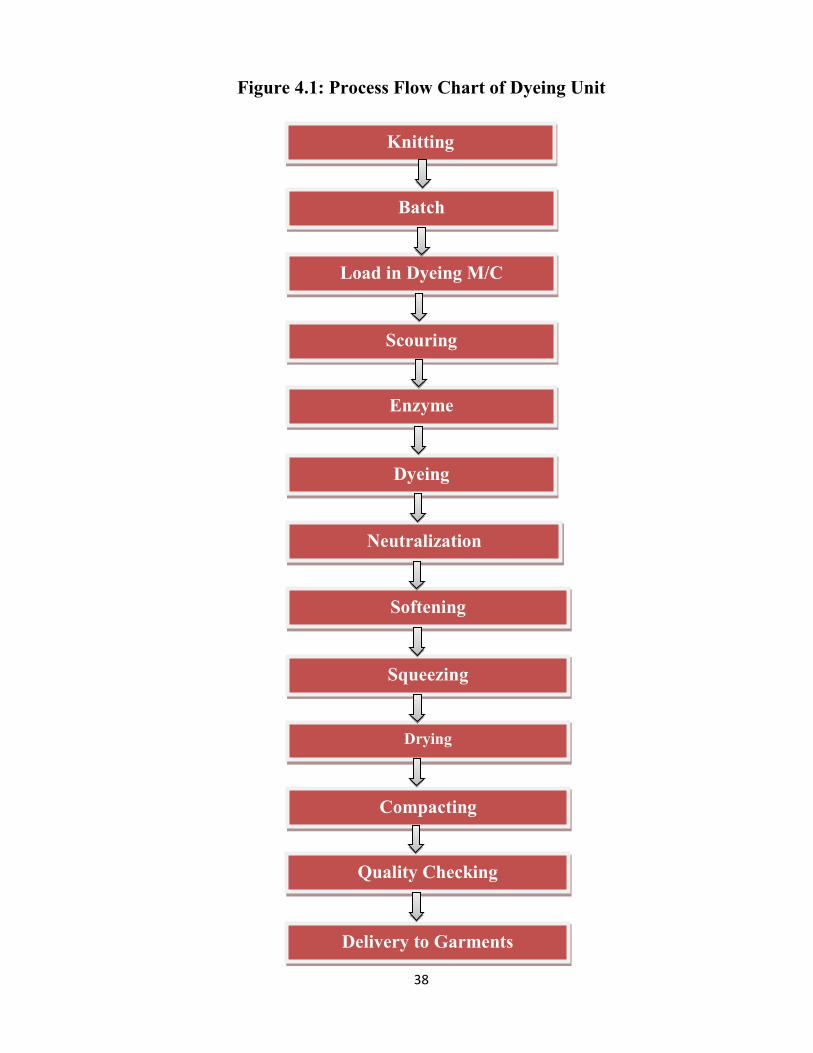
38
Figure 4.1: Process Flow Chart of Dyeing Unit
Knitting
Batch
Load in Dyeing M/C
Scouring
Enzyme
Dyeing
Neutralization
Softening
Squeezing
Drying
Compacting
Quality Checking
Delivery to Garments

39
CHATER 5 ANALYSIS AND FINDINGS
As explained previously regarding the encountered problems of inventory control in the
Dyeing section of Reedisha Knitex, reorder point and order quantity are the most common
issues for inventory management. Identifying and analyzing these problems lead to the
practical solutions. Several inventory control methods can be utilized to determine reorder
point and order quantity. However, before selecting any approach to use, dyes chemical
inventory must be first classified. In order to improve inventory performance of the dyeing
section, action plan can be divided into two phrases–classifying dyes inventory and selecting
inventory control methods.
Classifying inventory must be performed when handling great number of product types.
Several classification models can be used to group the inventory. One of the most common
and effective approaches is ABC model that categorizes product based on its value. Having
classified the inventory, the next step is to select inventory control methods. In order to put
the right method in the right place, it must be remembered that different methods serve
different purposes and they require different levels of management.
In conclusion, activities that must be performed to solve the problems about ROP and order
quantity are inventory classification and selection of inventory control methods. However, it
is important to note that the result in this final thesis does not necessarily provide the final
solution for dyes inventory control, but some possibilities to improve dyes inventory control
in a dyeing unit of textile industry.
5.1 Classifying Inventory (ABC Analysis) The ABC analysis provides a mechanism for identifying items that will have a significant
impact on overall inventory cost while also providing a mechanism for identifying different
categories of stock that will require different management and controls. The ABC analysis
suggests that inventories of an organization are not of equal value. Thus, the inventory is
grouped into three categories (A, B, and C) in order of their estimated importance.
According to Onwubolu et al. (2006), classifying inventory items into A, B, C categories
should follow several steps:
Determine annual quantity usage of each item.

40
Multiply the annual quantity usage of each item by the cost of the item to obtain the total
annual value usage of each item.
Add the total value usage of all items to get the aggregate annual value inventory
expenditure.
Divide the total annual value usage of each item by the aggregate annual inventory
expenditure to obtain the percentage of total usage for each item.
List the items in rank order by percentage of aggregate usage.
Review annual usage distribution and classify items as A, B, or C.
Management policies for ABC Categorization:
Managing all the inventories will take personal time and costs money. ABC classification
shows that not all the inventories need to control with equal attention. ABC analysis for
prioritization allows the management to decide which items require most effort in
controlling.
A items should have tight inventory control under more experienced management. Re-
orders should be more frequent.
B items require medium attention for control. An important aspect of class B is the
monitoring of potential evolution toward class A or, in the contrary, toward the class C.
C items require minimum attention and may be kept under simple observation. Re-
ordering is less frequent.
ABC analysis of inventory leads to certain benefits in form of guidance to the manager
about level of control for each type of item, which are summarized in Table below.
Activity Group A Group B Group C
Monitoring Very Strict Strict Moderate
Safety stock to be kept Low Medium High
Level of control for issue Tight Moderate Low
Estimates of requirement Very Accurate Moderately Accurate May be low
Frequency of Purchase Most frequent Less frequent Least frequent
Turn over Maximum Medium Least
Management involvement Top level Middle level Lower level

41
Table 5.1: Items for ABC Analysis
SL No. Product Name Annual
Unit Cost (tk.) Total Cost % of Cost
Demand (kg) 1 Acetic Acid 137587 70 9631090 4.6 2 Neutracid 20505 92 1886460 0.9 3 Bio Polish Al 72751 326 23716826 11.2 4 CWS 227910 182 41479620 19.6 5 Caustic Soda 152056 35 5321960 2.5 6 Cibafix ECO 13352 395 5274040 2.49 7 Felosan NOF 111739 185 20671715 9.8 8 Secho SQD 70563 104 7338552 3.5 9 H2O2 207789 28 5818092 2.8 10 Hydrose 14320 64 916480 0.43 11 Leucophor BMB 702 650 456300 0.22 12 Optavon 4UD 95329 111 10581519 5 13 Croscolor ARI 4167 290 1208430 0.6 14 Salt Glubar 2592752 11 28520272 13.5 15 X MEN 73028 225 16431300 7.8 16 Lubatex ECS 141990 68 9655320 4.6 17 Soda Ash 510689 18 9192402 4.4 18 Cros Color ADM 23257 285 6628245 3.14 19 Crosprep PBS 5051 295 1490045 0.71 20 Permol R 63739 80 5099120 2.4 Total 4539276 211317788

42
Table 5.2: Arrange the items according to % of cost from higher to lower value
SL Product Name Annual Unit Cost Total % of
Cost Cumulative Classify
No. Demand
(kg) (tk.) Cost % 4 CWS 227910 182 41479620 19.60 19.60 A 14 Salt Glubar 2592752 11 28520272 13.50 33.10 A 3 Bio Polish Al 72751 326 23716826 11.20 44.30 A 7 Felosan NOF 111739 185 20671715 9.80 54.10 A 15 X MEN 73028 225 16431300 7.80 61.90 A 12 Optavon 4UD 95329 111 10581519 5.00 66.90 A 1 Acetic Acid 137587 70 9631090 4.60 71.50 B 16 Lubatex ECS 141990 68 9655320 4.60 76.10 B 17 Soda Ash 510689 18 9192402 4.40 80.50 B 8 Secho SQD 70563 104 7338552 3.50 84.00 B 18 Cros Color ADM 23257 285 6628245 3.14 87.14 B 9 H2O2 207789 28 5818092 2.80 89.94 B 5 Caustic Soda 152056 35 5321960 2.50 92.44 B 6 Cibafix ECO 13352 395 5274040 2.50 94.94 C 20 PERMOL R 63739 80 5099120 2.40 97.34 C 2 Neutracid 20505 92 1886460 0.90 98.24 C 19 Crosprep PBS 5051 295 1490045 0.70 98.94 C 13 Croscolor ARI 4167 290 1208430 0.60 99.54 C 10 Hydrose 14320 64 916480 0.40 99.94 C 11 Leucophor BMB 702 650 456300 0.20 100.00 C Total 4539276 211317788
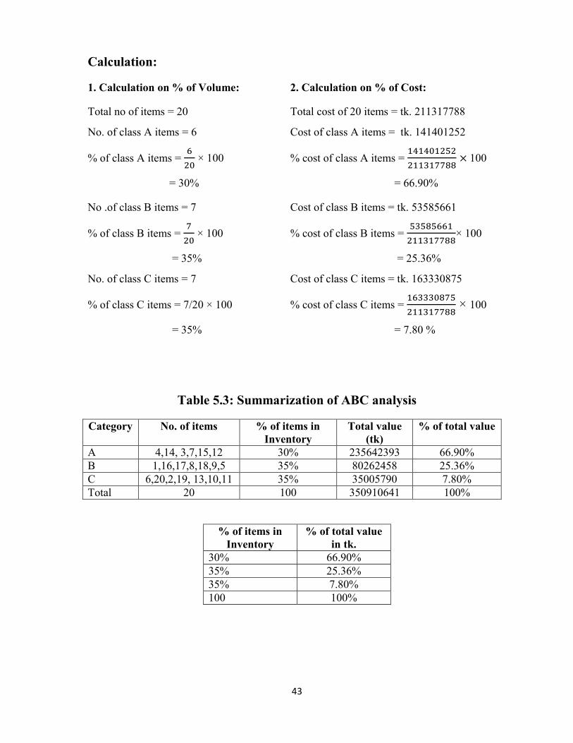
43
Calculation:
1. Calculation on % of Volume: 2. Calculation on % of Cost:
Total no of items = 20 Total cost of 20 items = tk. 211317788
No. of class A items = 6 Cost of class A items = tk. 141401252
% of class A items = 6
20 × 100 % cost of class A items =
141401252
211317788× 100
= 30% = 66.90%
No .of class B items = 7 Cost of class B items = tk. 53585661
% of class B items = 7
20 × 100 % cost of class B items =
53585661
211317788× 100
= 35% = 25.36%
No. of class C items = 7 Cost of class C items = tk. 163330875
% of class C items = 7/20 × 100 % cost of class C items = 163330875
211317788 × 100
= 35% = 7.80 %
Table 5.3: Summarization of ABC analysis
Category No. of items % of items in Inventory
Total value (tk)
% of total value
A 4,14, 3,7,15,12 30% 235642393 66.90% B 1,16,17,8,18,9,5 35% 80262458 25.36% C 6,20,2,19, 13,10,11 35% 35005790 7.80% Total 20 100 350910641 100%
% of items in Inventory
% of total value in tk.
30% 66.90% 35% 25.36% 35% 7.80% 100 100%

44
Figure 5.1: Graphic Representation of ABC Analysis
Source: Own Prepared
Figure 5.2: Typical representation of ABC analysis Source: Own prepared
A B C

45
5.2 Selecting Inventory Methods
5.2.1 Economic Order Quantity (EOQ) Model: (When to Order) Economic order quantity is the order quantity that minimizes total inventory holding costs and ordering costs. It is one of the oldest classical production scheduling models. The framework used to determine this order quantity is also known as Wilson EOQ Model or Wilson Formula. The model was developed by Ford W. Harris in 1913, but R. H. Wilson, a consultant who applied it extensively, is given credit for his in-depth analysis. EOQ applies only when demand for a product is constant over the year and each new order is delivered in full when inventory reaches zero. There is a fixed cost for each order placed, regardless of the number of units ordered. There is also a cost for each unit held in storage, commonly known as holding cost, sometimes expressed as a percentage of the purchase cost of the item. We want to determine the optimal number of units to order so that we minimize the total cost associated with the purchase, delivery and storage of the product. The required parameters to the solution are the total demand for the year, the purchase cost for each item, the fixed cost to place the order and the storage cost for each item per year. The number of times an order is placed will also affect the total cost.
Figure 5.3: Inventory usage over time Source: Own prepared

46
Underlying Assumptions: The ordering cost is constant.
The rate of demand is known, and spread evenly throughout the year.
The lead time is fixed.
The purchase price of the item is constant i.e. no discount is available
The replenishment is made instantaneously; the whole batch is delivered at once.
Only one product is involved.
EOQ is the quantity to order, so that the sum of ordering cost and holding cost is at its
minimum. These costs will be equal to one another at the minimized cost point.
EOQ= Q* = √2𝑅𝐴
𝑣𝑤
Variables v= Purchase price, unit production cost
Q= Order quantity
Q*= Optimal order quantity
A= Annual demand quantity
R= Fixed cost per order, setup cost (not per unit, typically cost of ordering and shipping and
handling. This is not the cost of goods)
H= vw = Annual holding cost per unit, also known as carrying cost or storage cost
Calculation: Sample item Felosan NOF
EOQ= Q* = √2𝑅𝐴
𝑣𝑤
Here, Annual demand A = 111739 kg Ordering cost per order R = Tk. 3500 Holding cost H= vw= tk. 2.78
Economic order quantity = Q* = √2𝑅𝐴
𝑣𝑤
= √2×3500×111739
2.78
= 16774 kg
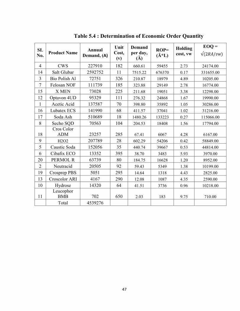
47
Table 5.4 : Determination of Economic Order Quantity
SL No. Product Name Annual
Demand, (A)
Unit Cost,
(v)
Demand per day,
(Ā)
ROP= (Ā*L)
Holding cost, vw
EOQ =
4 CWS 227910 182 660.61 59455 2.73 24174.00 14 Salt Glubar 2592752 11 7515.22 676370 0.17 331655.00 3 Bio Polish Al 72751 326 210.87 18979 4.89 10205.00 7 Felosan NOF 111739 185 323.88 29149 2.78 16774.00 15 X MEN 73028 225 211.68 19051 3.38 12298.00 12 Optavon 4UD 95329 111 276.32 24868 1.67 19990.00 1 Acetic Acid 137587 70 398.80 35892 1.05 30286.00 16 Lubatex ECS 141990 68 411.57 37041 1.02 31216.00 17 Soda Ash 510689 18 1480.26 133223 0.27 115066.00 8 Secho SQD 70563 104 204.53 18408 1.56 17794.00
18 Cros Color
ADM 23257 285 67.41 6067 4.28 6167.00 9 H2O2 207789 28 602.29 54206 0.42 58849.00 5 Caustic Soda 152056 35 440.74 39667 0.53 44814.00 6 Cibafix ECO 13352 395 38.70 3483 5.93 3970.00 20 PERMOL R 63739 80 184.75 16628 1.20 8952.00 2 Neutracid 20505 92 59.43 5349 1.38 10199.00 19 Crosprep PBS 5051 295 14.64 1318 4.43 2825.00 13 Croscolor ARI 4167 290 12.08 1087 4.35 2590.00 10 Hydrose 14320 64 41.51 3736 0.96 10218.00
11 Leucophor
BMB 702 650 2.03 183 9.75 710.00 Total 4539276

48
5.2.2 The Total Cost Function The single-item EOQ formula finds the minimum point of the following cost function:
Purchase cost: This is the variable cost of goods.
Annual purchase cost= Unit price × Annual demand quantity.
= v × A
Ordering cost: This is the cost of placing orders: each order has a fixed cost R, and we need
to order A/Q times per year.
Annual Ordering cost = Fixed order cost × no. of order
= R × A/Q
Holding cost: This is the cost for holding one unit of inventory for one year. The average
quantity in stock (between fully replenished and empty) is Q/2.
Annual Holding cost = Holding cost for one unit × Average inventory
= H × Q/2
Total cost = Annual purchase cost + Annual ordering cost + Annual holding cost TC = (Annual Demand × Unit Cost) + (No. of Order × Ordering Cost) + (Avg Inv × Holding
Cost)
TC = (A×v)+( 𝑨
𝑸×R) +( 𝑸
𝟐×H)
To determine the minimum point of the total cost curve, partially differentiate the total cost
with respect to Q (assume all other variables are constant) and set to 0:
0 = - 𝑅𝐴
𝑄2 + H/2
Solving for Q gives Q* (the optimal order quantity):
𝑄 ∗2 = 2𝐴𝑅
𝐻
Therefore Economic Order Quantity
Q* = √𝟐𝑹𝑨
𝑯
Q* is independent of v; it is a function of only R, A, H

49
Figure 5.4: Total cost as a function of order quantity Source: Own prepaed
Calculation: Sample item Felosan NOF
TC = (A×v) + ( 𝑨
𝑸∗×R) + ( 𝑸∗
𝟐×H)
Here,
TC= Total Cost
A = Annual Demand = 111739 kg
v = Unit Cost = Tk 185
Q = Order Quantity
Q* = Economic Order Quantity = 16774 kg
R = Ordering Cost per Order = Tk. 3500
H = Holding Cost = Tk. 2.78
Total cost = TC= (111739 × 185) + (111739
16774 × 3500) + (
16774
2× 2.78)
= (20671715 + 24500 + 23315.86)
= Tk. 20719531

50
Calculation: Sample item Felosan NOF (Total cost for non EOQ Quantity)
Total Cost = (Annual Demand × Unit Cost) + ( No. of Order × Ordering Cost) + (Avg. Inventory × Holding Cost) TC = (A×v) + (
𝐴
𝑄×R) + (
𝑄
2×H)
Here
Annual demand, A = 111739 kg
Unit cost, v = tk. 185
Order Quantity, Q= 23400 kg
Ordering cost per order, R= tk. 3500
Holding cost per unit per year= tk. 2.78
For Q= 23400 kg,
TC= (111739×185) + (111739
23400× 3500) + (
23400
2× 2.78)
= (20671715 + 16713.10 + 32526)
= Tk. 20720954.1
The difference between total cost for Q= 23400 kg and for Q*= 16774kg is (2072095410 – 20719531) = Tk. 1423.10 which is greater than EOQ quantity.
If order quantity Q = 12200 kg
TC = (111739×185) + (111739
12200× 3500) + (
12200
2× 2.78)
= (20671715 + 325905.42 + 16598)
= Tk. 21014578.42
The difference between total cost for Q = 12200 kg and for Q* = 16774kg
= (21014578.420 – 20719531) = Tk. 295047.42 which is greater than EOQ quantity.
So optimal order quantity Q= 16774kg is appropriate, which minimizes total cost for holding inventory.
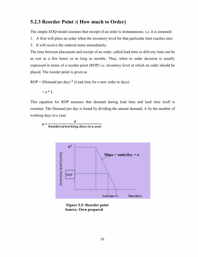
51
5.2.3 Reorder Point :( How much to Order) The simple EOQ model assumes that receipt of an order is instantaneous. i.e. it is assumed:
1. A firm will place an order when the inventory level for that particular item reaches zero
2. It will receive the ordered items immediately.
The time between placement and receipt of an order, called lead time or delivery time can be
as sort as a few hours or as long as months. Thus, when to order decision is usually
expressed in terms of a reorder point (ROP) i.e. inventory level at which an order should be
placed. The reorder point is given as
ROP = (Demand per day) * (Lead time for a new order in days)
= a * L
This equation for ROP assumes that demand during lead time and lead time itself is
constant. The Demand per day is found by dividing the annual demand, A by the number of
working days in a year.
a = 𝑨
𝑵𝒖𝒎𝒃𝒆𝒓𝒐𝒇𝒘𝒐𝒓𝒌𝒊𝒏𝒈 𝒅𝒂𝒚𝒔 𝒊𝒏 𝒂 𝒚𝒆𝒂𝒓
Figure 5.5: Reorder point Source: Own prepared

52
Table 5.7: Determination of Reorder Point
Sl No. Product Name Annual Demand (A) Unit Cost
(v) Demand per
day, (Ā) ROP
(Ā*L)
4 CWS 227910 182 660.61 59455
14 Salt Glubar 2592752 11 7515.22 676370
3 Bio Polish Al 72751 326 210.87 18979
7 Felosan NOF 111739 185 323.88 29149
15 X MEN 73028 225 211.68 19051
12 Optavon 4UD 95329 111 276.32 24868
1 Acetic Acid 137587 70 398.80 35892
16 Lubatex ECS 141990 68 411.57 37041
17 Soda Ash 510689 18 1480.26 133223
8 Secho SQD 70563 104 204.53 18408
18 Cros Color ADM 23257 285 67.41 6067
9 H2O2 207789 28 602.29 54206
5 Caustic Soda 152056 35 440.74 39667
6 Cibafix ECO 13352 395 38.70 3483
20 PERMOL R 63739 80 184.75 16628
2 Neutracid 20505 92 59.43 5349
19 Crosprep PBS 5051 295 14.64 1318
13 Croscolor ARI 4167 290 12.08 1087
10 Hydrose 14320 64 41.51 3736
11 Leucophor BMB 702 650 2.03 183

53
Calculation: Sample item Felosan NOF
No. of working days in a year = (365-20) = 345 days
Carrying rate, w = 0.015 per unit per year
Ordering cost per order, R = tk. 3500
Lead time, L = 90 days
Annual demand, A = 111739 kg
Reorder Point = Demand per day × Lead time
ROP = 𝑨𝒏𝒏𝒖𝒂𝒍 𝒅𝒆𝒎𝒂𝒏𝒅
𝑵𝒐. 𝒐𝒇 𝒘𝒐𝒓𝒌𝒊𝒏𝒈 𝒅𝒂𝒚𝒔 𝒊𝒏 𝒂 𝒚𝒆𝒂𝒓 × Lead time
= 𝐴
345× L
= 111739
345 × 90
= 29149 kg

54
5.2.4 Dynamic Lot Sizing Technique (Wagner-Whitin Method)
Table 5.8 Determination of ordering policy under Wagner-Whitin method
Class A Item:
4. Crosoft NBC (CWS)
Month Jan Feb March April May June Unit Price (tk) Demand(kg) 25527 17704 31010 12779 16381 12346 182 Month July August Sept. October Nov Dec Demand(kg) 23432 7726 26513 15368 26800 1225 Total (kg) 227910
14. Salt Glubar
Month Jan Feb March April May June Unit Price (tk) Demand(kg) 200597 311957 177116 294928 138818 137286 11 Month July August Sept. October Nov Dec Demand(kg) 205293 129454 339364 156439 226500 275000 Total (kg) 2592752
Sl No Month Order Quantity (kg) 1 January 12779 2 Feb 28727 3 April 31158 4 June 41881 5 August 39125 Total No of order= 5 153670
Sl No Month Order Quantity(kg) 1 Jan 433746 2 March 472033 3 June 339364 4 July 382939 5 Sept 275000 Total No of order= 5 1903082
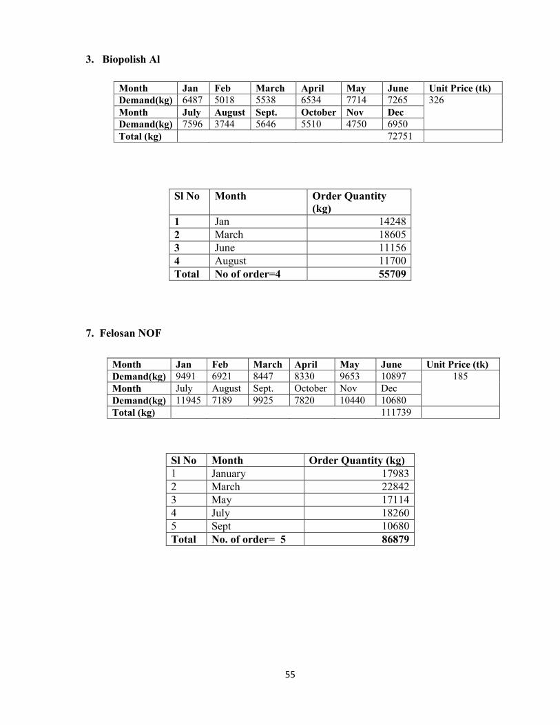
55
3. Biopolish Al
Month Jan Feb March April May June Unit Price (tk) Demand(kg) 6487 5018 5538 6534 7714 7265 326 Month July August Sept. October Nov Dec Demand(kg) 7596 3744 5646 5510 4750 6950 Total (kg) 72751
7. Felosan NOF
Sl No Month Order Quantity (kg)
1 Jan 14248 2 March 18605 3 June 11156 4 August 11700 Total No of order=4 55709
Month Jan Feb March April May June Unit Price (tk) Demand(kg) 9491 6921 8447 8330 9653 10897 185 Month July August Sept. October Nov Dec Demand(kg) 11945 7189 9925 7820 10440 10680 Total (kg) 111739
Sl No Month Order Quantity (kg) 1 January 17983 2 March 22842 3 May 17114 4 July 18260 5 Sept 10680 Total No. of order= 5 86879

56
15. X MEN
Month Jan Feb March April May June Unit Price (tk)
Demand(kg) 3843 3538 4456 3594 6153 3285 225 Month July August Sept. October Nov Dec Demand(kg) 5603 6313 7604 5118 13080 10440 Total (kg) 73028
12. Optavon 4UD
Month Jan Feb March April May June Unit Price (tk)
Demand(kg) 6922 5660 7858 8098 7480 9209 111 Month July August Sept. October Nov Dec Demand(kg) 9040 6582 8596 7734 7800 10350 Total (kg) 95329
Sl No Month Order Quantity (kg)
1 January 9747 2 March 8888 3 May 13917 4 July 18198 5 Sept 10440 Total No of Order = 5 61190
Sl No Month Order Quantity (kg)
1 Jan 8098 2 Feb 16689 3 April 9040 4 May 15178 5 July 25884 Total No of Order= 5 74889
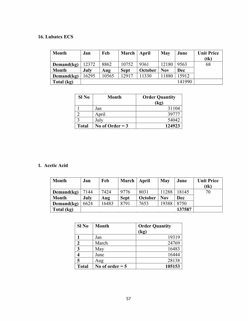
57
16. Lubatex ECS
Month Jan Feb March April May June Unit Price (tk)
Demand(kg) 12372 8862 10752 9361 12180 9563 68 Month July Aug Sept October Nov Dec Demand(kg) 16295 10565 12917 11330 11880 15912 Total (kg) 141990
1. Acetic Acid
Month Jan Feb March April May June Unit Price (tk)
Demand(kg) 7144 7424 9776 8031 11288 18145 70 Month July Aug Sept October Nov Dec Demand(kg) 6624 16483 8791 7653 19388 8750 Total (kg) 137587
Sl No Month Order Quantity (kg)
1 Jan 31104 2 April 39777 3 July 54042 Total No of Order = 3 124923
Sl No Month Order Quantity (kg)
1 Jan 19319 2 March 24769 3 May 16483 4 June 16444 5 Aug 28138 Total No of order = 5 105153
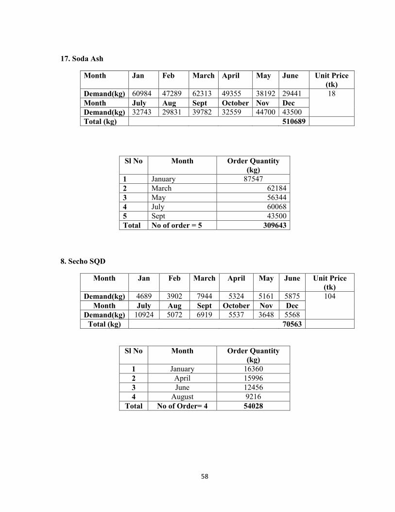
58
17. Soda Ash
Month Jan Feb March April May June Unit Price (tk)
Demand(kg) 60984 47289 62313 49355 38192 29441 18 Month July Aug Sept October Nov Dec Demand(kg) 32743 29831 39782 32559 44700 43500 Total (kg) 510689
8. Secho SQD
Month Jan Feb March April May June Unit Price (tk)
Demand(kg) 4689 3902 7944 5324 5161 5875 104 Month July Aug Sept October Nov Dec
Demand(kg) 10924 5072 6919 5537 3648 5568 Total (kg) 70563
Sl No Month Order Quantity (kg)
1 January 87547 2 March 62184 3 May 56344 4 July 60068 5 Sept 43500 Total No of order = 5 309643
Sl No Month Order Quantity (kg)
1 January 16360 2 April 15996 3 June 12456 4 August 9216
Total No of Order= 4 54028

59
18. Croscolor ADM
Month Jan Feb March April May June Unit Price (tk)
Demand(kg) 2895 1917 2199 714 1201 2120 285 Month July Aug Sept October Nov Dec Demand(kg) 2181 981 1840 1229 2600 3380 Total (kg) 23257
9. H2O2
Month Jan Feb March April May June Unit Price (tk)
Demand(kg) 11538 16112 27019 9822 16804 22611 28 Month July Aug Sept October Nov Dec
Demand(kg) 13202 22415 13209 14259 19530 21270 Total (kg) 207789
Sl No Month Order Quantity (kg)
1 Jan 4035 2 April 3162 3 June 3069 4 Aug 5980 Total No of order= 4 16246
Sl No Month Order Quantity (kg)
1 January 26625 2 March 35813 3 May 35624 4 July 33789 5 Sept 21270
Total No of order = 5 153121

60
5. Caustic Soda
Month Jan Feb March April May June Unit Price (tk)
Demand(kg) 9607 8146 30984 8046 12974 10723 35 Month July Aug Sept October Nov Dec
Demand(kg) 11149 11119 11032 8377 9900 20000 Total (kg) 152056
6. Cibafix Eco
Month Jan Feb March April May June Unit Price (tk)
Demand(kg) 749 797 924 692 884 704 395 Month July Aug Sept October Nov Dec
Demand(kg) 1499 890 1535 1638 1090 1950 Total (kg) 13352
Sl No Month Order Quantity (kg)
1 January 21020 2 March 21872 3 May 22151 4 July 18277 5 September 20000
Total No of order= 5 103320
Sl No Month Order Quantity (kg)
1 January 2280 2 April 3924 3 July 2728 4 September 1950
Total No of order= 4 10882

61
20. Permol R
Month Jan Feb March April May June Unit Price (tk)
Demand(kg) 3884 3763 4562 5456 6841 4512 80 Month July Aug Sept October Nov Dec
Demand(kg) 7392 2769 5296 7384 5760 6120 Total (kg) 63739
3. Neutracid
Month Jan Feb March April May June Unit Price (tk)
Demand(kg) 1630 1339 1087 1558 1795 747 92 Month July Aug Sept October Nov Dec
Demand(kg) 900 1670 2035 2024 3200 2520 Total (kg) 20505
Sl No Month Order Quantity (kg)
1 January 5456 2 Feb 11353 3 April 10161 4 June 12680 5 August 11880
Total No of order= 5 51530
Sl No Month Order Quantity (kg)
1 January 4100 2 April 2570 3 June 4059 4 August 5720
Total No of order= 4 16449
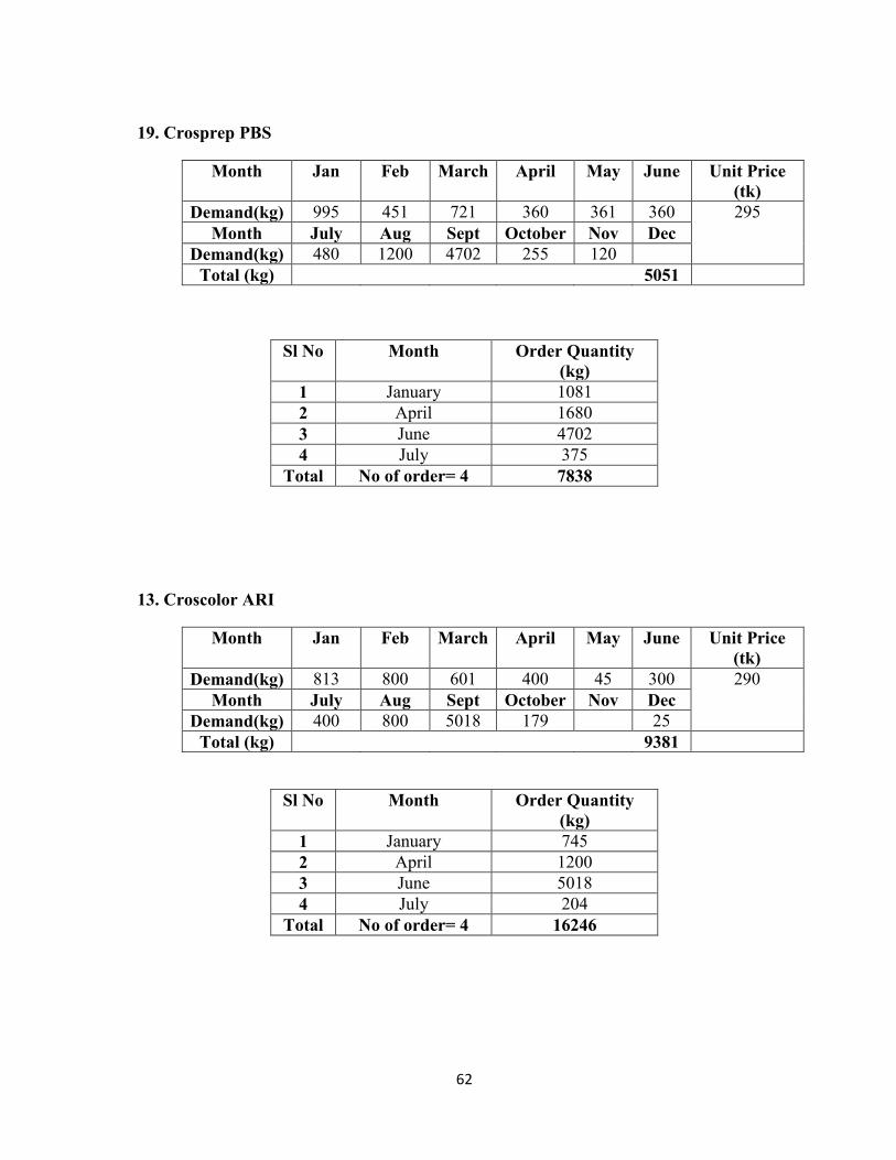
62
19. Crosprep PBS
Month Jan Feb March April May June Unit Price (tk)
Demand(kg) 995 451 721 360 361 360 295 Month July Aug Sept October Nov Dec
Demand(kg) 480 1200 4702 255 120 Total (kg) 5051
13. Croscolor ARI
Month Jan Feb March April May June Unit Price (tk)
Demand(kg) 813 800 601 400 45 300 290 Month July Aug Sept October Nov Dec
Demand(kg) 400 800 5018 179 25 Total (kg) 9381
Sl No Month Order Quantity (kg)
1 January 1081 2 April 1680 3 June 4702 4 July 375
Total No of order= 4 7838
Sl No Month Order Quantity (kg)
1 January 745 2 April 1200 3 June 5018 4 July 204
Total No of order= 4 16246

63
10. Hydrose
Month Jan Feb March April May June Unit Price (tk)
Demand(kg) 1203 932 499 733 1096 2199 64 Month July Aug Sept October Nov Dec
Demand(kg) 1509 879 1064 1105 1300 1800 Total (kg) 14319
11. Leucophor BMB
Month Jan Feb March April May June Unit Price (tk)
Demand(kg) 120 70 97 49 58 51 650 Month July Aug Sept October Nov Dec
Demand(kg) 5 84 20 46 100 Total (kg) 702
Sl No Month Order Quantity (kg)
1 January 1829 2 March 3708 3 May 3048 4 August 3100
Total No of order= 4 16246
Sl No Month Order Quantity (kg)
1 January 49 2 February 114 3 May 150 4 September 100
Total No of order= 4 413
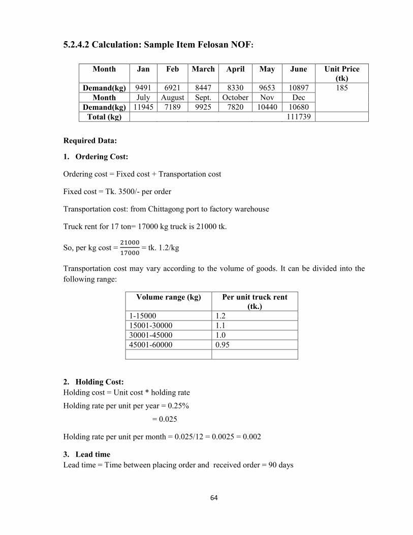
64
5.2.4.2 Calculation: Sample Item Felosan NOF:
Required Data:
1. Ordering Cost:
Ordering cost = Fixed cost + Transportation cost
Fixed cost = Tk. 3500/- per order
Transportation cost: from Chittagong port to factory warehouse
Truck rent for 17 ton= 17000 kg truck is 21000 tk.
So, per kg cost = 21000
17000 = tk. 1.2/kg
Transportation cost may vary according to the volume of goods. It can be divided into the following range:
Volume range (kg) Per unit truck rent (tk.)
1-15000 1.2 15001-30000 1.1 30001-45000 1.0 45001-60000 0.95
2. Holding Cost: Holding cost = Unit cost * holding rate Holding rate per unit per year = 0.25%
= 0.025
Holding rate per unit per month = 0.025/12 = 0.0025 = 0.002
3. Lead time Lead time = Time between placing order and received order = 90 days
Month Jan Feb March April May June Unit Price (tk)
Demand(kg) 9491 6921 8447 8330 9653 10897 185 Month July August Sept. October Nov Dec
Demand(kg) 11945 7189 9925 7820 10440 10680 Total (kg) 111739

65
Calculation: 1. For demand of the month of April = 8330 kg, place order in the month of January.
Ordering cost = (monthly demand * per unit transport cost) + Fixed Cost
= (8330 * 1.2) + 3500
= Tk. 13496/-
Holding Cost = Zero Quantity ordered in January = 8330 kg
2. For demand of the month of May = 9653 kg, place order in the month of January or February
If order place in January, holding cost, hc= (9653*.002*185) = tk. 3572/-
If order place in Feb , ordering cost, oc = (9653*0.1) + 3500 = tk. 4465/-
hcoc, so place order in the month of January = 9653 kg
3. For demand of the month of June = 10897 kg, place order in the month of January or March
If order place in January, holding cost for two month, hc= (10897*.002*185*2) = tk. 8064/-
If order place in March , ordering cost, oc = (10897*0.1) + 3500 = tk. 4590/-
ochc, so place order in the month of March = 10897 kg
4. For demand of the month of July = 11945 kg, place order in the month of March or April
If order place in March, holding cost for one month, hc= (11945*.002*185) = tk. 4420/-
If order place in April , ordering cost, oc = (11945*0.2) + 3500 = tk. 5889/-
hcoc, so place order in the month of March = 11945 kg
5. For demand of the month of August = 7189 kg, place order in the month of March or May
If order place in March, holding cost for two month, hc= (7189*.002*185*2) = tk. 5320/-
If order place in May , ordering cost, oc = (7189*0.1) + 3500 = tk. 4219/-
ochc, so place order in the month of May = 7189 kg
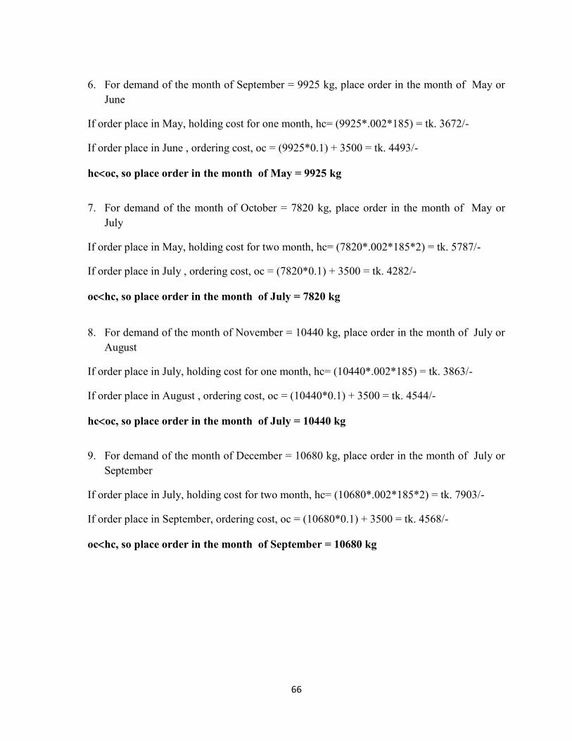
66
6. For demand of the month of September = 9925 kg, place order in the month of May or June
If order place in May, holding cost for one month, hc= (9925*.002*185) = tk. 3672/-
If order place in June , ordering cost, oc = (9925*0.1) + 3500 = tk. 4493/-
hcoc, so place order in the month of May = 9925 kg
7. For demand of the month of October = 7820 kg, place order in the month of May or July
If order place in May, holding cost for two month, hc= (7820*.002*185*2) = tk. 5787/-
If order place in July , ordering cost, oc = (7820*0.1) + 3500 = tk. 4282/-
ochc, so place order in the month of July = 7820 kg
8. For demand of the month of November = 10440 kg, place order in the month of July or August
If order place in July, holding cost for one month, hc= (10440*.002*185) = tk. 3863/-
If order place in August , ordering cost, oc = (10440*0.1) + 3500 = tk. 4544/-
hcoc, so place order in the month of July = 10440 kg
9. For demand of the month of December = 10680 kg, place order in the month of July or September
If order place in July, holding cost for two month, hc= (10680*.002*185*2) = tk. 7903/-
If order place in September, ordering cost, oc = (10680*0.1) + 3500 = tk. 4568/-
ochc, so place order in the month of September = 10680 kg

67
Table 5.9: Summarization of result From above calculation, the results are summarized as below:
Table 5.10: Comparison Between EOQ Model and Wagner- Whitin Model
SL No.
Terms EOQ Model Wagner- Whitin Model
1 Annual Demand(kg) 111739 111739 2 Unit Cost(tk.) 185 3 Order Quantity(kg) 16744 17376(avg) 4 No of order 7 5 5 Annual ordering cost(tk.) 24500 37050 6 Annual holding cost(tk.) 23316 42600 7 Total cost(tk.) 47816 79650
From the above table, it is found that for inventory management EOQ model is more
appropriate than Wagner-Whitin Model. Total cost for holding inventory for one year is less
than WW model. Quantity per order and no. of order is also appropriate. For developing
inventory situation of dyeing unit of Reedisha Knitex Ltd. EOQ model may apply.
Month of Order Ordering Quantity (kg) January (8330 + 9653) = 17983 kg March (10897 + 11945 = 22842 kg May (7189 + 9925) = 17114 kg July (7820+ 10440) = 18260 kg September 10680 kg Total no of order = 5 Total Order Quantity = 86879 kg

68
CHAPTER 6 CONCLUSION & RECOMMENDATION
6.1 Conclusion From the above study it is found that in most of the cases industry does not follow the
modern inventory management system. The company selected for our research work is
Reedisha Knitex Ltd. Here raw materials are ordered through experience or when inventory
levels become low in the warehouse. They keep three month stock of the raw materials and
then place order for the next lot. As a result the company faces the problem of overstocking
or under stocking. If consumption of chemicals for any month is lower than the expected
rate or much higher than the company has to meet the demand domestically or by rented
from another company which carries a huge expense for the company. Again all raw
materials need not review in the same manner. By doing ABC analysis we categorize the
items and give different level of control to different items.
Therefore, the company needs a formalized inventory system to minimize operational costs.
If the Economic Order Quantity model is objectively used, with the aid of some judgment by
the management, holding costs and ordering costs will become low. The use of this model
will help the company to know the exact amount of raw materials to order and when to place
new orders for each raw material.
From Wagner-Whitin Model it is found that by comparing ordering cost and holding cost for
a particular month, we can determine whether place order in that month or next month. By
applying the model we can minimize the number of order and thus total cost of maintaining
inventory become optimal.
By comparing EOQ model& Wagner-Whitin model it is found that EOQ model is more
appropriate for inventory cost reduction. From reorder point calculation it can be determined
when next order place.
69
6.2 Recommendations Since there is no formal inventory control system employed by Reedisha Knitex Ltd, to
manage inventories for its raw materials, some aspects need to be improved in order to
minimize the raw materials inventory costs. The following are recommended:
1. A large company like Reedisha Knitex Ltd. should improve their ways of keeping records
about purchasing and the daily consumption of the raw materials. If possible, the company
should computerize these systems.
2. Lack of awareness on the quantitative techniques of managing inventories indicates that
storekeepers and supplies staff are lacking some business management skills, therefore these
staff should be undergoing on job training about stores and supplies management to improve
their knowledge and competence in the field.
3. It is also suggested that periodic review where inventory are reviewed in a regular interval
may be the appropriate policy for the company to solve the ‘when to order’ problem.
6.3 Limitation of the Study: Due to restriction of some departments as per company policy required data collection is not
possible. Also it was so difficult to collect data from all available department and sections
alone within limited time.
Economic order quantity calculation is based on some assumption. Here demand is assumed
to be constant over the period. But in practice demand is variable during the period. Most of
the company does not calculate inventory carrying cost. The standard rule of thumb for
inventory carrying cost is 25% of inventory value on hand.
This research is built on comparison between existing activities and estimated activities. Due
to the assumptions connected with estimations, the results could be questionable in terms of
its credibility. However, our viewpoint is that the estimations are based on a solid
investigation therefore the study is relatively convictive.

70
Figure 6: Main Chemical Store of Reedisha Knittex Ltd.

71
Figure 7: Stock of Chemical of Felosan NOF

72
Figure 8: Stock of Chemical of Crosoft NBC
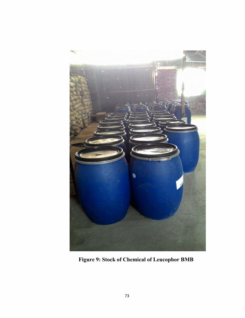
73
Figure 9: Stock of Chemical of Leucophor BMB
74
References [1] Philips RS, 1987. Operations Research Principles and Practice.2nd edition.John Wiley and Sons.
[2] Wild T, 2002. Best Practice in Inventory Management. Butterworth – Heinemann, 2nd edition, August, 2002. ISBN – 13: 398 -07506511586.
[3] Axsater S, 2006. Inventory Control.Springer. ISBN 978 – 0 387-33250-s
[4] Taha HA, 1997. Operations Research.An Introduction.3rd edition. Upper Saddle River, NJ: Prentice Hall.
[5] Ravindran RS, Solberg R, Phillips RS, 1987. Operations Research.Principles and Practice, 2nd edition.John Wiley.
[6] Carter, S., & Evans, D. (2006). Enterprise and Small Business-Principles, Practice and Policy.Har-low: FT Prentice Hall.
[7] Chapman, S., Ettkin, L. P., & Helms, M. M. (2000). Do Small Businesses Need Supply Chain Management? IIE Solutions, 32(8), 31-35.
[8] Chopra, S., &Meindl, P. (2001). Supply Chain Management: Strategy, Planning, and Operation. Englewood Cliffs: Prentice-Hall.
[9] Christopher, M. (1998). Logistics and Supply Chain Management. London: Pitman.
[10] Coyle, J. J., Bardi, E. J., & Langley, C. J. Jr. (2003). The Management of Business Logistic: A Supply Chain Perspective (7th ed.). Mason: South-Western.
[11] Davenport, T. H. (2000). Mission Critical: Realizing the Promise of Enterprise Systems. Boston: Harvard Business School Press.
[12] ENSR (1997). The European Observatory for SMEs-Fifth Annual Report, European Network for SME Research, Zoetermeer: EIM Small Business Research and Consultancy.
ENSR (2004).Highlights for the 2003 Observatory. European Commission, Brussels.
75
[13] Heizer, Render, Rajashekhr Operation Management, Ninth Edition, pp 449-461
[14] http://en.wikipedia.org/wiki/Inventorymanagement#Evolution, viewed on 15-Nov-2014 3:55 PM
[15] Gaither, N. Grazier, G. 2002 Operation Management. South-Western Thomson Learning
[16] Guan, L. Hansen, D. R. Mowen, M. 2009 Cost Management. 6th Edition. South Western Cengage Learning
[17] www.supply chain metric.com/inventory finance.htm, viewed on 1.11.2014 1.20 PM
[18] en.m.wikipedia.org/wiki/Dynamic_lot-size_model, viewed on 3 Dec 2014 on 10.00 AM
[19] en.m.wikipedia.org/wiki/Inventory, viewed on 3 Dec 2014 on 2.00 PM
[20] www.lokad.com/definition-inventory-costs , viewed on 18 Nov 2014 on 11.00 AM
[21] en.m.wikipedia.org/wiki/Economic_Order_quantity, viewed on 25 Nov 2014 on 8.00 PM
[22] Chase-Jacods-Aquifano-Agarwal, Operations Management for compative Advantage, 11thEditionpp pp 635-640
[23]inventory management optimization as part of Operational Risk Management, page 213-222, April 2009
[24] GrzegorzMichalski, Value based inventory management- EOQ modification, Page33-34, 2004
[25] The international Journal of logistic management. Volume 19: issue 2: page212-232, August 2008
[26] Optimal lot size decisions under The Wagner-Whitin Model with Backorders, Second world conference on POM, Cancun, Mexico, May 2004
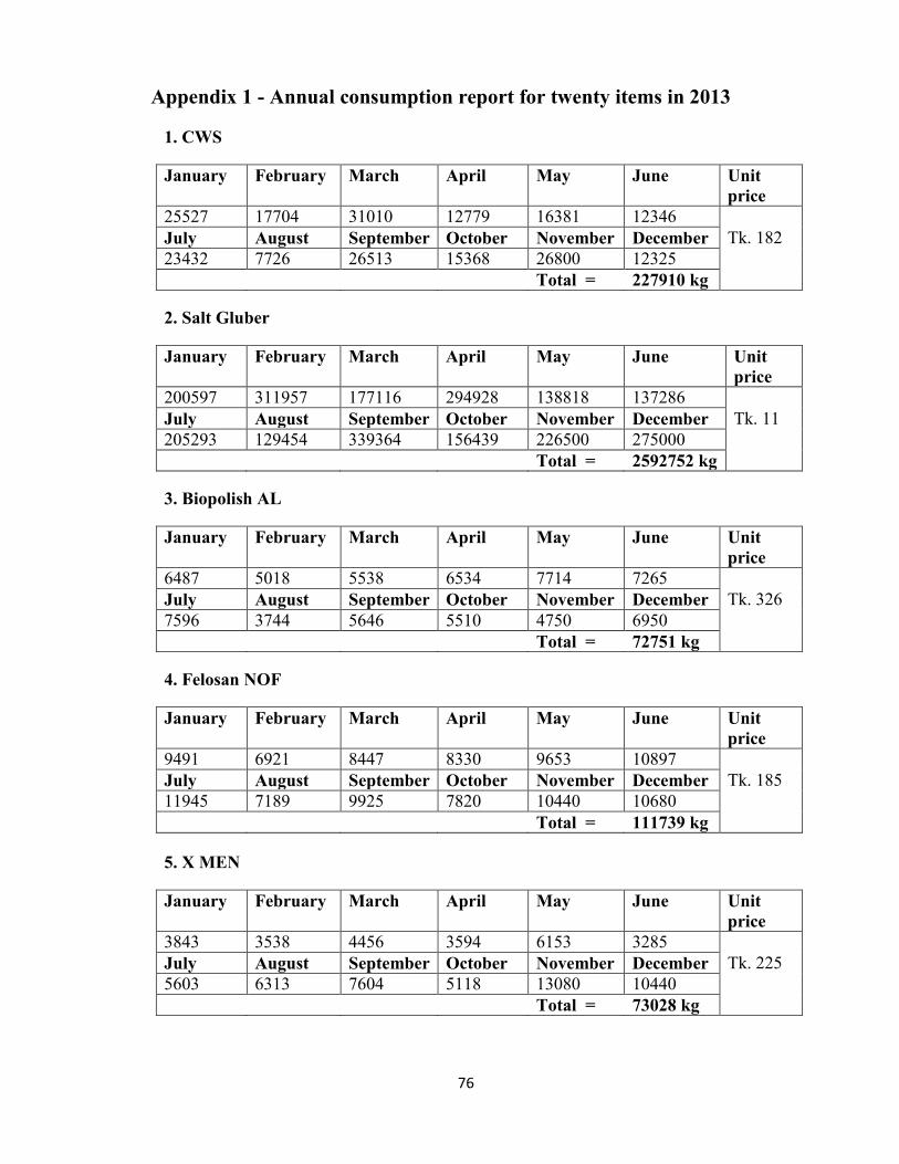
76
Appendix 1 - Annual consumption report for twenty items in 2013
1. CWS
January February March April May June Unit price
25527 17704 31010 12779 16381 12346 July August September October November December Tk. 182 23432 7726 26513 15368 26800 12325 Total = 227910 kg
2. Salt Gluber
January February March April May June Unit price
200597 311957 177116 294928 138818 137286 July August September October November December Tk. 11 205293 129454 339364 156439 226500 275000 Total = 2592752 kg
3. Biopolish AL
January February March April May June Unit price
6487 5018 5538 6534 7714 7265 July August September October November December Tk. 326 7596 3744 5646 5510 4750 6950 Total = 72751 kg
4. Felosan NOF
January February March April May June Unit price
9491 6921 8447 8330 9653 10897 July August September October November December Tk. 185 11945 7189 9925 7820 10440 10680 Total = 111739 kg
5. X MEN
January February March April May June Unit price
3843 3538 4456 3594 6153 3285 July August September October November December Tk. 225 5603 6313 7604 5118 13080 10440 Total = 73028 kg

77
6. Optavon 4UD
January February March April May June Unit price
6922 5660 7858 8098 7480 9209 July August September October November December Tk. 111 9040 6582 8596 7734 7800 10350 Total = 95329 kg
7. Acetic Acid
January February March April May June Unit price
7144 7424 9776 8031 11288 18145 July August September October November December Tk. 70 6624 16483 8791 7653 19388 8750 Total = 137587 kg
8. Lubatex ECS
January February March April May June Unit price
12372 8862 10752 9361 12180 9563 July August September October November December Tk. 68 16295 10565 12917 11330 11880 15912 Total = 141990 kg
9. Soda Ash
January February March April May June Unit price
60984 47289 62313 49355 38192 29441 July August September October November December Tk. 18 32743 29831 39782 32559 44700 43500 Total = 510689 kg
10. Secho SQD
January February March April May June Unit price
4689 3902 7944 5324 5161 5875 July August September October November December Tk. 104 10924 5072 6919 5537 3648 5568 Total = 70563 kg

78
11. Cros Color ADM
January February March April May June Unit price
2895 1917 2199 714 1201 2120 July August September October November December Tk. 285 2181 981 1840 1229 2600 3380 Total = 23257 kg
12. H2O2
January February March April May June Unit price
11538 16112 27019 9822 16804 22611 July August September October November December Tk. 28 13202 22415 13209 14259 19530 21270 Total = 207789 kg
13. Caustic Soda
January February March April May June Unit price
9607 8146 30984 8046 12974 10723 July August September October November December Tk. 35 11149 11119 11032 8377 9900 20000 Total = 152056 kg
14. Cibafix Eco
January February March April May June Unit price
749 797 924 692 884 704 July August September October November December Tk. 395 1499 890 1535 1638 1090 1950 Total = 13352 kg
15. Permol R
January February March April May June Unit price
3884 3763 4562 5456 6841 4512 July August September October November December Tk. 80 7392 2769 5296 7384 5760 6120 Total = 63739 kg

79
16. Neutracid
January February March April May June Unit price
1630 1339 1087 1558 1795 747 July August September October November December Tk. 92 900 1670 2035 2024 3200 2520 Total = 20505 kg
17. Crosprep PBS
January February March April May June Unit price
995 451 721 360 361 360 July August September October November December Tk. 295 480 1200 4702 255 120 Total = 7838 kg
18. Cros Color ARI
January February March April May June Unit price
813 800 601 400 45 300 July August September October November December Tk. 290 400 800 5018 17 25
Total = 9381 kg
19. Hydrose
January February March April May June Unit price
1203 932 499 733 1096 2199 July August September October November December Tk. 64 1509 879 1064 1105 1300 1800 Total = 14320 kg
20. Leucophor BMB
January February March April May June Unit price
120 70 97 49 58 51 July August September October November December Tk. 650 5 84 20 46 100 Total = 702 kg
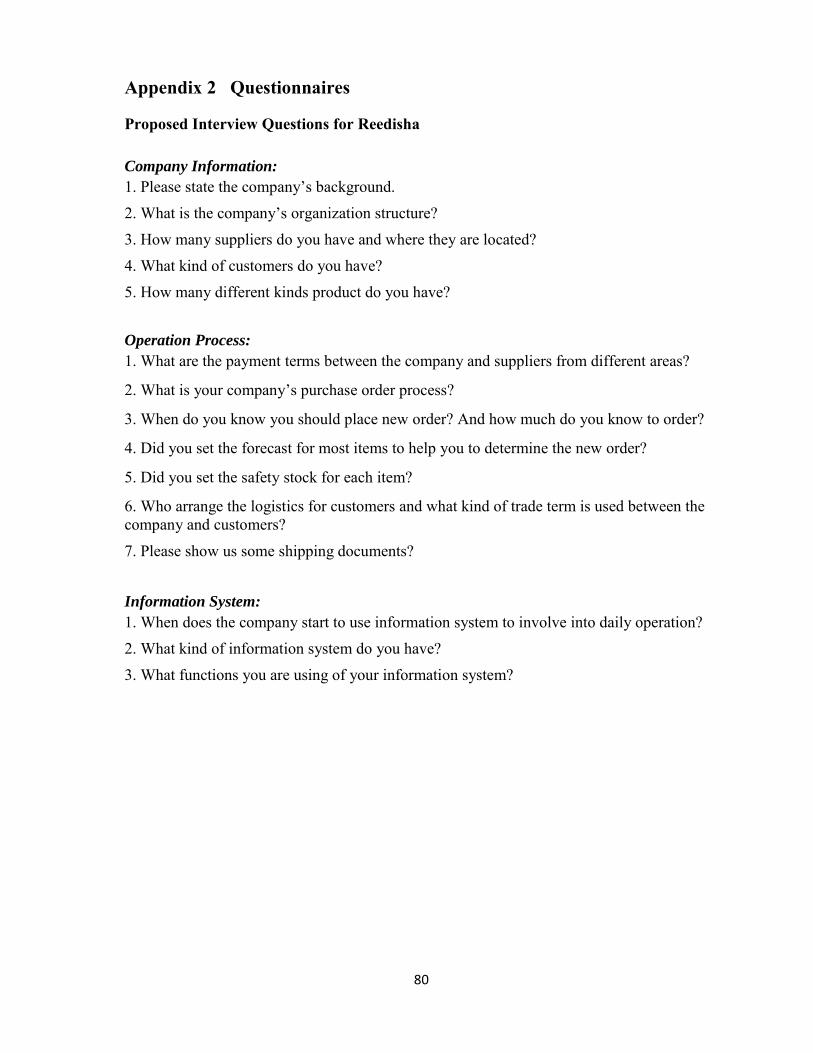
80
Appendix 2 Questionnaires
Proposed Interview Questions for Reedisha
Company Information:
1. Please state the company’s background.
2. What is the company’s organization structure?
3. How many suppliers do you have and where they are located?
4. What kind of customers do you have?
5. How many different kinds product do you have?
Operation Process:
1. What are the payment terms between the company and suppliers from different areas?
2. What is your company’s purchase order process?
3. When do you know you should place new order? And how much do you know to order?
4. Did you set the forecast for most items to help you to determine the new order?
5. Did you set the safety stock for each item?
6. Who arrange the logistics for customers and what kind of trade term is used between the company and customers?
7. Please show us some shipping documents?
Information System:
1. When does the company start to use information system to involve into daily operation?
2. What kind of information system do you have?
3. What functions you are using of your information system?
Related Documents