The Pennsylvania State University The Graduate School College of Engineering DEVELOPMENT OF AN ANALYTICAL DESIGN TOOL FOR JOURNAL BEARINGS A Thesis in Mechanical Engineering by Richard K. Naffin © 2009 Richard K. Naffin Submitted in Partial Fulfillment of the Requirements for the Degree of Master of Science August 2009

Welcome message from author
This document is posted to help you gain knowledge. Please leave a comment to let me know what you think about it! Share it to your friends and learn new things together.
Transcript

The Pennsylvania State University
The Graduate School
College of Engineering
DEVELOPMENT OF AN ANALYTICAL
DESIGN TOOL FOR JOURNAL BEARINGS
A Thesis in
Mechanical Engineering
by
Richard K. Naffin
© 2009 Richard K. Naffin
Submitted in Partial Fulfillment of the Requirements
for the Degree of
Master of Science
August 2009

The thesis of Richard K. Naffin was reviewed and approved* by the following: Liming Chang Professor of Mechanical Engineering Thesis Adviser Gita Talmage Professor of Mechanical Engineering Karen A. Thole Professor of Mechanical Engineering Head of the Department of Mechanical Engineering *Signatures are on file in the Graduate School

iii
Abstract
Reliable and efficient journal bearings operate with sufficient load capacity, low
frictional loss, low heat generation, and a sufficient supply of lubricating oil. To design
such bearings, values of the bearing design parameters are selected and used to calculate
bearing performance variables. The performance variables are then used to describe the
operational state of the bearing, aiding the designer in deciding whether the selected
values of the design parameters are optimal or not. In the current design methods, these
performance variables are often solved by interpolating and extracting solutions from
design tables. This technique may become tedious and inconvenient, especially when
trying to compile a large number of results to generate solution curves of the performance
variables.
This research develops an improved design method for journal bearings. The
solution is a design tool which uses analytic design modules to calculate the different
design considerations of the bearing system. Each module focuses on a single design
aspect and calculates the associated performance variables using a series of analytic
equations. This analytic method is implemented into a computer program and forms a
basic CAD package capable of generating solution curves of the performance variables.
These curves aid the designer in selecting the best design parameters for the system.
Thus, this basic analytic design tool produces similar results to the current manual
approach but in a manner which is more modern, time-efficient, user-friendly, and cost-
effective.
iv
Table of Contents
List of Figures....................................................................................................................vi
List of Tables....................................................................................................................vii
Nomenclature..................................................................................................................viii
Acknowledgements...........................................................................................................xi
Chapter 1: Introduction....................................................................................................1
Chapter 2: The Load Capacity Module...........................................................................8
2.1 Description of the Journal Bearing....................................................................8
2.2 The Simplified Models....................................................................................11
2.2.1 The Long Bearing Model..................................................................11
2.2.2 The Short Bearing Model..................................................................13
2.2.3 The Finite Bearing Technique..........................................................14
2.3 Development of an Analytic Finite Bearing Model.........................................15
2.4 Evaluation of the Finite Bearing Model...........................................................23
2.5 Refinement of the Finite Bearing Model.........................................................25
2.6 Summary of the Load Capacity Module..........................................................30
Chapter 3: The Temperature Module............................................................................32
3.1 Current Temperature Rise Calculation............................................................32
3.2 Analytic Equation for the Friction Factor........................................................35
3.3 Analytic Equation for the Inflow Factor..........................................................38
3.4 Analytic Equation for the Side Leakage Factor...............................................41

v
3.5 Summary of the Temperature Module.............................................................44
Chapter 4: Development of an Analytic Design Tool...................................................46
4.1 Summary and Integration of the Individual Modules......................................46
4.2 Implementation of the Core Design Calculations............................................51
4.3 Packaging the Basic Design Tool....................................................................55
4.4 Demonstrations of the Design Tool.................................................................59
4.4.1 Example 1.........................................................................................59
4.4.2 Example 2.........................................................................................63
Chapter 5: Summary and Recommendations...............................................................71
Bibliography.....................................................................................................................75
Appendix A: The Numerical Method Design Tables....................................................76
Appendix B: Sample Viscosity-Temperature Chart.....................................................80
Appendix C: MATLAB Code for the Bearing CAD Tool............................................81

vi
List of Figures
Figure 1-1 Shape of a Journal Bearing..........................................................................1
Figure 2-1 Geometry of a Journal Bearing....................................................................8
Figure 2-2 Shape of the Bearing Pressure Distribution in both the a) Circumferential and b) Axial Directions..............................................................................10
Figure 2-3 Dimensionless Load versus Slenderness Ratio Data for the Simplification Models When the Eccentricity Ratio is 0.5...............................................17
Figure 2-4 Generation of the Dimensionless Load versus Slenderness Ratio Curve-fit
When the Eccentricity Ratio is 0.5............................................................18 Figure 2-5 Dimensionless Load versus Slenderness Ratio Curve Family...................22
Figure 4-1 Schematic of Integrated Model..................................................................49
Figure 4-2 Schematic of Basic Design Tool................................................................56
Figure 4-3 Solution Curves for a) Minimum Film Thickness, b) Friction Power Loss, c) Lubricant Side Leakage, and d) Outlet Temperature with Respect to the Clearance Ratio..........................................................................................61
Figure 4-4 Design Solution Curves of the a) Eccentricity Ratio and b) Minimum Film
Thickness with Respect to the Inlet Viscosity...........................................66 Figure 4-5 Design Solution Curves of the a) Friction Coefficient and b) Power Loss
with Respect to the Inlet Viscosity............................................................67 Figure 4-6 Design Solution Curves of the Lubricant a) Flow and b) Temperature
Conditions with Respect to the Inlet Viscosity..........................................68 Figure B-1: A Common Viscosity-Temperature Chart. This particular chart may be
used for the SAE oil grades 10, 20, 30, 40, 50, 60, and 70........................80

vii
List of Tables
Table 2-1 Error Evaluation of Preliminary Analytic-Finite-Bearing Model.............23
Table 2-2 Error Evaluation of Analytic-Finite-Bearing Model with Adjusted Mesh Points.........................................................................................................26
Table 2-3 Error Evaluation of Corrected Analytic-Finite-Bearing Model.................28
Table 2-4 Error Evaluation of the Film-Thickness-Performance Factor...................29
Table 3-1 Error Evaluation of the Preliminary Friction-Factor Equation..................36
Table 3-2 Error Evaluation of the Corrected Friction-Factor Equation.....................37 Table 3-3 Error Evaluation of the Preliminary Inflow-Factor Equation....................39
Table 3-4 Error Evaluation of the Corrected Inflow-Factor Equation.......................40
Table 3-5 Error Evaluation of the Preliminary Side-Leakage-Factor Equation.........42
Table 3-6 Error Evaluation of the Corrected Side-Leakage-Factor Equation............44 Table 4-1 List of Input Parameters Used in the Clearance Ratio Verification
Test.............................................................................................................60 Table 4-2 List of Input Parameters Used in the Inlet Viscosity Verification
Test.............................................................................................................64 Table A-1 The Finite-Bearing Design Tables as Compiled in Booser [1]..................76

viii
Nomenclature
Symbol Description of Symbol Units
AL Long-Bearing-Eccentricity-Ratio Function in Log Scale Dimensionless
AS Short-Bearing-Eccentricity-Ratio Function in Log Scale Dimensionless
C0 0th Coefficient of Finite Analytic Equation Dimensionless
C1 1st Coefficient of Finite Analytic Equation Dimensionless
C2 2nd Coefficient of Finite Analytic Equation Dimensionless
C3 3rd Coefficient of Finite Analytic Equation Dimensionless
CS Short-Bearing-Model Correction Factor Dimensionless
CL Long-Bearing-Model Correction Factor Dimensionless
Cf Friction-Coefficient Correction Factor Dimensionless
Cin Inflow Correction Factor Dimensionless
Cleak Side-Leakage-Flow Correction Factor Dimensionless
c Radial Clearance of Journal Bearing m
ch Specific Heat of Selected Lubricant J/(kg/°C)
D Journal Diameter m
e Eccentricity Between Bearing/Journal Centers m
f Coefficient of Friction Dimensionless
fL(ε) Long-Bearing-Eccentricity-Ratio Function Dimensionless
fS(ε) Short-Bearing-Eccentricity-Ratio Function Dimensionless
h Film Thickness m
h Film-Thickness-Performance Factor Dimensionless

ix
hmin Minimum Film Thickness m
L Bearing Length m
N Journal Rotational Speed rev/s or rpm
Ploss Frictional Power Loss Watts or Horsepower
p Bearing Pressure Distribution Pa
Qavg Average Lubricant Flow of Bearing m3/s
Qin Lubricant Inflow of Bearing Loaded Region m3/s
Qleak Lubricant Side Leakage Flow of Bearing m3/s
Qx Lubricant Circumferential Flow of Bearing m3/s
inQ Loaded-Region-Inflow-Performance Factor Dimensionless
leakQ Side-Leakage-Flow-Performance Factor Dimensionless
R Journal Radius m
R1 Bearing Radius m
R2 Journal Radius m
(R/c)f Frictional-Loss-Performance Factor Dimensionless
S Sommerfeld Number Dimensionless
Tavg Lubricant Average Temperature °C
Tin Lubricant Temperature at Bearing Inlet °C
Tout Maximum Lubricant Temperature °C
U Tangential Surface Velocity of Journal m/s
W Applied Load N
W Dimensionless Load Dimensionless

x
X Slenderness Ratio in Log Scale Dimensionless
XL Long Bearing Mesh Point in Log Scale Dimensionless
XS Short Bearing Mesh Point in Log Scale Dimensionless
x Circumferential Coordinate of Journal Bearing m
Y Dimensionless Load in Log Scale Dimensionless
z Axial Coordinate of Journal Bearing m
α Circumferential Angle of Pressure Termination Point degree, °
β Viscosity-Temperature Coefficient 1/°C
ΔT Lubricant Temperature Rise °C
Δε Eccentricity-Ratio Error Tolerance Dimensionless
ε Eccentricity Ratio Dimensionless
εhigh Maximum Eccentricity Ratio Dimensionless
εlow Minimum Eccentricity Ratio Dimensionless
θ Circumferential Angle of Journal Bearing degree, °
μ Lubricant Viscosity Pa-s
μavg Average Lubricant Viscosity Pa-s
μin Inlet Lubricant Viscosity Pa-s
π 3.14 Dimensionless
ρ Lubricant Density kg/m3
ω Journal Rotational Speed rad/s

xi
Acknowledgements
I would like to sincerely thank my academic advisor at the Pennsylvania State
University, Dr. Liming Chang, for granting me the opportunity to pursue this research.
His honest guidance went beyond simply providing assistance with this research, as his
advice helped strengthen my personal weaknesses as well. He is a very patient advisor
who strives to see his students continue to develop their skills and succeed after college.
I owe him a debt of gratitude.
I would also like to thank Dr. Gita Talmage, who was willing to review this
thesis. She provided many suggestions which enhanced the value of this work. I also
appreciate the advice she provided in enhancing my presentation skills.

1
Chapter 1: Introduction
A journal bearing is a very useful component when it comes to supporting load in
rotating machinery. As illustrated in Figure 1-1.a, a cylindrical bearing encases a
rotating shaft known as the journal. These two parts are kept separated from each other
through the process of hydrodynamic lubrication.
Figure 1-1: Shape of a Journal Bearing Source: Cameron, Alastair. Basic Lubrication Theory. 3rd ed. New York: A. Cameron/Ellis Horwood
Ltd., 1981. p. 128

2
Consider a non-rotating journal that is subjected to a downward applied load as in Figure
1-1.b. When the journal begins to rotate clockwise, the supplied lubricant is dragged into
the journal bearing in the direction of the motion. The flow continuity of the lubricant
induces a pressure that is generated in the converging portion of the bearing system
which is labeled with an ‘X’ in Figure 1-1.b. This pressure is known as the
hydrodynamic pressure. It reduces the inflow and increases the outflow of the lubricant
in that converging portion of the journal bearing, so that the flow continuity is
maintained. If the pressure is sufficiently high, it causes the journal to lift away from the
bearing surface as illustrated in Figure 1-1.c. This is the basis of hydrodynamic
lubrication in a journal bearing. If designed correctly, the hydrodynamic pressure keeps
the journal and bearing surfaces sufficiently separated during normal operation.
There are many features to the journal bearing which makes it popular to use in
industrial applications. High toleration to dirt, low cost, small diameter, low running
friction, and low noise are a few benefits suggested by Engineers Edge [2], an online
engineering website. Such beneficial features allow the journal bearing to be widely used
in various rotating systems, such as steam turbines, engines, pumps, motors, gearboxes,
and milling systems. According to the bearing manufacturer STI, these engineering
systems typically involve high horsepower and load [3]. With such extreme operating
conditions, it is critical that the bearing operates efficiently and reliably.
Reliable journal bearings operate with sufficient load capacity, low frictional loss,
low heat generation, and a sufficient supply of lubricant oil. Designers satisfy each of
these requirements by selecting optimal values of the bearing design parameters of
bearing length and clearance ratio, as well as selecting the proper lubricant grade. The

3
other design parameters of applied load, journal diameter, and journal rotational speed are
typically governed by the engineering system for which the bearing is being designed.
All of these parameters are used to determine the bearing performance variables, which
are physical quantities used to describe the operational state of the bearing such as the
film thickness, lubricant temperature rise, friction, and oil flow.
Depending on the bearing geometry, the performance variables are solved by
calculating analytic equations or by extracting data off of bearing design tables. Journal
bearing geometry is characterized by the slenderness ratio L/D, the bearing length over
journal diameter [4]. Using this ratio, some bearings may be classified as either infinitely
short or long. For a bearing to be considered long, different sources suggest that the
slenderness ratio be larger than a value of L/D = 2 [5] to L/D = 4 [4]. Likewise, for a
bearing to be considered short, the slenderness ratio should be smaller than a value of
L/D = 1/4 [4] to L/D = 1/3 [6]. These long and short bearing geometries simplify the
governing equations of the system into analytic approximations, forming simplified
models. For the bearings in between, known as finite bearings, no widely accepted
analytic approximations exist. In practice, the slenderness ratio varies from about 0.125
in the narrowest of bearings to about 2 [4]. For the majority of bearings in this range of
slenderness ratios, use of either simplified model does not provide meaningful design
solutions. Instead, the governing equations are solved numerically by either a finite
difference method or a finite element method [7]. The resulting finite bearing solutions
are compiled as a series of dimensionless performance factors that have been plotted or
tabulated into charts or tables, such as the tables [1] referenced in Appendix A. As
illustrated in the appendix, these tables tabulate the performance factors used to calculate

4
the performance variables of the nominal film thickness, oil flow, and coefficient of
friction. The factors are tabulated with respect to the slenderness ratio and a variable
referred to as the Sommerfeld number, a dimensionless combination of the design
parameters. Once the Sommerfeld number and L/D of a system is determined, the
performance factors are extracted from the table and used to calculate the performance
variables.
These design tables are widely used in the current design methods for journal
bearings, which usually consider both the load capacity and temperature aspects of the
system. Many of these current calculation procedures obtain meaningful design solutions
by calculating the bearing performance variables using the average viscosity of the
lubricant, where the corresponding average temperature needs to be determined. Arnell
[8] describes one such technique. Arnell’s iterative process, which uses design charts,
may be modified to be used with the design tables [1] of Appendix A. An “intuitive”
average temperature of the lubricant is initially estimated by the designer. Its
corresponding average viscosity is used to determine the Sommerfeld number. Once the
Sommerfeld number is calculated, the corresponding values of the performance factors
for the coefficient of friction and oil flow are “looked up” in the table. These factors are
used in the supplemental equations provided by the design table to calculate both the
temperature rise and average temperature of the bearing lubricant. This calculated
average temperature is compared to the estimated value. If the difference between these
two temperatures is not within a selected error tolerance, a new average temperature is
estimated and new data is extracted from the table. This procedure is repeated until the
temperature difference is less than the required tolerance. The designer then uses the

5
corresponding viscosity of the final average temperature to obtain the final performance
factors for the friction coefficient and oil flow and subsequently calculate the respective
performance variables. Then, the load capacity is determined by finding the
corresponding dimensionless factor in the table and using it to calculate the minimum
film thickness.
The above iterative procedure does contain some weaknesses, despite its
usefulness. The extraction process of the performance factors from the design tables is
time-consuming, tedious, and inconvenient. For each iteration step involved in
determining the average temperature, the value of the Sommerfeld number changes.
Therefore, for each step, the designer is required to manually extract new performance
factors from the table to aid in calculating the temperature rise. The data provided in the
design tables are also discrete in nature, resulting in the designer often interpolating
between the provided data points to obtain and extract the performance factor values.
Furthermore, this manual design method is not very practical to use when generating
solution curves of the bearing performance variables. This task requires running the
above design method several times before enough data points are compiled to make
meaningful curves. Consequently, the current design method is antiquated. Today, many
engineering design calculations are being developed or implemented into computer
programs. Such programs run the tedious calculations for the designer. In addition, the
solutions are saved and transferred to other programs for future work or reference.
It is desirable to modernize and improve the efficiency of the current design
procedure by developing a design method which is analytic in nature. This proposed
method would use continuous, analytic equations to calculate each performance factor

6
instead of extracting data from design tables. These analytic equations would then be
used to develop a bearing design model which would include both the load capacity and
temperature considerations of the bearing system. The continuous nature of the model
equations would allow coverage of the entire bearing geometry range, removing the need
to interpolate data. In addition, the analytic nature of this design model would allow the
development of a computer-aided design (CAD) tool. CAD is the application of
computer technology and software to planning, performance, and implementing the
design process [9]. This CAD package would be capable of generating solution curves of
the performance variables used to locate optimal design parameters. The curves would
be generated in an automatic fashion, cutting down the amount of time needed in the
design stage of engineering. The output would also be formulated into computer files
which would transfer the solutions to other software packages, allowing the CAD
package to interface with other design programs. This same transfer file could even be
sent through the internet to other computers, allowing the designer to communicate with
other designers on a global level. In summary, the aim of this project is to produce a
bearing design tool which will deliver results similar to the current manual approach, but
in a much more convenient and timely manner.
The focus of this research, which is the development of an analytic bearing design
tool, is broken into the following chapters. In Chapter 2, an analytic load-capacity design
module is developed to calculate film thickness. In Chapter 3, an analytic temperature
module is developed to calculate the lubricant temperature rise of the bearing. These two
modules are then integrated together in Chapter 4 to develop a basic design model. This
model is implemented as a computer program and further expanded into a CAD tool

7
capable of generating solution curves for multiple bearing performance variables.
Finally, Chapter 5 summarizes the bearing design package and its contributions to the
future of engineering design.

8
Chapter 2: The Load Capacity Module
2.1 Description of the Journal Bearing
This chapter focuses on the development of an analytic module which will aid in
the load-capacity design aspect of the journal bearing. Load capacity is the ability of a
bearing to support load and may be measured by calculating the nominal film thickness
required to separate the surfaces of the journal and bearing. The film thickness may be
calculated using nominal values of the bearing design parameters, which include the
bearing length, journal diameter, radial clearance, inlet viscosity of the lubricant, applied
load, and journal rotational speed. The geometric parameters are illustrated in
Figure 2-1.
Figure 2-1: Geometry of a Journal Bearing
Source: Arnell, R.D., et al. Tribology: Principles and Design Applications. 1st ed. London: MacMillan Education Ltd, 1991. p. 162

9
In Figure 2-1, R1 represents the radius of the bearing, while R2 is the radius of the
journal. The nominal difference between R1 and R2 is the radial clearance c. The offset
between the journal center C and bearing center O is known as the eccentricity e. From
this geometry, an equation for the film thickness in terms of θ is determined [8]:
cos1cos
c
ecech (2.1.1)
In equation (2.1.1), θ is measured from the point of maximum clearance. The minimum
film thickness occurs at point F, where θ = 180º, giving:
1min ch (2.1.2)
In equation (2.1.2), ε = e/c and is known as the eccentricity ratio. This ratio is considered
the dimensionless performance factor for load capacity.
The loading conditions of the journal bearing are governed by the Reynolds
equation. During steady-state operation, the equation is in the following form [10]:
dx
dhU
z
ph
zx
ph
x633
(2.1.3)
In deriving the Reynolds equation, it is assumed that the flow is laminar, the fluid is
incompressible, the fluid viscosity remains constant, and no slip occurs between the fluid
and solid surfaces [7]. In equation (2.1.3), the film thickness h is given by equation
(2.1.1). The coordinate x is related to the circumferential coordinate θ and journal radius
R by:
Rx (2.1.4)
The tangential surface velocity U and angular velocity ω of the journal are related by:
RU (2.1.5)

10
The shape of the hydrodynamic pressure distribution p of equation (2.1.3) is illustrated in
Figure 2-2, where p(x,z) = 0 is the gage pressure.
a. b.
Figure 2-2: Shape of the Bearing Pressure Distribution in both the a) Circumferential and b) Axial Directions
The circumferential boundary conditions for equation (2.1.3) are given as [11]:
0,0 zp (2.1.6)
and
0,,
zx
pzp (2.1.7)
These two boundary equations form the Reynolds boundary condition, which contains an
unknown boundary point α that needs to be determined in the solution process [7].

11
Meanwhile, the axial boundary conditions for equation (2.1.3) are given as [11]:
02
,
L
xp (2.1.8)
and
00,
xz
p (2.1.9)
With these boundary conditions considered, no analytic solution exists for the Reynolds
equation in the above form. The system needs to be solved using numerical methods.
Under certain geometric conditions, however, equation (2.1.3) may be simplified to yield
analytic approximations. These approximations are known as either the long or short
bearing models and are described in the next section.
2.2 The Simplified Models
The geometry of the journal bearing is described by the slenderness ratio L/D, the
bearing length over journal diameter [4]. Using this ratio, journal bearings may be
categorized as either long, short, or finite bearings.
2.2.1 The Long Bearing Model
When the slenderness ratio L/D is sufficiently large, the magnitude of the axial
pressure variation becomes negligible compared to the pressure variation in the
circumferential direction. Therefore, the following assumption may be made:
z
p
x
p
(2.2.1)

12
Furthermore, it may be assumed that the oil film pressure does not change in the axial
direction [7]. Thus, equation (2.1.3) simplifies to [7]:
dx
dhU
dx
dph
dx
d 63
(2.2.2)
This is the long bearing model. However, a closed-form solution for this model cannot
be obtained using the Reynolds boundary condition because of the unknown boundary
point, α. By assuming that the pressure distribution terminates at the minimum film
thickness instead, which occurs at θ = π, α becomes zero. This simplification is known as
the half-Sommerfeld boundary condition and is written as [7]:
00 pp (2.2.3)
It is now possible to analytically solve equation (2.2.2) with the boundary condition
(2.2.3). The solution yields the following pressure distribution in terms of θ [5]:
222
2
cos12
cos2sin6
c
Rp 0 (2.2.4)
0p 2 (2.2.5)
Equation (2.2.4) is then integrated over the surface area that the pressure distribution acts
on to find the following hydrodynamic pressure load equation [5]:
22
2
12222
2
3
12
4
4
3
c
LDW (2.2.6)
Equation (2.2.6) may then be used to solve the bearing eccentricity ratio ε and
subsequently calculate hmin. When using the half-Sommerfeld boundary condition,
though, the calculated load may be lower than that obtained using the Reynolds boundary
condition for a wide range of operating conditions. Therefore, the long bearing model is

13
considered to provide conservative solutions for any journal bearing of a slenderness ratio
of L/D ≥ 3 [6].
2.2.2 The Short Bearing Model
When L/D is sufficiently small, the magnitude of the circumferential pressure
variation becomes very small compared to the pressure variation in the axial direction.
Therefore, the following assumption may be made [10]:
z
p
x
p
(2.2.7)
Using this assumption, equation (2.1.3) simplifies to:
dx
dhU
z
ph
z63
(2.2.8)
This is the short bearing model. Analytically solving equation (2.2.8) with the axial
boundary conditions:
02
,
L
xp (2.1.8)
and
00,
xz
p (2.1.9)
yields the following pressure distribution equation [10]:
dx
dhLz
h
Uzxp
4
3,
22
3
LzL
2
1
2
1 (2.2.9)
Equation (2.2.9) is then rewritten in terms of θ [10]:
2
2
32 4cos1
sin3, z
L
czp
0 and LzL
2
1
2
1 (2.2.10)

14
0, zp 2 and LzL2
1
2
1 (2.2.11)
Like the long bearing model, equation (2.2.10) is integrated over the surface area the
pressure distribution acts on to produce the following load equation [10]:
2
12
222
3
162.018
c
LDW (2.2.12)
Equation (2.2.12) may then be used to solve the bearing eccentricity ratio ε and
subsequently calculate hmin. The short bearing model is considered to provide reasonable
solutions for any journal bearing of a slenderness ratio of L/D ≤ 1/4 [4].
2.2.3 The Finite Bearing Technique
Finite bearings, which fall in the geometric range ¼ < L/D < 3, lack an analytic
model to aid in their load capacity calculations. Instead, these bearings are designed
using solutions based on numerical methods [7] which are tabulated as dimensionless
performance factors. These factors, which are used to calculate the different performance
variables, are dependent on the Sommerfeld number for a range of slenderness ratios, as
presented in the design tables of Appendix A [1]. The Sommerfeld number is defined as
[1]:
W
NDL
c
RS
2
(A1.1)
where N is the journal rotational speed in rev/s.
The current load-capacity design process for finite bearings involves extracting
the eccentricity ratio ε from the design tables. For example, consider a bearing in which
L/D = 1/2 and has a Sommerfeld number equal to S = 0.55. After locating the L/D = ½

15
table, the designer scrolls down the Sommerfeld number column. Because S falls in
between the table values of S = 0.5093 and S = 0.6337, the variable ε may be obtained
using a linear interpolation technique. The resulting value is then input into equation
(2.1.2) to calculate hmin. This design process may be tedious, time-consuming and
inconvenient for the designer due to the iterative techniques that are often involved when
designing journal bearings. It is necessary to develop a calculation process for finite
bearings which is completely analytic in nature. The proposed design model is to consist
of continuous equations which relate W and ε, similar to what equations (2.2.6) and
(2.2.12) do of the long and short bearing models.
2.3 Development of an Analytic Finite Bearing Model
A dimensionless load parameter may first be defined as:
WD
cW
4
2
(2.3.1)
Substituting equation (2.3.1) into equation (2.2.6) yields a dimensionless load equation
for the long bearing model:
D
LW
22
2
12222
124
43
L/D ≥ 3.0 (2.3.2)
Equation (2.3.2) may be written as:
D
LfW L L/D ≥ 3.0 (2.3.3)

16
where fL(ε) is a function dependent on the eccentricity ratio. Similarly, substituting
equation (2.3.1) into equation (2.2.12) yields a dimensionless load equation for the short
bearing model:
3
2
12
22162.0
18
D
LW
L/D < 1/4 (2.3.4)
which may be written as:
3
D
LfW S L/D < 1/4 (2.3.5)
where fS(ε) is a function dependent on the eccentricity ratio. After taking the logarithm of
both sides, both equations (2.3.3) and (2.3.5) respectively become:
D
LfW L loglog)log( L/D ≥ 3.0 (2.3.6)
and
D
LfW S log3log)log( L/D < 1/4 (2.3.7)
Equations (2.3.6) and (2.3.7) now relate )log(W to log(L/D) by two straight-line
segments, which are illustrated in Figure 2-3 for ε = 0.5.

17
Figure 2-3: Dimensionless Load versus Slenderness Ratio Data for the Simplification Models When the Eccentricity Ratio is 0.5
In Figure 2-3, the short and long bearing models are separated by the finite
bearing range. Data obtained using the tabulated numerical solutions [1] may be placed
into this range. Finite-bearing-data points corresponding to ε = 0.5 are shown in Figure
2-4, along with the same straight-line segments from Figure 2-3.

18
Figure 2-4: Generation of the Dimensionless Load versus Slenderness Ratio Curve-fit
When the Eccentricity Ratio is 0.5
In Figure 2-4, a polynomial trend line is overlaid on top of the data for all three bearing
ranges. The shape of this trend line matches the data fairly well. It has also been found
that similar polynomial trend lines overlay the data for the other eccentricity ratios.
Therefore, a polynomial equation may be used in developing the finite bearing model.
The order of the polynomial to use is determined by the number of boundary conditions
required to connect the finite model to both the long and short bearing models.
The finite bearing equation to be developed may initially be expressed as:
XfY , 1/4 < L/D < 3 (2.3.8)
where Y = )log(W and X = log(L/D). The short and long bearing model equations may
also be written in similar forms. Equation (2.3.7) is written as:
XAY S 3 L/D < 1/4 (2.3.9)

19
and (2.3.6) as:
XAY L L/D ≥ 3.0 (2.3.10)
where AS = Sflog and AL = Lflog . Equation (2.3.8) may now be anchored to
the short and long bearing models in these forms, where the lower and upper matching
(mesh) points are assigned as XS = log(1/4) and XL = log(3) respectively. The solutions of
equations (2.3.8) and (2.3.9) must match when X = XS. Similarly, when X = XL, equations
(2.3.8) and (2.3.10) must match. In addition, the equations must connect with equal
slopes at these mesh points to create a smooth curve. Therefore, the boundary condition
equations used to connect the finite and short bearing models are:
SSS XAXf 3, (2.3.11)
3
,
SXXdX
Xdf (2.3.12)
and those to connect the finite and long bearing models are:
LLL XAXf , (2.3.13)
1
,
LXXdX
Xdf (2.3.14)
Between the two mesh points, there are a total of four boundary conditions. Thus, to
obtain a smooth curve, equation (2.3.8) is written as a third order polynomial in the
following form:
oCXCXCXCXfY 12
23
3, 1/4 < L/D < 3 (2.3.15)
Substituting equation (2.3.15) into equations (2.3.11) thru (2.3.14) yields respectively:
SSoSSS XACXCXCXC 312
23
3 (2.3.16)
323 122
3 CXCXC SS (2.3.17)

20
LLoLLL XACXCXCXC 12
23
3 (2.3.18)
and
123 122
3 CXCXC LL (2.3.19)
The coefficients of equation (2.3.15) may now be determined by simultaneously solving
these four equations to give:
SLLSSL
SLLSLS
LSSL
SLLLSS
XXXXXX
XXXXXX
XXXX
XXXAXA
C22
224433
22
3
332
633
2
233
(2.3.20)
SL
SL
XX
XCXCC
2
332 23
23
2 (2.3.21)
SS XCXCC 22
31 233 (2.3.22)
LLLLLo XCXCXCXAC 12
23
3 (2.3.23)
The preliminary analytic-finite-bearing model to aid in calculating the load
capacity may be summarized as:
oCXCXCXCXfY 12
23
3, 1/4 < L/D < 3 (2.3.15)
where:
Y = )log(W
X = log(L/D)
SLLSSL
SLLSLS
LSSL
SLLLSS
XXXXXX
XXXXXX
XXXX
XXXAXA
C22
224433
22
3
332
633
2
233
(2.3.20)

21
SL
SL
XX
XCXCC
2
332 23
23
2 (2.3.21)
SS XCXCC 22
31 233 (2.3.22)
LLLLLo XCXCXCXAC 12
23
3 (2.3.23)
In equations (2.3.20) thru (2.3.23):
XS = log(1/4)
XL = log(3)
22
2
12222
124
43loglog
LL fA (2.3.24)
2
12
22162.0
18loglog
SS fA (2.3.25)
Bearing design systems where X < XS are to be solved using the short bearing model,
equation (2.3.9). Similarly, systems where X > XL are to be solved using the long bearing
model, equation (2.3.10).
The solutions of the preliminary finite-bearing model are plotted in Figure 2-5
along with the results of the short and long bearing models. Combined, the solutions of
each model form a series of curves relating W to L/D. Each curve corresponds to a
unique eccentricity ratio. This family of curves ranges from ε = 0.1 (bottom curve) to 0.9
(top curve) in increments of Δε = 0.1, corresponding to light to heavy loading conditions.

22
Figure 2-5: Dimensionless Load versus Slenderness Ratio Curve Family
The finite bearing model does provide a continuous analytical relationship between
W and L/D across the slenderness ratio range ¼ < L/D < 3. It also bridges the gap
between the short and long bearing models. However, no evidence has been presented
yet to support the validity of this model other than that it has a meaningful trend. An
evaluation is performed next to verify and to refine the model.

23
2.4 Evaluation of the Finite Bearing Model
An evaluation of the preliminary finite model is performed. By extracting L/D
and ε from the design tables [1], the dimensionless load ModelW is solved using the
analytic model summarized in section 2.3 and used in the following calculation:
100
Table
ModelTable
W
WWError (in %) (2.4.1)
where TableW is the result of converting the table value of S using the following equation:
SD
LW1
8
1
(2.4.2)
Equation (2.4.2) is obtained by combining equations (2.3.1) and (A1.1).
The results of equation (2.4.1) are presented in Table 2-1. The short bearing
model is used when L/D = 1/8 and 1/6. At L/D = 1/4, both the short and finite models
yield the same results.
Table 2-1: Error Evaluation of Preliminary Analytic-Finite-Bearing Model
The evaluation shows that the preliminary finite model significantly overestimates the
numerical method. The errors are most severe when L/D ≥ ¾ for lightly-loaded bearings
and between ¼ ≤ L/D ≤ 1.0 for heavily-loaded bearings. It may also be observed, that as

24
the load (or ε) increases, the severity of the error increases for shorter bearings and
reduces for longer bearings. The analytic solutions are reasonably accurate when both
L/D and ε are small and somewhat accurate when both are large.
The error patterns observed in Table 2-1 may be analyzed using basic
hydrodynamic theory. The Reynolds equation contains the pressure variation terms ∂p/∂x
and ∂p/∂z, whose nominal magnitudes vary as the bearing geometry changes. Figure 2-2
illustrates that increasing the load or ε increases the circumferential pressure variation
∂p/∂x. On the other hand, increasing L/D reduces the axial pressure variation ∂p/∂z.
Therefore, the long bearing assumption,
z
p
x
p
(2.2.1)
is more valid when the values of both L/D and ε are high, explaining the reduced errors in
that geometric region. Similarly, the short bearing assumption,
z
p
x
p
(2.2.7)
is more valid when both L/D and ε are low, accounting for the low errors in that
geometric range. Both simplification models have limitations. The short-bearing-model
assumption (2.2.7) does not accurately represent heavily-loaded short bearings, as it loses
its effectiveness due to the higher magnitude of ∂p/∂x generated under heavy loading.
The long-bearing-model assumption (2.2.1), on the other hand, does not accurately
represent lightly-loaded long bearings, as it loses its effectiveness due to the lower
magnitude of ∂p/∂x generated under light loading. These hydrodynamic insights will
help guide the refinement of the finite bearing model.

25
2.5 Refinement of the Finite Bearing Model
The consideration of the limitations existing on both simplification models plays a
key role in determining the mesh point positions of the finite model. If the assumption of
a simplification model produces large errors at the chosen mesh point, the anchored finite
model will carry the inaccuracies. Observations of Table 2-1 suggest that the short
bearing model produces errors as high as 38% for heavily-loaded bearings at the chosen
mesh point of L/D = ¼. But, the errors are reduced when L/D is either 1/6 or 1/8. It
would be more desirable to choose one of these lower slenderness ratios as the new mesh
point. The upper mesh point, on the other hand, is located at L/D = 3, where it is not
possible to compare the analytic and numerical solutions directly. However, moving the
mesh point to a slenderness ratio higher than L/D = 3 theoretically decreases the
magnitude of ∂p/∂z, potentially improving the validity of the long bearing assumption.
Therefore, it is possible to reduce the error for both the finite and simplification models
by simply adjusting the mesh points.
New positions of both mesh points are found using a trial-and-error approach.
The smallest errors are calculated by setting the lower and upper mesh points to
L/D = 1/8 and 4.75 respectively. Choosing these new mesh points does not alter any of
the previously developed analytic equations summarized in section 2.3. Only the
parameters XS and XL are adjusted such that XS = log(1/8) and XL = log(4.75). The error
evaluation of this modified finite model is presented in Table 2-2.

26
Table 2-2: Error Evaluation of Analytic-Finite-Bearing Model with Adjusted Mesh Points
The adjustments made to the mesh point positions have significantly reduced the errors of
the finite model. The maximum error is now less than 14%, as compared to 56% found
in the preliminary model. Two distinct error trends may now be observed. For relatively
short bearings, the errors increase in a somewhat exponential manner as the load (or ε)
increases. This particular trend is most pronounced at L/D = 1/8, the short bearing mesh
point. As the slenderness ratio of the bearing becomes larger, the errors vary in a more
linear fashion as the load increases. The finite bearing model underestimates for heavily-
loaded long bearings and overestimates for lightly-loaded long bearings at L/D = 2.
These observations suggest that the accuracy of the finite bearing model may further be
improved at both the long and short bearing mesh points.

27
At the mesh point positions, it may be possible to reduce the errors of the finite
model by modifying both the short and long bearing model equations with respect to ε.
The short-bearing-error trend may be corrected by modifying the eccentricity ratio term
fS(ε) in the dimensionless load equation (2.3.5). The short bearing errors increase in an
exponential trend as load or ε increases, where the error is close to zero at ε = 0.1.
Therefore, the term fS(ε) is modified with an exponential correction factor CS(ε):
2
12
22
2
12
22
162.018
1.00.1
162.018
B
ss
A
Cf
(2.5.1)
By taking the logarithm of equation (2.5.1), the expression for AS of equation (2.3.25) is
modified as:
2
12
22162.0
181.00.1log
BS AA (2.5.2)
The coefficients A and B are unknowns to be determined. Through a trial-and-error
approach, the best fit to minimize the errors is obtained when A = 0.7 and B = 10. Thus,
equation (2.5.2) becomes:
2
12
22
10 162.018
1.07.00.1log
SA (2.5.3)
Similarly, the long-bearing-error trend is corrected by modifying fL(ε) in equation (2.3.3).
Because the long bearing errors vary fairly linearly with respect to ε, the term fL(ε) is
modified with a linear correction factor CL(ε):
22
2
12222
22
2
12222
124
43
124
43
BACf LL (2.5.4)

28
By taking the logarithm of equation (2.5.4), the expression for AL of equation (2.3.24)
becomes:
22
2
12222
124
43log
BAAL (2.5.5)
The best-fit values for A and B are found to be 0.91 and 0.19 respectively, yielding:
22
2
12222
124
4319.091.0log
LA (2.5.6)
With the above modifications made to AS and AL, the finite bearing model continues to be
meshed to the short and long bearing models at L/D = 1/8 and 4.75.
The solutions of this refined model are once again evaluated by comparing them
against the tabulated numerical solutions. The results of the evaluation are presented in
Table 2-3.
Table 2-3: Error Evaluation of Corrected Analytic-Finite-Bearing Model
By refining the eccentricity ratio terms AL and AS, the majority of the finite model errors
are now below 5%. This value is exceeded only at a few of the bearing geometries
considered. The maximum observed error in Table 2-3 is 5.8%, which is reduced from

29
13.7% found in Table 2-2. These observations suggest that the finite bearing model has
been substantially improved using the above correction factors.
The finite bearing model may further be evaluated using the dimensionless film
thickness h , which is defined as [1]:
1min
c
hh (2.5.7)
The model is evaluated by comparing the calculated results of h to that of the tabulated
data:
100
Table
ModelTable
h
hhError (2.5.8)
The evaluation starts by selecting an eccentricity ratio from the design tables of Appendix
A. A dimensionless film thickness Tableh is calculated by converting this table value of ε
to Tableh using equation (2.5.7). The corresponding values of S and L/D are extracted
from the design table and used in the finite model equations to obtain the analytic ε-
solution, which is converted to Modelh also using (2.5.7). The results of the dimensionless-
film-thickness-error analysis are presented in Table 2-4.
Table 2-4: Error Evaluation of the Film-Thickness-Performance Factor

30
It is observed that the film thickness errors in Table 2-4 are small in magnitude. The
values of these errors generally remain below 2% for most of the bearing geometry range.
Only a few heavily-loaded bearings have errors between 2% to 4%. Therefore, this
modified bearing model may be used as the load-capacity design module.
2.6 Summary of the Load Capacity Module
The load-capacity design module is summarized as follows.
1. Calculate a value of the dimensionless load:
WD
cW
4
2
(2.3.1)
2. Determine a bearing eccentricity ratio ε by solving the following equations with a
sound iterative technique:
Y = )log(W
X = log(L/D)
XA
CXCXCXC
XA
Y
L
s
012
23
3
3
75.4/
75.4/8/1
8/1/
DL
DL
DL
(2.6.1)
where:
22
2
12222
124
4319.091.0log
LA (2.5.6)
2
12
22
10 162.018
1.07.00.1log
SA (2.5.3)

31
SLLSSL
SLLSLS
LSSL
SLLLSS
XXXXXX
XXXXXX
XXXX
XXXAXA
C22
224433
22
3
332
633
2
233
(2.3.20)
SL
SL
XX
XCXCC
2
332 23
23
2 (2.3.21)
SS XCXCC 22
31 233 (2.3.22)
LLLLLo XCXCXCXAC 12
23
3 (2.3.23)
XS = log(1/8)
XL = log(4.75)
3. Calculate the minimum film thickness hmin:
1min ch (2.1.2)
An analytic design module is now developed to aid in determining the load capacity of
journal bearings. Another important design aspect is the temperature rise of the lubricant
in the loaded region of the bearing. The development of an analytic-temperature design
module is presented in the next chapter.
32
Chapter 3: The Temperature Module
3.1 Current Temperature Rise Calculation
Another important design aspect to consider is the temperature conditions of the
lubricant flowing through the bearing. Stresses are generated within the lubricant oil
because of shearing of the lubricant film. Work done against these stresses appears as
heat within the lubricant, causing a temperature rise across the bearing and a
simultaneous reduction in the viscosity of the lubricating oil [9]. The current design
methods calculate the bearing performance variables using the average viscosity μavg of
the lubricant at an average temperature Tavg.
The average temperature may be determined using the design aspects of
temperature rise, frictional loss, and oil flow. An equation for Tavg is [9]:
2
TTT inavg
(3.1.1)
In equation (3.1.1), Tin is the temperature of the lubricant entering the loaded region of
the bearing just downstream of the feedhole. The temperature of the oil at this point is
that of the mixture of the supply oil and the recirculating oil [7]. It may be possible to
meaningfully estimate Tin using the ambient temperature of the lubricant supply. An
expression for the temperature rise ΔT may then be developed using the following
equation for heat equilibrium:
fWUTQc avgh (3.1.2)
According to Cameron [10], equation (3.1.2) assumes that the heat is primarily removed
from the bearing by the oil flow. In the equation, ch and ρ are the lubricant specific heat

33
and density, respectively. The coefficient of friction is represented by f. The term Qavg is
the average flow rate of the lubricant and is approximated in equation (A1.7) of
Appendix A [1]:
2leak
inavgQQQ (3.1.3)
The amount of lubricant entering the loaded region of the bearing is represented as Qin.
The side leakage Qleak is the amount of lubricant lost out of the axial ends of the bearing
during normal operation. By first rearranging equation (3.1.2) and then combining it with
(3.1.3), the following equation for ΔT [1] results:
in
leakinh Q
QQc
RNfWT
2
11
2
(3.1.4)
Equation (3.1.4) is similar to (A1.7) of Appendix A. In equation (3.1.4), the journal
rotational speed N is measured in revolutions per second. The performance variables f,
Qin, and Qleak are unknowns to be determined.
The unknown variables in equation (3.1.4) may be solved using dimensionless
performance factors tabulated in the design tables [1] presented in Appendix A. The
tables provide numerical values for the dimensionless factors (R/c)f, inQ and leakQ .
Equations which relate these factors to their respective quantitative performance variables
are also provided. The inflow Qin is related to its dimensionless counterpart inQ by [1]:
inin QDLcN
Q2
(A1.3)
and the side leakage Qleak is related to leakQ by [1]:
leakleak QDLcN
Q2
(A1.2)

34
Combining equation (3.1.4) with (A1.2) and (A1.3) produces:
in
leakin
h
Q
fc
R
LDc
WT
2
11
4
(3.1.5)
Equation (3.1.5) may be used to calculate a temperature rise in terms of (R/c)f, inQ and
leakQ .
The current design procedure to calculate the lubricant temperature rise is very
similar to the load capacity method described in section 2.2.3. The Sommerfeld number
S of the system is first calculated. The designer locates the correct L/D table from among
the provided tables and searches for the calculated S in the Sommerfeld number column.
The designer then extracts the corresponding values of the performance factors (R/c)f,
inQ and leakQ . If the Sommerfeld number falls in between two of the provided data
points, a linear interpolation technique may be used to extract each of the factors. These
three factors are used in equation (3.1.5) to calculate ΔT.
This design procedure is time-consuming and inconvenient. It is desirable to
develop acceptable analytic equations for the performance factors of (R/c)f, inQ and
leakQ and thus calculate the temperature rise more efficiently. The subsequent sections of
this chapter develop and refine the analytic-performance-factor equations. These
equations are packaged together as an analytical design module for determining the
temperature conditions in the loaded region of the bearing.

35
3.2 Analytic Equation for the Friction Factor
An equation for the friction factor (R/c)f may be developed from the following
expression for f:
c
R
W
NDLf
22 (3.2.1)
Equation (3.2.1) is known as the Petroff equation and is derived assuming that the journal
and bearing are concentric and that the system is fully flooded [12]. Multiplying the ratio
R/c on both sides of the equation results in:
Sfc
R 22 (3.2.2)
where S is the Sommerfeld number defined by the following equation:
W
NDL
c
RS
2
(N is in rev/s) (A1.1)
Equation (3.2.2) provides a simple and convenient analytic expression for (R/c)f.
The results of this equation may now be compared to the numerical data tabulated in
Appendix A using the following evaluation:
100
)/(
)/()/(%
table
equationtable
fcR
fcRfcRError (3.2.3)
The evaluation results are presented in Table 3-1.

36
Table 3-1: Error Evaluation of the Preliminary Friction-Factor Equation
It is observed that equation (3.2.2) underestimates the numerical solutions across the
entire bearing geometry range. The magnitude of the errors becomes more severe as ε (or
load) increases. Meanwhile, the errors increase modestly as L/D increases. The errors
reach as high as 57% to 67% at ε = 0.9. On the other hand, the errors are less than 1.0%
at ε = 0.1. These results suggest that equation (3.2.2) is a reasonable approximation for
lightly-loaded bearings. The accuracy of this approximation, though, deteriorates as the
load increases.
It is possible to improve the accuracy of equation (3.2.2) for heavily-loaded
bearings. A correction factor is developed using the error trends in Table 3-1. Across the
entire slenderness ratio range, the errors increase in a somewhat exponential manner as
the load (or ε) increases. As the slenderness ratio L/D increases, there is a mild linear
error increase. These observations suggest modifying equation (3.2.2) with a correction
factor Cf which is dependent on both L/D and ε:
SED
LAS
D
LCf
c
R Bf
22 20.12,
(3.2.4)

37
where A, B, and E in the correction factor are unknowns to be determined. By trial and
error, the errors are minimized when A = 0.56, E = 1.93, and B = 4, yielding:
SD
Lf
c
R 24 293.156.00.1
(3.2.5)
With the addition of this correction factor, the friction factor (R/c)f is now made
dependent on both the slenderness ratio and eccentricity ratio of the bearing.
The results of equation (3.2.5) are once again compared against the numerical
solutions in Table 3-2 below.
Table 3-2: Error Evaluation of the Corrected Friction-Factor Equation
As observed in Table 3-2, equation (3.2.5) slightly underestimates the results for bearings
with ε ≤ 0.6 across the entire L/D range. Meanwhile, the solutions are somewhat
overestimated in the range 0.6 < ε ≤ 0.85. A sharp turn in error occurs for bearings with
ε > 0.85, resulting in equation (3.2.5) to once again underestimate the numerical
solutions. Nevertheless, this modified friction-factor equation significantly reduces the
errors of (R/c)f. The maximum observed error is now less than 8.5% as compared to 67%

38
observed with the equation (3.2.2). Equation (3.2.5) is taken to be the analytic equation
for the friction factor (R/c)f.
3.3 Analytic Equation for the Inflow Factor
An analytic expression for inQ may be developed using the equation for the
circumferential inflow of the loaded region Qin. A general expression for the
circumferential flow Qx is expressed as [10]:
L
x
phUhQx
122
3
(3.3.1)
In the equation, 2
Uh is the velocity-induced flow while
x
ph
12
3
is the pressure-
induced flow. By inspection of Figure 2-2.a, it is assumed the loaded region of the
bearing begins at θ = 0. Also illustrated in Figure 2-2.a, the pressure gradient x
p
is
considered very small at θ = 0, allowing it to be neglected as a first-order approximation.
Both assumptions are used to simplify equation (3.3.1), which, when combined with
(2.1.1), produces the following expression for the inlet flow [10]:
1
2
DNLcQin (3.3.2)
Equation (3.3.2) is very similar to (A1.3) of Appendix A. Thus, a first-order
approximation for the dimensionless inflow factor inQ is:
1inQ (3.3.3)

39
Equation (3.3.3) may be evaluated by comparing its results for inQ to the
numerical data tabulated in Appendix A using the following evaluation:
100%
tablein
equationintablein
Q
QQError (in %) (3.3.4)
The results of the evaluation are presented in Table 3-3.
Table 3-3: Error Evaluation of the Preliminary Inflow-Factor Equation
The above evaluation shows that equation (3.3.3) overestimates the numerical solutions
for inQ across the entire bearing geometry range. The errors progressively become more
severe as both L/D and ε increase. The errors are as large as 99% for long bearings with
L/D = 2.0. For short bearings with L/D = 1/8, the errors are all less than 0.25%. These
observations suggest that equation (3.3.3) is a reasonable flow rate approximation for
short bearings under any loading condition. However, its accuracy deteriorates for
heavily-loaded long bearings.
Using these error trends, it is possible to improve the accuracy of equation (3.3.3)
with a correction factor. The errors increase as both L/D and ε increase. As the

40
slenderness ratio varies, the behavior of the error trend is highly exponential in nature.
Meanwhile, as ε varies, the error trend behaves in a more linear manner. These
observations suggest modifying equation (3.3.3) with the following L/D-and-ε-dependent
correction factor Cin:
11.00.11,
B
inin D
LEA
D
LCQ (3.3.5)
The errors are minimized by assigning A = 0.26, E = 0.01, and B = 1.2 in the correction
factor, yielding:
11.001.026.00.1
2.1
D
LQin (3.3.6)
With this modified expression, the inflow performance factor is now dependent on both
the slenderness ratio and eccentricity ratio of the bearing.
The results of equation (3.3.6) are once again compared against the numerical
solutions of inQ in Table 3-4.
Table 3-4: Error Evaluation of the Corrected Inflow-Factor Equation

41
The modified-inflow-factor equation (3.3.6) produces a maximum observed error of
approximately 5.91%, which is significantly lower than 99% calculated using equation
(3.3.3). Furthermore, only a few of the bearing geometries considered contain errors
which exceed 3%. Equation (3.3.6) is taken to be the analytic equation for the inflow
factor inQ .
3.4 Analytic Equation for the Side Leakage Factor
An analytic expression for leakQ may be developed using the equation for side
leakage Qleak. Since side leakage is the amount of lubricant lost out of the axial ends of
the bearing, it is measured by simply taking the difference between the circumferential
flows entering and leaving the loaded region of the bearing. One first-order
approximation is to assume that the loaded region occurs between the bearing
circumferential angles 0 ≤ θ ≤ π. Furthermore, Figure 2-2.a illustrates that the
circumferential pressure gradient x
p
is very small at both the inflow and outflow points
of the loaded region. The pressure gradient x
p
may then be neglected when θ = 0 and
θ = π as another first-order approximation. Therefore, Qleak may be expressed as [10]:
2
21
21
2
DLcNDNLcDNLcQleak (3.4.1)
Comparing equations (3.4.1) and (A1.2), a first-order approximation for leakQ is
developed:
2leakQ (3.4.2)

42
Like the equations for the dimensionless inflow and friction, equation (3.4.2) may
then be evaluated by comparing its results to the data presented in Appendix A using the
following evaluation:
100%
tableleak
equationleaktableleak
Q
QQError (in %) (3.4.3)
The results of this evaluation are shown in Table 3-5.
Table 3-5: Error Evaluation of the Preliminary Side-Leakage-Factor Equation
This evaluation reveals that equation (3.4.2) overestimates the numerical solutions for
leakQ across the entire bearing geometry range. The magnitude of the errors increases
exponentially as L/D increases. For bearings with L/D ≥ 0.75, it is observed that the
errors vary in a somewhat linear manner as the loading (or ε) changes. The errors are
above 100% for long bearings with L/D = 2.0. For short bearings with L/D = 1/8, the
error magnitude is approximately 0.4% for all loading conditions. These observations

43
suggest that equation (3.4.2) is a reasonable flow rate approximation for short bearings
but is ineffective for longer bearings.
It is possible to improve the accuracy of equation (3.4.2) with a correction factor.
The error trends in Table 3-5 behave very similar to those observed in Table 3-3 of the
inflow factor. This observation suggests modifying equation (3.4.2) with a correction
factor identical to that used in equation (3.3.5):
21.00.12,
B
leakleak D
LEA
D
LCQ (3.4.4)
The best-fit values for A, E, and B of the correction factor Cleak are found to be 0.03, 0.23,
and 1.2 respectively, yielding:
21.023.003.00.12.1
D
LQleak (3.4.5)
Similar to the modified inflow-factor equation, the expression for leakQ is now dependent
on both L/D and ε.
The results of equation (3.4.5) are once again compared against the numerical
solutions in Table 3-6.

44
Table 3-6: Error Evaluation of the Corrected Side-Leakage-Factor Equation
The modified-side-leakage-factor equation (3.4.5) produces a maximum observed error
of approximately 8.70%, which is significantly lower than 118% calculated using
equation (3.4.2). The largest errors occur when L/D >1. For all bearings with L/D ≤ 1.0,
the solutions are calculated within 3% of the table data. Equation (3.4.5) is taken as the
analytic equation for the side leakage factor leakQ .
3.5 Summary of the Temperature Module
The temperature module used to calculate both the average temperature and
temperature rise is summarized below.
1. Calculate a Sommerfeld number S:
W
NDL
c
RS
2
(N is in rev/s) (A1.1)
2. Compute the friction and flow factors:
SD
Lf
c
R 24 293.156.00.1
(3.2.5)

45
11.001.026.00.1
2.1
D
LQin (3.3.6)
21.023.003.00.12.1
D
LQleak (3.4.5)
3. Calculate a temperature rise ΔT:
in
leakin
h
Q
fc
R
LDc
WT
2
11
4
(3.1.5)
4. Calculate an average temperature Tavg:
2
TTT inavg
(3.1.1)
An analytic module has now been developed to calculate both the temperature rise
and average temperature of the loaded region of a bearing. A journal-bearing-design
model may now be developed by integrating this temperature module with the load
capacity module developed in Chapter 2. The integration of these two modules and the
subsequent development of a CAD tool for the bearing design are presented in the next
chapter.

46
Chapter 4: Development of an Analytic Design Tool
4.1 Summary and Integration of the Individual Modules
Two analytic modules have been developed in the previous chapters, each
calculating solutions for different design aspects of a journal bearing. The load capacity
module is summarized below.
1. Calculate the dimensionless load:
WD
cW
avg 4
2
(2.3.1)
where the lubricant average viscosity μavg in the loaded region of the bearing is evaluated
at the average lubricant temperature Tavg.
2. Determine a bearing eccentricity ratio ε by solving the following equations with a
sound iterative technique:
Y = )log(W
X = log(L/D)
XA
CXCXCXC
XA
Y
L
s
012
23
3
3
75.4/
75.4/8/1
8/1/
DL
DL
DL
(2.6.1)
where:
22
2
12222
124
4319.091.0log
LA (2.5.6)

47
2
12
22
10 162.018
1.07.00.1log
SA (2.5.3)
SLLSSL
SLLSLS
LSSL
SLLLSS
XXXXXX
XXXXXX
XXXX
XXXAXA
C22
224433
22
3
332
633
2
233
(2.3.20)
SL
SL
XX
XCXCC
2
332 23
23
2 (2.3.21)
SS XCXCC 22
31 233 (2.3.22)
LLLLLo XCXCXCXAC 12
23
3 (2.3.23)
XS = log(1/8)
XL = log(4.75)
The temperature module, developed in Chapter 3, is summarized below.
1. Calculate a Sommerfeld number S:
W
NDL
c
RS
2
(N is in rev/s) (A1.1)
2. Compute the friction and flow factors:
SD
Lf
c
R 24 293.156.00.1
(3.2.5)
11.001.026.00.1
2.1
D
LQin (3.3.6)
21.023.003.00.12.1
D
LQleak (3.4.5)

48
3. Calculate a temperature rise ΔT:
in
leakin
h
Q
fc
R
LDc
WT
2
11
4
(3.1.5)
4. Calculate an average temperature Tavg:
2
TTT inavg
(3.1.1)
5. Determine the lubricant average viscosity μavg:
μavg = f(Tavg) (4.1.1)
where any available viscosity-temperature chart or equation may be used.
The load capacity and temperature modules are interrelated, as each is dependent
on the other. The load capacity module calculates the bearing eccentricity ratio using the
lubricant average viscosity, requiring the value of the corresponding average temperature.
The temperature module, on the other hand, calculates the value of the average
temperature using the bearing eccentricity ratio. Therefore, these two modules need to be
integrated to form a basic design model. This integrated model should simultaneously
satisfy all of the equations comprising both modules and determine the bearing
performance variables from a set of input design parameters. The integration of the two
modules is schematically illustrated in the flow chart in Figure 4-1.

49
Figure 4-1: Schematic of Integrated Model

50
The bearing design parameters to input into the integrated model include the bearing
length, journal diameter, clearance ratio, applied load, journal speed, and inlet viscosity
of the lubricant. Other parameters to input include the specific heat, density, and inlet
temperature of the lubricant. The designer then provides a meaningful initial estimate of
the lubricant average temperature Tavg. Using a viscosity-temperature relation, the
corresponding average viscosity is calculated as a function of the average temperature,
inlet temperature, and inlet viscosity of the lubricating oil. Then, the dimensionless load
and slenderness ratio values are calculated and the eccentricity ratio determined in the
load capacity module using a reasonable iterative technique. Next, the temperature
module is called to calculate the friction and flow factors and subsequently the lubricant
temperature rise ΔT and average temperature Tavg. The difference between the calculated
Tavg and the estimated value is determined. This temperature difference is compared to
an error tolerance for the average temperature that is selected by the designer. If the
temperature difference is greater than this error tolerance, the average of the calculated
and estimated temperature values is taken to be the new average temperature and the
calculations are repeated. This iterative process continues until the temperature
difference is below the required tolerance, satisfying the equations for both the load
capacity and temperature modules. Then, the values for the bearing performance
variables such as hmin, Qleak, Qin, f, and ΔT are calculated. These variables help evaluate
the load capacity, frictional loss, heat generation, and lubricant flow conditions of the
bearing.

51
4.2 Implementation of the Core Design Calculations
The basic design model outlined in section 4.1 is written as a computer program.
The program is divided into six routines, including:
1. Program Driver Routine
2. Input Routine
3. Viscosity-Temperature Relation Routine
4. Load Capacity Routine
5. Temperature Routine
6. Output Routine
The function of the ‘program driver’ is to coordinate the other five routines in the order
dictated by the flowchart in Figure 4-1. These five routines, or subroutines, then perform
their specific calculations in the design process.
The driver routine first calls the input subroutine, which supplies all of the
necessary input parameters for the calculations. The designer accesses the input file and
assigns estimated values to the following design parameters:
1. Bearing Length L – in meters
2. Journal Diameter D – in meters
3. Clearance Ratio c/R – unitless
4. Applied Load W – in Newtons
5. Journal Rotational Speed N – in revolutions per minute
6. Lubricant Inlet Viscosity μin – in Pascal seconds

52
The designer then supplies the estimate of the lubricant inlet temperature Tin (in °C) as
discussed in Chapter 3, as well as the density (kg/m3), specific heat (J/(kg-°C)), and, if
used, the viscosity-temperature coefficient β (1/°C) of the lubricating oil. In addition, the
designer provides an initial estimate of the lubricant average temperature Tavg (in °C).
Furthermore, the designer provides acceptable error tolerances for both the bearing
eccentricity ratio Δε and the average temperature. It is recommended to set the
temperature tolerance within 1 - 2 °C. Finally, the designer specifies whether to use the
default lubricant viscosity-temperature relation of the program or supply one’s own
model.
The driver routine then calls the viscosity-temperature subroutine to calculate the
average viscosity of the lubricant. The viscosity is calculated using either the default or
user-specified viscosity-temperature relation. The default relation is a non-linear
equation known as the Barus model and is presented in the references [13] and [11]. The
equation is written as:
inavg TTinavg e (4.2.1)
If the user wishes to use one’s own relation, the expression and associated parameters or
factors are to be written into the viscosity-temperature subroutine, overriding equation
(4.2.1). The designer is free to use any equation which calculates a lubricant viscosity as
a function of the corresponding temperature, lubricant inlet viscosity, and inlet
temperature.
Next, the driver routine calls the load capacity subroutine, which uses the
bisection method [14] to iteratively solve the load capacity equations for a bearing
eccentricity ratio. First, values for the maximum eccentricity ratio εhigh and minimum

53
eccentricity ratio εlow of the bearing are assigned as 1- Δε and Δε respectively, where the
error tolerance Δε is assigned in the input subroutine. The dimensionless load W of the
bearing is calculated using equation (2.3.1). After supplying the slenderness ratio L/D to
this load capacity subroutine, a function f(ε) is defined by moving all of the terms in
equation (2.6.1) to the right-hand side. This function is equal to zero only when an
eccentricity ratio solution satisfying (2.6.1) is found. Calculating f(ε) using both εlow and
εhigh yields two residuals f(εlow) and f(εhigh). If the product of these two residuals is
negative, the eccentricity ratio solution falls between εlow and εhigh. This range is bisected,
and the value of either εlow or εhigh is updated depending on which half of the range
contains the solution. The updating process continues to narrow the range of εlow to εhigh
until εhigh – εlow ≤ Δε. Then, the calculations stop, and the solution is assigned as εhigh with
an error less than Δε.
The eccentricity ratio solution may also theoretically fall below εlow (= Δε) or
above εhigh (= 1 - Δε), even though such occurrences are practically impossible. When the
eccentricity ratio is less than εlow = Δε, the bearing load is approximately zero [5]. By
inspection of equation (A1.1), the resulting Sommerfeld number is extremely high.
Likewise, when the eccentricity ratio is greater than εhigh = 1 – Δε, the bearing load is
nearly infinite [5], and the Sommerfeld number is extremely low. The occurrence of
either situation is detected by the bisection method when the product of the residuals
f(Δε) and f(1- Δε) is positive. The program then calculates the Sommerfeld number. If
the value is greater than 1.0, the solution is assigned as Δε; otherwise, it is assigned as
1- Δε with an error less than Δε.

54
After a bearing eccentricity ratio is calculated, the driver routine calls the
temperature subroutine to determine the lubricant average temperature and temperature
rise using the temperature module equations outlined in section 4.1. The Sommerfeld
number is calculated using the lubricant average viscosity determined by the viscosity-
temperature subroutine. The friction and flow factors are calculated using ε determined
by the load capacity subroutine. After the average temperature Tavg of the lubricant is
determined, the temperature subroutine calculates the difference between this current
value and its previous estimate. If this temperature difference is greater than the
specified error tolerance, the average of these two temperature values is taken to be the
new ‘estimated’ average temperature. Then, the viscosity-temperature, load capacity, and
temperature module calculations are repeated. Once the difference between the
calculated and estimated average temperatures is below the specified error tolerance, the
final calculated Tavg is taken to be the average-temperature solution of the bearing.
Once a solution which satisfies all of the model equations is obtained, the driver
routine calls the output subroutine to calculate and present the bearing performance
variables of design interest. These variables include:
1. Minimum Film Thickness hmin – in meters
2. Coefficient of Friction f
3. Lubricant Side Leakage Qside – in m3/s
4. Lubricant Inflow of Bearing Loaded Region Qin – in m3/s
5. Lubricant Temperature Rise ΔT – in °C

55
4.3 Packaging the Basic Design Tool
By expanding the core design program described in section 4.2, the development
of a basic CAD tool is now in order. This design tool (CAD package) is developed to
assist the bearing designer in generating solution curves of the bearing performance
variables. The performance variables are plotted with respect to a selected design
parameter, so that the curve trends may aid the designer in determining the best value of
that parameter. The flow chart of Figure 4-2 schematically illustrates how this design
tool uses the core program to generate these solution curves. In addition, a sample code
written in MATLAB [15] is provided in Appendix C.

56
Figure 4-2: Schematic of Basic Design Tool

57
As illustrated in Figure 4-2, the basic CAD package is composed of three parts:
an input routine, a calculation routine, and an output routine. The input routine of the
package is an expanded version of the input subroutine of section 4.2. In addition to the
routine allowing the designer to provide nominal values of the bearing input parameters,
it also allows the designer to select one of the parameters to vary from a list of options.
For the purposes of designing an efficient and reliable journal bearing, the parameters of
bearing length, clearance ratio, and inlet lubricant viscosity may be selected by the
designer to be varied. The parameters of applied load, rotational speed, and journal
diameter are typically governed by the engineering system the bearing is being designed
to fit. However, this package is designed to allow these parameters to be varied too. The
designer is also free to choose the minimum, maximum, and increment values of the
selected design parameter. Next, the calculation routine iteratively solves both the
average temperature and eccentricity ratio solutions using the viscosity-temperature, load
capacity, and temperature subroutines as described in section 4.2. The solutions of the
performance variables are then stored in a column of a solution matrix for later use in the
output routine. To begin compiling data for the curves, the calculation routine is set-up
to initially calculate the performance variables using the minimum value of the selected
design parameter. The results are saved in the first column of the solution matrix. The
selected design parameter is then updated using the specified increment, and new
performance variables are then calculated and stored in the next column of the solution
matrix. The calculation routine is developed to repeat this process until the maximum
value of the selected design parameter is reached and the corresponding results stored.
The CAD package then calls the output routine to plot a series of continuous solution

58
curves, each representing a performance variable. The solution curves are plotted by
extracting the generated data from the solution matrix and plotting it with respect to the
selected design parameter.
This CAD package may be used to generate solution curves for multiple
performance variables of the bearing system. It yields solutions for the basic
performance variables of:
1. Minimum Film Thickness hmin – in meters
2. Eccentricity Ratio ε
3. Coefficient of Friction f
4. Lubricant Side Leakage Qside – in m3/s
5. Lubricant Inflow of Bearing Loaded Region Qin – in m3/s
6. Lubricant Temperature Rise ΔT – in °C
It then calculates the frictional power loss Ploss for the given design using [1]:
NDfWPloss (in Watts) (4.3.1)
7.745
NDfWPloss
(in horsepower (hp)) (4.3.2)
where N is in rev/s. Another performance variable that is calculated is the maximum
lubricant temperature Tout:
Tout = Tin + ΔT (4.3.3)
which is the lubricant temperature at the end of the loaded region of the bearing.
The trends of the solution curves may aid the designer in identifying the best
combination of the design parameters for the bearing system. For example, a design
scenario provides estimated values for each of the six design parameters, as well as a
range for each. The designer selects to vary one of these parameters and supplies its

59
minimum, maximum, and increment values into the input routine. The CAD package
calculates as directed, outputs the solution curves with respect to the selected parameter,
and saves each plot for future reference. Then, the designer goes back to the input,
selects another design parameter to vary, adjusts the minimum, maximum, and increment
values accordingly, and plots and saves these new curves. The designer repeats this
process, generating curves of every performance variable for each design parameter in a
relatively short amount of time. The designer may then use the combined trends of these
solution curves to select more optimal values of the design parameters.
4.4 Demonstrations of the Design Tool
4.4.1 Example 1
The benefits of using the CAD package in place of the design table method are
illustrated by comparing the two methods using the following example. A practical
design problem is used, where the clearance ratio is varied in the range
0.0002 < c/R < 0.005. Table 4-1 provides a list of nominal values of the parameters that
are used. The Barus equation is used to relate the viscosity and temperature parameters.
The solution curves are presented in Figure 4-3.

60
Table 4-1: List of Input Parameters Used in the Clearance Ratio Verification Test
Input Parameter Value Units
Journal Rotational Speed N 3600 rpm
Applied Load W 6650 N
Lubricant Inlet Temperature Tin 49 ° C
Length of Bearing L 0.05 m
Diameter of Journal D 0.05 m
Inlet Viscosity μin 0.028 Pa-s
Lubricant Specific Heat ch 1760 J/kg-°C
Lubricant Density ρ 880 kg/m3
Viscosity-Temperature Coefficient β 0.033 1/°C
Minimum Clearance Ratio c/R 0.000125 --
Maximum Clearance Ratio c/R 0.005 --
Clearance Ratio Increment 0.00005 --
Estimated Average Temperature Tavg 80 ° C
Average Temperature Tolerance 1 ° C
Eccentricity Ratio Tolerance 0.0001 --

61

62
In Figure 4-3, solutions for both the CAD package and the manual design-table
method are plotted for the performance variables of film thickness, frictional power loss,
lubricant side leakage, and outlet temperature. The CAD-generated solutions form
continuous curves which span the selected range of the clearance ratio. On the other
hand, the design table solutions consist of discrete data points scattered across the same
range of c/R. The handful of table solutions presented in Figure 4-3 took a few hours of
design work to manually calculate, as each data point required multiple iterations to
converge to the solution. Using the CAD package, it took only a few minutes to fill in
the input routine, run the calculation routine, and generate all of the solution curves.
Some differences exist between the design table and CAD-generated solutions though.
The magnitude and trends of these differences are observed in the error analysis tables of
the film thickness (Table 2-4), friction factor (Table 3-2), and side leakage factor (Table
3-6) when L/D = 1. None of these error evaluations contain errors which exceed 10%,
suggesting the CAD package produces reasonable approximations for the solutions
obtained by the design table method.
The solution curves presented in Figure 4-3 are then used to aid the designer in
selecting the best value of the clearance ratio. By observation of the performance
variable trends, the journal bearing operates fairly efficiently and reliably when
c/R = 0.002. At this value, the film thickness peaks at a sufficient magnitude while the
maximum (outlet) temperature is relatively low. In addition, the lubricant side leakage is
neither very low nor high. Using this selected clearance ratio, the designer simply
extracts the corresponding performance variables from each curve as needed.

63
4.4.2 Example 2
A second example is provided to showcase the steps a designer would take to
solve a design problem while using the bearing CAD package. For this example, the
designer is to explore the effects that the lubricant inlet viscosity has on the performance
of a bearing system. The nominal values of the bearing length, radial clearance, journal
diameter, journal rotational speed, and applied load are provided in Table 4-2 for this
system. An estimated inlet temperature is also provided.

64
Table 4-2: List of Input Parameters Used in the Inlet Viscosity Verification Test
Input Parameter Value Units
Journal Rotational Speed N 1000 rpm
Applied Load W 20000 N
Lubricant Inlet Temperature Tin 40 ° C
Length of Bearing L 0.06 m
Diameter of Journal D 0.0762 m
Clearance Ratio c/R 0.00075 --
Lubricant Specific Heat ch 1900 J/kg-°C
Lubricant Density ρ 850 kg/m3
Viscosity-Temperature Coefficient β 0.036 1/°C
Minimum Inlet Viscosity μin 0.005 Pa-s
Maximum Inlet Viscosity μin 0.9 Pa-s
Inlet Viscosity Increment 0.01 Pa-s
Estimated Average Temperature Tavg 50 ° C
Average Temperature Tolerance 1 ° C
Eccentricity Ratio Tolerance 0.0001 --
RMS Surface Roughness of Journal 0.7 μm
RMS Surface Roughness of Bearing 0.7 μm

65
In Table 4-2, the lubricant properties of density, specific heat, and the viscosity-
temperature coefficient are estimated nominal values. Furthermore, the Barus equation is
used in the viscosity-temperature subroutine. For the purposes of this demonstration, a
rather large range for the inlet viscosity is selected, where the viscosity varies from
0.005 ≤ μin ≤ 0.9 Pa-s. The solution curves generated by the CAD program are presented
in Figures 4-4 thru 4-6.

66
Figure 4-4: Design Solution Curves of the a) Eccentricity Ratio and b) Minimum Film Thickness with Respect to the Inlet Viscosity

67
Figure 4-5: Design Solution Curves of the a) Friction Coefficient and b) Power Loss with Respect to the Inlet Viscosity

68
Figure 4-6: Design Solution Curves of the Lubricant a) Flow and b) Temperature Conditions with Respect to the Inlet Viscosity

69
The designer uses these generated curves to extract an optimal value of the inlet
viscosity and subsequently select the corresponding SAE grade. During the selection
process, however, the following design limits are to be considered:
1. The maximum lubricant temperature is to be no more than 120 ºC.
2. The eccentricity ratio is to remain within the range 0.3 ≤ ε ≤ 0.7.
3. The minimum film thickness should be greater than or at least equal to 20 times
the combined RMS values for the surfaces [1].
If the first two design limitations are met, the designer is free to choose any lubricant
inlet viscosity from within the range of 0.025 < μin < 0.21 Pa-s. The bounds of this range
are presented in each plot. Using the SAE viscosity-temperature chart [12] in Appendix
B, it is observed that the grades SAE 20, 30, and 40 fall within this viscosity range when
Tin = 40 ºC. The inlet viscosities of these grades are 0.03, 0.05, and 0.12 Pa-s
respectively. Considering the third limit, the allowable minimum film thickness for this
bearing is approximately 14 μm. By inspection of Figure 4-4.b, the oil grade which best
fits this film thickness is SAE 40. By following the lines traced on each plot, the
corresponding values for the performance variables are extracted from each of the
solution curves:
ε = 0.5
hmin = 0.0000145 m
f = 0.00425
Ploss = 350 W
Qside = 0.0000029 m3/s
Qin = 0.0000047 m3/s

70
ΔT = 65 ºC
Tout = 105ºC
As illustrated by this example, these solutions are obtained without tedious
manual calculations. The results are presented in convenient curve plots which may be
used to extract the performance variables of the bearing system. Therefore, the CAD
package provides bearing design solutions which are obtained in an efficient, user-
friendly manner.

71
Chapter 5: Summary and Recommendations
Reliable and efficient journal bearings operate with sufficient load capacity, low
frictional loss, low heat generation, and a sufficient supply of lubricant oil. To design
such bearings, values of the bearing design parameters are selected and used to calculate
bearing performance variables. The performance variables are then used to describe the
operational state of the bearing, aiding the designer in deciding whether the selected
values of the design parameters are optimal or not. In the current design methods, these
performance variables are often solved by interpolating and extracting solutions from
design tables. This technique may become tedious and time-consuming, especially when
trying to compile a large number of results to generate solution curves of the performance
variables.
This research develops an improved design method for journal bearings. The
solution is a design tool which uses analytic design modules to calculate the different
design considerations of the bearing system. Each module focuses on a single design
aspect and calculates the associated performance variables using a series of analytic
equations. This analytic method is implemented into a computer program and forms a
basic CAD package capable of generating solution curves of the performance variables.
These curves aid the designer in selecting the best design parameters for the system.
Thus, this analytic design tool produces similar results to the current manual approach but
in a much more convenient and timely manner.
The basic design tool is structured as two analytic design modules, the load
capacity and temperature modules. Each module consists of a series of analytic equations

72
which use the bearing design parameters to yield a set of performance factors. The
design parameters used in these equations include the bearing length, journal diameter,
clearance ratio, applied load, rotational speed, and lubricant inlet viscosity. The resulting
performance factors are used to calculate quantitative solutions for the performance
variables of film thickness, lubricant side leakage, lubricant inflow, coefficient of
friction, and temperature rise. The film thickness is calculated using the load capacity
module. The temperature rise, coefficient of friction, and flow variables are calculated
using the temperature module. These two design modules are interrelated. The load
capacity module calculates the eccentricity ratio using the lubricant average temperature
and corresponding viscosity. The temperature module yields both the lubricant
temperature rise and average temperature using the bearing eccentricity ratio. The
modules are integrated together to develop a basic design model which simultaneously
satisfies all of the module equations and determines the bearing performance variables
from a set of input parameters. This design model is implemented as a computer program
and expanded to form a basic CAD tool capable of generating solution curves for
numerous performance variables of the journal bearing system with respect to any one of
the six design parameters.
The major advantage that the bearing CAD tool presented here has over the
current methods is its efficiency. The design tool contains a series of analytic equations
which calculate the performance factors. On the other hand, the current methods
manually extract the same solutions from design tables. The analytic equations of the
CAD tool are continuous and are capable of calculating for journal bearings of any size
or loading condition. The design tables, on the other hand, contain discrete data points

73
and require interpolation steps to extract the performance factor values. The CAD tool is
also more user-friendly, in that once the input parameters are supplied to the program, the
temperature and load capacity solutions are iteratively solved in an automated fashion. In
the current method, these same iteration steps are performed manually, increasing the
possibility of introducing human errors into the design process. Furthermore, to develop
a solution curve using the current methods, it would take hours of design work to
calculate enough data to generate a meaningful trend. Meanwhile, the same work is
completed in a few minutes using the CAD package. Reduced design time cuts the cost
spent on design work, making the journal bearing more cost-effective. Finally, a
computer program allows for globalization. The solutions of the CAD tool may be saved
into computer files which may easily be transferred via the internet to other designers and
individuals involved in the manufacturing process such as project managers, customers,
site engineers, machinists, etc. The ability to transfer data using the internet is especially
useful at the present time, as it is common that the various design and manufacturing
stages of a product may take place in different locations around the world.
The future of engineering design lies with the development of computer-aided
design tools. It is recommended that the bearing CAD tool presented here be integrated
with other CAD programs. This tool may be written as its own computer program,
calculating solutions solely for journal bearing systems. The solutions may then be saved
directly into computer files which may be accessed by other computer programs to use as
input. The bearing CAD tool may also be included in a larger design program. One
possibility is to develop a CAD package where each component of a large engineering
system is designed using a separate design module. These different design modules are

74
then integrated together, similar to how the design modules of the journal bearing design
tool are integrated with one another. Each module focuses on a single design aspect and
may be dependent on output from the other modules.
By modernizing the current design methods of journal bearings, a potentially
powerful design tool will result. It will be able to generate numerous solution curves of
the performance variables for journal bearings of almost any geometry. The design tool
will be accurate, time-efficient, reliable, and user-friendly. It may even be integrated
with other existing CAD programs to aid in the design of broader engineering problems.
The CAD tool provided here not only has the potential for improving the design process
of journal bearings, but it may motivate future designers to develop similar CAD tools to
replace manual design procedures of other engineering systems as well.

75
Bibliography
[1] M. M. Khonsari, Tribology Data Handbook: Journal Bearing Design and
Analysis. Boca Raton: CRC Press LLC, 1997. [2] Engineers Edge, 2008. [Online] Available: <http://www.engineersedge.com/beari ng_application.htm>. [Accessed: 27 May 2008] [3] STI Field Application Note: Journal Bearings, Sales Technology, Inc., 1999.
[Online]. Available: <http://www.stiweb.com/appnotes.jb>. [Accessed: 27 May 2008]
[4] J. A. Williams, Engineering Tribology. Oxford: Oxford University Press, 1994. [5] B. J. Hamrock, Fundamentals of Fluid Film Lubrication. New York: McGraw-
Hill, Inc., 1994. [6] A. M. Batchelor, and G.W. Stachowiak, Engineering Tribology, 3rd ed. Boston:
Butterworth-Heinemann, 2005. [7] Y. Hori, Hydrodynamic Lubrication. Tokyo: Springer-Verlag, 2006. [8] R. D. Arnell, Tribology: Principles and Design Applications, 1st ed. London:
MacMillan Education Ltd, 1991. [9] B. J. Hamrock, Bo Jacobson, and Steven R. Schmid, Fundamentals of Machine
Elements. Boston: WCB/McGraw-Hill, 1999. [10] A. Cameron, Basic Lubrication Theory, 3rd ed. New York: A. Cameron/Ellis
Horwood Ltd., 1981. [11] J. Y. Jang, and M.M. Khonsari, "Design of Bearings on the Basis of
Thermohydrodynamic Analysis," Proc. Instn Mech. Engrs, Part J: J. Engineering Tribology, vol. 218, pp. 355-363, 2004.
[12] J. E. Shigley, Mechanical Engineering Design, 7th ed. New York: McGraw-Hill, Inc., 2004.
[13] J. C. P. Claro, L. Costa, A. S. Miranda, and M. Fillon, "An Analysis of the Influence of Oil Supply Conditions on the Thermohydrodynamic Performance of a Single-Groove Journal Bearing," Proc. Instn Mech. Engrs, Part J: J. Engineering Tribology, vol. 217, pp. 133-144, 2003.
[14] R. W. Hornbeck, Numerical Methods. New York: Quantum, 1975. [15] MATLAB. Edition 7.6.0. Natick, Ma.: The MathWorks, Inc., 2008.
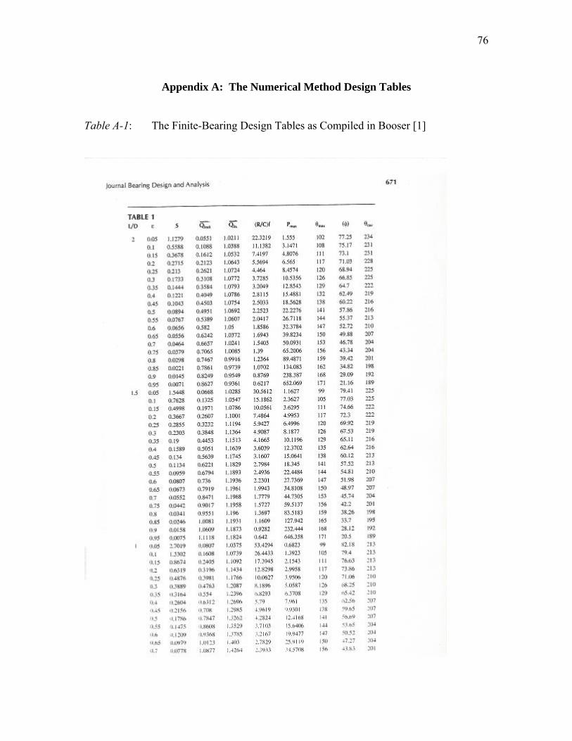
76
Appendix A: The Numerical Method Design Tables
Table A-1: The Finite-Bearing Design Tables as Compiled in Booser [1]

77

78

79
Source: M. M. Khonsari, Tribology Data Handbook: Journal Bearing Design and Analysis. Boca Raton: CRC Press LLC, 1997. p. 671 - 674. Book Compiled by E. Michael Booser.

80
Appendix B: Sample Viscosity-Temperature Chart
Figure B-1: A Common Viscosity-Temperature Chart. This particular chart may be used
for the SAE oil grades 10, 20, 30, 40, 50, 60, and 70.
Source: Shigley, Joesph E. Mechanical Enginering Design. 7th ed. New York: McGraw-Hill, Inc., 2004

81
Appendix C: MATLAB Code for the Bearing CAD Tool
Routine: MainDesign.m clear all; %Journal Bearing Design Calculator %By: Richard K. Naffin %2009 Penn State University Graduate Student %Advisor: Dr. Liming Chang %The following CAD tool may be used to aid in the design of full journal %bearings. %This program has not been developed to solve for partial journal bearings. %Note: This program may be used if the following parameters %are predefined, or whose values are being optimized. %-Load on Bearing %-Rotational Speed of Journal %-Bearing inlet conditions %-Bearing Length %-Journal Diameter %-Clearance Ratio %-Lubricant Type or Grade %This program will output values for the following design considerations: %-Minimum Film Thickness %-Power Loss of Bearing System %-Average Flow Temperature and Temperature Rise %-Leakge Flow Rate %-Outlet Flow Temperature %Before running this program, go to the m-file Input.m and supply the %necessary input parameters. Input %Fill this out! %Once the correct parameters are supplied, run the program to calculate %through the following code. Current_Range_Value=Range_Min; i=0;

82
while Current_Range_Value<Range_Max i=i+1; Current_Range_Value = Current_Range_Value + increment; if BigChoice==1 L=Current_Range_Value; elseif BigChoice==2 Clearance_ratio=Current_Range_Value; elseif BigChoice==3 P=Current_Range_Value; elseif BigChoice==4 RPM=Current_Range_Value; elseif BigChoice==5 D=Current_Range_Value; elseif BigChoice==6 viscinlet=Current_Range_Value; else %N/A. end Temp_Residual=2; while Temp_Residual>Tavg_tol Relationship_Module %This subroutine assigns the viscosity-temperature relationship %based on selection in input subroutine Epsilon_Iterative %This subroutine solves the eccentricity ratio TempChange_Output %The subroutine first calculates the performance parameters of %the friction, side leakage, and inflow. %This allows for temperature change to be solved, %Which may be used to calculate 'T_average_calc' end Performance_Calculation end Output Subroutine: Input.m

83
%Please assign a value for the variable 'BigChoice' %To calculate design output with respect to the bearing length, select 1') %To calculate design output with respect to the clearance ratio, select 2') %To calculate design output with respect to the applied load, select 3') %To calculate design output with respect to the journal's speed, select 4') %To calculate design output with respect to the bearing diameter, select 5') %To calculate design output with respect to the inlet viscosity, select 6') %If you already know what to select for each input parameter, select 7') BigChoice=2; Verify=2; %No, select 1. Yes, select 2 %Bearing Input Parameters %Begin by filling in the following input about your bearing. %If one of these parameters is selected to vary over a range, %Set it equal to zero in this list. RPM=3600; %Journal Rotational Speed in rotations per minute P=6650; %Applied Radial Load in Newtons Tinlet=49; %Estimation of Bearing Inlet Temperature in Celsius. %Estimation Based on Ambient Temperature of Supplied %Lubricant. L=0.05; %Bearing Length in meters D=0.05; %Journal Diameter in meters Clearance_ratio=0; %The clearnance ratio, or c/R %Please supply the Lubricant Viscosity at the bearing inlet which %corresponds to the inlet temperature supplied previously. viscinlet=0.028; %in Pa*s. Set equal to zero if varied %Please select the viscosity-temperature relationship to use.

84
%To use the Barus Equation (default), set 'Tv_relate' equal to 1. %To use the Other Relationships, set 'Tv_relate' equal to 2') Tv_relate=1; %If you know the lubricant grade that you wish to use, please supply %the following values. If you don't know the actual grade, please supply %nominal values of these material properties. specific_heat=1760; %Specific Heat of the Lubricant in J/(Kg/C). %Typically, it is 1900 J/(Kg/C) density=880; %Nominal Density of Supplied Lubricant in Kg/m^3 %If you choose to use the default temperature-viscosity relation please %fill in the following: B=0.033; %Baurus Constant of the Lubricant in 1/Celsius. %This factor is needed if you want to use the %default viscosity-temperature relation or if it %used in YOUR CHOSEN relation. %If this factor is not needed in YOUR CHOSEN %viscosity-temperature relation, set it to zero. %Now, if are varying one of the input parameters, select the range %to calculate output for. %Supply the values in the corresponding units as specified in above list. Range_Min=0.000125; %set value to 0 if not varying an input Range_Max=0.005; %set value to 1 if not varying an input %Please supply the increment change of the varied input. %It is recommended to select an increment change which will result %in the program only increasing the parameter approximately 100 times %across the range. increment = 0.00005; %set value to 1 if not varying an input %Please supply an estimated value of the average temperature T_average_guess=80; %in deg Celsius %Please supply acceptable error tolerances for the following: Tavg_tol=1; %Tolerance of average temeperature in deg C eta_tol=0.0001; %Tolerance of eccentricity ratio

85
%This completes the input file Subroutine: Relationship_Module.m %Chooses the Temperature-Viscosity Relationship if Tv_relate == 1 %This is the default equation. DO NOT CHANGE! visc=viscinlet*exp(-B*(T_average_guess-Tinlet)); else %If you do not want to use the default equation, please supply %your own in the space provided before the 'end' statment. %Your equation must follow the following format: % %-You must use the the variables 'viscinlet', 'Tinlet', and % 'T_average_guess'as input into the equation. % %-The equation must output the variable 'visc', which is the % average viscosity of the system end Subroutine: Epsilon_Iterative.m %Preliminary Set-up Code %Due to time-constraints, the bisection method is not programmed into this %module. Instead, a simpler iterative method is used that produces %reasonable results for bearings of eccentricity ratios greater than %0.0001 %Conversion of Shaft Speed from rpm to rev/s N=RPM/60; %Conversion of Shaft Speed from rev/s to physical units (m/s or in/s) U=N*(D*pi); %Conversion of speed from rev/s to rad/s omega=N*2*pi; %The following code defines the boundary conditions of the %Derived Finite Curve-Fit %L/D Input SR=L/D; loSR=log10(SR);

86
%Curve-Fit Boundary Conditions XS=log10(1/8); XL=log10(4.75); %Radial Clearance Calculation c=(0.5*D)*Clearance_ratio; %Start of Load Capacity Module Code to find Epsilon %Known Dimensionless Force on Bearing Wbarknown=(P*c^2)/(visc*omega*D^4); %Initial Epsilon eta=0; Residual=1; %The following while loop will run until the known dimensionless bearing %force matches that calculated from the Analytical Curve-Fit Equation while Residual>0 %Code that creates the incremental values of epsilon eta=eta+0.0001; %The correctiion factors used to keep error below 5% Correctionfactorshort=1-(0.7*(eta-.1)^10); Correctionfactorlong=0.91+(0.19*eta); %Solving for Long Bearing eccentricity function EL=(3*eta*sqrt((4*eta^2)+pi^2-(pi^2*eta^2)))/(4*(2+eta^2)*(1-eta^2)); %Solving for Short Bearing eccentricity function ES=(pi*eta*sqrt(1+0.62*(eta^2)))/(8*(1-(eta)^2)^2); if SR>4.75 Yl=log10(Correctionfactorlong*EL)+loSR; Wbarcurve=10^Yl; elseif SR<0.125 Ys=log10(Correctionfactorshort*ES)+(3*loSR); Wbarcurve=10^Ys; else %Defines the Dimensionless loads at the boundary conditions %Equations include any correction factors Wlong=log10(Correctionfactorlong*EL)+XL; Wlongp=1; Wshort=log10(Correctionfactorshort*ES)+(3*XS); Wshortp=3; %The curve-fit constants for Wbar

87
%Below define the 4 constants that make-up of the curve-fit equation %These constants are functions of the dimensionless loads at the %boundary conditions and the eccentricity function equations. C3d=XS^3-XL^3+(((3*XS^4)+(3*XL^4)-(6*XL^2*XS^2))/(2*(XL-XS)))+(3*XS^2*XL)-(3*XL^2*XS); C3w=(Wshort-Wlong+(Wshortp*XL)-(Wlongp*XS)-((Wlongp-Wshortp)/(2*(XL-XS)))*(XS^2-XL^2))/C3d; C2w=(Wlongp-Wshortp-(3*C3w*XL^2)+(3*C3w*XS^2))/(2*(XL-XS)); C1w=Wshortp-(3*C3w*XS^2)-(2*C2w*XS); Conw=Wlong-(C3w*XL^3)-(C2w*XL^2)-(C1w*XL); %The final form of the curve-fit eqaution Yw=(C3w*loSR^3)+(C2w*loSR^2)+(C1w*loSR)+Conw; Wbarcurve=10^Yw; end %When residual equals zero, the loop will end and the current %value of epsilon will output Residual=Wbarknown-Wbarcurve; end %Computing Sommerfeld Number Sommerfeld=SR/(8*pi*Wbarcurve); Subroutine: TempChange_Output.m %Computing coefficient of frction dim_friction=(1+((0.56*SR+1.93)*(eta)^4))*(2*pi^2*Sommerfeld); f1=(dim_friction*c)/(0.5*D); %Attitude Angle Angle=atan((pi*sqrt(1-eta^2))/(4*pi)); %in rad %Calculating the Side Leakage Qside_factor=(1.0-((0.03*eta+0.23)*(SR-0.1)^1.2)); Qside_bar=2*eta*Qside_factor; Qside=0.5*pi*D*c*N*L*Qside_bar; %Calculating the Flow Rate Entering the Loaded Region Qin_factor=(1.0-((0.26*eta+0.01)*(SR-0.1)^1.2)); Qin_bar=(eta+1)*Qin_factor; Q_in=0.5*pi*D*c*N*L*Qin_bar;

88
%Calculating the Temperature Rise Temperature_Change=(4*pi*P*dim_friction)/(density*specific_heat*L*D*pi*Qin_bar*(1-(0.5*(Qside_bar/Qin_bar)))); T_average_calc=Tinlet+(0.5*Temperature_Change); %Residul and Looping Calculations Temp_Residual=abs(T_average_calc-T_average_guess); T_average_guess=0.5*(T_average_calc+T_average_guess); Subroutine: Performance_Calculation.m %Computing Minimum Film Thickness hmin=c*(1-eta); %Computing Power loss in Watts Power_Loss=f1*P*U; %Computing Power loss in HP Power_Loss_HP=Power_Loss/745.7; %Computing the Outlet Temperature T_out=Tinlet+Temperature_Change; Vary_hmin(i)=hmin; Vary_eta(i) = eta; Vary_Qside(i) = Qside; Vary_Q_in(i) = Q_in; Vary_SR(i) = SR; Vary_f1(i) = f1; Vary_Power_Loss(i) = Power_Loss; Vary_T_average_calc(i) = T_average_calc; Vary_Temperature_Change(i) = Temperature_Change; Vary_T_out(i)=T_out; Vary_Clearance_ratio(i) = Clearance_ratio; Vary_P(i) = P; Vary_RPM(i) = RPM; Vary_viscinlet(i) = viscinlet;

89
Subroutine: Output.m if BigChoice==1 figure(1) plot(Vary_SR,Vary_eta) title('Eccentricity Ratio') xlabel('Slenderness Ratio, L/D') ylabel('Epsilon') grid on figure(2) plot(Vary_SR,Vary_hmin) title('Minimum Film Thickness') xlabel('Slenderness Ratio, L/D') ylabel('hmin (in meters)') grid on figure(3) subplot(2,1,1); plot(Vary_SR,Vary_Qside) title('Lubricant Side Leakage') xlabel('Slenderness Ratio, L/D') ylabel('Flow Rate (in m^3/s)') grid on subplot(2,1,2); plot(Vary_SR,Vary_Q_in) title('Lubricant Inflow') xlabel('Slenderness Ratio, L/D') ylabel('Flow Rate (in m^3/s)') grid on figure(5) plot(Vary_SR,Vary_Power_Loss) title('Power Loss') xlabel('Slenderness Ratio, L/D') ylabel('Power Loss (in W)') grid on figure(6) plot(Vary_SR,Vary_f1) title('Coefficient of Friction') xlabel('Slenderness Ratio, L/D') ylabel('f (dimensionless)') grid on figure(7) plot(Vary_SR,Vary_T_average_calc,Vary_SR,Vary_T_out) title('Temperature') xlabel('Slenderness Ratio, L/D') ylabel('Tavg (in deg C)') legend('Average Temperature','Outlet Temperature') grid on figure(8)

90
plot(Vary_SR,Vary_Temperature_Change) title('Temperature Change') xlabel('Slenderness Ratio, L/D') ylabel('delt T (in deg C)') grid on elseif BigChoice==2 figure(1) plot(Vary_Clearance_ratio,Vary_eta) title('Eccentricity Ratio') xlabel('Clearance Ratio, c/R') ylabel('Epsilon') grid on figure(2) plot(Vary_Clearance_ratio,Vary_hmin) title('Minimum Film Thickness') xlabel('Clearance Ratio, c/R') ylabel('hmin (in meters)') grid on figure(3) subplot(2,1,1); plot(Vary_Clearance_ratio,Vary_Qside) title('Lubricant Side Leakage') xlabel('Clearance Ratio, c/R') ylabel('Flow Rate (in m^3/s)') grid on subplot(2,1,2); plot(Vary_Clearance_ratio,Vary_Q_in) title('Lubricant Inflow') xlabel('Clearance Ratio, c/R') ylabel('Flow Rate (in m^3/s)') grid on figure(5) plot(Vary_Clearance_ratio,Vary_Power_Loss) title('Power Loss') xlabel('Clearance Ratio, c/R') ylabel('Power Loss (in W)') grid on figure(6) plot(Vary_Clearance_ratio,Vary_f1) title('Coefficient of Friction') xlabel('Clearance Ratio, c/R') ylabel('f (dimensionless)') grid on figure(7) plot(Vary_Clearance_ratio,Vary_T_average_calc) title('Average Temperature') xlabel('Clearance Ratio, c/R') ylabel('Tavg (in deg C)') grid on

91
figure(8) plot(Vary_Clearance_ratio,Vary_Temperature_Change) title('Temperature Change') xlabel('Clearance Ratio, c/R') ylabel('delt T (in deg C)') grid on figure(9) plotyy(Vary_Clearance_ratio,Vary_eta,Vary_Clearance_ratio,Vary_hmin) title('Load Capacity Conditions') xlabel('Clearance Ratio, c/R') legend('Film Thickness','Eccentricity Ratiio') grid on elseif BigChoice==3 figure(1) plot(Vary_P,Vary_eta) title('Eccentricity Ratio') xlabel('Load (in N)') ylabel('Epsilon') grid on figure(2) plot(Vary_P,Vary_hmin) title('Minimum Film Thickness') xlabel('Load (in N)') ylabel('hmin (in meters)') grid on figure(3) subplot(2,1,1); plot(Vary_P,Vary_Qside) title('Lubricant Side Leakage') xlabel('Load (in N)') ylabel('Flow Rate (in m^3/s)') grid on subplot(2,1,2); plot(Vary_P,Vary_Q_in) title('Lubricant Inflow') xlabel('Load (in N)') ylabel('Flow Rate (in m^3/s)') grid on figure(5) plot(Vary_P,Vary_Power_Loss) title('Power Loss') xlabel('Load (in N)') ylabel('Power Loss (in W)') grid on figure(6) plot(Vary_P,Vary_f1) title('Coefficient of Friction')

92
xlabel('Load (in N)') ylabel('f (dimensionless)') grid on figure(7) plot(Vary_P,Vary_T_average_calc) title('Average Temperature') xlabel('Load (in N)') ylabel('Tavg (in deg C)') grid on figure(8) plot(Vary_P,Vary_Temperature_Change) title('Temperature Change') xlabel('Load (in N)') ylabel('delt T (in deg C)') grid on elseif BigChoice==4 figure(1) plot(Vary_RPM,Vary_eta) title('Eccentricity Ratio') xlabel('Rotation (in RPM)') ylabel('Epsilon') grid on figure(2) plot(Vary_RPM,Vary_hmin) title('Minimum Film Thickness') xlabel('Rotation (in RPM)') ylabel('hmin (in meters)') grid on figure(3) subplot(2,1,1); plot(Vary_RPM,Vary_Qside) title('Lubricant Side Leakage') xlabel('Rotation (in RPM)') ylabel('Flow Rate (in m^3/s)') grid on subplot(2,1,2); plot(Vary_RPM,Vary_Q_in) title('Lubricant Inflow') xlabel('Rotation (in RPM)') ylabel('Flow Rate (in m^3/s)') grid on figure(5) plot(Vary_RPM,Vary_Power_Loss) title('Power Loss') xlabel('Rotation (in RPM)') ylabel('Power Loss (in W)') grid on figure(6)

93
plot(Vary_RPM,Vary_f1) title('Coefficient of Friction') xlabel('Rotation (in RPM)') ylabel('f (dimensionless)') grid on figure(7) plot(Vary_RPM,Vary_T_average_calc) title('Average Temperature') xlabel('Rotation (in RPM)') ylabel('Tavg (in deg C)') grid on figure(8) plot(Vary_RPM,Vary_Temperature_Change) title('Temperature Change') xlabel('Rotation (in RPM)') ylabel('delt T (in deg C)') grid on elseif BigChoice==5 figure(1) plot(Vary_SR,Vary_eta) title('Eccentricity Ratio') xlabel('Slenderness Ratio, L/D') ylabel('Epsilon') grid on figure(2) plot(Vary_SR,Vary_hmin) title('Minimum Film Thickness') xlabel('Slenderness Ratio, L/D') ylabel('hmin (in meters)') grid on figure(3) subplot(2,1,1); plot(Vary_SR,Vary_Qside) title('Lubricant Side Leakage') xlabel('Slenderness Ratio, L/D') ylabel('Flow Rate (in m^3/s)') grid on subplot(2,1,2); plot(Vary_SR,Vary_Q_in) title('Lubricant Inflow') xlabel('Slenderness Ratio, L/D') ylabel('Flow Rate (in m^3/s)') grid on figure(5) plot(Vary_SR,Vary_Power_Loss) title('Power Loss') xlabel('Slenderness Ratio, L/D') ylabel('Power Loss (in W)') grid on

94
figure(6) plot(Vary_SR,Vary_f1) title('Coefficient of Friction') xlabel('Slenderness Ratio, L/D') ylabel('f (dimensionless)') grid on figure(7) plot(Vary_SR,Vary_T_average_calc) title('Average Temperature') xlabel('Slenderness Ratio, L/D') ylabel('Tavg (in deg C)') grid on figure(8) plot(Vary_SR,Vary_Temperature_Change) title('Temperature Change') xlabel('Slenderness Ratio, L/D') ylabel('delt T (in deg C)') grid on figure(9) subplot(2,1,1); plot(Vary_SR,Vary_eta) title('Eccentricity Ratio') xlabel('Slenderness Ratio, L/D') ylabel('Epsilon') grid on subplot(2,1,2); plot(Vary_SR,Vary_hmin) title('Minimum Film Thickness') xlabel('Slenderness Ratio, L/D') ylabel('hmin (in meters)') grid on elseif BigChoice==6 figure(1) plot(Vary_viscinlet,Vary_eta) title('Eccentricity Ratio') xlabel('Inlet Viscosity, Pa*s') ylabel('Epsilon') grid on figure(2) plot(Vary_viscinlet,Vary_hmin) title('Minimum Film Thickness') xlabel('Inlet Viscosity, Pa*s') ylabel('hmin (in meters)') grid on figure(3) subplot(2,1,1); plot(Vary_viscinlet,Vary_Qside) title('Lubricant Side Leakage')

95
xlabel('Inlet Viscosity, Pa*s') ylabel('Flow Rate (in m^3/s)') grid on subplot(2,1,2); plot(Vary_viscinlet,Vary_Q_in) title('Lubricant Inflow') xlabel('Inlet Viscosity, Pa*s') ylabel('Flow Rate (in m^3/s)') grid on figure(5) plot(Vary_viscinlet,Vary_Power_Loss) title('Power Loss') xlabel('Inlet Viscosity, Pa*s') ylabel('Power Loss (in W)') grid on figure(6) plot(Vary_viscinlet,Vary_f1) title('Coefficient of Friction') xlabel('Inlet Viscosity, Pa*s') ylabel('f (dimensionless)') grid on figure(7) plot(Vary_viscinlet,Vary_T_average_calc) title('Average Temperature') xlabel('Inlet Viscosity, Pa*s') ylabel('Tavg (in deg C)') grid on figure(8) plot(Vary_viscinlet,Vary_Temperature_Change,Vary_viscinlet,Vary_T_out) title('Temperature Conditions') xlabel('Inlet Viscosity, Pa*s') ylabel('Temperature (in deg C)') legend('Temperature Change','Outlet Temperature') grid on else fprintf('The eccentricity ratio is %f.', eta); disp(' ') fprintf('The minimum film thickness is %f m.', hmin); disp(' ') fprintf('The coefficicent of friction is %f.', f1); disp(' ') fprintf('The Power loss of this bearing is %f Watts.', Power_Loss); disp(' ') fprintf('Or the power loss can be written in the form of %f HP.', Power_Loss_HP); disp(' ') fprintf('The leakage flow rate of this bearing is %f m^3/s.', Qside); disp(' ') fprintf('The lubricant flow rate into the loaded region of bearing is %f m^3/s.', Q_in);

96
disp(' ') fprintf('The temperature rise of the loaded region of bearing is %f deg C.',Temperature_Change); disp(' ') fprintf('The outlet temperature of the loaded region of bearing is %f deg C.',T_out); disp(' ') end
Related Documents


![Research & Reviews: Journal of Pharmacognosy and … · 2019. 7. 12. · Chromatography [22-27] Thin layer chromatography Thin layer chromatography is an important analytical tool](https://static.cupdf.com/doc/110x72/609dce74358211097a29305c/research-reviews-journal-of-pharmacognosy-and-2019-7-12-chromatography.jpg)