Development of a Simpliﬁed Adaptive Finite Element Model ...

Development of a Simplified Adaptive

Finite Element Model of the Gulf Stream

Nicola Stone

August 20, 2006

Abstract

The goal of this dissertation is to look at the feasibility of incorporating a

moving adaptive mesh refinement procedure into an existing finite element

model of the shallow water equations. The Stommel model simulates simple

oceanic flows including western boundary currents like the Gulf Stream.

This dissertation describes the finite element formulation of the Stommel

equations, a modified form of the shallow water equations. The feasibility

of including a mesh movement procedure based on monitor functions is

looked at, with a study of one particular monitor. Results are shown for a

specific mesh velocity and for mesh velocities computed from this monitor.

We conclude that the monitor function used is a promising start at finding

a way to allow the mesh to dynamically evolve with the flow, in applications

such as this.

i

Acknowledgements

I would like to acknowledge Mike Baines and Emmanuel Hanert

who jointly supervised this dissertation. I am grateful for the help and

knowledge they have given me to enable me to complete this disser-

tation. The staff and students of the Mathematics and Meteorology

departments, particularly those involved with the MSc, have also been

very supportive throughout my MSc studies. I would also like to thank

my family and friends for their understanding during a very busy year.

I would also like to recognise the financial assistance provided by

the NERC studentship.

Declaration

I confirm that this work is my own and the use of all other material

from other sources has been properly and fully acknowledged.

Nicola Stone.

Contents

1 Introduction 1

2 The Stommel Model 5

2.1 The Shallow Water Equations . . . . . . . . . . . . . . 5

2.2 The Stommel Model . . . . . . . . . . . . . . . . . . . 6

2.3 Scale Analysis . . . . . . . . . . . . . . . . . . . . . . . 8

3 Numerical Solution to the Stommel Problem 11

3.1 Finite Element Formulation . . . . . . . . . . . . . . . 11

3.2 Temporal Discretisation . . . . . . . . . . . . . . . . . 13

3.3 Computation . . . . . . . . . . . . . . . . . . . . . . . 14

3.3.1 Mass Matrix Entries . . . . . . . . . . . . . . . 14

3.3.2 Computing the solution . . . . . . . . . . . . . 15

3.4 Initial Conditions . . . . . . . . . . . . . . . . . . . . . 16

3.5 Stommel Solution . . . . . . . . . . . . . . . . . . . . . 17

4 Moving Mesh Adaptation 19

4.1 Moving Mesh Methods . . . . . . . . . . . . . . . . . . 19

4.2 Mesh Velocity Principle . . . . . . . . . . . . . . . . . 20

iii CONTENTS

5 Solving for the Mesh Velocities 23

5.1 Finite Element Formulation . . . . . . . . . . . . . . . 23

5.1.1 Stiffness Matrix Entries . . . . . . . . . . . . . 24

5.1.2 Load Vector Entries . . . . . . . . . . . . . . . 26

5.1.3 Mesh Velocities . . . . . . . . . . . . . . . . . . 27

6 Implementation of the Mesh Velocities 29

6.1 Interpolating the Mesh Velocities onto the P1 nodes . . 29

6.2 Moving the Mesh . . . . . . . . . . . . . . . . . . . . . 30

6.3 Interpolating the Mesh Velocities onto the PNC1 nodes . 30

6.4 Moving the Solution . . . . . . . . . . . . . . . . . . . 31

7 Numerical Simulations and Results 33

7.1 Simple westward mesh movement . . . . . . . . . . . . 34

7.1.1 Results for simple westward mesh movement . . 34

7.2 Conservation based mesh movement . . . . . . . . . . . 36

7.2.1 Results for conservation based mesh movement 36

7.3 Flow based mesh movement . . . . . . . . . . . . . . . 39

7.3.1 Results for flow based mesh movement . . . . . 40

7.4 Combined mesh movement . . . . . . . . . . . . . . . . 40

7.4.1 Results of combined mesh movement . . . . . . 40

8 Conclusion 42

9 Further Work 46

List of Figures

2.1 Depth of the fluid (1-D) . . . . . . . . . . . . . . . . . 6

3.1 P1 and PNC1 basis functions . . . . . . . . . . . . . . . 12

3.2 Initial Mesh . . . . . . . . . . . . . . . . . . . . . . . . 16

3.3 Stommel solution on a square domain . . . . . . . . . . 17

5.1 Dimensions of an element in the mesh . . . . . . . . . . 25

6.1 Averaging the element velocities to obtain the mesh ve-

locities on the nodes . . . . . . . . . . . . . . . . . . . 30

6.2 Averaging the element velocities to get the mesh veloc-

ities on the mid segments . . . . . . . . . . . . . . . . . 31

7.1 Solution after 1000 time steps with α = 0.5. . . . . . . 35

7.2 Solution after 50,000 time steps with α = 0.01. . . . . . 35

7.3 Solution after 1000 time steps using conservation principle 37

7.4 Solution after 25000 time steps using conservation prin-

ciple . . . . . . . . . . . . . . . . . . . . . . . . . . . . 38

7.5 Solution after 3000 time steps using flow based mesh

movement . . . . . . . . . . . . . . . . . . . . . . . . . 39

v LIST OF FIGURES

7.6 Solution after 9000 time steps using combined conserva-

tion/flow based mesh movement . . . . . . . . . . . . . 41

List of Tables

2.1 Scales for each parameter in the Stommel equations . . 9

Chapter 1

Introduction

Traditionally, ocean models used structured grids, reflecting the com-

putational resources that were available at the time. Now ocean mod-

ellers are starting to use unstructured and adapting meshes more.

Unstructured meshes have many advantages over structured meshes.

The coastline and basin geometry can be better represented. Also, the

mesh can be easily adapted to give an increased local mesh resolution,

or a dynamically adaptive mesh [4]. In the first case, a high resolution

grid can be placed in an area of interest with lower resolution in less

important areas, to give optimal use of computer power. In a North

Atlantic model, for example, we might place a higher resolution grid

in the region of the Gulf Stream. In the second case, we can have a

mesh which moves to follow certain aspects of the solution, for example

eddies moving across a basin.

Adaptive meshes are useful as we may not know the positions of

developing flow features before the model is run. The resolution of the

model can be changed to optimally resolve the flow. Adaptive methods

can also be incorporated into existing models and may give increased

2 Introduction

efficiency and accuracy of the solution.

This dissertation will investigate the feasibility of using adaptive

mesh movement in the Stommel model. The mesh movement is deter-

mined by following a certain feature (fluid volume) of the solution in

Stommel’s equations of ocean circulation with a prescribed vorticity.

We will be looking at the possibility of including mesh movement into

an existing two-dimensional finite element model. The existing model

uses an implicit time discretisation with a black box solver the solve the

equations. To avoid having to invert a matrix, this has been changed to

an explicit scheme for this dissertation. The mesh movement is based

on the idea of having a monitor function to determine how the mesh

will move. The monitor function we have chosen is the depth of the

ocean H = h+ η, where h is the resting depth of the fluid and η is the

surface elevation, and the prescribed vorticity of the mesh is taken to

be zero.

We start by stating the shallow water equations in Chapter 2. Then

we briefly describe how Stommel simplified these equations to create a

model which describes the creation of western boundary layers in areas

of the ocean such as the Gulf Stream. Scale analysis is performed on

these equations to determine the dominant terms, which allow us to

make assumptions of the nature of the solution without first having to

solve the equation.

In Chapter 3 we look at how the governing equations of Stommel’s

model are formulated using finite elements, and then discretised in

time [1]. We then describe how the solution is computed. The initial

conditions of the model are stated, along with the initial mesh. The

elevation solution on a fixed mesh is then described as a motivation to

3 Introduction

explore the possibility of moving the mesh to follow a flow.

The idea of generating a mesh velocity from the conservation of

a monitor function [8] is introduced in Chapter 4. We have chosen

one particular monitor function which ensures that the volume of fluid

in each element remains constant over all time. This is one of many

monitor functions that could be used to move the mesh. Likewise, the

choice of zero mesh vorticity is only one of many choices that can be

made.

Then an equation for the mesh velocity induced by this monitor

function is formulated using finite element methods in Chapter 5. The

entries of the resulting stiffness matrix and load vector are then derived,

and a mesh velocity calculated for each element.

Chapter 6 describes how this element velocity is interpolated onto

the nodes, and the mid-segments of the elements in the mesh. The

mesh node velocity is then used in a mesh movement equation to move

the mesh. As the true solution should not change when the mesh is

modified, the mid-segment velocity is used in advection terms included

in the governing equations to compensate for the mesh movement.

The results of numerical simulations carried out to move the mesh

are shown in Chapter 7. These test situations look at the suitability of

different ideas for mesh movement. The first test carried out is a simple

prescribed westerly mesh movement, given that we know the solution

travels to the west. Then the results for the conservation of volume

principle are discussed. The next test involves the Lagrangian idea

of moving the mesh according to the flow velocity which is a special

case of the computed velocity when the vorticity of the mesh is equal

to the vorticity of the fluid. The last test is a linear combination of

4 Introduction

the monitor function mesh velocity and the flow velocity based mesh

movement.

Chapter 8 draws conclusions on the methods used within the dis-

sertation, and on the feasibility of using the conservation of a monitor

function to prescribe the mesh movement. Problems with the tests in

chapter 7 are also addressed.

Finally in Chapter 9, ideas for further work are discussed. These

are ideas that would have been interesting to investigate, had the dis-

sertation not been limited by time constraints.

Chapter 2

The Stommel Model

This chapter will describe the Stommel model, looking at the govern-

ing equations and how the model is represented using finite element

methods. Then the time discretisation will be described, along with

how the results are computed. This is followed by results of a fixed

mesh finite element model of the Stommel model in a square domain.

2.1 The Shallow Water Equations

The shallow water equations on domain Ω with boundary dΩ

∂η

∂t+∇ · (Hu) = 0, (2.1)

∂u

Dt+ u · ∇u + fez × u = −g∇η +

ν

H∇ · (H∇u)

+τ η − τ b

ρ0H, (2.2)

are solved for η(x, t), the surface elevation, and u(x, t), the depth-

averaged velocity. In these equations H = h + η is the depth of the

fluid , where h(x) is the resting depth of the fluid, as shown in Figure

2.1, ez is a unit vector in the vertical direction, g is the gravitational

6 The Stommel Model

acceleration, ν is the eddy viscosity, τ η and τ b are the surface and

bottom stresses respectively and ρ0 is the homogeneous density of the

fluid.

-

6

6

?

6? 6

?

ez

h

η

H

Figure 2.1: Depth of the fluid (1-D)

Equations (2.1) and (2.2) describe the development of an incom-

pressible flow of constant density on the surface of the sphere. They

are only relevant when the scale of the region of flow is much larger

than the depth of the fluid, as in the oceans where the depth is much

smaller in proportion to the size of the ocean. Equation (2.1) describes

conservation of mass over the domain, and (2.2) describes the momen-

tum balance.

2.2 The Stommel Model

The Stommel model is a simplification of these shallow water equa-

tions. It contains two important forces acting on ocean flow, rotational

forces and wind effects, and allows us to model the wind-driven ocean

circulation. An important effect of wind driven circulation in the ocean

basins is the strong western boundary currents. The Gulf Stream in the

North Atlantic is one such current, transporting warm tropical water

to higher latitudes.

7 The Stommel Model

The shallow water equations of the previous section describe the

motion of fluid on the surface of a sphere. The Stommel model simpli-

fies this by considering the motion of fluid in Cartesian coordinates on

an f -plane, where to first order the Coriolis parameter is constant.

Stommel [5] tried to understand the cause of the intensification of

these boundary currents, by proposing the following

• considering the Coriolis parameter changing with latitude at a

constant rate by letting f = f0 + βy (β-plane approximation.)

• including a bottom friction term, so keeping the higher order

terms and the ability to satisfy conditions of no normal flow over

the boundaries.

Then, also neglecting non-linear and diffusion terms, the governing

equations of the Stommel model become

∂η

∂t+ h∇ · u = 0, (2.3)

∂u

∂t+ (f0 + βy)ez × u = −g∇η − γu +

τ η

ρh. (2.4)

In these equations, x = (x, y) is the spatial coordinate, h is the resting

depth of the fluid which is assumed constant, f0 is the reference value of

the Coriolis parameter, β is the reference value of the Coriolis parame-

ter first derivative in the y direction, ez is a unit vector in the vertical

direction, g is the gravitational acceleration, γ is a linear friction coef-

ficient, ρ is the homogeneous density of the fluid, τ η is the wind stress

acting on the surface of the fluid and ∇ is the two dimensional gradient

operator. The domain Ω is the interval [0,L]×[0,L]. Stommel assumed

a simple form for the wind stress

τx = −τ0 cos

(πy

yn

), 0 ≤ y ≤ L,

8 The Stommel Model

τy = 0.

These equations are solved subject to no-normal flow boundary condi-

tions, u · n = 0 on ∂Ω.

We note that the there is an analytic solution to the Stommel equa-

tion, so we know that the solution moves westward to create a boundary

layer at the western boundary. We might then think that we could just

prescribe the mesh movement to be to the west for all time. The results

for this idea are shown in Chapter 7.

2.3 Scale Analysis

We now use scale analysis to compare the important terms in the Stom-

mel equations in relation to the other terms. This gives us an insight

into the flow of the fluid before we solve the equations. It may also help

us to determine possibilities for monitor functions that could be used

to move the mesh. The parameters we will use for scaling are shown

in Table 2.1.

The existing code that we are using solves the dimensionless shallow

water equations. The dimensional variables are multiplied by a scale

factor to make them dimensionless. If we choose scale factors carefully,

we end up with a set of equations where all variables and coordinates

are of order 1. Scaling is as follows:

x′ = Lhx,

u′ = Uu,

h′ = Lvh,

9 The Stommel Model

Parameter Description Scale

E vertical surface elevation 1 m

U horizontal velocity 0.1 m s−1

Lh horizontal length 1× 106 m

Lv vertical length 1× 103 m

T time scale 1× 104 s

f Coriolis term 1× 10−4 s−1

β beta term 1× 10−11 m−1 s−1

g gravitational term 10 m2 s−1

γ drag coefficient 1× 10−4 (dimensionless)

ρ density 1× 103 kg m−3

τ wind stress 0.2 kg m−1 s−2

Table 2.1: Scales for each parameter in the Stommel equations

η′ = E, η

t′ = Tt,

where ′ denotes a dimensional variable. These dimensional variables

are then replaced in the equations by their dimensionless expressions.

The continuity equation then reads

E

T

∂η

∂t+LvU

Lh

h∇ · u = 0.

We can then evaluate the relative importance of each term in the equa-

tion by dividing each term by the same dimensional factor. For this

equation, we divide through by ET

to obtain

∂η

∂t+LvUT

LhEh∇ · u = 0,

where LvUTLhE

is a dimensionless number. If this was large then the

divergence term would be of more importance than the time derivative.

10 The Stommel Model

We want these two terms to be of equal importance as it would not be

sensible to neglect one of the two terms in the equation. Therefore in

the code we choose T = LhELvU

, so that both terms are of equal importance

in the equation (as the dimensionless number is equal to 1). This

is a way of determining a timescale, which we do not know exactly

beforehand.

We do the same for the momentum equation to obtain

U

T

∂u

∂t+ U (f0 + βLhy) ez × u = − E

Lh

g∇η − Uγu +τ

ρLv

τ η

ρh.

This time we divide through by the dimensional factor in front of the

Coriolis term (f0U). Therefore we obtain the dimensionless equation:

1

f0T

∂u

∂t+

(1 +

βLh

f0

y

)ez × u = − gE

f0ULh

∇η − γ

f0

u +τ

ρf0ULv

τ η

ρh.

In the existing code, U is chosen so that gEf0ULh

= 1. This means that

U = gEf0Lh

. The remaining scale factors are shown in Table 2.1. With

these scales, we can see that the dimensionless numbers in front of the

time derivative term, the gravitational term and the drag term are all

equal to 1. The leading terms in this equation are the Coriolis term

(dimensionless number equal to 1.1) and the pressure gradient term

(dimensionless number equal to 2). This suggests that the rotational

property of the flow velocity and wind stresses are dominant features

of these equations. We might then consider using the flow velocities as

a basis for mesh movement. Results for using this Lagrangian idea are

presented and discussed in Chapter 7.

Chapter 3

Numerical Solution to the

Stommel Problem

We now look at, following Hanert [1], how the Stommel problem is

formulated using the finite element method.

3.1 Finite Element Formulation

First we multiply each equation by a test function and then integrate

over the domain. The test functions we use are η for the continuity

equation and u for the momentum equation. This gives us the weak

formulation of equations (2.3) and (2.4) on Ω as

∫Ω

∂η

∂tηdΩ + h

∫∂Ω

u · nηdΓ

︸︷︷︸=0

−h∫Ω

u · ∇ηdΩ = 0, (3.1)

∫Ω

∂u

∂tudΩ +

∫Ω

(f + βy)(ez × u)udΩ

+g∫Ω

∇ηudΩ + γ∫Ω

uudΩ−∫Ω

τ η

ρhudΩ. = 0, (3.2)

12 Numerical Solution to the Stommel Problem

where the divergence term has been integrated by parts and the re-

sulting boundary integral can therefore be removed as u · n = 0 on

∂Ω.

To make the finite element approximation, we use a mixture of con-

forming (P1) and nonconforming basis functions (PNC1 ). The conform-

ing nodes are on the vertices of the triangulation, whilst the noncon-

forming nodes are on the mid segment of the triangulation (Figure 3.1).

This PNC1 -P1 finite element pair is very good for solving the shallow

water equations [3]. This is due to the orthogonality of the shape func-

tions, which allows us to reduce the computational cost of the scheme.

The nonconforming elements are discontinuous everywhere, except at

the mid segments. They are a compromise between continuous and

discontinuous approximations.

Figure 3.1: P1 and PNC1 basis functions

We replace u and η in (3.1) and (3.2) by their discrete approxima-

tions uh and ηh as follows. Let

η ≈ ηh =NV∑i=1

ηiφi,

u ≈ uh =NS∑j=1

ujψj,

where ηi and uj represent the elevation and velocity nodal values, φi

and ψj represent the elevation and velocity basis functions, and NV


and NS are the number of vertices and segments in the mesh. The

nodal values are then calculated using the Galerkin method; replacing

η by φi (1 ≤ i ≤ NV ), and u by (ψj, 0) and (0, ψj) (1 ≤ j ≤ NS) in

(3.1) and (3.2). This results in

dηj

dt

∫Ω

φiφjdΩ− huj

∫Ω

∇φiψjdΩ = 0, (3.3)

duj

dt

∫Ω

ψiψjdΩ + (f0 + βyj)(ez × uj)∫Ω

ψiψjdΩ

+gηj

∫Ω

ψi∇φjdΩ + γuj

∫Ω

ψiψjdΩ−∫Ω

τ η

ρhψidΩ = 0, (3.4)

Note that in the second term of equation (3.4) we have also approxi-

mated y ≈ yj.

3.2 Temporal Discretisation

We need to also discretise equations (3.3) and (3.4) in time. For a given

time step ∆t = tn+1 − tn, we have the following equations.

ηn+1 − ηn

∆t

∫Ω

φiφjdΩ = huj

∫Ω

∇φiψjdΩ

≡ fη(η,u), (3.5)

un+1 − un

∆t

∫Ω

ψiψjdΩ = −(f0 + βyj)(ez × uj)∫Ω

ψiψjdΩ

−gηj

∫Ω

ψi∇φjdΩ− γuj

∫Ω

ψiψjdΩ

+∫Ω

τ η

ρhψidΩ

≡ fu(η,u), (3.6)

Where fη and fu are used in the Adams Bashforth scheme as described

below.


We now use the third order Adams Bashforth scheme to solve these

equations for η and u. This gives us two matrix systems

Aηηn+1 = bη,

Auun+1 = bu,

where

Ai,jη =

∫Ω

φiφjdΩ,

Ai,ju =

∫Ω

ψiψjdΩ,

and

biη =

∑j

ηnj

∫Ω

φiφjdΩ +∆t

12

(23fn

η − 16fn−1η + 5fn−2

η

) ,bi

u =∑j

unj

∫Ω

ψiψjdΩ +∆t

12

(23fn

u − 16fn−1u + 5fn−2

u

) .These can be solved by inverting the mass matrices Aη and Au.

3.3 Computation

We now discuss how the entries of the mass matrices are computed to

simplify the calculation of the solution.

3.3.1 Mass Matrix Entries

The entries of the mass matrices Aη and Au for each element are

Ai,jη =

∫Ωe

φiφjdΩ,

Ai,ju =

∫Ωe

ψiψjdΩ.


So we have for each element

Ai,jη =

∆area

12

2 1 1

1 2 1

1 1 2

, (3.7)

Ai,ju =

∆area

3

1 0 0

0 1 0

0 0 1

.These are then assembled to form mass matrices for the whole domain.

An alternative to inverting these large matrices is to note that Au

is a diagonal matrix, so when computing the solution we can think of

it as a vector Adiagu containing all of the diagonal entries of Au. Aη

however is not diagonal so it is not so simple to create a vector in this

way. However, if we assume the mass of each element is concentrated

at its nodes then the matrix can be converted into a diagonal matrix

by lumping the off diagonal entries in Aη onto the diagonal. Then this

diagonal matrix can be represented by the vector Adiagη .

3.3.2 Computing the solution

To compute the solution it is now easier to represent the two systems

as one system

Adiag

...

ηj

...

uj

...

n+1

= b,

where Adiag contains all of the entries from Adiagη and Adiag

u , and b

contains all of the entries from bη and bu. We can then compute the


solution for ηj and uj simply by dividing b by Adiag.

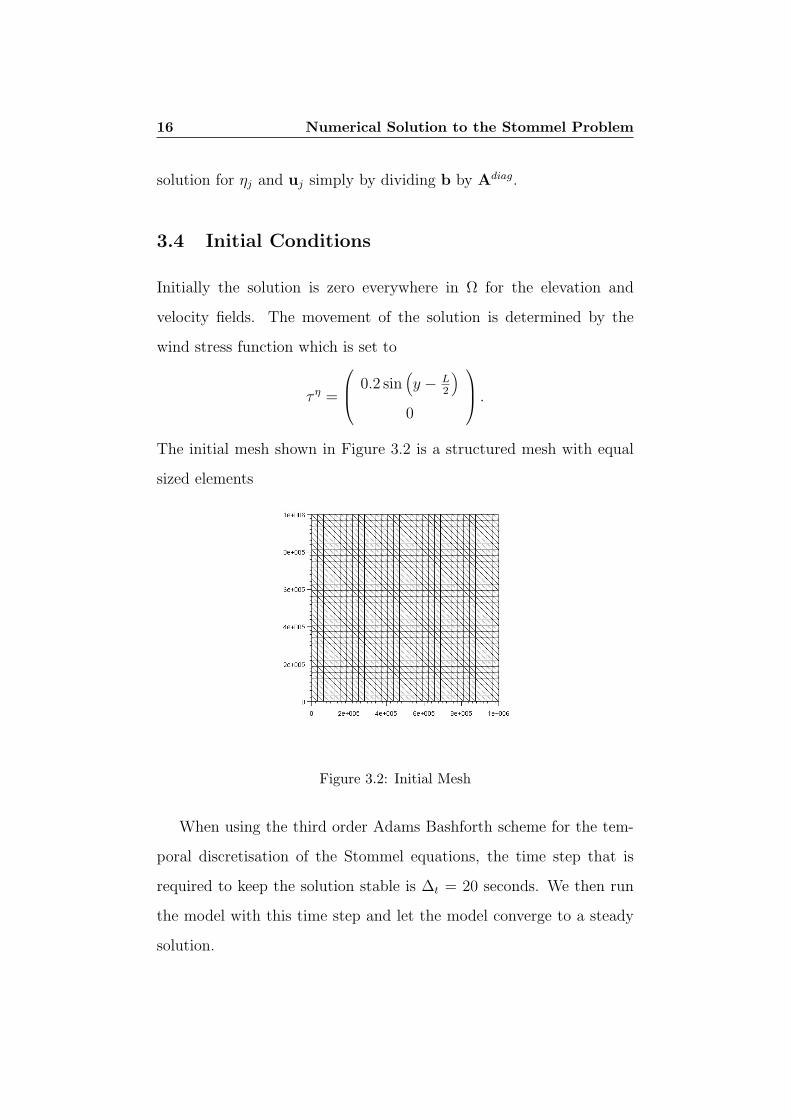
3.4 Initial Conditions

Initially the solution is zero everywhere in Ω for the elevation and

velocity fields. The movement of the solution is determined by the

wind stress function which is set to

τ η =

0.2 sin(y − L

2

)0

.The initial mesh shown in Figure 3.2 is a structured mesh with equal

sized elements

Figure 3.2: Initial Mesh

When using the third order Adams Bashforth scheme for the tem-

poral discretisation of the Stommel equations, the time step that is

required to keep the solution stable is ∆t = 20 seconds. We then run

the model with this time step and let the model converge to a steady

solution.


Figure 3.3: Stommel solution on a square domain

3.5 Stommel Solution

The results for the Stommel problem show a strong western intensifi-

cation (Figure 3.3). The flow created by the wind stress is initially in

the same direction as the wind stresses, from the west to the east in the

top half of the region, and from the east to the west in the bottom half

of the region. The flow starts to rotate around the centre of the region.

Then because of the change in Coriolis parameter with latitude, the

solution moves west creating the boundary current. The flow is south-

ward for most of the region, and then returns in a swift northward jet

on the western boundary. This motion idealises the Gulf Stream in

which a narrow western boundary current returns the southward inte-

rior flow to the north. If Stommel had not included the Coriolis term

in his equations, the solution would be centred in the middle of the

domain with no westerly movement.

This solution leads us to explore a mesh that moves with the flow.


As the flow moves towards the west, we wish to move the mesh with it

to increase the resolution in the developing boundary layer.

Chapter 4

Moving Mesh Adaptation

To adapt the mesh as the solution changes, we aim to find a velocity for

each node in the mesh. This section will look at the principles behind

the moving mesh, and how the mesh adaptation principle is formulated

to calculate the mesh velocities.

4.1 Moving Mesh Methods

Moving mesh methods, or r-adaptive methods, move the positions of a

fixed number of nodes in the mesh so that the nodes follow a feature

or become concentrated in certain areas of the solution. In principle

these methods are easy to implement and fixed mesh models can be

easily adapted to incorporate moving adaptive meshes. As there is

no addition and deletion of nodes, difficulties in restarting the time

integration procedure are avoided. Another benefit is the ability of the

mesh to move in a quasi-Lagrangian manner. If the mesh points were

to move with the flow velocity, this would lead to reduced transport

velocity in relation to the mesh, with the possibility of using large time

20 Moving Mesh Adaptation

steps.

There are also drawbacks to these methods. The number of nodes

is constant, which may not always be optimal because the level of

dynamic behaviour may vary during the simulation. There is also the

possibility that inappropriately shaped or tangled meshes may occur.

There are many ways of moving the mesh. We will be looking at a

moving mesh method which creates mesh velocities based on monitor

functions as described by Wells [8]. We require a monitor function to

control the relative density of mesh points. The method we will discuss

is based on a conservation principle, where the monitor function is to be

conserved in time, which will then lead to mesh movement. A Eulerian

conservation law can be derived from the conservation principle. We

can obtain a unique mesh velocity when this conservation law is used

along with a curl condition, which gives the rotational properties of the

mesh.

4.2 Mesh Velocity Principle

We now following [7] with (h+ eta) as the choice of monitor function.

In this project, the principle behind the mesh movement is to find

a velocity x such that the volume of water in each patch Ωc of the

domain Ω is constant in time. That is,

∫Ωc

(h+ η)dΩ = constant in time, (4.1)

is true for each element. From this it follows that

d

dt

∫Ωc

(h+ η)dΩ = 0. (4.2)


Using the Reynolds Transport Theorem we can change this La-

grangian form of the conservation principle into an Eulerian form. This

Theorem states that the rate of change of the integral of a property,

N , over a moving control volume is equal to the integral of the rate of

change of N over the control volume plus the net flux of N through

the control surface. So we can rewrite (4.2) as∫Ωc

∂(h+ η)

∂tdΩ +

∮∂Ωc

(h+ η)x · ndΓ = 0,

where x is the boundary velocity. As h is constant it can be removed

from the first integral. Also, as η is small compared with h, we replace

h+ η by h in the second integral. Then using Gauss’ Theorem on the

second integral we obtain∫Ωc

(∂η

∂t+∇ · (hx)

)dΩ = 0, (4.3)

where x is any velocity consistent with the boundary velocity. If we

use the continuity equation (2.3) from the shallow water equations, we

can replace ∂η∂t

in (4.3) to give∫Ωc

∇ · (−hu + hx) dΩ = 0.

It follows that

∇ · (−hu + hx) = 0,

and so

∇ · (hx) = ∇ · (hu).

This equation is not sufficient to determine x but if we use Helmholtz

decomposition Theorem, and let ∇× x = 0, we have that

x = ∇p, (4.4)


where p is the mesh velocity potential. We then have

∇ · (h∇p) = ∇ · (hu), (4.5)

which has a unique solution, given p on the boundary or given ∂p∂n

on

the boundary and one prescribed value of p.

Chapter 5

Solving for the Mesh

Velocities

5.1 Finite Element Formulation

We need to formulate a weak form of (4.5) so it can be solved using the

finite element method. First we introduce a test function w, a partition

of unity, into (4.1) giving∫Ωc

w(h+ η)dΩ = C.

Then using a generalisation of the Reynolds Transport Theorem, and

setting x = ∇p as before,∫Ω

w∇ · (h∇p)dΩ =∫Ω

w∇ · (hu)dΩ.

Integration by parts on both sides gives

−∮

∂Ω

wh∇p·ndΓ+∫Ω

h∇w·∇pdΩ = −∮

∂Ω

whu·ndΓ+∫Ω

h∇w·udΩ. (5.1)

The boundary terms then cancel as they are either zero on the inner

boundaries, or ∇p·n = u·n = 0 on the outer boundary. This condition

24 Solving for the Mesh Velocities

means that the mesh velocity has no component in the outward normal

direction to the boundary, and so none of the mesh or the fluid leaves

the boundary. We can also divide both sides by the constant h. The

weak form (5.1) can then be expressed in finite element form by letting

the continuous functions w and p be represented by the piecewise func-

tions φ and P respectively, where φ is the P1 basis function described

in section 2.2. We then represent P =∑jPjφj. The finite element form

is therefore ∫Ω

∇φi · ∇φjdΩPj =∫Ω

∇w · udΩ,

which can be written in matrix vector form

KP = f , (5.2)

where K is a stiffness matrix and f is a load vector.

5.1.1 Stiffness Matrix Entries

On the left hand side of (5.2), we have a stiffness matrix K. The entries

of this matrix for each of the elements Ωe are given by

Keij =

∫Ωe

∇φi · ∇φjdΩ.

As ∇φi and ∇φj are constants, we can take these out of the integral.

This then gives

Keij = ∇φi · ∇φj

∫Ωe

dΩ

where ∫Ωe

dΩ = area of element ≡ ∆area.

We also have that ∇φi = |∇φi|ni, where ni is the normal vector in the

direction of the node i.


ZZ

ZZ

ZZ

ZZZ

s

s

s

A

B

C

a

b

cα

β

γ

ZZ

ZZ

ZZ

ZZZ

CCO

/PPq

ss

s

s

ss

A

B

C

LM

N

nAnB

nC

Figure 5.1: Dimensions of an element in the mesh

Looking at the element as in Figure 5.1, if we consider φB and φC ,

then

∇φB · ∇φC = |∇φB| |∇φC |nB · nC

=1

MB

1

NCcos(π − α),

and the area of the element is

∆area =aAL

2=ab sin γ

2.

Therefore

KeBC =

ab sin γ cosα

2ab sin γ sinα

= −cotα

2.

The other off diagonal entries in K are calculated similarly. The

diagonal entries are found by noting that φA+φB +φC = 1 everywhere,

that is to say ∇φA +∇φB +∇φC = 0 everywhere. So∫Ωe

∇φA · ∇φAdΩ = −∫Ωe

∇φA · ∇φBdΩ−∫Ωe

∇φA · ∇φCdΩ


=cot γ

2+

cot β

2

Therefore we have the stiffness matrix for the element to be

Ke =1

2

cot β + cot γ − cot γ − cot β

− cot γ cotα+ cot γ − cotα

− cot β − cotα cotα+ cot β

Then this is assembled with the stiffness matrices for the whole domain,

which are calculated in the same way.

5.1.2 Load Vector Entries

On the right hand side of the equation (5.2), we have a load vector f .

The entries of this vector for each of the elements are given by

f ei =

∫Ωe

∇φi · udΩ.

We can take the dot product of ∇φi and u outside the integral as this

is a scalar constant for each element. We also know the flow velocities

u on the mid-segments of each element, so we can approximate u ≈3∑

k=1ukψk, as in Section 3.1. So for one element we have

f ei = ∇φi ·

(3∑

k=1

ukψk

) ∫Ωe

dΩ,

where again∫

Ωe

dΩ = ∆area and ∇φi = |∇φi|ni. If we again look at

Figure 5.1 and consider φB, we have that

|∇φB| =1

BM=

1

a sin γ,

nB =1

BM(xA − xL, yA − yL) =

1

asinγ(xA − xL, yA − yL),


and

∆area =ba sin γ

2.

Therefore,

f eB =

ba sin γ

2a2 sin2 γ(xA − xL, yA − yL) ·

(3∑

k=1

ukψk

),

=b

2a sin γ(xA − xL, yA − yL) ·

(3∑

k=1

ukψk

).

The other entries in f are calculated similarly and so we have

f ei = ∆area|∇φi|ni · (u1 + u2 + u3) ,

as uiψi = ui for all i. This is then assembled over the whole domain

with other load vector which are calculated similarly.

5.1.3 Mesh Velocities

Once the stiffness matrix and load vector have been computed, the

system (5.2) can then be solved to find the mesh velocity potential,

p, on each node using a conjugate gradient solver. Then we can find

the mesh velocities. To get the mesh velocities, we need to find the

gradient of the potential velocity at the nodes of the mesh as in (4.4).

This may be computed using a finite element formulation as follows.

Multiplying by a test function w and integrating over Ω we get

∫Ω

wxdΩ =∫Ω

w∇pdΩ.

Then substituting the basis function φi for w, and approximating p ≈ P =∑jPjφj

and x ≈ X =∑j

Xjφj gives

∑j

Xj

∫Ω

φiφjdΩ =∑j

Pj∇φj

∫Ω

φidΩ, (5.3)


which can then be solved for Xj using a conjugate gradient solver.

However, we note that the integral on the left hand side of the

equation gives the same mass matrix as in (3.7). To simplify the cal-

culations this could again be lumped to give ∆area

3I for each element,

where I is the identity matrix. On the right hand side the integral is

equal to ∆area

3.

Therefore we have that

∑j

Xj =∑j

Pj∇φj.

To simplify this further, we consider the velocity computed on each

element, which we will call the element velocity,

xΩe =3∑

j=1

Pj∇φj.

However, this way of simplifying the calculation of the mesh velocity

leads to a lot of averaging which may compromise the values of the

mesh velocities. This is not as serious as it seems, since the main

solver remains the Stommel equations.

Chapter 6

Implementation of the Mesh

Velocities

We now discuss how the mesh velocities calculated in the previous

chapter are implemented to move the mesh and the solution.

6.1 Interpolating the Mesh Velocities onto the P1

nodes

The velocities have been found for each cell. We need to interpolate

these onto the nodes of the mesh to enable nodal mesh movement. To

do this we take an area weighted average of the element velocities in

the elements surrounding each node (Figure 6.1) as follows:

xi =

∑e∈patch

|Ωe|xΩe∑e∈patch

|Ωe|.

Now we have approximated the mesh velocities on the nodes we can

use these to move the mesh.

30 Implementation of the Mesh Velocities

A

AA

AA

EEEEEEE

BBBBBBB

AA

AAA

si

Ω1

Ω2

Ω3

Ω4

Ω5

Ω6

Figure 6.1: Averaging the element velocities to obtain the mesh velocities

on the nodes

6.2 Moving the Mesh

We do not want to compute the mesh velocities every time step because

of the small time step required for a stable solution due to the explicit

time scheme. We will therefore move the mesh every nmesh time steps,

as follows:

xn+1 = xn + ∆t nmesh xnmesh (6.1)

We can do this because of the independence of the mesh equation

from the solution equations.

6.3 Interpolating the Mesh Velocities onto the PNC1

nodes

We now interpolate the mesh velocities onto the same PNC1 nodes as

the flow velocities on the mid-segments of each element. To do this

we take a weighted average of the element velocities over two adjacent


elements as follows:

xi =

2∑e=1

|Ωe|xΩe

2∑e=1

|Ωe|.

@@

@@@

PPPPPPP

qiΩ1 Ω2

Figure 6.2: Averaging the element velocities to get the mesh velocities on

the mid segments

These velocities can now be used to modify the solution.

6.4 Moving the Solution

When the mesh has been moved, we need to modify the solution so

that it relates to the correct position in the mesh. After including the

mesh adaptation procedure an extra term is required in each of the

governing equations of the Stommel model as shown below.

By the chain rule for the conservation equation (2.3),

∂η

∂t

∣∣∣∣∣m

=∂η

∂t

∣∣∣∣∣s

+ x · ∇η, (6.2)

and similarly for the momentum equation (2.4),

∂u

∂t

∣∣∣∣∣m

=∂u

∂t

∣∣∣∣∣s

− x · ∇u. (6.3)

where m denotes the moving solution and s denotes the stationary

solution.


The extra terms are advection terms, which counterbalance the

movement of the mesh, and make sure that the change in mesh does

not also change the solution.

Formulating the new terms using the finite element method with

the same test functions as described in Chapter 3, gives, for the extra

term in (6.2)

−∫Ω

φix · ∇ηdΩ, (6.4)

and for (6.3)

−∫Ω

φix · ∇udΩ. (6.5)

We can then include (6.4) in fη and (6.4) in fu, in equations (3.5)

and (3.6) respectively, at the time step when the mesh is moved.

Chapter 7

Numerical Simulations and

Results

As mentioned before, there are many methods for moving the mesh.

We now look at several tests for moving the mesh. We set the mesh

velocities:

• in a westward direction, given that we know the solution moves

to the west.

• according to the conservation principle described in Chapter 4,

• equal to the flow velocities,

• a mixture of the two above tests.

For each case, we put these velocities into equation (6.1) to move the

mesh, and also move the solution as described in Chapter 6.

34 Numerical Simulations and Results

7.1 Simple westward mesh movement

We start with a special example of setting the mesh velocities in the

same direction as we know the solution is moving. We use the following

mesh velocity equation

x =

−αx(1− x)

0

,with different values of α. This is a simplified mesh movement, as

we already know the direction that the solution will take. In other

applications, we may not know how the solution evolves over time, and

therefore would not be able to make this kind of assumption over which

direction the mesh velocities should be travelling in.

7.1.1 Results for simple westward mesh movement

For all values of α > 0 the mesh moves towards the west with varying

speeds. When α = 0.5, the mesh moves westwards very rapidly, even

before the solution starts to move. This leads to instability in the mesh

due to very narrow elements in the western region of the mesh and after

1693 time steps the solution blows up. Before this happens, however,

the solution is not distorted by the mesh movement.

This leads us to look at smaller values of α to see if the solution

remains stable as the mesh changes. Using α = 0.01 gives better results

in that, as well as there being no distortion in the solution, the solution

remains stable up to maximum of 50,000 time steps that the solution

is run for. This is not to say that it will always be stable for this

value of α. The solution will eventually blow up as the elements in the

western side of the mesh become very narrow, but takes longer to do


Figure 7.1: Solution after 1000 time steps with α = 0.5.

so as α→ 0.

Figure 7.2: Solution after 50,000 time steps with α = 0.01.

This simplified mesh movement is very easy to implement, but is

a little crude. It is also not straightforward to move the mesh at a

similar speed as the solution, and some sort of guess work is needed

to determine the value of α to use to gain the best results. We know

that the solution moves westward and a boundary layer forms on the


western boundary, but we do not know the speed at which the solution

moves towards the west. Maybe a solution to these problems would be

a variable α, which starts small as the solution starts rotating, then

increases as the solution moves west, and finally decreases to zero as

the boundary layer is formed and the westerly movement is stopped at

the boundary.

7.2 Conservation based mesh movement

The second test is to use the mesh velocities that were described in

Chapter 4. The principle here is one of conservation of the volume of

water in a patch of elements over time. For this we have that

x = ∇p.

In this case we expect the mesh to preserve the volume of water in a

patch as the solution evolves through time. This means that patches

of fluid over deeper regions may contain smaller elements than patches

of fluid over shallower regions.

7.2.1 Results for conservation based mesh movement

The mesh velocity principle in Chapter 4 depends on the volume of

water in each patch of elements being conserved over time. The effect

of this conservation can be seen most at the start of the simulation.

After 1000 time steps the elevation solution is a diagonally shaped

band running from the south west to the north east of the region. This

is due to the nature of the initial wind function; to the east in the

north of the domain and to the west in the south of the domain. The


diagonal band has highest elevation in the centre of the diagonal, with

decreasing elevation on either side.

Figure 7.3: Solution after 1000 time steps using conservation principle

Note that in Figure 7.3 the velocities are not actually causing the

mesh to leave the region. The length of the arrows has been exaggerated

to show the direction of the mesh movement.

Using the conservation principle, we would expect patches of ele-

ments to be smaller in the area of high elevation, and larger in the area

of low elevation. The results show mesh velocities directed into the high

elevation in the north east and south west of the region. This suggests

that the elements are being pushed together, and therefore reducing

in size. In the low elevation areas, we see the mesh velocities moving

away from these regions, suggesting that the elements are being pulled

apart, or increasing in size. This is what we expected to happen when

we used this principle.

As the elevation solution settles down into a rotating movement,

the regions of high elevation are in the centre of the rotation, and the


Figure 7.4: Solution after 25000 time steps using conservation principle

low elevation areas are near the boundaries. Because of the volume

preservation, we would expect the patches of elements to be larger

around the edges, and smaller in the centre of the rotation. Then as

the solution moves westwards, we would expect the patches of elements

in the western region to get smaller with the increased elevation, and

patches of elements in the eastern region to grow. The results we get

show that in the centre of the rotation, and around the boundaries, the

patches are well preserved over time see Figure 7.4 .

However, in the rest of the domain the conservation principle does

not seem to have the same effect. This may be due to the number of

nodes in the mesh being constant. This means that the patches that

are growing in size are fighting for the space within the mesh, or the

elements that are reducing in size are not doing so fast enough for the

space to be created for the growing elements to fill. It could also be a

result of the distortion in the mesh, leading to the solution becoming

unstable, which may create more distortion in the mesh. The very


narrow elements that are generated in parts of the mesh lead to the

solution blowing up.

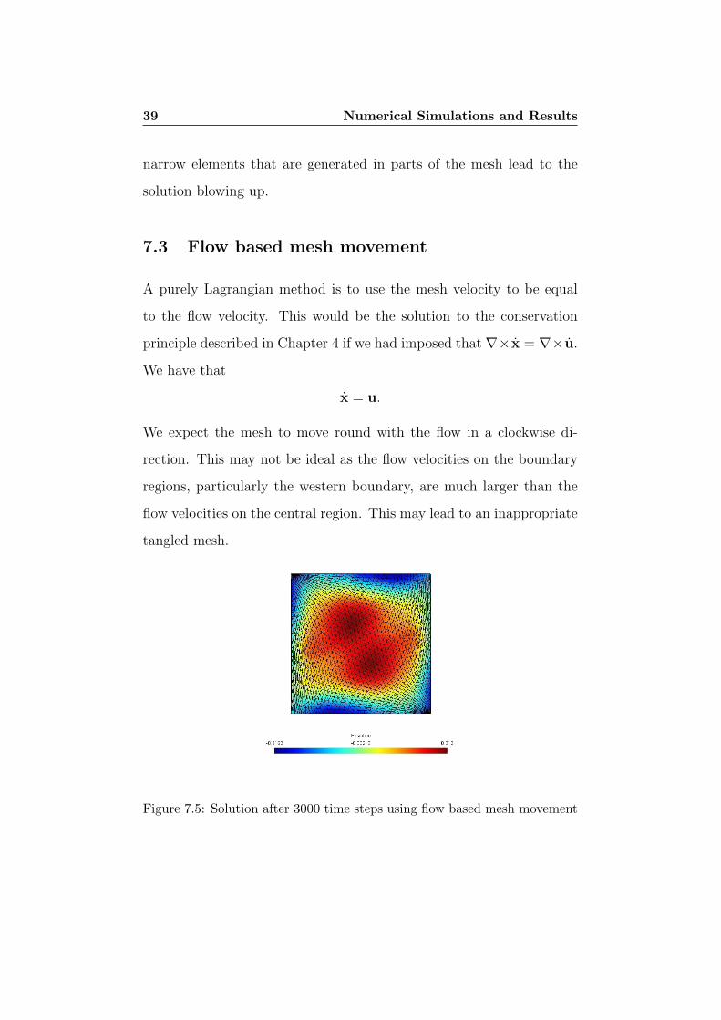
7.3 Flow based mesh movement

A purely Lagrangian method is to use the mesh velocity to be equal

to the flow velocity. This would be the solution to the conservation

principle described in Chapter 4 if we had imposed that ∇×x = ∇×u.

We have that

x = u.

We expect the mesh to move round with the flow in a clockwise di-

rection. This may not be ideal as the flow velocities on the boundary

regions, particularly the western boundary, are much larger than the

flow velocities on the central region. This may lead to an inappropriate

tangled mesh.

Figure 7.5: Solution after 3000 time steps using flow based mesh movement


7.3.1 Results for flow based mesh movement

The results confirm that the mesh moves in a clockwise direction around

the centre of the region. The solution has been distorted by rotation

as well. There is a smaller movement of nodes in the central region

due to the smaller flow velocities here. The boundary condition u · n

= 0 means that the boundary nodes are stationary. This leads to very

narrow elements in the four corners of the domain. The nodes become

very close together on the boundary of the region, and the solution

blows up after 3020 time steps.

7.4 Combined mesh movement

The last test we will look at is when the mesh velocities are calculated

using a linear combination of the mesh velocities used in the previous

two tests as follows,

x = αu + (1− α)∇p.

This corresponds to

∇× x = α∇u.

We choose different values of α between 0 and 1. With a larger α we

expect more rotation in the mesh than with a smaller value of α.

7.4.1 Results of combined mesh movement

Using α = 0.5 gives results very similar to the results obtained when

equating the mesh velocity to the flow velocity. This is because the flow

velocities along the eastern and western boundary are larger in magni-

tude than the mesh velocities generated by the conservation principle,


whereas the flow velocity in the centre of the domain is comparable

to the mesh velocities. We obtain the same narrow elements on the

boundaries as before which cause the solution to blow up. Putting

α = 0.1 gives slightly better results, but the flow velocities are still

overpowering the conservation velocities, and again the solution blows

up.

Figure 7.6: Solution after 9000 time steps using combined conservation/flow

based mesh movement

By decreasing α the solution tends towards that of the conservation

principle solution as we would expect. The solution also becomes more

stable with the reduction in α.

Chapter 8

Conclusion

This dissertation has considered the possibility of incorporating a mov-

ing mesh method into an existing model of a special form of the shallow

water equations, the Stommel model.

First we looked at how Stommel formed equations that describe

the formation of a strong western boundary current such as the Gulf

Stream. Then scale analysis was performed on these equations to de-

termine the dominant terms. The result of this was that the rotational

property of these velocities is an important part of the solution. This

led us to investigate whether equating the mesh velocity to the flow

velocities was a good strategy for moving the mesh. We saw in Chap-

ter 7 that this resulted in a rotational mesh which became unstable

very quickly. This is a result of the boundary nodes being restricted

to remain on the boundary, as there is only flow velocity tangential to

the boundary. Therefore the boundary nodes were able to move along

the boundary which led to a bunching of nodes in the four corners of

the domain.

We then discussed how the Stommel model was formulated using

43 Conclusion

finite elements following [1]. These finite element equations were then

discretised in time using an explicit Adams Bashforth method of order

3. The resulting mass matrix on the left hand side of the equation was

lumped to enable us to avoid invertion of a matrix. Explicit methods,

however, are not as stable as implicit methods, and a small time step

of ∆t = 20 seconds was required to keep a stable solution over the

simulation. The initial conditions and mesh were then stated, followed

by a description of how the solution evolves to form a western boundary

layer over time. This formation of the boundary layer is one motivation

for including a moving mesh procedure into the model.

In Chapter 4 a description of moving mesh methods was given,

along with the benefits and drawbacks of using moving meshes. Then

the use of a monitor function was introduced as in [8]. This disser-

tation has described the use of a conservation principle containing a

monitor function together with a prescribed vorticity. This then gives

rise to a conservation law from which we can obtain the mesh velocity.

The conservation principle was applied to the chosen monitor func-

tion, fluid depth. In a finite element context, this prescribed that the

volume of fluid in a patch of elements is constant for all time. The

Reynolds Transport Theorem was then used along with Gauss’ Theo-

rem to change the equation from a Lagrangian to a Eulerian form in

order to find the velocities. Then Helmholtz Decomposition Theorem

was used and setting ∇× x = 0, to determine an equation for the mesh

velocity x = ∇p in terms of the gradient of a velocity potential p.

The finite element formulation of this equation was described in

Chapter 5. The calculation of the resulting stiffness matrix and load

vector elements was described in terms of the dimensional properties of

44 Conclusion

each element. Then the equations were solved for the velocity potential

using a conjugate gradient solver. A description of how x = ∇p could

be solved using finite elements was then given. We then simplified the

calculation by lumping the resulting mass matrix, so the use of a sparse

matrix solver is not required. A further simplification was to find a ve-

locity for each element which is constant over the whole element. This

was then be interpolated onto the mesh nodes for mesh movement, and

onto the mid-segment nodes for advecting the solution to compensate

for the mesh movement. Whilst this simplification makes the com-

putation easier, the process of calculating the mesh velocity for each

element, and then having to interpolate this onto the mesh may have

caused a slight loss of accuracy in the mesh velocities, but should not

alter the solution.

The interpolation equations for generating nodal, and mid-segment

velocities from the element velocities was described in Chapter 6. Av-

erages were weighted according to the areas of the elements to try to

obtain more accurate interpolations to the node velocities and mid-

segment velocities. This averaging is not ideal as we could have calcu-

lated the mesh velocity straight from the finite element form in Section

5.2, and then used the average of the end points of a segment to de-

termine the mid-segment velocities. However, use of computational

time was an issue because of the small time step required for a sta-

ble solution. Therefore we chose the simplifications over the perhaps

slight increase in accuracy. The equations of mesh movement were

then stated. The mesh velocity was not calculated at every time step

as the reduced time step means that the solution did not move very

quickly over the simulation. The extra terms that arise in the solution

45 Conclusion

equations at the time step when the mesh movement occurs are stated,

followed by the finite element formulation of these terms.

Chapter 7 discussed the results of numerical simulations for a num-

ber of test cases for different mesh movement ideas. These ideas were

based on the ideas generated throughout the dissertation. The first

was a special case, as the Stommel model has an analytic solution so

we know that the elevation field flows westwards, considering purely

westward movement of the mesh. This gave a very simple computation

of the mesh velocity, but was also very crude, and the solution blew

up because of the gathering of very narrow elements on the western

boundary. A modified version of this idea is discussed in Chapter 9.

The main idea in this dissertation was to conserve the depth function

over a patch of elements with a prescribed mesh velocity. The results

show that this is been a promising start to describing a moving mesh

procedure for these equations. The time restriction for this disserta-

tion means that other monitor functions or curl properties of the depth

monitor function have not been able to be investigated. Some ideas for

other curl properties or monitor functions are in Chapter 9. Another

test was to set the mesh velocity to be equal to the flow velocity, equiv-

alent to choosing the vorticity of the mesh to be equal to the vorticity

of the fluid. This resulted in a very twisted mesh and an unstable

solution. The final idea was to take a linear combination of the conser-

vation based velocities and the flow velocity. The results showed that

the flow velocity overpowered the conservation velocities, and a very

small ratio of flow to conservation based mesh movement was required

for the solution to remain stable for any length of time.

Chapter 9

Further Work

The scope of work in this dissertation is limited by time available to

carry out the work. Given more time, there are other areas that would

be interesting to investigate. Several of these are given below.

More complex equations for western mesh movement Perhaps an

improved equation to use to move the mesh west would include a term

that would allow for the size of the boundary layer, using the analytic

solution to the Stommel equations. This could be used to make sure

the size of the elements in this boundary layer do not become too small.

This would of course only apply for the Stommel problem and not for

general equations.

Other monitor functions The monitor function described in this dis-

sertation is just one of many that could be used as a basis for mesh

movement. Use of different monitors that may give better results could

be investigated. Other monitor functions that could be used include

• vorticity or potential vorticity

47 Further Work

• fluid surface gradient,

|∇η|

• area on the surface of the solution,

√1 + (∇η)2

The latter two would be more suitable for moving points in areas with

large gradients, as in a boundary layer

Differing curl properties of mesh velocity We could investigate

other curl properties using ∇ × x = ∇ × q, where q is some variable

used to determine the mesh velocity, along with a monitor function. In

this case, x is not only the gradient of a potential function, but

x = q +∇p.

For the monitor function we have used, we have looked at the cases

when; ∇ × x = 0 taking q = 0, ∇ × x = ∇ × u where q = u, and

∇× x = αu which is equivalent to taking q = αu .

Modelling tides with a moving mesh The possibility of using a

moving mesh to show the rising and falling of the coastlines with tides

could also be looked at. This could be done by prescribing the surface

elevation on the boundaries to rise and fall over time. The boundary

condition would need to be changed from u·n = 0 on ∂Ω to u · n = x·n

to enable the mesh to move in and out of the domain.

Grid generation Different initial grids could be generated using an

equidistribution procedure. As the initial solution for η and u is zero

48 Further Work

over the whole domain, the grid could be generated using the initial

wind stress. An alternative would be to include a feature such a Gaus-

sian hill into the domain so that the initial elevation field is not zero,

and the mesh could be generated by equidistributing the volume of

fluid over the domain.

Other applications The principles outlined in this dissertation could

be used to introduce mesh movement into other models of fluid flow,

such as the Navier Stokes equations.

Bibliography

[1] Hanert, E., 2004. Towards a Finite Element Ocean Circulation

Model. PhD Thesis.

[2] Hanert, E., Le Roux, D.Y., Legat, V., Deleersnijder, E., 2005.

An efficient eulerian finite element method for the shallow water

equations. Ocean Modelling 10, 115-136.

[3] Hua, B.L., Thomasset, F., 1984. A noise-free finite element scheme

for the two-layer shallow water equations. Tellus 36A, 157-165.

[4] Piggott, M.D., Pain, C.C., Gorman, G.J., Power, P.W., Goddard,

A.J.H, 2005. h, r and hr adaptivity with applications in numerical

ocean modelling. Ocean Modelling 10, 95-113.

[5] Stommel, H., 1948. The westward intensification of wind-driven

ocean currents. Trans. Amer. Geophys. Union, 29, 202-206.

[6] Tang, T., 2005. Moving mesh methods for computational fluid

dynamics. Contemporary Mathematics 383, 141-173.

[7] Wells, B.V., Baines, M.J., Glaister, P., 2004. Generation of Arbi-

trary Lagrangian-Euler (ALE) velocities, based on moniter func-

tions, for the solution of compressible fluid equations. International

Journal for Numerical Methods in Fluids 1, 1-6.

50 BIBLIOGRAPHY

[8] Wells, B.V., 2004 A Moving Mesh Finite Element Method for the

Numerical Solution of Partial Differential Equations and Systems.

PhD Thesis.

Development of a Simpliﬁed Adaptive Finite Element Model ...

Documents