HAL Id: tel-03228497 https://tel.archives-ouvertes.fr/tel-03228497 Submitted on 18 May 2021 HAL is a multi-disciplinary open access archive for the deposit and dissemination of sci- entific research documents, whether they are pub- lished or not. The documents may come from teaching and research institutions in France or abroad, or from public or private research centers. L’archive ouverte pluridisciplinaire HAL, est destinée au dépôt et à la diffusion de documents scientifiques de niveau recherche, publiés ou non, émanant des établissements d’enseignement et de recherche français ou étrangers, des laboratoires publics ou privés. Development of a robotic cell for the printing of electronic circuits on free form surfaces and industrial applications Gioia Furia To cite this version: Gioia Furia. Development of a robotic cell for the printing of electronic circuits on free form surfaces and industrial applications. Mechanics of materials [physics.class-ph]. Université Grenoble Alpes [2020-..], 2021. English. NNT : 2021GRALI015. tel-03228497

Welcome message from author
This document is posted to help you gain knowledge. Please leave a comment to let me know what you think about it! Share it to your friends and learn new things together.
Transcript

HAL Id: tel-03228497https://tel.archives-ouvertes.fr/tel-03228497
Submitted on 18 May 2021
HAL is a multi-disciplinary open accessarchive for the deposit and dissemination of sci-entific research documents, whether they are pub-lished or not. The documents may come fromteaching and research institutions in France orabroad, or from public or private research centers.
L’archive ouverte pluridisciplinaire HAL, estdestinée au dépôt et à la diffusion de documentsscientifiques de niveau recherche, publiés ou non,émanant des établissements d’enseignement et derecherche français ou étrangers, des laboratoirespublics ou privés.
Development of a robotic cell for the printing ofelectronic circuits on free form surfaces and industrial
applicationsGioia Furia
To cite this version:Gioia Furia. Development of a robotic cell for the printing of electronic circuits on free form surfacesand industrial applications. Mechanics of materials [physics.class-ph]. Université Grenoble Alpes[2020-..], 2021. English. NNT : 2021GRALI015. tel-03228497


FURIA Gioia
2

FURIA Gioia
3
TABLE OF CONTENT
GENERAL INTRODUCTION
1. CONTEXT OF THE PROJECT ............................................................................................................ 11
2. OBJECTIVES OF THE THESIS .......................................................................................................... 13
3. MAIN OBSTACLES AND THESIS STRUCTURE .......................................................................... 14
4. BIBLIOGRAPHY .................................................................................................................................... 16
5. TABLE OF FIGURES ............................................................................................................................ 16
CHAPTER 1: BIBLIOGRAPHY
INTRODUCTION ................................................................................................................................... 23 1
HIGH PRECISION FABRICATION PROCESS ............................................................................... 24 2
Robotic arm: architecture and cinematic .......................................................................... 24 2.1
Manufacturing process ............................................................................................................. 25 2.2
Main issues causing inaccuracies .......................................................................................... 26 2.3
Inaccuracies related to the object ................................................................................ 27 2.3.1
Inaccuracies linked to the process .............................................................................. 28 2.3.2
Inaccuracies related to the static accuracy of the robot ..................................... 28 2.3.3
Mesure in-situ ............................................................................................................................... 30 2.4
Position of the measuring phase in the manufacturing process ...................... 30 2.4.1
Integration of the measuring equipment in the working area ......................... 31 2.4.2
FUNCTIONAL MATERIALS PRINTING ........................................................................................ 33 3
Direct and contactless printing process ............................................................................. 33 3.1
Aerosol .................................................................................................................................... 34 3.1.1
Inkjet ....................................................................................................................................... 35 3.1.2
Jetting ...................................................................................................................................... 36 3.1.3
Extrusion ............................................................................................................................... 36 3.1.4
Comparison ........................................................................................................................... 37 3.1.5
Physical and chemical properties ......................................................................................... 38 3.2
Physico-chemistry of the ink ......................................................................................... 38 3.2.1
Rheological behaviour of the ink .................................................................................. 40 3.2.2
Conductive property of printed tracks ...................................................................... 42 3.2.3
Metallic inks.......................................................................................................................... 43 3.2.4
Carbon based ink ................................................................................................................ 46 3.2.5
Conductive polymers ........................................................................................................ 47 3.2.6

FURIA Gioia
4
Substrates used in electronic printing ................................................................................ 48 3.3
Substrates characteristics ............................................................................................... 48 3.3.1
Substrates studied in literature .................................................................................... 50 3.3.2
Molded cellulose ................................................................................................................. 51 3.3.3
Micro Fibrillated cellulose (MFC) ................................................................................ 52 3.3.4
Annealing types ........................................................................................................................... 52 3.4
Thermal annealing ............................................................................................................. 53 3.4.1
Chemical annealing ............................................................................................................ 53 3.4.2
Electrical annealing ........................................................................................................... 54 3.4.3
Plasma annealing ................................................................................................................ 55 3.4.4
Microwave annealing ........................................................................................................ 56 3.4.5
Photonic annealing ............................................................................................................ 56 3.4.6
CONNECTED OR FUNCTIONAL OBJECT ..................................................................................... 60 4
Molded Interconnect Devices (MID) .................................................................................... 60 4.1
Fabrication process ........................................................................................................... 60 4.1.1
Research project examples ............................................................................................. 62 4.1.2
Industrial application examples ................................................................................... 62 4.1.3
Additive manufacturing of 2D multilayer functional devices .................................... 63 4.2
Paper microfluidic .............................................................................................................. 63 4.2.1
Papertouch ............................................................................................................................ 64 4.2.2
Additive manufacturing of 3D functional objects ........................................................... 65 4.3
Multimaterials objects additive manufacturing process .................................... 65 4.3.1
Industrial application examples ................................................................................... 67 4.3.2
Robotic for 3D printing ............................................................................................................. 69 4.4
Research project examples ............................................................................................. 69 4.4.1
Industrial application examples ................................................................................... 71 4.4.2
CONCLUSION ........................................................................................................................................ 74 5
BIBLIOGRAPHY .................................................................................................................................... 75 6
TABLE OF FIGURES ............................................................................................................................ 83 7
TABLE OF TABLES .............................................................................................................................. 84 8
CHAPTER 2: ROBOTIC CELL AND OFF-LINE PROGRAMMING SOFTWARE
DEVELOPMENT
INTRODUCTION ................................................................................................................................... 90 1
3D SIMULATION AND POST-PROCESSOR SOFTWARE ....................................................... 91 2

FURIA Gioia
5
VAL 3 language ............................................................................................................................. 92 2.1
Structure of VAL3 language: application and program. ...................................... 92 2.1.1
Control of movement ........................................................................................................ 92 2.1.2
Presentation of simulation and off-line programming tools ...................................... 95 2.2
Stäubli Robotics Suite (SRS) ........................................................................................... 96 2.2.1
Commercial industrial tools ........................................................................................... 96 2.2.2
Rhinoceros 3D plugin ....................................................................................................... 97 2.2.3
Comparative table .............................................................................................................. 98 2.2.4
Choice of a simulation and off-line programming tool ................................................. 99 2.3
Generation accuracy of the object in the working environment ....................................101 3
Mesh generation methods: bibliography focus .............................................................101 3.1
Scanning tools ....................................................................................................................102 3.1.1
From points cloud to mesh generation ....................................................................104 3.1.2
Mesh quality evaluation .........................................................................................................109 3.2
Process implementation and characterisation ..............................................................112 3.3
Scan step implementation.............................................................................................112 3.3.1
Reverse engineering step implementation ............................................................120 3.3.2
Process validation .....................................................................................................................127 3.4
Process description .........................................................................................................127 3.4.1
Examples ..............................................................................................................................128 3.4.2
Criteria validation .....................................................................................................................134 3.5
3D ELECTRONIC CIRCUITS PRINTING .....................................................................................137 4
Electronic circuit printing on 3D objects: bibliography focus .................................137 4.1
The CAD model of the part on which the material will be deposited ..........137 4.1.1
The chosen tool .................................................................................................................137 4.1.2
The path pattern ...............................................................................................................138 4.1.3
The process requirements and parameters ...........................................................138 4.1.4
Required printing quality ......................................................................................................139 4.2
Projection process ....................................................................................................................139 4.3
Printing process .........................................................................................................................142 4.4
PRINTING ROBOTIC CELL .............................................................................................................143 5
Cell requirement ........................................................................................................................143 5.1
Schematic diagram and description ..................................................................................143 5.2
3D Simulation environment and interface description ..............................................145 5.3
Cell criteria validation .............................................................................................................152 5.4
CONCLUSION ......................................................................................................................................153 6

FURIA Gioia
6
BIBLIOGRAPHY ..................................................................................................................................154 7
TABLE OF FIGURES ..........................................................................................................................157 8
TABLE OF TABLES ............................................................................................................................158 9
CHAPTER 3: APPLICATIONS
INTRODUCTION .................................................................................................................................164 1
PRINTING ON 3D OBJECTS ............................................................................................................165 2
Printed lines characterisation ..............................................................................................165 2.1
Printing tool implementation ......................................................................................165 2.1.1
Robot speed analysis.......................................................................................................166 2.1.2
2D Printing tests ...............................................................................................................169 2.1.3
Predictive model creation......................................................................................................170 2.2
Model theory ......................................................................................................................170 2.2.1
Analysis and results.........................................................................................................171 2.2.2
Printed line conductivity ...............................................................................................174 2.2.3
Predictive model and quality validation ..........................................................................176 2.3
Process description .........................................................................................................176 2.3.1
Example ................................................................................................................................177 2.3.2
Criteria validation .....................................................................................................................180 2.4
Precise control of the number of drops deposited .......................................................181 2.5
Conclusion....................................................................................................................................183 2.6
2D MULTI-MATERIAL APPLICATIONS: USE FOR THE MANUFACTURING OF 3ENCAPSULATED MICROFLUIDIC DEVICES ......................................................................................185
Spontaneous capillary flow ...................................................................................................185 3.1
Capillary force ....................................................................................................................185 3.1.1
Dynamic of spontaneous capillary flow...................................................................186 3.1.2
Manufacturing of paper microfluidic medical diagnostic devices .........................187 3.2
Prerequisite for a medical diagnostic tool ..............................................................187 3.2.1
State of the art of the manufacturing of paper microfluidic devices ............189 3.2.2
Developed manufacturing process ............................................................................190 3.2.3
Development of the required functionalities .................................................................193 3.3
Paper spray coating .........................................................................................................193 3.3.1
Capillary system................................................................................................................197 3.3.2
Heating system ..................................................................................................................204 3.3.3
Towards a point of care diagnostic medical devices ...................................................211 3.4

FURIA Gioia
7
CONCLUSION ......................................................................................................................................212 4
BIBLIOGRAPHY ..................................................................................................................................214 5
TABLE OF FIGURES ..........................................................................................................................217 6
TABLE OF TABLES ............................................................................................................................218 7
GENERAL CONCLUSION
CONCLUSION ......................................................................................................................................222 1
PERSPECTIVES ...................................................................................................................................224 2
RÉSUME ÉTENDU
INTRODUCTION .................................................................................................................................229 1
DÉVELOPEMENT D’UNE CELLULE ROBOTISÉE POUR L’IMPRESSION DE CIRCUITS 2ÉLECTRONIQUES ........................................................................................................................................232
Réalisation de la cellule robotisée ......................................................................................232 2.1
Description de la cellule .................................................................................................232 2.1.1
Développement du post-processeur .........................................................................234 2.1.2
Développement du processus d’impression ..................................................................235 2.2
APPLICATIONS ...................................................................................................................................238 3
Impression de pistes conductrices sur des objets 3D .................................................238 3.1
2.1.1 Tests d’impression : matériel et méthode ..............................................................238
Etude d’un modèle prédictif de la géométrie des pistes ...................................239 3.1.1
Exemple d’impression de pistes sur un objet 3D .................................................241 3.1.2
Impression 2D de dispositifs médicaux multimatériaux ...........................................243 3.2
Processus de fabrication ................................................................................................243 3.2.1
Obtention de propriétés barrières par dépôt d’une couche de MFC par 3.2.2spray 246
Impression de chemins capillaires ............................................................................247 3.2.3
Résistances chauffantes imprimées ..........................................................................248 3.2.4
CONCLUSION ......................................................................................................................................250 4
BIBLIOGRAPHIE ................................................................................................................................252 5
TABLE DES FIGURES .......................................................................................................................253 6
ABSTRACT .....................................................................................................................................................254
RESUMÉ ..........................................................................................................................................................254

FURIA Gioia
8

FURIA Gioia
9
GENERAL INTRODUCTION

FURIA Gioia
10
TABLE OF CONTENT
1. CONTEXT OF THE PROJECT ............................................................................................................ 11
2. OBJECTIVES OF THE THESIS .......................................................................................................... 13
3. MAIN OBSTACLES AND THESIS STRUCTURE .......................................................................... 14
4. BIBLIOGRAPHY .................................................................................................................................... 16
5. TABLE OF FIGURES ............................................................................................................................ 16

FURIA Gioia
11
1. CONTEXT OF THE PROJECT
A growing demand for prototyping processes is emerging in the fields of electronics and
connected objects to simplify and automate the process of integrating electronic
components into 3D objects. For this reason, plastronics is developing and is really
starting to appear on the market since the 2000s. [1]
This discipline, which combines plastics processing and electronics, facilitates the
integration of electronics into objects in order to make them functional. To do this,
certain electronic functions and links between components are no longer supported by a
conventional 2D electronic board (PCB: Printed Circuit Board) but directly integrated on
the 3D object.
In order to offer a versatile and easy to implement alternative for prototyping and small
series, printed electronics is also widely considered. This technology consists in printing
an electrically conductive ink on the surface of already formed 3D objects in order to
create the electronic functions deported on the object and the links with a possible PCB
board. For small series, the advantages of this technique are the following:
- No restriction of materials for the manufacturing of the object. Due to the
plurality of inks (viscous, fluid, aqueous or solvent based, metallic or organic ...)
and deposit systems (pressure, worm, drop ejection ...) existing, the printing of a
quality circuit can be achieved on any material.
- Additive technology: on the one hand, only the necessary amount of material is
used, there is no waste. On the other hand, the process is direct, the conductive
tracks are created in a single step.
In the same time, the industrial robotics market is in constant evolution, there are today
more than two million industrial robots in the world.
Since 1987, IFR (International Federation of Robotics) has been collecting worldwide
sales data for industrial robots, so as illustrated in Figure 1, the market has more than
tripled in 10 years.

FURIA Gioia
12
Figure 1: Worldwide annual supply of Industrial Robots from IFR
Many robot models have been developed to meet the requirements of new applications
in terms of weight to be carried, range of motion, speed and precision.
In the industrial field, the most widespread robots are robot arms, in areas such as
welding, painting or assembly.
An increasing number of high-tech sectors are starting to use industrial robots such as
telecommunication, Internet of things (Iot) and additive manufacturing and many small
and medium enterprises (SMEs) are wondering about the integration of robots in their
structure.
However today no simple system of use is available on the market for 3D electronic
printing. At the research level, developments are focused on the use of Cartesian X,Y,Z
printers, sometimes with a 4th axis of rotation, supporting print heads to deposit the
conductive tracks during the manufacture of the object [2], [3] or on 2,5D objects[4], [5].

FURIA Gioia
13
2. OBJECTIVES OF THE THESIS
The subject of the first part of the thesis, collaboration between the SME Mind and the
laboratory LGP2 (Laboratoire Génie des Procédés Papetiers), is the creation of a robotic
cell for the prototyping and production of small series of cellulose-based connected
objects functionalized on the surface by direct circuit printing.
The printing of conductive tracks allows the integration of electronic functions directly
on the surface of the object without the systematic transfer of one or more conventional
2D electronic boards and the replacement of electrical wires between components by
printed conductive tracks.
All operations will be performed by 6-axis robots on which will be mounted various
working tools, including a laser scanner and one or more printing heads.
The platform will be completed by a dedicated software allowing the management of the
whole production process and the automatic creation of the machine code for the
piloting of the manufacturing process. This software, equipped with a simplified
interface and calibration protocol, will allow both the use of the prototyping line by
people who are not experts in robotics and a high speed in the customization of printed
circuits and product changeover.
The second part of the thesis, collaboration between Carnot Polynat and the LGP2,
consist in using the developed cell for the manufacturing of multi-layers cellulose-based
medical tests.

FURIA Gioia
14
3. MAIN OBSTACLES AND THESIS STRUCTURE
The goal of this project is to provide an answer to the problem of the electronic
functionalization of 3D objects to make them functional by an automated process,
versatile, easy to implement and compatible with prototyping and small series.
The main obstacles to achieving this goal are the development and implementation of a
direct writing process on 3D objects using a six-axis multi-tool industrial robot. This
lock, which represents the heart of the project, covers:
- aspects concerning the sources of inaccuracies that impact the process like the
object geometry, which can be a macro-geometrical default or a positioning
default between the object and the robot. Thus, a trajectory designed from a
theoretical geometry and position is not necessarily valid. [6], [7]
- aspects concerning the identification/implementation of deposition techniques
adapted to the process (e.g. extrusion, spray, jetting, ...) ;
- the development of a protocol for managing the movements of the robotic arm
enabling the deposition of conductive tracks
The thesis will therefore be structured as illustrate in Figure 2.
After this introduction chapter, a review of the literature will be conducted (chapter 1);
then two main contributions will be made:
- chapter 2 describes the integration and qualification of all the tools on the 6-axis
robot as well as the creation of a demonstration cell and the dedicated control
software.
- chapter 3 presents applications tested with the developed cell . Two main
applications are tested, the production of small series of cellulose-based multi-
layers medical tests and example of simple 3D connected objects.
Finally, conclusions will be done and perspectives will be discussed.

FURIA Gioia
15
Figure 2 : Thesis structure

FURIA Gioia
16
4. BIBLIOGRAPHY
[1] D. Unnikrishnan, « Mid technology potential for RF passive components and antennas », Univ. GRENOBLE, p. 246, 2006.
[2] M. Ahmadloo et P. Mousavi, « A novel integrated dielectric-and-conductive ink 3D printing technique for fabrication of microwave devices », in 2013 IEEE MTT-S International Microwave Symposium Digest (MTT), juin 2013, p. 1‑3, doi: 10.1109/MWSYM.2013.6697669.
[3] C. Shemelya et al., « Multi-functional 3D printed and embedded sensors for satellite qualification structures », in 2015 IEEE SENSORS, nov. 2015, p. 1‑4, doi: 10.1109/ICSENS.2015.7370541.
[4] B. Y. Ahn et al., « Planar and Three-Dimensional Printing of Conductive Inks », JoVE J. Vis. Exp., no 58, p. e3189, déc. 2011, doi: 10.3791/3189.
[5] J. Hörber, J. Glasschröder, M. Pfeffer, J. Schilp, M. Zaeh, et J. Franke, « Approaches for Additive Manufacturing of 3D Electronic Applications », Procedia CIRP, vol. 17, p. 806‑811, déc. 2014, doi: 10.1016/j.procir.2014.01.090.
[6] B. Loriot, « Automation of Acquisition and Post-processing for 3D Digitalisation », Theses, Université de Bourgogne, 2009.
[7] S. Khalfaoui, « Production automatique de modèles tridimensionnels par numérisation 3D », Dijon, 2012.
5. TABLE OF FIGURES
Figure 1: Worldwide annual supply of Industrial Robots from ................................................. 12 Figure 2 : Thesis structure ........................................................................................................................ 15

FURIA Gioia
17

FURIA Gioia
18

FURIA Gioia
19
CHAPTER 1: BIBLIOGRAPHY

FURIA Gioia
20
TABLE OF CONTENT
1 INTRODUCTION ................................................................................................................................... 23
2 HIGH PRECISION FABRICATION PROCESS ............................................................................... 24
2.1 Robotic arm: architecture and cinematic .......................................................................... 24
2.2 Manufacturing process ............................................................................................................. 25
2.3 Main issues causing inaccuracies .......................................................................................... 26
2.3.1 Inaccuracies related to the object ................................................................................ 27
2.3.2 Inaccuracies linked to the process .............................................................................. 28
2.3.3 Inaccuracies related to the static accuracy of the robot ..................................... 28
2.4 Mesure in-situ ............................................................................................................................... 30
2.4.1 Position of the measuring phase in the manufacturing process ...................... 30
2.4.2 Integration of the measuring equipment in the working area ......................... 31
3 FUNCTIONAL MATERIALS PRINTING ........................................................................................ 33
3.1 Direct and contactless printing process ............................................................................. 33
3.1.1 Aerosol .................................................................................................................................... 34
3.1.2 Inkjet ....................................................................................................................................... 35
Continuous Inkjet ........................................................................................................... 35 3.1.2.1
Drop of Demand ............................................................................................................. 35 3.1.2.2
3.1.3 Jetting ...................................................................................................................................... 36
3.1.4 Extrusion ............................................................................................................................... 36
3.1.5 Comparison ........................................................................................................................... 37
3.2 Physical and chemical properties ......................................................................................... 38
3.2.1 Physico-chemistry of the ink ......................................................................................... 38
Surface tension................................................................................................................ 38 3.2.1.1
Colloidal stability ........................................................................................................... 39 3.2.1.2
3.2.2 Rheological behaviour of the ink .................................................................................. 40
3.2.3 Conductive property of printed tracks ...................................................................... 42
Resistivity and conductivity ...................................................................................... 42 3.2.3.1
Quality index .................................................................................................................... 43 3.2.3.2
3.2.4 Metallic inks.......................................................................................................................... 43
Micro/nanoparticles inks ........................................................................................... 44 3.2.4.1
Inks based on metal salts (Metallo Organic Decomposition MOD) ............ 45 3.2.4.2
Studies have been carried out by .............................................................................................. 45

FURIA Gioia
21
Catalytic inks .................................................................................................................... 45 3.2.4.3
Inks causing a redox reaction .................................................................................... 45 3.2.4.4
3.2.5 Carbon based ink ................................................................................................................ 46
3.2.6 Conductive polymers ........................................................................................................ 47
3.3 Substrates used in electronic printing ................................................................................ 48
3.3.1 Substrates characteristics ............................................................................................... 48
Roughness ......................................................................................................................... 48 3.3.1.1
Porosity .............................................................................................................................. 49 3.3.1.2
Surface energy ................................................................................................................. 49 3.3.1.3
Thermal stability ............................................................................................................ 49 3.3.1.4
3.3.2 Substrates studied in literature .................................................................................... 50
3.3.3 Molded cellulose ................................................................................................................. 51
3.3.4 Micro Fibrillated cellulose (MFC) ................................................................................ 52
3.4 Annealing types ........................................................................................................................... 52
3.4.1 Thermal annealing ............................................................................................................. 53
3.4.2 Chemical annealing ............................................................................................................ 53
3.4.3 Electrical annealing ........................................................................................................... 54
3.4.4 Plasma annealing ................................................................................................................ 55
3.4.5 Microwave annealing ........................................................................................................ 56
3.4.6 Photonic annealing ............................................................................................................ 56
Infrared annealing ......................................................................................................... 57 3.4.6.1
Laser annealing ............................................................................................................... 57 3.4.6.2
Intense Pulsed Light annealing (IPL) ..................................................................... 58 3.4.6.3
4 CONNECTED OR FUNCTIONAL OBJECT ..................................................................................... 60
4.1 Molded Interconnect Devices (MID) .................................................................................... 60
4.1.1 Fabrication process ........................................................................................................... 60
Laser direct structuring (LDS) .................................................................................. 60 4.1.1.1
Laser subtractive structuring (LSS) ........................................................................ 61 4.1.1.2
Microstamping ................................................................................................................ 61 4.1.1.3
Bi-injection ....................................................................................................................... 61 4.1.1.4
Inkjet ................................................................................................................................... 61 4.1.1.5
4.1.2 Research project examples ............................................................................................. 62
Electronic field ................................................................................................................ 62 4.1.2.1
4.1.3 Industrial application examples ................................................................................... 62

FURIA Gioia
22
Medical field ..................................................................................................................... 62 4.1.3.1
Automotive field ............................................................................................................. 62 4.1.3.2
Telecommunication field ............................................................................................ 63 4.1.3.3
4.2 Additive manufacturing of 2D multilayer functional devices .................................... 63
4.2.1 Paper microfluidic .............................................................................................................. 63
4.2.2 Papertouch ............................................................................................................................ 64
4.3 Additive manufacturing of 3D functional objects ........................................................... 65
4.3.1 Multimaterials objects additive manufacturing process .................................... 65
Material deposit .............................................................................................................. 65 4.3.1.1
Photopolymerisation .................................................................................................... 66 4.3.1.2
Manufacturing on powder bed ................................................................................. 67 4.3.1.3
4.3.2 Industrial application examples ................................................................................... 67
Voxel8 ................................................................................................................................. 68 4.3.2.1
Nano Dimension ............................................................................................................. 68 4.3.2.2
Optomec-Stratasys ........................................................................................................ 69 4.3.2.3
4.4 Robotic for 3D printing ............................................................................................................. 69
4.4.1 Research project examples ............................................................................................. 69
+Lab –Milan Polytechnic University ....................................................................... 70 4.4.1.1
BatiPrint3D-Nantes ....................................................................................................... 70 4.4.1.2
4.4.2 Industrial application examples ................................................................................... 71
Stratasys ............................................................................................................................ 71 4.4.2.1
Drawn ................................................................................................................................. 72 4.4.2.2
Poietis ............................................................................................................................. 72 4.4.2.3
Bioassemblybot .......................................................................................................... 73 4.4.2.4
5 CONCLUSION ........................................................................................................................................ 74
6 BIBLIOGRAPHY .................................................................................................................................... 75
7 TABLE OF FIGURES ............................................................................................................................ 83
8 TABLE OF TABLES .............................................................................................................................. 84

FURIA Gioia
23
INTRODUCTION 1
The objective of this chapter is to analyze in depth the literature dealing with the
manufacturing process of 3D molded cellulose objects including surface printed
electronic circuits by robotic printing, to highlight the most influential parameters and
the means to control them.
The first part describes the process of printing electronic circuits on 3D parts. It
highlights the main problems encountered and presents the measurement means used
to control the process as well as their integration during manufacturing.
The second part deals with the parameters involved in the printing of conductive tracks
and the study of research work to understand and optimize them.
The third part focuses on the printing technologies that enable the manufacture of
functionalized 3D objects, the related research topics and their main industrial
applications.

FURIA Gioia
24
HIGH PRECISION FABRICATION PROCESS 2
In the literature, a lot of work exists on the analysis of robotic processes such as welding,
cutting or milling [1], [2] . Robotic manufacturing processes using poly-articulated
structures allow great flexibility in the design of the parts to be produced and are
beginning to interest fields such as additive manufacturing and architecture. [3]
Robotic arm: architecture and cinematic 2.1
The structures of the robotic arm type have a serial architecture with 6 degrees of
freedom, i.e. they are composed of 6 kinematic rotational links arranged one after the
other as illustrated in Figure 3.
Figure 3: Architecture 6-axis robot [4]
The use of 6-axis structures is beginning to develop because they provide a real
advantage for the development of complex parts. Academic and industrial work has
enabled to propose ways of improving their performance [4] but their accuracy and
repeatability are not yet equal to that of machine tools. [5]
The ability of a structure to generate motion is directly related to its architecture. Each
movement is generated by the displacement of an axis composed of a control part which
controls the servo-control in position and speed of the movement and an operative part
composed of the motorization and guiding systems allowing the movement.
Along a trajectory, the speed variation, acceleration and jerk parameters are imposed by
the manufacturer of the robotic arm in order not to overload the various elements.
These parameters are implemented in the robot controller and will directly influence
the speed of the trajectory.
Initially, industrial robots were programmed by manual teach-in. The programming of a
trajectory was done by manually teaching each crossing point. This method was

FURIA Gioia
25
therefore not sensitive to part positioning errors relative to the robot. Then, with the
arrival of robotic CAD, Offline Programming methods appeared, trajectories were
created digitally and the robot had to reach theoretical positions rather than taught
positions. A lot of work has been done on off-line programming methods and their
optimization for industrial applications. [6], [7]
Manufacturing process 2.2
The part development processes, regardless of the process used, are relatively similar in
approach. The objective is to manipulate a tool in relation to a part by means of a
supporting structure.
These processes can be broken down into four steps: [8]
Design: this step consists of defining the geometry of the object and generating the CAD
(Computer Aided Design) model.
Generation of trajectories: this second phase allows to define the parameters related to
the process and to generate a CAM (Computer Aided Manufacturing) model.
Post-processing: during this step the generated trajectories are translated into the
appropriate language for the production system.
Execution: In this last phase of execution, the instructions are sent to the system which
physically performs the manufacturing operation.
By analogy we can decompose the process studied in this thesis, of robotic printing of
electronic circuits on 3D objects in several steps illustrated in Figure 4.
Figure 4: Manufacturing process

FURIA Gioia
26
Design
Step 1: Importing the part model into a CAD software. Positioning of the model in the
workspace and orientation in relation to the print head according to the surfaces to be
printed.
Step 2: Drawing the electronic tracks on the CAD model.
Trajectories generation
Step 3: Definition of printing parameters and generation of trajectories.
Post-processing
Step 4: Generation of files in robot language. Import of the files into the robot software
and management of the I/Os of the different sensors.
Execution
Step 5: Simulation in the robot software or in manual mode
Step 6: Adjustments
Step 7: Printing the conductive tracks on the 3D object
Step 8: Annealing of printed tracks
A track of study envisaged in this thesis will then be to manufacture the 3D object with
an adapted print head mounted on the robot then to come as explained previously, to
print the circuits on the surface. In this case the step 1 consists in drawing the 3D object
in the CAD software and during the step 3, the generated trajectories will be those of the
object and those of the conductive tracks.
Generally speaking, the manufacturing process involves many parameters that increase
the sources of inaccuracy, which has a direct impact on the quality of the final object,
especially when the process requires a high level of precision.
These parameters have been the subject of bibliographical research, presented in the
following paragraphs.
Main issues causing inaccuracies 2.3
In their works, Buschhaus, Wagner et Franke, [9] decompose the total inaccuracy of a
process of handling a part by a robotic arm in relation to a fixed tool into the sum of the
errors related to the robot, the manipulator, the tool and the part as illustrated in Figure
5.

FURIA Gioia
27
Figure 5 :Parameters that influence process quality [9]
Thus the analysis of the manufacturing chain of the process studied in this work makes
it possible to highlight the main sources of inaccuracies related to the object, the process
and the static accuracy of the robot and to consider areas for improvement.
Inaccuracies related to the object 2.3.1
These may be macrogeometric defects and/or defects in the accuracy of positioning of
the part in relation to the robot.
Indeed, depending on the manufacturing tolerances of the part, there may be geometric
differences between the CAD model of the object and the real object. Or some objects do
not have a CAD model. Thus, a path drawn from a theoretical geometry and a theoretical
positioning is not necessarily valid.
In order to compensate for these defects, it is necessary to obtain a CAD model that is as
real as possible in order to be able to draw accurate electronic tracks.
One possible solution is to digitize the object, i.e. to obtain a digital representation of its
surface geometry in the form of a point cloud or mesh using an external sensor. A data
processing system is used to obtain the 3D coordinates of the object from the raw data
provided by the sensor. [10]–[12]
This implies the addition of a preliminary step more or less long depending on the level
of accuracy to be achieved and the development of an additional interface to process the
data retrieved by the sensor.

FURIA Gioia
28
Inaccuracies linked to the process 2.3.2
The chosen process also imposes constraints which, if not properly controlled, can lead
to defects in the manufacturing process and thus to a deficient or non-functional object.
In the case of printing interconnections or passive components such as RFID circuits, it
is necessary to have a high degree of process control to achieve very high accuracy of
printing head positioning along the trajectory.
As illustrated in Figure 6, Redinger et al. [13], [14] printed by inkjet lines with a width of
160µm with 100µm spacing for RFID system applications.
Thus, the movements of the print head, its orientation and inclination with respect to
the support condition the quality of the print. So it is important to control them.
Figure 6: Inkjet printing of passive components [14]
In addition, the CAD model does not take into account the material of the object and
depending on the surface condition of the object, problems may arise depending on the
print head used and the required printing distance between the head and the media.
Indeed, some print heads require a printing distance of a few micrometers, which is of
the same order of magnitude as the surface roughness of some substrates. [15], [16]
Inaccuracies related to the static accuracy of the robot 2.3.3
In order to reduce the errors between the trajectory from the CAD and the trajectory in
the real environment, a manual adjustment of the trajectory or a calibration phase
before the start of the task can be considered.
Studies have been carried out on robot, workspace and tool calibration.
In the field of 3D printers, calibration procedures are proposed in particular to correct
defects related to the flatness of the plate. [17]
The firmware Repetier or Marlin offer the G29 control for checking the flatness of the

FURIA Gioia
29
platen in 5 or 9 points. An inductive or capacitive sensor is mounted on the print head
which will be placed at different points evenly distributed on the platen. The printer will
make a correction relative to the flatness of the plate.
Also with the aim of improving positioning accuracy, calibration methods have been
developed for 6-axis systems. The objective is to identify the actual geometrical
parameters of the robot, i.e. the lengths of the arms and their orientation with respect to
the axes of rotation in order to improve the accuracy of the robot end device. This may
involve calibration with or without sensors.
In general, calibration involves four steps: modelling, measurement, identification and
compensation. [18], [19]
Khalil et Besnard [20], [21] propose a comparison between different autonomous
calibration methods without external sensors.
Calibration with multi-plane links is regularly used in research work on robotic arms
[22]. This method consists in using the articular coordinates of a set of configurations in
which the end of the end effector is in contact with a plane. Then, the geometrical
parameters are identified using minimization algorithms. Finally, the new parameter
values are integrated into the control, which compensates the precision error. As
illustrated in Figure 7, calibration is carried out with a calibration block machined with
small tolerances and the contact can be checked by a probe.
Figure 7: Sensor and calibration cube [22]
Other more expensive calibration methods using external measurement sensors such as
theodolites, camera, laser or acoustic sensor can be used. Khalil et Dombre [23] present
a comparison of these systems.
Buschhaus, Wagner et Franke, [9] propose a closed-loop calibration method, the
principle of which is to send the robot to reference marks, measure the deviation and
apply correction coefficients as illustrated in Figure 8.

FURIA Gioia
30
Figure 8 : Calibration method example [9]
In conclusion, to guarantee the accuracy of the robot in its work cell, it is necessary to
know and control the different sources of error.
Various sensor technologies are available for measurement and control. However, in
order to ensure that the control is time-efficient and allows for a high level of reactivity
in correcting defects, the measurement must be integrated as far as possible into the
manufacturing phase.
Measure in-situ 2.4
Position of the measuring phase in the manufacturing process 2.4.1
The measuring phase can be done post-process, after manufacturing or in situ during
the manufacturing phase. [24], [25]
Post-process measurement is time-consuming because it requires the object to be
moved to the measuring equipment and defects can only be detected after manufacture.
However, it leaves the tool available for further production.
The in-situ measurement is carried out at the same time as the manufacturing process,
without moving the object. It can be done in-process without stopping the means of
production during the measuring phase or on-machine when manufacturing is stopped
as illustrated in Figure 9.

FURIA Gioia
31
Figure 9: In-situ measure inspired from [25]
The in-process measurement allows to be very reactive on the correction to be made
during the manufacturing process. However, it is complex to implement because the
manufacturing and measurement phases must communicate and operate at the same
time without risk of collision.
This method is used in the industry to monitor machining for example, because it allows
to improve quality without impacting productivity. [26]
On-machine measurement, carried out when manufacturing is stopped, takes into
account the measurement phase in the manufacturing phase and thus allows good
reactivity in correcting defects by making corrective actions possible directly in the
manufacturing environment. However, as manufacturing is stopped, productivity is
reduced.
Setting up an in-situ measurement system requires taking into account certain
constraints such as :
The duration of the measurement phase so that it is not limiting for the manufacturing
process.
The management of the communication between the manufacturing data and the
measured data so that the phases exchange and work properly.
Integration of the measuring equipment in the working area 2.4.2
Various studies have been carried out on the integration of measuring equipment during
production.
Poulhaon et al. [27] propose a method to adjust the machining path in real time
according to part defect measurement data. The measurement is performed In-process
with a laser sensor.
Shabadi et al. [28] simulate the surface quality of workpieces by measuring the data

FURIA Gioia
32
obtained from images of the milling tool.
Ko et al. [29] integrate a laser plane on a machine tool and present comparative results
between measurements made with a Coordinate Measuring Machine (CMM) and the
results obtained with the developed On-machine measuring system.
In the field of additive manufacturing, the need to control print stability has also led to
various studies. [30]–[32]
Tapia et Elwany [33] and Everton et al. [34] present a review of tools, measurement and
real-time control methods used in the specific case of additive metal fabrication.
Sammons et al. [35] investigate the use of displacement sensors to control layer height
during printing. Other work presents the use of IR sensors to monitor the temperature
of materials during manufacturing. [36]
Patents have also been filed on the development of new control methods and systems.
[37], [38]
The installation of measuring systems and the analysis of the resulting data allow on the
one hand the improvement of the quality of the obtained parts but also the optimization
and development of additive manufacturing techniques.
In conclusion, a perfect control of the stages of the manufacturing process requires the
implementation of methods for measuring and controlling the manufacturing
parameters. This expertise is an essential element to allow a continuous improvement
of the process, to obtain high quality parts and in an industrial vision to remain
competitive.
The following paragraph presents the bibliographical study of the parameters
influencing the printing quality of conductive tracks.

FURIA Gioia
33
FUNCTIONAL MATERIALS PRINTING 3
Functional materials printing depend on the compatibility between four main elements:
the printing technology, the ink, the substrate and the annealing method.
Direct and contactless printing process 3.1
Direct printing processes also called digital printing have been developed or have
known a great evolution in the past few years because they allow to meet growing
demands of flexibility, development rapidity, low cost and waste reduction. These
processes are also able to reach high production volume which makes them particularly
suitable for microelectronic industry.
Few definitions, very generalists have been proposed in the literature to describe direct
printing process such as:
Any technique able to deposit various materials type on different substrate according to
a defined pattern. [39]
Thereafter, Hon, Li and Hutching [40] propose a definition enabling the differentiation
between direct printing processes and rapid prototyping processes :
All the processes able to deposit with a high precision level functional or structural
material on a substrate with a digitally defined pattern.
Finally, Zhang et al. [41] present a definition combining few of the precedent definitions
and define as direct printing technique any additive technique that enable the deposit of
electronic components and functional pattern on various type of materials without using
mask or subsequent engraving operation. The deposit of a material is followed by a
sintering or drying operation in order to enable the material to reach its performances.
Direct and contactless printing processes can be classified in three main printing
categories by drop ejection, energy beam or material deposition; these main categories
themselves subdivided in different technologies are illustrated in Figure 10 and will be
described in the following sections and compared in section 3.3.1.5.

FURIA Gioia
34
Figure 10 : Different types of direct printing technology
Aerosol 3.1.1
As illustrated in Figure 11, an aerosol printing system is composed by two main
elements an atomizer and a deposition head. The ink in liquid form is supplied in the
atomizer where it is transformed in a dense vapor of droplets that have a size from 1 to
5µm. The vapour is then conducted to the deposition head by an inert gas flow where it
is concentrated in a annular gas sheath. The jet formed is printed on the substrate.
Figure 11: Aerosol printing head functional schema [41]
This technology allows to use fluid with a wide range of viscosity from 0.7 to 2500 Pa.s
and to print with a maximal speed around 10 m/min. The printing head height from the
substrate can be adjusted between 1 and 5 mm and the printed lines can reached a
Direct printing process
Drop ejection
Ink-jet Aerosol Jetting
Energy beam
Laser
Filament
Pump Extrusion

FURIA Gioia
35
minimal width of 10 µm with a minimal distance between lines of 20 µm. [41]
Inkjet 3.1.2
As illustrated in Figure 12, it exists two variants of inkjet process: Continuous InkJet
(CIJ) and Drop of Demand (DOD).
Figure 12: CIJ printing head (A), thermal DOD printing head (B) et piezo electric printing
head (C) functional schema from [42]
Continuous Inkjet 3.1.2.1
Continuous ink-jet technology is based on the ejection of a continuous flow of ink
droplets. At the nozzles exist droplets are charged by an electrode and selectively
deviated by the application of an electric field. The undesirable droplets are sent in a
tank and recycled. The resolutions that can be reached with this technology remain
limited as well as the inks that can be compatible with the application of an electric field.
Drop on Demand 3.1.2.2
The drop of demand method is based on the generation of drop just when it is needed.
The ejection of a drop by the nozzle is made by an overpressure in the ink-jet head. This
overpressure is created either by a thermic element in the ink container which under an
impulsion vaporizes locally the ink solvent; a gas bubble is formed that create an
overpressure.
Or by a piezo-electric element in a wall of the ink container chamber which is deformed
under the action of an electric impulsion. The chamber volume is therefore reduced
which creates the ejection of a drop.
In printed electronic, the piezo electric method is the most used because it allows to
adjust the drop characteristics, size, volume and frequency by controlling the impulsion

FURIA Gioia
36
generation.
This technic also allows to reach high resolution printing with minimal lines width
between 10 and 50 µm. [43]
Jetting 3.1.3
As illustrated in Figure 13, the operating principle of a jetting head is a combination
between a pneumatic and a mechanic system. The ink is put under pressure and injected
in the chamber. A piston controlled by a piezoelectric element open and closes the
nozzle according to the signal send to the piezoelectric element.
Figure 13: Jetting printing head schema (A) anf functional cycle (B)[15]
The impulsions can be divided in four steps:
- Rising phase corresponding to the time required to open completely the nozzle
- Open time during which the nozzle remains open
- Falling phase corresponding to the time required to close the nozzle
- Delay phase between two cycles
This technology allows the ejection of materials with a viscosity between 0.05 and 200
Pa.s and also until 2 000 Pa.s according to the suppliers. [15]
Extrusion 3.1.4
The extrusion of filament printing method is different from the other methods described
before because the material flows in continue instead of being ejected in droplets form.
As illustrated in Figure 14, the extrusion of ink can be done by the application of a
pneumatic or mechanic pressure on a container or through a syringe that sends the ink
on an endless screw. One of the main difficulties of this technique is to control the
extrusion stoppage. [44]

FURIA Gioia
37
Figure 14: Functional schema of extrusion printing head from [45]
Comparison 3.1.5
As summarized in Table 1, each direct printing technology has its own characteristics in
terms of minimal line width, minimal line thickness, maximum printing speed, ink
viscosity and distance between printing head and substrate during printing.
The highest printing speed can be reached with inkjet and jetting printing technology.
Aerosol and inkjet allow to print very thin lines.
When printing on a 3D surface maintaining a constant distance between printing head
and substrate can be challenging, thus to have the possibility to print around 1 mm from
the substrate enables a greater flexibility; it can be done with all these printing
technology except with extrusion that requires a distance around 0,2 mm.
Finally ink with a high viscosity can be printed with aerosol or jetting printing systems.
Printing
process
Minimal
line width
(µm)
Minimal
Thickness
(µm)
Maximum
printing
speed
(mm/s)
Ink
viscosity
(Pa.s)
Printing
head to
substrate
distance
(mm)
Aerosol 10 1 10 0,7-2500 1-5
Inkjet 20 0,01 80 0,001-0,1 1
Jetting 400 20 100 0,05-200 1
Extrusion 250 10 20 0,05-2000 0,2
Table 1: Direct printing process comparison
Once the printing process has been defined, it is a question of choosing an ink whose
characteristics are compatible with it and which corresponds to the desired
functionality, in the case of this thesis the study deals with inks for printed electronics.
FURIA Gioia
38
Physical and chemical properties 3.2
The type of conductive ink that can be used with contactless printing process is limited
by its physical and chemical properties; a presentation of the main characteristic is
made in this part.
The three broad categories of ink for printed electronics are then presented: metallic
inks, carbon inks and conductive polymers
Physico-chemistry of the ink 3.2.1
Whatever its nature, an ink is always composed of three elements: [46]
- The functional material: for traditional printing ink this is the colour substance in
the form of pigments; for printed electronic ink this is conductive materials in the
form of metallic salts, nanoparticles or polymers. It represents between 1 and
40% of ink mass percentage according to the application.
- The vehicles: it is the ink majority phase between 60% and 95% of ink mass
percentage. It is composed of solvants and/or polymers. It allows the suspension
of the functional material and the adjustment of viscosity according to the
printing process. It serves as a binder between functional materials and support.
- The additives: these elements varied in nature, they allow to adjust the ink
rheological properties and are chosen according to the application. The can
represent up to 10% of the ink mass loading
The ink rheological and physico-chemical properties study is necessary to choose an ink
adapted to the printing process used.
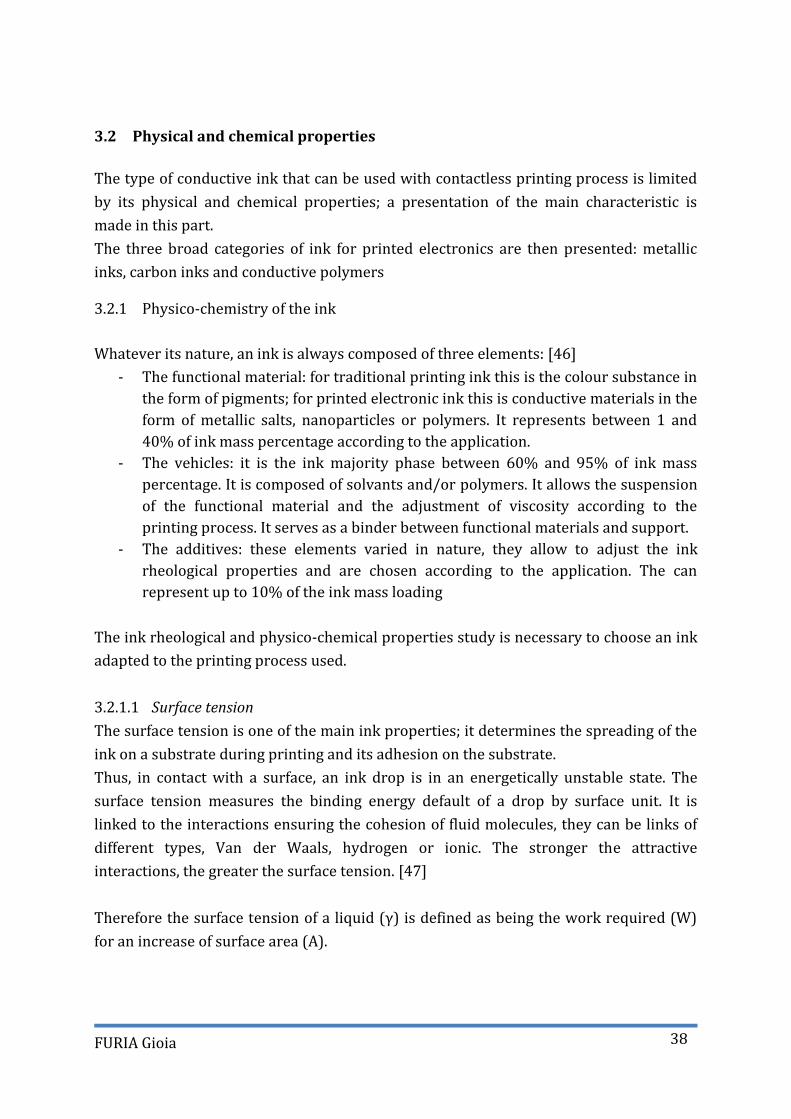
Surface tension 3.2.1.1
The surface tension is one of the main ink properties; it determines the spreading of the
ink on a substrate during printing and its adhesion on the substrate.
Thus, in contact with a surface, an ink drop is in an energetically unstable state. The
surface tension measures the binding energy default of a drop by surface unit. It is
linked to the interactions ensuring the cohesion of fluid molecules, they can be links of
different types, Van der Waals, hydrogen or ionic. The stronger the attractive
interactions, the greater the surface tension. [47]
Therefore the surface tension of a liquid (γ) is defined as being the work required (W)
for an increase of surface area (A).

FURIA Gioia
39
It is expressed by γ = 𝛿𝑊
𝑑𝐴 (1)
with γ (N.m-1) the surface tension
W (N.m) the provided work
A (m²) the surface area
The measure of contact angle (θ) between a deposited drop and a substrate allows the
prediction of the spread of the fluid on the substrate. As illustrated in Figure 15, several
cases can be distinguished
- θ = 0 : the substrate is completely wet
- θ<90°C : the substrate is hydrophilic
- 90°C <θ<150° : the substrate is hydrophobic
- 150°C<θ : the substrate is super hydrophobic
Figure 15: Drop spreading on a substrate
Colloidal stability 3.2.1.2
Inks are composed of suspensions of particles, pigments or nanoparticles and must be
stable in order to be printed.
Suspensions of particles smaller than one micrometre in size, which is the case for inks
based on nanosilver particles for printed electronics, are known as colloidal
suspensions.
However because of Brownian motion between particles, a colloidal suspension is never
in equilibrium, as the particles tend to aggregate or sediment. It is therefore essential to
stabilize these inks to allow their use.
The stabilization of nanoparticles depends on the interactions between the particles and
the solvent and the attractions of the particles to each other, linked to the Van der Waals
interactions.
These interactions result from the presence of different electrical polarizations between
the solid particles and the liquid phase. The intensity of the attraction linked to the Van
der Waals interactions varies proportionally to the difference of polarity between the
phases and inversely proportional to the distance between particles.[48]

FURIA Gioia
40
Thus Van der Waals’ interaction between two colloidal spheres in solution is defined by
the equation:
VVdW= − 𝐻𝑅
12𝑑 (2)
with H (J) Hamaker constant of the system
R (m) particles radius
D (m) distance between particles
In order to stabilize a colloidal suspension, the particles must therefore be kept at
distance. There are three types of stabilization: electrostatic, steric and electrosteric.
Electrostatic stabilization
Electrostatic stabilization is based on the electrostatic repulsion of particles of same
charge. In the case of suspensions based on metallic nanoparticles, ions are adsorbed on
the surface of the particles and create an electric field that causes the particles to repel
each other and stabilize the suspension.
This stabilization requires a polar solvent in order to solvate the ions, the grater the
ionic strength of the solvent, the more free charges in solution and the better the
stabilization.
Steric stabilization
Steric stabilization is based on the steric hindrance of molecules adsorbed on the
particles surface. This stabilization is used in the case of suspensions in which the
solvent has a low ionic strength, the solvent must in this case swell the adsorbed
molecules to allow total coverage of the particles.
Electrosteric stabilization
Electrosteric stabilization is a combination of the two previous types of stabilization. In
this case the macromolecules surrounding the particles are themselves charged and the
stabilization is done by steric and static repulsion. The solvent must have a polar
character and allow the solvatation of the macromolecules.
Rheological behaviour of the ink 3.2.2
The rheological analysis of an ink consists in studying its deformation under shear
stress. A fluid can be modelled as a stack of layers that slide relative to each other, which
creates a shear stress at the interface between each layer. Viscosity (η) quantifies the
flow resistance of a fluid. [49]

FURIA Gioia
41
It relates stress (τ) to shear rate (γ) by the equation: η = 𝜏
𝛾 (3)
with η (Pa.s) viscosity
γ (s-1) shear rate
τ (Pa) shear stress
In the case of Newtonian fluids such as water or oil, the constraint is proportional to the
shear rate, viscosity is thus constant.
In the case of non-Newtonian fluids, viscosity is not constant; it depends of the shear
rate. If viscosity decreases when shear rate increase, the fluid is said to be
rheofluidifying and if viscosity increases when shear rate increases, the fluid is said to be
rheothickening.
Finally some fluids are said to be threshold fluids, in this case the flow only takes place if
a sufficiently high stress is applied.
The most commonly observed law of behaviour for threshold fluids is the Hershel-
Bulkley law:
τ = τ0 + Kγn (4)
with τ (Pa) shear stress
τ0 (Pa) threshold constraint
K fluid constant
γ (s-1) shear rate
n flow index
As illustrated in Figure 16when n=1 this law becomes the Bingham law and K plastic
viscosity.
Figure 16: Rheological behaviour of fluids without critical stress (a) and with critical
stress (b)
In the case of the suspensions, the rheological behaviour is more complex to model, it
depends of parameters such as the volume fraction of the particles in suspension, their

FURIA Gioia
42
size and the nature of the interactions between particles.
For very dilute suspensions of spherical particles in a Newtonian fluid, Einstein’s law
expresses viscosity as a function of the volume fraction of solid particles according to the
equation:
ηrel = ηsusp
ηf = 1+2,5 ϕ (5)
with ηrel (Pa.s) relative viscosity
ηsusp (Pa.s) suspension viscosity
ηf (Pa.s) viscosity of suspending fluid
ϕ volume fraction of spherical particles
This relation takes into account the effect of Brownian motion due to the agitation of the
solid particles suspended in the fluid phase.
Numerous works have allowed to propose empirical laws in the case of suspensions
more concentrated in solid particles in Newtonian fluids.
The Kreiger-Douherty model provides an estimation of viscosity according to the
following equation: ηsusp
ηf = (1-
𝜙
𝜙𝑚) -2,5 ϕm (6)
with ηsusp (Pa.s) suspension viscosity
ηf (Pa.s) viscosity of the suspending fluid
ϕ volume fraction of spherical particles
ϕm theoretical maximum volume fraction of the particles
Works have been conducted in the case of non-Newtonian suspensions but currently no
theoretical model can predict their rheological behaviour.
Conductive property of printed tracks 3.2.3
Resistivity and conductivity 3.2.3.1
Electrical resistivity characterizes the ability of a material to conduct an electrical
current. A low resistivity means that the material allows electrical charges to pass
through.
Resistivity is defined as the inverse of conductivity:
ρ = 1
𝑐 (7)

FURIA Gioia
43
with ρ (Ω.m) electrical resistivity
c (Ω.m)-1 or (S.m-1 ) conductivity
The resistance of a straight piece of material is defined as:
R = ρ 𝐿
𝑆 (8)
with R (Ω) resistance
ρ (Ω.m) electrical resistivity
L (m) piece length
S (m2) straight section area
Quality index 3.2.3.2
In the case of RFID circuits, the performance of the inductive loop is characterized by the
quality index (Q) proportional to the ratio of inductance and antenna resistance such as:
𝑄 = 2𝜋. 𝑓.𝐿
𝑅 (9)
with Q (without unit) quality index
f (Hz) frequency
L (H) inductance
R (Ω) resistance
Metallic inks 3.2.4
Metallic inks are formulated from metal; the choice of metal is done according to the
required electrical performances, its stability and its cost.
As illustrated in Figure 17, it exists four categories of metallic inks: micro nanoparticles
based ink, inks based on metal salts, catalytic inks and inks causing redox reaction. [43]

FURIA Gioia
44
Figure 17: Different types of metallic inks [43]
Micro/nanoparticles inks 3.2.4.1
Micro or nanoparticles inks are composed of particles of the order of ten micrometres in
size. These inks are essentially used with traditional printing process and are not
compatible with ink-jet process but can be used with other direct printing technique
such as filament extrusion.
The works conducted by Tricot et al. [50] have resulted in conductivities of the order of
3.106 S.m-1 for an ink based on silver microparticles printed with a worm screw pump
system on thermoplastic substrates PC and ABS.
The advantages of these inks are their low cost and the ability to be printed on rough
substrates. However, their main limitation is a high deposition thickness compared to
the other conductive inks.
The nanoparticles based inks are the most widespread and are the object of numerous
studies because they have a high potential for ink-jet printing and allow patterns with a
good level of electrical conductivity. The most widely used inks are silver nanoparticles
inks since they have good conductive properties. Studies have been conducted on the
use of cheaper conductive metals such as coper or aluminium, but these are not usable
because they oxidise quickly at ambient air.
The works conducted by Cauchois et al. [51] have shown hat above a certain size the
melting temperature of the metal decreases sharply, which is an advantage for this type
of ink; indeed for these inks a lower annealing temperature could be used and therefore

FURIA Gioia
45
it allows the use of a wider range of substrate.
Recently, Albrecht et al. [52] compared conductive properties of silver nanoparticles
inks printed by ink-jet and pulsed light annealing on nine paper substrates and ten
polymer films. Conductivity between 10 and 40.106 S.m-1 have been obtained.
The main limitation of nanoparticles based inks is their formulation complexity due to
the addition of stabilizer to prevent nanoparticle aggregation and stabilize the colloidal
suspension.
Inks based on metal salts (Metallo Organic Decomposition MOD) 3.2.4.2
MOD inks are composed of metal salts in high concentration dissolved in organic or
aqueous solvents. After printing, an annealing step causes the salts to decompose into
conductive metal. The most commonly used salt is a silver complex, which gives
conductivities close to those of mass silver.
Studies have been carried out by Wu et al. [53] on the formulation of metallic salts
allowing annealing at a lower temperature of about 100°C.
Valeton et al. [54] studied the room temperature UV annealing of a silver salt ink and
obtained conductivities of 6,3.106 S.m-1.
Catalytic inks 3.2.4.3
The working principle of a catalytic ink is to use a reducing agent to convert metal ions
into metal. Palladium is the most commonly used catalyst because it allows a very fast
reaction. Works have been done by Byeon et Roberts [55] on the use of cheaper
catalysts, so by using silver as catalyst they obtained a conductivity of 12,7.106 S.m-1 .
Inks causing a redox reaction 3.2.4.4
Jet-ink printing systems with two ink droplet generation channels have been developed
to separately eject a metal ions solution and a reducing agent solution. When two drops
contact the substrate, a metal film is formed as a result of a redox reaction. The works of
Kao et al. [56] has shown that the reaction takes place within seconds and results in
films with conductivities of 8. 106 S.m-1.

FURIA Gioia
46
Carbon based ink 3.2.5
Carbon based ink were the first conductive ink to be developed. Their conductivity is
relatively low, so research is focusing on inks based on different forms of carbon
particles illustrated in Figure 18, graphite, graphene, carbon nanotubes and fullerenes.
Figure 18: Carbon molecular structure [57]
Carbon nanotubes (CNT) are cylindrical forms of carbon, they allow to reach theoretical
conductivity value close to those of metals, but after implementation in the fabrication of
a conductive ink, the maximum measured values are around 10.102 S.m-1.
CNTs are used in the manufacture of transparent electrodes, transistors for RFID chips
and sensors. [58]
The graphene discovered more recently is a hexagonal monoplanar structure and has a
high potential due to its intrinsic conductivity close to the best metals. The average
measured conductivity is around 30.102 S.m-1 but some studies have obtained
conductivities of 25.103 S.m-1. The applications are similar to those of CNT. [59], [60]
Graphite is a material of lower cost composed of stack of graphene sheets. In battery
anodes, it is used as active material and is added of carbon black nanoparticles to
increase conductivity. [61]

FURIA Gioia
47
Conductive polymers 3.2.6
Currently some conductive polymers offer a good compromise between speed of
chemical synthesis, cost and conductive properties.
PEDOT:PSS is the most widely used as it has a high conductivity of up to 14.104 S.m-1,
polyaniline (PAni) and polypyrrole (PPy) are also used. Their chemical formulations are
presented in Figure 19.
Conductive polymers are used for applications such as batteries, OLED (Organic Light-
Emitting Diode) displays and organic solar cells.
Figure 19: Chemical formulations of conductive polymers from [62]
In summary, a comparison of the electrical conductivities of the different types of
metallic ink presented in Table 2 shows that inks based on silver micro or nanoparticles
are the most efficient.

FURIA Gioia
48
Type of inks Conductivity Applications
Micro /Nanoparticles
based inks
31 106 S.m-1
(Kamyshny et al. 2005)
Sensors
RFID
NFC
Inks based on metal salts 6 106 S.m-1
(Valeton et al. 2009)
Catalytic inks 12 106 S.m-1
(Byeon et Roberts 2012)
Redox inks 8 106 S.m-1
(Kao et al. 2011)
CNT 10 102 S.m-1
(Loiseau et al. 2006)
Electrodes
Transistors for RFID
Chips
Sensors
Graphene 25 103 S.m-1
(Castro Neto et al.)
PEDOT:PSS 14 104 S.m-1
(Kim et al. 2011)
OLED,
Organic solar cells
PAni 3,67 102 S.m-1
(Xu et al. 2014)
PPy 22 102 S.m-1
(Feng et al. 2014)
Table 2: Characteristics of various types of inks
Substrates used in electronic printing 3.3
The substrate is the final key element in the printing process and its properties have a
major influence on the print quality.
The most commonly used substrates in the field of printed electronics today are plastic
substrates.
Substrates characteristics 3.3.1
Several characteristics are to be taken into account in the choice of substrate.
Roughness 3.3.1.1
The surface of a part is never perfectly smooth; it depends on the manufacturing
process, the tools used to manufacture the parts and the material.
The set of micro geometrical defects of the surface defines the roughness, which can be

FURIA Gioia
49
determined by measuring different parameters illustrated in Figure 20.
The arithmetic mean deviation Ra is the most widely used indicator of roughness, it is
defined as the arithmetic mean of the deviations from the mean line and is expressed in
µm.
The roughness of the substrate influences the definition of the printing and must be
adapted to the printing height and therefore influences the choice of printing system.
Figure 20: Roughness definition criteria
Porosity 3.3.1.2
The porosity is a numerical value expressed between 0 and 1 equal to the ratio between
the void volume and the total volume of the substrate.
It has a direct impact on the penetration of the ink into the substrate.
Surface energy 3.3.1.3
Surface energy is the force that exists at the interface between two different substrates.
In order to achieve good ink spread and adhesion between the ink and the substrate, the
surface tension of the ink must be lower than the surface energy of the substrate.
Thermal stability 3.3.1.4
The thermal stability of the substrate, i.e. its resistance to temperature, is an important
criterion for optimising the annealing step required after printing conductive inks to
achieve optimum electrical properties.
Finally, the cost and the renewable or recyclable aspect of a support are also to be taken
into account in the choice of substrate material and quality according to the desired
application.

FURIA Gioia
50
Substrates studied in literature 3.3.2
Studies are currently focusing on increasingly complex substrates and flexible media for
printed electronics; in particular on plastic substrates such as Polyethylene
Terephthalate (PET), Polyethylene Naphthalate (PEN) and Polyamide (PI). Plastic
substrates have good surface properties with roughnesses of a few nanometres; some
plastics also achieve optical properties equivalent to those of glass.[63]
Paper is an interesting medium with many advantages such as low cost and, depending
on the type of paper, resistance to temperatures of around 200°C. However, it is still
little used because of its surface properties, it is indeed a rough support with a high
porosity. Recent studies have led to the development of papers suitable for electronic
printing.[64]–[67]
In their works Ihalainen et al. [68] study the physical properties of different papers and
analyse their effects on the print quality and electrical performance of printed patterns.
They obtained conductivities equivalent to the results obtained on plastic films and
printed a transistor prototype.
There are also research topics on substrates such as glass, textiles or ceramics. The
characteristics of the various substrates studied in literature are summarized in Table 3.
Substrate Roughness
(nm)
Sintering
Temp (°C)
Surface
energy
(mJ.m-2)
Transparent References
Glass 1 600 50-70 Yes Chou et al 2009
Ceramic 200 1500 30-60 No Faddoul 2012
PET 3 70 44 Yes MacDonald et al.
2014 PEN 5 120 40 Yes
PI 1,5 270 47 Yes
PW Paper 10 000 140 No Harting et al. 2009
PowerCoat 30 200 36 No Thenot et al. 2014
Photo Paper 10 150 40 No Kawahara et al. 2013
Filter Paper 20 000 140 No Anderson et al. 2012
Table 3: Substrate characteristics
In almost all works, 2D planer substrates are used, but in this thesis the objective are

FURIA Gioia
51
both print on 3D objects based on recyclable materials, therefore the support used for
this thesis is molded cellulose; it is presented in the following paragraph.
Molded cellulose 3.3.3
Molded cellulose is made from recycled fibres, mainly from cardboard boxes,
newspapers and water. Depending on the application, additives can be added in order to
obtain particular characteristics in terms of strength, impermeability or colouring.
Molded cellulose manufacturing process is divided into four steps:
Pulping
Cellulose pulp is prepared by suspending recycled fibres previously washed in water,
this is the pulping operation.
Molding
The cellulose pulp is then moulded, resulting in a fibrous mat with the shape of the
mould.
Two molding technologies exist in industry:
a flat process, in which a perforated mould is dipped into the liquid paste, under the
effect of suction, the fibres are deposited on the mould while the water drains out
through the holes. A fibrous mat of the shape of the mould is obtained which is
transferred to a conveyor.
a rotary process, in this case the moulds are placed on a multi-sided drum, which is
rotated in the dough. A suction system draws the dough into the moulds, and when they
come out of the preparation a counter-mould comes to press the objects.
Pressing
The formed object is then pressed; this step aims to stabilize the object dimensionally in
order to ensure accurate dimensions and a good surface finish.
Drying
The object is then dried. Drying can be done either directly in the mould, it is done by
increasing the temperature and pressure of the mould. Either by one or more passages
in a tunnel, the barely pressed objects are placed on a conveyor belt and taken to an
oven.
Moulded cellulose is nowadays the subject of numerous patents and finds applications in

FURIA Gioia
52
many sectors.
In the food sector, the egg carton is still the first application of moulded cellulose, but it
is increasingly finding its way into the market for trays, cup holders and fruit trays as
well as in the horticultural sector for plant pots and buckets.
In recent years, we have seen the emergence of innovative applications such as wine
bottles [69], water bottles [70] or beer bottles [71] in molded cellulose.
In the medical sector moulded cellulose is increasingly competing with plastic on
products such as medical beans.
Finally, the use of moulded cellulose is also progressing in the packaging and industrial
cushioning sector. It is used in particular for the transport of electronic products,
measuring devices, hygiene products and for shoe boxes.
Micro Fibrillated cellulose (MFC) 3.3.4
In order to print electronic circuits with a fine resolution, to obtain thin and
homogeneous lines and therefor reach good conductivities, a smooth substrate surface
with a low roughness is require which is often a problem with cellulosic substrates.
Recently, microfibrillated cellulose have been used to obtain substrates with good
surface quality, surface roughness of 300 nm have been obtained. [72]
Microfibrillated cellulose are obtained after a fibrillation process of cellulose fibres and
are made of crystalline and amorphous parts. MFC can be produced from a wide range of
cellulose such as wood, annual plants and vegetables.
MFC have applications in numerous fields thanks to its mechanical and barrier
properties.
Researches on MFC substrate for printed electronics have been conducted for the
fabrication of RFID devices, electronic papers, cellulose-based batteries and substrates
for biosensors. [73], [74]
Annealing types 3.4
Annealing is the next step after printing and is essential to obtain good conductive
properties of the printed pattern, especially in the case of printing with metallic inks.
This step consists of raising the temperature of the ink to a few hundred degrees in
order to lead to the coalescence of the particles between them and guarantee good
conductivity, but also to eliminate encapsulants, organic molecules present in the
composition of the ink to obtain good printability.
In order not to deform the printing substrate, the temperature reached is limited by the
glass transition temperature of the latter, however if the temperature is too low the

FURIA Gioia
53
electrical characteristics of the printed pattern will be limited.
To obtain good conductivity properties, one solution is to choose a substrate resistant to
high temperatures, but the choice of substrate is often guided by its price, and the
cheapest substrates often have a lower glass transition temperature.
In general, the sintering temperature is between 50% and 80% of the melting
temperature of the metal, but for nanoparticles it is reduced to between 20% and 30%
of the melting temperature. [75] A second line of study to solve the temperature limit
problem caused by the carrier material may be to reduce the size of the ink particles to
allow low temperature annealing. However, reducing the particle size results in an
increase of the amount of organic molecules that must then be removed.
Finally, alternative annealing methods have been investigated that allow the ink to be
selectively heated.[76] The temperature of the substrate is then limited and the
annealing time reduced
Thermal annealing 3.4.1
Thermal annealing is the most commonly used annealing technique. It consists of
heating the printed pattern in a hot air oven or tunnel at sintering temperatures often
above 200°C.
These high temperatures limit the use of certain potentially interesting polymer
substrates and paper supports. Polyimide is one of the few substrates resistant to these
temperatures but its cost remains high.
In addition, thermal annealing requires at least 1 hour to achieve good ink conductivity,
which limits its use on industrial production lines.
Chemical annealing 3.4.2
Chemical annealing involves adding a substance to the ink to transform the non-
conductive particles into their conductive equivalents.
In the case of chemical annealing of nanoparticles, the addition of a sintering agent to
the ink causes destabilization of the metal particles by dissolving the organic molecules
present in the ink.
Wakuda et al. [77] have studied the dissolution of dodecyclamine molecules of a silver
nanoparticle-based ink by dipping in different alcohols for up to 2 hours. They showed
that dodecyclamine molecules dissolve rapidly in alcohol and obtained a conductivity
1,4.105 S.m-1 for a 2-hour soak in methanol.

FURIA Gioia
54
Magdassi et al. [78] have developed an approach that involves depositing an additional
layer of cationic polymers on a silver ink composed of polyacrylic acid encapsulant to
initiate coalescence. These tests resulted in conductivities of 106 S.m-1 for conductive
patterns printed on photo paper.
In the continuation of these works, Grouchko et al. [79] developed an integrated
chemical annealing process, starting as soon as the ink dries and obtained excellent
conductivities of the order of 26.106 S.m-1.
Laboratory tests were carried out by Layani et al. [80] with this annealing for the
manufacture of electroluminescent devices as a first step towards industrial
applications.
Finally, Allen et al. [81] proposed a chemical annealing approach with silanol groups in a
humid environment and obtained conductivities of 1.106 S.m-1. This approach is
interesting because silicate or alumina-based varnishes are often used in paper printing
to accelerate drying.
This method is still the subject of numerous studies in order to understand its
mechanisms.
Electrical annealing 3.4.3
Electrical annealing is a fast operation that lasts only a few seconds and is called rapid
electrical annealing (RES). As illustrated in Figure 21(A), it is based on the application of
a direct current directly to the printed pattern and therefore causes localized heating.
An initial drying in the open air or in an oven allows the solvents to evaporate and to
control the initial resistance of the printed pattern which will have to remain high
enough to induce heating.
Figure 21: Electrical annealing direct current (A) and alternating current (B) [82], [83]
Allen et al. [82] et Hummelgard et al. [84] have studied the annealing of silver
nanoparticles and shown that it is carried out in two phases. The first phase, lasting a

FURIA Gioia
55
few milliseconds, corresponds to the carbonization of the encapsulant and the
contacting of the nanoparticles, and is characterized by a rapid drop in resistivity. Then
during the second phase, the resistivity continues to drop for several seconds, due to the
improved contact between the nanoparticles. This results in a homogeneous electrical
pattern.
Alstato et al. [85] have shown that the activation of coalescence in the first phase enables
temperatures of 250°C to be reached for silver nanoparticle inks while the photo paper
supporting the pattern does not exceed 60°C.
Allen et al. [82] have compared electrical and thermal annealing for a silver nanoparticle
ink and have shown that a one-minute electrical annealing allows to reach conductivities
of 15 à 30.106 S.m-1, whereas a 20-minute thermal annealing at 120°C allows to reach
conductivities of 3.105 S.m-1.
Likewise Roberson et al. [86] studied microparticle-based inks and obtained
conductivities twice as high with a one-minute electrical anneal than with a thermal
oven anneal.
However, a major disadvantage of this technique is the inhomogeneous annealing in the
case of short lines, very long lines or lines with variable thicknesses. This annealing also
results in poor ink adhesion to the substrate compared to standard oven annealing.
Finally, one of the limitations of electrical annealing for industrial applications is that it
requires contact with the pattern to be annealed.
To overcome these problems, Allen et al.[83] studied the use of alternating current
instead of direct current. As illustrated in Figure 21(B), this technique consists in placing
at 1 mm from the pattern to be annealed a coaxial electrical module capable of creating
an electromagnetic field, which thus generates an electrical current in the printed
pattern and leads to heating of the ink by Joule effect. The results obtained show that a
homogeneous annealing is obtained; some parameters still need to be optimised to
improve the performance of this annealing but it offers an interesting industrial
solution.
Plasma annealing 3.4.4
Plasma annealing consists of placing the printed pattern in the environment of an
ionized gas. The interaction between the ink and the ions excited in the plasma as well
as the generation of ultraviolet radiation causes the ink to be annealed.
One of the criteria is to use a plasma with a low temperature to avoid deformation of the
substrate.

FURIA Gioia
56
Reinhold et al. [87] studied annealing of nanoparticles silver inks in a low-pressure
argon plasma and obtained conductivities of 1.106 S.m-1. Wolf et al. [88] showed its
application for annealing RFID antennas printed with an ink based on silver
nanoparticles and obtained conductivities of 15.106 S.m-1.
However, annealing in low pressure argon plasma requires a few tens of minutes and
modifies the surface wettability of the substrate which prevents a subsequent printing
step. Moreover, at low pressure, the ions penetrate the ink only slightly, which leads to
an inhomogeneous annealing.
Microwave annealing 3.4.5
Microwave annealing involves exposing the printed pattern to microwaves. This
requires that the material absorbs these microwaves. Ma et al. [89] showed that
although pure materials reflect waves, small particles absorb waves well. In addition, the
polymers most commonly used as substrates are transparent to microwaves, thus
allowing selective annealing of inks.
Microwave annealing is a fast process but the penetration of microwaves into the main
conductive materials is very low, which limits the thickness of the deposited ink to 1 to 2
µm in order to have a homogeneous annealing.
Subsequently Perelaer et al. [90] proposed a two-step method with pre-treatment by
pulsed light, which makes it possible to obtain conductivities of the order of 3.106 S.m-1
in less than 15 secondes.
Microwave annealing in particular, coupled with photonic annealing, has made it
possible to obtain very good results in very short times of the order of a few seconds,
which makes it interesting for industrial applications. However, the non-uniformity of
the annealing due to small variations in ink thickness remains a constraint and limits for
the moment microwave annealing to small-scale applications.
Photonic annealing 3.4.6
Photonic annealing consists of irradiating the conductive ink with electromagnetic
radiation ranging from ultraviolet to infrared. In the case of metallic inks, as the
absorption characteristics of the metals used in conductive inks are far from those of the
main substrates, the use of selected radiation allows selective annealing of the
conductive inks.
Different types of radiation can be used, such as infrared annealing, pulsed light
annealing or laser annealing.

FURIA Gioia
57
Infrared annealing 3.4.6.1
In the case of infrared annealing of metallic inks, the most commonly used wavelength
ranges are near infrared (NIR) and medium infrared (MIR).
Early work using infrared lamps for annealing printed tracks was carried out by
Deunnelin et al. [91]. The results showed that IR drying at wavelengths between 8 and
15 µm for 2 minutes achieved the same performance as oven drying at 200° for 5
minutes for tracks printed in inkjet with nanosilver-based inks on paper and glass
substrates. This method speeds up the annealing process but does not allow selective
heating of the ink as the glass and paper substrates have reached 180°C and 210°C
respectively.
A more selective approach put forward by Cherrington et al. [92] is to work in NIR at
wavelengths between 0.7 and 4 µm because plastic substrates absorb little in this
wavelength range, whereas the absorption of metallic inks is very high.
Tobjörk et al. [93] have carried out annealing tests with IR lamps with an emission peak
at 4µm of gold and silver nanoparticle-based inks on paper and glass substrates. They
reached conductivities of the order of 4.106 S.m-1 in a only a few seconds.
IR annealing is a fast method, allowing to obtain good conductivities and applicable on
industrial production lines. One of the main limitations of IR annealing is the choice of
substrate, as it can only be used with substrates having good temperature resistance. It
appears to be well suited for paper substrates.
Laser annealing 3.4.6.2
Laser annealing of metallic inks consists of exposing the printed tracks to a laser beam.
The wavelength is adapted to correspond to the maximum absorption of the ink. The ink
particles absorb the laser radiation, the ink film heats up, which leads to annealing. The
temperature rise of the ink must be controlled and kept as low as possible to avoid heat
dissipation in the substrate. Argon lasers are the most commonly used lasers, they can
work at wavelengths between 488 nm and 515 nm and achieve a rapid rise in ink
temperature. Temperatures of 500 °C have been reached on substrates such as glass or
PI. The very rapid temperature rise during annealing allows good conductivity to be
achieved in very short periods of time, but too rapid evaporation of organic compounds
leads to rough surfaces and inhomogeneous annealing.
The use of pulsed lasers allows a high energy density to be transferred to the ink while
reducing heat dissipation to the substrate [94], [95], [96]. The works of Kupulainen et al.
[97] focused on the optimization of conductivities as a function of annealing time.
However, this technique remains complex to implement.
In order to improve the understanding of laser annealing, Maekawa et al. [95] studied
the influence of wavelength on annealing by conducting tests at wavelengths outside the
absorption maxima of silver nanoparticle-based ink. They showed that the use of lasers

FURIA Gioia
58
with high wavelengths allows fast surface annealing but leads to inhomogeneous
annealing and poor ink adhesion to the substrate.
Laser annealing is a fast and flexible method since it allows the wavelength to be
adjusted to the substrate. However, it remains expensive and complex to implement on
industrial production lines.
Intense Pulsed Light annealing (IPL) 3.4.6.3
Intense pulsed light annealing is a thermal annealing technique that uses the heat
generated by the absorption of visible light in the material to raise the temperature.
The most commonly used light source for IPL annealing is Xenon light, which emits
radiation between 200 nm and 1200 nm, covering the entire visible spectrum.
A lot of work has been done on IPL technology in order to better understand its process
and better control the different parameters. Indeed, each substrate ink system has its
own optimal parameters, which requires optimization work at each material change.
Theoretical models have been proposed in order to predict the experimental conditions
as accurately as possible. [98],[99],[100].
Annealing by IPL has many advantages, such as good energy efficiency, high selectivity,
fast annealing and the possibility to work in ambient air, and is promising for industrial
production lines.
Various annealing method characteristics are summarized in Table 4. The easiest
method is thermal annealing but it is not compatible with industrial application thanks
to its long duration time.

FURIA Gioia
59
Annealing
method Implementation Duration Homogeneity
Selecti
vity Substrate
Thermal Easy 30-60 min good no
not compatible with
plastic substrates
not resistant to high
temperatures
Chemical
Phenomenon
still poorly
understood
variable variable no Plastic
substrates
Electrical
Medium
Requires contact
Requires poorly
conductive print
few ms medium yes Plastic
substrates
Plasma Difficult few s good no Plastic substrate
Microwave Easy few ms poor yes All substrates
Photonic Easy few ms poor yes All substrates
Table 4: Annealing method characteristics
In conclusion, the printing quality of electronic tracks depends on the adequacy between
the different parameters studied in this paragraph: the printing process, the ink, the
substrate and the annealing.
The following paragraph presents a state of the art of academic research and industrial
developments on the manufacturing of connected 3D objects.

FURIA Gioia
60
CONNECTED OR FUNCTIONAL OBJECT 4
Two 3D connected objects manufacturing technics and their applications will be
presented in this paragraph: Molded Interconnected Devices (MID) and additive
manufacturing of 3D functionalized objects. In the last part the development of robotic
for 3D printing will be discussed.
Molded Interconnect Devices (MID) 4.1
MID manufacturing is born in the United States in the 1980’s and appears as promising
thanks to its technologic, economic and environmental advantages. It has been the
subject of various research studies in particular in Japan and Germany in order to allow
its industrial development.
This technology aims to provide functionality to 3D molded thermoplastic pieces by
integrating electronic circuits with a direct process.
The main Plastronic markets are automotive, telecommunication and medical. Big
industries like Siemens, Volkswagen, BMW and Schneider electric have already
integrated MID in their products. [101]
Fabrication process 4.1.1
MID fabrication is divided in several steps. In a first step the 3D piece is manufactured
with a molding by injection process. Melted granules of thermoplastic are injected in a
mold then cooled. It’s a classic process for the manufacturing of thermoplastic parts in
large series.
There then follow the steps of circuits structuration and metallization, that can be done
with various process.
Laser direct structuring (LDS) 4.1.1.1
The main used process for the structuration of electronic tracks is laser direct
structuring. This process has been developed at the University of Lemgo in Germany in
cooperation with the society LPKF Laser & Electronics and a patent was deposited in
2002. [102]
The parts are manufactured in single layout molds and with thermoplastic specifically
charged. They are then subjected to a laser beam to define the tracks layout by
activating the additive directly on the part and to a selective metallization in a copper

FURIA Gioia
61
bath.
The main advantages of this technic are a high flexibility in the design of parts and the
possibility to use a large range of plastic material such as ABS PC (Acrylonitrile
Butadiene Styrene Poly Carbonate), PBT (Poly Butilene Terephtalate) and PEEK
(PolyEther Ether Ketone).
Laser subtractive structuring (LSS) 4.1.1.2
Laser subtractive structuring process is also largely used in MID manufacturing. In this
process, the part is first chemically activated and covered with a metallic layer, then a
laser beam defines the conductive tracks by eliminating the non useful area.
This method requires several steps and is therefore more expensive but unlike LDS
technology it doesn’t requires plastic specifically charged.
Microstamping 4.1.1.3
Microstamping or soft lithography is also used in specific applications where high
definition is not required. Although less accurate than laser process, this technology has
the advantages of being rapid and economic.
It has been developed in 1993 by Whitesides and Kumar [103] and consists in
depositing ink on a substrate by mechanic contact of an inked stamp.
Bi-injection 4.1.1.4
Bi-injection is to make two successive casts of two different thermoplastic materials for
the manufacturing of one part.
This process is expensive and complex, mainly used in telecommunication sector for the
production of large series. It allows to obtain dimensional tolerances lower than 400 µm
and it is thus used for the manufacturing of complex 3D objects.
Studies have been done on the development of software tools for the design of parts to
be producted by bi-injection. [104]
Inkjet 4.1.1.5
Recently research works have been done on the use of ink-jet for the printing of circuits
directly on the surface of 3D objects.
Ink-jet technology presents the advantages of being simple, economic and without
producing waste. One of the limits is the use of a substrate with low surface roughness
in order to obtain good electronic tracks conductivity.
Studies have been conducted by Van Osch at al. [105] and Kao et al.[56], [106] on tracks
dimension, conductivity and on the development of surface treatment in order to allow
their use on a larger variety of substrates.

FURIA Gioia
62
Research project examples 4.1.2
Electronic field 4.1.2.1
The research works of Paulsen et al. [107] and Hörber et al. [108] have shown the
potential of MID in association with direct printing technics such as aerosol. They have
printed sensors and electronic tracks on a polyamide 6 (PA6) thermoplastic substrate
molded in reservoir shape, with a silver ink. Sensors measure the level of water
introduce in the reservoir, a LED turn on when the maximum level is reached and the
pump is reversed.
Another example of research works that use aerosol is the integration of a thermometer
on a polyamide 10TX substrate.
Industrial application examples 4.1.3
MID have a great industrial potential in particular in the field of medical equipment’s,
automotive, electronics and in the telecommunications.
Medical field 4.1.3.1
Siemens Audiologishe Technik GmbH has developed a hearing aid using MID technology
which allows to reduce pieces assembly time. [109]
The company 2E Mechatronic has manufactured by LDS high performance and energy
efficient lighting elements by using LED in particular for the dental field.
Automotive field 4.1.3.2
MID are the subjects of numerous developments in the automotive field.
Volkswagen has designed a multi-function car wheel by replacing electrical wiring by
printed tracks.
BMW has integrated plastronic parts in its wheel and has developed plastronic
motorbike handles illustrated in Figure 22. This elements regroups numerous
functionalities, klaxon, starter and flashing lights that requires the welding of a lot o
wires connecting the buttons and the electronic card. The use of MID technology has
allowed to integrate all the components in the plastic part and to eliminate the wires to
weld.
Mercedes Benz has also used this technology for the manufacturing of car keys in one
piece.
Bosch has developed pressure sensor in plastronic, the use of this technology has
allowed to reduce significantly the parts volume.

FURIA Gioia
63
Finally, the society Harting has designed a distance sensor with LDS, this sensor is used
cruise control. [110]
Figure 22: Plastronic motorcycle handles and steering wheel BMW
Telecommunication field 4.1.3.3
MID technology is also used for the mobile phone because it allows to reduce the
number of components.
The society Molex has commercialised a small terrestrial antenna working at 2,4 GHz.
This antenna manufactured by LDS weighs 0,03g ad can be used without connexion
wires. This type of antenna is used in portable electronic devices for the Bluetooth and
Wi-Fi functions. [111]
Additive manufacturing of 2D multilayer functional devices 4.2
Paper microfluidic 4.2.1
Research in microfluidic has seen a strong emulation in recent years particularly for
point of care medical diagnostics for developing countries.
Paper has become a widely use substrate in microfluidic in particular because it is an
inexpensive material and can be easily burnt or recycled.
Paper is used to realise test strip such as pregnancy test or pH for alimentary or
environmental control but another field called “Lab on Paper” is growing strongly.
Unlike test strip, fluid only flows between barriers that define a microfluidic channel.
[112]–[114].
This domain characterized by the manipulation of systems with a sub-millimetric
characteristic dimension and requires numerous manufacturing steps to obtain
functionalities such as :

FURIA Gioia
64
- Microfluidic circuit
- Detection which may require pick and place of components
- Conductive parts like resistance in order to heat the fluid to be analysed or
electrodes to perform electrochemical measurements
- Surface treatment to functionalize a part of a system or to selectively protect
areas
These steps are not trivial and require sophisticated phases, precision in manufacturing
and expert operators in order to correctly integrate all the functionalities in the system.
It also has an impact on the manufacturing cost, which is problematic particularly if the
objective is to produce low-cost devices; hence, the need to find an optimized and
automatic manufacturing process.
Only a few companies like Fluidigm have been able to build reliable fabrication
processes and with huge investments. [115]
Therefor microfluidic devices produced by 3D printing have been developed since
additive manufacturing allows to shorten prototyping step, to personalize devices,
accelerate R&D and decrease costs. This process is still limited for small series
production. [116]–[118]
Papertouch 4.2.2
Paper Touch a LGP2 spin-off aims to market a new interactive paper. The process
consists in integrating printed electronics circuits during paper fabrication in order to
obtain a classically looking paper with electronics inside. Demonstrators such as a tactile
paper numerical keypad consisting of a matrix of electrodes has been developed but also
connected printed antennas capable of reacting to the approach of a smartphone
equipped with NFC technology; the energy of this signal is then sufficient to light up
LEDs or transmit data. [119], [120]
Figure 23: Papertouch tactile flower

FURIA Gioia
65
The process has been developed thanks to printing head adapted on 3D printers and
manual pick and place. The start-up is currently looking to optimize process speed and
precision and to industrialize the production of small series.
Robotic printing solutions are being considered in order to be able to offer a
PaperTouch production process in-house, so that once the printer is convinced of the
market, a robotic module could be installed on the production line.
Additive manufacturing of 3D functional objects 4.3
Multimaterials objects additive manufacturing process 4.3.1
Additive manufacturing regroups all the process that allows to manufacture by adding
material an object from a numerical model. First essentially dedicated to prototyping,
additive manufacturing is undergoing a strong growth in particular for the
manufacturing of complex parts or small series. [121]
Three main additive manufacturing exist, photo-polymerisation, material deposit and
powder bed.
Material deposit 4.3.1.1
This technic gathers the process that enables the manufacturing of pieces by material
deposit; it can be metallic projection, liquid polymer projection or fused deposition
modelling (FDM). FDM process is the most widespread in the domestic and industrial
fields.
Generally, this is machines with 3 translations axis, that have an horizontal plate and
nozzles based above the plate. The mobility is done either by the plate or by the nozzles.
One or several nozzles deposit a material strand, when the first layer is completed, the
plate move away from a few tenths of millimetre from the nozzles (or counterwise) and
the deposit process start again as illustrated in Figure 24(A).
The material is in the form of solid wire of polymer in the case of FDM, in the form of
metallic powder or ceramic in the case of CLAD process (construction laser additive
direct) or in the form of liquid polymer in the case of Polyjet illustrated in Figure 24(B)
These technics enable the manufacturing of a wide diversity of parts more or less
complex; in the case of hollow parts it is necessary to print a support that will be
removed once the piece will be printed.

FURIA Gioia
66
Figure 24: Operating principle additive manufacturing by molten yarn deposition (A)
and Polyjet process (B)
Photopolymerisation 4.3.1.2
The main used photopolymerisation process and the first that have been used in
industry is stereolithography (SLA). This process consists in the polymerization of a
liquid resin under the acton of radiation.
The machine is composed of a tank filled with resin inside which is an horizontal plate
which move vertically. A laser source sends a beam and under radiation the resin
polymerizes at the point of impact as illustrated in Figure 25. At the end of each layer the
plate moves down in order to allow the polymerization of a new material layer. Once the
piece is completed, a cleaning phase enables the elimination of the non-polymerized
resin.
The materials that can be used are limited to the light-curing resins.
Studies have been conducted by Leigh et al. [122] and have enable the integration of
metallic particles in the resin in order to make it conductive.
Figure 25: Operating principle of the stereolithography process

FURIA Gioia
67
Manufacturing on powder bed 4.3.1.3
This technic includes the processes of selective laser sintering (SLS) and selective laser
melting (SLM).
The machines are composed with a first tank containing the material under the form of
powder and a second container where the part will be manufactured. An horizontal roll
allows to decant powder layers from a plate to the other one and a mobile nozzle, that
move above the second plate, sends a laser beam that locally heats up the material as
illustrated in Figure 26. At the end of each layer, the container with the powder moves
one step up and the one containing the part moves one step down. At the end of the
process the unaggregated powder is removed to recover the piece.
The material is a metallic powder in the case of SLM and ceramic or polymer in the case
of SLS.
Figure 26: Operating principle of the powder bed manufacturing process
However all these technics are more or less compatible with the manufacturing of multi-
material parts that imposes constraints on the type of materials to print and on the
distribution of materials in the piece [123], [124]. This thematic is the object of
numerous works in order to manufacture parts with different mechanic and physical
properties and the possibilities continue to grow.
Industrial application examples 4.3.2
The market of functionalized 3D printing is today essentially dominated by small
enterprise and start-up.
The alliance of 3D printing and printed electronic has a high potential particularly in the

FURIA Gioia
68
medical field for the printing of medical equipment’s smart and personalized.
Voxel8 4.3.2.1
The first 3D printer that enables the printing of electronic circuits has been
commercialized by the company Voxel8 in 2015 at the cost of 9000$ [125].
The printer used a FDM technology, the parts are manufactured from PLA polymer and
silver conductive ink; electronic components can be added during the printing process.
Voxel8 announces to have obtained circuits conductivities are 2.106 S.m-1, which is
higher than the conductivity obtained with conductive filaments available on the
market.
The printer is sold with the Autodesk Project Wire 3D software, which allows to monitor
the whole manufacturing steps, piece design creation, the deposit of components and
the drawing of electronic tracks.
Some examples of realisation illustrated in Figure 27 can be cited :[126]
- a quadcopter whith a body in thermoplastic and an electronic circuit integrated
inside
- 3D RFID antenna with complex shapes, in collaboration with a research
laboratory on the antenna (MITRE) in order to develop high performance and
low cost antenna
-
This printer is today essentially dedicated to R&D applications.
Figure 27: Voxel8 printer and its main applications
Nano Dimension 4.3.2.2
The company NanoDimension, direct competitor of Voxel8, commercializes the 3D
DragonFly 2020 printer. It allows to print electronic tracks with jet-ink process and
boards with dielectric polymer ink. The society sold also a software dedicated to the
drawing of conductive tracks and develops its own conductive inks with silver
nanoparticles.
The printer allows to print lines with a 100 µm width with 125 µm spaces between lines

FURIA Gioia
69
and a minimum layer thickness of 3 µm.
They do also research works on conductive inks with nickel. [127]
Some examples of application illustrated in Figure 28 can be cited:
- a Arduino card prototype
- electronic components, sensors, resistances and capacitors
Figure 28: NanoDimension printer and its main applications
Optomec-Stratasys 4.3.2.3
In 2012, the companies Optomec specialized in direct printing solutions for electronic
printing and Stratasys specialised in 3D printer, have join forces to create an hybrid
printing system allowing to print electronic tracks directly on 3D printed objects. The
electronic printing technology used is based on an aerosol system and FDM technology
for the object manufacturing.
They also work on antennas, capacitors and resistors.
Robotic for 3D printing 4.4
The potential of additive manufacturing of functionalized multi-materials objects is
huge, its main limits are the dimension of the objects to print, the printing of several
materials and the possibility to print on curved surfaces.
Research project examples 4.4.1
To be able to find a solution for the problematic of printing on curved surfaces, the

FURIA Gioia
70
professor Chen from the California University has worked on a new concept of 3D
printer on which the nozzle has 6 degrees of freedom[128].
Thereafter, studies have been conducted on the use of 6-axis robots for the additive
manufacturing in particular in the architecture and aeronautic fields but few
publications have been done.
+Lab –Milan Polytechnic University 4.4.1.1
In 2014, the laboratories of 3D printing and chemistry from the Milan Polytechnic
University have started to develop a new continuous manufacturing process inspired
from the silk worms’ behaviour for the manufacturing of objects in composite with glass
fibbers. To this end, they use a Kuka 6-axis robot called Atropos illustrated in Figure 29.
These works results in 2016 in a patent.
The printing process is divided in several steps, the first step consists to draw the object
in the Rhinoceros 3D software, in a second step the robot printing path is generated in
the algorithm editor Grasshopper and KUKA lprc. Atropos is then able to print the
composite along the toolpath, in the same time a UV source induces the photocuring of
the composite.
Atropos has won in 2017 the JEC Composite Innovation award for 3D printing.
Works are in progress to optimise process, increase printing speed and to develop new
resins and annealing methods.
Figure 29: Atropos robot
BatiPrint3D-Nantes 4.4.1.2
The research teams from the laboratory LS2N (Laboratoire des Sciences du Numérique
de Nantes) et GeM (Instit de Recherche en Génie Civil et Mécanique) in collaboration
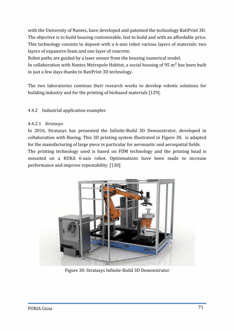
FURIA Gioia
71
with the University of Nantes, have developed and patented the technology BatiPrint 3D.
The objective is to build housing customizable, fast to build and with an affordable price.
This technology consists to deposit with a 6-axis robot various layers of materials: two
layers of expansive foam and one layer of concrete.
Robot paths are guided by a laser sensor from the housing numerical model.
In collaboration with Nantes Metropole Habitat, a social housing of 95 m² has been built
in just a few days thanks to BatiPrint 3D technology.
The two laboratories continue their research works to develop robotic solutions for
building industry and for the printing of biobased materials [129].
Industrial application examples 4.4.2
Stratasys 4.4.2.1
In 2016, Stratasys has presented the Infinite-Build 3D Demonstrator, developed in
collaboration with Boeing. This 3D printing system illustrated in Figure 30, is adapted
for the manufacturing of large piece in particular for aeronautic and aerospatial fields.
The printing technology used is based on FDM technology and the printing head is
mounted on a KUKA 6-axis robot. Optimisations have been made to increase
performance and improve repeatability. [130]
Figure 30: Stratasys Infinite-Build 3D Demonstrator

FURIA Gioia
72
Drawn 4.4.2.2
The start-up Drawn provides a 3D printing service for furniture and large dimensions
decorative objects. The manufacturing of furniture is done with FDM technology; the
designers have mounted an extrusion printing head on an industrial 6-axis robot named
Galatea. The company has developed their own furniture product range and also works
in collaboration with designers for the production of small series. [131]
In the medical field, two companies provide robotic printing cells for the printing of
tissue structures.
Poietis 4.4.2.3
Poietis is a spin-off from INSERM and University of Bordeaux. AS illustrated in Figure 31,
they have developed the Next-Generation Bioprinting (NGB) platform based on their
expertise in high resolution Laser Assisted Bioprinting. They provide a printing cell with
a Stäubli 6-axis robot and equipped with micro-valves, extrusion printing head, a
microscope and a laser. It offers the possibility to print with a large range of
biomaterials and hydrogels.
The cell is supported with dedicated software that enables the management of the full
bioprinting protocol from tissue design to manufacturing. [132]
Figure 31: Poietis robotic cell

FURIA Gioia
73
Bioassemblybot 4.4.2.4
The company Advanced Solutions Life Sciences has developed a 6-axis robotic printing
cell called Bioassemby Bot illustrated in Figure 32. They incorporated modular heads on
an Epson robotic arm.
The cell is equipped with a camera, a temperature control system and modular printing
head that can be loaded with up to ten materials for one printing run.
A dedicated software called Tissue Structure information Modeling (TSIM) has been
developed to control the printing process and automatically generate robotic code.
They reached to print tissue structures with a resolution of 20 µm in a 300 mm by 250
mm by 150 mm build volume. [133]
Figure 32: Bioassemblybot robotic cell

FURIA Gioia
74
CONCLUSION 5
There is a growing demand for prototyping processes in the fields of electronics and
connected objects to simplify and automate the process of integrating electronic
components into 3D objects.
In order to offer a versatile and easy to implement alternative for prototyping and small
series, printed electronics is widely considered.
However, today no easy to use system is available on the market for 3D electronic
printing.
The challenge of this thesis is to develop a new process for prototyping 3D electronic
objects that can be adapted to paper materials and that allows :
- to integrate electronic functions directly on the surface of the object without the
systematic transfer of conventional 2D electronic board.
- to replace electrical wires between components
The main lock to be studied is the adequacy between the required manufacturing
process accuracy and flexibility and the tool developed and the expectations of the
market.

FURIA Gioia
75
BIBLIOGRAPHY 6
[1] C. Dumas, « Development of methods for metal and composite parts trimming with a robot », Theses, Université de Nantes, 2011.
[2] A. Poyet, « Contrôle redondant de la position d’un robot par capteurs externes. Applications en milieux médical et industriel », Theses, Institut National Polytechnique de Grenoble - INPG, 1996.
[3] S. Campocasso, V. Hugel, et B. Vayre, « Génération de trajectoires pour la fabrication additive par dépôt de fil robotisé multi-axes - Application à une tubulure torique », in 15ème Colloque national AIP-Primeca, La Plagne, France, avr. 2017, p. 1‑5, Consulté le: août 27, 2018. [En ligne]. Disponible sur: https://hal.archives-ouvertes.fr/hal-01517799.
[4] A. Olabi, « Improving the accuracy of industrial robots for high speed machining applications », Theses, Arts et Métiers ParisTech, 2011.
[5] A. Klimchik, A. Ambiehl, S. Garnier, B. Furet, et A. Pashkevich, « Efficiency evaluation of robots in machining applications using industrial performance measure », Robot. Comput.-Integr. Manuf., vol. 48, p. 12–29, 2017.
[6] M. A. S. Arikan et T. Balkan, « Process Simulation and Paint Thickness Measurement for Robotic Spray Painting », CIRP Ann., vol. 50, no 1, p. 291‑294, janv. 2001, doi: 10.1016/S0007-8506(07)62124-6.
[7] P. Neto et N. Mendes, « Direct off-line robot programming via a common CAD package », Robot. Auton. Syst., vol. 61, no 8, p. 896‑910, août 2013, doi: 10.1016/j.robot.2013.02.005.
[8] C. Tournier, « Contribution to the design of free-form surfaces<br />the machining surface in 5-axis iso scallop machining », Theses, École normale supérieure de Cachan - ENS Cachan, 2001.
[9] A. Buschhaus, M. Wagner, et J. Franke, « Inline calibration method for robot supported process tasks with high accuracy requirements », in 2017 IEEE International Conference on Advanced Intelligent Mechatronics (AIM), juill. 2017, p. 682‑687, doi: 10.1109/AIM.2017.8014096.
[10] S. Larsson et J. A. P. Kjellander, « Motion control and data capturing for laser scanning with an industrial robot », Robot. Auton. Syst., vol. 54, no 6, p. 453‑460, juin 2006, doi: 10.1016/j.robot.2006.02.002.
[11] T. Várady, R. R. Martin, et J. Cox, « Reverse engineering of geometric models—an introduction », Comput.-Aided Des., vol. 29, no 4, p. 255‑268, avr. 1997, doi: 10.1016/S0010-4485(96)00054-1.
[12] S. Larsson et J. a. P. Kjellander, « An Industrial Robot and a Laser Scanner as a Flexible Solution Towards an Automatic System for Reverse Engineering of Unknown Objects », nov. 2008, p. 341‑350, doi: 10.1115/ESDA2004-58277.
[13] D. Redinger, S. Molesa, S. Yin, R. Farschi, et V. Subramanian, « An ink-jet-deposited passive component process for RFID », IEEE Trans. Electron Devices, vol. 51, no 12, p. 1978‑1983, déc. 2004, doi: 10.1109/TED.2004.838451.
[14] V. Subramanian et al., « Printed electronics for low-cost electronic systems: Technology status and application development », in ESSCIRC 2008 - 34th European Solid-State Circuits Conference, sept. 2008, p. 17‑24, doi: 10.1109/ESSCIRC.2008.4681785.
[15] J. Ledesma-Fernandez, C. Tuck, et R. Hague, « HIGH VISCOSITY JETTING OF CONDUCTIVE AND DIELECTRIC PASTES FOR PRINTED ELECTRONICS », p. 16.

FURIA Gioia
76
[16] J. Viviari, « Auger Valve Dispensing », p. 5. [17] J. Francois, « Sensors and issues for automatic bed leveling and height
adjustment ». http://www.tridimake.com/2015/12/bed-leveling-tramming-sensors.html (consulté le sept. 09, 2020).
[18] Z. Roth, B. Mooring, et B. Ravani, « An overview of robot calibration », IEEE J. Robot. Autom., vol. 3, no 5, p. 377‑385, oct. 1987, doi: 10.1109/JRA.1987.1087124.
[19] N. Juneja et A. A. Goldenberg, « Kinematic calibration of a re-configurable robot (RoboTwin) », in Proceedings of International Conference on Robotics and Automation, avr. 1997, vol. 4, p. 3178‑3183 vol.4, doi: 10.1109/ROBOT.1997.606772.
[20] S. Besnard, W. Khalil, et G. Garcia, « Geometric calibration of robots using multiple plane constraints », in Advances in robot kinematics, Springer, 2000, p. 61–70.
[21] W. Khalil et S. Besnard, « Geometric calibration of robots with flexible joints and links », J. Intell. Robot. Syst., vol. 34, no 4, p. 357–379, 2002.
[22] H. Hage, « Identification et simulation physique d’un robot Stäubli TX90 pour le fraisage à grande vitesse », phdthesis, Université Pierre et Marie Curie - Paris VI, 2012.
[23] W. Khalil et E. Dombre, Modeling, Identification and Control of Robots. Butterworth-Heinemann, 2004.
[24] K. Vacharanukul et S. Mekid, « In-process dimensional inspection sensors », Measurement, vol. 38, no 3, p. 204‑218, oct. 2005, doi: 10.1016/j.measurement.2005.07.009.
[25] L. Dubreuil, « Mesure In-situ par moyens optiques », Paris Saclay, 2017. [26] M. Ritou, « Spindle instrumentation for tool condition monitoring of complex
workpiece manufacturing in milling », Theses, Université de Nantes ; Ecole Centrale de Nantes (ECN), 2006.
[27] F. Poulhaon, A. Leygue, M. Rauch, J.-Y. Hascoet, et F. Chinesta, « Simulation-based adaptative toolpath generation in milling processes », Int. J. Mach. Mach. Mater., vol. 15, no 3‑4, p. 263‑284, janv. 2014, doi: 10.1504/IJMMM.2014.060552.
[28] H. H. Shahabi et M. M. Ratnam, « Simulation and measurement of surface roughness via grey scale image of tool in finish turning », Precis. Eng., vol. 43, p. 146‑153, janv. 2016, doi: 10.1016/j.precisioneng.2015.07.004.
[29] T. J. Ko, J. W. Park, H. S. Kim, et S. H. Kim, « On-machine measurement using a noncontact sensor based on a CAD model », Int. J. Adv. Manuf. Technol., vol. 32, no 7‑8, p. 739‑746, avr. 2007, doi: 10.1007/s00170-005-0383-4.
[30] M. Mani, B. Lane, A. Donmez, S. Feng, S. Moylan, et R. Fesperman, « Measurement Science Needs for Real-time Control of Additive Manufacturing Powder Bed Fusion Processes », National Institute of Standards and Technology, NIST IR 8036, févr. 2015. doi: 10.6028/NIST.IR.8036.
[31] T. G. Spears et S. A. Gold, « In-process sensing in selective laser melting (SLM) additive manufacturing », Integrating Mater. Manuf. Innov., vol. 5, no 1, p. 2, déc. 2016, doi: 10.1186/s40192-016-0045-4.
[32] M. Grasso et B. M. Colosimo, « Process defects and in situ monitoring methods in metal powder bed fusion: a review », Meas. Sci. Technol., vol. 28, no 4, p. 044005, 2017, doi: 10.1088/1361-6501/aa5c4f.
[33] G. Tapia et A. Elwany, « A Review on Process Monitoring and Control in Metal-Based Additive Manufacturing », J. Manuf. Sci. Eng., vol. 136, no 6, p. 060801-060801‑10, oct. 2014, doi: 10.1115/1.4028540.
[34] S. K. Everton, M. Hirsch, P. Stravroulakis, R. K. Leach, et A. T. Clare, « Review of in-

FURIA Gioia
77
situ process monitoring and in-situ metrology for metal additive manufacturing », Mater. Des., vol. 95, p. 431‑445, avr. 2016, doi: 10.1016/j.matdes.2016.01.099.
[35] P. M. Sammons, D. A. Bristow, et R. G. Landers, « Height Dependent Laser Metal Deposition Process Modeling », J. Manuf. Sci. Eng., vol. 135, no 5, p. 054501-054501‑7, sept. 2013, doi: 10.1115/1.4025061.
[36] J. Benda, « Temperature controlled selective laser sintering », in Proceedings of the Solid Freeform Fabrication Symposium, 1994, vol. 5, p. 277–284.
[37] M. Chung et A.-L. Allanic, « Sintering using thermal image feedback », nov. 2004. [38] T. M. Chung et J. P. Partanen, « Continuous calibration of a non-contact thermal
sensor for laser sintering », août 2005. [39] A. Pique et D. B. Chrisey, Direct-Write Technologies for Rapid Prototyping
Applications: Sensors, Electronics, and Integrated Power Sources. Elsevier, 2001. [40] K. K. B. Hon, L. Li, et I. M. Hutchings, « Direct writing technology—Advances and
developments », CIRP Ann., vol. 57, no 2, p. 601‑620, janv. 2008, doi: 10.1016/j.cirp.2008.09.006.
[41] Y. Zhang, C. Liu, et D. Whalley, « Direct-write techniques for maskless production of microelectronics: A review of current state-of-the-art technologies », in 2009 International Conference on Electronic Packaging Technology High Density Packaging, août 2009, p. 497‑503, doi: 10.1109/ICEPT.2009.5270702.
[42] B. Derby, « Inkjet Printing of Functional and Structural Materials: Fluid Property Requirements, Feature Stability, and Resolution », Annu. Rev. Mater. Res., vol. 40, no 1, p. 395‑414, 2010, doi: 10.1146/annurev-matsci-070909-104502.
[43] S.-P. Chen, H.-L. Chiu, P.-H. Wang, et Y.-C. Liao, « Inkjet printed conductive tracks for printed electronics », ECS J. Solid State Sci. Technol., vol. 4, no 4, p. P3026–P3033, 2015.
[44] « Archimed pumps ». Consulté le: sept. 09, 2020. [En ligne]. Disponible sur: https://webmail.grenoble-inp.fr/service/home/~/?auth=co&loc=fr&id=355&part=3.
[45] « 3D Bioprinters you need to know. | Five Bioprinters on the Market. » https://www.biogelx.com/3d-bioprinters-you-need-to-know/ (consulté le sept. 09, 2020).
[46] A. BLAYO, « Formulation des encres pour l’impression ». Ed. Techniques Ingénieur, 2007.
[47] P.-G. de Gennes et F. Brochard-Wyart, Gouttes, bulles, perles et ondes. Humensis, 2015.
[48] J.-M. D. MEGLIO, « Colloïdes et nanosciences », p. 15, 2007. [49] H. A. Barnes, J. F. Hutton, et K. Walters, An Introduction to Rheology. Elsevier,
1989. [50] F. Tricot et al., « Fabrication of 3D conductive circuits: print quality evaluation of
a direct ink writing process », RSC Adv., vol. 8, no 46, p. 26036‑26046, 2018, doi: 10.1039/C8RA03380C.
[51] R. CAUCHOIS, M. SAADAOUI, et K. INAL, « Impression et recuit de nanoparticules métalliques pour l’électronique imprimée », Ref : TIP155WEB - « Nanosciences et nanotechnologies », janv. 10, 2014. /base-documentaire/innovation-th10/nanotechnologies-pour-l-electronique-l-optique-et-la-photonique-42198210/impression-et-recuit-de-nanoparticules-metalliques-pour-l-electronique-imprimee-re222/ (consulté le juill. 24, 2018).
[52] A. Albrecht, A. Rivadeneyra, A. Abdellah, P. Lugli, et J. F. Salmerón, « Inkjet

FURIA Gioia
78
printing and photonic sintering of silver and copper oxide nanoparticles for ultra-low-cost conductive patterns », J. Mater. Chem. C, vol. 4, no 16, p. 3546‑3554, 2016, doi: 10.1039/C6TC00628K.
[53] J.-T. Wu, S. L.-C. Hsu, M.-H. Tsai, et W.-S. Hwang, « Inkjet printing of low-temperature cured silver patterns by using AgNO3/1-dimethylamino-2-propanol inks on polymer substrates », J. Phys. Chem. C, vol. 115, no 22, p. 10940–10945, 2011.
[54] J. J. Valeton et al., « Room temperature preparation of conductive silver features using spin-coating and inkjet printing », J. Mater. Chem., vol. 20, no 3, p. 543–546, 2010.
[55] J. H. Byeon et J. T. Roberts, « Silver deposition on a polymer substrate catalyzed by singly charged monodisperse copper nanoparticles », ACS Appl. Mater. Interfaces, vol. 4, no 5, p. 2515–2520, 2012.
[56] Z.-K. Kao, Y.-H. Hung, et Y.-C. Liao, « Formation of conductive silver films via inkjet reaction system », J. Mater. Chem., vol. 21, no 46, p. 18799‑18803, 2011, doi: 10.1039/C1JM13506F.
[57] « Raman Spectroscopy of Graphene », AZoM.com, oct. 11, 2013. https://www.azom.com/article.aspx?ArticleID=10130 (consulté le août 21, 2018).
[58] A. Loiseau, P. Launois, P. Petit, S. Roche, et J.-P. Salvetat, Understanding carbon nanotubes, vol. 677. 2006.
[59] A. H. Castro Neto, F. Guinea, N. M. R. Peres, K. S. Novoselov, et A. K. Geim, « The electronic properties of graphene », Rev. Mod. Phys., vol. 81, no 1, p. 109‑162, janv. 2009, doi: 10.1103/RevModPhys.81.109.
[60] A. K. Geim et K. S. Novoselov, « The rise of graphene », Nat. Mater., vol. 6, no 3, p. 183‑191, mars 2007, doi: 10.1038/nmat1849.
[61] D. Beneventi et al., « Pilot-scale elaboration of graphite/microfibrillated cellulose anodes for Li-ion batteries by spray deposition on a forming paper sheet », Chem. Eng. J., vol. 243, p. 372‑379, mai 2014, doi: 10.1016/j.cej.2013.12.034.
[62] V. Faure, « Controle of conducting partern formation by inkjet printing : Multi-scale control of material transfert in nanometric suspensions », Theses, Université Grenoble Alpes, 2017.
[63] W. A. MacDonald et al., « Latest advances in substrates for flexible electronics », J. Soc. Inf. Disp., vol. 15, no 12, p. 1075‑1083, doi: 10.1889/1.2825093.
[64] P. Andersson et al., « Active Matrix Displays Based on All-Organic Electrochemical Smart Pixels Printed on Paper », Adv. Mater., vol. 14, no 20, p. 1460‑1464, 2002, doi: 10.1002/1521-4095(20021016)14:20<1460::AID-ADMA1460>3.0.CO;2-S.
[65] R. Bollström et al., « A multilayer coated fiber-based substrate suitable for printed functionality », Org. Electron., vol. 10, no 5, p. 1020–1023, 2009.
[66] D. Tobjörk et R. Österbacka, « Paper Electronics », Adv. Mater., vol. 23, no 17, p. 1935‑1961, doi: 10.1002/adma.201004692.
[67] V. Thenot, « Impression et recuits sélectifs d’encres métalliques sur papier–Optimisation des propriétés électriques de boucles RFID-HF en vue d’une production industrielle », PhD Thesis, Grenoble Alpes, 2017.
[68] P. Ihalainen, A. Määttänen, J. Järnström, D. Tobjörk, R. Österbacka, et J. Peltonen, « Influence of Surface Properties of Coated Papers on Printed Electronics », Ind. Eng. Chem. Res., vol. 51, no 17, p. 6025‑6036, mai 2012, doi: 10.1021/ie202807v.
[69] « MarcelGreen.com ». http://www.marcelgreen.com/article/Paperboy-les-bouteilles-de-vin-en-carton-3690#.W1mYydIzbtR (consulté le juill. 26, 2018).

FURIA Gioia
79
[70] « Green Fiber Bottle – ecoXpac ». http://www.ecoxpac.dk/green-fiber-bottle/ (consulté le juill. 26, 2018).
[71] « Newsroom » Carlsberg and Partners to Develop Biogradable Wood-Fiber Bottle « Carlsberg Group », Carlsberg Group. https://carlsberggroup.com/newsroom/carlsberg-and-partners-to-develop-biogradable-wood-fiber-bottle/ (consulté le juill. 26, 2018).
[72] K. Shanmugam, H. Nadeem, C. Browne, G. Garnier, et W. Batchelor, « Engineering surface roughness of nanocellulose film via spraying to produce smooth substrates », Colloids Surf. Physicochem. Eng. Asp., vol. 589, p. 124396, févr. 2020, doi: 10.1016/j.colsurfa.2019.124396.
[73] C. Salas, T. Nypelö, C. Rodriguez-Abreu, C. Carrillo, et O. J. Rojas, « Nanocellulose properties and applications in colloids and interfaces », Curr. Opin. Colloid Interface Sci., vol. 19, no 5, p. 383‑396, oct. 2014, doi: 10.1016/j.cocis.2014.10.003.
[74] Y. Neuvo et S. Ylönen, « Bit Bang Rays to the Future », p. 286. [75] J. R. Groza, « Nanosintering », Nanostructured Mater., vol. 12, no 5, p. 987‑992,
janv. 1999, doi: 10.1016/S0965-9773(99)00284-6. [76] S. Wünscher, R. Abbel, J. Perelaer, et U. S. Schubert, « Progress of alternative
sintering approaches of inkjet-printed metal inks and their application for manufacturing of flexible electronic devices », J. Mater. Chem. C, vol. 2, no 48, p. 10232‑10261, 2014, doi: 10.1039/C4TC01820F.
[77] D. Wakuda, M. Hatamura, et K. Suganuma, « Novel method for room temperature sintering of Ag nanoparticle paste in air », Chem. Phys. Lett., vol. 441, no 4, p. 305‑308, juin 2007, doi: 10.1016/j.cplett.2007.05.033.
[78] S. Magdassi, M. Grouchko, O. Berezin, et A. Kamyshny, « Triggering the sintering of silver nanoparticles at room temperature », ACS Nano, vol. 4, no 4, p. 1943–1948, 2010.
[79] M. Grouchko, A. Kamyshny, C. F. Mihailescu, D. F. Anghel, et S. Magdassi, « Conductive inks with a “built-in” mechanism that enables sintering at room temperature », ACS Nano, vol. 5, no 4, p. 3354–3359, 2011.
[80] M. Layani, M. Grouchko, S. Shemesh, et S. Magdassi, « Conductive patterns on plastic substrates by sequential inkjet printing of silver nanoparticles and electrolyte sintering solutions », J. Mater. Chem., vol. 22, no 29, p. 14349–14352, 2012.
[81] M. Allen, J. Leppäniemi, M. Vilkman, A. Alastalo, et T. Mattila, « Substrate-facilitated nanoparticle sintering and component interconnection procedure », Nanotechnology, vol. 21, no 47, p. 475204, 2010.
[82] M. L. Allen et al., « Electrical sintering of nanoparticle structures », Nanotechnology, vol. 19, no 17, p. 175201, 2008.
[83] M. Allen, A. Alastalo, M. Suhonen, T. Mattila, J. Leppaniemi, et H. Seppa, « Contactless electrical sintering of silver nanoparticles on flexible substrates », IEEE Trans. Microw. Theory Tech., vol. 59, no 5, p. 1419–1429, 2011.
[84] M. Hummelg\a ard, R. Zhang, H.-E. Nilsson, et H. akan Olin, « Electrical sintering of silver nanoparticle ink studied by in-situ TEM probing », PLoS One, vol. 6, no 2, p. e17209, 2011.
[85] A. T. Alastalo, H. Seppä, J. H. Leppäniemi, M. J. Aronniemi, M. L. Allen, et T. Mattila, « Modelling of nanoparticle sintering under electrical boundary conditions », J. Phys. Appl. Phys., vol. 43, no 48, p. 485501, 2010, doi: 10.1088/0022-3727/43/48/485501.

FURIA Gioia
80
[86] D. A. Roberson, R. B. Wicker, et E. MacDonald, « Ohmic Curing of Printed Silver Conductive Traces », J. Electron. Mater., vol. 41, no 9, p. 2553‑2566, sept. 2012, doi: 10.1007/s11664-012-2140-4.
[87] I. Reinhold et al., « Argon plasma sintering of inkjet printed silver tracks on polymer substrates », J. Mater. Chem., vol. 19, no 21, p. 3384–3388, 2009.
[88] F. M. Wolf, J. Perelaer, S. Stumpf, D. Bollen, F. Kriebel, et U. S. Schubert, « Rapid low-pressure plasma sintering of inkjet-printed silver nanoparticles for RFID antennas », J. Mater. Res., vol. 28, no 9, p. 1254‑1261, mai 2013, doi: 10.1557/jmr.2013.73.
[89] J. Ma et al., « Systematic study of microwave absorption, heating, and microstructure evolution of porous copper powder metal compacts », J. Appl. Phys., vol. 101, no 7, p. 074906, 2007.
[90] J. Perelaer, R. Abbel, S. Wünscher, R. Jani, T. van Lammeren, et U. S. Schubert, « Roll-to-Roll Compatible Sintering of Inkjet Printed Features by Photonic and Microwave Exposure: From Non-Conductive Ink to 40% Bulk Silver Conductivity in Less Than 15 Seconds », Adv. Mater., vol. 24, no 19, p. 2620‑2625, mai 2012, doi: 10.1002/adma.201104417.
[91] A. Denneulin, A. Blayo, C. Neuman, et J. Bras, « Infra-red assisted sintering of inkjet printed silver tracks on paper substrates », J. Nanoparticle Res., vol. 13, no 9, p. 3815‑3823, sept. 2011, doi: 10.1007/s11051-011-0306-2.
[92] M. Cherrington, T. C. Claypole, D. Deganello, I. Mabbett, T. Watson, et D. Worsley, « Ultrafast near-infrared sintering of a slot-die coated nano-silver conducting ink », J. Mater. Chem., vol. 21, no 21, p. 7562‑7564, 2011, doi: 10.1039/C1JM10630A.
[93] D. Tobjörk et al., « IR-sintering of ink-jet printed metal-nanoparticles on paper », Thin Solid Films, vol. 520, no 7, p. 2949‑2955, janv. 2012, doi: 10.1016/j.tsf.2011.10.017.
[94] R. Lesyuk, W. Jillek, Y. Bobitski, et B. Kotlyarchuk, « Low-energy pulsed laser treatment of silver nanoparticles for interconnects fabrication by ink-jet method », Microelectron. Eng., vol. 88, no 3, p. 318‑321, mars 2011, doi: 10.1016/j.mee.2010.11.037.
[95] K. Maekawa et al., « Drop-on-Demand Laser Sintering With Silver Nanoparticles for Electronics Packaging », IEEE Trans. Compon. Packag. Manuf. Technol., vol. 2, no 5, p. 868‑877, mai 2012, doi: 10.1109/TCPMT.2011.2178606.
[96] P. Peng, A. Hu, et Y. Zhou, « Laser sintering of silver nanoparticle thin films: microstructure and optical properties », Appl. Phys. A, vol. 108, no 3, p. 685‑691, sept. 2012, doi: 10.1007/s00339-012-6951-1.
[97] T. Kumpulainen, J. Pekkanen, J. Valkama, J. Laakso, R. Tuokko, et M. Mäntysalo, « Low temperature nanoparticle sintering with continuous wave and pulse lasers », Opt. Laser Technol., vol. 43, no 3, p. 570‑576, avr. 2011, doi: 10.1016/j.optlastec.2010.08.002.
[98] J. S. Kang, J. Ryu, H. S. Kim, et H. T. Hahn, « Sintering of Inkjet-Printed Silver Nanoparticles at Room Temperature Using Intense Pulsed Light », J. Electron. Mater., vol. 40, no 11, p. 2268, nov. 2011, doi: 10.1007/s11664-011-1711-0.
[99] R. Abbel et al., « Photonic flash sintering of silver nanoparticle inks: a fast and convenient method for the preparation of highly conductive structures on foil », MRS Commun., vol. 2, no 4, p. 145‑150, déc. 2012, doi: 10.1557/mrc.2012.28.
[100] H.-J. Hwang, W.-H. Chung, et H.-S. Kim, « In situ monitoring of flash-light sintering of copper nanoparticle ink for printed electronics », Nanotechnology, vol. 23, no

FURIA Gioia
81
48, p. 485205, 2012, doi: 10.1088/0957-4484/23/48/485205. [101] J. Frank, Three-Dimensional Molded Interconnect Devices (3D-MID). 2014. [102] « LPKF Laser & Electronics ». http://www.lpkfusa.com/ (consulté le août 16,
2018). [103] A. Kumar et G. M. Whitesides, « Features of gold having micrometer to centimeter
dimensions can be formed through a combination of stamping with an elastomeric stamp and an alkanethiol ‘‘ink’’ followed by chemical etching », Appl. Phys. Lett., vol. 63, no 14, p. 2002‑2004, oct. 1993, doi: 10.1063/1.110628.
[104] Y. Zhuo, J. Peng, et Y. J. Wu, « Design and Simulation of Molded Interconnect Devices with Two Shot Molding », in Advanced Materials Research, 2011, vol. 295, p. 1651–1655.
[105] T. H. Van Osch, J. Perelaer, A. W. de Laat, et U. S. Schubert, « Inkjet printing of narrow conductive tracks on untreated polymeric substrates », Adv. Mater., vol. 20, no 2, p. 343–345, 2008.
[106] H. Kao, C.-L. Cho, L.-C. Chang, C.-S. Yeh, B.-W. Wang, et H.-C. Chiu, « Inkjet printing RF bandpass filters on liquid crystal polymer substrates », Thin Solid Films, vol. 544, p. 64–68, 2013.
[107] J. A. Paulsen, M. Renn, K. Christenson, et R. Plourde, « Printing conformal electronics on 3D structures with Aerosol Jet technology », in 2012 Future of Instrumentation International Workshop (FIIW) Proceedings, oct. 2012, p. 1‑4, doi: 10.1109/FIIW.2012.6378343.
[108] J. Hörber, J. Glasschröder, M. Pfeffer, J. Schilp, M. Zaeh, et J. Franke, « Approaches for Additive Manufacturing of 3D Electronic Applications », Procedia CIRP, vol. 17, p. 806‑811, déc. 2014, doi: 10.1016/j.procir.2014.01.090.
[109] « 3-D MID e.V. Forschungsvereinigung Räumliche Elektronische Baugruppen ». https://www.3d-mid.de/cms/front_content.php?idcat=5&display_errorpage=1 (consulté le août 16, 2018).
[110] plombard, « Qu’est-ce qu’un MID ? », Plastronique. http://www.plastronique.com/plastronique/quest-ce-quun-mid/ (consulté le août 28, 2018).
[111] « Molex ». https://www.molex.com/molex/capabilities/capabilities.jsp?key=mid__lds_technology (consulté le août 23, 2018).
[112] T. Akyazi, L. Basabe-Desmonts, et F. Benito-Lopez, « Review on microfluidic paper-based analytical devices towards commercialisation », Anal. Chim. Acta, vol. 1001, p. 1‑17, févr. 2018, doi: 10.1016/j.aca.2017.11.010.
[113] D. M. Cate, J. A. Adkins, J. Mettakoonpitak, et C. S. Henry, « Recent Developments in Paper-Based Microfluidic Devices », nov. 21, 2014. http://pubs.acs.org/doi/abs/10.1021/ac503968p (consulté le sept. 18, 2019).
[114] A. Apilux, W. Dungchai, W. Siangproh, N. Praphairaksit, C. S. Henry, et O. Chailapakul, « Lab-on-Paper with Dual Electrochemical/Colorimetric Detection for Simultaneous Determination of Gold and Iron », Anal. Chem., vol. 82, no 5, p. 1727‑1732, mars 2010, doi: 10.1021/ac9022555.
[115] « Fluidigm | IFCs ». https://www.fluidigm.com/ifcs (consulté le avr. 01, 2020). [116] K. C. Bhargava, B. Thompson, et N. Malmstadt, « Discrete elements for 3D
microfluidics », Proc. Natl. Acad. Sci., vol. 111, no 42, p. 15013‑15018, oct. 2014, doi: 10.1073/pnas.1414764111.
[117] K. G. Lee et al., « 3D printed modules for integrated microfluidic devices », RSC

FURIA Gioia
82
Adv., vol. 4, no 62, p. 32876‑32880, 2014, doi: 10.1039/C4RA05072J. [118] A. K. Au, N. Bhattacharjee, L. F. Horowitz, T. C. Chang, et A. Folch, « 3D-printed
microfluidic automation », Lab. Chip, vol. 15, no 8, p. 1934‑1941, 2015, doi: 10.1039/C5LC00126A.
[119] « PaperTouch, des circuits imprimés dans le papier », CNRS Le journal. https://lejournal.cnrs.fr/nos-blogs/de-la-decouverte-a-linnovation/papertouch-des-circuits-imprimes-dans-le-papier (consulté le avr. 01, 2020).
[120] « PaperTouch, le papier interactif qui révolutionne le packaging ou l’édition », Les Echos, oct. 10, 2019. https://www.lesechos.fr/pme-regions/innovateurs/papertouch-le-papier-interactif-qui-revolutionne-le-packaging-ou-ledition-1138808 (consulté le avr. 01, 2020).
[121] F. Laverne, F. Segonds, et P. Dubois, « Fabrication additive - Principes généraux », p. 20, 2016.
[122] S. J. Leigh, R. J. Bradley, C. P. Purssell, D. R. Billson, et D. A. Hutchins, « A simple, low-cost conductive composite material for 3D printing of electronic sensors », PloS One, vol. 7, no 11, p. e49365, 2012.
[123] P. Muller, « Additive Manufacturing of Functionally Graded Materials (FGM) parts », Theses, Ecole Centrale de Nantes (ECN), 2013.
[124] A. T. Gaynor, N. A. Meisel, C. B. Williams, et J. K. Guest, « Multiple-material topology optimization of compliant mechanisms created via PolyJet three-dimensional printing », J. Manuf. Sci. Eng., vol. 136, no 6, p. 061015, 2014.
[125] « Voxel8 », Voxel8 - Multi Material Footwear Manufacturing. https://www.voxel8.com/ (consulté le août 22, 2018).
[126] « Case Studies », Voxel8. http://store.voxel8.com/case-studies/ (consulté le août 23, 2018).
[127] N. Dimension, « Dragonfly 2020 Pro ». https://www.nano-di.com/dragonfly-2020-pro (consulté le août 23, 2018).
[128] « Innovation : Une imprimante 3D 6 axes pour imprimer sur des surfaces courbes », Semageek, oct. 17, 2013. http://www.semageek.com/innovation-une-imprimante-3d-6-axes-pour-imprimer-sur-des-surfaces-courbes/ (consulté le août 23, 2018).
[129] « Accueil », Yhnova. http://batiprint3d.fr/ (consulté le août 23, 2018). [130] J. Vurpillat, « 3D Demonstrators Designed for Bigger, Lighter Auto and Aerospace
Parts », Stratasys Blog, août 24, 2016. http://blog.stratasys.com/2016/08/24/infinite-build-robotic-composite-3d-demonstrator/ (consulté le août 28, 2018).
[131] « Drawn - Impression 3D grand format - Mobilier et objets déco imprimés », Drawn. //www.drawn.fr/ (consulté le août 23, 2018).
[132] « BIOPRINTERS », Poietis - 4D Bioprinting | Next Generation Bioprinting. https://poietis.com/bioprinters/ (consulté le mars 27, 2020).
[133] « Life Sciences | Leader in Bio Printing & Tissue Fabrication », Advanced Solutions - Life Sciences. https://lifesciences.solutions/ (consulté le mars 27, 2020).
FURIA Gioia
83
TABLE OF FIGURES 7
Figure 3: Architecture 6-axis robot [4] ................................................................................................ 24
Figure 4: Manufacturing process ............................................................................................................ 25
Figure 5 :Parameters that influence process quality [9] ............................................................... 27
Figure 6: Inkjet printing of passive components [14] .................................................................... 28
Figure 7: Sensor and calibration cube [22] ........................................................................................ 29
Figure 8 : Calibration method example [9] ......................................................................................... 30
Figure 9: In-situ measure inspired from [25] .................................................................................... 31
Figure 10 : Different types of direct printing technology ............................................................. 34
Figure 11: Aerosol printing head functional schema [41] ............................................................ 34
Figure 12: CIJ printing head (A), thermal DOD printing head (B) et piezo electric printing head (C) functional schema from [42] ................................................................................................. 35
Figure 13: Jetting printing head schema (A) anf functional cycle (B)[15] ............................. 36
Figure 14: Functional schema of extrusion printing head from [45] ....................................... 37
Figure 15: Drop spreading on a substrate .......................................................................................... 39
Figure 16: Rheological behaviour of fluids without critical stress (a) and with critical stress (b) .......................................................................................................................................................... 41
Figure 17: Different types of metallic inks [43] ............................................................................... 44
Figure 18: Carbon molecular structure [57] ...................................................................................... 46
Figure 19: Chemical formulations of conductive polymers from [62] .................................... 47
Figure 20: Roughness definition criteria ............................................................................................. 49
Figure 21: Electrical annealing direct current (A) and alternating current (B) [82], [83] ............................................................................................................................................................................. 54
Figure 22: Plastronic motorcycle handles and steering wheel BMW ...................................... 63
Figure 23: Papertouch tactile flower .................................................................................................... 64
Figure 24: Operating principle additive manufacturing by molten yarn deposition (A) and Polyjet process (B) .............................................................................................................................. 66
Figure 25: Operating principle of the stereolithography process ............................................. 66
Figure 26: Operating principle of the powder bed manufacturing process .......................... 67
Figure 27: Voxel8 printer and its main applications ...................................................................... 68
Figure 28: NanoDimension printer and its main applications ................................................... 69
Figure 29: Atropos robot ........................................................................................................................... 70
Figure 30: Stratasys Infinite-Build 3D Demonstrator .................................................................... 71
Figure 31: Poietis robotic cell .................................................................................................................. 72
Figure 32: Bioassemblybot robotic cell ............................................................................................... 73

FURIA Gioia
84
TABLE OF TABLES 8
Table 1: Direct printing process comparison .................................................................................... 37 Table 2: Characteristics of various types of inks .............................................................................. 48 Table 3: Substrate characteristics .......................................................................................................... 50 Table 4: Annealing method characteristics ........................................................................................ 59

FURIA Gioia
85

FURIA Gioia
86

FURIA Gioia
87
CHAPTER 2: ROBOTIC CELL AND OFF-LINE PROGRAMMING SOFTWARE DEVELOPMENT

FURIA Gioia
88
TABLE OF CONTENT
1 INTRODUCTION ................................................................................................................................... 90
2 3D SIMULATION AND POST-PROCESSOR SOFTWARE ....................................................... 91
2.1 VAL 3 language ............................................................................................................................. 92
2.1.1 Structure of VAL3 language: application and program. ...................................... 92
2.1.2 Control of movement ........................................................................................................ 92
The succession of points in a frame. ....................................................................... 92 2.1.2.1
The type of trajectory between points. ................................................................. 94 2.1.2.2
The type of junction between trajectory points. ................................................ 94 2.1.2.3
The speed .......................................................................................................................... 95 2.1.2.4
2.2 Presentation of simulation and off-line programming tools ...................................... 95
2.2.1 Stäubli Robotics Suite (SRS) ........................................................................................... 96
2.2.2 Commercial industrial tools ........................................................................................... 96
2.2.3 Rhinoceros 3D plugin ....................................................................................................... 97
2.2.4 Comparative table .............................................................................................................. 98
2.3 Choice of a simulation and off-line programming tool ................................................. 99
3 Generation accuracy of the object in the working environment ....................................101
3.1 Mesh generation methods: bibliography focus .............................................................101
3.1.1 Scanning tools ....................................................................................................................102
Mechanical sensors with contact ...........................................................................102 3.1.1.1
Laser triangulation sensors .....................................................................................102 3.1.1.2
3.1.2 From points cloud to mesh generation ....................................................................104
Mesh generation method ..........................................................................................105 3.1.2.1
Mesh simplification method ....................................................................................106 3.1.2.2
Mesh generation quality ............................................................................................108 3.1.2.3
3.2 Mesh quality evaluation .........................................................................................................109
3.3 Process implementation and characterisation ..............................................................112
3.3.1 Scan step implementation.............................................................................................112
Mounting and calibration .........................................................................................112 3.3.1.1
Scan trajectory definition .........................................................................................113 3.3.1.2
VAL 3 code structure and data sharing ...............................................................115 3.3.1.3
Laser scanner characterisation ..............................................................................116 3.3.1.4
3.3.2 Reverse engineering step implementation ............................................................120

FURIA Gioia
89
Mesh generation and quality measurement ......................................................120 3.3.2.1
Data smoothing: Surface simplification algorithm .........................................124 3.3.2.2
Accuracy and curvature threshold ........................................................................127 3.3.2.3
3.4 Process validation .....................................................................................................................127
3.4.1 Process description .........................................................................................................127
3.4.2 Examples ..............................................................................................................................128
3.5 Criteria validation .....................................................................................................................134
4 3D ELECTRONIC CIRCUITS PRINTING ....................................................................................137
4.1 Electronic circuit printing on 3D objects: bibliography focus .................................137
4.1.1 The CAD model of the part on which the material will be deposited ..........137
4.1.2 The chosen tool .................................................................................................................137
4.1.3 The path pattern ...............................................................................................................138
4.1.4 The process requirements and parameters ...........................................................138
4.2 Required printing quality ......................................................................................................139
4.3 Projection process ....................................................................................................................139
4.4 Printing process .........................................................................................................................142
5 PRINTING ROBOTIC CELL .............................................................................................................143
5.1 Cell requirement ........................................................................................................................143
5.2 Schematic diagram and description ..................................................................................143
5.3 3D Simulation environment and interface description ..............................................145
5.4 Cell criteria validation .............................................................................................................152
6 CONCLUSION ......................................................................................................................................153
7 BIBLIOGRAPHY ..................................................................................................................................154
8 TABLE OF FIGURES ..........................................................................................................................157
9 TABLE OF GRAPHICS ...................................................................... Erreur ! Signet non défini.
10 TABLE OF TABLES ............................................................................................................................158

FURIA Gioia
90
INTRODUCTION 1
This chapter presents the different steps that have been necessary for the design and
assembly of a robotic cell for the prototyping and the production of small series of 3D
connected objects functionalized by electronic printing, pick and place of electronic
components and post-treatment steps. It presents also an off-line programming
approach for drawing conductive paths on 3D objects and automatically generating the
trajectory and printing program for a 6-axis robot.
Conductive path printing allows to integrate electronic functions directly onto the
surface of a pre-existing object without systematically report 2D electronic cards and to
replace connecting wires between components.
All the unit operations are carried out with a 6-axis robot on which the various tools are
mounted, i.e. a laser scanner and various printing heads.
The robotic cell hardware is completed by a software and the associated interface for
the management of the global process and the automatic creation of the robotic
programs. The interface allows the use of the cell by operators without skills in robotic
programming.
This chapter is divided into four parts:
- Section 1, which presents the base of robot language and the choice criteria of a
3D simulation and post-processing tool necessary to develop an off-line
programming approach.
- Section 2, which focuses on the reconstruction accuracy of the object in the
working environment. It deals with reverse engineering and surface
simplification methods.
- Section 3, which discusses about the printing of the 3D electronic circuits
- Section 4, which describes the full robotic cell and the dedicated software
developed in this study.

FURIA Gioia
91
3D SIMULATION AND POST-PROCESSOR SOFTWARE 2
Two approaches are currently used for developing robotic applications:
- On-line programming, which is the most used method and it consists in teaching
manually robot positions point by point and, for a given trajectory, coding on the
robot terminal the sequence of movements. This method allows precise
positioning of the robot and is very useful for simple and cyclic movements.
However, it requires frequent downtimes and skilled operators familiar with
robot programming.
- Off-line programming, where the sequence of movements is coded, tested in a
simulation tool and loaded on the robot controller. Numerous off-line
programming software have been developed by robot manufacturers such as
RobotStudio by ABB , non-manufacturers such as PowerMill by Autodesk or
Delmia by Dassault Systemes and also academics. [1] This programming method
is often used in research and in SME for the production of small series, when
robot programs require to be often changed. This method allows to test a lot of
different configurations and to automate path planning. Depending on the chosen
software, programming can be intuitive and rapid. However, virtual simulation
tools can diverge from the real robot movement and a direct test routine on the
robotic arm is necessary to validate the virtual trajectory and positioning
accuracy and speed.
For this study, an off-line programming approach has been chosen in order to precisely
program complex trajectory, speed set-up of prototypes and also limit the effect of
programming skills gap between operators.
In order to be able to choose the right programming tools, some basic concepts of the
Stäubli VAL 3 language are presented to illustrate the structure of typical robot
programs and the different robot movement control modes provided by the VAL 3
language. Then, a state of the art of some simulation and off-line programming tools
supporting Stäubli robots is presented and discussed in order to explain the choice of an
adequate programming tool that will be used in this study.

FURIA Gioia
92
VAL 3 language 2.1
Structure of VAL3 language: application and program. 2.1.1
A VAL3 application is standalone software which allows controlling the robot and the
input-output ports associated to the controller.
It consists of minimum four files:
- start.pgx file
- stop.pgx file
- .dtx file
- .pjx file
All the other programs (path generation, connection with external sensors…) are written
in additional .pgx files.
A program is a sequence of VAL3 instructions to execute. It allows improving application
readability.
- The start program is called when a VAL3 application is launched. This program is
filled with all the needed operations to execute the application: variables
initialisation, I/O configuration, tasks creation, etc.
- The stop program is called when the application stops. This program is filled with
all the needed operation to properly close the application: I/O reset, tasks
closure, etc.
- The .dtx file lists all variables, I/O, parameters and points.
- The .pjx file lists all the programs of the application.
Control of movement 2.1.2
To define a robot trajectory, several elements must be indicated, i.e.:
The succession of points in a frame. 2.1.2.1
The type of point allows to define the position and the orientation of the tool center
point (TCP) in a reference frame. A point is defined by a position in a cartesian reference
frame and a type of configuration.
As illustrated in Figure 33, different frames are automatically defined: World frame
corresponding to the robot base and flange frame.

FURIA Gioia
93
Figure 33: World and flange frames
The TCP position is described by 6 coordinates : 3 translations (x,y,z) and 3 rotations
(rx,ry,rz).
The configuration type defines the allowed configurations i.e. the different possibilities
to reach a point. It is declined in three configurations: shoulder, elbow and wrist. For
each one some configuration could be forbidden or imposed as shown in Figure 34
Figure 34: Robot configuration shoulder (A), elbow (B), wrist (C) from [2]

FURIA Gioia
94
The type of trajectory between points. 2.1.2.2
Three types of movement exist: point to point, straight line and curve:
- movej allows point to point movements: a point-to-point movement is a
movement in which only the start and final coordinates are required. Between
these points, the tool center follows a trajectory defined by the system in order to
optimize the speed of the movement
- movel allows straight line movements: In a straight-line movement, the tool
center moves along a straight line. The orientation is linearly interpolated
between the starting orientation and the final orientation of the tool.
- movec allows circular movements: In a circular movement, the tool center moves
alonga circular arc defined by 3 points, and the tool orientation is interpolated
between start, intermediate and end orientation.
To print electric circuits/devices the trajectory of the printing tool must be accurately
controlled and the straight line is the movement mode which forces the robot arm to
pass as close as possible to the trajectory points. The robot TCP passes through each
point and the TCP orientation is linearly interpolated between the start and end
orientations.
The type of junction between trajectory points. 2.1.2.3
The sequence of the movements between adjacent points should be managed. Without
trajectory smoothing the robot stops at every angle and slows down considerably, which
does not allow to attain a high print precision both in terms of ink dispensing accuracy
and path geometry.
It is possible to reduce this phenomenon by blending the trajectory around the angles.
As illustrated in Figure 35, the blend is defined by two parameters, i.e. the leave and
reach points. These parameters determine the distance from which the robot leaves and
reaches the defined trajectory.

FURIA Gioia
95
Figure 35: Illustration of blend, leave and reach from [2]
The speed 2.1.2.4
The type mdesc defines movement parameters such as speed, acceleration and blend. It
is structured in eight fields:
- 3 joint speed constraints : joint acceleration, maximal joint speed and joint
deceleration
- 2 Cartesian speed constraints : maximal translation and rotation speed of the tool
centre point
- 3 blend constraints: blend mode (off, joint or Cartesian), leave and reach distance
between respectively blend starting, ending point and successive point.
To sum up, for a printing application a trajectory is defined by a movel ( point, tool,
mdesc) command defining a straight line movement.
In order to have an accurate trajectory start and end, the approach to the starting and
ending points can also be defined with translation movements.
Nowadays, VAL3 Stäubli language is integrated in some simulation and off-line
programming tools; some of them are presented in the following section.
Presentation of simulation and off-line programming tools 2.2
Several simulation and off-line programming tools will be presented in this paragraph:
Staubli's proprietary tool, commercial industrial tools and consumer tools. At the end of
the paragraph a comparison of the different tools and the choice of the tool used in the
further work will be presented.

FURIA Gioia
96
Stäubli Robotics Suite (SRS) 2.2.1
SRS is the Stäubli brand specific software package allowing the development and
simulation of robotic applications. The package is sold with the robot.
It allows an easy programming of VAL3 application, helps on VAL3 language and
debugging. A terminal emulator illustrated in Figure 36 enables the 3D visualisation of
robot movement.
The software also allows the bidirectional transfer of files between the computer and
the robot controller.
Figure 36: SRS interface
Commercial industrial tools 2.2.2
Robotmaster is the leader in industrial robot off-line programing. It works with all major
brands and model of robots and end effectors. It proposes a user friendly simulation
interface to create and modify robot positions. Robotmaster also offers various modules
specialized in different applications such as welding, polishing, machining, cutting and
additive manufacturing.
Delfoi is a post-processing software working with Visual Component simulation
platform. The company has been acquired by Kuka in 2017 but remains compatible with
the major robotic brands and offers three specific options for welding, cutting and
painting.

FURIA Gioia
97
RobotDK is a simulation and off-line programming software. It generates off-line
programs for the major brands of robot. It proposes options for robot calibration and
specific uses such as welding, spraying and cutting.
These types of industrial post-processor are very robust and efficient for the
programming long series and standard applications.
Rhinoceros 3D plugin 2.2.3
Rhinoceros 3D is a commercial 3D computer-aided design (CAD) application software
developed by Robert McNeel & Associates. Rhinoceros is used in the field of architecture,
industrial design, and engineering for applications such as computer-aided design
(CAD), computer-aided manufacturing (CAM), rapid prototyping, 3D printing, and
reverse engineering.
Grasshopper is a visual programming language and environment that runs within the
Rhinoceros 3D application as illustrated in Figure 37
Figure 37: Grasshopper code example
RhinoRobot from Kinematic illustrated in Figure 38 is a robotic simulation and off-line
programming plugin for Rhinoceros 3D. It is an open software that operates with
Grasshopper and could be freely customised and adapted by the users in function of
their needs.
This software is already used in a research project free-form additive manufacturing by
a 6 axis robot at Polytechnico di Milano [3].

FURIA Gioia
98
Figure 38: RhinoRobot interface
Comparative table 2.2.4
In order to choose the most suitable off-line programming software for the application
of printing electronic circuits on 3D objects developed in these works, some functions
are required. Indeed complex trajectories must be printable, which requires the ability
to automatically calculate points from a 3D CAD model. In addition, it is necessary to
connect various tools that require specific control modes; for example, in order to
guarantee a regular deposit of material, it is necessary to be able to synchronize the
linear speed of the robot's movement with the printing tool. This requires the selection
of an adaptative tool.
The required criteria are evaluated in this table :
- Robot compatibility :
Define if the software supports Stäubli TX260 robot model : Yes (Y) / No (N)
- VAL3 knowledge :
Characterize the level of knowledge in VAL3 language required to program
0 : no knowledge required
1 : knowledge required but software propose VAL3 code help
2 : high level of knowledge required
- Simulation : Specify if the software proposes a simulation environment
- Automated programming : Specify if the points coordinates can be automatically
calculated from a toolpath design.
- Customization: Characterise the possibility to add specific tools, I/O…
- Cost : range of purchase price

FURIA Gioia
99
Nam
e
TX
2
Co
mp
atib
ilit
y
VA
L3
kn
ow
led
ge
Sim
ula
tio
n
Au
tom
ated
pro
gram
min
g
Cu
sto
miz
atio
n
Co
st
SRS Y 1 Y N Y 1 k€
Robotmaster Y 0 Y Y
N
Specifi
c add-
on
10-40k€
RoboDK Y 0 Y Y
N
Specifi
c add-
on
3-12k€
Delfoi Y 0 Y Y
N
Specifi
c add-
on
20-50k€
RhinoRobot Y 2 Y Y Y
2k€
with
Rhinoceros
3D licence
Table 5: Post-processor software comparison
Choice of a simulation and off-line programming tool 2.3
The key scientific problem is to be able to print complex electronic circuit by discretising
a trajectory lying on a complex surface in a huge number of points and automatically
generating point’s coordinates providing both the spatial position (x, y, z) and the
angular orientation of the normal to the surface (ϑx, ϑy, ϑz).
The criteria for selecting the software are the ease of learning, the customizability and
the cost.
According to Table 5, the RhinoRobot plugin of Rhinoceros 3D fits the customizability
and cost criteria. The only critical point is the fact that it requires a high level in VAL3
programming; SRS native Stäubli software will also be used to code and debug the

FURIA Gioia
100
application before to be implemented in the post processor but it will not be enough by
itself, since it does not allow the automatic calculation of complex trajectories on a CAD
model.
Once the programming tool has been chosen, the next step is to define and implement
the various steps for printing electronic circuits on any 3D objects.
Each of the following sections will be organized as follows: bibliographic focus,
presentation of the evaluation criteria, implementation, characterization and validation
of the developed process.

FURIA Gioia
101
Generation accuracy of the object in the working environment 3
To reach high quality printing, inaccuracies related to the object must be limited. These
may include macro geometrical defaults or positioning inaccuracies of the object relative
to the robot.
The objective of this first step is to position and reconstruct the 3D object with high
precision in order to limit the variability between the real and reconstructed surface and
to control and understand variables affecting the reconstruction precision.
The major targets of this step are to attain high points position precision, to collect high
density of points and to obtain a final accurate mesh of the object surface as output data.
Mesh generation methods: bibliography focus 3.1
Recent research studies [4–6] focus on the development and the optimisation of 3D
scanning systems in order to obtain an accurate model of 3D objects and their absolute
position with respect to a reference cartesian frame/origin dictated by the scanning
device. Thus, a basic scanning device has the role to capture and record data to produce
the numerical model of a physical object.
To be used in RhinoRobot, the reconstructed 3D object must be a mesh i.e. a 3D
representation composed of vertices, edges and surfaces as illustrated in Figure 39.
Vertices are individual points defined by their x, y and z coordinates. The lines
connecting two vertices are called edges and a face is defined by connecting a minimum
of 3 vertices. Mesh models are easy to construct and to use, they allow to know the
location and the normal of each face which is essential to define tool orientation and
position.
Figure 39: Mesh vertices, edges and faces illustration

FURIA Gioia
102
In this paragraph the various scanning tools, mesh generation and mesh simplification
method are presented and analysed.
Scanning tools 3.1.1
The scanning equipment should be rapid, accurate, robust and integrated to the
production tool in order to obtain a high production rate. In the literature, sensors are
divided in two categories: sensors with contact and contactless sensors. The resultant
measurement techniques illustrated in Figure 40 can be divided in six categories:
mechanical, optical, pneumatic, ultrasonic, electrical and thermic.
Figure 40 : Different types of sensors (inspired from [6])
Mechanical sensors with contact 3.1.1.1
Sensors with contact are used extensively in metrology by the quality of their data. The
main types are rigid probes, touch-trigger probes and scanning probes.
They are directly in contact with the object and transmit to the treatment system
presence, absence and position information.
This type of sensor is currently used for poly-articulated systems calibration.
Contactless sensors are widely used in the industry because they offer a good
compromise between rapidity and data accuracy and also allow to scan a wide variety of
objects. The most widespread are optical sensors and in particular triangulation sensors.
Laser triangulation sensors 3.1.1.2
Laser triangulation sensors include a CMOS/CCD detector and a laser light source. As
illustrated in Figure 41(A), they operate on the principle that a laser beam is projected
on the object to measure and a part of this beam is reflected via focusing optics onto a
detector. Progressively that the target shifts, the laser beam moves on the detector.
The detector sends a signal which is utilized to measure the relative distance to the
object. This data is usually available in binary data through an analog or RS232 output.

FURIA Gioia
103
As illustrated in Figure 41(B, C), these sensors can be of two types: point laser and line
laser.
Figure 41: laser triangulation principle (A) point laser (B) and laser line scanner (C)
from[8–10]
In this study the sensor has been selected in order to
- mount it on the robot arm to increase precision by having a single frame of
reference (i.e. the world frame of the 6 axis robot). Indeed a sensor mounted on
the arm and operating in the same frame of the dispensing tool can minimize
position errors due to the absence of absolute calibration; position errors caused
by robot kinematics are repeated during the scan and printing which minimizes
the relative positioning inaccuracy of the two tools.
- integrate it in the production system in order to reach shorter cycle time
According to the needs and sensors characteristics sum up in Table 6, while the laser
sensor is slower than the laser scanner, it fits with the precision and cost parameters.
Thereafter, a microEspilon laser triangulation sensor will be used in this project.

FURIA Gioia
104
Sensor type Mechanical probe Laser triangulation
sensor
Laser Scanner (Laser line
triangulation) Acquisition speed -- + ++
Precision + + + Cost ? 2k€ 10k€
Ease of use Requires complex
trajectories for complex objects
Requires several points of view for complex objects
Requires few points of view for complex
objects Table 6: Sensor comparison
From points cloud to mesh generation 3.1.2
During the scanning phase, errors may occur in points recording and lead to an
inaccurate object reconstruction. These deviations may be linked to
- the type and characteristics of the scanner
- the colour, texture or brightness of the object
- the reflexion of the laser spot at edges
- the presence of objects in the background of the scanning space
- the scanning resolution
Consequently, the point cloud and reconstructed mesh often show defects. The defects
produced in the acquisition phase are directly linked to the chosen scanning tool and
result in noisy data and too large volume of data produced by the scanning tool. These
defects can compromise or increase post-treatment time.
The optimization/removal of defects produced during the acquisition step is a complex
and time consuming operation. Moreover, the literature on this subject is poor and, most
of the time, real-time data acquisition algorithms are necessary. In this study the choice
has been made to work with scanning tool constraints and to optimize the mesh
reconstruction phase.
In general, problems linked to the mesh generation phase consist in shape and details
alteration introduced by the reconstruction algorithm such as breaks or step-like
defaults that will introduce inhomogeneity in trajectory and in robot movement.
In order to optimize the mesh generation phase, two successive steps are required,
namely: a point cloud treatment phase followed by a mesh triangulation and mesh
simplification treatment applied directly on the cloud of points or if not adapted or
sufficient, on the generated object.

FURIA Gioia
105
In mesh simplification treatment, two main issues should be taken into consideration: i)
the method used to simplify the mesh and ii) the indicators used to measure the
simplified mesh quality.
Mesh generation method 3.1.2.1
Mesh generation algorithms consist in creating a triangulation i.e. a mesh of the surface
from raw scanning data. As illustrated in Figure 42, the process is divided into two steps:
- treatment of data to extract the area of interest, in this study this treatment is not
required, the area of interest is selected by choosing the scanning zone; only a Z
threshold is implemented in order to remove points outside the measuring area
of the laser which returns 466mm.
- construction of a triangulation and meshing of the area, these steps are
automatically done in Grasshopper with the Delaunay triangulation components
as illustrated in Figure 42.
Figure 42: Grasshopper code for mesh triangulation
Various triangulation algorithms exist according to the type of raw scanning data. In this
study, scanning data consist in a cloud of points and the main and stronger method used
in this case is the Delaunay triangulation algorithm. The algorithm is applied on the
points cloud, it consists in maximizing the minimum angle in order to generate a mesh
i.e. no point is inside a circumscribed sphere as illustrated in Figure 43.
The acquired data are often noisy, triangulation is complex and must therefore be
treated. It is also necessary to apply a post-treatment in order to simplify the mesh
created from this data in order to smooth noise, remove redundancy and speed display.

FURIA Gioia
106
Figure 43: Delaunay triangulation
Mesh simplification method 3.1.2.2
Various research studies deal with mesh simplification methods [4,11]; they can be
divided into two classes applying a local or global simplification. The more accurate
methods perform a local iterative simplification whereas global direct simplification
methods are performed in one step and produce meshes with a low quality.
The main direct methods are the following:
- Definition of limits: points in the background or foreground of the object can be
eliminated by defining cut-off points. For example, all the recorded points outside
a volume encompassing the object to be scanned are deleted. Aberrant points can
also be eliminated by defining a maximum deviation between two consecutive or
close points.
- Filtering: measurement noise can also be linked to the colour, texture or
brightness of the object. In this case the use of a low pass, median or moving
average filter can decrease noise and smooth reconstructed elements. However
filter will be applied on all the parts including edges and may warp the object.
The main local iterative methods illustrated in Figure 44 are mesh simplification
algorithm:
- Faces merging: Figure 44(A): This method consists in merging into a polygon
coplanar faces and then re-triangulates them in new faces. [12,13]
- Vertex removal: Figure 44(B): This method removes one vertex and the faces
surrounding this vertex. The resulting surface is retriangulated. At each iteration
each vertex of the mesh is evaluated. It is an efficient method but the object shape
and small details are not preserved. This method has been the subject of various
studies to increase efficiency and decrease loss of details. [14,15]

FURIA Gioia
107
- Edge Collapse: Figure 44(C): This method consists in replacing an edge by a
vertex. All the faces connected by the edge will be connected by the new vertex
and the faces which shared the deleted edge will be deleted. At each iteration the
location of the new vertex influences the quality of the simplified mesh. [16,17]
Figure 44: simplification algorithms illustration
A comparative table of the denoising methods is presented in Table 7. The criteria
evaluated in this table are:
- Denoising robustness: specify the method accuracy and reliability.
- Preservation of details: characterize the quality of details’ preservation
- Smoothing quality: characterize the quality of the obtained mesh in terms of
smoothness and homogeneity to ensure regular robot movement
- Treatment time : evaluate the time required by the various processes

FURIA Gioia
108
Definition of limits Filtering Surface
simplification
Denoising
robustness
- + ++
Preservation of
details
+ - -/+
Depends of iteration
number
Smoothing quality - - +
Treatment time ++ - +
Table 7: Denoising methods comparison
According to Table 7 and the need of details quality and quick treatment time, surface
simplification methods appear as the most suitable solution.
Mesh generation quality 3.1.2.3
In literature, various works exist on reverse engineering and particularly on the analysis
and accuracy of the reconstructed object shape. Indeed, object can be complex and
scanned data are often noisy, thus the mesh generation accuracy should be monitored
and analysed. In previous studies indicators [18–25] like the geometrical distance
between vertex or normal deviation between meshes, the curvature and triangle quality
are explored to characterize the entire mesh shape.
Proposed methods are based on the analysis of the curvature distributions which
describes the object shape. Locally curvature values can be an estimation of the surface
roughness and can thus quantify the noise. Statistical representations like histograms
are used to visualize and compare numerical data, for example statistics are applied on
curvature distribution histograms in order to detect homogeneous curvature intervals
and quantify mesh quality.

FURIA Gioia
109
Criteria References
Geometrical distance
[18]
Normal deviation
[18]
Curvature
[19–21]
Triangle quality
[22–24]
Visual indicator
[25]
Table 8: Criteria in literature
Various mesh analysis tool have also been developed and are presented in the literature.
Metro, developed by Cignoni et al. [26] is a tool allowing to compare two meshes, a
triangulated mesh and its simplified model. It gives numerical results like surface area,
mesh volume, maximum and minimum geometric distances between raw and simplified
meshes. It gives also a colored view of the mesh according to the obtained results.
Zhou et al.[27] presented a tool for comparing qualitatively surface meshes using
surface metrics. It allows also to analyse the influence of simplification method and how
the mesh is degraded according to the simplification used. Various visualisation
methods are also presented like side by side viewing.
The tool MESH, developed by Aspert et al.[28] estimates the distance between two mesh
models with the Hausdorff distance. It provides the minimum, maximum and mean
distance values and a coloured mesh view.
Another tool named MeshDev presented by Roy at al. [18] proposes a deviation metric
to compute a local difference between two meshes.
Finally, Silva et al. [29] developed a tool called PolyMeCo which provides an integrated
environment to compare meshes with various mesh quality measure and visualization
options.
The criteria used in this study are presented in the next paragraph.
Mesh quality evaluation 3.2
Key scientific problems are linked to the difficulties to obtain a smoothed surface with
the optimal number of points while remaining faithful to the object and without
degrading the precision of reconstruction especially in curve and edge areas.

FURIA Gioia
110
The aim is therefore to obtain an optimal quantity of data while maintaining the
required precision.
The suggested approach is divided in several steps.
The first step is the construction of a mesh by triangulation. Then, a smooth mesh is
generated after mesh simplification treatment taking into account the constraints linked
to the precision, size, shape and treatment time.
Each step should be analysed by mathematical and statistical methods and controlled by
criteria. Criteria are automatically calculated in Grasshopper and numerical and visual
results are used to evaluate the deviation.
The mesh quality is monitored by three exclusion criteria whose function is to select
valid meshes:
- The geometrical distance between measured (red points in Figure 45) and
smooth points (green points in Figure 45) standard deviation indicator 𝜎
expressed in mm
𝜎 = √1
𝑚∑ (𝑑𝑖 − 𝑑)2𝑚
1 ≤ 𝛿 ( 1 )
with d(mm) the mean deviation
di (mm) the deviation at point i
m the number of points
Figure 45: distance between measured and smoothed points
The required standard deviation depends on the printing tool used. Generalizing,

FURIA Gioia
111
whatever the tool, the maximum deviation should be 20% of the required
printing distance. The deviation is calculated in Grasshopper and the mesh is
coloured according to the deviation green areas are under the set limit, yellow
areas are around the limit and red areas are above the limit.
- The normal deviation index N: it measures the deviation between surface
normals of the geometrical mesh and the smoothed mesh as illustrated in Figure
46. Normal deviation is directly related with mesh rendering and thus printing
tool orientation; a strong deviation may results in wrong tool path orientation.
Figure 46: Deviation between triangulated and smoothed faces normal
- The mesh quality indicator Q: it is estimated by an analysis of the curvature
distribution. The mesh curvature distribution is analysed and the mean curvature
standard deviation SD is calculated and compared to defined thresholds to
determine mesh quality. The process is detailed in paragraph 3.3.2.3.
When the set of parameters which reached the required value are defined, selection
criteria are used to choose between various valid meshes:.
- Time criteria: they include scanning and algorithm treatment time. The global
process time should be the shortest possible, thus resolution should be
maximised and the number of algorithm loops minimized.
- Triangle quality criterium: it consists in calculating the percentage of faces that
have a minimum angle close to 60° which corresponds to the percentage of
triangle that are close to equilateral triangle. The percentage of angle under 55° is
monitored to evaluate the mesh.

FURIA Gioia
112
With the different presented indicators, the differences between the raw and simplified
mesh can be quantified and an estimation of the processed mesh quality can be
obtained.
Threshold parameters should be set by the user and a visual representation can be
presented in order to highlight the area of interest, i.e. the area where it is possible to
print.
Process implementation and characterisation 3.3
As illustrated in Figure 47, the constructed process consists of two main steps; scan and
reverse engineering, which are themselves divided into several stages.
Figure 47: Process steps
The various steps are detailed in the corresponding paragraph throw sequence
diagrams.
A sequence diagram reads as follows:
- an arrow corresponds to an action performed by one actor on another
- a note to the right of the actor describes the steps taken as a result of the action
by this actor
Scan step implementation 3.3.1
The chosen laser was the Micro-Epsilon optoNCDT 1420-100 because of its small
dimensions 46x30x20 mm and low weight (around 60 g). It’s technical characteristics: a
measuring range of 100 mm, repeatability of 4µm and precision fit to the project needs
for an accessible cost.
Mounting and calibration 3.3.1.1
The Micro-Epsilon laser sensor is mounted on the axis 6 in y direction.

FURIA Gioia
113
It is linked to the CS9 robot controller with a serial RS232 connection in order to send
orders from the VAL3 program to the laser and exchange data. The sensor is also linked
to a digital I/O port to activate the laser beam and to the computer via USB in order to
configure the laser and analyse data with the dedicated software.
The placement of the laser sensor on the flange and the positioning with the printing
tool has to be calibrated; the calibration must be carried out each time the tools are
reassembled. To ensure an accurate calibration the laser sensor is mounted on the
flange with a micrometric adjustment table as illustrated in Figure 48.
Figure 48: Scanner laser mounting and calibration
The calibration procedure consists in using the printing tool as reference and printing
fives drops on a 2D plane in order to draw a cross. The point coordinate x,y are precisely
recorded in world frame and flange tool.
The laser sensor is then positioned in the center point coordinate with a z coordinate of
100 mm above 2D plane level. The position of the laser in the X direction is precise since
it is fixed on a metal plate of known and constant dimensions. The laser sensor point is
adjusted in Y direction with the micrometric screw in order to be superposed with the
printed point.
The x, y laser sensor translation accuracy along the cross lines is verified.
Then laser height (z coordinate) is set to 400 mm above the 2D plane level. The points
coordinate deviation in x and y is measured and tool rx, ry, rz coordinates are calculated
and entered in the software in order to correct the tool angular offset. This protocol is
iterated until tool translation along the z axis does not induce a shift of the laser spot.
Scan trajectory definition 3.3.1.2
The steps of the developed code are schematized in the sequence diagram in Figure 49,
in the diagrams, the arrows correspond to an action carried out by the actor from which
the arrow starts on the actor on which the arrow arrives. The actions are described in

FURIA Gioia
114
the text boxes to the right of the actor performing them.
Figure 49: Scan step sequence diagram
As described in Figure 49, the scan trajectory is defined according to the size (area to
scan), complexity (scanning resolution) of the object to scan and the laser scanner
performances (visibility height…).
The choice was made to limit the scan to a map of altitudes (2D plane). This strategy has
certain advantages such as the retrieval of a grid of ordered data which facilitates the
analysis of the obtained mesh and the successive treatments.
The choice of this strategy however limits the variety of shapes that will be possible but
this limitation is acceptable for the application of this thesis.
The laser sensor path is defined with a polyline in a 2D plane and laser sensor TCP
orientation is defined as perpendicular to the plane.
A second area can be defined in order to scan with smaller precision the flat areas or
areas that will not be printed. Both areas are then combined and the scan trajectory is
discretised according to the defined resolutions as illustrated in Figure 50.
Others constraints in order to minimize measure noise and vibrations are added, this
constraints are linked to the robot arm speed and acceleration.

FURIA Gioia
115
Figure 50: Scan area
VAL 3 code structure and data sharing 3.3.1.3
The VAL3 function Sio type is used to link a VAL3 variable to a serial port.
The serial link is initialized in VAL3 and configured using the instruction
sioControl(siChannel, nParameters) to set the laser serial link parameters:
- Baudrate : communication speed in bauds
- Bits : number of bits per byte, it should be 5, 6, 7 or 8
- Parity : parity control, it should be "none", "even" ou "odd"
- Flowcontrol : the control of the flow rate, it should be "none" or "hardware"
- Mode: the mode of communication, for a serial link "rs232"
- Stopbits : number of stop bits per byte, it should be 1 or 2
- End of string : ASCII code for the string termination character
- Time out: maximum response time for the communication channel
Laser sensor movement is described with moveL ( ) function and without blend, i.e. the
robot stops in each point in order to take a measure.
The trajectory is programmed in such a way that the robot stops at each point. Thus, in
each point the command “TRIGGERSW” is send to the laser.
A signal processor in the sensor calculates the distance of the laser spot on the measured
object to the sensor. The distance value is output by the RS422 connection as unsigned
digital value, 16 bits per value are being transmitted.
The output value is divided into three bytes with the sequence Low Byte, Medium Byte,
High Byte.
The instruction sioGet(siInput,l_nData) is used to read a characters table on siInput and
returns the number of characters read.

FURIA Gioia
116
The distance is obtained by the formulas:
x = Low Byte + (Medium Byte – 64) ∗ 64 + (High Byte − 128) ∗ 4096 ( 2 )
d =1
100(
102
65520 x − 1) ∗ MR ( 3 )
with MR the laser measuring range in mm for the optoNCDT 1420-100 MR =100 mm
The robot controller and the laser sensor work separately during a scan phase, thus to
merge all data a string line is constructed with the following data:
- Clock () i.e. internal robot time in second with a precision of one millisecond
- getMoveId( ) i.e. the numerical value indicating the robot position on the
trajectory
- TCP point coordinates (x, y, z) and rotations (rx, ry, rz)
- Laser sensor distance from the object calculated with equation 3
Laser scanner characterisation 3.3.1.4
The first point is to define the necessary resolution according to the sensor
characteristics, the required precision result and the needed time.
As illustrated in Figure 51, a calibration cube is scanned with different resolutions
defined by the step between measured points. The raw points are visualized in the 3D
software and the cube face length is measured and compared to the real calibrated
length of 95.131 mm.

FURIA Gioia
117
Figure 51: Cube calibration and it reconstruction
The data analysis shows a loss of precision in the second sharp angle of the calibration
cube. As illustrated in Figure 52 according to the scanning path, it can be caused by a
loss of reception signal, thus during a few number of points the returned laser beam is
hidden by the cube. Various solutions can be considered to face this “shadow “problem:
- To position the object and particularly the critical area according to the scan
trajectory orientation. This solution is used but not sufficient when the object has
sharp angle or critical geometries in various directions.
- To do several scanning pass with different orientation. In this case, the scanning
phase will be time consuming and the mesh generation may be complex. Indeed,
the association of several scanning clouds of points will add noise and the final
mesh quality will be altered. This solution will still be considered combined with
area specific variations in the scan resolution to save scanning time.
- To change the laser scanner X/Y direction by rotating around Z-axes during the
scan according to the area geometry. This solution is complex and requires to
know precisely the positioning error generated by the change of orientation. If
the error is too significant this solution is not valid. This solution will not be
envisaged.
- To add other 2D scans with different orientation around the object and assemble
them This solution will be implemented but the points cloud obtained is quite
noisy due to measurement inaccuracies which leads to imprecision in the mesh
generation.

FURIA Gioia
118
Figure 52: Data loss in scanning path illustration
The loss of data or alteration of data due to the object geometry can occur with various
geometries and is quantified for the calibration cube in Figure 53.
The impact of the scanner laser beam on the surface is an ellipse of 0.750 *1 mm and the
resulting measure is an average on the ellipse. As illustrated in Figure 53, distance
measurements closest to the theoretical distance are obtained at scan resolutions of less
than 0.7 mm, so in order to ensure a good recovery and no loss of details, the resolution
should be smaller than the ellipse smallest diameter. The measured distance with a
resolution of 1 mm is similar to the distance measured with a resolution of 0.7 mm but
this is due to the fact that in this case with a resolution of 1 mm the scanner point falls
right on the end of the cube, so the measured distance is more accurate than with
resolution values of 0.8 or 0.9 mm. This strategy required of huge quantity of point and
consequently a time consuming scanning phase. To reach the optimal quantity of
scanned points, i.e. enough dots to have a good resolution in the areas to be printed and
an acceptable scan time, the resolution should be correctly adjust according to the area
geometrical complexity.

FURIA Gioia
119
Figure 53 : Measured distance in function of scanning resolution
Furthermore, according to Figure 54, for a constant scanned section of 100 cm², the
number of measured points is inversely proportional to the square resolution and
consequently the scanning time is twelve times lower between resolutions of 0.2 mm
and 0.7 mm respectively 360 000 and 30 000 points and even two times lower between
resolutions of 1.5 mm and 2 mm respectively 30 000 and 15 000 points.
Consequently, in order to limit the scanning time and data deviation, the choice has been
made to use a resolution of 0.7 mm when it is required to print on complex geometry
areas, 1 mm for simple geometry areas and 2 mm for 2D areas.
Figure 54 : Number of measured points as a function of the scanning resolution

FURIA Gioia
120
Reverse engineering step implementation 3.3.2
The reverse engineering steps from points cloud to mesh visualisation are illustrated in
Figure 55. From the scan data .csv file, a mesh is generated in Grasshopper. The user can
choose the area of interest and the required smoothing parameters in order to obtain a
coloured mesh visualisation.
Figure 55: Mesh generation sequence diagram
Mesh generation and quality measurement 3.3.2.1
The quantity of acquired data in the .csv file and consequently the size of the points
cloud depend on the defined resolution of the scan trajectory. The obtained .csv file is
imported in grasshopper and points are positioned as function of the (x, y) TCP
coordinates and the laser to object z distance.
Foreground and background are often scanned with the object, it is also necessary to set
an altitude limit point to remove non-required points as illustrated in Figure 56.

FURIA Gioia
121
Figure 56: Cloud of point with different altitude limit points
Finally, the construction of a triangulation and meshing of the area are performed, these
steps are automatically done in Grasshopper with the Delaunay triangulation
component.
The scanning process generates noise which has an impact on mesh generation
accuracy. Noise can be quantified with curvature analysis.
The study of the local curvature of a surface S at a point P is defined as a function of a
direction corresponding to the plane defined by each vector tangent to the point P and
the normal vector as illustrated in Figure 57.
The intersection between this plane and the surface S, allows to obtain a C curve and to
calculate the associated curvature. For a point different curvatures are obtained
corresponding to the different directions.
The local curvature of a surface at a point is therefore defined by two main curvatures,
the minimum and maximum curvature obtained; and by two main directions, the two
directions corresponding to the tangent vectors for which the minimum and maximum
curvatures have been reached.

FURIA Gioia
122
Figure 57: Calculation of the local curvature of a point on a surface
In the case of a mesh which does not represent a continuous surface, the discrete
curvature information is defined in the same way, main directions and curvatures, for a
set of vertices close to the considered point.
The calculation of this discrete curvature information is obtained by the study of the
angles between the triangles adjacent to the vertices.
The calculation of the principal curvature on each vertex is performed in Grasshopper
by the MeshCurvature component illustrated in Figure 58.
The component parameters to be set are:
- Curvature type: it allows to choose the curvature to be calculated (min, max,
mean or Gaussian)
- Radius: it allows to adjust the radius in which the calculation is made, the smaller
the radius, the more precise the calculation is around the point, the larger the
radius, the more average the calculation.
- Method: it allows to choose the calculation method (quadratic or cubic fitting)
Figure 58: Mesh curvature Grasshopper component
The two-steps approach used in this study consists first of: i)segmenting the mesh into
homogeneous curvature areas and ii) removing the small areas with less than 50 faces
with significant curvatures corresponding to the object corner.
The segmentation and filtering of various meshes has been done and results are
reported in Table 9.

FURIA Gioia
123
Table 9 : Meshes segmentation results
When analysing the results for the semi-sphere, cone and cup, a decrease of the number
of homogeneous curved areas can be noticed when increasing the scan resolution (i.e.
the distance beween two adjacent sampling points), which shows that: increasing the
meshes picture resolution
(mm)
number of
areas after
segmentation
number of
areas with
more than 50
faces
semi-sphere 0,7 223 7
semi-sphere 1 106 4
semi-sphere 2 53 3
cone 0,7 23 3
cone 1 16 2
cone 2 10 2
cup 0,7 170 9
cup 1 128 7
cup 2 51 2
bottom grey piece 314 5
cover 118 11
side grey piece 74 7
sole 229 7
pale 935 46
side guitare 110 7
top battery 382 37
shoe hold 26 2

FURIA Gioia
124
resolution simplifies the obtained mesh and some details are lost. By comparing the
results for the sphere and the cone, it can be noticed that this phenomenon is
increasingly visible the more complex the object is, i.e. the more details it has.
The number of homogeneous areas after segmentation is therefore a reflection of the
complexity of the mesh. As illustrated in Figure 59, after filtering the areas by size and
curvature, the mesh obtained corresponds to the potentially printable areas without the
edges and corners. The greater the number of areas, the more complex the object is.
Thus, meshes with more than 10 homogeneous zones after filtration can be considered
complex.
Figure 59 : Top grey piece meshes segmentation before and after filtering
In order not to overload the calculation time of the program and to be consistent with
the scanning strategy which consists in defining a more precise resolution for the area to
be printed. The choice was made to analyse only this area.
The area of interest i.e. the area on which the print will be made is selected and the
standard deviation of the mean curvature (SD) is calculated and compared to threshold
values defined according to the homogeneity and quality of the robot movement along a
straight line drawn on the object.
Depending on the quality of the area to be printed, a smoothing to a greater or lesser
extent is applied. The characteristics of the smoothing are detailed in the following
paragraph.
Motion tests were performed on several objects to define the threshold values and the
results are presented in section 2.4.2.
Data smoothing: Surface simplification algorithm 3.3.2.2
The surface simplification chosen method is a surface relaxation method which consists
in iteratively smoothing the surface by moving a Pi point surrounded by n vertices
sharing faces with Pi which is moved according to the equation (4) as illustrated in
Figure 60 :

FURIA Gioia
125
𝑃′𝑖 = 𝑃𝑖 +
1
𝑛∑ (𝑃𝑗 − 𝑃𝑖)𝑛−1
𝑗=0 ( 4 )
The objective is to smooth the mesh preserving the number of faces and keeping the
general shape.
Figure 60: relaxation method
As illustrated in Figure 61 an excessive number of relaxations can lead to a loss of detail.
Therefore, a compromise between deviation from the original shape and smoothing
should be found.
To visualize the point’s deviation as a function of the number of algorithm loops, colours
are added. The deviation level in mm can be set according to the required precision (i.e.
0.2 mm in this study). Red areas show a deviation higher than the set level, yellow areas
show a deviation equal to the set level and green areas show a deviation lower than the
set level.
As illustrated in Figure 61, the calibration cube mesh model is smoothed with different
algorithm loops. As the number of algorithm loops increases point’s deviation, especially
in area with sharp angle, it tends to round the object shape up to the generation of a
continuously curved surface after 500 loops).
Figure 61: evolution of the shape according to the number of algorithm loops and a
precision of 0.2 mm.

FURIA Gioia
126
Figure 62 illustrates the median deviation i.e. the value that cuts the set of values into
two equal parts according to the number of smoothing algorithm loops for the
calibration cube. The first observation is that the deviation increases with the number of
smoothing algorithm loops. The median deviation is also higher with high resolution; for
example after one algorithm loop, the median deviation for resolutions of 0.2 mm and 2
mm are respectively of 0.022 mm and 0.259 mm.
A maximum median deviation is set depending on the tool used for printing. If the limit
is set to 0.2 mm, until 5 loops the resolution should be smaller or equal to 0.7 mm.
Figure 62 : Median deviation according to the number of smoothing algorithm loops
Curvature distribution analysis has been made for three objects, a semi-sphere, a cone
and a cup. The results are computed and presented in paragraph 3.4.2.

FURIA Gioia
127
Accuracy and curvature threshold 3.3.2.3
In addition, to keep only the printable mesh areas, the obtained mesh is then filtered by
maximum deviation from the raw values and by slope angle. The values are chosen
according to the precision needed for the printing step depending on the printing head
geometry and the printing tool head required distance from the object to print. The
lower the distance between the printing tool head and the object is, the lower the
deviation value should be set. The maximum slope angle is chosen in function of the
used tool geometry and so the parts accessibility. For example, as illustrated in Figure
63, the jetting head does not allow access to certain areas of the semi-sphere, the semi-
sphere mesh is therefore filtered with a maximum angle of 20 degree and reduced to the
accessible areas.
Figure 63: Filtered mesh
Process validation 3.4
Process description 3.4.1
To sum up, a laser point triangulation is used to capture the 3D substrate geometry. The
collected points’ cloud is converted into a mesh model of the object and a smoothing
procedure removes sensor’s noise before the model can be used for drawing the circuit
on.
The defined process is divided in four phases implemented in Grasshopper:
- Scanning and Data acquisition
- Mesh construction
- Mesh segmentation and area of interest selection
- Surface smoothing and filtering
- Model creation
Examples of scanned object treatment and analysis are presented in the following

FURIA Gioia
128
paragraph.
In order to define the mesh quality thresholds, the robot motion homogeneity analysis is
performed by simulating the robot motion along a straight line drawn on the raw mesh
and after 1, 3 and 5 smoothing algorithm loops. Qualitative indicators (Low, Medium,
Good and High) are assigned to each mesh and following the analysis of several
examples, threshold values are defined to determine the different categories.
As illustrated in Figure 64 :
- Low quality meshes correspond to grid pattern with strong deformations in all
directions.
- Medium quality meshes correspond to grid pattern with small deformations in all
directions.
- Good quality meshes correspond to grid pattern with deformations in the edges.
- High quality meshes correspond to grid pattern without deformation.
Figure 64: Various meshes quality examples
Examples 3.4.2
Semi-sphere
The parameters used in the scanning phase are:
Scanning area: 80 x 80 mm
Resolution: 0.7, 1 and 2 mm
Scanning time: 45, 30 and 10min

FURIA Gioia
129
Figure 65: Mesh segmentation with 0,7 and 1 mm resolution scanning
Figure 66: 1 mm resolution semi-spheres reconstruction with 1, 3 and 5 algorithm loops
Figure 67: Area of interest analysis

FURIA Gioia
130
The top of semi-sphere mesh is selected as area of interest and analysed.
The analysis shows that the mean curvature standard deviation decreases when the
number of algorithm loops increases and distance deviation increase when the number
of algorithm loops increases.
Indeed, as reported in the table of Figure 67, the mean curvature standard deviation of
the mesh with a resolution of 0.7 mm without smoothing is of 2.80E-02 mm and mesh
quality is low whereas the mean curvature standard deviation of the mesh with a
resolution of 2 mm without smoothing is of 8.20E-03 mm (3.5 times lower ) and mesh
quality is high.
Furthermore, as illustrated in the graph of Figure 67, the decrease of standard deviation
is higher when the resolution is higher (0.7 mm) and required a higher number of
algorithm loops to obtain a good smoothing.
However too much algorithm loops lead to a significant distance deviation; particularly
with low scan resolution meshes.
Indeed, taking 0.02 mm as distance deviation threshold value, three meshes are
considered to be of good or high quality.
These observations can be explained by the fact that a low scan resolution smoothes the
angles and the details of the shapes.
Observations can be made that when the raw mesh quality is low, five algorithm loops
are required to reach a good mesh quality. When raw mesh quality is medium, one
algorithm loop allows to reach a good mesh quality and three algorithm loops allow to
reach a high mesh quality.
Finally, when raw mesh quality is high, one algorithm loop ensures the homogenization
of triangle geometry.
Cone
Parameters used in the cone scanning phase are:
Scanning area: 80 x 80 mm
Resolution: 0.7, 1 and 2 mm
Scanning time: 45, 30 and 10 min

FURIA Gioia
131
Figure 68: Mesh segmentation with 0.7 and 2 mm resolution scanning
Figure 69: 2 mm resolution cone reconstruction with 1, 3 and 5 algorithm loops
Figure 70: Area of interest analysis

FURIA Gioia
132
The bottom conic part of the cone mesh is selected as area of interest and analysed.
The analysis show that the mean curvature standard deviation decrease when the
number of algorithm loop increases and distance deviation increase when the number of
algorithm loop increases.
Indeed, as reported in the table of Figure 70, the mean curvature standard deviation of
the mesh with a resolution of 0.7 mm without smoothing is of 2.50E-02 and mesh
quality is medium whereas the mean curvature standard deviation of the mesh with a
resolution of 2 mm without smoothing is of 7.40E-03 (3.4 times lower) and mesh quality
is high.
Furthermore, as illustrated in the graph of Figure 70, the decrease of standard deviation
is higher when the resolution is higher (0.7 mm) and required a higher number of
algorithm loops to obtain a good smoothing.
However too much algorithm loops lead to a significant distance deviation; particularly
with low scan resolution meshes.
Indeed, taking 0.02 mm as distance deviation threshold value, five meshes are
considered to be of good or high quality.
These observations can be explained by the fact that a low scan resolution smoothes the
angles and the details of the shapes.
Observations can be made that when the raw mesh quality is medium, three algorithm
loops are required to reach a good mesh quality and five loops to reach a high mesh
quality. When raw mesh quality is good, one algorithm loop allows to reach a high mesh
quality.
Finally, when raw mesh quality is high, one algorithm loop ensures the homogenization
of triangle geometry.
Cup
Parameters used in the cup scanning phase are:
Scanning area: 70 x 80 mm
Resolution: 0.7, 1 and 2 mm
Scanning time: 40, 25 and 8 min

FURIA Gioia
133
Figure 71: Mesh segmentation with 0.7 and 2 mm resolution scanning
Figure 72: 2 mm resolution cone reconstruction with 1, 3 and 5 algorithm loops
Figure 73: Area of interest analysis

FURIA Gioia
134
The top cylindric part of the cone mesh is selected as area of interest and analysed.
The analysis show that the mean curvature standard deviation decrease when the
number of algorithm loop increases and distance deviation increase when the number of
algorithm loop increases.
Indeed, as reported in the table of Figure 70, the mean curvature standard deviation of
the mesh with a resolution of 0.7 mm without smoothing is of 2.40E-02 and mesh
quality is medium whereas the mean curvature standard deviation of the mesh with a
resolution of 2 mm without smoothing is of 8.00E-03 (3 times lower) and mesh quality
is high.
Furthermore, as illustrated in the graph of Figure 73, the decrease of standard deviation
is higher when the resolution is higher (0.7 mm) and required a higher number of
algorithm loops to obtain a good smoothing.
However too much algorithm loops lead to a significant distance deviation; particularly
with low scan resolution meshes.
Indeed, taking 0.02 mm as distance deviation threshold value, six meshes are considered
to be of good or high quality.
These observations can be explained by the fact that a low scan resolution smoothes the
angles and the details of the shapes.
Observations can be made that when the raw mesh quality is medium, three algorithm
loops are required to reach a good mesh quality and five loops to reach a high mesh
quality. When raw mesh quality is good, one algorithm loop allows to reach a high mesh
quality.
Finally, when raw mesh quality is high, one algorithm loop ensures the homogenization
of triangle geometry.
Criteria validation 3.5
The parameters that reached the criteria i.e. meshes which, after smoothing, give a
standard deviation of less than 0.01 mm (high quality meshes) and a distance deviation
as small as possible, are computed in Table 10.

FURIA Gioia
135
Resolution
AoI raw
mesh
quality
Loop number
Deviation (mm)
Mean curvature standard deviation
(mm) Semi-
sphere AoI : 1 mm
Edges : 2 mm M 3 3.40E-02 9.00E-03
Cone AoI : 1 mm
Edges : 2 mm G 1 1.00E-02 1.00E-02
Cup AoI: 1 mm
Edges : 2 mm G 1 8.50E-03 9.20E-03
Table 10: Meshes criteria
In summary, the developed mesh reverse engineering process developed shows good
results in terms of point’s deviation and mesh mean curvature standard deviation with a
scan resolution of 0.7 mm. If the mesh does not contain sharp areas which can cause
scan inaccuracies due to “shadow” problem (c.f. paragraph 3.3.1.4 ), 1 mm scan
resolution also gives good results whereas a resolution of 2 mm smoothes the angles
regardless of the shape of the object.
After analysis of the results obtained, mean curvature standard deviation thresholds
were defined to determine the quality of the meshes. In addition, in order to automate
the smoothing process, a number of algorithm loops have been defined according to the
quality of the raw mesh in order to obtain a good or high quality working mesh.
Thus, a mesh is defined as being of:
- Low quality if the mean curvature standard deviation is higher than 0.025 mm
- Medium quality if the mean curvature standard deviation is between 0.015 mm
and 0.025 mm
- Good quality if the mean curvature standard deviation is between 0.010 mm and
0.015 mm
- High quality if the mean curvature standard deviation is lower than 0.010 mm
Furthermore, to obtain a mesh with a high or at least a good reconstruction quality, the
number of smoothing algorithm loops required is :
- Five loops if the raw mesh is of Law quality
- Three loops if the raw mesh is of medium quality
- One loop if the raw mesh is of good quality
- One loop if the raw mesh is of already high quality, only to ensure the
homogenization of triangle geometry

FURIA Gioia
136
In any case the number of algorithm loops required is reasonable and requires only a
few seconds of processing time; the time consuming process remains the scanning
phase. It is therefore necessary to optimize the choice of resolution according to the
areas of interest for printing and to define a lower resolution for the other areas of the
object in order to reduce the time required for this step.
Once the reconstructed mesh has been obtained, the next challenge is to print 3D
electronic circuits matching the targeted design and conductivity.
Indeed, in the field of electronic printing, it is important to control the fidelity between
the model circuit design and the printed circuit. The performance of printed electronic
circuits and components is highly dependent on the geometrical and morphological
characteristics of the printed pattern. Thus, the printed lines must be narrow, smooth,
even, straight, and as close as possible to attain a high specific line density and circuit
integration.
Hence, a good understanding and accurate control of the robot speed, line morphology,
minimum width, spacing, and notch are required for the successful printing of 3D
circuits.

FURIA Gioia
137
3D ELECTRONIC CIRCUITS PRINTING 4
Electronic circuit printing on 3D objects: bibliography focus 4.1
Publications on electronic printing with 6-axis robot are rare but tool path planning with
uniform material deposition is an important research topic especially in spray painting,
fused deposition modelling and welding processes. [30,31] but also in manufacturing
process like milling, cutting and grinding. The main goal is to move a tool along a
generated path above the workpiece in order to obtain the desired effect on this piece.
In this study, the objective is not to work on robot constraints, collision and kinematics
but to adapt printing parameters in order to reach high quality printing.
The bibliography will focus on the parameters that influence robot path planning with
uniform material deposition and automated path planning methods.
The main parameters that influence material distribution path are discussed below.
The CAD model of the part on which the material will be deposited 4.1.1
The object reconstruction formats, quality and smoothing have been detailed in the
previous paragraph. Material surface roughness, mesh quality and smoothness are
monitored by indicators. Indeed, according to the reconstruction quality deviations in
tool position or orientation may be observed.
The chosen tool 4.1.2
Among the available direct writing technologies, the conventional ink jet and paste piezo
jetting allow a high precision for dispensing of a wide variety of functional inks, i.e. from
conductive, photoelectric, and dielectric inks to the solder pastes necessary for the
manufacturing of printed electronic boards [32,33].
Despite their high performance, most of the time these contactless deposition processes
are implemented on 3- or 3+1-axis Cartesian robots, which limits their use for 2D or
2.5D substrates [34–36]. Over the years, poly articulated 6-axis robots have been
intensively used in the automotive and pharmaceutical industries for localised fluid
dispensing. Nevertheless, their use in high-precision freeform printing is still marginal.
The reason is that the intrinsic low accuracy in the predictive control of smoothness and
tool head speed in 3D trajectories requires the development of a multivariable process

FURIA Gioia
138
control approach based on 6-axis robot kinematics, printing head parameters, and
targeted electronic properties [37].
The path pattern 4.1.3
In this study the 3D circuit patterns can be obtained both by drawing the circuit directly
on the 3D part model or by projecting a 2D circuit pattern on the 3D mesh model.
The mapping of 2D texture onto curved surfaces has been studied a lot in computer
graphics domain. Various methods have been developed and the main problems are the
introduction of deformation and the need of computational complexity.
Environment mapping methods consist in mapping the 2D design to a simple object, a
sphere or a cube surrounding the surface. Intersection between the surface normal at
each point and the surrounding simple object are done; the design at that point is
assigned to the corresponding surface point [38,39]. The main defaults of these methods
are the introduction of local deformation and distortion.
Some approaches try to preserve the size of the mapped design onto the surface. For
each point, two curvatures in defined directions are calculated and they are used to
continuously vary the scale of the mapped design [40]. These methods are limited to
smooth surface with continuity.
Other methods propose to flatten the surface and then map the design onto the flattened
surface [41]. The flattening is controlled by a distortion metric set with a defined
threshold. This method allows discontinuities on the mapped design to minimize
distortion.
The challenge in this study is to preserve circuit dimension, tracks width and tracks
separation distances, after projection in order to maintain circuit conductivity and
global electronic behaviour of the printed circuit.
The process requirements and parameters 4.1.4
To generate a tool path the tool position, orientation, velocity and deposition
parameters have to be adjusted.
In spray painting various studies are focused on the optimisation of trajectory planning.
The main parameters that are studied are paint coverage, paint thickness, surface
quality and trajectory smoothness.[42]
In robotized cutting process the main parameter to monitor is the cutting force in order
to adjust cutting condition according to the tool trajectory. Cutting force simulation
models have been developed in order to anticipate cutting errors. [43]

FURIA Gioia
139
In welding, the orientation of the tool, welding work angle and the application force are
crucial to obtain good process results. [44]
And in fused deposition modelling studies has been done on deposition temperature,
thickness and width to control the deposition process. [45]
It is therefore essential to understand, simulate and monitor the influence of the main
tools parameters.
Required printing quality 4.2
The key scientific problem of this study was to develop a simple model to
- print 3D electronic circuits matching the targeted design and conductivity
- adapt the printing parameters of the printing head to the robot trajectory speed
The aim is to obtain printed circuits with an optimal quality in terms of geometry and
continuity.
The complexity of the circuit to print is monitored by one exclusion criteria:
- the circuit complexity index : it takes into consideration robot TCP speed
fluctuation on the circuit path, average speed and speed standard deviation are
calculated and compared to targeted speed. The further the average speed is
from the target speed and the greater the standard deviation, the more complex
the circuit is and the more speed changes are required by the robot to follow the
trajectory.
In order to preserve the circuit characteristics in terms of conductivity and performance,
the quality of printed circuits should be monitored by two selection criteria:
- the circuit deformation index: it corresponds to the length deviation between the
2D circuit segments and the projected circuit segments, it is expressed in
percentage.
- the printed lines width preservation index, expressed in percentage. Lines width
should be monitored in terms of width deviation and homogeneity calculated
with the standard deviation
Projection process 4.3
To project 2D circuits while minimizing deformation a process has been coded as
illustrated in Figure 74

FURIA Gioia
140
Figure 74: Projection process sequence diagram
The reconstructed mesh is flattened on a XY plane maintaining mesh triangle area as
shown in Figure 75.
Figure 75: mesh flattening
The 2D circuit is then projected on the flattened mesh and divided in multiple lines part
according to the triangles area. It is finally mapped on the 3D mesh maintaining each
circuit part dimension for each mesh triangle.
The differences in area of the faces are measured and the mesh is coloured according to
these differences in area.

FURIA Gioia
141
On the mesh shown in Figure 76, the average area difference is 0.08 mm2, the white
faces have almost no area difference, the blue faces have an area difference around 0.08
and the pink faces have an area difference around 0.2 mm2 .
Figure 76 : Mesh face area deviation
The circuit illustrated in Figure 77 has been projected onto three meshes: a semi-sphere,
a cone and a cup. For each mesh, deformation average, cumulated deformation in mm
and percentage are calculated.
Figure 77: Circuit projection

FURIA Gioia
142
As shown in Table 11, all the deviation are below the criteria of 10%. The maximum
deviation of 9.6% has been obtained for the projection on the semi-sphere for the
longest circuit line (421 mm). Globally, the developed process shows good results with
cumulated deviation between 2.5 % and 8.1% according to the mesh complexity and
circuit position on the mesh.
Table 11 : Projection deviation analysis
Printing process 4.4
In the field of electronic printing, it is important to control the fidelity between the
model circuit design and the printed circuit. The performance of printed electronic
circuits and components is highly dependent on the geometrical and morphological
characteristics of the printed pattern. Thus, the printed lines must be narrow, smooth,
even, straight, and as close as possible to attain a high specific line density and circuit
integration. Hence, the need for a good understanding and accurate control of the robot
speed, line morphology, minimum width, spacing, and notch.
A printing methodology to select and tune printing parameters in order to print 3D
electronic circuits matching the targeted design and conductivity will be detailed in
chapter 3.
theoretical lengthprojected
lengthdeviation
projected
lengthdeviation
projected
lengthdeviation
mm mm % mm % mm %
30 31,97 -6,6 28,87 3,8 29,79 0,7
30 31,97 -6,6 28,87 3,8 29,79 0,7
21 19,73 6,1 21,12 -0,6 21,45 -2,1
30 31,85 -6,2 28,83 3,9 31,15 -3,8
421 461,24 -9,6 402,98 4,3 428,90 -1,9
21 22,33 -6,3 20,97 0,2 20,64 1,7
30 31,85 -6,2 28,83 3,9 31,15 -3,8
average dev -5,0 2,7 -1,2
cumulated dev (mm) 47,5 20,3 14,7
cumulated dev (%) 8,14% 3,48% 2,53%
cone cupsemi-sphere

FURIA Gioia
143
PRINTING ROBOTIC CELL 5
Cell requirement 5.1
The developed robotic cell needs to respond to the needs of a research laboratory or
generally small enterprises i.e. it should be easy to be operated by people without
robotic skills, adapt to the manufacturing of prototypes with a set-up time as low as
possible. The cell should also be designed, installed and maintained at lower costs.
In order to respect these requirements, three general criteria have been fixed:
- a cell cost of maximum 150 k€
- a set-up time of 30-60 minutes
- easiness of learning i.e. a formation time around ½ day
Schematic diagram and description 5.2
The robotic cell is composed of a STAUBLI TX2 60 6 axis robot (670 mm range and 20
µm repeatability) and a CS9 controller associated with a manual SP2 control box.
The controller includes different connections, 2 bus slaves RT Ethernet, 1 master
EtherCAT, 2 ports Ethernet TCP/IP and 1 serial port RS232. Other modular connections
(digital I/O, analog I/O) have been added to connect all the tools and sensors.
Figure 78: Robotic cell and tools

FURIA Gioia
144
As illustrated in Figure 78 and Figure 79, the robot is equipped with:
- a Micro-Epsilon laser optoNCDT 1420-100 linked to the CS9 controller with a
serial RS232 connection in order to send orders from the VAL3 program to the
laser and to exchange data. It is also linked to the computer via USB in order to
configure the laser and analyse data with the dedicated software and to a digital
I/O to activate the laser beam.
- a Vermes Micro Dispensing Valve MDV 3200A is linked to the CS9 controller with
a serial RS232 connection in order to send orders from the VAL3 code to the
valve and exchange data.
- a Keyence Camera and a Juki nozzle use for picking system have been installed
for the further development of the project
- a Fisnar SV1000SS Spray linked to the CS9 controller via a digital I/O in order to
control spray activation and stop. The mounting and use of this tool is described
in chapter 3 paragraph 1.3.1.
- a DV 5425 needle valve connected to the pneumatic connections located on the
front arm of the robot. The mounting and use of this tool is described in chapter 3
pararaph 1.3.2.
The robotic cell is also composed of a computer working station and a socket is created
between the CS9 controller and the computer to retrieve data from the sensors.

FURIA Gioia
145
Figure 79: Electric schema
The safety of the user is assured by an automatic stop installed on the door of the cell.
Thus, when the robot works in automatic mode, the opening of the door causes the
immediate shut down of the 6 axis robot.
The defect caused should be cleared by a specific blue button in order to allow the 6 axis
robot to power-up.
In addition, the red emergency stop also cause the robot immediate shut down.
3D Simulation environment and interface description 5.3
The first step to customize the RhinoRobot simulation environment is the creation of
each tool 3D model and their implementation in the 3D environment as shown in Figure
80.
- Stäubli TX2 60 robot is available in RhinoRobot 3 library.
- Micro-Epsilon laser is positioned on axis 6 in y direction.
- Vermes Jetting 3D model is positioned on axis 6 in x direction.
- Preeflow Ecopen and Fisnar spray are positioned alternatively on axis 6 in –y
direction.
- Picking system and camera are positioned in z direction

FURIA Gioia
146
Figure 80: Tool implementation in RhinoRobot
A dedicated interface has been developed to make the link with Grasshopper, automate
all the process, robot program creation and transfer and make the cell usable by people
without robotic skills. The overall functioning of the interface is shown in the diagram in
Figure 81.

FURIA Gioia
147

FURIA Gioia
148
Figure 81 : Interface sequence diagram

FURIA Gioia
149
As illustrated in Figure 82, the interface is completely integrated in Rhinoceros 3D like
the previous RhinoRobot interface. The first window allows to load the required Rhino
file. When the file is loaded, the second window opens.
In the second window two main tabs are available:
- the process tab, where all the process is listed in four subtabs corresponding to
the process steps: Scan, Mesh, Projection and jetting.
- the spray tab allows to add an additional post-process treatment to protect
circuits.
In the first tab Scan, the scan trajectory can be defined by assigning the required
coordinates. Scan resolution is defined in the step parameter. When all the data are set
up the next step button allows to continue the process. It selects the scanner tool, creates
all the robot programs, sends it to the robot controller and opens the socket and the .csv
file to record scan data.
Figure 82: Developed interface windows 1 and 2
The scanning recording step is illustrated in Figure 83 in window 3, when the scan is
finished, the .csv file is automatically introduced in the grasshopper file and windows 4
is opened.
In windows 4, the parameters required for the mesh generation step can be set:
- repeat: this parameters allows to set the number of algorithm loops
- tolerance: this threshold expressed in mm*10 corresponds to the maximum
deviation points permitted. The mesh will be coloured according to this
threshold.

FURIA Gioia
150
- max angle: this threshold is expressed in degree and corresponds to the
maximum mesh surface curvature required to print. The area over this threshold
will be hidden.
When all the parameters are set, the next button enable to continue the process, all the
data are send in grasshopper file and the smoothed mesh is generated.
Figure 83: Developed interface window 3 and 4
The next step is the projection step illustrated in Figure 84 in window 5. The threshold
parameter sets the accuracy of the mesh flattening process. The apply button sends the
threshold value to grasshopper and starts the flattening.
The select curve button enables the selection of the circuit to print and its insertion in
grasshopper.
When the parameters are set, the next step button enables the selection of the jetting
tool, the projection of the circuit and the creation of the path programs to record TCP
speed.
A window like window 3 opens during the speed record process; when it is finished
window 6 opens.
Window 6, allows to select the variables required to automatically calculate jetting
parameters: drop equivalent diameter and line width can be set. The TCP offset i.e. the
distance between the support and the TCP can be adjusted depending on the tool.
Finally, the numbers of points on which to average speed can be adjusted according to
the surface to print, this averaging enables a diminution of the calculation time and

FURIA Gioia
151
resources.
The terminate button create the printing programs and sends it to the robot controller.
Figure 84: Developed interface window 5 and 6
When the printing process is finished, a post process treatment can be added with a
spray in order to protect circuit printed in surface.
The Spray tab is illustrated in Figure 85, Spray path can be defined by setting
coordinates.
Figure 85: Developed interface Spray tab

FURIA Gioia
152
Cell criteria validation 5.4
After several trial prints, the average set-up time is about 10 minutes plus the scanning
time, which varies greatly depending on the size of the object and the accuracy required.
This phase, which can range from 10 minutes to 1 hour or more, is the limiting step in
the process and is not in line with the objective of a fast print start-up. The replacement
of the point laser scanner by a line laser scanner should be considered even though it
increases the total cost of the cell.
The first version of the developed interface allows the use of the cell by external persons
not expert in robotics since it does not require the writing of any program in robot
language. The only interventions required by the user are the choice of design and
printing parameters. This interface seems to be suitable for Plug&Play use of the robot
cell.
Finally, the cell developed is within the initial budget foreseen.

FURIA Gioia
153
CONCLUSION 6
The work carried out in this first part led to the development of a robotic cell equipped
to scan objects and print electronic circuits on the surface.
Each step has been developed independently in order to achieve the accuracy and
quality criteria necessary for high-precision printing.
The limiting step is the scanning step which, due to the use of a single point laser
scanner, requires several tens of minutes to one hour, depending on the size of the
object. In future developments, for industrial applications, a laser beam may be
considered to overcome this point.
For the first printing tests, speeds of 15 mm/s, 30 mm/s and 50 mm/s were tested. The
limit being the ejection frequency of the jetting valve used. Other valves may be
considered later but for the developments of this study these speeds are sufficient and
require only a few seconds to minutes of printing depending on the size of the circuit.
A dedicated software, which allow the robotic programs automatic generation, has also
been developed to allow the cell to be use by people without robotic skills.
It is now a question of testing this cell on different applications in order to verify the
quality of printing and to carry out the necessary optimizations to obtain printed circuits
with the required geometrical characteristics and electronic functions. This is the
subject of the following chapter.

FURIA Gioia
154
BIBLIOGRAPHY 7[1] Z. Pan, J. Polden, N. Larkin, S.V. Duin, J. Norrish, Recent Progress on Programming
Methods for Industrial Robots, in: ISR 2010 41st Int. Symp. Robot. Robot. 2010 6th Ger. Conf. Robot., 2010: pp. 1–8.
[2] Manuel de référence VAL3, (n.d.). https://secure.staubli.com/Intranet_Applications/Robotics/Group/RobDoc.nsf/webkey/D28093501E@REF/$FILE/D28093501E.PDF (accessed April 6, 2020).
[3] +LAB, (n.d.). http://piulab.it/ (accessed August 23, 2018). [4] B. Loriot, Automation of Acquisition and Post-processing for 3D Digitalisation,
Theses, Université de Bourgogne, 2009. https://tel.archives-ouvertes.fr/tel-00371269 (accessed July 12, 2018).
[5] S. Khalfaoui, Production automatique de modèles tridimensionnels par numérisation 3D, Dijon, 2012. http://www.theses.fr/2012DIJOS046 (accessed July 12, 2018).
[6] N. Audfray, Une approche globale pour la métrologie 3D automatique multi-systèmes, phdthesis, École normale supérieure de Cachan - ENS Cachan, 2012. https://tel.archives-ouvertes.fr/tel-00907272/document (accessed July 17, 2018).
[7] K. Vacharanukul, S. Mekid, In-process dimensional inspection sensors, Measurement. 38 (2005) 204–218. https://doi.org/10.1016/j.measurement.2005.07.009.
[8] Triangulation laser | Micro-Epsilon France, (n.d.). https://www.micro-epsilon.fr/service/glossar/Laser-Triangulation.html (accessed August 24, 2018).
[9] Triangulation à ligne laser | Micro-Epsilon France, (n.d.). https://www.micro-epsilon.fr/service/glossar/Laser-Linien-Triangulation.html (accessed August 24, 2018).
[10] LPKF Laser & Electronics, (n.d.). http://www.lpkfusa.com/ (accessed August 16, 2018).
[11] W. Boehler, G. Heinz, A. Marbs, M. Siebold, 3D SCANNING SOFTWARE: AN INTRODUCTION, (n.d.) 5.
[12] P. Hinker, C. Hansen, Geometric optimization, in: Proc. Vis. 93, 1993: pp. 189–195. https://doi.org/10.1109/VISUAL.1993.398868.
[13] A.D. Kalvin, R.H. Taylor, Superfaces: polygonal mesh simplification with bounded error, IEEE Comput. Graph. Appl. 16 (1996) 64–77. https://doi.org/10.1109/38.491187.
[14] W.J. Schroeder, J.A. Zarge, W.E. Lorensen, Decimation of triangle meshes, in: Proc. 19th Annu. Conf. Comput. Graph. Interact. Tech., Association for Computing Machinery, New York, NY, USA, 1992: pp. 65–70. https://doi.org/10.1145/133994.134010.
[15] M. Soucy, D. Laurendeau, Multiresolution Surface Modeling Based on Hierarchical Triangulation, Comput. Vis. Image Underst. 63 (1996) 1–14. https://doi.org/10.1006/cviu.1996.0001.
[16] H. Hoppe, Efficient implementation of progressive meshes, Comput. Graph. 22 (1998) 27–36. https://doi.org/10.1016/S0097-8493(97)00081-2.
[17] H. Hoppe, T. DeRose, T. Duchamp, J. McDonald, W. Stuetzle, Mesh optimization, in: Proc. 20th Annu. Conf. Comput. Graph. Interact. Tech., Association for Computing Machinery, Anaheim, CA, 1993: pp. 19–26. https://doi.org/10.1145/166117.166119.

FURIA Gioia
155
[18] M. ROY, S. FOUFOU, F. TRUCHETET, MESH COMPARISON USING ATTRIBUTE DEVIATION METRIC, Int. J. Image Graph. (2011). https://doi.org/10.1142/S0219467804001324.
[19] S. Gauthier, W. Puech, R. Bénière, G. Subsol, Analysis of digitized 3D mesh curvature histograms for reverse engineering, Comput. Ind. 92–93 (2017) 67–83. https://doi.org/10.1016/j.compind.2017.06.008.
[20] S. Rusinkiewicz, Estimating curvatures and their derivatives on triangle meshes, in: Proc. 2nd Int. Symp. 3D Data Process. Vis. Transm. 2004 3DPVT 2004, 2004: pp. 486–493. https://doi.org/10.1109/TDPVT.2004.1335277.
[21] J.S.-S. Chen, H.-Y. Feng, Automatic prismatic feature segmentation of scanning-derived meshes utilising mean curvature histograms, Virtual Phys. Prototyp. 9 (2014) 45–61. https://doi.org/10.1080/17452759.2013.866874.
[22] J.R. Shewchuk, What is a Good Linear Element? Interpolation, Conditioning, and Quality Measures, (n.d.) 12.
[23] R.P. Bhatia, K.L. Lawrence, Two-dimensional finite element mesh generation based on stripwise automatic triangulation, Comput. Struct. 36 (1990) 309–319. https://doi.org/10.1016/0045-7949(90)90131-K.
[24] H. Graf, S.P. Serna, A. Stork, Adaptive Quality Meshing for “on-the-fly” Volumetric Mesh Manipulations within Virtual Environments, in: 2006 IEEE Symp. Virtual Environ. Hum.-Comput. Interfaces Meas. Syst., 2006: pp. 178–183. https://doi.org/10.1109/VECIMS.2006.250817.
[25] S. Silva, J. Madeira, B.S. Santos, There is More to Color Scales than Meets the Eye: A Review on the Use of Color in Visualization, in: 2007 11th Int. Conf. Inf. Vis. IV 07, 2007: pp. 943–950. https://doi.org/10.1109/IV.2007.113.
[26] P. Cignoni, C. Rocchini, R. Scopigno, Metro: Measuring Error on Simplified Surfaces, Comput. Graph. Forum. 17 (1998) 167–174. https://doi.org/10.1111/1467-8659.00236.
[27] L. Zhou, A. Pang, Metrics and visualization tools for surface mesh comparison, in: Vis. Data Explor. Anal. VIII, International Society for Optics and Photonics, 2001: pp. 99–110. https://doi.org/10.1117/12.424920.
[28] N. Aspert, D. Santa-Cruz, T. Ebrahimi, MESH: measuring errors between surfaces using the Hausdorff distance, in: Proc. IEEE Int. Conf. Multimed. Expo, 2002: pp. 705–708 vol.1. https://doi.org/10.1109/ICME.2002.1035879.
[29] S. Silva, J. Madeira, B.S. Santos, PolyMeCo—An integrated environment for polygonal mesh analysis and comparison, Comput. Graph. 33 (2009) 181–191. https://doi.org/10.1016/j.cag.2008.09.014.
[30] Heping Chen, T. Fuhlbrigge, Xiongzi Li, Automated industrial robot path planning for spray painting process: A review, in: 2008 IEEE Int. Conf. Autom. Sci. Eng., 2008: pp. 522–527. https://doi.org/10.1109/COASE.2008.4626515.
[31] D. Ding, C. Shen, Z. Pan, D. Cuiuri, H. Li, N. Larkin, S. van Duin, Towards an automated robotic arc-welding-based additive manufacturing system from CAD to finished part, Comput.-Aided Des. 73 (2016) 66–75. https://doi.org/10.1016/j.cad.2015.12.003.
[32] J. Ledesma-Fernandez, C. Tuck, R. Hague, HIGH VISCOSITY JETTING OF CONDUCTIVE AND DIELECTRIC PASTES FOR PRINTED ELECTRONICS, (n.d.) 16.
[33] H. Jia, Z. Hua, M. Li, J. Zhang, J. Zhang, A jetting system for chip on glass package, in: 2009 Int. Conf. Electron. Packag. Technol. High Density Packag., 2009: pp. 954–960. https://doi.org/10.1109/ICEPT.2009.5270564.
[34] F. Tricot, C. Venet, D. Beneventi, D. Curtil, D. Chaussy, T. P. Vuong, J. E. Broquin, N.

FURIA Gioia
156
Reverdy-Bruas, Fabrication of 3D conductive circuits: print quality evaluation of a direct ink writing process, RSC Adv. 8 (2018) 26036–26046. https://doi.org/10.1039/C8RA03380C.
[35] D.J. Roach, C.M. Hamel, C.K. Dunn, M.V. Johnson, X. Kuang, H.J. Qi, The m4 3D printer: A multi-material multi-method additive manufacturing platform for future 3D printed structures, Addit. Manuf. 29 (2019) 100819. https://doi.org/10.1016/j.addma.2019.100819.
[36] B. Urasinska-Wojcik, N. Chilton, P. Todd, C. Elsworthy, M. Bates, G. Roberts, G.J. Gibbons, Integrated manufacture of polymer and conductive tracks for real-world applications, Addit. Manuf. 29 (2019) 100777. https://doi.org/10.1016/j.addma.2019.06.028.
[37] A. Mitchell, U. Lafont, M. Hołyńska, C. Semprimoschnig, Additive manufacturing — A review of 4D printing and future applications, Addit. Manuf. 24 (2018) 606–626. https://doi.org/10.1016/j.addma.2018.10.038.
[38] J.F. Blinn, M.E. Newell, Texture and reflection in computer generated images, Commun. ACM. 19 (1976) 542–547. https://doi.org/10.1145/360349.360353.
[39] N. Greene, Environment Mapping and Other Applications of World Projections, IEEE Comput. Graph. Appl. 6 (1986) 21–29. https://doi.org/10.1109/MCG.1986.276658.
[40] Y. Kurzion, T. Moller, R. Yagel, Size preserving pattern mapping, in: Proc. Vis. 98 Cat No98CB36276, 1998: pp. 367–373. https://doi.org/10.1109/VISUAL.1998.745325.
[41] Piecewise surface flattening for non-distorted texture mapping | ACM SIGGRAPH Computer Graphics, (n.d.). https://dl.acm.org/doi/abs/10.1145/127719.122744 (accessed March 17, 2020).
[42] M.A.S. Arikan, T. Balkan, Process Simulation and Paint Thickness Measurement for Robotic Spray Painting, CIRP Ann. 50 (2001) 291–294. https://doi.org/10.1016/S0007-8506(07)62124-6.
[43] Ph. Lorong, J. Yvonnet, G. Coffignal, S. Cohen, Contribution of computational mechanics in numerical simulation of machining and blanking: State-of-the-Art, Arch. Comput. Methods Eng. 13 (2006) 45–90. https://doi.org/10.1007/BF02905931.
[44] H. Fang, S. Ong, A. Nee, Robot path planning optimization for welding complex joints, Int. J. Adv. Manuf. Technol. 90 (2017) 3829–3839. https://doi.org/10.1007/s00170-016-9684-z.
[45] D. Ding, Z. Pan, D. Cuiuri, H. Li, Wire-feed additive manufacturing of metal components: technologies, developments and future interests, Int. J. Adv. Manuf. Technol. 81 (2015) 465–481. https://doi.org/10.1007/s00170-015-7077-3.
[46] D. Soltman, V. Subramanian, Inkjet-Printed Line Morphologies and Temperature Control of the Coffee Ring Effect, Langmuir. 24 (2008) 2224–2231. https://doi.org/10.1021/la7026847.
FURIA Gioia
157
TABLE OF FIGURES 8 Figure 33: World and flange frames ...................................................................................................... 93 Figure 34: Robot configuration shoulder (A), elbow (B), wrist (C) from [2] ........................ 93 Figure 35: Illustration of blend, leave and reach from [2]............................................................ 95 Figure 36: SRS interface ............................................................................................................................. 96 Figure 37: Grasshopper code example ................................................................................................. 97 Figure 38: RhinoRobot interface ............................................................................................................ 98 Figure 39: Mesh vertices, edges and faces illustration ................................................................101 Figure 40 : Different types of sensors (inspired from [6]) .........................................................102 Figure 41: laser triangulation principle (A) point laser (B) and laser line scanner (C) from[8–10] ....................................................................................................................................................103 Figure 42: Grasshopper code for mesh triangulation ..................................................................105 Figure 43: Delaunay triangulation .......................................................................................................106 Figure 44: simplification algorithms illustration ...........................................................................107 Figure 45: distance between measured and smoothed points .................................................110 Figure 46: Deviation between triangulated and smoothed faces normal ............................111 Figure 47: Process steps ..........................................................................................................................112 Figure 48: Scanner laser mounting and calibration ......................................................................113 Figure 49: Scan step sequence diagram.............................................................................................114 Figure 50: Scan area ..................................................................................................................................115 Figure 51: Cube calibration and it reconstruction.........................................................................117 Figure 52: Data loss in scanning path illustration .........................................................................118 Figure 53 : Measured distance in function of scanning resolution .........................................119 Figure 54 : Number of measured points in function of scanning resolution.......................119 Figure 55: Mesh generation sequence diagram ..............................................................................120 Figure 56: Cloud of point with different altitude limit points ...................................................121 Figure 57: Calculation of the local curvature of a point on a surface .....................................122 Figure 58: Mesh curvature Grasshopper component ...................................................................122 Figure 59 : Top grey piece meshes segmentation before and after filtering .......................124 Figure 60: relaxation method ................................................................................................................125 Figure 61: evolution of the shape according to the number of algorithm loops and a precision of 0.2 mm. ..................................................................................................................................125 Figure 62 : Median deviation according to the number of smoothing algorithm loops .126 Figure 63: Filtered mesh ..........................................................................................................................127 Figure 64: Various meshes quality examples ..................................................................................128 Figure 65: Mesh segmentation with 0,7 and 1 mm resolution scanning ..............................129 Figure 66: 1 mm resolution semi-sphère reconstruction with 1, 3 and 5 algorithm loops ...........................................................................................................................................................................129 Figure 67: Area of interest analysis .....................................................................................................129 Figure 68: Mesh segmentation with 0,7 and 2 mm resolution scanning ..............................131 Figure 69: 2 mm resolution cone reconstruction with 1, 3 and 5 algorithm loops ..........131 Figure 70: Area of interest analysis .....................................................................................................131 Figure 71: Mesh segmentation with 0,7 and 2 mm resolution scanning ..............................133 Figure 72: 2 mm resolution cone reconstruction with 1, 3 and 5 algorithm loops ..........133 Figure 73: Area of interest analysis .....................................................................................................133 Figure 74: Projection process sequence diagram ..........................................................................140 Figure 75: mesh flattening ......................................................................................................................140

FURIA Gioia
158
Figure 76 : Mesh face area deviation ..................................................................................................141 Figure 77: Circuit projection ..................................................................................................................141 Figure 78: Robotic cell and tools ..........................................................................................................143 Figure 79: Electric schema ......................................................................................................................145 Figure 80: Tool implementation in RhinoRobot ............................................................................146 Figure 81 : Interface sequence diagram ............................................................................................148 Figure 82: Developed interface windows 1 and 2 .........................................................................149 Figure 83: Developed interface window 3 and 4 ...........................................................................150 Figure 84: Developed interface window 5 and 6 ...........................................................................151 Figure 85: Developed interface Spray tab .........................................................................................151
TABLE OF TABLES 9
Table 5: Post-processor software comparison ................................................................................. 99
Table 6: Sensor comparison ...................................................................................................................104
Table 7: Denoising methods comparison ..........................................................................................108
Table 8: Criteria in literature .................................................................................................................109
Table 9 : Meshes segmentation results ..............................................................................................123
Table 10: Meshes criteria ........................................................................................................................135
Table 11 : Projection deviation analysis ............................................................................................142

FURIA Gioia
159

FURIA Gioia
160

FURIA Gioia
161
CHAPTER 3: APPLICATIONS

FURIA Gioia
162
TABLE OF CONTENT
1 INTRODUCTION .................................................................................................................................164
2 PRINTING ON 3D OBJECTS ............................................................................................................165
2.1 Printed lines characterisation ..............................................................................................165
2.1.1 Printing tool implementation ......................................................................................165
2.1.2 Robot speed analysis.......................................................................................................166
Speed data .......................................................................................................................166 2.1.2.1
Speed analysis ...............................................................................................................166 2.1.2.2
Analysis and results ....................................................................................................168 2.1.2.3
2.1.3 2D Printing tests ...............................................................................................................169
Conductive ink and substrates ...............................................................................169 2.1.3.1
Printed line morphology ...........................................................................................169 2.1.3.2
Line conductivity ..........................................................................................................170 2.1.3.3
2.2 Predictive model creation......................................................................................................170
2.2.1 Model theory ......................................................................................................................170
2.2.2 Analysis and results.........................................................................................................171
2.2.3 Printed line conductivity ...............................................................................................174
2.3 Predictive model and quality validation ..........................................................................176
2.3.1 Process description .........................................................................................................176
2.3.2 Example ................................................................................................................................177
Printing with constant jetting parameters .........................................................178 2.3.2.1
Printing parameter optimisation ...........................................................................179 2.3.2.2
2.4 Criteria validation .....................................................................................................................180
2.5 Precise control of the number of drops deposited .......................................................181
2.6 Conclusion....................................................................................................................................183
3 2D MULTI-MATERIAL APPLICATIONS: USE FOR THE MANUFACTURING OF ENCAPSULATED MICROFLUIDIC DEVICES ......................................................................................185
3.1 Spontaneous capillary flow ...................................................................................................185
3.1.1 Capillary force ....................................................................................................................185
3.1.2 Dynamic of spontaneous capillary flow...................................................................186
3.2 Manufacturing of paper microfluidic medical diagnostic devices .........................187
3.2.1 Prerequisite for a medical diagnostic tool ..............................................................187
3.2.2 State of the art of the manufacturing of paper microfluidic devices ............189
3.2.3 Developed manufacturing process ............................................................................190

FURIA Gioia
163
Interest of using a 6-axis robot ...............................................................................190 3.2.3.1
Target device design and manufacturing process description ..................191 3.2.3.2
3.3 Development of the required functionalities .................................................................193
3.3.1 Paper spray coating .........................................................................................................193
Coated substrate formation .....................................................................................193 3.3.1.1
Coated substrate analysis .........................................................................................194 3.3.1.2
3.3.1.2.1.1.1 Results ........................................................................................................195
3.3.2 Capillary system................................................................................................................197
Capillary path formulation .......................................................................................198 3.3.2.1
Capillary path analysis ...............................................................................................198 3.3.2.2
Results ..............................................................................................................................199 3.3.2.3
3.3.3 Heating system ..................................................................................................................204
Heating system printing ............................................................................................205 3.3.3.1
Heating system analysis ............................................................................................207 3.3.3.2
Results ..............................................................................................................................209 3.3.3.3
3.4 Towards a point of care diagnostic medical devices ...................................................211
4 CONCLUSION ......................................................................................................................................212
5 BIBLIOGRAPHY ..................................................................................................................................214
6 TABLE OF FIGURES ..........................................................................................................................217
7 TABLE OF TABLES ............................................................................................................................218

FURIA Gioia
164
INTRODUCTION 1
The multipurpose robotic cell and control protocol developed in this study can be
potentially used for a broad spectrum of applications. Nevertheless, depending on the
target appliance, the cell, on board tools, and the process control protocols must be
further modified/optimized in order to match with the constrains dictated by the
geometry, composition and physical characteristics of the final product.
Two target applications were selected in order to evaluate the reliability of the
developed robotic cell, i.e.:
i) Printed electronics, namely printing conductive circuits on 2D and3D objects.
The major constrain of this application is the ability to deposit arrays of
continuous-conductive paths with regular section and controlled
thickness/width. A fine control of geometric positioning (env 50 µm) and of
conductive inks dispensing (robot speed-dispensing tool synchronisation)
must be therefore attained in order to use the robotic cell for this application.
ii) The automated production of paper devices for medical diagnostic. Fluidic
biomedical devices on paper are composed by the assembly several functional
materials. The major constrain of this application are the
identification/formulation of adequate functional inks, their corresponding
dispensing tools and the definition of a fabrication protocol.

FURIA Gioia
165
PRINTING ON 3D OBJECTS 2
After preliminary operations detailed in Chapter 2 (i.e. object scan/positioning in the
robot work space and circuit projection), conductive paths printing requires the fine
tuning of printing parameters of the 6-axis robot arm equipped with a piezo jetting print
head in order to print 3D electronic circuits matching the targeted design and
conductivity.
One of the main issues is to synchronize the drops ejection speed with the speed of the
tool displacement.
Printed lines characterisation 2.1
Printing tool implementation 2.1.1
The robot is equipped with a piezo jetting dispensing valve (Vermes MDV 3200A).
The valve is compatible with aqueous fluid, organic solvent and weak acid and base
and it is particularly suited for medium to high viscous fluid up to 2.106 mPas. The
dispensable quantity varies between 0.3 nL up to 200 µL per cycle for high viscous
fluids. The maximum dispensing frequency is 3 kHz which can allow to reach high
speed.
Figure 86 illustrates the behaviour of the valve and the parameters that could be
adjusted. In this study Rising (RI), Open Time (OT) and Falling (FA) are used with the
recommended factory values, i.e. RI = 0.5 ms, OT= 2 ms and FA= 0.2 ms. Whereas, the
delay time (DL) was varied between 0.1 and 1000 ms in order to tune the dispensing
frequency between 1 and 350 Hz.
Figure 86: Jetting valve parameters from [1]

FURIA Gioia
166
Robot speed analysis 2.1.2
Speed data 2.1.2.1
The control of the robot speed to move the printing head with a constant speed over a
3D substrate struggles with the typical speed fluctuations of 6-axis robots which are
affected by the trajectory design, target speed, and smoothing trajectory corners with
circular arcs defined by blend parameters in the Staubli VAL3 code presented in
chapter 2 in paragraph 1.1.2.3. This parameters defined in VAL3 code are automatically
applied to each point of the trajectory to smooth the angle between two consecutive
points.
The method chosen in this study is based on the preliminary analysis of robot speed
data and the subsequent adjustment of printing parameters.
A VAL3 program was written based on the Motion add-on to retrieve robot speed data.
The function used was $getSpeedFbk(tTool), which returns the cartesian speed of the
TCP updated every 4 ms with each new feedback from the drives. This speed was
measured on the arm with a feedback delay of 4 ms.
Speed analysis 2.1.2.2
Figure 87: (A)Printing pattern and (B) reconstructed trajectory in function of speed. The
green points correspond to a TCP speed lower than the targeted speed of 30 mm/s, the
yellow points are close to the targeted speed, and the red points are higher than the
targeted speed.
The speed and position data collected along a step-shaped planar trajectory with
increasing distances (from 1 to 5 mm) between lines were retrieved in a csv file, and the
trajectory was reconstructed in Rhinoceros 3D with a colour variation corresponding to
the speed variation, as shown in Figure 87.
In order to avoid to stop the robot trajectory at each point, it is possible to blend the
trajectory close to the points.

FURIA Gioia
167
In the VAL 3 program, 3 speeds and 3 blends (0.01, 0.1, and 1 mm) were tested and two
printed patterns were used. Model patterns were composed by four adjacent step shape
segments with different bending radius with the angle 0 and 1 mm radius.
For each targeted speed, measurements were taken on the 4 trajectories.
An analysis was made on 2D patterns to compare the speed fluctuations with the
targeted speed.
Hence, for each configuration, according to norm 9238 [2], the exactitude, repeatability,
and fluctuation were calculated using equations (1, 2, 3).
The exactitude of a trajectory speed is the error between the average and the target
(controlled) speed obtained during n repetitions along the full trajectory. It is expressed
as a percentage of the controlled speed and calculated as follows:
𝐸 =𝑣−𝑣𝑐
𝑣𝑐∗ 100 ( 1 )
where
𝑣 = 1
𝑛 ∑ 𝑣𝑗 is the arithmetic average speed over the full trajectory,
𝑣𝑗 = 1
𝑚 ∑ 𝑣𝑖𝑗 is the arithmetic average speed calculated on a trajectory,
𝑣𝑐 is the controlled speed,
𝑣𝑖𝑗 is the speed achieved for the i measure and j trajectories and
m is the number of measures along the trajectory.
The repeatability of the trajectory speed is the closeness of agreement between the
speeds achieved for the same controlled speed. It is expressed as a percentage of the
controlled speed and calculated as follows:
𝑅 = ∓ (3 𝑆𝑣
𝑣𝑐∗ 100) ( 2 )
with
𝑆𝑣 = √∑(𝑣𝑗 − 𝑣)2
𝑛 − 1
The fluctuation of the trajectory speed is the maximum speed deviation during a cycle
for a controlled speed. Fluctuation of trajectory speed is defined as the maximum
deviation of the speed fluctuation for each cycle.
𝐹 = [ 𝑚𝑎𝑥(𝑣𝑖𝑗) − 𝑚𝑖𝑛(𝑣𝑖𝑗) ] ( 3 )

FURIA Gioia
168
Analysis and results 2.1.2.3
The results of the analysis of speed variation on two 2D patterns (Angle Radius = 0 mm
and Angle Radius = 1 mm) reported in Figure 88 and Figure 89 show that speed
exactitude and fluctuation over the test step-shape line are strongly affected by the
target speed and the presence of sharp angles. The speed fluctuations heterogeneously
distributed along the printing path and attaining 25 mm/s for a target speed of 50 mm/s
clearly indicate that the speed control dictated by the 6-axis robot kinematics can
represent a bottleneck for high-speed precision ink dispensing and drop overlapping
control along complex trajectories.
The repeatability values are constant and low, around 0.01 %, regardless of the set of
parameters. Consequently, the repeatability is independent of the targeted speed and
blend.
Thus, in order to limit strong speed fluctuations, circuit designs with circular angles are
to be preferred.
Figure 88: Speed variation analysis with an angle radius of 0 mm
Figure 89: Speed variation analysis with an angle radius of 1 mm.

FURIA Gioia
169
2D Printing tests 2.1.3
Conductive ink and substrates 2.1.3.1
The conductive ink used is the Henkel Loctite Edag 418SS. It is a 66.6 wt% silver
microparticles ink with a density of 1.98 g/cm3. After printing, the ink was dried in an
air circulation oven for 30 min at a temperature of 90 °C
Five sheets with different surface properties were selected and used as model printing
substrates:
- Two commercial sheets for flexible printed electronics: a 100 µm thickness PET
sheet supplied by Lyreco (PET) and a coated paper, PowerCoat® (PC), supplied
by Arjowiggins.
- An 80 g/m² and 113 µm thickness commercial printing–writing paper, supplied
by Inapa (PW).
- A non-oriented paper sheet, 120 g/m² (SF), produced using softwood fibres and a
Rapidt Khoten hand sheet former.
- A non-oriented and calendered paper sheet (CSF), obtained by compressing SF
sheets under a soft nip roll press using a linear load of 980 kN/m.
Printed line morphology 2.1.3.2
Printed lines were characterised using a binocular magnifier Zeiss Stereo Discovery v20
equipped with a lens Zeiss Plan s 1.0x fwd 81 mm.
The images were taken with a magnification factor x10. For the printing–writing paper
and hand sheets, observations were made in bright field, whereas for the glossy PET and
PowerCoat, observations were made in darkfields.
The images were then processed with a Python script using the OpenCV library.
The drop diameter was obtained by approximating the drop with a circle and calculating
its diameters. The equivalent diameter (D0) is obtained by averaging the diameters over
ten drops. The equivalent radius (R0) is also deducted.
The width (W) of the printed lines was obtained by calculating the distance between the
upper edge and the lower edge pixel by pixel, and an average value was calculated for
segments with a cumulative length of 5 cm.
The thickness of the printed drops and lines and the substrates roughness were
measured with an Alicona Infinite Focus optical profilmeter. This optical profilmeter is
based on focal variation technology. The sample is placed under a microscope objective
and is illuminated by modulated light. After defining a range of altitude to be analysed,
the system records the light reflected at each point of the analysed area while varying
the distance between the objective and the sample to cover the defined range. The
analysis of the contrast differences between the records at different altitudes at each

FURIA Gioia
170
point allow the construction of the 3D image of the analysed area.
Line conductivity 2.1.3.3
The resistivity ρ (Ωm) of the lines was calculated from the measured width w (m),
thickness e (m), length L (m), and resistance R (Ω) according to the following equation:
𝜌 = 𝑅 ∗𝑤∗𝑒
𝐿 ( 4 )
The conductivity σ (S/m) can be deduced by the equation
𝜎 = 1
𝜌 ( 5 )
Predictive model creation 2.2
Model theory 2.2.1
To obtain a dimensionless model to predict the printed line geometry independently of
the substrate material/morphology and the conditions of the valve (e.g. progressive
clogging), the morphological characteristics of single droplets can be used. The size of a
single droplet depends on the drop volume, which is linked to the jetting set parameters,
nozzle diameter, and interaction between the droplet and the support.
Soltman et al. [3], who studied inkjet printing, defined five basic line morphologies
illustrated in Figure 90: individual drops (a), scalloped (b) , uniform (c) , bulging (d) ,
and stacked coins (e) and developed a model determining the line width as the inverse
square of spacing.

FURIA Gioia
171
Figure 90: Principal printed line behaviours from[3]
Similar observations can be presented for piezo-jetting printing, except for the stacked
coins behaviour.
If the drops are too far apart to interact, the line is composed of a succession of
individual drops. The lower limit is achieved when the drop frequency is too low
because the ink has sufficient time to form a skin on the nozzle.
As drop spacing decreases, isolated drops overlap but maintain rounded contact lines
and the line appears as scalloped. Further decrease of the drop spacing leads to a
uniform line. Further reduction of the drop spacing leads to an increase in overlapping
and line width.
To obtain a simple mathematic model to describe the lines obtained by piezo jetting,
different combinations of the following printing parameters were used:
- drop frequency, by adjusting the delay in ms between drops;
- space between drops, by adjusting the print-head translation speed.
Analysis and results 2.2.2
The aspect ratio of the deposed drop orthogonal section determined by the image
analysis is close to one for every substrate; therefore, the ink/substrate contact area was
approximated by a circle.
The effects of substrate type and droplet spreading upon deposition were assumed as
the dominant parameters affecting the geometry of full lines obtained by drop
overlapping. Thus, the unit drop diameter was used considering the effect of the printing
substrate on drop deposition in a dimensionless model.

FURIA Gioia
172
Figure 91: Drops and lines on printing writing paper, PowerCoat®, and PET.
Figure 91 illustrates drops and lines on PW paper, PC, and PET and shows that the
geometry of drops depends on the substrate on which they are printed and particularly
on the substrate porosity and roughness. As illustrated in Figure 7, the paper substrates
have a high roughness of approximately 10000 nm, whereas the PET and PowerCoat
substrates have a lower roughness, of approximately 1 and 10 nm, respectively.
Drop diameter depends on the interaction between the support and the ink. In line with
the typical slip-stick behaviour of fluid droplets spreading over rough substrates and the
general trend that, for similar materials, the more porous the substrate is, the lower the
diameter, drops printed on PW, SF, and CSF materials have the lowest diameter and on
PC and PET the highest. Because of the drop diameter decrease when increasing the
substrate roughness, the drop thickness progressively decreased from 42 µm on the PW
substrate to 14 µm on PET, as shown in Figure 92.

FURIA Gioia
173
Figure 92: Ra of various substrates and individual drop diameter (d) and peak height (e).
The spreading behaviour of unit drops is representative of the behaviour of overlapping
drop trains, i.e. lines; thus, the drop diameter can be used to take into account the effect
of substrate properties, i.e. roughness and surface energy, and of the printing head
operating conditions, i.e. nozzle diameter and drop volume and ejection speed in a
dimensionless model.
The line average width divided by the drop equivalent diameter is traced in the y-axis
and drop spacing (DL* speed) divided by drop equivalent radius in the x-axis. The
resulting graphic leads to a model similar to that obtained by Soltman et al. [3] for inkjet
on smooth substrates.
Erreur ! Source du renvoi introuvable. shows that experimental data can be
interpolated with reasonable accuracy by the equation y = 1,0451 x-0,51, with R² of 0.80.
All the data, regardless of the substrates, are in the tolerance of +/- 2σ (40 µm), except
some data corresponding to a speed of 50 mm/s.
d(µm) e(µm)
PW 450 40
PET 600 14
PC 580 20
SF 425 42
CSF 500 30

FURIA Gioia
174
Figure 93 : Graphical representation of the dimensionless model. The red dashed lines
correspond to the incertitude of the model calculated with the incertitude of line
average and drop equivalent diameter.
Printed line conductivity 2.2.3
To find a simple model that describes the printed lines, two geometrical models, a
rectangular and a semi-elliptical section model, were evaluated and compared, as
illustrated in Figure 94.
Figure 94: Line section geometry
The dry ink density was experimentally calculated by ejecting 500 drops, measuring the
dry weight, and calculating the drop volume for each substrate. Thus, an average dry
density of 4.7 g/cm3 was obtained and the dry volume of one drop was calculated.

FURIA Gioia
175
Then, for each substrate and each set of parameters, the number of drops for a distance
equal to a drop diameter was calculated, and the dry volume of the segment section of
one diameter length was deducted. The theoretical thickness of the line was calculated
for the two models, according to the following equations:
𝑒𝑟𝑒𝑐𝑡𝑎𝑛𝑔𝑙𝑒 𝑠𝑒𝑐𝑡𝑖𝑜𝑛 = 𝑉𝑑𝑟𝑦
𝑤×𝐷 (6)
𝑒𝑠𝑒𝑚𝑖 𝑒𝑙𝑙𝑖𝑝𝑠𝑒 𝑠𝑒𝑐𝑡𝑖𝑜𝑛 = 4𝑉𝑑𝑟𝑦
𝜋×𝑤×𝐷 (7)
Thus, the thickness obtained for the ellipse section model is higher than the one for the
rectangle section.
The lines printed on the PW substrate are analysed with an optical profilmeter and the
obtained thickness values and image section validate the elliptical section geometry of
the lines, as illustrated in Figure 95.
Figure 95: Line section profiles as obtained by optical profilometry and fitting of the line
cross section with a rectangular and semi elliptical model.
For each support and set of parameters, the electrical resistance R of 35 mm length lines
was measured. The corresponding resistivity and conductivity are calculated according
to equations 6 and 7.
For each substrate, the conductivity as a function of the ratio of drop spacing by drop
equivalent radius is plotted in Figure 96. The conductivities of lines printed on
substrates with the lowest roughness, i.e. PET and PC, are quite similar and 1.4 to 3

FURIA Gioia
176
times higher than the conductivities of lines printed on PW and SF, respectively. The
conductivity of lines printed on SF is the lowest, as its rough surface induces the
generation of lines with irregular edges and high resistance.
Figure 96 : Conductivity as a function of the ratio of drop spacing to drop equivalent
radius.
Predictive model and quality validation 2.3
Process description 2.3.1
To print circuits with the required quality an automated process which includes the
different algorithms previously developed has been coded as illustrated in Figure 97.
In the diagrams, the arrows correspond to an action carried out by the actor from which
the arrow starts on the actor on which the arrow arrives. The actions are described in
the text boxes to the right of the actor performing them.

FURIA Gioia
177
Figure 97: Jetting printing process sequence diagram
This step is implemented after the scan, mesh generation and circuit projections
processes described in chapter 2.
Example 2.3.2
As a representative case study, a 3D circuit is printed on a paper cup according to the
developed methodology.
After scanning the printing substrate with the laser sensor to position with exactitude
the cellulose object in the robot working volume, the 3D mesh of the printing surface is
generated. A 2D circuit is projected on the 3D model as shown in Figure 98. The black
lines correspond to the tracks to be printed and the blue lines correspond to the linking
movements between two tracks.

FURIA Gioia
178
Figure 98: Projected circuit design
From a first run made without printing, speed data are retrieved, and the trajectory
followed by the printing head is reconstructed in colour according to the speed, as
shown in Figure 99. The target speed was 15 mm/s, whereas the recorded translation
speed along the trajectory is subjected to large fluctuations and ranges from 7 to 16
mm/s. In this example, yellow lines correspond to an average speed of 7,5 mm/s and red
lines corresponds to an average speed of 14,5 mm/s. Blue lines correspond to the
linking movements between two tracks.
Figure 99: Trajectory representation in function of speed with a target speed of 15
mm/s.
Printing with constant jetting parameters 2.3.2.1
Without adjusting the printing parameters (i.e. the drop ejection frequency and drop
number) the speed fluctuations lead to a heterogeneous circuit with irregular lines, as
shown in Figure 100. In Table 12, the measured line width is compared to the data
predicted with the developed predictive model, and it is within the tolerance of 10 µm.
The speed fluctuations generated by the robot kinematics induce large variations in the
line width when the printing head works with a constant drop ejection frequency. For a
targeted coverage of 50%, the observed 70% width variation is not compatible with the
tolerance required to print electronic circuits. Therefore, synchronisation of the drop

FURIA Gioia
179
ejection frequency to the translation speed is necessary to reduce line width
fluctuations.
Figure 100: Printed line width with a constant DL of 19 ms
Table 12: Comparison between the measured and predicted line width with constant DL
Printing parameter optimisation 2.3.2.2
Given that real time synchronisation is not supported by the piezo jetting valve used in
this study and many other commercial jetting print heads, circuit segmentation was
used to lower the line width variations, i.e. the division of the circuit in discrete
segments with low speed fluctuation and where the average segment speed is used to
synchronise the printing head. The segmentation can be done as precisely as desired.
As a function of the targeted coverage ratio, the line width is defined, and the developed
predictive model is used to calculate the jetting delay (DL) corresponding to each
segment speed. In addition, as a function of the chosen substrate and defined width, a
conductivity value or line resistance can be estimated.
The various printing parameters are presented in Figure 101.
speed
V
equivalen
t diameter
D0
delay
DL
coverage
C
ratio of distance
between drops
and equivalent
radius
Dx/R0
ratio of width
and equivalent
diameter
w/D0
predicted
width
w
measured
average
width
w
mean
relative
error
mm/s µm ms % µm µm %
7,5 500 19 67,5 0,65 1,31 653 660 1,0
14,5 500 19 37,1 1,26 0,93 467 475 1,7

FURIA Gioia
180
Figure 101: Printing parameters
Thus, as presented in Table 13, to have a circuit with constant line width, the delay DL
must vary from 32.5 ms for a tool speed of 7.1 mm/s to 14.0 ms for a tool speed of 15
mm/s. The printed circuit lines are homogeneous, as shown in figure 31. The line width
was measured for two different DLs and compared to the width predicted with the
developed predictive model, and they were within the tolerance.
In addition, the paper cup can be assimilated to a paper substrate; hence, using the
conductivity curve of SF, the conductivity of the circuit can be estimated.
Table 13: Comparison between measured and predicted line width with adjusted DL
Criteria validation 2.4
As shown in Figure 102 and Figure 103, the printed circuit on a paper cup after speed
analysis steps and printing parameters adjustments is:
- Compliant with the 2D design with a projection deviation of 3%
- Compliant with the circuit lines target geometry with a line width
deviation of 40 µm
- Homogeneous to ensure a stable electric conductivity with a line width
homogeneity of 5 µm
V D0 DL C Dx/R0 w/D0 predicted wmeasured
average wσ
mm/s µm ms % µm µm S/m
7,1 500 32,5 530
9 500 25,1 530
14,5 500 14,5 520
15 500 14,0 520
1,09E+065251,00 1,0550

FURIA Gioia
181
Figure 102: Printed circuit on paper cup with adjusted parameters
Projection deviation
Complexity Width deviation
Width homogeneity
% mm/s µm µm
3 Average
speed :25 Std dev : 6,5
40 5
Figure 103: Criteria summary
A first printing test with a simple circuit model allows to validate the projection method,
indeed we obtain a very low deformation between the 2D circuit and the projected
circuit.
In the same way the algorithm developed to synchronize the speed of ejection of the
drops according to the speed of the TCP to obtain a homogeneous circuit achieves good
results in terms of deviation and homogeneity of the width of the printed tracks.
Precise control of the number of drops deposited 2.5
During the different printing processes, a difficulty appeared on trajectories with many
short speed variations, due to the reaction time of the jetting valve when sending a
VALVE:OPEN command. This command required a time of 50 ms for a baud rate of 115
200 bits/s to be set.
This reaction time means that the controller has difficulty in sequencing frequent
commands with a small number of drops to eject. In this case the communication
between the robot and the jetting valve controller overloads and fails.

FURIA Gioia
182
To face this problem different solutions can be considered: (i) find another way of
communication between the robot controller and the jet valve controller or (ii) process
trajectories to smooth out small and frequent speed changes.
In this study the second solution was considered and an algorithm was developed to
control the length and frequency of the speed change segments.
The main steps of the algorithm are as follows:
- division of the speed range into three categories defined according to the
standard deviation σ of the speed range.
Speed domain 1 (SD1) is defined as [0; mean speed -σ]
Speed domain 2 (SD2) is defined as [mean speed –σ; mean speed+ σ]
Speed domain 3 (SD3) is defined as[ mean speed+ σ; max speed]
- visualization of the curve divided into speed segments as illustrated in
Figure 104(A) and zoom in Figure 104 (B) where the top curve represents the
speed variation along the trajectory
- calculation of the ejection frequency (DL) and the number of drops (DN)
for each segment with the algorithm presented previously
- verification of conditions
DN > 10 drops (value chosen after various printing tests)
Segment SD is different from the previous segment SD
- definition of a cutting points (points in brown in the visualization in Figure
104 (C)
- visualization of the drops to print (points in pink in the visualization in
Figure 104 (C and D)

FURIA Gioia
183
Figure 104: Visualization of the algorithm execution
This algorithm allows a very precise control and understanding of the trajectory to be
printed, number of drops deposited, and drop ejection frequency per segment. However,
it is time-consuming and would need to be coded in a more powerful language and
integrated into Grasshopper to reduce calculation time.
Conclusion 2.6
This paragraph describes an off-line programming approach for automatic generation of
printing parameters and programs for 6-axis robotic printing of conductive paths on 3D
objects.
The analyses of 2D printing on various substrates lead to the construction of a
dimensionless model. The proposed predictive model guarantees a good precision in the
prediction of line width and conductivity, thus assuring the functionality of the circuit
and the fitting between the designed pattern and the printed circuit.
The adjustment of printings parameters according to robot speed is essential to ensure
the homogeneity of 3D printed circuits.
The proposed methodology from design to printing with the scanning, mesh

FURIA Gioia
184
reconstruction, circuit projection, and speed analysis steps is very useful for prototype
and short series applications when it is necessary to change frequently the substrate and
dimensions of the 3D object.
This paragraph finally presents an example of the functionalisation of a paper cup by
printing on his surface a conductive capacitor. Thus, this study provides new insights
into high precision printing on 3D substrates with a 6-axis robot for applications in
various domains.

FURIA Gioia
185
2D MULTI-MATERIAL APPLICATIONS: USE FOR THE 3
MANUFACTURING OF ENCAPSULATED MICROFLUIDIC DEVICES
The second application selected to test the reliability of the robotic cell and of the
associated control protocol in multi material dispensing processes was the development
of a cellulose-based micro-fluidic platform for bio-medical analysis devices.
In order to make medical test devices more autonomous and portable, capillary
phenomena are increasingly used to manage and distribute in the device detection
microreactors to assay fluids. [4,5] This section is devoted to the presentation of some
elements of the theory of capillary flows. In this study, the fluids used are water-based
and the gas present is air.
Spontaneous capillary flow 3.1
Capillary force 3.1.1
Spontaneous capillary flows are due to the presence of capillary forces in a system. This
is the case, for example, with the phenomenon of capillary rise of a liquid in a tube.
The capillary force is due to the surface tension forces between the different phases in
presence. This force represents the energy gain due to the replacement of a solid-gas
(SG) surface by a solid-liquid (SL) surface. [6,7]
It can be expressed as a linear force in N/m according to the equation:
𝐹𝑐𝑎𝑝 = −(𝛾𝑆𝐿 − 𝛾𝑆𝐺) = 𝛾 × cos 𝜃 (8)
with γ (N.m-1) the surface tension
θ the contact angle defined in chapter 1
In the case of a tube, the equation becomes:
𝐹𝑐𝑎𝑝 = 2 × 𝜋 × 𝑅 × 𝛾 × cos 𝜃 (9)
with R (m) the tube radius
γ (N.m-1) the surface tension
θ the contact angle
For a liquid wetting a surface, the capillary force is positive, the liquid rises. For a non-
wetting liquid, the capillary force is negative, the liquid goes down.
When the capillary force that pulls the liquid upwards is compensated by the weight of
the liquid column, the rise of the liquid reaches a maximum height h defined by:

FURIA Gioia
186
ℎ = 2 × 𝛾 × cos 𝜃
𝜌 ×𝑅 ×𝑔 (10)
with R (m) the tube radius
γ (N.m-1) the surface tension
θ the contact angle
ρ (kg. m-3) the liquid density
g (m.s -2) the acceleration of gravity
The importance of gravity in relation to capillarity can be evaluated by the number of
Bond (Bo), a dimensionless quantity which is expressed according to the equation:
𝐵𝑜 = ∆𝜌 ×𝑔 × 𝐿2
𝛾 (11)
with γ (N.m-1) the surface tension
Δρ (kg. m-3) the difference of density between the liquid and the surrounding fluid
g (m.s -2) the acceleration of gravity
L (m) characteristic length of the system
The characteristic length at which gravity becomes negligible (i.e. Bo = 1) is called
capillary length (Lc) and is expressed according to the equation:
𝐿𝑐 = √𝛾
∆𝜌 ×𝑔 ( 12 )
In the case of a water/air system, Lc is equal to 2.7 mm. This length is significant
compared to the characteristic dimensions in microfluidics, therefore gravity can be
omitted in microfluidics systems.
Dynamic of spontaneous capillary flow 3.1.2
The dynamics of a spontaneous capillary flow is the result of a balance between capillary
force and wall friction force and depends on several parameters.
The capillary force depends on the channel geometry, the contact angle of the liquid and
its surface tension.
The frictional force depends on the channel geometry, the rheology of the fluid and the
flow velocity.
In the case of uniform cross-section channel through which a Newtonian fluid flows, the
capillary force and the friction force are expressed according to the following equations.
𝐹𝑐𝑎𝑝 = 𝛾 × ∑ 𝑝𝑖 × cos 𝜃𝑖𝑖 ( 13 )
𝐹𝑓𝑟𝑖𝑐 = −𝜇 × 𝑉 × 𝑥(𝑡) ×𝛤
𝜆 ( 14 )

FURIA Gioia
187
with γ (N.m-1) the surface tension
μ (Pa.s) the fluid viscosity
θ the contact angle
λ (m) the average friction length
V (m3) the volume of fluid
Γ(m) perimeter length of the channel section
In microfluidic systems the inertia is marginal in relation to viscosity forces, the filling
length of the channel and the filling speed are therefore expressed according to the
equations:
𝑥(𝑡) = √𝛾
𝜇 × cos 𝜃 × 2 × 𝜆 × 𝑡 ( 15 )
𝑉(𝑡) = √𝛾
𝜇 × cos 𝜃 ×
𝜆
2 ×𝑡 ( 16 )
with γ (N.m-1) the surface tension
μ (Pa.s) the fluid viscosity
θ the contact angle
λ (m) the average friction length
In the case of a cylindrical channel the filling law called Lucas-Washburn's law is
expressed according to the equation:
𝑥(𝑡) = √𝛾
𝜇 × cos 𝜃 × 2 ×
𝑅
2 × 𝑡 ( 17 )
Manufacturing of paper microfluidic medical diagnostic devices 3.2
Prerequisite for a medical diagnostic tool 3.2.1
In 2003 the World Health Organization (WHO) introduced under the name ASSURED a
list of pre-requisites that a Point-of-Care diagnostic instrument must satisfy, listed
below:[8,9]
- Affordable: fair price
- Sensitive: faux-negatives must be avoided
- Specific: faux-positives must be avoided
- User-friendly: easy to use without training
- Rapid and Robust: fast result and easy storage
- Equipment free: functioning without external equipment
- Delivered: available for countries in need

FURIA Gioia
188
There are different types of diagnoses.
Some, such as strip tests, allow very easy detection by a reaction that causes a change in
colour, allowing the detection of certain molecules. Strip tests are easy to use, portable,
but their targets are limited. [10]
Immunoassays are tests that rely on the interaction of antibodies and antigens and the
detection is done by a marker specific to the antibody or antigen. These markers can be
of different types: electroluminescent, fluorescent, colorimetric etc. Immunoassay tests
are also easy to use and portable but their sensitivity is quite low.[11]
Finally, DNA amplification tests are more difficult to set up because they require
complex sample preparation. This technique requires temperature cycles to amplify the
DNA before detection. The LAMP (loop mediated isothermal amplification) amplification
method is the fastest and most robust and is done by colorimetric detection.[12]
Microfluidics has been largely inspired by developments in microelectronics. Indeed,
silicon was one of the first supports used in microfluidics but its cost means that it is less
and less used in favour of other materials. Nevertheless, it is still used for applications
requiring high resolution or integrating electronics.[13]
Glass is also used since its transparency and compatibility with microelectronic
processes make it interesting. However, like silicon it is quite expensive.
As a result, the use of polymeric materials has been widely developed. They have many
advantages such as their great diversity, the transparency of some of them and their low
cost, which means that they can be used to manufacture non-reusable point-of-care
diagnostic devices. The polymers most commonly used in microfluidics are polymethyl
methacrylate (PMMA) and polymethylsiloxane (PDMS).[14]
The increasing use of polymers has led to the development of micro-fabrication
processes on polymers.
Work has been carried out on the development of photolithography on polymers but
this process often remains complex to implement.
Micromachining is one of the simplest techniques to use, a tool cuts the support
according to a CAD-drawn pattern, which makes the process very flexible. The
manufacturing costs related to this process are quite important because the parts are
manufactured one by one, so it remains dedicated to the manufacturing of prototypes
and r&d.
Processes based on mould replication such as casting, injection moulding and
thermoforming are widely used as they allow the manufacture of a large number of
devices at the same time. However, they require substantial initial investment,
particularly for the manufacture of quality moulds.
In recent years, microfluidic devices have begun to be made by additive manufacturing,

FURIA Gioia
189
particularly in stereolithography. The advantages of this technique are a good resolution
and the realization of complex and closed microfluidic circuits in a single step. Many
studies are in progress on material development but the manufacturing time remains
quite long and this process is for the moment mainly used for prototyping and
R&D.[15,16]
In order to obtain a complete device many steps are then necessary such as the addition
of conductive elements or surface treatments. These steps are often expensive and often
complex to integrate in a low cost industrial process. [17]
State of the art of the manufacturing of paper microfluidic devices 3.2.2
Due to its low cost, the paper material appears to be promising for the production of
point-of-care diagnostic systems. Paper has some other advantages such as its light
weight and biodegradability, the transport of fluids in its hydrophilic fibrous network by
capillary action without external power supply and the possibility of storing reactive in
inactive form in its fibre network.
The first paper based microfluidic devices was introduced by Whitesides et al. in 2007
[18] and then numerous studies [19–21] have focused on the creation of microfluidic
channels within sheets of paper, resulting in complex microfluidic circuits with small,
well-defined channels.
These channels are manufactured by making their contours hydrophobic; the different
techniques used to make areas hydrophobic are:
- wax or polystyrene screen printing [22]
- inkjet printing of functional materials [23]
- laser direct writing (LDW) techniques to polymerize impregnate paper [24]
- Corona treatment with masks to modify surface [25]
- Paper thermoforming [26]
However, flow in fibrous structures is more complex than spontaneous capillary flow; it
depends on many factors such as ambient humidity, paper density and porosity. Studies
have shown that capillary upwelling time in fibrous structures varies greatly.[27]
In addition, the fibrous structure of the paper can have a filtering effect on some fluids
such as blood, which is often used in medical diagnostic tests.
This can be an advantage because the fibre matrix becomes an integral part of the
system with a filtering function; but it can also have disadvantages because particles in
some fluids can obstruct the fibre structure and interfere with the capillary path.[28–30]
In this study, an automated multimaterials process for the manufacturing of paper based

FURIA Gioia
190
point of care devices has been developed and is presented in the following paragraph.
Developed manufacturing process 3.2.3
Interest of using a 6-axis robot 3.2.3.1
The objective of this study is to manufacture a paper-based point of care diagnostic
device with a process that enables to do all the required steps without manual
operations.
Thus, in the developed robot cell, the robot arm is equipped with 6 different tools, a
scanner laser, a jetting valve, a spray, a pneumatic valve, a picking system and a camera,
which are calibrated in relation to each other and can be used successively in the same
manufacturing operation.
In addition, circuit printing with a jetting valve mounted on a 6-axis robot is more
accurate than with a jetting valve mounted on a 3D printer.
As shown in Figure 105 the case of a 3D printer, printing errors occur when the print
head changes direction from Y to X due to vibrations when the print head decelerates. As
illustrated in Figure 106 (A), thicker conductive lines can also be seen at the corners
because the drop ejection speed during printing is constant.
Figure 105: Printing defaults with 3D printer
While as illustrated in Figure 106 (B), when printing with a 6-axis robot, the printing is
blended in the angles and homogeneous on the trajectory, this is due to the robustness
of the robot, to the fact that the speed is more homogeneous on the trajectory and that

FURIA Gioia
191
the printing (the speed of ejection of the drops) is synchronized with the speed of the
printing tool fixed on the robot arm.
Figure 106 : Edges printed with a 3D printer (A) and a 6-axis robot (B)
Target device design and manufacturing process description 3.2.3.2
The target microfluidic device requires the following characteristics:
- To be composed of a maximum of cellulosic materials for easy recycling
- To be light
- To have water barrier properties
- To be able to heat a fluid
- To be able to analyse a fluid according to its microfluidic characteristics
In this perspective, in order to meet the different criteria, various materials have been
considered:
- A 12,4 g/m² and 35 µm thickness commercial tea filter paper, supplied by PDM
Industries (FP) used as matrix. This paper is light and resistant and provides
mechanical resistance to the whole device. [31]
- A commercial microfibrillated cellulose (MFC) from bleached Kraft pulp at 3%
consistency supplied by Weidmann Fiber Technology used for paper substrate
coating. Previous studies have shown that a MFC coating provide strength and
barrier properties to paper. [32–34]
- The previously used Henkel silver ink to print the heating element. Its resistivity
allows to print resistance that heat with an applied voltage of 5V.[35]
- SiO2 nanopowder with particle size of -325 mesh supplied by Sigma-Aldrich and
cellulose microcrystalline (CµC) with particle size of +60 to +200 mesh supplied

FURIA Gioia
192
by Sigma-Aldrich were prepared. Previous studies have used SiO2 particles with
MFC to produced porous papers. [36] Thus; these particles are mixed with MFC
to obtain porous mixture in order to provide a capillary property.
Figure 107: Manufacturing process of a paper microfluidic device

FURIA Gioia
193
The manufacturing process proposed to obtain a paper microfluidic device as illustrated
in Figure 107, is divided into several steps:
- The wetted filter paper is placed on a vacuum table.
- The filter paper is spray coated with MFC.
- The needed electronic components are printed.
- The printed components are covered by spray coating of MFC.
- The capillary path is printed.
- Protection masks and detection components are deposited with pick & place.
- The deposited elements are covered by spray coating of MFC.
- The device is encapsulated with a 2nd layer of filter paper.
- The obtained device is oven-dried at 120°C during 30 min.
All the steps will be described in the following paragraph.
Development of the required functionalities 3.3
Paper spray coating 3.3.1
Coated substrate formation 3.3.1.1
As illustrated in Figure 108, MFC was spray coated onto wetted filter paper substrate
using a Fisnar SV1000SS Spray mounted on the robot and linked to the CS9 controller
via a digital I/O in order to control spray activation and stop.
The spray deposition of MFC is done using a grid-like trajectory set in Grasshopper.
After deposition water is removed by vacuum suction in order to obtain an
homogeneous coating.

FURIA Gioia
194
Figure 108: MFC spray coating formation
A calibration of the spray should be done to find the operating conditions and
consequently adjust robot speed according to the required basis weight of the MFC
coating expressed according the equation:
𝑏𝑤𝑀𝐹𝐶 =𝑚 ×𝑐
2×𝐷 × tan 𝜃 ×𝑉 (18)
with m (g.s-1) the mass flow of the MFC slurry
c (%) the consistency of the MFC slurry
D (m) the distance between the spray nozzle and the substrate
θ (°) the spray jet angle
V (mm. s-1) the robot speed
First the spray mass flow is measured according to the adjusted spray opening.
Then the robot speed is defined between 15 mm. s-1 and 60 mm. s-1 in order to deposit a
MFC layer with a basis weight between 5 g.m-1 and 30 g.m-2.
After spray coating on the wetted filter paper, the excess of water is removed by vacuum
suction by waiting 3 to 5 minutes depending on the MFC quantity deposited.
The coated substrate is then dried 30 minutes at 90°C in a vacuum dryer.
Coated substrate analysis 3.3.1.2
In order to characterize the MFC coating various analyses have been made.
The sheet topology was examined by taking images of the coated papers with a 500X
magnification optical microscope.
The sheet surface roughness was evaluated using an Alicona Infinite Focus optical

FURIA Gioia
195
profilmeter; the surface roughness is calculated as the root mean square of the vertical
distance to the mean profile height and calculated as the average of 10 measures per
sample.
The sheet thickness was measured with a Adamel Lhogarmy MI20 mechanical Caliper;
the average thickness is calculated as the average of 10 measures per sample.
Finally, the sheet air permeability was measured with a Bendtsen and is defined as the
average air flow rate through an area unit under a unit of pressure difference in a unit of
time. It is expressed in cm3/(m2⋅Pa⋅s).
Results 3.3.1.3
As show in Table 14, coated papers have a measured basis weight close to the weight
calculated theoretically by adding the weight of the filter paper and the basis weight of
the MFC layer calculated with equation 1. This observation allows to conclude that the
MFC layer deposited by spraying is homogeneous and that the MFC is retained by the
filter paper during water vacuum suction.
Considering that the MFC film is homogeneous and that the MFC slurry penetrates
weakly into the substrate, the thickness of the coated paper can be calculated according
to the equation:
𝑒 = 𝑒𝑠 + 𝑏𝑤𝑀𝐹𝐶
𝜌𝑀𝐹𝐶 (19)
with es (µm) the thickness of the filter paper
bwMFC (g.m-2) the basis weight of the MFC coating
ρMFC (g.m-3) the apparent density of the MFC film
As shown in Figure 109, coated papers have a measured thickness close to the thickness
calculated theoretically with equation (19). In addition thickness increase linearly with
the quantity of MFC deposited. Both observations confirm that the MFC film is formed on
the surface of the filter paper.
Table 14 : MFC spray layer characteristics
V bwMFC th bwMFC σ eth e σ
mm/s g/m² g/m² g/m² µm µm µm
15 32 34 3,2 60,4 67,4 1,5
30 16 19 1,3 47,7 52,8 0,8
60 8 7 0,8 41,3 43,4 0,9

FURIA Gioia
196
Figure 109 : MFC spray layer thickness according to basis weight
As illustrated in Figure 110, the images obtained by optical microscope show that the
pores of the filter paper are plugged with 15 g/m² of deposited MFC and that the surface
of the substrate is homogeneously coated with 30 g/m² of deposited MFC.
Figure 110 : MFC spray layer optical microscope images
The results of air permeability measure reported in Figure 111, are in accordance with
the conclusion obtained with optical microscopy images analysis; indeed Bendtsen air
permeability decreases with the increase of MFC deposited quantity.

FURIA Gioia
197
Figure 111 : MFC spray layer Bentsen permeability according to basis weight
Capillary system 3.3.2
As illustrated in Figure 112, capillary path are printed on a MFC layer sprayed on tea
filter paper and encapsulated under an identical layer (MFC + tea filter paper), leaving in
contact with the air only the deposition area of the fluid to be tested.
Figure 112: Capillary path printing

FURIA Gioia
198
Capillary path formulation 3.3.2.1
Slurries of MFC that allow to have a cohesive structure, mixed with SiO2 nanopowder
with particle size of -325 mesh (44 µm) supplied by Sigma-Aldrich and cellulose
microcrystalline (CµC) with particle size of +60 (250 µm) to +200 mesh (74 µm)
supplied by Sigma-Aldrich were prepared.
The slurries were produced with SiO2 / CµC weight fraction between 50% and 90 % by
adding 0,15g to 1,35g of SiO2 / CµC to 5g of MFC hydrogel at 3%.
In order to define the right formulation, samples are molded and dried in oven at 90°C
during 30 minutes.
As illustrated in Figure 113, molded capillary path were first produced to analyse it
independently of the substrate. Then the various slurries were printed on the previously
30 g/m² coated paper using a needle valve mounted on the robot and linked to the robot
pneumatic valves in order to control needle opening and closing.
Figure 113 : Molded capillary path
Capillary path analysis 3.3.2.2
In order to analyze the particle distribution in the composite samples, section images
were taken using a scanning electronic microscope. Images were taken on sample after
drying and on rewetted dried at ambient air sample after water capillary rise tests.
The geometric density was calculated of the samples is calculated from sample mass and
volume measure with an electronic calliper.

FURIA Gioia
199
The samples gravimetric density was determined using the function powder wettability
measurement of a Biolin Scientific tensiometer and the equation:
𝜌𝑔𝑟𝑎𝑣 = 𝑚𝑎
𝑚𝑎−𝑚𝑙× (𝜌𝑙 − 𝜌𝑎) + 𝜌𝑎 (20)
with ma (g) the sample weight in air
ml (g) the sample weight in the test liquid (water)
ρa (g.m-3) the density of air
ρl (g.m-3) the density of test liquid (water)
Then the volume fraction of air, MFC, SiO2 and CµC were calculated according to the
equations:
ɸ𝑎𝑖𝑟 = 𝑊𝑝𝑎𝑟𝑡𝑖𝑐𝑙𝑒𝑠 × (1 − 𝜌𝑎𝑝𝑝
𝜌𝑝𝑎𝑟𝑡𝑖𝑐𝑙𝑒𝑠) + 𝑊𝑀𝐹𝐶 × (1 −
𝜌𝑎𝑝𝑝
𝜌𝑐𝑒𝑙𝑙𝑢𝑙𝑜𝑠𝑒) (21)
ɸ𝑝𝑎𝑟𝑡𝑖𝑐𝑙𝑒𝑠 = 𝑊𝑝𝑎𝑟𝑡𝑖𝑐𝑙𝑒𝑠 × ( 𝜌𝑎𝑝𝑝
𝜌𝑝𝑎𝑟𝑡𝑖𝑐𝑙𝑒𝑠) (22)
ɸ𝑀𝐹𝐶 = 𝑊𝑀𝐹𝐶 × (𝜌𝑎𝑝𝑝
𝜌𝑐𝑒𝑙𝑙𝑢𝑙𝑜𝑠𝑒) (23)
with ρapp (g.m-3) the apparent density
ρparticles (g.m-3) the particles (SiO2 or CµC) density
ρcellulose (g.m-3) the cellulose density
Wparticles the particles weight fraction
WMFC the MFC weight fraction
Finally the samples open porosity is obtained doing the difference between air volume
fractions obtained by the geometric and the gravimetric method.
The printability of the various blends is tested by printing and assess its ability to be
accurately printed.
Results 3.3.2.3
After drying only samples with at least 70% particles are usable for testing. Samples
with 50% and 60% particles are very deformed and brittle and cannot be cut properly
for measuring and testing. The tested sample composition is reported in Table 15

FURIA Gioia
200
Table 15 : Formulation composition
As illustrated in Figure 114, with both SiO2 and CµC, the addition of particles leads to
the formation of aggregates in the MFC matrix. Particularly with CµC particles, with a
mass fraction of 90% the sample has a stratified structure and is no longer
homogeneous.
Figure 114 : Scanning electronic microscope images
In addition, the sample thickness and consequently the geometrical apparent density
increase with the addition of particles.
Sample geometric and gravimetric densities are presented in Figure 115 and for all the
samples, the apparent gravimetric density is higher than the apparent geometric density
which can be explained by the presence of open and closed pores in the samples.
Indeed the total porosity is taken in consideration in the calculation of geometric
density, whereas in the measure of gravimetric density closed pores are not accessible
by the test liquid.
Formulation
NumberMFC%
MFC
quantity
SiO2%
(-325mesh)
SiO2
quantityCµC%
CµC
quantity
% g % g % g
1 30 5 70 0,35
2 20 5 80 0,6
3 10 5 90 1,35
4 30 5 70 0,35
5 20 5 80 0,6
6 10 5 90 1,35

FURIA Gioia
201
Figure 115 : Apparent density according to particles weight fraction
Then with the tensiometer the samples are inserted 2 mm into water and the weight
gain over time is measured each second during five minutes. Weight data are then
converted in height according to the equation:
𝑧(𝑡) = 𝑚(𝑡)
×𝐴 ×𝜌𝑙 (24)
The curve of the height in function of time are plotted for each sample and compared
with as reference the capillary rise in a blotting paper sticked on different layers of MFC:
raw (0P), one pass (1P) and three passes (3P) MFC.
As illustrated in Figure 116, the shape of the curves shows Lucas-Washburn's law such
as the height of capillary rise is equal to a function of the square root of time (h=f(√t)).
In a porous structure Lucas-Washburn’s law is expressed according to the equation:
ℎ(𝑡) = √𝛾 ×𝑟 ×cos ɸ×t
2 ×µ (25)
According to equation (25), the height of capillary rise is influenced by the
characteristics of the liquid (dynamic viscosity µ and surface tension γ) and by the pores
radius r of the capillary path.

FURIA Gioia
202
Figure 116 : Capillary rise height according to time
Among the reference samples, the best capillary rise of 14 mm after 30 s was obtained
for the blotting paper on a layer of 3-pass MFC.
The capillary upwelling results obtained with the samples prepared in this study are
generally lower than the values obtained on the reference samples. Except for sample 4
for which the capillary rise is higher (20 mm after 30 seconds) and sample 5 for which
the capillary rise is equivalent (11 mm after 30 seconds) to the MFC 0 and 1-pass
reference sample.
These results can be explained by the fact that the size of the particles influences the
capillary upwelling speed, in fact samples 1, 2 and 3 with the lowest capillary upwelling
are composed of silica particles whose size is smaller than the CµC particles.
In addition, the increase in the mass fraction of silica leads to an increase in the speed
and maximum capillary rise, whereas for CµC particles the opposite effect is observed,
the increase in the mass fraction of CµC leads to a decrease in the speed and maximum
capillary rise. This can be explained by the larger size of the CµC particles, which
introduced in too large quantity destructure the mixture and limit capillary rise. This
observation is related to the conclusions made on the images of the samples with the
electronic microscope.
Following these conclusions and in order to increase the height of capillary rise, new
samples were prepared by mixing SiO2 and CµC particles with the MFC gel according to
the proportions reported in Table 16.
The objective was to use the CµC particles to provide the required capillary high and the
Si02 particles to avoid the destructuration of the composite due to too much CµC

FURIA Gioia
203
particles.
Table 16 : Formulation composition
The capillary rise measures have been done on these samples and as illustrated in
Figure 117, curves have been plotted.
Figure 117 : Capillary rise height according to time
Samples 7 and 8 have a capillary upwelling rate broadly equivalent to sample 5 but
appear to be more homogeneous.
Then printing tests have been made with the various formulations, according to the
design of a 5 cm line. The capability to be printed in terms of capillary path definition,
aspect after drying and nozzle clogging have been evaluated and reported in Table 17
which summarize all the results.
Formulation
NumberMFC%
MFC
quantity
SiO2%
(-325mesh)
SiO2
quantityCµC%
CµC
quantity
% g % g % g
7 20 5 20 0,16 60 0,44
8 20 5 40 0,3 40 0,3
9 20 5 60 0,44 20 0,16

FURIA Gioia
204
Printability is qualified as:
- “-” when printing was difficult or impossible
- “+” when a line is obtained
Table 17 : Formulations analysis
The optimal compromise between capillary rise height and ease of printing is obtained
for formulations 7 and 8. After drying, formulation 7 has better mechanical
characteristics as it is less brittle, therefore it will be kept for printing capillary paths in
this study.
Heating system 3.3.3
As illustrated in Figure 118, heating element are printed on a MFC layer sprayed on tea
filter paper and encapsulated under an identical layer (MFC + tea filter paper).

FURIA Gioia
205
Figure 118: Heating element printing process
Heating system printing 3.3.3.1
The heating method use in this study is Joule heating, which is a simple heating method
regularly used in medical test devices that require heating [37,38].
The principle of this type of heating consists of the application of a current through a
resistive material to produce a release of heat.
The power dissipated in the form of heat is calculated by the equation:
𝑃𝐽 = 𝑈 × 𝑖 =𝑈2
𝑅 = 𝑅 × 𝑖2 (26)
With PJ dissipated power (W)
U applied voltage (V)
i intensity of flow current (A)
R electric resistance (Ω)
The printing of the heating systems is done by silver ink jetting printing on a tea filter
paper support covered with a 30 g/m² layer of spray-on MFC.
As shown in Figure 119, the heating elements consist of two conductive connections
connected to a central resistive part in the form of a serpentine coil. The entire element
is printed with conductive silver ink

FURIA Gioia
206
Figure 119 : Printed resistance models
Heating elements with varying dimensions have been printed on various substrate
Writing-Printing Paper, MFC layer, Pet and glass. The various elements dimensions,
length (L), width (W) and characteristic length (Lc) defined as the cumulative lengths
are reported in Table 18 .
Table 18 : Heating elements geometrical dimensions
Element 1 2 3 4 5 6
Lenght (mm) 20 20 20 40 40 40
Width (mm) 40 50 60 20 30 40
Lc (mm) 460 590 680 440 690 860

FURIA Gioia
207
Figure 120: Heating element printed on various substrates
Heating system analysis 3.3.3.2
As illustrated in Figure 121, the thermal measurements are performed with a thermal
camera controlled with the SpiderBot IR software. During the experiments, the heating
elements are connected to the voltage source by crocodile clips and temperature
measurements ans temperature maps of the samples illustrated in are obtained through
the software

FURIA Gioia
208
Figure 121: Experimental set-up for temperature measurements
Figure 122 : Temperature maps of the sample
In order to keep the test as far as possible equipment free, it is necessary to be able to
work with supply voltages less than or equal to 5 V in order to be able to imagine being
powered by the battery of a cell phone or a PC.
The temperature of the samples is measured with a supply voltage ranging from 0 to 5V
and the curves of temperature in function of power were plotted.
The objective is to find a relation in order to predict the heating temperature in function
of the substrate and the applied voltage.

FURIA Gioia
209
Results 3.3.3.3
Studies have been on the prediction of the heating temperature [39–41], the authors
have obtained with experimental data expressions that allow an accurate prediction of
the heating temperature.
The temperature measurements carried out on printing and writing paper allowed the
Figure 123 to be drawn. All the points can be assimilated to a linear trend curve with a
directing coefficient of 34 °C/W.
Figure 123 : Temperature according to power
The same measurements were made on the other supports. Table 19 summarizes the
different directing coefficients of the curves obtained.
A relationship between the diffusivity of the material and the temperature obtained has
been attempted to be established. A simple model illustrated in Figure 124 seems to be
able to be drafted such that the directing coefficient and consequently the temperature
reached with the same power applied decrease when the diffusivity increases. This
result should be validated by printing on additional supports.
Table 19: Directing coefficient and diffusivity of various substrates.
substrate coeff diffusivity
(°C.W-1) (10-6 m².s-1 )
PW 34 0,14
MFC 34 0,14
PET 33 0,17
Glass 11 0,5

FURIA Gioia
210
Figure 124 : Directing coefficient according to diffusivity
The rate of temperature rise and the temperature distribution on the heating element
were also analysed as shown on the Figure 125 and Figure 126 for the elements 40x20
and 40x40 printed on PW Paper.
Figure 125 : Temperature evolution according to time for an applied voltage of 5V
The heating elements are able to provide a fast heating, the stabilized temperature is
obtained in 40 to 50 second.
Furthermore after this time, the temperature distribution on the heating element is
relatively homogeneous in the center. A difference of 1 or 2°C can be measured between
the temperature read on the printed line and between them and a difference of about
20°C between the ends and the center of the sample can be observed.

FURIA Gioia
211
Figure 126 : Temperature distribution on the heating element
Towards a point of care diagnostic medical devices 3.4
The various functions required for the manufacturing of point of care diagnostic medical
devices on cellulose substrates have been developed, implemented in the robotic cell
and are functional. In this study they have been tested independently and a whole
automatic manufacturing process sequence has been proposed.
The next step would be to print complete devices with a dedicated application and to
test the manufacturing of mini-series of tests carried out with the robotic cell.

FURIA Gioia
212
CONCLUSION 4
In conclusion, it has been shown in this chapter that the developed robotic cell allows to
print electronic circuits on 3D objects according to an accurate process in order to
precisely define the printing parameters.
The first paragraph presents an off-line programming approach for printing conductive
paths on 3D objects and automatically generating the trajectory and printing program
for a 6-axis robot.
The aim of this study was to develop a simple model to
- adapt the printing parameters of a 6-axis robot arm equipped with a piezo jetting
print head
- print 3D electronic circuits matching the targeted design and conductivity.
For the jetting printing process, the analysis of different sets of parameters on 2D
patterns leads to a simple dimensionless predictive model for line width and
conductivity.
The model is based on the assumption that the behaviour of a single drop impacting the
printing substrate is close to that of a train of drops (i.e. lines). Thus, the diameter of
individual drops on a specific substrate can be used to consider the support properties
and jetting conditions in a dimensionless model.
The study also proposes a methodology to predict the circuit morphology by adapting
the jetting parameters as a function of the trajectory and the speed of the 6-axis robot.
The user can graphically design and modify the circuit in the 3D environment to match it
with the target line geometry and the expected conductivity of the conductive path.
Thus, the methodology guarantees a high flexibility and good precision in prediction.
The approach has been implemented and tested. As a representative case study, a 3D
circuit is printed on a disposable paper cup according to the proposed methodology.
In addition, the cell has been tested for 2D multi-material applications. The
manufacturing of 2D multimaterials medical devices is studied in paragraph 2. The
developed robotic cell has been used for this application because it offers the advantage
of being able to integrate different tools and thus be able to carry out successively
several steps in the same manufacturing operation.
Several functionalities have been tested and implemented in the robotic cell:
- the deposition by spray of an MFC layer to provide barrier to fluid and air
properties to the device
- the formulation and printing of a capillary path allowing, for medical
applications, the analysis or recognition of a fluid according to its microfluidic

FURIA Gioia
213
properties
- the printing of resistive element allowing to heat the fluid to be tested or a
reactive if required.
The various functionalities have been developed and tested independently and a whole
automatic manufacturing process sequence has been proposed.
This opens perspectives for the manufacturing of mini-series of point of care diagnostic
medical devices using this cell.

FURIA Gioia
214
BIBLIOGRAPHY 5
[1] User Manual MDS 3200+_RevI.pdf, (n.d.). [2] Norme NF ISO 9283.pdf, (n.d.). [3] D. Soltman, V. Subramanian, Inkjet-Printed Line Morphologies and Temperature
Control of the Coffee Ring Effect, Langmuir. 24 (2008) 2224–2231. https://doi.org/10.1021/la7026847.
[4] L. Gervais, Capillary Microfluidic Chips for Point-of-Care Testing, Infoscience. (2011). https://doi.org/10.5075/epfl-thesis-5047.
[5] D. Gosselin, Vers un dispositif de diagnostic point of care intégré: utilisation de la capillarité ainsi que des procédés de thermoformage et de sérigraphie., (n.d.) 173.
[6] P.-G. de Gennes, F. Brochard-Wyart, D. Quere, Capillarity and Wetting Phenomena: Drops, Bubbles, Pearls, Waves, Springer Science & Business Media, 2013.
[7] J. Berthier, K.A. Brakke, E. Berthier, Open Microfluidics, John Wiley & Sons, 2016. [8] H. Keller, K. White, and S. Hawkes, Mapping the landscape of diagnostics for
sexually transmitted infection, (2004). https://apps.who.int/iris/bitstream/handle/10665/68990/TDR_STI_IDE_04.1.pdf (accessed April 17, 2020).
[9] Requirements for high impact diagnostics in the developing world | Nature, (n.d.). https://www-nature-com.gaelnomade-1.grenet.fr/articles/nature05448 (accessed April 17, 2020).
[10] A. Legras, B. Cattier, D. Perrotin, Dépistage des infections urinaires dans un service de réanimation : intérêt des bandelettes réactives, Médecine Mal. Infect. 23 (1993) 34–36. https://doi.org/10.1016/S0399-077X(05)80997-7.
[11] R. Wong, H. Tse, Lateral Flow Immunoassay, Springer Science & Business Media, 2008.
[12] T. Notomi, Y. Mori, N. Tomita, H. Kanda, Loop-mediated isothermal amplification (LAMP): principle, features, and future prospects, J. Microbiol. 53 (2015) 1–5. https://doi.org/10.1007/s12275-015-4656-9.
[13] C. Iliescu, H. Taylor, M. Avram, J. Miao, S. Franssila, A practical guide for the fabrication of microfluidic devices using glass and silicon, Biomicrofluidics. 6 (2012) 016505. https://doi.org/10.1063/1.3689939.
[14] H. Becker, C. Gärtner, Polymer microfabrication technologies for microfluidic systems, Anal. Bioanal. Chem. 390 (2008) 89–111. https://doi.org/10.1007/s00216-007-1692-2.
[15] K.C. Bhargava, B. Thompson, N. Malmstadt, Discrete elements for 3D microfluidics, Proc. Natl. Acad. Sci. 111 (2014) 15013–15018. https://doi.org/10.1073/pnas.1414764111.
[16] K. G. Lee, K. Joo Park, S. Seok, S. Shin, D. Hyun Kim, J. Youn Park, Y. Seok Heo, S. Jae Lee, T. Jae Lee, 3D printed modules for integrated microfluidic devices, RSC Adv. 4 (2014) 32876–32880. https://doi.org/10.1039/C4RA05072J.
[17] S. Begolo, D. V. Zhukov, D. A. Selck, L. Li, R. F. Ismagilov, The pumping lid: investigating multi-material 3D printing for equipment-free, programmable generation of positive and negative pressures for microfluidic applications, Lab. Chip. 14 (2014) 4616–4628. https://doi.org/10.1039/C4LC00910J.
[18] A.W. Martinez, S.T. Phillips, M.J. Butte, G.M. Whitesides, Patterned Paper as a Platform for Inexpensive, Low-Volume, Portable Bioassays, Angew. Chem. Int. Ed.

FURIA Gioia
215
46 (2007) 1318–1320. https://doi.org/10.1002/anie.200603817. [19] D.M. Cate, J.A. Adkins, J. Mettakoonpitak, C.S. Henry, Recent Developments in
Paper-Based Microfluidic Devices, (2014). https://doi.org/10.1021/ac503968p. [20] Y. Yang, E. Noviana, M.P. Nguyen, B.J. Geiss, D.S. Dandy, C.S. Henry, Paper-Based
Microfluidic Devices: Emerging Themes and Applications, Anal. Chem. 89 (2017) 71–91. https://doi.org/10.1021/acs.analchem.6b04581.
[21] A. Kemal Yetisen, M. Safwan Akram, C. R. Lowe, Paper-based microfluidic point-of-care diagnostic devices, Lab. Chip. 13 (2013) 2210–2251. https://doi.org/10.1039/C3LC50169H.
[22] W. Dungchai, O. Chailapakul, C. S. Henry, A low-cost, simple, and rapid fabrication method for paper-based microfluidics using wax screen-printing, Analyst. 136 (2011) 77–82. https://doi.org/10.1039/C0AN00406E.
[23] K. Yamada, T.G. Henares, K. Suzuki, D. Citterio, Paper-Based Inkjet-Printed Microfluidic Analytical Devices, Angew. Chem. Int. Ed. (2018) 5294–5310. https://doi.org/10.1002/[email protected]/(ISSN)1521-3773.Microfluidics.
[24] P.J.W. He, I.N. Katis, R.W. Eason, C.L. Sones, Laser-based patterning for fluidic devices in nitrocellulose, Biomicrofluidics. 9 (2015) 026503. https://doi.org/10.1063/1.4919629.
[25] Y. Jiang, Z. Hao, Q. He, H. Chen, A simple method for fabrication of microfluidic paper-based analytical devices and on-device fluid control with a portable corona generator, RSC Adv. 6 (2016) 2888–2894. https://doi.org/10.1039/C5RA23470K.
[26] D. Gosselin, M.N. Belgacem, B. Joyard-Pitiot, J.M. Baumlin, F. Navarro, D. Chaussy, J. Berthier, Low-cost embossed-paper micro-channels for spontaneous capillary flow, Sens. Actuators B Chem. 248 (2017) 395–401. https://doi.org/10.1016/j.snb.2017.03.144.
[27] C. Castro, C. Rosillo, H. Tsutsui, Characterizing effects of humidity and channel size on imbibition in paper-based microfluidic channels, Microfluid. Nanofluidics. 21 (2017) 21. https://doi.org/10.1007/s10404-017-1860-4.
[28] H. Li, A.J. Steckl, Paper Microfluidics for Point-of-Care Blood-Based Analysis and Diagnostics, Anal. Chem. 91 (2019) 352–371. https://doi.org/10.1021/acs.analchem.8b03636.
[29] T. Songjaroen, W. Dungchai, O. Chailapakul, C. S. Henry, W. Laiwattanapaisal, Blood separation on microfluidic paper-based analytical devices, Lab. Chip. 12 (2012) 3392–3398. https://doi.org/10.1039/C2LC21299D.
[30] X. Yang, O. Forouzan, T. P. Brown, S. S. Shevkoplyas, Integrated separation of blood plasma from whole blood for microfluidic paper-based analytical devices, Lab. Chip. 12 (2012) 274–280. https://doi.org/10.1039/C1LC20803A.
[31] D. Beneventi, D. Chaussy, D. Curtil, L. Zolin, C. Gerbaldi, N. Penazzi, Highly Porous Paper Loading with Microfibrillated Cellulose by Spray Coating on Wet Substrates, Ind. Eng. Chem. Res. 53 (2014) 10982–10989. https://doi.org/10.1021/ie500955x.
[32] D. Beneventi, E. Zeno, D. Chaussy, Rapid nanopaper production by spray deposition of concentrated microfibrillated cellulose slurries, Ind. Crops Prod. 72 (2015) 200–205. https://doi.org/10.1016/j.indcrop.2014.11.023.
[33] K. Syverud, P. Stenius, Strength and barrier properties of MFC films, Cellulose. 16 (2008) 75. https://doi.org/10.1007/s10570-008-9244-2.
[34] K. Shanmugam, S. Varanasi, G. Garnier, W. Batchelor, Rapid preparation of smooth

FURIA Gioia
216
nanocellulose films using spray coating, Cellulose. 24 (2017) 2669–2676. https://doi.org/10.1007/s10570-017-1328-4.
[35] FDS-Henkel-ED418SS(1).pdf, (n.d.). [36] L.F. Krol, D. Beneventi, F. Alloin, D. Chaussy, Microfibrillated cellulose-SiO2
composite nanopapers produced by spray deposition, J. Mater. Sci. 50 (2015) 4095–4103. https://doi.org/10.1007/s10853-015-8965-5.
[37] G.D. Kaprou, G. Papadakis, D.P. Papageorgiou, G. Kokkoris, V. Papadopoulos, I. Kefala, E. Gizeli, A. Tserepi, Miniaturized devices for isothermal DNA amplification addressing DNA diagnostics, Microsyst. Technol. 22 (2016) 1529–1534. https://doi.org/10.1007/s00542-015-2750-x.
[38] L. K. Lafleur, J. D. Bishop, E. K. Heiniger, R. P. Gallagher, M. D. Wheeler, P. Kauffman, X. Zhang, E. C. Kline, J. R. Buser, S. Kumar, S. A. Byrnes, N.M. J. Vermeulen, N. K. Scarr, Y. Belousov, W. Mahoney, B. J. Toley, P. D. Ladd, B. R. Lutz, P. Yager, A rapid, instrument-free, sample-to-result nucleic acid amplification test, Lab. Chip. 16 (2016) 3777–3787. https://doi.org/10.1039/C6LC00677A.
[39] D. Moschou, N. Vourdas, G. Kokkoris, G. Papadakis, J. Parthenios, S. Chatzandroulis, A. Tserepi, All-plastic, low-power, disposable, continuous-flow PCR chip with integrated microheaters for rapid DNA amplification, Sens. Actuators B Chem. 199 (2014) 470–478. https://doi.org/10.1016/j.snb.2014.04.007.
[40] Y. Noguchi, A. Kawai, Local Heating System Integrated with Platinum Micro Heater and Photopolymer Microfluidic Channel, J. Photopolym. Sci. Technol. 26 (2013) 713–716. https://doi.org/10.2494/photopolymer.26.713.
[41] D. Gosselin, D. Chaussy, N. Belgacem, F. Navarro, J. Berthier, Heat Transfer Correlations for Free Convection from Suspended Microheaters, 203 (2016) 8.

FURIA Gioia
217
TABLE OF FIGURES 6
Figure 86: Jetting valve parameters from [1] ..................................................................................165
Figure 87: (A)Printing pattern and (B) reconstructed trajectory in function of speed. The green points correspond to a TCP speed lower than the targeted speed of 30 mm/s, the yellow points are close to the targeted speed, and the red points are higher than the targeted speed. ............................................................................................................................................166
Figure 88: Speed variation analysis with an angle radius of 0 mm ........................................168
Figure 89: Speed variation analysis with an angle radius of 1 mm. .......................................168
Figure 90: Principal printed line behaviours from[3] ..................................................................171
Figure 91: Drops and lines on printing writing paper, PowerCoat®, and PET. .................172
Figure 92: Ra of various substrates and individual drop diameter (d) and peak height (e). ...........................................................................................................................................................................173
Figure 93 : Graphical representation of the dimensionless model. The red dashed lines correspond to the incertitude of the model calculated with the incertitude of line average and drop equivalent diameter. .............................................................................................174
Figure 94: Line section geometry .........................................................................................................174
Figure 95: Line section profiles as obtained by optical profilometry and fitting of the line cross section with a rectangular and semi elliptical model. ......................................................175
Figure 96 : Conductivity as a function of the ratio of drop spacing to drop equivalent radius...............................................................................................................................................................176
Figure 97: Jetting printing process sequence diagram ................................................................177
Figure 98: Projected circuit design ......................................................................................................178
Figure 99: Trajectory representation in function of speed with a target speed of 15 mm/s. ..............................................................................................................................................................178
Figure 100: Printed line width with a constant DL of 19 ms .....................................................179
Figure 101: Printing parameters ..........................................................................................................180
Figure 102: Printed circuit on paper cup with adjusted parameters .....................................181
Figure 103: Criteria summary ...............................................................................................................181
Figure 104: Visualization of the algorithm execution ..................................................................183
Figure 105: Printing defaults with 3D printer ................................................................................190
Figure 106 : Edges printed with a 3D printer (A) and a 6-axis robot (B) .............................191
Figure 107: Manufacturing process of a paper microfluidic device .......................................192
Figure 108: MFC spray coating formation ........................................................................................194
Figure 109 : MFC spray layer thickness according to basis weight ........................................196
Figure 110 : MFC spray layer optical microscope images ..........................................................196
Figure 111 : MFC spray layer Bentsen permeability according to basis weight ................197
Figure 112: Capillary path printing .....................................................................................................197
Figure 113 : Molded capillary path ......................................................................................................198
Figure 114 : Scanning electronic microscope images ..................................................................200
Figure 115 : Apparent density according to particles weight fraction ..................................201
Figure 116 : Capillary rise height according to time .....................................................................202
Figure 117 : Capillary rise height according to time .....................................................................203
Figure 118: Heating element printing process ...............................................................................205
Figure 119 : Printed resistance models .............................................................................................206
Figure 120: Heating element printed on various substrates .....................................................207
Figure 121: Experimental set-up for temperature measurements .........................................208
Figure 122 : Temperature maps of the sample ...............................................................................208

FURIA Gioia
218
Figure 123 : Temperature according to power ...............................................................................209
Figure 124 : Directing coefficient according to diffusivity .........................................................210
Figure 125 : Temperature evolution according to time for an applied voltage of 5V .....210
Figure 126 : Temperature distribution on the heating element ..............................................211
TABLE OF TABLES 7
Table 1: Comparison between the measured and predicted line width with constant DL ...........................................................................................................................................................................179 Table 2: Comparison between measured and predicted line width with adjusted DL ...180 Table 3 : MFC spray layer characteristics .........................................................................................195 Table 4 : Formulation composition .....................................................................................................200 Table 5 : Formulation composition .....................................................................................................203 Table 6 : Formulation analysis ..............................................................................................................204 Table 7 : Heating elements geometrical dimensions ....................................................................206 Table 8: Directing coefficient and diffusivity of various substrates. ......................................209

FURIA Gioia
219

FURIA Gioia
220

FURIA Gioia
221
GENERAL CONCLUSION

FURIA Gioia
222
CONCLUSION 1
The work carried out within the framework of the thesis allowed the development of a
6-axis robotized cell allowing the printing of electronic circuits on the surface of free
form objects.
The cell is mainly composed of a STAUBLI TX2 60 6-axis robot and equipped with a
piezo jetting dispensing valve (Vermes MDV 3200A), a laser distance sensor (Micro-
Epsilon optoNCDT 1420-100) and other printing tools which have been added according
to the application.
This cell is suitable for prototyping and small series production of 3D objects integrating
surface electronics. Actually, conductive tracks and electronic functions can be printed
on the surface of 3D objects with speeds ranging from 15mm/s to 50 mm/s.
The proposed methodology from design to printing with a scanning phase, mesh
construction, circuit projection, and speed analysis steps is very useful for prototype and
short series applications when it is necessary to change frequently the substrate and
dimensions of the 3D object. Indeed, the limiting step is the scanning phase which can
last several tens of minutes to an hour; without considering this step which can be
improved by using a laser beam scanner, the process only takes a few minutes.
An off-line programming approach for printing conductive paths on 3D objects and
automatically generating the trajectory and printing program for a 6-axis robot has been
developed and a methodology to predict the circuit morphology by adapting the jetting
parameters as a function of the trajectory and the speed of the 6-axis robot has been
proposed. The proposed predictive model guarantees a good precision in the prediction
of line width and conductivity with a tolerance of 40µm, thus assuring the functionality
of the circuit and the fitting between the designed pattern and the printed circuit.
A dedicated interface that allows to manage the complete process has also been
developed. The programming environment used to develop the interface was composed
of Rhinoceros 3D and two additional plugins, i.e. Grasshopper and RhinoRobot from
Kinematic which has been customised and adapted for the developed process. The
interface developed to manage the printing process allows the use of the cell by people
who are not experts in robotics because its use does not require programming, as the
programs are generated automatically.
Finally, an example of the functionalisation of a paper cup by printing on its surface a
conductive capacitor has been presented.
This case of study allows to validate the projection method, indeed we obtain a very low
deformation between the 2D circuit and the projected circuit.

FURIA Gioia
223
In the same way the algorithm developed to synchronize the speed of ejection of the
drops according to the speed of the TCP to obtain a homogeneous circuit achieves good
results in terms of deviation and homogeneity of the width of the printed tracks.
Thus, this study provides new insights into high precision printing on 3D substrates
with a 6-axis robot for applications in various domains.
In addition, the developed robotic cell has been tested for 2D multi-material devices for
medical tests applications because it offers the advantage of being able to integrate
different tools and thus be able to carry out successively several steps in the same
manufacturing operation.
Various functionalities such as barrier properties, microfluidic properties and heating
capacity have been developed and tested independently and a whole automatic
manufacturing process sequence has been proposed.
This opens perspectives for the manufacturing of mini-series of point of care diagnostic
medical devices using this cell.
To conclude, the goal of this project, to provide an answer to the problem of the
electronic functionalization of 3D objects to make them functional by an automated
process, versatile, easy to implement and compatible with prototyping and small series
has been achieved.
The developed robotic cell allows to propose a Plug and Play solution to prototype 3D
electronic objects and multimaterials objects. It also opens new development
opportunities in the domain of electronic printing on freeform objects.

FURIA Gioia
224
PERSPECTIVES 2
In order to validate the robot cell developed, the tools and the software for 3D electronic
circuit printing that can be used by people without expertise in robotic programming
and compatible with industrial environments, various elements must be worked and
improved.
The following improvements will be the subject of a R&D booster project in
collaboration with two manufacturers, an integrator and a design office specialized in
connected objects and financed by the Rhone Alpes region.
1. The quality of the obtained functionalized objects and the comparison with
existing manufacturing processes
The electronic functions developed with robotic printing must be of sufficient quality to
be integrated into a connected object. For this, the qualification of the electrical
performances and the robustness of the printed functions must be carried out and the
results obtained are to be compared with functions realized from existing
manufacturing processes. Depending on the results, a study on the choice of inks used,
the adhesion surface interactions between the ink and the substrates and the dispensing
system used could be conducted to improve the functions realized with the robotic
platform.
2. Mechanical and electrical robustness
The platform must be sufficiently powerful to be implemented in small series
production. This requires:
- Optimized communication times between the different tools
- Robust cell to avoid any vibration. The operation of the robot generates
vibrations that must be absorbed by the frame to which it is attached therefor a
welded or solid profile frame is preferred.
- Stable and fast communication between the elements and an automatic reset.
In order to achieve these objectives, a study is to be carried out on the links used to link
the different tools of the platform together as well as on the architecture of the platform
itself and the materials used to build it.
3. The addition of functionalities necessary for use in an industrial environment
(pick&place, vision).
The proposed platform must be adapted to be used for the electronic functionalization
of objects required by the market. To this end, all the tools necessary for the
development of an electronic circuit must be integrated. This includes the incorporation

FURIA Gioia
225
of an automated system for placing electronic components on the printed tracks.
4. Testing of different deposition head geometries adapted to 3D printing
One of the objectives of robotic printing is to be able to print electronic functions on 3D
objects of any shape in order to be a versatile tool. To meet this requirement, a study
will be conducted on the size of the different print heads versus their dispensing
precision in order to find the best solutions to print on various objects while
maintaining the print quality necessary for the electronic circuits to function. This may
lead to the choice of a head ensuring the best compromise.
5. The optimization of the process management software
Finally, the platform must be able to be used as a "Plug and Play" tool by people without
robotics skills. The currently available version must therefore be improved to make it
more complete and intuitive and some code parts should be written with another
language to improve algorithms speed calculation.

FURIA Gioia
226

FURIA Gioia
227
RE SUME E TENDU EN FRANÇAIS

FURIA Gioia
228
TABLE OF CONTENT
1 INTRODUCTION .................................................................................................................................229
2 DÉVELOPEMENT D’UNE CELLULE ROBOTISÉE POUR L’IMPRESSION DE CIRCUITS ÉLECTRONIQUES ........................................................................................................................................232
2.1 Réalisation de la cellule robotisée ......................................................................................232
2.1.1 Description de la cellule .................................................................................................232
2.1.2 Développement du post-processeur .........................................................................234
2.2 Développement du processus d’impression ..................................................................235
3 APPLICATIONS ...................................................................................................................................238
3.1 Impression de pistes conductrices sur des objets 3D .................................................238
2.1.1 Tests d’impression : matériel et méthode ..............................................................238
3.1.1 Etude d’un modèle prédictif de la géométrie des pistes ...................................239
3.1.2 Exemple d’impression de pistes sur un objet 3D .................................................241
3.2 Impression 2D de dispositifs médicaux multimatériaux ...........................................243
3.2.1 Processus de fabrication ................................................................................................243
3.2.2 Obtention de propriétés barrières par dépôt d’une couche de MFC par spray 246
3.2.3 Impression de chemins capillaires ............................................................................247
3.2.4 Résistances chauffantes imprimées ..........................................................................248
4 CONCLUSION ......................................................................................................................................250
5 BIBLIOGRAPHIE ................................................................................................................................252
6 TABLE DES FIGURES .......................................................................................................................253

FURIA Gioia
229
INTRODUCTION 1
Il existe une demande croissante de procédés de prototypage dans les domaines de
l’électronique et des objets connectés afin de simplifier et d’automatiser le processus
d’intégration de composants électroniques sur des objets 3D.
Pour cette raison, la plastronique se développe et commence réellement à apparaître sur
le marché depuis les années 2000[1–3]. De grands groupes comme Schneider Electric,
BMW, Siemens, Harting Electronic, Festo y voient un intérêt croissant. Cette discipline,
alliant plasturgie et électronique, facilite l’intégration de composants électroniques dans
les objets afin de les rendre fonctionnels. Pour ce faire, certaines fonctions électroniques
et liaisons entre composants ne sont plus supportées par une carte électronique 2D
conventionnelle (PCB) mais directement intégrées sur l’objet 3D comme illustré sur la
Figure 127.
De nouveaux procédés ont été mis en place et sont en développement pour permettre
cette nouvelle méthode d’intégration d’électronique sur des objets 3D.
Figure 127: Poignée de moto plastronique et volant BMW
Afin de proposer une alternative polyvalente et facile à mettre en œuvre pour du
prototypage et des petites séries, l’électronique imprimée est largement considérée.
Cette technologie consiste à imprimer une encre conductrice en surface d’objets 3D déjà
formés afin de créer des fonctions électroniques sur l’objet et les liaisons avec une
éventuelle carte PCB.
Pour de petites séries, le principal atout de cette technique est la possibilité de
fonctionnaliser tous types d’objets, quel que soit le matériaux qui les constituent grâce
en particulier à (i) la pluralité des encres utilisables (visqueuses, fluides, base aqueuse
ou à solvant, métallique ou organique …) et (ii) des différents systèmes de déposes
existants (pression, vis sans fin, éjection de gouttes…), afin de réaliser l’impression de
circuits de qualité.
Les technologies additives présentent aussi les avantages d’une part que seule la

FURIA Gioia
230
quantité de matière nécessaire est utilisée, il n’y a pas de déchet et d’autre part que le
procédé est direct, les pistes conductrices sont créées en une seule étape.
L’électronique imprimée apparait donc comme une solution prometteuse pour
l’intégration de circuits électroniques en surface d’objets 3D et des imprimantes
permettant l’impression de pistes conductrices commencent à être commercialisé tel
que l’imprimante Voxel8 illustrée en Figure 128.
Figure 128: Imprimante Voxel8 et impression de pistes conductrices
En même temps, le marché des robots industriels est en constante évolution, plus de
deux millions de robots industriels sont actuellement installés dans le monde. Ce
nombre a plus que triplé en dix ans d’après les chiffres de l’IFR (International Federation
of Robotics).
De nombreux modèles de robots industriels ont été développés afin de répondre aux
besoins de nouvelles applications, en termes de poids, vitesse et précision.
Dans le domaine industriel, les robots les plus répandus sont les robots 6-axes, ils sont
utilisés dans des domaines tels sur la soudure, la peinture ou l’assemblage et de plus en
plus dans des domaines de pointe tels que les télécommunications, l’Internet des objets
et la fabrication additive.
De plus, de nombreuses petites et moyennes entreprises souhaitent intégrer des robots
industriels dans leur structure.

FURIA Gioia
231
Figure 129: Robot Atropos développé à l’école Polytechnique de Milan
Cependant actuellement aucun système simple d’utilisation n’existe pour le marché de
l’électronique imprimée sur objets 3D.
Au niveau de la recherche, des développements existent sur l’utilisation d’imprimantes
cartésiennes avec parfois un 4ème axe de rotation, sur laquelle est installé une tête
d’impression pour imprimer des pistes conductrices pendant le cycle de fabrication de
l’objet [4,5] ou sur des objets 2,5D [6,7].
Ainsi, l’objectif de cette thèse est de développer un moyen de prototypage pour
l’impression de circuits électroniques sur des objets de forme quelconque par
impression directe robotisée.
Les principales tâches réalisées durant la thèse sont les suivantes :
- La mise en place d'une cellule robotisée de prototypage
- Le développement d'un post-processeur, c'est-à-dire un protocole permettant de
gérer les mouvements du robot afin d'imprimer avec précision des pistes
conductrices sur des objets en 3D
- L’automatisation des paramètres d’impression par la construction de modèles
prédictifs de la géométrie et de la conductivité des circuits ainsi que du dépôt des
gouttes d’encre
- La réalisation d'échantillons 3D et 2D multimatériaux

FURIA Gioia
232
DÉVELOPEMENT D’UNE CELLULE RO OTISÉE POUR L’IMPRESSION 2
DE CIRCUITS ÉLECTRONIQUES
Réalisation de la cellule robotisée 2.1
Description de la cellule 2.1.1
Une cellule robotisée complète a été conçue et assemblée au LGP2 dans le cadre de cette
thèse de doctorat. La cellule robotisée, illustrée sur la Figure 130, est composée d'un
robot 6 axes STAUBLI TX2 60 (portée de 670 mm et répétabilité de 20 µm) et d'un
contrôleur CS9 associé à un boîtier de commande manuelle SP2.
Le contrôleur comprend différentes connexions, 2 bus esclaves RT Ethernet, 1 maître
EtherCAT, 2 ports Ethernet TCP/IP et 1 port série RS232. D'autres connexions
modulaires (E/S numériques, E/S analogiques) ont été ajoutées pour connecter tous les
outils et capteurs.
Figure 130 : Cellule robotisée
Comme l'illustre la Figure 131, le robot est équipé de :
- un scanner laser Micro-Epsilon optoNCDT 1420-100 relié au contrôleur CS9 par
une connexion série RS232 afin d'envoyer les commandes du programme VAL3
au laser et d'échanger des données. Le scanner laser est également relié à
l'ordinateur par USB afin de configurer le laser et analyser les données avec un
logiciel dédié. Il est enfin relié à une entrée/sortie numérique pour activer le
faisceau laser.

FURIA Gioia
233
- une valve jetting Vermes MDV 3200A reliée au contrôleur CS9 par une connexion
série RS232 qui permet d'envoyer les commandes du code VAL3 à la valve et
d'échanger des données.
- un spray Fisnar SV1000SS relié au contrôleur CS9 via une E/S numérique afin de
contrôler l'activation et l'arrêt du spray.
- une valve à pointeau DV 5425 reliée aux raccords pneumatiques situés sur le bras
avant du robot.
- une caméra Keyence et un système de buse Juki pour la dépose de composants
ont été installés et seront utilisés pour des développements ultérieurs du projet.
La cellule robotique est également composée d'un poste de travail informatique et une
liaison socket a été créée entre le contrôleur CS9 et l'ordinateur pour récupérer les
données des capteurs.
Figure 131: Schéma des connections des différents outils dans la cellule robotisée
La sécurité de l'utilisateur est assurée par un capteur d’arrêt automatique installé sur la
porte de la cellule. Ainsi, lorsque le robot fonctionne en mode automatique, l'ouverture
de la porte provoque l'arrêt immédiat du robot 6 axes et l’arrêt provoqué doit être effacé
par l’actionnement d’un bouton bleu spécifique afin de permettre la mise sous tension
du robot 6 axes.
De plus, tous les boutons d’arrêt d'urgence rouges provoquent également l'arrêt
immédiat du robot.

FURIA Gioia
234
Développement du post-processeur 2.1.2
L'environnement de programmation utilisé est composé de Rhinoceros 3D et de deux
plugins supplémentaires, Grasshopper et RhinoRobot. Rhinoceros 3D est un logiciel
commercial de conception assistée par ordinateur (CAO) en 3D développé par Robert
McNeel & Associates. Rhinoceros 3D est utilisé dans le domaine de l'architecture, du
design industriel et de l'ingénierie pour des applications telles que la conception assistée
par ordinateur (CAO), la fabrication assistée par ordinateur (FAO), le prototypage
rapide, l'impression 3D et la rétro-ingénierie.
Grasshopper est un langage de programmation visuel et un environnement qui
fonctionne dans l'application 3D de Rhinoceros.
RhinoRobot de Kinematic est un plugin de simulation robotique et de programmation
hors ligne pour Rhinoceros 3D. Il s'agit d'un logiciel ouvert qui fonctionne avec
Grasshopper et qui peut être librement personnalisé et adapté par l'utilisateur en
fonction de ses besoins.
La première étape pour personnaliser l'environnement de simulation de RhinoRobot est
la création d'un modèle 3D de chaque outil et sa mise en œuvre dans l'environnement
3D comme le montre la Figure 132.
Le robot Stäubli TX2 60 est disponible dans la bibliothèque RhinoRobot.
Figure 132: Intégration des outils dans RhinoRobot

FURIA Gioia
235
La deuxième étape est la programmation hors ligne, c'est-à-dire le développement des
programmes en langage Val3 Stäubli afin de créer automatiquement des programmes
d'impression robotique à partir de la trajectoire 3D.
Les coordonnées des points sont obtenues grâce à la cinématique de Rhinorobot et
intégrées dans les programmes.
Les codes des différentes actions sont implémentés afin de s’intégrer automatiquement
dans le programme :
- l'initialisation des connexions série / socket / numériques
- outils On/Off
- le réglage des paramètres d'impression, c'est-à-dire le nombre de gouttes et le
délai.
Enfin, une interface dédiée, complétement intégrée dans Rhinocéros 3D a été
développée pour faire le lien avec Grasshopper, automatiser tout le processus, la
création et le transfert des programmes vers le contrôleur du robot et rendre la cellule
utilisable par des personnes non expertes en robotique.
Développement du processus d’impression 2.2
Dans le domaine de l’électronique imprimée, il est important de contrôler la fidélité
entre le modèle du circuit à imprimer et le circuit imprimé. Les performances des
circuits électroniques imprimés et des composants dépendent fortement des
caractéristiques géométriques et morphologiques du modèle imprimé. Ceci nécessite
une grande précision et une parfaite maîtrise du processus d’impression. Ainsi afin
d'être indépendant des défauts géométriques et de la précision du positionnement des
pièces dans l'espace de travail, une méthode de scan, construction d’un maillage de
l’objet et projection du circuit à imprimer a été développée. Le processus est schématisé
dans la Figure 133.

FURIA Gioia
236
Figure 133: Processus d'impression
La première étape consiste à scanner la pièce à imprimer. Un balayage 2D est utilisé,
c'est-à-dire que la trajectoire de balayage suivie par le bras du robot et le scanner laser
se trouvent sur un plan. Le premier balayage est horizontal, les dimensions X et Y et la
hauteur du balayage peuvent être ajustées en fonction des dimensions de l'objet. Les
distances entre les points peuvent également être définies selon les zones, en fonction
de la définition nécessaire du balayage.
D'autres balayages 2D peuvent également être réalisés avec une orientation différente
du plan de balayage autour de l'objet. Tous les scans sont ensuite assemblés.
Les coordonnées des points sont récupérées dans un fichier .csv et implémentées dans
Grasshopper pour construire une représentation de l'objet 3D positionné avec précision
dans l'environnement de travail. Pour être utilisé dans RhinoRobot, l'objet 3D construit
doit être sous la forme d'un maillage, c'est-à-dire une représentation 3D composée de
sommets, d'arêtes et de surfaces comme illustré sur la Figure 134.
Figure 134: Sommets, arêtes et surfaces d'un maillage

FURIA Gioia
237
L'acquisition de données par un laser produit des milliers de points de mesure. Les
données acquises sont souvent bruitées et doivent donc être traitées. Il est nécessaire de
simplifier le maillage créé à partir de ces données afin de lisser le bruit, d'éliminer la
redondance et d'accélérer la construction 3D. La méthode de lissage choisie est basée
sur un algorithme qui supprime de manière itérative les polygones ayant le bord
commun le plus court. Le nombre d'itérations a été testé et défini afin d'obtenir un
maillage lissé qui ne s'écarte pas trop de l'original.
Le modèle de circuit 2D à imprimer est ensuite projeté sur la surface du maillage 3D. Le
circuit 3D obtenu est discrétisé par RhinoRobot et les coordonnées des points sont
automatiquement implémentées dans le programme d'impression du robot.
Afin d’atteindre une haute qualité d’impression, une bonne compréhension et un
contrôle précis de la vitesse du robot, de la morphologie des lignes, de la largeur
minimale et de l'espacement entre lignes est nécessaire.
Une méthodologie d'impression pour sélectionner et régler les paramètres d'impression
afin d'imprimer des circuits électroniques 3D correspondant aux géométries du modèle
et à la conductivité visée sera détaillée dans le paragraphe suivant (paragraphe 3
‘applications’).

FURIA Gioia
238
APPLICATIONS 3
Impression de pistes conductrices sur des objets 3D 3.1
Pendant la phase d'impression, la fréquence d’éjection des gouttes d’encre et la vitesse
de translation de la tête d'impression doivent être synchronisées avec précision afin de
contrôler la géométrie du motif déposé. Afin de développer un modèle simple pour
prédire la largeur des pistes conductrices déposées par jetting, une étude paramétrique
a été réalisée pour trouver des corrélations entre la fréquence d’éjection des gouttes
d’encre, la vitesse d'impression et le volume des gouttelettes/diamètre d'étalement sur
différents substrats.
2.1.1 Tests d’impression : matériel et méthode
L'encre conductrice utilisée est l'encre Henkel Loctite Edag 418SS. Il s'agit d'une encre à
base de microparticules d'argent, d'une densité de 1,98 g/cm3. Après l'impression,
l'encre est séchée dans une étuve pendant 30 minutes à une température de 90°C.
Les substrats sélectionnés sont :
- une feuille de PET de 100 microns d'épaisseur fournie par Lyreco (PET).
- un papier dédié à l’électronique imprimée PowerCoat® d’Arjowiggins (PC).
- un papier impression-écriture de 80g/m² de 113 microns d'épaisseur fourni par
Inapa (PW).
- des formettes non orientées : 120 g/m² (SF), fabriquées à partir de fibres de bois
tendre et d’un appareil de fabrication de formettes dynamiques selon un
protocole standard.
- des formettes non orientée et calandrée (CSF), obtenues en pressant les
formettes SF entre deux rouleaux avec une charge linéaire de 100 kg/mm.
La valve jetting piézoélectrique Vermes utilisée est compatible avec les fluides aqueux,
les solvants organiques, les acides et bases faibles et convient particulièrement aux
fluides de moyenne à haute viscosité jusqu'à 2.106 mPas. La quantité d’encre déposée
varie entre 0,3 nL et 200µL par cycle pour les fluides à haute viscosité et la fréquence
maximale d’éjection des gouttes d’encre est de 3 kHz, ce qui permet d'imprimer des
lignes continues même à des vitesses de déplacement élevées.
La Figure 135 illustre le comportement de la valve et les paramètres qui peuvent être
réglés. Dans cette étude, les temps de montée (RI), d'ouverture (OT) et de remplissage
(FA) sont utilisés avec les valeurs d'usine recommandées, c'est-à-dire RI = 0,5 ms, OT = 2
ms et FA = 0,2 ms. Alors que le temps d’éjection entre gouttes (DL) a été testé sur une
gamme entre 0,1 et 1000 ms afin de régler la fréquence d’éjection entre 1 et 350 Hz.

FURIA Gioia
239
Figure 135 : Cycle d'éjection des gouttes [8]
Les lignes imprimées ont été caractérisées à l'aide d'une loupe binoculaire Zeiss Stereo
Discovery v20 équipée d'un objectif Zeiss Plan s 1.0x fwd 81 mm.
Les images ont ensuite été traitées avec un script Python en utilisant la bibliothèque
OpenCV.
Le diamètre de la goutte a été obtenu en approximant la goutte avec un cercle et en
calculant ses diamètres. Le diamètre équivalent (D0) est obtenu en calculant la moyenne
des diamètres sur dix gouttes. Le rayon équivalent (R0) est également déduit.
La largeur (W) des lignes imprimées a été obtenue en calculant la distance entre le bord
supérieur et le bord inférieur, pixel par pixel, et une valeur moyenne a été calculée pour
les segments d'une longueur cumulée de 5 cm.
L'épaisseur des gouttes et des lignes imprimées et la rugosité des substrats ont été
mesurées avec un profilomètre optique Alicona Infinite Focus.
Etude d’un modèle prédictif de la géométrie des pistes 3.1.1
Pour obtenir un modèle sans dimension permettant de prédire la géométrie de la ligne
imprimée indépendamment du substrat et des conditions de la valve, les
caractéristiques morphologiques des gouttelettes individuelles peuvent être utilisées. En
effet, la taille d'une gouttelette unique dépend du volume de la goutte, qui est lui-même
lié aux paramètres de la valve jetting, au diamètre de la buse et à l'interaction entre la
gouttelette et le support.
Soltman et al. [9], qui ont étudié l'impression jet d'encre, ont défini cinq morphologies de
base des lignes illustrées dans la Figure 136: gouttes individuelles (a), dentelées (b),
uniformes (c), bombées (d) et empilées (e) et ont développé un modèle permettant de
déterminer la largeur des lignes comme étant l'inverse du carré de l'espacement entre
les gouttes.

FURIA Gioia
240
Figure 136: Principales morphologies des gouttes [9]
Des observations similaires peuvent être présentées pour l'impression jetting, à
l'exception du comportement des gouttes empilées.
Si les gouttes sont trop éloignées pour interagir, la ligne est composée d'une succession
de gouttes individuelles. La limite inférieure est atteinte lorsque la fréquence des
gouttes est trop faible, l'encre a alors suffisamment de temps pour rester sur la buse et
pour former une peau sur la buse.
Lorsque l'espacement entre les gouttes diminue, les gouttes isolées se chevauchent et la
ligne apparaît comme dentelée. Une diminution supplémentaire de l'espacement des
gouttes permet d'obtenir une ligne uniforme. Plus l'espacement des gouttes est réduit
plus le chevauchement des gouttes augmente et ainsi que la largeur de la ligne.
Afin d'obtenir un modèle mathématique simple pour décrire les lignes obtenues par
impression jetting, différentes combinaisons des paramètres d'impression suivants ont
été utilisées :
- la fréquence des gouttes, en ajustant le délai en ms entre les gouttes ;
- l'espace entre les gouttes, en ajustant la vitesse de translation de la tête
d'impression.
L’analyse des résultats permet d’observer que le comportement d'étalement d’une
goutte unitaire est représentatif du comportement du train de gouttes qui se
chevauchent, c'est-à-dire des lignes ; ainsi, le diamètre de la goutte peut être utilisé pour
prendre en compte l'effet des propriétés du substrat ( rugosité et énergie de surface) et
des conditions de fonctionnement de la tête d'impression, (diamètre de la buse et
volume de la goutte) et la vitesse d'éjection dans un modèle sans dimension.
Ainsi, la largeur moyenne de la ligne divisée par le diamètre équivalent de la goutte est
tracée sur l'axe des y en fonction de l'espacement des gouttes (vitesse*DL) divisé par le
rayon équivalent de la goutte sur l'axe des x. Le graphique résultant conduit à un modèle

FURIA Gioia
241
similaire à celui obtenu par Soltman et al. [9] pour l’impression jet d'encre sur des
substrats lisses.
La Figure 137 montre que les données expérimentales peuvent être interpolées avec
une précision raisonnable par l'équation y = 1,0451 x-0,51, avec R² de 0,80.
Toutes les données, quels que soient les substrats, sont dans la tolérance de +/- 2σ (40
µm), sauf certaines données correspondant à une vitesse de 50 mm/s.
Figure 137 : Représentation graphique du modèle adimensionnel proposé
Le modèle proposé a été codé et implémenté dans le post processeur afin d’obtenir en
automatique dans le programme robot les paramètres d’impression.
Exemple d’impression de pistes sur un objet 3D 3.1.2
Comme étude de cas représentative, un circuit 3D est imprimé sur un gobelet en papier
selon la méthodologie développée précédemment.
Après avoir scanné le substrat d'impression avec le capteur laser pour positionner avec
exactitude l'objet dans le volume de travail du robot, le maillage 3D de la surface
d'impression est généré. Un circuit 2D est projeté sur le modèle 3D comme le montre la
Figure 138 (A). Les lignes noires correspondent aux pistes à imprimer et les lignes
bleues correspondent aux mouvements de liaison entre deux pistes.

FURIA Gioia
242
Figure 138 : Projection du circuit (A) et Segmentation en gamme de vitesse (B)
A partir d'un premier passage effectué sans impression, les données de vitesse sont
récupérées et la trajectoire suivie par la tête d'impression est reconstruite en couleur en
fonction de la vitesse, comme le montre la Figure 138 (B). Dans cet exemple, la vitesse
cible était de 15 mm/s, alors que la vitesse de translation enregistrée le long de la
trajectoire est soumise à de grandes fluctuations et varie de 7 à 16 mm/s. Dans cet
exemple, les lignes jaunes correspondent à une vitesse moyenne de 7,5 mm/s et les
lignes rouges correspondent à une vitesse moyenne de 14,5 mm/s. Les lignes bleues
correspondent aux mouvements de liaison entre deux pistes.
Ainsi, en utilisant le modèle développé pour avoir un circuit avec une largeur de ligne
constante de 525 µm, le temps entre l’éjection des gouttes DL doit varier de 32,5 ms
pour une vitesse d'outil de 7,5 mm/s à 14,0 ms pour une vitesse d'outil de 14,5 mm/s.
Les résultats de largeur des lignes imprimées mesurés sont dans la tolérance du modèle
développé.
Figure 139 : Circuit imprimé sur un gobelet en carton avec les paramètres d'impression
issus du modèle prédictif développé

FURIA Gioia
243
L'algorithme développé pour synchroniser la vitesse d'éjection des gouttes en fonction
de la vitesse de déplacement de la tête de jetting pour obtenir un circuit homogène
permet d'atteindre de bons résultats en termes d'homogénéité de la largeur des pistes
imprimées.
De plus, un premier test d'impression avec un modèle de circuit simple illustré sur la
Figure 139 permet de valider la méthode de projection, grâce à une très faible
déformation entre le circuit 2D et le circuit projeté.
Impression 2D de dispositifs médicaux multimatériaux 3.2
La deuxième application sélectionnée pour tester la robustesse de la cellule robotisée et
du protocole de contrôle associé est le dépôt multi-matériaux avec comme objectif le
développement d'une plateforme microfluidique à base de cellulose pour des dispositifs
d'analyse biomédicale.
Pour ce type d’application médicales, afin de rendre les dispositifs d'analyse médicale
plus autonomes et portables, les phénomènes capillaires sont de plus en plus utilisés.
Processus de fabrication 3.2.1
Dans la cellule robotisée développée, le bras du robot est équipé de 6 outils différents,
un scanner laser, une valve de jetting, un spray, une valve pneumatique, un système de
dépôt des composants électroniques et une caméra, qui sont calibrés les uns par rapport
aux autres et peuvent donc être utilisés successivement dans la même opération de
fabrication.
De plus, l'impression de circuits avec une valve de jetting montée sur un robot à 6 axes
est plus précise qu'avec une valve de jetting montée sur une imprimante 3D.
Le dispositif microfluidique à développer doit présenter les caractéristiques suivantes :
- Être composé d'un maximum de matériaux cellulosiques afin de favoriser le recyclage.
- Être léger.
- Avoir des propriétés barrières à l'eau et à l’air.
- Pouvoir chauffer un fluide.
- Pouvoir analyser un fluide en fonction de ses caractéristiques microfluidiques.
Dans cette perspective, afin de répondre aux différents critères, divers matériaux ont été
pris en compte :
- Un papier filtre à thé commercial de 12,4 g/m² et de 35 µm d'épaisseur, fourni

FURIA Gioia
244
par PDM Industries (FP), utilisé comme support. Ce papier est léger et résistant à
l’état humide et offre une résistance mécanique à l'ensemble du dispositif[10].
- Des microfibrilles de cellulose commerciale (MFC) provenant de pâte Kraft
blanchie à 3 % de consistance fournie par Weidmann Fiber Technology et utilisée
pour le revêtement du papier filtre thé. Des études antérieures ont montré qu'un
revêtement MFC confère au papier une résistance et des propriétés barrières
[11–13].
- L'encre argent Henkel utilisée précédemment pour imprimer l'élément
chauffant. Sa résistivité permet d'imprimer la résistance de chauffe avec une
tension appliquée de 5V [14].
- Des particules de SiO2 d'une taille de -325 mesh fournies par Sigma-Aldrich et de
la cellulose microcristalline (CµC) d'une taille de particules de +60 à +200 mesh
fournie par Sigma-Aldrich. Des études antérieures ont utilisé des particules de
SiO2 avec MFC pour produire des papiers poreux. Ainsi, ces particules sont
mélangées avec des MFC pour obtenir un mélange poreux afin de développer les
propriétés de capillarité [15].

FURIA Gioia
245
Figure 140: Processus de fabrication d'un dispositif
Le procédé de fabrication proposé pour obtenir un dispositif microfluidique en papier,
illustré sur la Figure 140, se divise en plusieurs étapes :
- Le papier filtre mouillé est placé sur une table d’aspiration.
- Le papier filtre est enduit de MFC par spray.
- Les composants électroniques nécessaires sont imprimés.
- Les composants imprimés sont recouverts d'une couche de MFC par spray.
- Le chemin capillaire est imprimé.
- Un masque de protection et les composants de détection sont déposés par pick &
place.
- Les éléments déposés sont recouverts d'une couche de MFC par spray.
- L’ensemble est encapsulé dans une deuxième couche de papier filtre.

FURIA Gioia
246
- Le dispositif obtenu est séché à 120°C pendant 30 minutes.
- Toutes les étapes seront décrites dans les paragraphes suivants.
Obtention de propriétés barrières par dépôt d’une couche de MFC par spray 3.2.2
Une couche de MFC est déposée par spray sur le papier filtre thé humidifié à l'aide du
spray Fisnar SV1000SS monté sur le robot et relié au contrôleur CS9 par une
entrée/sortie numérique afin de contrôler l'activation et l'arrêt de la pulvérisation.
Le dépôt par pulvérisation de MFC se fait à l'aide d'une trajectoire en forme de grille
définie dans Grasshopper.
Après le dépôt, l'eau est éliminée par aspiration sous vide afin d'obtenir une couche de
MFC homogène.
Un calibrage du spray doit être effectué afin de déterminer les conditions de
fonctionnement et, par conséquent, d'ajuster la vitesse du robot en fonction du
grammage que l’on souhaite obtenir pour la couche de MFC.
Afin de caractériser le revêtement MFC, diverses analyses ont été effectuées.
La morphologie de la couche a été examinée en prenant des images des couches avec un
microscope optique avec un grossissement de 500X.
La rugosité de la surface des couches a été évaluée à l'aide d'un profilomètre optique
Alicona Infinite Focus.
L'épaisseur de la feuille a été mesurée à l'aide d'un calibre mécanique Adamel Lhogarmy
MI20.
Enfin, la perméabilité à l'air de la feuille a été mesurée avec un appareil Bendtsen et est
définie comme le débit d'air moyen à travers une unité de surface sous une unité de
différence de pression dans une unité de temps. Elle est exprimée en cm3/(m2⋅Pa⋅s).
Les résultats des mesures permettent de dire que, les échantillons de papier filtre thé
recouverts de couches de MFC ont un grammage mesuré proche du grammage calculé
théoriquement en additionnant le grammage du papier filtre et grammage de la couche
MFC calculé. Cette observation permet de conclure que la couche de MFC déposée par
spray est homogène et que les MFC sont retenues par le papier filtre lors de l'aspiration
de l'eau sous vide.
De plus, les papiers couchés ont une épaisseur mesurée proche de l'épaisseur calculée
théoriquement et l'épaisseur augmente linéairement avec la quantité de MFC déposée.
Ces deux observations confirment donc que le film de MFC se forme à la surface du
papier filtre.
Les images obtenues au microscope optique montrent que les pores du papier filtre sont

FURIA Gioia
247
bouchés par 15 g/m² de MFC déposés et que la surface du substrat est recouverte de
façon homogène à partir de 30 g/m² de MFC déposés.
Les résultats des mesures de perméabilité à l'air sont conformes à la conclusion obtenue
par l'analyse des images de microscopie optique ; en effet, la perméabilité à l'air diminue
avec l'augmentation de la quantité de MFC déposée.
Une couche de MFC de 30 g/m² permet donc d’obtenir les propriétés barrières
nécessaires.
Impression de chemins capillaires 3.2.3
Des formulations à base de MFC permettant d'avoir une structure cohésive, mélangées à
des particules de SiO2 de -325 mesh (44 µm) fournie par Sigma-Aldrich et de la cellulose
microcristalline (CµC) de +60 (250 µm) à +200 mesh (74 µm) fournie par Sigma-Aldrich
ont été préparées.
Les échantillons ont été produits avec un pourcentage de SiO2 / CµC compris entre 50%
et 90% en ajoutant 0,15g à 1,35g de SiO2 / CµC à 5g d'hydrogel MFC à 3%.
Afin de définir la bonne formulation, les échantillons sont moulés et séchés dans une
étuve à 90°C pendant 30 minutes.
Des échantillons moulés ont d'abord été produits pour analyser les formulations et
mesurer leur capacité de remontée capillaire. Ensuite, les différentes formulations ont
été imprimées sur le papier filtre thé couché avec 30 g/m² de MFC à l'aide d'une valve
pneumatique montée sur le robot et reliée aux vannes pneumatiques du robot afin de
contrôler l'ouverture et la fermeture de l'aiguille.
Afin d'analyser la distribution des particules dans les échantillons préparés, des images
de coupe ont été prises à l'aide d'un microscope à balayage électronique.
Les densités géométrique et gravimétrique des échantillons ainsi que les fractions
volumiques des différents composants ont été calculées.
Enfin, la porosité ouverte des échantillons est obtenue en faisant la différence entre les
fractions de volume d'air obtenues par la méthode géométrique et la méthode
gravimétrique.
L'imprimabilité des différents mélanges est testée par impression et évalue sa capacité à
être imprimée avec précision.
Les résultats des mesures ont permis de tracer les courbes de hauteur de remontée
capillaire et d’observer que les courbes obtenues suivent la loi de Lucas-Washburn telle
que la hauteur de remontée capillaire est égale à une fonction de la racine carrée du
temps mis par le liquide pour remonter le long de l’échantillon.
Selon cette loi, la hauteur de remontée capillaire est influencée par les caractéristiques

FURIA Gioia
248
du liquide (viscosité et tension de surface) et par la taille des pores du chemin capillaire.
Les résultats obtenus sont en concordance avec ces paramètres, en effet une hauteur de
remontée capillaire plus importante est observée pour les échantillons à base de CµC
dont la dimension des particules est plus importante que celle des particules de SiO2.
Cependant l’ajout d’une grande quantité de CµC (80 à 90 %) semble venir déstructurer
le mélange et dégrade alors la capacité de remontée capillaire.
Suite à ses conclusions, des échantillons composés à la fois de CµC et de SiO2 ont été
produits afin d’utiliser les propriétés des deux composants et améliorer la hauteur de
remontée capillaire.
Les hauteurs de remontée capillaire les plus hautes ont été obtenues pour les
échantillons composés de 20% de MFC, 20% de SiO2 et 60% de CµC et de 20% de MFC,
40% de SiO2 et 40% de CµC.
Les tests d’impression ont permis de sélectionner l’échantillon composé de 20% de MFC,
20% de SiO2 et 60% de CµC qui présente une bonne capacité d’imprimabilité et une
bonne tenue après séchage.
Résistances chauffantes imprimées 3.2.4
La méthode de chauffage utilisée dans cette étude est le chauffage par effet Joule, c’est
une méthode de chauffage simple régulièrement utilisée dans les dispositifs de tests
médicaux qui nécessitent un chauffage.
Le principe de ce type de chauffage consiste à appliquer un courant à travers un
matériau résistif pour produire un dégagement de chaleur.
Pour que le test puisse être autant que possible réalisé sans d'équipements, il est
nécessaire de pouvoir travailler avec des tensions d'alimentation inférieures ou égales à
5 V afin de pouvoir être alimenté par la batterie d'un téléphone portable ou d'un PC par
exemple.
La température des échantillons est donc mesurée avec une caméra thermique pour une
tension d'alimentation allant de 0 à 5V et les courbes de température en fonction de la
puissance ont été tracées.
L'objectif est de trouver une relation afin de prédire la température de chauffage en
fonction du substrat défini et de la tension appliquée pour l’application envisagée.
Ainsi les courbes de la température en fonction de la puissance appliquée ont été tracées
pour chaque support d’impression testé (Verre, PET, MFC, papier impression-écriture).
Pour chaque support une courbe directrice linéaire peut être tracé dont le coefficient
dépend du support.
Ces coefficients ont été reliés aux coefficients de diffusivité des supports et une relation
simple semble pouvoir être décrite tel que le coefficient directeur et donc la température

FURIA Gioia
249
atteinte pour une tension appliquée diminue avec l’augmentation du coefficient de
diffusivité. Ces résultats obtenus sur quatre matériaux différents doivent être validés par
des tests sur d’autres supports.
Enfin, l'augmentation de la température et la répartition de la température sur l'élément
chauffant ont également été analysés.
Les éléments chauffants sont capables de fournir un chauffage rapide, une température
stabilisée entre 40°C et 100°C est obtenue en 40 à 50 secondes.
De plus, après ce temps, la répartition de la température sur l'élément chauffant est
relativement homogène au centre. Une différence de 1 ou 2°C peut être mesurée entre la
température lue sur la ligne imprimée et entre elles et une différence d'environ 20°C
entre les extrémités et le centre de l'échantillon peut être observé.
En conclusion, les différentes fonctions requises pour la fabrication de dispositifs
médicaux microfluidiques sur des substrats cellulosiques ont été développées, mises en
œuvre grâce à la cellule robotisée et sont fonctionnelles. Il faut préciser que dans cette
étude, les différentes fonctions ont été testées de manière indépendante et une séquence
de processus de fabrication entièrement automatique a été proposée.
L'étape suivante consisterait à imprimer des dispositifs complets avec une application
dédiée et à tester la fabrication de mini-séries de tests effectués avec la cellule robotisée.

FURIA Gioia
250
CONCLUSION 4
Les travaux réalisés dans le cadre de cette thèse ont permis le développement d'une
cellule robotisée 6 axes permettant l'impression de circuits électroniques à la surface
d'objets de forme quelconque.
La cellule est principalement composée d'un robot 6 axes STAUBLI TX2 60 et équipée
d'une valve de jetting (Vermes MDV 3200A), d'un scanner laser (Micro-Epsilon
optoNCDT 1420-100) et d'autres outils d'impression qui ont été ajoutés en fonction des
applications testées.
Cette cellule est adaptée au prototypage et à la production en petite série d'objets 3D
intégrant de l'électronique de surface. En effet, la cellule permet l’impression des pistes
conductrices et des fonctions électroniques sur la surface d'objets 3D.
La méthodologie proposée, de la conception à l'impression avec une phase de
numérisation, de construction du maillage, de projection de circuits et d'analyse de la
vitesse, est très utile pour les applications de prototypage et de petites séries pour
lesquelles il est nécessaire de changer fréquemment le substrat et les dimensions de
l'objet 3D.
Une approche de programmation hors ligne permettant l'impression de trajectoires
conductrices sur des objets 3D et la génération automatique de la trajectoire et du
programme robot d'impression a été développée. Une méthodologie pour prédire la
morphologie du circuit en adaptant les paramètres de projection en fonction de la
trajectoire et de la vitesse du robot 6 axes a été proposée. Le modèle prédictif proposé
garantit une bonne précision dans la prédiction de la largeur et de la conductivité des
lignes, assurant ainsi la fonctionnalité du circuit et l'ajustement entre le modèle conçu et
le circuit imprimé.
Une interface dédiée qui permet de gérer le processus complet a également été
développée pour gérer le processus d'impression rendant ainsi possible l'utilisation de
la cellule par des personnes qui ne sont pas des experts en robotique car son utilisation
ne nécessite pas de programmation, les programmes étant générés automatiquement.
Enfin, un exemple de la fonctionnalisation d'un gobelet en papier par l'impression sur sa
surface d'un condensateur conducteur a été présenté. Ainsi, cette étude apporte de
nouvelles connaissances sur l'impression sur des substrats en 3D avec un robot à 6 axes
pour des applications dans divers domaines.
En outre, la cellule robotique développée a été testée pour la fabrication de dispositifs
multi-matériaux 2D pour des applications de tests médicaux car elle offre l'avantage de
pouvoir intégrer différents outils et donc de pouvoir réaliser successivement plusieurs
étapes dans une même opération de fabrication.

FURIA Gioia
251
Diverses fonctionnalités telles que les propriétés barrières, les propriétés
microfluidiques et la capacité de chauffage ont été développées et testées
indépendamment et toute une séquence de processus de fabrication automatique a été
proposée.
Cela ouvre des perspectives pour la fabrication de mini-séries de dispositifs médicaux de
diagnostic au point de service à l'aide de cette cellule.

FURIA Gioia
252
BIBLIOGRAPHIE 5
[1] plombard, Qu’est-ce qu’un MID ?, Plastronique. (n.d.). http://www.plastronique.com/plastronique/quest-ce-quun-mid/ (accessed August 28, 2018).
[2] J. Frank, Three-Dimensional Molded Interconnect Devices (3D-MID), 2014. [3] N. Heininger, W. John, H.-J. Bo\s sler, Manufacturing of molded interconnect
devices from prototyping to mass production with laser direct structuring, in: Int. Congr. MID, 2004.
[4] M. Ahmadloo, P. Mousavi, A novel integrated dielectric-and-conductive ink 3D printing technique for fabrication of microwave devices, in: 2013 IEEE MTT- Int. Microw. Symp. Dig. MTT, 2013: pp. 1–3. https://doi.org/10.1109/MWSYM.2013.6697669.
[5] C. Shemelya, L. Banuelos-Chacon, A. Melendez, C. Kief, D. Espalin, R. Wicker, G. Krijnen, E. MacDonald, Multi-functional 3D printed and embedded sensors for satellite qualification structures, in: 2015 IEEE Sens., 2015: pp. 1–4. https://doi.org/10.1109/ICSENS.2015.7370541.
[6] B.Y. Ahn, S.B. Walker, S.C. Slimmer, A. Russo, A. Gupta, S. Kranz, E.B. Duoss, T.F. Malkowski, J.A. Lewis, Planar and Three-Dimensional Printing of Conductive Inks, JoVE J. Vis. Exp. (2011) e3189. https://doi.org/10.3791/3189.
[7] J. Hörber, J. Glasschröder, M. Pfeffer, J. Schilp, M. Zaeh, J. Franke, Approaches for Additive Manufacturing of 3D Electronic Applications, Procedia CIRP. 17 (2014) 806–811. https://doi.org/10.1016/j.procir.2014.01.090.
[8] User Manual MDS 3200+_RevI.pdf, (n.d.). [9] D. Soltman, V. Subramanian, Inkjet-Printed Line Morphologies and Temperature
Control of the Coffee Ring Effect, Langmuir. 24 (2008) 2224–2231. https://doi.org/10.1021/la7026847.
[10] D. Beneventi, D. Chaussy, D. Curtil, L. Zolin, C. Gerbaldi, N. Penazzi, Highly Porous Paper Loading with Microfibrillated Cellulose by Spray Coating on Wet Substrates, Ind. Eng. Chem. Res. 53 (2014) 10982–10989. https://doi.org/10.1021/ie500955x.
[11] D. Beneventi, D. Chaussy, D. Curtil, L. Zolin, E. Bruno, R. Bongiovanni, M. Destro, C. Gerbaldi, N. Penazzi, S. Tapin-Lingua, Pilot-scale elaboration of graphite/microfibrillated cellulose anodes for Li-ion batteries by spray deposition on a forming paper sheet, Chem. Eng. J. 243 (2014) 372–379. https://doi.org/10.1016/j.cej.2013.12.034.
[12] D. Beneventi, E. Zeno, D. Chaussy, Rapid nanopaper production by spray deposition of concentrated microfibrillated cellulose slurries, Ind. Crops Prod. 72 (2015) 200–205. https://doi.org/10.1016/j.indcrop.2014.11.023.
[13] K. Syverud, P. Stenius, Strength and barrier properties of MFC films, Cellulose. 16 (2008) 75. https://doi.org/10.1007/s10570-008-9244-2.
[14] FDS-Henkel-ED418SS(1).pdf, (n.d.). [15] L.F. Krol, D. Beneventi, F. Alloin, D. Chaussy, Microfibrillated cellulose-SiO2
composite nanopapers produced by spray deposition, J. Mater. Sci. 50 (2015) 4095–4103. https://doi.org/10.1007/s10853-015-8965-5.

FURIA Gioia
253
TABLE DES FIGURES 6
Figure 127: Poignée de moto plastronique et volant BMW .......................................................229
Figure 128: Imprimante Voxel8 et impression de pistes conductrices .................................230
Figure 129: Robot Atropos développé à l’école Polytechnique de Milan .............................231
Figure 130 : Cellule robotisée ................................................................................................................232
Figure 131: Schéma des connections des différents outils dans la cellule robotisée ......233
Figure 132: Intégration des outils dans RhinoRobot ...................................................................234
Figure 133: Processus d'impression ...................................................................................................236
Figure 134: Sommets, arêtes et surfaces d'un maillage ..............................................................236
Figure 135 : Cycle d'éjection des gouttes [8] ...................................................................................239
Figure 136: Principales morphologies des gouttes [9] ................................................................240
Figure 137 : Représentation graphique du modèle adimensionnel proposé .....................241
Figure 138 : Projection du circuit (A) et Segmentation en gamme de vitesse (B) ............242
Figure 139 : Circuit imprimé sur un gobelet en carton avec les paramètres d'impression issus du modèle prédictif développé ..................................................................................................242
Figure 140: Processus de fabrication d'un dispositif ...................................................................245

FURIA Gioia
254
ABSTRACT
The objective of this thesis is the development of a 6-axis robotic cell allowing the printing of
electronic circuits on the surface of freeform objects and adapted to the prototyping and small
series production of 3D objects integrating surface electronics.
The manufacturing method proposed, from design to printing with a phase of scanning, mesh
construction, circuit projection and speed analysis, is very useful for prototyping and small
series applications where it is necessary to frequently change the substrate and the dimensions
of the 3D object.
An off-line programming approach allowing the printing of conductive trajectories on 3D objects
and the automatic generation of the trajectory and the printing robot program has been
developed. And a methodology to predict the circuit morphology by adapting the projection
parameters according to the trajectory and the speed of the 6-axis robot has been proposed.
A dedicated interface to manage the complete process has also been developed to control the
printing process making it possible for people who are not experts in robotics to use the cell
because its use does not require programming, the programs being generated automatically.
Finally, prototypes were presented.
Key-words: 6-axis robot, electronic printing, jetting valve, freeform objects.
RESUMÉ
L’objectif de cette thèse est le développement d'une cellule robotisée 6 axes permettant
l'impression de circuits électroniques à la surface d'objets de forme quelconque et adaptée au
prototypage et à la production en petite série d'objets 3D intégrant de l'électronique de surface.
La méthode de fabrication proposée se divise en plusieurs phases : une phase de numérisation,
une phase de construction du maillage, une phase de projection de circuits, une phase d'analyse
de la vitesse et une phase d’impression. Ce processus est flexible et très utile pour les
applications de prototypage et de petites séries pour lesquelles il est nécessaire de changer
fréquemment le substrat et les dimensions de l'objet 3D.
Une approche de programmation hors ligne permettant l'impression de trajectoires
conductrices sur des objets 3D et la génération automatique de la trajectoire et du programme
robot d'impression a été développée. Et une méthodologie pour prédire la morphologie du
circuit en adaptant les paramètres de projection en fonction de la trajectoire et de la vitesse du
robot 6 axes a été proposée.
Une interface dédiée qui permet de gérer le processus complet a également été développée pour
gérer le processus d'impression rendant ainsi possible l'utilisation de la cellule par des
personnes qui ne sont pas des experts en robotique car son utilisation ne nécessite pas de
programmation, les programmes étant générés automatiquement.
Enfin, des prototypes ont été présentés.
Mots clés : robot 6 axes, électronique imprimée, valve jetting, objets 3D.
Related Documents