The University of Queensland Development of a Parallel Adaptive Cartesian Cell Code to Simulate Blast in Complex Geometries By Joseph Tang B.E. (Mechanical and Space) A thesis submitted for the degree of Doctor of Philosophy at The University of Queensland in June 2008 Principal Supervisor: Doctor Peter Jacobs Associate Supervisor: Doctor Michael Macrossan Division of Mechanical Engineering, School of Engineering, The University of Queensland, Australia.

Welcome message from author
This document is posted to help you gain knowledge. Please leave a comment to let me know what you think about it! Share it to your friends and learn new things together.
Transcript
The University of Queensland
Development of a Parallel Adaptive
Cartesian Cell Code to Simulate
Blast in Complex Geometries
By
Joseph Tang
B.E. (Mechanical and Space)
A thesis submitted for the degree of
Doctor of Philosophy at
The University of Queensland in June 2008
Principal Supervisor: Doctor Peter Jacobs
Associate Supervisor: Doctor Michael Macrossan
Division of Mechanical Engineering,
School of Engineering,
The University of Queensland,
Australia.

Statement of Originality
This thesis is composed of my original work, and contains no
material previously published or written by another person
except where due reference has been made in the text. I have
clearly stated the contribution by others to jointly-authored
works that I have included in my thesis.
I have clearly stated the contribution of others to my thesis as
a whole, including statistical assistance, survey design, data
analysis, significant technical procedures, professional edito-
rial advice, and any other original research work used or re-
ported in my thesis. The content of my thesis is the result
of work I have carried out since the commencement of my
research higher degree candidature and does not include a
substantial part of work that has been submitted to qualify
for the award of any other degree or diploma in any univer-
sity or other tertiary institution. I have clearly stated which
parts of my thesis, if any, have been submitted to qualify for
another award.
I acknowledge that an electronic copy of my thesis must be
lodged with the University Library and, subject to the Gen-
eral Award Rules of The University of Queensland, imme-
diately made available for research and study in accordance
with the Copyright Act 1968. I acknowledge that copyright of
all material contained in my thesis resides with the copyright
holder(s) of that material.
Joseph Tang
i
Publications
Published Works by the Author Incorporated into the Thesis
Tang, J. “Another alternative method for blast wave simulation in complex geometries
using Virtual Cell Embedding”, 10th International Workshop on Shock-Tube Technology,
Brisbane, Australia, 2006. Partially incorporated in Chapters 2, 11, 8 and 11.
Tang, J. “A simple axisymmetric extension to virtual cell embedding”, International
Journal for Numerical Methods in Fluids, Vol. 55, No. 8, 2007, pp. 785–791. Partially
incorporated in Chapter 6 and Appendix D.
Tang, J. “A simple parallel adaptive mesh CFD method suitable for small engineering
workstations”, submitted to Parallel Processing Letters, 2008. Partially incorporated in
Chapters 5 and 14.
Tang, J. “CFD simulation of blast in an internal geometry using a cartesian cell code”,
16th Australasian Fluid Mechanics Conference, Gold Coast, Australia, 2007. Partially
incorporated in Chapters 14 and 15.
Tang, J. “Free-field blast parameter errors from cartesian cell representations of bursting
sphere-type charges”. Shock Waves, Vol. 18, pp. 11–20. Incorporated in Chapter 10.
Tang, J. “Theory manual to OctVCE – a cartesian cell CFD code with special applica-
tion to blast wave problems”, Report 2007/12, Department of Mechanical Engineering,
University of Queensland, 2007. Partially incorporated in Chapter 4.
Published Works by the Author Relevant to the Thesis but not Forming
Part of it
Tang, J. “User guide for shock and blast simulation with the OctVCE code (version
3.5+)”, Report 2007/13, Department of Mechanical Engineering, University of Queens-
land, 2007.
ii

Acknowledgements
I would firstly like to thank the Australian Government for the Australian Postgrad-
uate Research Award and the Mechanical Engineering Department for the Research
Scholarship.
I am grateful to my supervisor Peter Jacobs for his guidance and very helpful advice,
who encouraged and enlightened me on numerous occasions when I felt hindered in my
progress. I am very thankful to have had such a gentle and friendly supervisor. I also
thank my fellow postgraduates Brendan O’Flaherty and especially Rowan Gollan for
their assistance and fruitful discussions on many topics. I also appreciate the help of
Martin Nicholls for his help in answering my questions about the computing facilties
used for this thesis. Without the help of these people, my research would have been
much more daunting.
I am indebted to and grateful to my parents and sister for their love, encouragement
and support during this period. Their presence has helped make this time of my life far
more tolerable than it would have been.
Lastly, but most importantly, I thank my Lord and Saviour, Jesus Christ, for being with
me throughout this period and giving me the strength to arrive at this point, for “much
study wearies the body” (Eccl 12:12). He is my ultimate Supervisor, for I know that
“whatever you do, work at it with all your heart, as working for the Lord ... it is the
Lord Christ you are serving” (Col 3:24-25).
iii
Abstract
The modelling of blast propagation in urban environments generated by explosions
allows prediction of blast loading on structures, which in turn has useful applications
like damage assessment and improvement of structural design. However such an exercise
is often realizable only with Computational Fluid Dynamics simulations, which can be
difficult to perform because of the geometric complexity of the blast environment.
This thesis describes the development of the code OctVCE designed especially for
modelling shock and blast effects in complex structural geometries. This code is designed
for practical engineering use where high resolution is unnecessary. It uses a finite-volume
formulation of the unsteady Euler equations with second-order explicit Runge-Kutta
timestepping and linear interpolation with a minmod-based limiter. Flux solvers used
are the Advection Upwind Splitting Method variant (AUSMDV) and the Equilibrium
Flux Method (EFM). No fluid-structure coupling or chemical reactions are modelled,
and gas models can be perfect gas or the real-gas JWL model.
The code uses the Virtual Cell Embedding (VCE) Cartesian cell method to au-
tomatically generate grids in complex geometries. This method is chosen because of
its simplicity, robustness and generality. Additional efficiency in computational perfor-
mance and memory usage is obtained by implementing an octree-based mesh adaptation
scheme in the code. The parallel implementation of the code using the shared-memory
OpenMP paradigm is also described.
The code is verified to establish reliability of the numerical implementation via test
cases like the method of manufactured solutions, an ideal shock tube problem, supersonic
flow over wedge and cone geometries and a supersonic vortex problem. The code is then
validated to demonstrate its reliability and usefulness in simulating more realistic shock
and blast problems. Test cases presented increase in geometric complexity and include
unsteady shock interaction with wedge and cylinder geometries and blast interaction
with barriers, axisymmetric containers, simple arrangements of cuboidal structures and
complex cityscape buildings.
As part of a design exercise for the development of a static-firing test facility, OctVCE
is applied to modelling internal blast in a shipping container geometry. It is found that
very large amplification of pressures and impulse exists within the structure (by at
least a factor of ten) due to blast confinement. It was not always easy to demonstrate
convergence, especially along edges and corners of the geometry, due to the coarseness
iv

of the grids employed in the simulations. However, the impulse could still be computed
with fairly low error.
The serial and parallel performance of the code is measured for some of these cases.
The performance profiles indicate that substantial savings in storage and execution time
is achieved on adaptive meshes compared to equivalent uniform meshes. Execution
time is also considerably shortened through the use of parallel processing. However,
code performance can still be significantly enhanced, and several aspects of the code
are identified in the last chapter in which improvements can be made in future work.
These include more efficient parallel implementation, better adaptation indicators, less
conservative timestepping and importantly reduction of memory usage.
v

Keywords and Australian and New Zealand
Standard Research Classifications
Keywords
Blast, numerical simulation, Cartesian cell, virtual cell embedding, complex geometry
Australian and New Zealand Standard Research Classifications (ANZSRC)
091501 100%
vi
Contents
Statement of Originality i
List of Publications ii
Acknowledgements iii
Abstract iv
Keywords and ANZSRC vi
Nomenclature xxii
1 Introduction 1
1.1 The Need for Numerical Simulation . . . . . . . . . . . . . . . . . . . . . 1
1.1.1 Previous CFD Approaches to Blast Modelling . . . . . . . . . . . 3
1.2 Characteristics of Explosive Blasts . . . . . . . . . . . . . . . . . . . . . 4
1.2.1 Scaling Laws . . . . . . . . . . . . . . . . . . . . . . . . . . . . . 7
1.3 Scope of Thesis . . . . . . . . . . . . . . . . . . . . . . . . . . . . . . . . 8
2 Meshes for Complex Geometries 9
2.1 Body-fitted Grids . . . . . . . . . . . . . . . . . . . . . . . . . . . . . . . 9
2.2 Grid-free and Particle Methods . . . . . . . . . . . . . . . . . . . . . . . 10
2.3 Cartesian Grid Methods . . . . . . . . . . . . . . . . . . . . . . . . . . . 11
2.3.1 Cut Cells . . . . . . . . . . . . . . . . . . . . . . . . . . . . . . . 12
2.3.2 Curvature-Corrected Symmetry Technique . . . . . . . . . . . . . 12
2.3.3 Surface Approximation . . . . . . . . . . . . . . . . . . . . . . . . 13
2.4 The Virtual Cell Embedding Method . . . . . . . . . . . . . . . . . . . . 13
2.4.1 VCE Resolution Issues . . . . . . . . . . . . . . . . . . . . . . . . 14
2.4.2 Dealing with Small Cells . . . . . . . . . . . . . . . . . . . . . . . 15
2.4.3 VCE Staircased Representation . . . . . . . . . . . . . . . . . . . 16
2.4.4 VCE Surface Noise . . . . . . . . . . . . . . . . . . . . . . . . . . 17
vii
2.4.5 Geometric Evaluations . . . . . . . . . . . . . . . . . . . . . . . . 17
2.4.6 Example VCE-generated Mesh . . . . . . . . . . . . . . . . . . . . 18
3 Mesh Adaptation 19
3.1 Explicit Storage . . . . . . . . . . . . . . . . . . . . . . . . . . . . . . . . 20
3.2 Enforcement of Grid Regularity . . . . . . . . . . . . . . . . . . . . . . . 21
3.3 Cell Refinement and Coarsening Method . . . . . . . . . . . . . . . . . . 21
3.4 Degeneracies during Adaptation . . . . . . . . . . . . . . . . . . . . . . . 23
3.5 Adaptation Indicators . . . . . . . . . . . . . . . . . . . . . . . . . . . . 24
4 Flow Simulation Algorithm 26
4.1 Governing Equations . . . . . . . . . . . . . . . . . . . . . . . . . . . . . 27
4.2 Finite-Volume Discretization . . . . . . . . . . . . . . . . . . . . . . . . . 28
4.2.1 Axisymmetric VCE Method . . . . . . . . . . . . . . . . . . . . . 29
4.3 Reconstruction . . . . . . . . . . . . . . . . . . . . . . . . . . . . . . . . 29
4.3.1 Interpolation . . . . . . . . . . . . . . . . . . . . . . . . . . . . . 30
4.3.2 Limiting . . . . . . . . . . . . . . . . . . . . . . . . . . . . . . . . 31
4.3.3 No Reconstruction for Intersected Cells . . . . . . . . . . . . . . . 32
4.4 Flux Solvers . . . . . . . . . . . . . . . . . . . . . . . . . . . . . . . . . . 32
4.5 Equations of State . . . . . . . . . . . . . . . . . . . . . . . . . . . . . . 33
4.5.1 Ideal Gas Equation of State . . . . . . . . . . . . . . . . . . . . . 33
4.5.2 JWL Equation of State . . . . . . . . . . . . . . . . . . . . . . . . 33
4.6 Initial Conditions . . . . . . . . . . . . . . . . . . . . . . . . . . . . . . . 34
4.6.1 Calculating Correct Conditions . . . . . . . . . . . . . . . . . . . 35
4.7 Boundary Conditions . . . . . . . . . . . . . . . . . . . . . . . . . . . . . 35
4.7.1 Wall Boundary Condition . . . . . . . . . . . . . . . . . . . . . . 36
4.7.2 Inflow/Outflow Boundary Conditions . . . . . . . . . . . . . . . . 36
4.8 Numerical Instabilities . . . . . . . . . . . . . . . . . . . . . . . . . . . . 37
4.8.1 CFL cut-back Procedure . . . . . . . . . . . . . . . . . . . . . . . 37
4.8.2 Axisymmetric Numerical Jetting . . . . . . . . . . . . . . . . . . 38
4.9 Point-inclusion Queries . . . . . . . . . . . . . . . . . . . . . . . . . . . . 38
5 Parallel Computing 40
5.1 Domain Decomposition Methods . . . . . . . . . . . . . . . . . . . . . . 40
viii
5.2 Popular Parallel Architectures . . . . . . . . . . . . . . . . . . . . . . . . 42
5.3 Parallel Programming . . . . . . . . . . . . . . . . . . . . . . . . . . . . 43
5.4 Parallel Performance Measures . . . . . . . . . . . . . . . . . . . . . . . . 43
5.5 Parallel Implementation . . . . . . . . . . . . . . . . . . . . . . . . . . . 45
5.5.1 Parallel Flow Solution and Output . . . . . . . . . . . . . . . . . 46
5.5.2 Parallel Mesh Adaptation . . . . . . . . . . . . . . . . . . . . . . 48
5.5.3 Problems with the Parallel Method . . . . . . . . . . . . . . . . . 53
6 Verification and Validation 54
6.1 Verification via the Method of Manufactured Solutions . . . . . . . . . . 56
6.1.1 Manufactured Solution for Two-Dimensional Geometry . . . . . . 57
6.1.2 Results from Two-Dimensional Method of Manufactured Solution 59
6.1.3 Manufactured Solution for Three-Dimensional Geometry . . . . . 61
6.1.4 Results from Three-Dimensional Method of Manufactured Solution 62
6.1.5 Performance of the Method of Manufactured Solutions . . . . . . 62
6.1.6 Concluding Remarks . . . . . . . . . . . . . . . . . . . . . . . . . 63
6.2 Verification with Sod’s Shock Tube Problem . . . . . . . . . . . . . . . . 65
6.2.1 Results for Sod’s Shock Tube Problem . . . . . . . . . . . . . . . 66
6.3 Verification of Supersonic Wedge and Conical Flow . . . . . . . . . . . . 69
6.3.1 Program of Simulations . . . . . . . . . . . . . . . . . . . . . . . 69
6.3.2 Results for Supersonic Flow past Wedge . . . . . . . . . . . . . . 71
6.3.3 Results for Supersonic Flow Past Cone . . . . . . . . . . . . . . . 74
6.3.4 Performance of Wedge and Conical Flow Solution . . . . . . . . . 79
6.4 Verification of Supersonic Vortex Flow . . . . . . . . . . . . . . . . . . . 80
6.4.1 Results for the Supersonic Vortex Problem . . . . . . . . . . . . . 81
7 Validation - Shock Diffraction Over Wedge 84
7.1 Results for the Shock Diffraction Over Wedge . . . . . . . . . . . . . . . 86
7.2 Serial Performance . . . . . . . . . . . . . . . . . . . . . . . . . . . . . . 92
7.3 Parallel Performance . . . . . . . . . . . . . . . . . . . . . . . . . . . . . 93
8 Validation – Shock Diffraction Over Cylinder 97
8.1 Results for Shock Diffraction Over Cylinder . . . . . . . . . . . . . . . . 98
ix
9 Validation - One-Dimensional Spherical Blast Waves 101
9.1 Description of Simulations . . . . . . . . . . . . . . . . . . . . . . . . . . 101
9.2 Results . . . . . . . . . . . . . . . . . . . . . . . . . . . . . . . . . . . . . 102
9.2.1 Comparison of Helium Charge Solutions . . . . . . . . . . . . . . 102
9.2.2 Comparison of Different Charge Solutions . . . . . . . . . . . . . 103
9.3 Non-reflecting Boundary Condition Test . . . . . . . . . . . . . . . . . . 106
10 Validation – TNT Blast 109
10.1 One-Dimensional TNT Blast . . . . . . . . . . . . . . . . . . . . . . . . . 109
10.2 Axisymmetric TNT Blast . . . . . . . . . . . . . . . . . . . . . . . . . . 111
10.3 Error Quantification in the Axisymmetric Solutions . . . . . . . . . . . . 113
10.3.1 Actual Errors . . . . . . . . . . . . . . . . . . . . . . . . . . . . . 114
10.3.2 Estimated Errors . . . . . . . . . . . . . . . . . . . . . . . . . . . 116
10.3.3 Conclusions . . . . . . . . . . . . . . . . . . . . . . . . . . . . . . 117
10.4 Three-Dimensional TNT Blast . . . . . . . . . . . . . . . . . . . . . . . . 118
10.4.1 Parallel Performance of the Simulations . . . . . . . . . . . . . . . 119
11 Validation - Blast Walls 122
11.1 Blast Wall Scenario 1 . . . . . . . . . . . . . . . . . . . . . . . . . . . . . 124
11.1.1 Performance of the Simulation . . . . . . . . . . . . . . . . . . . . 126
11.2 Blast Wall Scenario 2 . . . . . . . . . . . . . . . . . . . . . . . . . . . . . 126
11.2.1 Performance of the Simulations . . . . . . . . . . . . . . . . . . . 127
11.3 Blast Wave Clearing Simulation . . . . . . . . . . . . . . . . . . . . . . . 130
11.3.1 Performance of the Simulations . . . . . . . . . . . . . . . . . . . 131
12 Validation - Explosion in Axisymmetric Container 133
12.1 Explosion in Containment Facility – R4 Run . . . . . . . . . . . . . . . . 134
12.2 Explosion in Containment Facility – R7 Run . . . . . . . . . . . . . . . . 136
13 Validation - Blast in Simple Street and Obstacle Geometries 138
13.1 Blast in Street with Right Angle Bend . . . . . . . . . . . . . . . . . . . 138
13.2 Blast in Three-Obstacle Environment . . . . . . . . . . . . . . . . . . . . 140
14 Validation - Explosion in Complex Cityscape 145
14.1 Results . . . . . . . . . . . . . . . . . . . . . . . . . . . . . . . . . . . . . 146
x
14.2 Performance . . . . . . . . . . . . . . . . . . . . . . . . . . . . . . . . . . 150
14.2.1 Parallel Performance . . . . . . . . . . . . . . . . . . . . . . . . . 151
14.3 Effect of Adjusting Adaptation Criteria . . . . . . . . . . . . . . . . . . . 154
15 Application Study – Modelling Explosion in Shipping Container Ge-
ometries 157
15.1 Results . . . . . . . . . . . . . . . . . . . . . . . . . . . . . . . . . . . . . 158
15.1.1 Selected Pressure Histories . . . . . . . . . . . . . . . . . . . . . . 158
15.1.2 Impulse and Pressure Wall Contours . . . . . . . . . . . . . . . . 160
15.1.3 Average wall errors . . . . . . . . . . . . . . . . . . . . . . . . . . 163
15.1.4 Pressure Amplification and Failure on the Outlet Wall . . . . . . 165
15.1.5 Performance . . . . . . . . . . . . . . . . . . . . . . . . . . . . . . 166
15.2 Explosion in a More Complex Facility . . . . . . . . . . . . . . . . . . . . 166
16 Summary, Conclusions and Future Work 168
16.1 Comparison with a Similar Code . . . . . . . . . . . . . . . . . . . . . . 171
16.2 Access to the Source Code . . . . . . . . . . . . . . . . . . . . . . . . . . 173
Bibliography 174
A Mixing at the Explosion Core 193
A.1 Adaptation Parameters for Blast Simulation . . . . . . . . . . . . . . . . 194
B One-dimensional Spherical Code 196
C Finite Energy Release in Cylindrical Charges 198
D Axisymmetric Virtual Cell Embedding (VCE) method 204
D.1 Obtaining cell-centre and interface radial co-ordinates . . . . . . . . . . . 204
D.2 Obtaining the wall radial co-ordinate . . . . . . . . . . . . . . . . . . . . 204
D.3 Euler Equations in Axisymmetric Geometry . . . . . . . . . . . . . . . . 205
D.4 Volume per radian expression . . . . . . . . . . . . . . . . . . . . . . . . 206
D.5 Area per radian of interfaces . . . . . . . . . . . . . . . . . . . . . . . . . 207
D.5.1 Interfaces normal to radial axis . . . . . . . . . . . . . . . . . . . 207
D.5.2 Interfaces normal to axial axis . . . . . . . . . . . . . . . . . . . . 207
D.5.3 Wall interface . . . . . . . . . . . . . . . . . . . . . . . . . . . . . 207
xi
E Integrated Pressure Force Over a Cone 209
E.1 Degeneracies with the Axisymmetric Code . . . . . . . . . . . . . . . . . 210
F Flux Calculation Schemes 214
F.1 AUSMDV Scheme . . . . . . . . . . . . . . . . . . . . . . . . . . . . . . . 214
F.2 EFM Scheme . . . . . . . . . . . . . . . . . . . . . . . . . . . . . . . . . 216
G Mixture Equation of State 218
G.1 Sound Speed . . . . . . . . . . . . . . . . . . . . . . . . . . . . . . . . . . 219
H Non-reflecting Boundary Conditions 222
H.1 Outflow . . . . . . . . . . . . . . . . . . . . . . . . . . . . . . . . . . . . 222
H.2 Inflow . . . . . . . . . . . . . . . . . . . . . . . . . . . . . . . . . . . . . 223
I Alternating Digital Tree (ADT) structures 224
J Linhart’s Point-inclusion Queries 228
J.1 Polygon Query . . . . . . . . . . . . . . . . . . . . . . . . . . . . . . . . 228
J.2 Polyhedron Query . . . . . . . . . . . . . . . . . . . . . . . . . . . . . . . 228
K OctVCE Data Structures 231
xii
List of Tables
6.1 Table of constants for 2D manufactured solution . . . . . . . . . . . . . . 57
6.2 Meshes for 2D manufactured solution . . . . . . . . . . . . . . . . . . . . 58
6.3 Order of accuracy for 2D manufactured solution . . . . . . . . . . . . . . 60
6.4 Table of constants for 3D manufactured solution . . . . . . . . . . . . . . 61
6.5 Meshes for 3D manufactured solution . . . . . . . . . . . . . . . . . . . . 62
6.6 Density-based order of accuracy for 3D Method of Manufactured Solution 62
6.7 Energy-based order of accuracy for 3D Method of Manufactured Solution 62
6.8 Performance statistics for shock tube problem on uniform and adapted
mesh . . . . . . . . . . . . . . . . . . . . . . . . . . . . . . . . . . . . . . 67
6.9 Analytic solution for supersonic flow past wedge and cone . . . . . . . . . 69
6.10 AUSMDV grid convergence orders for supersonic vortex problem . . . . . 82
6.11 EFM grid convergence orders for supersonic vortex problem . . . . . . . 82
6.12 AUSMDV subcell convergence orders for supersonic vortex problem . . . 83
6.13 EFM subcell convergence orders for supersonic vortex problem . . . . . . 83
7.1 Initial flow conditions for shock diffraction problem . . . . . . . . . . . . 85
7.2 Serial performance for shock diffraction over wedge simulations (reported
values in percentages) . . . . . . . . . . . . . . . . . . . . . . . . . . . . . 93
7.3 Observed speedups for shock diffraction over wedge simulations . . . . . 93
7.4 Parallel performance statistics for shock diffraction over wedge simulations 95
8.1 Initial flow conditions for shock over cylinder problem . . . . . . . . . . . 97
10.1 Overpressure error summary statistics . . . . . . . . . . . . . . . . . . . . 117
10.2 Impulse error summary statistics . . . . . . . . . . . . . . . . . . . . . . 117
10.3 Parallel performance for axisymmetric TNT blast simulations . . . . . . 120
10.4 Parallel performance for 3D TNT blast simulations . . . . . . . . . . . . 121
14.1 Complex cityscape, gauge 1 peak quantities . . . . . . . . . . . . . . . . 148
14.2 Complex cityscape, gauge 3 peak quantities . . . . . . . . . . . . . . . . 148
14.3 Complex cityscape, gauge 11 peak quantities . . . . . . . . . . . . . . . . 148
xiii
14.4 Complex cityscape, Rose’s gauge 11 peak quantities [175] . . . . . . . . . 148
14.5 Complex cityscape, gauge 21 peak quantities . . . . . . . . . . . . . . . . 148
14.6 Complex cityscape, Rose’s gauge 21 peak quantities [175] . . . . . . . . . 149
14.7 Complex cityscape, average relative error for left-end wall . . . . . . . . . 150
14.8 Performance statistics for different mesh levels . . . . . . . . . . . . . . . 150
14.9 Parallel performance statistics for complex cityscape simulations . . . . . 152
14.10Performance for different refinement criteria (complex cityscape) . . . . . 154
15.1 Estimated average relative errors for each face . . . . . . . . . . . . . . . 164
15.2 Estimated average relative errors (excluding edges) for each face . . . . . 164
15.3 Smaller domain error estimates on south face . . . . . . . . . . . . . . . . 164
15.4 Better estimate of larger domain errors on south face . . . . . . . . . . . 165
C.1 Sensor locations for cylindrical warhead explosion (from [11]) . . . . . . . 199
C.2 Initial conditions for cylindrical warhead (taken from [11]) . . . . . . . . 201
xiv
List of Figures
1.1 Typical blast wave profile . . . . . . . . . . . . . . . . . . . . . . . . . . 5
1.2 Height-of-burst scenario . . . . . . . . . . . . . . . . . . . . . . . . . . . 7
2.1 VCE method . . . . . . . . . . . . . . . . . . . . . . . . . . . . . . . . . 14
2.2 Pseudocode of cell merging algorithm . . . . . . . . . . . . . . . . . . . . 15
2.3 Staircased VCE representation . . . . . . . . . . . . . . . . . . . . . . . . 16
2.4 Comparison of planar and staircased VCE flow over a wedge . . . . . . . 16
2.5 VCE-generated surface noise for supersonic wedge flow . . . . . . . . . . 17
2.6 Gridding UQ geometry . . . . . . . . . . . . . . . . . . . . . . . . . . . . 18
3.1 Refining an octree . . . . . . . . . . . . . . . . . . . . . . . . . . . . . . . 20
3.2 Cell with multiple neighbours . . . . . . . . . . . . . . . . . . . . . . . . 21
3.3 Cell refining pseudocode . . . . . . . . . . . . . . . . . . . . . . . . . . . 22
3.4 Cell coarsen checking pseudocode . . . . . . . . . . . . . . . . . . . . . . 22
3.5 Cell coarsening pseudocode . . . . . . . . . . . . . . . . . . . . . . . . . . 22
3.6 Solid cell refinement degeneracy . . . . . . . . . . . . . . . . . . . . . . . 24
4.1 Example of numerical jetting for 2D axisymmetric blast simulation . . . 38
5.1 Non-Uniform Memory Access architecture . . . . . . . . . . . . . . . . . 42
5.2 Domain decomposition from cell list . . . . . . . . . . . . . . . . . . . . . 45
5.3 Example code for OpenMP parallel implementation . . . . . . . . . . . . 46
5.4 Example code for OpenMP parallel flow update stage . . . . . . . . . . . 47
5.5 Numerical sub-domains for blast in cityscape problem . . . . . . . . . . . 49
5.6 Interface connectivity update for parallel adaptation . . . . . . . . . . . . 50
5.7 Vertex groups for parallel adaptation . . . . . . . . . . . . . . . . . . . . 51
5.8 Example code for OpenMP parallel adaptation . . . . . . . . . . . . . . . 52
6.1 Analytic density field of 2D manufactured solution . . . . . . . . . . . . . 58
6.2 Comparison of density fields for 2D manufactured solution . . . . . . . . 59
6.3 L2 density norms . . . . . . . . . . . . . . . . . . . . . . . . . . . . . . . 60
xv
6.4 Execution time vs mesh size for Method of Manufactured Solutions . . . 63
6.5 Relative execution time vs mesh size for Method of Manufactured Solutions 64
6.6 Uniform grid for 2D Sod shock tube problem . . . . . . . . . . . . . . . . 65
6.7 Two-dimensional shock tube results (0.6 ms) . . . . . . . . . . . . . . . . 66
6.8 Two- and three-dimensional shock tube results (0.6 ms) . . . . . . . . . . 66
6.9 Adapted mesh and equivalent uniform mesh shock tube result (0.6 ms) . 67
6.10 Shock tube results at 1.3 ms . . . . . . . . . . . . . . . . . . . . . . . . . 68
6.11 Shock tube results at 2.0 ms . . . . . . . . . . . . . . . . . . . . . . . . . 68
6.12 Pressure distribution over cone surface . . . . . . . . . . . . . . . . . . . 71
6.13 Wedge pressure contours for various grids, 64 subcells . . . . . . . . . . . 71
6.14 Wedge solution error vs grid size for various subcells . . . . . . . . . . . . 72
6.15 Wedge solution error vs subcell resolution for various grids . . . . . . . . 74
6.16 Cone pressure contours for various grids, 64 subcells . . . . . . . . . . . . 75
6.17 Cone solution error vs grid size for various subcells . . . . . . . . . . . . 76
6.18 Cone density contours for various subcells, level 8 mesh (from [204]) . . . 77
6.19 Cone solution error vs subcell resolution for various grids . . . . . . . . . 77
6.20 Maximum errors vs subcell resolution for cone (From [204]) . . . . . . . . 78
6.21 Performance of wedge and cone solutions on 64 subcells . . . . . . . . . . 79
6.22 Pressure contours for supersonic vortex simulations . . . . . . . . . . . . 81
6.23 Solution norm vs subcell resolution for supersonic vortex problem (AUS-
MDV) . . . . . . . . . . . . . . . . . . . . . . . . . . . . . . . . . . . . . 83
7.1 Flow features in shock diffraction over wedge problem (from [189]) . . . . 85
7.2 Numerical domain for shock diffraction over wedge study . . . . . . . . . 85
7.3 Frame 2 results for shock diffraction over wedge study . . . . . . . . . . . 87
7.4 Frame 4 results for shock diffraction over wedge study . . . . . . . . . . . 87
7.5 Frame 6 results for shock diffraction over wedge study . . . . . . . . . . . 88
7.6 Frame 8 results for shock diffraction over wedge study . . . . . . . . . . . 89
7.7 Frame 9 results for shock diffraction over wedge study . . . . . . . . . . . 89
7.8 Frame 11 results for shock diffraction over wedge study . . . . . . . . . . 90
7.9 Frame 11 closeup of Kelvin-Helmholtz instability . . . . . . . . . . . . . 91
7.10 Flowfield measurements for shock diffraction over wedge study . . . . . . 91
xvi
8.1 Shock cylinder density contours. Top figure – current results, bottom
figure – Quirk’s [153] . . . . . . . . . . . . . . . . . . . . . . . . . . . . . 98
8.2 Adapted grid for shock over a cylinder . . . . . . . . . . . . . . . . . . . 99
8.3 Shock cylinder pressure histories . . . . . . . . . . . . . . . . . . . . . . . 100
9.1 Comparison of computed traces of one-dimensional blast simulation . . . 102
9.2 Comparison of computed trajectories of one-dimensional blast simulation 103
9.3 One-dimensional blast at 1.5 ms . . . . . . . . . . . . . . . . . . . . . . . 104
9.4 One-dimensional blast at 3 ms . . . . . . . . . . . . . . . . . . . . . . . . 105
9.5 One-dimensional blast at 7.5 ms . . . . . . . . . . . . . . . . . . . . . . . 105
9.6 Computed trajectories for one-dimensional blast simulation . . . . . . . . 106
9.7 One-dimensional blast at 19.5 ms (non-reflecting test case) . . . . . . . . 107
9.8 One-dimensional blast at 22.5 ms (non-reflecting test case) . . . . . . . . 107
9.9 One-dimensional blast at 30 ms (non-reflecting test case) . . . . . . . . . 108
10.1 One-dimensional TNT blast parameters . . . . . . . . . . . . . . . . . . . 110
10.2 Initial grid for 2D axisymmetric TNT blast simulation . . . . . . . . . . 111
10.3 Two-dimensional TNT blast parameters . . . . . . . . . . . . . . . . . . 112
10.4 Example pressure history from TNT blast . . . . . . . . . . . . . . . . . 113
10.5 Actual axisymmetric TNT parameter relative errors vs distance . . . . . 114
10.6 Contours for 3D TNT Blast simulation . . . . . . . . . . . . . . . . . . . 118
10.7 Three-dimensional blast parameters for TNT blast . . . . . . . . . . . . . 119
10.8 Parallel speedup for TNT blast simulations . . . . . . . . . . . . . . . . . 120
11.1 Blast wall configuration. Source [161] . . . . . . . . . . . . . . . . . . . . 122
11.2 Initial grid for blast wall simulation . . . . . . . . . . . . . . . . . . . . . 123
11.3 Solution to Chapman’s [48] blast wall problem . . . . . . . . . . . . . . . 124
11.4 Solution to Chapman’s [48] blast wall problem, longer domain . . . . . . 125
11.5 Pressure history for blast wall scenario 1 . . . . . . . . . . . . . . . . . . 126
11.6 Solution to Rice’s [123] blast wall problem at 146 µs . . . . . . . . . . . . 128
11.7 Solution to Rice’s [123] blast wall problem at 246 µs . . . . . . . . . . . . 129
11.8 Pressure histories for blast wall scenario 2 . . . . . . . . . . . . . . . . . 130
11.9 Blast wave clearing geometry and structure . . . . . . . . . . . . . . . . . 131
11.10Blast wave clearing trace results . . . . . . . . . . . . . . . . . . . . . . . 132
xvii
12.1 Containment facility schematic. Source [129] . . . . . . . . . . . . . . . . 133
12.2 Pressure contours for R4 simulation of explosion in containment facility . 135
12.3 Pressure contours in the s-t plane for R4 simulation of explosion in con-
tainment facility . . . . . . . . . . . . . . . . . . . . . . . . . . . . . . . . 136
12.4 Lind’s pressure contours in the s-t plane for the R4 simulation [129] . . . 136
12.5 Pressure contours in the s-t plane for R7 simulation of explosion in con-
tainment facility . . . . . . . . . . . . . . . . . . . . . . . . . . . . . . . . 137
12.6 Lind’s pressure contours in the s-t plane for the R7 simulation [129] . . . 137
13.1 Right angle bend street layout. Source [173] . . . . . . . . . . . . . . . . 139
13.2 Three-obstacle layout. Source [190] . . . . . . . . . . . . . . . . . . . . . 139
13.3 Results for blast in street with right angle bend . . . . . . . . . . . . . . 140
13.4 Contours for blast in three-obstacle environment . . . . . . . . . . . . . . 141
13.5 Results for blast in three-obstacle environment . . . . . . . . . . . . . . . 143
13.6 Example of adaptation-generated noise in pressure trace . . . . . . . . . 144
14.1 Complex cityscape geometry. From [39] . . . . . . . . . . . . . . . . . . . 145
14.2 Pressure histories for blast in complex cityscape . . . . . . . . . . . . . . 147
14.3 Contours on left-end wall of blast in complex cityscape . . . . . . . . . . 149
14.4 Parallel speedups for blast in cityscape simulations . . . . . . . . . . . . 152
14.5 Pressure histories from parallel simulations (blast in complex cityscape) . 153
14.6 Grids for different adaptation criteria . . . . . . . . . . . . . . . . . . . . 155
14.7 Pressure histories from different adaptation criteria . . . . . . . . . . . . 156
15.1 Diagram of rocket motor testing facility . . . . . . . . . . . . . . . . . . . 158
15.2 Selected traces for explosion in shipping container problem . . . . . . . . 159
15.3 South face contours for explosion in shipping container problem . . . . . 161
15.4 East face contours (L9 grid) for explosion in shipping container problem . 162
15.5 North face contours (L9 grid) for explosion in shipping container problem 162
15.6 Top face contours (L9 grid) for explosion in shipping container problem . 163
15.7 Initial geometry and contours for more complex motor testing facility . . 167
15.8 Overpressure above duct exit of motor testing facility . . . . . . . . . . . 167
A.1 Schlieren of 2D axisymmetric blast in its early stages . . . . . . . . . . . 193
A.2 Experimentation with adaptation parameters for blast simulation . . . . 195
xviii
C.1 Cylindrical warhead numerical domain and sensor locations (from [11]) . 199
C.2 Temperature and grid for cylindrical warhead detonation . . . . . . . . . 200
C.3 Pressure histories for cylindrical warhead detonation . . . . . . . . . . . 202
D.1 Two surface normal configurations . . . . . . . . . . . . . . . . . . . . . 205
D.2 Axisymmetric cell illustration . . . . . . . . . . . . . . . . . . . . . . . . 206
E.1 Diagram of cone . . . . . . . . . . . . . . . . . . . . . . . . . . . . . . . . 209
E.2 Axisymmetric corner cell . . . . . . . . . . . . . . . . . . . . . . . . . . . 210
E.3 Axisymmetric cell cut by cone . . . . . . . . . . . . . . . . . . . . . . . . 211
E.4 Axisymmetric corner cell degeneracy . . . . . . . . . . . . . . . . . . . . 212
E.5 Axisymmetric conical degeneracy . . . . . . . . . . . . . . . . . . . . . . 212
H.1 Diagram for non-reflecting BC illustration . . . . . . . . . . . . . . . . . 222
I.1 Constructing an ADT . . . . . . . . . . . . . . . . . . . . . . . . . . . . 224
I.2 ADT building algorithm . . . . . . . . . . . . . . . . . . . . . . . . . . . 225
I.3 Bounding box illustration . . . . . . . . . . . . . . . . . . . . . . . . . . 226
I.4 General geometric searching algorithm for ADTs . . . . . . . . . . . . . . 226
J.1 Polygon halfline illustration . . . . . . . . . . . . . . . . . . . . . . . . . 228
J.2 Polyhedron halfline illusration . . . . . . . . . . . . . . . . . . . . . . . . 229
J.3 Polygon projection . . . . . . . . . . . . . . . . . . . . . . . . . . . . . . 229
J.4 Halfline passing through polyhedron vertex . . . . . . . . . . . . . . . . . 230
J.5 Halfline passing through edge and vertex . . . . . . . . . . . . . . . . . . 230
K.1 Basic flow-related data structures . . . . . . . . . . . . . . . . . . . . . . 231
K.2 List data structure . . . . . . . . . . . . . . . . . . . . . . . . . . . . . . 232
K.3 Vertex data structure . . . . . . . . . . . . . . . . . . . . . . . . . . . . . 232
K.4 Cell data structure . . . . . . . . . . . . . . . . . . . . . . . . . . . . . . 232
xix
Nomenclature
a Sound speed (m/s)
A Area (m2)
AUSMDV Advection Upwind Splitting Method with flux difference and vector splitting
α Angle
b Barrier portion
β Barrier fraction
CFL Courant, Friedrichs, Lewy
Cp, Cv Specific heat J/(kg.K)
DSM Distributed-Shared Memory
e Experimentally determined serial fraction, intensive internal energy (J/kg)
E Elapsed time, total intensive energy (J/kg), error
EFM Equilibrium Flux Method
ε Error, indicator, serial fraction
f Solution, mass fraction
F Face, Force
F Flux
GCI Grid Convergence Index
γ Ratio of specific heats
h Specific enthalpy (J/kg)
H Halfline, Height, Total enthalpy (J/kg)
i, j,k Unit vectors
JWL Jones-Wilkins-Lee
l, L Length (m), level
L2 L2 norm
m Gradient, Mass (kg)
M Mach number
n Problem size
n Normal vector
N Number
xx
NUMA Non-Uniform Memory Access
OctVCE Octree Virtual Cell Embedding
ω Overhead fraction
p Order of accuracy, number of processors
p Point
P Pressure (Pa), number or processors
PPM Piecewise parabolic method
φ Parallel portion of a code
Φ Limiter value
Q Source term, any quantity
r Grid refinement factor, radius (m)
R Distance (m), Gas constant, J/(kg.K)
ρ Density (kg/m3)
s Distance (m), entropy
S Sum
Sp Speedup
σ Serial portion of a code
t Time (s)
T Temperature (K)
u Velocity (m/s)
u,v Velocity vector
U State vector
v Velocity (m/s), Specific volume (m3/kg)
v Relative volume of explosion products
V Volume (m3)
VCE Virtual Cell Embedding
w Velocity (m/s)
W Charge mass (kg)
x, y, z Co-ordinate directions
xxi

Subscripts
∞ Freestream conditions
0 Ambient conditions, solid conditions
a Ambient conditions
avg Average
c Child, Centre
c Centroid
i Interface, cell centre index, species index
i ± 12
Cell interface index
if Interface
l, L Left
min Minimum
n Neighbour, Normal
o Parallel overhead
p Parent, Explosion products
r, R Right
s Subcell, entropy, surface
w Wall
x, y, z Co-ordinate directions
Superscripts
L Left
n Number
R Right
xxii
Chapter 1
Introduction
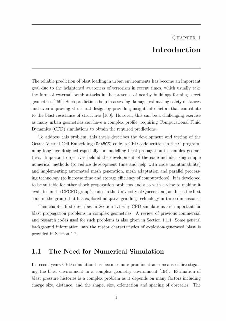
The reliable prediction of blast loading in urban environments has become an important
goal due to the heightened awareness of terrorism in recent times, which usually take
the form of external bomb attacks in the presence of nearby buildings forming street
geometries [159]. Such predictions help in assessing damage, estimating safety distances
and even improving structural design by providing insight into factors that contribute
to the blast resistance of structures [160]. However, this can be a challenging exercise
as many urban geometries can have a complex profile, requiring Computational Fluid
Dynamics (CFD) simulations to obtain the required predictions.
To address this problem, this thesis describes the development and testing of the
Octree Virtual Cell Embedding (OctVCE) code, a CFD code written in the C program-
ming language designed especially for modelling blast propagation in complex geome-
tries. Important objectives behind the development of the code include using simple
numerical methods (to reduce development time and help with code maintainability)
and implementing automated mesh generation, mesh adaptation and parallel process-
ing technology (to increase time and storage efficiency of computations). It is developed
to be suitable for other shock propagation problems and also with a view to making it
available in the CFCFD group’s codes in the University of Queensland, as this is the first
code in the group that has explored adaptive gridding technology in three dimensions.
This chapter first describes in Section 1.1 why CFD simulations are important for
blast propagation problems in complex geometries. A review of previous commercial
and research codes used for such problems is also given in Section 1.1.1. Some general
background information into the major characteristics of explosion-generated blast is
provided in Section 1.2.
1.1 The Need for Numerical Simulation
In recent years CFD simulation has become more prominent as a means of investigat-
ing the blast environment in a complex geometry environment [194]. Estimation of
blast pressure histories is a complex problem as it depends on many factors including
charge size, distance, and the shape, size, orientation and spacing of obstacles. The
1
1.1. THE NEED FOR NUMERICAL SIMULATION
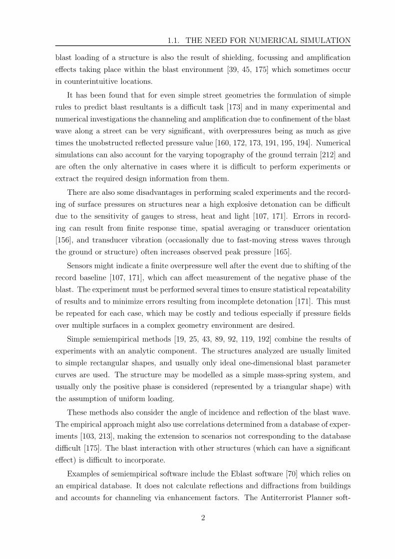
blast loading of a structure is also the result of shielding, focussing and amplification
effects taking place within the blast environment [39, 45, 175] which sometimes occur
in counterintuitive locations.
It has been found that for even simple street geometries the formulation of simple
rules to predict blast resultants is a difficult task [173] and in many experimental and
numerical investigations the channeling and amplification due to confinement of the blast
wave along a street can be very significant, with overpressures being as much as give
times the unobstructed reflected pressure value [160, 172, 173, 191, 195, 194]. Numerical
simulations can also account for the varying topography of the ground terrain [212] and
are often the only alternative in cases where it is difficult to perform experiments or
extract the required design information from them.
There are also some disadvantages in performing scaled experiments and the record-
ing of surface pressures on structures near a high explosive detonation can be difficult
due to the sensitivity of gauges to stress, heat and light [107, 171]. Errors in record-
ing can result from finite response time, spatial averaging or transducer orientation
[156], and transducer vibration (occasionally due to fast-moving stress waves through
the ground or structure) often increases observed peak pressure [165].
Sensors might indicate a finite overpressure well after the event due to shifting of the
record baseline [107, 171], which can affect measurement of the negative phase of the
blast. The experiment must be performed several times to ensure statistical repeatability
of results and to minimize errors resulting from incomplete detonation [171]. This must
be repeated for each case, which may be costly and tedious especially if pressure fields
over multiple surfaces in a complex geometry environment are desired.
Simple semiempirical methods [19, 25, 43, 89, 92, 119, 192] combine the results of
experiments with an analytic component. The structures analyzed are usually limited
to simple rectangular shapes, and usually only ideal one-dimensional blast parameter
curves are used. The structure may be modelled as a simple mass-spring system, and
usually only the positive phase is considered (represented by a triangular shape) with
the assumption of uniform loading.
These methods also consider the angle of incidence and reflection of the blast wave.
The empirical approach might also use correlations determined from a database of exper-
iments [103, 213], making the extension to scenarios not corresponding to the database
difficult [175]. The blast interaction with other structures (which can have a significant
effect) is difficult to incorporate.
Examples of semiempirical software include the Eblast software [70] which relies on
an empirical database. It does not calculate reflections and diffractions from buildings
and accounts for channeling via enhancement factors. The Antiterrorist Planner soft-
2

1.1. THE NEED FOR NUMERICAL SIMULATION
ware [13] uses scaled blast parameters with empirical shielding algorithms to provide
structural damage evaluations. More recent attempts include useage of a large exper-
imental database to train artificial neural networks to predict the blast environment
behind blast barriers [161] much faster than CFD could. A series of numerical simula-
tions was also performed to provide empiricial formulae to predict reflected pressure and
impulse in blast wave interaction with standalone columns [186]. These are useful and
fast design tools, but limited in application and would not model the blast environment
in general complex geometry adequately.
Another more sophisticated semiempirical method are the Low Altitude Multiple
Burst (LAMB) shock addition rules [94]. These rules require path lengths for rays along
which waves travel. The ray paths describing multiple reflections are calculated and
the pressure history from each ray is superposed. The LAMB rules are used by the
BLASTX code [33], the ASLAR code [117] and Needham’s code [139]. All these codes
are much faster than CFD and rely to an extent on empirical formulae and/or CFD
calculations, limiting their applicability to certain classes of simple geometry. It is still
difficult to model multiple complex building blast wave interactions [139, 171], which is
why CFD is the preferred option for such problems.
1.1.1 Previous CFD Approaches to Blast Modelling
This section gives a brief overview of prominent CFD codes used to model blast in
complex geometries. Codes employing unstructured grids have been quite popular due
to automatic grid generation capability. A popular unstructured commercial code is
AUTODYN [104], designed especially for blast propagation problems from high explosive
sources. It employs both finite-element and finite-volume solvers and can model full
fluid-structure interaction.
It also employs a time-saving method where a one-dimensional spherical analysis
between the explosive centre and nearest surface is performed before remapping the so-
lution to higher dimensions, removing the requirement for highly resolved multidimen-
sional grids early in the simulation. AUTODYN has been used to model a variety of
blast propagation problems in complex external and internal geometries [7, 48, 74, 159].
Another commerical unstructured code implementing the remapping capability is Chi-
nook [165] which has been used to model blast in urban scenarios.
A well known research code is Lohner’s unstructured finite element FEM-FCT code
[131], which can also model coupled fluid-structure interaction. This is a sophisticated
code which has been previously used to model explosions in very complex geometries like
tanks and underground carparks and airplanes [21, 22, 23]. A similar research code has
3
1.2. CHARACTERISTICS OF EXPLOSIVE BLASTS
been developed by Timofeev et al [211, 212, 220] which uses finite-volume unstructured
meshes. This has been used to compute blast wave propagation over complex terrains
generated by high explosives and volcanic blasts.
The SHAMRC code is a Cartesian cell Eulerian finite-difference code designed spe-
cially for the calculation of airblast propagation [12]. Rigid boundaries are assumed for
structural surfaces and it appears to allow only grid-oriented obstacles. It has been used
to calculate blast loads on office buildings and in internal room detonations [138]. An-
other well known Eulerian mesh code is CTH [93], which can simulate complex problems
involving fluid-structure interaction like penetration, perforation and explosive detona-
tion. It does not appear to have been used to model blast propagation in complex
geometries.
Cieslak et al [54] developed a cut-cell Cartesian cell code to simulate blast propaga-
tion for geometries like gun attenuators. The CEBAM code [56, 57] has been used to
simulate blast from gas explosions and solid explosives in complex geometries like off-
shore installations. It uses a finite volume formulation within a structured, curvilinear
framework to solve the conservation laws, but does not explicitly represent sub-grid scale
structures, implementing a porosity model to account for the effect of these obstacles.
The code which has the most features in common with OctVCE is Air3d developed
by Rose [171]. It is quite memory-efficient and fast compared to AUTODYN, and uses
Cartesian cells with the assumption of rigid surfaces, originally only handling grid-
aligned structures. It was further extended concurrently with OctVCE to incorporate
more general complex geometries and adaptive octree meshing in the ftt_air3d code1
[174, 177]. Air3d and ftt_air3d has been used extensively to model blast propagation
problems in a variety of simple and complex urban building environments [160, 171,
172, 173, 174, 175, 178, 193, 194]. The development of ftt_air3d and OctVCE has been
independent and has resulted in a number of different design decisions being made.
Sections 14.2 and 16.1 compare some differences between the ftt_air3d and OctVCE
codes.
1.2 Characteristics of Explosive Blasts
This section gives an overview of the main characteristics of blasts from explosive
charges. Fuller treatment of this subject can be found in many texts [19, 92, 119, 192].
An explosion is the phenomenon resulting from a rapid release of energy, usually of
such strength and occuring in such a small volume as to produce an audible pressure
1http://gow.epsrc.ac.uk/ViewGrant.aspx?GrantRef=GR/S04109/01, accessed May 2008
4
1.2. CHARACTERISTICS OF EXPLOSIVE BLASTS
wave [19, 119]. For high explosives, the energy release is caused by chemical detonation
which is nearly all transferred to the blast wave [92, 192], and initially consists mostly
of internal (rather than kinetic) energy [41].
The detonation products (commonly referred to as the explosive fireball) are quite
complex and formed by various processes including dissociation and ionization [119].
Very quickly the density in this fireball becomes lower than the surrounding air due to
a partial vacuum being created from the outward momentum of the air induced by the
primary blast wave. Under the influence of gravity the fireball rises and draws debris
into its centre, forming the well known ‘mushroom cloud’.
Accurate modelling of these products require modelling chemical reactions, but this
is outside the scope of this thesis (see Chapter 4). Many chemical explosives are oxygen-
deficient [101]; the energy release does not all occur at detonation because of insuffi-
cient oxygen to achieve complete oxidization, but also occurs later in combustion of the
explosive products as they mix with air (afterburning). TNT has a significant oxygen-
deficiency of 75% [101] but the effect of afterburning on the incident shock is small [120].
However, afterburning can affect flow speed and thus later parts of the blast wave.
It is well known that all blast waves quickly develop a spherical profile [19, 119, 120],
even for non-spherical charges. As long as energy release is sufficiently rapid the same
general configuration of the blast wave will result. The contact surface between the
detonation products and ambient gas usually becomes irregular with a high level of
mixing [25], but the uniformity of the spherical shock is not affected greatly (even with
afterburning). An analytical solution to the free-field wave structure (i.e. without any
obstacles) is difficult to obtain [25], although early attempts were made for both the
near- and far-field [19]. A numerical solution to the spherically symmetric conservation
equations is the preferred method, and was first attempted by Brode [40].
The blast wave is the dominant damage mechanism when the explosion occurs in
the vicinity of structures. Important features of this wave are shown in Figure 1.1
which shows the overpressure history at a point in space away from the explosion. This
figure only characterizes free-field burst because numerous reflections and shock wave
interactions are expected for a blast environment comprising of structures.
The severity of blast loading is usually characterized by the peak overpressure. How-
ever, damage is usually caused only if the positive phase duration is long relative to the
period of natural vibration of the structure [89]. Hence the peak impulse (the maximum
value of the pressure integral over time) is also an equally (if not more) important blast
parameter [171, 195]. The peak overpressure is usually of the order of gigapascals at the
explosion but decreases rapidly as the shock propagates outward, being quite well de-
scribed by the ideal gas law [119], and usually being too weak for structural engineering
5
1.2. CHARACTERISTICS OF EXPLOSIVE BLASTS
Figure 1.1: Typical blast wave profile
considerations after a scaled distance of 30 m/kg1/3 [171] (scaled distances are explained
on page 7).
A negative phase occurs due to a partial vacuum being created surrounding the
explosion. Eventually the displaced atmosphere will rush inward to fill this volume, thus
creating a suction phase in the explosion process. The negative phase lasts up to three
times as long as the positive phase but is usually less damaging than the positive phase,
and thus ignored [19, 119]. In some cases it can be a significant loading mechanism,
although measuring it experimentally can be difficult [172]. But it is the cause of much
broken glass being blown onto the streets in an urban environment blast.
The relationship with distance of blast parameters like peak overpressure, impulse
etc. for a free-field TNT burst has been measured empirically and documented in many
sources, sometimes supplied with curve fits [19, 25, 92, 103, 119, 192]. These curves
can also be developed from numerical simulation [41, 171] and correlations exist even
for differently shaped charges [43]. These relationships have also been documented for
hemispherical bursts on the ground, which are different from free-field burst because
realistic surfaces are not perfectly reflecting [201].
The profile in Figure 1.1 is not entirely accurate as a weaker secondary shock is
also produced after the explosion, which may have some contribution to the positive
impulse [25, 41, 92]. The deceleration of the contact surface produces an outward
moving rarefaction wave and an imploding secondary shock, which may be initially
swept outward. After implosion this shock expands outward and partially reflects off
the contact surface again, further imploding and repeating the process, although each
time the shock decreases in intensity. Thus only the secondary shock is usually seen,
and it does not usually catch up to the incident shock. Because the secondary shock is
much weaker than the incident shock, it is usually ignored [171].
In a height-of-burst scenario when the charge is detonated above the ground the
blast wave will reflect from the ground, as shown in Figure 1.2. There are three types
6
1.2. CHARACTERISTICS OF EXPLOSIVE BLASTS
of reflections – normal reflection (directly underneath the burst), oblique reflection (an-
gle of incidence less than 40 degrees) and Mach stem reflection for larger angles of
incidence. The overpressure in reflected waves may be much greater than the incident
shock, especially behind the Mach stem [19, 193].
Figure 1.2: Height-of-burst scenario
1.2.1 Scaling Laws
When two spherical charges made of the same explosive are detonated in the same at-
mosphere and have the same geometry but are of different scales, Hopkinson ‘cube-root’
scaling applies [119, 120]. This scaling law is based on fundamentals of geometrical simi-
larity, and can eliminate charge mass as a parameter in describing blast wave properties.
These two charges will exhibit the same property Q behind the primary shock (e.g. in
overpressure) at the same scaled distance.
The scaled distance is Z = R/W 1/3 where R is the distance from the centre of
the explosion and W the mass of the explosive. Pressure history profiles will also be
identical at the same scaled distance if time is also scaled i.e. tsc = t/W 1/3. Impulse
can be scaled either by a time scale (like positive phase duration) or by W 1/3. This
scaling law is approximate when comparing the blast waves between two different types
of explosives with different energy release rates that exhibit afterburning [120]. The
scaling law does not apply if the flowfield is spherically asymmetric [120], but this is an
acceptable limitation as departures from sphericity only occur close to the fireball.
It is also common to compare explosive blast effects in terms of equivalency to the
burst from a spherical TNT charge, expressed as an equivalent mass of TNT. The
simplest equivalency is comparison in terms of blast energy, but equivalencies can also
be based on peak overpressure or impulse [213], which are not always equal (or parallel)
due to factors like the oxygen deficiency [101]. Charge shape can also complicate the
equivalency, and more complex scalings formulate TNT equivalence varying with scaled
distance (looking at either pressure or impulse) [120, 201].
7
1.3. SCOPE OF THESIS
1.3 Scope of Thesis
Chapter 2 reviews different CFD methods used to model flows in complex geometries,
concluding in Section 2.4 with a discussion of the Virtual Cell Embedding (VCE) method
[124], a simple Cartesian cell method that automatically generates a mesh in arbitrary
geometries. This thesis is thus also an application study into the suitability of the VCE
gridding method in simulating blast propagation and loading in complex geometries.
Chapter 3 describes the mesh adaptation procedure implemented by OctVCE, which
uses a recursive octree data structure as its basis for refining and coarsening cells. This
section discusses pseudocode of important adaptation routines, degeneracies encountered
and adaptation indicators.
Chapter 4 reviews and describes various aspects involved in the numerical method-
ology of the code including the scope, governing equations, flux solvers, equations of
state, initial and boundary conditions and point-inclusion queries. More detailed cover-
age of these aspects can also be found in the Appendix. Some discussion will centre on
potential instabilities with the code resulting from the conjuction of the VCE gridding
method with the numerical flow calculation methodology. Chapter 5 reviews parallel
computing methods in general and describes the shared-memory parallel implementa-
tion of the OctVCE code in Section 5.5. While the work in this thesis was being done,
the availability of multiple core processors became common. In the near-future all en-
gineering workstations are expected to have multiple cores. Useful measures of parallel
performance will also be discussed.
Chapter 6 presents four different verification test cases to demonstrate the reliability
of the numerical implementation – the Method of Manufactured Solutions (Section 6.1),
ideal shock tube problem, supersonic flow over wedges and cones and supersonic vortex
flow. Chapters 7 to 14 cover validation test cases to determine the credibility and accu-
racy of the code in solving realistic blast and shock propagation problems. Examples are
shock diffraction over wedges and cylinders (Chapters 7 to 8), explosive bursting sphere
problems (Chapters 9 and 10), blast in axisymmetric containers and in environments
comprising of simple rectangular prismatic geometries (Chapters 11 to 13), and blast in
complex city scape geometries (Chapter 14).
Profiling of the code will also be performed for a number of these test cases to
establish its performance in serial and parallel execution. Chapter 15 focusses on an
application study of the code where an explosion in an internal geometry is modelled.
This shows the code being used in a design process where the geometry, although some-
what simplified, had to retain its essentially complex features. Finally all results are
summarized in Chapter 16 and some improvements to the code are also suggested.
8
Chapter 2
Meshes for Complex Geometries
The simulation of blast propagation in complex geometries usually requires the mesh to
encompass the domain. This can be time-consuming if performed manually, and thus
automated grid generation methods are preferred. To reduce code development and
maintenance time, simple methods are also preferred over complex ones. This section
gives an overview of the three main approaches (body-fitted, grid-free and cartesian grid
methods) used to generate grids and perform numerical simulations in environments with
complex surface geometry.
2.1 Body-fitted Grids
Structured grids basically consist of rectangular or hexahedral cells stored in an array,
with neighbouring connectivities regularly determined by array indices [79]. They can
be ‘body-fitted’ and may require metrics and transformations to map the physical grid
into computational space where flow equations are solved. They are an efficient data
structure as connectivity is fixed and not explicitly stored, and can be organized into
blocks of structured grids when performing simulations in parallel.
Structured grids require some degree of user interaction in their construction, and
can be tedious to create for complex geometries [79, 106]. Metric terms add some
additional complexity to the code, and the fixed connectivity prevents implementation
of h-refinement where cells are added or deleted. Chimera or overset grids [72] are
popular for moving body problems and consist of overlapping patches of structured
grids fitted around each body. Effort still has to be put into generating structured grids
around each body [106] and there is the additional complexity of hole-cutting, stencil
identification, interpolation coefficients and inter-grid communication associated with
the chimera grid approach [72].
Unstructured grids are composed of an arbitrary collection of randomly oriented
cells which do not typically have a repeatable topological structure. They are com-
monly composed of triangles or tetrahedral cells, which can be generated by Delaunay
triangulation, advancing-front methods or tree-based techniques (where an initial Carte-
sian mesh adjusts boundary elements before undergoing tessellation) [29, 79]. All these
9
2.2. GRID-FREE AND PARTICLE METHODS
methods allow a high degree of automation [45]. Unstructured grids can also be body-
fitted, and for some grid construction algorithms like the advancing-front method a
surface mesh composed of triangular panels may also be required.
Compared to structured grids, unstructured grids are much more taxing on memory
and solution time [118], and can also be difficult and cumbersome to code. They are
more inefficient at filling the domain [51] and have poorer shock-capturing ability [27]
due to irregular numerical interfaces causing some refraction and scattering of waves
[64]. Generating an appropriate surface mesh can also be challenging [1, 128], and may
still require a degree of user-interactivity [140]. Research into generating quadrilateral
or hexahedral unstructured grids has also been undertaken [29]. Hexahedral meshes
have more regularity than tetrahedral meshes and are comparatively more accurate,
time-efficient and memory-efficient [1, 27, 29, 30].
However, automated grid generation for unstructured hexahedral meshes has not
reached as advanced a stage compared to tetrahedral meshes [29, 200]. Blacker [31]
provides a good overview of various methods for hexahedral mesh generation, including
use of primitives (applicable only to a class of specialized geometries), decomposition into
recognizable primitive shapes, advancing-front techniques and overlay grids. Advancing-
front techniques for hexahedral meshes include a whisker weaving scheme [207] and
plastering scheme [32, 198]. These methods are still an active area of research and can
be quite complex to implement and time intensive. A surface mesh also needs to be
specified.
One of the more widely used hexahedral grid generation schemes is the overlay grid
method [183]. The volume to be meshed is initially overlayed with a mesh of hexahedral
cells and cell nodes on the body surfaces are adjusted to fit to the surface. Sometimes
mixed cell types (tetrahedral and hexahedral) result due to degeneracies. Depending
on the methods considered, the algorithmic complexity of the overlay grid method may
still be higher than for some Cartesian cell methods.
2.2 Grid-free and Particle Methods
Another method to solve flows in complex geometry is the ‘grid-free’ approach [197].
This approach essentially solves the conservation equations using least squares fitting of
nodes in the domain to approximate derivatives. This method is ‘grid-free’ in the sense
that the nodes can be generated using any means [197]. However these methods do not
guarantee global conservation and are slower than mesh-based counterparts, and need to
introduce some artificial dissipation [132]. The least squares procedure can be complex,
requiring inversion of geometric matricies and thus depends on the stencil of grid points
10
2.3. CARTESIAN GRID METHODS
chosen to prevent ill-conditioning. Other difficult degeneracies include insufficient nodal
density, surface discontinuities and thin bodies.
Particle methods discretize the fluid (a Lagrangian approach) rather than the flow
domain (Eulerian approach). These also can be meshed-based, like the popular Arbi-
trary Lagrangian-Eulerian (ALE) methods [134], and thus suffer from the disadvantages
associated with unstructured grids. Lagrangian mesh-based approaches can result in se-
vere mesh distortion and entangling and thus require remapping, but this introduces
numerical diffusion [84].
A well-known gridless method is the Smoothed Particle Hydrodynamics (SPH) method
[137] in which the fluid is represented by a collection of fluid pseduo-particles. This
method, originally applied to astrophysical problems, is good for simulating flows where
fluid interfaces are important, and has seen extension to other applications in recent
times. However SPH is computationally expensive and offers lower resolution compared
to contemporary finite-volume methods [38], also requiring artificial viscosity. Particle
penetration problems associated for shocked flows exist and boundary conditions (even
just reflecting boundaries) are more difficult to handle than with finite-volume methods
[143]. At least for blast propagation problems, Eulerian methods are still preferrable,
simpler to implement and more established.
Another particle method used to model blast propagation is the Direct Simulation
Monte Carlo (DSMC) method of Sharma et al [184, 185]. This method is derived from
kinetic theory and uses a statistically representative set of particles which are tracked
in their collisions with each other and with boundaries. Sharma et al have modified the
method to use a much larger timestep than the mean collision time. DSMC thus gives
approximate results and is faster than continuum methods, but has lower resolution and
statistical scatter. This method is promising but has not seen wider application and
usage compared to finite-volume methods.
2.3 Cartesian Grid Methods
Cartesian grids are composed of axis-aligned hexahedral (often cubical) finite-volume
cells which treat solid geometries as ‘immersed’ within the mesh. Cells that are com-
pletely obstructed or unobstructed are ignored or treated normally respectively. Various
approaches exist to treat partially obstructed or intersected cells [4, 45, 65, 106, 121, 124,
128, 153, 174]. These methods vary in complexity and accuracy. Because the number of
cells is usually a small fraction of all the cells, the additional calculations on intersected
cells usually involve small overhead [224].
11
2.3. CARTESIAN GRID METHODS
Problems with Cartesian grids usually relate to flaws in surface representation, thin
bodies or very small cells. Very small intersected cells lead to ineffiencies as the global
timestep needs to be drastically reduced to ensure stability of the flow update scheme for
each and every cell. Various methods have been developed to circumvent this problem
[77, 145] but an easy approach is simply to merge a small cell with a larger neighbouring
cell [59, 153].
Cartesian grids have a high degree of automation, can incorporate mesh adaptation
fairly easily. To an extent, they also have the benefits of the structured grids over
unstructured grids like better efficiency and accuracy. They have been used for aero-
dynamics applications [1], incompressible flows [226] and blast propagation problems
in urban geometries [177, 194]. The Cartesian grid approach is chosen for this thesis
because of its past usage and advantages over other methods.
2.3.1 Cut Cells
As bodies are usually surface triangulated, each triangular facet might represent a wall
interface for the Cartesian finite-volume cell intersected by that facet. Cut cell meth-
ods preserve with full fidelity the surface definition for each intersected cell [4, 50, 54].
However these methods are very complex, requiring tedious computational geometry
routines to perform intersections and possible re-triangulations to extract the wetted
body surface for each cell. Further work has to go into accounting for numerous geo-
metrical degeneracies, which arise because of floating point representations of cell and
vertex positions.
2.3.2 Curvature-Corrected Symmetry Technique
This method, developed by Dadone [64, 65], does not require the complex topological
description of intersected cells, insteading relying on reflected ghost cells near surfaces.
An assumed flow-field model represents the effect of the surface; this model satisfies the
normal momentum equation and accounts for surface curvature effects, consisting of a
vortex flow of constant entropy and total enthalpy. Surface values are obtained through
interpolation. This method has been used to solve flows over circular objects and airfoil
geometries. It may still be more complicated to implement than other Cartesian cell
methods because it requires reflecting ghost nodes through a body and calculating body
curvature.
12
2.4. THE VIRTUAL CELL EMBEDDING METHOD
2.3.3 Surface Approximation
This method has many variants (varying in complexity) but generally approximates the
surface by representing the portion of the body in an intersected cell as a single planar
surface. Some methods only admit certain types of intersected cells [66, 106, 128, 153].
By admitting more cell types, the body surface can be represented more accurately,
but this can be a cumbersome exercise. Other methods allow the planar surface to
be computed generally using computational geometry routines or empirical geometric
formulae [121, 124, 145, 174, 224].
Another method, not really suitable here, is the Porosity/Distributed Resistance
(PDR) approach [45, 56, 78] where all (or just small-scale) obstacles are not actually
resolved, but their effect accounted for by introducing appropriate porosities and dis-
tributed resistances into the flow equations. This approach has been used to model
heat exhanger geometries and gas explosions in petrochemical processing installations
[45], and is really only suitable for predicting global flow effects. PDR parameters like
resistance terms are often empirically derived (or calculated from high resolution simu-
lations), and can be difficult and expensive to extend to more complex configurations.
2.4 The Virtual Cell Embedding Method
The Virtual Cell Embedding (VCE) method, developed by Landsberg et al [124, 125]
is chosen for this thesis due to its simplicity and robustness. It is a general surface
approximation method (Section 2.3.3) and is based purely on a point-inclusion test,
being equally suitable for convex or concave bodies or surfaces given by an analytic
or arbitrary polyhedral definition. The VCE method has been used for simulations of
flows over ship superstructures [124], blasts in pressure vessels [129] and dispersion of
contaminants over complex city geometries [37]. This thesis combines the VCE method
with hierarchical grid refinement (Chapter 3) and will explore the suitability of the VCE
to model blast propagation in complex geometries.
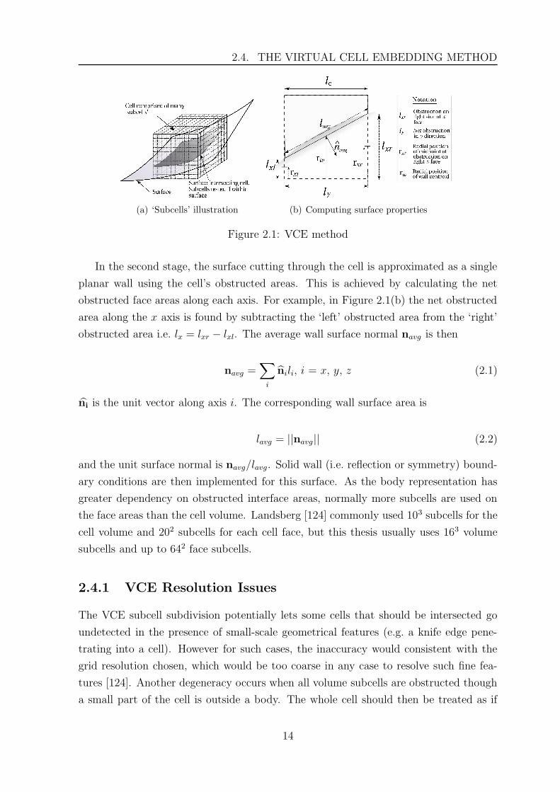
The first stage of VCE involves subdividing an intersected cell into a lattice of
‘subcells’ (Figure 2.1(a)) each with its associated centroid. A subcell is labelled as
inside/outside a body if its centroid is inside/outside. In this manner a summation of
subcell volumes will yield the approximate unobstructed cell volume. Each cell face
is also divided into ‘sub-areas’ to determine the approximate unobstructed face area.
These subcells are not stored in memory; they are simply counting aids to determine
the proper cell face areas and volume. Clearly the more subcells are used the better the
obstruction is approximated.
13
2.4. THE VIRTUAL CELL EMBEDDING METHOD
(a) ‘Subcells’ illustration (b) Computing surface properties
Figure 2.1: VCE method
In the second stage, the surface cutting through the cell is approximated as a single
planar wall using the cell’s obstructed areas. This is achieved by calculating the net
obstructed face areas along each axis. For example, in Figure 2.1(b) the net obstructed
area along the x axis is found by subtracting the ‘left’ obstructed area from the ‘right’
obstructed area i.e. lx = lxr − lxl. The average wall surface normal navg is then
navg =∑
i
nili, i = x, y, z (2.1)
ni is the unit vector along axis i. The corresponding wall surface area is
lavg = ||navg|| (2.2)
and the unit surface normal is navg/lavg. Solid wall (i.e. reflection or symmetry) bound-
ary conditions are then implemented for this surface. As the body representation has
greater dependency on obstructed interface areas, normally more subcells are used on
the face areas than the cell volume. Landsberg [124] commonly used 103 subcells for the
cell volume and 202 subcells for each cell face, but this thesis usually uses 163 volume
subcells and up to 642 face subcells.
2.4.1 VCE Resolution Issues
The VCE subcell subdivision potentially lets some cells that should be intersected go
undetected in the presence of small-scale geometrical features (e.g. a knife edge pene-
trating into a cell). However for such cases, the inaccuracy would consistent with the
grid resolution chosen, which would be too coarse in any case to resolve such fine fea-
tures [124]. Another degeneracy occurs when all volume subcells are obstructed though
a small part of the cell is outside a body. The whole cell should then be treated as if
14
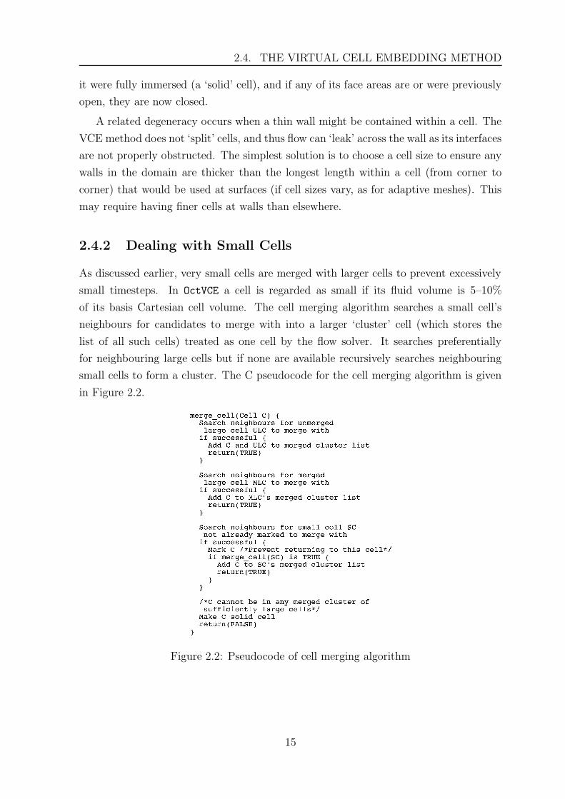
2.4. THE VIRTUAL CELL EMBEDDING METHOD
it were fully immersed (a ‘solid’ cell), and if any of its face areas are or were previously
open, they are now closed.
A related degeneracy occurs when a thin wall might be contained within a cell. The
VCE method does not ‘split’ cells, and thus flow can ‘leak’ across the wall as its interfaces
are not properly obstructed. The simplest solution is to choose a cell size to ensure any
walls in the domain are thicker than the longest length within a cell (from corner to
corner) that would be used at surfaces (if cell sizes vary, as for adaptive meshes). This
may require having finer cells at walls than elsewhere.
2.4.2 Dealing with Small Cells
As discussed earlier, very small cells are merged with larger cells to prevent excessively
small timesteps. In OctVCE a cell is regarded as small if its fluid volume is 5–10%
of its basis Cartesian cell volume. The cell merging algorithm searches a small cell’s
neighbours for candidates to merge with into a larger ‘cluster’ cell (which stores the
list of all such cells) treated as one cell by the flow solver. It searches preferentially
for neighbouring large cells but if none are available recursively searches neighbouring
small cells to form a cluster. The C pseudocode for the cell merging algorithm is given
in Figure 2.2.
Figure 2.2: Pseudocode of cell merging algorithm
15
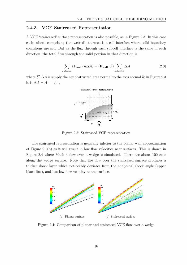
2.4. THE VIRTUAL CELL EMBEDDING METHOD
2.4.3 VCE Staircased Representation
A VCE ‘staircased’ surface representation is also possible, as in Figure 2.3. In this case
each subcell comprising the ‘wetted’ staircase is a cell interface where solid boundary
conditions are set. But as the flux through each subcell interface is the same in each
direction, the total flow through the solid portion in that direction is
∑
subcells
(Fwall · n∆A) = (Fwall · n)∑
subcells
∆A (2.3)
where∑
∆A is simply the net obstructed area normal to the axis normal n; in Figure 2.3
it is ∆A = A+ − A−.
Figure 2.3: Staircased VCE representation
The staircased representation is generally inferior to the planar wall approximation
of Figure 2.1(b) as it will result in low flow velocities near surfaces. This is shown in
Figure 2.4 where Mach 4 flow over a wedge is simulated. There are about 100 cells
along the wedge surface. Note that the flow over the staircased surface produces a
thicker shock layer which noticeably deviates from the analytical shock angle (upper
black line), and has low flow velocity at the surface.
(a) Planar surface (b) Staircased surface
Figure 2.4: Comparison of planar and staircased VCE flow over a wedge
16
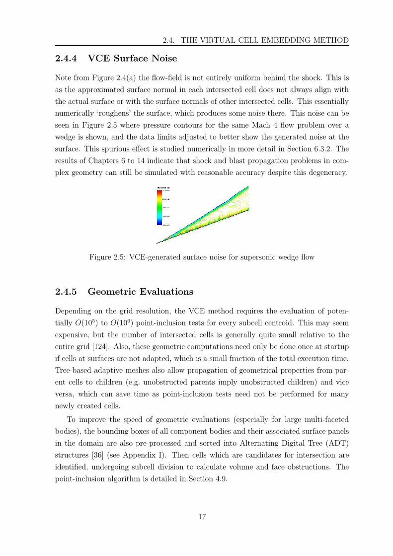
2.4. THE VIRTUAL CELL EMBEDDING METHOD
2.4.4 VCE Surface Noise
Note from Figure 2.4(a) the flow-field is not entirely uniform behind the shock. This is
as the approximated surface normal in each intersected cell does not always align with
the actual surface or with the surface normals of other intersected cells. This essentially
numerically ‘roughens’ the surface, which produces some noise there. This noise can be
seen in Figure 2.5 where pressure contours for the same Mach 4 flow problem over a
wedge is shown, and the data limits adjusted to better show the generated noise at the
surface. This spurious effect is studied numerically in more detail in Section 6.3.2. The
results of Chapters 6 to 14 indicate that shock and blast propagation problems in com-
plex geometry can still be simulated with reasonable accuracy despite this degeneracy.
Figure 2.5: VCE-generated surface noise for supersonic wedge flow
2.4.5 Geometric Evaluations
Depending on the grid resolution, the VCE method requires the evaluation of poten-
tially O(105) to O(106) point-inclusion tests for every subcell centroid. This may seem
expensive, but the number of intersected cells is generally quite small relative to the
entire grid [124]. Also, these geometric computations need only be done once at startup
if cells at surfaces are not adapted, which is a small fraction of the total execution time.
Tree-based adaptive meshes also allow propagation of geometrical properties from par-
ent cells to children (e.g. unobstructed parents imply unobstructed children) and vice
versa, which can save time as point-inclusion tests need not be performed for many
newly created cells.
To improve the speed of geometric evaluations (especially for large multi-faceted
bodies), the bounding boxes of all component bodies and their associated surface panels
in the domain are also pre-processed and sorted into Alternating Digital Tree (ADT)
structures [36] (see Appendix I). Then cells which are candidates for intersection are
identified, undergoing subcell division to calculate volume and face obstructions. The
point-inclusion algorithm is detailed in Section 4.9.
17
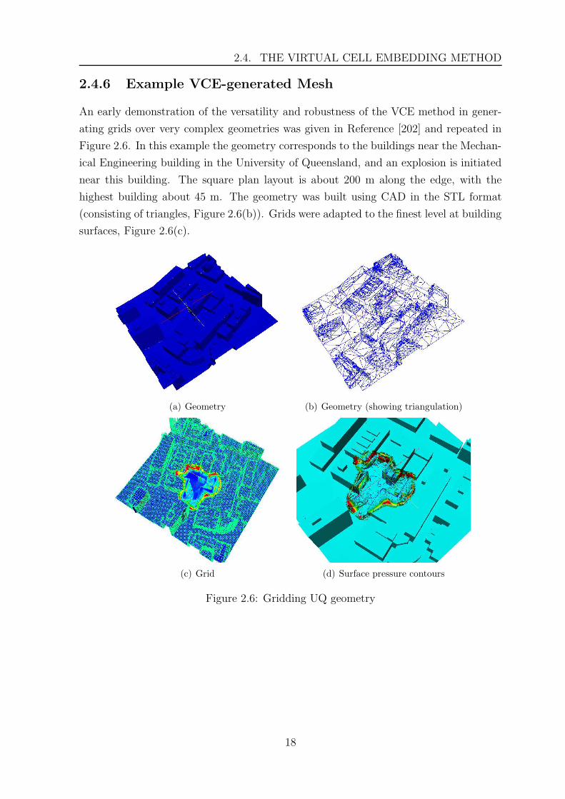
2.4. THE VIRTUAL CELL EMBEDDING METHOD
2.4.6 Example VCE-generated Mesh
An early demonstration of the versatility and robustness of the VCE method in gener-
ating grids over very complex geometries was given in Reference [202] and repeated in
Figure 2.6. In this example the geometry corresponds to the buildings near the Mechan-
ical Engineering building in the University of Queensland, and an explosion is initiated
near this building. The square plan layout is about 200 m along the edge, with the
highest building about 45 m. The geometry was built using CAD in the STL format
(consisting of triangles, Figure 2.6(b)). Grids were adapted to the finest level at building
surfaces, Figure 2.6(c).
(a) Geometry (b) Geometry (showing triangulation)
(c) Grid (d) Surface pressure contours
Figure 2.6: Gridding UQ geometry
18
Chapter 3
Mesh Adaptation
Mesh adaptation is a feature that adapts the grid to important flow features, allowing
more accurate solutions to be obtained with fewer cells, resulting in significant savings
in execution time [174]. One method of mesh adaptation, r -refinement, involves redis-
tributing a fixed number of cells. For Cartesian cell approahces, this method is not as
popular as h-refinement [26] where cells are added or deleted appropriately (and the
width h of a cell is divided) because the grid distortion can be complicated to manage
[228], and in many cases a grid redistribution will not resolve important features as well
as h-refinement [59].
This thesis implements isotropic refinement where only one type of refined cell is
created. Anisotropic refinement allows different types of cells to be created depending
on the state of the local flow. This approach can result in even greater savings in cells
[3, 50] where flow is predominantly unidirectional, but blast propagation in complex
geometries is a more multidirectional problem which is suited to isotropic refinement
[79]. Anisotropic refinement will also involve complicated data structures which would
be more tedious to implement.
The Adaptive Mesh Refinement (AMR) method developed by Berger [24, 26] relies
on adding or deleting entire patches of block-structured meshes rather than refining
or coarsening individual cells (a tree-based method). Different timesteps are used on
different patches (but are appropriately subcycled and interleaved to preserve time accu-
racy), and adaptation is guided by error estimation based on Richardson extrapolation.
Because entire patches are added, about 30% of added cells are usually unnecessary
[1, 118] which might lead to large memory requirements [177].
AMR might still be more memory efficient and faster than tree-based approaches
because of structured mesh usage, which avoids the slower indirect addressing (pointers)
common in tree-based meshes [24]. However, the AMR method is not used for this thesis
due to its complexity [72, 81] in managing a dynamically changing collection of meshes,
which need periodic rebuilding as the solution evolves over time [118].
OctVCE thesis implements the octree structure [51, 181] for mesh adaptation. This
involves an isotropic division of a parent cubical cell undergoing refinement to yield
eight children cells (and vice versa for the coarsening process), as shown in Figure 3.1.
19
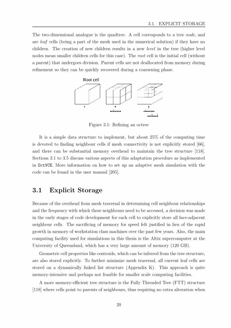
3.1. EXPLICIT STORAGE
The two-dimensional analogue is the quadtree. A cell corresponds to a tree node, and
are leaf cells (being a part of the mesh used in the numerical solution) if they have no
children. The creation of new children results in a new level in the tree (higher level
nodes mean smaller children cells for this case). The root cell is the initial cell (without
a parent) that undergoes division. Parent cells are not deallocated from memory during
refinement so they can be quickly recovered during a coarsening phase.
Figure 3.1: Refining an octree
It is a simple data structure to implement, but about 25% of the computing time
is devoted to finding neighbour cells if mesh connectivity is not explicitly stored [66],
and there can be substantial memory overhead to maintain the tree structure [118].
Sections 3.1 to 3.5 discuss various aspects of this adaptation procedure as implemented
in OctVCE. More information on how to set up an adaptive mesh simulation with the
code can be found in the user manual [205].
3.1 Explicit Storage
Because of the overhead from mesh traversal in determining cell neighbour relationships
and the frequency with which these neighbours need to be accessed, a decision was made
in the early stages of code development for each cell to explicitly store all face-adjacent
neighbour cells. The sacrificing of memory for speed felt justified in lieu of the rapid
growth in memory of workstation class machines over the past few years. Also, the main
computing facility used for simulations in this thesis is the Altix supercomputer at the
University of Queensland, which has a very large amount of memory (120 GB).
Geometric cell properties like centroids, which can be inferred from the tree structure,
are also stored explicitly. To further minimize mesh traversal, all current leaf cells are
stored on a dynamically linked list structure (Appendix K). This approach is quite
memory-intensive and perhaps not feasible for smaller scale computing facilities.
A more memory-efficient tree structure is the Fully Threaded Tree (FTT) structure
[118] where cells point to parents of neighbours, thus requiring no extra alteration when
20
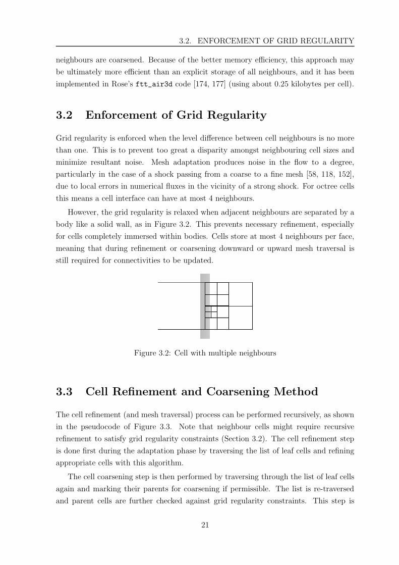
3.2. ENFORCEMENT OF GRID REGULARITY
neighbours are coarsened. Because of the better memory efficiency, this approach may
be ultimately more efficient than an explicit storage of all neighbours, and it has been
implemented in Rose’s ftt_air3d code [174, 177] (using about 0.25 kilobytes per cell).
3.2 Enforcement of Grid Regularity
Grid regularity is enforced when the level difference between cell neighbours is no more
than one. This is to prevent too great a disparity amongst neighbouring cell sizes and
minimize resultant noise. Mesh adaptation produces noise in the flow to a degree,
particularly in the case of a shock passing from a coarse to a fine mesh [58, 118, 152],
due to local errors in numerical fluxes in the vicinity of a strong shock. For octree cells
this means a cell interface can have at most 4 neighbours.
However, the grid regularity is relaxed when adjacent neighbours are separated by a
body like a solid wall, as in Figure 3.2. This prevents necessary refinement, especially
for cells completely immersed within bodies. Cells store at most 4 neighbours per face,
meaning that during refinement or coarsening downward or upward mesh traversal is
still required for connectivities to be updated.
Figure 3.2: Cell with multiple neighbours
3.3 Cell Refinement and Coarsening Method
The cell refinement (and mesh traversal) process can be performed recursively, as shown
in the pseudocode of Figure 3.3. Note that neighbour cells might require recursive
refinement to satisfy grid regularity constraints (Section 3.2). The cell refinement step
is done first during the adaptation phase by traversing the list of leaf cells and refining
appropriate cells with this algorithm.
The cell coarsening step is then performed by traversing through the list of leaf cells
again and marking their parents for coarsening if permissible. The list is re-traversed
and parent cells are further checked against grid regularity constraints. This step is
21
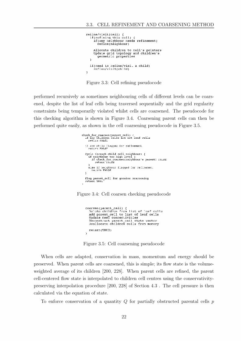
3.3. CELL REFINEMENT AND COARSENING METHOD
Figure 3.3: Cell refining pseudocode
performed recursively as sometimes neighbouring cells of different levels can be coars-
ened, despite the list of leaf cells being traversed sequentially and the grid regularity
constraints being temporarily violated whilst cells are coarsened. The pseudocode for
this checking algorithm is shown in Figure 3.4. Coarsening parent cells can then be
performed quite easily, as shown in the cell coarsening pseudocode in Figure 3.5.
Figure 3.4: Cell coarsen checking pseudocode
Figure 3.5: Cell coarsening pseudocode
When cells are adapted, conservation in mass, momentum and energy should be
preserved. When parent cells are coarsened, this is simple; its flow state is the volume-
weighted average of its children [200, 228]. When parent cells are refined, the parent
cell-centered flow state is interpolated to children cell centres using the conservativity-
preserving interpolation procedure [200, 228] of Section 4.3 . The cell pressure is then
calculated via the equation of state.
To enforce conservation of a quantity Q for partially obstructed parental cells p
22
3.4. DEGENERACIES DURING ADAPTATION
undergoing refinement, the quantity ∆ is calculated which represents the degree of non-
conservation where
∆ = QpVp −n∑
c=1
QcVc (3.1)
Vp is the parent cell volume, and Vc is the child cell volume; summing over n children cells
Vp =∑n
c=1 Vc. Qc is the interpolated value of Q to child cell c from the reconstruction
procedure of Section 4.3. To preserve conservation, the proper value of Q for the child
cell c is
Q = Qc +∆
nVc(3.2)
Based on the conservative timestepping criterion in Equation 4.7 it takes at least 4
timesteps for a shock to cross a cell, so adaptation every 5 timesteps is sufficient to
ensure adapted flow features never leave a fine mesh region and lose resolution [118].
Interleaved timestepping for different cell levels is not implemented. Cells adjacent
to those cells that are actually flagged for refinement are also refined to the highest
permissible level to act as a ‘buffer’ layer.
3.4 Degeneracies during Adaptation
During adaptation geometric properties between cells must be consistent and airtight.
As cell geometric properties are derived from VCE subcell division (Section 2.4), parental
cells (having larger subcells) will not compute areas or volumes as accurately as children
cells, and this must be accounted for. If adaptation of partially obstructed cells is
allowed, one degeneracy occurs during the refinement stage as shown in Figure 3.6.
Here an intersected parent cell is refined but as a result of obstruction, one of its
children are made ‘solid’. Thus an interface area on the parent which was previously
unobstructed is now obstructed. This new information must be remembered if the
parent is coarsened and thus geometric information from children should be used during
coarsening. Adaptation can also break up merged cell clusters that were formed because
of the small cell degeneracy discussed in Section 2.4.2. When this occurs, pointers and
associated data structures must be deallocated properly, and should small cells still exist
after adaptation, re-merging with new cells should be done at this stage.
23
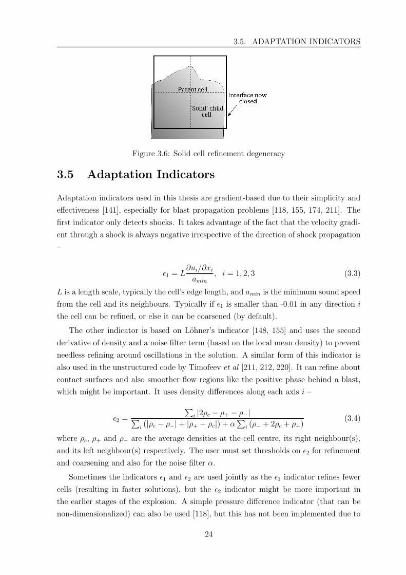
3.5. ADAPTATION INDICATORS
Figure 3.6: Solid cell refinement degeneracy
3.5 Adaptation Indicators
Adaptation indicators used in this thesis are gradient-based due to their simplicity and
effectiveness [141], especially for blast propagation problems [118, 155, 174, 211]. The
first indicator only detects shocks. It takes advantage of the fact that the velocity gradi-
ent through a shock is always negative irrespective of the direction of shock propagation
–
ε1 = L∂ui/∂xi
amin, i = 1, 2, 3 (3.3)
L is a length scale, typically the cell’s edge length, and amin is the minimum sound speed
from the cell and its neighbours. Typically if ε1 is smaller than -0.01 in any direction i
the cell can be refined, or else it can be coarsened (by default).
The other indicator is based on Lohner’s indicator [148, 155] and uses the second
derivative of density and a noise filter term (based on the local mean density) to prevent
needless refining around oscillations in the solution. A similar form of this indicator is
also used in the unstructured code by Timofeev et al [211, 212, 220]. It can refine about
contact surfaces and also smoother flow regions like the positive phase behind a blast,
which might be important. It uses density differences along each axis i –
ε2 =
∑i |2ρc − ρ+ − ρ−|∑
i (|ρc − ρ−| + |ρ+ − ρc|) + α∑
i (ρ− + 2ρc + ρ+)(3.4)
where ρc, ρ+ and ρ− are the average densities at the cell centre, its right neighbour(s),
and its left neighbour(s) respectively. The user must set thresholds on ε2 for refinement
and coarsening and also for the noise filter α.
Sometimes the indicators ε1 and ε2 are used jointly as the ε1 indicator refines fewer
cells (resulting in faster solutions), but the ε2 indicator might be more important in
the earlier stages of the explosion. A simple pressure difference indicator (that can be
non-dimensionalized) can also be used [118], but this has not been implemented due to
24

3.5. ADAPTATION INDICATORS
its similarity with the ε1 indicator. Adaptation ‘regions’, which allow one to switch off
mesh adaptation in some regions of the solution domain (implemented in the ftt_air3d
code [177]), is not implemented here.
25
Chapter 4
Flow Simulation Algorithm
This section reviews and describes various important aspects in the numerical method-
ology behind OctVCE, including the governing equations, time integration scheme, flux
solvers used, equations of state, implementation of initial and boundary conditions, in-
terpolation or reconstruction method and point-inclusion query algorithm. It will be
useful first to make some general comments as to the scope of the methodology.
Firstly, where possible, simple methods or methods already implemented in the
MB_CNS code [109] (developed here at the University of Queensland) will be used. This
will help streamline the process of eventually incorporating OctVCE as a submodule of
MB_CNS, and also cuts down on code development time. Viscous effects can be ignored
[160, 185] as blast propagation and loading problems are dominated by convection pro-
cesses. The code will thus solve the unsteady Euler (compressible, inviscid) flow equa-
tions (Section 4.1).
Very accurate modelling of blast interaction with structures would require modelling
fluid-structure interaction and multi-material shock physics, which can be challenging
and tedious to code. This thesis considers only those class of blast propagation problems
where structures are considered rigid and non-deforming and the pressure load is desired
at some point(s) in space. This is a good assumption to hold in many cases even
when buildings are subjected to intense loading because of the strength of modern-day
reinforced concrete or steel-framed structures [160, 193]. The most significant damage to
buildings usually occur at glazed areas like windows, and transfer of momentum to the
building is small, justifying rigid boundary condition implementation and decoupling
blast-structure interaction.
Chemical reactions are not modelled as this is computationally expensive and really
only needed for accurate modelling of the explosive fireball, which is not the focus
of this thesis. It has been demonstrated in numerous blast propagation simulations
[160, 174, 211, 212] that accurate chemical modelling of detonation is not required for
good results in the mid- to far-field (see Sections 1.2 and 1.1.1). The most important
quantity is the energy released [19, 171, 211].
Due to the adoption of the VCE Cartesian grid method (Section 2.3) a finite-volume
scheme [96] is favored for the discretization of the flow equations, as almost all Cartesian
26
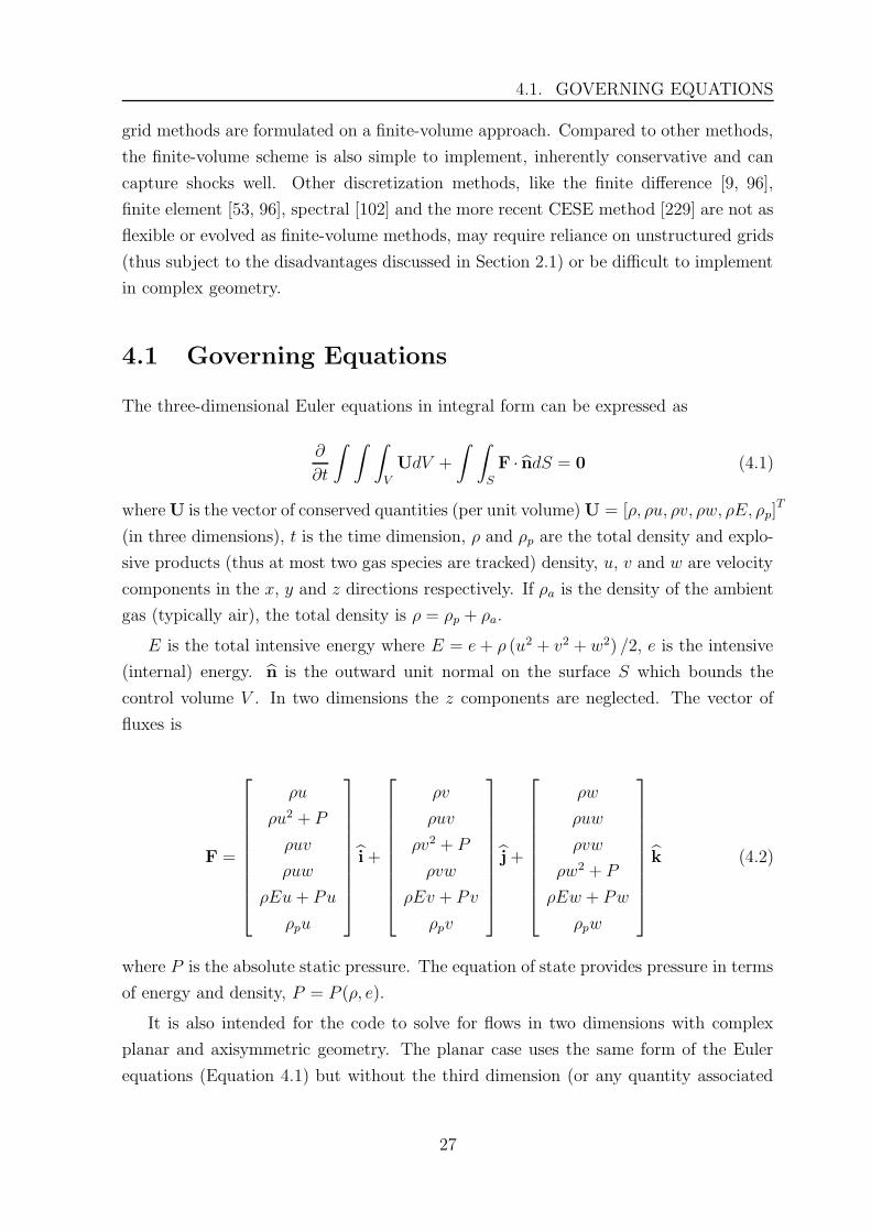
4.1. GOVERNING EQUATIONS
grid methods are formulated on a finite-volume approach. Compared to other methods,
the finite-volume scheme is also simple to implement, inherently conservative and can
capture shocks well. Other discretization methods, like the finite difference [9, 96],
finite element [53, 96], spectral [102] and the more recent CESE method [229] are not as
flexible or evolved as finite-volume methods, may require reliance on unstructured grids
(thus subject to the disadvantages discussed in Section 2.1) or be difficult to implement
in complex geometry.
4.1 Governing Equations
The three-dimensional Euler equations in integral form can be expressed as
∂
∂t
∫ ∫ ∫
V
UdV +
∫ ∫
S
F · ndS = 0 (4.1)
where U is the vector of conserved quantities (per unit volume) U = [ρ, ρu, ρv, ρw, ρE, ρp]T
(in three dimensions), t is the time dimension, ρ and ρp are the total density and explo-
sive products (thus at most two gas species are tracked) density, u, v and w are velocity
components in the x, y and z directions respectively. If ρa is the density of the ambient
gas (typically air), the total density is ρ = ρp + ρa.
E is the total intensive energy where E = e + ρ (u2 + v2 + w2) /2, e is the intensive
(internal) energy. n is the outward unit normal on the surface S which bounds the
control volume V . In two dimensions the z components are neglected. The vector of
fluxes is
F =
ρu
ρu2 + P
ρuv
ρuw
ρEu + Pu
ρpu
i +
ρv
ρuv
ρv2 + P
ρvw
ρEv + Pv
ρpv
j +
ρw
ρuw
ρvw
ρw2 + P
ρEw + Pw
ρpw
k (4.2)
where P is the absolute static pressure. The equation of state provides pressure in terms
of energy and density, P = P (ρ, e).
It is also intended for the code to solve for flows in two dimensions with complex
planar and axisymmetric geometry. The planar case uses the same form of the Euler
equations (Equation 4.1) but without the third dimension (or any quantity associated
27
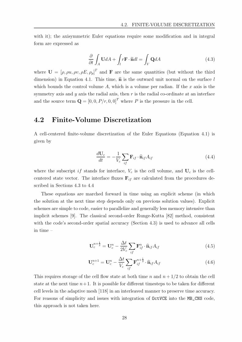
4.2. FINITE-VOLUME DISCRETIZATION
with it); the axisymmetric Euler equations require some modification and in integral
form are expressed as
∂
∂t
∫
A
UdA +
∫
l
rF · ndl =
∫
V
QdA (4.3)
where U = [ρ, ρu, ρv, ρE, ρp]T and F are the same quantities (but without the third
dimension) in Equation 4.1. This time, n is the outward unit normal on the surface l
which bounds the control volume A, which is a volume per radian. If the x axis is the
symmetry axis and y axis the radial axis, then r is the radial co-ordinate at an interface
and the source term Q = [0, 0, P/r, 0, 0]T where P is the pressure in the cell.
4.2 Finite-Volume Discretization
A cell-centered finite-volume discretization of the Euler Equations (Equation 4.1) is
given by
dUc
dt= − 1
Vc
∑
if
Fif · nifAif (4.4)
where the subscript if stands for interface, Vc is the cell volume, and Uc is the cell-
centered state vector. The interface fluxes Fif are calculated from the procedures de-
scribed in Sections 4.3 to 4.4
These equations are marched forward in time using an explicit scheme (in which
the solution at the next time step depends only on previous solution values). Explicit
schemes are simple to code, easier to parallelize and generally less memory intensive than
implicit schemes [9]. The classical second-order Runge-Kutta [82] method, consistent
with the code’s second-order spatial accuracy (Section 4.3) is used to advance all cells
in time –
Un+ 1
2
c = Unc − ∆t
2Vc
∑
if
Fnif · nifAif (4.5)
Un+1c = Un
c − ∆t
Vc
∑
if
Fn+ 1
2
if · nifAif (4.6)
This requires storage of the cell flow state at both time n and n + 1/2 to obtain the cell
state at the next time n+1. It is possible for different timesteps to be taken for different
cell levels in the adaptive mesh [118] in an interleaved manner to preserve time accuracy.
For reasons of simplicity and issues with integration of OctVCE into the MB_CNS code,
this approach is not taken here.
28
4.3. RECONSTRUCTION
To prevent instability in the solution the timestep must be chosen to be smaller than
the minimum time taken for physical processes operating in the solution domain, which
in this case is the crossing of an acoustic wave signal across a cell [62]. A conservative
timestep [50] for each cell c is
∆tc
V=
CFL∑if Aif(a + |u · nif |)
(4.7)
where the CFL number [62] CFL ≤ 1 (typically 0.5), a is the soundspeed in the cell
and u the fluid velocity. Aif is the interface area for a face of the cell, which varies
for Cartesian cells. It is quite conservative, taking into account intersected cells which
might have smaller volumes and interface areas than unobstructed cells, and requires at
least 4 timesteps for a wave to cross an unobstructed cell. The global timestep for the
whole solution with n cells would be
minn
(∆t1, ∆t2, ..., ∆tn)
4.2.1 Axisymmetric VCE Method
For the axisymmetric Euler equations (Equation 4.3), the cell-centered finite-volume
discretization is given by
dUc
dt= − 1
Ac
∑
if
rifFif · nif lif + Q (4.8)
where the volume per radian Ac = Arc, A is the cell area and rc the cell’s average radial
co-ordinate. An axisymmetric extension to VCE has been developed as part of this
thesis [204] and is repeated in Appendix D.
4.3 Reconstruction
In finite-volume methods, the values of the flow variables in the vector of fluxes Fif
in Equation 4.4 are usually interpolated from the cell centre to the cell interface to
establish greater than first order spatial accuracy. The interpolation process is limited
for flows containing strong gradients or discontinuities as it can overshoot, causing high
frequency noise and even instability and failure in the flow solution [97]. In regions with
high gradients the limiter should cause the interpolation to revert to first order and in
regions of smooth flow should allow normal interpolation to proceed.
29
4.3. RECONSTRUCTION
Limiters must satisfy the Total Variation Diminishing (TVD) constraints [14, 97],
which is a minimum requirement for many CFD codes [171]. TVD schemes prohibit the
generation of new extrema, are monotonicity preserving [97] and are generally restricted
to second-order accuracy [14]. However, because TVD schemes suppress noise in solu-
tions, they may sometimes cause of loss of genuine extrema [14, 110]. The process of
interpolation and limiting is termed reconstruction and in this code is multidimensional
in nature [218] as the Cartesian cells are not always aligned with the flow direction.
4.3.1 Interpolation
The most common interpolation procedure is linear interpolation of flow variables ρ, u
and e from the cell centre to cell interfaces, which achieves second-order spatial accuracy.
This requires computation of flow gradients, which can be an expensive step. Gradients
can be computed using the Green-Gauss approach [5, 66, 80] or least squares approach
[5, 20]. Both these approaches require a cloud of neighbouring points (usually values at
nearby cell centres) around the cell centre.
The least squares gradient calculation is chosen due to its reliability and somewhat
easier implementation [5]. This scheme, also detailed in [50], is as follows. For each cell
c, over all its neighbours n (h-refined cells may have more than one neighbour on each
interface), the difference in centroidal co-ordinates is summed and placed in the inverse
(symmetric) reconstruction matrix –
R−1 =
∑n (∆x)2
∑n (∆y∆x)∑n (∆z∆x)
∑n (∆x∆y)
∑n (∆y)2∑n (∆z∆y)
∑n (∆x∆z)
∑n (∆y∆z)∑n (∆z)2
(4.9)
where ∆{ · } = { · }n − { · }c. If two-dimensional flow is simulated the third row and
column of this matrix is ignored. If the gradient of a flow quantity Q is desired, the
3 × 1 vector r is calculated as
r =∑
n
(cn − cc) ((Q)n − (Q)c) (4.10)
where c stands for a cell centroid and subscript c denotes the cell centre. Then the
cell-centered gradient vector of Q would be
∇ (Qc) = Rr (4.11)
The flow quantity Q can now be interpolated to any point p within the cell using the
expression
30
4.3. RECONSTRUCTION
Q (p) = Φ ·∇ (Qc) · (p − cc) (4.12)
Now Φ is a limiter value that ensures no new extrema are created and prevents spuri-
ous oscillations in the numerical solution. It is determined according to the procedure
described in Section 4.3.2.
For reasons of simplicity and efficiency, interpolation to the centre of cell interfaces
is performed and only face-adjacent neighbours are chosen for the reconstruction matrix
(Equation 4.9); neighbours which only share edge or corner connectivity are ignored.
This means that the least squares calculation collapses to one-dimensional differencing
to obtain the gradients for uniform Cartesian cells.
4.3.2 Limiting
Whilst there exist several ways by which the limiter Φ can be determined [218], the
multidimensional min-mod type limiter of Barth [20] is chosen for its simplicity. This
type of limiter is also used in Rose’s Air3d code and has proven to be useful for many
blast simulations [171, 176]. This is a non-differentiable limiter which may hamper
convergence of steady state solutions [218] but is adequate when modelling unsteady
blast waves.
For a flow quantitiy Q and looking over all a cell’s neighbours n, let
Qmin = minn
(Qc, Qn) (4.13)
and
Qmax = maxn
(Qc, Qn) (4.14)
where subscript c denotes the cell-centred value. Then the unlimited value of Q is
interpolated to a point p coinciding with each cell corner j –
Qj = Qc + ∇ (Qc) · (pj − cc) (4.15)
The limiter value for the flow quantity q at cell corner j is thus φQj and is determined
by
φQj =
min(1, Qmax−Qc
Qj−Qc
), if Qj − Qc > 0
min(1, Qmin−Qc
Qj−Qc
), if Qj − Qc < 0
1 , if Qj − Qc = 0
(4.16)
The global limiter (for a cubical cell there are 8 corners) for this cell is finally
Φ = min(φQ
1 , φQ2 , ..., φQ
8
)(4.17)
31
4.4. FLUX SOLVERS
It is possible to have multiple limiters for each flow variable, or a single limiter from the
minimum of each limiters, though it has been found that the extreme gradients at the
start of a explosion simulation will cause the code to fail unless a single limiter is used.
After a while multiple limiters can be used safely.
4.3.3 No Reconstruction for Intersected Cells
Because the VCE method (Section 2.4) does not actually store position vectors of par-
tially obstructed cell interfaces for intersected cells, interpolation cannot be performed to
the wall surface. An averaging procedure, much like in axisymmetric VCE extension of
Section 4.2.1 can be developed to compute the position vectors of the interfaces but this
is difficult and potentially expensive to apply to the wall surface itself in three dimen-
sions. Thus for simplicity and efficiency, no reconstruction is performed at intersected
cells, although the scheme is still globally second-order accurate. This may also be pre-
ferrable since the VCE method can generate spurious noise at surfaces (Section 2.4.4)
which can be damped to an extent by reverting to a first-order scheme there.
4.4 Flux Solvers
Once the flow variables are reconstructed appropriately to the interface, the vector of
fluxes Fif (Equation 4.2) is calculated with a flux solver. The most common flux solvers
are one-dimensional, where the flux convection speed is independent of the tangen-
tial interfacial velocity and fluxes are computed through each interface independently.
This approach has worked well in practice [97, 170] and is adopted here because of its
widespread usage and simplicity. Many flux solvers are upwind schemes which account
for the physically correct manner in which information propagates between cells [199].
Upwind schemes broadly include difference splitting schemes which solve the exact
or approximate Riemann problem [85, 154, 214], vector splitting schemes with the flux
combining of forward and backward vectors [217], kinetic theory based [150] methods
or the very popular Advection Upwind Splitting Method (AUSM) type schemes [221]
which use different splittings for convective and pressure terms. These methods vary in
computational expense and accuracy. Exact Riemann solvers are accurate but expensive,
approximate Riemann solvers are cheaper but require some fixes and suffer from odd-
even decoupling [154], kinetic theory methods are quite dissipative and AUSM-based
methods are fairly cheap, nearly as good as difference splitting schemes, but can have
pressure oscillations.
The main flux solver used in this thesis is the AUSMDV scheme [221]. This scheme
32
4.5. EQUATIONS OF STATE
resolves shock waves accurately without excessive dissipation and is also the solver of
choice in the MB_CNS code [109]. AUSM-based schemes are also less dependent on fluid
thermodynamics, which is useful in this thesis as real gas models can be incorporated
(Section 4.5). It is quite simple to code, fairly efficient, and found to be suitable for
blast propagation problems in the Air3d code [171].
The kinetic theory based Equilibrium Flux Method (EFM) [150] is also implemented.
This flux solver is especially useful at shocks to damp oscillations, which can lead to odd-
even decoupling (in which perturbations at a shock are aphysically amplified, leading
to flow instability) even for the AUSMDV method [110, 154]. An adaptive flux solver
(switching from AUSMDV to EFM at shocks) is also employed by the MB_CNS code
[109]. The AUSMDV and EFM flux solvers are covered in greater detail in Appendix F.
4.5 Equations of State
In the code, the ambient gas (usually initially at atmospheric conditions) is modelled
as an ideal, calorically perfect gas, and the detonation products can be modelled either
as an ideal gas or with the real gas JWL equation of state [127]. Despite the significant
non-ideal effects near the fireball, using an ideal gas for both the explosive products and
ambient gas is computationally faster and adequate for many blast effects problems in
which the main objective is the determination of blast loads [41, 144, 166, 174, 211].
4.5.1 Ideal Gas Equation of State
The ideal gas equation of state is P = P (ρ, e) = ρe(γ − 1) where P is static pressure, ρ
density and e intensive energy, and γ is the ratio of specific heats Cp/Cv. It is assumed
the gas is calorically perfect with constant specific heats and internal energy e = CvT .
Thus the temperature-dependent form is P = P (ρ, T ) = ρRT where the gas constant
R = Cv(γ−1). If there is a mixture of ambient gas and explosion products, the mixture
specific heat is given by the mass fraction-weighted expression Cv = faCv,a+fpCv,p where
fa and fp are the mass fractions of the ambient gas and explosive products, fa = 1− fp.
A similar expression for Cp can be found for the mixture and thus γ for the equation of
state.
4.5.2 JWL Equation of State
The JWL equation of state [127] is a popular real gas equation of state used to model
explosive detonation. It is an empirical equation of state calibrated based on the cylinder
33
4.6. INITIAL CONDITIONS
expansion test and has been extensively used to model other applications of explosives
[146]. Being empirical, it already takes into account (to some extent) afterburning effects
[101]. The JWLB equation of state [17] is a more advanced version which better describes
the gas behaviour in other states not close to adiabatic expansion e.g. if the detonation
products are re-shocked. The JWL equation of state for the explosion products is
Pp = Pp (ρp, ep) = A
(1 − ω
R1v
)e−R1ev + B
(1 − ω
R2v
)e−R2ev + ωρpep (4.18)
where v is the relative volume of the explosion products v = ρ0,p/ρp and ρ0,p is the initial
undetonated density of the explosive. ep is the specific internal energy of the explosive
products, and A, B, R1, R2 and ω are expermentally-determined constants. All these
values (including ρ0,p and ep) can be found in References [126, 127].
A temperature-dependent form has been developed by Baker [17, 18] originally for
the JWLB equation of state, but applicable to the JWL form if the additional JWLB
terms are discounted –
Pp = Pp (ρp, T ) = Ae−R1ev + Be−R2ev + ρpωCv,pT (4.19)
ep = ep (ρp, T ) =A
R1ρ0,p
e−R1ev +B
R2ρ0,p
e−R2ev + Cv,pT (4.20)
The specific heat of the explosion products Cv,p is assumed constant, and is usually a
derived value (from Equation 4.19) if temperature and pressure at a given condition is
known (usually the initial explosive condition, like the Chapman-Jouguet condition).
Mader [133] provides initial detonation temperatures for some explosives. If the JWL
equation of state is used in simulations, a combined JWL-ideal gas equation of state
may be required near the fireball where there is some mixing of detonation products
and ambient gas. The derivation is left to Appendix G and G.1.
4.6 Initial Conditions
In OctVCE the charge or bomb is represented by a group of high pressure and temperature
cells tuned to give the correct blast energy which approximate the charge shape, known
as the ‘balloon analogue’ or ‘isothermal bursting sphere’ model [144, 166, 174, 211]. This
approach has been found to be a simple and adequate initial condition to use for the
mid- to far-field regimes, as the dominant variable affecting the primary shock intensity
is the initial energy released [19, 41, 144, 166, 171, 211]. This approach has produced
34
4.7. BOUNDARY CONDITIONS
very good correlation with experimental TNT blast distance curves from as close as 0.3
m/kg1/3 to the charge [171], even using ideal gas for the charge. Afterburning also affects
the blast intensity [166], and the negative phase and secondary shock are more sensitive
to initial conditions [166], but these effects are not so significant for many realistic blast
loading problems [171, 174].
The initial charge shape can be adjusted, which has an effect on the early blast wave
[40, 211], although a spherical blast wave pattern develops fairly close to the charge
(see Section 1.2). To enable better resolution of the early stages of the explosion on
expensive multi-dimensional meshes, a remapping strategy can be used which maps a
highly resolved one-dimensional spherically symmetric solution to higher dimensions be-
fore the blast passes any surface [104, 171, 174]. This requires some effort to implement,
is inapplicable for non-spherical charges, and may be difficult to perform if geometry is
close to the charge. There is also some loss in resolution when solutions are remapped
to lower resolution meshes. Chapters 10 to 14 explore the accuracy of blast propagation
simulations where remapping is not performed.
4.6.1 Calculating Correct Conditions
To ensure correct blast energy and charge mass, the density of the charge is set to
ρ = m/V where V is the volume of the cells representing the charge and m the charge
mass. The balloon gas intensive energy is equal to the intensive blast energy. The
pressure is then calculated via the equation of state. For the JWL equation of state
(Section 4.5.2), the value ρ0,p can be adjusted to this value of ρ, although this is not
necessary. This is a simplistic use of the JWL equation as no simulation of finite-
rate burning of the explosive material is performed, but this initial condition would
correspond roughly to the final state of the detonation products following a confined
explosion. In axisymmetric geometry, the volume V and mass m are expressed as a
volume and mass per radian respectively. The volume per radian of any axisymmetric
volume V is V/(2π). The mass per radian is obtained using the expression ρV . The
volume per radian of a Cartesian cell is Arc where A is the cell’s area and rc the cell’s
average radial co-ordinate.
4.7 Boundary Conditions
As only rigid structures are considered in this thesis, allowable boundary conditions
are wall and inflow/outflow boundary conditions. All these boundary conditions are
implemented by fabricating appropriate state vector values Ub at a given cell’s interface.
35
4.7. BOUNDARY CONDITIONS
4.7.1 Wall Boundary Condition
Solid surfaces in intersected cells are represented as a cell interface with an outward
normal vector n (see Section 2.4). This wall boundary condition Ub (which is identical
to the symmetry boundary condition) has the same state of flow at the interface but
with a reversed normal velocity component to ensure zero mass flux. Thus if u is the
flow velocity at the cell interface Ub = [ρ, ρ (u − 2 (u · n) n) , ρE, ρp]T .
4.7.2 Inflow/Outflow Boundary Conditions
Inflow/outflow boundary conditions are implemented at the boundaries of the compu-
tational domain where flow is permitted to flow in or out. In the code, individual flow
variables can be set to fixed or extrapolated values. Usually the domain is sufficiently
large to encompass the entire blast environment and the exiting blast typically induces
outflow. If the flow is supersonic, all variables can be extrapolated [9] as characteristics
all point outward.
Problems with boundary specification arise when the outflow is subsonic. For such
cases, non-reflecting boundary conditions might be implemented which attempt to min-
imize boundary effects from influencing the solution within the domain. This topic has
been a subject of much research [61, 216]. Many non-reflecting boundary conditions
involve linearization at the boundary about uniform conditions and setting all incoming
wave amplitudes to zero [61]. Popular non-reflecting boundary conditions are based on
characteristic analysis [61], like the Thompson boundary conditions [209, 210]. These
methods are usually developed (and possibly exact) for one-dimensional problems and
in multidimensions usually prescribe a predominant direction of wave propagation, typ-
ically normal to the boundary. Some reflections will occur for outgoing non-isentropic
or oblique waves [116, 216].
More advanced approaches use buffer zones or absorbing layers near boundaries
where some filtering or numerical damping is usually performed [61, 162]. This can be
done by introducing artificial dissipation, increasing physical viscosity or adding a linear
friction coefficient to the governing equations. The solution would be aphysical in this
region, and more complicated formulations of this damping (typically called Perfectly
Matched Layers) can be implemented which minimize the reflectivity of the absorbing
layer itself [61, 88]. These methods can be ad hoc and involve parameters which require
manual tuning like the buffer zone size.
As many of these methods are computationally expensive and complicated to im-
plement, only Thompson’s [210] non-reflecting boundary conditions are implemented in
OctVCE. This method is simple and proven to be quite robust [61], and performs best
36
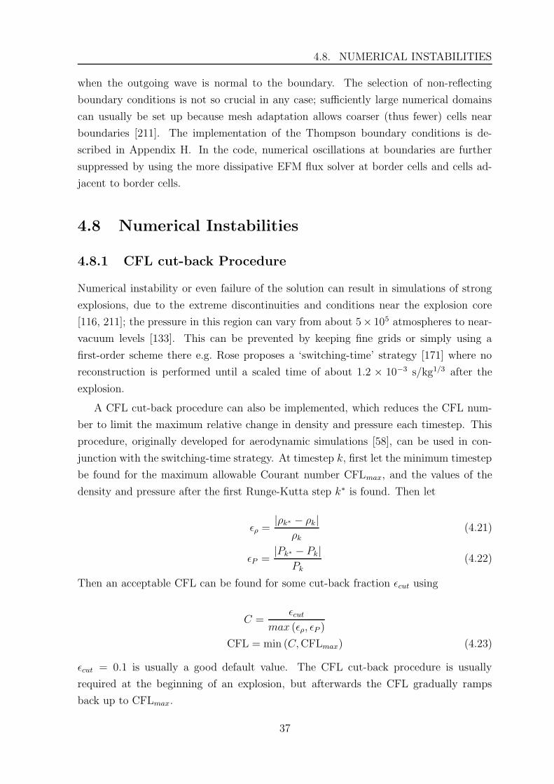
4.8. NUMERICAL INSTABILITIES
when the outgoing wave is normal to the boundary. The selection of non-reflecting
boundary conditions is not so crucial in any case; sufficiently large numerical domains
can usually be set up because mesh adaptation allows coarser (thus fewer) cells near
boundaries [211]. The implementation of the Thompson boundary conditions is de-
scribed in Appendix H. In the code, numerical oscillations at boundaries are further
suppressed by using the more dissipative EFM flux solver at border cells and cells ad-
jacent to border cells.
4.8 Numerical Instabilities
4.8.1 CFL cut-back Procedure
Numerical instability or even failure of the solution can result in simulations of strong
explosions, due to the extreme discontinuities and conditions near the explosion core
[116, 211]; the pressure in this region can vary from about 5× 10⁵ atmospheres to near-
vacuum levels [133]. This can be prevented by keeping fine grids or simply using a
first-order scheme there e.g. Rose proposes a ‘switching-time’ strategy [171] where no
reconstruction is performed until a scaled time of about 1.2 × 10⁻³ s/kg1/3 after the
explosion.
A CFL cut-back procedure can also be implemented, which reduces the CFL num-
ber to limit the maximum relative change in density and pressure each timestep. This
procedure, originally developed for aerodynamic simulations [58], can be used in con-
junction with the switching-time strategy. At timestep k, first let the minimum timestep
be found for the maximum allowable Courant number CFLmax, and the values of the
density and pressure after the first Runge-Kutta step k∗ is found. Then let
ερ =|ρk∗ − ρk|
ρk(4.21)
εP =|Pk∗ − Pk|
Pk(4.22)
Then an acceptable CFL can be found for some cut-back fraction εcut using
C =εcut
max (ερ, εP )
CFL = min (C, CFLmax) (4.23)
εcut = 0.1 is usually a good default value. The CFL cut-back procedure is usually
required at the beginning of an explosion, but afterwards the CFL gradually ramps
back up to CFLmax.
37
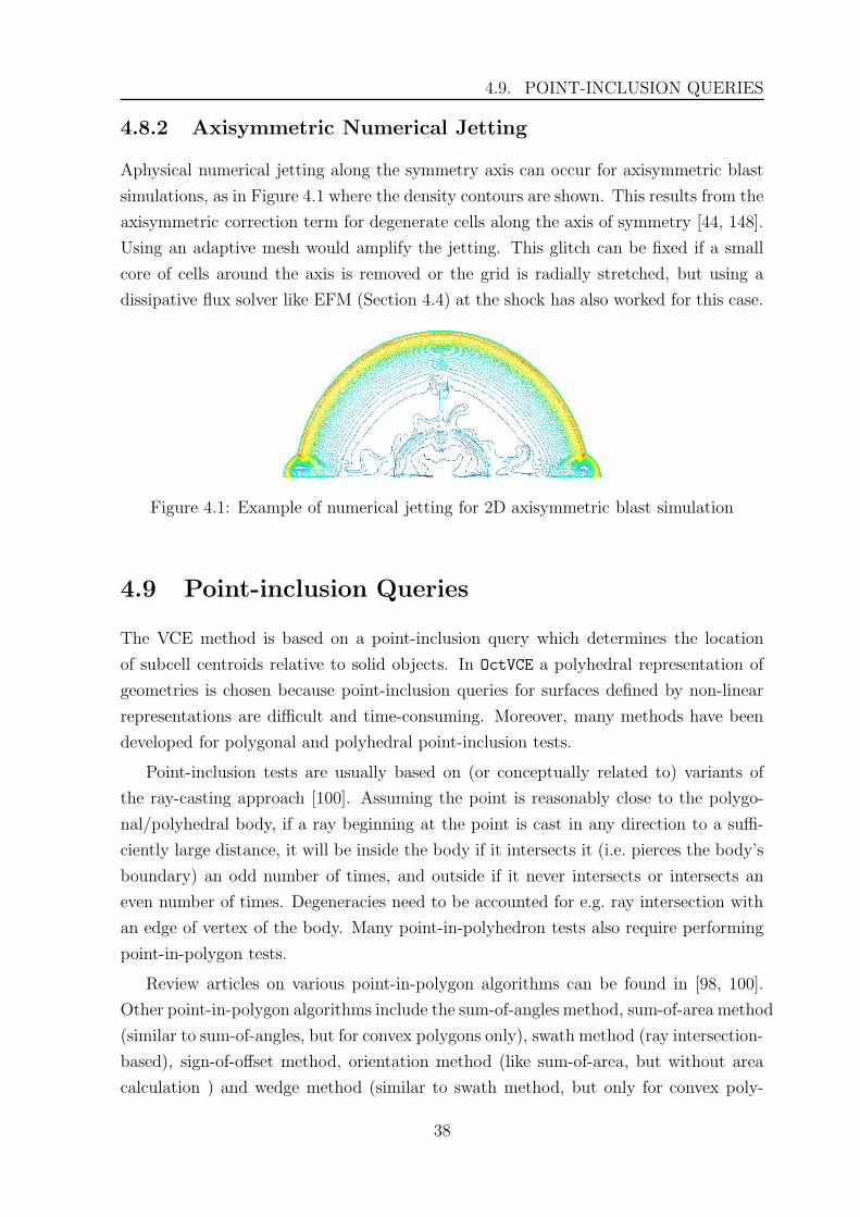
4.9. POINT-INCLUSION QUERIES
4.8.2 Axisymmetric Numerical Jetting
Aphysical numerical jetting along the symmetry axis can occur for axisymmetric blast
simulations, as in Figure 4.1 where the density contours are shown. This results from the
axisymmetric correction term for degenerate cells along the axis of symmetry [44, 148].
Using an adaptive mesh would amplify the jetting. This glitch can be fixed if a small
core of cells around the axis is removed or the grid is radially stretched, but using a
dissipative flux solver like EFM (Section 4.4) at the shock has also worked for this case.
Figure 4.1: Example of numerical jetting for 2D axisymmetric blast simulation
4.9 Point-inclusion Queries
The VCE method is based on a point-inclusion query which determines the location
of subcell centroids relative to solid objects. In OctVCE a polyhedral representation of
geometries is chosen because point-inclusion queries for surfaces defined by non-linear
representations are difficult and time-consuming. Moreover, many methods have been
developed for polygonal and polyhedral point-inclusion tests.
Point-inclusion tests are usually based on (or conceptually related to) variants of
the ray-casting approach [100]. Assuming the point is reasonably close to the polygo-
nal/polyhedral body, if a ray beginning at the point is cast in any direction to a suffi-
ciently large distance, it will be inside the body if it intersects it (i.e. pierces the body’s
boundary) an odd number of times, and outside if it never intersects or intersects an
even number of times. Degeneracies need to be accounted for e.g. ray intersection with
an edge of vertex of the body. Many point-in-polyhedron tests also require performing
point-in-polygon tests.
Review articles on various point-in-polygon algorithms can be found in [98, 100].
Other point-in-polygon algorithms include the sum-of-angles method, sum-of-area method
(similar to sum-of-angles, but for convex polygons only), swath method (ray intersection-
based), sign-of-offset method, orientation method (like sum-of-area, but without area
calculation ) and wedge method (similar to swath method, but only for convex poly-
38
4.9. POINT-INCLUSION QUERIES
gons). Generally those methods that are based on routine computation of trigonometric
quantities are less efficient, which is why the ray casting method is still a popular and
efficient method [130, 223].
There have also been numerous point-in-polyhedron algorithms developed [75, 99,
111], which can vary in complexity. Many methods reduce dimensionality of the prob-
lem by projecting planar images of the polyhedral facets along with an image of the
point being tested. This thesis implements the simple polyhedral point-inclusion test
by Linhart [130] which is also a ray intersection-based projection method. Degeneracies
are resolved by associating with each point of intersection a certain positive or negative
weight. Linhart’s method is also applicable for the point-in-polygon test, which needs
to be performed for polyhedron queries. This method is described in Appendix J.
39
Chapter 5
Parallel Computing
Simulating blast propagation in three dimensions can involve large meshes, which usually
mean long execution times. More computing power can be achieved if processors are
combined in parallel to solve a single problem. Another motivation for parallel solutions
is the increased memory resources of a multi-processor system, which might be necessary
for large simulations.
Ideally the parallelization strategy should be fairly portable and scale proportionally
with the number of processors. However parallel computing methods can be complicated
to implement, as can determining the theoretical code performance [95]. As most of the
computing time is usually spent in a relatively small portion of the code [147], the
optimal parallelization method requires insight into the underlying algorithms. Scaling
to more processors usually results in scaling in memory resources which can have an
adverse effect on performance; efficient use of memory is also an important consideration
for parallel solutions.
The most common way of solution parallelization in CFD problems is through do-
main decomposition, where the same code is executed on different sections of the nu-
merical domain. A brief survey of popular domain decomposition methods will be given
in Section 5.1. Section 5.2 outlines parallel computing architectures, and Sections 5.3
and 5.4 respectively discuss parallel programming methods and parallel performance
measures. Finally Section 5.5 describes the shared-memory parallelization strategy for
the OctVCE code in particular.
5.1 Domain Decomposition Methods
Domain decomposition is a challenging problem which involves partitioning the mesh
and assigning each portion to a separate processor. Twin goals are achieving a good
load balance (equal amount of computational work per processor) and minimizing the
edge-cut or interprocessor communication. This is a large field of research, and jour-
nals devoted to domain decomposition methods and other aspects of parallel computing
include Concurrency, Journal of Parallel and Distributed Computing and Parallel Com-
puting. A number of review articles have also been written [69, 215]. In many cases,
different methods perform best for different problems [215].
40
5.1. DOMAIN DECOMPOSITION METHODS
A number of methods varying in sophistication have been developed. One of the more
simple and popular methods is the recursive co-ordinate bisection method [187, 215] and
its variations. This method performs well for small numbers of processors [215] (eight
or less) and when the mesh is evenly spread over a simple domain [69]. It basically
partitions the domain according to the co-ordinates of the verticies perpendicular to
the co-ordinate direction to achieve an equal load on either side of the cut [215]. This
process is repeated recursively on each subdomain until the required number of subdo-
mains is obtained. This method can generate decompositions efficiently [69] but does
not minimize the edge-cut as well as other methods. The edge-cut is important for
distributed-memory parallelism because it determines the amount of communication
required between processors.
Other methods involve mapping the mesh into an octree structure and basing the
partition on the octree representation [76]. Recursive bisection can also be applied to
this representation [135]. Octree partitioning involves traversals of the tree structure to
accumulate octants or subtrees into successive partitions. Like the recursive bisection
method, it is incremental in its dynamic load balancing; small changes in the mesh
(through mesh adaptation) produce small changes in the partitions, resulting in little
migration or data movement between processors. This is an important goal of iterative
dynamic load balancing techniques [219] as overheads involved with moving application
data can be high [69].
Other more complicated methods are graph-based, like the recursive spectral (or
eigenvalue) [187], multilevel [91] or diffusive [63] methods. These methods often produce
the best quality partitions for mesh-based partial differential equation simulations [69].
The mesh is seen as a graph where verticies represent data to be partitioned. The goal of
graph partitioning is to assign equal total vertex weight to partitions while minimizing
the weight of cut edges [69]. Well known mesh partitioning tools include METIS [114,
115] and JOSTLE [222] which use multilevel iterative partitioning algorithms. These
libraries are very sophisticated, can be implemented in parallel and seek to minimize
data redistribution times during dynamic load balancing.
Another popular mesh partitioning method is the space-filling curve (SFC) method
[69, 149]. This approach maps the multi-dimensional data to one dimension along the
SFC. An object’s co-ordinates are converted to a key representing its position along the
SFC through a physical domain; sorting the keys orders the objects which are assigned
into weighted pieces for each processor [69]. Like recursive bisection methods, SFC
methods generally incur higher communication costs than graph partitioners, but these
methods are also dynamically incremental.
41
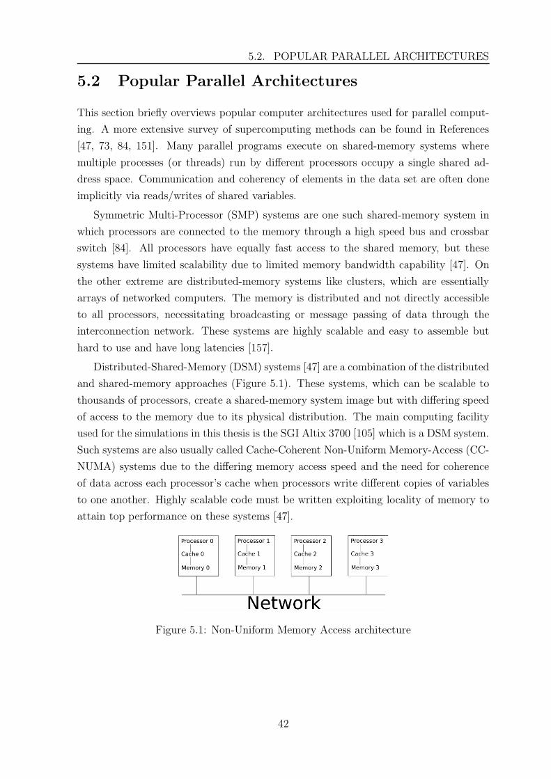
5.2. POPULAR PARALLEL ARCHITECTURES
5.2 Popular Parallel Architectures
This section briefly overviews popular computer architectures used for parallel comput-
ing. A more extensive survey of supercomputing methods can be found in References
[47, 73, 84, 151]. Many parallel programs execute on shared-memory systems where
multiple processes (or threads) run by different processors occupy a single shared ad-
dress space. Communication and coherency of elements in the data set are often done
implicitly via reads/writes of shared variables.
Symmetric Multi-Processor (SMP) systems are one such shared-memory system in
which processors are connected to the memory through a high speed bus and crossbar
switch [84]. All processors have equally fast access to the shared memory, but these
systems have limited scalability due to limited memory bandwidth capability [47]. On
the other extreme are distributed-memory systems like clusters, which are essentially
arrays of networked computers. The memory is distributed and not directly accessible
to all processors, necessitating broadcasting or message passing of data through the
interconnection network. These systems are highly scalable and easy to assemble but
hard to use and have long latencies [157].
Distributed-Shared-Memory (DSM) systems [47] are a combination of the distributed
and shared-memory approaches (Figure 5.1). These systems, which can be scalable to
thousands of processors, create a shared-memory system image but with differing speed
of access to the memory due to its physical distribution. The main computing facility
used for the simulations in this thesis is the SGI Altix 3700 [105] which is a DSM system.
Such systems are also usually called Cache-Coherent Non-Uniform Memory-Access (CC-
NUMA) systems due to the differing memory access speed and the need for coherence
of data across each processor’s cache when processors write different copies of variables
to one another. Highly scalable code must be written exploiting locality of memory to
attain top performance on these systems [47].
Figure 5.1: Non-Uniform Memory Access architecture
42
5.3. PARALLEL PROGRAMMING
5.3 Parallel Programming
The Message Passing Interface (MPI) standard [87, 112, 151] and the OpenMP standard
[34, 47, 112, 151] are popular application programming interfaces for explicit paralleliza-
tion (where the user controls the parallelization) on distributed and shared-memory
systems respectively. They consist of a set of compiler directives, library functions and
environment variables. In MPI, processes can communicate with other processes by
sending and receiving messages. The parallel implementation using OpenMP of the
OctVCE code is discussed in greater detail in Section 5.5, but OpenMP will be described
in some more detail below.
An advantage with OpenMP (and shared-memory parallel programming in general)
is its ability to support incremental parallelism where an application can be parallelized
in stages and usually require little modification to the source code [47, 151]. Parallel
regions like loops are specified through the use of compiler directives which can be
ignored when the code is executed in serial. It uses a fork/join model of parallelism
where a master thread (or process) is forked into a team of threads of execution when a
parallel construct is created, and the threads synchronized and joined again at the end
of the section. However due to limited floating-point representations, operations like
reductions may not yield precisely the same result in parallel as those in serial [47].
Each thread usually corresponds to a processor and executes within the same shared
address space as the serial program, but it can have its own stack and copy of the vari-
ables. Co-ordination of the threads is important (under both shared and distributed-
memory models) when they access shared variables as they may simultaneously mod-
ify/read the same variable, resulting in a race condition and incorrect values of the
variables. Race conditions can be removed by restructuring the code or using explicit
synchronization of threads (a point where each thread must wait for all others to arrive).
Synchronizations require communication between threads, and along with their forking
and joining can have high overhead [28, 47].
5.4 Parallel Performance Measures
In most parallel applications the speedup scales less than linearly with the number of
processors because some portions of the code have not been parallelized and there are
additional overheads like communication time, thread-related overheads like barriers
and syncrhonization and load balancing [47]. Amdahl’s law [8] is a simple but useful
formula that sets limits on the speedup. Let the inherently serial portion of the code be
σ(n) and φ(n) the parallel portion of the code for problem size n. Assuming the serial
43
5.4. PARALLEL PERFORMANCE MEASURES
percentage of the code ε = σ(n)σ(n)+φ(n)
, and remaining percentage 1− ε can be parallelized,
and neglecting other overheads like memory contention, latencies etc. Amdahl’s law
states
Sp ≤1
ε + 1−εp
(5.1)
where Sp is the maximum speedup and p is the number of processors. This expression
shows the large effect of even a small serial portion in the code; even if 90% of the code
can be parallelized, the speedup will be no larger than 4.7 for an 8 processor simulation.
This derivation assumes ε is independent of the problem size, but it has been observed
occasionally that on some cache-friendly codes ε decreases as a function of problem
size [73, 112], increasing the upper bound on Sp. This can sometimes lead to linear
speedup, and superlinear speedup (Sp > p) can be occasionally observed, although this
is usually due to poor memory access or cache mismanagement on a single processor.
Amdahl’s law ignores parallel overheads, which can be large, especially for memory-
intensive applications due to more communication time [73]. A more realistic limit to
the speedup thus requires knowledge of the overhead time, which can be difficult to
ascertain. However, usually time spent in overhead has lower complexity than time
spent in execution (the Amdahl effect [151]).
The inverse of Amdahl’s law can be used to estimate the experimentally determined
serial fraction of a code (serial portion plus parallel overhead) when it is run on p
processors. This is a very useful formula and is often termed the Karp-Flatt metric [113],
which states that given a parallel computation exhibiting speedup Sp on p processors
where p > 1, the experimentally determined serial fraction e is
e =1/Sp − 1/p
1 − 1/p(5.2)
Now e = (σ(n) + to) / (σ(n) + φ(n)) where to is the overhead time. This e would be an
upper bound to the actual serial code fraction, and if the same simulation is performed
in parallel for increasing number of processors p, an increasing e can give an indication
of the magnitude and increase of parallel overhead. Alternatively, it might be possible
to extrapolate the e versus p graph back to a 1 processor result to estimate the true
serial fraction ε. More discussion on the Karp-Flatt metric is also found in Section 7.3
where it is also used to profile the parallel performance of the code.
44
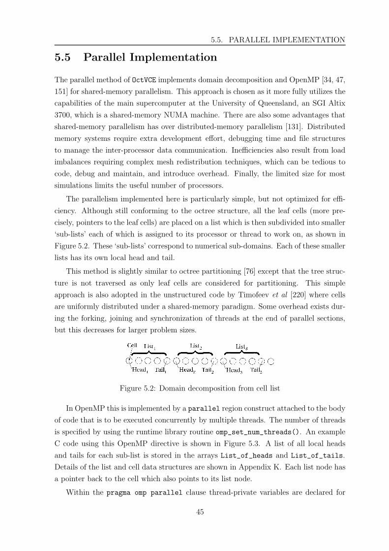
5.5. PARALLEL IMPLEMENTATION
5.5 Parallel Implementation
The parallel method of OctVCE implements domain decomposition and OpenMP [34, 47,
151] for shared-memory parallelism. This approach is chosen as it more fully utilizes the
capabilities of the main supercomputer at the University of Queensland, an SGI Altix
3700, which is a shared-memory NUMA machine. There are also some advantages that
shared-memory parallelism has over distributed-memory parallelism [131]. Distributed
memory systems require extra development effort, debugging time and file structures
to manage the inter-processor data communication. Inefficiencies also result from load
imbalances requiring complex mesh redistribution techniques, which can be tedious to
code, debug and maintain, and introduce overhead. Finally, the limited size for most
simulations limits the useful number of processors.
The parallelism implemented here is particularly simple, but not optimized for effi-
ciency. Although still conforming to the octree structure, all the leaf cells (more pre-
cisely, pointers to the leaf cells) are placed on a list which is then subdivided into smaller
‘sub-lists’ each of which is assigned to its processor or thread to work on, as shown in
Figure 5.2. These ‘sub-lists’ correspond to numerical sub-domains. Each of these smaller
lists has its own local head and tail.
This method is slightly similar to octree partitioning [76] except that the tree struc-
ture is not traversed as only leaf cells are considered for partitioning. This simple
approach is also adopted in the unstructured code by Timofeev et al [220] where cells
are uniformly distributed under a shared-memory paradigm. Some overhead exists dur-
ing the forking, joining and synchronization of threads at the end of parallel sections,
but this decreases for larger problem sizes.
Figure 5.2: Domain decomposition from cell list
In OpenMP this is implemented by a parallel region construct attached to the body
of code that is to be executed concurrently by multiple threads. The number of threads
is specified by using the runtime library routine omp_set_num_threads(). An example
C code using this OpenMP directive is shown in Figure 5.3. A list of all local heads
and tails for each sub-list is stored in the arrays List_of_heads and List_of_tails.
Details of the list and cell data structures are shown in Appendix K. Each list node has
a pointer back to the cell which also points to its list node.
Within the pragma omp parallel clause thread-private variables are declared for
45
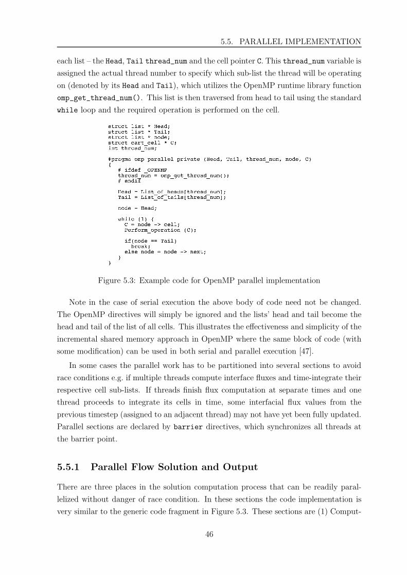
5.5. PARALLEL IMPLEMENTATION
each list – the Head, Tail thread_num and the cell pointer C. This thread_num variable is
assigned the actual thread number to specify which sub-list the thread will be operating
on (denoted by its Head and Tail), which utilizes the OpenMP runtime library function
omp_get_thread_num(). This list is then traversed from head to tail using the standard
while loop and the required operation is performed on the cell.
Figure 5.3: Example code for OpenMP parallel implementation
Note in the case of serial execution the above body of code need not be changed.
The OpenMP directives will simply be ignored and the lists’ head and tail become the
head and tail of the list of all cells. This illustrates the effectiveness and simplicity of the
incremental shared memory approach in OpenMP where the same block of code (with
some modification) can be used in both serial and parallel execution [47].
In some cases the parallel work has to be partitioned into several sections to avoid
race conditions e.g. if multiple threads compute interface fluxes and time-integrate their
respective cell sub-lists. If threads finish flux computation at separate times and one
thread proceeds to integrate its cells in time, some interfacial flux values from the
previous timestep (assigned to an adjacent thread) may not have yet been fully updated.
Parallel sections are declared by barrier directives, which synchronizes all threads at
the barrier point.
5.5.1 Parallel Flow Solution and Output
There are three places in the solution computation process that can be readily paral-
lelized without danger of race condition. In these sections the code implementation is
very similar to the generic code fragment in Figure 5.3. These sections are (1) Comput-
46
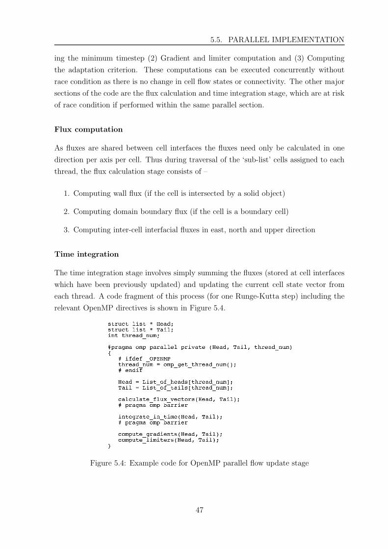
5.5. PARALLEL IMPLEMENTATION
ing the minimum timestep (2) Gradient and limiter computation and (3) Computing
the adaptation criterion. These computations can be executed concurrently without
race condition as there is no change in cell flow states or connectivity. The other major
sections of the code are the flux calculation and time integration stage, which are at risk
of race condition if performed within the same parallel section.
Flux computation
As fluxes are shared between cell interfaces the fluxes need only be calculated in one
direction per axis per cell. Thus during traversal of the ‘sub-list’ cells assigned to each
thread, the flux calculation stage consists of –
1. Computing wall flux (if the cell is intersected by a solid object)
2. Computing domain boundary flux (if the cell is a boundary cell)
3. Computing inter-cell interfacial fluxes in east, north and upper direction
Time integration
The time integration stage involves simply summing the fluxes (stored at cell interfaces
which have been previously updated) and updating the current cell state vector from
each thread. A code fragment of this process (for one Runge-Kutta step) including the
relevant OpenMP directives is shown in Figure 5.4.
Figure 5.4: Example code for OpenMP parallel flow update stage
47
5.5. PARALLEL IMPLEMENTATION
Solution output
The parallel solution output methodology depends on the file format required by the
grid visualizer. In this case the VTK file format is used [15] where a unique listing of cell
verticies also need to be output. The necessitated the use of the vertex data structure
(shown in Appendix K) which stores pointers to all leaf cells sharing the vertex (and
which is also pointed to by these cells). The verticies are stored in a global list and are
uniquely numbered for each cell sub-domain in which they reside. All verticies belonging
to the sub-domain are first written into the corresponding file. As each cell in the sub-
domain also points to these numbered verticies the mesh connectivity information for
them is then written as the code traverses each sub-list. Finally the required flow
quantities are reconstructed to each vertex, averaged and written.
5.5.2 Parallel Mesh Adaptation
The mesh adaptation process requires significant ‘house-keeping’ code to manage the
changing grid e.g. updating intefacial and vertex connectivities, flux vectors etc. Im-
plementing this in parallel requires even more code, and additional measures must be
adopted to avoid race conditions. Thus it is more difficult to straightforwardly use the
same serial adaptation code. Race conditions will exist as cell connectivity might be
read and written to concurrently.
That the cell merging process is performed in serial for simplicity as it may potentially
require cells from across separate domains. Any cells that require adaptation are no
longer members of the large merged cell cluster, and only after adaptation will cell
merging proceed for remaining small cells and newly adapted cells. This section gives
an overview of the parallel mesh adaptation process.
Adding cells to sub-lists in parallel
With the addition or deletion of cells in each sub-domain (or sub-list), the newly formed
children cells or parent cell are inserted into the sub-list at the location where the original
parent or children cells were respectively. This is done to ensure sub-domains attain a
measure of contiguity which would not occur if new cells are placed at the front or back
of the list. Given the cell numbering scheme, in some cases sub-domains will only be
diagonally contiguous and can occasionally be spatially separated.
After adaptation these sub-lists are all joined into the global list of cells which is
repartitioned to yield an equal number of cells for each sub-domain. This is done via
a simple counting technique. An example of the numerical sub-domains for the blast
48
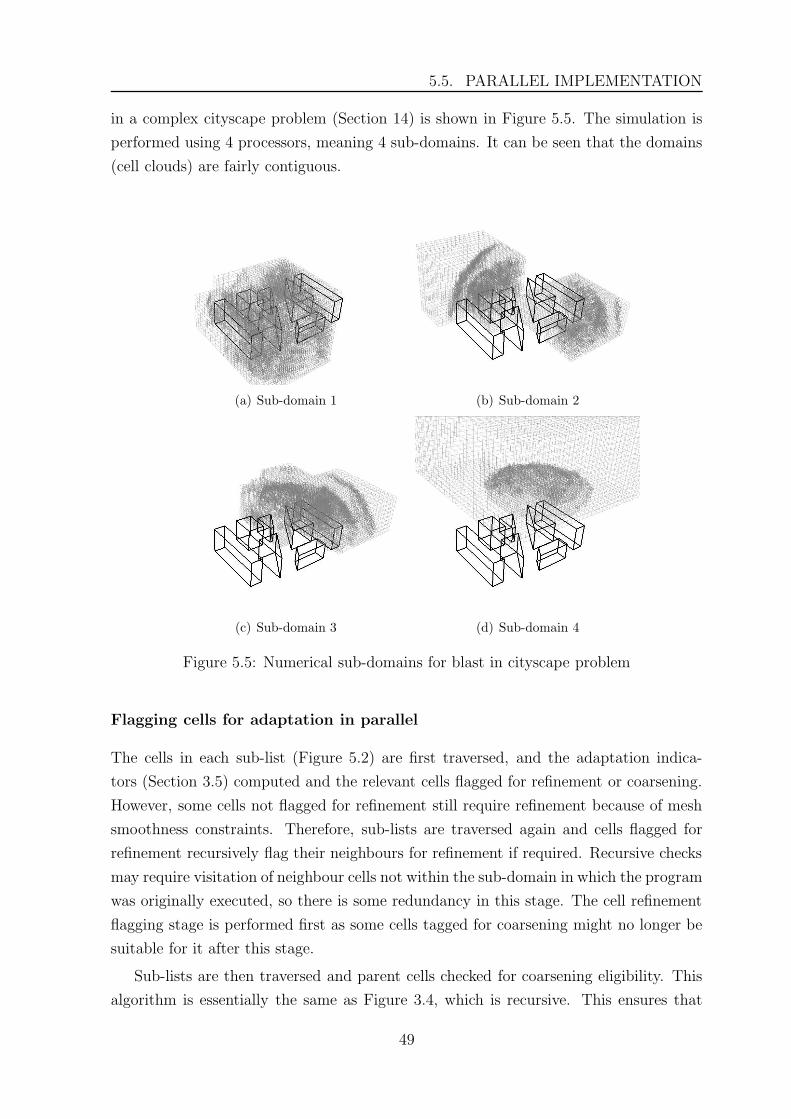
5.5. PARALLEL IMPLEMENTATION
in a complex cityscape problem (Section 14) is shown in Figure 5.5. The simulation is
performed using 4 processors, meaning 4 sub-domains. It can be seen that the domains
(cell clouds) are fairly contiguous.
(a) Sub-domain 1 (b) Sub-domain 2
(c) Sub-domain 3 (d) Sub-domain 4
Figure 5.5: Numerical sub-domains for blast in cityscape problem
Flagging cells for adaptation in parallel
The cells in each sub-list (Figure 5.2) are first traversed, and the adaptation indica-
tors (Section 3.5) computed and the relevant cells flagged for refinement or coarsening.
However, some cells not flagged for refinement still require refinement because of mesh
smoothness constraints. Therefore, sub-lists are traversed again and cells flagged for
refinement recursively flag their neighbours for refinement if required. Recursive checks
may require visitation of neighbour cells not within the sub-domain in which the program
was originally executed, so there is some redundancy in this stage. The cell refinement
flagging stage is performed first as some cells tagged for coarsening might no longer be
suitable for it after this stage.
Sub-lists are then traversed and parent cells checked for coarsening eligibility. This
algorithm is essentially the same as Figure 3.4, which is recursive. This ensures that
49
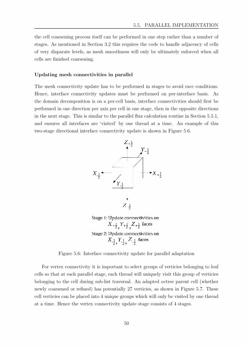
5.5. PARALLEL IMPLEMENTATION
the cell coarsening process itself can be performed in one step rather than a number of
stages. As mentioned in Section 3.2 this requires the code to handle adjacency of cells
of very disparate levels, as mesh smoothness will only be ultimately enforced when all
cells are finished coarsening.
Updating mesh connectivities in parallel
The mesh connectivity update has to be performed in stages to avoid race conditions.
Hence, interface connectivity updates must be performed on per-interface basis. As
the domain decomposition is on a per-cell basis, interface connectivities should first be
performed in one direction per axis per cell in one stage, then in the opposite directions
in the next stage. This is similar to the parallel flux calculation routine in Section 5.5.1,
and ensures all interfaces are ‘visited’ by one thread at a time. An example of this
two-stage directional interface connectivity update is shown in Figure 5.6.
Figure 5.6: Interface connectivity update for parallel adaptation
For vertex connectivity it is important to select groups of verticies belonging to leaf
cells so that at each parallel stage, each thread will uniquely visit this group of verticies
belonging to the cell during sub-list traversal. An adapted octree parent cell (whether
newly coarsened or refined) has potentially 27 verticies, as shown in Figure 5.7. These
cell verticies can be placed into 4 unique groups which will only be visited by one thread
at a time. Hence the vertex connectivity update stage consists of 4 stages.
50

5.5. PARALLEL IMPLEMENTATION
Figure 5.7: Vertex groups for parallel adaptation
Parallel refinement stages
Given the necessary steps for parallel connectivity update, the parallel refinement stages
are enumerated below. Each of these stages end in a synchronization barrier.
1. Allocate memory to children cells and set their state vectors accordingly
2. Update interface connectivities in east, north, upper directions, and vertex con-
nectivities for group 1 verticies (from Figure 5.7)
3. Update interface connectivities in west, south, lower directions, and vertex con-
nectivities for group 2 verticies
4. Update vertex connectivities for group 3 verticies (Figure 5.7)
5. Update vertex connectivities for group 4 verticies
Parallel coarsening stages
Similar to (but performed after) the refinement stage, the parallel coarsening stages are
enumerated below. Each of these stages end in a synchronization barrier. Also, sub-lists
are slightly modified prior to this step so that sibling leaf cells are not spread across
different sub-lists.
1. Set parent state vector, update interface connectivities in east, north and upper
directions, and vertex connectivities for group 1 verticies (from Figure 5.7)
51
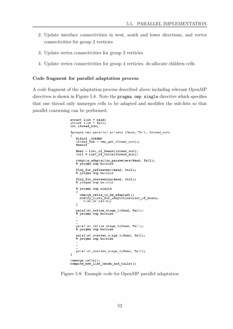
5.5. PARALLEL IMPLEMENTATION
2. Update interface connectivities in west, south and lower directions, and vertex
connectivities for group 2 verticies
3. Update vertex connectivities for group 3 verticies
4. Update vertex connectivities for group 4 verticies, de-allocate children cells
Code fragment for parallel adaptation process
A code fragment of the adaptation process described above including relevant OpenMP
directives is shown in Figure 5.8. Note the pragma omp single directive which specifies
that one thread only unmerges cells to be adapted and modifies the sub-lists so that
parallel coarsening can be performed.
Figure 5.8: Example code for OpenMP parallel adaptation
52
5.5. PARALLEL IMPLEMENTATION
5.5.3 Problems with the Parallel Method
On NUMA machines like the SGI Altix, locality of data is important for good per-
formance [47]. Recalling the discussion in Section 5.2, NUMA systems have a shared-
memory address space to all processors but memory access times are substantially faster
if a data element is on a node’s cache or in nearby memory. A well-structured code ex-
ploits locality so that the majority of requests are to data residing on a node’s local
memory and thus the majority of references are cache hits. Communication overheads
for referencing memory not connected to the node can be quite high1, as much as 20-50%.
The parallel adaptation method does allocate cells to reside on the local memory of
each node of the cpuset. If the adaptation process were not parallelized there would be a
less uniform distribution of data across nodes, leading to increased communication over-
head. This also means a smaller parallel code fraction, further limiting the theoretical
speedup from Amdahl’s law (Equation 5.1). However, the mesh repartitioning strat-
egy implemented via simple cell counting does not always lead to good locality as it is
problem-depedent; some sub-domains may undergo more refinement and cells allocated
by one thread may be assigned to remote threads that will need frequent access to the
data. A further complication is thread migration from processor to processor, leading
to a higher degree of remote access. The dplace command can help tie threads to pro-
cessors, and the numactl command allows interleaved (round-robin) memory allocation
to prevent bottlenecks. These will only partly increase efficiency.
The code also makes significant storage demands (see Appendix K for the cell data
structure), requiring at a minimum 988 bytes per cell, and a nominal operational storage
of 3 kB per cell (which includes other data structures like lists and pointers). This leads
to performance inefficiencies with more cache misses and longer communication time.
In some cases cpusets consisting of several nodes needed to be requested just for the
memory, even if a single processor simulation was performed.
The parallel method relies on partitioning parallel sections into several stages via
synchronization barriers, which can be quite expensive [47] and cause the parallelism to
become somewhat fine-grained and thus inefficient. Sections 10.4.1, 14.2 and 7.3 display
parallel performance statistics of the code for different simulations. They indicate that
considerable overhead does exist for parallel simulations, but this occurs mainly from
communication and not barrier overheads. The results encouragingly suggest a fairly
high parallel fraction of the code. OctVCE is likely to perform better on SMP systems but
this has not been investigated. Further work would focus on reducing storage and using
a more effective domain decomposition method exploiting locality on NUMA machines.
1http://nf.apac.edu.au/facilities/userguide/, accessed June 2008
53
Chapter 6
Verification and Validation
To establish the credibility of the OctVCE code it must be verified and validated for a
range of test cases. Verification is generally understood to be the activity of establish-
ing the reliability and accuracy of the numerical methodology i.e. solving the equations
right [168, 169]. It typically involves evaluating the discretization error against a known
solution (typically analytic) and establishing the order of accuracy through a grid con-
vergence study. Validation, which is usually done after verification, is demonstrating
how well the mathematical model actually represents the physical system i.e. solving
the right equations [168].
Verification can help demonstrate the stability and robustness of the numerical
scheme and provide good confidence that no programming errors in the code exist
[142, 180], although it cannot identify errors that result in a loss of efficiency [168].
The test cases used in the verification process, having generally analytic solutions, are
usually geometrically simple and not related to problems that the code is normally de-
signed for (in this case blast propagation), and the observed order of accuracy can be
problem-specific [168] and influenced to an extent by boundary conditions [142]. For
CFD problems, verification test cases usually involve smooth flows as analytic solutions
for shocked flows are rare or do not exercise all terms in the numerical scheme.
Validation test cases are typically those problems for which the code is designed,
and usually involve comparison to experimental or previously verified numerical data
[169]. Better confidence in the code’s predictive ability for such problems will be gen-
erally established if a larger number and varied range of such test cases are chosen. In
simulations of validation cases and other complex problems a popular method of esti-
mating the error is through Richardson extrapolation [163, 164], which is a technique
for combining solutions from two different grids to give a more accurate estimate for the
exact solution. If f1 is the fine-grid solution and f2 the coarser-grid solution, the exact
(grid-independent) result can be estimated as
fexact = f1 +f1 − f2
rp − 1(6.1)
where r is the refinement factor (which would be 2 if the grid is doubled in each direction)
and p the order of accuracy. This equation is generally p + 1-order accurate for upwind
54
methods [168]. The estimated fractional error to the fine grid solution is thus
E = (f1 − f2) / (f1 (rp − 1)) (6.2)
which is usually a good approximation if E << 1.
Richardson extrapolation may not consistenly work in some situations and is gen-
erally used with caution at those places where the solution is not smooth e.g. peak
overpressure at a shock and in the presence of non-linear flux limiters [168]. It can also
be difficult to determine a value of r for non-uniformly refined meshes [167]. A con-
sistently decreasing value of E (as grids are refined) demonstrates a convergence (the
asymptotic range of solution convergence having been attained) and thus at least three
differently-refined grids need to be employed to ascertain asymptoticity. The quantity
GCI = 3 |E| (6.3)
is the Grid Convergence Index (GCI) proprosed by Roache [168, 179] which provides an
error band where a safety factor of 3 (and the absolute value) is used for conservatism.
If the observed order of accuracy matches the formal order (typically for fine-grid solu-
tions), the safety factor can be reduced to 1.25.
Sections 6.1 to 6.4 of this chapter present four different verification test cases. In
Chapters 7 to 14, a number of different validation test cases will be presented. Not all
of these are blast propagation problems from charge detonations; some (like Chapters 7
and 8) are more mundane shock propagation problems to demonstrate the versatility
and accuracy of the VCE method for different flow problems. As mesh-convergent solu-
tions can be quite difficult to obtain, especially for three-dimensional blast propagation
problems [171], many of these validation cases will use Richardson extrapolation to test
for convergence trends and estimate the magnitude and sign of errors. Profiling of the
code will also be done for some simulations to establish its performance in serial and
parallel executions.
55
6.1. VERIFICATION VIA THE METHOD OF MANUFACTURED SOLUTIONS
6.1 Verification via the Method of Manufactured
Solutions
The first verification exercise uses the Method of Manufactured Solutions, which is a
general and quite robust verification methodology that allows all terms in the governing
equations to be exercised [142, 168, 180]. An analytic solution is chosen (or ‘manu-
factured’) and passed through the flow equations, generating source terms as a result.
These source terms are input into the solution procedure and compared with the an-
alytic solution for code verification. This process is repeated on a series of uniformly
refined grids to obtain an order of accuracy.
The analytic solution bears no relation to any physical problem but is simply used for
verification purposes. It requires the code to specify arbitrary source terms and bound-
ary conditions, which can be difficult to implement [83]. Guidelines for appropriate
choice of manufactured solutions include generality (so that all terms can be exercised),
smoothness, ensuring no derivatives vanish, and ensuring no predominance of any one
particular term in the governing equations [180]. This method cannot be used to detect
code deficiencies affecting efficiency or robustness; its only purpose is to highlight any
spatial discretization errors. Also, it relies on uniform refinement of the grid to properly
obtain the order of accuracy.
The global discretization error for all mesh points can be given by the L2 or ‘root
mean square’ norm –
L2 =
(∑Nn=1 |Qnum,n − Qexact,n|
N
) 1
2
(6.4)
where N is the total number of cells, Qnum is the computed solution (e.g. in density
or energy) and Qexact the exact solution. The order of accuracy p calculated from two
mesh levels k and k + 1 is then
p = ln
(Lk+1
Lk
)/ln (r) (6.5)
Alternatively, if a series of L2 norms are obtained for several different mesh levels, p can
be obtained by a power-law fit (in the form of L = c1 + c2rp, c1 and c2 being constants)
to the curve in the L2 versus r graph (c1 should be theoretically zero). The observed
order of accuracy is compared with the formal order of accuracy, which for the code is
p = 2 due to implementation of reconstruction (Section 4.3).
56
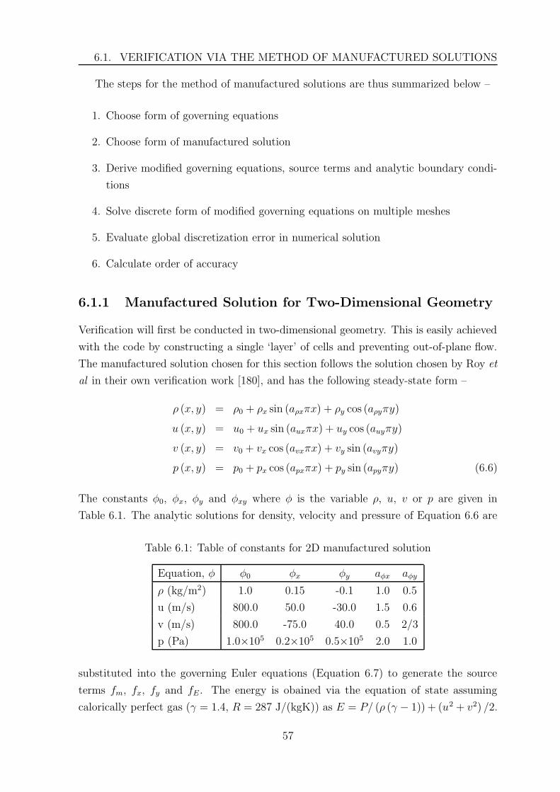
6.1. VERIFICATION VIA THE METHOD OF MANUFACTURED SOLUTIONS
The steps for the method of manufactured solutions are thus summarized below –
1. Choose form of governing equations
2. Choose form of manufactured solution
3. Derive modified governing equations, source terms and analytic boundary condi-
tions
4. Solve discrete form of modified governing equations on multiple meshes
5. Evaluate global discretization error in numerical solution
6. Calculate order of accuracy
6.1.1 Manufactured Solution for Two-Dimensional Geometry
Verification will first be conducted in two-dimensional geometry. This is easily achieved
with the code by constructing a single ‘layer’ of cells and preventing out-of-plane flow.
The manufactured solution chosen for this section follows the solution chosen by Roy et
al in their own verification work [180], and has the following steady-state form –
ρ (x, y) = ρ0 + ρx sin (aρxπx) + ρy cos (aρyπy)
u (x, y) = u0 + ux sin (auxπx) + uy cos (auyπy)
v (x, y) = v0 + vx cos (avxπx) + vy sin (avyπy)
p (x, y) = p0 + px cos (apxπx) + py sin (apyπy) (6.6)
The constants φ0, φx, φy and φxy where φ is the variable ρ, u, v or p are given in
Table 6.1. The analytic solutions for density, velocity and pressure of Equation 6.6 are
Table 6.1: Table of constants for 2D manufactured solution
Equation, φ φ0 φx φy aφx aφy
ρ (kg/m2) 1.0 0.15 -0.1 1.0 0.5
u (m/s) 800.0 50.0 -30.0 1.5 0.6
v (m/s) 800.0 -75.0 40.0 0.5 2/3
p (Pa) 1.0×10⁵ 0.2×10⁵ 0.5×10⁵ 2.0 1.0
substituted into the governing Euler equations (Equation 6.7) to generate the source
terms fm, fx, fy and fE. The energy is obained via the equation of state assuming
calorically perfect gas (γ = 1.4, R = 287 J/(kgK)) as E = P/ (ρ (γ − 1)) + (u2 + v2) /2.
57
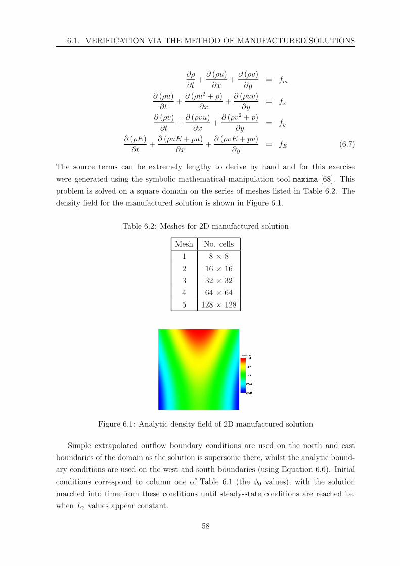
6.1. VERIFICATION VIA THE METHOD OF MANUFACTURED SOLUTIONS
∂ρ
∂t+
∂ (ρu)
∂x+
∂ (ρv)
∂y= fm
∂ (ρu)
∂t+
∂ (ρu2 + p)
∂x+
∂ (ρuv)
∂y= fx
∂ (ρv)
∂t+
∂ (ρvu)
∂x+
∂ (ρv2 + p)
∂y= fy
∂ (ρE)
∂t+
∂ (ρuE + pu)
∂x+
∂ (ρvE + pv)
∂y= fE (6.7)
The source terms can be extremely lengthy to derive by hand and for this exercise
were generated using the symbolic mathematical manipulation tool maxima [68]. This
problem is solved on a square domain on the series of meshes listed in Table 6.2. The
density field for the manufactured solution is shown in Figure 6.1.
Table 6.2: Meshes for 2D manufactured solution
Mesh No. cells
1 8 × 8
2 16 × 16
3 32 × 32
4 64 × 64
5 128 × 128
Figure 6.1: Analytic density field of 2D manufactured solution
Simple extrapolated outflow boundary conditions are used on the north and east
boundaries of the domain as the solution is supersonic there, whilst the analytic bound-
ary conditions are used on the west and south boundaries (using Equation 6.6). Initial
conditions correspond to column one of Table 6.1 (the φ0 values), with the solution
marched into time from these conditions until steady-state conditions are reached i.e.
when L2 values appear constant.
58
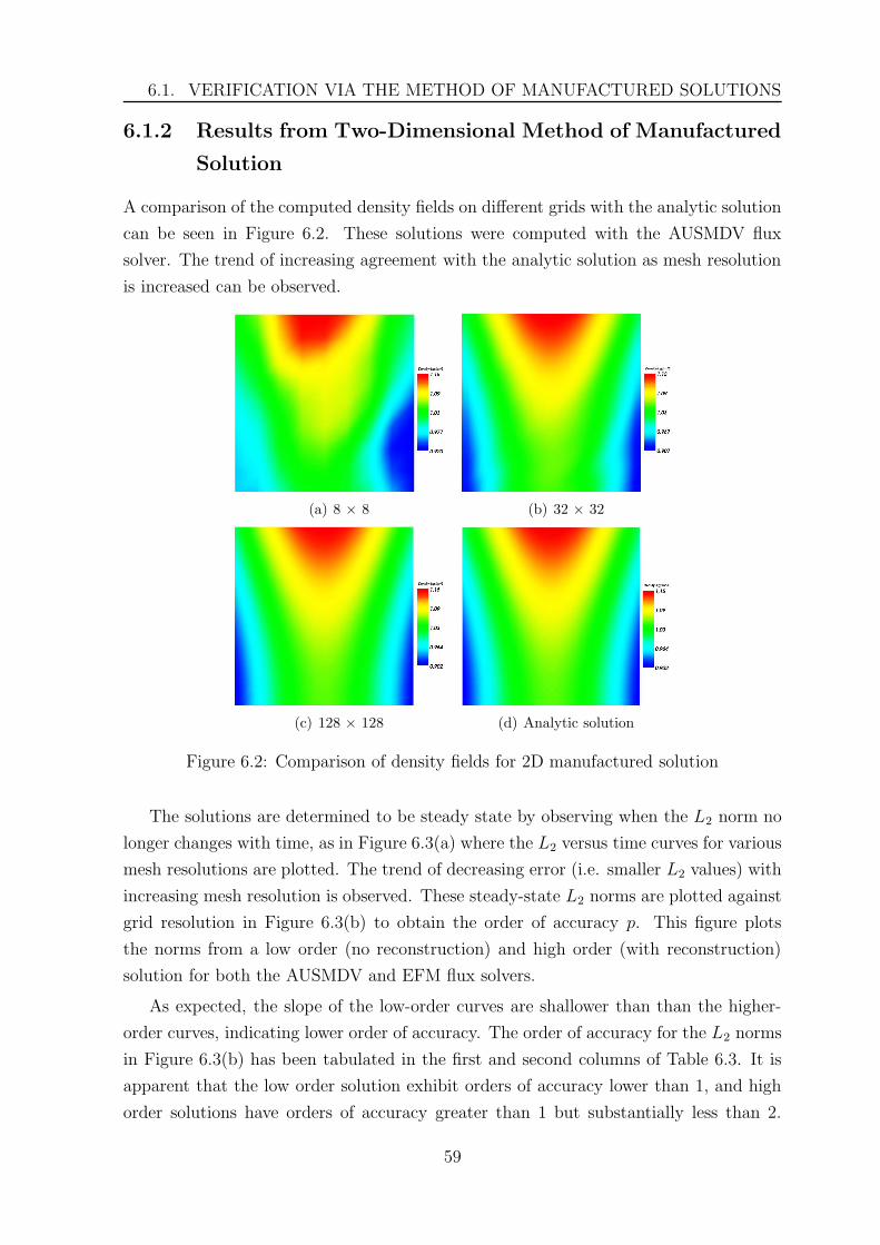
6.1. VERIFICATION VIA THE METHOD OF MANUFACTURED SOLUTIONS
6.1.2 Results from Two-Dimensional Method of Manufactured
Solution
A comparison of the computed density fields on different grids with the analytic solution
can be seen in Figure 6.2. These solutions were computed with the AUSMDV flux
solver. The trend of increasing agreement with the analytic solution as mesh resolution
is increased can be observed.
(a) 8 × 8 (b) 32 × 32
(c) 128 × 128 (d) Analytic solution
Figure 6.2: Comparison of density fields for 2D manufactured solution
The solutions are determined to be steady state by observing when the L2 norm no
longer changes with time, as in Figure 6.3(a) where the L2 versus time curves for various
mesh resolutions are plotted. The trend of decreasing error (i.e. smaller L2 values) with
increasing mesh resolution is observed. These steady-state L2 norms are plotted against
grid resolution in Figure 6.3(b) to obtain the order of accuracy p. This figure plots
the norms from a low order (no reconstruction) and high order (with reconstruction)
solution for both the AUSMDV and EFM flux solvers.
As expected, the slope of the low-order curves are shallower than than the higher-
order curves, indicating lower order of accuracy. The order of accuracy for the L2 norms
in Figure 6.3(b) has been tabulated in the first and second columns of Table 6.3. It is
apparent that the low order solution exhibit orders of accuracy lower than 1, and high
order solutions have orders of accuracy greater than 1 but substantially less than 2.
59
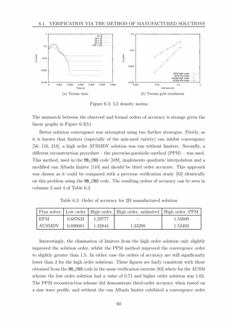
6.1. VERIFICATION VIA THE METHOD OF MANUFACTURED SOLUTIONS
1e-04
0.001
0.01
0.1
1
0 0.001 0.002 0.003 0.004 0.005 0.006
L2 n
orm
Time (s)
8 x 816 x 1632 x 3264 x 64
128 x 128
(a) Versus time
1e-04
0.001
0.01
0.1
0.001 0.01 0.1 1
L2 n
orm
Cell size (m)
EFM high orderEFM low order
AUSM high orderAUSM low order
(b) Versus grid resolution
Figure 6.3: L2 density norms
The mismatch between the observed and formal orders of accuracy is strange given the
linear graphs in Figure 6.3(b).
Better solution convergence was attempted using two further strategies. Firstly, as
it is known that limiters (especially of the min-mod variety) can inhibit convergence
[50, 110, 218], a high order AUSMDV solution was run without limiters. Secondly, a
different reconstruction procedure – the piecewise-parabolic-method (PPM) – was used.
This method, used in the MB_CNS code [109], implements quadratic interpolation and a
modified van Albada limiter [110] and should be third order accurate. This approach
was chosen as it could be compared with a previous verification study [83] identically
on this problem using the MB_CNS code. The resulting orders of accuracy can be seen in
columns 3 and 4 of Table 6.3.
Table 6.3: Order of accuracy for 2D manufactured solution
Flux solver Low order High order High order, unlimited High order, PPM
EFM 0.697632 1.29777 - 1.55609
AUSMDV 0.690081 1.32844 1.33298 1.53493
Interestingly, the elimination of limiters from the high order solution only slightly
improved the solution order, whilst the PPM method improved the convergence order
to slightly greater than 1.5. In either case the orders of accuracy are still significantly
lower than 2 for the high order solutions. These figures are fairly consistent with those
obtained from the MB_CNS code in the same verification exercise [83] where for the AUSM
scheme the low order solution had a value of 0.71 and higher order solution was 1.62.
The PPM reconstruction scheme did demonstrate third-order accuracy when tested on
a sine wave profile, and without the van Albada limiter exhibited a convergence order
60
6.1. VERIFICATION VIA THE METHOD OF MANUFACTURED SOLUTIONS
of 1.9. Although this is still substantially less than 3, the single-point quadrature of the
fluxes in the solution integration scheme (Section 4.2) implies truncation orders of 2 at
best [82].
It will be shown in Sections 6.1.4 and 6.4 that better matches between observed
and formal orders of accuracy result for different verification problems. As mentioned
previously, observed orders of accuracy seem quite dependent on both the nature of the
problem and the solution procedure [168].
6.1.3 Manufactured Solution for Three-Dimensional Geometry
The manufactured solution in Equation 6.6 will now be extended to fully test all terms
in the formulation of the three-dimensional Euler equations. In steady-state form, the
solution has the form –
ρ (x, y, z) = ρ0 + ρx sin (aρxπx) + ρy cos (aρyπy) + ρz cos (aρzπz)
u (x, y, z) = u0 + ux sin (auxπx) + uy cos (auyπy) + uz cos (auzπz)
v (x, y, z) = v0 + vx cos (avxπx) + vy sin (avyπy) + vz sin (avzπz)
w (x, y, z) = w0 + wx cos (awxπx) + wy sin (awyπy) + wz sin (awzπz)
p (x, y, z) = p0 + px cos (apxπx) + py sin (apyπy) + pz sin (apzπz) (6.8)
The constants for this solution are given in Table 6.4. Note that these values in two
dimensions are identical to those in Table 6.1 with additional values provided for the
third dimensional component. Like in Section 6.1.1, the source terms are generated by
substituting the analytic solution into the Euler equations.
Table 6.4: Table of constants for 3D manufactured solution
Equation, φ φ0 φx φy φz aφx aφy aφz
ρ (kg/m2) 1 0.15 -0.1 0.12 1 1.5 2
u (m/s) 800 50 -30 20 1.5 0.6 0.5
v (m/s) 800 -75 40 -25 0.5 2/3 1
w (m/s) 800 40 -40 20 0.3 0.5 2
p (Pa) 1.0×10⁵ 0.2×10⁵ 0.5×10⁵ 0.25×10⁵ 2.0 1.0 0.5
The solution methodology is identical to the two-dimensional verification exercise
in Section 6.1.1. However, due to the large number of cells that would be required
in a three-dimensional solution, only three mesh resolutions are considered, which are
tabulated in Table 6.5.
61
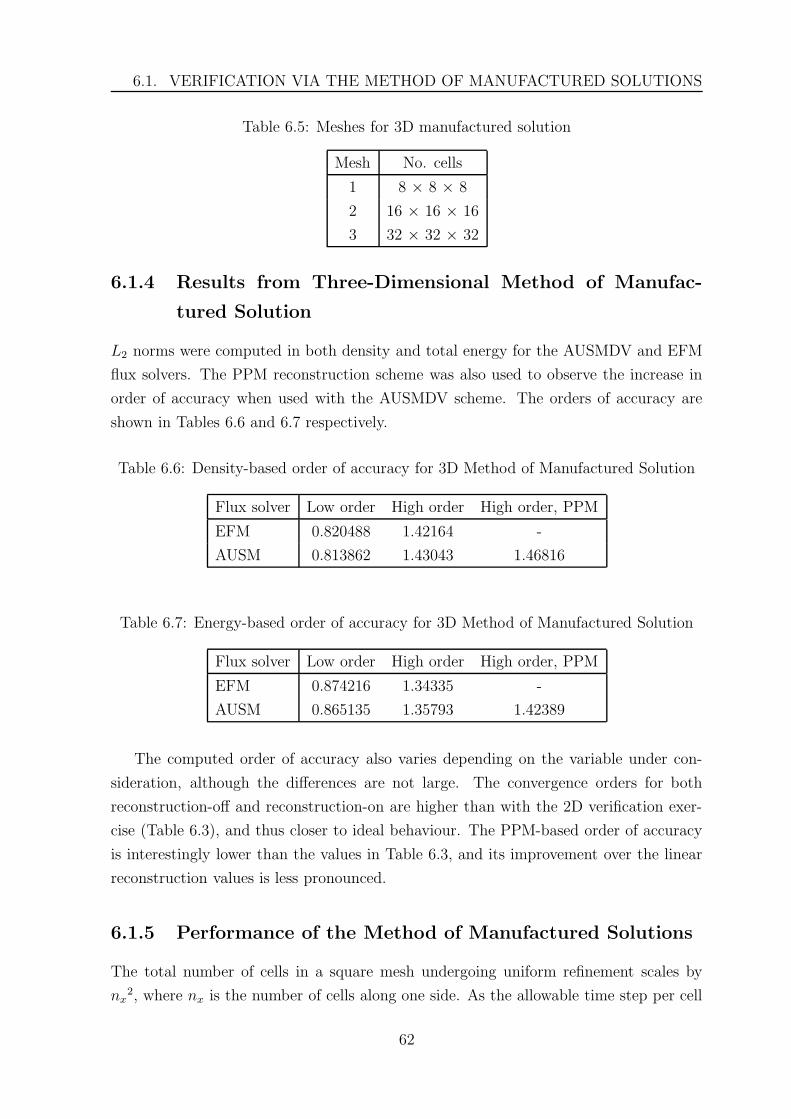
6.1. VERIFICATION VIA THE METHOD OF MANUFACTURED SOLUTIONS
Table 6.5: Meshes for 3D manufactured solution
Mesh No. cells
1 8 × 8 × 8
2 16 × 16 × 16
3 32 × 32 × 32
6.1.4 Results from Three-Dimensional Method of Manufac-
tured Solution
L2 norms were computed in both density and total energy for the AUSMDV and EFM
flux solvers. The PPM reconstruction scheme was also used to observe the increase in
order of accuracy when used with the AUSMDV scheme. The orders of accuracy are
shown in Tables 6.6 and 6.7 respectively.
Table 6.6: Density-based order of accuracy for 3D Method of Manufactured Solution
Flux solver Low order High order High order, PPM
EFM 0.820488 1.42164 -
AUSM 0.813862 1.43043 1.46816
Table 6.7: Energy-based order of accuracy for 3D Method of Manufactured Solution
Flux solver Low order High order High order, PPM
EFM 0.874216 1.34335 -
AUSM 0.865135 1.35793 1.42389
The computed order of accuracy also varies depending on the variable under con-
sideration, although the differences are not large. The convergence orders for both
reconstruction-off and reconstruction-on are higher than with the 2D verification exer-
cise (Table 6.3), and thus closer to ideal behaviour. The PPM-based order of accuracy
is interestingly lower than the values in Table 6.3, and its improvement over the linear
reconstruction values is less pronounced.
6.1.5 Performance of the Method of Manufactured Solutions
The total number of cells in a square mesh undergoing uniform refinement scales by
nx2, where nx is the number of cells along one side. As the allowable time step per cell
62
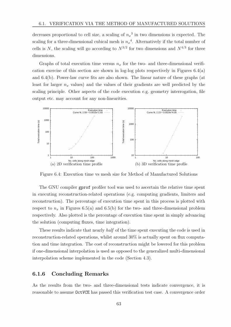
6.1. VERIFICATION VIA THE METHOD OF MANUFACTURED SOLUTIONS
decreases proportional to cell size, a scaling of nx3 in two dimensions is expected. The
scaling for a three-dimensional cubical mesh is nx4. Alternatively if the total number of
cells is N , the scaling will go according to N 3/2 for two dimensions and N 4/3 for three
dimensions.
Graphs of total execution time versus nx for the two- and three-dimensional verifi-
cation exercise of this section are shown in log-log plots respectively in Figures 6.4(a)
and 6.4(b). Power-law curve fits are also shown. The linear nature of these graphs (at
least for larger nx values) and the values of their gradients are well predicted by the
scaling principle. Other aspects of the code execution e.g. geometry interrogation, file
output etc. may account for any non-linearities.
1
10
100
1000
10000
1 10 100 1000
Tot
al e
xecu
tion
time
(s)
No. cells along mesh edge
Execution timeCurve fit, 2.59 + 0.0015x^2.93
(a) 2D verification time profile
10
100
1000
10000
1 10 100
Tot
al e
xecu
tion
time
(s)
No. cells along mesh edge
Execution timeCurve fit, 2.23 + 0.0024x^4.05
(b) 3D verification time profile
Figure 6.4: Execution time vs mesh size for Method of Manufactured Solutions
The GNU compiler gprof profiler tool was used to ascertain the relative time spent
in executing reconstruction-related operations (e.g. computing gradients, limiters and
reconstruction). The percentage of execution time spent in this process is plotted with
respect to nx in Figures 6.5(a) and 6.5(b) for the two- and three-dimensional problem
respectively. Also plotted is the percentage of execution time spent in simply advancing
the solution (computing fluxes, time integration).
These results indicate that nearly half of the time spent executing the code is used in
reconstruction-related operations, whilst around 30% is actually spent on flux computa-
tion and time integration. The cost of reconstruction might be lowered for this problem
if one-dimensional interpolation is used as opposed to the generalized multi-dimensional
interpolation scheme implemented in the code (Section 4.3).
6.1.6 Concluding Remarks
As the results from the two- and three-dimensional tests indicate convergence, it is
reasonable to assume OctVCE has passed this verification test case. A convergence order
63
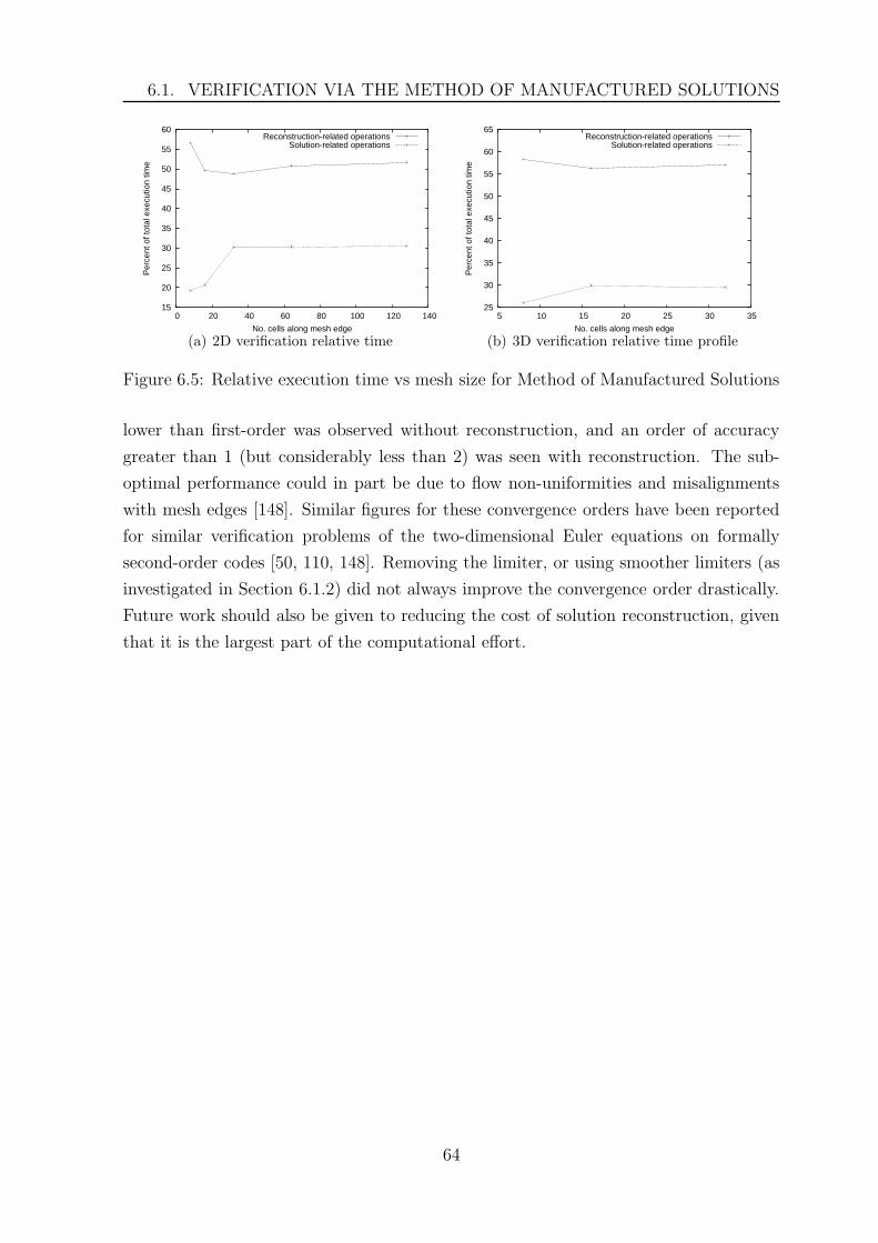
6.1. VERIFICATION VIA THE METHOD OF MANUFACTURED SOLUTIONS
15
20
25
30
35
40
45
50
55
60
0 20 40 60 80 100 120 140
Per
cent
of t
otal
exe
cutio
n tim
e
No. cells along mesh edge
Reconstruction-related operationsSolution-related operations
(a) 2D verification relative time
25
30
35
40
45
50
55
60
65
5 10 15 20 25 30 35
Per
cent
of t
otal
exe
cutio
n tim
e
No. cells along mesh edge
Reconstruction-related operationsSolution-related operations
(b) 3D verification relative time profile
Figure 6.5: Relative execution time vs mesh size for Method of Manufactured Solutions
lower than first-order was observed without reconstruction, and an order of accuracy
greater than 1 (but considerably less than 2) was seen with reconstruction. The sub-
optimal performance could in part be due to flow non-uniformities and misalignments
with mesh edges [148]. Similar figures for these convergence orders have been reported
for similar verification problems of the two-dimensional Euler equations on formally
second-order codes [50, 110, 148]. Removing the limiter, or using smoother limiters (as
investigated in Section 6.1.2) did not always improve the convergence order drastically.
Future work should also be given to reducing the cost of solution reconstruction, given
that it is the largest part of the computational effort.
64
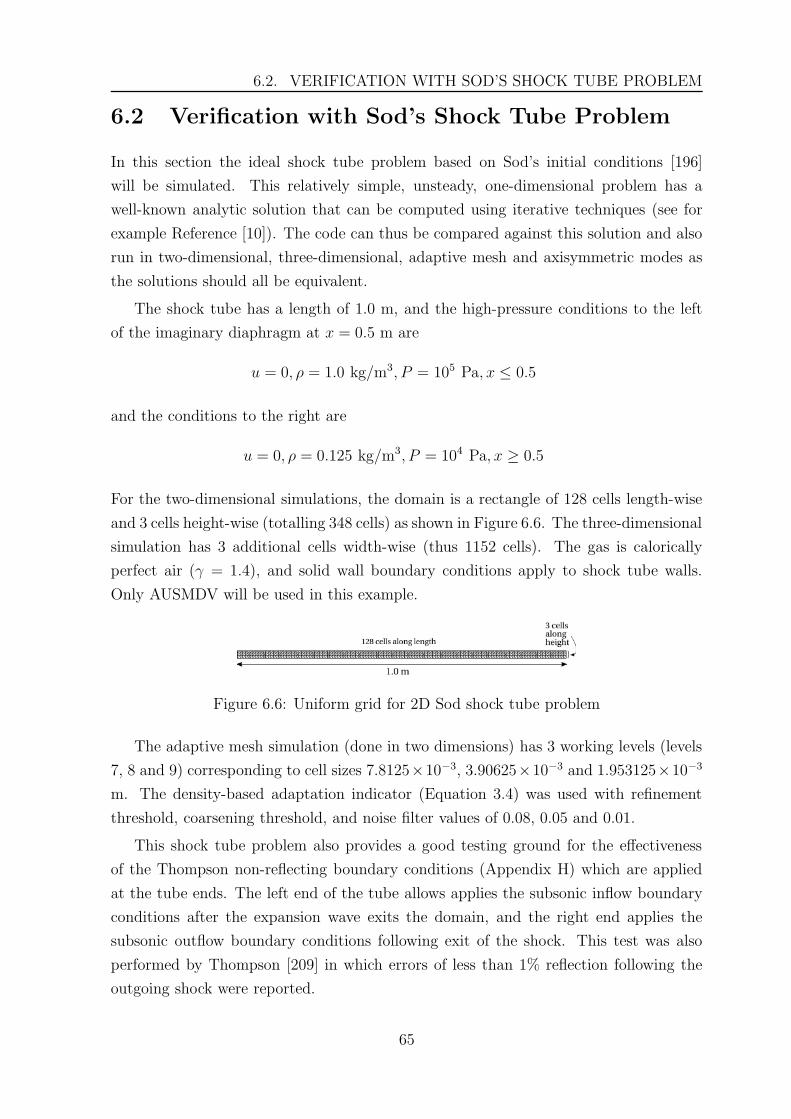
6.2. VERIFICATION WITH SOD’S SHOCK TUBE PROBLEM
6.2 Verification with Sod’s Shock Tube Problem
In this section the ideal shock tube problem based on Sod’s initial conditions [196]
will be simulated. This relatively simple, unsteady, one-dimensional problem has a
well-known analytic solution that can be computed using iterative techniques (see for
example Reference [10]). The code can thus be compared against this solution and also
run in two-dimensional, three-dimensional, adaptive mesh and axisymmetric modes as
the solutions should all be equivalent.
The shock tube has a length of 1.0 m, and the high-pressure conditions to the left
of the imaginary diaphragm at x = 0.5 m are
u = 0, ρ = 1.0 kg/m3, P = 105 Pa, x ≤ 0.5
and the conditions to the right are
u = 0, ρ = 0.125 kg/m3, P = 104 Pa, x ≥ 0.5
For the two-dimensional simulations, the domain is a rectangle of 128 cells length-wise
and 3 cells height-wise (totalling 348 cells) as shown in Figure 6.6. The three-dimensional
simulation has 3 additional cells width-wise (thus 1152 cells). The gas is calorically
perfect air (γ = 1.4), and solid wall boundary conditions apply to shock tube walls.
Only AUSMDV will be used in this example.
Figure 6.6: Uniform grid for 2D Sod shock tube problem
The adaptive mesh simulation (done in two dimensions) has 3 working levels (levels
7, 8 and 9) corresponding to cell sizes 7.8125×10⁻³, 3.90625×10⁻³ and 1.953125×10⁻³
m. The density-based adaptation indicator (Equation 3.4) was used with refinement
threshold, coarsening threshold, and noise filter values of 0.08, 0.05 and 0.01.
This shock tube problem also provides a good testing ground for the effectiveness
of the Thompson non-reflecting boundary conditions (Appendix H) which are applied
at the tube ends. The left end of the tube allows applies the subsonic inflow boundary
conditions after the expansion wave exits the domain, and the right end applies the
subsonic outflow boundary conditions following exit of the shock. This test was also
performed by Thompson [209] in which errors of less than 1% reflection following the
outgoing shock were reported.
65
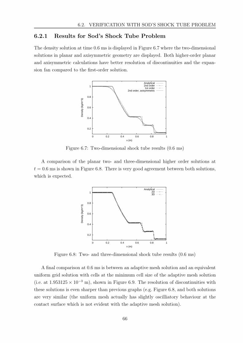
6.2. VERIFICATION WITH SOD’S SHOCK TUBE PROBLEM
6.2.1 Results for Sod’s Shock Tube Problem
The density solution at time 0.6 ms is displayed in Figure 6.7 where the two-dimensional
solutions in planar and axisymmetric geometry are displayed. Both higher-order planar
and axisymmetric calculations have better resolution of discontinuities and the expan-
sion fan compared to the first-order solution.
0.2
0.4
0.6
0.8
1
0 0.2 0.4 0.6 0.8 1
Den
sity
(kg
/m^3
)
x (m)
Analytical2nd order1st order
2nd order, axisymmetric
Figure 6.7: Two-dimensional shock tube results (0.6 ms)
A comparison of the planar two- and three-dimensional higher order solutions at
t = 0.6 ms is shown in Figure 6.8. There is very good agreement between both solutions,
which is expected.
0.2
0.4
0.6
0.8
1
0 0.2 0.4 0.6 0.8 1
Den
sity
(kg
/m^3
)
x (m)
Analytical2D3D
Figure 6.8: Two- and three-dimensional shock tube results (0.6 ms)
A final comparison at 0.6 ms is between an adaptive mesh solution and an equivalent
uniform grid solution with cells at the minimum cell size of the adaptive mesh solution
(i.e. at 1.953125× 10⁻³ m), shown in Figure 6.9. The resolution of discontinuities with
these solutions is even sharper than previous graphs (e.g. Figure 6.8, and both solutions
are very similar (the uniform mesh actually has slightly oscilliatory behaviour at the
contact surface which is not evident with the adaptive mesh solution).
66
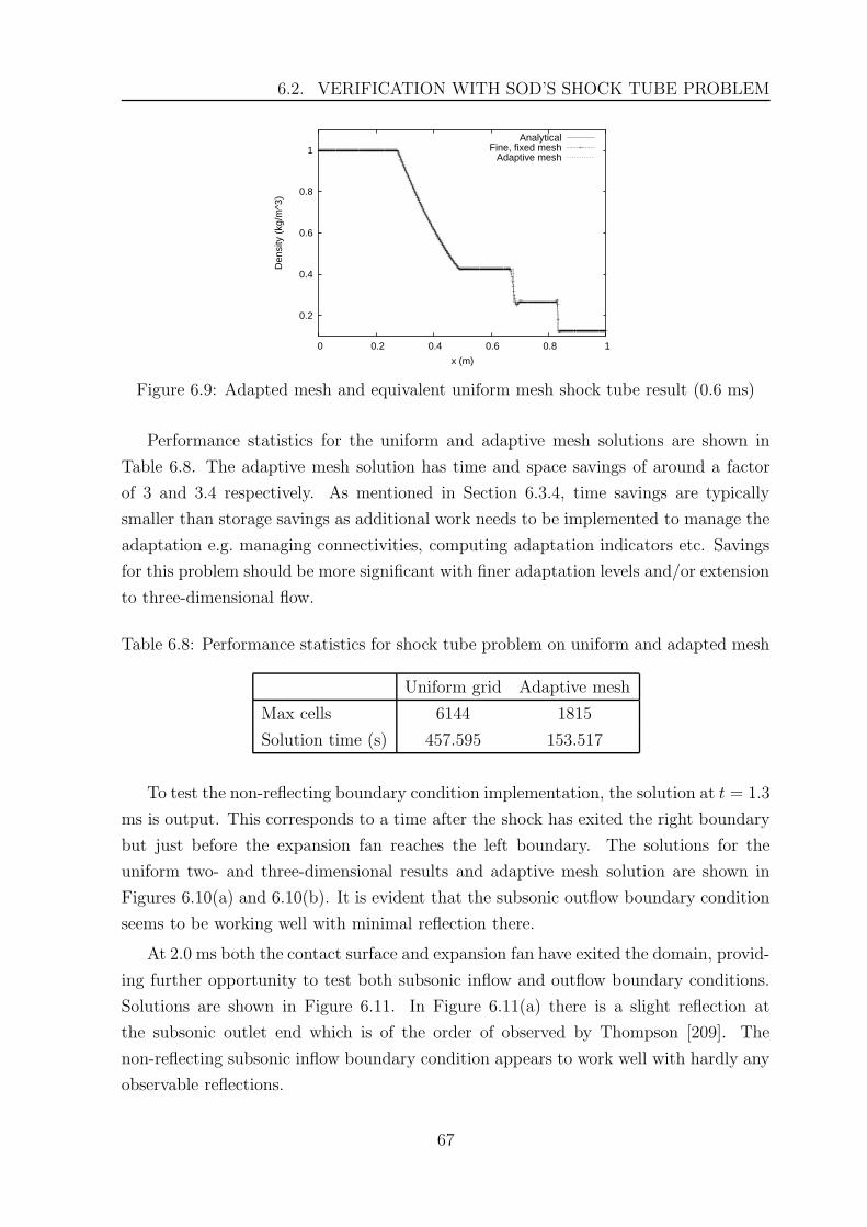
6.2. VERIFICATION WITH SOD’S SHOCK TUBE PROBLEM
0.2
0.4
0.6
0.8
1
0 0.2 0.4 0.6 0.8 1
Den
sity
(kg
/m^3
)
x (m)
AnalyticalFine, fixed mesh
Adaptive mesh
Figure 6.9: Adapted mesh and equivalent uniform mesh shock tube result (0.6 ms)
Performance statistics for the uniform and adaptive mesh solutions are shown in
Table 6.8. The adaptive mesh solution has time and space savings of around a factor
of 3 and 3.4 respectively. As mentioned in Section 6.3.4, time savings are typically
smaller than storage savings as additional work needs to be implemented to manage the
adaptation e.g. managing connectivities, computing adaptation indicators etc. Savings
for this problem should be more significant with finer adaptation levels and/or extension
to three-dimensional flow.
Table 6.8: Performance statistics for shock tube problem on uniform and adapted mesh
Uniform grid Adaptive mesh
Max cells 6144 1815
Solution time (s) 457.595 153.517
To test the non-reflecting boundary condition implementation, the solution at t = 1.3
ms is output. This corresponds to a time after the shock has exited the right boundary
but just before the expansion fan reaches the left boundary. The solutions for the
uniform two- and three-dimensional results and adaptive mesh solution are shown in
Figures 6.10(a) and 6.10(b). It is evident that the subsonic outflow boundary condition
seems to be working well with minimal reflection there.
At 2.0 ms both the contact surface and expansion fan have exited the domain, provid-
ing further opportunity to test both subsonic inflow and outflow boundary conditions.
Solutions are shown in Figure 6.11. In Figure 6.11(a) there is a slight reflection at
the subsonic outlet end which is of the order of observed by Thompson [209]. The
non-reflecting subsonic inflow boundary condition appears to work well with hardly any
observable reflections.
67
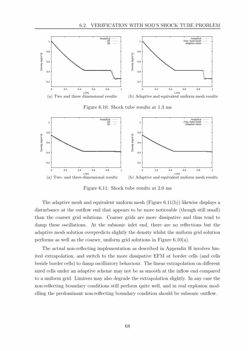
6.2. VERIFICATION WITH SOD’S SHOCK TUBE PROBLEM
0.2
0.4
0.6
0.8
1
0 0.2 0.4 0.6 0.8 1
Den
sity
(kg
/m^3
)
x (m)
Analytical2D3D
(a) Two and three dimensional results
0.2
0.4
0.6
0.8
1
0 0.2 0.4 0.6 0.8 1
Den
sity
(kg
/m^3
)
x (m)
AnalyticalFine, fixed mesh
Adaptive mesh
(b) Adaptive and equivalent uniform mesh results
Figure 6.10: Shock tube results at 1.3 ms
0.2
0.4
0.6
0.8
1
0 0.2 0.4 0.6 0.8 1
Den
sity
(kg
/m^3
)
x (m)
Analytical2D3D
(a) Two- and three-dimensional results
0.2
0.4
0.6
0.8
1
0 0.2 0.4 0.6 0.8 1
Den
sity
(kg
/m^3
)
x (m)
AnalyticalFine, fixed mesh
Adaptive mesh
(b) Adaptive and equivalent uniform mesh results
Figure 6.11: Shock tube results at 2.0 ms
The adaptive mesh and equivalent uniform mesh (Figure 6.11(b)) likewise displays a
disturbance at the outflow end that appears to be more noticeable (though still small)
than the coarser grid solutions. Coarser grids are more dissipative and thus tend to
damp these oscillations. At the subsonic inlet end, there are no reflections but the
adaptive mesh solution overpredicts slightly the density whilst the uniform grid solution
performs as well as the coarser, uniform grid solutions in Figure 6.10(a).
The actual non-reflecting implementation as described in Appendix H involves lim-
ited extrapolation, and switch to the more dissipative EFM at border cells (and cells
beside border cells) to damp oscilliatory behaviour. The linear extrapolation on different
sized cells under an adaptive scheme may not be as smooth at the inflow end compared
to a uniform grid. Limiters may also degrade the extrapolation slightly. In any case the
non-reflecting boundary conditions still perform quite well, and in real explosion mod-
elling the predominant non-reflecting boundary condition should be subsonic outflow.
68
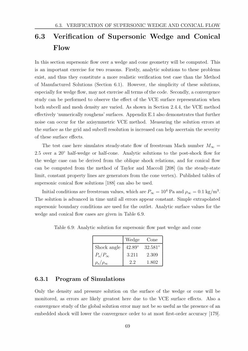
6.3. VERIFICATION OF SUPERSONIC WEDGE AND CONICAL FLOW
6.3 Verification of Supersonic Wedge and Conical
Flow
In this section supersonic flow over a wedge and cone geometry will be computed. This
is an important exercise for two reasons. Firstly, analytic solutions to these problems
exist, and thus they constitute a more realistic verification test case than the Method
of Manufactured Solutions (Section 6.1). However, the simplicity of these solutions,
especially for wedge flow, may not exercise all terms of the code. Secondly, a convergence
study can be performed to observe the effect of the VCE surface representation when
both subcell and mesh density are varied. As shown in Section 2.4.4, the VCE method
effectively ‘numerically roughens’ surfaces. Appendix E.1 also demonstrates that further
noise can occur for the axisymmetric VCE method. Measuring the solution errors at
the surface as the grid and subcell resolution is increased can help ascertain the severity
of these surface effects.
The test case here simulates steady-state flow of freestream Mach number M∞ =
2.5 over a 20◦ half-wedge or half-cone. Analytic solutions to the post-shock flow for
the wedge case can be derived from the oblique shock relations, and for conical flow
can be computed from the method of Taylor and Maccoll [208] (in the steady-state
limit, constant property lines are generators from the cone vertex). Published tables of
supersonic conical flow solutions [188] can also be used.
Initial conditions are freestream values, which are P∞ = 104 Pa and ρ∞ = 0.1 kg/m3.
The solution is advanced in time until all errors appear constant. Simple extrapolated
supersonic boundary conditions are used for the outlet. Analytic surface values for the
wedge and conical flow cases are given in Table 6.9.
Table 6.9: Analytic solution for supersonic flow past wedge and cone
Wedge Cone
Shock angle 42.89◦ 32.581◦
Ps/P∞ 3.211 2.309
ρs/ρ∞ 2.2 1.802
6.3.1 Program of Simulations
Only the density and pressure solution on the surface of the wedge or cone will be
monitored, as errors are likely greatest here due to the VCE surface effects. Also a
convergence study of the global solution error may not be so useful as the presence of an
embedded shock will lower the convergence order to at most first-order accuracy [179].
69
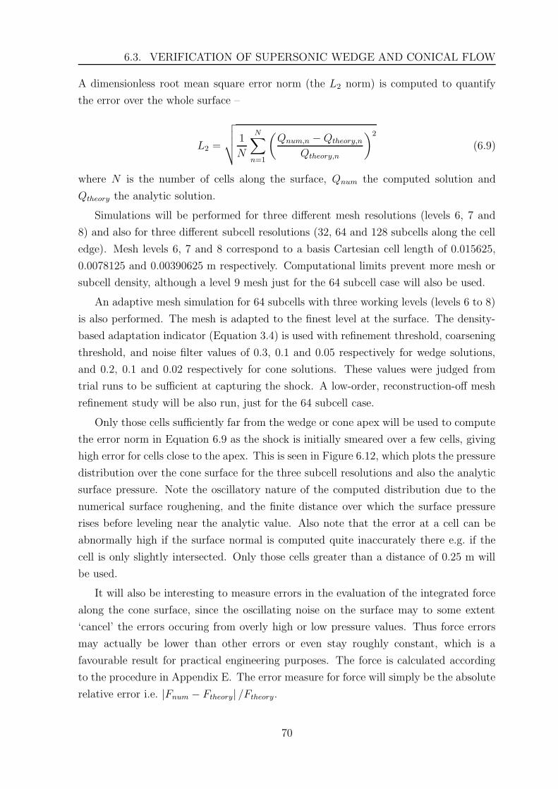
6.3. VERIFICATION OF SUPERSONIC WEDGE AND CONICAL FLOW
A dimensionless root mean square error norm (the L2 norm) is computed to quantify
the error over the whole surface –
L2 =
√√√√ 1
N
N∑
n=1
(Qnum,n − Qtheory,n
Qtheory,n
)2
(6.9)
where N is the number of cells along the surface, Qnum the computed solution and
Qtheory the analytic solution.
Simulations will be performed for three different mesh resolutions (levels 6, 7 and
8) and also for three different subcell resolutions (32, 64 and 128 subcells along the cell
edge). Mesh levels 6, 7 and 8 correspond to a basis Cartesian cell length of 0.015625,
0.0078125 and 0.00390625 m respectively. Computational limits prevent more mesh or
subcell density, although a level 9 mesh just for the 64 subcell case will also be used.
An adaptive mesh simulation for 64 subcells with three working levels (levels 6 to 8)
is also performed. The mesh is adapted to the finest level at the surface. The density-
based adaptation indicator (Equation 3.4) is used with refinement threshold, coarsening
threshold, and noise filter values of 0.3, 0.1 and 0.05 respectively for wedge solutions,
and 0.2, 0.1 and 0.02 respectively for cone solutions. These values were judged from
trial runs to be sufficient at capturing the shock. A low-order, reconstruction-off mesh
refinement study will be also run, just for the 64 subcell case.
Only those cells sufficiently far from the wedge or cone apex will be used to compute
the error norm in Equation 6.9 as the shock is initially smeared over a few cells, giving
high error for cells close to the apex. This is seen in Figure 6.12, which plots the pressure
distribution over the cone surface for the three subcell resolutions and also the analytic
surface pressure. Note the oscillatory nature of the computed distribution due to the
numerical surface roughening, and the finite distance over which the surface pressure
rises before leveling near the analytic value. Also note that the error at a cell can be
abnormally high if the surface normal is computed quite inaccurately there e.g. if the
cell is only slightly intersected. Only those cells greater than a distance of 0.25 m will
be used.
It will also be interesting to measure errors in the evaluation of the integrated force
along the cone surface, since the oscillating noise on the surface may to some extent
‘cancel’ the errors occuring from overly high or low pressure values. Thus force errors
may actually be lower than other errors or even stay roughly constant, which is a
favourable result for practical engineering purposes. The force is calculated according
to the procedure in Appendix E. The error measure for force will simply be the absolute
relative error i.e. |Fnum − Ftheory| /Ftheory.
70
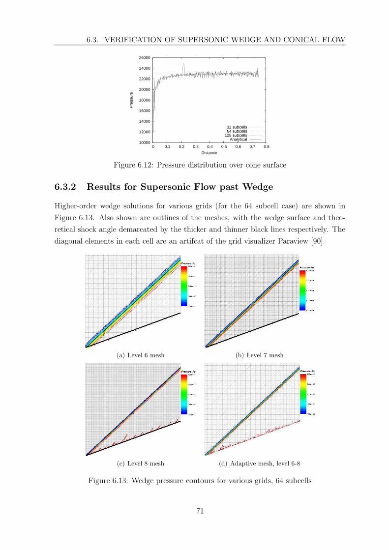
6.3. VERIFICATION OF SUPERSONIC WEDGE AND CONICAL FLOW
10000
12000
14000
16000
18000
20000
22000
24000
26000
0 0.1 0.2 0.3 0.4 0.5 0.6 0.7 0.8
Pre
ssur
e
Distance
32 subcells64 subcells
128 subcellsAnalytical
Figure 6.12: Pressure distribution over cone surface
6.3.2 Results for Supersonic Flow past Wedge
Higher-order wedge solutions for various grids (for the 64 subcell case) are shown in
Figure 6.13. Also shown are outlines of the meshes, with the wedge surface and theo-
retical shock angle demarcated by the thicker and thinner black lines respectively. The
diagonal elements in each cell are an artifcat of the grid visualizer Paraview [90].
(a) Level 6 mesh (b) Level 7 mesh
(c) Level 8 mesh (d) Adaptive mesh, level 6-8
Figure 6.13: Wedge pressure contours for various grids, 64 subcells
71
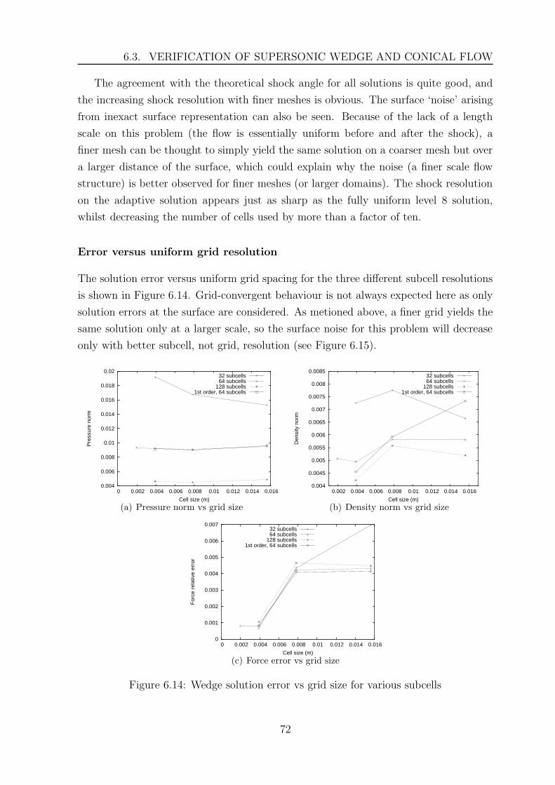
6.3. VERIFICATION OF SUPERSONIC WEDGE AND CONICAL FLOW
The agreement with the theoretical shock angle for all solutions is quite good, and
the increasing shock resolution with finer meshes is obvious. The surface ‘noise’ arising
from inexact surface representation can also be seen. Because of the lack of a length
scale on this problem (the flow is essentially uniform before and after the shock), a
finer mesh can be thought to simply yield the same solution on a coarser mesh but over
a larger distance of the surface, which could explain why the noise (a finer scale flow
structure) is better observed for finer meshes (or larger domains). The shock resolution
on the adaptive solution appears just as sharp as the fully uniform level 8 solution,
whilst decreasing the number of cells used by more than a factor of ten.
Error versus uniform grid resolution
The solution error versus uniform grid spacing for the three different subcell resolutions
is shown in Figure 6.14. Grid-convergent behaviour is not always expected here as only
solution errors at the surface are considered. As metioned above, a finer grid yields the
same solution only at a larger scale, so the surface noise for this problem will decrease
only with better subcell, not grid, resolution (see Figure 6.15).
0.004
0.006
0.008
0.01
0.012
0.014
0.016
0.018
0.02
0 0.002 0.004 0.006 0.008 0.01 0.012 0.014 0.016
Pre
ssur
e no
rm
Cell size (m)
32 subcells64 subcells
128 subcells1st order, 64 subcells
(a) Pressure norm vs grid size
0.004
0.0045
0.005
0.0055
0.006
0.0065
0.007
0.0075
0.008
0.0085
0.002 0.004 0.006 0.008 0.01 0.012 0.014 0.016
Den
sity
nor
m
Cell size (m)
32 subcells64 subcells
128 subcells1st order, 64 subcells
(b) Density norm vs grid size
0
0.001
0.002
0.003
0.004
0.005
0.006
0.007
0 0.002 0.004 0.006 0.008 0.01 0.012 0.014 0.016
For
ce r
elat
ive
erro
r
Cell size (m)
32 subcells64 subcells
128 subcells1st order, 64 subcells
(c) Force error vs grid size
Figure 6.14: Wedge solution error vs grid size for various subcells
72
6.3. VERIFICATION OF SUPERSONIC WEDGE AND CONICAL FLOW
Note in Figure 6.14(a) the surface pressure norm is seen to increase slightly for finer
grids using 32 subcells, whilst for finer subcell resolutions the norms remain somewhat
constant. The low-order density norm is also lower than the higher-order value at one
point (Figure 6.14(b)). These counter-intuitive results might be expected, as depending
on how the surface intersects the mesh, it is possible that coarser mesh or subcell
resolutions actually perform better for a given test case. The low-order pressure solution
closely coincides with the higher-order result; this may be expected given the absence
of reconstruction at surfaces (Section 4.3.3). However, it does not always coincide (e.g.
in the density or force solution) due to the presence of reconstruction away from the
surface. All these errors are fairly low, typically much less than 2%.
The force errors (Figure 6.14(c)) seem to generally decrease for finer meshes. For
nearly all mesh resolutions, these errors do not seem so dependent on subcell resolution
compared to the pressure or density norm. The force errors do not exceed 0.7% even for
the coarsest mesh. This result is quite encouraging, suggesting that obtaining a quite
accurate force value does not require a high grid or subcell resolution.
Error vs subcell resolution
This time the solution errors versus the inverse of the number of subcells are plotted
for the three main uniform grid levels in Figure 6.15. Also shown are adaptive mesh
errors, just for the 64 subcell case. As better subcell resolution means better surface
representation, it should be expected that these graphs show decreasing error for more
subcells.
The fairly linear decrease of the pressure surface norm with increasing subcell res-
olution (for all meshes) can be seen in Figure 6.15(a). The adaptive pressure error
is very close to the finest 64 subcell uniform grid result. The apparently superlinear
decrease of density surface norm with increasing subcell resolution is also observed in
Figure 6.15(b). However, the adaptive density error is significantly lower than the 64
subcell uniform grid result.
The force errors (Figure 6.15(c)) do not seem to display subcell-convergent behaviour
and seem to stay roughly constant. This is probably due to the partial cancellation
of surface pressure noise as described in Section 6.3.1. However, the errors seem to
increase slightly for the 128 subcell case, but this may simply be the accidental result
of the numerical surface roughening described above. The adaptive solution error again
is lower than the finest uniform mesh result (it just may be that cancellation is not so
good for this subcell value).
73
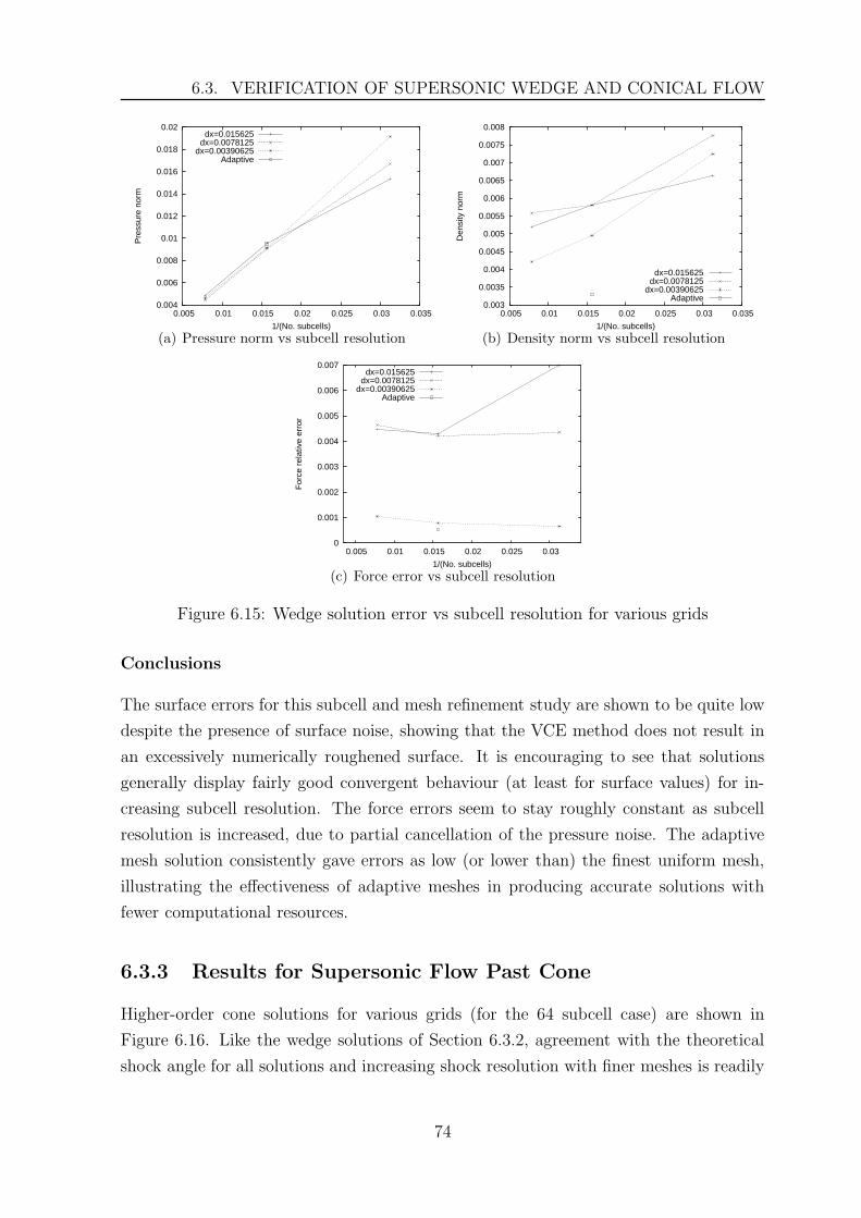
6.3. VERIFICATION OF SUPERSONIC WEDGE AND CONICAL FLOW
0.004
0.006
0.008
0.01
0.012
0.014
0.016
0.018
0.02
0.005 0.01 0.015 0.02 0.025 0.03 0.035
Pre
ssur
e no
rm
1/(No. subcells)
dx=0.015625dx=0.0078125
dx=0.00390625Adaptive
(a) Pressure norm vs subcell resolution
0.003
0.0035
0.004
0.0045
0.005
0.0055
0.006
0.0065
0.007
0.0075
0.008
0.005 0.01 0.015 0.02 0.025 0.03 0.035
Den
sity
nor
m
1/(No. subcells)
dx=0.015625dx=0.0078125
dx=0.00390625Adaptive
(b) Density norm vs subcell resolution
0
0.001
0.002
0.003
0.004
0.005
0.006
0.007
0.005 0.01 0.015 0.02 0.025 0.03
For
ce r
elat
ive
erro
r
1/(No. subcells)
dx=0.015625dx=0.0078125
dx=0.00390625Adaptive
(c) Force error vs subcell resolution
Figure 6.15: Wedge solution error vs subcell resolution for various grids
Conclusions
The surface errors for this subcell and mesh refinement study are shown to be quite low
despite the presence of surface noise, showing that the VCE method does not result in
an excessively numerically roughened surface. It is encouraging to see that solutions
generally display fairly good convergent behaviour (at least for surface values) for in-
creasing subcell resolution. The force errors seem to stay roughly constant as subcell
resolution is increased, due to partial cancellation of the pressure noise. The adaptive
mesh solution consistently gave errors as low (or lower than) the finest uniform mesh,
illustrating the effectiveness of adaptive meshes in producing accurate solutions with
fewer computational resources.
6.3.3 Results for Supersonic Flow Past Cone
Higher-order cone solutions for various grids (for the 64 subcell case) are shown in
Figure 6.16. Like the wedge solutions of Section 6.3.2, agreement with the theoretical
shock angle for all solutions and increasing shock resolution with finer meshes is readily
74
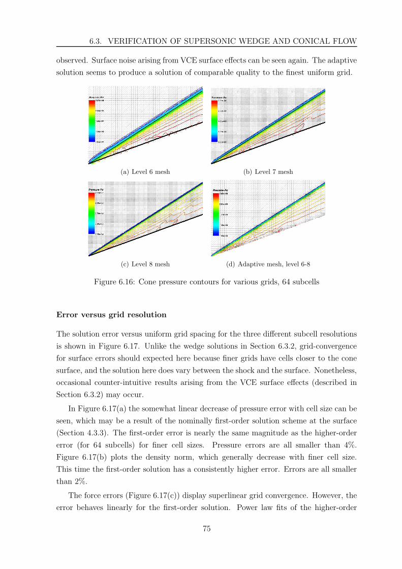
6.3. VERIFICATION OF SUPERSONIC WEDGE AND CONICAL FLOW
observed. Surface noise arising from VCE surface effects can be seen again. The adaptive
solution seems to produce a solution of comparable quality to the finest uniform grid.
(a) Level 6 mesh (b) Level 7 mesh
(c) Level 8 mesh (d) Adaptive mesh, level 6-8
Figure 6.16: Cone pressure contours for various grids, 64 subcells
Error versus grid resolution
The solution error versus uniform grid spacing for the three different subcell resolutions
is shown in Figure 6.17. Unlike the wedge solutions in Section 6.3.2, grid-convergence
for surface errors should expected here because finer grids have cells closer to the cone
surface, and the solution here does vary between the shock and the surface. Nonetheless,
occasional counter-intuitive results arising from the VCE surface effects (described in
Section 6.3.2) may occur.
In Figure 6.17(a) the somewhat linear decrease of pressure error with cell size can be
seen, which may be a result of the nominally first-order solution scheme at the surface
(Section 4.3.3). The first-order error is nearly the same magnitude as the higher-order
error (for 64 subcells) for finer cell sizes. Pressure errors are all smaller than 4%.
Figure 6.17(b) plots the density norm, which generally decrease with finer cell size.
This time the first-order solution has a consistently higher error. Errors are all smaller
than 2%.
The force errors (Figure 6.17(c)) display superlinear grid convergence. However, the
error behaves linearly for the first-order solution. Power law fits of the higher-order
75
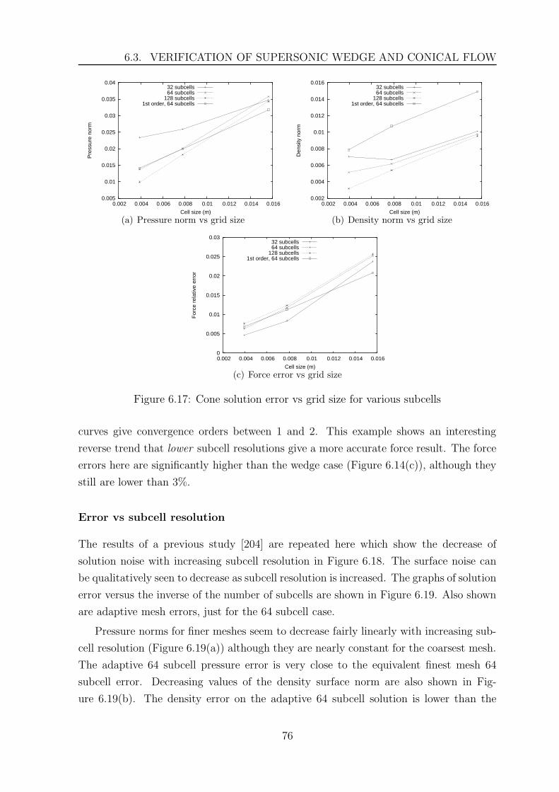
6.3. VERIFICATION OF SUPERSONIC WEDGE AND CONICAL FLOW
0.005
0.01
0.015
0.02
0.025
0.03
0.035
0.04
0.002 0.004 0.006 0.008 0.01 0.012 0.014 0.016
Pre
ssur
e no
rm
Cell size (m)
32 subcells64 subcells
128 subcells1st order, 64 subcells
(a) Pressure norm vs grid size
0.002
0.004
0.006
0.008
0.01
0.012
0.014
0.016
0.002 0.004 0.006 0.008 0.01 0.012 0.014 0.016
Den
sity
nor
m
Cell size (m)
32 subcells64 subcells
128 subcells1st order, 64 subcells
(b) Density norm vs grid size
0
0.005
0.01
0.015
0.02
0.025
0.03
0.002 0.004 0.006 0.008 0.01 0.012 0.014 0.016
For
ce r
elat
ive
erro
r
Cell size (m)
32 subcells64 subcells
128 subcells1st order, 64 subcells
(c) Force error vs grid size
Figure 6.17: Cone solution error vs grid size for various subcells
curves give convergence orders between 1 and 2. This example shows an interesting
reverse trend that lower subcell resolutions give a more accurate force result. The force
errors here are significantly higher than the wedge case (Figure 6.14(c)), although they
still are lower than 3%.
Error vs subcell resolution
The results of a previous study [204] are repeated here which show the decrease of
solution noise with increasing subcell resolution in Figure 6.18. The surface noise can
be qualitatively seen to decrease as subcell resolution is increased. The graphs of solution
error versus the inverse of the number of subcells are shown in Figure 6.19. Also shown
are adaptive mesh errors, just for the 64 subcell case.
Pressure norms for finer meshes seem to decrease fairly linearly with increasing sub-
cell resolution (Figure 6.19(a)) although they are nearly constant for the coarsest mesh.
The adaptive 64 subcell pressure error is very close to the equivalent finest mesh 64
subcell error. Decreasing values of the density surface norm are also shown in Fig-
ure 6.19(b). The density error on the adaptive 64 subcell solution is lower than the
76
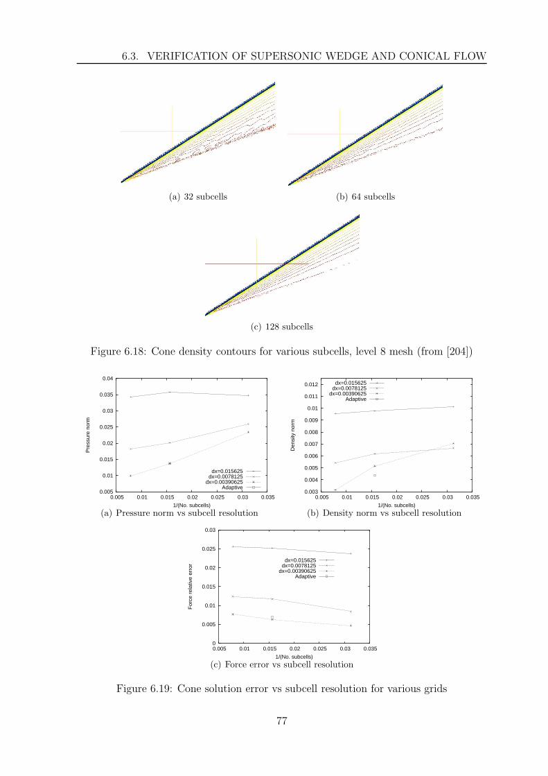
6.3. VERIFICATION OF SUPERSONIC WEDGE AND CONICAL FLOW
(a) 32 subcells (b) 64 subcells
(c) 128 subcells
Figure 6.18: Cone density contours for various subcells, level 8 mesh (from [204])
0.005
0.01
0.015
0.02
0.025
0.03
0.035
0.04
0.005 0.01 0.015 0.02 0.025 0.03 0.035
Pre
ssur
e no
rm
1/(No. subcells)
dx=0.015625dx=0.0078125
dx=0.00390625Adaptive
(a) Pressure norm vs subcell resolution
0.003
0.004
0.005
0.006
0.007
0.008
0.009
0.01
0.011
0.012
0.005 0.01 0.015 0.02 0.025 0.03 0.035
Den
sity
nor
m
1/(No. subcells)
dx=0.015625dx=0.0078125
dx=0.00390625Adaptive
(b) Density norm vs subcell resolution
0
0.005
0.01
0.015
0.02
0.025
0.03
0.005 0.01 0.015 0.02 0.025 0.03 0.035
For
ce r
elat
ive
erro
r
1/(No. subcells)
dx=0.015625dx=0.0078125
dx=0.00390625Adaptive
(c) Force error vs subcell resolution
Figure 6.19: Cone solution error vs subcell resolution for various grids
77
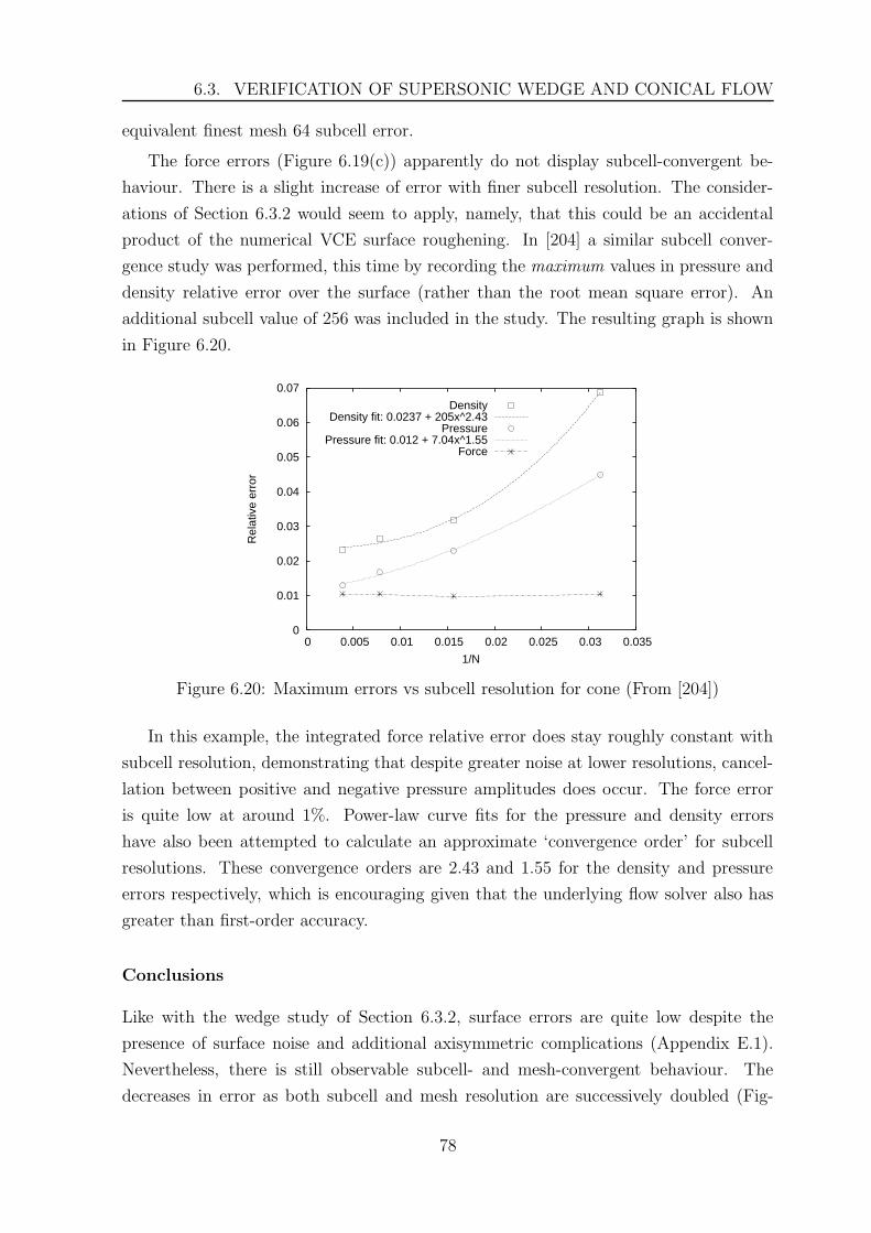
6.3. VERIFICATION OF SUPERSONIC WEDGE AND CONICAL FLOW
equivalent finest mesh 64 subcell error.
The force errors (Figure 6.19(c)) apparently do not display subcell-convergent be-
haviour. There is a slight increase of error with finer subcell resolution. The consider-
ations of Section 6.3.2 would seem to apply, namely, that this could be an accidental
product of the numerical VCE surface roughening. In [204] a similar subcell conver-
gence study was performed, this time by recording the maximum values in pressure and
density relative error over the surface (rather than the root mean square error). An
additional subcell value of 256 was included in the study. The resulting graph is shown
in Figure 6.20.
0
0.01
0.02
0.03
0.04
0.05
0.06
0.07
0 0.005 0.01 0.015 0.02 0.025 0.03 0.035
Rel
ativ
e er
ror
1/N
DensityDensity fit: 0.0237 + 205x^2.43
PressurePressure fit: 0.012 + 7.04x^1.55
Force
Figure 6.20: Maximum errors vs subcell resolution for cone (From [204])
In this example, the integrated force relative error does stay roughly constant with
subcell resolution, demonstrating that despite greater noise at lower resolutions, cancel-
lation between positive and negative pressure amplitudes does occur. The force error
is quite low at around 1%. Power-law curve fits for the pressure and density errors
have also been attempted to calculate an approximate ‘convergence order’ for subcell
resolutions. These convergence orders are 2.43 and 1.55 for the density and pressure
errors respectively, which is encouraging given that the underlying flow solver also has
greater than first-order accuracy.
Conclusions
Like with the wedge study of Section 6.3.2, surface errors are quite low despite the
presence of surface noise and additional axisymmetric complications (Appendix E.1).
Nevertheless, there is still observable subcell- and mesh-convergent behaviour. The
decreases in error as both subcell and mesh resolution are successively doubled (Fig-
78
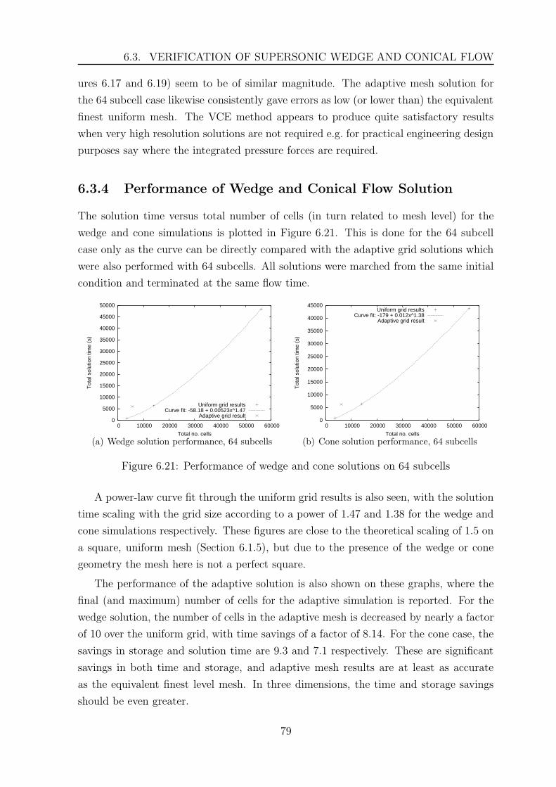
6.3. VERIFICATION OF SUPERSONIC WEDGE AND CONICAL FLOW
ures 6.17 and 6.19) seem to be of similar magnitude. The adaptive mesh solution for
the 64 subcell case likewise consistently gave errors as low (or lower than) the equivalent
finest uniform mesh. The VCE method appears to produce quite satisfactory results
when very high resolution solutions are not required e.g. for practical engineering design
purposes say where the integrated pressure forces are required.
6.3.4 Performance of Wedge and Conical Flow Solution
The solution time versus total number of cells (in turn related to mesh level) for the
wedge and cone simulations is plotted in Figure 6.21. This is done for the 64 subcell
case only as the curve can be directly compared with the adaptive grid solutions which
were also performed with 64 subcells. All solutions were marched from the same initial
condition and terminated at the same flow time.
0
5000
10000
15000
20000
25000
30000
35000
40000
45000
50000
0 10000 20000 30000 40000 50000 60000
Tot
al s
olut
ion
time
(s)
Total no. cells
Uniform grid resultsCurve fit: -58.18 + 0.00523x^1.47
Adaptive grid result
(a) Wedge solution performance, 64 subcells
0
5000
10000
15000
20000
25000
30000
35000
40000
45000
0 10000 20000 30000 40000 50000 60000
Tot
al s
olut
ion
time
(s)
Total no. cells
Uniform grid resultsCurve fit: -179 + 0.012x^1.38
Adaptive grid result
(b) Cone solution performance, 64 subcells
Figure 6.21: Performance of wedge and cone solutions on 64 subcells
A power-law curve fit through the uniform grid results is also seen, with the solution
time scaling with the grid size according to a power of 1.47 and 1.38 for the wedge and
cone simulations respectively. These figures are close to the theoretical scaling of 1.5 on
a square, uniform mesh (Section 6.1.5), but due to the presence of the wedge or cone
geometry the mesh here is not a perfect square.
The performance of the adaptive solution is also shown on these graphs, where the
final (and maximum) number of cells for the adaptive simulation is reported. For the
wedge solution, the number of cells in the adaptive mesh is decreased by nearly a factor
of 10 over the uniform grid, with time savings of a factor of 8.14. For the cone case, the
savings in storage and solution time are 9.3 and 7.1 respectively. These are significant
savings in both time and storage, and adaptive mesh results are at least as accurate
as the equivalent finest level mesh. In three dimensions, the time and storage savings
should be even greater.
79
6.4. VERIFICATION OF SUPERSONIC VORTEX FLOW
6.4 Verification of Supersonic Vortex Flow
This two-dimensional test case is an inviscid supersonic vortex bounded by two circular,
ninety-degree arcs, and is chosen because it has a smooth, analytic solution [6] and can
be compared with previous solutions [110, 148]. This test case is also worth performing
as a global order of convergence can be computed, and this problem has a slightly more
complex geometry compared to the wedge and cone study of Section 6.3. The flow
conditions are chosen to be identical to those of References [6, 110, 148].
The initial flow condition chosen for the domain is
ρ = 1.0, P = 1.0, u = v = 0
The inner arc radius is at ri = 1 and the outer arc radius at ro = 1.384. The analytic
density as a function of radius r for this flowfield is
ρ (r) = ρi
[1 +
γ − 1
2Mi
2
(1 −
(ri
r
)2)] 1
γ−1
(6.10)
where the inlet Mach number at the inner radius is Mi = 2.25 and density ρi = 1.
The pressure Pi = 1/γ and it varies throughout the flowfield according to the isentropic
relation P = Piργ. The inflow (at x = 0) is distributed inversely proportional to the
radius i.e. ui = (Mi/r) i.
The global discretization error is computed two different ways, a dimensionless L1
norm representing ‘average’ error (Equation 6.11) –
L1 =1
N
∑∣∣∣∣Qnum − Qexact
Qexact
∣∣∣∣ (6.11)
where N is the number of cells, Qnum is the computed numerical solution (in this case it
will be density) and Qexact the exact solution. Another error measure is the dimensionless
root mean square norm already enunciated in Equation 6.9.
Like Section 6.1, the grid convergence order is obtained from simulations on three
successivly-refined uniform grids. They are mesh levels 5, 6, and 7 corresponding to
cell sizes of 0.04325, 0.021625, and 0.0108125 m respectively. Three different subcell
resolutions are also used (32, 64, and 128 subcells) to observe error behavior with subcell
refinement.
The flux solvers are AUSMDV and EFM, and a first-order (no reconstruction) grid
convergence study will also be performed with AUSMDV. As the circular walls are rep-
resented by polygons, care was taken to position the points along the arc circumference
such that their distance was at least five times smaller than the smallest cell size, to
minimize errors from the geometry representation itself.
80
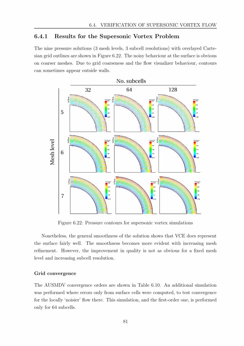
6.4. VERIFICATION OF SUPERSONIC VORTEX FLOW
6.4.1 Results for the Supersonic Vortex Problem
The nine pressure solutions (3 mesh levels, 3 subcell resolutions) with overlayed Carte-
sian grid outlines are shown in Figure 6.22. The noisy behaviour at the surface is obvious
on coarser meshes. Due to grid coarseness and the flow visualizer behaviour, contours
can sometimes appear outside walls.
Figure 6.22: Pressure contours for supersonic vortex simulations
Nonetheless, the general smoothness of the solution shows that VCE does represent
the surface fairly well. The smoothness becomes more evident with increasing mesh
refinement. However, the improvement in quality is not as obvious for a fixed mesh
level and increasing subcell resolution.
Grid convergence
The AUSMDV convergence orders are shown in Table 6.10. An additional simulation
was performed where errors only from surface cells were computed, to test convergence
for the locally ‘noisier’ flow there. This simulation, and the first-order one, is performed
only for 64 subcells.
81
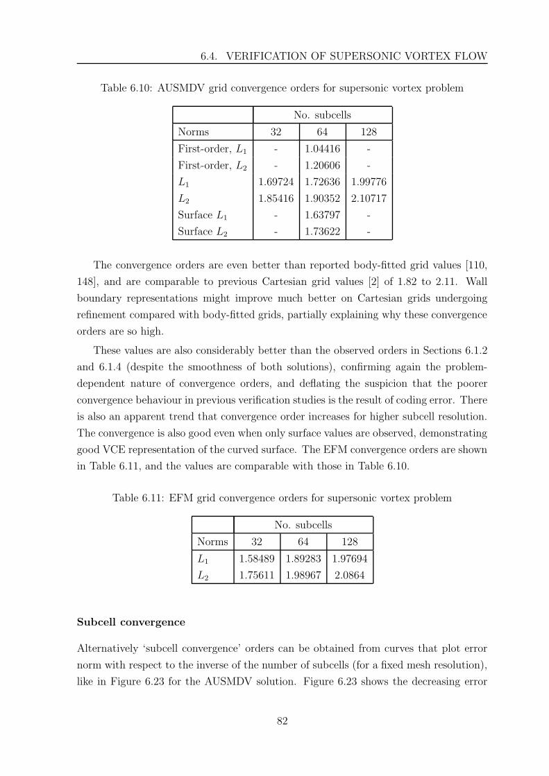
6.4. VERIFICATION OF SUPERSONIC VORTEX FLOW
Table 6.10: AUSMDV grid convergence orders for supersonic vortex problem
No. subcells
Norms 32 64 128
First-order, L1 - 1.04416 -
First-order, L2 - 1.20606 -
L1 1.69724 1.72636 1.99776
L2 1.85416 1.90352 2.10717
Surface L1 - 1.63797 -
Surface L2 - 1.73622 -
The convergence orders are even better than reported body-fitted grid values [110,
148], and are comparable to previous Cartesian grid values [2] of 1.82 to 2.11. Wall
boundary representations might improve much better on Cartesian grids undergoing
refinement compared with body-fitted grids, partially explaining why these convergence
orders are so high.
These values are also considerably better than the observed orders in Sections 6.1.2
and 6.1.4 (despite the smoothness of both solutions), confirming again the problem-
dependent nature of convergence orders, and deflating the suspicion that the poorer
convergence behaviour in previous verification studies is the result of coding error. There
is also an apparent trend that convergence order increases for higher subcell resolution.
The convergence is also good even when only surface values are observed, demonstrating
good VCE representation of the curved surface. The EFM convergence orders are shown
in Table 6.11, and the values are comparable with those in Table 6.10.
Table 6.11: EFM grid convergence orders for supersonic vortex problem
No. subcells
Norms 32 64 128
L1 1.58489 1.89283 1.97694
L2 1.75611 1.98967 2.0864
Subcell convergence
Alternatively ‘subcell convergence’ orders can be obtained from curves that plot error
norm with respect to the inverse of the number of subcells (for a fixed mesh resolution),
like in Figure 6.23 for the AUSMDV solution. Figure 6.23 shows the decreasing error
82
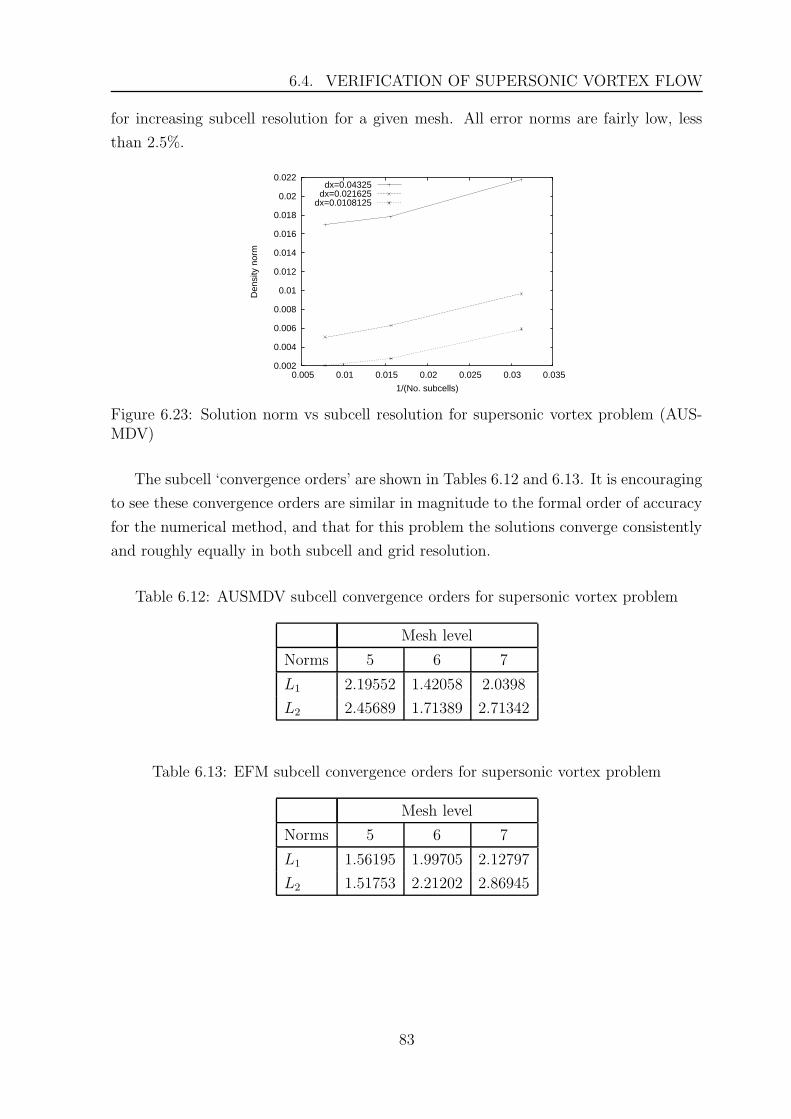
6.4. VERIFICATION OF SUPERSONIC VORTEX FLOW
for increasing subcell resolution for a given mesh. All error norms are fairly low, less
than 2.5%.
0.002
0.004
0.006
0.008
0.01
0.012
0.014
0.016
0.018
0.02
0.022
0.005 0.01 0.015 0.02 0.025 0.03 0.035
Den
sity
nor
m
1/(No. subcells)
dx=0.04325dx=0.021625
dx=0.0108125
Figure 6.23: Solution norm vs subcell resolution for supersonic vortex problem (AUS-MDV)
The subcell ‘convergence orders’ are shown in Tables 6.12 and 6.13. It is encouraging
to see these convergence orders are similar in magnitude to the formal order of accuracy
for the numerical method, and that for this problem the solutions converge consistently
and roughly equally in both subcell and grid resolution.
Table 6.12: AUSMDV subcell convergence orders for supersonic vortex problem
Mesh level
Norms 5 6 7
L1 2.19552 1.42058 2.0398
L2 2.45689 1.71389 2.71342
Table 6.13: EFM subcell convergence orders for supersonic vortex problem
Mesh level
Norms 5 6 7
L1 1.56195 1.99705 2.12797
L2 1.51753 2.21202 2.86945
83
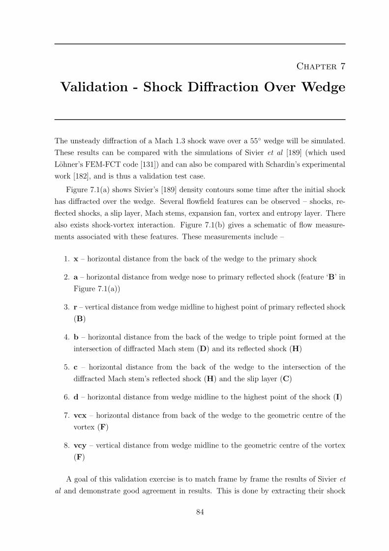
Chapter 7
Validation - Shock Diffraction Over Wedge
The unsteady diffraction of a Mach 1.3 shock wave over a 55◦ wedge will be simulated.
These results can be compared with the simulations of Sivier et al [189] (which used
Lohner’s FEM-FCT code [131]) and can also be compared with Schardin’s experimental
work [182], and is thus a validation test case.
Figure 7.1(a) shows Sivier’s [189] density contours some time after the initial shock
has diffracted over the wedge. Several flowfield features can be observed – shocks, re-
flected shocks, a slip layer, Mach stems, expansion fan, vortex and entropy layer. There
also exists shock-vortex interaction. Figure 7.1(b) gives a schematic of flow measure-
ments associated with these features. These measurements include –
1. x – horizontal distance from the back of the wedge to the primary shock
2. a – horizontal distance from wedge nose to primary reflected shock (feature ‘B’ in
Figure 7.1(a))
3. r – vertical distance from wedge midline to highest point of primary reflected shock
(B)
4. b – horizontal distance from the back of the wedge to triple point formed at the
intersection of diffracted Mach stem (D) and its reflected shock (H)
5. c – horizontal distance from the back of the wedge to the intersection of the
diffracted Mach stem’s reflected shock (H) and the slip layer (C)
6. d – horizontal distance from wedge midline to the highest point of the shock (I)
7. vcx – horizontal distance from back of the wedge to the geometric centre of the
vortex (F)
8. vcy – vertical distance from wedge midline to the geometric centre of the vortex
(F)
A goal of this validation exercise is to match frame by frame the results of Sivier et
al and demonstrate good agreement in results. This is done by extracting their shock
84
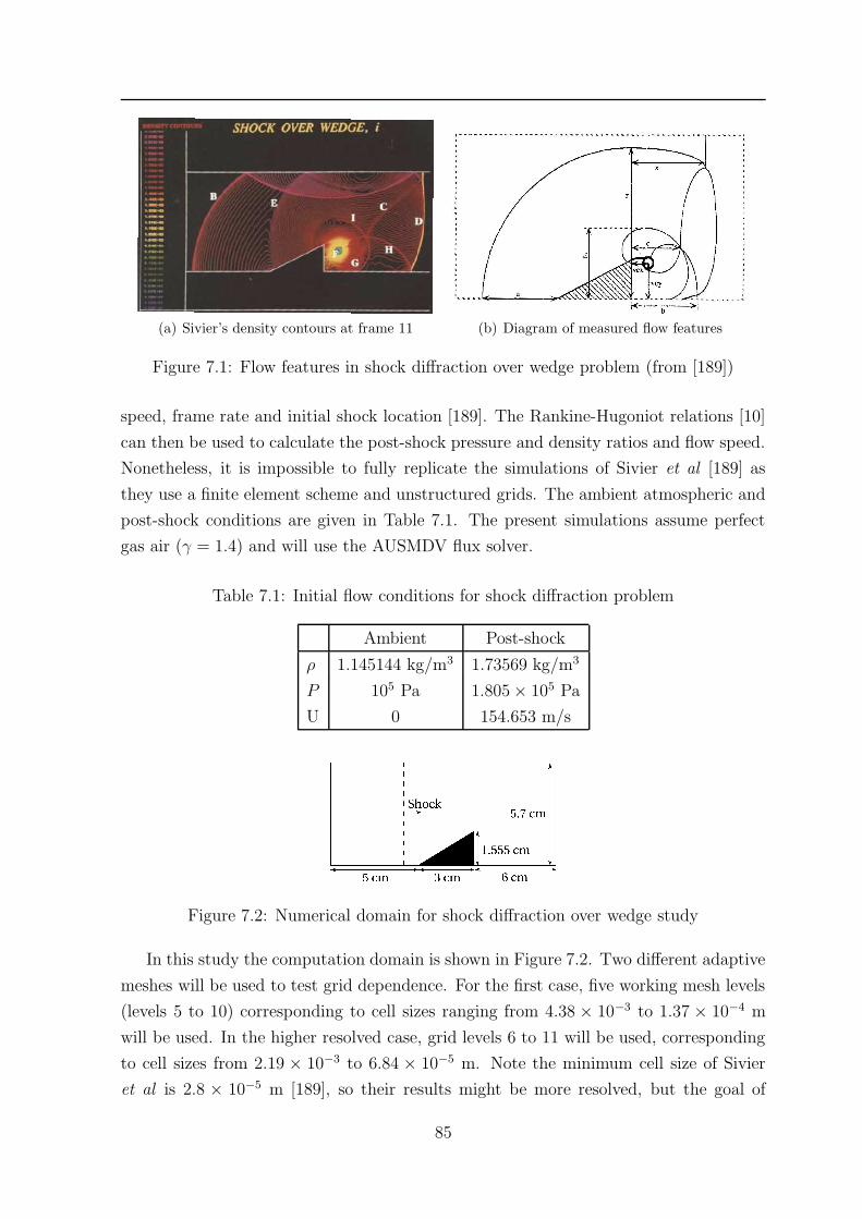
(a) Sivier’s density contours at frame 11 (b) Diagram of measured flow features
Figure 7.1: Flow features in shock diffraction over wedge problem (from [189])
speed, frame rate and initial shock location [189]. The Rankine-Hugoniot relations [10]
can then be used to calculate the post-shock pressure and density ratios and flow speed.
Nonetheless, it is impossible to fully replicate the simulations of Sivier et al [189] as
they use a finite element scheme and unstructured grids. The ambient atmospheric and
post-shock conditions are given in Table 7.1. The present simulations assume perfect
gas air (γ = 1.4) and will use the AUSMDV flux solver.
Table 7.1: Initial flow conditions for shock diffraction problem
Ambient Post-shock
ρ 1.145144 kg/m3 1.73569 kg/m3
P 105 Pa 1.805 × 10⁵ Pa
U 0 154.653 m/s
Figure 7.2: Numerical domain for shock diffraction over wedge study
In this study the computation domain is shown in Figure 7.2. Two different adaptive
meshes will be used to test grid dependence. For the first case, five working mesh levels
(levels 5 to 10) corresponding to cell sizes ranging from 4.38 × 10⁻³ to 1.37 × 10⁻⁴ m
will be used. In the higher resolved case, grid levels 6 to 11 will be used, corresponding
to cell sizes from 2.19 × 10⁻³ to 6.84 × 10⁻⁵ m. Note the minimum cell size of Sivier
et al is 2.8 × 10⁻⁵ m [189], so their results might be more resolved, but the goal of
85
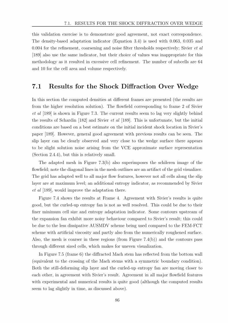
7.1. RESULTS FOR THE SHOCK DIFFRACTION OVER WEDGE
this validation exercise is to demonstrate good agreement, not exact correspondence.
The density-based adaptation indicator (Equation 3.4) is used with 0.063, 0.035 and
0.004 for the refinement, coarsening and noise filter thresholds respectively; Sivier et al
[189] also use the same indicator, but their choice of values was inappropriate for this
methodology as it resulted in excessive cell refinement. The number of subcells are 64
and 10 for the cell area and volume respectively.
7.1 Results for the Shock Diffraction Over Wedge
In this section the computed densities at different frames are presented (the results are
from the higher resolution solution). The flowfield corresponding to frame 2 of Sivier
et al [189] is shown in Figure 7.3. The current results seem to lag very slightly behind
the results of Schardin [182] and Sivier et al [189]. This is unfortunate, but the initial
conditions are based on a best estimate on the initial incident shock location in Sivier’s
paper [189]. However, general good agreement with previous results can be seen. The
slip layer can be clearly observed and very close to the wedge surface there appears
to be slight solution noise arising from the VCE approximate surface representation
(Section 2.4.4), but this is relatively small.
The adapted mesh in Figure 7.3(b) also superimposes the schileren image of the
flowfield; note the diagonal lines in the mesh outlines are an artifact of the grid visualizer.
The grid has adapted well to all major flow features, however not all cells along the slip
layer are at maximum level; an additional entropy indicator, as recommended by Sivier
et al [189], would improve the adaptation there.
Figure 7.4 shows the results at Frame 4. Agreement with Sivier’s results is quite
good, but the curled-up entropy fan is not as well resolved. This could be due to their
finer minimum cell size and entropy adaptation indicator. Some contours upstream of
the expansion fan exhibit more noisy behaviour compared to Sivier’s result; this could
be due to the less dissipative AUSMDV scheme being used compared to the FEM-FCT
scheme with artificial viscosity and partly also from the numerically roughened surface.
Also, the mesh is coarser in these regions (from Figure 7.4(b)) and the contours pass
through different sized cells, which makes for uneven visualization.
In Figure 7.5 (frame 6) the diffracted Mach stem has reflected from the bottom wall
(equivalent to the crossing of the Mach stems with a symmetric boundary condition).
Both the still-deforming slip layer and the curled-up entropy fan are moving closer to
each other, in agreement with Sivier’s result. Agreement in all major flowfield features
with experimental and numerical results is quite good (although the computed results
seem to lag slightly in time, as discussed above).
86
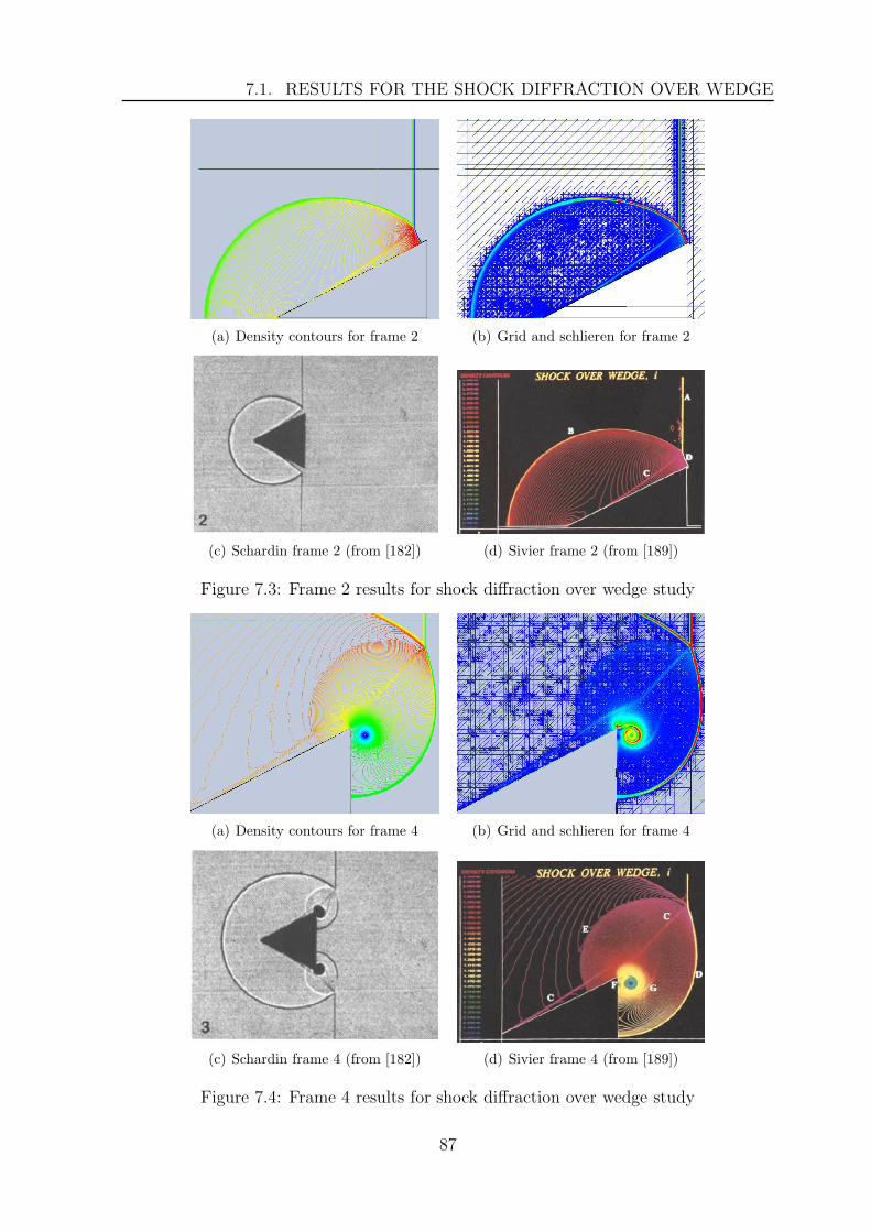
7.1. RESULTS FOR THE SHOCK DIFFRACTION OVER WEDGE
(a) Density contours for frame 2 (b) Grid and schlieren for frame 2
(c) Schardin frame 2 (from [182]) (d) Sivier frame 2 (from [189])
Figure 7.3: Frame 2 results for shock diffraction over wedge study
(a) Density contours for frame 4 (b) Grid and schlieren for frame 4
(c) Schardin frame 4 (from [182]) (d) Sivier frame 4 (from [189])
Figure 7.4: Frame 4 results for shock diffraction over wedge study
87
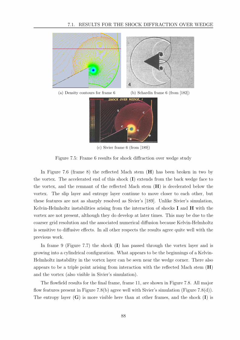
7.1. RESULTS FOR THE SHOCK DIFFRACTION OVER WEDGE
(a) Density contours for frame 6 (b) Schardin frame 6 (from [182])
(c) Sivier frame 6 (from [189])
Figure 7.5: Frame 6 results for shock diffraction over wedge study
In Figure 7.6 (frame 8) the reflected Mach stem (H) has been broken in two by
the vortex. The accelerated end of this shock (I) extends from the back wedge face to
the vortex, and the remnant of the reflected Mach stem (H) is decelerated below the
vortex. The slip layer and entropy layer continue to move closer to each other, but
these features are not as sharply resolved as Sivier’s [189]. Unlike Sivier’s simulation,
Kelvin-Helmholtz instabilities arising from the interaction of shocks I and H with the
vortex are not present, although they do develop at later times. This may be due to the
coarser grid resolution and the associated numerical diffusion because Kelvin-Helmholtz
is sensitive to diffusive effects. In all other respects the results agree quite well with the
previous work.
In frame 9 (Figure 7.7) the shock (I) has passed through the vortex layer and is
growing into a cylindrical configuration. What appears to be the beginnings of a Kelvin-
Helmholtz instability in the vortex layer can be seen near the wedge corner. There also
appears to be a triple point arising from interaction with the reflected Mach stem (H)
and the vortex (also visible in Sivier’s simulation).
The flowfield results for the final frame, frame 11, are shown in Figure 7.8. All major
flow features present in Figure 7.8(b) agree well with Sivier’s simulation (Figure 7.8(d)).
The entropy layer (G) is more visible here than at other frames, and the shock (I) is
88
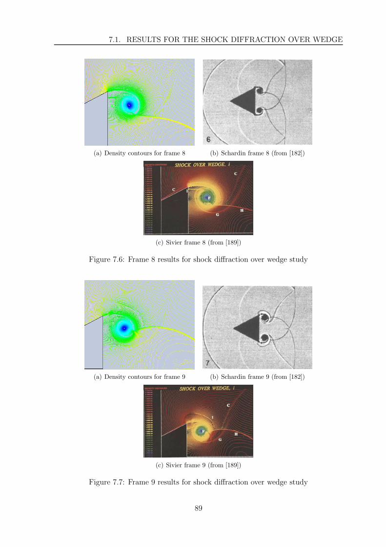
7.1. RESULTS FOR THE SHOCK DIFFRACTION OVER WEDGE
(a) Density contours for frame 8 (b) Schardin frame 8 (from [182])
(c) Sivier frame 8 (from [189])
Figure 7.6: Frame 8 results for shock diffraction over wedge study
(a) Density contours for frame 9 (b) Schardin frame 9 (from [182])
(c) Sivier frame 9 (from [189])
Figure 7.7: Frame 9 results for shock diffraction over wedge study
89
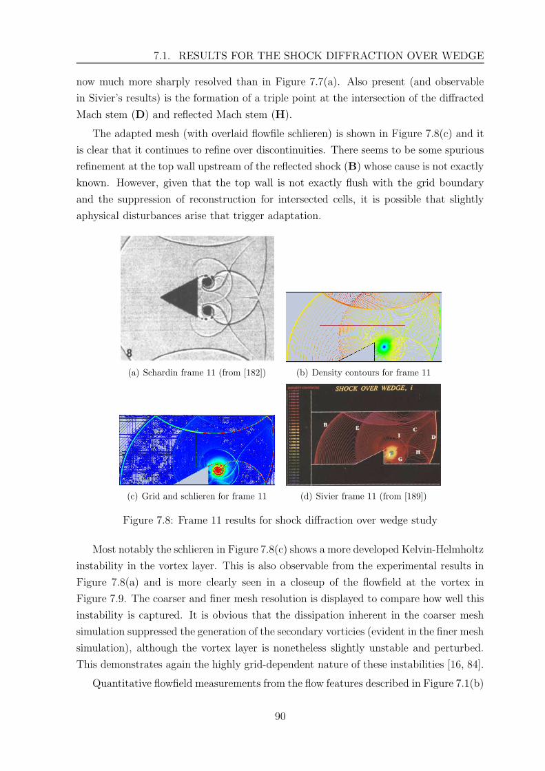
7.1. RESULTS FOR THE SHOCK DIFFRACTION OVER WEDGE
now much more sharply resolved than in Figure 7.7(a). Also present (and observable
in Sivier’s results) is the formation of a triple point at the intersection of the diffracted
Mach stem (D) and reflected Mach stem (H).
The adapted mesh (with overlaid flowfile schlieren) is shown in Figure 7.8(c) and it
is clear that it continues to refine over discontinuities. There seems to be some spurious
refinement at the top wall upstream of the reflected shock (B) whose cause is not exactly
known. However, given that the top wall is not exactly flush with the grid boundary
and the suppression of reconstruction for intersected cells, it is possible that slightly
aphysical disturbances arise that trigger adaptation.
(a) Schardin frame 11 (from [182]) (b) Density contours for frame 11
(c) Grid and schlieren for frame 11 (d) Sivier frame 11 (from [189])
Figure 7.8: Frame 11 results for shock diffraction over wedge study
Most notably the schlieren in Figure 7.8(c) shows a more developed Kelvin-Helmholtz
instability in the vortex layer. This is also observable from the experimental results in
Figure 7.8(a) and is more clearly seen in a closeup of the flowfield at the vortex in
Figure 7.9. The coarser and finer mesh resolution is displayed to compare how well this
instability is captured. It is obvious that the dissipation inherent in the coarser mesh
simulation suppressed the generation of the secondary vorticies (evident in the finer mesh
simulation), although the vortex layer is nonetheless slightly unstable and perturbed.
This demonstrates again the highly grid-dependent nature of these instabilities [16, 84].
Quantitative flowfield measurements from the flow features described in Figure 7.1(b)
90
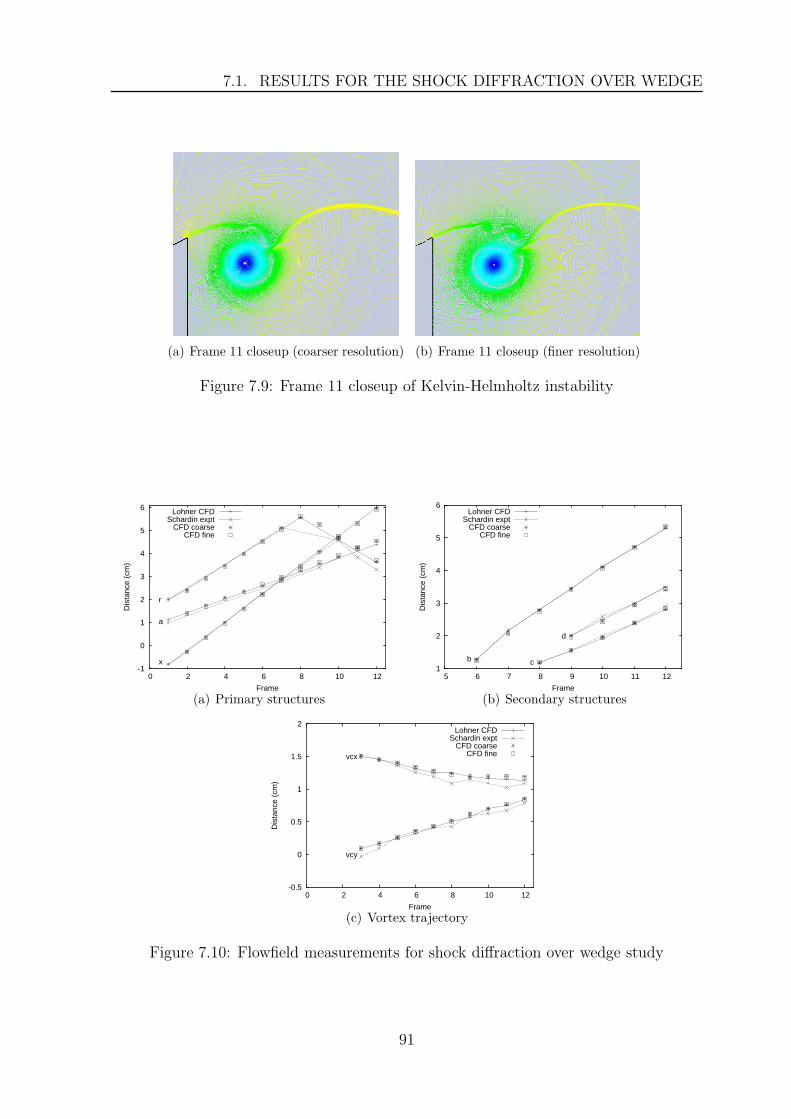
7.1. RESULTS FOR THE SHOCK DIFFRACTION OVER WEDGE
(a) Frame 11 closeup (coarser resolution) (b) Frame 11 closeup (finer resolution)
Figure 7.9: Frame 11 closeup of Kelvin-Helmholtz instability
-1
0
1
2
3
4
5
6
0 2 4 6 8 10 12
Dis
tanc
e (c
m)
Frame
r
a
x
Lohner CFDSchardin expt
CFD coarseCFD fine
(a) Primary structures
1
2
3
4
5
6
5 6 7 8 9 10 11 12
Dis
tanc
e (c
m)
Frame
b c
d
Lohner CFDSchardin expt
CFD coarseCFD fine
(b) Secondary structures
-0.5
0
0.5
1
1.5
2
0 2 4 6 8 10 12
Dis
tanc
e (c
m)
Frame
vcx
vcy
Lohner CFDSchardin expt
CFD coarseCFD fine
(c) Vortex trajectory
Figure 7.10: Flowfield measurements for shock diffraction over wedge study
91
7.2. SERIAL PERFORMANCE
are plotted in Figure 7.10, where results from the two grid resolutions are shown to
observe grid dependence. The primary flow structures (a, r and x) and the secondary
flow structures (b, c and d) are plotted in Figures 7.10(a) and 7.10(b) respectively.
Agreement with previous results is quite good, with nearly grid-independent behaviour.
In Figure 7.10(c) the vortex position (vcx and vcy) is plotted. Agreement with
Sivier’s result is quite good, and possible explanations of discrepancies with Schardin’s
experiments include the difficulty of locating the vortex and the complex interaction of
the reflected Mach stem with the vortex [189]. These results demonstrate that OctVCE,
despite the issues with flow noise at surfaces (Section 2.4.4), has the ability to provide
an accurate and fairly well-resolved simulation of this problem. Along with Sivier et al
[189], it is reasonable to assert that surface wedge pressures would also be estimated
well.
7.2 Serial Performance
The serial performance of the simulations is profiled using the GNU profiler gprof.
The relative percentages of time spent in important portions of the code are shown in
Table 7.2 for the two different resolution simulations. The important sections of the
code are –
1. Reconstruction-related operations – computing gradients, limiters, reconstruction
2. Solution advancement – computing fluxes, timesteps, boundary conditions, time
integration
3. Adaptation – computing adaptation indicators, refining and coarsening the mesh
4. Geometric operations – point-inclusion tests, calculating cell geometric properties
5. Connectivity management – updating mesh connectivity, list operations
6. Output – writing solutions to output files
It is clear that reconstruction-related operations are a large fraction of the computa-
tion time, and the relative difference between these operations and solution advancement
is quite similar to the performance figures in Section 6.1.5. It might be worthwhile for
future work to investigate more efficient ways to perform reconstruction. There ap-
pears to be good efficiency in the adaptation process, but connectivity management is
a necessary overhead on an adaptive scheme, meaning a net overhead of around 10%
for the entire adaptation process. This is actually a fairly significant figure that can
92
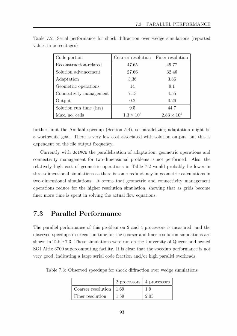
7.3. PARALLEL PERFORMANCE
Table 7.2: Serial performance for shock diffraction over wedge simulations (reported
values in percentages)
Code portion Coarser resolution Finer resolution
Reconstruction-related 47.65 49.77
Solution advancement 27.66 32.46
Adaptation 3.36 3.86
Geometric operations 14 9.1
Connectivity management 7.13 4.55
Output 0.2 0.26
Solution run time (hrs) 9.5 44.7
Max. no. cells 1.3 × 10⁵ 2.83 × 10⁵
further limit the Amdahl speedup (Section 5.4), so parallelizing adaptation might be
a worthwhile goal. There is very low cost associated with solution output, but this is
dependent on the file output frequency.
Currently with OctVCE the parallelization of adaptation, geometric operations and
connectivity management for two-dimensional problems is not performed. Also, the
relatively high cost of geometric operations in Table 7.2 would probably be lower in
three-dimensional simulations as there is some redundancy in geometric calculations in
two-dimensional simulations. It seems that geometric and connectivity management
operations reduce for the higher resolution simulation, showing that as grids become
finer more time is spent in solving the actual flow equations.
7.3 Parallel Performance
The parallel performance of this problem on 2 and 4 processors is measured, and the
observed speedups in execution time for the coarser and finer resolution simulations are
shown in Table 7.3. These simulations were run on the University of Queensland owned
SGI Altix 3700 supercomputing facility. It is clear that the speedup performance is not
very good, indicating a large serial code fraction and/or high parallel overheads.
Table 7.3: Observed speedups for shock diffraction over wedge simulations
2 processors 4 processors
Coarser resolution 1.69 1.9
Finer resolution 1.59 2.05
93
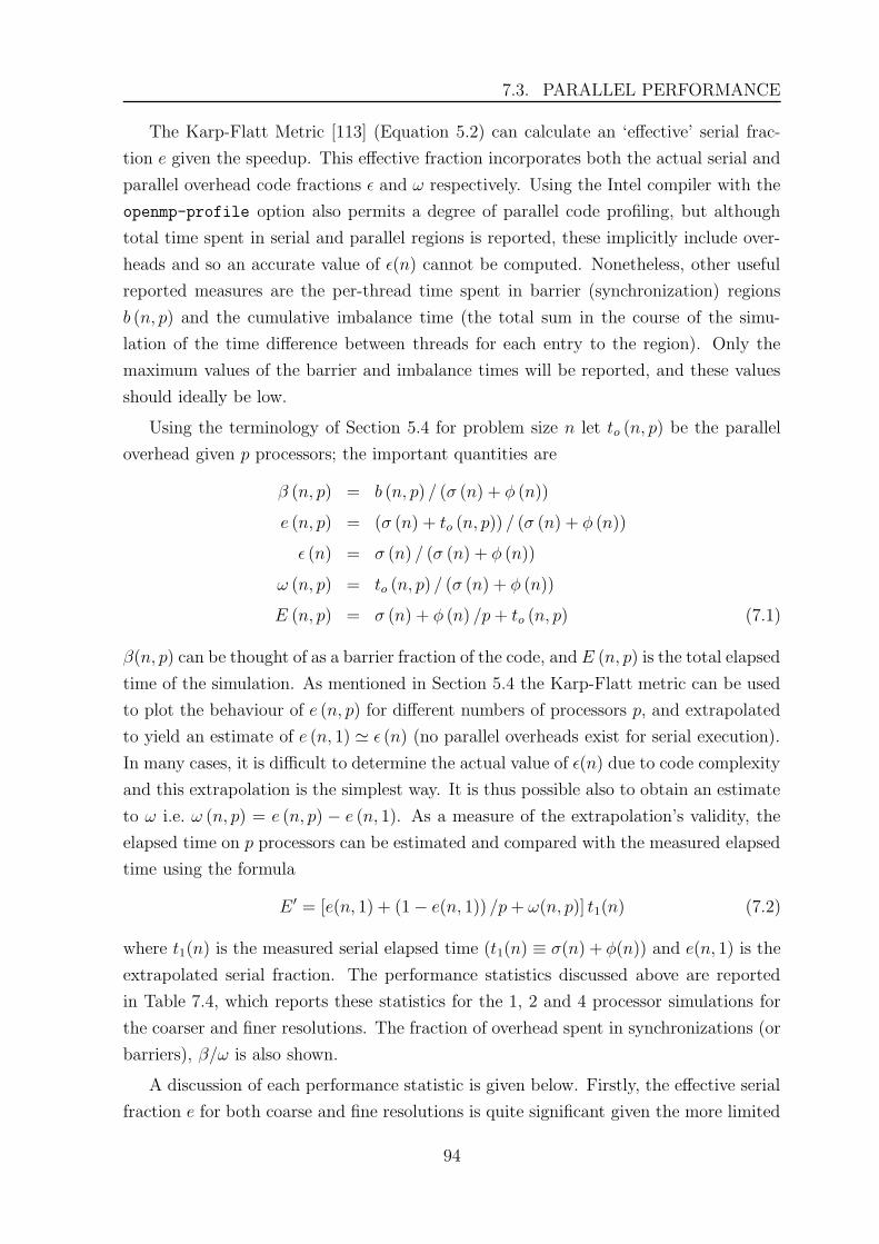
7.3. PARALLEL PERFORMANCE
The Karp-Flatt Metric [113] (Equation 5.2) can calculate an ‘effective’ serial frac-
tion e given the speedup. This effective fraction incorporates both the actual serial and
parallel overhead code fractions ε and ω respectively. Using the Intel compiler with the
openmp-profile option also permits a degree of parallel code profiling, but although
total time spent in serial and parallel regions is reported, these implicitly include over-
heads and so an accurate value of ε(n) cannot be computed. Nonetheless, other useful
reported measures are the per-thread time spent in barrier (synchronization) regions
b (n, p) and the cumulative imbalance time (the total sum in the course of the simu-
lation of the time difference between threads for each entry to the region). Only the
maximum values of the barrier and imbalance times will be reported, and these values
should ideally be low.
Using the terminology of Section 5.4 for problem size n let to (n, p) be the parallel
overhead given p processors; the important quantities are
β (n, p) = b (n, p) / (σ (n) + φ (n))
e (n, p) = (σ (n) + to (n, p)) / (σ (n) + φ (n))
ε (n) = σ (n) / (σ (n) + φ (n))
ω (n, p) = to (n, p) / (σ (n) + φ (n))
E (n, p) = σ (n) + φ (n) /p + to (n, p) (7.1)
β(n, p) can be thought of as a barrier fraction of the code, and E (n, p) is the total elapsed
time of the simulation. As mentioned in Section 5.4 the Karp-Flatt metric can be used
to plot the behaviour of e (n, p) for different numbers of processors p, and extrapolated
to yield an estimate of e (n, 1) ' ε (n) (no parallel overheads exist for serial execution).
In many cases, it is difficult to determine the actual value of ε(n) due to code complexity
and this extrapolation is the simplest way. It is thus possible also to obtain an estimate
to ω i.e. ω (n, p) = e (n, p) − e (n, 1). As a measure of the extrapolation’s validity, the
elapsed time on p processors can be estimated and compared with the measured elapsed
time using the formula
E ′ = [e(n, 1) + (1 − e(n, 1)) /p + ω(n, p)] t1(n) (7.2)
where t1(n) is the measured serial elapsed time (t1(n) ≡ σ(n) + φ(n)) and e(n, 1) is the
extrapolated serial fraction. The performance statistics discussed above are reported
in Table 7.4, which reports these statistics for the 1, 2 and 4 processor simulations for
the coarser and finer resolutions. The fraction of overhead spent in synchronizations (or
barriers), β/ω is also shown.
A discussion of each performance statistic is given below. Firstly, the effective serial
fraction e for both coarse and fine resolutions is quite significant given the more limited
94
7.3. PARALLEL PERFORMANCE
Table 7.4: Parallel performance statistics for shock diffraction over wedge simulations
1 processor 2 processors 4 processors
Coarse Finer Coarse Finer Coarse Finer
Single processor time (s) t1 34237 160903
‘Effective’ serial fraction e 0.183 0.26 0.367 0.316
Extrapolated serial 0.0915 0.231
fraction e(n, 1)
Overhead fraction ω 0.0919 0.028 0.276 0.0854
Barrier fraction β 0.009 0.0087 0.0793 0.0154
Barrier/overhead β/ω 0.104 0.306 0.288 0.18
Imbalance time/elapsed time 0.0033 0.0029 0.0563 0.0106
Estimated elapsed time (s) E ′ 21831 103623 20347 81847
Measured elapsed time (s) E 20232 101364 17978 78402
parallelization of the two-dimensional code discussed in Section 7.2, and it increases for
more processors due to parallel overhead (time spent in process startup, communication
or synchronization). The increase (between 2 and 4 processors) is 0.184 and 0.056 for
the coarser and finer grid results respectively. The increase is smaller for the finer grid
result, probably due to the Amdahl effect [151] (Section 5.4) where the parallel overhead
fraction typically decreases for larger problem sizes as to has a lower complexity than φ.
The extrapolated serial fraction e(n, 1) ' ε appears to be smaller for the coarser grid
result. Perhaps one cause of this stems from the longer execution time in some serial
operations for larger problem sizes like list traversals which utilize indirect addressing.
However the value of e(n, 1) is an estimate and the serial fraction ε may be different if
executed using the resources of more processors.
The overhead fractions ω are based on extrapolated ε values and for the coarser
grid result are very signficant, being larger than its extrapolated serial fraction, and
increasing by about a factor of 3 between 2 and 4 processors. The overheads for the
finer grid result are consistently smaller (the Amdahl effect) by about 70% and also
increase by about a factor of 3. They are also smaller than its extrapolated serial
fraction. The barrier fractions β are smaller than the overhead fractions as expected,
and are generally smaller for the finer resolution simulation. The predominant parallel
overheads appear to consist of communication overheads.
Imbalance times are quite small (demonstrating good load balancing), and appear
to increase for more processors, and is less significant for the finer resolution, indicating
95

7.3. PARALLEL PERFORMANCE
better performance in parallel regions. Estimated elapsed times E ′ also compare quite
well with actual elapsed times E (indicating a reasonably sound extrapolation of e(n, 1)),
but are somewhat larger. Thus could be due to the conservatism in the ω estimates.
Also, the elapsed 1 processor time t1(n) used to compute E ′ in Equation 7.2 may have
been smaller if it were run with the increased memory resources of a parallel simulation.
The performance statistics suggest a fairly large fraction of the code remains serial
for this problem, limiting parallel efficiency. Moreover, parallel overheads are also quite
significant, and increase considerably with more processors. Synchronization times also
form a significant portion of these overheads, although communication time is apparently
the dominant factor. This behaviour is expected for a NUMA machine like the Altix
and the minimal exploitation of locality of storage (and large memory requirements) of
the code as described in Section 5.5.3.
96
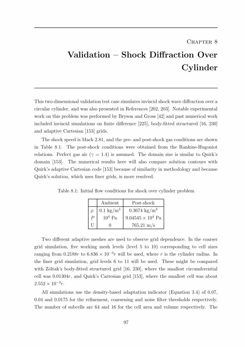
Chapter 8
Validation – Shock Diffraction Over
Cylinder
This two-dimensional validation test case simulates inviscid shock wave diffraction over a
circular cylinder, and was also presented in References [202, 203]. Notable experimental
work on this problem was performed by Bryson and Gross [42] and past numerical work
included inviscid simulations on finite difference [225], body-fitted structured [16, 230]
and adaptive Cartesian [153] grids.
The shock speed is Mach 2.81, and the pre- and post-shock gas conditions are shown
in Table 8.1. The post-shock conditions were obtained from the Rankine-Hugoniot
relations. Perfect gas air (γ = 1.4) is assumed. The domain size is similar to Quirk’s
domain [153]. The numerical results here will also compare solution contours with
Quirk’s adaptive Cartesian code [153] because of similarity in methodology and because
Quirk’s solution, which uses finer grids, is more resolved.
Table 8.1: Initial flow conditions for shock over cylinder problem
Ambient Post-shock
ρ 0.1 kg/m3 0.3674 kg/m3
P 104 Pa 9.04545 × 10⁴ Pa
U 0 765.21 m/s
Two different adaptive meshes are used to observe grid dependence. In the coarser
grid simulation, five working mesh levels (level 5 to 10) corresponding to cell sizes
ranging from 0.2188r to 6.836 × 10⁻³r will be used, where r is the cylinder radius. In
the finer grid simulation, grid levels 6 to 11 will be used. These might be compared
with Zoltak’s body-fitted structured grid [16, 230], where the smallest circumferential
cell was 0.01304r, and Quirk’s Cartesian grid [153], where the smallest cell was about
2.552 × 10⁻³r.
All simulations use the density-based adaptation indicator (Equation 3.4) of 0.07,
0.04 and 0.0175 for the refinement, coarsening and noise filter thresholds respectively.
The number of subcells are 64 and 16 for the cell area and volume respectively. The
97
8.1. RESULTS FOR SHOCK DIFFRACTION OVER CYLINDER
adaptive flux solver is implemented (Section 4.4) where EFM operates at shocks and
AUSMDV is used elsewhere.
Pressure traces are recorded at locations around the cylinder corresponding to angles
φ = 0◦, 30◦, 40◦, 60◦, 90◦, 120◦, 150◦ and 180◦. The traces record surface pressure
normalized by ambient pressure against nondimensional time tu/r where t, r and u are
the time, cylinder radius and incident shock velocity respectively.
8.1 Results for Shock Diffraction Over Cylinder
Figure 8.1 compares density contours from the finer grid simulation with Quirk’s con-
tours [153]. The comparison is quite good, and all important flow features are resolved
well (the shock, contact discontinuity, vortex and vortex stem).
Figure 8.1: Shock cylinder density contours. Top figure – current results, bottom figure– Quirk’s [153]
However, contours behind the bow shock are not smooth and exhibit noticeable
noise, which could be due to noise being generated at the shock (AUSMDV is used in
most of the flow). This results from a discretized stepped representation of the curved
bow shock, creating artifical shear layers which stream into the stagnation region. Also
Figure 8.2, which shows the corresponding grid, has a less uniform distribution of mesh
levels near this region, which makes for a noisier visualization of contours.
98
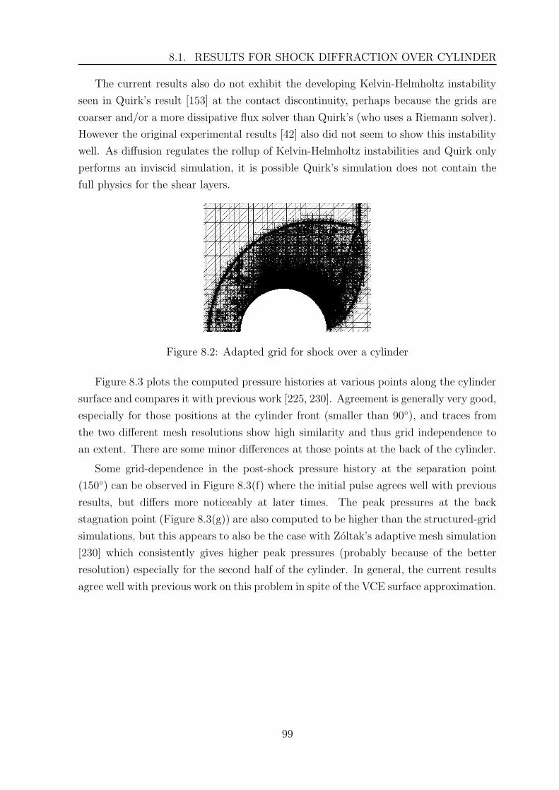
8.1. RESULTS FOR SHOCK DIFFRACTION OVER CYLINDER
The current results also do not exhibit the developing Kelvin-Helmholtz instability
seen in Quirk’s result [153] at the contact discontinuity, perhaps because the grids are
coarser and/or a more dissipative flux solver than Quirk’s (who uses a Riemann solver).
However the original experimental results [42] also did not seem to show this instability
well. As diffusion regulates the rollup of Kelvin-Helmholtz instabilities and Quirk only
performs an inviscid simulation, it is possible Quirk’s simulation does not contain the
full physics for the shear layers.
Figure 8.2: Adapted grid for shock over a cylinder
Figure 8.3 plots the computed pressure histories at various points along the cylinder
surface and compares it with previous work [225, 230]. Agreement is generally very good,
especially for those positions at the cylinder front (smaller than 90◦), and traces from
the two different mesh resolutions show high similarity and thus grid independence to
an extent. There are some minor differences at those points at the back of the cylinder.
Some grid-dependence in the post-shock pressure history at the separation point
(150◦) can be observed in Figure 8.3(f) where the initial pulse agrees well with previous
results, but differs more noticeably at later times. The peak pressures at the back
stagnation point (Figure 8.3(g)) are also computed to be higher than the structured-grid
simulations, but this appears to also be the case with Zoltak’s adaptive mesh simulation
[230] which consistently gives higher peak pressures (probably because of the better
resolution) especially for the second half of the cylinder. In general, the current results
agree well with previous work on this problem in spite of the VCE surface approximation.
99
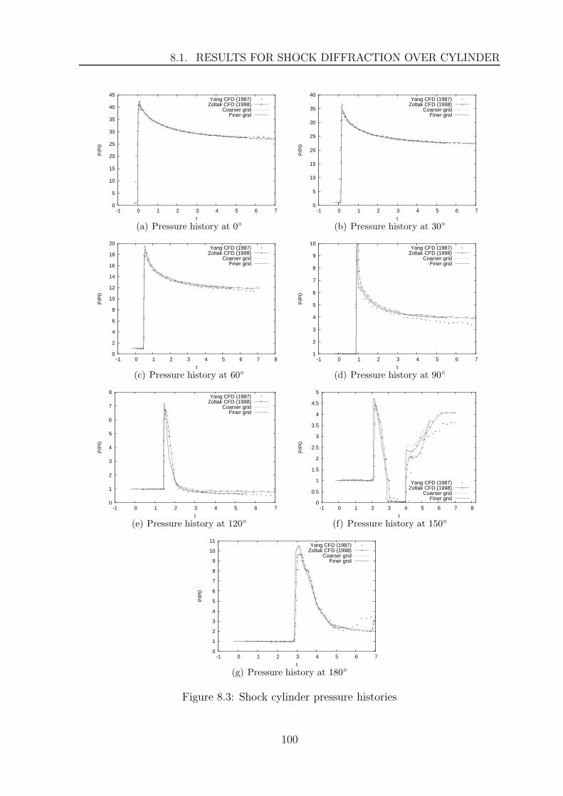
8.1. RESULTS FOR SHOCK DIFFRACTION OVER CYLINDER
0
5
10
15
20
25
30
35
40
45
-1 0 1 2 3 4 5 6 7
P/P
0
t
Yang CFD (1987)Zoltak CFD (1998)
Coarser gridFiner grid
(a) Pressure history at 0◦
0
5
10
15
20
25
30
35
40
-1 0 1 2 3 4 5 6 7
P/P
0
t
Yang CFD (1987)Zoltak CFD (1998)
Coarser gridFiner grid
(b) Pressure history at 30◦
0
2
4
6
8
10
12
14
16
18
20
-1 0 1 2 3 4 5 6 7 8
P/P
0
t
Yang CFD (1987)Zoltak CFD (1998)
Coarser gridFiner grid
(c) Pressure history at 60◦
1
2
3
4
5
6
7
8
9
10
-1 0 1 2 3 4 5 6 7
P/P
0
t
Yang CFD (1987)Zoltak CFD (1998)
Coarser gridFiner grid
(d) Pressure history at 90◦
0
1
2
3
4
5
6
7
8
-1 0 1 2 3 4 5 6 7
P/P
0
t
Yang CFD (1987)Zoltak CFD (1998)
Coarser gridFiner grid
(e) Pressure history at 120◦
0
0.5
1
1.5
2
2.5
3
3.5
4
4.5
5
-1 0 1 2 3 4 5 6 7 8
P/P
0
t
Yang CFD (1987)Zoltak CFD (1998)
Coarser gridFiner grid
(f) Pressure history at 150◦
0
1
2
3
4
5
6
7
8
9
10
11
-1 0 1 2 3 4 5 6 7
P/P
0
t
Yang CFD (1987)Zoltak CFD (1998)
Coarser gridFiner grid
(g) Pressure history at 180◦
Figure 8.3: Shock cylinder pressure histories
100
Chapter 9
Validation - One-Dimensional Spherical
Blast Waves
This section simulates spherical blast waves using the second-order one-dimensional code
to solve the unsteady Euler equations in one-dimensional spherical geometry (described
in Appendix B). This will help establish the validity of results obtained from the one-
dimensional code which, in turn, is used to verify OctVCE. The test case will be compared
with the numerical results of Ritzel and Matthews [166], who investigated the use of the
“balloon analogue” model (Section 4.6) to initiate explosions.
9.1 Description of Simulations
The initial charge or balloon conditions are a pressure of 30,000 atmospheres and tem-
perature of 3600 K for the helium gas. The energy of the charge is equivalent to 0.25
kg of Pentolite with a specific energy of 6.55 MJ/kg [166]. The blast energy is related
to the balloon gas pressure and volume via the ideal gas relation
E =(P − P0) V
γ − 1(9.1)
where E is the total blast energy, P the initial gas pressure, P0 ambident pressure, V
volume and γ ratio of specific heats. Using Equation 9.1, the initial charge radius and
density of around 0.0441 m and 406.24 kg/m3 are calculated respectively (γ = 1.667).
Assumed ambient conditions for the air are P0 = 101.325 kPa and ρ0 = 1.2 kg/m3.
Ritzel and Matthews used a flux-corrected transport (FCT) scheme with an element
size of 5 mm [166]. To obtain exact correspondence in energy the number of cells within
the charge must be an integer multiple of its radius and the closest cell size to Ritzel’s
that can be used is around 4.9 mm (9 cells in the charge). Further simulations are also
performed assuming the same blast energy but different charge conditions –
1. A first-order simulation without reconstruction, to demonstrate increased accuracy
of the second-order scheme.
101
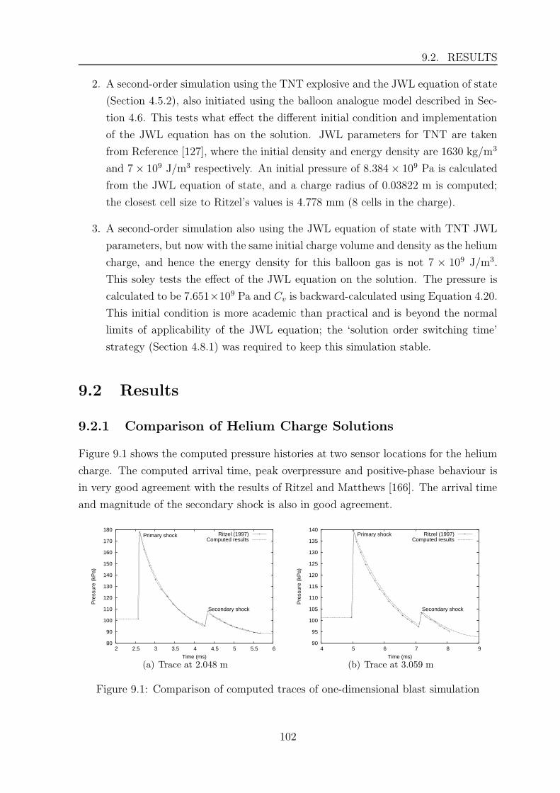
9.2. RESULTS
2. A second-order simulation using the TNT explosive and the JWL equation of state
(Section 4.5.2), also initiated using the balloon analogue model described in Sec-
tion 4.6. This tests what effect the different initial condition and implementation
of the JWL equation has on the solution. JWL parameters for TNT are taken
from Reference [127], where the initial density and energy density are 1630 kg/m3
and 7 × 10⁹ J/m3 respectively. An initial pressure of 8.384 × 10⁹ Pa is calculated
from the JWL equation of state, and a charge radius of 0.03822 m is computed;
the closest cell size to Ritzel’s values is 4.778 mm (8 cells in the charge).
3. A second-order simulation also using the JWL equation of state with TNT JWL
parameters, but now with the same initial charge volume and density as the helium
charge, and hence the energy density for this balloon gas is not 7 × 10⁹ J/m3.
This soley tests the effect of the JWL equation on the solution. The pressure is
calculated to be 7.651×10⁹ Pa and Cv is backward-calculated using Equation 4.20.
This initial condition is more academic than practical and is beyond the normal
limits of applicability of the JWL equation; the ‘solution order switching time’
strategy (Section 4.8.1) was required to keep this simulation stable.
9.2 Results
9.2.1 Comparison of Helium Charge Solutions
Figure 9.1 shows the computed pressure histories at two sensor locations for the helium
charge. The computed arrival time, peak overpressure and positive-phase behaviour is
in very good agreement with the results of Ritzel and Matthews [166]. The arrival time
and magnitude of the secondary shock is also in good agreement.
80
90
100
110
120
130
140
150
160
170
180
2 2.5 3 3.5 4 4.5 5 5.5 6
Pre
ssur
e (k
Pa)
Time (ms)
Primary shock
Secondary shock
Ritzel (1997)Computed results
(a) Trace at 2.048 m
90
95
100
105
110
115
120
125
130
135
140
4 5 6 7 8 9
Pre
ssur
e (k
Pa)
Time (ms)
Primary shock
Secondary shock
Ritzel (1997)Computed results
(b) Trace at 3.059 m
Figure 9.1: Comparison of computed traces of one-dimensional blast simulation
102
9.2. RESULTS
The wave diagram comparing trajectories of primary and secondary shocks and the
contact surface is shown in Figure 9.2. Note for the spherical shock problem the contact
surface’s position is roughly constant [25]. Very good agreement between current and
past results can be observed. The results give good confidence in the simple spherical
one-dimensional code.
0
2
4
6
8
10
0 0.5 1 1.5 2 2.5 3 3.5 4
Tim
e (m
s)
Dist (m)
Ritzel primary shockRitzel secondary shock
Ritzel contact surfaceComputed results
Figure 9.2: Comparison of computed trajectories of one-dimensional blast simulation
9.2.2 Comparison of Different Charge Solutions
The second-order helium, first-order helium and two JWL solutions are compared at
different times in this section. The solutions at an early time of 1.5 ms are shown in
Figure 9.3. Note the “JWL altered TNT equiv” line corresponds to the simulation where
the “altered” JWL equation of state is used but on a gas with the same volume and
density as the helium balloon gas, as opposed to the “proper” TNT solution (with more
realistic TNT initial conditions), labelled as the “JWL TNT equiv” line.
As expected the first-order solution more poorly resolves the primary and secondary
shocks, and consequently underestimates the peak overpressure. The primary shock
strength and positive phase wave behaviour between all solutions are quite similar,
although primary shocks of the TNT solutions seem to lag in arrival time slightly. The
main difference in solutions occur after the positive phase; the proper TNT solution
exhibits a much larger and delayed secondary shock and even reverse flow. It would
seem this is mainly caused by the different initial condition of the proper TNT solution,
since the altered TNT solution also uses the JWL equation but is much more similar to
the helium solution.
Figure 9.4 shows the solutions at 3 ms. The poorer resolution of the first-order solu-
tion is evident, especially of the secondary shock. The agreement between all solutions
103
9.2. RESULTS
60
80
100
120
140
160
180
200
220
240
260
0 0.2 0.4 0.6 0.8 1 1.2 1.4 1.6
Pre
ssur
e (k
Pa)
Distance (m)
2nd order, perf gas1st order, perf gas
JWL TNT equivJWL altered TNT equiv
(a) Pressure
0
0.5
1
1.5
2
2.5
0 0.2 0.4 0.6 0.8 1 1.2 1.4 1.6
Den
sity
(kg
/m^3
)
Distance (m)
2nd order, perf gas1st order, perf gas
JWL TNT equivJWL altered TNT equiv
(b) Density
-200
-150
-100
-50
0
50
100
150
200
250
0 0.2 0.4 0.6 0.8 1 1.2 1.4 1.6
Vel
ocity
(m
/s)
Distance (m)
2nd order, perf gas1st order, perf gas
JWL TNT equivJWL altered TNT equiv
(c) Flow velocity
Figure 9.3: One-dimensional blast at 1.5 ms
in the positive phase is also more pronounced, and, as with Figure 9.3, the only signifi-
cant difference occurs with the proper TNT solution after the positive phase, which as
mentioned above is likely mainly due to its different initial condition. The altered TNT
solution has an unusual discontinuity near the explosion core that may be a numerical
artifact triggered by the sudden switching of the solution order.
The solutions at 7.5 ms are shown in Figure 9.5. At this time there is very close
agreement with all solutions in the positive phase region. The pressure near the explosion
core appears to be rising back to the ambient value at this time. The contact surfaces of
the helium and proper TNT solutions are also visible at around x = 0.5 m. This surface
is not captured well for the first-order or altered TNT solutions probably as a result
of being run first-order at earlier times. The proper TNT solution also has apparently
developed a tertiary shock, and its secondary shock continues to be larger in magnitude
and lag behind the other solutions. The first-order solution can no longer represent the
secondary shock effectively.
The wave diagram of all solutions is shown Figure 9.6. Wave trajectories amongst
all solutions agree very well with each other except for the secondary shock trajectory
of the proper TNT solution. It appears the main cause of this different secondary
shock trajectory is due to the different initial condition rather than usage of the JWL
104
9.2. RESULTS
60
80
100
120
140
160
0 0.5 1 1.5 2
Pre
ssur
e (k
Pa)
Distance (m)
2nd order, perf gas1st order, perf gas
JWL TNT equivJWL altered TNT equiv
(a) Pressure
0
0.2
0.4
0.6
0.8
1
1.2
1.4
1.6
1.8
0 0.5 1 1.5 2
Den
sity
(kg
/m^3
)
Distance (m)
2nd order, perf gas1st order, perf gas
JWL TNT equivJWL altered TNT equiv
(b) Density
-100
-50
0
50
100
150
0 0.5 1 1.5 2
Den
sity
(kg
/m^3
)
Distance (m)
2nd order, perf gas1st order, perf gas
JWL TNT equivJWL altered TNT equiv
(c) Flow velocity
Figure 9.4: One-dimensional blast at 3 ms
85
90
95
100
105
110
115
120
125
130
0 0.5 1 1.5 2 2.5 3 3.5 4
Pre
ssur
e (k
Pa)
Distance (m)
2nd order, perf gas1st order, perf gas
JWL TNT equivJWL altered TNT equiv
(a) Pressure
0.2
0.4
0.6
0.8
1
1.2
1.4
0 0.5 1 1.5 2 2.5 3 3.5 4
Den
sity
(kg
/m^3
)
Distance (m)
2nd order, perf gas1st order, perf gas
JWL TNT equivJWL altered TNT equiv
(b) Density
-30
-20
-10
0
10
20
30
40
50
60
0 0.5 1 1.5 2 2.5 3 3.5 4
Vel
ocity
(m
/s)
Distance (m)
2nd order, perf gas1st order, perf gas
JWL TNT equivJWL altered TNT equiv
(c) Flow velocity
Figure 9.5: One-dimensional blast at 7.5 ms
105
9.3. NON-REFLECTING BOUNDARY CONDITION TEST
equation of state. On this scale it is difficult to notice the small differences in primary
shock arrival time between the helium and TNT solutions.
0
2
4
6
8
10
12
14
0 0.5 1 1.5 2 2.5 3 3.5 4
Tim
e (m
s)
Dist (m)
Ritzel primary shockRitzel secondary shock
Ritzel contact surface2nd order, perf gas1st order, perf gas
JWL TNT equivJWL altered TNT equiv
Figure 9.6: Computed trajectories for one-dimensional blast simulation
These results demonstrate that mid- to far-field behaviour of the positive-phase wave-
form is nearly independent of charge initial conditions or equation of state usage. They
confirm that the dominant parameter determining primary shock intensity and positive
phase impulse is the initial explosive energy (Section 4.6), and thus using a perfect gas
balloon model is an acceptable approach for mid- to far-field regimes. Large differences
occur in the negative phase, which are also corroborated by Ritzel’s numerical exper-
iments [166] which indicated that a denser balloon gas caused a more severe negative
phase and stronger secondary shock.
9.3 Non-reflecting Boundary Condition Test
A final test case will investigate the performance of the non-reflecting outlet boundary
condition (Appendix H) after the primary shock exits the domain. The helium solution
is simulated on a truncated domain (8 m long) and compared with the solution on a
longer domain using the same cell size. The solution at 19.5 ms is shown in Figure 9.7
after the primary shock has left the domain (but before the secondary shock). No
reflections can be observed in pressure, density or velocity. Note the velocity in the
positive phase is less than 20 m/s meaning subsonic flow.
The solution at 22.5 ms is shown in Figure 9.8, which is after the secondary shock
has left the domain. The pressure and velocity (Figures 9.8(a) and 9.8(c) respectively)
do not display reflections, but there exists some upstream influence of the boundary
condition that causes the negative phase solution to deviate slightly.
The solution at 30 ms is shown in Figure 9.9 well after the negative phase has left
106
9.3. NON-REFLECTING BOUNDARY CONDITION TEST
96
98
100
102
104
106
108
110
6 6.5 7 7.5 8 8.5
Pre
ssur
e (k
Pa)
Distance (m)
Longer domainNonreflecting BC
(a) Pressure
1.16
1.18
1.2
1.22
1.24
1.26
1.28
6 6.5 7 7.5 8 8.5
Den
sity
(kg
/m^3
)
Distance (m)
Longer domainNonreflecting BC
(b) Density
-10
-5
0
5
10
15
20
6 6.5 7 7.5 8 8.5
Vel
ocity
(m
/s)
Distance (m)
Longer domainNonreflecting BC
(c) Flow velocity
Figure 9.7: One-dimensional blast at 19.5 ms (non-reflecting test case)
97
98
99
100
101
102
103
104
105
1 2 3 4 5 6 7 8 9
Pre
ssur
e (k
Pa)
Distance (m)
Longer domainNonreflecting BC
(a) Pressure
0.8
0.9
1
1.1
1.2
1.3
1 2 3 4 5 6 7 8 9
Den
sity
(kg
/m^3
)
Distance (m)
Longer domainNonreflecting BC
(b) Density
-8
-6
-4
-2
0
2
4
6
8
1 2 3 4 5 6 7 8
Vel
ocity
(m
/s)
Distance (m)
Longer domainNonreflecting BC
(c) Flow velocity
Figure 9.8: One-dimensional blast at 22.5 ms (non-reflecting test case)
107
9.3. NON-REFLECTING BOUNDARY CONDITION TEST
the domain. This time the upstream influence from the boundary is more noticeable,
which extends leftward until the small inward-moving reflection wave. The density
solution (Figure 9.9(b)) still seems to display very good agreement with the longer
domain solution. The subsonic outlet non-reflecting boundary condition seems to work
quite well even some time after the secondary shock has exited the domain, although it
performs more poorly at later times. Similar performance might be expected in multi-
dimensional simulations when a wave parallel to the boundary exits the domain. For
oblique exiting waves, there may be small reflections [116, 210].
97
98
99
100
101
102
103
104
105
2 4 6 8 10 12
Pre
ssur
e (k
Pa)
Distance (m)
Longer domainNonreflecting BC
(a) Pressure
0.7
0.8
0.9
1
1.1
1.2
1.3
2 4 6 8 10 12
Den
sity
(kg
/m^3
)
Distance (m)
Longer domainNonreflecting BC
(b) Density
-8
-6
-4
-2
0
2
4
6
8
2 4 6 8 10 12
Vel
ocity
(m
/s)
Distance (m)
Longer domainNonreflecting BC
(c) Flow velocity
Figure 9.9: One-dimensional blast at 30 ms (non-reflecting test case)
108
Chapter 10
Validation – TNT Blast
The calculation of free-field blast parameters versus scaled distance following the explo-
sion of a spherical TNT charge is an important test case for this code given the wealth of
data on this problem [19, 25, 40, 119, 171, 192]. The material for this section appeared in
Reference [206] by the author. Simulations are first performed with the one-dimensional
spherical code and compared with data from the CONWEP program [103], Kinney’s
explosives text of [119] and the study by Cullis and Huntington-Thresher [101], and the
explosions are initiated using the balloon gas approach like in Chapter 9.
Simulations are also performed in two and three dimensions and compared with
the one-dimensional result. They should ideally be identical to the one-dimensional
result, but this is not always attainable as the charge representation is asymmetrically
‘discretized’ in the radial direction by a Cartesian representation with the balloon gas
or bursting sphere model (Section 4.6). The blast also does not usually propagate along
the mesh direction and will give slightly different results depending on what direction
one is looking. Multi-dimensional simulations are also usually quite expensive and use
coarser grids that may give solutions that are not grid-independent.
The simulations use the JWL parameters for TNT taken from Reference [127], like
in Section 9.1. A charge mass of 1 kg is used, thus all reported distances are also scaled
values. Assumed ambient air conditions are P0 = 101.325 kPa and ρ0 = 1.2 kg/m3.
10.1 One-Dimensional TNT Blast
The initial JWL TNT conditions in Section 9.1 are used here for the TNT charge, and
an initial temperature of 2900 K is assumed [133]. A simulation is also performed where
a mass- and energy-equivalent volume of perfect gas air is used for the balloon gas.
The results are shown in Figure 10.1; note Cullis’ results [101] were only reported to a
distance of 8 m/kg1/3. Grid-independence is virtually attained with 40 cells through the
charge. The impulse is normalized by positive phase duration, and CONWEP data was
not obtainable directly but extracted from Cullis’ paper [101]. Error bars in Cullis’ data
series are used to cover their range of results and for the impulse plot the CONWEP
result lies within this range.
109
10.1. ONE-DIMENSIONAL TNT BLAST
10
100
1000
10000
100000
0 1 2 3 4 5 6 7 8 9
Ove
rpre
ssur
e (k
Pa)
Distance from charge (m)
Kinney (1985)Huntington-Thresher CONWEP (2001)
Huntington-Thresher results (2001)1D, air
1D, JWL
(a) Peak overpressure
0
2
4
6
8
10
12
14
16
18
20
0 1 2 3 4 5 6 7 8 9
Tim
e of
arr
ival
(m
s)
Distance from charge (m)
Kinney (1985)Huntington-Thresher CONWEP (2001)
Huntington-Thresher results (2001)1D, air
1D, JWL
(b) Primary shock arrival time
1
10
100
1000
10000
0 1 2 3 4 5 6 7 8 9
Impu
lse/
Dur
atio
n (P
aS/m
S)
Distance from charge (m)
Kinney (1985)Huntington-Thresher results (2001)
1D, air1D, JWL
(c) Scaled peak impulse
0
1
2
3
4
5
0 1 2 3 4 5 6 7 8 9
Dur
atio
n (m
s)
Distance from charge (m)
Kinney (1985)Huntington-Thresher CONWEP (2001)
Huntington-Thresher results (2001)1D, air
1D, JWL
(d) Positive phase duration
Figure 10.1: One-dimensional TNT blast parameters
In general the results agree well with existing data, especially in pressure and impulse
(often the most important quantities), and differences between the JWL and air solutions
are very small. These results indicate that a perfect gas bursting sphere approach can
produce good correlation with experimental data of important blast parameters from as
close as 0.5 m/kg1/3, which has also been observed by Rose [171]. The one-dimensional
solution can thus be used to compute the error from multi-dimensional simulations (see
Section 10.3).
Cullis and Huntington-Thresher mention that the finite gauge rise time may have
caused their arrival time to be overpredicted slightly, as appears evident in Figure 10.1(b).
The greatest discrepancies occur with the positive phase duration (Figure 10.1(d)), al-
though the current results follow Kinney’s line fairly closely. Positive phase duration
appears to be a difficult quantity to measure, and has been known to vary by more
than one order of magnitude in experimental results [146]. Poor agreement in computed
results and CONWEP values was also observed by Rose [171]. Cullis suggests that
CONWEP might overestimate this value due to afterburning effects [101].
110
10.2. AXISYMMETRIC TNT BLAST
10.2 Axisymmetric TNT Blast
Simulations are performed in two-dimensional axisymmetric geometry and with adap-
tive quadtree meshes with typically 4 working levels. To investigate convergence, five
different meshes are used with minimum cell sizes of 0.1875, 9.375 ×10⁻², 4.688 ×10⁻²,
2.344 ×10⁻² and 1.172 ×10⁻² m (successive grid doubling). The coarser of these grids
can only represent the charge in one cell, and thus not all solutions may be in the asymp-
totic range of convergence (this is demonstrated below). The finest cell size is chosen to
correspond roughly with a common fine cell size used by Rose et al [171, 175] in their
three-dimensional simulations of blast interaction with buildings.
An example of an initial coarse Cartesian cell charge representation is shown in
Figure 10.2. The curved line represents the spherical charge; cells intersected by or
within that volume are initiated to the charge or balloon conditions (again, diagonal
lines are an artifact of the grid visualizer Paraview [90]). A plane of symmetry at x = 0 is
assumed. To save costs, smaller computational domains are used for finer grids. Domain
sizes vary from 6 to 20 m; experience has shown these distances are sufficient for a blast
wave profile to develop. Sensor locations are placed on the radial axis at around 0.2 m
increments close to the charge, and around 1 m increments farther away.
Ideal gas air is used for the balloon gas. The density of this gas depends on the volume
of the cells representing the charge and is adjusted for each grid (using the method in
Section 4.6.1) such that the charge has a mass of 1 kg. The balloon gas pressure is
adjusted to give the correct blast energy equivalent to a 1 kg TNT charge. An adaptive
flux solver (Section 4.4) is used with EFM at shocks and AUSMDV elsewhere. The
density-based adaptation indicator (Equation 3.4) is used and typical values for the
refinement, coarsening and noise filter thresholds are 0.3, 0.02 and 0.008 respectively.
However these thresholds are adjusted slightly for each mesh as the indicators perform
differently for different mesh resolutions, and are chosen to give a good but not excessive
degree of refinement in the region leading up to the primary shock.
Figure 10.2: Initial grid for 2D axisymmetric TNT blast simulation
111
10.2. AXISYMMETRIC TNT BLAST
The calculated blast parameters are shown in Figure 10.3 and compared with the
one-dimensional spherical result. The overpressure plot shows a trend of convergence
toward the one-dimensional result as the cell size decreases, and coarser grids usually
underpredict the overpressure. At distances less than about 1 m the differences between
the solutions are not so consistent; this is probably a result of the near-field effect of
the initial explosive shape, which has a significant effect on the blast waveform at this
range [40, 211]. The scaled impulse plot also shows reasonable agreement between one-
dimensional and axisymmetric solutions with finer grids generally giving a better result.
However it is shown later that convergence is not so easy to demonstrate for (non-scaled)
impulse. Arrival time is quite grid-independent, and positive phase duration seems to
be the most grid-dependent parameter (but its convergence can still be observed).
1
10
100
1000
10000
0.1 1 10 100
Ove
rpre
ssur
e (k
Pa)
Distance from charge (m)
1D, airdx=0.1875 m
dx=9.375e-2 mdx=4.6875e-2 m
dx=2.34375e-2 mdx=1.171875e-2 m
(a) Overpressure
0
5
10
15
20
25
30
35
0 2 4 6 8 10 12 14
Tim
e of
arr
ival
(m
s)
Distance from charge (m)
1D, airdx=0.1875 m
dx=9.375e-2 mdx=4.6875e-2 m
dx=2.34375e-2 mdx=1.171875e-2 m
(b) Arrival time
1
10
100
1000
10000
5 10 15 20 25
Impu
lse/
Dur
atio
n (P
aS/m
S)
Distance from charge (m)
1D, airdx=0.1875 m
dx=9.375e-2 mdx=4.6875e-2 m
dx=2.34375e-2 mdx=1.171875e-2 m
(c) Scaled impulse
0
1
2
3
4
5
0.1 1 10
Dur
atio
n (m
s)
Distance from charge (m)
1D, airdx=0.1875 m
dx=9.375e-2 mdx=4.6875e-2 m
dx=2.34375e-2 mdx=1.171875e-2 m
(d) Positive phase duration
Figure 10.3: Two-dimensional TNT blast parameters
An example pressure history at 11 m radial distance showing convergence of the
axisymmetric solutions is shown in Figure 10.4. The differences between sucessive peaks
become increasingly smaller and the positive phase waveform takes better shape. There
is a noticeable finite rise time to peak overpressure on coarser grids because of the poorer
shock resolution. The secondary shock is very difficult to resolve even on the fine grids,
but this feature is not so important.
112
10.3. ERROR QUANTIFICATION IN THE AXISYMMETRIC SOLUTIONS
-6
-4
-2
0
2
4
6
8
10
20 25 30 35 40 45 50
Ove
rpre
ssur
e (k
Pa)
Time (ms)
1D solutiondx=2.34375e-2 m
dx=4.6875e-2 mdx=9.375e-2 m
dx=0.1875 m
Figure 10.4: Example pressure history from TNT blast
10.3 Error Quantification in the Axisymmetric So-
lutions
This study takes the results of Section 10.2 and quantifies the differences between the
axisymmetric result and the virtually grid-independent one-dimensional spherical result
(Section 10.1) for the different axisymmetric grids1. As mentioned above, these errors
result from grid coarseness and the discretization of the spherical charge volume into a
‘staircased’ Cartesian representation.
Only the peak overpressure and peak impulse parameters (versus distance) will be
considered as these are the most important quantities from an engineering perspective.
Pressure sensors are also placed along both radial and diagonal (parallel to i + j) direc-
tions. Diagonal sensors might be expected to yield least accurate results and suffer most
from numerical diffusion as wave propagation is most misaligned to the mesh along the
diagonal.
It is hoped that this study will provide both a guide to the magnitude of the errors at
a given scaled distance and an assessment of the quality of error estimates computed from
grid refinement studies, which are based on Richardson extrapolation (Equations 6.2
and 6.3). As a guide to the quality of an error estimate, it will be useful to produce
statements like ‘the estimated error has a x% chance of being too large/small, and (i)
it will be too large/small by no more than value y 90% of the time, (ii) it will be too
large/small by an average of z%’. This study might then also be applicable for more
complicated blast problems where fine grid resolution is too costly to attain. A study
of the errors in the near-field may also help determine the scaled range below which the
balloon gas charge representation (and estimated error) is unsuitable.
1This section is taken from Reference [206] and is a more condensed version of that paper.
113
10.3. ERROR QUANTIFICATION IN THE AXISYMMETRIC SOLUTIONS
10.3.1 Actual Errors
At every sensor point, the relative error in blast parameters is computed as (fe − f) /fe
where fe is the ‘exact’ solution (the one-dimensional result) and f the axisymmetric
solution. These errors are plotted in Figure 10.5 along both sensor lines (radial and
diagonal). A discussion of the errors is given below.
0
0.1
0.2
0.3
0.4
0.5
0.6
0.7
0.8
0.9
0.1 1 10 100
Rel
ativ
e er
ror
in o
verp
ress
ure
Distance from charge (m)
dx=0.1875 mdx=9.375e-2 m
dx=4.6875e-2 mdx=2.34375e-2 m
dx=1.171875e-2 m
(a) Overpressure error (radial)
0
0.1
0.2
0.3
0.4
0.5
0.6
0.7
0.8
0.9
0.1 1 10 100
Rel
ativ
e er
ror
in o
verp
ress
ure
(dia
gona
l)
Distance from charge (m)
dx=0.1875 mdx=9.375e-2 m
dx=4.6875e-2 mdx=2.34375e-2 m
dx=1.171875e-2 m
(b) Overpressure error (diagonal)
0.001
0.01
0.1
1
10
0.1 1 10 100
Abs
olut
e re
lativ
e er
ror
in im
puls
e
Distance from charge (m)
dx=0.1875 mdx=9.375e-2 m
dx=4.6875e-2 mdx=2.34375e-2 m
dx=1.171875e-2 m
(c) Impulse error (radial)
1e-04
0.001
0.01
0.1
1
10
100
0.1 1 10 100
Abs
olut
e re
lativ
e er
ror
in im
puls
e (d
iago
nal)
Distance from charge (m)
dx=0.1875 mdx=9.375e-2 m
dx=4.6875e-2 mdx=2.34375e-2 m
dx=1.171875e-2 m
(d) Impulse error (diagonal)
Figure 10.5: Actual axisymmetric TNT parameter relative errors vs distance
Overpressure
It is clear from the graph of overpressure error along the radial axis (Figure 10.5(a)) that
after about 1 m the solutions are converging. Coarser grids always tend to produce lower
overpressures because of poorer shock resolution. Errors prior to 1 m are very large and
do not behave so consistently because of the still-significant effect of the initial charge
shape on the developing waveform which is forming into a more radially symmetric
pattern. This suggests for this range of cell sizes a ‘cut-off’ distance of 1-2 m at which
the balloon gas approach is appropriate when estimating error based on grid refinement
studies. The curves are not always smooth, and increase slightly for larger distances
probably because of numerical diffusion.
114
10.3. ERROR QUANTIFICATION IN THE AXISYMMETRIC SOLUTIONS
The errors along the diagonal direction (Figure 10.5(b)) are quite similar to those
along the radial direction. Errors also do not behave consistently before about 1 m, and
have steeper increase with distance after 1 m as numerical diffusion is more severe along
this direction. Although the solutions are converging at these distances, the differences
between errors for each grid are not always consistent, which will affect the Richardson
extrapolation-based error estimator.
It is likely that this is at least partly due to the different adaptation indicators
used. Although convergence to the one-dimensional waveform is still generally exhibited
(Figure 10.4), different indicators are used for different grids, and these were adjusted
(by trial and error) to be appropriate for that grid. If used on another grid it might
result in excessive or inadequate refinement. Although the grid near the primary shock
is usually refined, the region leading up to it (i.e. positive phase) does not always have
the same degree of refinement, which ultimately has an effect on the solution.
Ideally in performing grid refinement studies the grid should be uniformly refined, or
at least the same adaptation indicators used. But this can be computationally expensive
for many multi-dimensional blast problems. This study focusses on the quality of the
error estimation procedure in spite of this departure from ideality, and thus might be
more relevant for practical purposes. It appears that a cell size of smaller than the finest
cell (length 0.0117 m) is required to keep errors less than 10%.
Impulse
Convergent behaviour is difficult to observe with impulse (Figures 10.5(c) and 10.5(d)),
and the curves are much less smooth than the overpressure error curves. The absolute
value of the errors are taken because they are sometimes negative and a logarithmic
scale is used for the ordinate to better show the errors. The errors are quite high within
1 m of the charge because of the effect of the initial charge shape, but within that range
it is generally the case that finer grids do give lower errors.
It appears that the selected range of grid sizes is not within the range of convergence,
but it is still interesting to see how well the Richardon extrapolation error estimators
work. Impulse might be a more difficult quantity to converge (perhaps requiring very
costly finer grids) as the area under the finite rise time to the peak pressure (as shown
in Figure 10.4) may offset the loss in area resulting from a lower peak in coarser meshes.
Despite the lack of convergent behaviour at larger distances, all errors for the different
grids are around (or substantially less than) 10%, which is a much lower value than
coarser-grid overpressure errors. This is an encouraging result as impulse is often the
most important engineering quantity.
115
10.3. ERROR QUANTIFICATION IN THE AXISYMMETRIC SOLUTIONS
10.3.2 Estimated Errors
The estimated errors for overpressure and impulse for each grid are computed based
on the GCI (Equation 6.3 p.g. 6) and compared with the actual error for every grid
resolution and at every sensor point. This is done with each graph in Figure 10.5.
Important summary statistics for each graph are the maximum over- and underestima-
tion (the maximum values of how much larger/smaller the GCI is relative to the actual
error), average values of over- and underestimation, 90th over- and under-estimation
percentile (the value below which 90% of the over- and underestimation values fall) and
fraction (out of all sensors) which overestimate. Overestimations are preferred due to
conservatism in the design process.
The GCI error can be signed in the case of overpressure (i.e. 3E from Equation 6.3) as
it is always underestimated but given the erratic impulse error behaviour (Figures 10.5(c)
and 10.5(d)) should be taken as an absolute value for this quantity (i.e. 3|E|, the stan-
dard definition of GCI). The assumed refinement factor r = 2, and p = 1 for overpressure
(the scheme reverts to nominally first-order at shocks) and p = 2 for impulse errors (the
flow is nominally second-order in the smooth positive phase). However only those sen-
sors after 2 m from the charge are used, since it is found that this is the range where
the error estimates start to be more consistently conservative.
The error statistics are shown in Tables 10.1 and 10.2. These tables also display
the statistics for the p = 1.5 case, as it is proposed that this rounded figure may help
the overpressure and impulse GCI to be slightly less and more conservative respectively
(whilst still attaining a good fraction of overestimations). These tables will hopefully
be a reasonable guide to the magnitude and probability of over- and underestimations
that occur when estimating error from grid refinement (due to grid coarseness and the
departure of the discretized charge from the ideal spherical shape).
Overpressure error summary
The overpressure error summary statistics are shown in Table 10.1 and are for the
signed error. With p = 1 the fraction of overestimations is around 90%, but the average
overestimation value is 30-40%, which might be excessively conservative. Taking p =
1.5 reduces the average overestimation (and its 90th percentile) by a factor of 2-4,
whilst keeping average underestimation about the same. The overestimation fraction
is not as high, especially along the diagonal direction at 60%, but this might still be
preferred in lieu of the smaller overestimation magnitude. Because of the low number
of underestimations, the 90th underestimation percentile is computed to be the same
value as the maximum underestimation value.
116
10.3. ERROR QUANTIFICATION IN THE AXISYMMETRIC SOLUTIONS
Table 10.1: Overpressure error summary statistics
Radial Radial Diagonal Diagonal
(p = 1) (p = 1.5) (p = 1) (p = 1.5)
Maximum overestimation 0.587455 0.178413 0.676975 0.226954
Maximum underestimation 0.214859 0.262645 0.122117 0.201611
Average overestimation 0.303943 0.0798927 0.376296 0.152875
Average underestimation 0.114163 0.0802441 0.0480577 0.0665265
90th overestimation percentile 0.527328 0.147001 0.647733 0.220307
90th underestimation percentile 0.214859 0.262645 0.122117 0.122851
Fraction of overestimations 0.941176 0.882353 0.85 0.6
Table 10.2: Impulse error summary statistics
Radial Radial Diagonal Diagonal
(p = 2) (p = 1.5) (p = 2) (p = 1.5)
Maximum overestimation 0.092165 0.157443 0.0452596 0.0767958
Maximum underestimation 0.0338829 0.031263 0.0517206 0.0513935
Average overestimation 0.0246888 0.0427211 0.0215482 0.0433587
Average underestimation 0.0132443 0.0134597 0.021764 0.0202336
90th overestimation percentile 0.0573218 0.100296 0.0434746 0.0745365
90th underestimation percentile 0.0224399 0.031263 0.0439641 0.0513935
Fraction of overestimations 0.588235 0.764706 0.65 0.8
Impulse error summary
The impulse error summary statistics are shown in Table 10.2 and are for the absolute
error. Over- and underestimation magnitudes are substantially smaller than for over-
pressure since impulse errors are lower. In some cases the error is reduced by nearly an
order of magnitude from the equivalent overpressure result. If p = 2 the average overes-
timation is within 2.5%, and if p = 1.5 the average overestimation rises to within 4.5%
(with similar underestimation values), but the fraction of overestimations also increases
to close to 80% in both radial and diagonal directions.
10.3.3 Conclusions
Errors in blast parameters between the axisymmetric simulations and an equivalent one-
dimensional result have been studied. The errors behave similarly along both radial and
117
10.4. THREE-DIMENSIONAL TNT BLAST
diagonal directions. Error estimates based on grid refinement studies have also been
investigated. The absolute error should be taken for the impulse parameter because of
difficulty in convergence of this quantity, but these errors are substantially lower than
overpressure errors. Error estimation based on the GCI with a refinement factor of r = 2
and solution order of p = 1.5 seems to work reasonably well, and data on the quality of
these estimations has been provided in terms of the probability and magnitude of error
over- and underestimations. For this range of grid sizes, a near-field limit of around
2 m/kg1/3 is chosen because of the unreliability of error estimates smaller than this
distance. It remains to be seen if these results are also applicable for the much more
expensive three-dimensional simulations.
10.4 Three-Dimensional TNT Blast
This problem will be finally simulated in three-dimensional geometry. It is performed
only using one grid resolution as it is more computationally expensive than axisymmetric
simulations, and the convergence results computed in Section 10.3 might applicable to
this case too. The simulation has 4 mesh levels with the coarsest and finest grid sizes
being 0.1875 and 2.344 ×10² m respectively. ‘Quarter-space’ symmetry is used where
the x, y and z planes all constitute symmetry planes. Figure 10.6 shows the solution
some time after the initial burst; the left plane plots pressure contours, the right plane
density contours and the bottom plane the grid with superimposed schlieren. There
seems to be excessively dense refinement between the two shocks.
Figure 10.6: Contours for 3D TNT Blast simulation
The blast parameters are plotted in Figure 10.7. Results are plotted for traces along
the vertical [0, 0, 1] direction and the [1, 1, 1] diagonal direction, and compared with
118
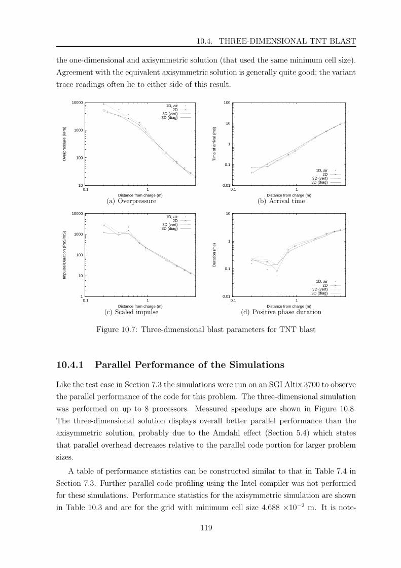
10.4. THREE-DIMENSIONAL TNT BLAST
the one-dimensional and axisymmetric solution (that used the same minimum cell size).
Agreement with the equivalent axisymmetric solution is generally quite good; the variant
trace readings often lie to either side of this result.
10
100
1000
10000
0.1 1
Ove
rpre
ssur
e (k
Pa)
Distance from charge (m)
1D, air2D
3D (vert)3D (diag)
(a) Overpressure
0.01
0.1
1
10
100
0.1 1
Tim
e of
arr
ival
(m
s)
Distance from charge (m)
1D, air2D
3D (vert)3D (diag)
(b) Arrival time
1
10
100
1000
10000
0.1 1
Impu
lse/
Dur
atio
n (P
aS/m
S)
Distance from charge (m)
1D, air2D
3D (vert)3D (diag)
(c) Scaled impulse
0.01
0.1
1
10
0.1 1
Dur
atio
n (m
s)
Distance from charge (m)
1D, air2D
3D (vert)3D (diag)
(d) Positive phase duration
Figure 10.7: Three-dimensional blast parameters for TNT blast
10.4.1 Parallel Performance of the Simulations
Like the test case in Section 7.3 the simulations were run on an SGI Altix 3700 to observe
the parallel performance of the code for this problem. The three-dimensional simulation
was performed on up to 8 processors. Measured speedups are shown in Figure 10.8.
The three-dimensional solution displays overall better parallel performance than the
axisymmetric solution, probably due to the Amdahl effect (Section 5.4) which states
that parallel overhead decreases relative to the parallel code portion for larger problem
sizes.
A table of performance statistics can be constructed similar to that in Table 7.4 in
Section 7.3. Further parallel code profiling using the Intel compiler was not performed
for these simulations. Performance statistics for the axisymmetric simulation are shown
in Table 10.3 and are for the grid with minimum cell size 4.688 ×10⁻² m. It is note-
119
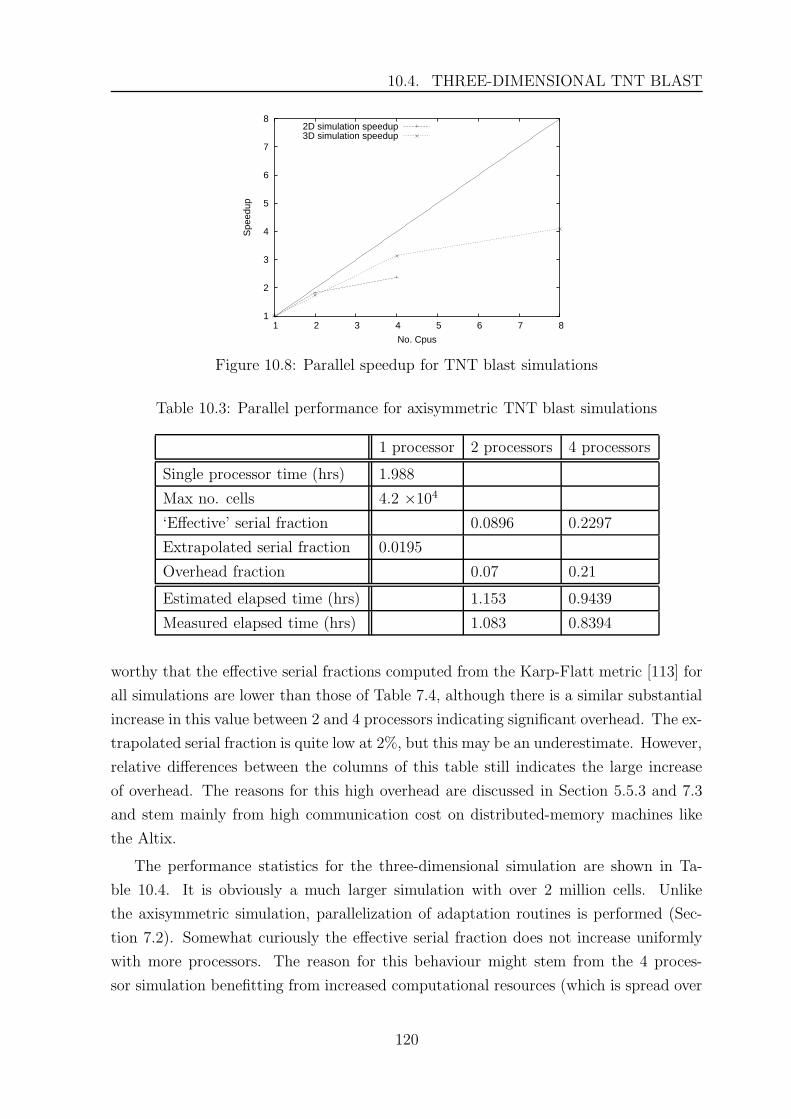
10.4. THREE-DIMENSIONAL TNT BLAST
1
2
3
4
5
6
7
8
1 2 3 4 5 6 7 8
Spe
edup
No. Cpus
2D simulation speedup3D simulation speedup
Figure 10.8: Parallel speedup for TNT blast simulations
Table 10.3: Parallel performance for axisymmetric TNT blast simulations
1 processor 2 processors 4 processors
Single processor time (hrs) 1.988
Max no. cells 4.2 ×10⁴
‘Effective’ serial fraction 0.0896 0.2297
Extrapolated serial fraction 0.0195
Overhead fraction 0.07 0.21
Estimated elapsed time (hrs) 1.153 0.9439
Measured elapsed time (hrs) 1.083 0.8394
worthy that the effective serial fractions computed from the Karp-Flatt metric [113] for
all simulations are lower than those of Table 7.4, although there is a similar substantial
increase in this value between 2 and 4 processors indicating significant overhead. The ex-
trapolated serial fraction is quite low at 2%, but this may be an underestimate. However,
relative differences between the columns of this table still indicates the large increase
of overhead. The reasons for this high overhead are discussed in Section 5.5.3 and 7.3
and stem mainly from high communication cost on distributed-memory machines like
the Altix.
The performance statistics for the three-dimensional simulation are shown in Ta-
ble 10.4. It is obviously a much larger simulation with over 2 million cells. Unlike
the axisymmetric simulation, parallelization of adaptation routines is performed (Sec-
tion 7.2). Somewhat curiously the effective serial fraction does not increase uniformly
with more processors. The reason for this behaviour might stem from the 4 proces-
sor simulation benefitting from increased computational resources (which is spread over
120
10.4. THREE-DIMENSIONAL TNT BLAST
Table 10.4: Parallel performance for 3D TNT blast simulations
1 processor 2 processors 4 processors 8 processors
Single processor time (hrs) 137.68
Max no. cells 2.27 ×10⁶
‘Effective’ serial fraction 0.155 0.0918 0.1356
Extrapolated serial fraction 0.0918
Overhead fraction 0.0632∗ 0∗ 0.0438∗
Estimated elapsed time (hrs) 83.86∗ 43.9∗ 34.3∗
Measured elapsed time (hrs) 79.51 43.9 33.54
dual-processor nodes). Hence an extrapolation of the serial fraction cannot be per-
formed, and the minimum effective fraction of 0.0918 is used. This represents an upper
bound to the actual serial fraction, and is consistent with the axisymmetric result.
Because of this the overhead for the 4 processor job is by definition zero, and thus
reported figures of overhead are relative to the 4 processor performance. The estimated
elapsed time is thus equal with the actual elapsed time if the overhead is zero (henced
the starred values). Relative increases in overhead are considerably smaller than the
axisymmetric values in Table 10.3, which is due to the Amdahl effect and also perhaps
the increased code parallelization.
The performance statistics show encouragingly that the code appears to be fairly
well parallelized (less than 10% of operations are serial). Obviously, more work can still
be done to increase performance efficiency. In terms of actual elapsed time the code
can obtain results in an reasonable timeframe on 8 processors, although it would be
advisable to do initial low resolution calculations if rapid hazard analysis is required.
121
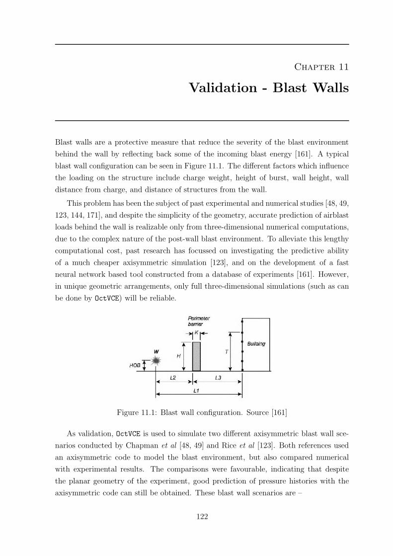
Chapter 11
Validation - Blast Walls
Blast walls are a protective measure that reduce the severity of the blast environment
behind the wall by reflecting back some of the incoming blast energy [161]. A typical
blast wall configuration can be seen in Figure 11.1. The different factors which influence
the loading on the structure include charge weight, height of burst, wall height, wall
distance from charge, and distance of structures from the wall.
This problem has been the subject of past experimental and numerical studies [48, 49,
123, 144, 171], and despite the simplicity of the geometry, accurate prediction of airblast
loads behind the wall is realizable only from three-dimensional numerical computations,
due to the complex nature of the post-wall blast environment. To alleviate this lengthy
computational cost, past research has focussed on investigating the predictive ability
of a much cheaper axisymmetric simulation [123], and on the development of a fast
neural network based tool constructed from a database of experiments [161]. However,
in unique geometric arrangements, only full three-dimensional simulations (such as can
be done by OctVCE) will be reliable.
Figure 11.1: Blast wall configuration. Source [161]
As validation, OctVCE is used to simulate two different axisymmetric blast wall sce-
narios conducted by Chapman et al [48, 49] and Rice et al [123]. Both references used
an axisymmetric code to model the blast environment, but also compared numerical
with experimental results. The comparisons were favourable, indicating that despite
the planar geometry of the experiment, good prediction of pressure histories with the
axisymmetric code can still be obtained. These blast wall scenarios are –
122
1. Referring to Figure 11.1, in the scenario of Chapman et al [48, 49], the charge mass
was the equivalent of 60 g of TNT, with a height of burst at 0.15 m, a distance to
the structure L1 = 1.05 m and a distance to the wall L2 = 0.6 m. The wall height
is 0.3 m and its thickness is 0.02 m. The only pressure transducer was located 0.3
m up the structure.
2. In the scenario of Rice et al [123], the charge mass was 0.513 g of PETN at a
height of burst of 0.0134 m, a distance to the structure L1 = 0.167 m and a
distance to the wall L2 = 0.1 m. The wall height was 0.0535 m, and its thickness
is estimated to be about 0.01 m. Rice et al also performed a three-dimensional
simulation, which yielded a similar solution to the axisymmetric result. Three
pressure transducers were located at 0.04, 0.08 and 0.12 m up the structure.
Cell sizes were not specified in either of these references. In both cases, the computa-
tional domain stretches from the symmetry axis to the structure, as shown in Figure 11.2.
This approach avoids the problem with axisymmetric obstructed corner cells (between
the structure and the floor) as discussed in Appendix E.1, although corner cells exist at
the junction of the blast barrier and the ground. A non-reflecting boundary condition
is placed on the top boundary and its effectiveness will also be tested later. Standard
air at atmospheric conditions is used for the ambient gas.
Figure 11.2: Initial grid for blast wall simulation
The JWL equation of state is used to simulate the explosion products. Explosive
JWL parameters are taken from Reference [127]. However, given the balloon method of
charge initialization (Sections 4.6 and 10.2), the charge balloon densities and pressures
have to be modified somewhat to ensure correct blast energy and mass. For both
scenarios, five working mesh levels (level 5 to level 9) are used, but a higher resolution
simulation with level 10 cell sizes are also performed to observe grid dependence. Both
simulations use the density-based adaptation indicator (Section 3.4) of 0.3, 0.1 for the
123
11.1. BLAST WALL SCENARIO 1
refinement and coarsening thresholds respectively. In the first simulation, a noise filter
threshold of 0.017 is used, and in the second simulation this value is 0.04. AUSMDV is
used as the flux solver and 64 subcells are used.
11.1 Blast Wall Scenario 1
This section displays the solution to the blast wall problem of Chapman et al [48]. This
test case was also performed by the author in Reference [202]. Density contours at
various times are shown in Figure 11.3. Note at times some contours appear to pass
through the blast barrier but this is due to the wall being so thin that no coarse cells
are actually fully immersed in it.
(a) Solution at 1.2 ms (b) Solution at 1.8 ms
(c) Solution at 2.4 ms (d) Solution at 3.0 ms
Figure 11.3: Solution to Chapman’s [48] blast wall problem
To test the non-reflecting boundary condition, a simulation with the same minimum
and maximum cell size is performed, but with the upper boundary extended. The
solution on this extended boundary simulation is shown in Figure 11.4. There is very
good agreement between the solutions in Figure 11.3 and 11.4.
124
11.1. BLAST WALL SCENARIO 1
(a) Solution at 1.2 ms (b) Solution at 1.8 ms
(c) Solution at 2.4 ms (d) Solution at 3.0 ms
Figure 11.4: Solution to Chapman’s [48] blast wall problem, longer domain
The pressure history is shown in Figure 11.5, and compared with Chapman’s results
[48]. There appears to be a discrepancy in primary wave arrival time, and it is too large
to be accounted for by the detonation time of the charge if initiated from the centre.
However peak pressures (especially for the finer resolution mesh) and positive phase
behaviour agree well with past results. There is also a large reflection at around 2.8 ms
not present in Chapman’s result, but this is due to reflection from the symmetry axis
which Chapman et al did not model.
It is not known why the discrepancy in arrival time is so large. Although Chapman
et al [48] did not explicitly state the blast energy, there is sufficient agreement in peak
overpressures and positive phase behaviour to suggest only a small discrepancy with
their actual blast energy. Perhaps their results were somehow offset in time, but this
was not specified. In any case, arrival time is not a particularly useful engineering
quantity in blast wave modelling, so this problem is not very serious.
125
11.2. BLAST WALL SCENARIO 2
-20
0
20
40
60
80
100
120
140
160
0 0.5 1 1.5 2 2.5 3
Ove
rpre
ssur
e (k
Pa)
Time (ms)
Smith experiment (1995)Smith AUTODYN (1995)
CFD coarser gridCFD finer grid
Figure 11.5: Pressure history for blast wall scenario 1
11.1.1 Performance of the Simulation
A uniform mesh simulation with all cells at the same size as the minimum cell size in
the lower resolution adaptive mesh simulation was performed to see how significant the
savings in solution time would be. Both were run on 1 processor. The uniform mesh
simulation had 260830 cells with an elapsed time of 22.5 hours. The adaptive mesh
simulation had a maximum of 55000 cells and took 4.9 hours. This means savings of
a factor of 4.74 and 4.59 in storage and solution time respectively. With an increasing
problem size in three-dimensional meshes, the savings would be expected to be even
larger.
11.2 Blast Wall Scenario 2
This section displays the solution to the blast wall problem of Rice et al [123]. As Rice
et al also performed a three-dimensional planar simulation, it also seems appropriate
to perform one here. This simulation has four working mesh levels corresponding to
cell sizes of 6.25 × 10⁻³ m to 7.8125 × 10⁻⁴ m. It is performed in ‘quarter-space’
i.e. assuming two symmetry planes, the ‘in-plane’ symmetry plane corresponding to the
structure centreline, and a ‘back-plane’ symmetry condition at the charge centre parallel
with the barrier. Reflections from the back-plane symmetry condition would arrive too
late to interfere with the presssure histories in the positive phase.
Density contours at 146 µs are shown in Figure 11.6 and compared with the results
of Rice et al. Although there is generally good agreement in major flow features, there
are still noticeable differences, especially near the symmetry axis. Rice’s simulations use
a much finer resolution, so current results do not resolve certain features as well. The
126
11.2. BLAST WALL SCENARIO 2
diffracted shock behind the barrier is so weak that the adaptation criteria fail to refine
it. In the axisymmetric solution, apparent numerical jetting along the axis is seen, but
it is interesting to note that the shadowgraph results also show that detonation products
above the charge have apparently been ejected ahead of the primary blast wave.
Density contours at 246 µs are shown in Figure 11.7. There are some noticeable
differences, especially between the axisymmetric solutions. Unlike Rice’s results the
current solutions seem to be at a more advanced stage; they show the reflected shock
from the structure already interacting with the vortex slip layer. Also, the reflections
behind the blast barrier are so weak no grid adaptation is present there and thus features
there are not well-resolved.
The apparent time-wise difference in solutions is also reflected in the pressure his-
tories (Figure 11.8). Apart from this discrepancy, agreement in peak overpressure and
positive phase wave behaviour with the axisymmetric solution is good, particularly for
gauges 2 and 3. The three-dimensional result, because of the coarser grids and planar
symmetry, has a noticeably lower peak pressure, and a delayed reflection in gauge 2.
Some grid-dependence in the axisymmetric solutions can still be seen. The difficulty of
obtaining mesh convergent solutions in three dimensions to this blast wall problem is
noted in [171].
The discrepancy in arrival time, like in Section 11.1, is puzzling. There may again
be a time offset in Rice’s results. Perhaps the axisymmetric corner cell degeneracy
encountered at the barrier (Appendix E.1) may affect the solution and arrival time,
so it is worthwhile to perform two additional simulations – (a) one where the barrier
dimensions are adjusted slightly to align exactly with the mesh lines (avoiding the
obstructed corner cell degeneracy), and (b) one without the barrier. The arrival times
at gauges 1 and 2 are affected by the presence of the barrier, but there is a direct
‘line-of-sight’ from the charge to gauge 3, so the arrival time at that sensor should be
independent of the barrier’s presence. This result is confirmed in Figure 11.8(d) which
shows the arrival times of the actual barrier, grid-aligned barrier and no barrier cases
to be nearly identical. Thus, it is likely that there is another explanation of the arrival
time discrepancy – probably a misreporting of one or more of the modelling parameters.
11.2.1 Performance of the Simulations
The three-dimensional solution had a maximum of around 1.4 million cells with an
elapsed time of 67.4 hours running on 4 processors. The finer resolution two-dimensional
solution had a maximum of 79000 cells, running for 11.95 hours on 2 processors. Clearly,
significant savings in computation time can be made if the problem can be solved in
127
11.2. BLAST WALL SCENARIO 2
(a) Rice 3D (from [123]) (b) Rice 2D (from [123])
(c) 3D contours (d) 2D contours
(e) 2D grid (f) Shadowgraph (from [123])
Figure 11.6: Solution to Rice’s [123] blast wall problem at 146 µs
128
11.2. BLAST WALL SCENARIO 2
(a) Rice 3D (from [123]) (b) Rice 2D (from [123])
(c) 3D contours (d) 2D contours
(e) 2D grid (f) Shadowgraph (from [123])
Figure 11.7: Solution to Rice’s [123] blast wall problem at 246 µs
129
11.3. BLAST WAVE CLEARING SIMULATION
-50
0
50
100
150
200
250
0 0.05 0.1 0.15 0.2 0.25 0.3
Ove
rpre
ssur
e (k
Pa)
Time (ms)
Rice 2D result (2000)Rice 3D result (2000)
CFD 2D finerCFD 2D coarser
CFD 3D
(a) Gauge 1
-50
0
50
100
150
200
250
300
350
400
450
-0.1 -0.05 0 0.05 0.1 0.15 0.2 0.25 0.3 0.35
Ove
rpre
ssur
e (k
Pa)
Time (ms)
Rice 2D result (2000)Rice 3D result (2000)
CFD 2D finerCFD 2D coarser
CFD 3D
(b) Gauge 2
-50
0
50
100
150
200
250
300
350
400
450
500
0 0.05 0.1 0.15 0.2 0.25 0.3
Ove
rpre
ssur
e (k
Pa)
Time (ms)
Rice 2D result (2000)Rice 3D result (2000)
CFD 2D finerCFD 2D coarser
CFD 3D
(c) Gauge 3
-100
0
100
200
300
400
500
600
700
0.16 0.18 0.2 0.22 0.24 0.26 0.28 0.3 0.32 0.34
Ove
rpre
ssur
e (k
Pa)
Time (ms)
Rice 2D result (2000)Rice 3D result (2000)
Actual barrierGrid-aligned barrier
No barrier
(d) Gauge 3, barrier test
Figure 11.8: Pressure histories for blast wall scenario 2
axisymmetric geometry.
11.3 Blast Wave Clearing Simulation
As further validation, the blast wave clearing simulation from Rose [171, 176] is per-
formed. This is a fully three-dimensional problem, and strictly not a blast wall simu-
lation as there is only one structure in the blast environment. Details of the problem
geometry are shown in Figure 11.9 and taken from [176]. The charge is equivalent in
energy to 27.26 g of TNT, detonated at a height of 0.1 m and 0.15 m from the structure.
The charge energy density is 4.52 × 10⁶ J/kg, and in the simulation is assumed to be
composed of high density air. In Rose’s simulation, the charge is initially simulated
in a one-dimensional spherical calculation and remapped to two and three dimensions
before the wave reaches the structure. A uniform mesh cell size of 1 cm was used, with
a numerical domain of 2.5 × 0.5 × 0.4 m.
In the simulations here, an adaptive mesh is used with four working levels corre-
sponding to cell sizes of 0.0172 to 0.1375 m. This mesh is so coarse it could only
130
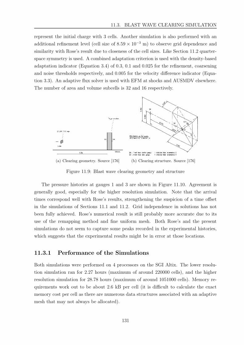
11.3. BLAST WAVE CLEARING SIMULATION
represent the initial charge with 3 cells. Another simulation is also performed with an
additional refinement level (cell size of 8.59 × 10⁻³ m) to observe grid dependence and
similarity with Rose’s result due to closeness of the cell sizes. Like Section 11.2 quarter-
space symmetry is used. A combined adaptation criterion is used with the density-based
adaptation indicator (Equation 3.4) of 0.3, 0.1 and 0.025 for the refinement, coarsening
and noise thresholds respectively, and 0.005 for the velocity difference indicator (Equa-
tion 3.3). An adaptive flux solver is used with EFM at shocks and AUSMDV elsewhere.
The number of area and volume subcells is 32 and 16 respectively.
(a) Clearing geometry. Source [176] (b) Clearing structure. Source [176]
Figure 11.9: Blast wave clearing geometry and structure
The pressure histories at gauges 1 and 3 are shown in Figure 11.10. Agreement is
generally good, especially for the higher resolution simulation. Note that the arrival
times correspond well with Rose’s results, strengthening the suspicion of a time offset
in the simulations of Sections 11.1 and 11.2. Grid independence in solutions has not
been fully achieved. Rose’s numerical result is still probably more accurate due to its
use of the remapping method and fine uniform mesh. Both Rose’s and the present
simulations do not seem to capture some peaks recorded in the experimental histories,
which suggests that the experimental results might be in error at those locations.
11.3.1 Performance of the Simulations
Both simulations were performed on 4 processors on the SGI Altix. The lower resolu-
tion simulation ran for 2.27 hours (maximum of around 220000 cells), and the higher
resolution simulation for 28.78 hours (maximum of around 1051000 cells). Memory re-
quirements work out to be about 2.6 kB per cell (it is difficult to calculate the exact
memory cost per cell as there are numerous data structures associated with an adaptive
mesh that may not always be allocated).
131
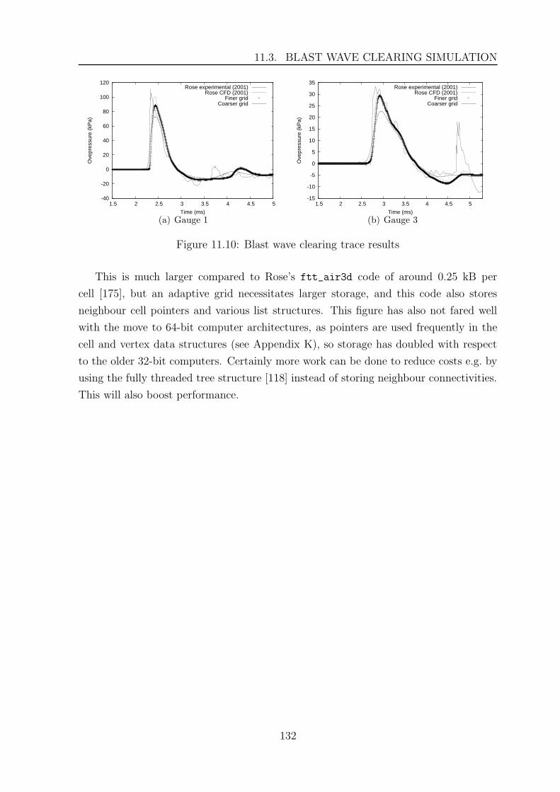
11.3. BLAST WAVE CLEARING SIMULATION
-40
-20
0
20
40
60
80
100
120
1.5 2 2.5 3 3.5 4 4.5 5
Ove
pres
sure
(kP
a)
Time (ms)
Rose experimental (2001)Rose CFD (2001)
Finer gridCoarser grid
(a) Gauge 1
-15
-10
-5
0
5
10
15
20
25
30
35
1.5 2 2.5 3 3.5 4 4.5 5
Ove
pres
sure
(kP
a)
Time (ms)
Rose experimental (2001)Rose CFD (2001)
Finer gridCoarser grid
(b) Gauge 3
Figure 11.10: Blast wave clearing trace results
This is much larger compared to Rose’s ftt_air3d code of around 0.25 kB per
cell [175], but an adaptive grid necessitates larger storage, and this code also stores
neighbour cell pointers and various list structures. This figure has also not fared well
with the move to 64-bit computer architectures, as pointers are used frequently in the
cell and vertex data structures (see Appendix K), so storage has doubled with respect
to the older 32-bit computers. Certainly more work can be done to reduce costs e.g. by
using the fully threaded tree structure [118] instead of storing neighbour connectivities.
This will also boost performance.
132
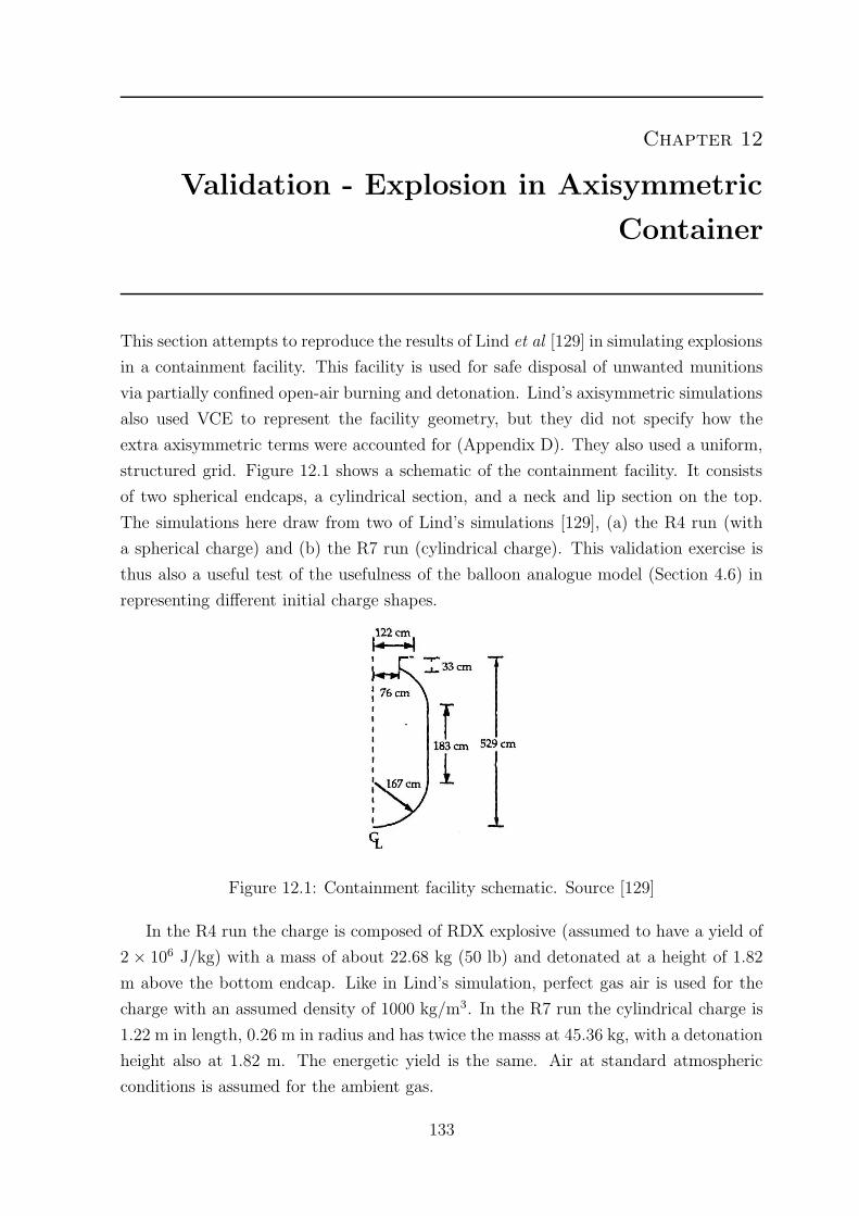
Chapter 12
Validation - Explosion in Axisymmetric
Container
This section attempts to reproduce the results of Lind et al [129] in simulating explosions
in a containment facility. This facility is used for safe disposal of unwanted munitions
via partially confined open-air burning and detonation. Lind’s axisymmetric simulations
also used VCE to represent the facility geometry, but they did not specify how the
extra axisymmetric terms were accounted for (Appendix D). They also used a uniform,
structured grid. Figure 12.1 shows a schematic of the containment facility. It consists
of two spherical endcaps, a cylindrical section, and a neck and lip section on the top.
The simulations here draw from two of Lind’s simulations [129], (a) the R4 run (with
a spherical charge) and (b) the R7 run (cylindrical charge). This validation exercise is
thus also a useful test of the usefulness of the balloon analogue model (Section 4.6) in
representing different initial charge shapes.
Figure 12.1: Containment facility schematic. Source [129]
In the R4 run the charge is composed of RDX explosive (assumed to have a yield of
2 × 10⁶ J/kg) with a mass of about 22.68 kg (50 lb) and detonated at a height of 1.82
m above the bottom endcap. Like in Lind’s simulation, perfect gas air is used for the
charge with an assumed density of 1000 kg/m3. In the R7 run the cylindrical charge is
1.22 m in length, 0.26 m in radius and has twice the masss at 45.36 kg, with a detonation
height also at 1.82 m. The energetic yield is the same. Air at standard atmospheric
conditions is assumed for the ambient gas.
133
12.1. EXPLOSION IN CONTAINMENT FACILITY – R4 RUN
Both adaptive-mesh simulations use four working mesh levels (level 5 to 8), but a
higher resolution simulation (levels 5 to 9) is also performed to observe grid dependence.
These correspond to cell sizes of 0.0137 m to 0.21875 m for the finer resolution simulation,
which has a minimum cell size around the nominal fine-grid cell size in Lind’s simulations
(1 cm). The density-based adaptation indicator (Equation 3.4) is used with 0.3, 0.1 and
0.04 for the refinement, coarsening and noise filter thresholds respectively. An adaptive
flux solver is implemented with EFM at shocks and AUSMDV elsewhere, and 64 subcells
are used.
As the code cannot handle thin wall degeneracies, the facility’s walls are set with a
wall thickness larger than the maximum distance within a cell (the diagonal spanning
a cell’s corners). Thus at no point will a cell be split by the container walls and thus
‘leak’ some gas to the exterior. This is unlikely to affect the results much, since the
focus is on loads on the internal walls of the facility. However, cells at the walls are kept
at the highest permissible level both to increase resolution and reduce wall thickness.
Non-reflecting boundary conditions are placed on domain boundaries.
12.1 Explosion in Containment Facility – R4 Run
Pressure contours for the R4 run at selected times are shown in Figure 12.2, and may be
compared with Lind’s snapshots. A transparent outline of the adapted mesh is overlaid
on top of the contours. Note the complex shock interactions, reflections and focussing
that occur in these plots. The top non-reflecting boundary condition also seems to work
well in supressing reflections, as in Section 11.
The pressure as a function of time and distance along the wall for both grids is shown
in Figure 12.3 and is qualitatively comparable to Lind’s result (Figure 12.4) in terms of
shock trajectories and locations of maxima. Note the presence of fairly noisy contours
even prior to the arrival of the primary shock. These pressure variations stem from a
perturbed flowfield because of the degeneracies associated with obstructed axisymmetric
cells discussed in Appendix E.1. However, they are relatively very small, and do not
seem to have a debilitating effect on the contours above the primary shock.
Nonetheless, there is a considerable difference in the maximum values between the
grids, indicating grid independence has not yet been fully achieved. However Lind’s runs
also did not aim for grid-independent solutions as, somewhat curiously, their coarser
resolution simulations were more conservative in terms of overpressure.
It is possible to give a more accurate estimate to the peak overpressure by using
Richardson-extrapolation [163, 164] (Equation 6.1). In this case, with an assumed order
134
12.1. EXPLOSION IN CONTAINMENT FACILITY – R4 RUN
Figure 12.2: Pressure contours for R4 simulation of explosion in containment facility
of accuracy of 1 (as the scheme reverts to first-order at shocks) and a grid refinement
factor of 2, the estimated true solution fe is simply fe = 2f1 − f2, where f1 and f2
are the finer and coarser resolution solutions respectively. Thus the estimated true
peak overpressure for this simulation is 81.55 atm, which is quite close to Lind’s fine-
grid result of 83.3 atm. This is a good indication that the code can give reasonably
accurate solutions in complex geometry even with all the attendant problems involved
with axisymmetric VCE surface representation.
The local maximum near the bottom end of the lower endcap is due to shock fo-
cussing there. The pressure at focus points is a particularly grid-dependent result [54]
as according to analytic theory the pressure is actually infinite at these locations [52].
Thus this pressure is an averaged value in the vicinity of focus, which in turn depends
on grid resolution. However the fine grid result of 48.45 atm is fairly close to Lind’s
coarse grid result of 55.4 atm. Simulations for the R4 run were run on 2 processors in
parallel; the lower resolution simulation had an elapsed time of 25 minutes (maximum
135
12.2. EXPLOSION IN CONTAINMENT FACILITY – R7 RUN
(a) Coarser resolution (b) Finer resolution
Figure 12.3: Pressure contours in the s-t plane for R4 simulation of explosion in con-tainment facility
Figure 12.4: Lind’s pressure contours in the s-t plane for the R4 simulation [129]
9700 cells), the higher resolution run had an elapsed time of 58 minutes (maximum of
21000 cells).
12.2 Explosion in Containment Facility – R7 Run
The pressure-time history along the wall for the cylindrical charge case is seen in Fig-
ure 12.5. These results are again qualitatively comparable to Lind’s result (Figure 12.6),
although slight differences can be observed. Nonetheless the location of peak overpres-
sures is predicted well. The magnitude of the peak overpressures again varies signifi-
cantly between the two resolution simulations. They all seem to occur at the bottom
of the endcap due to shock focussing there, which is sensitive to the grid resolution, as
mentioned in Section 12.1.
Via the same Richardson-extrapolation procedure the estimated actual peak over-
pressures for the peaks at around 2.5 ms and 9 ms are 188 atm and 489 atm respectively,
136
12.2. EXPLOSION IN CONTAINMENT FACILITY – R7 RUN
which are quite close in value to Lind’s result (186 atm and 496 atm respectively). The
initial peak pressure at this focus point is the most problematic result; the extrapolated
peak pressure there is only 162 atm, which is much lower than Lind’s result of 340 atm.
It is not known why this disagreement is so severe when compared to the other peaks.
Apart from the issues at focus points, it is also possible that Lind’s uniform grid may
have better preserved the peak pressure than the adapted grid given its sensitivity to
charge shape.
(a) Coarser resolution (b) Finer resolution
Figure 12.5: Pressure contours in the s-t plane for R7 simulation of explosion in con-tainment facility
Figure 12.6: Lind’s pressure contours in the s-t plane for the R7 simulation [129]
The simulations show that OctVCE seems able to give comparably accurate results
to Lind’s results [129]. It is possible, like with Lind [129], to feed the pressure-time data
from Figures 12.3 and 12.5 into a simplified structural loading model to yield the wall
tension. Simulations for the R7 run were run on 1 processor; the lower resolution simu-
lation had an elapsed time of 86 minutes (maximum 10200 cells), the higher resolution
run had an elapsed time of 285 minutes (maximum of 25000 cells). This is significantly
longer than the R4 run (even accounting for the 1 processor), but it is likely due to a
consistently larger number of cells over a longer time.
137
Chapter 13
Validation - Blast in Simple Street and
Obstacle Geometries
This section tests the ability of OctVCE to model the three-dimensional blast environ-
ment in simple street and obstacle geometries, which are essentially arragements of two
or more (typically grid-aligned) rectangular prismatic bodies. In the case of street ge-
ometries, the obstacles are arranged and scaled to represent buildings in realistic street
layouts. Manually gridding the computational domain can still be tedious if the ar-
rangement of objects is complicated. The resulting flow-field can be quite complex with
multiple shock interactions and reflections, and formulation of simple semi-empirical
rules is difficult [194], and can lead to drastic under- or over-predictions of pressures
and impulses.
Blast channeling and shielding in various street configurations has been the subject
of numerous investigations [74, 160, 172, 193, 195]. Significant enhancement (as much
as a factor of four) to both peak overpressure and peak positive phase impulse was
observed, and sometimes the effect of shielding can be reduced considerably by blast
channeling. Reference [194] provides a good overview of these studies. In two-building
simulations, overpressure amplification in the rear wall of the front structure (due to
shock reflection) of more than two times the incident value was observed [160, 191].
Simulations of two different obstacle scenarios are performed here. The first is a
scaled street configuration with a right angle bend which is taken from the blast sim-
ulations of Rose and Smith [173]. The basic layout, dimensions and charge and gauge
locations can be seen in Figure 13.1. Further detail on this simulation is provided in
Section 13.1.
The second simulation is the three-obstacle scenario by Sklavounos and Rigas [190].
The basic geometry is shown in Figure 13.2, and further details on the dimensions are
provided in Section 13.2.
13.1 Blast in Street with Right Angle Bend
This simulation is based on the one performed by Rose and Smith [173] where a blast
propagates around a right angle bend in a street. The basic plan layout of the street
138
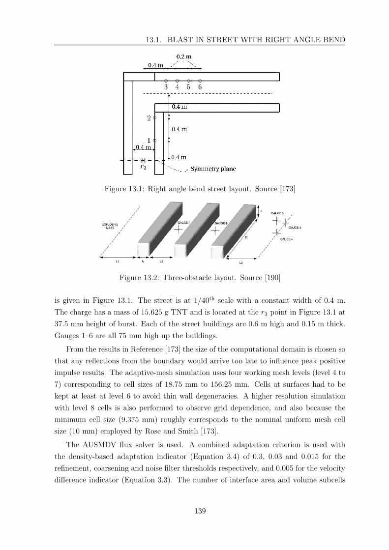
13.1. BLAST IN STREET WITH RIGHT ANGLE BEND
Figure 13.1: Right angle bend street layout. Source [173]
Figure 13.2: Three-obstacle layout. Source [190]
is given in Figure 13.1. The street is at 1/40th scale with a constant width of 0.4 m.
The charge has a mass of 15.625 g TNT and is located at the r3 point in Figure 13.1 at
37.5 mm height of burst. Each of the street buildings are 0.6 m high and 0.15 m thick.
Gauges 1–6 are all 75 mm high up the buildings.
From the results in Reference [173] the size of the computational domain is chosen so
that any reflections from the boundary would arrive too late to influence peak positive
impulse results. The adaptive-mesh simulation uses four working mesh levels (level 4 to
7) corresponding to cell sizes of 18.75 mm to 156.25 mm. Cells at surfaces had to be
kept at least at level 6 to avoid thin wall degeneracies. A higher resolution simulation
with level 8 cells is also performed to observe grid dependence, and also because the
minimum cell size (9.375 mm) roughly corresponds to the nominal uniform mesh cell
size (10 mm) employed by Rose and Smith [173].
The AUSMDV flux solver is used. A combined adaptation criterion is used with
the density-based adaptation indicator (Equation 3.4) of 0.3, 0.03 and 0.015 for the
refinement, coarsening and noise filter thresholds respectively, and 0.005 for the velocity
difference indicator (Equation 3.3). The number of interface area and volume subcells
139
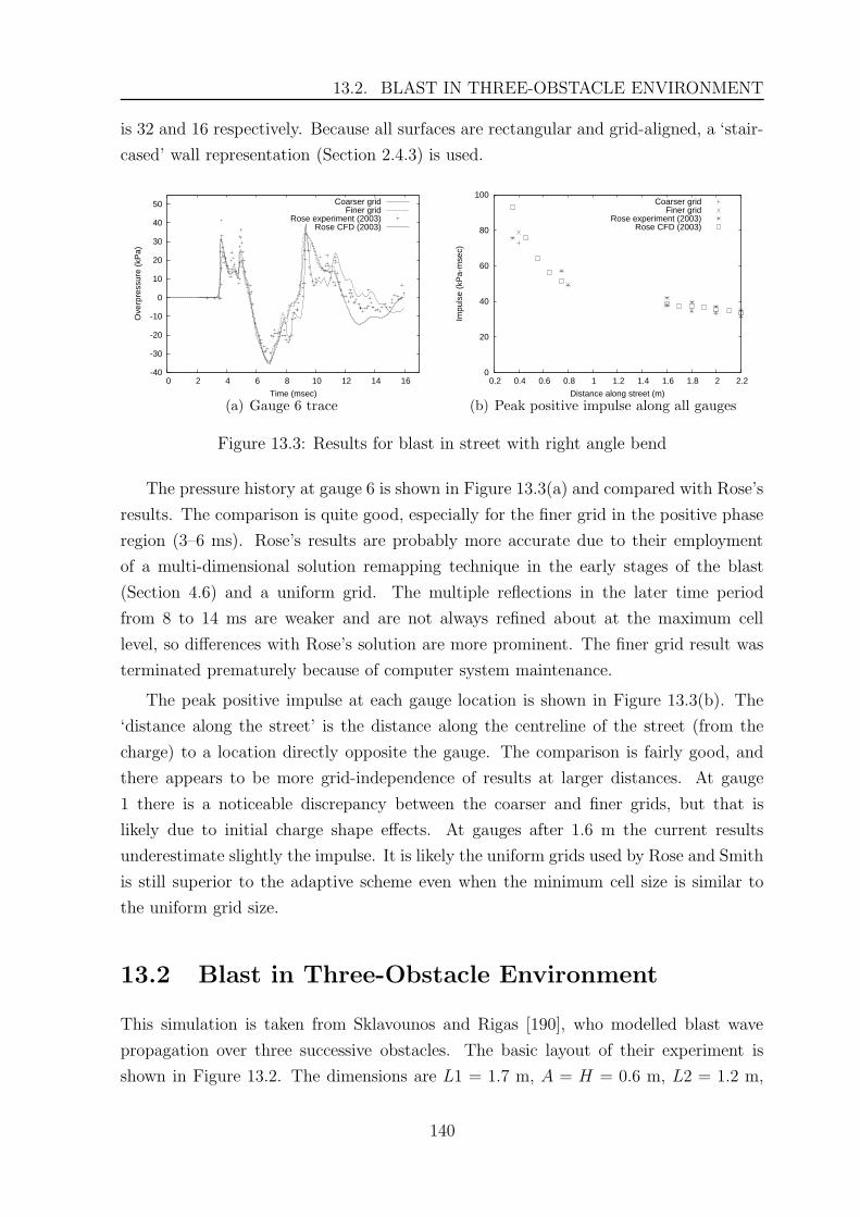
13.2. BLAST IN THREE-OBSTACLE ENVIRONMENT
is 32 and 16 respectively. Because all surfaces are rectangular and grid-aligned, a ‘stair-
cased’ wall representation (Section 2.4.3) is used.
-40
-30
-20
-10
0
10
20
30
40
50
0 2 4 6 8 10 12 14 16
Ove
rpre
ssur
e (k
Pa)
Time (msec)
Coarser gridFiner grid
Rose experiment (2003)Rose CFD (2003)
(a) Gauge 6 trace
0
20
40
60
80
100
0.2 0.4 0.6 0.8 1 1.2 1.4 1.6 1.8 2 2.2
Impu
lse
(kP
a-m
sec)
Distance along street (m)
Coarser gridFiner grid
Rose experiment (2003)Rose CFD (2003)
(b) Peak positive impulse along all gauges
Figure 13.3: Results for blast in street with right angle bend
The pressure history at gauge 6 is shown in Figure 13.3(a) and compared with Rose’s
results. The comparison is quite good, especially for the finer grid in the positive phase
region (3–6 ms). Rose’s results are probably more accurate due to their employment
of a multi-dimensional solution remapping technique in the early stages of the blast
(Section 4.6) and a uniform grid. The multiple reflections in the later time period
from 8 to 14 ms are weaker and are not always refined about at the maximum cell
level, so differences with Rose’s solution are more prominent. The finer grid result was
terminated prematurely because of computer system maintenance.
The peak positive impulse at each gauge location is shown in Figure 13.3(b). The
‘distance along the street’ is the distance along the centreline of the street (from the
charge) to a location directly opposite the gauge. The comparison is fairly good, and
there appears to be more grid-independence of results at larger distances. At gauge
1 there is a noticeable discrepancy between the coarser and finer grids, but that is
likely due to initial charge shape effects. At gauges after 1.6 m the current results
underestimate slightly the impulse. It is likely the uniform grids used by Rose and Smith
is still superior to the adaptive scheme even when the minimum cell size is similar to
the uniform grid size.
13.2 Blast in Three-Obstacle Environment
This simulation is taken from Sklavounos and Rigas [190], who modelled blast wave
propagation over three successive obstacles. The basic layout of their experiment is
shown in Figure 13.2. The dimensions are L1 = 1.7 m, A = H = 0.6 m, L2 = 1.2 m,
140
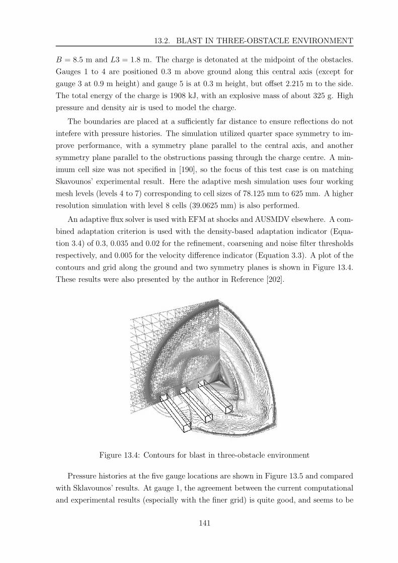
13.2. BLAST IN THREE-OBSTACLE ENVIRONMENT
B = 8.5 m and L3 = 1.8 m. The charge is detonated at the midpoint of the obstacles.
Gauges 1 to 4 are positioned 0.3 m above ground along this central axis (except for
gauge 3 at 0.9 m height) and gauge 5 is at 0.3 m height, but offset 2.215 m to the side.
The total energy of the charge is 1908 kJ, with an explosive mass of about 325 g. High
pressure and density air is used to model the charge.
The boundaries are placed at a sufficiently far distance to ensure reflections do not
intefere with pressure histories. The simulation utilized quarter space symmetry to im-
prove performance, with a symmetry plane parallel to the central axis, and another
symmetry plane parallel to the obstructions passing through the charge centre. A min-
imum cell size was not specified in [190], so the focus of this test case is on matching
Skavounos’ experimental result. Here the adaptive mesh simulation uses four working
mesh levels (levels 4 to 7) corresponding to cell sizes of 78.125 mm to 625 mm. A higher
resolution simulation with level 8 cells (39.0625 mm) is also performed.
An adaptive flux solver is used with EFM at shocks and AUSMDV elsewhere. A com-
bined adaptation criterion is used with the density-based adaptation indicator (Equa-
tion 3.4) of 0.3, 0.035 and 0.02 for the refinement, coarsening and noise filter thresholds
respectively, and 0.005 for the velocity difference indicator (Equation 3.3). A plot of the
contours and grid along the ground and two symmetry planes is shown in Figure 13.4.
These results were also presented by the author in Reference [202].
Figure 13.4: Contours for blast in three-obstacle environment
Pressure histories at the five gauge locations are shown in Figure 13.5 and compared
with Sklavounos’ results. At gauge 1, the agreement between the current computational
and experimental results (especially with the finer grid) is quite good, and seems to be
141
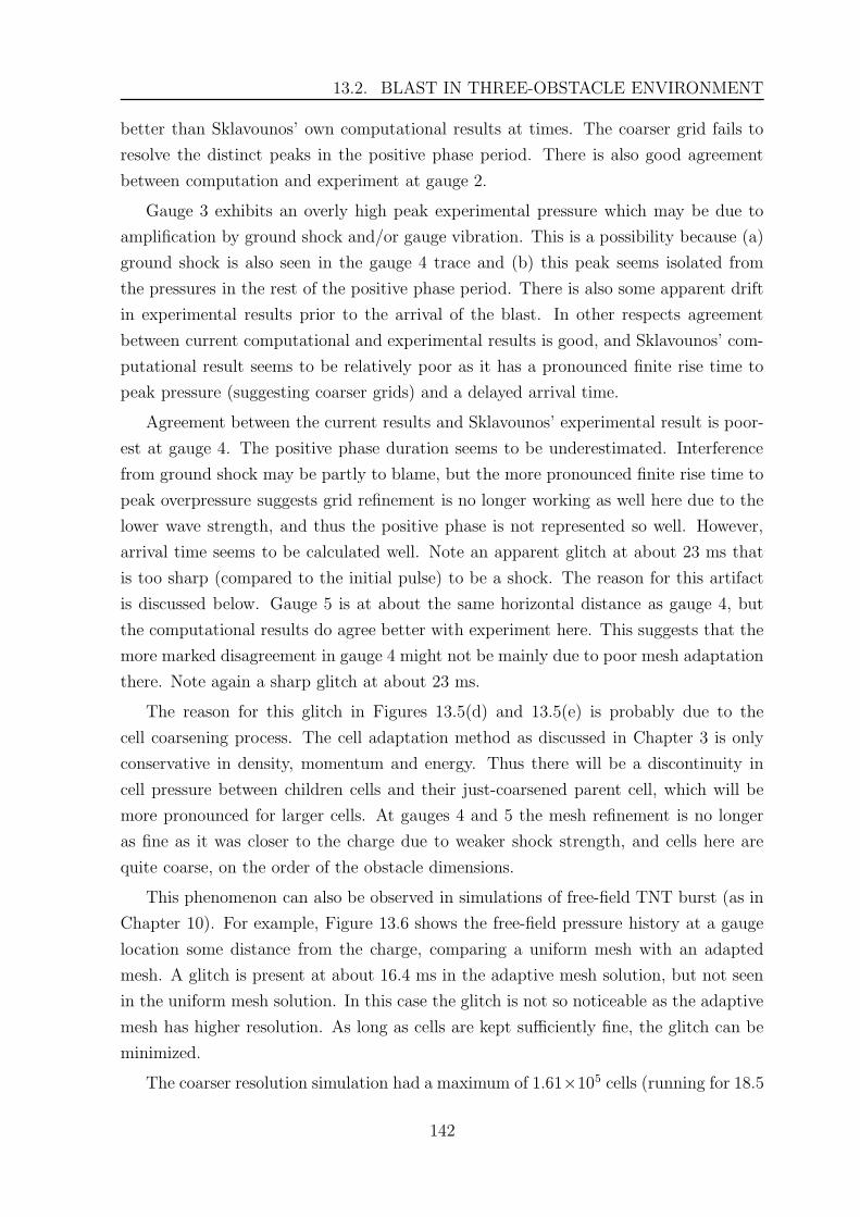
13.2. BLAST IN THREE-OBSTACLE ENVIRONMENT
better than Sklavounos’ own computational results at times. The coarser grid fails to
resolve the distinct peaks in the positive phase period. There is also good agreement
between computation and experiment at gauge 2.
Gauge 3 exhibits an overly high peak experimental pressure which may be due to
amplification by ground shock and/or gauge vibration. This is a possibility because (a)
ground shock is also seen in the gauge 4 trace and (b) this peak seems isolated from
the pressures in the rest of the positive phase period. There is also some apparent drift
in experimental results prior to the arrival of the blast. In other respects agreement
between current computational and experimental results is good, and Sklavounos’ com-
putational result seems to be relatively poor as it has a pronounced finite rise time to
peak pressure (suggesting coarser grids) and a delayed arrival time.
Agreement between the current results and Sklavounos’ experimental result is poor-
est at gauge 4. The positive phase duration seems to be underestimated. Interference
from ground shock may be partly to blame, but the more pronounced finite rise time to
peak overpressure suggests grid refinement is no longer working as well here due to the
lower wave strength, and thus the positive phase is not represented so well. However,
arrival time seems to be calculated well. Note an apparent glitch at about 23 ms that
is too sharp (compared to the initial pulse) to be a shock. The reason for this artifact
is discussed below. Gauge 5 is at about the same horizontal distance as gauge 4, but
the computational results do agree better with experiment here. This suggests that the
more marked disagreement in gauge 4 might not be mainly due to poor mesh adaptation
there. Note again a sharp glitch at about 23 ms.
The reason for this glitch in Figures 13.5(d) and 13.5(e) is probably due to the
cell coarsening process. The cell adaptation method as discussed in Chapter 3 is only
conservative in density, momentum and energy. Thus there will be a discontinuity in
cell pressure between children cells and their just-coarsened parent cell, which will be
more pronounced for larger cells. At gauges 4 and 5 the mesh refinement is no longer
as fine as it was closer to the charge due to weaker shock strength, and cells here are
quite coarse, on the order of the obstacle dimensions.
This phenomenon can also be observed in simulations of free-field TNT burst (as in
Chapter 10). For example, Figure 13.6 shows the free-field pressure history at a gauge
location some distance from the charge, comparing a uniform mesh with an adapted
mesh. A glitch is present at about 16.4 ms in the adaptive mesh solution, but not seen
in the uniform mesh solution. In this case the glitch is not so noticeable as the adaptive
mesh has higher resolution. As long as cells are kept sufficiently fine, the glitch can be
minimized.
The coarser resolution simulation had a maximum of 1.61×10⁵ cells (running for 18.5
142
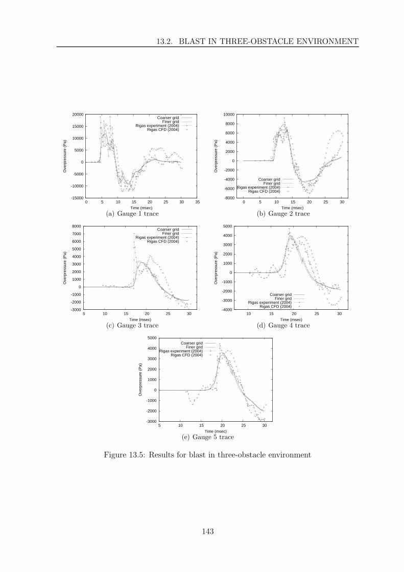
13.2. BLAST IN THREE-OBSTACLE ENVIRONMENT
-15000
-10000
-5000
0
5000
10000
15000
20000
0 5 10 15 20 25 30 35
Ove
rpre
ssur
e (P
a)
Time (msec)
Coarser gridFiner grid
Rigas experiment (2004)Rigas CFD (2004)
(a) Gauge 1 trace
-8000
-6000
-4000
-2000
0
2000
4000
6000
8000
10000
0 5 10 15 20 25 30
Ove
rpre
ssur
e (P
a)
Time (msec)
Coarser gridFiner grid
Rigas experiment (2004)Rigas CFD (2004)
(b) Gauge 2 trace
-3000
-2000
-1000
0
1000
2000
3000
4000
5000
6000
7000
8000
5 10 15 20 25 30
Ove
rpre
ssur
e (P
a)
Time (msec)
Coarser gridFiner grid
Rigas experiment (2004)Rigas CFD (2004)
(c) Gauge 3 trace
-4000
-3000
-2000
-1000
0
1000
2000
3000
4000
5000
10 15 20 25 30
Ove
rpre
ssur
e (P
a)
Time (msec)
Coarser gridFiner grid
Rigas experiment (2004)Rigas CFD (2004)
(d) Gauge 4 trace
-3000
-2000
-1000
0
1000
2000
3000
4000
5000
5 10 15 20 25 30
Ove
rpre
ssur
e (P
a)
Time (msec)
Coarser gridFiner grid
Rigas experiment (2004)Rigas CFD (2004)
(e) Gauge 5 trace
Figure 13.5: Results for blast in three-obstacle environment
143
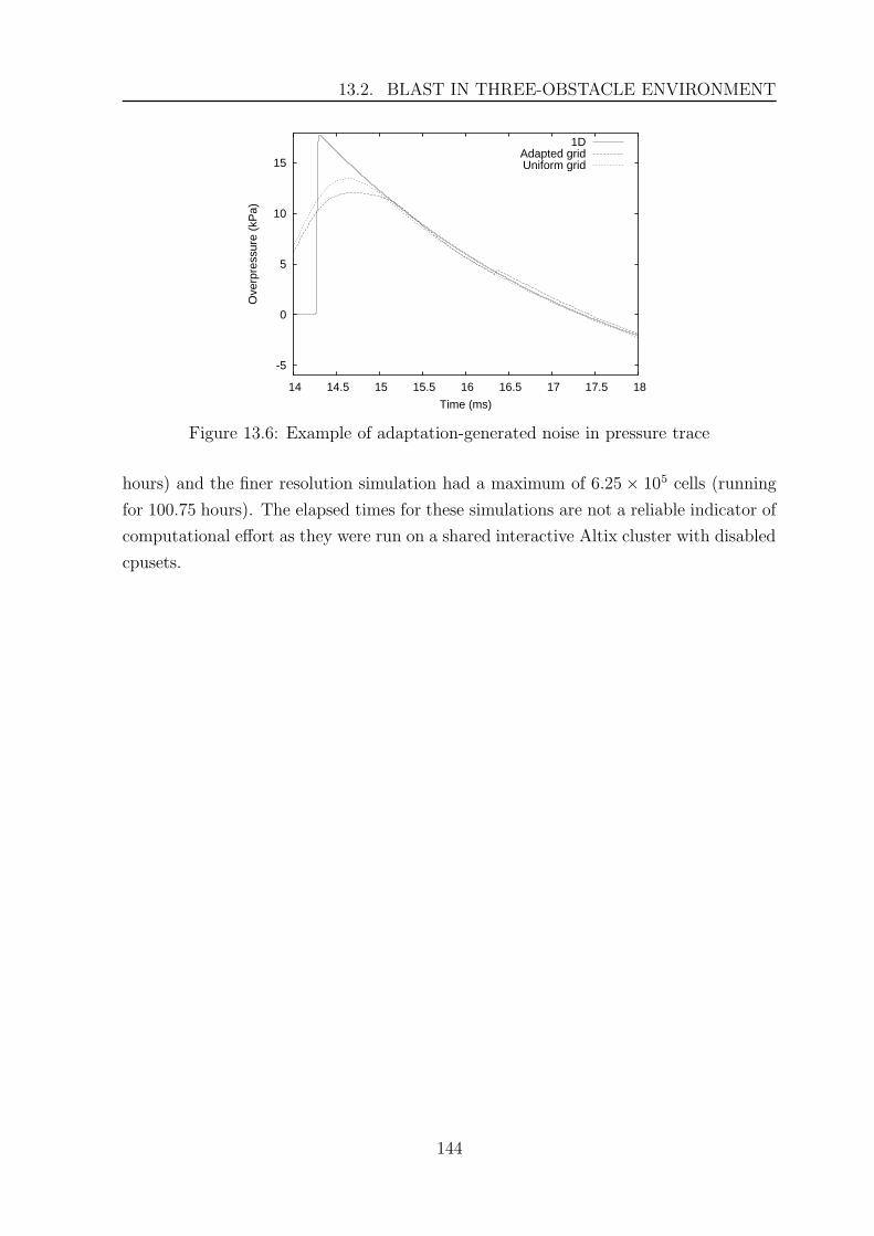
13.2. BLAST IN THREE-OBSTACLE ENVIRONMENT
-5
0
5
10
15
14 14.5 15 15.5 16 16.5 17 17.5 18
Ove
rpre
ssur
e (k
Pa)
Time (ms)
1DAdapted gridUniform grid
Figure 13.6: Example of adaptation-generated noise in pressure trace
hours) and the finer resolution simulation had a maximum of 6.25 × 10⁵ cells (running
for 100.75 hours). The elapsed times for these simulations are not a reliable indicator of
computational effort as they were run on a shared interactive Altix cluster with disabled
cpusets.
144
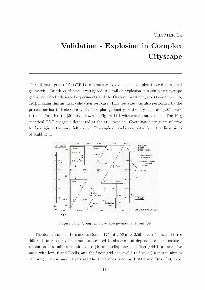
Chapter 14
Validation - Explosion in Complex
Cityscape
The ultimate goal of OctVCE is to simulate explosions in complex three-dimensional
geometries. Brittle et al have investigated in detail an explosion in a complex cityscape
geometry with both scaled experiments and the Cartesian-cell ftt_air3d code [39, 175,
194], making this an ideal validation test case. This test case was also performed by the
present author in Reference [203]. The plan geometry of the cityscape at 1/50th scale
is taken from Brittle [39] and shown in Figure 14.1 with some annotations. The 16 g
spherical TNT charge is detonated at the EC1 location. Coordinates are given relative
to the origin at the lower left corner. The angle α can be computed from the dimensions
of building 1.
Figure 14.1: Complex cityscape geometry. From [39]
The domain size is the same as Rose’s [175] at 2.56 m × 2.56 m × 2.56 m, and three
different, increasingly finer meshes are used to observe grid dependence. The coarsest
resolution is a uniform mesh level 6 (40 mm cells), the next finer grid is an adaptive
mesh with level 6 and 7 cells, and the finest grid has level 6 to 8 cells (10 mm minimum
cell size). These mesh levels are the same ones used by Brittle and Rose [39, 175].
145
14.1. RESULTS
The coarsest mesh represents the charge as a cube because of the relatively large cell
sizes. Due to computational resource constraints, a level 9 mesh simulation could not
be performed.
The assumed specific energy of the charge is 4520 kJ/kg, which is represented with
the ballon analogue model (Section 4.6), and thus its pressure and density is modified to
represent correct blast energy and mass depending on the grid resolution. The ambient
gas is air at standard conditions (density of 1.2 kg/m3 and pressure 101.325 kPa). A
combined adaptation criterion is implemented with the density-based adaptation indi-
cator (Equation 3.4) of 0.3, 0.05 and 0.03 for the refinement, coarsening and noise filter
thresholds respectively, and 0.01 for the velocity difference indicator (Equation 3.3). An
adaptive flux solver is used (Section 4.4) with EFM at shocks and AUSMDV elsewhere.
The number of interface area and volume subcells is 32 and 16 respectively.
14.1 Results
Pressure histories at gauge locations 1, 3, 11 and 21 are shown in Figure 14.2 and com-
pared with the results of Brittle and Rose [39, 175]. There is generally good agreement,
especially for the finest resolution mesh in the positive phase. Agreement in peak over-
pressure is poorest at gauge 11. These results demonstrate that the balloon analogue
model of charge representation can produce acceptable pressure histories, although the
remapping procedure implemented by ftt_air3d [177] which remaps an initial highly
resolved one-dimensional solution to multidimensions would still produce more accurate
results.
In less major details there are more noticeable differences with Rose’s result, like
the poorer resolution of secondary waves e.g. for gauge 21 where the train of waves at
around 6 ms are not captured well. This is probably partly due to the cruder balloon
analogue model, but also because of the time-dependent cell size at surfaces. Intersected
or partially obstructed cells were kept at the maximum level in Rose’s simulation, but
this was not enforced in OctVCE, which allows a varying cell size at surfaces for faster
results. If the resolution of secondary details is not a priority, the current methodology
seems sufficient.
Increments between the coarse, finer and finest mesh solutions in peak pressure and
impulse are shown in Tables 14.1 to 14.6; increasingly smaller differences suggest con-
vergent behaviour. Gauge 1 (Table 14.1), being the gauge least shielded from the blast,
appears to demonstrate the best convergent behaviour in both pressure and impulse.
Coarser resolutions in fact overpredict the peak impulse, a result also observed by Brittle
[39], which might be a useful result if conservatism is desired.
146
14.1. RESULTS
-50
0
50
100
150
200
250
0 1 2 3 4 5 6 7 8
Ove
rpre
ssur
e (k
Pa)
Time (msec)
Coarsest gridMedium grid
Finest gridRose experiment (2005)
Rose CFD (2005)
(a) Gauge 1 trace
-40
-30
-20
-10
0
10
20
30
40
50
60
70
0 1 2 3 4 5 6 7 8
Ove
rpre
ssur
e (k
Pa)
Time (msec)
Coarsest gridMedium grid
Finest gridRose experiment (2005)
Rose CFD (2005)
(b) Gauge 3 trace
-40
-20
0
20
40
60
80
0 1 2 3 4 5 6 7 8
Ove
rpre
ssur
e (k
Pa)
Time (msec)
Coarsest gridMedium grid
Finest gridRose experiment (2005)
Rose CFD (2005)
(c) Gauge 11 trace
-60
-40
-20
0
20
40
60
80
100
0 2 4 6 8 10 12
Ove
rpre
ssur
e (k
Pa)
Time (msec)
Coarsest gridMedium grid
Finest gridRose experiment (2005)
Rose CFD (2005)
(d) Gauge 21 trace
Figure 14.2: Pressure histories for blast in complex cityscape
Gauge 3 (Table 14.2) does not appear to demonstrate convergent behaviour in pres-
sure, and the increments in impulse actually change sign. This behaviour is also repeated
for gauges 11 and 21 (Tables 14.3 and 14.5), however gauge 21 has convergent pressure.
Rose’s data [175] for gauges 11 and 21 are shown in Tables 14.4 and 14.6. Rose’s gauge
21 results also show apparent lack of convergence in overpressure and also impulse.
It is clear that mesh convergence is not always easy to demonstrate, and depends on
the gauge location and quantity under consideration. Convergence may be hampered by
the adaptive mesh and complex nature of the wave interactions [175], or perhaps only
consistently demonstrable on very fine meshes. In the simulations here, constant cell size
at surfaces is also not enforced, which may hinder convergence. It may be particularly
difficult to observe convergence in peak pressure as it is a shock-dependent quantity
and thus quite sensitive to grid resolution and flux limiters. Perhaps the coarsest mesh
is too coarse to be in the asymptotic convergence range. Nonetheless, correspondence
with Rose’s experimental results still seems reasonably good, even if mesh convergence
has not been fully attained everywhere.
Figures 14.3(a) and 14.3(c) show the peak pressure and impulse contours respectively
on the entire surface of the left-end wall (on which is placed gauges 3 to 11). They
147
14.1. RESULTS
Table 14.1: Complex cityscape, gauge 1 peak quantities
No. Pressure Impulse Inc. pressure Inc. impulse
levels (kPa) (kPa-msec) (kPa) (kPa-msec)
1 98 35.58 - -
2 130 29.89 31.9 -5.694
3 149 28.94 19.07 -0.949
Table 14.2: Complex cityscape, gauge 3 peak quantities
No. Pressure Impulse Inc. pressure Inc. impulse
levels (kPa) (kPa-msec) (kPa) (kPa-msec)
1 21 17.12 - -
2 30.8 14.85 9.845 -2.27
3 43.6 15 12.7 0.1503
Table 14.3: Complex cityscape, gauge 11 peak quantities
No. Pressure Impulse Inc. pressure Inc. impulse
levels (kPa) (kPa-msec) (kPa) (kPa-msec)
1 35.5 16.91 - -
2 39.4 16.07 3.83 -0.84
3 43.84 18.02 4.47 1.96
Table 14.4: Complex cityscape, Rose’s gauge 11 peak quantities [175]
No. Pressure Impulse Inc. pressure Inc. impulse
levels (kPa) (kPa-msec) (kPa) (kPa-msec)
1 30.2 16.2 - -
2 44.3 19.3 14.1 3.1
3 53.9 19.7 9.6 0.4
Table 14.5: Complex cityscape, gauge 21 peak quantities
No. Pressure Impulse Inc. pressure Inc. impulse
levels (kPa) (kPa-msec) (kPa) (kPa-msec)
1 46.9 38.4 - -
2 72.1 38.49 25.16 0.997
3 86.2 40.08 14.17 1.584
148
14.1. RESULTS
Table 14.6: Complex cityscape, Rose’s gauge 21 peak quantities [175]
No. Pressure Impulse Inc. pressure Inc. impulse
levels (kPa) (kPa-msec) (kPa) (kPa-msec)
1 47.6 40.4 - -
2 66.5 40.9 18.9 0.5
3 88.1 40.2 21.6 -0.7
were obtained by distributing about 1000 trace points over the wall, and are shown for
the finest resolution mesh. These contours are compared with Rose’s result [175] in
Figures 14.3(b) and 14.3(c). There is generally good agreement in the magnitude and
location of the various ‘hot spots’, some of which are due to wave coalesence. Rose
compared these contours to unshielded CONWEP data to demonstrate the inadequacy
of simple line-of-sight methods for blast problems in complex geometries due to multiple
shock reflection and diffraction [175].
(a) Peak pressure contours (b) Rose’s peak pressure contours [175]
(c) Peak impulse contours (d) Rose’s peak impulse contours [175]
Figure 14.3: Contours on left-end wall of blast in complex cityscape
Although a mesh convergence analysis was performed for individual gauge results,
it is also interesting to perform it for these pressure and impulse contours. The incre-
mentals in peak pressure and impulse are computed for each sensor on the face and
compared with the next higher level mesh to yield an absolute relative error for the
149
14.2. PERFORMANCE
sensor. This quantity is then summed over all sensors to yield an average relative error
per sensor point on this face. A decreasing error might indicate convergence. These
errors are shown in Table 14.7. Convergence in impulse is observed but apparently not
in pressure, although the difference is by less than 1%. This demonstrates again the
difficulty of obtaining convergence consistently for all quantities for the meshes used in
this simulation. Note also that impulse errors are substantially smaller than pressure
errors, sometimes by an order of magnitude.
Table 14.7: Complex cityscape, average relative error for left-end wall
No. levels Avg. pressure error Avg. impulse error
1–2 0.154 0.0347
2–3 0.163 0.0123
14.2 Performance
The performance for the various mesh resolution simulations are shown in Table 14.8
and compared to Rose’s ftt_air3d results [175]. The current simulations were all
conducted on four processors in parallel, and elapsed times cannot be directly compared
with Rose’s results. Thus in the second major column of Table 14.8 the elapsed time is
normalized by the coarsest resolution elapsed time.
OctVCE seems to exhibit slightly poorer scaling in relative time. Rose’s simulation
also used less cells especially for the finest mesh simulation. The most significant dif-
ference is in memory consumption, with the current code using as much as 15 times
more memory. Some of this overhead comes from explicit neighbour connectivities and
also additional data structures for parallel processing e.g. lists. This larger memory
consumption undoubtedly affects performance.
Table 14.8: Performance statistics for different mesh levels
Max no. cells Relative time Max memory (GB)
No. levels OctVCE ftt_air3d OctVCE ftt_air3d OctVCE ftt_air3d
1 2.57 ×10⁵ 2.62 ×10⁵ 1 1 0.528 0.058
2 5.8 ×10⁵ 4.3 ×10⁵ 3.42 3.29 1.33 0.088
3 2.06 ×10⁶ 1.44 ×10⁶ 23.15 18.67 4.65 0.317
A single processor simulation using the finest resolution (3 levels) was performed
for analysis of parallel performance, and this took 234.78 CPU hours, which is much
150
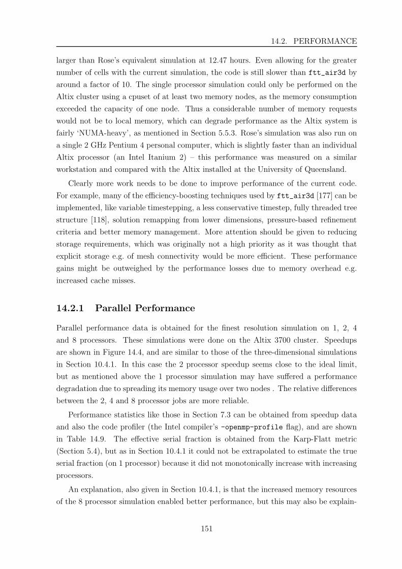
14.2. PERFORMANCE
larger than Rose’s equivalent simulation at 12.47 hours. Even allowing for the greater
number of cells with the current simulation, the code is still slower than ftt_air3d by
around a factor of 10. The single processor simulation could only be performed on the
Altix cluster using a cpuset of at least two memory nodes, as the memory consumption
exceeded the capacity of one node. Thus a considerable number of memory requests
would not be to local memory, which can degrade performance as the Altix system is
fairly ‘NUMA-heavy’, as mentioned in Section 5.5.3. Rose’s simulation was also run on
a single 2 GHz Pentium 4 personal computer, which is slightly faster than an individual
Altix processor (an Intel Itanium 2) – this performance was measured on a similar
workstation and compared with the Altix installed at the University of Queensland.
Clearly more work needs to be done to improve performance of the current code.
For example, many of the efficiency-boosting techniques used by ftt_air3d [177] can be
implemented, like variable timestepping, a less conservative timestep, fully threaded tree
structure [118], solution remapping from lower dimensions, pressure-based refinement
criteria and better memory management. More attention should be given to reducing
storage requirements, which was originally not a high priority as it was thought that
explicit storage e.g. of mesh connectivity would be more efficient. These performance
gains might be outweighed by the performance losses due to memory overhead e.g.
increased cache misses.
14.2.1 Parallel Performance
Parallel performance data is obtained for the finest resolution simulation on 1, 2, 4
and 8 processors. These simulations were done on the Altix 3700 cluster. Speedups
are shown in Figure 14.4, and are similar to those of the three-dimensional simulations
in Section 10.4.1. In this case the 2 processor speedup seems close to the ideal limit,
but as mentioned above the 1 processor simulation may have suffered a performance
degradation due to spreading its memory usage over two nodes . The relative differences
between the 2, 4 and 8 processor jobs are more reliable.
Performance statistics like those in Section 7.3 can be obtained from speedup data
and also the code profiler (the Intel compiler’s -openmp-profile flag), and are shown
in Table 14.9. The effective serial fraction is obtained from the Karp-Flatt metric
(Section 5.4), but as in Section 10.4.1 it could not be extrapolated to estimate the true
serial fraction (on 1 processor) because it did not monotonically increase with increasing
processors.
An explanation, also given in Section 10.4.1, is that the increased memory resources
of the 8 processor simulation enabled better performance, but this may also be explain-
151
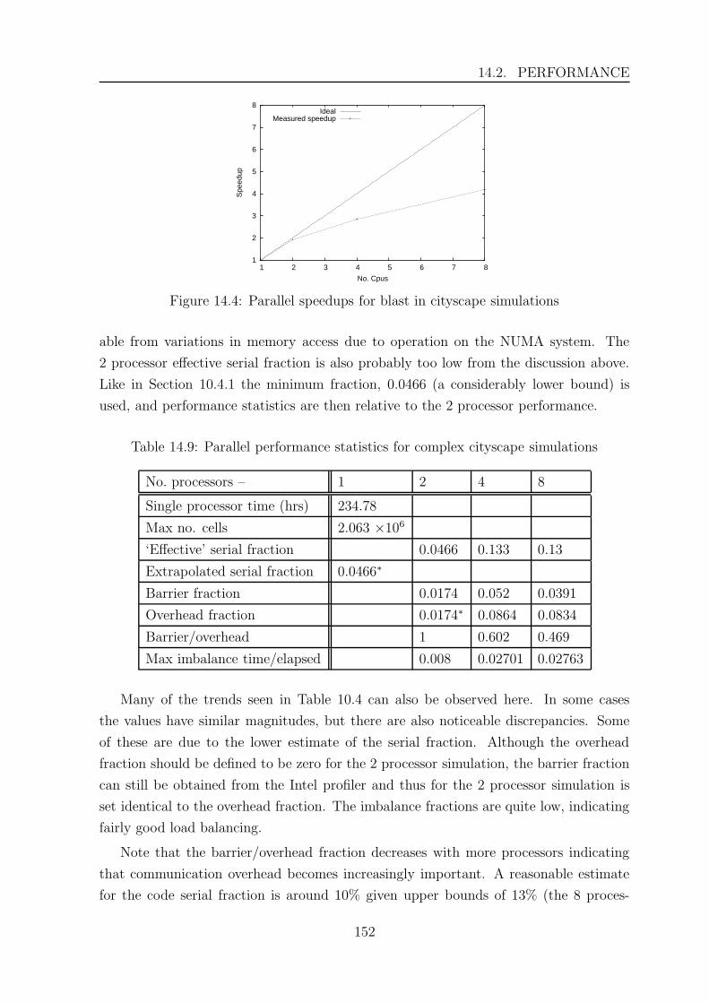
14.2. PERFORMANCE
1
2
3
4
5
6
7
8
1 2 3 4 5 6 7 8
Spe
edup
No. Cpus
IdealMeasured speedup
Figure 14.4: Parallel speedups for blast in cityscape simulations
able from variations in memory access due to operation on the NUMA system. The
2 processor effective serial fraction is also probably too low from the discussion above.
Like in Section 10.4.1 the minimum fraction, 0.0466 (a considerably lower bound) is
used, and performance statistics are then relative to the 2 processor performance.
Table 14.9: Parallel performance statistics for complex cityscape simulations
No. processors – 1 2 4 8
Single processor time (hrs) 234.78
Max no. cells 2.063 ×10⁶
‘Effective’ serial fraction 0.0466 0.133 0.13
Extrapolated serial fraction 0.0466∗
Barrier fraction 0.0174 0.052 0.0391
Overhead fraction 0.0174∗ 0.0864 0.0834
Barrier/overhead 1 0.602 0.469
Max imbalance time/elapsed 0.008 0.02701 0.02763
Many of the trends seen in Table 10.4 can also be observed here. In some cases
the values have similar magnitudes, but there are also noticeable discrepancies. Some
of these are due to the lower estimate of the serial fraction. Although the overhead
fraction should be defined to be zero for the 2 processor simulation, the barrier fraction
can still be obtained from the Intel profiler and thus for the 2 processor simulation is
set identical to the overhead fraction. The imbalance fractions are quite low, indicating
fairly good load balancing.
Note that the barrier/overhead fraction decreases with more processors indicating
that communication overhead becomes increasingly important. A reasonable estimate
for the code serial fraction is around 10% given upper bounds of 13% (the 8 proces-
152
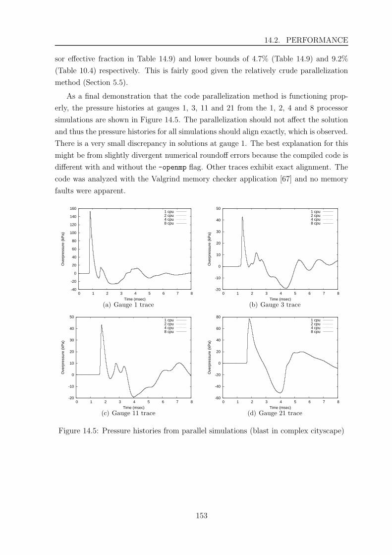
14.2. PERFORMANCE
sor effective fraction in Table 14.9) and lower bounds of 4.7% (Table 14.9) and 9.2%
(Table 10.4) respectively. This is fairly good given the relatively crude parallelization
method (Section 5.5).
As a final demonstration that the code parallelization method is functioning prop-
erly, the pressure histories at gauges 1, 3, 11 and 21 from the 1, 2, 4 and 8 processor
simulations are shown in Figure 14.5. The parallelization should not affect the solution
and thus the pressure histories for all simulations should align exactly, which is observed.
There is a very small discrepancy in solutions at gauge 1. The best explanation for this
might be from slightly divergent numerical roundoff errors because the compiled code is
different with and without the -openmp flag. Other traces exhibit exact alignment. The
code was analyzed with the Valgrind memory checker application [67] and no memory
faults were apparent.
-40
-20
0
20
40
60
80
100
120
140
160
0 1 2 3 4 5 6 7 8
Ove
rpre
ssur
e (k
Pa)
Time (msec)
1 cpu2 cpu4 cpu8 cpu
(a) Gauge 1 trace
-20
-10
0
10
20
30
40
50
0 1 2 3 4 5 6 7 8
Ove
rpre
ssur
e (k
Pa)
Time (msec)
1 cpu2 cpu4 cpu8 cpu
(b) Gauge 3 trace
-20
-10
0
10
20
30
40
50
0 1 2 3 4 5 6 7 8
Ove
rpre
ssur
e (k
Pa)
Time (msec)
1 cpu2 cpu4 cpu8 cpu
(c) Gauge 11 trace
-60
-40
-20
0
20
40
60
80
0 1 2 3 4 5 6 7 8
Ove
rpre
ssur
e (k
Pa)
Time (msec)
1 cpu2 cpu4 cpu8 cpu
(d) Gauge 21 trace
Figure 14.5: Pressure histories from parallel simulations (blast in complex cityscape)
153
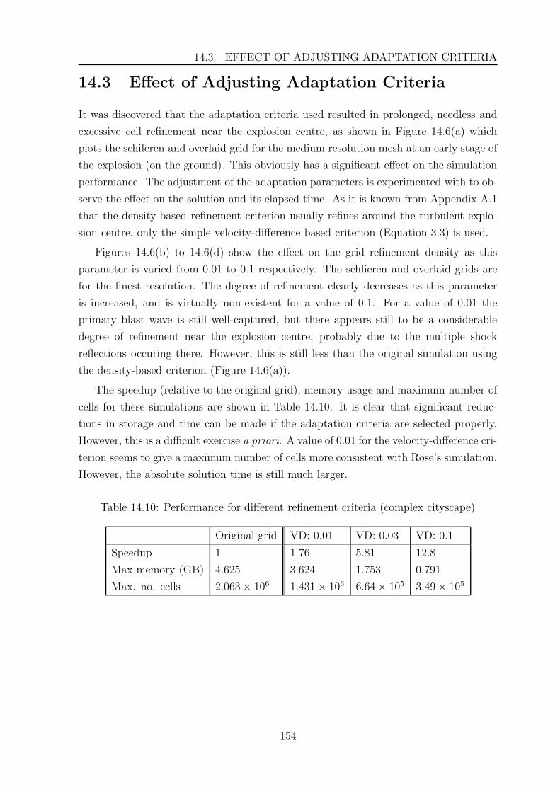
14.3. EFFECT OF ADJUSTING ADAPTATION CRITERIA
14.3 Effect of Adjusting Adaptation Criteria
It was discovered that the adaptation criteria used resulted in prolonged, needless and
excessive cell refinement near the explosion centre, as shown in Figure 14.6(a) which
plots the schileren and overlaid grid for the medium resolution mesh at an early stage of
the explosion (on the ground). This obviously has a significant effect on the simulation
performance. The adjustment of the adaptation parameters is experimented with to ob-
serve the effect on the solution and its elapsed time. As it is known from Appendix A.1
that the density-based refinement criterion usually refines around the turbulent explo-
sion centre, only the simple velocity-difference based criterion (Equation 3.3) is used.
Figures 14.6(b) to 14.6(d) show the effect on the grid refinement density as this
parameter is varied from 0.01 to 0.1 respectively. The schlieren and overlaid grids are
for the finest resolution. The degree of refinement clearly decreases as this parameter
is increased, and is virtually non-existent for a value of 0.1. For a value of 0.01 the
primary blast wave is still well-captured, but there appears still to be a considerable
degree of refinement near the explosion centre, probably due to the multiple shock
reflections occuring there. However, this is still less than the original simulation using
the density-based criterion (Figure 14.6(a)).
The speedup (relative to the original grid), memory usage and maximum number of
cells for these simulations are shown in Table 14.10. It is clear that significant reduc-
tions in storage and time can be made if the adaptation criteria are selected properly.
However, this is a difficult exercise a priori. A value of 0.01 for the velocity-difference cri-
terion seems to give a maximum number of cells more consistent with Rose’s simulation.
However, the absolute solution time is still much larger.
Table 14.10: Performance for different refinement criteria (complex cityscape)
Original grid VD: 0.01 VD: 0.03 VD: 0.1
Speedup 1 1.76 5.81 12.8
Max memory (GB) 4.625 3.624 1.753 0.791
Max. no. cells 2.063 × 10⁶ 1.431 × 10⁶ 6.64 × 10⁵ 3.49 × 10⁵
154
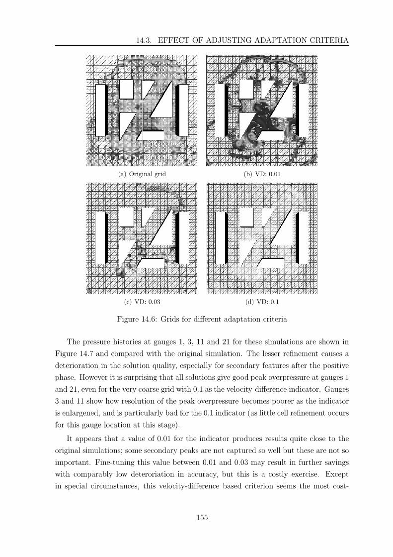
14.3. EFFECT OF ADJUSTING ADAPTATION CRITERIA
(a) Original grid (b) VD: 0.01
(c) VD: 0.03 (d) VD: 0.1
Figure 14.6: Grids for different adaptation criteria
The pressure histories at gauges 1, 3, 11 and 21 for these simulations are shown in
Figure 14.7 and compared with the original simulation. The lesser refinement causes a
deterioration in the solution quality, especially for secondary features after the positive
phase. However it is surprising that all solutions give good peak overpressure at gauges 1
and 21, even for the very coarse grid with 0.1 as the velocity-difference indicator. Gauges
3 and 11 show how resolution of the peak overpressure becomes poorer as the indicator
is enlargened, and is particularly bad for the 0.1 indicator (as little cell refinement occurs
for this gauge location at this stage).
It appears that a value of 0.01 for the indicator produces results quite close to the
original simulations; some secondary peaks are not captured so well but these are not so
important. Fine-tuning this value between 0.01 and 0.03 may result in further savings
with comparably low deteroriation in accuracy, but this is a costly exercise. Except
in special circumstances, this velocity-difference based criterion seems the most cost-
155
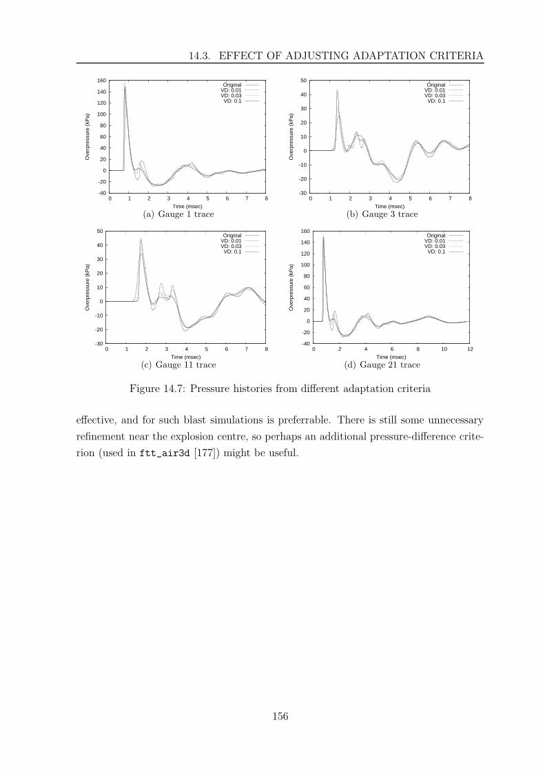
14.3. EFFECT OF ADJUSTING ADAPTATION CRITERIA
-40
-20
0
20
40
60
80
100
120
140
160
0 1 2 3 4 5 6 7 8
Ove
rpre
ssur
e (k
Pa)
Time (msec)
OriginalVD: 0.01VD: 0.03VD: 0.1
(a) Gauge 1 trace
-30
-20
-10
0
10
20
30
40
50
0 1 2 3 4 5 6 7 8
Ove
rpre
ssur
e (k
Pa)
Time (msec)
OriginalVD: 0.01VD: 0.03
VD: 0.1
(b) Gauge 3 trace
-30
-20
-10
0
10
20
30
40
50
0 1 2 3 4 5 6 7 8
Ove
rpre
ssur
e (k
Pa)
Time (msec)
OriginalVD: 0.01VD: 0.03VD: 0.1
(c) Gauge 11 trace
-40
-20
0
20
40
60
80
100
120
140
160
0 2 4 6 8 10 12
Ove
rpre
ssur
e (k
Pa)
Time (msec)
OriginalVD: 0.01VD: 0.03
VD: 0.1
(d) Gauge 21 trace
Figure 14.7: Pressure histories from different adaptation criteria
effective, and for such blast simulations is preferrable. There is still some unnecessary
refinement near the explosion centre, so perhaps an additional pressure-difference crite-
rion (used in ftt_air3d [177]) might be useful.
156
Chapter 15
Application Study – Modelling Explosion
in Shipping Container Geometries
This application study was originally reported by the author in Reference [203] and
models an explosion in an internal geometry resembling a shipping container. The
stems from the recent consideration by the Centre of Hypersonics (The University of
Queensland) into the possibility of testing rocket motors in a confined facility, which is
a modified shipping container with roof vents for the inlet and outlet. Open-air rocket
testing is not preferred because the noise generated from the turbulent plume is quite
high at 120-130 decibels. This section presents a very simplified numerical simulation of
the worst-case scenario when the mainly nondetonable rocket propellant explodes, with
the goal of obtaining contours of peak overpressures and impulses on the (assumed rigid)
internal walls. This is essentially a design study and no opportunity for a supplemental
experimental study could be performed.
The propellant for the proposed Wagtail rocket [35] weighs 20 kg and is predomi-
nantly composed of ammonium perchlorate, which is normally very difficult to detonate
[158]. In light of this fact and the inability of the code to model propellant burning, a
conservative TNT equivalence value of 1 to 1 is assumed, and thus the charge in the
simulation consists of 20 kg of TNT. Although an explosion of this mass of TNT within
a shipping container with only 5 mm thick walls will result in failure of the facility,
the simulation can be thought to model the explosion in any rigid structure with the
same internal geometry, and it will still be interesting to observe the magnitude of peak
pressures. This study is thus a study into blast confinement effects.
A diagram of the testing facility is shown in Figure 15.1. The walls are modelled as
smooth, flat surfaces. The explosive source is located along the container centerline, 3
m from the intake end and 1 m off the floor. However, a plane of symmetry along the
container centerline is not used. An energy density of 4520 kJ/kg of TNT is assumed
[19]; the charge is initialized with the balloon analogue model (Section 4.6). It is assumed
to be composed of perfect gas air.
Three minimum adaptive grids are used to observe grid dependence. The coarsest
resolution uses four working levels (level 4 to 7) with cell sizes 0.2344 m to 1.875 m, and
is denoted the L7 mesh. Like in Section 12 the cells are kept at level 7 at walls as the
157
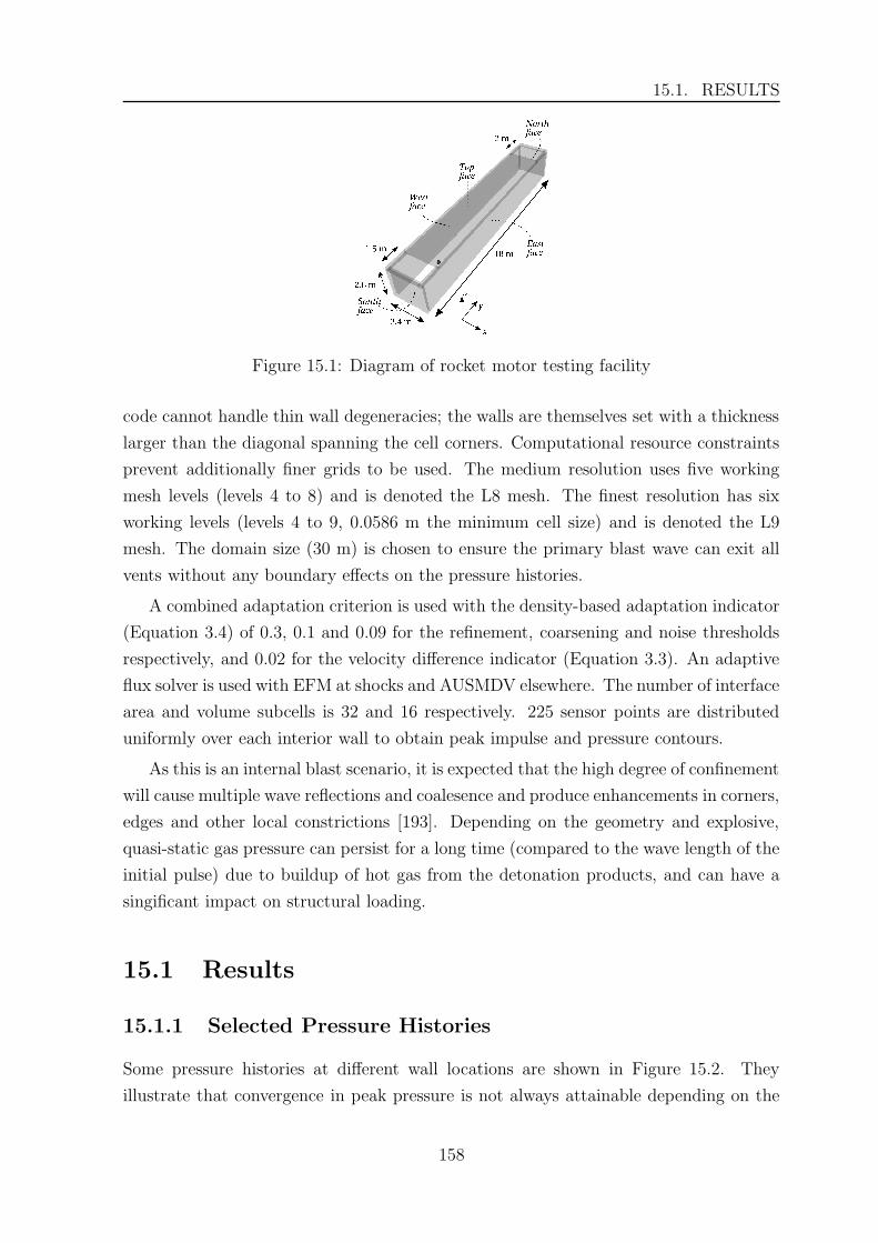
15.1. RESULTS
Figure 15.1: Diagram of rocket motor testing facility
code cannot handle thin wall degeneracies; the walls are themselves set with a thickness
larger than the diagonal spanning the cell corners. Computational resource constraints
prevent additionally finer grids to be used. The medium resolution uses five working
mesh levels (levels 4 to 8) and is denoted the L8 mesh. The finest resolution has six
working levels (levels 4 to 9, 0.0586 m the minimum cell size) and is denoted the L9
mesh. The domain size (30 m) is chosen to ensure the primary blast wave can exit all
vents without any boundary effects on the pressure histories.
A combined adaptation criterion is used with the density-based adaptation indicator
(Equation 3.4) of 0.3, 0.1 and 0.09 for the refinement, coarsening and noise thresholds
respectively, and 0.02 for the velocity difference indicator (Equation 3.3). An adaptive
flux solver is used with EFM at shocks and AUSMDV elsewhere. The number of interface
area and volume subcells is 32 and 16 respectively. 225 sensor points are distributed
uniformly over each interior wall to obtain peak impulse and pressure contours.
As this is an internal blast scenario, it is expected that the high degree of confinement
will cause multiple wave reflections and coalesence and produce enhancements in corners,
edges and other local constrictions [193]. Depending on the geometry and explosive,
quasi-static gas pressure can persist for a long time (compared to the wave length of the
initial pulse) due to buildup of hot gas from the detonation products, and can have a
singificant impact on structural loading.
15.1 Results
15.1.1 Selected Pressure Histories
Some pressure histories at different wall locations are shown in Figure 15.2. They
illustrate that convergence in peak pressure is not always attainable depending on the
158
15.1. RESULTS
sensor location. Figures 15.2(a) to 15.2(d) are examples of sensors located at either
corners or edges in the geometry. These histories do not show convergence in peak
overpressure; however Figure 15.2(c) apparently shows convergence in the second peak.
Figures 15.2(e) and 15.2(f) show pressure histories away from edges, and convergence
in peak overpressure is more demonstrable.
-2000
0
2000
4000
6000
8000
10000
12000
14000
16000
0 2 4 6 8 10
Ove
rpre
ssur
e (k
Pa)
Time (msec)
L7L8L9
(a) West face - floor, corner
-500
0
500
1000
1500
2000
2500
3000
3500
4000
4500
5000
0 2 4 6 8 10 12 14O
verp
ress
ure
(kP
a)Time (msec)
L7L8L9
(b) West face - South face edge
0
200
400
600
800
1000
1200
1400
1600
1800
2000
0 5 10 15 20 25 30 35 40
Ove
rpre
ssur
e (k
Pa)
Time (msec)
L7L8L9
(c) East face - floor edge
-500
0
500
1000
1500
2000
2500
0 5 10 15 20 25 30 35 40
Ove
rpre
ssur
e (k
Pa)
Time (msec)
L7L8L9
(d) North face - floor edge
0
200
400
600
800
1000
1200
1400
1600
0 5 10 15 20 25 30 35 40
Ove
rpre
ssur
e (k
Pa)
Time (msec)
L7L8L9
(e) West face convergent example
0
200
400
600
800
1000
1200
1400
1600
0 5 10 15 20 25
Ove
rpre
ssur
e (k
Pa)
Time (msec)
L7L8L9
(f) Top face convergent example
Figure 15.2: Selected traces for explosion in shipping container problem
Numerical convergence in peak overpressure was also found to be difficult in previ-
ous simulations [175] (see also Section 14.1), and particularly with gauge readings at
structural corners in an internal geometry [136]. Rose et al [175] state that convergence
159
15.1. RESULTS
may be difficult to demonstrate when initial pulses are comprised of several (previously)
distinct waves, although secondary pulses might be easier to converge. In this case,
the inconsistent convergent behaviour might be because a shock wave travelling into an
edge or corner geometry is analogous to shock focussing, due to symmetry of the solid
boundary condition. As discussed in Section 12.1 the pressure at such focus points is a
particularly grid-dependent result and difficult to resolve [54].
Hence convergence is more readily expected for sensors away from edges, which is
observed. Another factor influencing non-convergence at edges is that the finest cell sizes
are not always used at surfaces; depending on the geometry and adaptation criteria the
grid may not be adapted to the finest level at some sensor points, especially those far
from the charge. The range of grid sizes for this study may not be in the asymptotic
convergence range, which may need to be quite fine. Also VCE ‘rounds off’ corners unless
a staircased representation is used. The existence of ‘small cells’ (Section 2.4.2) at edges
and corners, and a locally first-order scheme, may also contribute to the deterioration
of accuracy.
15.1.2 Impulse and Pressure Wall Contours
Contours of peak overpressure and impulse along the facility’s interior walls are shown
in Figures 15.3 to 15.5. Figure 15.3 shows peak quantities along the south face, or
inlet-end wall. This figure gives an example of the different peak overpressure solutions
on different resolutions, which do differ noticeably, although general features are pre-
served. These differences are used in computing average wall errors in Section 15.1.3.
Peak overpressures are of the order of tens of megapascals. Maximum values increase
with increasing resolution, and the solution is symmetrical about the centreline. It is
interesting that the local maxima in the higher resolution simulations are slightly away
from the corners and do not correspond to the height of burst. The maximum impulse
occurs along the floor edge due to the shock focussing there and the charge height of
burst.
Figure 15.4 shows the peak quantities along the east face or long side wall for the
L9 grid. Note that peak values occur at the charge location, and are greatest at corners
and edges due to focussing. The impulse is nearly constant along the wall section from
the charge to the outlet vent. The peak pressures and impulse increase at the north face
(or outlet-end wall) due to shock reflection there.
Figure 15.5 shows contours for the L9 grid along the north face, or outlet-end wall,
which is farthest from the charge. By this stage there might have been much coalesence
of waves, and some numerical diffusion has occured, so the contours are more smoothly
160
15.1. RESULTS
(a) Peak ovepressure, L7 grid (b) Peak impulse, L7 grid
(c) Peak ovepressure, L8 grid (d) Peak impulse, L8 grid
(e) Peak overpressure, L9 grid (f) Peak impulse, L9 grid
Figure 15.3: South face contours for explosion in shipping container problem
161
15.1. RESULTS
varying. Peak pressure occurs at the facility floor and has attenuated to the order of
megapascals. Impulse values are also greatest at the floor.
(a) Peak ovepressure
(b) Peak impulse
Figure 15.4: East face contours (L9 grid) for explosion in shipping container problem
(a) Peak ovepressure (b) Peak impulse
Figure 15.5: North face contours (L9 grid) for explosion in shipping container problem
Figure 15.6 plots peak values for the L9 grid along the interior ceiling, or top face.
There exists a local maximum in pressure directly above the charge itself, although peak
values occur at edges (at the charge location) due to focussing. The effect of venting
on reducing peak values can be seen on the impulse plot where a marked decrease can
be observed. The impulse is nearly constant along the section from the charge to the
outlet vent.
162
15.1. RESULTS
(a) Peak ovepressure
(b) Peak impulse
Figure 15.6: Top face contours (L9 grid) for explosion in shipping container problem
15.1.3 Average wall errors
Like in Table 14.7 an average error for the whole wall can be estimated by calculating
the relative error between grids to obtain an average relative error per sensor point. This
relative error is identical to the Richardson-extrapolated error if the refinement factor
and solution order are 2 and 1 respectively. Decreasing errors for higher resolutions
indicate convergence. These errors are shown in Table 15.1. Note that errors in pressure
are quite high, and are as much as an order of magnitude higher than impulse errors.
This behaviour is also seen in Tables 10.1 and 10.2 and 14.7. Although impulse errors
are quite low, convergence has not been achieved either in impulse or pressure (except
for the top face pressure).
As the greatest sources of error typically lie at corners and edges, it might be inter-
esting to calculate this error excluding those sensors at corners/edges. The results are
tabulated in Table 15.2. It is noteworthy that more wall faces do display convergent
behaviour, although not always consistently in both the impulse and pressure. Conver-
gence seems to depend on what quantity is computed, and even how it is computed.
Pressure errors have been reduced by at least a factor of 2 compared to Table 15.1 and
no impulse error exceeds 0.4%. The north face, being located farthest from the charge
and more affected by wave coalesence, interaction, focussing and numerical diffusion,
does not converge in either impulse or pressure.
As a final exercise, a simulation is performed on a series of much finer grids by
reducing the domain size to only encompass the inlet-end (south) wall and the charge
163
15.1. RESULTS
Table 15.1: Estimated average relative errors for each face
Face Impulse error Pressure error
East face (L7-L8) 0.00764954 0.139601
East face (L8-L9) 0.0086392 0.149198
South face (L7-L8) 0.00735129 0.169336
South face (L8-L9) 0.0102446 0.247718
North face (L7-L8) 0.00840221 0.0288078
North face (L8-L9) 0.0120841 0.150225
Top face (L7-L8) 0.00899833 0.17061
Top face (L8-L9) 0.0124166 0.140126
Table 15.2: Estimated average relative errors (excluding edges) for each face
Face Impulse error Pressure error
East face (L7-L8) 0.00322188 0.075768
East face (L8-L9) 0.0031481 0.0710504
South face (L7-L8) 0.00212314 0.0719346
South face (L8-L9) 0.00175235 0.0649372
North face (L7-L8) 0.00289666 0.00655631
North face (L8-L9) 0.00440226 0.0627783
Top face (L7-L8) 0.00308275 0.0817211
Top face (L8-L9) 0.00315627 0.0409477
(with a symmetry boundary condition at the charge). Thus up until an early time
(around 5 ms) the solution on this wall can be compared with the larger domain runs,
until effects from the boundary cause divergences in the solution. Minimum cell sizes
used in these adaptive-mesh simulations are 0.00732 m, 0.0146 m and 0.0293 m. Average
facial errors between these solutions are shown in Table 15.3. In this case convergence
for both impulse and pressure is observed, showing that these finer resolutions appear
to be within the asymptotic convergence range.
Table 15.3: Smaller domain error estimates on south face
Grid Impulse error Pressure error
Medium-coarsest grid 0.00951 0.143
Finest-medium 0.00533 0.0964
164
15.1. RESULTS
A better estimate of the larger-domain errors can be thus computed by comparing the
solution to the finest smaller-domain grid (up until 5 ms). The results are in Table 15.4
and the estimated errors for the south face in Table 15.1 are reproduced here. These
better error estimates show that the larger-domain peak impulse errors are around 3%
(even for the coarsest mesh), which is quite good, but peak overpressure errors are no
smaller than 23%. The pressure errors do in fact converge on this calculation, but
impulse does not converge monotonically.
Table 15.4: Better estimate of larger domain errors on south face
Better estimate Previous estimate
Grid level Impulse error Pressure error Impulse error Pressure error
L7 0.0329 0.353 - -
L8 0.0345 0.33 0.00735 0.169
L9 0.0226 0.232 0.01 0.248
These simulations demonstrate the difficulty of obtaining convergence for this prob-
lem, which is also noted in Section 14.1 and in Reference [171]. The simplest means
to obtain convergent solutions is to employ finer meshes, but this can result in exces-
sive resource usage (time and storage) for the current code. It is still encouraging that
impulse errors have been shown to be quite low (no larger than 3.5%).
15.1.4 Pressure Amplification and Failure on the Outlet Wall
The effect of confinement can be quantified by observing how much larger the overpres-
sures are at the far-end outlet wall and outlet vent compared to a free-field air burst.
It is found that on the finest resolution mesh (L9 mesh) the average peak overpressure
on the outlet wall (north face) and outlet vent is 1.66 MPa and 0.5 MPa respectively.
The peak overpressure at the vent corresponds to a reflected shock from the outlet wall.
Using scaled spherical TNT free-field data from Kinney [119], at the same straight-line
scaled distance to the outlet wall the overpressure is around 0.024 MPa. Assuming a
shock with this overpressure undergoes normal reflection, the reflected overpressure is
calculated via the Rankine-Hugoniot relations to be 0.053 MPa. This means amplifica-
tion factors at the outlet wall and vent of at least 31 and 9.4 respectively.
Approximating the outlet wall as a simply-supported flat plate of thickness 5 mm
subject to the uniform load of 1.66 MPa, it is possible to calculate the maximum wall
stress (located at the wall center) by a simple formula obtainable from a standard
solid mechanics text [227]. As the wall is a nearly square section, the stress is simply
165
15.2. EXPLOSION IN A MORE COMPLEX FACILITY
0.2874q(L/t)2 where q is the load, L and t are the length and thickness respectively. It
is computed to be 110 GPa; this is clearly much higher than the tensile strength of the
steel wall (which is on the order of hundreds of megapascals), making failure a certainty.
If wall failure alone is being investigated, it is unnecessary to use numerical simulation
as hand calculation via Kinney’s free-field scaled data [119] is sufficient to demonstrate
this. As the reflected overpressure is calculated to be 0.053 MPa (based on Kinney’s
curve), the computed stress is 3.5 GPa, which is still too high. In reality the walls are
corrugated, effectively raising stiffness, and are not simply supported at their edges.
More detailed modelling of the wall response is best obtained via a finite element simu-
lation.
15.1.5 Performance
All simulations for the longer-domain simulations (used to generate Tables 15.1 and 15.2)
were run in parallel on the SGI Altix cluster using 8 processors. The L7 mesh had a
maximum of about 106,000 cells, running for 2.5 hours and required about 0.3 GB of
memory. The L8 mesh had a maximum of 452,000 cells, elapsed time 9.6 hours and
required 1.2 GB memory. The L9 mesh had a maximum of 2,120,000 cells, elapsed
time of 69.13 hours and required 5.6 GB memory. Based on these figures the memory
requirements are at most 2.95 kB per cell, which is slightly more than the value of 2.6
calculated in Section 11.3.
15.2 Explosion in a More Complex Facility
A more complicated geometry for the motor testing facility was considered in which
the facility is partially buried on a hill side, with the outlet being a duct to enclose the
rocket plume to reduce noise. A simulation was briefly performed mainly to test how
well the code can handle this more complex geometry. A diagram of this geometry is
shown in Figure 15.7. Also shown are the density contours and the superimposed grid
on the vertical plane along the duct. The charge in this case is equivalent to 60 kg of
TNT (a larger motor size) and three adaptive mesh simulations were performed with a
minimum cell size of about 20 cm (level 7), 10 cm (level 8) and 5 cm (level 9).
The results show that no ‘leakage’ of the gas from inside of the duct to the surround-
ing atmosphere has occured, because the cells are refined to the highest level at the
walls. The focussing of the shock in the duct has resulted in a stronger blast wave at
the duct exit, evident from the better mesh adaptation compared to the blast escaping
from the inlet and entryway. It appears from Figure 15.8 that the overpressure directly
166
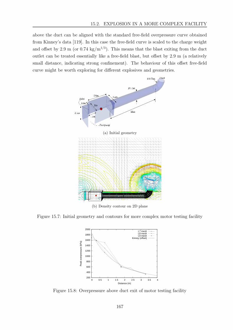
15.2. EXPLOSION IN A MORE COMPLEX FACILITY
above the duct can be aligned with the standard free-field overpressure curve obtained
from Kinney’s data [119]. In this case the free-field curve is scaled to the charge weight
and offset by 2.9 m (or 0.74 kg/m1/3). This means that the blast exiting from the duct
outlet can be treated essentially like a free-field blast, but offset by 2.9 m (a relatively
small distance, indicating strong confinement). The behaviour of this offset free-field
curve might be worth exploring for different explosives and geometries.
(a) Initial geometry
(b) Density contour on 2D plane
Figure 15.7: Initial geometry and contours for more complex motor testing facility
200
400
600
800
1000
1200
1400
1600
1800
2000
0 0.5 1 1.5 2 2.5 3 3.5 4
Pea
k ov
erpr
essu
re (
kPa)
Distance (m)
L7 meshL8 meshL9 mesh
Kinney (offset)
Figure 15.8: Overpressure above duct exit of motor testing facility
167
Chapter 16
Summary, Conclusions and Future Work
This thesis has described the design and testing of the CFD code OctVCE to model the
problem of blast propagation in complex geometries. The main design intent behind this
code is reliable prediction of blast loading in complex environments which is fast enough
to be used in a design process. This in turn can aid assessment of critical damage zones
and improve design of public spaces and structures. The code validation process has led
to a better insight into its accuracy and limitations and has helped identify a number
of areas and problems with the code that can be improved as future work.
Chapter 1 gave reasons why numerical simulation is in many cases the superior or
even necessary approach, compared to empiricial or semiempirical methods, for solving
this problem. An overview of previous attempts and codes also used in modelling blast
propagation in realistic geometries was provided, and the basic characteristics of explo-
sive blasts was discussed. Chapter 2 then presented different CFD methods which could
be used to simulate flows in complex geometries, concluding with a discussion on differ-
ent Cartesian cell methods and their advantages. A detailed discussion was provided of
the VCE method and its associated shortcomings.
Chapter 3 then discussed the octree data structure and how it could be utilized as the
basis for mesh adaptation in the code. Some algorithms in the form of pseudo-code were
presented to demonstrate the recursive nature of the mesh adaptation process. Some
measures that could be taken to increase speed (by sacrificing memory) and handle
degeneracies were also discussed, and the two different adaptation indicators used in
the code (based on velocity and density differences) were presented.
Chapter 4 centered on the numerical methodology of the code. The governing equa-
tions being solved, their method of discretization and integration, flux solvers used
(the AUSMDV [221] and EFM [150] schemes), reconstruction method and equations of
state were described. This section also reviewed the boundary conditions used in the
code and described how initial explosions or charges are represented in the numerical
simulation using the ‘balloon analogue’ or isothermal bursting sphere approach. Some
point-inclusion query methods were also reviewed.
Chapter 5 provided a review of parallel computing, parallel programming methods
and parallel performance measures, like Amdahl’s law [8] and its inverse (the useful
168
Karp-Flatt metric [113]). Section 5.5 described the shared-memory parallel implemen-
tation of the code.
Chapter 6 proceeded to the verification stage of code testing to establish the reli-
ability of the code programming in its implementation of the numerical methodology.
Four different test cases were considered. The first case, the Method of Manufactured
Solutions (Section 6.1), demonstrated higher-order behaviour of the code (between 1
and 2). In the second case (Section 6.2), the code was shown to provide solutions in
good agreement with the classic Sod shock tube problem, and an adaptive mesh solution
had a factor of savings of up to 3 in time and storage compared to the uniform grid
result. The non-reflecting boundary conditions were also tested with this problem and
shown to work well.
Section 6.3 demonstrated convergence as both subcell and grid resolution increased
for supersonic flow over simple wedge and cone geometry. Importantly, the surface so-
lution noise arising from the approximative nature of the VCE method (discussed in
Section 2.4.4) was shown not to be significant for practical engineering purposes e.g. if
integrated pressure forces are desired. Adaptive mesh solutions resulted in savings of
up to 9 times in storage and 7 times in time compared to comparable uniformly-refined
mesh solutions, demonstrating the large gains in efficiency obtainable from mesh adap-
tation. Section 6.4, which dealt with supersonic vortex flow, demonstrated very good
grid convergence (sometimes as high as the formal order of accuracy) of the numerical
result to the analytic solution.
Chapters 7 to 14 then described the numerous validation tests undergone by the
code to establish how well it can solve realistic blast and shock propagation problems.
In Chapter 7 the shock diffraction over a wedge was simulated, and good agreement
with previous experimental and numerical data was shown. The code performance
was also profiled for this simulation. Serial profiling showed that reconstruction-related
operations dominated the calculation, suggesting that future work should target this
area to improve efficiency. However, fairly good efficiency in the adaptation procedure
was achieved. Parallel profiling (using the Karp-Flatt metric) showed a serial fraction
for this calculation of approximately 10-20%, and significant overheads due to execution
of the code on a NUMA system and the non-local nature of parallelization and work
distribution among threads. This suggests that if any future development of the code
is to occur, it should focus on more complex parallel implementations and importantly
on improving the code’s memory efficiency.
Chapter 8 presented a simulation of shock interaction with cylindrical geometry
which showed good agreement with previous numerical work on this problem. Chapter 9
validated the one-dimensional spherical solver and demonstrated the accuracy of the
169
isothermal bursting sphere solution with previous experimental and numerical data. It
confirmed the findings of previous studies [166, 171] that the initial energy release is the
most important factor when peak overpressure or postive impulse in the mid- to far-field
regimes is desired. Non-reflecting boundary conditions were also tested for this problem
and shown to work well. Chapter 10 proceeded to simulate spherical TNT blast for
both the one-, two- and three-dimensional solvers. Convergence of the two- and three-
dimensional solvers to the one-dimensional result was demonstrated, and the errors due
to discretization and staircasing of the charge were measured. Parallel profiling of the
simulations showed large parallel overhead, but around 10% serial fraction to the code.
Chapter 11 concerned simulations of blast near single barrier structures. Good agree-
ment with previous data was shown, although there was a puzzling discrepancy in blast
arrival times. Simulations employing the non-reflecting boundary conditions performed
well when compared with larger-domain simulations. Savings of up to 5 times in time
were observed between adaptive and uniformly-refined mesh solutions. However, the
code was shown to be quite memory inefficient, which can impact performance consid-
erably. Chapter 12 demonstrated the code’s ability to simulate well explosions in com-
plex axisymmetric containers. The current results were somewhat inferior to previous
numerical results of commensurate resolution, but comparable accuracy was obtained
when Richardson extrapolation [163, 164] of the results was performed using solutions
from different meshes.
Chapter 13 tested the code in simulations of blast in three-dimensional environments
consisting of simple grid-aligned rectangular-prismatic geometries, and the results com-
pared well with previous experimental and numerical data. Chapter 14 focussed on
simulations of blast in a more complex urban environment, and fairly good agreement
with past results was achieved without the need for multi-dimensional remapping of an
initial one-dimensional spherical result [171]. Parallel profiling of the code showed a
serial portion of around 10% as before, and significant parallel overheads.
It was also observed that for this simulation, unnecessary and excessive refinement of
the mesh occured near the fireball due to the adaptation criteria employed, and future
work might also consider using a pressure-difference based indicator to prevent needless
refinement in this region. It is difficult to know a priori what values of the adaptation
indicators are optimum for the simulation; only guidelines can be provided. Convergence
of solutions was not always demonstrable, although there were reliable trends. The
previous data for this problem was supplied from Rose’s ftt_air3d code [174], which is
also an octree adaptive mesh, Cartesian cell code developed concurrently with OctVCE.
Comparison of the codes’ performance for this problem showed that ftt_air3d is much
more efficient time-wise and storage-wise.
170
16.1. COMPARISON WITH A SIMILAR CODE
Chapter 15 focussed on an application study of the code in simulations of internal
blast in a shipping container geometry. Regrettably there was no opportunity for ex-
perimental work to supplement the numerical study, but the work was part of a design
process which helped in the evaluation of options for the rocket test facility. Conver-
gence of solutions was not always easy to demonstrate due to the coarseness of the grids,
and shock focussing at the edges and corners of the geometry. Nonetheless the simu-
lations demonstrated very large amplification of pressures and positive impulses within
the structure due to confinement of the blast.
Many of the validation simulations demonstrated that acceptable (but still some-
what inferior) solutions can be obtained without the need for first remapping a one-
dimensional result before the blast passes the nearest surface feature. It would appear
that the OctVCE code has been shown to be a reliable tool in simulating blast propaga-
tion in complex geometries, as per the aims of the thesis, and more generally that the
VCE method and octree mesh adaptation appears suitable for such problems.
16.1 Comparison with a Similar Code
The ftt_air3d code of Rose et al [174] is similar to, more advanced than and developed
at about the same time as the OctVCE code, and has greater time and memory efficiency.
It may be instructive to compare and contrast the two codes in case future work in
improving or extending OctVCE is undertaken.
The ftt_air3d code [174, 177] is written in FORTRAN and due to implementation of
the Fully Threaded Tree (FTT) structure [118] (discussed in greater depth in Section 3.1)
is much more memory-efficient than OctVCE, which stores mesh connectivity, geometric
data and other information explicitly. Lower memory requirements contribute to overall
better performance due to fewer cache misses. ftt_air3d also appears to use a one-
dimensional form of reconstruction whilst OctVCE uses multi-dimensional reconstruction
requiring inversion of matricies. In OctVCE this forms a significant portion (50%) of the
calculation code (as mentioned above) and given the success of ftt_air3d, it may be
that multi-dimensional reconstruction is not required for such problems.
Another very significant time-saving strategy used in ftt_air3d is the use of local
but interleaved timestepping (depending on cell level) and an apparently less conserva-
tive timestep. ftt_air3d seems to use a timestep based on the expression
∆t =∆x
max (a + |ui|)(16.1)
with the maximum taken over the three directions i = x, y, z [176]. If this expression is
171
16.1. COMPARISON WITH A SIMILAR CODE
compared with Equation 4.7 and assuming the (a + u) term is constant, Equation 4.7
gives a timestep which is 6 times smaller than Equation 16.1 in three dimensions. As
it is very simple in OctVCE to increase the timestep e.g. by increasing the CFL or
adopting Equation 16.1, this might be worth exploring for future simulations. To ensure
stability and proper shock tracking, the mesh adaptation frequency can be increased and
more aggressive cell merging undertaken to ensure large cells everywhere. Also, a less
conservative CFL “cut-back” procedure (Section 4.8.1, page 37) might be used e.g.
setting a larger value of εcut.
The adaptation indicators in OctVCE were chosen because of past success [148, 155,
211], capability to refine cells about other discontinuities like slip layers and provision of
some refinement in the positive phase region of the blast. This can sometimes result in
excessive refinement about relatively unimportant regions like the explosive products.
This problem may not be present in ftt_air3d, which uses a simple pressure difference
indicator. It also provides for some degree of refinement behind the blast by testing if
the number of times a cell is considered for coarsening reaches some threshold value.
ftt_air3d also allows specification of regions where mesh refinement can be switched
off, which is not implemented in OctVCE.
Unlike OctVCE, ftt_air3d also supports remapping of one-dimensional spherical
solutions to multi-dimensions, which can produce well-resolved blast profiles and save
save solution time in the early stages of the explosion. Compared to OctVCE which
allocated or deallocated memory (corresponding to refining or coarsening respectively)
on a per cell basis, ftt_air3d appears to be more efficient in its handling of memory
by allocating or deallocating stacks of cells. Codes that frequently allocate or deallocate
memory do suffer from performance ineffiencies due to memory management overhead
[105, 174], and the memory in OctVCE might become more fragmented over time than
with ftt_air3d [177].
However, OctVCE does have parallel processing capability, unlike ftt_air3d, and it
can handle geometry constructed of arbitrary surface polygons instead of just convex
polygons (required by ftt_air3d) due to the generality of the VCE method. A disadvan-
tage is possibly more time spent in computing geometrical operations like point-inclusion
queries. Due to the axisymmetric extension to the VCE method, OctVCE can also sim-
ulate axisymmetric flows in complex geometry in addition to the simple height-of-burst
problem. A parallel OctVCE solution conjoined with a less conservative timestepping
strategy discussed above might be competitive with a ftt_air3d run. The parallel im-
plementation (Section 5.5) seems to perform well given the inherently serial portion of
the code, but still could be more efficient, due to the large memory requirements and
locality issues when executed on a NUMA machine (as discussed above).
172
16.2. ACCESS TO THE SOURCE CODE
Further work might thus first focus on reducing memory usage without comprimis-
ing the basic numerical methodology. It may still be possible to achieve performance
competitive with ftt_air3d despite the relatively simple parallelization method, ex-
plicit storage of neighbouring connectivity and use of list structures to access cells. For
example, some relatively simple improvements to the cell data structure (Figure K.4
in Appendix K) can be made without requiring too much alterations to the code.
The gradient and limiters structures could be combined into a single limited
gradient quantity, as in ftt_air3d, and geometric data like interface areas, volumes
and surface normals really only require storage for intersected cells, being easily derived
for unobstructed cells based on cell level. These additional complexities arise because
intersected cells in OctVCE are not always at the finest level (unlike ftt_air3d), which
require more storage to handle these special cases. Given the accuracy of the method, it
may also be sufficient to use a single interface flux vector, even if the interface is shared
by two or more cells at finer level.
16.2 Access to the Source Code
The OctVCE program source code and user manual can be found in
http://www.mech.uq.edu.au/staff/jacobs/cfcfd/.
173
Bibliography
[1] M J Aftosmis. Solution adapative Cartesian grid methods for aerodynamics flows
with complex geometries, 1997. 28th Computational Fluid Dynamics Lecture
Series, VKILS 1997-02.
[2] M J Aftosmis, G Adomavicus, and M J Berger. A parallel multilevel method for
adaptively refined cartesian grids with embedded boundaries. In 38th Aerospace
Sciences Meeting and Exhibit, 2000. AIAA 2000–0808.
[3] M J Aftosmis, M J Berger, and J E Melton. Adaptation and surface modeling for
Cartesian mesh methods, 1995. AIAA–95–1725–CP.
[4] M J Aftosmis, M J Berger, J E Melton, and M D Wong. 3D applications of a
Cartesian grid Euler method. In 33rd Aerospace Sciences Meeting and Exhibit,
1995. AIAA 95–0853.
[5] M J Aftosmis, D Gaitonde, and T Sean Tavares. On the accuracy, stability and
monotonicity of various reconstruction algorithms for unstructured meshes. In
32nd Aerospace Sciences Meeting and Exhibit, 1994. AIAA 94–0415.
[6] M J Aftosmis, D Gaitonde, and T S Tavares. Behaviour of linear reconstruction
techniques on unstructured meshes. AIAA Journal, 33(11):2039–2049, 1995.
[7] Daniel Ambrosini, B Luccioni, A Jacinto, and R Danesi. Location and mass of
explosive from structural damage. Engineering Structures, 27:167–176, 2005.
[8] G Amdahl. The validity of the single processor approach to achieving large scale
computing capabilities. In AFIPS Conference Proceedings, pages 483–485, 1967.
[9] J D Anderson. Computational Fluid Dynamics: the Basics with Applications.
McGraw-Hill, New York, 1995.
[10] J D Anderson. Modern Compressible Flow: With Historical Perspective. McGraw-
Hill Higher Education, New York, 3rd edition, 2003.
[11] J G Anderson, G Katselis, and C Caputo. Analysis of a Generic Warhead Part
I: Experimental and Computational Assessment of Free Field Overpressure, 2002.
DSTO Weapons Systems Division, Australia, DSTO-TR-1313.
174
BIBLIOGRAPHY
[12] B J Armstrong, D D Rickman, J T Baylot, and T L Bevins. Code Validation
Studies for Blast in Urban Terrain. In Proceedings of 2002 HPC User’s Group
Conference, 2002.
[13] U.S. Army. The Antiterrorist Planner Software – A Tool for Vulernability As-
sessment of Facilities and Force Protection Planning, 1988. U.S. Army Engineer
Waterways Experiment Station, 3909 Halls Ferry Road, Vicksburg, MS 39180-
6199.
[14] M Arora and P L Roe. A Well-Behaved TVD Limiter for High-Resolution Calcu-
lations of Unsteady Flow. Journal of Computational Physics, 132(1):3–11, 1997.
[15] L S Avila. The VTK user’s guide. Kitware, Inc., Clifton Park, NY, 2004.
[16] A Bagabir and D Drikakis. Numerical experiments using high-resolution schemes
for unsteady, inviscid, compressible flows. Computer Methods in Applied Mechan-
ics and Engineering, 193:4675–4705, 2004.
[17] E L Baker. An Explosives Products Thermodynamic Equation of State Appropri-
ate for Material Acceleration and Overdriven Detonation: Theoretical Background
and Formulation, 1991. ARAED-TR-911013, U.S. Army Armament Research, De-
velopment and Engineering Center, Picatinney Arsenal, New Jersey.
[18] E L Baker and D L Littlefield. Implementation of a High Explosive Equation of
State into an Eulerian Hydrocode. In AIP Conference Proceedings, volume 706,
pages 375–378, 2004.
[19] W E Baker, P A Cox, P S Westine, J J Kulesz, and R A Strehlow. Explosion
Hazards and Evaluation. Elsevier, New York, 1983.
[20] T J Barth. On Unstructured Grids and Solvers, 1990. von Karman Institute for
Fluid Dynamics, Lecture Series 1990–03.
[21] J D Baum, L Hong, E Mestreau, and C Deel. Assessment of the terrorist attack
on the US Embassy in Nairobi, Kenya. In Proceedings of the 10th International
Symposium on Interaction of the Effects of Munitions with Structures, San Diego,
2001.
[22] J D Baum and R Lohner. Numerical simulation of a shock interaction with a
modern main battlefield tank, 1991. AIAA-91-1666.
[23] J D Baum, H Luo, and R Lohner. Numerical simulation of a blast inside in the
world trade center, 1995. AIAA 95-0085.
175
BIBLIOGRAPHY
[24] J Bell, M Berger, J Saltzman, and M Welcome. Three-dimensional adaptive
mesh refinement for hyperbolic conservation laws. SIAM Journal of Scientific
Computing, 15(1):127–138, 1994.
[25] G Ben-dor, O Igra, and T Elperin. Handbook of Shock Waves, volume 2. Academic
Press, San Diego, 2001.
[26] M J Berger. Adaptive Mesh Refinement for Hyperbolic Partial Differential Equa-
tions. Journal of Computational Physics, 53:484–512, 1984.
[27] M J Berger and R J LeVeque. An Adaptive Cartesian Mesh Algorithm for the
Euler Equations in Arbitrary Geometries, 1989. AIAA 89–1930–CP.
[28] R Berrendorf and G Nieken. Performance characteristics for OpenMP constructs
on different parallel computer architectures. Concurrency: Practice and Experi-
ence, 12:1261–1273, 2000.
[29] R Biswas and R Strawn. Tetrahedral and hexahedral mesh adaptation for CFD
problems. Applied Numerical Mathematics, 26(1–2):135–151, 1998.
[30] T Blacker. Meeting the challenge for automated conformal hexahedral meshing.
In 9th International Meshing Roundtable, New Orleans, 2000.
[31] T Blacker. Auotmated Conformal Hexahedral Meshing Constraints, Challenges
and Opportunities. Engineering with Computers, 17:201–210, 2001.
[32] T D Blacker and R J Meyers. Seams and Wedges in Plastering: A 3-D Hexahedral
Mesh Generation Algorithm. Engineering with Computers, 9:83–93, 1993.
[33] BLASTX, 1996. U.S. Army Engineer Waterways Experiment Station, Mississippi.
[34] OpenMP Architecture Review Board. OpenMP C and C++ Application Program
Interface, 2002. Version 2.0.
[35] D Bond, B Trinh, and D Fox. Wagtail Solid Rocket Project, 2007. University of
Queensland MECH4552 Design Project Report.
[36] J Bonet and J Peraire. An Alternating Digital Tree (ADT) algorithm for 3D geo-
metric searching and intersection problems. International Journal for Numerical
Methods in Engineering, 31:1–17, 1991.
[37] J P Boris. The threat of chemical and biological terrorism: preparing a response.
Computing in Science and Engineering, 4(2):22–32, 2002.
176
BIBLIOGRAPHY
[38] S Børve, M Omang, and J Trulsen. Regularized smoothed particle hydrodynam-
ics with improved multi-resolution handling. Journal of Computational Physics,
208:345–367, 2005.
[39] M A Brittle. Blast propagation in a geometrically complex urban environment.
Master’s thesis, Royal Military College of Science Engineering Systems Depart-
ment, 2004.
[40] H L Brode. Numerical Solutions of Spherical Blast Waves. Journal of Applied
Physics, 26:766–775, 1955.
[41] H L Brode. Blast Wave from a Spherical Charge. Physics of Fluids, 2:217–229,
1959.
[42] A E Bryson and R W F Gross. Diffraction of Strong Shocks by Cones, Cylinders,
and Spheres. Journal of Fluid Mechanics, 10:1–16, 1961.
[43] P S Bulson. Explosive Loading of Engineering Structures. E and FM Spon, UK,
1997.
[44] J L Cambier, S Tokarcik, and D K Prabhu. Numerical simulations of unsteady
flow in a hypersonic shock tunnel facility. In AIAA 17th Aerospace Ground Testing
Conference, Nashville, TN, 1992.
[45] R S Cant, W N Dawes, and A M Savill. Advanced CFD and Modeling of Accidental
Explosions. Annual Review of Fluid Mechanics, 36:97–119, 2004.
[46] Y A Cengel and M A Boles. Thermodynamics: an engineering approach. McGraw
Hill, New York, 4th edition, 2002.
[47] R Chandra, L Dagum, D Kohr, D Maydan, J McDonald, and R Menon. Parallel
Programming in OpenMP. Academic Press, USA, 2001.
[48] T C Chapman, T A Rose, and P D Smith. Blast wave simulation using AU-
TODYN2D: a parametric study. International Journal of Impact Engineering,
16(5/6):777–787, 1995.
[49] T C Chapman, T A Rose, and P D Smith. Reflected blast wave resultants behind
cantilever walls: A new prediction technique. International Journal of Impact
Engineering, 16(3):397–403, 1995.
[50] E F Charlton. An Octree Solution to Conservation–laws over Arbitrary Regions
(OSCAR) with Applications to Aircraft Aerodynamics. PhD thesis, The University
of Michigan, 1997.
177
BIBLIOGRAPHY
[51] E F Charlton and K G Powell. An Octree Solution to Conservation-laws over
Arbitrary Regions, 1997. AIAA 97-0198.
[52] R F Chisnell. An analytic description of converging shock waves. Journal of Fluid
Mechanics, 354:357–375, 1998.
[53] T J Chung. Computational fluid dynamics. Cambridge University Press, Cam-
bridge, 2002.
[54] S Cieslak, S B Kheil, I Choquet, and A Merlen. Cut cell strategy for 3-D blast
waves numerical simulations. Shock Waves, 10:421–429, 2001.
[55] J F Clarke and M McChesney. The dynamics of real gases. Butterworths, London,
1964.
[56] J K Clutter. A reduced combustion model for vapor cloud explosions validated
against full-scale data. Journal of Loss Prevention in the Process Industries,
14:181–192, 2001.
[57] J K Clutter, J T Mathis, and M W Stahl. Modeling environmental effects in
the simulation of explosion events. International Journal of Impact Engineering,
34:973–989, 2007.
[58] W J Coirier. An Adaptively-Refined, Cartesian, Cell-Based Scheme for the Euler
and Navier-Stokes Equations. PhD thesis, The University of Michigan, 1994.
[59] W J Coirier and K G Powell. An Accuracy Assessment of Cartesian-Mesh Ap-
proaches for the Euler Equations, 1993. AIAA 93–3335–CP.
[60] P Colella and H M Glaz. Efficient Solution Algorithms for the Riemann Problem
for Real Gases. Journal of Computational Physics, 49:264–289, 1985.
[61] T Colonius. Modeling Artifical Boundary Conditions for Compressible Flow. An-
nual Review of Fluid Mechanics, 36:315–345, 2004.
[62] R Courant, K Friedrichs, and H Lewy. On the Partial Difference Equations of
Mathematical Physics. IBM Journal, 11(2):215–234, 1967.
[63] G Cybenko. Dynamic load balancing for distributed memory multiprocessors.
Journal of Parallel and Distributed Computing, 7:279–301, 1989.
[64] A Dadone. Cartesian grid computation of inviscid flows about multiple bodies. In
41st Aerospace Sciences Meeting and Exhibit, 2003. AIAA 2003-1121.
178
BIBLIOGRAPHY
[65] A Dadone and B Grossman. An Immersed Body Methodology for Inviscid Flows
on Cartesian Grids. In 40th Aerospace Sciences Meeting and Exhibit, 2002. AIAA
2002–1059.
[66] D De Zeeuw and K G Powell. An Adaptively Refined Cartesian Mesh Solver for
the Euler Equations. Journal of Computational Physics, 104:56–68, 1993.
[67] Valgrind developers. Valgrind. ¡http://www.valgrind.org/¿, accessed May 2008.
[68] Maxima development team. Maxima, a computer algebra system.
¡http://maxima.sourceforge.net/¿, accessed May 2008.
[69] K D Devine, E G Boman, R T Heaphy, B A Hendrickson, J D Teresco, J Faik, J E
Flaherty, and L G Gervasio. New challenges in dynamic load balancing. Applied
Numerical Mathematics, 52:133–152, 2005.
[70] J M Dewey and A van Netten. Calculating Blast-Effects Distances in Urban
Environments. In 17th International Symposium on Military Aspects of Blast and
Shock, Las Vegas, Nevada USA, 2002.
[71] D Drikakis, F Grinstein, and D Youngs. On the computation of instabilities and
symmetry-breaking in fluid mechanics. Progress in Aerospace Sciences, 41:609–
641, 2005.
[72] J A Edwards and T Ren. Vortex Interaction with an Aerofoil Using Chimera
and the AMR algorithm. In AIAA Atmospheric Flight Mechanics Conference and
Exhibit, volume AIAA 2002–4806, 2002.
[73] H El-Rewini and M Abd-El-Barr. Advanced Computer Architecture and Parallel
Processing. John Wiley and Sons, Inc, Hoboken, New Jersey, 2005.
[74] G E Fairlie, N F Johnson, and K C Moran. Validated Numerical Simulations of
Blast Loads on Structures. In 16th International Symposium on Military Aspects
of Blast and Shock, Oxford, England, 2000.
[75] F R Feito and J C Torres. Inclusion test for general polyhedra. Computers and
Graphics, 21(1):23–30, 1997.
[76] J E Flaherty, R M Loy, M S Shephard, B K Szymanski, J D Teresco, and L H
Ziantz. Adaptive Local Refinement with Octree Load-Balancing for the Paral-
lel Solution of Threee-Dimensional Conservation Laws. Journal of Parallel and
Distributed Computing, 47:139–152, 1997.
179
BIBLIOGRAPHY
[77] H Forrer and R Jeltsch. A higher order boundary treatment for cartesian-grid
methods. Journal of Computational Physics, 140:259–277, 1998.
[78] C E Fothergill, S Chynoweth, P Roberts, and A Packwood. Evaluation of a CFD
porous model for calculating ventilation in explosion hazard assessments. Journal
of Loss Prevention in the Process Industries, 16:341–347, 2003.
[79] P J Frey and P L George. Mesh generation : application to finite elements. Hermes
Science Publishing, Paris, 2000.
[80] N T Frink. Upwind Scheme for Solving the Euler Equations on Unstructured
Tetrahedral Meshes. AIAA Journal, 30(1):70–77, 1992.
[81] B Fryxell, K Olson, P Picker, F X Timmes, M Zingale, D Q Lamb, P MacNeice,
R Rosner, J W Truran, and H Tufo. FLASH: An adaptive mesh hydrodynamics
code for modeling astrophysical thermonuclear flashes. The Astrophysical Journal
Supplement Series, 131:273–334, 1999.
[82] C F Gerald and P O Wheatley. Applied Numerical Analysis. Pearson, Boston,
7th edition, 2004.
[83] R Gollan. Verification Exercises for a Compressible Flow Code. In 10th Interna-
tional Workshop on Shock-Tube Technology, Brisbane, Australia, 2006.
[84] R J Goozee. Simulation of a Complete Shock Tunnel Using Parallel Computer
Codes. PhD thesis, The University of Queensland, 2003.
[85] J J Gottlieb and C P T Groth. Assessment of Riemann Solvers for Unsteady One-
Dimensional Inviscid Flows of Perfect Gases. Journal of Computational Physics,
78(2):437–458, 1988.
[86] J A Greenough and J W Jacobs. A Numerical Study of Shock-Acceleration of a
Diffuse Helium Cylinder. In Proceedings of the Fifth International Workshop on
Comrpessible Turbulent Mixing, 1996.
[87] W Gropp, E Lusk, and A Skjellum. Using MPI: Portable Parallel Programming
with the Message-Passing Interface. The MIT Press, Cambridge, Massachusetts,
1994.
[88] M E Hayder, F Q Hu, and M Y Hussaini. Toward Perfectly Absorbing Boundary
Conditions for Euler Equations. AIAA Journal, 37(8), 1999.
[89] M Held. Blast Waves in Free Air. Propellants, Explosives, Pyrotechnics, 8:1–7,
1983.
180
BIBLIOGRAPHY
[90] A Henderson and J Ahrens. The ParaView guide. Kitware, Clifton Park, NY,
2004.
[91] B Hendrickson. Graph partitioning and parallel solvers: Has the emperor no
clothes, 1998. Lecture notes in Computer Science, 1457: 218–225.
[92] J Henrych. The Dynamics of Explosion and Its Use. Elsevier Scientific Publishing
Company, Czechoslovakia, 1979.
[93] E Hertel, J Bell, M Elrick, A Farnsworth, G Kerley, J McGlaun, S Petney, S Silling,
P Taylor, and L Yarrington. CTH: A Software Family for Multi-Dimensional Shock
Physics Analysis. In Proceedings of the 19th International Symposium on Shock
Waves, pages 377–382, France, 1993.
[94] S Hikida and S Needham. Low Altitude Multiple Burst (LAMB) Model, Volume
1: Shock Description. S-Cubed, Albuquerque, New Mexico, 1981.
[95] M D Hill and J R Larus. Cache considerations for multiprocessor programmers.
Communications of the ACM, 33(8):97–102, 1990.
[96] C Hirsch. Numerical Computation of Internal and External Flows. Volume 1:
Fundamentals of Numerical Discretization, volume 1. Wiley, England, 1988.
[97] C Hirsch. Numerical Computation of Internal and External Flows. Volume 2:
Computational Methods for Inviscid and Viscous Flows, volume 2. Wiley, England,
1988.
[98] K Hormann and A Agathos. The point in polygon problem for arbitrary polygons.
Computational Geometry, 20:131–144, 2001.
[99] W P Horn and D L Taylor. A Theorem to Determine the Spatial Containment
Point in a Planar Polyhedron. Computer Vision, Graphics and Image Processing,
45:106–116, 1989.
[100] C W Huang and T Y Shih. On the complexity of point-in-polygon algorithms.
Computers and Geosciences, 23(1):109–118, 1997.
[101] W K E Huntington-Thresher and I G Cullis. TNT blast scaling for small charges.
In 19th International Symposium of Ballistics, pages 647–654, 2001.
[102] M Y Hussaini and T A Zang. Spectral Methods in Fluid Dynamics. Annual
Review of Fluid Mechanics, 19:339–367, 1987.
181
BIBLIOGRAPHY
[103] D W Hyde. CONWEP: Conventional Weapons Effects Program. Waterways Ex-
periment Station, Vicksburg, MS, USA, 1991.
[104] Century Dynamics Inc. Autodyn user’s manual-version 4.2, 1997.
[105] Silicon Graphics Inc. Linux Application Tuning Guide, 2005. SGI Manual 007-
4639-005.
[106] D M Ingram, D M Causon, and C G Mingham. Developments in cartesian cut
cell methods. Mathematics and Computers in Simulation, 61(3–6):561–572, 2003.
[107] M M Ismail and S G Murray. Study of the Blast Wave Parameters from Small
Scale Explosions. Propellants, Explosives, Pyrotechnics, 18:11–17, 1993.
[108] M M Ismail and S G Murray. Study of the Blast Waves from the Explosion of
Nonspherical Warheads. Propellants, Explosives, Pyrotechnics, 18:132–138, 1993.
[109] P A Jacobs. MB CNS: A computer program for the simulation of transient com-
pressible flows, 1996. Department of Mechanical Engineering Report 10/96, The
University of Queensland, Australia.
[110] I A Johnston. Simulation of Flow Around Hypersonic Blunt–Nosed Vehicles for
the Calibration of Air Data Systems. PhD thesis, The University of Queensland,
1999.
[111] Y E Kalay. Determining the Spatial Containment of a Point in General Polyhedra.
Computer Graphics and Image Processing, 19:303–334, 1982.
[112] G E Karniadakis and R M Kirby. Parallel Scientific Computing in C++ and MPI.
Cambridge University Press, United Kingdom, 2003.
[113] A H Karp and H P Flatt. Measuring parallel processor performance. Communi-
cations of the ACM, 33(5):539–543, 1990.
[114] G Karypis and V Kumar. METIS - a Software Package for Partitioning Unstruc-
tured Graphs, Partitioning Meshes, and Computing Fill-Reducing Orderings of
Sparse Matrices. Version 4.0, 1998. University of Minnesota Report.
[115] G Karypis, K Schloegel, and V Kumar. ParMETIS - Parallel Graph Partitioning
and Sparse Matrix Ordering Library. version 3.1, 2003. University of Minnesota
Report.
182
BIBLIOGRAPHY
[116] K Kato, T Aoki, S Kubota, and M Yoshida. A numerical scheme for strong blast
wave driven by explosion. International Journal for Numerical Methods in Fluids,
51:1335–1353, 2006.
[117] M P Kerry, B J Bibby, A J Martin, and R Garforth. Engineering level coupled
blast flow and damage module with rapid input scene generator for multibuilding
environments. In 17th International Symposium on Military Aspects of Blast and
Shock, Las Vegas, Nevada USA, 2002.
[118] A M Khokhlov. Fully Threaded Tree Algorithms for Adaptive Refinement Fluid
Dynamics Simulations. Journal of Computational Physics, 143:519–543, 1998.
[119] G F Kinney. Explosive Shocks in Air. Springer-Verlag Berlin Heidelberg, 2nd
edition, 1985.
[120] H Kleine, J M Dewey, K Ohashi, T Mizukaki, and K Takayama. Studies of the
TNT equivalence of silver azide charges. Shock Waves, 13:123–138, 2003.
[121] A Klomfass. A Cartesian grid finite-volume method for the simulation of gasdy-
namic flows about geometrically complex objects. In 26th International Sympo-
sium on Shock Waves, 2007.
[122] A L Kuhl. Mixing in Explosions, 1993. Lawrence Livermore National Laboratory
Report UCRL-JC-115690.
[123] Rice D L, Giltrud M E, Luo H, Mestreau E, and Baum J. Experimental and
Numerical Investigation of Shock Diffraction About Blast Walls. In Proceedings
of the 16th International Symposium of the Military Aspects of Blast and Shocks,
pages 335–342, Oxford, 2000.
[124] A M Landsberg and J P Boris. The Virtual Cell Embedding method: a simple
approach for gridding complex geometries, 1997. AIAA–97–1982.
[125] A M Landsberg, J P Boris, T R Young, and R J Scott. Computing Complex
Shocked Flows Through the Euler Equations. In Shock waves at Marseille: Pro-
ceedings of the 19th International Symposium on Shock Waves, pages 421–426,
1993.
[126] E Lee, M Finger, and W Collins. JWL Equation of State Coefficients for High
Explosives, 1973. Lawrence Livermore Laboratory Report No. UCID-16189.
[127] E L Lee, H C Horning, and J W Kury. Adiabatic Expansion of High Explosive
Detonation Products, 1968. University of California Report No. UCRL–50422.
183
BIBLIOGRAPHY
[128] W Lin and C J Chen. Automatic grid generation of complex geometries in
Cartesian co–ordinates. International Journal for Numerical Methods in Fluids,
28:1303–1324, 1998.
[129] C A Lind, J P Boris, and E S Oran. The Effect of Charge Shape on Partially
Confined Detonations. Journal of Pressure Vessel Technology, 120:313–318, 1998.
[130] J Linhart. A quick point-in-polyhedron test. Computers and Graphics,
14(3/4):445–447, 1990.
[131] R Lohner, J D Baum, C Charman, and D Pelessone. Fluid–structure interaction
simulations using parallel computers, 2003. Lecture notes in Computer Science,
2565: 3–23.
[132] H Luo, J D Baum, and R Lohner. A hybrid Cartesian grid and gridless method
for compressible flows. Journal of Computational Physics, 214(2):618–632, 2006.
[133] C L Mader. Numerical modeling of explosives and propellants. CRC Press, Boca
Raton, 1998.
[134] A Masud, M Bhanabhagvanwala, and R A Khurram. An adaptive mesh rezoning
scheme for moving boundary flows and fluid-structure interaction. Computers and
Fluids, 36:77–91, 2007.
[135] T Minyard and Y Kallinderis. Octree partitioning of hybrid grids for parallel
adaptive viscous flow simulations. International journal for numerical methods in
fluids, 26:57–58, 1998.
[136] A Miura, A Matsuo, T Mizukaki, T Shiraishi, G Utsunomiya, K Takayama, and
I Nojiri. Reflection and Diffraction Phenomena of Blast Wave Propagation in
Nuclear Fuel Cycle Facility. JSME International Journal, Series B, 42(2):287–
292, 2004.
[137] J J Monaghan. Smoothed Particle Hydrodynamics. Reports on Progress in
Physics, 68:1703–1759, 2005.
[138] C Needham, K Potter, and S Hikida. Structure load calculations for a full-scale
office building. In 16th International Symposium on Military Aspects of Blast and
Shock, pages 129–136, Oxford, England, 2000.
[139] C E Needham. Blast Loads and Propagation around and over a Building. In 26th
International Symposium on Shock Waves, 2007.
184
BIBLIOGRAPHY
[140] M Nemec, M J Aftosmis, and T H Pulliam. CAD–Based Aerodynamic Design
of Complex Configurations Using a Cartesian Method. In 42nd AIAA Aerospace
Sciences Meeting and Exhibit, 2004. NAS Technical Report NAS–04–001.
[141] P Nithiarasu and O C Zienkiewicz. Adaptive mesh generation for fluid mechanics
problems. International Journal for Numerical Methods in Engineering, 47:629–
662, 2000.
[142] W L Oberkampf and T G Trucano. Verification and validation in computational
fluid dynamics. Progress in Aerospace Sciences, 38:209–272, 2002.
[143] M Omang, S Børve, and J Trulsen. Numerical simulations of shock wave reflection
phenomena in non-stationary flows using regularized smoothed particle hydrody-
namics (rsph). Shock Waves, 16:167–177, 2006.
[144] M Omang, S Børve, and J Trulsen. Modelling High Explosives using Smoothed
Particle Hydrodynamics. In 26th International Symposium on Shock Waves, 2007.
[145] P B Pember, J B Bell, P Colella, W Y Crutchfield, and M L Welcome. An
Adaptive Cartesian Grid Method for Unsteady Compressible Flow in Irregular
Regions. Journal of Computational Physics, 120:278–304, 1995.
[146] P Person and J Lee. Rock blasting and explosives engineering. CRC Press, Boca
Raton, Fla, 1994.
[147] W P Petersen and P Arbenz. Introduction to Parallel Computing: A Practical
Guide with Examples in C. Oxford University Press, USA, 2004.
[148] P R Petrie. Numerical Simulation of Diaphragm Rupture. PhD thesis, The Uni-
versity of Queensland, 1997.
[149] J R Pilkington and S B Baden. Dynamic partitioning of non-uniform structured
workloads with space filling curves. IEEE Transactions on Parallel and Distributed
Systems, 7(3):288–300, 1996.
[150] D I Pullin. Direct Simulation Methods for Compressible Inviscid Ideal-Gas Flow.
Journal of Computational Physics, 34(2):231–244, 1980.
[151] M J Quinn. Parallel programming in C with MPI and OpenMP. McGraw-Hill,
Dubuque, Iowa, 2004.
[152] J J Quirk. An Adaptive Grid Algorithm For Computational Shock Hydrodynamics.
PhD thesis, Cranfield Institute of Technology College of Aeronautics, 1991.
185
BIBLIOGRAPHY
[153] J J Quirk. An alternative to unstructured grids for computing gas dynamic flows
around arbitrarily complex two–dimensional bodies. Computers Fluids, 23(1):125–
142, 1994.
[154] J J Quirk. A Contribution to the Great Riemann Solver Debate. International
Journal for Numerical Methods in Fluids, 18(6):555–574, 1994.
[155] Lohner R, Yang C, Baum J D, Luo H, Pelessone D, and Charman C M. The Nu-
merical Simulation of Strongly Unsteady Flow with Hundreds of Moving Bodies.
International Journal for Numerical Methods in Fluids, 31:113–120, 1999.
[156] S Rahman, E Timofeev, H Kleine, and K Takayama. On pressure measurements
in blast wave flow fields generated by milligram charges. In 26th International
Symposium on Shock Waves, 2007.
[157] B Rajkumar. High Performance Cluster Computing: Architectures and Systems.
Prentice Hall, NJ, USA, 1999.
[158] J W Reed. Analysis of the Accidental Explosion at Pepcon, Henderson, Nevada,
1988. Sandia National Laboratories Report SAND88–2902 UC–70.
[159] A M Remennikov. A review of methods for predicting bomb blast effects on
buildings. Journal of Battlefield Technology, 6(3):5–10, 2003.
[160] A M Remennikov and T A Rose. Modelling blast loads on buildings in complex
city geometries. Computers and Structures, 83:2197–2205, 2005.
[161] A M Remennikov and T A Rose. Predicting the effectiveness of blast wall barriers
using neural networks. International Journal of Impact Engineering, 34(12):1907–
1923, 2007.
[162] S K Richards, X Zhang, X X Chen, and P A Nelson. The evaluation of non-
reflecting boundary conditions for duct acoustic computation. Journal of Sound
and Vibration, 270:539–557, 2004.
[163] L F Richardson. The Approximate Arithmetical Solution by Finite Differences
of Physical Problems Involving Differential Equations, with an Application to
the Stresses in a Masonry Dam. Transactions of the Royal Society of London,
210:307–357, 1908. Series A.
[164] L F Richardson. The Deferred Approach to the Limit. Transactions of the Royal
Society of London, 226:229–361, 1927. Series A.
186
BIBLIOGRAPHY
[165] R C Ripley, B Rosen, D V Ritzel, and D R Whitehouse. Small-scale modelling of
explosive blasts in urban scenarios. In 21st International Symposium on Ballistics,
pages 885–892, Adelaide, South Australia, 2004.
[166] D V Ritzel and K Matthews. An adjustable explosion–source model for CFD blast
calculations. In 21st International Symposium on Shock Waves, 1997. Paper 6590.
[167] P J Roache. Quantification of uncertainty in computational fluid dynamics. An-
nual Review of Fluid Mechanics, 29:123–160, 1997.
[168] P J Roache. Verification and Validation in Computational Science and Engineer-
ing. Hermosa Publishers, Albuquerque, New Mexico, 1998.
[169] P J Roache. Verification of Codes and Calculations. AIAA Journal, 36(5):696–701,
1998.
[170] P Roe. A Survey of Upwind Differencing Techniques, 1988. Lecture notes in
Physics, 323:69–78.
[171] T A Rose. An Approach to the Evaluation of Blast Loads on Finite and Semi-
Infinite Structures. PhD thesis, Cranfield University, Engineering Systems De-
partment, 2001.
[172] T A Rose and P D Smith. Influence of the principal geometrical parameters of
straight city streets on positive and negative phase blast wave impulses. Interna-
tional Journal of Impact Engineering, 27:359–376, 2002.
[173] T A Rose and P D Smith. The influence of street junctions on blast wave impulses
produced by vehicle bombs. In Proceedings of the 11th International Symposium
on Interaction of the Effects of Munitions with Structures, New Orleans, USA,
2003.
[174] T A Rose and P D Smith. Development of an adaptive mesh CFD code for high
explosive blast simulation. In Proceedings of the 12th International Symposium on
Interaction of the Effects of Munitions with Structures, New Orleans, USA, 2005.
[175] T A Rose, P D Smith, and M Brittle. Analysis of a generic cityscape using an
adaptive mesh CFD code. In Proceedings of the 12th International Symposium on
Interaction of the Effects of Munitions with Structures, New Orleans, USA, 2005.
[176] T A Rose, P D Smith, and S A Forth. A Computational Tool for the Evalulation
of Blast-Structure Interactions, Air3d version 9 users’ guide. Engineering Systems
Department, Cranfield University, UK, 2006.
187
BIBLIOGRAPHY
[177] T A Rose, P D Smith, and S A Forth. A Computational Tool for the Evalu-
lation of Blast-Structure Interactions, ftt 3d users’ guide. Engineering Systems
Department, Cranfield University, UK, 2006.
[178] T A Rose, P D Smith, and J H May. The interaction of oblique blast waves with
buildings. Shock Waves, 16:35–44, 2006.
[179] C J Roy. Grid Convergence Error Analysis for Mixed-Order Numerical Schemes.
AIAA Journal, 41(4):595–604, 2003.
[180] C J Roy, Nelson C C, T M Smith, and C C Ober. Verification of Euler/Navier-
Stokes codes using the method of manufactured solutions. International Journal
for Numerical Methods in Fluids, 44:599–620, 2004.
[181] H Samet. The design and analysis of spatial data structures. Addison–Wesley
Publishing Company Inc, Massachusetts, 1990.
[182] H Schardin. Stossrohre [Shock Tubes], pages 716–720. Springer Verlag, New York,
1966. Edited by Oertel H.
[183] R Schneiders. A Grid-based Algorithm for the Generation of Hexahedral Element
Meshes. Engineering with Computers, 12:168–177, 1996.
[184] A Sharma and L N Long. Numerical simulation of the blast impact problem using
the Direct Simulation Monte Carlo (DSMC) method. Journal of Computational
Physics, 200(1):211–237, 2004.
[185] A Sharma, L N Long, and T Krauthammer. Using the Direct Simulation Monte
Carlo approach for the blast–impact problem. In 17th International Symposium
on the Effects of Blast and Shock, 2002.
[186] Y Shi, H Hao, and Z X Li. Numerical simulation of blast wave interaction with
structure columns. Shock Waves, 17:113–133, 2007.
[187] H Simon. Partitioning of unstructured problems for parallel processing. Computing
Systems in Engineering, 2:135–148, 1991.
[188] J L Sims. Tables for Supersonic Flow Around Right Circular Cones at Zero Angle
of Attack, 1964. NASA SP-3004.
[189] S Sivier, E Loth, J Baum, and R Lohner. Vorticity produced by shock wave
diffraction. Shock Waves, 2:31–41, 1992.
188
BIBLIOGRAPHY
[190] S Sklavounos and F Rigas. Computer simulation of shock waves transmission in
obstructed terrains. Journal of Loss Prevention in the Process Industries, 17:407–
417, 2004.
[191] J E Slater, D V Ritzel, and P A Thibault. Development of computational methods
and conduct of experimental tests for blast loading analysis. In Proceedings of the
3rd International Conference on Structures under Shock and Impact, pages 383–
392, 1993.
[192] P D Smith and J G Hetherington. Blast and Ballistic Loading of Structures.
Butterworth and Heinemann Ltd., Oxford, 1994.
[193] P D Smith and T A Rose. Blast loading and building robustness. Progress in
Structural Engineering and Materials, 4:213–223, 2002.
[194] P D Smith and T A Rose. Blast wave propagation in city streets – an overview.
Progress in Structural Engineering and Materials, 8:16–28, 2005.
[195] P D Smith, G P Whalen, L J Feng, and T A Rose. Blast loading on buildings
from explosions in city streets. Structrues and Buildings, 146(1):47–55, 2001.
[196] G A Sod. A survey of several finite difference methods for systems of nonlinear
hyperbolic conservation laws. Journal of Computational Physics, 27(1):1–31, 1978.
[197] D Sridar and N Balakrishnan. An upwind finite difference scheme for meshless
solvers. Journal of Computational Physics, 189:1–29, 2003.
[198] M L Staten, S J Owen, and T D Blacker. Unconstrained plastering – a new all
hexahedral mesh generation algorithm. In International Conference on Adaptive
Modeling and Simulation, Barcelona, 2005.
[199] J L Steger and R Warming. Flux Vector Splitting of the Inviscid Gasdynamic
Equations with Application to Finite-Difference Methods. Journal of Computa-
tional Physics, 40(2):263–293, 1981.
[200] M Sun and K Takayama. A solution–adaptive technique using unstructured hex-
ahedral grids. In 15th AIAA Computational Fluid Dynamics Conference, 2001.
AIAA–2001–2656.
[201] M M Jr. Swisdak. Explosion Effects and Properties, Part 1: Explosion Effects in
Air, 1975. NSWC/WOL/TR 75-116, Naval Surface Weapons Center, White Oak,
USA, 1975.
189
BIBLIOGRAPHY
[202] J Tang. Another alternative method for blast wave simulation in complex geome-
tries using Virtual Cell Embedding. In 10th International Workshop on Shock-Tube
Technology, Brisbane, Australia, 2006.
[203] J Tang. CFD simulation of blast in an internal geometry using a Cartesian cell
code. In 16th Australasian Fluid Mechanics Conference, Gold Coast, Australia,
2007.
[204] J Tang. A simple axisymmetric extension to virtual cell embedding. International
Journal for Numerical Methods in Fluids, 55(8):785–791, 2007.
[205] J Tang. User guide for shock and blast simulation with the OctVCE code (version
3.5+), 2007. University of Queensland Mechanical Engineering Report 2007/13.
[206] J Tang. Free-field blast parameter errors from cartesian cell representations of
bursting sphere-type charges. Shock Waves, 18:11–20, 2008.
[207] T Tautges, T Blacker, and S Mitchell. The Whisker Weaving Algorithm: A
connectivity-based method for constructing all-hexahedral finite element meshes.
International Journal for Numerical Methods in Engineering, 39:3327–3349, 1996.
[208] G I Taylor and J W Maccoll. The air pressure on a cone moving at high speed I.
Proceedings of the Royal Society of London Series A, 139:278–311, 1933.
[209] K W Thompson. Time-Dependent Boundary Conditions for Hyperbolic Systems.
Journal of Computational Physics, 68(1):1–24, 1987.
[210] K W Thompson. Time-Dependent Boundary Conditions for Hyperbolic Systems,
II. Journal of Computational Physics, 89(2):439–461, 1990.
[211] E Timofeev, P Voinovich, and K Takayama. Adaptive Unstructured Simulation
of Three–Dimensional Blast waves with Ground Surface Effect. In 36th Aerospace
Sciences Meeting and Exhibit, 1998. AIAA 98–0544.
[212] E V Timofeev, P A Voinovich, A O Galyukov, T Saito, and K Takayama. On the
adaptive unstructured simulations of blast wave propagation and attenuation in
complex geometries and various media: an illustrated view. Computational Fluid
Dynamics Journal, 12(22):171–177, 2003.
[213] TM5-1300. Design of Structures to Resist the Effects of Accidental Explosions,
1991. U.S. Department of the Army Technical Manual TM 5-1300.
[214] E F Toro. Riemann Solvers and Numerical Methods for Fluid Dynamics, A Prac-
tical Introduction. Springer-Verlag, Berlin, 1997.
190
BIBLIOGRAPHY
[215] N Touheed, P Selwood, P K Jimack, and M Berzins. A comparison of some
dynamic load-balancing algorithms for a parallel adaptive flow solver. Parallel
Computing, 26:1535–1554, 2000.
[216] S Tsynkov. Numerical solution of problems on unbounded domains. Applied
Numerical Mathematics, 27:465–532, 1998.
[217] B Van Leer. Flux Vector Splitting for the Euler Equations. In Proceedings of the
8th International Conference on Numerical Methods in Fluid Dynamics, Berlin,
1982.
[218] V Venkatakrishnan. Convergence to Steady State Solutions of the Euler Equations
on Unstructured Grids with Limiters. Journal of Computational Physics, 118:120–
130, 1995.
[219] V Vidwans, Y Kallinderis, and V Venkatakrishnan. Parallel dynamic load-
balancing algorithm for three-dimensional adaptive unstructured grids. AIAA
Journal, 32(3):497–505, 1994.
[220] P A Voinovich, E V Timofeev, T Saito, K Takayama, Y Yodo, and A O Galyukov.
An adaptive shock-capturing method in real 3-D applications. In 22nd Interna-
tional Symposium on Shock Waves, Imperial College, London, UK, 1999.
[221] Y Wada and M S Liou. An Accurate and Robust Flux Splitting Scheme for Shock
and Contact Discontinuities. SIAM Journal of Scientific Computing, 18(3):633–
657, 1997.
[222] C Walshaw, M Cross, and M G Everett. Parallel dynamic graph partitioning for
adaptive unstructured meshes. Journal of Parallel and Distributed Computing,
47:102–108, 1997.
[223] H Wu, J Gong, D Li, and W Shi. An algebraic algorithm for point inclusion query.
Computers and Graphics, 24(4):517–522, 2000.
[224] G Yang, D M Causon, and D M Ingram. Calculation of compressible flows about
complex moving geometries using a three-dimensional Cartesian cut cell method.
International Journal for Numerical Methods in Fluids, 33:1121–1151, 2000.
[225] J Y Yang, Y Liu, and H Lomax. Computation of Shock Wave Reflection by
Circular Cylinders. AIAA Journal, 25:683–689, 1987.
191
BIBLIOGRAPHY
[226] T Ye, R Mittal, H Udaykumar, and W Shyy. An accurate Cartesian grid method
for viscous incompressible flows with complex immersed boundaries. Journal of
Computational Physics, 156:209–240, 1999.
[227] W C Young. Roark’s Formulas for Stress and Strain. McGraw-Hill Book Company,
USA, 6th edition, 1989.
[228] S J Zhang, J Liu, and Y S Chen. Adaptation for hybrid unstructured grid with
hanging node method. In 15th AIAA Computational Fluid Dynamics Conference,
2001. AIAA 2001–2657.
[229] Z C Zhang, S T Yu, and S C Chang. A Space-Time Conservation Element and
Solution Element Method for Solving the Two- and Three-Dimensional Unsteady
Euler Equations Using Quadrilateral and Hexahedral Meshes. Journal of Compu-
tational Physics, 175:168–199, 2002.
[230] J Zoltak and D Drikakis. Hybrid upwind methods for the simulation of unsteady
shock-wave diffraction over a cylinder. Computer Methods in Applied Mechanics
and Engineering, 162:165–185, 1998.
192
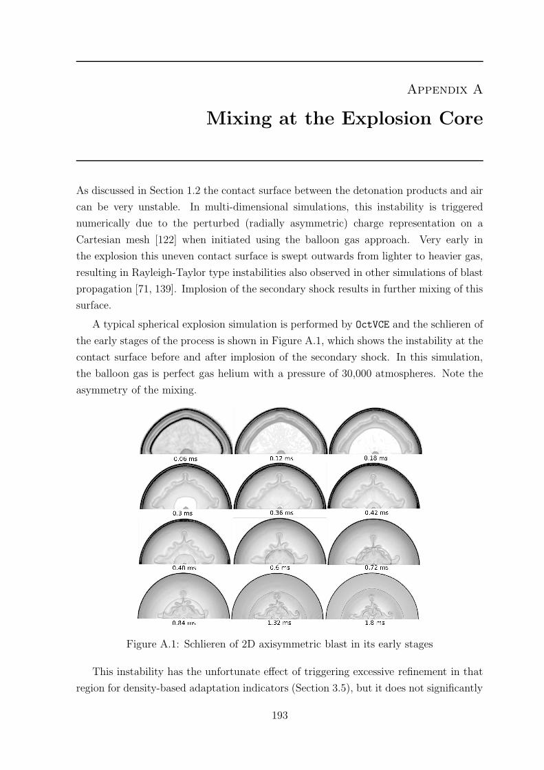
Appendix A
Mixing at the Explosion Core
As discussed in Section 1.2 the contact surface between the detonation products and air
can be very unstable. In multi-dimensional simulations, this instability is triggered
numerically due to the perturbed (radially asymmetric) charge representation on a
Cartesian mesh [122] when initiated using the balloon gas approach. Very early in
the explosion this uneven contact surface is swept outwards from lighter to heavier gas,
resulting in Rayleigh-Taylor type instabilities also observed in other simulations of blast
propagation [71, 139]. Implosion of the secondary shock results in further mixing of this
surface.
A typical spherical explosion simulation is performed by OctVCE and the schlieren of
the early stages of the process is shown in Figure A.1, which shows the instability at the
contact surface before and after implosion of the secondary shock. In this simulation,
the balloon gas is perfect gas helium with a pressure of 30,000 atmospheres. Note the
asymmetry of the mixing.
Figure A.1: Schlieren of 2D axisymmetric blast in its early stages
This instability has the unfortunate effect of triggering excessive refinement in that
region for density-based adaptation indicators (Section 3.5), but it does not significantly
193
A.1. ADAPTATION PARAMETERS FOR BLAST SIMULATION
affect the blast wave and positive phase (Section 1.2). It may be advantageous to use a
pressure-based indicator to avoid this needless refinement.
A.1 Adaptation Parameters for Blast Simulation
As discussed in Section 3.5, OctVCE implements two types of adaptation indicators –
(a) a density-based indicator and (b) velocity-based indicator. Default values for the
refinement threshold are 0.3 and 0.01 for indicators (a) and (b) respectively. Lowering
these thresholds allow better shock-capturing at larger distances from the blast, but at
the cost of excessive cell refinement nearer the explosion. Indicator (a), which can also
refine the positive phase behind the shock, require coarsening and noise filter thresholds
to be set, and a small test of different values for these thresholds is shown in Figure A.2,
which simulates the same blast problem above.
Five adaptive mesh levels are used. The numbers beside the letters R, C and F
stand for refinement, coarsening and noise filter thresholds respectively. The primary
shock is at a scaled distance of about 13.3 m/kg1/3 and it is difficult to refine about the
secondary shock without resulting excessive refinement elsewhere. The resolution of the
positive phase was not found to be so dependent on the refinement threshold, so only
the coarsening and noise filter values were varied.
Note the turbulent core region is always refined about, which can be wasteful. The
degree of refinement shows a dependence on the noise filter threshold and coarsening
threshold. Decreasing the coarsening threshold is more likely to confine refinement to
the positive phase behind the blast, whilst decreasing the noise filter also tended to
result in more refinement in the core region. For this problem, the simulation with a
coarsening and noise filter threshold of 0.03 and 0.005 respectively seems to produce
the best degree of refinement at the shock and positive phase, which persisted until
a scaled distance of around 25 m/kg1/3. Selection of optimal adaptation parameters
requires some trial and error, but this is characteristic of any adaptive method. In the
simulations of this thesis, the coarsening threshold ranges from 0.01 to 0.1 and the noise
filter threshold from 0.001 to 0.1.
194
A.1. ADAPTATION PARAMETERS FOR BLAST SIMULATION
Figure A.2: Experimentation with adaptation parameters for blast simulation
195
Appendix B
One-dimensional Spherical Code
This section briefly describes key features of the simple one-dimensional code written
for validating OctVCE for those test cases with radial symmetry (e.g. chapters 9 and 10).
This code allows an accurate fine-grid spherically symmetric one-dimensional solution
to be obtained with little cost. The spherical integral Euler equations can be expressed
as∂
∂t
∫
V
Ur2dr +
∫
S
r2F · n = Q (B.1)
where U = [ρ, ρu, ρE, ρp]T and the vector of fluxes is
F =
ρu
ρu2 + P
ρEu + Pu
ρpu
r (B.2)
where r is the unit vector in the radial direction, in reality a one-dimensional vector like
the interface outward-normal n. The source term is Q = [0, 2PrL, 0, 0] where L is the
cell length. The cell-centered finite volume discretization is simply
dUc
dtr2cL = −
∑
if
r2ifFif · nif + Q (B.3)
The solution marching procedure is essentially the same that used by OctVCE (Sec-
tion 4.2) reduced to one dimension. Hence a second-order Runge-Kutta time integration
procedure and the AUSMDV flux solver is used (Appendix F.1). In performing these
simulations care must be taken to have the correct charge radius (represented by the
balloon gas) and have an integral number of cells within the charge to obtain exact
correspondence in blast energy.
Rose recommends around 50 computational cells through the explosive charge for
grid-independent solutions [171]. The initial time might also be offset by the detonation
time (time for the detonation wave, starting from the charge centre, to engulf the whole
constant-volume charge). As the detonation speed is usually very high (of the order of
O (103) m/s), this offset is normally very small and noticeable only for trace points close
to the charge.
196
The CFL cutback procedure (Section 4.8.1) is also used to prevent instability, and
thus the solution order ‘switching-time’ scheme described in Section 4.8.1 is unnecessary.
The one dimensional code employs an upwind biased third-order interpolation scheme
with MINMOD-type limiter [110, 148] and also in the MB_CNS code [109]. This scheme
should be suitable for unsteady one-dimensional blast wave problems and is summarized
below.
Suppose reconstruction of a quantity Q is desired for interface value Qi+1/2. On this
reconstruction scheme cell-centered values from four cells are required, Qi−1, Qi, Qi+1
and Qi+2. Let ∆−i = Qi − Qi−1 and ∆+
i = Qi+1 − Qi. To reconstruct Q to the left side
of the interface, the formula is used –
QLi+1/2 = Qi +
1
4
[(1 − κ) MINMOD
(∆−
i , b∆+i
)+ (1 + κ)MINMOD
(b∆−
i , ∆+i
)]
(B.4)
where b is a biasing parameter and κ a blending parameter. To reconstruct Q to the
right side of the interface the formula is
QRi+1/2 = Qi+1−
1
4
[(1 − κ) MINMOD
(∆−
i+1, b∆+i+1
)+ (1 + κ) MINMOD
(b∆+
i+1, ∆−i+1
)]
(B.5)
Default values of b = 2 and κ = 1/3 are used. The MINMOD function is given by
MINMOD (x, y) = sign (x) max (0, min [|x| , y · sign (x)]) (B.6)
Reflecting (solid wall) boundary conditions are used for the ghost cells at the left and
right ends of the domain. Two ghost cells are used, and the outermost ghost cell uses
reflected conditions from the cells adjacent to the border cells.
197
Appendix C
Finite Energy Release in Cylindrical
Charges
An extension to the code was considered in this thesis to incorporate a finite rate of
energy release from ignition points within the charge in a very simplified model of
detonation, much like the approach of Timofeev et al [211, 212]. In this ‘finite-rate-
release’ model, detonation proceeds radially at a preset speed from specified ignition
points until all the explosive is consumed. This can be readily implemented in the
code as it already represents the initial charge as a group of high pressure cells. Thus,
cells representing the charge are essentially treated as solid objects until activation to
appropriate gas conditions when the detonation wave passes their centroids.
With this approach an additional degree of realism in modelling the blast waveform
and overpressures may be obtainable for near-field modelling, although this extension
may prove inadequate as the complex chemistry of the explosive detonation and af-
terburning is not taken into account. It would probably be more suitable for cheaper
two-dimensional simulations as this increased realism may only be noticeable on highly-
resolved meshes.
To observe the differences in solution compared to the ‘instantaneous-release’ det-
onation model where all cells are initially active and filled with high pressure gas, an
axisymmetric simulation of cylindrical warhead detonation is performed. This draws
from the experimental and numerical study of Anderson et al [11], whose axisymmetric
simulations also assumed perfect gas, instantaneous energy release of the explosion, but
incorporated a simple afterburning model. Because of the radially asymmetrical charge
shape, free-field overpressure and energy distribution near the charge is dependent on
charge orientation and even location of initiation [108] and thus makes an interesting
test case for this study.
A diagram of the numerical domain and pressure sensor locations is shown in Fig-
ure C.1. The warhead is positioned at a height of 2015 mm. This domain and minimum
cell size (10 mm) is chosen to be the same as Anderson’s [11] but an adaptive mesh
simulation is used with coarsest allowable cell size of 160 mm. Actual sensor locations
are given in Table C.1.
198
Figure C.1: Cylindrical warhead numerical domain and sensor locations (from [11])
Table C.1: Sensor locations for cylindrical warhead explosion (from [11])
Sensor number X location (mm) Y location (mm)
1 1010 1000
2 1980 2010
3 2520 2000
4 2950 2040
5 3550 2000
6 2010 2610
7 2560 2600
8 2960 2590
The initial conditions for the charge are given in Table C.2 and have also been
taken from Anderson [11]. The simulation applies the JWL equation of state to the
explosion products (Composition B explosive, like in Anderson’s experiments) with JWL
parameters provided by Reference [127]. As the charge is discretized by finite-volume
cells its actual diameter and length are slightly different from the reported nominal
values, but the density and pressure of the cells is adjusted to give the correct energy.
The simulation is performed with an adaptive flux solver (EFM at shocks, AUSMDV
elsewhere) and density-based adaptation indicator (Equation 3.4) of 0.3, 0.1 and 0.013
for the refinement, coarsening and noise thresholds respectively.
Figure C.2 shows a progression of temperature and grids in the early stages of the
explosion when initiated from three points along the charge centreline (which can be
seen in the initial plot, Figure C.2(a)). These points at located at heights of 1939 mm,
2015 mm (charge centre) and 2091 mm. The consumption of the explosive is nearly
complete at about 14.4 ms (Figure C.2(d)).
199
(a) 0 ms (b) 9.48 ms
(c) 11.5 ms (d) 14.4 ms
(e) 17.8 ms (f) 35.5 ms
(g) 64.9 ms
Figure C.2: Temperature and grid for cylindrical warhead detonation
200
Table C.2: Initial conditions for cylindrical warhead (taken from [11])
Diameter 360 mm
Length 720 mm
Blast energy 4.00925 ×10⁷ J
Ambient Pressure 101.325 kPa
Ambient Temperature 298 K
Pressure histories from the various sensor locations are shown in Figure C.3 and
compared with Anderson’s results. A simulation is also performed assuming the instan-
taneous detonation model for comparison. The results show that observable differences
exist between the finite-rate-release and instantaneous detonation solutions, which in
turn differ with Anderson’s pressure histories. This is to be expected as Anderson took
into account afterburning which was not implemented here.
There is also a lag in blast wave arrival time relative to the experimental results.
Modelling accurately the actual detonation process might yield better arrival time re-
sults, but this is not so important. Except for sensor 1, the finite-rate-release model
has an arrival time either earlier than or equal with the instantaneous model. The det-
onation speed through the charge is too rapid relative to the scale of the waveforms to
make much difference in arrival time here. At sensors 6 to 8, arrival times from both
solutions are nearly coincident.
At sensors 1, 3 and 8 the finite-rate-release model seems to give slightly better peak
overpressures relative to experimental results compared to the instantaneous detonation
model. However, the decay rate for the initial pulse is much sharper for the finite-rate-
release model than the instantaneous one. It is also interesting that the current results
seem on the whole to yield better peak overpressures (and comparably good positive
phase) as Anderson’s numerical results, compared to experiment. However, in some
cases the experimental pressure histories are not very good (particularly with sensor
6), presumably because of sensor vibration. Also, in many cases the numerical simula-
tions display secondary shocks which are not clearly distinguishable in the experimental
pressure histories.
The results show that whilst there is a notable difference between finite-rate-release
and instantaneous detonation models, the finite-rate-release approach does not produce
consistently better solutions (when compared to experimental results) in either peak
overpressure or positive phase waveform, at least for this problem. It may still be a
useful option to have in some cases, but here the instantaneous detonation model seems
to yield fairly good results even in the near-field (discounting the arrival time discrep-
201
-500
0
500
1000
1500
2000
0 0.5 1 1.5 2 2.5 3 3.5 4 4.5
Ove
rpre
ssur
e (k
Pa)
Time (ms)
Anderson CFD (2002)Anderson expt (2002)
InstantaneousFinite release
(a) Sensor 1 pressure history
-500
0
500
1000
1500
2000
2500
0 0.5 1 1.5 2 2.5 3 3.5
Ove
rpre
ssur
e (k
Pa)
Time (ms)
Anderson CFD (2002)Anderson expt (2002)
InstantaneousFinite release
(b) Sensor 2 pressure history
-200
0
200
400
600
800
1000
1200
1400
0 1 2 3 4 5 6
Ove
rpre
ssur
e (k
Pa)
Time (ms)
Anderson CFD (2002)Anderson expt (2002)
InstantaneousFinite release
(c) Sensor 3 pressure history
-100
0
100
200
300
400
500
600
700
800
900
0 1 2 3 4 5 6 7
Ove
rpre
ssur
e (k
Pa)
Time (ms)
Anderson CFD (2002)Anderson expt (2002)
InstantaneousFinite release
(d) Sensor 4 pressure history
-50
0
50
100
150
200
250
300
350
400
450
0 1 2 3 4 5 6 7 8
Ove
rpre
ssur
e (k
Pa)
Time (ms)
Anderson CFD (2002)Anderson expt (2002)
InstantaneousFinite release
(e) Sensor 5 pressure history
-200
0
200
400
600
800
1000
1200
1400
0 0.5 1 1.5 2 2.5 3 3.5 4
Ove
rpre
ssur
e (k
Pa)
Time (ms)
Anderson CFD (2002)Anderson expt (2002)
InstantaneousFinite release
(f) Sensor 6 pressure history
-100
0
100
200
300
400
500
600
700
800
0 1 2 3 4 5 6 7 8
Ove
rpre
ssur
e (k
Pa)
Time (ms)
Anderson CFD (2002)Anderson expt (2002)
InstantaneousFinite release
(g) Sensor 7 pressure history
-100
0
100
200
300
400
500
600
0 1 2 3 4 5 6 7 8
Ove
rpre
ssur
e (k
Pa)
Time (ms)
Anderson CFD (2002)Anderson expt (2002)
InstantaneousFinite release
(h) Sensor 8 pressure history
Figure C.3: Pressure histories for cylindrical warhead detonation
202

ancy). Better correspondence with experimental results is probably only achievable in
the near-field through detailed modelling of the chemistry of the detonation process.
This extension to the code requires further development and exploration.
203
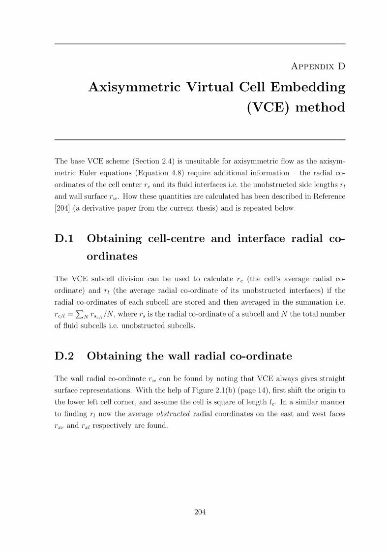
Appendix D
Axisymmetric Virtual Cell Embedding
(VCE) method
The base VCE scheme (Section 2.4) is unsuitable for axisymmetric flow as the axisym-
metric Euler equations (Equation 4.8) require additional information – the radial co-
ordinates of the cell center rc and its fluid interfaces i.e. the unobstructed side lengths rl
and wall surface rw. How these quantities are calculated has been described in Reference
[204] (a derivative paper from the current thesis) and is repeated below.
D.1 Obtaining cell-centre and interface radial co-
ordinates
The VCE subcell division can be used to calculate rc (the cell’s average radial co-
ordinate) and rl (the average radial co-ordinate of its unobstructed interfaces) if the
radial co-ordinates of each subcell are stored and then averaged in the summation i.e.
rc/l =∑
N rsc/l/N , where rs is the radial co-ordinate of a subcell and N the total number
of fluid subcells i.e. unobstructed subcells.
D.2 Obtaining the wall radial co-ordinate
The wall radial co-ordinate rw can be found by noting that VCE always gives straight
surface representations. With the help of Figure 2.1(b) (page 14), first shift the origin to
the lower left cell corner, and assume the cell is square of length lc. In a similar manner
to finding rl now the average obstructed radial coordinates on the east and west faces
rxr and rxl respectively are found.
204
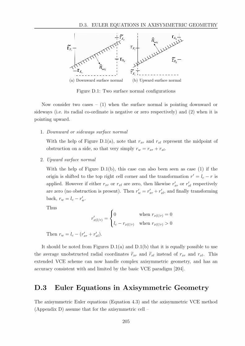
D.3. EULER EQUATIONS IN AXISYMMETRIC GEOMETRY
(a) Downward surface normal (b) Upward surface normal
Figure D.1: Two surface normal configurations
Now consider two cases – (1) when the surface normal is pointing downward or
sideways (i.e. its radial co-ordinate is negative or zero respectively) and (2) when it is
pointing upward.
1. Downward or sideways surface normal
With the help of Figure D.1(a), note that rxr and rxl represent the midpoint of
obstruction on a side, so that very simply rw = rxr + rxl.
2. Upward surface normal
With the help of Figure D.1(b), this case can also been seen as case (1) if the
origin is shifted to the top right cell corner and the transformation r′ = lc − r is
applied. However if either rxr or rxl are zero, then likewise r′xr or r′xl respectively
are zero (no obstruction is present). Then r′w = r′xr + r′xl, and finally transforming
back, rw = lc − r′w.
Thus
r′x(l/r) =
0 when rx(l/r) = 0
lc − rx(l/r) when rx(l/r) > 0
Then rw = lc − (r′xr + r′xl).
It should be noted from Figures D.1(a) and D.1(b) that it is equally possible to use
the average unobstructed radial coordinates rxr and rxl instead of rxr and rxl. This
extended VCE scheme can now handle complex axisymmetric geometry, and has an
accuracy consistent with and limited by the basic VCE paradigm [204].
D.3 Euler Equations in Axisymmetric Geometry
The axisymmetric Euler equations (Equation 4.3) and the axisymmetric VCE method
(Appendix D) assume that for the axisymmetric cell –
205
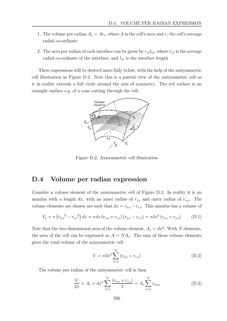
D.4. VOLUME PER RADIAN EXPRESSION
1. The volume per radian Ac = Arc, where A is the cell’s area and rc the cell’s average
radial co-ordinate
2. The area per radian of each interface can be given by rif lif , where rif is the average
radial co-ordinate of the interface, and lif is the interface length
These expressions will be derived more fully below, with the help of the axisymmetric
cell illustration in Figure D.2. Note this is a partial view of the axisymmetric cell as
it in reality extends a full circle around the axis of symmetry. The red surface is an
example surface e.g. of a cone cutting through the cell.
Figure D.2: Axisymmetric cell illustration
D.4 Volume per radian expression
Consider a volume element of the axisymmetric cell of Figure D.2. In reality it is an
annulus with a length dx, with an inner radius of ri,s and outer radius of ro,s. The
volume elements are chosen are such that dx = ro,s − ri,s. This annulus has a volume of
Ve = π(ro,s
2 − ri,s2)dx = πdx (ro,s + ri,s) (ro,s − ri,s) = πdx2 (ro,s + ri,s) (D.1)
Note that the two-dimensional area of the volume element, Ae = dx2. With N elements,
the area of the cell can be expressed as A = NAe. The sum of these volume elements
gives the total volume of the axisymmetric cell –
V = πdx2
N∑
i=1
(ro,s + ri,s) (D.2)
The volume per radian of the axisymmetric cell is then
V
2π= Ac = dx2
N∑
i=1
(ro,s + ri,s)
2= Ae
N∑
i=1
ravg (D.3)
206
D.5. AREA PER RADIAN OF INTERFACES
where ravg is the average radial co-ordinate of the volume element. Assuming the volume
per radian of the cell is its area A = NAe multipled by some radial value r, then
Ar = NAe = Ae
N∑
i=1
ravg (D.4)
which means that r =∑
ravg/N = rc i.e. the average radial co-ordinate of the cell from
the volume elements.
D.5 Area per radian of interfaces
D.5.1 Interfaces normal to radial axis
For any unobstructed interfaces normal to (i.e. pierced by) the radial axis, the interface
area is simply that of the cylindrical area of the annulus (the cell length). This is
A = 2πrl, where r is the annulus radius, and l is the (axial) length of the cell. Thus the
area per radian is A/ (2π) = rl. Thus for example the top face of the cell is rol.
D.5.2 Interfaces normal to axial axis
The interfaces normal to the axial axis are the cross-sectional area of the cell annulus.
Thus the area is
A = π(r2
2 − r12)
= π (r2 + r1) (r2 − r1) = πlif (r2 + r1) (D.5)
where r2 and r1 is the outer and inner radius of the annulus. The interface length
lif = r2 − r1. In the case of an unobstructed interface like the axisymmetric cell of
Figure D.2 the front and back interfaces have area of π (ro2 − ri
2). Thus the area per
radian is
A/ (2π) = lif (r2 + r1) /2 = lifravg (D.6)
where ravg is the average radial co-ordinate of the interface.
D.5.3 Wall interface
An example wall interface of a conical surface can be seen by the red surface in Fig-
ure D.2. An area element of this interface is dA = 2πrdl where r and dl are the radius
and length of area element respectively. In VCE the variation of the interface radius
207
D.5. AREA PER RADIAN OF INTERFACES
can be described by the linear relation r = r1 + mx (recall VCE only represents planar
surfaces). Thus if dl =√
dr2 + dx2 = dx√
m2 + 1. Thus
dA = 2π (r1 + mx)√
m2 + 1dx (D.7)
The area elements are integrated from x1 to x2 (the axial length of the cell is x2 − x1)
to give the total area –
∫ x2
x1
dA = 2π√
m2 + 1
∫ x2
x1
(r1 + mx) dx (D.8)
= 2π√
m2 + 1
[r1x +
mx2
2
]x2
x1
(D.9)
= 2π√
m2 + 1 (x2 − x1)
[r1 + m
x1 + x2
2
](D.10)
= 2π√
m2 + 1 (x2 − x1) (r1 + mxavg) (D.11)
= 2π√
m2 + 1 (x2 − x1) ravg (D.12)
where ravg is radial midpoint of the interface line length. Note that the slant length of
the interface l = (x2 − x1)√
m2 + 1. Thus A = 2πlravg. The area per radian is thus
A/ (2π) = lravg. Thus for all interfaces the area per radian is rif lif .
208
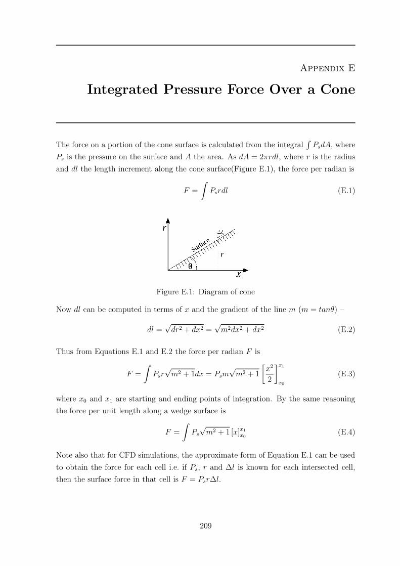
Appendix E
Integrated Pressure Force Over a Cone
The force on a portion of the cone surface is calculated from the integral∫
PsdA, where
Ps is the pressure on the surface and A the area. As dA = 2πrdl, where r is the radius
and dl the length increment along the cone surface(Figure E.1), the force per radian is
F =
∫Psrdl (E.1)
Figure E.1: Diagram of cone
Now dl can be computed in terms of x and the gradient of the line m (m = tanθ) –
dl =√
dr2 + dx2 =√
m2dx2 + dx2 (E.2)
Thus from Equations E.1 and E.2 the force per radian F is
F =
∫Psr
√m2 + 1dx = Psm
√m2 + 1
[x2
2
]x1
x0
(E.3)
where x0 and x1 are starting and ending points of integration. By the same reasoning
the force per unit length along a wedge surface is
F =
∫Ps
√m2 + 1 [x]x1
x0(E.4)
Note also that for CFD simulations, the approximate form of Equation E.1 can be used
to obtain the force for each cell i.e. if Ps, r and ∆l is known for each intersected cell,
then the surface force in that cell is F = Psr∆l.
209
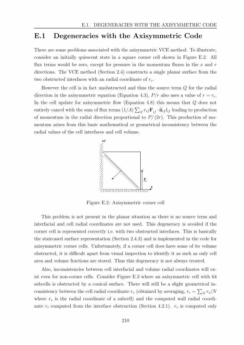
E.1. DEGENERACIES WITH THE AXISYMMETRIC CODE
E.1 Degeneracies with the Axisymmetric Code
There are some problems associated with the axisymmetric VCE method. To illustrate,
consider an initially quiescent state in a square corner cell shown in Figure E.2. All
flux terms would be zero, except for pressure in the momentum fluxes in the x and r
directions. The VCE method (Section 2.4) constructs a single planar surface from the
two obstructed interfaces with an radial coordinate of rc.
However the cell is in fact unobstructed and thus the source term Q for the radial
direction in the axisymmetric equation (Equation 4.3), P/r also uses a value of r = rc.
In the cell update for axisymmetric flow (Equation 4.8) this means that Q does not
entirely cancel with the sum of flux terms (1/A)∑
if rifFif · nif lif leading to production
of momentum in the radial direction proportional to P/ (2r). This production of mo-
mentum arises from this basic mathematical or geometrical inconsistency between the
radial values of the cell interfaces and cell volume.
Figure E.2: Axisymmetric corner cell
This problem is not present in the planar situation as there is no source term and
interfacial and cell radial coordinates are not used. This degeneracy is avoided if the
corner cell is represented correctly i.e. with two obstructed interfaces. This is basically
the staircased surface representation (Section 2.4.3) and is implemented in the code for
axisymmetric corner cells. Unfortunately, if a corner cell does have some of its volume
obstructed, it is difficult apart from visual inspection to identify it as such as only cell
area and volume fractions are stored. Thus this degeneracy is not always treated.
Also, inconsistencies between cell interfacial and volume radial coordinates will ex-
ist even for non-corner cells. Consider Figure E.3 where an axisymmetric cell with 64
subcells is obstructed by a conical surface. There will still be a slight geometrical in-
consistency between the cell radial coordinate rc (obtained by averaging, rc =∑
N rs/N
where rs is the radial coordinate of a subcell) and the computed wall radial coordi-
nate ri computed from the interface obstruction (Section 4.2.1). rc is computed only
210
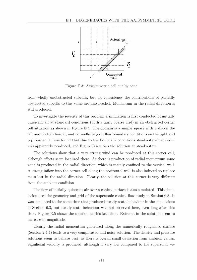
E.1. DEGENERACIES WITH THE AXISYMMETRIC CODE
Figure E.3: Axisymmetric cell cut by cone
from wholly unobstructed subcells, but for consistency the contributions of partially
obstructed subcells to this value are also needed. Momentum in the radial direction is
still produced.
To investigate the severity of this problem a simulation is first conducted of initially
quiescent air at standard conditions (with a fairly coarse grid) in an obstructed corner
cell situation as shown in Figure E.4. The domain is a simple square with walls on the
left and bottom border, and non-reflecting outflow boundary conditions on the right and
top border. It was found that due to the boundary conditions steady-state behaviour
was apparently produced, and Figure E.4 shows the solution at steady-state.
The solutions show that a very strong wind can be produced at this corner cell,
although effects seem localized there. As there is production of radial momentum some
wind is produced in the radial direction, which is mainly confined to the vertical wall.
A strong inflow into the corner cell along the horizontal wall is also induced to replace
mass lost in the radial direction. Clearly, the solution at this corner is very different
from the ambient condition.
The flow of initially quiescent air over a conical surface is also simulated. This simu-
lation uses the geometry and grid of the supersonic conical flow study in Section 6.3. It
was simulated to the same time that produced steady-state behaviour in the simulations
of Section 6.3, but steady-state behaviour was not observed here, even long after this
time. Figure E.5 shows the solution at this late time. Extrema in the solution seem to
increase in magnitude.
Clearly the radial momentum generated along the numerically roughened surface
(Section 2.4.4) leads to a very complicated and noisy solution. The density and pressure
solutions seem to behave best, as there is overall small deviation from ambient values.
Significant velocity is produced, although it very low compared to the supersonic ve-
211
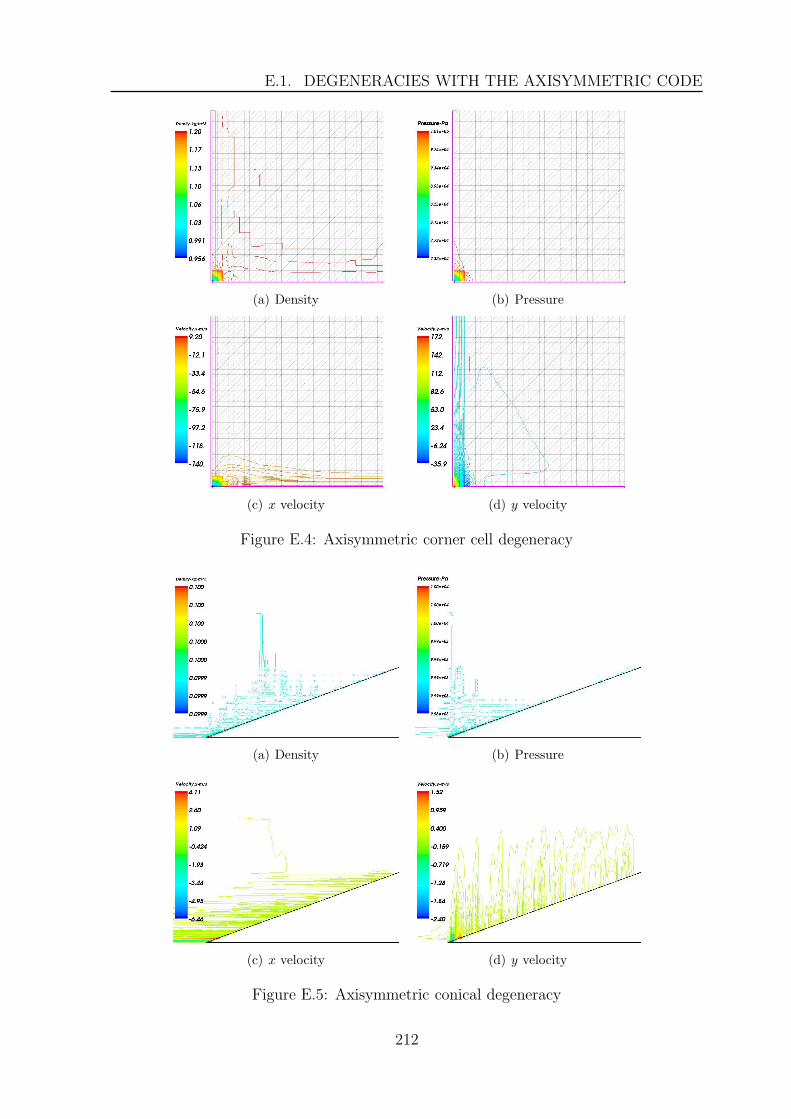
E.1. DEGENERACIES WITH THE AXISYMMETRIC CODE
(a) Density (b) Pressure
(c) x velocity (d) y velocity
Figure E.4: Axisymmetric corner cell degeneracy
(a) Density (b) Pressure
(c) x velocity (d) y velocity
Figure E.5: Axisymmetric conical degeneracy
212
E.1. DEGENERACIES WITH THE AXISYMMETRIC CODE
locities studied in Section 6.3. A vortex-like feature also appears present at the cone
tip, and this is where the extrema in velocity occur; it may have initially risen with the
inducing of horizontal flow into an obsturcted cell at the cone tip to replace mass loss
in the radial direction.
The effects of this axisymmetric degeneracy on solutions with initial quiescent state
(in addition to numerical surface roughening) can be quite significant. Divergent or
convergent solutions seem to both be possible depending on the boundary condition
and geometry. It is difficult to predict the effect this degeneracy has on flows with more
interesting initial conditions. However, these effects may not always prove detrimental
to solutions in simulations of practical interest. For example, it is shown in Section 6.3
that convergent and accurate solutions of supersonic conical flow can nonetheless be
produced. In the axisymmetric blast wall simulations of Section 11, good overpressure
traces can be computed despite the presence of problematic corner cells. Perhaps relative
to much stronger or sudden features like a blast or shock wave, the effect on the flow
produced by such degeneracies (which do not increase so fast) is minimal.
213
Appendix F
Flux Calculation Schemes
This section summarizes the algorithms for the AUSMDV and EFM schemes to calculate
the interface flux Fif · nif in Equation 4.4. More detailed descriptions of the schemes
can be found in References [110, 148, 150, 221].
F.1 AUSMDV Scheme
This scheme combines flux differencing and vector splitting. At an interface the left state
has flow parameters density ρL, explosion products density ρp,L, velocity uL, pressure
PL and total enthalpy HL, and the right state ρR, uR, PR and HR. To begin, the normal
velocity components at the left and right of an interface are obtained (in an interface
frame of reference) –
uL = uL · nif (F.1)
uR = uR · nif (F.2)
Tangential velocity vectors relative to the interface are
vL = uL − uLnif (F.3)
vR = uR − uRnif (F.4)
Functions αL and αR are designed to avoid dissipation at contact discontinuities –
αL =2PL/ρL
PL/ρL + PR/ρR(F.5)
αL =2PR/ρR
PL/ρL + PR/ρR
(F.6)
Define the interface sound speed at the interface am as
am = max (aL, aR) (F.7)
and individual splitting terms
u+L =
αL
[(uL+am)2
4am− uL+|uL|
2
]+ uL+|uL|
2, if |uL|
am≤ 1
uL+|uL|2
otherwise(F.8)
u−R =
αR
[−(uR−am)2
4am− uR−|uR|
2
]+ uR−|uR|
2, if |uR|
am≤ 1
uR−|uR|2
otherwise(F.9)
214
F.1. AUSMDV SCHEME
Second-order pressure splittings are given by
P±L/R =
14PL/R
(uL/R
am± 1)2 (
2 ∓ uL/R
am
), if
uL/R
am≤ 1
PL/RuL/R±|uL/R|
2uL/Rotherwise
(F.10)
and the interface pressure term is
P1/2 = P+L + P−
R (F.11)
The switching factor s is based on the pressure difference across the interface –
s =1
2min
[1,
K |PR − PL|min (PL, PR)
](F.12)
with sensitivity constant K set to 10. The mass flux is given by the vector splitting
G = u+LρL + u−
RρR (F.13)
For explosion products the mass flux of the explosion products would similar be Gp =
u+Lρp,L + u−
Rρp,R. The AUSMV momentum flux (vector splitting) is
LV = ρLuLu+L + ρRuRu−
R (F.14)
and the AUSMD momentum flux (flux differencing) is
LD =1
2[G (uL + uR) − |G| (uR − uL)] (F.15)
and the normal momentum flux is a mixture of the AUSMV and AUSMD momentum
fluxes
Ln =
(1
2+ s
)LV +
(1
2− s
)LD + P1/2 (F.16)
The tangential component of the momentum flux is
Lt =1
2[G (vL + vR) − |G| (vR − vL)] (F.17)
and thus the interface momentum flux is
L = Lnnif + Lt (F.18)
The total enthalpy flux is
H =1
2[G (HL + HR) − |G| (HR − HL)] (F.19)
Thus the flux Fif · nif is
Fif · nif =
G
L
H
Gp
(F.20)
215
F.2. EFM SCHEME
The glitch at the sonic expansion point is fixed by modifying the flux for two cases (1)
when uL − cL < 0 and uR − cR > 0 and (2) when uL + cL < 0 and uR + cR > 0. For case
(1)
Fif · nif =
G − C∆ (u − a) ∆ρ
L − C∆ (u − a) ∆ (ρu)
H − C∆ (u − a) ∆ (H)
Gp − C∆ (u − a) ∆ (ρp)
(F.21)
where ∆ () = ()R − ()L and the constant parameter C has a value of 0.125. For case (2)
Fif · nif =
G − C∆ (u + a)∆ρ
L − C∆ (u + a) ∆ (ρu)
H − C∆ (u + a) ∆ (H)
Gp − C∆ (u + a) ∆ (ρp)
(F.22)
F.2 EFM Scheme
As with the AUSMDV scheme, at the interface left state the flow parameters are ρL,
explosion products density ρp,L with mass fraction fL, velocity uL, pressure PL, total
enthalpy HL, specific heat Cv,L and temperature TL. The right state similarly has
parameters ρR, ρp,R, fR, uR, PR, HR, Cv,R and TR. To begin, the gas ‘constants’ are
derived for each state –
RL =PL
ρLTL(F.23)
RR =PR
ρRTR(F.24)
The normal velocity components at the left and right of an interface uL and uR are
obtained from Equation F.1 and F.2. An averaging function is defined
α =
√ρL√
ρL +√
ρR(F.25)
The averaged gas constants for the interface are
Cv = αCv,L + (1 − α)Cv,R (F.26)
R = αRL + (1 − α)RR (F.27)
Cp = Cv + R (F.28)
γ = Cp/Cv (F.29)
216
F.2. EFM SCHEME
Now define the values
C =1
2
γ + 1
γ − 1(F.30)
CL =√
2RLTL (F.31)
CR =√
2RRTR (F.32)
WL =1
2(1 + erf (uL/CL)) (F.33)
DL =1
2√
πe−u2
L (F.34)
WR =1
2(1 − erf (uR/CR)) (F.35)
DR = − 1
2√
πe−u2
R (F.36)
The mass flux from the left state is
mL = WLρLuL + DLCLρL (F.37)
and the mass flux from the right state
mR = WRρRuR + DRCRρR (F.38)
The total interface mass flux is thus
G = mL + mR (F.39)
For the explosion products the mass flux Gp depends on which direction the wind is
blowing, and is fLm if m > 0, else fRm otherwise. The momentum flux is
L = mLuL + mRuR + nif (WLPL + WRPR) (F.40)
and the enthalpy flux is
H = WLρLuLHL+WRρRuRHR+DLCLρL
(|uL|2
2+ C
PL
ρL
)+DRCRρR
(|uR|2
2+ C
PR
ρR
)
(F.41)
The flux Fif · nif is the same expression as given by Equation F.20.
217
Appendix G
Mixture Equation of State
A combined equation of state is required for cells close to the fireball with a mixture
of explosion products (when modelled by the JWL equation of state, Section 4.5.2)
and ambient gas (modelled by the ideal gas equation of state). However given the
insensitivity of the blast wave in mid- to far-field on initial condition (Section 4.6) it is
not always necessary to obtain a fully realistic thermodynamic model of this mixture.
A common, simple approach is to obtain an average ratio of specific heats from
the two gases, γavg, to be used in a ‘γ-law’ ideal equation of state P = ρe (γavg − 1)
[24, 86, 177]. A harmonic average is used to calculated γavg –
γavg = 1 +1
f1
γ1−1+ f2
γ2−1
(G.1)
where f1 and f2 are the mass fractions of the two gases, f2 = 1 − f1 and γ1 and γ2
their respective ratio of specific heats. A different harmonic average may be used for
the sound speed formula [24] a =√
ΓaP/ρ where
Γa =1
f1/γ1 + f2/γ2
(G.2)
The harmonic average for the gas γ is used in multifluid volume-of-fluid algorithms [86]
which are designed to track interfaces and treat different species as thermodynamically
distinct entities. Pressure and internal energy within a cell is assumed to be at equi-
librium amongst the species. For the JWL equation of state the gas γ of the explosion
products may be approximated as an effective value [177] based on comparison with the
ideal gas law
γp = γp (ρp, e) =P (ρp, e)
ρpe+ 1 (G.3)
where P (ρp, e) is the JWL equation of state (Equation 4.18) for pressure and e the
internal energy. Additive partial pressure is not assumed; the JWL equation of state
in Equation G.3 is used just to obtain an appropriate γ value. Brode [40] notes that a
constant γ assumption is also reasonable because of a fairly low range of γ behaviour
[60]. Another simple analytical expression for the adiabatic JWL γ is also derived by
Baker [17].
218
G.1. SOUND SPEED
Another, perhaps more thermodynamically consistent approach is to assume ther-
mal equilibrium and Dalton’s law of additive partial pressures of each species. This is
approximate for real gases due to intermolecular forces, but can be used with reasonable
accuracy when combined with a real gas equation of state [46]. This approach is simple
due to the linear dependence of pressure on temperature for both the JWL and ideal
gases. In a mixture the pressure consists of the sum of the partial pressures for the
ambient gas Pa and explosion products Pp –
P = Pa (ρa, T ) + Pp (ρp, T ) (G.4)
The combined internal energy is the mass-fraction weighted average of each species’
internal energies
e = faea (ρa, T ) + fpep (ρp, T ) (G.5)
Given the equation of state expressions in Section 4.5.1 and Equations 4.19 and 4.20
the mixture pressure is
P = Ae−R1ev + Be−R2ev +
(ωCv,p
v0v+ ρaRa
)T (G.6)
and the mixture internal energy is
e = fp
(Av0
R1e−R1ev +
Bv0
R2e−R2ev
)+ Cv,mixT (G.7)
where the relative volume of the explosion products v = ρ0,p/ρp, fa and fp are the
mass fractions of the ambient gas and explosion products respectively, and the mixture
specific heat Cv,mix = faCv,a +fpCv,p. A derivation of sound speed based on this mixture
equation of state is given in Appendix G.1.
To minimize JWL equation of state evaluations, the strategy of Lohner et al [131,
155] is used to treat as ambient gas those mixtures with only a small amount of explosive
products. If ρp is small (or vp large) ω/ (Riv) ≈ 0 which appear in the JWL equation
(Equation 4.18). Then the term with the lowest value of R is chosen (given this vanishes
last) and ambient gas is assumed when Ce−Rlev < δ where δ is a small threshold value of
order O (10−3) and C the JWL constant corresponding to the exponential term in the
JWL equation with the lowest value of R, Rl. When this occurs, pressure has linear
dependence on density, as in an ideal gas.
G.1 Sound Speed
In this section, the sound speed a of a mixture of detonation products and ambient
gas will be derived given the equation of state for JWL and ideal gases in Appendix G
219
G.1. SOUND SPEED
assuming additive partial pressures. This expression would be particularly simple if an
averaged gas γavg were used (a = γavgP/ρ), and for mixtures of ideal, calorically perfect
gases this is obtained from the mass-fraction weighted average of the specific heats. For
the more complicated case, the derviation uses thermodynamic principles. The general
expression for a in either real or ideal gases [55] is
a2 =∂P
∂ρ
∣∣∣s,fi
(G.8)
where subscripts s and fi means entropy and mass fractions are held constant, thus
∂ρi/∂ρ = fi. It is common to eliminate entropy in the expression by using the energy
form of the equation of state, e = e (ρ, P ), taking its differential, de = ∂e∂ρ
|P dρ+ ∂e∂P
|ρ dP
and for an isentropic process (as in an infinitely weak sound wave) de = −Pdv, thus
after further derivation
a2 =v2(P − ρ2 ∂e
∂ρ|P)
ρ2 ∂e∂P
|ρ(G.9)
Thus it is necessary to derive the quantities ∂e∂ρ
|P and ∂e∂P
|ρ for the mixture.
Now the mixture internal energy is the mass-fraction weighted average of each
species’ internal energy, e =∑
i fiei, thus
∂e
∂ρ
∣∣∣P
=∑
i
fi∂ei
∂ρ
∣∣∣P
(G.10)
Now assuming an energy form of the equation of state with temperature as a variable
for each species, ei = ei (ρi, T ), the chain rule for partial differentiation gives
∂ei
∂ρ
∣∣∣P
=∂ei
∂ρi
∣∣∣T
∂ρi
∂ρ
∣∣∣P
+∂ei
∂T
∣∣∣ρi
∂T
∂ρ
∣∣∣P
(G.11)
But the specific heat of each species Cv,i = ∂ei/∂T |ρiby definition and ∂ei/∂ρi |T can
be derived from each species’ equation of state. It remains for the derivative ∂T/∂ρ |Pto be found.
Using a pressure form of the equation of state with temperature dependency and ad-
ditive pressures from each species, P =∑
i Pi =∑
i Pi (ρi, T ) where temperature equilib-
rium is assumed. Fortunately for many real gas equations of state like the van der Waals,
virial and JWL equation of state the temperature dependency is often linear and hence
inversion of the pressure summation is usually possible, with T = T (P, ρ1, ρ2, ..., ρn).
Thus∂T
∂ρ
∣∣∣P
=∑
i
fi∂T
∂ρi
∣∣∣P
(G.12)
220
G.1. SOUND SPEED
Hence the final expression for ∂e/∂ρ |P is
∂e
∂ρ
∣∣∣P
=∑
i
fi2 ∂ei
∂ρi
∣∣∣T
+ Cv
∑
i
fi∂T
∂ρi
∣∣∣P
(G.13)
where Cv is for the mixture, Cv =∑
i fiCv,i. Given the energy and pressure forms of
the mixture and JWL equation of state in Section 4.5.2, the derivatives ∂ep/∂ρp |T and
∂T/∂ρp |P can be analytically derived and are
∂ep
∂ρp
∣∣∣T
=A
ρp2e−R1ev +
B
ρp2e−R2ev (G.14)
∂T
∂ρp
∣∣∣P
= − (ρaRa + ωρpCv,p)−1
(AR1ρ0
ρp2
e−R1ev +BR2ρ0
ρp2
e−R2ev + ωTCv,p
)(G.15)
For the ambient, calorically perfect and ideal gas, ea = ea (T ), ∂ea/∂ρa |T = 0, and
easily ∂T∂ρa
|P = −TRa/ (ρaRa + ωρpCv,p).
As before the mixture internal energy e =∑
i fiei, thus
∂e
∂P
∣∣∣ρ
=∑
i
fi∂ei
∂P
∣∣∣ρ
(G.16)
In this case as ρ is held constant then given the assumption in Equation G.8 that fi is
constant, all ρi are also constant. Thus ∂ρi/∂ρ |ρ = 0 and with ei = ei (ρi, T ) the chain
rule for partial differentiation gives
∂ei
∂P
∣∣∣ρ
=∂ei
∂T
∣∣∣ρi
∂T
∂P
∣∣∣ρ
(G.17)
Note again that ∂ei/∂T |ρi= Cv,i, and once more assuming the mixture temperature
T = T (P, ρi) then
∂e
∂P
∣∣∣ρ
= Cv∂T
∂P
∣∣∣ρ
(G.18)
The derivative ∂T/∂P |ρ is readily obtained from the mixture equation of state (Ap-
pendix G) since all ρi are held constant, and for a mixture of JWL and ideal gases is∂T∂P
|ρ = (ωρpCv,p + ρaRa)−1.
221
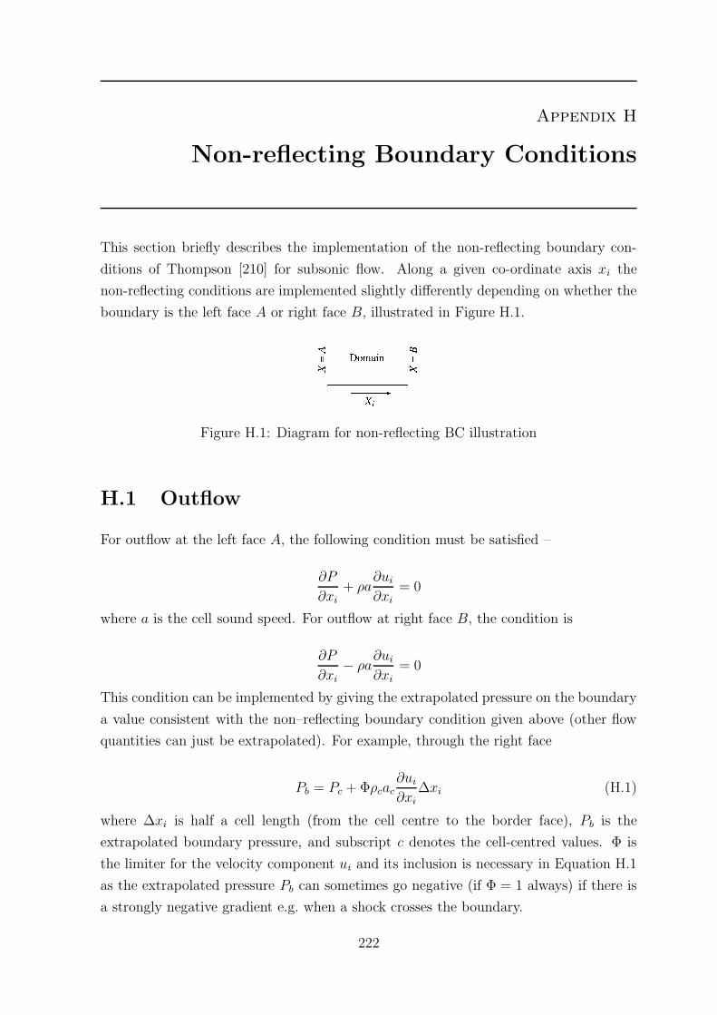
Appendix H
Non-reflecting Boundary Conditions
This section briefly describes the implementation of the non-reflecting boundary con-
ditions of Thompson [210] for subsonic flow. Along a given co-ordinate axis xi the
non-reflecting conditions are implemented slightly differently depending on whether the
boundary is the left face A or right face B, illustrated in Figure H.1.
Figure H.1: Diagram for non-reflecting BC illustration
H.1 Outflow
For outflow at the left face A, the following condition must be satisfied –
∂P
∂xi+ ρa
∂ui
∂xi= 0
where a is the cell sound speed. For outflow at right face B, the condition is
∂P
∂xi− ρa
∂ui
∂xi= 0
This condition can be implemented by giving the extrapolated pressure on the boundary
a value consistent with the non–reflecting boundary condition given above (other flow
quantities can just be extrapolated). For example, through the right face
Pb = Pc + Φρcac∂ui
∂xi∆xi (H.1)
where ∆xi is half a cell length (from the cell centre to the border face), Pb is the
extrapolated boundary pressure, and subscript c denotes the cell-centred values. Φ is
the limiter for the velocity component ui and its inclusion is necessary in Equation H.1
as the extrapolated pressure Pb can sometimes go negative (if Φ = 1 always) if there is
a strongly negative gradient e.g. when a shock crosses the boundary.
222
H.2. INFLOW
H.2 Inflow
Subsonic inflow is a rarely-used boundary condition for the type of simulations con-
sidered in this thesis as outflow boundary conditions are typically enforced at domain
boundaries for exiting blast waves. For inflow at the left face A, these conditions must
be satisfied –
a2 ∂ρ
∂xi
− ∂P
∂xi
= 0
∂u2
∂xi
= 0
∂u3
∂xi
= 0
∂P
∂xi+ ρa
∂ui
∂xi= 0
For inflow at the right B, the conditions become
a2 ∂ρ
∂xi
− ∂P
∂xi
= 0
∂u2
∂xi
= 0
∂u3
∂xi= 0
∂P
∂xi− ρa
∂ui
∂xi= 0
These four equations mean that four extrapolated flow variables must be set to satisfy
the non-reflecting boundary condition.
223
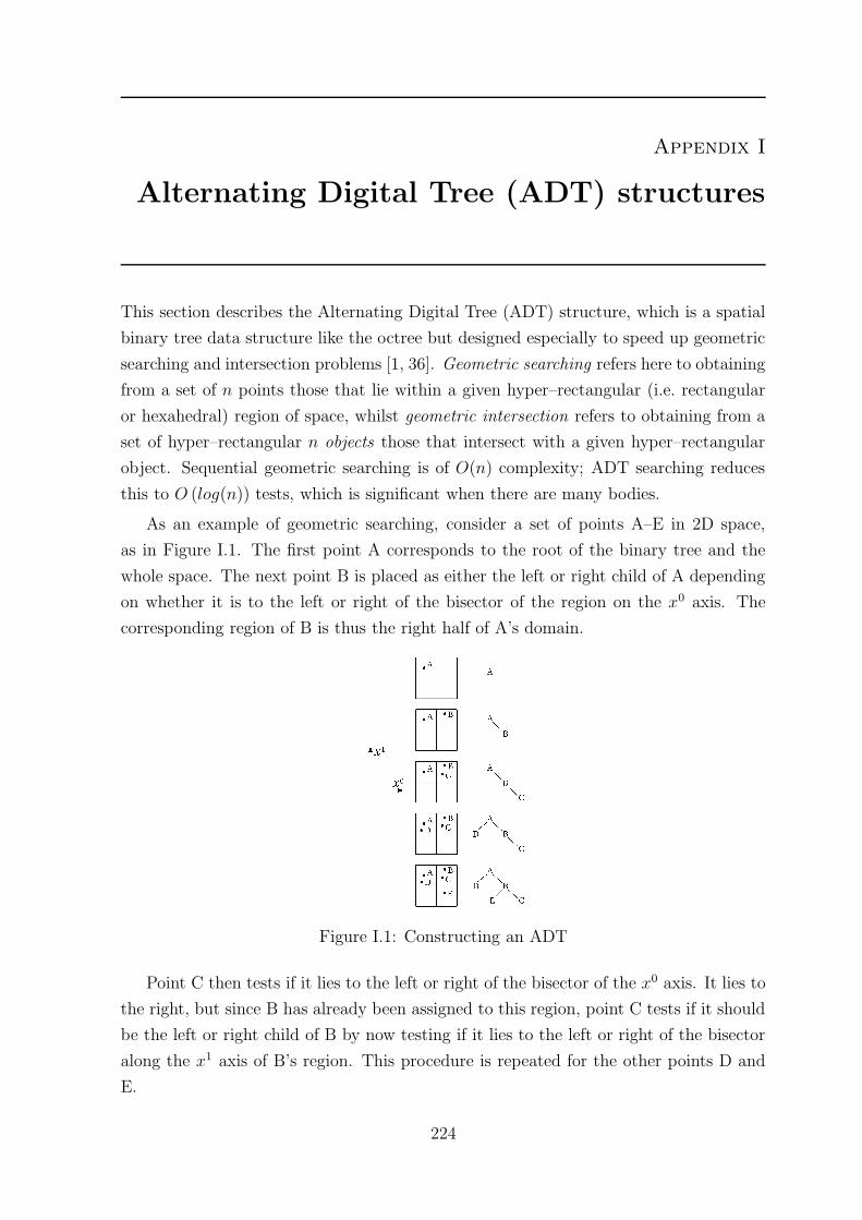
Appendix I
Alternating Digital Tree (ADT) structures
This section describes the Alternating Digital Tree (ADT) structure, which is a spatial
binary tree data structure like the octree but designed especially to speed up geometric
searching and intersection problems [1, 36]. Geometric searching refers here to obtaining
from a set of n points those that lie within a given hyper–rectangular (i.e. rectangular
or hexahedral) region of space, whilst geometric intersection refers to obtaining from a
set of hyper–rectangular n objects those that intersect with a given hyper–rectangular
object. Sequential geometric searching is of O(n) complexity; ADT searching reduces
this to O (log(n)) tests, which is significant when there are many bodies.
As an example of geometric searching, consider a set of points A–E in 2D space,
as in Figure I.1. The first point A corresponds to the root of the binary tree and the
whole space. The next point B is placed as either the left or right child of A depending
on whether it is to the left or right of the bisector of the region on the x0 axis. The
corresponding region of B is thus the right half of A’s domain.
Figure I.1: Constructing an ADT
Point C then tests if it lies to the left or right of the bisector of the x0 axis. It lies to
the right, but since B has already been assigned to this region, point C tests if it should
be the left or right child of B by now testing if it lies to the left or right of the bisector
along the x1 axis of B’s region. This procedure is repeated for the other points D and
E.
224
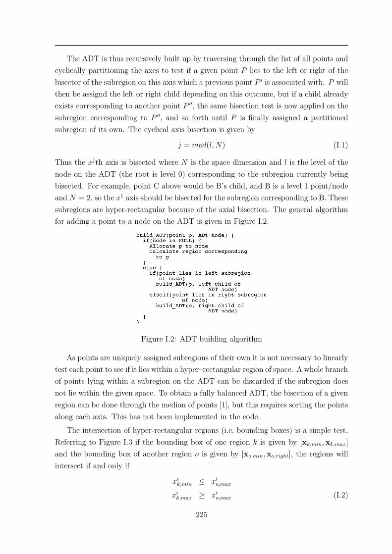
The ADT is thus recursively built up by traversing through the list of all points and
cyclically partitioning the axes to test if a given point P lies to the left or right of the
bisector of the subregion on this axis which a previous point P ′ is associated with. P will
then be assignd the left or right child depending on this outcome, but if a child already
exists corresponding to another point P ′′, the same bisection test is now applied on the
subregion corresponding to P ′′, and so forth until P is finally assigned a partitioned
subregion of its own. The cyclical axis bisection is given by
j = mod(l, N) (I.1)
Thus the xjth axis is bisected where N is the space dimension and l is the level of the
node on the ADT (the root is level 0) corresponding to the subregion currently being
bisected. For example, point C above would be B’s child, and B is a level 1 point/node
and N = 2, so the x1 axis should be bisected for the subregion corresponding to B. These
subregions are hyper-rectangular because of the axial bisection. The general algorithm
for adding a point to a node on the ADT is given in Figure I.2.
Figure I.2: ADT building algorithm
As points are uniquely assigned subregions of their own it is not necessary to linearly
test each point to see if it lies within a hyper–rectangular region of space. A whole branch
of points lying within a subregion on the ADT can be discarded if the subregion does
not lie within the given space. To obtain a fully balanced ADT, the bisection of a given
region can be done through the median of points [1], but this requires sorting the points
along each axis. This has not been implemented in the code.
The intersection of hyper-rectangular regions (i.e. bounding boxes) is a simple test.
Referring to Figure I.3 if the bounding box of one region k is given by [xk,min,xk,max]
and the bounding box of another region o is given by [xo,min,xo,right], the regions will
intersect if and only if
xik,min ≤ xi
o,max
xik,max ≥ xi
o,max (I.2)
225
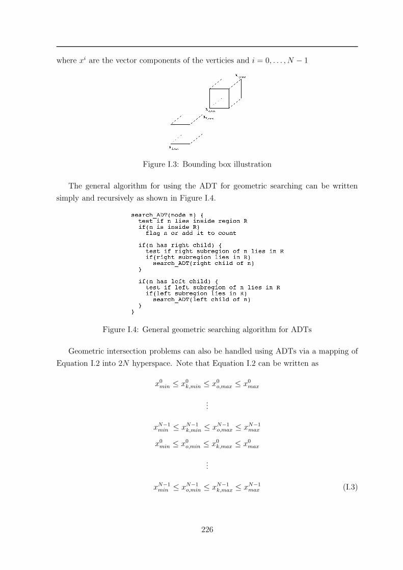
where xi are the vector components of the verticies and i = 0, . . . , N − 1
Figure I.3: Bounding box illustration
The general algorithm for using the ADT for geometric searching can be written
simply and recursively as shown in Figure I.4.
Figure I.4: General geometric searching algorithm for ADTs
Geometric intersection problems can also be handled using ADTs via a mapping of
Equation I.2 into 2N hyperspace. Note that Equation I.2 can be written as
x0min ≤ x0
k,min ≤ x0o,max ≤ x0
max
...
xN−1min ≤ xN−1
k,min ≤ xN−1o,max ≤ xN−1
max
x0min ≤ x0
o,min ≤ x0k,max ≤ x0
max
...
xN−1min ≤ xN−1
o,min ≤ xN−1k,max ≤ xN−1
max (I.3)
226
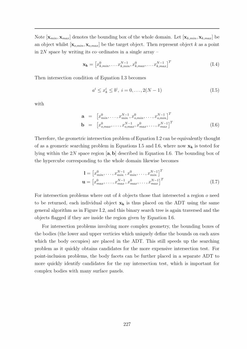
Note [xmin,xmax] denotes the bounding box of the whole domain. Let [xk,min,xk,max] be
an object whilst [xo,min,xo,max] be the target object. Then represent object k as a point
in 2N space by writing its co–ordinates in a single array –
xk =[x0
k,min, . . . xN−1k,min, x0
k,max, . . . xN−1k,max
]T(I.4)
Then intersection condition of Equation I.3 becomes
ai ≤ xik ≤ bi, i = 0, . . . , 2(N − 1) (I.5)
with
a =[x0
min, . . . , xN−1min , x0
o,min, . . . , xN−1o,min
]T
b =[x0
o,max, . . . , xN−1o,max, x
0max, . . . , x
N−1max
]T(I.6)
Therefore, the geometric intersection problem of Equation I.2 can be equivalently thought
of as a geomeric searching problem in Equations I.5 and I.6, where now xk is tested for
lying within the 2N space region [a,b] described in Equation I.6. The bounding box of
the hypercube corresponding to the whole domain likewise becomes
l =[x0
min, . . . , xN−1min , x0
min, . . . , xN−1min
]T
u =[x0
max, . . . , xN−1max , x0
max, . . . , xN−1max
]T(I.7)
For intersection problems where out of k objects those that intersected a region o need
to be returned, each individual object xk is thus placed on the ADT using the same
general algorithm as in Figure I.2, and this binary search tree is again traversed and the
objects flagged if they are inside the region given by Equation I.6.
For intersection problems involving more complex geometry, the bounding boxes of
the bodies (the lower and upper verticies which uniquely define the bounds on each axes
which the body occupies) are placed in the ADT. This still speeds up the searching
problem as it quickly obtains candidates for the more expensive intersection test. For
point-inclusion problems, the body facets can be further placed in a separate ADT to
more quickly identify candidates for the ray intersection test, which is important for
complex bodies with many surface panels.
227
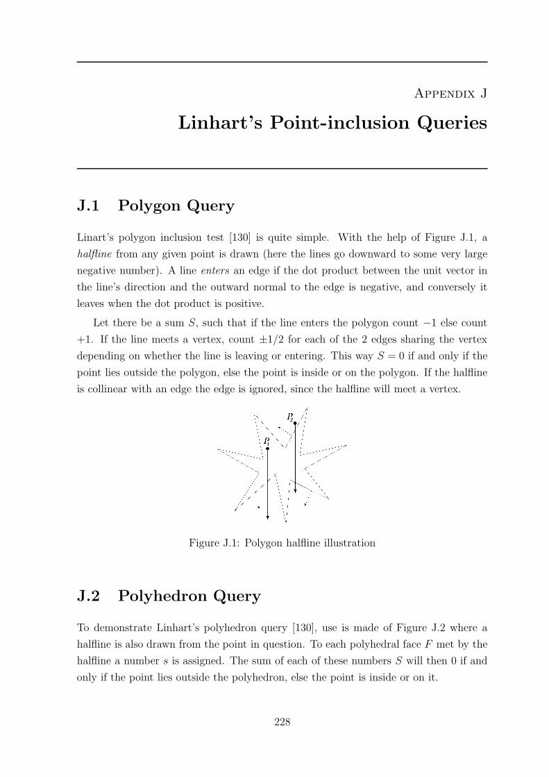
Appendix J
Linhart’s Point-inclusion Queries
J.1 Polygon Query
Linart’s polygon inclusion test [130] is quite simple. With the help of Figure J.1, a
halfline from any given point is drawn (here the lines go downward to some very large
negative number). A line enters an edge if the dot product between the unit vector in
the line’s direction and the outward normal to the edge is negative, and conversely it
leaves when the dot product is positive.
Let there be a sum S, such that if the line enters the polygon count −1 else count
+1. If the line meets a vertex, count ±1/2 for each of the 2 edges sharing the vertex
depending on whether the line is leaving or entering. This way S = 0 if and only if the
point lies outside the polygon, else the point is inside or on the polygon. If the halfline
is collinear with an edge the edge is ignored, since the halfline will meet a vertex.
Figure J.1: Polygon halfline illustration
J.2 Polyhedron Query
To demonstrate Linhart’s polyhedron query [130], use is made of Figure J.2 where a
halfline is also drawn from the point in question. To each polyhedral face F met by the
halfline a number s is assigned. The sum of each of these numbers S will then 0 if and
only if the point lies outside the polyhedron, else the point is inside or on it.
228
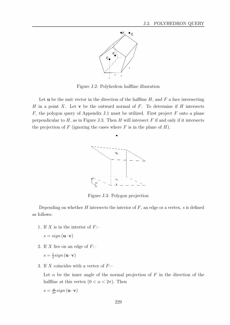
J.2. POLYHEDRON QUERY
Figure J.2: Polyhedron halfline illusration
Let u be the unit vector in the direction of the halfline H, and F a face intersecting
H in a point X. Let v be the outward normal of F . To determine if H intersects
F , the polygon query of Appendix J.1 must be utilized. First project F onto a plane
perpendicular to H, as in Figure J.3. Then H will intersect F if and only if it intersects
the projection of F (ignoring the cases where F is in the plane of H).
Figure J.3: Polygon projection
Depending on whether H intersects the interior of F , an edge or a vertex, s is defined
as follows:
1. If X is in the interior of F :–
s = sign (u ·v)
2. If X lies on an edge of F :–
s = 12sign (u ·v)
3. If X coincides with a vertex of F :–
Let α be the inner angle of the normal projection of F in the direction of the
halfline at this vertex (0 < α < 2π). Then
s = α2π
sign (u ·v)
229
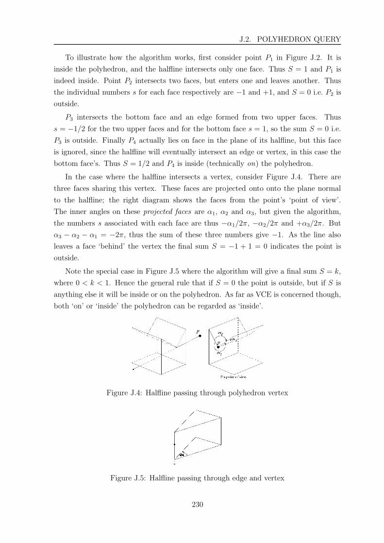
J.2. POLYHEDRON QUERY
To illustrate how the algorithm works, first consider point P1 in Figure J.2. It is
inside the polyhedron, and the halfline intersects only one face. Thus S = 1 and P1 is
indeed inside. Point P2 intersects two faces, but enters one and leaves another. Thus
the individual numbers s for each face respectively are −1 and +1, and S = 0 i.e. P2 is
outside.
P3 intersects the bottom face and an edge formed from two upper faces. Thus
s = −1/2 for the two upper faces and for the bottom face s = 1, so the sum S = 0 i.e.
P3 is outside. Finally P4 actually lies on face in the plane of its halfline, but this face
is ignored, since the halfline will eventually intersect an edge or vertex, in this case the
bottom face’s. Thus S = 1/2 and P4 is inside (technically on) the polyhedron.
In the case where the halfline intersects a vertex, consider Figure J.4. There are
three faces sharing this vertex. These faces are projected onto onto the plane normal
to the halfline; the right diagram shows the faces from the point’s ‘point of view’.
The inner angles on these projected faces are α1, α2 and α3, but given the algorithm,
the numbers s associated with each face are thus −α1/2π, −α2/2π and +α3/2π. But
α3 − α2 − α1 = −2π, thus the sum of these three numbers give −1. As the line also
leaves a face ‘behind’ the vertex the final sum S = −1 + 1 = 0 indicates the point is
outside.
Note the special case in Figure J.5 where the algorithm will give a final sum S = k,
where 0 < k < 1. Hence the general rule that if S = 0 the point is outside, but if S is
anything else it will be inside or on the polyhedron. As far as VCE is concerned though,
both ‘on’ or ‘inside’ the polyhedron can be regarded as ‘inside’.
Figure J.4: Halfline passing through polyhedron vertex
Figure J.5: Halfline passing through edge and vertex
230
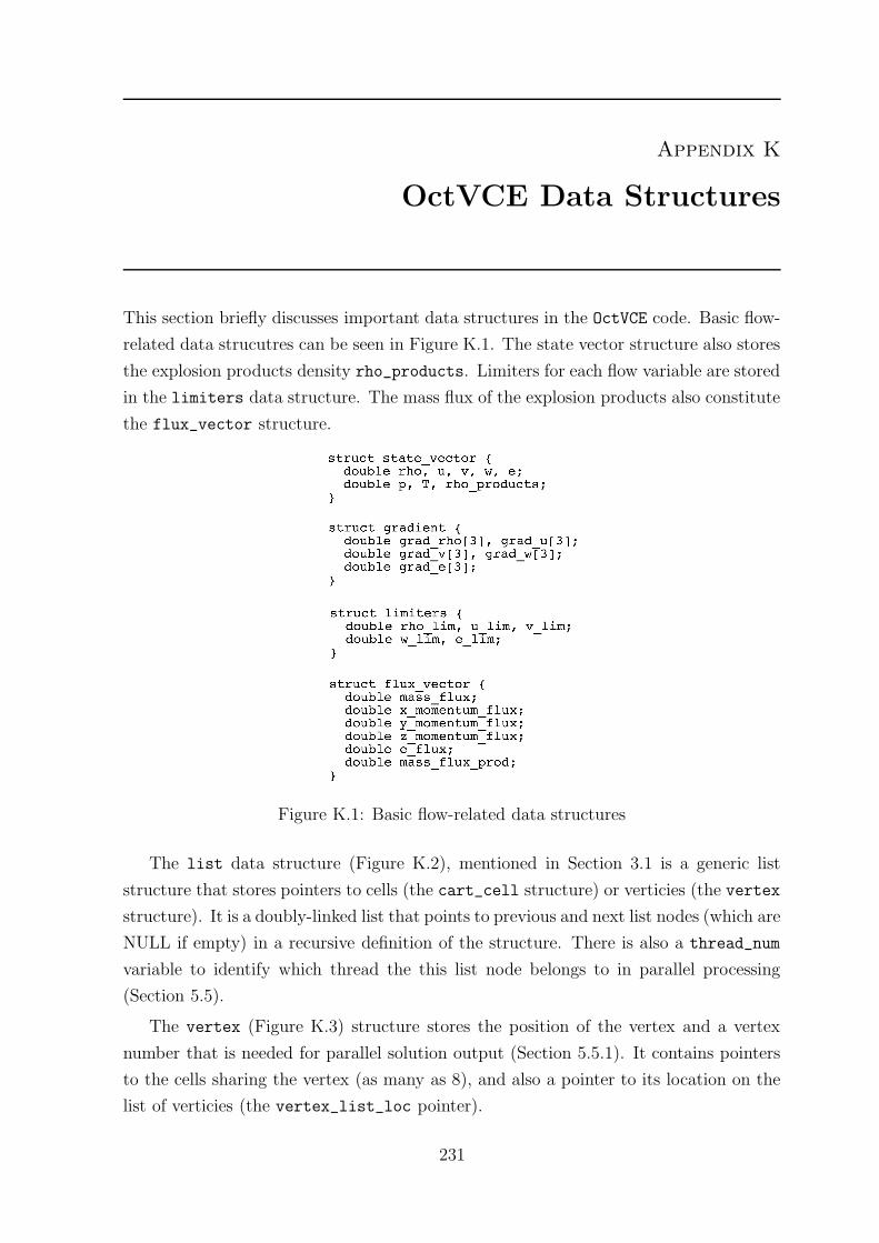
Appendix K
OctVCE Data Structures
This section briefly discusses important data structures in the OctVCE code. Basic flow-
related data strucutres can be seen in Figure K.1. The state vector structure also stores
the explosion products density rho_products. Limiters for each flow variable are stored
in the limiters data structure. The mass flux of the explosion products also constitute
the flux_vector structure.
Figure K.1: Basic flow-related data structures
The list data structure (Figure K.2), mentioned in Section 3.1 is a generic list
structure that stores pointers to cells (the cart_cell structure) or verticies (the vertex
structure). It is a doubly-linked list that points to previous and next list nodes (which are
NULL if empty) in a recursive definition of the structure. There is also a thread_num
variable to identify which thread the this list node belongs to in parallel processing
(Section 5.5).
The vertex (Figure K.3) structure stores the position of the vertex and a vertex
number that is needed for parallel solution output (Section 5.5.1). It contains pointers
to the cells sharing the vertex (as many as 8), and also a pointer to its location on the
list of verticies (the vertex_list_loc pointer).
231
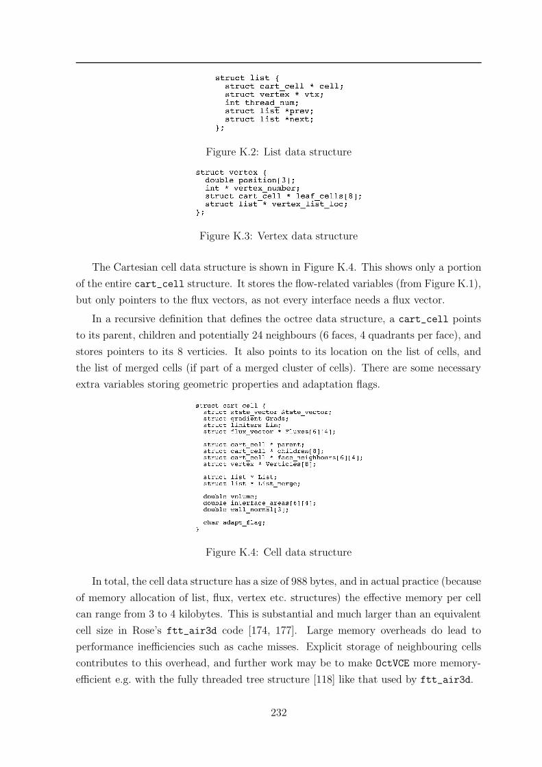
Figure K.2: List data structure
Figure K.3: Vertex data structure
The Cartesian cell data structure is shown in Figure K.4. This shows only a portion
of the entire cart_cell structure. It stores the flow-related variables (from Figure K.1),
but only pointers to the flux vectors, as not every interface needs a flux vector.
In a recursive definition that defines the octree data structure, a cart_cell points
to its parent, children and potentially 24 neighbours (6 faces, 4 quadrants per face), and
stores pointers to its 8 verticies. It also points to its location on the list of cells, and
the list of merged cells (if part of a merged cluster of cells). There are some necessary
extra variables storing geometric properties and adaptation flags.
Figure K.4: Cell data structure
In total, the cell data structure has a size of 988 bytes, and in actual practice (because
of memory allocation of list, flux, vertex etc. structures) the effective memory per cell
can range from 3 to 4 kilobytes. This is substantial and much larger than an equivalent
cell size in Rose’s ftt_air3d code [174, 177]. Large memory overheads do lead to
performance inefficiencies such as cache misses. Explicit storage of neighbouring cells
contributes to this overhead, and further work may be to make OctVCE more memory-
efficient e.g. with the fully threaded tree structure [118] like that used by ftt_air3d.
232
Related Documents


