Development of a Novel Fiber-Coupled Three Degree-of-Freedom

Development of a Novel Fiber-Coupled

Three Degree-of-Freedom Displacement

Interferometer

by

Steven R. Gillmer

Submitted in Partial Fulfillmentof the

Requirements for the Degree

Master of Science

Supervised by

Jonathan D. Ellis

Department of Mechanical EngineeringArts, Sciences and Engineering

Edmund A. Hajim School of Engineering and Applied Sciences

University of RochesterRochester, New York

2013

ii

Dedication

This thesis is dedicated to my godfather, Thomas Clarke, whose passion for science

and technology has inspired me to be where I am today.

iii

Curriculum Vitae

Steven R. Gillmer was born in Albuquerque, New Mexico. He attended the

University of Rochester, and graduated cum laude with a Bachelor of Science

degree in Mechanical Engineering in 2011. He began master’s studies in Mechanical

Engineering at the University of Rochester in 2011. He pursued his research in

opto-mechanics and precision engineering under the advisement of Dr. Jonathan D.

Ellis.

iv

Acknowledgments

Thank you to Dr. Jonathan Ellis, whose skills and expertise in the field of

displacement interferometry were invaluable for this research. I would also like to

thank Dr. Thomas Brown and Dr. John Lambropoulos for serving on my thesis

committee and offering their input for my research. A special thank you to Helen

Clarke for all of the editing she did on the writing in this thesis. Finally, I would like

to thank my mother, Virginia Gillmer, for all of her support throughout my graduate

education.

v

Abstract

Heterodyne displacement interferometry is a widely accepted methodology capable of

measuring displacements with sub-nanometer resolution. The objective of this thesis

is to demonstrate a compact, fiber-delivered displacement measuring interferometer

which can be used to simultaneously calibrate the linear motion and rotational errors

of a translating stage using a single measurement beam. Heterodyne interferometry

is ideal for this type of high resolution stage feedback sensing because of its high

dynamic range, high signal-to-noise ratio, and direct traceability to the meter.

There are a variety of benefits to fiber-delivered interferometers for stage

metrology. First, the interferometer alignment is decoupled from the laser alignment.

The overall setup can be divided into subsystems to more easily identify and rectify

misalignments. Simplified alignment and division into subsystems increases the

stability of the structure because the metrology footprint is significantly reduced.

Many beam routing optics can be eliminated and the heterodyne laser (a heat source)

can also be isolated from the stage measurement site.

Ongoing work towards a compact, three degree-of-freedom fiber-delivered

heterodyne interferometer will be presented. This novel interferometer utilizes

differential wavefront sensing to measure target mirror displacement, pitch, and

yaw. Differential wavefront sensing uses a quadrant photodiode to measure four

vi

spatially separated interference signals within a single optical interference beam.

Based on the geometry of the detector and the interference phase in each quadrant,

the displacement and changes in target pitch and yaw can be measured.

vii

Table of Contents

Dedication ii

Curriculum Vitae iii

Acknowledgments iv

Abstract v

List of Figures x

1 Introduction 1

1.1 Applications . . . . . . . . . . . . . . . . . . . . . . . . . . . . . . . . 3

1.2 Displacement Interferometry Theory . . . . . . . . . . . . . . . . . . 6

1.3 Displacement Interferometry Background . . . . . . . . . . . . . . . . 14

1.4 Towards a Multi-DOF Interferometer . . . . . . . . . . . . . . . . . . 21

2 Working Principles of the Multi-DOF Interferometer 23

2.1 Acousto-Optic Modulators . . . . . . . . . . . . . . . . . . . . . . . . 25

viii

2.2 Fiber Optic Coupling . . . . . . . . . . . . . . . . . . . . . . . . . . . 29

2.3 Differential Wavefront Sensing . . . . . . . . . . . . . . . . . . . . . . 33

2.4 Preliminary Benchtop Data . . . . . . . . . . . . . . . . . . . . . . . 36

2.5 Technology Summary . . . . . . . . . . . . . . . . . . . . . . . . . . . 41

3 System Design 42

3.1 First Design Iteration . . . . . . . . . . . . . . . . . . . . . . . . . . . 50

3.2 Second Design Iteration . . . . . . . . . . . . . . . . . . . . . . . . . 61

3.3 Future Design Implementations . . . . . . . . . . . . . . . . . . . . . 73

4 Interferometer Qualification 75

4.1 Benchtop Qualification Measurements . . . . . . . . . . . . . . . . . . 75

4.2 Working Prototype Qualification . . . . . . . . . . . . . . . . . . . . 95

4.3 Qualification Analysis . . . . . . . . . . . . . . . . . . . . . . . . . . 99

5 Periodic Nonlinearity 102

5.1 The Michelson Interferometer . . . . . . . . . . . . . . . . . . . . . . 105

5.2 Theory . . . . . . . . . . . . . . . . . . . . . . . . . . . . . . . . . . . 108

5.3 Laboratory Data . . . . . . . . . . . . . . . . . . . . . . . . . . . . . 111

5.4 Future Error Reduction . . . . . . . . . . . . . . . . . . . . . . . . . . 119

6 Conclusion 121

6.1 Measurement Uncertainty . . . . . . . . . . . . . . . . . . . . . . . . 121

6.2 Future System Improvements . . . . . . . . . . . . . . . . . . . . . . 125

6.3 Final Remarks . . . . . . . . . . . . . . . . . . . . . . . . . . . . . . . 128

ix

Bibliography 131

A Simulating Periodic Nonlinearity 137

x

List of Figures

1.1 Renishaw’s ML10 optical interferometer measuring yaw . . . . . . . . 2

1.2 Abbe error is amplified at the measurement point of interest . . . . . 4

1.3 Wafer stage metrology in optical lithography . . . . . . . . . . . . . . 5

1.4 The homodyne Michelson interferometer . . . . . . . . . . . . . . . . 7

1.5 Homodyne interferometry signal processing . . . . . . . . . . . . . . . 8

1.6 The heterodyne Michelson interferometer . . . . . . . . . . . . . . . . 10

1.7 Homodyne interferometer measuring strain propogation through 1060

aluminum . . . . . . . . . . . . . . . . . . . . . . . . . . . . . . . . . 15

1.8 Measuring the refractive index of air and laser stability . . . . . . . . 16

1.9 Beam leakage in the heterodyne Michelson interferometer . . . . . . . 18

1.10 Generation of a split frequency using acousto-optic modulators . . . . 20

1.11 Spatially separated beams in a Joo-type interferometer . . . . . . . . 21

2.1 A typical effect of periodic nonlinearity . . . . . . . . . . . . . . . . . 24

2.2 Full schematic of the multi-DOF interferometer . . . . . . . . . . . . 25

2.3 Sources of periodic nonlinearity as a result of Zeeman splitting . . . . 26

xi

2.4 Creation of a split frequency using acousto-optic modulators . . . . . 27

2.5 Propagating misalignment through a free space optical metrology system 30

2.6 Transition from a free space interferometry system to a fiber-coupled

setup . . . . . . . . . . . . . . . . . . . . . . . . . . . . . . . . . . . . 31

2.7 Close-up schematic of the multi-DOF interferometer . . . . . . . . . . 32

2.8 Phase differences on a quadrant photodetector . . . . . . . . . . . . . 34

2.9 Linear ramp with error in open loop . . . . . . . . . . . . . . . . . . . 36

2.10 Noise floor at constant voltage . . . . . . . . . . . . . . . . . . . . . . 37

2.11 Pitch and yaw sensitivity in open-loop scanning . . . . . . . . . . . . 38

2.12 Random step test for measurement reproducibility . . . . . . . . . . . 39

2.13 Increasing the split frequency to accommodate higher doppler shifts . 40

3.1 Kelvin clamp schematics . . . . . . . . . . . . . . . . . . . . . . . . . 44

3.2 Thermal drift with the benchtop interferometer . . . . . . . . . . . . 45

3.3 First and second design iterations of the interferometer . . . . . . . . 46

3.4 Geometrical optical analysis on interferometer beam paths . . . . . . 48

3.5 Optimized beam spacing for the interferometer . . . . . . . . . . . . . 49

3.6 First design iteration schematic . . . . . . . . . . . . . . . . . . . . . 50

3.7 First design iteration Solidworks assembly . . . . . . . . . . . . . . . 51

3.8 Fold mirror kinematic mounts on the first design iteration . . . . . . 52

3.9 Close-up of the fold mirror kinematic mounts . . . . . . . . . . . . . . 53

3.10 The critical face on the first design iteration . . . . . . . . . . . . . . 54

3.11 Critical face subassembly . . . . . . . . . . . . . . . . . . . . . . . . . 55

xii

3.12 Kinematically mounted beamplitters on the first design iteration . . . 56

3.13 Kinematically mounted beamsplitter close-up . . . . . . . . . . . . . 57

3.14 Invar optical mount with critical faces . . . . . . . . . . . . . . . . . 58

3.15 Baseplate designated on the first design iteration . . . . . . . . . . . 60

3.16 Baseplate close-up on the first design iteration . . . . . . . . . . . . . 60

3.17 From concept to reality in the second design iteration . . . . . . . . . 61

3.18 Second design iteration Solidworks assembly . . . . . . . . . . . . . . 62

3.19 Fiber collimator kinematic mounts designated on the second design

iteration . . . . . . . . . . . . . . . . . . . . . . . . . . . . . . . . . . 63

3.20 Fiber collimator kinematic mounts close-up . . . . . . . . . . . . . . . 64

3.21 Fiber collimator squeeze clamps designated on the second design

iteration . . . . . . . . . . . . . . . . . . . . . . . . . . . . . . . . . . 65

3.22 Von Mises stress analysis on the fiber collimator squeeze clamps . . . 66

3.23 Optical support structure designated on the second design iteration . 67

3.24 Stress analysis on the Invar optical support structure . . . . . . . . . 68

3.25 Stainless steel base designated on the second design iteration . . . . . 69

3.26 Kinematically mounted optical support structure . . . . . . . . . . . 70

3.27 Base support structure of the interferometer and selected features . . 71

3.28 Monitoring interference as the working prototype assembly cures

under a UV source . . . . . . . . . . . . . . . . . . . . . . . . . . . . 72

3.29 The final assembled prototype of the multi-DOF interferometer . . . 73

4.1 Qualifying the interferometer against the Renishaw ML10 . . . . . . . 76

xiii

4.2 Initial scaling factor of 2.15 in yaw qualification . . . . . . . . . . . . 77

4.3 Azimuthal misalignment decreases scaling factor in yaw . . . . . . . . 78

4.4 Further azimuthal misalignment continues to decrease scaling factor

in yaw . . . . . . . . . . . . . . . . . . . . . . . . . . . . . . . . . . . 79

4.5 Final azimuthal misalignment increases scaling factor in yaw . . . . . 79

4.6 Initial scaling factor in pitch qualification . . . . . . . . . . . . . . . . 80

4.7 Change in pitch scaling factor as a result of azimuthal misalignment . 81

4.8 Scaling factor of 2.10 with pitch and yaw combined and summed in

quadrature . . . . . . . . . . . . . . . . . . . . . . . . . . . . . . . . . 82

4.9 Scaling factor varies with pitch and yaw combined and summed in

quadrature . . . . . . . . . . . . . . . . . . . . . . . . . . . . . . . . . 83

4.10 Scaling factor is sometimes below one with pitch and yaw combined

and summed in quadrature . . . . . . . . . . . . . . . . . . . . . . . . 83

4.11 Qualification agreement for small displacements . . . . . . . . . . . . 84

4.12 Z-displacement qualification for a linear ramp . . . . . . . . . . . . . 85

4.13 Z-displacement qualification for a sine wave . . . . . . . . . . . . . . 85

4.14 Cosine error schematic . . . . . . . . . . . . . . . . . . . . . . . . . . 86

4.15 Consistent scaling factor using one focusing lens in yaw . . . . . . . . 88

4.16 Scaling factor is not affected by misalignment using one focusing lens,

qualifying yaw . . . . . . . . . . . . . . . . . . . . . . . . . . . . . . . 88

4.17 Scaling factor is not affected by further misalignment using one

focusing lens, qualifying yaw . . . . . . . . . . . . . . . . . . . . . . . 89

4.18 Scaling factor is valid for sine inputs, qualifying yaw . . . . . . . . . . 89

xiv

4.19 Consistent scaling factor still evident in pitch qualification, using one

focusing lens . . . . . . . . . . . . . . . . . . . . . . . . . . . . . . . . 90

4.20 Consistent scaling factor is evident in pitch qualification when

misaligned, using one focusing lens . . . . . . . . . . . . . . . . . . . 90

4.21 Consistent scaling factor is evident in pitch qualification for sine input,

using one focusing lens . . . . . . . . . . . . . . . . . . . . . . . . . . 91

4.22 Variable location of quadrant photodetector changes scaling . . . . . 92

4.23 Further variable scaling with variable quadrant photodetector location 93

4.24 No scaling factor using a telescope to focus measurement beam . . . . 93

4.25 Telescope scaling factor in pitch . . . . . . . . . . . . . . . . . . . . . 94

4.26 Large scaling factor using telescope in yaw qualification . . . . . . . . 94

4.27 Qualification measurement setup of the working multi-DOF prototype

vs. the Renishaw ML10 . . . . . . . . . . . . . . . . . . . . . . . . . 96

4.28 45 mm linear ramp qualification between the Renishaw ML10 and the

working prototype of the multi-DOF interferometer . . . . . . . . . . 97

4.29 Scaling factor persisted in rotation measurements with the multi-DOF

interferometer working prototype . . . . . . . . . . . . . . . . . . . . 98

4.30 Overfilling detector drastically reduces tip/tilt sensitivity . . . . . . . 99

4.31 Preliminary analytical simulations of the multi-DOF interferometer

naturally produce the scaling factor required for agreement between

the Renishaw ML10 and the multi-DOF system . . . . . . . . . . . . 101

5.1 Typical effect of periodic nonlinearity on a linear ramp . . . . . . . . 104

5.2 Michelson heterodyne interferometer . . . . . . . . . . . . . . . . . . 105

xv

5.3 Michelson interferometer showing optical mixing . . . . . . . . . . . . 106

5.4 Phasor diagram representations of periodic nonlinearity . . . . . . . . 111

5.5 Optical misalignment experiment to examine resulting periodic

nonlinearity . . . . . . . . . . . . . . . . . . . . . . . . . . . . . . . . 112

5.6 Effect of slight misalignment on the multi-DOF interferometer . . . . 113

5.7 Linear polarizers to limit periodic nonlinearity . . . . . . . . . . . . . 114

5.8 Periodic nonlinearity still exists with polarizer implemented . . . . . 114

5.9 Periodic nonlinearity in a meticulously aligned system . . . . . . . . . 116

5.10 Nonlinearity in all four quadrants of the quadrant photodiode . . . . 116

5.11 Sub-microradian nonlinearity in rotation and sub-nanometer nonlin-

earity in Z-displacement . . . . . . . . . . . . . . . . . . . . . . . . . 117

5.12 Periodic nonlinearity exists using wedge beamsplitters to scatter ghost

reflections . . . . . . . . . . . . . . . . . . . . . . . . . . . . . . . . . 119

6.1 Periodic nonlinearity amplified using measurement fiber detection . . 126

6.2 Attempted pitch qualification using measurement fiber detection . . . 127

6.3 Multi-DOF interferometer as a fiber probe on a 5-axis CMM . . . . . 128

A.1 Screen shot of the multi-DOF interferometer modeled using FRED

optical software . . . . . . . . . . . . . . . . . . . . . . . . . . . . . . 138

A.2 Schematic of initial multi-DOF interferometer used in the FRED

simulation . . . . . . . . . . . . . . . . . . . . . . . . . . . . . . . . . 138

A.3 Control scenario irradiance output . . . . . . . . . . . . . . . . . . . . 139

A.4 FRED simulation schematic to observe amplitude of ghost reflections 140

xvi

A.5 Irradiance output as a result of ghost reflections . . . . . . . . . . . . 141

A.6 Periodic nonlinearity simulation resulting from ghost reflections . . . 142

1

1 Introduction

Heterodyne displacement interferometry is a widely accepted method used for high

resolution stage metrology [1–3]. Optical heterodyne interferometers are typically

capable of measurements with sub-nanometer resolution and uncertainty, that is, if

the proper precautions are taken to ensure a confined environment and if a sufficiently

frequency stabilized source is used [4]. Although the interferometer which will be

discussed throughout this thesis utilizes a laser source, interferometry itself does not

necessarily imply the interference of optical signals. In general, interferometry simply

denotes the concept of interference, which may also involve radio waves [5].

The subject of this thesis is a novel fiber-coupled interferometer that is capable

of monitoring three degrees of freedom – displacement and changes in pitch and

yaw – of a moving stage using a single beam incident on a small plane mirror target.

Other displacement interferometers capable of measuring multiple degrees of freedom

simultaneously include the system developed for use in the Laser Interferometer

Space Antenna (LISA) [6], the 6-degree of freedom optical sensor for machine

tool error characterization [7] and the multi-degree of freedom measuring system

developed specifically for coordinate measurement machine error calibrations [8].

2

The interferometer discussed throughout this thesis was developed with a similar

design to that used in the LISA project, but has been condensed to a compact size

using, in part, architectures developed by Joo and colleagues [9–11].

Commercial interferometers are only capable of monitoring one or at most two

degrees of freedom during a single measurement, and in doing so they typically utilize

multiple retroreflectors. Renishaw’s ML10 interferometer is capable of measuring

Z-displacement, changes in pitch and yaw, squareness and straightness, however,

only one of these calibrations can be recorded during a single measurement. If any

other degree of freedom is desired, the retroreflectors must be detached from the

measurement stage and reattached in a different configuration. The Renishaw ML10

utilizes the setup shown in Figure 1.1 to record yaw measurements.

Figure 1.1: Renishaw’s ML10 optical interferometry system uses multipleretroreflectors to create a differential yaw measurement. The retroreflectors arerelatively bulky on small micro-positioning stages and must be reconfigured if otherdegrees of freedom are to be measured.

The interferometer that is the subject of this thesis, which will be called the

multi degree-of-freedom interferometer (or multi-DOF interferometer), utilizes a

much smaller profile on a measurement surface than a commercial system such

3

as Renishaw’s. The beam diameter that was used in the research conducted for

this thesis was nominally 3 mm. Therefore, two immediate improvements over

commercial systems are evident: The ability to monitor three degrees of freedom

simultaneously and the ability to do so by attaching a relatively small mirror to the

measurement surface.

1.1 Applications

There are a wide variety of applications for multi-DOF interferometers. Two

representative examples include the calibration of micro-positioning stages and the

metrology of wafer stages in the optical lithography industry. The calibration of

micro-positioning stages is subject to a phenomenon known as Abbe error. As

these small stages are calibrated in the Z-direction, the measurements must not

only include Z-displacements, but the inevitable nanoscale and sometimes microscale

pitch and yaw errors the stages exhibit while displacing. The rotational positioning

errors are unavoidable due to error sources such as manufacturing tolerances.

Abbe error specifically refers to small inevitable errors that are amplified at the

measurement point of interest through the moment arm that connects measurement

axis to the point of interest. The retroreflector setups which commercial systems

require for rotational calibrations are very bulky which hinders the possibility of

direct measurement at the point of interest. Instead, calibrations are typically

recorded off-axis and run through a transformation matrix from the measurement

site. This method of indirect measurement tends to decrease the accuracy of a

calibration because information is inevitably lost or skewed when passed through

a transformation matrix. Additionally, the mass of the interferometer target

4

distorts the dynamic performance of the stage, leading to less accurate calibrations.

The multi-DOF interferometer has the capability of monitoring displacements and

rotations directly at the point of interest due to its small beam profile and

thus, less information is lost in translation from an off-axis calibration point.

Figure 1.2 demonstrates the capability of the interferometer to measure directly

at the measurement point of interest using a small beam profile.

Figure 1.2: Abbe error is produced when measurements are taken off-axis from themeasurement point of interest. The multi-DOF interferometer has the capability ofmeasuring directly at the measurement point of interest due to its relatively smallbeam profile on the measurement mirror.

The second previously mentioned application of the multi-DOF interferometer

is in the metrology of wafer stages in the optical lithography industry. As a wafer

stage translates during lithographic printing, again, it inevitably exhibits not only

translation motions, but undesirable rotational errors which must be addressed. To

do so, at least six interferometers must constantly track the translating wafer stage

to account for all six degrees of freedom. The undesirable motions of the stage

are incorporated into feedback control to correct the errors in real time. Refer to

5

Figure 1.3: The metrology of wafer stages in the optical lithography industry requiresat least six interferometers to monitor all six degrees of freedom.

Figure 1.3 for a full schematic of the metrology involved in monitoring all six degrees

of freedom of a lithography stage.

A multi-DOF interferometer could simplify many metrology aspects in the

lithography industry. The full metrology package would be reduced to three

interferometers (three with redundancy for rotation self-calibration) while still

monitoring all six degrees of freedom. Currently the optical lithography industry

is pushing wafer sizes to over 450 mm, but with larger wafers comes larger – and

heavier – wafer stages. A smaller beam profile on the stage mirror would allow for

wafer stages to be made as small as possible to reduce weight, which would thus

increase printing efficiency.

6

Metrology systems will be further simplified if the multi-DOF interferometer is

fiber-coupled, which was a large research focus of this thesis as well. Not only will

the number of interferometers be reduced to three, the alignment required for the

entire system would be greatly reduced with the implementation of fiber-coupling.

Metrology systems in the lithography industry are mostly free-space delivered, so

a misalignment early in the system propagates downstream to every component

after it. The free-space delivery means that each interferometers’ alignment is

coupled to each other, leading to a more complex metrology system. Fiber-coupled

interferometers do not suffer from this drawback. A misalignment before the signals

are launched into fibers does not affect the alignment of each individual interferometer

downstream. Also, a misalignment in one fiber-coupled interferometer can be

corrected for independently from the others because each interferometer would be

individually coupled to the laser source. These concepts will be discussed in detail

in Chapter 2. To continue with the introduction into the field of displacement

interferometry, an overview of the measurement theory will be discussed followed

by a background discussion containing a number of selected historical advances.

1.2 Displacement Interferometry Theory

Displacement interferometers fall into one of two categories – homodyne and

heterodyne. These two categories describe the operating principle of the

interferometer, namely amplitude modulation or frequency modulation, respectively.

The concepts of homodyne and heterodyne signal transmission are not unique to

optics, they are both used in the transmission of radio waves. AM radio (or amplitude

modulated) uses the same working principles as a homodyne interferometer and FM

7

radio (or frequency modulated) obeys the same principles of a heterodyne optical

metrology system. Furthermore, AM radio signals are considered noisy compared to

FM radio signals for the same reasons that frequency modulated interferometers

possess superior signal integrity to amplitude modulated interferometers. The

working principles behind each type of interferometer will be discussed next.

1.2.1 The Homodyne Interferometer

The homodyne interferometer relies on a change in overall signal amplitude, from

varying effects of interference, as a measurement signal phase shifts with respect to a

reference signal. The term homodyne describes the use of a single optical frequency

which is divided into a reference and measurement path. A Michelson interferometer

is a simple way to describe both a heterodyne and homodyne system, and one such

Michelson homodyne example can be seen in Figure 1.4.

Figure 1.4: The homodyne interferometer utilizes a single optical frequency to trackdeviations in amplitude. Changes in the optical path length in the measurement armyields varying interference based on retroreflector 2 displacements. (PD-photodiode,BS-beamsplitter, RR-retroreflector)

As RR2 translates towards or away from the beamsplitter, the measurement

8

and reference signals constructively or destructively interfere, resulting in varying

AC signal amplitudes at the photodiode. Before the signals are recorded, they are

passed through a rectifier which essentially takes the absolute value of recorded

AC measurements and then they are passed through a low-pass filter to create a

simple DC output based on the interference between reference and measurement

signals. The varying levels of interference depending on the relative phase between

measurement and reference signals in a homodyne interferometer can be seen in

Figure 1.5.

Figure 1.5: AC signals in the homodyne interferometer are passed through a rectifierto essentially take the absolute value and then passed through a low-pass filter tocreate a simple DC output which is directly proportional to stage displacement.

One drawback of the homodyne interferometer compared to a heterodyne system

is that it is direction insensitive. In reference to Figure 1.5, the interference signal

in the second row registers as the same output as the interference signal in the

9

fourth row, even though the measurement phase (dotted red) has continued to shift

in the same direction relative to the reference phase. Unfortunately, one does not

know whether the measurement phase has switched directions between the third and

fourth rows or continued to shift in the same direction. Another drawback is the

homodyne interferometer’s sensitivity to spurious fluctuations in amplitude from the

laser source. Fluctuations such as this can be filtered out in a heterodyne system

which does not depend on an amplitude modulation for accurate measurements.

1.2.2 The Heterodyne Interferometer

The heterodyne interferometer is a natural progression from its homodyne

counterpart towards higher resolution measurements. Heterodyning is a method

which is based on the interference of two beams with slightly different frequencies

and the result of this interference is called the split frequency (or beat frequency).

Through signal processing, the interference between beams of slightly different optical

frequencies results in the difference between the two interfering frequencies. Before

interference, the two beams are fed through the reference and measurement arms

of a heterodyne interferometer where a modulation in phase in the measurement

arm can be discerned with respect to the reference path. To once again relate back

to the FM radio wave analogy, the irradiance recorded at the reference photodiode

creates the equivalent of a local oscillator while the measurement beam interfering

with the slightly different frequency from the reference path carries the actual signal

of interest. Polarizations are typically employed in these interferometers to ensure

that signals do not interfere until it is desired. A standard heterodyne Michelson

interferometer schematic can be seen in Figure 1.6.

In the schematic, two collinear and orthogonally polarized beams are supplied

10

Figure 1.6: The heterodyne Michelson interferometer outputs two collinear andorthogonally polarized beams which are separated through a polarizing beamsplitterinto the measurement and reference paths of the interferometer. (PBS-polarizingbeamsplitter, PD-photodiode, RR-retroreflector)

from the laser source at slightly different frequencies. About 10% of the beams

are immediately separated using a beamsplitter and passed through a 45 polarizer

to create reference interference. The remaining 90% of the beams are fed into

the interferometer where they are split by a polarizing beamsplitter into the

reference and measurement arms of the interferometer. At this point the polarizing

beamsplitter has split polarizations, and thus each frequency, into the reference

and measurement paths. The measurement path is subjected to a translating

retroreflector displacement which creates a change in optical path length, but

more importantly, a Doppler shift corresponding to a retroreflector that is moving

towards or away from the interferometer. The Doppler shifted light manifests as a

frequency modulation relative to the reference signal taken before the interferometer

and is detected as a directionally sensitive displacement. The resulting frequency

modulation is related to the physical displacement of the moving retroreflector

11

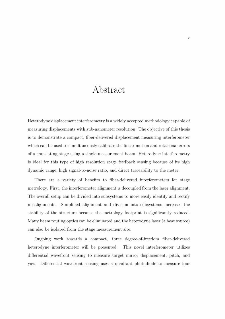
through

∆φ = φ2 − φ1 =2πNη∆z

λ, (1.1)

where φ2 represents the change in phase seen in the measurement arm of the

interferometer, φ1 represents the phase reading at the reference photodetector, N

is the interferometer fold factor (2 in the case of Figure 1.6) which corresponds to

the number of passes to and from the measurement target, η is the refractive index of

the surrounding medium, ∆z is the change in physical displacement of the target, and

λ is the wavelength of light (632.8 nm in the case of the lasers used for this research).

The interference of two electric fields with different frequencies is represented as the

superposition of the two:

E = E1 + E2 = E01e−i(ω1t+φ1) + E02e

−i(ω2t+φ2), (1.2)

where E01 and E02 represent the amplitude values of the two signals, ω1,2 designates

the two heterodyne angular frequencies that vary with time, t, and φ1,2 designates the

phase shifts in the reference and measurement arm of the interferometer, respectively.

The detected irradiance is proportional to the square of the amplitude given in

Equation 1.2 and is given by

I ∝ |E|2 = |E01e−i(ω1t+φ1) + E02e

−i(ω2t+φ2)|2

= (E01e−i(ω1t+φ1) + E02e

−i(ω2t+φ2))(E∗

01ei(ω1t+φ1) + E∗

02ei(ω2t+φ2)

= |E01|2 + |E02|

2 + 2<(E01E∗

02e−i(∆ωt+∆φ))

= I1 + I2 + 2√

I1I2 cos(∆ωt+∆φ),

(1.3)

where, ∆ω represents the angular split frequency, ω1 − ω2, and an asterisk denotes

12

a complex conjugate. It should also be noted that Equation 1.3 designates a change

in phase, φ1,2 in each of the interfering electric fields. While this may be true for the

measurement signal, it is assumed that there is no change in phase in the reference

signal of a heterodyne interferometer. With this in mind, it is convenient to represent

the reference and measurement irradiance readings as simplified proportionality

terms, given by

PDr → Ir ∝ Ar cos[2π(f1 − f2)t] (1.4)

PDm → Im ∝ Am cos[2π(f1 − f2)t+∆φ], (1.5)

where angular frequency has been converted to temporal frequency and amplitude

terms have been simplified to Ar and Am. In the above equations, the subscript r

denotes the reference measurement and the subscript m denotes the measurement

signal. The measurement signal is subjected to a frequency modulation or change in

phase, ∆φ, in response to a moving target mirror.

The transition from a phase modulation to physical displacement is not easily

evident yet. The signal processing which takes place after the measurement and

reference signal are recorded is what yields a simple time varying phase measurement

with respect to the reference signal. From Equations 1.4 and 1.5, in-phase and

quadrature signals are generated to represent the detected modulation as a sine and

cosine component. The in-phase measurement is created by multiplying the reference

irradiance by the measurement irradiance. Similarly, the quadrature signal is created

by multiplying the sine of the reference signal (simply the cosine term with a 90

phase shift) by the measurement signal. The in-phase, I, and quadrature, Q, signals

are represented by

13

I = RcM = cos(2πfst) cos(2πfst+∆φ)

Q = RsM = cos(

2πfst+π

2

)

cos(2πfst+∆φ),(1.6)

where fs is the split frequency, f1 − f2, Rc is the cosine component of the reference

signal, Rs is the sine component of the reference signal, M is the measurement signal

and ∆φ is the change in phase due to target mirror displacement. The terms in

Equation 1.6 can be manipulated using the common trigonometric identity,

2 cosA cosB = cos(A+B) + cos(A− B). (1.7)

When Equation 1.6 is manipulated using Equation 1.7, two terms are created, a

high frequency term, cos(A + B), with a frequency value too high to detect and a

lower frequency term, cos(A−B), which has evolved into the simple in-phase, I, and

quadrature, Q, terms in Equation 1.8.

I =1

2cos(∆φ)

Q =1

2sin(∆φ)

(1.8)

Phase is thus determined from the arctangent of the in-phase and quadrature terms,

∆φ = arctan(Q

I

)

, (1.9)

and converted to physical displacement using Equation 1.1. With these working

principles in mind, the development of the displacement interferometry industry

may now be examined.

14

1.3 Displacement Interferometry Background

Optical interferometry was first used to measure displacements in 1892 when the

standard meter was defined by Albert Michelson and Rene Benoit at the International

Bureau of Weights and Measures (BIPM) in France [12]. It would not be until the

invention of the Helium-Neon gas laser in 1960 that the displacement interferometry

industry would truly take off. Not long after this invention, one of the first

displacement interferometers was created in 1965 by Barker, et al. [13]. Barker’s

research team at Sandia National Laboratories was attempting to measure the strain

propagation through aluminum after an applied impact. They eventually did so

by using a homodyne displacement interferometer from which they achieved an

accuracy of 0.025 µm at free surface velocities up to 0.1 mm/µs. The resolution

of this interferometer was at least one order of magnitude better than other methods

they had attempted to use to measure strain propagation. As discussed in the

previous section, homodyne interferometry systems are limited. Barker and his team

discussed the problems they ran into which included the need for a high frequency

photodetector and recording system as well as a collimated, low-noise laser source.

These laser sources are much more readily available today than they would have been

a mere five years after the He-Ne gas laser was invented. The setup used by Barker,

et al. is shown in Figure 1.7.

In Figure 1.7, the entire interferometer is housed within a vacuum chamber to

mitigate environmental effects on refractive index. Under an applied impact small

strain effects propagate through a sample of 1060 aluminum and can be detected

on the opposite surface from the applied force. The homodyne laser source is split

50/50 at the non-polarizing beamsplitter (BS) into the measurement and reference

arm of the interferometer. Strain propagations produce small local displacements

15

Figure 1.7: The Homodyne interferometer system used by Barker, et al. to measuresub-micrometer level effects of strain propagation (adapted from Reference [13]).(PD-photodiode, BS-beamsplitter)

in the surface which manifest as small changes in phase in the measurement arm

of the interferometer. Changes in interference, and thus phase, are detected at the

measurement photodiode (PDm). Even though this interferometer was limited, its

creators still realized the need to stabilize the environment to mitigate uncertainty

as a result of changes in refractive index.

The year after Barker, et al. published their work, a more precise determination

of the refractive index of air was published by Edlen [14]. This uncertainty source

and its effect on displacement measuring interferometry was heavily investigated

by Estler in 1985 [4]. Estler’s paper discusses that the two dominant uncertainty

sources in laser interferometers are the laser stability and the refractive index of air.

16

He tested these two sources of uncertainty with the setup shown in Figure 1.8.

Figure 1.8: The setup used by Estler to investigate the refractive index of air andlaser stability in relation to their effects on displacement measuring interferometers(Adapted from Reference [4]). (PD-photodiode, PBS-polarizing beam splitter, QWP-quarter-wave plate)

The setup shown in Figure 1.8 is a plane mirror interferometer which is insensitive

to small tip and tilt rotations of the measurement mirror. Estler monitored laser

stability by creating a beat frequency between a reference Iodine-stabilized He-Ne

laser source and a commercial Zeeman split HP laser. He determined that the short-

term frequency stability of the HP laser was about ±2 parts in 109, which was better

than the absolute uncertainty that he eventually deduced from changes in refractive

index.

To accurately determine the refractive index of air, pressure, temperature,

humidity, and CO2 concentration of the surrounding environment must be monitored.

CO2 concentration was deemed completely negligible for the system in Figure 1.8

and was not measured. Humidity and pressure were monitored with a pressure

and humidity sensor placed before the beamsplitting optics. Temperature effects

17

were monitored using a thermistor array that spanned the measurement arm of the

interferometer which allowed for the observation of temperature gradients. In the

end, the uncertainty in refractive index due to pressure variations was calculated to

be ±2 parts in 108. The uncertainty in refractive index as a result of temperature

variation was ±1 part in 108, and humidity effects contributed ±0.5 parts in 108

to the overall refractive index uncertainty [4]. As a result of these sources, Estler

calculated an absolute uncertainty in refractive index of ±8.5 parts in 108. These

results show that although laser stability is important to consider for a heterodyne

system, a stable refractive index is slightly more so due to its higher contribution

to the uncertainty of measurement (that is, if a sufficiently stable laser is available

to use). Uncertainties from other error sources would continue to be investigated

through the 1980s.

The uncertainty of displacement interferometer measurements continued to

improve in 1987 when Norman Bobroff investigated residual errors as a result

of air turbulence and imperfect optics [15]. As discussed previously, one of the

main applications of displacement interferometry is in the metrology of lithography

stages. Frequently in lithographic printing, a turbulent air flow is introduced in

an effort to reduce contaminants which could affect the resolution of the print.

Turbulent airflow is not something that was investigated towards the completion

of this thesis, and therefore, the results of Bobroff’s air turbulence experiments

will not be discussed in detail. His more applicable error sources which will be

discussed are the periodic nonlinearities created as a result of frequency mixing at

the launch site, in addition to the beam leakage within an interferometer that occurs

as a result of imperfect beamsplitting optics. This periodic error source was first

observed by Quenelle [16] and later experimentally demonstrated by Sutton [17].

18

Periodic nonlinearity is typically a 1-5 nm sinusoid which is superimposed on top of

a nominal signal [17–19]. The phenomenon is discussed in detail in Chapter 5, but

for now, it is simplest to understand periodic nonlinearity as a 1-5 nm error source

for a given measurement. If the standard Michelson interferometer from Figure 1.6

is considered, ideally the launch site produces two collinear perfectly orthogonally

polarized beams. However, in reality, this is never the case. Polarizations of the two

beams are never orthogonal, and the result is the two beams tend to interfere before

entering the interferometer. Interference at the launch site creates frequency mixing

and a non-ideal fringe contrast. In addition, beamsplitting optics are never perfect

which results in a phenomenon known as beam leakage and therefore, additional

periodic nonlinearities [20, 21]. Techniques to minimize the effects of these error

sources will be discussed in Chapter 5 along with the implementation of these

techniques.

Figure 1.9: Visualization of beam leakage which is a result of imperfect beamsplittingoptics. This effect is a source of periodic nonlinearity which will be discussed inChapter 5. (PD-photodiode, PBS-polarizing beam splitter, RR-retroreflector)

Beam leakage can be visualized using the Michelson interferometer shown in

Figure 1.9. In this schematic, ideally the polarizing beamsplitter (PBS) splits one

polarization state and thus one frequency into the reference arm of the interferometer

19

while letting the perpendicularly polarized beam pass into the measurement arm.

Optical coatings are never perfect, so as a result, an unwanted portion of the f1

beam leaks into the measurement arm and a portion of the f2 beam leaks into the

reference arm. The resulting periodic nonlinearity creates measurement error.

Another considerable limitation in the previously discussed Michelson laser

interferometer is the megahertz-range split frequency which is frequently generated

using Zeeman splitting. In order to measure faster moving stages, the split frequency

must be increased in order to be able to discern a high frequency Doppler shift. As

the split frequency moves into the megahertz range, signal integrity becomes more

of an issue for data processing (i.e.: signal cross talk, ground bounce, and signal

distortion). In addition, a megahertz range split frequency is often not a viable option

to use with benchtop interferometer setups. The benchtop interferometer setups used

for this research utilize a commercial lock-in amplifier (Stanford Research Systems:

SRS-830) to lock to a reference frequency measured at the reference photodetector.

These lock-in amplifiers cannot lock to a signal greater than 100 kHz, making a

megahertz-range split frequency unrealistic to use for this research. In 1989, Tanaka,

et al. utilized acousto-optic modulators to generate a tunable split frequency [22],

and as a result, simplified data analysis. A schematic of acousto-optic modulators

(AOMs) are shown in Figure 1.10.

The diagram in Figure 1.10 utilizes a standard He-Ne frequency stabilized laser

which is split through a non-polarizing beamsplitter and fed into two AOMs. The

effect of the AOMs is they both increase the 473 THz input frequency by around

80 MHz. The top AOM in Figure 1.10 increases the frequency by 80.00 MHz while

the bottom AOM increases the input frequency by 80.07 MHz. If these two signals are

used as the heterodyne source for a displacement interferometer, the split frequency

20

Figure 1.10: Acousto-optic modulators (AOMs) are capable of creating a kHz rangesplit frequency. The split frequency is also tunable if one AOM is switched out foran AOM at a higher driving frequency. (BS-50/50 beamsplitter)

(f2 − f1) is 70 kHz and the SRS-830 commercial lock-in amplifier can now be used

for data processing. In 2000, Lawall and Kessler utilized acousto-optic modulators

in a displacement interferometer setup and achieved an accuracy on the order of

10 pm [23]. They attribute a large portion of this accuracy to a much lower residual

periodic error than was seen with a Zeeman split laser.

The use of acousto-optic modulators eliminates periodic nonlinearity as a result

of frequency mixing at the launch site. Periodic error can be further minimized by

spatially separating the launch beams into the interferometer which was successfully

demonstrated by Joo, et al. in 2009 [10]. Spatial separation of launch beams

minimizes the other source of periodic nonlinearity shown in Figure 1.9, beam

leakage. Joo, et al. minimized periodic error to less than 0.15 nm using the set up

shown in Figure 1.11. In this figure, the f1 and f2 beams both enter the interferometer

and are split 50/50 through a non-polarizing beamsplitter into the reference and

measurement arms of the interferometer. Both beams in the measurement arm reflect

off a retroreflector (RR) and head back into the non-polarizing beamsplitter where

they are reflected once more and interfere with the beams from the reference arm.

Another interesting attribute of this Joo-type interferometer is that optical

21

Figure 1.11: Spatially separated beams utilized by Joo, et al. to minimize periodicerror to less than 0.15 nm (adapted from Reference [10]). (RR-retroreflector, NPBS-non-polarizing beam splitter)

resolution was also increased by a factor of two. This is because one photodetector

(PD1 for example) sees a phase shift in one direction as a result of the measurement

retroreflector displacement. The other photodetector (PD2 in this case) sees a phase

shift in the exact opposite direction as seen on PD1, effectively increasing optical

resolution by a factor of two.

1.4 Towards a Multi-DOF Interferometer

The overview of heterodyne measurement theory along with a discussion of the

evolution of the field have provided a foundation for developing a multi-degree of

freedom interferometer. Numerous technological advances were introduced in the

preceeding sections which will be elaborated on in coming chapters. Chapter 2 will

22

provide an overview of the full working principles behind the custom multi-DOF

interferometer. Preliminary testing results will also be presented along with the

working principles. Chapter 3 presents the foundation of why this work is grounded

in mechanical engineering and provides explanations for precision engineering design

decisions. The precision design of the interferometer was run through two complete

iterations before arriving at a satisfactory assembly; both designs will be explored.

Renishaw’s ML10 interferometric system was briefly mentioned at the beginning of

this introduction. This specific model was used as an example because measurements

from the ML10 are qualified against the multi-DOF interferometer in Chapter 4.

Chapter 5 delves into the depths of periodic nonlinearity and its sources, along

with how the phenomenon affected this research. Finally, the concluding chapter

will present a calculated uncertainty analysis for this interferometer in addition to

outlining future work.

23

2 Working Principles of the

Multi-DOF Interferometer

As the optical metrology industry continues to expand, more and more custom

interferometer configurations are being developed for project-specific applications.

Many of these configurations have been created in pursuit of the complete elimination

of periodic nonlinearity [9,10,24–26]. Periodic nonlinearity, its sources, and effects on

polarization encoded interferometers will be discussed in detail in Chapter 5; however,

it is necessary to introduce the topic to gain an understanding of the motivations for

the development of the multi-DOF interferometer.

Periodic nonlinearity is a consequence of using polarization encoded interfer-

ometers. Transitions between linear and circular polarizations are employed so

the interference of the reference and measurement signals of an interferometer can

be extended through multiple passes. Collinear, orthogonally polarized beams

ideally do not interfere. In practice however, polarizations are never perfect and

slight ellipticities in nominally linearly polarized light is one source of periodic

nonlinearity (PNL). Other sources which may contribute to the phenomenon include

optical misalignments, imperfect beamsplitting optics, ghost reflections, and the non-

orthogonality of nominally linear and orthogonally polarized beams. The effect of

24

PNL on a measurement is the superposition of an additional sinusoid on top of the

nominal signal, typically with an amplitude of 1 to 5 nanometers [17]. The effect can

be further visualized in Figure 5.1.

Figure 2.1: A typical effect of periodic nonlinearity on a measured linear ramp.Periodic nonlinearity typically results in 1-5 nm of error. Many of the technologiesin the multi-DOF interferometer have been implemented to avoid this result. Axesare displayed in terms of optical wavelength.

It is no accident that the majority of custom interferometer configurations are

being developed with the primary goal of decreasing the amplitude of periodic

nonlinearity. The three main error sources which limit displacement interferometry

systems are laser frequency stability [27], changes in refractive index in non-common

optical paths [4], and finally, periodic nonlinearity in the measured phase [16,19,28].

Commercial stabilized lasers can readily provide frequency stability on the order

of 1 part in 109 and refractive index can be measured up to 1 part in 108

(the limit of Edlen’s empirically derived refractive index equations). If refractive

25

index fluctuations can be appropriately controlled in a confined environment, the

limiting factor in high resolution measurements will be periodic nonlinearity; this is

particularly the case for measurements with small optical path differences. The multi-

DOF interferometer was designed with these error sources in mind and, in theory,

should be periodic error free. A full overview schematic is provided in Figure 2.2.

Figure 2.2: A full setup schematic of the multi-DOF interferometer.

Three critical technologies have been employed in Figure 2.2, each of which will

be discussed in succeeding sections. Acousto-optic modulators create a tunable

split frequency, the heterodyne signals are coupled into polarization-maintaining

fibers and eventually launched into the interferometer, and finally, interfering tilted

wavefronts are incident on a quadrant photodiode which has the ability to measure

Z-displacement simultaneously with changes in pitch and yaw of a moving stage.

2.1 Acousto-Optic Modulators

The first Michelson heterodyne interferometers utilized a collinear and orthogonally

linearly polarized source which was passed through a polarizing beamsplitter to

separate reference and measurement arms of the interferometer [29]. This technique

26

was soon thereafter adapted using a Zeeman split laser to create a collinear and

orthogonally polarized source which still utilized polarizing optics to create a

reference and measurement signal [30]. Limitations to this setup have since been

realized. In the quest for high-resolution measurements, one must remember that two

sources of periodic nonlinearity are ellipticities of nominally linearly polarized beams

and non-orthogonalities of nominally mutually orthogonal output states. Both error

sources inevitably exist in Zeeman split sources. Figure 2.3 provides a visualization

of this concept.

Figure 2.3: Common sources of periodic nonlinearity as a result of using a Zeemansplit laser. (a) ideal Zeeman split output (b) realistic output of Zeeman laser(exaggerated for clarity).

Instead of pursuing a better Zeeman split laser, a common solution to avoid PNL

as a result of these imperfect polarization states is to spatially separate the launch

into the interferometer. To create a spatial separation, a polarizing beamsplitter

can be used to separate frequencies from a Zeeman source, or a stabilized laser can

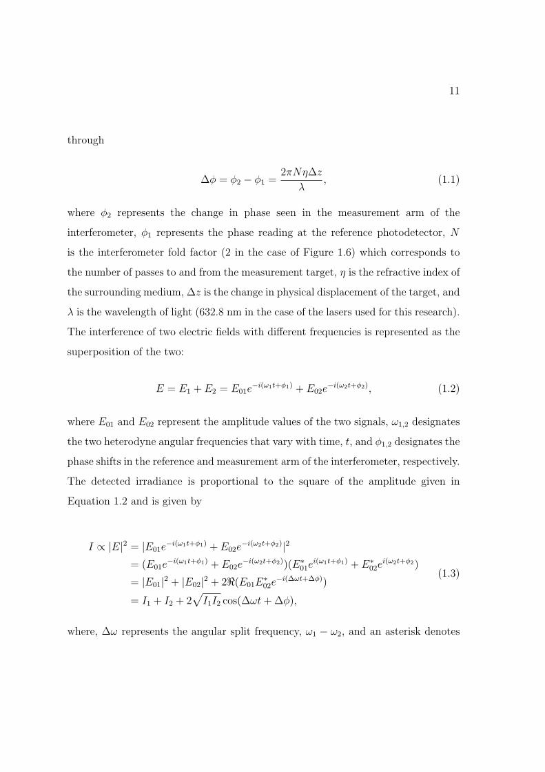
27

be split and fed through two acousto-optic modulators (or AOMs) to create the

heterodyne frequency. A common method of utilizing a spatially separated launch

created by passing through two AOMs is shown in Figure 2.4 and can also be seen

in the full schematic shown in Figure 2.2.

Figure 2.4: Acousto-optic modulators are a convenient technology used to create aheterodyne frequency when a spatially separated launch is desired. The above setupcreates a 70 kHz split frequency when the beams are interfered and the resultingsignals are low-pass filtered.

Acousto-optic modulators utilize a birefringent glass material which is subjected

to an acoustic driving frequency. Light passing through an acoustically driven

medium is deflected at the Bragg angle in addition to increased in frequency in

proportion to the order of the deflected beam. The deflection of incident light is

given by

sin(θ) =mλ

2Λ, (2.1)

in which θ represents the Bragg angles, m = 0,±1,±2, ... is the diffraction order, λ is

the wavelength of incident light, and Λ is the wavelength of the driving acoustic wave.

The acousto-optic modulators used in the multi-DOF interferometer are optimized to

output maximum power in the first order upshifted beam (m = 1). This optimization

is utilized in parallel with the knowledge of how phonons will scatter in response to

28

the acoustic driving frequency. Light scattering into an angle of mθ represents the

interaction of m phonons whose energies are added to the scattered photons. The

change of frequency of incident light as it passes through an acousto-optic modulator

can be written as

∆f =mEphonon

h, (2.2)

where h is Planck’s constant and Ephonon is the phonon energy. It should be noted

that the upshifted frequency is dependent on the diffraction order, m, which can be

seen as a spatial separation of multiple outputs. In the case of m = 1, or the first-

order upshifted beam, the output from the AOM is the incident frequency of light

plus the acoustic driving frequency. Utilizing this concept in addition to two AOMs

driving at slightly different acoustic frequencies is what creates the split frequency in

the multi-DOF interferometer. We know that reference and measurement heterodyne

measurements follow

Ir ∝ Ar cos[2π(f1 − f2)t] and

Im ∝ Am cos[2π(f1 − f2)t+ φz],(2.3)

where Ar and Am are simplified amplitude terms, f1 and f2 are the two first-order

upshifted outputs from two AOMs driving at slightly different frequencies, t is time

and φz is the change in phase as a result of measurement target displacement.

When the reference and measurement signals interfere, Equation 2.3 shows that

the reference and measurement signal are proportional to the cosine of the difference

between the frequencies of the interfering beams. Furthermore, split frequencies are

easily tunable using AOMs. Faster moving stages create higher Doppler shifts which

must be discernible in relation to the heterodyne frequency, f1−f2. If higher Doppler

shifts must be measured, one AOM can simply be switched out for a replacement

29

which drives at a higher acoustic frequency, in turn, increasing the split frequency

of the interferometer. This places additional requirements on the interferometer

detection and signal processing electronics.

2.2 Fiber Optic Coupling

The second critical technology implemented in the multi-DOF interferometer is a

fiber-coupled launch. Fiber-coupled interferometers have a variety of advantages

over free space systems. First, the interferometer is decoupled from the laser,

a significant heat source. Dividing the full system into laser and interferometer

subsystems makes high accuracy measurements more robust. At the beginning of

this chapter it was mentioned that one of the three main error sources that limit

the accuracy of a displacement interferometry system is changes in refractive index.

With fiber-coupled interferometers, the interferometer itself can be isolated in an

environmental containment system and completely separated from the laser heat

source. Furthermore, for applications such as EUV lithography which must operate

in vacuum, fiber-coupled interferometers are ideal because fibers can be easily fed

into the vacuum chamber – as opposed to free space beams being fed through an

entry window.

The other main advantage of fiber-coupled interferometers is the ability to

quickly identify and rectify misalignments. Figure 2.5 demonstrates the effect of

a misalignment in a free-space optical metrology system propagating to all of the

interferometers downstream. The consequence of a propagating misalignment such as

this typically is that a technician must come out to the lithography site to completely

realign the system and all of its components.

30

Figure 2.5: The effect of a misalignment propagating through a free space opticalinterferometry system. (a) An aligned plane mirror system (b) The consequence ofthe denoted misalignment propagates to all interferometers.

Fiber-coupled interferometers, on the other hand, do not suffer from the same

drawback as demonstrated in Figure 2.5. A completely fiber-coupled optical

metrology system creates the ability to more quickly identify and correct individual

misalignments. To expand on this concept, a misalignment in a beamsplitter towards

the beginning of the light stream will not necessarily propagate to one or all of the

interferometers. Furthermore, a misalignment in one interferometer of a multi-DOF

metrology system can be independently isolated and realigned without touching

the rest of the aligned interferometers. The transition to a fiber-coupled optical

metrology system, along with the implementation of multi-DOF interferometers can

be visualized in Figure 2.6.

Also, an additional advantage exists for companies who choose to switch to a

fiber-coupled optical metrology system. The ability to more quickly identify and

rectify misalignments reduces downtime should a misalignment occur. Reduction of

downtime means more product output for the company.

31

Figure 2.6: The transition from a free space interferometry system to a fiber-coupledsetup. (a) Free space system monitoring all six degrees of freedom of a translatingwafer stage. (b) A fiber-coupled metrology system which can still monitor all sixdegrees of freedom. It should be noted that a misalignment in one interferometer canbe independently realigned without touching any of the other aligned interferometers.

Despite the advantages of fiber-coupled optical metrology systems, disadvantages

must be addressed as well. The primary disadvantage is the artificial Doppler shifts

created within the fibers as a result of mechanical and/or thermal stresses. Thermal

and mechanical perturbations manifest themselves as artificial readings if the proper

precautions are not taken in the design of the interferometer as well as in the phase

measurement circuitry. The multi-DOF interferometer utilizes an optical reference

so artificial Doppler shifts which occur in one of the fibers will cancel out at the

measurement and reference photodiodes. In Figure 2.2, these artificial Doppler shifts

are denoted by the θ1 and θ2 terms. Figure 2.7 shows a close-up of the actual

interferometer itself where the artificial signals created in one fiber, for example, will

eventually be read at the reference and measurement photodetectors. The same will

be true for the artificial readings in the other fiber which, again, is split and directed

to the reference and measurement photodetectors. As a result of this setup, no

artificial readings are created because unwanted frequency components will cancel.

32

Figure 2.7: A close-up schematic of the multi-DOF interferometer. Artificial dopplershifts in each fiber may not necessarily be the same; however, this is accounted for byusing an optical reference after the fibers. Since the same artificial signals are seen inthe interference of both beams at both reference and measurement photodetectors,the effects cancel out.

33

Other ways in which artificially created Doppler shifts within the fibers may lead

to errors exist. The SRS-830 lock-in amplifiers which are used to take readings with

the interferometer in this research have a maximum locking frequency of 100 kHz.

Most preliminary measurements were acquired using a 70 kHz split frequency, so if

an artificial frequency component of over 30 kHz is created, the lock-in amplifiers will

not lock and measurements would be disrupted. Furthermore, the phase detection

algorithm must be able to track a constantly moving reference signal. This can be

obtained using methods such as a phase-locked loop, which is a common method of

electronic signal processing for this type of measurement.

In summary, if the architecture of a fiber-coupled interferometer is designed such

that it is symmetric and utilizes an optical reference after the fibers, artificial Doppler

shifts will cancel in the signal processing. This is contingent on the interferometer also

being equipped with the proper phase detection electronics to be able to constantly

track a moving reference signal. Finally, the magnitude of the mechanically or

thermally induced artificial signals must be quantified to make sure that the locking

algorithm which is utilized in phase detection will not lose a lock on the reference

signal. Common perturbations have been extensively quantified by Richard C.G.

Smith, and have been deemed negligible for the low speed measurements that will

be presented at the end of this chapter [31].

2.3 Differential Wavefront Sensing

The technique of Differential Wavefront Sensing (or DWS) was originally proposed

by Morrison, et al. in 1994 for use in the alignment of optical interferometers [32].

The technique has since been experimentally qualified by Muller, et al. in the sub-

34

Rayleigh alignment of laser beams [26]. Differential Wavefront Sensing had only

been utilized for beam alignment until Schuldt, et al. successfully used it to back

out Z-displacement simultaneously with changes in pitch and yaw in the Laser

Interferometer Space Antenna (LISA) prototype system [6]. The resolution limits

that Schuldt and his team were able to achieve were impressive: a 2 pm Hz−1/2

noise floor in translation and a 1 nrad Hz−1/2 noise floor in pitch and yaw. These

noise levels were obtained using a custom FPGA circuit much like the one being

developed for the multi-DOF interferometer in addition to a similar interferometer

architecture. By building from their findings, it is theoretically possible to achieve the

same resolution in vacuum needed to match or exceed the resolution limits currently

needed in wafer stage metrology for the lithography industry.

Figure 2.8: A schematic showing the differences in phase across the differentialwavefront sensor and how they correspond to a pitch or yaw.

The DWS technique uses a quadrant photodiode which is essentially four

photodetectors in a 2x2 array. The spacing between the centroids of the

photodetectors must be known very precisely because it is used in the calculations

of pitch and yaw. Figure 2.7 shows the measurement beam of the interferometer

35

incident on the quadrant photodiode (denoted by DWS) with a tilted wavefront with

respect to the reference beam. By creating a weighted average over all four detectors,

pitch and yaw measurements are created while a Z-displacement measurement is

the global average over all four quadrants. Figure 2.8 demonstrates a simplified

explanation of the phase differentials used to create the angular measurements. In

Figure 2.8a, a characteristically different phase reading in the B and D quadrants

compared to the A and C quadrants is evident. Furthermore, in Figure 2.8b a

difference in phase can be seen in the A and B quadrants compared to the C and D

quadrants. The weighted average is created using

Z − displacement ∝φA + φB + φC + φD

4

Pitch ∝(φA + φB)− (φC + φD)

L1

Y aw ∝(φA + φC)− (φB + φD)

L2

,

(2.4)

where letters symbolize the phase readings in each quadrant and L1 and L2 are

the distances between centroids on the quadrature photodetector. Utilizing this

method, the multi-DOF interferometer is capable of making three degree-of-freedom

measurements using a very small profile on the stage mirror compared to commercial

tip/tilt sensitive displacement interferometers. The multi-DOF interferometer was

qualified against one of these commercial interferometers and those results are

discussed in Chapter 3. Before qualification, however, preliminary results were

recorded to examine the tip/tilt sensitivity of the interferometer. The results are

discussed next.

36

2.4 Preliminary Benchtop Data

The following measurements were obtained using a benchtop setup of the multi-DOF

interferometer. Results were recorded in collaboration with the company InSituTec,

who was interested in utilizing the interferometer for micro-motion stage calibrations.

These measurements were presented at the 27th ASPE Annual Meeting in San Diego,

CA [33].

One of the first preliminary measurements involved running a small piezo

actuation stage (the Physik Instrumente P-611.3S Nanocube®) through a 100 µm

open-loop linear ramp. For this first measurement, only one SRS-830 lock-in

amplifier was available for use, so a single photodetector was used instead of a quad

photodetector. As mentioned, the stage was in open-loop control and therefore was

not expected to move linearly. The results of this experiment are shown in Figure 2.9.

Figure 2.9: First preliminary measurement run using a single photodetector insteadof the quad photodetector. Measured stage was the Physik Instrumente P-611.3SNanocube® and the linear error is within the specifications of the piezo stage.

37

After this first preliminary measurement, three more lock-in amplifiers were

obtained to acquire full three degree-of-freedom measurements. A custom

titanium flexure-based piezo stage was provided by InSituTec (part number

IT.PS.X20.TI.CS.RZ) which contained a built in capacitance sensor and sub-50 pm

positioning resolution. The first test was run with the stage held at a constant voltage

to examine the noise floor of all three degrees of freedom in the interferometer. The

results are shown in Figure 2.10 and were obtained using a sampling frequency of

1 kHz and a final low pass filter at 300 Hz.

Figure 2.10: Preliminary noise measurements conducted on InSituTec’sIT.PS.X20.TI.CS.RZ micro-positioning stage with 300 Hz low-pass filter imple-mented. Stage was held at a constant position. Data axes have been offset forclarity.

The results of Figure 2.10 are encouraging for first measurements and demonstrate

an easily attainable low noise floor obtained in open-loop control. After these

measurements were recorded, the same stage was run in open-loop through a 20 µm

scanning range of motion to demonstrate displacement, pitch and yaw sensitivity.

38

The results are shown in Figure 2.11 and are within the specifications of the stage.

Figure 2.11: Initial measurement of InSituTec’s IT.PS.X20.TI.CS.RZ stage in open-loop scanning; 20 µm, pk-pk of Z-displacement with 0.9 µrad and 0.4 µrad of pitchand yaw motion, respectively.

Finally, the built in capacitance sensor within the piezo stage was utilized

to examine the repeatability and accuracy of Z-displacement measurements.

Measurements were made using a custom linearization algorithm to increase the

accuracy of the stage in closed-loop control. Fifty random steps at random locations

within the 19 µm work volume were performed and the difference between the

internal sensor and the interferometer was calculated after settling. The error is

calculated from a single measurement point (no averaging). Figure 2.12 shows the

result of closed-loop control random steps. Clearly, there are no correlations relating

to the stage position nor the step size, signifying the linearization algorithm is not

showing bias. It is evident that, under its own built-in closed-loop control, the stage

is capable of sub-nanometer positioning. Furthermore, step response repeatability

39

Figure 2.12: Error after settling for 50 random steps of varying sizes and varyinglocations throughout the work volume of InSituTec’s IT.PS.X20.TI.CS.RZ stage.The x-axis designates the initial starting position of the stage while the y-axisdesignates the controlled step size from that initial location. Red error bars representthe interferometer’s measurement error compared to the stage’s built in capacitancesensor. The standard deviation of the error is 0.386 nm over all 50 random steps

was independent of initial stage position and step size, signifying a robust stage

controller and more importantly, an interferometer capable of reliable high-resolution

measurements.

One of the major benefits of this interferometry system is the ability to switch

the acousto-optic modulators to increase the split frequency to accommodate higher

Doppler shifts. The following measurements were run after switching out one of the

AOMs to change the split frequency from 70 kHz to 5 MHz. In doing so, the SRS-830

lock-in amplifiers could no longer be used as they can only lock to a maximum of

100 kHz reference frequency.

In order to record these measurements, Chen Wang, an electrical engineer within

40

the Precision Instrumentation Group created his own custom phasemeter using a

$500 demonstration board. The measured stage was also switched to a stepper

stage with a stated specification of achieving 400 mm/s velocities. This stage was

run in open-loop through a 9 mm range of motion to demonstrate the viability of

high-velocity measurements with the interferometer. The results can be seen in

Figure 2.13.

Figure 2.13: A stepper stage was run in open-loop to demonstrate theinterferometer’s capabilities in high-velocity measurements. One AOM was switchedout to increase the split frequency to 5 MHz in order to accommodate a higherdoppler shift.

Figure 2.13 demonstrates a high dynamic range for the multi-DOF interferometer.

Since one potential application of this research is wafer metrology for the lithography

industry, the capability for high-velocity measurements is extremely valuable. Wafer

stages move at velocities faster than 1 m/s, however, no stage capable of such

41

high speeds was available for measurement. Since no other high-velocity stages

were available for use, the high-speed stepper stage is adequate for a preliminary

demonstration of an AOM-driven tunable split frequency.

2.5 Technology Summary

To conclude, preliminary measurements have provided a solid trajectory for future

work. A high level of tip and tilt sensitivity was observed in the interferometer;

however, with these results alone there is no way to know if the pitch and yaw values

are correct. Towards this end, a qualification of the pitch and yaw measurements of

the interferometer against a commercial system will be provided in Chapter 4.

In terms of Z-displacement, there was a close agreement between the built

in capacitance sensor in InSituTec’s IT.PS.X20.TI.CS.RZ piezoelectric stage and

the multi-DOF interferometer. This tested positioning stage cites a sub-50 pm

positioning resolution and the standard deviation between the interferometer and

the positioning stage over 50 random steps was 386 pm [33].

Creating a split frequency using acousto-optic modulators has been demonstrated

as a very reliable method when a spatially separated launch is desired to minimize

periodic nonlinearity. It is also very simple to create a tunable split frequency

to accommodate higher doppler shifts by switching out one of the AOMs. Fiber

effects on the interferometer have been qualified and deemed negligible if the proper

precautions are taken in the design of the interferometer and phase detection

circuitry.

42

43

3 System Design

One of the most critical design considerations for the multi-DOF interferometer was

thermal sensitivity. When designing a displacement interferometer such as this, it is

important to remember that the tool is used to detect sub-nanometer displacements.

Therefore, a thermal deformation in the assembly could very likely produce a false

measurement. Furthermore, displacement interferometers are alignment sensitive,

meaning a thermal deformation as a result of over-constraining a component could

theoretically produce a deformation which could yield a misalignment and its

resulting effects (non-ideal fringe contrast, periodic nonlinearity, loss of signal).

Mechanical engineering techniques to avoid these consequences tend to evolve into

the field of precision design. A variety of mounting techniques and design principles

exist specifically to tackle thermal problems such as these. Some examples include the

use of kinematic mounts, thermally matching materials so they expand at nominally

the same rates, and most importantly, a critical evaluation of how to apply these

precision engineering principles.

Kinematic mounting in the multi-DOF interferometer was designed using the

principles of a Kelvin clamp [34]. The most important concept involved with this

44

type of mounting is maintaining that the structure is never over-constrained; i.e.,

exactly six degrees of freedom are constrained for a stationary object. A schematic

explaining the two versions of a Kelvin clamp that were used in the multi-DOF

interferometer can be seen in Figure 3.1.

Figure 3.1: Kelvin clamp kinematic mounting schemes to avoid over-constrainedsystems. (a) Three ball in v-groove mounts produce thermal insensitivity about thecenter of the triangle. (b) flat/v-groove/cone mounting scheme keeps the cone pointstationary while allowing the other points expand freely away from that point.

The two variations of the Kelvin clamp were eventually used in the mounting

of fiber collimators at fiber detection sites and in the mounting of the main Invar

optical support structure to a stainless steel base. The designs of both of these

will be elaborated on later in the chapter. A general rule in precision design is to

try to kinematically mount dissimilar materials whenever possible. Slight thermal

expansion is usually inevitable, even in a relatively well controlled laboratory setting

such as the one where the research for this thesis was conducted. The temperature

control in that laboratory was nominally 20 ± 0.5C over one hour. Despite this

45

relatively stable environment, preliminary benchtop testing of the interferometer

using modular components yielded a slight thermal drift. This result can be seen in

Figure 3.2.

0 10 20 30 40 50 60

−30

−20

−10

0

10

20

30

Time [min]

Dis

plac

emen

t [µm

]

0 10 20 30 40 50 60

−30

−20

−10

0

10

20

30

Time [min]

Dis

plac

emen

t [µm

]

Disp −6

−4

−2

0

2

4

6

Rot

atio

n [µr

ad]

−6

−4

−2

0

2

4

6

Rot

atio

n [µr

ad]

YawPitch

Figure 3.2: Preliminary benchtop testing of the interferometer yielded a slightthermal drift over the span of one hour, even though the laboratory is temperaturecontrolled to within 20± 0.5C.

Simple stress analyses were performed on multiple components within the

interferometer, but in general, the assembly will never be subjected to considerably

high stresses. Vibration effects are usually extremely important to quantify for

precision systems; however, this interferometer will typically be used on a vibration

isolation table which will damp resonance effects from outside forces. Despite this,

an evaluation of natural frequencies should not be avoided in any precision system,

and a full vibration analysis will be extremely important in future work.

The system design of the interferometer went through two full iterations before

46

arriving at a satisfactory assembly. Both designs will be presented, the first of

which will only be discussed briefly because it was not manufactured. The decision

to completely redesign the interferometer was based on the capability of a compact

design, which arguably was not fulfilled in the first iteration. Figure 3.3 demonstrates

the transition between iterations of the interferometer.

Figure 3.3: First and second design iterations of the multi-DOF interferometer. Theinterferometer was completely redesigned to achieve a smaller footprint than the firstiteration.

Before both interferometers were designed, a geometrical optical analysis was

conducted to examine the alignment requirements of the beamsplitters. It had

already been hypothesized that cube beamsplitters would produce unwanted ghost

reflections which could contribute to periodic error [35], so the decision was made to

utilize plate beamsplitters with a 30 arcmin wedge to scatter ghost reflections. As can

47

be seen in Figure 3.3, the plate beamsplitters are mounted at a very specific angle

in both iterations. Tight, micrometer-level tolerances were placed on the optical

support structure which was manufactured using Wire-EDM (Electrical Discharge

Machining). The angle between the beamsplitting faces must be 90, however, the

alignment of the beams at the output was still very important and needed to be

simulated. The analysis was done in a Solidworks sketch in which Snell’s law and

the law of reflection were used to determine beam paths for the measurement and

reference signals. Figure 3.4 displays the model in sketch mode. All refraction and

reflection angles are created using driven equations all related back to the original

input angle of the two beams. Figure 3.5 shows the model out of sketch mode after

output beams have been made coincident. It was determined that if the measurement

and reference beams were both launched into the interfereomter with a parallel

orientation, they would overlap collinearly at the output but would be angularly

offset by around 0.5. This angular offset was eventually addressed in the angular

alignment of fold mirrors in the interferometer.

After this basic optical analysis was conducted to simulate beam paths, the

interferometer was designed around the beamsplitter orientations. Due to the

interferometer’s alignment sensitivity, the first design iteration utilized tip/tilt

adjustable kinematic mounting at every launch and fold mirror surface. However,

the consequence of this complicated mounting was that the footprint of the entire

interferometer was much bigger than desired. In the second design iteration of the

interferometer, the launch site was not kinematically mounted which condensed the

design considerably. The first and second design iterations will now be discussed.

Although the first iteration was fully designed, only general figures will be presented

to give a concise overview.

48

Figure 3.4: Beam paths in the interferometer were simulated using a Solidworkssketch. The reference path is overlaid with a dotted orange line and the measurementpath is overlaid with a blue line for clarity. Beamsplitter boundaries are overlaid inred.

49

Figure 3.5: The interferometer Solidworks model out of sketch mode withmeasurement and reference beams made collinear at the output. Beam input spacingwas optimized to be 15.904 mm. The rest of the interferometer was designed aroundthis model.

50

3.1 First Design Iteration

Although the first design iteration was never manufactured, it is still useful to

present design decisions that went into this first interferometer as many of the same

principles were used in the final design. Multiple mechanical design constraints

for interferometer configurations were considered. After evaluating many of the

advantages and disadvantages, the interferometer configuration shown in Figure 3.6

was chosen for the first iteration. Through the month of September, 2012, this first

iteration was designed in Solidworks and is visualized in Figure 3.7. In this section,

each component will be presented and discussed. To begin with, the fold mirror

kinematic mounting assemblies will be presented.

Figure 3.6: The first iteration design of the multi-DOF interferometer was based onthis schematic.

51

Figure 3.7: Solidworks design of the first iteration of the multi-DOF interferometer.Top two images with aluminum casing, bottom two with aluminum casing hidden.Interferometer relies heavily on magnetically preloaded kinematic mounts.

3.1.1 Fold Mirror Kinematic Mounts

The interferometer, as previously stated, is alignment sensitive, which is why the

fold mirrors were not rigidly mounted. Alignment of the launch and detection beams

can be individually adjusted using the feature shown in Figure 3.9.

The mounts were designed using a three point Kelvin clamp to promote thermal

insensitivity. The center image of Figure 3.9 shows the three set screw support

points. The set screws are supplied by Thorlabs and have a M2.5-0.20 thread for fine

adjustment (200 µm of travel per revolution). Supporting the screws are threaded

52

Figure 3.8: First iteration interferometer designating the fold mirror kinematicmounts.

53

Figure 3.9: Left: full kinematic assembly designed to support fold mirrors, Center:Back support plate which contains set screws for tip/tilt adjustment, Right: Mirrorsupport face which magnetically mates to the back support plate.

bronze bushings which press fit into their respective support holes. The set screws

mate to the six dowel pins which lay in machined v-grooves. It can also be seen

in Figure 3.9 that the center and right images are magnetically preloaded with six

neodymium permanent magnets. This structure is capable of fine adjustment in

tip and tilt using the Thorlabs set screws in addition to the capability for fast and

easy assembly and disassembly from using preload magnets. The Kelvin clamp is

designed such that the three set points are rotationally positioned 120 from each

other. The axes of the v-grooves intersect in the middle of the part which happens to

be coincident with the nominal axis at which the incoming laser beam would travel.

This design promotes thermal insensitivity because, as the front mirror support face

expands and contracts relative to the back support as a result of thermal expansion,

for example, the mirror is still nominally held in the same position and will minimally

affect the alignment of an incoming beam. It will be shown in the next section

that this same principle is applied to the kinematic mounting scheme for the fiber

collimators.

54

3.1.2 Mounting Fiber Collimators on the Critical Face

Figure 3.10: Interferometer configuration designating the critical face which is usedto support kinematically mounted fiber collimators.

Before the design of the first iteration, it was determined that the interferometer

configuration shown in Figure 3.10 was advantageous because it is not too wide, and

only requires one critical face for mounting fiber collimator packages. The one critical

face makes the interferometer installation easier than needing access from multiple

sides. The critical face shown in Figure 3.10 uses the same kinematic mounting

principle which was discussed in the previous section to mount the fold mirrors. The

subassembly is shown in more detail in Figure 3.11.

55

Figure 3.11: Top Left and Right: Full critical face subassembly. Bottom Left:Critical face support structure. Bottom Right: Fiber collimator kinematic mountswhich are magnetically preloaded.

From the previous section, all four fiber collimator mounts use the same thermally

insensitive Kelvin clamp mounting scheme to ensure that as the mounts thermally

expand and contract relative to the support structure, the fiber collimators remain

nominally in the same location. All four collimator mounts can also be adjusted

in pitch and yaw using fine pitch set screws in the same fashion the fold mirror

kinematic mounting scheme did. All mounts are magnetically preloaded for easy

and fast assembly and disassembly while still maintaining a strong and stationary

connection. It can be seen in the top right image of Figure 3.11 that the support

structure rigidly mounts to the baseplate of the interferometer with three countersunk

holes. It is critical that this support face be mounted rigidly to the baseplate of

the interferometer, and for that reason, a reinforcing L-bracket was implemented to

further constrain the support structure of the critical face assembly (Figure 3.11) to

56

the baseplate of the interferometer (shown later in Figure 3.16). This L-bracket can

be seen in Figure 3.10 as well.

3.1.3 Kinematic Mounting of Beamsplitting Components

Figure 3.12: Image of the interferometer designating kinematically mountedbeamplitting components.

The interferometer’s beamsplitting components are the most alignment sensitive

parts in the entire assembly. For this reason, the two beamsplitters were designed to

be epoxied to a wire-EDM’ed mounting surface which is then magnetically preloaded

and supported with a 3-point Kelvin clamp using the same working principle of

57

the other kinematic mounts in the first iteration interferometer. The mounting

surface is responsible for holding four critical components: the two beamsplitters,

the stationary reference mirror, and one fold mirror in the reference arm of the

interferometer. A detailed view of the subassembly can be seen in Figure 3.13.

Figure 3.13: Beamsplitter mounting scheme employing Kelvin Clamp for thermalinsensitivity.

The Kelvin clamp mounting principle is more important in this beamsplitter

mount design compared to the fold mirror kinematic mounts and the fiber collimator

kinematic mounts. This is because the mounting surface is wire-EDM’ed Invar,

which has a similar thermal expansion coefficient to Fused Silica, the material of

the beamsplitting components (Invar CTE: 1.2 x 10−6 mm−K

and Fused Silica CTE:

0.55 x 10−6 mm−K

). These two materials are reasonably thermally matched so the

58

epoxied interface will not exhibit too much stress from thermal loading when both

materials expand at different rates. Thermally mismatched materials produce stress

concentrations at the epoxy interface, creating unwanted deformations which can

affect beam quality and/or alignment. Returning to the Kelvin clamp mechanism,

the Invar part will expand at a different rate than the stainless steel support structure

of this subassembly which makes it very critical that the beamsplitting optics remain

nominally in the same location to ensure robust measurements. The Kelvin clamp

achieves this working principle.

If the Invar part and optics were to be assembled, wire-EDM’ed offset plates

would have been used to create the offset from the bottom surface that is seen in

the bottom left image of Figure 3.13. Optics would have been further aligned using

critical faces on the invar part. These critical faces are labeled in Figure 3.14.

Figure 3.14: Invar optical mount designating critical faces for alignment which willbe wire-EDM’ed.

59

As shown in Figure 3.14, the Invar optical mount requires four critical surfaces

with tight tolerances to ensure alignment. In addition to these four critically flat

surfaces, it can be seen that each surface has a corresponding alignment ridge

for constraining lateral motions. The location of the tips of these ridges was

toleranced tightly as well to ensure alignment. Also, a protruding ridge towards

the top of Figure 3.14 maintains that the reference mirror will not be touched if

the interferometer is pushed up to a measurement surface (almost to the point of

contact).

3.1.4 Interferometer Baseplate

The interferometer baseplate is a simple stainless steel structure which has the main

working principle of ensuring complete stiffness to the assembly. The plate is designed

to be manufactured using a 7/16” plate of stainless steel, cut to size. The interface

between the baseplate and critical face which supports the fiber collimators and their

kinematic mounts is reinforced by the L-bracket which can be seen in Figure 3.15

which will also be made of stainless steel. The baseplate on its own can be seen in

Figure 3.16.

On the right image of Figure 3.16 it can be seen that the baseplate is designed

to accommodate socket head cap screws. The screw locations are counter-bored so

they are hidden from view and the interferometer will still lie flat on a surface.

60

Figure 3.15: The interferometer baseplate designated on the full assembly.

Figure 3.16: 7/16” baseplate support for a stiff interferometer.

61

3.2 Second Design Iteration

The same kinematic mounting principles from Figure 3.1 were applied to the second

design iteration of the multi-DOF interferometer. After the first iteration had been

completely designed, the capability for a more compact assembly became apparent.

Some of the components and methodologies from the first design iteration were

used in the second design iteration. The same kinematic mounting scheme for

the fiber collimators (shown in Figure 3.11) is still used in the new interferometer

configuration. In addition, the Invar optical support structure is still kinematically

mounted to a stainless steel base, although the configuration of the mounting was

switched from what is shown in Figure 3.1a to that of Figure 3.1b. Figures 3.17 and

3.18 provide an overview of the final interferometer and design considerations will

be discussed next.

Figure 3.17: The transition from concept to reality in the second design iteration ofthe multi-DOF interferometer. Solidworks model shown.

62

Figure 3.18: A full view of the second iteration of the multi-DOF interferometer.

3.2.1 Fiber Collimator Kinematic Mounts

A goal of the multi-DOF interferometer was to have a completely fiber delivered

and fiber detected system. To achieve this, a fiber detection assembly needed

to be created which had fine tip/tilt adjustment to maximize coupling efficiency.

Thorlabs aspheric fiber collimators were purchased and the kinematic mounts shown

in Figure 3.20 were designed around them. The mounting face was drilled and tapped

for the 11 mm x 0.5 in. mounting thread which the collimators possessed. The same

Kelvin clamping scheme which is seen in every kinematic mount in the first iteration

63

design was used. This Kelvin clamp design is simple to manufacture. As seen in

Figure 3.20, dowel pins rest in v-grooves which are manufactured to a given depth

using a 90 pointed end mill. The fine pitch set screws and their copper threaded

bushings are press fit into a reamed through hole.

Figure 3.19: Fiber collimator kinematic mounts designated on the full assembly.

The only major difference between this kinematic mount and the mounts from

the first iteration design is that preloaded springs have replaced magnets. The

Neodymium magnets that were used in the first iteration were bulky for the preloaded

force they generated. Springs, conversely, provide the same preload force with a

smaller design footprint. These preload springs can be seen throughout the second

64

Figure 3.20: Left: Full kinematic assembly used to mount detection fiber collimators,Center: Front mounting face, Right: Back support face with set screws shown.

design iteration.

The fiber collimator kinematic mounts are connected to the base of the

interferometer via countersunk #8-32 socket head cap screws from the bottom of

the stainless steel base. The countersunk holes in the base of the interferometer are

slotted to allow lateral translation and the mounts themselves can be shimmed to a

variable height if that adjustment is needed.

3.2.2 Fiber Collimator Squeeze Clamps

To achieve a compact design, some of the kinematic mounting from the first design

iteration was eliminated. The replacement mounting fixtures for the fiber launch into

the interferometer became the squeeze clamps which are designated in Figure 3.21.

These clamps were manufactured out of stainless steel and the mounting holes

were drilled with a loose tolerance to allow angular adjustment of the input launch

angle into the interferometer beamsplitters. Figure 3.22 provides an overview of

the mechanical analysis which was run on the fixtures. A finite element model

was created using Solidworks Simlulation Xpress – a linearized finite element tool.

65

Figure 3.21: Fiber collimator squeeze clamps designated on the full assembly.

The clamps were analyzed using a Von Mises stress analysis because the material is

considered ductile since it is designed to yield. The squeeze clamp yields along the

line of highest stress when a force close to 12 lb (53.4 N) is applied. This force value

was deemed a reasonable load for a person to apply using an Allen wrench to tighten

the restraining #4-40 screws which tighten the clamps.

66

Figure 3.22: Von Mises stress analysis performed on the fiber collimator squeezeclamps. The stresses seen in this figure are a result of a 6 lb squeezing force. Thematerial yields when a squeezing force close to 12 lb is applied.

3.2.3 Optical Support Structure

The beamsplitters in the multi-DOF interferometer are made of Fused Silica, and it

was previously noted that this glass material is relatively thermally matched to Invar.

To mitigate thermal effects, the optical support structure which beamsplitters and

fold mirrors are epoxied to was created out of Invar. The critical faces which are used

to align optical components were wire-EDM’ed with micrometer-level tolerances. The

optical support structure needed to accommodate three set screw locations which

give the part variable height and tip/tilt adjustment if required. These set screws

are longer versions of those seen in the fiber collimator kinematic mounts and utilize

the same threaded brass bushings for actuation.

67

Figure 3.23: Optical support structure designated on the full assembly.

Since the Invar part is kinematically mounted to the stainless steel base via

preloaded springs, the stresses as a result of this loading were predicted using a

linearized finite element analysis (Solidworks Simulation Xpress). Each preload

spring produces nominally a 5 lb (22.2 N) restraining force at each of the dowel

pin’s recessed v-grooves. The results of a Von Mises stress analysis can be seen in

Figure 3.24. In this figure it is evident that the induced stresses in the part are

far below the yield strength of Invar so deformations were deemed negligible in that

they would not produce misalignments. Furthermore, any small misalignments from

deformations produced in the optical support structure could still be corrected by

68

adjusting the alignment of the squeeze-clamped launch beams into the interferometer.

The Invar part is mated kinematically to the stainless steel base which will be

discussed next.

Figure 3.24: Stress analysis performed on the Invar optical support structure. Thestresses seen in this figure are a result of a 5 pound preload force from each of thefive springs. The induced stresses are so far below the yield stress of the materialthat deformation was deemed negligible.

3.2.4 Stainless Steel Base

Besides the Invar optical support structure, all additional components are

manufactured using 304 stainless steel for stiffness. Stainless steel is typically

chosen in opto-mechanics applications due to its superior resistance to deformation

compared to aluminum in addition to a lower thermal expansion coefficient.

The stainless steel base mates to the Invar optical support structure via a

69

Figure 3.25: 304 Stainless steel base designated on the full assembly.

kinematic mounting scheme which can be seen in Figure 3.26. This mating scheme

places the ball-in-cone origin of the kinematic mount at a coplanar location compared

to the reference mirror of the interferometer. The result of this placement is that

the optical support structure will tend to expand or contract in the perpendicular

direction from the reference mirror. As a result, the same expansion is seen in the

measurement and reference arms of the interferometer, so they cancel. The flat of the

kinematic mount is made out of tungsten carbide. This material was chosen because

it is harder than the stainless steel set screw which it supports and tungsten carbide

has a lower coefficient of friction on stainless steel when compared to a stainless-

70

Figure 3.26: The stainless steel base of the interferometer mates to the opticalsupport structure via a kinematic mount shown here. The mount is designed tothat thermal expansion produces the same change in length in the measurement andreference arms of the interferometer, thus, they cancel out.

71

steel-on-stainless-steel coefficient. A low coefficient of friction is desired to let the

structure expand and contract freely without producing unwanted deformations in

the Invar material. It is also advantageous that tungsten carbide is harder than

304 stainless steel because deformations will contribute to friction during thermal

expansion.

The base structure has two sets of mounting holes. One set adapts to #8-32

screws from the bottom of the part and the other adapts to 1/4”-20 screws from

the top. As previously mentioned, the countersunk mounting holes which the fiber

collimator kinematic mounts mate to are slotted, allowing for translation.

Figure 3.27: The base support structure of the interferometer and a selected numberof features.

72

3.2.5 Assembly

All discussed parts from the second design iteration were manufactured and

assembled to arrive at a compact working prototype. Special care was taken in

the assembly process to ensure that the interferometer was capable of making

measurements before all components were locked in place using a UV curing adhesive.

In order to do this, the optics on the Invar optical support structure were aligned

and interference signals were monitored as the adhesive was curing. The described

setup is shown in Figure 3.28 in which four interference signals (three from the quad

photodetector and one from the reference channel) can be seen in the background

as the assembly cures. The adhesive used (Dymax OP-4-20632) was designed

specifically for optical component assembly and has a very low coefficient of thermal

expansion for minimal thermal drift.

Figure 3.28: Monitoring interference as the working prototype assembly cures undera UV source.

73

After curing, the optical support structure was mounted to the stainless steel

base using preload springs. The final working assembly can be seen in Figure 3.29.

Figure 3.29: The final assembled prototype of the multi-DOF interferometer.

3.3 Future Design Implementations

After two full design iterations, the multi-DOF interferometer was considered

satisfactory. A qualification of this precision design in comparison to the benchtop

setup and Renishaw’s ML10 displacement interferometer is presented in Chapter 4.

Some changes and additions would enhance the design but are beyond the scope

of this work. A selection of commercial interferometers have a fine yaw adjustment,

so the measurement beam can be easily aligned to a target mirror or retroreflector.

74

A fixture such as this could be designed and attached to the interferometer using

its 1/4”-20 mounting holes. Furthermore, the design of simple inserts which can

be wedged into the fiber collimator mounting locations for optical alignment would

prove advantageous to the interferometer. These types of alignment fixtures are

frequently available with commercial systems.

It was previously mentioned that a vibration analysis was not performed on the

interferometer. This is critical for any precision engineering project, and if time

constraints had allowed, a full vibration analysis would have been performed on

this assembly. Instead, it is left as future work on the interferometer, and in the

meantime, the tool will only be used on vibration isolation tables.

75

4 Interferometer Qualification

Qualification measurements between Renishaw’s ML10 interferometry system, a

benchtop setup of the multi-DOF interferometer and the working prototype from

Chapter 3 were conducted. Qualification measurements between the benchtop

interferometer and the Renishaw system will be presented first, followed by a

discussion of the qualification between the working prototype and the Renishaw

system. It will be shown that an inconsistent scaling factor existed between the two

interferometers and most of the time, the multi-DOF interferometer needed to be

scaled by a factor greater than 1 to increase its tip/tilt sensitivity.

4.1 Benchtop Qualification Measurements

For the qualification of the benchtop interferometer, a micro-positioning stage

(Physik Instrumente P-611.3S Nanocube®) was outfitted with a small plane mirror

target for the multi-DOF interferometer and a differential retroreflector setup for

Renishaw’s ML10 interferometer. The two measurement targets were epoxied on

opposite ends of the translating stage to record the same displacement, pitch and

76

yaw measurements. The first setup implemented was to qualify yaw in the multi-

DOF interferometer against the Renishaw system. The setup of both interferometers

measuring oppposite sides of the same stage can be seen in Figure 4.1.

Figure 4.1: Setup implemented to qualify the benchtop multi-DOF interferometeragainst the Renishaw ML10 interferometer. Left: A full overview of both systems,the Renishaw laser source can be seen at the top of the image. Right: A close upof the Renishaw differential retroreflectors and the multi-DOF target mirror epoxiedto opposite ends of the same stage.

The stage was initially displaced through a 50 µm linear ramp to observe yaw.

As more measurements were recorded, an inconsistent scaling factor became evident

between the interferometers. Yaw readings were less sensitive than the Renishaw

system while pitch measurements seemed to have a higher rotational sensitivity.

Figure 4.2 demonstrates a scaling factor which would continue to vary throughout

further measurements. After the 2.15 scaling factor was observed in Figure 4.2,

the Renishaw beamsplitting optics were slightly rotated to investigate how robust

its measurements were to misalignments. These beamsplitting optics can be seen

77

in Figure 4.1 just before the mounted retroreflectors on the piezo stage. The

beamsplitting portion of the measurement system was rotated in the azimuthal

direction relative to the differential retroreflector setup and was never rotated more

than 1 degree between measurement iterations. The small rotation yielded the results

shown in Figure 4.3 in which the scaling factor was shown to decrease slightly, but

was still significant.

0 5 10 15 20 25 30−2

2

6

10

14

18

Time [s]

Yaw

[µra

d]

0 5 10 15 20 25 30−2

2

6

10

14

18

Time [s]

Yaw

[µra

d]

Multi−DOFMulti−DOF (2.15 scaling)Renishaw

Figure 4.2: Initial scaling factor that was observed between the Renishaw ML10and the multi-DOF interferometer. Figures 4.3 through 4.5 demonstrate how thisscaling factor changed with an azimuthal rotational misalignment of the Renishawbeamsplitters.

Since the scaling factor had decreased with the rotation of the Renishaw

beamsplitters, the same iterative rotations were continued further in the azimuthal

direction to see if the scaling factor would continue to decrease. The interferometer

was rotated twice more and those results can be seen in Figures 4.4 and 4.5. Between

each iteration, again, the beamsplitters were not rotated more than a degree. In

Figure 4.4, it can be seen that the scaling factor does continue to decrease. However,

78

0 5 10 15 20 25 30−2

26

101418

Time [s]

Yaw

[µra

d]

0 5 10 15 20 25 30−2

26

101418

Time [s]

Yaw

[µra

d]Multi−DOFMulti−DOF (2.10 scaling)Renishaw

Figure 4.3: The Renishaw beamsplitter setup which yielded the results in Figure 4.2was subjected to an azimuthal rotational misalignment of less than a degree. Theresulting change in scaling factor is seen here. Noisy data compared to other figuresis due to a lack of an environmental containment box which was incorporated for allother measurements.

when the beamsplitters are rotated once more, the scaling factor increases to 2.20 as

seen in Figure 4.5.

Initially, it was hypothesized that the scaling factor seen in Figures 4.2 through 4.5

was nominally 2 because the interferometer fold factor had not been incorporated

into one of the measurements (multi-DOF or Renishaw). The conversion from a

change in phase to physical displacement contains an interferometer fold factor of 2

which represents a pass to the target mirror and a reflection back. It was unlikely

that Renishaw had left the fold factor out of their signal processing algorithm, so

the multi-DOF algorithm was double checked. Multi-DOF measurements did indeed

incorporate the value of 2, and so the source of the scaling factor was still unknown.

The scaling factor would continue to vary throughout the rest of the qualifying

measurements and would not necessarily stay close to a value of 2.

79

0 5 10 15 20 25 30−2

2

6

10

14

18

Time [s]

Yaw

[µra

d]

0 5 10 15 20 25 30−2

2

6

10

14

18

Time [s]

Yaw

[µra

d]

Multi−DOFMulti−DOF (2.06 scaling)Renishaw

Figure 4.4: The Renishaw system’s beamsplitters were once again subjected to afurther azimuthal rotational misalignment. This misalignment took place betweenthe results of Figure 4.3 and this figure.

0 5 10 15 20 25 30−2

26

101418

Time [s]

Yaw

[µra

d]

0 5 10 15 20 25 30−2

26

101418

Time [s]

Yaw

[µra

d]

Multi−DOFMulti−DOF (2.20 scaling)Renishaw

Figure 4.5: A final azimuthal rotation of Renishaw’s beamsplitting componentsproduced an increase in scaling factor. This result is different from that of Figures 4.2through 4.4 because azimuthal rotations in the same direction had produced adecreasing scaling factor until this point.

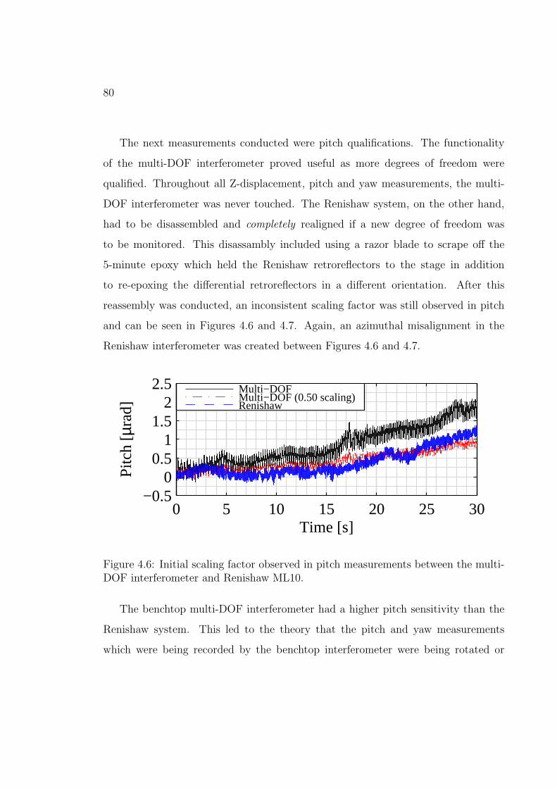
80

The next measurements conducted were pitch qualifications. The functionality

of the multi-DOF interferometer proved useful as more degrees of freedom were

qualified. Throughout all Z-displacement, pitch and yaw measurements, the multi-

DOF interferometer was never touched. The Renishaw system, on the other hand,

had to be disassembled and completely realigned if a new degree of freedom was

to be monitored. This disassambly included using a razor blade to scrape off the

5-minute epoxy which held the Renishaw retroreflectors to the stage in addition

to re-epoxing the differential retroreflectors in a different orientation. After this

reassembly was conducted, an inconsistent scaling factor was still observed in pitch

and can be seen in Figures 4.6 and 4.7. Again, an azimuthal misalignment in the

Renishaw interferometer was created between Figures 4.6 and 4.7.

0 5 10 15 20 25 30−0.5

00.5

11.5

22.5

Time [s]

Pitc

h [µ

rad]

0 5 10 15 20 25 30−0.5

00.5

11.5

22.5

Time [s]

Pitc

h [µ

rad]

Multi−DOFMulti−DOF (0.50 scaling)Renishaw

Figure 4.6: Initial scaling factor observed in pitch measurements between the multi-DOF interferometer and Renishaw ML10.

The benchtop multi-DOF interferometer had a higher pitch sensitivity than the

Renishaw system. This led to the theory that the pitch and yaw measurements

which were being recorded by the benchtop interferometer were being rotated or

81

0 5 10 15 20 25 30−0.5

00.5

11.5

22.5

Time [s]

Pitc

h [µ

rad]

0 5 10 15 20 25 30−0.5

00.5

11.5

22.5

Time [s]

Pitc

h [µ

rad]

Multi−DOFMulti−DOF (0.30 scaling)Renishaw

Figure 4.7: Change in pitch scaling factor as a result of Renishaw beamsplitterazimuthal rotational misalignment. The misalignment was created between theresults obtained in Figure 4.6 and this figure.

rolled somehow before arriving at the quadrant photodiode. To further evaluate

this hypothesis, pitch and yaw were combined and summed in quadrature. This

procedure was not trivial because the Renishaw system could only monitor one degree

of freedom at a time. As a result, pitch and yaw measurements from completely

separate test runs had to be analyzed in quadrature, which could potentially yield

misleading results. Precautions were taken to ensure this analysis was valid; the

piezo stage was never moved, nor the benchtop interferometer ever realigned. The

only inconsistency that existed between preliminary pitch and yaw measurements

was to move the quadrant photodiode closer or further away from the interferometer

to increase the signal in all four quadrants and improve fringe contrast. This had

been performed many times in the past when measurements were being taken with

the multi-DOF interferometer, assuming the distance of the quadrant photodetector

from the actual interferometer would not affect tip/tilt sensitivity. Later in the

82

discussion of these qualifications, it will become evident that changing the quadrant

photodiode location is not necessarily viable to achieve consistent measurements if

interfering wavefronts are not flat.

Essentially random iterations of measurement were combined and summed in

quadrature to see if there was still a scaling factor between interferometers. The

results can be seen in Figures 4.8 through 4.10. Between these three figures, the

scaling factor fluctuates wildly. At times, the nominal scaling factor of 2 from the

initial yaw measurements is evident (Figure 4.8). In other instances, the scaling

factor exceeded a value of 4 (Figure 4.9) and sometimes fell below 1 (Figure 4.10).

0 5 10 15 20 25 300

4

8

12

16

20

Time [s]

Qua

drat

ure

[µrad

]

0 5 10 15 20 25 300

4

8

12

16

20

Time [s]

Qua

drat

ure

[µrad

]

Multi−DOFMulti−DOF (2.10 scaling)Renishaw

Figure 4.8: Pitch and yaw measurements were combined and summed in quadratureto compare the full amplitude of tip/tilt sensitivity between interferometers. Pitchand yaw readings were selected at random as only one degree of rotational freedomcould be monitored at a time using the Renishaw interferometer.

The method of combining and summing pitch and yaw measurements from

both interferometers in quadrature yielded inconsistencies. However, as more pitch

measurements were recorded, it seemed that the qualifications were valid for small

83

0 5 10 15 20 25 300

4

8

12

16

20

Time [s]

Qua

drat

ure

[µrad

]

0 5 10 15 20 25 300

4

8

12

16

20

Time [s]

Qua

drat

ure

[µrad

]

Multi−DOFMulti−DOF (4.20 scaling)Renishaw

Figure 4.9: Further comparison of random pitch and yaw data combined and summedin quadrature yielded a varying scaling factor.

0 5 10 15 20 25 300

4

8

12

16

20

Time [s]

Qua

drat

ure

[µrad

]

0 5 10 15 20 25 300

4

8

12

16

20

Time [s]

Qua

drat

ure

[µrad

]

Multi−DOFMulti−DOF (0.75 scaling)Renishaw

Figure 4.10: Pitch and yaw data combined and summed in quadrature sometimescreated qualifications between interferometers which could not be accurately scaled.

84

rotations. Still measuring pitch with the Renishaw system, the same piezo stage was

run through a low amplitude sine wave and the corresponding pitch values agreed

very well between interferometers. This result can be seen in Figure 4.11.

0 5 10 15 20 25−2

−1

0

1

2

3

Time [s]

Pitc

h [µ

rad]

0 5 10 15 20 25−2

−1

0

1

2

3

Time [s]

Pitc

h [µ

rad]

Multi−DOF (no scaling)Renishaw

Figure 4.11: Qualifications between interferometers may be valid for small rotations.The data in this figure is one such example.

Before investigating the source of the inconsistent scaling factor further, the

Renishaw system was assembled to record Z-displacements (benchtop interferometer

was not touched). Z-displacement qualifications between interferometers agreed

within a micrometer for a linear ramp and sine wave. Refer to Figures 4.12 and

4.13 to observe a qualification between the two. The sub-micrometer agreement

between results is expected; the quadrant photodiode is essentially four displacement

interferometers measuring the same nominal change in phase across a wavefront, so

the global average over all four detectors was expected to yield relatively reliable

results. The calculation of pitch and yaw involves a weighted average, mentioned in

Chapter 2, which is probably not as consistent.

The errors in Figures 4.12 and 4.13 are attributed to cosine error. Cosine error is

85

0 5 10 15 20 250

20

40

60

80

100

Time [s]

Z−

Dis

plac

emen

t [µm

]

0 5 10 15 20 250

20

40

60

80

100

Time [s]

Z−

Dis

plac

emen

t [µm

] Multi−DOF (no scaling)Renishaw

−0.5

0

0.5

1

Err

or [µ

m]

−0.5

0

0.5

1

Err

or [µ

m]

Error

Figure 4.12: The qualification of Z-displacement between interferometers had amaximum error of about 0.5 µm over a 85 µm ramp.

0 5 10 15 20 25−30

−20

−10

0

10

20

30

40

Time [s]

Z−

Dis

plac

emen

t [µm

]

0 5 10 15 20 25−30

−20

−10

0

10

20

30

40

Time [s]

Z−

Dis

plac

emen

t [µm

] Multi−DOF (no scaling)Renishaw

−2

−1

0

1

2

Err

or [µ

m]

−2

−1

0

1

2

Err

or [µ

m]

Error

Figure 4.13: The qualification of Z-displacement between interferometers was alsovalid to within ± 0.75 µm for a sine wave.

86

created when the axis of the measurement beam is not parallel to the axis of motion

of the stage. The end result is the stage displaces at a slight angle relative to the

optical measurement axis, and thus, the interferometer records a cosine component of

the actual displacement taking place. A schematic explaining this concept is shown

in Figure 4.14. In reference to Figure 4.12, the maximum error reading was nominally

500 nm. The result of a cosine error calculation over a 85 µm range of motion yields

cos−1(85 µm/85.5 µm) = 6.2. If we consider that this error could occur in either

the Renishaw system or the benchtop multi-DOF system, approximately 3 of cosine

error per interferometer is within reason for nominal alignment given the relatively

short travel range of the piezo stage.

Figure 4.14: The errors in Figures 4.12 and 4.13 are attributed to cosine error. Theeffect of cosine error is that one or both interferometers measure a cosine componentof the actual displacement taking place.

Up until this point the quadrant photodiode had been moved slightly closer or

farther away from the interferometer to optimize signal output in all four quadrants.

To minimize all variables, the quadrant photodiode was held at a constant location for

87

the succeeding measurements. In addition to this, a focusing lens was implemented

before the quadrant photodiode which had been previously demonstrated to increase

fringe contrast in each of the quadrants. The focusing lens was used to focus the

light to a point, and then as it was expanding past this point, the wavefront was

captured on the quadrant detector when the beam radius was slightly larger (by

about 0.25 mm) than the size of the quadrant detector. Overfilling the detector like

this should not have affected results as the wavefront tilt angle should theoretically

be constant, regardless of the size of the beam diameter. It would soon be realized

that this was only true for flat wavefronts, which also is an assumption made in pitch

and yaw calculations when using the quadrant photodiode [26].

Utilizing this setup, pitch and yaw qualification measurements produced an

interesting phenomenon, they were all scaled by exactly 3.325. Figures 4.15 through

4.17 are the result of repeated yaw measurements while rotating the Renishaw

beamsplitters between iterations in the azimuthal direction. Azimuthal rotations no

longer produced a slight change in scaling factor as was seen in Figures 4.2 through

4.4. The 3.325 scaling factor was surprisingly robust and still held true for a sine

wave (shown in Figure 4.18).

At this point, the Renishaw system was again completely disassembled,

reassembled and realigned to record pitch measurements. The focusing lens and

quadrant photodiode were not touched. The scaling factor of 3.325 was again valid

for pitch measurements, and results can be seen in Figures 4.19 and 4.20 in which

the Renishaw beamsplitting optics were rotated in the azimuthal direction between

measurements. A sine wave yielded the results shown in Figure 4.21 in which the

3.325 scaling factor was still consistent.

The 3.325 scaling factor was robust through the measurements made in

88

0 5 10 15 20 25 3005

1015202530

Time [s]

Yaw

[µra

d]

0 5 10 15 20 25 3005

1015202530

Time [s]

Yaw

[µra

d]

Multi−DOFMulti−DOF (3.325 scaling)Renishaw

Figure 4.15: Utilizing one focusing lens before the quadrant photodiode, a scalingfactor of 3.325 was created which was valid for all Renishaw measurements despitebeamsplitter azimuthal rotational misalignments.

0 5 10 15 20 25 3005

1015202530

Time [s]

Yaw

[µra

d]

0 5 10 15 20 25 3005

1015202530

Time [s]

Yaw

[µra

d]

Multi−DOFMulti−DOF (3.325 scaling)Renishaw

Figure 4.16: First iteration of an azimuthal rotational misalignment on Renishawsystem beamsplitters: 3.325 scaling factor is still valid between interferometers.

89

0 5 10 15 20 25 3005

1015202530

Time [s]

Yaw

[µra

d]

0 5 10 15 20 25 3005

1015202530

Time [s]

Yaw

[µra

d]

Multi−DOFMulti−DOF (3.325 scaling)Renishaw

Figure 4.17: Second iteration of an azimuthal rotational misalignment on Renishawsystem beamsplitters: 3.325 scaling factor is still valid between interferometers.

0 5 10 15 20 25−10−6−2

26

10

Time [s]

Yaw

[µra

d]

0 5 10 15 20 25−10−6−2

26

10

Time [s]

Yaw

[µra

d]

Multi−DOFMulti−DOF (3.325 scaling)Renishaw

Figure 4.18: Utilizing one focusing lens before the quadrant photodiode, the 3.325scaling factor is valid between interferometers for a sine wave.

90

0 5 10 15 20 25 30−2

0

2

4

6

Time [s]

Pitc

h [µ

rad]

0 5 10 15 20 25 30−2

0

2

4

6

Time [s]

Pitc

h [µ

rad]

Multi−DOFMulti−DOF (3.325 scaling)Renishaw

Figure 4.19: Still utilizing one focusing lens before the quadrant photodiode, pitchmeasurements agreed between interferometers with a 3.325 scaling factor as well.

0 5 10 15 20 25 30−2

0

2

4

6

Time [s]

Pitc

h [µ

rad]

0 5 10 15 20 25 30−2

0

2

4

6

Time [s]

Pitc

h [µ

rad]

Multi−DOFMulti−DOF (3.325 scaling)Renishaw

Figure 4.20: The Renishaw interferometer’s beamsplitters were subjected to anazimuthal rotational misalignment after the data from Figure 4.19 was taken. Theresult still obeys the 3.325 scaling factor between interferometers.

91

0 5 10 15 20 25

−2

0

2

4

Time [s]

Pitc

h [µ

rad]

0 5 10 15 20 25

−2

0

2

4

Time [s]

Pitc

h [µ

rad]

Multi−DOFMulti−DOF (3.325 scaling)Renishaw

Figure 4.21: The qualification measurements for a sine wave were consistent witha 3.325 scaling factor. These results still utilize a focusing lens and quadrantphotodiode location that is the same as that in the results of Figure 4.15.

Figures 4.15 through 4.21; however, the value of 3.325 seemed to be somewhat

arbitrary. A factor of 2 could have made sense given the interferometer fold factor

of 2 which is supposed to be incorporated into the conversion from phase to physical

displacement, but a factor of 3.325 did not make sense.

The eventual conclusion was that the scaling value of 3.325 had been correcting

for an imperfect wavefront (imperfect in that it was not flat). The method of

using a single focusing lens to overfill the quadrant photodiode was producing

interfering wavefronts with spherical shapes. Flat collimated wavefronts are desired

for consistent measurements; otherwise, a change in the distance of the quadrant

photodetector from the interferometer would theoretically produce different results

as the measured phase in all four quadrants would not be consistent. To test this

theory, the quadrant detector was moved closer to the focusing lens, and as expected,

the scaling factor changed. This result can be seen in Figures 4.22 and 4.23. The

92

interferometer was already set up to record pitch, so those measurements were used to

demonstrate the inconsistencies produced from a spherical wavefront. It is expected

that the same change in scaling factor under the same changing circumstances would

be seen in yaw as well.

0 5 10 15 20 25−2

0

2

4

Time [s]

Pitc

h [µ

rad]

0 5 10 15 20 25−2

0

2

4

Time [s]

Pitc

h [µ

rad]

Multi−DOFMulti−DOF (1.40 scaling)Renishaw

Figure 4.22: Still utilizing a single focusing lens, the location of the quadrantphotodetector was moved to prove that the focusing lens was producing a sphericalwavefront. This wavefront creates inconsistent pitch and yaw scaling factorsdepending on the location of the quadrant photodetector.

To correct for the errors associated with slightly spherical wavefronts on the

photodetector, the expanding lens was replaced with a two lens telescope which

expanded the beam at a 2:1 ratio to overfill the detector. The telescope produced a

much more collimated output than was seen with the single expanding lens. With

the implementation of the telescope, the data seen in Figures 4.24 through 4.26 are

produced, unfortunately with a fluctuating scaling factor again.

Measurements in Figure 4.24 were nominally close with no scaling; however, the

benchtop multi-DOF interferometer seemed to observe a linear increase in pitch while

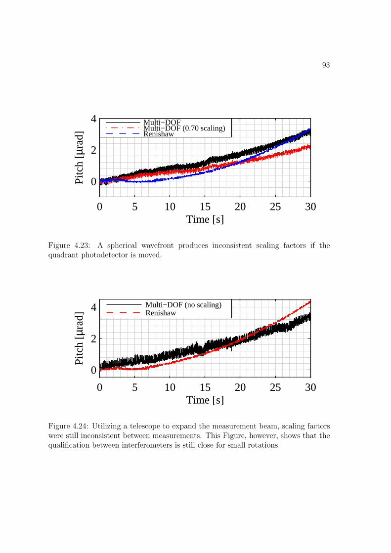
93

0 5 10 15 20 25 30

0

2

4

Time [s]

Pitc

h [µ

rad]

0 5 10 15 20 25 30

0

2

4

Time [s]

Pitc

h [µ

rad]

Multi−DOFMulti−DOF (0.70 scaling)Renishaw

Figure 4.23: A spherical wavefront produces inconsistent scaling factors if thequadrant photodetector is moved.

0 5 10 15 20 25 30

0

2

4

Time [s]

Pitc

h [µ

rad]

0 5 10 15 20 25 30

0

2

4

Time [s]

Pitc

h [µ

rad]

Multi−DOF (no scaling)Renishaw

Figure 4.24: Utilizing a telescope to expand the measurement beam, scaling factorswere still inconsistent between measurements. This Figure, however, shows that thequalification between interferometers is still close for small rotations.

94

0 5 10 15 20 25−2

0

2

4

6

Time [s]

Pitc

h [µ

rad]

0 5 10 15 20 25−2

0

2

4

6

Time [s]

Pitc

h [µ

rad]

Multi−DOFMulti−DOF (1.70 scaling)Renishaw

Figure 4.25: No components were touched between the measurements taken inFigure 4.24 and 4.25. The qualification between interferometers is close to within amicroradian without scaling.

0 5 10 15 20 25

4

12

20

28

Time [s]

Yaw

[µra

d]

0 5 10 15 20 25

4

12

20

28

Time [s]

Yaw

[µra

d]

Multi−DOFMulti−DOF (5.0 scaling)Renishaw

Figure 4.26: Scaling factor between interferometers using an expanding telescopeincreased to as high as 5.

95

the Renishaw system observed a quadratic increase. Corrections between trends of

different orders such as these can not be corrected using a single scaling factor.

Without touching either interferometer, pitch measurements were recorded over

a sine wave in which a 1.70 scaling factor was apparent (Figure 4.25). Finally,

the Renishaw system was completely disassembled and reassembled to record yaw

measurements, and an unprecedented scaling factor of 5 was observed (Figure 4.26).

These results do not create any discernable trajectory – as far as scaling factors

or corrections go – to arrive at a better agreement between interferometers. The

working prototype of the multi-DOF interferometer was being assembled in parallel

with the presented benchtop qualification measurements. Theoretically, the same

inconsistent scaling factor should be evident in the prototype qualification against

the Renishaw system, and those results are presented next.

4.2 Working Prototype Qualification

The assembled working prototype of the multi-DOF interferometer (discussed in

Chapter 3) was qualified against the RenishawML10 to test functionality. The results

of the benchtop qualification were obtained by displacing a small micro-positioning

stage (Physik Instrumente P-611.3S Nanocube®) through a normal translational

range of motion and the detected rotational errors were within the specifications of

the stage. For the prototype qualification, the Aerotech FiberMax® 5-axis servo

positioning stage was utilized for an additional check to ensure measurements were

valid. When a 0.01 yaw command was given to the FiberMax®, the Renishaw

system detected this range of motion extremely well; the multi-DOF working

prototype on the other hand, did not. This result builds on the findings from the

96

previous section in that the Renishaw system is now evidently more reliable than the

multi-DOF interferometer. Figure 4.27 shows three snapshots of the qualification

setup used to measure the FiberMax® stage from opposite ends.

Figure 4.27: The working prototype of the multi-DOF interferometer was qualifiedagainst the Renishaw ML10 using the Aerotech FiberMax® 5-axis servo positioningstage. Top Left: Overview of both systems measuring opposite ends of the stage.Bottom Left: The environmental containment system used to mitigate changesin refractive index. Right: The view from the multi-DOF working prototype inqualification measurements.

The results of a Z-displacement qualification were in close agreement between

interferometers. Prior to measurement, a CCD camera was attached to the

translating stage and the multi-DOF interferometer was aligned as well as possible

to the axis of stage displacement. The Renishaw system was also aligned to the

97

axis of displacement using the alignment fixtures provided with the interferometer.

This method of aligning using plastic inserts with the Renishaw system is not as

accurate as using a CCD array, however, this procedure was not performed in

benchtop qualification measurements and thus results are expected to be in closer

agreement. Results of a 45 mm ramp can be seen in Figure 4.28. The final

disagreement between interferometers reached as high as 329.1 µm. Although this

disagreement is discouraging, the final reading of the multi-DOF working prototype

was 44.6588 mm while the Renishaw ML10 read a 44.3297 mm final displacement.

Therefore, the multi-DOF interferometer was in closer agreement to the servo reading

of the FiberMax® which recorded a final displacement of 45.0000 mm.

0 5 10 15 20 25 30 35 400

10

20

30

40

Time [s]

Z−

Dis

plac

emen

t [m

m]

0 5 10 15 20 25 30 35 400

10

20

30

40

Time [s]

Z−

Dis

plac

emen

t [m

m]

Multi−DOF (no scaling)Renishaw

050100150200250300350400

Err

or [µ

m]

050100150200250300350400

Err

or [µ

m]

Error

Figure 4.28: 45 mm linear ramp qualification between the Renishaw ML10 andthe working prototype of the multi-DOF interferometer. The final displacementreading of the working prototype was 44.6588 mm while the Renishaw ML10 reada 44.3297 mm final displacement. The built in servo sensor of the measured stagerecorded a 45.0000 mm final displacement, thus, the multi-DOF interferometer wasin better agreement than the Renishaw ML10.

98

The stage was also run through a 0.01 range of motion (approximately 175 µrad)

to qualify yaw between interferometers. The results can be seen in Figure 4.29 in

which a scaling factor is still evident. Although the exact source of the scaling is not

known, the findings presented in the qualification of the benchtop system against the

Renishaw ML10 demonstrate a possible source of error from imperfect (or not flat)

interfering wavefronts. To test this theory, the quadrant photodiode was overfilled

at a ratio of 6:1 using a two lens system. Overfilling the detector in this fashion

ensures that only the center portions of both gaussian beams are detected, and thus

maintains that detected wavefronts are as flat as possible. The results can be seen

in Figure 4.30 in which the rotational sensitivity of the interferometer was greatly

reduced, presumably because so much information was discarded and not factored

into the weighted average.

0 5 10 15 20 25−180

−140

−100

−60

−20

20

Time [s]

Yaw

[µra

d]

0 5 10 15 20 25−180

−140

−100

−60

−20

20

Time [s]

Yaw

[µra

d]

Multi−DOFRenishaw

Figure 4.29: An inconsistent scaling factor persisted in yaw qualifications betweenthe multi-DOF working prototype and the Renishaw ML10.

99

0 5 10 15 20 25−180

−140

−100

−60

−20

20

Time [s]

Yaw

[µra

d]

0 5 10 15 20 25−180

−140

−100

−60

−20

20

Time [s]

Yaw

[µra

d]

Multi−DOFRenishaw

Figure 4.30: Overfilling the detector drastically reduces tip/tilt sensitivity. Thederived weighted average equation used to calculated pitch and yaw assumes flatwavefronts. Overfilling the detector maintains that the incident wavefronts areapproximately flat in that the detected irradiance is a result of the center ofinterfering gaussian beams.

4.3 Qualification Analysis

The inconsistencies in scaling factors between the Renishaw ML10 and the multi-

DOF interferometer are erratic. Despite this, progress was still made towards more

robust and reliable measurements. It is already evident that Z-displacements agree

relatively well between interferometers (Figures 4.12, 4.13 and 4.28). Furthermore, it

appears that under controlled conditions in which all components of the multi-DOF

interferometer are locked in place, measurements can be calibrated with a scaling

factor to achieve valid results (the 3.325 scaling factor in Figures 4.15 through 4.21).

The scaling factor of 3.325 seemed to be correcting for a spherical wavefront being

produced by the focusing lens in addition to any other sources of error.

In future work, the derivation used to arrive at the pitch and yaw weighted

100

average equations will need to be examined to ensure the rotational measurements it

yields are traceable to length and thus angle. More investigation into how pitch and

yaw are calculated is needed because it seems odd that Z-displacement qualifications

between interferometers are so exceptional while pitch and yaw qualifications are

inconsistent. The original expression presented by Muller, et al. [26] to determine

the intensity in one quadrant of a circular quadrant photodiode is

I1 = 2|E1E2|

∫ R

0

∫ π

4

−π

4

r(

e−2r

2

ω20

)

cos(βkr cos θ − ωt)dθdr, (4.1)

where β is the tilt angle between wavefronts and is less than 1, r and θ are cylindrical

coordinates on the quadrant photodiode’s surface and k = 2πλ. Since the quadrant

detector used for this research is square, Equation 4.1 needs to be converted to

Cartesian coordinates before being evaluated. The weighted average discussed in

Chapter 2 that is used to calculate pitch and yaw was also used by Schuldt, et al.

in the calculations used for the LISA project [6]. The integral given in Equation 4.1

will be reevaluated in future work to assess the validity of the weighted average for

the specific quadrant detector used in this research. In parallel with a background

investigation of this calculation, many more qualification measurements will need to

be recorded, especially with interferometers other than the Renishaw ML10.

As a complement to the work discussed in this thesis, Richard C.G.

Smith has provided a working analytic simulation for multi-DOF interferometer

measurements [31]. Preliminary simulation results demonstrate a scaling factor

dependence on detected beam diameter and possibly beam curvature. For small

yaw ranges of motion, as seen in Figure 4.29, his simulation produces a 1.2388

scaling factor for the multi-DOF interferometer. Implementing this scaling factor

into previously discussed results yields a close agreement between interferometers.

101

The implemented scaling factor can be seen in Figure 4.31.

0 5 10 15 20 25−180

−140

−100

−60

−20

20

Time [s]

Yaw

[µra

d]

0 5 10 15 20 25−180

−140

−100

−60

−20

20

Time [s]

Yaw

[µra

d]

Multi−DOFRenishawMulti−DOF (1.2388 scaling)

Figure 4.31: Preliminary analytical simulations of the multi-DOF interferometernaturally produce the scaling factor required for agreement between the RenishawML10 and the multi-DOF system.

The analytical simulation clearly has a lot of potential for reliable multi-DOF

interferometer measurements. The model is still being developed but seems to be on

the right path towards identifying the source of the inconsistent scaling factor.

102

103

5 Periodic Nonlinearity

The three main error sources that limit the performance of a displacement

interferometry system are the laser frequency stability [27], refractive index

fluctuations in non-common optical paths [4], and periodic nonlinearity in the

measured phase [16, 19, 28]. This chapter is mainly concerned with the third source

of error – periodic nonlinearity (or PNL for the remainder of this discussion).

Polarization encoded interferometers frequently exhibit PNL in which the resolution

of the interferometer is typically limited to 1-5 nanometers [16]; however, resolution

limits could potentially exceed 25 nm under severe system misalignments [18]. A

schematic of the effect of PNL on a linear ramp is shown in Figure 5.1. Ideally, what

an interferometer measures is linearly proportional to the physical displacement of the

target stage. However, under the effects of PNL, a nonlinearity with a periodicity of

one cycle per 2π change in optical path length is superimposed on top of the ideally

linear output. In its simplest principles and for all intents and purposes of this

discussion, PNL is a consequence of signal cross-talk between different frequencies

of linearly polarized beams. Although the discussion of PNL in this thesis will

concentrate primarily on its effect on heterodyne systems, it is important to note that

104

PNL can exist in homodyne interferometers as well [36–38]. Thus PNL is an effect

created as a consequence of using polarization encoded signals, not heterodyning.

Figure 5.1: A typical effect of periodic nonlinearity on a measured linear ramp.Periodic nonlinearity typically results in 1-5 nm of error, but there are techniqueswhich can be implemented to avoid this result. Axes are displayed in terms ofwavelength.

Periodic nonlinearity was first observed by Quenelle [16] and was soon after

demonstrated experimentally by Sutton [17] using the pressure scanning technique.

These two authors paved the way for the first full mathematical derivation of the

PNL phenomenon which was presented by Rosenbluth and Bobroff [20]. Their

derivation of optical sources of PNL was conducted using the heterodyne Michelson

interferometer very similar to the one shown in Figure 5.2. Many other authors have

theoretically evaluated sources of PNL [21, 28, 36, 39–41]. All of these theoretical

analyses have been conducted using the same Michelson setup (Figure 5.2); however,

DeFreitas and Player [28] have laid the foundation for examining sources of PNL in

105

setups that differ from the classical Michelson orientation. Their paper provides a

detailed analysis of the polarization effects which lead to PNL in addition to outlining

the derivation required to predict PNL in custom interferometer configurations using

Jones Calculus. Before discussing the PNL that was observed with the multi-DOF

interferometer, a detailed outline of the phenomenon pertaining to the Michelson

interferometer will be discussed.

5.1 The Michelson Interferometer

The primary source of error in this discussion of periodic nonlinearity is a result of

optical mixing. Optical mixing is further distinguished into two categories, namely

polarization mixing and frequency mixing, depending on the mechanism by which

the optical mixing was created [15]. These two sources of PNL both occur in the

simple heterodyne Michelson interferometer which has been previously discussed and

is shown in Figure 5.2.

Figure 5.2: The common heterodyne Michelson interferometer which is typicallysubjected to polarization mixing and frequency mixing.

106

In Figure 5.2, polarization mixing typically occurs before the linearly polarized

and mutually orthogonal beams at frequencies f1 and f2 enter the polarizing

beamsplitter. Polarization mixing is a result of a slight ellipticity of the two nominally

linearly polarized output states. Furthermore, the mutually orthogonal output

states are never perfectly orthogonal, which leads to additional polarization mixing.

Frequency mixing, on the other hand, occurs as the two beams pass through the

polarizing beamsplitter in Figure 5.2. Ideally, the polarizing beamsplitter splits both

polarization states so that one frequency is present in each arm of the interferometer.

In practice however, the separation of polarizations is imperfect, leading to a small

portion of an unwanted frequency component in each arm of the interferometer

(Figure 5.3). Both forms of optical mixing result in the interference of heterodyne

signals before it is desired. These effects can largely be avoided by spatially separating

polarization states and avoiding the use of polarizing optics [10], but those corrections

will be discussed in a later section of this chapter.

Figure 5.3: Interferometer showing optical mixing.

107

Other effects tend to create PNL in all displacement interferometry systems and are

not limited to the Michelson orientation. Optical misalignments can contribute to

the effect [18] as well as ghost reflections off normal surfaces [24]. To summarize all

potential PNL pitfalls, the primary sources of optical mixing include the following:

• Ellipticity of linearly polarized beams

• Optical misalignments within the system

• Imperfect beamsplitting optics

• Ghost reflections

• Non-orthogonality of linearly polarized incident beams

The Michelson interferometer has long been the industry standard in the field of

optical metrology due to its simplicity [12, 13]. The standard is changing, however,

in an effort to eliminate errors such as periodic nonlinearity which are tough to avoid

in the heterodyne Michelson configuration. Custom configurations have since been

developed that limit the chances of PNL; for examples, see references [9, 10, 24, 25].

The multi-DOF interferometer is one such interferometer which utilizes a spatially

separated launch and avoids using polarizing optics to reduce the chances of PNL.

A mathematical derivation of the multi-DOF interferometer’s PNL using Jones

Calculus is the subject of future work and can be performed using the outline

proposed by De Freitas and Player [28]. In the following section, however, a

theoretical derivation PNL within the Michelson setup is provided. The following

derivation has been appended from Bobroff [15] and Badami [42].

108

5.2 Theory

We refer to Figure 5.3 to observe the effects of optical mixing. The amplitudes

of the interferometer’s nominal signals are denoted by Am and Ar to represent the

measurement and reference arms, respectively. Unwanted frequency leakage into both

arms of the interferometer is designated by amplitudes αm and αr to denote leakage

signals into the measurement and reference arms, respectively. Although the ideal

interferometer has only two interfering signals, the actual output as a consequence

of optical mixing has four components. With this in mind, the resulting intensity

output at the measurement photodetector is proportional to

I ∝ |E|2 = |Ame−i(ω1t+∆φ1)+Are

−i(ω2t+∆φ2)+αme−i(ω2t+∆φ1)+αre

−i(ω1t+∆φ2)|2. (5.1)

We can expand Equation 5.1 to yield

I ∝ |E|2 = |Am|2 + |Ar|

2 + |αm|2 + |αr|

2

+ 2<

AmA∗

re−i(∆ωt+∆φ) + (Amα

∗

m + A∗

rαr)e−i(∆ωt)

+ α∗

mαre−i(∆ωt−∆φ) + (Amα

∗

r + A∗

rαm)ei(∆φ)

,

(5.2)

where an asterisk superscript represents the complex conjugate, ∆ω denotes the

angular split frequency of the interferometer and ∆φ represents changes in the optical

path difference between the reference and measurement arm of the interferometer.

This phase change, ∆φ, is related to the corresponding change in physical path length

by

∆φ =2πN∆x

λ, (5.3)

109

where N is the interferometer fold factor. In Equation 5.2 the |Am|2 + |Ar|

2 +

|αm|2 + |αr|

2 term represents a constant DC offset. The AmA∗

re−i(∆ωt+∆φ) portion

of the equation represents the nominal signal of the interferometer and the terms

(Amα∗

m + A∗

rαr)e−i(∆ωt) and α∗

mαre−i(∆ωt−∆φ) are the undesired mixing terms at the

split frequency, ∆ω, that cause periodic nonlinearity in the measured signal. Finally,

the (Amα∗

r + A∗

rαm)ei(∆φ) portion of the equation can be described as a homodyne

modulation term which is assumed to be near-DC. Using a bandpass filter, we can

remove the signal offset and homodyne modulation components to describe the AC

intensity variation at an arbitrary split frequency by

IAC ∝ <

(AmA∗

re−i∆φ + Amα

∗

m + A∗

rαr + α∗

mαrei∆φ)e−i∆ωt

. (5.4)

It is convenient to normalize all signals from Equation 5.4 to the nominal signal,

resulting in

IAC ∝ <

(Ω0e−i∆φ + Ω1 + Ω2e

i∆φ)AmA∗

re−i∆ωt

, (5.5)

where Ω0,Ω1 and Ω2 now represent amplitudes of interference terms relative to the

nominal AC signal,

Ω0 = 1

Ω1 =α∗

m

A∗

r

+αr

Am

Ω2 =α∗

mαr

AmA∗

r

.

(5.6)

If we now take the real part of Equation 5.5, we arrive at

IAC ∝ Ω0 cos(∆ωt+∆φ) + Ω1 cos(∆ωt) + Ω2 cos(∆ωt−∆φ), (5.7)

110

where the second and third terms of Equation 5.7 are sources of first and second

order periodic error, respectively. Equation 5.7 becomes the fundamental expression

which can be used to model periodic nonlinearity in the Michelson interferometer.

First order error is represented with the Ω1 amplitude and this will be assumed to be

the dominate source of periodic nonlinearity. A phasor diagram is a convenient way

to visualize how Equation 5.7 manifests itself as an oscillating signal superimposed

on top of the nominal change in phase. Equation 5.7 can be expanded into

quadratures using the sum and difference formulas of the cosine identity, i.e.

cos(A±B) = cos(A) cos(B)∓ sin(A) sin(B). The result yields

cos(∆ωt±∆φ) = cos(∆ωt) cos(∆φ)∓ sin(∆ωt) sin(∆φ). (5.8)

If we associate each quadrature – cos(∆ωt) and sin(∆ωt) – with the X and Y axes

of a Cartesian coordinate system, the phasor diagrams in Figure 5.4 are created

which represent the nominal signal (Figure 5.4a) and first-order periodic nonlinearity

(Figure 5.4b). It can be seen in Figure 5.4b that as the nominal measurement signal

tracks through a full 360 change in phase, the first order periodic error vector traces

through its own maximum and minimum relative to the origin. Second order periodic

error is not displayed; however, the effect of the second harmonic would simply be

an additional sinusoid superposition on top of the nominal signal which oscillates

through two full cycles during one period of the nominal phase measurement.

111

Figure 5.4: Phasor diagram representations of periodic nonlinearity (a) Nominalheterodyne signal with no mixing (b) First-order periodic nonlinearity.

5.3 Laboratory Data

Although the multi-DOF interferometer was designed so that it was theoretically

immune to PNL, the error still persisted. A variety of alternative sources of periodic

error were investigated, the first of which was the overall alignment sensitivity of the

interferometer. Badami and Patterson [18] have demonstrated the effects of optical

misalignments within the Michelson interferometer. In their work, the polarizing

beamsplitter within the Michelson setup was rotated through the azimuthal angle

relative to the axis of the measurement signal through the interferometer. At

nominal alignment, approximately 1 nm pk-pk of PNL was observed; however, as

the beamsplitter was rotated through a range of ±20 of misalignment, the error

was amplified to as high as 25 nm pk-pk of first order error. It was hypothesized

that a similar PNL error source existed with the mult-DOF interferometer, so the

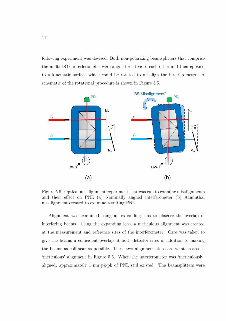
112

following experiment was devised. Both non-polarizing beamsplitters that comprise

the multi-DOF interferometer were aligned relative to each other and then epoxied

to a kinematic surface which could be rotated to misalign the interferometer. A

schematic of the rotational procedure is shown in Figure 5.5.

Figure 5.5: Optical misalignment experiment that was run to examine misalignmentsand their effect on PNL (a) Nominally aligned interferometer (b) Azimuthalmisalignment created to examine resulting PNL.

Alignment was examined using an expanding lens to observe the overlap of

interfering beams. Using the expanding lens, a meticulous alignment was created

at the measurement and reference sites of the interferometer. Care was taken to

give the beams a coincident overlap at both detector sites in addition to making

the beams as collinear as possible. These two alignment steps are what created a

‘meticulous’ alignment in Figure 5.6. When the interferometer was ‘meticulously’

aligned, approximately 1 nm pk-pk of PNL still existed. The beamsplitters were

113

then rotated to slightly misalign the system, which amplified the PNL.

0 2 4 6 8 10 12 14 16 18 20−10−7.5

−5−2.5

02.5

57.510

Fringe Number

Dis

p. E

rror

[nm

]

0 2 4 6 8 10 12 14 16 18 20−10−7.5

−5−2.5

02.5

57.510

Fringe Number

Dis

p. E

rror

[nm

] Nominal AlignmentMeticulous Alignment

Figure 5.6: Effect of slight misalignment on the multi-DOF interferometer. Refer toFigure 5.5 for a schematic of the created misalignment. Nominal alignment exhibitedapproximately 5 nm pk-pk PNL while meticulous alignment exhibited approximately1 nm pk-pk PNL.

It was expected that PNL would be amplified under azimuthal rotational

misalignments of the interferometer because this effect has been demonstrated in

the experiments conducted by Badami and Patterson [18]. What was not expected

was the 1 nm pk-pk of PNL which was still evident with a very meticulously aligned

system. A logical next step would be to examine the linear polarization quality of the

input beams. To do this, two linear polarizers were placed in front of each launch to

ensure that the polarization-maintaining fibers did not induce elliptical polarizations.

The setup shown in Figure 5.7 was implemented and the results of the experiment

can be seen in Figure 5.8.

Figure 5.8 shows that the resulting PNL, even with polarizers implemented,

reached 4 nm pk-pk in Z-displacement and 3 µrad pk-pk in rotational data. The

114

Figure 5.7: Linear polarizers were implemented into the interferometer to limit PNLas a result of elliptical polarizations.

0 1 2 3 4 5 6 7 8−4

−2

0

2

4

6

Fringe Number

Dis

p. E

rror

[nm

]

0 1 2 3 4 5 6 7 8−4

−2

0

2

4

6

Fringe Number

Dis

p. E

rror

[nm

]

Z−Displacement−8

−6

−4

−2

0

2

4

6∆

Rot

atio

n E

rror

[µra

d]

−8

−6

−4

−2

0

2

4

6∆

Rot

atio

n E

rror

[µra

d]YawPitch

Figure 5.8: PNL still existed with a polarizer after the launch site.

115

meticulous alignment experiment (Figure 5.6), established the standard for the lowest

achievable level of PNL up to this point. That meticulously aligned interferometer

had to be taken down and re-aligned before the polarizer experiment was run, so

the 4 nm pk-pk level of PNL in Z-displacement shown in Figure 5.8 can mainly be

attributed to very slight misalignments in the system. A slight ellipticity of the input

beams in a well aligned system has been shown to contirbute on the order of 1 nm pk-

pk of PNL [43]. Even if the ellipticity of the input beams had been contributing to

the levels of PNL, from these two experiments we know that misalignments in the

system are much more critical to maintaining high-resolution measurements than

very slight ellipticities of the input beams. In Figure 5.8, it could be inferred that

the dominant source of PNL was a result of slight misalignments in the system and

the polarization-maintaining fibers were not inducing considerable ellipticities in the

launch polarization states of the interferometer. These results were confirmed when

the interferometer was once again, very meticulously aligned and first order PNL

was reduced below detectable levels in Z-displacement. These results are shown in

Figure 5.9 in which first order PNL is not evident in Z-displacement. Z measurements

seem to exhibit second order PNL, if anything, and are on the order of 500 pm pk-

pk. Rotational PNL was on the order of 200 nm pk-pk in pitch and 400 nm pk-

pk in yaw. Although the lack of first order PNL is encouraging in Figure 5.9, it

is important to remember that Z-displacement in the multi-DOF interferometer is

actually an average of four separate phase measurements. With this in mind we refer

to Figure 5.10 in which picometer levels of PNL are evident in most quadrants, but

up to 1 nm pk-pk of first-order PNL can be seen in quadrant D.

The meticulously aligned interferometer which yielded the results shown in

Figures 5.9 and 5.10 is capable of yielding high resolution measurements with

116

0 1 2 3 4 50

0.5

1

1.5

Fringe Number

Dis

p. E

rror

[nm

]

0 1 2 3 4 50

0.5

1

1.5

Fringe Number

Dis

p. E

rror

[nm

] Displacement

0

0.5

1

1.5

∆ R

otat

ion

Err

or [µ

rad]

0

0.5

1

1.5

∆ R

otat

ion

Err

or [µ

rad]Yaw

Pitch

Figure 5.9: Periodic nonlinearity as a result of a very meticulously aligned system.Interferometer was re-aligned from the setup which produced the results in Figure 5.8in an attempt to completely eliminate PNL from misalignments.

0 1 2 3 4 501234567

Fringe Number

Dis

p. E

rror

[nm

]

0 1 2 3 4 501234567

Fringe Number

Dis

p. E

rror

[nm

]

Quadrant AQuadrant BQuadrant CQuadrant D

Figure 5.10: Although first order periodic nonlinearity was not evident in Z-displacement in Figure 5.9, the nonlinearity had only been averaged out from thefour quadrants of the measurement detector.

117

sub-microradian nonlinearity in rotation and sub-nanometer nonlinearity in Z-

displacement. A representative 50 µm pk-pk sine sweep was carried out to confirm

these levels of precision and is shown in Figure 5.11.

0 1 2 3 4 5−30

−15

0

15

30

Time [s]

Z−

Dis

plac

emen

t [µm

]

0 1 2 3 4 5−30

−15

0

15

30

Time [s]

Z−

Dis

plac

emen

t [µm

] Displacement

−8

−4

0

4

8

∆ R

otat

ion

[µrad

]

−8

−4

0

4

8

∆ R

otat

ion

[µrad

]

YawPitch

Figure 5.11: The interferometer under current resolution limits exhibits sub-microradian PNL in rotation and sub-nanometer PNL in Z-displacement.

It seems that we have reached the limit of how well we can align the system by

hand, yet PNL still persists. Furthermore, we have ruled out PNL resulting from

ellipticity in launch polarizations. Sub-nanometer levels of PNL have been attributed

to ghost reflections when no alternative dominate error source is evident [10, 24].

The remaining levels of PNL were attributed to ghost reflections as well. To test

this hypothesis, all sources that could potentially create ghost reflections must be

examined. Until now, all experiments had been carried out using FC/PC fiber

launches and are one source of ghost reflections. In addition, the interferometer

is comprised of two cube beamsplitters whose perpendicular surfaces could be a

considerable source of ghosting. The effect of ghost reflections was simulated using

118

a simplified model which assumes no sources of PNL on the reference detector.

The governing equation for this simulation (Equation 5.7) was derived from the

Michelson interferometer which is why the reference detector is assumed to be ideal.

Nonetheless, the simulation yielded a 1 nm pk-pk level of PNL as a result of ghost

reflections. A summary of the simulation can be seen in Appendix A. In practice, the

simulation is not completely valid for the multi-DOF interferometer because the same

nominal amplitude of ghost reflections is present in the reference and measurement

signals. Without an ideal reference, free of its own sources of PNL, the actual

simulation becomes much more complicated. Since the same nominal amplitude of

ghosting is present in the measurement and reference channels of the interferometer,

the effects could presumably cancel themselves out (when in phase) and would hence

yield sub-nanometer levels of PNL which are indeed present in Figure 5.10.

Experimentally, effects of ghosting were examined by replacing the cube

beamsplitters with plate beamsplitters which also had a 30 arcmin wedge specifically

designed to scatter ghost reflections. The interferometer aligned with wedge

beamplitters produced the results shown in Figure 5.12 in which 12 nm pk-pk of PNL

existed. These results were counterintuitive at first but have since been attributed

to misalignments within the system, which is much harder to align with the wedge

beamplitters compared to the cube beamsplitters.

119

0 1 2 3 4 5−10

−6

−2

2

6

10

Fringe Number

Dis

p. E

rror

[nm

]

0 1 2 3 4 5−10

−6

−2

2

6

10

Fringe Number

Dis

p. E

rror

[nm

] Displacement

−10

−5

0

5

10

∆ R

otat

ion

Err

or [µ

rad]

−10

−5

0

5

10

∆ R

otat

ion

Err

or [µ

rad]Yaw

Pitch

Figure 5.12: Interferometer measurement conducted using wedge beamsplitters toscatter ghost reflections. High levels of PNL are evident which are attributed tosystem misalignments.

5.4 Future Error Reduction

At the present state, approximately 500 pm pk-pk of periodic nonlinearity in

Z-displacement and 400 nm pk-pk of periodic nonlinearity in rotation are the

driving resolution limits of the interferometer. The source of this nonlinearity

has been attributed mainly to ghost reflections; however, it has also been shown

that PNL within the interferometer is very sensitive to slight misalignments

(Figure 5.6). Misalignment effects dominated the interferometer wedge beamsplitter

setup (Figure 5.12) which theoretically should have reduced PNL levels further from

what was examined in Figure 5.10. Going forward, a much more involved PNL

simulation as a result of ghost reflections, misalignments, and elliptical polarizations

all within a custom intererometer setup needs to be created to accurately model

the results obtained in the laboratory. DeFreitas and Player [28] have outlined a

120

convenient method of modeling PNL in custom interferometer setups using Jones

Calculus and a similar approach will need to applied to this interferometer. Cosijns,

et al. [43] have also established very reliable models which incorporate misalignments

and elliptical polarizations in the Michelson interferometer, and a similar approach

will need to be appended to the custom multi-DOF simulation.

The subject of periodic nonlinearity is vast within the displacement

interferometry industry. Although the subject is relatively well understood, its

effects in custom interferometer configurations will be very valuable as the state of

the industry starts to produce new setups in an effort to constantly push resolution

limits. Many commercial displacement measuring interferometers frequently state

a nonlinearity of 1 nm pk-pk. These resolution limitations are becoming obsolete

and have been exceeded by authors such as Joo, et al. [9] and Wu, et al. [24]. This

chapter merely serves as a brief introduction to periodic nonlinearity within the

specified setup, but this phenomenon could easily be investigated for quite some

time. As previously stated, the multi-DOF interferometer is theoretically periodic

error free. To successfully eliminate the phenomenon, an incredible amount of

care will need to put into aligning the interferometer in addition to the previously

suggested full simulation. Conveniently, sub-Rayleigh beam alignment methods have

already been demonstrated using a quadrant photodetector [26] which the multi-

DOF interferometer already contains. This alignment technique outlined by Muller,

et al. could be implemented into the multi-DOF interferometer to examine alignment

quality and further rule out PNL as a result of misalignments.

121

6 Conclusion

Ongoing work in the development of the multi-DOF interferometer has been

presented. As a culmination of this research, progress will be evaluated in addition to

outlining a trajectory for future work with this system. Measurements from a high-

resolution metrology instrument such as this interferometer are not complete without

a stated uncertainty. A brief error analysis has been conducted on the measurements

made for this thesis which will be presented first. Concluding remarks will outline

challenges in creating a completely fiber launched and detected interferometer in

addition to outlining other future system improvements.

6.1 Measurement Uncertainty

The methods used to evaluate the uncertainty associated with any particular

measurement are discussed in “A Beginner’s Guide to Uncertainty of Measurement”

provided by the National Physical Laboratory [44]. It is important to remember that

a particular instrument does not possess uncertainty, the individual measurements it

performs possess uncertainty. The analysis presented here is a result of the specific

122

conditions which exist in the laboratory where the measurements for this thesis were

conducted.

The measurement uncertainty derived for the multi-DOF interferometer is based

on the governing phase equation

∆φ =2πNη∆zf

c, (6.1)

where N is the interferometer fold factor (2 in the case of the multi-DOF design),

∆z is the change in physical displacement, η is the refractive index, f is the optical

frequency and c is the speed of light. After taking the time derivative of phase,

Equation 6.1 can be reorganized to observe a change in length. The time derivative

of phase is

d∆φ

dt=

2πN

c

(

ηfd∆z

dt+∆zη

df

dt+∆zf

dη

dt

)

. (6.2)

Since data analysis occurs on discrete time intervals, the dt term may be set to one

to simplify the equation. Equation 6.2 may then be rearranged to form an expression

for change in length, given by

∆z =c∆φ

2πNηf−

z∆f

f−

z∆η

η. (6.3)

Using Equation 6.3, a first order uncertainty expansion can be created using the

relationship

U2Y =

n∑

i=1

(∂Y

∂yi

)2

U2yi, (6.4)

where UY is the uncertainty, Y will be the function shown in Equation 6.3, yi are

123

uncertainty parameters from the equation, and Uyi is the uncertainty of those specific

uncertainty parameters. After inserting Equation 6.3 into Equation 6.4, the result

is six separate expressions from which the uncertainty can be analyzed individually.

The uncertainty contributions from individual components are

U∆z(∆φ) =c

2πNηf(U∆φ) ∼= 122.9 pm

U∆z(η) =( −∆φc

2πNη2f+

z∆η

η2

)

(Uη) ∼= 0 pm

U∆z(f) =( −∆φc

2πNf 2η+

z∆f

f 2

)

(Uf ) ∼= 0 pm

U∆z(∆f) =−z

f(U∆f ) ∼= 1.84 nm

U∆z(∆η) =−z

η(U∆η) ∼= 999.7 pm

U∆z(z) =(−∆f

f−

∆η

η

)

(Uz) ∼= 0 pm,

(6.5)

where the contributions from each term are a result of the input values shown in

Table 6.1.

Table 6.1: Uncertainty parameters for Equation 6.3 inserted into Equation 6.4.

Parameter Nominal Fractional AbsoluteValue Uncertainty Uncertainty

Speed of light (c) 299792458 m/s - -Fold factor (N) 2 - -Phase change (∆φ) 2.44 mrad - 2.44 mradRefractive index (η) 1.000275457 - 1 x 10−8

Change in ref. index (∆η) 4.88 x 10−7 - 1 x 10−8

Frequency (f) 473612214 MHz 1 x 10−8 -Frequency change (∆f) 4 MHz - 4+Uf MHzNominal length (z) 0.1 m - 100 nm

In Table 6.1, c and N are known. Phase change, ∆φ, was determined by

124

running a phase accuracy performance test on the SRS-830 lock-in amplifiers used

in the research for this thesis. This phase accuracy measurement is outlined in

the working manual for the lock-in amplifiers and yielded a phase accuracy value

of 2.44 mrad (which translates to 0.12 nm). The parameters needed to calculate

refractive index, η, accurately are temperature, pressure and relative humidity for

the modified Edlen equation [14] which has since been updated by Birch and Downs

[45, 46]. The laboratory in which this research was conducted typically operates in

a temperature of 20 ± 0.5C (rectangular distribution, k=1). Pressure and relative

humidity have been determined from a local weather database [47]. The pressure

used was 102.9 ± 0.2 kPa (rectangular distribution, k=1) and the relative humidity

was assumed a constant 67%; both of which are the nominal values for upstate

New York where these measurements were conducted. These values yielded the

nominal value of refractive index along with the change of refractive index from the

modified Edlen equation in Table 6.1. The resolution limit of the modified Edlen

equation is 1 part in 108 due to the resolution limits of the empirical data from

which it was derived. This 1 part in 108 resolution limit can be seen as the absolute

uncertainty in refractive index and the change in refractive index. The nominal value

for frequency in Table 6.1 is for red light from a He-Ne frequency stabilized source

and the corresponding uncertainty is readily available using commercial lasers. The

change in frequency was obtained from the specification sheet for the He-Ne laser used

for this research and represents stability over one hour. The absolute uncertainty of

the nominal target distance is 100 nm which is a conservative estimate considering

overall uncertainty is expected to be at least one order of magnitude lower than

that. Combining parameters from Equation 6.5 into a root-sum square calculation,

the uncertainty for a change in measured displacement is 2.10 nm. After imposing a

coverage factor of k=2, the overall uncertainty for a change in measured displacement

125

becomes 4.20 nm, providing a level of confidence of approximately 95%.

The stated uncertainty value of 4.20 nm is close to the resolution limits of

the multi-DOF interferometer given the amplitudes of periodic nonlinearity seen

throughout this thesis (typically 1-5 nm). As periodic nonlinearity levels continue

to decrease and the resolution of the interferometer increases, the measurement

uncertainty will need to be improved with better environmental containment and

better monitoring of refractive index.

6.2 Future System Improvements

An auxiliary research focus in the developoment of the multi-DOF interferometer

was to completely fiber-couple the system, that is, fiber launched and detected. In

the pursuit of this goal, a high density imaging fiber was purchased through Myriad

Fiber Imaging, Inc. (fiber type FIGH-50-1100N). Imaging bundles like this one had

been previously shown to transmit tilted wavefronts. Unfortunately when this fiber

was actually tested with the interferometer, it produced substantial levels of periodic

nonlinearity at the output compared to freespace detection. While the interferometer

was being qualified against the Renishaw ML10, the imaging fiber was inserted into

the setup. The resulting periodic nonlinearity can be seen in Figure 6.1.

High levels of periodic nonlinearity make the interferometer essentially useless in

qualification measurements. The data from Figure 6.1 was collected during a pitch

qualification against the Renishaw system. The actual attempted qualification can

be seen in Figure 6.2.

A lot of work obviously still needs to be done before the interferometer

can be completely fiber-coupled. While the reference signal can simply be

126

Figure 6.1: To completely fiber-couple the interferometer, an imaging fiber wasutilized to transmit tilted wavefronts to the quadrant photodiode. The result atthe output was 13 nm PNL in Z-displacement, 50 µrad PNL in pitch and 15 µradPNL in yaw.

transmitted through a multi-mode fiber, the measurement signal requires a much

more complicated waveguide which does not distort the tilt angle of interferring

wavefronts. The source of periodic nonlinearity within the fiber may be mode mixing

between individual fiber cores, as the imaging fiber is basically a high density fiber

bundle. Other fiber bundles will need to be examined for the measurement fiber

detection site. One such option is a simple quad fiber bundle which detects four

separate phase readings and transmits those signals to the four photodetectors on

the quadrant photodiode.

If fiber detection at the measurement site becomes viable, new applications open

up for the multi-DOF interferometer. One such product could be a fiber probe

incorporated onto a 5-axis coordinate measurement machine (or CMM). The fiber

probe would be extremely useful in the metrology of freeform optics which sometimes

127

0 5 10 15 20 25 30−40

−20

0

20

40

Time [s]

Pitc

h [µ

rad]

0 5 10 15 20 25 30−40

−20

0

20

40

Time [s]

Pitc

h [µ

rad]

Multi−DOF (Fiber Detected)Renishaw

Figure 6.2: Fiber detection qualification of the interferometer against the RenishawML10. High levels of periodic nonlinearity created through the imaging fiberwhile transmitting the measurement interference signal yielded essentially uselessqualification results.

exhibits fringe contrast issues with current white light techniques in addition to small

aperture measurement limits. A completely fiber-coupled multi-DOF interferometer

could be incorporated onto a 5-axis CMM and, with the implementation of feedback

control, would be able to sweep over freeform surfaces. A displacement interferometer

would be ideal for this type of optical probe due to its fine resolution limits in addition

to a high dynamic range. Figure 6.3 demonstrates the multi-DOF interferometer

being used as an optical probe sweeping over a freeform surface.

128

Figure 6.3: A fiber-fed and fiber-detected multi-DOF interferometer could beincorporated into a 5-axis coordinate measurement machine to be used as an opticalprobe. With the implementation of feedback control, the fiber probe would be ableto sweep across freeform surfaces.

6.3 Final Remarks

The multi-DOF interferometer being used as a fiber probe is contingent on a

compact design. The working prototype discussed in Chapter 3 already has a

relatively small profile compared to many commercial systems. However, if this

interferometer becomes smaller, alignment of the beamsplitting optics will become

increasingly difficult. Assembling the working prototype of the interferometer is

already challenging enough with such small optical components. The design of a

reliable industrial assembly process would prove useful for the current setup as well

as in future smaller iterations.

The continued research and development of the multi-DOF interferometer

requires a multi-disciplinary approach. Before the interferometer can be used for

129

metrology in the optical lithography industry, the resolution of the interferometer

will need to be below 1 nanometer in Z-displacement, and will probably need to

be on the order of 10s of nanoradians in pitch and yaw. Towards this end, custom

phase detection electronics will need to be developed with a low noise floor and the

environment where measurements are taken will need to be extremely well monitored

and probably in vacuum. Also, the amplitude of periodic nonlinearity will need to

be significantly reduced – hopefully to undetectable levels. This Master’s thesis has

laid the foundation for the theory and predominant considerations needed in the

continued improvement of the system. Displacement interferometry measurement

theory, precision design principles, and a critical evaluation of all presented results

have provided a path forward in the advancement of the multi-DOF interferometer.

130

131

Bibliography

[1] P. Hariharan. Optical Interferometry. Academic Press, 2003.

[2] S.J. Bennett. Length and displacement measurement by laser interferometry.

Optical Transducers and Techniques in Engineering Measurement, pages 135–

159, 1983.

[3] C.R. Steinmetz. Sub-micron position measurement and control on precision

machine tools with laser interferometry. Precision Engineering, 12(1):12–24,

1990.

[4] W.T. Estler. High-accuracy displacement interferometry in air. Applied Optics,

24(6):808–815, 1985.

[5] W.H. Steel. Interferometry. Cambridge University Press, 1983.

[6] T. Schuldt, M. Gohlke, D. Weise, U. Johann, A. Peters, and C. Braxmaier.

Picometer and nanoradian optical heterodyne interferometry for translation and

tilt metrology of the lisa gravitational reference sensor. Classical and Quantum

Gravity, 26(8), 2009.

[7] J.J. Kroll. Six degree of freedom optical sensor for dynamic measurement of

linear axes. PhD thesis, University of North Carolina, Charlotte, 2003.

132

[8] P.S. Huang J. Ni and S.M. Wu. A multi-degree-of-freedom measuring system

for CMM geometric errors. Journal of Engineering for Industry, 114:362–369,

1992.

[9] K-N. Joo, J.D. Ellis, E.S. Buice, J.W. Spronck, and R.H. Munnig Schmidt. High

resolution heterodyne interferometer without detectable periodic nonlinearity.

Optics Express, 18(2):1159–1165, 2010.

[10] K-N. Joo, J.D. Ellis, J.W. Spronck, P.J.M. van Kan, and R.H. Minnig Schmidt.

Simple heterodyne laser interferometer with subnanometer periodic errors.

Optics Letters, 34(3):386–388, 2009.

[11] J.D. Ellis, A.J.H. Meskers, J.W. Spronck, and R.H. Munnig Schmidt. Fiber-

coupled displacement interferometry without periodic nonlinearity. Optics

Letters, 36:3584–3586, 2011.

[12] A. Michelson and R. Benoit. Determination experimentale de la valcur du metre

en longueurs d’ondes lumineuses. Trav. Et Mem. Bur. Int. Poids et Mes., 1:1–83,

1895.

[13] L.M. Barker and R.E. Hollenbach. Interferometer technique for measuring the

dynamic mechanical properties of materials. American Institute of Physics:

Review of Scientific Instruments, 36:1617–1620, 1965.

[14] B. Edlen. The refractive index of air. Metrologia, 2(2):71–80, 1966.

[15] N. Bobroff. Residual errors in laser interferometry from air turbulence and

nonlinearity. Applied Optics, 26(13):2676–2682, 1987.

[16] R. Quenelle. Nonlinearity in interferometer measurements. Hewlett-Packard

Journal, 34(4):10, 1983.

133

[17] C.M. Sutton. Non-linearity in length measurement using heterodyne laser

michelson interferometry. Journal of Physics E: Scientific Instruments,

20(10):1290–1292, 1987.

[18] V.G. Badami and S.R. Patterson. A frequency domain method for

the measurement of nonlinearity in heterodyne interferometry. Precision

Engineering, 24(1):41–49, 2000.

[19] W. Hou and G. Wilkening. Investigation and compensation of the nonlinearity

of heterodyne interferometers. Precision Engineering, 14(2):91–98, 1992.

[20] A.E. Rosenbluth and N. Bobroff. Optical sources of nonlinearity in heterodyne

interferometers. Precision Engineering, 12(1):7–11, 1990.

[21] W. Augustyn and P. Davis. An analysis of polarization mixing errors in distance

measuring interferometers. Journal of Vacuum Science and Technology B,

8(6):2032–2036, 1990.

[22] M. Tanaka, T. Yamagami, and K. Nakayama. Linear interpolation of periodic

error in a heterodyne laser interferometer at subnanometer levels. IEEE

Transactions on Instrumentation and Measurement, 38(2):552–554, 1989.

[23] J. Lawall and E. Kessler. Michelson interferometry with 10 pm accuracy.

American Institute of Physics, 71(7):2669–2676, 2000.

[24] C-M. Wu, J. Lawall, and R.D. Deslattes. Heterodyne interferometer with

subatomic periodic nonlinearity. Applied Optics, 38(19):4089–4094, 1999.

[25] T. Schmitz and J. Beckwith. Acousto-optic displacement-measuring

interferometer: a new heterodyne interferometer with Angstrom-level periodic

error. Journal of Modern Optics, 49(13):2105–2114, 2002.

134

[26] H. Muller, S-W. Chiow, Q. Long, C. Vo, and S. Chu. Active sub-rayleigh

alignment of parallel or antiparallel laser beams. Optics Letters, 30(24):3323–

3325, 2005.

[27] N. Bobroff. Recent advances in displacement measuring interferometry.

Measurement Science and Technology, 4:907–926, 1993.

[28] J.M. De Freitas and M.A. Player. Polarization effects in heterodyne

interferometry. Journal of Modern Optics, 42(9):1875–1899, 1995.

[29] N.A. Massie, R.D. Nelson, and S. Holly. High-performance real-time heterodyne

interferometry. Applied Optics, 18(11):1797–1803, 1979.

[30] G.E. Sommargren. Optical heterodyne profilometry. Applied Optics, 20(4):610–

618, 1981.

[31] R.C.G. Smith. Fiber effects in displacement interferometry. Master’s thesis,

University of Rochester, Unpublished manuscript.

[32] E. Morrison, B.J. Meers, D.I. Robertson, and H. Ward. Automatic alignment

of optical interferometers. Applied Optics, 33(22):5041–5049, 1994.

[33] S.R. Gillmer, R.G.C. Smith, S.C. Woody, J. Tarbutton, and J.D. Ellis.

Miniature, fiber-coupled 3-DOF interferometer for precision micro-motion stage

metrology. In Proceedings of the 27th ASPE Annual Meeting, San Diego, CA,

21-26 October 2012.

[34] J.E. Furse. Kinematic design of fine mechanisms in instruments. Journal of

Physics E: Scientific Instruments, 14(3):264–271, 1981.

135

[35] C-m. Wu. Periodic nonlinearity resulting from ghost reflections in heterodyne

interferometry. Optics Communications, 215(1-3):17–23, 2003.

[36] C-M. Wu and C-S. Su. Nonlinearity in measurements of length by optical

interferometry. Measurement Science and Technology, 7(1):62–68, 1996.

[37] F. Petru and O. Cıp. Problems regarding linearity of data of a laser

interferometer with a single-frequency laser. Precision Engineering, 23(1):39–50,

1999.

[38] P.L.M. Heydemann. Determination and correction of quadrature fringe

measurement errors in interferometers. Applied Optics, 20(19):3382–3384, 1981.

[39] Y. Xie and Y-Z. Wu. Zeeman laser interferometer errors for high-precision

measurements. Applied Optics, 31(7):881–884, 1992.

[40] J.M. DeFreitas and M.A. Player. Importance of rotational beam alignment in

the generation of second harmonic errors in laser heterodyne interferometry.

Measurement Science and Technology, 4(10):1173–1176, 1993.

[41] B. Li and J-W. Liang. Effects of polarization mixing on the dual-wavelength

heterodyne interferometer. Applied Optics, 36(16):3668–3672, 1997.

[42] V.G. Badami. Investigation and compensation of periodic nonlinearities in

heterodyne interferometry. PhD thesis, University of North Carolina, Charlotte,

1999.

[43] S.J.A.G. Cosijns, H. Haitjema, and P.H.J. Schellekens. Modeling and

verifying non-linearities in heterodyne displacement interferometry. Precision

Engineering, 26:448–455, 2002.

136

[44] S. Bell. A Beginner’s Guide to Uncertainty of Measurement. National Physical

Laboratory, Teddington, Middlesex, United Kingdom, 1999.

[45] K.P. Birch and M.J. Downs. An updated edlen equation for the refractive index

of air. Metrologia, 30(3):155–162, 1993.

[46] K.P. Birch and M.J. Downs. Correction to the updated edlen equation for the

refractive index of air. Metrologia, 31(4):315–316, 1994.

[47] New york current condition maps, 2013: http://www.usairnet.com/weather/maps/current/new-

york/.

137

A Simulating Periodic

Nonlinearity

FRED optical analysis software was used to generate a working model of the

multi-DOF displacement interferometer. The generated model is shown next which

accounts for ghost reflections off all surfaces

After a working simulation was created, amplitudes of ghost reflections had to be

examined to generate a Ω1 coefficient from Equation 5.7. The amplitudes of ghost

reflections relative to the nominal signal were created utilizing a strategic placement

of 100% absorbing surfaces in FRED. This was done in two steps; first, the setup

shown in Figure A.2 was run with 0.1% reflections on each optical surface, 90%

reflection on both mirrors (MM andMR), and 100% absorbance at both fiber launches

assuming an APC fiber launch is implemented to scatter ghost reflections from fiber

tips. This initial step was used as a control scenario to observe the magnitude of

the irradiance output on the measurement photodetector (PDM). The irradiance

output from the setup in Figure A.2 is shown in Figure A.3.

The control scenario yielded an integrated power over the entire analysis detector

surface of 40.24 µW, it is now our task to figure out what percentage of that power

is generated from ghost reflections. The dimensionless coefficient that represents

138

Figure A.1: Screen shot of the multi-DOF interferometer modeled using FREDoptical software.

Figure A.2: Schematic of initial multi-DOF interferometer used in the FREDsimulation.

139

Figure A.3: Control scenario, setup in Figure A.2 modeled using 0.1% reflectionson each optical surface, 90% reflection on both mirrors (MM and MR), and 100%absorbance at both fiber launches assuming an APC fiber launch is implemented toscatter ghost reflections from fiber tips. Integrated Power is 40.24 µW.

140

that percentage of ghost reflections becomes the Ω1 coefficient from Equation 5.7.

To examine pure ghost reflections at the measurement detector, the setup shown in

Figure A.4 was implemented.

Figure A.4: FRED simulation schematic to observe amplitude of ghost reflectionsrelative to nominal signal.

The irradiance output in Figure A.5 was generated using the setup in Figure A.4.

It should be noted that the Ω1 coefficient from Equation 5.6 contains two sources of

PNL – one from the frequency leakage into the reference arm of the previously shown

Michelson interferometer and one from the frequency leakage into the measurement

arm. Both terms from the Ω1 coefficient are detected at the measurement

photodetector in Figure 5.3. For the purposes of our multi-DOF interferometer

setup, only ghost reflections from the measurement beam (red) in Figure A.4 are

significant because most of the ghost reflections from the reference beam (blue)

are detected on the reference photodetector. With this reasoning in mind, the Ω1

coefficient from Equation 5.6 now only contains one term which is the ratio of the

irradiance output from Figure A.5 over the irradiance output from Figure A.3. This

141

Figure A.5: Analysis of ghost reflections using the setup in Figure A.4. IntegratedPower = 0.1858 µW.

ratio (0.1858 µW/40.24 µW) is equal to 0.00462. Using this coefficient, a MATLAB

simulation was run with an overall displacement of 15 fringes (at 633 nm wavelength).

The measured phase incorporates the Ω1 coefficient of 0.00462 using the following

expression [24]:

Φ(t)meas = tan−1

( 12sin(φ)

12cos(φ) + Ω1

)

(A.1)

Measured phase is calculated from Equation A.1, unwrapped, detrended and

converted to physical displacement to arrive at the result shown in Figure A.6 and

a nominal PNL of 1 nm pk-pk.

142

0 1 2 3 4 5 6 7 8 9 10−0.5

−0.25

0

0.25

0.5

Fringes

Dis

plac

emen

t [nm

]

0 1 2 3 4 5 6 7 8 9 10−0.5

−0.25

0

0.25

0.5

Fringes

Dis

plac

emen

t [nm

]

Simulated PNL

Figure A.6: Periodic Nonlinearity simulation resulting from ghost reflections on themeasurement detector using the setup shown in Figure A.4. Nominal PNL 1 nmpk-pk.