POLITECNICO DI MILANO Facoltà di Ingegneria Industriale Dipartimento di Ingegneria Aerospaziale Corso di Laurea in Ingegneria Aeronautica Development of a Dynamics Simulator for Foiling Boats Dynamic Behaviour Analysis Relatore: Prof. Pierangelo Masarati Tesi di laurea di: Franco Lovato, Matr. 836432 Anno accademico 2016/2017

Welcome message from author
This document is posted to help you gain knowledge. Please leave a comment to let me know what you think about it! Share it to your friends and learn new things together.
Transcript
POLITECNICO DI MILANO
Facoltà di Ingegneria Industriale Dipartimento di Ingegneria Aerospaziale
Corso di Laurea in Ingegneria Aeronautica
Development of a Dynamics Simulator for Foiling Boats Dynamic Behaviour Analysis
Relatore:
Prof. Pierangelo Masarati
Tesi di laurea di:
Franco Lovato, Matr. 836432
Anno accademico 2016/2017
Contents
1 Introduction 7
1.1 The Loads At Play . . . . . . . . . . . . . . . . . . . . . . . . . . . . . . . 7
1.2 Foiling . . . . . . . . . . . . . . . . . . . . . . . . . . . . . . . . . . . . . . 10
1.3 The C-Class Catamaran . . . . . . . . . . . . . . . . . . . . . . . . . . . . 11
1.4 Dynamic Analysis . . . . . . . . . . . . . . . . . . . . . . . . . . . . . . . . 13
2 The C-Class Catamaran 15
2.1 The Boat . . . . . . . . . . . . . . . . . . . . . . . . . . . . . . . . . . . . 16
2.1.1 The Model . . . . . . . . . . . . . . . . . . . . . . . . . . . . . . . . 16
2.2 The Wing Sail . . . . . . . . . . . . . . . . . . . . . . . . . . . . . . . . . . 18
2.2.1 The Model . . . . . . . . . . . . . . . . . . . . . . . . . . . . . . . . 19
2.3 The Foil . . . . . . . . . . . . . . . . . . . . . . . . . . . . . . . . . . . . . 21
2.3.1 The Model . . . . . . . . . . . . . . . . . . . . . . . . . . . . . . . . 22
2.4 The Rudder . . . . . . . . . . . . . . . . . . . . . . . . . . . . . . . . . . . 24
2.4.1 The Model . . . . . . . . . . . . . . . . . . . . . . . . . . . . . . . . 25
2.5 Peculiar Issues . . . . . . . . . . . . . . . . . . . . . . . . . . . . . . . . . . 27
3 The Software 28
3.1 General Introduction . . . . . . . . . . . . . . . . . . . . . . . . . . . . . . 28
3.2 Windage . . . . . . . . . . . . . . . . . . . . . . . . . . . . . . . . . . . . . 30
3.3 MBDyn . . . . . . . . . . . . . . . . . . . . . . . . . . . . . . . . . . . . . 32
3.3.1 Application . . . . . . . . . . . . . . . . . . . . . . . . . . . . . . . 32
3.4 Vortex Lattice Method . . . . . . . . . . . . . . . . . . . . . . . . . . . . . 34
3.4.1 General Idea . . . . . . . . . . . . . . . . . . . . . . . . . . . . . . . 34
3.4.2 The Method . . . . . . . . . . . . . . . . . . . . . . . . . . . . . . . 35
3.4.3 Implementation . . . . . . . . . . . . . . . . . . . . . . . . . . . . . 36
3.4.4 Wind Profile . . . . . . . . . . . . . . . . . . . . . . . . . . . . . . . 36
3.4.5 Water surface . . . . . . . . . . . . . . . . . . . . . . . . . . . . . . 37
3.4.6 Viscous Drag . . . . . . . . . . . . . . . . . . . . . . . . . . . . . . 38
3.5 PID Controllers . . . . . . . . . . . . . . . . . . . . . . . . . . . . . . . . . 40
3.5.1 Theory . . . . . . . . . . . . . . . . . . . . . . . . . . . . . . . . . . 40
3.5.2 Tuning . . . . . . . . . . . . . . . . . . . . . . . . . . . . . . . . . . 40
3.6 Optimization . . . . . . . . . . . . . . . . . . . . . . . . . . . . . . . . . . 42
3.6.1 The Method . . . . . . . . . . . . . . . . . . . . . . . . . . . . . . . 42
2
4 Applications 44
4.1 Validation . . . . . . . . . . . . . . . . . . . . . . . . . . . . . . . . . . . . 45
4.1.1 VLM Validation . . . . . . . . . . . . . . . . . . . . . . . . . . . . . 45
4.1.2 Viscous Drag . . . . . . . . . . . . . . . . . . . . . . . . . . . . . . 48
4.2 Results . . . . . . . . . . . . . . . . . . . . . . . . . . . . . . . . . . . . . . 50
4.2.1 The Basic Case . . . . . . . . . . . . . . . . . . . . . . . . . . . . . 51
4.2.2 Changing Wind . . . . . . . . . . . . . . . . . . . . . . . . . . . . . 53
4.2.3 Optimization Under Changing Wind . . . . . . . . . . . . . . . . . 55
5 Conclusions 57
3
List of Figures
1 Loads On A Sailing Boat. . . . . . . . . . . . . . . . . . . . . . . . . . . . 7
2 Hydrofoil.[2] . . . . . . . . . . . . . . . . . . . . . . . . . . . . . . . . . . . 10
3 Foiling KiteSurf.[3] . . . . . . . . . . . . . . . . . . . . . . . . . . . . . . . 10
4 The Maserati Multi70.[4] . . . . . . . . . . . . . . . . . . . . . . . . . . . . 10
5 Multi70’s Foil.[4] . . . . . . . . . . . . . . . . . . . . . . . . . . . . . . . . 10
6 C Class Catamaran.[5] . . . . . . . . . . . . . . . . . . . . . . . . . . . . . 11
7 C-class Catamaran.[5] . . . . . . . . . . . . . . . . . . . . . . . . . . . . . 15
8 The Wing Sail.[6] . . . . . . . . . . . . . . . . . . . . . . . . . . . . . . . . 18
9 The Sail Model. . . . . . . . . . . . . . . . . . . . . . . . . . . . . . . . . . 19
10 The Foil. . . . . . . . . . . . . . . . . . . . . . . . . . . . . . . . . . . . . . 21
11 Foil Cant of �20�. . . . . . . . . . . . . . . . . . . . . . . . . . . . . . . . 21
12 Foil Cant of 20�. . . . . . . . . . . . . . . . . . . . . . . . . . . . . . . . . 21
13 The Foil Model. . . . . . . . . . . . . . . . . . . . . . . . . . . . . . . . . . 22
14 The Rudders.[7] . . . . . . . . . . . . . . . . . . . . . . . . . . . . . . . . . 24
15 Capsized. . . . . . . . . . . . . . . . . . . . . . . . . . . . . . . . . . . . . 25
16 The Rudder Model.[8] . . . . . . . . . . . . . . . . . . . . . . . . . . . . . 25
17 Software Structure . . . . . . . . . . . . . . . . . . . . . . . . . . . . . . . 28
18 The Wind Triangle. . . . . . . . . . . . . . . . . . . . . . . . . . . . . . . . 30
19 Wind Shear, Reference Height: 10m, Reference Speed: 10m/s. . . . . . . . 37
20 Cl↵=0 and Cl,↵ Comparison . . . . . . . . . . . . . . . . . . . . . . . . . . 46
21 Aspect Ratio Comparison . . . . . . . . . . . . . . . . . . . . . . . . . . . 47
22 Finite Wing Comparison Example . . . . . . . . . . . . . . . . . . . . . . . 47
23 Friction Cd Comparison . . . . . . . . . . . . . . . . . . . . . . . . . . . . 48
24 Boat’s speed evolution in time, in X direction . . . . . . . . . . . . . . . . 51
25 Heeling moment evolution in time . . . . . . . . . . . . . . . . . . . . . . . 52
26 Boat’s speed evolution in time, in X direction . . . . . . . . . . . . . . . . 53
27 Heeling moment variation in time . . . . . . . . . . . . . . . . . . . . . . . 54
28 Heeling moment variation in time . . . . . . . . . . . . . . . . . . . . . . . 55
29 Heeling moment variation in time . . . . . . . . . . . . . . . . . . . . . . . 56
4
Abstract
The aim of the presented project is to develop a dynamics simulator capable
of analyzing the dynamic behaviour of a C Class catamaran in foiling condition,
and to simulate the work demanded to the crew in order to keep a stable and fast
navigation.
In order to do so, MBDyn, a multibody dynamics simulator, has been employed as
the core of the software, while the aerodynamic and hydrodynamic loads are eval-
uated by a self made Vortex Lattice Method.
The boat’s stability and the following of the desired course are ensured by PID
controllers, while the optimum sail regulation is periodically looked upon by an op-
timization process, in order to simulate a crew that tries to best exploit the wind
power at disposition.
The results of a characteristic condition are shown: the boat’s behavior under chang-
ing wind, where the crew best exploit the wind condition before and after the per-
turbation. This is intended as an example of possible applications of the developed
software.
5
Abstract
Lo scopo del progetto presentato e di sviluppare un simulatore di dinamica ca-
pace di analizzare il comportamento dinamico di un catamarano di classe C in
condizioni di foiling, e di simulare il lavoro richiesto all’equipaggio al fine di man-
tenere una navigazione stabile e veloce.
Per fare cio, MBDyn, un simulatore di dinamica multicorpo, e stato utilizzato come
cuore del programma, mentre i carichi aerodinamici e idrodinamici sono stati valu-
tati tramite un metodo a reticolo di vortici sviluppato autonomamente.
La stabilita dell’imbarcazione e il mantenimento della rotta scelta sono garantiti
da una serie di controllori PID, mentre la regolazione ottimale della vela e peri-
odicamente analizzata da un processo di ottimizzazione, allo scopo di simulare un
equipaggio che cerca di sfruttare al meglio il vento a disposizione.
Vengono presentati i risultati di un caso tipico: il comportamento dell’imbarcazione
nel caso di vento variabile, dove l’equipaggio sfrutta al meglio le condizioni disponi-
bili prima e dopo la perturbazione. Questo si intende come possibile applicazione
del programma sviluppato.
6
1 Introduction
1.1 The Loads At Play
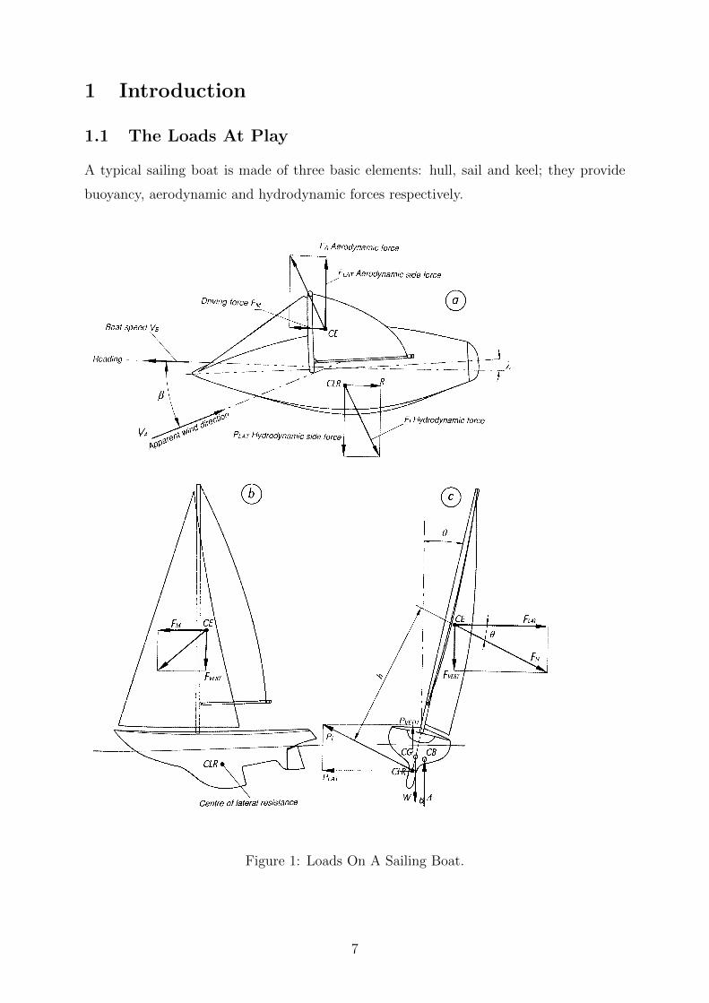
A typical sailing boat is made of three basic elements: hull, sail and keel; they provide
buoyancy, aerodynamic and hydrodynamic forces respectively.
Figure 1: Loads On A Sailing Boat.
7

From Figure 1, taken from [1]:
• CG: the centre of gravity, centre of e↵ort of gravity loads
• CE: the centre of e↵ort of the aerodynamic loads on the sail
• CB: centre of e↵ort of buoyancy loads
• CLR: centre of lateral resistance, the centre of e↵ort of the hydrodynamic loads
exerted by the keel and hull
• Heading: the direction of the boat’s motion
• VB: the boat’s speed
• VA: the apparent wind direction, the sum of the true wind and the boat’s velocity
• �: the angle between the apparent wind direction and the VB, also known as True
Wind Angle
• �: the angle between the Heading and the boat’s longitudinal axis, also known as
Leeway
• FA: the aerodynamic force exerted by the sail
• FM : the driving force, the one propelling the boat
• FLat: the component of FA in the lateral direction, perpendicular to the Heading
• FV ERT : the vertical component of FA
• ✓: the roll angle, known as Heeling
• FH : the component of FA contributing to the heeling moment
• FI : the hydrodynamic load exerted by the keel and hull
• R: the resistance, the component of FI in the heading direction
• PLAT : the hydrodynamic side force, the component of FI in the lateral direction
• PI : the component of FI contributing to the heeling moment
• h: the distance between the CE and CLR, the arm of the heeling moment
• PV ERT : the component of FI in the vertical direction
8
• W: the wight load of the boat
• �: the buoyancy load
• b: the distance between CB and CG, the arm of the counter heeling moment
The aerodynamic force produced by the sail may be decomposed in two components:
thrust, in the direction of motion of the boat, and side force, perpendicular to the thrust.
The thrust is balanced by hydrodynamic resistance, produced by both hull and keel. To
balance the side force is the purpose of the keel. A destabilizing heeling (nautical for
rolling) and pitching moments are exerted by both aero and hydrodynamic forces, which
need to be countered by the buoyancy of the hull. This is possible because heeling, for
example, causes an asymmetry in the volume of hull immersed in water, so the buoyancy’s
centre of e↵ort moves exerting a stabilizing moment. The yaw balance is guaranteed by
the rudder.
This description used to apply to all sailing boats before the 60s, but then the aeronautical
technology made its appearance in the sailing world. With the introduction of wing sails
and foiling boats the loads scheme changed, the average speed increased drastically and
so the e↵ort needed in order to keep the boat stable and on course grew.
9
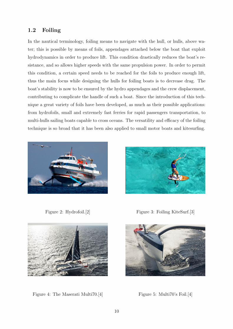
1.2 Foiling
In the nautical terminology, foiling means to navigate with the hull, or hulls, above wa-
ter; this is possible by means of foils, appendages attached below the boat that exploit
hydrodynamics in order to produce lift. This condition drastically reduces the boat’s re-
sistance, and so allows higher speeds with the same propulsion power. In order to permit
this condition, a certain speed needs to be reached for the foils to produce enough lift,
thus the main focus while designing the hulls for foiling boats is to decrease drag. The
boat’s stability is now to be ensured by the hydro appendages and the crew displacement,
contributing to complicate the handle of such a boat. Since the introduction of this tech-
nique a great variety of foils have been developed, as much as their possible applications:
from hydrofoils, small and extremely fast ferries for rapid passengers transportation, to
multi-hulls sailing boats capable to cross oceans. The versatility and e�cacy of the foiling
technique is so broad that it has been also applied to small motor boats and kitesurfing.
Figure 2: Hydrofoil.[2] Figure 3: Foiling KiteSurf.[3]
Figure 4: The Maserati Multi70.[4] Figure 5: Multi70’s Foil.[4]
10
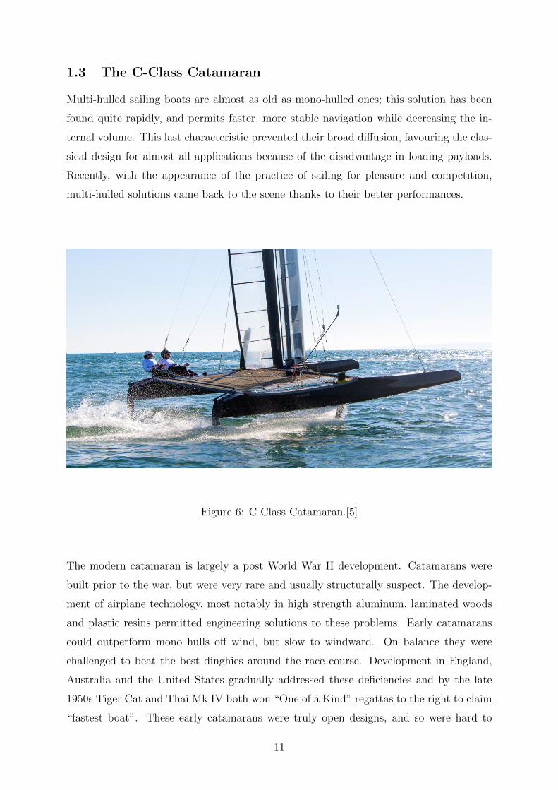
1.3 The C-Class Catamaran
Multi-hulled sailing boats are almost as old as mono-hulled ones; this solution has been
found quite rapidly, and permits faster, more stable navigation while decreasing the in-
ternal volume. This last characteristic prevented their broad di↵usion, favouring the clas-
sical design for almost all applications because of the disadvantage in loading payloads.
Recently, with the appearance of the practice of sailing for pleasure and competition,
multi-hulled solutions came back to the scene thanks to their better performances.
Figure 6: C Class Catamaran.[5]
The modern catamaran is largely a post World War II development. Catamarans were
built prior to the war, but were very rare and usually structurally suspect. The develop-
ment of airplane technology, most notably in high strength aluminum, laminated woods
and plastic resins permitted engineering solutions to these problems. Early catamarans
could outperform mono hulls o↵ wind, but slow to windward. On balance they were
challenged to beat the best dinghies around the race course. Development in England,
Australia and the United States gradually addressed these deficiencies and by the late
1950s Tiger Cat and Thai Mk IV both won “One of a Kind” regattas to the right to claim
“fastest boat”. These early catamarans were truly open designs, and so were hard to
11
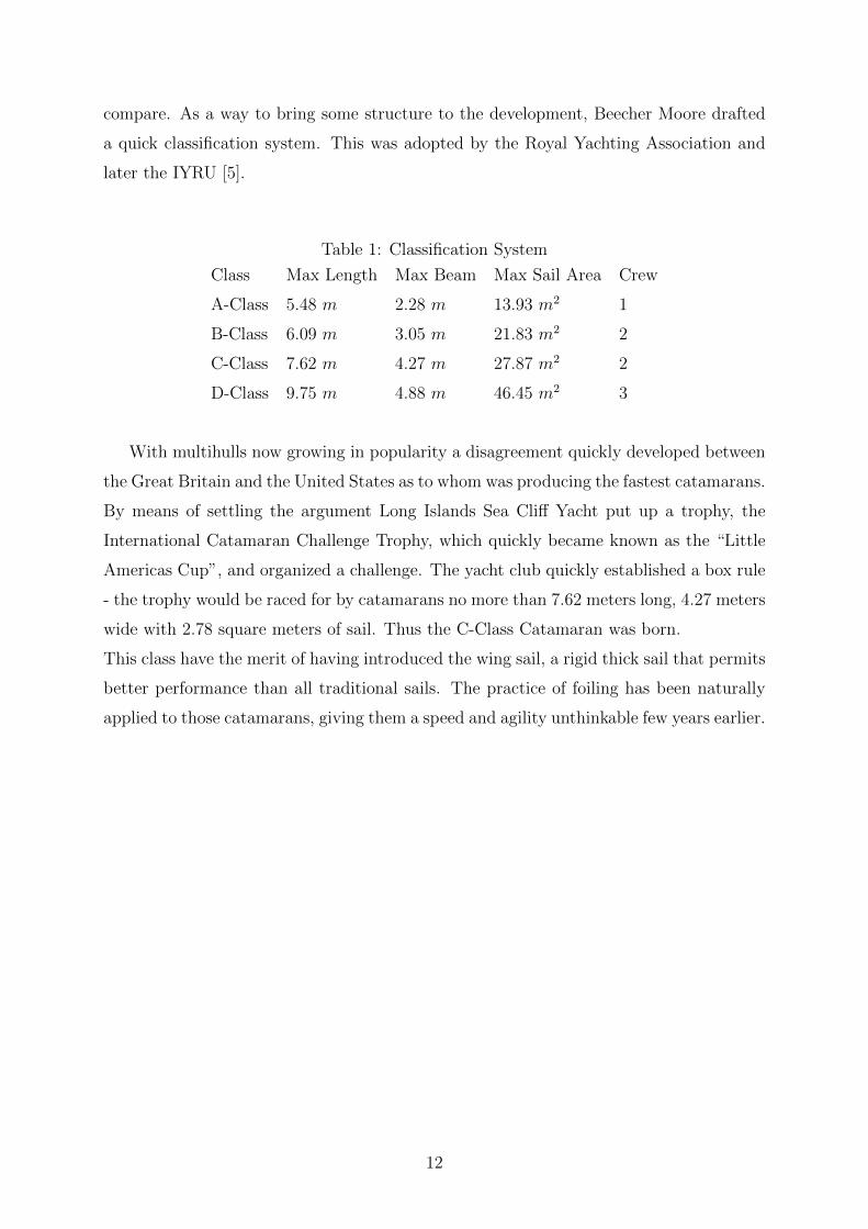
compare. As a way to bring some structure to the development, Beecher Moore drafted
a quick classification system. This was adopted by the Royal Yachting Association and
later the IYRU [5].
Table 1: Classification System
Class Max Length Max Beam Max Sail Area Crew
A-Class 5.48 m 2.28 m 13.93 m
2 1
B-Class 6.09 m 3.05 m 21.83 m
2 2
C-Class 7.62 m 4.27 m 27.87 m
2 2
D-Class 9.75 m 4.88 m 46.45 m
2 3
With multihulls now growing in popularity a disagreement quickly developed between
the Great Britain and the United States as to whom was producing the fastest catamarans.
By means of settling the argument Long Islands Sea Cli↵ Yacht put up a trophy, the
International Catamaran Challenge Trophy, which quickly became known as the “Little
Americas Cup”, and organized a challenge. The yacht club quickly established a box rule
- the trophy would be raced for by catamarans no more than 7.62 meters long, 4.27 meters
wide with 2.78 square meters of sail. Thus the C-Class Catamaran was born.
This class have the merit of having introduced the wing sail, a rigid thick sail that permits
better performance than all traditional sails. The practice of foiling has been naturally
applied to those catamarans, giving them a speed and agility unthinkable few years earlier.
12
1.4 Dynamic Analysis
With the increase of speed and agility the decrease of stability came naturally; the rapidity
and abruptness of changes in the loads at play, being the cause a wind gust, a wave
or a command, make the handling of a foiling sailing boat a di�cult and tiring task.
Furthermore, the need to win the competition asks not only to reach high speeds, but
also to be able to reach them in all conditions and to maintain them as long as possible.
During the progress of any kind of regatta the boat encounters a variety of wind conditions,
so the adaptability is a necessity.
But versatility is not enough to win: a foiling boat needs to keep foiling for as much
time as possible, in order not to waist precious seconds. Thus, the capacity of performing
complex maneuvers in foiling condition is now mandatory. A clear example is given by
the current America’s cup competition: the crews recently managed to perform a whole
race in foiling condition; not for an instant since the start sounded have the hulls touched
water.
In order to ensure high performances, stability and maneuverability a dynamic simulator
can prove itself a useful instrument in the designing phase: it could allow the designing
team to study the dynamic behaviour of the boat way before its construction.
To analyse the dynamic behaviour of a system means to:
• Produce a model representing it, as precisely as possible
• Compute all the loads applied to it
• Solve the equations of dynamics, considering all loads and inertia of the system
• Study the system’s response, in order to obtain informations about its behaviour
A great deal of informations can be acquired by a dynamic simulation about the dynamic
behaviour of a sailing boat, depending on the precision of the model at hand and on the
way the loads are being computed.
For instance, in order to evaluate the ability of the boat to stay stable di↵erent models of
gust may be applied, or di↵erent sea contritions, e.g. to evaluate the disturb caused by
waves hitting the boat from di↵erent directions. This could also find a helpful application
in choosing the best course to follow during a race. A classical analysis could be the
simulation of a manuever in order to understand in details how it can be performed and
improved.
Improving the model means to broaden the applicability af the dynamic analysis; two
13
interesting aspects that can be studied are the interactions loads-structure and the crew
response. The first needs a good representation of the structure, and increases the compu-
tational cost since an iterative method is necessary to correctly evaluate the deformations
but permits to know when and where the maximum loads will stress the structure. The
second demands an accurate description of the controllers dynamics and the typical re-
sponse of a trained crew. This analysis could allow the designers to understand if a boat
is actually controllable by an average crew, and if a particular manuever can or can’t be
performed.
So, with enough data at disposal it is possible to develop a variety of tools for the simu-
lator, in order to analyse di↵erent aspects of a sailing boat’s dynamic, thus obtaining a
powerful and versatile instrument.
14
2 The C-Class Catamaran
The C-Class Catamaran is a high-performance developmental class sailing catamaran.
They are very light boats which use rigid wing sails and can sail at twice the speed of the
wind. They are used for match races known as the International Catamaran Challenge
Trophy and its successor the International C-Class Catamaran Championship - both often
referred to as the ”Little America’s Cup”.
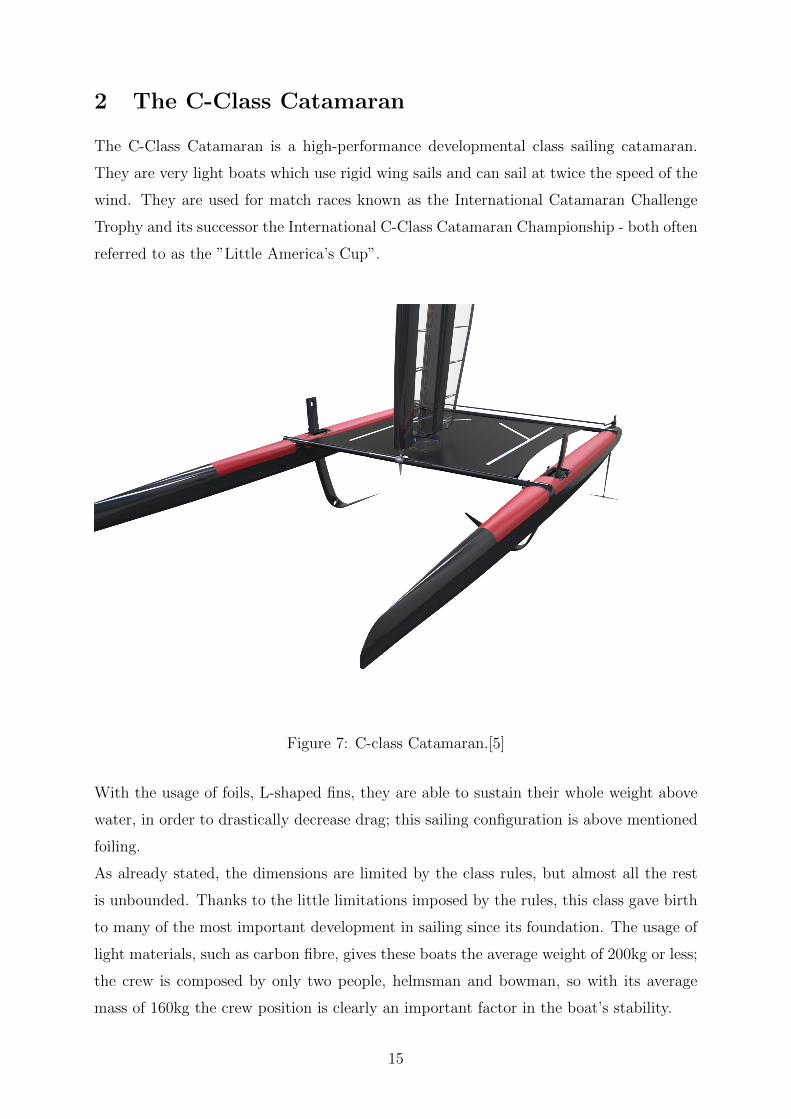
Figure 7: C-class Catamaran.[5]
With the usage of foils, L-shaped fins, they are able to sustain their whole weight above
water, in order to drastically decrease drag; this sailing configuration is above mentioned
foiling.
As already stated, the dimensions are limited by the class rules, but almost all the rest
is unbounded. Thanks to the little limitations imposed by the rules, this class gave birth
to many of the most important development in sailing since its foundation. The usage of
light materials, such as carbon fibre, gives these boats the average weight of 200kg or less;
the crew is composed by only two people, helmsman and bowman, so with its average
mass of 160kg the crew position is clearly an important factor in the boat’s stability.
15
2.1 The Boat
The boat model presented here is part of a project developed by a Swiss design studio;
the available data regard exclusively the wing sail, foil and rudder, because for handling
reasons the actual boat is a little di↵erent from the presented one. The actual foil and
rudders have been changed a little, but no data about them are freely obtainable. Yet
data about the aerodynamic and hydrodynamic behaviour of the presented surfaces were
available, and the analysis proposed has only an example intent, so for the current needs
that was enough.
Basic data about the boat were available:
• Its weight: 210 kg;
• The relative position of the wing, the foil, the rudders and the overall centre of
mass;
• The inertia moment about the CM;
• The maximum displacements of the crew, with respect to the boat’s CM.
Unfortunately, no data about the structure were available, so no loads-structure cou-
pling has been taken into account.
2.1.1 The Model
Because of the few available data, the model developed in MBDyn to represent the boat
is very simple: a mass body attached to a structural node represents the boat’s CM, and
the same applies for the crew. The chosen reference system is fixed with respect to Earth,
so it’s inertial, and oriented initially with X-axis coincident with the longitudinal boat
axis pointing from stern to bow, Z-axis vertical pointing up, while Y-axis is defined with
the right-hand rule.
The relative position of the crew with respect to the boat is controlled through a total
joint by a PID controller, in order to help balancing the pitching moment. All loads
are applied to the CM, so the dynamic solution is quite trivial. All degrees of freedom
are left unconstrained for the CM, with the exception of the rotation around X-axis:
since all available data are referred to null roll angle, it has been chosen to inhibit that
rotation and keep the total rolling moment below the maximum one balancable by the
16

crew displacement.
That been said, the PID controller for the crew position in y direction is actually present
in the software, and can be activated in order to study the system’s dynamics with all
degrees of freedom unconstrained.
17
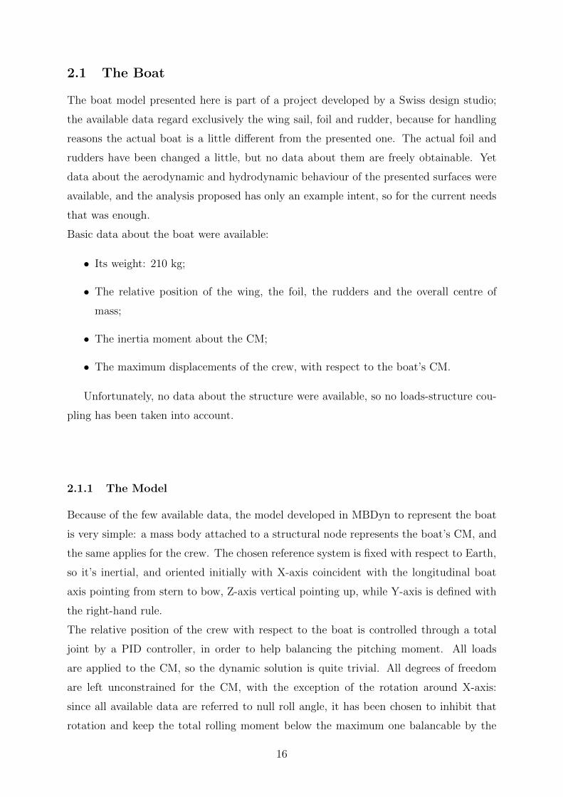
2.2 The Wing Sail
Sails can be used to propel a boat not only by means of their aerodynamic drag, that al-
lows them to function only if going windward, but also exploiting their ability to produce
lift. So, aerodynamically, a sail behaves similar to a very thin wing, with the di↵erence
that its shape changes with the wind speed and angle of attack. For cruising ships the
necessity to remove the sail frequently, rapidly and easily prevents the usage of rigid sails.
This is not true for racing ones.
Figure 8: The Wing Sail.[6]
The better performances of thick wings is a well known fact, so rigid and thick sails
have been designed and used since the 60s. The model currently in use on C-class cata-
marans is made of two wings, one operating as the main element and the other as a flap,
of equal chord length. The structure is quite similar to that of a classical wing, with ribs
and spars (the main one being the mast) covered with elastic skin.
18
The taper is studied in order to provide the maximum propulsive force while keeping the
heeling moment as low as possible; the highest part of the wing is immersed in faster wind,
but it also exerts the highest moment, so a compromise is needed. A peculiar feature of
the wing sail is the possibility to tune the twist: both wings can change the distribution
and value of the relative orientation in order to follow the change in height of the apparent
wind direction.
The mechanism allowing the relative rotation at each section keeps the fissure at a desired
width, and the main wing at an outer position with respect to the secondary wing; this
is done in order to keep the secondary wing out of the main wing’s wake.
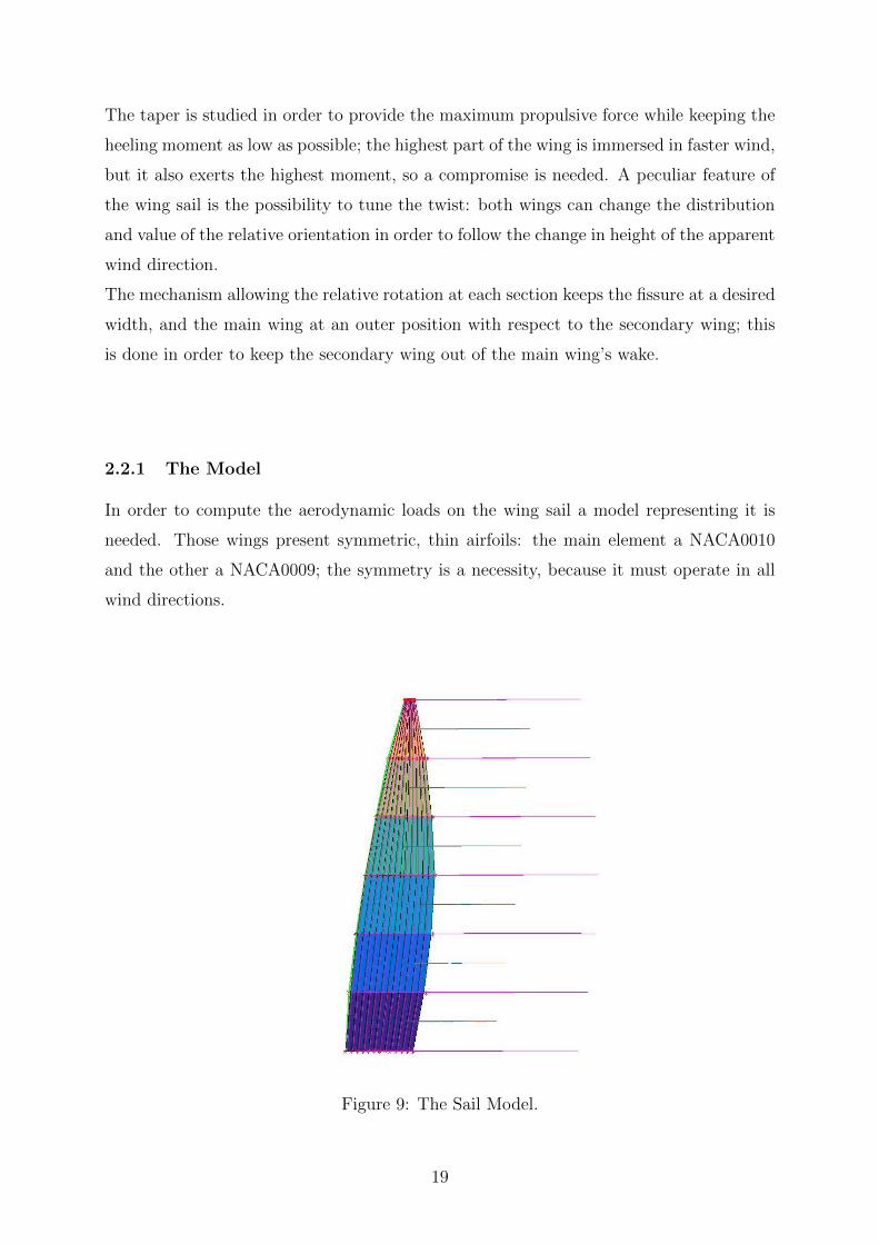
2.2.1 The Model
In order to compute the aerodynamic loads on the wing sail a model representing it is
needed. Those wings present symmetric, thin airfoils: the main element a NACA0010
and the other a NACA0009; the symmetry is a necessity, because it must operate in all
wind directions.
Figure 9: The Sail Model.
19
Thanks to those characteristics their aerodynamic properties are well represented by a
flat surface; the loss of information about its thickness is of little concern because, being it
small, its e↵ects are mostly important when regarding the stall behaviour, a phenomenon
not representable with the Velocity Potential Theory. The two aspects that most need
care are the chord distribution and the relative motion between the two elements: they
are analysed together, in order to take into account their mutual influence, so it become
mandatory to pay attention on the fissure dimension and to avoid contact between the
wake of the main element and the secondary one.
20
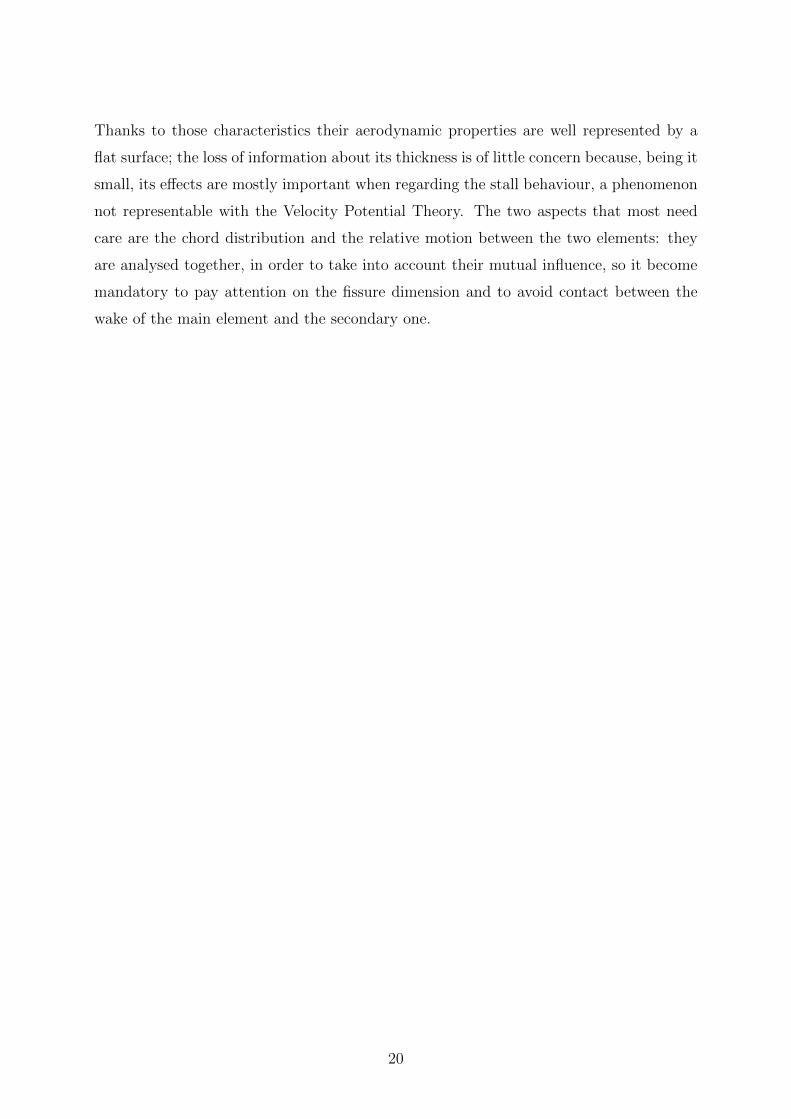
2.3 The Foil
All sailing boats are provided with a keel, a ”fin” that has the purpose of balancing the
lateral force exerted by the sail and so keeping the side speed low. A foil does that and
much more: thanks to its ”L” shape it presents an horizontal surface that exerts a vertical
force that lifts the hulls above sea level.
Figure 10: The Foil.
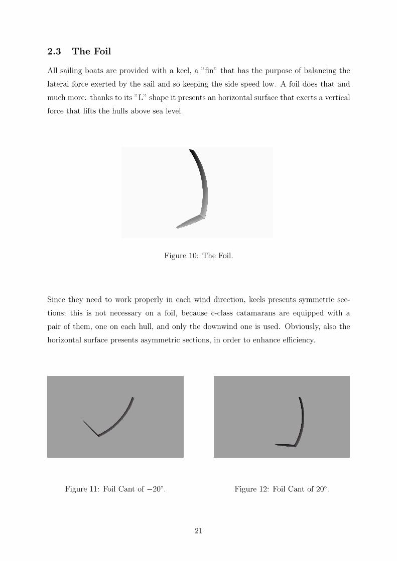
Since they need to work properly in each wind direction, keels presents symmetric sec-
tions; this is not necessary on a foil, because c-class catamarans are equipped with a
pair of them, one on each hull, and only the downwind one is used. Obviously, also the
horizontal surface presents asymmetric sections, in order to enhance e�ciency.
Figure 11: Foil Cant of �20�. Figure 12: Foil Cant of 20�.
21
Along the years, a great number of foils with very di↵erent shapes have been developed,
depending on the needs, the aims (and the imagination) of the designers. The capacity
to sustain the boat’s weight while producing drag low enough to permit the speed to
rise above the minimum foiling condition, which is the lowest speed at which the foil can
produce enough lift to balance the boat’s weight, make it in many ways quite similar to
a classical wing. The main di↵erence is the fluid in which it operates; the high density of
water allows small surface to exert high hydrodynamical loads, while producing a lot of
viscous drag (much more than in air). Foil orientation can be regulated in order to make
them exert the correct amount of load; this can be done by rotating them around two
axis: the first parallel to the transversal boat axis, the other parallel to the longitudinal
one. The first regulation is called foil rake, and increases the vertical load exerted; the
second one, called foil cant, has the purpose to rotate the global direction of the force
exerted: for low speeds more surface is needed in the production of vertical force, but
for higher speeds less surface is necessary, so the foiler can be rotated to a more vertical
position in order to exert more lateral force and lower the side speed.
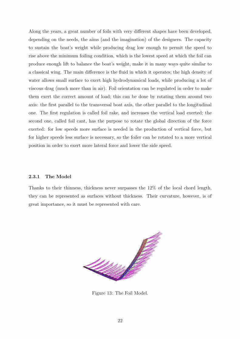
2.3.1 The Model
Thanks to their thinness, thickness never surpasses the 12% of the local chord length,
they can be represented as surfaces without thickness. Their curvature, however, is of
great importance, so it must be represented with care.
Figure 13: The Foil Model.
22
The main issue regarding their model is the intersection with the water surface; a need
to consider both fluids arises. To simplify, only the surface below water level is studied
and therefore modelled; the absence of the emerged portion is of little concern because,
being air density so less than water’s, the loads by it exerted are a small portion of the
overall forces, so they can be easily neglected. Also, since the thickest portion o a foil is in
the area connecting with the hull and thus never modelled because emerged, this solution
enforces the hypotheses of low thickness.
23

2.4 The Rudder
Foiling ships are way less stable than classical ones, so a need to balance pitch arises; this
is achieved through the usage of T-shaped rudders. As for a airplane’s tail, the vertical
surface controls the yaw while the horizontal controls the pitch. Each hull has a rudder,
so there are two rudders in each c-class catamaran; this is done for the sake of symmetry,
in order to keep the roll moment balanced.
Figure 14: The Rudders.[7]
Rudders can be oriented around the vertical axis, to regulate the yaw, and around the
horizontal axis, to regulate the pitch. In some cases, the two rudders can be oriented
separately: this is done to produce a component of moment around the longitudinal boat
axis, but is seldom used because of the necessity to keep the controls simple. Keep in
mind that there cannot be automatic controllers on board, and because of the high speeds
and loads exerted during navigation a small error or delay can produce catastrophic con-
sequences.
24
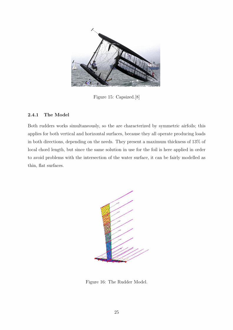
Figure 15: Capsized.[8]
2.4.1 The Model
Both rudders works simultaneously, so the are characterized by symmetric airfoils; this
applies for both vertical and horizontal surfaces, because they all operate producing loads
in both directions, depending on the needs. They present a maximum thickness of 13% of
local chord length, but since the same solution in use for the foil is here applied in order
to avoid problems with the intersection of the water surface, it can be fairly modelled as
thin, flat surfaces.
Figure 16: The Rudder Model.
25
A problem peculiar with “T” shaped surfaces is the intersection of the horizontal and
vertical portions; there, the two vortex lattices intersect, causing singularities problems.
This is avoided by leaving a small gap between the two surfaces, so small that it doesn’t
have a sensible e↵ect on the flow but wide enough to avoid intersection issues.
26
2.5 Peculiar Issues
C class catamarans are agile and fast, but quite di�cult to handle especially whit strong
winds. The reasons are various, the most important of them being:
• The weight: being so light gives this boat a small inertia and puts the centre of
gravity above water (typically around 3 meters), making it quite unstable.
• The crew: representing almost half of the overall weight, the crew need to move
quite a lot while manoeuvring in order to compensate for the rolling and pitching
moments.
• The wing sail: because of its high performances, the wing sail is di�cult to set,
since a little excess of loads can lead to a capsize, a thing at least unpleasant.
• The foiling condition: sailing above water is a complex activity, because much work
on the controls is needed to keep the boat stable. Searching for the configuration
that allows the fastest route can be quite challenging, while avoiding to hit the
water.
• The speed: those boats can reach the speed of 65 km/h, so a collision can be
extremely dangerous for the crew.
For all those reasons, the ability to predict the dynamic behaviour of a C class cata-
maran, and more generally of any foiling boat, is much appreciated not only in the design
process, but also in the training of the crew.
27

3 The Software
3.1 General Introduction
As previously stated, the purpose of the developed software is to analyse the dynamic
behaviour of a C class catamaran, as precisely as possible, in order to evaluate its stability
and response to disturbs and commands. Thus a multy-body dynamics software is needed,
coupled with an aerodynamic model. For this purpose, MBDyn has been chosen as
the software’s core, mostly because of its versatility and the possibility to interface it
with external solvers. In order to compute the fluid dynamical loads MBDyn has been
connected with a VLM software, through the Python’s interface.
Figure 17: Software Structure
28
Where:
• Everything labelled as Old comes from the previous time step
• Current, obviously, refers to the current time step
• The new sail regulation, when available, is applied to the current time step
• New loads are used to start the next time step
The python script serves only as a communicator and to start the simulation; at the
initial time step, the loads are all null and the kinematics is dictated by the initial values
imposed in MBDyn. The kinematics is used by the VLM in order to compute the new
loads, while the PID controllers act on the foil and rudder in order to keep the assigned
values, to maintain a stable navigation. The loads are then passed to MBDyn, which
computes the new kinematics and moves to the next time step.
Before computing the new loads, the VLM checks if the overall force in the direction of
motion is less or more than 1, in absolute value; that would mean that the highest speed
possible at that configuration is reached. If the condition is met, then the optimisation
process begins: the simulation is paused, while the optimizer looks for the sail regulation
that better exploit the current condition. When the new regulation is found, it is gradually
applied to the sail, and the simulation continues.
29
3.2 Windage
To better estimate the overall loads applied to the system, the contribute of the aero-
dynamic drag produced by all elements outside water has been added; this contribute is
regarded as Windage. This could be taken into account thanks to previous analysis done
on the boat: RANS computations provided the drag coe�cient of all elements exposed to
the wind, with the sole exception of the sail. The data are stored in a 2-D array, ordered
by increasing AWA (Apparent Wind Angle, the angle at which the total wind meets the
longitudinal boat axis), and divided in 3 colons, one for each component of the total force.
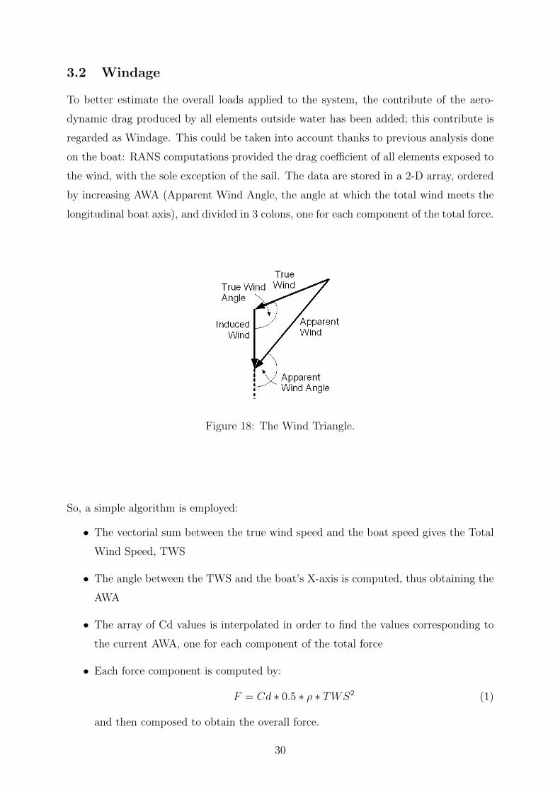
Figure 18: The Wind Triangle.
So, a simple algorithm is employed:
• The vectorial sum between the true wind speed and the boat speed gives the Total
Wind Speed, TWS
• The angle between the TWS and the boat’s X-axis is computed, thus obtaining the
AWA
• The array of Cd values is interpolated in order to find the values corresponding to
the current AWA, one for each component of the total force
• Each force component is computed by:
F = Cd ⇤ 0.5 ⇤ ⇢ ⇤ TWS
2 (1)
and then composed to obtain the overall force.
30
The Windage e↵ect depends on the wind direction, so it has the e↵ect to lower the
boat’s speed when sailing upwind but increases it when sailing windward. In both cases,
the correct evaluation of this contribution helps to give a good prediction of the global
behaviour of the system.
31
3.3 MBDyn
From MBDyn’s website [9]:
“MBDyn is the first and possibly the only free general purpose Multibody Dynamics
analysis software, released under GNU’s GPL 2.1.
It has been developed at the Dipartimento di Scienze e Tecnologie Aerospaziali (for-
merly Dipartimento di Ingegneria Aerospaziale) of the University ”Politecnico di Milano”,
Italy. MBDyn features the integrated multidisciplinary simulation of multibody, multi-
physics systems, including nonlinear mechanics of rigid and flexible bodies (geometrically
exact and composite-ready beam and shell finite elements, component mode synthesis
elements, lumped elements) subjected to kinematic constraints, along with smart mate-
rials, electric networks, active control, hydraulic networks, and essential fixed-wing and
rotorcraft aerodynamics.”
MBDyn o↵ers the possibility to develop complex dynamical models, including structural
informations; it has been tested on a wide range of applications, from helicopters to wind
turbine, demonstrating its great versatility. The possibility to interface it with external
softwares is one of the main reason it has been chosen for this project; not only for aero-
dynamic loads computation, but also for the configuration optimization.
3.3.1 Application
The motion of a boat, once neglecting the deformation of its structure, is governed by
the equations of motion of a rigid body: those can be split in a translation motion of a
point, which for simplicity has been chosen the centre of mass, and the rotation of the
body around it. The equation for the variation of the linear momentum referred to the
centre of mass is:
mXG = R (2)
where m is the mass of the boat. R is the total force acting on the boat obtained via:
R = Fhydro + Faero +mg (3)
where Fhydro is the sum of all hydrodynamic forces exerted by the appendages, Faero is
the sum of all aerodynamic forces exerted by the sail plus the Windage contribution and
32

mg is the gravity force.
In order to solve the equation for the variation of angular momentum first of all is necessary
to define two reference systems: one referred to the fixed domain, the principal reference
system and one that rotates with boat, secondary reference system. It can be shown
that the union of the unit-vector i, j, k of the secondary reference system expressed in
the principal system generates the rotation matrix from one system to the other. The
equation of variation of angular momentum, referred to the principal reference system,
can be finally expressed as: [10]
¯T
¯IG
¯T
�1! + ! ⇥ ¯
T
¯IG
¯T
�1! = MG (4)
where ! is the angular velocity, ¯IG is the matrix of the moment of inertia:
¯IG =
2
664
IXX IXY IXZ
IY X IY Y IY Z
IZX IZY IZZ
3
775 (5)
and MG is the total moment around the rotation centre acting on the boat expressed in
the principal reference system. The total moment can be expressed as:
MG = Mhydro +Maero (6)
These equations form a system of 6 second order ordinary di↵erential equations, three
for the translation motion and three for the rotation. The translation equations are not
coupled and can be resolved separately. The rotation ones, except when the rotation is
around one single axis, are coupled non-linear equations and have to be resolved as a
coupled system.
33
3.4 Vortex Lattice Method
3.4.1 General Idea
Since an optimization process requires many iterations of any computation, to avoid an
excessive cost properly simplified methods are required. For aerodynamics the potential
theory o↵ers a series of powerful and versatile instruments with varying degrees of preci-
sion. Some basic hypotheses have to be respected for these methods to adhere su�ciently
to reality, the main ones being:
• A su�ciently high Reynolds number, so that the boundary layers, where most of
viscous phenomena happen, are thin enough to justify treating the flow as inviscid.
• A su�ciently low Mach number, so that compressibility e↵ects are small enough
to justify treating the flow as incompressible, or doing so and then using simple
compressibility corrections afterwards.
• A su�ciently streamlined body, so that separations do not occur.
The last requirement does not only impose constraints on the body shape but also on its
orientation in the flow field. This condition has the consequences of limiting the analysis
to conditions of attached flow only, so particular attention on the sail, foiler and rudders
orientation is needed. With these hypotheses, it is possible to define a flow potential �
and apply the Laplace equation to it r2� = 0 . Suitable boundary conditions to take
into account the shape of the body are generated imposing null normal component of
the velocity on its boundary: @�/@n = 0. Common methods use virtual singularities to
model the shape of the body and of its trail, then exploit the linearity of the problem to
divide the flow potential into a known undisturbed flow field �1 and an unknown distur-
bance flow field ' caused by the virtual singularities. The intensities of said singularities
are then found by applying the boundary conditions to the flow field disturbance they
generate. These methods are called “panel methods referring to the discrete elements in
which the geometry of the object considered is divided. Usually one virtual singularity
and one boundary condition is considered for each panel, but additional conditions may be
present, mainly concerning the trail. Once the flow field around the body is unequivocally
determined, aerodynamic forces acting on it are found applying the Bernoulli theorem to
find pressure distributions or the Kutta-Zhukowsky theorem to find the actual forces.
34
3.4.2 The Method
The Vortex Lattice method uses a series of “horseshoe vortices to model the lifting proper-
ties of a surface, and the flow perturbations caused by its trail. The vortices are composed
by a finite segment, located on the panel (at 1/4 of its chord, along its span) plus two
semi-infinite segments of equal circulation, starting at the panel and moving along the flow
field, which have the double function of ensuring the conservation of circulation (Kelvins
theorem D�/Dt = 0) and representing the trail of the object.
Vortices are not su�cient to take into account the aerodynamic e↵ects of the thickness of
an object, therefore only thin surfaces are modelled with su�cient precision. The panels
can be oriented relatively arbitrarily so a vast range of twists and curvatures of the surface
can be analyzed.
The problem consists in finding the intensity of each horseshoe vortex by imposing that
the component of the velocity normal to each panel is null at control points located at
3/4 of the panel’s chord (and at half the span of the panel). The influence of a vortex on
the flow field can be calculated by applying the Biot-Savart law for line vortices: [11]
V(x) =�
4 · ⇡ · r1 ⇥ r2|r1 ⇥ r2|2
·r0 ·
✓r1|r1|
� r2|r2|
◆�(7)
With r1 = x � x1, r2 = x � x2, r0 = r1 � r2, where x1 and x2 are respectively the
starting and final point of the vortex segment. By considering the normal component of
the velocity induced by each vortex (supposing its circulation unitary) on each control
point the influence matrix is generated, where each element Mij is the velocity induced
on the control point on panel i by the vortex on panel j. Defining then a vector {�j}containing all the circulations, the problem can be written as:
[Mij] · {�j} = �{V1 · ni} (8)
Where V1 · ni is the vector containing the components of the undisturbed velocity
normal to each panel at each control point. By imposing that it is equal to the one induced
by the vortices, with changed sign, the boundary condition on each panel is respected.
The problem is solved by inverting the influence matrix and calculating the circulations.
Once they are known the actual velocity field can be calculated, by applying again the
Biot-Savart law.
The force acting on each panel (with induced drag already considered) is found by applying
the Kutta-Zhukowsky lift theorem:
F = ⇢ ·V ⇥ � (9)
35
Then, resultant forces and moments, their evolution along the surface and adimen-
sional coe�cients can be calculated from the results.
3.4.3 Implementation
The method presents some features above the basic implementation; the software orients
the nodes of each panel so that the positions of the points at 1/4 and at 3/4 of the chord
are consistent with arbitrary local wind directions and accepts in input a non-uniform flow
field. Another di↵erence from the classical implementation is the use of modified horse-
shoe vortices composed of five finite segments and two infinite ones, inspired by those
implemented in the software Tornado[12]. This is done so that the first part of the trail
vortices is aligned with the panel sides while the final part is aligned with the velocity.
The length of the finite parts of the trail can be specified, and has been kept low to avoid
excessive dispersion of the trail vortices.
Some of the characteristics of the problem at hand require specific tools in order to treat
them correctly.
3.4.4 Wind Profile
Being the boat immersed in the atmospheric boundary layer, the wind speed increases
with the distance from the sea surface. For that reason, the software must be able to work
with a non uniform flow field. It may appear incorrect to analyze such a case with the
use of potential theory: this flow field is in fact rotational, while one of the fundamental
hypothesis of the potential theory is that it must only be applied to irrotational flows.
The doubt is discarded remembering that the irrotationality introduced by the flow field
is way lower than the amount injected by the vortex lattice, so it can be considered as an
acceptable imprecision.
36
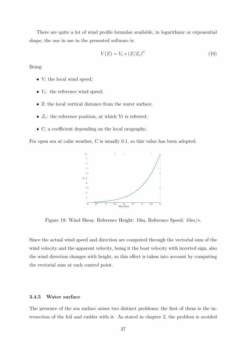
There are quite a lot of wind profile formulae available, in logarithmic or exponential
shape; the one in use in the presented software is:
V (Z) = Vr ⇤ (Z/Zr)C (10)
Being:
• V: the local wind speed;
• Vr: the reference wind speed;
• Z: the local vertical distance from the water surface;
• Zr: the reference position, at which Vr is referred;
• C: a coe�cient depending on the local orography;
For open sea at calm weather, C is usually 0.1, so this value has been adopted.
Figure 19: Wind Shear, Reference Height: 10m, Reference Speed: 10m/s.
Since the actual wind speed and direction are computed through the vectorial sum of the
wind velocity and the apparent velocity, being it the boat velocity with inverted sign, also
the wind direction changes with height, so this e↵ect is taken into account by computing
the vectorial sum at each control point.
3.4.5 Water surface
The presence of the sea surface arises two distinct problems; the first of them is the in-
tersection of the foil and rudder with it. As stated in chapter 2, the problem is avoided
37
by representing only the submersed portion, with little loss of precision.
The second, and less trivial, problem is the interference caused by the surface on the
water flow. It may appear similar to the classical interference of a solid boundary, but
the actual e↵ect on the flow is the opposite: while the proximity of a wall has a positive
e↵ect on the lift production of aerodynamic surface, the water surface has the e↵ect of
reducing the lift exerted. In other words, the e�ciency of an hydrodynamic surface lowers
when nearing to the surface of the water.
This e↵ect can be taken into account by a Vortex Lattice Method through the use of an
expedient similar to the mirror e↵ect used for the wall proximity. A specular copy of the
hydrodynamic surface if produced and placed symmetrically to it with respect to the wa-
ter surface; when computing the influence matrix the influence of the image is taken into
account, but (and here lies the di↵erence with the mirror e↵ect) the velocity induced by
the image is changed in sign. This method, with little imagination, is called anti-mirror
e↵ect.
3.4.6 Viscous Drag
C class catamarans produce an incredible small quantity of drag, if compared with non
foiling boats; that is because of their ability to lift the hulls outside the water. Thanks to
their shapes, the foil and rudders are capable of great e�ciency, and the friction caused
by the airflow is way less then the one produced by the water flow. For those reasons,
it becomes mandatory to take into account the viscous drag produced by the surfaces
immersed in water.
In order to do so, an analytical method is applied for the computation of the viscous drag
coe�cient. First, the friction coe�cient is computed for each section over the foiler and
rudders:
Cf =1
(3.46 ⇤ logRe� 5.6)2(11)
being Re the local Reynolds number, computed with the local chord length.
Than the local viscous drag coe�cient is computed through:
Cd = (1 + 1.2 ⇤ t/c+ 70 ⇤ (t/c)4) ⇤ Cf ⇤ 2 (12)
Being:
38
• t: the local thickness;
• c: the local chord length.
Finally, the total viscous drag force is computed through:
Fvisc = Cd ⇤ q ⇤ area (13)
Being:
• q: the dynamic pressure;
• area: the area of the portion of surface where the Cd is being computed.
39
3.5 PID Controllers
In order to keep the boat stable in (almost) every condition, PID controllers are respon-
sible to the continuous regulation of the foil and the rudders.
3.5.1 Theory
A proportional-integral-derivative controller (PID controller) is a control loop feedback
mechanism commonly used in industrial control systems. A PID controller continuously
calculates an error value e(t) as the di↵erence between a desired setpoint and a measured
process variable and applies a correction based on proportional, integral, and derivative
terms which give their name to the controller type. [13]
The controller attempts to minimize the error over time by adjustment of a control variable
u(t), in the case at hand the foil’s or rudder’s orientation, to a new value determined by
a weighted sum:
u(t) = Kpe(t) +Ki
Z t
0
e(⌧) d⌧ +Kdde(t)
dt
, (14)
where Kp, Ki and Kd, all non-negative, denote the coe�cients for the proportional, in-
tegral, and derivative terms, respectively (sometimes denoted P, I, and D). The main
issue with PID controllers is the tuning, which is the choosing of the gains values; many
methods are available, from completely manual to all automatic. For the controllers in
use, the tuning done was mostly Ziegler-Nichols method, and manual when the previous
failed.
3.5.2 Tuning
In order to exploit an automatized tuning method a simplified model representing the
whole system is needed; this is because automatic tuning tools are basically optimization
processes that permit to find the best combination of coe�cients, but in order to do so
they need to evaluate the system response a high number of times. Since a simplified
model with a behaviour su�ciently similar to the real system could not be reproduced,
the need for an alternative arose.
40
The Ziegler-Nichols [14] method has been applied successfully for almost all controllers.
The method consists in the following steps: [15]
• All gains are set to 0
• The proportional gain is increased until it reaches the ultimate gain, Ku, at which
the output of the loop starts to stably oscillate
• Ku and the oscillation period Tu are used to set the gains as follows
Kp = 0.6 ⇤Ku (15)
Ki = 1.2 ⇤Ku/Tu (16)
Kd = 3 ⇤Ku ⇤ Tu/40 (17)
This method, however, is not universally e↵ective; it usually causes high overshoots, and
doesn’t guarantee stability. When it occurred, manual tuning proved necessary.
This method is slow and tedious, but with enough patience permits to obtain the desired
response. The procedure is the following:
• As in the previous method, all gains are set to 0
• Kp is increased until the response oscillates, then its value is halved
• Ki is increased until the o↵set to the desired value is minimized
• Increase Kd to reduce oscillations and overshooting
In the actual state, the controllers role is to find a regulation that keeps the system stable;
at the present moment there is no interest in the amount of overshoot or time delay, they
just need to be low enough to reduce the computational cost. So, the tuning process has
been considered concluded when the system could stabilize itself rapidly enough when
subject to the applied disturbs and loads.
41
3.6 Optimization
While the boat is kept stable, the sail needs to be regulated in order to best exploit the
wind power available at the current configuration. In order to do so, an optimization
process in needed. Many optimization algorithm are available, each best suited for dif-
ferent problems. The chosen one is a gradient method, because of its (relatively) low
computational cost. The method, thanks to the Matlab function fmincon [16], is applied
through an Interior Point Algorithm [17], which has been chosen because of its ability to
find solutions for non-linear problems.
3.6.1 The Method
While the simulation is running, the software waits for it to reach the condition of total X
force less than 1N, positive or negative. When this condition is satisfied, the simulation
pauses and the optimization process starts: it searches for the sail regulation that, at
the current configuration, produces the most thrust without exerting a heeling moment
above the maximum one, to ensure stability. In order to assure that the solution keeps
improving, the optimization is asked to look upon solutions that only provide higher
thrust than the previous.
The optimization problem is composed by the following elements:
• The evaluation function: the function that computes the performance of a possible
regulation. This is done through the VLM in order to compute the loads exerted
by the wing sail.
• The set of parameters: their combination represents a possible configuration, and
needs to be tested.
• The parameters values boundaries: the parameter’s space needs to be limited, in
order to only look upon feasible solutions.
• The non linear constraint: this is the mathematical formulation of the need to keep
the heeling moment below the maximum balancable by the crew, and the increase
in thrust.
Since also the foil and rudders contribute to the total heeling moment, the one produced
by those elements at the instant in which the simulation is paused is taken into account
when evaluating the sail configuration: it is added to the one exerted by the sail, and
their sum is then kept below the maximum value.
42
The simulation then proceeds, and the sail regulation is changed in small steps until
reaching the desired one. Since the problem is non linear, the exact amount of heeling
moment cannot be accurately predicted. For this reason, a controller is always active
to ensure that the maximum moment is not surpassed: it changes, and stops, the sail
movement in the case of overload. This tool is also mandatory if the running simulation
presents a varying wind or the execution of a maneuver, because the angle at which the
airflow will meet the sail will change in time.
43

4 Applications
A dynamics simulator can serve many purposes, and can help the designer in many ways:
from handling, stability to disturbs, reaction to commands, manuevers execution to loads-
structure coupling many are the aspects in which a dynamics simulator proves itself a
valuable instrument.
In this chapter, some simple examples of applications will be presented, with the sole
intent of discussing the software’s potential.
The topic of the application presented is the analysis of the adaptability of the C class in
changing weather. This is a common topic in sailing, since usually the wind is anything
but homogeneous: wind variations are extremely common while sailing near shore, and
are also present in open seas. This is not only caused by the weather instability, but also
because the high levels of turbulence contained in the first layer of the atmosphere causes
great uncertainties in the wind flow. For all those reasons, sail trimming is a restless task.
Before showing the results, it is mandatory to explain their reliability; the various modules
are tested inside the limits of their applicability, as reported in what follows.
44
4.1 Validation
MBDyn has been used in a great variety of occasions, so its validity is not questioned
here.
The VLM has been written in a previous project (named SAPO, SAils Performance Op-
timization), modified and improved for the current needs; thus, validation is mandatory.
The tools available are:
• The underlying theory
• Tornado, an open source VLM
• XFoil, an open source 2D panel code
• Data about the friction drag of the foil
The analysis conducted has the aim to verify the accordance between the developed
VLM results with those given by the theory, Tornado and XFoil, when the models are
comparable. The available data on the foil will be helpful to validate the friction drag’s
model.
4.1.1 VLM Validation
To test the Vortex lattice code written, some comparisons with other methods have been
made. One test has been done on an ”infinite” wing, a wing of uniform chord and twist
with an exaggerated aspect ratio (AR = 10000), to allow comparisons with 2D methods
(XFOIL, run in non-viscous mode, and a simple point vortices method) as well as with
the free vortex lattice software Tornado.
This has been done for varying curvatures of the surface. As expected, the Cl�↵ curves
obtained were linear, which allowed a direct comparisons of the values of the Cl↵=0 and
Cl,↵.
The variation of the Cl,↵ is in line with the ones found for the point vortices and
XFOIL (although XFOIL starts from a greater value due to the small amount of thick-
ness that had to be added for it to run properly). The value keeps relatively close to the
2 · ⇡ found from thin airfoils theory, departing from it with increasing curvature, as the
hypotheses of said theory are valid only up to a certain value of it.
Tornado instead seems less a↵ected by the added curvature, possibly due to the fact that
45
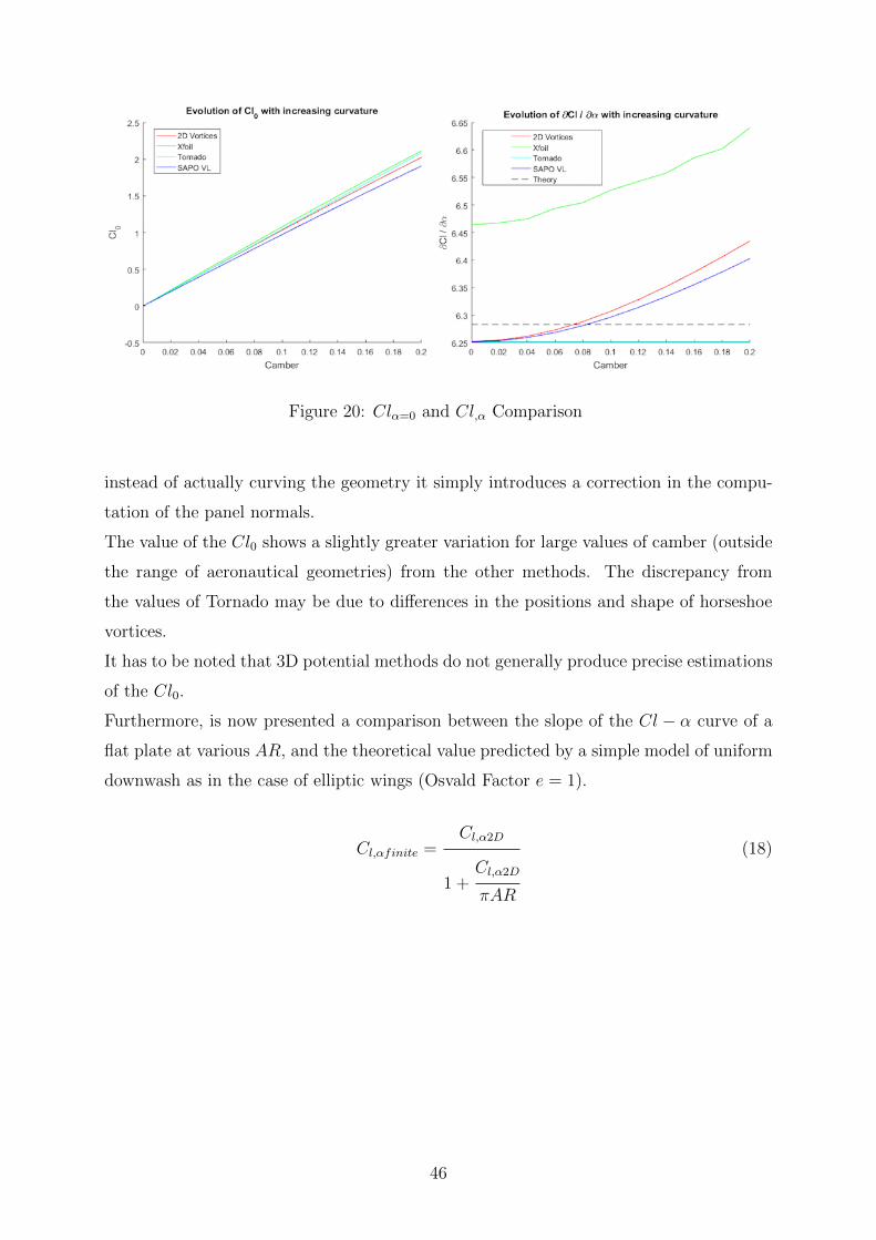
Figure 20: Cl↵=0 and Cl,↵ Comparison
instead of actually curving the geometry it simply introduces a correction in the compu-
tation of the panel normals.
The value of the Cl0 shows a slightly greater variation for large values of camber (outside
the range of aeronautical geometries) from the other methods. The discrepancy from
the values of Tornado may be due to di↵erences in the positions and shape of horseshoe
vortices.
It has to be noted that 3D potential methods do not generally produce precise estimations
of the Cl0.
Furthermore, is now presented a comparison between the slope of the Cl � ↵ curve of a
flat plate at various AR, and the theoretical value predicted by a simple model of uniform
downwash as in the case of elliptic wings (Osvald Factor e = 1).
Cl,↵finite =Cl,↵2D
1 +Cl,↵2D
⇡AR
(18)
46
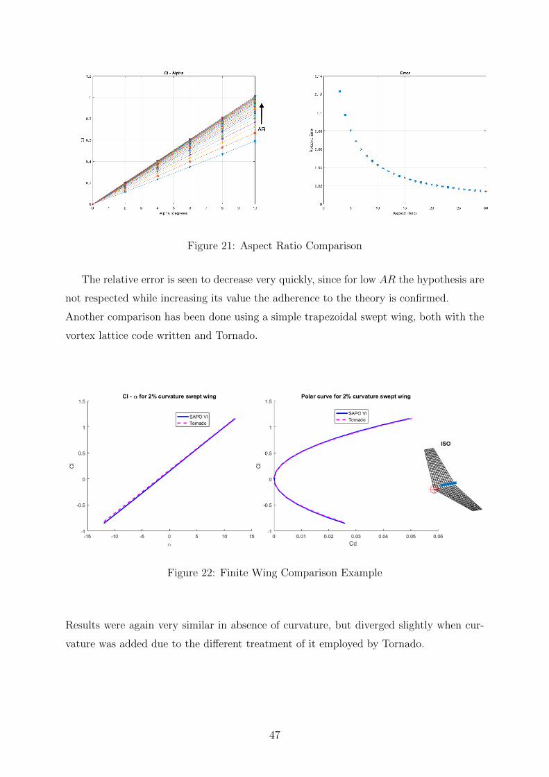
Figure 21: Aspect Ratio Comparison
The relative error is seen to decrease very quickly, since for low AR the hypothesis are
not respected while increasing its value the adherence to the theory is confirmed.
Another comparison has been done using a simple trapezoidal swept wing, both with the
vortex lattice code written and Tornado.
Figure 22: Finite Wing Comparison Example
Results were again very similar in absence of curvature, but diverged slightly when cur-
vature was added due to the di↵erent treatment of it employed by Tornado.
47
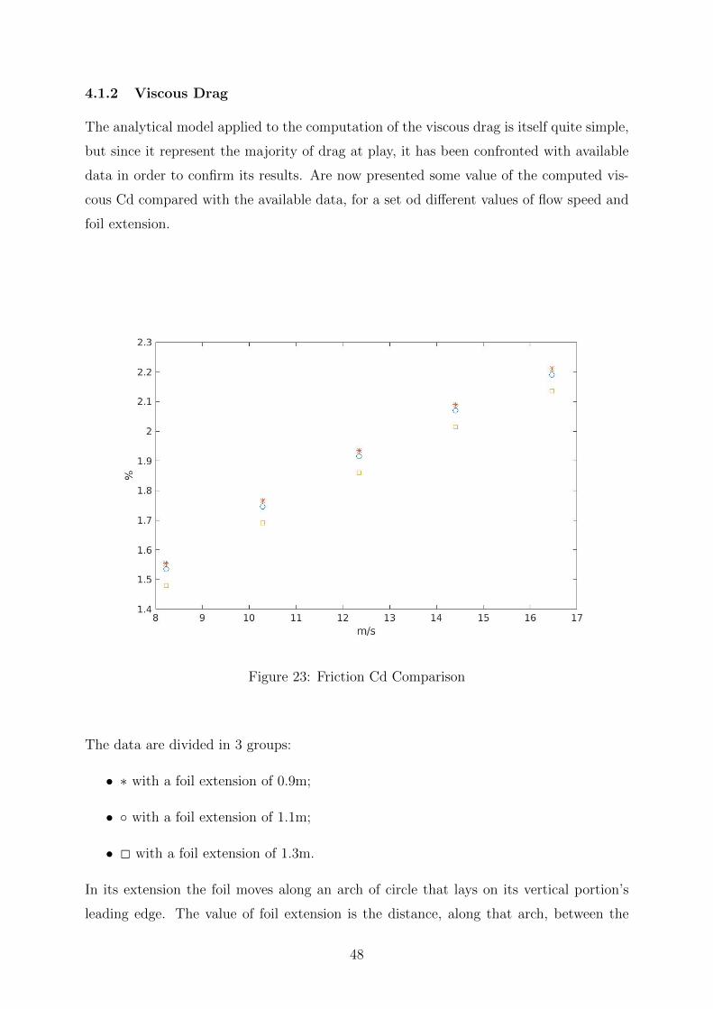
4.1.2 Viscous Drag
The analytical model applied to the computation of the viscous drag is itself quite simple,
but since it represent the majority of drag at play, it has been confronted with available
data in order to confirm its results. Are now presented some value of the computed vis-
cous Cd compared with the available data, for a set od di↵erent values of flow speed and
foil extension.
Figure 23: Friction Cd Comparison
The data are divided in 3 groups:
• ⇤ with a foil extension of 0.9m;
• � with a foil extension of 1.1m;
• 2 with a foil extension of 1.3m.
In its extension the foil moves along an arch of circle that lays on its vertical portion’s
leading edge. The value of foil extension is the distance, along that arch, between the
48
rest position and the desired one. It can be varied depending on the intentions of the
crew, basically to vary the boat’s height above water. All evaluation have been performed
with the foil in default position, which means cant and rake null, since they do not a↵ect
significantly the friction drag production.
The values found are less then the reference, so drag is a little underestimated, more if the
foil extension lowers. The errors may be caused by di↵erences in evaluating the chords,
thickness or their distribution. Possibly, further analysis may lead to better adherence of
the results, yet the obtained one was considered good enough.
49
4.2 Results
Some examples of the possible analysis that the program can perform are now shown
and discussed. The aim is to show the ability of the system to adapt and handle new
conditions keeping the navigation stable and fast. The data presented are not intended
to actually evaluate the true boat’s behaviour, because in order to do so a better model
of system’s inertial properties is mandatory, and the controllers should be tuned to mimic
fairly an actual human crew. Nevertheless, a good idea about how those analysis can be
conducted and to what can be expected can be surely obtained by the following examples.
The parameters on which the optimization process acts are:
• ↵: the angle between the main element’s chord of the wing sail and the longitudinal
boat’s axis
• �: the angle between the second element’s and the main’s chord
• twist1: the angle between the top and the base sections of the main element
• twist2: the angle between the top and the base sections of the second element
The twist is uniformly applied on both elements, in order to reduce the parameter’s
number; with more computational power its distribution can be optimized. This could be
useful, since the wind profile is not linear. When defining ↵ and � the reference section
is the bottom one.
The wind direction is defined as the angle between the true wind and the X-axis of the
fixed reference system.
All simulations are conducted with a fixed time step of 0.01 seconds, starting near an
equilibrium condition:
• Initial heading speed: 6.9 m/s
• Initial lateral speed: 0.1 m/s
• Vertical position: 0.7 m above water
• Null values for yaw, pitch and roll angles
• Initial sail regulation: ↵ = 10�, � = �11�, twist1 = 20�, twist2 = 20�
• Fixed foil extension: 1.3 m
• Initial wind speed: 7.2 m/s
50
• Initial TWA: 50�
Three simulations are here presented:
1. Fixed wind conditions: simply to show how the optimization process performs in
stable conditions
2. Changing wind without performance optimization: to show how the controllers work
in order to keep the boat stable
3. Changing wind with performance optimization: to show how the system adapts to
the new condition and then enhances its performances
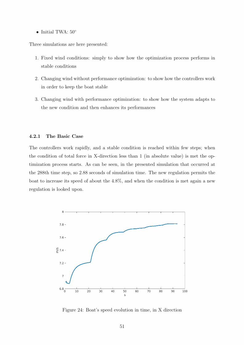
4.2.1 The Basic Case
The controllers work rapidly, and a stable condition is reached within few steps; when
the condition of total force in X-direction less than 1 (in absolute value) is met the op-
timization process starts. As can be seen, in the presented simulation that occurred at
the 288th time step, so 2.88 seconds of simulation time. The new regulation permits the
boat to increase its speed of about the 4.8%, and when the condition is met again a new
regulation is looked upon.
Figure 24: Boat’s speed evolution in time, in X direction
51
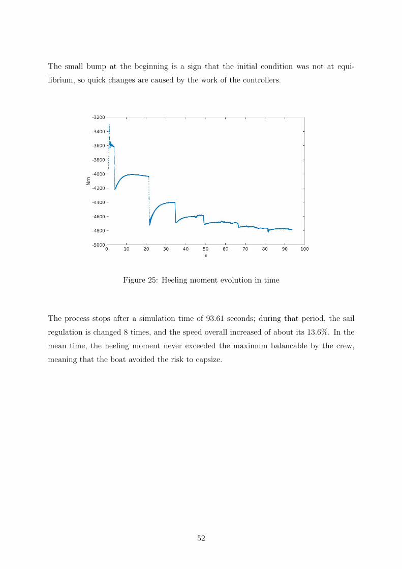
The small bump at the beginning is a sign that the initial condition was not at equi-
librium, so quick changes are caused by the work of the controllers.
Figure 25: Heeling moment evolution in time
The process stops after a simulation time of 93.61 seconds; during that period, the sail
regulation is changed 8 times, and the speed overall increased of about its 13.6%. In the
mean time, the heeling moment never exceeded the maximum balancable by the crew,
meaning that the boat avoided the risk to capsize.
52
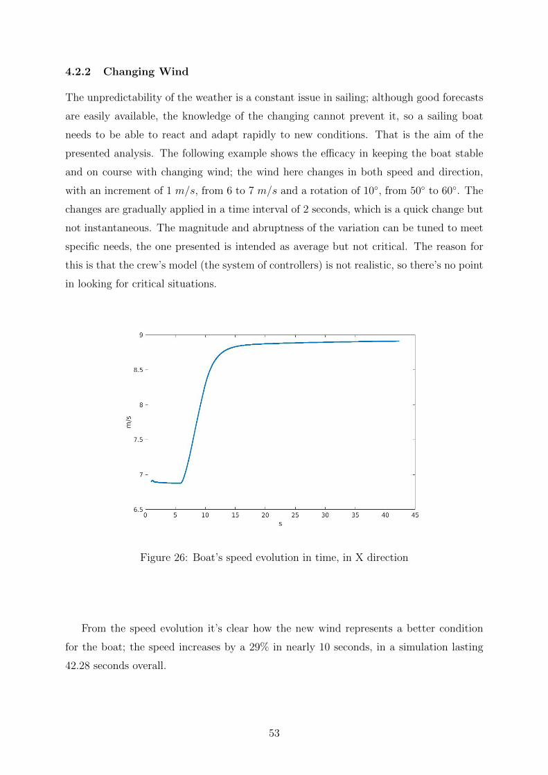
4.2.2 Changing Wind
The unpredictability of the weather is a constant issue in sailing; although good forecasts
are easily available, the knowledge of the changing cannot prevent it, so a sailing boat
needs to be able to react and adapt rapidly to new conditions. That is the aim of the
presented analysis. The following example shows the e�cacy in keeping the boat stable
and on course with changing wind; the wind here changes in both speed and direction,
with an increment of 1 m/s, from 6 to 7 m/s and a rotation of 10�, from 50� to 60�. The
changes are gradually applied in a time interval of 2 seconds, which is a quick change but
not instantaneous. The magnitude and abruptness of the variation can be tuned to meet
specific needs, the one presented is intended as average but not critical. The reason for
this is that the crew’s model (the system of controllers) is not realistic, so there’s no point
in looking for critical situations.
Figure 26: Boat’s speed evolution in time, in X direction
From the speed evolution it’s clear how the new wind represents a better condition
for the boat; the speed increases by a 29% in nearly 10 seconds, in a simulation lasting
42.28 seconds overall.
53
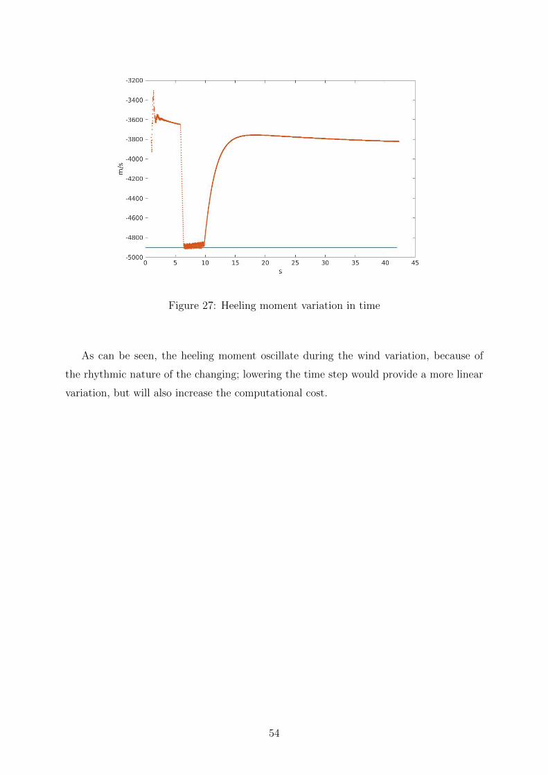
Figure 27: Heeling moment variation in time
As can be seen, the heeling moment oscillate during the wind variation, because of
the rhythmic nature of the changing; lowering the time step would provide a more linear
variation, but will also increase the computational cost.
54

4.2.3 Optimization Under Changing Wind
The last example is a merging of the other two: first the software finds the optimal reg-
ulation for the initial condition, then the wind changes and finally the new condition is
optimized. This is to show a complete process of simulating a foiling sailing boat with a
crew that continuously tries to increase its speed in changing wind conditions: the work
needed in order to keep the boat stable during a perturbation, and the ability to find an
optimal solution after the disturb are here tested.
Figure 28: Heeling moment variation in time
In the first phase the system reaches equilibrium and than, as in the first example, begins
the optimization process; the maximum speed reached in this phase is of almost 8.1m/s,
with an increase of about the 17% of the initial speed.
After 100 seconds the wind starts to change; as in the previous simulation, the wind in-
creases its speed of 1m/s and the direction changes from 50� to 60�, all in a time interval
of 2 seconds.
In this phase, the boat’s speed increases because of the more favouring conditions, and
the controllers are busy keeping the system stable. Again, the maximum heeling moment
is never reached, so the navigation is safe.
55
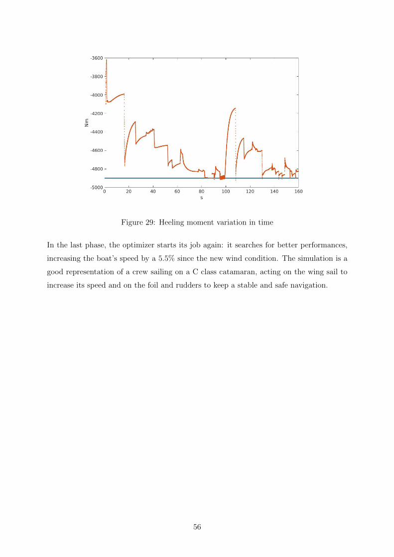
Figure 29: Heeling moment variation in time
In the last phase, the optimizer starts its job again: it searches for better performances,
increasing the boat’s speed by a 5.5% since the new wind condition. The simulation is a
good representation of a crew sailing on a C class catamaran, acting on the wing sail to
increase its speed and on the foil and rudders to keep a stable and safe navigation.
56

5 Conclusions
The developed software is a dynamics simulator for foiling boats dynamic behaviour anal-
ysis; it has been applied to the model of a C class catamaran, in order to study how it
responds to commands and disturbs. Furthermore, the software is able to simulate the
work of a crew, acting on the foil and rudders in order to keep a stable navigation and on
the wing sail to increase the cruising speed.
Some examples of its usage are presented, but many other applications are possible. The
first goal for future improvement will be a better model of the boat, containing also the
structural characteristics in order to analyse the loads-structure interactions. The next
step will be tuning the controllers in order to better represent the actual behaviour of a
crew: the time delay, precision and sensibility are important to evaluate the actual han-
dling di�culties, to avoid excessive loads. The ability to rapidly determine if a certain
design improves or worsens the handling can prove extremely helpful to better enhance
the boat’s performance without e↵ecting the stability and manuevrability over the maxi-
mum manageable by the crew.
The VLM can, and will, be improved: the main issue here is the applicability of the
method, which is limited to fully attached flows. In order to guarantee this condition
universally, a tool that checks the flow condition can be implemented; computing the
boundary layer thickness, through TODO equations, it would be possible to know if the
flow is attached or not. Keeping the sail in attached conditions only will guarantee the
accuracy of the results, although it would limit the possible solutions. There exists solu-
tions of partial detachment of the flow that are optimal for pushing the boat, and that
cannot correctly analysed by a VLM.
A typical problem of hydrodynamic surfaces is cavitation; this can be detected easily by
computing the local pressure and checking if it is below the vapour pressure at the current
temperature. This can be helpful in order to design foils and rudders that, in all their
possible applications, will never encounter this condition.
In conclusion, the developed software would certainly prove itself a helpful instrument
in the design of high performance sailing or motor boats, even more if they navigate in
foiling condition.
57
References
[1] Fabio Fossati Aero-Hydrodynamics and the Performance of Sailing Yachts 2009: In-
ternational Marine/McGraw-Hill
[2] wikipedia.org (Hydrofoil)
[3] progression.me (Hydrofoil)
[4] maserati.soldini.it (Gallery)
[5] c-class.org (Class History)
[6] kategreene.net (Homepage)
[7] boatdesign.net (C Class Catamaran Design)
[8] sailinganarchy.com (tipping point)
[9] mbdyn.org (Homepage)
[10] Diego Pigozzi Meccanica Razionale 2009: Edizioni Libreria Progetto Padova
[11] John D. Anderson Fundamentals of Aerodynamics 2011: McGraw-Hill
[12] Tomas Melin, A Vortex Lattice MATLAB Implementation for Linear Aerodynamic
Wing Applications,Master Thesis, KTH.
[13] Araki M. CONTROL SYSTEMS, ROBOTICS, AND AUTOMATION Vol. II - PID
Control, Kyoto University, Japan
[14] J.G. ZIEGLER and N. B. NICHOLS Optimum Settings for Automatic Controllers
Transactions of the ASME. 64: 759768.
[15] Brian R Copeland The Design of PID Controllers using Ziegler Nichols TuningMarch
2008
[16] uk.mathworks.com (fmincon)
[17] uk.mathworks.com (Interior Point Algorithm)
58
Related Documents