DEVELOPMENT OF A DSP-FPGA-BASED RESOLVER-TO ...

DEVELOPMENT OF A DSP-FPGA-BASED RESOLVER-TO-DIGITAL CONVERTER FOR STABILIZED GUN PLATFORMS

A THESIS SUBMITTED TO THE GRADUATE SCHOOL OF NATURAL AND APPLIED SCIENCES

OF MIDDLE EAST TECHNICAL UNIVERSITY

BY

YASİN ZENGİN

IN PARTIAL FULFILLMENT OF THE REQUIREMENTS FOR

THE DEGREE OF MASTER OF SCIENCE IN

ELECTRICAL AND ELECTRONICS ENGINEERING

MAY 2010

Approval of the thesis:

DEVELOPMENT OF A DSP-FPGA-BASED RESOLVER-TO-DIGITAL

CONVERTER FOR STABILIZED GUN PLATFORMS

submitted by YASİN ZENGİN in partial fulfillment of the requirements for the degree of Master of Science in Electrical and Electronics Engineering Department, Middle East Technical University by,

Prof. Dr. Canan Özgen Dean, Graduate School of Natural and Applied Sciences Prof. Dr. İsmet Erkmen Head of Department, Electrical and Electronics Engineering

Prof. Dr. İsmet Erkmen Supervisor, Electrical and Electronics Engineering Dept., METU Prof. Dr. Aydan M. Erkmen Co-Supervisor, Electrical and Electronics Engineering Dept., METU

Examining Committee Members:

Prof. Dr. Kemal Leblebicioğlu Electrical and Electronics Engineering Dept., METU

Prof. Dr. İsmet Erkmen Electrical and Electronics Engineering Dept., METU Assist. Prof. Afşar Saranlı Electrical and Electronics Engineering Dept., METU

Assist. Prof. Emre Tuna Electrical and Electronics Engineering Dept., METU

Bülent Bilgin, M.Sc. Manager, ASELSAN Date: 31.05.2010

iii

I hereby declare that all information in this document has been obtained and presented in accordance with academic rules and ethical conduct. I also declare that, as required by these rules and conduct, I have fully cited and referenced all material and results that are not original to this work.

Name, Last name : Yasin ZENGİN

Signature :

iv

ABSTRACT

DEVELOPMENT OF A DSP-FPGA-BASED

RESOLVER-TO-DIGITAL CONVERTER FOR

STABILIZED GUN PLATFORMS

ZENGİN, Yasin

M. Sc., Department of Electrical and Electronics Engineering

Supervisor: Prof. Dr. İsmet ERKMEN

Co-Supervisor: Prof. Dr. Aydan M. ERKMEN

May 2010, 163 pages

Resolver, due to its reliability and durability, has been used for the aim of shaft

position sensing of military rotary systems such as tank turrets and gun stabilization

platforms for decades. Ready-to-use resolver-to-digital converter integrated circuits

which convert the resolver signals into position and speed measurements are

utilized in servo systems most commonly. However, the ready-to-use integrated

circuits increase the dependency of the servo system to hardware components which

in turn decrease the efficiency and flexibility of the servo system for changing

system structures such as for changing resolver carrier frequency or changing

position and speed sensors. The proposed solution to increase the efficiency and

flexibility of the servo system is a software-based resolver-to-digital converter

which does not require aforesaid special hardware components and presents a

complete software-based solution for the conversion. The proposed software-based

resolver-to-digital converter makes use of common programmable hardware

v

components, that is, FPGA and DSP which form the heart of the servo controller

technology in recent years.

The proposed structure for the conversion has three components. The first

component is the signal conditioner which minimizes the disturbances coming from

the resolver signals as harmonic distortions and noise. The second component, the

phase-sensitive demodulator, as the name implies, is responsible for phase-sensitive

demodulation of resolver signals. The third component is the estimator filter. In

order to determine the optimal estimator filter, five different estimator filters with

the aforesaid two components are implemented in ASELSAN’s stabilized gun

system STAMP and they are compared in terms of both estimation performance and

computational complexity. The implemented filters include nonlinear observer type

filter which is already proposed in the literature for resolver conversion, tracking

differentiator adapted to resolver conversion and kalman filters adapted to resolver

conversion in different forms such as linear kalman filter, extended kalman filter

and unscented kalman filter. At the end of the study, stability and sensitivity

analyses are also performed for the proposed system.

Keywords: Phase-sensitive demodulation, harmonic distortions on resolver signals,

software-based resolver-to-digital conversion, Kalman filtering.

vi

ÖZ

STABİLİZE SİLAH PLATFORMLARI İÇİN DSP VE

FPGA TABANLI RESOLVER-SAYISAL ÇEVİRİCİ

GELİŞTİRİLMESİ

ZENGİN, Yasin

Yüksek Lisans, Elektrik ve Elektronik Mühendisliği Ana Bilim Dalı

Tez Yöneticisi: Prof. Dr. İsmet ERKMEN

Ortak Tez Yöneticisi: Prof. Dr. Aydan M. ERKMEN

Mayıs 2010, 163 sayfa

Dayanıklılığı ve güvenilirliğinden dolayı resolver, yıllardır tank tareti ve silah

stabilizasyon platformu gibi askeri amaçlı döner sistemlerde kullanılmaktadır. Hali

hazırda kullanıma hazır olarak sunulan ve yoğun bir şekilde servo sistemlerde

kullanılmakta olan resolver-sayısal çevirici tümleşik devreleri, resolver sinyallerini

kullanarak pozisyon ve hız ölçümünü gerçekleştirmektedirler. Ancak, kullanıma

hazır olarak sunulan bu devreler, servo sistemin donanıma bağımlılığını artırmakta

ve servo sistemin değişken resolver taşıyıcı frekanslarında resolverlerin veya

değişken pozisyon ve hız sensörlerinin kullanıldığı değişken sistem yapılarına uyum

sağlayabilme yetisini ve servo sistemin verimliliğini azaltmaktadır. Bu tez

kapsamında soruna önerilen çözüm ise özelleşmiş donanım yapılarına ihtiyacı

ortadan kaldıran ve yazılım üzerine kurulu bir yazılım-tabanlı resolver-sayısal

çeviricidir. Önerilen yazılım-tabanlı resolver-sayısal çevirici, son yıllarda servo

kontrolcü teknolojisinin vazgeçilmez programlanabilir donanım parçaları olan

FPGA ve DSP işlemcileri kullanmaktadır.

vii

Çevrim için önerilen yapı üç bileşenden oluşmaktadır. Birinci bileşen resolver

sinyallerindeki harmonik bozulmalar ve gürültü gibi bozucu etkileri en aza

indirgemek için kullanılan sinyal iyileştiricidir. İkinci bileşen, isminden de

anlaşılacağı gibi, resolver sinyallerinin faza-duyarlı çözümünü gerçekleştiren faza-

duyarlı çözücüdür. Sonuncu bileşen ise tahminleyici filtredir. Resolver çevrimi için

kullanılabilecek en iyi tahminleyici filtreyi bulabilmek amacıyla, beş farklı

tahminleyici filtre bahsi geçen diğer iki bileşen ile birlikte ASELSAN’ın stabilize

silah sistemi STAMP’a uygulanmış ve bu filtreler hem tahminleme performansı

hem de işlemsel karmaşıklık açılarından karşılaştırılmıştır. Uygulanan tahminleyici

filtreler; literatürde resolver çevrimi için önerilmiş bulunan doğrusal-olmayan filtre,

resolver çevrimine uyarlanmış takiplemeli türevleyici ve kalman filtrenin doğrusal

kalman filtre, kapsamlı kalman filtre ve kokusuz kalman filtre olmak üzere resolver

çevrimine uyarlanmış üç farklı formunu içermektedir. Çalışmanın sonunda önerilen

sistem için kararlılık ve duyarlılık analizleri de gerçekleştirilmiştir.

Anahtar Kelimeler: Faza-duyarlı çözüm, resolver sinyallerinde harmonik

bozulmalar, yazılım-tabanlı resolver-sayısal çevrim, Kalman filtreleme.

viii

To My Family and Love

ix

ACKNOWLEDGEMENTS

I would like to express my sincere thanks and gratitude to my supervisors Prof. Dr.

İsmet ERKMEN and Prof. Dr. Aydan M. ERKMEN for their belief,

encouragements, advice and criticism throughout this study.

I would like to thank ASELSAN Inc. for facilities provided for the completion of

this thesis.

I would like to express my thanks to my friends and colleagues for their support and

fellowship.

I would like to thank TÜBİTAK for its support on scientific and technological

researches.

I would like to express my special appreciation to my family for their endless

support and encouragements.

x

TABLE OF CONTENTS

ABSTRACT ...................................................................................................................................... IV

ÖZ ...................................................................................................................................................... VI

ACKNOWLEDGEMENTS ............................................................................................................. IX

TABLE OF CONTENTS .................................................................................................................. X

LIST OF TABLES ........................................................................................................................ XIII

LIST OF FIGURES ....................................................................................................................... XV

NOMENCLATURE ....................................................................................................................... XX

CHAPTERS

1. INTRODUCTION .......................................................................................................................... 1

1.1 MOTIVATION .............................................................................................................................. 1

1.2 OBJECTIVES AND CONTRIBUTIONS OF THE THESIS ..................................................................... 4

1.3 OUTLINE OF THE THESIS ............................................................................................................. 7

2. LITERATURE SURVEY .............................................................................................................. 8

2.1 SERVO SYSTEM COMPONENTS .................................................................................................... 8

2.1.1 Servo Motors and Servo Drives ......................................................................................... 8

2.1.2 Field Orientated Control of Torque ................................................................................. 13

2.2 OCEAN WAVE SPECTRA AND SERVO DRIVE BANDWIDTH REQUIREMENTS .............................. 16

2.3 SAMPLING THEOREM AND ALIASING ........................................................................................ 18

2.4 ESTIMATION AND KALMAN FILTERING..................................................................................... 20

2.4.1 Characteristics of Random Variables ............................................................................... 21

2.4.2 Kalman Filtering .............................................................................................................. 23

2.5 RESOLVERS AND RESOLVER-TO-DIGITAL CONVERSION ........................................................... 32

2.5.1 Resolver-to-Digital Conversion Methods Proposed in the Literature .............................. 34

2.5.2 Tracking Differentiators .................................................................................................. 37

2.6 CONCLUSION OF THE LITERATURE SURVEY ............................................................................. 38

3. DEVELOPMENT OF A DSP-FPGA-BASED RESOLVER-TO-DIGITAL CONVERTER 41

xi

3.1 PROPOSED RESOLVER-TO-DIGITAL CONVERTER ...................................................................... 41

3.1.1 Components of the Proposed RDC .................................................................................. 44

3.1.2 Forming the System Structure for the Proposed RDC ..................................................... 45

3.2 RESOLVER SIGNAL IMPERFECTIONS AND FILTERING RESOLVER SIGNALS TO IMPROVE

RESOLVER-TO-DIGITAL CONVERSION ACCURACY ......................................................................... 46

3.2.1 Resolver Signal Imperfections - Low and High Frequency Harmonic Distortions in

Resolver Signals ....................................................................................................................... 46

3.2.2 Disturbing Effects of Resolver Signal Imperfections on Software-Based Conversion

Performance .............................................................................................................................. 48

3.2.3 Position Estimation Error due to Resolver Signal Imperfections and Resultant

Disturbances on Torque and Speed of the Motor ..................................................................... 51

3.2.4 Improvement in Position Estimation Accuracy with Minimization of Resolver Signal

Imperfections in the Experimental System ............................................................................... 67

3.3 FPGA-BASED PHASE-SENSITIVE DEMODULATOR .................................................................... 71

3.3.1 Realization of Modulus Function and Half-Period Integrator in FPGA .......................... 73

3.3.2 Phase-Detector ................................................................................................................. 77

3.3.3 Construction of Demodulated Signals in DSP ................................................................. 79

3.3.4 Benefit of the Proposed FPGA-based Phase-Sensitive Demodulator .............................. 80

3.4 POSITION AND SPEED ESTIMATION FROM DEMODULATED RESOLVER SIGNALS ....................... 80

3.4.1 Implementation of the Estimator Filters .......................................................................... 82

4. PERFORMANCE ANALYSIS OF THE PROPOSED RESOLVER-TO-DIGITAL

CONVERTER .................................................................................................................................. 95

4.1 CONSTRUCTING MODELS FOR SIMULATIVE AND REAL-TIME PERFORMANCE TESTS AND TUNING

THE ESTIMATOR FILTERS ............................................................................................................... 96

4.1.1 Constructing Simulation Models of the Estimator Filters for Tuning Procedure ............ 96

4.1.2 Tuning the Filters ........................................................................................................... 100

4.1.3 Running the Estimator Filters in the Experimental System for Real-time Performance

Tests ........................................................................................................................................ 101

4.2 SIMULATIVE AND REAL-TIME ESTIMATION PERFORMANCES OF THE FILTERS ........................ 103

4.2.1 Simulative and Real-time Performances of the Nonlinear Observer ............................. 103

4.2.2 Simulative and Real-time Performances of the Tracking Differentiator ....................... 106

4.2.3 Simulative and Real-time Performances of the LKF ..................................................... 109

4.2.4 Simulative and Real-time Performances of the EKF ..................................................... 111

4.2.5 Simulative and Real-time Performances of the UKF ..................................................... 114

4.3 COMPARATIVE ANALYSIS OF THE REAL-TIME ESTIMATION PERFORMANCES OF THE ESTIMATOR

FILTERS ........................................................................................................................................ 117

4.3.1 Comparison of the Estimator Filters for Torque Loop’s Performance .......................... 119

xii

4.3.2 Comparison of the Estimator Filters for Speed and Position Loops’ Performances ...... 123

4.3.3 Comparison of the Estimator Filters for Filtering Performances and Computational

Complexity ............................................................................................................................. 129

4.4 STABILITY AND SENSITIVITY ANALYSES ................................................................................ 131

4.4.1 Stability Analysis ........................................................................................................... 131

4.4.2 Sensitivity Analysis ....................................................................................................... 133

5. CONCLUSION AND FUTURE WORK .................................................................................. 149

5.1 CONCLUSION OF THE THESIS .................................................................................................. 149

5.2 FUTURE WORK ....................................................................................................................... 152

REFERENCES ............................................................................................................................... 154

APPENDICES

A. HARDWARE AND SOFTWARE ........................................................................................... 158

xiii

LIST OF TABLES

TABLES

Table 3-1 Forming system structure ........................................................................ 46

Table 3-2 Distortion levels in pure resolver signals normalized to fundamental

component ........................................................................................................... 48

Table 3-3 Aliases of the resolver signals’ components in the experimental system

where the Nyquist frequency is 7.7 kHz ............................................................. 49

Table 3-4 Calculated maximum percentage errors at the demodulator outputs due to

low-frequency harmonics ( D ) and high-frequency harmonics ( E ) .............. 52

Table 3-5 Position estimation error due to delay introduced by the different order

anti-aliasing filters in the experimental system ................................................... 57

Table 3-6 Anti-aliasing filter’s performance ............................................................ 59

Table 3-7 Performance of the digital high-pass filter .............................................. 66

Table 3-8 Improvement in error values with minimization of resolver signal

imperfections ....................................................................................................... 68

Table 3-9 Delays and position estimation errors due to filtering in the experimental

system .................................................................................................................. 70

Table 3-10 Phase-detector’s outputs for position signal’s quadrant ........................ 79

Table 4-1 Tuned Parameters of the estimator filters and corresponding performance

parameters obtained in simulation environment ............................................... 100

Table 4-2 Performance parameters of the Nonlinear Observer in simulation and

real-time ............................................................................................................. 106

Table 4-3 Performance parameters of the Tracking Differentiator in simulation and

real-time ............................................................................................................. 109

Table 4-4 Performance parameters of the LKF in simulation and real-time ......... 111

Table 4-5 Performance parameters of the EKF in simulation and real-time ......... 114

xiv

Table 4-6 Performance parameters of the UKF in simulation and real-time ......... 116

Table 4-7 Results of the real-time performance tests of the estimator filters ........ 119

Table 4-8 System speed estimation error values calculated by multiplying real-time

resolver speed estimation error values by system gear ratio (1/120) ................ 126

Table 4-9 Position and speed loops’ performances with different estimator filters for

a position command trajectory of 0.09375sin(2 )ft rad ................................. 127

xv

LIST OF FIGURES

FIGURES

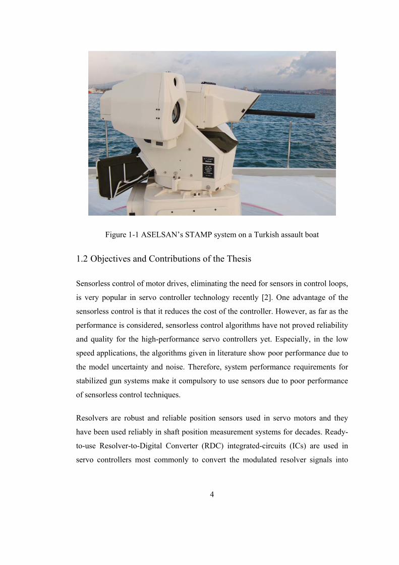
Figure 1-1 ASELSAN’s STAMP system on a Turkish assault boat .......................... 4

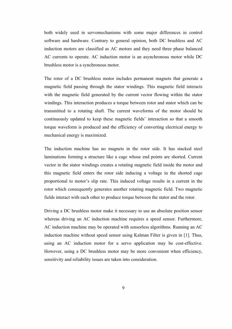
Figure 2-1 Generalized structure of a servo drive controller ................................... 11

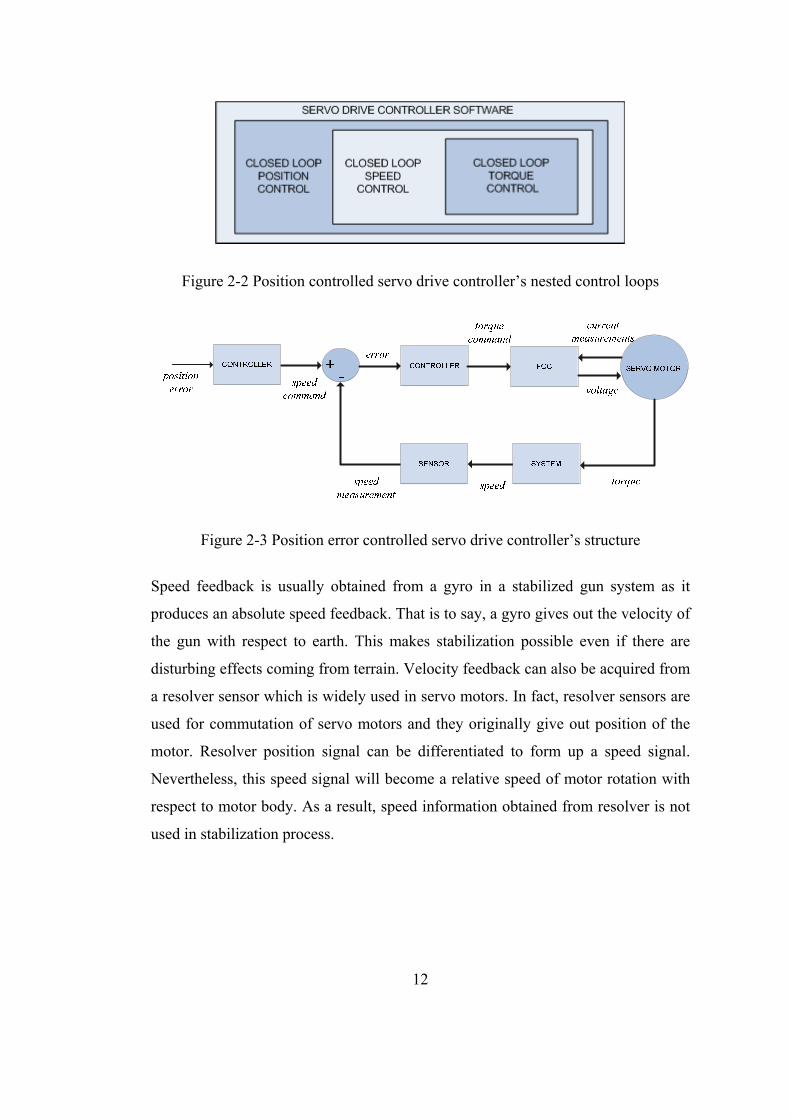
Figure 2-2 Position controlled servo drive controller’s nested control loops .......... 12

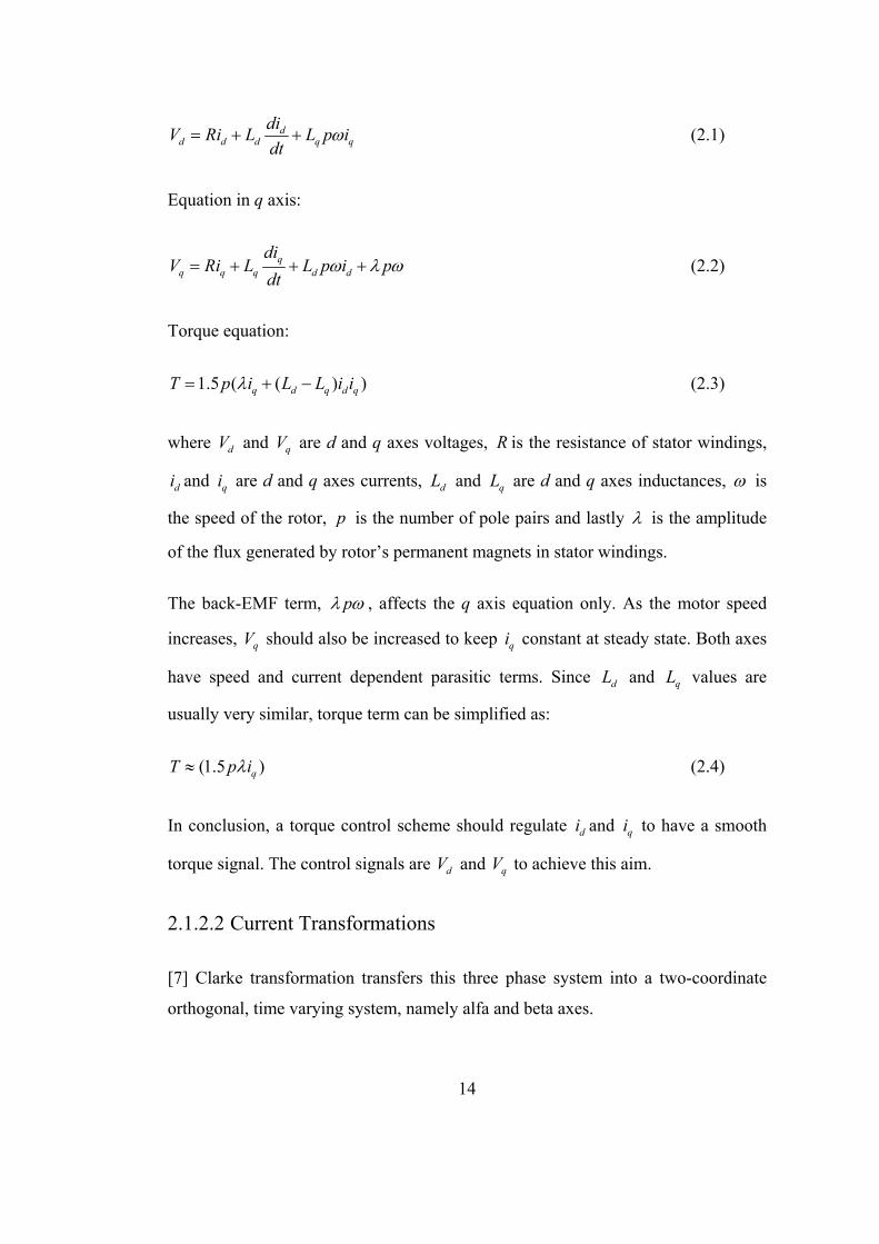
Figure 2-3 Position error controlled servo drive controller’s structure .................... 12

Figure 2-4 Pierson-Moskowitz sea spectrum with respect to wind speed [10] ....... 17

Figure 2-5 JONSWAP sea spectrum with respect to fetch when a constant speed

wind is present [10] ............................................................................................. 18

Figure 2-6 Aliasing in sampling [10] ....................................................................... 19

Figure 2-7 Anti-aliasing filtering and analog-to-digital conversion ........................ 20

Figure 2-8 Resolver and resolver signals ................................................................. 32

Figure 2-9 Resolver format signals as motor rotates ............................................... 34

Figure 2-10 Comparative test results for implemented differentiators in [23] ........ 38

Figure 3-1 Resolver and resolver signals ................................................................. 42

Figure 3-2 ASELSAN’s stabilized gun system STAMP on a STEWARD platform

............................................................................................................................. 43

Figure 3-3 Proposed software-based RDC and details related to implementation of it

in real-time (R.S. in the block diagram stands for “Realized System”) .............. 44

Figure 3-4 Pure resolver signal sin( / 2)sin wt (blue signal) and its FFT (red

signal) .................................................................................................................. 47

Figure 3-5 Actual position, estimated erroneous position and position estimation

error with respect to time (s) ............................................................................... 53

Figure 3-6 Effect of misinforming position signal on torque feedback signal

(horizontal axis is time axis in seconds) .............................................................. 54

xvi

Figure 3-7 Oscilloscope screen showing torque signal (red signal where 10V means

maximum torque) with 1% torque ripple and ripple’s disturbing effect on speed

of the experimental system (blue signal where 10V corresponds to 100°/sec) ... 55

Figure 3-8 Proposed mixed-signal signal conditioner to obtain distortion-free and

noise-free digital resolver signals (R.S. stands for “Realized System”) ............. 56

Figure 3-9 Pure resolver sine signal and its FFT (red signal) on the above scope

screen and resolver sine signal after filtered by the anti-aliasing filter and its FFT

(red signal) on the below scope screen ................................................................ 58

Figure 3-10 Reconstruction of resolver signals by low-pass filtering ..................... 60

Figure 3-11 Digital interpolation filter parameters and demanded magnitude

response ............................................................................................................... 62

Figure 3-12 Realized magnitude and phase responses of digital interpolation filter

implemented in FPGA ......................................................................................... 62

Figure 3-13 Sampled resolver signal (red signal) and reconstructed resolver signal

(blue signal) observed in real-time by the help of Chipscope software .............. 63

Figure 3-14 Digital high-pass filter parameters and demanded magnitude response

............................................................................................................................. 64

Figure 3-15 Realized magnitude and phase responses of the high-pass filter

implemented in FPGA ......................................................................................... 65

Figure 3-16 Resolver signal’s states from output of the anti-aliasing filter to the

input of the demodulator passing through the interpolation filter and digital high-

pass filter ............................................................................................................. 66

Figure 3-17 Actual position, estimated position and position estimation error when

resolver signal imperfections are minimized ....................................................... 68

Figure 3-18 Effect of erroneous position signal on torque estimate signal after

resolver signal imperfections are minimized ....................................................... 69

Figure 3-19 Phase-sensitive demodulator implemented in FPGA ........................... 72

Figure 3-20 Quadrants ............................................................................................. 73

Figure 3-21 Demodulation by modulus and half-period integration ....................... 74

Figure 3-22 Structure realizing modulus function and half-period integration in

FPGA ................................................................................................................... 75

Figure 3-23 Modulus function realized in FGPA .................................................... 76

xvii

Figure 3-24 Realization of the Backward Euler accumulator with reset input in

FPGA ................................................................................................................... 77

Figure 3-25 Reconstructed reference signal (blue), sine signal (green) and cosine

signal (red) when the position is within the fourth and first quadrant ................ 78

Figure 3-26 Detection of the phase of resolver format signals with respect to

reference signal .................................................................................................... 79

Figure 3-27 Pure differentiation of servo position signal versus speed estimate by an

estimator filter ..................................................................................................... 81

Figure 3-28 Block diagram showing the implementation of the Nonlinear Observer

in DSP .................................................................................................................. 83

Figure 3-29 Block diagram showing the realization of the Tracking Differentiator in

DSP ...................................................................................................................... 84

Figure 3-30 Block diagram showing the implementation of LKF in DSP .............. 89

Figure 3-31 Algorithmic state machine showing the realization of the EKF in DSP

............................................................................................................................. 91

Figure 3-32 Algorithmic state machine showing the realization of the UKF in DSP

............................................................................................................................. 94

Figure 4-1 Simulation model ................................................................................... 97

Figure 4-2 Gun-stabilization system block diagram ................................................ 97

Figure 4-3 Noise on the resolver channel in the gun stabilization system when

resolver speed is zero and position is 41.22° ...................................................... 99

Figure 4-4 Noise-free position signal and noisy sine and cosine signals used as input

to estimator filters in simulation environment .................................................... 99

Figure 4-5 Experimental system for real-time performance tests .......................... 101

Figure 4-6 Schematically summary of the experimental system used in real-time

performance tests ............................................................................................... 103

Figure 4-7 Position estimation performance of the Nonlinear Observer in simulation

........................................................................................................................... 104

Figure 4-8 Speed estimation performance of the Nonlinear Observer in simulation

........................................................................................................................... 104

Figure 4-9 Position estimation performance of the Nonlinear Observer in real-time

........................................................................................................................... 105

xviii

Figure 4-10 Speed estimation performance of the Nonlinear Observer in real-time

........................................................................................................................... 105

Figure 4-11 Position estimation performance of the Tracking Diff. in simulation 107

Figure 4-12 Speed estimation performance of the Tracking Diff. in simulation ... 107

Figure 4-13 Position estimation performance of the Tracking Diff. in real-time .. 108

Figure 4-14 Speed estimation performance of theTracking Diff. in real-time ...... 108

Figure 4-15 Position estimation performance of the LKF in simulation ............... 109

Figure 4-16 Speed estimation performance of the LKF in simulation................... 110

Figure 4-17 Position estimation performance of the LKF in real-time .................. 110

Figure 4-18 Speed estimation performance of the LKF in real-time ..................... 111

Figure 4-19 Position estimation performance of the EKF in simulation ............... 112

Figure 4-20 Speed estimation performance of the EKF in simulation................... 112

Figure 4-21 Position estimation performance of the EKF in real-time .................. 113

Figure 4-22 Speed estimation performance of the EKF in real-time ..................... 113

Figure 4-23 Position estimation performance of the UKF in simulation ............... 114

Figure 4-24 Speed estimation performance of the UKF in simulation .................. 115

Figure 4-25 Position estimation performance of the UKF in real-time ................. 115

Figure 4-26 Speed estimation performance of the UKF in real-time ..................... 116

Figure 4-27 Real-time demodulated cosine signal and its Power Spectral Density

estimate .............................................................................................................. 118

Figure 4-28 Simplified block diagram of the torque control loop with Field

Orientated Control (FOC) in the servo system .................................................. 120

Figure 4-29 Simulation model in Simulink to observe the torque estimation error for

filters’ position estimation errors ...................................................................... 121

Figure 4-30 Torque estimation errors for estimator filters’ position outputs ........ 122

Figure 4-31 Block diagram of the speed control loop in the non-stabilized servo

system ................................................................................................................ 123

Figure 4-32 Position error controlled non-stabilized servo system ....................... 124

Figure 4-33 Non-stabilized gun control system’s simulation model ..................... 125

Figure 4-34 Measuring servo system speed and position tracking errors in

simulation environment using running mean method in Simulink ................... 127

xix

Figure 4-35 Scope screen showing position tracking performance of the servo

system in transient and steady-state for changing position estimation error values

when a position command trajectory of 0.09375sin(2 )ft rad is applied to the

servo system ...................................................................................................... 128

Figure 4-36 Accuracy and computational complexity graphs of the estimator filters

(not scaled to real values) .................................................................................. 130

Figure 4-37 Flow of the error from the demodulator to the position tracking

performance of the servo system ....................................................................... 134

Figure 4-38 Kalman filter divided into two components for sensitivity analysis .. 134

Figure 4-39 Steady-state error with respect to resolver speed and where speed

varies from 1 rad/s to 100 rad/s and varies from 1010 to 510 .................... 137

Figure 4-40 Error signal’s settling for different values of the filter parameter . 138

Figure 4-41 Sensitivity of the nonlinear transfer function to demodulator output

percentage errors S and C .......................................................................... 141

Figure 4-42 Position estimation error in steady-state due to Gaussian demodulator

output errors while the resolver rotor rotates with a speed of 2 rad/s ........... 141

Figure 4-43 Scope screen showing torque ripple and sin and cos signals when a

torque demand of 50% and a demodulator output error of 1% are present in the

system ................................................................................................................ 143

Figure 4-44 Deviation of the projectile from the target for the proposed system .. 146

Figure 4-45 Projectile deviation with respect to the demodulator output error ..... 147

Figure A-1 Experimental set-up ............................................................................. 158

Figure A-2 DSP CPU, EMIF, EDMA and external memory ................................. 159

Figure A-3 FPGA’s role in the hardware ............................................................... 160

Figure A-4 5 kHz resolver used in experimental set-up ........................................ 161

Figure A-5 AC servo motor used in the experimental set-up ................................ 161

Figure A-6 Tapped-delay line FIR structure .......................................................... 163

Figure A-7 MAC FIR filter design interface in ISE program ................................ 163

xx

NOMENCLATURE

RDC : Resolver-to-Digital Converter

IC : Integrated Circuit

ADC : Analog-to-Digital Converter

FPGA : Field-Programmable Gate Array

FOC : Field Orientated Control

PWM : Pulse-Width-Modulation

SVPWM : Space Vector Pulse-Width-Modulation

JONSWAP : Joint North Sea Wave Observation Project

LKF : Linear Kalman Filter

EKF : Extended Kalman Filter

UKF : Unscented Kalman Filter

DSP : Digital Signal Processor

PLL : Phase Locked Loop

: Resolver position

w : Resolver signals’ carrier frequency

xxi

: Resolver speed

FFT : Fast Fourier Transform

S : Demodulator output percentage error for sine channel

C : Demodulator output percentage error for cosine channel

: Estimated position

FIR : Finite Impulse Response

IIR : Infinite Impulse Response

sT : Sampling Period

kK : Kalman gain matrice

k : Innovation or error

k : Position estimate of Kalman filter

k : Speed estimate of Kalman filter

ka : Acceleration estimate of Kalman filter

k : Actual resolver position

: Resolver position estimation error

T : Torque tracking error

: System tracking error

: System position tracking error

xxii

Tf : Torque ripple frequency

,C S : C or S

1

CHAPTER 1

INTRODUCTION

1.1 Motivation

Servomechanism is a device which enables automatic control means on a

mechanism. The term servomechanism is only used for devices which make use of

feedback signals from the mechanism that is being controlled. Using feedback

signals, a servomechanism attempts to correct the performance of the mechanism

according to the command set. Although any type of system using closed loop

control can be classified as a servomechanism, motion control systems are the

leading area of usage nowadays. In general, controlled states for such systems are

position, speed, acceleration and torque.

Servomechanisms should have an input, an output, a calculator calculating the error

between the input and output, an amplifier calculating the actuation and an actuator

to eliminate the error. From this point of view, the first servomechanism was the

sheep steering engine used on the SS Great Eastern which is launched in 1858.

Thereafter, servomechanisms were used in fire-control systems and navigation

systems. After a century, servomechanisms are used in many applications ranging

from aeronautical to automotive [3].

Military fire-control is one of the disciplines that use servomechanisms since its

invention. Fire-control concept is developed to improve hitting performance of

weapon systems. These military systems are designed to improve the performance

of the weapon systems in terms of rapidness of firing and hitting accuracy. A Fire-

2

control system combines a number of components such as a fire-control computer, a

servomechanism to direct the gun and a gun to fire on the target. Advanced fire-

control systems have ability to interface with more components improving firing

accuracy such as fire control radar, thermal and day cameras and laser range finder.

Moreover, more complex fire-control systems have additional sensors. These

additional sensors measure the disturbing effects deflecting the system performance

from the trajectory in demand. For instance, in a stabilized gun platform, fire-

control computer usually has an interface with a gyro in order to measure

disturbance deflecting the gun’s velocity from the velocity in demand. Using the

negative feedback law, the computer continually computes the necessary correction

signal for the actuators to keep the gun’s velocity at desired value. This is the

concept of gun stabilization. Gun stabilization is an important concept for fire-

control systems. Disturbances coming from terrain will adversely affect the

performance of a fire-control system without gun stabilization.

Eventually a fire-control system is a servomechanism with its ability to sense

feedbacks coming from the mechanism. Servomechanisms should be able to

manipulate time-based derivative of a parameter to be able to control it. For

instance, a servomechanism designed to control the velocity of a robot arm should

be able to change time-based derivative of velocity, that is, acceleration of the robot

arm. In general, acceleration is not a direct controllable variable in

servomechanisms because acceleration sensors available in the marketplace either

show poor performance or are so expensive that making a cost-effective system

solution very difficult. That is to say, today’s systems do not allow making use of

acceleration sensors to control velocity of a mechanism. Therefore, controlling

velocity of a mechanism is usually realized by using torque feedback or an indirect

way of sensing torque, namely by calculating torque from phase currents of servo

motors. This way of speed control is a good solution when engineers care system

cost, performance and reliability.

3

In contrast to general opinion, servomechanisms do not necessarily have a servo

motor. For instance systems with closed loop temperature control are also

servomechanisms although they do not have servo motors. However, motion control

applications make it necessary to use servo motors in control. A motor is an

electromechanical energy converter generating a force on its rotating shaft when

supplied with direct current or three phase alternating current depending on the type

of the motor. A servo motor is a type of motor which gives out some information

related to its motion such as shaft position and speed. These may be referred as the

most common feedbacks of servo motors. Processing feedback signals from servo

motors and other sensors, the servo controller continually controls the voltage

supplied to motor in order to correct the motion of the servomechanism. The

command signal for a servo controller may be one of position, speed and torque

commands.

ASELSAN is the leading company of Turkish defense industry in designing and

producing stabilized fire-control systems. ASELSAN’s STAMP (Figure 1-1) and

STOP systems are stabilized marine gun systems equipped with advanced fire-

control and servo controller units. Systems can be used with various naval guns

including 12.7, 25 and 30 mm guns. They have several sensors to perform gun

stabilization and target tracking on both day and night conditions. Fire on the move

ability of the systems facilitates challenging military missions at sea.

The main motivation of this thesis is to improve the servo drive abilities of STAMP

and STOP systems. It is intended to solve the challenging issues observed during

the design stage of STAMP and STOP systems. Actually, these issues are not

unique to the systems but they can be seen as general issues and they can be

attributed to servo control concept.

4

Figure 1-1 ASELSAN’s STAMP system on a Turkish assault boat

1.2 Objectives and Contributions of the Thesis

Sensorless control of motor drives, eliminating the need for sensors in control loops,

is very popular in servo controller technology recently [2]. One advantage of the

sensorless control is that it reduces the cost of the controller. However, as far as the

performance is considered, sensorless control algorithms have not proved reliability

and quality for the high-performance servo controllers yet. Especially, in the low

speed applications, the algorithms given in literature show poor performance due to

the model uncertainty and noise. Therefore, system performance requirements for

stabilized gun systems make it compulsory to use sensors due to poor performance

of sensorless control techniques.

Resolvers are robust and reliable position sensors used in servo motors and they

have been used reliably in shaft position measurement systems for decades. Ready-

to-use Resolver-to-Digital Converter (RDC) integrated-circuits (ICs) are used in

servo controllers most commonly to convert the modulated resolver signals into

5

digital speed and position measurements. One disadvantage of this hardware-based

conversion method is that adapting the hardware of the servo controller to the

ready-to-use RDC ICs increases the cost of the servo drive considerably. Moreover,

different position and speed sensors may be used to provide position and speed in a

servo system. For instance, digital encoders coupled to servo motors are widely

used in servo applications recently. For such a servo system structure, RDC ICs on

the hardware become useless and this approach results in less cost-effective and less

volume-effective servo controllers. On the other hand, hardware modifications to

remove the RDC ICs will also increase the cost when one takes mass-production

issues into consideration. Hardware configuration management for different system

solutions will be another expensive burden of hardware modifications. Hence, if a

software-based method which eliminates the need for RDC ICs to realize resolver-

to-digital conversion is introduced, servo controller and servo system design and

production costs will be reduced. Besides minimizing the costs, software-based

RDC will enhance more flexible servo controllers since making software

modifications is much more feasible and manageable than making hardware

modifications.

In recent years, digital controllers have been used widely in servo applications. This

trend of making use of digital controllers stem from the fact that working with

digital signals by the help of computer technology is more advantageous when one

takes flexibility, improvability, simplicity, cost and accuracy of control systems into

consideration. Since cost effectiveness is the key point in engineering, low-cost

computers are of great importance in developing hardware for digital servo

controllers. Digital Signal Processor (DSP) integrated circuits with proper

peripherals realize these requirements in servo controllers. Digital control of

dynamical systems also necessitates utilizing Analog-to-Digital Converters (ADC)

because dynamical systems may have several analog interfaces. Hence, both DSP

and ADCs are widely used in servo controllers to provide cost-effective and optimal

performance solutions for servo system applications. Besides DSP and ADCs, servo

controllers usually have Field-Programmable Gate Array (FPGA) chips to resolve

6

the hardware functions, for instance, to read data from digital sensors and to provide

interface with digital input-output signals. Therefore, a digital control board used in

a servo controller may be considered to have three fundamental components; DSP,

ADCs and FPGA.

Consequently, the main goal of this thesis is to develop a software-based resolver-

to-digital converter which performs the conversion by using analog-to-digital

converters and common programmable hardware components; DSP and FPGA. The

method will eliminate the need for RDC ICs in servo controllers and open the doors

to more flexible and compact servo controller designs. It will also reduce design and

production costs considerably.

The thesis proposes a software-based method for phase sensitive demodulation of

resolver signals using Field-Programmable Gate Array (FPGA) and ADCs. Besides

demodulation algorithm, the thesis also makes use of estimator filters to realize

conversion using a Digital Signal Processor. The implemented estimator filters are

Tracking Differentiator adapted to resolver conversion, Linear Kalman filter,

Extended Kalman Filter, Unscented Kalman Filter and a filter proposed in the

literature. The thesis compares the said estimator filters in terms of noise

suppression performance, tracking performance and computational complexity in

the experimental system.

Since the system is applied to a naval stabilized gun platform, bandwidth of

disturbances coming from the sea is examined by the help of ocean wave spectra.

To have a fair performance comparison between the estimator filters, an input set

for the filters is constructed by taking system requirements, spectral analysis of

ocean waves and noise characteristics of naval servo systems all into consideration.

Resolver signals are susceptible to electromagnetic contamination and harmonic

distortions. Hence, the thesis focuses on understanding the noise and harmonic

distortions on resolver signals and disturbing effects of them on position and speed

signals. This is important to understand the acceptable error levels in the servo

7

system resulting from the resolver. In order to minimize the disturbances coming

from such resolver signal imperfections, the thesis proposes a mixed-signal signal

conditioner.

At the end of the study, stability and sensitivity analyses are also performed for the

proposed system.

1.3 Outline of the Thesis

In the first chapter of the thesis, the motivation, objectives and contributions of the

thesis are given. In the second chapter, the literature survey conducted on the

related subjects is presented. In the third chapter, proposed software-based resolver-

to-digital converter is explained in details. The fourth chapter gives performance,

stability and sensitivity analyses of software-based Resolver-to-Digital converter.

The fifth chapter concludes the study and refers to the future works. Finally in

Appendix section details related to programming and hardware are given.

8

CHAPTER 2

LITERATURE SURVEY

This chapter gives a background for the thesis study. More specifically, the first

section of this chapter summarizes the essential components of a servo system. The

first section is also important for performance and sensitivity analyses since it

covers the necessary information related to servo system modeling. The second

section of this chapter gives an insight into the ocean wave spectra from which we

extract the bandwidth requirements for servo controllers in naval applications. The

required bandwidth should be known to design a well-tuned system which operates

satisfactorily in the sea environment. The third section gives some rules of thumb

related to control system design such as sampling theorem and aliasing. The fourth

section deals with random variables and Kalman filtering which will be necessary

for designing the estimator filters. Lastly, the fifth section inspects the similar

studies performed by researchers for estimation of position and speed from resolver

signals.

2.1 Servo System Components

2.1.1 Servo Motors and Servo Drives

A servo motor can be classified as AC or DC according to electrical supply,

brushed or brushless according to its commutation and synchronous or

asynchronous according to its slip. The most commonly used servo motors in

today’s servomechanisms are DC brushless and AC induction motors. They are

9

both widely used in servomechanisms with some major differences in control

software and hardware. Contrary to general opinion, both DC brushless and AC

induction motors are classified as AC motors and they need three phase balanced

AC currents to operate. AC induction motor is an asynchronous motor while DC

brushless motor is a synchronous motor.

The rotor of a DC brushless motor includes permanent magnets that generate a

magnetic field passing through the stator windings. This magnetic field interacts

with the magnetic field generated by the current vector flowing within the stator

windings. This interaction produces a torque between rotor and stator which can be

transmitted to a rotating shaft. The current waveforms of the motor should be

continuously updated to keep these magnetic fields’ interaction so that a smooth

torque waveform is produced and the efficiency of converting electrical energy to

mechanical energy is maximized.

The induction machine has no magnets in the rotor side. It has stacked steel

laminations forming a structure like a cage whose end points are shorted. Current

vector in the stator windings creates a rotating magnetic field inside the motor and

this magnetic field enters the rotor side inducing a voltage in the shorted cage

proportional to motor’s slip rate. This induced voltage results in a current in the

rotor which consequently generates another rotating magnetic field. Two magnetic

fields interact with each other to produce torque between the stator and the rotor.

Driving a DC brushless motor make it necessary to use an absolute position sensor

whereas driving an AC induction machine requires a speed sensor. Furthermore,

AC induction machine may be operated with sensorless algorithms. Running an AC

induction machine without speed sensor using Kalman Filter is given in [1]. Thus,

using an AC induction motor for a servo application may be cost-effective.

However, using a DC brushless motor may be more convenient when efficiency,

sensitivity and reliability issues are taken into consideration.

10

A fair comparison between AC induction motors and DC brushless motors is made

in [4]. The paper can be summarized as following. DC brushless motors can be

operated with almost unity power factor while the peak power factor value for an

AC induction machine may be 85%. Moreover, DC brushless motors are more

suitable for the applications where sensitive control of position and speed is

required. The disadvantage of DC brushless motors is that copper, eddy and

hysteresis losses become comparable to output power when driving the motor in

low torque-low speed demands. This is due to the fact that DC brushless motor has

a constant direct magnetic field density generated by the permanent magnets. This

prevents optimizing the magnetic field density so as to minimize copper, eddy and

hysteresis losses. On the contrary, direct axis magnetic field density can be adjusted

by the voltage to frequency ratio in an AC induction motor. Therefore, using AC

induction motor may be more efficient in terms of copper, eddy and hysteresis

losses. Although having these advantages, all in all, DC brushless motor will be

more efficient. Moreover, AC induction motors are not suitable when the aim is

sensitive position and speed control of a servomechanism.

In conclusion, when efficiency, sensitivity and reliability considerations are taken

into account, using DC brushless motors will be more effective in a stabilized gun

application since there are limited power source and high sensitivity requirements.

A servo drive controller corrects the performance of a servo motor by using

command and feedback signals. It is responsible for managing a servo motor to be

able to ensure position and speed of a servomechanism. It attempts to eliminate the

error between the command and feedback by providing servo motors with three

phase balanced currents.

A servo drive controller is composed of hardware components, software

components, interfaces with command and feedback signals and power elements

transferring power to servo motor. In general, a processor board, a gate driver

circuitry and sensors constitute the hardware components. Processor board is

11

programmed using embedded software developing tools. Interfaces with command

and feedback signals are provided by either analog or digital channels. Power

MOSFETs and IGBTs are used as power elements in servo drives.

Figure 2-1 Generalized structure of a servo drive controller

In a position controlled servo drive, three control loops are used to increase the

performance and accuracy. The main and innermost loop is reserved for torque

control. In general, torque control is achieved using Field Orientated Control (FOC)

technique with Space Vector Pulse-Width-Modulation (SVPWM). FOC uses

current feedbacks and motor position to apply the right current vector so that the

servo motor can produce torque. The loop over the torque loop is the speed loop.

Taking command and feedback signals, speed loop regulates the speed of the motor

by actuating the torque loop. The outermost loop in a position controlled servo drive

is the position loop. To keep position in control, position loop induces the speed

loop. This is the cascade control of position. Cascade control improves the

performance of a servo system considerably [2].

If the aim is tracking a target, as in the case of naval stabilized gun platform, a

position error controlled servo drive should be implemented. This is due to the fact

that the target pointer in a fire-control system usually gives relative position of the

target with respect to the gun. In other words, a servo drive controller used in a fire-

control system usually takes the position error between the target and the gun. In

order to eliminate this error, it is enough that servo drive controller has the ability to

change the speed of the gun. Since the command is already the same with the

position error itself, there is no need for an additional position sensor.

12

Figure 2-2 Position controlled servo drive controller’s nested control loops

Figure 2-3 Position error controlled servo drive controller’s structure

Speed feedback is usually obtained from a gyro in a stabilized gun system as it

produces an absolute speed feedback. That is to say, a gyro gives out the velocity of

the gun with respect to earth. This makes stabilization possible even if there are

disturbing effects coming from terrain. Velocity feedback can also be acquired from

a resolver sensor which is widely used in servo motors. In fact, resolver sensors are

used for commutation of servo motors and they originally give out position of the

motor. Resolver position signal can be differentiated to form up a speed signal.

Nevertheless, this speed signal will become a relative speed of motor rotation with

respect to motor body. As a result, speed information obtained from resolver is not

used in stabilization process.

13

2.1.2 Field Orientated Control of Torque

Most of servo drive controllers designed today implement Field Orientated Control

technique to manage torque of servo motors. Field Orientated Control eliminates

disadvantages of classical torque control techniques by using projections which

transfers a three phase time dependent system into a two phase time independent

system. The disadvantages of classical control techniques are summarized in [5].

Classical torque control techniques does not have three phase imbalance

management,

Classical torque control techniques enforce operating with sinusoidal

references which is so difficult,

Classical torque control techniques cannot prevent motor from

uncontrollable high peak and transient currents.

Field Orientated Control uses some projections transferring three phase time and

speed dependent system into a two co-ordinate time independent system (rotor

reference frame, dq frame). By implementing two transformations called Clarke

transformation and Park transformation, the stator currents may be handled as if

they are time and speed independent variables.

2.1.2.1 Mathematical Model of a Permanent Magnet Synchronous

Motor

Before giving Park and Clarke transformations, it will be useful to examine motor

model in rotor reference frame. An AC brushless motor can be modeled as a

Permanent Magnet Synchronous Machine with sinusoidal flux distribution. The

motor electrical model can be summarized by the following equation sets in rotor

reference frame (dq frame) [6].

Equation in d axis:

14

dd d d q q

diV Ri L L p i

dt (2.1)

Equation in q axis:

qq q q d d

diV Ri L L p i p

dt (2.2)

Torque equation:

1.5 ( ( ) )q d q d qT p i L L i i (2.3)

where dV and qV are d and q axes voltages, R is the resistance of stator windings,

di and qi are d and q axes currents, dL and qL are d and q axes inductances, is

the speed of the rotor, p is the number of pole pairs and lastly is the amplitude

of the flux generated by rotor’s permanent magnets in stator windings.

The back-EMF term, p , affects the q axis equation only. As the motor speed

increases, qV should also be increased to keep qi constant at steady state. Both axes

have speed and current dependent parasitic terms. Since dL and qL values are

usually very similar, torque term can be simplified as:

(1.5 )qT p i (2.4)

In conclusion, a torque control scheme should regulate di and qi to have a smooth

torque signal. The control signals are dV and qV to achieve this aim.

2.1.2.2 Current Transformations

[7] Clarke transformation transfers this three phase system into a two-coordinate

orthogonal, time varying system, namely alfa and beta axes.

15

1 2

3 3

alfa a

beta a b

i i

i i i

(2.5)

Park transformation transfers two coordinate time varying system into a time

invariant system, namely direct and quadrature axes.

cos sin

sin cos

d alfa beta

q alfa beta

i i i

i i i

(2.6)

Direct axis is aligned to rotor flux while quadrature axis is orthogonal to rotor flux.

Therefore, d component is called the flux component, while q component is called

the torque component. What we want to control are two orthogonal, time

independent current variables, di and qi , which are responsible for producing flux

and torque respectively. The flux component of the current vector should be

regulated at zero when a permanent magnet motor is used. Therefore, closed loop

control of di and qi is required. Widely, a proportional-integral-derivative

controller is used as controller due to its simplicity and reliability.

Inverse Park Transformation takes voltages qV and dV in rotating reference frame,

and gives orthogonal components alfaV and betaV , the voltage vectors in rotating

reference frame. Following equations describe the Inverse Park Transformation:

cos sin

sin cos

alfa d q

beta d q

V V V

V V V

(2.7)

2.1.2.3 Space Vector Pulse Width Modulation

Motor terminal voltages, qV and dV are realized by help of Space Vector Pulse-

Width-Modulation (SVPWM) and a PWM inverter. SVPWM calculates necessary

duty-cycles to generate gate switching signals for power elements in the inverter

16

structure. The inverter transfers power from bus bar to servo motor by switching in

accordance with these gate switching signals. SVPWM technique minimizes

harmonic contents of sinusoidal phase voltages applied to servo motor [8].

Minimum-harmonic-content sinusoidal phase voltages also minimize copper, eddy

and hysteresis losses of servo motor. Implementation of SVPWM with a software

switched pattern is explained in a detailed way in [9].

2.2 Ocean Wave Spectra and Servo Drive Bandwidth Requirements

In a servo drive application, bandwidth of speed and torque loops should be

adjusted such that it covers the frequency spectrum of whole disturbing effects

coming from terrain and servomechanism itself. For a naval system, frequency

spectrum of external disturbances can be explained using ocean wave spectra. This

is due to the fact that external disturbances in a naval system are dominantly

originated from sea surface waves. Since the main goal of a naval stabilized gun

system is to stabilize its gun at sea, the bandwidth of the servo drive system should

be fixed by taking sea wave spectrum into consideration. There are also some

internal disturbances caused by several effects within the system. Internal

disturbances generally affect the torque loop performance. Hence these effects will

not be handled in the thesis.

Surveying ocean wave spectrum is a way to describe the external disturbances in a

naval stabilized gun system. Using an idealized spectrum, required bandwidth of

speed loop can be found so that servo drive can compensate for disturbances

coming from sea. One of these idealized spectrums is the Pierson & Moskowitz

Spectrum proposed in 1964. [10]

Firstly, a definition of fully developed sea should be made. Surface waves stem

from the wind. When the wind blows for a long time over a sea which is deep and

large enough, surface waves start to move in accordance with the wind. If a sea

satisfies these criteria, it is called as a fully developed sea. Pierson & Moskowitz

Spectrum is defined for a fully developed sea. Another concept is the developing

17

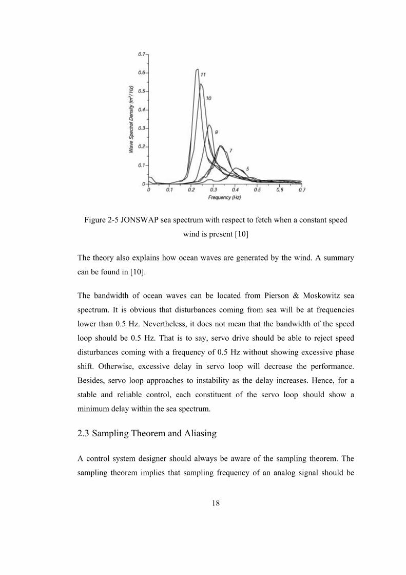
sea concept. A sea which has not yet reached steady state with the wind is called a

developing sea. Searching for Joint North Sea Wave Observation Project

(JONSWAP), Hasselman et al., (1973), claimed that wave spectrum is never fully

developed and changes continuously with time and distance. Then a new spectrum,

JONSWAP spectrum is formed. Although proposal of Hasselman disproves the

Pierson-Moskowitz Spectrum of a fully developed sea, two spectrums are very

similar except for the fact that for JONSWAP spectrum the wave energy increases

with time and distance from a lee shore (called fetch in mathematical derivations of

the JONSWAP spectrum) [10].

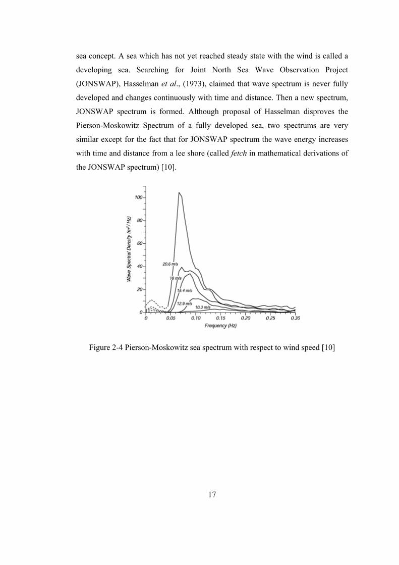
Figure 2-4 Pierson-Moskowitz sea spectrum with respect to wind speed [10]

18

Figure 2-5 JONSWAP sea spectrum with respect to fetch when a constant speed

wind is present [10]

The theory also explains how ocean waves are generated by the wind. A summary

can be found in [10].

The bandwidth of ocean waves can be located from Pierson & Moskowitz sea

spectrum. It is obvious that disturbances coming from sea will be at frequencies

lower than 0.5 Hz. Nevertheless, it does not mean that the bandwidth of the speed

loop should be 0.5 Hz. That is to say, servo drive should be able to reject speed

disturbances coming with a frequency of 0.5 Hz without showing excessive phase

shift. Otherwise, excessive delay in servo loop will decrease the performance.

Besides, servo loop approaches to instability as the delay increases. Hence, for a

stable and reliable control, each constituent of the servo loop should show a

minimum delay within the sea spectrum.

2.3 Sampling Theorem and Aliasing

A control system designer should always be aware of the sampling theorem. The

sampling theorem implies that sampling frequency of an analog signal should be

19

chosen as Ws>2Wmax, also known as Nyquist criterion, where Wmax is the highest-

frequency component present in continuous time signal. However, practical

considerations on the closed loop system generally make it necessary to sample at a

frequency much higher than 2Wmax. Usually, Ws is chosen to be 10Wmax to 20Wmax

[11].

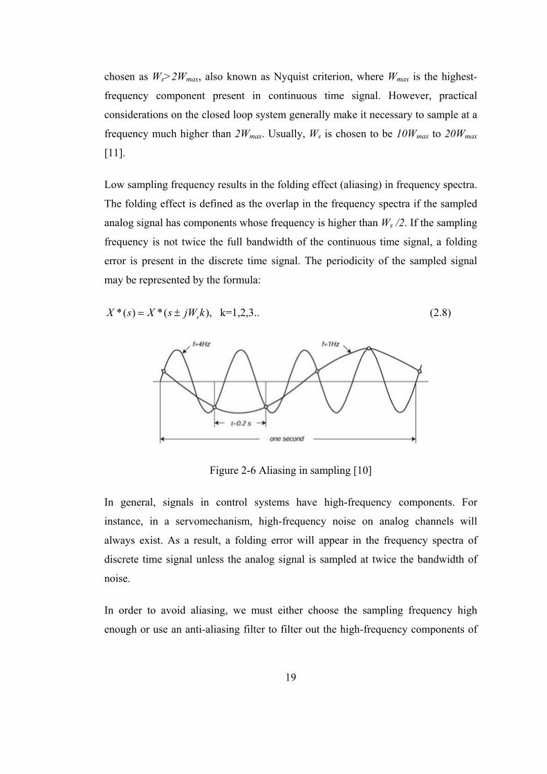
Low sampling frequency results in the folding effect (aliasing) in frequency spectra.

The folding effect is defined as the overlap in the frequency spectra if the sampled

analog signal has components whose frequency is higher than Ws /2. If the sampling

frequency is not twice the full bandwidth of the continuous time signal, a folding

error is present in the discrete time signal. The periodicity of the sampled signal

may be represented by the formula:

*( ) *( ), k=1,2,3..sX s X s jW k (2.8)

Figure 2-6 Aliasing in sampling [10]

In general, signals in control systems have high-frequency components. For

instance, in a servomechanism, high-frequency noise on analog channels will

always exist. As a result, a folding error will appear in the frequency spectra of

discrete time signal unless the analog signal is sampled at twice the bandwidth of

noise.

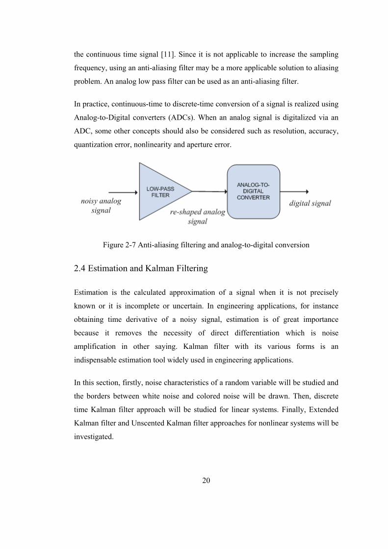
In order to avoid aliasing, we must either choose the sampling frequency high

enough or use an anti-aliasing filter to filter out the high-frequency components of

20

the continuous time signal [11]. Since it is not applicable to increase the sampling

frequency, using an anti-aliasing filter may be a more applicable solution to aliasing

problem. An analog low pass filter can be used as an anti-aliasing filter.

In practice, continuous-time to discrete-time conversion of a signal is realized using

Analog-to-Digital converters (ADCs). When an analog signal is digitalized via an

ADC, some other concepts should also be considered such as resolution, accuracy,

quantization error, nonlinearity and aperture error.

Figure 2-7 Anti-aliasing filtering and analog-to-digital conversion

2.4 Estimation and Kalman Filtering

Estimation is the calculated approximation of a signal when it is not precisely

known or it is incomplete or uncertain. In engineering applications, for instance

obtaining time derivative of a noisy signal, estimation is of great importance

because it removes the necessity of direct differentiation which is noise

amplification in other saying. Kalman filter with its various forms is an

indispensable estimation tool widely used in engineering applications.

In this section, firstly, noise characteristics of a random variable will be studied and

the borders between white noise and colored noise will be drawn. Then, discrete

time Kalman filter approach will be studied for linear systems. Finally, Extended

Kalman filter and Unscented Kalman filter approaches for nonlinear systems will be

investigated.

21

2.4.1 Characteristics of Random Variables

A random variable is a variable whose value is not exactly known before the

process actually runs. For instance, noise on the analog channel of a system is a

random variable whose value cannot be known exactly but can be expressed with a

mean and variance by help of statistical data. Hence, random variables can be

expressed by some probability laws. Moreover, some probability density and

distribution functions can be written based on the statistical data collected for them.

The most common probability distribution function seen in nature is the Gaussian

distribution. A random variable is called as Gaussian if it has a probability density

function expressed by the formula:

2

2

1 ( )( ) exp

22

xpdf x

(2.9)

In this formula, is the mean and 2 is the variance. A Gaussian distribution with

zero mean will have a peak at zero point in its probability density plot. This shows

that, the expected value of this random variable is zero. Variance of a Gaussian

distribution, which is square of standard deviation, informs us about the possible

deviations of the random variable from its mean.

When a random variable, for instance process noise or measurement noise in a

dynamical system, is independent of its past and future values for all time, this

random variable is named as white noise. If a random variable does not satisfy

above condition, it is a colored noise. The power spectrum of a random variable

which is defined as the Fourier transform of the autocorrelation determines the color

content of the random variable. The Wiener-Khintchine equations show the relation

between the Fourier transform and the autocorrelation function for a continuous

time system.

22

( ) ( )

1( ) ( )

2

jw

jw

S w R e d

R S w e dw

(2.10)

For the discrete domain these equations may be stated as follows:

( ) ( ) , [ , ]

1( ) ( )

2

jwk

k

jwk

S w R k e w

R k S w e dw

(2.11)

Mathematically speaking, a white noise will have equal power at all frequencies in

both continuous time and discrete time domains. A continuous time white noise will

have an autocorrelation function given by the expression:

( ) (0) ( )R R (2.12)

In this expression, ( ) is the continuous-time impulse function. Similarly, a

discrete time white noise will have an autocorrelation function given by the

expression:

2 0( )

0 0

kR k

k

(2.13)

Therefore, power spectrum expression for a continuous time white noise process

will be:

( ) (0) for all wS w R (2.14)

For a discrete time white noise process it will be:

2( ) (0) , [ , ]S w R w (2.15)

23

This implies that a white noise will have constant power at all frequencies. Another

concept is uncorrelated noise. An uncorrelated noise vector implies that the

elements of the vector are uncorrelated with each other resulting in a diagonal

covariance matrice of the form

21

22

2

0 . . 0

0 . . 0

. . . . .

. . . . .

0 0 . . n

(2.16)

This section gives some introductory information about a Gaussian, white and

uncorrelated random variable. This is important to understand the conditions under

which the Kalman filter shows its optimal performance. More information about

random variables is revealed in a great detail in [12].

2.4.2 Kalman Filtering

Estimating state of a linear system is a common problem for most of engineering

disciplines. Kalman filter is a tool that solves this problem optimally for linear

systems. Any linear system can be expressed by the equations:

1 1 1 1k k k k k k

k k k k

x F x G u w

y H x v

(2.17)

In these representations of dynamical system, x is the state of the system, u is the

input to the system, y is the output of the system, w is the process noise and v is

the measurement noise. Since process noise and measurement noise are random

variables, the estimate of the state will also be a random variable. Hence, error

between the estimate and the actual state is also a random variable. What Kalman

filter does is to minimize expected value of this random variable while estimating

the state at each time when a new output data of the system is available.

24

When process noise and measurement noise are both Gaussian, zero-mean, white,

and uncorrelated, Kalman filter is the best linear estimator for the estimation

problem. Although there is an open door of designing nonlinear filters showing

better performance, the best linear solution of the estimation problem is the Kalman

filtering. For the cases when process noise and measurement noise are not Gaussian,

Kalman filter still gives out the optimal linear solution even though some nonlinear

ways of getting better performance may still exist [12].

2.4.2.1 Discrete Time Kalman Filter

The discrete time Kalman filter has two update processes for each time step called

time update and measurement update. In the time update step, a priori estimate of

the state is made based on the system dynamics already known without using the

measurement at that time step. After calculating priori state estimate, time update

step for calculation of priori estimation error covariance is applied. In the

measurement update process, measurement is taken into account to form up

posteriori state estimate and estimation error covariance. Measurement update

process makes it necessary to calculate a gain matrice called Kalman filter gain.

Kalman filter gain is calculated to correct the priori state estimate and estimation

error covariance taking the measurement into account.

Any system can be formulated in state-space form using state and output update

equations and noise processes:

1 1 1 1

{ }

{ }

{ } 0

k k k k k k

k k k k

Tk j k kj

Tk j k kj

Tk j

x F x G u w

y H x v

E w w Q

E v v R

E w v

(2.18)

In the above formulation, w is process noise and v is measurement noise. is

Kronecker delta function. Noise processes are white, zero-mean, uncorrelated

25

processes and their covariance matrices kQ and kR are known. Then the algorithm

[12] may be summarized as follows:

1. The first step is the initialization of the Kalman filter. 0x is the best estimate

of initial state of system. 0P is the uncertainty in estimating the initial state

of the system.

0 0

0 0 0 0 0

( )

{( )( ) }T

x E x

P E x x x x

(2.19)

2. The following equations should be evaluated at each time step when a new

output data of the system is available.

Priori estimation error covariance:

1 1 1 1T

k k k k kP F P F Q (2.20)

Kalman filter gain:

1( )T Tk k k k k k kK P H H P H R (2.21)

Priori state estimate:

1 1 1 1k k k k kx F x G u (2.22)

Posteriori state estimate:

( )k k k k k kx x K y H x (2.23)

For posteriori estimation error covariance, there are three different

expressions defined in literature two of which are given here:

26

( ) ( )

( )

T Tk k k k k k k k k

k k k k

P I K H P I K H K R K

P I K H P

(2.24)

There are two types of covariance measurement update equations. The first type

Joseph stabilized covariance measurement update equation which guarantees kP to

be symmetric positive definite as long as the initial covariance is symmetric positive

definite. Although the second form is the simplest in terms of computational

burden, it does not guarantee symmetry and positive definiteness [12].

In real time applications, Kalman filter gain can be calculated offline to save

computational effort due to the fact that Kalman gain is not dependent on

measurements and system dynamics does not change with time for a linear time-

invariant system. As a result, Kalman gain can be calculated using only system

parameters ( , , , ,F G H R Q ) which are known before the system actually runs [12].

Although Kalman filter is derived for linear systems, it can be expanded to

nonlinear systems. This will be very useful because most real systems show

nonlinear dynamics. Using first order Taylor series expansion for linearization,

Extended Kalman filter is a way of estimation in nonlinear systems. However, it is

not the only way. Another way of estimation in nonlinear systems is Unscented

Kalman filter which uses Unscented Transforms to transfer Gaussians through

nonlinear system dynamics.

2.4.2.2 Extended Kalman Filter

Most of real systems have nonlinear dynamics. To be able to estimate the states of a

nonlinear system using a discrete time Kalman filter, we should first discretize the

system dynamics.

Any nonlinear system can be formulated by the following system equations:

27

1 1 1 1

1

( , , )

( , )k k k k k

k k k k

x f x u w

y h x v

(2.25)

In (2.25), w is process noise and v is measurement noise. Noise processes are

white, zero-mean, uncorrelated processes and their covariance matrices kQ and kR

are known. Then the discrete time extended Kalman filter algorithm can be

summarized [12] by the following equations:

1. The first step is the initialization of the Kalman filter. 0x is the best estimate

of initial state of system. 0P is the uncertainty in estimating the initial state

of the system.

0 0

0 0 0 0 0

( )

{( )( ) }T

x E x

P E x x x x

(2.26)

2. The following equations should be evaluated at each time step when a new

output data of the system is available.

Partial derivatives of 1kf with respect to state and process noise are

evaluated around posteriori estimate of state.

11 1

11 1

( )

( )

kk k

kk k

fF x x

xf

L x xw

(2.27)

Time update of the state estimate and estimation error covariance is

carried out.

1 1 1 1 1 1

1 1 1,( , 0)

T Tk k k k k k k

k k k k

P F P F L Q L

x f x u

(2.28)

28

Partial derivatives of kh with respect to state and measurement noise are

evaluated around priori estimate of state.

( )

( )

kk k

kk k

hH x x

xh

M x xv

(2.29)

Measurement update of the state estimate and estimation error

covariance is carried out.

1( )

[ ( ,0)]

( )

T T Tk k k k k k k k k

k k k k k k

k k k k

K P H H P H M R M

x x K y h x

P I K H P

(2.30)

Extended Kalman filter gain cannot be calculated offline due to the fact that

Kalman gain is dependent on partial differentiations at each mean point. Therefore,

Extended Kalman filter seems to need more computational effort while running in

real-time.

2.4.2.3 Unscented Kalman Filter

Extended Kalman Filter approximates nonlinear system functions using Taylor

series expansion for transformation of Gaussian signals. However, Taylor series

expansion is not the only way to perform this transformation through the nonlinear

system dynamics. There is one more way which may give better results. It is the

Unscented Transform. In this section of the thesis, a summary of the Unscented

Kalman filter from [13] will be given.

Unscented Kalman Filter makes use of Unscented Transform to linearize nonlinear

system functions. Let us assume we have a nonlinear function called f. The first step

of linearization is to extract sigma points from the Gaussian signal and calculate the

weights corresponding to these sigma points. For an n-dimensional Gaussian signal,

29

there will be 2n+1 sigma points which are located at mean and two points

symmetrically chosen with respect to the mean.

The equations to choose sigma points for a Gaussian ( , )N are given as:

0

( ( ) ), for i=1,..,n

( ( ) ), for i=n+1,..,2n

i

i

X

X n

X n

(2.31)

In (2.31), 2 ( )n n and parameters and determine the locations of the

symmetrical sigma points. For each sigma point, there exist two weights which are

calculated according to the following rules:

0

0 2(1 )

1, for i=1,..,2n

2( )

m

c

i im c

wn

wn

w wn

(2.32)

The parameter is optimally 2 when the distribution is an exact Gaussian. In the

second step, sigma points should be passed through nonlinear function f.

( )i iY f X (2.33)

The third and final step of the unscented transform is to calculate new mean and

covariance parameters of resulting Gaussian. The parameters can be calculated from

the equations:

2

0

2

0

'

' ( ')( ')

ni im

i

ni i i Tc

i

w Y

w Y Y

(2.34)

30

The system equations of a nonlinear system can be expressed as follows:

( 1) ( ( ), ( ), ) ( )

( ) ( ( ), ) ( )

x k g x k u k k w k

y k h x k k v k

(2.35)

In the above given expression, w is the process noise and v is the measurement

noise. Noise is white, zero mean and uncorrelated. A summary of the Unscented

Kalman Filter algorithm is given below.

The inputs for the algorithm are 1t , 1t , tu and tz . In the first step,

sigma points are extracted from the previous estimate and estimation

error covariance.

1 1 1 1 1 1( )t t t t t tX (2.36)

Calculated sigma points are passed through the nonlinear function g with

the input tu .

*1( , )t t tX g u X (2.37)

Mean and variance parameters are calculated from the sigma points.

2* *

0

2* * * * *

0

( )( )

ni i

t m ti

ni i i T

t c t t t ti

w X

w X X Q

(2.38)

A new set of sigma points are extracted and passed through the nonlinear

function h.

* * * * *( )

( )t t t t t t

t t

X

Z h X

(2.39)

31

Using these new sigma points, prediction *tz and uncertainty tS is

calculated.

2*

0

2* *

0

( )( )

ni i

t m ti

ni i i T

t c t t t ti

z w Z

S w Z z Z z R

(2.40)

Cross covariance between state and observation is calculated.

2

, * *

0

( )( )n

x z i i i Tt c t t t t

i

w X Z z

(2.41)

The Kalman gain is calculated using cross covariance matrix.

, 1x zt t tK S (2.42)

Finally, estimation update is completed by calculating the parameters t

and t . The outputs of the algorithm are the parameters t and t .

* *

*

( )t t t t t

Tt t t t t

K z z

K S K

(2.43)

Unscented Kalman Filter makes use of Unscented Transform to transform Gaussian

signals through the nonlinear functions. The algorithm is more complex compared

to the Extended Kalman Filter which uses only the first order term of Taylor series

expansion. Although, asymptotic complexity seems to be the same when UKF and

EKF are compared, in fact, the EKF is faster in practical applications. Although

estimation performance of UKF is better than that of EKF generally, in most

practical applications EKF and UKF show very similar performance [13].

However, if the system has intensive nonlinearities, EKF may generate unreliable

estimates [25]. In that case, using UKF will upgrade the estimation performance

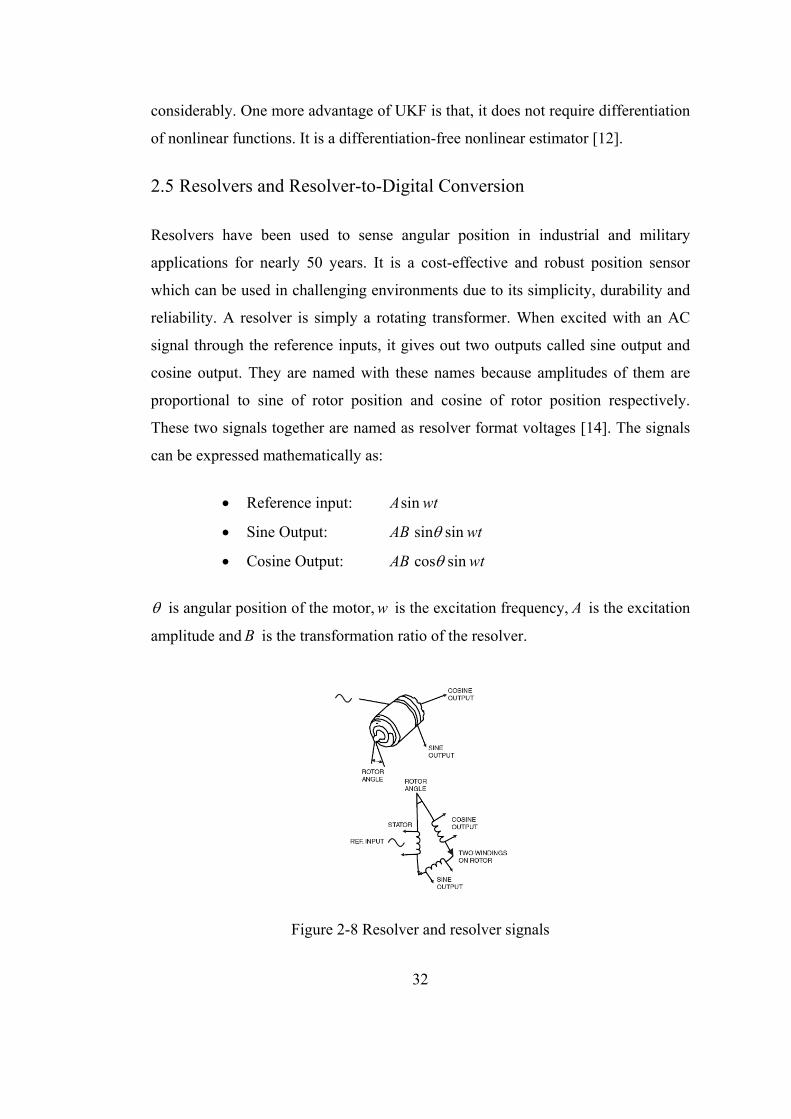
32

considerably. One more advantage of UKF is that, it does not require differentiation

of nonlinear functions. It is a differentiation-free nonlinear estimator [12].

2.5 Resolvers and Resolver-to-Digital Conversion

Resolvers have been used to sense angular position in industrial and military

applications for nearly 50 years. It is a cost-effective and robust position sensor

which can be used in challenging environments due to its simplicity, durability and

reliability. A resolver is simply a rotating transformer. When excited with an AC

signal through the reference inputs, it gives out two outputs called sine output and

cosine output. They are named with these names because amplitudes of them are

proportional to sine of rotor position and cosine of rotor position respectively.

These two signals together are named as resolver format voltages [14]. The signals

can be expressed mathematically as:

Reference input: sinA wt

Sine Output: sin sin AB wt

Cosine Output: cos sin AB wt

is angular position of the motor, w is the excitation frequency, A is the excitation

amplitude and B is the transformation ratio of the resolver.

Figure 2-8 Resolver and resolver signals

33

Resolvers make interface electronics necessary to get a digital angular position

measurement. This interface electronics converting resolver format voltages into

meaningful digital data is called as Resolver-to-Digital converter. There are

different types of Resolver-to-Digital converters available in the market. However,

the most effective types are tracking type Resolver-to-Digital converters [14]. The

advantages of the tracking type converters over other type converters are:

Ratio metric Operation

Noise Immunity

Instant Digital Data

Velocity voltage outputs.

Besides the advantages of tracking type Resolver-to-Digital converters, there are

still some problems with this type of converters. These problems [14] are

summarized as follows:

Digital output lags actual position during acceleration.

Flickering exists when the digital data is not an exact representation of the

input angle.

Common and differential phase shifts and distortions on the resolver

format voltages may affect the performance of the conversion badly and

result in noisy speed and position signals.

Speed voltages exist on the resolver format voltages which deteriorate the

conversion performance.

To eliminate these disadvantages, many methods are described in the literature. The

inspected methods are handled in the next section.

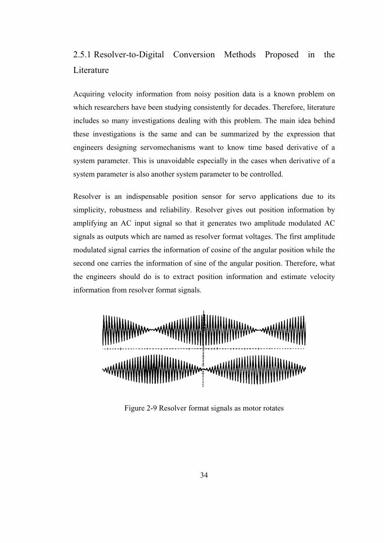
34

2.5.1 Resolver-to-Digital Conversion Methods Proposed in the

Literature

Acquiring velocity information from noisy position data is a known problem on

which researchers have been studying consistently for decades. Therefore, literature

includes so many investigations dealing with this problem. The main idea behind

these investigations is the same and can be summarized by the expression that

engineers designing servomechanisms want to know time based derivative of a

system parameter. This is unavoidable especially in the cases when derivative of a

system parameter is also another system parameter to be controlled.

Resolver is an indispensable position sensor for servo applications due to its

simplicity, robustness and reliability. Resolver gives out position information by

amplifying an AC input signal so that it generates two amplitude modulated AC

signals as outputs which are named as resolver format voltages. The first amplitude

modulated signal carries the information of cosine of the angular position while the

second one carries the information of sine of the angular position. Therefore, what

the engineers should do is to extract position information and estimate velocity

information from resolver format signals.

Figure 2-9 Resolver format signals as motor rotates

35

Literature survey performed on resolver-to-digital conversion give rise to a useful

knowledge about the conversion process. A summary of literature survey performed

on resolver conversion is given in this section.

Sarma, Agrawal and Udupa have developed a software based Resolver-to-Digital

converter using a DSP based reference generator [15]. Since the reference

frequency changes from resolver to resolver, software based reference generator

implies a more flexible Resolver-to-Digital converter which can be used with any

resolver. Demodulation of resolver format voltages is made using synchronous

amplitude demodulation technique. They sampled resolver format voltages at the

peaks of reference signal. After demodulation, they used a look-up-table including

arctangent values for a complete 360° rotation in order to get the position

information from sine and cosine envelops. Although results show a good

performance in position estimation, velocity estimation problem is not dealt in the

paper. Hence, the method can be seen as a trigonometric calculator rather than an

estimator. Similar solutions are given in [16, 17, 18].

Harnefors [2] used a Linear Kalman Filter structure to estimate position and speed

from noisy resolver format voltages. He used dq transformation matrice to have a

steady-state Discrete Time Algebraic Riccati equation so that Kalman filter gain

matrice could be calculated offline before the system actually runs. This results in a

reduction in computational burden. Furthermore, in the study, he has formed up the

system model in such a way that the acceleration error present in a tracking resolver

conversion process is eliminated.

Bellini and Bifaretti [19] used a Discrete Time Kalman filter with a Phase Locked

Loop based filter to estimate position and speed of a resolver. Since a PLL structure

is implemented, using a Steady State Linear Kalman filter becomes sufficient for

estimation. Furthermore, this model of system was formed up so that the filter can

also perform an estimation of the acceleration. Therefore, the outputs of the filter do

not lag the actual state even if acceleration is present in the motion. Moreover, it is

36

stated that by the help of the filter, noise on the speed output is reduced compared to

other methods.

Kaewjinda and Konghirun [20] implemented digital version of a classical tracking

type Resolver-to-Digital converter using a Digital Signal Processor. The algorithm

is confirmed in a vector controlled drive system of a Permanent Magnet

Synchronous Machine. Moreover, offset calibration of resolver is made to eliminate

offset errors in angle sensing. They also introduced a digital tracking type Resolver-

to-Digital converter with a hardware error calculation algorithm [34]. Both

structures they introduced are very similar to tracking type resolver-to-Digital

converters except for the fact that the algorithms are implemented in a Digital

Signal Processor.

Harnefors and Nee [21] designed a nonlinear observer for resolver-to-digital

conversion process. Actually, the observer is a generic type observer that can be

adapted to several processes. For instance, the observer can be used for estimating

speed and position of a PMSM using fundamental excitation. The same algorithm

may also be used for saliency and signal injection to estimate position of a PMSM

with different d and q axes’ inductances. Lastly, the algorithm can also be employed

for resolver position and speed estimation process. The algorithm makes use of a

nonlinear observer whose structure can be configured according to one of the above

described processes. The study also includes stability and noise analyses of the

proposed filter. The analyses are very useful from the view of practical

implementations.

Lastly, Murray and Li designed a digital tracking resolver-to-digital converter in

[22]. The converter makes use of a hardware error calculation scheme and a DSP

IC, namely, TMS320C14. The converter is simply a digitized version of the

classical tracking type RDC. The proposed method utilizes a hardware component

to realize the error calculation and a DSP to implement the tracking loop.

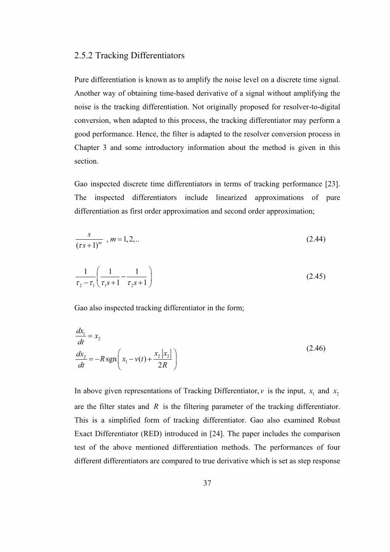
37

2.5.2 Tracking Differentiators

Pure differentiation is known as to amplify the noise level on a discrete time signal.

Another way of obtaining time-based derivative of a signal without amplifying the

noise is the tracking differentiation. Not originally proposed for resolver-to-digital

conversion, when adapted to this process, the tracking differentiator may perform a

good performance. Hence, the filter is adapted to the resolver conversion process in

Chapter 3 and some introductory information about the method is given in this

section.

Gao inspected discrete time differentiators in terms of tracking performance [23].

The inspected differentiators include linearized approximations of pure

differentiation as first order approximation and second order approximation;

, 1, 2,..( 1)m

sm

s

(2.44)

2 1 1 2

1 1 1

1 1s s

(2.45)

Gao also inspected tracking differentiator in the form;

12

2 221sgn ( )

2

dxx

dt

x xdxR x v t

dt R

(2.46)

In above given representations of Tracking Differentiator, v is the input, 1x and 2x

are the filter states and R is the filtering parameter of the tracking differentiator.

This is a simplified form of tracking differentiator. Gao also examined Robust

Exact Differentiator (RED) introduced in [24]. The paper includes the comparison

test of the above mentioned differentiation methods. The performances of four

different differentiators are compared to true derivative which is set as step response

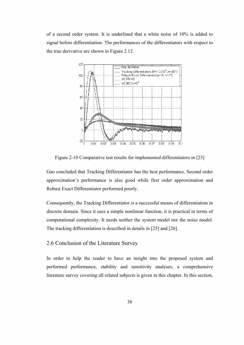
38

of a second order system. It is underlined that a white noise of 10% is added to

signal before differentiation. The performances of the differentiators with respect to

the true derivative are shown in Figure 2.12.

Figure 2-10 Comparative test results for implemented differentiators in [23]

Gao concluded that Tracking Differentiator has the best performance. Second order

approximation’s performance is also good while first order approximation and

Robust Exact Differentiator performed poorly.

Consequently, the Tracking Differentiator is a successful means of differentiation in

discrete domain. Since it uses a simple nonlinear function, it is practical in terms of

computational complexity. It needs neither the system model nor the noise model.

The tracking differentiation is described in details in [25] and [26].

2.6 Conclusion of the Literature Survey

In order to help the reader to have an insight into the proposed system and

performed performance, stability and sensitivity analyses, a comprehensive

literature survey covering all related subjects is given in this chapter. In this section,

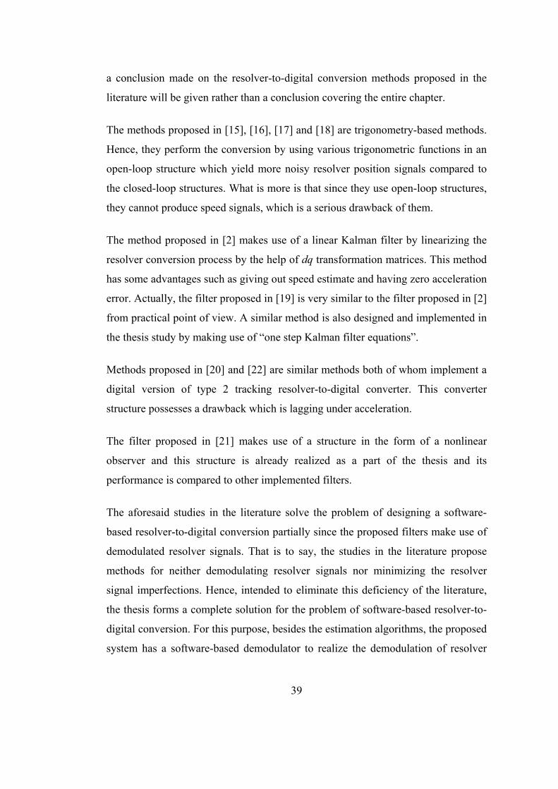
39

a conclusion made on the resolver-to-digital conversion methods proposed in the

literature will be given rather than a conclusion covering the entire chapter.

The methods proposed in [15], [16], [17] and [18] are trigonometry-based methods.

Hence, they perform the conversion by using various trigonometric functions in an

open-loop structure which yield more noisy resolver position signals compared to

the closed-loop structures. What is more is that since they use open-loop structures,

they cannot produce speed signals, which is a serious drawback of them.

The method proposed in [2] makes use of a linear Kalman filter by linearizing the

resolver conversion process by the help of dq transformation matrices. This method

has some advantages such as giving out speed estimate and having zero acceleration

error. Actually, the filter proposed in [19] is very similar to the filter proposed in [2]

from practical point of view. A similar method is also designed and implemented in

the thesis study by making use of “one step Kalman filter equations”.

Methods proposed in [20] and [22] are similar methods both of whom implement a

digital version of type 2 tracking resolver-to-digital converter. This converter

structure possesses a drawback which is lagging under acceleration.

The filter proposed in [21] makes use of a structure in the form of a nonlinear

observer and this structure is already realized as a part of the thesis and its

performance is compared to other implemented filters.

The aforesaid studies in the literature solve the problem of designing a software-

based resolver-to-digital conversion partially since the proposed filters make use of

demodulated resolver signals. That is to say, the studies in the literature propose

methods for neither demodulating resolver signals nor minimizing the resolver

signal imperfections. Hence, intended to eliminate this deficiency of the literature,

the thesis forms a complete solution for the problem of software-based resolver-to-

digital conversion. For this purpose, besides the estimation algorithms, the proposed

system has a software-based demodulator to realize the demodulation of resolver

40

signals and a signal conditioner to minimize the disturbances coming from resolver

signal imperfections. Moreover, the thesis introduces novel methods for estimation

of position and speed from demodulated resolver signals such as Extended Kalman

filter, Unscented Kalman filter and Tracking Differentiator approaches.

41

CHAPTER 3

DEVELOPMENT OF A DSP-FPGA-BASED

RESOLVER-TO-DIGITAL CONVERTER

3.1 Proposed Resolver-to-Digital Converter

Resolvers have been used to sense angular position in industrial and military

applications for nearly 50 years. It is a cost-effective and robust position sensor

which can be used in challenging environments due to its simplicity, durability and

reliability. Resolvers require an electronics interface which is named as resolver-to-

digital converter for converting resolver signals into digital position and speed

measurements. Since the proper current vector applied to a servo motor is

calculated using motor shaft position, resolver-to-digital converter is the heart of a

servo controller when servo motors coupled to resolver sensors are present in the

servo system.

A resolver sensor is simply a rotating transformer. Excited by a high frequency

reference signal, the resolver sensor gives out two signals which are named as

resolver format signals. Resolver format signals carry the shaft position information

through differential channels and at the end of these channels a resolver-to-digital

converter waits to convert resolver format signals into digital angular position and

angular velocity signals.

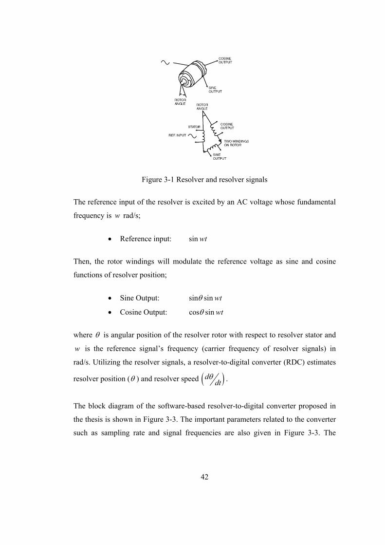
42

Figure 3-1 Resolver and resolver signals

The reference input of the resolver is excited by an AC voltage whose fundamental

frequency is w rad/s;

Reference input: sin wt

Then, the rotor windings will modulate the reference voltage as sine and cosine

functions of resolver position;

Sine Output: sin sin wt

Cosine Output: cos sin wt

where is angular position of the resolver rotor with respect to resolver stator and

w is the reference signal’s frequency (carrier frequency of resolver signals) in

rad/s. Utilizing the resolver signals, a resolver-to-digital converter (RDC) estimates

resolver position ( ) and resolver speed ddt

.

The block diagram of the software-based resolver-to-digital converter proposed in

the thesis is shown in Figure 3-3. The important parameters related to the converter

such as sampling rate and signal frequencies are also given in Figure 3-3. The

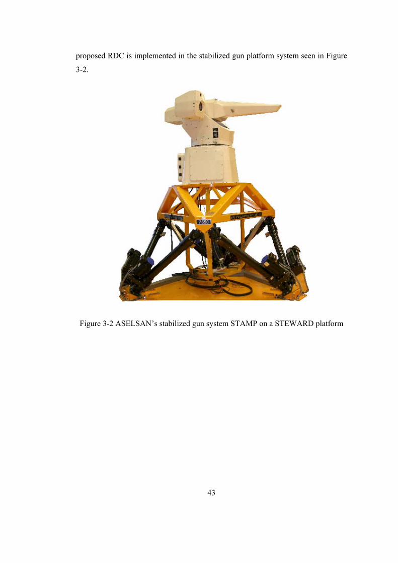
43

proposed RDC is implemented in the stabilized gun platform system seen in Figure

3-2.

Figure 3-2 ASELSAN’s stabilized gun system STAMP on a STEWARD platform

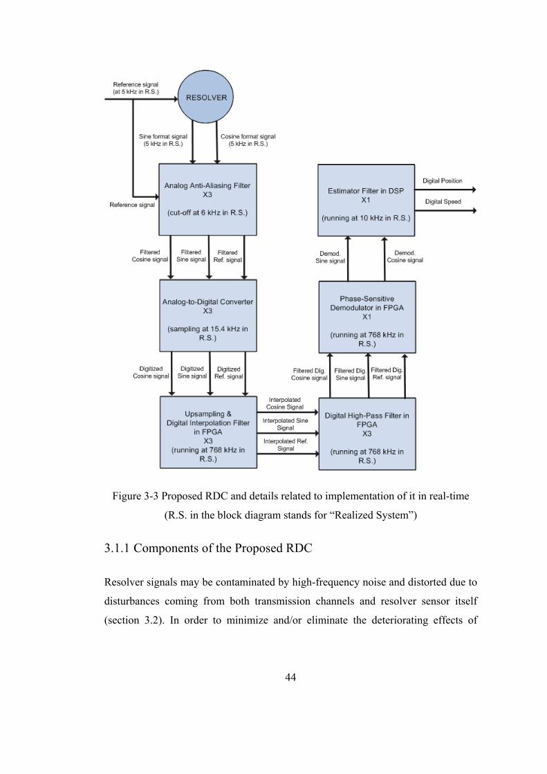
44

Figure 3-3 Proposed RDC and details related to implementation of it in real-time

(R.S. in the block diagram stands for “Realized System”)

3.1.1 Components of the Proposed RDC

Resolver signals may be contaminated by high-frequency noise and distorted due to

disturbances coming from both transmission channels and resolver sensor itself

(section 3.2). In order to minimize and/or eliminate the deteriorating effects of

45

resolver signal imperfections on RDC’s performance, analog anti-aliasing filters

and digital filters are utilized in the proposed structure.

The proposed system has three analog-to-digital converters (ADCs) to digitize three

resolver signals (section 3.2.3.2). Before the digitization, three anti-aliasing filters

are used to minimize the high-frequency distortions and noise present in resolver

signals (section 3.2.3.1). After sampling, digital interpolation filters, implemented

in the Field-Programmable Gate Array (FPGA), reconstruct the resolver signals

from sampled signals (section 3.2.3.2). In order to eliminate the low-frequency

harmonic distortions and DC offset present in the reconstructed resolver signals,

digital high-pass filters are also implemented in the FPGA (section 3.2.3.3).

The core of the proposed RDC is the estimator filter that estimates the resolver

position ( ) and speed ddt

from the demodulated resolver signals, namely

sin and cos signals (section 3.4). Hence, to provide the estimator filter with

sin and cos signals, the proposed RDC also has a phase-sensitive demodulator

implemented in FPGA (section 3.3).

3.1.2 Forming the System Structure for the Proposed RDC

DSP and FPGA, both having advantages and disadvantages, actually they are not

competitors but they may be complementary parts of an efficient system. Floating-

point tasks with lower sampling rates and increased arithmetic complexity suit the

DSP more whereas fixed-point arithmetic tasks with higher sampling rates and

repetitive behavior suit the FPGA more. For instance, realizing a floating-point

multiplier in FPGA is unreasonable since it will cover much area (logic gates) in

FPGA while DSP’s Central Processing Unit (CPU) with its highly-developed

arithmetic sub-units will realize the operation with a little effort. On the other hand,

FPGA can handle high-frequency data streams easily where DSP cannot handle

them efficiently. As a result, in the proposed system, software components that

require higher sampling rates are embedded into the FPGA whereas software

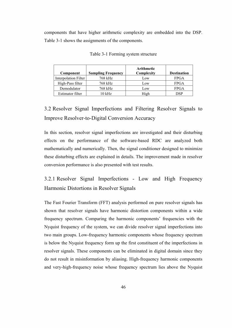
46

components that have higher arithmetic complexity are embedded into the DSP.

Table 3-1 shows the assignments of the components.

Table 3-1 Forming system structure

Component Sampling Frequency Arithmetic Complexity Destination

Interpolation Filter 768 kHz Low FPGA High-Pass filter 768 kHz Low FPGA

Demodulator 768 kHz Low FPGA Estimator filter 10 kHz High DSP

3.2 Resolver Signal Imperfections and Filtering Resolver Signals to

Improve Resolver-to-Digital Conversion Accuracy

In this section, resolver signal imperfections are investigated and their disturbing

effects on the performance of the software-based RDC are analyzed both

mathematically and numerically. Then, the signal conditioner designed to minimize

these disturbing effects are explained in details. The improvement made in resolver

conversion performance is also presented with test results.

3.2.1 Resolver Signal Imperfections - Low and High Frequency

Harmonic Distortions in Resolver Signals

The Fast Fourier Transform (FFT) analysis performed on pure resolver signals has

shown that resolver signals have harmonic distortion components within a wide

frequency spectrum. Comparing the harmonic components’ frequencies with the

Nyquist frequency of the system, we can divide resolver signal imperfections into

two main groups. Low-frequency harmonic components whose frequency spectrum

is below the Nyquist frequency form up the first constituent of the imperfections in

resolver signals. These components can be eliminated in digital domain since they

do not result in misinformation by aliasing. High-frequency harmonic components

and very-high-frequency noise whose frequency spectrum lies above the Nyquist

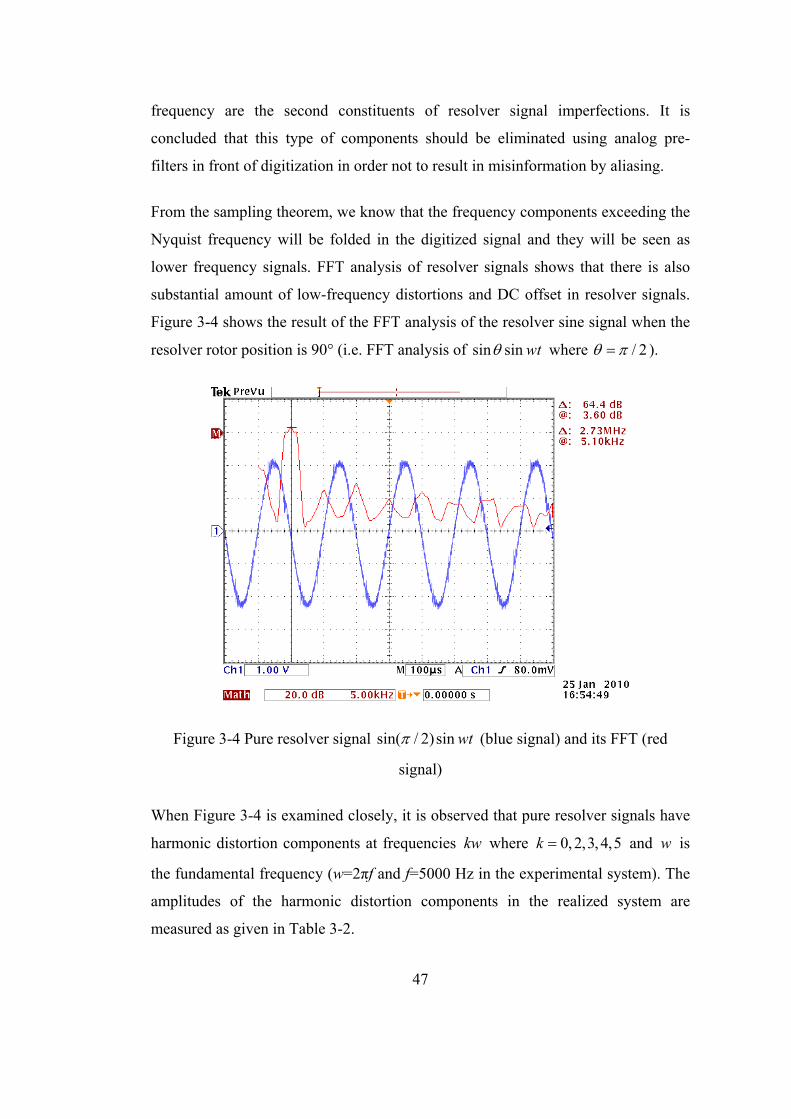
47

frequency are the second constituents of resolver signal imperfections. It is

concluded that this type of components should be eliminated using analog pre-

filters in front of digitization in order not to result in misinformation by aliasing.

From the sampling theorem, we know that the frequency components exceeding the

Nyquist frequency will be folded in the digitized signal and they will be seen as

lower frequency signals. FFT analysis of resolver signals shows that there is also

substantial amount of low-frequency distortions and DC offset in resolver signals.

Figure 3-4 shows the result of the FFT analysis of the resolver sine signal when the

resolver rotor position is 90° (i.e. FFT analysis of sin sin wt where / 2 ).

Figure 3-4 Pure resolver signal sin( / 2)sin wt (blue signal) and its FFT (red

signal)

When Figure 3-4 is examined closely, it is observed that pure resolver signals have

harmonic distortion components at frequencies kw where 0,2,3,4,5k and w is

the fundamental frequency (w=2πf and f=5000 Hz in the experimental system). The

amplitudes of the harmonic distortion components in the realized system are

measured as given in Table 3-2.

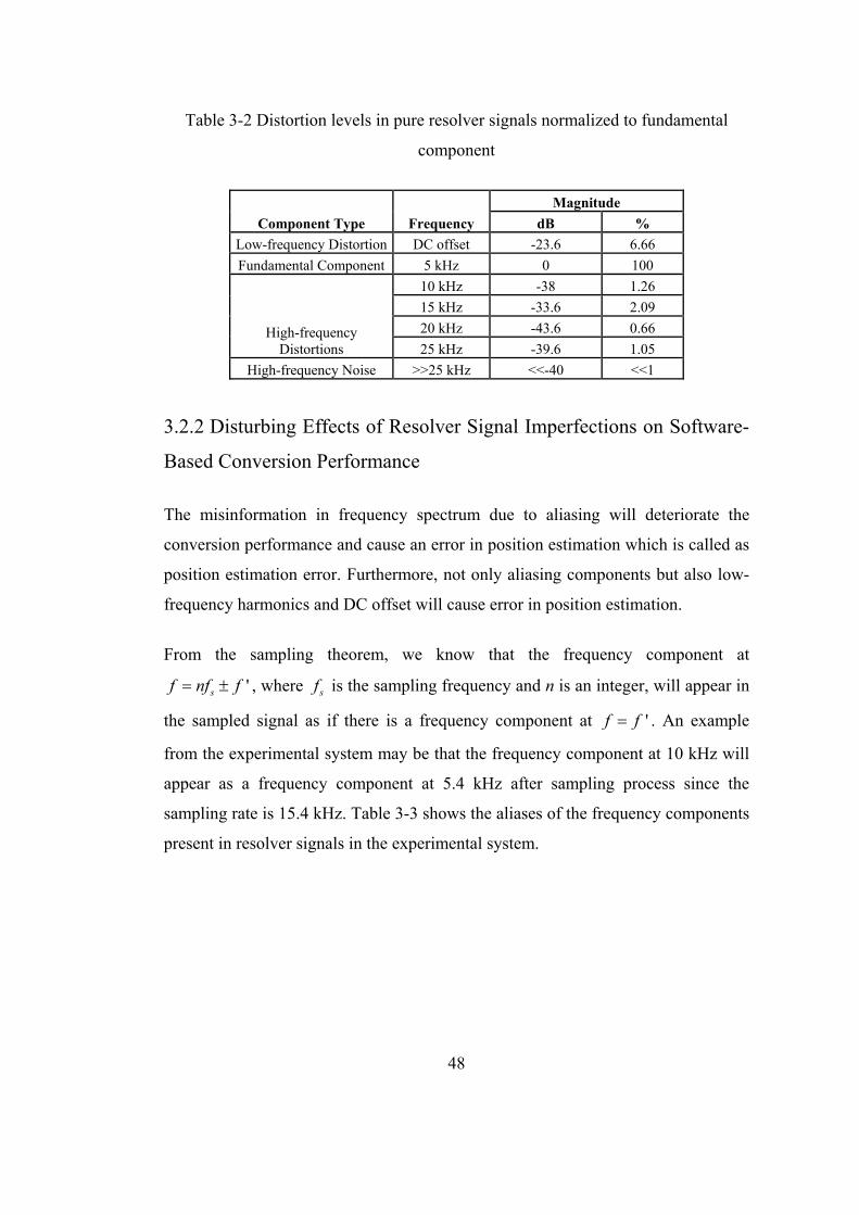
48

Table 3-2 Distortion levels in pure resolver signals normalized to fundamental

component

Component Type Frequency

Magnitude

dB %

Low-frequency Distortion DC offset -23.6 6.66

Fundamental Component 5 kHz 0 100

High-frequency Distortions

10 kHz -38 1.26

15 kHz -33.6 2.09

20 kHz -43.6 0.66

25 kHz -39.6 1.05

High-frequency Noise >>25 kHz <<-40 <<1

3.2.2 Disturbing Effects of Resolver Signal Imperfections on Software-

Based Conversion Performance

The misinformation in frequency spectrum due to aliasing will deteriorate the

conversion performance and cause an error in position estimation which is called as

position estimation error. Furthermore, not only aliasing components but also low-

frequency harmonics and DC offset will cause error in position estimation.

From the sampling theorem, we know that the frequency component at

'sf nf f , where sf is the sampling frequency and n is an integer, will appear in

the sampled signal as if there is a frequency component at 'f f . An example

from the experimental system may be that the frequency component at 10 kHz will

appear as a frequency component at 5.4 kHz after sampling process since the

sampling rate is 15.4 kHz. Table 3-3 shows the aliases of the frequency components

present in resolver signals in the experimental system.

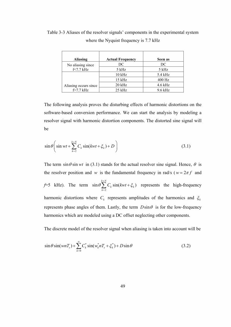
49

Table 3-3 Aliases of the resolver signals’ components in the experimental system

where the Nyquist frequency is 7.7 kHz

Aliasing Actual Frequency Seen as

No aliasing since f<7.7 kHz

DC DC 5 kHz 5 kHz

Aliasing occurs since f>7.7 kHz

10 kHz 5.4 kHz 15 kHz 400 Hz 20 kHz 4.6 kHz 25 kHz 9.6 kHz

The following analysis proves the disturbing effects of harmonic distortions on the

software-based conversion performance. We can start the analysis by modeling a

resolver signal with harmonic distortion components. The distorted sine signal will

be

2

sin sin sin( )k N

k kk

wt C kwt D

(3.1)

The term sin sin wt in (3.1) stands for the actual resolver sine signal. Hence, is

the resolver position and w is the fundamental frequency in rad/s ( 2w f and

f=5 kHz). The term 2

sin sin( )k N

k kk

C kwt

represents the high-frequency

harmonic distortions where kC represents amplitudes of the harmonics and k

represents phase angles of them. Lastly, the term sinD is for the low-frequency

harmonics which are modeled using a DC offset neglecting other components.

The discrete model of the resolver signal when aliasing is taken into account will be

* * *

0

sin sin( ) sin( ) sins k k s kk

wnT C w nT D

(3.2)

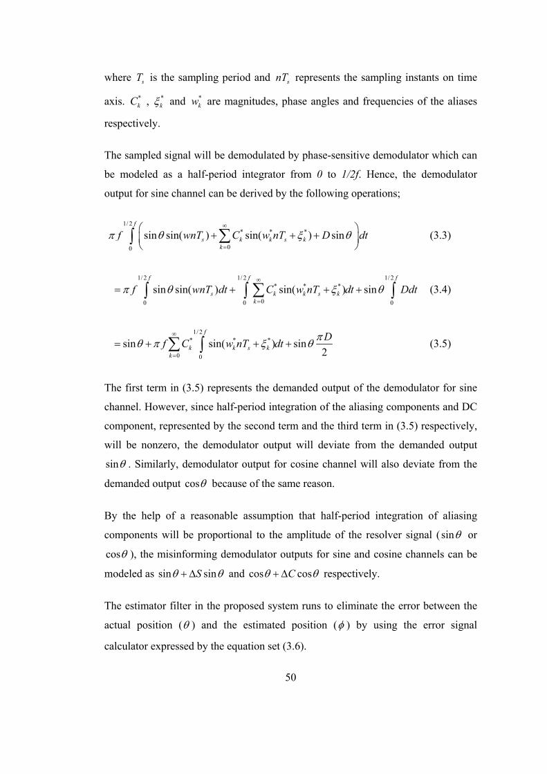
50

where sT is the sampling period and snT represents the sampling instants on time

axis. *kC , *

k and *kw are magnitudes, phase angles and frequencies of the aliases

respectively.

The sampled signal will be demodulated by phase-sensitive demodulator which can

be modeled as a half-period integrator from 0 to 1/2f. Hence, the demodulator

output for sine channel can be derived by the following operations;

1/ 2

* * *

00

sin sin( ) sin( ) sinf

s k k s kk

f wnT C w nT D dt

(3.3)

1/ 2 1/ 2 1/ 2* * *

00 0 0

sin sin( ) sin( ) sinf f f

s k k s kk

f wnT dt C w nT dt Ddt

(3.4)

1/ 2* * *

0 0

sin sin( ) sin2

f

k k s kk

Df C w nT dt

(3.5)

The first term in (3.5) represents the demanded output of the demodulator for sine

channel. However, since half-period integration of the aliasing components and DC

component, represented by the second term and the third term in (3.5) respectively,

will be nonzero, the demodulator output will deviate from the demanded output

sin . Similarly, demodulator output for cosine channel will also deviate from the

demanded output cos because of the same reason.

By the help of a reasonable assumption that half-period integration of aliasing

components will be proportional to the amplitude of the resolver signal ( sin or

cos ), the misinforming demodulator outputs for sine and cosine channels can be

modeled as sin sinS and cos cosC respectively.

The estimator filter in the proposed system runs to eliminate the error between the

actual position ( ) and the estimated position ( ) by using the error signal

calculator expressed by the equation set (3.6).

51

sin cos cos sin sin( ) (3.6)

We can assume that the estimator filter tracks the position information carried by

the demodulator outputs with zero error.

sin cos cos sin sin( ) 0 (3.7)

However, when the demodulator output is misinforming as in the case of software-

based demodulator, although the estimator filter tracks the demodulator outputs

with zero error, it will track the actual position with a nonzero error. If we write the

misinforming demodulator outputs into (3.7), the tracking error will be found

as

(sin sin )cos (cos cos )sin 0S C (3.8)

sin( ) sin cos cos sin 0S C (3.9)

sin( ) cos sin sin cosC S (3.10)

Hence, the analysis proves that resolver signal imperfections degrade the

conversion accuracy and induce a nonzero position estimation error. Moreover, the

analysis shows that the estimation error is dependent on the actual position ( ),

estimated position ( ) and demodulator output deviations ( S and C ).

3.2.3 Position Estimation Error due to Resolver Signal Imperfections

and Resultant Disturbances on Torque and Speed of the Motor

Since there are many aliases in the digitized resolver signals and their frequencies,

amplitudes and phases are not exactly known, it seems challenging to calculate an

approximate value for the position estimation error due to aliasing components.

However, an upper limit can be calculated using the information given in Table 3-2

and Table 3-3 with the assumption that amplitudes of the aliases cannot exceed the

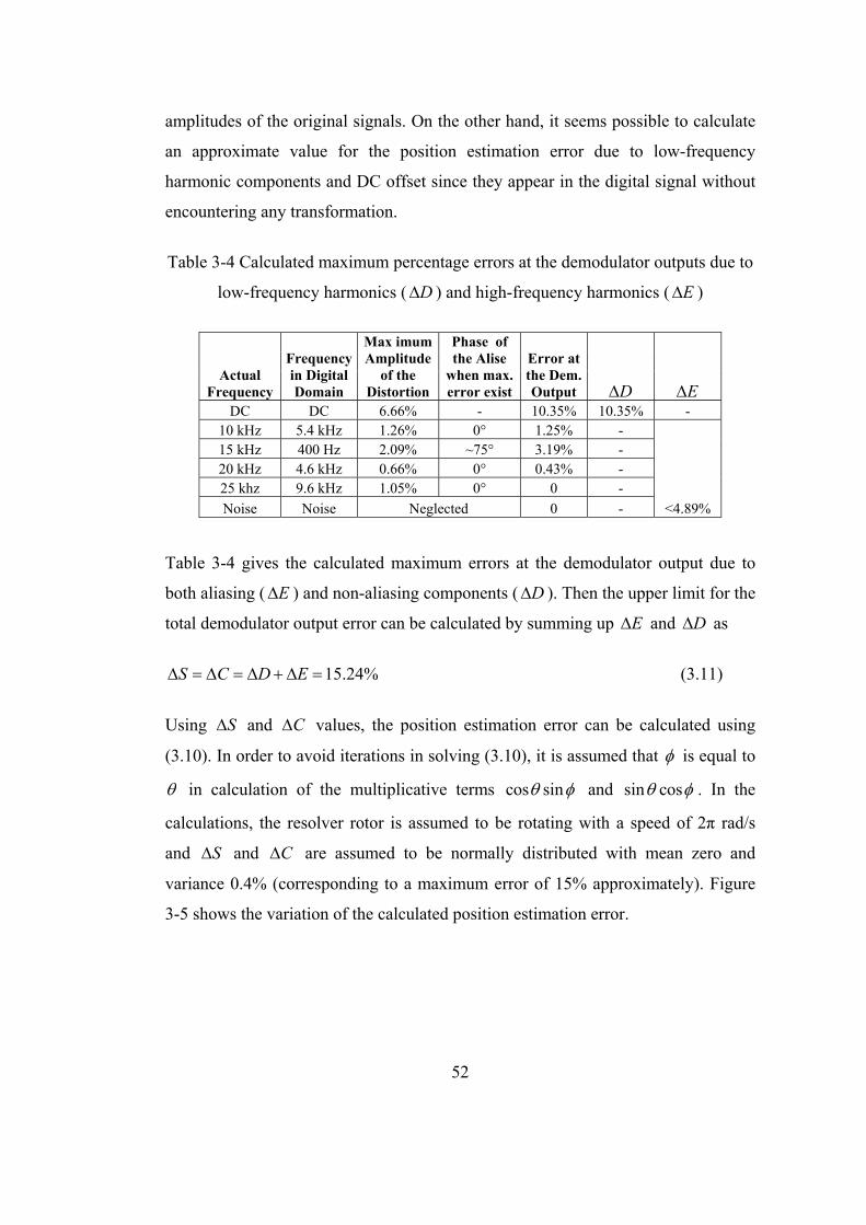
52

amplitudes of the original signals. On the other hand, it seems possible to calculate

an approximate value for the position estimation error due to low-frequency

harmonic components and DC offset since they appear in the digital signal without

encountering any transformation.

Table 3-4 Calculated maximum percentage errors at the demodulator outputs due to

low-frequency harmonics ( D ) and high-frequency harmonics ( E )

Actual Frequency

Frequency in Digital Domain

Max imum Amplitude

of the Distortion

Phase of the Alise

when max. error exist

Error at the Dem. Output D E

DC DC 6.66% - 10.35% 10.35% - 10 kHz 5.4 kHz 1.26% 0° 1.25% -

<4.89%

15 kHz 400 Hz 2.09% ~75° 3.19% - 20 kHz 4.6 kHz 0.66% 0° 0.43% - 25 khz 9.6 kHz 1.05% 0° 0 -

Noise Noise Neglected 0 -

Table 3-4 gives the calculated maximum errors at the demodulator output due to

both aliasing ( E ) and non-aliasing components ( D ). Then the upper limit for the

total demodulator output error can be calculated by summing up E and D as

15.24%S C D E (3.11)

Using S and C values, the position estimation error can be calculated using

(3.10). In order to avoid iterations in solving (3.10), it is assumed that is equal to

in calculation of the multiplicative terms cos sin and sin cos . In the

calculations, the resolver rotor is assumed to be rotating with a speed of 2π rad/s

and S and C are assumed to be normally distributed with mean zero and

variance 0.4% (corresponding to a maximum error of 15% approximately). Figure

3-5 shows the variation of the calculated position estimation error.

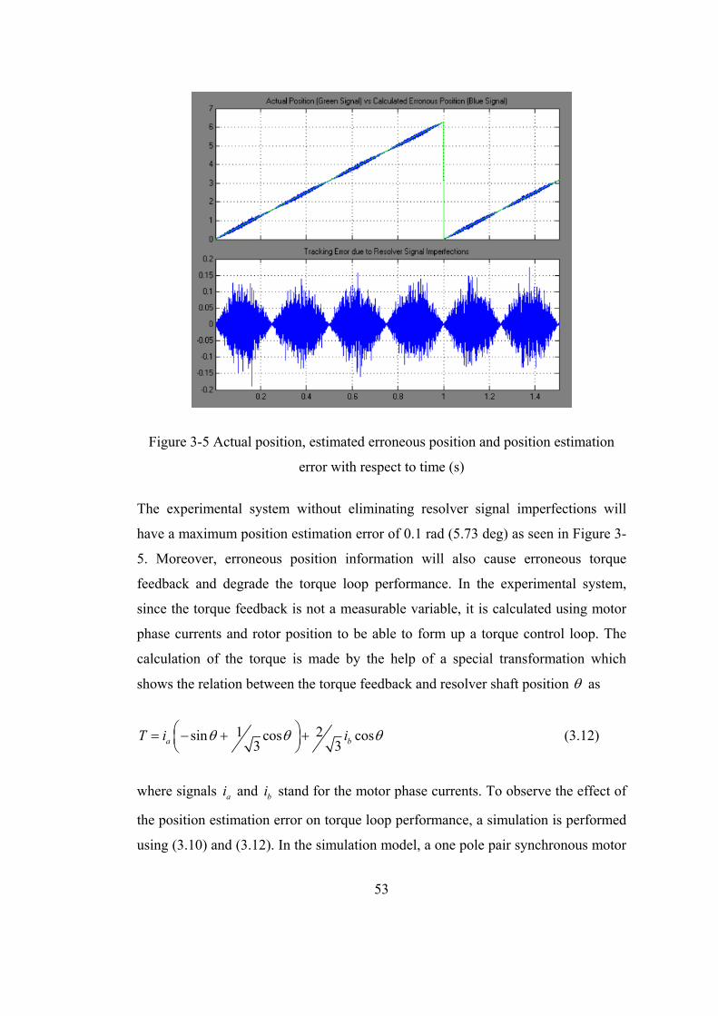
53

Figure 3-5 Actual position, estimated erroneous position and position estimation

error with respect to time (s)

The experimental system without eliminating resolver signal imperfections will

have a maximum position estimation error of 0.1 rad (5.73 deg) as seen in Figure 3-

5. Moreover, erroneous position information will also cause erroneous torque

feedback and degrade the torque loop performance. In the experimental system,

since the torque feedback is not a measurable variable, it is calculated using motor

phase currents and rotor position to be able to form up a torque control loop. The

calculation of the torque is made by the help of a special transformation which

shows the relation between the torque feedback and resolver shaft position as

1 2sin cos cos3 3a bT i i

(3.12)

where signals ai and bi stand for the motor phase currents. To observe the effect of

the position estimation error on torque loop performance, a simulation is performed

using (3.10) and (3.12). In the simulation model, a one pole pair synchronous motor

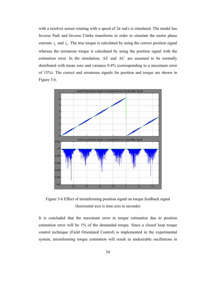
54

with a resolver sensor rotating with a speed of 2π rad/s is simulated. The model has

Inverse Park and Inverse Clarke transforms in order to simulate the motor phase

currents ai and bi . The true torque is calculated by using the correct position signal

whereas the erroneous torque is calculated by using the position signal with the

estimation error. In the simulation, S and C are assumed to be normally

distributed with mean zero and variance 0.4% (corresponding to a maximum error

of 15%). The correct and erroneous signals for position and torque are shown in

Figure 3-6.

Figure 3-6 Effect of misinforming position signal on torque feedback signal

(horizontal axis is time axis in seconds)

It is concluded that the maximum error in torque estimation due to position

estimation error will be 1% of the demanded torque. Since a closed loop torque

control technique (Field Orientated Control) is implemented in the experimental

system, misinforming torque estimation will result in undesirable oscillations in

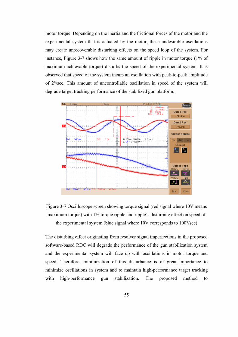
55

motor torque. Depending on the inertia and the frictional forces of the motor and the

experimental system that is actuated by the motor, these undesirable oscillations

may create unrecoverable disturbing effects on the speed loop of the system. For

instance, Figure 3-7 shows how the same amount of ripple in motor torque (1% of

maximum achievable torque) disturbs the speed of the experimental system. It is

observed that speed of the system incurs an oscillation with peak-to-peak amplitude

of 2°/sec. This amount of uncontrollable oscillation in speed of the system will

degrade target tracking performance of the stabilized gun platform.

Figure 3-7 Oscilloscope screen showing torque signal (red signal where 10V means

maximum torque) with 1% torque ripple and ripple’s disturbing effect on speed of

the experimental system (blue signal where 10V corresponds to 100°/sec)

The disturbing effect originating from resolver signal imperfections in the proposed

software-based RDC will degrade the performance of the gun stabilization system

and the experimental system will face up with oscillations in motor torque and

speed. Therefore, minimization of this disturbance is of great importance to

minimize oscillations in system and to maintain high-performance target tracking

with high-performance gun stabilization. The proposed method to

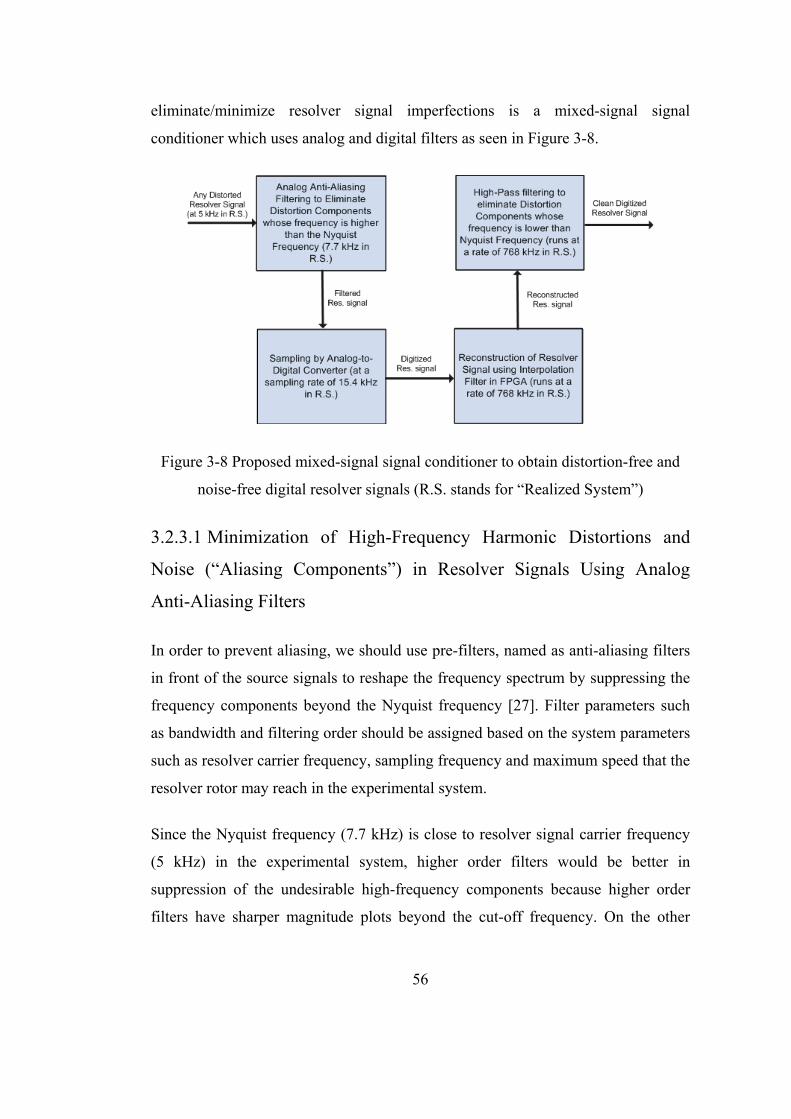
56

eliminate/minimize resolver signal imperfections is a mixed-signal signal

conditioner which uses analog and digital filters as seen in Figure 3-8.

Figure 3-8 Proposed mixed-signal signal conditioner to obtain distortion-free and

noise-free digital resolver signals (R.S. stands for “Realized System”)

3.2.3.1 Minimization of High-Frequency Harmonic Distortions and

Noise (“Aliasing Components”) in Resolver Signals Using Analog

Anti-Aliasing Filters

In order to prevent aliasing, we should use pre-filters, named as anti-aliasing filters

in front of the source signals to reshape the frequency spectrum by suppressing the

frequency components beyond the Nyquist frequency [27]. Filter parameters such

as bandwidth and filtering order should be assigned based on the system parameters

such as resolver carrier frequency, sampling frequency and maximum speed that the

resolver rotor may reach in the experimental system.

Since the Nyquist frequency (7.7 kHz) is close to resolver signal carrier frequency

(5 kHz) in the experimental system, higher order filters would be better in

suppression of the undesirable high-frequency components because higher order

filters have sharper magnitude plots beyond the cut-off frequency. On the other

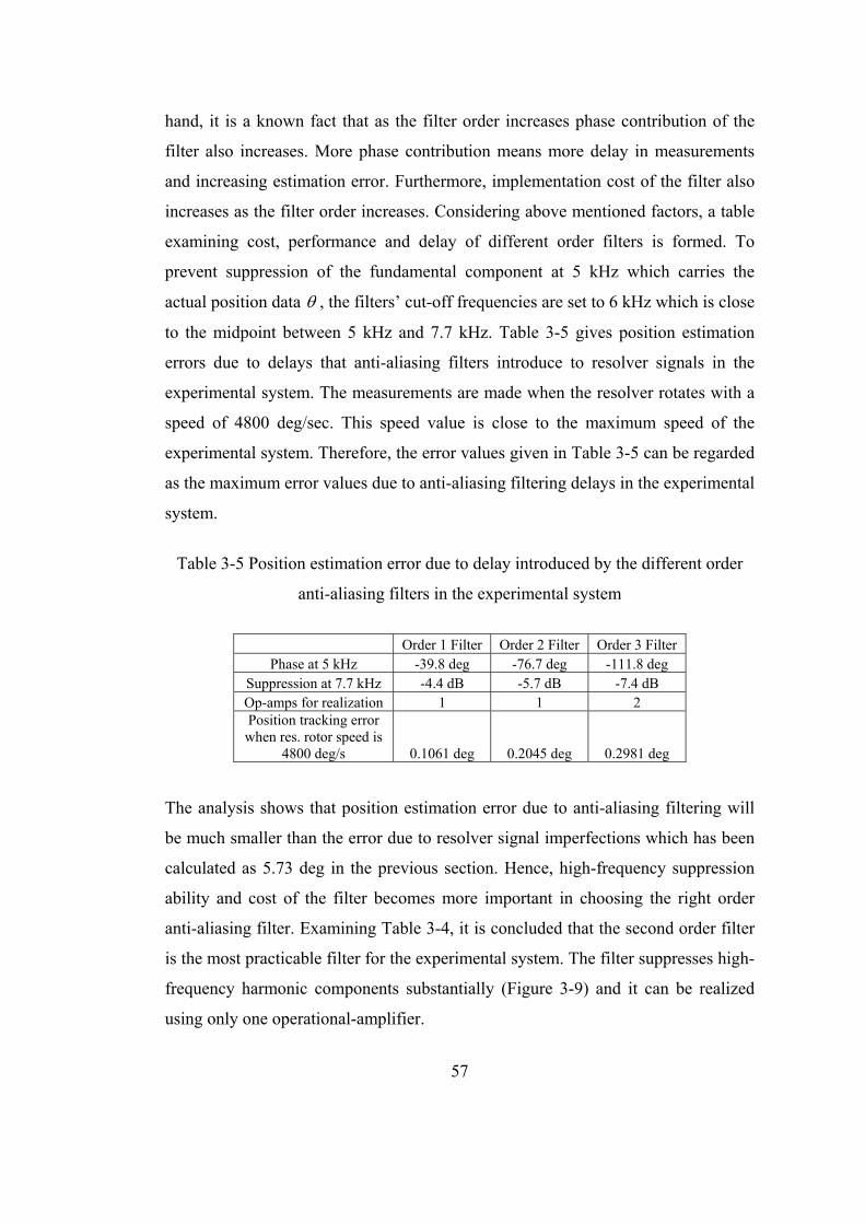
57

hand, it is a known fact that as the filter order increases phase contribution of the

filter also increases. More phase contribution means more delay in measurements

and increasing estimation error. Furthermore, implementation cost of the filter also

increases as the filter order increases. Considering above mentioned factors, a table

examining cost, performance and delay of different order filters is formed. To

prevent suppression of the fundamental component at 5 kHz which carries the

actual position data , the filters’ cut-off frequencies are set to 6 kHz which is close

to the midpoint between 5 kHz and 7.7 kHz. Table 3-5 gives position estimation

errors due to delays that anti-aliasing filters introduce to resolver signals in the

experimental system. The measurements are made when the resolver rotates with a

speed of 4800 deg/sec. This speed value is close to the maximum speed of the

experimental system. Therefore, the error values given in Table 3-5 can be regarded

as the maximum error values due to anti-aliasing filtering delays in the experimental

system.

Table 3-5 Position estimation error due to delay introduced by the different order

anti-aliasing filters in the experimental system

Order 1 Filter Order 2 Filter Order 3 Filter Phase at 5 kHz -39.8 deg -76.7 deg -111.8 deg

Suppression at 7.7 kHz -4.4 dB -5.7 dB -7.4 dB Op-amps for realization 1 1 2 Position tracking error when res. rotor speed is

4800 deg/s 0.1061 deg 0.2045 deg 0.2981 deg

The analysis shows that position estimation error due to anti-aliasing filtering will

be much smaller than the error due to resolver signal imperfections which has been

calculated as 5.73 deg in the previous section. Hence, high-frequency suppression

ability and cost of the filter becomes more important in choosing the right order

anti-aliasing filter. Examining Table 3-4, it is concluded that the second order filter

is the most practicable filter for the experimental system. The filter suppresses high-

frequency harmonic components substantially (Figure 3-9) and it can be realized

using only one operational-amplifier.

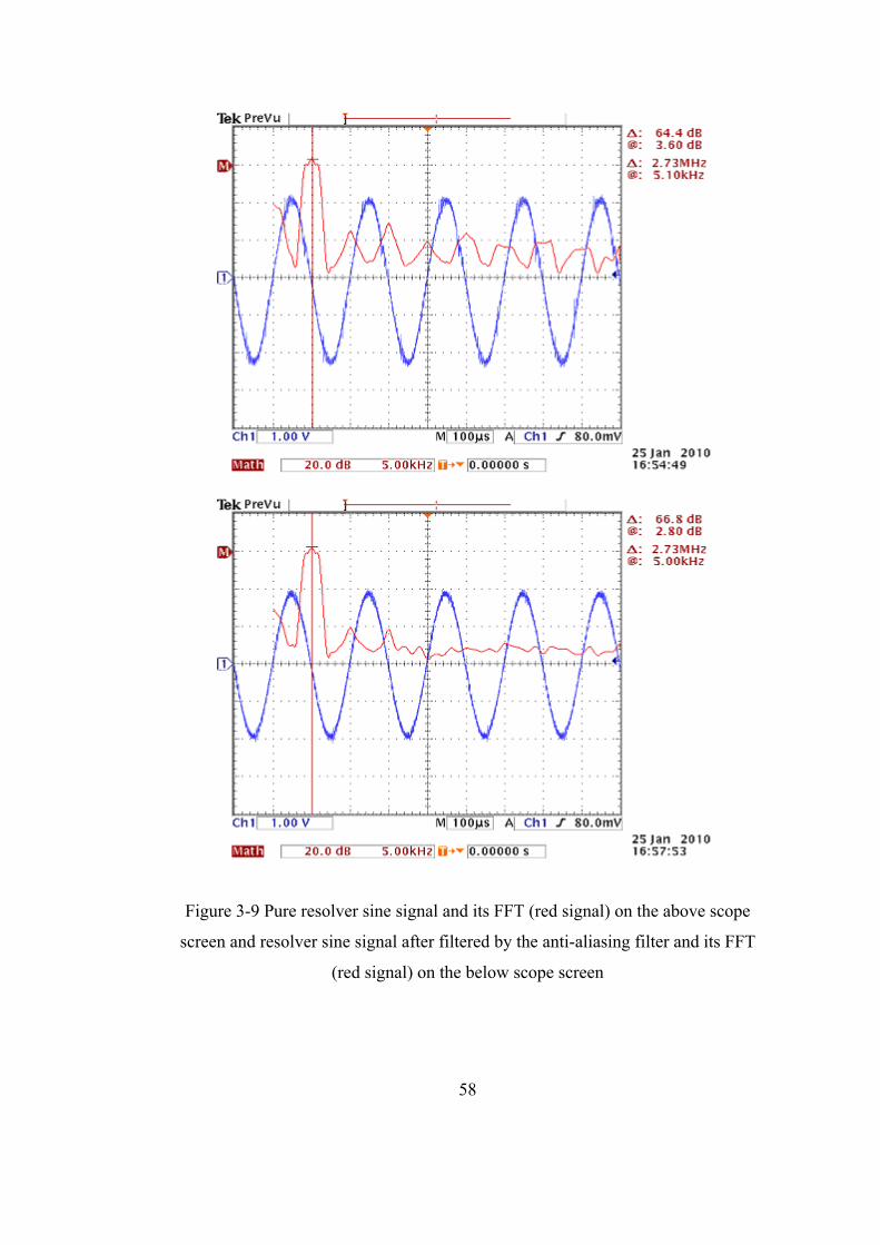
58

Figure 3-9 Pure resolver sine signal and its FFT (red signal) on the above scope

screen and resolver sine signal after filtered by the anti-aliasing filter and its FFT

(red signal) on the below scope screen

59

The filter improves the accuracy of the demodulated data by 62.37%. The details

related to the filter’s performance are given in Table 3-6.

Table 3-6 Anti-aliasing filter’s performance

Before Anti-aliasing Filtering

Frequency

Amplitude of Harmonic Dist. dB

Amplitude of Harmonic

Dist. %

Error at demodulator

output E

10 kHz -38 1.26 1.25%

<4.89 %

15 kHz -33.6 2.09 3.19%

20 kHz -43.6 0.66 0.43%

25 kHz -39.6 1.05 0%

After Anti-aliasing Filtering

Frequency

Amplitude of Harmonic Dist. dB

Amplitude of Harmonic

Dist. %

Error at demodulator

output E

10 kHz -42.8 0.72 0.71%

<1.84%

15 kHz -43.6 0.66 1.00%

20 kHz <-52.8 <0.2 <0.13%

25 kHz <-52.8 <0.2 0%

Suppression of High-frequency Harmonic

Distortions at Demodulator Output 62.37%

3.2.3.2 Digitization and Reconstruction of Filtered Resolver Signals in

FPGA

Analog-to-digital conversion rate should satisfy the Nyquist criterion for the

fundamental component to guarantee the feasibility of the software-based resolver-

to-digital converter. ADCs used in the experimental system have a sampling rate of

15.4 kHz and they satisfy the Nyquist criterion for the fundamental frequency 5

kHz. Their conversion resolution is 16 bit in signed fixed-point arithmetic (two’s

complement form).

From the sampling theorem we know that if the sampling frequency is sufficiently

high compared to the bandwidth of the continuous-time signal (ws>2Bandwidth),

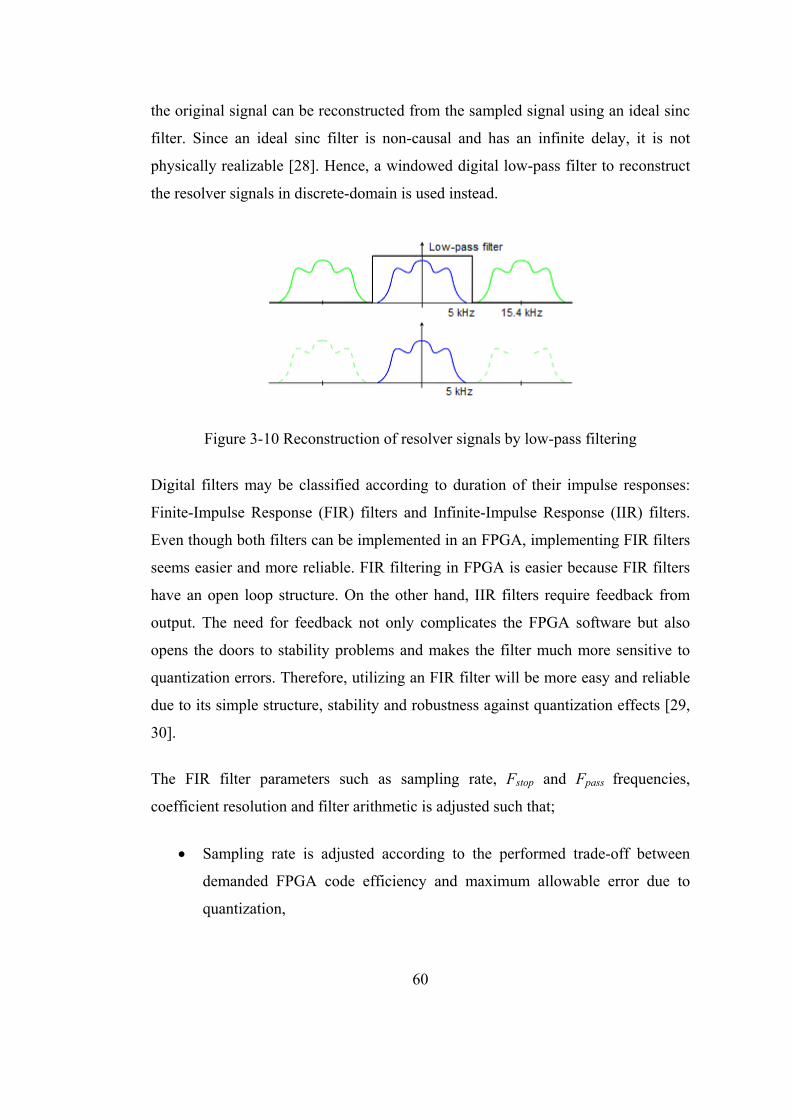
60

the original signal can be reconstructed from the sampled signal using an ideal sinc

filter. Since an ideal sinc filter is non-causal and has an infinite delay, it is not

physically realizable [28]. Hence, a windowed digital low-pass filter to reconstruct

the resolver signals in discrete-domain is used instead.

Figure 3-10 Reconstruction of resolver signals by low-pass filtering

Digital filters may be classified according to duration of their impulse responses:

Finite-Impulse Response (FIR) filters and Infinite-Impulse Response (IIR) filters.

Even though both filters can be implemented in an FPGA, implementing FIR filters

seems easier and more reliable. FIR filtering in FPGA is easier because FIR filters

have an open loop structure. On the other hand, IIR filters require feedback from

output. The need for feedback not only complicates the FPGA software but also

opens the doors to stability problems and makes the filter much more sensitive to

quantization errors. Therefore, utilizing an FIR filter will be more easy and reliable

due to its simple structure, stability and robustness against quantization effects [29,

30].

The FIR filter parameters such as sampling rate, Fstop and Fpass frequencies,

coefficient resolution and filter arithmetic is adjusted such that;

Sampling rate is adjusted according to the performed trade-off between

demanded FPGA code efficiency and maximum allowable error due to

quantization,

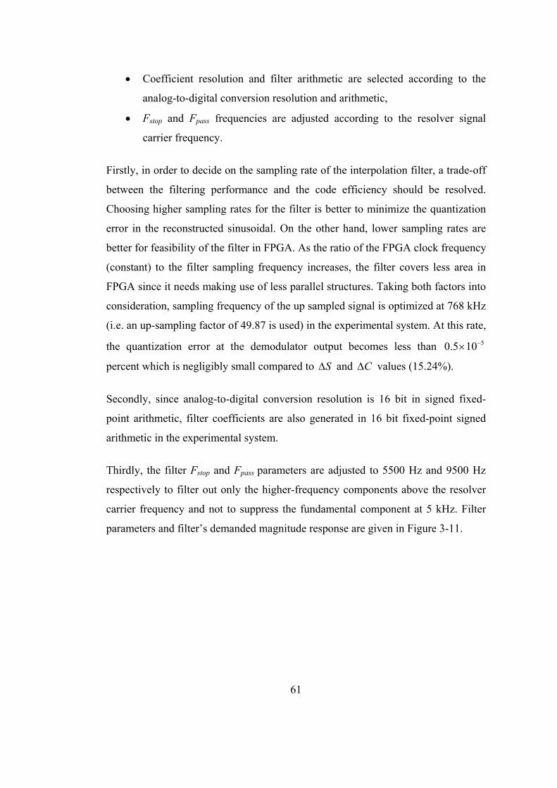
61

Coefficient resolution and filter arithmetic are selected according to the

analog-to-digital conversion resolution and arithmetic,

Fstop and Fpass frequencies are adjusted according to the resolver signal

carrier frequency.

Firstly, in order to decide on the sampling rate of the interpolation filter, a trade-off

between the filtering performance and the code efficiency should be resolved.

Choosing higher sampling rates for the filter is better to minimize the quantization

error in the reconstructed sinusoidal. On the other hand, lower sampling rates are

better for feasibility of the filter in FPGA. As the ratio of the FPGA clock frequency

(constant) to the filter sampling frequency increases, the filter covers less area in

FPGA since it needs making use of less parallel structures. Taking both factors into

consideration, sampling frequency of the up sampled signal is optimized at 768 kHz

(i.e. an up-sampling factor of 49.87 is used) in the experimental system. At this rate,

the quantization error at the demodulator output becomes less than 50.5 10

percent which is negligibly small compared to S and C values (15.24%).

Secondly, since analog-to-digital conversion resolution is 16 bit in signed fixed-

point arithmetic, filter coefficients are also generated in 16 bit fixed-point signed

arithmetic in the experimental system.

Thirdly, the filter Fstop and Fpass parameters are adjusted to 5500 Hz and 9500 Hz

respectively to filter out only the higher-frequency components above the resolver

carrier frequency and not to suppress the fundamental component at 5 kHz. Filter

parameters and filter’s demanded magnitude response are given in Figure 3-11.

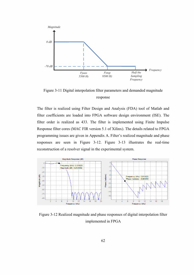
62

Figure 3-11 Digital interpolation filter parameters and demanded magnitude

response

The filter is realized using Filter Design and Analysis (FDA) tool of Matlab and

filter coefficients are loaded into FPGA software design environment (ISE). The

filter order is realized as 433. The filter is implemented using Finite Impulse

Response filter cores (MAC FIR version 5.1 of Xilinx). The details related to FPGA

programming issues are given in Appendix A. Filter’s realized magnitude and phase

responses are seen in Figure 3-12. Figure 3-13 illustrates the real-time

reconstruction of a resolver signal in the experimental system.

Figure 3-12 Realized magnitude and phase responses of digital interpolation filter

implemented in FPGA

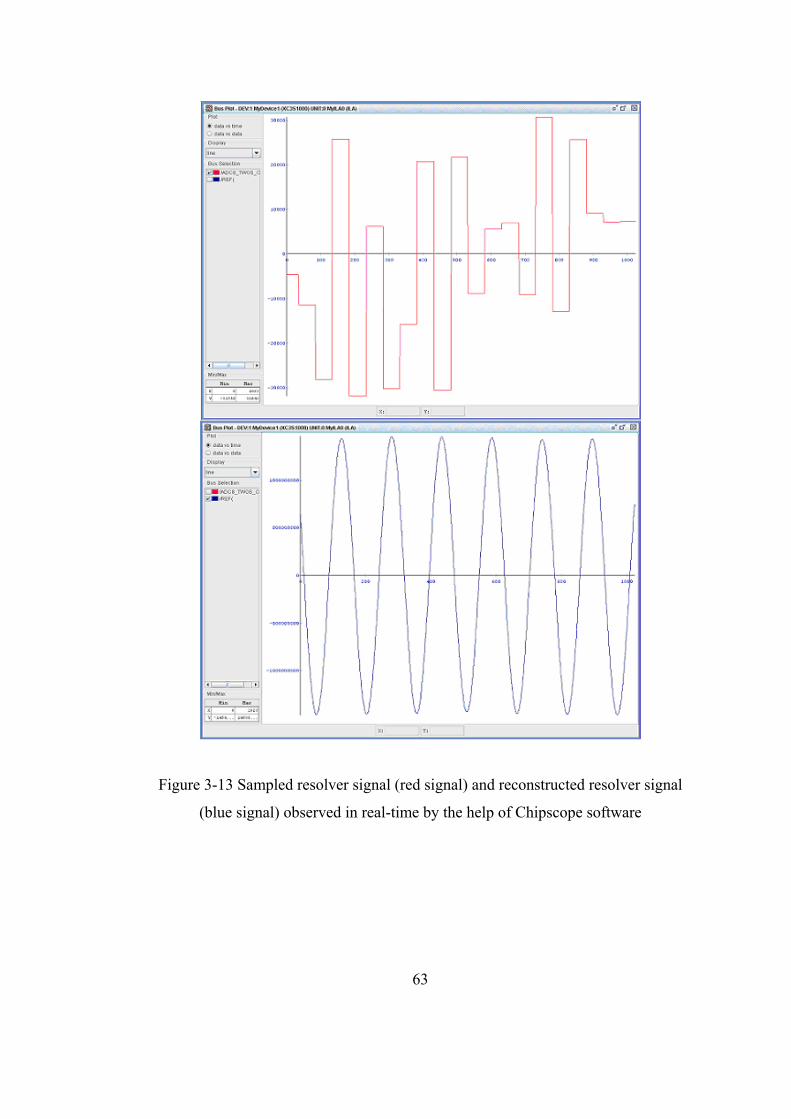
63

Figure 3-13 Sampled resolver signal (red signal) and reconstructed resolver signal

(blue signal) observed in real-time by the help of Chipscope software

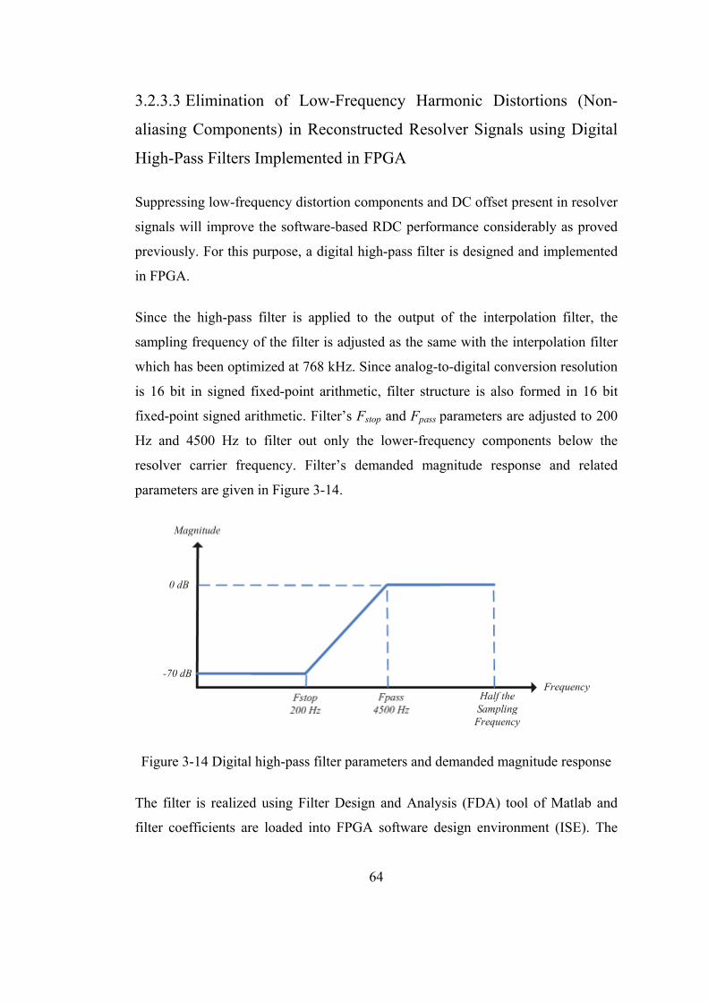
64

3.2.3.3 Elimination of Low-Frequency Harmonic Distortions (Non-

aliasing Components) in Reconstructed Resolver Signals using Digital

High-Pass Filters Implemented in FPGA

Suppressing low-frequency distortion components and DC offset present in resolver

signals will improve the software-based RDC performance considerably as proved

previously. For this purpose, a digital high-pass filter is designed and implemented

in FPGA.

Since the high-pass filter is applied to the output of the interpolation filter, the

sampling frequency of the filter is adjusted as the same with the interpolation filter

which has been optimized at 768 kHz. Since analog-to-digital conversion resolution

is 16 bit in signed fixed-point arithmetic, filter structure is also formed in 16 bit

fixed-point signed arithmetic. Filter’s Fstop and Fpass parameters are adjusted to 200

Hz and 4500 Hz to filter out only the lower-frequency components below the

resolver carrier frequency. Filter’s demanded magnitude response and related

parameters are given in Figure 3-14.

Figure 3-14 Digital high-pass filter parameters and demanded magnitude response

The filter is realized using Filter Design and Analysis (FDA) tool of Matlab and

filter coefficients are loaded into FPGA software design environment (ISE). The

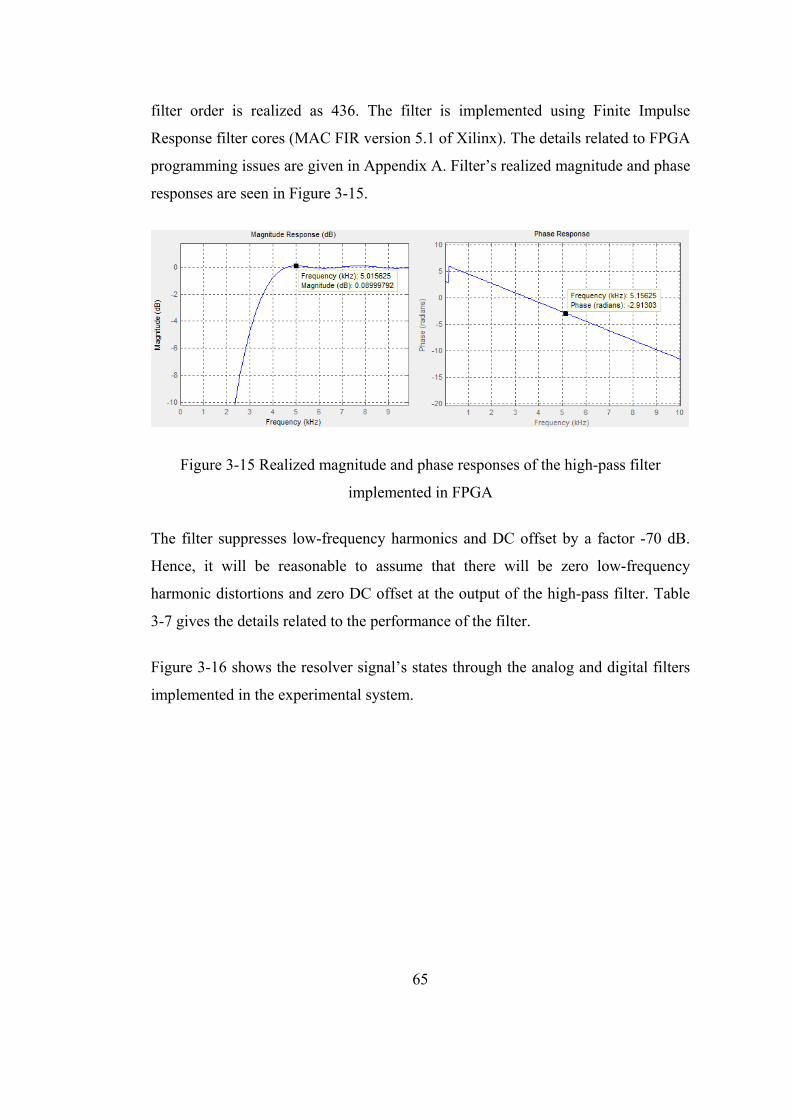
65

filter order is realized as 436. The filter is implemented using Finite Impulse

Response filter cores (MAC FIR version 5.1 of Xilinx). The details related to FPGA

programming issues are given in Appendix A. Filter’s realized magnitude and phase

responses are seen in Figure 3-15.

Figure 3-15 Realized magnitude and phase responses of the high-pass filter

implemented in FPGA

The filter suppresses low-frequency harmonics and DC offset by a factor -70 dB.

Hence, it will be reasonable to assume that there will be zero low-frequency

harmonic distortions and zero DC offset at the output of the high-pass filter. Table

3-7 gives the details related to the performance of the filter.

Figure 3-16 shows the resolver signal’s states through the analog and digital filters

implemented in the experimental system.

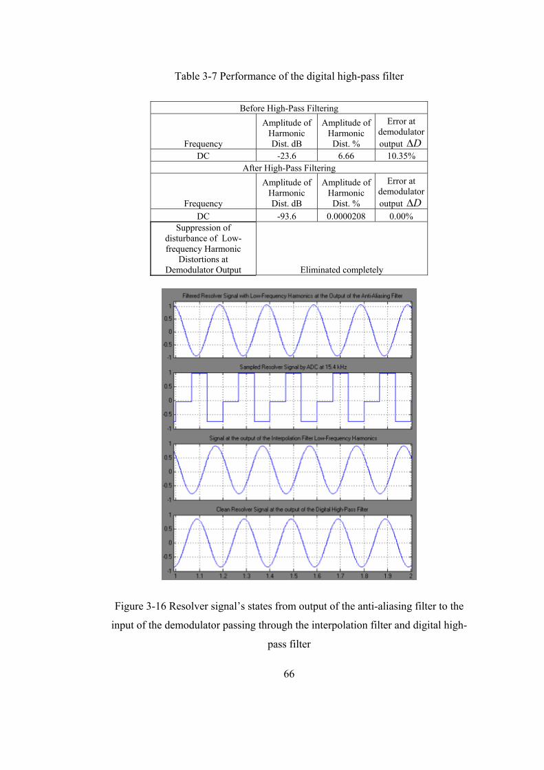
66

Table 3-7 Performance of the digital high-pass filter

Before High-Pass Filtering

Frequency

Amplitude of Harmonic Dist. dB

Amplitude of Harmonic

Dist. %

Error at demodulator output D

DC -23.6 6.66 10.35% After High-Pass Filtering

Frequency

Amplitude of Harmonic Dist. dB

Amplitude of Harmonic

Dist. %

Error at demodulator output D

DC -93.6 0.0000208 0.00% Suppression of

disturbance of Low-frequency Harmonic

Distortions at Demodulator Output Eliminated completely

Figure 3-16 Resolver signal’s states from output of the anti-aliasing filter to the

input of the demodulator passing through the interpolation filter and digital high-

pass filter

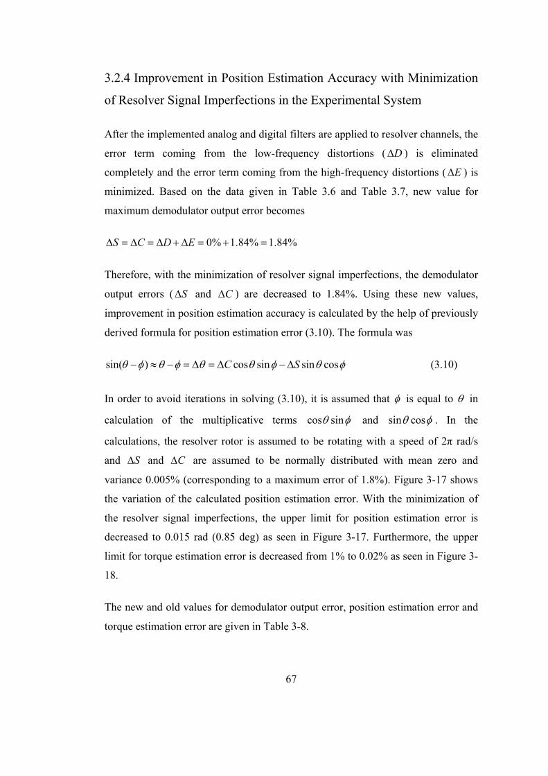
67

3.2.4 Improvement in Position Estimation Accuracy with Minimization

of Resolver Signal Imperfections in the Experimental System

After the implemented analog and digital filters are applied to resolver channels, the

error term coming from the low-frequency distortions ( D ) is eliminated

completely and the error term coming from the high-frequency distortions ( E ) is

minimized. Based on the data given in Table 3.6 and Table 3.7, new value for

maximum demodulator output error becomes

0% 1.84% 1.84%S C D E

Therefore, with the minimization of resolver signal imperfections, the demodulator

output errors ( S and C ) are decreased to 1.84%. Using these new values,

improvement in position estimation accuracy is calculated by the help of previously

derived formula for position estimation error (3.10). The formula was

sin( ) cos sin sin cosC S (3.10)

In order to avoid iterations in solving (3.10), it is assumed that is equal to in

calculation of the multiplicative terms cos sin and sin cos . In the

calculations, the resolver rotor is assumed to be rotating with a speed of 2π rad/s

and S and C are assumed to be normally distributed with mean zero and

variance 0.005% (corresponding to a maximum error of 1.8%). Figure 3-17 shows

the variation of the calculated position estimation error. With the minimization of

the resolver signal imperfections, the upper limit for position estimation error is

decreased to 0.015 rad (0.85 deg) as seen in Figure 3-17. Furthermore, the upper

limit for torque estimation error is decreased from 1% to 0.02% as seen in Figure 3-

18.

The new and old values for demodulator output error, position estimation error and

torque estimation error are given in Table 3-8.

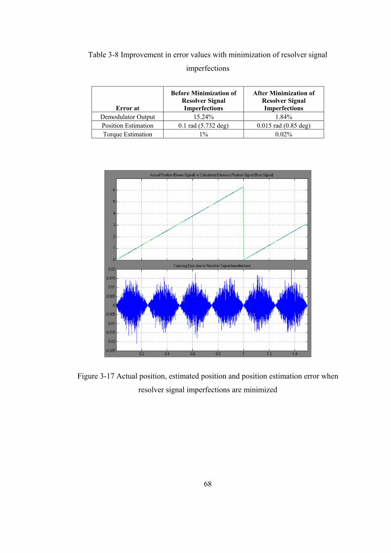
68

Table 3-8 Improvement in error values with minimization of resolver signal

imperfections

Error at

Before Minimization of Resolver Signal Imperfections

After Minimization of Resolver Signal Imperfections

Demodulator Output 15.24% 1.84% Position Estimation 0.1 rad (5.732 deg) 0.015 rad (0.85 deg) Torque Estimation 1% 0.02%

Figure 3-17 Actual position, estimated position and position estimation error when

resolver signal imperfections are minimized

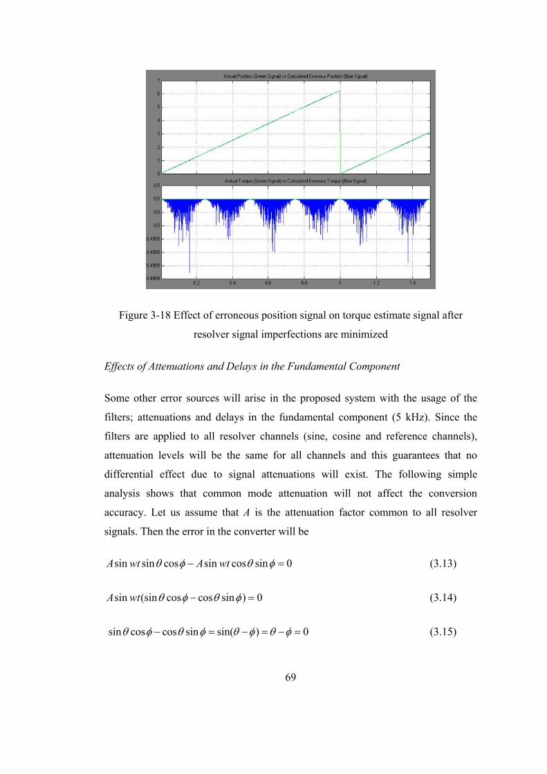
69

Figure 3-18 Effect of erroneous position signal on torque estimate signal after

resolver signal imperfections are minimized

Effects of Attenuations and Delays in the Fundamental Component

Some other error sources will arise in the proposed system with the usage of the

filters; attenuations and delays in the fundamental component (5 kHz). Since the

filters are applied to all resolver channels (sine, cosine and reference channels),

attenuation levels will be the same for all channels and this guarantees that no

differential effect due to signal attenuations will exist. The following simple

analysis shows that common mode attenuation will not affect the conversion

accuracy. Let us assume that A is the attenuation factor common to all resolver

signals. Then the error in the converter will be

sin sin cos sin cos sin 0A wt A wt (3.13)

sin (sin cos cos sin ) 0A wt (3.14)

sin cos cos sin sin( ) 0 (3.15)

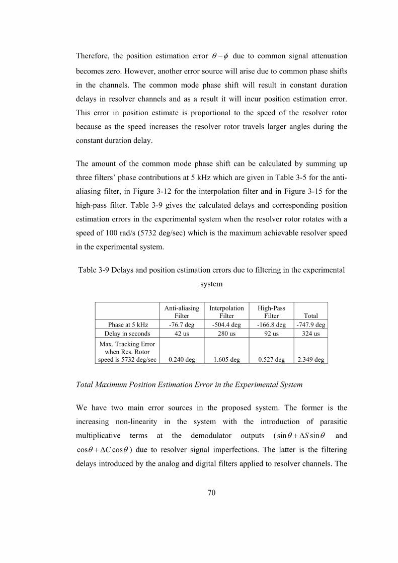
70

Therefore, the position estimation error due to common signal attenuation

becomes zero. However, another error source will arise due to common phase shifts

in the channels. The common mode phase shift will result in constant duration

delays in resolver channels and as a result it will incur position estimation error.

This error in position estimate is proportional to the speed of the resolver rotor

because as the speed increases the resolver rotor travels larger angles during the

constant duration delay.

The amount of the common mode phase shift can be calculated by summing up

three filters’ phase contributions at 5 kHz which are given in Table 3-5 for the anti-

aliasing filter, in Figure 3-12 for the interpolation filter and in Figure 3-15 for the

high-pass filter. Table 3-9 gives the calculated delays and corresponding position

estimation errors in the experimental system when the resolver rotor rotates with a

speed of 100 rad/s (5732 deg/sec) which is the maximum achievable resolver speed

in the experimental system.

Table 3-9 Delays and position estimation errors due to filtering in the experimental

system

Anti-aliasing

Filter Interpolation

Filter High-Pass

Filter Total Phase at 5 kHz -76.7 deg -504.4 deg -166.8 deg -747.9 deg

Delay in seconds 42 us 280 us 92 us 324 us

Max. Tracking Error when Res. Rotor

speed is 5732 deg/sec 0.240 deg 1.605 deg 0.527 deg 2.349 deg

Total Maximum Position Estimation Error in the Experimental System

We have two main error sources in the proposed system. The former is the

increasing non-linearity in the system with the introduction of parasitic

multiplicative terms at the demodulator outputs ( sin sinS and

cos cosC ) due to resolver signal imperfections. The latter is the filtering

delays introduced by the analog and digital filters applied to resolver channels. The

71

first error is limited to 0.015 rad with the minimization of the resolver signal

imperfections. The second error is proportional to the resolver speed and it delays

the measurements. Based on the data in Table 3-8 and Table 3-9, the position

estimation error due to distortions, noise and delays can be formulated as follows

(0.015 0.00040965 ) radMaxPositionEstimationError (3.16)

where is the resolver speed in rad/s. Since the maximum achievable resolver

rotor speed is 100 rad/s in the experimental system, the maximum position

estimation error becomes

0.015 rad 0.00040965 s 100 rad/s = 0.019 rad

Even if the system has this level of error in position estimation, torque control loop

will be affected so negligibly that error in torque estimation will be 0.02% of the

demanded torque.

3.3 FPGA-Based Phase-Sensitive Demodulator

Processing the reconstructed resolver signals sin sinwt , sin coswt and sin wt ,

the phase-sensitive demodulator gives out sin and cos signals. In order to

realize the said function, the proposed structure makes use of two modulus

functions, two half-period integrators and one phase-detector. The block diagram of

the system is seen in Figure 3-19.

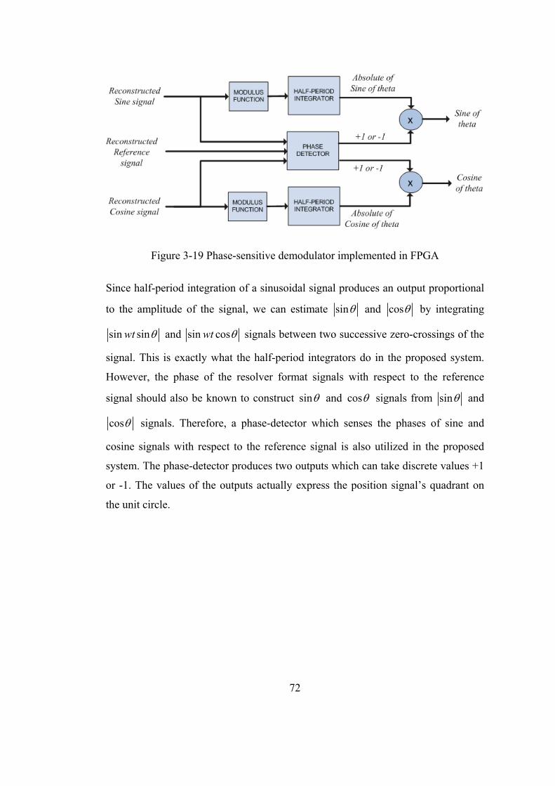
72

Figure 3-19 Phase-sensitive demodulator implemented in FPGA

Since half-period integration of a sinusoidal signal produces an output proportional

to the amplitude of the signal, we can estimate sin and cos by integrating

sin sinwt and sin coswt signals between two successive zero-crossings of the

signal. This is exactly what the half-period integrators do in the proposed system.

However, the phase of the resolver format signals with respect to the reference

signal should also be known to construct sin and cos signals from sin and

cos signals. Therefore, a phase-detector which senses the phases of sine and

cosine signals with respect to the reference signal is also utilized in the proposed

system. The phase-detector produces two outputs which can take discrete values +1

or -1. The values of the outputs actually express the position signal’s quadrant on

the unit circle.

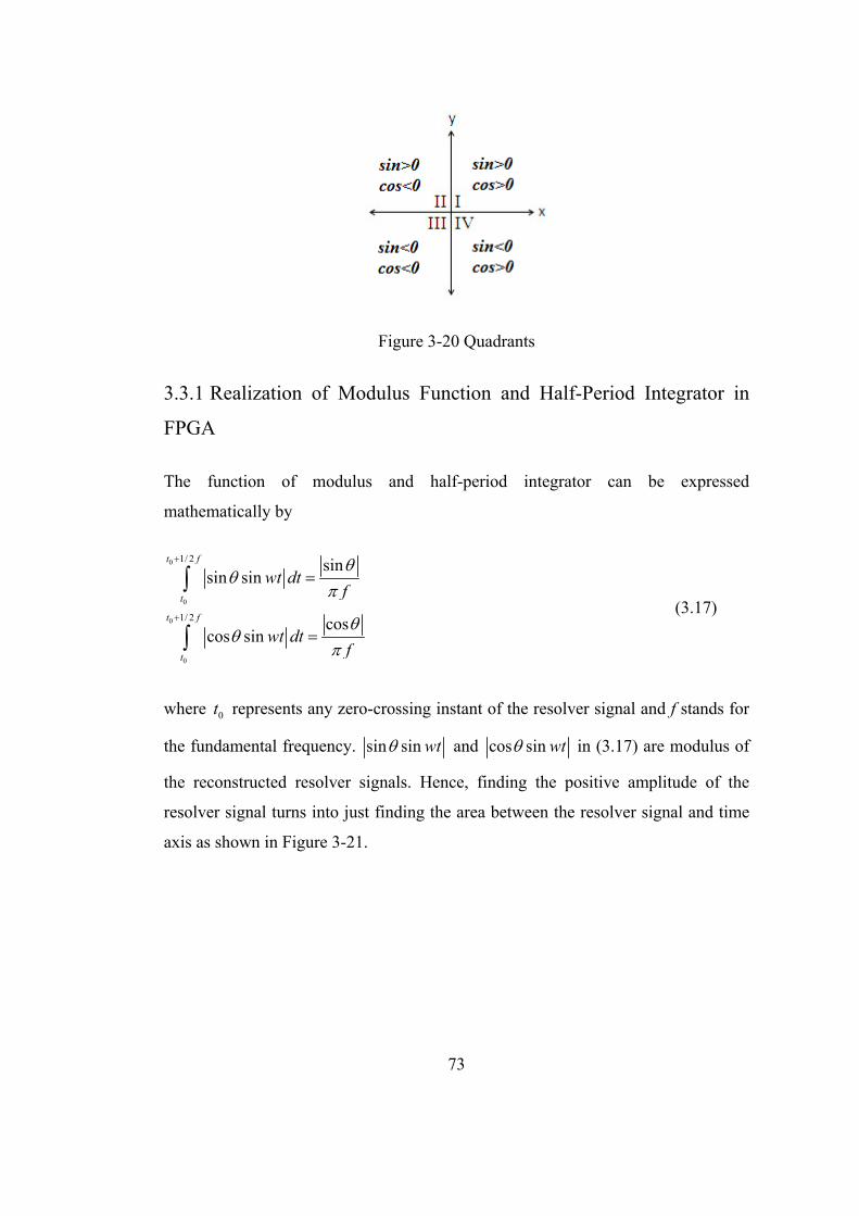
73

Figure 3-20 Quadrants

3.3.1 Realization of Modulus Function and Half-Period Integrator in

FPGA

The function of modulus and half-period integrator can be expressed

mathematically by

0

0

0

0

1/ 2

1/ 2

sinsin sin

coscos sin

t f

t

t f

t

wt dtf

wt dtf

(3.17)

where 0t represents any zero-crossing instant of the resolver signal and f stands for

the fundamental frequency. sin sin wt and cos sin wt in (3.17) are modulus of

the reconstructed resolver signals. Hence, finding the positive amplitude of the

resolver signal turns into just finding the area between the resolver signal and time

axis as shown in Figure 3-21.

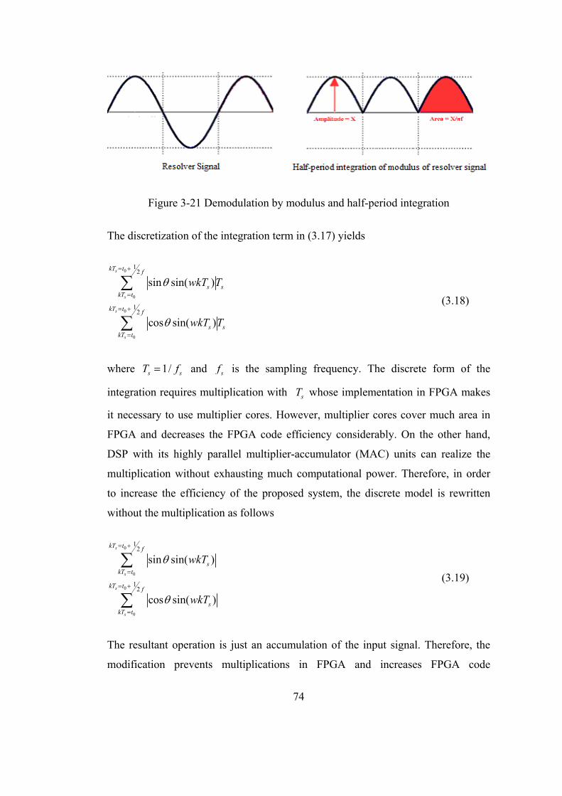
74

Figure 3-21 Demodulation by modulus and half-period integration

The discretization of the integration term in (3.17) yields

0

0

0

0

12

12

sin sin( )

cos sin( )

s

s

s

s

kT t f

s skT t

kT t f

s skT t

wkT T

wkT T

(3.18)

where 1/s sT f and sf is the sampling frequency. The discrete form of the

integration requires multiplication with sT whose implementation in FPGA makes

it necessary to use multiplier cores. However, multiplier cores cover much area in

FPGA and decreases the FPGA code efficiency considerably. On the other hand,

DSP with its highly parallel multiplier-accumulator (MAC) units can realize the

multiplication without exhausting much computational power. Therefore, in order

to increase the efficiency of the proposed system, the discrete model is rewritten

without the multiplication as follows

0

0

0

0

12

12

sin sin( )

cos sin( )

s

s

s

s

kT t f

skT t

kT t f

skT t

wkT

wkT

(3.19)

The resultant operation is just an accumulation of the input signal. Therefore, the

modification prevents multiplications in FPGA and increases FPGA code

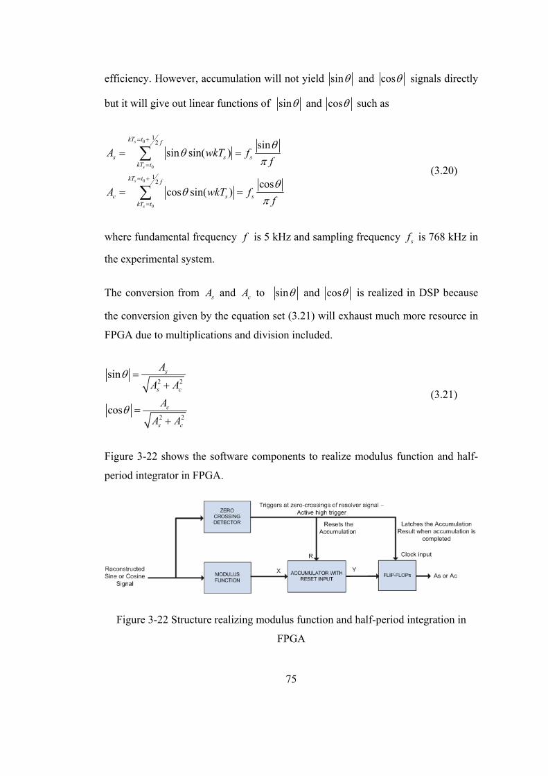
75

efficiency. However, accumulation will not yield sin and cos signals directly

but it will give out linear functions of sin and cos such as

0

0

0

0

12

12

sinsin sin( )

coscos sin( )

s

s

s

s

kT t f

s s skT t

kT t f

c s skT t

A wkT ff

A wkT ff

(3.20)

where fundamental frequency f is 5 kHz and sampling frequency sf is 768 kHz in

the experimental system.

The conversion from sA and cA to sin and cos is realized in DSP because

the conversion given by the equation set (3.21) will exhaust much more resource in

FPGA due to multiplications and division included.

2 2

2 2

sin

cos

s

s c

c

s c

A

A A

A

A A

(3.21)

Figure 3-22 shows the software components to realize modulus function and half-

period integrator in FPGA.

Figure 3-22 Structure realizing modulus function and half-period integration in

FPGA

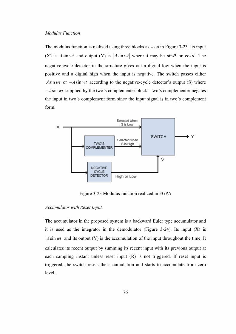
76

Modulus Function

The modulus function is realized using three blocks as seen in Figure 3-23. Its input

(X) is sinA wt and output (Y) is sinA wt where A may be sin or cos . The

negative-cycle detector in the structure gives out a digital low when the input is

positive and a digital high when the input is negative. The switch passes either

sinA wt or sinA wt according to the negative-cycle detector’s output (S) where

sinA wt supplied by the two’s complementer block. Two’s complementer negates

the input in two’s complement form since the input signal is in two’s complement

form.

Figure 3-23 Modulus function realized in FGPA

Accumulator with Reset Input

The accumulator in the proposed system is a backward Euler type accumulator and

it is used as the integrator in the demodulator (Figure 3-24). Its input (X) is

sinA wt and its output (Y) is the accumulation of the input throughout the time. It

calculates its recent output by summing its recent input with its previous output at

each sampling instant unless reset input (R) is not triggered. If reset input is

triggered, the switch resets the accumulation and starts to accumulate from zero

level.

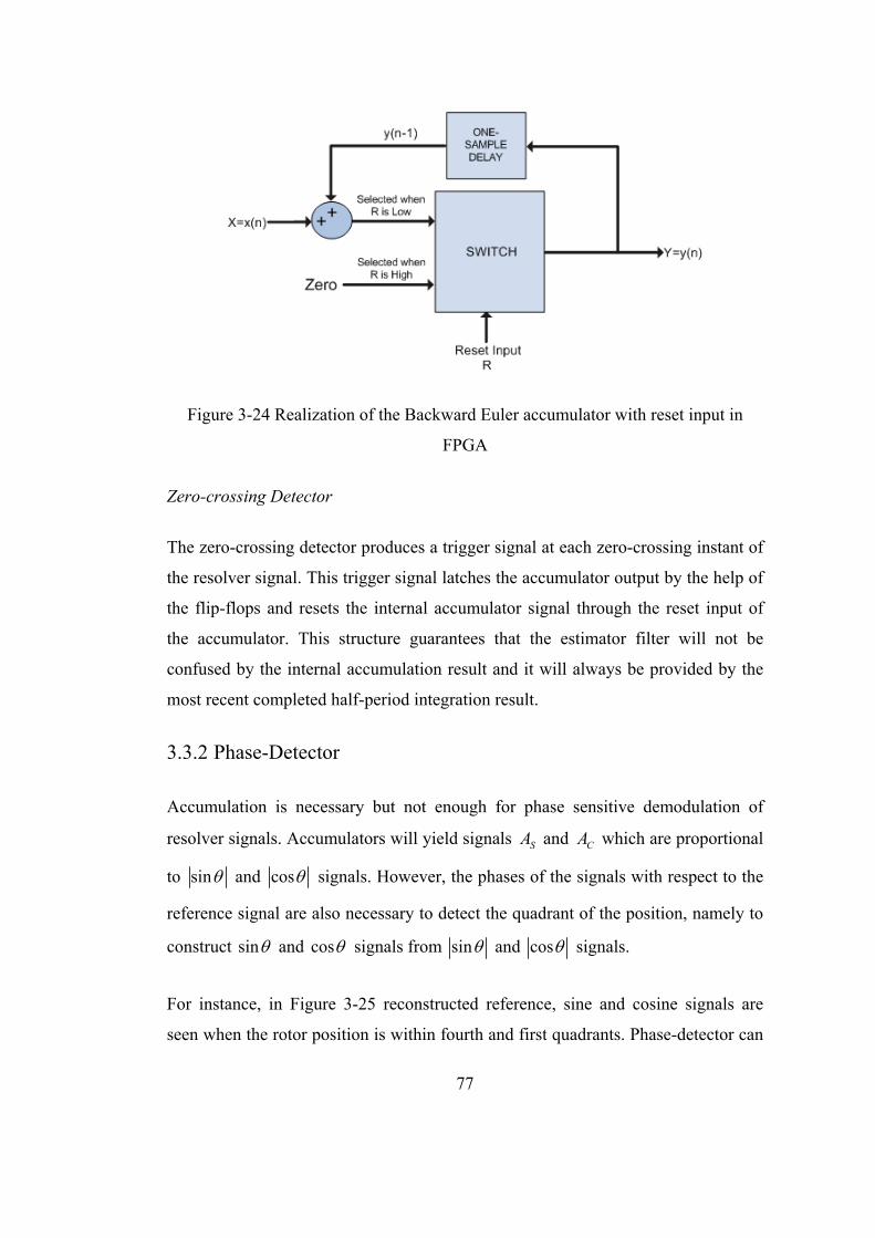
77

Figure 3-24 Realization of the Backward Euler accumulator with reset input in

FPGA

Zero-crossing Detector

The zero-crossing detector produces a trigger signal at each zero-crossing instant of

the resolver signal. This trigger signal latches the accumulator output by the help of

the flip-flops and resets the internal accumulator signal through the reset input of

the accumulator. This structure guarantees that the estimator filter will not be

confused by the internal accumulation result and it will always be provided by the

most recent completed half-period integration result.

3.3.2 Phase-Detector

Accumulation is necessary but not enough for phase sensitive demodulation of

resolver signals. Accumulators will yield signals SA and CA which are proportional

to sin and cos signals. However, the phases of the signals with respect to the

reference signal are also necessary to detect the quadrant of the position, namely to

construct sin and cos signals from sin and cos signals.

For instance, in Figure 3-25 reconstructed reference, sine and cosine signals are

seen when the rotor position is within fourth and first quadrants. Phase-detector can

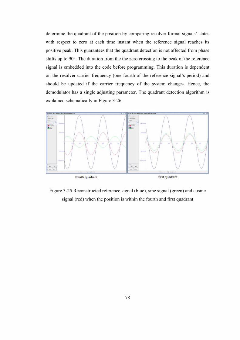
78

determine the quadrant of the position by comparing resolver format signals’ states

with respect to zero at each time instant when the reference signal reaches its

positive peak. This guarantees that the quadrant detection is not affected from phase

shifts up to 90°. The duration from the the zero crossing to the peak of the reference

signal is embedded into the code before programming. This duration is dependent

on the resolver carrier frequency (one fourth of the reference signal’s period) and

should be updated if the carrier frequency of the system changes. Hence, the

demodulator has a single adjusting parameter. The quadrant detection algorithm is

explained schematically in Figure 3-26.

Figure 3-25 Reconstructed reference signal (blue), sine signal (green) and cosine

signal (red) when the position is within the fourth and first quadrant

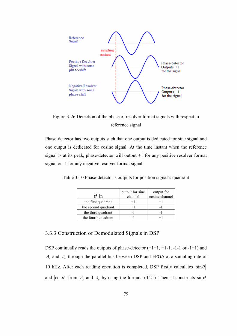
79

Figure 3-26 Detection of the phase of resolver format signals with respect to

reference signal

Phase-detector has two outputs such that one output is dedicated for sine signal and

one output is dedicated for cosine signal. At the time instant when the reference

signal is at its peak, phase-detector will output +1 for any positive resolver format

signal or -1 for any negative resolver format signal.

Table 3-10 Phase-detector’s outputs for position signal’s quadrant

in output for sine

channel output for

cosine channel the first quadrant +1 +1

the second quadrant +1 -1 the third quadrant -1 -1

the fourth quadrant -1 +1

3.3.3 Construction of Demodulated Signals in DSP

DSP continually reads the outputs of phase-detector (+1+1, +1-1, -1-1 or -1+1) and

sA and cA through the parallel bus between DSP and FPGA at a sampling rate of

10 kHz. After each reading operation is completed, DSP firstly calculates sin

and cos from sA and cA by using the formula (3.21). Then, it constructs sin

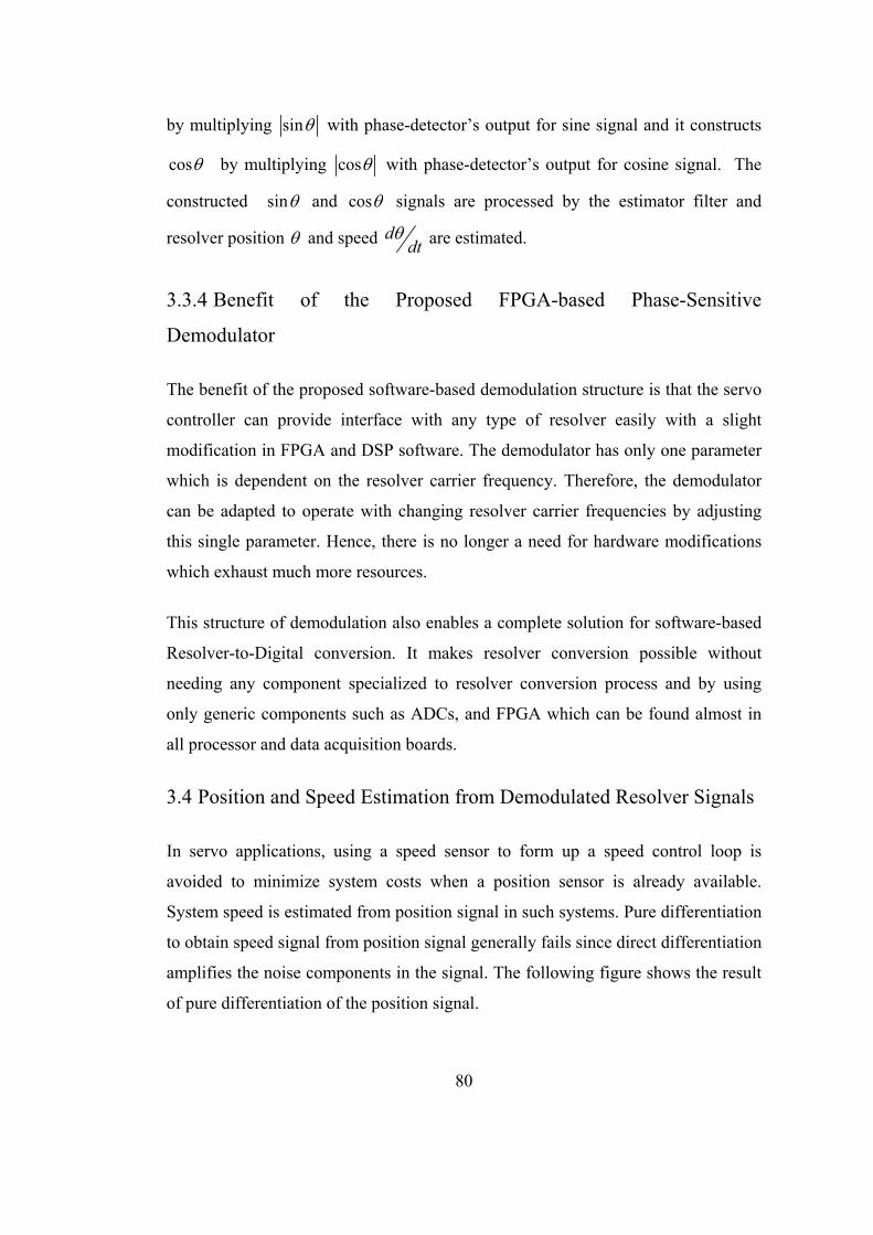
80

by multiplying sin with phase-detector’s output for sine signal and it constructs

cos by multiplying cos with phase-detector’s output for cosine signal. The

constructed sin and cos signals are processed by the estimator filter and

resolver position and speed ddt

are estimated.

3.3.4 Benefit of the Proposed FPGA-based Phase-Sensitive

Demodulator

The benefit of the proposed software-based demodulation structure is that the servo

controller can provide interface with any type of resolver easily with a slight

modification in FPGA and DSP software. The demodulator has only one parameter

which is dependent on the resolver carrier frequency. Therefore, the demodulator

can be adapted to operate with changing resolver carrier frequencies by adjusting

this single parameter. Hence, there is no longer a need for hardware modifications

which exhaust much more resources.

This structure of demodulation also enables a complete solution for software-based

Resolver-to-Digital conversion. It makes resolver conversion possible without

needing any component specialized to resolver conversion process and by using

only generic components such as ADCs, and FPGA which can be found almost in

all processor and data acquisition boards.

3.4 Position and Speed Estimation from Demodulated Resolver Signals

In servo applications, using a speed sensor to form up a speed control loop is

avoided to minimize system costs when a position sensor is already available.

System speed is estimated from position signal in such systems. Pure differentiation

to obtain speed signal from position signal generally fails since direct differentiation

amplifies the noise components in the signal. The following figure shows the result

of pure differentiation of the position signal.

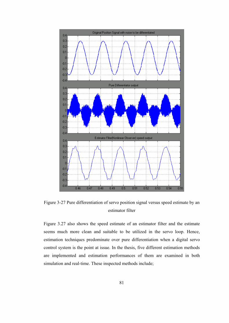
81

Figure 3-27 Pure differentiation of servo position signal versus speed estimate by an

estimator filter

Figure 3.27 also shows the speed estimate of an estimator filter and the estimate

seems much more clean and suitable to be utilized in the servo loop. Hence,

estimation techniques predominate over pure differentiation when a digital servo

control system is the point at issue. In the thesis, five different estimation methods

are implemented and estimation performances of them are examined in both

simulation and real-time. These inspected methods include;

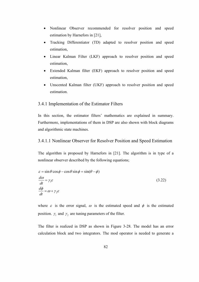
82

Nonlinear Observer recommended for resolver position and speed

estimation by Harnefors in [21],

Tracking Differentiator (TD) adapted to resolver position and speed

estimation,

Linear Kalman Filter (LKF) approach to resolver position and speed

estimation,

Extended Kalman filter (EKF) approach to resolver position and speed

estimation,

Unscented Kalman filter (UKF) approach to resolver position and speed

estimation.

3.4.1 Implementation of the Estimator Filters

In this section, the estimator filters’ mathematics are explained in summary.

Furthermore, implementations of them in DSP are also shown with block diagrams

and algorithmic state machines.

3.4.1.1 Nonlinear Observer for Resolver Position and Speed Estimation

The algorithm is proposed by Harnefors in [21]. The algorithm is in type of a

nonlinear observer described by the following equations;

1

2

sin cos cos sin sin( )

d

dtd

dt

(3.22)

where is the error signal, is the estimated speed and is the estimated

position. 1 and 2 are tuning parameters of the filter.

The filter is realized in DSP as shown in Figure 3-28. The model has an error

calculation block and two integrators. The mod operator is needed to generate a

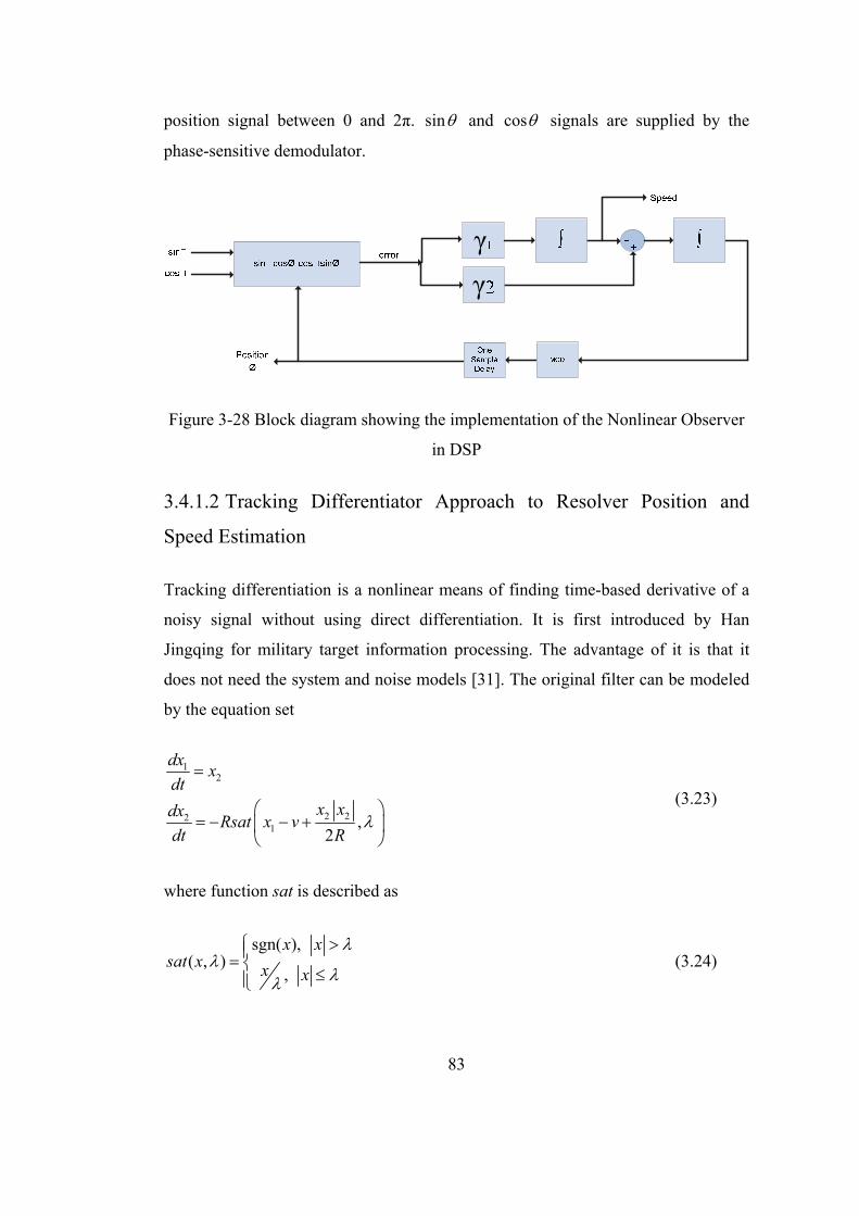
83

position signal between 0 and 2π. sin and cos signals are supplied by the

phase-sensitive demodulator.

Figure 3-28 Block diagram showing the implementation of the Nonlinear Observer

in DSP

3.4.1.2 Tracking Differentiator Approach to Resolver Position and

Speed Estimation

Tracking differentiation is a nonlinear means of finding time-based derivative of a

noisy signal without using direct differentiation. It is first introduced by Han

Jingqing for military target information processing. The advantage of it is that it

does not need the system and noise models [31]. The original filter can be modeled

by the equation set

12

2 221 ,

2

dxx

dt

x xdxRsat x v

dt R

(3.23)

where function sat is described as

sgn( ), ( , )

,

x xsat x x x

(3.24)

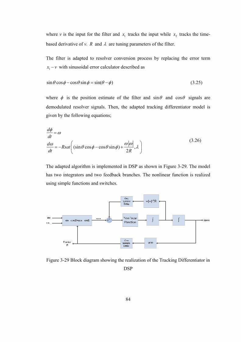
84

where v is the input for the filter and 1x tracks the input while 2x tracks the time-

based derivative of v. R and are tuning parameters of the filter.

The filter is adapted to resolver conversion process by replacing the error term

1x v with sinusoidal error calculator described as

sin cos cos sin sin( ) (3.25)

where is the position estimate of the filter and sin and cos signals are

demodulated resolver signals. Then, the adapted tracking differentiator model is

given by the following equations;

(sin cos cos sin ) ,2

d

dt

dRsat

dt R

(3.26)

The adapted algorithm is implemented in DSP as shown in Figure 3-29. The model

has two integrators and two feedback branches. The nonlinear function is realized

using simple functions and switches.

Figure 3-29 Block diagram showing the realization of the Tracking Differentiator in

DSP

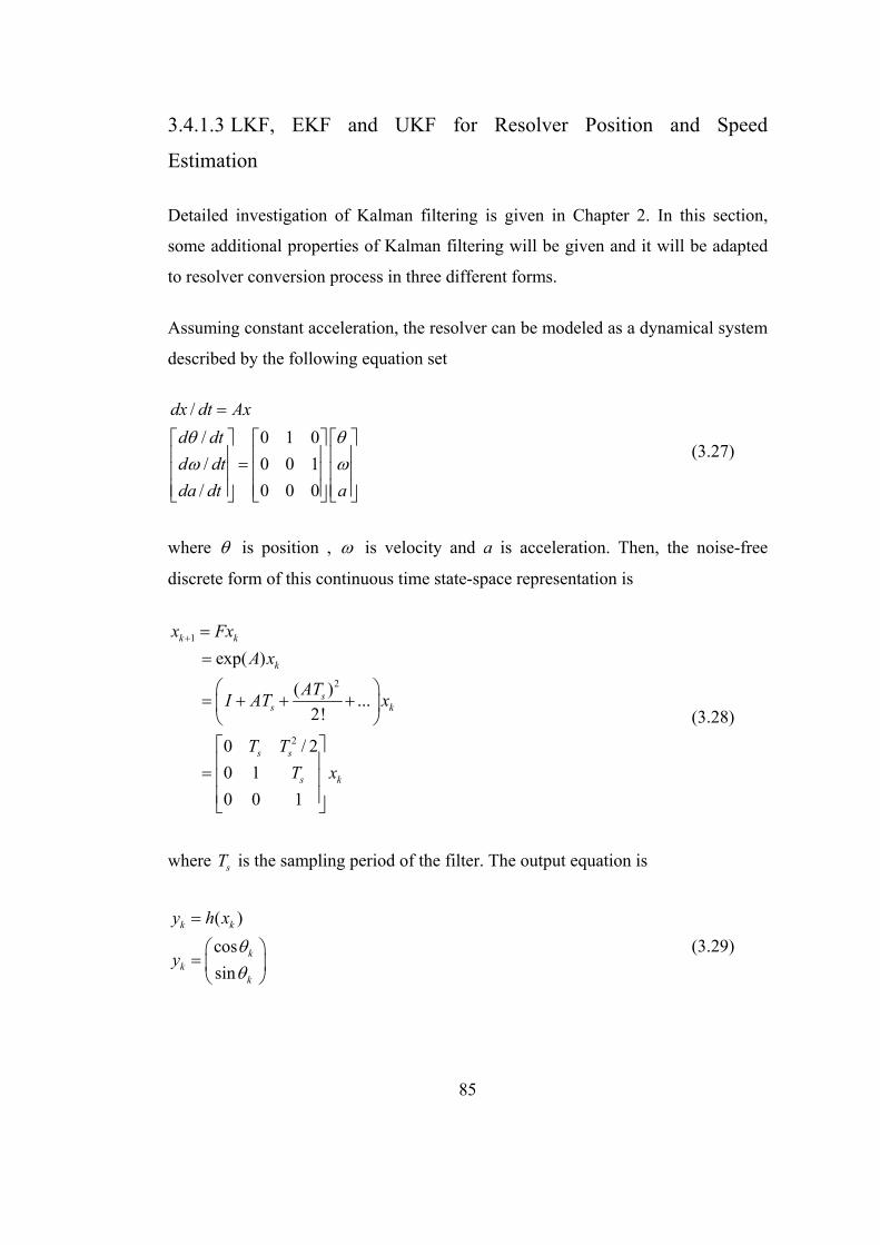
85

3.4.1.3 LKF, EKF and UKF for Resolver Position and Speed

Estimation

Detailed investigation of Kalman filtering is given in Chapter 2. In this section,

some additional properties of Kalman filtering will be given and it will be adapted

to resolver conversion process in three different forms.

Assuming constant acceleration, the resolver can be modeled as a dynamical system

described by the following equation set

/

/ 0 1 0

/ 0 0 1

/ 0 0 0

dx dt Ax

d dt

d dt

da dt a

(3.27)

where is position , is velocity and a is acceleration. Then, the noise-free

discrete form of this continuous time state-space representation is

1

2

2

exp( )

( ) ...

2!

0 / 2

0 1

0 0 1

k k

k

ss k

s s

s k

x Fx

A x

ATI AT x

T T

T x

(3.28)

where sT is the sampling period of the filter. The output equation is

( )

cos

sin

k k

kk

k

y h x

y

(3.29)

86

where h is the nonlinear function in resolver conversion process. If the process

noise and measurement noise are also taken into consideration, the system equations

will be of the form

1

( )k k k

k k k

x Fx

y h x v

(3.30)

where is the process noise and v is the measurement noise. The error covariance

matrices for process noise and measurement noise are represented by kQ and kR

respectively.

{ }

{ }

Tk j k

Tk j k

E Q

E v v R

(3.31)

This mathematical model of the resolver conversion is used in the derived Kalman

filter equations implemented as a part of the thesis (i.e. LKF, EKF and UKF).

3.4.1.3.1 Linear Kalman Filter Approach to Resolver Position and

Speed Estimation

The advantage of this filter arises in real-time because the algorithm does not

require continuous update for the Kalman gain. The Kalman gain is solved once

before the filter actually runs and then the filter runs using this constant Kalman

gain. Therefore, the real-time algorithm does not exhaust any processing power for

solving Kalman gain continually. However, to derive this computationally efficient

Kalman filter algorithm, we should make use of “one-step Kalman filter equations”.

One-Step Kalman Filter Equations

One-step Kalman filter equations are given in the literature for obtaining efficient

Kalman filter algorithms [12]. The aim is to get a priori estimate without calculating

posteriori estimate.

87

Priori state estimate is

1 ( ( ))k k k k k k kx F x K y H x (3.32)

where the term ( )k k ky H x is named as innovation. It is the error between real

output of the system and the estimate.

Priori error covariance is

11 ( )T T T T

k k k k k k k k k k k k k k kP F P F F P H H P H R H P F Q (3.33)

This is called discrete-time Algebraic Riccati Equation (DARE). If components of

(3.33) are linear and time-invariant, the DARE would converge to a steady-state

solution and it will be possible to calculate the Kalman gain offline before the

system actually runs.

1( )T Tk k k k k k kK P H H P H R (3.34)

However, resolver conversion process has nonlinear dynamics with measurements

carried by nonlinear functions of , that is, sin and cos .

Linearizing Resolver Conversion Process and LKF for Resolver Conversion

To be able to use linear Kalman filter in resolver conversion, nonlinear dynamics of

the model should be linearized. In fact, it is simply writing the innovation term as

sin cos cos sin sin( )k k k k k k k (3.35)

where k is priori position estimate at k’th sample, sin k and cos k are

measurements at k’th sample and cos k and sin k

are cosine of priori position

estimate and sine of priori position estimate respectively. The innovation term

expressed by (3.35) can be approximated by k k for small .

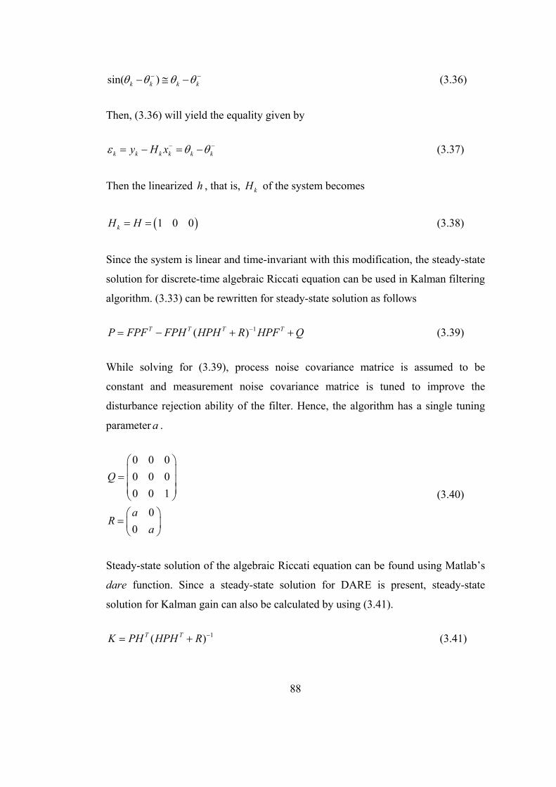
88

sin( )k k k k (3.36)

Then, (3.36) will yield the equality given by

k k k k k ky H x (3.37)

Then the linearized h , that is, kH of the system becomes

1 0 0kH H (3.38)

Since the system is linear and time-invariant with this modification, the steady-state

solution for discrete-time algebraic Riccati equation can be used in Kalman filtering

algorithm. (3.33) can be rewritten for steady-state solution as follows

1( )T T T TP FPF FPH HPH R HPF Q (3.39)

While solving for (3.39), process noise covariance matrice is assumed to be

constant and measurement noise covariance matrice is tuned to improve the

disturbance rejection ability of the filter. Hence, the algorithm has a single tuning

parameter a .

0 0 0

0 0 0

0 0 1

0

0

Q

aR

a

(3.40)

Steady-state solution of the algebraic Riccati equation can be found using Matlab’s

dare function. Since a steady-state solution for DARE is present, steady-state

solution for Kalman gain can also be calculated by using (3.41).

1( )T TK PH HPH R (3.41)

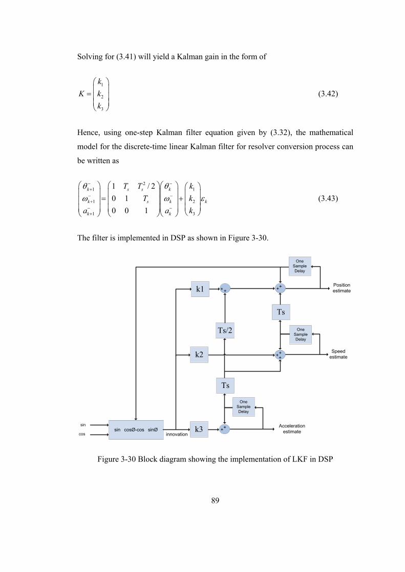
89

Solving for (3.41) will yield a Kalman gain in the form of

1

2

3

k

K k

k

(3.42)

Hence, using one-step Kalman filter equation given by (3.32), the mathematical

model for the discrete-time linear Kalman filter for resolver conversion process can

be written as

21 1

1 2

1 3

1 / 2

0 1

0 0 1

k s s k

k s k k

k k

T T k

T k

a a k

(3.43)

The filter is implemented in DSP as shown in Figure 3-30.

sin�cosØ-cos�sinØsin�

cos� innovation

++k1

++k2

++k3

One Sample Delay

Accelerationestimate

+

One Sample Delay

Ts

Ts

Ts/2

++

One Sample Delay

Speed estimate

Position estimate

Figure 3-30 Block diagram showing the implementation of LKF in DSP

90

3.4.1.3.2 Extended Kalman Filter Approach to Resolver Position and

Speed Estimation

EKF requires calculation of partial derivatives of the non-linear function h with

respect to x at mean points at each time step.

0 0sin( )( )

0 0 cos( )kk

k k

k

hH x x

x

(3.44)

Since kH is position and time dependent, this modification results in a time-varying

algebraic Riccati equation. As a result, Kalman gain will also be time-varying. This

implies that the algorithm will continuously solve the DARE and calculate the

Kalman gain at each time step. This will increase computational burden

considerably. Solving the nonlinearity by the help of the partial derivative, the

Kalman algorithm is implemented by the continuous update of the steps given in

Figure 3-31. The mathematical formulation for each step is given in section 2.5.2.2

where Extended Kalman Filter algorithm is explained in details.

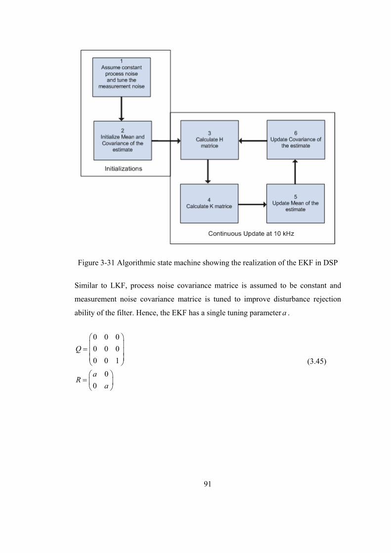
91

Figure 3-31 Algorithmic state machine showing the realization of the EKF in DSP

Similar to LKF, process noise covariance matrice is assumed to be constant and

measurement noise covariance matrice is tuned to improve disturbance rejection

ability of the filter. Hence, the EKF has a single tuning parameter a .

0 0 0

0 0 0

0 0 1

0

0

Q

aR

a

(3.45)

92

3.4.1.3.3 Unscented Kalman Filter Approach to Resolver Position and

Speed Estimation

UKF is similar to EKF when the computational complexity is considered. On the

other hand, it is more successful when the system has severe nonlinearities [12]. In

hope of a better estimation performance, UKF algorithm is implemented for

resolver conversion process.

The unscented transformation is a way of passing Gaussian signals through

nonlinear functions. Instead of linearization with differentiation as the EKF, the

UKF makes use of unscented transforms while passing Gaussian signals through

nonlinear functions. Hence, the unscented transformation is applied to h in the

proposed system.

Assuming a Gaussian with dimension n with mean and covariance , there will

be 2n+1 sigma points symmetrically located with respect to the mean. This

selection of sigma points relies on a deterministic method and some parameters are

needed to locate these deterministic points. For resolver conversion, there are 7

sigma points since the dimensionality of the state vector is 3. Each sigma point has

two weights which are used in recovering mean and covariance after the sigma

points are passed through the nonlinear function h.

The equations to choose sigma points iX for a Gaussian ( , )N are given as

0 , for i=0

( ( ) ), for i=1,2,3

( ( ) ), for i=4,5,6

i

i

X

X n

X n

(3.46)

where 2 ( )n n and and are the parameters which determine the

locations of the symmetrical sigma points. For each sigma point, there exist two

weights imw and i

cw which are calculated according to the following rules

93

0

0 2(1 )

1, for i=1,..,7

2( )

m

c

i im c

wn

wn

w wn

(3.47)

where the parameter is optimally 2 when the distribution is an exact Gaussian.

Second step of unscented transform is passing sigma points through the nonlinear

function h.

( )i iY h X (3.48)

iY is the output of the nonlinear function for each sigma point. The third and final

step of the unscented transform is to calculate new mean ' and covariance ' of

the resultant Gaussian. The parameters can be calculated from the equations

2

0

2

0

'

' ( ')( ')

ni im

i

ni i i Tc

i

w Y

w Y Y

(3.49)

The equations are simple but they will be enough to increase the computational

complexity considerably because the algorithm calculates sigma points and weights

at each time step. Solving the nonlinearity by the help of unscented transform, the

Kalman algorithm is implemented by the continuous update of the steps given in

Figure 3-32. The mathematical formulation for each step is given in section 2.5.2.3

where Unscented Kalman Filter algorithm is explained in details.

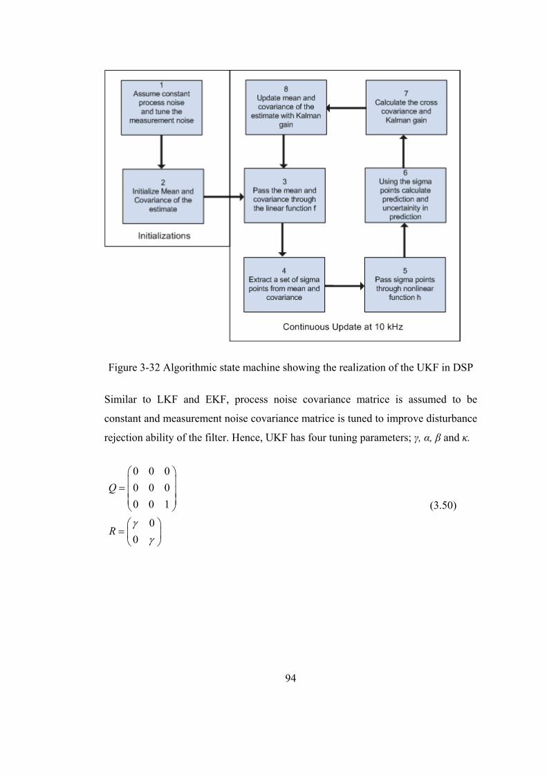
94

Figure 3-32 Algorithmic state machine showing the realization of the UKF in DSP

Similar to LKF and EKF, process noise covariance matrice is assumed to be

constant and measurement noise covariance matrice is tuned to improve disturbance

rejection ability of the filter. Hence, UKF has four tuning parameters; γ, α, β and κ.

0 0 0

0 0 0

0 0 1

0

0

Q

R

(3.50)

95

CHAPTER 4

PERFORMANCE ANALYSIS OF THE PROPOSED

RESOLVER-TO-DIGITAL CONVERTER

One of the most important performance criterions for resolver converters is the

conversion bandwidth. External disturbances coming from sea have a bandwidth of

0.5 Hz according to both Pierson & Moskowitz and JONSWAP spectrums as

analyzed in Chapter 2. Hence, stabilization at sea requires that the position sensor

utilized on the stabilization system, for instance a resolver with a RDC, track input

signals coming at a frequency spectrum 0.5 Hz.

Noise suppression ability is another important performance criterion for resolver

converters since a resolver, operating in a noisy environment where high motor

phase currents are flowing closely, generates electromagnetically contaminated

output signals. Moreover, disturbances coming from the resolver channels and

demodulator degrade the conversion performance. Hence, the converter should be

robust against the noise and said disturbances to maintain high-performance

tracking.

Taking above mentioned performance criterions into consideration, models for

simulation and real-time tests are constructed in this chapter. The estimator filters

are tuned in simulation environment and tuned filters are implemented in an

experimental STAMP system. Filters’ performances are observed in real-time in the

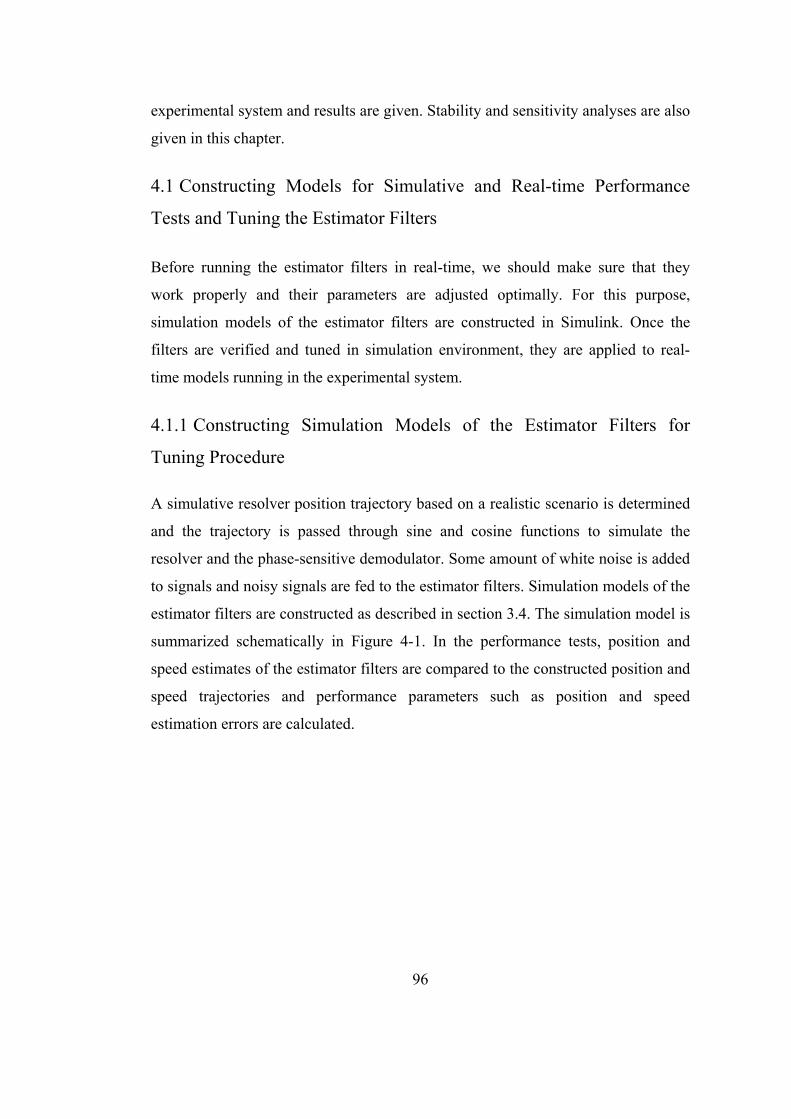
96

experimental system and results are given. Stability and sensitivity analyses are also

given in this chapter.

4.1 Constructing Models for Simulative and Real-time Performance

Tests and Tuning the Estimator Filters

Before running the estimator filters in real-time, we should make sure that they

work properly and their parameters are adjusted optimally. For this purpose,

simulation models of the estimator filters are constructed in Simulink. Once the

filters are verified and tuned in simulation environment, they are applied to real-

time models running in the experimental system.

4.1.1 Constructing Simulation Models of the Estimator Filters for

Tuning Procedure

A simulative resolver position trajectory based on a realistic scenario is determined

and the trajectory is passed through sine and cosine functions to simulate the

resolver and the phase-sensitive demodulator. Some amount of white noise is added

to signals and noisy signals are fed to the estimator filters. Simulation models of the

estimator filters are constructed as described in section 3.4. The simulation model is

summarized schematically in Figure 4-1. In the performance tests, position and

speed estimates of the estimator filters are compared to the constructed position and

speed trajectories and performance parameters such as position and speed

estimation errors are calculated.

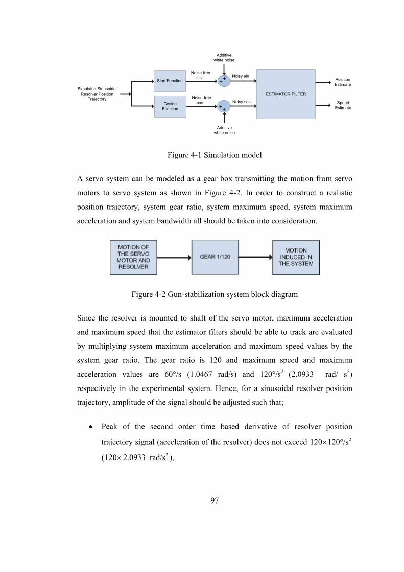
97

Additive white noise

Sine Function

Cosine Function

Simulated Sinusoidal Resolver Position

TrajectoryNoisy cos�

++

++

Additive white noise

Noisy sin�

ESTIMATOR FILTER

Position Estimate

Speed Estimate

Noise-free sin�

Noise-free cos�

Figure 4-1 Simulation model

A servo system can be modeled as a gear box transmitting the motion from servo

motors to servo system as shown in Figure 4-2. In order to construct a realistic

position trajectory, system gear ratio, system maximum speed, system maximum

acceleration and system bandwidth all should be taken into consideration.

Figure 4-2 Gun-stabilization system block diagram

Since the resolver is mounted to shaft of the servo motor, maximum acceleration

and maximum speed that the estimator filters should be able to track are evaluated

by multiplying system maximum acceleration and maximum speed values by the

system gear ratio. The gear ratio is 120 and maximum speed and maximum

acceleration values are 60°/s (1.0467 rad/s) and 120°/s2 (2.0933 rad/ s2)

respectively in the experimental system. Hence, for a sinusoidal resolver position

trajectory, amplitude of the signal should be adjusted such that;

Peak of the second order time based derivative of resolver position

trajectory signal (acceleration of the resolver) does not exceed 2120 120°/s

( 2120 2.0933 rad/s ),

98

Peak of the first order time based derivative of resolver position trajectory

signal (speed of the resolver) does not exceed 120 60°/s

(120 1.0467 rad/s ).

Regarding above mentioned considerations and system bandwidth (0.5 Hz),

simulative resolver position trajectory is constructed as

2

039.8sin(2 ) radft

(4.1)

where f is chosen as 0.4Hz . Then, simulative resolver speed trajectory can be

found by taking derivative of the position trajectory with respect to time such that

100cos(2 ) rad/s d ftdt (4.2)

where f is 0.4Hz .

In the simulation model, noise process is assumed to be white, uncorrelated and

zero mean Gaussian process. Variance of the noise is extracted from real noise data

collected from the stabilized gun system while resolver is stationary and resolver

position is close to 45° (Figure 4-3). Using var and mean functions of Matlab,

variance of the signal is found as 6.90735x10-5 where mean of it is found as 0.6589

corresponding to a resolver position of 41.22°. Hence, white noise signals with the

same variance are added to noise-free cos and sin signals. Then, noisy resolver

signals are fed to the estimator filters and filters are tuned based on the performance

observations made in simulation environment.

99

Figure 4-3 Noise on the resolver channel in the gun stabilization system when

resolver speed is zero and position is 41.22°

Figure 4-4 shows the simulative position trajectory ( ) and constructed sin and

cos signals with additive white noise.

Figure 4-4 Noise-free position signal and noisy sine and cosine signals used as input

to estimator filters in simulation environment

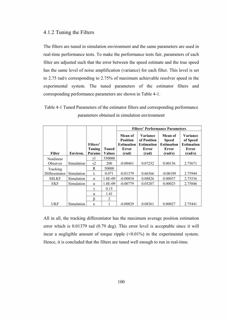
100

4.1.2 Tuning the Filters

The filters are tuned in simulation environment and the same parameters are used in

real-time performance tests. To make the performance tests fair, parameters of each

filter are adjusted such that the error between the speed estimate and the true speed

has the same level of noise amplification (variance) for each filter. This level is set

to 2.75 rad/s corresponding to 2.75% of maximum achievable resolver speed in the

experimental system. The tuned parameters of the estimator filters and

corresponding performance parameters are shown in Table 4-1.

Table 4-1 Tuned Parameters of the estimator filters and corresponding performance

parameters obtained in simulation environment

Filter Environ.

Filters’ Tuning Params

Tuned Values

Filters’ Performance Parameters

Mean of Position

Estimation Error (rad)

Variance of Position Estimation

Error (rad)

Mean of Speed

Estimation Error (rad/s)

Variance of Speed

Estimation Error (rad/s)

Nonlinear Observer Simulation

γ1 350000-0.00461 0.07252 0.00136 2.75671 γ2 200

Tracking Differentiator Simulation

R 50000 -0.01379 0.66366 -0.00189 2.75944 λ 0.071

SSLKF Simulation α 1.8E-09 -0.00854 0.08826 0.00037 2.75536 EKF Simulation α 1.8E-09 -0.00779 0.05207 0.00025 2.75846

UKF Simulation

γ 0.15

-0.00829 0.08361 0.00027 2.75441

α 1.41 β 2 κ 1

All in all, the tracking differentiator has the maximum average position estimation

error which is 0.01379 rad (0.79 deg). This error level is acceptable since it will

incur a negligible amount of torque ripple (<0.01%) in the experimental system.

Hence, it is concluded that the filters are tuned well enough to run in real-time.

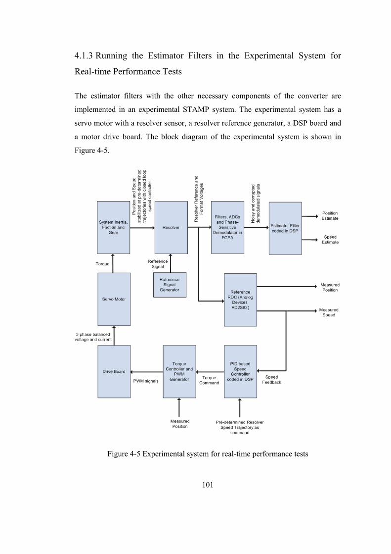
101

4.1.3 Running the Estimator Filters in the Experimental System for

Real-time Performance Tests

The estimator filters with the other necessary components of the converter are

implemented in an experimental STAMP system. The experimental system has a

servo motor with a resolver sensor, a resolver reference generator, a DSP board and

a motor drive board. The block diagram of the experimental system is shown in

Figure 4-5.

Figure 4-5 Experimental system for real-time performance tests

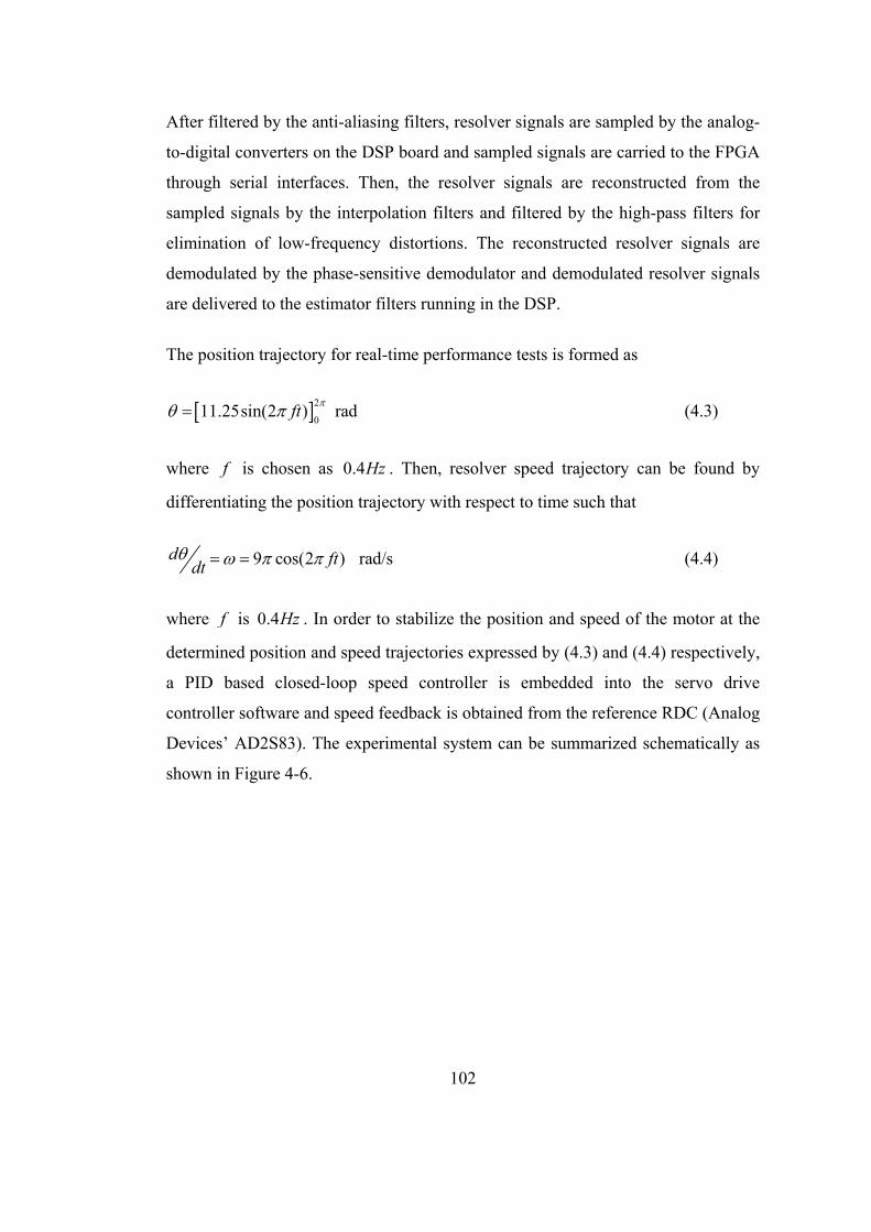
102

After filtered by the anti-aliasing filters, resolver signals are sampled by the analog-

to-digital converters on the DSP board and sampled signals are carried to the FPGA

through serial interfaces. Then, the resolver signals are reconstructed from the

sampled signals by the interpolation filters and filtered by the high-pass filters for

elimination of low-frequency distortions. The reconstructed resolver signals are

demodulated by the phase-sensitive demodulator and demodulated resolver signals

are delivered to the estimator filters running in the DSP.

The position trajectory for real-time performance tests is formed as

2

011.25sin(2 ) radft

(4.3)

where f is chosen as 0.4Hz . Then, resolver speed trajectory can be found by

differentiating the position trajectory with respect to time such that

9 cos(2 ) rad/s d ftdt (4.4)

where f is 0.4Hz . In order to stabilize the position and speed of the motor at the

determined position and speed trajectories expressed by (4.3) and (4.4) respectively,

a PID based closed-loop speed controller is embedded into the servo drive

controller software and speed feedback is obtained from the reference RDC (Analog

Devices’ AD2S83). The experimental system can be summarized schematically as

shown in Figure 4-6.

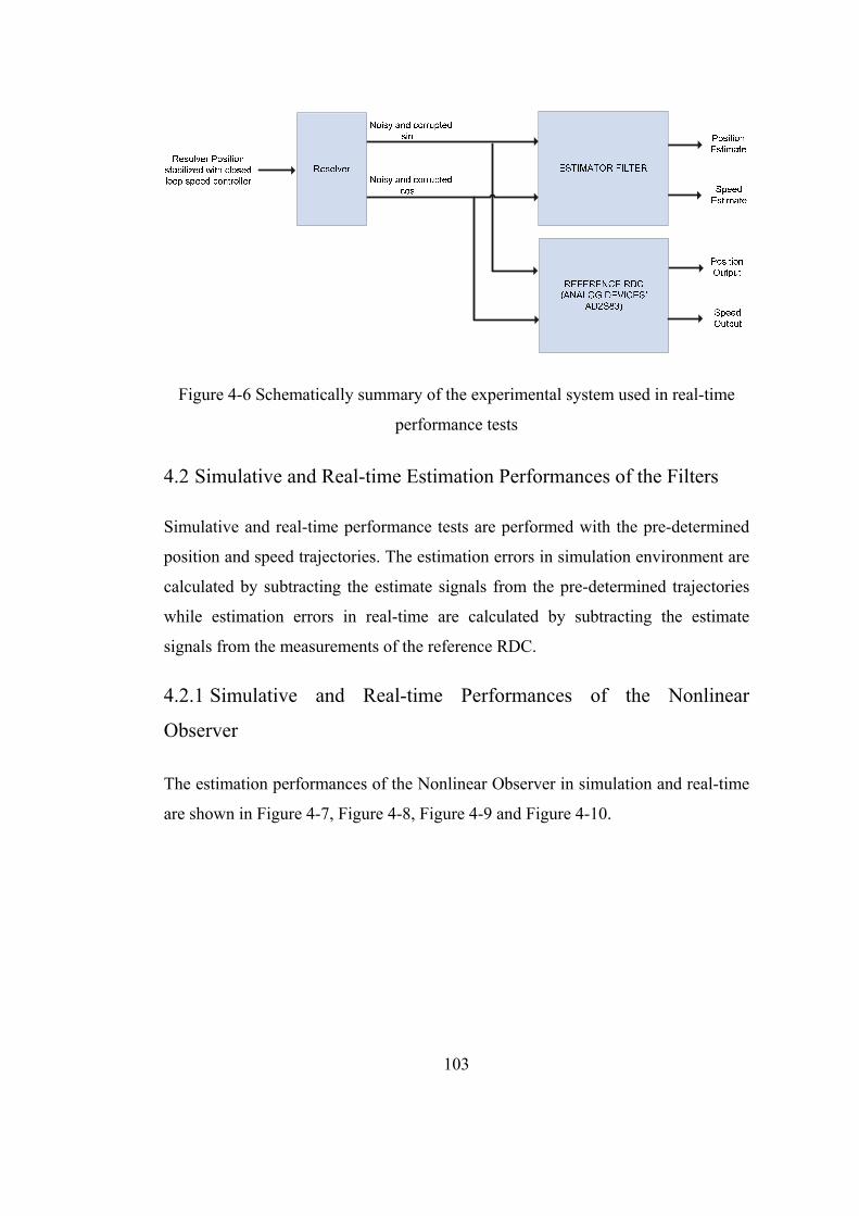
103

Figure 4-6 Schematically summary of the experimental system used in real-time

performance tests

4.2 Simulative and Real-time Estimation Performances of the Filters

Simulative and real-time performance tests are performed with the pre-determined

position and speed trajectories. The estimation errors in simulation environment are

calculated by subtracting the estimate signals from the pre-determined trajectories

while estimation errors in real-time are calculated by subtracting the estimate

signals from the measurements of the reference RDC.

4.2.1 Simulative and Real-time Performances of the Nonlinear

Observer

The estimation performances of the Nonlinear Observer in simulation and real-time

are shown in Figure 4-7, Figure 4-8, Figure 4-9 and Figure 4-10.

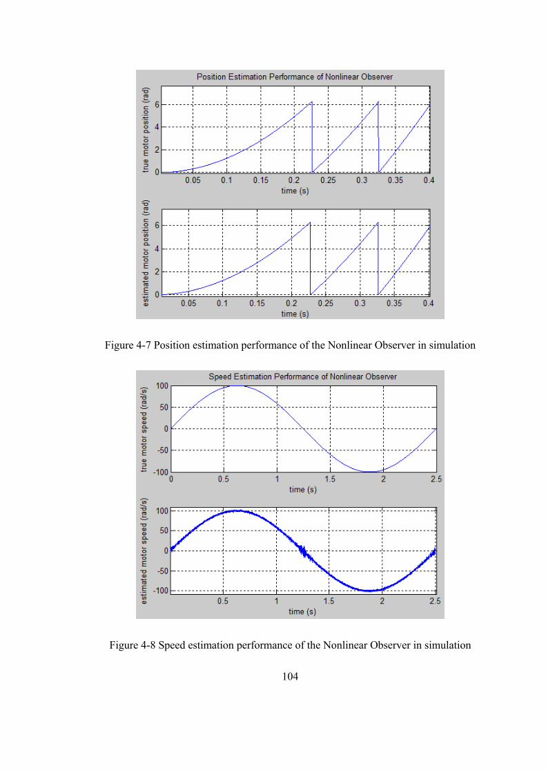
104

Figure 4-7 Position estimation performance of the Nonlinear Observer in simulation

Figure 4-8 Speed estimation performance of the Nonlinear Observer in simulation

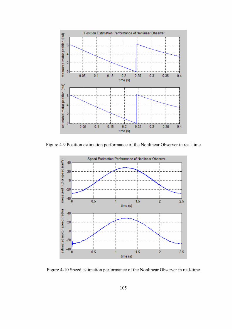
105

Figure 4-9 Position estimation performance of the Nonlinear Observer in real-time

Figure 4-10 Speed estimation performance of the Nonlinear Observer in real-time

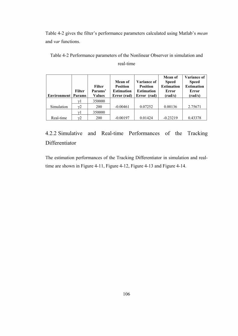
106

Table 4-2 gives the filter’s performance parameters calculated using Matlab’s mean

and var functions.

Table 4-2 Performance parameters of the Nonlinear Observer in simulation and

real-time

EnvironmentFilter

Params

Filter Params’ Values

Mean of Position

Estimation Error (rad)

Variance of Position

Estimation Error (rad)

Mean of Speed

Estimation Error (rad/s)

Variance of Speed

Estimation Error (rad/s)

Simulation

γ1 350000

-0.00461 0.07252 0.00136 2.75671 γ2 200

Real-time

γ1 350000

-0.00197 0.01424 -0.23219 0.43378 γ2 200

4.2.2 Simulative and Real-time Performances of the Tracking

Differentiator

The estimation performances of the Tracking Differentiator in simulation and real-

time are shown in Figure 4-11, Figure 4-12, Figure 4-13 and Figure 4-14.

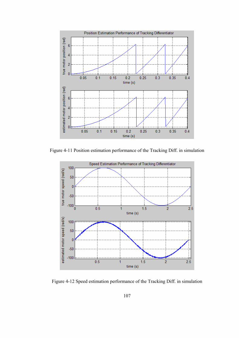
107

Figure 4-11 Position estimation performance of the Tracking Diff. in simulation

Figure 4-12 Speed estimation performance of the Tracking Diff. in simulation

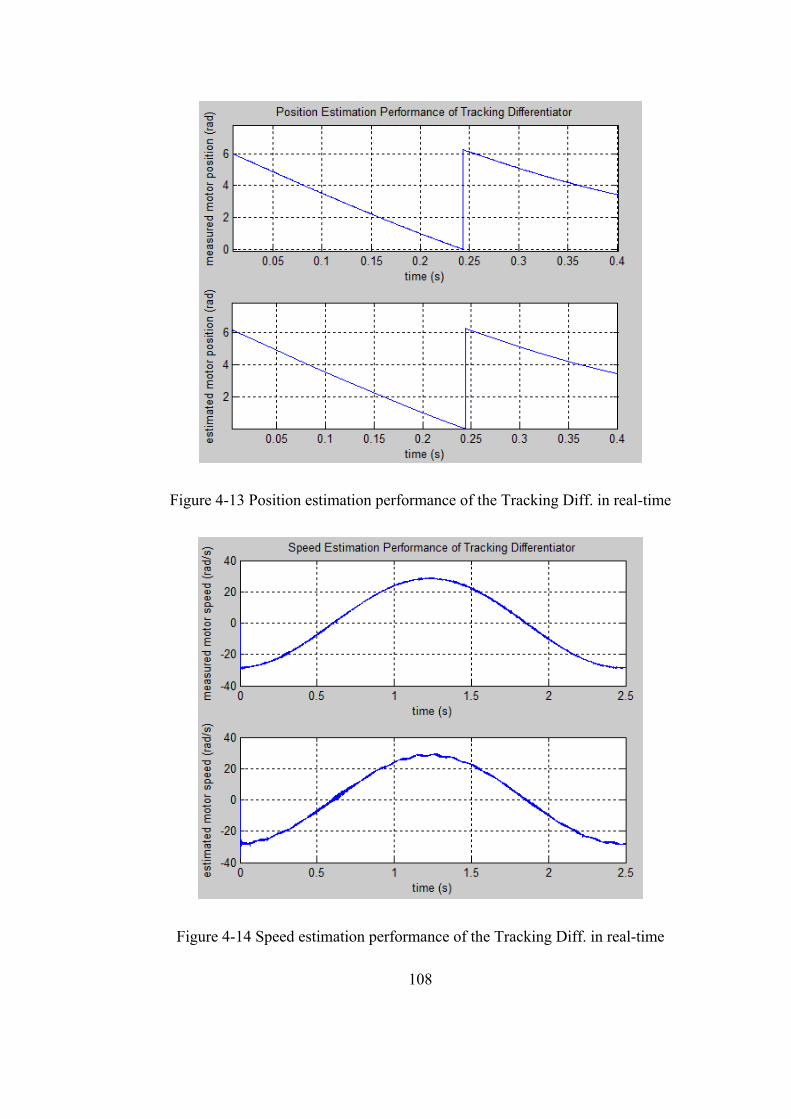
108

Figure 4-13 Position estimation performance of the Tracking Diff. in real-time

Figure 4-14 Speed estimation performance of the Tracking Diff. in real-time

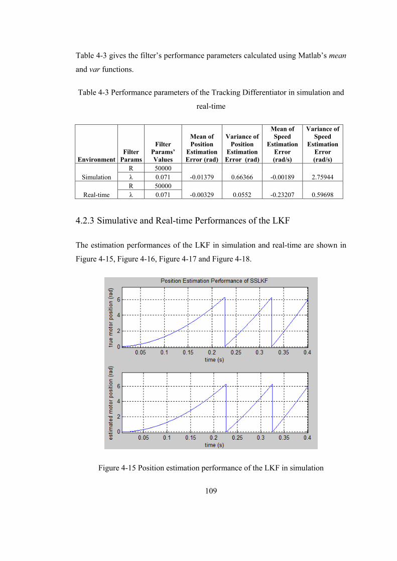
109

Table 4-3 gives the filter’s performance parameters calculated using Matlab’s mean

and var functions.

Table 4-3 Performance parameters of the Tracking Differentiator in simulation and

real-time

Environment Filter

Params

Filter Params’ Values

Mean of Position

Estimation Error (rad)

Variance of Position

Estimation Error (rad)

Mean of Speed

Estimation Error (rad/s)

Variance of Speed

Estimation Error (rad/s)

Simulation R 50000

-0.01379 0.66366 -0.00189 2.75944 λ 0.071

Real-time R 50000

-0.00329 0.0552 -0.23207 0.59698 λ 0.071

4.2.3 Simulative and Real-time Performances of the LKF

The estimation performances of the LKF in simulation and real-time are shown in

Figure 4-15, Figure 4-16, Figure 4-17 and Figure 4-18.

Figure 4-15 Position estimation performance of the LKF in simulation

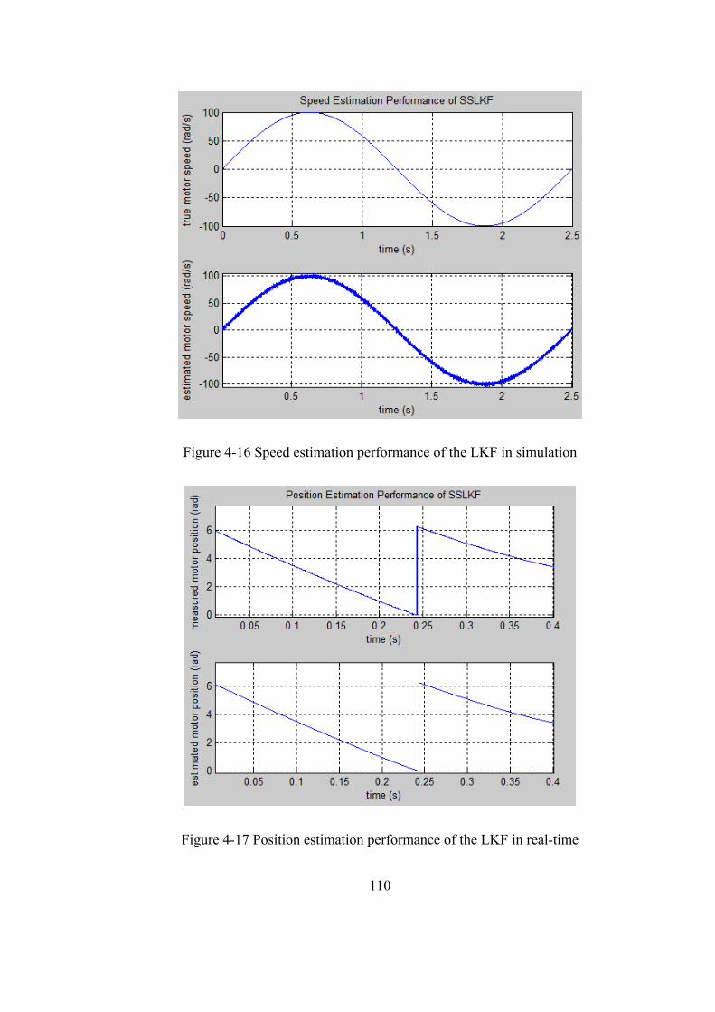
110

Figure 4-16 Speed estimation performance of the LKF in simulation

Figure 4-17 Position estimation performance of the LKF in real-time

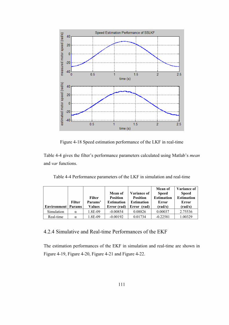
111

Figure 4-18 Speed estimation performance of the LKF in real-time

Table 4-4 gives the filter’s performance parameters calculated using Matlab’s mean

and var functions.

Table 4-4 Performance parameters of the LKF in simulation and real-time

Environment Filter

Params

Filter Params’ Values

Mean of Position

Estimation Error (rad)

Variance of Position

Estimation Error (rad)

Mean of Speed

Estimation Error (rad/s)

Variance of Speed

Estimation Error (rad/s)

Simulation α 1.8E-09 -0.00854 0.08826 0.00037 2.75536 Real-time α 1.8E-09 -0.00192 0.01734 -0.22581 1.00329

4.2.4 Simulative and Real-time Performances of the EKF

The estimation performances of the EKF in simulation and real-time are shown in

Figure 4-19, Figure 4-20, Figure 4-21 and Figure 4-22.

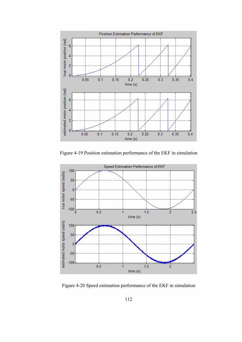
112

Figure 4-19 Position estimation performance of the EKF in simulation

Figure 4-20 Speed estimation performance of the EKF in simulation

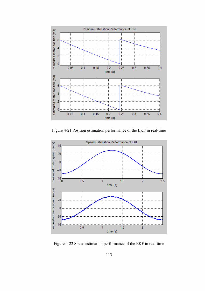
113

Figure 4-21 Position estimation performance of the EKF in real-time

Figure 4-22 Speed estimation performance of the EKF in real-time

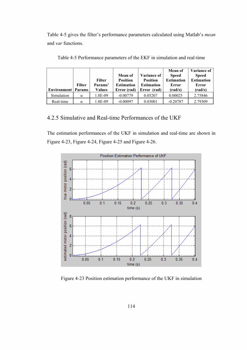
114

Table 4-5 gives the filter’s performance parameters calculated using Matlab’s mean

and var functions.

Table 4-5 Performance parameters of the EKF in simulation and real-time

Environment Filter

Params

Filter Params’ Values

Mean of Position

Estimation Error (rad)

Variance of Position

Estimation Error (rad)

Mean of Speed

Estimation Error (rad/s)

Variance of Speed

Estimation Error (rad/s)

Simulation α 1.8E-09 -0.00779 0.05207 0.00025 2.75846

Real-time α 1.8E-09 -0.00097 0.03001 -0.20787 2.79309

4.2.5 Simulative and Real-time Performances of the UKF

The estimation performances of the UKF in simulation and real-time are shown in

Figure 4-23, Figure 4-24, Figure 4-25 and Figure 4-26.

Figure 4-23 Position estimation performance of the UKF in simulation

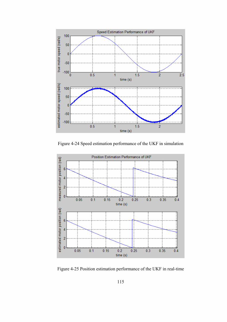
115

Figure 4-24 Speed estimation performance of the UKF in simulation

Figure 4-25 Position estimation performance of the UKF in real-time

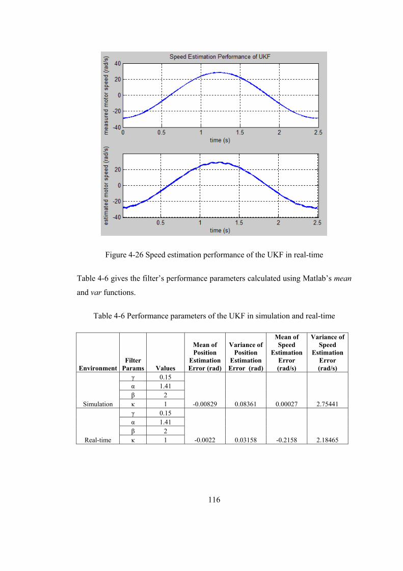
116

Figure 4-26 Speed estimation performance of the UKF in real-time

Table 4-6 gives the filter’s performance parameters calculated using Matlab’s mean

and var functions.

Table 4-6 Performance parameters of the UKF in simulation and real-time

Environment Filter

Params Values

Mean of Position

Estimation Error (rad)

Variance of Position

Estimation Error (rad)

Mean of Speed

Estimation Error (rad/s)

Variance of Speed

Estimation Error (rad/s)

Simulation

γ 0.15

-0.00829 0.08361 0.00027 2.75441

α 1.41 β 2 κ 1

Real-time

γ 0.15

-0.0022 0.03158 -0.2158 2.18465

α 1.41 β 2 κ 1

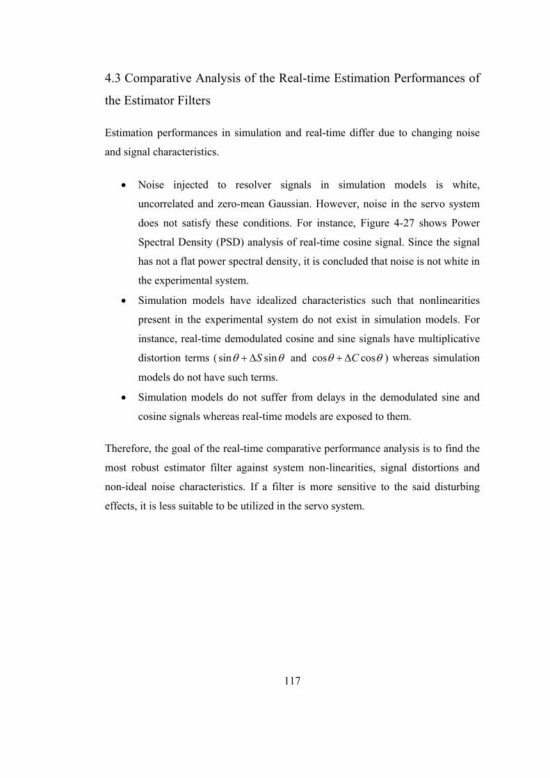
117

4.3 Comparative Analysis of the Real-time Estimation Performances of

the Estimator Filters

Estimation performances in simulation and real-time differ due to changing noise

and signal characteristics.

Noise injected to resolver signals in simulation models is white,

uncorrelated and zero-mean Gaussian. However, noise in the servo system

does not satisfy these conditions. For instance, Figure 4-27 shows Power

Spectral Density (PSD) analysis of real-time cosine signal. Since the signal

has not a flat power spectral density, it is concluded that noise is not white in

the experimental system.

Simulation models have idealized characteristics such that nonlinearities

present in the experimental system do not exist in simulation models. For

instance, real-time demodulated cosine and sine signals have multiplicative

distortion terms ( sin sinS and cos cosC ) whereas simulation

models do not have such terms.

Simulation models do not suffer from delays in the demodulated sine and

cosine signals whereas real-time models are exposed to them.

Therefore, the goal of the real-time comparative performance analysis is to find the

most robust estimator filter against system non-linearities, signal distortions and

non-ideal noise characteristics. If a filter is more sensitive to the said disturbing

effects, it is less suitable to be utilized in the servo system.

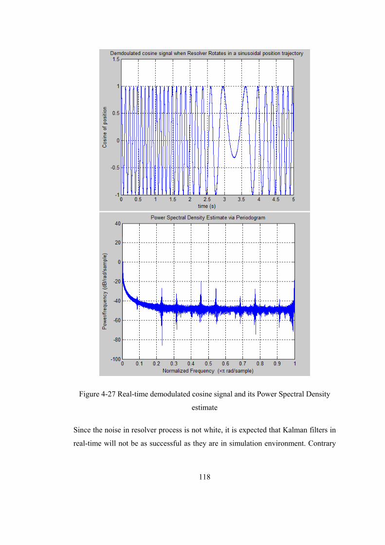
118

Figure 4-27 Real-time demodulated cosine signal and its Power Spectral Density

estimate

Since the noise in resolver process is not white, it is expected that Kalman filters in

real-time will not be as successful as they are in simulation environment. Contrary

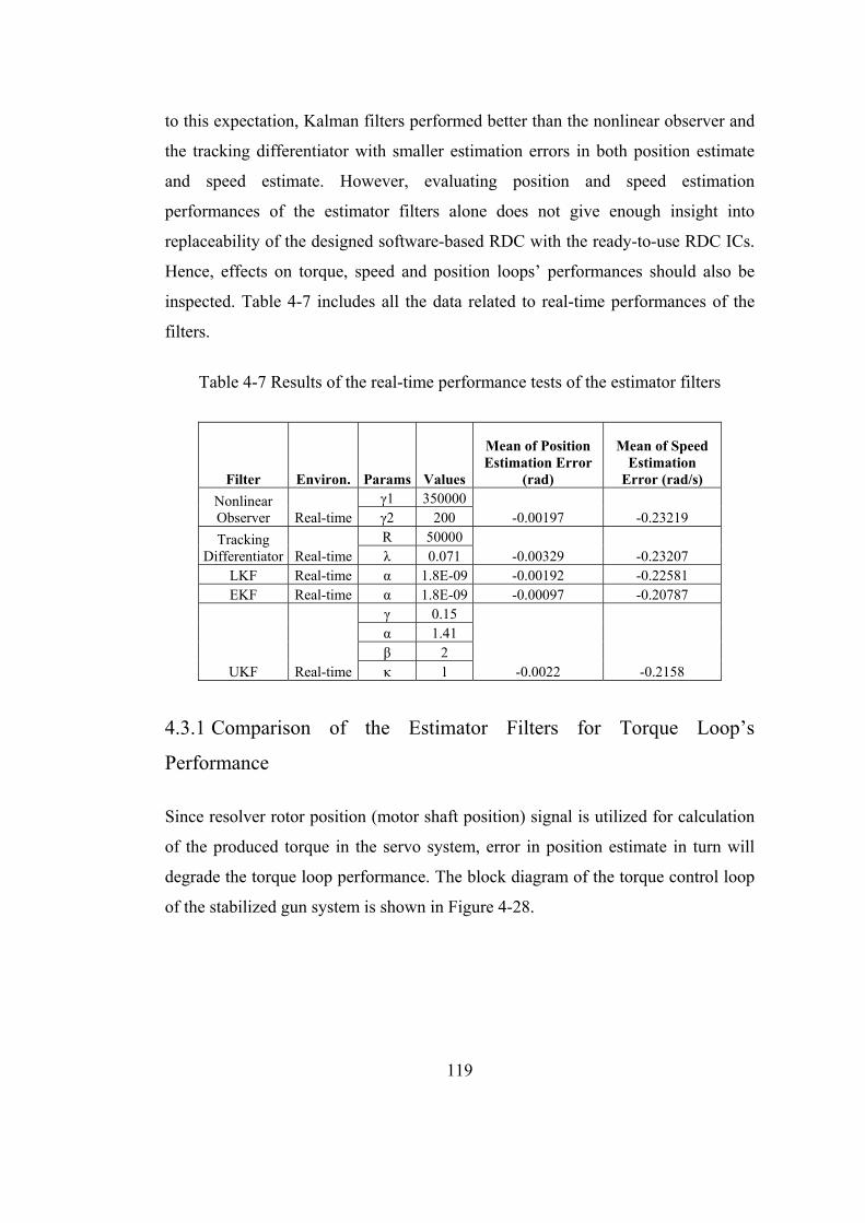
119

to this expectation, Kalman filters performed better than the nonlinear observer and

the tracking differentiator with smaller estimation errors in both position estimate

and speed estimate. However, evaluating position and speed estimation

performances of the estimator filters alone does not give enough insight into

replaceability of the designed software-based RDC with the ready-to-use RDC ICs.

Hence, effects on torque, speed and position loops’ performances should also be

inspected. Table 4-7 includes all the data related to real-time performances of the

filters.

Table 4-7 Results of the real-time performance tests of the estimator filters

Filter Environ. Params Values

Mean of Position Estimation Error

(rad)

Mean of Speed Estimation

Error (rad/s)

Nonlinear Observer Real-time

γ1 350000-0.00197 -0.23219 γ2 200

Tracking Differentiator Real-time

R 50000 -0.00329 -0.23207 λ 0.071

LKF Real-time α 1.8E-09 -0.00192 -0.22581 EKF Real-time α 1.8E-09 -0.00097 -0.20787

UKF Real-time

γ 0.15

-0.0022 -0.2158

α 1.41 β 2 κ 1

4.3.1 Comparison of the Estimator Filters for Torque Loop’s

Performance

Since resolver rotor position (motor shaft position) signal is utilized for calculation

of the produced torque in the servo system, error in position estimate in turn will

degrade the torque loop performance. The block diagram of the torque control loop

of the stabilized gun system is shown in Figure 4-28.

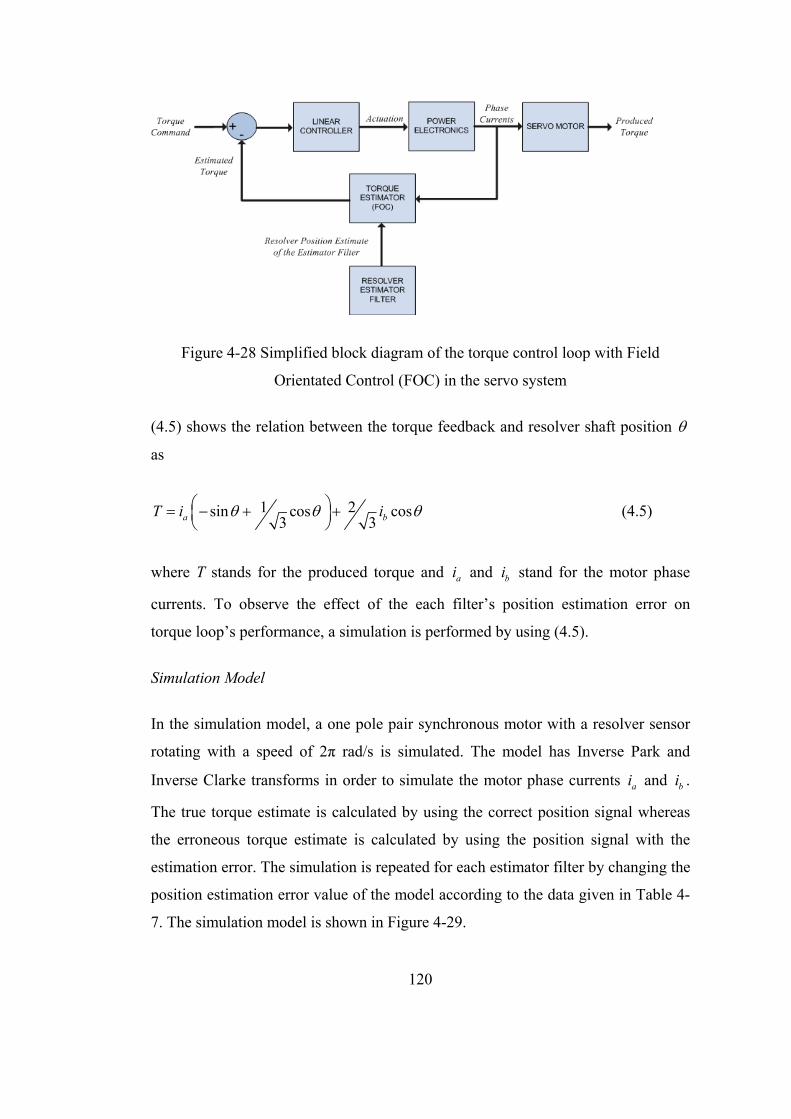
120

Figure 4-28 Simplified block diagram of the torque control loop with Field

Orientated Control (FOC) in the servo system

(4.5) shows the relation between the torque feedback and resolver shaft position

as

1 2sin cos cos3 3a bT i i

(4.5)

where T stands for the produced torque and ai and bi stand for the motor phase

currents. To observe the effect of the each filter’s position estimation error on

torque loop’s performance, a simulation is performed by using (4.5).

Simulation Model

In the simulation model, a one pole pair synchronous motor with a resolver sensor

rotating with a speed of 2π rad/s is simulated. The model has Inverse Park and

Inverse Clarke transforms in order to simulate the motor phase currents ai and bi .

The true torque estimate is calculated by using the correct position signal whereas

the erroneous torque estimate is calculated by using the position signal with the

estimation error. The simulation is repeated for each estimator filter by changing the

position estimation error value of the model according to the data given in Table 4-

7. The simulation model is shown in Figure 4-29.

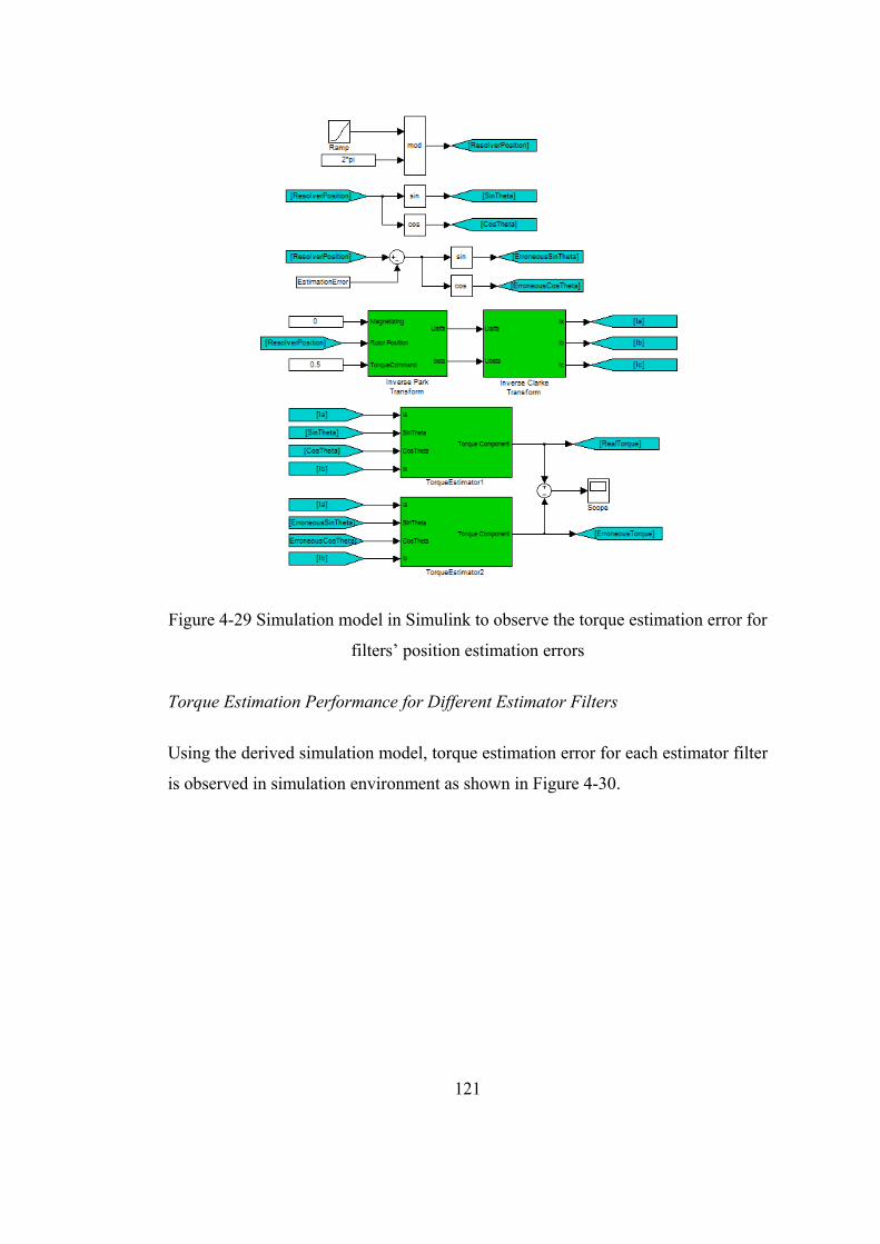
121

Figure 4-29 Simulation model in Simulink to observe the torque estimation error for

filters’ position estimation errors

Torque Estimation Performance for Different Estimator Filters

Using the derived simulation model, torque estimation error for each estimator filter

is observed in simulation environment as shown in Figure 4-30.

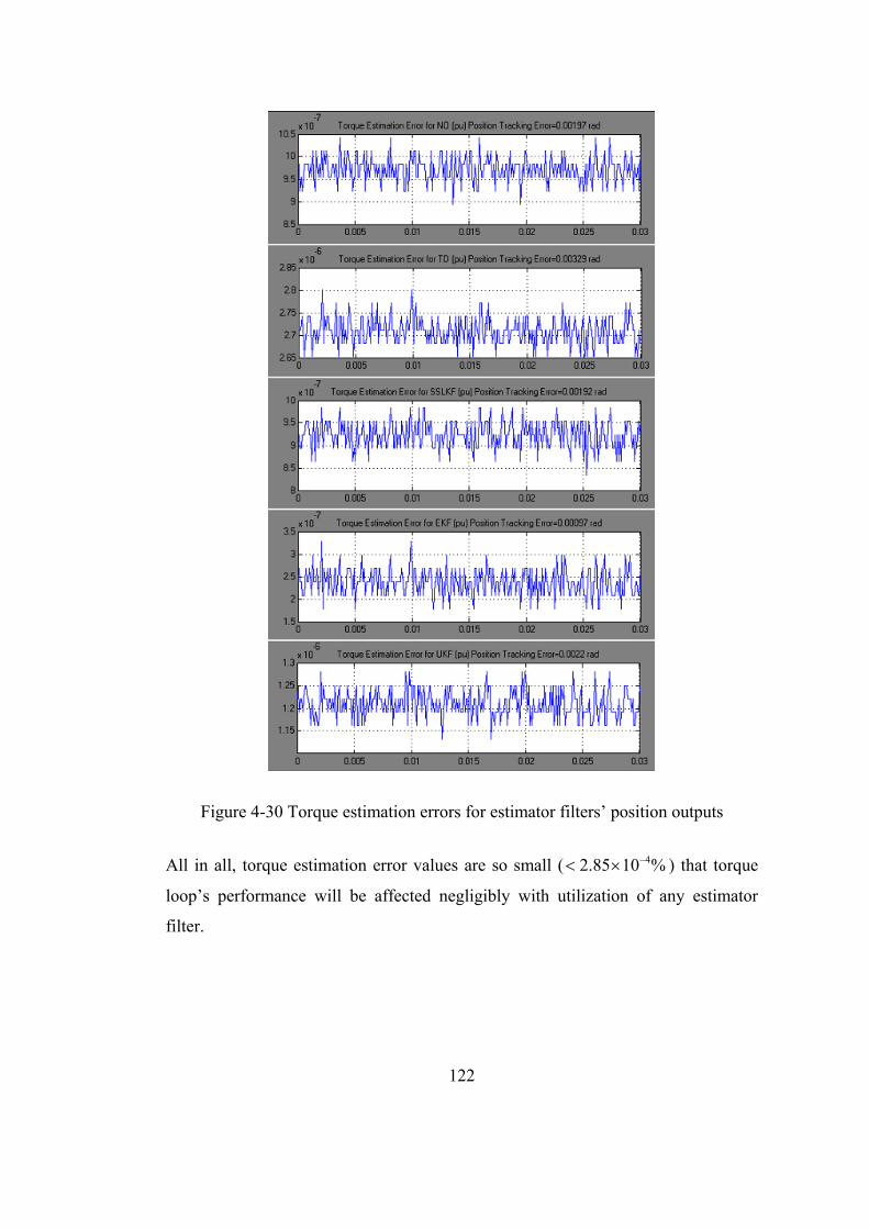
122

Figure 4-30 Torque estimation errors for estimator filters’ position outputs

All in all, torque estimation error values are so small ( 42.85 10 % ) that torque

loop’s performance will be affected negligibly with utilization of any estimator

filter.

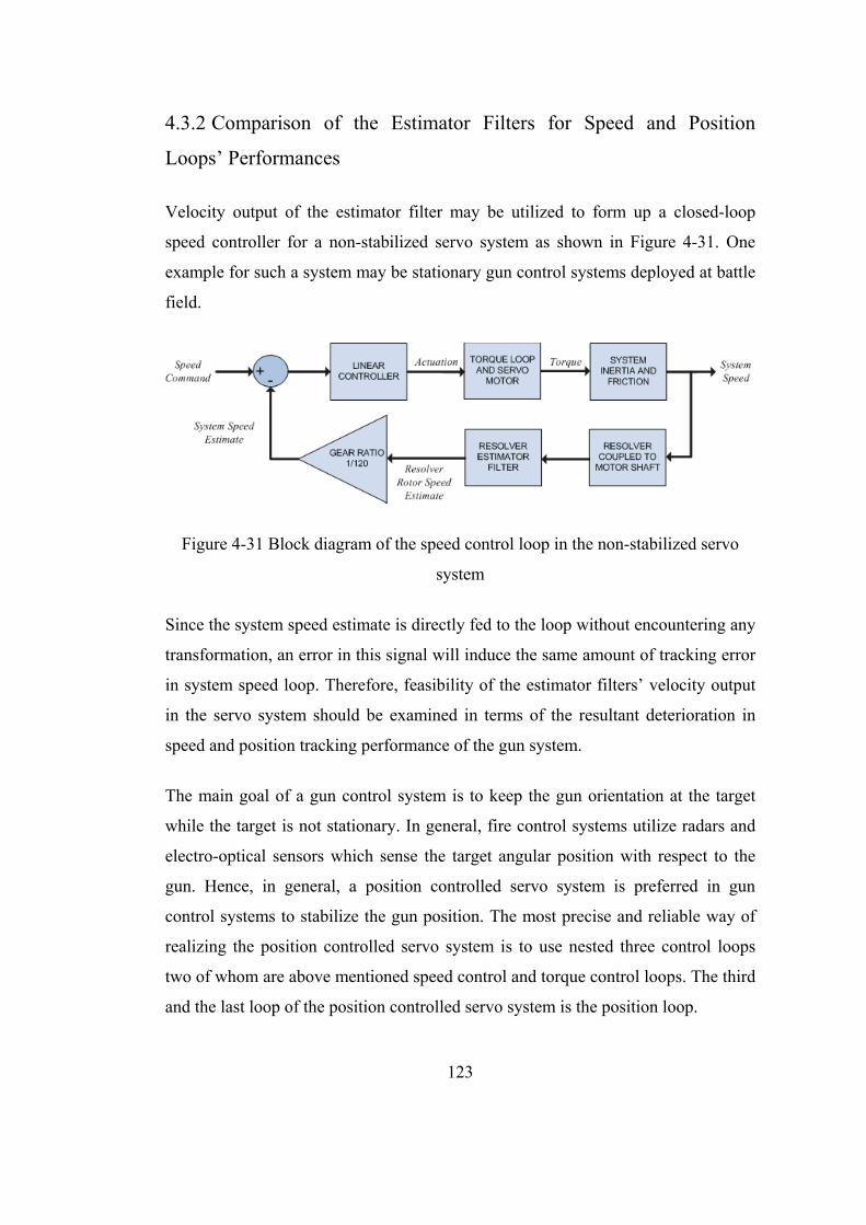
123

4.3.2 Comparison of the Estimator Filters for Speed and Position

Loops’ Performances

Velocity output of the estimator filter may be utilized to form up a closed-loop

speed controller for a non-stabilized servo system as shown in Figure 4-31. One

example for such a system may be stationary gun control systems deployed at battle

field.

Figure 4-31 Block diagram of the speed control loop in the non-stabilized servo

system

Since the system speed estimate is directly fed to the loop without encountering any

transformation, an error in this signal will induce the same amount of tracking error

in system speed loop. Therefore, feasibility of the estimator filters’ velocity output

in the servo system should be examined in terms of the resultant deterioration in

speed and position tracking performance of the gun system.

The main goal of a gun control system is to keep the gun orientation at the target

while the target is not stationary. In general, fire control systems utilize radars and

electro-optical sensors which sense the target angular position with respect to the

gun. Hence, in general, a position controlled servo system is preferred in gun

control systems to stabilize the gun position. The most precise and reliable way of

realizing the position controlled servo system is to use nested three control loops

two of whom are above mentioned speed control and torque control loops. The third

and the last loop of the position controlled servo system is the position loop.

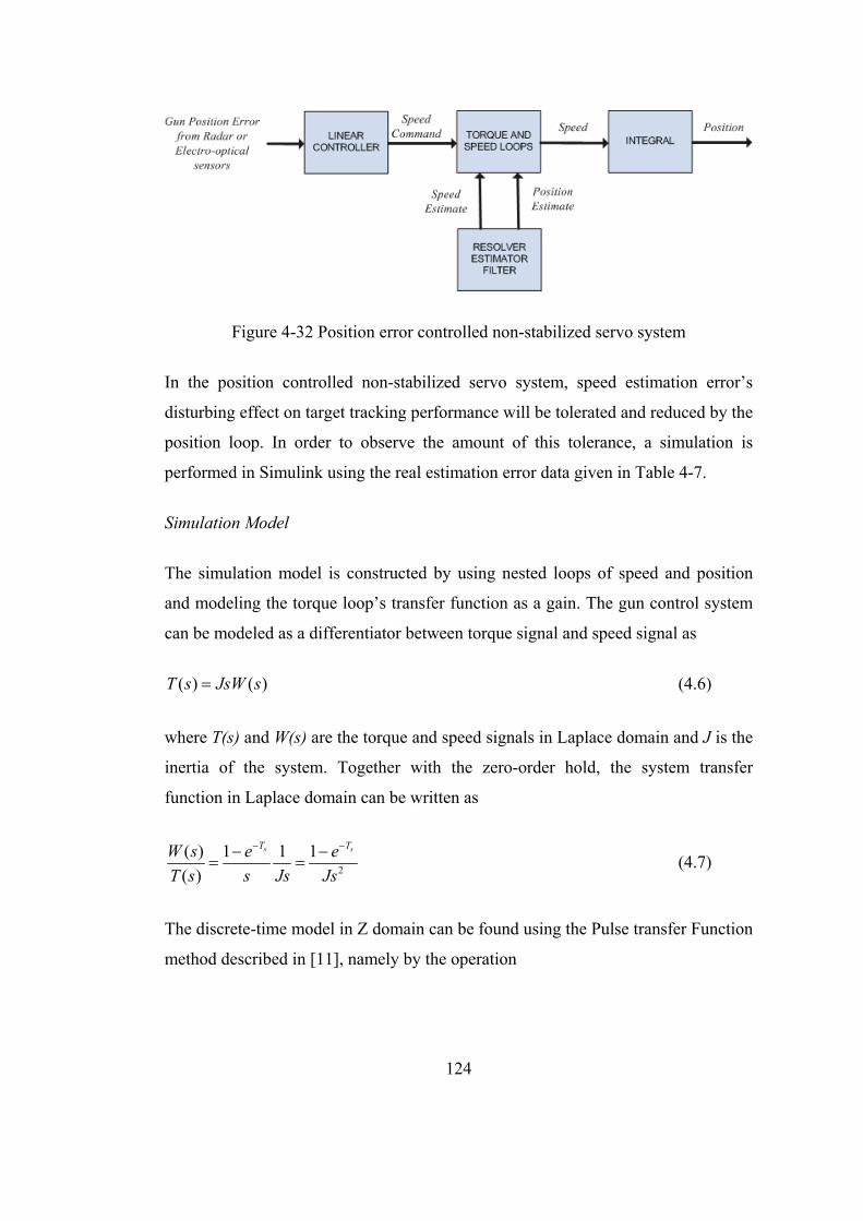
124

Figure 4-32 Position error controlled non-stabilized servo system

In the position controlled non-stabilized servo system, speed estimation error’s

disturbing effect on target tracking performance will be tolerated and reduced by the

position loop. In order to observe the amount of this tolerance, a simulation is

performed in Simulink using the real estimation error data given in Table 4-7.

Simulation Model

The simulation model is constructed by using nested loops of speed and position

and modeling the torque loop’s transfer function as a gain. The gun control system

can be modeled as a differentiator between torque signal and speed signal as

( ) ( )T s JsW s (4.6)

where T(s) and W(s) are the torque and speed signals in Laplace domain and J is the

inertia of the system. Together with the zero-order hold, the system transfer

function in Laplace domain can be written as

2

( ) 1 1 1

( )

s sT TW s e e

T s s Js Js

(4.7)

The discrete-time model in Z domain can be found using the Pulse transfer Function

method described in [11], namely by the operation

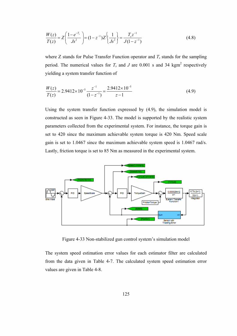
125

11

2 2 1

( ) 1 1(1 )

( ) (1 )

sTsT zW z e

Z z ZT z Js Js J z

(4.8)

where Z stands for Pulse Transfer Function operator and Ts stands for the sampling

period. The numerical values for Ts and J are 0.001 s and 34 kgm2 respectively

yielding a system transfer function of

1 55

1

( ) 2.9412 102.9412 10

( ) (1 ) 1

W z z

T z z z

(4.9)

Using the system transfer function expressed by (4.9), the simulation model is

constructed as seen in Figure 4-33. The model is supported by the realistic system

parameters collected from the experimental system. For instance, the torque gain is

set to 420 since the maximum achievable system torque is 420 Nm. Speed scale

gain is set to 1.0467 since the maximum achievable system speed is 1.0467 rad/s.

Lastly, friction torque is set to 85 Nm as measured in the experimental system.

Figure 4-33 Non-stabilized gun control system’s simulation model

The system speed estimation error values for each estimator filter are calculated

from the data given in Table 4-7. The calculated system speed estimation error

values are given in Table 4-8.

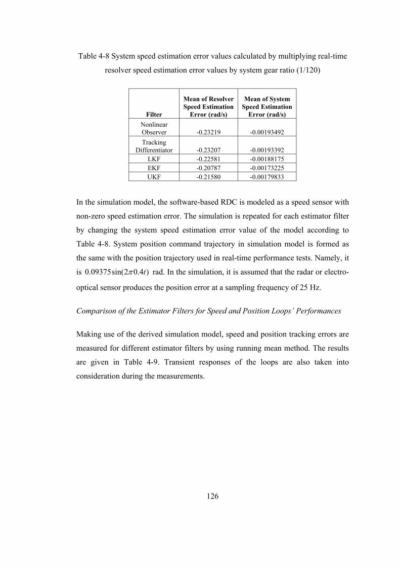
126

Table 4-8 System speed estimation error values calculated by multiplying real-time

resolver speed estimation error values by system gear ratio (1/120)

Filter

Mean of Resolver Speed Estimation

Error (rad/s)

Mean of System Speed Estimation

Error (rad/s)

Nonlinear Observer -0.23219 -0.00193492

Tracking Differentiator -0.23207 -0.00193392

LKF -0.22581 -0.00188175 EKF -0.20787 -0.00173225 UKF -0.21580 -0.00179833

In the simulation model, the software-based RDC is modeled as a speed sensor with

non-zero speed estimation error. The simulation is repeated for each estimator filter

by changing the system speed estimation error value of the model according to

Table 4-8. System position command trajectory in simulation model is formed as

the same with the position trajectory used in real-time performance tests. Namely, it

is 0.09375sin(2 0.4 )t rad. In the simulation, it is assumed that the radar or electro-

optical sensor produces the position error at a sampling frequency of 25 Hz.

Comparison of the Estimator Filters for Speed and Position Loops’ Performances

Making use of the derived simulation model, speed and position tracking errors are

measured for different estimator filters by using running mean method. The results

are given in Table 4-9. Transient responses of the loops are also taken into

consideration during the measurements.

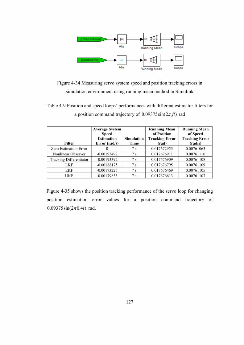
127

Figure 4-34 Measuring servo system speed and position tracking errors in

simulation environment using running mean method in Simulink

Table 4-9 Position and speed loops’ performances with different estimator filters for

a position command trajectory of 0.09375sin(2 )ft rad

Filter

Average System Speed

Estimation Error (rad/s)

Simulation Time

Running Mean of Position

Tracking Error (rad)

Running Mean of Speed

Tracking Error (rad/s)

Zero Estimation Error 0 7 s 0.017672955 0.00761063 Nonlinear Observer -0.00193492 7 s 0.017676911 0.00761110

Tracking Differentiator -0.00193392 7 s 0.017676909 0.00761108 LKF -0.00188175 7 s 0.017676795 0.00761109 EKF -0.00173225 7 s 0.017676469 0.00761105 UKF -0.00179833 7 s 0.017676613 0.00761107

Figure 4-35 shows the position tracking performance of the servo loop for changing

position estimation error values for a position command trajectory of

0.09375sin(2 0.4 )t rad.

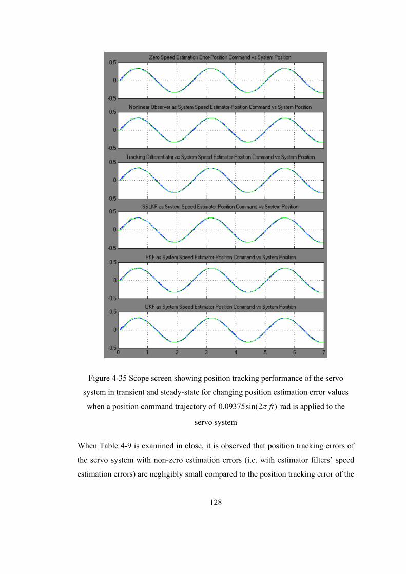
128

Figure 4-35 Scope screen showing position tracking performance of the servo

system in transient and steady-state for changing position estimation error values

when a position command trajectory of 0.09375sin(2 )ft rad is applied to the

servo system

When Table 4-9 is examined in close, it is observed that position tracking errors of

the servo system with non-zero estimation errors (i.e. with estimator filters’ speed

estimation errors) are negligibly small compared to the position tracking error of the

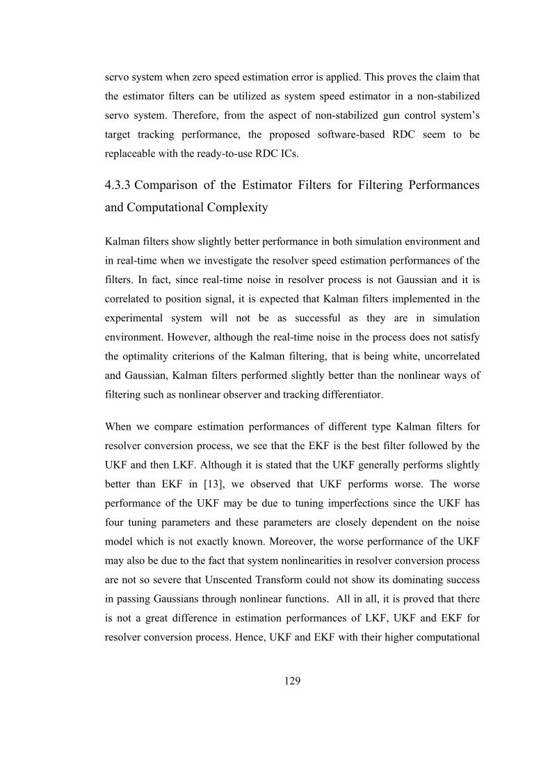
129

servo system when zero speed estimation error is applied. This proves the claim that

the estimator filters can be utilized as system speed estimator in a non-stabilized

servo system. Therefore, from the aspect of non-stabilized gun control system’s

target tracking performance, the proposed software-based RDC seem to be

replaceable with the ready-to-use RDC ICs.

4.3.3 Comparison of the Estimator Filters for Filtering Performances

and Computational Complexity

Kalman filters show slightly better performance in both simulation environment and

in real-time when we investigate the resolver speed estimation performances of the

filters. In fact, since real-time noise in resolver process is not Gaussian and it is

correlated to position signal, it is expected that Kalman filters implemented in the

experimental system will not be as successful as they are in simulation

environment. However, although the real-time noise in the process does not satisfy

the optimality criterions of the Kalman filtering, that is being white, uncorrelated

and Gaussian, Kalman filters performed slightly better than the nonlinear ways of

filtering such as nonlinear observer and tracking differentiator.

When we compare estimation performances of different type Kalman filters for

resolver conversion process, we see that the EKF is the best filter followed by the

UKF and then LKF. Although it is stated that the UKF generally performs slightly

better than EKF in [13], we observed that UKF performs worse. The worse

performance of the UKF may be due to tuning imperfections since the UKF has

four tuning parameters and these parameters are closely dependent on the noise

model which is not exactly known. Moreover, the worse performance of the UKF

may also be due to the fact that system nonlinearities in resolver conversion process

are not so severe that Unscented Transform could not show its dominating success

in passing Gaussians through nonlinear functions. All in all, it is proved that there

is not a great difference in estimation performances of LKF, UKF and EKF for

resolver conversion process. Hence, UKF and EKF with their higher computational

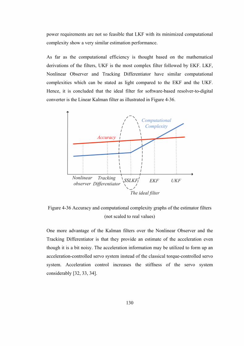
130

power requirements are not so feasible that LKF with its minimized computational

complexity show a very similar estimation performance.

As far as the computational efficiency is thought based on the mathematical

derivations of the filters, UKF is the most complex filter followed by EKF. LKF,

Nonlinear Observer and Tracking Differentiator have similar computational

complexities which can be stated as light compared to the EKF and the UKF.

Hence, it is concluded that the ideal filter for software-based resolver-to-digital

converter is the Linear Kalman filter as illustrated in Figure 4-36.

Figure 4-36 Accuracy and computational complexity graphs of the estimator filters

(not scaled to real values)

One more advantage of the Kalman filters over the Nonlinear Observer and the

Tracking Differentiator is that they provide an estimate of the acceleration even

though it is a bit noisy. The acceleration information may be utilized to form up an

acceleration-controlled servo system instead of the classical torque-controlled servo

system. Acceleration control increases the stiffness of the servo system

considerably [32, 33, 34].

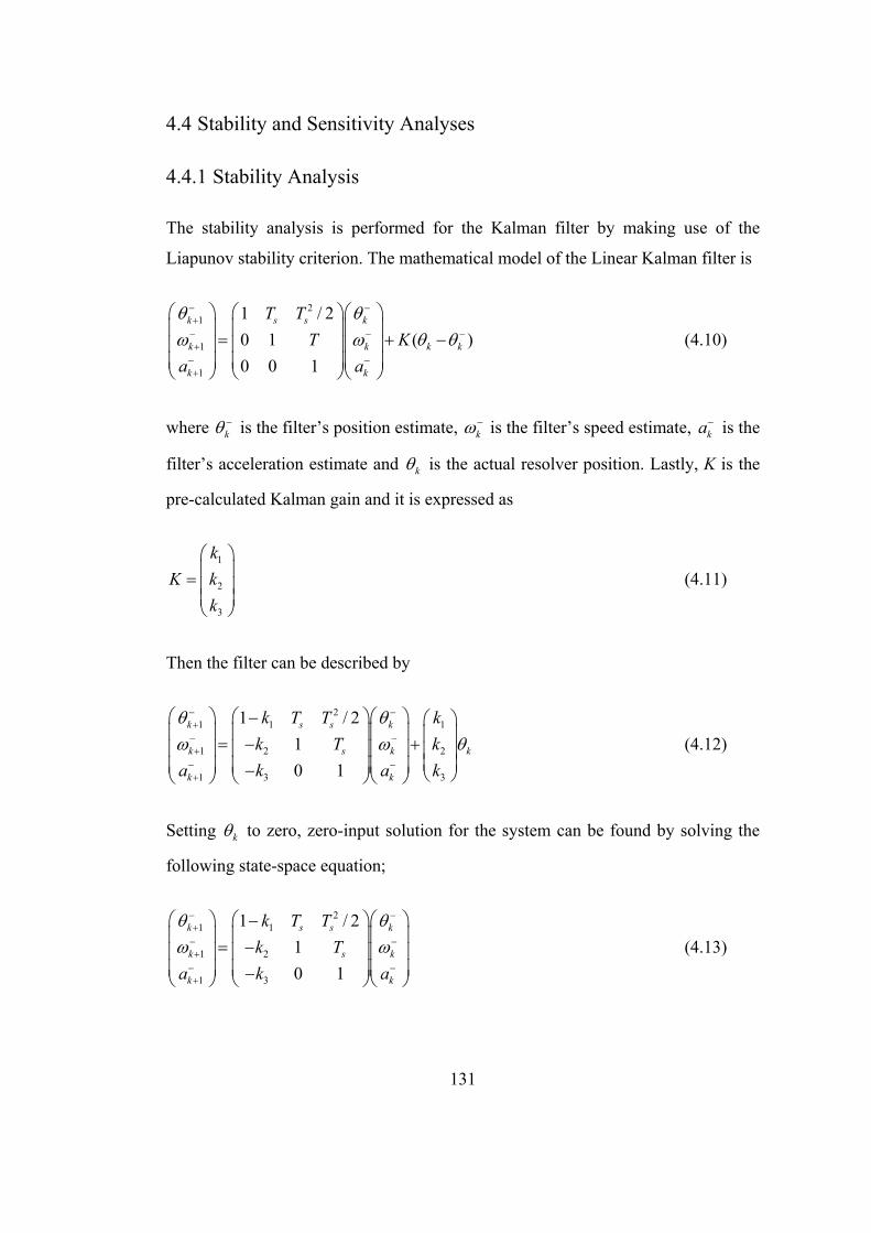
131

4.4 Stability and Sensitivity Analyses

4.4.1 Stability Analysis

The stability analysis is performed for the Kalman filter by making use of the

Liapunov stability criterion. The mathematical model of the Linear Kalman filter is

21

1

1

1 / 2

0 1 ( )

0 0 1

k s s k

k k k k

k k

T T

T K

a a

(4.10)

where k is the filter’s position estimate, k

is the filter’s speed estimate, ka is the

filter’s acceleration estimate and k is the actual resolver position. Lastly, K is the

pre-calculated Kalman gain and it is expressed as

1

2

3

k

K k

k

(4.11)

Then the filter can be described by

21 1 1

1 2 2

1 3 3

1 / 2

1

0 1

k s s k

k s k k

k k

k T T k

k T k

a k a k

(4.12)

Setting k to zero, zero-input solution for the system can be found by solving the

following state-space equation;

21 1

1 2

1 3

1 / 2

1

0 1

k s s k

k s k

k k

k T T

k T

a k a

(4.13)

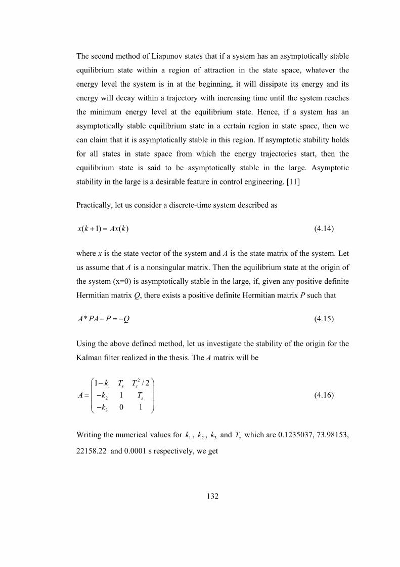
132

The second method of Liapunov states that if a system has an asymptotically stable

equilibrium state within a region of attraction in the state space, whatever the

energy level the system is in at the beginning, it will dissipate its energy and its

energy will decay within a trajectory with increasing time until the system reaches

the minimum energy level at the equilibrium state. Hence, if a system has an

asymptotically stable equilibrium state in a certain region in state space, then we

can claim that it is asymptotically stable in this region. If asymptotic stability holds

for all states in state space from which the energy trajectories start, then the

equilibrium state is said to be asymptotically stable in the large. Asymptotic

stability in the large is a desirable feature in control engineering. [11]

Practically, let us consider a discrete-time system described as

( 1) ( )x k Ax k (4.14)

where x is the state vector of the system and A is the state matrix of the system. Let

us assume that A is a nonsingular matrix. Then the equilibrium state at the origin of

the system (x=0) is asymptotically stable in the large, if, given any positive definite

Hermitian matrix Q, there exists a positive definite Hermitian matrix P such that

*A PA P Q (4.15)

Using the above defined method, let us investigate the stability of the origin for the

Kalman filter realized in the thesis. The A matrix will be

21

2

3

1 / 2

1

0 1

s s

s

k T T

A k T

k

(4.16)

Writing the numerical values for 1k , 2k , 3k and sT which are 0.1235037, 73.98153,

22158.22 and 0.0001 s respectively, we get

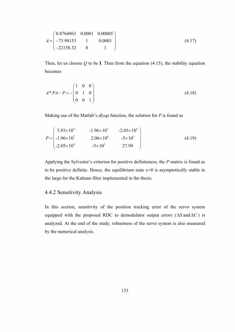
133

0.8764963 0.0001 0.00005

73.98153 1 0.0001

22158.32 0 1

A

(4.17)

Then, let us choose Q to be I. Then from the equation (4.15), the stability equation

becomes

1 0 0

* 0 1 0

0 0 1

A PA P

(4.18)

Making use of the Matlab’s dlyap function, the solution for P is found as

11 7 6

7 6 3

4 3

3.93 10 -1.96 10 -2.05 10

-1.96 10 2.06 10 -5 10

-2.05 10 -5 10 27.99

P

(4.19)

Applying the Sylvester’s criterion for positive definiteness, the P matrix is found as

to be positive definite. Hence, the equilibrium state x=0 is asymptotically stable in

the large for the Kalman filter implemented in the thesis.

4.4.2 Sensitivity Analysis

In this section, sensitivity of the position tracking error of the servo system

equipped with the proposed RDC to demodulator output errors ( S and C ) is

analyzed. At the end of the study, robustness of the servo system is also measured

by the numerical analysis.

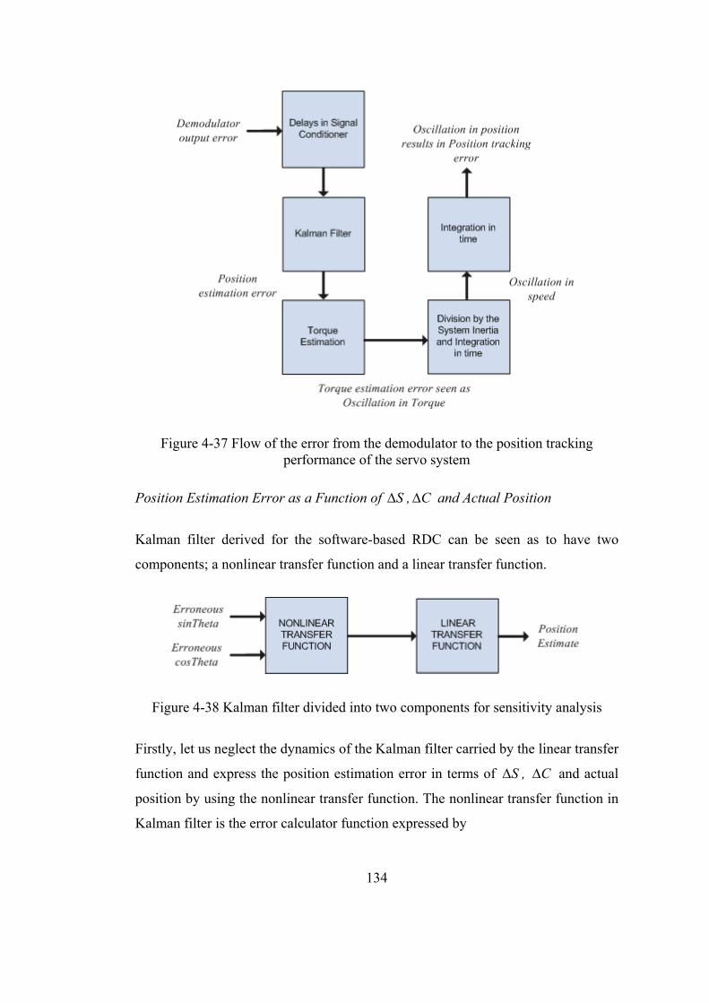
134

Figure 4-37 Flow of the error from the demodulator to the position tracking performance of the servo system

Position Estimation Error as a Function of S , C and Actual Position

Kalman filter derived for the software-based RDC can be seen as to have two

components; a nonlinear transfer function and a linear transfer function.

Figure 4-38 Kalman filter divided into two components for sensitivity analysis

Firstly, let us neglect the dynamics of the Kalman filter carried by the linear transfer

function and express the position estimation error in terms of S , C and actual

position by using the nonlinear transfer function. The nonlinear transfer function in

Kalman filter is the error calculator function expressed by

135

sin cos cos sin (4.20)

where is the actual resolver position and is the position estimate of the filter.

From the analysis performed in section 3.2.2, we know that if the Kalman filter

shows zero steady-state error, the position estimation error will be

cos sin sin cosC S (4.21)

Then, (4.21) can be expanded as

cos sin( ) sin cos( )C S (4.22)

Further expanding will yield

( , , ) cos (sin cos cos sin )

sin (cos cos sin sin )

C S C

S

(4.23)

Since will be very close to zero, we can assume cos to be 1 and sin to

be 0. Then, (4.23) will be reduced to

( , , ) cos sin sin cosC S C S (4.24)

Hence, the position estimation error due to demodulator output errors and actual

position can be approximated by (4.24).

This analysis gives the behavior of the filter with the assumption that the kalman

filter will track the input with zero steady-state error. However, for some values of

the filter parameter the assumption may not hold, that is, filter may show non-

zero steady-state error. Hence, the following analysis is performed to include the

Kalman filter’s dynamics in the sensitivity analysis as well.

Position Estimation Error as a Function of Filter Parameter and Resolver Speed

The Kalman filter is modeled by the following state-space representation;

136

21 1

1 2

1 3

1 / 2

0 1 ( )

0 0 1

k s s k

k s k k k

k k

T T k

T k

a a k

(4.25)

where k is the filter’s position estimate, k

is the filter’s speed estimate, ka is the

filter’s acceleration estimate and k is the actual resolver position. Lastly, K is the

pre-calculated Kalman gain and it is expressed by

1

2

3

k

K k

k

(4.26)

Let us make use of Z-transform method in extracting the transfer function of the

filter. The following equations can be written in Z domain.

1 13( )a z a k z (4.27)

1 1 12 ( ) sz k z T z a (4.28)

21 1 1 1

1( )2s

s

Tz k z T z z a (4.29)

where the following definitions are given

k

k

k

k

a Z a

Z

Z

Z

(4.30)

Writing (4.27) into (4.28), an expression for in terms of and is derived.

When the derived expression and (4.27) are both written into (4.29), the following

linear transfer function is obtained.

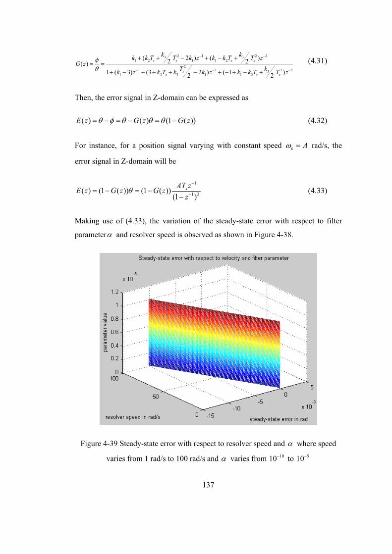
137

2 1 2 23 31 2 1 1 2

21 2 2 33

1 2 3 1 1 2

( 2 ) ( )2 2( )1 ( 3) (3 2 ) ( 1 )2 2

s s s s

ss s s

k kk k T T k z k k T T zG z

T kk z k T k k z k k T T z

(4.31)

Then, the error signal in Z-domain can be expressed as

( ) ( ) (1 ( ))E z G z G z (4.32)

For instance, for a position signal varying with constant speed k A rad/s, the

error signal in Z-domain will be

1

1 2( ) (1 ( )) (1 ( ))

(1 )sAT z

E z G z G zz

(4.33)

Making use of (4.33), the variation of the steady-state error with respect to filter

parameter and resolver speed is observed as shown in Figure 4-38.

Figure 4-39 Steady-state error with respect to resolver speed and where speed

varies from 1 rad/s to 100 rad/s and varies from 1010 to 510

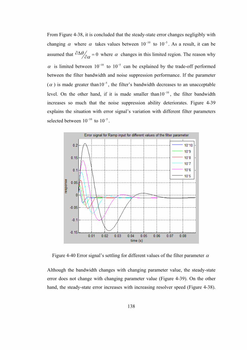
138

From Figure 4-38, it is concluded that the steady-state error changes negligibly with

changing where takes values between 1010 to 510 . As a result, it can be

assumed that 0

where changes in this limited region. The reason why

is limited between 1010 to 510 can be explained by the trade-off performed

between the filter bandwidth and noise suppression performance. If the parameter

( ) is made greater than 510 , the filter’s bandwidth decreases to an unacceptable

level. On the other hand, if it is made smaller than 1010 , the filter bandwidth

increases so much that the noise suppression ability deteriorates. Figure 4-39

explains the situation with error signal’s variation with different filter parameters

selected between 1010 to 510 .

Figure 4-40 Error signal’s settling for different values of the filter parameter

Although the bandwidth changes with changing parameter value, the steady-state

error does not change with changing parameter value (Figure 4-39). On the other

hand, the steady-state error increases with increasing resolver speed (Figure 4-38).

139

Hence, we can claim that the estimation error is dependent on not only the resolver

position but also resolver speed. This situation can be explained mathematically by

the final-value theorem. The steady-state error will be

1 1 1 1

1 0 1 2 3 41 1 1 11 1

1 2 3 4

0 1 2 3 4

1 2

(1 )(1 )(1 )(1 )( ) lim (1 ) ( ) lim

(1 )(1 )(1 )(1 )

(1 )(1 )(1 )(1 )

(1 )(1 )(1

z z

b b z b z b z b zA z E z A

a z a z a z a z

b b b b bA

a a a

3 4)(1 )a

(4.34)

where A is the actual resolver speed in rad/s and ib and ia are filter coefficients

calculated with the filter parameter . Hence, the theorem reveals that there will

always be a finite steady-state error whose amplitude is proportional to resolver

speed while the resolver rotates with a constant speed. By using the assumption

0

and numerical values of ib and ia , position estimation error due to

constant resolver speed can be formulated as

( ) 0.0000375 radA A (4.35)

Position Estimation Error Due to Filtering Delays

Another error source is the filtering delays which stem from implementation of anti-

aliasing filter, interpolation filter and high-pass filter on resolver channels. The

expression (4.36) has been derived in section 3.2.5 and it gives the position

estimation error with respect to resolver speed as

( ) 0.00040965 rad (4.36)

where is the resolver speed in rad/s.

Total Position Estimation Error

Making use of (4.24), (4.35) and (4.36), the total position estimation error can be

approximated by the following expression;

140

( , , , , ) cos sin sin cos

0.0000375 0.00040965 rad

C S A C S

A

(4.37)

where C and S are demodulator output percentage errors for cosine and sine

channels respectively, A is the constant resolver speed in rad/s and is the

resolver speed in rad/s. Since the expression is derived for constant speed case, the

third and the fourth terms can be unified reducing (4.37) to

( , , , ) cos sin sin cos 0.00044715C S A C S A (4.38)

Then, sensitivity of the position estimation error to C and S can be found using

partial derivatives such as

cos sinC

(4.39)

and

sin cosS

(4.40)

The sensitivity of the position estimation error to filter parameter has been found

as negligibly small in the region where the filter has acceptable bandwidth and

noise rejection performance. Similarly, we can also neglect the sensitivity of the

position estimation error to constant speed A since the related coefficient in (4.38) is

negligibly small. Hence, the sensitivity of the position estimation error to filter

parameter and resolver speed is assumed to be zero throughout the sensitivity

analysis.

Figure 4-40 visualizes sensitivity of the nonlinear transfer function to demodulator

output percentage errors S and C .

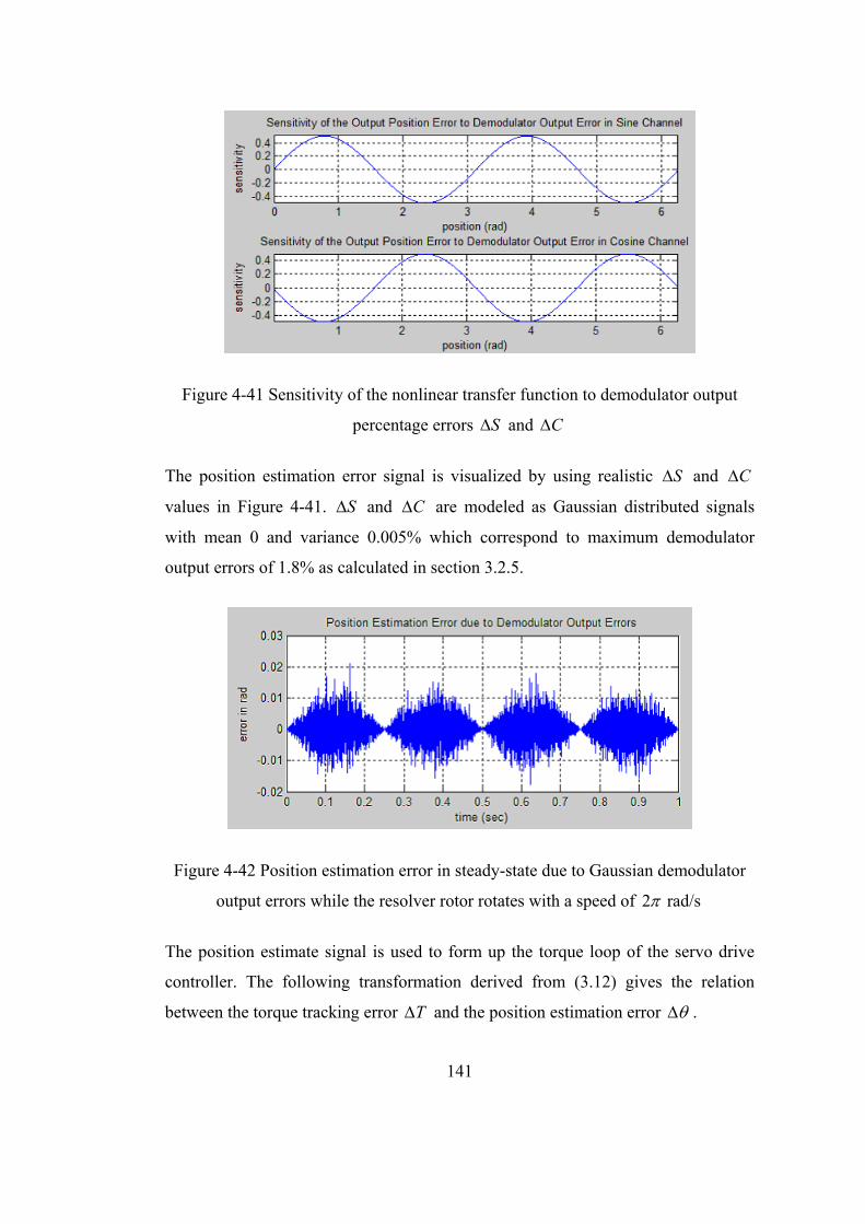
141

Figure 4-41 Sensitivity of the nonlinear transfer function to demodulator output

percentage errors S and C

The position estimation error signal is visualized by using realistic S and C

values in Figure 4-41. S and C are modeled as Gaussian distributed signals

with mean 0 and variance 0.005% which correspond to maximum demodulator

output errors of 1.8% as calculated in section 3.2.5.

Figure 4-42 Position estimation error in steady-state due to Gaussian demodulator

output errors while the resolver rotor rotates with a speed of 2 rad/s

The position estimate signal is used to form up the torque loop of the servo drive

controller. The following transformation derived from (3.12) gives the relation

between the torque tracking error T and the position estimation error .

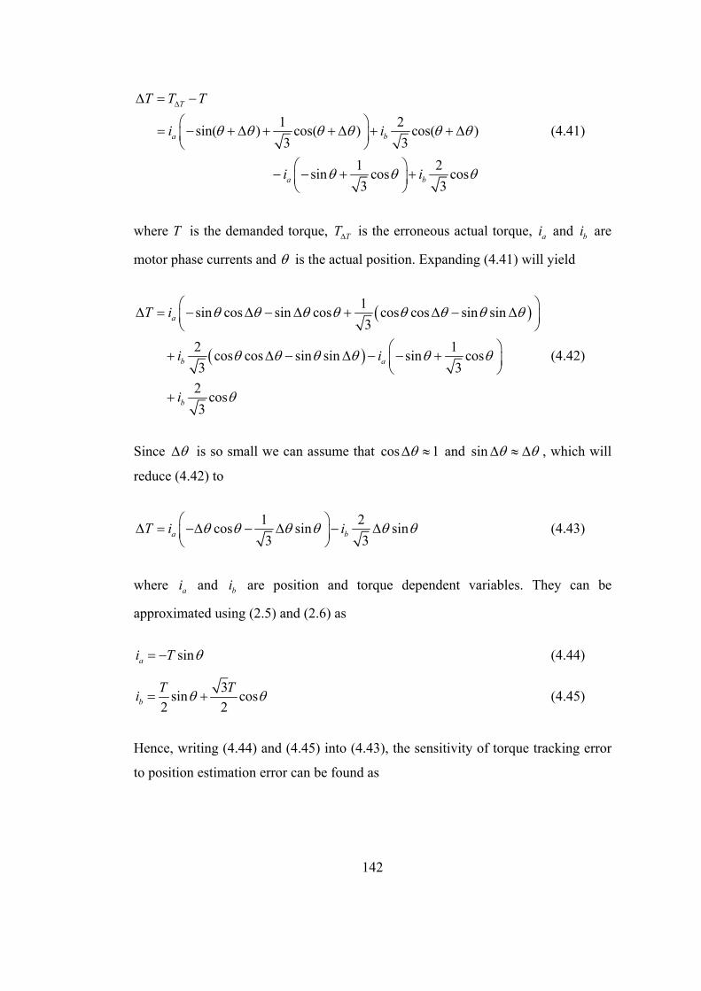
142

1 2 sin( ) cos( ) cos( )

3 3

1 2 sin cos cos

3 3

T

a b

a b

T T T

i i

i i

(4.41)

where T is the demanded torque, TT is the erroneous actual torque, ai and bi are

motor phase currents and is the actual position. Expanding (4.41) will yield

1sin cos sin cos cos cos sin sin

3

2 1 cos cos sin sin sin cos

3 3

2 cos

3

a

b a

b

T i

i i

i

(4.42)

Since is so small we can assume that cos 1 and sin , which will

reduce (4.42) to

1 2cos sin sin

3 3a bT i i

(4.43)

where ai and bi are position and torque dependent variables. They can be

approximated using (2.5) and (2.6) as

sinai T (4.44)

3sin cos

2 2b

T Ti (4.45)

Hence, writing (4.44) and (4.45) into (4.43), the sensitivity of torque tracking error

to position estimation error can be found as

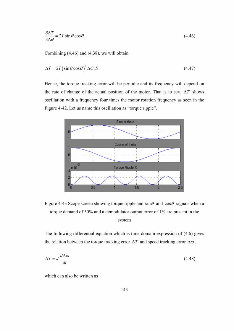
143

2 sin cosT

T

(4.46)

Combining (4.46) and (4.38), we will obtain

22 sin cos ,T T C S (4.47)

Hence, the torque tracking error will be periodic and its frequency will depend on

the rate of change of the actual position of the motor. That is to say, T shows

oscillation with a frequency four times the motor rotation frequency as seen in the

Figure 4-42. Let us name this oscillation as “torque ripple”.

Figure 4-43 Scope screen showing torque ripple and sin and cos signals when a

torque demand of 50% and a demodulator output error of 1% are present in the

system

The following differential equation which is time domain expression of (4.6) gives

the relation between the torque tracking error T and speed tracking error .

dT J

dt

(4.48)

which can also be written as

144

2

1

1t

t

TdtJ

(4.49)

where J is the inertia of the system. Then, the sensitivity of speed tracking error to

torque tracking error can be derived by differentiating both sides of (4.49) with

respect to T .

2 2

1 1

2 1

1 1 1( )

t t

t t

TTdt dt t t

T T J J T J

(4.50)

Similarly, the system position tracking error is the time-based integral of the

system speed tracking error .

2

1

t

t

dt (4.51)

Hence, the sensitivity function can be written as

2 2

1 1

2 1( )t t

t t

dt dt t t

(4.52)

Consequently, an oscillation on the torque signal will induce an oscillation on the

system speed at the same frequency. Similarly an oscillation on the speed signal

will induce an oscillation on the position signal at the same frequency. Hence, 2t

and 1t values in (4.50) and (4.52) should be determined based on the torque ripple

frequency. If we perform the worst case analysis, the integration time 2 1( )t t

should be chosen as

2 11( ) 2 T

t t f (4.53)

145

where Tf is the frequency of the torque ripple which has been determined as four

times the motor rotation frequency from (4.47).

The overall sensitivity function which relates the system position tracking error to

the demodulator output error can be found from the chain rule as

, ,

T

C S C S T

(4.54)

which yields (4.55) by (4.52), (4.50), (4.46), (4.40) and (4.39).

2 2

2 1

2cos sin

,

Tt t

C S J

(4.55)

Then, for any value of C or S , let us call them 'C and 'S , can be

found by the integral term

', '

2 2

2 1

0

2, cos sin ', '

,

C S Td C S t t C S

C S J

(4.56)

When (5.56) is inspected closely, it is observed that T and J works adversely, that

is, as the torque demand T increases, position tracking error increases whereas as

the inertia of the system J increases, position tracking error decreases for a constant

demodulator output error. It is also concluded that the position tracking error is

dependent on the actual motor position ( ). Moreover, as 2 1( )t t increases, in

other words, as the frequency of the torque tracking error decreases, position

tracking error increases. This result makes it necessary that the analysis will be

performed for a determined operation frequency of the motor. Hence, let us assume

that the motor operates at a very low frequency, namely 1 Hz inducing a 4 Hz

torque ripple. Then, 2 1( )t t can be calculated as 0.125 s from (4.53). Let us also

assume that there is a torque demand of 71.2 Nm which induces the maximum

permissible acceleration in the system (120°/sec2). This operation condition may be

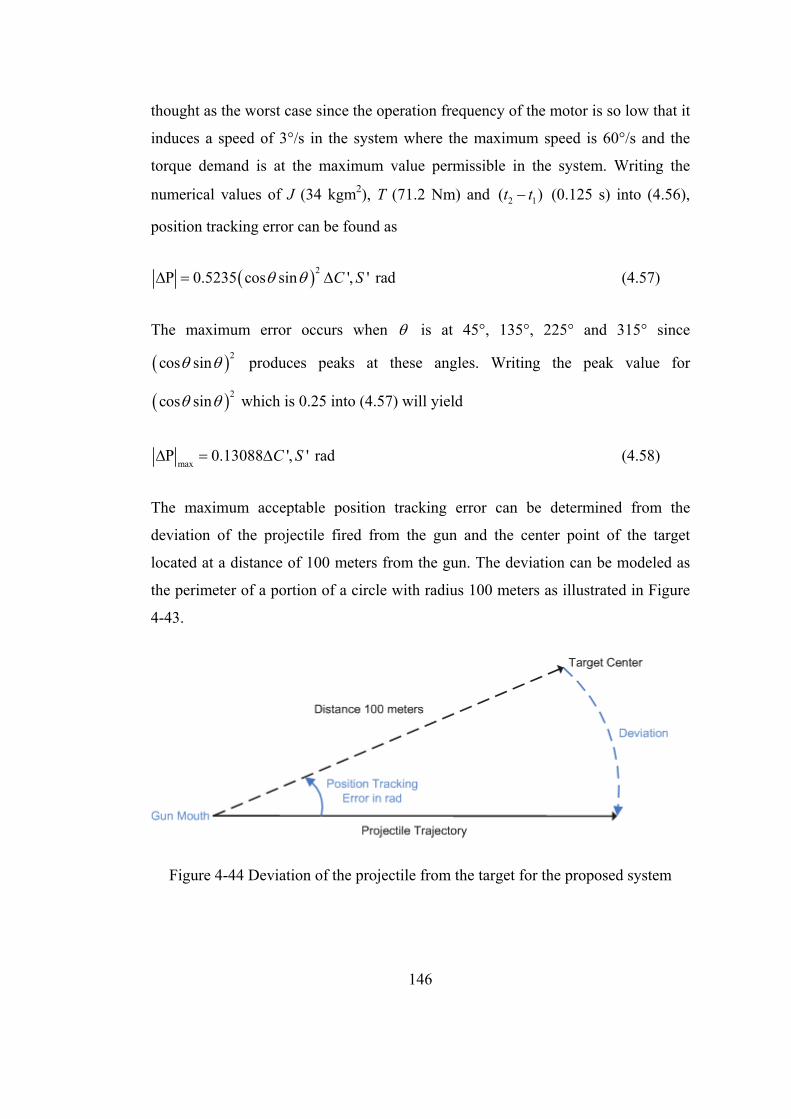
146

thought as the worst case since the operation frequency of the motor is so low that it

induces a speed of 3°/s in the system where the maximum speed is 60°/s and the

torque demand is at the maximum value permissible in the system. Writing the

numerical values of J (34 kgm2), T (71.2 Nm) and 2 1( )t t (0.125 s) into (4.56),

position tracking error can be found as

20.5235 cos sin ', ' radC S (4.57)

The maximum error occurs when is at 45°, 135°, 225° and 315° since

2cos sin produces peaks at these angles. Writing the peak value for

2cos sin which is 0.25 into (4.57) will yield

max0.13088 ', ' radC S (4.58)

The maximum acceptable position tracking error can be determined from the

deviation of the projectile fired from the gun and the center point of the target

located at a distance of 100 meters from the gun. The deviation can be modeled as

the perimeter of a portion of a circle with radius 100 meters as illustrated in Figure

4-43.

Figure 4-44 Deviation of the projectile from the target for the proposed system

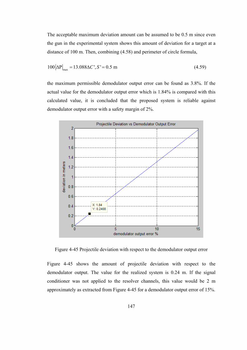
147

The acceptable maximum deviation amount can be assumed to be 0.5 m since even

the gun in the experimental system shows this amount of deviation for a target at a

distance of 100 m. Then, combining (4.58) and perimeter of circle formula,

max100 13.088 ', ' 0.5 mC S (4.59)

the maximum permissible demodulator output error can be found as 3.8%. If the

actual value for the demodulator output error which is 1.84% is compared with this

calculated value, it is concluded that the proposed system is reliable against

demodulator output error with a safety margin of 2%.

Figure 4-45 Projectile deviation with respect to the demodulator output error

Figure 4-45 shows the amount of projectile deviation with respect to the

demodulator output. The value for the realized system is 0.24 m. If the signal

conditioner was not applied to the resolver channels, this value would be 2 m

approximately as extracted from Figure 4-45 for a demodulator output error of 15%.

148

It is important to state that the error values determined by this analysis are the

maximum errors that the probability of seeing these levels of errors is very low

because;

The demodulator output error values has been calculated for the worst case

analysis,

Improving effects of the closed-loop control are neglected in the analysis

and transients are taken into consideration since the system is more

vulnerable to such imperfections in transients,

Operating frequency and system acceleration values are selected to

guarantee the worst case analysis.

In conclusion, the proposed system is claimed to be robust against the most

effective imperfection, that is, demodulator output error, under the most severe

condition it can face up with.

Sensitivity of Errors to Analog-to-Digital Conversion Rate

Analog-to-digital conversion rate comes up as the most important parameter of the

proposed system. As the conversion rate goes towards infinity, frequency cut-off

points of the anti-aliasing filter and the interpolation filter also move along the

frequency axis towards the infinity. In the limit point, that is, in continuous-time

domain, as a matter of fact, we neither need the anti-aliasing filter nor the

interpolation filter since necessity for these filters arises from the digitization of the

converter. Therefore, as the analog-to-digital conversion rate comes down along the

frequency axis from infinity to Nyquist rate, the position estimation error of the

software-based RDC increases due to both increasing filtering delays and increasing

aliasing.

149

CHAPTER 5

CONCLUSION AND FUTURE WORK

5.1 Conclusion of the Thesis

The objective of this thesis has been stated to develop a software-based resolver-to-

digital converter to be utilized in weapon systems. The motivation behind this

objective is to enhance the servo controllers used in weapon systems in terms of

adaptability to changing system structures. For this purpose, enhancing the

independency of the servo system to hardware components in realization of system

functions becomes more of an issue. Hence, a software-based resolver-to-digital

converter which eliminates the need for special hardware components for resolver

conversion contributes to this motivation.

Excited with a reference signal, a resolver gives out two amplitude modulated

signals. Measuring the reference signal and the amplitude modulated signals, the

software-based RDC estimates position and speed of the resolver by the help of

three components. These components can be specified as signal conditioner, phase-

sensitive demodulator and estimator filter.

The resolver signals have harmonic distortions and high-frequency noise due to

several imperfections present in the servo system. Such imperfections may decrease

the quality of the demodulation, which consequently increases the position

estimation error. Increased position estimation error in turn induces oscillations on

the torque signal. As a consequence of the torque oscillations, the speed of the

system also oscillates, which may prevent the weapon system from realizing its

main function that is stabilizing the speed of the gun. Therefore, at the beginning of

150

the thesis study, an analysis examining the levels of harmonic distortions and noise

present in resolver signals and their possible effects on torque and speed of the

servo system is performed. Based on the result of the analysis, it is concluded that

suppression of the harmonic distortions and noise is indispensable for the

experimental system to obtain ripple-free torque and speed signals. Hence, a mixed-

signal signal conditioner is designed to be used in front of the phase-sensitive

demodulator. The signal conditioner suppresses the deteriorating effects of the

resolver signal imperfections on the demodulation. Namely, the demodulator output

error is decreased from 15.24% to 1.84% by the application of the signal

conditioner. As a result, amplitude of the oscillations on the torque signal is

decreased from 1% to 0.02% where the latter value is proved to be an acceptable

torque error value by the sensitivity analysis.

The phase sensitive demodulator, as the name implies, demodulates the amplitude

modulated resolver signals by also sensing their phases with respect to the reference

signal. For realization of this function, the demodulator utilizes several components

which may be specified as zero-crossing detectors, half-period integrators, a phase

detector, two’s complementers, negative cycle detectors and some other logic

elements. The performance of the designed demodulator is highly satisfactory that

the quantization error at the demodulator output becomes less than 50.5 10

percent. The developed demodulator reduces the effort consumed for adaptation of

the servo system to a different sensor. Furthermore, the demodulator provides

interface with any type of resolver without needing any hardware modification and

by changing only one parameter embedded in the FPGA code.

Several estimator filters are analyzed in both simulation environment and in real-

time. The real-time analysis is performed on a DSP board which has necessary

components to realize the aforesaid signal conditioner and FPGA-based phase

sensitive demodulator. The analyzed estimator filters are;

Nonlinear observer proposed in [21]

151

Tracking differentiator adapted to resolver conversion process

Linear Kalman filter adapted to resolver conversion process

Extended Kalman filter adapted to resolver conversion process

Unscented Kalman filter adapted to resolver conversion process

Since the algorithms are implemented in real-time, not only the estimation

performances but also algorithmic complexities of the algorithms are of great

importance. Less complexity with higher performance is always the point where we

would like to reach for a real-time system. In the implemented algorithms, although

the complexity increases severely from nonlinear observer to unscented kalman

filter, the estimation accuracy does not increase in a parallel manner to the

increasing complexity. At the end of the performed performance analyses, it is

concluded that the most practicable filter for resolver conversion is the Linear

Kalman filter.

Stability and sensitivity analyses are also performed for the proposed system. The

system is proved to be stable according to Liapunov’s stability criterion and robust

against the most effective disturbances of the system which can be specified as

demodulator output errors and delays in filtering circuits. The sensitivity analysis

also shows that it is possible to improve the performance of the proposed system by

increasing the sampling frequency of the analog-to-digital converters since

increased sampling frequency will decrease the level of the aforesaid disturbances.

The replacebility of the ready-to-use RDC IC’s with the proposed software-based

RDC is proved by the performed analyses. The effects of the position and speed

estimation errors on system torque, system speed and system position are analyzed

and it is observed that the performance of the servo system equipped with the

proposed system is highly satisfactory.

152

5.2 Future Work

Torque produced by the servo motor fluctuates due to several reasons in a servo

system. Torque ripples can be classified according to their frequency spectrum;

high-frequency ripple components and low frequency ripple components. Absorbed

by the inertia, high-frequency ripple components generally do not result in

disturbing effects on the system performance. On the other hand, low-frequency

ripple components have dramatic effects on the system performance. Low-

frequency ripple components spread into the system speed and turn into real

motions which deflect the system performance from the demanded behavior.

Moreover, these ripples prevent designers from increasing speed loop gains

sufficiently because they are amplified more by higher controller gains. On the

other hand, decreasing the gains, a more serious problem is observed. Lower speed

loop gains result in unsatisfactory system performance and deteriorates tracking

abilities of the servo system. That is to say, the torque ripple problem which may be

seen as a simple problem turns into a serious one.

During the thesis study, it is observed that low bandwidth of torque loop results in

torque ripples in the servo system. This is due to the fact that torque loop cannot

compensate for disturbing effects coming from gears of the system. Since these

disturbing effects’ frequency spectrum exceeds the bandwidth of the torque loop,

the loop can not respond fast enough and oscillations are observed on the torque

signal. Uncompensated back-EMF and nonlinear characteristics of drive electronics

and motor decreases the torque loop’s bandwidth and amplifies the torque ripples.

PWM inverter, connected series to motor resistance and inductance, enables

transferring electrical power from a DC bus to the servo motor using sinusoidal

modulated PWM signals. The servo motor converts electrical energy into

mechanical energy and it produces torque on the rotating shaft. This energy transfer

is realized with three phase balanced AC currents. An AC servo motor produces a

ripple-free torque signal when current waveforms are pure sinusoidals and do not

153

show harmonic distortions. However, nonlinearities and imperfections of PWM

inverter, servo motor and drive electronics result in harmonic distortions in the

current waveforms. As a result, torque shows fluctuations which eventually corrupt

the speed loop and deteriorate its performance.

In summary, torque fluctuations will always exist in a servo system with a wide

frequency spectrum. Low frequency components may result from nonlinear motor

characteristics, PWM dead band, nonlinear resistance and inductance of motor

windings, nonlinear effects of the bus, snubber circuits, PWM inverter, gain and

offset errors in current sensing and voltage drop across the switching elements.

High-frequency ripple components may stem from position sensor inaccuracies, low

bandwidth current sensors, PWM modulation technique, inadequate bus capacity,

low sampling-time and low frequency PWM signals. High-frequency fluctuations in

a heavy system may be absorbed by the inertia. However, if low frequency torque

ripples are present in torque, then speed of the system will also fluctuate. Needless

to say that this will occur if the frequency of the fluctuations is within the system

bandwidth. Consequently, low frequency torque fluctuations are not welcome in a

servo drive system and should be minimized possibly. Hence, the future work will

cover an analysis of this problem and propose a method for removal of the problem

with compensation of back-EMF and nonlinear effects. The method may make use

of neural networks such as Echo State Network for identification of back-EMF and

nonlinear effects.

154

REFERENCES

[1] “Sensorless Control with Kalman Filter on TMS320 Fixed-Point DSP”, Texas

Instruments Europe, July 1997.

[2] L. Harnefors, “Speed Estimation from Noisy Resolver Signals”, Royal Institute

of Technology, Stockholm, Sweden, 1996.

[3] Wikipedia Organization, “Servomechanism”, “en.wikipedia.org”, November

2009.

[4] Wally Rippel, “Induction Versus DC Brushless Motors”,

“www.teslamotors.com”, January 2007.

[5] “Field Orientated Control of 3-Phase AC Motors”, Texas Instruments Europe,

February 1998.

[6] Grenier, D., L.-A. Dessaint, O. Akhrif, Y. Bonnassieux and B. LePioufle,

"Experimental Nonlinear Torque Control of a Permanent Magnet Synchronous

Motor Using Saliency," IEEE Transactions on Industrial Electronics, Vol. 44, No.

5, October 1997, pp. 680-687.

[7] Ong, Chee-Mun., “Dynamic Simulation of Electric Machinery”, Prentice Hall,

1998.

[8] A. Ometto, “Modulation Techniques”, Università degli Studi di L’Aquila.

[9] Zhenyu Yu, “Space-Vector PWM with TMS320C24x/F24x Using Hardware

and Software Determined Switching Patterns”, Texas Instruments, March 1999.

155

[10] Robert H. Stewart, “Ocean Wave Spectra”, Department of Oceanography,

Texas A&M University, 2005.

[11] Katsuhiko Ogata, “Discrete-Time Control Systems”, Prentice Hall Inc, New

Jersey, pp. 90-121, 327-336, 1995.

[12] Dan Simon, “Optimal State Estimation”, John Wiley and Sons Inc, New

Jersey, pp. 53-58, 123-145, 433-457, 2006.

[13] Sebestian Thrun, Wolfram Burgard and Dieter Fox, “Probabilistic Robotics”,

MIT Press, London, England, 2005, pp. 67-71.

[14] Geoffrey S. Boyes, “Synchro and Resolver Conversion”, Memory Devices

Ltd., London, Great Britain, 1980, pp. 7-45.

[15] Santanu Sarma, V.K. Agrawal and Subramanya Udupa, “Software-Based

Resolver-to-Digital Conversion Using a DSP”, IEEE Transactions on Industrial

Electronics, Vol. 55, No. 1, pp. 371-379, January 2008.

[16] Mohieddine Benammar, Lazhar Ben-Brahim, Mohd A. Alhamadi, “A Novel

Resolver-to-360° Linearized Converter”, IEEE Sensors Journal, Vol. 4, No. 1, pp.

96-101, February 2004.

[17] Mohieddine Benammar, Lazhar Ben-Brahim, Mohd A. Alhamadi, “A High

Precision Resolver-to-DC Converter”, IEEE Transactions on Instrumentation and

Measurement, Vol. 54, No. 6, pp. 2289-2296, December 2005.

[18] Mohieddine Benammar, Mohd A. Alhamadi, Nasser Al-Emadi, Mohammed

Al-Hitmi, “A New Angle Determination Method for Resolvers”, Electrical

Engineering Department, College of Engineering, Qatar University, 2008 IEEE.

156

[19] Armondo Bellini, Stefano Bifaretti and Stefano Constantini, “A PLL-Based

Filter for Speed Noise Reduction in Drives using a Resolver Transducer”,

Department of Electronic Engineering, University of Rome, IEEE 2002.

[20] Weera Kaewjinda and Mongkol Konghirun, “A DSP-based Vector Control of

PMSM Servo Drive Using Resolver Sensor”, King Mongkut’s University of

Technology, Department of Electrical Engineering, Bangkok, IEEE 2006.

[21] Lennart Harnefors and Hans-Peter Nee, “A General Algorithm for Speed and

Position Estimation of AC Motors”, IEEE Transactions on Industrial Electronics,

Vol. 47, No. 1, February 2000.

[22] B. A. Murray and W.D. Li, “A Digital Tracking R/D Converter with Hardware

Error Calculation Using a TMS320C14”, Department of Electronic Engineering,

Dublin City University, Ireland, 1993.

[23] Zhiqiang Gao, “From linear to nonlinear control means: a practical

progression”, Department of Electrical and Computer Enginnering, Cleveland State

University, USA, 2001.

[24] A. Levant,“Robust exact differentiation via sliding mode technique”,

Automatica, 34 (3), pp. 379-384, 1998.

[25] Y. X. Su, Dong Sun, B.Y. Duan, “Design of an enhanced nonlinear PID

controller”, Mechatronics 15 (2005), pp. 1005-1024.

[26] Guohui Qiao, Minglei Sun, Rong Zhang, Guanghua Zong and Shouzhong Li,

“An Improved Self-Adaptive Tracking Differentiator”, Proc. 2009 IEEE

International Conference on Information and Automation, pp. 980-984.

[27] Adrian Davies and Phil Fennessy, “Digital Imaging for Photographers”, Focal

Press, p. 30, 2001.

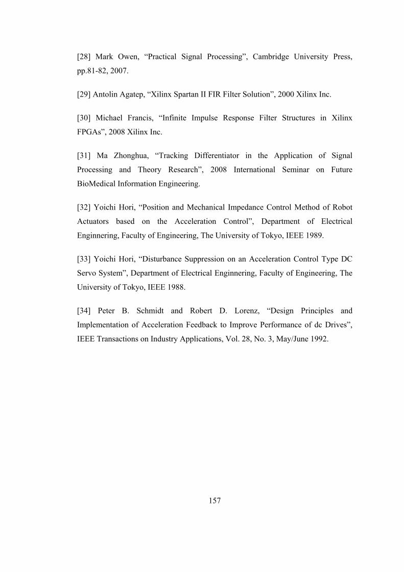
157

[28] Mark Owen, “Practical Signal Processing”, Cambridge University Press,

pp.81-82, 2007.

[29] Antolin Agatep, “Xilinx Spartan II FIR Filter Solution”, 2000 Xilinx Inc.

[30] Michael Francis, “Infinite Impulse Response Filter Structures in Xilinx

FPGAs”, 2008 Xilinx Inc.

[31] Ma Zhonghua, “Tracking Differentiator in the Application of Signal

Processing and Theory Research”, 2008 International Seminar on Future

BioMedical Information Engineering.

[32] Yoichi Hori, “Position and Mechanical Impedance Control Method of Robot

Actuators based on the Acceleration Control”, Department of Electrical

Enginnering, Faculty of Engineering, The University of Tokyo, IEEE 1989.

[33] Yoichi Hori, “Disturbance Suppression on an Acceleration Control Type DC

Servo System”, Department of Electrical Enginnering, Faculty of Engineering, The

University of Tokyo, IEEE 1988.

[34] Peter B. Schmidt and Robert D. Lorenz, “Design Principles and

Implementation of Acceleration Feedback to Improve Performance of dc Drives”,

IEEE Transactions on Industry Applications, Vol. 28, No. 3, May/June 1992.

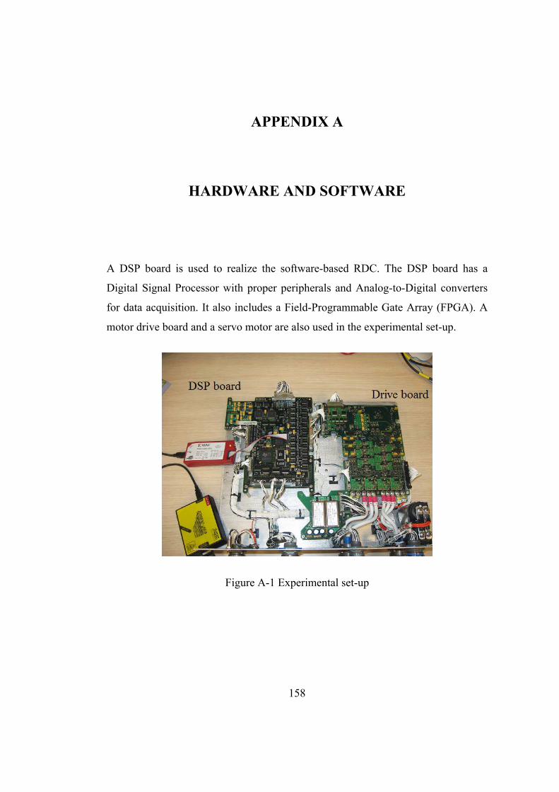
158

APPENDIX A

HARDWARE AND SOFTWARE

A DSP board is used to realize the software-based RDC. The DSP board has a

Digital Signal Processor with proper peripherals and Analog-to-Digital converters

for data acquisition. It also includes a Field-Programmable Gate Array (FPGA). A

motor drive board and a servo motor are also used in the experimental set-up.

Figure A-1 Experimental set-up

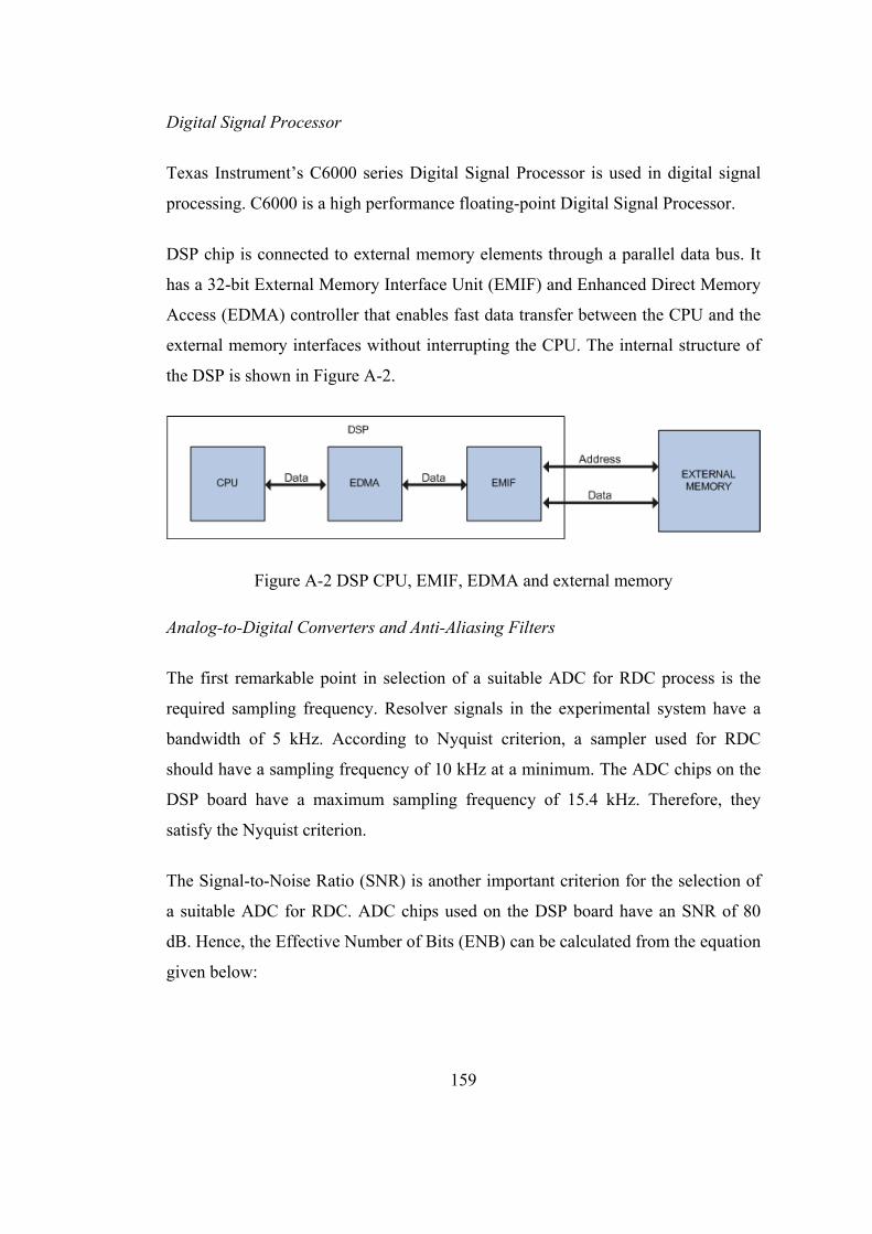
159

Digital Signal Processor

Texas Instrument’s C6000 series Digital Signal Processor is used in digital signal

processing. C6000 is a high performance floating-point Digital Signal Processor.

DSP chip is connected to external memory elements through a parallel data bus. It

has a 32-bit External Memory Interface Unit (EMIF) and Enhanced Direct Memory

Access (EDMA) controller that enables fast data transfer between the CPU and the

external memory interfaces without interrupting the CPU. The internal structure of

the DSP is shown in Figure A-2.

Figure A-2 DSP CPU, EMIF, EDMA and external memory

Analog-to-Digital Converters and Anti-Aliasing Filters

The first remarkable point in selection of a suitable ADC for RDC process is the

required sampling frequency. Resolver signals in the experimental system have a

bandwidth of 5 kHz. According to Nyquist criterion, a sampler used for RDC

should have a sampling frequency of 10 kHz at a minimum. The ADC chips on the

DSP board have a maximum sampling frequency of 15.4 kHz. Therefore, they

satisfy the Nyquist criterion.

The Signal-to-Noise Ratio (SNR) is another important criterion for the selection of

a suitable ADC for RDC. ADC chips used on the DSP board have an SNR of 80

dB. Hence, the Effective Number of Bits (ENB) can be calculated from the equation

given below:

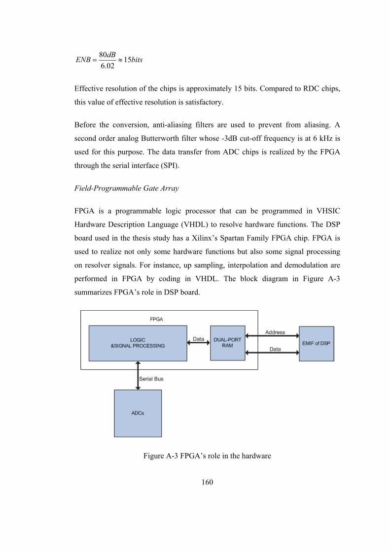
160

8015

6.02

dBENB bits

Effective resolution of the chips is approximately 15 bits. Compared to RDC chips,

this value of effective resolution is satisfactory.

Before the conversion, anti-aliasing filters are used to prevent from aliasing. A

second order analog Butterworth filter whose -3dB cut-off frequency is at 6 kHz is

used for this purpose. The data transfer from ADC chips is realized by the FPGA

through the serial interface (SPI).

Field-Programmable Gate Array

FPGA is a programmable logic processor that can be programmed in VHSIC

Hardware Description Language (VHDL) to resolve hardware functions. The DSP

board used in the thesis study has a Xilinx’s Spartan Family FPGA chip. FPGA is

used to realize not only some hardware functions but also some signal processing

on resolver signals. For instance, up sampling, interpolation and demodulation are

performed in FPGA by coding in VHDL. The block diagram in Figure A-3

summarizes FPGA’s role in DSP board.

Figure A-3 FPGA’s role in the hardware

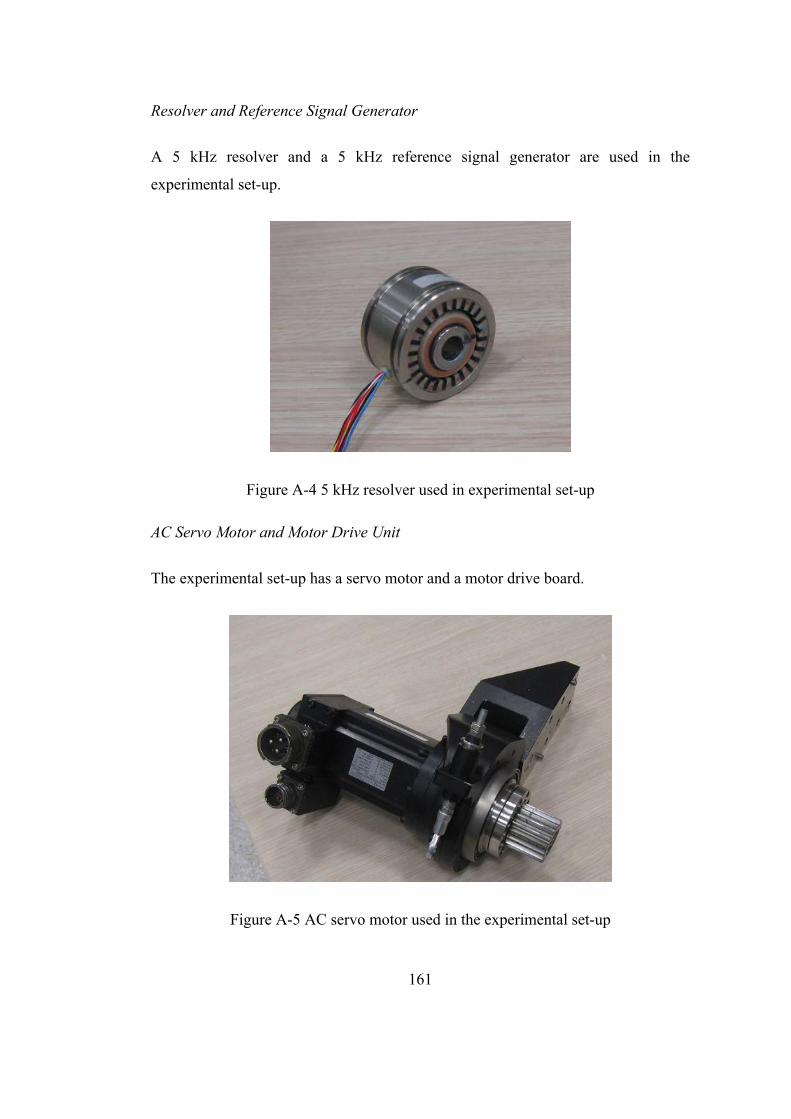
161

Resolver and Reference Signal Generator

A 5 kHz resolver and a 5 kHz reference signal generator are used in the

experimental set-up.

Figure A-4 5 kHz resolver used in experimental set-up

AC Servo Motor and Motor Drive Unit

The experimental set-up has a servo motor and a motor drive board.

Figure A-5 AC servo motor used in the experimental set-up

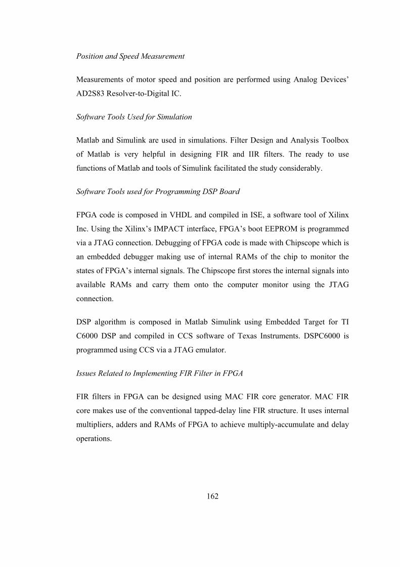
162

Position and Speed Measurement

Measurements of motor speed and position are performed using Analog Devices’

AD2S83 Resolver-to-Digital IC.

Software Tools Used for Simulation

Matlab and Simulink are used in simulations. Filter Design and Analysis Toolbox

of Matlab is very helpful in designing FIR and IIR filters. The ready to use

functions of Matlab and tools of Simulink facilitated the study considerably.

Software Tools used for Programming DSP Board

FPGA code is composed in VHDL and compiled in ISE, a software tool of Xilinx

Inc. Using the Xilinx’s IMPACT interface, FPGA’s boot EEPROM is programmed

via a JTAG connection. Debugging of FPGA code is made with Chipscope which is

an embedded debugger making use of internal RAMs of the chip to monitor the

states of FPGA’s internal signals. The Chipscope first stores the internal signals into

available RAMs and carry them onto the computer monitor using the JTAG

connection.

DSP algorithm is composed in Matlab Simulink using Embedded Target for TI

C6000 DSP and compiled in CCS software of Texas Instruments. DSPC6000 is

programmed using CCS via a JTAG emulator.

Issues Related to Implementing FIR Filter in FPGA

FIR filters in FPGA can be designed using MAC FIR core generator. MAC FIR

core makes use of the conventional tapped-delay line FIR structure. It uses internal

multipliers, adders and RAMs of FPGA to achieve multiply-accumulate and delay

operations.

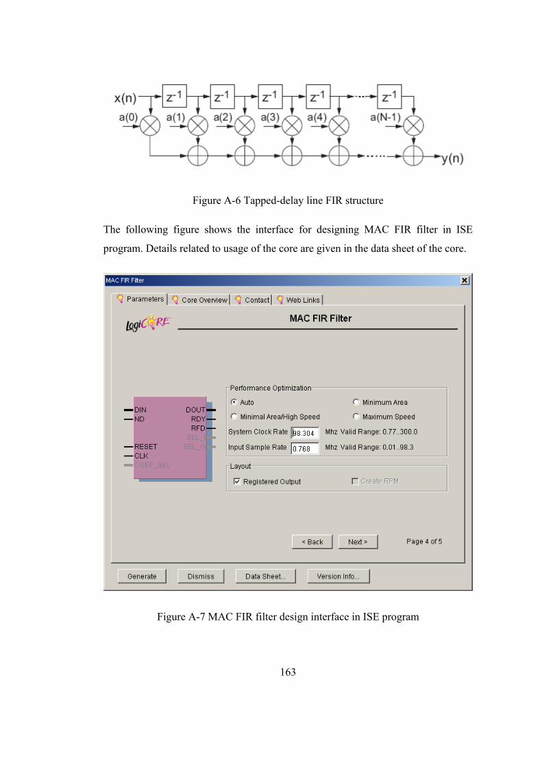
163

Figure A-6 Tapped-delay line FIR structure

The following figure shows the interface for designing MAC FIR filter in ISE

program. Details related to usage of the core are given in the data sheet of the core.

Figure A-7 MAC FIR filter design interface in ISE program