Development of a data analytics-driven information system for instant, temporary personalised discount offers by Zandaline Els Thesis presented in partial fulfilment of the requirements for the degree of Master of Engineering (Industrial Engineering) in the Faculty of Engineering at Stellenbosch University Supervisor: Prof JF Bekker April 2019

Welcome message from author
This document is posted to help you gain knowledge. Please leave a comment to let me know what you think about it! Share it to your friends and learn new things together.
Transcript
Development of a data analytics-driven information
system for instant, temporary personalised discount
offers
by
Zandaline Els
Thesis presented in partial fulfilment of the requirements for the degree of
Master of Engineering (Industrial Engineering) in the Faculty of Engineering
at Stellenbosch University
Supervisor: Prof JF Bekker
April 2019

Declaration
By submitting this thesis electronically, I declare that the entirety of the work con-
tained therein is my own, original work, that I am the sole author thereof (save to
the extent explicitly otherwise stated), that reproduction and publication thereof
by Stellenbosch University will not infringe any third party rights and that I have
not previously in its entirety or in part submitted it for obtaining any qualification.
Date: April 2019
Copyright © 2019 Stellenbosch University
All rights reserved
i
Stellenbosch University https://scholar.sun.ac.za

Acknowledgements
This study became a reality with the support from many individuals to whom
I would like to express my sincere gratitude. I would like to express my sincere
gratitude to my supervisor, Professor James Bekker. Thank you for the guidance
throughout this learning process.
To my USMA friends, who walked this path with me. Thank you for all the sup-
port, tips and memories. Then to my other friends, who did not always understand
what I meant, but encouraged me regardless.
To my family, for their unconditional love and specifically my parents for providing
me with this opportunity.
Lastly, thank you to Altron Bytes Systems Integration for the financial support
and Ms Anne Erikson for the language editing.
“Be fearless in the pursuit of what sets your soul on fire.” – Jennifer Lee
ii
Stellenbosch University https://scholar.sun.ac.za
Abstract
Enterprises have started including the targeting of customers with personalised
discount offers in their business strategies in order to seek a competitive advan-
tage over their peers. This innovation has been made possible by the integration of
knowledge and new technology such as data analytics, mobile- and cloud comput-
ing and the internet-of-things. Along with these digital technologies, the emphasis
on customer experience became the distinguishing factor amongst retail outlets.
A novel approach is presented in this study to create personalised discount offers
during a customer’s visit to one of many participating retail outlets. It focuses
on the individual customer’s purchasing history, which makes it different from the
loyalty programmes that are currently in use.
A simulator is developed to create pseudo-customer data containing purchasing
behaviour, whereafter a demonstrator is developed which provides a holistic view
of the customer’s behaviour in retail outlets. The demonstrator creates instant,
temporary personalised discount offers based on the purchasing tendencies of that
customer across various retail outlets. The model illustrates the utilisation of cus-
tomer behavioural data to identify unique cross-selling and upselling opportunities
to ultimately improve customer experience.
The cross-selling and upselling creates opportunities for alternative revenue streams
and this study provides a business case to display the business value of this system.
iii
Stellenbosch University https://scholar.sun.ac.za

Opsomming
Ondernemings het begin om kliente te teiken deur persoonlike afslagaanbied-
ings in hul sakestrategiee in te sluit ten einde ’n mededingende voordeel oor hul
ewekniee te soek. Hierdie innovasie is moontlik gemaak deur die integrasie van
kennis en nuwe tegnologie soos data-analise, mobiele- en wolkrekenaars en die
internet-van-dinge. Saam met hierdie digitale tegnologie het die klem op kliente-
ervaring die onderskeidende faktor onder kleinhandelaars geword.
‘n Nuwe benadering word in hierdie studie aangebied om persoonlike afslagaan-
biedings te skep tydens ’n klient se besoek aan een van die deelnemende klein-
handelwinkels. Dit fokus op die individuele klient se aankoopgeskiedenis, wat dit
anders maak as die lojaliteitsprogramme wat tans gebruik word.
‘n Simulator is ontwikkel om pseudo-klientedata te skep wat koopsgedrag bevat,
waarna ’n demonstrator ontwikkel is wat ’n holistiese oorsig gee van die klient se
koopgedrag in kleinhandelwinkels. Die demonstrator skep onmiddellike, tydelike
persoonlike afslagaanbiedings gebaseer op die aankoopneigings van daardie klient
by verskillende winkels. Die model illustreer die gebruik van klientegedragdata om
unieke kruis- en opverkoopsgeleenthede te identifiseer ten einde die kliente-ervaring
te verbeter.
Die kruis- en opverkope skep geleenthede vir alternatiewe inkomstestrome en hier-
die studie bied ’n besigheidsgeval om die besigheidswaarde van hierdie stelsel te
vertoon.
iv
Stellenbosch University https://scholar.sun.ac.za
Contents
Nomenclature xiv
1 Introduction 1
1.1 Research background . . . . . . . . . . . . . . . . . . . . . . . . . . . . . . . . 1
1.2 Research assignment . . . . . . . . . . . . . . . . . . . . . . . . . . . . . . . . 3
1.3 Objectives . . . . . . . . . . . . . . . . . . . . . . . . . . . . . . . . . . . . . . 3
1.4 Scope . . . . . . . . . . . . . . . . . . . . . . . . . . . . . . . . . . . . . . . . 3
1.5 Research methodology . . . . . . . . . . . . . . . . . . . . . . . . . . . . . . . 4
1.6 Deliverables envisaged . . . . . . . . . . . . . . . . . . . . . . . . . . . . . . . 6
1.7 Structure of this study . . . . . . . . . . . . . . . . . . . . . . . . . . . . . . . 6
1.8 Chapter 1 summary . . . . . . . . . . . . . . . . . . . . . . . . . . . . . . . . . 6
2 Literature study 7
2.1 Customer relationship management . . . . . . . . . . . . . . . . . . . . . . . . 7
2.1.1 Overview of CRM . . . . . . . . . . . . . . . . . . . . . . . . . . . . . . 8
2.1.2 CRM activities . . . . . . . . . . . . . . . . . . . . . . . . . . . . . . . 9
2.1.3 CRM analysis . . . . . . . . . . . . . . . . . . . . . . . . . . . . . . . 10
2.2 Marketing strategies and approaches . . . . . . . . . . . . . . . . . . . . . . . 11
2.2.1 Overview of marketing . . . . . . . . . . . . . . . . . . . . . . . . . . . 12
2.2.2 Different marketing strategies and approaches . . . . . . . . . . . . . . 14
2.3 Pricing and special offers . . . . . . . . . . . . . . . . . . . . . . . . . . . . . . 18
2.4 Cross-selling and upselling . . . . . . . . . . . . . . . . . . . . . . . . . . . . . 22
2.5 Customer profiling and customer segmentation . . . . . . . . . . . . . . . . . . 24
2.5.1 Overview of customer profiling and customer segmentation . . . . . . . 24
2.5.2 Approaches to develop customer profiles . . . . . . . . . . . . . . . . . 26
2.6 Knowledge discovery analysis . . . . . . . . . . . . . . . . . . . . . . . . . . . 27
2.6.1 Customer Lifetime Value . . . . . . . . . . . . . . . . . . . . . . . . . . 27
2.6.2 Market Basket Analysis . . . . . . . . . . . . . . . . . . . . . . . . . . 30
2.6.3 Sequential Pattern Analysis . . . . . . . . . . . . . . . . . . . . . . . . 34
2.6.4 Acquisition Pattern Analysis . . . . . . . . . . . . . . . . . . . . . . . . 41
2.6.5 Survival Analysis . . . . . . . . . . . . . . . . . . . . . . . . . . . . . . 43
2.7 Big Data . . . . . . . . . . . . . . . . . . . . . . . . . . . . . . . . . . . . . . . 45
2.7.1 Overview of Big Data . . . . . . . . . . . . . . . . . . . . . . . . . . . . 45
2.7.2 Big Data Characteristics . . . . . . . . . . . . . . . . . . . . . . . . . . 47
v
Stellenbosch University https://scholar.sun.ac.za
CONTENTS
2.8 Big Data Analytics . . . . . . . . . . . . . . . . . . . . . . . . . . . . . . . . . 50
2.8.1 Overview of Big Data Analytics . . . . . . . . . . . . . . . . . . . . . . 50
2.8.2 Big Data Analytic processes . . . . . . . . . . . . . . . . . . . . . . . . 52
2.8.3 Different Big Data Analytical tools and techniques . . . . . . . . . . . 57
2.9 Data security and privacy . . . . . . . . . . . . . . . . . . . . . . . . . . . . . 69
2.10 System architecture . . . . . . . . . . . . . . . . . . . . . . . . . . . . . . . . . 71
2.11 Literature synthesis . . . . . . . . . . . . . . . . . . . . . . . . . . . . . . . . . 73
2.12 Chapter 2 summary . . . . . . . . . . . . . . . . . . . . . . . . . . . . . . . . . 74
3 System architecture 75
3.1 Object-Process Methodology . . . . . . . . . . . . . . . . . . . . . . . . . . . . 75
3.2 Personalised Discount Offer architecture . . . . . . . . . . . . . . . . . . . . . 76
3.3 Schematic view of the proposed system . . . . . . . . . . . . . . . . . . . . . . 83
3.4 Chapter 3 summary . . . . . . . . . . . . . . . . . . . . . . . . . . . . . . . . . 84
4 Design and development of the simulator 85
4.1 Simulator design and development methodology . . . . . . . . . . . . . . . . . 85
4.2 Design of the simulator . . . . . . . . . . . . . . . . . . . . . . . . . . . . . . . 85
4.2.1 Entities . . . . . . . . . . . . . . . . . . . . . . . . . . . . . . . . . . . 86
4.2.2 Entity–Relationship . . . . . . . . . . . . . . . . . . . . . . . . . . . . . 87
4.2.3 Data dictionary . . . . . . . . . . . . . . . . . . . . . . . . . . . . . . . 90
4.3 Development of the simulator . . . . . . . . . . . . . . . . . . . . . . . . . . . 95
4.3.1 Customers table . . . . . . . . . . . . . . . . . . . . . . . . . . . . . . . 96
4.3.2 PDO Types table . . . . . . . . . . . . . . . . . . . . . . . . . . . . . . 96
4.3.3 Outlets table . . . . . . . . . . . . . . . . . . . . . . . . . . . . . . . . 96
4.3.4 Orders table . . . . . . . . . . . . . . . . . . . . . . . . . . . . . . . . . 96
4.3.5 Products table . . . . . . . . . . . . . . . . . . . . . . . . . . . . . . . 99
4.3.6 Customers Preferences table . . . . . . . . . . . . . . . . . . . . . . . . 100
4.3.7 Outlets Products table . . . . . . . . . . . . . . . . . . . . . . . . . . . 101
4.3.8 Transactional History table . . . . . . . . . . . . . . . . . . . . . . . . 102
4.3.9 Personalised Discount Offers, Personalised Discount Offers Accepted,
Personalised Discount Offers Rejected and
Personalised Discount Offers Origin tables . . . . . . . . . . . . . . . . 102
4.4 Chapter 4 summary . . . . . . . . . . . . . . . . . . . . . . . . . . . . . . . . . 103
vi
Stellenbosch University https://scholar.sun.ac.za
CONTENTS
5 Design and development of the PDO demonstrator 104
5.1 PDO demonstrator design and development
methodology . . . . . . . . . . . . . . . . . . . . . . . . . . . . . . . . . . . . . 104
5.2 Design of the PDO demonstrator . . . . . . . . . . . . . . . . . . . . . . . . . 104
5.2.1 Analytical approaches for the PDO predictor . . . . . . . . . . . . . . . 105
5.2.1.1 Arithmetical average approach . . . . . . . . . . . . . . . . . 106
5.2.1.2 Weighted average approach . . . . . . . . . . . . . . . . . . . 110
5.2.1.3 Repurchase curve analysis approach . . . . . . . . . . . . . . 114
5.2.2 Design of the PDO predictor . . . . . . . . . . . . . . . . . . . . . . . . 117
5.2.3 Comparison and evaluation of NPD-analysis approaches for the PDO
predictor . . . . . . . . . . . . . . . . . . . . . . . . . . . . . . . . . . . 120
5.2.3.1 Key performance indicators for the comparison and evaluation 120
5.2.3.2 Comparison and evaluation between the WAA and the RCAA 121
5.2.3.3 Comparison and evaluation between the RCAA and the WRCAA122
5.3 Development of the PDO demonstrator . . . . . . . . . . . . . . . . . . . . . . 125
5.4 New customer entering the system . . . . . . . . . . . . . . . . . . . . . . . . . 129
5.5 Chapter 5 summary . . . . . . . . . . . . . . . . . . . . . . . . . . . . . . . . . 134
6 Experiments and results 136
6.1 Methodology for experiments and results . . . . . . . . . . . . . . . . . . . . . 136
6.2 Comparison and evaluation of results obtained from PDO demonstrator . . . . 136
6.3 PDO demonstrator example employing the RCAA . . . . . . . . . . . . . . . . 138
6.3.1 Customer journey example employing the RCAA . . . . . . . . . . . . 139
6.4 PDO demonstrator example employing the
WRCAA . . . . . . . . . . . . . . . . . . . . . . . . . . . . . . . . . . . . . . . 143
6.4.1 Customer journey example employing the WRCAA . . . . . . . . . . . 144
6.5 Chapter 6 summary . . . . . . . . . . . . . . . . . . . . . . . . . . . . . . . . . 148
7 Conclusion 149
7.1 Business case . . . . . . . . . . . . . . . . . . . . . . . . . . . . . . . . . . . . 149
7.2 Summary of work done . . . . . . . . . . . . . . . . . . . . . . . . . . . . . . . 151
7.3 Appraisal of work . . . . . . . . . . . . . . . . . . . . . . . . . . . . . . . . . . 153
7.4 Future research . . . . . . . . . . . . . . . . . . . . . . . . . . . . . . . . . . . 154
7.5 Chapter 7 summary . . . . . . . . . . . . . . . . . . . . . . . . . . . . . . . . . 154
References 155
vii
Stellenbosch University https://scholar.sun.ac.za
List of Figures
1.1 Research design map . . . . . . . . . . . . . . . . . . . . . . . . . . . . . . . . 4
1.2 Summary of phases in research methodology . . . . . . . . . . . . . . . . . . . 6
2.1 Customer life cycle . . . . . . . . . . . . . . . . . . . . . . . . . . . . . . . . . 11
2.2 Marketing process . . . . . . . . . . . . . . . . . . . . . . . . . . . . . . . . . . 12
2.3 The 4Ps of the marketing mix . . . . . . . . . . . . . . . . . . . . . . . . . . . 13
2.4 Marketing communications . . . . . . . . . . . . . . . . . . . . . . . . . . . . . 13
2.5 Direct marketing vs mass marketing . . . . . . . . . . . . . . . . . . . . . . . . 14
2.6 Cross-sell vs. upsell . . . . . . . . . . . . . . . . . . . . . . . . . . . . . . . . . 23
2.7 Customer segmentation vs. customer profiling . . . . . . . . . . . . . . . . . . 25
2.8 Knowledge discovery process . . . . . . . . . . . . . . . . . . . . . . . . . . . . 27
2.9 BCG customer value matrix . . . . . . . . . . . . . . . . . . . . . . . . . . . . 30
2.10 Big Data definition . . . . . . . . . . . . . . . . . . . . . . . . . . . . . . . . . 46
2.11 Examples of high-velocity Big Data datasets produced every minute include
tweets, video, emails and Gbs of diagnostic data generated from monitoring a
jet engine . . . . . . . . . . . . . . . . . . . . . . . . . . . . . . . . . . . . . . 48
2.12 Data that has high veracity and can be analysed quickly has more value to a
business . . . . . . . . . . . . . . . . . . . . . . . . . . . . . . . . . . . . . . . 49
2.13 Multidisciplinary nature of data mining . . . . . . . . . . . . . . . . . . . . . . 50
2.14 Big Data Analytics . . . . . . . . . . . . . . . . . . . . . . . . . . . . . . . . . 51
2.15 Overview of the KDD process . . . . . . . . . . . . . . . . . . . . . . . . . . . 53
2.16 CRISP-DM process model methodology . . . . . . . . . . . . . . . . . . . . . . 55
2.17 CRISP-DM life cycle . . . . . . . . . . . . . . . . . . . . . . . . . . . . . . . . 56
2.18 Classification example . . . . . . . . . . . . . . . . . . . . . . . . . . . . . . . 59
2.19 Clustering example . . . . . . . . . . . . . . . . . . . . . . . . . . . . . . . . . 62
2.20 Customer profiling system . . . . . . . . . . . . . . . . . . . . . . . . . . . . . 68
2.21 Data mining for the mix marketing framework . . . . . . . . . . . . . . . . . . 69
3.1 Top-level system architecture of proposed demonstrator model for personalised
discount offers . . . . . . . . . . . . . . . . . . . . . . . . . . . . . . . . . . . 80
3.2 Zoomed-in system architecture of the Customer Acquisitioning process from
Figure 3.1 . . . . . . . . . . . . . . . . . . . . . . . . . . . . . . . . . . . . . . 81
3.3 Zoomed-in system architecture of the Checkout Processing process from Figure
3.2 . . . . . . . . . . . . . . . . . . . . . . . . . . . . . . . . . . . . . . . . . . 82
viii
Stellenbosch University https://scholar.sun.ac.za
LIST OF FIGURES
3.4 Schematic view of the proposed demonstrator model . . . . . . . . . . . . . . 84
4.1 Schematic view of simulator functionalities . . . . . . . . . . . . . . . . . . . . 86
4.2 Extended Entity-Relationship diagram of the simulator . . . . . . . . . . . . . 89
4.3 Data connection between Matlab and SQL Server . . . . . . . . . . . . . . . . 95
4.4 Example of the customer’s last purchase date update . . . . . . . . . . . . . . 97
4.5 Frequency of outlets visited if outlets = 5 following a binomial distribution . . 98
4.6 Frequency of outlets visited if outlets = 50 following a binomial distribution . 99
4.7 Beta distribution for identifying the Outlet IDs . . . . . . . . . . . . . . . . . 99
4.8 Frequency of customers’ visits to outlets following a beta distribution . . . . . 100
5.1 Example of a product with a periodical tendency . . . . . . . . . . . . . . . . 105
5.2 Schematic view of PDO demonstrator functionalities . . . . . . . . . . . . . . 105
5.3 Arithmetic average calculation of next purchase date . . . . . . . . . . . . . . 106
5.4 Frequency of 4Ti values . . . . . . . . . . . . . . . . . . . . . . . . . . . . . . 115
5.5 Cumulative probability of days between purchases for Product Y . . . . . . . 116
5.6 Repurchase probability of days between purchases for Product Y . . . . . . . 116
5.7 Example of a PDO within range of the NPD . . . . . . . . . . . . . . . . . . . 118
5.8 Relationship-matrix . . . . . . . . . . . . . . . . . . . . . . . . . . . . . . . . . 118
5.9 Example of a relationship-matrix . . . . . . . . . . . . . . . . . . . . . . . . . 119
5.10 Schematic overview of different PDO scenarios . . . . . . . . . . . . . . . . . . 120
5.11 Repurchase curves using RCAA at different time lengths . . . . . . . . . . . . 124
5.12 Repurchase curves using WRCAA at different time lengths . . . . . . . . . . . 124
5.13 RFM classes for example dataset . . . . . . . . . . . . . . . . . . . . . . . . . 130
5.14 Silhouette plot for evaluating the number of clusters . . . . . . . . . . . . . . . 131
5.15 Cluster assignments for example dataset based on RFM values . . . . . . . . . 132
6.1 Repurchase curves using RCAA at different time lengths for Customer M’s
Product 133 . . . . . . . . . . . . . . . . . . . . . . . . . . . . . . . . . . . . . 143
6.2 Repurchase curves using WRCAA at different time lengths for Customer M’s
Product 133 . . . . . . . . . . . . . . . . . . . . . . . . . . . . . . . . . . . . . 148
7.1 Business model canvas . . . . . . . . . . . . . . . . . . . . . . . . . . . . . . . 150
ix
Stellenbosch University https://scholar.sun.ac.za
List of Tables
2.1 CRM core activities . . . . . . . . . . . . . . . . . . . . . . . . . . . . . . . . . 9
2.2 Direct marketing campaign types . . . . . . . . . . . . . . . . . . . . . . . . . 15
2.3 Pricing strategies . . . . . . . . . . . . . . . . . . . . . . . . . . . . . . . . . . 19
2.4 Advantages and disadvantages of RFM . . . . . . . . . . . . . . . . . . . . . . 28
2.5 Association rule mining . . . . . . . . . . . . . . . . . . . . . . . . . . . . . . . 31
2.6 Basket table example . . . . . . . . . . . . . . . . . . . . . . . . . . . . . . . . 32
2.7 Transactional dataset . . . . . . . . . . . . . . . . . . . . . . . . . . . . . . . . 33
2.8 Association rules for transactional dataset. . . . . . . . . . . . . . . . . . . . . 33
2.9 Advantages of SPA . . . . . . . . . . . . . . . . . . . . . . . . . . . . . . . . . 35
2.10 Customer transaction dataset. . . . . . . . . . . . . . . . . . . . . . . . . . . . 36
2.11 Customer sequence dataset . . . . . . . . . . . . . . . . . . . . . . . . . . . . . 36
2.12 Large item set and a possible mapping . . . . . . . . . . . . . . . . . . . . . . 37
2.13 Transformed dataset . . . . . . . . . . . . . . . . . . . . . . . . . . . . . . . . 37
2.14 Summary of Apriori-based algorithms . . . . . . . . . . . . . . . . . . . . . . . 39
2.15 Summary of pattern growth algorithms . . . . . . . . . . . . . . . . . . . . . . 41
2.16 Survival analysis applications . . . . . . . . . . . . . . . . . . . . . . . . . . . 45
2.17 KDD process . . . . . . . . . . . . . . . . . . . . . . . . . . . . . . . . . . . . 54
2.18 Categories of data analytics . . . . . . . . . . . . . . . . . . . . . . . . . . . . 58
2.19 Classification techniques . . . . . . . . . . . . . . . . . . . . . . . . . . . . . . 60
2.20 Clustering techniques . . . . . . . . . . . . . . . . . . . . . . . . . . . . . . . . 63
2.21 Regression techniques . . . . . . . . . . . . . . . . . . . . . . . . . . . . . . . . 66
2.22 Anonymisation methods . . . . . . . . . . . . . . . . . . . . . . . . . . . . . . 71
3.1 OPM legend . . . . . . . . . . . . . . . . . . . . . . . . . . . . . . . . . . . . . 76
4.1 Illustrating the symbols and meanings of the Extended Entity–Relationship
diagram. . . . . . . . . . . . . . . . . . . . . . . . . . . . . . . . . . . . . . . . 87
4.2 Illustrating the different relationships of the Extended Entity–Relationship di-
agram. . . . . . . . . . . . . . . . . . . . . . . . . . . . . . . . . . . . . . . . . 88
4.3 Customers table data dictionary . . . . . . . . . . . . . . . . . . . . . . . . . . 90
4.4 Retailers table data dictionary . . . . . . . . . . . . . . . . . . . . . . . . . . . 90
4.5 Branches table data dictionary . . . . . . . . . . . . . . . . . . . . . . . . . . . 91
4.6 Preferences table data dictionary . . . . . . . . . . . . . . . . . . . . . . . . . 91
4.7 Product Categories table data dictionary . . . . . . . . . . . . . . . . . . . . . 91
x
Stellenbosch University https://scholar.sun.ac.za
LIST OF TABLES
4.8 Personalised Discount Offer Types table data dictionary . . . . . . . . . . . . 91
4.9 Products table data dictionary . . . . . . . . . . . . . . . . . . . . . . . . . . . 92
4.10 Outlets table data dictionary . . . . . . . . . . . . . . . . . . . . . . . . . . . . 92
4.11 Orders table data dictionary . . . . . . . . . . . . . . . . . . . . . . . . . . . . 92
4.12 Transactional History table data dictionary . . . . . . . . . . . . . . . . . . . . 93
4.13 Personalised Discount Offers table data dictionary . . . . . . . . . . . . . . . . 93
4.14 Customers Preferences table data dictionary . . . . . . . . . . . . . . . . . . . 94
4.15 Outlets Products table data dictionary . . . . . . . . . . . . . . . . . . . . . . 94
4.16 Personalised Discount Offers Accepted table data dictionary . . . . . . . . . . 94
4.17 Personalised Discount Offers Rejected table data dictionary . . . . . . . . . . . 94
4.18 Personalised Discount Offers Origin table data dictionary . . . . . . . . . . . . 95
4.19 Customer purchasing behaviour type . . . . . . . . . . . . . . . . . . . . . . . 97
4.20 Verification of Customers Preferences table . . . . . . . . . . . . . . . . . . . . 101
5.1 Customer Z’s Product Y transactional history and AAA NPD prediction . . . 108
5.2 Customer Z’s Product Y transactional history and WAA NPD prediction . . . 112
5.3 Comparison between AAA and WAA when including and excluding quantity
from NPD prediction for Customer Z’s Product X . . . . . . . . . . . . . . . . 114
5.4 KPI 1: WAA and RCAA mean absolute difference in days . . . . . . . . . . . 121
5.5 KPI 2: WAA and RCAA accuracy . . . . . . . . . . . . . . . . . . . . . . . . 122
5.6 KPI 1: RCAA and WRCAA mean absolute difference in days . . . . . . . . . 123
5.7 KPI 2: RCAA and WRCAA accuracy . . . . . . . . . . . . . . . . . . . . . . . 125
5.8 Decision rules of example data . . . . . . . . . . . . . . . . . . . . . . . . . . . 133
6.1 KPI 1: PDO demonstrator mean absolute difference in days utilising RCAA
and WRCAA . . . . . . . . . . . . . . . . . . . . . . . . . . . . . . . . . . . . 137
6.2 KPI 2: PDO demonstrator accuracy utilising RCAA and WRCAA . . . . . . . 138
6.3 Percentages of different PDOs accepted by all customers using the RCAA in
the PDO demonstrator . . . . . . . . . . . . . . . . . . . . . . . . . . . . . . . 139
6.4 Percentages of different PDOs accepted by Customer M using the RCAA . . . 139
6.5 Transactional history of Customer M’s Product 133 using the RCAA . . . . . 140
6.6 Percentages of different PDOs accepted by all customers using the WRCAA in
the PDO demonstrator . . . . . . . . . . . . . . . . . . . . . . . . . . . . . . . 144
6.7 Percentages of different PDOs accepted by Customer M using the WRCAA . . 144
6.8 Transactional history of Customer M’s Product 133 using the WRCAA . . . . 145
xi
Stellenbosch University https://scholar.sun.ac.za
Nomenclature
Acronyms
AAA Arithmetical average approach
AHP Analytic Hierarchy Process
AI Artificial Intelligence
AL Active Learning
APA Acquistion Pattern Analysis
BCG Boston Consulting Group
BDA Big Data Analytics
CART Classification and Regression Trees
CCSM Cache-based Constrained Sequence Miner
CEM Customer Experience Management
CEO Chief Executive Officer
CLV Customer Lifetime Value
CRISP Cross Industry Standard Process
CRM Customer Relationship Management
DD Data Dictionary
EERD Extended Entity-Relationship Diagram
FK Foreign Key
FMCG Fast-Moving Consumer Goods
GSP Generalised Sequential Patterns
IBM Index Bit Map
IDC International Data Corporation
xii
Stellenbosch University https://scholar.sun.ac.za
Nomenclature
IoT Internet of Things
KDD Knowledge Discovery from Data
LAPIN LAst Position INduction
LP Last Purchase
LPIN-SPAM Last Position Induction Sequential Pattern Mining
MBA Market Basket Analysis
MFS Maximal Frequent Sequences
MS Microsoft®
MSPS Maximal Sequential Patterns using Sampling
NPD Next Purchase Date
ODBC Open Database Connectivity
OPD Object–Process Diagram
OPL Object–Process Language
OPM Object–Process Methodology
PDO Personalised Discount Offer
PK Primary Key
PPDP Privacy-Preserving Data Publishing
PREFIXSPAN PREFIX-projected Sequential PAtterN mining
RCAA Repurchase curve analysis approach
RE-HACKLE Regular Expression-Highly Adaptive Constrained Local Extractor
RFM Recency, Frequency, Monetary
RL Reinforcement Learning
SEMMA Sample, Explore, Modify, Model and Access
SL Supervised Learning
xiii
Stellenbosch University https://scholar.sun.ac.za

Nomenclature
SLP Miner Sequential pattern mining with Length-decreasing suPport
SOH Stock on Hand
SOM Self-Organising Maps
SPA Sequential Pattern Analysis
SPADE Sequential PAttern Discovery using Equivalence classes
SPAM Sequential PAttern Mining
SPIRIT Sequential Pattern mIning with Regular expressIon consTraints
SU Stellenbosch University
SVM Support Vector Machines
UL Unsupervised Learning
WAA Weighted average approach
WRCAA Weighted repurchase curve analysis approach
xiv
Stellenbosch University https://scholar.sun.ac.za
Chapter 1
Introduction
This chapter contains a short background in order to understand where the study originated
from. To ensure the study is successful, objectives are set that must be achieved in the study.
These objectives are also stated in this chapter. The scope of the thesis is stated to identify
the boundaries of the study and its complexity. Lastly a research methodology is given to
describe how the study is executed in order to achieve the objectives.
1.1 Research background
Imagine the chaos the life of a Chief Executive Officer (CEO) would be if he forgot his phone at
home on a Monday morning. All scheduled meetings would be forgotten, no online information
would be available and there would be no communication with the world. This demonstrates
the level of dependency on technology the world has fallen into. In the past, before the
transformation to a digital world began, communication was done differently. Future events
were confirmed and life did not happen at such a fast pace. But with the ever-increasing rush
to achieve more and be more productive, an attitude change towards new technology became
necessary.
The transformation to a more digital world is not a bad thing. The International Data
Corporation (IDC) identified the so-called ‘3rd Platform’ in 2007. This platform is built on
four technology pillars, namely; mobile computing, cloud services, big data analytics and social
networking (Gens, 2013). Along with this, the IDC identified the first series of innovation
accelerators that depend on the 3rd Platform, where the Internet of Things (IoT) is one of
the most promising ones. The Internet of Things can be explained as all devices that connect
and communicate with each other via the internet. These range from coffee machines and
alarm clocks to automated robots. This innovation makes the transfer of Big Data possible
and with that a whole new world of innovation can exist.
As the world became more advanced in the technology spectrum, the cost of living also
underwent an exponential change over time. Lately, more and more retail stores propose
discount offers to their customers. One reason for this is the competitive attitude that started
to exist between rival retail stores and the fact that living costs kept increasing. But now that
all stores have discount offers and loyalty programmes, retail stores need a new initiative to
ensure that their customer experience is superior.
The use of social media has proven to be a source of communication that reaches more
and more people. It was always evident that most young adults (aged 18 to 29) use social
1
Stellenbosch University https://scholar.sun.ac.za
1.1 Research background
media. According to a survey done by Perrin (2015), the percentage of young adults using
social media has increased from 12% in 2005 to 90% in 2015. The interesting fact is that the
percentage of adults between the age of 30 and 49 using social media has increased by 77%
from 2005 to 2015. Along with that, in 2005 the percentage of adults aged 65+ using social
media was only 2%. This has increased to an astonishing 35% in 2015. It is clear that social
media is being used more amongst all age groups, leading to the capture of a bigger variety
of data to be analysed.
An industry partner of the industrial engineering department at Stellenbosch University
used a TM Forum use case as a starting block to introduce this topic (Russom, 2016). The use
case explained that a communication service provider used the location of customers to send
them personalised discount offers (PDO). These offers are based on customers’ preferences and
acceptance history. The customers give the service provider permission to use their personal
information and data. They also allow the receipt of advertisements and offers relevant to
them.
The use case gave a generalised idea of the topic and was redefined by using the following
scenario:
As a customer walks into one of many participating stores, they will receive personalised
discount offers on certain items in that store. These discount offers are only valid for this
specific individual at that point in time.
This can be enabled by using the purchasing behaviour of customers and determining
which items they would be susceptible to. Using historic information, customer profiles can
be created and personalised special offers can be determined. Along with the customer profiles,
the efficiency of marketing can also be analysed and improved.
In the real world, customers must subscribe to this service and allow the company to access
their buying history and location in real time. The retail groups and suppliers have to partner
with the company and buy in to the service. This means that the respective entities have
to subscribe and pay the company to be part of this service. The customers can download a
mobile application provided by the company and use it for free. The suppliers or retail groups
are able to send personalised offers to customers.
The industry partner’s main focus is the customers and how they experience services. This
use case was seen as an opportunity to improve customer experience, targeted marketing and
ultimately generate higher revenues.
2
Stellenbosch University https://scholar.sun.ac.za
1.2 Research assignment
1.2 Research assignment
The industry partner wants to improve customer experience and targeted marketing by propos-
ing personalised discounts offers to individuals at a time when customers are potentially the
most susceptible to offers. This is done by creating customer profiles. A large quantity of
data must be processed and analysed to create customer profiles in order to specify which
offers can be made available to each individuals.
Usually, a student solves a research problem, but the nature of this topic rather requires a
research assignment. What means, a formulated task must be executed instead of a problem
being solved. The assignment at hand is thus to develop a demonstrator that creates and uses
customer profiles to determine the best personalised discount offers for specific individuals in
real time at one of many participating retail outlets.
1.3 Objectives
From the research assignment, two objectives were identified by the researcher to be fulfiled
at the completion of the study. The two objectives are:
1. To design and develop a simulation model to create pseudo-customer data showing
purchasing behaviour at various stores.
2. To design and develop a demonstrator, which uses data analytic techniques to create
and analyse customer profiles and identify suitable personalised discount offers.
These objectives will be fulfilled following a predefined research methodology discussed in
Section 1.5.
1.4 Scope
A simulation model is used to create data about customers’ purchasing behaviour. The
study focuses on fast-moving consumer goods (FMCG) that are purchased periodically; these
typically include food items (fresh and tinned), toiletries and cleaning products. It is assumed
for the purpose of this study that a finite number of retail groups provide the personalised
discount offers. This implies that sales data are created by using a limited product list. No
implementation of this study is foreseen, due to limited time.
3
Stellenbosch University https://scholar.sun.ac.za
1.5 Research methodology
Secondary
data analysis,
modelling and simulation
studies, historical studies,
content analysis,
textual analysis
Ethnographic design,
participatory research,
surveys, experiments,
comparitive studies,
evaluation research
Discourse analysis,
conversational
analysis, life history
methodology
Conceptual studies,
philosophical
analyses, theory and,
model building
Methodological
studies
Existng data Primary data
Non-empirical
Empirical
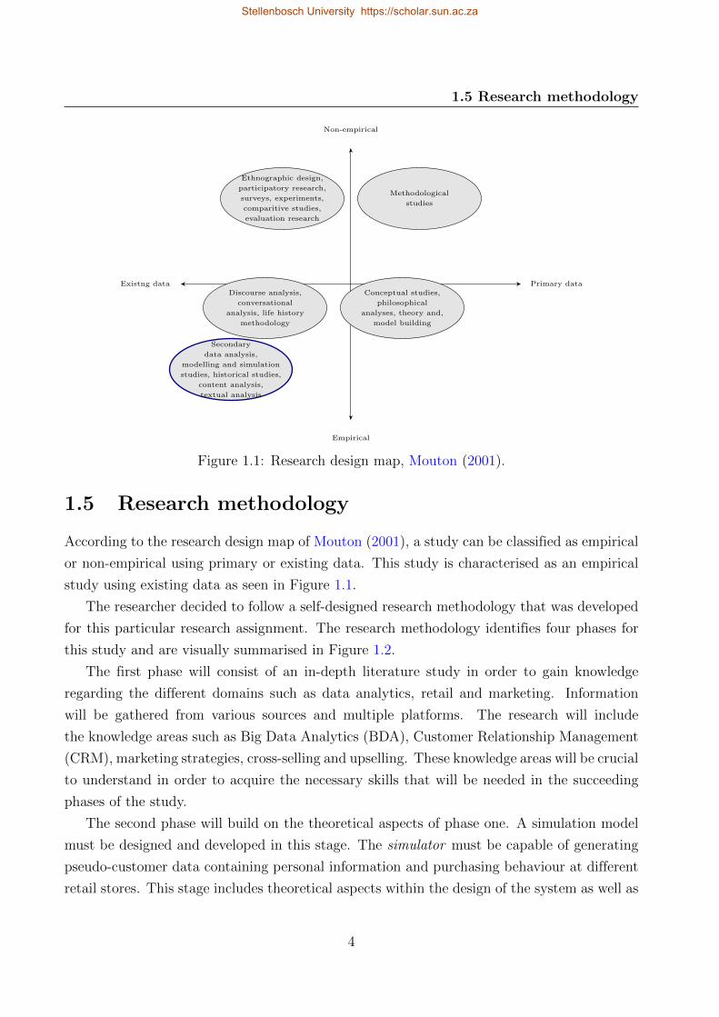
Figure 1.1: Research design map, Mouton (2001).
1.5 Research methodology
According to the research design map of Mouton (2001), a study can be classified as empirical
or non-empirical using primary or existing data. This study is characterised as an empirical
study using existing data as seen in Figure 1.1.
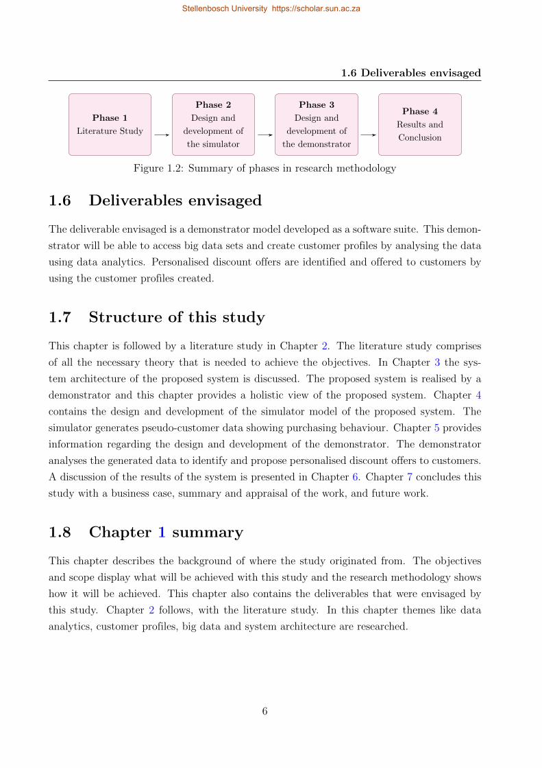
The researcher decided to follow a self-designed research methodology that was developed
for this particular research assignment. The research methodology identifies four phases for
this study and are visually summarised in Figure 1.2.
The first phase will consist of an in-depth literature study in order to gain knowledge
regarding the different domains such as data analytics, retail and marketing. Information
will be gathered from various sources and multiple platforms. The research will include
the knowledge areas such as Big Data Analytics (BDA), Customer Relationship Management
(CRM), marketing strategies, cross-selling and upselling. These knowledge areas will be crucial
to understand in order to acquire the necessary skills that will be needed in the succeeding
phases of the study.
The second phase will build on the theoretical aspects of phase one. A simulation model
must be designed and developed in this stage. The simulator must be capable of generating
pseudo-customer data containing personal information and purchasing behaviour at different
retail stores. This stage includes theoretical aspects within the design of the system as well as
4
Stellenbosch University https://scholar.sun.ac.za
1.5 Research methodology
technical development of the system. The simulator will be verified by first creating smaller
datasets with only a few customers and evaluating their purchasing patterns. The researcher
will also introduce variation by including different distributions in the data. This stage and
the next will be the most time-consuming phases in the study. Objective 1 will be achieved
within the second phase of the study.
The design and development of the demonstrator is done in the third phase. The demon-
strator must be able to analyse customer data to create customer profiles using the simulated
data. Employing the created customer profiles, the demonstrator must also be able to identify
personalised discount offers to individuals. This can all be done by using data analytics in the
design and development of the demonstrator. At least two different data analytic techniques
must be used in the demonstrator in order to evaluate the models.
Since this is a very novel approach and there are no comprehensive datasets available the
researcher will place the focus on the comparison and evaluation of the analytical methods
rather than the validation thereof.
The industry partner do not have access to real data including purchasing behaviour of
customers at different outlets and for this reason simulated data is the only option. The
following step will be for the industry partner to evaluate the proposed system by using real
data.
An evaluation data set will be used during the design of the demonstrator to evaluate
and compare the different analysis approaches. This data set will be simulated before the
evaluation commences and the results must verify that the simulated data output are as
expected.
Thereafter, PDOs will be introduced in the system and the demonstrator will incorpo-
rate the continued simulation of pseudo-customer data showing purchasing behaviour which
is achieved within phase two. The PDO demonstrator will be evaluated whether it can cor-
rectly predict and propose PDOs even with the interference of promotional efforts in normal
purchasing behaviour.
The fourth and final phase will include a discussion of the results composed by the demon-
strator, incorporating the various data analytic techniques explaining the outcome of the
study. This phase will also discuss the business value of this innovation along with a business
case. Executing this phase will achieve Objective 2. The conclusion of the study must be in
line with the research assignment.
5
Stellenbosch University https://scholar.sun.ac.za
1.6 Deliverables envisaged
Phase 1
Literature Study
Phase 2
Design and
development of
the simulator
Phase 3
Design and
development of
the demonstrator
Phase 4
Results and
Conclusion
Figure 1.2: Summary of phases in research methodology
1.6 Deliverables envisaged
The deliverable envisaged is a demonstrator model developed as a software suite. This demon-
strator will be able to access big data sets and create customer profiles by analysing the data
using data analytics. Personalised discount offers are identified and offered to customers by
using the customer profiles created.
1.7 Structure of this study
This chapter is followed by a literature study in Chapter 2. The literature study comprises
of all the necessary theory that is needed to achieve the objectives. In Chapter 3 the sys-
tem architecture of the proposed system is discussed. The proposed system is realised by a
demonstrator and this chapter provides a holistic view of the proposed system. Chapter 4
contains the design and development of the simulator model of the proposed system. The
simulator generates pseudo-customer data showing purchasing behaviour. Chapter 5 provides
information regarding the design and development of the demonstrator. The demonstrator
analyses the generated data to identify and propose personalised discount offers to customers.
A discussion of the results of the system is presented in Chapter 6. Chapter 7 concludes this
study with a business case, summary and appraisal of the work, and future work.
1.8 Chapter 1 summary
This chapter describes the background of where the study originated from. The objectives
and scope display what will be achieved with this study and the research methodology shows
how it will be achieved. This chapter also contains the deliverables that were envisaged by
this study. Chapter 2 follows, with the literature study. In this chapter themes like data
analytics, customer profiles, big data and system architecture are researched.
6
Stellenbosch University https://scholar.sun.ac.za
Chapter 2
Literature study
The previous chapter presented the motivation for this study and specified how the study will
be executed to achieve the set objectives. This chapter consists of the following:
2.1 Customer Relationship Management
2.2 Marketing strategies and approaches
2.3 Pricing and special offers
2.4 Cross-selling and upselling
2.5 Customer profiling and customer segmentation
2.6 Knowledge discovery analysis
2.7 Big Data
2.8 Big Data Analytics
2.9 Data security and privacy
2.10 Systems architecture
2.1 Customer relationship management
The customer is the main variable in most enterprises and thus the management of the cus-
tomer is crucial to ensure a successful future for the company. In the context of this study, the
customer and their specific needs are addressed by the proposed model. For this, Customer
Relationship Management (CRM) needs to be understood in order to create a system which
fulfils the needs of the customers. The importance of CRM within an enterprise is explained
in this section. This is accomplished by emphasising how to improve customer relationships
using core activities and different CRM approaches.
7
Stellenbosch University https://scholar.sun.ac.za
2.1 Customer relationship management
2.1.1 Overview of CRM
CRM is the area within a business that allows the company to engage in customer interaction.
CRM provides strategies, tools, processes and guidelines to build profitable relationships with
customers. This lends support to the business strategy of a company and ensures success
in a competitive marketplace (Mumuni and O’Reilly, 2014; Ngai et al., 2009; Soltani and
Navimipour, 2016). According to Tsiptsis and Chorianopoulos (2009), CRM has two main
objectives, which are:
1. Customer retention through customer satisfaction.
2. Customer development through customer insight.
Reinartz et al. (2004) identified three levels at which CRM can be practised, namely:
functional, customer-facing, and company-wide. One of the objectives of the customer-facing
perspective is to create a single view of a customer across all channels. Relationship initi-
ation, maintenance and termination are the three dimensions or stages incorporated in the
customer-facing level to ensure CRM process implementation. Reinartz et al. (2004) concep-
tualised a framework for the processes of CRM and evaluated the impact of the processes
on economic performance. This was subdivided into two performance measure types: per-
ceptual and objective. The activities identified by Reinartz et al. (2004) were acquisition
management, recovery management, cross-sell and upsell management, referral management
and exit management. These activities were accompanied by a customer evaluation at each
stage which led to nine subdimensions.
Mumuni and O’Reilly (2014) furthered this research by investigating the impact on busi-
ness performance having four dimensions: market share, revenue growth, profitability and
overall improvement. In contrast with the research of Reinartz et al. (2004), Mumuni and
O’Reilly (2014) evaluated the impact of the CRM processes on the individual dimensions as
well as the combined dimensions. The core activities within the three dimensions identified
by Reinartz et al. (2004) were adapted by Mumuni and O’Reilly (2014) and they are the focus
of Subsection 2.1.2.
Customer Experience Management (CEM) is not a domain within CRM, but rather built
upon CRM principles. A holistic definition of customer experience is defined by Gentile et al.
(2007) as: “The customer experience originates form a set of interactions between a customer
and a product, a company, or part of its organisation, which provoke a reaction. This experi-
ence is strictly personal and implies the customer’s involvement at different levels”. Du Plessis
and De Vries (2016) present an overview of important works in literature on customer expe-
rience and it is evident that CEM has recently become increasingly important. Customer
experience is important as it is becoming the distinguishing factor between competitors.
8
Stellenbosch University https://scholar.sun.ac.za
2.1 Customer relationship management
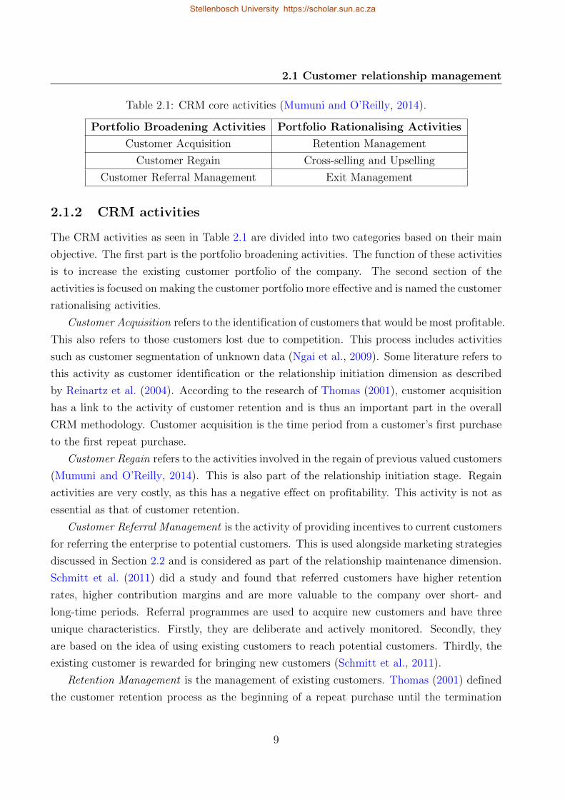
Table 2.1: CRM core activities (Mumuni and O’Reilly, 2014).
Portfolio Broadening Activities Portfolio Rationalising Activities
Customer Acquisition Retention Management
Customer Regain Cross-selling and Upselling
Customer Referral Management Exit Management
2.1.2 CRM activities
The CRM activities as seen in Table 2.1 are divided into two categories based on their main
objective. The first part is the portfolio broadening activities. The function of these activities
is to increase the existing customer portfolio of the company. The second section of the
activities is focused on making the customer portfolio more effective and is named the customer
rationalising activities.
Customer Acquisition refers to the identification of customers that would be most profitable.
This also refers to those customers lost due to competition. This process includes activities
such as customer segmentation of unknown data (Ngai et al., 2009). Some literature refers to
this activity as customer identification or the relationship initiation dimension as described
by Reinartz et al. (2004). According to the research of Thomas (2001), customer acquisition
has a link to the activity of customer retention and is thus an important part in the overall
CRM methodology. Customer acquisition is the time period from a customer’s first purchase
to the first repeat purchase.
Customer Regain refers to the activities involved in the regain of previous valued customers
(Mumuni and O’Reilly, 2014). This is also part of the relationship initiation stage. Regain
activities are very costly, as this has a negative effect on profitability. This activity is not as
essential as that of customer retention.
Customer Referral Management is the activity of providing incentives to current customers
for referring the enterprise to potential customers. This is used alongside marketing strategies
discussed in Section 2.2 and is considered as part of the relationship maintenance dimension.
Schmitt et al. (2011) did a study and found that referred customers have higher retention
rates, higher contribution margins and are more valuable to the company over short- and
long-time periods. Referral programmes are used to acquire new customers and have three
unique characteristics. Firstly, they are deliberate and actively monitored. Secondly, they
are based on the idea of using existing customers to reach potential customers. Thirdly, the
existing customer is rewarded for bringing new customers (Schmitt et al., 2011).
Retention Management is the management of existing customers. Thomas (2001) defined
the customer retention process as the beginning of a repeat purchase until the termination
9
Stellenbosch University https://scholar.sun.ac.za
2.1 Customer relationship management
of the relationship. Data from existing customers are analysed in order to find ways to
retain these customers and this forms part of the relationship maintenance stage described
by Reinartz et al. (2004). The problem emerges when this information is used to develop
strategies for customer acquisition as well. Thomas (2001) argues that customer retention
and customer acquisition are dependent processes and CRM decisions must take this biased
factor into account. In the research of Salazar et al. (2015), one can find other benefits
associated with retaining customers.
Cross-selling and Upselling are methods used to retain customers (Krishna and Ravi,
2016). From the empirical analysis done by Mumuni and O’Reilly (2014), cross-selling and
upselling were the only portfolio rationalising activities which had a significant influence on
the individual performance dimensions. The empirical analysis showed that organisations with
higher CRM-compatibility have a stronger impact from the cross-selling and upselling activi-
ties on the combined performance dimensions. In the context of this study, cross-selling and
upselling are fundamental principles within the proposed model. Cross-selling and upselling
are discussed at greater length in Section 2.4.
Exit Management contains the activities related to helping unprofitable customers exit
the customer portfolio. This forms part of the termination dimension identified by Reinartz
et al. (2004). These typically focus on customers who are of low-value to the enterprise or
problematic customers. Thus, it is more profitable for the company to use their resources on
higher-valued customers.
2.1.3 CRM analysis
Customers are an enterprise’s main source of revenue and thus the management of these
customers must be a top priority for the enterprise (Tsiptsis and Chorianopoulos, 2009).
CRM information can be used to gain knowledge about the customer and provide insights
into the needs of the customer. CRM consists of three components which are operational
CRM, analytical CRM and collaborative CRM. Dyche and Wesley (2002) describe analytical
CRM to be the only way in which a company can maintain a progressive relationship with its
customers. Operational CRM is used to execute sales and services based on the knowledge
gained from the analytical CRM component (Krishna and Ravi, 2016).
Tsiptsis and Chorianopoulos (2009) highlight this as the point where analytical CRM can
be beneficial to address the two objectives of CRM mentioned earlier – customer retention
and customer development. Data mining and machine learning are used for these analytical
purposes and these techniques are further explained in Section 2.8. Collaborative CRM is exe-
cuted when technology is implemented to satisfy the needs of customers in real time (Krishna
and Ravi, 2016). This study focus mainly on analytical CRM from this point onwards.
10
Stellenbosch University https://scholar.sun.ac.za
2.2 Marketing strategies and approaches
Acquire new
customers
Retain profitable
customers
Enchance
profitability of
existing customers
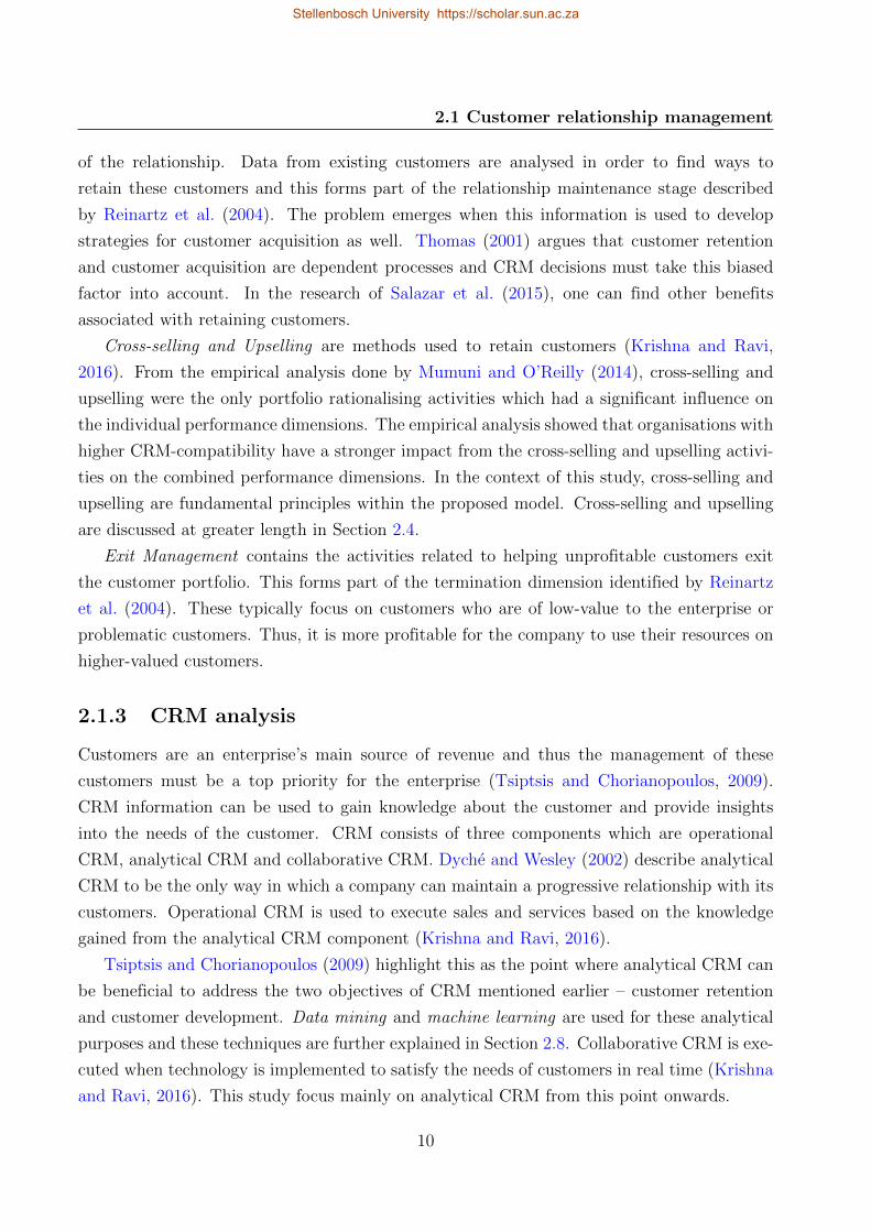
Figure 2.1: Customer life cycle (Krishna and Ravi, 2016).
The customer life cycle is divided into three phases as seen in Figure 2.1. Acquiring a
new customer has already been discussed as being the first CRM core activity. As mentioned,
segmentation can be used for this phase of the customer life cycle. Another approach to be used
is direct marketing which is one of the focus topics in Subsection 2.2.2. The phase of enhancing
the profitability of existing customers can be accomplished by investigating the Customer
Lifetime Value (CLV) and conducting a Market Basket Analysis (MBA). These concepts are
discussed in Section 2.6. In certain domains fraud detection, default detection and credit
card scoring can also be used (Krishna and Ravi, 2016). The last phase, retaining profitable
customers, is achieved by preforming customer churn detection and sentiment analysis.
CRM is not only achieved by activities such as marketing and sales but spreads beyond that
to developing and maintaining relationships with customers. Salazar et al. (2007) defines CRM
as not only a management philosophy that seeks to create, develop and enhance beneficial
relationships with customers, but to maximise organisational profit and performance.
CRM and marketing are used concurrently within literature as well as in practice. CRM is
focused on the relationship with the customer, while marketing assists with building profitable
relationships with customers. With that said, the following section sheds some light on how
marketing approaches can be used to achieve some core CRM activities discussed in this
section.
2.2 Marketing strategies and approaches
A lot of different marketing strategies and approaches exist in literature and within the indus-
try. The appropriate strategy and approach are defined by the industry the enterprise is in
and the business strategy the enterprise has chosen. In this section an overview of marketing
in general is given followed by different methods of communication with customers. This
11
Stellenbosch University https://scholar.sun.ac.za
2.2 Marketing strategies and approaches
Understand the
marketplace and
customer needs
and wants
Design a
customer value-
driven marketing
scheme
Construct an inte-
grated marketing
programme
that delivers
superior value
Engage customers
build profitable
relationships, and
create customer
delight
Capture value
from customers to
create profits and
customer equity
Create value for customers and
build customer relationships
Capture value from
customers
in return
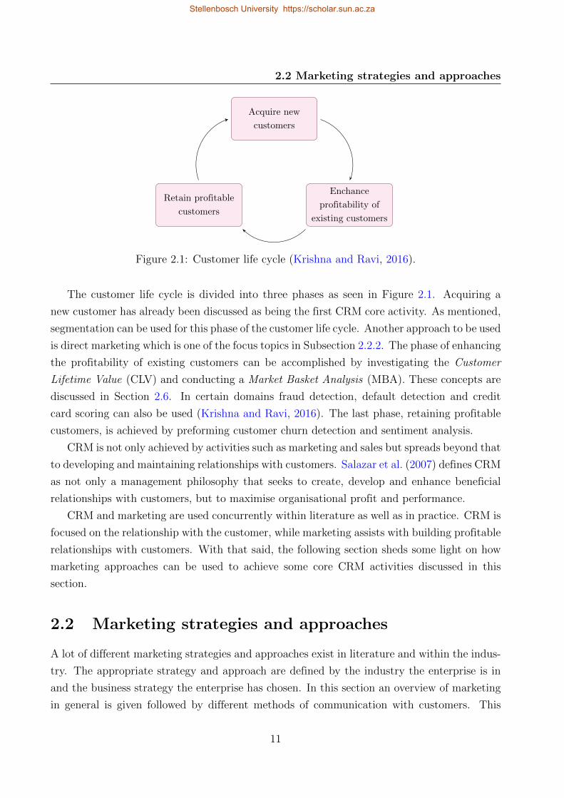
Figure 2.2: Marketing process (Kotler et al., 2018).
knowledge is required to find the ultimate means for marketing products and communicating
with customers.
2.2.1 Overview of marketing
Marketing has numerous definitions, from broadly defined to a very specific business context.
According to Kotler et al. (2018), marketing is the process by which companies engage with
customers, build strong customer relationships, and create customer value in order to capture
value from customers in return. The marketing process for creating and capturing customer
value is summarised in Figure 2.2 and is discussed in great detail by Kotler et al. (2018).
The first four steps shown are focused on creating value for the customer and from this a
customer-driven marketing strategy is designed. This is done by answering two questions: (1)
deciding which customers the company will serve and (2) deciding how they will best serve
their targeted customers. After choosing on an appropriate marketing strategy, an appropriate
mix marketing framework is used (Kotler et al., 2018). This is done by using a marketing
plan that consists of a blend of the marketing mix elements. The marketing mix framework
is a set of tools used to transform and implement the marketing strategy of the company.
The term marketing mix was first conceptualised by Neil Borden in 1964. Borden (1964)
proposed the approach of mix marketing in order to translate marketing strategies and plans
into action. There were 12 mix marketing elements mentioned. In 1969 these 12 mix marketing
elements where shortened by E. Jerome McCarthy into four elements, also known as the 4Ps:
product, price, place, promotion (Kubiak and Weichbroth, 2010).
Goi (2009) conducted a study to identify the criticism in literature on the 4P framework
and the propositions different researchers had for the mix model framework. A wide variety
of different propositions arose. Some authors proposed more Ps, such as people, participants
and process. From the work of Goi (2009) it was concluded that most of the literature still
used the 4Ps as a defining view of a marketing mix framework. For the purpose of this study
it is advised to adopt the 5P model with people as the added P. This decision was based on
12
Stellenbosch University https://scholar.sun.ac.za
2.2 Marketing strategies and approaches
Target
customers
Intended
positioning
Product
Variety
Quality
Design
Features
Brand name
Packaging Services
Price
List Price
Discounts
Allowances
Payment period
Credit terms
Place
Channels
Coverage
Locations
Inventory
Transportation
Logistics
Promotion
Advertising
Personal selling
Sales promotion
Public relations
Direct and digital
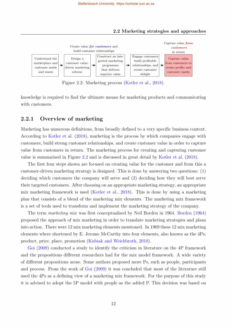
Figure 2.3: The 4Ps of the marketing mix (Kotler et al., 2018).
1:1
Direct marketing
Segment-based marketing
Mass marketing
Figure 2.4: Marketing communications (Bounsaythip and Rinta-Runsala, 2001).
the importance of the customer as highlighted by Section 2.1. Figure 2.3 visualises the 4Ps of
the marketing mix and their associated marketing tools.
In order to understand the marketing process, it is important to understand the different
means in which a marketing strategy can be communicated to customers. There are different
strategies to communicate marketing campaigns to different customers. This also answers the
first question of a customer-driven marketing strategy stated earlier: deciding which customers
the company will serve. Figure 2.4 visually explains the expense to revenue return ratio that
is yielded from different communication approaches. The approaches are explained in more
detail in Subsection 2.2.2.
It is clear to see that one-to-one marketing is much more effective based on the return
ratio (Wedel and Kamakura, 2002). This type of marketing campaign sets the focus on each
individual customer and their specific need and is much more effective than mass marketing.
Thomas et al. (2007) explained that these are not only marketing tactics, but marketing
strategies. Strategies are the plans or methods whereas a tactic is the device used for accom-
13
Stellenbosch University https://scholar.sun.ac.za
2.2 Marketing strategies and approaches
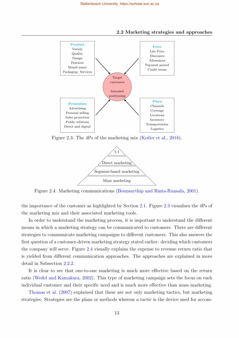
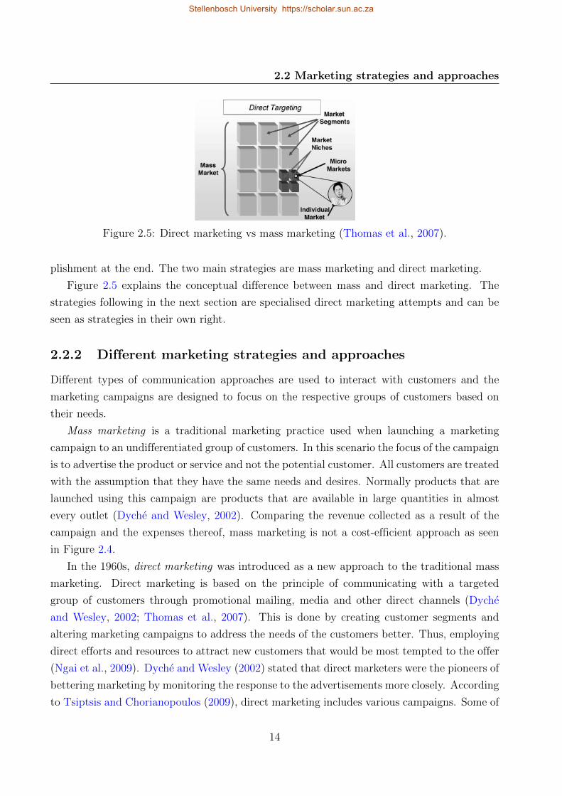
Figure 2.5: Direct marketing vs mass marketing (Thomas et al., 2007).
plishment at the end. The two main strategies are mass marketing and direct marketing.
Figure 2.5 explains the conceptual difference between mass and direct marketing. The
strategies following in the next section are specialised direct marketing attempts and can be
seen as strategies in their own right.
2.2.2 Different marketing strategies and approaches
Different types of communication approaches are used to interact with customers and the
marketing campaigns are designed to focus on the respective groups of customers based on
their needs.
Mass marketing is a traditional marketing practice used when launching a marketing
campaign to an undifferentiated group of customers. In this scenario the focus of the campaign
is to advertise the product or service and not the potential customer. All customers are treated
with the assumption that they have the same needs and desires. Normally products that are
launched using this campaign are products that are available in large quantities in almost
every outlet (Dyche and Wesley, 2002). Comparing the revenue collected as a result of the
campaign and the expenses thereof, mass marketing is not a cost-efficient approach as seen
in Figure 2.4.
In the 1960s, direct marketing was introduced as a new approach to the traditional mass
marketing. Direct marketing is based on the principle of communicating with a targeted
group of customers through promotional mailing, media and other direct channels (Dyche
and Wesley, 2002; Thomas et al., 2007). This is done by creating customer segments and
altering marketing campaigns to address the needs of the customers better. Thus, employing
direct efforts and resources to attract new customers that would be most tempted to the offer
(Ngai et al., 2009). Dyche and Wesley (2002) stated that direct marketers were the pioneers of
bettering marketing by monitoring the response to the advertisements more closely. According
to Tsiptsis and Chorianopoulos (2009), direct marketing includes various campaigns. Some of
14
Stellenbosch University https://scholar.sun.ac.za
2.2 Marketing strategies and approaches
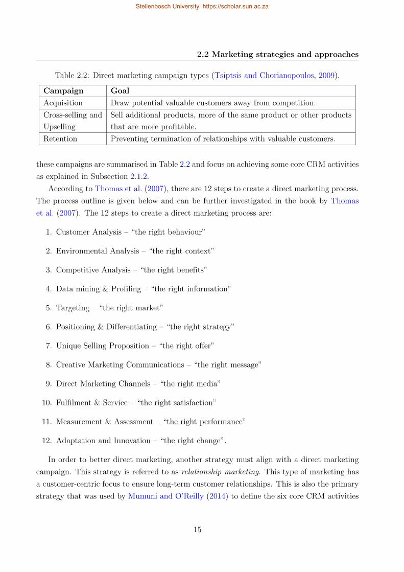
Table 2.2: Direct marketing campaign types (Tsiptsis and Chorianopoulos, 2009).
Campaign Goal
Acquisition Draw potential valuable customers away from competition.
Cross-selling and
Upselling
Sell additional products, more of the same product or other products
that are more profitable.
Retention Preventing termination of relationships with valuable customers.
these campaigns are summarised in Table 2.2 and focus on achieving some core CRM activities
as explained in Subsection 2.1.2.
According to Thomas et al. (2007), there are 12 steps to create a direct marketing process.
The process outline is given below and can be further investigated in the book by Thomas
et al. (2007). The 12 steps to create a direct marketing process are:
1. Customer Analysis – “the right behaviour”
2. Environmental Analysis – “the right context”
3. Competitive Analysis – “the right benefits”
4. Data mining & Profiling – “the right information”
5. Targeting – “the right market”
6. Positioning & Differentiating – “the right strategy”
7. Unique Selling Proposition – “the right offer”
8. Creative Marketing Communications – “the right message”
9. Direct Marketing Channels – “the right media”
10. Fulfilment & Service – “the right satisfaction”
11. Measurement & Assessment – “the right performance”
12. Adaptation and Innovation – “the right change”.
In order to better direct marketing, another strategy must align with a direct marketing
campaign. This strategy is referred to as relationship marketing. This type of marketing has
a customer-centric focus to ensure long-term customer relationships. This is also the primary
strategy that was used by Mumuni and O’Reilly (2014) to define the six core CRM activities
15
Stellenbosch University https://scholar.sun.ac.za
2.2 Marketing strategies and approaches
mentioned in Table 2.1. Paley (2007) defines relationship marketing as “the practice of build-
ing long-term satisfying relations with key parties – customers, suppliers and distributors –
in order to retain long-term preference and business.”
Traditionally, relationship marketing would refer to the interaction between suppliers and
consumers. In the article by Paas et al. (2005), the authors acknowledge another long-term
relationship that cannot be avoided any longer: the relationship between customers and prod-
ucts. Lately, there is a growing interest in customer retention and with that marketing at-
tention shifted from being mutually independent activities to being loyalty-based cross-selling
and upselling opportunities.
The relationship with a customer is based on three dimensions according to Paas et al.
(2005): the length of time, the balance of interest, and the direction and intensity of commu-
nication. In the past, transactions were seen as discrete events not containing any significant
value. More recently, the long-term relationship between a customer and supplier is expressed
via transactions. This is seen when investigating the popularity of customer loyalty pro-
grammes and CRM programmes within the CRM domain.
Paas et al. (2005) identified four customer-product interactions. The most known concept
is that of customer needs. When the needs of a customer are identified, appropriate product
recommendations can be made. Alongside the customer needs, is the life cycle hypothesis.
Throughout the life cycle of the product or the customer the needs change and this shows
that acquisitions do not occur randomly. Another interaction is the one related to revealed
preferences. The problem with this concept is that customer-product interactions are based
on actual acquisitions, where the argument rises that customers do not acquire a product they
do not need. Thus, this relates to revealing customer needs and does not explain customer-
product interactions.
The last concept is brand loyalty. Unlike the other concepts mentioned in this section,
brand loyalty is of significant value for the analysis of product-customer interaction. Brand
loyalty expresses the customer’s consistent preference for a particular brand by purchasing
the offer repeatedly.
Personalised marketing campaigns are used by companies to target specific customers
(Kamber et al., 2012; Khodakarami and Chan, 2013). Thomas et al. (2007) explain that
direct marketing goes beyond the market segmentations and focuses on micro-markets as well
as on individual customers. This aspect of direct marketing is known as one-on-one marketing
or targeted marketing. The idea of customising the offer presented to a customer based on an
individuals’ needs and the personalisation of the customer are the key concepts of one-to-one
marketing. When pairing this marketing strategy with the technological innovations of today,
16
Stellenbosch University https://scholar.sun.ac.za
2.2 Marketing strategies and approaches
it is possible to customise the marketing message individuals receive and the means whereby
they receive it.
Dyche and Wesley (2002) and Changchien et al. (2004) identify two main approaches of
personalisation. First is rule-based personalisation or content-based, where established rules
dictate the personalisation. This approach measures the degree of similarity between items
which customers purchased in the past (Bose and Chen, 2009; Changchien et al., 2004). For
example if someone buys a book online, the recommender system would recommend the next
book of the series to the buyer before the checkout point. Rule-based personalisation is
normally hard-coded into the software and is therefore difficult to maintain.
The second type is that of adaptive personalisation, also known as collaborative filtering.
This type of personalisation learns as time passes: adaptive personalisation uses the behaviour
of similar customers or tries to find similarities between customers’ preferences. Thus, for
example, a customer buys a film of a certain genre, the system will recommend another film
of the same genre. Both these types of filtering are used for recommender systems in the
e-commerce industry (Dean, 2014; Erl et al., 2015; Kamber et al., 2012).
Wedel and Kamakura (2002) state that even with one-to-one marketing, customer segmen-
tation is not precluded. Enterprises develop a limited number of marketing strategies which
are based on the different available segments. Some companies have developed one-to-one
marketing strategies to increase their profits, but the usage thereof as an implementation
tactic does not prevent market segmentation as a general approach.
Customer data are used to identify the needs of an individual for the purpose of direct
marketing. These concepts are referred to as customer segmentation and profiling and are
further discussed in Section 2.5.
According to Chen et al. (2005a) and Jiao et al. (2006), one-to-one marketing campaigns
are supported by analysing and predicting customer behaviour to personalise marketing cam-
paigns. One-to-one marketing is used alongside relationship marketing to enhance customer
retention. The idea of targeted marketing is one of the core principles of this study when look-
ing at different marketing strategies. This study focuses on personalising offers for individuals
and with that a one-to-one marketing strategy is used.
The following section will focus on pricing and special offer strategies which are seen as
part of the marketing mix framework. For the purpose of this study, this is discussed in a
section on its own in order to emphasise its importance.
17
Stellenbosch University https://scholar.sun.ac.za
2.3 Pricing and special offers
2.3 Pricing and special offers
Pricing strategies and tactics are covered widely in literature. Depending on the product or
service, the business strategy and marketing strategy, different pricing tactics can be used.
Price is also one of the 5Ps mentioned in the framework of the marketing mix and is thus a
vital element to discuss.
For the purpose of this study, this section will place the focus on pricing for promotional
reasons which relate to the promotions and pricing strategies that are referred to in Section
2.2.
Pricing guidelines were established in the book by Paley (2007) in order to increase the
chances of success. The guidelines are as follows:
1. Establish the pricing objectives.
2. Develop a demand schedule for the product.
3. Examine competitors’ pricing.
4. Select the pricing method.
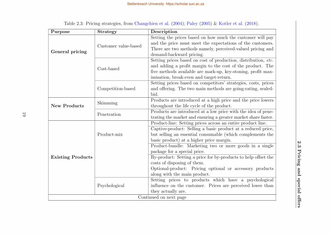
Changchien et al. (2004); Paley (2005); and Kotler et al. (2018) provide literature regarding
pricing strategies in great detail. Some of the pricing strategies are summarised in Table 2.3.
18
Stellenbosch University https://scholar.sun.ac.za
2.3
Pricin
gandsp
ecia
loffe
rs
Table 2.3: Pricing strategies, from Changchien et al. (2004); Paley (2005) & Kotler et al. (2018).
Purpose Strategy Description
General pricingCustomer value-based
Setting the prices based on how much the customer will payand the price must meet the expectations of the customers.There are two methods namely, perceived-valued pricing anddemand-backward pricing.
Cost-based
Setting prices based on cost of production, distribution, etc.and adding a profit margin to the cost of the product. Thefive methods available are mark-up, key-stoning, profit max-imisation, break-even and target-return.
Competition-basedSetting prices based on competitors’ strategies, costs, pricesand offering. The two main methods are going-rating, sealed-bid.
New ProductsSkimming
Products are introduced at a high price and the price lowersthroughout the life cycle of the product.
PenetrationProducts are introduced at a low price with the idea of pene-trating the market and ensuring a greater market share faster.
Existing Products
Product-mix
Product-line: Setting prices across an entire product line.Captive-product: Selling a basic product at a reduced price,but selling an essential consumable (which complements thebasic product) at a higher price margin.Product-bundle: Marketing two or more goods in a singlepackage for a special price.By-product: Setting a price for by-products to help offset thecosts of disposing of them.Optional-product: Pricing optional or accessory productsalong with the main product.
PsychologicalSetting prices to products which have a psychologicalinfluence on the customer. Prices are perceived lower thanthey actually are.
Continued on next page
19
Stellenbosch University https://scholar.sun.ac.za
Stellenbosch University https://scholar.sun.ac.za
2.3
Pricin
gandsp
ecia
loffe
rs
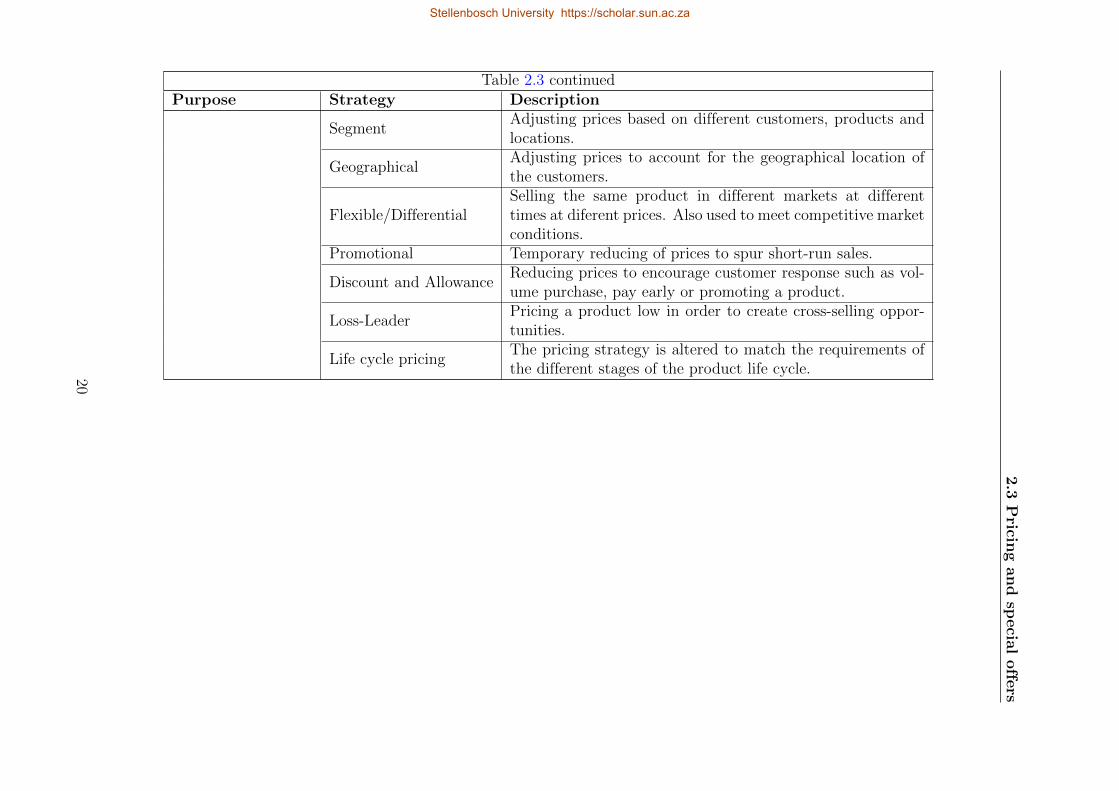
Table 2.3 continuedPurpose Strategy Description
SegmentAdjusting prices based on different customers, products andlocations.
GeographicalAdjusting prices to account for the geographical location ofthe customers.
Flexible/DifferentialSelling the same product in different markets at differenttimes at diferent prices. Also used to meet competitive marketconditions.
Promotional Temporary reducing of prices to spur short-run sales.
Discount and AllowanceReducing prices to encourage customer response such as vol-ume purchase, pay early or promoting a product.
Loss-LeaderPricing a product low in order to create cross-selling oppor-tunities.
Life cycle pricingThe pricing strategy is altered to match the requirements ofthe different stages of the product life cycle.20
Stellenbosch University https://scholar.sun.ac.za
Stellenbosch University https://scholar.sun.ac.za
2.3 Pricing and special offers
From Table 2.3, a promotional pricing strategy is the most relevant in this study. The
discount and allowance and the loss-leader pricing strategies can also be incorporated in this
study along with the promotional pricing strategy.
Promotions is also one of the 5Ps in the marketing mix framework. Promotional pricing
is when products are temporarily sold at a lower price than the listed price (Kotler et al.,
2018). Sales promotions are all the promotional efforts that cannot be classified as advertising,
personal selling or publicity. Paley (2005) defines the difference between sales promotion and
advertising as: sales promotion is an incentive to buy and advertising offers a reason to buy.
The customer is encouraged to buy a product because of added value or providing special
incentive. Also, sales promotions are part of the overall marketing strategy and involve a
variety of company functions in order to work efficiently.
Two types of promotional strategies exist, according to Campbell and Diamond (1990).
The author also states that most customers have a reference price of what the product they
are looking for might cost. The two categories of promotions are (1) non-monetary promotions
and (2) monetary promotions. Non-monetary promotions refer to promotions which have an
added product or service. Monetary promotions are usually discounts and rebates. Customers
perceive these types of promotions differently. Normally, non-monetary promotions can be
seen as a gain and are considered separately from the reference price a customer might have,
whereas monetary promotions can be viewed as a potential loss and can sometimes affect
the reference price of the customer. It is for this reason that determining an appropriate
promotional strategy and price is essential.
Promotions provide an area for creativity and flexibility, and can be implemented by using
one of the following applications (Paley, 2007):
1. Consumer promotions: Samples, coupons, cash refunds, premiums, free trials, war-
ranties, and demonstrations.
2. Trade promotions: Buying allowances, free goods, cooperate advertising, display al-
lowance, push money, video conferencing and dealer sales contests.
3. Sales force promotions: Bonuses, contests, and sales rallies.
Discounts are simply when a retailer sells products at a lower price in order to increase
sales and reduce inventories. Special event offers are used in certain seasons to draw more
customers. Limited-time offers or flash sales are used to create buying urgency. This form
of promotion also makes the customer feel special to have received the offer. The researcher
sees this type of promotion as the cornerstone of this study.
21
Stellenbosch University https://scholar.sun.ac.za
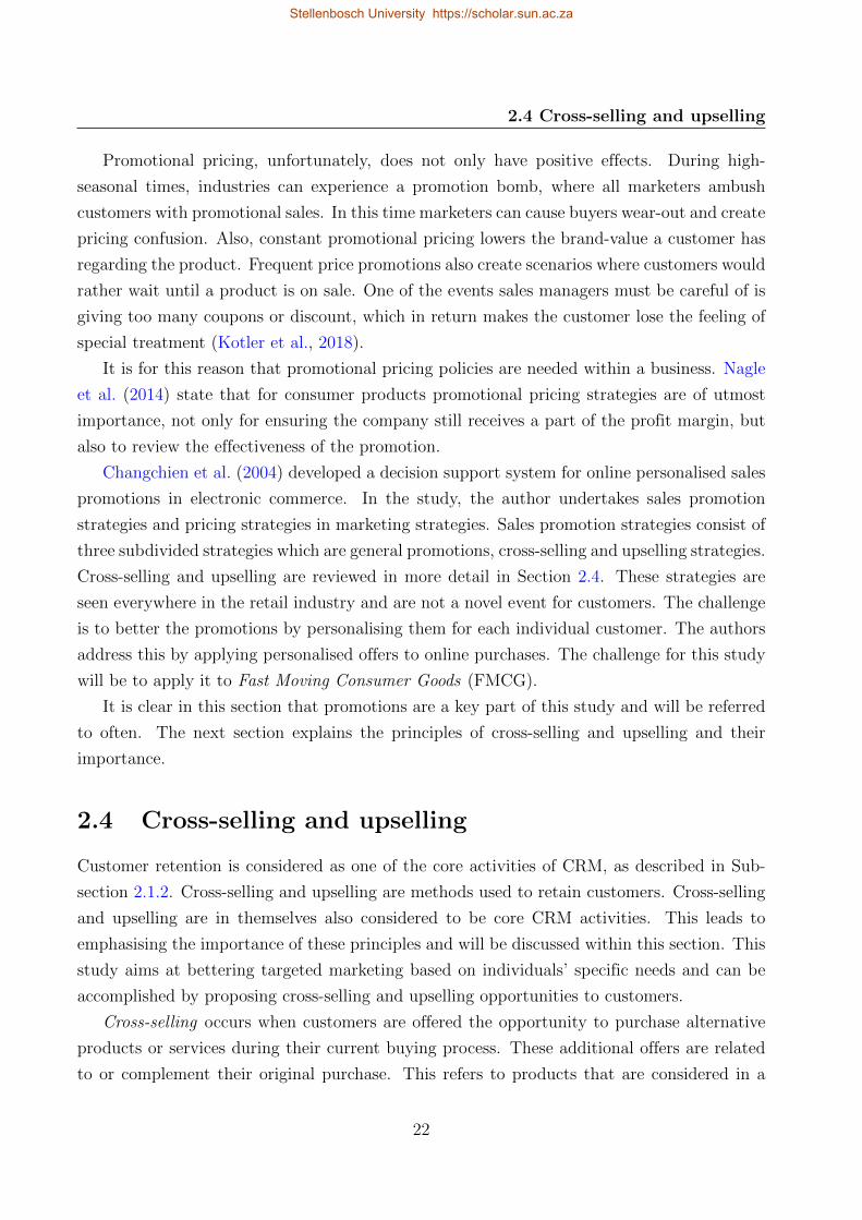
2.4 Cross-selling and upselling
Promotional pricing, unfortunately, does not only have positive effects. During high-
seasonal times, industries can experience a promotion bomb, where all marketers ambush
customers with promotional sales. In this time marketers can cause buyers wear-out and create
pricing confusion. Also, constant promotional pricing lowers the brand-value a customer has
regarding the product. Frequent price promotions also create scenarios where customers would
rather wait until a product is on sale. One of the events sales managers must be careful of is
giving too many coupons or discount, which in return makes the customer lose the feeling of
special treatment (Kotler et al., 2018).
It is for this reason that promotional pricing policies are needed within a business. Nagle
et al. (2014) state that for consumer products promotional pricing strategies are of utmost
importance, not only for ensuring the company still receives a part of the profit margin, but
also to review the effectiveness of the promotion.
Changchien et al. (2004) developed a decision support system for online personalised sales
promotions in electronic commerce. In the study, the author undertakes sales promotion
strategies and pricing strategies in marketing strategies. Sales promotion strategies consist of
three subdivided strategies which are general promotions, cross-selling and upselling strategies.
Cross-selling and upselling are reviewed in more detail in Section 2.4. These strategies are
seen everywhere in the retail industry and are not a novel event for customers. The challenge
is to better the promotions by personalising them for each individual customer. The authors
address this by applying personalised offers to online purchases. The challenge for this study
will be to apply it to Fast Moving Consumer Goods (FMCG).
It is clear in this section that promotions are a key part of this study and will be referred
to often. The next section explains the principles of cross-selling and upselling and their
importance.
2.4 Cross-selling and upselling
Customer retention is considered as one of the core activities of CRM, as described in Sub-
section 2.1.2. Cross-selling and upselling are methods used to retain customers. Cross-selling
and upselling are in themselves also considered to be core CRM activities. This leads to
emphasising the importance of these principles and will be discussed within this section. This
study aims at bettering targeted marketing based on individuals’ specific needs and can be
accomplished by proposing cross-selling and upselling opportunities to customers.
Cross-selling occurs when customers are offered the opportunity to purchase alternative
products or services during their current buying process. These additional offers are related
to or complement their original purchase. This refers to products that are considered in a
22
Stellenbosch University https://scholar.sun.ac.za
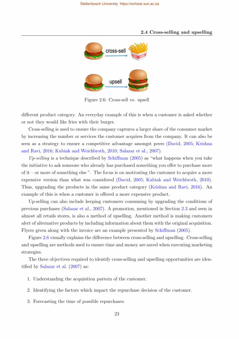
2.4 Cross-selling and upselling
Figure 2.6: Cross-sell vs. upsell
different product category. An everyday example of this is when a customer is asked whether
or not they would like fries with their burger.
Cross-selling is used to ensure the company captures a larger share of the consumer market
by increasing the number or services the customer acquires from the company. It can also be
seen as a strategy to ensure a competitive advantage amongst peers (David, 2005; Krishna
and Ravi, 2016; Kubiak and Weichbroth, 2010; Salazar et al., 2007).
Up-selling is a technique described by Schiffman (2005) as “what happens when you take
the initiative to ask someone who already has purchased something you offer to purchase more
of it – or more of something else ”. The focus is on motivating the customer to acquire a more
expensive version than what was considered (David, 2005; Kubiak and Weichbroth, 2010).
Thus, upgrading the products in the same product category (Krishna and Ravi, 2016). An
example of this is when a customer is offered a more expensive product.
Up-selling can also include keeping customers consuming by upgrading the conditions of
previous purchases (Salazar et al., 2007). A promotion, mentioned in Section 2.3 and seen in
almost all retails stores, is also a method of upselling. Another method is making customers
alert of alternative products by including information about them with the original acquisition.
Flyers given along with the invoice are an example presented by Schiffman (2005).
Figure 2.6 visually explains the difference between cross-selling and upselling. Cross-selling
and upselling are methods used to ensure time and money are saved when executing marketing
strategies.
The three objectives required to identify cross-selling and upselling opportunities are iden-
tified by Salazar et al. (2007) as:
1. Understanding the acquisition pattern of the customer.
2. Identifying the factors which impact the repurchase decision of the customer.
3. Forecasting the time of possible repurchases.
23
Stellenbosch University https://scholar.sun.ac.za
2.5 Customer profiling and customer segmentation
The Market Basket Analysis (MBA), amongst others, is one of the well-known knowledge
discovery methods used in practice to pursue these objectives (Krishna and Ravi, 2016; Kubiak
and Weichbroth, 2010; Tsiptsis and Chorianopoulos, 2009). The different analysis approaches
are discussed in Section 2.6.
The analysis of customer data with knowledge discovery analysis and data mining methods,
described in Section 2.6 and Subsection 2.8.3 respectively, is an effective manner to identify
cross-selling and upselling opportunities (Kubiak and Weichbroth, 2010; Salazar et al., 2007).
Effective cross-selling and upselling can only happen when retailers fully understand customers
in terms of their needs. This is where analytical CRM is the main focus to create customer
segments and customer profiles and build a better relationship with the customers.
Customer segmentation and profiling are discussed by the researcher in the upcoming
section. For the purpose of this study, it is important to understand that using customer
profiles and data mining leads to cross-sell and upsell opportunities which can be presented
to the customer with their personalised offer and by doing this the company creates customer
value and customer retention.
2.5 Customer profiling and customer segmentation
This section presents an overview of customer profiling and customer segmentation, the
difference between the two and how it is used in this study. Approaches to develop customer
profiles are investigated and explained.
2.5.1 Overview of customer profiling and customer segmentation
The terms customer profiles and profiling have been seen in recent literature reviews. Cus-
tomer profiling and customer segmentation are often used interchangeably.
Customer profiling attempts to create a model of the customer used to decide on appro-
priate strategies and tactics to meet the demand of the customer by creating a customer
profile (Shaw et al., 2001). Customer profiles describe customers based on their attributes
(Bounsaythip and Rinta-Runsala, 2001). According to Adomavicius and Tuzhilin (2001), a
comprehensive customer profile consists of two sub-profiles: factual and behavioural. The
factual profile tells who the customer is and behavioural profile describes what the customer
does.
Customer profiling is a tool used to personalise individuals in order to understand and
provide to their unknown needs. This improves customer service for better customer satis-
faction and customer retention, which is one of the core CRM activities listed in Subsection
2.1.2. Marketers use these profiles for targeted marketing in which they present an offer to
24
Stellenbosch University https://scholar.sun.ac.za
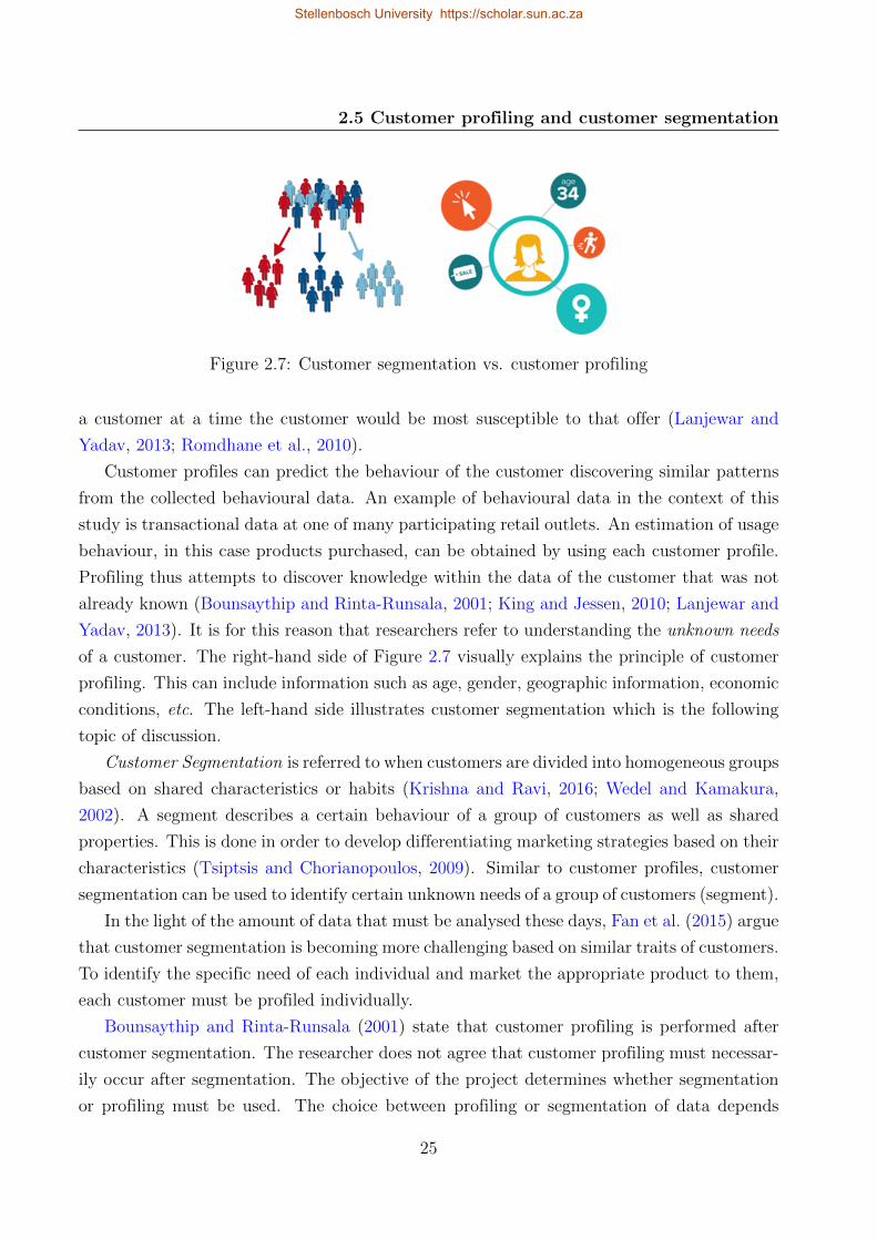
2.5 Customer profiling and customer segmentation
Figure 2.7: Customer segmentation vs. customer profiling
a customer at a time the customer would be most susceptible to that offer (Lanjewar and
Yadav, 2013; Romdhane et al., 2010).
Customer profiles can predict the behaviour of the customer discovering similar patterns
from the collected behavioural data. An example of behavioural data in the context of this
study is transactional data at one of many participating retail outlets. An estimation of usage
behaviour, in this case products purchased, can be obtained by using each customer profile.
Profiling thus attempts to discover knowledge within the data of the customer that was not
already known (Bounsaythip and Rinta-Runsala, 2001; King and Jessen, 2010; Lanjewar and
Yadav, 2013). It is for this reason that researchers refer to understanding the unknown needs
of a customer. The right-hand side of Figure 2.7 visually explains the principle of customer
profiling. This can include information such as age, gender, geographic information, economic
conditions, etc. The left-hand side illustrates customer segmentation which is the following
topic of discussion.
Customer Segmentation is referred to when customers are divided into homogeneous groups
based on shared characteristics or habits (Krishna and Ravi, 2016; Wedel and Kamakura,
2002). A segment describes a certain behaviour of a group of customers as well as shared
properties. This is done in order to develop differentiating marketing strategies based on their
characteristics (Tsiptsis and Chorianopoulos, 2009). Similar to customer profiles, customer
segmentation can be used to identify certain unknown needs of a group of customers (segment).
In the light of the amount of data that must be analysed these days, Fan et al. (2015) argue
that customer segmentation is becoming more challenging based on similar traits of customers.
To identify the specific need of each individual and market the appropriate product to them,
each customer must be profiled individually.
Bounsaythip and Rinta-Runsala (2001) state that customer profiling is performed after
customer segmentation. The researcher does not agree that customer profiling must necessar-
ily occur after segmentation. The objective of the project determines whether segmentation
or profiling must be used. The choice between profiling or segmentation of data depends
25
Stellenbosch University https://scholar.sun.ac.za
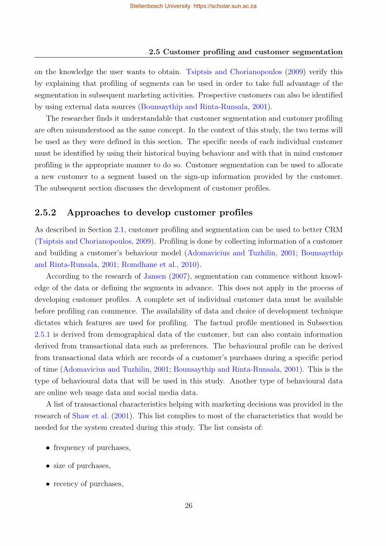
2.5 Customer profiling and customer segmentation
on the knowledge the user wants to obtain. Tsiptsis and Chorianopoulos (2009) verify this
by explaining that profiling of segments can be used in order to take full advantage of the
segmentation in subsequent marketing activities. Prospective customers can also be identified
by using external data sources (Bounsaythip and Rinta-Runsala, 2001).
The researcher finds it understandable that customer segmentation and customer profiling
are often misunderstood as the same concept. In the context of this study, the two terms will
be used as they were defined in this section. The specific needs of each individual customer
must be identified by using their historical buying behaviour and with that in mind customer
profiling is the appropriate manner to do so. Customer segmentation can be used to allocate
a new customer to a segment based on the sign-up information provided by the customer.
The subsequent section discusses the development of customer profiles.
2.5.2 Approaches to develop customer profiles
As described in Section 2.1, customer profiling and segmentation can be used to better CRM
(Tsiptsis and Chorianopoulos, 2009). Profiling is done by collecting information of a customer
and building a customer’s behaviour model (Adomavicius and Tuzhilin, 2001; Bounsaythip
and Rinta-Runsala, 2001; Romdhane et al., 2010).
According to the research of Jansen (2007), segmentation can commence without knowl-
edge of the data or defining the segments in advance. This does not apply in the process of
developing customer profiles. A complete set of individual customer data must be available
before profiling can commence. The availability of data and choice of development technique
dictates which features are used for profiling. The factual profile mentioned in Subsection
2.5.1 is derived from demographical data of the customer, but can also contain information
derived from transactional data such as preferences. The behavioural profile can be derived
from transactional data which are records of a customer’s purchases during a specific period
of time (Adomavicius and Tuzhilin, 2001; Bounsaythip and Rinta-Runsala, 2001). This is the
type of behavioural data that will be used in this study. Another type of behavioural data
are online web usage data and social media data.
A list of transactional characteristics helping with marketing decisions was provided in the
research of Shaw et al. (2001). This list complies to most of the characteristics that would be
needed for the system created during this study. The list consists of:
� frequency of purchases,
� size of purchases,
� recency of purchases,
26
Stellenbosch University https://scholar.sun.ac.za
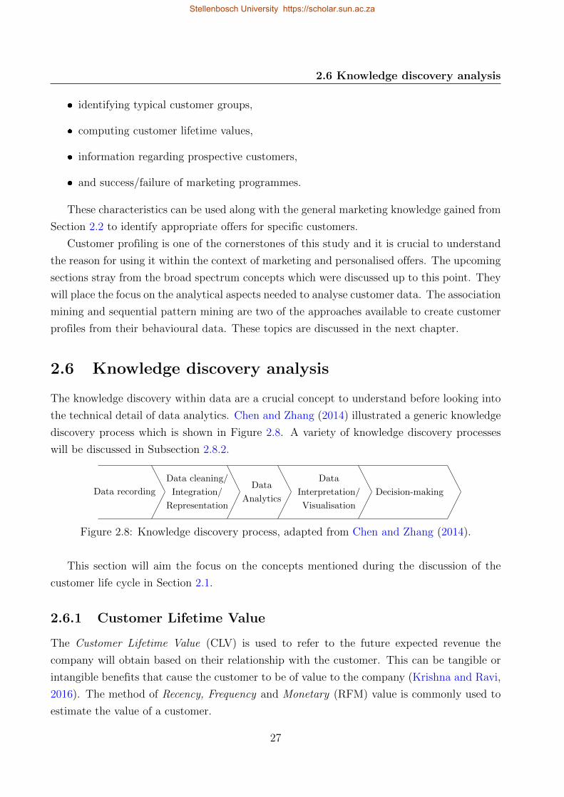
2.6 Knowledge discovery analysis
� identifying typical customer groups,
� computing customer lifetime values,
� information regarding prospective customers,
� and success/failure of marketing programmes.
These characteristics can be used along with the general marketing knowledge gained from
Section 2.2 to identify appropriate offers for specific customers.
Customer profiling is one of the cornerstones of this study and it is crucial to understand
the reason for using it within the context of marketing and personalised offers. The upcoming
sections stray from the broad spectrum concepts which were discussed up to this point. They
will place the focus on the analytical aspects needed to analyse customer data. The association
mining and sequential pattern mining are two of the approaches available to create customer
profiles from their behavioural data. These topics are discussed in the next chapter.
2.6 Knowledge discovery analysis
The knowledge discovery within data are a crucial concept to understand before looking into
the technical detail of data analytics. Chen and Zhang (2014) illustrated a generic knowledge
discovery process which is shown in Figure 2.8. A variety of knowledge discovery processes
will be discussed in Subsection 2.8.2.
Data recording
Data cleaning/
Integration/
Representation
Data
Analytics
Data
Interpretation/
Visualisation
Decision-making
Figure 2.8: Knowledge discovery process, adapted from Chen and Zhang (2014).
This section will aim the focus on the concepts mentioned during the discussion of the
customer life cycle in Section 2.1.
2.6.1 Customer Lifetime Value
The Customer Lifetime Value (CLV) is used to refer to the future expected revenue the
company will obtain based on their relationship with the customer. This can be tangible or
intangible benefits that cause the customer to be of value to the company (Krishna and Ravi,
2016). The method of Recency, Frequency and Monetary (RFM) value is commonly used to
estimate the value of a customer.
27
Stellenbosch University https://scholar.sun.ac.za
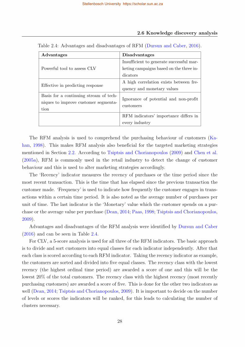
2.6 Knowledge discovery analysis
Table 2.4: Advantages and disadvantages of RFM (Dursun and Caber, 2016).
Advantages Disadvantages
Powerful tool to assess CLV
Insufficient to generate successful mar-
keting campaigns based on the three in-
dicators
Effective in predicting responseA high correlation exists between fre-
quency and monetary values
Basis for a continuing stream of tech-
niques to improve customer segmenta-
tion
Ignorance of potential and non-profit
customers
RFM indicators’ importance differs in
every industry
The RFM analysis is used to comprehend the purchasing behaviour of customers (Ka-
han, 1998). This makes RFM analysis also beneficial for the targeted marketing strategies
mentioned in Section 2.2. According to Tsiptsis and Chorianopoulos (2009) and Chen et al.
(2005a), RFM is commonly used in the retail industry to detect the change of customer
behaviour and this is used to alter marketing strategies accordingly.
The ‘Recency’ indicator measures the recency of purchases or the time period since the
most recent transaction. This is the time that has elapsed since the previous transaction the
customer made. ‘Frequency’ is used to indicate how frequently the customer engages in trans-
actions within a certain time period. It is also noted as the average number of purchases per
unit of time. The last indicator is the ‘Monetary’ value which the customer spends on a pur-
chase or the average value per purchase (Dean, 2014; Paas, 1998; Tsiptsis and Chorianopoulos,
2009).
Advantages and disadvantages of the RFM analysis were identified by Dursun and Caber
(2016) and can be seen in Table 2.4.
For CLV, a 5-score analysis is used for all three of the RFM indicators. The basic approach
is to divide and sort customers into equal classes for each indicator independently. After that
each class is scored according to each RFM indicator. Taking the recency indicator as example,
the customers are sorted and divided into five equal classes. The recency class with the lowest
recency (the highest ordinal time period) are awarded a score of one and this will be the
lowest 20% of the total customers. The recency class with the highest recency (most recently
purchasing customers) are awarded a score of five. This is done for the other two indicators as
well (Dean, 2014; Tsiptsis and Chorianopoulos, 2009). It is important to decide on the number
of levels or scores the indicators will be ranked, for this leads to calculating the number of
clusters necessary.
28
Stellenbosch University https://scholar.sun.ac.za
2.6 Knowledge discovery analysis
The number of clusters can be calculated by
Number of Clusters = LevelRecency × LevelFrequency × LevelMonetary.
Using the example of a 5-score analysis, the number of clusters is 125 (5×5×5). Thus, the
level of each class for a respective indicator is the number of the scoring analysis representing
the class. The CLV can be calculated as the product of the scores from the three RFM
indicators. To make this clear, for a 2-score analysis (eight clusters), above or below average,
the top RFM score would be eight and thus would this also be the CLV.
Previous work highlighted different scoring methods (Dursun and Caber, 2016). It was
criticised that ‘the customer quantile method’ either grouped customers with different be-
haviour together and arbitrarily divided customers with similar behaviour. From this the
‘customer behaviour quantile scoring’ was proposed. This method scored customers based on
each quantile having almost equal monetary values. A weighted approach was also identified
which examines the relative importance of the RFM indicators via the Analytic Hierarchy
Process (AHP) algorithm (Dursun and Caber, 2016). An evaluation of this approach would
look like
RFM score = (LevelRecency ×WeightRecency) + (LevelFrequency ×WeightFrequency) +
(LevelMonetary ×WeightMonetary).
Another method of using the RFM is using the original data instead of the coded data.
The mean for each RFM indicator is calculated and the RFM scores are indicated as above
average using ‘^’, and below average using ‘_’. This type of scoring analysis will have eight
clusters.
k–means, a common clustering algorithm, is used to evaluate the optimal number of clus-
ters depending on the customer data being analysed. More about clustering can be found in
Section 2.8. Based on the optimal number of clusters, an appropriate scoring analysis can
be chosen. For each RFM indicator, the clusters are scored and the product of these scores
identifies the CLV.
Figure 2.9 shows the growth matrix of the Boston Consulting Group (BCG), which classifies
customers into four segments based on their customer value. The four groups are the best
customer, frequent customer, spender customer, and uncertain customer (Chen et al., 2005a).
RFM models can be used to evaluate the CLV scores of customer segments and place
them within one of the four groups of the BCG growth matrix, or each individual cluster can
represent a different type of customer and, thus, an alternative marketing strategy must be
used. Applications of RFM models can be found in Dursun and Caber (2016), Chen et al.
(2005a) and Dean (2014).
29
Stellenbosch University https://scholar.sun.ac.za
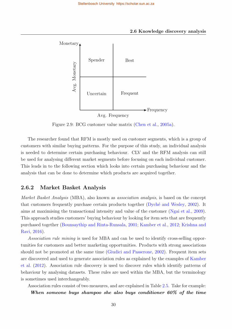
2.6 Knowledge discovery analysis
Uncertain Frequent
Spender Best
Monetary
FrequencyAvg. Frequency
Avg.
Mon
etar
y
Figure 2.9: BCG customer value matrix (Chen et al., 2005a).
The researcher found that RFM is mostly used on customer segments, which is a group of
customers with similar buying patterns. For the purpose of this study, an individual analysis
is needed to determine certain purchasing behaviour. CLV and the RFM analysis can still
be used for analysing different market segments before focusing on each individual customer.
This leads in to the following section which looks into certain purchasing behaviour and the
analysis that can be done to determine which products are acquired together.
2.6.2 Market Basket Analysis
Market Basket Analysis (MBA), also known as association analysis, is based on the concept
that customers frequently purchase certain products together (Dyche and Wesley, 2002). It
aims at maximising the transactional intensity and value of the customer (Ngai et al., 2009).
This approach studies customers’ buying behaviour by looking for item sets that are frequently
purchased together (Bounsaythip and Rinta-Runsala, 2001; Kamber et al., 2012; Krishna and
Ravi, 2016).
Association rule mining is used for MBA and can be used to identify cross-selling oppor-
tunities for customers and better marketing opportunities. Products with strong associations
should not be promoted at the same time (Giudici and Passerone, 2002). Frequent item sets
are discovered and used to generate association rules as explained by the examples of Kamber
et al. (2012). Association rule discovery is used to discover rules which identify patterns of
behaviour by analysing datasets. These rules are used within the MBA, but the terminology
is sometimes used interchangeably.
Association rules consist of two measures, and are explained in Table 2.5. Take for example:
When someone buys shampoo she also buys conditioner 60% of the time
30
Stellenbosch University https://scholar.sun.ac.za
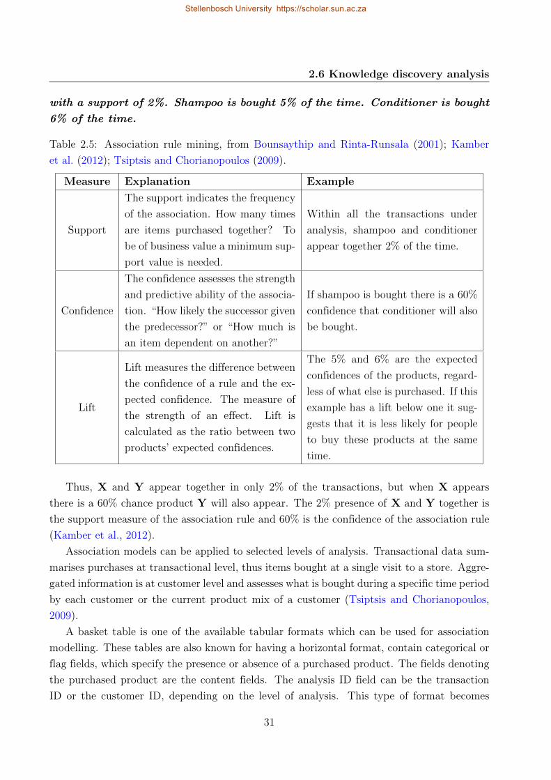
2.6 Knowledge discovery analysis
with a support of 2%. Shampoo is bought 5% of the time. Conditioner is bought
6% of the time.
Table 2.5: Association rule mining, from Bounsaythip and Rinta-Runsala (2001); Kamber
et al. (2012); Tsiptsis and Chorianopoulos (2009).
Measure Explanation Example
Support
The support indicates the frequency
of the association. How many times
are items purchased together? To
be of business value a minimum sup-
port value is needed.
Within all the transactions under
analysis, shampoo and conditioner
appear together 2% of the time.
Confidence
The confidence assesses the strength
and predictive ability of the associa-
tion. “How likely the successor given
the predecessor?” or “How much is
an item dependent on another?”
If shampoo is bought there is a 60%
confidence that conditioner will also
be bought.
Lift
Lift measures the difference between
the confidence of a rule and the ex-
pected confidence. The measure of
the strength of an effect. Lift is
calculated as the ratio between two
products’ expected confidences.
The 5% and 6% are the expected
confidences of the products, regard-
less of what else is purchased. If this
example has a lift below one it sug-
gests that it is less likely for people
to buy these products at the same
time.
Thus, X and Y appear together in only 2% of the transactions, but when X appears
there is a 60% chance product Y will also appear. The 2% presence of X and Y together is
the support measure of the association rule and 60% is the confidence of the association rule
(Kamber et al., 2012).
Association models can be applied to selected levels of analysis. Transactional data sum-
marises purchases at transactional level, thus items bought at a single visit to a store. Aggre-
gated information is at customer level and assesses what is bought during a specific time period
by each customer or the current product mix of a customer (Tsiptsis and Chorianopoulos,
2009).
A basket table is one of the available tabular formats which can be used for association
modelling. These tables are also known for having a horizontal format, contain categorical or
flag fields, which specify the presence or absence of a purchased product. The fields denoting
the purchased product are the content fields. The analysis ID field can be the transaction
ID or the customer ID, depending on the level of analysis. This type of format becomes
31
Stellenbosch University https://scholar.sun.ac.za
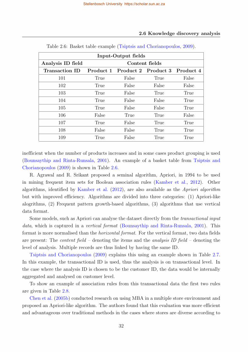
2.6 Knowledge discovery analysis
Table 2.6: Basket table example (Tsiptsis and Chorianopoulos, 2009).
Input-Output fields
Analysis ID field Content fields
Transaction ID Product 1 Product 2 Product 3 Product 4
101 True False True False
102 True False False False
103 True False True True
104 True False False True
105 True False False True
106 False True True False
107 True False True True
108 False False True True
109 True False True True
inefficient when the number of products increases and in some cases product grouping is used
(Bounsaythip and Rinta-Runsala, 2001). An example of a basket table from Tsiptsis and
Chorianopoulos (2009) is shown in Table 2.6.
R. Agrawal and R. Srikant proposed a seminal algorithm, Apriori, in 1994 to be used
in mining frequent item sets for Boolean association rules (Kamber et al., 2012). Other
algorithms, identified by Kamber et al. (2012), are also available as the Apriori algorithm
but with improved efficiency. Algorithms are divided into three categories: (1) Apriori-like
alogrithms, (2) Frequent pattern growth-based algorithms, (3) algorithms that use vertical
data format.
Some models, such as Apriori can analyse the dataset directly from the transactional input
data, which is captured in a vertical format (Bounsaythip and Rinta-Runsala, 2001). This
format is more normalised than the horizontal format. For the vertical format, two data fields
are present: The content field – denoting the items and the analysis ID field – denoting the
level of analysis. Multiple records are thus linked by having the same ID.
Tsiptsis and Chorianopoulos (2009) explains this using an example shown in Table 2.7.
In this example, the transactional ID is used, thus the analysis is on transactional level. In
the case where the analysis ID is chosen to be the customer ID, the data would be internally
aggregated and analysed on customer level.
To show an example of association rules from this transactional data the first two rules
are given in Table 2.8.
Chen et al. (2005b) conducted research on using MBA in a multiple store environment and
proposed an Apriori-like algorithm. The authors found that this evaluation was more efficient
and advantageous over traditional methods in the cases where stores are diverse according to
32
Stellenbosch University https://scholar.sun.ac.za
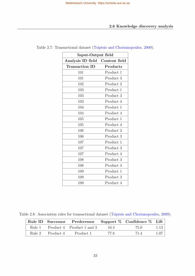
2.6 Knowledge discovery analysis
Table 2.7: Transactional dataset (Tsiptsis and Chorianopoulos, 2009).
Input-Output field
Analysis ID field Content field
Transaction ID Products
101 Product 1
101 Product 3
102 Product 2
103 Product 1
103 Product 3
103 Product 4
104 Product 1
104 Product 4
105 Product 1
105 Product 4
106 Product 2
106 Product 3
107 Product 1
107 Product 3
107 Product 4
108 Product 3
108 Product 4
109 Product 1
109 Product 3
109 Product 4
Table 2.8: Association rules for transactional dataset (Tsiptsis and Chorianopoulos, 2009).
Rule ID Successor Predecessor Support % Confidence % Lift
Rule 1 Product 4 Product 1 and 3 44.4 75.0 1.13
Rule 2 Product 4 Product 1 77.8 71.4 1.07
33
Stellenbosch University https://scholar.sun.ac.za
2.6 Knowledge discovery analysis
size, location and product mix. The article includes alterations in the algorithm to overcome
problems such as seasonal sales and some stores not selling certain products. This article can
be helpful in this study and will be referred to again.
Other related literature on association rule mining is Adomavicius and Tuzhilin (2001);
Giudici and Passerone (2002); Au and Chan (2003); Chen et al. (2005a); Demiriz (2004); Jiao
et al. (2006); Lee et al. (2006) and Wang et al. (2004).
For the focus of this study, association rule mining and thus MBA will be an appropriate
approach to create customer profiles based on analysing the customers’ transactional history.
Association rule mining is also suitable for identifying cross-selling and upselling opportunities.
When adding a time element to MBA it is often seen as Sequence Pattern Analysis (SPA)
and this will be the next topic of discussion.
2.6.3 Sequential Pattern Analysis
Alongside association-rule mining, Sequential Pattern Analysis (SPA) exists when adding the
factor of time with the association rule modelling. This creates the analysis of associations
over time in order to discover patterns or series of events happening in a specific sequence.
The generation of sequential association rules are analogous to those mentioned in MBA with
the difference that if things happen in a certain sequence, the probability of a certain event
to occur next is increased (Tsiptsis and Chorianopoulos, 2009).
As with association rule mining (which was first mentioned by Agrawal and Srikant in
1994), SPA was also investigated by these researchers in 1995 (Changchien et al., 2004; Mooney
and Roddick, 2013). SPA is defined as “Given a database of sequences, where each sequence
consists of a list of transactions ordered by transaction time and each transaction is a set
of items, sequential pattern mining is to discover all sequential patterns with a user-specified
minimum support, where the support of a pattern is the number of data-sequences that contain
the pattern” (Mooney and Roddick, 2013).
In the research by Mooney and Roddick (2013), a variety of reformulations of this definition
are provided. Since association mining started within transactional data, this was the same
start for SPA. However, this type of analysis can be used in various domains and applica-
tions such as genome searching (biotechnology), alarm data in telecommunications networks
(telecommunication) and population health data (health care).
SPA algorithms can also be categorised in the same categories as association rule mining.
The categories as described by Mooney and Roddick (2013) are (1) Apriori-like, (2) horizontal
or vertical format, or (3) projection-based pattern growth algorithms. The variety of domains in
which SPA can be used led to algorithmic developments in each domain respectively. Frequent
item sets, mentioned in Subsection 2.6.2, are used for normal association rule mining and
sequential rule mining. The difference comes where Apriori-like algorithms for MBA discover
34
Stellenbosch University https://scholar.sun.ac.za
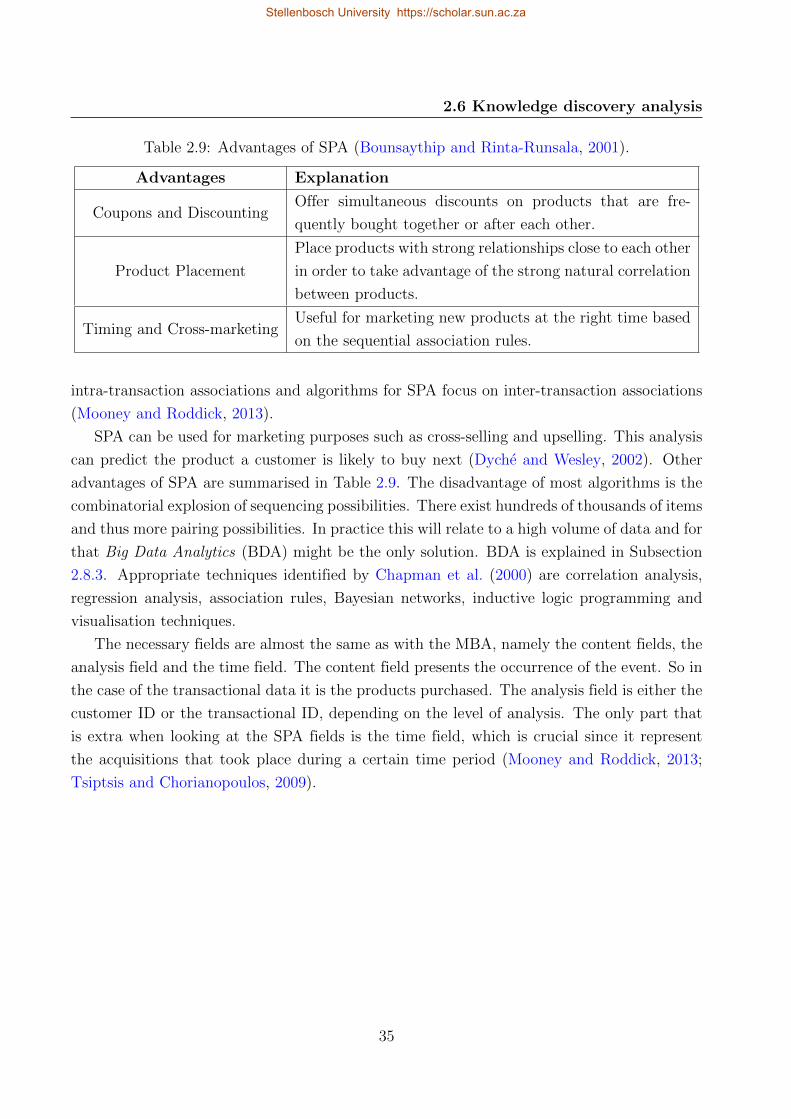
2.6 Knowledge discovery analysis
Table 2.9: Advantages of SPA (Bounsaythip and Rinta-Runsala, 2001).
Advantages Explanation
Coupons and DiscountingOffer simultaneous discounts on products that are fre-
quently bought together or after each other.
Product Placement
Place products with strong relationships close to each other
in order to take advantage of the strong natural correlation
between products.
Timing and Cross-marketingUseful for marketing new products at the right time based
on the sequential association rules.
intra-transaction associations and algorithms for SPA focus on inter-transaction associations
(Mooney and Roddick, 2013).
SPA can be used for marketing purposes such as cross-selling and upselling. This analysis
can predict the product a customer is likely to buy next (Dyche and Wesley, 2002). Other
advantages of SPA are summarised in Table 2.9. The disadvantage of most algorithms is the
combinatorial explosion of sequencing possibilities. There exist hundreds of thousands of items
and thus more pairing possibilities. In practice this will relate to a high volume of data and for
that Big Data Analytics (BDA) might be the only solution. BDA is explained in Subsection
2.8.3. Appropriate techniques identified by Chapman et al. (2000) are correlation analysis,
regression analysis, association rules, Bayesian networks, inductive logic programming and
visualisation techniques.
The necessary fields are almost the same as with the MBA, namely the content fields, the
analysis field and the time field. The content field presents the occurrence of the event. So in
the case of the transactional data it is the products purchased. The analysis field is either the
customer ID or the transactional ID, depending on the level of analysis. The only part that
is extra when looking at the SPA fields is the time field, which is crucial since it represent
the acquisitions that took place during a certain time period (Mooney and Roddick, 2013;
Tsiptsis and Chorianopoulos, 2009).
35
Stellenbosch University https://scholar.sun.ac.za
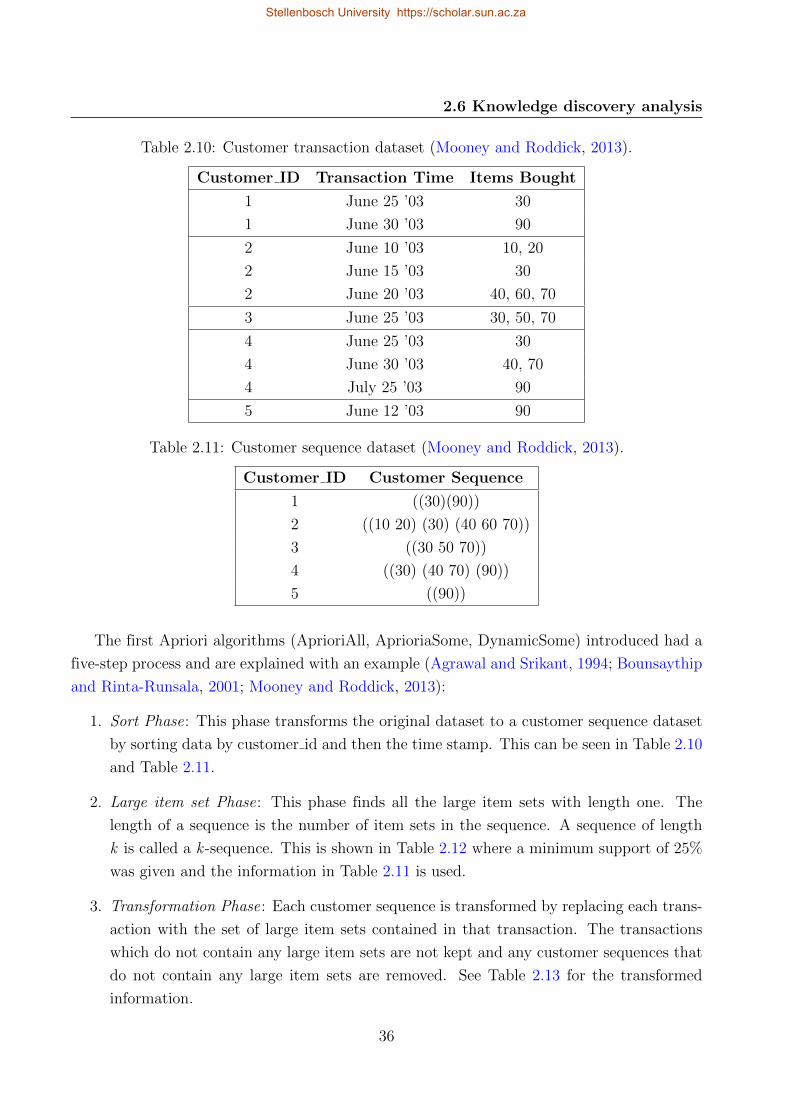
2.6 Knowledge discovery analysis
Table 2.10: Customer transaction dataset (Mooney and Roddick, 2013).
Customer ID Transaction Time Items Bought
1 June 25 ’03 30
1 June 30 ’03 90
2 June 10 ’03 10, 20
2 June 15 ’03 30
2 June 20 ’03 40, 60, 70
3 June 25 ’03 30, 50, 70
4 June 25 ’03 30
4 June 30 ’03 40, 70
4 July 25 ’03 90
5 June 12 ’03 90
Table 2.11: Customer sequence dataset (Mooney and Roddick, 2013).
Customer ID Customer Sequence
1 ((30)(90))
2 ((10 20) (30) (40 60 70))
3 ((30 50 70))
4 ((30) (40 70) (90))
5 ((90))
The first Apriori algorithms (AprioriAll, AprioriaSome, DynamicSome) introduced had a
five-step process and are explained with an example (Agrawal and Srikant, 1994; Bounsaythip
and Rinta-Runsala, 2001; Mooney and Roddick, 2013):
1. Sort Phase: This phase transforms the original dataset to a customer sequence dataset
by sorting data by customer id and then the time stamp. This can be seen in Table 2.10
and Table 2.11.
2. Large item set Phase: This phase finds all the large item sets with length one. The
length of a sequence is the number of item sets in the sequence. A sequence of length
k is called a k -sequence. This is shown in Table 2.12 where a minimum support of 25%
was given and the information in Table 2.11 is used.
3. Transformation Phase: Each customer sequence is transformed by replacing each trans-
action with the set of large item sets contained in that transaction. The transactions
which do not contain any large item sets are not kept and any customer sequences that
do not contain any large item sets are removed. See Table 2.13 for the transformed
information.
36
Stellenbosch University https://scholar.sun.ac.za
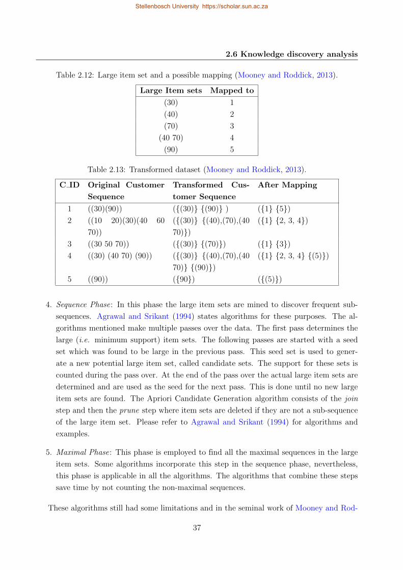
2.6 Knowledge discovery analysis
Table 2.12: Large item set and a possible mapping (Mooney and Roddick, 2013).
Large Item sets Mapped to
(30) 1
(40) 2
(70) 3
(40 70) 4
(90) 5
Table 2.13: Transformed dataset (Mooney and Roddick, 2013).
C ID Original Customer
Sequence
Transformed Cus-
tomer Sequence
After Mapping
1 ((30)(90)) ({(30)} {(90)} ) ({1} {5})2 ((10 20)(30)(40 60
70))
({(30)} {(40),(70),(40
70)})({1} {2, 3, 4})
3 ((30 50 70)) ({(30)} {(70)}) ({1} {3})4 ((30) (40 70) (90)) ({(30)} {(40),(70),(40
70)} {(90)})({1} {2, 3, 4} {(5)})
5 ((90)) ({90}) ({(5)})
4. Sequence Phase: In this phase the large item sets are mined to discover frequent sub-
sequences. Agrawal and Srikant (1994) states algorithms for these purposes. The al-
gorithms mentioned make multiple passes over the data. The first pass determines the
large (i.e. minimum support) item sets. The following passes are started with a seed
set which was found to be large in the previous pass. This seed set is used to gener-
ate a new potential large item set, called candidate sets. The support for these sets is
counted during the pass over. At the end of the pass over the actual large item sets are
determined and are used as the seed for the next pass. This is done until no new large
item sets are found. The Apriori Candidate Generation algorithm consists of the join
step and then the prune step where item sets are deleted if they are not a sub-sequence
of the large item set. Please refer to Agrawal and Srikant (1994) for algorithms and
examples.
5. Maximal Phase: This phase is employed to find all the maximal sequences in the large
item sets. Some algorithms incorporate this step in the sequence phase, nevertheless,
this phase is applicable in all the algorithms. The algorithms that combine these steps
save time by not counting the non-maximal sequences.
These algorithms still had some limitations and in the seminal work of Mooney and Rod-
37
Stellenbosch University https://scholar.sun.ac.za

2.6 Knowledge discovery analysis
dick (2013), a summarised table shows some improved algorithms. This summary can be seen
in Table 2.14.
38
Stellenbosch University https://scholar.sun.ac.za
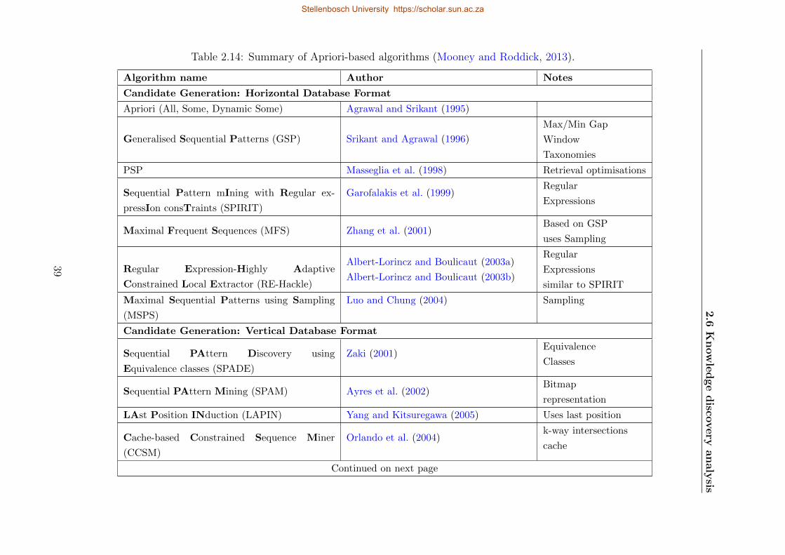
2.6
Knowledgedisco
very
analysis
Table 2.14: Summary of Apriori-based algorithms (Mooney and Roddick, 2013).
Algorithm name Author Notes
Candidate Generation: Horizontal Database Format
Apriori (All, Some, Dynamic Some) Agrawal and Srikant (1995)
Generalised Sequential Patterns (GSP) Srikant and Agrawal (1996)
Max/Min Gap
Window
Taxonomies
PSP Masseglia et al. (1998) Retrieval optimisations
Sequential Pattern mIning with Regular ex-
pressIon consTraints (SPIRIT)
Garofalakis et al. (1999)Regular
Expressions
Maximal Frequent Sequences (MFS) Zhang et al. (2001)Based on GSP
uses Sampling
Regular Expression-Highly Adaptive
Constrained Local Extractor (RE-Hackle)
Albert-Lorincz and Boulicaut (2003a)
Albert-Lorincz and Boulicaut (2003b)
Regular
Expressions
similar to SPIRIT
Maximal Sequential Patterns using Sampling
(MSPS)
Luo and Chung (2004) Sampling
Candidate Generation: Vertical Database Format
Sequential PAttern Discovery using
Equivalence classes (SPADE)
Zaki (2001)Equivalence
Classes
Sequential PAttern Mining (SPAM) Ayres et al. (2002)Bitmap
representation
LAst Position INduction (LAPIN) Yang and Kitsuregawa (2005) Uses last position
Cache-based Constrained Sequence Miner
(CCSM)
Orlando et al. (2004)k-way intersections
cache
Continued on next page
39
Stellenbosch University https://scholar.sun.ac.za
Stellenbosch University https://scholar.sun.ac.za
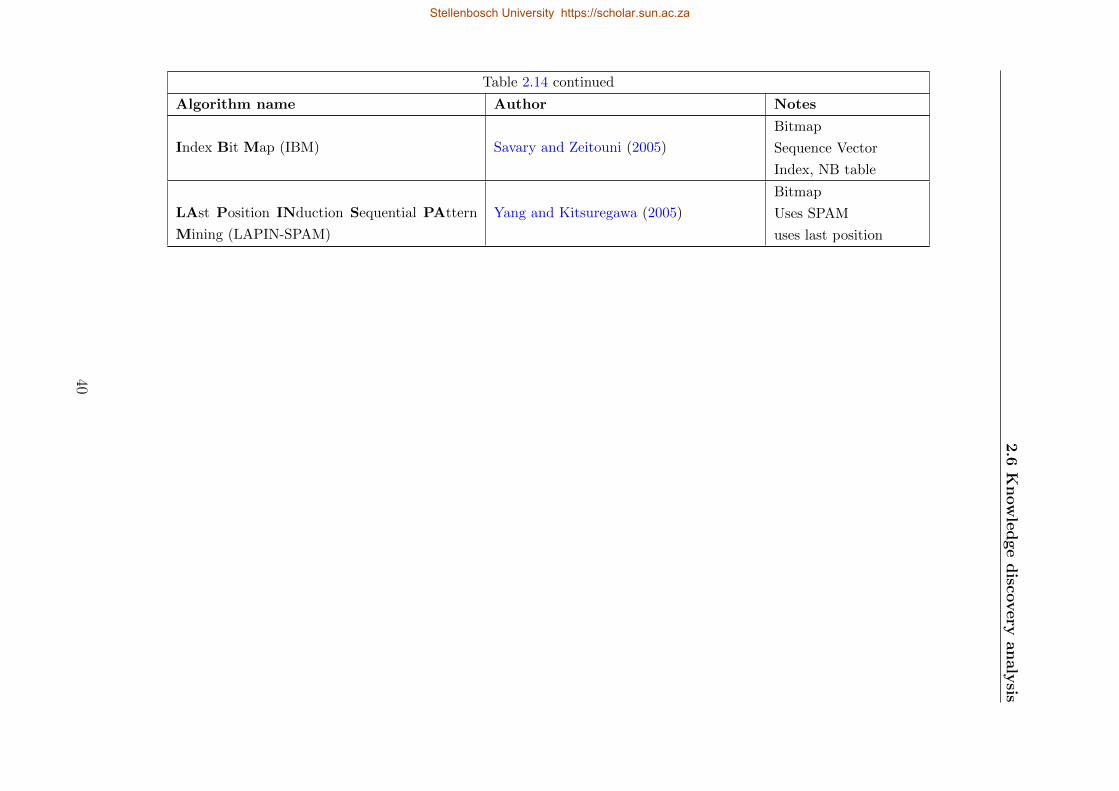
2.6
Knowledgedisco
very
analysis
Table 2.14 continued
Algorithm name Author Notes
Index Bit Map (IBM) Savary and Zeitouni (2005)
Bitmap
Sequence Vector
Index, NB table
LAst Position INduction Sequential PAttern
Mining (LAPIN-SPAM)
Yang and Kitsuregawa (2005)
Bitmap
Uses SPAM
uses last position
40
Stellenbosch University https://scholar.sun.ac.za
Stellenbosch University https://scholar.sun.ac.za
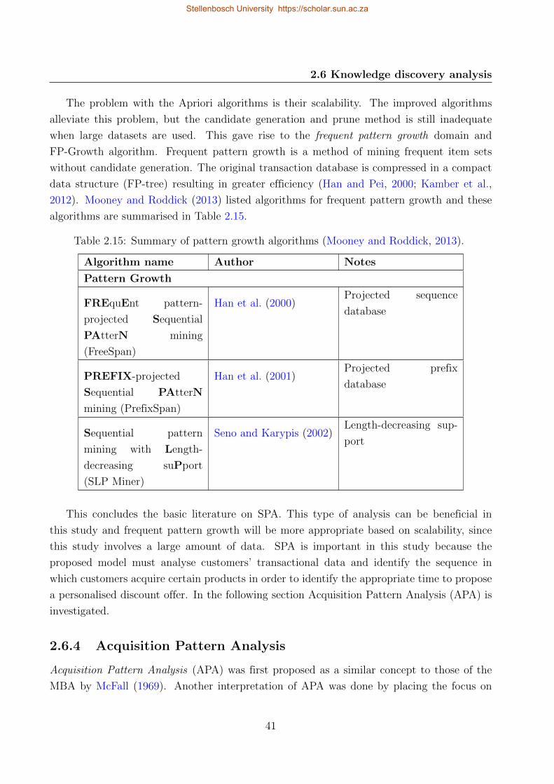
2.6 Knowledge discovery analysis
The problem with the Apriori algorithms is their scalability. The improved algorithms
alleviate this problem, but the candidate generation and prune method is still inadequate
when large datasets are used. This gave rise to the frequent pattern growth domain and
FP-Growth algorithm. Frequent pattern growth is a method of mining frequent item sets
without candidate generation. The original transaction database is compressed in a compact
data structure (FP-tree) resulting in greater efficiency (Han and Pei, 2000; Kamber et al.,
2012). Mooney and Roddick (2013) listed algorithms for frequent pattern growth and these
algorithms are summarised in Table 2.15.
Table 2.15: Summary of pattern growth algorithms (Mooney and Roddick, 2013).
Algorithm name Author Notes
Pattern Growth
FREquEnt pattern-
projected Sequential
PAtterN mining
(FreeSpan)
Han et al. (2000)Projected sequence
database
PREFIX-projected
Sequential PAtterN
mining (PrefixSpan)
Han et al. (2001)Projected prefix
database
Sequential pattern
mining with Length-
decreasing suPport
(SLP Miner)
Seno and Karypis (2002)Length-decreasing sup-
port
This concludes the basic literature on SPA. This type of analysis can be beneficial in
this study and frequent pattern growth will be more appropriate based on scalability, since
this study involves a large amount of data. SPA is important in this study because the
proposed model must analyse customers’ transactional data and identify the sequence in
which customers acquire certain products in order to identify the appropriate time to propose
a personalised discount offer. In the following section Acquisition Pattern Analysis (APA) is
investigated.
2.6.4 Acquisition Pattern Analysis
Acquisition Pattern Analysis (APA) was first proposed as a similar concept to those of the
MBA by McFall (1969). Another interpretation of APA was done by placing the focus on
41
Stellenbosch University https://scholar.sun.ac.za
2.6 Knowledge discovery analysis
the sequence in which acquisitions are made rather than the composition of the item set.
This lead to the same idea as the SPA. A third definition of the APA was suggested by
combining the MBA and the SPA to reach the fundamental goal of the APA and relationship
marketing, to identify the needs of a customer in order to ensure their satisfaction by making
recommendations on marketing activities (Paas et al., 2005).
APA investigates the acquisition pattern of products in order to forecast future acquisitions
(Paas and Molenaar, 2005). APA is relevant in industries where a customer has various
objectives but due to financial constraints, they cannot be fulfilled. On this aspect, APA
is differentiated from the previously discussed section. APA is mostly considered for the
durable goods and financial sector services (Paas, 1998; Paas and Molenaar, 2005). APA
is advantageous for increasing customer retention and cross-selling opportunities in these
respective markets.
Previous studies of APA were usually done on survey data. Paas (2009) conducted research
to investigate if APA can be applied to transactional data as well. The research shown
that transactional data can also be used for APA in the financial industry. The research
unfortunately did not determine if this is the case for durable products as well. The challenge
for this study is to determine whether the APA can only be used for durable goods or if it
can be used for Fast Moving Consumer Goods (FMCG).
Paas et al. (2005) proposed two consecutive steps that the APA should consist of: (1) the
definition of the product set, and (2) the investigation of the order in which the products are
acquired for each product set. The sequence of these steps is crucial as important information
will be lost if the order is reversed. In this research the authors empirically showed how these
two steps are executed to combine both the MBA and the SPA.
Mokken scaling is mostly used in literature for APA and also in the research of Paas et al.
(2005). Mokken scaling introduces a step-wise approach which insures that vital information
is not lost. The model separates the tests by allocating items to item sets and by investigating
the sequence in which customers purchase the products. The other available techniques do
not include the step-wise approach. Other modelling techniques for APA are Purchase Trees,
Guttman Scaling, Parametric Scaling, Latent Class Analysis. The reader is referred to Paas
(1998), Paas and Molenaar (2005), Paas et al. (2005), Salazar et al. (2007) for information
regarding association rule mining and MBA.
For cross-selling and upselling opportunities the repurchasing behaviour of a customer is
important. In the research of Salazar et al. (2007), the authors state two aspects important
for repurchase behaviour. The first is the acquisition pattern of the customer and the second
is the factors that have the greatest influence on repurchase behaviour. The latter is explained
in Subsection 2.6.5.
This subsection illustrated how acquisition patterns can be found, but it is mostly limited
42
Stellenbosch University https://scholar.sun.ac.za
2.6 Knowledge discovery analysis
to the financial services market and durable goods. This provides the opportunity to determine
if it can be applied for FMCG along with other analyses such as the MBA, SPA and survival
analysis, discussed next.
2.6.5 Survival Analysis
Harrell (2015) describes the use of survival analysis as the analysis of data in which the time
of a specific occurrence is of interest. This can be failure time, survival time or event time.
Survival analysis techniques are well established in the domain of healthcare. The techniques
are designed to predict the probability that a patient, who is undergoing medical treatment,
will survive until time t (Harrell, 2015; Kamber et al., 2012). However, survival analysis can
also be applied in the CRM domain.
As mentioned in Subsection 2.6.4, there are factors that have an impact on the repurchase
behaviour of customers. These can be customer satisfaction, brand commitment and purchase
experience. In the study by Salazar et al. (2007), survival analysis is used to address this aspect
of repurchase behaviour. Within the survival analysis domain, there are numerous techniques
to be used in different scenarios. For the purpose of repurchasing behaviour it is found that
the best choices are Cox regression and binary logic regression (Salazar et al., 2007).
Since the sequence of customer acquisitions has already been investigated by the preceding
sections and survival analysis introduces the factors responsible for repurchasing, the only part
to discuss is when the next purchase will occur. It is of utmost importance to estimate the
appropriate time to offer the most favourable product to the customer. This will ensure that
marketing opportunities are fully utilised.
A time sequence is introduced to address this problem. This analysis focuses on when
the next occurrence and in the case of this study, the next transaction will take place. The
two main aspects are the fact that a repurchase will happen and the time period in which
it is most likely to happen. This information can be derived from the survival analysis done
earlier. One of the outputs from the survival analysis is the survival curve which plots the
probability of a repurchase against time. This can be used to estimate when a repurchase
might take place (Salazar et al., 2007).
The Cox proportional hazard model is one of the popular techniques along with the Kaplan-
Meier estimate (Kamber et al., 2012). The advantages of the Cox proportional hazard model
is summarised by Lariviere and Van Den Poel (2005) as:
i. It allows for incorporating time-varying covariates and both discrete and continuous mea-
surements of event times.
ii. It can handle observations that did not experience the event.
43
Stellenbosch University https://scholar.sun.ac.za
2.6 Knowledge discovery analysis
iii. It appears to be robust and requires few assumptions.
The Cox proportional hazard for customer n at time t, given his vector of covariates xn
can be written as
hn(t, xn) = h0exp(βxn)
in which h0 represents the baseline hazard.
A disadvantage overlooked is the assumption of proportionality. Proportionality indicates
that the hazard for any individual i is a fixed proportion γij of the hazard of any other
individual where
γij =hi(t, xi)
hj(t, xj)=h0exp(βxi)
h0exp(βxj)= exp {β(xi − xj)} .
In the case where proportionality is violated another technique must be used. Survival
forests are used in the research of Lariviere and Van Den Poel (2004, 2005).
Trigger events happen within a customer’s life cycle and allow the company to predict the
future behaviour of a customer (Malthouse, 2007). The Cox proportional hazard model and
discrete-time models facilitate time-dependent covariates. Trigger analysis is differentiated
whether trigger events only happen at time 0 or are they repeated events. In the case of
transactional data, trigger events are repeated and are an option for the Cox proportional
hazard model. Trigger events are used for loyalty programmes, financial services, retail web-
sites, etc. (Malthouse, 2007).
Another popular technique for estimating survival is the Kaplan-Meier estimator, which
is a non-parametric estimator (Bland and Altman, 1998). The probabilities of survival are
presented in a survival curve, where the graph is a step function. Sudden changes in the
estimated probability corresponds to the time at which the events happen (Lariviere and Van
Den Poel, 2005; Rosset et al., 2003). Harrell (2015) can be used as reference to illustrate in
detail how the Cox proportional hazard model, Kaplan-Meier estimator and other techniques
are defined.
Table 2.16 displays references to literature where survival analysis has been used.
This section provided an overview of the analysis needed to estimate the time of the next
repurchase. This, along with the APA, which indicates the sequence of acquisitions, provides
marketers with the knowledge to create cross-selling and upselling offers to customers. The
researcher finds that in the case of this particular study and scenario, a combination of these
analysis methods must be used to obtain the goal of the proposed model. This next section
presents a holistic view of Big Data and explains when a dataset is considered Big Data.
44
Stellenbosch University https://scholar.sun.ac.za
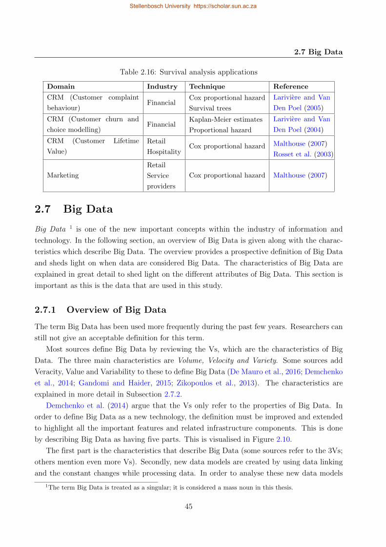
2.7 Big Data
Table 2.16: Survival analysis applications
Domain Industry Technique Reference
CRM (Customer complaint
behaviour)Financial
Cox proportional hazard
Survival trees
Lariviere and Van
Den Poel (2005)
CRM (Customer churn and
choice modelling)Financial
Kaplan-Meier estimates
Proportional hazard
Lariviere and Van
Den Poel (2004)
CRM (Customer Lifetime
Value)
Retail
HospitalityCox proportional hazard Malthouse (2007)
Rosset et al. (2003)
Marketing
Retail
Service
providers
Cox proportional hazard Malthouse (2007)
2.7 Big Data
Big Data 1 is one of the new important concepts within the industry of information and
technology. In the following section, an overview of Big Data is given along with the charac-
teristics which describe Big Data. The overview provides a prospective definition of Big Data
and sheds light on when data are considered Big Data. The characteristics of Big Data are
explained in great detail to shed light on the different attributes of Big Data. This section is
important as this is the data that are used in this study.
2.7.1 Overview of Big Data
The term Big Data has been used more frequently during the past few years. Researchers can
still not give an acceptable definition for this term.
Most sources define Big Data by reviewing the Vs, which are the characteristics of Big
Data. The three main characteristics are Volume, Velocity and Variety. Some sources add
Veracity, Value and Variability to these to define Big Data (De Mauro et al., 2016; Demchenko
et al., 2014; Gandomi and Haider, 2015; Zikopoulos et al., 2013). The characteristics are
explained in more detail in Subsection 2.7.2.
Demchenko et al. (2014) argue that the Vs only refer to the properties of Big Data. In
order to define Big Data as a new technology, the definition must be improved and extended
to highlight all the important features and related infrastructure components. This is done
by describing Big Data as having five parts. This is visualised in Figure 2.10.
The first part is the characteristics that describe Big Data (some sources refer to the 3Vs;
others mention even more Vs). Secondly, new data models are created by using data linking
and the constant changes while processing data. In order to analyse these new data models
1The term Big Data is treated as a singular; it is considered a mass noun in this thesis.
45
Stellenbosch University https://scholar.sun.ac.za
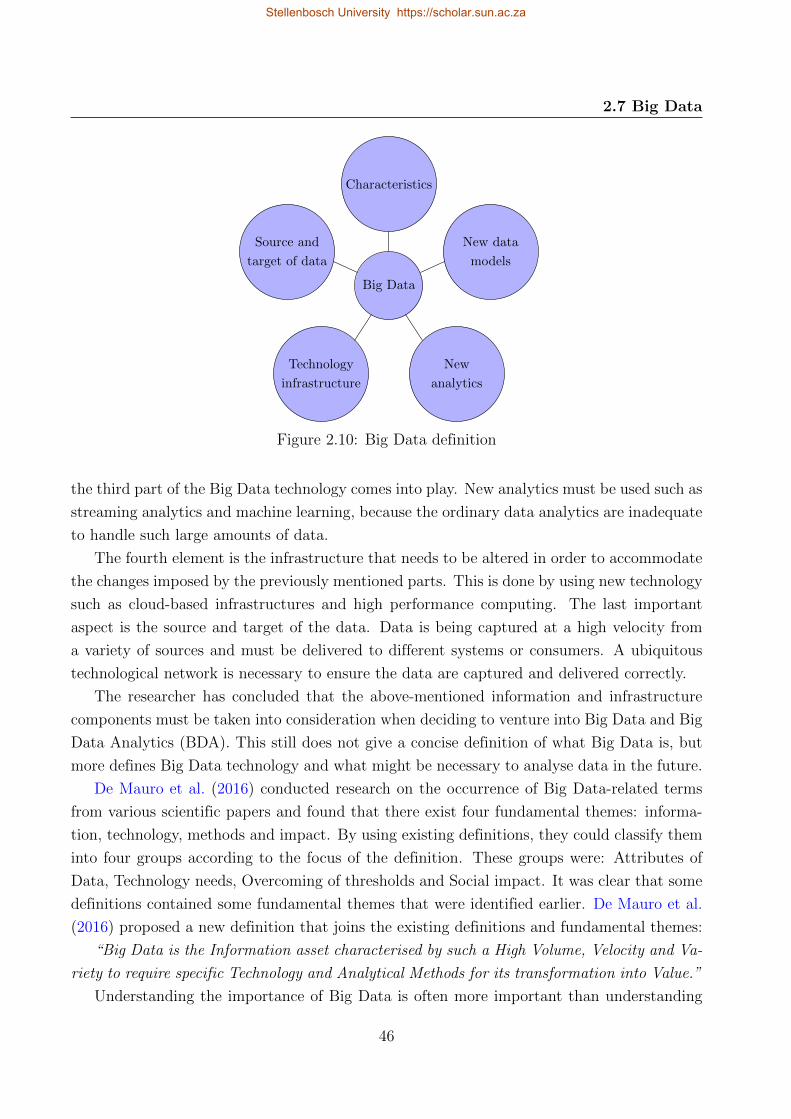
2.7 Big Data
Big Data
Characteristics
Source and
target of data
New data
models
Technology
infrastructure
New
analytics
Figure 2.10: Big Data definition
the third part of the Big Data technology comes into play. New analytics must be used such as
streaming analytics and machine learning, because the ordinary data analytics are inadequate
to handle such large amounts of data.
The fourth element is the infrastructure that needs to be altered in order to accommodate
the changes imposed by the previously mentioned parts. This is done by using new technology
such as cloud-based infrastructures and high performance computing. The last important
aspect is the source and target of the data. Data is being captured at a high velocity from
a variety of sources and must be delivered to different systems or consumers. A ubiquitous
technological network is necessary to ensure the data are captured and delivered correctly.
The researcher has concluded that the above-mentioned information and infrastructure
components must be taken into consideration when deciding to venture into Big Data and Big
Data Analytics (BDA). This still does not give a concise definition of what Big Data is, but
more defines Big Data technology and what might be necessary to analyse data in the future.
De Mauro et al. (2016) conducted research on the occurrence of Big Data-related terms
from various scientific papers and found that there exist four fundamental themes: informa-
tion, technology, methods and impact. By using existing definitions, they could classify them
into four groups according to the focus of the definition. These groups were: Attributes of
Data, Technology needs, Overcoming of thresholds and Social impact. It was clear that some
definitions contained some fundamental themes that were identified earlier. De Mauro et al.
(2016) proposed a new definition that joins the existing definitions and fundamental themes:
“Big Data is the Information asset characterised by such a High Volume, Velocity and Va-
riety to require specific Technology and Analytical Methods for its transformation into Value.”
Understanding the importance of Big Data is often more important than understanding
46
Stellenbosch University https://scholar.sun.ac.za
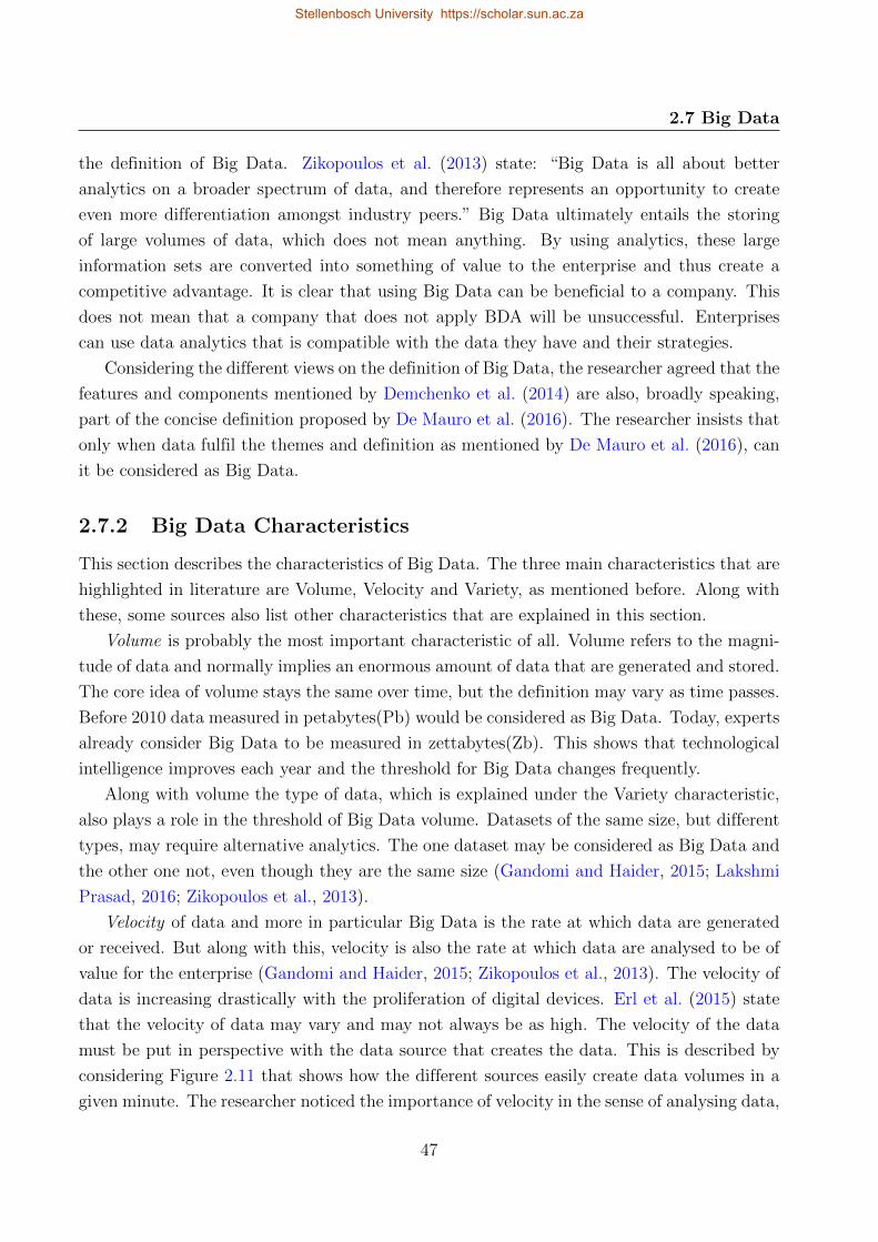
2.7 Big Data
the definition of Big Data. Zikopoulos et al. (2013) state: “Big Data is all about better
analytics on a broader spectrum of data, and therefore represents an opportunity to create
even more differentiation amongst industry peers.” Big Data ultimately entails the storing
of large volumes of data, which does not mean anything. By using analytics, these large
information sets are converted into something of value to the enterprise and thus create a
competitive advantage. It is clear that using Big Data can be beneficial to a company. This
does not mean that a company that does not apply BDA will be unsuccessful. Enterprises
can use data analytics that is compatible with the data they have and their strategies.
Considering the different views on the definition of Big Data, the researcher agreed that the
features and components mentioned by Demchenko et al. (2014) are also, broadly speaking,
part of the concise definition proposed by De Mauro et al. (2016). The researcher insists that
only when data fulfil the themes and definition as mentioned by De Mauro et al. (2016), can
it be considered as Big Data.
2.7.2 Big Data Characteristics
This section describes the characteristics of Big Data. The three main characteristics that are
highlighted in literature are Volume, Velocity and Variety, as mentioned before. Along with
these, some sources also list other characteristics that are explained in this section.
Volume is probably the most important characteristic of all. Volume refers to the magni-
tude of data and normally implies an enormous amount of data that are generated and stored.
The core idea of volume stays the same over time, but the definition may vary as time passes.
Before 2010 data measured in petabytes(Pb) would be considered as Big Data. Today, experts
already consider Big Data to be measured in zettabytes(Zb). This shows that technological
intelligence improves each year and the threshold for Big Data changes frequently.
Along with volume the type of data, which is explained under the Variety characteristic,
also plays a role in the threshold of Big Data volume. Datasets of the same size, but different
types, may require alternative analytics. The one dataset may be considered as Big Data and
the other one not, even though they are the same size (Gandomi and Haider, 2015; Lakshmi
Prasad, 2016; Zikopoulos et al., 2013).
Velocity of data and more in particular Big Data is the rate at which data are generated
or received. But along with this, velocity is also the rate at which data are analysed to be of
value for the enterprise (Gandomi and Haider, 2015; Zikopoulos et al., 2013). The velocity of
data is increasing drastically with the proliferation of digital devices. Erl et al. (2015) state
that the velocity of data may vary and may not always be as high. The velocity of the data
must be put in perspective with the data source that creates the data. This is described by
considering Figure 2.11 that shows how the different sources easily create data volumes in a
given minute. The researcher noticed the importance of velocity in the sense of analysing data,
47
Stellenbosch University https://scholar.sun.ac.za
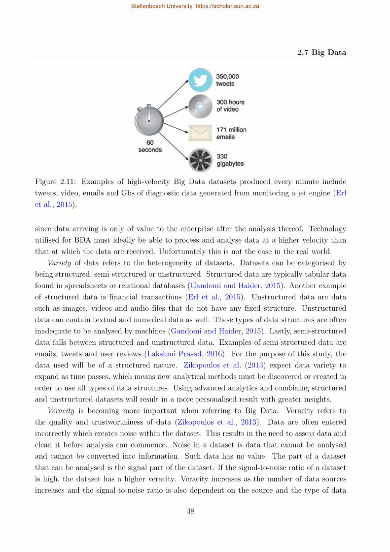
2.7 Big Data
Figure 2.11: Examples of high-velocity Big Data datasets produced every minute include
tweets, video, emails and Gbs of diagnostic data generated from monitoring a jet engine (Erl
et al., 2015).
since data arriving is only of value to the enterprise after the analysis thereof. Technology
utilised for BDA must ideally be able to process and analyse data at a higher velocity than
that at which the data are received. Unfortunately this is not the case in the real world.
Variety of data refers to the heterogeneity of datasets. Datasets can be categorised by
being structured, semi-structured or unstructured. Structured data are typically tabular data
found in spreadsheets or relational databases (Gandomi and Haider, 2015). Another example
of structured data is financial transactions (Erl et al., 2015). Unstructured data are data
such as images, videos and audio files that do not have any fixed structure. Unstructured
data can contain textual and numerical data as well. These types of data structures are often
inadequate to be analysed by machines (Gandomi and Haider, 2015). Lastly, semi-structured
data falls between structured and unstructured data. Examples of semi-structured data are
emails, tweets and user reviews (Lakshmi Prasad, 2016). For the purpose of this study, the
data used will be of a structured nature. Zikopoulos et al. (2013) expect data variety to
expand as time passes, which means new analytical methods must be discovered or created in
order to use all types of data structures. Using advanced analytics and combining structured
and unstructured datasets will result in a more personalised result with greater insights.
Veracity is becoming more important when referring to Big Data. Veracity refers to
the quality and trustworthiness of data (Zikopoulos et al., 2013). Data are often entered
incorrectly which creates noise within the dataset. This results in the need to assess data and
clean it before analysis can commence. Noise in a dataset is data that cannot be analysed
and cannot be converted into information. Such data has no value. The part of a dataset
that can be analysed is the signal part of the dataset. If the signal-to-noise ratio of a dataset
is high, the dataset has a higher veracity. Veracity increases as the number of data sources
increases and the signal-to-noise ratio is also dependent on the source and the type of data
48
Stellenbosch University https://scholar.sun.ac.za
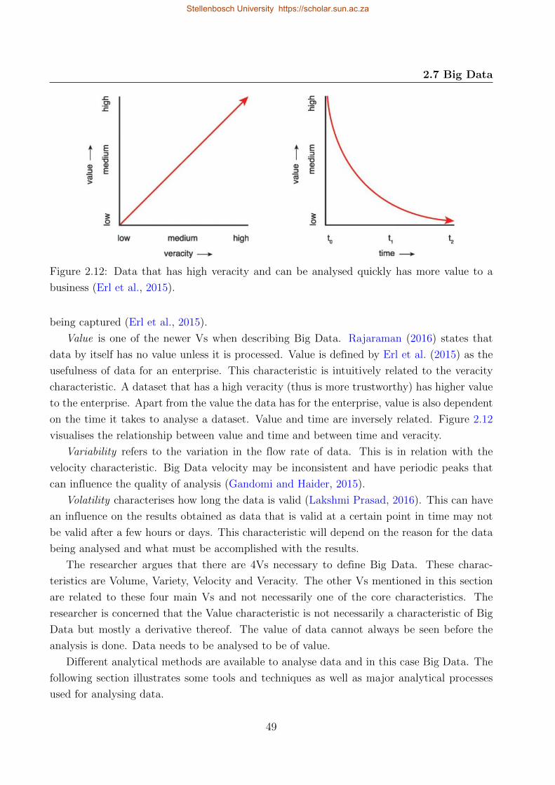
2.7 Big Data
Figure 2.12: Data that has high veracity and can be analysed quickly has more value to a
business (Erl et al., 2015).
being captured (Erl et al., 2015).
Value is one of the newer Vs when describing Big Data. Rajaraman (2016) states that
data by itself has no value unless it is processed. Value is defined by Erl et al. (2015) as the
usefulness of data for an enterprise. This characteristic is intuitively related to the veracity
characteristic. A dataset that has a high veracity (thus is more trustworthy) has higher value
to the enterprise. Apart from the value the data has for the enterprise, value is also dependent
on the time it takes to analyse a dataset. Value and time are inversely related. Figure 2.12
visualises the relationship between value and time and between time and veracity.
Variability refers to the variation in the flow rate of data. This is in relation with the
velocity characteristic. Big Data velocity may be inconsistent and have periodic peaks that
can influence the quality of analysis (Gandomi and Haider, 2015).
Volatility characterises how long the data is valid (Lakshmi Prasad, 2016). This can have
an influence on the results obtained as data that is valid at a certain point in time may not
be valid after a few hours or days. This characteristic will depend on the reason for the data
being analysed and what must be accomplished with the results.
The researcher argues that there are 4Vs necessary to define Big Data. These charac-
teristics are Volume, Variety, Velocity and Veracity. The other Vs mentioned in this section
are related to these four main Vs and not necessarily one of the core characteristics. The
researcher is concerned that the Value characteristic is not necessarily a characteristic of Big
Data but mostly a derivative thereof. The value of data cannot always be seen before the
analysis is done. Data needs to be analysed to be of value.
Different analytical methods are available to analyse data and in this case Big Data. The
following section illustrates some tools and techniques as well as major analytical processes
used for analysing data.
49
Stellenbosch University https://scholar.sun.ac.za
2.8 Big Data Analytics
Figure 2.13: Multidisciplinary nature of data mining (Dean, 2014).
2.8 Big Data Analytics
Analytical methods are needed to extract unknown knowledge from large datasets which
cannot be recognised by a human being. Data mining is the process used to analyse datasets
described in the preceding sections. Previous academic literature delivers a wide variety
of methods and techniques available to analyse datasets described in Subsection 2.7.2. The
detailed explanation of the different processes, methods, tools and techniques was not provided
in previous sections, and will therefore be the focus of this section.
2.8.1 Overview of Big Data Analytics
A variety of data mining tools are available. Each of these tools are designed to analyse a
certain type of data. These tools can also be used in conjunction with each other and it is
here where some people get confused between the different terminology and the use thereof.
Figure 2.13 from Dean (2014) illustrates the inter-connection between the different types of
analysis and knowledge areas.
This study has a focal point within the combined area of data mining, knowledge discov-
ery in databases (KDD), machine learning, artificial intelligence (AI) and pattern recognition.
Within literature, these terminologies have sometimes been used in a confusing and overlap-
ping way. Thus, the researcher compiled a high level diagram of BDA as part of USMA (2017).
This diagram can be viewed in Figure 2.14.
BDA is composed of different processes which provide a methodology to analyse data. The
processes encompass a finite number of steps or phases, of which data mining is one.
Data mining is the physical process of discovering patterns and gaining knowledge from
50
Stellenbosch University https://scholar.sun.ac.za
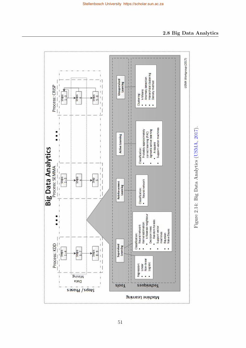
2.8 Big Data Analytics
Fig
ure
2.14
:B
igD
ata
Anal
yti
cs(U
SM
A,
2017
).
51
Stellenbosch University https://scholar.sun.ac.za
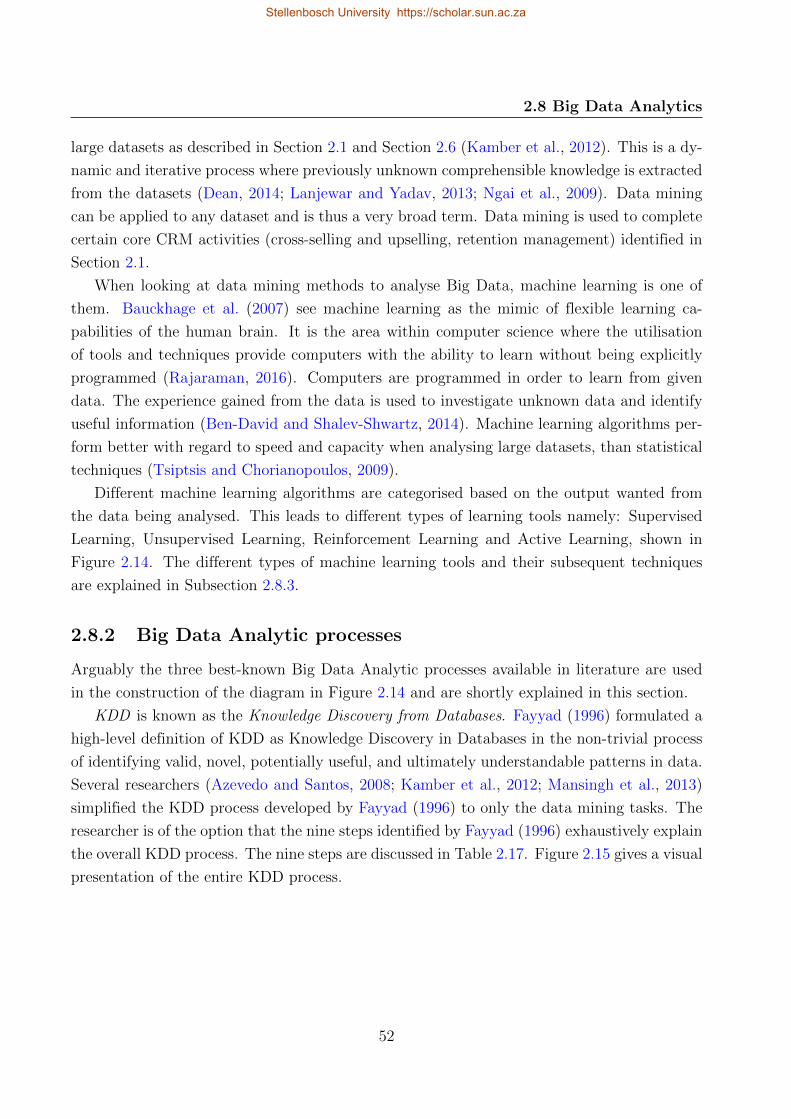
2.8 Big Data Analytics
large datasets as described in Section 2.1 and Section 2.6 (Kamber et al., 2012). This is a dy-
namic and iterative process where previously unknown comprehensible knowledge is extracted
from the datasets (Dean, 2014; Lanjewar and Yadav, 2013; Ngai et al., 2009). Data mining
can be applied to any dataset and is thus a very broad term. Data mining is used to complete
certain core CRM activities (cross-selling and upselling, retention management) identified in
Section 2.1.
When looking at data mining methods to analyse Big Data, machine learning is one of
them. Bauckhage et al. (2007) see machine learning as the mimic of flexible learning ca-
pabilities of the human brain. It is the area within computer science where the utilisation
of tools and techniques provide computers with the ability to learn without being explicitly
programmed (Rajaraman, 2016). Computers are programmed in order to learn from given
data. The experience gained from the data is used to investigate unknown data and identify
useful information (Ben-David and Shalev-Shwartz, 2014). Machine learning algorithms per-
form better with regard to speed and capacity when analysing large datasets, than statistical
techniques (Tsiptsis and Chorianopoulos, 2009).
Different machine learning algorithms are categorised based on the output wanted from
the data being analysed. This leads to different types of learning tools namely: Supervised
Learning, Unsupervised Learning, Reinforcement Learning and Active Learning, shown in
Figure 2.14. The different types of machine learning tools and their subsequent techniques
are explained in Subsection 2.8.3.
2.8.2 Big Data Analytic processes
Arguably the three best-known Big Data Analytic processes available in literature are used
in the construction of the diagram in Figure 2.14 and are shortly explained in this section.
KDD is known as the Knowledge Discovery from Databases. Fayyad (1996) formulated a
high-level definition of KDD as Knowledge Discovery in Databases in the non-trivial process
of identifying valid, novel, potentially useful, and ultimately understandable patterns in data.
Several researchers (Azevedo and Santos, 2008; Kamber et al., 2012; Mansingh et al., 2013)
simplified the KDD process developed by Fayyad (1996) to only the data mining tasks. The
researcher is of the option that the nine steps identified by Fayyad (1996) exhaustively explain
the overall KDD process. The nine steps are discussed in Table 2.17. Figure 2.15 gives a visual
presentation of the entire KDD process.
52
Stellenbosch University https://scholar.sun.ac.za
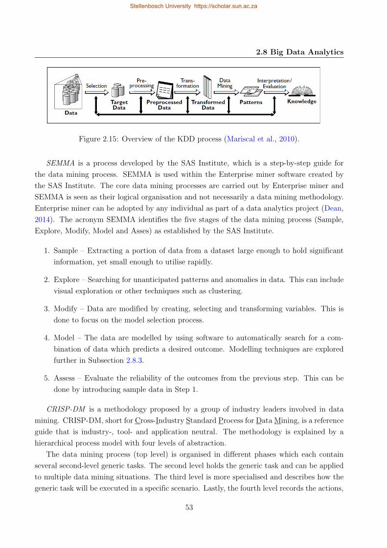
2.8 Big Data Analytics
Figure 2.15: Overview of the KDD process (Mariscal et al., 2010).
SEMMA is a process developed by the SAS Institute, which is a step-by-step guide for
the data mining process. SEMMA is used within the Enterprise miner software created by
the SAS Institute. The core data mining processes are carried out by Enterprise miner and
SEMMA is seen as their logical organisation and not necessarily a data mining methodology.
Enterprise miner can be adopted by any individual as part of a data analytics project (Dean,
2014). The acronym SEMMA identifies the five stages of the data mining process (Sample,
Explore, Modify, Model and Asses) as established by the SAS Institute.
1. Sample – Extracting a portion of data from a dataset large enough to hold significant
information, yet small enough to utilise rapidly.
2. Explore – Searching for unanticipated patterns and anomalies in data. This can include
visual exploration or other techniques such as clustering.
3. Modify – Data are modified by creating, selecting and transforming variables. This is
done to focus on the model selection process.
4. Model – The data are modelled by using software to automatically search for a com-
bination of data which predicts a desired outcome. Modelling techniques are explored
further in Subsection 2.8.3.
5. Assess – Evaluate the reliability of the outcomes from the previous step. This can be
done by introducing sample data in Step 1.
CRISP-DM is a methodology proposed by a group of industry leaders involved in data
mining. CRISP-DM, short for Cross-Industry Standard Process for Data Mining, is a reference
guide that is industry-, tool- and application neutral. The methodology is explained by a
hierarchical process model with four levels of abstraction.
The data mining process (top level) is organised in different phases which each contain
several second-level generic tasks. The second level holds the generic task and can be applied
to multiple data mining situations. The third level is more specialised and describes how the
generic task will be executed in a specific scenario. Lastly, the fourth level records the actions,
53
Stellenbosch University https://scholar.sun.ac.za
2.8 Big Data Analytics
Table 2.17: KDD process, adapted from Fayyad (1996) and Mariscal et al. (2010).
Steps Explanation
1. Understanding of the
application domain.
Developing an understanding of the relevant prior knowledge, and
the goals of the end user. This step is dependent on the user.
2. Target dataset.
Creating or selecting a dataset, or focusing on a subset of vari-
ables or data samples, on which discovery is to be performed.
This includes homogeneity of data, dynamics, changes over time,
sampling strategy, etc.
3. Data cleaning and pre-
processing.
This step includes basic operations such as: Removal of noise and
outliers, Collecting information to account for noise, Strategies for
missing data fields, etc.
4. Data reduction and
transformation.
Exploring useful features to represent data. Dimensionality reduc-
tion/transformation methods to reduce number of variables under
consideration. Projecting data to spaces where solutions are easier
to find.
5. Choosing the data-
mining task or function.
This step includes deciding on the model purpose of the model
and the goal of the data mining functionality (e.g. Classification,
regression, clustering, etc.)
6. Choosing the data-
mining algorithms(s).
The selection of techniques to be used for identifying patterns or
fitting models to the data. The choice of appropriate models and
parameters is critical.
7. Data mining. This is the physical step of searching for hidden patterns in data.
8. Evaluating output of
Step 7.
The interpretation of the results from Step 7 and deciding if the
outputs are deemed knowledge. The outcome of this step might
require alterations in previous steps and restarting the whole pro-
cess.
9. Consolidating discov-
ered knowledge.
Incorporating the knowledge into the performance system, taking
action based on the knowledge found or simply documenting it and
reporting it to users. This step also includes identifying potential
conflicts with previously believed/extracted knowledge.
54
Stellenbosch University https://scholar.sun.ac.za
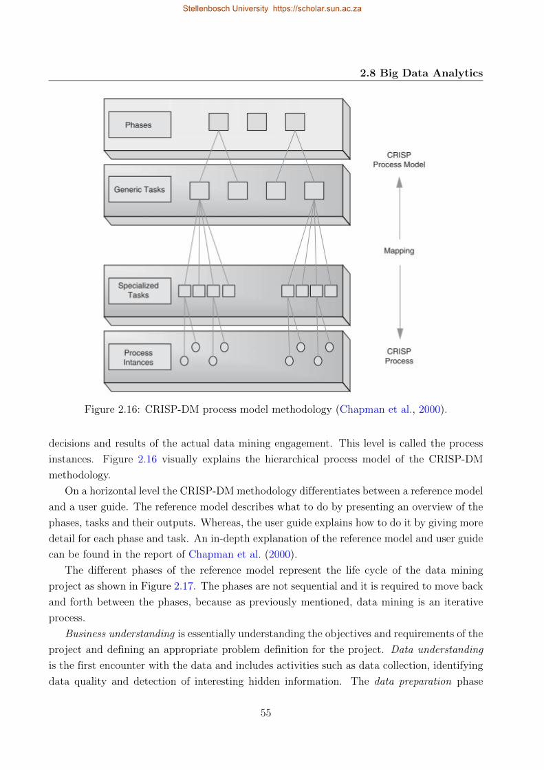
2.8 Big Data Analytics
Figure 2.16: CRISP-DM process model methodology (Chapman et al., 2000).
decisions and results of the actual data mining engagement. This level is called the process
instances. Figure 2.16 visually explains the hierarchical process model of the CRISP-DM
methodology.
On a horizontal level the CRISP-DM methodology differentiates between a reference model
and a user guide. The reference model describes what to do by presenting an overview of the
phases, tasks and their outputs. Whereas, the user guide explains how to do it by giving more
detail for each phase and task. An in-depth explanation of the reference model and user guide
can be found in the report of Chapman et al. (2000).
The different phases of the reference model represent the life cycle of the data mining
project as shown in Figure 2.17. The phases are not sequential and it is required to move back
and forth between the phases, because as previously mentioned, data mining is an iterative
process.
Business understanding is essentially understanding the objectives and requirements of the
project and defining an appropriate problem definition for the project. Data understanding
is the first encounter with the data and includes activities such as data collection, identifying
data quality and detection of interesting hidden information. The data preparation phase
55
Stellenbosch University https://scholar.sun.ac.za
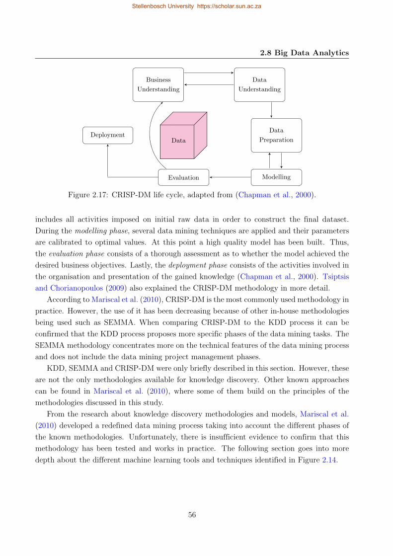
2.8 Big Data Analytics
Data
Business
Understanding
Data
Understanding
Data
Preparation
ModellingEvaluation
Deployment
Figure 2.17: CRISP-DM life cycle, adapted from (Chapman et al., 2000).
includes all activities imposed on initial raw data in order to construct the final dataset.
During the modelling phase, several data mining techniques are applied and their parameters
are calibrated to optimal values. At this point a high quality model has been built. Thus,
the evaluation phase consists of a thorough assessment as to whether the model achieved the
desired business objectives. Lastly, the deployment phase consists of the activities involved in
the organisation and presentation of the gained knowledge (Chapman et al., 2000). Tsiptsis
and Chorianopoulos (2009) also explained the CRISP-DM methodology in more detail.
According to Mariscal et al. (2010), CRISP-DM is the most commonly used methodology in
practice. However, the use of it has been decreasing because of other in-house methodologies
being used such as SEMMA. When comparing CRISP-DM to the KDD process it can be
confirmed that the KDD process proposes more specific phases of the data mining tasks. The
SEMMA methodology concentrates more on the technical features of the data mining process
and does not include the data mining project management phases.
KDD, SEMMA and CRISP-DM were only briefly described in this section. However, these
are not the only methodologies available for knowledge discovery. Other known approaches
can be found in Mariscal et al. (2010), where some of them build on the principles of the
methodologies discussed in this study.
From the research about knowledge discovery methodologies and models, Mariscal et al.
(2010) developed a redefined data mining process taking into account the different phases of
the known methodologies. Unfortunately, there is insufficient evidence to confirm that this
methodology has been tested and works in practice. The following section goes into more
depth about the different machine learning tools and techniques identified in Figure 2.14.
56
Stellenbosch University https://scholar.sun.ac.za
2.8 Big Data Analytics
2.8.3 Different Big Data Analytical tools and techniques
In this section the researcher continues with the explanation of the BDA diagram in Section
2.8.1. Within the machine learning application, there are a variety of learning tools and
techniques that can be used for different types of data. The different tools to be used are
based on the various methods of machine learning. Only the fundamentals of machine learning
are discussed and references to more detailed literature are provided.
Supervised Learning (SL) is when the model learns from a set of training data, which
contains predefined examples. These models require training datasets with historical data
and the training data are thus labelled. A target variable is available in the test data and the
model must correctly predict or classify the observations. The model is trained with input
examples to predict desired output variables. The generated output can be compared with
the known correct output. Thus, with supervised learning the analysts know what they are
looking for (Agrawal and Srikant, 1994; Bounsaythip and Rinta-Runsala, 2001; Dean, 2014;
Kamber et al., 2012; Lakshmi Prasad, 2016; Tsiptsis and Chorianopoulos, 2009).
In contrast to SL, Unsupervised Learning (UL) refers to models that do not use training
data. The input example datasets are unlabelled and no target variable exist. Thus, there
is no distinction between test and training data. The analyst does not know what to look
for and needs to find the structure in the data (Dean, 2014; Kamber et al., 2012; Lakshmi
Prasad, 2016). Association rule modelling described in Subsection 2.6.2 is an example of an
unsupervised technique.
Active Learning (AL) is a method where the user actively participates in the learning
process. The user can be prompted to label an example that was part of an unlabelled set.
The model acquires knowledge from human users with the goal of optimising the model quality.
This happens during the training time of the model (Ben-David and Shalev-Shwartz, 2014;
Kamber et al., 2012).
Reinforcement Learning (RL) is explained as mapping situations to actions. Reward and
penalty signals are used for evaluating the action of the learner. The learner must discover
which action yields the best reward by choosing them but the learner is not told which action
to take. This evaluates the learner’s response in an initially unknown environment. The goal is
to maximise a numerical reward system. This learning method not only affects the immediate
step and reward, but also the subsequent rewards throughout the process (Schmidhuber, 2015;
Sutton and Barto, 1998).
The various learning methods can be subdivided into different techniques based on the data
to be analysed. The technique contains data models and their assorted algorithms as seen in
Figure 2.14. The data models (Classification, Clustering, Regression, etc.) are created based
on the type of patterns that can be found within the data mining tasks. These tasks can be
classified into four general types based on the results they contain. The data analytics behind
57
Stellenbosch University https://scholar.sun.ac.za
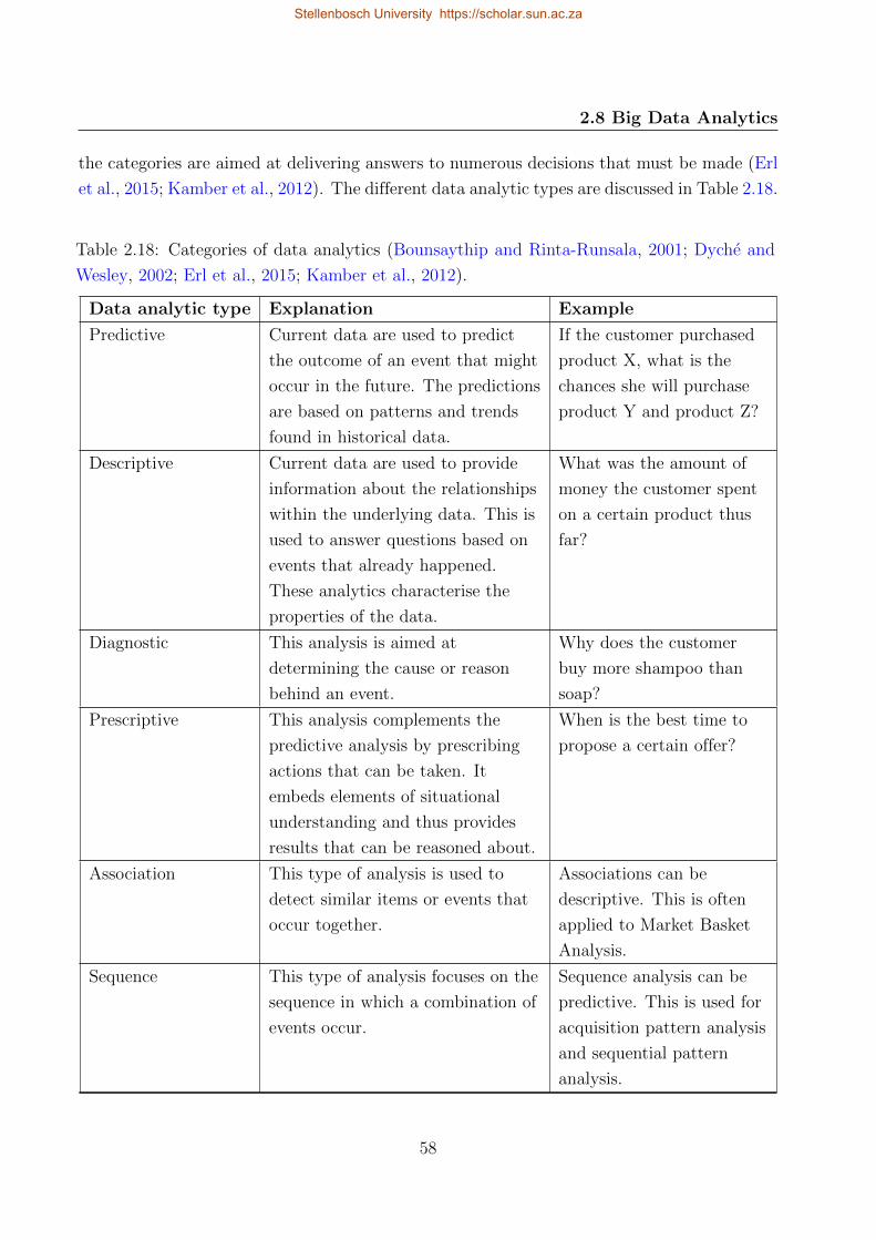
2.8 Big Data Analytics
the categories are aimed at delivering answers to numerous decisions that must be made (Erl
et al., 2015; Kamber et al., 2012). The different data analytic types are discussed in Table 2.18.
Table 2.18: Categories of data analytics (Bounsaythip and Rinta-Runsala, 2001; Dyche and
Wesley, 2002; Erl et al., 2015; Kamber et al., 2012).
Data analytic type Explanation Example
Predictive Current data are used to predict
the outcome of an event that might
occur in the future. The predictions
are based on patterns and trends
found in historical data.
If the customer purchased
product X, what is the
chances she will purchase
product Y and product Z?
Descriptive Current data are used to provide
information about the relationships
within the underlying data. This is
used to answer questions based on
events that already happened.
These analytics characterise the
properties of the data.
What was the amount of
money the customer spent
on a certain product thus
far?
Diagnostic This analysis is aimed at
determining the cause or reason
behind an event.
Why does the customer
buy more shampoo than
soap?
Prescriptive This analysis complements the
predictive analysis by prescribing
actions that can be taken. It
embeds elements of situational
understanding and thus provides
results that can be reasoned about.
When is the best time to
propose a certain offer?
Association This type of analysis is used to
detect similar items or events that
occur together.
Associations can be
descriptive. This is often
applied to Market Basket
Analysis.
Sequence This type of analysis focuses on the
sequence in which a combination of
events occur.
Sequence analysis can be
predictive. This is used for
acquisition pattern analysis
and sequential pattern
analysis.
58
Stellenbosch University https://scholar.sun.ac.za
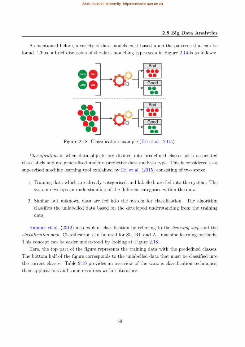
2.8 Big Data Analytics
As mentioned before, a variety of data models exist based upon the patterns that can be
found. Thus, a brief discussion of the data modelling types seen in Figure 2.14 is as follows:
Figure 2.18: Classification example (Erl et al., 2015).
Classification is when data objects are divided into predefined classes with associated
class labels and are generalised under a predictive data analysis type. This is considered as a
supervised machine learning tool explained by Erl et al. (2015) consisting of two steps:
1. Training data which are already categorised and labelled, are fed into the system. The
system develops an understanding of the different categories within the data.
2. Similar but unknown data are fed into the system for classification. The algorithm
classifies the unlabelled data based on the developed understanding from the training
data.
Kamber et al. (2012) also explain classification by referring to the learning step and the
classification step. Classification can be used for SL, RL and AL machine learning methods.
This concept can be easier understood by looking at Figure 2.18.
Here, the top part of the figure represents the training data with the predefined classes.
The bottom half of the figure corresponds to the unlabelled data that must be classified into
the correct classes. Table 2.19 provides an overview of the various classification techniques,
their applications and some resources within literature.
59
Stellenbosch University https://scholar.sun.ac.za
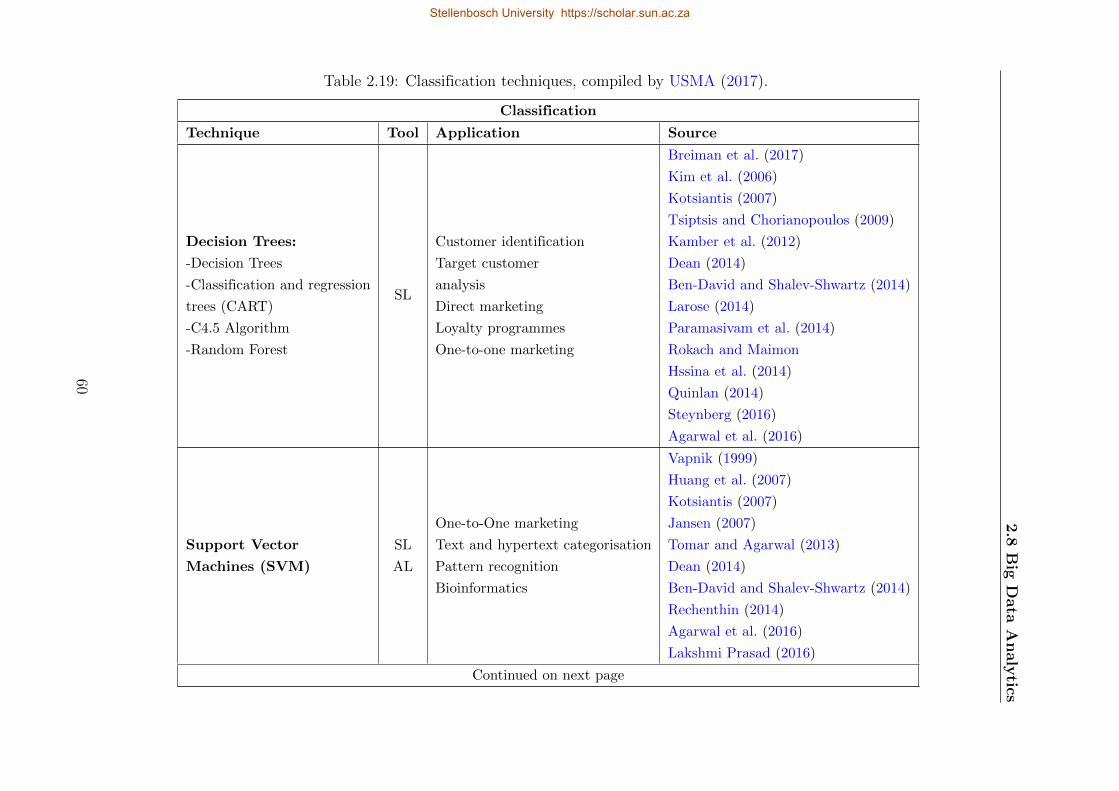
2.8
Big
Data
Analytics
Table 2.19: Classification techniques, compiled by USMA (2017).
Classification
Technique Tool Application Source
Decision Trees:
-Decision Trees
-Classification and regression
trees (CART)
-C4.5 Algorithm
-Random Forest
SL
Customer identification
Target customer
analysis
Direct marketing
Loyalty programmes
One-to-one marketing
Breiman et al. (2017)
Kim et al. (2006)
Kotsiantis (2007)
Tsiptsis and Chorianopoulos (2009)
Kamber et al. (2012)
Dean (2014)
Ben-David and Shalev-Shwartz (2014)
Larose (2014)
Paramasivam et al. (2014)
Rokach and Maimon
Hssina et al. (2014)
Quinlan (2014)
Steynberg (2016)
Agarwal et al. (2016)
Support Vector
Machines (SVM)
SL
AL
One-to-One marketing
Text and hypertext categorisation
Pattern recognition
Bioinformatics
Vapnik (1999)
Huang et al. (2007)
Kotsiantis (2007)
Jansen (2007)
Tomar and Agarwal (2013)
Dean (2014)
Ben-David and Shalev-Shwartz (2014)
Rechenthin (2014)
Agarwal et al. (2016)
Lakshmi Prasad (2016)
Continued on next page
60
Stellenbosch University https://scholar.sun.ac.za
Stellenbosch University https://scholar.sun.ac.za
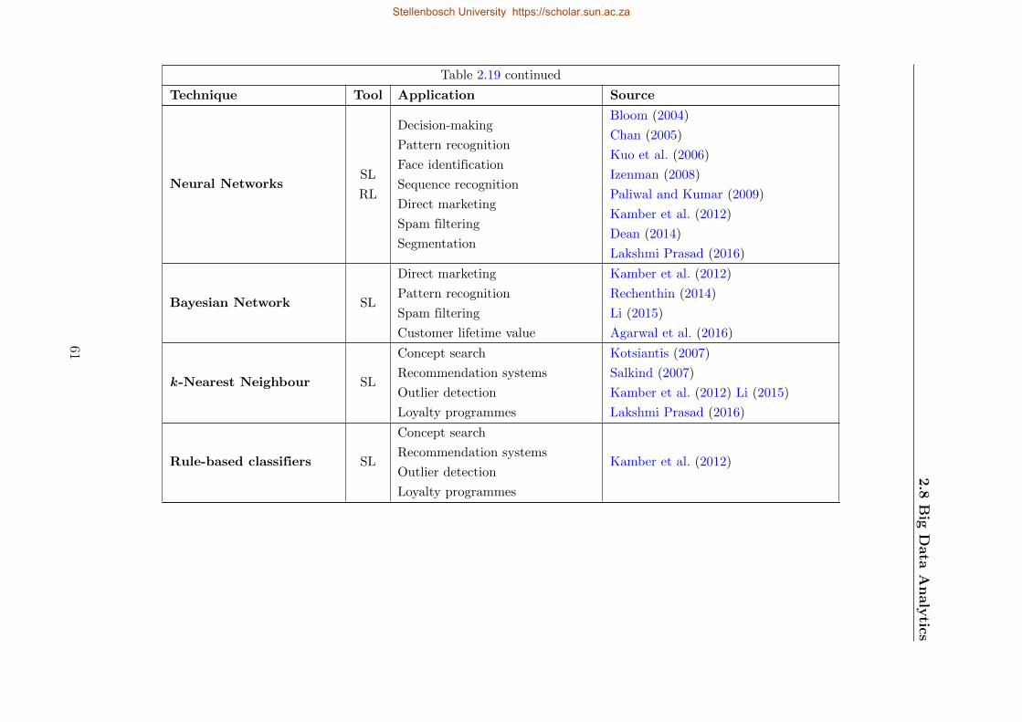
2.8
Big
Data
Analytics
Table 2.19 continued
Technique Tool Application Source
Neural NetworksSL
RL
Decision-making
Pattern recognition
Face identification
Sequence recognition
Direct marketing
Spam filtering
Segmentation
Bloom (2004)
Chan (2005)
Kuo et al. (2006)
Izenman (2008)
Paliwal and Kumar (2009)
Kamber et al. (2012)
Dean (2014)
Lakshmi Prasad (2016)
Bayesian Network SL
Direct marketing
Pattern recognition
Spam filtering
Customer lifetime value
Kamber et al. (2012)
Rechenthin (2014)
Li (2015)
Agarwal et al. (2016)
k-Nearest Neighbour SL
Concept search
Recommendation systems
Outlier detection
Loyalty programmes
Kotsiantis (2007)
Salkind (2007)
Kamber et al. (2012) Li (2015)
Lakshmi Prasad (2016)
Rule-based classifiers SL
Concept search
Recommendation systems
Outlier detection
Loyalty programmes
Kamber et al. (2012)
61
Stellenbosch University https://scholar.sun.ac.za
Stellenbosch University https://scholar.sun.ac.za
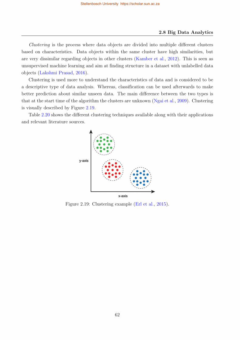
2.8 Big Data Analytics
Clustering is the process where data objects are divided into multiple different clusters
based on characteristics. Data objects within the same cluster have high similarities, but
are very dissimilar regarding objects in other clusters (Kamber et al., 2012). This is seen as
unsupervised machine learning and aim at finding structure in a dataset with unlabelled data
objects (Lakshmi Prasad, 2016).
Clustering is used more to understand the characteristics of data and is considered to be
a descriptive type of data analysis. Whereas, classification can be used afterwards to make
better prediction about similar unseen data. The main difference between the two types is
that at the start time of the algorithm the clusters are unknown (Ngai et al., 2009). Clustering
is visually described by Figure 2.19.
Table 2.20 shows the different clustering techniques available along with their applications
and relevant literature sources.
Figure 2.19: Clustering example (Erl et al., 2015).
62
Stellenbosch University https://scholar.sun.ac.za
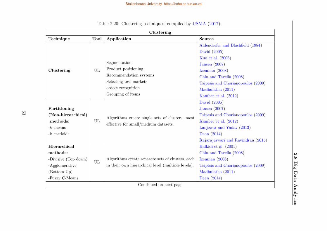
2.8
Big
Data
Analytics
Table 2.20: Clustering techniques, compiled by USMA (2017).
Clustering
Technique Tool Application Source
Clustering UL
Segmentation
Product positioning
Recommendation systems
Selecting test markets
object recognition
Grouping of items
Aldenderfer and Blashfield (1984)
David (2005)
Kuo et al. (2006)
Jansen (2007)
Izenman (2008)
Chiu and Tavella (2008)
Tsiptsis and Chorianopoulos (2009)
Madhulatha (2011)
Kamber et al. (2012)
Partitioning
(Non-hierarchical)
methods:
-k–means
-k–medoids
ULAlgorithms create single sets of clusters, most
effective for small/medium datasets.
David (2005)
Jansen (2007)
Tsiptsis and Chorianopoulos (2009)
Kamber et al. (2012)
Lanjewar and Yadav (2013)
Dean (2014)
Rajarajeswari and Ravindran (2015)
Hierarchical
methods:
-Divisive (Top down)
-Agglomerative
(Bottom-Up)
-Fuzzy C-Means
ULAlgorithms create separate sets of clusters, each
in their own hierarchical level (multiple levels).
Halkidi et al. (2001)
Chiu and Tavella (2008)
Izenman (2008)
Tsiptsis and Chorianopoulos (2009)
Madhulatha (2011)
Dean (2014)
Continued on next page
63
Stellenbosch University https://scholar.sun.ac.za
Stellenbosch University https://scholar.sun.ac.za
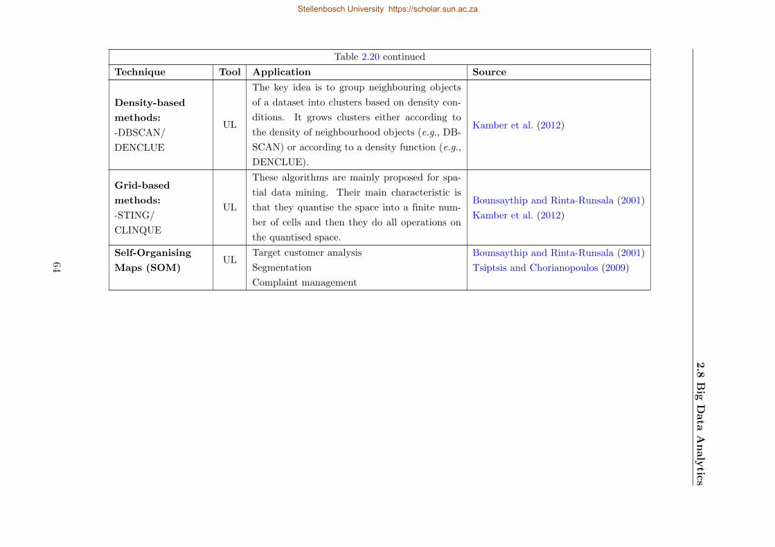
2.8
Big
Data
Analytics
Table 2.20 continued
Technique Tool Application Source
Density-based
methods:
-DBSCAN/
DENCLUE
UL
The key idea is to group neighbouring objects
of a dataset into clusters based on density con-
ditions. It grows clusters either according to
the density of neighbourhood objects (e.g., DB-
SCAN) or according to a density function (e.g.,
DENCLUE).
Kamber et al. (2012)
Grid-based
methods:
-STING/
CLINQUE
UL
These algorithms are mainly proposed for spa-
tial data mining. Their main characteristic is
that they quantise the space into a finite num-
ber of cells and then they do all operations on
the quantised space.
Bounsaythip and Rinta-Runsala (2001)
Kamber et al. (2012)
Self-Organising
Maps (SOM)UL
Target customer analysis
Segmentation
Complaint management
Bounsaythip and Rinta-Runsala (2001)
Tsiptsis and Chorianopoulos (2009)
64
Stellenbosch University https://scholar.sun.ac.za
Stellenbosch University https://scholar.sun.ac.za

2.8 Big Data Analytics
Regression explores the relationship between a dependent variable and an independent
variable within a given dataset (Erl et al., 2015). Regression can also be used to predict
a value of a certain variable based on the values of other variables, given a linear or non-
linear model of dependency. Regression is a predictive type of data analysis which is the
same as classification. The difference is that regression is used for continuous valued variables
(Bounsaythip and Rinta-Runsala, 2001). Table 2.21 summarises the various types of regression
models, some of their applications and references within literature.
65
Stellenbosch University https://scholar.sun.ac.za
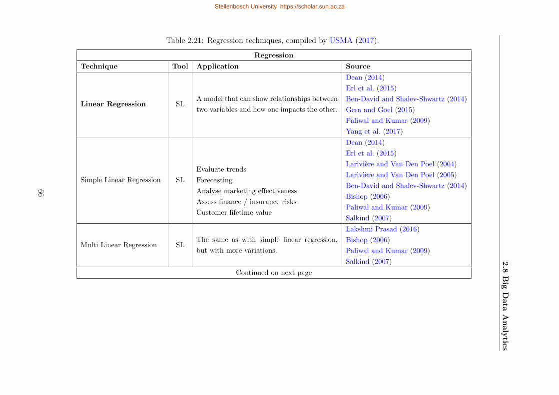
2.8
Big
Data
Analytics
Table 2.21: Regression techniques, compiled by USMA (2017).
Regression
Technique Tool Application Source
Linear Regression SLA model that can show relationships between
two variables and how one impacts the other.
Dean (2014)
Erl et al. (2015)
Ben-David and Shalev-Shwartz (2014)
Gera and Goel (2015)
Paliwal and Kumar (2009)
Yang et al. (2017)
Simple Linear Regression SL
Evaluate trends
Forecasting
Analyse marketing effectiveness
Assess finance / insurance risks
Customer lifetime value
Dean (2014)
Erl et al. (2015)
Lariviere and Van Den Poel (2004)
Lariviere and Van Den Poel (2005)
Ben-David and Shalev-Shwartz (2014)
Bishop (2006)
Paliwal and Kumar (2009)
Salkind (2007)
Multi Linear Regression SLThe same as with simple linear regression,
but with more variations.
Lakshmi Prasad (2016)
Bishop (2006)
Paliwal and Kumar (2009)
Salkind (2007)
Continued on next page
66
Stellenbosch University https://scholar.sun.ac.za
Stellenbosch University https://scholar.sun.ac.za
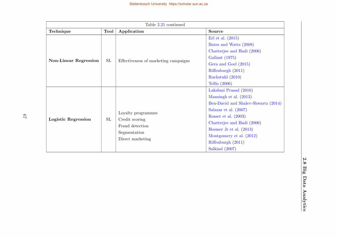
2.8
Big
Data
Analytics
Table 2.21 continued
Technique Tool Application Source
Non-Linear Regression SL Effectiveness of marketing campaigns
Erl et al. (2015)
Bates and Watts (2008)
Chatterjee and Hadi (2006)
Gallant (1975)
Gera and Goel (2015)
Riffenburgh (2011)
Ruckstuhl (2010)
Tellis (2006)
Logistic Regression SL
Loyalty programmes
Credit scoring
Fraud detection
Segmentation
Direct marketing
Lakshmi Prasad (2016)
Mansingh et al. (2013)
Ben-David and Shalev-Shwartz (2014)
Salazar et al. (2007)
Rosset et al. (2003)
Chatterjee and Hadi (2006)
Hosmer Jr et al. (2013)
Montgomery et al. (2012)
Riffenburgh (2011)
Salkind (2007)
67
Stellenbosch University https://scholar.sun.ac.za
Stellenbosch University https://scholar.sun.ac.za
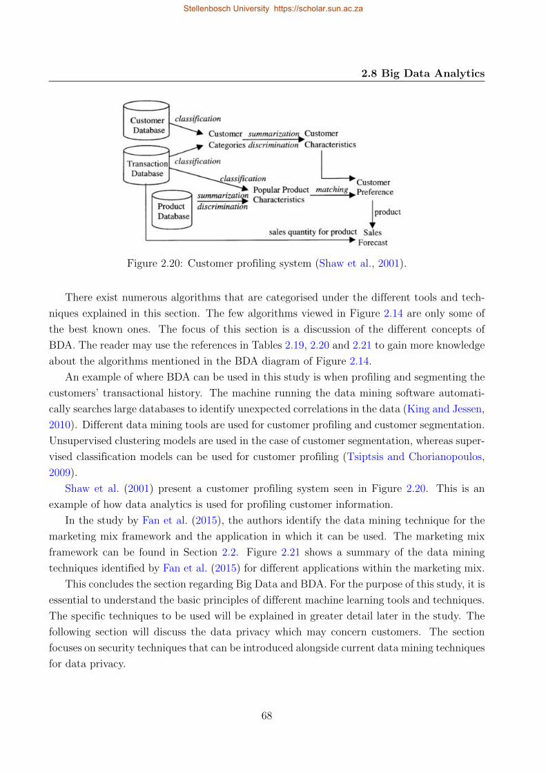
2.8 Big Data Analytics
Figure 2.20: Customer profiling system (Shaw et al., 2001).
There exist numerous algorithms that are categorised under the different tools and tech-
niques explained in this section. The few algorithms viewed in Figure 2.14 are only some of
the best known ones. The focus of this section is a discussion of the different concepts of
BDA. The reader may use the references in Tables 2.19, 2.20 and 2.21 to gain more knowledge
about the algorithms mentioned in the BDA diagram of Figure 2.14.
An example of where BDA can be used in this study is when profiling and segmenting the
customers’ transactional history. The machine running the data mining software automati-
cally searches large databases to identify unexpected correlations in the data (King and Jessen,
2010). Different data mining tools are used for customer profiling and customer segmentation.
Unsupervised clustering models are used in the case of customer segmentation, whereas super-
vised classification models can be used for customer profiling (Tsiptsis and Chorianopoulos,
2009).
Shaw et al. (2001) present a customer profiling system seen in Figure 2.20. This is an
example of how data analytics is used for profiling customer information.
In the study by Fan et al. (2015), the authors identify the data mining technique for the
marketing mix framework and the application in which it can be used. The marketing mix
framework can be found in Section 2.2. Figure 2.21 shows a summary of the data mining
techniques identified by Fan et al. (2015) for different applications within the marketing mix.
This concludes the section regarding Big Data and BDA. For the purpose of this study, it is
essential to understand the basic principles of different machine learning tools and techniques.
The specific techniques to be used will be explained in greater detail later in the study. The
following section will discuss the data privacy which may concern customers. The section
focuses on security techniques that can be introduced alongside current data mining techniques
for data privacy.
68
Stellenbosch University https://scholar.sun.ac.za
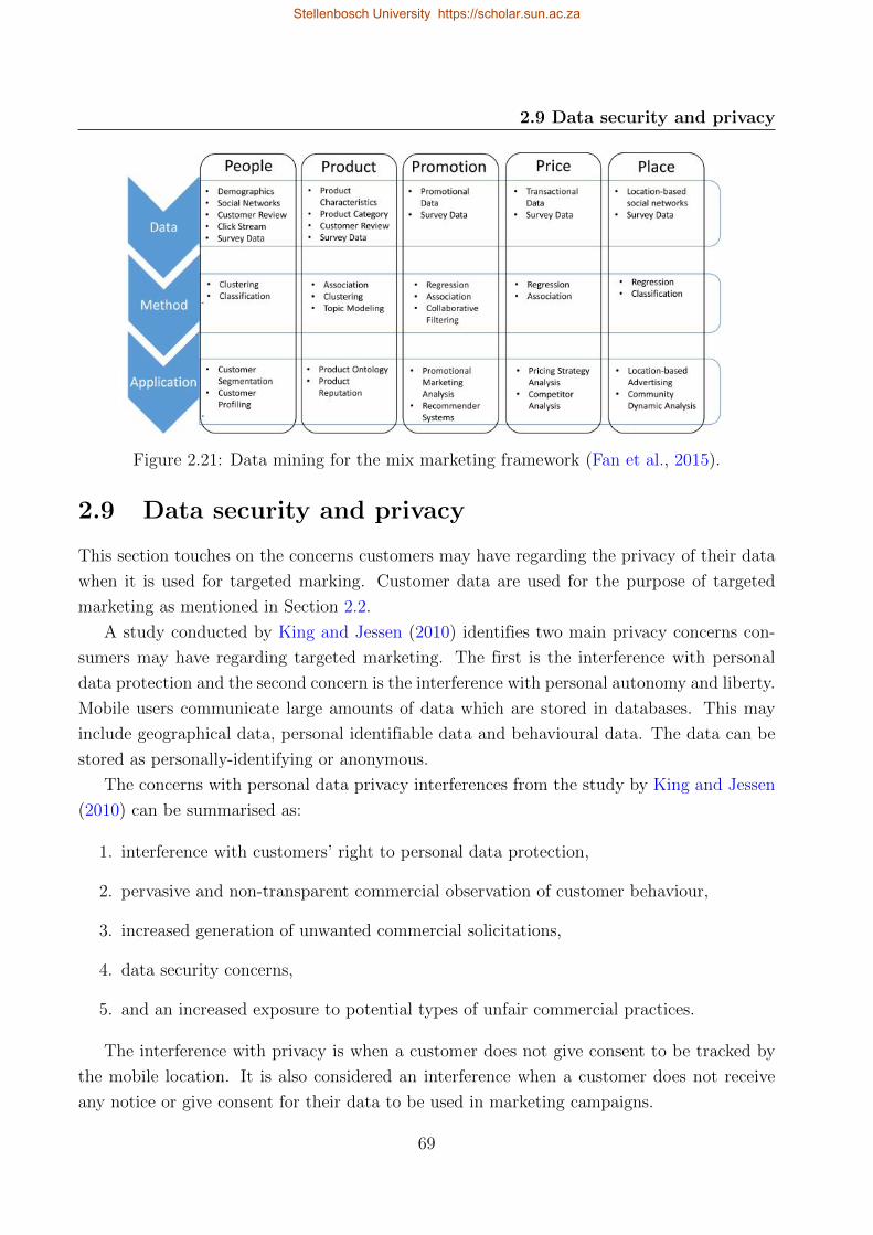
2.9 Data security and privacy
Figure 2.21: Data mining for the mix marketing framework (Fan et al., 2015).
2.9 Data security and privacy
This section touches on the concerns customers may have regarding the privacy of their data
when it is used for targeted marking. Customer data are used for the purpose of targeted
marketing as mentioned in Section 2.2.
A study conducted by King and Jessen (2010) identifies two main privacy concerns con-
sumers may have regarding targeted marketing. The first is the interference with personal
data protection and the second concern is the interference with personal autonomy and liberty.
Mobile users communicate large amounts of data which are stored in databases. This may
include geographical data, personal identifiable data and behavioural data. The data can be
stored as personally-identifying or anonymous.
The concerns with personal data privacy interferences from the study by King and Jessen
(2010) can be summarised as:
1. interference with customers’ right to personal data protection,
2. pervasive and non-transparent commercial observation of customer behaviour,
3. increased generation of unwanted commercial solicitations,
4. data security concerns,
5. and an increased exposure to potential types of unfair commercial practices.
The interference with privacy is when a customer does not give consent to be tracked by
the mobile location. It is also considered an interference when a customer does not receive
any notice or give consent for their data to be used in marketing campaigns.
69
Stellenbosch University https://scholar.sun.ac.za
2.9 Data security and privacy
The concern regarding personal autonomy and liberty is when the customer is unaware
that personal information is used for targeted marketing purposes. This can lead to customers
not being able to exercise their personal autonomy because they are unaware of the profiles
created and used for marketing. This again can be rectified by gaining customers access to the
profile based on their information after receiving their consent to use the personal information
in the first place (King and Jessen, 2010). Information regarding European Union and United
States of America regulatory frameworks for targeted advertising can also be found in the
study conducted by King and Jessen (2010).
The concerns grow relating to data mining and creating customer profiles. Wu et al.
(2014) conducted a study about data mining in Big Data. Within this study, Wu et al. (2014)
mentioned that data privacy is one of the important issues within certain domain applications.
Simple data transmissions, for example peoples’ locations, do not create concern, but can
create serious privacy concerns if a customer’s location is freely available over a certain time
period. Another concern is domain and application knowledge. An example to explain this
concern is used with the definition of privacy preservation.
There exist two common approaches to protect the privacy of customer data. The one
approach is the simplest one which is restricting the data. This means adding access control
on data entries so only certain individuals are granted access to it. A common challenge with
this is inventing secured certification or mechanisms for access control (Wu et al., 2014).
The second approach and mostly used is anonymising data fields to ensure that sensitive
information cannot be revealed. The objective of this approach is to introduce variation into
the collected data in order to ensure a certain number of privacy goals. In response to privacy
protection, privacy-preserving data mining is used (Kamber et al., 2012; Fung et al., 2010;
Wu et al., 2014).
Dalenius (Fung et al., 2010) defines privacy preservation as: “access to the published data
should not enable the adversary to learn anything extra about any target victim compared to
no access to the database, even with the presence of any adversary’s background knowledge
obtained from other sources.” An example of this is when the adversary knows Customer
X has an age Y years older than the average of an African woman and has access to sta-
tistical information about the average age of African women, then Customer X’s privacy is
compromised.
According to Fung et al. (2010), the data holder has a data table
D(Explicit Identifier, Quasi Identifier, Sensitive Attributes, Non-Sensitive Attributes),
as the most basic form of Privacy Preserving Data Publishing (PPDP).
Explicit Identifier is an attribute like name which explicitly identifies individuals.
70
Stellenbosch University https://scholar.sun.ac.za
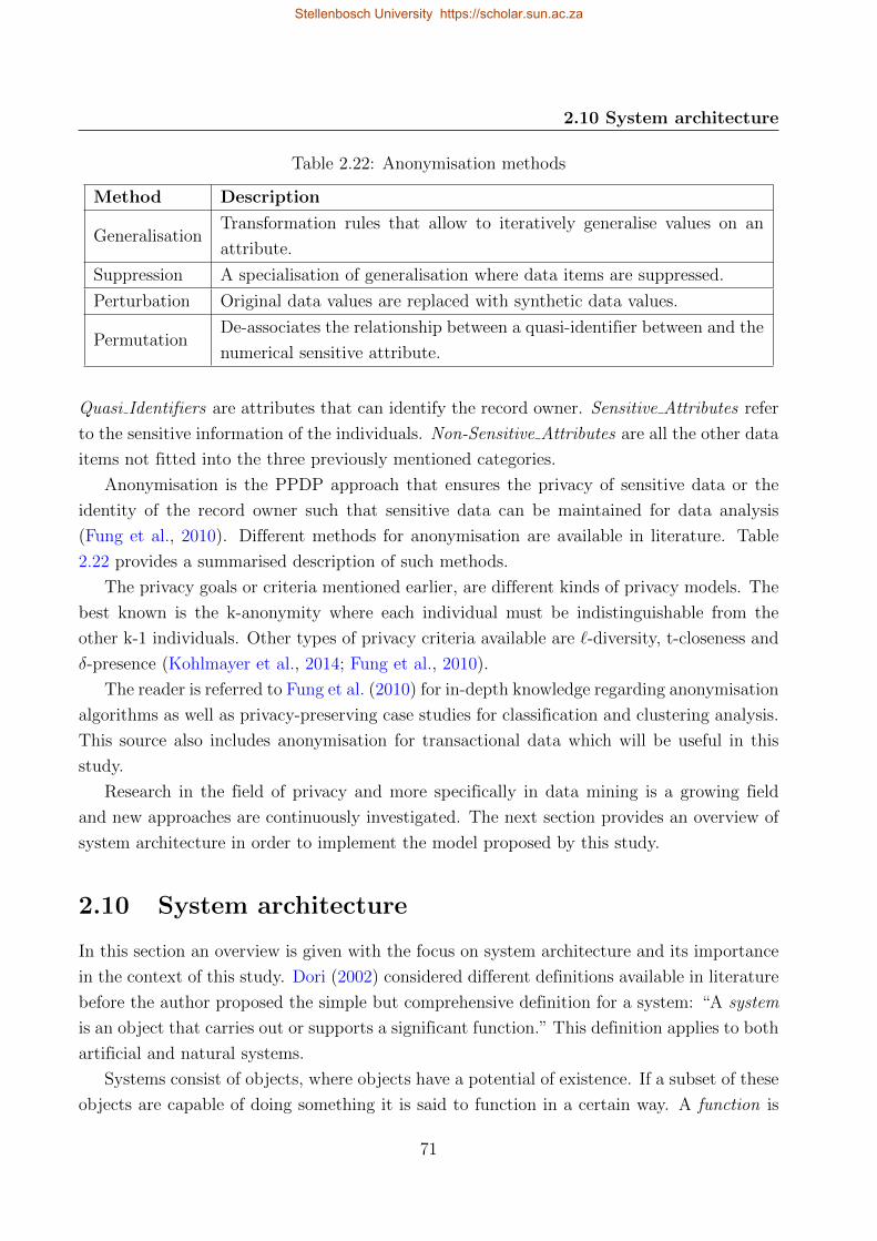
2.10 System architecture
Table 2.22: Anonymisation methods
Method Description
GeneralisationTransformation rules that allow to iteratively generalise values on an
attribute.
Suppression A specialisation of generalisation where data items are suppressed.
Perturbation Original data values are replaced with synthetic data values.
PermutationDe-associates the relationship between a quasi-identifier between and the
numerical sensitive attribute.
Quasi Identifiers are attributes that can identify the record owner. Sensitive Attributes refer
to the sensitive information of the individuals. Non-Sensitive Attributes are all the other data
items not fitted into the three previously mentioned categories.
Anonymisation is the PPDP approach that ensures the privacy of sensitive data or the
identity of the record owner such that sensitive data can be maintained for data analysis
(Fung et al., 2010). Different methods for anonymisation are available in literature. Table
2.22 provides a summarised description of such methods.
The privacy goals or criteria mentioned earlier, are different kinds of privacy models. The
best known is the k-anonymity where each individual must be indistinguishable from the
other k-1 individuals. Other types of privacy criteria available are `-diversity, t-closeness and
δ-presence (Kohlmayer et al., 2014; Fung et al., 2010).
The reader is referred to Fung et al. (2010) for in-depth knowledge regarding anonymisation
algorithms as well as privacy-preserving case studies for classification and clustering analysis.
This source also includes anonymisation for transactional data which will be useful in this
study.
Research in the field of privacy and more specifically in data mining is a growing field
and new approaches are continuously investigated. The next section provides an overview of
system architecture in order to implement the model proposed by this study.
2.10 System architecture
In this section an overview is given with the focus on system architecture and its importance
in the context of this study. Dori (2002) considered different definitions available in literature
before the author proposed the simple but comprehensive definition for a system: “A system
is an object that carries out or supports a significant function.” This definition applies to both
artificial and natural systems.
Systems consist of objects, where objects have a potential of existence. If a subset of these
objects are capable of doing something it is said to function in a certain way. A function is
71
Stellenbosch University https://scholar.sun.ac.za
2.10 System architecture
defined by Dori (2002) as: “An attribute of an object that describes the rationale behind its
existence, the intent for which it was built, the purpose for which it exists, the goal it serves,
or the set of phenomena or behaviours it exhibits.” All systems are objects, but it is based
on the function to determine if an object is a system. This is explained via examples that are
presented in Dori (2002).
The universe consists of both natural and artificial systems. The difference between these
two systems comes in where natural systems are not associated with a premeditated goal or
purpose that the function of an artificial system exhibits. The goal of a system is the human’s
intention of what the system is supposed to do. The function which a system possesses
translates this goal to a practical outcome (Dori, 2002). As time passes artificial systems
become more complex and revolutionary. With this, the fundamental reason for artificial
systems stays the same: to improve the lives of humans.
According to Dori (2002), system architecture is the overall system’s structure-behaviour
combination, which enables it to attain its function while embodying the architect’s concept.
The concept of a system is the strategies the system architect uses for the system’s architecture.
The architecture of a system is a vital part in creating a new system in order to understand
the structure and behaviour of the system and designing it in such a way that it will achieve
the desired goal. This is especially so in the world of today, where diverse and complex
innovations are created.
It is important to understand the difference between the function of a system and its the
dynamics. The function of a system answers the ‘what the system does’ and ‘why the system
does it’ type of questions. Contrary to this, the dynamics of a system refer to the question of
‘how the system does it’. Thus, the dynamics of the system refer to the behaviour and how
the system acts to attain the function.
The function of a system can be better understood by considering the system as having two
parts: the structure and the behaviour. The structure refers to the entirety of the system and
the relationship between components which do not change over time. Behaviour is dynamic
and changes as time passes. These changes are obtained within one or more subsystems that
are incorporated in the system.
Dori (2002) states that it is impossible to separate the structure and the behaviour of a
system because the dynamics determine what happens to the system. In some scenarios the
combination of structure and behaviour is needed for the system to function and attain the
specified goal.
In order to design a system capable of analysing Big Data, Chen and Zhang (2014) sum-
marised seven crucial principles to keep in mind. The principles are:
1. Good architectures and frameworks are necessary and on the top priority.
2. Support a variety of analytical methods.
72
Stellenbosch University https://scholar.sun.ac.za
2.11 Literature synthesis
3. No size fits all.
4. Bring the analysis to data.
5. Processing must be distributable for in-memory computation.
6. Data storage must be distributable for in-memory storage.
7. Coordination is needed between processing and data units.
It is important to acknowledge the basic principle of systems for the purpose of this study,
as well as the importance of a well-defined system architecture in order to design a system
with the correct structure and dynamics to achieve the particular goal. The following section
will synthesise the knowledge gained up to this point in order to create perspective within the
goals of this study.
2.11 Literature synthesis
CRM explains in broad perspective the management of the relationship of an enterprise with
its customers and the importance of this. One of the activities to retain customers is to
providing them with cross-selling and upselling opportunities to increase their customer expe-
rience. Cross-selling and upselling are methods used to retain customers and aim at bettering
targeted marketing based on customer product usage. It is for this reason that marketing
is of importance since it places the focus on the communication between the enterprise and
its customers. Various marketing strategies are available and personalised marketing strate-
gies are necessary if individual customers are targeted. Where marketing strategies focus on
communication with the customer, pricing strategies and special offers focus on what is being
communicated. Pricing strategies include promotional pricing which is used to define what
is offered to the customer and the cost implications to the enterprise. Pricing strategies are
used when offering cross-sell or upsell products.
In order to create personalised cross-selling and upselling offers, the customer must be
known and this is the point where customer profiles are of importance. Customer profiles
describe the customers in a factual and behavioural manner. Knowledge can be discovered
within the data of customers by analysing the customer profiles, where after enterprises can
identify the needs of their customers more accurately. Analytics are tools and techniques
needed to analyse the data and various options are available. Big Data Analytics are also
available to be applied to datasets defined as Big Data. When the behaviour of the customer
is known the appropriate marketing strategy and pricing strategy can be applied to ensure
customer satisfaction when attempting to create cross-sell and upsell offers to retain customers.
73
Stellenbosch University https://scholar.sun.ac.za
2.12 Chapter 2 summary
The concept of analysing customer data creates the opportunity for data security risk and
it is for this reason that when analysing customer data, data security and privacy must be
fully understood and implemented. In creating a system which incorporates some of these
knowledge areas a system architecture is necessary. It is important to gain the required
theoretical knowledge regarding system architectures in order to utilise it.
2.12 Chapter 2 summary
In this chapter, elements of the literature required to understand the different knowledge
areas included in this study were described. CRM, marketing and pricing strategies, cross-
selling and upselling and customer profiles were discussed to better understand each topic and
their relationship with each other. Knowledge discovery, Big Data and Big Data Analytics
were investigated as these are included in the technical development of the study. A literature
synthesis was also provided to fully understand the purpose of each knowledge area discussed in
the study, where they are related and the relationship between them. The literature provided
about system architecture is applied to develop an architecture for the proposed system of
this study. This will be the topic of discussion in the next chapter.
74
Stellenbosch University https://scholar.sun.ac.za
Chapter 3
System architecture
At the end of the previous chapter, system architecture was broadly explained. In this chapter
the researcher presents more detail regarding the methodology followed for the system archi-
tecture in this study. Furthermore, the researcher constructed an architecture for the desired
system which is also presented in this chapter.
The researcher must identify an appropriate methodology to be utilised in the construction
of the system architecture of the proposed system. Thereafter, the researcher will use the
identified methodology to create the architecture and explain the relevance of each part within
the process. The researcher must also visualise the proposed model with the different parts.
3.1 Object-Process Methodology
In order to construct a system architecture, it is important to identify and understand the
methodology that is necessary to do this. Object-Process Methodology (OPM) is an intuitive
methodology that models the complexity of systems in a coherent way. Development and
support is needed throughout the life cycle of artificial models. This calls for a comprehensive
methodology that includes all challenging points in the evolution of a system (Dori, 2002).
As mentioned in Section 2.10, system models consist of three main aspects which are the
function, the structure and the behaviour of the system. These aspects are alike for both
artificial and natural systems, which makes OPM an unambiguous approach to gain a holistic
view of a system. OPM is an ISO certified methodology (ISO 19450) which declares that it
is sufficient for practitioners to use OPM as a modelling paradigm to conceptualise systems
in varying amounts of detail.
Alongside the holistic view OPM provides, it also includes a textual counterpart. Object-
Process Language (OPL), which is an automatically generated description of the desired sys-
tem, is a description extracted from the visual description of the diagram and provided in a
subset of natural English (Dori, 2002). According to Dori (2002), OPL has two goals. One is
to convert the Object-Process Diagram (OPD) into a natural language that can be understood
by users. This also includes stakeholders with low-level programming knowledge. The second
goal is to present an infrastructure for further application development. The value of using
OPM is in the visual graphics and semantics which make it easy to understand.
The researcher will follow the OPM to design the system architecture for the proposed
model. Designing an architecture for the desired system is crucial in order to understand the
interconnection between different processes and to gain an overall view of the desired system.
The architecture design ensures that the researcher addresses the problem set by the problem
75
Stellenbosch University https://scholar.sun.ac.za
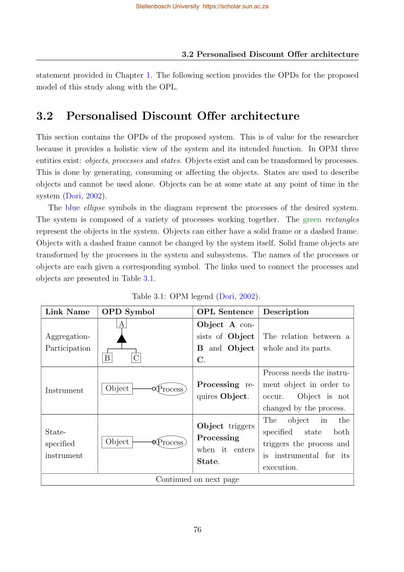
3.2 Personalised Discount Offer architecture
statement provided in Chapter 1. The following section provides the OPDs for the proposed
model of this study along with the OPL.
3.2 Personalised Discount Offer architecture
This section contains the OPDs of the proposed system. This is of value for the researcher
because it provides a holistic view of the system and its intended function. In OPM three
entities exist: objects, processes and states. Objects exist and can be transformed by processes.
This is done by generating, consuming or affecting the objects. States are used to describe
objects and cannot be used alone. Objects can be at some state at any point of time in the
system (Dori, 2002).
The blue ellipse symbols in the diagram represent the processes of the desired system.
The system is composed of a variety of processes working together. The green rectangles
represent the objects in the system. Objects can either have a solid frame or a dashed frame.
Objects with a dashed frame cannot be changed by the system itself. Solid frame objects are
transformed by the processes in the system and subsystems. The names of the processes or
objects are each given a corresponding symbol. The links used to connect the processes and
objects are presented in Table 3.1.
Table 3.1: OPM legend (Dori, 2002).
Link Name OPD Symbol OPL Sentence Description
Aggregation-
Participation
A
B C
Object A con-
sists of Object
B and Object
C.
The relation between a
whole and its parts.
Instrument Object ProcessProcessing re-
quires Object.
Process needs the instru-
ment object in order to
occur. Object is not
changed by the process.
State-
specified
instrument
Object Processe
Object triggers
Processing
when it enters
State.
The object in the
specified state both
triggers the process and
is instrumental for its
execution.
Continued on next page
76
Stellenbosch University https://scholar.sun.ac.za
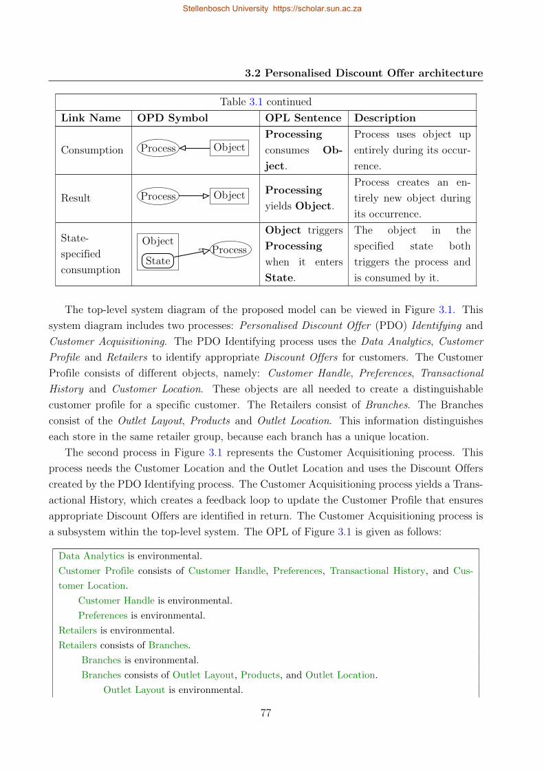
3.2 Personalised Discount Offer architecture
Table 3.1 continued
Link Name OPD Symbol OPL Sentence Description
Consumption Process ObjectProcessing
consumes Ob-
ject.
Process uses object up
entirely during its occur-
rence.
Result Process Object Processing
yields Object.
Process creates an en-
tirely new object during
its occurrence.
State-
specified
consumption
ObjectProcess
Statee
Object triggers
Processing
when it enters
State.
The object in the
specified state both
triggers the process and
is consumed by it.
The top-level system diagram of the proposed model can be viewed in Figure 3.1. This
system diagram includes two processes: Personalised Discount Offer (PDO) Identifying and
Customer Acquisitioning. The PDO Identifying process uses the Data Analytics, Customer
Profile and Retailers to identify appropriate Discount Offers for customers. The Customer
Profile consists of different objects, namely: Customer Handle, Preferences, Transactional
History and Customer Location. These objects are all needed to create a distinguishable
customer profile for a specific customer. The Retailers consist of Branches. The Branches
consist of the Outlet Layout, Products and Outlet Location. This information distinguishes
each store in the same retailer group, because each branch has a unique location.
The second process in Figure 3.1 represents the Customer Acquisitioning process. This
process needs the Customer Location and the Outlet Location and uses the Discount Offers
created by the PDO Identifying process. The Customer Acquisitioning process yields a Trans-
actional History, which creates a feedback loop to update the Customer Profile that ensures
appropriate Discount Offers are identified in return. The Customer Acquisitioning process is
a subsystem within the top-level system. The OPL of Figure 3.1 is given as follows:
Data Analytics is environmental.
Customer Profile consists of Customer Handle, Preferences, Transactional History, and Cus-
tomer Location.
Customer Handle is environmental.
Preferences is environmental.
Retailers is environmental.
Retailers consists of Branches.
Branches is environmental.
Branches consists of Outlet Layout, Products, and Outlet Location.
Outlet Layout is environmental.
77
Stellenbosch University https://scholar.sun.ac.za
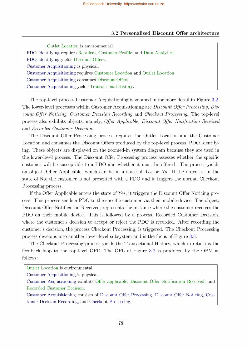
3.2 Personalised Discount Offer architecture
Outlet Location is environmental.
PDO Identifying requires Retailers, Customer Profile, and Data Analytics.
PDO Identifying yields Discount Offers.
Customer Acquisitioning is physical.
Customer Acquisitioning requires Customer Location and Outlet Location.
Customer Acquisitioning consumes Discount Offers.
Customer Acquisitioning yields Transactional History.
The top-level process Customer Acquisitioning is zoomed in for more detail in Figure 3.2.
The lower-level processes within Customer Acquisitioning are Discount Offer Processing, Dis-
count Offer Noticing, Customer Decision Recording and Checkout Processing. The top-level
process also exhibits objects, namely, Offer Applicable, Discount Offer Notification Received
and Recorded Customer Decision.
The Discount Offer Processing process requires the Outlet Location and the Customer
Location and consumes the Discount Offers produced by the top-level process, PDO Identify-
ing. These objects are displayed on the zoomed-in system diagram because they are used in
the lower-level process. The Discount Offer Processing process assesses whether the specific
customer will be susceptible to a PDO and whether it must be offered. The process yields
an object, Offer Applicable, which can be in a state of Yes or No. If the object is in the
state of No, the customer is not presented with a PDO and it triggers the normal Checkout
Processing process.
If the Offer Applicable enters the state of Yes, it triggers the Discount Offer Noticing pro-
cess. This process sends a PDO to the specific customer via their mobile device. The object,
Discount Offer Notification Received, represents the instance where the customer receives the
PDO on their mobile device. This is followed by a process, Recorded Customer Decision,
where the customer’s decision to accept or reject the PDO is recorded. After recording the
customer’s decision, the process Checkout Processing, is triggered. The Checkout Processing
process develops into another lower-level subsystem and is the focus of Figure 3.3.
The Checkout Processing process yields the Transactional History, which in return is the
feedback loop to the top-level OPD. The OPL of Figure 3.2 is produced by the OPM as
follows:
Outlet Location is environmental.
Customer Acquisitioning is physical.
Customer Acquisitioning exhibits Offer applicable, Discount Offer Notification Received, and
Recorded Customer Decision.
Customer Acquisitioning consists of Discount Offer Processing, Discount Offer Noticing, Cus-
tomer Decision Recording, and Checkout Processing.
78
Stellenbosch University https://scholar.sun.ac.za
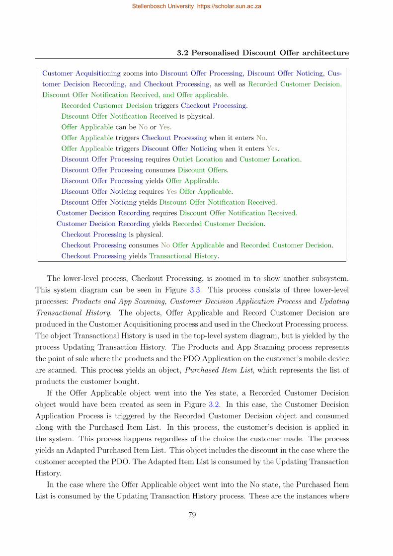
3.2 Personalised Discount Offer architecture
Customer Acquisitioning zooms into Discount Offer Processing, Discount Offer Noticing, Cus-
tomer Decision Recording, and Checkout Processing, as well as Recorded Customer Decision,
Discount Offer Notification Received, and Offer applicable.
Recorded Customer Decision triggers Checkout Processing.
Discount Offer Notification Received is physical.
Offer Applicable can be No or Yes.
Offer Applicable triggers Checkout Processing when it enters No.
Offer Applicable triggers Discount Offer Noticing when it enters Yes.
Discount Offer Processing requires Outlet Location and Customer Location.
Discount Offer Processing consumes Discount Offers.
Discount Offer Processing yields Offer Applicable.
Discount Offer Noticing requires Yes Offer Applicable.
Discount Offer Noticing yields Discount Offer Notification Received.
Customer Decision Recording requires Discount Offer Notification Received.
Customer Decision Recording yields Recorded Customer Decision.
Checkout Processing is physical.
Checkout Processing consumes No Offer Applicable and Recorded Customer Decision.
Checkout Processing yields Transactional History.
The lower-level process, Checkout Processing, is zoomed in to show another subsystem.
This system diagram can be seen in Figure 3.3. This process consists of three lower-level
processes: Products and App Scanning, Customer Decision Application Process and Updating
Transactional History. The objects, Offer Applicable and Record Customer Decision are
produced in the Customer Acquisitioning process and used in the Checkout Processing process.
The object Transactional History is used in the top-level system diagram, but is yielded by the
process Updating Transaction History. The Products and App Scanning process represents
the point of sale where the products and the PDO Application on the customer’s mobile device
are scanned. This process yields an object, Purchased Item List, which represents the list of
products the customer bought.
If the Offer Applicable object went into the Yes state, a Recorded Customer Decision
object would have been created as seen in Figure 3.2. In this case, the Customer Decision
Application Process is triggered by the Recorded Customer Decision object and consumed
along with the Purchased Item List. In this process, the customer’s decision is applied in
the system. This process happens regardless of the choice the customer made. The process
yields an Adapted Purchased Item List. This object includes the discount in the case where the
customer accepted the PDO. The Adapted Item List is consumed by the Updating Transaction
History.
In the case where the Offer Applicable object went into the No state, the Purchased Item
List is consumed by the Updating Transaction History process. These are the instances where
79
Stellenbosch University https://scholar.sun.ac.za
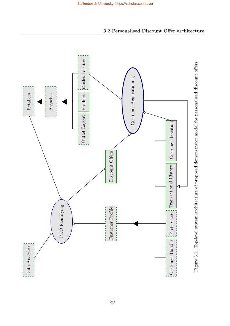
3.2 Personalised Discount Offer architecture
Dis
count
Off
ers
Dat
aA
nal
yti
cs
PD
OId
enti
fyin
g
Cust
omer
Pro
file
Cust
omer
Han
dle
Pre
fere
nce
sT
ransa
ctio
nal
His
tory
Cust
omer
Loca
tionC
ust
omer
Acq
uis
itio
nin
g
Ret
aile
rs
Bra
nch
es
Outl
etL
oca
tion
Pro
duct
sO
utl
etL
ayou
t
Fig
ure
3.1:
Top
-lev
elsy
stem
arch
itec
ture
ofpro
pos
eddem
onst
rato
rm
odel
for
per
sonal
ised
dis
count
offe
rs
80
Stellenbosch University https://scholar.sun.ac.za
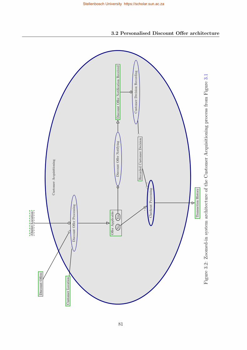
3.2 Personalised Discount Offer architecture
Cu
stom
erA
cqu
isit
ion
ing
Dis
cou
nt
Off
erN
otif
yin
g
Off
erA
pp
lica
ble
Dis
cou
nt
Off
erP
roce
ssin
g
Ou
tlet
Loca
tion
Dis
cou
nt
Off
ers
Cu
stom
erL
oca
tion
No
Yes
Dis
cou
nt
Off
erN
otifi
cati
onR
ecei
ved
Cu
stom
erD
ecis
ion
Rec
ord
ing
Rec
ord
edC
ust
omer
Dec
isio
n
Ch
ecko
ut
Pro
cess
ing
Tra
nsa
ctio
nH
isto
ry
e
e
e
Fig
ure
3.2:
Zoom
ed-i
nsy
stem
arch
itec
ture
ofth
eC
ust
omer
Acq
uis
itio
nin
gpro
cess
from
Fig
ure
3.1
81
Stellenbosch University https://scholar.sun.ac.za
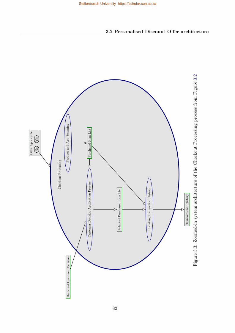
3.2 Personalised Discount Offer architecture
Ch
ecko
ut
Pro
cess
ing Pro
du
ctan
dA
pp
Sca
nn
ing
Off
erA
pp
lica
ble
No
Yes
Cu
stom
erD
ecis
ion
App
lica
tion
Pro
cess
Pu
rch
ased
Item
Lis
t
Rec
ord
edC
ust
omer
Dec
isio
n
Ad
apte
dP
urc
has
edIt
emL
ist
Up
dat
ing
Tra
nsa
ctio
nH
isto
ry
Tra
nsa
ctio
nal
His
tory
e
e
Fig
ure
3.3:
Zoom
ed-i
nsy
stem
arch
itec
ture
ofth
eC
hec
kout
Pro
cess
ing
pro
cess
from
Fig
ure
3.2
82
Stellenbosch University https://scholar.sun.ac.za
3.3 Schematic view of the proposed system
customers did not receive any PDOs. The Updating Transaction History updates and yields
the Transactional History of the specific customer. The Transactional History is an object in
the top-level system diagram and is the feedback loop that in return is used as part of the
Customer Profile. The system is also updated with the customer’s decision to accept or reject
the PDO. The OPL of the Checkout Processing process is given as,
Offer Applicable can be No or Yes.
Offer Applicable triggers Checkout Processing when it enters No.
Recorded Customer Decision triggers Customer Decision Application Process.
Checkout Processing is physical.
Checkout Processing exhibits Purchased Item List and Adapted Purchased Item List.
Checkout Processing consists of Products and App Scanning, Customer Decision Application
Process, and Updating Transaction History.
Checkout Processing consumes No Offer Applicable.
Checkout Processing zooms into Products and App Scanning, Customer Decision Application
Process, and Updating Transaction History, as well as Adapted Purchased Item List and Pur-
chased Item List.
Products and App Scanning is physical.
Products and App Scanning yields Purchased Item List.
Customer Decision Application Process consumes Purchased Item List and Recorded
Customer Decision.
Customer Decision Application Process yields Adapted Purchased Item List.
Updating Transaction History consumes Adapted Purchased Item List and Purchased
Item List.
Updating Transaction History yields Transactional History.
3.3 Schematic view of the proposed system
The previous section explained the system architecture of the proposed system. This sec-
tion will provide a schematic overview of the proposed system, which will be presented as a
demonstrator model and the different parts and their functionalities. The proposed system
is referred to as a demonstrator since the implementation thereof is beyond the scope of this
study.
The researcher decided to use simulated data in the proposed model in order to overcome
ethical issues. The model requires the data to be in a very specific format and this is another
contributing reason why the researcher decided to use simulated data. The PDO demonstrator
requires a simulator, which simulates all the necessary data and a PDO predictor, which
provides PDOs to customers. These two subsystems will be distinctly referred to from this
point onwards. Figure 3.4 visualises the relationship and difference in functionality between
83
Stellenbosch University https://scholar.sun.ac.za
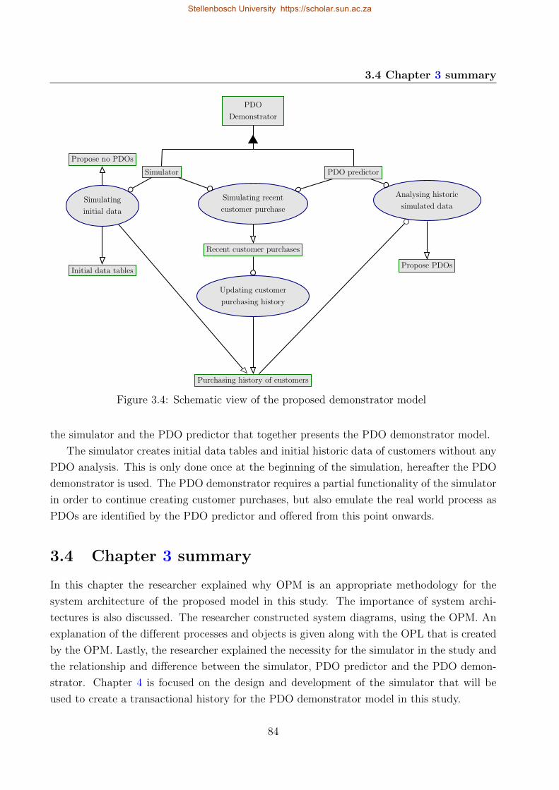
3.4 Chapter 3 summary
PDO
Demonstrator
Simulator PDO predictor
Simulating
initial data
Simulating recent
customer purchase
Analysing historic
simulated data
Recent customer purchases
Updating customer
purchasing history
Purchasing history of customers
Propose no PDOs
Initial data tablesPropose PDOs
Figure 3.4: Schematic view of the proposed demonstrator model
the simulator and the PDO predictor that together presents the PDO demonstrator model.
The simulator creates initial data tables and initial historic data of customers without any
PDO analysis. This is only done once at the beginning of the simulation, hereafter the PDO
demonstrator is used. The PDO demonstrator requires a partial functionality of the simulator
in order to continue creating customer purchases, but also emulate the real world process as
PDOs are identified by the PDO predictor and offered from this point onwards.
3.4 Chapter 3 summary
In this chapter the researcher explained why OPM is an appropriate methodology for the
system architecture of the proposed model in this study. The importance of system archi-
tectures is also discussed. The researcher constructed system diagrams, using the OPM. An
explanation of the different processes and objects is given along with the OPL that is created
by the OPM. Lastly, the researcher explained the necessity for the simulator in the study and
the relationship and difference between the simulator, PDO predictor and the PDO demon-
strator. Chapter 4 is focused on the design and development of the simulator that will be
used to create a transactional history for the PDO demonstrator model in this study.
84
Stellenbosch University https://scholar.sun.ac.za

Chapter 4
Design and development of the
simulator
The previous chapter informed the reader about the system architecture of the proposed
model. This chapter encompasses the design and development of the simulator. The simulator
is used to create initial pseudo-customer data containing personal information and purchasing
behaviour. The methodology followed for the design and development of the simulator will
initiate this chapter.
4.1 Simulator design and development methodology
This chapter represents the start of phase two of the research methodology explained in Section
1.5. The researcher will start the design of the simulator by identifying the functionalities
needed within the simulator. During this part the researcher must identify the entities needed
in the system as well as the entity-relationships that exist between them. This will be realised
by using an Extended Entity–Relationship Diagram (EERD). In order to create these entities,
a data dictionary is needed to describe the attributes of each entity. After the design of the
simulator the researcher must develop the simulator and for this a database will be needed.
The researcher must identify the database to be used as well as the program to be used for
the development of the simulator. The researcher must explain how the entities are populated
during the development of the simulator.
4.2 Design of the simulator
The design of the simulator commenced based on the system architecture using Object Process
Methodology (OPM) as described in Chapter 3. The goal of the simulator can be divided into
two parts or functionalities. It is initially used to populate empty data tables so that data
is available for analysis. Then it is used to create an initial customer purchasing history and
thereafter the continued simulation of the customer purchasing history. A summary of this
can be seen in Figure 4.1. The functionality of the continued customer purchasing history
simulation will be used within the PDO demonstrator which is the subject of discussion in
Chapter 5.
85
Stellenbosch University https://scholar.sun.ac.za
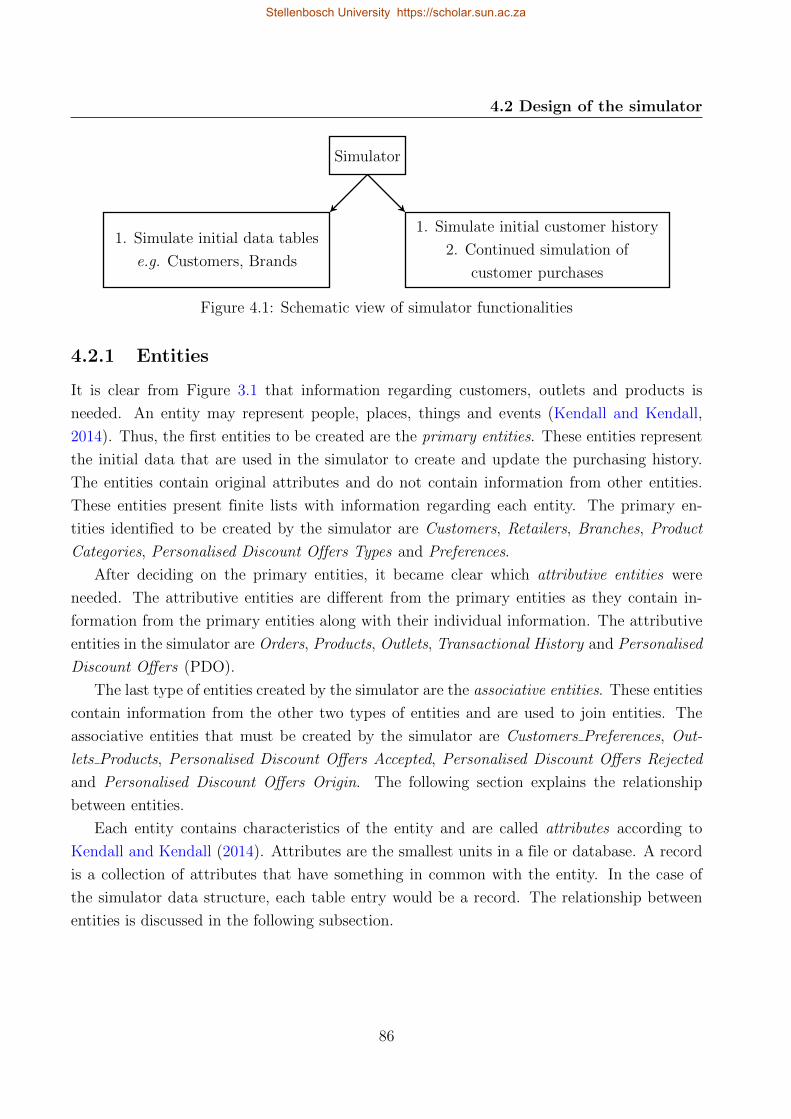
4.2 Design of the simulator
Simulator
1. Simulate initial data tables
e.g. Customers, Brands
1. Simulate initial customer history
2. Continued simulation of
customer purchases
Figure 4.1: Schematic view of simulator functionalities
4.2.1 Entities
It is clear from Figure 3.1 that information regarding customers, outlets and products is
needed. An entity may represent people, places, things and events (Kendall and Kendall,
2014). Thus, the first entities to be created are the primary entities. These entities represent
the initial data that are used in the simulator to create and update the purchasing history.
The entities contain original attributes and do not contain information from other entities.
These entities present finite lists with information regarding each entity. The primary en-
tities identified to be created by the simulator are Customers, Retailers, Branches, Product
Categories, Personalised Discount Offers Types and Preferences.
After deciding on the primary entities, it became clear which attributive entities were
needed. The attributive entities are different from the primary entities as they contain in-
formation from the primary entities along with their individual information. The attributive
entities in the simulator are Orders, Products, Outlets, Transactional History and Personalised
Discount Offers (PDO).
The last type of entities created by the simulator are the associative entities. These entities
contain information from the other two types of entities and are used to join entities. The
associative entities that must be created by the simulator are Customers Preferences, Out-
lets Products, Personalised Discount Offers Accepted, Personalised Discount Offers Rejected
and Personalised Discount Offers Origin. The following section explains the relationship
between entities.
Each entity contains characteristics of the entity and are called attributes according to
Kendall and Kendall (2014). Attributes are the smallest units in a file or database. A record
is a collection of attributes that have something in common with the entity. In the case of
the simulator data structure, each table entry would be a record. The relationship between
entities is discussed in the following subsection.
86
Stellenbosch University https://scholar.sun.ac.za
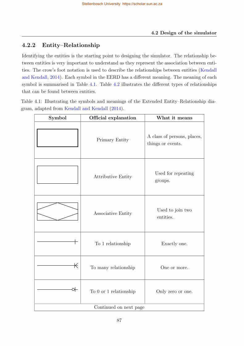
4.2 Design of the simulator
4.2.2 Entity–Relationship
Identifying the entities is the starting point to designing the simulator. The relationship be-
tween entities is very important to understand as they represent the association between enti-
ties. The crow’s foot notation is used to describe the relationships between entities (Kendall
and Kendall, 2014). Each symbol in the EERD has a different meaning. The meaning of each
symbol is summarised in Table 4.1. Table 4.2 illustrates the different types of relationships
that can be found between entities.
Table 4.1: Illustrating the symbols and meanings of the Extended Entity–Relationship dia-
gram, adapted from Kendall and Kendall (2014).
Symbol Official explanation What it means
Primary EntityA class of persons, places,
things or events.
Attributive EntityUsed for repeating
groups.
Associative EntityUsed to join two
entities.
To 1 relationship Exactly one.
To many relationship One or more.
To 0 or 1 relationship Only zero or one.
Continued on next page
87
Stellenbosch University https://scholar.sun.ac.za
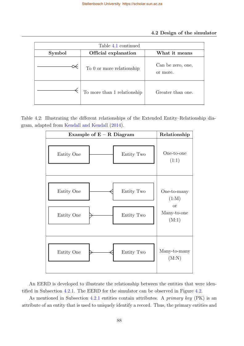
4.2 Design of the simulator
Table 4.1 continued
Symbol Official explanation What it means
To 0 or more relationshipCan be zero, one,
or more.
To more than 1 relationship Greater than one.
Table 4.2: Illustrating the different relationships of the Extended Entity–Relationship dia-
gram, adapted from Kendall and Kendall (2014).
Example of E – R Diagram Relationship
Entity One Entity Two One-to-one
(1:1)
Entity One Entity Two
Entity One Entity Two
One-to-many
(1:M)
or
Many-to-one
(M:1)
Entity One Entity Two Many-to-many
(M:N)
An EERD is developed to illustrate the relationship between the entities that were iden-
tified in Subsection 4.2.1. The EERD for the simulator can be observed in Figure 4.2.
As mentioned in Subsection 4.2.1 entities contain attributes. A primary key (PK) is an
attribute of an entity that is used to uniquely identify a record. Thus, the primary entities and
88
Stellenbosch University https://scholar.sun.ac.za
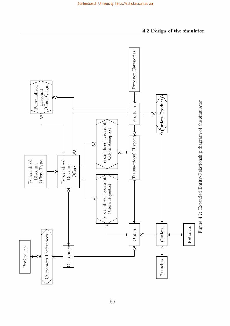
4.2 Design of the simulator
Ord
ers
Ret
aile
rs
Outl
ets
Bra
nch
es
Tra
nsa
ctio
nal
His
tory
Pro
duct
Cat
egor
ies
Pro
duct
s
Cust
omer
s
Pre
fere
nce
s
Cust
omer
sP
refe
rence
s
Per
sonal
ised
Dis
count
Off
ers
Per
sonal
ised
Dis
count
Off
ers
Typ
eP
erso
nal
ised
Dis
count
Off
ers
Ori
gin
Outl
ets
Pro
duct
sO
utl
ets
Pro
duct
s
Per
sonal
ised
Dis
count
Off
ers
Acc
epte
dP
erso
nal
ised
Dis
count
Off
ers
Rej
ecte
d
Fig
ure
4.2:
Exte
nded
Enti
ty-R
elat
ionsh
ipdia
gram
ofth
esi
mula
tor
89
Stellenbosch University https://scholar.sun.ac.za
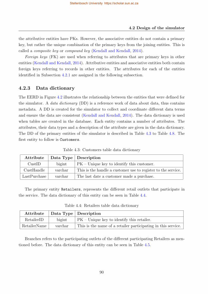
4.2 Design of the simulator
the attributive entities have PKs. However, the associative entities do not contain a primary
key, but rather the unique combination of the primary keys from the joining entities. This is
called a composite key or compound key (Kendall and Kendall, 2014).
Foreign keys (FK) are used when referring to attributes that are primary keys in other
entities (Kendall and Kendall, 2014). Attributive entities and associative entities both contain
foreign keys referring to records in other entities. The attributes for each of the entities
identified in Subsection 4.2.1 are assigned in the following subsection.
4.2.3 Data dictionary
The EERD in Figure 4.2 illustrates the relationship between the entities that were defined for
the simulator. A data dictionary (DD) is a reference work of data about data, thus contains
metadata. A DD is created for the simulator to collect and coordinate different data terms
and ensure the data are consistent (Kendall and Kendall, 2014). The data dictionary is used
when tables are created in the database. Each entity contains a number of attributes. The
attributes, their data types and a description of the attribute are given in the data dictionary.
The DD of the primary entities of the simulator is described in Table 4.3 to Table 4.8. The
first entity to follow is Customers.
Table 4.3: Customers table data dictionary
Attribute Data Type Description
CustID bigint PK – Unique key to identify this customer.
CustHandle varchar This is the handle a customer use to register to the service.
LastPurchase varchar The last date a customer made a purchase.
The primary entity Retailers, represents the different retail outlets that participate in
the service. The data dictionary of this entity can be seen in Table 4.4.
Table 4.4: Retailers table data dictionary
Attribute Data Type Description
RetailerID bigint PK – Unique key to identify this retailer.
RetailerName varchar This is the name of a retailer participating in this service.
Branches refers to the participating outlets of the different participating Retailers as men-
tioned before. The data dictionary of this entity can be seen in Table 4.5.
90
Stellenbosch University https://scholar.sun.ac.za
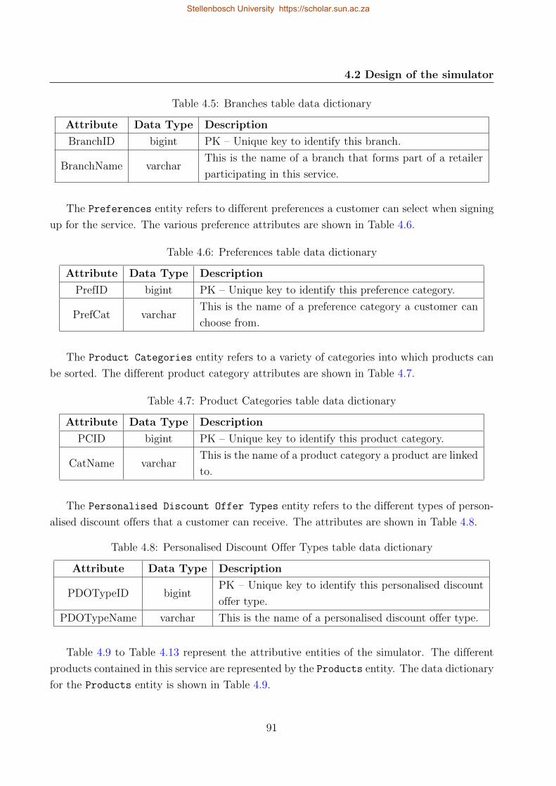
4.2 Design of the simulator
Table 4.5: Branches table data dictionary
Attribute Data Type Description
BranchID bigint PK – Unique key to identify this branch.
BranchName varcharThis is the name of a branch that forms part of a retailer
participating in this service.
The Preferences entity refers to different preferences a customer can select when signing
up for the service. The various preference attributes are shown in Table 4.6.
Table 4.6: Preferences table data dictionary
Attribute Data Type Description
PrefID bigint PK – Unique key to identify this preference category.
PrefCat varcharThis is the name of a preference category a customer can
choose from.
The Product Categories entity refers to a variety of categories into which products can
be sorted. The different product category attributes are shown in Table 4.7.
Table 4.7: Product Categories table data dictionary
Attribute Data Type Description
PCID bigint PK – Unique key to identify this product category.
CatName varcharThis is the name of a product category a product are linked
to.
The Personalised Discount Offer Types entity refers to the different types of person-
alised discount offers that a customer can receive. The attributes are shown in Table 4.8.
Table 4.8: Personalised Discount Offer Types table data dictionary
Attribute Data Type Description
PDOTypeID bigintPK – Unique key to identify this personalised discount
offer type.
PDOTypeName varchar This is the name of a personalised discount offer type.
Table 4.9 to Table 4.13 represent the attributive entities of the simulator. The different
products contained in this service are represented by the Products entity. The data dictionary
for the Products entity is shown in Table 4.9.
91
Stellenbosch University https://scholar.sun.ac.za
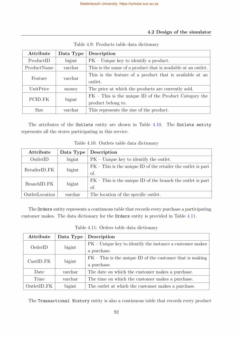
4.2 Design of the simulator
Table 4.9: Products table data dictionary
Attribute Data Type Description
ProductID bigint PK – Unique key to identify a product.
ProductName varchar This is the name of a product that is available at an outlet.
Feature varcharThis is the feature of a product that is available at an
outlet.
UnitPrice money The price at which the products are currently sold.
PCID FK bigintFK – This is the unique ID of the Product Category the
product belong to.
Size varchar This represents the size of the product.
The attributes of the Outlets entity are shown in Table 4.10. The Outlets entity
represents all the stores participating in this service.
Table 4.10: Outlets table data dictionary
Attribute Data Type Description
OutletID bigint PK – Unique key to identify the outlet.
RetailerID FK bigintFK – This is the unique ID of the retailer the outlet is part
of.
BranchID FK bigintFK – This is the unique ID of the branch the outlet is part
of.
OutletLocation varchar The location of the specific outlet.
The Orders entity represents a continuous table that records every purchase a participating
customer makes. The data dictionary for the Orders entity is provided in Table 4.11.
Table 4.11: Orders table data dictionary
Attribute Data Type Description
OrderID bigintPK – Unique key to identify the instance a customer makes
a purchase.
CustID FK bigintFK – This is the unique ID of the customer that is making
a purchase.
Date varchar The date on which the customer makes a purchase.
Time varchar The time on which the customer makes a purchase.
OutletID FK bigint The outlet at which the customer makes a purchase.
The Transactional History entity is also a continuous table that records every product
92
Stellenbosch University https://scholar.sun.ac.za
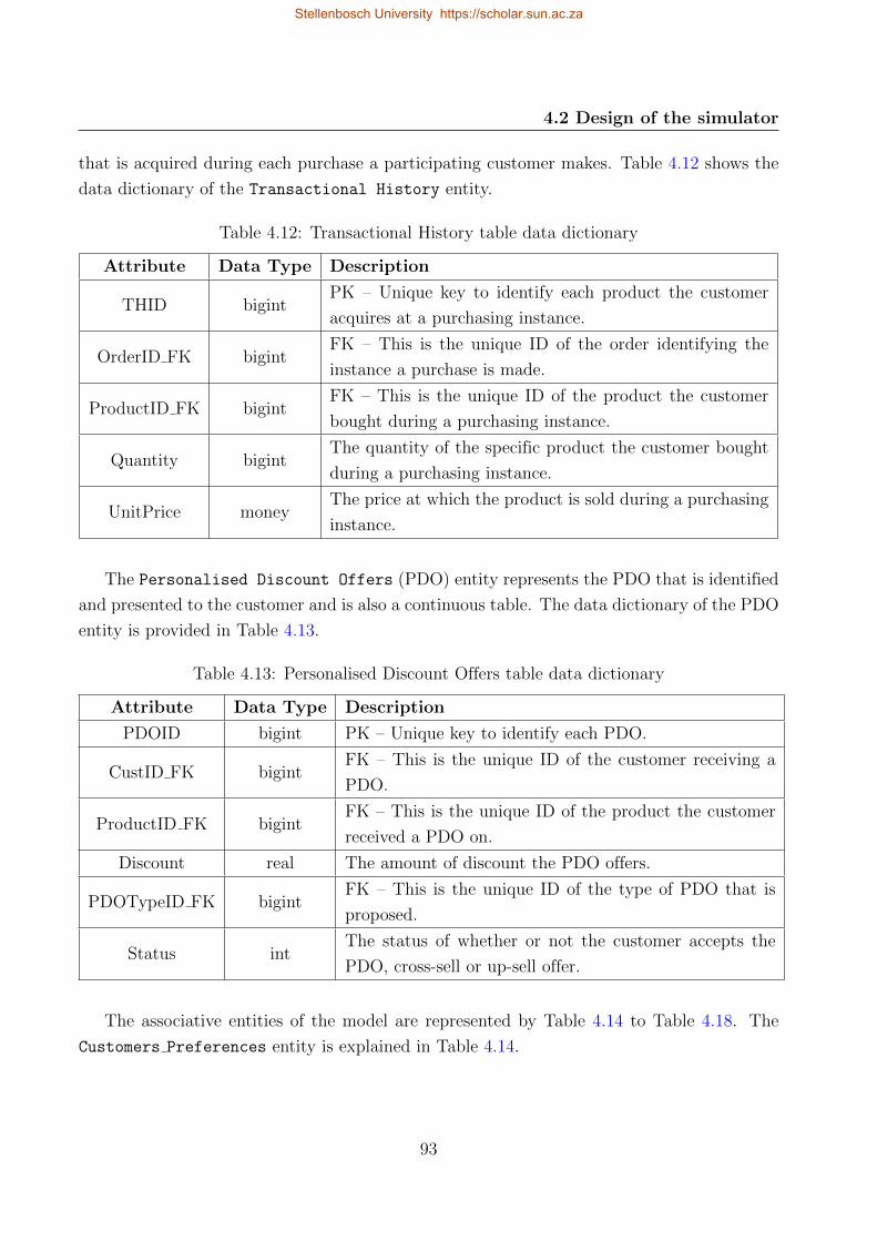
4.2 Design of the simulator
that is acquired during each purchase a participating customer makes. Table 4.12 shows the
data dictionary of the Transactional History entity.
Table 4.12: Transactional History table data dictionary
Attribute Data Type Description
THID bigintPK – Unique key to identify each product the customer
acquires at a purchasing instance.
OrderID FK bigintFK – This is the unique ID of the order identifying the
instance a purchase is made.
ProductID FK bigintFK – This is the unique ID of the product the customer
bought during a purchasing instance.
Quantity bigintThe quantity of the specific product the customer bought
during a purchasing instance.
UnitPrice moneyThe price at which the product is sold during a purchasing
instance.
The Personalised Discount Offers (PDO) entity represents the PDO that is identified
and presented to the customer and is also a continuous table. The data dictionary of the PDO
entity is provided in Table 4.13.
Table 4.13: Personalised Discount Offers table data dictionary
Attribute Data Type Description
PDOID bigint PK – Unique key to identify each PDO.
CustID FK bigintFK – This is the unique ID of the customer receiving a
PDO.
ProductID FK bigintFK – This is the unique ID of the product the customer
received a PDO on.
Discount real The amount of discount the PDO offers.
PDOTypeID FK bigintFK – This is the unique ID of the type of PDO that is
proposed.
Status intThe status of whether or not the customer accepts the
PDO, cross-sell or up-sell offer.
The associative entities of the model are represented by Table 4.14 to Table 4.18. The
Customers Preferences entity is explained in Table 4.14.
93
Stellenbosch University https://scholar.sun.ac.za
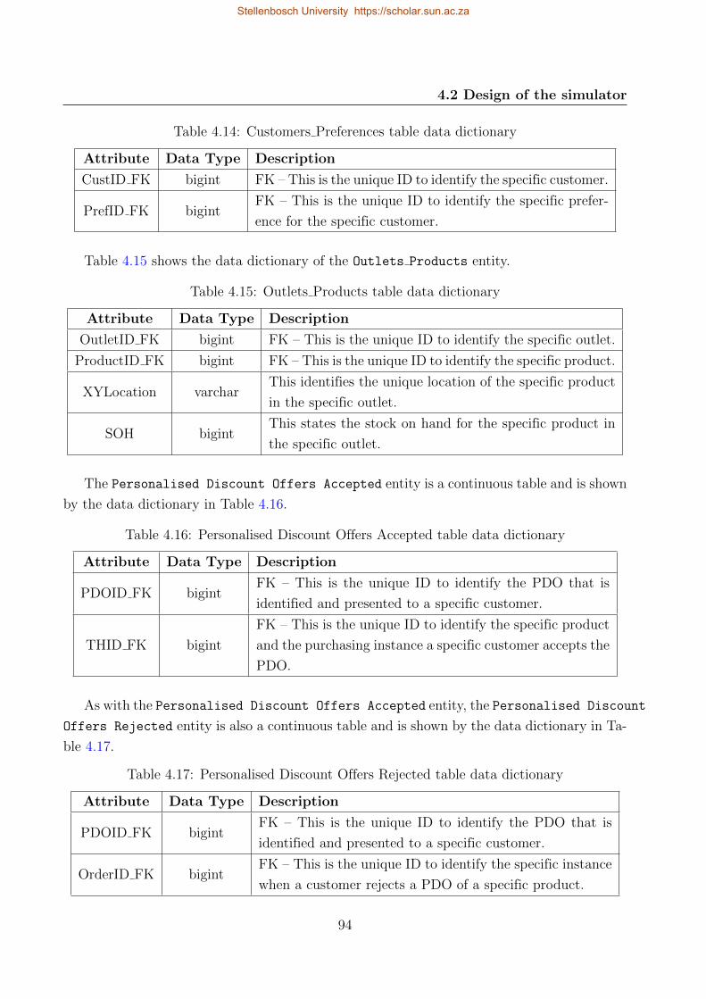
4.2 Design of the simulator
Table 4.14: Customers Preferences table data dictionary
Attribute Data Type Description
CustID FK bigint FK – This is the unique ID to identify the specific customer.
PrefID FK bigintFK – This is the unique ID to identify the specific prefer-
ence for the specific customer.
Table 4.15 shows the data dictionary of the Outlets Products entity.
Table 4.15: Outlets Products table data dictionary
Attribute Data Type Description
OutletID FK bigint FK – This is the unique ID to identify the specific outlet.
ProductID FK bigint FK – This is the unique ID to identify the specific product.
XYLocation varcharThis identifies the unique location of the specific product
in the specific outlet.
SOH bigintThis states the stock on hand for the specific product in
the specific outlet.
The Personalised Discount Offers Accepted entity is a continuous table and is shown
by the data dictionary in Table 4.16.
Table 4.16: Personalised Discount Offers Accepted table data dictionary
Attribute Data Type Description
PDOID FK bigintFK – This is the unique ID to identify the PDO that is
identified and presented to a specific customer.
THID FK bigint
FK – This is the unique ID to identify the specific product
and the purchasing instance a specific customer accepts the
PDO.
As with the Personalised Discount Offers Accepted entity, the Personalised Discount
Offers Rejected entity is also a continuous table and is shown by the data dictionary in Ta-
ble 4.17.
Table 4.17: Personalised Discount Offers Rejected table data dictionary
Attribute Data Type Description
PDOID FK bigintFK – This is the unique ID to identify the PDO that is
identified and presented to a specific customer.
OrderID FK bigintFK – This is the unique ID to identify the specific instance
when a customer rejects a PDO of a specific product.
94
Stellenbosch University https://scholar.sun.ac.za
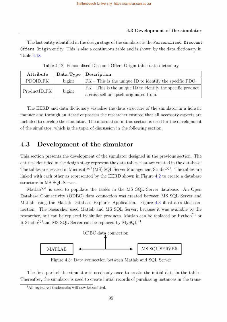
4.3 Development of the simulator
The last entity identified in the design stage of the simulator is the Personalised Discount
Offers Origin entity. This is also a continuous table and is shown by the data dictionary in
Table 4.18.
Table 4.18: Personalised Discount Offers Origin table data dictionary
Attribute Data Type Description
PDOID FK bigint FK – This is the unique ID to identify the specific PDO.
ProductID FK bigintFK – This is the unique ID to identify the specific product
a cross-sell or upsell originated from.
The EERD and data dictionary visualise the data structure of the simulator in a holistic
manner and through an iterative process the researcher ensured that all necessary aspects are
included to develop the simulator. The information in this section is used for the development
of the simulator, which is the topic of discussion in the following section.
4.3 Development of the simulator
This section presents the development of the simulator designed in the previous section. The
entities identified in the design stage represent the data tables that are created in the database.
The tables are created in Microsoft®1(MS) SQL Server Management Studio®1. The tables are
linked with each other as represented by the EERD shown in Figure 4.2 to create a database
structure in MS SQL Server.
Matlab®1 is used to populate the tables in the MS SQL Server database. An Open
Database Connectivity (ODBC) data connection was created between MS SQL Server and
Matlab using the Matlab Database Explorer Application. Figure 4.3 illustrates this con-
nection. The researcher used Matlab and MS SQL Server, because it was available to the
researcher, but can be replaced by similar products. Matlab can be replaced by Python�1 or
R Studio®1and MS SQL Server can be replaced by MySQL�1.
MATLAB MS SQL SERVER
ODBC data connection
Figure 4.3: Data connection between Matlab and SQL Server
The first part of the simulator is used only once to create the initial data in the tables.
Thereafter, the simulator is used to create initial records of purchasing instances in the trans-
1All registered trademarks will now be omitted.
95
Stellenbosch University https://scholar.sun.ac.za
4.3 Development of the simulator
action tables (Transactional History and Orders). This functionality is used within the PDO
demonstrator that will be discussed in Chapter 5. The first tables populated are the pri-
mary entities: Customers, Retailers, Branches, Product Categories, Personalised Discount
Off Types and Preferences. These are the simplest since they only contain list information.
4.3.1 Customers table
The customer IDs are populated from one to the number of customers participating in the
system. The customer handles are populated as the entity name and the associated ID digit.
For example, the customer with CustID as one is given the CustHandle “Customer 1”.
The LastPurchase date of each customer is given as an initial date at the beginning
of service. After this the last purchase attribute is updated every time a customer visits a
participating outlet. Except for the last purchase attribute, the Retailers, Branches, Product
Categories and Preferences tables are populated in the same manner.
4.3.2 PDO Types table
There are three different types of personalised discount offers a customer can receive, thus the
IDs are populated from one to three. The first PDOTypeName is a normal PDO, the second
type is a cross-sell PDO and lastly the third type is an upsell PDO.
4.3.3 Outlets table
The IDs of the outlets identify each unique store that consist of a retailer and a branch with a
unique location. An assumption is made that every branch accommodates each retailer. Thus,
if five branches and five retailers are participating in this service, 25 outlets are populated.
The locations are assigned as “RetailerID FK, BranchID FK” to ensure each outlet has a
unique location in the model. If an outlet represents RetailerID FK one and BranchID FK
two, the unique location would be “1, 2”.
4.3.4 Orders table
This table is populated to contain a history for a certain number of days until a certain point
in time. From this point onwards new order records are individually added to the Orders
table and the table is updated.
The purchasing behaviour of customers are very complex and it is for this reason that
the researcher simplified it to three main groups. The researcher identified the three groups
based on known behaviour qualities. The first type is customers who buy their groceries
monthly. These customers are also divided into a group of customers who make purchases at
96
Stellenbosch University https://scholar.sun.ac.za
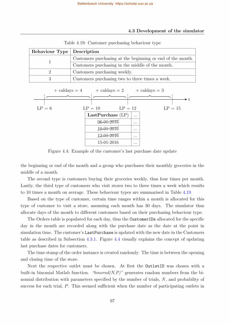
4.3 Development of the simulator
Table 4.19: Customer purchasing behaviour type
Behaviour Type Description
1Customers purchasing at the beginning or end of the month.
Customers purchasing in the middle of the month.
2 Customers purchasing weekly.
3 Customers purchasing two to three times a week.
t
LP = 6
+ caldays = 4
LP = 10
+ caldays = 2
LP = 12
+ caldays = 3
LP = 15
LastPurchase (LP) ...
((((((06-01-2016 ...
((((((10-01-2016 ...
((((((12-01-2016 ...
15-01-2016 ...
Figure 4.4: Example of the customer’s last purchase date update
the beginning or end of the month and a group who purchases their monthly groceries in the
middle of a month.
The second type is customers buying their groceries weekly, thus four times per month.
Lastly, the third type of customers who visit stores two to three times a week which results
to 10 times a month on average. These behaviour types are summarised in Table 4.19.
Based on the type of customer, certain time ranges within a month is allocated for this
type of customer to visit a store, assuming each month has 30 days. The simulator thus
allocate days of the month to different customers based on their purchasing behaviour type.
The Orders table is populated for each day, thus the CustomerIDs allocated for the specific
day in the month are recorded along with the purchase date as the date at the point in
simulation time. The customer’s LastPurchase is updated with the new date in the Customers
table as described in Subsection 4.3.1. Figure 4.4 visually explains the concept of updating
last purchase dates for customers.
The time stamp of the order instance is created randomly. The time is between the opening
and closing time of the store.
Next the respective outlet must be chosen. At first the OutletID was chosen with a
built-in binomial Matlab function. “binornd(N,P)” generates random numbers from the bi-
nomial distribution with parameters specified by the number of trials, N , and probability of
success for each trial, P . This seemed sufficient when the number of participating outlets in
97
Stellenbosch University https://scholar.sun.ac.za
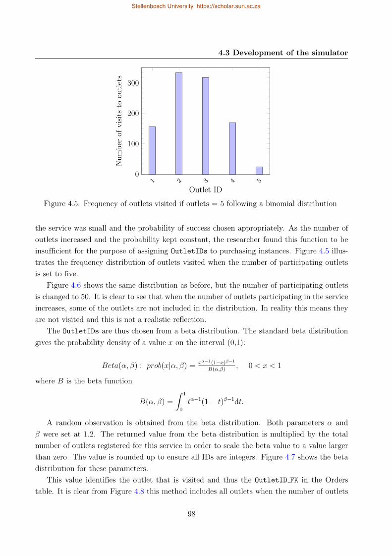
4.3 Development of the simulator
1 2 3 4 50
100
200
300
Outlet ID
Num
ber
ofvis
its
toou
tlet
s
Figure 4.5: Frequency of outlets visited if outlets = 5 following a binomial distribution
the service was small and the probability of success chosen appropriately. As the number of
outlets increased and the probability kept constant, the researcher found this function to be
insufficient for the purpose of assigning OutletIDs to purchasing instances. Figure 4.5 illus-
trates the frequency distribution of outlets visited when the number of participating outlets
is set to five.
Figure 4.6 shows the same distribution as before, but the number of participating outlets
is changed to 50. It is clear to see that when the number of outlets participating in the service
increases, some of the outlets are not included in the distribution. In reality this means they
are not visited and this is not a realistic reflection.
The OutletIDs are thus chosen from a beta distribution. The standard beta distribution
gives the probability density of a value x on the interval (0,1):
Beta(α, β) : prob(x|α, β) = xα−1(1−x)β−1
B(α,β), 0 < x < 1
where B is the beta function
B(α, β) =
∫ 1
0
tα−1(1− t)β−1dt.
A random observation is obtained from the beta distribution. Both parameters α and
β were set at 1.2. The returned value from the beta distribution is multiplied by the total
number of outlets registered for this service in order to scale the beta value to a value larger
than zero. The value is rounded up to ensure all IDs are integers. Figure 4.7 shows the beta
distribution for these parameters.
This value identifies the outlet that is visited and thus the OutletID FK in the Orders
table. It is clear from Figure 4.8 this method includes all outlets when the number of outlets
98
Stellenbosch University https://scholar.sun.ac.za
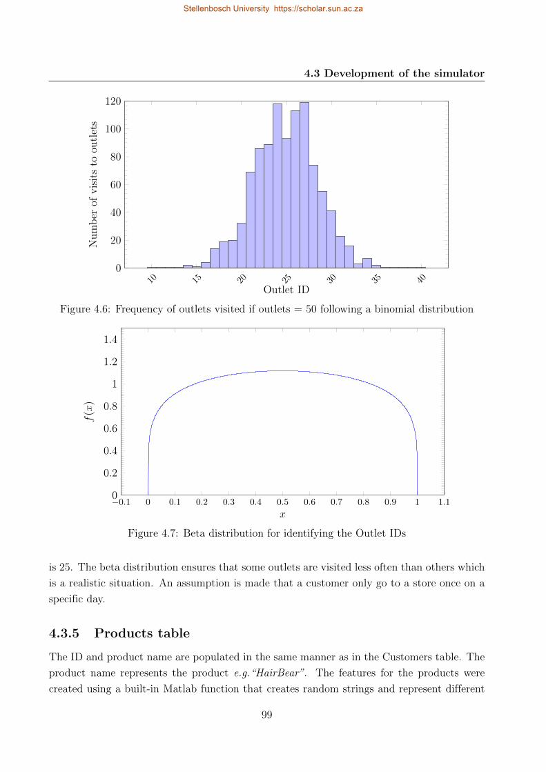
4.3 Development of the simulator
10 15 20 25 30 35 400
20
40
60
80
100
120
Outlet ID
Num
ber
ofvis
its
toou
tlet
s
Figure 4.6: Frequency of outlets visited if outlets = 50 following a binomial distribution
−0.1 0 0.1 0.2 0.3 0.4 0.5 0.6 0.7 0.8 0.9 1 1.10
0.2
0.4
0.6
0.8
1
1.2
1.4
x
f(x
)
Figure 4.7: Beta distribution for identifying the Outlet IDs
is 25. The beta distribution ensures that some outlets are visited less often than others which
is a realistic situation. An assumption is made that a customer only go to a store once on a
specific day.
4.3.5 Products table
The ID and product name are populated in the same manner as in the Customers table. The
product name represents the product e.g.“HairBear”. The features for the products were
created using a built-in Matlab function that creates random strings and represent different
99
Stellenbosch University https://scholar.sun.ac.za
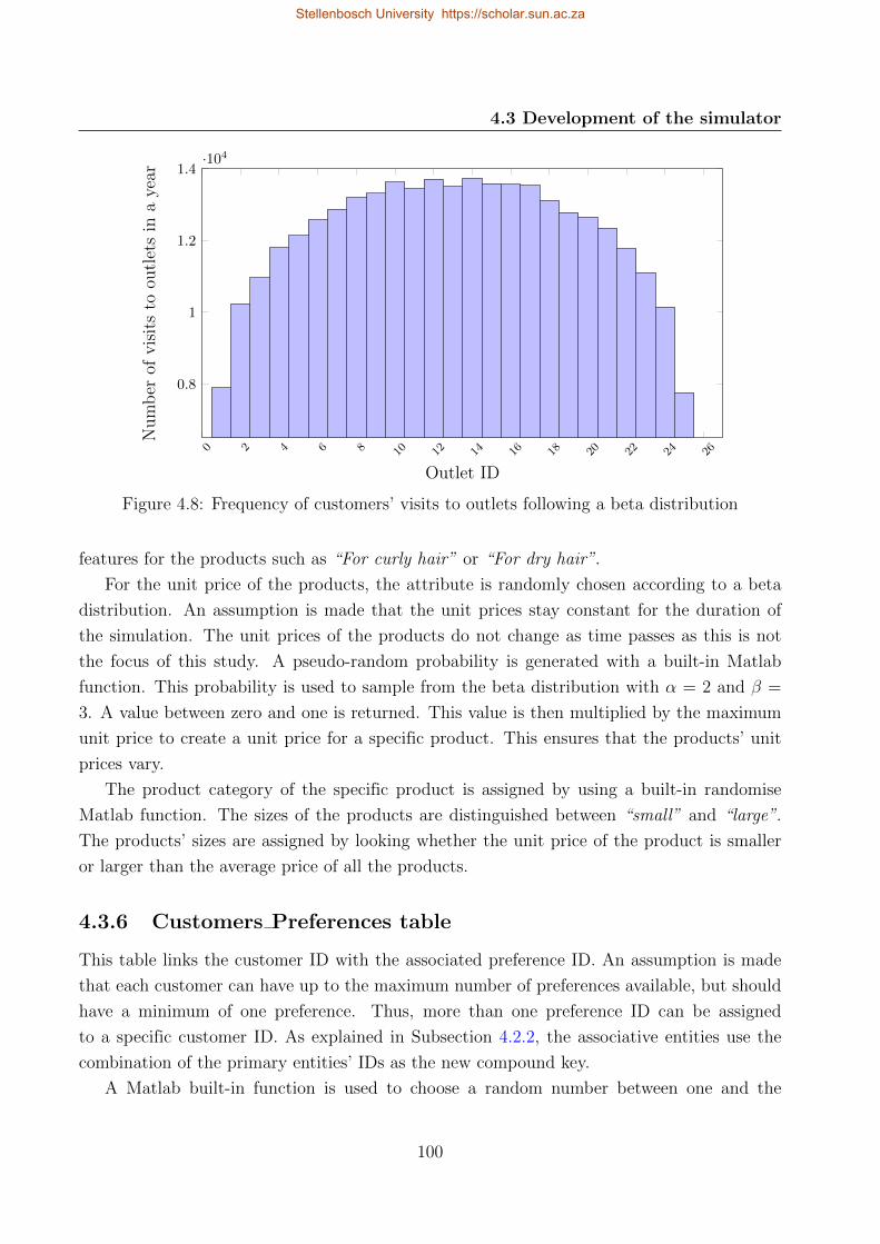
4.3 Development of the simulator
0 2 4 6 8 10 12 14 16 18 20 22 24 26
0.8
1
1.2
1.4·104
Outlet ID
Num
ber
ofvis
its
toou
tlet
sin
aye
ar
Figure 4.8: Frequency of customers’ visits to outlets following a beta distribution
features for the products such as “For curly hair” or “For dry hair”.
For the unit price of the products, the attribute is randomly chosen according to a beta
distribution. An assumption is made that the unit prices stay constant for the duration of
the simulation. The unit prices of the products do not change as time passes as this is not
the focus of this study. A pseudo-random probability is generated with a built-in Matlab
function. This probability is used to sample from the beta distribution with α = 2 and β =
3. A value between zero and one is returned. This value is then multiplied by the maximum
unit price to create a unit price for a specific product. This ensures that the products’ unit
prices vary.
The product category of the specific product is assigned by using a built-in randomise
Matlab function. The sizes of the products are distinguished between “small” and “large”.
The products’ sizes are assigned by looking whether the unit price of the product is smaller
or larger than the average price of all the products.
4.3.6 Customers Preferences table
This table links the customer ID with the associated preference ID. An assumption is made
that each customer can have up to the maximum number of preferences available, but should
have a minimum of one preference. Thus, more than one preference ID can be assigned
to a specific customer ID. As explained in Subsection 4.2.2, the associative entities use the
combination of the primary entities’ IDs as the new compound key.
A Matlab built-in function is used to choose a random number between one and the
100
Stellenbosch University https://scholar.sun.ac.za
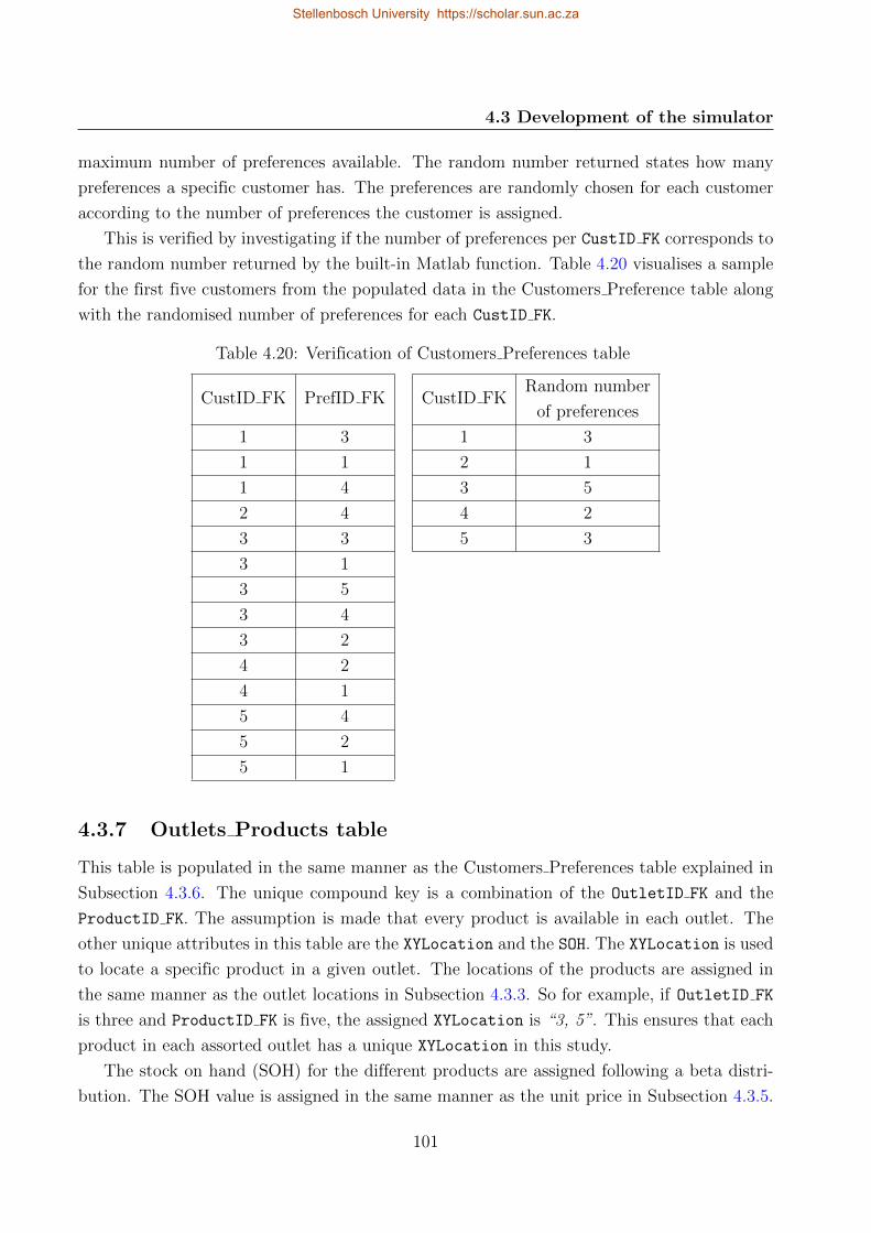
4.3 Development of the simulator
maximum number of preferences available. The random number returned states how many
preferences a specific customer has. The preferences are randomly chosen for each customer
according to the number of preferences the customer is assigned.
This is verified by investigating if the number of preferences per CustID FK corresponds to
the random number returned by the built-in Matlab function. Table 4.20 visualises a sample
for the first five customers from the populated data in the Customers Preference table along
with the randomised number of preferences for each CustID FK.
Table 4.20: Verification of Customers Preferences table
CustID FK PrefID FK CustID FKRandom number
of preferences
1 3 1 3
1 1 2 1
1 4 3 5
2 4 4 2
3 3 5 3
3 1
3 5
3 4
3 2
4 2
4 1
5 4
5 2
5 1
4.3.7 Outlets Products table
This table is populated in the same manner as the Customers Preferences table explained in
Subsection 4.3.6. The unique compound key is a combination of the OutletID FK and the
ProductID FK. The assumption is made that every product is available in each outlet. The
other unique attributes in this table are the XYLocation and the SOH. The XYLocation is used
to locate a specific product in a given outlet. The locations of the products are assigned in
the same manner as the outlet locations in Subsection 4.3.3. So for example, if OutletID FK
is three and ProductID FK is five, the assigned XYLocation is “3, 5”. This ensures that each
product in each assorted outlet has a unique XYLocation in this study.
The stock on hand (SOH) for the different products are assigned following a beta distri-
bution. The SOH value is assigned in the same manner as the unit price in Subsection 4.3.5.
101
Stellenbosch University https://scholar.sun.ac.za
4.3 Development of the simulator
A random probability is used to sample from the beta distribution with α = 3 and β = 2.
The value returned between zero and one is multiplied by the maximum number of products
to assign the SOH value for each individual product. An assumption is made that there is
always SOH and the SOH is manually updated as orders arrive and is excluded from the scope
of this study.
4.3.8 Transactional History table
The Transactional History table is populated based on the Orders table. For each OrderID
in the Orders table, a transactional history is created. This table states each product that a
customer acquires with each order, as well as the quantity and the price the customer paid
for it.
Depending on the customer purchasing behaviour type explained in Table 4.19, various
number of items are bought by the customers. Every customer has a base basket which
contains products that are bought regularly. An assumption is made that any customer can
buy any product at any participating outlet.
The quantity of each product is chosen being one, two or three and having weights of 0.5,
0.3 and 0.2 respectively. The stock on hand for the acquired products is also updated in the
Outlets Products table.
The unit price of the specified product is obtained from the Products table. In the event
where discount is received the UnitPrice attribute in the Transactional History table will
take the discount into account. The transactional information contained in this table is vital
regarding the purchasing behaviour of a customer. This information will be used by the PDO
predictor in the PDO demonstrator that will identify individual personalised discount offers
in Chapter 5.
4.3.9 Personalised Discount Offers, Personalised Discount Offers
Accepted, Personalised Discount Offers Rejected and
Personalised Discount Offers Origin tables
These four tables are created during this part of the study. However, these tables are not
populated by the simulator. The tables will be used in the next part of the study, which is
the PDO demonstrator. The PDO identified by the PDO predictor will be recorded in the
Personalised Discount Offers table. This table will identify each unique offer by having a
PDOID. Each ID will be assigned the product and to whom the offer is presented, along with
the discount applicable. The PDO type is recorded based on the type of offer presented. The
PDO table includes a status attribute which is zero or one. The zero status represents the
rejection of an offer. A status of one indicates the acceptance of an offer.
102
Stellenbosch University https://scholar.sun.ac.za
4.4 Chapter 4 summary
If a customer accepts an offer, the PDOID is assigned to the THID from the Transactional
History table where the specified product is acquired and the discount is applied. This event
is recorded in the Personalised Discount Offers Accepted table. If the customer rejects an
offer, the PDOID is assigned to the OrderID from the Orders table which specifies information
regarding the purchase instance of the customer. As with the acceptance event, the rejection
event is recorded in the Personalised Discount Offers Rejected table.
When a PDO was a cross-sell or upsell offer based on another product, the product from
which the cross-sell or upsell originated is recorded in the Personalised Discount Offers Origin
table where the PDOID FK refers to the PDO proposed to the customer and ProductID FK
refers to the product from where the cross-sell or upsell offer originated. These two primary
keys from other tables serve as the new compound key in this table. The population of these
tables are the fundamental elements of the PDO demonstrator.
4.4 Chapter 4 summary
This chapter presents the design and development of the simulator. The simulator is used
for generating pseudo-customer data in this study, the main reason for which is overcoming
ethical issues. The simulator is designed using methods from Kendall and Kendall (2014).
Using the design stage of the simulator, the researcher was able to develop the simulator using
Matlab and MS SQL Server.
The design and development stage of the simulator was an iterative process and for such an
intricate system, the researcher found it wise to first create the tables with only few records.
This was done to ensure the answers are controllable and predictable for validation purposes.
It is essential for the information simulated in this part of the study to be correct since it is
employed in the PDO demonstrator, which is the topic of discussion in the following chapter.
103
Stellenbosch University https://scholar.sun.ac.za
Chapter 5
Design and development of the PDO
demonstrator
The previous chapter informed the reader about the design and development of the simulator.
The simulator creates pseudo-customer historical data, which will now be used in the PDO
demonstrator. This chapter represents the design and development of the PDO demonstrator
in order to propose personalised discount offers to customers. This chapter will start with the
methodology used, followed by the design and development of the system. Lastly, the chapter
will explain the process of onboarding a new customer to the system.
5.1 PDO demonstrator design and development
methodology
This chapter initiates the third phase of the research methodology identified in Section 1.5.
This phase can be divided into two sub-phases namely 1) the design and 2) the development of
the PDO demonstrator. During the design sub-phase the researcher must identify approaches
to predict and propose PDOs to customers. These alternatives must be evaluated and the
most appropriate one will be utilised as the PDO predictor within the PDO demonstrator.
The researcher must then investigate cross-sell and upsell techniques and how to apply them
in the PDO demonstrator.
Once these factors have been determined, the second sub-phase of the PDO demonstrator
can commence, which is the development of the PDO demonstrator. Lastly, the researcher
will investigate the process of on-boarding a new customer in the system.
5.2 Design of the PDO demonstrator
The goal of the demonstrator is to analyse customer transactional history using the PDO
predictor and propose personalised discount offers (PDOs) to applicable customers based on
products bought periodically. Figure 5.1 illustrates a product with a periodical tendency.
Number one to five show the instances when the product was purchased and the 4Ti indicate
the times between two subsequent purchases. When the 4Ti of all purchases are relatively
the same, the product has a periodical tendency.
The PDO demonstrator can be divided into two parts based on functionality. The first
part consists of the analysis of the historical customer data that will identify potential PDOs
104
Stellenbosch University https://scholar.sun.ac.za
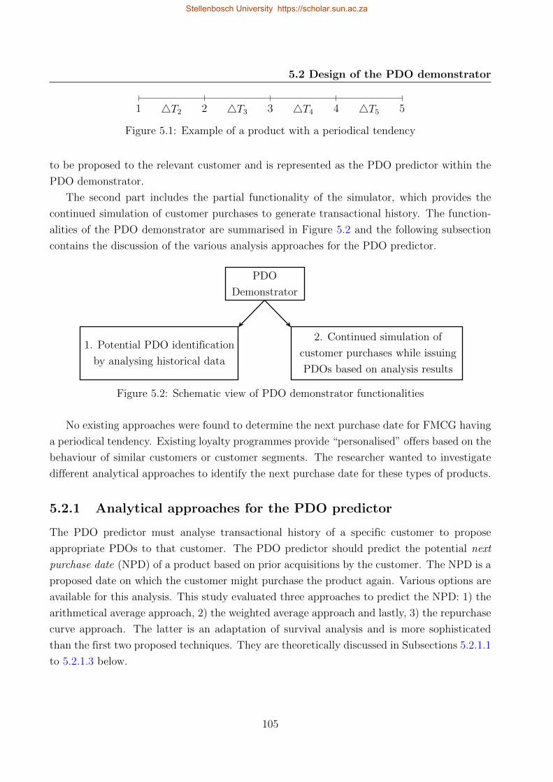
5.2 Design of the PDO demonstrator
4T2 4T3 4T4 4T51 2 3 4 5
Figure 5.1: Example of a product with a periodical tendency
to be proposed to the relevant customer and is represented as the PDO predictor within the
PDO demonstrator.
The second part includes the partial functionality of the simulator, which provides the
continued simulation of customer purchases to generate transactional history. The function-
alities of the PDO demonstrator are summarised in Figure 5.2 and the following subsection
contains the discussion of the various analysis approaches for the PDO predictor.
PDO
Demonstrator
1. Potential PDO identification
by analysing historical data
2. Continued simulation of
customer purchases while issuing
PDOs based on analysis results
Figure 5.2: Schematic view of PDO demonstrator functionalities
No existing approaches were found to determine the next purchase date for FMCG having
a periodical tendency. Existing loyalty programmes provide “personalised” offers based on the
behaviour of similar customers or customer segments. The researcher wanted to investigate
different analytical approaches to identify the next purchase date for these types of products.
5.2.1 Analytical approaches for the PDO predictor
The PDO predictor must analyse transactional history of a specific customer to propose
appropriate PDOs to that customer. The PDO predictor should predict the potential next
purchase date (NPD) of a product based on prior acquisitions by the customer. The NPD is a
proposed date on which the customer might purchase the product again. Various options are
available for this analysis. This study evaluated three approaches to predict the NPD: 1) the
arithmetical average approach, 2) the weighted average approach and lastly, 3) the repurchase
curve approach. The latter is an adaptation of survival analysis and is more sophisticated
than the first two proposed techniques. They are theoretically discussed in Subsections 5.2.1.1
to 5.2.1.3 below.
105
Stellenbosch University https://scholar.sun.ac.za
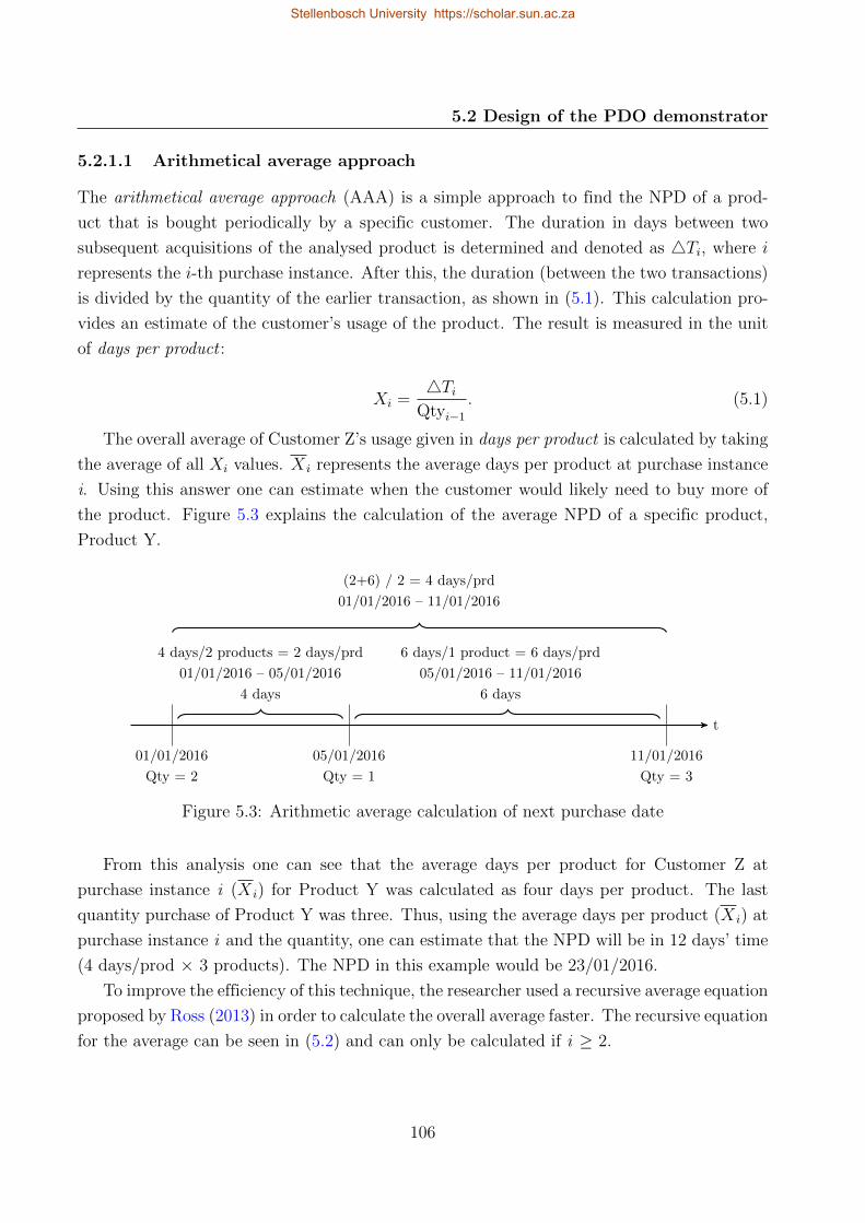
5.2 Design of the PDO demonstrator
5.2.1.1 Arithmetical average approach
The arithmetical average approach (AAA) is a simple approach to find the NPD of a prod-
uct that is bought periodically by a specific customer. The duration in days between two
subsequent acquisitions of the analysed product is determined and denoted as 4Ti, where i
represents the i-th purchase instance. After this, the duration (between the two transactions)
is divided by the quantity of the earlier transaction, as shown in (5.1). This calculation pro-
vides an estimate of the customer’s usage of the product. The result is measured in the unit
of days per product :
Xi =4Ti
Qtyi−1
. (5.1)
The overall average of Customer Z’s usage given in days per product is calculated by taking
the average of all Xi values. X i represents the average days per product at purchase instance
i. Using this answer one can estimate when the customer would likely need to buy more of
the product. Figure 5.3 explains the calculation of the average NPD of a specific product,
Product Y.
t
01/01/2016
Qty = 2
4 days/2 products = 2 days/prd
01/01/2016 – 05/01/2016
4 days
05/01/2016
Qty = 1
6 days/1 product = 6 days/prd
05/01/2016 – 11/01/2016
6 days
11/01/2016
Qty = 3
(2+6) / 2 = 4 days/prd
01/01/2016 – 11/01/2016
Figure 5.3: Arithmetic average calculation of next purchase date
From this analysis one can see that the average days per product for Customer Z at
purchase instance i (X i) for Product Y was calculated as four days per product. The last
quantity purchase of Product Y was three. Thus, using the average days per product (X i) at
purchase instance i and the quantity, one can estimate that the NPD will be in 12 days’ time
(4 days/prod × 3 products). The NPD in this example would be 23/01/2016.
To improve the efficiency of this technique, the researcher used a recursive average equation
proposed by Ross (2013) in order to calculate the overall average faster. The recursive equation
for the average can be seen in (5.2) and can only be calculated if i ≥ 2.
106
Stellenbosch University https://scholar.sun.ac.za
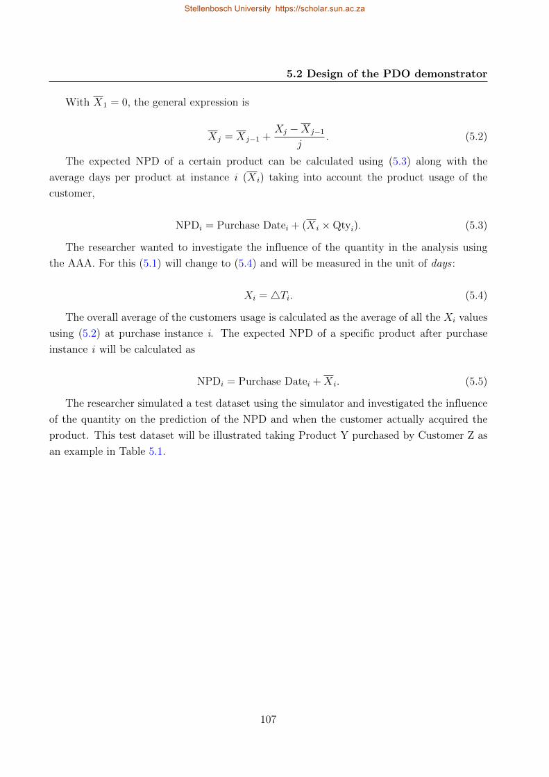
5.2 Design of the PDO demonstrator
With X1 = 0, the general expression is
Xj = Xj−1 +Xj −Xj−1
j. (5.2)
The expected NPD of a certain product can be calculated using (5.3) along with the
average days per product at instance i (X i) taking into account the product usage of the
customer,
NPDi = Purchase Datei + (X i ×Qtyi). (5.3)
The researcher wanted to investigate the influence of the quantity in the analysis using
the AAA. For this (5.1) will change to (5.4) and will be measured in the unit of days :
Xi = 4Ti. (5.4)
The overall average of the customers usage is calculated as the average of all the Xi values
using (5.2) at purchase instance i. The expected NPD of a specific product after purchase
instance i will be calculated as
NPDi = Purchase Datei +X i. (5.5)
The researcher simulated a test dataset using the simulator and investigated the influence
of the quantity on the prediction of the NPD and when the customer actually acquired the
product. This test dataset will be illustrated taking Product Y purchased by Customer Z as
an example in Table 5.1.
107
Stellenbosch University https://scholar.sun.ac.za
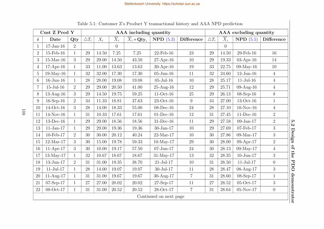
5.2
Desig
nofth
ePDO
demonstra
tor
Table 5.1: Customer Z’s Product Y transactional history and AAA NPD prediction
Cust Z Prod Y AAA including quantity AAA excluding quantity
i Date Qty 4Ti Xi X i X i ∗Qtyi NPD (5.3) Difference 4Ti X i NPD (5.5) Difference
1 17-Jan-16 2 0 0
2 15-Feb-16 1 29 14.50 7.25 7.25 22-Feb-16 23 29 14.50 29-Feb-16 16
3 15-Mar-16 3 29 29.00 14.50 43.50 27-Apr-16 10 29 19.33 03-Apr-16 14
4 17-Apr-16 1 33 11.00 13.63 13.63 30-Apr-16 19 33 22.75 09-May-16 10
5 19-May-16 1 32 32.00 17.30 17.30 05-Jun-16 11 32 24.60 12-Jun-16 4
6 16-Jun-16 1 28 28.00 19.08 19.08 05-Jul-16 10 28 25.17 11-Jul-16 4
7 15-Jul-16 2 29 29.00 20.50 41.00 25-Aug-16 12 29 25.71 09-Aug-16 4
8 13-Aug-16 3 29 14.50 19.75 59.25 11-Oct-16 25 29 26.13 08-Sep-16 8
9 16-Sep-16 2 34 11.33 18.81 37.63 23-Oct-16 9 34 27.00 13-Oct-16 1
10 14-Oct-16 3 28 14.00 18.33 55.00 08-Dec-16 24 28 27.10 10-Nov-16 4
11 14-Nov-16 1 31 10.33 17.61 17.61 01-Dec-16 12 31 27.45 11-Dec-16 2
12 13-Dec-16 1 29 29.00 18.56 18.56 31-Dec-16 11 29 27.58 09-Jan-17 2
13 11-Jan-17 1 29 29.00 19.36 19.36 30-Jan-17 10 29 27.69 07-Feb-17 3
14 10-Feb-17 2 30 30.00 20.12 40.24 22-Mar-17 10 30 27.86 09-Mar-17 3
15 12-Mar-17 3 30 15.00 19.78 59.33 10-May-17 29 30 28.00 09-Apr-17 2
16 11-Apr-17 3 30 10.00 19.17 57.50 07-Jun-17 24 30 28.13 09-May-17 4
17 13-May-17 1 32 10.67 18.67 18.67 31-May-17 13 32 28.35 10-Jun-17 3
18 13-Jun-17 2 31 31.00 19.35 38.70 21-Jul-17 10 31 28.50 11-Jul-17 0
19 11-Jul-17 1 28 14.00 19.07 19.07 30-Jul-17 11 28 28.47 08-Aug-17 3
20 11-Aug-17 1 31 31.00 19.67 19.67 30-Aug-17 7 31 28.60 08-Sep-17 1
21 07-Sep-17 1 27 27.00 20.02 20.02 27-Sep-17 11 27 28.52 05-Oct-17 3
22 08-Oct-17 1 31 31.00 20.52 20.52 28-Oct-17 7 31 28.64 05-Nov-17 0
Continued on next page
108
Stellenbosch University https://scholar.sun.ac.za
Stellenbosch University https://scholar.sun.ac.za
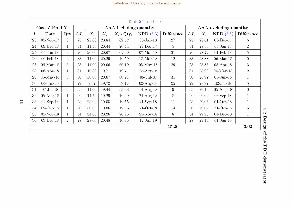
5.2
Desig
nofth
ePDO
demonstra
tor
Table 5.1 continued
Cust Z Prod Y AAA including quantity AAA excluding quantity
i Date Qty 4Ti Xi X i X i ∗Qtyi NPD (5.3) Difference 4Ti X i NPD (5.5) Difference
23 05-Nov-17 3 28 28.00 20.84 62.52 06-Jan-18 27 28 28.61 03-Dec-17 6
24 09-Dec-17 1 34 11.33 20.44 20.44 29-Dec-17 5 34 28.83 06-Jan-18 2
25 04-Jan-18 3 26 26.00 20.67 62.00 07-Mar-18 31 26 28.72 01-Feb-18 5
26 06-Feb-18 2 33 11.00 20.29 40.59 18-Mar-18 12 33 28.88 06-Mar-18 0
27 06-Mar-18 3 28 14.00 20.06 60.19 05-May-18 29 28 28.85 03-Apr-18 3
28 06-Apr-18 1 31 10.33 19.71 19.71 25-Apr-18 11 31 28.93 04-May-18 2
29 06-May-18 3 30 30.00 20.07 60.21 05-Jul-18 31 30 28.97 03-Jun-18 1
30 04-Jun-18 3 29 9.67 19.72 59.17 02-Aug-18 25 29 28.97 02-Jul-18 5
31 07-Jul-18 2 33 11.00 19.44 38.88 14-Aug-18 9 33 29.10 05-Aug-18 0
32 05-Aug-18 1 29 14.50 19.29 19.29 24-Aug-18 8 29 29.09 03-Sep-18 1
33 02-Sep-18 1 28 28.00 19.55 19.55 21-Sep-18 11 28 29.06 01-Oct-18 1
34 02-Oct-18 1 30 30.00 19.86 19.86 21-Oct-18 14 30 29.09 31-Oct-18 5
35 05-Nov-18 1 34 34.00 20.26 20.26 25-Nov-18 8 34 29.23 04-Dec-18 1
36 03-Dec-18 2 28 28.00 20.48 40.95 12-Jan-19 28 29.19 01-Jan-19
15.26 3.62
109
Stellenbosch University https://scholar.sun.ac.za
Stellenbosch University https://scholar.sun.ac.za
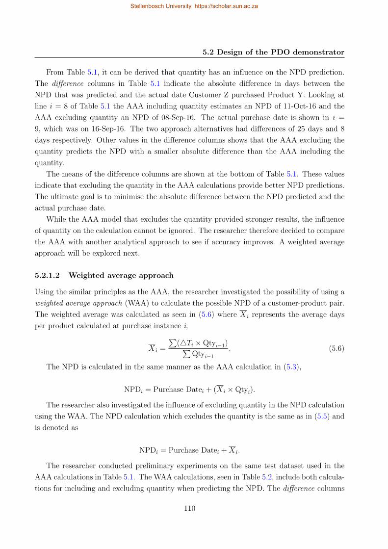
5.2 Design of the PDO demonstrator
From Table 5.1, it can be derived that quantity has an influence on the NPD prediction.
The difference columns in Table 5.1 indicate the absolute difference in days between the
NPD that was predicted and the actual date Customer Z purchased Product Y. Looking at
line i = 8 of Table 5.1 the AAA including quantity estimates an NPD of 11-Oct-16 and the
AAA excluding quantity an NPD of 08-Sep-16. The actual purchase date is shown in i =
9, which was on 16-Sep-16. The two approach alternatives had differences of 25 days and 8
days respectively. Other values in the difference columns shows that the AAA excluding the
quantity predicts the NPD with a smaller absolute difference than the AAA including the
quantity.
The means of the difference columns are shown at the bottom of Table 5.1. These values
indicate that excluding the quantity in the AAA calculations provide better NPD predictions.
The ultimate goal is to minimise the absolute difference between the NPD predicted and the
actual purchase date.
While the AAA model that excludes the quantity provided stronger results, the influence
of quantity on the calculation cannot be ignored. The researcher therefore decided to compare
the AAA with another analytical approach to see if accuracy improves. A weighted average
approach will be explored next.
5.2.1.2 Weighted average approach
Using the similar principles as the AAA, the researcher investigated the possibility of using a
weighted average approach (WAA) to calculate the possible NPD of a customer-product pair.
The weighted average was calculated as seen in (5.6) where X i represents the average days
per product calculated at purchase instance i,
X i =
∑(4Ti ×Qtyi−1)∑
Qtyi−1
. (5.6)
The NPD is calculated in the same manner as the AAA calculation in (5.3),
NPDi = Purchase Datei + (X i ×Qtyi).
The researcher also investigated the influence of excluding quantity in the NPD calculation
using the WAA. The NPD calculation which excludes the quantity is the same as in (5.5) and
is denoted as
NPDi = Purchase Datei +X i.
The researcher conducted preliminary experiments on the same test dataset used in the
AAA calculations in Table 5.1. The WAA calculations, seen in Table 5.2, include both calcula-
tions for including and excluding quantity when predicting the NPD. The difference columns
110
Stellenbosch University https://scholar.sun.ac.za

5.2 Design of the PDO demonstrator
indicate the absolute difference between the NPD predicted for Product X and the actual date
Customer Z bought Product X.
Lines i = 7–10 for example the WAA including the quantity in the NPD calculation had
much larger differences comparing to the NPD calculation which excludes quantity. This oc-
curs everytime the quantity value is larger than one. This can be an indication that Customer
Z purchased Product Y periodically without any relation to the quantity previously bought.
By inspecting the other values in the difference columns it is clear to see that by including
the quantity in the NPD predictions using the WAA is not as close to the actual purchase
date as the NPD prediction excluding the quantity. At the bottom of Table 5.2 the means
of the difference columns are calculated and one can see that by excluding the quantity more
accurate predictions can be made.
111
Stellenbosch University https://scholar.sun.ac.za
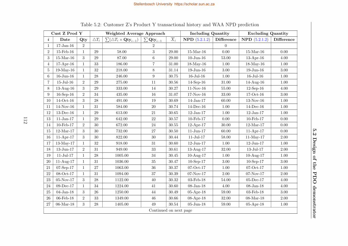
5.2
Desig
nofth
ePDO
demonstra
tor
Table 5.2: Customer Z’s Product Y transactional history and WAA NPD prediction
Cust Z Prod Y Weighted Average Approach Including Quantity Excluding Quantity
i Date Qty 4Ti
∑(4Ti ×Qtyi−1)
∑Qtyi−1 Xi NPD (5.2.1.2) Difference NPD (5.2.1.2) Difference
1 17-Jan-16 2 2 0
2 15-Feb-16 1 29 58.00 3 29.00 15-Mar-16 0.00 15-Mar-16 0.00
3 15-Mar-16 3 29 87.00 6 29.00 10-Jun-16 53.00 13-Apr-16 4.00
4 17-Apr-16 1 33 186.00 7 31.00 18-May-16 1.00 18-May-16 1.00
5 19-May-16 1 32 218.00 8 31.14 19-Jun-16 3.00 19-Jun-16 3.00
6 16-Jun-16 1 28 246.00 9 30.75 16-Jul-16 1.00 16-Jul-16 1.00
7 15-Jul-16 2 29 275.00 11 30.56 14-Sep-16 31.00 14-Aug-16 1.00
8 13-Aug-16 3 29 333.00 14 30.27 11-Nov-16 55.00 12-Sep-16 4.00
9 16-Sep-16 2 34 435.00 16 31.07 17-Nov-16 33.00 17-Oct-16 3.00
10 14-Oct-16 3 28 491.00 19 30.69 14-Jan-17 60.00 13-Nov-16 1.00
11 14-Nov-16 1 31 584.00 20 30.74 14-Dec-16 1.00 14-Dec-16 1.00
12 13-Dec-16 1 29 613.00 21 30.65 12-Jan-17 1.00 12-Jan-17 1.00
13 11-Jan-17 1 29 642.00 22 30.57 10-Feb-17 0.00 10-Feb-17 0.00
14 10-Feb-17 2 30 672.00 24 30.55 12-Apr-17 30.00 12-Mar-17 0.00
15 12-Mar-17 3 30 732.00 27 30.50 11-Jun-17 60.00 11-Apr-17 0.00
16 11-Apr-17 3 30 822.00 30 30.44 11-Jul-17 58.00 11-May-17 2.00
17 13-May-17 1 32 918.00 31 30.60 12-Jun-17 1.00 12-Jun-17 1.00
18 13-Jun-17 2 31 949.00 33 30.61 13-Aug-17 32.00 13-Jul-17 2.00
19 11-Jul-17 1 28 1005.00 34 30.45 10-Aug-17 1.00 10-Aug-17 1.00
20 11-Aug-17 1 31 1036.00 35 30.47 10-Sep-17 3.00 10-Sep-17 3.00
21 07-Sep-17 1 27 1063.00 36 30.37 07-Oct-17 1.00 07-Oct-17 1.00
22 08-Oct-17 1 31 1094.00 37 30.39 07-Nov-17 2.00 07-Nov-17 2.00
23 05-Nov-17 3 28 1122.00 40 30.32 03-Feb-18 54.00 05-Dec-17 4.00
24 09-Dec-17 1 34 1224.00 41 30.60 08-Jan-18 4.00 08-Jan-18 4.00
25 04-Jan-18 3 26 1250.00 44 30.49 05-Apr-18 59.00 03-Feb-18 3.00
26 06-Feb-18 2 33 1349.00 46 30.66 08-Apr-18 32.00 08-Mar-18 2.00
27 06-Mar-18 3 28 1405.00 49 30.54 05-Jun-18 59.00 05-Apr-18 1.00
Continued on next page
112
Stellenbosch University https://scholar.sun.ac.za
Stellenbosch University https://scholar.sun.ac.za
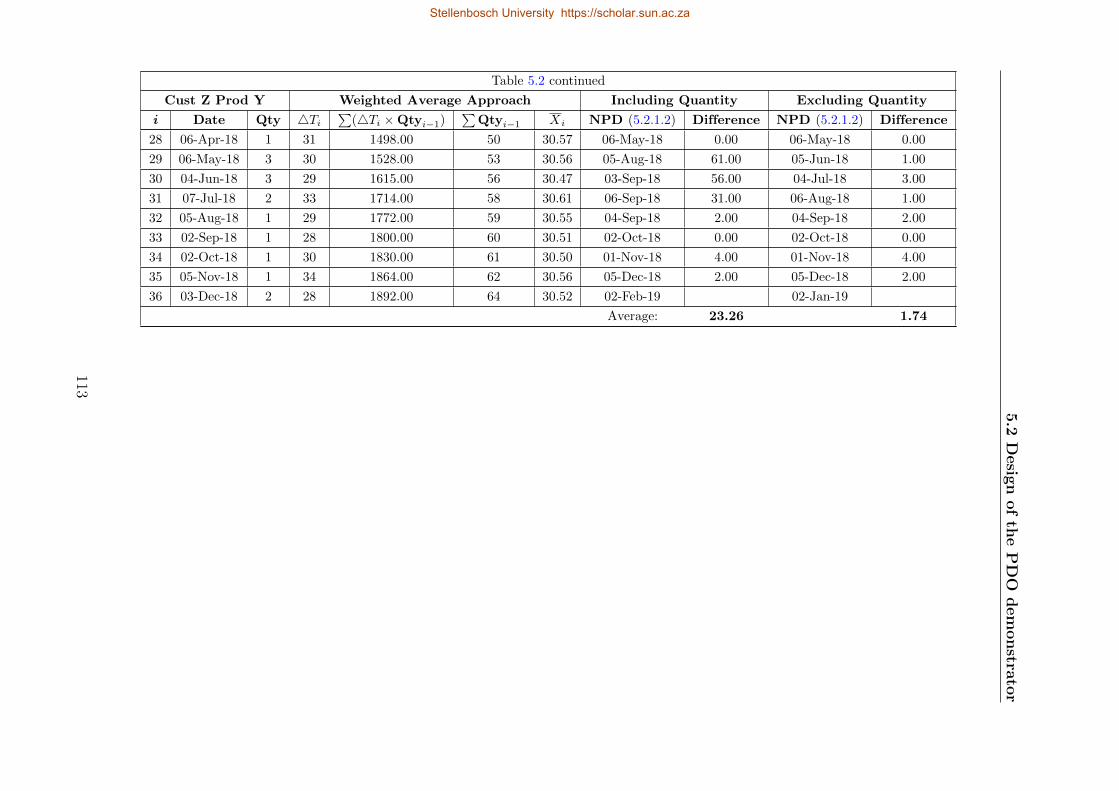
5.2
Desig
nofth
ePDO
demonstra
tor
Table 5.2 continued
Cust Z Prod Y Weighted Average Approach Including Quantity Excluding Quantity
i Date Qty 4Ti
∑(4Ti ×Qtyi−1)
∑Qtyi−1 Xi NPD (5.2.1.2) Difference NPD (5.2.1.2) Difference
28 06-Apr-18 1 31 1498.00 50 30.57 06-May-18 0.00 06-May-18 0.00
29 06-May-18 3 30 1528.00 53 30.56 05-Aug-18 61.00 05-Jun-18 1.00
30 04-Jun-18 3 29 1615.00 56 30.47 03-Sep-18 56.00 04-Jul-18 3.00
31 07-Jul-18 2 33 1714.00 58 30.61 06-Sep-18 31.00 06-Aug-18 1.00
32 05-Aug-18 1 29 1772.00 59 30.55 04-Sep-18 2.00 04-Sep-18 2.00
33 02-Sep-18 1 28 1800.00 60 30.51 02-Oct-18 0.00 02-Oct-18 0.00
34 02-Oct-18 1 30 1830.00 61 30.50 01-Nov-18 4.00 01-Nov-18 4.00
35 05-Nov-18 1 34 1864.00 62 30.56 05-Dec-18 2.00 05-Dec-18 2.00
36 03-Dec-18 2 28 1892.00 64 30.52 02-Feb-19 02-Jan-19
Average: 23.26 1.74
113
Stellenbosch University https://scholar.sun.ac.za
Stellenbosch University https://scholar.sun.ac.za
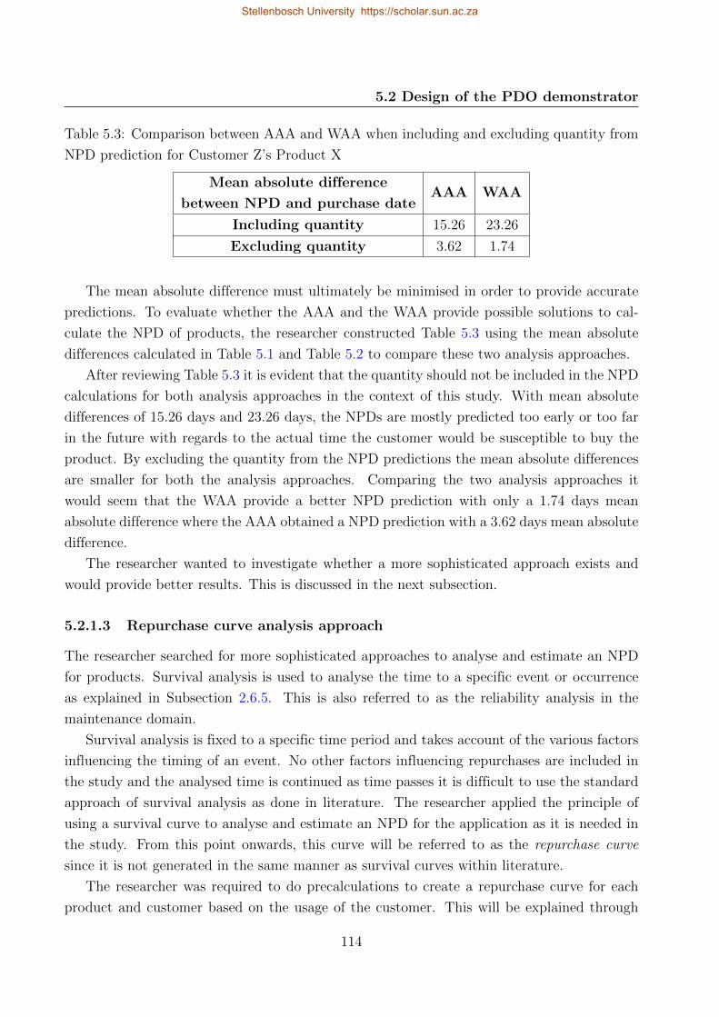
5.2 Design of the PDO demonstrator
Table 5.3: Comparison between AAA and WAA when including and excluding quantity from
NPD prediction for Customer Z’s Product X
Mean absolute difference
between NPD and purchase dateAAA WAA
Including quantity 15.26 23.26
Excluding quantity 3.62 1.74
The mean absolute difference must ultimately be minimised in order to provide accurate
predictions. To evaluate whether the AAA and the WAA provide possible solutions to cal-
culate the NPD of products, the researcher constructed Table 5.3 using the mean absolute
differences calculated in Table 5.1 and Table 5.2 to compare these two analysis approaches.
After reviewing Table 5.3 it is evident that the quantity should not be included in the NPD
calculations for both analysis approaches in the context of this study. With mean absolute
differences of 15.26 days and 23.26 days, the NPDs are mostly predicted too early or too far
in the future with regards to the actual time the customer would be susceptible to buy the
product. By excluding the quantity from the NPD predictions the mean absolute differences
are smaller for both the analysis approaches. Comparing the two analysis approaches it
would seem that the WAA provide a better NPD prediction with only a 1.74 days mean
absolute difference where the AAA obtained a NPD prediction with a 3.62 days mean absolute
difference.
The researcher wanted to investigate whether a more sophisticated approach exists and
would provide better results. This is discussed in the next subsection.
5.2.1.3 Repurchase curve analysis approach
The researcher searched for more sophisticated approaches to analyse and estimate an NPD
for products. Survival analysis is used to analyse the time to a specific event or occurrence
as explained in Subsection 2.6.5. This is also referred to as the reliability analysis in the
maintenance domain.
Survival analysis is fixed to a specific time period and takes account of the various factors
influencing the timing of an event. No other factors influencing repurchases are included in
the study and the analysed time is continued as time passes it is difficult to use the standard
approach of survival analysis as done in literature. The researcher applied the principle of
using a survival curve to analyse and estimate an NPD for the application as it is needed in
the study. From this point onwards, this curve will be referred to as the repurchase curve
since it is not generated in the same manner as survival curves within literature.
The researcher was required to do precalculations to create a repurchase curve for each
product and customer based on the usage of the customer. This will be explained through
114
Stellenbosch University https://scholar.sun.ac.za
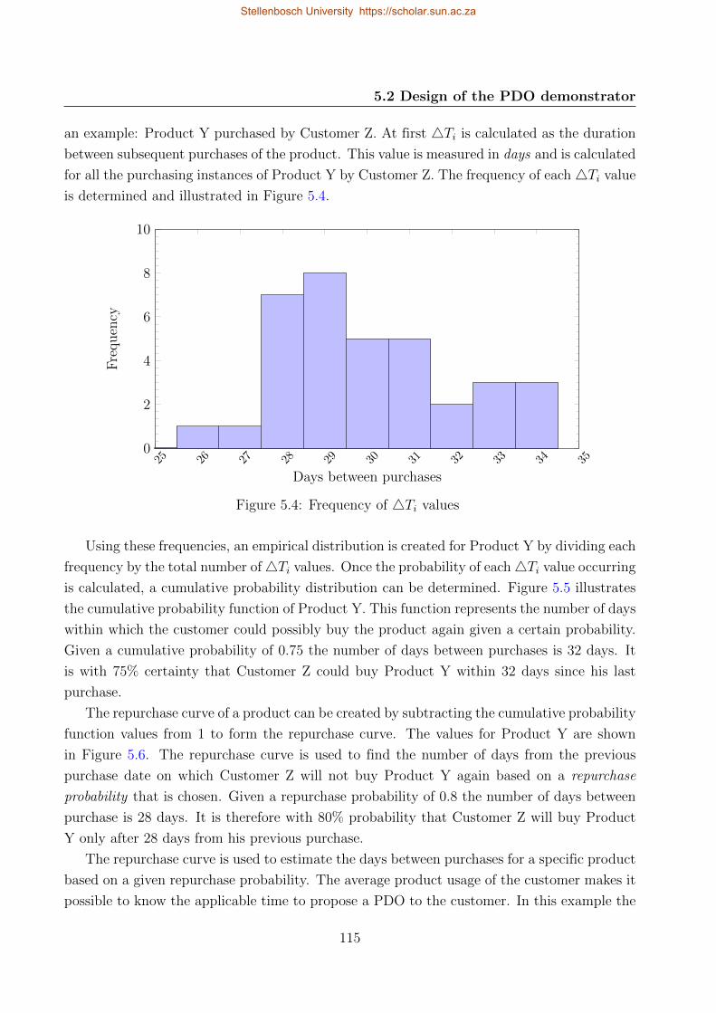
5.2 Design of the PDO demonstrator
an example: Product Y purchased by Customer Z. At first 4Ti is calculated as the duration
between subsequent purchases of the product. This value is measured in days and is calculated
for all the purchasing instances of Product Y by Customer Z. The frequency of each4Ti value
is determined and illustrated in Figure 5.4.
25 26 27 28 29 30 31 32 33 34 350
2
4
6
8
10
Days between purchases
Fre
quen
cy
Figure 5.4: Frequency of 4Ti values
Using these frequencies, an empirical distribution is created for Product Y by dividing each
frequency by the total number of4Ti values. Once the probability of each4Ti value occurring
is calculated, a cumulative probability distribution can be determined. Figure 5.5 illustrates
the cumulative probability function of Product Y. This function represents the number of days
within which the customer could possibly buy the product again given a certain probability.
Given a cumulative probability of 0.75 the number of days between purchases is 32 days. It
is with 75% certainty that Customer Z could buy Product Y within 32 days since his last
purchase.
The repurchase curve of a product can be created by subtracting the cumulative probability
function values from 1 to form the repurchase curve. The values for Product Y are shown
in Figure 5.6. The repurchase curve is used to find the number of days from the previous
purchase date on which Customer Z will not buy Product Y again based on a repurchase
probability that is chosen. Given a repurchase probability of 0.8 the number of days between
purchase is 28 days. It is therefore with 80% probability that Customer Z will buy Product
Y only after 28 days from his previous purchase.
The repurchase curve is used to estimate the days between purchases for a specific product
based on a given repurchase probability. The average product usage of the customer makes it
possible to know the applicable time to propose a PDO to the customer. In this example the
115
Stellenbosch University https://scholar.sun.ac.za
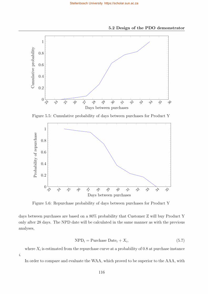
5.2 Design of the PDO demonstrator
23 24 25 26 27 28 29 30 31 32 33 34 35 360
0.2
0.4
0.6
0.8
1
Days between purchases
Cum
ula
tive
pro
bab
ilit
y
Figure 5.5: Cumulative probability of days between purchases for Product Y
23 24 25 26 27 28 29 30 31 32 33 34 350
0.2
0.4
0.6
0.8
1
Days between purchases
Pro
bab
ilit
yof
repurc
has
e
Figure 5.6: Repurchase probability of days between purchases for Product Y
days between purchases are based on a 80% probability that Customer Z will buy Product Y
only after 28 days. The NPD date will be calculated in the same manner as with the previous
analyses,
NPDi = Purchase Datei +Xi, (5.7)
where Xi is estimated from the repurchase curve at a probability of 0.8 at purchase instance
i.
In order to compare and evaluate the WAA, which proved to be superior to the AAA, with
116
Stellenbosch University https://scholar.sun.ac.za
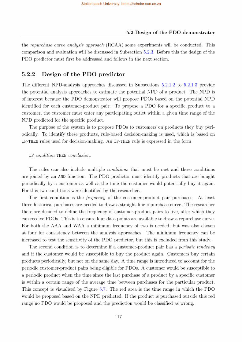
5.2 Design of the PDO demonstrator
the repurchase curve analysis approach (RCAA) some experiments will be conducted. This
comparison and evaluation will be discussed in Subsection 5.2.3. Before this the design of the
PDO predictor must first be addressed and follows in the next section.
5.2.2 Design of the PDO predictor
The different NPD-analysis approaches discussed in Subsections 5.2.1.2 to 5.2.1.3 provide
the potential analysis approaches to estimate the potential NPD of a product. The NPD is
of interest because the PDO demonstrator will propose PDOs based on the potential NPD
identified for each customer-product pair. To propose a PDO for a specific product to a
customer, the customer must enter any participating outlet within a given time range of the
NPD predicted for the specific product.
The purpose of the system is to propose PDOs to customers on products they buy peri-
odically. To identify these products, rule-based decision-making is used, which is based on
IF-THEN rules used for decision-making. An IF-THEN rule is expressed in the form
IF condition THEN conclusion.
The rules can also include multiple conditions that must be met and these conditions
are joined by an AND function. The PDO predictor must identify products that are bought
periodically by a customer as well as the time the customer would potentially buy it again.
For this two conditions were identified by the researcher.
The first condition is the frequency of the customer-product pair purchases. At least
three historical purchases are needed to draw a straight-line repurchase curve. The researcher
therefore decided to define the frequency of customer-product pairs to five, after which they
can receive PDOs. This is to ensure four data points are available to draw a repurchase curve.
For both the AAA and WAA a minimum frequency of two is needed, but was also chosen
at four for consistency between the analysis approaches. The minimum frequency can be
increased to test the sensitivity of the PDO predictor, but this is excluded from this study.
The second condition is to determine if a customer-product pair has a periodic tendency
and if the customer would be susceptible to buy the product again. Customers buy certain
products periodically, but not on the same day. A time range is introduced to account for the
periodic customer-product pairs being eligible for PDOs. A customer would be susceptible to
a periodic product when the time since the last purchase of a product by a specific customer
is within a certain range of the average time between purchases for the particular product.
This concept is visualised by Figure 5.7. The red area is the time range in which the PDO
would be proposed based on the NPD predicted. If the product is purchased outside this red
range no PDO would be proposed and the prediction would be classified as wrong.
117
Stellenbosch University https://scholar.sun.ac.za
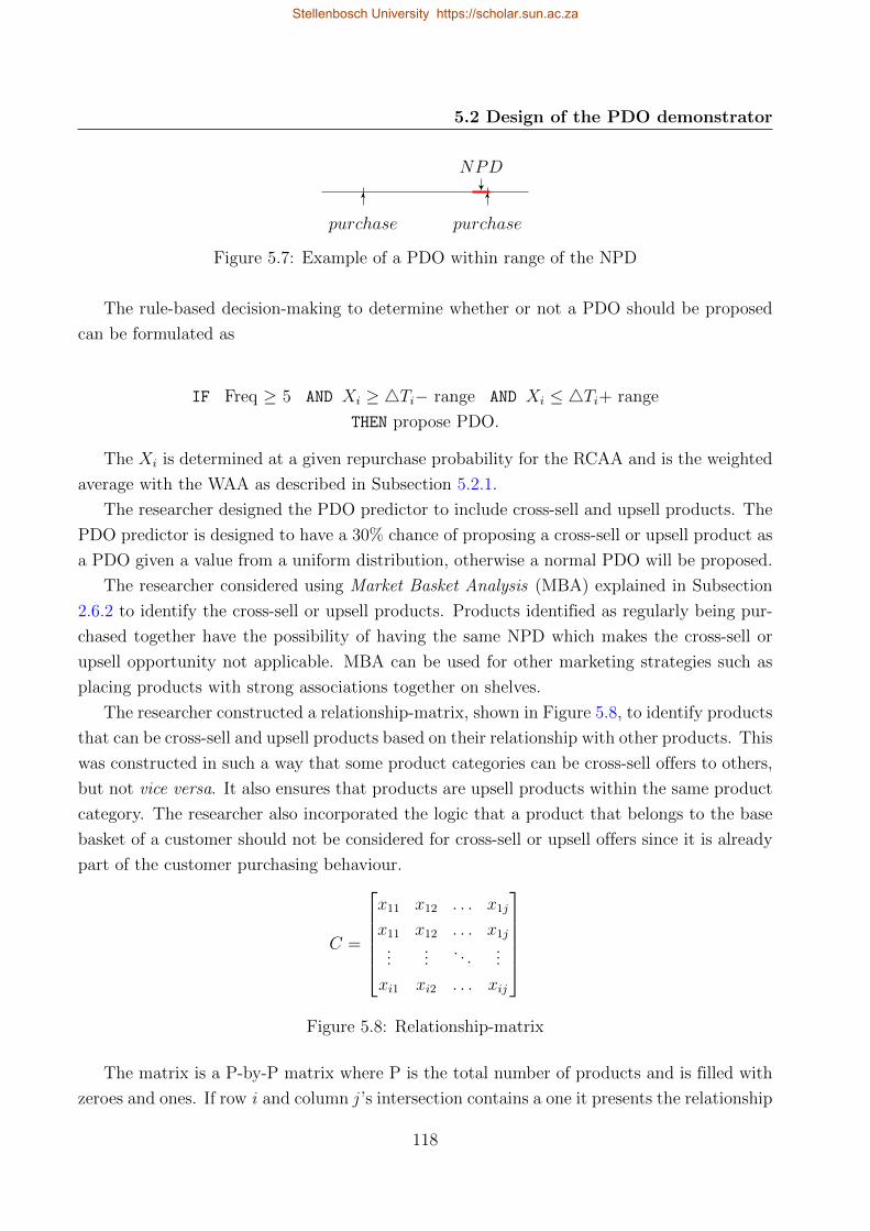
5.2 Design of the PDO demonstrator
purchase purchase
NPD
Figure 5.7: Example of a PDO within range of the NPD
The rule-based decision-making to determine whether or not a PDO should be proposed
can be formulated as
IF Freq ≥ 5 AND Xi ≥ 4Ti− range AND Xi ≤ 4Ti+ range
THEN propose PDO.
The Xi is determined at a given repurchase probability for the RCAA and is the weighted
average with the WAA as described in Subsection 5.2.1.
The researcher designed the PDO predictor to include cross-sell and upsell products. The
PDO predictor is designed to have a 30% chance of proposing a cross-sell or upsell product as
a PDO given a value from a uniform distribution, otherwise a normal PDO will be proposed.
The researcher considered using Market Basket Analysis (MBA) explained in Subsection
2.6.2 to identify the cross-sell or upsell products. Products identified as regularly being pur-
chased together have the possibility of having the same NPD which makes the cross-sell or
upsell opportunity not applicable. MBA can be used for other marketing strategies such as
placing products with strong associations together on shelves.
The researcher constructed a relationship-matrix, shown in Figure 5.8, to identify products
that can be cross-sell and upsell products based on their relationship with other products. This
was constructed in such a way that some product categories can be cross-sell offers to others,
but not vice versa. It also ensures that products are upsell products within the same product
category. The researcher also incorporated the logic that a product that belongs to the base
basket of a customer should not be considered for cross-sell or upsell offers since it is already
part of the customer purchasing behaviour.
C =
x11 x12 . . . x1j
x11 x12 . . . x1j...
.... . .
...
xi1 xi2 . . . xij
Figure 5.8: Relationship-matrix
The matrix is a P-by-P matrix where P is the total number of products and is filled with
zeroes and ones. If row i and column j ’s intersection contains a one it presents the relationship
118
Stellenbosch University https://scholar.sun.ac.za
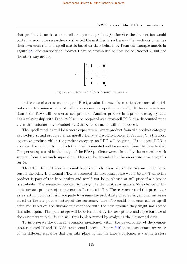
5.2 Design of the PDO demonstrator
that product i can be a cross-sell or upsell to product j otherwise the intersection would
contain a zero. The researcher constructed the matrices in such a way that each customer has
their own cross-sell and upsell matrix based on their behaviour. From the example matrix in
Figure 5.9, one can see that Product 1 can be cross-selled or upselled to Product 2, but not
the other way around.
C =
0 1 . . . 0
0 0 . . . 1...
.... . .
...
1 1 . . . 0
Figure 5.9: Example of a relationship-matrix
In the case of a cross-sell or upsell PDO, a value is drawn from a standard normal distri-
bution to determine whether it will be a cross-sell or upsell opportunity. If the value is larger
than 0 the PDO will be a cross-sell product. Another product in a product category that
has a relationship with Product Y will be proposed as a cross-sell PDO at a discounted price
given the customer buys Product Y. Otherwise, an upsell will be proposed.
The upsell product will be a more expensive or larger product from the product category
as Product Y, and proposed as an upsell PDO at a discounted price. If Product Y is the most
expensive product within the product category, no PDO will be given. If the upsell PDO is
accepted the product from which the upsell originated will be removed from the base basket.
The percentages used in the design of the PDO predictor were selected by the researcher with
support from a research supervisor. This can be amended by the enterprise providing this
service.
The PDO demonstrator will emulate a real world event where the customer accepts or
rejects the offer. If a normal PDO is proposed the acceptance rate would be 100% since the
product is part of the base basket and would not be purchased at full price if a discount
is available. The researcher decided to design the demonstrator using a 50% chance of the
customer accepting or rejecting a cross-sell or upsell offer. The researcher used this percentage
as a starting point as it is inadequate to assume the probability of accepting an offer increases
based on the acceptance history of the customer. The offer could be a cross-sell or upsell
offer and based on the customer’s experience with the new product they might not accept
this offer again. This percentage will be determined by the acceptance and rejection rate of
the customers in real life and will thus be determined by analysing their historical data.
To incorporate the different scenarios mentioned within the development of the demon-
strator, nested IF and IF ELSE statements is needed. Figure 5.10 shows a schematic overview
of the different scenarios that can take place within the time a customer is visiting a store
119
Stellenbosch University https://scholar.sun.ac.za
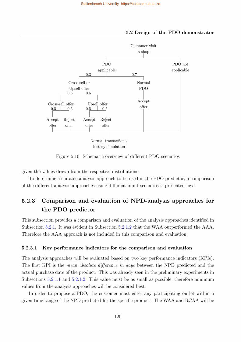
5.2 Design of the PDO demonstrator
Customer visit
a shop
PDO
applicable0.3 0.7
PDO not
applicable
Normal
PDO
Cross-sell or
Upsell offer0.5 0.5
Cross-sell offer0.5 0.5
Upsell offer0.50.5
Accept
offer
Reject
offer
Reject
offer
Accept
offer
Accept
offer
Normal transactional
history simulation
Figure 5.10: Schematic overview of different PDO scenarios
given the values drawn from the respective distributions.
To determine a suitable analysis approach to be used in the PDO predictor, a comparison
of the different analysis approaches using different input scenarios is presented next.
5.2.3 Comparison and evaluation of NPD-analysis approaches for
the PDO predictor
This subsection provides a comparison and evaluation of the analysis approaches identified in
Subsection 5.2.1. It was evident in Subsection 5.2.1.2 that the WAA outperformed the AAA.
Therefore the AAA approach is not included in this comparison and evaluation.
5.2.3.1 Key performance indicators for the comparison and evaluation
The analysis approaches will be evaluated based on two key performance indicators (KPIs).
The first KPI is the mean absolute difference in days between the NPD predicted and the
actual purchase date of the product. This was already seen in the preliminary experiments in
Subsections 5.2.1.1 and 5.2.1.2. This value must be as small as possible, therefore minimum
values from the analysis approaches will be considered best.
In order to propose a PDO, the customer must enter any participating outlet within a
given time range of the NPD predicted for the specific product. The WAA and RCAA will be
120
Stellenbosch University https://scholar.sun.ac.za
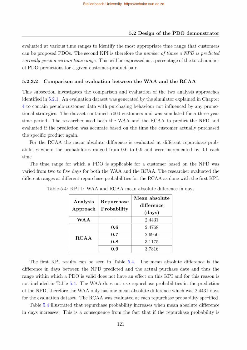
5.2 Design of the PDO demonstrator
evaluated at various time ranges to identify the most appropriate time range that customers
can be proposed PDOs. The second KPI is therefore the number of times a NPD is predicted
correctly given a certain time range. This will be expressed as a percentage of the total number
of PDO predictions for a given customer-product pair.
5.2.3.2 Comparison and evaluation between the WAA and the RCAA
This subsection investigates the comparison and evaluation of the two analysis approaches
identified in 5.2.1. An evaluation dataset was generated by the simulator explained in Chapter
4 to contain pseudo-customer data with purchasing behaviour not influenced by any promo-
tional strategies. The dataset contained 5 000 customers and was simulated for a three year
time period. The researcher used both the WAA and the RCAA to predict the NPD and
evaluated if the prediction was accurate based on the time the customer actually purchased
the specific product again.
For the RCAA the mean absolute difference is evaluated at different repurchase prob-
abilities where the probabilities ranged from 0.6 to 0.9 and were incremented by 0.1 each
time.
The time range for which a PDO is applicable for a customer based on the NPD was
varied from two to five days for both the WAA and the RCAA. The researcher evaluated the
different ranges at different repurchase probabilities for the RCAA as done with the first KPI.
Table 5.4: KPI 1: WAA and RCAA mean absolute difference in days
Analysis
Approach
Repurchase
Probability
Mean absolute
difference
(days)
WAA – 2.4431
RCAA
0.6 2.4768
0.7 2.6956
0.8 3.1175
0.9 3.7816
The first KPI results can be seen in Table 5.4. The mean absolute difference is the
difference in days between the NPD predicted and the actual purchase date and thus the
range within which a PDO is valid does not have an effect on this KPI and for this reason is
not included in Table 5.4. The WAA does not use repurchase probabilities in the prediction
of the NPD, therefore the WAA only has one mean absolute difference which was 2.4431 days
for the evaluation dataset. The RCAA was evaluated at each repurchase probability specified.
Table 5.4 illustrated that repurchase probability increases when mean absolute difference
in days increases. This is a consequence from the fact that if the repurchase probability is
121
Stellenbosch University https://scholar.sun.ac.za
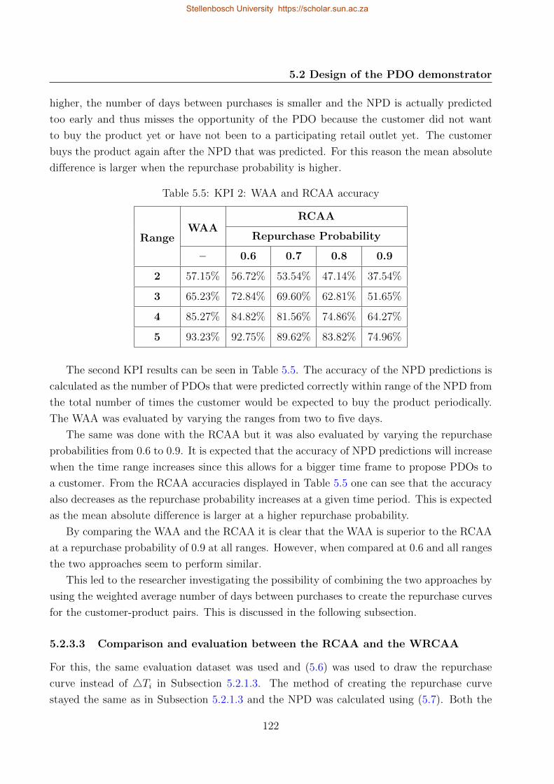
5.2 Design of the PDO demonstrator
higher, the number of days between purchases is smaller and the NPD is actually predicted
too early and thus misses the opportunity of the PDO because the customer did not want
to buy the product yet or have not been to a participating retail outlet yet. The customer
buys the product again after the NPD that was predicted. For this reason the mean absolute
difference is larger when the repurchase probability is higher.
Table 5.5: KPI 2: WAA and RCAA accuracy
RangeWAA
RCAA
Repurchase Probability
– 0.6 0.7 0.8 0.9
2 57.15% 56.72% 53.54% 47.14% 37.54%
3 65.23% 72.84% 69.60% 62.81% 51.65%
4 85.27% 84.82% 81.56% 74.86% 64.27%
5 93.23% 92.75% 89.62% 83.82% 74.96%
The second KPI results can be seen in Table 5.5. The accuracy of the NPD predictions is
calculated as the number of PDOs that were predicted correctly within range of the NPD from
the total number of times the customer would be expected to buy the product periodically.
The WAA was evaluated by varying the ranges from two to five days.
The same was done with the RCAA but it was also evaluated by varying the repurchase
probabilities from 0.6 to 0.9. It is expected that the accuracy of NPD predictions will increase
when the time range increases since this allows for a bigger time frame to propose PDOs to
a customer. From the RCAA accuracies displayed in Table 5.5 one can see that the accuracy
also decreases as the repurchase probability increases at a given time period. This is expected
as the mean absolute difference is larger at a higher repurchase probability.
By comparing the WAA and the RCAA it is clear that the WAA is superior to the RCAA
at a repurchase probability of 0.9 at all ranges. However, when compared at 0.6 and all ranges
the two approaches seem to perform similar.
This led to the researcher investigating the possibility of combining the two approaches by
using the weighted average number of days between purchases to create the repurchase curves
for the customer-product pairs. This is discussed in the following subsection.
5.2.3.3 Comparison and evaluation between the RCAA and the WRCAA
For this, the same evaluation dataset was used and (5.6) was used to draw the repurchase
curve instead of 4Ti in Subsection 5.2.1.3. The method of creating the repurchase curve
stayed the same as in Subsection 5.2.1.3 and the NPD was calculated using (5.7). Both the
122
Stellenbosch University https://scholar.sun.ac.za
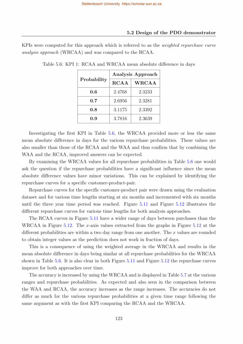
5.2 Design of the PDO demonstrator
KPIs were computed for this approach which is referred to as the weighted repurchase curve
analysis approach (WRCAA) and was compared to the RCAA.
Table 5.6: KPI 1: RCAA and WRCAA mean absolute difference in days
ProbabilityAnalysis Approach
RCAA WRCAA
0.6 2.4768 2.3233
0.7 2.6956 2.3281
0.8 3.1175 2.3392
0.9 3.7816 2.3639
Investigating the first KPI in Table 5.6, the WRCAA provided more or less the same
mean absolute difference in days for the various repurchase probabilities. These values are
also smaller than those of the RCAA and the WAA and thus confirm that by combining the
WAA and the RCAA, improved answers can be expected.
By examining the WRCAA values for all repurchase probabilities in Table 5.6 one would
ask the question if the repurchase probabilities have a significant influence since the mean
absolute difference values have minor variations. This can be explained by identifying the
repurchase curves for a specific customer-product-pair.
Repurchase curves for the specific customer-product pair were drawn using the evaluation
dataset and for various time lengths starting at six months and incremented with six months
until the three year time period was reached. Figure 5.11 and Figure 5.12 illustrates the
different repurchase curves for various time lengths for both analysis approaches.
The RCAA curves in Figure 5.11 have a wider range of days between purchases than the
WRCAA in Figure 5.12. The x-axis values extracted from the graphs in Figure 5.12 at the
different probabilities are within a two day range from one another. The x values are rounded
to obtain integer values as the prediction does not work in fraction of days.
This is a consequence of using the weighted average in the WRCAA and results in the
mean absolute difference in days being similar at all repurchase probabilities for the WRCAA
shown in Table 5.6. It is also clear in both Figure 5.11 and Figure 5.12 the repurchase curves
improve for both approaches over time.
The accuracy is increased by using the WRCAA and is displayed in Table 5.7 at the various
ranges and repurchase probabilities. As expected and also seen in the comparison between
the WAA and RCAA, the accuracy increases as the range increases. The accuracies do not
differ as much for the various repurchase probabilities at a given time range following the
same argument as with the first KPI comparing the RCAA and the WRCAA.
123
Stellenbosch University https://scholar.sun.ac.za
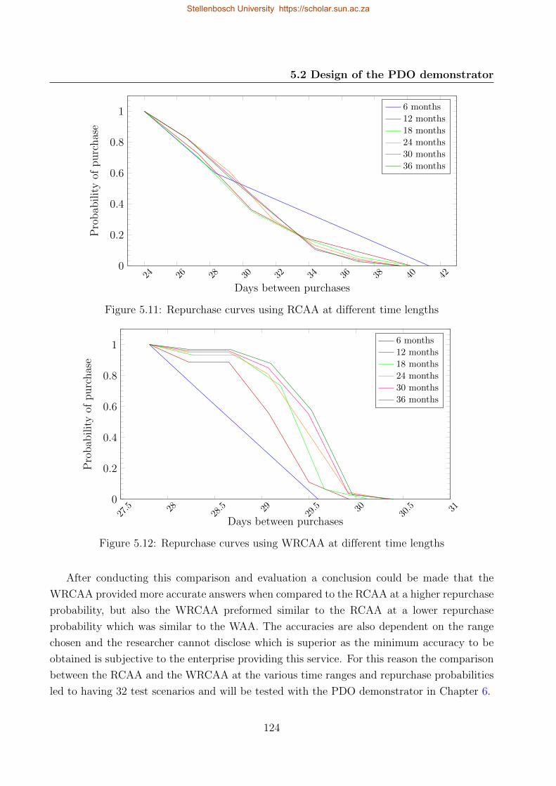
5.2 Design of the PDO demonstrator
24 26 28 30 32 34 36 38 40 420
0.2
0.4
0.6
0.8
1
Days between purchases
Pro
bab
ilit
yof
purc
has
e6 months
12 months
18 months
24 months
30 months
36 months
Figure 5.11: Repurchase curves using RCAA at different time lengths
27.5 28
28.5 29
29.5 30
30.5 31
0
0.2
0.4
0.6
0.8
1
Days between purchases
Pro
bab
ilit
yof
purc
has
e
6 months
12 months
18 months
24 months
30 months
36 months
Figure 5.12: Repurchase curves using WRCAA at different time lengths
After conducting this comparison and evaluation a conclusion could be made that the
WRCAA provided more accurate answers when compared to the RCAA at a higher repurchase
probability, but also the WRCAA preformed similar to the RCAA at a lower repurchase
probability which was similar to the WAA. The accuracies are also dependent on the range
chosen and the researcher cannot disclose which is superior as the minimum accuracy to be
obtained is subjective to the enterprise providing this service. For this reason the comparison
between the RCAA and the WRCAA at the various time ranges and repurchase probabilities
led to having 32 test scenarios and will be tested with the PDO demonstrator in Chapter 6.
124
Stellenbosch University https://scholar.sun.ac.za
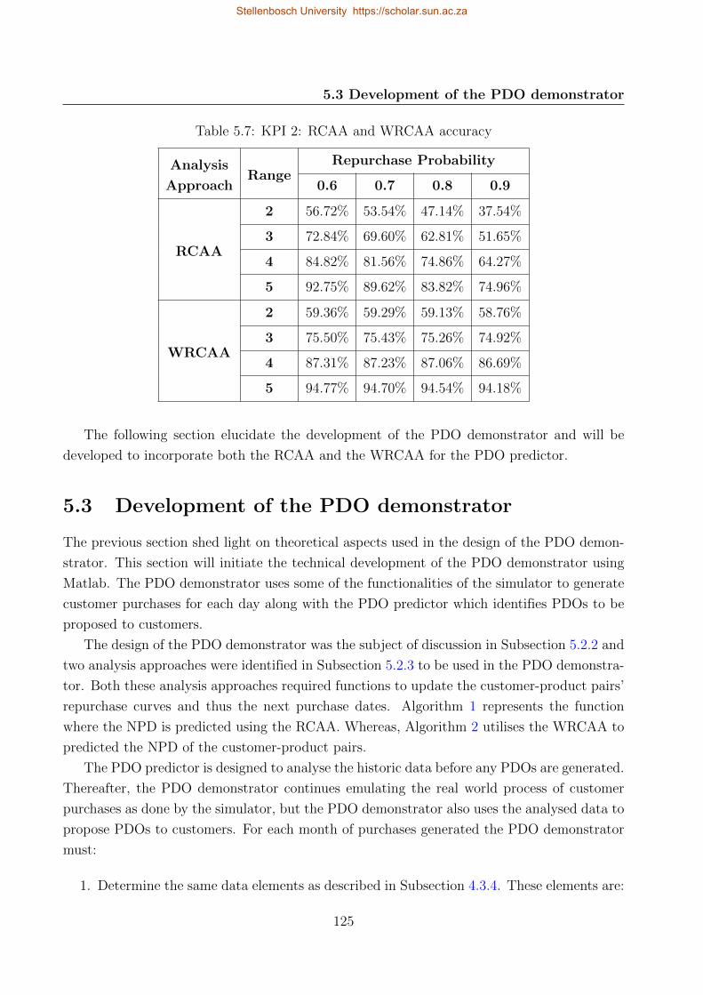
5.3 Development of the PDO demonstrator
Table 5.7: KPI 2: RCAA and WRCAA accuracy
Analysis
ApproachRange
Repurchase Probability
0.6 0.7 0.8 0.9
RCAA
2 56.72% 53.54% 47.14% 37.54%
3 72.84% 69.60% 62.81% 51.65%
4 84.82% 81.56% 74.86% 64.27%
5 92.75% 89.62% 83.82% 74.96%
WRCAA
2 59.36% 59.29% 59.13% 58.76%
3 75.50% 75.43% 75.26% 74.92%
4 87.31% 87.23% 87.06% 86.69%
5 94.77% 94.70% 94.54% 94.18%
The following section elucidate the development of the PDO demonstrator and will be
developed to incorporate both the RCAA and the WRCAA for the PDO predictor.
5.3 Development of the PDO demonstrator
The previous section shed light on theoretical aspects used in the design of the PDO demon-
strator. This section will initiate the technical development of the PDO demonstrator using
Matlab. The PDO demonstrator uses some of the functionalities of the simulator to generate
customer purchases for each day along with the PDO predictor which identifies PDOs to be
proposed to customers.
The design of the PDO demonstrator was the subject of discussion in Subsection 5.2.2 and
two analysis approaches were identified in Subsection 5.2.3 to be used in the PDO demonstra-
tor. Both these analysis approaches required functions to update the customer-product pairs’
repurchase curves and thus the next purchase dates. Algorithm 1 represents the function
where the NPD is predicted using the RCAA. Whereas, Algorithm 2 utilises the WRCAA to
predicted the NPD of the customer-product pairs.
The PDO predictor is designed to analyse the historic data before any PDOs are generated.
Thereafter, the PDO demonstrator continues emulating the real world process of customer
purchases as done by the simulator, but the PDO demonstrator also uses the analysed data to
propose PDOs to customers. For each month of purchases generated the PDO demonstrator
must:
1. Determine the same data elements as described in Subsection 4.3.4. These elements are:
125
Stellenbosch University https://scholar.sun.ac.za
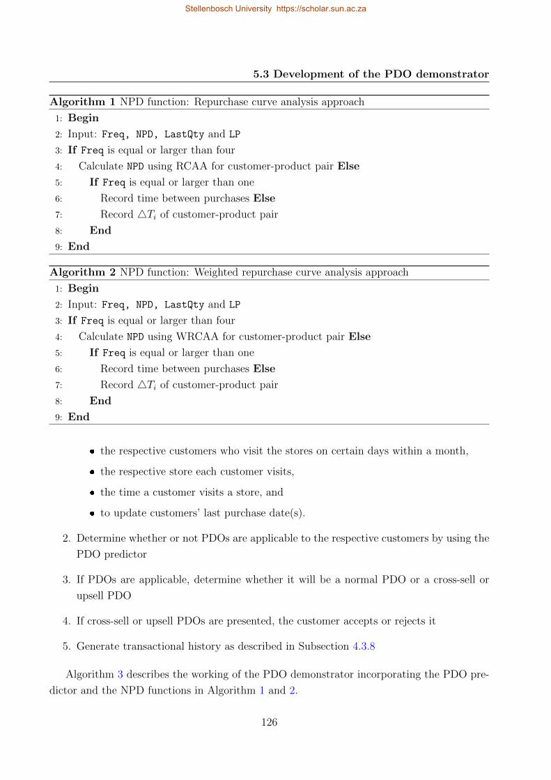
5.3 Development of the PDO demonstrator
Algorithm 1 NPD function: Repurchase curve analysis approach
1: Begin
2: Input: Freq, NPD, LastQty and LP
3: If Freq is equal or larger than four
4: Calculate NPD using RCAA for customer-product pair Else
5: If Freq is equal or larger than one
6: Record time between purchases Else
7: Record 4Ti of customer-product pair
8: End
9: End
Algorithm 2 NPD function: Weighted repurchase curve analysis approach
1: Begin
2: Input: Freq, NPD, LastQty and LP
3: If Freq is equal or larger than four
4: Calculate NPD using WRCAA for customer-product pair Else
5: If Freq is equal or larger than one
6: Record time between purchases Else
7: Record 4Ti of customer-product pair
8: End
9: End
� the respective customers who visit the stores on certain days within a month,
� the respective store each customer visits,
� the time a customer visits a store, and
� to update customers’ last purchase date(s).
2. Determine whether or not PDOs are applicable to the respective customers by using the
PDO predictor
3. If PDOs are applicable, determine whether it will be a normal PDO or a cross-sell or
upsell PDO
4. If cross-sell or upsell PDOs are presented, the customer accepts or rejects it
5. Generate transactional history as described in Subsection 4.3.8
Algorithm 3 describes the working of the PDO demonstrator incorporating the PDO pre-
dictor and the NPD functions in Algorithm 1 and 2.
126
Stellenbosch University https://scholar.sun.ac.za
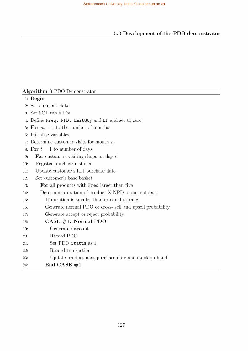
5.3 Development of the PDO demonstrator
Algorithm 3 PDO Demonstrator
1: Begin
2: Set current date
3: Set SQL table IDs
4: Define Freq, NPD, LastQty and LP and set to zero
5: For m = 1 to the number of months
6: Initialise variables
7: Determine customer visits for month m
8: For t = 1 to number of days
9: For customers visiting shops on day t
10: Register purchase instance
11: Update customer’s last purchase date
12: Set customer’s base basket
13: For all products with Freq larger than five
14: Determine duration of product X NPD to current date
15: If duration is smaller than or equal to range
16: Generate normal PDO or cross- sell and upsell probability
17: Generate accept or reject probability
18: CASE #1: Normal PDO
19: Generate discount
20: Record PDO
21: Set PDO Status as 1
22: Record transaction
23: Update product next purchase date and stock on hand
24: End CASE #1
127
Stellenbosch University https://scholar.sun.ac.za
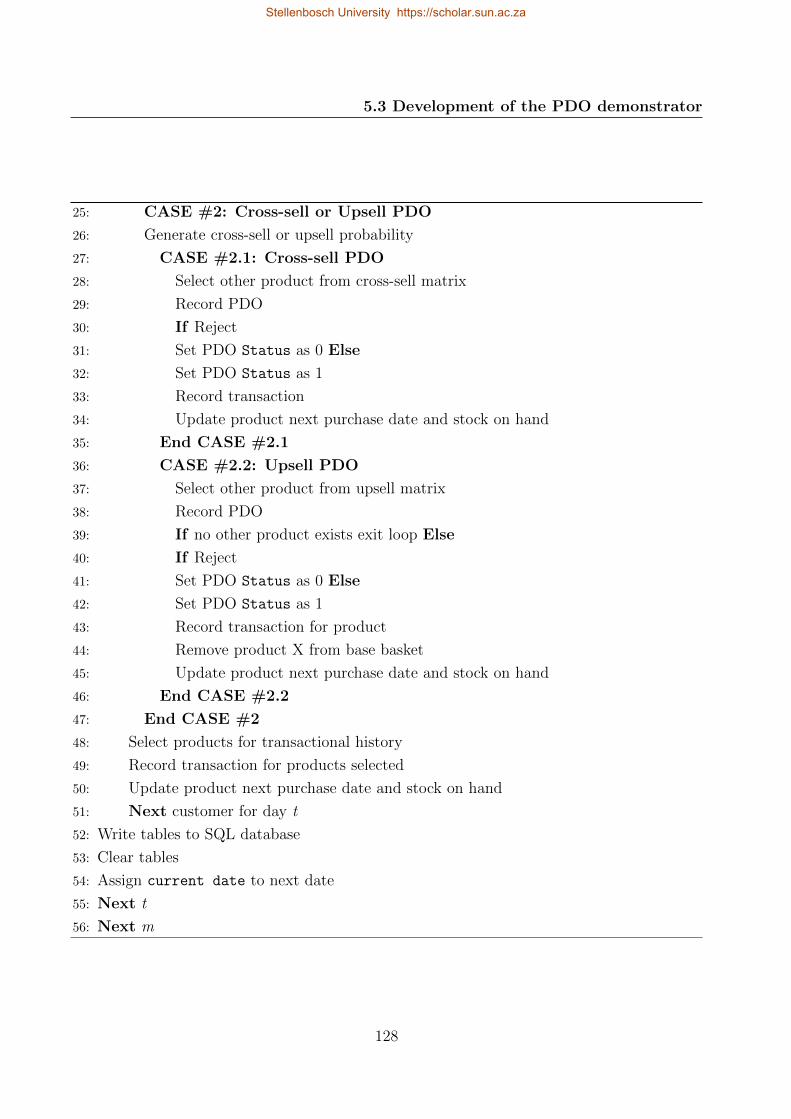
5.3 Development of the PDO demonstrator
25: CASE #2: Cross-sell or Upsell PDO
26: Generate cross-sell or upsell probability
27: CASE #2.1: Cross-sell PDO
28: Select other product from cross-sell matrix
29: Record PDO
30: If Reject
31: Set PDO Status as 0 Else
32: Set PDO Status as 1
33: Record transaction
34: Update product next purchase date and stock on hand
35: End CASE #2.1
36: CASE #2.2: Upsell PDO
37: Select other product from upsell matrix
38: Record PDO
39: If no other product exists exit loop Else
40: If Reject
41: Set PDO Status as 0 Else
42: Set PDO Status as 1
43: Record transaction for product
44: Remove product X from base basket
45: Update product next purchase date and stock on hand
46: End CASE #2.2
47: End CASE #2
48: Select products for transactional history
49: Record transaction for products selected
50: Update product next purchase date and stock on hand
51: Next customer for day t
52: Write tables to SQL database
53: Clear tables
54: Assign current date to next date
55: Next t
56: Next m
128
Stellenbosch University https://scholar.sun.ac.za
5.4 New customer entering the system
The NPDs are updated each time a product is bought. Algorithm 3 also illustrates the
different cases where the PDO predictor predicts a PDO and the PDO demonstrator proposes
the different types of PDOs: normal, cross-sell and upsell. The demonstrator will be executed
using each of the NPD functions. The following section discusses the event when a new
customer enters the system.
5.4 New customer entering the system
This section discusses the event when a new customer enters the system. Since the new
customer has no historical transactional data, the system will use machine learning techniques
to place the new customer in a customer segment. Customer segmentation is explained in
Section 2.5.
When a new customer signs up for this service of personalised discount offers they are
prompted to enter preferences from a list. A minimum of one preference entry is required to
complete this process. The new customer is allocated to a customer segment based on the
preferences and purchasing behaviour of customers within that segment.
This process is done in two steps:
1. Cluster customers based on RFM values.
2. Decision rules for allocating new customers to clusters.
The existing customers are clustered based on their transactional history using the RFM
analysis explained in Subsection 2.6.1 using a 5-score analysis.
For each RFM indicator a minimum and maximum value are determined and the indica-
tors are divided into five equal classes using (5.8) as the class size for each RFM indicator
individually.
Indicator class size =Indicator max− Indicator min
5(5.8)
Customers are allocated R, F and M values based on the class they belong to based on
each individual RFM indicator. After the R, F and M value for each customer is assigned,
the k–means clustering algorithm is utilised to divide the customers into clusters based on
their R, F and M values. The k–means clustering algorithm was identified as an unsupervised
machine learning technique in Table 2.20 and is a commonly used algorithm for clustering.
An example dataset is used for the practical and visual explanation of this section. Figure
5.13 explains the classes of each RFM indicator. The recency parameter is measured on the
LastPurchase attribute of each customer. The earliest last purchase date (Indicator min)
is the start date of the recency parameter (lowest recency) and the latest last purchase date
129
Stellenbosch University https://scholar.sun.ac.za
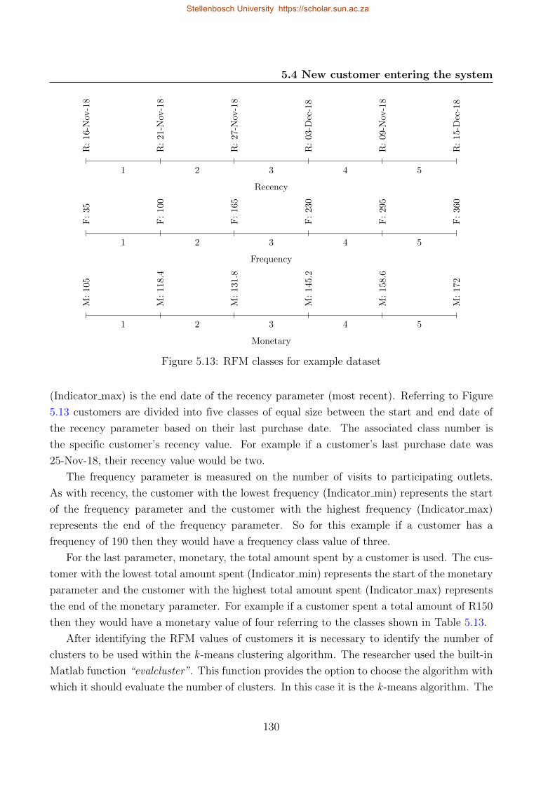
5.4 New customer entering the system
1 2 3 4 5
R:
16-N
ov-1
8
R:
21-N
ov-1
8
R:
27-N
ov-1
8
R:
03-D
ec-1
8
R:
09-N
ov-1
8
R:
15-D
ec-1
8
Recency
1 2 3 4 5
F:
35
F:
100
F:
165
F:
230
F:
295
F:
360
Frequency
1 2 3 4 5
M:
105
M:
118.
4
M:
131.
8
M:
145.
2
M:
158.
6
M:
172
Monetary
Figure 5.13: RFM classes for example dataset
(Indicator max) is the end date of the recency parameter (most recent). Referring to Figure
5.13 customers are divided into five classes of equal size between the start and end date of
the recency parameter based on their last purchase date. The associated class number is
the specific customer’s recency value. For example if a customer’s last purchase date was
25-Nov-18, their recency value would be two.
The frequency parameter is measured on the number of visits to participating outlets.
As with recency, the customer with the lowest frequency (Indicator min) represents the start
of the frequency parameter and the customer with the highest frequency (Indicator max)
represents the end of the frequency parameter. So for this example if a customer has a
frequency of 190 then they would have a frequency class value of three.
For the last parameter, monetary, the total amount spent by a customer is used. The cus-
tomer with the lowest total amount spent (Indicator min) represents the start of the monetary
parameter and the customer with the highest total amount spent (Indicator max) represents
the end of the monetary parameter. For example if a customer spent a total amount of R150
then they would have a monetary value of four referring to the classes shown in Table 5.13.
After identifying the RFM values of customers it is necessary to identify the number of
clusters to be used within the k -means clustering algorithm. The researcher used the built-in
Matlab function “evalcluster”. This function provides the option to choose the algorithm with
which it should evaluate the number of clusters. In this case it is the k -means algorithm. The
130
Stellenbosch University https://scholar.sun.ac.za
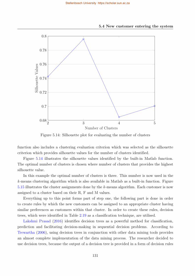
5.4 New customer entering the system
2 3 4 50.68
0.7
0.72
0.74
0.76
0.78
0.8
Number of Clusters
Silhou
ette
Val
ues
Figure 5.14: Silhouette plot for evaluating the number of clusters
function also includes a clustering evaluation criterion which was selected as the silhouette
criterion which provides silhouette values for the number of clusters identified.
Figure 5.14 illustrates the silhouette values identified by the built-in Matlab function.
The optimal number of clusters is chosen where number of clusters that provides the highest
silhouette value.
In this example the optimal number of clusters is three. This number is now used in the
k -means clustering algorithm which is also available in Matlab as a built-in function. Figure
5.15 illustrates the cluster assignments done by the k -means algorithm. Each customer is now
assigned to a cluster based on their R, F and M values.
Everything up to this point forms part of step one, the following part is done in order
to create rules by which the new customers can be assigned to an appropriate cluster having
similar preferences as customers within that cluster. In order to create these rules, decision
trees, which were identified in Table 2.19 as a classification technique, are utilised.
Lakshmi Prasad (2016) identifies decision trees as a powerful method for classification,
prediction and facilitating decision-making in sequential decision problems. According to
Trewartha (2006), using decision trees in conjunction with other data mining tools provides
an almost complete implementation of the data mining process. The researcher decided to
use decision trees, because the output of a decision tree is provided in a form of decision rules
131
Stellenbosch University https://scholar.sun.ac.za
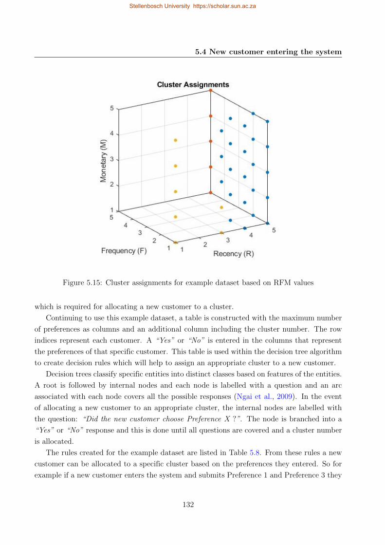
5.4 New customer entering the system
Figure 5.15: Cluster assignments for example dataset based on RFM values
which is required for allocating a new customer to a cluster.
Continuing to use this example dataset, a table is constructed with the maximum number
of preferences as columns and an additional column including the cluster number. The row
indices represent each customer. A “Yes” or “No” is entered in the columns that represent
the preferences of that specific customer. This table is used within the decision tree algorithm
to create decision rules which will help to assign an appropriate cluster to a new customer.
Decision trees classify specific entities into distinct classes based on features of the entities.
A root is followed by internal nodes and each node is labelled with a question and an arc
associated with each node covers all the possible responses (Ngai et al., 2009). In the event
of allocating a new customer to an appropriate cluster, the internal nodes are labelled with
the question: “Did the new customer choose Preference X ?”. The node is branched into a
“Yes” or “No” response and this is done until all questions are covered and a cluster number
is allocated.
The rules created for the example dataset are listed in Table 5.8. From these rules a new
customer can be allocated to a specific cluster based on the preferences they entered. So for
example if a new customer enters the system and submits Preference 1 and Preference 3 they
132
Stellenbosch University https://scholar.sun.ac.za
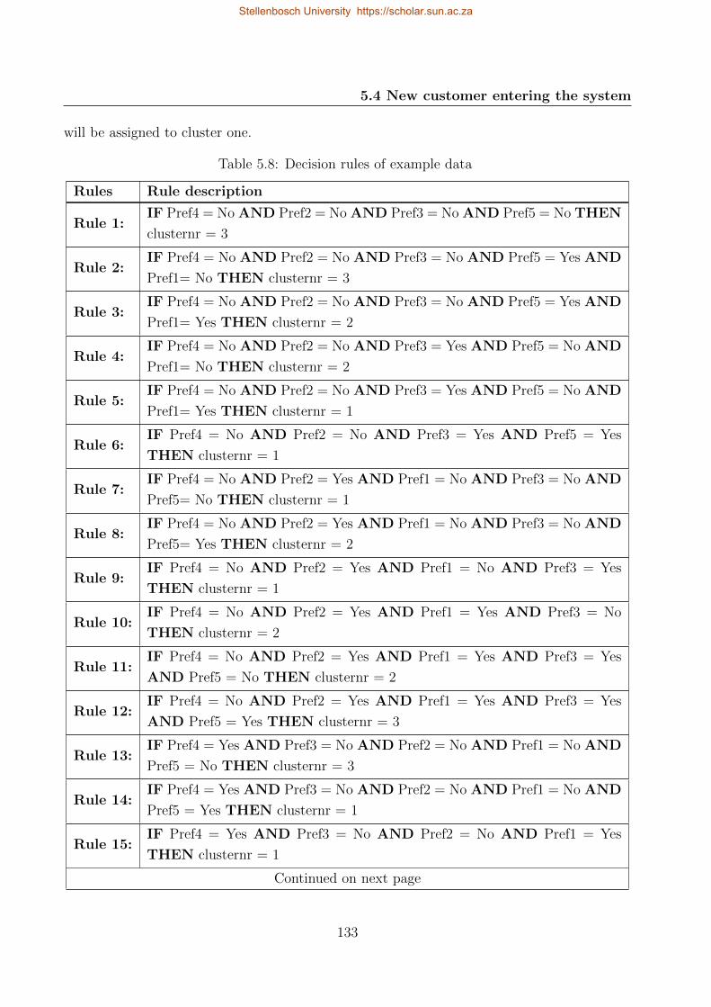
5.4 New customer entering the system
will be assigned to cluster one.
Table 5.8: Decision rules of example data
Rules Rule description
Rule 1:IF Pref4 = No AND Pref2 = No AND Pref3 = No AND Pref5 = No THEN
clusternr = 3
Rule 2:IF Pref4 = No AND Pref2 = No AND Pref3 = No AND Pref5 = Yes AND
Pref1= No THEN clusternr = 3
Rule 3:IF Pref4 = No AND Pref2 = No AND Pref3 = No AND Pref5 = Yes AND
Pref1= Yes THEN clusternr = 2
Rule 4:IF Pref4 = No AND Pref2 = No AND Pref3 = Yes AND Pref5 = No AND
Pref1= No THEN clusternr = 2
Rule 5:IF Pref4 = No AND Pref2 = No AND Pref3 = Yes AND Pref5 = No AND
Pref1= Yes THEN clusternr = 1
Rule 6:IF Pref4 = No AND Pref2 = No AND Pref3 = Yes AND Pref5 = Yes
THEN clusternr = 1
Rule 7:IF Pref4 = No AND Pref2 = Yes AND Pref1 = No AND Pref3 = No AND
Pref5= No THEN clusternr = 1
Rule 8:IF Pref4 = No AND Pref2 = Yes AND Pref1 = No AND Pref3 = No AND
Pref5= Yes THEN clusternr = 2
Rule 9:IF Pref4 = No AND Pref2 = Yes AND Pref1 = No AND Pref3 = Yes
THEN clusternr = 1
Rule 10:IF Pref4 = No AND Pref2 = Yes AND Pref1 = Yes AND Pref3 = No
THEN clusternr = 2
Rule 11:IF Pref4 = No AND Pref2 = Yes AND Pref1 = Yes AND Pref3 = Yes
AND Pref5 = No THEN clusternr = 2
Rule 12:IF Pref4 = No AND Pref2 = Yes AND Pref1 = Yes AND Pref3 = Yes
AND Pref5 = Yes THEN clusternr = 3
Rule 13:IF Pref4 = Yes AND Pref3 = No AND Pref2 = No AND Pref1 = No AND
Pref5 = No THEN clusternr = 3
Rule 14:IF Pref4 = Yes AND Pref3 = No AND Pref2 = No AND Pref1 = No AND
Pref5 = Yes THEN clusternr = 1
Rule 15:IF Pref4 = Yes AND Pref3 = No AND Pref2 = No AND Pref1 = Yes
THEN clusternr = 1
Continued on next page
133
Stellenbosch University https://scholar.sun.ac.za
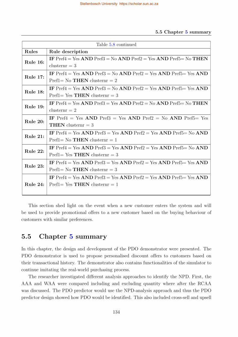
5.5 Chapter 5 summary
Table 5.8 continued
Rules Rule description
Rule 16:IF Pref4 = Yes AND Pref3 = No AND Pref2 = Yes AND Pref5= No THEN
clusternr = 3
Rule 17:IF Pref4 = Yes AND Pref3 = No AND Pref2 = Yes AND Pref5= Yes AND
Pref1= No THEN clusternr = 2
Rule 18:IF Pref4 = Yes AND Pref3 = No AND Pref2 = Yes AND Pref5= Yes AND
Pref1= Yes THEN clusternr = 3
Rule 19:IF Pref4 = Yes AND Pref3 = Yes AND Pref2 = No AND Pref5= No THEN
clusternr = 2
Rule 20:IF Pref4 = Yes AND Pref3 = Yes AND Pref2 = No AND Pref5= Yes
THEN clusternr = 3
Rule 21:IF Pref4 = Yes AND Pref3 = Yes AND Pref2 = Yes AND Pref5= No AND
Pref1= No THEN clusternr = 1
Rule 22:IF Pref4 = Yes AND Pref3 = Yes AND Pref2 = Yes AND Pref5= No AND
Pref1= Yes THEN clusternr = 3
Rule 23:IF Pref4 = Yes AND Pref3 = Yes AND Pref2 = Yes AND Pref5= Yes AND
Pref1= No THEN clusternr = 3
Rule 24:
IF Pref4 = Yes AND Pref3 = Yes AND Pref2 = Yes AND Pref5= Yes AND
Pref1= Yes THEN clusternr = 1
This section shed light on the event when a new customer enters the system and will
be used to provide promotional offers to a new customer based on the buying behaviour of
customers with similar preferences.
5.5 Chapter 5 summary
In this chapter, the design and development of the PDO demonstrator were presented. The
PDO demonstrator is used to propose personalised discount offers to customers based on
their transactional history. The demonstrator also contains functionalities of the simulator to
continue imitating the real-world purchasing process.
The researcher investigated different analysis approaches to identify the NPD. First, the
AAA and WAA were compared including and excluding quantity where after the RCAA
was discussed. The PDO predictor would use the NPD-analysis approach and thus the PDO
predictor design showed how PDO would be identified. This also included cross-sell and upsell
134
Stellenbosch University https://scholar.sun.ac.za

5.5 Chapter 5 summary
offers.
The WAA and RCAA were compared and evaluated using an evaluation dataset generated
by the simulator. The approaches were evaluated based on two KPIs identified in this chapter.
The WAA and RCAA were combined to create the WRCAA and the latter was compared
to the RCAA based on the two KPIs. This comparison and evaluation led to developing the
PDO demonstrator by including both the RCAA and WRCAA. This chapter also contains
the pseudocode for the PDO demonstrator.
Lastly, the event when a new customer enters the system was also investigated and de-
cision rules were generated to allocate the new customer to an appropriate cluster based on
preferences similar to other existing customers.
The results obtained from the PDO demonstrator along with a discussion thereof will be
presented in the following chapter.
135
Stellenbosch University https://scholar.sun.ac.za
Chapter 6
Experiments and results
The previous chapter explained the PDO demonstrator design and development along with
a comparison and evaluation of various analysis approaches. This chapter will discuss the
experiments and results that were obtained by executing the experiments with the PDO
demonstrator. The methodology followed will initiate this chapter.
6.1 Methodology for experiments and results
This chapter initiates the fourth and final phase identified by the research methodology in
Section 1.5. The researcher must execute the 32 scenarios identified in Chapter 5 using the
PDO demonstrator. The scenarios must be evaluated for both KPIs identified in Subsection
5.2.3 utilising both the RCAA and WRCAA in the PDO demonstrator. The results of the
experiments must be discussed and the researcher must provide a customer journey example
for a chosen repurchase probability and time range.
6.2 Comparison and evaluation of results obtained from
PDO demonstrator
The evaluation and comparison conducted in Subsection 5.2.3 used an evaluation dataset that
was simulated using the simulator designed in Chapter 4 before the evaluation and comparison
commenced. The evaluation dataset did not contain any promotional influences and was used
to test the various NPD-analysis approaches.
This section will display the results obtained by evaluating the PDO demonstrator with the
32 scenarios when promotional efforts are introduced. These promotional influences are intro-
duced by the personalised discount offers (PDOs). The PDO demonstrator will continuously
emulate the real-world process of customer purchases along with introducing promotional
efforts identified by the PDO predictor. If a PDO is identified, the PDO demonstrator can
propose it as a normal PDO, cross-sell PDO or upsell PDO. These promotional efforts will
affect the customers’ normal purchasing behaviour. The capability of predicting accurate
NPDs by the PDO predictor must be evaluated when promotional influences are present.
The mean absolute difference in days between the NPD predicted and the actual purchase
date is presented in Table 6.1 for the various repurchase probabilities and ranges. The values
are similar for both the RCAA and the WRCAA at the different repurchase probabilities and
136
Stellenbosch University https://scholar.sun.ac.za
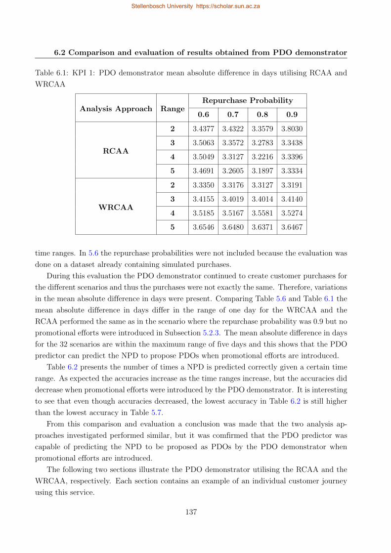
6.2 Comparison and evaluation of results obtained from PDO demonstrator
Table 6.1: KPI 1: PDO demonstrator mean absolute difference in days utilising RCAA and
WRCAA
Analysis Approach RangeRepurchase Probability
0.6 0.7 0.8 0.9
RCAA
2 3.4377 3.4322 3.3579 3.8030
3 3.5063 3.3572 3.2783 3.3438
4 3.5049 3.3127 3.2216 3.3396
5 3.4691 3.2605 3.1897 3.3334
WRCAA
2 3.3350 3.3176 3.3127 3.3191
3 3.4155 3.4019 3.4014 3.4140
4 3.5185 3.5167 3.5581 3.5274
5 3.6546 3.6480 3.6371 3.6467
time ranges. In 5.6 the repurchase probabilities were not included because the evaluation was
done on a dataset already containing simulated purchases.
During this evaluation the PDO demonstrator continued to create customer purchases for
the different scenarios and thus the purchases were not exactly the same. Therefore, variations
in the mean absolute difference in days were present. Comparing Table 5.6 and Table 6.1 the
mean absolute difference in days differ in the range of one day for the WRCAA and the
RCAA performed the same as in the scenario where the repurchase probability was 0.9 but no
promotional efforts were introduced in Subsection 5.2.3. The mean absolute difference in days
for the 32 scenarios are within the maximum range of five days and this shows that the PDO
predictor can predict the NPD to propose PDOs when promotional efforts are introduced.
Table 6.2 presents the number of times a NPD is predicted correctly given a certain time
range. As expected the accuracies increase as the time ranges increase, but the accuracies did
decrease when promotional efforts were introduced by the PDO demonstrator. It is interesting
to see that even though accuracies decreased, the lowest accuracy in Table 6.2 is still higher
than the lowest accuracy in Table 5.7.
From this comparison and evaluation a conclusion was made that the two analysis ap-
proaches investigated performed similar, but it was comfirmed that the PDO predictor was
capable of predicting the NPD to be proposed as PDOs by the PDO demonstrator when
promotional efforts are introduced.
The following two sections illustrate the PDO demonstrator utilising the RCAA and the
WRCAA, respectively. Each section contains an example of an individual customer journey
using this service.
137
Stellenbosch University https://scholar.sun.ac.za
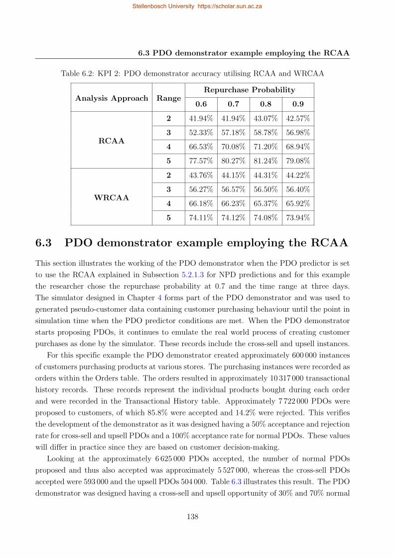
6.3 PDO demonstrator example employing the RCAA
Table 6.2: KPI 2: PDO demonstrator accuracy utilising RCAA and WRCAA
Analysis Approach RangeRepurchase Probability
0.6 0.7 0.8 0.9
RCAA
2 41.94% 41.94% 43.07% 42.57%
3 52.33% 57.18% 58.78% 56.98%
4 66.53% 70.08% 71.20% 68.94%
5 77.57% 80.27% 81.24% 79.08%
WRCAA
2 43.76% 44.15% 44.31% 44.22%
3 56.27% 56.57% 56.50% 56.40%
4 66.18% 66.23% 65.37% 65.92%
5 74.11% 74.12% 74.08% 73.94%
6.3 PDO demonstrator example employing the RCAA
This section illustrates the working of the PDO demonstrator when the PDO predictor is set
to use the RCAA explained in Subsection 5.2.1.3 for NPD predictions and for this example
the researcher chose the repurchase probability at 0.7 and the time range at three days.
The simulator designed in Chapter 4 forms part of the PDO demonstrator and was used to
generated pseudo-customer data containing customer purchasing behaviour until the point in
simulation time when the PDO predictor conditions are met. When the PDO demonstrator
starts proposing PDOs, it continues to emulate the real world process of creating customer
purchases as done by the simulator. These records include the cross-sell and upsell instances.
For this specific example the PDO demonstrator created approximately 600 000 instances
of customers purchasing products at various stores. The purchasing instances were recorded as
orders within the Orders table. The orders resulted in approximately 10 317 000 transactional
history records. These records represent the individual products bought during each order
and were recorded in the Transactional History table. Approximately 7 722 000 PDOs were
proposed to customers, of which 85.8% were accepted and 14.2% were rejected. This verifies
the development of the demonstrator as it was designed having a 50% acceptance and rejection
rate for cross-sell and upsell PDOs and a 100% acceptance rate for normal PDOs. These values
will differ in practice since they are based on customer decision-making.
Looking at the approximately 6 625 000 PDOs accepted, the number of normal PDOs
proposed and thus also accepted was approximately 5 527 000, whereas the cross-sell PDOs
accepted were 593 000 and the upsell PDOs 504 000. Table 6.3 illustrates this result. The PDO
demonstrator was designed having a cross-sell and upsell opportunity of 30% and 70% normal
138
Stellenbosch University https://scholar.sun.ac.za
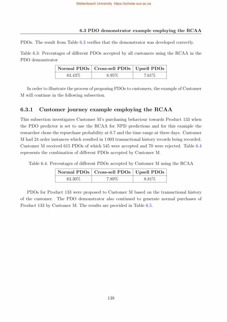
6.3 PDO demonstrator example employing the RCAA
PDOs. The result from Table 6.3 verifies that the demonstrator was developed correctly.
Table 6.3: Percentages of different PDOs accepted by all customers using the RCAA in the
PDO demonstrator
Normal PDOs Cross-sell PDOs Upsell PDOs
83.43% 8.95% 7.61%
In order to illustrate the process of proposing PDOs to customers, the example of Customer
M will continue in the following subsection.
6.3.1 Customer journey example employing the RCAA
This subsection investigates Customer M’s purchasing behaviour towards Product 133 when
the PDO predictor is set to use the RCAA for NPD predictions and for this example the
researcher chose the repurchase probability at 0.7 and the time range at three days. Customer
M had 24 order instances which resulted in 1 003 transactional history records being recorded.
Customer M received 615 PDOs of which 545 were accepted and 70 were rejected. Table 6.4
represents the combination of different PDOs accepted by Customer M.
Table 6.4: Percentages of different PDOs accepted by Customer M using the RCAA
Normal PDOs Cross-sell PDOs Upsell PDOs
83.30% 7.89% 8.81%
PDOs for Product 133 were proposed to Customer M based on the transactional history
of the customer. The PDO demonstrator also continued to generate normal purchases of
Product 133 by Customer M. The results are provided in Table 6.5.
139
Stellenbosch University https://scholar.sun.ac.za
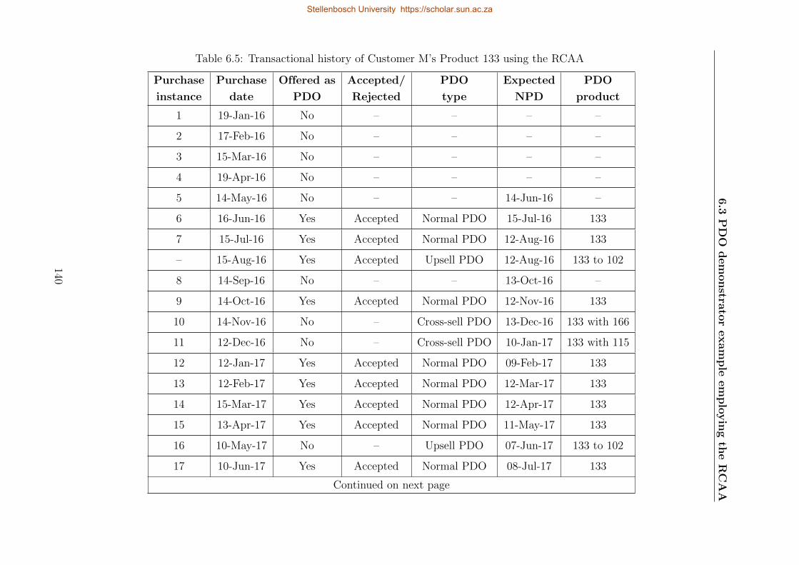
6.3
PDO
demonstra
torexample
employingth
eRCAA
Table 6.5: Transactional history of Customer M’s Product 133 using the RCAA
Purchase
instance
Purchase
date
Offered as
PDO
Accepted/
Rejected
PDO
type
Expected
NPD
PDO
product
1 19-Jan-16 No – – – –
2 17-Feb-16 No – – – –
3 15-Mar-16 No – – – –
4 19-Apr-16 No – – – –
5 14-May-16 No – – 14-Jun-16 –
6 16-Jun-16 Yes Accepted Normal PDO 15-Jul-16 133
7 15-Jul-16 Yes Accepted Normal PDO 12-Aug-16 133
– 15-Aug-16 Yes Accepted Upsell PDO 12-Aug-16 133 to 102
8 14-Sep-16 No – – 13-Oct-16 –
9 14-Oct-16 Yes Accepted Normal PDO 12-Nov-16 133
10 14-Nov-16 No – Cross-sell PDO 13-Dec-16 133 with 166
11 12-Dec-16 No – Cross-sell PDO 10-Jan-17 133 with 115
12 12-Jan-17 Yes Accepted Normal PDO 09-Feb-17 133
13 12-Feb-17 Yes Accepted Normal PDO 12-Mar-17 133
14 15-Mar-17 Yes Accepted Normal PDO 12-Apr-17 133
15 13-Apr-17 Yes Accepted Normal PDO 11-May-17 133
16 10-May-17 No – Upsell PDO 07-Jun-17 133 to 102
17 10-Jun-17 Yes Accepted Normal PDO 08-Jul-17 133
Continued on next page
140
Stellenbosch University https://scholar.sun.ac.za
Stellenbosch University https://scholar.sun.ac.za
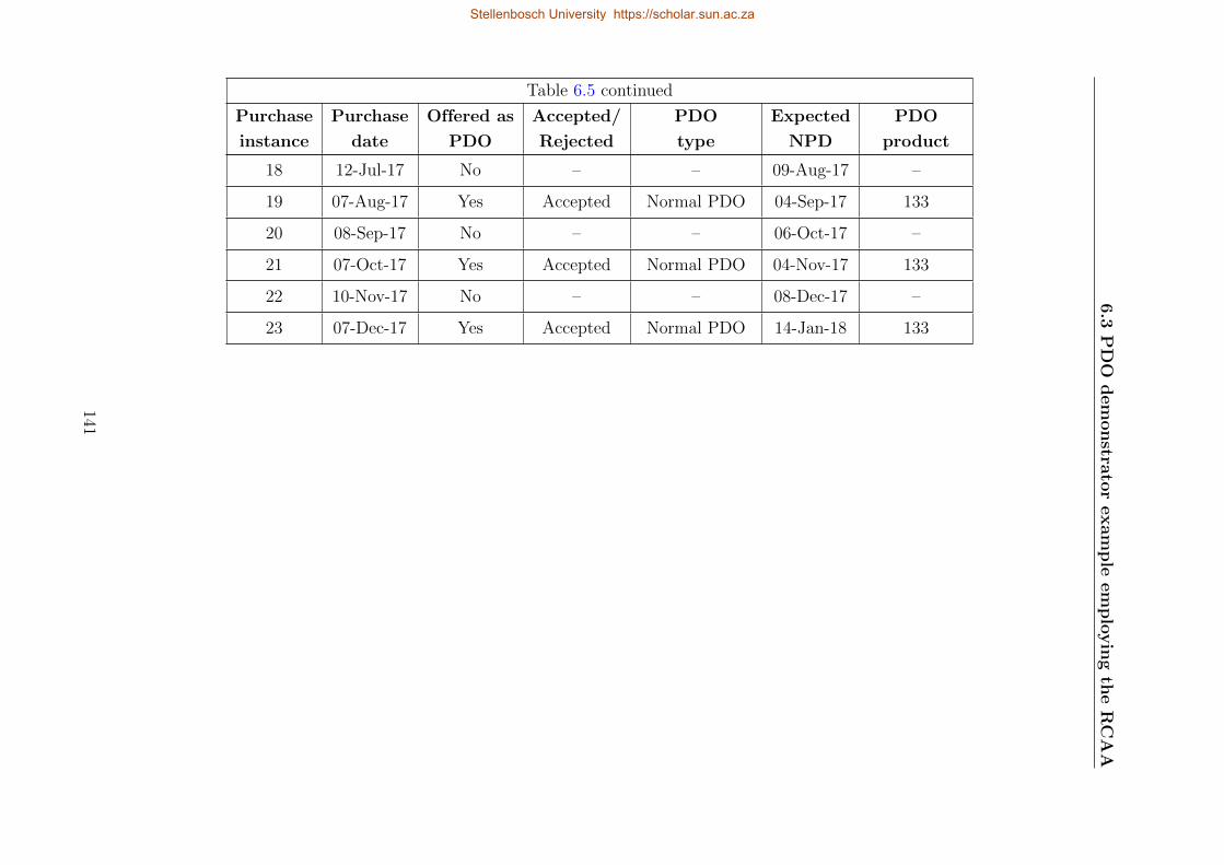
6.3
PDO
demonstra
torexample
employingth
eRCAA
Table 6.5 continued
Purchase
instance
Purchase
date
Offered as
PDO
Accepted/
Rejected
PDO
type
Expected
NPD
PDO
product
18 12-Jul-17 No – – 09-Aug-17 –
19 07-Aug-17 Yes Accepted Normal PDO 04-Sep-17 133
20 08-Sep-17 No – – 06-Oct-17 –
21 07-Oct-17 Yes Accepted Normal PDO 04-Nov-17 133
22 10-Nov-17 No – – 08-Dec-17 –
23 07-Dec-17 Yes Accepted Normal PDO 14-Jan-18 133
141
Stellenbosch University https://scholar.sun.ac.za
Stellenbosch University https://scholar.sun.ac.za
6.3 PDO demonstrator example employing the RCAA
From Table 6.5 purchase instances 1 to 5 represent the first five occasions where Customer
M purchased Product 133. No PDOs are proposed within this time as the minimum frequency
for the customer-product pair was not met yet. The minimum frequency was set to five as
explained in Subsection 5.2.2. PDOs are only proposed after the minimum frequency is met
and for this reason the first NPD prediction is only calculated at purchase instance five. The
expected NPD is calculated and shown in column six and it was predicted that Customer M
would purchase Product 133 again on 14-Jun-16.
Product 133 was purchased again on 16-Jun-16 at purchase instance 6 and because Product
133 was purchased within a three day range of the NPD predicted it was proposed and
purchased as a normal PDO. This event occurred for purchase instance 7 and 9.
In the row between purchase instance 7 and 8 on 15-Aug-16 it was estimated that Customer
M would be susceptible to buy Product 133 again. The PDO was presented as an upsell offer
for Product 102 and Customer M accepted this offer. For this reason there is no purchase
of Product 133 on this date in the row between purchase instance 7 and 8. Column three
identifies that a PDO was offered and accepted and one can see in the last column of Table 6.5
that Product 102 was purchased as an upsell from Product 133. A customer does not buy the
original product when an upsell is proposed so in this case Product 133 was not purchased and
for this reason the expected NPD remained 12-Aug-16. The events where the PDO product
column states 133 with x represents the PDO of Product 133 being cross-sold to Product x
and the case of an upsell the PDO product column indicates 133 to x.
The upsell offer caused an interference in the periodical purchase pattern of Product 133
and Customer M purchased Product 133 as a normal purchase on 14-Sep-16 where after a
new NPD was predicted for 13-Oct-16. On 14-Oct-16 Customer M purchased Product 133
as a normal PDO at purchase instance nine. At purchase instance 10 and 11, Product 133
was purchased but not with a PDO even though it was within a three day range of the NPD.
Both of these times the PDO demonstrator identified Product 133 to be proposed as a PDO,
but proposed it as a cross-sell offer. When a cross-sell offer is proposed the product from
which the cross-sell originated must also be bought in order to qualify for the discount. Thus
at purchase instance 10, Product 166 was purchased at a discount and Product 133 at the
normal price. At purchase instance 11, Product 115 was presented as the cross-sell offer from
Product 133. Customer M did not accept this offer, but still purchased product 133 at the
normal price.
For instances 12 to 15, Product 133 was proposed as a normal PDO because it was within
a three day range of the NPD predicted and thus also purchased at a discounted price. On
10-May-16 at purchase instance 16, Product 102 was proposed as an upsell offer based on
the NPD of Product 133. The customer rejected this offer and purchased Product 133 at the
normal price. Column three shows that Product 133 was thus not purchased due to a PDO.
142
Stellenbosch University https://scholar.sun.ac.za

6.4 PDO demonstrator example employing theWRCAA
At purchase instances 17, 19, 21 and 23 Product 133 was proposed as a normal PDO and
also accepted. At purchase instances 18, 20 and 22 Product 133 were recorded as normal
purchases because the purchase dates was not within a three day range of the predicted NPD.
The difference between the purchase date and the predicted NPD was 4, 4 and 6 days for
purchase instance 18, 20 and 22, respectively.
This section illustrates that the demonstrator is capable of proposing PDOs to customers
based on their historical data using the RCAA. The next section will discuss the results of
the demonstrator using WRCAA.
25 30 35 40 45 50 55 60 65 700
0.2
0.4
0.6
0.8
1
Days between purchases
Pro
bab
ilit
yof
purc
has
e
6 months
12 months
18 months
24 months
Figure 6.1: Repurchase curves using RCAA at different time lengths for Customer M’s Product
133
In Figure 6.1 the repurchase curve for Customer M’s Product 133 is presented for different
time lengths. During the 12 month time period the interference of the upsell offer in the row
between purchase instance 7 and 8 of Table 6.5 influenced the periodical purchase pattern
and this influence can also be seen in the repurchase curves of the customer-product pair in
Figure 6.1. It is clear to see that as time passes the repurchase curve improves as a result of
more historical behaviour available.
6.4 PDO demonstrator example employing the
WRCAA
This section illustrates the working of the PDO demonstrator, similar to the example in
Section 6.3, but now the PDO predictor is set to use the WRCAA explained in Subsection
143
Stellenbosch University https://scholar.sun.ac.za
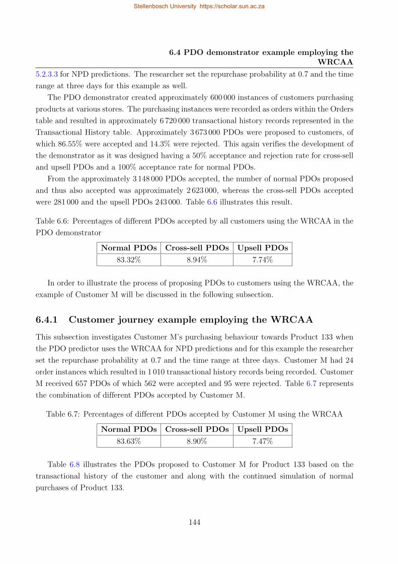
6.4 PDO demonstrator example employing theWRCAA
5.2.3.3 for NPD predictions. The researcher set the repurchase probability at 0.7 and the time
range at three days for this example as well.
The PDO demonstrator created approximately 600 000 instances of customers purchasing
products at various stores. The purchasing instances were recorded as orders within the Orders
table and resulted in approximately 6 720 000 transactional history records represented in the
Transactional History table. Approximately 3 673 000 PDOs were proposed to customers, of
which 86.55% were accepted and 14.3% were rejected. This again verifies the development of
the demonstrator as it was designed having a 50% acceptance and rejection rate for cross-sell
and upsell PDOs and a 100% acceptance rate for normal PDOs.
From the approximately 3 148 000 PDOs accepted, the number of normal PDOs proposed
and thus also accepted was approximately 2 623 000, whereas the cross-sell PDOs accepted
were 281 000 and the upsell PDOs 243 000. Table 6.6 illustrates this result.
Table 6.6: Percentages of different PDOs accepted by all customers using the WRCAA in the
PDO demonstrator
Normal PDOs Cross-sell PDOs Upsell PDOs
83.32% 8.94% 7.74%
In order to illustrate the process of proposing PDOs to customers using the WRCAA, the
example of Customer M will be discussed in the following subsection.
6.4.1 Customer journey example employing the WRCAA
This subsection investigates Customer M’s purchasing behaviour towards Product 133 when
the PDO predictor uses the WRCAA for NPD predictions and for this example the researcher
set the repurchase probability at 0.7 and the time range at three days. Customer M had 24
order instances which resulted in 1 010 transactional history records being recorded. Customer
M received 657 PDOs of which 562 were accepted and 95 were rejected. Table 6.7 represents
the combination of different PDOs accepted by Customer M.
Table 6.7: Percentages of different PDOs accepted by Customer M using the WRCAA
Normal PDOs Cross-sell PDOs Upsell PDOs
83.63% 8.90% 7.47%
Table 6.8 illustrates the PDOs proposed to Customer M for Product 133 based on the
transactional history of the customer and along with the continued simulation of normal
purchases of Product 133.
144
Stellenbosch University https://scholar.sun.ac.za
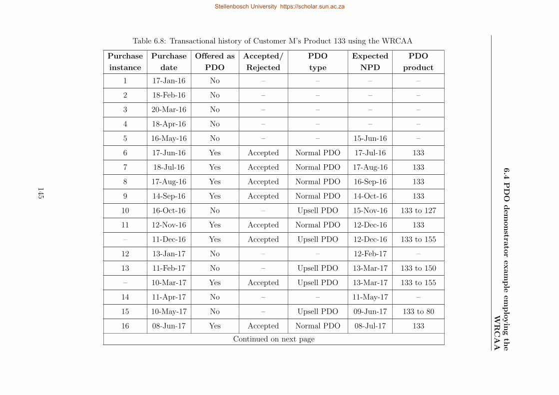
6.4
PDO
demonstra
torexample
employingth
eW
RCAA
Table 6.8: Transactional history of Customer M’s Product 133 using the WRCAA
Purchase
instance
Purchase
date
Offered as
PDO
Accepted/
Rejected
PDO
type
Expected
NPD
PDO
product
1 17-Jan-16 No – – – –
2 18-Feb-16 No – – – –
3 20-Mar-16 No – – – –
4 18-Apr-16 No – – – –
5 16-May-16 No – – 15-Jun-16 –
6 17-Jun-16 Yes Accepted Normal PDO 17-Jul-16 133
7 18-Jul-16 Yes Accepted Normal PDO 17-Aug-16 133
8 17-Aug-16 Yes Accepted Normal PDO 16-Sep-16 133
9 14-Sep-16 Yes Accepted Normal PDO 14-Oct-16 133
10 16-Oct-16 No – Upsell PDO 15-Nov-16 133 to 127
11 12-Nov-16 Yes Accepted Normal PDO 12-Dec-16 133
– 11-Dec-16 Yes Accepted Upsell PDO 12-Dec-16 133 to 155
12 13-Jan-17 No – – 12-Feb-17 –
13 11-Feb-17 No – Upsell PDO 13-Mar-17 133 to 150
– 10-Mar-17 Yes Accepted Upsell PDO 13-Mar-17 133 to 155
14 11-Apr-17 No – – 11-May-17 –
15 10-May-17 No – Upsell PDO 09-Jun-17 133 to 80
16 08-Jun-17 Yes Accepted Normal PDO 08-Jul-17 133
Continued on next page
145
Stellenbosch University https://scholar.sun.ac.za
Stellenbosch University https://scholar.sun.ac.za
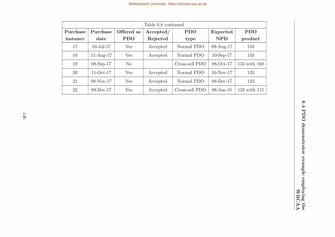
6.4
PDO
demonstra
torexample
employingth
eW
RCAA
Table 6.8 continued
Purchase
instance
Purchase
date
Offered as
PDO
Accepted/
Rejected
PDO
type
Expected
NPD
PDO
product
17 10-Jul-17 Yes Accepted Normal PDO 09-Aug-17 133
18 11-Aug-17 Yes Accepted Normal PDO 10-Sep-17 133
19 08-Sep-17 No – Cross-sell PDO 08-Oct-17 133 with 168
20 11-Oct-17 Yes Accepted Normal PDO 10-Nov-17 133
21 08-Nov-17 Yes Accepted Normal PDO 08-Dec-17 133
22 09-Dec-17 Yes Accepted Cross-sell PDO 08-Jan-18 133 with 115
146
Stellenbosch University https://scholar.sun.ac.za
Stellenbosch University https://scholar.sun.ac.za
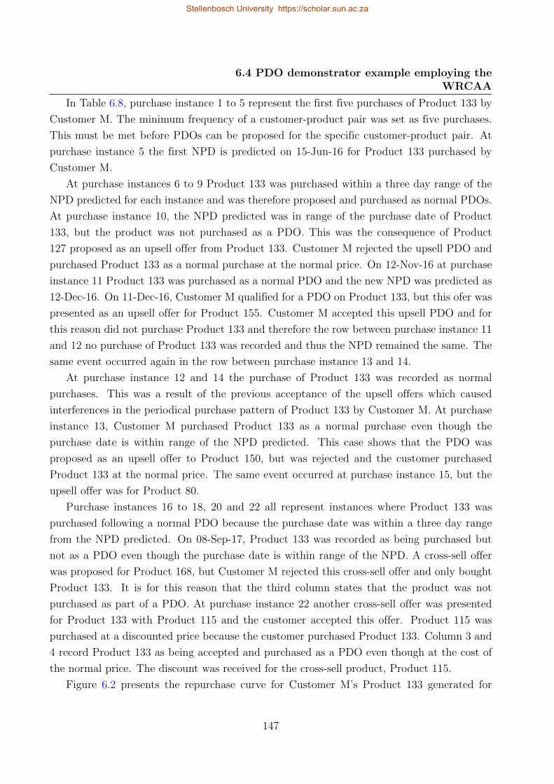
6.4 PDO demonstrator example employing theWRCAA
In Table 6.8, purchase instance 1 to 5 represent the first five purchases of Product 133 by
Customer M. The minimum frequency of a customer-product pair was set as five purchases.
This must be met before PDOs can be proposed for the specific customer-product pair. At
purchase instance 5 the first NPD is predicted on 15-Jun-16 for Product 133 purchased by
Customer M.
At purchase instances 6 to 9 Product 133 was purchased within a three day range of the
NPD predicted for each instance and was therefore proposed and purchased as normal PDOs.
At purchase instance 10, the NPD predicted was in range of the purchase date of Product
133, but the product was not purchased as a PDO. This was the consequence of Product
127 proposed as an upsell offer from Product 133. Customer M rejected the upsell PDO and
purchased Product 133 as a normal purchase at the normal price. On 12-Nov-16 at purchase
instance 11 Product 133 was purchased as a normal PDO and the new NPD was predicted as
12-Dec-16. On 11-Dec-16, Customer M qualified for a PDO on Product 133, but this ofer was
presented as an upsell offer for Product 155. Customer M accepted this upsell PDO and for
this reason did not purchase Product 133 and therefore the row between purchase instance 11
and 12 no purchase of Product 133 was recorded and thus the NPD remained the same. The
same event occurred again in the row between purchase instance 13 and 14.
At purchase instance 12 and 14 the purchase of Product 133 was recorded as normal
purchases. This was a result of the previous acceptance of the upsell offers which caused
interferences in the periodical purchase pattern of Product 133 by Customer M. At purchase
instance 13, Customer M purchased Product 133 as a normal purchase even though the
purchase date is within range of the NPD predicted. This case shows that the PDO was
proposed as an upsell offer to Product 150, but was rejected and the customer purchased
Product 133 at the normal price. The same event occurred at purchase instance 15, but the
upsell offer was for Product 80.
Purchase instances 16 to 18, 20 and 22 all represent instances where Product 133 was
purchased following a normal PDO because the purchase date was within a three day range
from the NPD predicted. On 08-Sep-17, Product 133 was recorded as being purchased but
not as a PDO even though the purchase date is within range of the NPD. A cross-sell offer
was proposed for Product 168, but Customer M rejected this cross-sell offer and only bought
Product 133. It is for this reason that the third column states that the product was not
purchased as part of a PDO. At purchase instance 22 another cross-sell offer was presented
for Product 133 with Product 115 and the customer accepted this offer. Product 115 was
purchased at a discounted price because the customer purchased Product 133. Column 3 and
4 record Product 133 as being accepted and purchased as a PDO even though at the cost of
the normal price. The discount was received for the cross-sell product, Product 115.
Figure 6.2 presents the repurchase curve for Customer M’s Product 133 generated for
147
Stellenbosch University https://scholar.sun.ac.za
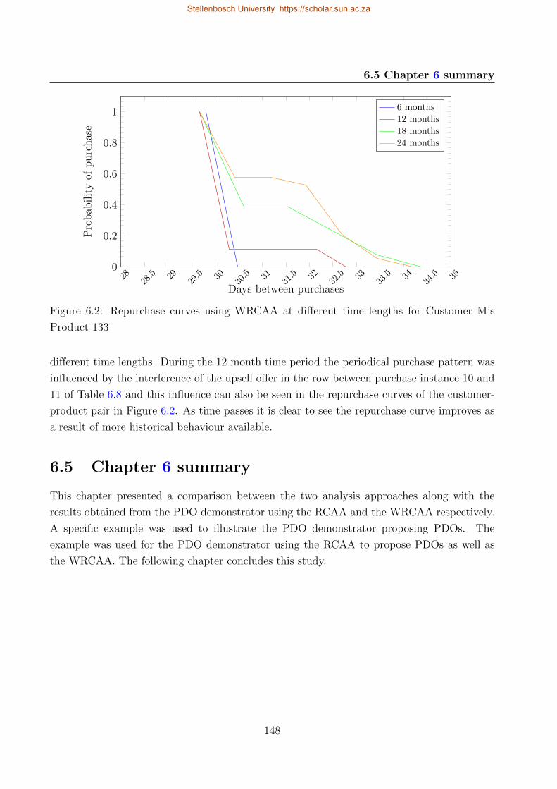
6.5 Chapter 6 summary
2828.5 29
29.5 30
30.5 31
31.5 32
32.5 33
33.5 34
34.5 35
0
0.2
0.4
0.6
0.8
1
Days between purchases
Pro
bab
ilit
yof
purc
has
e
6 months
12 months
18 months
24 months
Figure 6.2: Repurchase curves using WRCAA at different time lengths for Customer M’s
Product 133
different time lengths. During the 12 month time period the periodical purchase pattern was
influenced by the interference of the upsell offer in the row between purchase instance 10 and
11 of Table 6.8 and this influence can also be seen in the repurchase curves of the customer-
product pair in Figure 6.2. As time passes it is clear to see the repurchase curve improves as
a result of more historical behaviour available.
6.5 Chapter 6 summary
This chapter presented a comparison between the two analysis approaches along with the
results obtained from the PDO demonstrator using the RCAA and the WRCAA respectively.
A specific example was used to illustrate the PDO demonstrator proposing PDOs. The
example was used for the PDO demonstrator using the RCAA to propose PDOs as well as
the WRCAA. The following chapter concludes this study.
148
Stellenbosch University https://scholar.sun.ac.za
Chapter 7
Conclusion
The results of the proposed model were discussed in the previous chapter. This chapter
concludes the discussion of the study. A business model for the service, a summary of the
work done in the study and an appraisal of the work are presented. Lastly, suggestions for
future work based on the study are provided.
7.1 Business case
This section sheds some light on the business proposition this study has. The researcher
proposed a business model for this service by applying the Business Model Canvas designed
by Osterwalder and Pigneur (2013). The nine building blocks are stated and refined for this
initiative and shown in Figure 7.1. The researcher populated the nine building blocks with
the focus on this study.
The proposed service suggests a new and alternative way of thinking and conducting
business within the retail domain. The relationship between retailers and suppliers is of
utmost importance, not only for ensuring products are available on the shelves at reasonable
prices, but also ensuring promotional offers are available to customers.
The researcher conducted interviews with individuals working in the retail domain. The
conversations were focused on understanding how the relationship between retailers and sup-
pliers works and the decision-making process for discounted offers. Known knowledge was
shared and no information regarding retailers was disclosed (Bronkhorst, 2018; Snyman, 2017).
From these interviews the researcher could confirm that creating promotional offers can be
a stressful task for both the retailers and the suppliers. The relationship between these two
parties is tense and often not as one would like it to be. With this new innovation, the
retailer-supplier relationship can be strengthened by gaining purchasing behaviour informa-
tion regarding customers.
The question still stands: How will a supplier or retailer create revenue by proposing
discounted offers? The proposed system creates a holistic view of customers by including all
their purchases from different retailers. The system records transactional data of customers at
all the outlets subscribed to this service. The system can thus propose a personalised discount
offer (PDO) to a customer at a specific store that is different from where the customer usually
buys a specific product. The retail store thus sells a product that would normally be bought
at another store at a lower profit margin. These offers are instant and temporary, which expire
when the customer leaves the store. The PDOs proposed can also include cross-sell and upsell
products which ensures a higher profit margin and can also include a larger volume acquired.
149
Stellenbosch University https://scholar.sun.ac.za
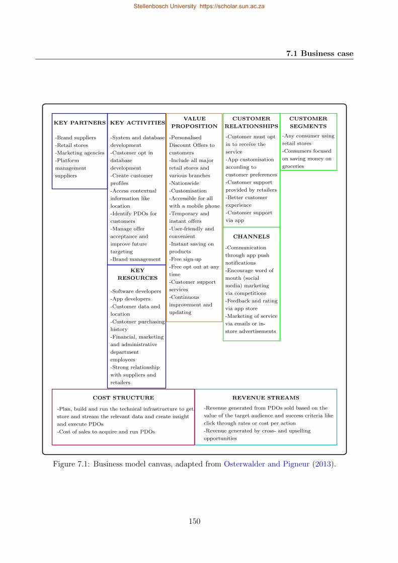
7.1 Business case
KEY PARTNERS
-Brand suppliers
-Retail stores
-Marketing agencies
-Platform
management
suppliers
KEY ACTIVITIES
-System and database
development
-Customer opt in
database
development
-Create customer
profiles
-Access contextual
information like
location
-Identify PDOs for
customers
-Manage offer
acceptance and
improve future
targeting
-Brand management
KEY
RESOURCES
-Software developers
-App developers
-Customer data and
location
-Customer purchasing
history
-Financial, marketing
and administrative
department
employees
-Strong relationship
with suppliers and
retailers
VALUE
PROPOSITION
-Personalised
Discount Offers to
customers
-Include all major
retail stores and
various branches
-Nationwide
-Customisation
-Accessible for all
with a mobile phone
-Temporary and
instant offers
-User-friendly and
convenient
-Instant saving on
products
-Free sign-up
-Free opt out at any
time
-Customer support
services
-Continuous
improvement and
updating
CUSTOMER
RELATIONSHIPS
-Customer must opt
in to receive the
service
-App customisation
according to
customer preferences
-Customer support
provided by retailers
-Better customer
experience
-Customer support
via app
CHANNELS
-Communication
through app push
notifications
-Encourage word of
mouth (social
media) marketing
via competitions
-Feedback and rating
via app store
-Marketing of service
via emails or in-
store advertisements
CUSTOMER
SEGMENTS
-Any consumer using
retail stores
-Consumers focused
on saving money on
groceries
COST STRUCTURE
-Plan, build and run the technical infrastructure to get,
store and stream the relevant data and create insight
and execute PDOs
-Cost of sales to acquire and run PDOs
REVENUE STREAMS
-Revenue generated from PDOs sold based on the
value of the target audience and success criteria like
click through rates or cost per action
-Revenue generated by cross- and upselling
opportunities
Figure 7.1: Business model canvas, adapted from Osterwalder and Pigneur (2013).
150
Stellenbosch University https://scholar.sun.ac.za
7.2 Summary of work done
These aspects make the proposed system different from existing loyalty programmes.
This initiative creates an opportunity for retailers to acquire potential customers by im-
proving the customer experience at the alternative outlet by proposing PDOs to them based
on their purchasing history. Customer experience is also improved by proposing PDOs via
push notifications when entering a store, thus customers do not have to check whether or not
they qualify for a PDO. None of the retailers receive information regarding other retailers
as the customer information is private and owned by the enterprise hosting this initiative.
Using the data gathered, further data analyses can be done in order to gain more information
regarding market satisfaction and preferences, which in turn can be provided to the suppliers
and retailers.
In order for this innovation to be successful some considerations are necessary. A mobile
application is necessary for the system to capture the relevant transactional data of the cus-
tomers and along with this a platform is required to access relevant informations regarding
participating retail outlets, e.g. outlet location. This innovation targets customers who have
access to mobile devices and data connectivity. Customers must subscribe to this PDO service
and be willing to share their location, purchasing behaviour and personal information in order
to receive personalised discount offers in return. The application must be used regularly in
order to benefit from the PDO opportunities which include cross-sell and upsell offers and
customers will be provided the opportunity to opt out at anytime. The retailers must partic-
ipate in this initiative in order for it to be attainable and also to receive beneficial value from
the service.
All enterprises are motivated to create a profit for the business and in order to do so the
customer relationship must have the highest priority. The personalisation of offers ensures a
higher acceptance rate and by including cross-selling and upselling offers, enterprises can ex-
pect an additional revenue stream. The personalisation of discount offers ultimately enhances
the customer experience and customer satisfaction, bettering the customer relationship.
7.2 Summary of work done
Chaper 1 introduced the study topic with a background and research assignment. The
objectives of the study are stated within this chapter along with a research methodology
determining how the objectives would be achieved. A scope of the study and deliverables
envisaged are also included in Chapter 1.
This chapter was followed by a literature study undertaken in Chapter 2. The literature
study provided a broad knowledge foundation to understand the essence of the study. This
study included a variety of domains such as Customer Relationship Management (CRM),
marketing, cross-selling and upselling, and data analytics. Most of the knowledge areas dis-
151
Stellenbosch University https://scholar.sun.ac.za
7.2 Summary of work done
cussed in the literature study are related back to the customer and were thus fundamental
to the study. CRM focuses on the relationship between customers and enterprises and pro-
vides activities to strengthen this relationship. One of the activities included marketing which
reflects on the communication between enterprises and customers. Cross-selling and upselling
are methods of retaining customers and also an important aspect when looking at proposing
offers to customers. The other aspects not directly related to the customer such as system
architecture, data analytics and Big Data were important to understand, because they would
be used in the study.
Chapter 3 introduced the proposed system by explaining the system architecture. The
system architecture was developed using Object-Process Methodology (OPM). OPM was
used because of the holistic view it provided of the proposed system. This chapter also
included some literature regarding OPM. The architecture of the proposed system was visu-
alised by three Object-Process Diagrams (OPD) accompanied by Object-Process Language
(OPL) which was generated for the desired system. The OPL described the system architec-
ture in natural language to make it easier for stakeholders to understand. Lastly, this chapter
schematically explained the relationship between the simulator and demonstrator models that
were necessary for the completion of the study.
Chapter 4 initiated the design and development of the proposed system starting with the
simulator. The simulator was designed to simulate pseudo-customer data showing purchasing
behaviour. The reason for simulating the customer behaviour was to overcome ethical issues
and to ensure the data are not lacking any information. The simulator was designed using
an Extended Entity-Relationship Diagram (EERD). The entities were identified by referring
back to the proposed architecture explained in Chapter 3. A theoretical description of the
entity–relationships was provided. The data tables of the proposed system were designed by
using the data dictionary provided in this chapter. The description of the development of the
simulator was done by discussing the population of each data table with data values. The
physical data tables were generated and populated using Matlab® and stored in Microsoft®
SQL Server, which served as the database for the system. The customer purchasing behaviour
was also stored in the database. On completion of Chapter 4, the first objective of the study
stated in Chapter 1 was achieved.
Chapter 5 contains the design and development of the PDO demonstrator. The PDO
demonstrator was designed to analyse the simulated data generated in order to identify and
propose PDOs to specific customers. The PDO demonstrator was also designed to propose
cross-sell and upsell products. In order to propose a personalised offer to a customer, one
must estimate when the customer anticipated buying the product again. This was done
designing the PDO predictor which analysed the historical transactional data of a customer.
Four analysis techniques were investigated where two of them were eventually used. These
152
Stellenbosch University https://scholar.sun.ac.za
7.3 Appraisal of work
were the arithmetical average technique, the weighted average technique, a repurchase curve
technique followed by a weighted repurchase curve technique. These analysis techniques were
compared and evaluated in order to identify the superior analysis approaches that were used
in the PDO predictor. From the evaluation, 32 test scenarios where identified to be executed
by the PDO demonstrator.
Chapter 6 comprised of a discussion of the results provided by the PDO demonstrator.
The PDO demonstrator was capable of proposing PDOs using the identified NPD-analysis
approaches. This chapter summarises the evaluation of the PDO demonstrator by introducing
the 32 test scenarios. An individual customer journey example was also presented to state
the difference between the RCAA and the WRCAA. The PDO demonstrator was capable of
proposing PDOs to customers based on their historical purchasing behaviour. Objective 2
was fulfilled by the completion of the work described in this chapter.
A business case was provided in Section 7.1 to shed light on the business proposition of
this innovation. An alternative way of proposing discount offers is recommended by proposing
personalised offers based on customer specific purchasing behaviour.
7.3 Appraisal of work
This section presents an appraisal of the work done during this study. The researcher found
that this topic is applicable within the field of industrial engineering and can contribute to
the retail domain. It is key for the reader to understand how this initiative differentiates
itself from existing loyalty programmes. The existing loyalty programmes are retail group
specific and thus only gather information regarding the current customers. The proposed
offers are rarely personalised and in the cases where they are, it is based on frequently bought
products and not periodically bought products. No other loyalty programme tries to propose
personalised offers to new customers.
The researcher does not propose this initiative to replace any existing discount offer system,
since the current systems focus on general public discount offers. This innovation is proposed
as an additional revenue stream created by targeting individual customers with personalised
offers. The researcher suggests an alternative approach of agreeing upon specialised offers
between retailers and suppliers. This could be a challenging process to implement in practice,
but can provide a stronger supplier-retailer relationship.
The system was developed using simulated data which might not reflect real life data
realistically. The researcher introduced different distributions to ensure the data values are
mixed. The acceptance and rejection probability was defined by the researcher, but in reality
this probability will be determined from analysing the customer data. The probability of
cross-sell and upsell opportunities can be altered by the enterprises and can even be adjusted
153
Stellenbosch University https://scholar.sun.ac.za
7.4 Future research
for different suppliers and retailers according to an agreement between the respective parties.
This innovation is focused on the retail setting within South Africa and the technology
available for the consumers in South Africa. Walgreens in the United States of America
partnered with Aisle 411 and Google Project Tango to create a 3D augmented reality to
Walgreens. Aisle 411 helps a customer search and map products to where they are located on
the shelf, whereas Project Tango can determine a user’s location within the store (Aisle411 and
Google Project Tango and Walgreens). This innovation proposes more a game-like shopping
experience and is limited to a Tango device and Walgreens store. This innovation does not
show any personalised discount offers based on specific customer transactional history.
So, the proposed system will ideally be compatible on any device and focuses on more
than one retailer and supplier. The essence of the developed system is that it proposes PDOs
to customers based on their transactional history. The value of the work lies in the analysis
of the transactional history data of a specific customer.
7.4 Future research
This study opens avenues for future work. This includes investigating other techniques for
analysing specific product repurchasing intervals to identify suitable instances to propose
PDOs. It will be beneficial to test the PDO demonstrator on actual customer data gathered
within South Africa. It is important to investigate the technical difficulties of implementing
this initiative in South Africa and determining the cost of the development and implementation
of a real system. The implementation of the proposed system will require experts from other
domains, e.g. marketing. The prospect of influencing potential customers and retailers is one
of the many exciting, challenging aspects of industrial engineering. If the system is successfully
implemented the next step would be to implement the option of proposing PDOs to customers
as the customers pass the PDO product in the aisle.
7.5 Chapter 7 summary
This chapter concludes this study with a business case which describes the business proposition
of this innovation. This is accompanied by a summary of the work done and an appraisal
thereof. The study is concluded with an outline of suggestions for possible future work.
154
Stellenbosch University https://scholar.sun.ac.za
References
G. Adomavicius and A. Tuzhilin. Using data mining methods to build customer profiles.
Computer, 34(2):74–81, 2001. DOI: http://dx.doi.org/10.1109/2.901170. 24, 26, 34
A. Agarwal, C. Baechle, R. S. Behara, and V. Rao. Multi-method approach to wellness
predictive modeling. Journal of Big Data, 3(1):15, 2016. DOI: http://dx.doi.org/10.
1186/s40537-016-0049-0. 60, 61
R. Agrawal and R. Srikant. Fast Algorithms for Mining Association Rules. In Proceedings of
the 20th VLDB Conference, pages 487–499, 1994. ISBN 1-55860-153-8. 36, 37, 57
R. Agrawal and R. Srikant. Mining sequential patterns. In Proceedings of the Eleventh
International Conference on Data Engineering, pages 3–14, 1995. DOI: http://dx.doi.
org/10.1109/ICDE.1995.380415. 39
Aisle411 and Google Project Tango and Walgreens. Aisle411. http://www.xpertekcontact.
co.za/aisle-411/index.html?re=1&te=1. [Online Accessed: 30/05/2018]. 154
H. Albert-Lorincz and J.-F. Boulicaut. A framework for frequent sequence mining under gen-
eralized regular expression constraints. In Proceedings of the Second International Workshop
on Knowledge Discovery in Inductive Databases, pages 2–16, 2003a. ISBN 953-6690-34-9.
39
H. Albert-Lorincz and J.-F. Boulicaut. Mining frequent sequential patterns under regular
expressions: a highly adaptative strategy for pushing constraints. In Proceedings of the
Third SIAM International Conference on Data Mining, pages 316–320, 2003b. DOI: http:
//dx.doi.org/10.1137/1.9781611972733.37. 39
M. Aldenderfer and R. Blashfield. Cluster analysis. Quantitative applications in the social
sciences. Sage Publications, 1984. DOI: http://dx.doi.org/10.4135/9781412983648. 63
W.-H. Au and K. C. C. Chan. Mining Fuzzy Association Rules in a Bank-Account Database.
IEEE Transactions on Fuzzy Systems, 11(2):238–248, 2003. DOI: http://dx.doi.org/10.
1109/TFUZZ.2003.809901. 34
J. Ayres, J. Flannick, J. Gehrke, and T. Yiu. Sequential pattern mining using a bitmap
representation. In Proceedings of the eighth ACM SIGKDD international conference on
Knowledge discovery and data mining, pages 429–435, 2002. DOI: http://dx.doi.org/
10.1145/775047.775109. 39
155
Stellenbosch University https://scholar.sun.ac.za
REFERENCES
A. Azevedo and M. F. Santos. KDD, SEMMA and CRISP-DM: a parallel overview. In IASIS
European Conference on Data Mining, volume 8, pages 182–185, 2008. ISBN 978-972-8924-
63-8. 52
D. M. Bates and D. G. Watts. Nonlinear regression analysis and its applications. 2008. DOI:
http://dx.doi.org/10.1002/9780470316757. 67
C. Bauckhage, B. Gorman, C. Thurau, and M. Humphrys. Learning human behavior from
analyzing activities in virtual environments. In J. H. Israel and A. Naumann, editors, MMI
Interaktiv - Human: Vol. 1, No. 12, pages 3–17, 2007. http://dl.gi.de/handle/20.500.
12116/5326 [Online Accessed: 17/05/2017]. 52
S. Ben-David and S. Shalev-Shwartz. Understanding Machine Learning: From Theory to
Algorithms. Cambridge: Cambridge University Press, New York, 2014. DOI: http://dx.
doi.org/10.1017/CBO9781107298019. 52, 57, 60, 66, 67
C. M. Bishop. Pattern recognition and machine learning. Springer, 2006. ISBN 978-1-4939-
3843-8. 66
J. M. Bland and D. G. Altman. Survival probabilities (Kaplan-Meier). British Medical Journal,
317(7172):1572, 1998. DOI: https://doi.org/10.1136/bmj.317.7172.1572. 44
J. Z. Bloom. Tourist market segmentation with linear and non-linear techniques. Tourism
Management, 25(6):723–733, 2004. DOI: https://doi.org/10.1016/j.tourman.2003.
07.004. 61
N. H. Borden. The Concept of the Marketing Mix. Journal of Advertising Research, 2
(Classics):7–12, 1964. ISSN 0021-8499. 12
I. Bose and X. Chen. Quantitative models for direct marketing: A review from systems
perspective. European Journal of Operational Research, 195(1):1–16, 2009. DOI: http:
//dx.doi.org/10.1016/j.ejor.2008.04.006. 17
C. Bounsaythip and E. Rinta-Runsala. Overview of Data Mining for Customer Behavior
Modeling. Research report, VTT Information Technology, June 2001. https://www.inf.
utfsm.cl/~mcriff/Tesistas/lista-papers/customerprofiling.pdf [Online Accessed:
30/08/2017]. 13, 24, 25, 26, 30, 31, 32, 35, 36, 57, 58, 64, 65
L. Breiman, J. Friedman, C. J. Stone, and R. A. Olshen. Classification and regression trees.
Chapman and Hall, 2017. ISBN 0412048418. 60
J. Bronkhorst, 2018. Personal interview with Jannes Bronkhorst. 149
156
Stellenbosch University https://scholar.sun.ac.za
REFERENCES
L. Campbell and W. D. Diamond. Framing and sales promotions: The characteristics of a
”Good Deal”. Journal of Consumer Marketing, 7(4):25–31, 1990. DOI: http://dx.doi.
org/10.1108/EUM0000000002586. 21
C.-C. H. Chan. Online auction customer segmentation using a neural network model. Inter-
national Journal of Applied Science and Engineering, 3(2):101–109, 2005. ISSN 1727-2394.
https://www.cyut.edu.tw/~ijase/index1_en.htm. 61
S. W. Changchien, C. F. Lee, and Y. J. Hsu. On-line personalized sales promotion in electronic
commerce. Expert Systems with Applications, 27(1):35–52, 2004. DOI: https://doi.org/
10.1016/j.eswa.2003.12.017. 17, 18, 19, 22, 34
P. Chapman, J. Clinton, R. Kerber, T. Khabaza, T. Reinartz, C. Shearer, and R. Wirth. Crisp-
Dm 1.0. Technical report, 2000. https://www.the-modeling-agency.com/crisp-dm.pdf
[Online Accessed: 30/08/2017]. 35, 55, 56
S. Chatterjee and A. S. Hadi. Regression analysis by example. John Wiley & Sons, 4th edition,
2006. DOI: http://dx.doi.org/10.1002/0470055464. 67
C. L. P. Chen and C. Y. Zhang. Data-intensive applications, challenges, techniques and
technologies: A survey on Big Data. Information Sciences, 275:314–347, 2014. DOI: http:
//dx.doi.org/10.1016/j.ins.2014.01.015. 27, 72
M.-C. Chen, A.-L. Chiu, and H.-H. Chang. Mining changes in customer behavior in retail
marketing. Expert Systems with Applications, 28(4):773–781, 2005a. DOI: http://dx.doi.
org/10.1016/j.eswa.2004.12.033. 17, 28, 29, 30, 34
Y.-L. Chen, K. Tang, R.-J. Shen, and Y.-H. Hu. Market basket analysis in a multiple store
environment. Decision Support Systems, 40(2):339–354, 2005b. DOI: http://dx.doi.org/
10.1016/j.dss.2004.04.009. 32
S. Chiu and D. Tavella. Chapter 7 - Introduction to Data Mining. In Data Mining
and Market Intelligence for Optimal Marketing Returns, pages 137–192. Butterworth-
Heinemann, Boston, 2008. ISBN 978-0-7506-8234-3. DOI: http://dx.doi.org/10.1016/
B978-0-7506-8234-3.00007-1. 63
F. R. David. E-Crm From a Supply Chain Management Perspective. Information Systems
Management, 22(1):37–44, 2005. DOI: http://dx.doi.org/10.1201/1078/44912.22.1.
20051201/85737.5. 23, 63
A. De Mauro, M. Greco, and M. Grimaldi. A formal definition of Big Data based on its
essential features. Library Review, 65(3):122–135, 2016. DOI: http://dx.doi.org/10.
1108/LR-06-2015-0061. 45, 46, 47
157
Stellenbosch University https://scholar.sun.ac.za
REFERENCES
J. Dean. Big Data, Data Mining, and Machine Learning: Value creation for business leaders
and practitioners. John Wiley & Sons, Hoboken, N.J., 2014. ISBN 978-1-118-61804-2.
https://books.google.co.za/books?isbn=1118920708. 17, 28, 29, 50, 52, 53, 57, 60,
61, 63, 66
Y. Demchenko, C. De Laat, and P. Membrey. Defining architecture components of the Big
Data Ecosystem. In International Conference on Collaboration Technologies and Systems,
pages 104–112, 2014. DOI: http://dx.doi.org/10.1109/CTS.2014.6867550. 45, 47
A. Demiriz. Enhancing Product Recommender Systems on Sparse Binary Data. Data Min-
ing and Knowledge Discovery, 9(2):147–170, 2004. DOI: http://dx.doi.org/10.1023/B:
DAMI.0000031629.31935.ac. 34
D. Dori. Object-Process Methodology. Springer, Berlin, 2002. DOI: http://dx.doi.org/10.
1007/978-3-642-56209-9. 71, 72, 75, 76
L. Du Plessis and M. De Vries. Towards a holistic customer experience management framework
for enterprises. South African Journal of Industrial Engineering, 27(3):23–36, 2016. DOI:
http://dx.doi.org/10.7166/27-3-1624. 8
A. Dursun and M. Caber. Using data mining techniques for profiling profitable hotel cus-
tomers: An application of RFM analysis. Tourism Management Perspectives, 18:153–160,
2016. DOI: http://dx.doi.org/10.1016/j.tmp.2016.03.001. 28, 29
J. Dyche and P. A. Wesley. The CRM handbook: A business guide to customer relationship
management. Addison Wesley, Boston, 2002. ISBN 0201730626. https://books.google.
co.za/books?isbn=0201730626. 10, 14, 17, 30, 35, 58
T. Erl, W. Khattak, and P. Buhler. Big Data Fundamentals: Concepts, Drivers & Techniques.
Prentice Hall Press, New Jersey, 1st edition, 2015. ISBN 0134291077. https://books.
google.co.za/books?isbn=0134291077. 17, 47, 48, 49, 58, 59, 62, 65, 66, 67
S. Fan, R. Y. K. Lau, and J. L. Zhao. Demystifying Big Data Analytics for Business Intel-
ligence Through the Lens of Marketing Mix. Big Data Research, 2(1):28–32, 2015. DOI:
http://dx.doi.org/10.1016/j.bdr.2015.02.006. 25, 68, 69
U. M. Fayyad. Data mining and knowledge discovery: making sense out of data. IEEE Expert:
Intellegent Systems and Their Applications, 11(5):20–25, 1996. DOI: http://dx.doi.org/
10.1109/64.539013. 52, 54
B. C. Fung, K. Wang, A. W.-C. Fu, and S. Y. Philip. Introduction to privacy-preserving
data publishing. Chapman & Hall/CRC, Boca Raton, FL, 1st edition, 2010. ISBN
9781420091502. https://books.google.co.za/books?isbn=1420091506. 70, 71
158
Stellenbosch University https://scholar.sun.ac.za
REFERENCES
A. Gallant. Nonlinear regression. The American Statistician, 29(2):73–81, 1975. DOI: http:
//dx.doi.org/10.2307/2683268. 67
A. Gandomi and M. Haider. Beyond the hype: Big data concepts, methods, and analytics.
International Journal of Information Management, 35(2):137–144, 2015. DOI: http://dx.
doi.org/10.1016/j.ijinfomgt.2014.10.007. 45, 47, 48, 49
M. N. Garofalakis, R. Rastogi, and K. Shim. SPIRT: Sequential pattern mining with reg-
ular expression constraints. In 25th International Conference on Very Large Databases,
VLDB‘99, pages 223–234, 1999. ISBN 1-55860-615-7. http://www.vldb.org/conf/1999/
P22.pdf [Online Accessed: 30/07/2017]. 39
F. Gens. The 3rd Platform: Enabling Digital Transformation, 2013. http:
//achievabledigitaltransformation.com/tcs-white-paper_244515.pdf [Online Ac-
cessed: 15/05/2017]. 1
D. Gentile, N. Spiller, and G. Noci. How to sustain the customer experience: An overview
of experience components that co-create value with the customer. European Management
Journal, 25(5):395–410, 2007. DOI: http://dx.doi.org/10.1016/j.emj.2007.08.0054.
8
M. Gera and S. Goel. Data mining-techniques, methods and algorithms: A review on tools
and their validity. International Journal of Computer Applications, 113(18), 2015. DOI:
http://dx.doi.org/10.5120/19926-2042. 66, 67
P. Giudici and G. Passerone. Data mining of association structures to model consumer be-
haviour. Computational Statistics & Data Analysis, 38(4):533–541, 2002. DOI: http:
//dx.doi.org/10.1016/S0167-9473(01)00077-9. 30, 34
C. L. Goi. A Review of Marketing Mix: 4Ps or More? International Journal of Marketing
Studies, 1(1):2–15, 2009. DOI: http://dx.doi.org/10.5539/ijms.v1n1p2. 12
M. Halkidi, Y. Batistakis, and M. Vazirgiannis. On clustering validation techniques. Journal
of intelligent information systems, 17(2):107–145, 2001. DOI: https://doi-org.ez.sun.
ac.za/10.1023/A:1012801612483. 63
J. Han and J. Pei. Mining frequent patterns by pattern-growth. ACM SIGKDD Explorations
Newsletter, 2(2):14–20, 2000. DOI: http://dx.doi.org/10.1145/380995.381002. 41
J. Han, J. Pei, B. Mortazavi-Asl, Q. Chen, U. Dayal, and M.-C. Hsu. Freespan: frequent
pattern-projected sequential pattern mining. In Proceedings of the sixth ACM SIGKDD
international conference on Knowledge discovery and data mining, pages 355–359, 2000.
DOI: http://dx.doi.org/10.1145/347090.347167. 41
159
Stellenbosch University https://scholar.sun.ac.za
REFERENCES
J. Han, J. Pei, B. Mortazavi-Asl, H. Pinto, Q. Chen, U. Dayal, and M. Hsu. Prefixspan:
Mining sequential patterns efficiently by prefix-projected pattern growth. In Proceedings
of the 17th International Conference of Data Engineering, pages 215–224, 2001. DOI:
http://dx.doi.org/10.1109/ICDE.2001.914830. 41
F. E. Harrell. Regression Modeling Strategies, volume 64. Springer, Cham, 2nd edition, 2015.
DOI: http://dx.doi.org/10.1007/978-1-4757-3462-1. 43, 44
D. W. Hosmer Jr, S. Lemeshow, and R. X. Sturdivant. Applied Logistic Regression, volume
398. John Wiley & Sons, 2013. ISBN 978-0-470-58247-3. 67
B. Hssina, A. Merbouha, H. Ezzikouri, and M. Erritali. A comparative study of decision tree
ID3 and C4.5. International Journal of Advanced Computer Science and Applications, 4
(2):13–19, 2014. DOI: http://dx.doi.org/10.14569/SpecialIssue.2014.040203. 60
J.-J. Huang, G.-H. Tzeng, and C.-S. Ong. Marketing segmentation using support vector
clustering. Expert systems with applications, 32(2):313–317, 2007. DOI: http://dx.doi.
org/10.1016/j.eswa.2005.11.028. 60
A. J. Izenman. Modern Multivariate Statistical Techniques: regression, classification, and
Manifold Learning, volume 1. Springer, 2008. DOI: http://dx.doi.org/10.1007/
978-0-387-78189-1. 61, 63
S. M. H. Jansen. Customer segmentation for a mobile telecommunications company based
on service usage behavior. PhD thesis, University of Maastricht, 2007. https://pdfs.
semanticscholar.org/7a3a/688783e0424bd89f7413138bbfc24deeef8f.pdf [Online Ac-
cessed: 03/06/2017]. 26, 60, 63
J. R. Jiao, Y. Zhang, and M. Helander. A Kansei mining system for affective design. Expert
Systems with Applications, 30(4):658–673, 2006. DOI: http://dx.doi.org/10.1016/j.
eswa.2005.07.020. 17, 34
R. Kahan. Using database marketing techniques to enhance your one-to-one marketing ini-
tiatives. Journal of Consumer Marketing, 15(5):491–493, 1998. DOI: http://dx.doi.org/
10.1108/07363769810235965. 28
M. Kamber, J. Han, and J. Pei. Data Mining: Concepts and Techniques. Morgan Kaufmann
Publishers, Waltham, MA, 3rd edition, 2012. ISBN 978-0-12-381479-1. DOI: https://doi.
org/10.1016/C2009-0-61819-5. 16, 17, 30, 31, 32, 41, 43, 52, 57, 58, 59, 60, 61, 62, 63,
64, 70
160
Stellenbosch University https://scholar.sun.ac.za
REFERENCES
K. E. Kendall and J. E. Kendall. Systems Analysis and Design. Pearson Education, 9th edi-
tion, 2014. ISBN 0273788515. https://books.google.co.za/books?isbn=0273788515.
86, 87, 88, 90, 103
F. Khodakarami and Y. E. Chan. Exploring the role of customer relationship management
(CRM) systems in customer knowledge creation. Information & Management, 51(1):27–42,
2013. DOI: http://dx.doi.org/10.1016/j.im.2013.09.001. 16
S.-Y. Kim, T.-S. Jung, E.-H. Suh, and H.-S. Hwang. Customer segmentation and strategy de-
velopment based on customer lifetime value: A case study. Expert systems with applications,
31(1):101–107, 2006. DOI: https://doi.org/10.1016/j.eswa.2005.09.004. 60
N. J. King and P. W. Jessen. Profiling the mobile customer - Privacy concerns when be-
havioural advertisers target mobile phones - Part I. Computer Law and Security Review, 26
(5):455–478, 2010. DOI: http://dx.doi.org/10.1016/j.clsr.2010.07.001. 25, 68, 69,
70
F. Kohlmayer, F. Prasser, C. Eckert, and K. A. Kuhn. A flexible approach to distributed data
anonymization. Journal of Biomedical Informatics, 50:62–76, 2014. DOI: http://dx.doi.
org/10.1016/j.jbi.2013.12.002. 71
P. Kotler, G. Armstrong, and M. O. Opresnik. Principles of marketing. Pearson, 17th edition,
2018. ISBN 9780134492513. https://books.google.co.za/books?isbn=1292220171. 12,
13, 18, 19, 21, 22
S. B. Kotsiantis. Supervised machine learning: A review of classification techniques. In
Proceedings of the 2007 Conference on Emerging Artificial Intelligence Applications in
Computer Engineering: Real Word AI Systems with Applications in eHealth, HCI, Infor-
mation Retrieval and Pervasive Technologies, pages 3–24, 2007. ISBN 978-1-58603-780-2.
http://dl.acm.org/citation.cfm?id=1566770.1566773. 60, 61
G. J. Krishna and V. Ravi. Evolutionary computing applied to customer relationship manage-
ment: A survey. Engineering Applications of Artificial Intelligence, 56:30–59, 2016. ISSN
09521976. DOI: http://dx.doi.org/10.1016/j.engappai.2016.08.012. 10, 11, 23, 24,
25, 27, 30
B. F. Kubiak and P. Weichbroth. Cross-and up-selling techniques in e-
commerce activities. Journal of Internet Banking and Commerce, 15(3):1–
7, 2010. ISSN 1204-5357. http://www.icommercecentral.com/open-access/
cross-and-upselling-techniques-in-ecommerce-activities-1-7.php?aid=38427
[Online Accessed = 03/05/2017]. 12, 23, 24
161
Stellenbosch University https://scholar.sun.ac.za
REFERENCES
R. Kuo, Y. An, H. Wang, and W. Chung. Integration of self-organizing feature maps neural
network and genetic k-means algorithm for market segmentation. Expert systems with
applications, 30(2):313–324, 2006. DOI: http://dx.doi.org/10.1016/j.eswa.2005.07.
036. 61, 63
Y. Lakshmi Prasad. Big Data Analytics Made Easy. Notion Press, Inc., 1st edition, 2016.
ISBN 9781946390721. https://books.google.co.za/books?isbn=1946390720. 47, 48,
49, 57, 60, 61, 62, 66, 67, 131
R. Lanjewar and O. P. Yadav. Understanding of Customer Profiling and Segmentation Us-
ing K-Means Clustering Method for Raipur Sahkari Dugdh Sangh Milk Products. In-
ternational Journal of Research in Computer and Communication Technology, 2(3):103–
107, 2013. http://www.ijrcct.org/index.php/ojs/article/view/189/147 [Online Ac-
cessed: 07/07/2017]. 25, 52, 63
B. Lariviere and D. Van Den Poel. Investigating the role of product features in preventing
customer churn, by using survival analysis and choice modeling: The case of financial
services. Expert Systems with Applications, 27(2):277–285, 2004. DOI: http://dx.doi.
org/10.1016/j.eswa.2004.02.002. 44, 45, 66
B. Lariviere and D. Van Den Poel. Investigating the post-complaint period by means of
survival analysis. Expert Systems with Applications, 29(3):667–677, 2005. DOI: http:
//dx.doi.org/10.1016/j.eswa.2005.04.035. 43, 44, 45, 66
D. T. Larose. Discovering knowledge in data: an introduction to data mining. John Wiley &
Sons, 2nd edition, 2014. ISBN 1118873572. https://books.google.co.za/books?isbn=
1118873572. 60
T.-S. Lee, C.-C. Chiu, Y.-C. Chou, and C.-J. Lu. Mining the customer credit using clas-
sification and regression tree and multivariate adaptive regression splines. Computational
Statistics & Data Analysis, 50(4):1113–1130, 2006. DOI: http://dx.doi.org/10.1016/j.
csda.2004.11.006. 34
R. Li. Top 10 data mining algorithms, explained, 2015. http://www.kdnuggets.com/2015/
05/top-10-data-mining-algorithms-explained.html [Online Accessed: 27/07/2017].
61
C. Luo and S. M. Chung. A scalable algorithm for mining maximal frequent sequences using
sampling. In 16th IEEE International Conference on Tools with Artificial Intelligence, pages
156–165. IEEE, 2004. 39
162
Stellenbosch University https://scholar.sun.ac.za
REFERENCES
T. S. Madhulatha. Comparison between k-means and k-medoids clustering algorithms. Ad-
vances in Computing and Information Technology, pages 472–481, 2011. DOI: http:
//dx.doi.org/10.1007/978-3-642-22555-0_48. 63
E. C. Malthouse. Mining for trigger events with survival analysis. Data Mining and Knowledge
Discovery, 15(3):383–402, 2007. DOI: http://dx.doi.org/10.1007/s10618-007-0074-x.
44, 45
G. Mansingh, L. Rao, K.-M. Osei-Bryson, and A. Mills. Profiling internet banking users: A
knowledge discovery in data mining process model based approach. Information Systems
Frontiers, pages 193–215, 2013. DOI: http://dx.doi.org/10.1007/s10796-012-9397-2.
52, 67
G. Mariscal, O. Marban, and C. Fernandez. A survey of data mining and knowledge discovery
process models and methodologies. The Knowledge Engineering Review, 25(2):137–166,
2010. DOI: http://dx.doi.org/10.1017/S0269888910000032. 53, 54, 56
F. Masseglia, F. Cathala, and P. Poncelet. The psp approach for mining sequential patterns.
In European Symposium on Principles of Data Mining and Knowledge Discovery, pages
176–184. Springer, 1998. DOI: http://dx.doi.org/10.1007/BFb0094818. 39
J. McFall. Priority Patterns and Consumer Behavior. Journal of Marketing, 33(4):50–55,
1969. DOI: http://dx.doi.org/10.2307/1248673. 41
D. C. Montgomery, E. A. Peck, and G. G. Vining. Introduction to linear regression analysis.
John Wiley & Sons, 5th edition, 2012. ISBN 1119180171. 67
C. H. Mooney and J. F. Roddick. Sequential Pattern Mining: Approaches and Algo-
rithms. ACM Computing Surveys, 45, 2013. DOI: http://dx.doi.org/10.1145/2431211.
2431218. 34, 35, 36, 37, 39, 41
J. Mouton. How to succeed in your master’s and doctoral studies: A South African guide and
resource book. Van Schaik, 2001. 4
A. G. Mumuni and K. O’Reilly. Examining the Impact of Customer Relationship Management
on Deconstructed Measures of Firm Performance. Journal of Relationship Marketing, 13
(2):89–107, 2014. DOI: http://dx.doi.org/10.1080/15332667.2014.910073. 8, 9, 10,
15
T. T. Nagle, J. E. Hogan, and J. Zale. The Strategy and Tactics of Pricing: A Guide to
Growing More Profitably. Pearson, 5th edition, 2014. ISBN 978-1-292-02323-6. https:
//books.google.co.za/books?isbn=1292036419. 22
163
Stellenbosch University https://scholar.sun.ac.za
REFERENCES
E. W. T. Ngai, L. Xiu, and D. C. K. Chau. Application of data mining techniques in customer
relationship management: A literature review and classification. Expert Systems with Ap-
plications, 36:2592–2602, 2009. DOI: http://dx.doi.org/10.1016/j.eswa.2008.02.021.
8, 9, 14, 30, 52, 62, 132
S. Orlando, R. Perego, and C. Silvestri. A new algorithm for gap constrained sequence mining.
In SAC Proceedings of the 2004 ACM symposium on Applied computing, pages 540–547,
2004. DOI: http://dx.doi.org/10.1145/967900.968014. 39
A. Osterwalder and Y. Pigneur. Business Model Generation: A Handbook for Visionaries,
Game Changers, and Challengers. John Wiley & Sons., 2013. ISBN 978-1-118-65640-2.
149, 150
L. Paas. Acquisition pattern analysis for evolutionary database marketing. The Ser-
vice Industries Journal, 29(6):805–812, 2009. DOI: http://dx.doi.org/10.1080/
02642060902749336. 42
L. J. Paas. Mokken scaling characteristic sets and acquisition patterns of durable- and financial
products. Journal of Economic Psychology, 19:353–376, 1998. DOI: http://dx.doi.org/
10.1016/S0167-4870(98)00011-7. 28, 42
L. J. Paas and I. W. Molenaar. Analysis of acquisition patterns: A theoretical and empirical
evaluation of alternative methods. International Journal of Research in Marketing, 22(1):
87–100, 2005. DOI: http://dx.doi.org/10.1016/j.ijresmar.2004.04.001. 42
L. J. Paas, A. A. A. Kuijlen, and T. B. C. Poiesz. Acquisition pattern analysis for relationship
marketing: A conceptual and methodological redefinition. The Service Industries Journal,
25(5):661–673, 2005. DOI: http://dx.doi.org/10.1080/02642060500100999. 16, 42
N. Paley. The Manager’s Guide to COMPETITIVE MARKETING STRATEGIES. Thoro-
good, London, 3rd edition, 2005. ISBN 1854183702. https://books.google.co.za/
books?isbn=1854183656. 18, 19, 21
N. Paley. The Marketing Strategy Desktop Guide. Thorogood, 2nd edition, 2007. ISBN
9781854184900. https://books.google.co.za/books?isbn=1854184903. 16, 18, 21
M. Paliwal and U. A. Kumar. Neural networks and statistical techniques: A review of ap-
plications. Expert systems with applications, 36(1):2–17, 2009. DOI: http://dx.doi.org/
10.1016/j.eswa.2007.10.005. 61, 66
V. Paramasivam, T. S. Yee, S. K. Dhillon, and A. S. Sidhu. A methodological review of
data mining techniques in predictive medicine: An application in hemodynamic prediction
164
Stellenbosch University https://scholar.sun.ac.za
REFERENCES
for abdominal aortic aneurysm disease. Biocybernetics and Biomedical Engineering, 34(3):
139–145, 2014. DOI: http://dx.doi.org/10.1016/j.bbe.2014.03.003. 60
A. Perrin. Social Media Usage: 2005-2015. Pew Research Center, pages 1–11, 2015. http://
www.pewinternet.org/2015/10/08/social-networking-usage-2005-2015/ [Online Ac-
cessed: 03/03/2017]. 2
J. R. Quinlan. C4. 5: programs for machine learning. Elsevier, 2014. ISBN 1-55860-238-0. 60
A. Rajarajeswari and R. M. Ravindran. A comparative study of k-means k-medoid and
enhanced k-medoid algorithms. International Journal of Advance Foundation and Research
in Computer (IJAFRC), 2(8):7–10, 2015. https://pdfs.semanticscholar.org/6854/
e0d6554fefaa69d561e4133dc7149d33606d.pdf [Online Accessed: 04/04/2017]. 63
V. Rajaraman. Big data analytics. Resonance, 21(8), 2016. DOI: http://dx.doi.org/10.
1007/s12045-016-0376-7. 49, 52
M. D. Rechenthin. Machine-learning classification techniques for the analysis and prediction
of high-frequency stock direction. The University of Iowa, 2014. https://ir.uiowa.edu/
etd/4732/. 60, 61
W. Reinartz, M. Krafft, and W. D. Hoyer. The Customer Relationship Management Process
: Its Measurement and Impact on Performance. Journal of Marketing Research, 41(3):
293–305, 2004. DOI: http://dx.doi.org/10.1509/jmkr.41.3.293.35991. 8, 9, 10
R. Riffenburgh. Statistics in Medicine. Elsevier Science, 2011. ISBN 9780080541747. https:
//books.google.co.za/books?id=zoipeXzsA7IC. 67
L. Rokach and O. Maimon. Data mining with decision trees: theory and applications. ISBN
978-9814590082. 60
L. B. Romdhane, N. Fadhel, and B. Ayeb. An efficient approach for building customer profiles
from business data. Expert Systems with Applications, 37(2):1573–1585, 2010. DOI: http:
//dx.doi.org/10.1016/j.eswa.2009.06.050. 25, 26
S. M. Ross. Simulation. Academic Press, 5th edition, 2013. ISBN 978-0-12-415825-2. 106
S. Rosset, E. Neumann, U. Eick, and N. Vatnik. Customer Lifetime Value Models for Decision
Support. Data Mining and Knowledge Discovery, 7(3):321–339, 2003. DOI: http://dx.
doi.org/10.1023/A:1024036305874. 44, 45, 67
A. Ruckstuhl. Introduction to nonlinear regression. 2010. https://pdfs.semanticscholar.
org/8fa1/3fead47cc6ecf3d27de9e682dcef36c77502.pdf. 67
165
Stellenbosch University https://scholar.sun.ac.za
REFERENCES
P. Russom. Big Data Analytics Guidebook. TMforum Research, (May):73–76, 2016. 2
M. T. Salazar, T. Harrison, and J. Ansell. An approach for the identification of cross-sell
and up-sell opportunities using a financial services customer database. Journal of Financial
Services Marketing, 12(2):115–131, 2007. DOI: http://dx.doi.org/10.1057/palgrave.
fsm.4760066. 11, 23, 24, 42, 43, 67
M. T. Salazar, T. Harrison, and J. Ansell. An Analytical Framework to Stimulate Cross-
Selling and Retention in the UK Financial Services Industry: A Case Study. Revolution
in Marketing: Market Driving Changes, (1):246–251, 2015. DOI: http://dx.doi.org/10.
1007/978-3-319-11761-4_112. 10
N. J. Salkind. Encyclopedia of measurement and statistics, volume 1. Sage, 2007. ISBN
1-4129-1611-9. 61, 66, 67
L. Savary and K. Zeitouni. Indexed Bit Map (IBM) for mining frequent sequences. In 9th
European Conference on Principles and Practice of Knowledge Discovery in Databases,
pages 659–666. Springer, 2005. DOI: http://dx.doi.org/10.1007/11564126_70. 40
S. Schiffman. Upselling Techniques: That Really Works! Adams Media, Avon, 1st edition,
2005. ISBN 9781440500855. https://books.google.co.za/books?isbn=1440500851. 23
J. Schmidhuber. Deep Learning in neural networks: An overview. Neural Networks, 61:85–117,
2015. DOI: http://dx.doi.org/10.1016/j.neunet.2014.09.003. 57
P. Schmitt, B. Skiera, and C. Van den Bulte. Referral programs and customer value. Journal
of Marketing, 75(1):46–59, 2011. DOI: http://dx.doi.org/10.1509/jmkg.75.1.46. 9
M. Seno and G. Karypis. SLPMiner: An algorithm for finding frequent sequential patterns
using length-decreasing support constraint. In Proceedings of the 2002 IEEE International
Conference on Data Mining, pages 418–425, 2002. DOI: http://dx.doi.org/10.1109/
ICDM.2002.1183937. 41
M. J. Shaw, C. Subramaniam, G. Woo, and M. E. Welge. Knowledge management and
data mining for marketing. Decision Support Systems, 31(1):127–137, 2001. DOI: http:
//dx.doi.org/10.1016/S0167-9236(00)00123-8. 24, 26, 68
R. Snyman, 2017. Personal interview with Ruellyn Snyman. 149
Z. Soltani and N. J. Navimipour. Customer relationship management mechanisms: A sys-
tematic review of the state of the art literature and recommendations for future research.
Computers in Human Behavior, 61:667–688, 2016. DOI: http://dx.doi.org/10.1016/j.
chb.2016.03.008. 8
166
Stellenbosch University https://scholar.sun.ac.za
REFERENCES
R. Srikant and R. Agrawal. Mining sequential patterns: Generalizations and performance
improvements. In International Conference on Extending Database Technology, pages 1–17.
Springer, 1996. 39
R. Steynberg. A framework for identifying the most likely successful underprivileged ter-
tiary bursary applicants. PhD thesis, Stellenbosch: Stellenbosch University, 2016. http:
//scholar.sun.ac.za/handle/10019.1/100336. 60
R. S. Sutton and A. G. Barto. Reinforcement learning: an introduction, volume 9. The MIT
Press, 1998. ISBN 0262193981. https://books.google.co.za/books?isbn=0262193981.
57
G. J. Tellis. Modeling marketing mix. Handbook of marketing research, pages 506–522, 2006.
67
A. R. Thomas, D. M. Lewison, W. J. Hauser, and L. M. Foley. Direct marketing in action:
cutting-edge strategies for finding and keeping the best customers. Praeger, 2007. ISBN
0275992233. https://books.google.co.za/books?isbn=0275992233. 13, 14, 15, 16
J. S. Thomas. A Methodology for Linking Customer Acquisition to Customer Retention.
Journal of Marketing Research, 38(2):262–268, 2001. DOI: http://dx.doi.org/10.1509/
jmkr.38.2.262.18848. 9, 10
D. Tomar and S. Agarwal. A survey on data mining approaches for healthcare. International
Journal of Bio-Science and Bio-Technology, 5(5):241–266, 2013. DOI: http://dx.doi.
org/10.14257/ijbsbt.2013.5.5.25. 60
D. Trewartha. Investigating data mining in MATLAB. Master’s thesis, Department of Sci-
ence, Rhodes University, Grahamstown, 2006. http://pppj2012.ru.ac.za/g03t2052/
CSHnsThesis.pdf. 131
K. Tsiptsis and A. Chorianopoulos. Data Mining Techniques in CRM: Inside Customer Seg-
mentation. John Wiley & Sons, Chichester, 1st edition, 2009. ISBN 978-0-470-74397-3. 8,
10, 14, 15, 24, 25, 26, 28, 31, 32, 33, 34, 35, 52, 56, 57, 60, 63, 64, 68
USMA. USMA Working Group, Dept. of Industrial Engineering, Stellenbosch University.
Unit for Systems Modelling and Analysis, 2017. 50, 51, 60, 63, 66
V. Vapnik. The Nature of Statistical Learning Theory. Springer Science & Business Media,
1999. ISBN 0387987800. https://books.google.co.za/books?isbn=0387987800. 60
167
Stellenbosch University https://scholar.sun.ac.za
REFERENCES
Y.-F. Wang, Y.-L. Chuang, M.-H. Hsu, and H.-C. Keh. A personalized recommender system
for the cosmetic business. Expert Systems with Applications, 26(3):427–434, 2004. DOI:
http://dx.doi.org/10.1016/j.eswa.2003.10.001. 34
M. Wedel and W. Kamakura. Introduction to the special issue on market segmentation.
International Journal of Research in Marketing, 19:181–183, 2002. https://ssrn.com/
abstract=2395277. 13, 17, 25
X. Wu, X. Zhu, G. Q. Wu, and W. Ding. Data mining with big data. IEEE Transactions
on Knowledge and Data Engineering, 26(1):97–107, 2014. DOI: http://dx.doi.org/10.
1109/TKDE.2013.109. 70
L. Yang, S. Liu, S. Tsoka, and L. G. Papageorgiou. A regression tree approach using
mathematical programming. Expert Systems with Applications, 78:347–357, 2017. DOI:
https://doi.org/10.1016/j.eswa.2017.02.013. 66
Z. Yang and M. Kitsuregawa. LAPIN-SPAM: An improved algorithm for mining sequential
pattern. In 21st International Conference on Data Engineering Workshops, 2005., pages
1222–1222. IEEE, 2005. 39, 40
M. J. Zaki. SPADE: An efficient algorithm for mining frequent sequences. Machine learning,
42(1-2):31–60, 2001. DOI: https://doi-org.ez.sun.ac.za/10.1023/A:1007652502315.
39
M. Zhang, B. Kao, C.-L. Yip, and D. Cheung. A GSP-based efficient algorithm for mining
frequent sequences. In Proceedings of IC-AI’001, 2001. 39
P. C. Zikopoulos, D. DeRoos, K. Parasuraman, T. Deutsch, D. Corrigan, and J. Giles. Harness
the Power of Big Data. McGraw-Hill, 2013. ISBN 9780071808187. https://books.google.
co.za/books?isbn=0071808183. 45, 47, 48
168
Stellenbosch University https://scholar.sun.ac.za
Related Documents