1 Development of a CNC Milling Maching using a Laser Global Control System and Vectorization Application Rui Graça Instituto Superior Técnico Lisbon, Portugal [email protected] Abstract—The use of computer numerical control routers (CNC) has become extremely popular due to the high-quality results that can be achieved. CNC machines are very versatile and can use different types of tools, making them able to perform a large variety of tasks, such as cutting, engraving and drilling materials like wood, plastic or even hard metals like steel. To control the positioning of the CNC machine, G-code instructions are used. These instructions specify where and how fast the machine should move and are usually sent by an external computer application through a serial interface, such as USB. This project focuses on the development of a computer application to control a laser CNC and generate the necessary G- code to design a generic engraved pattern, based on an image of the layout. Keywords—Computer numerical control, Laser, G-code, Image to Tool Path Converter. I. INTRODUCTION Computer numerical controlled machines, or CNC machines, are incredibly versatile and allow the production of a variety of different types of products and materials. From milling to 3D printing and pick and place’s and from hard metal work to soft wood and plastics, the CNC machines dominate the industry of mass production because of their automation, precision and reliability. CNC’s utilize stepper and/or servo motors to control their positioning. These are in turn controlled by a micro-controller, which determines the amount and frequency of the steps that each motor should do, or voltage level for the servo motors, to move the tool to a certain position. Although a CNC machine is an amazing piece of technology it will not do anything unless it receives instructions. These instructions, commonly G-codes, are usually stored in a flash memory or sent by an external computer and tell the CNC to where and how it should move and operate. The files that contain the instructions are generated from computer-aided design (CAD) software, which convert object models into G-code instructions. This project focus on the development of an application to control and generate G-code instructions from normal image files, like Bitmap (BMP) or Portable Network Graphics (PNG), and more complex vector files, like Scalable Vector Graphics (SVG). for a CNC with a Laser, to cut and engrave drawings in soft materials like wood and plastic. II. COMPUTER NUMERICAL CONTROL A computer numerical control, or CNC, is a system that controls the functions of a machine, using coded instructions. Because its operation is fully automated, it is widely used in mass production industries, as it provides greater accuracy and precision than manual processes [1]. Most common CNC machines allow a three-axes movement control through either stepper or servo motors and, depending on the application, are used with a vast range of tools, such as drills, lasers or extruders. The control of the CNC machine is done by the NCK (Numerical Control Kernel), which can be implemented by a FPGA (Field-Programmable Gate Array) or, most commonly, by a MCU (Microcontroller Unit). The NCK translates instructions into physical actions, such as interpolation of the motor movements or the tool activations. These instructions can be manually written or generated by a computer-aided manufacturing software, or CAM, and sent to the NCK or stored in a memory for later use. III. G-CODE G-code is the most widely used CNC programming language, available in a variety, and largely proprietary, implementations. The instructions of G-code can indicate movement paths, either straight lines or curves, the speed of the movements, also known as feed rate, activate tool specific options and change the configurations of a machine. However, note that not all G-code instructions work for every CNC machine, as most automated machines have specific functions, and cannot perform every task. There are two types of functions. Preparatory functions, which starts with the letter ‘G’, and miscellaneous functions, which starts with the letter ‘M’. Each function is identified by the corresponding letter and an integer number. The number of functions available depends on the CNC machine firmware. Note that some functions are specific to certain CNC machines, and other codes may be used for different functions, in different machines. The functions available are usually stated by the manufacture of the CNC firmware. However, most CNC implementations support the generic movement functions, like linear and circular movements.

Welcome message from author
This document is posted to help you gain knowledge. Please leave a comment to let me know what you think about it! Share it to your friends and learn new things together.
Transcript

1
Development of a CNC Milling Maching using a Laser Global Control System and Vectorization Application
Rui Graça
Instituto Superior Técnico
Lisbon, Portugal
Abstract—The use of computer numerical control routers
(CNC) has become extremely popular due to the high-quality
results that can be achieved. CNC machines are very versatile
and can use different types of tools, making them able to perform
a large variety of tasks, such as cutting, engraving and drilling
materials like wood, plastic or even hard metals like steel. To
control the positioning of the CNC machine, G-code instructions
are used. These instructions specify where and how fast the
machine should move and are usually sent by an external
computer application through a serial interface, such as USB.
This project focuses on the development of a computer
application to control a laser CNC and generate the necessary G-
code to design a generic engraved pattern, based on an image of
the layout.
Keywords—Computer numerical control, Laser, G-code, Image
to Tool Path Converter.
I. INTRODUCTION
Computer numerical controlled machines, or CNC
machines, are incredibly versatile and allow the production of
a variety of different types of products and materials. From
milling to 3D printing and pick and place’s and from hard
metal work to soft wood and plastics, the CNC machines
dominate the industry of mass production because of their
automation, precision and reliability. CNC’s utilize stepper
and/or servo motors to control their positioning. These are in
turn controlled by a micro-controller, which determines the
amount and frequency of the steps that each motor should do,
or voltage level for the servo motors, to move the tool to a
certain position.
Although a CNC machine is an amazing piece of
technology it will not do anything unless it receives
instructions. These instructions, commonly G-codes, are
usually stored in a flash memory or sent by an external
computer and tell the CNC to where and how it should move
and operate. The files that contain the instructions are
generated from computer-aided design (CAD) software, which
convert object models into G-code instructions.
This project focus on the development of an application to
control and generate G-code instructions from normal image
files, like Bitmap (BMP) or Portable Network Graphics
(PNG), and more complex vector files, like Scalable Vector
Graphics (SVG). for a CNC with a Laser, to cut and engrave
drawings in soft materials like wood and plastic.
II. COMPUTER NUMERICAL CONTROL
A computer numerical control, or CNC, is a system that
controls the functions of a machine, using coded instructions.
Because its operation is fully automated, it is widely used in
mass production industries, as it provides greater accuracy and
precision than manual processes [1]. Most common CNC
machines allow a three-axes movement control through either
stepper or servo motors and, depending on the application, are
used with a vast range of tools, such as drills, lasers or
extruders.
The control of the CNC machine is done by the NCK
(Numerical Control Kernel), which can be implemented by a
FPGA (Field-Programmable Gate Array) or, most commonly,
by a MCU (Microcontroller Unit). The NCK translates
instructions into physical actions, such as interpolation of the
motor movements or the tool activations. These instructions
can be manually written or generated by a computer-aided
manufacturing software, or CAM, and sent to the NCK or
stored in a memory for later use.
III. G-CODE
G-code is the most widely used CNC programming
language, available in a variety, and largely proprietary,
implementations. The instructions of G-code can indicate
movement paths, either straight lines or curves, the speed of
the movements, also known as feed rate, activate tool specific
options and change the configurations of a machine. However,
note that not all G-code instructions work for every CNC
machine, as most automated machines have specific functions,
and cannot perform every task.
There are two types of functions. Preparatory functions,
which starts with the letter ‘G’, and miscellaneous functions,
which starts with the letter ‘M’. Each function is identified by
the corresponding letter and an integer number. The number of
functions available depends on the CNC machine firmware.
Note that some functions are specific to certain CNC
machines, and other codes may be used for different functions,
in different machines. The functions available are usually
stated by the manufacture of the CNC firmware. However,
most CNC implementations support the generic movement
functions, like linear and circular movements.

2
IV. TOOL PATHING METHODS
Tool pathing is the process of generating CAM
instructions from an image representation, from either a CAD
image format or just a regular raster image. This process is
entirely dependent on the type of machine in use, either being
for milling or cutting, and its tool, for example drill or laser.
Because of this, tool pathing can be implemented to follow the
edge of a figure or to create a path to pass through the inside,
or outside, of the entire figure, depending on the application. It
also depends on the source image format, raster or vector. In
the industry, a vector representation is normally used, such as
the Gerber format, as it contains information relative to
physical dimensions.
Tool paths generated from raster images often have less
quality, with staircase-like edges, depending on the image
pixel density. However, they can be used to generate filling
paths (or roughing paths), which are used to path large image
segments, because they are easier to map solid figures. On the
other hand, vector images are easier to path the edges, or
finishing paths, as the vectors/paths are already defined.
However, they are slightly more complicated when it comes to
pathing the inside part of a figure, and can generate overlaps
in the paths, which can cause problems in a laser CNC. A
solution to this is to rasterize the vector image and use the
raster version to fill the figures. A similar process can be
applied to the tool pathing of raster images, using
vectorization processes to generate the finish path. The filling
paths can be generated in several different ways. The two most
common are the zig-zag method and the counter-parallel, or
spiral method.
Fig. 1. Counter-parallel (left) and zig-zag (right) methods.
In the zig-zag method the tool moves back and forth, parallel
to the vector of direction. It is designed to optimize the
amount of straight line motion of the tool and is mostly used
for roughing. The milling can be bidirectional or
unidirectional, in which the tool is only activated in one of the
directions and as soon as it finishes the tool is rapidly
repositioned on a new parallel line [2]. There are also other
variants of this strategy that include the use of arcs, or even
the shape of the boundary of a part as references for the zig-
zag path. The zig-zag tool path has the disadvantage of
creating many stop and turn points, which may increase the
time it takes to machine something.
In the counter-parallel strategy the tool moves in a series
of closed paths and uses extra cutter path segments to link
each closed path. Most common implementations use offset
curves of the boundaries of the objects as the closed paths.
This method involves more intense computations than the zig-
zag method and, in most cases, is only more efficient with
simple shapes. Because of this, some tool pathing algorithms
first simulate the paths by the two methods and then choose
the most efficient to actually machine the job [3].
V. APPLICATION
The application was developed in C#, to be supported in
any Windows machine with at least the .NET Framework
version 4.5 and uses the Windows Forms (WinForms) library
to implement the graphical user interface (GUI). The
application is event-driven, meaning that it only processes
information when a new event is called/invoked, from either a
button press or a new serial message. When there is nothing
else to be processed all its threads are suspended, freeing the
processor for any other applications that the computer might
be running. Figure 2 illustrates the application structure.
Fig. 2. Application Structure.
The GUI Event Manager is the main class of the
application and it is responsible for initializing all the GUI
components (buttons, panels, etc.), as well as all its event
handlers. To prevent any GUI lag or freeze, all the time-
consuming tasks are executed in background threads, leaving
the GUI event manager free to process any new events. The
CNC Control Manager (CNC-CM) handles every interaction
between the CNC machine and the application. It allows the
control of the CNC movement, the laser power and the
set/change of some properties like the distance units or home
position. All these properties are synchronized with the
Configurations Manager, allowing the application to display
the current settings. The configurations are also saved in a file,
so that the application loads the previous session settings on
start up. The CNC-CM also handles the printing and
simulation of a G-Code file. The file is automatically
simulated after loading, or after any related configuration is
changed, for example if the home position changes. Finally,
the Tool Pathing Manager (TPM) handles every process
related with image operations, including all the pre-tool
pathing operations like image filters and SVG image file
format conversions.
A. CNC Control Manager (CNC-CM)
The GUI offers the basic controls for moving and
calibrating the CNC, such as positioning control, speed, laser
power, move and/or set of custom home position. It also
provides information relative to the tool location via both
numeric displays, for each axis, and a panel with the 2D
representation of the CNC print area. This panel also displays
the result of the simulation of a G-Code file. There is also a
serial console that can be used for both reading and sending G-
Code commands and reading warning and error messages.
Figure 4 shows the application after loading a G-Code file.

3
Fig. 3. Application: G-code preview.
The CNC-CM operates in a background worker thread,
which is active whenever a new command or file are sent, or a
new G-Code file is simulated. Receiving commands from the
CNC are handled in two ways: if printing a file or sending
commands the received messages are handled by the
background worker; if the worker is idle (not sending
anything) the received messages are handled as asynchronous
events. The messages that are usually handled asynchronously
are the start, stop and hardware fault warnings, which may
force a state change or the sending of a command sequence.
For example, when a start message is received, a sequence of
initialization and calibration commands are sent. The
hardware fault forces the disconnection of the application,
freeing all the COM port resources.
The background worker, for printing files, method uses a
queue to store or wait for new messages, in a producer-
consumer like communication. This allows the application to
wait for the acknowledge of commands in a sleep-mode state,
without actively checking the input buffer for new messages.
This operation can be both paused or canceled through
external signals from the GUI Event Manager and its progress
is updated on every new acknowledge received (“ok” in G-
Code), allowing the application to display the current position
and configurations.
The CNC-CM also has a G-Code simulator, which is used
to preview a G-code file before printing. The simulation
validates the syntax of every command and checks if a G-
Code instruction might send the CNC tool to a position out of
the boundaries of the CNC, which might be corrected by
setting the home position in a different location. It also takes
into consideration the configurations, such as units and
relative/absolute movement, set when the simulation starts and
possible changes that may occur during the printing operation.
Every valid movement, both lines and arcs, instruction is
drawn in an image which is displayed at the end of the
simulation. This includes the arc movements, which in order
to be drawn using the default system functions
(System.Drawing Library) require the calculation of the
starting angle, relative to the X axis, and the sweeping angle,
relative to the starting point. It is also required to determine
the center point in the case of the arc functions defined with
the radius.
B. Tool Pathing – Raster Images
The application offers the possibility of tool pathing the
entire image or just the edges around the figures, using edge
detecting filters, and provides some other quality improving
filters, such as sharp and blur. These filters are chosen and
applied before the tool path process and the result is displayed
on a picture panel.
Fig. 4. Application: Tool path result preview.
Image Filters
The filters implemented were the color to black and white,
color inversion, sharp, blur and four different edge detection
filters: SXOR, Robert’s cross, Sobel and Prewitt operators.
Because the image size can be considerably big (high
definition images can have up to 2 million pixels), all the
filters are implemented in multi-thread, processing each
horizontal line of pixels in parallel, speeding up the process up
to eight times, depending on the central processing unit (CPU)
number of processors.
The color to BW filter is the most used because the tool
pathing can’t be performed in colored images. To convert it to
a BW version it is necessary to convert it to a gray scale
version first. A simple red, green and blue (RBG) image uses
24 bits per pixel to store the color information, 8 bits per
color. The gray scale image compresses the color information
to 8 bits total by applying the following expression, to each
pixel [4]:
𝐺𝑟𝑎𝑦 = 0.3 × 𝑅𝑒𝑑 + 0.59 × 𝐺𝑟𝑒𝑒𝑛 + 0.11 × 𝐵𝑙𝑢𝑒 (1)
The resulting Gray Color value is compared with a
threshold value, between 0 and 255 (the higher the value the
lighter the gray color), resulting in an image with a single bit
per pixel, where the value 0 is a black pixel and a value of 1 is
a white pixel. Nine different versions of BW versions are
stored at the same time, with depth values between 10%
(threshold of 25) and 90% (threshold of 230), to allow a faster
GUI update. Every time a new filter (other than the color to
black and white) is applied, the nine BW versions are replaced
with new ones.
The color inversion filter, or negative filter, changes the
color of each pixel to the respective inverse. In a BW image, it
swaps all pixels with 1 to 0 and vice-versa. In a RGB image, it
applies the following expression to the three color
components:
𝐼𝑛𝑣𝑒𝑟𝑠𝑒 𝐶𝑜𝑙𝑜𝑟 = 255 − 𝑂𝑟𝑖𝑔𝑖𝑛𝑎𝑙 𝐶𝑜𝑙𝑜𝑟 (2)
The sharp and blur filters are used to increase or decrease
the image details, respectively. These use kernel convolution.
The convolution is performed by sliding the kernel over the
image, generally starting at the top left corner, so as to move
the kernel through all the positions where the kernel fits
entirely within the boundaries of the image. Each kernel
position corresponds to a single output pixel, the value of
which is calculated by multiplying together the kernel value
and the underlying image pixel value for each of the cells in
the kernel, and then adding all these numbers together [5]. The

4
kernels used for the sharp and blue filter are illustrated on the
figure 5.
Fig. 5. Sharp kernel (Left) and blur kernel (Right).
The filters are only applied if the user chooses to, through
the user interface, and they are only applied to the color image
version, or original version, and afterwards nine new black
and white images are determined. The blur filter is a low-pass
filter and is useful to remove noise from the image, especially
prior to the application of an edge detection filter. The sharp
filter is a high-pass filter and can be used to enhance minute
details in the image.
Edge detection filters were also implemented, so if the
desired result are just the edges of the figures, image filters
can be applied to the image, before tool-pathing, to leave just
the edge pixels. The implemented edge detection filters are the
SXOR, Robert’s cross, Sobel and Prewitt operators.
The SXOR, or simple XOR, based image edge detection
algorithm, introduced by Adrian Diaconu and Ion Sima [6], is
a simple and very effective solution for edge detection in BW
or grayscale images. As the name suggests, this algorithm is
based on the bitwise XOR logical operation and its structure,
for a BW image represented by a matrix I_0 of the pixel
values of size m × n, is as follows [6]:
a) Detection of horizontal edges:
For 𝑖 = 1:𝑚, 𝐼𝐻𝐸(𝑖, ∶) = 𝐼0(𝑖, : ) ⊕ 𝐼0(𝑖 + 1, : ) (3)
b) Detection of vertical edges:
For 𝑗 = 1: 𝑛, 𝐼𝑉𝐸(: , 𝑗) = 𝐼0(: , 𝑗) ⊕ 𝐼0(: , 𝑗 + 1) (4)
c) Image edge computation:
For 𝑖 = 1:𝑚 and for 𝑗 = 1: 𝑛, 𝐼𝐻𝑉𝐸(𝑖, 𝑗) = 𝐼𝐻𝐸(𝑖, 𝑗) ∨ 𝐼𝑉𝐸(𝑖, 𝑗) (5)
The symbol ⊕ represents the bitwise XOR logical
operation and the symbol ∨ the bitwise OR logical operation.
The Robert’s cross, Sobel and Prewitt operators use
kernel convolutions, illustrated in figures 6, 7 and 8, just like
the sharp and blur filters.
Fig. 6. Robert’s cross operator [6].
Fig. 7. Prewitt Operator Kernels.
Fig. 8. Sobel Operator Kernels.
Each filter uses two kernels, one that detects horizontal
edges and another for the vertical edges. Each kernel is
convolved separately with the original image pixel matrix,
originating two measurements of the gradient component,
called 𝐺𝑥 and 𝐺𝑦. The combination of the two forms the
absolute magnitude of the gradient at each point, as equation
(6) illustrates [7].
|𝐺| = √𝐺𝑥2 + 𝐺𝑦
2 ≈ |𝐺𝑥| + |𝐺𝑦| (6)
These algorithms tend to produce better, less noisy results
in grayscale and colored images, but require more processing.
The Sobel operator is more sensitive to the diagonal edge and
the Prewitt operator is more sensitive to horizontal and vertical
edges [8].
Tool-Pathing
The image tool pathing is executed in a background
thread, just like the CNC communication and the G-Code
simulation. It is divided in five steps: Pixel density
adjustment; Image segmentation; Segment pathing; Segment
Connection and last, but defiantly not least, the G-Code file
generation.
To better fit the tool paths within the image pixels,
without overlapping, the image pixel density (pixels per inch)
can be scaled so that each pixel has the same width (and
height) of the tool diameter. This can introduce a small
deviation in the image total size, as the tool diameter is not
always as multiple of the image original size. However, this
deviation is usually negligible because the laser diameter is
very small (under 0.2mm).
The image pixel density scaling consists in the resampling
of the pixels, using one of the following interpolations
(available in the System.Drawing.Drawing2D .NET library):
nearest neighbor and bicubic interpolation. The nearest
neighbor is the simplest interpolation method and it preserves
the image pixel arrangement, as the new pixels color are equal
to the nearest original pixel. It is only used in very small
images, for example 100 by 100 pixel image, to enable the
printing of pixel-art images. If used in bigger images it will
enlarge the pixel staircase effect in diagonal lines. The bicubic
interpolation offers a much more smoother scaling due to the
cubic spline used to calculate the color of the new pixels, as it
takes into consideration the color of the pixels surrounding the
original pixel (bicubic interpolation considers 16 pixels, 4 by
4) [9]. Using this interpolation on an 8-bit BW image, where
the value 0 is the black color and 255 white, requires a BW
conversion after interpolation. The bicubic interpolation is
also used when the image pixel density needs to be reduced
(laser size bigger then original pixel), although in this situation
the resulting image has a much bigger deviation from the
original, and in extreme cases the image can be completely
distorted.
Fig. 9. Image interpolation: Original image (middle), nearest neighbor (left)
and bicubic (right).

5
After the pixel density adjustment, the BW bitmap image
is also converted to a two-dimensional bit array, using the
BitArray2D class (based on the Java2s implementation [10]),
in order to utilize less memory in the tool-pathing processes
that follow. This reduces the image size by eight times, which
is extremely important for larger images. The BitArray2D
bits do not contain information about the color, but instead
which pixels are to be pathed, marked or removed by the tool.
A value of 1 means it is to be removed.
To improve the time it takes to generate the tool path, a
multi-thread approach is taken, where the image is divided
into several segments, to be processed in parallel. The way
that the image is divided is different for each of the two
implemented tool pathing algorithms. With the Zig-Zag tool
pathing, each line of pixels (rows if the number of rows is less
than the number of columns, columns otherwise) is processed
in parallel. With the contour-parallel tool pathing, or spiral,
the image is split into isolated pixel ‘islands’, or segments.
The division of the image into segments, when using the spiral
tool pathing, is done in two parts, one to find new segments
and one to find all the pixels in each segment. A second set of
a BitArray2D is used to keep track of all the processed pixels.
Every time a new pixel that has not been processed and is
marked to be path is found, a new list of all the pixels
contained in that segment of pixels is created.
To find all the pixels of a segment, a search algorithm
based on Dijkstra’s shortest-path algorithm is used [11]. Once
a new pixel to remove is found it is added to a linked list. All
its neighbor pixels (above, below, left and right pixels) are
then checked and all that are marked to be removed are also
added to the list. This cycle is repeated every time a new pixel
is added to the list, or in other words until every pixel
contained in the segment is marked as processed. When the
list is completed it is then converted to a structure containing a
new BitArray2D class, with just the necessary dimensions to
store the segment. If, for example, the segment was a square
composed of four pixels, the width and height of the
BitArray2D representation would have a value of two. The
structure also contains a reference point, with the offset values
of the segment with respect to the bottom left corner of the
total image. After processing a segment, the search for new
segments resumes, skipping all the already processed pixels,
until all pixels have been marked has processed.
The pathing of the segments, generated in the previous
step, consists in finding and listing all the necessary lines to
cover all the segment pixels. The initial unpathed segments are
stored in a list which is processed in parallel, in both spiral and
zig-zag methods, and the result is stored in a new list, which
contains a sub-list of lines (ToolLine) per segment. The
ToolLine class is used to store the information relative to each
line path, including the starting and ending points and whether
or not the tool should be active.
On the spiral method, the path lines are drawn between
two corners of the outer edge of the image. Once the outer
edge is completed, the path moves inward until either every
pixel is pathed, or a dead end is reached. If a dead end is
reached, the remaining pixels became a new segment, and the
process is repeated until every pixel is pathed. The corner
search implementation is as follows:
a) Search the segment for the starting corner, starting in the
bottom row. The current searching direction is set to Top.
Fig. 10. Starting point of the segment pathing.
b) Check the neighboring points. If the searching direction is
Top, the left neighbor will be verified first and if it isn’t a
valid point the top neighbor is verified and if it isn’t a
valid point as well the right is verified. If the first valid
point is to the left or to the right, a new corner is set, a
new line (defined with the ToolLine class) is stored in a
path list and the searching direction changes to Left or
Right, depending on which valid point was detected. If
the first valid point is to the top, then the search continues
in the same direction. If there are no valid points, then a
dead end was reached. In this situation the current point is
set as a corner and the final line is added to the list. This
list is stored in a second list containing all the segment
paths. A similar logic is applied for the other three
searching directions, Left, Right and Bottom to ensure a
clockwise spiral path. Before moving to the next pixel,
the current is set as invalid, to make certain that the same
point isn’t pathed more than once.
Fig. 11. Segment pathing dead end.
c) After reaching a dead end, a final search is performed, to
check if there are still any valid points. If there are the
process is repeated and the following lines stored in a new
segment.
Fig. 12. Segment pathing completed, with two new sub segments.
On the zig-zag method, the segments are rows or columns
of pixels and so the pathing consists simply in defining the
lines where the pixels are marked to be pathed. If multiple
lines are defined within the same line of pixels, they get
separated into new segments. This is done to optimize the
connection of the segments, making the connection to the
nearest path instead of the next in the same line of pixels. It
also as the benefit of reusing the same implementation for
both zig-zag and the spiral implementations.
After all segments are pathed, they need to be sorted and
connected. The list of segments (list of lists of ToolLines) is
converted to a single, sorted, list of ToolLines and additional
ToolLines are added between each segment, marked with the
tool deactivated. The segments are inserted in the new list in
order, the first being the closest to the bottom left corner, the
second being the closest to the first and so on, till every
segment has been inserted. When a new segment is inserted

6
into the new list, it is also removed from the original, to
simplify the search.
This is a very simple way to sort the path segments,
focusing on the efficiency of the cutting/engraving operation
instead of the processing time, as the total number of sorting
iterations is:
∑(𝑛 − 𝑘)
𝑛
𝑘=1
=𝑛2 − 𝑛
2(7)
If, for example, the total number of segments is one
thousand, the total number of iterations will be around five
hundred thousand, which can take a very substantial time to
process.
As mentioned before, in the Zigzag algorithm, the
separation of the lines in the same pixel line into segments
results in a reduction of distance traveled while the tool isn’t
active.
The G-Code file generated in the tool pathing from a
raster image has two sections, a header and the body. All the
initializations are described in the header, including the unit
system, distance type (absolute or relative) and the home
position. All these settings are chosen in the configurations
menu of the application. The body contains all the ToolLines,
converted to G-Code, with the pixel values converted to
millimeters, or inches, and with the feedrate (‘F’ parameter)
and laser (‘E’ parameter) power specified in the
configurations. All the lines which have the laser active use
the linear G-Code function ‘G01’ and the ones who don’t use
the rapid movement function ‘G00’.
To improve the performance of the application, instead of
concatenating all the strings with the commands, they are
instead appended in a list, which is in the end converted to a
single string. The concatenation of strings involves allocating
a new place in memory with the size of the two strings, that
are being merged, then copying both to the new location and
finally freeing the space of the two original strings. Storing the
strings that are being converted from the ToolLines in a list
and then concatenating them all together in the end,
significantly reduces the time spent creating the G-code file.
C. Tool Pathing – Vector Images
As with the raster images, the application offers the
possibility of tool pathing just the edges or the entire image,
using the rasterized image for the filling path and the SVG
vectors for finish contour path, to smoothen the edges around
the figures of the image.
The SVG image file consists on a list of vectors, written
in a XML format. The SVG library, developed by vvvv.org
[12], was used to parse the file and convert it to a list of C#
structs containing the information of each SVG element, such
as their points, formats, transformations (for example rotation
or skew), etc... These structs are later converted into simpler
elements, lines and circular arcs, because these are the ones
that the G-code can describe. The SVG library is also used to
create a raster version of the image, to be used for the filling
path.
The application converts the SVG elements into simpler
elements right after loading the image, keeping the list of
elements stored until the image is closed. These elements are
stored in a SVG_Path class, which contains the starting and
ending points and the center point or radius if it is a circular
arc. All paths are grouped into their respective SVG_Object.
All paths inside an object undergo the same transformations,
which are applied at the end of the path conversions. The list
of SVG_Objects is stored in the class SVG_Image, which
also keeps all the information regarding the image, like width
and height. Image scaling can later be applied to better
rasterize the image and to fit the tool diameter size.
The tool pathing of the image, with both fill and contour
paths, uses the same methodology of the raster images, using
the rasterized version of the SVG image to create the fill
ToolLines. After creating the G-code string of instructions of
the filling path, all paths in the SVG_Image are converted to
G-code and appended to the rest of the string.
SVG Element Conversions
The ellipse element in the SVG image is defined by the
following parameters: x-coordinate of the center point; y-
coordinate of the center point; x-axis radius; y-axis radius;
transformation matrix. Note that the x and y radii represent the
smallest and biggest radius value, ignoring any possible figure
transformation.
An approximation of an ellipse can be described in G-
Code, by using several circular arcs to represent parts of the
ellipse. The more arcs used, the better representation of the
ellipse will be. The implementation of this operation follows
the approximation of an ellipse by circular arcs, proposed by
David Eberly [13] and it is divided into two parts: selection of
the ellipse points that are going to be used to generate the arcs
and the calculation of the center points of each arc. The
approximation is performed in the first quadrant, top right
quarter of the ellipse and reflected for the other three
quadrants.
To approximate the ellipse, the points where the radius is
the smallest and the biggest need to be aligned with the X and
Y axes, so that the ellipse can be represented by the following
expression: 𝑥2
𝑅𝑥2+𝑦2
𝑅𝑦2= 1 (8)
The 𝑅𝑥 and 𝑅𝑦
are the two axis-align radii and 𝑥 and 𝑦 are the
coordinates of any point in the ellipse edge.
Considering the selected ellipse points as 𝑃𝑖 → (𝑥𝑖 , 𝑦𝑖), where 0 ≤ 𝑖 ≤ 𝑛, 𝑛 being the number of points per quadrant,
and a normalization of the location of the ellipse, where the
center is in the origin 𝐶 → (0,0), the first and last points are
always 𝑃0 → (𝑅𝑥, 0) and 𝑃𝑛 → (0, 𝑅𝑦). The minimum number
of arcs per quadrant is two, which means the minimum
number of selected points is three.
The selection of the intermediate points, 𝑃1 and 𝑃2 in the
example above, is based on the weighted averages of the
curvatures [13]. Given the parameterized functions of the
ellipse in both axes:
𝑥(𝑡) = 𝑅𝑥 cos(𝑡) , 𝑦(𝑡) = 𝑅𝑦 sin(𝑡) , 0 ≤ 𝑡 ≤ 2𝜋 (9)
The curvature 𝐾(𝑥, 𝑦) is given by:
𝐾(𝑥, 𝑦) =𝑅𝑥𝑅𝑦
((𝑅𝑦𝑥𝑅𝑥)2
+ (𝑅𝑥𝑦𝑅𝑦)2
)
32
(10)

7
Given a specified curvature, the corresponding point (𝑥, 𝑦) can be calculated using both (26) and (27) equations,
obtaining the two following expressions:
𝑥 = 𝑅𝑥√|𝜆 − 𝑅𝑥
2
𝑅𝑦2 − 𝑅𝑥
2| , 𝑦 = 𝑅𝑦√|
𝜆 − 𝑅𝑦2
𝑅𝑦2 − 𝑅𝑥
2| (11)
where 𝜆 is given by:
𝜆 = (𝑅𝑥𝑅𝑦𝐾
)
23
(12)
By knowing the curvature of the points 𝑃0, 𝐾0 = 𝐾(𝑅𝑥, 0) =
𝑅𝑥/𝑅𝑦2, and 𝑃𝑛, 𝐾𝑛 = 𝐾(0, 𝑅𝑦) = 𝑅𝑦/𝑅𝑥
2, the weighted
averages of the curvatures of the intermediate points are given
by [12]:
𝐾𝑖 = (1 −𝑖
𝑛)𝐾0 + (
𝑖
𝑛)𝐾𝑛 , 𝑖 = 0, … , 𝑛
Finally, each point intermediate point 𝑃𝑖 is calculated from
(30) and (31) using the curvature in (32). A center of a circular arc can be determined given 3 of its
points. For each center 𝐶𝑖, the corresponding three points are
𝑃𝑖−1, 𝑃𝑖 and 𝑃𝑖+1. The points 𝑃𝑖 and 𝑃𝑖+1 are the starting and
ending point respectively, for the intermediate arc. As for the
arcs with the centers 𝐶0 and 𝐶𝑛 the starting and ending points
are 𝑃𝑖−1 and 𝑃𝑖+1. All arcs have a counter-clockwise direction.
The center point of the arc that passes through three given
points 𝑃1, 𝑃2 and 𝑃3, can be obtained from the intersection of
the two lines that cross the middle of the 𝑃1𝑃2 and 𝑃2𝑃3 line
segments, orthogonally, as illustrated in the figure 13.
Fig. 13. Center point of the arc that passes through all three points.
Considering the two equations of the orthogonal lines
𝑂𝐿12(𝑥) = 𝑎𝑥 + 𝑏 and 𝑂𝐿23(𝑥) = 𝑐𝑥 + 𝑑, the intersection
point 𝐶(𝐶𝑥, 𝐶𝑦) is given as:
𝐶𝑥 =𝑑 − 𝑏
𝑐 − 𝑎, 𝐶𝑦 = 𝑎𝐶𝑥 + 𝑏 (13)
Where the values of 𝑎, 𝑏, 𝑐 and 𝑑 are:
{
𝑎 = −
𝑃2𝑥 − 𝑃1𝑥𝑃2𝑦 − 𝑃1𝑦
𝑏 =𝑃1𝑦 + 𝑃2𝑦
2−𝑃1𝑥 + 𝑃2𝑥
2× 𝑎
𝑐 = −𝑃3𝑥 − 𝑃2𝑥𝑃3𝑦 − 𝑃2𝑦
𝑑 =𝑃2𝑦 + 𝑃3𝑦
2−𝑃2𝑥 + 𝑃3𝑥
2× 𝑐
(14)
Equations (8) through (13), take only into consideration
the first quadrant of an ellipse centered on the origin point,
𝐶𝑒𝑙𝑙𝑖𝑝𝑠𝑒 → (0,0). To determine the remaining arcs, both ellipse
and center points are mirrored, by inverting the sign of their 𝑥
and/or 𝑦 components, accordingly to the respective quadrant.
The starting and ending points of the arcs of the second and
fourth quadrant are also swapped, to keep the counter-
clockwise direction. Finally, the value of the center of the
ellipse is added to all the arc points and centers. Using three
arcs per quadrant, and applying all the procedures mentioned
above, the resulting approximation is illustrated in the figure
15.
Fig. 14. Simulation of the approximated result.
The quality of the approximation depends on the number
of arcs used and on the ratio between the biggest and the
smallest radius of the ellipse. The bigger the difference the
more arcs are needed to better approximate the ellipse. The
number of arcs per quadrant chosen is equal to eight times the
relation between the biggest and the smallest radius, rounded
to the nearest integer. This allows a smoother transition
between the arcs, for ellipses with a greater radius ratio, while
also reducing the number of unnecessary arcs for ellipses with
a lesser radius ratio.
There are two types of Bezier curves defined in an SVG
image: quadratic and cubic. They are defined with a starting
and ending point and one control point, for the quadratic
curve, or two control points for the cubic curve. The
parameterized functions of both curves are [30]:
{𝐵𝑄(𝑡) = (1 − 𝑡)
2𝑆 + 2𝑡(1 − 𝑡)𝐶 + 𝑡2𝐸 , 0 ≤ 𝑡 ≤ 1
𝐵𝐶(𝑡) = (1 − 𝑡)3𝑆 + 3𝑡(1 − 𝑡)2𝐶1 + 3𝑡
2(1 − 𝑡)𝐶2 + 𝑡3𝐸 , 0 ≤ 𝑡 ≤ 1
(15)
Where 𝑆 represents the starting point, 𝐸 the ending point and
𝐶, 𝐶1 and 𝐶2 the control points. To generalize the conversion
of the two types of Bezier curves, all quadratic curves are
converted to cubic curves with two new control points, using
the following conversion [14].
𝐶1 =1
3(2𝐶 + 𝑆), 𝐶2 =
1
3(2𝐶 + 𝐸) (16)
To convert the Bezier curve into a set of lines, the
algorithm of De Casteljau is used. This algorithm is used to
divide the curve into two new curves, both with lesser
curvature than the original, which means that both are closer
to a line than the original. This process can be repeated several
times to reduce even further the curvature, or the error of the
approximation.
Considering the original curve as 𝐵𝑂 , with 𝑆𝑂, 𝐶𝑂1, 𝐶𝑂2
and 𝐸𝑂 points and the two derivative curves as 𝐵𝐹 , with 𝑆𝐹,
𝐶𝐹1, 𝐶𝐹2 and 𝐸𝐹 , for the first curve and 𝐵𝑆, with 𝑆𝑆, 𝐶𝑆1, 𝐶𝑆2
and 𝐸𝑆, for the second curve, the De Casteljau algorithm
defines the points of the new curves as follows [15]:
𝐵𝐹 → (𝑆𝐹 = 𝑆𝑂), (𝐶𝐹1 =𝑆𝑂 + 𝐶𝑂1
2) ,
( 𝐶𝐹2 =𝐶𝐹12+𝐶𝑂1 + 𝐶𝑂2
4) , (𝐸𝐹 =
𝐶𝐹2 + 𝐶𝑆12
) (17)
8
𝐵𝑆 → (𝑆𝑆 =𝐶𝐹2 + 𝐶𝑆1
2) , (𝐶𝑆1 =
𝐶𝑆22+𝐶𝑂1 + 𝐶𝑂2
4) ,
(𝐶𝑆2 =𝐶𝑆2 + 𝐸𝑂
2) , (𝐸𝑆 = 𝐸𝑂) (18)
Figure 16 illustrates the points of the new curves, while
using the De Casteljau algorithm.
Fig. 15. Illustration of the De Casteljau algorithm [15].
The De Casteljau algorithm promotes a recursive solution
for the line approximation, from a Bezier curve, as it allows
the continuously splitting of the derivative curves until their
direct line approximation (a line which the starting and ending
points are equaled to the curve) has a minimal error. The error
of the line approximation of each curve is the greatest of the
perpendicular distances between the two control points and the
line segment 𝑆𝐸. The distance 𝐷 between each of the control
points and the line segment is given by the following equation:
𝐷 =|(𝐸𝑦 − 𝑆𝑦)𝐶𝑥 − (𝐸𝑥 − 𝑆𝑥)𝐶𝑦 + 𝐸𝑥𝑆𝑦 − 𝐸𝑦𝑆𝑥 |
√(𝐸𝑦 − 𝑆𝑦)2+ (𝐸𝑥 − 𝑆𝑥)
2
(19)
The acceptable distance error in the application,
corresponds to 1% of the distance between the start and end
points of the curve.
There are several image transformations that can be
applied to the objects of the SVG images, such as translation,
scaling, rotation and skew. These transformations are applied
by multiplying a transformation matrix with all points of a
SVG element (a figure or a group of figures), as shown in
equation (20), considering the original point values as
𝑃𝑜(𝑥𝑜 , 𝑦𝑜) and the transformed points as 𝑃𝑇(𝑥𝑇 , 𝑦𝑇).
[𝑥𝑜𝑦𝑜1] × [
𝑎 𝑐 𝑒𝑏 𝑑 𝑓0 0 1
] = {
𝑥𝑇 = 𝑥𝑜𝑎 + 𝑦𝑜𝑐 + 𝑒
𝑦𝑇 = 𝑥𝑜𝑏 + 𝑦𝑜𝑑 + 𝑓(20)
Different values of 𝑎, 𝑏, 𝑐, 𝑑, 𝑒 and 𝑓 results in different
transformations.
VI. FINAL RESULTS
A. Tool Pathing Performance
The tool pathing performance was characterized in terms of the application performance, that is, the time it takes the application to process an image into a G-code file and in terms of efficiency, or the time it takes each resulting G-code file to complete the cutting/engraving operation. The computer used in these tests add an Intel i5-7200 duo core (capable of running 4 simultaneous threads) with a 2.5GHz clock frequency and 8GB of ram, the following two images were used, both with 7 different resample factors (same image but with more or less pixels):
a) An image (Image A) with a very compressed distribution of pixels to remove (black pixels):
Fig. 16. Image with a compact distribution of pixels to remove.
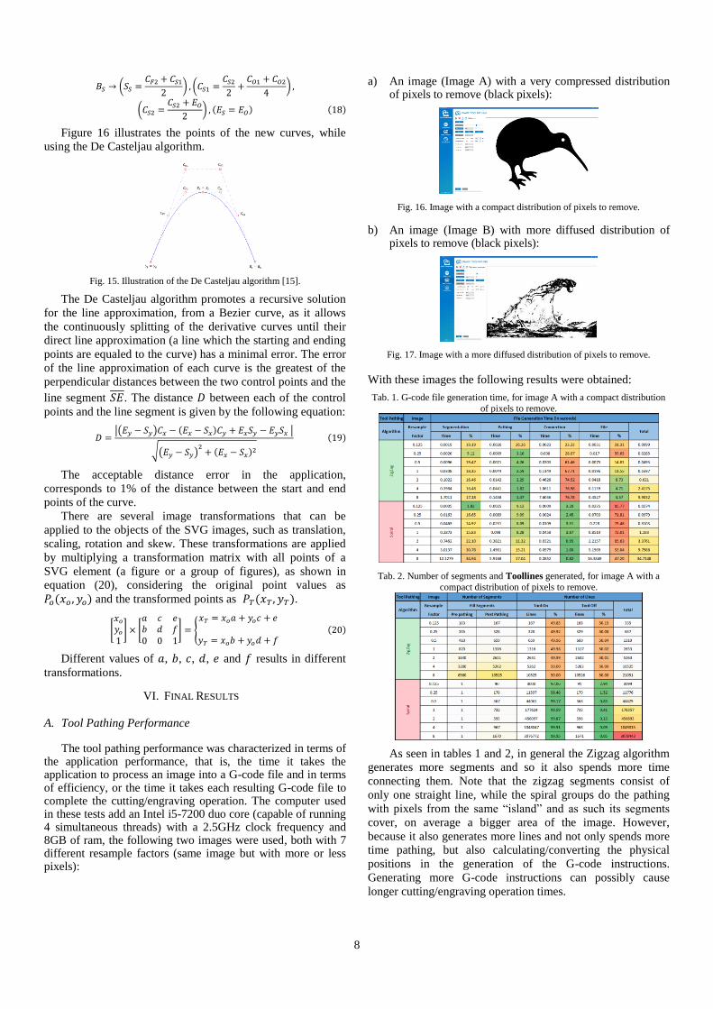
b) An image (Image B) with more diffused distribution of pixels to remove (black pixels):
Fig. 17. Image with a more diffused distribution of pixels to remove.
With these images the following results were obtained:
Tab. 1. G-code file generation time, for image A with a compact distribution
of pixels to remove.
Tab. 2. Number of segments and Toollines generated, for image A with a
compact distribution of pixels to remove.
As seen in tables 1 and 2, in general the Zigzag algorithm
generates more segments and so it also spends more time
connecting them. Note that the zigzag segments consist of
only one straight line, while the spiral groups do the pathing
with pixels from the same “island” and as such its segments
cover, on average a bigger area of the image. However,
because it also generates more lines and not only spends more
time pathing, but also calculating/converting the physical
positions in the generation of the G-code instructions.
Generating more G-code instructions can possibly cause
longer cutting/engraving operation times.

9
Also note that the number of segments pre-pathing in the
zigzag is equal to the height (in pixels) of the image, this being
the biggest size of it, and the number of segments pre-pathing
in the spiral is one, because of the very compressed
distribution of pixels to remove.
Tab. 3. G-code file generation time, for image B with a diffused distribution
of pixels to remove.
Tab 4. Number of segments and Toollines generated, for image B with a
diffused distribution of pixels to remove.
Compared with the previous tables, in a more diffused
distribution of pixels to remove, the Zigzag algorithm
generates even more segments, as the groups of pixels to
remove, in the same line, are larger and so it creates more
segments per each image column/row. An obvious Achilles
heel is the segment connection. Because the number of
iterations of the sorting cycle scales quadratically with the
number of segments, as shown in equation (7), it degrades the
application performance for large image files.
One possible way to solve this issue is to do a less
intensive search, looking for just a few groups of segments
that are at a similar distance from the origin point (bottom left
corner). This would lead, however, to an increase in the
cut/engraving operation time. The difference between the total
number of lines between the two algorithms is smaller than the
previous image set, however the spiral still generates more
instructions.
As for the efficiency of each algorithm the following distances
(CNC travelling) were obtained, using a resolution of one
pixel per millimeter:
Tab. 5. Number of Toollines generated and distance to be travelled by the
CNC tool, for the image with a compact distribution of pixels to remove.
The obvious big difference between the two algorithms is
the distance that the CNC tool has to travel while not
cutting/engraving. Assuming that the CNC tool moves at a
constant speed, ignoring the accelerations and decelerations
while turning direction, and considering the characteristics of
the CNC used, with a maximum feedrate of 1300 millimeters
per minute, the estimated time of completion for the worst
situations (8x resample factors) would be approximately 31.49
hours for the zigzag and 34.39 hours for the spiral, a 9%
increase in time. In this situation, the zigzag was also the
fastest to produce the G-code file, taking only 9 seconds
against the 35, approximately, for the spiral.
Tab. 6. Number of Toollines generated and distance to be travelled by the CNC tool, for image B with a diffused distribution of pixels to remove.
From table 6 it is seen that, again, the difference on the
distance while the tool is not cutting/engraving is still
substantial. Assuming the same feedrate as before, the
estimated time of completion for the worst situations (8x
resample factors) would be approximately 22.75 hours for the
zigzag and 28.45 hours for the spiral, a 25% increase in time.
This means that, despite taking 14 minutes tool pathing, the
zigzag algorithm produced a G-Code file that is approximately
6 hours faster than the spiral, which only took a minute to
toolpath.
This shows that not always is the fastest algorithm the
most efficient overall. Despite of this, there is still a lot of
room for improvement.
VII. CONCLUSIONS
The objective of this project was to develop a computer
application capable of controlling a CNC machine and tool
path the most commonly used types of image files. The CNC
was controlled with G-code instructions that describe what
type of movement and how far the CNC tool should move. In
order to abstract the user from the instructions and ease on the
operations, like calibrating, printing and also tool pathing, a

10
graphical user interface was design for the application, using
the windows forms. It also includes a G-code simulator, which
parses a given file for the compatible G-code instructions and
draws its result, allowing the user to preview the file and
position the CNC and or the material, before printing.
As for the tool pathing of images, this project focused on
the pathing of raster images, implementing two of the most
used methods, the zig-zag and the parallel-contour (spiral),
while also including a pathing option for vector images,
specifically the SVG format, with a counter path to smooth the
edges of the filling path.
For the testes performed, the zig-zag method is the most
efficient, in both time and quality of the cutting/engraving
operation, despite taking longer to generate the file, in some
circumstances. While both try to minimize the distance
travelled with the laser turned off, the spiral method also tries
to create longer paths with the laser turned on, which leads to
fewer number of path segments, with the start and end points
more far apart. The sorting algorithm, used to connect the
segments, only tries to minimize the distance to the next path,
while sorting, and not the total distance of connection, which
can get unnecessarily long, especially in the spiral method,
because of this. To solve this issue, the sorting algorithm
would have to take into consideration multiple path
combinations, which could drastically affect the time it takes
to generate the tool path file. Using the GPU to process the
tool pathing could not only help solving this problem, but also
improve the overall processing time.
Regarding the SVG images, the conversion of Bezier and
ellipses, to simple lines and circular arcs, was achieved, there
were some problems with the alignment of the contour with
the filling path. This was more evident on images with
transformations, like rotation or skew, which made the
rendered version of the image, used for the filling path,
slightly offset from the contour path.
The project was far more complex than was expected,
however it also allowed for a better understanding of the
subject of image processing and the control of CNC machines.
Future Work
As mentioned before, the sorting algorithm for the
connection paths could be improve, to consider multiple path
combinations, to improve the spiral tool pathing method. The
use of graphical tools, like OpenGL, to achieve more parallel
processing would also improve the application performance.
CAD files, like the Gerber file, could also be added to increase
the image format compatibility.
The G-Code Generated by the tool pathing can be used
for a laser and a drill, by choosing the respective option.
Regarding the laser, a dynamic diameter could also be
implemented, by adjusting both the power, feed-rate and
height, although it would heavily dependent on the type and
color of the material. A similar strategy could be used for the
drill, with pauses add to the path to change the drill, however
it would be less practical.
One of the biggest limitations of the SVG pathing was its
filling path, which was generated from a rasterized version of
the image. This was done to reuse the functionality of the
raster image tool pathing implementation, as the main
objective was the smoothen jagged the edges around the
image. However, a filling path directly generated from the
SVG image would increase the quality of the cut/engrave.
REFERENCES
[1] Denford Limited, "G and M Programming for CNC Milling Machines",
Brighouse, 2012.
[2] P. Selvaraj and P. Radhakrishnan, "Algorithm for Pocket Milling using Zig-zag Tool Path," Defense Science Journal, vol. 56, no. 2, pp. 117-127, April 2006.
[3] Z. Yao and S. K. Gupta, "Cutter path generation for 2.5D milling by combining multiple different cutter path patterns.," International Journal of Production Research, vol. 42, no. 11, pp. 2141-2161, 2004.
[4] C. Poynton, “The magnitude of nonconstant luminance errors,” em A Technical Introduction to Digital Video, New York, John Wlley & Sons, 1996.
[5] “Convolution”, Available: https://homepages.inf.ed.ac.uk/rbf/HIPR2/ convolve.htm [Accessed January 2018]
[6] A.-V. Diaconu and I. Sima, ""Simple, XOR based, Image Edge Detection"," 27-29 June 2013. [Online]. Available: http://www.sdettib.pub.ro/admin/images/articol/2013-06-25-2658253455-ECAI_2013_1.pdf. [Accessed 25 December 2016].
[7] R. . Fisher, A. Perkins and E. Wolfart, "Roberts Cross Edge Detector," 2003. [Online]. Available: http://homepages.inf.ed.ac.uk/rbf/HIPR2/ roberts.htm. [Accessed 25 December 2016].
[8] L. Bin and M. S. Yeganeh, "Comparison for Image Edge Detection Algorithms," July-Agost 2012. [Online]. Available: http://www.iosrjournals.org/iosr-jce/papers/vol2-issue6/A0260104.pdf?id=2214. [Accessed 25 December 2016].
[9] P. Getreuer, Linear Methods for Image Interpolation, Cachan: Image Processing On Line, 2011.
[10] "Java2s," Massachusetts Institute of Technology, [Online]. Available: http://www.java2s.com/Code/CSharp/Collections-Data-Structure/BitArray2D.htm. [Accessed September 2017].
[11] C. E. l. R. L. R. C. S. Tomas H. Cormen, “Introduction To Algorithms,” 2 ed., MIT Press and McGraw-Hill, 1990, pp. 595-601.
[12] vvvvv.org, “SVG library (2.3.0 release),” 28 December 2018. [Online]. Available: https://vvvv.org/. [Acedido em 1 April 2017].
[13] D. Eberly, "Approximating an Ellipse by Circular Arcs," 13 January 2002. [Online]. Available: https://www.geometrictools.com/ Documentation/ApproximateEllipse.pdf. [Accessed July 2017].
[14] G. Farin, Curves and Surfaces for Computer-Aided Geometric Design, 4 ed., Academic Press, 1992.
[15] F. Yamaguchi, Curves and Surfaces in Computer Aided Geometric Design, Tokyo: Nikkan Kogyo Shinbun, Co., 1988.
Related Documents