Development of a CBM based service indicator for UFD ...

Development of aCBM based service indicator

for UFD replacements- An introductory study

Victor Lundqvist & Johan Åkesson

Master’s Thesis inBiomedical Engineering

2017

Faculty of Engineering LTHDepartment of Biomedical Engineering

Supervisor Baxter: Erik WallenborgSupervisor LTH: Frida Sandberg

Baxter International Inc.

Abstract

Dialysis is a life-sustaining treatment for many people around the world. In or-der to meet the high demands on the dialysis machines, replaceable parts mustbe exchanged in proper time. Condition based maintenance (CBM) bases itsservice decisions on the actual health status of the component. The goal ofthis master’s thesis was to develop an algorithm based on machine learning,constituting the first step of a CBM based service indicator monitoring thedialysis ultra filter (UFD) of Baxter’s AK 98 dialysis machine.

Real treatment data retrieved from ten dialysis machines have been an-alyzed. Signals believed to be relevant to the UFD status were preprocessedand analyzed. From them different features were extracted whereof some werefound in CBM related literature. Two different feature selection methods wereused to select 10 out of the 178 available features. Different labeling meth-ods were tested and evaluated together with other relevant parameters in thealgorithm.

The final algorithm used a k-nearest neighbors (kNN) classifier withk = 12. The classification accuracy was approximately twice as good as a ran-dom guess. The main reason for not achieving a better result was that only sixfeatures appeared to contain relevant information regarding the UFD status.Furthermore, these features were derived from the same signal and closelyrelated. Despite this, the developed algorithm did show promising result indetecting the UFD degradation level but further development will be needed.The main focus should be to improve the signal quality and/or find morerelevant signals and/or features.

Preface

This is a thesis for the degree Master of Science in Biomedical Engineeringat the Faculty of Engineering (LTH) of Lund University. The project wascarried out at Baxter International Inc., Lund in the spring and summer of2017. First of all we would like to direct a huge thanks to our supervisor atBaxter, Erik Wallenborg, for your great support and endless stream of ideasand encouragement. We also would like to give a big thanks to our manager atBaxter, Ivan Fulöp, for enabling this project and making sure we were givenall the help and support we needed. Furthermore we would like to thank oursupervisor at LTH, Frida Sandberg, for your theoretical expertise and helpwith this report. Finally we would like to thank all other people at Baxterwho were involved or showed interest in our project.

iii

Contents

List of Abbreviations ixList of Figures xiList of Tables xii1. Introduction 1

1.1 Aim . . . . . . . . . . . . . . . . . . . . . . . . . . . . . . . . 21.2 Disposition . . . . . . . . . . . . . . . . . . . . . . . . . . . . 2

2. Background 42.1 Physiology and pathology of the kidneys . . . . . . . . . . . . 4

2.1.1 Formation of ultrafiltrate . . . . . . . . . . . . . . . . 42.1.2 Reabsorption and secretion in the nephron . . . . . . . 62.1.3 Endocrine function . . . . . . . . . . . . . . . . . . . . 62.1.4 Kidney failure and treatment options . . . . . . . . . . 6

2.2 Hemodialysis . . . . . . . . . . . . . . . . . . . . . . . . . . . 72.2.1 Vascular access . . . . . . . . . . . . . . . . . . . . . . 72.2.2 Dialysis fluid . . . . . . . . . . . . . . . . . . . . . . . 82.2.3 Solute exchange in the dialyzer . . . . . . . . . . . . . 9

2.3 AK 98 dialysis machine . . . . . . . . . . . . . . . . . . . . . . 112.3.1 Fluid unit . . . . . . . . . . . . . . . . . . . . . . . . . 11

2.3.1.1 Water intake and heating system . . . . . . . 122.3.1.2 Chemical disinfectants intake . . . . . . . . . 122.3.1.3 Mixing and conductivity control system . . . 122.3.1.4 Degassing/flow pump system . . . . . . . . . 132.3.1.5 Fluid output - UF control system . . . . . . 13

2.3.2 UFD . . . . . . . . . . . . . . . . . . . . . . . . . . . . 142.3.3 Disinfection programs . . . . . . . . . . . . . . . . . . 152.3.4 Regulation of main flow . . . . . . . . . . . . . . . . . 162.3.5 Taration . . . . . . . . . . . . . . . . . . . . . . . . . . 17

2.4 Condition based maintenance . . . . . . . . . . . . . . . . . . 182.4.1 Related work . . . . . . . . . . . . . . . . . . . . . . . 19

2.5 Machine learning . . . . . . . . . . . . . . . . . . . . . . . . . 212.5.1 Supervised learning . . . . . . . . . . . . . . . . . . . . 22

v

CONTENTS

2.5.1.1 k-fold cross validation . . . . . . . . . . . . . 232.5.1.2 k-nearest neighbors . . . . . . . . . . . . . . 232.5.1.3 Evaluation . . . . . . . . . . . . . . . . . . . 24

3. Data 253.1 Log files . . . . . . . . . . . . . . . . . . . . . . . . . . . . . . 253.2 Analyzed signals . . . . . . . . . . . . . . . . . . . . . . . . . 26

3.2.1 Flow pump derived signals . . . . . . . . . . . . . . . . 263.2.2 HPG . . . . . . . . . . . . . . . . . . . . . . . . . . . . 273.2.3 UF channel 1 . . . . . . . . . . . . . . . . . . . . . . . 273.2.4 PD . . . . . . . . . . . . . . . . . . . . . . . . . . . . . 273.2.5 Blood leak detector . . . . . . . . . . . . . . . . . . . . 273.2.6 Suction pump derived signals . . . . . . . . . . . . . . 27

4. Method 294.1 Localizing UFD replacements . . . . . . . . . . . . . . . . . . 304.2 Localizing hypochlorite disinfections . . . . . . . . . . . . . . 304.3 Preprocessing of signals . . . . . . . . . . . . . . . . . . . . . 304.4 Labeling of data . . . . . . . . . . . . . . . . . . . . . . . . . . 324.5 Feature extraction . . . . . . . . . . . . . . . . . . . . . . . . 33

4.5.1 Features derived from time-domain . . . . . . . . . . . 344.5.2 Features derived from frequency-domain . . . . . . . . 354.5.3 Features derived through cross-correlation . . . . . . . 36

4.6 Split of data into training and test sets . . . . . . . . . . . . . 374.7 Flow compensation . . . . . . . . . . . . . . . . . . . . . . . . 374.8 Feature normalization . . . . . . . . . . . . . . . . . . . . . . 384.9 Feature selection . . . . . . . . . . . . . . . . . . . . . . . . . 39

4.9.1 Two-stage feature selection and weighting technique . 394.9.2 Sequential forward selection . . . . . . . . . . . . . . . 41

4.10 Classification using kNN . . . . . . . . . . . . . . . . . . . . . 414.11 Evaluation . . . . . . . . . . . . . . . . . . . . . . . . . . . . . 42

5. Results 435.1 Preprocessing of signals . . . . . . . . . . . . . . . . . . . . . 435.2 Flow compensation . . . . . . . . . . . . . . . . . . . . . . . . 445.3 Feature selection . . . . . . . . . . . . . . . . . . . . . . . . . 44

5.3.1 Time series . . . . . . . . . . . . . . . . . . . . . . . . 445.3.2 Box plots . . . . . . . . . . . . . . . . . . . . . . . . . 465.3.3 TFSWT . . . . . . . . . . . . . . . . . . . . . . . . . . 475.3.4 SFS . . . . . . . . . . . . . . . . . . . . . . . . . . . . 495.3.5 Evaluation of feature selection methods . . . . . . . . 50

5.4 Labeling of data . . . . . . . . . . . . . . . . . . . . . . . . . . 515.5 Windowing and choice of k . . . . . . . . . . . . . . . . . . . . 555.6 Evaluation . . . . . . . . . . . . . . . . . . . . . . . . . . . . . 56

vi

CONTENTS

6. Discussion 596.1 Localizing UFD replacements . . . . . . . . . . . . . . . . . . 596.2 Analyzed signals . . . . . . . . . . . . . . . . . . . . . . . . . 606.3 Preprocessing of signals . . . . . . . . . . . . . . . . . . . . . 606.4 Flow compensation . . . . . . . . . . . . . . . . . . . . . . . . 616.5 Feature selection . . . . . . . . . . . . . . . . . . . . . . . . . 626.6 Labeling of data . . . . . . . . . . . . . . . . . . . . . . . . . . 63

6.6.1 Effects of missing data . . . . . . . . . . . . . . . . . . 636.6.2 Compensation of unbalanced data . . . . . . . . . . . 646.6.3 Other alternatives . . . . . . . . . . . . . . . . . . . . 64

6.7 Windowing and choice of k . . . . . . . . . . . . . . . . . . . . 656.8 Algorithm development . . . . . . . . . . . . . . . . . . . . . . 656.9 Evaluation and final thoughts . . . . . . . . . . . . . . . . . . 66

6.9.1 Single versus multiple machine analysis . . . . . . . . 666.9.2 Hypothesis regarding the UFD degradation . . . . . . 67

6.10 Ethics . . . . . . . . . . . . . . . . . . . . . . . . . . . . . . . 686.11 Future work . . . . . . . . . . . . . . . . . . . . . . . . . . . . 68

7. Conclusion 70Bibliography 72

vii

List of Abbreviations

µ Mean

σ Standard deviation

c1−10 Sum of the 10 largest Fourier coefficients

ck Fourier coefficient

ckIQR Interquartile range of Fourier coefficients

ckQ1 Lower quartile of Fourier coefficients

ckQ2 Median of Fourier coefficients

ckQ3 Upper quartile of Fourier coefficients

L1 Labeling based on time

L2 Labeling based on hypochlorite disinfections

Q1 Lower quartile

Q2 Median

Q3 Upper quartile

BYVA Bypass valve

CBM Condition based maintenance

CCM Maximum value from cross-correlation

CCTD Cross-correlation time delay

CI Crest indicator

CKD Chronic kidney disease

CLI Clearance indicator

ix

Cond. cell Conductivity cell

DF Dominant frequency

DIVA Direct valve

DRVA Degass restrictor valve

EPO Erythropoietin

FFT Fast Fourier transform

FIVA Filter valve

GFR Glomerular filtration rate

HPG High pressure guard

II Impulse indicator

IQR Interquartile range

kNN k-nearest neighbors

KU Kurtosis

Max Maximum value

Min Minimum value

PD Pressure dialysis transducer

RMS Root mean square

RO Reverse osmosis

RUL Remaining useful life

SFS Sequential forward selection

SI Shape indicator

SK Skewness

TAVA Taration valve

TFSWT Two-stage feature selection and weighting technique

UFD Dialysis ultra filter

ZEVA Zeroing valve

x

List of Figures

List of Figures

2.1 A nephron, the functional unit of the kidney . . . . . . . . . . . . 52.2 Water purifying process . . . . . . . . . . . . . . . . . . . . . . . 92.3 The dialyzer . . . . . . . . . . . . . . . . . . . . . . . . . . . . . . 102.4 The AK 98 dialysis machine . . . . . . . . . . . . . . . . . . . . . 112.5 Flow path of the fluid unit . . . . . . . . . . . . . . . . . . . . . . 122.6 Localization and appearance of the UFD . . . . . . . . . . . . . . 152.7 The different phases during a taration . . . . . . . . . . . . . . . 172.8 Workflow of general CBM methods . . . . . . . . . . . . . . . . . 202.9 Example of a two-dimensional feature space . . . . . . . . . . . . 232.10 Confusion matrix with three different classes . . . . . . . . . . . 24

3.1 A magnification of the most relevant part of the fluid path . . . . 263.2 The eight most important sensor signals . . . . . . . . . . . . . . 28

4.1 Illustration of the two different labeling methods . . . . . . . . . 334.2 An example of the (HPG−PD) signal . . . . . . . . . . . . . . . 344.3 Median flow of UF channel 1 - all log files of a single machine . . 37

5.1 Result of the preprocessing of the signal HPG-pressure . . . . . . 435.2 Flow compensation of the feature median of HPG-PD . . . . . . 445.3 Time series of the features mean of (HPG−PD) and mean of suc-

tion pump current . . . . . . . . . . . . . . . . . . . . . . . . . . 455.4 Time series of the feature mean of blood leak detector . . . . . . . 465.5 Box plots of the feature mean of flow pump cycle . . . . . . . . . 475.6 Box plots of the feature mean of (HPG−PD) . . . . . . . . . . . 475.7 Results from the feature selection using SFS . . . . . . . . . . . . 505.8 Comparison between TFSWT and SFS . . . . . . . . . . . . . . . 515.9 Evaluation of labeling methods - 12 labels, single machine . . . . 525.10 Evaluation of labeling methods - 4 labels, single machine . . . . . 525.11 Evaluation of labeling methods - 12 labels, multiple machine . . . 545.12 Evaluation of labeling methods - 4 labels, multiple machine . . . 545.13 Classification accuracy for different segment lengths and k . . . . 56

xi

5.14 Classification accuracy for the 5 machines from the evaluation set 575.15 Confusion matrices derived from the evaluation set . . . . . . . . 57

List of Tables

2.1 Summary of cleaning and decalcification programs . . . . . . . . 16

4.1 Signal pairs used for cross-correlation . . . . . . . . . . . . . . . . 364.2 Flow compensated features . . . . . . . . . . . . . . . . . . . . . 38

5.1 Result from the single machine TFSWT . . . . . . . . . . . . . . 485.2 Result from the multiple machine TFSWT . . . . . . . . . . . . . 485.3 Result from the single machine SFS . . . . . . . . . . . . . . . . 495.4 Result from the multiple machine SFS . . . . . . . . . . . . . . . 505.5 Comparison of labeling methods - 12 labels, single machine . . . 535.6 Comparison of labeling methods - 4 labels, single machine . . . . 535.7 Comparison of labeling methods in multiple machine analysis . . 55

xii

1Introduction

End-stage kidney disease is a serious condition requiring renal replacementtherapy either as dialysis treatment or kidney transplant if not to be fatal.As of 2010, 2 million people worldwide required dialysis treatment to stayalive [1]. However, this number likely represented less than 10 % of those whowere actually in need of it [2].

In hemodialysis a dialysis machine is used to replace the kidneys’ functionto remove waste products and excess fluid from the blood. Due to the criticalhealth status of the patients in combination with the fact that the treatmentis a time consuming activity, the demands on the dialysis treatment withrespect to quality and efficiency are high.

Since a dialysis machine at a clinic is used by multiple patients it is ofhigh importance that the system is carefully disinfected between treatmentsto avoid contagion. These disinfection programs in combination with the fre-quent use cause a natural wear on the components. In order to meet the highdemands of quality and efficiency on the treatments these components mustbe replaced in appropriate time.

Condition based maintenance (CBM) is an approach that has receivedan increased amount of interest in the scientific research area of maintenanceduring the latest years [3]. It is a preventative approach which bases its servicedecisions on the actual health status of the component. This can be comparedto traditional preventative maintenance which bases its service decisions solelyon time or production hours since last service [4]. One desirable measure toretrieve from a CBM algorithm is the remaining useful life (RUL) of thecomponent of interest.

1

Chapter 1. Introduction

1.1 Aim

According to the current guidelines [5], the replacement of the dialysis ultra-filter (UFD) in Baxter’s dialysis machine AK 98 should be conducted whenone of the following three limits have been exceeded:

• 90 days since last UFD replacement

• 150 heat disinfections

• 12 hypochlorite disinfections

Thereby the actual status of the filter is not taken into consideration.This means that the remaining capacity of the UFD is practically unknownwhen the filter is replaced. As a consequence of this the UFD may be replacedtoo early, resulting in increased costs and environmental impact. A methodindicating a suitable time to exchange the UFD based on its current status,or RUL, is thereby desirable.

In order to develop a CBM based service indicator for UFD replacementsthree different steps are necessary to perform. The first step is to develop analgorithm which is able to detect different degradation levels of the UFD anddecide the current level. The second step is to perform a long term study ofhow the UFD is degraded when it is not replaced. The third step is to analyzehow well the UFD fulfills its intended purpose during different degradationlevels. This analyze should find the level where the intended purpose is nolonger fulfilled and from this result map each degradation level of the UFDto a specific RUL.

The data being logged in an AK 98 dialysis machine regarding pumpvelocities, pressures, temperatures, power usage etcetera is currently almostexclusively used for troubleshooting. The aim of this master’s thesis is toperform the first step in the development of the CBM based UFD serviceindicator mentioned above, based on data analysis of these log files. To achievethis, a machine learning approach will be tested and evaluated.

1.2 Disposition

This report starts off with a basic description of relevant topics in Chapter 2.This includes a section about the physiology and pathology of the kidneys, ageneral explanation of the hemodialysis treatment and the dialysis machinefollowed by a more specific description of Baxter’s AK 98 dialysis machinewhich is analyzed in this report. It also includes a section about CBM andprevious research in this area as well as a short description of machine learn-ing.

2

1.2 Disposition

The sensor signals from the AK 98 log files analyzed in this report aredescribed in Chapter 3. Chapter 4 explains how these signals were prepro-cessed, how features were extracted and selected from these log files andfinally how the classification was done. The results from these different stepsare presented in Chapter 5, followed by a discussion of the results and pos-sible future work in Chapter 6. Finally, the conclusions from the report aresummarized in Chapter 7.

3

2Background

2.1 Physiology and pathology of the kidneys

The kidneys are approximately 11 centimeters long, bean-shaped organs lo-cated on each side of the vertebral column in the cavity behind the peri-toneum. Despite the small size they receive about 20 − 25 % of the cardiacoutput which is needed if they should be able to perform their physiologicalfunction [6]. These functions can be subdivided into three distinct categories;excretory, regulatory and endocrine function. Briefly, the excretory functionis to filter the blood by removing metabolic waste products and toxins and ex-crete it through the urine. The regulatory function includes the regulation ofbody fluid, electrolyte balance and acid-base balance. Finally, the endocrinefunction is made up of the production and activation of different hormones in-volved in the formation of red blood cells, calcium metabolism and regulationof blood pressure and blood flow.

The dialysis machine tries to mimic some of the functions of the kidneyand a basic understanding of the physiology of the kidney is necessary tounderstand what the dialysis machine is intended to do, why it is importantand finally how the dialysis machine works.

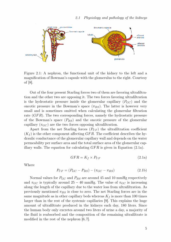
2.1.1 Formation of ultrafiltrateThe functional unit of the kidney is the nephron, consisting of a glomerulusand a tubule, see Figure 2.1. The glomerulus is a cluster of small blood vesselssurrounded by a capsule called Bowman’s capsule and the space in betweenthese two structures is called the Bowman’s space. This structure is respon-sible for the formation of the ultrafiltrate, the first step of urine production.The filtration process is basically the same as in other capillaries in the body,the differences are the greater Starling forces, and most dominantly, highercapillary permeability present in the glomeruli [7]. The Starling forces affect-ing the filtration rate are the hydrostatic and oncotic pressures present insideas well as outside the glomerular capillaries. The oncotic (or colloid osmotic)pressure is an osmotic pressure exerted by proteins that are not able to passthrough a blood vessel wall.

4

2.1 Physiology and pathology of the kidneys

Figure 2.1: A nephron, the functional unit of the kidney to the left and amagnification of Bowman’s capsule with the glomerulus to the right. Courtesyof [8].

Out of the four present Starling forces two of them are favoring ultrafiltra-tion and the other two are opposing it. The two forces favoring ultrafiltrationis the hydrostatic pressure inside the glomerular capillary (PGC) and theoncotic pressure in the Bowman’s space (πBS). The latter is however verysmall and is sometimes omitted when calculating the glomerular filtrationrate (GFR). The two corresponding forces, namely the hydrostatic pressureof the Bowman’s space (PBS) and the oncotic pressure of the glomerularcapillary (πGC) are the two forces opposing ultrafiltration.

Apart from the net Starling forces (PUF ) the ultrafiltration coefficient(Kf ) is the other component affecting GFR. The coefficient describes the hy-draulic conductance of the glomerular capillary wall and depends on the waterpermeability per surface area and the total surface area of the glomerular cap-illary walls. The equation for calculating GFR is given in Equation (2.1a).

GFR = Kf × PUF (2.1a)

WherePUF = (PGC − PBS)− (πGC − πBS) (2.1b)

Normal values for PGC and PBS are around 45 and 10 mmHg respectivelyand πGC is typically around 25 − 40 mmHg. The value of πGC is increasingalong the length of the capillary due to the water loss from ultrafiltration. Aspreviously mentioned πBS is close to zero. The net Starling forces are in thesame magnitude as in other capillary beds whereas Kf is more than 100 timeslarger than in the rest of the systemic capillaries [9]. This explains the hugeamount of ultrafiltrate produced in the kidneys each day, 180 liters. Sincethe human body only excretes around two liters of urine a day, a majority ofthe fluid is reabsorbed and the composition of the remaining ultrafiltrate ismodified in the rest of the nephron [6, 7].

5

Chapter 2. Background

2.1.2 Reabsorption and secretion in the nephronThe ultrafiltrate is collected in the Bowman’s space which is contiguous withthe tubule, a long tube with different segments, each with its own specificfunction. The function of the tubule is to modify the composition of theultrafiltrate through reabsorption and secretion of water and solutes. Thisoccurs through both active and passive transport. The tubules from differentnephrons merge to a collecting duct where the last modifications are done,producing final urine. This is then transported through the renal pelvis andureters to the bladder where it is stored. Thereby no modification of eithervolume or composition is done in these parts.

The vast majority of the 180 liters ultrafiltrated water is reabsorbed inthe tubule. Since sodium is the most abundant electrolyte in the extracellularfluid, the same is true for the blood and thereby the ultrafiltrate. In fact, theamount of sodium filtered by the kidneys each day is equivalent to approxi-mately 1.5 kg of table salt [10]. This demands a very effective reabsorptionin the tubule, about 99.6 % of the sodium is reabsorbed. Chloride repre-sents another electrolyte with high concentration in the ultrafiltrate that isreabsorbed effectively. Other solvents that are reabsorbed include phosphate,calcium, glucose, amino acids and proteins (although only a small fraction isfiltered in the first place) [11].

Other substances must instead be secreted. The most important exampleis potassium, which only appears in small concentrations in the blood andthereby in the ultrafiltrate since it is mainly stored intracellular. To compen-sate for the daily intake, potassium must be actively secreted. Other examplesof substances being secreted are small anions e.g. p-aminohippurate [12].

2.1.3 Endocrine functionThe kidneys are active in the production and regulation of different hormoneswith diverse physiological effects. Renin is released into the bloodstream as aresponse to decreased blood pressure in the afferent arterioles (preglomerulararterioles) which through a complex signaling pathway have the final effectsof increased blood volume and blood pressure. Erythropoietin, or EPO, isreleased by cells in the cortex and outer medulla of the kidney in response toa fall in local tissue PO2, stimulating the production of red blood cells in bonemarrow. Cells of the proximal tubule convert inactive vitamin D to its activeform which in turn regulates calcium and phosphorus metabolism. In additionto these hormones the kidneys also secrete prostaglandins and various kininsthat regulate local circulation within the kidneys [6].

2.1.4 Kidney failure and treatment optionsA person can usually sustain a normal life with just one functional kidney.The total kidney function measured as GFR may be as low as 25 % beforeclear symptoms of renal failure appear [13].

6

2.2 Hemodialysis

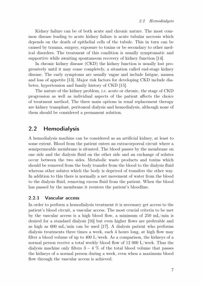
Kidney failure can be of both acute and chronic nature. The most com-mon disease leading to acute kidney failure is acute tubular necrosis whichdepends on the death of epithelial cells of the tubule. This in turn can becaused by trauma, surgery, exposure to toxins or be secondary to other med-ical disorders. The treatment of this condition is usually symptomatic andsupportive while awaiting spontaneous recovery of kidney function [14].

In chronic kidney disease (CKD) the kidney function is usually lost pro-gressively until it may cease completely, a situation called end-stage kidneydisease. The early symptoms are usually vague and include fatigue, nauseaand loss of appetite [13]. Major risk factors for developing CKD include dia-betes, hypertension and family history of CKD [15].

The nature of the kidney problem, i.e. acute or chronic, the stage of CKDprogression as well as individual aspects of the patient affects the choiceof treatment method. The three main options in renal replacement therapyare kidney transplant, peritoneal dialysis and hemodialysis, although none ofthem should be considered a permanent solution.

2.2 Hemodialysis

A hemodialysis machine can be considered as an artificial kidney, at least tosome extent. Blood from the patient enters an extracorporeal circuit where asemipermeable membrane is situated. The blood passes by the membrane onone side and the dialysis fluid on the other side and an exchange of solutesoccur between the two sides. Metabolic waste products and toxins whichshould be removed from the body transfer from the blood to the dialysis fluidwhereas other solutes which the body is deprived of transfers the other way.In addition to this there is normally a net movement of water from the bloodto the dialysis fluid, removing excess fluid from the patient. When the bloodhas passed by the membrane it reenters the patient’s bloodline.

2.2.1 Vascular accessIn order to perform a hemodialysis treatment it is necessary get access to thepatient’s blood circuit, a vascular access. The most crucial criteria to be metby the vascular access is a high blood flow, a minimum of 250 mL/min isdesired for a standard dialysis [16] but even higher flows are preferable andas high as 600 mL/min can be used [17]. A dialysis patient who performsdialysis treatments three times a week, each 4 hours long, at high flow mayfilter a blood volume of up to 400 L/week. As a comparison, the kidneys of anormal person receive a total weekly blood flow of 12 000 L/week. Thus thedialysis machine only filters 3 − 4 % of the total blood volume that passesthe kidneys of a normal person during a week, even when a maximum bloodflow through the vascular access is achieved.

7


2.2.2 Dialysis fluidThe quality standard on normal drinking water is based on a weekly intakeof approximately 14 liters, all of it passing through the selective gut barrier.A hemodialysis patient may be exposed to 300 − 500 liters of dialysis fluidper week through the synthetic dialyzer membrane, a barrier without theprotective abilities of the mucous membranes in the gastrointestinal system.Due to this close contact between the dialysis fluid and the patient’s bloodthe purity of normal drinking water is not enough [18].

Water contaminants can be divided into three major groups: particulates,dissolved substances and microorganisms. The particulates are the largest andinclude minerals and colloids which are responsible for the turbidity of water.Dissolved substances are of both organic and inorganic (ions and salts) nature.Microorganisms are mainly represented by bacteria and their degradationproducts (endotoxins), but also include fungi and viruses [18].

The dialysis fluid is prepared through two different processes, the firstprocess is responsible for filtering and purifying the water to as high degreeas possible. This is done in a central water treatment plant located in thehospital. The second process adds substances to the purified water to give itthe correct composition of the final dialysis fluid. This is done separately ineach dialysis machine continuously through the treatment and is adjusted tofit each patient’s individual need.

The water purifying process conducted at the water treatment plant in-volves several steps, see Figure 2.2. First the water passes through mechan-ical filters to remove larger particles. If the water includes chloramines, asubstance being used increasingly as a substitute for chlorine as disinfectant,it needs to be removed due to its high toxicity for dialysis patients. Whenpresent, chloramines are effectively removed by carbon filters. The next stepis removal of calcium and magnesium through a softener before the final pu-rification step which occurs in the reverse osmosis (RO) unit.

During RO, an applied pressure forces water through a semipermeablemembrane which is basically only permeable to water. Thereby it removesmost of the contaminants present in water, both organic and inorganic. Themain purpose of the steps preceding the RO is simply to remove substancesthat may damage the RO-membrane. After the RO unit the water is storedand ready for distribution to the dialysis machines. The process of turningthe purified water into final dialysis fluid is discussed in Section 2.3.1.3, butsimplified it includes the addition of two different concentrates (A and B)containing ions and bicarbonate [8, 19].

With the removal of chloramines by the charcoal filters no disinfectant ispresent in the water and the bacterial growth will increase in the circuit upto the RO unit where it should be removed. However, if the RO unit and thedistribution system between it and the dialysis machines are not maintained

8

2.2 Hemodialysis

Figure 2.2: The different steps of the water purifying process. Courtesy of [8].

in a proper way a regrowth is possible. Because of this a regular disinfectionscheme is of high importance to reduce the microbiological contamination toas high degree as possible [8].

2.2.3 Solute exchange in the dialyzerThe blood that leaves the patient through the vascular access enters thearterial bloodline of the extracorporeal circuit. To prevent the blood fromclotting an anticoagulant, often heparin, is administered to the patient. Thisis done either by injecting it directly into the patient’s bloodstream prior totreatment or through a pump, located in the arterial bloodline, continuouslyduring the treatment. The dose is carefully adjusted since both too muchand too little anticoagulant possesses a risk to the patient. In addition tothe eventual pump with anticoagulant the arterial bloodline also includes apump and pressure sensor to adjust the blood pressure as well as a clampthat immediately may stop the blood flow to the dialysis machine if problemoccurs.

At the end of the arterial bloodline the dialyzer is situated. This is thepart of the dialysis machine where the blood and the dialysis fluid interactand an exchange of water and solutes occur, see Figure 2.3.

As previously described the dialyzer is a semipermeable membrane thatseparates the blood and the dialysis fluid. The membrane is permeable towater and small solutes, e.g. ions, but potentially also microorganisms andtoxins which is why the dialysis fluid needs to go through such a thoroughlypurification process.

There are mainly two different transport mechanisms across the mem-brane, ultrafiltration and diffusion. The semipermeable membrane of the di-alyzer corresponds to the vessel walls of the glomerulus when the process ofultrafiltration is considered. The same forces are active in both cases, i.e. hy-drostatic and oncotic pressures on either side of the membrane and it is the net

9


Figure 2.3: The dialyzer, the connection between the arterial bloodline andthe dialysis fluid. Courtesy of [8].

Starling force that is guiding the ultrafiltration as described in Section 2.1.1.During dialysis the hydrostatic pressures dominate and the gradient they giverise to is usually deliberately set to favor water movement from blood to dial-ysis fluid [20]. Since the hydrostatic pressures on either side of the membraneare controlled by the dialysis machine the hydrostatic gradient is easy to reg-ulate as compared to the oncotic gradient which can only be adjusted on thedialysis fluid side.

The other main transport mechanism across the membrane is diffusionwhich is the net movement of a solute from a higher to a lower concentra-tion. A solute for which the membrane is permeable may move between thetwo compartments as if the membrane does not exist. The composition ofthe dialysis fluid decides which way permeable solutes transfer. Thereby it isthe composition of the dialysis fluid that ultimately decides the compositionof the blood when the treatment section is ended. To maintain a concentra-tion gradient between the blood and dialysis fluid, and thereby the intendedmovement of solvents, it is important to keep a continuous flow of both flu-ids. To maximize the concentration gradient and diffusional flow across theentire length of the membrane the dialyzer is constructed so the fluids flowin opposite directions. Diffusion is also responsible for the passive transportthat occurs in the tubuli of the nephrons described in Section 2.1.2.

When the blood has passed the dialyzer it is returned to the patientthrough the venous bloodline. This part of the circuit contains a drip chamberand air detector which protects the patient from potentially dangerous airbubbles. The venous bloodline also contains a pressure sensor and a clampwhich may stop the blood from returning to the patient in certain alarmsituations, e.g. when air bubbles are detected.

The dialyzer and the hemodialysis machine in general is an acceptable

10

2.3 AK 98 dialysis machine

substitute for the excretory and regulatory functions of the kidney. However,it does not try to replace the kidneys’ endocrine function. Hence a patientwith kidney failure usually needs injections and medications in addition tothe dialysis treatment to compensate for this.


The AK 98 dialysis machine, Figure 2.4, is intended to perform hemodialysistreatments on patients suffering from renal failure or fluid overload. It maybe used both in clinics and in a home care environment [5]. The AK 98 ismanufactured by Baxter International Inc., previously Gambro Lundia AB.The first version was taken into commercial use in 2015 and it is a furtherdevelopment of the AK 96.

Figure 2.4: The AK 98 dialysis machine.

The principles of hemodialysis presented above hold true for the AK 98dialysis machine as well. Below is a technical description of the AK 98 ingeneral with a specific focus on the parts analyzed in this thesis.

2.3.1 Fluid unitFigure 2.5 shows the flow path of the fluid unit during treatment which issubdivided into the following five main subsystems: [21]

• Water intake and heating system

• Chemical disinfectants intake

• Mixing and conductivity control system

• Degassing/flow pump system

• Fluid output - UF control system

11


Figure 2.5: Flow path of the fluid unit. Courtesy of [5].

2.3.1.1 Water intake and heating systemThe water intake and heating system in the lower left part starts with the purewater inlet and ends with the heater. It includes two pressure regulators (PR 1and PR 2 ) which lower the water supply pressure in two steps to about + 130mmHg, relative the air pressure, which is monitored by INPS. Between thepressure regulators two heat exchangers are situated which uses the outgoingwater to rise the temperature of the incoming water. The incoming wateris raised to its final temperature when it passes through the heater. Thetemperature is regulated both by a temperature transducer at the heater’soutlet as well as one in conductivity cell B (cond. cell B), further down thefluid path. The temperature should be around body temperature, the exactvalue is set manually by the operator.

2.3.1.2 Chemical disinfectants intakeThe chemical disinfectants intake is placed on the rear side of the machine,in the upper left of Figure 2.5. For protective reasons it is equipped with twovalves (CHVA and CBVA), controlled separately. Apart from these intakesthere is another possible intake for chemicals in a different part of the system,the BiCart cartridge holder described in Section 2.3.1.3.

2.3.1.3 Mixing and conductivity control systemThe mixing and conductivity system is the part after the heater to cond. cellB. The main flow goes from the heater and follows the circuit to the left and

12


above pump A and B where it then fuses with the outlet of pump A. Thispump controls the addition of concentrate A to the purified water.

The composition of concentrate A may vary and is chosen based on eachpatient’s individual needs. It is stored as a liquid in a canister and containsa number of different electrolytes and sometimes dextrose. The purified wa-ter and concentrate A is mixed in the mixing chamber forming prepared Adialysis fluid. The conductivity of this fluid is proportional to the amountof A concentrate added. Since the content of concentrate A is known theconductivity measure gives the actual concentration of concentrate A in theprepared A dialysis fluid. This is measured in conductivity cell A (cond. cellA) which through feedback loops regulates pump A.

Concentrate B is made up of bicarbonate and cannot be stored in the samecanister as concentrate A since it would generate salt precipitates. It may bedelivered to hospitals either dissolved in water in ready-to-use canisters orin solid form as a BiCart cartridge. If solid it has to be dissolved beforeadministration to the dialysis fluid. Through slow and continuous additionof purified water the bicarbonate of the BiCart cartridge is dissolved and asaturated solution is achieved - concentrate B. The addition of concentrateB to the prepared A dialysis fluid is regulated through pump B. The fluid ismixed and the conductivity of the final dialysis fluid is measured by cond.cell B which in turn regulates pump B.

2.3.1.4 Degassing/flow pump systemThe degassing/flow pump system is the part after cond. cell B to conductivitycell P (cond. cell P). The mixing of the A and B concentrates generates freegas, carbon dioxide, which will disturb conductivity and flow measurementsif not removed. In addition to the carbon dioxide created, air may enter thedialysis fluid in various parts of the system e.g. through the A concentrate orthe BiCart. A bypass tube in the top of the second mixing chamber divertsthe gas away from the fluid temporarily when passing cond. cell B, but doesnot remove it. This is instead done by the degassing circuit. In the flowrestrictor a negative pressure is created, expanding the gas to larger bubbleswhich is released through the top of the degassing chamber. The flow pumpsituated in between the flow restrictor and degassing chamber is responsiblefor generating the negative degassing pressure. Cond. cell P measures theconductivity and temperature and acts as a guard which let the dialysis fluidbypass the dialyzer if these values differ from the set values.

2.3.1.5 Fluid output - UF control systemThe fluid output - UF control system is the remaining part of the fluidunit, after cond. cell P. The pressure is monitored in the high pressure guard(HPG) and then enters channel 1 of the UF-measuring cell which measuresthe fluid flow. If no alarms have been raised previously in the system the fluidis passed through the Direct Valve (DIVA) allowing it to pass the UFD and the

13


dialyzer. It then passes the pressure dialysis transducer (PD), and a deaeratingchamber before returning through channel 2 of the UF-measuring cell. Theflow measured in channel 1 is subtracted from the flow of channel 2 givingthe actual UF rate. As described in Section 2.2.3 this is mainly dependenton the hydrostatic pressure gradient over the dialyzer which is calculated bysubtracting the PD value from the pressure of the venous bloodline. The UFrate is regulated by the suction pump through its effect on PD. UFS channel1 and 2 are used by the protective system which is used as supervision ofthe UF control system among other things. They measure the same flow asthe UF measuring cell and thereby provide independent flow data for the UFprotective system.

In the case of an alarm situation, e.g. the conductivity or temperature isoutside its limits, the dialyzer needs to be bypassed to not endanger the pa-tient. This is accomplished through the opening of the Bypass Valve (BYVA)and the closing of DIVA and the Taration Valve (TAVA).

Conductivity cell C is optional, when present it may calculate the effec-tiveness of the treatment. The last part of the fluid unit includes a blood leak-age detector, the aforementioned suction pump as well as the heat exchangersbefore the dialysis fluid is lead to the drain.

2.3.2 UFDThe physical localization of the optional UFD in the AK 98 is in the base ofthe machine cabinet, as seen in Figure 2.6a. In the fluid path, when present,it is located between the UF-measuring cell and the dialyzer. The UFD servesthe purpose of being the last outpost in the purifying system of the dialysisfluid before the patient is exposed to it through the dialyzer membrane. Thisis done by removing possible contamination by bacteria and endotoxins thatmay still be left in the fluid [5].

On the macroscopic level the UFD is a 35 cm long cylinder with 4 open-ings, one in each end and two on the side as can be seen in Figure 2.6b.Between the two ends of the cylinder the filter mass is situated and sur-rounded by a plastic cover. On the microscopic level the filter mass is madeup of a large amount of hollow fibers spanning the length of the cylinder.Along these fibers numerous pores are situated, providing an opening to theempty space between the fibers and the plastic cover.

The function of the UFD resembles that of a coffee filter, it separates largerparticles from water. The dialysis fluid enters the UFD through the bottomopening where it is spread across the fibers. With the opening in the top beingclosed the pressure forces water molecules and other small particles throughthe pores of the fibers into the space between the fibers and the cover. Fromthis space the dialysis fluid is drained through the upper opening on the side,the other being closed. This process leaves the contaminants of the dialysisfluid trapped inside the fibers. During disinfections the opening in the top

14


(a) Rear view of the AK 98.

(b) Macroscopic view of the UFD.

Figure 2.6: Localization and appearance of the UFD.

is open to rinse the UFD from the larger particles trapped inside the fibers.The use of the four openings of the UFD is illustrated in Figure 2.5 where theopening of the Filter Valve (FIVA) during disinfection enables rinsing. Thelower opening on the side, being constantly closed, is left out in this Figure.

During normal usage of the AK 98 dialysis machine the UFD is degradedover time. The precipitates formed by mixing the A and B concentrate grad-ually clog the UFD, reducing the amount of available fibers and pores. Apartfrom this, the disinfection programs using either heat or hypochlorite speedup the degradation, especially hypochlorite has a severe effect on the lifetimeof the UFD. Hence there are three different parameters at present involved inindicating when to exchange the UFD, namely days since last UFD replace-ment, number of disinfections using heat and number of disinfections usinghypochlorite. As mentioned in Section 1.1 these limits are set to 90 days,150 runs and 12 runs respectively. During normal usage this leads to a UFDexchange every 1− 3 months.

2.3.3 Disinfection programsA number of different disinfection programs are available in the AK 98 dialysismachine. They differ in their duration, recommended usage intervals and effi-ciency against different contaminants. A summary of the different disinfectionprograms available can be seen in Table 2.1.

15


Table 2.1: Summary of cleaning and decalcification programs. Allthese programs have high disinfectant efficiency as well. The recom-mendation is to perform a heat disinfection with or without citric acidafter every treatment.

Decalci-ficationefficiency

Cleaningefficiency

Duration(minutes) Schedule

CLEANCART Aand heat None High 47 -

CLEANCART Cand heat High Medium 47 Every 3rd

treatmentCitric acidand heat High Medium 50 -

Hypochlorite None High 50 Every 7thtreatment day

There are two main types of disinfection programs, heat disinfections andchemical disinfections. In heat disinfections the inlet water is heated to 93degrees Celsius and flushed through the fluid unit a number of cycles. Heatdisinfections may be combined with either cleaning or decalcification pro-grams. The purpose of cleaning programs is to remove fat, protein and otherorganic material whereas decalcification programs remove calcium-carbonatedeposits. When performing cleaning in combination with heat, a CLEAN-CART A cartridge is used. Decalcification in combination with heat is doneeither with the use of citric acid or a CLEANCART C cartridge.

During chemical disinfections the entire fluid path is filled with a concen-trated disinfectant which remains there for a certain dwell time before thefluid path is rinsed and drained. The chemical disinfectants used are basedon either hypochlorite or peracetic acid, the latter being used mainly to fillthe fluid path during storage when the machine is not intended to be usedfor 7 days or more. Disinfection with hypochlorite removes organic material.

The recommendation from Baxter is to perform a heat disinfection pro-gram with or without citric acid after every treatment. At least after every3rd treatment the recommendation is to perform a heat disinfection usingCLEANCART C and at least every 7th treatment day it is recommendedto perform a hypochlorite disinfection after first running a heat disinfectionusing CLEANCART C.

2.3.4 Regulation of main flowThe main dialysis fluid flow can be adjusted between 300 − 700 mL/min insteps of 20 mL/min. The flow is chosen individually for each patient and is

16


rarely changed during a treatment. The control of the main flow is done bythe adjustable Degass Restrictor Valve (DRVA) which is connected in par-allel with the 200 mL/min flow restrictor. As previously mentioned the flowpump is responsible for creating the negative degassing pressure in the flowrestrictor. The control of the flow pump is done by comparing the measureddegassing pressure to the set point. Thereby the flow pump is not directlyregulated by the desired main flow. However, a higher main flow will indi-rectly increase the workload on the flow pump since it has to work harder tomaintain the same degassing pressure.

2.3.5 TarationThe dialysis fluid passing through channel 2 of the UF-measuring cell containsan addition of ultrafiltrate and diffusional products from the patient’s blood.Biological substances derived this way will form a deposit called biofilm onthe channel walls. Biofilm is made up of bacteria surrounded by protectivepolysaccharide slime. This biofilm will reduce the area of channel 2, affectingits accuracy which will lead to miscalculations of the UF rate. To compensatefor this a calibration takes place every 30 minutes, a process called taration.This process starts with the opening of the Zeroing Valve (ZEVA) followedby the closing of DIVA, TAVA and BYVA, see Figure 2.7a. This leads to zeroflow through both channels of the UF-measuring cell and an offset value foreach channel is stored. Then ZEVA closes and BYVA opens, placing bothchannels in series, see Figure 2.7b. The calibration coefficient for channel 2is changed until both channels displays the same flow. The two offsets andthe calibration coefficient make up the calibrations values. If they differ toomuch between two tarations the latest is not approved and a new taration isscheduled in 5 minutes instead of 30.

(a) Zero flow phase. (b) Differential flow phase.

Figure 2.7: The different phases during a taration. Courtesy of [21].

17


2.4 Condition based maintenance

The traditional ways in performing maintenance of components in machinesand larger systems are based on either corrective or preventative mainte-nance. In corrective maintenance a component is not replaced until it fails.This leads to a maximal utilization of each component’s lifetime assuminga degraded component does not reduce the lifetime of other components.However, in complex systems this assumption rarely applies. In a worst casescenario the failure of a single component may lead to catastrophic failuremaking this approach inappropriate for many systems, among them systemsinvolving human safety e.g. airplanes and medical devices. In addition to this,the approach may also lead to longer downtimes when waiting for spare partsand service technicians to carry out the maintenance [4, 22].

Preventative maintenance aims at replacing components before they fail.Usually this is conducted in a time based manner with scheduled mainte-nance based on the component’s historical failure information. Deciding acorrect time interval of the maintenance is crucial if this approach should besuccessful. This is not as simple as it may seem. If one would schedule themaintenance time as the historical mean time until failure and assuming anormal distributed failure rate, half of the machines would already be brokenbefore maintenance takes place. If the maintenance time is chosen too shortit would result in a large amount of unnecessary service episodes of healthymachines. The optimal time period is one that minimizes the cost of bothmaintenance and failure [4, 22].

Both corrective and preventative maintenance thus have their drawbacks.A third maintenance approach which tries to overcome these has received anincreased amount of interest over the years, namely CBM. The main idea isto perform maintenance in a preventative manner, but instead of basing iton time since last service it takes the actual health status of the machine inconsideration. In [3] CBM is defined as

"[...] a decisionmaking strategy to enable real-time diagnosis of im-pending failures and prognosis of future equipment health, wherethe decision to perform maintenance is reached by observing the’condition’ of the system and its components."

This definition incorporates two important concepts within CBM, diagnosticsand prognostics. Diagnostics is the process of detecting a fault in the moni-tored system, localizing the fault to a specific component and determine thenature of the fault. Prognostics is the process of predicting failures, i.e. de-termine whether a failure is impending and estimate when it will occur. Thisestimate of time left before failure occurs is called remaining useful life [23].

The methods used in diagnostics and prognostics can be divided into threedifferent subgroups with increasing complexity, experience-based, data-driven

18

2.4 Condition based maintenance

and model-based [4]. Experience-based approaches are the most simple andrely on statistical information regarding historical failure rates. Based on this,distributions of failure rates over time are developed which can be used tocreate a maintenance schedule. However, this is a form of preventative main-tenance without any predictive qualities. Hence it could not be considered atrue prognostic method.

Model-based approaches exhibit the highest potential when it comes todeveloping prognostic algorithms. They are based on physics-of-failure modelsderived from first principles and thereby require an in depth knowledge of thesystem and what happens when it fails. If such a model is feasible to developit has the benefit of being able to be used regardless of load or operatingconditions. However, in many situations the system under observation is toocomplex to be described through first principles. In these situations data-driven approaches are a better choice. They make use of historical data ofmeasured signals from the system in all stages from fully functional to failure.Through analysis of the progress of specific features derived from these signalsit is possible to develop prognostic algorithms of the systems RUL. Thismaster’s thesis focuses on data-driven approaches [4].

2.4.1 Related workThe use of prognostic algorithms in CBM is a rather new phenomenon andthe research in this area grows rapidly [3, 23]. The recent developments inCBM are driven by advancements in sensor technologies and improvementsin the collection, storage and processing capabilities of sensor data [4]. Themajority of the developed models are application specific and not general-ized [3]. However, the workflow of general CBM methods all follow the sameframework [24]. An illustration of this can be seen in Figure 2.8.

The research literature in CBM is focused into two main categories;mechanical- and electrical engineering [24]. The area of mechanical engineer-ing includes analysis of complete systems as well as smaller subsystems, butthey usually narrows down to an analysis of simple, single mechanical com-ponents such as ball bearings, bearings and gears. Implementation of CBMin the field of electrical engineering is focused around RUL estimation ofbatteries.

No literature concerning CBM of fluid filters has been found. However,development of data-driven CBM methods does not only share a commonworkflow, they are also based on a limited amount of statistical and machinelearning algorithms. Hence a review of the current status of this research fieldis of interest in this master’s thesis, although the selection of analyzed signalsand the feature extraction from these have to be made without any knowledgebased on prior research.

In a review article from 2011, an extensive analysis of the modeling devel-opments for estimating the RUL of that time is presented [25]. The authors

19


Figure 2.8: Workflow of general CBM methods.

also go through previous review articles within the field of maintenance re-lated issues in general and CBM in particular. From their review of publishedpapers they concluded there was no comprehensive review regarding statisti-cal based data-driven approaches for RUL estimation, hence the focus of theirarticle. For the interested reader, [26–30] provides a summary of the researchwithin the broader area of maintenance related issues and [3,23,31–35] givesan overview of older progress regarding CBM.

In a more recent review article from 2015 with focus on data-driven ap-proaches a list with commonly used time-domain features is presented. Inaddition to this a number of different standard methods within data-drivenprognostic are described, among them Markovian process-based models, re-gression based models and proportional hazard model [24].

With the aim set for the industry and companies in their initial phaseof developing prognostic algorithms [36] made an attempt to summarize theprognostic modeling options available. The models proposed are classified asbelonging either to knowledge based, life expectancy, artificial neural networksor physical models. The paper does not solely describe the methods availablebut it also gives a detailed explanation about situations when the methods aresuitable and when they should be avoided. An example of this is knowledgebased expert systems which can be considered when the problem area is wellunderstood and the operating conditions are stable but it should be avoidedwhen the opposite holds true or a very accurate estimation of the RUL isrequired.

20

2.5 Machine learning

One example of a model developed for a specific case is presented in [37]where the gear crack level is identified through the use of a k-nearest neigh-bors (kNN) classifier. In the article a total of 25 different features derived fromvibration data are tested for three different gear crack levels. Out of these fea-tures, 10 are derived from the time-domain, 4 from the frequency-domain andthe remaining 11 features were specially developed for gear damage detection.To select and weight the features best suited for detecting gear crack levelin the current experimental setup a two-stage feature selection and weight-ing technique (TFSWT) via Euclidean distance evaluation technique is used.Seven out of the 25 features are selected and given weights between 0.64 and1.0. Based on a test/training set of 36/36 or 48/24 samples an accuracy of 86- 100 % is achieved based on the number of neighbors chosen.

In [38] an algorithm to determine the RUL of an elevator door motionsystem is demonstrated. Two features derived from an encoder monitoringthe door displacement are extracted. Logistic regression is used to map thestatus of the system from normal (0) to failure (1). This is used together withan ARMA model to estimate the RUL.

In machinery CBM signals such as vibration, temperature and pressurefrom different components are often used. In [39] a prognostic algorithm de-ciding the RUL of bearings of a high pressure pump is presented. A totalof 10 different statistical parameters from the time domain and 4 parame-ters from the frequency domain are derived from vibration signals from threeaccelerometers on the pump housing and tested as features. Out of these, 4are selected for the final analysis where the bearing failure status is dividedinto 6 stages from maximal to minimal RUL. The machine learning algo-rithm support vector machines is used as the classifier. The result of the RULestimation closely follows the true remaining life of the bearings.


Machine learning covers the field of developing algorithms that may betrained, or learned, with a data set and based on this are able to predictthe identity, or class, of new data. This field can be subdivided into threedifferent areas, supervised learning, unsupervised learning and reinforcementlearning [40]. In supervised learning the class of the data is known and maytherefore guide in the learning process. This is the area of machine learningthat will be used in this master’s thesis and it will be described in Sec-tion 2.5.1.

In unsupervised learning the class of the data is not known. Thereby theaim is to discover how the data may be organized in different clusters [41]. Anexample of this could be to find specific areas of the brain associated with acertain task. Another example could be finding expression patterns of genes

21


associated with cancer tumors.In reinforcement learning the task is to find suitable actions in a given

situation. These algorithms are not given examples of output in the formof classes, but must instead find the solution itself through a trial and er-ror process. Examples of this are algorithms developed to play games likebackgammon and chess [40].

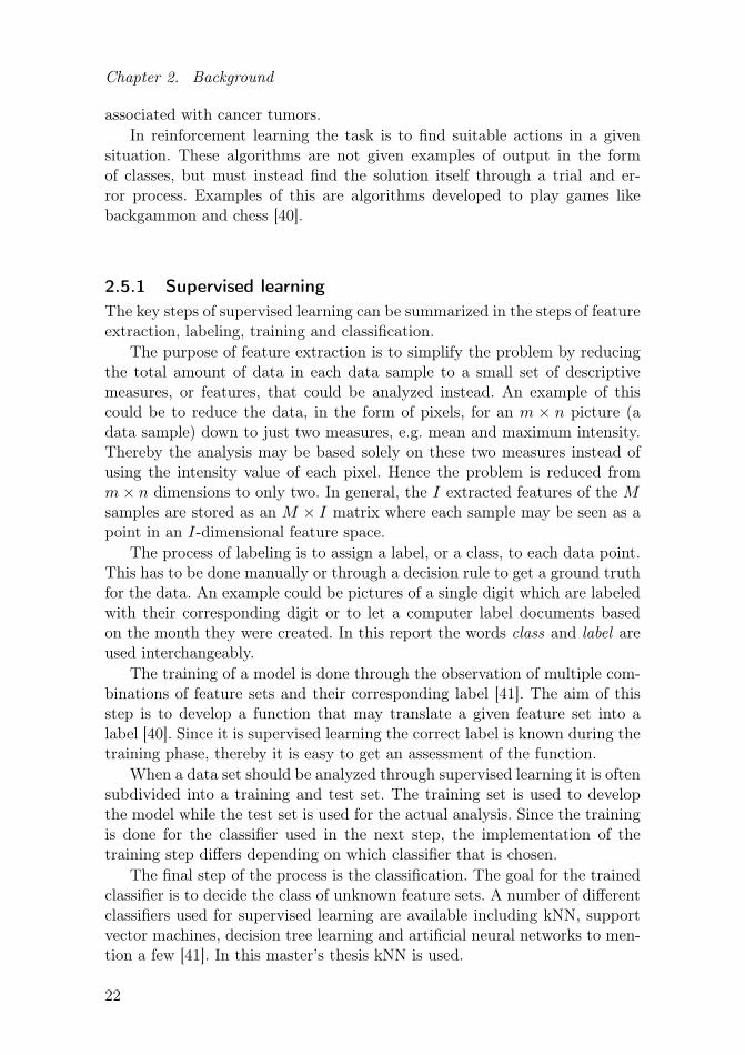
2.5.1 Supervised learningThe key steps of supervised learning can be summarized in the steps of featureextraction, labeling, training and classification.

The purpose of feature extraction is to simplify the problem by reducingthe total amount of data in each data sample to a small set of descriptivemeasures, or features, that could be analyzed instead. An example of thiscould be to reduce the data, in the form of pixels, for an m × n picture (adata sample) down to just two measures, e.g. mean and maximum intensity.Thereby the analysis may be based solely on these two measures instead ofusing the intensity value of each pixel. Hence the problem is reduced fromm× n dimensions to only two. In general, the I extracted features of the Msamples are stored as an M × I matrix where each sample may be seen as apoint in an I-dimensional feature space.

The process of labeling is to assign a label, or a class, to each data point.This has to be done manually or through a decision rule to get a ground truthfor the data. An example could be pictures of a single digit which are labeledwith their corresponding digit or to let a computer label documents basedon the month they were created. In this report the words class and label areused interchangeably.

The training of a model is done through the observation of multiple com-binations of feature sets and their corresponding label [41]. The aim of thisstep is to develop a function that may translate a given feature set into alabel [40]. Since it is supervised learning the correct label is known during thetraining phase, thereby it is easy to get an assessment of the function.

When a data set should be analyzed through supervised learning it is oftensubdivided into a training and test set. The training set is used to developthe model while the test set is used for the actual analysis. Since the trainingis done for the classifier used in the next step, the implementation of thetraining step differs depending on which classifier that is chosen.

The final step of the process is the classification. The goal for the trainedclassifier is to decide the class of unknown feature sets. A number of differentclassifiers used for supervised learning are available including kNN, supportvector machines, decision tree learning and artificial neural networks to men-tion a few [41]. In this master’s thesis kNN is used.

22


2.5.1.1 k-fold cross validationOne way of splitting the data into a training and test set in an organized wayis through k-fold cross validation. This method splits the data into k differentgroups, using one group for the test set and the remaining k−1 groups for thetraining set. The classification is repeated a total of k times allowing everygroup to be used as test set once, with the result being the mean of all kclassifications. [41]

2.5.1.2 k-nearest neighborsThe classification method kNN is despite its simplicity successful in a widerange of classification problems [41]. The training step is very simple andonly includes storing the feature set of the different training data points. Toclassify a test data point, the Euclidean distances between it and all trainingdata points are calculated. The k closest training data points are chosen andthe most frequent label among them determines the label of the test datapoint.

An example of a two-dimensional feature space including a test data pointand training data set with 3 different classes can be seen in Figure 2.9. Ascan be seen in the figure these two features are enough to separate the threeclasses into distinct clusters, using only one of these features would not beenough. If a kNN classifier would be used in this case the test point would beclassified as class 0, independent of the value of k.

−0.5 1.0 2.5Feature 1

−0.25

0.50

1.25

Feature 2

Class 0Class 1Class 2Test

Figure 2.9: Example of a two-dimensional feature space.

Different weighting techniques are available when using kNN. One op-tion is to base the weighting on the distance between the test point and itsneighbors, giving closer neighbors a larger weight. This is done by assigninga neighbor at distance d to the test point the weight 1/d.

23


2.5.1.3 EvaluationTo evaluate the result the quantity of classifier accuracy can be used. This isachieved through the division of the number of correct classified test pointswith the total number of test points.

A more sophisticated evaluation method is to use a confusion matrix, seeFigure 2.10. It gives a better visualization of the performance, allowing theinterpreter to analyze the classification of each label in more depth. The rowsof the confusion matrix represent the classification of the actual label, i.e.row 1 shows how test data points with the actual label 1 are classified. Incontrast, the columns represent the prediction of labels, i.e. column 1 showsthe true label of test points predicted to be label 1. This means that each rowsums up to one which is not necessarily true for each column.

Out of the confusion matrix in the figure it can be seen that 9.7 % respec-tively 10.4 % of the test points with label 1 are wrongly classified as label 0and label 2, whereas 80.0 % are correctly classified as label 1. Thereby all thecorrect classified test points are positioned on the diagonal going from thetop left to the bottom right corner. A perfect classification would result ina confusion matrix where all squares on the diagonal have the value 1.0 andthe remaining squares the value 0.0. Hence, the darker the diagonal is in aconfusion matrix, the better the classification is.

0 1 2Predicted class

0

1

2

True

class

0.9 0.1 0.0

0.097 0.8 0.104

0.0 0.105 0.895

0.0

0.2

0.4

0.6

0.8

1.0

Figure 2.10: Confusion matrix with three different classes.

24

3Data

The data analyzed in this master’s thesis is derived from the log files of 10dialysis machines of model AK 98 located at a hospital. Thus the data isderived from treatments of real patients. The log files are compressed to .zipformat where each file contains approximately one month of data acquisition.A total of 10− 13 .zip files from each machine were analyzed, correspondingto a total time frame of 8− 12 months.

3.1 Log files

The internal memory of the AK 98 may contain data for about one month ofmachine runs during normal usage, i.e. 2−3 treatments a day of approximately3−4 hours. The logging is initiated each time the machine starts. Thereby it isnot only actual treatments that are logged but all machine runs, including e.g.disinfections and services. When the memory runs out the oldest entries areoverwritten. Because of this a monthly extraction of the .zip files is suitableif no data should be lost.

The process of extracting the .zip files results in the saving of each ma-chine run in a separate file. In addition to this, two other files are generated,containing information about which parameters that have been logged andhow this logging was done.

There are three different ways a parameter may be logged. The first op-tion is to log every update which is the standard for e.g. alarms. The secondoption is to log with a predefined time interval although this option is rarelyused. The third option, the delta-method, is to store a new value only when apredefined change from the last logged value has been exceeded. This change,or delta, is chosen based on each signal’s individual characteristic. This re-duces the amount of data stored but also results in an uneven sampling ratefor each signal.

The data from all sensors and valves in Figure 2.5 are available in the logfiles. In addition to this, a number of different machine processes and statesas well as manual input to the machine are logged. This adds up to a total ofover 400 different parameters available.

25

Chapter 3. Data

3.2 Analyzed signals

Out of the extensive amount of sensor data available it is only the signalsbelieved to have some relationship to the UFD status that have been analyzed.The sensors responsible for these signals are visualized in Figure 3.1 which isa magnification of the lower right part of Figure 2.5. To be able to perform asuitable preprocessing of these signals it is not only sensor data that has beenretrieved from the log files, but also logged information regarding machinestates. A brief description of the signals most relevant to this master’s thesiswill follow below in Sections 3.2.1−3.2.6. An example of each of these signalsfrom a standard run can be seen in Figure 3.2.

Figure 3.1: A magnification of the most relevant part of the fluid path situatedin proximity to the UFD.

3.2.1 Flow pump derived signalsAs described in Section 2.3.4, the flow pump is responsible for keeping a con-stant degassing pressure and thereby it is indirectly affected by an increasedmain flow. The parameter flow pump cycle measures the workload of the flowpump given in percentage of its maximum capacity. It is logged with thedelta-method with a delta of 1.5 percentage points.

The parameter flow pump current is related to flow pump cycle. It de-scribes the electrical current used by the flow pump and is measured in mAand logged with a delta of 10 mA.

26


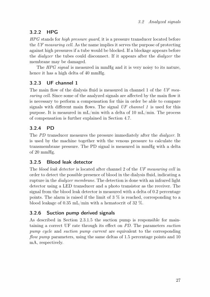
3.2.2 HPGHPG stands for high pressure guard, it is a pressure transducer located beforethe UF measuring cell. As the name implies it serves the purpose of protectingagainst high pressures if a tube would be blocked. If a blockage appears beforethe dialyzer the tubes could disconnect. If it appears after the dialyzer themembrane may be damaged.

The HPG signal is measured in mmHg and it is very noisy to its nature,hence it has a high delta of 40 mmHg.

3.2.3 UF channel 1The main flow of the dialysis fluid is measured in channel 1 of the UF mea-suring cell. Since some of the analyzed signals are affected by the main flow itis necessary to perform a compensation for this in order be able to comparesignals with different main flows. The signal UF channel 1 is used for thispurpose. It is measured in mL/min with a delta of 10 mL/min. The processof compensation is further explained in Section 4.7.

3.2.4 PDThe PD transducer measures the pressure immediately after the dialyzer. Itis used by the machine together with the venous pressure to calculate thetransmembrane pressure. The PD signal is measured in mmHg with a deltaof 20 mmHg.

3.2.5 Blood leak detectorThe blood leak detector is located after channel 2 of the UF measuring cell inorder to detect the possible presence of blood in the dialysis fluid, indicating arupture in the dialyzer membrane. The detection is done with an infrared lightdetector using a LED transducer and a photo transistor as the receiver. Thesignal from the blood leak detector is measured with a delta of 0.2 percentagepoints. The alarm is raised if the limit of 3 % is reached, corresponding to ablood leakage of 0.35 mL/min with a hematocrit of 32 %.

3.2.6 Suction pump derived signalsAs described in Section 2.3.1.5 the suction pump is responsible for main-taining a correct UF rate through its effect on PD. The parameters suctionpump cycle and suction pump current are equivalent to the correspondingflow pump parameters, using the same deltas of 1.5 percentage points and 10mA, respectively.

27

Chapter 3. Data

0

50

100Pe

rcen

t (%) Flo) %(m% cycle

0

100

200

mA

Flo) %(m% c(rrent

0

500

mmHg

HPG

0

500

mL/min

UF channel 1

−500

0

mmHg

PD

0

10

Percen

t (%) Blood lea detector

14 15 16 17 18 190

50

100

Percen

t (%) S(ction %(m% cycle

14 15 16 17 18 190

200

400

mA

S(ction %(m% c(rrent

Cloc time

Figure 3.2: An example of the eight most important sensor signals used for theanalysis in this master’s thesis. The depicted signals are all derived from thesame log file. The tarations occurring every 30 minutes during the treatmentare easily detected in some of the signals.

28

4Method

This project was subdivided into two distinct parts. The first part was the al-gorithm development which constituted the vast majority. The second, muchsmaller part was the evaluation of the developed algorithm. In order to avoidbiasing, the 10 machines available for analysis were split into two sets withfive machines each. One of these sets was used for the algorithm developmentwhereas the other was used for the evaluation of the final algorithm.

The five machines from the algorithm development set were used in thetime consuming process of finding the best features and parameter settings.Thus, for the five machines in the evaluation set only these selected featuresand optimal parameter settings were used during the classification. The finalevaluation of the algorithm was therefore based on data that were never usedin the development phase.

In the multiple classifications during the algorithm development the train-ing and test data were derived from the five machines of the algorithm de-velopment set. In the evaluation of the algorithm the training and test datawere derived from the 5 machines of the evaluation set. Thus, the two setswere never mixed. In both cases k-fold cross validation was used.

The method used during the algorithm development was subdivided intoshorter steps. The first step was to localize when the UFD replacements andhypochlorite disinfections had taken place in the analyzed machines. Rele-vant signals were then chosen and preprocessed in order to remove noise andunwanted segments. Based on the found occasions for UFD replacements andhypochlorite disinfections the data was labeled in two different ways. A num-ber of different descriptive features were calculated. To be able to analyze alldata together, features that were affected by the main flow were compensated.All features were then normalized and tested to find which ones that werethe best to separate different labels. The best features were selected and fedto a classifier which used training data to classify test data. The predictedlabel was compared to the true label. The classification step was repeateda number of times to test different parameter settings during the algorithmdevelopment phase. These steps are further explained in the sections below.

29

Chapter 4. Method

In order to study whether the algorithm was machine specific or not alltests were run in parallel for two different cases, the single respectively mul-tiple machine analyses. In the single machine analysis the machines wereanalyzed one by one whereas they were analyzed all together in the multiplemachine analysis.

4.1 Localizing UFD replacements

Since no information regarding the occurrences of the UFD replacementswas available, this had to be retrieved from the log files. When one of thethree counters indicating time for UFD replacement has reached its limit anattention is raised. After the UFD replacement the operator needs to press abutton to confirm the replacement and remove the attention, thereby resettingthe three different counters. This procedure is logged in Process 153 in thestate machine, TimeBetweenUfdChangeProc, as a state change from any stateto state five, ResetUfdReminder. The log files containing UFD replacementswere saved in a separate list and removed from the rest of the data set.

4.2 Localizing hypochlorite disinfections

To retrieve information regarding when hypochlorite disinfections were con-ducted the signals FI_DisinfTypeID and FI_DisinfType− StartStopwere analyzed. All log files were gone through to find occasions whenFI_DisinfTypeID was set to eight, indicating hypochlorite disinfection.The corresponding start and stop times for each disinfection program werecollected through FI_DisinfTypeStartStop. In instances when no stop timewas found this way the end time was chosen as the end point of the log file.From these times the duration of the disinfection could be calculated, onlythose exceeding 45 minutes were saved as true disinfections. When a log filecontained both a hypochlorite disinfection and a treatment episode the timenotifications of each were used to determine how to label the log file.

4.3 Preprocessing of signals

During the extraction of the .zip files each machine run is saved in a separatelog file. The first step in the preprocessing was to remove log files corre-sponding to disinfections, services and shorter treatments. To achieve thisthe signal MACHINE_MODE was used to detect which files that containeda treatment episode and the duration of it. Only files containing a single treat-ment episode with a duration of more than 90 minutes were further analyzed.Files with multiple treatment episodes or an episode shorter than 90 minuteswere discarded due to unstable signal behavior and to remove factory runs.

30


When the files of interest were selected, the signals retrieved from eachfile were preprocessed further. Since the logging is initiated when the machineis turned on, each file does not only include data collected during treatment,but also data from start-up, functional check, blood line preparation, pre-treatment, post treatment, disinfections and service. To remove unwanteddata only the time frame corresponding to actual treatment was used. Thiswas selected as the time frame when MACHINE_MODE was set to 4, whichequals treatment, resulting in a continuous signal of at least 90 minutes. Thispart of the signal included tarations which largely affect some of the signalsas can be seen in Figure 3.2. It could also contain episodes when the UFDwas bypassed due to e.g. alarms. To remove these unwanted episodes the sig-nal O_DIVAOPEN was used. Since some signals exhibited unstable signalbehavior around the opening and closing of DIVA an extra cutoff of 4 secondswas used in both cases.

The data remaining after these steps varied greatly between different sig-nals, it could differ as much as a factor 30 in number of samples betweendifferent signals of the same treatment episode. To be able to compare thedifferent signals from the same file they had to be uniformly resampled. Thiswas done by using linear interpolation with a sample frequency of 100 Hz,which was enough to avoid aliasing.

Some of the signals behaved unstable in the start-up phase of the treat-ment. Due to this, the first ten minutes were discarded from all signals. Fromthis point forward, log file refers to a log file that has gone through the pre-processing steps up to this point.

The final, optional, step in the preprocessing was to segment each signalinto smaller time windows of equal duration. The length of the time windowwas set manually by the adjustable parameter window length. It was alsopossible to reject this step and keep the entire treatment as a single segment.In this report window lengths of 5, 15 and 30 minutes have been analyzed inaddition to the no windowing option.

The steps of the preprocessing are summarized in chronological order be-low:

• Discard runs with treatment episodes < 90 min.

• Discard runs with multiple treatment episodes.

• Only keep data corresponding to MACHINE_MODE = 4 (treatment).

• Only keep data when main flow is passing UFD (DIVA = open) withan extra cutoff margin of 4 seconds.

• Resample signals through linear interpolation.

• Discard first 10 minutes of each signal.

• Subdivide signals into shorter segments (optional).

31

Chapter 4. Method

4.4 Labeling of data

Two different methods for labeling the data have been tested. The first methodwas based on the number of log files between two adjacent UFD replacements.Based on the parameter number of labels, which was variable, the log files weredivided into equally large groups based on their chronological order. If thenumber of log files and number of labels were not divisible the extra log fileswere split as evenly as possible. E.g. if there were 62 log files between twoadjacent UFD replacements and number of labels was set to 3, each labelshould contain 20.67 log files. However, since the log files were not split thenumber of log files in each label was rounded to the closest integer. Thuslabel 0 is assigned to log file 1 to 20.67 ≈ 21, label 1 is assigned to log file22 to 2 × 20.67 = 41.33 ≈ 41 and label 2 is thereby assigned to log file42 to 62, resulting in 21, 20 and 21 log files with label 0, 1 respectively 2.Independent of number of labels, label 0 always corresponds to the log filesimmediately succeeding a UFD replacement, hence the longest RUL of theUFD. Consequently, the last label always corresponds to log files immediatelypreceding the next UFD replacement, hence the shortest RUL of the UFD.

The second labeling method was based on the number of hypochloritedisinfections the UFD had experienced. Label 0 was assigned to log files witha UFD exposed to zero hypochlorite disinfections. This corresponded to logfiles situated in between a UFD replacement and the first hypochlorite disin-fection. Label 1 was assigned to log files with a UFD exposed to 1 hypochlo-rite disinfection, corresponding to log files between the first and the secondhypochlorite disinfection and so on.

In Figure 4.1 a comparison between the two different labeling methodson a synthetic data set of 63 log files and three labels can be seen. The bluevertical lines symbolize filter replacements and the red lines hypochlorite dis-infections. Due to the irregular occurrences of these disinfections this methodgive rise to some discrepancies in the number of log files in each label. Thesediscrepancies may be large for a small data set but decreases with the sizeof it due to a reduced impact of randomness. The 63rd log file is situatedafter the second filter replacement, hence the labeling is reset from 0 for bothmethods.

Both labeling methods share some common characteristics. When the logfiles are subdivided into shorter segments, each segment is assigned the samelabel as the log file it is derived from. Log files preceding the first registeredfilter replacement and treatments succeeding the last registered filter replace-ment of each machine are discarded due to uncertainty of how they shouldbe labeled.

32

4.5 Feature extraction

0 10 20 30 40 50 60Log file #

Method 2

Method 1

Method 2

Method 1

Method 2

Method 1

UFD replacementHypochlorite disinfectionLabel 0Label 1Label 2

Figure 4.1: Illustration of the two different labeling methods. With method1 the log files are close to being evenly distributed, the first 21 log files areassigned label 0, the following 20 log files are assigned label 1 and the last21 are assigned label 2. Method 2 are based on the hypochlorite disinfections(red vertical lines), occurring after the 19th and 35th log files. This results inassigning label 0 to the first 19 log files, label 1 to the succeeding 16 log files(log file number 20−35) and label 2 to the last 27 log files.


A total of eight different signals have been analyzed. Seven of these wereobtained directly from the log files. These are presented in Figure 3.2, exceptfor the signal UF channel 1 which is used for the flow compensation. The8th analyzed signal was created as the difference between two of the signals,the HPG and PD pressures, and is presented in Figure 4.2. On all of thesesignals, 21 different measurements have been calculated, where 15 are in thetime-domain and 6 in the frequency-domain. In addition to this two differentcross-correlation based measurements have been calculated for five differentsignal pairs.

The combination of a measure and a signal is defined as a feature. With21 measurements calculated from 8 signals in addition to 2 measurementscalculated from 5 signal pairs a total of 178 different features were extractedfrom each log file. This was done either for the entire signal or individuallyfor each segment when windowing was used.

33

Chapter 4. Method

14 15 16 17 18Clock time

100

150

200

250

mmHg

Figure 4.2: An example of the (HPG−PD) signal after preprocessing. It isderived from the same treatment episode as the signals in Figure 3.2.

4.5.1 Features derived from time-domainThe first 4 of the measurements derived from the time-domain correspondsto the standardized moments in probability theory, i.e. mean (µ), standarddeviation (σ), skewness (SK) and kurtosis (KU) presented in Equations (4.1)−(4.4).

µ =1

N

N∑n=1

xn (4.1)

σ =

√√√√ 1

N − 1

N∑n=1

(xn − µ)2 (4.2)

SK =

∑Nn=1(xn − µ)3

(N − 1)σ3(4.3)

KU =

∑Nn=1(xn − µ)4

(N − 1)σ4(4.4)

The next 6 measurements are mentioned in [24] as commonly used time-domain features in CBM. Those are maximum value (max), root mean square(RMS), crest indicator (CI), clearance indicator (CLI), shape indicator (SI)and impulse indicator (II) presented in Equations (4.5)− (4.10).

34


max = maxn=1,...,N

xn (4.5)

RMS =

√√√√ 1

N

N∑n=1

(xn)2 (4.6)

CI =max |x|RMS

(4.7)

CLI =max |x|

( 1N

∑Nn=1

√|xn|)2

(4.8)

SI =RMS

1N

∑Nn=1 |xn|

(4.9)

II =max |x|

1N

∑Nn=1 |xn|

(4.10)

In addition to these measurements another 5 were used, namely minimumvalue (min), lower quartile (Q1), median (Q2), upper quartile (Q3) and in-terquartile range (IQR). The equation for calculating the minimum value ispresented in Equation (4.11). The median of a data set is the value that sepa-rates the higher half of the values from the lower half. The lower quartile is thevalue that separates the lowest 25 % of the data from the highest 75 %. Theupper quartile is correspondingly the value that separates the lowest 75 %of the data from the highest 25 %. The interquartile range is the differencebetween the upper and the lower quartile.

min = minn=1,...,N

xn (4.11)

4.5.2 Features derived from frequency-domainThe fast Fourier transform (FFT) was used to transform the data from time-domain to frequency-domain, see Equation (4.12). To take advantage of theFFT’s special feature making it much faster for data of length 2p, where p isa natural number, zero padding was used.

The measurements used in the frequency domain are the dominant fre-quency (DF ), the sum of the 10 largest Fourier coefficients (c1−10), lowerquartile (ckQ1), median (ckQ2), upper quartile (ckQ3) and interquartile range(ckIQR) of the Fourier coefficient. The equations for calculating the DF andFourier coefficients (ck) are given in Equations (4.13)−(4.14).

35

Chapter 4. Method

Xk =N−1∑n=0

xne−i2πnkN , k = 0, ..., N − 1 (4.12)

DF = arg maxk

(ck) (4.13)

ck =|Xk|N

(4.14)

4.5.3 Features derived through cross-correlationCross-correlation is used to detect correspondences between two time series.All signals derived from the fluid unit of the AK 98 are part of the same systemsubdivided into different smaller control systems. Even if two signals are notin direct connection through a control loop where one of them regulates theother, they may still exhibit some dynamic behavior. The idea behind usingfeatures derived through cross-correlation was to analyze signal pairs believedto have some connection and detect if a clogging of the UFD could have aneffect on their potential dynamic behavior.

Five different signal pairs were analyzed through cross-correlation. Thesesignal pairs are presented in Table 4.1 and they were chosen based on an ex-pected connectivity. The equation for cross-correlation is presented in Equa-tion (4.15), here assuming signals of equal length. From the result of thecross-correlation two different measures were derived, the maximum value(CCM) and the time delay (CCTD), see Equations (4.16)−(4.17).

Table 4.1: Signal pairs used for cross-correlation.

Signal 1 Signal 2 AbbreviationFlow pump cycle Suction pump cycle Pair 1

Flow pump current Suction pump current Pair 2Flow pump cycle (HPG−PD) Pair 3Flow pump cycle HPG Pair 4

Suction pump cycle PD Pair 5

ryx(k) =1

N

N−1−k∑n=0

xnyn+k, k = ±0, ...±N − 1 (4.15)

CCM = maxk=±0,...,±N−1

(|ryx(k)|) (4.16)

TD = arg maxk

(|ryx(k)|) 1

FS, FS = sampling frequency (4.17)

36

4.6 Split of data into training and test sets

4.6 Split of data into training and test sets

When the feature extraction was completed the log files were split into atraining and test set using k-fold cross validation [41]. When windowing wasused all windows derived from the same log file were kept as a unit belongingto either the training or the test set. When no further explanation is givenregarding the split of the data into training and test sets the following holdstrue.

Since 5 machines were used for the algorithm development it was naturalto use k = 5 in the k-fold cross validation during the multiple machine analy-sis. The log files were grouped according to which dialysis machine they werederived from. Thereby the log files from a dialysis machine were never splitbetween the training and test sets and every machine could be used as testset once.

For comparison, k = 5 was used in the single machine analysis as well.Thereby 80 % of the log files were assigned to the training set and 20 % tothe test set.

4.7 Flow compensation

When the median flow of UF channel 1 was analyzed for all the log files of asingle machine it was found that 3 different main flows were probably used;500, 600 and 700 mL/min as seen in Figure 4.3. When the different featureswere plotted against main flow it became apparent that some, but not all,were affected by the flow. To make the algorithm independent of main flowthis had to be compensated for.

500 550 600 650 700Days since 1/1-2015

500

600

700

mL/min

Figure 4.3: Illustration of the median flow of UF channel 1 for all log files ofa single machine when no windowing was used. Each sample corresponds tothe median flow of a single log file.

37

Chapter 4. Method

The compensation was done individually for each of the 178 features. Or-dinary least squares regression was used to estimate the relationship betweenthe samples of a feature and main flow, see Equation (4.18), where x is themain flow vector, y is the samples of the i:th feature (fi), and 1 is a col-umn vector of ones with the same length as x. The sample points were thentransferred to a 600 mL/min main flow using β0, see Equation (4.19).

β = [β0 β1]T = (XTX)−1XTy (4.18)

WhereX = [x 1]

x = [x(0), . . . , x(N−1)]T

Andy = fi

ycomp = y + (β0(600× 1− x)) (4.19)

An example of this compensation is presented in Figure 5.2 were both orig-inal and compensated samples of a feature are plotted. Which features thatfinally used the compensation are presented in Table 4.2. This decision wasbased on visual assessment of the plot of original and compensated samplesfor each feature and the corresponding linear fit.

Table 4.2: The 7 measurements from the 6 signals below con-stitutes the 42 features that were flow compensated. The corre-sponding equations are given in brackets.

MeasurementsFlow pump cycle

Mean (4.1), Max (4.5), RMS (4.6),Flow pump current

Lower and Higher Quartile,HPG

Median and Min (4.11)(HPG−PD)Suction pump cycle

Suction pump current

4.8 Feature normalization

In order to give each feature the same possible impact on the classificationresult, independent of the scale of the feature, they had to be normalized.This was done through the use of the Min-Max normalization method given

38

4.9 Feature selection

in Equation (4.20) where f ′m,i is the normalized value of sample m for thefeature i. Thereby all features are scaled to the range [0, 1].

f ′m,i =fm,i −min fi

max fi −min fi(4.20)


Two different methods to perform feature selection were tested and evaluated.The first method was the TFSWT based on Euclidean distance evaluationtechnique described in [37]. As the name implies it also includes weighting ofthe selected features but this step was not implemented. The second methodwas sequential forward selection (SFS).

When classification was done during the TFSWT and SFS the classifierused was kNN with k = 10, using the weighting technique based on distancementioned in Section 2.5.1.2. The labeling was done with the first labelingmethod, time based labeling, using 12 labels. No windowing was used.

4.9.1 Two-stage feature selection and weighting techniqueThis method is a comparison of the average distances of the feature samplesbetween and within the different labels. This ratio is higher the better afeature is at separating the different labels, indicating a large distance betweensamples of different labels and a short distance between samples of the samelabel.

The first step of this method is to calculate the average distanceD betweenthem samples of the feature i of label c, see Equation (4.21).Mc is the numberof samples for label c.

Dc,i =

√√√√ 1

Mc × (Mc − 1)

Mc∑l,m=1

(fm,c,i − fl,c,i)2, l 6= m (4.21)

Then the average distance is calculated within (w) each feature as

D(w)i =

1

C

C∑c=1

Dc,i (4.22)

The variance factor for each feature is calculated as

V(w)i =

max(Dc,i)

min(Dc,i)(4.23)

39

Chapter 4. Method

The average feature value of all samples for the same label is calculated as

ac,i =1

Mc

Mc∑m=1

fm,c,i (4.24)

Out from this the average distance between (b) samples of different labels iscalculated as

D(b)i =

√√√√ 1

C × (C − 1)

C∑c,l=1

(al,i − ac,i)2, c 6= l (4.25)

The variance factor between different labels is defined as

V(b)i =

max(|al,i − ac,i|)min(|al,i − ac,i|)

, c, l = 1, 2, . . . , C, c 6= l (4.26)

The variance factor λ for each feature is calculated as

λi =

(V

(w)i

max(V(w)i )

+V

(b)i

max(V(b)i )

)−1(4.27)

The ratio of D(b)i and D

(w)i is calculated and combined with the variance

factor as

Ei = λiD

(b)i

D(w)i

(4.28)

These values are normalized with the maximum value to obtain the finalevaluation criteria

Ei =Ei

max(Ei)(4.29)

The closer the value of Ei is to 1, the better the corresponding featureis to separate the C different labels. With the introduction of a predefinedthreshold σ, only features fulfilling the criteria Ei ≥ σ may be selected.

The TFSWT was done individually for each of the 5 machines in thealgorithm development set during the single machine analysis. To be able tomake a comparison with the other feature selection method, SFS, the 10 bestfeatures for both methods were chosen without the use of any threshold. Thus5 feature sets with 10 features each were generated.

40

4.10 Classification using kNN

Each machine was split into a training and test set corresponding to 80 %respectively 20 % of the log files. All feature sets were used for classificationof the test set from the five machines. The mean accuracy for each featureset was calculated and the best feature set was chosen.

In the multiple machines analysis the TFSWT was done once using all thedata from the 5 machines in the algorithm development set. Thus the featureset with the 10 best features was obtained at once.

4.9.2 Sequential forward selectionAs compared to the previous method which aims at finding the best individualfeatures and then combining them, this method tries to find a combinationof features that perform well. SFS is an iterative method starting with anempty feature set. In the first iteration each feature is tested individually andthe one generating the highest classification accuracy is added to the emptyfeature set. In the second iteration all remaining features are tested one byone in combination with the feature from the selected feature set. The featuregenerating the highest classification accuracy in combination with the alreadyselected feature is added to the feature set and so on. The iterations continueuntil either a predefined number of features are selected or the improvementbetween two iterations is below a certain threshold.

The SFS was done individually for each of the 5 machines in the algorithmdevelopment set during the single machine analysis. Each machine was splitinto the same training and test set used in the TFSWT. The test sets weresaved for later use whereas the training sets were split once more using k-fold cross validation with k = 5. Each of these splits was used to select onefeature giving the best accuracy. These 5 accuracies were compared and thefeature corresponding to the highest was chosen. The SFS was repeated until10 features were selected. Thus one feature set was created for each machine.These feature sets were then evaluated using the original test set which wasnot used to select the features. The mean accuracy of every feature set usedon all machines was calculated and the one generating the highest accuracywas chosen.

In the multiple machines analysis the procedure was the same with theexception of the initial split which were neglected. Each machine made up itsown group in the 5-fold cross validation. This resulted in a single feature set,therefore no evaluation of different feature sets was necessary.

4.10 Classification using kNN

The classification method used in this report was kNN. The test and trainingdata were vectors of length 10, corresponding to the 10 different featuresselected through the methods discussed in Section 4.9. The value of k was

41

Chapter 4. Method

varied between 1 and 50. The weighting technique mentioned in Section 2.5.1.2giving closer neighbors a larger weight was used.

When windowing was used a voting procedure was implemented to decidethe classification of each log file as a unit. All windows derived from thesame log file, and their classification result, were given one vote and the labelreceiving the most votes was chosen. If two labels received the same amountof votes the one with the smallest label number was chosen.

4.11 Evaluation

In order to test the developed algorithm on previously unused data the 5machines from the evaluation set were used. During this final test the specificfeatures and parameters chosen during the algorithm development step forthe single respectively multiple machine analyses were used. Both analyseswere conducted using k-fold cross validation with k = 5, thereby the trainingdata was derived from the machines in the evaluation set.

During the evaluation it was only the training data that was used to cal-culate the flow compensation parameter which were then, if necessary, used tocompensate both the training and test data. In a similar manner, the featuresfrom the training set were normalized first and the maximum and minimumvalue encountered here were saved and used during the normalization of thefeatures in the test set as well.

42

5Results


The final result of the preprocessing of the signal HPG-pressure from a 5 hourlong log file is presented in Figure 5.1. The blue part is the raw data whereasthe orange parts are the segments remaining after the preprocessing. Theupper part shows the signal from the entire machine run, thereby it includesthe steps of e.g. start-up, functional check and disinfection. The lower part isa magnification of the part of the signal whenMACHINE_MODE is set totreatment, occurring approximately between 7.15 am and 11.30 am. As canbe seen the first part of the treatment episode exhibits somewhat unstablesignal behavior, which explains why the first 10 minutes are discarded. Thetarations are easily detected as the temporary pressure drops occurring every30 minutes. As can be seen, these are discarded as well.

−500

0

500

7 8 9 10 11 12Clock time

200

400

Raw dataPreprocessed data

mmHg

Figure 5.1: Result from the preprocessing of the signal HPG-pressure.

43

Chapter 5. Results


The compensation of one of the flow sensitive features,median of (HPG−PD),is illustrated in Figure 5.2. The blue points represent the original, uncompen-sated, samples whereas the orange points represent the compensated ones.The figure shows all the samples from a single machine using a time windowof 30 minutes from the aforementioned feature. It is worth noting that themain flows of 500 and 700 mL/min have been used more frequently than themain flow of 600 mL/min in the current machine. This holds true for theother machines as well.

400 450 500 550 600 650 700 750 800mL/min

75

100

125

150

175

200

225

250

275

mmHg

Regression lineUncompensated featureCompensated feature

Figure 5.2: Result of the flow compensation for the feature median of(HPG−PD).


In order to analyze the extracted features, four different approaches wereused. Two different types of plots, time series and box plots, were used to geta subjective visual assessment of the features. In addition to this the objectivefeature selection techniques of TFSWT and SFS were used.

5.3.1 Time seriesTo examine how the values of the different features varied during the analyzedtime frame a time series plot was used. Since the analyzed machines wereproduced from 2015 and onward, the date 01/01/2015 was used as day 0. The

44


date and start hour for each machine run were used as x-value in these plots.The occasions for UFD replacements were marked with a blue vertical line. Ifa feature exhibiting a periodicity coinciding with the UFD replacements werefound this would be a strong indicator that the primary aim of this report,to develop an algorithm which can be used in a service indicator for UFDreplacements, would be feasible. A few of the analyzed features did exhibitsuch a behavior. Those were the mean, max, RMS, median, lower quartileand upper quartile of the signal (HPG−PD). One of these features, meanof (HPG−PD), is shown in Figure 5.3a. The majority did not exhibit anyclear relationship with the UFD replacements. For comparison, one of thesefeatures, mean of suction pump current is shown in Figure 5.3b.

450 500 550 600 650 700 750 800Days since 1/1/2015

−0.5

0.5

1.5

mmHg

(normalize

d)

UFD re lacementMean of (HPG-PD)

(a) Mean of (HPG−PD).

450 500 550 600 650 700 750 800Days since 1/1/2015

−0.5

0.5

1.5mA (normalize

d)UFD replacementMean of s ction p mp c rrent

(b) Mean of suction pump current.

Figure 5.3: Time series of the features mean of (HPG−PD) and mean of suc-tion pump current. In (a) a clear relationship between the feature and theUFD replacements can be seen. The same pattern with gradually decliningvalues which are "reset" in connection with the UFD replacements are re-peated between all UFD replacements. In (b) no such relationship can beseen.

These time series plots were also used to detect other possible time depen-dencies that had nothing to do with UFD replacements. If such features ex-isted they could possibly damage the developed algorithm, introducing pseudorelationships. As a matter of fact, a couple of features derived from the sig-nal blood leak detector did show promising classification results in the initialphase of the algorithm development. However, when they were visualized withtime series plots as seen in Figure 5.4, it became apparent that their time de-pendency had nothing to do with the UFD status but was instead a gradualdrift over time. This gradual drift lead to lower feature values for the firstlabels (just after a UFD replacement) compared to the last (just before thenext UFD replacement), no matter which of the UFD replacements they weresituated in between.

45

Chapter 5. Results

500 550 600 650 700Days since 1/1/2015

−0.5

0.5

1.5Pe

rcen

% (n

orm

alize

d)UFD replacemen Mean of blood leak de ec or

Figure 5.4: Time series of the feature mean of blood leak detector. No rela-tionship with UFD replacements can be seen, instead there is a gradual driftover time. The short segment with missing data around day 540 is either dueto the fact that the machine has not been used, or more probable, that theselog files are overwritten since the monthly extraction is delayed.

This could be compared to a hypothetical feature which simply countedthe days since last UFD replacement. Such a feature would always increase itsvalue with higher label number. As such, it would achieve high classificationresults but the feature would have absolutely no connection with actual statusof the UFD, hence be useless from a CBM point of view.

Due to this, the features derived from the signal blood leak detector couldnot be used and they were therefore discarded for the rest of the algorithmdevelopment.

5.3.2 Box plotsIn addition to the time series plots, another manual evaluation of the fea-tures was done. This was achieved by analyzing the box plots for each featureindividually, visualizing a possible difference between the labels. For the ma-jority of the features there were no obvious differences between the labels, oneexample of such a feature is given in Figure 5.5. The only features that didshow a clear both visual and statistical significant difference between labelswere the same as those mentioned in Section 5.3.1 found to exhibit a period-icity coinciding with the UFD replacements. This result was achieved bothfor single machines as well as when the machines were analyzed all together.An example of this is given in Figure 5.6.

46


0 1 2 3 4 5 6 7 8 9 10 11Label #

55

60

65

70Pe

rcen

t (%)

(a) One machine.

0 1 2 3 4 5 6 7 8 9 10 11Label #

55

60

65

70

75

Percen

t (%)

(b) All machines.

Figure 5.5: Box plots of the feature mean of flow pump cycle. No obviousrelationship between feature value and label number can be seen.

0 1 2 3 4 5 6 7 8 9 10 11Label #

150

170

190

210

mmHg

(a) One machine.

0 1 2 3 4 5 6 7 8 9 10 11Label #

120

140

160

180

200

220

mmHg

(b) All machines.

Figure 5.6: Box plots of the feature mean of (HPG−PD). A clear relationshipcan be seen as a gradual decrease of feature value with label number.

5.3.3 TFSWTThe 10 features receiving the highest normalization scores, Ei, for each ma-chine in the single and multiple machine analyses are presented in Table 5.1respectively Table 5.2. The feature set with the highest mean accuracy in thesingle machine analysis, Table 5.1a, was chosen.

47

Chapter 5. Results

Table 5.1: Result from the single machine TFSWT. The flow pump and suc-tion pump are abbreviated as FP respectively SP. The other abbreviationsare given in Section 4.5.

(a) Machine 1

Feature Ei

Q3 (HPG−PD) 1.00Q2 (HPG−PD) 0.96RMS (HPG−PD) 0.95µ (HPG−PD) 0.94Q1 (HPG−PD) 0.88Q3 FP cycle 0.30RMS FP cycle 0.30µ FP cycle 0.30Q2 FP cycle 0.30Q1 FP cycle 0.29Mean acc. (%) 20.3

(b) Machine 2

Feature Ei

Q1 (HPG−PD) 1.00Q3 (HPG−PD) 0.73RMS (HPG−PD) 0.28Q3 FP current 0.27Q3 FP cycle 0.26Max (HPG−PD) 0.25Q3 HPG 0.25Max HPG 0.23RMS HPG 0.23Min FP current 0.22Mean acc. (%) 18.4

(c) Machine 3

Feature Ei

Q3 (HPG−PD) 1.00Q2 (HPG−PD) 0.99µ (HPG−PD) 0.75Q1 (HPG−PD) 0.70RMS (HPG−PD) 0.69CI (HPG−PD) 0.31II (HPG−PD) 0.30CLI (HPG−PD) 0.29Min (HPG−PD) 0.27Max (HPG−PD) 0.25Mean acc. (%) 16.9

(d) Machine 4

Feature Ei

Q3 (HPG−PD) 1.00Q2 (HPG−PD) 0.91RMS (HPG−PD) 0.91µ (HPG−PD) 0.88Q1 (HPG−PD) 0.86Max (HPG−PD) 0.52Min (HPG−PD) 0.28CLI (HPG−PD) 0.26II (HPG−PD) 0.26CI (HPG−PD) 0.25Mean acc. (%) 16.9

(e) Machine 5

Feature Ei

Q1 (HPG−PD) 1.00Q3 (HPG−PD) 0.70RMS (HPG−PD) 0.47Max (HPG−PD) 0.46µ (HPG−PD) 0.45SK PD 0.36RMS FP cycle 0.30Q2 SP cycle 0.30ckQ2(HPG−PD) 0.30µ FP cycle 0.29Mean acc. (%) 19.5

Table 5.2: Result from the multiple machine TFSWT.

Feature Ei

RMS (HPG−PD) 1.00µ (HPG−PD) 0.99Q1 (HPG−PD) 0.89Q2 (HPH−PD) 0.69Max (HPG−PD) 0.37Q3 (HPG−PD) 0.35RMS HPG 0.21Max HPG 0.20µ HPG 0.19Q2 HPG 0.18Mean acc. (%) 15.4

48


5.3.4 SFSThe 10 selected features and the accuracy in each step during the SFS for thesingle and multiple machine analyses are presented in Table 5.3 respectivelyTable 5.4. These results are visualized in Figure 5.7. Even though the accura-cies vary between the different machines an overall behaviour may be noticedwhich becomes especially clear when the mean (Figure 5.7a) and the resultfrom the multiple machine analysis (Figure 5.7b) are studied. It appears asthey all share the common characteristic of a gradual decreased improvementfor each added feature. In most of the cases the improvement after feature 6−7is practically non-existing. The feature set with the highest mean accuracy inthe single machine analysis, Table 5.3e, was chosen.

Table 5.3: Result from the single machine SFS. The features were added oneby one resulting in a successively larger feature set. The accuracy at each stepcorresponds to the accuracy using the entire feature set selected up to thatpoint. It is given in percent (%). The feature in the top of each table was theone selected first.

(a) Machine 1

Feature Acc. (%)Q1 (HPG−PD) 16.5CCTD Pair 1 22.1KU SP current 21.6DF FP cycle 22.3IQR HPG 22.8CCM Pair 4 22.6IQR (HPG−PD) 21.6c1−10 FP cycle 21.4Max (HPG−PD) 21.4DF PD 21.9Mean acc. (%) 16.3

(b) Machine 2

Feature Acc. (%)RMS (HPG−PD) 18.9ckIQR (HPG−PD) 21.2SI FP cycle 22.8DF FP cycle 23.7IQR FP current 24.3CCM Pair 1 24.9Q1 (HPG−PD) 25.1SI SP current 24.5KU FP cycle 24.1KU (HPG−PD) 24.1Mean acc. (%) 15.8

(c) Machine 3

Feature Acc. (%)Q2 (HPG−PD) 19.3c1−10 SP current 22.3DF FP cycle 23.4KU FP cycle 23.7DF PD 23.4KU SP current 22.9SI SP cycle 22.6CCM Pair 3 22.6RMS (HPG−PD) 22.1µ (HPG−PD) 22.3Mean acc. (%) 16.8

(d) Machine 4

Feature Acc. (%)µ (HPG−PD) 15.9σ FP cycle 20.7DF SP cycle 23.4DF PD 23.9SI FP cycle 24.6KU (HPG−PD) 24.3KU FP cycle 25.5DF FP cycle 26.0CCM Pair 2 25.5ckIQR PD 25.5Mean acc. (%) 18.1

(e) Machine 5

Feature Acc. (%)Q3 (HPG−PD) 18.9II FP cycle 21.3IQR HPG 22.6CCM Pair 3 23.4IQR FP cycle 23.2SI SP current 22.9SI (HPG−PD) 22.1CCM Pair 5 22.6CCM Paie 1 22.1ckQ1 SP cycle 21.8Mean acc. (%) 19.2

49

Chapter 5. Results

Table 5.4: Result from the multiple machine SFS.

Feature Acc. (%)Q3 (HPG−PD) 15.7ckQ3 FP current 18.1ckQ1 SP current 18.6DF FP current 18.8Q2 (HPG−PD) 18.9ckQ2 SP current 19.2ckQ2 FP current 19.0DF FP cycle 19.2CCM Pair 2 19.1KU FP cycle 19.0Mean acc. (%) 19.0

2 4 6 8 10# of features added

16

18

20

22

24

26

Accu

racy (%

)

Machine 1Machine 2Machine 3Machine 4Machine 5Mean

(a) Single machine analysis.

2 4 6 8 10# of features added

16

17

18

19

20

Accu

racy (%

)

(b) Multiple machine analysis.

Figure 5.7: Results from the feature selection using SFS in the single andmultiple machine analyses. As can be seen for the mean in 5.7a and the singleplot in 5.7b the accuracy dropped when 5 respectively 6 features had beenselected.

5.3.5 Evaluation of feature selection methodsIn Figure 5.8 the result from both the TFSWT and SFS are summarized. Ascan be seen, the results from the two different methods are hard to separate.Even though the mean accuracy slightly favors the feature set derived throughTFSWT in the single machine analysis, the difference is not large enough tosay that this method is preferable. However, since it did perform best thefeature set derived from the TFSWT (Table 5.1a) was chosen for the singlemachine analysis.

In the multiple machine analysis the evaluation of the two different meth-ods gave another result. In this case the difference between the two methodswas larger and the feature set selected through SFS performed best. Thusthis feature set (Table 5.4) was chosen for the multiple machine analysis.

Worth noting, an accuracy of about 20 % should be compared to therandom result when using 12 labels which is 1/12 ≈ 8.3 %.

50


TFSWT SFS TFSWT SFS

5

10

15

20

25

30Ac

curacy (%

)

Single Machine Multiple Machine

Figure 5.8: Comparison between TFSWT and SFS in the single and multiplemachine analyses. The single machine part shows the result of using the se-lected feature set on each of the five machines (blue) and the mean of these(orange).


The evaluation of the different labeling methods was performed with numberof labels set to 12 respectively 4 in both the single and multiple machineanalyses. For the first labeling method (L1), based on time, the parameternumber of labels can easily be adjusted. For the second method (L2), basedon hypochlorite disinfections, the value of this parameter is decided by themaximum number of hypochlorite disinfections present between any two UFDreplacements for each machine. Hence this parameter is below 12 for most ofthe machines. When only 4 labels were used with this method the originallabel 0 and 1 were merged to the new label 0, original label 2 and 3 weremerged to the new label 1, original label 4 and 5 were merged to the new label2 and the remaining original labels (6+) were merged to the new label 3.

The results from the single machine analysis can be seen in Fig-ures 5.9−5.10. For simplification only one confusion matrix correspondingto one machine is presented in each case. The desired darker diagonal men-tioned in Section 2.5.1.3, indicating a good classification result, may be seenin Figure 5.10 for both labeling methods. It is not as apparent in Figure 5.9

51

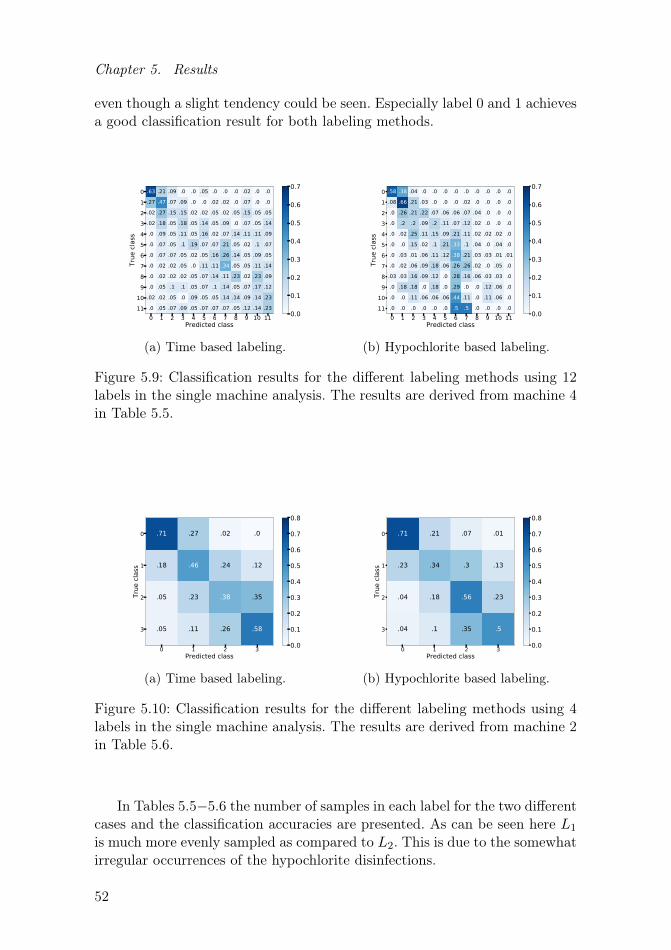
Chapter 5. Results

even though a slight tendency could be seen. Especially label 0 and 1 achievesa good classification result for both labeling methods.

0 1 2 3 4 5 6 7 8 9 10 11Predicted class

0123456789

1011

True

class

.63 .21 .09 .0 .0 .05 .0 .0 .0 .02 .0 .0

.27 .47 .07 .09 .0 .0 .02 .02 .0 .07 .0 .0

.02 .27 .15 .15 .02 .02 .05 .02 .05 .15 .05 .05

.02 .18 .05 .18 .05 .14 .05 .09 .0 .07 .05 .14.0 .09 .05 .11 .05 .16 .02 .07 .14 .11 .11 .09.0 .07 .05 .1 .19 .07 .07 .21 .05 .02 .1 .07.0 .07 .07 .05 .02 .05 .16 .26 .14 .05 .09 .05.0 .02 .02 .05 .0 .11 .11 .34 .05 .05 .11 .14.0 .02 .02 .02 .05 .07 .14 .11 .23 .02 .23 .09.0 .05 .1 .1 .05 .07 .1 .14 .05 .07 .17 .12.02 .02 .05 .0 .09 .05 .05 .14 .14 .09 .14 .23.0 .05 .07 .09 .05 .07 .07 .07 .05 .12 .14 .23

0.0

0.1

0.2

0.3

0.4

0.5

0.6

0.7

(a) Time based labeling.

0 1 2 3 4 5 6 7 8 9 10 11Predicted class

0123456789

1011

True

class

.58 .38 .04 .0 .0 .0 .0 .0 .0 .0 .0 .0

.08 .66 .21 .03 .0 .0 .0 .02 .0 .0 .0 .0.0 .26 .21 .22 .07 .06 .06 .07 .04 .0 .0 .0.0 .2 .2 .09 .2 .11 .07 .12 .02 .0 .0 .0.0 .02 .25 .11 .15 .09 .21 .11 .02 .02 .02 .0.0 .0 .15 .02 .1 .21 .33 .1 .04 .0 .04 .0.0 .03 .01 .06 .11 .12 .38 .21 .03 .03 .01 .01.0 .02 .06 .09 .18 .06 .26 .26 .02 .0 .05 .0.03 .03 .16 .09 .12 .0 .28 .16 .06 .03 .03 .0.0 .18 .18 .0 .18 .0 .29 .0 .0 .12 .06 .0.0 .0 .11 .06 .06 .06 .44 .11 .0 .11 .06 .0.0 .0 .0 .0 .0 .0 .5 .5 .0 .0 .0 .0

0.0

0.1

0.2

0.3

0.4

0.5

0.6

0.7

(b) Hypochlorite based labeling.

Figure 5.9: Classification results for the different labeling methods using 12labels in the single machine analysis. The results are derived from machine 4in Table 5.5.

0 1 2 3Predicted class

0

1

2

3

True

class

.71 .27 .02 .0

.18 .46 .24 .12

.05 .23 .38 .35

.05 .11 .26 .58

0.0

0.1

0.2

0.3

0.4

0.5

0.6

0.7

0.8



0

1

2

3

True

class

.71 .21 .07 .01

.23 .34 .3 .13

.04 .18 .56 .23

.04 .1 .35 .5

0.0

0.1

0.2

0.3

0.4

0.5

0.6

0.7

0.8


Figure 5.10: Classification results for the different labeling methods using 4labels in the single machine analysis. The results are derived from machine 2in Table 5.6.

In Tables 5.5−5.6 the number of samples in each label for the two differentcases and the classification accuracies are presented. As can be seen here L1

is much more evenly sampled as compared to L2. This is due to the somewhatirregular occurrences of the hypochlorite disinfections.

52


Table 5.5: Classification accuracy given in percent (%) and number of samplespresent in labels 0−11 for the two different labeling methods for each of themachines in the single machine analysis. For L1 number of labels is set to 12whereas it varies between 8−12 for L2. Thereby the classification accuraciesare not directly comparable between the two methods except for machine 4.

Number of samples in each label0 1 2 3 4 5 6 7 8 9 10 11 Acc. (%)

Machine 1 L1 43 43 43 43 43 43 42 43 43 43 43 43 19.4L2 70 82 93 67 81 59 33 15 10 3 2 - 35.7

Machine 2 L1 50 51 50 53 49 50 52 49 53 50 51 50 18.6L2 58 76 61 70 103 96 88 50 6 - - - 31.9

Machine 3 L1 38 41 38 38 40 38 38 40 38 38 41 38 20.8L2 49 50 66 61 84 54 53 49 - - - - 31.1

Machine 4 L1 43 45 41 44 44 42 43 44 44 42 44 43 22.7L2 26 62 68 56 53 48 72 65 32 17 18 2 27.4

Machine 5 L1 40 39 40 39 40 41 38 40 39 39 40 40 15.2L2 59 52 86 45 59 49 83 40 2 - - - 25.7

Table 5.6: Classification accuracy given in percent (%) and number of samplespresent in labels 0−3 for the two different labeling methods for each of themachines in the single machine analysis. For both methods on all machinesnumber of labels is set to 4.

Number of samplesin each label

0 1 2 3 Acc. (%)

Machine 1 L1 129 129 128 129 51.8L2 152 160 140 63 57.3

Machine 2 L1 151 152 154 151 53.0L2 134 131 199 144 53.1

Machine 3 L1 117 116 116 117 48.5L2 99 127 138 102 49.2

Machine 4 L1 129 130 131 129 51.6L2 88 124 101 206 52.6

Machine 5 L1 119 120 117 119 42.1L2 111 131 108 125 44.0

In Figures 5.11−5.12 the results from the multiple machine analysis with12 respectively 4 labels can be seen. In Table 5.7 the corresponding number ofsamples in each label and the classification accuracy can be seen. Once againthe L2 method suffers from imbalance in the data with very few samples forthe last 4 labels. This can readily be seen in Figure 5.11 where the last 4columns are almost completely blank. As with the single machine analysisthe diagonals are more prominent in the 4 labels case, particularly for L1.

53

Chapter 5. Results

0 1 2 3 4 5 6 7 8 9 10 11Predicted class

0123456789

1011

True

class

.58 .2 .11 .01 .02 .02 .03 .01 .0 .01 .0 .0

.22 .28 .12 .11 .08 .04 .03 .03 .02 .03 .02 .02

.21 .15 .13 .12 .09 .04 .05 .05 .05 .04 .03 .03

.07 .08 .13 .1 .08 .09 .09 .12 .06 .05 .06 .06

.07 .09 .12 .06 .07 .1 .1 .07 .08 .09 .06 .06

.06 .08 .06 .07 .07 .17 .08 .1 .07 .07 .06 .09

.02 .04 .06 .08 .08 .07 .13 .12 .13 .08 .1 .09.0 .05 .05 .09 .05 .06 .11 .14 .11 .1 .12 .12.01 .06 .04 .07 .05 .06 .14 .09 .16 .08 .15 .1.0 .03 .05 .05 .06 .06 .09 .1 .12 .13 .17 .14.02 .02 .05 .07 .08 .05 .09 .12 .09 .1 .18 .14.01 .02 .03 .07 .07 .04 .09 .08 .08 .14 .14 .22

0.0

0.1

0.2

0.3

0.4

0.5

0.6

0.7


0 1 2 3 4 5 6 7 8 9 10 11Predicted class

0123456789

1011

True

class

.66 .22 .07 .03 .02 .0 .0 .0 .0 .0 .0 .0.2 .33 .21 .11 .07 .02 .02 .03 .0 .0 .0 .0.11 .23 .2 .11 .15 .08 .08 .04 .0 .0 .0 .0.03 .17 .24 .13 .15 .11 .11 .05 .01 .0 .0 .0.01 .08 .14 .11 .22 .17 .2 .07 .01 .0 .0 .0.0 .03 .15 .09 .19 .2 .24 .09 .0 .0 .0 .0.02 .04 .12 .09 .29 .2 .16 .08 .01 .0 .0 .0.0 .07 .12 .07 .2 .2 .26 .05 .01 .0 .0 .0.02 .04 .12 .12 .24 .12 .26 .08 .0 .0 .0 .0.0 .05 .1 .05 .45 .1 .25 .0 .0 .0 .0 .0.0 .05 .0 .1 .25 .2 .25 .15 .0 .0 .0 .0.0 .0 .0 .0 .0 .5 .0 .5 .0 .0 .0 .0

0.0

0.1

0.2

0.3

0.4

0.5

0.6

0.7


Figure 5.11: Classification results for the different labeling methods using 12labels in the multiple machine analysis.


0

1

2

3

True

class

.69 .19 .08 .05

.25 .29 .25 .21

.1 .23 .35 .33

.06 .18 .31 .45

0.0

0.1

0.2

0.3

0.4

0.5

0.6

0.7



0

1

2

3

True

class

.68 .23 .06 .03

.25 .35 .23 .17

.05 .24 .36 .35

.05 .19 .42 .35

0.0

0.1

0.2

0.3

0.4

0.5

0.6

0.7


Figure 5.12: Classification results for the different labeling methods using 4labels in the multiple machine analysis.

The major drawback with L2 is the imbalanced labeling it generates. Eventhough most labels contain approximately the same number of samples thereis often one or more labels with a significant different number of samples,either higher or lower. Such an imbalance poses a big problem since kNN isknown to be sensitive to this phenomenon. This can easily be understood asit is more likely for a test point to be close to one of the 200 training pointsbelonging to class X than any of the 5 training points belonging to class Y(if the classes are not well separated). In a multiple class problem this willin theory lead to that the classifier will have a tendency to more often assignthe most frequently occurring labels in the training data to the test data.

An example of this can be seen in Figure 5.9b where a lot of test pointsare wrongly classified as label 6 which is seen as the colored column abovelabel 6. It comes as no surprise that label 6 has the most samples when L2

for machine 4 is looked upon in Table 5.5.

54

5.5 Windowing and choice of k

Table 5.7: Classification accuracy and number of samples present in labels0−11 for the two different labeling methods using 12 respectively 4 labels inthe multiple machine analysis.

Number of samples in each label0 1 2 3 4 5 6 7 8 9 10 11 Acc. (%)

12 labels L1 214 219 212 217 216 214 213 216 217 212 219 214 19.0L2 262 322 374 299 380 306 329 219 50 20 20 2 23.3

4 labels L1 645 647 646 645 - - - - - - - - 44.4L2 584 673 686 640 - - - - - - - - 42.4

Even though L2 seems to perform best when classification accuracy isconcerned this can be argued. Due to the problem mentioned above the classi-fication accuracies for L2 could not be completely trusted since they probablyare good at classifying the few most frequently occurring labels but bad atthe others. For the single machine, 12 label case they also appear better thanthey are since they often have fewer labels than L1.

When the 4 label case is analyzed the two methods perform about thesame for the single machine analysis, and for the multiple machine analysisL1 is actually slightly better.

An advantage with L1 is that it is much more flexible when the parameternumber of labels is concerned and it can easily be tuned to contain more labelsthan what is possible with L2. All this adds up to the decision that L1, thetime based labeling method, is the preferred method in both the single andmultiple machine analyses.


The value of k, number of neighbors in kNN, was varied between 1−50 for eachof the 4 different window lengths tested on the signals. These were 5, 15 and30 minutes as well as when the signals were kept as a single segment, the nowindow option. The mean accuracy for the 5 machines in the single machineanalysis is presented in Figure 5.13a for each of the tested segment lengths.The corresponding result for the multiple machine analysis is presented inFigure 5.13b.

As can be seen in Figure 5.13 the best performance in both cases isachieved with the no window option. The accuracy follows no clear over-all pattern with respect to k, hence it is difficult to choose an optimal value.However, in both cases there are an overall initial increase in accuracy withincreasing k before the accuracy flattens out around k = 10. These points,k = 12 and k = 13 were chosen as the final values for k in the single andmultiple machine analyses respectively.

55

Chapter 5. Results

0 10 20 30 40 50k

16.5

17.5

18.5

19.5

20.5

Accuracy (%

)

No Window30 min15 min5 min

(a) Single machine analysis.

0 10 20 30 40 50k

15

16

17

18

19

Accuracy (%

)

No Window30 min15 min5 min

(b) Multiple machine analysis.

Figure 5.13: Classification accuracy for different segment lengths and differentvalues of k in kNN.

5.6 Evaluation

The final result of using the developed algorithm on the 5 machines in theevaluation set is visualized in Figure 5.14. Here the classification accuracy foreach of the 5 machines in the single machine analysis is displayed as well astheir mean together with the result from the multiple machine analysis. Theresult is presented for three different values of the parameter number of labels;3, 6 and 12. For each case the last bar displays the comparison accuracy whichwould be achieved by assigning each test point a label at random, assuminguniform distribution. Hence it is calculated as 1 divided by number of labels.

As can be seen in the figure all classification accuracies are higher thanthe comparison accuracy, in many cases almost twice as high. Independentof number of labels, the mean accuracy from the single machine analysis isalways higher than the accuracy from the multiple machine analysis. Therebythe single machine approach is selected as the preferred one.

In Figure 5.15 three different confusion matrices derived from machine 10where the value of number of labels have been altered are displayed. In allof the three matrices the classification of label 0 stands out, being correctlyclassified in 66 %, 57 % and 49 % of the cases when 3, 6 respectively 12 labelswere used. When 12 labels are used the comparison accuracy is as low as8.3 %, making the classification almost 6 times as good as a random guess.The other classification result using 12 labels is not as remarkable. For the 3and 6 label cases the situation is a bit better, the diagonal is more visible,especially when 3 labels are used. Another thing worth noticing is that inall matrices the upper right and lower left corners are inhabited with lownumbers. This is a good thing, meaning that the lower and higher labels arerarely mixed up, which they should not be since they represent completelydifferent levels of the UFD degradation.

56

5.6 Evaluation

3 6 120

10

20

30

40

50

60

Accu

racy

(%)

Number of labels

Machine 6Machine 7Machine 8Machine 9Machine 10Mean of machine 6-10Multiple machinesComparison

Figure 5.14: Classification accuracy for the 5 machines from the evaluationset. The results from both the single and multiple machine analyses as wellas the comparison accuracies are presented.

0 1 2Predicted class

0

1

2

True

class

.66 .23 .1

.17 .47 .36

.06 .27 .68

0.0

0.1

0.2

0.3

0.4

0.5

0.6

0.7

(a) 3 labels

0 1 2 3 4 5Predicted class

0

1

2

3

4

5

True

class

.57 .26 .05 .05 .02 .06

.23 .31 .21 .11 .1 .03

.03 .2 .3 .1 .13 .24

.01 .17 .21 .21 .17 .23

.0 .08 .1 .15 .33 .34

.02 .05 .09 .14 .26 .440.0

0.1

0.2

0.3

0.4

0.5

0.6

0.7

(b) 6 labels

0 1 2 3 4 5 6 7 8 9 10 11Predicted class

0123456789

1011

True

class

.49.23.12.12.02 .0 .0 .02 .0 .0 .0 .0

.26.16.21.07.05 .0 .02.05.02.05.05.07

.07.25.23.11.09.16 .0 .05.02.02 .0 .0

.09.05.23.02.16.09.12.05.07.07 .0 .05.0 .07.07.12.28.07.05.05.14.07.07.02.0 .07.05.07.11.14.09.05.07.11.11.14.0 .0 .09.09.09.07 .2 .05.11.14.07.09.0 .05.14.02.16.07.14 .0 .05.12.16.09.0 .0 .02.05.09 .0 .12.07.19.12.09.26.0 .0 .0 .05.07.02.14.12.14.16.21.09.0 .07.02 .0 .07.05.11.02.18.25.11.11.0 .02.05.02.02.02.16.07.07.09.26.21

0.0

0.1

0.2

0.3

0.4

0.5

0.6

0.7

(c) 12 labels

Figure 5.15: Confusion matrices derived from machine 10 in the single machineanalysis with different values of number of labels.

57

Chapter 5. Results

To summarize, the developed algorithm uses the 10 features presentedin Table 5.1a derived through the TFSWT feature selection method. Thelabeling method used is L1, time based labeling. No windowing is used andnumber of neighbors in the kNN classifier is set to 12. The algorithm shouldbe used on single machines, not mixing training and test data from differentmachines. With these settings the classifier achieves an accuracy about twiceas good as a random guess.

58

6Discussion

6.1 Localizing UFD replacements

The information regarding the occurrences of UFD replacements were re-trieved manually from the log files. However, it is not actual replacementsthat are logged but rather when the operator presses the button to confirma UFD replacement. These are two separate things. When one of the threecounters indicating time for UFD replacement has reached its limit an atten-tion is raised. It is still possible to perform a treatment but the attention willremain raised. To remove this attention the only thing the operator has todo is to press the button confirming the UFD is replaced, even if this is notdone. There is currently no other way to tell whether the UFD has actuallybeen replaced or not. This poses two different problems. The first problemis that the entire analysis in this report relies on the assumption that theseconfirmations correspond to actual UFD replacements. If this premise doesnot hold true the results in this report probably does not hold true either.

However, two things suggest that the confirmation is done in connectionwith a UFD replacement. The most prominent is the result from the timeseries which show a clear relationship between some of the features and theUFD replacements. The other is the fact that the analyzed machines aresituated at a hospital believed to have high standard on the maintenanceof their dialysis machines. This in turn is based on two facts. The first factis that the clinic has accepted to send all their log files to Baxter. If theywould mismanage their machines this could easily be detected. The secondfact is their compliance with the recommended disinfection schedule, whichwas confirmed during the analysis.

To return to the two different problems with the confirmation of UFDreplacement, the second problem is that clinics may easily skip these replace-ments. Whether this is done intentionally by the clinic to save money, orunintentionally by an operator misclicking the confirmation button, this maypose a danger to the patient. If the UFD is not replaced in time it may notfulfill its purpose of purifying the dialysis fluid through removal of a possiblecontamination by bacteria and endotoxins.

59

Chapter 6. Discussion

With respect to patient safety, a method to detect true occasions forUFD replacements may be desirable. Even though this was not the aim ofthe report, the results suggest that this may be a simpler task to solve. Out ofthe time series plot of e.g. the feature mean of (HPG−PD) in Figure 5.3a it iseasy to detect probable occasions for UFD replacements even when they arenot marked. Based on this a more sophisticated model could be developed,even though the simple visual assessment of this plot probably would do finein many situations.


When the master’s thesis was initiated our hypothesis was that there would bea gradual clogging of the UFD with time. From the vast amount of availablesignals from the log files only those believed to have some connection withthe UFD clogging were analyzed. The signals derived from the two differentpumps were believed to show an increased workload and power consumptionin response to this. The HPG and PD pressures was thought to experiencea gradual increase respectively decrease with respect to the clogging of theUFD situated in between them. Thereby the signal created as the differencebetween these two pressures were expected to increase with time. However, theanalysis gave the opposite result. The pressure difference did in fact decreasewith time as shown in Figures 5.3a and 5.6. The reason for this is explained inSection 6.9.2. As a consequence of this result the signal derived from the bloodleak detector was added to the analysis in a later phase. This is explained inSection 6.9.2 as well.


Due to the uneven sampling rate of the signals they were resampled usinglinear interpolation. Thereby it was possible to e.g. retrieve the (HPG−PD)signal and perform FFT. However, interpolation has the downside of intro-ducing errors in the data. With linear interpolation this error is proportionalto the squared distance between adjacent points [42]. Thereby it is rathersafe to use it on the signals that are frequently sampled, e.g. HPG- and PDpressure. The problem is that especially three of the analyzed signals, suc-tion pump cycle, suction pump current and blood leak detector, have very fewsamples. In fact, sometimes their sample rate was as low as one sample perhour.

In the case of the features derived from the signal blood leak detector thiswas not a problem since they were discarded due to other reasons explainedin Section 5.3.1. However, the features derived from the two different signalsfrom the suction pump were available during the feature selection step. The

60


TFSWT almost never selected one of these features but they were selectedmore frequently by the SFS, even though they were never selected as one ofthe best features. Thereby they did not have much impact on the final result.

The error introduced through interpolation in the time-domain may prop-agate to all domains demanding a correct time structure. Thereby the featuresderived from the frequency-domain and through cross-correlation are affectedas well.


The implementation of the flow compensation was important for the devel-oped algorithm. Although not all extracted features were in need of flowcompensation, each and every one of the ten features selected for the finalsolution were flow compensated. If no compensation would be done these fea-tures would hold information regarding both the UFD status and the mainflow. Since it is only the UFD status that is of interest, using uncompensatedfeatures would blur the result. As a comparison, the mean accuracy using 12labels in Figure 5.14 is 17.2 % when flow compensation is used, as comparedto 14.1 % without flow compensation.

The flow compensation used in this report compensates the features. An-other possibility would be to instead compensate the signals before the fea-tures are extracted. The main reason for choosing to compensate the featuresand not the signals was simply that the need of flow compensation was discov-ered once the features were already extracted. Therefore the implementationcould be done faster if these were compensated and not the signals. If thesignals would be compensated directly they would first have to be resampledtogether with the signal UF channel 1. If a high enough sampling frequencyto avoid aliasing would be used (100 Hz) this would result in several hundredmillions of data samples for each signal on every machine and it would notbe feasible to perform a flow compensation on such a large amount of data.For comparison, when the features are compensated the data is reduced by afactor 106.

Independent of whether it is the signals or features that are compensatedthere is always a risk with manipulating data in this way, information maybe lost or added. However, when the features are plotted against main flowas in figure 5.2 it appears as they have a clear linear relationship. Thereforethe procedure of flow compensation could be considered safe to use in thesecases.

A simplification that has been done during the flow compensation is toequalize the flow in UF channel 1 and 2. This is not totally true since theflow in UF channel 2 contains the addition of the ultrafiltrate from the pa-tient. The signals derived from the fluid path succeeding the dialyzer should

61


therefore preferably be compensated with UF channel 2 instead. The simpli-fication of only using UF channel 1 is done for two reasons. Firstly, two ofthe affected signals, PD-pressure and blood leak detector, were not in need ofany flow compensation at all. Secondly, the contribution of the ultrafiltrateis small compared to the volume of the dialysis fluid, mostly in the order of1−2 %.


The two different feature selection methods used in this report, TFSWT andSFS, have one fundamental difference worth emphasizing. The TFSWT an-alyzes all the features one by one, giving each feature a normalization scorebetween 0 and 1. The SFS on the other hand selects a set of features whichperforms well together. However, it is a greedy algorithm by its nature sinceit selects the best feature, then the best feature in combination with the firstand so on. The combination of features it selects is thereby not necessarily thevery best. But still, choosing 10 features which perform well together shouldlogically give a better classification result than choosing the 10 features per-forming best individually. The reason for this is that several features may berelated to each other, describing more or less the same characteristic of thedata that is analyzed. If one such feature is selected, adding another of the re-lated features barely improves the result since practically no new informationis given to the classifier.

With this taken into consideration a couple of interesting things may benoted from the feature selection step. The most important result is that bothmethods always select some of features derived from the (HPG−PD) signalas the first feature. Hence this signal should be the one best describing thedegradation of the UFD. This result is in consistency with the analysis of theboxplots as well as the time series of each individual feature.

Another interesting result is the features selected in position 2−10, whichshow large differences between the two methods. The TFSWT has a strongtendency of selecting features derived from the (HPG−PD) signal, with someadditions of features derived mainly from the FP cycle and HPG signals(Tables 5.1 and 5.2). The features selected are almost exclusively from thetime-domain. The SFS on the other hand exhibits much more variation inthe feature selection (Tables 5.3 and 5.4). All signals are present and fromthese, features derived from both the time-domain, frequency-domain andthrough cross-correlation are selected. No clear pattern can be found. Thisresult suggests two things. Firstly, this apparently random selection patternindicates that the features selected on position 2−10 by the SFS containslittle information regarding the degradation of the UFD. Secondly the resultindicates that there is a strong relationship among some of the features derived

62


from the (HPG−PD) signal. The reason for this is that even though manyof these features received high normalization scores through the TFSWT,usually only one or maybe two of them is present among the 10 featuresselected by the SFS. This result is reasonable since features such as the mean,RMS and the different quartiles should be closely related.

All this in combination with the ambiguous result in Figure 5.8 regardingwhich feature selection method that gives the best feature set, points in thesame direction. It is only some of the time-domain based features from thesignal (HPG−PD) that contain relevant information regarding the status ofthe UFD. Besides, these features are closely related. Thereby, as long as one ofthese features is present in the feature set it does not make any big differencewhich the other ones are.

The problem with interpolation described in Section 6.3 makes the fea-tures derived from the frequency-domain and through cross-correlation un-reliable. Since there was no success in introducing these features they weredismissed on an early stage to instead focus on more promising aspects of thealgorithm. Their non-success could either be due to a total lack of informationregarding the UFD status or be a consequence of errors introduced throughinterpolation. Therefore a further analysis needs to be done before featuresderived from the frequency-domain and through cross-correlation could besaid to be of interest or not when analyzing the UFD status.


6.6.1 Effects of missing dataBoth of the labeling methods analyzed in this report rely on a correct nota-tion of the UFD replacements. As described in Section 6.1 all the notationsare believed to correspond to true UFD replacements. However, it is still pos-sible that some replacements are missed. If the monthly extractions of the.zip files from the dialysis machines are delayed and data is overwritten thereis a risk that information regarding a UFD replacement is lost. Such episodesof missing data have actually been found on several of the analyzed machines,one example can be seen in Figure 5.4. These episodes vary in length, rang-ing from a couple of days up to over a month. During these episodes it isimpossible to determine by certainty if and when a UFD replacement havetaken place. But through analysis of the time series of e.g. the feature mean of(HPG−PD) together with the duration between the different UFD replace-ments it is possible to detect pattern deviations where one can suspect thata UFD replacement is missed.

The analysis in this report is based solely on the confirmed UFD replace-ments. Thereby it is probable that some replacements are missed. This wouldresult in an incorrect labeling since the labeling is not reset properly. The

63


possible error introduced this way propagates through the succeeding analy-sis all the way to the final classification. Since overwritten data is relativelycommonly occurring it poses a great problem to the analysis in this report,affecting the final evaluation accuracy achieved by the algorithm.

The labeling method based on hypochlorite disinfections is even more sen-sitive to missing data. Since these disinfections occur with such short intervalsit is almost certain that they are missed during longer episodes with missingdata. Even a short episode of just a day or two has a rather high risk ofleading to errors in the labeling.

It is not only information regarding UFD replacements and hypochloritedisinfections that are missed. A large amount of treatments are also lost,causing an offset in the labeling. This affects the result even further.

6.6.2 Compensation of unbalanced dataAs mentioned in Section 5.4 the labeling method based on hypochlorite disin-fections generates unbalanced data, which is a big problem when using kNN.For simplification, the analysis in this report has handled the data as beingbalanced. However, different ways of dealing with this have been discussedbut due to the limited time they have not been implemented. A review ondifferent techniques available are presented in [43]. These include simple ap-proaches as over- and undersampling as well as more sophisticated methodson algorithm level. In oversampling new samples of the minority class arecreated either synthetically or through replication of existing samples. Un-dersampling is the opposite where samples of the majority class are randomlyeliminated. Examples from the article on the algorithm level are to assigndifferent weights for the classes in a kNN classifier or to implement a costfunction with different costs for different misclassifications.

Since the analyzed data for some machines have as few as two samples forsome labels it might be difficult to compensate this through over- or under-sampling. A compensation on the algorithm level might have greater success.It could even be necessary to merge the minority labels before performingadditional compensation.

6.6.3 Other alternativesNone of the tested labeling methods result in a totally consistent labeling. Be-tween filter replacement x and y, label z could correspond to a UFD that hasbeen used between e.g. 50−60 days, whereas it could correspond to a usageof e.g. 58−69 days between filter replacements (x+1) and (y+1). The numberof days (and number of hypochlorite disinfections) between two filter replace-ments affect the labeling. However, since the analyzed dialysis machines havebeen used in a routinely fashion there are mostly only small variations ine.g. the number of days between UFD replacements and the interval between

64


hypochlorite disinfections. Thereby the result of using these labeling methodsis fairly consistent after all.

There are however methods that would give an even more consistent label-ing. One example would be to use the actual usage time of each machine andlabel the data after strict limits. An even better approach would be to basethe labeling on the total volume of dialysis fluid that has passed through theUFD, thereby different main flows would be taken into consideration as well.This could be further developed and include all the different machine modes,not only treatment, and use different weights depending on how demandingthe different usages are on the UFD. The complexity of the labeling could beimmensely increased.

To be able to analyze other aspects of the algorithm as well, a rathersimplified labeling method was finally chosen. Apart from the fairly consistentlabeling it generates, its biggest strength is the almost completely balanceddata it produces. With this said, a future improvement of the algorithm thatprobably would have a reasonable impact on its performance would be tobase the labeling on the volume of dialysis fluid passing the UFD.


With the introduction of windowing the sample size increased substantially.For the five minute time window the sample size increased 40-fold with respectto when each treatment episode was kept as a single sample. The optimal sizeof the feature set is largely unaffected by the sample size when using kNN [44].Thereby the same feature set could be used for all window lengths.

The parameter k on the other hand is affected by the sample size. It shouldalso be chosen with consideration taken to the noise level of the data wherenoisier data is better handled with a larger k [40].

The parameter number of labels naturally affects the number of samples ineach label. Thus it is possible that the value of k should be chosen differentlywhen number of labels is adjusted in the future.

6.8 Algorithm development

The main focus during this master’s thesis has been to develop the algorithm,not to optimize it performance-wise. Thereby a couple of simplifications havebeen made along the way. In addition to this, the algorithm has not beenimplemented in a strict logical and chronological order. The need of somesteps have been thought of in a later stage and they have therefore beenimplemented there and then, even though the algorithm would have beenfaster to execute if the code was rewritten. One example of this is the tenminute cutoff used in the preprocessing of each signal. As for now this step

65


is one of the latest, but it would be more natural to do it before the linearinterpolation.

Some other simplifications worth mentioning is the discarding of the logfiles containing UFD replacements and the ones succeeding the last filterexchange. Since the UFD replacements occurred once every 1−3 month andthere were usually three separate treatment episodes each day it is only asmall fraction of the log files that are discarded this way. In fact, it was onlyabout half of these log files that did contain a treatment episode. Thereby thefraction of lost data is even smaller. Since the amount of available log fileswas never a problem this simplification could be accepted.

The reason to discard the log files succeeding the last filter exchange ofeach machine was due to the problem it arose with the time based labeling.However, the labeling method based on hypochlorite disinfections could easilyuse these log files. Still they were not used, the reasons are twofold. Firstlythe use of these log files would make the data even more imbalanced sinceit would mainly add samples of the first labels. Secondly it would make thecomparison between the labeling methods harder since they would not bebased on the same data.

Apart from these simplifications a couple of more could be mentioned butthey are only interesting from a code optimization point of view. Since theyhave no relation to the performance of the algorithm they are not discussedhere. However, if someone else in the future would continue the work fromthis point it could be relevant to know that improvements can be done in thisarea.

6.9 Evaluation and final thoughts

6.9.1 Single versus multiple machine analysisDuring the evaluation the final result of the single versus multiple machineanalyses was received, slightly in favor of the single machine analysis. Thisindicates that the developed algorithm contains machine specific parametersto some extent. There are a couple of possible explanations to this but it allnarrows down to the signals derived from the log files. The analyzed machinesare obviously not identical but rather exhibit small differences in e.g. theirsensor offsets or wear of different components. These differences propagateand could manifest themselves in different parts of the algorithm when thetwo cases are compared.

One explanation could be that a gradual decrease or increase in featurevalue with label number is drowned by different sensor offsets in the machinesfrom the multiple machine analysis. This would result in a feature which isinterpreted as bad, whereas the single machine analysis would detect the truepotential of the feature. However, this does not seem to be the case when the

66

6.9 Evaluation and final thoughts

top selected features are studied.Another possibility is that the machines react differently to a varied main

flow. This would favor the individual flow compensation performed in thesingle machine analysis. Whether this holds true for the current algorithm ishard to tell based on the results presented but is a possible explanation.

Most likely the fact that the training and test data points are derivedfrom the same machine is the best explanation for the better result with thesingle machine analysis.

If the developed algorithm based on single machine analysis would be im-plemented on a brand new machine this would require a couple of months ofusage before the algorithm could be trained and a result could be achieved.However, if the multiple machine analysis was to be used instead a classifica-tion result could be achieved already for the very first log file. After all, theresult when using the multiple machine analysis is almost as good as for thesingle machine analysis, see Figure 5.14.

6.9.2 Hypothesis regarding the UFD degradationAn interesting result from the evaluation is the high classification accuracy ofthe very first label, label 0. This result stands out and is achieved independentof the value of number of labels. An explanation for this may be found in theboxplots of the most relevant features, see Figure 5.6. Here the largest pressuredrop is seen between the first and second label. This pattern was seen amongall the six features mentioned in Section 5.3.1 on all machines. The differencecould sometimes be even more prominent than in the figure. This indicatesthat the speed of the degradation of the UFD right after the replacement ishigh and then declines.

Another very interesting result was the development of the pressure dropacross the UFD measured as (HPG−PD). As stated previously our hypothesiswas that this would increase with the clogging of the UFD. In reality thepressure drop decreased with time.

These two findings led to the new hypothesis that the UFD was not gettingclogged but rather damaged, and the reason for this were the hypochloritedisinfections. This would explain both findings. Since these disinfections areknown to severely reduce the lifetime of the UFD it is reasonable to thinkthat the first disinfection would have a large impact. This in combinationwith the weekly scheduling of these disinfections would result in the firstdisinfection occurring somewhere around label 0 and 1 which could therebyexplain the large difference between these labels. The hypochlorite has theeffect of damaging the filter mass by increasing the diameter of the pores.Thereof the decreased pressure drop.

It was this hypothesis that led to both the analysis of the blood leak de-tector and the implementation of the labeling method based on hypochloritedisinfections in the later stages of the algorithm development. The idea be-

67


hind the blood leak detector was that the increased diameter of the pores inthe UFD would lead to lower filtering capacity, letting more contaminantsthrough, making the dialysis fluid less transparent which could then be de-tected by the sensitive sensor. Despite its name it was therefore not intendedto detect blood. However, the result was not satisfying. Instead a slow drift ofthe sensor or maybe the wear of some component caused a slowly increasedsteady-state of the signal, making it inappropriate to use in the algorithm aspreviously mentioned.

6.10 Ethics

Even though the log files analyzed in this master’s thesis are derived fromactual treatments of real patients no personal information is available in thelog files. Most of the data available in the log files is strictly machine relatedeven though some data is derived directly from, or has a close connection to,the patient e.g. venous blood pressure or ultrafiltered volume. However, thisdata cannot be used to identify the patient. Besides, only machine relateddata is used in this report. In addition to this, the analyzed data has beenapproved for this usage.

The purpose of CBM is to maximize the use of the analyzed component.As compared to preventative maintenance this reduces the number of unnec-essary replacements, hence it leads to reduced environmental impact. Anothermaintenance approach is corrective maintenance where a component is notreplaced until it fails. When a UFD is concerned this would not be acceptablesince it could endanger the health of the patient. If both ethics regarding sus-tainability and patient’s safety is taken into consideration a CBM approachof UFD replacements would be ideal.

6.11 Future work

This report has shown that the possibility to develop a CBM based serviceindicator for UFD replacements looks promising. However, a few steps remain.The algorithm presented in this report may detect different degradation levelsof the UFD and decide the current level to some extent. Basically it is onlybased on a few closely related features derived from the same signal. Thereforethe most important task in the future development of this algorithm will be tofind more signals and/or features containing relevant information regardingthe UFD status. Alternatively the information contained in the already foundrelevant signal could be enhanced. This could possibly be done either throughan effective noise reduction or through the implementation of a high, constantsampling frequency of the signals in the AK 98 dialysis machine.

68

6.11 Future work

An implementation of a constant sampling frequency may have many pos-itive consequences. It could make the analysis of signals currently sampled ata very low frequency more rewarding and eliminate the need of interpolation.Maybe more important, it would give the analysis of the features derived fromthe frequency-domain and through cross-correlation much more meaning. Ahigh, constant sampling frequency could simply open a wide range of possi-bilities. The big problem with this is the limited internal memory of the AK98. The data collection would thereby have to be done in a different way. Abetter solution to this would also benefit future studies of this kind.

To get a more fair estimation of the performance of the algorithm it couldbe tested on data that is not incomplete, or where the missing data is com-pensated in some way. With such data available it would be interesting torerun the steps where the different parameter settings were selected as well.

Possible future improvements of the algorithm also include things men-tioned previously in the discussion, e.g. compensation of the imbalanced datain the labeling method based on hypochlorite disinfections and the optimiza-tion of the algorithm.

An alternative option for the future work could be to develop the algo-rithm that could detect true occasions for UFD replacements presented inSection 6.1 if there is a need.

As mentioned in the aim, Section 1.1, the development of the currentalgorithm is just the first out of three steps in the implementation of theCBM service indicator. Before those steps are done nothing can really be saidabout the RUL of the UFD no matter how sophisticated the algorithm is.With this said a final clarification can be made. This report does not aimat finding an optimal setting for the parameter number of labels. What thisparameter really does is an adjustment of the time resolution of the algorithm,i.e. if each label should correspond to one day, week or month in the final CBMservice indicator. Hence the value of this parameter should be decided lateron when the potential of the final service indicator is fully known.

69

7Conclusion

This master’s thesis resulted in an algorithm based on the machine learningtechnique kNN with the aim of classifying the degradation level of the UFDfilter in Baxter’s AK 98 dialysis machine. It was concluded that the analyzedsignals derived from the log files of real dialysis treatments were in need ofpreprocessing in order to segment out the relevant parts. Some of the analyzedsignals were affected by the main flow of the dialysis fluid, therefore a flowcompensation was needed. The two feature selection methods TFSWT andSFS were used and from their result the conclusion was drawn that out ofall the 178 available features only 6 did exhibit a clear relationship with theUFD degradation level. It could further be concluded that they were all closelyrelated and derived from the same signal which gave the pressure drop acrossthe UFD filter. These features were mean, max, RMS, median, lower quartileand upper quartile.

Out of the two tested labeling methods, time based labeling was chosenas the best even though the other method gave promising result but neededfurther development. It was tested to split the signals into smaller segmentsof various lengths, but the original length was in the end concluded the best.The number of neighbors in kNN was evaluated and set to 12 and 13 in thesingle and multiple machine analysis respectively. The single machine analysisperformed the best and it was concluded that some machine specific charac-teristics were present but not so prominent. These setting resulted in a finalclassification accuracy of 53.8 %, 31.3 %, and 17.2 % when 3, 6 respectively12 labels were used. Thereby the classification is roughly twice as good as arandom guess.

During the development of the algorithm it was discovered that any ofthe six best features could be used with great certainty to determine whenUFD replacements had taken place. This finding could be further developedif there is an interest in implementing such a feature into the AK 98 to beused e.g. if the UFD replacement notification is mistakenly removed.

The final algorithm did show promising result in detecting the UFD degra-dation level but further development will be needed. As far as the algorithmis concerned, the main focus should be to improve the signal quality and/or

70

Chapter 7. Conclusion

find more relevant signals and/or features. However, the algorithm is just thefirst step. A study regarding the long term degradation of the UFD as well asan analysis concerning the UFD function in different degradation levels arenecessary to be performed before a CBM based service indicator of the UFDcould be implemented in the AK 98.

71

Bibliography

[1] T. Liyanage, T. Ninomiya, V. Jha, B. Neal, H. M. Patrice, I. Okpechi,M.-h. Zhao, J. Lv, A. X. Garg, J. Knight, A. Rodgers, M. Gallagher,S. Kotwal, A. Cass, and V. Perkovic, “Worldwide access to treatmentfor end-stage kidney disease: a systematic review,” The Lancet, vol. 385,no. 9981, pp. 1975–1982, 2015.

[2] W. G. Couser, G. Remuzzi, S. Mendis, and M. Tonelli, “The contributionof chronic kidney disease to the global burden of major noncommunicablediseases,” Kidney international, vol. 80, no. 12, pp. 1258–1270, 2011.

[3] Y. Peng, M. Dong, and M. J. Zuo, “Current status of machine prognosticsin condition-based maintenance: a review,” The International Journal ofAdvanced Manufacturing Technology, vol. 50, no. 1, pp. 297–313, 2010.

[4] S. Butler, Prognostic algorithms for condition monitoring and remain-ing useful life estimation. PhD thesis, National University of Ireland,Maynooth, 2012.

[5] Baxter International Inc., AK 98 Dialysis Machine - Operator’s Manual,May 2016.

[6] G. Giebisch and E. Windhager, Medical Physiology: A Cellular andMolecular approach, ch. Organization of the Urinary System, pp. 749–766. Saunders Elsevier, 2009.

[7] G. Giebisch and E. Windhager, Medical Physiology: A Cellular andMolecular approach, ch. Glomerular Filtration and Renal Blood Flow,pp. 767–781. Saunders Elsevier, 2009.

[8] Gambro Lundia AB (Baxter International Inc.), Internal education ma-terial, 2009.

[9] L. S. Costanzo, Physiology. Saunders Elsevier, Philadelphia, PA, 2006.

72

BIBLIOGRAPHY

[10] G. Giebisch and E. Windhager, Medical Physiology: A Cellular andMolecular approach, ch. Transport of Sodium and Chloride, pp. 782–796.Saunders Elsevier, 2009.

[11] G. Giebisch and E. Windhager, Medical Physiology: A Cellular andMolecular approach, ch. Transport of Urea, Glucose, Phosphate, Cal-cium, Magnesium, and Organic Solutes, pp. 797–820. Saunders Elsevier,2009.

[12] G. Giebisch and E. Windhager, Medical Physiology: A Cellular andMolecular approach, ch. Transport of Potassium, pp. 821–834. SaundersElsevier, 2009.

[13] G. Nyberg and A. Jönsson, Njursjukvård. Studentlitteratur, 2004.

[14] C. M. Kjellstrand and B. P. Teehan, Replacement of Renal Functionby Dialysis, ch. Acute Renal Failure, pp. 822–862. Kluwer AcademicPublishers, 1996.

[15] A. S. Levey, J. Coresh, E. Balk, A. T. Kausz, A. Levin, M. W. Steffes,R. J. Hogg, R. D. Perrone, J. Lau, and G. Eknoyan, “National kidneyfoundation practice guidelines for chronic kidney disease: Evaluation,classification, and stratification,” Annals of Internal Medicine, vol. 139,no. 2, pp. 137–147, 2003.

[16] A. Santoro, C. Canova, A. Freyrie, and E. Mancini, “Vascular access forhemodialysis.,” Journal of Nephrology, vol. 19, no. 3, pp. 259–264, 2006.

[17] R. P. Uldall, Dialysis Therapy, ch. Vascular Access for Hemodialysis,pp. 5–22. Hanley & Belfus, 1992.

[18] B. J. Canaud and C. M. Mion, Replacement of Renal Function by Dialy-sis, ch. Water Treatment for Contemporary Hemodialysis, pp. 231–255.Kluwer Academic Publishers, 1996.

[19] R. A. Ward, Dialysis Therapy, ch. Mechanlical Aspects of Dialysis,pp. 31–64. Hanley & Belfus, 1992.

[20] L. W. Henderson, Replacement of Renal Function by Dialysis, ch. Bio-physics of Ultrafiltration and Hemofiltration, pp. 114–145. Kluwer Aca-demic Publishers, 1996.

[21] Baxter International Inc., AK 98 Dialysis Machine - Service Manual,10 ed., 2016.

[22] F. Camci, Process monitoring, diagnostics and prognostics using supportvector machines and hidden Markov models. PhD thesis, Wayne StateUniversity, Detroit, 2005.

73

BIBLIOGRAPHY

[23] A. K. Jardine, D. Lin, and D. Banjevic, “A review on machinery di-agnostics and prognostics implementing condition-based maintenance,”Mechanical systems and signal processing, vol. 20, no. 7, pp. 1483–1510,2006.

[24] K. L. Tsui, N. Chen, Q. Zhou, Y. Hai, and W. Wang, “Prognostics andhealth management: A review on data driven approaches,” MathematicalProblems in Engineering, vol. 2015, 2015.

[25] X.-S. Si, W. Wang, C.-H. Hu, and D.-H. Zhou, “Remaining useful lifeestimation–a review on the statistical data driven approaches,” Europeanjournal of operational research, vol. 213, no. 1, pp. 1–14, 2011.

[26] D. I. Cho and M. Parlar, “A survey of maintenance models for multi-unit systems,” European Journal of Operational Research, vol. 51, no. 1,pp. 1–23, 1991.

[27] R. Reinertsen, “Residual life of technical systems; diagnosis, predictionand life extension,” Reliability Engineering & System Safety, vol. 54,no. 1, pp. 23–34, 1996.

[28] P. A. Scarf, “On the application of mathematical models in maintenance,”European Journal of Operational Research, vol. 99, no. 3, pp. 493–506,1997.

[29] H. Wang, “A survey of maintenance policies of deteriorating systems,”European Journal of Operational Research, vol. 139, no. 3, pp. 469–489,2002.

[30] E. Zio, “Reliability engineering: Old problems and new challenges,” Re-liability Engineering & System Safety, vol. 94, no. 2, pp. 125–141, 2009.

[31] R. Kothamasu, S. H. Huang, and W. H. VerDuin, “System health mon-itoring and prognostics–a review of current paradigms and practices,”in Handbook of maintenance management and engineering, pp. 337–362,Springer, 2009.

[32] A. Heng, S. Zhang, A. C. Tan, and J. Mathew, “Rotating machineryprognostics: State of the art, challenges and opportunities,” MechanicalSystems and Signal Processing, vol. 23, no. 3, pp. 724–739, 2009.

[33] N. Gorjian, L. Ma, M. Mittinty, P. Yarlagadda, and Y. Sun, “A review ondegradation models in reliability analysis,” Engineering Asset LifecycleManagement, pp. 369–384, Sept. 2009.

74

BIBLIOGRAPHY

[34] N. Gorjian, L. Ma, M. Mittinty, P. Yarlagadda, and Y. Sun, “A reviewon reliability models with covariates,” Engineering Asset Lifecycle Man-agement, pp. 385–397, Sept. 2009.

[35] J. Van Noortwijk, “A survey of the application of gamma processes inmaintenance,” Reliability Engineering & System Safety, vol. 94, no. 1,pp. 2–21, 2009.

[36] J. Sikorska, M. Hodkiewicz, and L. Ma, “Prognostic modelling optionsfor remaining useful life estimation by industry,” Mechanical Systems andSignal Processing, vol. 25, no. 5, pp. 1803–1836, 2011.

[37] Y. Lei and M. J. Zuo, “Gear crack level identification based on weighted knearest neighbor classification algorithm,” Mechanical Systems and Sig-nal Processing, vol. 23, no. 5, pp. 1535–1547, 2009.

[38] J. Yan, M. Koc, and J. Lee, “A prognostic algorithm for machine perfor-mance assessment and its application,” Production Planning & Control,vol. 15, no. 8, pp. 796–801, 2004.

[39] H.-E. Kim, A. C. Tan, J. Mathew, E. Y. Kim, and B.-K. Choi, “Machineprognostics based on health state estimation using svm,” ProceedingsThird World Congress on Engineering Asset Management and IntelligentMaintenance Systems Conference, vol. 199, pp. 834–845, 2008.

[40] C. M. Bishop, Pattern Recognition and Machine Learning. Springer,2006.

[41] T. Hastie, R. Tibshirani, and J. Friedman, Elements of Statistical Learn-ing. Springer, second edition ed., 2009.

[42] S. L. Eshkabilov, MATLAB R©/Simulink R© Essentials:MATLAB R©/Simulink R© for Engineering Problem Solving and Nu-merical Analysis, ch. Experimental Data Analysis, pp. 560–648. LuluPublishing Services, 2016.

[43] S. Kotsiantis, D. Kanellopoulos, and P. Pintelas, “Handling imbalanceddatasets: A review,” GESTS International Transactions on ComputerScience and Engineering, vol. 30, no. 1, pp. 25–36, 2006.

[44] J. Hua, Z. Xiong, J. Lowey, E. Suh, and E. R. Dougherty, “Optimalnumber of features as a function of sample size for various classificationrules,” Bioinformatics, vol. 21, no. 8, pp. 1509–1515, 2004.

75

Development of a CBM based service indicator for UFD ...

Documents