Development, implementation and application of a ...

Fakultat fur Physik

Master’s thesis

Development, implementation and application

of a Stochastic Rotation Dynamics algorithm

for granular matter

Arne Wolf Zantop

[email protected]

Advisor & First Referee: Dr. Marco G. Mazza

Second Referee: Prof. Dr. Stefan Klumpp

Due: September 12, 2017

Max-Planck-Institut furDynamik und Selbstorganisation

Abteilung DynamikKomplexer Fluide NESM

Abstract

In this work we present an extension of the well-known particle based stochasticrotation dynamics method for the simulation of hydrodynamics of granular gases.We use an effective local coefficient of restitution to render energy dissipation de-pendent on local macroscopic observables, while locally conserving density and mo-mentum. We derive the granular Boltzmann equation and demonstrate that ourmodel obeys linear granular hydrodynamic equations. Furthermore, we derive a for-mula for the kinematic viscosity of the model fluid in two dimensions. We presentresults from simulations with a software implementation for general purpose graph-ics cards, that we successfully test and benchmarked with analytical predictions forstandard stochastic rotation dynamics. For the granular system we observe that ourprediction of the kinematic viscosity compares well with the results obtained fromsimulations. In this context we find that for low shear driving the fluid becomesunstable and develops shear bands. In the simulations of a freely cooling granulargas the temperature evolution follows the prediction of Haff’s law over several ordersof magnitude in both time and temperature. Furthermore, we observe clustering forlower coefficients of restitution. The emergence and dynamics of the cluster comparewell with expectations based on theory, experiments and simulations. The clusteringsets in as the global Mach number exceeds one. Subsequently, density fluctuationsgrow while we observe a change in the power law of the temperature evolution. Theclusters exhibit a higher cooling rate than dilute regions, hence, density and tem-perature become anti-correlated. This locally leads to supersonic flow. After theiremergence, clusters move, collide and thus grow further. The velocity distributionfunction compares well with theoretical predictions. The shape of the reduced ve-locity distribution function changes with time as predicted, and the evolution ofthe second Sonine coefficient qualitative matches with analytical predictions. In ourdiscussion we provide criteria for the selection of model parameters, and identify theeffects of the finite system size.

i

ii

Contents

1 Introduction 11.1 Motivation . . . . . . . . . . . . . . . . . . . . . . . . . . . . . . . . . 11.2 Granular matter - a phenomenological point of view . . . . . . . . . . 3

1.2.1 Granular collisions . . . . . . . . . . . . . . . . . . . . . . . . 41.3 Theory . . . . . . . . . . . . . . . . . . . . . . . . . . . . . . . . . . . 7

1.3.1 The coefficient of restitution . . . . . . . . . . . . . . . . . . . 71.3.2 Temperature of a granular gas - Haff’s law . . . . . . . . . . . 81.3.3 Boltzmann-Enskog equation for a granular gas . . . . . . . . . 101.3.4 Granular hydrodynamics . . . . . . . . . . . . . . . . . . . . . 12

1.3.4.1 Preconditions . . . . . . . . . . . . . . . . . . . . . . 121.3.4.2 Hydrodynamic equations . . . . . . . . . . . . . . . . 12

1.3.5 Standard stochastic rotation dynamics . . . . . . . . . . . . . 141.3.5.1 Algorithm . . . . . . . . . . . . . . . . . . . . . . . . 141.3.5.2 Computational complexity of SRD . . . . . . . . . . 171.3.5.3 Streaming viscosity of standard SRD . . . . . . . . . 171.3.5.4 Numerical shear simulation . . . . . . . . . . . . . . 191.3.5.5 Coupling to boundaries . . . . . . . . . . . . . . . . 201.3.5.6 Interpretation . . . . . . . . . . . . . . . . . . . . . . 21

2 Granular stochastic rotation dynamics 232.1 Motivation . . . . . . . . . . . . . . . . . . . . . . . . . . . . . . . . . 232.2 Dissipative modification . . . . . . . . . . . . . . . . . . . . . . . . . 242.3 Granular SRD algorithm . . . . . . . . . . . . . . . . . . . . . . . . . 25

2.3.0.1 Thoughts on alternative collision rules . . . . . . . . 262.3.1 Boltzmann equation . . . . . . . . . . . . . . . . . . . . . . . 26

2.3.1.1 Liouville equation . . . . . . . . . . . . . . . . . . . 272.3.1.2 Conservation laws . . . . . . . . . . . . . . . . . . . 272.3.1.3 Boltzmann approximation . . . . . . . . . . . . . . . 292.3.1.4 Hydrodynamic equations . . . . . . . . . . . . . . . . 33

2.4 GSRD streaming viscosity . . . . . . . . . . . . . . . . . . . . . . . . 382.5 Numerical Implementation . . . . . . . . . . . . . . . . . . . . . . . . 41

2.5.1 General purpose graphics processing units . . . . . . . . . . . 412.5.2 Details of the hardware-tailored implementation . . . . . . . 412.5.3 Algorithm summary . . . . . . . . . . . . . . . . . . . . . . . 452.5.4 Data structuring . . . . . . . . . . . . . . . . . . . . . . . . . 45

iii

2.5.5 Random number generators . . . . . . . . . . . . . . . . . . . 482.5.6 Controlling and using the code . . . . . . . . . . . . . . . . . 48

3 Results 493.1 Simulation parameters . . . . . . . . . . . . . . . . . . . . . . . . . . 493.2 Code validation via streaming viscosity measurements . . . . . . . . . 493.3 Granular SRD - Haff’s law . . . . . . . . . . . . . . . . . . . . . . . . 533.4 GSRD streaming viscosity . . . . . . . . . . . . . . . . . . . . . . . . 553.5 Inhomogeneous cooling state . . . . . . . . . . . . . . . . . . . . . . . 58

3.5.1 Clustering . . . . . . . . . . . . . . . . . . . . . . . . . . . . . 583.5.2 Cluster growth . . . . . . . . . . . . . . . . . . . . . . . . . . 61

3.6 Velocity distribution function . . . . . . . . . . . . . . . . . . . . . . 63

4 Discussion 654.1 Coarse-graining via the mean collision time . . . . . . . . . . . . . . . 654.2 Finite size effects . . . . . . . . . . . . . . . . . . . . . . . . . . . . . 654.3 Rotation angle and inhomogeneous cooling . . . . . . . . . . . . . . . 67

5 Outlook 715.1 Driving by shaking . . . . . . . . . . . . . . . . . . . . . . . . . . . . 71

6 Conclusion 76

Appendix I

Bibliography III

Acknowledgements V

Erklarung VII

iv

List of Figures

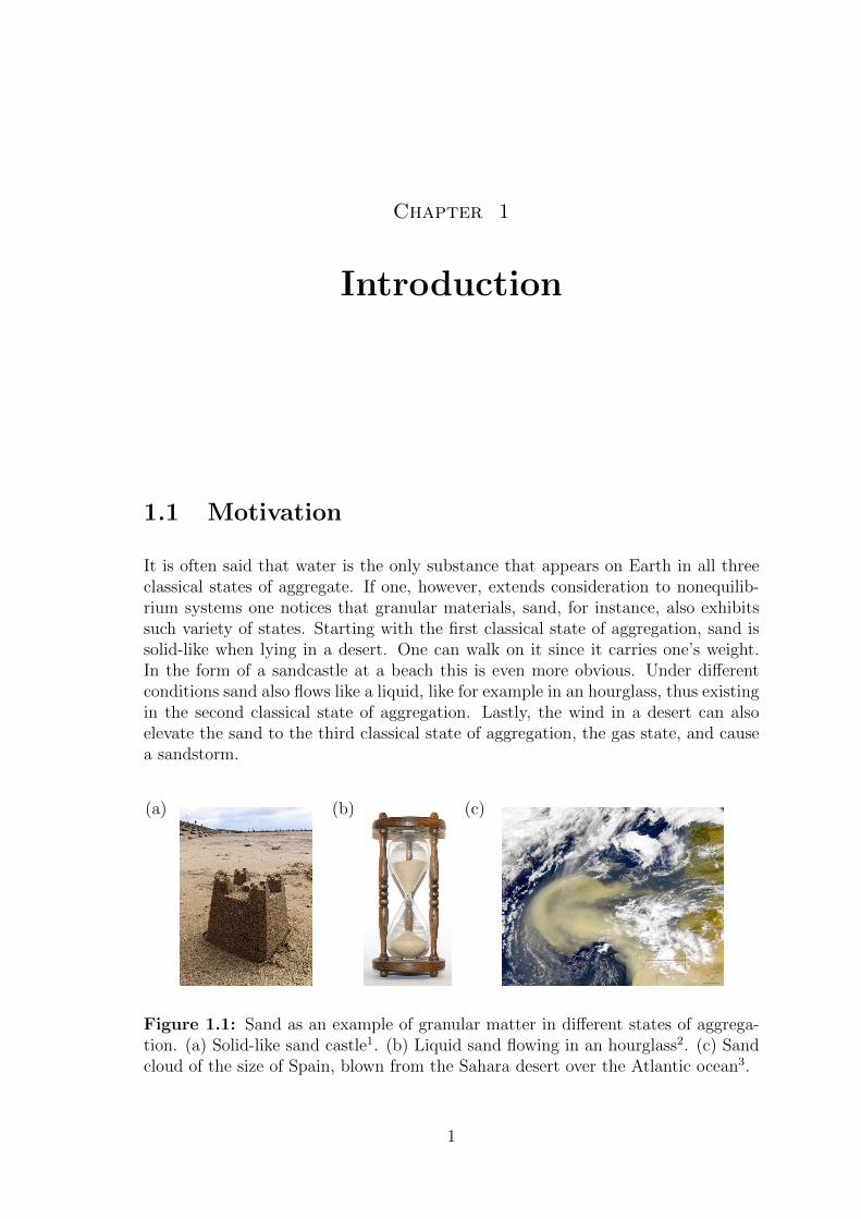
1.1 Sand as an example of granular matter in different states of aggre-gation. (a) Solid-like sand castle1. (b) Liquid sand flowing in anhourglass2. (c) Sand cloud of the size of Spain, blown from the Sa-hara desert over the Atlantic ocean3. . . . . . . . . . . . . . . . . . . 1

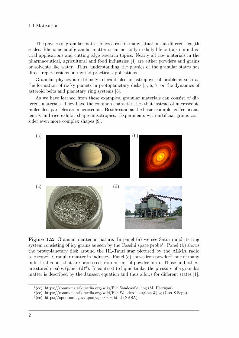
1.2 Granular matter in nature: In panel (a) we see Saturn and its ringsystem consisting of icy grains as seen by the Cassini space probe1.Panel (b) shows the protoplanetary disk around the HL-Tauri starpictured by the ALMA radio telescope2. Granular matter in industry:Panel (c) shows iron powder3, one of many industrial goods that areprocessed from an initial powder form. Those and others are storedin silos (panel (d)4). In contrast to liquid tanks, the pressure of agranular matter is described by the Janssen equation and thus allowsfor different states [1]. . . . . . . . . . . . . . . . . . . . . . . . . . . 2

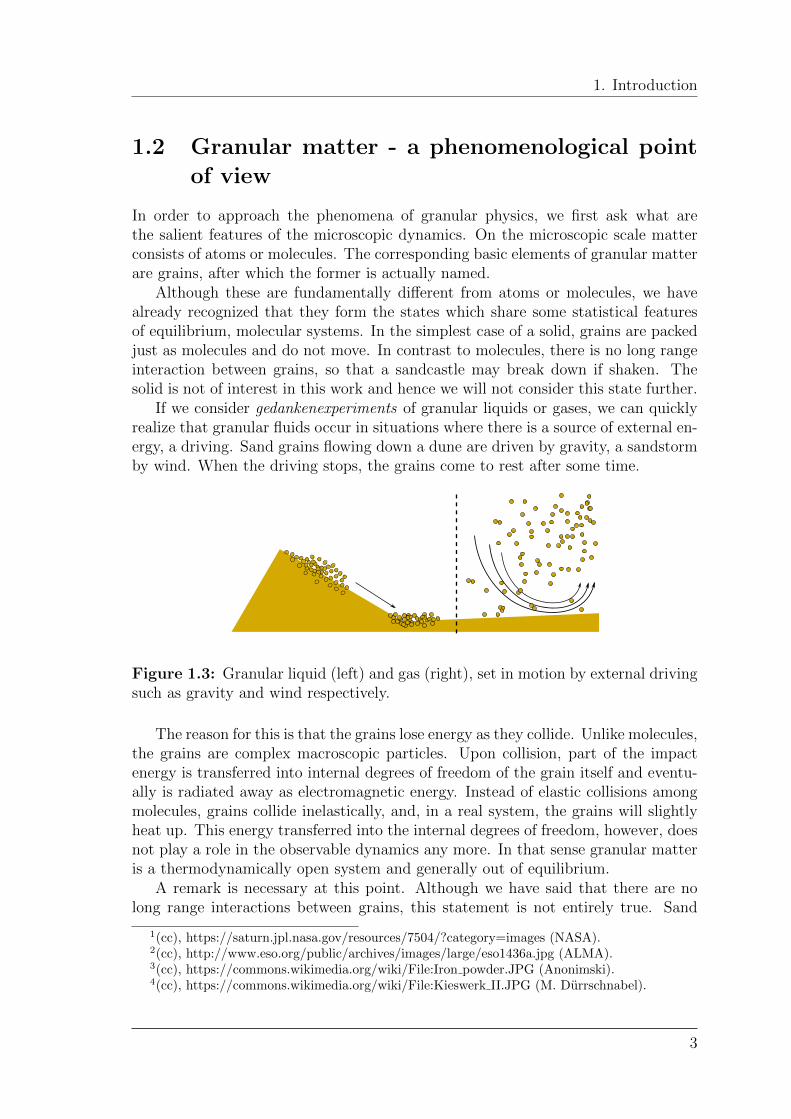
1.3 Granular liquid (left) and gas (right), set in motion by external driv-ing such as gravity and wind respectively. . . . . . . . . . . . . . . . . 3

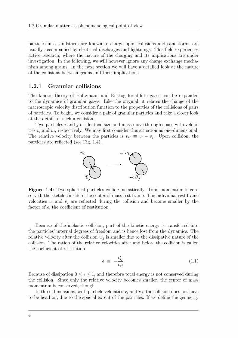
1.4 Two spherical particles collide inelastically. Total momentum is con-served; the sketch considers the center of mass rest frame. The indi-vidual rest frame velocities vi and vj are reflected during the collisionand become smaller by the factor of ϵ, the coefficient of restitution. . 4

1.5 (a) Particles i and j move through space and collide. Upon collision,the particles are reflected. In three dimensions the relative velocitydecomposes in a normal and tangential to the contact surface. . . . . 5

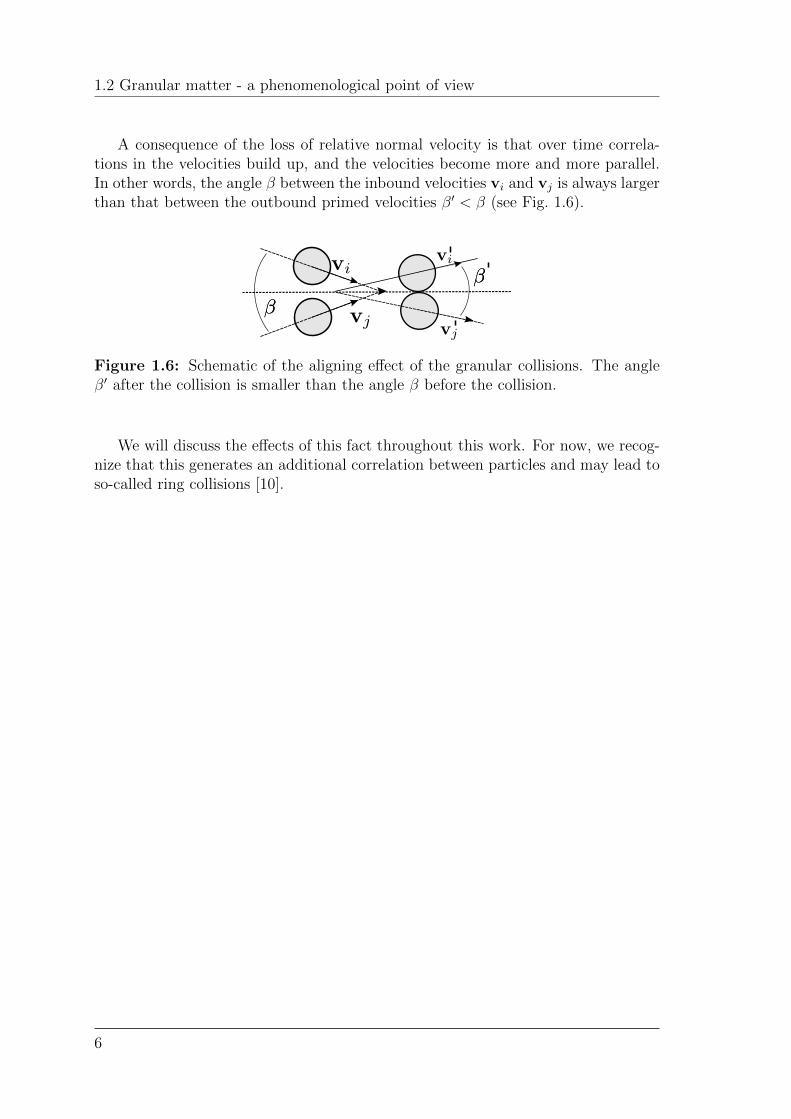
1.6 Schematic of the aligning effect of the granular collisions. The angleβ′ after the collision is smaller than the angle β before the collision. . 6

1.7 The collision cylinder of a reference particle moving with respect tothe background. For particles of diameter σ, the volume of this cylin-der is ⟨vij⟩S∆t. The higher the density the shorter the mean freepath and the more frequent particles will collide. The square root ofthe temperature scales the mean time between collisions. . . . . . . . 9

1.8 Sketch of the geometry leading to the direct collision rate ν− (Eq. (1.16)).The scattering unit vector e = xij/∥xij∥ is the normal to the scatter-ing surface, the basis of the scattering cylinder. The cylinder accountsfor all possible collisions that hit the infinitesimal scattering surfacearound e. . . . . . . . . . . . . . . . . . . . . . . . . . . . . . . . . . 11

v

LIST OF FIGURES

1.9 stochastic rotation dynamics (SRD) particles move for the time ∆twith independent continuous velocities in the free streaming step.Generally, particles are point-like and thus can overlap. . . . . . . . . 14

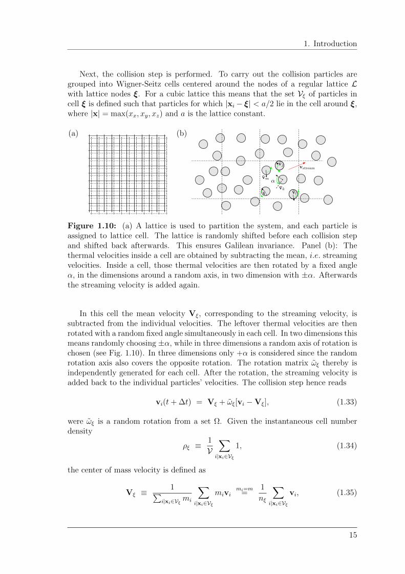
1.10 (a) A lattice is used to partition the system, and each particle isassigned to lattice cell. The lattice is randomly shifted before eachcollision step and shifted back afterwards. This ensures Galilean in-variance. Panel (b): The thermal velocities inside a cell are obtainedby subtracting the mean, i.e. streaming velocities. Inside a cell, thosethermal velocities are then rotated by a fixed angle α, in the dimen-sions around a random axis, in two dimension with ±α. Afterwardsthe streaming velocity is added again. . . . . . . . . . . . . . . . . . . 15

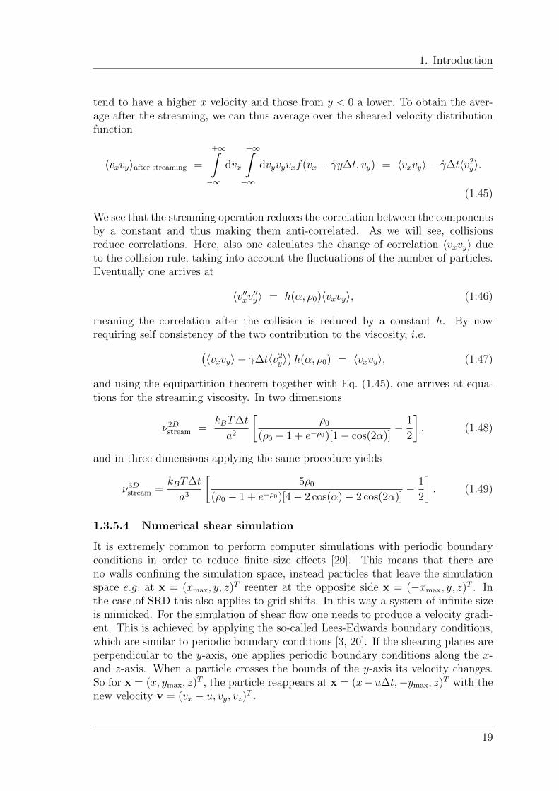
1.11 (a) Sketch of the shear flow simulation where periodic images areshifted in x and move with velocity u(y). (b) Instantaneous linearvelocity profile after some relaxation time obtained in our simulations. 20

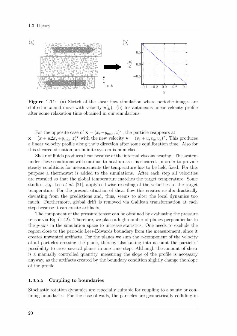
1.12 Collisions with a wall sketched with the lower gray layer. The wallscontain ghost particles that are not translated in the streaming step.(a) Geometry of a bounce back collision. This type leads to no-slipboundary conditions of the wall. (b) Simple reflection creating a slipboundary condition. . . . . . . . . . . . . . . . . . . . . . . . . . . . 21

2.1 Parallel reduction via recursion, for summations, logical evaluationor similar. For an ideal parallel hardware with parallel capabilities asnumerous as the data, the runtime becomes O(logN) for input dataN . . . . . . . . . . . . . . . . . . . . . . . . . . . . . . . . . . . . . . 42

vi

LIST OF FIGURES

2.2 Hardware sketch of the used computers. Those feature one NvidiaK20xm GPU with separate graphic RAM, and an octo-core CPUwith the system RAM and hard drive storage. GPUs are optimal forsimple arithmetic computations and execute those in a highly parallelfashion and thus much faster even though its lower clock rate. In con-trast, CPUs are more versatile and thus faster on non-parallelizabletasks. In terms of memory there are several layers. The CPU RAM iseffectively infinite in our perspective, just as hard disk drive (HDD)space. Because the SRD is computationally cheap its memory usagebecomes more important. As usual for GPGPU applications the in-terconnection between GPU and CPU is a bottleneck. Here, the con-nection of the GPU to its RAM becomes a computational bottleneck,too. Parallelism is possible at different stages. The GPU providestwo copy engines that can handle data transfer with the CPU asyn-chronously from computations. On the CPU this can be done, too,using different cores. So if grid based quantities are of interest forwriting to disk, the CPU can assign workload, while a second CPUcore waits for the asynchronous data transfer to finish. At the sametime the GPU can update particle velocities. More precisely said,the GPU combines 14 streaming multiprocessors with 192 cores each.For a more detailed description on intra-GPU concurrency and syn-chronization abilities please refer to the main text. (The K40 GPUfeature 16 streaming multiprocessors and a RAM size of 12 GiB.) . . 44

2.3 Code flowchart divided into an overview in panel (a) and details ofthe step internal(...) member of the simulation box class inpanel (b). Functions and workflow are represented by red cards andred arrows respectively. Parallel CUDA-GPU-functions are repre-sented by purple cards. The central simulation box instance ap-pears in green. All CUDA calls are performed in the init gpu(...)

and step internal(...) members. Besides the rotation-translationroutine every CUDA-helper-function mostly performs only one task.Functions with a gray dot need synchronization. CPU and GPUcompute times are superimposed, also with data transfer. CUDAfunction calls are launched with individual blocks and grid sizes re-garding synchronization necessities of the respective code segment.Thread numbers are chosen to fit processor number so that functionsperform loops over subsets of the workload. . . . . . . . . . . . . . . . 46

vii

LIST OF FIGURES

2.4 Object structure and summarized object descriptions of the imple-mented program. Objects are denoted as green cards, membershipusage between objects is symbolized as blue arrows, strongly linkedclasses are connected with purple arrows. Routines are presentedas red cards, control flows as red arrows. Classes are grouped intophysics representatives (on gray) and memory managing objects (onpink). The center of the simulation is the simulation box classaround which everything is built, the most basic and widely usedinstance is of the struct vektor. After the main function requested asimulation details struct it generates a simulation box instance andcalls its public control functions. The class itself handles the detailsin dedicated private functions, including e.g. simulation steps withGPU-addressing and data output. . . . . . . . . . . . . . . . . . . . . 47

3.1 Snapshot of the sheared system averaged over 1000 states for a rota-tion angle α = 120. Panel (a) shows the density in the x/y plane.Since we look at an average, the density does not need to be in integernumbers. Still we see fluctuations, also in panel (b) that shows thecells’ streaming velocities Vξ,x in the direction along which the systemis sheared. . . . . . . . . . . . . . . . . . . . . . . . . . . . . . . . . 50

3.2 Kinetic viscosity νstream = ηstream/n0 viscosity of the 2D SRD fluid asa function of the SRD rotation angle α. . . . . . . . . . . . . . . . . . 51

3.3 Kinematic viscosity νstream = ηstream/n0 of the 3D SRD fluid as a func-tion of the SRD rotation angle α. The streaming viscosity divergesat zero and reaches a local maximum at 180. . . . . . . . . . . . . . 52

3.4 State of the freely cooling 3D GSRD gas with ϵ = 0.995 after ∼ 105

collision and streaming steps. We show a cross section perpendicularto the z-axis. In panel (a) we see the instantaneous number densityin the non-shifted grid linearly color encoded. In panel (b) we see theinstantaneous cell temperature. The system is not perfectly homo-geneous anymore though we can see that the variations extent overonly one order of magnitude which is actually small. Furthermore, thedenser regions are colder than the dilute regions due to their higherϵξ,eff mimicking the increased collision rate in those regions. . . . . . . 53

3.5 Granular temperature of the freely cooling granular system as a func-tion of time. The evolution perfectly follows Haff’s law over six ordersof magnitude. After some initial time the decay of GSRD tempera-ture has a slope of −2 in the double logarithmic plot. . . . . . . . . . 54

viii

LIST OF FIGURES

3.6 Kinematic viscosity of the 2D GSRD fluid with ρ0 = 10/V . In the leftpanel (a) we see the kinematic viscosity νkin = µkin/ρ0 as a function ofthe GSRD rotation angle α. In the right panel (b) we see the relativedeviation from the theory for granular fluids, and from the standardtheory, for comparison. We see a good agreement with the theory witha maximum deviation of 4%, which represents a good improvementfrom the standard theory. The effective coefficient of restitution isnot constant due to the different equilibrium temperatures resultingfrom different shear rates. Overall, the values lie around ϵξ,eff = 0.998.The reason for the worse agreement at high α is the instability of thehomogeneous state. For increasing α the shear heating becomes lessimportant, so that for angles slightly larger than 40 the system needsa high shear rate to remain stationary. This in turn contradicts ourassumptions for the derivation of Eq. (3.1). . . . . . . . . . . . . . . . 55

3.7 Kinematic viscosity of the 2D SRD fluid for a mean density of ρ0 =20/V . In the left panel (a) we see the kinematic viscosity νkin =µkin/ρ0 as a function of the SRD rotation angle α. In the right panel(b) we see the relative deviation from the granular theory and thestandard theory, for comparison. Also here, we see a good agree-ment with at maximum 9% error. We attribute the deviation atthe small rotation angle α to the resulting slower mixing and highertemperature we obtain in these simulations. In the same range ofα < 27.5 also the standard theory exhibits an increasing deviation.The standard theory’s deviation from the computed values also in-creases linearly with decreasing α as we have seen in Fig. 3.6(b). . . . 56

3.8 Shear simulation of the 2D GSRD fluid that developed a shear con-densation for α = 50 and initial ϵξ,eff = 0.946. The momentumtransport across the band is disrupted and the band continues tocontract. Like in Fig. 3.4, also here we see the result of the higherdissipation rate in denser regions - the shear band is colder than therest of the system. . . . . . . . . . . . . . . . . . . . . . . . . . . . . 57

3.9 Density profile of the freely cooling GSRD system for ϵ = 0.98, withinitially T (t0) = 100 Tref and ∆t = 0.01. Panel (a) shows the systemclose to the transition to the inhomogeneous cooling state. Panel (b):at t = 104∆t the system has developed clusters, the density variesover 3 orders of magnitude. These clusters continue to grow in size,as can be seen in panels (c) and (b) and also continue to contract. . 58

ix

LIST OF FIGURES

3.10 Details of the freely cooling system in a cross-section perpendicularto the z-axis at 6.5 × 104∆t. Panel (a) shows the density, panel(b) the temperature. In panel (c) the streaming profile is visualizedwith a streamline plot where the line width is proportional to theflow velocity in the plane. Panel (d) shows the local Mach numberin the system. We observe that dense clusters are cold and streammacroscopically with supersonic velocities. Also in the streamlineplot, we observe vortices in the flow field. . . . . . . . . . . . . . . . . 59

3.11 3D density configuration of the GSRD system at (a) t = 2×103∆t and(b) t = 104∆t. The figures are obtained with ray-tracing. The lightpermittivity of each GSRD cell proportional to its density. Hence,the middle along the diagonal appears darker due to the longer lightpaths. We can see denser clusters that have filament-like shapes thatextend in all directions with no preferred direction. . . . . . . . . . . 60

3.12 Cooling behavior of the GSRD fluid for ϵ = 0.98. Panel (a) shows thedevelopment of the mean kinetic energy of the convective degrees offreedom and granular temperature as a function of time with a fit ofHaff’s law. We see rather good agreement up to t < 3× 103∆t wherethe curve of Ekin and T cross and hence the global Mach number Mexceeds one. The temperature follows a different power law after-wards. Panel (b) shows the development of the standard deviation ofthe density distribution σ(ρ) relative to t = 0. The fluctuations σ(ρ)only slowly increase until t ≃ 3× 103∆t when the behavior changes.In the following, the fluctuations increase quickly hence indicating atransition to the inhomogeneous cooling state, coinciding with thechange of slope in the cooling behavior and Mach number M > 1. . 61

3.13 Detailed cooling behavior of the GSRD fluid for ϵ = 0.98 in the inho-mogeneous cooling state. We show the development of the granulartemperature as a function of t > 3× 103∆t, i.e., the region indicatedin the inset. In this region the cooling behavior changes to a powerlaw T (t) ∼ t1.55. With the saturation of the clusters the slope beginsto approach -2 again. . . . . . . . . . . . . . . . . . . . . . . . . . . . 62

3.14 Scaled velocity distribution function f of the 3D SRD fluid. Thedistribution has a stronger tail than the Maxwell-Boltzmann distri-bution. . . . . . . . . . . . . . . . . . . . . . . . . . . . . . . . . . . 64

3.15 Second Sonine coefficient as a function of time for four different coeffi-cients of restitution. First, there is a decrease followed by an approachback towards zero. Minima are lower for higher ϵξ,eff(t0). At aroundt = 4 × 103∆t the systems for the ϵξ,eff = 0.935, 0.96 come close tothe transition to the inhomogeneous cooling state where we see anunexpected positive value of a2. The development of a2 well agreeswith analytical predictions of Brilliantov and Poschel [2] for a variablecoefficient of restitution. . . . . . . . . . . . . . . . . . . . . . . . . . 64

x

LIST OF FIGURES

4.1 Density fluctuations σ(ρξ)2 as a function of M for different ∆t. The

solid line show a power law with exponent two, the dotted line apower law with exponent 3. The developments start from weak fluc-tuations. For smaller ∆t we observe lower initial fluctuations. For∆t

√T (t0) < a/2 we observe clustering for M < 1. In this case the

algorithm’s inherent collisional transport leads to unphysical behav-ior. For ∆t

√T (t0) > a/2 the dynamics follow a common trajectory.

Crossing M = 1 the slope increases due to cluster formation. Weconclude ∆t

√T (t0) > a/2 as a necessary condition for choosing the

input parameters ∆t and T (t0). The hydrodynamic theory predictsa universal scaling low stating that all trajectories below M < 1 con-verge to a power law σ(ρξ)

2 ∝ M2. Although we see a tendency forthis behavior, we find little evidence for that. In the inhomogeneouscooling all curve approach a power law with exponent 3. . . . . . . . 66

4.2 Granular temperature and mean kinetic energy of the freely coolingGSRD system with ϵ = 0.98 in (a) a large system size of 1203 cellsand (b) a small system size of 303 cells. In both systems the kineticenergy decreases with a power law slower than the temperature. Atapproximately t = 105∆t the cluster length scale reaches 30a, thelinear size of the smaller system (b). This system contracts to onebig cluster that does not move due to momentum conservation. Weobserve this process by a sudden drop of kinetic energy in (b) of 3orders of magnitude in one decade of time. . . . . . . . . . . . . . . 67

4.3 Development of the granular temperature T/T0 (green circles) andmean kinetic energy Ekin/kBT0 (blue squares) in the freely coolingsystem as a function of time. The slope in the double logarithmic plotchanges with the GSRD rotation angle α, decreasing for higher angles.Due to finite sizes effects the kinetic energy curves exhibit suddendrops at ca. t ≃ 104∆t for the systems with α > 11. This is becausethe collisional viscosity increases with α and, moreover, in contrastto the streaming viscosity, it does not depend on the temperature[3]. Hence, for α large, collisional contributions apparently becomedominant at a premature state of the evolution. . . . . . . . . . . . . 68

4.4 Change of streaming viscosity with temperature compared to the col-lisional viscosity of standard SRD [3]. For larger α eventually thecollisional viscosity becomes dominant as the temperature decreases.This also applies for the granular system because qualitatively thecurves do not change. In this graph we present the analytical func-tions for ρ0 = 5 and ∆t = 1. . . . . . . . . . . . . . . . . . . . . . . 69

4.5 Clustering of the 3D GSRD system if collisional viscosity becomesdominant. In the cross sections (a) of the number density and (b)temperature we also observe an anti-correlation. The clusters developin lumpy shapes because the system does not become supersonic. . . 69

xi

5.1 Sketch of a granular system under the influence of gravity driven byshaking. In the simulations’ setup periodic boundaries are appliedalong the x- and y-axis. Along the z-dimension the system is con-fined by walls where the wall at z = 0 conducts a periodic oscillation.Lastly, particles are accelerated by a gravity force F/m = −gz. Par-ticles are sketched with red and blue circles representing large andsmall thermal velocities, respectively. . . . . . . . . . . . . . . . . . . 72

5.2 Granular SRD in a driven system. (a) The fluid forms a dense layerelevated at some height z over the ground at z = 0, towards whichthe gravitational force is pointing. (b) The layer below the denselayer is in contact with the vibrating ground and is hence hotter thanthe dense layer lying above. (c) Viewed from above, the dense layeritself show variations in density that form a pattern. (d) The granulartemperature also in this system is anti-correlated to the density, i.e.,where the fluid is denser the temperature is lower. . . . . . . . . . . 73

A.1 Evolution of the freely-cooling 3D GSRD fluid for ϵ = 0.975 on agrid of 2003 cells. The transition to inhomogeneous cooling sets in atapproximately t = 103∆t. Subsequently, the formed clusters mergeas they move through the system and form larger clusters. The max-imum density grows larger for this bigger system, what we can see inpanel (d), since the limit of the cluster length scale is larger here. . . I

xii

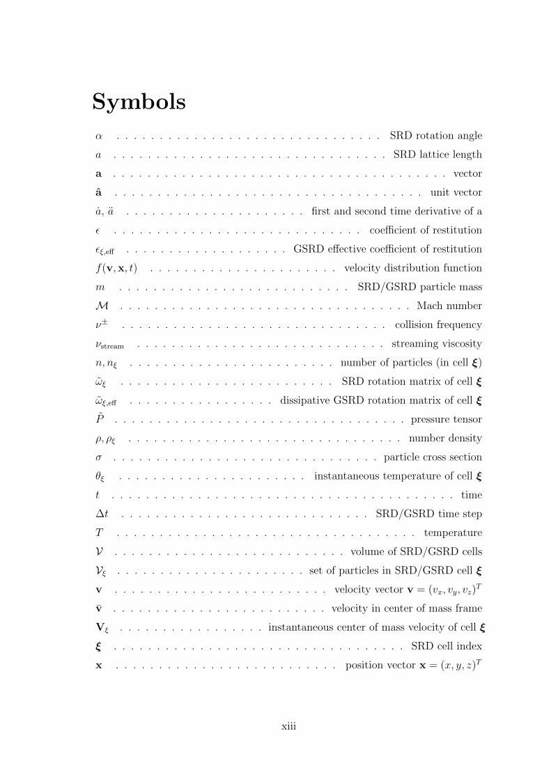
Symbols

α . . . . . . . . . . . . . . . . . . . . . . . . . . . . . . . SRD rotation angle

a . . . . . . . . . . . . . . . . . . . . . . . . . . . . . . . . SRD lattice length

a . . . . . . . . . . . . . . . . . . . . . . . . . . . . . . . . . . . . . . . vector

a . . . . . . . . . . . . . . . . . . . . . . . . . . . . . . . . . . . . unit vector

a, a . . . . . . . . . . . . . . . . . . . . . first and second time derivative of a

ϵ . . . . . . . . . . . . . . . . . . . . . . . . . . . . . coefficient of restitution

ϵξ,eff . . . . . . . . . . . . . . . . . . . GSRD effective coefficient of restitution

f(v,x, t) . . . . . . . . . . . . . . . . . . . . . . velocity distribution function

m . . . . . . . . . . . . . . . . . . . . . . . . . . . SRD/GSRD particle mass

M . . . . . . . . . . . . . . . . . . . . . . . . . . . . . . . . . . Mach number

ν± . . . . . . . . . . . . . . . . . . . . . . . . . . . . . . . collision frequency

νstream . . . . . . . . . . . . . . . . . . . . . . . . . . . . . streaming viscosity

n, nξ . . . . . . . . . . . . . . . . . . . . . . . . number of particles (in cell ξ)

ωξ . . . . . . . . . . . . . . . . . . . . . . . . . SRD rotation matrix of cell ξ

ωξ,eff . . . . . . . . . . . . . . . . . dissipative GSRD rotation matrix of cell ξ

P . . . . . . . . . . . . . . . . . . . . . . . . . . . . . . . . . . pressure tensor

ρ, ρξ . . . . . . . . . . . . . . . . . . . . . . . . . . . . . . . . number density

σ . . . . . . . . . . . . . . . . . . . . . . . . . . . . . . . particle cross section

θξ . . . . . . . . . . . . . . . . . . . . . . instantaneous temperature of cell ξ

t . . . . . . . . . . . . . . . . . . . . . . . . . . . . . . . . . . . . . . . . time

∆t . . . . . . . . . . . . . . . . . . . . . . . . . . . . . SRD/GSRD time step

T . . . . . . . . . . . . . . . . . . . . . . . . . . . . . . . . . . . temperature

V . . . . . . . . . . . . . . . . . . . . . . . . . . . volume of SRD/GSRD cells

Vξ . . . . . . . . . . . . . . . . . . . . . . set of particles in SRD/GSRD cell ξ

v . . . . . . . . . . . . . . . . . . . . . . . . . velocity vector v = (vx, vy, vz)T

v . . . . . . . . . . . . . . . . . . . . . . . . . velocity in center of mass frame

Vξ . . . . . . . . . . . . . . . . . instantaneous center of mass velocity of cell ξ

ξ . . . . . . . . . . . . . . . . . . . . . . . . . . . . . . . . . . SRD cell index

x . . . . . . . . . . . . . . . . . . . . . . . . . . position vector x = (x, y, z)T

xiii

xiv

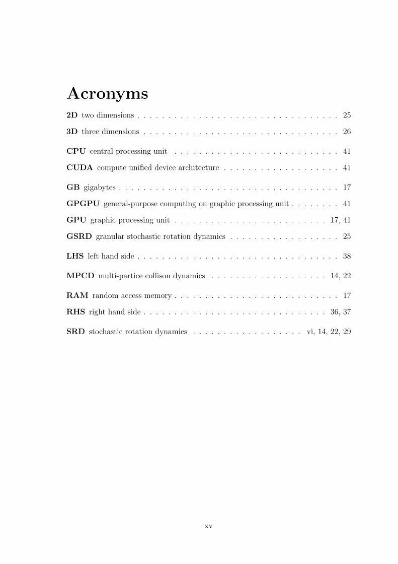
Acronyms2D two dimensions . . . . . . . . . . . . . . . . . . . . . . . . . . . . . . . . . 25

3D three dimensions . . . . . . . . . . . . . . . . . . . . . . . . . . . . . . . . 26

CPU central processing unit . . . . . . . . . . . . . . . . . . . . . . . . . . . 41

CUDA compute unified device architecture . . . . . . . . . . . . . . . . . . . 41

GB gigabytes . . . . . . . . . . . . . . . . . . . . . . . . . . . . . . . . . . . . 17

GPGPU general-purpose computing on graphic processing unit . . . . . . . . 41

GPU graphic processing unit . . . . . . . . . . . . . . . . . . . . . . . . . 17, 41

GSRD granular stochastic rotation dynamics . . . . . . . . . . . . . . . . . . 25

LHS left hand side . . . . . . . . . . . . . . . . . . . . . . . . . . . . . . . . . 38

MPCD multi-partice collison dynamics . . . . . . . . . . . . . . . . . . . 14, 22

RAM random access memory . . . . . . . . . . . . . . . . . . . . . . . . . . . 17

RHS right hand side . . . . . . . . . . . . . . . . . . . . . . . . . . . . . . 36, 37

SRD stochastic rotation dynamics . . . . . . . . . . . . . . . . . . vi, 14, 22, 29

xv

xvi

Chapter 1

Introduction

1.1 Motivation

It is often said that water is the only substance that appears on Earth in all threeclassical states of aggregate. If one, however, extends consideration to nonequilib-rium systems one notices that granular materials, sand, for instance, also exhibitssuch variety of states. Starting with the first classical state of aggregation, sand issolid-like when lying in a desert. One can walk on it since it carries one’s weight.In the form of a sandcastle at a beach this is even more obvious. Under differentconditions sand also flows like a liquid, like for example in an hourglass, thus existingin the second classical state of aggregation. Lastly, the wind in a desert can alsoelevate the sand to the third classical state of aggregation, the gas state, and causea sandstorm.

(a) (b) (c)

Figure 1.1: Sand as an example of granular matter in different states of aggrega-tion. (a) Solid-like sand castle1. (b) Liquid sand flowing in an hourglass2. (c) Sandcloud of the size of Spain, blown from the Sahara desert over the Atlantic ocean3.

1

1.1 Motivation

The physics of granular matter plays a role in many situations at different lengthscales. Phenomena of granular matter occur not only in daily life but also in indus-trial applications and cutting edge research topics. Nearly all raw materials in thepharmaceutical, agricultural and food industries [4] are either powders and grainsor solvents like water. Thus, understanding the physics of the granular states hasdirect repercussions on myriad practical applications.

Granular physics is extremely relevant also in astrophysical problems such asthe formation of rocky planets in protoplanetary disks [5, 6, 7] or the dynamics ofasteroid belts and planetary ring systems [8].

As we have learned from these examples, granular materials can consist of dif-ferent materials. They have the common characteristics that instead of microscopicmolecules, particles are macroscopic. Beside sand as the basic example, coffee beans,lentils and rice exhibit shape anisotropies. Experiments with artificial grains con-sider even more complex shapes [9].

(a) (b)

(c) (d)

Figure 1.2: Granular matter in nature: In panel (a) we see Saturn and its ringsystem consisting of icy grains as seen by the Cassini space probe1. Panel (b) showsthe protoplanetary disk around the HL-Tauri star pictured by the ALMA radiotelescope2. Granular matter in industry: Panel (c) shows iron powder3, one of manyindustrial goods that are processed from an initial powder form. Those and othersare stored in silos (panel (d)4). In contrast to liquid tanks, the pressure of a granularmatter is described by the Janssen equation and thus allows for different states [1].

1(cc), https://commons.wikimedia.org/wiki/File:Sandcastle1.jpg (M. Harrigan).2(cc), https://commons.wikimedia.org/wiki/File:Wooden hourglass 3.jpg (User:S Sepp).3(cc), https://apod.nasa.gov/apod/ap000303.html (NASA).

2

1. Introduction

1.2 Granular matter - a phenomenological point

of view

In order to approach the phenomena of granular physics, we first ask what arethe salient features of the microscopic dynamics. On the microscopic scale matterconsists of atoms or molecules. The corresponding basic elements of granular matterare grains, after which the former is actually named.

Although these are fundamentally different from atoms or molecules, we havealready recognized that they form the states which share some statistical featuresof equilibrium, molecular systems. In the simplest case of a solid, grains are packedjust as molecules and do not move. In contrast to molecules, there is no long rangeinteraction between grains, so that a sandcastle may break down if shaken. Thesolid is not of interest in this work and hence we will not consider this state further.

If we consider gedankenexperiments of granular liquids or gases, we can quicklyrealize that granular fluids occur in situations where there is a source of external en-ergy, a driving. Sand grains flowing down a dune are driven by gravity, a sandstormby wind. When the driving stops, the grains come to rest after some time.

Figure 1.3: Granular liquid (left) and gas (right), set in motion by external drivingsuch as gravity and wind respectively.

The reason for this is that the grains lose energy as they collide. Unlike molecules,the grains are complex macroscopic particles. Upon collision, part of the impactenergy is transferred into internal degrees of freedom of the grain itself and eventu-ally is radiated away as electromagnetic energy. Instead of elastic collisions amongmolecules, grains collide inelastically, and, in a real system, the grains will slightlyheat up. This energy transferred into the internal degrees of freedom, however, doesnot play a role in the observable dynamics any more. In that sense granular matteris a thermodynamically open system and generally out of equilibrium.

A remark is necessary at this point. Although we have said that there are nolong range interactions between grains, this statement is not entirely true. Sand

1(cc), https://saturn.jpl.nasa.gov/resources/7504/?category=images (NASA).2(cc), http://www.eso.org/public/archives/images/large/eso1436a.jpg (ALMA).3(cc), https://commons.wikimedia.org/wiki/File:Iron powder.JPG (Anonimski).4(cc), https://commons.wikimedia.org/wiki/File:Kieswerk II.JPG (M. Durrschnabel).

3

1.2 Granular matter - a phenomenological point of view

particles in a sandstorm are known to charge upon collisions and sandstorms areusually accompanied by electrical discharges and lightnings. This field experiencesactive research, where the nature of the charging and its implications are underinvestigation. In the following, we will however ignore any charge exchange mecha-nism among grains. In the next section we will have a detailed look at the natureof the collisions between grains and their implications.

1.2.1 Granular collisions

The kinetic theory of Boltzmann and Enskog for dilute gases can be expandedto the dynamics of granular gases. Like the original, it relates the change of themacroscopic velocity distribution function to the properties of the collisions of pairsof particles. To begin, we consider a pair of granular particles and take a closer lookat the details of such a collision.

Two particles i and j of identical size and mass move through space with veloci-ties vi and vj, respectively. We may first consider this situation as one-dimensional.The relative velocity between the particles is vij ≡ vi − vj. Upon collision, theparticles are reflected (see Fig. 1.4).

Figure 1.4: Two spherical particles collide inelastically. Total momentum is con-served; the sketch considers the center of mass rest frame. The individual rest framevelocities vi and vj are reflected during the collision and become smaller by thefactor of ϵ, the coefficient of restitution.

Because of the inelastic collision, part of the kinetic energy is transferred intothe particles’ internal degrees of freedom and is hence lost from the dynamics. Therelative velocity after the collision v′ij is smaller due to the dissipative nature of thecollision. The ration of the relative velocities after and before the collision is calledthe coefficient of restitution

ϵ ≡ −v′ijvij

. (1.1)

Because of dissipation 0 ≤ ϵ ≤ 1, and therefore total energy is not conserved duringthe collision. Since only the relative velocity becomes smaller, the center of massmomentum is conserved, though.

In three dimensions, with particle velocities vi and vj, the collision does not haveto be head on, due to the spacial extent of the particles. If we define the geometry

4

1. Introduction

of the collision with the unit vector

e ≡ ri − rj∥ri − rj∥

=rij

∥rij∥,

the relative velocity vij ≡ vi − vj decomposes into the parts normal vnij and tan-

gential vtij to the contact surface of the particles, in the rest frame of the system

(see Fig. 1.5). In general, particles are not completely spherically symmetric andhave a friction acting between the surfaces. This makes the collision more complexin the way that the particles’ rotational degrees of freedom enter the dynamics andmoreover the collision then also affects the tangential motion.

If the reflection is assumed to act only on vnij, this is for our case sufficient. In this

case only the translational degrees of freedom enter the dynamics. The velocitiesafter the collision are then given by

v′i = vi −

1 + ϵ

2(vij · e) e, (1.2)

v′j = vj +

1 + ϵ

2(vij · e) e.

(a) (b)

Figure 1.5: (a) Particles i and j move through space and collide. Upon collision,the particles are reflected. In three dimensions the relative velocity decomposes ina normal and tangential to the contact surface.

In our case, the situation becomes analogous to the one dimensional case for thenormal component vn

ij so that

ϵ ≡ −vn′ij

vnij

. (1.3)

We stress that in granular collisions, total momentum and mass are conserved, whileenergy is dissipated.

5

1.2 Granular matter - a phenomenological point of view

A consequence of the loss of relative normal velocity is that over time correla-tions in the velocities build up, and the velocities become more and more parallel.In other words, the angle β between the inbound velocities vi and vj is always largerthan that between the outbound primed velocities β′ < β (see Fig. 1.6).

Figure 1.6: Schematic of the aligning effect of the granular collisions. The angleβ′ after the collision is smaller than the angle β before the collision.

We will discuss the effects of this fact throughout this work. For now, we recog-nize that this generates an additional correlation between particles and may lead toso-called ring collisions [10].

6

1. Introduction

1.3 Theory

1.3.1 The coefficient of restitution

To derive a kinetic model suitable for analytical treatment and also numerical sim-ulations we consider the simplest geometry: two spherical particles. Their elasticproperties are then fully described by their radii and Young modulus. So when par-ticles collide, the impact will lead to a deformation. The energy dissipated in thenormal direction will be completely transferred into the viscoelastic deformation ofthe two particles.

The result of this approach is that the dissipation solely depends on the impactvelocity according to

ϵ ∼vn

ij

1/5. (1.4)

A common, albeit drastic, simplification of this so-called viscoelastic model as-sumes

ϵ = const.

This assumption considerably simplifies analytical calculations and is moreover welljustified in situations where the velocity distribution in the system is narrow andthe system in a stationary state.

The stiffer the particles are, the shorter the collision time, i.e., the time thatthe two particles touch, will be. This is an important condition for the assumptionof pairwise collisions only, that we will make in the following. For coefficients ofrestitution close to one, this assumption holds better but when ϵ is considerablydifferent than one the situation is more problematic.

In general, a classical system consisting of N particles is described by coupledNewton’s equations of motion

mixi = F(x1, . . . ,xN ,v1, . . . ,vN) (1.5)

for all particles i = 1, . . . , N . In the absence of long range interactions (i.e. elec-trostatics) particles will move ballistically on straight trajectories until they collide,and after the collision they will move on straight paths again. If the gas is dilute andthe timescale of a single collision sufficiently small, ternary collisions are negligibleand collisions will dominantly be binary. Instead of the full Newton’s equation ofmotion, the system is described by a simpler pairwise interaction

meffxij = F[xij,vij] (1.6)

with xij = xi − xj and the effective mass of the two body system

meff =mimj

mi +mj

. (1.7)

7

1.3 Theory

Together with an initial condition this gives a full description of a single collision.Between collisions the force F is zero.

Under the restriction of our assumptions, the dynamics are hence completelydescribed by the property of a pair collision. While the dynamics of the singlecollision are not important, the change of the velocities before and after the collisionsis what matters. Since the coefficient of restitution is the key property of a single paircollision, we can conclude that the coefficient of restitution is actually completelysufficient to describe the dynamics of a granular gas. It is moreover the only thingthat distinguishes it from an ordinary molecular gas [10].

1.3.2 Temperature of a granular gas - Haff’s law

The fact that in a granular gas there is a constant loss of kinetic energy makes itan out-of-equilibrium system. Still, like molecular gases, we can treat the granulargas with the tools of statistical mechanics. For this we consider a system in thethermodynamic limit, i.e., consisting of a large number of particles N contained insome volume V . As for a molecular gas the number density is ρ ≡ N/V . Moreover,particle velocities are randomly distributed, and if no macroscopic flow is present,the average velocity ⟨v⟩ will be zero. Though, like in molecular gases there arefluctuations around the mean velocity. In analogy to the temperature of a moleculargas, the granular temperature is defined as the mean energy per degree of freedom,that is the variance of the velocity

3

2kBT =

⟨1

2m∥v − ⟨v⟩∥2

⟩, (1.8)

where kB is Boltzmann’s constant and the angular brackets denote average over theparticles. This temperature is of course different from the temperature of the grainsthemselves, and as we have stated earlier not coupled to the former. The collisionsconserve number density and center of mass velocity, but not energy. Hence, thegranular gas cools down, even in an externally force free environment. We investigatethe granular temperature to monitor the state of the system.

In the early stage the granular gas cools down without the occurrence of anyspatial inhomogeneity, which is called the homogeneous cooling state. In the follow-ing, we assume these conditions to hold in order to derive Haff’s law describing thecooling of a homogeneous granular gas. The decay of temperature ∆T during a timeinterval ∆t is described by the number of collisions that occur during this time andthe velocity of the colliding particles. In the thermodynamic limit we can work withthe averages of those.

The frequency of collisions is obtained via the volume of the so-called collisioncylinder multiplied by the number density. With ⟨vij⟩ ∝

√T , the collision frequency

in ∆t is

ν(∆t) ∝ ρσ2√T∆t. (1.9)

8

1. Introduction

Figure 1.7: The collision cylinder of a reference particle moving with respect to thebackground. For particles of diameter σ, the volume of this cylinder is ⟨vij⟩S∆t. Thehigher the density the shorter the mean free path and the more frequent particles willcollide. The square root of the temperature scales the mean time between collisions.

The volume of the collision cylinder accounts for the space the particle sweepsthrough during ∆t with respect to all other particles. The diameter of two par-ticle diameters 2σ (cf. Fig. 1.7) originates from the fact that particles touch withtheir centers of mass distance being equal to σ.

The average energy difference before and after a collision is given by

1

2meff⟨v′2ij − v2ij⟩ ∝ −(1− ϵ2)T, (1.10)

where we have used Eq. (1.3) and assumed a constant coefficient of restitution. Theproduct of Eq. (1.9) and Eq. (1.10) gives the average amount of thermal energydissipated during ∆t

∆T

∆t∝ −ρσ2(1− ϵ2)T 3/2 ≃ dT

dt. (1.11)

The solution to Eq. (1.11) yields Haff’s law [11], that is, the temperature evolutionof the homogeneous granular gas

T (t) =T (t0)

(1 + t/τ0)2(1.12)

with τ−10 ∝ nσ2(1 − ϵ2)

√T (t0). For systems in which the coefficient of restitution

depends on the collision velocity, the exponent of this power law changes. With thedependence of 1− ϵ2 ∝ ⟨(vnij)1/5⟩ ∝ T 1/10 obtained for viscoelastic particles, thisleads to

T (t) =T (t0)

(1 + t/τ ′0)5/3

. (1.13)

In both cases, the dissipation leads to a power-law cooling of the granular gas [10].

9

1.3 Theory

1.3.3 Boltzmann-Enskog equation for a granular gas

The Boltzmann-Enskog equation relates the dynamics of macroscopic quantities tothe properties of the microscopic dynamics, i.e., the collisions of particles. Thetheory’s main concern is the velocity distribution function f(v,x, t) which gives theprobability to encounter a particle with velocity v at position x and time t. It isnormalized such that integrating over the whole 6 dimensional phase space gives thetotal number of particles N in the system∫

dxdvf(v,x, t) = N, (1.14)

where we simplified the notation by dropping the integrations interval bounds of±∞ and by using a single integral sign. In the presence of an external force F, theBoltzmann-Enskog equation reads(

∂

∂t+ v∇x +

F

m∇v

)f(v,x, t) =

∂f

∂t

coll

. (1.15)

While the left hand side of Eq. (1.15) accounts the change due to streaming andexternal forces, the right hand side denotes the effect of the change of f(v,x, t) dueto a collision. The right hand side is an integral, the so-called collision integral, whichis a non-linear function of f since multiple particles participate in a collision. Inthe following we will only consider binary collisions. The dynamics of the momentsof the velocity distribution function are obtained by integration. Following [10],we sketch the derivation of the Boltzmann-Enskog equation via direct and inversecollisions for a homogeneous system.

Consider the probability of a state f(v, t). It can only change in two ways,i.e., either a collision occurs and decreases the probability because its outcome isdifferent or another collision’s result equals the current state of interest such thatthe probability increases. The first possibility is called direct collision, the secondindirect collision. Their frequencies during a time interval ∆t are denoted with ν−

and ν+, respectively. We recall the scattering cylinder for these frequencies. Theprobability of scatterer in the volume dxi, which is determined by the scatteringvector e, is f(vj, t)dvjdxi. The cross section of the cylinder is σ2de and its lengthvij∆t.

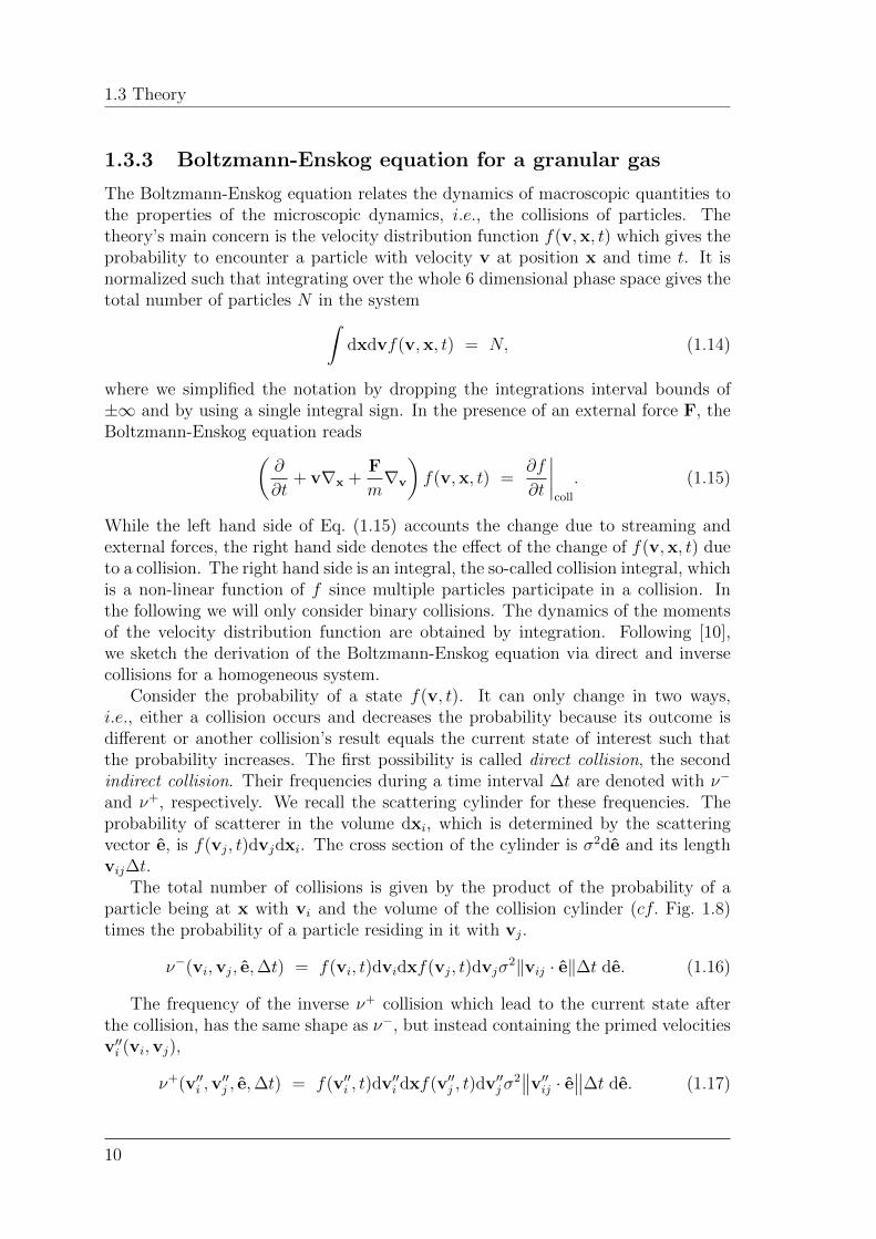
The total number of collisions is given by the product of the probability of aparticle being at x with vi and the volume of the collision cylinder (cf. Fig. 1.8)times the probability of a particle residing in it with vj.

ν−(vi,vj, e,∆t) = f(vi, t)dvidxf(vj, t)dvjσ2∥vij · e∥∆t de. (1.16)

The frequency of the inverse ν+ collision which lead to the current state afterthe collision, has the same shape as ν−, but instead containing the primed velocitiesv′′i (vi,vj),

ν+(v′′i ,v

′′j , e,∆t) = f(v′′

i , t)dv′′i dxf(v

′′j , t)dv

′′jσ

2v′′

ij · e∆t de. (1.17)

10

1. Introduction

Figure 1.8: Sketch of the geometry leading to the direct collision rate ν−

(Eq. (1.16)). The scattering unit vector e = xij/∥xij∥ is the normal to the scatteringsurface, the basis of the scattering cylinder. The cylinder accounts for all possiblecollisions that hit the infinitesimal scattering surface around e.

Via the primed velocities that lead the unprimed velocities after the collision

v′′i = vi −

1 + ϵ

2ϵ(vij · e) e, (1.18)

v′′j = vj +

1 + ϵ

2ϵ(vij · e) e,

Eq. (1.17) is actually a function of the unprimed velocities.The change in f is given by integration over the frequency of the direct and

inverse collision. In order to write down the integral one needs to transform theintegration to common variables of integration. The determinant of the Jacobianmatrix for the mapping of v′′ to v is

Dv′′

Dv=

1

ϵ.

Another factor of 1/ϵ comes from the change of variables in the collision cylinderv′′ij · e

= 1ϵ∥vij · e∥. Using the Heaviside step function Θ(x) to assure that only

velocities that lead to collisions are considered, the Boltzmann equation is obtained

∂f(vi, t)

∂t

coll

= σ2

∫dvj

∫de Θ(−vij · e)∥vij · e∥

× [1

ϵ2f(v′′

i , t)f(v′′j , t)− f(vi, t)f(vj, t)] (1.19)

≡ I(f, f).

The first of the summands on the right hand side represents the inverse collisions,increasing the probability of the current state, the second represents direct collisions.These method of derivation is quite intuitive, though a few facts have to be pointedout separately. First, particle positions were considered mutually independent in

11

1.3 Theory

the derivation, while in reality, pairs have a joint distribution function f2(vi,vj, t)that doesn’t necessarily factor out. The assumption of independent positions isvalid in dilute gases. A more realistic approximation, however, is f2(vi,vj, t) ≈g(σ)f(vi, t)f(vj, t), where g(σ) is the pair correlation function at contact distance,hence including excluded volume effects. In this context, the factor of g(σ) is calledthe Enskog factor. Including it into Eq. (1.19), it becomes

∂f(vi, t)

∂t

coll

= g(σ)I(f, f). (1.20)

A second remark comes from the nature of collisions. One condition of the Boltz-mann Stoßzahlansatz is that the colliding particles’ velocities are initially uncorre-lated, i.e. the assumption of molecular chaos. The aligning effect sketched in Fig. 1.6though leads to ring collision, such that this assumption is potentially not fulfilled[10].

1.3.4 Granular hydrodynamics

1.3.4.1 Preconditions

The dynamics of the moments of the velocity distribution function, that are directlylinked to macroscopic observables, can also be obtained via the Boltzmann equa-tion. While for the derivation of Haff’s law, spatial homogeneity is assumed, smallgradients are assumed here. This means that the microscopic scales of the mean freepath and mean collision time are small with respect to the length L and time scaleT , respectively, of the macroscopic dynamics. Gradients are assumed to be smallsuch that over the macroscopic length scales, the variation is of the order of the ob-servable itself, for the temperature ∆T ∼ T/L. Another important condition is thatthe macroscopic flow velocities are sufficiently smaller than the thermal velocities,so that the flow is well in the subsonic regime, i.e., with the local Mach number

M =

√⟨v⟩2T

≪ 1 (1.21)

being well below one. Asking for this condition of subsonic flow is a rather trickyundertaking, because granular collisions not only lead to an increasing alignmentof particle velocities, but also the dissipative nature steadily changes the ratio ofEq. (1.21) to the undermining of the assumption of this condition. Flow can thusbecome supersonic, and in the case of the viscoelastic model of ϵ becomes subsonicagain [10].

1.3.4.2 Hydrodynamic equations

In order to obtain the observables’ dynamics, we separately multiply the BoltzmannEq. (1.15) with the moments

Ji ∈ 1,v,V2 (1.22)

12

1. Introduction

with the local velocity V = v − u. Their expectation values under the distribu-tion function correspond to the macroscopic observables. Integrating over vi thusyields dynamic equations for the latter [10]. For the first two moments there is nochange due to the collision integral, since the individual collisions conserve bothmass and total momentum. For the temperature (J3 = V2) the collisional contri-bution doesn’t vanish: ∫

dvmV2

2g(σ)I(f, f) =

3

2nTζ. (1.23)

The cooling rate ζ is defined by

ζ(x, t) =πmg(σ)σ2

24nT

∫dvidvjv

3ijf(x,vi, t)f(x,vj, t)(1− ϵ2). (1.24)

Note that with vij ∼√T the integral is of the order ∼ T 3/2. With the macroscopic

flow velocity u, the hydrodynamics equations for granular gases read

∂ρ

∂t+∇(ρu) = 0, (1.25)

∂u

∂t+ u · ∇u+

1

ρm∇ · P = 0, (1.26)

∂T

∂t+ u · ∇T +

2

3ρ

(P : ∇u+∇ · q

)+ ζT = 0, (1.27)

where the vector q denotes the heat flux

q =

∫dv

m

2V2Vf(v,x, t) (1.28)

and P the pressure tensor defined by

Pij =

∫dvm

(vivj −

1

3δijV

2

)f(v,x, t) + nTδij. (1.29)

Here, we used the notation of δij for the Kronecker delta. Moreover, we use shortnotation ab with no space between vectors for the dyadic product a ⊗ b, and forthe total contraction of two tensors a and b

a : b ≡ Tr(a · b

).

To obtain a closed description of the hydrodynamics, one has to express the pressuretensor P and heat flux q in therms of the fields ρ,u and T . In linear order, these read

Pij = pδij − η(∇iuj +∇jui −2

3δij∇ · u) (1.30)

q = −κ∇T − µ∇ρ, (1.31)

where p is the hydrostatic pressure, η the shear viscosity, κ the thermal conductivity,in general, these are also functions of the hydrodynamic field (for full expressionsrefer to e.g. [12, 13]).

13

1.3 Theory

1.3.5 Standard stochastic rotation dynamics

The standard SRD method [14] is a rather recent, well established mesoscopicmethod to model hydrodynamics. It is computationally efficient and well tunable.Since it is a particle based method, it is especially easy to couple to a solute. Fur-thermore, because of its mathematical simplicity, the system can be thoroughlytreated analytically. Since its introduction, numerous articles about the derivationof hydrodynamic equations and transport coefficients have been published [14, 15, 3].After its introduction a number of similar and modified algorithms have been pub-lished [16]. The family of algorithms that it formed are called multi-partice collisondynamics (MPCD). It reproduces full hydrodynamics with thermal fluctuations. Itis used to model solvent dynamics in simulations of colloids, polymers and activeswimmers [17].

1.3.5.1 Algorithm

The SRD model considers particles that move in continuous space with continuousvelocities and constitute the SRD fluid. Their movement and collisions are describedby simplified rules. The dynamic stages of the real fluid consist of two steps: (i) thefree streaming, and (ii) the collisions between the particles [14]. One after another,these stages occur with a fixed time interval in between. While the free streaming istreated exactly, the collisions are represented by a simplified coarse-grained collisionmodel. The aim of the streaming is to macroscopically transport mass, momentumand energy. Additionally, the collision redistributes these quantities among theparticles.

Figure 1.9: SRD particles move for the time ∆t with independent continuousvelocities in the free streaming step. Generally, particles are point-like and thus canoverlap.

We consider a system of N particles of mass mi, which reside and move in a con-tinuous d-dimensional space with individual positions xi and continuous velocitiesvi, i ∈ [1, N ] (see Fig. 1.9). In the free streaming step particles are advanced bytheir individual velocities for the duration of the time step ∆t according to

xi(t+∆t) = xi(t) + vi∆t. (1.32)

14

1. Introduction

Next, the collision step is performed. To carry out the collision particles aregrouped into Wigner-Seitz cells centered around the nodes of a regular lattice Lwith lattice nodes ξ. For a cubic lattice this means that the set Vξ of particles incell ξ is defined such that particles for which |xi − ξ| < a/2 lie in the cell around ξ,where |x| = max(xx, xy, xz) and a is the lattice constant.

(a) (b)

Figure 1.10: (a) A lattice is used to partition the system, and each particle isassigned to lattice cell. The lattice is randomly shifted before each collision stepand shifted back afterwards. This ensures Galilean invariance. Panel (b): Thethermal velocities inside a cell are obtained by subtracting the mean, i.e. streamingvelocities. Inside a cell, those thermal velocities are then rotated by a fixed angleα, in the dimensions around a random axis, in two dimension with ±α. Afterwardsthe streaming velocity is added again.

In this cell the mean velocity Vξ, corresponding to the streaming velocity, issubtracted from the individual velocities. The leftover thermal velocities are thenrotated with a random fixed angle simultaneously in each cell. In two dimensions thismeans randomly choosing ±α, while in three dimensions a random axis of rotation ischosen (see Fig. 1.10). In three dimensions only +α is considered since the randomrotation axis also covers the opposite rotation. The rotation matrix ωξ thereby isindependently generated for each cell. After the rotation, the streaming velocity isadded back to the individual particles’ velocities. The collision step hence reads

vi(t+∆t) = Vξ + ωξ[vi −Vξ], (1.33)

were ωξ is a random rotation from a set Ω. Given the instantaneous cell numberdensity

ρξ ≡ 1

V∑

i|xi∈Vξ

1, (1.34)

the center of mass velocity is defined as

Vξ ≡ 1∑i|xi∈Vξ

mi

∑i|xi∈Vξ

mivimi=m=

1

nξ

∑i|xi∈Vξ

vi, (1.35)

15

1.3 Theory

where nξ is the instantaneous number of particles in cell ξ and V = a3 the volumeof a single cell. Finally, the instantaneous local temperature of a SRD cell is definedas

θξ ≡ 1

3nξ

∑i|xi∈Vξ

mi∥vi −Vξ∥2. (1.36)

In the following, we generally consider equal masses mi = m. The dynamics gener-ated by these two rules conserve mass, momentum and energy. Mass conservationfollows by definition, momentum conservation can be easily proven by

Vξ(t+∆t) =1

nξ

∑i|xi∈Vξ

vi(t+∆t) =1

nξ

∑i|xi∈Vξ

(Vξ + ω[vi −Vξ]) (1.37)

=1

nξ

∑i|xi∈Vξ

Vξ + ω1

nξ

∑i|xi∈Vξ

vi =ωVξ

− ω1

nξ

∑i|xi∈Vξ

Vξ =ωVξ

= Vξ.

Similarly, energy conservation follows from

θξ(t+∆t) =m

3nξ

∑i|xi∈Vξ

||vi(t+∆t)−Vξ(t+∆t) =Vξ

||2 =m

3nξ

∑i|xi∈Vξ

∥ω[vi −Vξ]∥2

(1.38)

=m

3nξ

∑i|xi∈Vξ

[v2i − vT

i Vξ −VTξ vi +V2

ξ ] =m

3nξ

∑i|xi∈Vξ

∥vi −Vξ∥2

= θξ,

where we have used that for two arbitrary vectors a and b it holds (aω)T (ωb) = aTbbecause det(ω) = 1. For the standard SRD method, a Boltzmann equation has beenderived from the Liouville’s equation and it has been shown that the model yieldscorrect linear hydrodynamic equations [14]. In another approach solely consideringtransport through virtual surfaces in the fluid, the same result has been obtained[15].

The random grid shift was introduced by Ihle and Kroll [18] to ensure Galileaninvariance. In this procedure, first a random shift in the interval [−a/2, a/2] in spaceis applied to all particle positions. While it was not introduced in the beginning, ithas been shown, that not applying a random shift to the grid introduces spuriouscorrelations at low temperatures. Those are spatially anisotropies due to the shapeof the lattice and originate from the fact that often the same particles participatein subsequent collisions.

16

1. Introduction

1.3.5.2 Computational complexity of SRD

The SRD method has some major advantages that make it very suitable for numeri-cal simulations. Maybe the most remarkable fact is that SRD is an O(N) algorithm.This is because there is no pair interaction that has to be calculated. Another im-portant property of the algorithm is that the fundamental quantities used are 1-bodyobservables. Basically the mass and momentum per cell have to be calculated everystep. Those are simple sums of particle properties. This gives the algorithm thepossibility of an immense parallel speedup on parallel hardware, especially usingvector accelerators or graphic cards.

Calculations of the cell-wise quantities Vξ, ρξ, θξ generally needs exclusive oratomic read/write access to the cells memory sections. However, the number ofprocessor units #P is very small compared to the typical number of particles N onthe hardware

O(#P ) = 103 ≪ O(N) = 108. (1.39)

Typically, there are on average 5 to 25 particles in a cell ξ. Hence, the situationwhere multiple processors access the same memory locations are rare. This is favor-able because these accesses have to be exclusive to guarantee memory consistency.Multiple exclusive access attempts on parallel hardware are called exclusive accesscollisions. These accesses have to be performed in sequential order, thus their pro-cessing is slow.

Given a fixed size parallel hardware, the algorithm becomes more efficient forincreasing number of particles because less exclusive access collisions are occur-ring. Eventually, the algorithm boils down to summing on parallel hardware plusindependent calculation on cells and on particles. The latter is computationallymore expensive, the former needs synchronization, though sums are of complexityO( logN) on parallel hardware. The bottleneck and size limit are mainly given bythe memory size and memory bus. Since not even cells’ states fit in any cache,all storage resides in the lowest layer i.e. the random access memory (RAM). TheNvidia graphic processing unit (GPU) cards that we used have separate graphicRAM with sizes of either 6 gigabytes (GB) for the Tesla K20Xm card and 12 GBfor the Tesla K40 card. With single precision floating point numbers, simulationswith 200 million particles and 2003 cells can be performed within short time.

1.3.5.3 Streaming viscosity of standard SRD

For the SRD fluid, there are two contributions to the kinematic viscosity ν = η/ρthat originate from the two steps of the model. The total kinematic viscosity reads

ν = νstream + νcoll, (1.40)

where νstream and νcoll denote the contribution from the SRD streaming step and col-lision step, respectively. The streaming viscosity νstream is usually clearly dominant,and thus the collisional part can be neglected.

17

1.3 Theory

In this section we derive expressions for the streaming viscosity of the fluid.Because precise theoretical predictions are available for the viscosity, comparing itwith the numerical results provides an important benchmark of our implementation.

The first approach [14] to derive the transport coefficients used the Chapman-Enskog approach, another study was done using the Green-Kubo formula [19]. An-other approach by Kikuchi et al. [3] shows excellent agreement with simulationresults for the viscosity.

If the time between collisions ∆t is sufficiently large, the streaming contributionto the viscosity is major and the collisional viscosity negligible. We consider a systemunder shear with a rate of γ = ∂ux/∂y in the x direction. This system can eitherbe in two or three dimensions. Here we consider two dimensions. The system underthis condition relaxes to a steady state where the velocity profile in the sheareddirection x is linear in y such that u = (γy, 0)T .

The corresponding off-diagonal entry of the pressure tensor will be determinedby the shear rate γ and shear viscosity η as

σxy = η∂ux

∂y. (1.41)

The pressure tensor element can be evaluated in the simulations following its defi-nition

σxy = −( flux of x momentum through a plane of constant y). (1.42)

Or in other words, σxy equals the x momentum carried by all particles that havevelocities vy large enough to cross the plane in ∆t. The velocity vx at y is differentaccording to the profile, thus σxy reads

σxy = − ρ

∆t

+∞∫−∞

dvx

0∫−∞

dy

+∞∫+y/∆t

dvy vxf(vx − γy, vy)

+ρ

∆t

+∞∫−∞

dvx

+∞∫0

dy

−y/∆t∫−∞

dvy vxf(vx − γy, vy), (1.43)

for a plane at y = 0 and can be reduced to

σxy = − γρ∆t

2⟨v2y⟩ − ρ⟨vxvy⟩, (1.44)

where averages are with respect to the velocity distribution f . There are two contri-butions, the first from thermal fluctuations and the second from correlation betweenvx and vy.

The correlation changes due to both stages of the SRD method. A closed expres-sion can be found via a self consistency ansatz between the streaming and collisionalcontribution. We first consider the streaming contribution. Particles from y > 0

18

1. Introduction

tend to have a higher x velocity and those from y < 0 a lower. To obtain the aver-age after the streaming, we can thus average over the sheared velocity distributionfunction

⟨vxvy⟩after streaming =

+∞∫−∞

dvx

+∞∫−∞

dvyvyvxf(vx − γy∆t, vy) = ⟨vxvy⟩ − γ∆t⟨v2y⟩.

(1.45)

We see that the streaming operation reduces the correlation between the componentsby a constant and thus making them anti-correlated. As we will see, collisionsreduce correlations. Here, also one calculates the change of correlation ⟨vxvy⟩ dueto the collision rule, taking into account the fluctuations of the number of particles.Eventually one arrives at

⟨v′′xv′′y⟩ = h(α, ρ0)⟨vxvy⟩, (1.46)

meaning the correlation after the collision is reduced by a constant h. By nowrequiring self consistency of the two contribution to the viscosity, i.e.(

⟨vxvy⟩ − γ∆t⟨v2y⟩)h(α, ρ0) = ⟨vxvy⟩, (1.47)

and using the equipartition theorem together with Eq. (1.45), one arrives at equa-tions for the streaming viscosity. In two dimensions

ν2Dstream =

kBT∆t

a2

[ρ0

(ρ0 − 1 + e−ρ0)[1− cos(2α)]− 1

2

], (1.48)

and in three dimensions applying the same procedure yields

ν3Dstream =

kBT∆t

a3

[5ρ0

(ρ0 − 1 + e−ρ0)[4− 2 cos(α)− 2 cos(2α)]− 1

2

]. (1.49)

1.3.5.4 Numerical shear simulation

It is extremely common to perform computer simulations with periodic boundaryconditions in order to reduce finite size effects [20]. This means that there areno walls confining the simulation space, instead particles that leave the simulationspace e.g. at x = (xmax, y, z)

T reenter at the opposite side x = (−xmax, y, z)T . In

the case of SRD this also applies to grid shifts. In this way a system of infinite sizeis mimicked. For the simulation of shear flow one needs to produce a velocity gradi-ent. This is achieved by applying the so-called Lees-Edwards boundary conditions,which are similar to periodic boundary conditions [3, 20]. If the shearing planes areperpendicular to the y-axis, one applies periodic boundary conditions along the x-and z-axis. When a particle crosses the bounds of the y-axis its velocity changes.So for x = (x, ymax, z)

T , the particle reappears at x = (x−u∆t,−ymax, z)T with the

new velocity v = (vx − u, vy, vz)T .

19

1.3 Theory

(a) (b)

−0.4 −0.2 0.0 0.2 0.4y

−0.5

0.0

0.5

v x(y

)

Figure 1.11: (a) Sketch of the shear flow simulation where periodic images areshifted in x and move with velocity u(y). (b) Instantaneous linear velocity profileafter some relaxation time obtained in our simulations.

For the opposite case of x = (x,−ymax, z)T , the particle reappears at

x = (x+ u∆t,+ymax, z)T with the new velocity v = (vx +u, vy, vz)

T . This producesa linear velocity profile along the y direction after some equilibration time. Also forthis sheared situation, an infinite system is mimicked.

Shear of fluids produces heat because of the internal viscous heating. The systemunder these conditions will continue to heat up as it is sheared. In order to providesteady conditions for measurements the temperature has to be held fixed. For thispurpose a thermostat is added to the simulations. After each step all velocitiesare rescaled so that the global temperature matches the target temperature. Somestudies, e.g. Lee et al. [21], apply cell-wise rescaling of the velocities to the targettemperature. For the present situation of shear flow this creates results drasticallydeviating from the predictions and, thus, seems to alter the local dynamics toomuch. Furthermore, global drift is removed via Galilean transformation at eachstep because it can create artifacts.

The component of the pressure tensor can be obtained by evaluating the pressuretensor via Eq. (1.42). Therefore, we place a high number of planes perpendicular tothe y-axis in the simulation space to increase statistics. One needs to exclude theregion close to the periodic Lees-Edwards boundary from the measurement, since itcreates unwanted artifacts. For the planes we sum the x-component of the velocityof all particles crossing the plane, thereby also taking into account the particles’possibility to cross several planes in one time step. Although the amount of shearis a manually controlled quantity, measuring the slope of the profile is necessaryanyway, as the artifacts created by the boundary condition slightly change the slopeof the profile.

1.3.5.5 Coupling to boundaries

Stochastic rotation dynamics are especially suitable for coupling to a solute or con-fining boundaries. For the case of walls, the particles are geometrically colliding in

20

1. Introduction

Figure 1.12: Collisions with a wall sketched with the lower gray layer. The wallscontain ghost particles that are not translated in the streaming step. (a) Geometryof a bounce back collision. This type leads to no-slip boundary conditions of thewall. (b) Simple reflection creating a slip boundary condition.

the streaming step. Thereby, the shape of the walls is not restricted by the SRDlattice geometry and can thus be arbitrarily curved. With the so-called bounce backrule (Fig. 1.12(a)) no-slip boundary conditions can be generated [21].

In addition to the modification on the streaming step, the rotation step is alsomodified. This is because on the one hand, the grid shift performed before groupingparticles into cells generates voids next to walls and on the other hand the reducedmean particle number in cells next to the walls alter the layer physical properties.To circumvent this, walls are filled with non-moving “ghost” particles. These donot move although they have a thermal velocity that is periodically and randomlyreassigned. Their position only changes with the grid shift.

In the rotation step, the ghost particles are then considered for the calculationof the cell-wise quantities ρξ,Vξ and θξ, a rotation step is though not performed forthem.

The target temperature with which the random thermal velocities of ghost par-ticles are assigned gives the additional freedom to give walls a temperature andconstruct simulations with thermal heating.

By applying forces to particles a Poiseuille flow experiment can be set up. Inpractice the simulation space is confined by no-slip walls instead of periodic bound-aries, that are applied in the remaining dimensions. To generate streaming in a waythat does not affect all simulation space, particles are accelerated in one dimensionin a narrow region of the length of a few simulation cells.

1.3.5.6 Interpretation

Coarse graining addresses the interesting point: what is essential to describe thephysics of the system under consideration? What can be simplified or neglected whileretaining the phenomena of interest. So what is essential for the hydrodynamics ofa medium? What microscopic properties does the medium need to have so thatthe continuum treatment yields the correct equations. If we take a look at the SRD

21

1.3 Theory

method, we need to consider the two steps of the method. Via the streaming, SRD bydefinition generates macroscopic transport processes. At this point, i.e. consideringonly the streaming of SRD, it actually equals an ideal gas. The collision rule thatis defined changes this because there are no collisions in an ideal gas. Collisionshave in common with the streaming step that they conserve mass, momentum andenergy. However, the collision rule redistributes them locally among the collidingparticles. This leads to the relaxation to equilibrium and to the Maxwell Boltzmannvelocity distribution.

As has been shown [14], this produces a system following the Navier-Stokes hy-drodynamic equations, so that the essential ingredients necessary to retrieve hydro-dynamics are the conservation laws, a streaming transport and local redistributionof the moments of the velocity distribution function via some process similar tocollisions. With a look at the Boltzmann-Enskog equation we remark that we have,although the method is particle based, simplified the collision integral part of itwhile preserving its fundamental properties.

The reduction to these features is even more drastic in other algorithms of thefamily of multi-particle collision dynamics. In the widely used MPCD-AT [16], i.e.the multi-particle collision method with Anderson thermostat, particle velocitiesafter the collision are randomly reassigned such that the moments of the velocitydistributions function (mass, momentum and energy) are locally conserved. Hence,after the collisions the mean and variance equal to the pre-collision conditions, usinglocal rescaling to make the local temperature match. This algorithm also fulfillshydrodynamic equations and exhibits a quicker local relaxation time compared toSRD. The SRD algorithm has also been adapted to model complex fluids like liquidcrystals [21]. In this work, additional degrees of freedom for the local order anddirector were given to standard SRD particles and additional dynamics for thosedegrees of freedom were introduced.

22

Chapter 2

Granular stochastic rotationdynamics

2.1 Motivation

The standard stochastic rotation dynamics (discussed in Sec. 1.3.5) method hasseveral advantages, such as the good runtime efficiency, the good paralleliseablil-ity, i.e. ease of implementations with graphic cards, and, importantly analyticaltreatability. Compared to methods that discretize continuous equations such as theNavier-Stokes hydrodynamic model, via, for example finite volumes, the methodSRD does not suffer from instabilities. Even if those arguments were left aside, theassumptions and simplifications underlying the model are tremendously efficient andfascinating from the physics point of view. An extension of stochastic rotation dy-namics to granular systems is highly desirable because it might offer many insightsinto the physics of granular materials, on the one hand, and the potential of the SRDmethod, on the other hand. It has been said [10] that the coefficient of restitutionϵ is the only physical difference of granular from molecular gases. Of course, thegranular system behaves more and more like a molecular as ϵ approaches one.

We consider the modification of the SRD method, instead of the also popularMPCD-AT method because the latter inherently provides a Maxwell-Boltzmanndistribution of the particle velocities. In a granular system this is unsuitable be-cause the velocity distributions of nonequilibrium systems do not follow Maxwell-Boltzmann. In contrast to MPCD, the standard SRD method does not impose adhoc the Maxwell-Boltzmann, rather it dynamically reaches it.

23

2.2 Dissipative modification

2.2 Dissipative modification

As a first approach to account for the energy loss during collisions of granular par-ticles, we consider a modification of the standard collision rule in Eq. (1.33) firstlybecause the dissipation is a feature of the collisions, and secondly because once therotation step of a simulation is reached all local quantities are already summed upand reduced on parallel hardware.

As in standard SRD we want to guarantee mass and momentum conservation.Hence, also in the present case we subtract the mean velocity in each cell to obtainthe thermal velocities. To mimic the dissipation we reduce the magnitude the rotatedthermal velocities. At this point we reconsider the physics yielding Haff’s law andFig. 1.7. Performing a simple rescaling of the thermal velocities

vi(t+∆t) = Vξ(t) + ϵωξ(vi(t)−Vξ(t)) thermal

)

generates an exponential cooling law because the instantaneous local temperatureat the new time step reads

θξ(t+∆t) =1

3

∑i∈Vξ

mi ∥vi(t+∆t)−Vξ∥2 = ϵ2θξ(t).

Hence

∆θξ∆t

= − (1− ϵ2)θξ∆t

∝ − θξ,

where we used det(ωξ) = 1, because ωξ is an orthogonal matrix. So, apparently thissimple-minded attempt fails to generate the correct cooling behavior. The reasonfor this failure is that the collisions in SRD are occurring at a fixed frequency definedby the time step ∆t. In a real granular gas collision rates for fast moving particlesare higher. Also in dense regions, particles collide more frequently. Accountingfor this via the collision rate is the obvious path in consideration of real granulargases. Introducing a locally variable collision rate to SRD is though not possible.The method would effectively become a multi-particle method but somehow event-driven in nature. We resolve this dilemma by realising that the interpretation of theSRD collision must be changed. So far, we considered the virtual particles’ collisionsas usual collisions, i.e. occurring after the average collision time. This now changessuch that granular SRD collisions represent multiple physical granular collisions pervirtual particle. In a hot region more collisions occur, hence if lattice cell Vξ ishotter, more energy is dissipated in it per representative collision. Moreover thedenser a region of the system is, the more collisions will occur. The dissipation in arepresentative collision must also increase with local density.

As we know from Section 1.3.2 about Haff’s law, the collision rate changes pro-portionally to ν(∆t) ∝ ρ

√T∆t. With that in mind, we introduce an effective

24

2. Granular stochastic rotation dynamics

coefficient of restitution that depends on both local temperature θξ and numberdensity ρξ

ϵξ,eff = 1− (1− ϵ2)σ2ρξ√

θξ∆t. (2.1)

In this new definition, ϵ enters squared because√

θξ has the dimension of a velocity.If ϵξ,eff is multiplied with a velocity, the product has the dimensions of an energy. Theproduct also contains the particles’ cross section σ2 so that it becomes dimensionless.In three dimensions, the modification is designed to mimic the physical collisions.

Let us consider one of the dominant pair collisions in the physical system. Thetwo colliding particles can be regarded as isolated from the rest of the system,following our assumptions. The binary system has an angular momentum and aplane perpendicular to it. The relative velocity is parallel to this plane. Similarlyin the SRD system the axis of rotation defines a plane. To incorporate the fact thatthe relative velocity lies in a plane perpendicular to the axis of angular momentum,and only this is affected by the dissipative collision, we apply dissipation only onthe rotated part of the thermal velocities.

The rule we have introduced has one interesting consequence: by applying it, weassume the system to be rather homogeneous at the length scale a of our observation.

2.3 Granular SRD algorithm

With the above considerations we introduce below the granular stochastic rotationdynamics (GSRD) method. The system consists of N particles with individualcontinuous positions xi and velocities vi for i ∈ 1 . . . N. We inherit from SRD thestreaming step

xi(t+∆t) = xi(t) + vi∆t. (2.2)

After the streaming step follows the GSRD rotation step. Again, we group particlesinto Wigner-Seitz cells with lattice constant a. The lattice nodes ξ are randomlyshifted by displacements with components distributed in the interval [−a/2, a/2] topreserve Galilean invariance. With the inherited definitions of the local instanta-neous density ρξ, streaming velocity Vξ and temperature θξ we define the rotationstep

vi(t+∆t) = Vξ(t) + ωξ,eff[vi(t)−Vξ(t)] (2.3)

where the granular, dissipative random rotation matrix ωξ is independently chosenfor each cell. In two dimensions (2D) the rotation matrix reads

ω2Dξ,eff ≡

[1− (1− ϵ2)σ2ρξ

√θξ∆t

]

ϵξ,eff(ρξ,θξ)

⎛⎝ cos(α) ± sin(α)

∓ sin(α) cos(α)

⎞⎠ (2.4)

25

2.3 Granular SRD algorithm

with the fixed angle of rotation α. The random rotations are generated by randomlychoosing ±α.

Similarly, we define the rotation matrix in three dimensions (3D) as

ω3Dξ,eff ≡

⎛⎜⎜⎜⎝ϵξ,eff(ρξ, θξ) cos(α) ϵξ,eff(ρξ, θξ) sin(α) 0

−ϵξ,eff(ρξ, θξ) sin(α) ϵξ,eff(ρξ, θξ) cos(α) 0

0 0 1

⎞⎟⎟⎟⎠ , (2.5)

where the axis of rotation r is generated randomly and independently in each celland at every collision step. For the above definition (2.5) we are free to choose r = zwithout loss of generality. We note that we don’t need to choose randomly between+α → −α in 3D since it is already included by the possibility of randomly choosingr equally to −r.

2.3.0.1 Thoughts on alternative collision rules

If we consider the 2D rule in Eq. (2.4) we might object that we are reducing themagnitude of the 2D thermal velocity vector. In contrast, a real binary collisiondoes not have to be head on, due to the spatial extent of the particles. Hence, thereal binary collision velocity splits in two parts normal and tangential to the contactsurface. The real collisions thereby do not alter the tangential component. Toresolve this and include this as a similar property in our collision, we might considera random dissipation axis d, mimicking the normal component, and dissipating onlyparallel to it. This alternative would read

vi(t+∆t) = Vξ(t) +d(ϵξ,eff(ρξ, θξ)− 1) d+ 1

ωξ[vi(t)−Vξ(t)].

Though it turns out that if we derive the cooling law for this rule, it does not changethe dynamics more than changing how the cooling rates depend on ϵ, but still yieldsHaff’s law. Since a single collision dissipates less energy, cooling becomes slower.Lastly, this rule would follow the same linear hydrodynamic equations.

Similar thoughts lead to the insight that as long as generating linear hydrody-namics is the only interest one might alternatively consider ω3D

ξ,eff ≡ ϵξ,effωξ and thusonly changing the cooling rate.

2.3.1 Boltzmann equation

In this section we will derive the Boltzmann equation for the evolution of the oneparticle probability density and show that the model we introduce obeys the correctlinear hydrodynamic equations. Since in the model collisions occur at a constantfrequency, the equations describe a discrete time dynamics. We will perform thetransition to a continuous treatment of time as late as possible.

Whenever an integration sign without bounds occurs, the integration over theentire accessible phase space is meant.

26

2. Granular stochastic rotation dynamics

2.3.1.1 Liouville equation

We start from the Liouville equation for the evolution of the probability densityP (v(N),x(N), t) of finding the system in the phase space point (v(N),x(N)), wherex(N) = (x1,x2, . . . ,xN) and v(N) = (v1,v2, . . . ,vN). For the discrete time dynamicscollisions occur only once in a given ∆t. So, during this time interval, the probabilityof the state P (v(N),x(N), t) will change. We distinguish two classes of collisions basedon their effect on P (v(N),x(N), t). Direct collisions occur with the probability ofcurrent state and reduce the probability since the state is transformed in the collision.The probability of direct collisions ν−(v(N),x(N), t), that reduce the probability ofP (v(N),x(N), t) is simply P (v(N),x(N), t) since collisions occur independent of theparticles’ positions and velocities.

Inverse collisions ν+(v(N),x(N), t) increase the probability of the current state ofinterest, and correspond to the probability of all the collisions that transform nearbystates into the current state through one of the possible physical interactions.

The full dynamics are described by the Liouville equation describing the evolu-tion of the probability density. It reads

P (v(N),x(N), t+∆t)− P (v(N),x(N), t)

∆t= C(P (t), P (t)) (2.6)

where the collision operator

C(P (t), P (t)) =1

∆t ∥Ω∥L∑ΩL

∫dv′(N)dx′(N)P (v′(N),x′(N), t)

×N∏i=1

[δ(vi −Vξ − ωξ(ρξ, θξ)[v

′i −Vξ])δ(xi − [x′

i + vi∆t]) → ν+(v(N),x(N),t)

− δ(vi − v′i)δ(xi − x′

i) → ν−(v(N),x(N),t)

]describes the change of P (v(N),x(N), t) due to collisions. The integral over productof δ-functions ν+ describes the probability of all states that, through a collision,become the current state and hence, increase the probability P (v(N),x(N)). Thereby,all rotations ωξ(ρξ, θξ) from the set of possible rotations Ω in all lattice cells L areconsidered. The product of δ-functions denoted by ν− describes the opposite, i.e.,the probability of the current state to transition into a nearby state in phase spaceand thus decrease P (v(N),x(N)). We can see the fact that the collisions occur in anunconditional fashion, or in other words particles need only to be in the same cellξ and not in direct contact, because both ν−(v(N),x(N), t) and ν+(v(N),x(N), t) areproducts of δ-functions.

2.3.1.2 Conservation laws

Since the collision operator in the Liouville equation is a continuous linear combi-nation of all possible collision and streaming transformations, it inherits the conser-

27

2.3 Granular SRD algorithm

vation laws from the individual collisions. The Jacobi determinant of the streamingtransformation is

det

(∂xiβ(t+∆t)

∂xiγ(t)

)= 1 (2.7)

with β, γ ∈ x, y, z. Hence during streaming, all the first three moments of thevelocity distribution function are conserved. We next focus on the collision transfor-mation. Number density is conserved by definition. The center of mass momentumin a single SRD-cell changes according to

nξVξ(t+∆t) =∑i|xi∈V

vi(t+∆t) =∑i|xi∈V

Vξ(t) + ωξ(ρξ, θξ(t))[vi(t)−Vξ(t) ∑(... )=0

]

=∑i|xi∈V

Vξ = nξVξ (2.8)

and hence is conserved, independent of the choice of the matrix ω(ρ, θ). We expectthe temperature not to be conserved:

θξ(t+∆t) =m

3nξ

∑i|xi∈V

∥vi(t+∆t)−Vξ(t+∆t)∥2

=m

3nξ

∑i|xi∈V

∥vi(t+∆t)−Vξ(t)∥2

=m

3nξ

∑i|xi∈V

∥ωξ(ρξ, θξ)[vi(t)−Vξ](t) ∥2

=m

3nξ

∑i|xi∈V

([vi(t)−Vξ(t)]T ωξ(ρξ, θξ)

T ωξ(ρξ, θξ)[vi(t)−Vξ(t)]).

We consider the rotation axis to coincide with the z-axis, so that without loss ofgenerality

ωTξ ωξ = (ϵξ,eff)

2

⎛⎜⎜⎜⎝1 0 0

0 1 0

0 0 1/(ϵξ,eff)2

⎞⎟⎟⎟⎠ . (2.9)

Using the equipartition theorem we can rewrite the thermal velocities vti ≡ (vi−Vξ)

components

m

nξ

∑i|xi∈V

(vtix(t))2 = θξ(t). (2.10)

28

2. Granular stochastic rotation dynamics

Using (2.9) and (2.10) we arrive at

θξ(t+∆t) =m

3nξ

∑i|xi∈V

(ϵξ,eff)2[(vtix(t))

2 + (vtiy(t))2 +

1

(ϵξ,eff(t))2(vtiz(t))

2]

=2 [ ϵξ,eff(ρξ, θξ(t)) ]

2 + 1

3θξ(t)

=3− 2(1− ϵ2) σ2n

√θξ∆t+ (1− ϵ2)2 σ4n2θξ∆t2

3θξ(t)

≃ 3− 2(1− ϵ2) σ2ρξ√θξ∆t

3θξ(t), (2.11)

where in the last step we have neglected the second order terms in dissipation (1−ϵ2)and time step. Thus, we obtain a decay rate of the thermal energy in a time stepthat reads

θξ(t+∆t)− θξ(t)

∆t= − 2(1− ϵ2) σ2ρξθξ(t)

3/2

3. (2.12)

As we can see, temperature decays upon collisions, in a fashion similar to realgranular collisions, where dT/dt ∝ nT 3/2, which is the evolution equation that givesHaff’s law [11].

2.3.1.3 Boltzmann approximation

We now turn to the calculations of the collision integral in the granular Boltzmannequation. To make progress, we need to assume that there are no correlationsamong colliding particles in both space and velocity so that we can write the jointprobability density as a product of the one particle probability density

P (v(N),x(N), t) =N∏i=1

P1(vi,xi, t). (2.13)

With this assumption we obtain the one particle density function

f(v,x, t) = NP1(v,x, t), (2.14)

for which we derive the equation of motion from the Liouville equation (2.6). Wewant to describe the evolution of f(v,x, t) completely by the local change of f(v,x, t)due to collisions. These collisions take place inside a SRD cell and affect all nparticles that are located in this cell. Thus, we focus on the time evolution ina single cell ξ so that ∥x− ξ∥ < 1/2, considering every case of n ≤ N particlesresiding in the cell. In order to do so, we divide the one particle probability densityinto two parts inside and outside of the cell

P1(vi,xi, t) = P1(vi,xi, t)[ Θ(∥xi − ξ∥ − 1/2) + Θ(−∥xi − ξ∥+ 1/2) ],

29

2.3 Granular SRD algorithm

where Θ(x) denotes the Heaviside step function. We can then integrate separatelyfor the N−n particles outside and the n inside the cell. For particles inside, we onlyintegrate over the cell volume V(ξ), while for the remaining we drop the contributionof Θ(−∥xi − ξ∥+1/2). Further, all n out of N particles cases and all possible ω ∈ Ωrotations have to be considered. Multiplying both sides by δ(v − vi) δ(x − xi) forall i and integrating over all vi,xi, the collision integral in Eq. (2.6) becomes

f(v,x, t+∆t)− f(v,x, t)

∆t= ν+

ξ − ν−ξ

(2.15)=

1

∆t

N∑n=1

(N

n

)[∫ N∏i=n+1

dvidxiP1(vi,xi, t)Θ(∥xi − ξ∥ − 1/2)

]

+

∫V(ξ)

[n∏

i=1

dv′′i dxiP1(v

′′i ,xi, t)

]1

∥Ω∥∑i,ω∈Ω

δ(v −Vξ − ωξ(ρξ, θξ)[v′′i −Vξ])

× δ(x− [xi + vi∆])

−∫

V(ξ)

[n∏

i=1

dvidxiP1(vi,xi, t)

]1

∥Ω∥∑i,ω∈Ω

δ(v − vi) δ(x− xi)

.

The first integral multiplied with both products accounts for the particles that resideoutside of the current cell of interest. Using the normalisation of

∫dvdxP1(vi,xi, t) = 1,

and the fact that we are, in the respective case, considering n particles inside thecell ξ, it may be rewritten as

∫ N∏i=n+1

dvidxiP1(vi,xi, t)Θ(∥xi − ξ∥ − 1/2)

=

[∫dvdxP1(v,x, t)Θ(∥x− ξ∥ − 1/2)

]N−n

=(1− nξ

N

)N−n

.

In the limit of a large number of particles, we obtain

N !

n!(N − n)!

(1− nξ

N

)N−n N ≫ n−−−−→ Nn(N − n)!

n!(N − n)!

(1− nξ

N

)N N→∞−−−→ Nn e−nξ

n!.

30

2. Granular stochastic rotation dynamics

The factor of Nn can be taken into the definition of f(v,x, t) = NP1(v,x, t). Thecollision integral reads

f(v,x, t+∆t)− f(v,x, t)

∆t=

1

∆t

N∑n=1

e−nξ

n!

∫V(ξ)

[n∏

i=1

dv′′i dxif(v

′′i ,xi, t)

](2.16)

× 1

∥Ω∥∑i,ω∈Ω

δ(v −Vξ − ωξ(ρξ, θξ)[v′′i −Vξ]) δ(x− [xi + v∆t])

−∫

V(ξ)

[n∏

i=1

dvidxif(vi,xi, t)

]1

∥Ω∥∑i,ω∈Ω

δ(v − vi) δ(x− xi)

,

where the term resulting from the preceding calculation reflects the nature of thenumber of particles residing in one box during a collision that follows a Poisson dis-tribution. In order to obtain a more intuitive form of the collision integral, similarlyto Poschel and Brilliantov [10], we do a coordinate transformation between the pre-and post-collision velocities. To transform the integration we need to calculate theJacobi determinant of the collision step. For the collision of n particles in a singlecell, we may rewrite the collision transformation as

v(n)ξ = V

(n)ξ +

⎛⎜⎜⎜⎜⎜⎜⎝ωξ 0

0 ωξ. . .

. . . . . . 0

0 ωξ

⎞⎟⎟⎟⎟⎟⎟⎠[v(n)′′ξ −V

(n)ξ

]. (2.17)

where v(n)ξ = (v1, . . . ,vn) with the velocities v of all particles in the cell and Vξ =

(Vξ, . . . ,Vξ). The Jacobian for the ϵ = const. case reads

det

(∂v(n)

∂v(n)′′

)= det

⎛⎜⎜⎜⎜⎜⎜⎝ωξ 0

0 ωξ. . .

. . . . . . 0

0 ωξ

⎞⎟⎟⎟⎟⎟⎟⎠ . (2.18)

If we, without loss of generality, consider the rotation axis to coincide with the z-axisthe rotation-dissipation matrix becomes

ωξ =

⎛⎝ωξ,xy 0

0 1

⎞⎠where ωξ,xy is a two dimensional rotation matrix. We can then reorder the entriesof v(n) so that Eq. (2.18) transforms to

31

2.3 Granular SRD algorithm

det

⎛⎜⎜⎜⎜⎜⎜⎜⎜⎜⎜⎜⎜⎜⎜⎜⎝

1 0

0. . . . . .

. . . 1 0

0 ωξ,xy 0

0 ωξ,xy. . .

. . . . . . 0

0 ωξ,xy

⎞⎟⎟⎟⎟⎟⎟⎟⎟⎟⎟⎟⎟⎟⎟⎟⎠= det

⎛⎜⎜⎜⎜⎜⎜⎝ωξ,xy 0

0 ωξ,xy. . .

. . . . . . 0

0 ωξ,xy

⎞⎟⎟⎟⎟⎟⎟⎠ .

The matrix ωξ,xy is of m × m type with m = 2. Since it is a rotation followed bya multiplication, we can use the property of the determinant, that for an m × mmatrix

det(c ω) = cm det(ω)

to finally arrive at

det

(∂v(n)

∂v(n)′′

)= (ϵξ,eff)

2n. (2.19)

We now transform the first summand of Eq. (2.16) by changing the integration overthe pre- to the post-collision velocities, i.e. v′′

i → vi ∀i. The differentials changeaccording to

n∏i=1

dv′′i = det

(∂v(n)′′

∂v(n)

) n∏i=1

dvi =1

(ϵξ,eff)2n

n∏i=1

dvi. (2.20)

We obtain

f(v,x, t+∆t)− f(v,x, t)

∆t=

1

∆t

N∑n=1

e−nξ

n!

∫V(ξ)

[n∏

j=1

dvjdxj

](2.21)

1

(ϵξ,eff)2n1

∥Ω∥∑i,ω∈Ω

[n∏

j=1

f(v′′j ,xj, t)

]δ(v − vi) δ(x− [xi + v∆t])

−[

n∏j=1

f(vj,xj, t)

]1

∥Ω∥∑i,ω∈Ω

δ(v − vi) δ(x− xi)

.

We can see similarities to the physical Boltzmann-Enskog equation as derived byPoschel and Brilliantov [10]. Instead of a collision with two particles, we now havean n-particle collision, which results in n integrations and the product of n one-particle distribution function. Similarly, we see the non-equilibrium character in the

32

2. Granular stochastic rotation dynamics

imbalance created by the factor 1

(ϵξ,eff)2n

in front of the term due to inverse collisions. The power of 2n can be understoodconsidering that only the two thermal velocity perpendicular to the rotation axisare effected by the dissipation.

2.3.1.4 Hydrodynamic equations

We now consider a granular gas with small initial inhomogeneities. There will betransport phenomena of the zeroth, first and second moments of the velocity. Forthese we derive transport equations.

In order to do this, we need to consider small gradients in density and temper-ature. Here, small means that the length scale of the changes of the macroscopicobservables L are of the order of the observables and hence much larger than thelength scale of the microscopic dynamics, i.e. larger than the mean free path ofparticles l. For the temperature for example, this means that

∇T ∼ T

L, L ≫ l. (2.22)

We assume a similar condition for the density. Furthermore, for this treatment weneed to restrict ourselves to the regime of subsonic flows. This means that the flowvelocities u are much smaller than the square root of the temperature, i.e.

u ≪√

⟨v2⟩ ∼ vT ∼√T . (2.23)

These conditions are usually fulfilled in a molecular gas. For a granular gas, the sit-uation is different though, because of the dissipative nature of the collisions. Sincecollisions occur in the center of mass frame, the temperature decays while macro-scopic flows persists. This quickly leads to supersonic flows in the inhomogeneoussystem [10].

Let us now consider the macroscopic fields that can be observed. These cor-respond to the moments of the velocity distribution function, the zeroth i.e. localnumber density ρ(x, t), the first i.e. average local particle velocity u(x, t) and secondthe local temperature T (x, t). They are defined as

ρ(x, t) ≡∫

dvf(v,x, t), (2.24)

ρ(x, t)u(x, t) ≡∫

dv vf(v,x, t), (2.25)

ρ(x, t)T (x, t) ≡∫

dvm

3||v − u(x, t)

=V

||2f(v,x, t), (2.26)

Since the temperature is the only collision non-invariant moment of interest,we are especially interested in its behavior. For the following we change back theintegration variable of the first term of Eq. (2.21) which is more suitable. If condition

33

2.3 Granular SRD algorithm

(2.22) is met, we can neglect the change in temperature and density due to streamingin the collision integral via the δ(xi−[x+v∆t]) term. For δ(xi−[x+v∆t]) ≃ δ(xi−x)the Boltzmann equation becomes

f(v, ξ, t+∆t)− f(v, ξ, t)

∆t= (2.27)

1

∆t

N∑n=1

e−nξ

n!

∫V(ξ)

[n∏

i=1

dx dv′′i f(v

′′i ,x, t)

]1

∥Ω∥∑i,ω∈Ω

δ(v −Vξ − ωξ(ρξ, θξ)[v′′i −Vξ])

−∫

V(ξ)

[n∏

i=1

dx dvi f(vi,x, t)

]1

∥Ω∥∑i,ω∈Ω

δ(v − vi)

≡ I(f, f),

where we replaced the integrals∫V(ξ) dxiδ(x− xi) =

∫V(ξ) dx.

Under these conditions we calculate the changes of the expectation values ofthe moments Jj(v), j ∈ 1, 2, 3 of the velocity distribution function f , due to thecollision integral. We multiply (2.27) by each Jj(v) ∈ 1,v,V2 individually andintegrate over the velocity v⟨

∆Jj

∆t

⟩(ξ) =

∫dv I(f, f) Jj(v), j ∈ 1, 2, 3. (2.28)

To proceed, we change the notation in the first term of Eq. (2.27) so that bothterms can be written under the same integral. Plugging Eq. (2.27) into Eq. (2.28)and reordering terms, one obtains⟨∆Jj

∆t

⟩(ξ) =

∫dv

1

∆t

N∑n=1

e−nξ

n!

∫V(ξ)

[n∏

i=1

dx dvif(vi,x, t)

](2.29)

× 1

∥Ω∥∑ω∈Ω

n∑i=1

[δ(v −Vξ − ωξ(ρξ, θξ)[vi −Vξ])− δ(v − vi)

]Jj(v).

The collision rule conserves local density 1=J1(v) and local momentum v=J2(v)independent of the rotation ω ∈ Ω and ϵξ,eff, in the sum over all n particles partici-pating in the collision. This summation occurs in the last sum over i in Eq. (2.29).To evaluate this sum we move the integration over

∫dv under the sum over i. For

the density J1 = 1 we obtainn∑

i=1

∫dv

[. . .

]J1(v) =

n∑i=1

∫dv

[. . .

]1 (2.30)

=n∑

i=1

∫dv

[δ(v − Vξ + ωξ(ρξ, θξ)[vi −Vξ]

=vi

)− δ(v − vi)

]= 0.

For the momentum this procedure, ∀ω, ϵξ,eff, yieldsn∑

i=1

∫dv

[. . .

]v =

n∑i=1

[Vξ + ωξ(ρξ, θξ) [vi −Vξ] ∑

i(... )=0

− vi∑vi=Vξ

]= 0. (2.31)

34

2. Granular stochastic rotation dynamics

Consequently, from Eq. (2.30) and (2.31) follows that for j = 1, 2∫dv I(f, f) Jj = 0, (2.32)

as a consequence of the individual collisions’ conservation laws.With Eq. (2.32) we turn back to the dynamics of our macroscopic variables. In

the inhomogeneous system collisions are not the only mechanism that changes thevelocity distribution function. The transport through mass flux is included into thedynamics by (

∂

∂t+ v · ∇

) convective derivative

f(v,x, t) = I(f, f). (2.33)

In order to obtain the equation describing the dynamics of the density, we mul-tiply Eq. (2.33) by J1 = 1 and integrate both sidesover v [10]. After standard manipulation, we can transform the left hand side to

∂

∂t

∫dv f(v,x, t) +∇ ·

∫dv vf(v,x, t) =

∫dv I(f, f) Jj.

Because of Eq. (2.32), i.e. collisions conserve mass, and by using definitions (2.24)and (2.25) we arrive at the continuity equation

∂

∂tρ+∇ · (ρu) = 0. (2.34)

For momentum the approach is similar [10]. We will perform calculations here sincewe also want to specifically look at momentum transport in the sheared system andwe will encounter the stress tensor on our way.

The left of Eq. (2.33) for this case, after integrating over the velocity, becomes

∂

∂t

∫dv mvf +

∫dv mv (v · ∇)f =

∂

∂tρmu+∇ ·

∫dv mvvf, (2.35)

where again we use the short notation of vv = v ⊗ v for the dyadic product. Thefirst term can be rewritten as

∂

∂tρmu = u

∂ρm

∂t+ ρm

∂u

∂t= ρm

∂u

∂t− u∇ · (ρmu), (2.36)

where the continuity equation (2.34) has been used. By using the definition of thelocal velocity

V ≡ v − u (2.37)

the integral of the second summand of Eq. (2.35) transforms to∫dv mvvf =

∫m(V + u)(V + u)f(v)dv (2.38)

=

∫mVVf(v)dv +muu

∫f(v)dv + 2mu

∫Vf(v)dv. (2.39)

35

2.3 Granular SRD algorithm

The last term in Eq. (2.39) vanishes due to∫Vf(v)dv =

∫vf(v)dv − u

∫f(v)dv = u− u = 0.

The first term is the kinetic definition of the distribution to the pressure tensor

P (r, t) =

∫mVVf(v)dv.

Plugging back in these terms into Eq. (2.35), the second term may be further trans-formed to ∫

dv mvvf = ∇ · P +∇ ·muuρ

= ∇ · P + u∇ · (mρu) + (mρu · ∇)u,

so that the second term of Eq. (2.36) disappears and we arrive at the momentumtransport equation

∂u

∂t+ u · ∇u+

1

ρm∇ · P = 0, (2.40)

which is equal to the equation we have seen for real granular gases.For the temperature, the situation in general is complex. Since the collisions do

not conserve energy, the collision integral on the right hand side (RHS) of Eq. (2.33)does not vanish. Again we multiply both sides by the observable and integrate overthe velocity. First, we focus on the sum over i as in Eq. (2.30).With v′ = Vξ + ωξ(ρξ, θξ)[vi −Vξ] it reads

n∑i=1

∫dv

[. . .

]∥v − u∥2 =

n∑i=1

[v′2i + 2v′

iu+ u2 − (v2i − 2viu+ u2)

](2.41)

=n∑

i=1

[v′2i − v2

i ,

]where in the last step, we have used momentum conservation (Eq. (2.8)), i.e.,∑n

i v′i =

∑ni vi. Plugging back in the definition of v′ we obtain

n∑i=1

[v′2i − v2

i ,

]=

n∑i=1

[V2

ξ + ωξ(ρξ, θξ)[vi −Vξ ∑i(... )=0

]Vξ + ωξ(ρξ, θξ)[vi −Vξ]2 − v2i

]

=n∑

i=1

[ωξ(ρξ, θξ)[vi −Vξ]2 − (vi −Vξ)

2

]=

3n

m[ θξ(t+∆t)− θξ(t) ] (2.42)

36

2. Granular stochastic rotation dynamics

Using Eq. (2.42) and (2.12) we can transform the integral on the RHS of Eq. (2.33)to∫

dv I(f, f) J3(v) =

∫dv I(f, f) ∥v − u∥2 = (2.43)

− 3

m

N∑n=1

e−nξ

n!

∫V(ξ)

[n∏

i=1

dx dvif(vi,x, t)

]2σ2n2 (1− ϵ2) θξ(v1, . . . ,vn, t )

3/2

3V .

The cooling coefficient ζ is defined [10] via

− ζρT ≡ m

3

∫dv ∥v − u∥2 I(f, f). (2.44)

Combining equations (2.43) and (2.44) yields

ζ =2(1− ϵ2) σ2

Tnξ

N∑n=1

e−nξ

n!n2

∫V(ξ)

[n∏

i=1

dx dvif(vi,x, t)

]θξ(v1, . . . ,vn, t )

3/2. (2.45)

To solve this averages over the number of particles n and all vi, we need to performapproximations. We assumed gradients to be small so that the length scale of ourobservation neither density nor temperature varies strongly. For a sufficiently largenumber of particles we further expect temperature fluctuations to be independentof fluctuations of n. In other words, for a sufficiently large number of particles,the instantaneous temperature θξ =

m3n

∑ni=1 ∥vi −Vξ∥2 is close to the expectation

value of the summands. With θξ ≈ m3∥v − u∥2, we may then write

ζ ≈ 2(1− ϵ2) σ2

Tnξ

N∑

n=1

n2e−nξ

n!

[∫V(ξ)

dx dvf(v,x, t) =nξ

]n−1

× m

3

∫V(ξ)

dx dvf(v,x, t)∥v − u∥3/2

N→∞=

2m(1− ϵ2) σ2(nξ + 1)

3Tnξ

∫V(ξ)

dx dvf(v,x, t)∥v − u∥3/2. (2.46)

This result is similar to the same result for a physical system. Dependencies ofdensity and temperature match. In the factor 2

3(1− ϵ2) we recognize our dissipation

rule, where the dissipation takes place in the two dimensions perpendicular to therandom rotation axis. The integral in ζ becomes a constant by rescaling the velocities

c = v/√T

3and using the so-called Sonine expansion of f (refer to Chapter II.8 of

[10]). This procedure yields one equation for the temperature and another for theshape of the rescaled velocity distribution function f(c).

Similar to the derivation of the momentum transport equation one derives theheat transport equation [10]. Only here we obtain a contribution from the collision

37

2.4 GSRD streaming viscosity

integral. With the above defined cooling coefficient ζ we arrive at the heat transportequation

∂T

∂t+ u · ∇T +

2

3ρ

(P : ∇u+∇ · q

)+ ζT = 0, (2.47)

where the pressure tensor P and the heat flux q follow from the left hand side (LHS)Eq. (2.33) and are thus the same as for a real granular gas.

2.4 GSRD streaming viscosity

To obtain an experssion for the granular streaming viscosity, we apply the sameprocedure of the calculation of the velocity correlator of standard SRD to arrive ata corresponding expression for granular SRD. We start with deriving Eq. (1.46), forthe 2D system where velocities have the form v = (vx, vy)

T and again we use theshort notation v′′ for the post-collision velocities

v′′ = ωv − ωVξ +Vξ. (2.48)

We split the contribution to the center of mass velocityVξ into that of one test parti-cle with velocity v and the contribution of the remaining n−1 particles participatingin the collision. The sum of these are written as v so that

Vξ =v + v

n(2.49)

and

v′′ = ωv − 1

nωv − 1

nωv +

v

n+

v

n. (2.50)

We are interested in how the correlation of the two velocity components vx and vychanges during the collision. In order to arrive at an expression, we use the defini-tion of the rotation matrix

ω = ϵξ,eff

⎛⎝ cos(α) ± sin(α)

∓ sin(α) cos(α)

⎞⎠ . (2.51)

We obtain

v′′x = ϵξ,eff cos(α)

(vx −

vxn

− vxn

)± ϵξ,eff sin(α)

(vy −

vyn

− vyn

)+

vxn

+vxn

and

v′′y = ∓ϵξ,eff sin(α)

(vx −

vxn

− vxn

)+ ϵξ,eff cos(α)

(vy −

vyn

− vyn

)+

vyn

+vyn.

For further simplifications we assume molecular chaos, i.e. that the velocities ofdifferent molecules are uncorrelated. Hence ⟨vxvy⟩ = ⟨vyvx⟩ = 0.

38

2. Granular stochastic rotation dynamics

It also follows that ⟨vxvy⟩ = (n− 1)⟨vxvy⟩ which proves to be very useful in thefollowing simplifications, because we eventually want to arrive at an expression for⟨v′′xv′′y⟩. The following terms created by the multiplication of the sine and cosineterm with the last two terms of each of the velocities’ components disappear withthis assumption. First⟨(

vx −vxn

− vxn

)(vyn

+vyn

)⟩=

⟨(vx −

vxn

) vyn

⟩−⟨vxn

vyn

⟩= 0,

and secondly for both x and y component⟨(vy −

vyn

− vyn

)(vyn

+vyn

)⟩=

⟨(vy −

vyn

) vyn

⟩−⟨vyn

vyn

⟩= 0.

Also the terms that contain the product sin(α) cos(α) vanish due to the differentsign, so that the rotation axis or direction does not play a role. If then we multiplythe velocities’ components and average we arrive at

⟨v′′xv′′y⟩ = ϵ2ξ,eff

[cos2(α)− sin2(α)

]⟨(vy −

vyn

− vyn

)(vx −

vxn

− vxn

)⟩+⟨vxvy

n

⟩.

or

⟨v′′xv′′y⟩ = ϵ2ξ,effn− 1

ncos(2α) ⟨vyvy⟩+

⟨vxvy⟩n

=

[1− n− 1

n(1− ϵ2ξ,eff cos(2α))

]⟨vxvy⟩ (2.52)

This result does not yet include fluctuations in the number of particles. Before wetake them into account, we need to consider that also the effective coefficient ofrestitution depends on the number of particles. If we define

κ ≡ (1− ϵ2)σ2∆t√

θξ, (2.53)

the squared ϵξ,eff becomes ϵ2ξ,eff = 1−2nκ+n2κ2. The probability of finding n particlesin a cell follows the Poisson distribution P (n) = e−n0nn

0/n! for the homogeneoussystem n0, the probability to find the test particle in a cell with n−1 other particlesis nP (n)/n0. Hence, to account for fluctuations in the number of particles we rewriteEq. (2.52) as

⟨⟨v′′xv′′y⟩⟩n =∞∑n=1

nP (n)

n0

[1− n− 1

n(1− cos(2α))− (n− 1)2κ cos(2α)

+ (n2 − n)κ2 cos(2α)

]⟨vxvy⟩

=

[1− n0 − 1 + e−n0

n0

(1− cos(2α)) (2.54)

− (2n20κ+ (n2

0 − 2n0)κ2) cos(2α)

]⟨vxvy⟩ ≡ h(α, n)⟨vxvy⟩ .

39

2.4 GSRD streaming viscosity

We now know that there are two mechanisms acting on the correlation. The stream-ing step produces an increasing anti-correlation between the velocities’ componentsas can be seen in Eq. (1.45). The collision step reduces the correlations by thefactor of h(α, n). Hence, the resulting value strike a balance between these twomechanisms. We thus require self-consistency of Eq. (2.54 and (1.45) yielding Eq.(1.47). With the formula of the component of the stress tensor (1.44) we obtain theviscosity via

η2Dstream =ρ0θξ∆t

a2

(h

1− h+

1

2

),

and hence

η2Dstream = (2.55)

ρ0θξ∆t

a2

n0

(n0 − 1 + e−n0)[1− cos(2α)]− [2n0κ+ (ρ0 − 2)κ2] cos(2α)− 1

2

.

We will test the accuracy of this result in Chap. 3.

40

2. Granular stochastic rotation dynamics

2.5 Numerical Implementation

2.5.1 General purpose graphics processing units

We utilize GPUs to speed up the SRD simulations by parallelization compared tosequential execution on a central processing unit (CPU). GPUs are capable of per-forming the same operation on elements of a data array at the same time. Asthe name tells, the main application of GPU used to be as graphics accelerator.Though with improvements and increasing availability graphic cards are now usedfor general-purpose computing on graphic processing unit (GPGPU). We use a lan-guage extension to C/C++ which is provided by Nvidia for their GPUs, calledcompute unified device architecture (CUDA). With CUDA functions that are exe-cutable on GPUs may be written in C/C++. Usually these GPU functions are calledkernels to distinguish them from functions for the CPU. The main features of theCUDA extension is a new syntax to execute these kernels on the GPU. To achieveperformance benefits, it is essential to tailor the algorithmic implementation to thehardware. There are a number of features that make programming on systems witha GPU different (c.f. Fig. 2.2). GPUs have separate dedicated RAM with their ownmemory address space. The path between main RAM and GPU RAM generally isa computational bottleneck. For this reason memory transfer is kept at a minimumand hence almost all workload handled is on the GPU with the CPU acting as amanager and bookkeeper.

2.5.2 Details of the hardware-tailored implementation

In order to gain the most parallelization speedup, computational problems have tobe examined in terms of their interdependence and size. Dependencies have to besolved sequentially.

The simplest example occurring in our system is the translation and rotationof particles. Given that the rotation axes and the streaming velocities are pre-calculated, there is no need for communication between threads updating positionsand velocities of single particles. Problems of this type are called ’embarrassinglyparallel’ and, as the name suggest easy to parallelise.

Another problem occurring are sums of a species of values stored in an array.Here, the final result depends on all data elements. This operation (trivial on aCPU) becomes a bit problematic in a parallel environment where different threadsmight attempt to access the same memory location at the same time. Inconsistentresults might arise.

41

2.5 Numerical Implementation

Figure 2.1: Parallel reduction via recursion, for summations, logical evaluation orsimilar. For an ideal parallel hardware with parallel capabilities as numerous as thedata, the runtime becomes O(logN) for input data N .

This problem is effectively resolved by using a recursive sum such that at eachrecursion step the size of the problem is halved. Each thread in one step adds uptwo successive values; at the next step the number of items left to sum is halved,and so half the number of threads are necessary at this time step.

This procedure yields a computational complexity of O(logN) with the problemsize N . We encounter this problem for example in the calculation of the globaldrift velocity, or the pressure tensor. The present GPUs can provide a maximumnumber of 1024 threads grouped into a block. Threads in blocks can communicate.Communication is the most efficient within one of the 14 streaming multiprocessors,so with blocks of 192 threads each. Only for recursive sums bigger block sizes arebeneficial.

For the rotation step the quantities ρξ, Vξ and θξ need to be calculated at eachtime step. To tailor our problem to our architecture we organize the calculations inthe following way. In any SRD cell ξ, we provide an array of 14 elements for pre-results. We first start a function kernel using 14 blocks with block sizes of 192 threadseach. Inside the blocks summations of the pre-results, e.g. incrementing one elementρξ,i dedicated for the respective block i, is performed using atomic operations. Theseare operations that guarantee exclusive access to a memory address and are henceessential for parallel computing. This is because today’s processors’ instructions aredivided into multiple stages. These are steamed and may generally be executed outof order. In an atomic operation the multiple stages of an increment, i.e. simplifiedfetch, execute and write back, are guaranteed to be completed before another threadmay issue the next fetch on this memory element, so that the up-to-date state ofthe memory is read.

This synchronization capability is only possible within one streaming multipro-cessor, hence we use 14 pre-results and let the blocks process subsets of the wholedata. This is an operation concerned with particle properties. Next, we need toaddress issues at the SRD cell level, therefore less parallel in the sense of a less num-ber of elements. We issue small blocks and take advantage of a hardware functioncalled ’warp shuffle’. Threads are by designed grouped into warps consisting of upto 32 threads. Within a warp these ’shuffle’ can be used. It shifts the value of alocal variable between threads and hence provides a hardware function for recursivesummation which we use here. So, by combining functions for reduction of manycells and within a cell we sum velocities and number density and pre-calculate the

42

2. Granular stochastic rotation dynamics

rotation axes. With the now known streaming velocities we use a second two-stagereduction to calculate the cell temperatures. Lastly we also compute the effectivecoefficient of restitution for each cell.

For analyzing the data, there are additional functions that calculate the localproperties on a non-shifted grid. To minimize data transfer we average these cell-grid based observables already in the GPU memory space. To efficiently handlememory on the GPU we use the dedicated constant cache structure. Constants canbe stored there as read only data. Accessing these data is thus much faster. Wemainly store pointers to data as constants, beside some constants.

43

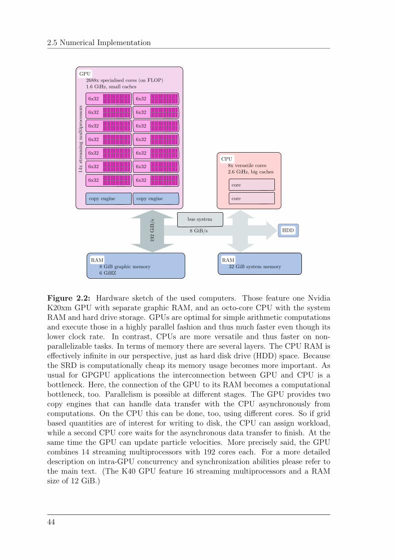
2.5 Numerical Implementation

CPU 8x versatile cores 2.6 GiHz, big caches

GPU 2688x specialised cores (on FLOP) 1.6 GiHz, small caches

6x32

copy engine copy engine

14x s

trea

min

g m

ult

ipro

cess

ors

6x32

6x32

6x32

6x32

6x32

6x32

6x32

6x32

6x32

6x32

6x32

6x32

6x32

bus system

RAM 8 GiB graphic memory 6 GiHZ

RAM 32 GiB system memory

core

core

192

GiB

/s

8 GiB/s HDD

Figure 2.2: Hardware sketch of the used computers. Those feature one NvidiaK20xm GPU with separate graphic RAM, and an octo-core CPU with the systemRAM and hard drive storage. GPUs are optimal for simple arithmetic computationsand execute those in a highly parallel fashion and thus much faster even though itslower clock rate. In contrast, CPUs are more versatile and thus faster on non-parallelizable tasks. In terms of memory there are several layers. The CPU RAM iseffectively infinite in our perspective, just as hard disk drive (HDD) space. Becausethe SRD is computationally cheap its memory usage becomes more important. Asusual for GPGPU applications the interconnection between GPU and CPU is abottleneck. Here, the connection of the GPU to its RAM becomes a computationalbottleneck, too. Parallelism is possible at different stages. The GPU provides twocopy engines that can handle data transfer with the CPU asynchronously fromcomputations. On the CPU this can be done, too, using different cores. So if gridbased quantities are of interest for writing to disk, the CPU can assign workload,while a second CPU core waits for the asynchronous data transfer to finish. At thesame time the GPU can update particle velocities. More precisely said, the GPUcombines 14 streaming multiprocessors with 192 cores each. For a more detaileddescription on intra-GPU concurrency and synchronization abilities please refer tothe main text. (The K40 GPU feature 16 streaming multiprocessors and a RAMsize of 12 GiB.)

44

2. Granular stochastic rotation dynamics

2.5.3 Algorithm summary

We use object oriented programming to benefit from high code re-usability an clarity.The procedure starts with interpreting an input file. (cf. Fig. 2.3(a)). Next, aninstance of the simulation box class is created (refer to next section). Then, stepsand writing data to disk functions are called following the simulation protocol of theinput file. A step combines many function calls, one of these are the step internal

function of the simulation box object which combines all CUDA kernel calls (Fig.2.3(b)).

The implementation of the SRD algorithm consists of the following steps

vni (t) = rξ(rξ · vi(t))

vti(t) = vi(t)− vn

i (t)

vi(t+∆t) = vni (t) + ϵξ,eff[cos(α)v

ti(t) + sin(α)(vt

i(t)× rξ)],

where rξ is the random rotation axis of cell ξ, analogous to the matrix multiplicationin Eq. (2.5).

2.5.4 Data structuring

We store physical quantities combined in a struct we call parameters. The mainfunction uses an object of the struct simulation to hold details of the protocol.The physical space is represented as a class simulation box instance. It has mem-bers holding particles’ positions, velocities, SRD grid based data, plus counters andbuffers. We bundle memory transfers between the different RAMs using the classmemory manager working on the data member of the async array objects.

For vector calculus we implement a struct vektor with member functions ded-icated to the certain operations. For the SRD local grid data there is a structsrd cell holding relevant structure. This approach has the advantage that addinga new parameter passed by the input file is really simple and non-error prone. Onecan just create a new member in the struct parameters while data copying and man-agement of the object remains the same. The same applies for the struct srd cell.Introducing the local effective coefficient of restitution was implemented by simplyadding a new member to the srd cell.

The data that we store in the GPU’s constant cache, as mentioned earlier, aremostly member pointers of the simulation box instance. For their variable namingwe simply add an underscore to the member name to which the pointer references.

45

2.5 Numerical Implementation

void main(...) (main.cpp) initialises, then repeatedly performs steps and sampling calls

auto interpret_input(...) (state.cpp)

reads input_file, checks directory, returns simulation struct

1. 2.

auto build_walls(...) (main.cpp)simulation_box instance • positions, velocities, fieldsconstructor sets up GPUmemory via init_gpu(...)3. creates with walls & params

4. steps

5. sampling

(a) Overview:

(b) Details of the step_internal member:

reduce to cell level locally sum up velocities and density with atomic operations

reduction procedure:1st. 14 independent multiprocessors

reduce to array[14] per srd_cell2nd. reduction inside cell

reduce in cells and prepare rotation generate cells' rotation vectors,

calculate streaming velocity

reduce thermal velocities to cell level

locking with mutexes

reduce thermal velocities in cells calculate effective coefficient of

restitution or thermostat scale

calculate global drift

copy to summation buffer, then sum up, norm result

calculate grid shift

rotate, translate, dissipate and shift

particle wise application of the SRD procedure: 1. remove streaming velocity, apply rotation

and apply dissipation rule

2. remove old grid-shift, apply forces perform collisions with walls 3. translate and apply new grid-shift

4. calculate pressure tensor components

star

t end

step_internal(...) & its calls details in panel (b)

4.5.

calculate fields for transfer to CPU calculate all quantities without grid shift

copy memory content (if this is sampling step)

Figure 2.3: Code flowchart divided into an overview in panel (a) and detailsof the step internal(...) member of the simulation box class in panel (b).Functions and workflow are represented by red cards and red arrows respec-tively. Parallel CUDA-GPU-functions are represented by purple cards. The cen-tral simulation box instance appears in green. All CUDA calls are performed inthe init gpu(...) and step internal(...) members. Besides the rotation-translation routine every CUDA-helper-function mostly performs only one task.Functions with a gray dot need synchronization. CPU and GPU compute timesare superimposed, also with data transfer. CUDA function calls are launched withindividual blocks and grid sizes regarding synchronization necessities of the respec-tive code segment. Thread numbers are chosen to fit processor number so thatfunctions perform loops over subsets of the workload.

46

2. Granular stochastic rotation dynamics

struct vektor (vektor.hpp)

• members:

double/float x,y,z

• member functions:

operators: +, +=, *, etc.

norm(), length(), dot_product(),

scaled_with(), periodic(), etc.

class random (random.hpp)

• members:

uint64_t s[] (state)

• member functions:

uniform_int( min, max), uniform_float(),

gaussian(), random_unit_vektor(), etc.

• implementations:

xoroshiro128+, xorshift1024*

struct simulation (state.hpp)

• description:

representation of the input file bundled

into parameters and procedual details.

• members:

class parameters object

equilibration -/sampling procedure details

struct parameters (data_structure.hpp)

• description:

holding all physically relevant parameters

• members:

dt, collision_angle, target_T, etc.

struct srd_cell (data_structure.hpp)

• description:

holding cell level observables e.g. mean

velocity also bundled for parallel access

and an independent random-number-generator

• members:

cell velocity, cell temperature, n, etc.

class simulation_box (simulation_box.hpp)

• description:

representation of the physical system holding all data

corresponding to it in private members.

Thus standalone, all simulation operations are performed

via public functions. Parallel CUDA calls, bundled in the

simulation_box.cu file (init_gpu(), step_internal()) rely

on helper functions in that file only.

The class members are copied into the constant GPU

memory and in GPU routines have an underscore in

the name hence e.g. particle[i] becomes particle_[i].

• members:

positions, velocities, fields, class parameters obj., etc.

non-gpu involving routines (simulation_box.cpp):

initialisation, file_io, write_config, step, etc.

gpu involving routines (simulation_box.cu):

init_gpu(), step_internal()

+ helper functions

struct particle (data_structure.hpp)

• members:

position r, velocity v

struct gpu_array (container_classes.hpp)

• description:

GPU memory space array, managed

by a memory_manager obj.

• members:

pointer to GPU memory,

operator [], data manipulation routines

struct async_array (container_classes.hpp)

• description:

double GPU and CPU memory arrays,

managed by a memory_manager obj.

• members:

pointers to both memory sections

operator [] for GPU/CPU seperate.

class memory_manager (managed_data.hpp)

• description:

copies between RAM/GPU-RAM

bundled into one operation (asynchonously)

• members:

managed object sizes, copy functions, etc.

void main(...) (main.cpp)

• description:

controls steps and sampling

Figure 2.4: Object structure and summarized object descriptions of the imple-mented program. Objects are denoted as green cards, membership usage betweenobjects is symbolized as blue arrows, strongly linked classes are connected withpurple arrows. Routines are presented as red cards, control flows as red arrows.Classes are grouped into physics representatives (on gray) and memory managingobjects (on pink). The center of the simulation is the simulation box class aroundwhich everything is built, the most basic and widely used instance is of the structvektor. After the main function requested a simulation details struct it generatesa simulation box instance and calls its public control functions. The class itselfhandles the details in dedicated private functions, including e.g. simulation stepswith GPU-addressing and data output.

47

2.5 Numerical Implementation

2.5.5 Random number generators

Artificial pseudo-random numbers are computer-generated numbers using certainalgorithms that together with the internal state of the generator are called randomnumber generator. Generating a random number alters the internal state of thegenerator according to the algorithm. Since the internal state has a binary memoryrepresentation, it is simple to recognize that this leads to a finite length sequence ofnumbers. Measures of the quality of a random number generator may be the lengthof the period of its sequence or how much subsets resemble uniform distribution ofvalues. It is commonly agreed that the SRD method does not need the statisticallybest random number generator since only few numbers are necessary. In contrast tothat, the MPCD method uses at least 3n random numbers per box with n particlesand collision steps and thus the quality of the generator is more critical.

For the present implementation we chose a rather new sort of generators of thexorshift family [22] in an exchangeable way to test them against each other. Onehas a significantly longer period, but the use of a shorter period does not changethe simulations.

For the implementation on GPUs we need to guarantee that the random numbersare independently generated. If different threads generate the rotation axes fordifferent SRD cells at the same time, this may cause problems. Instead of providingexclusive access to one common generator we provide independent generators foreach SRD cell so that no communication between threads is necessary. For theused xorshift generators so-called ’jump ahead’ functions are known, that alter thegenerators internal state equally to calling a certain high number of single randomnumber generation calls. This gives a number of independent sub-sequences thatare safe to call in parallel.

2.5.6 Controlling and using the code

The compiled code is fully flexible in the sense that all of its functions can beswitched on and off at runtime. For the appropriate settings, the code uses an inputfile to read all input parameters, which may be specified by the first input stringgiven to the executable. Hence, there are no pre-compiler definitions (hash-defines),instead consistent declaration of variables with the const flag is performed.

The code generates a logfile in ASCII to which it writes e.g. the temperatureor flux. Specific details are given in the simulation box::write log() functiondefinition. Structural data is written in binary at specified times.

48

Chapter 3

Results

3.1 Simulation parameters

We perform our simulation using dimensionless equations, where all quantities aregiven as multiples of the respective characteristic values of the system. Lengthsare multiples of the SRD lattice parameter a, mass as multiple of the (identical)SRD/GSRD particle mass m. The time unit is given via a reference thermal energy

tunit =a√

kBTref/m,

so that a particle moving with velocity v =√

kBTref/m at kBTref = 1 covers thelength a per unit of time. During the initialization of the system, particles arerandomly distributed in the system. The mean number of particles per cell n0 is animportant quantity since it controls for instance the viscosity of the fluid.

Other parameters that control the transport and relaxation processes are theSRD rotation angle α, and the mean collision time ∆t.

3.2 Code validation via streaming viscosity mea-

surements

Equations (1.48) and (1.49) give analytic predictions for the viscosities of the stan-dard SRD fluid in two and three dimensions [3], respectively, and show an excellentagreement with the results obtained from simulations. Hence, to test our newlydeveloped and implemented code we may also use this comparison to test, verifyand benchmark our implementation of the standard SRD model.

We simulate systems of sizes 32× 32 in 2D and 32× 32× 32 in 3D and initializeeach system with on average n0 = 5 particles per cell such that the system in totalcontains n0 particles times the number of cells, i.e. N = 5120 in 2D and N = 163840

49

3.2 Code validation via streaming viscosity measurements

in 3D. We apply a shear rate of γ∆t = 2/32 = 0.0625 at a reduced temperature ofT/Tref = 0.8 and ∆t = 1.

The particle velocities are initialized according to the Maxwell-Boltzmann distri-bution. The velocity profile relaxes to a linear profile induced by the shear quickly.For this reason we equilibrate the system for 10000 time steps. In the following50000 time steps we measure the flux of momentum every step and write the av-erage to disk every 100 time steps. Configurations are internally averaged on theGPU over 100 states each separated by 10 ∆t. During the simulation the densityfluctuates around n0 as can be seen in Fig. 3.1(a), just like we expect. The systemremains homogeneous during the whole simulated timespan. As we can see in Fig.3.1(b), a smooth velocity profile develops. Moreover, we can still see slight densityfluctuations which completely agree with our expectations. The SRD rotation angle

0 5 10 15 20 25 30

x/a

0

5

10

15

20

25

30

y/a

(a)

0 5 10 15 20 25 30

x/a

(b)

4.74

4.80

4.86

4.92

4.98

5.04

5.10

5.16

5.22

Nu

mb

erd

ensi

tynξ

−0.8−0.6−0.4−0.20.00.20.40.60.8

Str

eam

ing

velo

cityVξ,x

Figure 3.1: Snapshot of the sheared system averaged over 1000 states for a rotationangle α = 120. Panel (a) shows the density in the x/y plane. Since we look at anaverage, the density does not need to be in integer numbers. Still we see fluctuations,also in panel (b) that shows the cells’ streaming velocities Vξ,x in the direction alongwhich the system is sheared.

may be understood as representing an effective mean free path of the fluid, and inthat regard similar to the time between multi-particle collisions ∆t. This is becauseit controls how far a particle travels without significantly changing its direction. Italso controls how quickly the system locally relaxes to equilibrium. Because of thisinteresting feature we investigate the streaming viscosity as a function of the rota-tion angle α here. For the 2D system the streaming viscosity shown in Fig. 3.2(a)naturally diverges as α approaches 0 and because of the geometry also approaching180. At a rotation angle of 90 there is a global minimum because the parameterlimits for α are 0 and 180. The computed viscosity is in excellent agreement withthe theoretical prediction. We see that because there is a continuous heat produc-tion due to the shearing the system settles at higher temperature the higher theviscosity is, even though the thermostat constantly rescales the temperature.

For the 3D system the viscosity also diverges at α = 0 but not at α = 180

where instead we have a local maximum. The minimum now occurs at α ≈ 11π/18.

50

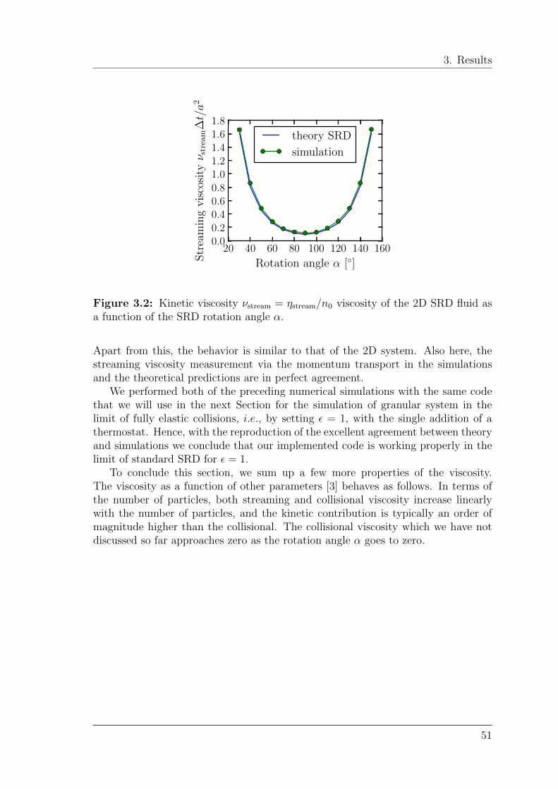
3. Results

20 40 60 80 100 120 140 160

Rotation angle α []

0.00.20.40.60.81.01.21.41.61.8

Str

eam

ing

vis

cosi

tyν s

trea

m∆t/a

2

theory SRD

simulation

Figure 3.2: Kinetic viscosity νstream = ηstream/n0 viscosity of the 2D SRD fluid asa function of the SRD rotation angle α.

Apart from this, the behavior is similar to that of the 2D system. Also here, thestreaming viscosity measurement via the momentum transport in the simulationsand the theoretical predictions are in perfect agreement.

We performed both of the preceding numerical simulations with the same codethat we will use in the next Section for the simulation of granular system in thelimit of fully elastic collisions, i.e., by setting ϵ = 1, with the single addition of athermostat. Hence, with the reproduction of the excellent agreement between theoryand simulations we conclude that our implemented code is working properly in thelimit of standard SRD for ϵ = 1.

To conclude this section, we sum up a few more properties of the viscosity.The viscosity as a function of other parameters [3] behaves as follows. In terms ofthe number of particles, both streaming and collisional viscosity increase linearlywith the number of particles, and the kinetic contribution is typically an order ofmagnitude higher than the collisional. The collisional viscosity which we have notdiscussed so far approaches zero as the rotation angle α goes to zero.

51

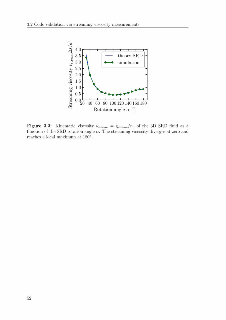
3.2 Code validation via streaming viscosity measurements

20 40 60 80 100 120 140 160 180

Rotation angle α []

0.0

0.5

1.0

1.5

2.0

2.5

3.0

3.5

4.0

Str

eam

ing

vis

cosi

tyν s

trea

m∆t/a

2

theory SRD

simulation

Figure 3.3: Kinematic viscosity νstream = ηstream/n0 of the 3D SRD fluid as afunction of the SRD rotation angle α. The streaming viscosity diverges at zero andreaches a local maximum at 180.

52

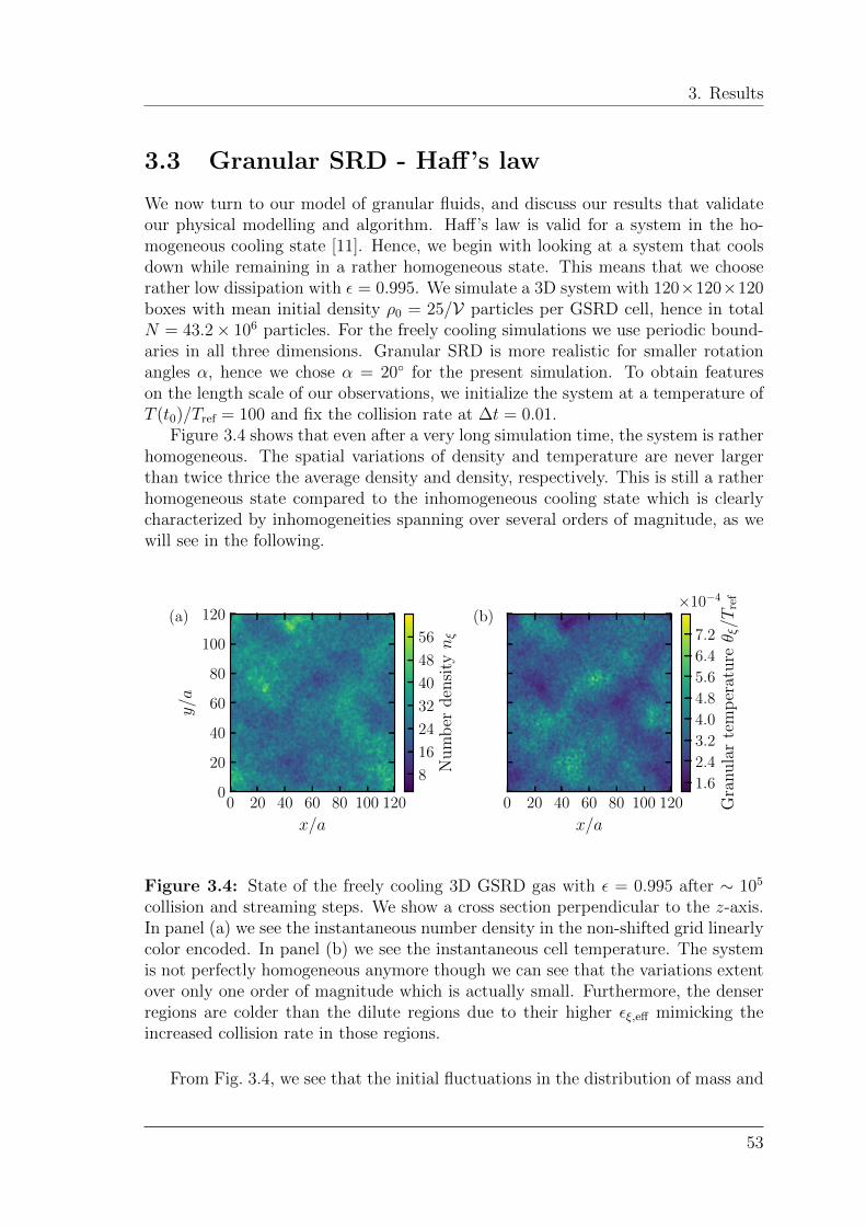
3. Results

3.3 Granular SRD - Haff’s law

We now turn to our model of granular fluids, and discuss our results that validateour physical modelling and algorithm. Haff’s law is valid for a system in the ho-mogeneous cooling state [11]. Hence, we begin with looking at a system that coolsdown while remaining in a rather homogeneous state. This means that we chooserather low dissipation with ϵ = 0.995. We simulate a 3D system with 120×120×120boxes with mean initial density ρ0 = 25/V particles per GSRD cell, hence in totalN = 43.2× 106 particles. For the freely cooling simulations we use periodic bound-aries in all three dimensions. Granular SRD is more realistic for smaller rotationangles α, hence we chose α = 20 for the present simulation. To obtain featureson the length scale of our observations, we initialize the system at a temperature ofT (t0)/Tref = 100 and fix the collision rate at ∆t = 0.01.

Figure 3.4 shows that even after a very long simulation time, the system is ratherhomogeneous. The spatial variations of density and temperature are never largerthan twice thrice the average density and density, respectively. This is still a ratherhomogeneous state compared to the inhomogeneous cooling state which is clearlycharacterized by inhomogeneities spanning over several orders of magnitude, as wewill see in the following.

0 20 40 60 80 100 120

x/a

0

20

40

60

80

100

120

y/a

(a)

0 20 40 60 80 100 120

x/a

×10−4

(b)

8

16

24

32

40

48

56

Nu

mb

erd

ensi

tynξ

1.6

2.4

3.2

4.0

4.8

5.6

6.4

7.2

Gra

nu

lar

tem

per

atu

reθ ξ/T

ref

Figure 3.4: State of the freely cooling 3D GSRD gas with ϵ = 0.995 after ∼ 105

collision and streaming steps. We show a cross section perpendicular to the z-axis.In panel (a) we see the instantaneous number density in the non-shifted grid linearlycolor encoded. In panel (b) we see the instantaneous cell temperature. The systemis not perfectly homogeneous anymore though we can see that the variations extentover only one order of magnitude which is actually small. Furthermore, the denserregions are colder than the dilute regions due to their higher ϵξ,eff mimicking theincreased collision rate in those regions.

From Fig. 3.4, we see that the initial fluctuations in the distribution of mass and

53

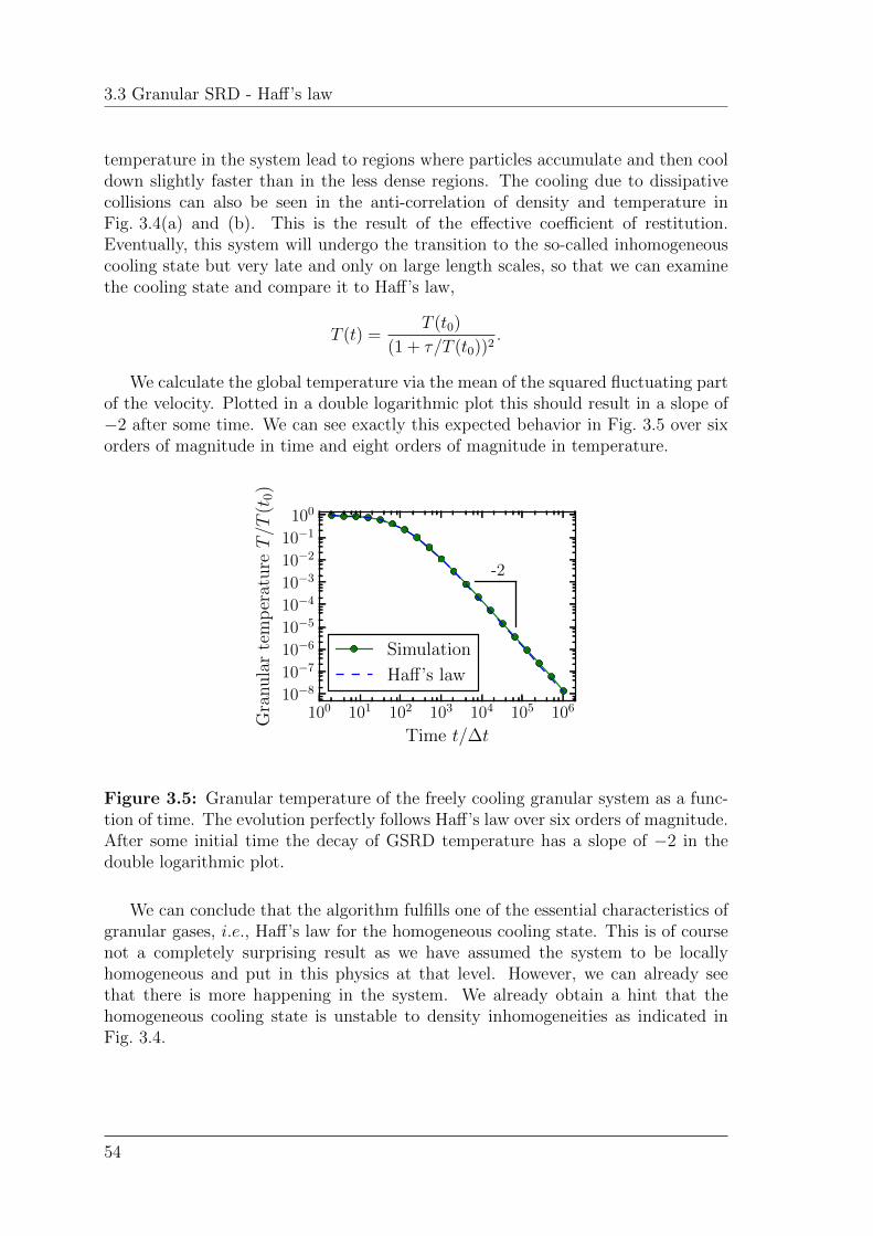
3.3 Granular SRD - Haff’s law

temperature in the system lead to regions where particles accumulate and then cooldown slightly faster than in the less dense regions. The cooling due to dissipativecollisions can also be seen in the anti-correlation of density and temperature inFig. 3.4(a) and (b). This is the result of the effective coefficient of restitution.Eventually, this system will undergo the transition to the so-called inhomogeneouscooling state but very late and only on large length scales, so that we can examinethe cooling state and compare it to Haff’s law,

T (t) =T (t0)

(1 + τ/T (t0))2.

We calculate the global temperature via the mean of the squared fluctuating partof the velocity. Plotted in a double logarithmic plot this should result in a slope of−2 after some time. We can see exactly this expected behavior in Fig. 3.5 over sixorders of magnitude in time and eight orders of magnitude in temperature.

100 101 102 103 104 105 106

Time t/∆t

10−8

10−7

10−6

10−5

10−4

10−3

10−2

10−1

100

Gra

nu

lar

tem

per

atu

reT/T

(t0)

-2

Simulation

Haff’s law

Figure 3.5: Granular temperature of the freely cooling granular system as a func-tion of time. The evolution perfectly follows Haff’s law over six orders of magnitude.After some initial time the decay of GSRD temperature has a slope of −2 in thedouble logarithmic plot.

We can conclude that the algorithm fulfills one of the essential characteristics ofgranular gases, i.e., Haff’s law for the homogeneous cooling state. This is of coursenot a completely surprising result as we have assumed the system to be locallyhomogeneous and put in this physics at that level. However, we can already seethat there is more happening in the system. We already obtain a hint that thehomogeneous cooling state is unstable to density inhomogeneities as indicated inFig. 3.4.

54

3. Results

3.4 GSRD streaming viscosity

We test the expressions in Eq. (3.1) for the GSRD kinematic viscosity with shearsimulations, similarly to what we did in Sect. 3.2 for standard SRD. Since the fluiddissipates energy it reaches a stationary state were all the heat induced by theshearing is at the same time dissipated. For this reason, no thermostat is necessaryin the simulations. Here, we simulate 2D 32×32-cell systems with density ρ0 = 10/Vand ρ0 = 20/V . Again we set ∆t = tunit. As predicted by Eq. (3.1), similarly tostandard SRD, the viscosity is low for rotation angles close to α = 90 Hence for theseparameters the heat production is really low and the system becomes more and moreunstable to exhibiting shear banding. For this reason, we need to increase the shearrate together with the rotation angle to keep the system in a stable state. However,if initially the system is completely at rest, it does not relax to the stationary shearedstate. In this case the cooling immediately leads to a contraction and the contactto the Lees-Edwards boundaries is disrupted. To help the system reach the desiredstate, we initialize it with a linear velocity profile along the z-axis and a temperatureclose to the assumed final equilibrium temperature.

20 25 30 35 40 45 50

Rotation angle α []

02468

1012141618

Str

eam

ing

vis

cosi

tyν s

trea

m∆t/a

2

(a) Simulation

Theory GSRD

Theory SRD

20 25 30 35 40 45 50

Rotation angle α []

0.00

0.02

0.04

0.06

0.08

0.10

0.12

Rel

ativ

ed

evia

tion

δνst

ream(b)

Figure 3.6: Kinematic viscosity of the 2D GSRD fluid with ρ0 = 10/V . In the leftpanel (a) we see the kinematic viscosity νkin = µkin/ρ0 as a function of the GSRDrotation angle α. In the right panel (b) we see the relative deviation from the theoryfor granular fluids, and from the standard theory, for comparison. We see a goodagreement with the theory with a maximum deviation of 4%, which represents agood improvement from the standard theory. The effective coefficient of restitutionis not constant due to the different equilibrium temperatures resulting from differentshear rates. Overall, the values lie around ϵξ,eff = 0.998. The reason for the worseagreement at high α is the instability of the homogeneous state. For increasing αthe shear heating becomes less important, so that for angles slightly larger than 40

the system needs a high shear rate to remain stationary. This in turn contradictsour assumptions for the derivation of Eq. (3.1).

55

3.4 GSRD streaming viscosity

If the heat input via the Lees-Edwards boundary is too low, the system formsone, sometimes also more, condensation bands. These cool down much more quicklythan the rest of the system, and contract more and more. Thereby in those regionsthe momentum transport is disrupted and the cooling dominates. This makes shearmeasurements in this parameter region unfeasible. With mean effective coefficientof restitution ϵξ,eff = 0.946 and α = 20 the system quickly reaches a state as shownin Fig. 3.8, where we see a band with 4 times larger density and with a temperaturean order of magnitude lower than the rest of the system.

Hence, all in all, there are two effects that complicate the shear measurement. Forlarger α, the system is sheared increasingly fast so that our theory loses its validity.On the other end, for small α, the higher temperature also results in a higherϵξ,eff which makes the assumption of the velocities of particles being uncorrelatedquestionable. Also with this condition local mixing and relaxation becomes slower.

In panels (b) of Fig. 3.6 and 3.7 we show the relative deviation

δνstream =νstream,measured − νkin,theory

νstream,theory

of the measurements to the theoretic predictions of Eq. (3.1) and for comparisonalso to Eq. (1.48).

20 25 30 35 40 45 50

Rotation angle α []

0

2

4

6

8

10

12

14

16

Str

eam

ing

vis

cosi

tyν s

trea

m∆t/a

2

(a) Simulation

Theory GSRD

Theory SRD

20 25 30 35 40 45 50

Rotation angle α []

0.00

0.02

0.04

0.06

0.08

0.10

0.12

0.14

0.16

Rel

ativ

ed

evia

tion

δνst

ream(b)

Figure 3.7: Kinematic viscosity of the 2D SRD fluid for a mean density of ρ0 =20/V . In the left panel (a) we see the kinematic viscosity νkin = µkin/ρ0 as a functionof the SRD rotation angle α. In the right panel (b) we see the relative deviationfrom the granular theory and the standard theory, for comparison. Also here, wesee a good agreement with at maximum 9% error. We attribute the deviation atthe small rotation angle α to the resulting slower mixing and higher temperaturewe obtain in these simulations. In the same range of α < 27.5 also the standardtheory exhibits an increasing deviation. The standard theory’s deviation from thecomputed values also increases linearly with decreasing α as we have seen in Fig.3.6(b).

56

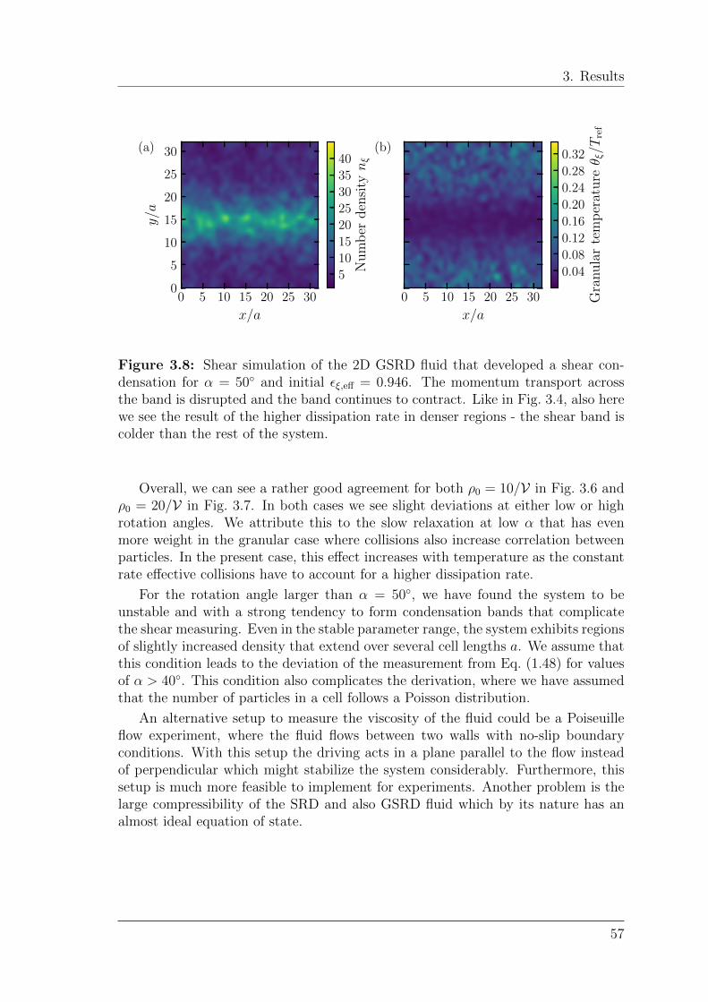
3. Results

0 5 10 15 20 25 30

x/a

0

5

10

15

20

25

30y/a

(a)

0 5 10 15 20 25 30

x/a

(b)

5

10

15

20

25

30

35

40

Nu

mb

erd

ensi

tynξ

0.04

0.08

0.12

0.16

0.20

0.24

0.28

0.32

Gra

nu

lar

tem

per

atu

reθ ξ/T

ref

Figure 3.8: Shear simulation of the 2D GSRD fluid that developed a shear con-densation for α = 50 and initial ϵξ,eff = 0.946. The momentum transport acrossthe band is disrupted and the band continues to contract. Like in Fig. 3.4, also herewe see the result of the higher dissipation rate in denser regions - the shear band iscolder than the rest of the system.

Overall, we can see a rather good agreement for both ρ0 = 10/V in Fig. 3.6 andρ0 = 20/V in Fig. 3.7. In both cases we see slight deviations at either low or highrotation angles. We attribute this to the slow relaxation at low α that has evenmore weight in the granular case where collisions also increase correlation betweenparticles. In the present case, this effect increases with temperature as the constantrate effective collisions have to account for a higher dissipation rate.

For the rotation angle larger than α = 50, we have found the system to beunstable and with a strong tendency to form condensation bands that complicatethe shear measuring. Even in the stable parameter range, the system exhibits regionsof slightly increased density that extend over several cell lengths a. We assume thatthis condition leads to the deviation of the measurement from Eq. (1.48) for valuesof α > 40. This condition also complicates the derivation, where we have assumedthat the number of particles in a cell follows a Poisson distribution.

An alternative setup to measure the viscosity of the fluid could be a Poiseuilleflow experiment, where the fluid flows between two walls with no-slip boundaryconditions. With this setup the driving acts in a plane parallel to the flow insteadof perpendicular which might stabilize the system considerably. Furthermore, thissetup is much more feasible to implement for experiments. Another problem is thelarge compressibility of the SRD and also GSRD fluid which by its nature has analmost ideal equation of state.

57

3.5 Inhomogeneous cooling state

3.5 Inhomogeneous cooling state

3.5.1 Clustering

In this section we want to investigate the dynamical features of granular clusters.For large coefficient of restitution, e.g. ϵ = 0.995 the freely-cooling granular gas inthe homogeneous cooling state exhibited indications of growing clusters. In orderto obtain well-developed clustering we reduce the coefficient of restitution as a firststep. To obtain clusters at the length scale of our observation it is further necessaryto further reduce the rotation angle to α = 10. This corresponds to a more dilutegas in which particles travel in the same direction longer without colliding, but mostimportantly it assures that the kinetic contribution to momentum diffusion remainsdominant as the system cools down (see Discussion).

0

20

40

60

80

100

120

y/a

(a) t ≈ 103∆t (b) t ≈ 104∆t

0 20 40 60 80 100 120

x/a

0

20

40

60

80

100

120

y/a

(c) t ≈ 105∆t

0 20 40 60 80 100 120

x/a

(d) t ≈ ×106∆t

101

Nu

mb

erd

ensi

tynξ

101

102

Nu

mb

erd

ensi

tynξ

101

102

Nu

mb

erd

ensi

tynξ

101

102

Nu

mb

erd

ensi

tynξ

Figure 3.9: Density profile of the freely cooling GSRD system for ϵ = 0.98, withinitially T (t0) = 100 Tref and ∆t = 0.01. Panel (a) shows the system close to thetransition to the inhomogeneous cooling state. Panel (b): at t = 104∆t the systemhas developed clusters, the density varies over 3 orders of magnitude. These clusterscontinue to grow in size, as can be seen in panels (c) and (b) and also continue tocontract.

In the following we investigate a system of 1203 cells with a initial density ofρ0 = 25/V , hence N = 43.2 × 106 particles. Also here, we simulate using periodic

58

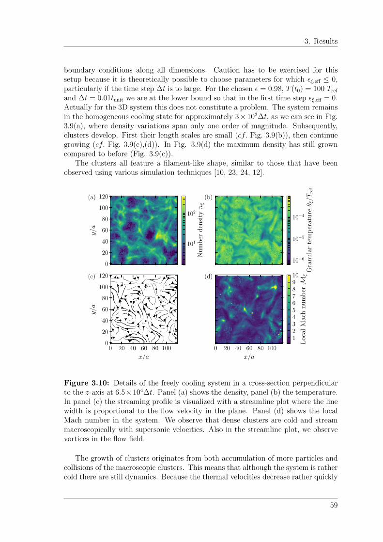
3. Results

boundary conditions along all dimensions. Caution has to be exercised for thissetup because it is theoretically possible to choose parameters for which ϵξ,eff ≤ 0,particularly if the time step ∆t is to large. For the chosen ϵ = 0.98, T (t0) = 100 Tref

and ∆t = 0.01tunit we are at the lower bound so that in the first time step ϵξ,eff = 0.Actually for the 3D system this does not constitute a problem. The system remainsin the homogeneous cooling state for approximately 3×103∆t, as we can see in Fig.3.9(a), where density variations span only one order of magnitude. Subsequently,clusters develop. First their length scales are small (cf. Fig. 3.9(b)), then continuegrowing (cf. Fig. 3.9(c),(d)). In Fig. 3.9(d) the maximum density has still growncompared to before (Fig. 3.9(c)).

The clusters all feature a filament-like shape, similar to those that have beenobserved using various simulation techniques [10, 23, 24, 12].

0

20

40

60

80

100

120

y/a

(a) (b)

0 20 40 60 80 100

x/a

0

20

40

60

80

100

120

y/a

(c)

0 20 40 60 80 100

x/a

(d)

101

102

Nu

mb

erd

ensi

tynξ

10−6

10−5

10−4

Gra

nu

lar

tem

per

atu

reθ ξ/T

ref

12345678910

Loca

lM

ach

nu

mb

erM

ξ

Figure 3.10: Details of the freely cooling system in a cross-section perpendicularto the z-axis at 6.5×104∆t. Panel (a) shows the density, panel (b) the temperature.In panel (c) the streaming profile is visualized with a streamline plot where the linewidth is proportional to the flow velocity in the plane. Panel (d) shows the localMach number in the system. We observe that dense clusters are cold and streammacroscopically with supersonic velocities. Also in the streamline plot, we observevortices in the flow field.

The growth of clusters originates from both accumulation of more particles andcollisions of the macroscopic clusters. This means that although the system is rathercold there are still dynamics. Because the thermal velocities decrease rather quickly

59

3.5 Inhomogeneous cooling state

in time, while the convective velocities decrease to a lesser extent, the granular gasflow becomes quickly supersonic. A measure of this dynamical feature is given by theMach number M = ∥v∥/vT . These supersonic flows can be seen in the map of thelocal Mach number shown in Fig. 3.10(d). Additionally, we show a streamline plotin Fig. 3.10(c) and local temperatures in Fig. 3.10(b). Their combination showsthat the higher cooling rates in the dense regions lead to bonding of particles tothe cluster due to the lower temperature and hence escape velocity. In this statethe clusters behave as macroscopic objects themselves because they stream withvelocities faster than their internal dynamics, as can be read from the local Machnumbers Mξ > 1.

The process of clusters growing continues until clusters have reached the size ofthe system and then saturates. For bigger system sizes this process of course takeslonger to finish. The evidence for this fact comes from smaller simulations where wehave observed this outcome after ∼ 106∆t. When the saturation sets in, the coolingfollows a power law T ∼ (1 + t)−2 again, similar to Haff’s law. This is because onceclusters have formed, cooling occurs inside them on small scales again, over whichthe system is homogeneous.

In simulations with a slightly lower coefficient of restitution of ϵ = 0.975 weobserve the transition to inhomogeneous cooling slightly earlier at ∼ 103∆t. Thissimulation was performed with a 2003 grid, a 3D rendered snapshot after ∼ 104∆tcan be seen in Fig. 3.11. These observations completely agree with findings obtainedwith an event driven simulation of Luding [23].

(a) (b)

Figure 3.11: 3D density configuration of the GSRD system at (a) t = 2 × 103∆tand (b) t = 104∆t. The figures are obtained with ray-tracing. The light permittivityof each GSRD cell proportional to its density. Hence, the middle along the diagonalappears darker due to the longer light paths. We can see denser clusters that havefilament-like shapes that extend in all directions with no preferred direction.

60

3. Results

3.5.2 Cluster growth

In the previous section we have looked at the cluster formation dynamics on macro-scopic length scale and have thereby observed that the density, velocity and temper-ature become inhomogeneous with a rather quick transition. The moment when thistransition occurs can be better identified via the standard deviation of the densitydistribution, that gives a measure of the fluctuations in the density. The time evo-lution of the fluctuation (cf. Fig. 3.12(b)) normalized with the initial value showsa pronounced change from almost constant to a linear growth after approximately3 × 103∆t. The standard deviation increases to around 7 times the initial value.Coinciding with that, we see that the mean kinetic energy of the system, which foridentical particles is defined as

Ekin ≡ 1

N

∑ξ

nξVξ (3.1)

crosses the curve of the temperature in Fig. 3.12(a) at about 3× 103∆t.

10−910−810−710−610−510−410−310−210−1

100

(a)

Ekin/kBT (t0)

T/T (t0)

Haff’s law

100 101 102 103 104 105 106

Time t/∆t

0

2

4

6

8

Den

sity

flu

ctu

atio

ns

〈(δρξ)2〉/〈[δρξ(t

0)]

2〉

(b)

×101

Figure 3.12: Cooling behavior of the GSRD fluid for ϵ = 0.98. Panel (a) showsthe development of the mean kinetic energy of the convective degrees of freedomand granular temperature as a function of time with a fit of Haff’s law. We seerather good agreement up to t < 3 × 103∆t where the curve of Ekin and T crossand hence the global Mach number M exceeds one. The temperature follows adifferent power law afterwards. Panel (b) shows the development of the standarddeviation of the density distribution σ(ρ) relative to t = 0. The fluctuations σ(ρ)only slowly increase until t ≃ 3×103∆t when the behavior changes. In the following,the fluctuations increase quickly hence indicating a transition to the inhomogeneouscooling state, coinciding with the change of slope in the cooling behavior and Machnumber M > 1.

61

3.5 Inhomogeneous cooling state

Figure 3.13 shows a close-up view of the temporal dependence of the temperature.One can observe that with insetting saturation there appears another change ofslope. The global cooling thereby increases. In the middle of the clustering regimethe slope of the power law becomes T (t) ∼ t1.55, then slowly returning to T (t) ∼t1.62. The change of slope during the inhomogeneous cooling state has also been

103 104 105 106

Time t/∆t

10−9

10−8

10−7

10−6

10−5

10−4

10−3

Gra

nu

lar

tem

per

atu

reT/T

(t0)

Haff’s Law

Simulation

Power law

103 106

10−1

10−3

10−5

Figure 3.13: Detailed cooling behavior of the GSRD fluid for ϵ = 0.98 in theinhomogeneous cooling state. We show the development of the granular temperatureas a function of t > 3× 103∆t, i.e., the region indicated in the inset. In this regionthe cooling behavior changes to a power law T (t) ∼ t1.55. With the saturation ofthe clusters the slope begins to approach -2 again.

observed in previous works [23, 24, 25, 26]. Saturation processes also agree withtheir observations. Different predictions for the exponent of the new power lawT (t) ∼ tb have been proposed. Brito and Ernst [25] predicted and observed adependence of T (t) ∼ t−3/2 in three dimension which comes close to what we findhere.

Likewise, in the simulations in [25], which are performed using event drivenmolecular dynamics simulations, a change back to Haff’s law is observed after thesaturation of clusters, in agreement with what we find.

62

3. Results

3.6 Velocity distribution function

The velocity distribution function for nonequilibrium granular gases deviates fromthe Maxwell-Boltzmann distribution [10]. In particular it decays slower, or in otherwords, has a longer tail at larger velocities.

We can determine the velocity distribution function also for the GSRD particles.It is convenient to express the distribution as a function of the scaled velocities

c ≡ v

∥vT∥, (3.2)

where the thermal velocity is given by T = m/2v2T . The scaled velocities are

distributed following a scaled distribution function

f(v, t) =ρ

∥vT (t)∥3f(c). (3.3)

It is convenient to write f(c) as an expansion

f(v, t) = ϕ(c)

[1 +

∞∑p=1

ap(t)Sp(c2)

], (3.4)

where the first term ϕ(c) ≡ π−3/2 exp(−c2) is the Maxwell distribution for the scaledvelocity. The following terms give corrections to the equilibrium Maxwell distribu-tion. A suitable set of orthogonal functions Sp(x) are the Sonine polynomials(closely related to the Laguerre polynomials) with corresponding coefficients ap Forthe granular velocity distribution function, it is sufficient to consider the first threeorders

S0(x) = 1,

S1(x) = − x+3

2,

S2(x) =x2

2− 5x

2+

15

8.

A plot of the GSRD particles’ velocity distribution is presented in Fig. 3.14. Weobserve a good agreement with observations from molecular dynamics simulationsperformed by Pathak et al. [26]. The second Sonine coefficient is of major importancein theories for the velocity distribution function in granular gases [2].

We observe that the second Sonine coefficient is not constant, but changes withtime. In more detail, we report a decrease of a2 over the first time period up tot = 5 × 102∆t, which is followed by an approach of a2 back towards zero. We cansee in Fig. 3.15 that for higher values of ϵ the curves have a lower minimum aroundt = 5× 102∆t.

These findings are qualitatively in good agreements with the analytical predic-tions and observations by Brilliantov and Poschel [2] for a variable coefficient ofrestitution.

63

3.6 Velocity distribution function

0 1 2 3 4 5 6

Scaled velocity c

10−5

10−4

10−3

10−2

10−1

100f

(c)

t = 6× 104∆t

Maxwell-Boltzmann

Sonine expansion

Figure 3.14: Scaled velocity distribution function f of the 3D SRD fluid. Thedistribution has a stronger tail than the Maxwell-Boltzmann distribution.

101 102 103 104

Time t/∆t

−10

−8

−6

−4

−2

0

2

a2×

103

εeff(t0) = 0.987

εeff(t0) = 0.975

εeff(t0) = 0.96

εeff(t0) = 0.935

Figure 3.15: Second Sonine coefficient as a function of time for four differentcoefficients of restitution. First, there is a decrease followed by an approach backtowards zero. Minima are lower for higher ϵξ,eff(t0). At around t = 4 × 103∆t thesystems for the ϵξ,eff = 0.935, 0.96 come close to the transition to the inhomogeneouscooling state where we see an unexpected positive value of a2. The development ofa2 well agrees with analytical predictions of Brilliantov and Poschel [2] for a variablecoefficient of restitution.

64

Chapter 4

Discussion

4.1 Coarse-graining via the mean collision time

By applying the SRD and GSRD algorithms we drastically coarse-grain the meancollision time to one single constant, i.e., the time step ∆t. This approximation iswell justified in homogeneous systems with small gradients and spatial variations.

As we have seen in this work and is also observed elsewhere, the freely coolinggranular gas develops spatial variations of the observables that range over severalorders of magnitude. Nevertheless, the global ∆t remains the same. It is hence nota priori clear if this is a good approximation. Clearly the time step ∆t controls howfinely the dissipation is resolved in space, and thus the cluster formation.

The system’s development of temperature and kinetic energy is well character-ized by the global Mach number M = v/

√T . Thus, observing the change in the

global Mach number in Fig. 4.1, we use the fluctuations in density as a measurefor clustering using different ∆t. Ironically, as the time step is too small, i.e. for∆t

√T (t0) < a/2 the intrinsic collisional transport phenomena of GSRD leads to

unphysical appearance of clusters for M < 1. If, however, ∆t√T (t0) > a/2 the

cluster dynamics does not depend on the choice of ∆t. Thus, we can conclude thatusing a global ∆t is a valid approximation and take ∆t

√T (t0) > a/2 as a condition

for choosing the input parameters ∆t and T (t0). On other end, the condition thatϵξ,eff > 0 for ∆t determines an upper bound for ∆t.

4.2 Finite size effects

We consider a freely cooling GSRD system with ϵ = 0.98 as in the previous Section.If we simulate a smaller system using only 303 cells, the cluster growth saturateswithin 106 time steps. If this occurs, we see a new interesting behavior. In Fig. 4.2 wesee the development of the mean kinetic energy of the convective degrees of freedom

65

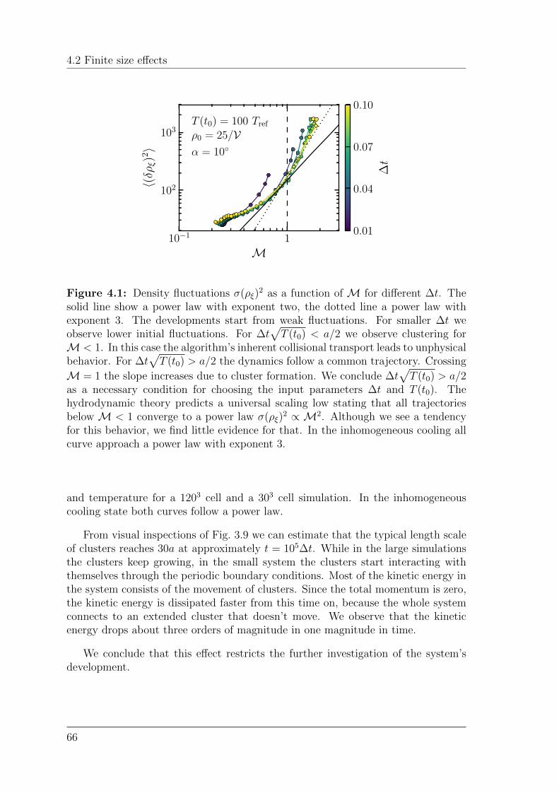
4.2 Finite size effects

10−1 1

M

102

103

〈(δρξ)2〉

T (t0) = 100 Tref

ρ0 = 25/Vα = 10

0.10

0.07

0.04

0.01

∆t

Figure 4.1: Density fluctuations σ(ρξ)2 as a function of M for different ∆t. The

solid line show a power law with exponent two, the dotted line a power law withexponent 3. The developments start from weak fluctuations. For smaller ∆t weobserve lower initial fluctuations. For ∆t

√T (t0) < a/2 we observe clustering for

M < 1. In this case the algorithm’s inherent collisional transport leads to unphysicalbehavior. For ∆t

√T (t0) > a/2 the dynamics follow a common trajectory. Crossing

M = 1 the slope increases due to cluster formation. We conclude ∆t√

T (t0) > a/2as a necessary condition for choosing the input parameters ∆t and T (t0). Thehydrodynamic theory predicts a universal scaling low stating that all trajectoriesbelow M < 1 converge to a power law σ(ρξ)

2 ∝ M2. Although we see a tendencyfor this behavior, we find little evidence for that. In the inhomogeneous cooling allcurve approach a power law with exponent 3.

and temperature for a 1203 cell and a 303 cell simulation. In the inhomogeneouscooling state both curves follow a power law.

From visual inspections of Fig. 3.9 we can estimate that the typical length scaleof clusters reaches 30a at approximately t = 105∆t. While in the large simulationsthe clusters keep growing, in the small system the clusters start interacting withthemselves through the periodic boundary conditions. Most of the kinetic energy inthe system consists of the movement of clusters. Since the total momentum is zero,the kinetic energy is dissipated faster from this time on, because the whole systemconnects to an extended cluster that doesn’t move. We observe that the kineticenergy drops about three orders of magnitude in one magnitude in time.

We conclude that this effect restricts the further investigation of the system’sdevelopment.

66

4. Discussion

100 101 102 103 104 105 106

Time t/∆t

10−1010−910−810−710−610−510−410−310−210−1

100

V = 1203a3(a)

T/T (t0)

Ekin/kBT (t0)

100 101 102 103 104 105 106

Time t/∆t

V = 303a3(b)

Figure 4.2: Granular temperature and mean kinetic energy of the freely coolingGSRD system with ϵ = 0.98 in (a) a large system size of 1203 cells and (b) a smallsystem size of 303 cells. In both systems the kinetic energy decreases with a powerlaw slower than the temperature. At approximately t = 105∆t the cluster lengthscale reaches 30a, the linear size of the smaller system (b). This system contractsto one big cluster that does not move due to momentum conservation. We observethis process by a sudden drop of kinetic energy in (b) of 3 orders of magnitude inone decade of time.

4.3 Rotation angle and inhomogeneous cooling

The SRD rotation angle α also plays a role in the cluster formation. From the calcu-lation of the viscosity we can conclude that shear heating increases as α decreases.Furthermore, α controls how far a particle travels in a certain direction withoutbeing significantly deflected.

We find that in the homogeneous cooling state the power law of the kinetic energyof the convective motion changes with α. For higher α the mean kinetic energy inthe system decreases with a power law Ekin ∝ t−τ with a higher exponent τ .

For granular gases, the kinetic energy curve has to cross the temperature curve,i.e. it has to become supersonic in order to exhibit clustering. From observations innature, theory or models as molecular dynamics simulations we know that clusteringis an essential feature of granular gases. For this reason one has to choose α ≤ 11.The curves of the higher rotation angles in Fig. 4.3(a), (b) and (c) show a decrease ofkinetic energy similar to that we have seen in Fig. 4.2(b) in the context of finite sizeeffects. Though now the phenomenon appears for systems in the subsonic state. Thereason is similar to that in Section 4.2. The collisional viscosity increases with α butis independent of the temperature [3]. However, for α → 0 the collisional viscosityvanishes. Hence, for α too large, as the system cools down GSRD collisions becomedominant at some point of the evolution. This leads to momentum diffusion overthe cell length a, thus propagating much faster than streaming.

67

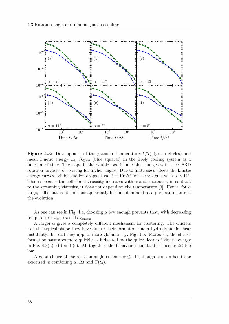
4.3 Rotation angle and inhomogeneous cooling

10−6

10−3

100

(a)

α = 25

(b)

α = 15

(c)

α = 13

102 104

Time t/∆t

10−6

10−3

100

(d)

α = 11

102 104

Time t/∆t

(e)

α = 7

102 104

Time t/∆t

(f)

α = 5

Figure 4.3: Development of the granular temperature T/T0 (green circles) andmean kinetic energy Ekin/kBT0 (blue squares) in the freely cooling system as afunction of time. The slope in the double logarithmic plot changes with the GSRDrotation angle α, decreasing for higher angles. Due to finite sizes effects the kineticenergy curves exhibit sudden drops at ca. t ≃ 104∆t for the systems with α > 11.This is because the collisional viscosity increases with α and, moreover, in contrastto the streaming viscosity, it does not depend on the temperature [3]. Hence, for αlarge, collisional contributions apparently become dominant at a premature state ofthe evolution.

As one can see in Fig. 4.4, choosing α low enough prevents that, with decreasingtemperature, νcoll exceeds νstream.

A larger α gives a completely different mechanism for clustering. The clusterslose the typical shape they have due to their formation under hydrodynamic shearinstability. Instead they appear more globular, cf. Fig. 4.5. Moreover, the clusterformation saturates more quickly as indicated by the quick decay of kinetic energyin Fig. 4.3(a), (b) and (c). All together, the behavior is similar to choosing ∆t toolow.

A good choice of the rotation angle is hence α ≤ 11, though caution has to beexercised in combining α, ∆t and T (t0).

68

4. Discussion

20 40 60 80 100 120 140 160 180

Rotation angle α []

0.0

0.2

0.4

0.6

0.8

1.0

1.2

ν∆t/a

2streaming viscosity

collisional viscosity

0.10.20.30.40.50.60.70.80.91.0

Tem

per

atu

reT/T

ref

Figure 4.4: Change of streaming viscosity with temperature compared to thecollisional viscosity of standard SRD [3]. For larger α eventually the collisionalviscosity becomes dominant as the temperature decreases. This also applies for thegranular system because qualitatively the curves do not change. In this graph wepresent the analytical functions for ρ0 = 5 and ∆t = 1.

0 20 40 60 80 100 120

x/a

0

20

40

60

80

100

120

y/a

(a)

0 20 40 60 80 100 120

x/a

(b)

101

102

Nu

mb

erd

ensi

tynξ

10−5

10−4

Gra

nu

lar

tem

per

atu

reθ ξ/T

ref

Figure 4.5: Clustering of the 3D GSRD system if collisional viscosity becomesdominant. In the cross sections (a) of the number density and (b) temperature wealso observe an anti-correlation. The clusters develop in lumpy shapes because thesystem does not become supersonic.

69

70

Chapter 5

Outlook

5.1 Driving by shaking

Driven granular systems are intensively studied because they can reach a steadystate and are thus easily controllable and observable. A common experimental setupconsists of a granular system under the influence of gravity that is driven by a shakerattached to the system’s container. The system undergoes periodic oscillations alongthe z-axis cf. Fig. 5.1. These increase the kinetic energy of particles colliding withthe ground.

We have carried out preliminary simulations of a vibrated granular system. Weimplement this by first adding a gravity force F/m = −gz that we apply on particlesusing Euler integration with a time step ∆t. While in the x and y dimension weapply periodic boundary conditions, along the z-axis we confine the system betweensolid walls using the bounce-back rule. The lower wall at z = 0 conducts periodicoscillations which serves as an energy source to the system.

During the simulation the system first compresses to a dense layer that remainsat some distance from the bottom wall cf. Fig. 5.2(a). This dense layer lies on ahot layer, cf. Fig. 5.2(b), that is in contact with the vibrating, bottom wall.

In the x- and y-dimension (cf. Fig. 5.2(c) and (d)), the system forms clustersthat appear to form patterns. These show an increase of their length scale withtime. Again we observe an anti-correlation between density and temperature.

A complication of the shaken system is that as the length scale of the apparentpattern grows, the granular gas eventually collapses when the length scale reachesthe system size. In other words, because SRD and also GSRD have a high compress-ibility, the mass in the system continues to accumulate in one point in space. Weconclude that further work is necessary to stabilize the steady state of a vibratedsystem. This should not coma as a surprise, since a vibrated system is subject tostrong forces and the granular dissipation is concentrated in a small fraction of thesystem’s volume.

71

5.1 Driving by shaking

(a), (b)

(c), (d)

zxy

g

Figure 5.1: Sketch of a granular system under the influence of gravity driven byshaking. In the simulations’ setup periodic boundaries are applied along the x- andy-axis. Along the z-dimension the system is confined by walls where the wall atz = 0 conducts a periodic oscillation. Lastly, particles are accelerated by a gravityforce F/m = −gz. Particles are sketched with red and blue circles representing largeand small thermal velocities, respectively.

72

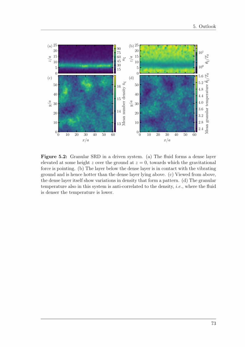
5. Outlook

0

5

10

15

20

25z/a

(a)

0

5

10

15

20

25

z/a

(b)

0 10 20 30 40 50 60

x/a

0

10

20

30

40

50

y/a

(c)

0 10 20 30 40 50 60

x/a

0

10

20

30

40

50

y/a

(d)

153045607590

nξ

100

101

θ ξ/T

0

13

14

15

16

Mea

nnu

mb

erd

ensi

tynξ

2.4

2.8

3.2

3.6

4.0

4.4

4.8

5.2

5.6

Mea

ngr

anu

lar

tem

per

atu

reθ ξ/T

0

Figure 5.2: Granular SRD in a driven system. (a) The fluid forms a dense layerelevated at some height z over the ground at z = 0, towards which the gravitationalforce is pointing. (b) The layer below the dense layer is in contact with the vibratingground and is hence hotter than the dense layer lying above. (c) Viewed from above,the dense layer itself show variations in density that form a pattern. (d) The granulartemperature also in this system is anti-correlated to the density, i.e., where the fluidis denser the temperature is lower.

73

5.1 Driving by shaking

74

75

Chapter 6

Conclusion

Granular materials are particularly intriguing because of the rich phenomenologythey exhibit. From industrial applications, to geophysical and astrophysical prob-lems, understanding their fundamental physics is of paramount importance. In thepast decades, considerable experimental, theoretical and numerical work has un-veiled myriad effects (often counterintuitive) occurring at different length scales ina granular system. For this reason, simulations often encounter the issue of finitesize effects. Having efficient models that can easily span a large range of length andenergy scales. The SRD technique offers a twofold advantage: (i) it is extremelycomputationally convenient as its computational complexity scales linearly with thesize of the system; (ii) because of its simplicity, it is amenable to exact analyticalpredictions. In this Master’s thesis we have taken a first concrete step towards ageneralization of the particle based SRD method, originally used to simulate thehydrodynamics of simple fluids, to the simulation of granular gases. The algorithmuses an effective local coefficient of restitution to render energy dissipation dependenton local mesoscopic observables, while locally conserving density and momentum.As we were able to show, the model obeys linear granular hydrodynamic equations,which have been rigorously derived by a number of authors in the past three decades.Furthermore, we derived a formula for the kinematic viscosity of the 2D GSRD fluid.

To test our derivations, we developed a software implementation for simulationon general purpose graphics cards that we successfully tested and benchmarkedwith analytical predictions for standard SRD. Turning to GSRD, we observe thatour prediction of the kinematic viscosity compares well with the results obtainedfrom our simulations. In this context we found that for low shear driving the fluidbecomes unstable and develops shear condensation.

In the simulations of a freely-cooling granular gas the temperature evolutionfollows the prediction of Haff’s law over several orders of magnitude in time andtemperature. Furthermore, we observe clustering for lower coefficients of restitution.The emergence and dynamics of the cluster compare well with expectations based

76

6. Conclusion

on theory, experiments and simulations. The clustering sets in as the global Machnumber exceeds one. Subsequently, the density fluctuations grow while we observe achange in the power law of the temperature evolution. The clusters exhibit a highercooling rate, hence density and temperature become anti-correlated. This locallyleads to supersonic flow. After their emergence, clusters move, collide and thus growfurther.

The velocity distribution function compares well with theoretical predictions.The distributions decay slower, a phenomenon known as high energy tail. Theshape of the reduced velocity distribution function changes with time as predicted.The second coefficient of the Sonine expansion qualitative matches with analyticalpredictions.

In our discussion we provide physical criteria for a critical selection of modelparameters, and identify the effects of the finite system size. Lastly, in our Outlookwe provide detailed information about the application of the GSRD method for thesimulation of granular matter under the influence of an external gravity force, drivenby a spatially oscillating boundary condition. We believe that the work initiatedhere is a useful contribution to the research on granular gases.

77

Appendix

0

50

100

150

200

y/a

(a) t ≈ 102∆t (b) t ≈ 103∆t

0 50 100 150 200

x/a

0

50

100

150

200

y/a

(c) t ≈ 5× 103∆t

0 50 100 150 200

x/a

(d) t ≈ 104∆t

101

Nu

mb

erd

ensi

tynξ

100

101

102

Nu

mb

erd

ensi

tynξ

100

101

102

Nu

mb

erd

ensi

tynξ

100

101

102

Nu

mb

erd

ensi

tynξ

Figure A.1: Evolution of the freely-cooling 3D GSRD fluid for ϵ = 0.975 on agrid of 2003 cells. The transition to inhomogeneous cooling sets in at approximatelyt = 103∆t. Subsequently, the formed clusters merge as they move through thesystem and form larger clusters. The maximum density grows larger for this biggersystem, what we can see in panel (d), since the limit of the cluster length scale islarger here.

I

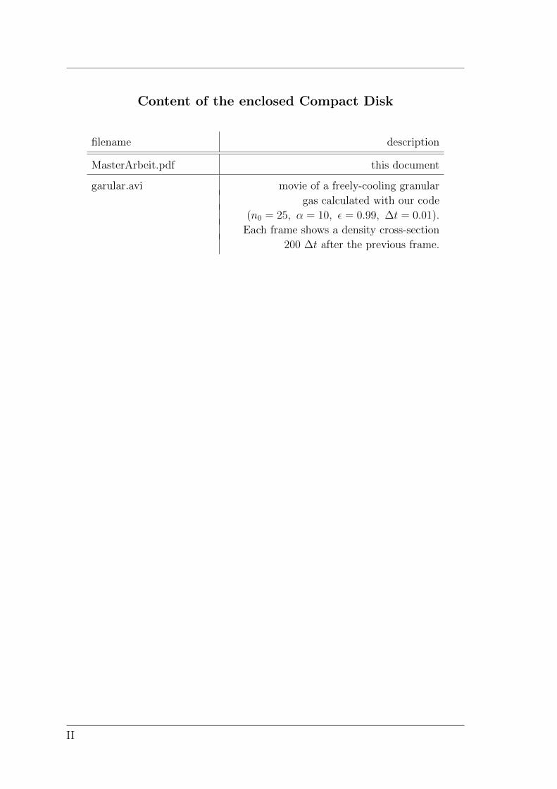
Content of the enclosed Compact Disk

filename description

MasterArbeit.pdf this document

garular.avi movie of a freely-cooling granular

gas calculated with our code

(n0 = 25, α = 10, ϵ = 0.99, ∆t = 0.01).

Each frame shows a density cross-section

200 ∆t after the previous frame.

II

Bibliography[1] L. Vanel and E. Clement, Pressure screening and fluctuations at the bottom of

a granular column, The European Physical Journal B-Condensed Matter andComplex Systems 11, 525 (1999).

[2] N. V. Brilliantov and T. Poschel, Velocity distribution in granular gases ofviscoelastic particles, Physical Review E 61, 5573 (2000).

[3] N. Kikuchi, C. Pooley, J. Ryder, and J. Yeomans, Transport coefficients of amesoscopic fluid dynamics model, The Journal of Chemical Physics 119, 6388(2003).

[4] P. Jop, Y. Forterre, and O. Pouliquen, A constitutive law for dense granularflows, arXiv preprint cond-mat/0612110 (2006).

[5] J. Chambers, Planetesimal formation by turbulent concentration, Icarus 208,505 (2010).

[6] S. Weidenschilling, Dust to planetesimals: Settling and coagulation in the solarnebula, Icarus 44, 172 (1980).

[7] J. E. Chambers, Planetary accretion in the inner solar system, Earth and Plan-etary Science Letters 223, 241 (2004).

[8] J. Schmidt, H. Salo, F. Spahn, and O. Petzschmann, Viscous overstability inSaturn’s b-ring: II. hydrodynamic theory and comparison to simulations, Icarus153, 316 (2001).

[9] A. G. Athanassiadis, M. Z. Miskin, P. Kaplan, N. Rodenberg, S. H. Lee, J. Mer-ritt, E. Brown, J. Amend, H. Lipson, and H. M. Jaeger, Particle shape effectson the stress response of granular packings, Soft Matter 10, 48 (2014).

[10] N. V. Brilliantov and T. Poschel, Kinetic theory of granular gases, (OxfordUniversity Press 2010).

[11] P. K. Haff, Grain flow as a fluid-mechanical phenomenon, Journal of FluidMechanics 134, 401 (1983).

[12] M. Hummel, J. P. Clewett, and M. G. Mazza, A universal scaling law for theevolution of granular gases, Europhysics Letters 114, 10002 (2016).

[13] M. Hummel, Hydrodynamics of granular gases: clustering, universality andimportance of subsonic convective waves, Phd. Thesis, Universitat Gottingen(2016).

[14] A. Malevanets and R. Kapral, Mesoscopic model for solvent dynamics, TheJournal of Chemical Physics 110, 8605 (1999).

III

BIBLIOGRAPHY

[15] C. Pooley and J. Yeomans, Kinetic theory derivation of the transport coefficientsof stochastic rotation dynamics, The Journal of Physical Chemistry B 109, 6505(2005).

[16] C. Holm and K. Kremer, Advanced computer simulation approaches for softmatter sciences III, vol. 221, (Springer 2008).

[17] J. Blaschke, M. Maurer, K. Menon, A. Zottl, and H. Stark, Phase separationand coexistence of hydrodynamically interacting microswimmers, Soft Matter12, 9821 (2016).

[18] T. Ihle and D. Kroll, Stochastic rotation dynamics: a galilean-invariant meso-scopic model for fluid flow, Physical Review E 63, 020201 (2001).

[19] A. Malevanets and R. Kapral, Solute molecular dynamics in a mesoscale solvent,The Journal of Chemical Physics 112, 7260 (2000).

[20] M. P. Allen and D. Tildseley, Computer Simulations of Liquids, (ClarendonPress 1987).

[21] K.-W. Lee and M. G. Mazza, Stochastic rotation dynamics for nematic liquidcrystals, The Journal of Chemical Physics 142, 164110 (2015).

[22] G. Marsaglia et al., Xorshift rngs, Journal of Statistical Software 8, 1 (2003).

[23] S. Luding, Structure and cluster formation in granular media, Pramana 64, 893(2005).

[24] S. Miller and S. Luding, Cluster growth in two-and three-dimensional granulargases, Physical Review E 69, 031305 (2004).

[25] R. Brito and M. Ernst, Extension of Haff’s cooling law in granular flows, Eu-rophysics Letters 43, 497 (1998).

[26] S. N. Pathak, Z. Jabeen, D. Das, and R. Rajesh, Energy decay in three-dimensional freely cooling granular gas, Physical Review Letters 112, 038001(2014).

IV

Acknowledgements

I want to thank my friends and family very much for supporting me the whole time.I apologize to my girlfriend who had to bear me a lot, and especially in momentswhere I was mentally absent thinking about physics. I am really glad about herpatience in that regard.

Thanks to Marco G. Mazza all the fruitful discussions and the steady help andencouragement, and Chamkor Singh for coffee breaks and explanations about gran-ular physics. In this manner I also want to very much thank Fabian Schwarzendahlfor discussions and even more for the nice time we spend climbing in the woods anddusty climbing gym.

I was also very happy about the nice and very friendly working environment atthe MPIDS, the company and help from all the group members, especially mention-ing Christine Linne and Hannes Hornischer making the long evenings in the institutemuch more pleasant. I will miss everyone.

I also want to thank my flatmates for tolerating the dirty kitchen.

Erklarung

Gemaß §12(9) der Prufungsordnung des Master-Studiengangs Physik an der Uni-versitat Gottingen:

Hiermit erklare ich, dass ich diese Abschlussarbeit selbstandig verfasst habe,keine anderen als die angegebenen Quellen und Hilfsmittel benutzt habe und alleStellen, die wortlich oder sinn- gemaß aus veroffentlichten Schriften entnommenwurden, als solche kenntlich gemacht habe. Daruber hinaus erklare ich, dass dieseAbschlussarbeit nicht, auch nicht auszugsweise, im Rahmen einer nichtbestandenenPrufung an dieser oder einer anderen Hochschule eingereicht wurde.

Des Weiteren versichere ich, dass die schriftliche Version dieser Abschlussarbeitmit der erganzend vorgelegten Version ubereinstimmt.

Gottingen, September 12, 2017

(Arne Wolf Zantop)