Development and testing of a process-based model (MOSES) for simulating soil processes, functions and ecosystem services

(This is a sample cover image for this issue. The actual cover is not yet available at this time.)

This article appeared in a journal published by Elsevier. The attachedcopy is furnished to the author for internal non-commercial researchand education use, including for instruction at the authors institution

and sharing with colleagues.

Other uses, including reproduction and distribution, or selling orlicensing copies, or posting to personal, institutional or third party

websites are prohibited.

In most cases authors are permitted to post their version of thearticle (e.g. in Word or Tex form) to their personal website orinstitutional repository. Authors requiring further information

regarding Elsevier’s archiving and manuscript policies areencouraged to visit:

http://www.elsevier.com/copyright

Author's personal copy

Ecological Modelling 222 (2011) 3795– 3810

Contents lists available at SciVerse ScienceDirect

Ecological Modelling

jo ur n al homep ag e: www.elsev ier .com/ locate /eco lmodel

Development and testing of a process-based model (MOSES) for simulating soilprocesses, functions and ecosystem services

M.J. Aitkenheada,∗, F. Albanitob, M.B. Jonesc, H.I.J. Blacka

a The James Hutton Institute, Craigiebuckler, Aberdeen AB15 8QH, Scotland, UKb Institute of Biological and Environmental Science, University of Aberdeen, Aberdeen AB24 3UU, Scotland, UKc Botany Department, School of Natural Sciences, Trinity College Dublin, Dublin 2, Ireland

a r t i c l e i n f o

Article history:Received 15 June 2011Received in revised form21 September 2011Accepted 23 September 2011

Keywords:SoilProcess modelEcosystem servicesCarbon poolSoil profile

a b s t r a c t

A novel process-based soil model (MOSES – Modelling Soil Ecosystem Services) is described and testedusing field data. The model is designed to provide information about a soil profile at approximately 1-cmdepth resolution, on a 1 min timestep. Conceptualisation of the model has targeted a set of soil ecosystemservice-related functions, including carbon sequestration, water buffering and biomass productivity, withthe model framework designed to allow inclusion of additional processes and functions over time. Pro-cesses implemented within the model include thermal conduction, water movement (using pedotransferfunctions to determine hydraulic conductivity, matric potential and related parameters), organic mat-ter pool dynamics and gas/solute diffusion. The organic matter status of the profile is initialised usingiterative runs of the RothC model to determine partition sizes of Decomposable Plant Material, ResistantPlant Material and other carbon pools. The outputs of the model are used to evaluate soil ecosystemservice provision. MOSES has been designed to allow the implementation of further soil processes in thefuture, with the intention of expanding the variety of soil ecosystem functions and services that can bemodelled. Validation of the model against detailed time-series field measurements of CO2 concentrationand emission, temperature and water content of a freely draining podzolic soil in Ireland have shown itto be effective at simulating these specific parameters, with statistically significant association betweenmeasured and modelled values of temperature at all depths, for saturation at shallow depths and for CO2

at all depths apart from the surface layer. Overall, the model was seen to perform better at shallow depth,with lower levels of accuracy in deeper layers. The model has also been shown capable of simulating soilfunctional provision, based on specific parameters and processes. The need to add additional processesto MOSES in order to improve the simulation of soil ecosystem service provision, multifunctionality andthe effects of external drivers such as climate change and management is discussed.

© 2011 Elsevier B.V. All rights reserved.

1. Introduction

Soils are essential to the delivery of many ecosystem goods andservices for the ultimate benefit and welfare of humankind (MEA,2005). At a most basic level, the formation and turnover of soils sup-port many ecosystem functions including nutrient cycling, waterdynamics, carbon exchanges etc. which in turn contribute to thedelivery of provisioning, regulating and cultural ecosystem services(e.g. crop productivity, pollution buffering, conservation of species,etc.). Degradation of the soil leads to a loss of crop yield, and there-fore adversely impacts human health (Lal, 2009). Climate changeis predicted to increase the risk of loss in effective soil functioning,

∗ Corresponding author. Tel.: +44 1224 395257.E-mail address: [email protected] (M.J. Aitkenhead).

acting particularly through its effects on soil microbial communi-ties (Waldrop and Firestone, 2006).

The modelling of soil dynamics over extended periods of time istherefore extremely important for developing our understanding ofhow different soils will respond to stress and how this will alter thecapacity for and maintenance of individual ecosystem functions.In this paper, we describe the rationale and methodology behindthe development of a new soil model called MOSES (ModellingSoil Ecosystem Services). MOSES includes many different categoriesof soil process, including thermal, hydraulic, biological and phys-ical. The model is designed to provide a process-based multilayerprofile simulation of many soil characteristics, with the values ofspecific parameters associated with a wide range of ecosystem ser-vices. MOSES includes many process implementations that haveappeared in other soil models, but in addition is designed to allowcontinuous further development and application beyond the cur-rent implementation.

0304-3800/$ – see front matter © 2011 Elsevier B.V. All rights reserved.doi:10.1016/j.ecolmodel.2011.09.014

Author's personal copy

3796 M.J. Aitkenhead et al. / Ecological Modelling 222 (2011) 3795– 3810

Many different kinds of soil model exist. Some are simple regres-sions of variables against one another, allowing researchers topredict the unknown characteristics of a soil. Others contain infor-mation about parameters from within multiple layers or horizonswithin the soil profile. Mass movement of water and other compo-nents, transformation of organic matter pools into one another andchanges to the chemical composition of individual layers withinthe profile can all be simulated over time as required.

The DNDC (DeNitrification-DeComposition) model (Li et al.,1992, 1997) is a process-based time series simulation model, com-posed of submodels that implement different types of processwithin their design. This concept, of having submodels that arepartially or completely removable from the overall model design(i.e. they can be turned off or on as required), makes model devel-opment easier by allowing the developer to test the influence ofspecific submodels, and also maintains an efficient structure bywhich parameters that impact one another are held within thesame section of the model code. In terms of model developmentand also in terms of flexibility and ease of use, the modular designis one that should be recommended. DNDC itself has been used toestimate greenhouse gas emissions at local and continental scales(Miehle et al., 2006; Levy et al., 2007), and contains submodels forthermal/hydraulic, organic matter decomposition and denitrifica-tion. It is driven by relatively simple climatic data and uses soiltextural and biochemical parameters as baseline data from whichto start a simulation. The strength of this approach is that it allowsa wide range of biogeochemical processes to be simulated. How-ever, the DNDC model operates on a daily timestep and simulatesa 100 cm profile in 5-cm layers, with processes that take placein shorter temporal or spatial resolutions unable to be simulated.In addition to including parameters and processes that are notincluded in DNDC or similar models, we have designed the MOSESmodel to operate on a 1-minute timestep with 1-cm layers. Othermodels that simulate the soil profile usually do so at a coarser scale(e.g. DyDOC (Michalzik et al., 2003)).

CENTURY is a soil model originally designed to model nutrientdynamics in the Great Plains of North America, but which has beengreatly revised and extended since its first development (Partonet al., 1988; Metherell et al., 1993). CENTURY has been used formany different purposes, including the dynamics of carbon in agri-cultural (Bricklemyer et al., 2007) and grassland soils (Qian et al.,2003). Another soil organic matter model with a modular designand similar data requirements to DNDC and CENTURY is ECOSSE(Smith et al., 2007; Smith et al., 2010b). This model contains sev-eral carbon-pool dynamics submodels, including Dissolved OrganicCarbon (DOC), methane and partitioning of the organic matter poolinto multiple fractions with different characteristics (e.g. varyingdecomposition rates in relation to moisture content, tempera-ture and pH). ECOSSE contains many relationships and processesseen within other organic soil models (e.g. decomposition, min-eralization, immobilization, nitrification, and denitrification) butincorporates a larger number of these processes than earlier mod-els, making it potentially more generally applicable. In addition,the ECOSSE model relies on RothC (Jenkinson and Rayner, 1977;Coleman et al., 1997) for initialisation of the organic matter pool, ina highly effective approach that has been replicated within MOSES.

Advantages of the inclusive, flexible approach include the abil-ity to simulate a wider range of scenarios and improvements tothe ability to capture realistic, dynamic behaviour. Potential dis-advantages of the approach however include the propagation ofuncertainties and errors within a more complex framework, andthe need to include more information at the beginning of a simu-lation.

Details of many other soil organic matter models have beenpublished, including NCSOIL (Molina et al., 1983), CANDY (Frankoet al., 1997), CQESTR (Rickman et al., 2001; Liang et al., 2009),

ROMUL (Chertov et al., 2001; Nadporozhskaya et al., 2006) andCN-SIM (Petersen et al., 2005a,b). The NCIM (Nitrogen CarbonInteraction Model) (Esser, 2007) is one of the most recent modelsdemonstrated, and emphasises the coupling of different cycles andprocesses for effective representation of the emergent dynamics ofsoil. This model has been used to determine the relative impactsof climate change, management practices and soil processes oncarbon sequestration in soil (Esser et al., 2011).

A subspecies of the soil organic matter model is that dealingwith bacterial population dynamics. As the ‘active’ partition of theorganic matter pool, the bacterial biomass partition’s size and activ-ity are vital in determining the rate of decomposition of otherpartitions (e.g. DPM – Decomposable Plant Material, RPM – Resis-tant Plant Material), and the nature of the decomposition products.Recent work in this field includes that by Gignoux et al. (2001) andZelenev et al. (2006). Each of the simulation models mentionedabove approaches simulation of the biomass partition in differentways, depending upon the theoretical relationships applied. Theydo not however split the biomass partition into multiple compo-nents, such as microbial, fungal and faunal, in the explicit mannerthat the model we present here does. NCSOIL does split the ‘activeorganic phase’ into two compartments, but these are not directlyrelated to specific ecological groupings, while CN-SIM splits themicrobial biomass into two pools but does not include the fungalor faunal pools.

The simulation of soil organic matter is closely tied to our abil-ity to represent other characteristics of the soil within modellingframeworks. Solid organic matter fractions cannot be representedwithout consideration of Dissolved Organic Carbon (DOC), whichleads into a requirement for soil hydrology (see below) andsoil solution chemistry. The ORCHESTRA modelling framework(Meeussen, 2003) has proved useful for the development of soilchemical models, while the model DyDOC (Michalzik et al., 2003)has been used to successfully model the production and transportof DOC in soil. Both of these models/frameworks, while success-ful in simulating the parameters and processes for which they aredesigned, are restricted however in their ability to include a widerrange of soil processes than their original intended design, implyinga need for a more flexible modelling approach.

While all organic matter models include some consideration ofwater content and its movement in the soil, they are generally notfocussed on this issue as strongly as existing soil water models.One exception to this is the DAISY model (Hansen et al., 1991). Dueto its additional sophistication, DAISY has been favourably com-pared to other soil organic matter models (Kröbel et al., 2010),although some researchers have pointed out areas where it couldbe improved further (Mueller et al., 1998; Gjettermann et al.,2008). These areas included the implementation of gaseous dif-fusion between soil layers, partitioning of the biomass pools usingdifferent activity rates, and more accurate representation of sorp-tion/desorption of DOC. Within the MOSES model, the first twoof these requirements have been implemented while the thirdremains an intended development in the future. Another modelthat includes soil carbon, hydrology and plant interactions is SPA(Soil-Plant-Atmosphere) (William et al., 2001), which includesmany of the same biological and physical relationships within theplant/soil system as MOSES, and goes into further detail regardingthe root distribution and water uptake than we have consideredhere.

Other soil models that include hydrological components includeDayCENT (Parton et al., 1998) and the ITE Edinburgh Forest Model(Thornley and Cannell, 1996; Arah et al., 1997). Simulation of soilwater can be carried out using methods with a range of complex-ity. The work of Touma (2009) has shown that the Van Genuchtenrelationship (Van Genuchten, 1980) is an accurate method of sim-ulating hydraulic conductivity. The relationship between water

Author's personal copy

M.J. Aitkenhead et al. / Ecological Modelling 222 (2011) 3795– 3810 3797

retention, matric potential and pore-size distribution is com-monly referred to as the Mualem-van Genuchten relationship, asit includes the work of Mualem (1976), and has been appliedoften in soil profile water dynamics (e.g. Kool and van Genuchten,1991).

Other work in this field largely involves the development ofpedotransfer functions relating soil particle size distribution andorganic matter content to hydraulic conductivity and includes thatof Gupta and Larson (1979), Michalzik et al. (2003), Han et al. (2008)and Lilly (2000). These pedotransfer functions allow relativelyaccurate prediction of hydraulic conductivity and matric potential,two parameters that are influenced by very small-scale struc-ture within the soil, using macroscopic parameters that are easilymeasured. The MOSES model uses the Mualem-van Genuchtenrelationship for the determination of hydraulic conductivity andmatric potential based on sand, silt, clay and organic matter con-tent.

Closely related to soil hydraulic conductivity is the concept ofgas- and water-based diffusion. The approximation of an unsatu-rated soil as a porous medium to which Darcy’s Law can be appliedrequires the parameterisation of soil diffusivity. Due to its com-plex composition and structure, this is never an easy task and isone that remains ‘unsolved’, although it has been tackled by manyresearchers. In recent years researchers have produced sophisti-cated models relating diffusivity to particle size distribution, matricpotential and the ‘tortuosity’ of soil structure (Moldrup et al., 2003,2004, 2005a,b). These models are much more complex than ear-lier models of soil diffusivity (for example Currie, 1970) and reflectour improved understanding of how small-scale soil pore structureis related to mass diffusivity. There is still uncertainty in the sub-ject however, largely in the parameterisation of tortuosity whichrepresents the complexity and path length available to particlesmoving through the soil. The calculation of bulk density in soilsbased on particle size distribution must also be determined accu-rately, as bulk density relates to pore space and size distribution,and through these to transport mechanisms throughout the profile.Various relationships have been developed to allow bulk densityto be calculated from particle size distribution and organic mattercontent, including those of Saini (1966), Rawls (1983), Ruehlmannand Körschens (2009), Keller and Håkansson (2010) and the workof Arvidsson (1998). Here we use the pedotransfer functions devel-oped by Keller and Håkansson (2010) to calculate bulk densitybased on sand, silt, clay and organic matter content. This relation-ship has been found to work well for a wide range of organic andmineral soils.

Considering that many different soil models that exist, twoquestions arise. The first of these is, which model is best? This is noteasily answered as individual models simulate different situationsbetter than others and a comprehensive evaluation of every possi-ble situation is both outside the scope of this work and technicallyinfeasible. The analysis of Smith et al., 1997 showed that one groupof organic soil models (RothC, CANDY, DNDC, CENTURY, DAISY andNCSOIL) did not differ greatly from one another in terms of accu-racy, while another group (SOMM (Chertov and Komarov, 1997),ITE and Verberne (Thornley and Verberne, 1989; Whitmore et al.,1997)) were also similar to each other but of poorer performancethan the first group. Feller and Bernoux (2008) in a summarizedhistory of carbon sequestration theory demonstrated the improvedunderstanding over time of the processes controlling soil organicmatter, and discussed the improvements in modelling that thishas led to. Similar improvements in our understanding of othersoil processes and their relationships with ecosystem services haveresulted in improvements in our abilities to simulate or otherwiserepresent soils as integrated systems. So the ability to adjust a soilmodel over time to incorporate additions to our knowledge base isimportant.

The second question, considering the number of models thatalready exist, and the accuracy that they can achieve, is why dowe need another soil model? The answer to this is two-fold. It istrue that many soil models are accurate in simulating the processesthat they are designed to model, and that they can be designed tocapture multiple processes taking place within the soil. However,each of the models discussed here and others has been designedto answer specific questions and to implement specific processes.There are no soil models that are designed with the inherent flex-ibility that would enable developers to add new processes easily.What is needed is a framework designed not only to allow accurateimplementation of a wide range of processes, but also to allow addi-tional processes of interest to be added in the future. An exampleis the fate of carbon pools when or if decomposed into break-down products. The number of factors and the process complexityinvolved in organic matter decomposition result in a requirementfor a set of submodels that can be connected/disconnected or addedto when either our understanding or questions change. Clapp andHayes (2006) for example discuss important questions that needto be answered about the relationships between organic materialin the soil and its resistance to decomposition under different con-ditions. Another reason why a new modelling framework wouldbe useful is that while those currently available can simulate thedynamics of specific parameters, they cannot easily produce out-puts that relate to descriptive terms of interest. If someone triedto classify a soil being modelled by CENTURY, DNDC or ECOSSEaccording to the WRB soil classification system (FAO, 1998), forexample, there would likely be insufficient profile information toallow a confident categorisation. A model is needed that includesthe parameters, processes and relationships necessary to allowusers to evaluate a wider range of soil characteristics and relatethem more directly to ecosystem services and functions. Such amodel would be able to address questions of resilience, resistanceand sensitivity to change of the whole soil system, rather than justof the individual processes.

One limiting factor of many soil models is the range of environ-mental, soil and vegetation types that they are designed to simulate.Very often, a soil model is extremely effective within its ‘niche’,but fails to provide accurate simulations when applied to situa-tions outside the design parameters. This can be due to a numberof reasons. For example the relationships which define the modelbehaviour are often based on work from a restricted bioclimatic orgeographical range. In addition, it is common practice when design-ing a simulation model to make assumptions about what kind ofevents, processes or characteristics the model must include. Oncethese assumptions have been made and the design of the modelimplemented, it can be difficult to redesign the model at a laterdate to include new processes, or to remove events that the modelassumes must take place. This limiting scope inherent in soil mod-els makes it difficult to simulate large, complex and interrelatedsituations such as the effects of climate or land use change accu-rately. The intention underlying the MOSES model is to allow thiscomplexity to be modelled by including a wider range of processesthan previously available within soil models, while at the same timeproviding answers to specific questions of soil ecosystem services.

Model initialisation is an important aspect to be consideredearly on in the design process. With soil organic matter mod-els, the partitioning of organic matter into several pools is vitalfor accurate simulation of the production of decomposition prod-ucts. Some organic matter partitions are much more resistant todecomposition than others, and the rate of application to differentpartitions varies greatly with soil management practice, vegeta-tion type and climate. Many soil organic matter models rely onRothC (Jenkinson and Rayner, 1977; Coleman et al., 1997). Thismodel of turnover and partitioning of carbon in soils has undergonemany updates and alterations, and continues to be used by many

Author's personal copy

3798 M.J. Aitkenhead et al. / Ecological Modelling 222 (2011) 3795– 3810

researchers. One of the reasons that RothC is so effective is that itrequires relatively simple inputs in order to accurately determinesoil organic matter partitioning. Another is that the relationshipsused within the model are easy to relate to real processes within thesoil (Zimmermann et al., 2007), making it not just accurate but easyto understand. RothC has been used for initialisation of organic mat-ter in several models, including ECOSSE (Smith et al., 2007), Struc-C(Malamoud et al., 2009), and the model to be described here. Theinitialisation of other parameters, such as soil water content andsoil solution composition, equilibrate much more rapidly than soilorganic matter composition and so can be initialised within a soilmodel using more a more simple approach (for example allowingthe model to run for a suitably large number of time steps prior tothe ‘experimental’ run). In the case of MOSES, the model is run forone year, on a one-minute timestep, to equilibrate parameters notassociated with solid organic matter.

In this work, we present the soil model MOSES and describe itsvalidation against a restricted dataset of carbon dioxide, tempera-ture and water content at several depths over a period of severalmonths. The use of Miscanthus in the field trial used to test theMOSES model allows us to investigate the potential of the model’sability to simulate specific ecosystem service provisions (biomassproductivity of a crop suitable for energy production and carbonsequestration, as shown by Dondini et al., 2010). This is achievedby using the parameters measured in the field experiment (tem-perature, saturation and carbon dioxide concentration at differentdepths) as indicators of ecosystem services, in addition to their usefor validating the MOSES model itself. A statistical comparison ofthe modelled and observed data is given, followed by a discussionof the capabilities of MOSES, its potential to improve on existing soilmodels and the future work that is planned to expand the model.

2. Model design

The design and operation of the MOSES model is intended tofacilitate the addition, removal and alteration of process submod-els as realistically and easily as possible. This has led to a modularconcept, with individual processes, or groups of processes, beingimplemented within separate subroutines. The core concept of themodel is that the changes to all parameters are calculated over asingle (1 min) time step, with each parameter being updated at theend of this timestep. The model simulates a soil profile consistingof 1 cm layers, with each layer containing parameters describingwater, organic matter, structure and other characteristics of thesoil. While other soil models (e.g. DNDC, ECOSSE) also operate onthe multi-layer profile principle, the spatial and temporal scale ofMOSES allows potentially more accurate process simulation andthe inclusion of processes that take place over short time periods(e.g. gas diffusion in sandy soils). Transfer of material and energybetween layers and alteration of the parameters within a layerare carried out within each time step. There is no restriction onthe number of layers simulated within a soil profile. This sectiongives details of the operation of specific subroutines, and of thesoil processes implemented within them. Currently, the model isimplemented in Visual Basic, with plans to translate it to C++ in thenear future (for ease of development in early stages vs. numericalcomputation speed later on). The main assumption built into theMOSES model is that the simulated soil is on level ground, withno lateral flows of material. This assumption does not restrict laterdevelopment of 2-D simulations with lateral flow, and indeed it isintended that at a later date slope and lateral movement of materialwill be included.

When comparing simulation against reality, it is necessary tocarry out an equilibriation of the model for a period prior to sim-ulating the measurements that were taken place in the field. If the

model is complex and contains large numbers of variables then it isdifficult if not impossible to initialise every variable to a value thatis seen at the start of a field experiment, without seeing some initialfluctuations that do not correspond to the reality of the situation.To do so would require an economically prohibitive level of fieldmeasurement data, and would in a sense negate the requirementfor a model in the first place. An example of this is the equilib-riation of water content distribution through the profile, whichalthough initialised to measured values may not be in equilib-rium with the calculated matric potential, porosity and hydraulicconductivity values. A pre-comparison run of one year is there-fore carried out for the period directly prior to the simulated fieldtrial, to allow the many soil parameters to achieve equilibrium.The climatic conditions used for this pre-comparison run are iden-tical to the first field trial year, with the assumption being thatthis represents the norm for the study site. While some parame-ters and processes may take longer than one year to equilibratein soil, it would also be dangerous to assume that the soil is inequilibrium overall; an equilibrium run of decades or centuriesmay result in a greatly different soil profile from the one beingsimulated.

2.1. Initialisation

2.1.1. Profile initialisationThe setup files are read and used to initialise specific vari-

ables such as organic matter content; sand, silt and clay fractions,porosity and bulk density. Also read into predefined arrays arethe climatic data, which is converted into 1-min timestep datafrom daily readings; the vegetation data, which contains infor-mation about growth rates on a monthly basis; parent materialcharacteristics such as hydraulic and thermal conductivity; andsite-specific information such as elevation, longitude, latitude, veg-etation type during each year and the duration of the requiredmodel run.

2.1.2. RothC initialisationThe RothC model is used to determine proportions of the organic

matter content in each of the five pools (DPM (DecomposablePlant Material), RPM (Resistant Plant Material), IOM (Inert OrganicMaterial), HUM (Humified Material) and Biomass). This initiali-sation is carried out using a similar method to that employed inSmith et al. (2007). Following this RothC initialisation process, addi-tional parameterisation of the simulated profile is carried out toinclude those organic matter parameters not included by RothC,including (A) splitting of the biomass pool into microbial, fungaland faunal components, (B) using the organic matter content ineach layer to re-determine the bulk density of that layer and tocalculate hydraulic conductivity, matric potential and other param-eters associated with soil texture, and (C) inclusion of soil gas andsolution components including DOC, methane, CO2 and nitrogencompounds.

2.2. Model operation

2.2.1. Date and timeAt each time step, it is necessary to calculate the time of day

(in minutes from midnight) and day of year. This information isused to calculate sun angle and maximum solar radiation, and alsoto identify the growth stage of the vegetation. When temperaturedata is not available or is only available in terms of maximum andminimum during a 24-h period, time of day is used as a proxy vari-able from which to calculate temperature, using a sine functionwith maximum temperature at 3 pm and minimum temperatureat 3 am.

Author's personal copy

M.J. Aitkenhead et al. / Ecological Modelling 222 (2011) 3795– 3810 3799

2.2.2. ThermalThermal energy transfer between layers, between the topmost

layer and the atmosphere, and between profile layers and theparent material are calculated by determining the thermal con-ductivity of layer components such as water, organic matter, soilair and minerals. Thermal flux to and from the atmosphere isdetermined by calculating the maximum insolation and estimat-ing albedo based on vegetation type and growth, and soil organicmatter content (using a pedotransfer function based on existingsoil data). A set of parent material layers, each 30 cm thick, is usedto simulate thermal transfer to a maximum depth of 10 m. Belowthis depth, it is assumed that the parent material temperature isconstant at the average air temperature of the simulated site loca-tion. For temperature and all other processes/parameters describedbelow, MOSES operates on a 1-min, 1 cm layer scale. Equation (1)describes the temperature change in a layer from one time step tothe next:

�T = �E

C(1)

where �T is the change in temperature, �E is the change in energyand C is the layer’s heat capacity (calculated from the summed heatcapacity of the component solid, liquid and gaseous phases). �E iscalculated by determining the rate of thermal exchange betweenneighbouring layers, with the rate of exchange being proportionalto the temperature difference and also to the thermal conductiv-ity. Thermal conductivity is calculated from the proportion of eachlayer that is solid, water or air and the relative thermal conductivityof each.

2.2.3. DiffusionGaseous diffusion of CO2 and CH4 through the soil gas

is calculated using Fick’s Law of diffusion (Wikipedia, 2011a)(http://en.wikipedia.org/wiki/Fick’s laws of diffusion), with addi-tional terms for tortuosity of pore space and water content. Theamount of CO2 and CH4 in the soil air is calculated using Henry’s Law(Wikipedia, 2011b) (http://en.wikipedia.org/wiki/Henry’s law) forsolubility of these molecules, taking into account temperature andthe total amount of each in a layer. Diffusion from the topmost layerinto the atmosphere is also calculated, to determine emission orsequestration of these greenhouse gases. The assumption is madethat no diffusion into the parent material takes place. Equation (2)describes the rate of diffusion between neighbouring layers L1 andL2, of a gaseous component G:

�G = D(�1 − �2)�x�

(2)

where �G is the rate of movement from layer L1 to layer L2, D is thediffusivity of the component G, �1 and �2 are the concentrations ofG in layers L1 and L2 respectively, � is the porosity of layer L1, x isthe distance between the middle of each layer, and � is the tortu-osity of layer L1. �G is calculated for both gaseous and dissolvedcomponents of G, with the diffusivity, porosity, concentration andtortuosity changing for gaseous and dissolved components of G inrelation to its solubility. It is not considered possible to include allof the relationships by which tortuosity, solubility and diffusivityare calculated in MOSES within this paper, and so further queriesshould be addressed to the lead author.

2.2.4. Water movementWater movement between soil layers is calculated based on the

hydraulic conductivity and potential difference between each layer.Hydraulic conductivity is calculated using a pedotransfer func-tion based on tortuosity, moisture content and total porosity, withtortuosity being dependant on sand, silt, clay and organic matterfractions (Van Genuchten, 1980). Water potential for each layer is

the summation of matric and gravimetric potential, with matricpotential (˚) being calculated using one form of the Mualem-vanGenuchten relationship (Equation (3)).

� =

((�s − �r/� − �r)

1/(1−(1/n)) − 1)1/n

˛(3)

where � is the water content, �r is the residual water content, �s isthe saturated water content, n is a variable associated with pore-size distribution (n > 1), and ̨ is a parameter related to the inverseof the air entry suction ( ̨ > 0).

2.2.5. LeachingMovement of water between layers resulted in a correspond-

ing movement of dissolved material within the water fraction. Thismovement, as a result of matric and gravimetric potential, drawsDOC, dissolved CO2 and methane from one layer to another. Whenmonitoring simulations, it was noted that rainfall events resultingin a ‘pulse’ of increased saturation down the profile also led to aspike in DOC that moved downwards, and that was accompaniedafter a delay by a spike in CO2 and methane levels moving throughthe profile due to increased biomass consumption of DOC. The sameprocess in reverse was observed when the soil was drying out, withwater being drawn upwards. Sorption of dissolved organic mat-ter or other solutes onto soil particles has not been implementedyet, although its implementation is considered a priority for futureefforts as it impacts on profile residence time of soil solutes.

2.2.6. Water uptake and transpirationWater uptake by vegetation results in reduction in saturation

at depth, with the level of uptake being affected by vegetationtype, rooting strategy, temperature and moisture content in thesoil. The plant root system is simulated as containing a total massM, which is distributed between the surface and maximum root-ing depth D. The root mass m at depth d is calculated by assuminga linear decrease in root proportion between the surface and D.Water uptake at saturation is proportional to the mass m at depth d,and decreases with matric potential according to the relationshipU(� ) = U(� 0)/(1 + (� /� 50)3) (Van Genuchten, 1987). The value of� 50 (the matric potential at which plant yield is reduced to 50%of normal) varies between plant species, and normally lies in therange −100 to −500 kPa. Uptake at � 0 is also related to season,with plant activity being assigned a monthly multiplication rate toreflect seasonal growth patterns.

2.2.7. Convert CO2Carbon dioxide is converted to biomass in MOSES at a rate con-

trolled by moisture, temperature and pH conditions in addition tothe existing quantity of CO2 available. An optimum conversion rateis determined, with this value being multiplied by the control fac-tors whose value equals e−˛|x|, where ̨ is a parameter controllingthe rate of change of the control factor as the relevant characteristicdeviates from the optimum value, and x is the difference betweenthe optimum and the current value. Values of ̨ can be differentfor values above or below the optimum, allowing sensitivity to begreater for example for saturation values below the optimum thanfor those above it. The values for the optimum value O, ˛high and˛low for moisture, temperature and pH were determined from var-ious literature sources, including Parton et al. (1988); Hansen et al.(1991); Li et al. (1997); Smith et al. (2010a); Michalzik et al. (2003).Some values were also derived using expert knowledge and cur-rent understanding of relevant biological, physical and chemicalprocesses. Conversion rates into each of the three biomass pools(Bacteria, Fungi and Fauna) were calculated using a different set ofparameter values, to reflect the characteristics of these pools. Con-version of CO2 into other solid organic matter pools, methane or

Author's personal copy

3800 M.J. Aitkenhead et al. / Ecological Modelling 222 (2011) 3795– 3810

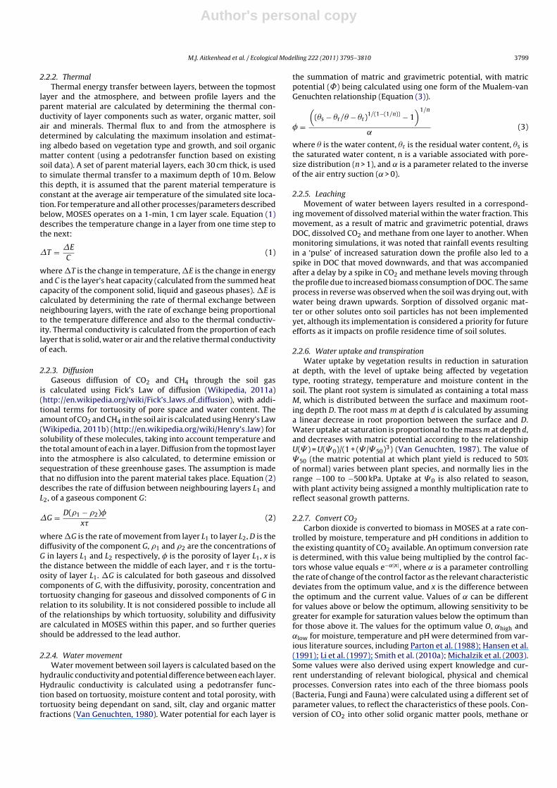
Table 1Parameterisation of control variables for CO2, CH4 and DOC pool transformation.

From To R T0 (◦C) Tneg (◦C) Tpos (◦C) pH0 pHneg pHpos S0 Sneg Spos

CO2 BIObacteria 100 25 10 10 6 1 1.5 0.5 0.25 0.15CO2 BIOfungi 20 20 10 10 5 2 2 0.25 0.5 0.2CH4 BIObacteria 20 25 10 10 6 1 1.5 0.5 0.25 0.15DOC HUM 5 10 10 20 5 2 3 0.25 1 0.2DOC BIObacteria 20 25 10 10 6 1 1.5 0.5 0.25 0.15DOC BIOfungi 20 20 10 10 5 2 2 0.2 0.4 0.4

DOC was assumed not to take place based on expert knowledge ofprocesses taking place within the soil, and discounting anaerobicconversion of CO2 into methane and other organic compounds (ashas been shown to take place by Conrad and Klose (1999) undercertain conditions).

2.2.8. Convert CH4Methane was converted into the bacteria, fungi and fauna

biomass sub-pools in the same manner as CO2, but with differentrate control variables as determined from the literature. The con-version of methane into other solid organic matter pools, CO2 orDOC was also assumed not to take place. In addition, the solubilityof methane was taken into account to allow only that fraction ofmethane that was dissolved in water to be taken up, thus reducingthe overall quantity available for uptake at any time. The same wasdone for carbon dioxide, although it has a much lower solubility atnormal pressure and temperature ranges and so was not affectedas much by this.

2.2.9. Convert DOCDissolved organic carbon was also converted into biomass pools

using moisture, temperature and pH control factors. It was assumedthat the entire quantity of DOC in any layer existed only in thesoluble form, making the entire quantity available for uptake.Table 1 gives the model parameter values for decomposition ofCO2, CH4 and DOC (where parameters are not given, e.g. for uptakeof methane by soil fauna, this implies that the conversion doesnot take place in the model). The parameter R is the proportionalrate constant for conversion per year (i.e. for conversion of CO2to BIObacteria under optimal conditions, the proportion of totalCO2 converted to bacteria is 100× the existing amount, equalling0.274 of the total available per day or 1.901 × 10−4 of the total per1-minute timestep). T0 is the optimum temperature for the conver-sion in ◦C, while Tneg and Tpos are the temperature control factors forcalculating conversion rate change due to temperature, also in ◦C.The control factor Tneg is applied when the temperature in thatlayer is less than T0, while Tpos is applied when the temperatureis greater than T0. The parameters pH0, pHneg and pHpos are simi-larly pH control factors for calculating conversion rate change dueto pH, while S0, Sneg and Spos are saturation control factors (usingsaturation expressed as S = 0 for zero moisture content and S = 1for completely saturated). Calculation of the proportional rate of

conversion P from one carbon pool to another uses the followingrelationship:

P = Re|T−T0|/Tneg e|pH−pH0|/pHpos e|S−S0|/Spos (4)

In Equation (4), it is assumed that the temperature T is below T0,that the pH is higher than pH0, and that the saturation S is higherthan S0. While this relationship does use rate constants and controlfactor concepts obtained from the literature, it is believed that therelationship given in this form is novel.

2.2.10. Convert RPM etc.RPM (Resistant Plant Material) is decomposed to methane, DOC

(Dissolved Organic Carbon), CO2, biomass, and the remaining threeorganic matter pools DPM (Decomposable Plant Material), IOM(Inert Organic Matter) and HUM (Humified Material) at differentrates. It is assumed that the conversion to all pools takes place asa result of interactions with biomass pools, with the conversionsbeing effectively byproducts of biomass decomposition of the pool.The same assumption is made for decomposition of DPM, IOM andHUM pools. As a result, the optimum temperature, moisture andpH factors for each decomposition process are the same and equalto those for optimum decomposition by biomass fractions. The rel-ative rates of production for each pool from RPM are smaller, andrelate to the amount of each produced as a byproduct of biomassactivity.

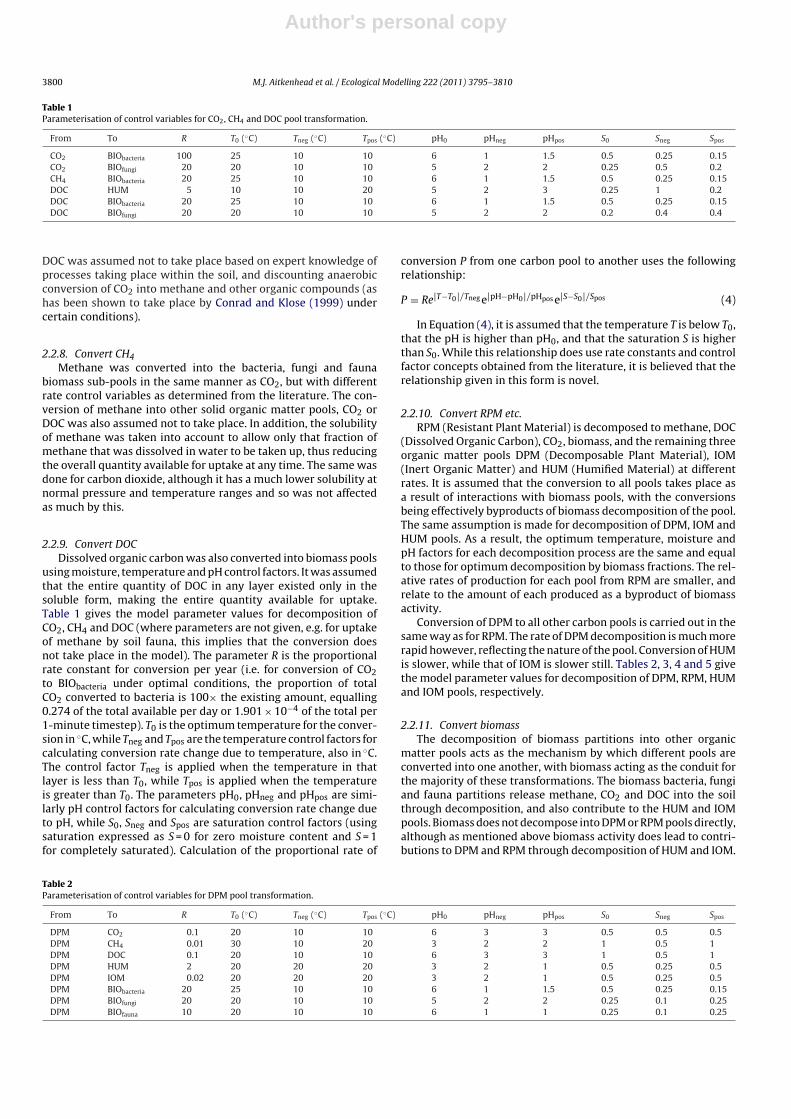
Conversion of DPM to all other carbon pools is carried out in thesame way as for RPM. The rate of DPM decomposition is much morerapid however, reflecting the nature of the pool. Conversion of HUMis slower, while that of IOM is slower still. Tables 2, 3, 4 and 5 givethe model parameter values for decomposition of DPM, RPM, HUMand IOM pools, respectively.

2.2.11. Convert biomassThe decomposition of biomass partitions into other organic

matter pools acts as the mechanism by which different pools areconverted into one another, with biomass acting as the conduit forthe majority of these transformations. The biomass bacteria, fungiand fauna partitions release methane, CO2 and DOC into the soilthrough decomposition, and also contribute to the HUM and IOMpools. Biomass does not decompose into DPM or RPM pools directly,although as mentioned above biomass activity does lead to contri-butions to DPM and RPM through decomposition of HUM and IOM.

Table 2Parameterisation of control variables for DPM pool transformation.

From To R T0 (◦C) Tneg (◦C) Tpos (◦C) pH0 pHneg pHpos S0 Sneg Spos

DPM CO2 0.1 20 10 10 6 3 3 0.5 0.5 0.5DPM CH4 0.01 30 10 20 3 2 2 1 0.5 1DPM DOC 0.1 20 10 10 6 3 3 1 0.5 1DPM HUM 2 20 20 20 3 2 1 0.5 0.25 0.5DPM IOM 0.02 20 20 20 3 2 1 0.5 0.25 0.5DPM BIObacteria 20 25 10 10 6 1 1.5 0.5 0.25 0.15DPM BIOfungi 20 20 10 10 5 2 2 0.25 0.1 0.25DPM BIOfauna 10 20 10 10 6 1 1 0.25 0.1 0.25

Author's personal copy

M.J. Aitkenhead et al. / Ecological Modelling 222 (2011) 3795– 3810 3801

Table 3Parameterisation of control variables for RPM pool transformation.

From To R T0 (◦C) Tneg (◦C) Tpos (◦C) pH0 pHneg pHpos S0 Sneg Spos

RPM CO2 0.01 20 10 10 6 3 3 0.5 0.5 0.5RPM CH4 0.01 30 10 20 3 2 2 1 0.5 1RPM DOC 0.01 20 10 10 6 3 3 1 0.5 1RPM HUM 0.2 20 20 20 3 2 1 0.5 0.25 0.5RPM IOM 0.001 20 20 20 3 2 1 0.5 0.25 0.5RPM BIObacteria 2 25 10 10 6 1 1.5 0.5 0.25 0.15RPM BIOfungi 2 20 10 10 5 2 2 0.25 0.1 0.25RPM BIOfauna 10 20 10 10 6 1 1 0.25 0.1 0.25

Table 4Parameterisation of control variables for HUM pool transformation.

From To R T0 (◦C) Tneg (◦C) Tpos (◦C) pH0 pHneg pHpos S0 Sneg Spos

HUM CO2 0.01 20 10 10 6 3 3 0.5 0.5 0.5HUM CH4 0.01 30 10 20 3 2 2 1 0.5 1HUM DOC 0.01 20 10 10 6 3 3 1 0.5 1HUM IOM 0.01 20 20 30 3 2 2 0.5 1 1HUM BIObacteria 0.1 25 10 10 6 1 1.5 0.5 0.25 0.15HUM BIOfungi 0.1 20 10 10 5 2 2 0.25 0.1 0.25HUM BIOfauna 0.05 20 10 10 6 1 1 0.25 0.1 0.25

Table 5Parameterisation of control variables for IOM pool transformation.

From To R T0 (◦C) Tneg (◦C) Tpos (◦C) pH0 pHneg pHpos S0 Sneg Spos

IOM CO2 1 × 10−5 20 10 10 6 3 3 0.5 0.5 0.5IOM CH4 1 × 10−5 30 10 20 3 2 2 1 0.5 1IOM DOC 1 × 10−5 20 10 10 6 3 3 1 0.5 1IOM BIObacteria 0.001 25 10 10 6 1 1.5 0.5 0.25 0.15IOM BIOfungi 0.001 20 10 10 5 2 2 0.25 0.1 0.25IOM BIOfauna 1 × 10−4 20 10 10 6 1 1 0.25 0.1 0.25

Table 6Parameterisation of control variables for bacterial biomass pool transformation.

From To R T0 (◦C) Tneg (◦C) Tpos (◦C) pH0 pHneg pHpos S0 Sneg Spos

BIObacteria CO2 0.1 30 10 30 3 2 2 0.25 0.25 0.5BIObacteria CH4 0.1 30 10 30 3 2 2 1 0.5 1BIObacteria DOC 0.1 30 10 30 3 2 2 1 0.5 1BIObacteria HUM 2.5 30 10 30 3 2 2 0.5 1 1BIObacteria IOM 0.005 30 10 30 3 2 2 0.5 1 1BIObacteria BIOfauna 1 20 10 10 6 2 2 0.25 0.25 0.25

Table 7Parameterisation of control variables for fungal pool transformation.

From To R T0 (◦C) Tneg (◦C) Tpos (◦C) pH0 pHneg pHpos S0 Sneg Spos

BIOfungi CO2 0.1 30 10 30 3 2 2 0.25 0.25 0.5BIOfungi CH4 0.1 30 10 30 3 2 2 1 0.5 1BIOfungi DOC 0.1 30 10 30 3 2 2 1 0.5 1BIOfungi DPM 0.5 30 10 30 3 2 2 1 0.5 1BIOfungi RPM 0.5 30 10 30 3 2 2 1 0.5 1BIOfungi HUM 0.5 30 10 30 3 2 2 1 0.5 1BIOfungi IOM 0.005 30 10 30 3 2 2 1 0.5 1BIOfungi BIObacteria 2 25 10 10 6 1 1.5 0.5 0.25 0.15BIOfungi BIOfauna 1 20 10 10 6 2 2 0.25 0.25 0.5

Table 8Parameterisation of control variables for faunal biomass pool transformation.

From To R T0 (◦C) Tneg (◦C) Tpos (◦C) pH0 pHneg pHpos S0 Sneg Spos

BIOfauna CO2 0.1 30 10 30 3 2 2 0.25 0.25 0.5BIOfauna CH4 0.1 30 10 30 3 2 2 1 0.5 1BIOfauna DOC 0.1 30 10 30 3 2 2 1 0.5 1BIOfauna HUM 1 30 10 30 3 2 2 1 0.5 1BIOfauna IOM 0.002 30 10 30 3 2 2 1 0.5 1BIOfauna BIObacteria 2 25 10 10 6 1 1.5 0.5 0.25 0.15BIOfauna BIOfungi 2 20 10 10 5 2 2 0.25 0.25 0.5

Author's personal copy

3802 M.J. Aitkenhead et al. / Ecological Modelling 222 (2011) 3795– 3810

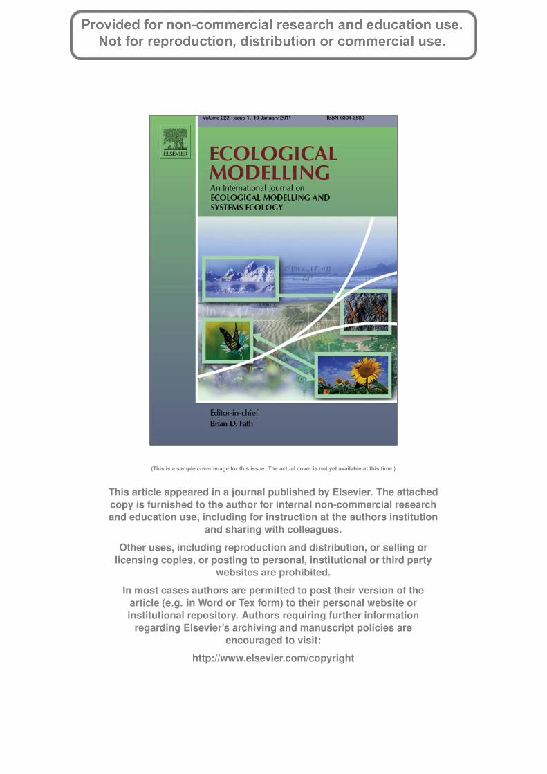
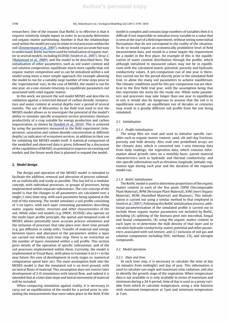
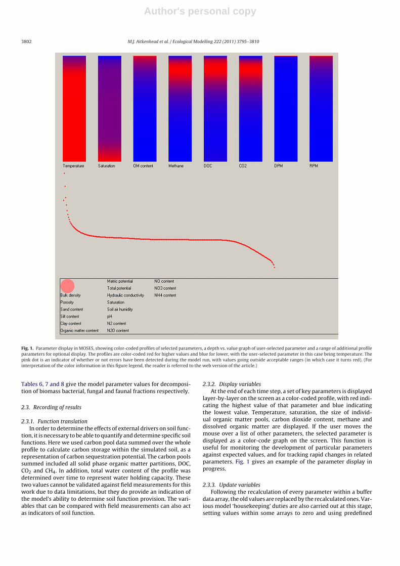
Fig. 1. Parameter display in MOSES, showing color-coded profiles of selected parameters, a depth vs. value graph of user-selected parameter and a range of additional profileparameters for optional display. The profiles are color-coded red for higher values and blue for lower, with the user-selected parameter in this case being temperature. Thepink dot is an indicator of whether or not errors have been detected during the model run, with values going outside acceptable ranges (in which case it turns red). (Forinterpretation of the color information in this figure legend, the reader is referred to the web version of the article.)

Tables 6, 7 and 8 give the model parameter values for decomposi-tion of biomass bacterial, fungal and faunal fractions respectively.

2.3. Recording of results

2.3.1. Function translationIn order to determine the effects of external drivers on soil func-

tion, it is necessary to be able to quantify and determine specific soilfunctions. Here we used carbon pool data summed over the wholeprofile to calculate carbon storage within the simulated soil, as arepresentation of carbon sequestration potential. The carbon poolssummed included all solid phase organic matter partitions, DOC,CO2 and CH4. In addition, total water content of the profile wasdetermined over time to represent water holding capacity. Thesetwo values cannot be validated against field measurements for thiswork due to data limitations, but they do provide an indication ofthe model’s ability to determine soil function provision. The vari-ables that can be compared with field measurements can also actas indicators of soil function.

2.3.2. Display variablesAt the end of each time step, a set of key parameters is displayed

layer-by-layer on the screen as a color-coded profile, with red indi-cating the highest value of that parameter and blue indicatingthe lowest value. Temperature, saturation, the size of individ-ual organic matter pools, carbon dioxide content, methane anddissolved organic matter are displayed. If the user moves themouse over a list of other parameters, the selected parameter isdisplayed as a color-code graph on the screen. This function isuseful for monitoring the development of particular parametersagainst expected values, and for tracking rapid changes in relatedparameters. Fig. 1 gives an example of the parameter display inprogress.

2.3.3. Update variablesFollowing the recalculation of every parameter within a buffer

data array, the old values are replaced by the recalculated ones. Var-ious model ‘housekeeping’ duties are also carried out at this stage,setting values within some arrays to zero and using predefined

Author's personal copy

M.J. Aitkenhead et al. / Ecological Modelling 222 (2011) 3795– 3810 3803

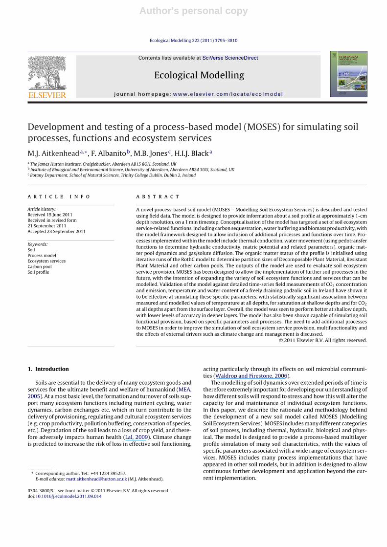
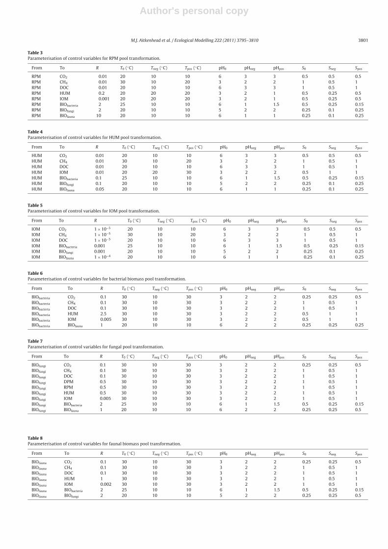
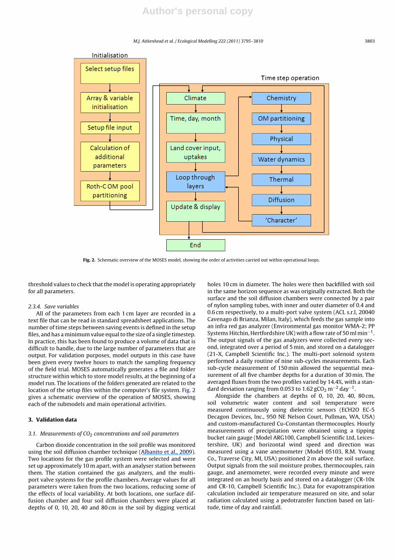
Fig. 2. Schematic overview of the MOSES model, showing the order of activities carried out within operational loops.

threshold values to check that the model is operating appropriatelyfor all parameters.

2.3.4. Save variablesAll of the parameters from each 1 cm layer are recorded in a

text file that can be read in standard spreadsheet applications. Thenumber of time steps between saving events is defined in the setupfiles, and has a minimum value equal to the size of a single timestep.In practice, this has been found to produce a volume of data that isdifficult to handle, due to the large number of parameters that areoutput. For validation purposes, model outputs in this case havebeen given every twelve hours to match the sampling frequencyof the field trial. MOSES automatically generates a file and folderstructure within which to store model results, at the beginning of amodel run. The locations of the folders generated are related to thelocation of the setup files within the computer’s file system. Fig. 2gives a schematic overview of the operation of MOSES, showingeach of the submodels and main operational activities.

3. Validation data

3.1. Measurements of CO2 concentrations and soil parameters

Carbon dioxide concentration in the soil profile was monitoredusing the soil diffusion chamber technique (Albanito et al., 2009).Two locations for the gas profile system were selected and wereset up approximately 10 m apart, with an analyser station betweenthem. The station contained the gas analyzers, and the multi-port valve systems for the profile chambers. Average values for allparameters were taken from the two locations, reducing some ofthe effects of local variability. At both locations, one surface dif-fusion chamber and four soil diffusion chambers were placed atdepths of 0, 10, 20, 40 and 80 cm in the soil by digging vertical

holes 10 cm in diameter. The holes were then backfilled with soilin the same horizon sequence as was originally extracted. Both thesurface and the soil diffusion chambers were connected by a pairof nylon sampling tubes, with inner and outer diameter of 0.4 and0.6 cm respectively, to a multi-port valve system (ACL s.r.l, 20040Cavenago di Brianza, Milan, Italy), which feeds the gas sample intoan infra red gas analyzer (Environmental gas monitor WMA-2; PPSystems Hitchin, Hertfordshire UK) with a flow rate of 50 ml min−1.The output signals of the gas analyzers were collected every sec-ond, integrated over a period of 5 min, and stored on a datalogger(21-X, Campbell Scientific Inc.). The multi-port solenoid systemperformed a daily routine of nine sub-cycles measurements. Eachsub-cycle measurement of 150 min allowed the sequential mea-surement of all five chamber depths for a duration of 30 min. Theaveraged fluxes from the two profiles varied by 14.4%, with a stan-dard deviation ranging from 0.053 to 1.62 gCO2 m−2 day−1.

Alongside the chambers at depths of 0, 10, 20, 40, 80 cm,soil volumetric water content and soil temperature weremeasured continuously using dielectric sensors (ECH2O EC-5Decagon Devices, Inc., 950 NE Nelson Court, Pullman, WA, USA)and custom-manufactured Cu-Constantan thermocouples. Hourlymeasurements of precipitation were obtained using a tippingbucket rain gauge (Model ARG100, Campbell Scientific Ltd, Leices-tershire, UK) and horizontal wind speed and direction wasmeasured using a vane anemometer (Model 05103, R.M. YoungCo., Traverse City, MI, USA) positioned 2 m above the soil surface.Output signals from the soil moisture probes, thermocouples, raingauge, and anemometer, were recorded every minute and wereintegrated on an hourly basis and stored on a datalogger (CR-10xand CR-10, Campbell Scientific Inc.). Data for evapotranspirationcalculation included air temperature measured on site, and solarradiation calculated using a pedotransfer function based on lati-tude, time of day and rainfall.

Author's personal copy

3804 M.J. Aitkenhead et al. / Ecological Modelling 222 (2011) 3795– 3810

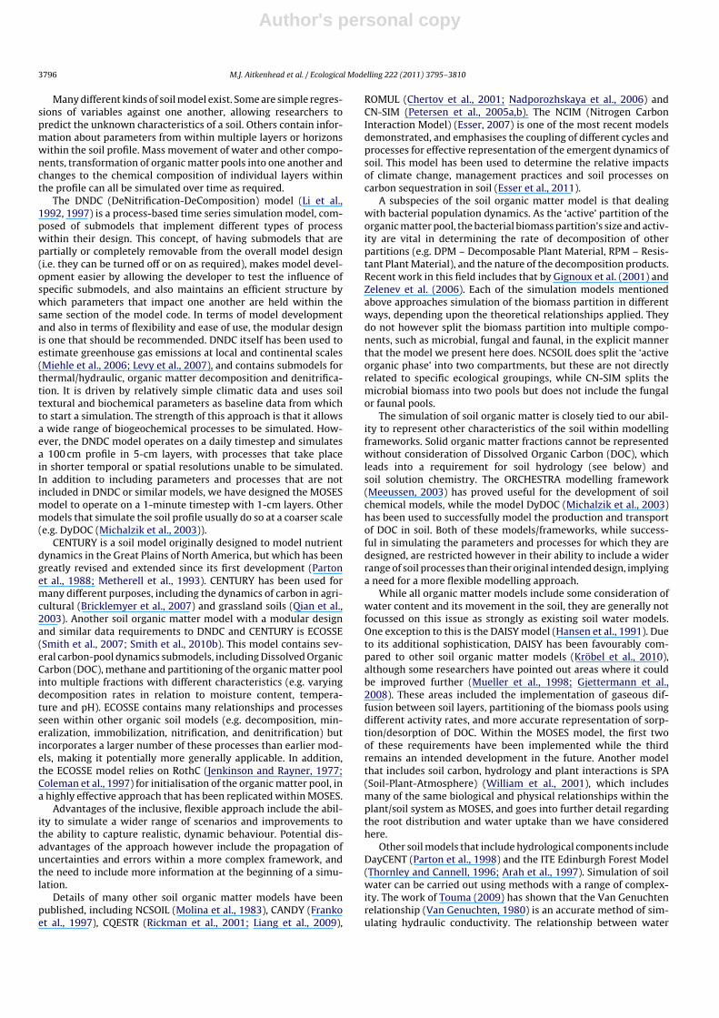
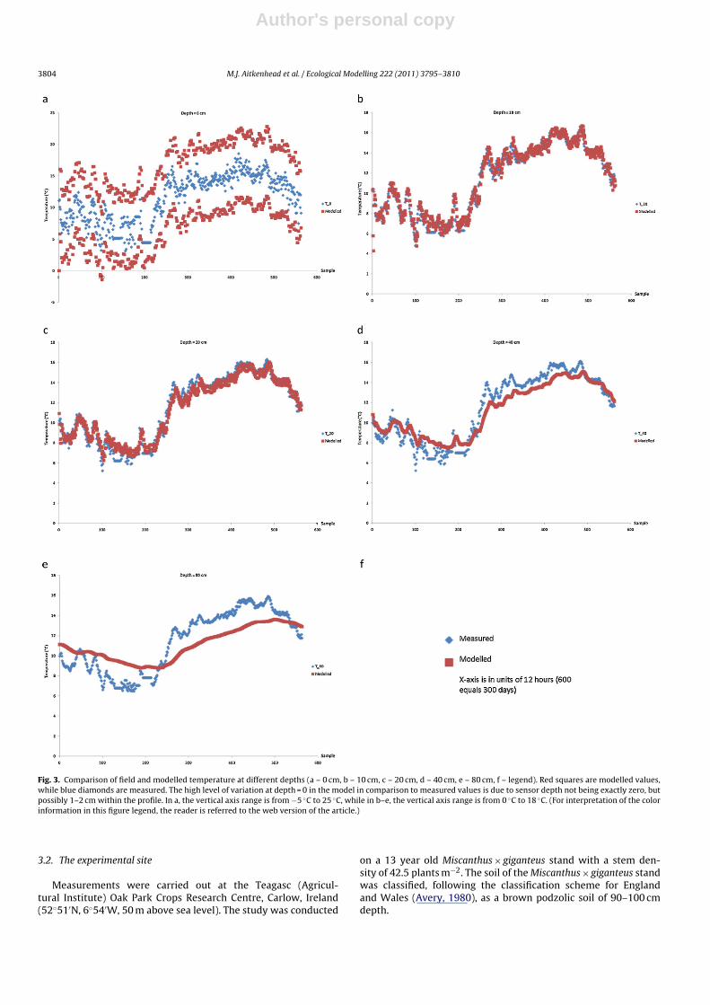
Fig. 3. Comparison of field and modelled temperature at different depths (a – 0 cm, b – 10 cm, c – 20 cm, d – 40 cm, e – 80 cm, f – legend). Red squares are modelled values,while blue diamonds are measured. The high level of variation at depth = 0 in the model in comparison to measured values is due to sensor depth not being exactly zero, butpossibly 1–2 cm within the profile. In a, the vertical axis range is from −5 ◦C to 25 ◦C, while in b–e, the vertical axis range is from 0 ◦C to 18 ◦C. (For interpretation of the colorinformation in this figure legend, the reader is referred to the web version of the article.)

3.2. The experimental site

Measurements were carried out at the Teagasc (Agricul-tural Institute) Oak Park Crops Research Centre, Carlow, Ireland(52◦51′N, 6◦54′W, 50 m above sea level). The study was conducted

on a 13 year old Miscanthus × giganteus stand with a stem den-sity of 42.5 plants m−2. The soil of the Miscanthus × giganteus standwas classified, following the classification scheme for Englandand Wales (Avery, 1980), as a brown podzolic soil of 90–100 cmdepth.

Author's personal copy

M.J. Aitkenhead et al. / Ecological Modelling 222 (2011) 3795– 3810 3805

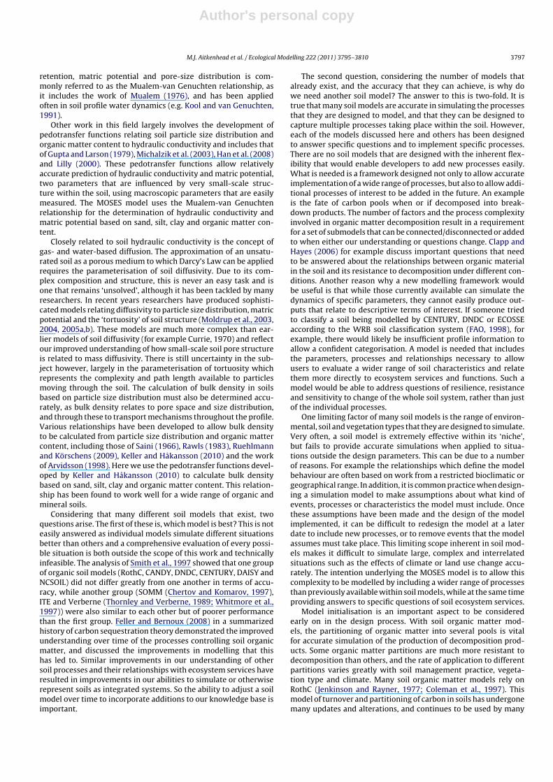
Fig. 4. Comparison of field and modelled saturation level at different depths (a – 0 cm, b – 10 cm, c – 20 cm, d – 40 cm, e – 80 cm, f – legend). Red squares are modelled values,while blue diamonds are measured. A lack of variation in saturation at depth in the model is due to issues with simulating correct water movement through unconsolidatedparent material below 1 m depth, and variation in the water table depth. In a, the vertical axis range is from 0% to 45%, while in b it is 0% to 30%, in c from 0% to 16%, in d from0% to 25% and in e from 0% to 12%. (For interpretation of the color information in this figure legend, the reader is referred to the web version of the article.)

The soil profile at the site was examined from the soil surfacedown to the bedrock and two well developed soil horizons wereidentified. A sandy silt loam A horizon was identified from the soilsurface to a depth of 35 cm, and sand with gravel Bh horizon wasidentified from a depth of 30 cm down to the bedrock at approxi-mately 100 cm.

4. Results

4.1. Temperature

Fig. 3 shows the measured vs. modelled temperature at depthsof 0, 10, 20, 40 and 80 cm within the soil profile, over the 281-day

Author's personal copy

3806 M.J. Aitkenhead et al. / Ecological Modelling 222 (2011) 3795– 3810

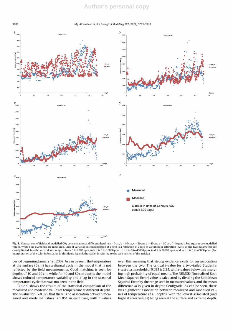
Fig. 5. Comparison of field and modelled CO2 concentration at different depths (a – 0 cm, b – 10 cm, c – 20 cm, d – 40 cm, e – 80 cm, f – legend). Red squares are modelledvalues, while blue diamonds are measured. Lack of variation in concentration at depth is a reflection of a lack of variation in saturation levels, as the two parameters areclosely linked. In a the vertical axis range is from 0 to 2000 ppm, in b it is 0 to 16000 ppm, in c it is 0 to 45000 ppm, in d it is 30000 ppm, and in e it is 0 to 40000 ppm. (Forinterpretation of the color information in this figure legend, the reader is referred to the web version of the article.)

period beginning January 1st, 2007. As can be seen, the temperatureat the surface (0 cm) has a diurnal cycle in the model that is notreflected by the field measurements. Good matching is seen fordepths of 10 and 20 cm, while for 40 and 80 cm depths the modelshows reduced temperature variability and a lag in the seasonaltemperature cycle that was not seen in the field.

Table 9 shows the results of the statistical comparison of themeasured and modelled values of temperature at different depths.The F-value for P = 0.025 that there is no association between mea-sured and modelled values is 5.051 in each case, with F values

over this meaning that strong evidence exists for an associationbetween the two. The critical t-value for a two-tailed Student’st-test at a threshold of 0.025 is 2.25, with t-values below this imply-ing high probability of equal means. The NRMSE (Normalised RootMean Squared Error) value is calculated by dividing the Root MeanSquared Error by the range seen in measured values, and the meandifference M is given in degree Centigrade. As can be seen, therewas significant association between measured and modelled val-ues of temperature at all depths, with the lowest associated (andhighest error values) being seen at the surface and extreme depth.

Author's personal copy

M.J. Aitkenhead et al. / Ecological Modelling 222 (2011) 3795– 3810 3807

Table 9Statistical comparison of measured and modelled temperature values at different depths. NRMSE = Normalised Root Mean Squared Error; M = mean temperature; t = t-testvalues.

r2 F Significant association? NRMSE M (◦C) t Significant bias?

T (0 cm) 0.4045 382 Yes 0.321 −0.172 0.585 NoT (10 cm) 0.9448 9750 Yes 0.067 −0.109 0.584 NoT (20 cm) 0.9526 11489 Yes 0.068 0.062 0.741 NoT (40 cm) 0.9235 6793 Yes 0.098 0.173 0.321 NoT (80 cm) 0.7517 1696 Yes 0.190 0.289 0.045 No

4.2. Saturation

Fig. 4 shows a comparison of the measured and simulated satu-ration for the profile. At shallow depths (0 and 10 cm) the simulatedsaturation shows peaks and troughs closely associated with thefield measurements. However, at depth, the model fails to simu-late the variability in soil saturation and instead describes a muchmore gradual change.

Table 10 gives the statistical comparison results for measuredand modelled values of saturation at different depths. The samethreshold F-values hold for significant association and bias as fortemperature, and the mean difference M is given in percentage ofsaturation. Association and mean error vary with depth, and below10 cm there is no significant association between measured andmodelled values, although the means are found to have no signifi-cant bias between them.

4.3. Carbon dioxide

In Fig. 5, we show the measured and simulated CO2 concentra-tions, in PPM, at the measurement depths. There is a large degree ofvariation within both the measured and simulated carbon dioxideconcentrations, with simulated day-to-day variation being muchgreater near the surface than at depth.

Table 11 shows the statistical comparison for measured andmodelled CO2 concentrations at different depths. Again, the samethreshold F-values apply for significant association and bias. Themean difference M is given in PPM. The only depth at which a sig-nificant association between measured and modelled values is notfound is at the surface, although absolute mean error increases withdepth. There is no significant bias between measured and modelledCO2 values. Disagreement between measured and modelled valuesat the surface is likely to be due to the rapid change in CO2 con-centration that occurs over a short distance near the surface, withslight differences between sensor depth and the depth at which themodelled results are taken from leading to the perceived error.

4.4. Soil functions

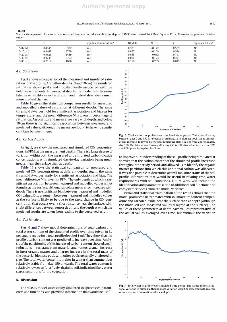
Figs. 6 and 7 show model determinations of total carbon andtotal water content of the simulated profile over time (given in kgper square metre for a total profile depth of 1 m). They show that theprofile’s carbon content was predicted to increase over time. Analy-sis of the partitioning of this increased carbon content showed smallreductions in resistant plant material and humus, a small increasein inert organic matter and a larger increase in the total mass ofthe bacterial biomass pool, with other pools generally unaltered insize. The total water content is higher in winter than summer, butrelatively stable from day 150 onwards. The total water content isrelatively low, even for a freely-draining soil, indicating likely waterstress conditions for the vegetation.

5. Discussion

The MOSES model successfully simulated soil processes, param-eters and functions, and provided information that would be useful

Fig. 6. Total carbon in profile over simulated time period. The upward swingbetween days 0 and 150 is reflective of an increase in biomass pool size as temper-atures increase, followed by the pool remaining stable in size from approximatelyday 150. The later upward swing after day 250 is reflective of an increase in DPMand RPM pools from plant leaf litter.

to improve our understanding of the soil profile being simulated. Itshowed that the carbon content of the simulated profile increasedthroughout the study period, and allowed us to identify the organicmatter partitions into which this additional carbon was allocated.It was also possible to determine overall moisture status of the soilprofile, information that would be useful in relating crop waterrequirements with soil conditions. Future work will include theidentification and parameterisation of additional soil functions andecosystem services from the model variables.

Visual and statistical examination of the results shows that themodel produces a better match with soil moisture content, temper-ature and carbon dioxide near the surface than at depth (althoughthe modelled and measured values disagree at the surface). Thevalues of these parameters at depth have values representative ofthe actual values averaged over time, but without the variation

Fig. 7. Total water in profile over simulated time period. The values reflect a sea-sonal variation in rainfall, although more variation would be expected with realisticrepresentation of saturation values at depth.

Author's personal copy

3808 M.J. Aitkenhead et al. / Ecological Modelling 222 (2011) 3795– 3810

Table 10Statistical comparison of measured and modelled saturation values at different depths. NRMSE = Normalised Root Mean Squared Error; M = mean saturation; t = t-test values.

r2 F Significant association? NRMSE M (%) t Significant bias?

S (0 cm) 0.2401 178 Yes 0.522 −4.08 0.000 NoS (10 cm) 0.0790 48 Yes 0.187 −0.49 0.000 NoS (20 cm) 0.0062 3.541 No 0.297 −2.01 0.000 NoS (40 cm) 0.0008 0.444 No 0.443 3.88 0.000 NoS (80 cm) 0.0001 0.037 No 0.379 −1.85 0.000 No

seen in the measured values. Statistical evaluation of the simulationshows a close match with all three variables down to 20 cm depth,with the correlation for saturation becoming greatly reduced belowthis depth. For CO2 concentration, simulated and measured valuesagreed well at 20 cm depth. However, in the soil layers deeper than40 cm, the level of agreement was reduced and the pattern in CO2throughout the year was not well represented. At 80 cm for exam-ple, the model could not reproduce a clear upward trend as wasseen in the experimental results.

We therefore conclude that while the model is parameterisedcorrectly and contains accurate implementations of the processesincluded, there is some mechanism or process that has not beenimplemented that is resulting in reduced accuracy at depth. If theprocesses that are present in the model had been implementedinaccurately, then errors would be expected to occur more evenlythroughout the profile.

From detailed interpretation of the simulation results, we pos-tulate that the main deficit in the model is in the calculation ofmoisture content at depth. Saturation level has a strong impact onbiomass activity and therefore CO2 production, and also to a strongdegree impacts on the thermal conductivity of the soil. The drainageof water out of the bottom of the profile is considered to be the mostlikely candidate for causing saturation problems at depth, as wehad assumed a low value of hydraulic conductivity for the parentmaterial (K = 10−9 ms−1). It is possible that the parent material, ifless consolidated, could have a higher hydraulic conductivity thanthis value. This would lead to a more freely draining soil at depth,resulting in higher variation in saturation over time. While the soilfrom which the field measurements were taken is considered fairlyrepresentative of soils in the region and is not therefore ‘unusual’, itdoes drain very freely and has higher clay content near the surfacethan at depth, both factors that will complicate the hydrodynamicsof the soil system in relation to the model. Further work will berequired to carry out sensitivity testing of MOSES to determine theeffects of moisture content, hydraulic conductivity and porosity ofparent material below the profile, and to produce a more accuraterepresentation. Specific changes to be made to MOSES to improvethe prediction of moisture content at depth include (a) the devel-opment of a more sophisticated parent material profile submodel,moving away from the current concept of a solid, relatively imper-meable mass right up to the bottom of the soil profile and towardsa more gradual transition between solid parent material at depthand structured soil at the profile base, and (b) inclusion of a setof processes for simulating the interactions between the soil waterand the water table itself, be it within the parent material or the soilprofile (e.g. fluctuations in water table depth with season, uptake ofwater from the water table when the soil matric potential increases,

diffusion of soil water chemical constituents between the soil waterand the water table).

A further error in the model that we have identified is thatof thermal transfer due to water movement. Currently, the onlytransfer of heat between layers takes place due to conduction, andwe have failed to consider the factor that water temperatures alsovary through the profile. As water moves between layers, it willalso be transporting thermal energy, and this could account for ahigher degree of thermal variation in the short term. This errorwill be revised in later work. Oversimplification of the vegetationsubmodel could also be causing prediction errors in moisture con-tent, with plant uptake at depth being more subject to variationthan has been represented here. We are also aware that the atmo-spheric conditions represented within the model have not takeninto account the effects of wind speed and atmospheric pressureon the diffusion of carbon dioxide out of the soil.

In addition to corrections to identified problems, further workon the model will include a more sophisticated plant water uptakesubmodel, as the current implementation of this does not takeinto account the response of different plant types to water stress.We also intend to validate MOSES against a wider variety of soil,climate and vegetation types, to identify further areas of improve-ment and missing processes that need to be implemented. One areaof addition that has been identified is that of bulk density and layerthickness. The variation of bulk density with organic matter contentas carbon is sequestered or lost, and the addition and removal ofsolid material from a layer, will lead to a requirement to adjust thelayer thickness. Currently, each layer is held at a constant 1 cm thick,which is physically unrealistic. Simulation of changes to layer thick-ness, and possibly even the addition of new ones or the removal oflayers that become thinner than some threshold value, would moreaccurately allow the simulation of changes to profile characteristicsover time. MOSES could also be used to simulate pedogenesis andtransformation of one soil type into another, with the inclusionof planned additional subroutines involving mineral weathering,clay/organic matter interactions and chemical equilibrium deter-mination.

The MOSES model has the potential to allow implementationof a greater range of processes than existing soil models, and todo so with finer temporal and profile depth resolution. This willallow more sophisticated simulation of soil development, and atthe same time give us the ability to express the model’s outputswithin a wider range of indicators. The MOSES model is designedto allow investigation of the effects of climate change, manage-ment practices and other drivers on soil ecosystem services. To dothis requires the ability to simulate a large number of processesat a wide range of spatial and temporal scales within the profile,

Table 11Statistical comparison of measured and modelled CO2 values at different depths. NRMSE = Normalised Root Mean Squared Error; M = mean concentration; t = t-test values.

r2 F Significant association? NRMSE M (PPM) t Significant bias?

CO2 (0 cm) 0.0008 0.456 No 0.223 −82 0.000 NoCO2 (10 cm) 0.2550 192 Yes 0.141 −351 0.002 NoCO2 (20 cm) 0.6147 895 Yes 0.095 48 0.891 NoCO2 (40 cm) 0.6790 1189 Yes 0.161 −1589 0.000 NoCO2 (80 cm) 0.3588 314 Yes 0.201 −3623 0.000 No

Author's personal copy

M.J. Aitkenhead et al. / Ecological Modelling 222 (2011) 3795– 3810 3809

and to relate these processes to soil properties that have directmeaning for land users. Future work will concentrate not only onimprovements and additions to the model itself, but also on theimplementation of mechanisms for interpreting the outputs in rela-tion to ecosystem services. Potential ecosystem service outputs thatcan be implemented using the model as it currently stands includebiomass productivity, carbon sequestration and water buffering,with these three services being extremely important for a widerange of human and environmental activities. In relation to the test-ing and application of MOSES, we have not yet carried out detailed,multi-factorial simulation experiments on how factors such as cli-mate, soil conditions and soil type impact upon soil processeswithin MOSES, but the intention is to do so. Once this work hasbeen carried out, the results will be reported in later publications.

Acknowledgements

The authors would like to thank Dr Marc Stutter for his advicein the development of this manuscript.

References

Albanito, F., Saunders, M., Jones, M.B., 2009. Automated diffusion chambers tomonitor diurnal and seasonal dynamics of the soil CO2 concentration profile.European Journal of Soil Science 60, 507–514.

Arah, J.R.M., Thornley, J.H.M., Poulton, P.R., Richter, D.D., 1997. Simulating trends insoil organic carbon in long-term experiments using the ITE (Edinburgh) Forestand Hurley Pasture ecosystem models. Geoderma 81 (1–2), 61–74.

Arvidsson, J., 1998. Influence of soil texture and organic matter content on bulkdensity, air content, compression index and crop yield in field and laboratorycompression experiments. Soil and Tillage Research 49 (1–2), 159–170.

Avery, B.W, 1980. Soil Classification for England and Wales: Higher Categories. Cran-field University, Soil Survey and Land Research Centre, Cranfield, England.

Bricklemyer, R.S., Miller, P.R., Turk, P.J., Paustian, K., Keck, T., Nielsen, G.A., 2007.Sensitivity of the century model to scale-related soil texture variability. SoilScience Society of America Journal 71 (3), 784–792.

Chertov, O.G., Komarov, A.S., 1997. SOMM: a model of soil organic matter dynamics.Ecological Modelling 94 (2–3), 177–189.

Chertov, O.G., Komarov, A.S., Nadporozhskaya, M., Bykhovets, S.S., Zudin, S.L., 2001.ROMUL—a model of forest soil organic matter dynamics as a substantial tool forforest ecosystem modelling. Ecological Modelling 138 (1–3), 289–308.

Clapp, C.E., Hayes, M.H.B., 2006. Milestones in soil organic matter studies. Soil Sci-ence 171 (6 Suppl. 1), S112–S115.

Coleman, K., Jenkinson, D.S., Crocker, G.J., Grace, P.R., Klír, J., Körschens, M., Poulton,P.R., Richter, D.D., 1997. Simulating trends in soil organic carbon in long-termexperiments using RothC-26.3. Geoderma 81 (1–2), 29–44.

Conrad, R., Klose, M., 1999. Anaerobic conversion of carbon dioxide to methane,acetate and propionate on washed rice roots. FEMS Microbiology Ecology 30(2), 147–155.

Dondini, M., Hastings, A., Saiz, G., Jones, M.B., Smith, P., 2010. The potential of Mis-canthus to sequester carbon in soils: comparing field measurements in Carlow.Ireland to model predictions. Global Change Biology Bioenergy 1 (6), 413–425.

Esser, G., 2007. Nitrogen carbon interaction model – NCIM, documentation:model version 3.00. Mitteilungen aus dem Institut für Pflanzenökologie derJustus–Liebig–Universität Giessen, 5 (in English), 57 pp.

Esser, G., Kattge, J., Sakalli, A., 2011. Feedback of carbon and nitrogen cycles enhancescarbon sequestration in the terrestrial biosphere. Global Change Biology 17,819–842.

F.A.O., 1998. World Reference Base for Soil Resources. Food and Agriculture Organi-zation of the United Nations, Rome.

Feller, C., Bernoux, M., 2008. Historical advances in the study of global terrestrial soilorganic carbon sequestration. Waste Management 28 (4), 734–740.

Franko, U., Crocker, G.J., Grace, P.R., Klír, J., Körschens, M., Poulton, P.R., Richter, D.D.,1997. Simulating trends in soil organic carbon in long-term experiments usingthe CANDY model. Geoderma 81 (1–2), 109–120.

Gignoux, J., House, J., Hall, D., Masse, D., Nacro, H.B., Abbadie, L., 2001. Design andtest of a generic cohort model of soil organic matter decomposition: The SOMKOmodel. Global Ecology and Biogeography 10 (6), 639–660.

Gjettermann, B., Styczen, M., Hansen, H.C.B., Vinther, F.P., Hansen, S., 2008. Chal-lenges in modelling dissolved organic matter dynamics in agricultural soil usingDAISY. Soil Biology and Biochemistry 40 (6), 1506–1518.

Gupta, S.C., Larson, W.E., 1979. Estimating soil water retention characteristics fromparticle size distribution, organic matter percent, and bulk density. WaterResources Research 15 (6), 1633–1635.

Han, H., Giménez, D., Lilly, A., 2008. Textural averages of saturated soil hydraulic con-ductivity predicted from water retention data. Geoderma 146 (1–2), 121–128.

Hansen, S., Jensen, H.E., Nielsen, N.E., Svendsen, H., 1991. Simulation of nitrogendynamics and biomass production in winter wheat using the Danish simulationmodel DAISY. Fertilizer Research 27 (2–3), 245–259.

Jenkinson, D.S., Rayner, J.H., 1977. The turnover of soil organic matter in some of theRothamsted classical experiments. Soil Science 123 (5), 298–305.

Keller, T., Håkansson, I., 2010. Estimation of reference bulk density from soil par-ticle size distribution and soil organic matter content. Geoderma 154 (3–4),398–406.

Kool, J.B., van Genuchten, M. Th., 1991. HYDRUS: One-dimensional variably satu-rated flow and transport model, including hysteresis and root water uptake.Version 3.3. Res. Rep. 124. U.S. Salinity Lab., Riverside, CA.

Kröbel, R., Sun, Q., Ingwersen, J., Chen, X., Zhang, F., Müller, T., Römheld, V., 2010.Modelling water dynamics with DNDC and DAISY in a soil of the North ChinaPlain: A comparative study. Environmental Modelling and Software 25 (4),583–601.

Lal, R., 2009. Soil degradation as a reason for inadequate human nutrition. FoodSecurity 1, 45–57.

Levy, P.E., Mobbs, D.C., Jones, S.K., Milne, R., Campbell, C., Sutton, M.A., 2007. Simu-lation of fluxes of greenhouse gases from European grasslands using the DNDCmodel. Agriculture, Ecosystems and Environment 121 (1–2), 186–192.

Li, C., Frolking, S., Crocker, G.J., Grace, P.R., Klír, J., Körchens, M., Poulton, P.R., 1997.Simulating trends in soil organic carbon in long-term experiments using theDNDC model. Geoderma 81 (1–2), 45–60.

Li, C., Frolking, S., Frolking, T.A., 1992. A model of nitrous oxide evolution from soildriven by rainfall events: 1. Model structure and sensitivity. Journal of Geophys-ical Research 97 (D9), 9759–9776.

Liang, Y., Gollany, H.T., Rickman, R.W., Albrecht, S.L., Follett, R.F., Wilhelm, W.W.,Novak, J.M., Douglas Jr., C.L., 2009. Simulating soil organic matter with CQESTR(v. 2. 0): Model description and validation against long-term experiments acrossNorth America. Ecological Modelling 220 (4), 568–581.

Lilly, A., 2000. The relationship between field-saturated hydraulic conductivity andsoil structure: Development of class pedotransfer functions. Soil Use and Man-agement 16 (1), 56–60.

Malamoud, K., McBratney, Alex.B., Minasny, B., Field, D.J., 2009. Modelling how car-bon affects soil structure. Geoderma 149 (1–2), 19–26.

Meeussen, J.C.L., 2003. ORCHESTRA: an object-oriented framework for implement-ing chemical equilibrium models. Environmental Science and Technology 37 (6),1178–1182.

M.E.A., 2005. MA (Millennium Ecosystem Assessment), Ecosystems and HumanWell-being: Synthesis. Island Press, Washington, DC, USA.

Metherell, A.K., Harding, L.A., Cole, C.V., Parton, W.J., 1993. CENTURY Soil organicmatter model environment. Technical documentation. Agroecosystem version4.0. Great Plains System Research Unit Technical Report, 4.

Michalzik, B., Tipping, E., Mulder, J., Lancho, J.F.G., Matzner, E., Bryant, C.L.,Clarke, N., Lofts, S., Esteban, M.A.V., 2003. Modelling the production andtransport of dissolved organic carbon in forest soils. Biogeochemistry 66 (3),241–264.

Miehle, P., Livesley, S.J., Feikema, P.M., Li, C., Arndt, S.K., 2006. Assessing productivityand carbon sequestration capacity of Eucalyptus globulus plantations using theprocess model Forest-DNDC: Calibration and validation. Ecological Modelling192 (1–2), 83–94.

Moldrup, P., Olesen, T., Komatsu, T., Yoshikawa, S., Schjønning, P., Rolston, D.E., 2003.Modeling diffusion and reaction in soils: X. A unifying model for solute and gasdiffusivity in unsaturated soil. Soil Science 168 (5), 321–337.

Moldrup, P., Olesen, T., Yoshikawa, S., Komatsu, T., Rolston, D.E., 2005b. Predictive-descriptive models for gas and solute diffusion coefficients in variably saturatedporous media coupled to pore-size distribution: II, Gas diffusivity in undisturbedsoil. Soil Science 170 (11), 854–866.

Moldrup, P., Olesen, T., Yoshikawa, S., Komatsu, T., Rolston, D.E., 2005a. Predictive-descriptive models for gas and solute diffusion coefficients in variably saturatedporous media coupled to pore-size distribution: I. Gas diffusivity in repackedsoil. Soil Science 170 (11), 843–853.

Moldrup, P., Olesen, T., Yoshikawa, S., Komatsu, T., Rolston, D.E., 2004. Three-porositymodel for predicting the gas diffusion coefficient in undisturbed soil. Soil ScienceSociety of America Journal 68 (3), 750–759.

Molina, J.A.E., Clapp, C.E., Shaffer, M.J., Chichester, F.W., Larson, W.E., 1983. NCSOIL,a model of nitrogen and carbon transformations in soil: description, calibration,and behaviour. Soil Science Society of America Journal 47 (1), 85–91.

Mualem, Y., 1976. A new model for predicting the hydraulic conductivity of unsat-urated porous media. Water Resources Research 12, 513–522.

Mueller, T., Magid, J., Jensen, L.S., Svendsen, H., Nielsen, N.E., 1998. Soil C and Nturnover after incorporation of chopped maize, barley straw and blue grassin the field: evaluation of the DAISY soil-organic-matter submodel. EcologicalModelling 111 (1), 1–15.

Nadporozhskaya, M.A., Mohren, G.M.J., Chertov, O.G., Komarov, A.S., Mikhailov, A.V.,2006. Dynamics of soil organic matter in primary and secondary forest succes-sion on sandy soils in the Netherlands: an application of the ROMUL model.Ecological Modelling 190 (3–4), 399–418.

Parton, W.J., Hartman, M., Ojima, D., Schimel, D., 1998. DAYCENT and its land surfacesubmodel: description and testing. Global and Planetary Change 19 (1–4), 35–48.

Parton, W.J, Stewart, J.W.B., Cole, C.V., 1988. Dynamics of C, N, P and S in grasslandsoils: a model. Biogeochemistry 5 (1), 109–131.

Petersen, B.M., Berntsen, J., Hansen, S., Jensen, L.S., 2005a. CN-SIM—a model for theturnover of soil organic matter. I. Long-term carbon and radiocarbon develop-ment. Soil Biology and Biochemistry 37 (2), 359–374.

Petersen, B.M., Jensen, L.S., Hansen, S., Pedersen, A., Henriksen, T.M., Sørensen, P.,Trinsoutrot-Gattin, I., Berntsen, J., 2005b. CN-SIM: a model for the turnover ofsoil organic matter. II. Short-term carbon and nitrogen development. Soil Biologyand Biochemistry 37 (2), 375–393.

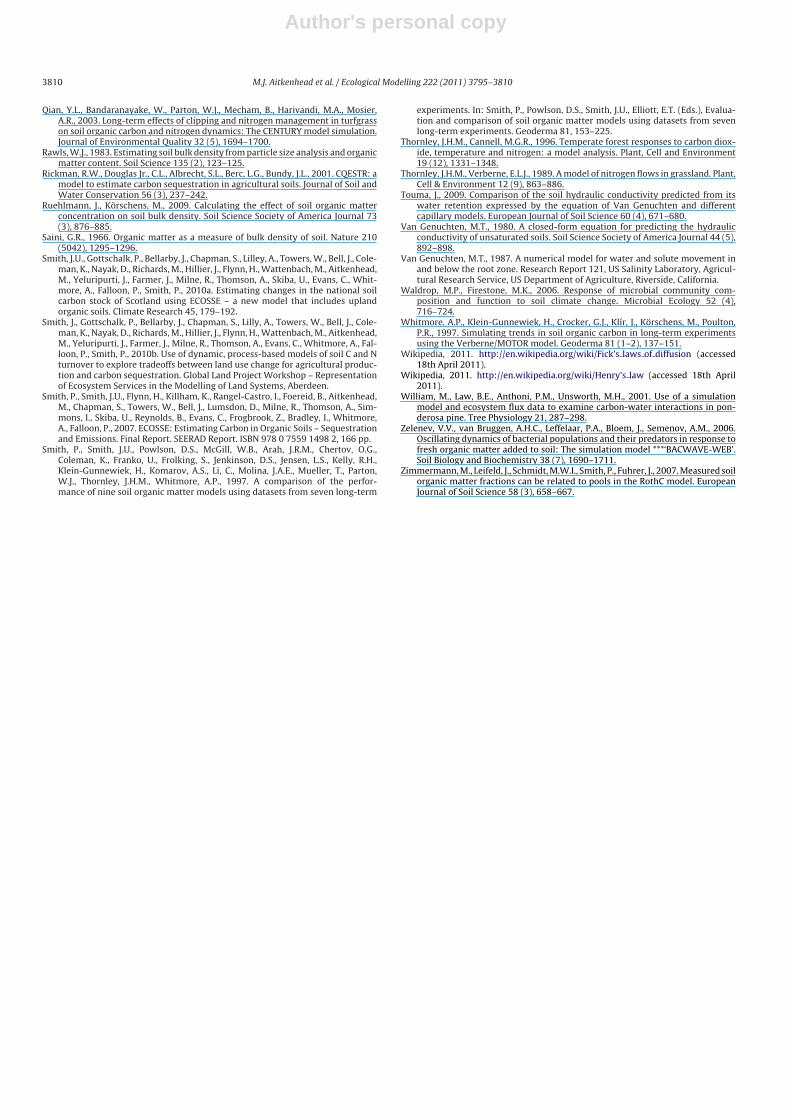
Author's personal copy

3810 M.J. Aitkenhead et al. / Ecological Modelling 222 (2011) 3795– 3810

Qian, Y.L., Bandaranayake, W., Parton, W.J., Mecham, B., Harivandi, M.A., Mosier,A.R., 2003. Long-term effects of clipping and nitrogen management in turfgrasson soil organic carbon and nitrogen dynamics: The CENTURY model simulation.Journal of Environmental Quality 32 (5), 1694–1700.

Rawls, W.J., 1983. Estimating soil bulk density from particle size analysis and organicmatter content. Soil Science 135 (2), 123–125.

Rickman, R.W., Douglas Jr., C.L., Albrecht, S.L., Berc, L.G., Bundy, J.L., 2001. CQESTR: amodel to estimate carbon sequestration in agricultural soils. Journal of Soil andWater Conservation 56 (3), 237–242.

Ruehlmann, J., Körschens, M., 2009. Calculating the effect of soil organic matterconcentration on soil bulk density. Soil Science Society of America Journal 73(3), 876–885.

Saini, G.R., 1966. Organic matter as a measure of bulk density of soil. Nature 210(5042), 1295–1296.

Smith, J.U., Gottschalk, P., Bellarby, J., Chapman, S., Lilley, A., Towers, W., Bell, J., Cole-man, K., Nayak, D., Richards, M., Hillier, J., Flynn, H., Wattenbach, M., Aitkenhead,M., Yeluripurti, J., Farmer, J., Milne, R., Thomson, A., Skiba, U., Evans, C., Whit-more, A., Falloon, P., Smith, P., 2010a. Estimating changes in the national soilcarbon stock of Scotland using ECOSSE – a new model that includes uplandorganic soils. Climate Research 45, 179–192.

Smith, J., Gottschalk, P., Bellarby, J., Chapman, S., Lilly, A., Towers, W., Bell, J., Cole-man, K., Nayak, D., Richards, M., Hillier, J., Flynn, H., Wattenbach, M., Aitkenhead,M., Yeluripurti, J., Farmer, J., Milne, R., Thomson, A., Evans, C., Whitmore, A., Fal-loon, P., Smith, P., 2010b. Use of dynamic, process-based models of soil C and Nturnover to explore tradeoffs between land use change for agricultural produc-tion and carbon sequestration. Global Land Project Workshop – Representationof Ecosystem Services in the Modelling of Land Systems, Aberdeen.

Smith, P., Smith, J.U., Flynn, H., Killham, K., Rangel-Castro, I., Foereid, B., Aitkenhead,M., Chapman, S., Towers, W., Bell, J., Lumsdon, D., Milne, R., Thomson, A., Sim-mons, I., Skiba, U., Reynolds, B., Evans, C., Frogbrook, Z., Bradley, I., Whitmore,A., Falloon, P., 2007. ECOSSE: Estimating Carbon in Organic Soils – Sequestrationand Emissions. Final Report. SEERAD Report. ISBN 978 0 7559 1498 2, 166 pp.

Smith, P., Smith, J.U., Powlson, D.S., McGill, W.B., Arah, J.R.M., Chertov, O.G.,Coleman, K., Franko, U., Frolking, S., Jenkinson, D.S., Jensen, L.S., Kelly, R.H.,Klein-Gunnewiek, H., Komarov, A.S., Li, C., Molina, J.A.E., Mueller, T., Parton,W.J., Thornley, J.H.M., Whitmore, A.P., 1997. A comparison of the perfor-mance of nine soil organic matter models using datasets from seven long-term

experiments. In: Smith, P., Powlson, D.S., Smith, J.U., Elliott, E.T. (Eds.), Evalua-tion and comparison of soil organic matter models using datasets from sevenlong-term experiments. Geoderma 81, 153–225.

Thornley, J.H.M., Cannell, M.G.R., 1996. Temperate forest responses to carbon diox-ide, temperature and nitrogen: a model analysis. Plant, Cell and Environment19 (12), 1331–1348.

Thornley, J.H.M., Verberne, E.L.J., 1989. A model of nitrogen flows in grassland. Plant,Cell & Environment 12 (9), 863–886.

Touma, J., 2009. Comparison of the soil hydraulic conductivity predicted from itswater retention expressed by the equation of Van Genuchten and differentcapillary models. European Journal of Soil Science 60 (4), 671–680.

Van Genuchten, M.T., 1980. A closed-form equation for predicting the hydraulicconductivity of unsaturated soils. Soil Science Society of America Journal 44 (5),892–898.

Van Genuchten, M.T., 1987. A numerical model for water and solute movement inand below the root zone. Research Report 121, US Salinity Laboratory, Agricul-tural Research Service, US Department of Agriculture, Riverside, California.

Waldrop, M.P., Firestone, M.K., 2006. Response of microbial community com-position and function to soil climate change. Microbial Ecology 52 (4),716–724.

Whitmore, A.P., Klein-Gunnewiek, H., Crocker, G.J., Klír, J., Körschens, M., Poulton,P.R., 1997. Simulating trends in soil organic carbon in long-term experimentsusing the Verberne/MOTOR model. Geoderma 81 (1–2), 137–151.

Wikipedia, 2011. http://en.wikipedia.org/wiki/Fick’s laws of diffusion (accessed18th April 2011).

Wikipedia, 2011. http://en.wikipedia.org/wiki/Henry’s law (accessed 18th April2011).

William, M., Law, B.E., Anthoni, P.M., Unsworth, M.H., 2001. Use of a simulationmodel and ecosystem flux data to examine carbon-water interactions in pon-derosa pine. Tree Physiology 21, 287–298.

Zelenev, V.V., van Bruggen, A.H.C., Leffelaar, P.A., Bloem, J., Semenov, A.M., 2006.Oscillating dynamics of bacterial populations and their predators in response tofresh organic matter added to soil: The simulation model ***‘BACWAVE-WEB’.Soil Biology and Biochemistry 38 (7), 1690–1711.

Zimmermann, M., Leifeld, J., Schmidt, M.W.I., Smith, P., Fuhrer, J., 2007. Measured soilorganic matter fractions can be related to pools in the RothC model. EuropeanJournal of Soil Science 58 (3), 658–667.