DEVELOPMENT AND APPLICATION OF EXPERIMENTAL …

DEVELOPMENT AND APPLICATION OF EXPERIMENTAL SOFTWARE FOR

A 21ST CENTURY OCCUPATIONAL PSYCHOPHYSICS RESEARCH TOOL-

BOX

HARSHA BANDARALAGE

Bachelor of Science, University of Saskatchewan, 2012

A Thesis

Submitted to the School of Graduate Studies

Of the University of Lethbridge

In Partial Fulfilment of the

Requirements for the Degree

MASTER OF SCIENCE

Department of Kinesiology

University of Lethbridge

LETHBRIDGE, ALBERTA, CANADA

© HARSHA BANDARALAGE, 2018

DEVELOPMENT AND APPLICATION OF EXPERIMENTAL SOFTWARE FOR

A 21ST CENTURY OCCUPATIONAL PSYCHOPHYSICS RESEARCH TOOL-

BOX

HARSHA BANDARALAGE

Date of Defence: August 28, 2018

Dr. J. Doan Associate Professor Ph. D

Supervisor

Dr. C. Gonzalez Associate Professor Ph. D

Thesis Examination Committee Member

Dr. M. Tata Associate Professor Ph. D

Thesis Examination Committee Member

I. Wong Instructor M.Sc

Chair, Thesis Examination Committee

iii

Dedication

This thesis is dedicated to my parents, the two individuals I will forever be in debt

to. Thank you for raising me to be the person I am today, and for the countless sacrifices

you have had to make over the years just so your children could have a better future than

you ever had.

iv

Abstract

In the fields of ergonomics and biomechanics, the use of bio-instrumentation for the

purpose of analysing work and reducing work related muskuloskeletal disorders for injury

prevention has become a new norm. It is equally important to employ these instruments in

ecologically-valid experimental work tasks that use relevant and controllable

manipulations of occupational psychophysics. The current thesis attempts to begin design

and validation of components for a 21st century occupational psychophysics toolbox that

couples relevant bio-instrumentation hardware (vision tracking, motion capture, and force

platforms) with custom Matlab based experimental software capable of image processing,

assessment of full body kinematics, and analysis of ground reaction force kinetics to study

the perceptions and actions at work tasks. I investigated the coupling between visual

attention and cueing, pre-handling perceptions, and manual material handling actions, with

the ultimate goal of understanding occupational behaviours and preventing injurious

occupational behaviours.

v

Acknowledgements

Thank you to Dr. Jon Doan, my supervisor, without whose support I couldn’t have

accomplished what I have been able to over the past 4 years. Thank you for believing in

me and my abilities, and providing me with proper guidance while encouraging me to stand

on my own. I will forever be grateful for the opportunity you’ve given me to shape up my

future career.

Thank you to Dr. Jarrod Blinch for your support and friendly advice that helped me

manage my research projects. You were a pleasure to work with, and I truly appreciate all

the small pointers you’ve given me over the years.

Thank you to my two lab colleagues, Dustin McCubbing and Brittany Mercier, who

helped me countless times in the lab with numerous tasks related to my research. You were

a pleasure to work with, and I couldn’t have asked for two better individuals to share my

graduate study journey with.

Thank you to the two undergraduate colleagues, Marina de Costa and Mellina

Fujihara, who helped me with data collection for my experiments. I appreciate your

dedication and willingness to assist me with my research, and wish you all the best with

your future endeavours.

Thank you to my wife, my constant support system over the past few years, for

motivating me and encouraging me to pursue my dreams and allowing me to achieve my

goals.

vi

Table of Contents

Dedication ....................................................................................................................................... iii Abstract ........................................................................................................................................... iv Acknowledgements ......................................................................................................................... v Table of Contents ........................................................................................................................... vi List of Tables ................................................................................................................................ viii List of Figures ................................................................................................................................. ix List of Abbreviations ...................................................................................................................... x 1.0 Bio-instrumentation ................................................................................................................. 1 1.1 Bio-instrumentation Components .......................................................................................... 1

1.1.1 Measurand .......................................................................................................................... 1 1.1.1.1 Bio-electric Measurands .............................................................................................. 3 1.1.1.2 Bio-magnetic Measurands ............................................................................................ 3 1.1.1.3 Bio-mechanical Measurands ........................................................................................ 4 1.1.1.4 Bio-chemical Measurands ............................................................................................ 5 1.1.1.5 Bio-hydraulic Measurands ........................................................................................... 5

1.1.2 Sensors ................................................................................................................................ 6 1.1.3 Signal Processing ................................................................................................................. 7 1.1.4 Output ............................................................................................................................... 11 1.1.5 Feedback Signal ................................................................................................................. 12

1.2 Bio-instrumentation potential in occupational biomechanics and psychophysics ........... 13 1.2.1 Vision Tracking .................................................................................................................. 17 1.2.2 Motion Capture ................................................................................................................. 20 1.2.3 Force Platforms ................................................................................................................. 24 1.2.4 Experimental Software ..................................................................................................... 26

1.3 Summary ................................................................................................................................. 32 1.4 Outline ..................................................................................................................................... 33 2.0 Quantifying Visual Attention for a Manual Materials Handling Task ............................. 34 2.1 Introduction ............................................................................................................................ 34 2.2 Methods ................................................................................................................................... 36

2.2.1 Study 1 .............................................................................................................................. 36 2.2.1.1 Experiment ................................................................................................................. 36 2.2.1.2 Protocol ...................................................................................................................... 39

2.2.2 Study 2 .............................................................................................................................. 39 2.2.2.1 Experiment ................................................................................................................. 39 2.2.2.2 Protocol ...................................................................................................................... 40

2.3 Analysis ................................................................................................................................... 40 2.4 Results ..................................................................................................................................... 43

2.4.1 Study 1 .............................................................................................................................. 43 2.4.2 Study 2 .............................................................................................................................. 48

2.5 Discussion ................................................................................................................................ 52 2.6 Conclusion .............................................................................................................................. 53 3.0 System Engineering Analysis of a Manual Materials Handling Task ............................... 54 3.1 Introduction ............................................................................................................................ 54 3.2 Method .................................................................................................................................... 57

3.2.1 Experiment: ....................................................................................................................... 57

vii

3.2.2 Protocol ............................................................................................................................. 58 3.2.3 Analysis ............................................................................................................................. 61

3.2.3.2 Kinematic Analysis .................................................................................................... 63 3.3 Results ..................................................................................................................................... 65

3.3.1 Affordances ....................................................................................................................... 65 3.3.2 Kinematics ......................................................................................................................... 67 3.3.3 Kinetics .............................................................................................................................. 73

3.4 Discussion ................................................................................................................................ 79 4.0 Global Discussion ................................................................................................................... 81 4.1 Introduction ............................................................................................................................ 81 4.2 Study 1..................................................................................................................................... 83 4.3 Study 2..................................................................................................................................... 85 4.4 Study 3..................................................................................................................................... 87 4.5 Software Development ........................................................................................................... 89

4.5.1 Vision Tracking Software ................................................................................................... 89 4.5.2 Kinetic Analysis Software .................................................................................................. 90 4.5.3 Synthesis ........................................................................................................................... 91

4.6 Limitations .............................................................................................................................. 92 4.7 Future Directions ................................................................................................................... 93 REFERENCES ............................................................................................................................. 95 Appendix A ................................................................................................................................. 105 Appendix B ................................................................................................................................. 106 Appendix C ................................................................................................................................. 113

viii

List of Tables

Table 3. 1 Tabulated results of the coefficients a0 and bn of the transfer functions ........... 74

ix

List of Figures

Figure 1. 1 A theoretical bio-instrumentation system .......................................................... 2

Figure 1. 2 A typical occupational work station. ............................................................... 16

Figure 1. 3 Recreating a suitcase handling work task in the laboratory ............................ 16

Figure 2. 1 Suitcase orientation during the handling task. ................................................. 38

Figure 2. 2 Handling motivation results. ........................................................................... 45

Figure 2. 3 Handling frequency results. ............................................................................. 45

Figure 2. 4 Attraction Index (AI) results. .......................................................................... 46

Figure 2. 5 Heat map results. ............................................................................................. 47

Figure 2. 6 Handling results from study 2 ......................................................................... 50

Figure 2. 7 Heat map results from study 2. ........................................................................ 51

Figure 3. 1 The experiment 3 setup ................................................................................... 60

Figure 3. 2 Horizontally placed suitcase with the two visual cue types. ........................... 60

Figure 3. 3 Normalized perceived affordance distances .................................................... 66

Figure 3. 4 Comparison of the x-factor angle for the three visual cueing groups. ............ 68

Figure 3. 5 Maximum shoulder rotation angle ................................................................... 70

Figure 3. 6 Comparison of maximum hip rotation angle ................................................... 70

Figure 3. 7 Comparison of maximum trunk lateral flexion angle ...................................... 71

Figure 3. 8 Maximum trunk axial rotation velocity. .......................................................... 72

Figure 3. 9 Comparison of the three visual cueing groups’ center of pressure (CoPr)

displacement ...................................................................................................................... 76

Figure 3. 10 Gender comparison of CoPr displacement results ......................................... 78

x

List of Abbreviations

AI – Attraction Index

MMH – Manual Materials Handling

ECG – Electrocardiogram

EMG – Electromyogram

EEG – Electroencephalogram

EOG – Electrooculograms

ERG – Electroretinograms

EDG - Electrodermograms

MCG – Magnetocardiogram

MMG – Magnetomyogram

MEG – Magnetoencephelogram

MSD – Muskuloskeletal Disorder

LED – Light Emitting Diode

GRF – Ground Reaction Force

COP – Centre of Pressure

COPx – Centre of Pressure in x-direction

COPy – Centre of Pressure in y-direction

COPr – Centre of Pressure resultant vector

ROI – Region of Interest

APA – Anticipatory Postural Adjustment

CoM – Centre of Mass

1

1.0 Bio-instrumentation

Bio-instrumentation is the measurement of living systems with bio-electronic

instruments, for the purpose of detecting, recording, processing and transmitting

physiological and behavioural information (Wise, 1991). Bio-instrumentation emphasizes

common principles and unique problems associated with making measurements in living

systems. A theoretical bio-instrument system is a combination of biology, sensors, interface

electronics, microcontrollers and computer programming, designed, validated, and

synchronized through the application of multiple disciplines including biology, optics,

mechanics, mathematics, electronics, and computer science (Enderle, 2006). The typical

construction of a bio-instrument contains numerous technical components that are designed

to complete unique tasks, including measuring, acquiring, processing, displaying, and

storing bio-information of biological systems (Figure 1.1).

1.1 Bio-instrumentation Components

1.1.1 Measurand

The physical quantity or the condition that can be measured using a bio-instrument

system is called the measurand (Figure 1.1). A measurand is a collective term for all kinds

of signals that can be measured and monitored from a living organism and can be

categorized according to the source that generates the signal and the kind of energy they

handle. The main measurand types are electrical, magnetic, mechanical, chemical, and bio-

hydraulic signals (Singh, 2011).

2

Figure 1. 1 A theoretical bio-instrumentation system using sensors to measure bio-signals

with data acquisition, storage and display capabilities, along with calibration and feedback

signals.

3

1.1.1.1 Bio-electric Measurands

Bio-electric signals are the electric signals that have a biological origin, and can be

generated by a particular anatomical structure such as a muscle or the brain, or a chemical

or a mechanical signal that is converted to an electric signal (Enderle, 2006). These

electrical signals are manifested as differences of potential between two points located in

some place of the living organism, either inside or on its surface (Valentinuzzi, 2004).

Valentinuzzi (2004), describes two types of bio-electrical signals that exist: traditional and

non-traditional bio-electrical signals. Traditional bio-electrical signals are the ones that are

generated by excitable tissues such as the nerve, skeletal muscle, cardiac muscle and

smooth muscles. These signals are gathered with the use of relatively large differential

electrodes such as electrocardiogram (ECG), electromyogram (EMG), and

electroencephalogram (EEG). On the other hand, the non-traditional bio-electric signals are

generated by other tissues such as the eye, or the skin which are capable of producing small

differences in potential. To capture bio-electric signals originated from the eye, bio-

engineers use electrooculograms (EOGs), and electroretinograms (ERGs), whereas

electrodermograms (EDGs) are used to capture electrical signals coming off of skin.

Therefore, generally, bio-electric signals provide researchers a proportional reflection of

bio-activity happening in a localized area of a living organism.

1.1.1.2 Bio-magnetic Measurands

The term bio-magnetism refers to magnetic fields generated by biological systems.

Bio-magnetic sources can be found in electric currents in diamagnetic, paramagnetic and

ferromagnetic substances found in the body (Williamson et al, 1983). Diamagnetic

substances such as water or water based bio-materials have a relative magnetic permeability

4

that is less than or equal to one, thus resulting in being repelled by the presence of a

magnetic field. Paramagnetic substances include most chemical elements and some

compounds, of which the relative magnetic permeability is greater than or equal to one,

therefore being attracted by external magnetic fields. Ferromagnetic substances such as iron

are the strongest type of magnetism, and they intensify the external magnetic fields

extremely when present. Just as for the case in bio-electric measurands, bio-magnetic

measurands are captured by an array of different bio-instruments that include

magnetocardiogram (MCG), magnetomyogram (MMG) and magnetoencephelogram

(MEG).

1.1.1.3 Bio-mechanical Measurands

Study of any moving organ, tissue, or systems of tissues with the methods of

mechanics is called bio-mechanics. The skeletal voluntary muscles, the involuntary

rhythmic contracting myocardium, all smooth muscles covering blood vessels produce bio-

mechanical signals that can be measured using various bio-instruments. Within all these

bio-mechanical signals, force, length, and angular changes are manifested as basic events

(measurements), while tension, acceleration and torque takes place as more complex events

(derivations). The electrical signals of skeletal, cardiac and smooth muscles trigger their

respective contractions, and thus, they develop force, F, usually accompanied by a change

in muscular length, L. The rate at which F and L change over time is an indication of

contractility that quantifies velocity of contraction and can be recorded using myograms

and cardiomyograms. Human locomotion and gait mechanics is a subject that was

pioneered by D.A Winter, and has been explored thoroughly over the years by countless

number of researchers (Winter, 1989; Davis et al., 1991; Hreljac, 1995; Medved, 2001). In

5

these studies, special attention is given to kinematic variables, in which bio-mechanical

modelling can be used to characterize locomotion and other fundamental behaviours by

treating the body as a complex multi-segmental mechanical system. Limbs, trunk, neck,

and head are modelled as segments linked with angular movements that generate specific

torques.

1.1.1.4 Bio-chemical Measurands

Bio-chemical signals generated from the human body include partial pressures of

the gasses in the blood, lungs and other tissues as well as concentrations of metabolites

(Singh, 2011). The metabolites are the substances that are necessary for certain metabolic

process in the body. These include glucose in the metabolism of sugar, starches, and amino

acids in the process of bio-synthesis of protein. Measuring the concentration of various ions

inside and in the vicinity of a cell by means of specific ion electrodes is an example of such

a signal. The bio-chemical signals produced by humans could depend on various factors

such as whether the person is at rest or in motion, ambient temperature and air pressure,

and oxygen content of the air. Special sensors are required to monitor these chemical

changes especially given the fact that these measures are invasive and at times need to be

observed over a long period of time. In return, they provide physicians and researchers with

specific characteristics of organs and tissues that are useful in treating patients with various

conditions.

1.1.1.5 Bio-hydraulic Measurands

Bio-hydraulics refers to the pressure and flow developed by fluids in certain body

cavities. In particular, hemodynamics, a sub category of bio-hydraulics, is of particular

interest to the medical professionals, where they study cardiovascular compartments and

6

their moving blood contents. Arterial blood pressure and blood flow are the two main bio-

hydraulic events that the researchers are interested in, and bio-instruments such as

sphygmomanometers and laser Doppler blood flowmeters are available in today’s industry

to measure these activities. Bio-hydraulic signals are also measured through one’s heartbeat

using a stethoscope, where the hydraulic events are being emitted as audible signals.

1.1.2 Sensors

In a bio-instrumentation system, a measurand is detected and converted to an

electrical signal with the use of a sensor or a transducer (Figure 1.1). The terms sensor and

transducer are used interchangeably in various literature, however it is important to

understand the subtle differences between the two terms. Strictly speaking, a sensor just

detects the signal under the original type of energy (electrical, mechanical, thermic,

magnetic, or chemical), whereas the transducer only transforms the small amount of energy

contained in a biological signal into electrical energy (Valentinuzzi, 2004). Thus, a

transducer literally ‘translates’ energy, but it requires a sensor, which is often well

immersed in the transducer, making it impossible to separate them. The aim of a sensor is

to produce an electronic signal which is proportional to the concentration of a specific

chemical or set of chemicals in a biological element (Turner et al., 1987). A sensor is

designed to minimize the disturbance to the measured variable and its environment, comply

with the requirements of the living system, and to offer maximum clarity to the input signal.

Some transducers’ output changes in response to a change in surroundings. These

outputs include resistance, capacitance or inductance. The variations in these different

outputs can be measured using a Wheatstone bridge circuitry organization such as strain

gauges, potentiometers, thermistors, and photoresistors (Valentinuzzi, 2004). The other

7

type of transducers produce a voltage or current in response to a change in environment.

Some examples include piezoelectric crystals, linear variable differential transformers, and

thermocouples. In both cases, sensors work as analytical tools that combine a bio-signal

recognition component off the human body with a physical transducer. The biological

sensing elements can be an enzyme, antibody, DNA sequence, or a microorganism.

Biosystems within an individual’s body selectively cause a bio-chemical reaction, which

the transducer converts into a measurable signal, thus providing the means of detecting it.

Sensors also have the capability of making use of a neural interface technology to detect

nerve and muscle activity. Electrodes that sit on the skin can measure muscle electrical

activity, brain electrical activity and eye movement (Tonneson & Withrow, 2006). The

electrical signals that the brain uses to control functions of human body have certain

measurable qualities including intensity and spectral characteristics, and that is exactly

what the sensors detect in order make associations between neural activities and animal

behaviors.

1.1.3 Signal Processing

The output from the bio-sensors are analog signals, which are continuous, and

require signal processing in order to comprehend and make inferences. These analog

signals are usually converted into digital format with the use of an analog to digital (A/D)

converter to make the signal storage and analysis more efficient and flexible. With the

recent developments in digital hardware and software technology, the digital techniques

offer much more powerful, easily implementable complex algorithms that are accurate and

not affected by unpredictable variables such as component aging and temperature. At the

8

same time, digital techniques allow the users to change and update design parameters more

freely by allowing recurring software modifications.

In bio-medical applications, acquiring a bio-signal directly via a sensor is not

sufficient most of the time, as the signals can be buried with many other irrelevant signals

(noise), or they might not be detectable from the outset. That is where signal processing

with the use of different transformation methods is required to enhance the signal, so that

the required information can be obtained. The processing of bio- signals poses some unique

challenges. This is mainly due to the complexity of the underlying system, and the need to

perform indirect, non-invasive measurements without altering the original signal. There are

a multitude of processing methods and algorithms that are currently available to bio-

medical engineers, however, in order to be successful, one must have a good understanding

of the goal of processing, test conditions and the underlying signal.

In signal processing, bio-signals are categorized into two main classes depending

on the signal characteristics. These two classes are continuous signals, which provide

information about the signal at any given time, and discrete signals that provide information

at a specific point in time. Most bio-signals are continuous, however, most of the current

signal processing tools are designed to process discrete signals, thus, bio- engineers tend to

transform continuous signals into discrete signals whenever it is possible (Proakis &

Manolakis, 1988).

Both continuous and discrete signals can be divided into two main groups called

deterministic and stochastic signals depending on their wave patterns (Cohen, 1986).

Deterministic signals are the ones that can be described exactly mathematically or

graphically. Real world bio-signals are never deterministic as there are always some

9

unknown and unpredictable noise associated with them that render them non-deterministic.

However, bio-analysts often model bio-signals as of deterministic waveforms in order to

simplify analysis and to make predictions with regards to signals’ behaviors. Deterministic

signals can be further divided into two categories as periodic and non-periodic signals.

Periodic signals have a basic wave form that repeats continuously on the time axis.

Sinusoidal signals, the most common type, are often used as the basis to model much more

complex periodic signals, in order to simplify their behaviours. On the other hand, most

deterministic signals are non-periodic and can be modelled as “almost periodic”. A good

example is the waveform of an ECG signal that has a variable period length and changes

its shape after every heartbeat and thus clearly a non-periodic waveform. Under certain

conditions such as a composite ECG consisting of maternal and fetal signal, however, the

period length can be almost constant, while continuing an identical wave shape which can

be modelled as an “almost periodic” wave form (Kay, 1988).

The other group of signals, stochastic signals, represent sample functions of a

stochastic process. This process produces sample functions, the infinite collection of which

is called the ensemble. Each sample function differs from the other in its fine details;

however, they all share the same distribution probabilities, i.e. random distribution

characteristics (Cohen, 1986). Stochastic signals can be categorized into stationary and

non-stationary signals depending on their corresponding structures. Stationary stochastic

processes are processes whose structures do not change in time, whereas non-stationary

processes are time dependant and require complex methods in which they cut the signal

durations into small segments, so that they can be considered as stationary.

10

The bio-signals collected by the sensors are generally represented in the time

domain, which characterizes the behavior of the signal with respect to time. However, often

in signal processing, these time domain signals are converted into frequency domain in

order to simplify the analysis process. There are multiple methods available to transform

time domain signals into frequency domain, but the most common transformation principle

is called the Fourier transform. Fourier transform is used to convert a signal of any shape

into a sum of infinite number of sinusoidal waves which makes the analyzing procedure

much simpler (Weitkunat, 1991). The other transform methods include Laplace transform

that is used in electronic circuits and control systems, Z transform that is commonly used

in digital signal processing, and Wavelet transform that is mainly used in image analysis

and data compression (Chui, 1992).

As mentioned earlier, bio-signals are often weak signals contaminated by noise.

When a bio-signal is acquired using a transducer from a certain muscle or elsewhere, it not

only picks up the electric potential generated by that certain muscle, but also from the

surrounding active muscles. Additional noise may also come from other electrical sources

surrounding the transducer which can be considered as random errors. Also, faulty

instruments as well as procedural errors caused by the researchers that are considered as

systematic errors may contaminate the bio-signal furthermore. Therefore, the first step of

signal processing is to enhance the signal by “cleaning” the noise without distorting the

signal. This is achieved by designing various types of filters (i.e. low-pass, high-pass, stop

band, Weiner, matched, etc.) and running the signals through them. Generally, a multi-

layered filtering process is sufficient to remove noise in most signals, however there are

instances where the signal and noise bandwidth overlap and noise amplitude is enough to

11

seriously corrupt or distort the signal. In such cases, desired response cannot be achieved

via traditional filtering (Aunon et al., 1981) and requires a process called averaging. Signal

averaging is a technique applied in the time domain that increases the strength of a signal

relative to noise that is obscuring it. It sums a set of temporal epochs of the signal together

with the superimposed noise, and by averaging them, the signal to noise ratio is increased,

allowing the users to remove noise relatively easy.

1.1.4 Output

Once the analog signals are digitized, they can be processed and stored in

specialized digital computers or micro-controllers (Tompkins and Webster, 1981), where

various types of signal conditioning can be applied.

Once the signal conditioning is completed, the results of the measurement process

need to be displayed to the user in a format that is easy and effective to comprehend. Such

formats may include numerical and graphical displays that exhibit data continuously or

discretely, in a permanent or a temporary manner. These data displaying methods are part

of an ever evolving field called data visualization, where the results are dependent on

efficient computational methods capable of achieving desired levels of interactivity with

the audience (Bajaj, 1998). In addition to displaying the processed digital signals, bio-

instruments are also capable of storing data, where they may be stored temporarily for short

term analysis, or permanently recorded for future reference. With the development of new

information technology in the recent years, data transmission has also been integrated into

bio-instruments, where collected data can be transmitted to various other instrumentation

systems for further analysis.

12

There are many other task specific components that are available for bio-

instrumentation systems. Some of these components are quite essential for the accurate

functioning of bio-instruments, thus require our attention. One such component is called

the calibration signal. In almost all bio-instrumentation tasks, the operator is required to

perform a calibration step, where a signal with amplitude and frequency is applied to the

instrumentation system at the sensor’s input. The calibration signal allows the input and

output signals to have a meaningful correlation by introducing a reference frame for the

system to adjust to. Without such information, the system is incapable of converting the

output of an instrument system to a meaningful representation of the measurand.

1.1.5 Feedback Signal

In a simplistic model of a bio-instrument, a measurand is collected from a bio-

sensor which then goes through signal processing before being displayed by an output

device. This process might hold true for a very short or single burst of physiological signals,

however it is often not the case in real life. Almost all of the bio-signals that are analyzed

by bio-instruments are continuous and ever changing systems. That is where a control

feedback signal is required in order to elicit the measurand, to adjust the sensor and signal

conditioner, and to direct the flow of output for display, storage and transmission. Feedback

signals accomplish these tasks by collecting physiological data and simulating a response

when needed, or by continuously sending back processed data to the measurand to perform

real-time analysis on input data.

There also exists a user-feedback system that tests the bio-instrument system’s

reading and interpretation qualities, where mathematical models are used to improve the

quantification process. Many times, the initial model that was used to study bio-systems

13

must be disposed of or modified because its results did not acceptably fit the real situation.

Thus it requires the researcher to look back, review, revise, study, search, and experiment

again, initiating an endless feedback loop to improve the quality of the bio-instrumentation

process.

1.2 Bio-instrumentation potential in occupational biomechanics and psychophysics

Occupational biomechanics is the study of the physical interaction of workers with

their tools, machines, and materials so as to enhance the workers’ performance while

minimizing the risk of musculoskeletal disorders (MSDs) (Chaffin et al., 1999). Analysing

the risks of work related MSDs is a challenging task with many obstacles. Dynamic, three

dimensional, anatomically complex and electromyography (EMG) driven models are well

equipped to simulate industrial manual materials handling tasks, however, they can only

be applied in controlled laboratory settings due to the complex nature of instrumentation

and data requirements of the current most-widely cited models. (Garg et al, 1982; McGill

et al, 1985; Marras et al, 1991, 1995). The multiple risk factors associated with work tasks

can be categorized into two groups; physical factors and psychosocial factors. Physical risk

factors such as high repetition, awkward posture, excessive force, static work, and vibration

affect the workers’ musculoskeletal systems directly (Punnett et al, 2004; Nunes et al,

2012), while the psychosocial factors such as work stress, high job demand, monotonous

work, and perceived injury risks affect the workers’ cognitive stress (Bongers et al, 2002;

Punnett & Wegman, 2004). Due to the complexity of these multiple risk factors and their

varying psychophysical attributes, use of single factor risk assessment models has proved

unconvincing in the past, and thus, a need for a new multi-factorial risk assessment model

has been raised (Fernandez & Marley, 2014).

14

The development of psychophysics methodology, a relatively new assessment

model for occupational loading, offers an efficient and timely solution to these challenges,

where it empirically quantifies subjective tolerance to occupational stress with the use of

the dependable variable, acceptable limit. Psychophysics offers an opportunity to study

worker perception of tasks involving occupational stressors, while gathering bio-

mechanical and physiological measurements simultaneously (Fernandez & Marley, 2014).

The workplace is an environment where many adults perform eight plus hours of

actions daily. Manual materials handling (MMH) is a frequent, repetitive workplace action

that has the potential of causing chronic musculoskeletal injuries among workers (Hagberg

et al., 1995). These injuries may stem from behavioral differences, with injury prone

workers making unsafe actions during their MMH duties (Marras et al., 2003). An

occupational handling task such as baggage handling at an airport (Figure 1.2) can be

performed in multiple ways, where the handling techniques could depend on numerous

biomechanical, physiological and psychosocial factors that have been shown to have

interactively and directly influence MMH musculoskeletal injuries (Ayoub and Dempsey,

1999). With the help of bio-instruments, researchers have been trying to emulate these

occupational MMH tasks in human performance laboratories (Figure 1.3) in an attempt to

identify the relevant risk factors and to reduce musculoskeletal injury risks at work places.

With respect to the bio-instrumentation basics that were discussed earlier, any

instrument setup that follows the typical bio-instrument structure and is capable of

collecting valid and reliable data in the occupation field or an occupation experiment could

be classified as a relevant occupational bio-instrument. These bio-instruments vary from

each other with respect to their functionality, technology, and the conditions in which they

15

operate, and offer a wide range of solutions to the researchers who look to address

ergonomic wellbeing of individuals. Bio-instruments such as EMG, transcranial Doppler,

dynamometers, motion capture, pressure sensors, and inertial measurement units are quite

relevant in biomechanical research and are often used in ergonomic laboratories all over

the world. In this thesis however, my aim was to understand and analyze both the perceptual

and biomechanical factors that could influence worker behaviours simultaneously, and

thus, vision tracking, motion capture, and force platforms were selected as the

occupationally pertinent bio-instruments.

16

Figure 1. 2 A typical occupational work station. In the picture, a baggage handler is seen

moving luggages off the conveyer belt. While it may appear to be a simple work task,

multiple perceptual and biomechanical factors are directly involved in such work tasks

that could potentially dictate the workers’ behaviour and safety during their shifts.

Figure 1. 3 Recreating a suitcase handling work task in the laboratory with different bio-

instruments in order to analyze the various factors associated in occupational handling

tasks. On the left, the subject is wearing a pair of vision tracking goggles that keeps track

of her visual attention during a suitcase handling task. On the right, the participant is

equipped with reflective markers on his body in order to track his biomechanical motion

using motion capture. He is also standing on a force platform that keeps track of his

kinetic profile during the handling task.

17

1.2.1 Vision Tracking

Vision tracking is a technique where an individual’s eye movement is measured so

that the researcher knows both where a person is looking at any given moment as well as

the sequence in which the person’s eyes are shifting from one location to another (Poole &

Ball, 2005). Tracking people’s eye movements at workplaces may help industrial engineers

understand visual and display based factors that could have an impact on workers’ cognitive

and physical behaviours. Thus, eye-movement recordings can provide an objective source

of worker’s visual targeting behaviours during work activities, which could potentially be

related to the way they complete their work tasks. In order to understand the impact of

vision tracking, it is worth exploring the functionalities of eye trackers and how they

operate.

Generally, there are two types of eye-tracking techniques: those that measure the

position of the eye relative to the head, and those that measure the orientation of the eye in

space, or the “point-of-regard” (Young & Seena, 1975). Most commercial eye-tracking

systems available today measure point-of-regard by keeping track of multiple ocular

features in order to differentiate head movement from eye rotation. Two such features are

the corneal-reflection and the pupil centre (Goldberg & Wichansky, 2003; Duchowski,

2007). These video-based eye trackers normally consist of a desktop computer setup with

an infrared camera that is either mounted to a table or attached to the head, alongside a

display monitor equipped with image processing software to locate and identify the features

of the eye used for tracking.

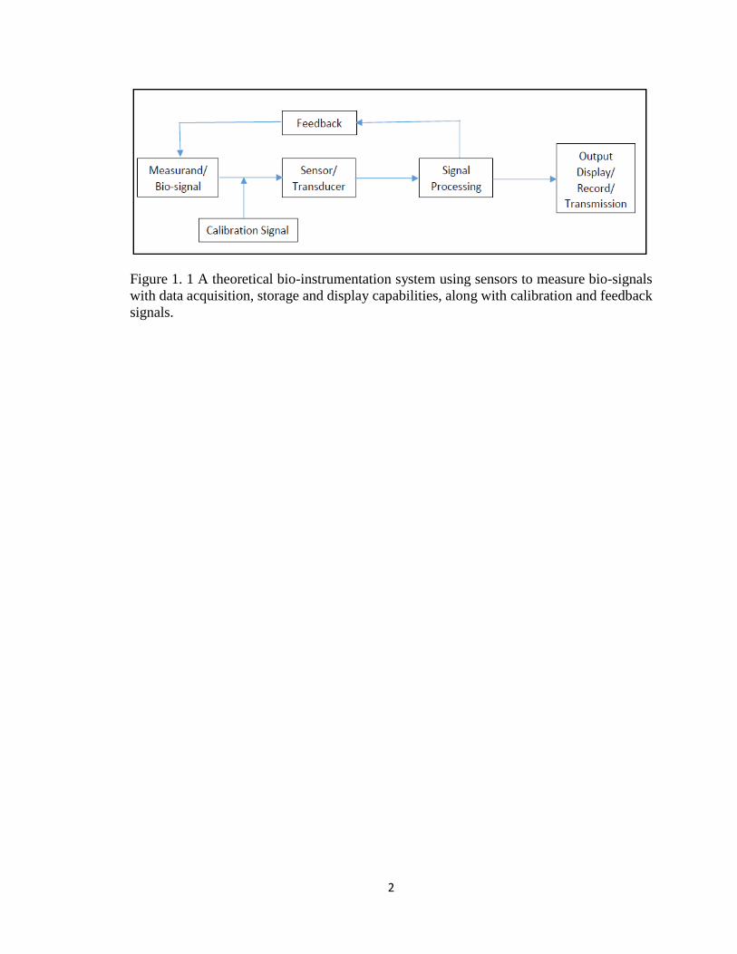
An infrared, corneal reflection eye tracking system relies upon the location of

observers’ pupils, relative to a small reflected light glint on the surface of the cornea (Young

18

& Sheena, 1975, Mulligan, 1997). A camera lens (the ‘eye’ camera) is focused upon the

observer’s eye that provides pupil movements to the researcher, and a second lens (the

‘scene’ camera) may also optionally be pointed towards the current visual display or scene

being viewed in order to study the subject’s visual targeting patterns. In the case of table-

mounted eye trackers, a scan converter is frequently used in place of the scene camera. The

light enters the retina and a large proportion of it is reflected back, making the pupil appear

as a bright, well defined disc, known as the “bright pupil” effect. There exists some cases

in which the pupil does not illuminate and results in “dark pupil”, thus eye trackers need to

be switched between these modes to find the most robust pupil imaging for a testing

environment. The corneal reflection is also generated by the infrared light, appearing as a

small, but sharp glint (Poole and Ball, 2005).

Once the image processing software has identified the centre of the pupil and the

location of the corneal reflection, the vector between them is measured, and, with further

trigonometric calculations, point of regard can be found. Video based eye trackers need to

be fine-tuned to each individual subject’s eye movements by a calibration process. The

calibration process is achieved by displaying a dot on the screen, and if the eye fixes for

longer than a certain threshold time and within a certain area, the system records that pupil-

centre/corneal-reflection relationship as corresponding to a specific horizontal and vertical

coordinate on the screen. This procedure is repeated over a 9 to 13 point grid-pattern to

gain an accurate calibration spread out over the whole screen.

After the calibration of the eye tracker is completed, the researcher can then collect

raw vision tracking data by recording the video feed coming in from the “eye” camera and

the “scene” camera. Within the raw data, there exists many types of eye-movements that

19

are vital for eye-tracking analysis. Saccades are commonly observed when watching an

observer’s eyes while conducting search tasks. They are small, frequent movements that

occur in both eyes at once, range from about 2-10 degrees of visual angle, and are

completed in about 10-100 ms (Shebilske & Fisher, 1983). Saccades have rotational

velocities of 500-900 degrees/second, resulting in very high acceleration (Carpenter, 1988),

and are typically observed about 250 ms following the onset of a visual target. Because of

their rapid velocity, there is a suppression of most vision during a saccade to prevent

blurring of the perceived visual scene.

Each saccade is followed by a fixation, where the eye has a 250-500 ms interval to

process visual information. In an encoding task such as browsing a web page or reading a

book, higher fixation frequency on a particular area can be indicative of greater interest in

the target, or it can be a sign that the target is complex in some way and more difficult to

encode (Jacob & Karn, 2003; Just & Carpenter, 1976). However, during a search task such

as looking for a particular tool at a workplace, a higher number of single fixations, or

clusters of fixations are often an indication of greater uncertainty in recognising a target

item (Jacob & Karn, 2003). Thus differentiating the type of task is extremely important

when trying to comprehend eye-tracking data.

Sequences of saccades and fixations form scanpaths, which describe the eye’s

movement from one point to another in a visual targeting activity. During a search task, the

most efficient scanpath is the one that is a straight line to a desired target, with relatively

short fixation duration at the target (Goldberg & Kotval, 1999). When analysing eye

tracking data, scanpaths can be quantitatively analysed by focusing on the derived measures

20

such as the duration, length, regularity, direction, spatial density, and the order of searches

which is also known as the transition matrix.

Blink rate and pupil size are two other measurements that eye researchers use as an

index of cognitive workload (Poole & Ball, 2005). A lower blink rate could be an indication

of higher workload where an individual’s visual attention is constantly being engaged,

while a higher blink rate may indicate fatigue (Brueneau, Sasse, & McCarthy, 2002;

Brookings, Wilson, & Swain, 1996). Larger pupils may also indicate more cognitive effort

(Marshall, 2000; Pomplun & Sunkara, 2003), though pupil size and blink rate can be

affected by other factors such as the ambient light levels, hence, pupil size, and blink rate

are less often used in eye tracking research.

1.2.2 Motion Capture

In order to accurately measure the motion of the body in 3D space, and to obtain a

comprehensive overview of the kinematics of various human movements, researchers use

a procedure called 3D motion analysis. It has a wide range of applications in numerous

industries that include military, entertainment, sports, robotics, bio-mechanics, and

ergonomics. While many human motion parameters and events can be measured using a

single video camera and 2D motion analysis, 3D motion analysis offers a lot more

functionalities in terms of kinematics. Motion capture used in ergonomics studies aim at

analyzing injury risks, work postures and bio-mechanics of workers in an industrial setting.

High precision motion data coupled with a high fidelity human model, based on

anthropometric and ergonomic considerations, may yield valuable data for these kinds of

studies, which currently rely mostly on static pose analyses (Bandouch et al., 2008).

21

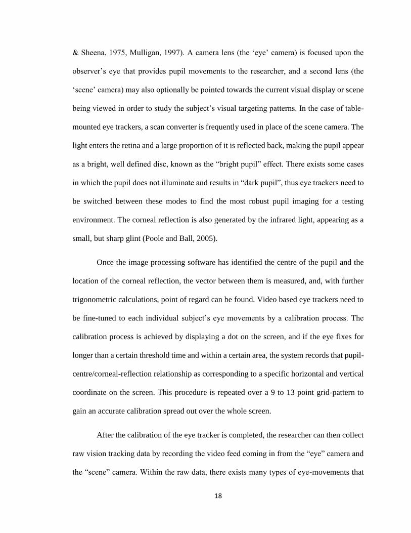
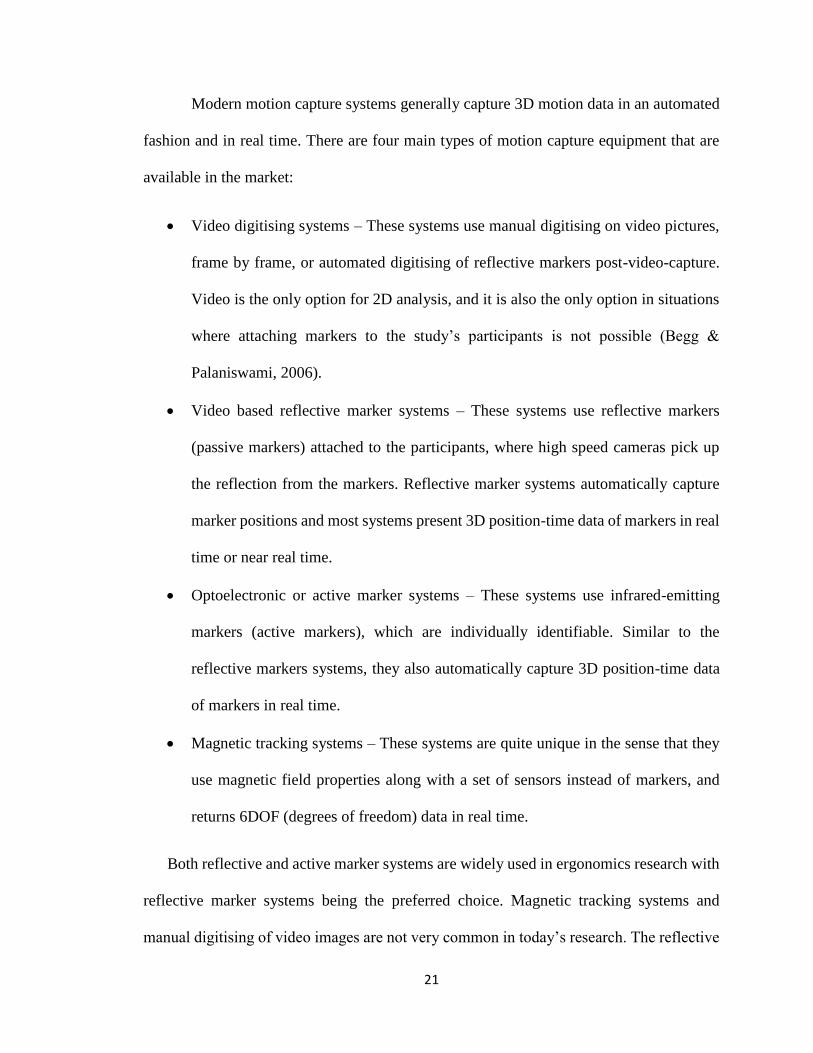
Modern motion capture systems generally capture 3D motion data in an automated

fashion and in real time. There are four main types of motion capture equipment that are

available in the market:

• Video digitising systems – These systems use manual digitising on video pictures,

frame by frame, or automated digitising of reflective markers post-video-capture.

Video is the only option for 2D analysis, and it is also the only option in situations

where attaching markers to the study’s participants is not possible (Begg &

Palaniswami, 2006).

• Video based reflective marker systems – These systems use reflective markers

(passive markers) attached to the participants, where high speed cameras pick up

the reflection from the markers. Reflective marker systems automatically capture

marker positions and most systems present 3D position-time data of markers in real

time or near real time.

• Optoelectronic or active marker systems – These systems use infrared-emitting

markers (active markers), which are individually identifiable. Similar to the

reflective markers systems, they also automatically capture 3D position-time data

of markers in real time.

• Magnetic tracking systems – These systems are quite unique in the sense that they

use magnetic field properties along with a set of sensors instead of markers, and

returns 6DOF (degrees of freedom) data in real time.

Both reflective and active marker systems are widely used in ergonomics research with

reflective marker systems being the preferred choice. Magnetic tracking systems and

manual digitising of video images are not very common in today’s research. The reflective

22

and active marker systems require markers to be attached to the participants and these

markers are either infrared light-emitting diodes (LEDs) for active marker systems, or solid

shapes covered with reflective tape for reflective marker systems. The output of these

systems are the x,y,z coordinates of each marker as a function of time.

The reflective marker systems use the reflections coming from the markers attached

to the participants using multiple video cameras. These high speed video cameras (166 –

500Hz) are equipped with infra-red flash illuminators that surround the camera lens, and

sends out pulses of infra-red light which are then reflected back into the lens from the

markers. Each camera records a 2D image with the markers appearing as bright dots. Image

processing systems isolate the marker dots in the image and record their position (Fisher,

2002). Since they are “passive” markers, each marker trajectory must be identified and

tracked. Markers are sometimes hidden from one or more cameras, so the trajectories can

be difficult to track. Therefore, it is recommended to have a minimum of 6 cameras for a

reflective marker system so that the researcher would not miss out on capturing all the

existing markers.

Once the visible markers have been located on the 2D camera images, the

coordinates of the centroid of each marker are noted and a series of intersecting rays are

mathematically projected from each camera position for each marker. Since the positions

and the lens parameters of each camera are known, the rays from the same marker must

intersect and the sets of 2D coordinates for each marker can be reconstructed and 3D

coordinates of each marker can be calculated (Shao et al., 2001). Finally, markers are

assigned to existing trajectories, and any ghost markers (visual noise due to shiny reflective

surfaces) are rejected using the image processing software. There are numerous

23

commercially available reflective marker systems in the market, but the most used systems

in research are Vicon (Oxford Metrics) and Cortex (Motion Analysis).

Active marker systems also have markers attached to the participant. Markers are

light emitting diodes (LEDs) that are powered and cabled and each LED pulses in a set

sequence. With only one marker flashing at any one time, the system can automatically

identify and track each marker. This is a considerable advantage of active markers systems

over reflective marker systems, however, there is also a down side to it. After sampling the

first marker, it must sample all other markers before it can sample the first marker again,

which means the sample rate reduces as the number of markers increases. The sequential

pulsing of active marker systems means marker occlusion and ghosting does not become

an issue as in the case with reflective marker systems. In addition, active marker systems

are also capable of detecting marker clusters placed together without any errors due to each

marker being uniquely identifiable. Active marker systems normally have three cameras

mounted in a rigid rectangular housing. Depending on the type of system that is being used,

two to three units is sufficient to collect 3D data to great accuracy (Corriveau et al., 2004;

Sadeghi et al., 2004). Two most commonly available active marker systems in the market

are OptoTrak (Northern Digital, NDI) and CODA (Charnwood Dynamics).

Magnetic tracking devices generate and sense magnetic fields. They are equipped

with a transmitter that emits magnetic fields, and a receiver that detects them. Each sensor

placed on the participant delivers six degrees of freedom (X, Y, Z, yaw, pitch, roll)

information to the processing computer. Also, the sensors do not require to be within the

line of sight of the receiver thus it is a significant advantage these systems carry over the

other motion capture systems. However, due to their inherent sensitivity to large metallic

24

objects, it becomes a challenge when trying to capture motion data in a big volume of space

(Perie et al., 2002). Therefore, magnetic tracking systems are used most often in animation

applications and are not usually the preferred tool for ergonomic analysis research and

testing.

For reflective and active marker systems, the basic output is 3D marker coordinates

moving in time, called “marker trajectories” (Begg & Palaniswami, 2006). These markers

create an “exo-skeleton” around the participant which has to be related to an “endo-

skeleton” model of the participant (Fisher, 2002). In order to convert the raw marker

coordinate data into useful 3D human body kinematics, there are a few steps that need be

followed. First, each body segment is defined using at least three external markers.

Segments can however, share markers if needed. Then, joint centres are defined using the

external marker data and pre-defined templates that creates a virtual skeleton for analysis

purposes. Finally, Euler angles are computed at each body segment and joint centre, where

local coordinates systems are defined in order to calculate local kinematics with respect to

a “parent” body segment. The equations for calculating joint coordinates and segment

orientations from external markers are often provided with the motion capture software.

Thus, it is the researcher’s task to understand and identify the types of kinematic metrics

that they need to analyze in a motion capture study, and use the software accordingly to get

the desired results.

1.2.3 Force Platforms

In ergonomics research, kinetics refers to the forces and moments that are

responsible for changing a body’s state of motion. Measuring internal muscular forces is

not possible without using invasive medical instruments, however, external muscle activity

25

can be measured using force platforms that provide valuable information on joint forces

and joint moments during various human activities. Force platforms are commonly used in

bio-mechanical lab settings to record and analyze foot-ground reaction forces and moment

time histories.

Foot-ground reaction forces (ground reaction forces, GRF) are reaction forces as a

result of contact between the foot and the ground, and form an integral part of human

movement analysis (Benedetti et al., 1998). There are two types of force platforms that are

widely used in research; those based on piezo-electric transducers such as Kistler, and those

based on strain-gauge transducers such as AMTI and Bertec (Begg & Palaniswami, 2006).

From a research perspective, there is not much difference between the two types as they

both essentially measure the same information, only the raw outputs of the systems are

different. The output from strain gauge transducer platforms is three orthogonal force

components (Fx, Fy, Fz) and three moments (Mx, My, Mz), whereas piezo-electric transducer

platforms output four vertical forces and four horizontal forces. In software, all systems

convert this raw data to the main information of interest in human movement analysis, that

is Fx (horizontal medio-lateral force or medial shear component), Fy (horizontal antero-

posterior force or AP shear component), Fz (vertical force component), centre of pressure

position (COP) and Tz (vertical torque; moment about a vertical axis passing through the

COP position).

Force platforms can be very stable devices and the data they produce are critical for

kinetic analyses in ergonomic studies. Ergonomic research tasks that involve lifting and

handling objects, pushing and pulling loads often have external forces along with gravity

acting on the participant’s body. Thus, force platforms provide an excellent basis to observe

26

how such external forces could induce different bio-mechanical behaviors in individuals

while comparing that data to their normal force profiles. As with a lot of bio-instruments,

force platform data can be recorded and analysed using third party software such as

LabView and Matlab, where the researchers have the freedom to explore different analysis

methods, compared to a limited number of predefined data analytics.

1.2.4 Experimental Software

The bio-instruments that are used in ergonomics research have the typical two main

components of experimental bio-instruments, namely hardware system for data collection,

transmission and storage, and a software component built mainly for data analysis. Many

of the bio-instrument systems commercially available today come with built-in software

packages that allow the researchers to analyze and present data in multiple ways. At the

same time, there also exists third party software that are capable of analysing various types

of bio-data by allowing the researchers to program the data analytics using numerous

programming languages. Following is a discussion of the software systems that were used

to analyze bio-data obtained from different bio-instruments in my research.

The goal of eye movement measurement and analysis is to gain insight into the

viewer’s attentive behavior. In vision tracking, the raw data coming in from an eye tracker

contains the x, y coordinates of the eye’s position with respect to the viewing area. Raw

eye movement data for a particular work task may appear informative to a certain extent,

however, without further analysis, the raw x, y coordinates do not reveal much information

about the subject’s visual attention. Although intuitively, and from the knowledge of the

task, it is possible to guess where a subject happened to be paying attention in the

environment, it is not possible to make any further quantitative inferences about the eye

27

movement data without the use of an eye-tracking software. Within the software, various

algorithms are programmed to identify fixations and saccades; the eye movements that best

indicate the locations of the subject’s visual attention.

Having the eye tracker calibrated prior to data collection allows the recorded x, y

coordinates to be accurate and aligned correctly on the scene camera footage. From a signal

processing standpoint, the raw x, y coordinate data are used to characterize the eye

movement signals in terms of salient eye movements such as saccades and fixations. The

analysis task is to locate regions where the x, y coordinates (signal) average changes

abruptly indicating the end of a fixation resulting in an onset of a saccade, and then to

observe a stationary characteristic indicating the beginning of a new fixation.

Before signal analysis, excessive noise in the eye movement signal must be

eliminated. Noise is caused mainly due to the inherent instability of the eye, and the

constant blinking. The latter, considered to be a significant nuisance, and generates strong

signal perturbation. However, often the eye-trackers are equipped with built-in filters to get

rid of blinks, and to return a value of (0, 0) whenever it loses sight of the salient features

needed to record eye movements. Noise caused due to various other sources is filtered out

by defining an “effective operating range” that is specified in terms of visual angle of the

subject. Any signal that falls outside the defined pixel range is therefore left out.

Once the noise is filtered out, next step is identifying saccades and fixations. There

are two main approaches to identifying these events; dwell-time fixation detection

algorithm and the velocity-based saccade detection (Duchowski, 2007). With the dwell-

time fixation detection method, the algorithms first look for a stationary signal that it

considers to be the fixation. Then a second criterion is observed where the size of the time

28

window specifying an acceptable range for fixation duration. This classification method

suggested by Anliker (1976), determines whether M of N points (x, y coordinates) lie

within a certain distance (D) of the mean (µ) of the signal. When the algorithm eventually

detects a saccade, the variance of the signal would exceed the threshold D indicating a real

positional change. An alternative to the dwell-time fixation detection method is the velocity

detection method (Anliker, 1976). In this method, the velocity of the signal is calculated

within a sample window and compared to a velocity threshold. If the sampled velocity is

smaller than the given threshold, then the sample window is deemed to belong to a fixation

signal, otherwise it is a saccade. Yarbus in his research (1967) observed that saccadic

velocity is nearly symmetrical (resembles a bell curve), and thus, using this observation a

velocity based prediction scheme can be implemented to approximate the arrival time and

location of the next fixation. The next fixation location can be approximated as soon as the

peak velocity is detected. Measuring elapsed time and distance traveled, and taking into

account the direction of the saccade, the prediction scheme essentially mirrors the left half

of the velocity profile to calculate the saccade’s end point (Duchowski, 2007).

The dwell-time fixation and velocity-based algorithms produce similar results, and

both methods can be combined to bolster the analysis by checking for agreement. Once the

fixations and saccades have been identified, visual attention results can be quantified and

graphically displayed using various plotting and image processing techniques. These

functionalities include fixation maps, scan-path visualizations, heat maps, and region of

interest (ROI) analyses. Fixation maps are time independent plots that display all the

fixations plotted over scene camera images to indicate the subject’s visual attention.

Durations of these fixations can be user inputted, so that the researchers can isolate specific

29

fixation lengths that they are interested in analyzing. Scan-path visualizations display both

the fixations and saccades graphically. These visualizations track the saccadic eye

movements using a line graph, while highlighting the fixations using circles of different

radii to indicate fixation durations. Heat maps are used to emphasize the strength of

fixations using different color schemes that generally demonstrate the areas on a screen

where the subject’s visual attention was heightened with respect to other areas. Different

color schemes such as grey, jet, hot, hsv, spring (Matlab) are used to overlay the fixations

on top of scene camera images to enhance the visual attention data, while making sure the

original image is still visible (Spakov et al., 2007). ROI analyses allow the researchers to

focus on a specific area of the visual data screen and analyze all the fixations and saccades

that were collected. In a case where multiple clusters of fixations are observed, this method

is quite valuable in filtering out any data signals that appear outside of the defined ROI

parameters. Matlab (Mathworks), a multi paradigm numerical computing environment and

a fourth generation programming language allows eye tracking researchers to perform all

the aforementioned graphical analyses and image processing with its built-in tool boxes

and graphical user interfaces, designed specifically to simplify eye-tracking analyses. In

this thesis, all the bio-data collected via various bio-instruments were analysed using

Matlab as it is the common practice in basic and applied science today.

The data collected from motion capture and force platforms are used to calculate

kinematic and kinetic metrics using programmable software such as C, C++, and Matlab.

In the case of Motion capture systems, recorded 3D positions (x, y, z) of each body segment

and joints are combined to produce a template that is a representation of the subject’s

skeleton. Using these 3D position data in a vector analysis software such as Matlab, the

30

researchers are then able to calculate the kinematic measures such as displacement,

velocity, acceleration, angular motion, and particle trajectories. Similarly, the force

platforms record the forces and torques that act upon a subject during a work task. With the

use of Matlab, researchers can calculate the kinetic measures such as ground reaction

forces, centre of pressure, forces acting on different body segments as well as resultant

forces and torques. By measuring kinetics and kinematics data simultaneously, joint forces

and moments can be calculated via a mathematical process known as inverse dynamics

(Begg & Palaniswami, 2006). Inverse dynamics is the process of computing the net joint

forces, joint moments and joint power, and the calculations require kinematics data

(positions and orientations of joints and segments as well as their linear and angular

velocities and accelerations), ground reaction force data and anthropometric data. Joint

moments are the result of forces produced by muscles and ligaments acting at a distance

from the joint centre. Joint power is the net rate of generating or absorbing energy by all

the muscles crossing a joint and is calculated as the product of the joint moment and the

angular velocity between the two segments defining the joint (Winter, 1990; Meglan &

Todd, 1994). Joint forces, moments and power during ergonomic activities are critical to

the understanding of injury prevention and proper work techniques. Thus, using the

appropriate software to perform the necessary bio-mechanical analyses becomes a vital

component in ergonomic research.

The field of bio-instrumentation is on a continuous climb with countless technical

advancements being made resulting in affordable, high functioning instruments with

incredible detection and computing powers. However, there still seems to be a missing link

when it comes to ergonomic experimental software development. A key word search of

31

“Ergonomics” and “Matlab” in the Pubmed biomedical database resulted in 30 articles,

while the ‘Web of Science’ database yielded 18 articles for the exact search as of January

of 2018, suggesting the lack of experimental software in ergonomics and the need for

further research in this field. Ergonomic researchers and biomechanists continue to prefer

using default software systems that bio-instrument manufactures produce over custom built

experimental software. Even though these default software offer numerous data analysis

methods that are well known, with high precision, they all have limitations that bind the

researchers to a set number of analysis techniques and prevents them from further

expanding their research into higher order analyses. Custom experimental software on the

other hand, offer all the analysis methods that the default software can offer, and allows the

luxury of adding in numerous high level analysis methods as well as novel analysis

principles that the researcher may want to experiment with. Numerical analysis software

such as Matlab, Labview and Analytica are capable of providing high-level numerical

analysis methods by either using already existing functionalities, where the user can

combine multiple built-in functions to create a high structured analysis program, or design

a completely new analysis program from ground up. The result is a well-structured high

level analysis program offering much more than the basic break down of data, and thought

provoking results which may induce even deeper discussions with regards to data analysis.

Therefore, it is imperative to explore the potential impact custom experimental analysis

software may have on ergonomic research and it requires further attention from

biomechanical and ergonomic researchers.

The purpose of my thesis is to begin the design and validation of a 21st century

occupational psychophysics toolbox that pairs off the shelf bio-instrumentation hardware

32

components, namely vision tracking, motion capture, and force platforms with custom

Matlab based experimental software capable of image processing, assessment of full body

kinematics and analysis of ground reaction force kinetics to comprehensively study

perception action coupling from select occupational tasks. It is hypothesised that unique

(and explanatory) characteristics of perception-action coupling in occupational behaviour

would be revealed through the logical experimental combination of conventional human

movement bio-instrumentation, custom scientific data analysis software, and ecologically

valid experimentally occupational tasks.

1.3 Summary

Bio-instrumentation is the development of technologies for the measurement and

manipulation of parameters within biological systems, focusing on the application of

engineering tools for scientific discovery and for the diagnosis and treatment of disease.

Though the bio-instruments may vary with their components and functionalities according

to the biological system that they are dealing with, in general they all have a common

instrumental set up comprised of sensors, calibration signals, signal processing unit,

feedback signals, and an output display and transmission feature. In the fields of

ergonomics and biomechanics, the use of bio-instrumentation for the purpose of analysing

work related MSDs for injury prevention has become the norm. Subsequently, the relatively

new assessment model, occupational psychophysics, has allowed the use of bio-instruments

to be more efficient by addressing both the perceptual and physiological challenges that

arise at work places.

In this thesis, I have made use of three commonly used bio-instruments, vision-

tracking, motion capture, and force platforms, and have coupled them with Matlab based

33

experimental programming in an attempt to identify the visual, kinematic and kinetic

concepts associated with occupational lifting tasks.

1.4 Outline

In Studies 1 and 2, I examined visual attention preceding a manual material

handling task, and associated visual attention with explicit pre-handling arousal, implicit

directional cues for action, and subsequent handling strategies. My goal was to differentiate

how negative and positive motivational states along with implicit visual cues could

influence MMH perceptions and actions that may lead to work related musculoskeletal

injuries. I used a pair of vision tracking goggles (ASL) to capture individual’s visual

attention data, and combined it with custom Matlab software to process, analyse and to

visually represent the results.

In Study 3, I observed the perceived horizontal affordance distance of workers

during an MMH task, and studied whether the affordance distances could be modified using

implicit directional cues. I performed a conventional motion capture kinematic assessment

and a postural kinetic evaluation by making use of two commonly used bio-instruments in

the industry, a high speed motion capture system and a force-platform. By combining the

two bio-instruments with another custom matlab software capable of modelling handling

behaviors into mathematical equations, I was able to discriminate handling behaviours by

visual cue type for work place risk assessment.

34

2.0 Quantifying Visual Attention for a Manual Materials Handling Task

2.1 Introduction

Visual attention is one of the key information contributors in the process of carrying

out the human activities of everyday life. Visual attention has four basic components; (i)

selection of the region of interest in the visual field, (ii) selection of feature dimensions and

values of interest in that region of interest, (iii) control of information flow through the

network of neurons that constitutes the visual system, and (iv) frequency and order of

shifting from one region of interest to the next (Tsotsos et al., 1995). It is noteworthy that

the first two components of visual attention occur prior to any subsequent action,

suggesting that predictive visual attention precedes actions in everyday activities, as

previously observed in natural behaviours and tasks such as walking (Marigold and Patla,

2008) and reaching (deBruin et al., 2014). The direction of visual attention is typically

defined by two behaviours of the eyes, specifically fixations, (where the visual gaze is

maintained on a single location), and saccades, (movements of the eyes between two

fixation points) (Duebel & Schneider, 1996). Measuring fixation patterns and saccadic

movements provides us with a means of studying visual attention, and associating those

behaviors with upcoming actions (Yarbus 1967; Hayhoe & Ballard, 2005). Measures of

real-world visual attention have been widely used in sports science, including table tennis,

golf, baseball, and darts, to examine the perception-action coupling, accuracy, efficiency,

and psychophysical status of athletes (Vickers, 1992, 1996, 1997). Numerous experimental

visual attention studies have used screen-based eye-tracking as a means to substantiate

possible relationships between visual attention and everyday human actions (see Nguyen

35

et al., 2016 for a review), and the technological advances continue to open new

environments for investigation (Hayhoe, 2018).

The workplace is an environment where many adults perform eight plus hours of

activities daily. Manual materials handling is a frequent, repetitive workplace activity that

has chronic potential for causing musculoskeletal injuries amongst workers (Hagberg et al.,

1995). These injuries may stem in part from behavioral differences, with injury prone

workers making specific unsafe actions during their manual materials handling duties

(Marras et al., 2000). Motion and principal component analyses identify the kinematic

evidence of these injury-risk behaviors (Marras et al., 1995; Wrigley et al., 2005), but less

is known about perceptual differences that may precede (and possibly predict) these

different action patterns (Bigos et al., 1991; Mullen, 2004). By identifying and quantifying

preceding visual attention patterns in the workplace, we might be able to predict personal

handling behaviours, and thus risk of work-related musculoskeletal disorder.

A manual materials handling task can be performed in multiple ways, where the

handling techniques could depend on numerous factors. Assuming the workers are

physically healthy and are familiar with their work tasks, their lifting patterns may be

determined by the visual attention patterns and the pre-lift instructions. For example,

workers fixated on an upstream object on an assembly line might move and lift differently

than workers attending to the decreasing space between them and the same object. With the

use of proper research and analysis methods, we might be able to predict differences in

handling techniques and work-related musculoskeletal loading by investigating

spatiotemporal characteristics of worker’s pre-lift visual attention patterns.

36

In this two-part experiment, our goal was to examine visual attention preceding a

manual material handling task, and to associate visual attention with explicit pre-handling

arousal (mental state), implicit directional cues for action (physical context), and

subsequent handling strategies (behaviour). In Study 1, participants were primed with one

of two handling task arousal states, then asked to grasp and move a suitcase while their

visual attention and handling behaviour were recorded. In Study 2, participants

performed the same task with the same primes plus additional visual cues proposed to

affect handling behaviour. Previous research has shown that visual cues do effect reaction

times, while automatically triggering orienting of attention (Posner, 1980; Tipples, 2002).

Although the influence of explicit and implicit cues on visual attention is well known,

their effectiveness in moderating manual materials handling tasks and work-related

activities requires further research. We hypothesized that pre-handling explicit contexts

would encourage participants to perform the manual materials handling activity with

different perceptual and behavioral strategies (Study 1), and that implicit visual cueing

would have the capability to influence the effects of the context, influencing participants

to handle the loads in differing manner (Study 2). We investigated the relationship

between visual attention and manual material handling actions, with the goal of

preventing injurious occupational behaviours.

2.2 Methods

2.2.1 Study 1

2.2.1.1 Experiment

Thirty-one university undergraduates (21.5 ± 4.5 years old, 17 female) with normal

or corrected-to-normal vision were recruited. A horizontally oriented suitcase (72 x 45 x

37

25cm) was securely fastened and fully supported on a LIDO WorkSet II dynamometer

(Loredan Inc, MA, USA; Figure 2.1), and was initially concealed under an eye tracker

calibration board prior to the work task. Participants’ heights were measured and the

suitcase was vertically adjusted so its vertical centre was at 53% of each participant’s

height. Participants were instructed to position their feet inside a 40cm square that was 25

cm posterior to the centre of the suitcase. A pair of Mobile Eye - XG vision tracking goggles

(Applied Science Laboratories, MA, USA) were worn by each participant. The goggles’

reflector lens and vision camera were each adjusted to capture eye movement data that were

within each individual’s para-central vision. Prior to the work task, each participant took

part in a calibration exercise of the goggles, where they stood in front of a horizontally-

oriented calibration board with nine markers placed on it, arranged in a 3 x 3 matrix (79 x

62cm). Participants were asked to focus their gaze on each of the markers for a few seconds,

while the vision-tracking software collected and calibrated the data from the goggles to

make sure that the right pupil was aligned with each marker.

38

Figure 2. 1 Suitcase orientation during the handling task. The suitcase is placed on a LIDO

dynamometer while the subject is also equipped with vision tracking goggles.

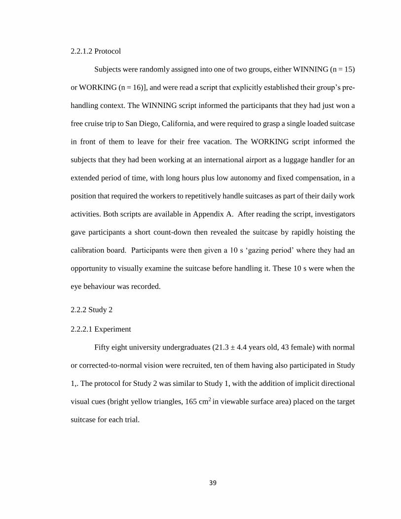
39

2.2.1.2 Protocol

Subjects were randomly assigned into one of two groups, either WINNING (n = 15)

or WORKING (n = 16)], and were read a script that explicitly established their group’s pre-

handling context. The WINNING script informed the participants that they had just won a

free cruise trip to San Diego, California, and were required to grasp a single loaded suitcase

in front of them to leave for their free vacation. The WORKING script informed the

subjects that they had been working at an international airport as a luggage handler for an

extended period of time, with long hours plus low autonomy and fixed compensation, in a

position that required the workers to repetitively handle suitcases as part of their daily work

activities. Both scripts are available in Appendix A. After reading the script, investigators

gave participants a short count-down then revealed the suitcase by rapidly hoisting the

calibration board. Participants were then given a 10 s ‘gazing period’ where they had an

opportunity to visually examine the suitcase before handling it. These 10 s were when the

eye behaviour was recorded.

2.2.2 Study 2

2.2.2.1 Experiment

Fifty eight university undergraduates (21.3 ± 4.4 years old, 43 female) with normal

or corrected-to-normal vision were recruited, ten of them having also participated in Study

1,. The protocol for Study 2 was similar to Study 1, with the addition of implicit directional

visual cues (bright yellow triangles, 165 cm2 in viewable surface area) placed on the target

suitcase for each trial.

40

2.2.2.2 Protocol

Participants were randomly divided into two groups [WINNING (n = 29) and

WORKING (n = 29)], and were read the corresponding WINNING or WORKING script

from Study 1. The implicit visual cues were arranged in two different orientations such that

they provided either a CONVENTIONAL cue or a COUNTER cue to the typical grasping

behaviours observed in Study 1. Orientation 1, consisting of two triangles positioned close

to the centre of the suitcase and pointing to both lateral ends of the suitcase was the

CONVENTIONAL cue to the WORKING script and COUNTER cue to the WINNING

script, while Orientation 2 (a single triangle positioned near the centre of the suitcase and

pointing to the front handle) was the CONVENTIONAL cue for the WINNING script and

the COUNTER cue for the WORKING script.

2.3 Analysis

All the activities in both experiments were captured using the scene camera of the

eye-tracker along with the corresponding vision data (pupil coordinates) for analysis.

For both experiments, two alternative suitcase grasp types were identified:

unimanual handling from the front handle or bimanual handling with one hand on the front

handle and the other on either side handle or side, or with opposite hands on each of the

right and left side handles (or sides) of the suitcase. Frequency of grasp types were

compared between groups to detect possible associations between handling techniques,

preceding perceptions, and implicit visual cues.

41

The vision tracking data collected from the eye-tracker were saved as Microsoft

Excel files, and contained the following information: Frame number, x and y coordinates

of the master spot in eye image pixels, x and y coordinates of the pupil center in eye image

pixels, pupil radius in eye image pixels, eye direction with respect to the scene image in

scene image pixels, mouse cursor position with respect to the scene image in scene image

pixels. From these data, we were interested in the master spot coordinates, which indicated

the visual targeting areas of individuals in the form of the eye-image pixels. Eye images

had a resolution of 768 pixels horizontally and 576 pixels vertically.

The first step of the vision tracking data analysis was noise filtering, where all

unavailable frames (resolution pixels greater than 768 horizontally and/or 576 vertically)

were removed from the collected data files. This was done by programing a Matlab function

(EyeFilter), in which the program explicitly searched for any error coordinates (-2000 or

coordinates outside of 768 x 576), and then filtered them out by deleting the corresponding

data that were associated with those frames.

The vision tracking data were then analysed using a Matlab based eye-tracking

software called ‘EyeMMV’ (Krassanakis et al., 2013). EyeMMV is a freely available eye-

tracker data analysis software that is capable of analysing vision tracking data and produces

various types of visually representative results in the form of heat maps, fixation maps, and

scan-path visualizations. When analyzing heat map results, it is important to keep in mind

that there are two factors that affect heat map results: the number of fixations and the

duration of those fixations. In our analysis, the heat maps are a product of these two factors,

where the higher the number of fixations and/or the greater the duration of each fixation,

the more intense the color of those resulting fixation areas. The data representation scheme

42

is a colour spectrum map, where the highest intensity corresponds to the color red. Some

coding modifications were added to the software in order to make sure that it was

compatible with the eye-tracker while providing us with added benefits. These

modifications included: (i) capability of handling Excel data files as input by adding in a

data file conversion subroutine, (ii) adjustments to the heat-map and fixation map generator

subroutines to accommodate the eye-tracker specific pixel resolutions and coordinate types,

and (iii) save functionality to all the functions that were available, so that the processed

data and images can be stored for future use (Appendix B).

In addition to all the analysis methods that were readily available through

EyeMMV, we’ve also developed a new functionality called Attraction Index (AI). The AI

is a number that was calculated in order to compare the visual attention on two or more

fixation points. The AI provides a quantified representation of the visual targeting results

compared to the traditional way of visually representing eye-tracking results. For the

purpose of current study, the AI identified the strength of visual attention amongst

participants during the suitcase handling task. It took into account three main factors;

number of fixations (number), duration of each fixation (duration), and the relative distance

(distance) of each fixation from one of the three handles of the suitcase, such that

𝐴𝑡𝑡𝑟𝑎𝑐𝑡𝑖𝑜𝑛 𝐼𝑛𝑑𝑒𝑥 =(number x duration)

distance

AI may provide a strong and simple indicator of the pre-movement visual attention.

The AI function was programmed in Matlab to produce an AI-map that would indicate the

fixation points of individuals with respect to the three handle points.

43

2.4 Results

2.4.1 Study 1

There was a clear distinction between the two groups for their handling motivation

and their subsequent handling techniques. The WINNING group had significantly

increased handling motivation that the WORKING group (Figure 2.2), based on their

physical response (pointing to a number on the response line) to the question ‘After just

hearing your instructions and getting into your role, how are you feeling right now about

handling this specific suitcase?’ where the response line ran from -5 (anchored with text

‘VERY BAD’) on the left to +5 (anchored with text ‘VERY GOOD) on the right, in equal

increments of 1 and with additional anchor text of ‘SOMEWHAT BAD’ between -3 and -

2, ‘NEUTRAL’ at 0, and ‘SOMEWHAT GOOD’ between + 2 and +3. The WINNING

group handled the suitcase only from the front handle on 73.3 % of trials, thus indicating

their preference for unimanual handling over bimanual handling. The WORKING group’s

preferred handling technique was front and side grasping (50% of the trials). When we

collapsed these results into unimanual handling and bimanual handling (including both

sides and front and side grasps), the WORKING group’s preferred handling technique was

bimanual (68.8% for WORKING; Figure 2.3). A two-way log-linear analysis was used to

produce a final statistical model that retained all effects. The likelihood ratio of this model

was [X2(0) = 0, p = 1]. This indicated that the highest-order interaction (the group by

handling interaction) was significant [X2(2) = 20.305, p < .001]. To interpret this

interaction, a chi-square test was performed comparing WORKING and WINNING

groups. There was a significant interaction between group and handling, selected, [X2(1) =

5.490, p = .032]. The odds ratio showed that the odds of selecting a unimanual grasp were

44

6.05 times higher with the WINNING than the WORKING script. Therefore, the analysis

suggested that bimanual handling was typically selected in the WORKING context,

whereas unimanual handling was typically selected with the WINNING script.

The vision tracking results were studied by comparing the heat maps of the two

groups. This analysis revealed that, for the WINNING group, the Attraction Index (AI)

was highest for the front handle (extending to the central region) of the suitcase, compared

to the WORKING group’s fixations, which were more distributed around the suitcase, but

falling predominantly on the left (direction of movement) side. These results are

summarized in Figure 2.4, and exemplar heat maps are shown in Figures 2.5a and 2.5b.

45

Figure 2. 2 Handling motivation results. Motivation was recorded on a subjective scale

ranging from -5 (feeling VERY BAD about handling this case) to +5 (feeling VERY

GOOD about handling this case). WINNING group had a higher motivation rating than the

WORKING group.

Figure 2. 3 Handling frequency results. WORKING group’s preferred a bimanual handling

technique while the WINNING group preferred a unimanual handling method.

46

,

Figure 2. 4 Attraction Index (AI) results. WORKING group’s highest AI was for the left

handle, while the WINNING group’s highest AI was for the front handle indicating their

preferred unimanual handling technique.

47

Figure 2. 5 Heat map results. 2.5a (top) shows that for the WINNING group a concentrated

fixation was visible at the centre of the suitcase. 2.5b (bottom) indicates a cluster of smaller

fixations spread around the left hand side of the suitcase.

48

2.4.2 Study 2

The WORKING group continued to display the highest percentage of bimanual

handling (76% of total trials), while the WINNING group’s preferred method of handling

was from the front handle (65% of total trials; Figure 2.6). Interestingly,

CONVENTIONAL cues strengthened the favoured behaviour of bimanual handling

amongst the WORKING group (100% of WORKING-CONVENTIONAL trials) while

members of the WINNING group seemed impervious to the cueing. A three-way loglinear

analysis was used to produce a final model that retained all effects. The likelihood ratio of

this model was [X2(0) = 0, p = 1]. This indicated that the highest-order interaction (the

group by cue by handling interaction) was significant, [X2(2) = 3.961, p < .047]. Separate

chi-square tests were performed for WORKING and WINNING scripts. For the

WORKING script, there was a significant association between the type of cue and whether

a unimanual or bimanual grasp was selected, [X2(1) = 5.639, p = .026]. This interaction

was caused by a mixture of unimanual and bimanual grasps with a COUNTER cue but only

bimanual grasps with a CONVENTIONAL cue. For the WINNING script, the association

between the type of cue and whether a unimanual or bimanual grasp was selected was not

significant, [X2(1) = 0.338, p .683]. Therefore, the analysis suggested that a unimanual

grasp was typically selected with the WINNING script regardless of the type of cue.

The visual cues for Study 2 were introduced for the purpose of studying any

possible superseding effect implicit directional visual cueing may have on typical manual

materials handling behaviours in the work place. As we observed from our results in Study

1, the WINNING group’s preferred handling method was from the front handle of the

suitcase, whereas the WORKING group preferred handling the suitcase with two hands. In

49

Study 2, we strategically placed visual counter cues on the suitcase for each group, which

we predicted would prompt opposite handling results as to what we observed in Study 1.

Thus, a pair of arrow cues pointed at the two side handles were placed on the suitcase for

the WINNING group, while a single arrow cue pointed towards the front handle was placed

on the suitcase for the WORKING group. The vision tracking results from Study 2

demonstrated distinct fixation patterns of the participants during their gaze period (Figure

2.7). The WINNING-COUNTER cue group had a concentrated fixation directed at the

front handle, despite the paired counter-cues pointing towards the sides (Figure 2.7a). The

WORKING-COUNTER group’s vision data looked a bit more scattered, however, there

was one particular concentrated heat signature directed right at the counter-cue arrow

(Figure 2.7b).

50

Figure 2. 6 Handling results from study 2 indicating the impact of counter and conventional

visual cueing on handling techniques. Counter cues had a greater impact on the WORKING

group by encouraging participants to attempt unimanual handling compared to the

conventional cues.

51

Figure 2. 7 Heat map results from study 2. 2.7a (top) shows a concentrated fixation at the

front handle of the suitcase for the WINNING group with counter cues. 2.7b (bottom)

shows a more scattered fixation pattern with one concentrated fixation on the counter

visual cue for the WORKING group.

52

2.5 Discussion

The introduction of implicit directional visual cues aligned in either conventional

or counter directions to preferred handling behaviours provided us with an opportunity to

study how visual attention to cues may encourage certain manual materials handling

techniques. Our results suggest that visual cues have an impact on the handling behaviours

of individuals. The percentage of unimanual handling remained the same for the WINNING

group when the cues were introduced, but the WORKING group’s bimanual preference

increased significantly with logically consistent cues. It is possible that consistent cues

provided assurance to the participants that they were performing the handling motion the

correct way. The counter visual cues for both groups did generally encourage more opposite

handling techniques as to conventions observed in Study 1, but it was not a significant

change. Further research focusing on the modifying effects of cues may prove valuable in

safely shaping work-related behaviours in actual workplaces. Following on our experiment,

it might be possible to ‘nudge’ workers to use safer handling techniques, namely bimanual

handling, by placing or projecting logically consistent visual cues on to the item to be lifted.

By studying individuals’ visual attention prior to a manual materials handling

activity, we hoped to gain more insight in to possible relationships that might exist between

perception and manual material handling techniques, as previous researchers have done for

sports (Vickers, 2009). Vision tracking results from Study 2 clearly indicated a

concentrated visual attention towards the front handle for the WINNING perception group.

The WORKING group’s heat signatures were concentrated on the implicit visual cue,

which supports our suggestion that visual cues could have a formative impact on

occupational visual attention and manual materials handling behaviour. The concept of

53

Attraction Index (AI) quantified the strength of each eye-fixation with respect to a certain

target location was derived. AI may be a useful tool when the visual targeting results are

not isolated enough to draw conclusions just through qualitative analysis. The WINNING

perception group had the highest AI for the front handle, which confirmed previous

findings of visual attention having an impact on spatial object manipulation. It also

indicated that for the WORKING group, the side handles (left and right) had higher AI

values compared to the front handle. Eye tracking may provide an excellent indicator of

visual and cognitive attention, and thus might be used as a tool to confirm the modification

of workers’ visual attention, to subsequently modify manual materials handling behaviour

to ultimately reduce injuries at work.

2.6 Conclusion

The purpose of this study was to examine visual attention preceding a MMH task,

and to associate visual attention with explicit pre-handling motivations, implicit directional

cues for action (physical context), and subsequent handling strategies (behaviour). I’ve

found that MMH behaviours were influenced by state conditions. Specifically, purpose and

motivation to handle a load changed preferred grasping behaviours (and subsequently

musculoskeletal load). Visual cues with directional sense seem to have potential to modify

grasping behaviour, even without specific instructions to attend to cues.

54

3.0 System Engineering Analysis of a Manual Materials Handling Task

3.1 Introduction

Manual materials handling (MMH) tasks are present in many service and industrial

workplaces today, and are a primary source of disabling musculoskeletal disorders (MSDs)

(Ayoub & Mital, 1989; Dempsey, 1998). MMH tasks such as lifting, lowering, pushing,

pulling, holding and carrying pose physical stresses to the worker that may accumulate into

stresses on the musculoskeletal and cardiovascular systems. If the stresses placed on these

systems exceed the capacity, the potential results are discomfort, fatigue or injury.

Biomechanical, physiological and psychophysical factors have been shown by previous

researchers to directly and interactively influence MMH musculoskeletal injuries (Ayoub

& Dempsey, 1999; Dempsey, 2010; Plamondon et al., 2010). Controlling these factors can

reduce musculoskeletal injury risks, but controls need to be capable of consistently

positively shaping behaviours for the majority of workers. Visual cueing has been shown

to have a direct influence on individuals’ orienting of visual attention, subsequently

modifying general behaviours (Posner & Cohen, 1984; Nevo et al., 2010), and thus may be

useful in modifying workers’ perception of safe affordance and subsequent behaviours

during MMH tasks.

Motion capture kinematic analysis is often used by researchers to identify detailed

biomechanics and work techniques associated with MMH tasks. Motion capture systems

record biomechanical movements at high frame rates then reconstruct the collected images

into coordinate based biomechanical models representing limbs and joints of the subjects.

The camera system is calibrated prior to data collection, where a virtual 3D space

representing the experimental space is set to collect motion data. The cameras capture 2D

55

images of the reflective markers that are placed on the subjects, which are later

reconstructed into 3D positional vectors with the help of the motion capture software. The

software compiles all the positional vectors in a continuous time sequence, which can then

be played back in the aforementioned virtual space. Once the positional data are filtered,

they can be analyzed using different numerical methods to calculate corresponding linear

and angular kinematics. The majority of previous MMH research has focused on using

kinematics for identifying the differences in handling techniques between novice and expert

workers, and how those techniques could potentially induce possible MSDs at the

workplace (Delisle et al., 1996; Plamondon et al., 2010; Gagnon et al., 2016). These studies

have looked at some of the variables associated with handling tasks such as foot

movements, knee bending, width of the base of support, the lifting dynamics, lifting and

tilting strategies, and their potential to reduce the risk of injury during handling operations.

The other side of the biomechanical assessment tool set are kinetic measures, which

also provide researchers with valuable information about behavioural changes consistently

induced by select controls on occupational demands. Relevant whole-body lifting kinetics

include pre-handle anticipatory postural adjustments (APAs) as well as handling behaviors

and post-handle corrective responses (Toussaint et al., 1998). A handling motion that

involves voluntary multi-joint movements often triggers a displacement in body’s centre of

mass (CoM), with respect to the base of support, that causes a disequilibrium in the system

(Commissaris et al, 1997). In order to counteract such disturbances of balance, individuals

initiate APAs, where reactive forces are being created to minimize the CoM perturbations

(Bouisset and Zattara, 1981, 1987; Lee et al., 1987). In a bimanual MMH task, the CoM

displacement is also affected by the moving of an external load, which causes the combined

56

CoM (individual and load) to shift with respect to the base of support. Previous studies

have indicated that the APAs in bimanual MMH tasks can be observed by analysing the

ground reaction force (GRF). For example, the rate of change of the horizontal momentum

equals the horizontal component of GRF, and the rate of change of the angular momentum

equals the moment effect of GRF with respect to the CoM (Toussaint et al., 1995). Thus, in

order to study different handling behaviours associated with bimanual MMH tasks in both

typical and controlled conditions, one could carefully analyse the GRF that will make way

to comprehend the whole-body kinetics during a handling motion.

When whole-body kinetics are derived for a MMH task, traditional analyses

methods tend to focus on specific time points in a handling task, particularly the point at

which the highest GRF is being applied to determine instantaneous compressive, shear, and

resultant soft tissue loads (Davies et al., 1998). While such methods have useful

contributions, they may not provide comprehensive details for a handling motion with

respect to continuity and cumulative loading. A system identification paradigm may prove

beneficial in these dynamic examples, as system identification provides the capability to

represent handling kinetic data in a continuous fashion. Davidson and colleagues (2015)

applied a system identification paradigm to a novel seated dynamic stabilization task, and

this approach was able to discriminate differences in neuromuscular control of posture

between healthy individuals and patients with lower back pain. Davidson et al. (2015) used

a 2nd order non-parametric model to simulate the responses they observed during the seating

task. By identifying the coefficients in those 2nd order systems, they were able to make

inferences on individuals’ neuromuscular control over the whole duration of the seating

exercise. A similar systems engineering approach may be applied to studying differences

57

in MMH task behaviours, where certain handling patterns could be modeled using

mathematical equations. Given the greater degrees of freedom for standing handling

compared to seated stationary posture, it is likely a higher order solution might be required.

Such a system analysis could prove valuable in categorizing handling behaviours in terms

of their risk value, which can then be used in industrial settings to promote safe work

environments.

In this study, we conducted a MMH experiment where we attempted to model

handling behaviours using conventional methods from motion capture kinematics and

postural kinetics, plus by modelling handling behaviors as 5th order non parametric system

equations. We attempted to modify handling behaviours by introducing implicit directional

visual cues into the MMH task. We hypothesized that different visual cues would induce

unique handling strategies among individuals, and hoped our system analysis approach

would be able to discriminate handling behaviours by visual cue type.

3.2 Method

3.2.1 Experiment:

Seventy nine healthy university undergraduates (20.74 ± 1.69 years old, 46 female)

were recruited and randomly assigned into three visual CUE groups; LEFT (n = 27),

RIGHT (n = 27) and NONE (n = 27). Each participant was equipped with 19 reflective

markers on their bodies for motion capture with the use of double sided stickers. A

horizontally aligned suitcase (72 x 45 x 25cm) was placed on a platform, and vertically

adjusted to be at 53% of each subject’s standing height (Pentalift, Guelf ON, Canada).

Participants were instructed to stand on a force platform (Bertec Corporation, Columbus

OH, USA) that was placed directly in front of the height adjusted suitcase (Figure 3.1).

58

Force platform was calibrated to collect force and moment data in x, y and z directions

relative to anteroposterior, mediolateral and longitudinal axes at a sampling rate of 600Hz.

A six-camera high speed motion capture system (Vicon Motus, Englewood CO, USA) was

calibrated to gather kinematic data of the subjects during their work task at a sampling rate

of 120Hz.

3.2.2 Protocol

Each participant was read a script that instructed them on how to handle the suitcase

as well as the supposed work environment that we were trying to recreate in the lab.

Participants were told that they were suitcase handlers at an international airport, where

their job was to pull suitcases on a baggage conveyer from right to left. Given the fact that

the hypothetical job environment requires them to repeat this task for 8 hours each day,

participants were asked to set their horizontal affordance distance that they perceived to be

safe and would keep them injury free during the work day. According to the randomly

assigned groups, implicit visual cues were placed on the suitcase to observe if different

visual cues would have an impact on the participants’ perceived safe affordance and the

corresponding suitcase handling techniques. CUE LEFT group was presented with a white

color arrow-head glued on top of the suitcase, pointed towards the participants’ left side

(Figure 3.2). Similarly, the CUE RIGHT group was presented with an exact replica of the

arrow-head directed towards participants’ right side (Figure 3.2). The CUE NONE group

was the control group, without any visual cue provided. Once each participant had selected

their safe horizontal affordance distance, suitcase was moved to that exact location and they

were asked to move it back (left) towards the initial position to simulate a MMH activity.

Each participant repeated the handling motion for three separate trials, and at the end of

59

each trial the suitcase was brought back to the safe horizontal distance picked at the

beginning of the experiment. Force platform and the motion capture systems were initiated

prior to the movement of the suitcase in order to capture the kinetic and kinematic data of

each participant.

60

Figure 3. 1 The experiment 3 setup. 3.1a (left) shows the posterior-anterior view of a

participant standing on a force platform. 3.1b (right) indicates the lateral view of the

participant with the suitcase placed horizontally on a sliding rail ready for pulling motion.

Participants’ were markered up with reflective markers for motion capture.

Figure 3. 2 Horizontally placed suitcase with the two visual cue types. 3.2a (left) shows

CUE LEFT where the arrow head points towards the left side. 3.2b (right) shows CUE

RIGHT with the arrow head pointing towards the right side. Three reflective markers were

also placed on the suitcase in order to track the suitcase’s movement in motion capture.

61

3.2.3 Analysis

3.3.3.1 Kinetic Analysis

The data collected from the force platform were saved as .csv files. These files

contained six columns of data, which accounted for force (Fx1, Fy1, Fz1), and moment (Mx1,

My1, Mz1) results. The data analysis was performed in Matlab (Appendix C), where they

were calibrated and filtered just prior to calculating individuals’ antero-posterior center of

pressure displacement in x, y and combined directions (CoPx, CoPy, CoPr).

𝐶𝑜𝑃𝑥 =𝑀𝑦

𝐹𝑧 (1)

𝐶𝑜𝑃𝑦 =𝑀𝑥

𝐹𝑧 (2)

𝐶𝑜𝑃𝑟 = √𝐶𝑜𝑃𝑥2 + 𝐶𝑜𝑃𝑦2 (3)

In order to accurately analyse the kinetics involved, suitcase handling motion was

separated into two stages called pre-handle and post-handle. These two stages were defined

using three onsets, start-onset, grasp-onset, and end-onset. The three onsets were identified

using a set of screening algorithms that searched and isolated the specific handling motion

events and their corresponding time frames. The start-onset represented the beginning of

the handling motion, and it was defined as the first instance the participants started rotating

their cores (hips and shoulders) to reach for the suitcase. Grasp-onset was defined as the

first instant participants had their hands placed on the suitcase moments before pulling it

towards the end position. It was identified by isolating the time frame where the hands

(one or both) started moving horizontally from right to left. Finally, the end-onset

represented the end of the handling motion, and was calculated by studying the position of

62

one of the reflective markers that was placed on the suitcase. Since the initial resting

position of the suitcase was known, the algorithm looked for a set of coordinates that fell

within 5 standard deviations of the initial resting position in the y-axis (where the suitcase

was horizontally being moved) and recorded its frame number as the end-onset. All the

data coordinates that fell within the start-onset and the grasp-onset were categorized as the

pre-handle stage, whereas the remaining coordinate data starting from the grasp-onset till

the end -onset were categorized as the post-handle stage.

The next step of the kinetic analysis was to resample all the pre-handle data sets

into uniform sized data sets in order to simplify the comparison process. Thus, each pre-

handle data set was resized into 101 data points using the Fourier transform. Once a set of

uniform pre-handle kinetic data set was acquired, the final step of the analysis was to

characterize the postural behavior of each participant using a nonlinear, non-parametric

system identification model. In our system identification paradigm, U(z) was the discrete

time input signal that represented the normalized affordance distance in the form of a step

function. Participants selected these distances as their safest horizontal affordance distance

prior to the handling activity. The output, Y(z), was the calculated CoPr displacement values

of individuals during the handling period. Once the input and the output signals were

defined, we then used Matlab’s system identification toolbox to model the lifting

behaviours in the form of a 5th order transfer function:

𝐻(𝑧) =𝑈(𝑧)

𝑌(𝑧)=

𝑎0𝑧−1+𝑎1𝑧−2+𝑎2𝑧−3+𝑎3𝑧−4

1+𝑏0𝑧−1+𝑏1𝑧−2+𝑏2𝑧−3+𝑏3𝑧−4+𝑏4𝑧−5 (4)

The system identification toolbox generates mathematical models of dynamic

systems with measured input and output data (Mathworks). It accommodates both

63

frequency and time domain data to identify continuous-time and discrete-time transfer

functions, process models, and state space models. For the current study, we looked at

discrete-time transfer functions that modelled the CoPr displacement in bimanual handling

motions. The toolbox allows the user to specify the number of poles and zeroes to be present

for each system, and calculates the accuracy of the said transfer function with respect to the

measured data set. The poles and zeroes correspond to the coefficients of the transfer

function which can provide valuable insight into a system’s behavior. In order to

successfully model the observed data, we compared a number of different variations of

number of poles and zeroes for each trial until a transfer function with the highest accuracy

was derived. These transfer functions were then averaged out for each coupling group, and

the resulting mean coefficients were compared to analyze the lifting strategies.

3.2.3.2 Kinematic Analysis

Prior to motion capture data collection, a nineteen point joint segment stick figure

was created in Vicon Motus software to represent a biomechanically accurate figure of the

participants. During testing, reflective markers were placed on these 19 specific joints of

the participants so that the infrared cameras could capture the motion of subjects and

recreate the biomechanical movements inside a virtual 3D space.

Once the data collection was completed, the software identified the 3D positions of

each of the 19 markers and tabulated the coordinate data with respect to time in a .csv file.

The next step of the analysis process was to digitize the marker data by connecting the 19

joints to form the full skeleton in each time frame so that we end up with a complete stick

figure over the work task time period without any missing data. In the instances where there

were some missing marker coordinates, the software used either the cubic reconstruction

64

or virtual reconstruction methods to interpolate missing data to complete each trial. Once

the digitization was completed, the data files were saved as Excel files and were used to

calculate relative kinematics using the corresponding 3d coordinate data.

For this particular experiment, we were interested in studying individuals’ trunk

rotation and trunk forward flexion during pre and post suitcase grasping. Thus, the

following kinematic formulas were implemented in excel to derive and calculate the two

aforementioned metrics.

𝑆ℎ𝑜𝑢𝑙𝑑𝑒𝑟 𝑇𝑤𝑖𝑠𝑡 = 𝑡𝑎𝑛−1 (𝑆ℎ𝑙𝑑_𝐿𝑦− 𝑆ℎ𝑙𝑑_𝑅𝑦

𝑆ℎ𝑙𝑑_𝑅𝑥− 𝑆ℎ𝑙𝑑_𝐿𝑥) ×

180 𝑑𝑒𝑔𝑟𝑒𝑒𝑠

𝜋 𝑟𝑎𝑑𝑠 (5)

𝐻𝑖𝑝 𝑇𝑤𝑖𝑠𝑡 = 𝑡𝑎𝑛−1 (𝐻𝑖𝑝_𝐿𝑦− 𝐻𝑖𝑝_𝑅𝑦

𝐻𝑖𝑝_𝑅𝑥− 𝐻𝑖𝑝_𝐿𝑥) ×

180 𝑑𝑒𝑔𝑟𝑒𝑒𝑠

𝜋 𝑟𝑎𝑑𝑠 (6)

Here, Shld_L, and Shld_R represent the left and right shoulders respectively, and

the subscripts x and y represent the corresponding 3d coordinates that they pertain to. Using

the normalized shoulder twist and hip twist values (normalized to the starting shoulder and

hip positions), we then calculated the ‘x factor’ that represented the body twist angle with

respect to the initial standing positions:

𝑥𝑓𝑎𝑐𝑡𝑜𝑟 = (|𝑆ℎ𝑜𝑢𝑙𝑑𝑒𝑟 𝑇𝑤𝑖𝑠𝑡 𝑁𝑜𝑟𝑚𝑎𝑙𝑖𝑧𝑒𝑑|) − 𝐻𝑖𝑝 𝑇𝑤𝑖𝑠𝑡 𝑁𝑜𝑟𝑚𝑎𝑙𝑖𝑧𝑒𝑑 (7)

Trunk position and forward flexion were then calculated using the following equations:

𝑡𝑟𝑢𝑛𝑘 𝑑𝑖𝑠𝑝𝑙𝑎𝑐𝑒𝑚𝑒𝑛𝑡 = √(𝐶7𝑥 − 𝐿4𝐿5𝑥)2 + (𝐶7𝑦 − 𝐿4𝐿5𝑦)2 (8)

𝑡𝑟𝑢𝑛𝑘 𝑓𝑜𝑟𝑤𝑎𝑟𝑑 𝑓𝑙𝑒𝑥𝑖𝑜𝑛 = 𝑡𝑎𝑛−1 ((𝑡𝑟𝑢𝑛𝑘 𝑑𝑖𝑠𝑝𝑙𝑎𝑐𝑒𝑚𝑒𝑛𝑡)2

𝐶7𝑧− 𝐿4𝐿5𝑧) ×

180 𝑑𝑒𝑔𝑟𝑒𝑒𝑠

𝜋 𝑟𝑎𝑑𝑠 (9)

65

3.3 Results

3.3.1 Affordances

The safe horizontal affordance distances for all the participants were normalized by

their height, and an average horizontal affordance distance value was calculated for each

CUE group. The CUE LEFT group had the smallest horizontal affordance (0.131 +/- 0.091

m/m), though this value failed to differ significantly from CUE RIGHT or CUE NONE

(0.156 +/- 0.086 m/m and 0.161 +/- 0.079 m/m, respectively). Non-normalised affordances

did differ significantly by GENDER (F(1, 75) = 4.362, p=.040), with males perceiving

larger safe affordances. As a CUE x GENDER interaction, males perceived increasingly

larger normalized affordances in the CUE RIGHT condition (Figure 3.3), though this

interaction failed to reach significance (F(1, 2) = 2.212, p=.117).

66

Figure 3. 3 Normalized perceived affordance distances in LEFT, NONE, and RIGHT cued

handling conditions. The difference between male and female participants in the CUE

RIGHT condition was equal to 15 cm.

67

3.3.2 Kinematics

The relationship between shoulder and hip angular deflection was defined as X-

factor, a commonly used descriptive in sports biomechanics (Kwon et al., 2013) that is also

highly relevant in occupational biomechanics. This measure showed a logical relationship

to CUE, with small increases from LEFT to NONE to RIGHT conditions as participants

increased their twist to initially grasp and handle the load (Figure 3.4). There were no

significant CUE or GENDER differences to X-factor.

68

Figure 3. 4 Comparison of the x-factor angle for the three visual cueing groups. X-factor

represents the amount of body twist during the suitcase pulling, where large and repetitive

twisting of upper torso over an extended period of time has been linked to lower back

injury risks (Marras et al, 1994).

69

These X-factor results are supported by an examination of maximum shoulder

rotation values, where males had significantly greater rotations particularly in the CUE

RIGHT condition (Figure 3.5), leading to a significant CUE x GENDER interaction (F(1,

2) = 4.360, p=.016). X-factor magnitudes may have been mitigated by hip rotation, as

increased hip rotation decreases X-factor. Maximum hip rotation approached a CUE x

GENDER interaction (F(1,2) = 2.670, p=.076), driven by a significant maximum hip

rotation difference in GENDER (F(1, 75) = 6.749, p=.011), wherein male participants

generated greater hip rotation at grasp, particularly in the CUE RIGHT condition (Figure

3.6). The CUE effect on maximum hip rotation was not significant (F(2, 75) = 2.451,

p=.093).

70

Figure 3. 5 Maximum shoulder rotation angle for the three visual cueing conditions and

two gender groups. Male participants had significantly larger rotations in the CUE RIGHT

condition.

Figure 3. 6 Comparison of maximum hip rotation angle for the three visual cueing

conditions and two gender groups. While males had greater real and normalised perceived

affordant distances for CUE RIGHT and NONE conditions, they minimised their rotation-

driven trunk loading by generating significantly greater hip rotation values (and

subsequently smaller X-factor values).

71

A near significant difference by GENDER also existed for trunk lateral flexion (F(1,

75) = 3.539, p=.064), with male participants generating greater flexions, particularly in

CUE NONE and CUE RIGHT conditions (Figure 3.7).

Figure 3. 7 Comparison of maximum trunk lateral flexion angle for the three visual cueing

conditions and two gender groups. Males addressed their greater real and normalised

perceived affordant distances for CUE RIGHT and NONE conditions by generating greater

hip rotation and trunk lateral flexion values.

72

Axial trunk velocity, another measure commonly associated with occupational

overloading (Marras et al., 1994) differed significantly with CUE (F(2,75) = 4.262,

p=.018), with increased velocities in the CUE RIGHT condition for both GENDER groups

(Figure 3.8). It is important to note this maximum is for the twist to grasp phase, not the

entire movement.

Figure 3. 8 Maximum trunk axial rotation velocity. Both groups used significantly

greater velocities to grasp and handle loads in the CUE RIGHT condition.

73

3.3.3 Kinetics

For each of the three visual cueing groups, an average transfer function was

calculated:

𝑇𝐹𝑐𝑜𝑛𝑡𝑟𝑜𝑙(𝑧) =−0.402𝑧−1 − 0.404𝑧−2 − 0.402𝑧−3 + 1.208𝑧−4

1 − 1.917𝑧−1 + 0.993𝑧−2 − 0.424𝑧−3 + 0.629𝑧−4 − 0.279𝑧−5

𝑇𝐹𝑙𝑒𝑓𝑡(𝑧) =−0.137𝑧−1 − 0.114𝑧−2 − 0.137𝑧−3 + 0.388𝑧−4

1 − 2.731𝑧−1 + 2.992𝑧−2 − 1.773𝑧−3 + 0.509𝑧−4 + 0.004𝑧−5

𝑇𝐹𝑟𝑖𝑔ℎ𝑡(𝑧) =−0.565𝑧−1 − 0.565𝑧−2 − 0.565𝑧−3 + 1.695𝑧−4

1 − 2.456𝑧−1 + 1.789𝑧−2 − 0.164𝑧−3 − 0.167𝑧−4 + 0.0003𝑧−5

Coefficients (poles and zeroes of the transfer functions) of these 5th order models

were compared (Table 3.1). Our results indicate that CUE RIGHT group had the lowest a0

value and the highest normalized b0 value (normalized by the corresponding a0 value)

compared to the other two groups. On the other hand, the CUE LEFT group had the highest

a0 value, and the lowest normalized b0 values among the three groups.

74

Table 3. 1 Tabulated results of the coefficients a0 and bn of the transfer functions for the three visual cueing groups. A0 value

represent the gain of each system that was modelled and is a good indication of the total CoP displacement of the subjects

during the work task. Bn values are the damping coefficients and are indicative of the time it takes each participant to regain

their balance to come back to the initial CoP position. Results indicate that the CUE RIGHT group had the lowest a0 value

indicating the highest CoP displacement in the negative direction. b0 value was the highest for the CUE RIGHT group among

the three groups, and that corresponds to a faster recovery time in order to counter balance the high CoP displacement.

𝒂𝟎 𝒃𝟎 × 𝒂𝟎 𝒃𝟏 × 𝒂𝟎 𝒃𝟐 × 𝒂𝟎 𝒃𝟑 × 𝒂𝟎 𝒃𝟒 × 𝒂𝟎

CONTROL −0.40 ± 0.05 0.77 ± 0.30 −0.40 ± 0.20 0.17 ± 0.10 −0.25 ± 0.10 0.11 ± 0.10

LEFT −0.14 ± 0.05 0.37 ± 0.20 −0.41 ± 0.30 0.24 ± 0.10 −0.07 ± 0.10 −0.0006 ± 0.10

RIGHT −0.57 ± 0.08 1.39 ± 0.40 −1.01 ± 0.20 0.09 ± 0.10 0.09 ± 0.10 −0.0002 ± 0.10

75

In systems engineering analysis, transfer functions represent the relationship

between a known input and the observed output of a system and thus provide us with some

valuable insight into how a system might be processing information and different factors

that may affect the outcome of the system. The coefficients of these said transfer functions

become increasingly important as each one of the coefficients may correspond to different

characteristics of the system. In general, the numerator coefficients (a0, a1, a2, a3) correspond

to the system gain, which determines the size of the steady state response of a system. The

denominator coefficients (b0, b1, b2, b3, b4) correspond to the damping constants that dictate

how much the system oscillates as the response decays toward steady state. These

definitions are purely mathematical, however once we apply the system engineering

principles into practical applications in order to model various physical systems, parallels

can be drawn between the theoretical definitions of the system coefficients and physical

characteristics.

Figures 3.9 and 3.10 provide the step response to each transfer function. The results

provided us a visual representation of how the visual cueing could affect handling

behaviours in terms of individuals’ CoPr displacement with respect to time. Results

indicated that the CUE RIGHT group had the highest CoPr reach among the three groups,

whereas the CUE LEFT coupling group had the lowest CoPr reach.

76

Figure 3. 9 Comparison of the three visual cueing groups’ center of pressure (CoPr) displacement during the work task. Cue-right group

displayed the highest (CoPr) and also the quickest of the three groups to achieve stability as indicated by the time the red line takes to

reach the steady state (dotted black line). On the other hand, the cue-left group had the shortest CoP displacement, though their time for

stabilizing is longer than the cue-right group.

77

Next step of our analysis was to categorize the handling kinetics by gender, and to

see whether males and females had reacted differently to visual cueing. The transfer

function results were analysed again by sub categorizing into male and females groups

within the 3 visual cueing groups. The results displayed a change in behaviour amongst

males in our experiment as they had reacted to the visual cues considerably more than the

female participants had (Figure 3.10). When compared, the male participants’ reaction time

towards the CUE RIGHT is considerably longer and vise-versa for the CUE LEFT.

78

Figure 3. 10 Gender comparison of CoPr displacement results for the suitcase handling task when the visual cues were present.

For the CUE LEFT group, male participants displayed an increase in CoPr displacement compared to the female participants,

while shortening their settling time (time to initial resting position). As per the CUE RIGHT group, CoPr displacement was

increased for both male and female participants. At the same time, male participants’ settling time had also increased drastically,

indicating a slower return to the starting position when the right cue was present.

79

3.4 Discussion

The horizontal affordance results indicated a possible link between the cue type and

gender, and in combination how those factors could influence what individuals may

perceive to be safe during ergonomic tasks. Specifically, the male participants had the

highest normalized horizontal affordance with the RIGHT cue, which led us to logically

conclude that the visual cue directed away from the participants prompted them to assume

a higher reaching distance. These affordance results along with the corresponding handling

behaviour results indicated that there were significant differences in kinematics that may

have been caused by cue direction. As a result of having higher horizontal affordance on

the right side, the male participants would have had to rotate their shoulders and hips at a

greater angle (also known as the X-factor) from the starting position. The higher X-factor

values would subsequently cause the participants to increase their internal angular

velocities while moving the suitcase from right left, which was evident in our axial trunk

velocity results that showed increased velocities in the RIGHT cue condition for both

gender groups.

Results from the force platform kinetic measures, and the subsequent systems

engineering analysis supported the kinematic results, where RIGHT cue had a greater

impact on individuals’ centre of pressure (CoPr) displacement during the handling task.

The step response analysis to the modelled transfer functions displayed the continuous

change in CoPr displacement as a function of time. Upon closer inspection, it was observed

that the male participants had the highest settling time, which is an indication of the amount

of time taken to reach CoPr equilibrium, when the handling task is completed. This is a

direct consequence of having a greater horizontal affordance distance at the beginning of

80

the work task, where the male participants would have to take longer than average amount

of time to rotate their bodies back to the initial standing position.

The unique nature of our results favoring gender based correlations that prompted

male participants’ MMH behaviours to be influenced by visual cueing could be explained

by previous research conducted on the subject of gender based perceptual differences.

Previous researchers have shown that males have greater bilateral brain activity during

visuospatial tasks whereas females have greater bilateral brain activity during phonological

tasks (Dittmar et al., 1993; Clements et al., 2006). Our suitcase handling experiment

coupled with visual cueing is very much a visuospatial task, thus it may have prompted

greater attention from male participants, which corresponds to triggering greater interest in

a target, in our case, the visual cues (Jacob & Karn, 2003).

The use of motion capture and force platform systems to study ergonomic

behaviours, particularly kinematic and kinetic measures, provide researchers with multiple

options to identify detailed biomechanics and work techniques associated with MMH tasks.

Combined with custom experimental software capable of assessing kinematics and kinetics

simultaneously, these bio-instrumentation systems could prove valuable in categorizing

handling behaviours in terms of their risk value, which might then be used in industrial

settings to promote safe work environments.

81

4.0 Global Discussion

4.1 Introduction

Bio-instrumentation allows the study of biological systems, through the use of bio-

electronic instruments that integrate sensors, interface electronics, microcontrollers, and

computer programming to capture micro and macro behaviours, and thus offer relevant

information and solutions in the fields of medicine, biomechanics, and ergonomics.

Occupational biomechanics, the study of the physical interaction of workers with their

tools, machines, and materials so as to enhance the workers’ performance while minimizing

the risk of MSDs is a challenging research area, due to the multiple interactive factors that

are associated with work context and worker perceptions and behaviours. The use of bio-

instruments allows occupational biomechanics investigators to analyze the physical and

psychosocial factors by combining experimental paradigms and measures from multiple

disciplines such as biology, optics, mechanics, physics, electronics, and computer science.

Occupational bio-measurements such as visual attention, 3D kinematics, and ground

reaction forces can be measured using standalone bio-instruments. However, combining

multiple bio-instruments in experimental settings has the potential to yield more

explanatory ergonomic analyses. For example, understanding the postural adjustments a

fatigued worker makes to control an unstable load might measure visual and haptic

perceptions, whole body kinetics and kinematics, plus relevant muscle activities.

Furthermore, continuing advancement in bio-technology allows researchers to constantly

update existing bio-instruments, introducing new instrumentation techniques to expand our

understanding of work, efficiency, and behaviour.

82

Standalone bio-instruments that are commercially available today have two main

components: hardware and analysis software. Hardware are the physical components of

bio-instruments, whereas the analysis software allows the researchers to perform various

data analytics on the corresponding bio-data. A majority of the bio-instruments in the

industry today come equipped with built-in software that permit a set number of analysis

methods that are highly efficient, but limiting the users into fixed forms of analyses, and

subsequently limiting them from further expanding their research. Custom built

experimental softwares, on the other hand, allow the researchers to program their own

analysis methods enabling well-structured high-level analyses that may allow deeper

discussions with regards to data analysis. Furthermore, custom experimental software has

the ability to synchronously incorporate multiple bio-instruments into one experimental

setup and to perform comprehensive data analyses between and within the instruments that

are involved in the setup. Previous researchers have often focused on select perspectives of

worker behavioural analyses, by performing single instrument experiments with

corresponding local data analyses (Cappelli & Duffy, 2006). In order to understand the

perceptions and actions at work, however, psychophysics methodologies coupled with

multiple bio-instrument setups may be required, which in turn may unravel the “bigger

picture”, helping us to understand how perceptions and actions are coupled in occupational

activities.

The current thesis attempts to start the design and face validation of a 21st century

occupational psychophysics toolbox, by combining typically standalone bio-instruments

and custom experimental software capable to analyze bio-instrumentation data. In

particular, my goal was to examine psychological and physical interactions that are relevant

83

in industrial tasks when assessing risks of work related MSDs. The hardware suite of the

bio-instrumentation setup featured a mobile vision tracking system, a passive marker

motion capture system, and a pair of force platforms with the goal of providing a

comprehensive biomechanical assessment within a simulated occupational workstation.

The custom Matlab softwares complemented the hardware by introducing algorithms

capable of functions including image and attention processing, full body linear and angular

kinematic measurement, and ground reaction force analyses that could assist biomechanists

and ergonomic researchers to study unique and integrated characteristics of perception-

action coupling in occupational behaviors. I conducted two unique MMH experiments that

were designed to test participants’ visual attention, preparatory and action handling

kinematics, and kinetic profiles in a simulated work place, which could collectively shed

light on perception based ergonomic actions and work-related musculoskeletal disorders.

4.2 Study 1

In chapter 2, I designed a pair of experiments that generated specific motivational

states amongst participant ‘workers’ performing a MMH task, to observe how positive or

negative motivational states could drive corresponding behaviours, specifically MMH

perceptions and actions. I simulated a baggage (suitcase) handling environment, where

‘workers’ would experience specific motivational states thanks to a fixed script with

combined mental, physical, and environmental factors, delivered by the investigator. By

measuring each individual’s motivation to perform a handling task on a Likert scale of

‘very bad’ to ‘very good’ prior to the completion of the work task, and analysing the

participants’ handling techniques, I hoped to differentiate how positive and negative

84

motivational states could influence MMH perceptions and actions that might eventually

lead to work related musculoskeletal injuries.

Visual attention is one of the key perceptual contributors in the process of selecting

and guiding human actions, and provides great insight into the relationship between

psychophysical states of individuals and their subsequent actions (Vickers, 1992). Previous

research supports the idea that visual attention precedes human behaviours (deBruin et al.,

2014), thus providing experimenters an opportunity to empirically connect perception and

action in MMH, and to test ergonomic strategies that might shape behaviours. Given that,

I used mobile vision tracking goggles within the MMH task to allow the participants’ visual

attention prior to the work task, to be carefully observed.

My results from Study 1 in chapter 2 indicated a clear connection between

participants’ motivations and their corresponding handling actions. There was a significant

difference between frequency of unimanual and bimanual grasp selected based on state

condition, wherein the odds ratio showed that the odds of selecting a unimanual grasp were

6.05 times higher with the positive motivation state than the negative motivation state.

Vision tracking results supported these findings, identifying a greater number of fixations

and relatively longer fixation durations directed at the centre of the suitcase for the positive

motivation state group compared to the negative motivation state group.

These results seem to follow the theory of ‘self-efficacy’ introduced by Albert

Bandura that refers to an individual’s belief about his or her capabilities to execute a

specific task within a given context (Bandura, 1977; Stajkovic & Luthans, 2003). There are

a number of determinants of self-efficacy, but relevant factors for worker behaviours is

primarily physiological and psychological arousal, which logically combine to influence

85

motivation and action in worker behaviours. Self-efficacy is measured on two scales:

Magnitude, the level of task difficulty that a person believes he or she is capable of

executing; and strength, which indicates whether the individual’s belief about magnitude is

strong and likely to produce perseverance in coping efforts, or weak and easily surrender

in the face of difficulty. In my case, the results could be interpreted as positive motivation

group possessing high levels of self-efficacy by predicting low magnitude and subsequently

high strength to handle the suitcase, thus prompting unimanual handling. On the other hand,

the negative motivation group may have had low self-efficacy due to their high estimation

of task magnitude and a relatively lower perceived strength to complete the task, resulting

in bimanual handling techniques.

4.3 Study 2

Better understanding of human perceptions and behaviours at the workplace may

be an important first step in minimizing workplace injury occurrences. However, it is also

important to identify the ways to correct and modify human behaviors at workplace using

practical methods. In the second experiment from Chapter 2, I studied the use of implicit

visual cues for modifying MMH behaviors. Previous research has shown that visual cues

do accommodate in changing actions, typically reaction times, by automatically triggering

orienting of attention (Posner, 1980; Tipples, 2002). Although the influence of explicit and

implicit cues on visual attention is well known, their effectiveness in moderating

occupational handling tasks and work-related activities requires further research. By

employing vision tracking, we expected to confirm previous findings of visual cues

influencing visual attention, while studying how cues could potentially affect perceptions

and actions during MMH tasks. The visual cues were arranged in two different orientations

86

such that they provided either a conventional cue or a counter cue to the handling

behaviours observed in Study 1. Orientation 1 - Two triangles pointing to either side of the

suitcase positioned close to the centre of the suitcase (counter cue – positive script;

conventional cue – negative script). Orientation 2 - A single triangle pointing to the front

handle positioned near the centre of the suitcase (counter cue – negative; conventional cue

- positive). The placement of the visual cues was strategically designed to influence

participants’ preferred handling methods, and we hoped to find potential changes in

handling techniques as well as pre-action visual attention when the cues were presented.

By exposing individuals to varying motivational states and implicit visual cues, and

measuring their visual attention, we wanted to perform a thorough analysis of perceptions

and actions at work, while exploring potential methods of modifying such behaviours in a

simulated workplace environment.

Results from Study 2 confirmed my findings in experiment 1 with regards to

positive and negative states having an influence over participants’ handling techniques. The

new information also confirmed that visual cues had influenced handling techniques.

Conventional cues reinforced the handling behaviour from experiment 1, particularly in

combination with the negative motivation state, where 100% of participants preferred

bimanual handling. Counter cues on the other hand yielded a mixture of unimanual and

bimanual grasps under the negative motivation state. For the positive motivation state, the

association between the type of cue and whether a unimanual or bimanual grasp was

selected was not significant, suggesting that a unimanual grasp was typically selected with

the positive script regardless of the type of cue. Vision tracking results also supported these

findings, where the positive motivation group continued to direct a concentrated fixation

87

on the front handle despite the counter cues, indicating the preferred unimanual handling

technique. In contrast, the negative motivation group directed attention at the counter cue,

despite still choosing a bimanual handling action 61.1% of the time. These results support

the potential of a single implicit cue to attract attention, though that attention failed to

influence participants’ handling actions significantly.

4.4 Study 3

In chapter 3, we implemented a similar experimental paradigm with a different set

of bio-instruments to study individuals’ kinematic and kinetic profiles during a MMH task.

In the past, researchers have often experimented with various instruments in order to collect

kinematic data from workers. Marras and colleagues developed a lumbar motion monitor

exoskeleton to capture three dimensional kinematics, specifically the instantaneous change

in trunk position, velocity and acceleration, in order to assess the risks of back injuries

(Marras et al., 1992). The use of motion capture systems along with force platforms to

measure full body kinematics and ground reaction force kinetics is a common practice in

today’s biomechanics research (Kim et al., 2013). A more recent study performed an

analysis of occupational hygiene among airport baggage handlers by focusing on workers’

trunk and upper arm angular changes, velocities, and accelerations, and aimed to

differentiate the correlations between postural exposures in different workstations

(Wahlstrom et al., 2016). We simulated a similar suitcase handling task coupled with

implicit visual cueing, in order to examine how visual cues may influence individuals’

perceived safe horizontal affordances. The two bio-instruments were then used to observe

and analyze how the corresponding horizontal affordant distances may dictate participants’

MMH behaviours, in particular their handling biomechanics.

88

Our results indicated that there were significant differences in kinematics that may

have been caused by cue direction. The relationship between shoulder and hip angular

deflection, also known as the X-factor, showed a predicted relationship to cue type, with

small increases from LEFT to NONE to RIGHT cue conditions as participants increased

their twist to initially grasp and handle the load. In particular, male participants had

significantly greater shoulder and hip rotations in the RIGHT cue condition. Axial trunk

velocity, another measure commonly associated with occupational overloading (Marras et

al., 1994) differed significantly with cue type, with increased velocities in the RIGHT cue

condition for both gender groups. Results from the kinetic analysis and the subsequent

systems engineering analysis supported the kinematic results, where RIGHT cue prompted

greater centre of pressure (CoPr) displacement among the participants during the handling

task. The step response analysis to the modelled transfer functions displayed the continuous

change in CoPr displacement as a function of time, and highlighted that male participants

had a greater settling time for RIGHT cue condition as a result of greater horizontal

affordant distance.

The unique nature of our results favoring gender based differences that prompted

male participants’ MMH behaviours to be influenced by visual cueing could be explained

by previous research conducted on the subject of gender based perceptual differences.

Previous researchers have shown that males have greater bilateral brain activity during

visuospatial tasks whereas females have greater bilateral brain activity during phonological

tasks (Dittmar et al., 1993; Clements et al., 2006). Our suitcase handling experiment

coupled with visual cueing is very much a visuospatial task, thus it may have prompted

89

greater attention from male participants, which corresponds to triggering greater interest in

a target, in our case, the visual cues (Jacob & Karn, 2003).

4.5 Software Development

As much as the hardware components of the bio-instruments are useful in collecting

data and designing experiments, the software system that complement the instruments

while allowing high level analyses play an equally important role in our attempt in

designing the psychophysics toolbox. Using Matlab, a multi paradigm numerical

computing environment and a fourth generation programming language, we had the

capability to create algorithms to address any analytical need starting from simple tasks

such as data filtering and data manipulation, to more complex analytical tasks including

mathematical modelling and bio-instrument specific variable derivation.

4.5.1 Vision Tracking Software

For vision tracking, different algorithms were created in order to process raw eye

tracking coordinate data, and to compare visual attention of individuals by quantifying the

results. I used an already existing Matlab based eye-tracking software named ‘EyeMMV’

(Krassanakis et al., 2013), and made necessary coding modifications to its subroutines in

order to perform the customized vision tracking analyses I was interested in. ‘Heat-maps’

in particular was one of the functions that was looked at as a method of visually representing

eye-tracking results. Heat maps are used to emphasize the strength of fixations by

combining the number of fixations and the durations of those fixations (Spakov et al.,

2007). The algorithm make use of different color schemes that generally demonstrate the

areas on a screen where the subject’s visual attention was heightened with respect to other

areas. I also developed a novel vision tracking functionality called the Attraction Index

90

(AI). The AI is a number, calculated in order to compare the visual attention of two or more

fixation points. For the purpose of current study, the (AI) identified and quantified the

strength of eye-fixations by taking three main factors into account; number of fixations

(number), duration of each fixation (duration), and the relative distance (distance) of each

fixation from one of the three handles of the suitcase. AI may provide an excellent indicator

of the pre-movement visual attention.

4.5.2 Kinetic Analysis Software

Traditional kinetic algorithms were programmed and applied to the force platform

data to analyze full body and segmental biomechanics. Three dimensional force and

moment data collected from the force platforms were used to calculate the antero-posterior

center of pressure displacements in x, y and combined directions (CoPx, CoPy, CoPr).

These measures are often used to derive and isolate external forces acting on different body

segments. At the same time, I explored a novel kinetic analysis method through Matlab

algorithm development, where the goal was to model MMH biomechanical movements

into mathematical models using a systems engineering approach. In the system

identification paradigm, the input signal was the normalized affordance distance in the form

of a step function. Participants selected these distances as their safest horizontal affordance

distance prior to the handling task. The output was the calculated CoPr displacement values

of individuals during the handling period. Once the input and the output signals were

defined, we then used Matlab’s system identification toolbox to model the lifting

behaviours in the form of a 5th order transfer function. By doing so, I expected to isolate

some of the finer kinetic details that may become visible, and help us in understanding the

biomechanics of handling tasks comprehensively.

91

4.5.3 Synthesis

Numerical analysis software such as Matlab, allows the researchers to make use of

numerous built-in functionalities along with programing capabilities to develop novel

analytical models from ground up that could ultimately result in comprehensive data

analyses. Furthermore, matlab’s graphical user interface functionalities make it relatively

easier to append multiple algorithms into one program, allowing the luxury to continuously

upgrade the analysis software by bringing in new instruments. Therefore, the back-end code

along with the graphical user interface act as the ‘toolbox’ that complements the hardware

by creating a virtual space for multiple standalone bio-instruments to exist as part of a larger

system.

The current thesis’ attempt to expand the perception-action paradigm in

occupational tasks for the purpose of injury prevention and modifying worker behaviors is

a timely subject. As the bio-instrumentation technology is constantly on the rise, the need

to use such instruments collectively at the work place in order to understand perceptions

and actions during everyday tasks is quite relevant. Employers are constantly exploring

ways to strengthen their workforce by preventing injuries and promoting safe work

procedures. Thus, seeking help from the biomechanists and ergonomists who conduct

research on the physical and perceptual behavioural implications at workplaces may be the

best possible method of addressing such issues. The current thesis used three different bio-

instruments that are commonly found in biomechanical laboratories, and combined them

with custom Matlab software for analysis in a simulated experimental space where we were

in charge of controlling the independent variables that needed attention. In the real world

however, the closely linked perception-action relationship is a difficult challenge to tackle

92

in such a short term with limited resources, though the work completed in this thesis does

provide certain solutions that may prove useful to the ergonomic community going forward.

4.6 Limitations

One of the main challenges ergonomists have is the subjective nature of assessing

occupational tasks. As a result, at times it has proven unsuccessful trying to quantify

physical and mental stressors that are associated with such tasks. Therefore, a set of bio-

instruments capable of representing an “acceptable limit” in ergonomic activities would

prove valuable to researchers trying to understand the worker perception of tasks involving

occupational stressors. As a combined unit, the hardware and software from my

‘psychophysics toolbox’ offer such capabilities with motion capture and force platforms

providing the biomechanical and physiological measurements that define acceptable limits

for work stressors, while vision tracking provides insight into individuals’ pre-action

strategies and their visuospatial awareness. The software component compliments the

hardware by signal processing, data analysing, and visually representing results to the

readers.

Our experimental work provide evidence supporting the perception-action theory

where certain actions could be influenced by changing preceding perceptions. It was also

observed that ergonomic actions could be moderated with the help of implicit visual cueing

as found by previous researchers (Posner, 1980). However, a number of challenges do arise

when we attempt to transfer our experimental work into real world applications. First and

foremost, it is a quite difficult task to simulate an exact replica of workplace like

environment in a biomechanical lab. A typical work shift of a MMH worker runs for eight

hours with a total of one hour break time in between. This would imply that the worker

93

may have to perform their handling tasks non-stop for couple of hours at times. However,

when we try to simulate a work task in the lab, the task is typically repeated only for 3 to 5

trials with considerable rest time in between. Thus, it does not replicate the same fast pace

work environment with added physical and mental stressors that could potentially induce

different workable actions from individuals in a lab compared to the actual workplace.

Secondly, the bio-instrumentation setups used for biomechanical testing are not mobile in

most cases, and requires considerable amount of time and manpower to set up and calibrate,

which could potentially prevent employers from seeking help from the ergonomic

researchers. There is also a case to be made on how feasible it is to have bio-instrumentation

setups at workplaces measuring individuals’ actions while not disturbing the normal

workplace environmental equilibrium. Therefore, transferring experimental work from a

laboratory to an actual workplace needs to be carefully monitored and may only be done

with appropriate collaboration of employers and ergonomic researchers.

4.7 Future Directions

Going forward, our work in bio-instrumentation and studying human perception

and actions for work related tasks could play a huge role in identifying unsafe work

practices and minimizing potential ergonomic injuries. As the bio-technology industry

make further developments, more and more novel bio-instruments and systems are being

introduced to the scientific community. As mentioned earlier, the main challenge the

researchers face today is to figure out how to transfer the experimental setups from the

laboratory to an actual workplace, and that is where newer technologies may provide more

appealing opportunities to the employers to implement such human measurement units at

workstations. Marker-less motion capture systems per instance may prove to be a more cost

94

and time effective method to implement at workplaces, where the workers would be free to

continue their normal work routines without much disturbance from the testing equipment.

Virtual reality devices in the form of safety goggles and head shields are being implemented

in workplaces to modify worker visual attention patterns thus promoting safe visuospatial

awareness among workers. In the current thesis, we only used 3 bio-instruments, but going

forward we could include more relevant bio-instruments to make the whole system work

more efficiently. Heart rate monitors and inertial measurement units are two such

instruments that would provide the researchers a lot more information regarding the

workers perceptual and action related behaviours.

Overall, the work that has been done in this thesis is may be important to the

ergonomic community, and has multiple applications to other related industries. Further

research and resources are required to expand and fine-tune the psychophysics toolbox in

order to transfer its effectiveness to the real world applications.

95

REFERENCES

Ambrosini, E., Costantini, M., & Sinigaglia, C. (2011). Grasping with the eyes. J

Neurophysiol, 106(3), 1437-1442.

Anliker, J. (1976). Eye movements - On-line measurement, analysis, and control. New

York, NY: Halsted Press.

Aunon, J. I., McGillem, C. D., & Childers, D. G. (1981). Signal processing in evoked

potential research: averaging and modeling. Crit Rev Bioeng, 5(4), 323-367.

Ayoub, M. M. (2000). Occupational Biomechanics (3rd ed.) Edited by Don B. Chaffin,

Gunnar B. J. Andersson, & Bernard J. Martin 1999, New York: John Wiley &

Sons, Inc. ISBN: 0–471–24697–2. Ergonomics in Design, 8(3), 33-34.

Ayoub, M. M., & Dempsey, P. G. (1999). The psychophysical approach to manual

materials handling task design. Ergonomics, 42(1), 17-31.

Bajaj, C. (1998). Visualization Paradigms. Austin, TX: John Wiley & Sons Ltd.

Bandouch, J., Engstler, F., & Beetz, M. (2008, 2008//). Accurate Human Motion Capture

Using an Ergonomics-Based Anthropometric Human Model. Paper presented at

the Articulated Motion and Deformable Objects, Berlin, Heidelberg.

Bandura, A. (1978). Self-efficacy: Toward a unifying theory of behavioral change.

Advances in Behaviour Research and Therapy, 1(4), 139-161.

Begg, R., & Palaniswami, M. (2006). Computational intelligence for movement sciences:

Neural networks and other emerging techniques. Hershey, PA: Idea Group Pub.

Benedetti, M. G., Catani, F., Leardini, A., Pignotti, E., & Giannini, S. (1998). Data

management in gait analysis for clinical applications. Clin Biomech (Bristol,

Avon), 13(3), 204-215.

Berrigan, F., Simoneau, M., Martin, O., & Teasdale, N. (2006). Coordination between

posture and movement: interaction between postural and accuracy constraints.

Experimental Brain Research, 170(2), 255-264.

Best, R., & Begg, R. (2006). Overview of Movement Analysis and Gait Features.

Computational Intelligence for Movement Sciences: Neural Networks and Other

Emerging Techniques. Melbourne: Idea Group Publishing.

96

Bigos SJ, Battie MC, Spengler DM, Fisher LD, Fordyce WE, Hansson TH, Nachemson

AL, Wortley MD. (1991). A prospective study of work perceptions and

psychosocial factors affecting the report of back injury. Spine, 16(1): 1–6.

Blinowska, K. J., & Zygierewicz, J. (2011). Practical Biomedical Signal Analysis Using

MATLAB: CRC Press, Inc.

Bongers, P., M Kremer, A., & ter Laak, J. (2002). Are psychosocial factors, risk factors

for symptoms and signs of the shoulder, elbow, or hand/wrist?: A review of the

epidemiological literature. American Journal of Industrial Medicine, (41): 315-

342.

Bouisset, S., & Zattara, M. (1981). A sequence of postural movements precedes voluntary

movement. Neuroscience Letters, 22(3), 263-270.

Bouisset, S., & Zattara, M. (1987). Biomechanical study of the programming of

anticipatory postural adjustments associated with voluntary movement. J Biomech,

20(8), 735-742.

Bronzino, J. D. (2006). The biomedical engineering handbook (3rd ed.). Boca Raton:

CRC/Taylor & Francis.

Brookings, J. B., Wilson, G. F., & Swain, C. R. (1996). Psychophysiological responses to

changes in workload during simulated air traffic control. Biol Psychol, 42(3), 361-

377.

Bruneau, D; Sasse, MA; McCarthy, JD; (2002) The Eyes Never Lie: The Use of

Eyetracking Data in HCI Research.Presented at: Proceedings of the CHI2002

Workshop on Physilogical Computing. Minneapolis. April 21.

Burgess, R. C. (1992). Digital biosignal processing. Electroencephalography and Clinical

Neurophysiology, 83(1), 92.

Cappozzo, A. (2003). Measurement of human locomotion, Vladimir Medved; CRC Press

LLC, Boca Raton, FL, 2001, pp. 255, ISBN 0-8493-7675-0. Journal of

Biomechanics, 36(1), 147-148.

Carpenter, R. H. S. (1988). Movements of the eyes. London: Pion.

Christe, B. L. (2009). Introduction to biomedical instrumentation: the technology of

patient care. Cambridge; New York: Cambridge University Press.

Chui, Charles K. (1992). An Introduction to Wavelets. San Diego: Academic Press.

97

Clements, A. M., Rimrodt, S. L., Abel, J. R., Blankner, J. G., Mostofsky, S. H., Pekar, J.

J., . . . Cutting, L. E. (2006). Sex differences in cerebral laterality of language and

visuospatial processing. Brain Lang, 98(2), 150-158.

Cohen, A. (1986). Biomedical signal processing. Boca Raton, FL: CRC Press.

Cole, W. G., Chan, G. L. Y., Vereijken, B., & Adolph, K. E. (2013). Perceiving

Affordances for Different Motor Skills. Experimental brain research.

Experimentelle Hirnforschung. Experimentation cerebrale, 225(3), 309-319.

Commissaris, D. A. C. M., & Toussaint, H. M. (1997). Anticipatory postural adjustments

in a bimanual, whole body lifting task with an object of known weight. Human

Movement Science, 16(4), 407-431.

Corriveau, H., Hébert, R., Raı̂che, M., & Prince, F. (2004). Evaluation of postural

stability in the elderly with stroke. Archives of Physical Medicine and

Rehabilitation, 85(7), 1095-1101.

Davidson, R. J., & Kaszniak, A. W. (2015). Conceptual and Methodological Issues in

Research on Mindfulness and Meditation. The American Psychologist, 70(7),

581–592.

Davis, K. G., Marras, W. S., & Waters, T. R. (1998). Reduction of spinal loading through

the use of handles. Ergonomics, 41(8), 1155-1168.

Davis, R. B., Õunpuu, S., Tyburski, D., & Gage, J. R. (1991). A gait analysis data

collection and reduction technique. Human Movement Science, 10(5), 575-587.

de Bruin, N., Bryant, D. C., & Gonzalez, C. L. (2014). "Left neglected," but only in far

space: spatial biases in healthy participants revealed in a visually guided grasping

task. Front Neurol, 5, 4.

Delisle, A., Gagnon, M., & Desjardins, P. (1996). Handgrip and Box Tilting Strategies in

Handling: Effect on Stability and Trunk and Knee Efforts. International journal of

occupational safety and ergonomics: JOSE, 22. 109-118.

Dempsey, P. G. (1998). A critical review of biomechanical, epidemiological,

physiological and psychophysical criteria for designing manual materials handling

tasks. Ergonomics, 41(1), 73-88.

Dittmar, M. L., Warm, J. S., Dember, W. N., & Ricks, D. F. (1993). Sex differences in

vigilance performance and perceived workload. J Gen Psychol, 120(3), 309-322.

Duchowski, A. T. (2007). Eye tracking methodology: theory and practice (2nd ed).

London: Springer.

98

Duebel H, Schneider W. (1996). Saccade target selection and object recognition:

Evidence for a common attentional mechanism. Vision Research, 36 (12): 1827 –

1837.

Enderle, J. D. (2006). Bioinstrumentation. San Rafael, CA: Morgan & Claypool

Publishers.

Faber, G. S., Kingma, I., & van Dieen, J. H. (2007). The effects of ergonomic

interventions on low back moments are attenuated by changes in lifting behaviour.

Ergonomics, 50(9), 1377-1391.

Fernandez, J. E., & Marley, R. J. (2014). The development and application of

psychophysical methods in upper-extremity work tasks and task elements.

International Journal of Industrial Ergonomics, 44(2), 200-206.

Friesen, C. K., & Kingstone, A. (1998). The eyes have it! Reflexive orienting is triggered

by nonpredictive gaze. Psychonomic Bulletin & Review, 5(3), 490-495.

G. Proakis, J., & Manolakis, D. (1992). Digital Signal Processing. New Jersey: Prentice-

Hall, Inc.

Gagnon, D., Plamondon, A., & Larivière, C. (2016). A biomechanical comparison

between expert and novice manual materials handlers using a multi-joint EMG-

assisted optimization musculoskeletal model of the lumbar spine. Journal of

Biomechanics, 49(13), 2938-2945.

Garg, A., Chaffin, D. B., & Freivalds, A. (1982). Biomechanical Stresses From Manual

Load Lifting: A Static vs Dynamic Evaluation. IIE Transactions (Institute of

Industrial Engineers), 14(4), 272-281.

Goldberg, J. H., & Wichansky, A. M. (2003). Chapter 23 - Eye Tracking in Usability

Evaluation: A Practitioner's Guide A2 - Hyönä, J. In R. Radach & H. Deubel

(Eds.), The Mind's Eye (pp. 493-516). Amsterdam: North-Holland.

Goldberg, J., & Kotval, X. (1999). Computer interface evaluation using eye movements:

Methods and constructs. International journal of industrial ergonomics. 24(6),

631-645.

Hagberg M, Silverstein B, Wells, R, Smith MJ, Hendrick HW, Carayon P, Peruse M.

(1995). Work-Related Musculoskeletal Disorders (WMSDs): A Reference Book for

Prevention. Taylor & Francis Ltd. (London UK).

Hayhoe, M. (2018). What can be learned for natural behaviour? Davida Teller Award

Lecture 2017. Journal of Vision, 18(4): 1-11.

99

Hayhoe, M., & Ballard, D. (2005). Eye movements in natural behavior. Trends Cogn Sci,

9(4), 188-194.

Henderson, J. M. (2003). Human gaze control during real-world scene perception. Trends

in Cognitive Sciences, 7(11), 498-504.

Hreljac, A. (1993). Determinants of the gait transition speed during human locomotion:

kinetic factors. Gait & Posture, 1(4), 217-223.

Hsiai, T. K. (2005). Valentinuzzi ME: Understanding the Human Machine, A Primer for

Bioengineering. BioMedical Engineering OnLine, 4(1), 8.

Isen, A. M., & Reeve, J. (2005). The Influence of Positive Affect on Intrinsic and

Extrinsic Motivation: Facilitating Enjoyment of Play, Responsible Work

Behavior, and Self-Control. Motivation and Emotion, 29(4), 295-323.

Jacob, R. J. K., & Karn, K. S. (2003). Commentary on Section 4 - Eye Tracking in

Human-Computer Interaction and Usability Research: Ready to Deliver the

Promises A2 - Hyönä, J. In R. Radach & H. Deubel (Eds.), The Mind's Eye (pp.

573-605). Amsterdam: North-Holland.

Just, M. A., & Carpenter, P. A. (1976). Eye fixations and cognitive processes. Cognitive

Psychology, 8(4), 441-480.

Kilbom, s., Armstrong, T., Buckle, P., Fine, L., Hagberg, M., Haring-Sweeney, M.,

Viikari-Juntura, E. (1996). Musculoskeletal Disorders: Work-related Risk Factors

and Prevention. Int J Occup Environ Health, 2(3), 239-246.

Kim, S., & Nussbaum, M. (2012). Performance evaluation of a wearable inertial motion

capture system for capturing physical exposures during manual material handling

tasks. Ergonomics, 56(2), 314-326.

Krassanakis, V., Filippakopoulou, V., & Nakos, B. (2014). EyeMMV toolbox: An eye

movement post-analysis tool based on a two-step spatial dispersion threshold for

fixation identification. Journal of Eye Movement Research, 7(1), 1-10.

Kwon, Y. H., Han, K. H., Como, C., Lee, S., & Singhal, K. (2013). Validity of the X-

factor computation methods and relationship between the X-factor parameters and

clubhead velocity in skilled golfers. Sports Biomech, 12(3), 231-246.

Land, M. F. (2006). Eye movements and the control of actions in everyday life. Progress

in Retinal and Eye Research, 25(3), 296-324.

100

Land, M., Mennie, N., & Rusted, J. (1999). The roles of vision and eye movements in the

control of activities of daily life. Perception, 28(11), 1311-1328.

Lee, W., Buchanan, T., & Rogers, M. W. (1987). Effects of arm acceleration and

behavioral conditions on the organization of postural adjustments during arm

flexion. Experimental Brain Research, 66(2), 257-270.

Liversedge, S. P., & Findlay, J. M. (2000). Saccadic eye movements and cognition.

Trends Cogn Sci, 4(1), 6-14.

M. Cappelli, T., & Duffy, V. (2006). Motion Capture for Job Risk Classifications

Incorporating Dynamic Aspects of Work. Digital Human Modeling for Design

and Engineering Conference, Lyon, 4-6. Warrendale: SAE International.

M. Toussaint, H., Commissaris, D., Van Dieen, J., S. Reijnen, J., Praet, S., & Beek, P.

(1995). Controlling the Ground Reaction Force During Lifting. Journal of Motor

Behaviors, 27(3), 225-234.

Marigold DS, Patla AE. (2008). Visual information from the lower visual field is

important for walking across multi-surface terrain. Experimental Brain Research,

188(1): 23 – 31.

Marras, W. S., & Sommerich, C. M. (1991). A three-dimensional motion model of loads

on the lumbar spine: I. Model structure. Hum Factors, 33(2), 123-137.

Marras, W. S., Davis, K. G., & Jorgensen, M. (2003). Gender influences on spine loads

during complex lifting. Spine J, 3(2), 93-99.

Marras, W. S., Fathallah, F. A., Miller, R. J., Davis, S. W., & Mirka, G. A. (1992).

Accuracy of a three-dimensional lumbar motion monitor for recording dynamic

trunk motion characteristics. International Journal of Industrial Ergonomics, 9(1),

75-87.

Marras, W. S., Lavender, S. A., Leurgans, S. E., Fathallah, F. A., Ferguson, S. A.,

Allread, W. G., & Rajulu, S. L. (1995). Biomechanical risk factors for

occupationally related low back disorders. Ergonomics, 38(2), 377-410.

Marshall, S. (2000). Method And Apparatus For Eye Tracking And Monitoring Pupil

Dilation To Evaluate Cognitive Activity. Manuscript, San Diego State University,

McGill, S. M., & Norman, R. W. (1985). Dynamically and statically determined low back

moments during lifting. J Biomech, 18(12), 877-885.

101

Milburn, I. (1990). Manual Materials Handling, by M. M Ayoub and A. Mital, Taylor &

Francis, 4 John Street, London WC1N 2ET, UK(1989),pp. iv +

352,£3500(h),isbn0-85066-790-9. Ergonomics, 33(12), 1569-1573.

Moeslund, T. B., Hilton, A., & Krüger, V. (2006). A survey of advances in vision-based

human motion capture and analysis. Computer Vision and Image Understanding,

104(2), 90-126.

Mullen J. (2004). Investigating factors that influence individual safety behavior at work.

Safety Research, 35: 275 – 285.

Nevo, I., Fitzpatrick, M., Thomas, R. E., Gluck, P. A., Lenchus, J. D., Arheart, K. L., &

Birnbach, D. J. (2010). The efficacy of visual cues to improve hand hygiene

compliance. Simul Healthc, 5(6), 325-331.

Nguyen T-H-C, Nebel J-C, Florez-Revuelta F. (2016). Recognition of activities of daily

living with egocentric vision: A review. Sensors, 16:72 – 96.

Nunes, I. L., & Bush, P. M. (2012). Work-Related Musculoskeletal Disorders Assessment

and Prevention. Orlando, FL: INTECH Open Access Publisher.

Perie, D., Tate, A. J., Cheng, P. L., & Dumas, G. A. (2002). Evaluation and calibration of

an electromagnetic tracking device for biomechanical analysis of lifting task.

Biomechanics 35(2). 293-297.

Plamondon, A., Denis, D., Delisle, A., Larivière, C., Salazar, E., & the, I. M. M. H. r. g.

(2010). Biomechanical differences between expert and novice workers in a

manual material handling task. Ergonomics, 53(10), 1239-1253.

Pomplun, M., & Sunkara, S. (2003). Pupil dilation as an indicator of cognitive workload

in human-computer interaction. HCI International 2003.

Poole, A., & Ball, L. (2006). Eye tracking in human-computer interaction and usability

research: Current status and future prospects. The Mind’s Eye: Cognitive and

Applied Aspects of Eye Movement Research. 573-605.

Porter, L. W., Bigley, G. A., & Steers, R. M. (2003). Motivation and work behavior.

Boston: McGraw-Hill/Irwin.

Posner, M. (1980). Orienting of Attention. Quarterly Journal of Experimental

Psychology, 32(1), 3-25.

Posner, M., & Cohen, Y. (1984). Components of visual orienting. Attention and

Performance, 32. 531-556.

102

Punnett, L., & Wegman, D. H. (2004). Work-related musculoskeletal disorders: the

epidemiologic evidence and the debate. Journal of Electromyography and

Kinesiology, 14(1), 13-23.

Robertson, D., E Caldwell, G., Hamill, J., Kamen, G., & N Whittlesey, S. (2013).

Research Methods in Biomechanics: Second edition (eBook).

Rodrigues, S. T., Vickers, J. N., & Williams, A. M. (2002). Head, eye and arm

coordination in table tennis. J Sports Sci, 20(3), 187-200.

Rose, J., & Gamble, J. G. (1994). Human walking. Baltimore: Williams & Wilkins.

Sadeghi, H., Prince, F., Zabjek, K. F., & Labelle, H. (2004). Simultaneous, bilateral, and

three-dimensional gait analysis of elderly people without impairments. Am J Phys

Med Rehabil, 83(2), 112-123.

Sakzewski, L., & Naser-ud-Din, S. (2015). Work-related musculoskeletal disorders in

Australian dentists and orthodontists: Risk assessment and prevention. Work,

52(3). 559-579.

Shao, J., Fraser, C., & Wrigley, T. (2001). Object Point Tracking in Photogrammetric

Measurement of Human Movement. The Photogrammetric Record, 17(97), 103-

117.

Shebilske, W. L., & Fisher, D. F. (1983). 9 - Eye Movements and Context Effects during

Reading of Extended Discourse. In K. Rayner (Ed.), Eye Movements in Reading

(pp. 153-179): Academic Press.

Singh, M. (2010). Introduction to Biomedical Instrumentation. New Delhi, India: PHI

learning Pvt. Ltd.

Špakov, O., & Miniotas, D. (2007). Visualization of eye gaze data using heat maps.

Electronics & Electrical Engineering 115(2). 55-58.

Stajkovic, A., & Luthans, F. (2003). Behavioral Management and Task Performance in

Organizations: Conceptual Background, Meta-Analysis, and Test of Alternative

Models. Personal Psychology, 56(1). 155-194.

Stapley, P., Pozzo, T., Cheron, G., & Grishin, A. (1999). Does the coordination between

posture and movement during whole-body reaching ensure centre of mass

stabilisation? Exp Brain Res. 129(1). 134-146.

103

Tipples, J. (2002). Eye gaze is not unique: Automatic orienting in response to

uninformative arrows. Psychonomic Bulletin & Review, 9(2), 314-318.

Toussaint, H. M., Michies, Y. M., Faber, M. N., Commissaris, D. A., & van Dieen, J. H.

(1998). Scaling anticipatory postural adjustments dependent on confidence of load

estimation in a bi-manual whole-body lifting task. Exp Brain Res, 120(1), 85-94.

Tsotsos JK, Culhane SM, Wai WYK, Lai Y, Davis N, Nuflo F. (1995). Modeling visual

attention via selective tuning. Artificial Intelligence, 78: 507 – 545.

Turner, A., Karube, I., Wilson, G., & J. Worsfold, P. (1987). Biosensors: fundamentals

and applications. London: Oxford University Press.

Tyson, L. H. (2008). Software techniques for two- and three-dimensional kinematic

measurements of biological and biomimetic systems. Bioinspiration &

Biomimetics, 3(3), 034001.

Vickers JN. (1992). Gaze control in putting. Perception, 21: 117 – 132.

Vickers JN. (1996). Visual control when aiming at a far target. Journal of Experimental

Psychology: Human Perception and Performance, 22: 342 – 354.

Vickers JN. (1997). Control of visual attention during the basketball free throw. American

Journal of Sports Medicine, 24: 94 – 97.

Vickers JN. (2009). Advances in coupling perception and action: The quite eye as a

bidirectional link between gaze, attention, and action. Progress in Brain

Research, 174: 279 – 288.

Urtasun, R., Fleet, D., & Fua, P. Temporal Motion Models for Monocular and Multiview

3–D Human Body Tracking 104(2-3).

Wahlström, J., Bergsten, E., Trask, C., Mathiassen, S. E., Jackson, J., & Forsman, M.

(2016). Full-Shift Trunk and Upper Arm Postures and Movements Among

Aircraft Baggage Handlers. The Annals of Occupational Hygiene, 60(8), 977-990.

Weitkunat, R. (1991). Digital Biosignal Processing: Oxford, UK: Elsevier Science Inc.

Winter, D. A. (1989). Biomechanics of normal and pathological gait: implications for

understanding human locomotor control. J Mot Behav, 21(4), 337-355.

Winter, D. A., & Winter, D. A. (1990). Biomechanics and motor control of human

movement. New York: Wiley.

104

Wise, D. L. (1991). Bioinstrumentation and biosensors. New York, NY: Marcel Dekker.

Wrigley AT, Albert WJ, Deluzio KJ, Stevenson JM. (2005). Differentiating lifting

technique between those who develop low back pain and those who do not.

Clinical Biomechanics, 20: 254 – 263.

Yarbus, A. L. (1967). Eye movements and vision. New York: Plenum.

105

Appendix A

Scenario 2: Baggage transferring environment (Script)

You are a baggage handler at an international airport, a position you’ve held for the past

24 months without promotion or increased wage. Your job is transferring suitcases

horizontally from the baggage train in front of you to a baggage conveyor on your left.

This task is performed 5 times per minute for an 8 hour shift, which would include 7

hours of work and 1chour of breaks. Your specific assigned flights are weekend charters

to sunny San Diego, so your average suitcase handled has a mass equal to the items an

adult would bring on a weekend away at a resort.

When I say ‘LOOK’, your target suitcase will be revealed. We want you to look at the

suitcase and find where you are going to grasp it to handle it for the next suitcase transfer

of your work shift. Only look, do not reach, until you hear the second command, which

will be ‘REACH’. When you hear reach, we want you to reach out and grasp the suitcase

so you are ready to handle it for the next suitcase transfer of your work shift. Do not

move the suitcase, merely grasp and hold until you hear the word ‘STOP’.

READY?

<Start eye tracker now>

<3 seconds>

LOOK

<10 seconds>

REACH

<10 seconds>

STOP.

106

Appendix B

Vision Tracking Analysis Code

%This function converts eye tracking data (excel/csv) files into txt files

%so that they can be used with the software 'eyeMMV'. It also filters out

%the noise (caused by blinking) so that the resulting text file can be used

%straightaway to analyze using 'eyeMMV'

function text_converter (data)

%save the input file name

[~,name,~] = fileparts(data);

fname = [name,'.txt'];

%read in the excel file

[rawData] = xlsread(data);

%eyeMMV only requires three parameters; x-cordinate, y-cordinate and the time

%(frame number in our case) to analyse eye tracking data. So we make three

%separate column vectors from the input excel file

xcord = rawData(:,7);

ycord = rawData(:,8);

time = rawData(:,1);

%correction for data files containing abnormal coordinate values.

%for k = 1:length(ycord)

% ycord(k)= ycord(k)+1999;

%end

%correct all the abnormal cordinate values to -2000. i.e: cordinates should

%be between 768x576

[m,~]=size(rawData);

for i = 1:1:m

if xcord(i,1) >768

xcord(i,1) = -2000;

elseif ycord(i,1)> 576

ycord(i,1) = -2000;

end

end

%combine the three column vectors to make a matrix

c = [xcord ycord time];

%now to remove the blinking noise. Our eyetracker displays bliniking noise

%as (-2000). So we remove any x or y cordinate value that is less than

%zero.

%step one: create an identical matrix but with the absolute values in it

a = abs(c);

107

%step two: compare the two matrices and then if the values are different, we

%assign a zero to that particular location of the value

[~,loc]= ismember(a,c,'rows');

%step three: get rid of all the locations (rows) containing the zeroes

%(that corresponds to -2000 value)

b = c(nonzeros(loc),:);

%take the transpose matrix, required for fprintf function

d = b';

%write the resulting matrix to a text file

%dlmwrite('.txt',b,'delimiter','\t','precision',4);

fileID = fopen (fname,'w');

fprintf(fileID,'%6.2f %8.2f %6.0f\r\n',d);

fclose(fileID);

end

………………………………………………………………………………………………………

%Combine_fixations function

%file works with 'fixation_plots.m' file where it calculates the attraction

%index of different handling techniques.

function combine_fixations(fix_list,ref_list,t1,m1,m2,m3)

m = 1;

[x1,y1,x2,y2,x3,y3,a1,a2,a3,delta_a1,delta_a2,delta_a3] =

fixation_plots(fix_list,ref_list,t1,m,m1);

% fprintf ('The Weighted Attraction of Positive Centre is %d \n', a1);

% fprintf ('The Weighted Attraction of Positive Right is %d \n', a2);

% fprintf ('The Weighted Attraction of Positive Left is %d \n', a3);

positive = [a3 a1 a2];

delta_positive = [delta_a3 delta_a1 delta_a2];

figure

plot(x1,y1,'bo')

hold on

plot(x2,y2,'bd');

hold on

plot(x3,y3,'bs');

hold on

[x1,y1,x2,y2,x3,y3,a1,a2,a3] = fixation_plots(fix_list,ref_list,t1,m1+1,m2);

% fprintf ('The Weighted Attraction of Negative Centre is %d \n', a1);

% fprintf ('The Weighted Attraction of Negative Right is %d \n', a2);

% fprintf ('The Weighted Attraction of Negative Left is %d \n', a3);

negative = [a3 a1 a2];

delta_negative = [delta_a3 delta_a1 delta_a2];

plot(x1,y1,'ro')

108

hold on

plot(x2,y2,'rd');

hold on

plot(x3,y3,'rs');

hold on

[x1,y1,x2,y2,x3,y3,a1,a2,a3] = fixation_plots(fix_list,ref_list,t1,m2+1,m3);

% fprintf ('The Weighted Attraction of Neutral Centre is %d \n', a1);

% fprintf ('The Weighted Attraction of Neutral Right is %d \n', a2);

% fprintf ('The Weighted Attraction of Neutral Left is %d \n', a3);

neutral = [a3 a1 a2];

delta_neutral = [delta_a3 delta_a1 delta_a2];

plot(x1,y1,'go')

hold on

plot(x2,y2,'gd');

hold on

plot(x3,y3,'gs');

hold on

plot([-160 160],[0 0],'k','LineWidth',1.5);

hold on

plot ([0 0],[-40 40],'k','LineWidth',1.5);

hold on

plot ([-110 -110],[-40 40],'k','LineWidth',1.5);

hold on

plot ([110 110], [-40 40],'k','LineWidth',1.5);

% text(0,0,'\leftarrow Front Handle');

title (sprintf('Fixations with respect to the three Handle Locations (Filter Radius = %d

pixels)',t1),'FontSize',20);

xlabel(sprintf('Normalized Horizontal Pixel Coordinate \n (Percentage

Values)'),'Color','k','FontSize',15);

ylabel(sprintf('Normalized Vertical Pixel Coordinate \n (Percentage

Values)'),'Color','k','FontSize',15);

xlim([-160 160]);

ylim([-40 40]);

%axis equal;

set (gca,'XGrid','on','YGrid','on');

set (gca,'Xtick',-160:10:160);

set (gca,'XtickLabel',-50:10:50);

legend ('Positive - Centre','Positive - Right','Positive - Left','Negative - Centre','Negative -

Right','Negative - Left','Neutral - Centre','Neutral - Right','Neutral - Left');

% v = get(h,'title');

% set(v,'string','Fixations');

disp([positive; negative; neutral]);

y = [positive;negative;neutral];

delta_y_upper = [delta_positive;delta_negative;delta_neutral];

109

errorbar_lower=zeros(size(y));

% set (gca,'YGrid','on');

%errorbar_groups(y,errorbar_lower,delta_y_upper);

figure

bar (y)

set (gca, 'YGrid','on');

%set (gcf,'XTck',1:3);

set (gca,'XTickLabel',{'Positive','Negative','Neutral'});

legend ('Left Handle','Front Handle','Right Handle');

% title ('Attraction Index of the Suitcase Handles','FontSize',20);

xlabel ('Motivation','FontSize',15);

ylabel ('Attraction Index','FontSize',15);

end

………………………………………………………………………………………………………

%Function fixation_plots compares a set of fixation points with a set of

%reference points and plot them on a normalized cartesian plane

function

[x_cen_diff,y_cen_diff,x_right_diff,y_right_diff,x_left_diff,y_left_diff,a1,a2,a3,delta_a1,delta_a2

,delta_a3]=fixation_plots(fixation_list,coordinate_list,t1,n1,n2)

%input files, reference coordinate list and the fixation coordinate list

data = load(fixation_list);

ref_points = load(coordinate_list);

%separate fixation points into x and y coordinates

x_data = data(:,1);

y_data = data(:,2);

duration = data(:,7);

%separate reference points into x y coordinates and also group into three

%sections; centre, right and left (corresponds to the three handling points)

x_centre = ref_points(:,1);

y_centre = ref_points(:,2);

x_right = ref_points(:,3);

y_right = ref_points(:,4);

x_left = ref_points(:,5);

y_left = ref_points(:,6);

%initialize matrices and arrays to be used in calculating the difference

%between the reference points and the fixation points

table5 = zeros(5);

table2 = zeros(5);

table1 = zeros(5);

x_left_diff = [];

y_left_diff = [];

x_right_diff = [];

y_right_diff = [];

110

x_cen_diff = [];

y_cen_diff = [];

r_cen_diff = 0;

r_right_diff = 0;

r_left_diff = 0;

a3 = [];

r_left_inv = [];

dur_left = [];

dur_right = [];

dur_cen = [];

%n1 and n2 represents the first and the last data set to be considered from

%the complete fixation and reference point list. Note that all three

%scenarios' data have been input as a single file but are in the order of

%positive, negative and neutral. So we first assess the positive set of

%data, so n1 and n2 tells the program up until which data point each

%scenario runs

for i = n1:n2

%calculate distance between the reference point and the fixation point

%using the function distance2p for centre, right and left coordinates

d1 = distance2p (x_data(i),y_data(i),x_centre(i),y_centre(i));

d2 = distance2p (x_data(i),y_data(i),x_right(i),y_right(i));

d3 = distance2p (x_data(i),y_data(i),x_left(i),y_left(i));

%check whether the distances calculated above are within the user

%required range. t1 is the radius distance to be defined by the user to

%filter out any non-required fixation points

if d1<t1

table1(i,:,:,:,:) = [x_data(i),y_data(i),x_centre(i),y_centre(i),duration(i)];

else if d2<t1

table2(i,:,:,:,:) = [x_data(i),y_data(i),x_right(i),y_right(i),duration(i)];

else if d3<t1

table5(i,:,:,:,:) = [x_data(i),y_data(i),x_left(i),y_left(i),duration(i)];

end

end

end

end

%remove all rows containg all zeros. 'any' function checks whether the

%table 1 has zeros in each row (2 represents search by row) and produces a

%column vector containing 1's and 0's for corresponding values (0 for zeros

%and 1's for other values). ~ means logical NOT

table1(~any(table1,2),:) = [];

table2(~any(table2,2),:) = [];

table5(~any(table5,2),:) = [];

%length of each data set; table 1 --> central coordinates; table 2 -->

%right coordinates, table 3 -->left coordinates

p = length(table1(:,1));

111

q = length(table2(:,1));

r = length(table5(:,1));

% disp(table2);

%fprintf ('number of left neutral fixations is %d\n',r);

for i=1:p

x_cen_diff(i)= (table1(i,3) - table1(i,1))/768*100;

y_cen_diff(i)= (table1(i,4) - table1(i,2))/768*100;

r_cen_diff(i)= sqrt(x_cen_diff(i).^2 + y_cen_diff(i).^2);

%r_cen_inv(i) = 1/r_cen_diff(i);

dur_cen(i) = table1(i,5);

end

% x_cen_diff = x_cen_diff/768 * 100;

% y_cen_diff = y_cen_diff/576 * 100;

% disp([x_cen_diff' y_cen_diff' r_cen_diff']);

%a1 = mean(r_cen_inv);

a1 = p * mean(dur_cen)/sum(r_cen_diff);

delta_a1 = sqrt((mean(dur_cen)^2 + p^2 +

(mean(dur_cen)^2+p^2)/sum(r_cen_diff)^2)/sum(r_cen_diff)^2);

% fprintf ('weighted attraction is %d \n',attraction);

for i=1:q

x_right_diff(i)= ((table2(i,3)- table2(i,1))/768 * 100);

y_right_diff(i)= (table2(i,4) - table2(i,2))/576 * 100;

r_right_diff(i)= sqrt(x_right_diff(i).^2 + y_right_diff(i).^2);

%r_right_inv(i) = 1/r_right_diff(i);

dur_right(i) = table2(i,5);

end

x_right_diff = x_right_diff + 110;

% y_right_diff = (y_right_diff/576 * 100);

%a2 = mean(r_right_inv);

a2 = q * mean(dur_right)/sum(r_right_diff);

delta_a2 = sqrt((mean(dur_right)^2 + p^2 +

(mean(dur_right)^2+p^2)/sum(r_right_diff)^2)/sum(r_right_diff)^2);

for i=1:r

x_left_diff(i)= ((table5(i,3) - table5(i,1))/768 * 100);

y_left_diff(i)= (table5(i,4) - table5(i,2))/576 * 100;

r_left_diff(i)= sqrt(x_left_diff(i).^2 + y_left_diff(i).^2);

%r_left_inv(i) = 1/r_left_diff(i);

dur_left(i) = table5(i,5);

end

%disp ([r_cen_diff' r_right_diff']);

x_left_diff = x_left_diff - 110;

% y_left_diff = (y_left_diff/576 * 100);

112

%a3 = mean(r_left_inv);

a3 = r*mean(dur_left)/sum(r_left_diff);

delta_a3 = sqrt((mean(dur_left)^2 + p^2 +

(mean(dur_left)^2+p^2)/sum(r_left_diff)^2)/sum(r_left_diff)^2);

% plot(x_cen_diff,y_cen_diff,'b*')

% hold on

% plot(x_right_diff,y_right_diff,'r+');

% hold on

% plot(x_left_diff,y_left_diff,'ys');

% hold on

end

………………………………………………………………………………………………………

………………………………………………………………………………………………………

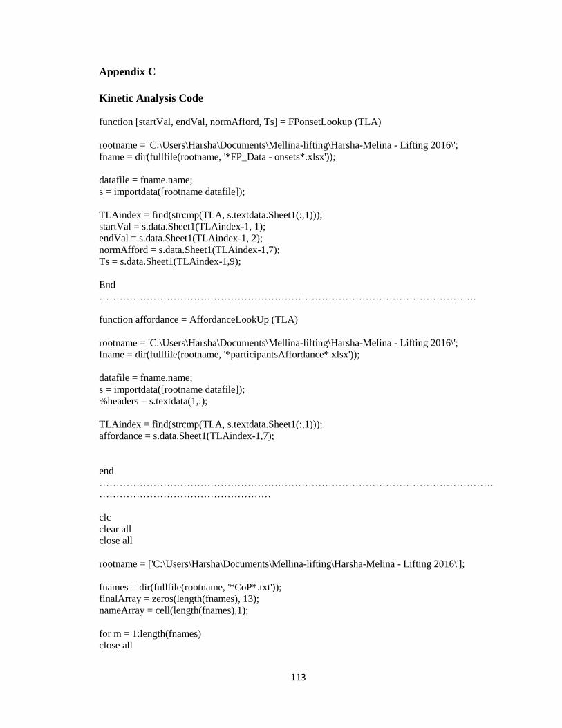
113

Appendix C

Kinetic Analysis Code

function [startVal, endVal, normAfford, Ts] = FPonsetLookup (TLA)

rootname = 'C:\Users\Harsha\Documents\Mellina-lifting\Harsha-Melina - Lifting 2016\';

fname = dir(fullfile(rootname, '*FP_Data - onsets*.xlsx'));

datafile = fname.name;

s = importdata([rootname datafile]);

TLAindex = find(strcmp(TLA, s.textdata.Sheet1(:,1)));

startVal = s.data.Sheet1(TLAindex-1, 1);

endVal = s.data.Sheet1(TLAindex-1, 2);

normAfford = s.data.Sheet1(TLAindex-1,7);

Ts = s.data.Sheet1(TLAindex-1,9);

End

………………………………………………………………………………………………….

function affordance = AffordanceLookUp (TLA)

rootname = 'C:\Users\Harsha\Documents\Mellina-lifting\Harsha-Melina - Lifting 2016\';

fname = dir(fullfile(rootname, '*participantsAffordance*.xlsx'));

datafile = fname.name;

s = importdata([rootname datafile]);

%headers = s.textdata(1,:);

TLAindex = find(strcmp(TLA, s.textdata.Sheet1(:,1)));

affordance = s.data.Sheet1(TLAindex-1,7);

end

………………………………………………………………………………………………………

……………………………………………

clc

clear all

close all

rootname = ['C:\Users\Harsha\Documents\Mellina-lifting\Harsha-Melina - Lifting 2016\'];

fnames = dir(fullfile(rootname, '*CoP*.txt'));

finalArray = zeros(length(fnames), 13);

nameArray = cell(length(fnames),1);

for m = 1:length(fnames)

close all

114

dataFile = fnames(m).name;

CoPdata = importdata([rootname dataFile]);

CoPr = CoPdata(:,3);

TLA = fnames(m).name(1:5);

nameArray(m,1) = {TLA};

[startVal, endVal, normAfford, Ts] = FPonsetLookup(TLA);

absLift = CoPr(startVal:endVal);

targetSize = [101 1];

rbLift = imresize(absLift, targetSize);

plot(absLift, 'r');

figure;

plot(rbLift, 'g');

t = 0:1:100;

td = 1;

input = (normAfford*heaviside(t-td))';

results = iddata(rbLift, input, Ts);

sys = tfest(results, 5, 'Ts', Ts);

finalArray(m,:) = [sys.num sys.den sys.Ts sys.Report.Fit.FitPercent];

end

% prompt = {'Please enter the file name:', 'Please enter the starting value:', 'Please enter the end

value:', 'Please enter the normalized affordance value:'};

% dlg_title = 'Input';

% num_lines = 1;

% defaultans = {'ASL_1CoP.txt','20','300','0.200'};

% answer = inputdlg(prompt,dlg_title,num_lines,defaultans);

%

% data = answer{1,1};

% G = str2double(answer{2,1});

% L = str2double(answer{3,1});

% affordance = str2double(answer{4,1});

%

% CoP = load(data);

% CoPr = CoP(:,3);

%

%

% % G = 138;

% % L = 346;

% abs_lift = CoPr(G:L);

% rb_lift = interpft(abs_lift,101);

%

%

% % figure

115

% % plot(abs_lift);

% figure

% plot(rb_lift);

%

%

% stepFunc = [zeros(1,1); affordance*ones(100,1)];

% %input function for system analysis

% inputFunc = stepFunc;

%

% outputFunc = rb_lift;

%

% assignin('base','input',inputFunc);

% assignin('base','output',outputFunc);

…………………………………………………………………………………………………

%This function calculates the start onset (G) and end onset (L), for

%individuals using the 'Load FP' data, specifically Mx data. Mx data is

%loaded from CalibrationEqns function and k is the number of indecies (6060)

function [G, L] = StartOnset (~,~)

k = 1;

while k ~= 0

prompt = {'Please enter the Calibrated file name:'};

dlg_title = 'Input';

num_lines = 1;

defaultans = {'ASL_1Calibrated.txt'};

answer = inputdlg(prompt,dlg_title,num_lines,defaultans);

%load the text data file

data = answer{1,1};

values = load(data);

Mx = values(:,4);

n = k;

% Build a low-pass filter

collection_frequency = 600; % Hz

[B A] = butter(2, 20 / collection_frequency / 2, 'low'); % 2nd order, 10 Hz

% Dual-pass filter the data (becomes a 4th order filter)

Mx_filtered = filtfilt(B, A, Mx); % this will return all NaNs if any value is NaN

Mx_edit = Mx_filtered;

Mx_edit2 = Mx_filtered;

Mx_edit3 = Mx_filtered;

% Use the first 100 frams (1000 ms) as the (hopefully) quiet baseline

Mx_mean = mean(Mx_filtered(1:100));

Mx_std = std(Mx_filtered(1:100));

116

% Find the first time each channel goes outside +/- 5 standard deviations

% (i.e. first fluctuation)

Mx_onset = min([ find(Mx_filtered > Mx_mean + 5*Mx_std, 1) find(Mx_filtered < Mx_mean -

5*Mx_std, 1) ]);

G = Mx_onset

Remove1 = (1:Mx_onset)';

Mx_edit(Remove1) = []; %indecies upto first onset value removed; Length of data array is

changed

%Find the second fluctuation point (value above +5 standard deviations)

next_onset = min(find(Mx_edit > Mx_mean + 5*Mx_std, 1));

%second onset value is equal to the first onset value plus the second

%fluctuating position. This is the Grasp onset (where the subjects touch the suitcase for the first

time)

Mx_onset2 = next_onset + Mx_onset;

L = Mx_onset2

Remove2 = (1:Mx_onset2)';

%indecies upto second onset point is removed; Length of the data array (i.e. Mx_edit) is

%changed again

Mx_edit2(Remove2) = [];

%Find the third fluctuation point (value less than -5 standard deviations)

third_onset = min(find(Mx_edit2 < Mx_mean - 5*Mx_std, 1));

%Thrid onset is the sum of previous two onset INDECIES and the last

%fluctuation indecies (due to changing data array length)

%Mx_onset3 = third_onset + Mx_onset2 + Mx_onset;

Mx_onset3 = third_onset + Mx_onset2;

Remove3 = (1:Mx_onset3)';

%Indecies upto third onset point is removed: Length of the data array (i.e.

%Mx_edit) is changed again

Mx_edit3(Remove3) = [];

%Find the fourth fluctuating point (i.e. value greater than +5 standard deviations)

fourth_onset = min(find(Mx_edit3 > Mx_mean + 5*Mx_std, 1));

%Final onset point is the sum of all three previous onset INDECIES and the

%index of the fourth fluctuating point

%End_onset = fourth_onset + third_onset + Mx_onset2 + Mx_onset

End_onset = fourth_onset + Mx_onset3;

figure;

%subplot(2,1,1), hold on, ylabel('Fx2');

%subplot(2,1,2),

hold on, ylabel('Mx (m)');

xlabel('Time (ms)');

title('Grasp & Lift Onsets');

%subplot(2,1,1), plot(Fx2_Fy2(:,1), 'c');

%subplot(2,1,2),

117

plot(Mx, 'm');

%subplot(2,1,1), plot(Fx2_Fy2_filtered(:,1), 'b');

%subplot(2,1,2),

plot(Mx_filtered, 'r');

%subplot(2,1,1), hline(Fx2_mean, 'k');

%subplot(2,1,2),

hline(Mx_mean, 'k');

%subplot(2,1,1), hline(Fx2_mean+5*Fx2_std, '--k');

%subplot(2,1,1), hline(Fx2_mean-5*Fx2_std, '--k');

%subplot(2,1,2),

hline(Mx_mean+5*Mx_std, '--k');

%subplot(2,1,2),

hline(Mx_mean-5*Mx_std, '--k');

%subplot(2,1,1), vline(Fx2_onset, 'g');

%subplot(2,1,2),

vline(Mx_onset, 'g');

vline(Mx_onset2, 'm');

vline(Mx_onset3, 'b');

vline(End_onset, 'g');

%return the two onset value indecies

% G = Mx_onset;

% L = LiftOnset + Mx_onset;

% Plot the two onset points over the Fy2 data

% figure;

% %subplot(2,1,1), hold on, ylabel('Fx2');

% %subplot(2,1,2),

% hold on, ylabel('Fy2 (m)');

% xlabel('Time (ms)');

% title('Grasp & Lift Onsets');

% %subplot(2,1,1), plot(Fx2_Fy2(:,1), 'c');

% %subplot(2,1,2),

% plot(Mx, 'm');

% %subplot(2,1,1), plot(Fx2_Fy2_filtered(:,1), 'b');

% %subplot(2,1,2),

% plot(Mx_filtered, 'r');

% %subplot(2,1,1), hline(Fx2_mean, 'k');

% %subplot(2,1,2),

% hline(Mx_mean, 'k');

% %subplot(2,1,1), hline(Fx2_mean+5*Fx2_std, '--k');

% %subplot(2,1,1), hline(Fx2_mean-5*Fx2_std, '--k');

% %subplot(2,1,2),

% hline(Mx_mean+5*Mx_std, '--k');

% %subplot(2,1,2),

% hline(Mx_mean-5*Mx_std, '--k');

% %subplot(2,1,1), vline(Fx2_onset, 'g');

% %subplot(2,1,2),

% vline(Mx_onset, 'g');

% vline(LiftOnset+Mx_onset, 'y');

% %vline(fmax_index,'b');

118

prompt2 = {'Enter 0 to exit, 1 to continue:'};

dlg_title2 = 'Exit Info';

num_lines2 = 1;

defaultans2 = {'1'};

answer2 = inputdlg(prompt2,dlg_title2,num_lines2,defaultans2);

k = str2double(answer2{1,1});

end

end

………………………………………………………………………………………………………

function [inputFunc, rbTotal2] = CalibrateSignals (~,~)

k = 1;

while k ~= 0

prompt = {'Please enter the file name:', 'Please enter the affordance distance:'};

dlg_title = 'Input';

num_lines = 1;

defaultans = {'ASL_1.txt','20'};

answer = inputdlg(prompt,dlg_title,num_lines,defaultans);

%data = input(prompt,'s');

data = answer{1,1};

%save the input file name

[~,name,~] = fileparts(data);

fname = [name,'Calibrated.txt'];

fname2 = [name,'CoP.txt'];

%load data from text file

values = load(data);

%break into separate arrays; changed column numbers according to the second

%experiments' data sets, i.e. columns 3 to 8 and only 1 forceplate (Sep 22,2016)

Fx_1 = values(:,3);

Fy_1 = values (:,4);

Fz_1 = values(:,5);

Mx_1 = values(:,6);

My_1 = values(:,7);

Mz_1 = values(:,8);

% Fx_2 = values(:,7);

% Fy_2 = values(:,8);

n = length(Fx_1);

119

%matirx A represents the force plate #1 data

A = [Fx_1 Fy_1 Fz_1 Mx_1 My_1 Mz_1];

%divide by 5 to get rid of the external gain

A_noGain = A/5;

%calibration matrix for force plate #1

CaliMatrix = [1260.6 28.1 2.2 4.8 -6.8 5.1; -50.7 1254.0 -2.3 -2.1 -10.6 4.7; 3.5 -3.0 1881.4 8.2 -

5.7 9.7; 2.9 -55.7 -2.3 583.8 -0.3 0.8; 53.8 2.9 -0.4 -1.3 408.1 0.8; 2.6 -3.6 -3.3 -0.3 -0.6 291.4];

%take transpose for matrix multiplication purposes

B = CaliMatrix.';

%matrix multiplication, Matrix C is the resultant (calibrated resultant) matrix

for i=1:n

C = A_noGain*B;

end

%take transpose of C to be used for fileID function

D = C';

%write the matrix D into a .txt file

fileID = fopen (fname,'w');

fprintf(fileID,'%8.5f %8.5f %8.5f %8.5f %8.5f %8.5f\r\n',D);

fclose(fileID);

% Build a low-pass filter

collection_frequency = 600; % Hz

[B, A] = butter(2, 20 / collection_frequency / 2, 'low'); % 2nd order, 10 Hz

C_filtered = zeros(6060,6);

for k = 1:6

% Dual-pass filter the data (becomes a 4th order filter)

C_filtered(:,k) = filtfilt(B, A, C(:,k)); % this will return all NaNs if any value is NaN

end

%COPx (centre of pressure in x-direction) = My/Fz and writting to txt file

COPx = -1*( C_filtered(:,5)./C_filtered(:,3));

COPy = (C_filtered(:,4)./C_filtered(:,3));

COPr = sqrt(COPx.^2 + COPy.^2);

COP_all = [COPx COPy COPr];

E = COP_all';

fileID2 = fopen(fname2, 'w');

fprintf(fileID2, '%8.5f %8.5f %8.5f\r\n', E);

fclose(fileID2);

prompt2 = {'Enter 0 to exit, 1 to continue:'};

dlg_title2 = 'Exit Info';

num_lines2 = 1;

defaultans2 = {'1'};

answer2 = inputdlg(prompt2,dlg_title2,num_lines2,defaultans2);

120

k = str2double(answer2{1,1});

end

end

………………………………………………………………………………………………………

%this function takes in the Fz data from the stance FP and finds the 'local

%minimum' value just before it goes down to the baseline value. 'Local

%minimum' represents the point when the participant's force in Z direction

%is in free-flow which indicates the end of the lift

function [EoL] = EndofLift (data)

%load data from text file

values = load(data);

%break into separate arrays

Fx_1 = values(:,1);

Fy_1 = values (:,2);

Fz_1 = values(:,3);

Mx_1 = values(:,4);

My_1 = values(:,5);

Mz_1 = values(:,6);

Fx_2 = values(:,7);

Fy_2 = values(:,8);

n = length(Fx_1);

%matirx A represents the force plate #1 data

A = [Fx_1 Fy_1 Fz_1 Mx_1 My_1 Mz_1];

%divide by 5 to get rid of the external gain

A_noGain = A/5;

%calibration matrix for force plate #1

CaliMatrix = [1260.6 28.1 2.2 4.8 -6.8 5.1; -50.7 1254.0 -2.3 -2.1 -10.6 4.7; 3.5 -3.0 1881.4 8.2 -

5.7 9.7; 2.9 -55.7 -2.3 583.8 -0.3 0.8; 53.8 2.9 -0.4 -1.3 408.1 0.8; 2.6 -3.6 -3.3 -0.3 -0.6 291.4];

%take transpose for matrix multiplication purposes

B = CaliMatrix.';

%matrix multiplication, Matrix C is the resultant (calibrated resultant) matrix

for i=1:n

C = A_noGain*B;

end

%take transpose of C to be used for fileID function

D = C';

[Gon , Lon] = GraspOnset (Fy_2, n);

%call function Fz_min_local

Fz_min_local = FzMinimum (C(:,3), Lon);

EoL = Fz_min_local;

display(Fz_min_local);

121

end

……………………………………………………………………………………………….............