Developing Theory Using Machine Learning Methods Files/19-032_1e1ab2d7-a3e3... · Key words: Machine learning, theory building, induction, abduction, decision trees, random forests,

Developing Theory Using Machine Learning Methods

Prithwiraj (Raj) Choudhury Ryan Allen Michael G. Endres

Working Paper 19-032

Working Paper 19-032

Copyright © 2018 by Prithwiraj (Raj) Choudhury, Ryan Allen, and Michael G. Endres

Working papers are in draft form. This working paper is distributed for purposes of comment and discussion only. It may not be reproduced without permission of the copyright holder. Copies of working papers are available from the author.

Developing Theory Using Machine Learning Methods

Prithwiraj (Raj) Choudhury Harvard Business School

Ryan Allen Harvard Business School

Michael G. Endres Harvard University

1

Developing Theory Using Machine Learning Methods

Prithwiraj (Raj) Choudhury,1 Ryan Allen1 and Michael G. Endres2

This draft October 15, 2018

We describe how to employ machine learning (ML) methods in theory development. Compared to

traditional causal inference methods, ML methods make far fewer a priori assumptions about the

functional form of the underlying model that best represents the data. Thus researchers could use

such methods to explore novel and robust patterns in data, allowing the researcher to engage in

inductive or abductive theory building. ML’s strengths include replicable identification of novel

patterns in data. ML methods also address several issues raised by scholars pertinent to the norms of

empirical research in the fields of strategy and management (such as “p-hacking” and confounding

local effects with global effects). We provide a step-by-step roadmap that illustrates how to use four

ML methods (decision trees, random forests, K-nearest neighbors and neural networks) to reveal

patterns in data that could be used for theory building. We also illustrate how ML methods can

illuminate interactions and non-linear effects better than traditional methods do. In summary, ML

methods could serve as a complement to existing theory-creating methods, such as multiple-case

inductive studies, as well as traditional methods of causal inference.

Key words: Machine learning, theory building, induction, abduction, decision trees, random forests, k-nearest neighbors, neural network, p-hacking

1 Harvard Business School. Corresponding author: Raj Choudhury (email: [email protected]). The authors thank Kathy Eisenhardt, Dan Levinthal, Joe Mahoney and participants at the 2018 Academy of Management and the 2018 Strategy Science conference held at the Wharton School for helpful comments on a prior draft. All errors remain ours. 2 Harvard Institute for Quantitative Social Science and Laboratory for Innovation Science at Harvard

2

INTRODUCTION

A new and burgeoning literature is urging researchers to adopt machine learning (ML)

methodologies (Athey and Imbens 2015; Mullainathan and Spiess 2017; Athey 2017). So far, ML

methodologies have been employed in social sciences to address a wide variety of prediction

problems (Ban et al. 2016, Li et al. 2016, Grushka-Cockayne et al. 2016). Even research in strategy

has begun to embrace the use of ML tools for predictive purposes (Menon, Lee and Tabakovic,

2018; Choudhury, Wang, Carlson and Khanna, 2018). But using ML methods for prediction alone

represents a rather limited opportunity for employing these methodologies for research in strategy

and management.

We argue that ML methodologies could have an even larger footprint in strategy and

management research if employed to explore novel and robust patterns in data, aiding researchers as

a tool for theory building. There is a rich prior literature on “data-driven theory building”

(Eisenhardt, 1989; Stokes, 1997; Nickerson, Yen and Mahoney, 2012, Eisenhardt, Graebner and

Sonenshein, 2016). In making a case for machine learning methods, Puranam et al. (2018) argue that

such methods can aid inductive theorizing by revealing robust, replicable associative patterns in data.

Although ML methods can be viewed as empirical, the core argument for why such methods can aid

theory building is as follows: strategy researchers’ workhorse empirical approach has been to use

linear3 models to regress a dependent variable on independent variables of interest, and then to

observe the significance, magnitude and direction of the global linear fit. But linear models make

certain assumptions about the functional form of the relationship between the independent variables

and the dependent variable, and the researcher might thus overlook novel interactive and nonlinear

3 By linear, we mean that the estimates depend on a linear combination of the covariates. The term nonlinear has been used by others, such as Shaver (2007), to characterize models such as logit, probit, Poisson and negative binomial, because the linear combination of covariates is the argument of a nonlinear function. This paper uses the word linear to refer to any model ƒ that relies on linear combinations of covariates, including logit, probit, Poisson, negative binomial, etc.

3

effects between variables,4 or heterogeneous effects among different subsets of the data. In contrast,

machine learning methodologies rely on less stringent a priori assumptions about the functional form

of the underlying model that best represents the data. Rather than forcing a model to fit the data,

ML methods allow researchers to construct a data-driven model. We thus argue that strategy and

management researchers can employ ML methodologies to find novel and robust patterns in data

that can advance theory building.5

Strategy and management scholarship should embrace ML methods for purposes of theory

building for several reasons. First, though there is a rich literature on the use of case-study research

for inductive theory building (Eisenhardt, 1989; Gioia and Chittipeddi, 1991), ML methods can

serve as a complement to theorizing using case studies. The latter method has several strengths, such

as generating insights from the juxtaposition of contradictory or paradoxical evidence (Eisenhardt,

1989) and its emphasis on developing constructs, measures and testable theoretical propositions

(Eisenhardt and Graebner, 2007). However, the complementarity between ML and case study

methods arises from the scale (at least in part) - the depth, mechanisms, openness of constructs and

theory favor cases, but the breadth, clarity of empirical patterns, and the potential for replicability

favor ML based methods. As Puranam et al. (2018) note, “algorithmic pattern detection” using ML

methods has high inter-subject reliability. In light of these features, ML methods could serve as an

important complement to case-study research for purposes of inductive theorizing.

4 It is possible to model nonlinear and interactive relationships in a linear model by including polynomial terms, dummy variables or interaction terms, but it is often difficult to explore alternate specifications systematically. As Edith Penrose famously asserted, “For the life of me I can’t see why it is reasonable (on grounds other than professional pride) to endow the economist with this ‘unreasonable degree of omniscience and prescience’ and not entrepreneurs” (Penrose 1952, page 813). Including too many terms can easily result in overfitting data, and it can be difficult for a researcher to be objective about which terms to include in or exclude from a model. Furthermore, polynomials may be a poor fit with certain nonlinearities, such as discontinuities in the data. By contrast, some ML models can handle discontinuities quite well. 5 The use of ML methods for theory building is within the tradition of using other “empirical” methods, such as simulation methods, for theory building (Davis, Eisenhardt and Bingham, 2007).

4

There is a second compelling reason why ML methods should be widely adopted in strategy

and management research. In addition to helping empirical researchers explore novel patterns in

their data, ML methods address several concerns related to the norms of empirical research noted by

scholars, including ‘p-hacking’ and confounding local effects with global effects (Shaver, 2007; Bettis

2012; Goldfarb and King 2016). As prior research has noted, a shortcoming of traditional workhorse

regression methods is that each point estimate (estimating the relationship between an independent

variable and a dependent variable) is usually reported in terms of a single global linear effect—

whether or not that global linear fit is an accurate depiction of the actual behavior of the data.

Worse, researchers sometimes tweak a model until it yields the much-desired asterisks (*) that

represent significance in a regression table (Shaver, 2007; Bettis 2012; Goldfarb and King 2016),

disregarding the fact that significance does not imply goodness-of-fit. Goldfarb and King (2016) and

Bettis (2012) both lament strategy researchers’ tendency to “search for stars” by trying out different

model specifications until they yield statistically significant relationships in the data, and then

retrofitting theories to explain the relationships—a practice that, statistically, often leads to false

positives. In summary, prior research has pointed out that empirical work in strategy and

management has become myopically focused on finding statistically significant results, at the peril of

reporting false positives (up to 40% of reported results, according to Goldfarb and King) and of

failing to understand the practical and theoretical importance of one’s findings. To remedy these

trends, Goldfarb and King suggest “apply[ing] a textbook strategy from the field of data mining by

randomly splitting their data in two before beginning statistical analysis” to minimize false positives.

As discussed below, ML techniques employ “cross-validation” that involves ex-ante splitting of data.

ML also offers solutions to other empirical concerns discussed above. For example, the plots that

represent predictions from our ML models (displayed in a later section) clearly illustrate locally

sensitive nonlinear effects—that is, how the relationship between the independent and dependent

5

variables changes over different ranges. And, rather than representing significance with the asterisk

threshold, relationships are displayed for many different samples of the data to show how sensitive

the predictions are to variation of covariates for different samples.

This paper makes two noteworthy contributions. First, we introduce a detailed step-by-step

procedure whereby four machine learning techniques (commonly used in the fields of computer

science and economics) that lend themselves to theory building could be used to explore novel and

robust patterns in the data. The four ML methods employed in this paper (described in detail in a

later section) consist of decision trees, random forests, K-nearest neighbors (KNN) and neural

network models. Our second contribution is to compare how well these models fit the data as

compared to methods of traditional inference, such as the Cox proportional hazards model and the

logistic regression. We demonstrate that modeling data using traditional linear methods may yield

deceptive results when compared to the ML models. The machine learning tools we use here are not

new—they have been used in the computer science literature and in practice for decades (Samuel

1959). To the best of our knowledge, however, only scant prior research addresses how ML

methods can assist data-driven theory building, notably Puranam et al. (2018) and recent physics and

engineering papers that use ML methods to discover the underlying principles that govern physical

phenomena (Rudy et al. 2018, Hirsh et al. 2018). This is the first paper we know of in strategy and

management that uses actual data to demonstrate how ML can be employed to uncover novel

patterns in data vis-à-vis traditional methods. An online supplement provides a python notebook

and data that allow readers to reproduce our results and learn the methods used in this paper.

To illustrate these contributions, we use data from a large Indian technology company

(hereafter, TECHCO) to study employee-level antecedents of turnover, with a focus on early-career

employees. Using a unique dataset of 1688 early-career workers freshly hired from college, our

analysis proceeds in three distinct steps. In the first step, we study the antecedents of employee

6

turnover. We use two traditional empirical methods for estimating factors that affect employee

turnover: a Cox proportional hazards (PH) survival model and a logistic regression model. In the

absence of ML tools, these would have been our default methods to study antecedents of employee

turnover. Notably, employees whose performance was superior during initial training tended to

experience far less turnover than employees who performed poorly during training. In the second

step, to demonstrate the usefulness of ML methods to explore novel and robust patterns in data, we

employ four ML methods: decision trees, random forests, nearest neighbor methods and neural

networks. Here, our analysis reveals that the effect of the training score on turnover changes

nonlinearly over time. Specifically, we find that the effect found by the traditional methods—that

higher training scores lead to lower turnover—obscured a second, more nuanced effect: that the

small group of employees with very low training scores (<4.0) were dramatically more likely to leave

TECHCO, but only during the first six months on the job. In the third step, we integrate the

insights generated by using the ML methods into the analysis using traditional methods and proceed

to engage in theory building. In other words, we use the insights generated by the ML methods, and

accordingly specify the model to be used for logistic regression. Once we do so, our results reveal

that, after the first six months of employment, for employees who did well during training (those

whose score was >4.0), the training score is significantly positively associated with a higher probability

of turnover. Meanwhile, only the small subset of employees who scored poorly were significantly

more likely to leave, and only during the first six months. The effect for this small subset was large

enough to drive a negative global effect opposite of the true positive effect for the large majority of

employees. We employ these insights to generate hypotheses that might explain the revealed

patterns in the data. It is possible that a well-trained econometrician could discover these or similar

patterns in the data without ML methods. However, it would be difficult and time consuming to do

7

so in a systematic way, especially with a larger number of covariates and a large set of interaction and

non-linear terms.

Our paper contributes to several literatures relevant to strategy and management scholars,

but primarily to the literature on data driven theory building. As Eisenhardt (1989) observes,

“analyzing data is the heart of building theory from case studies” (Eisenhardt, 1989; page 539); we

argue that building theory using ML methods shares this principle. Building theory from data is

arguably at the heart of the “problem finding, framing and formulating” steps outlined by

Nickerson, Yen and Mahoney (2012). More broadly, Stokes (1997) makes a persuasive case for using

data to build theory that seeks both fundamental understanding of a phenomenon and usefulness. In

summary, ML methods can help researchers build theory from data by serving as a complement to

small-sample case-study research. In light of the emerging “theory-based view of the firm” (Felin

and Zenger, 2016), which views economic actors as “theorists,” such methods could also help

managers extract useful theory from patterns in firm-specific data.

We also make a methodological contribution to the literature on statistical inference in

strategy (Shaver 1998; Shaver 2007; Wiseman 2009; Goldfarb and King, 2016). We argue and

demonstrate that it is possible to use insights from ML models to build better traditional models for

statistical inference. ML methods can complement traditional methods of statistical inference in

strategy and management research by avoiding the common biases of traditional inference methods

(such as p-hacking and conflating local effects with global effects).

A ROADMAP FOR DEVELOPING THEORY USING MACHINE LEARNING

This section presents a detailed step-by-step roadmap for developing theory using machine learning

methods. In the first step, we begin with an interesting question and a suitable dataset for data-

driven theory building. In the second step, we establish a baseline and study the research question

using traditional empirical methods. Here, we use two such methods: a Cox proportional hazards

8

(PH) survival model and a logistic regression model. In the third step, to demonstrate the capacity of

ML methods to reveal novel and robust patterns in data, we employ four ML methods: decision trees,

random forests, nearest neighbor methods and neural networks. We provide sub-steps explaining

the process of implementing the models and provide guidance on how to choose between different

ML methods. In the fourth step, we build a new theoretical model by comparing insights from the

relatively unconstrained ML models with prior literature and the baseline model from step 2. In the

fifth and final step, we update the baseline model from step 2 to reflect our new theoretical model

and perform statistical inference. Table 1 outlines the roadmap of theory building using ML

methods.

-------------------------------------- Insert Table 1 about here

--------------------------------------

1. Begin with an Interesting Research Question and Empirical Data

To illustrate our framework, we study the antecedents of turnover among early-career employees.

The literature on employee turnover is vast (Jovanovic 1979; Cotton and Tuttle, 1986; Hom and

Kinicki, 2001; Ton and Huckman, 2008); within strategy research, the literature explores both firm-

and employee-level antecedents and consequences of employee turnover (Campbell, Ganco, Franco

and Agarwal 2012; Carnahan, Kryscynski and Olson, 2017; Tan and Rider, 2017).

We use an internal dataset from a large Indian technology firm, TECHCO. The dataset

consists of individual employee-level data on 1688 employees deployed at TECHCO’s nine

production centers across India, including test scores, training performance, and demographic

information, as well as the production center’s age, distance from the employee’s hometown, and

linguistic similarity to the employee’s hometown language. For details on the empirical setting and

the dataset, see Appendix Section 2.

2. Study the Research Question Using Traditional Methods as a Baseline

9

To establish a baseline level of understanding, we study our research question using traditional

estimation methods: the Cox PH model and the logistic regression model. Results from using the

Cox model reported in Appendix Table A3 indicate that those who performed well during training

(Training CGPA) tended to be significantly less likely to leave than those who performed poorly (for

details on the Cox PH model see Appendix Section 4). In a traditional empirical strategic-

management study, we would confirm these findings with robustness checks and then unpack the

results in the discussion section. The Cox PH model, like most models used in empirical

management research, is a linear model.6 It assumes that a single line (in two dimensions) or hyper-

surface (in multiple dimensions) can reliably characterize the dependent variable to estimate the

survival probability. The Cox PH model also makes several important assumptions, including the

assumption of a constant hazard ratio between subjects over time.7 This means, for example, that it

is assumed that the effect of training performance (Training CGPA) on probability of turnover is the

same at time as at time . In our data, in fact, this assumption is violated, as evidenced

by the Schoenfeld residuals proportional hazards test (p-values from the test are displayed in Table

A4). The test tells us that we can reject the null hypothesis that hazards remain proportional over

time for three covariates: Training CGPA, Male and Language Similarity. We also reject the null of the

global test that the proportional hazard assumption is appropriate for these data. This test indicates

that a linear model may fail to capture nonlinearities in the relationships we are studying.

In order to explore more flexible interactive and nonlinear hypotheses, we reframe this

problem as a classification problem—that is, as a model with a categorical dependent variable. Using

the logistic regression model requires a transformation of the survival data to panel (long) format,

6 Note that the Cox PH model is often referred to as a semi-parametric model because no functional form assumptions are made about the baseline hazard function. But because the covariates are still modeled as a linear combination of covariates, it is considered a linear model for purposes of this paper. 7 Key assumptions for Cox PH: (1) that the hazard ratios are constant over time; (2) that covariates are combined linearly; and (3) that the time-independent piece of the hazard is well described by an exponential form.

10

which helps to reframe the survival estimation as a classification problem. Section 3 of the Appendix

demonstrates this transformation of data, and also shows how the survival loss function (which is

optimized to produce Cox PH parameter estimates) maps onto the log-loss function (which is

optimized to produce logistic regression parameter estimates).

With the data in panel form, it is possible to use a logistic regression to estimate the

probability of the event (turnover) in a given time interval, given the subject’s attributes . Results

from logistic regression estimation appear in Table A5 as raw coefficient estimates. We use the same

covariates as the Cox PH model analysis but include a dummy variable for each time interval

(months 1 through 40) in order to model time non-parametrically, making no functional form

assumptions about how time affects turnover probability.8 After exponentiating the coefficients to

odds ratios, the results from the logistic regression are almost identical to the results from the Cox

PH model—those who performed well during training (Training CGPA) tended to be significantly

less likely to leave than those who performed poorly. The slight differences arise from mathematical

technicalities, such as how to treat tied values in the Cox PH model, a slightly different loss function,

and the fact that the functional forms are only approximately equal (note that the approximation

becomes better as the time interval decreases).

Reframing the survival estimation as a classification problem and employing the logistic

regression establishes a foundation from which to launch into learning other ML methods that can

make more nuanced nonlinear predictions, model interactions between variables and model the

8 It should also be noted that the Cox PH model non-parametrically models how time affects survival by including a

baseline hazard for each time , . Thus it makes no assumptions about the functional form of how time affects survival. When using logistic regression on the reformatted data, however, it is necessary to model how time affects duration by including time as a covariate (or multiple covariates) in the model. Thus, the last step in the transformation from survival to classification data is to choose how to model time. For example, if time were modeled quadratically, we

would include covariates and in our model. However, modeling time quadratically (or with some other function) imposes functional form assumptions. Instead, for the logistic regression analysis we use a semiparametric approach, including a dummy variable for each and every time interval from the first month through the last month

.

11

coefficients as a function of time. For example, we have already demonstrated that the

proportional hazards assumption of the Cox PH model did not hold—that is, that the assumption

that hazard ratios were constant over time was violated. The logistic regression essentially makes the

same assumption—that a unit increase in some variable is associated with the same increase in the

log-odds of the event occurring in each time period. However, it would be interesting to see how the

effects of change over time. The question then is: why do we not model as a function of time?

It is, of course, possible to model as a function of time, but doing so in practice is rare in

management research. One explanation may be that it is difficult to know how to do so in a

systematic way. It is also difficult to be objective: because there is no clear guideline, a researcher

could adjust the model until it yields desired results (Simmons, Nelson, and Simonsohn 2011,

Goldfarb and King 2016). Perhaps most problematic is the fact that as is modeled as a function of

finer and finer intervals of time, the model will eventually overfit the data for any finite sized data

set. Imagine modeling both and as a function of each discrete time interval ( to )

in our data. The model would describe our in-sample data well. But the model would not necessarily

be generalizable—it might not describe other out-of-sample data well because any new example that

did not closely match an existing example in our data would be misclassified.9 This dilemma is well

known to management and economics scholars as the Bias-Variance Tradeoff (see Figure 1). As the

model is over-specified, its bias decreases but variance increases, making it non-generalizable—but

on the other hand an underspecified model is biased because it does not sufficiently describe the

data.

-------------------------------------- Insert Figure 1 about here

--------------------------------------

9 This is the case because the model would contain about 360 fit parameters, comparable to the number of Quit events in our data. Such a model would certainly overfit our data.

12

An advantage of machine learning is that it offers strategies for building and selecting

models that optimize the bias-variance tradeoff. Using ML techniques such as cross-validation and

regularization (discussed in more detail in a later section), we can loosen the assumption that

remains constant throughout each time interval, and objectively model as some function of time,

while still avoiding overfitting the data. Furthermore, we can capture nonlinearities in , which are

not represented by the fit functions of the traditional models. The next section introduces some

foundational ML algorithms that can be useful to empirical researchers for model building and

exploratory research.

3. Explore Patterns in the Data Using ML Methods

This section presents a general framework for machine learning problems and reframes the logistic

regression as an ML algorithm. We then introduce four machine-learning techniques for exploring

nuances in the functional form of the underlying distribution of the data: (1) decision trees, (2)

random forests, (3) K-nearest neighbors (KNN) and (4) neural networks. Reviewing these

techniques introduces management scholars to some of the most common ML models and

demonstrates that they reveal nuanced relationships in our data that the traditional methods missed.

The technical mathematical details of ML are outside the scope of this paper, but these models can

be implemented using free software packages in programming languages such as R and Python.

Section 5 of the Appendix provides detailed explanations, code and data (simulated based on the

data used in this paper) to help readers reproduce our results and apply the ML tools in their own

research.

Machine learning may be understood as both a collection of methods and as a process for

constructing models to make predictions. Here we will describe eight steps in the process of building

ML models. Our goal is to guide empirical researchers who wish to use ML for building data-driven

theory.

13

Sub-step 3.1: Select an appropriate loss function (i.e., an objective function or cost

function)10

The objective of the ML algorithm is to minimize loss (the output of the loss function) with respect

to the model parameters. Thus the first step in implementing an ML algorithm is to select an

appropriate loss function. In many statistical packages, it is unnecessary for the researcher to

explicitly select a loss function because it is included in implementation of the code for the model.

For pedagogical purposes, however, it is useful to frame the ML process around the loss function.

As a concrete example familiar to strategy researchers, implementing linear regression requires

minimizing the sum of squared errors loss. In this paper, sum of squared errors loss is an

inappropriate loss function, because in the context of survival analysis the assumptions of the OLS

loss function are violated (i.e. random variables are independent and Gaussian distributed). Instead,

for logistic regression and the other ML models we use in this paper, we use the log-loss function

where is the dependent binary variable that takes a value of 1 if an event occurred for a subject

in that time interval, and 0 otherwise. The term is our “hypothesis” (in this case, the

probability of classifying the observation as the event, ), which is the prediction produced

by our model of the data. This paper consistently uses this log-loss function for all of the ML

models considered. When we use different ML models (e.g., logistic regression, neural network), we

are simply changing the model that yields the value . Intuitively, this loss function punishes

bad hypotheses of which subject-time observations have a turnover event. For example, imagine

that an event occurs ( ) but the hypothesis is far off the mark: where

10 In most software package implementations, the appropriate loss function is included when the ML model is implemented. Understanding the loss function is key, however, to understanding how ML actually works.

14

(i.e., there is less than a one-in-a-thousand chance of an event occurring). When this

occurs, the second term in the loss function equation is “turned off” because . On

the other hand, the first term in the equation is . Because as

, this poor hypothesis severely punished the loss function: if , the added loss would be

infinite. As we will demonstrate in sub-step 6, to solve for the best-fit parameters , some

optimization algorithm will typically search values for iteratively until the loss function is

minimized.

Sub-step 3.2: Select the features (covariates) to include

Empirical researchers should use contextual knowledge to select relevant features (covariates or,

more generally, functions of covariates) that they are interested in studying. For typical ML

practitioners, predictive performance is the objective; often they include many extra features

(variables or polynomial or interaction terms of covariates), or even select the most predictive

features algorithmically. However, researchers hoping to use ML to build theory should consider

theoretical relevance during their selection. In our analysis, we had already selected the covariates we

were interested in studying when we ran the traditional models—but it is worth including feature

selection as a step in order to illustrate the general ML process. It is noteworthy that, unlike linear or

unregularized logistic regression, for many ML models (e.g., regularized logistic regression, neural

networks, neighbor methods) it is best practice to scale or normalize the feature values for better

model performance. Scaling often consists of converting each feature into a mean-zero unit-variance

score, which strips units from the features so that all numerical magnitudes are comparable across

features.

Sub-step 3.3: Select a model (fit function)

15

The next step is to select a model to make predictions for the loss function hypothesis, . We

will introduce several ML models: decision tree, random forest, KNN, and neural network.

Formally, each is simply using a different functional form for predicting .

As a concrete example, consider the logistic regression model, which is familiar to strategy

researchers. We illustrate where the hypothesis for logistic regression comes from, starting with the

logistic regression equation that was provided earlier:

Purely for notational purposes, we rename the terms of the logit function in order to conform to

notational norms in ML:

where , the probability of the event given , is renamed as the

“hypothesis”, and is changed to , which is a commonly used parameter notation in ML.

The above function, solved for , can be written in terms of the sigmoid function:

This is the hypothesis model for logistic regression used in the log-loss function. The equation is

exactly equivalent to the original logit function that we used for our logistic regression, but the

notation has been changed and the terms rearranged so that we can use it as a hypothesis in the loss

function.

Sub-step 3.4: Choose regularization

Regularization is any constraint that restricts the descriptive capacity of the model—essentially

smoothing the functional form of the predicted model—in order to prevent overfitting. Most

commonly, regularization consists of adding a regularization term to the loss function, or tuning the

16

hyperparameters11 of models. Often the ML loss functions will contain a regularization term.

Regularization terms in a loss function control for overfitting by punishing the loss function—that

is, by adding loss to any variable that carries too much weight. For example, the linear regression

with a common regularization term known as L2 (or ridge regression)12 is:

In our models, we sometimes include an L2 regularization term in the log-loss function:

The hyperparameter controls how strongly the loss function should be regularized, and can be

optimized via cross-validation (to be discussed in a later section). Note that L1 and L2 regularization

is sensitive to how the data is scaled, since the loss is no longer merely a function of linear

combination of covariates; thus, in these cases, standardizing the data is advisable. Other

regularization techniques involve tuning hyperparameters of the model. The above regularized

logistic regression has only one hyperparameter: . The other models we will introduce below can

include many other hyperparameters, which can be tuned to avoid overfitting. For example, in

neural networks, the number of layers, nodes, and connectivity (e.g. dropout) of the network can be

constrained or tuned to avoid overfitting. In decision trees, the termination rule for determining the

number of observations in a leaf node can be adjusted. In each case, tuning hyperparameters is a

delicate balancing act between bias (underfitting) and variance (overfitting).

11 A hyperparameter is any parameter of the model that is set before optimizing the loss function. These hyperparameters are not learned; instead they specify the model. 12 Strategy researchers may be more familiar with the regularization technique known as LASSO (or L1, in computer science), which adds the sum of the absolute value of the parameters, rather than the square of the parameters, to the regression equation.

17

Sub-step 3.5: Partition the sample for training, (cross-)validation and testing

Partitioning the sample of data is also extremely important for avoiding overfitting or underfitting

the data. The idea is that the model should be trained with a set of data that differs from the data

used to evaluate the model. Typically, the data are randomly partitioned into either three subsets

(training, validation and holdout test sets) or two subsets (training-validation and holdout test sets)

to be used for k-folds cross-validation. Using the first method, the loss function is minimized using

data from the training set (e.g., ~60% of the data), but the performance is then evaluated and

hyperparameters are tuned on the validation set (e.g., ~20% of data). The test set (e.g., ~20% of

data) is preserved as a holdout sample for final out-of-sample performance testing of the final

selected model (see sub-step 8). The other common validation method, and the one we use here, is

k-folds cross-validation, in which the training-validation data are partitioned into k equal-sized

subsets. One by one, each of the k subsets is used as the validation data; the other k-1 subsets are

used as the training data. The resulting k estimates are averaged for the final estimate. This paper

uses 10-fold cross-validation (k=10), a common choice for k. Cross-validation is less sensitive to the

idiosyncrasies of training and validation set selection, and usually gives more reliable evaluations for

smaller data sets, though it is more computationally intensive.

Sub-step 3.6: Fit the model on the training set and evaluate with validation set predictions

This is the core step, in which the actual “learning” in machine learning takes place. The fitted

model parameters are obtained when the regularized loss function is minimized on the training data

with respect to the model parameters using some optimization algorithm, such as (stochastic)

gradient descent, that searches the multidimensional landscape of the loss function for its lowest

point.13 Evaluation of the model is performed on the validation data using the unregularized loss

13 Detailed explanations of optimization algorithms are beyond the scope of this paper, but these algorithms are already implemented in many software packages. It is worth noting that, unless the optimization problem is convex (i.e., the loss function and any constraints are convex), there is generally no guarantee that the minimum found by such algorithms is a

18

function by comparing the fitted model’s predictions for the validation data to the actual outcomes

of the validation data using some metric (we use the log-loss score).

Sub-step 3.7: Repeat 3.1–3.6, varying the model, feature, hyperparameter and regularization

choices

Vary the models, features, hyperparameters and regularization repeatedly (e.g., by doing grid search

or, better, random searches of the hyperparameter space), searching for the model with the lowest

loss on the validation set (or the lowest cross-validation loss). It is difficult to know a priori which

choices will yield the best estimates—usually, ML practitioners try as many combinations of choices

as is feasible and select the best model. The loss function is minimized with respect to model

parameters on the training set; then the performance of that hypothesis is evaluated on the

validation set (or via cross-validation). For the purpose of model selection, the goal is to minimize

the loss of both the training and validation sets with respect to the hyperparameters, without the

validation loss diverging from the training loss. An example appears in Figure 2. The left-hand panel

plots the training and validation loss for logistic regression as a function of the inverse of L2

regularization, . It appears that the choice of does not make a substantial difference. This is the

case because our logistic regression already has relatively limited descriptive capacity (i.e., it is

biased), and regularization would only further restrict the model’s capacity to fit the data. The right-

hand panel plots the training and validation loss of the random forest model predictions as a

function of the “tree-depth” hyperparameter—the maximum number of branches from any node to

the root of the tree. Unlike logistic regression, the choice of tree-depth hyperparameter is impactful:

the random forest model has unbounded descriptive capacity, so the training loss approaches 0 as

global minimum. In the cases of linear and logistic regression, the loss function is convex by virtue of the linear hypotheses; thus this problem is not encountered. In general, however, the problem of multiple local minima is quite challenging. It is often present when fit results vary significantly with the choice of parameter initialization. Although there is no simple solution to the problem, it can sometimes be addressed with a better choice of initial parameter values

or stronger regularization.

19

regularization is removed. But if the model describes the training data too well, it does not generalize

to the validation data. It appears that the best choice for tree depth would be around 3 or 4—the

choice at which both training and validation losses are low, but validation loss has not diverged from

the training loss.

-------------------------------------- Insert Figure 2 about here

--------------------------------------

Sub-step 3.8: Evaluate final predictive performance using the holdout test set

Once the model, features, hyperparameters and regularization have been optimally tuned, the final

predictive performance is evaluated on the holdout test set. Because the holdout test set was not

used in any fitting or evaluation of models in the previous steps, it provides an out-of-sample test

for the performance of the model. In this paper we are less interested in predictive performance

than gaining insights from the model, so we do not discuss it in great depth here. Nevertheless, it is

worth including as a final step, both to understand the ML process and to ensure that the models

haven’t been overfit, which could lead to identifying false relationships in theory building.

Machine learning models and results

This section introduces four common machine learning models: decision trees, random forests, K-

nearest neighbors (KNN), and neural networks. Table 2 compares the four models. Each can be

understood by following the steps listed above: there is a regularized loss function, and an algorithm

iteratively tries different model parameters until that loss function is minimized using the estimates

from our hypothesized model .

-------------------------------------- Insert Table 2 about here

--------------------------------------

20

Decision Trees (Machine Learning Method 1). Decision trees are a foundational ML model. The

multidimensional space of features ( ) is repeatedly split along one axis, splitting on the

value of the feature that best minimizes the loss from the loss function. In other words, decision

trees partition so that each partition of is modeled as a constant function, with each constant

chosen to minimize total loss. The partitions are determined by scanning across all (or randomly

selected) features and all values of each feature, and determining the partition that yields the greatest

decrease in loss. Within each new partition created, the feature space is partitioned once again,

performing the same search and again minimizing the loss within each sub-partition. The process is

repeated, and the resolution of the model increases with each iteration. For an infinite training set,

the process can be repeated indefinitely; the total number of partitions (and the total number of

constants to be determined) grows exponentially with the depth. In practice, however, there is a

natural cutoff, attained when only a single data point remains within each partition. Modeling each

data point in the training set as a constant would model the in-sample data perfectly, but would not

generalize to out-of-sample data. To control for overfitting, the model is regularized by stopping

growth of the tree based on stopping conditions. All of these stopping condition choices are

hyperparameters of the decision tree model. Hyperparameters include the depth of the tree (recall

Figure 2), requiring each leaf to contain a minimum number of observations, requiring a specified

minimum decrease in the loss upon each split, or requiring that splits can occur only if the parent

node contains a minimum number of samples.

Our best-performing decision tree model allowed a maximum tree depth of 3, and allowed

splits only if the decrease in loss was greater than 0.0002. For this model, the data were not

normalized or standardized in any way. A representation of the decision tree partitions, obtained by

training on the full dataset using the hyperparameters specified above, appears in Figure 3. Note that

the top node of the tree is labeled . This means that, of all the values of

21

all the features in the model, the partition that most minimized loss was to split the data into the

36,493 observations whose training performance (Training CGPA) exceeded 3.995 and the 485

observations who scored less than 3.995. Following the left branch of the tree (labeled “True”), we

see that among those 485 observations with low training performance, the partition that best

minimizes the loss splits observations characterized by from those , and so on.

The leaf nodes (the terminal nodes in the tree) each contain a subset of the data, and display the

total entropy (normalized loss) contributed by the samples in that node. For an explanation of how

the total loss is calculated from the entropy in the leaf nodes, see Appendix Section 6.

-------------------------------------- Insert Figure 3 about here

--------------------------------------

It is interesting that the decision tree model splits along only two dimensions: Training CGPA

and Time. This is a clue to the empirical researcher that these dimensions probably contain

theoretically important nonlinearities and interactions; the other dimensions are more likely to be

well characterized by constant or linear functions. Below, we confirm that Training CGPA and Time

are in fact better modeled as piecewise constant interactive terms, while the other variables are

relatively well characterized by linear fits.

Random Forest (Machine Learning Method 2). One shortcoming of decision trees is that it is

difficult to know how to tune the hyperparameters that determine the stopping rule—the rules that

keep the tree from endlessly partitioning until the data are overfit or exhausted. Random forest

models provide a solution to this problem. Random forests are an ensemble-based approach: many

decision trees are generated, and the average (for random forest regression) or a consensus (for

random forest classification) of their predictions is used as the random forest prediction. Each

decision tree in the forest is generated by resampling the dataset (with replacement) at the unit of

22

analysis and randomly selecting a subset of features (without replacement). This process essentially

bootstraps estimates from many decision tree models.

In our case, using panel data, the dataset is sampled at the employee level, not the

observation level. In addition to the hyperparameters that require specification for decision trees,

random forests entail more hyperparameters: the size of the resampled dataset and selection of the

features used to construct the trees. This ensemble approach usually outperforms a single decision

tree because it is less sensitive to idiosyncrasies of the training data and to the choice of features

selected. In our best-performing model, we considered forests with 100 decision trees; for each tree,

we allowed a maximum tree depth of 3 and required a minimum of 100 samples per leaf. We also

allowed a maximum of 10 leaf nodes per decision tree in the forest. Although random forests

typically involve decision trees built from a randomly selected subset of features at each split,14 we

found that the best performance was achieved when all the features were used. For this model, the

data were not normalized or standardized in any way.

K-Nearest Neighbor (KNN) (Machine Learning Method 3). KNN, and neighbor methods in

general, learn the probability of an event for each data point from the outcomes of the surrounding

data points. In KNN, the predicted probability for data point is determined by taking the

mean of the outcome of the K data points most similar to . Usually similarity is based on a

distance measure, such as Euclidean distance, or more generally, Minkowski distance.

Because the hypothesis is learned from K neighboring points in the training set, loss

function minimization is not performed as with the other models presented in this paper. Instead,

the researcher can tune the model by adjusting the hyperparameter K to select the value that

minimizes the loss function. Because neighbor methods rely on distance measures, it is important to

14 It is usually recommended to take the number of randomly selected features to be equal to the square root of the total number of features for classification, or one-third of the total number for regression (Friedman et al. 2001)

23

appropriately scale the features in the data; these methods place features with potentially different

units on an identical footing. The performance of these models is therefore sensitive to such

choices, and implicitly introduces additional tunable hyperparameters (i.e., the relative-scale

hyperparameters associated with each feature). Neighbor methods like KNN are useful in that they

make no functional form assumptions at all. However, they can produce unreliable estimates in areas

where data are sparse, because the estimate for that area must be learned from more distant data

points. Another drawback is that each feature contributes the same weight to the calculated distance

so the model can be sensitive to irrelevant features. Furthermore, the model does not scale well—

prediction is slow with a large amount of data15.

In our best-performing KNN model, we standardize the data in the conventional way (by

subtracting the mean and dividing by the standard deviation) with one exception: for the time

feature, we subtract the mean but divide by a fixed reference time , which is taken to be a tunable

hyperparameter. Our reasoning is that time is not drawn from a distribution, but is dependent on

choices by the observer (namely, how long measurements were taken). For our model, we used

Manhattan distance as our distance metric, and took and .

Neural Network (Machine Learning Method 4). Artificial neural network models have attracted

growing attention in the last few years, and have driven such recent improvements in technologies as

image and voice recognition, translation, and autonomous vehicles. Artificial neural networks

roughly resemble the structure of biological neural networks: layers of computing nodes (like

neurons) are connected by weighted ties (like synapses) that transmit information. Figure 4 depicts

the general structure of an artificial neural network, which consists of an input layer of neurons (the

data), possibly one or more hidden layers and an output layer (predictions); each node of each layer

is connected by weights to each node of the next layer.

15 The computation time of the KNN model grows 𝑂(𝑛2)

24

-------------------------------------- Insert Figure 4 about here

--------------------------------------

The sum of the weighted data from the input layer is passed through to some function (an

“activation function”) in each node of the hidden layer. Then the output from each such node is

summed and passed to an activation function in each node of the output layer. The output layer

nodes are the model’s predictions. The network depicted in Figure 4 represents a multiclass

classification problem; for a single binary dependent variable like ours, the output layer consists of

only one node. A simple way to understand a neural network is to recognize that a logistic regression

is a neural network—a network with an input layer, no hidden layers and only one output layer node.

Each node from the input layer is weighted by and passed through to the activation function—in

this case, the sigmoid function —which produces predicted probabilities. As in logistic

regression, in more complex neural networks the weights of the nodes and layers are chosen to

produce predictions in the output layer that minimize loss of the loss function—usually the log-loss

function we discussed earlier.16 Compared to a logistic regression, the greater number of layers and

nodes in a neural network allows for highly complex non-linear hypotheses. With enough layers and

nodes, a neural network could in principle approximate any hypothesis, regardless of its complexity.

The ever-present problem to avoid when implementing neural networks is overfitting. To avoid

overfitting, hyperparameters such as the regularization term in the loss function, node connectivity,

number of layers and number of nodes can all be adjusted.

Our model uses a fully connected neural network with two hidden layers and ReLUs17

(Rectified Linear Units) as activation functions. The first hidden layer contains 32 nodes and the

second contains 12 nodes. The network is regularized using an L2 penalty term (coefficient: ) in

16 The optimization process is more difficult than it is for a logistic regression, and is solved using what is known as “the backpropagation algorithm”—essentially, an application of the “chain rule” for taking derivatives of nested functions. 17 The ReLU function is f(x)=max(0,x), a popular choice of activation function in neural networks.

25

the loss function—without such regularization, the model would be highly over-specified—and the

loss was optimized using the Adam (Kingma and Ba 2014) optimizer ( , ,

learning rate = 0.001). Detailed code for all these methods appears in the appendix.

Tools to Display ML model Predictions

This section illustrates two tools for displaying the results of using ML methods: partial dependence

plots and heat maps.

Partial Dependence Plots. Partial dependence plots display how the dependent variable changes

in response to changes in a single independent variable, while marginalizing (essentially, averaging)

over the values of the remaining variables (Friedman 2001). The partial dependence plots in Figure 5

show how our model prediction of the probability of a turnover event changes as a function of each

variable while averaging over the remaining variables (weighted according to their marginal

distribution). The figure displays the predicted marginal effect of each variable over its relevant

range, as predicted by the logistic regression model (on the left) and the random forest model (on

the right). The plot for each variable was generated by randomly selecting 500 observation-level

samples from the full dataset, and then for each sample predicting the outcome for different values

of the variable across the entire variable range while holding all other variable values fixed. The

predictions from each sample across each variable range are represented by orange lines. The result

is a distribution of 500 orange lines, one for each sample. Each plot also shows the typical partial

dependence, which is the average over of all the samples drawn (the dotted blue line). With the

exception of Time, which was modeled non-parametrically with a fixed effect for each interval, all

hypotheses of the logistic regression model were, by definition, linear.18 The random forest also

yielded dominantly linear hypotheses for most of the variables—except Time and Training CGPA.

18Note that the model predicts vanishing hazard for time slices t=0 and t=1, which contain no events

26

-------------------------------------- Insert Figure 5 about here

--------------------------------------

Heat maps. Another way to gain empirical insights from predicted models is to represent the

predicted probability of an event as color (heat) on a two-dimensional space of two feature variables,

while holding the other variables fixed at average values. The disadvantage of this approach is that it

is difficult to visualize the consistency of the estimate with variation in the remaining covariates, as

represented by the distribution of orange lines in the partial dependence plots. The advantage of

heat maps relative to the partial dependence plots is that they provide visually striking examples of

the nonlinear interactions between variables—in our case between Training CGPA and Time. Using

heat maps with a feature variable on each axis, it is possible to not only consider the isolated

nonlinear effects of single variables, but also how the effect of that variable depends on another.

Figure 6 displays the hazard of turnover predicted by each model, using the dimensions

Training CGPA and Time. We use these two dimensions because they serve as an illustrative example

with interesting nonlinear properties. We made similar plots for other combinations of variables (not

included), and found only non-interactive and linear effects, as expected.

-------------------------------------- Insert Figure 6 about here

--------------------------------------

One of the most striking insights from Figure 6 is the relatively poor model of the relationship

between Training CGPA, Time, and the hazard of turnover depicted in the logistic regression heat

map. The other models all capture the dramatically higher hazards predicted for the employees with

low training scores in their first months on the job. The linear logistic regression model, however,

can only produce a simple linear hypothesis: those with lower Training CGPA tend to have a higher

hazard of turnover—with different constant baseline hazards added to that hypothesis for each Time

due to the Time fixed effects. But that linear hypothesis does appear to represent reality—in the

27

other models the training scores did not appear to significantly affect hazards for any of the subjects

besides those with and . This is because Training CGPA was

not modeled as a function of Time in the logistic regression linear model, and was only modeled as a

global linear effect.

By contrast, in the decision tree heat map, there is a noticeable line splitting

and , exactly as in the representative decision tree

displayed in Figure 4. The random forest model gives similar insights—that the hazard of turnover

tends to increase over time, and that hazard is much higher for those with a training score below

about 4, especially around 6 months. We see that the negative effect of training score on turnover

estimated by the logistic and Cox models must have been driven by the narrow yellow strip of

employees with training scores below 4 at about month 6. Compared to the decision tree and

random forest predictions, the neural network predictions vary smoothly across the feature space,

and are not characterized as constants in each square region; however, because of the limited

amount of data, this model is not be as reliable as it would be with more observations.

Guidance on Choosing ML Methods

We provide some guidance on how to decide which ML model to use in different situations.

In practice, if prediction is the only objective then it is not uncommon to try many models and

select the model (or some weighted combination of models) that yields the best predictive

performance. However, different models may trade-off between bias and variance, interpretability

and predictive performance, or parameterization and computation time. Although it is difficult to

make generalizable claims about which model best suits each situation, in the last column of Table 2

we attempt to summarize some guiding rules.

For example, the logistic regression model is very easy to interpret because it yields beta

coefficients, but it may be highly biased if it fits a linear fit to nonlinear relationships in the data. The

28

random forest will almost always outperform the decision tree predictions, but decision trees are

easier to conceptualize and can be visualized with trees like Figure 3. KNN makes no

parameterization assumptions, truly making predictions without imposing a model on the data, but it

may not be computationally feasible with large amounts of data. Neural networks require large

amounts of data and computation, and fit smooth relationships in the data, but they are not easily

interpretable. There is no one best model—each has strengths and weaknesses that are highly

context-specific. Because it is difficult to know a priori which model is most appropriate for the data,

it is useful to try multiple models to understand the data from different angles, as we have in this

paper.

Predictive Performance of Models

In our data the only significant source of nonlinear interactive effects appears to be from

Training CGPA and Time, and only for a small subsample of the population; thus the differences

between the predictive performances of the different models are modest. A table of predictive

performance of each model is reported in Table A6. Predictive performance is also illustrated in

Figure 7 (left-hand panel), which shows training and cross-validation losses, with error bars

calculated from the variation among k-folds. Because fluctuations in performance for each model

are in part correlated with variation in samples, it is instructive to plot performance gains with

respect to a baseline model—in this case the logistic regression (Figure 7, right panel). By comparing

the differences in performance, the fluctuations associated with idiosyncrasies in the sample partially

cancel, resulting in a stronger signal for performance gains with respect to the baseline logistic

regression performance (a frequent trick in fields that routinely report predictive performance). We

find that the random forest and decision tree algorithms both offer small but statistically significant

(approximately 2-sigma) advantages over logistic regression. The reason for such small gains can be

attributed to the fact that the nonlinearities detected in Training CGPA over Time are only present in

29

a small subset of the data. Most of the data are modeled well by the linear features included in the

logistic regression.

-------------------------------------- Insert Figure 7 about here

--------------------------------------

Although the overall predictive performance gains of the ML models are only modestly

better than logistic regression, the increase in predictive performance for the small sample with low

Training CGPA in the first months was more salient. Using the decision tree model depicted in

Figure 3, we can calculate that the total loss from the 485 observations that were in the three leaf

nodes for which was 0.003. This small magnitude puts into perspective

how little overall predictive performance can be improved by correctly modeling the small subset of

low performers in their first months on the job. However, although the overall predictive

performance did not increase dramatically, our understanding of the relationships between variables

is greatly improved. The visualizations allow us to easily observe previously unseen nonlinear and

interactive effects in Training CGPA and Time.19

4. Build Theory Using ML-Generated Insights

Next we demonstrate how insights from the ML can be used to aid the researcher to build theory. In

the broader literature in organization science, Mantere and Ketokivi (2013) state the act of reasoning

on the part of managers and researchers alike takes three forms: deduction, induction and

abduction. Deductive reasoning takes the rule and the explanation as premises and derives the

observation. Inductive reasoning combines the observation and the explanation to infer the rule, thus

19 There are other measures of predictive performance, such as accuracy, AUC scores and F1 scores. We chose to use loss as the measure of performance because we have already introduced the concept of loss in this paper. Moreover, it is the metric for which we optimized, and a comparison of prediction metrics is beyond the scope of this paper. However, a word of caution is warranted about using accuracy (i.e., the number of correctly predicted observations divided by the total number) as a prediction performance metric. When the events in an outcome variable are imbalanced, accuracy creates a false impression of high predictive performance. For example, in the panel form of our data, only about 2% of observations are coded as turnover events; thus a trivial and entirely unhelpful model that always predicted “not turnover” would be 98% accurate.

30

moving from the particular to the general. Abduction begins with the rule and the observation; the

explanation is inferred if it accounts for the observation in light of the rule. We argue that ML

provides researchers with a novel and robust observation. The ML methods do not build theory

itself—rather it is an observational tool which the researcher can use to build theory. The process

may be inductive or abductive, depending on which is taken as given—the explanation or the rule.

In making a case for algorithmic induction using machine learning methods, Puranam et al.

(2018) build on prior scholarship (Glaeser and Strauss 1967, Lave and March 1993, Deetz, 1996,

etc.); they also highlight the importance of inductive inference in organization science, given that

induction attributes at least as much importance to explanation of phenomena as to testing the

deductively derived implications of axioms. Building on Lave and March (1993), the authors assert

that, in its classical form, the inductive method begins with observation of an empirical pattern,

which then becomes the target of theorizing with additional data. When using ML to abductively

build theory, researchers use ML observations and a general rule as premises and infer a specific

situational explanation.

To illustrate theory building using patterns in data revealed by the ML methods, consider

how the predictions from our models that revealed two novel patterns in the data: (1) employees with low

training scores exhibit a dramatically higher likelihood of turnover within the first six months; and (2) after the first

six months, there is a positive correlation between training scores and probability of turnover. Neither of these two

patterns was captured by our original linear model, prompting us to consider an update to our

previous linear hypotheses.

We juxtapose these patterns in the data against the prior theory literature on employee

turnover. The literature on employee turnover (Jovanovic 1979) assumes incomplete information on

job-worker match prior to hiring, and emphasizes that the information revealed after joining the

31

organization ultimately reveals the suitability of the match and determines turnover.20 This literature

also seems to suggest that the firm and employee must wait for a reasonable period of time to

observe on-the-job worker performance in order to determine the quality of a match. However, the

patterns that emerge from our data suggest that an early signal about the quality of job-worker

match could be provided by the worker’s performance during training. If the training process is

elaborate, and conducted over several weeks (as in the case of TECHCO), performance during

training could be a strong signal of job-worker match in the first few months. This pattern we

observe in the data could also be related to the firm “screening out” employees based on the

performance signal generated during training: notably Baker, Gibbs and Holmstrom (1994) find that

firms use incumbent employees' performance at a prior level to learn about their abilities and to

screen out the least able individuals. The second novel pattern in the data—the higher probability

that workers with higher training scores will experience turnover after six months—could be related

to “star” employees’ ability to use their early performance at a firm (i.e., their training scores) to

signal information to the external labor market.

Using the insights from the ML models and the previous literature, we update the logistic

regression to parsimoniously reflect the new patterns revealed in the data. We make two simple

modifications to the logistic regression estimation: (1) we run the model on two subsets of the data:

observations during the first six months on the job (First 6 months) and after 6 months (After 6

months); and (2) we add a dummy variable, Low CGPA (defined as 1 for employees with Training

20 Turnover is generated by the existence of a nondegenerate distribution of the worker's productivity across different jobs. The nondegeneracy is caused by assumed variation in the quality of a worker-employer match. This assumption is utilized across two categories of theoretical models. The first category of employee turnover model treats a job as an “experience good,” and assumes that the only way to determine the quality of a particular job-worker match is to form the match and "experience it." In this category of models, turnover occurs as a result of the arrival of information about the current job match. In a second category of models, jobs are pure search goods, and matches dissolve because of the arrival of new information about an alternative prospective match. An important implication of both sets of models is that, ex ante, the firm suffers from the shortcoming of having “imperfect information” on job-worker match; as a result, the firm must wait for further information to be revealed to determine the quality of job-worker match.

32

CGPA below 4, and 0 for everyone else) and add an interaction term between Low CGPA and

Training CGPA. By making these modifications, we now allow the linear model to fit piecewise linear

estimates for the effect of Training CGPA on turnover for two different time periods and compare

heterogeneous effects for employees who had high and low training scores.

To reiterate, the purpose of this study is not to engage in deep theory building, nor do we

claim theoretical insights generated by our analyses to be novel. Its purpose is to illustrate how novel

patterns in the data revealed by ML methods can serve as a starting point for theory building.

5. Estimate effects using an updated traditional model

Using the updated logistic regression, we can now obtain consistent estimates and statistical

significance for the parameters of interest. Although the machine learning tools presented in this

paper already provided valuable insights about the data, it is still useful to build traditional models in

order to obtain consistent estimates and tests of significance. The results from the updated logistic

regression, with piecewise estimation for Training CGPA and Time, reveal very different results than

the original logistic regression (see Table 3).

-------------------------------------- Insert Table 3 about here

--------------------------------------

The main takeaway from Table 3 is that the original global estimate of the effect of Training

CGPA on turnover (-0.887) was entirely driven by the dramatically higher probability of turnover for

those with scores below 4 in the first 6 months. The updated model reveals an effect with the opposite

sign for the large majority of the individuals represented in the data (those with Training CGPA above

4 after the first 6 months). Table 3 confirms that we have found a better model of the data, which

produces consistent parameter estimates and informs us which results are statistically significant.

33

DISCUSSION

This paper began with the goal of demonstrating how machine learning methodologies can help

researchers in strategy and management develop theory. Our exposition of four ML methods

(decision trees, random forests, K-nearest neighbors and neural networks), and our comparison of

insights generated using the ML methods with traditional methods (Cox proportional hazards model

and logistic regression), provide a roadmap for using these tools to build theory and add to the

literature on theory building and statistical inference in strategy research. To recap, insights from

using relatively unconstrained ML models helped us build a new logistic regression model, which

revealed that employees with training scores under 3.995 were much more likely to leave, but only

during the first six months on the job; thereafter, training scores had no effect on that group. For

the vast majority of the data set—employees with training scores above 3.995—higher scores

actually had a positive effect on turnover (though not quite significant at the level of 𝛼 = 0.05) after

the first six months. The positive sign of this effect was in direct opposition to the negative global

effect found by our original model.

Our paper makes several contributions. We provide a detailed step-by-step exposition of the

use of four ML methods that lend themselves well to building theory; we also present visual tools,

such as partial dependence plots and heat maps, that reveal novel and robust patterns in the

underlying data. We also highlight and demonstrate several advantages of using ML methods to

build theory. Rather than trying to force a series of researcher-specified models on the data until one

“works,” ML models are built from the data, making their selection more objective, appropriate to

the data and generalizable to other similarly distributed data. ML models are able to fit complex

functions to the data, while still generalizing to out-of-sample data. Because of cross-validation and

the use of holdout test sets, ML models are less sensitive to idiosyncrasies in a sample, which

minimizes the problem of finding false positives by merely seeking asterisks or interesting results

34

(Bettis 2012, Goldfarb and King 2007). ML models also allow researchers to focus on the

magnitude of effects, because asterisks are not automatically calculated with the estimates (and

because in some cases it may not be possible to calculate traditional significance). We also apply the

insights from our ML models to build traditional statistical models that yield p-values for inference,

allowing ML to complement to traditional methods.

It is our opinion that the use of ML tools in strategy and management research will help

overcome myopic focus on significance (asterisks), think beyond linear global fits, and help

researchers better understand the true nature of the phenomena they study. We view ML as a useful

complement to other statistical methods. It is a first step in building models that can represent

nonlinear and interactive effects by linearizing around smaller local areas (see Appendix Section 8).

It is possible that empirical researchers could uncover the effects demonstrated in this paper using

individual methods such as qualitative comparative analysis (QCA), or Gaussian distribution

approaches used in event history, individual visualization techniques such as binned scatter plots

(Starr and Goldfarb, 2018) or by using an approach that involves triangulation of these methods. We

believe ML methods can complement such existing methods of statistical inference.

ML methods have several limitations in how they can help management scholars build

theory. First and foremost, theory building using ML methods is fairly researcher dependent: the

researcher needs to specify a priori constructs (step 2 of our framework) and has to come up with a

theory and set of mechanisms relevant for the theory. In other words, ML methods only act as

observational tools and shed light on robust and interesting patterns in the data; the human

researcher needs to specific the constructs and identify theory and mechanisms through

complementary theory building methods such as cases. It is also important to recognize that, when

using ML, causal claims can only be made only if there is some source of exogenous variation—

exactly the same limitation that characterizes traditional models; in addition, data may suffer from

35

omitted variables bias. Shedding light on this would require traditional methods, including qualitative

methods such as field interviews. Using ML for more complicated causal analysis, such as using

instrumental variables, is a cutting-edge methodological topic in economics (Mullainathan and Spiess

2017). Moreover, this paper uses only supervised learning techniques—that is, techniques that try to

correctly classify data with a labeled dependent variable. Many applications of “unsupervised

learning” techniques could also be extremely valuable for using quantitative data to develop theory.

For example, dimensional reduction strategies, such as principal component analysis, could help

reveal the most important theoretical factors that drive a phenomenon. The methods in this paper,

though they are foundational supervised-learning models, are meant only as an introduction.

In conclusion, we argue that using ML methods for theory building could serve as a

complement to traditional methods of data-driven theory building, such as small-sample case studies

(Eisenhardt, 1989; Eisenhardt, Graebner and Sonenshein, 2016) and theory building using a fuzzy

set-theoretic approach (Fiss, 2007; 2011). While theory building using ML methods shares some of

the strengths of theory building approaches that use empirical data outlined by Eisenhardt and

Graebner (2007), e.g. it is likely to produce theory that is accurate, interesting and testable, it has

additional benefits of scale and precision in identifying empirical patterns. Theory-building using ML

methods is also highly replicable, given that the method depends on algorithms and replicable code.

In light of the “problem finding and problem solving” approach outlined by Nickerson, Yen and

Mahoney (2012), these methods could enable researchers to engage in problem finding using larger

samples of data than are amenable to small-sample case-study research. Such data-driven theorizing

could lead to insights that are both fundamental and useful, and would represent “theorizing in

Pasteur’s Quadrant,” as outlined by Stokes (1997).

36

REFERENCES

Athey, S., & Imbens, G. W. 2015. Machine learning methods for estimating heterogeneous causal effects. stat1050.5.

Athey, S. 2017. Beyond prediction: Using big data for policy problems. Science 355.6324: 483-485. Baker, G., Gibbs, M. and Holmstrom, B., 1994. The internal economics of the firm: evidence from

personnel data. The Quarterly Journal of Economics, 109(4), pp.881-919. Ban, G., Noureddine E., & Lim, A. EB. 2016. Machine learning and portfolio optimization.

Management Science, 64.3: 1136-1154. Bettis, R. A. 2012. The search for asterisks: Compromised statistical tests and flawed theories.

Strategic Management Journal, 33.1: 108-113. Burton, M. D., Sørensen, J. B., & Beckman, C. M. 2002. Coming from good stock: Career histories

and new venture formation. Campbell, B.A., Ganco, M., Franco, A.M. and Agarwal, R., 2012. Who leaves, where to, and why

worry? Employee mobility, entrepreneurship and effects on source firm performance. Strategic Management Journal, 33(1): 65-87.

Carnahan, S., Kryscynski, D. and Olson, D. 2017. When does corporate social responsibility reduce employee turnover? Evidence from attorneys before and after 9/11. Academy of Management Journal, 60(5): 1932-1962.

Carr, J. C., Boyar, S. L., & Gregory, B. T. 2008. The moderating effect of work—family centrality on work—family conflict, organizational attitudes, and turnover behavior. Journal of Management, 34.2: 244-262.

Choudhury, P., Carlson, N. A., Wang, D., & Khanna, T. 2018. Modeling Oral Business History Data: An Application to Markets and CEO Communication.

Cotton, J.L. & Tuttle, J.M., 1986. Employee turnover: A meta-analysis and review with implications for research. Academy of Management Review, 11(1): 55-70.

Cox, D. R. 1972. Regression models and life tables. J. R. Statist. Soc. B 34: 187-202. Cox, D. R. 2018. Analysis of Survival Data. Routledge. Cui, G., Wong, M. L., & Lui, HK. 2006. Machine learning for direct marketing response models:

Bayesian networks with evolutionary programming. Management Science, 52.4 : 597-612. Davis, J. P., Eisenhardt, K. M., & Bingham, C.B. 2007. Developing theory through simulation

methods. Academy of Management Review, 32 (2): 480-499. Deetz, S., 1996. Crossroads—Describing differences in approaches to organization science:

Rethinking Burrell and Morgan and their legacy. Organization Science, 7(2), pp.191-207. Eisenhardt, K. M. 1989. Building theories from case study research. Academy of Management

Review, 14(4): 532-550. Eisenhardt, K. M., & Graebner, M.E. 2007. Theory building from cases: Opportunities and

challenges. The Academy of Management Journal, 50(1): 25-32. Eisenhardt, K. M., Graebner, M. E., & Sonenshein, S. Grand challenges and inductive methods:

Rigor without rigor mortis. 1113-1123. Felin, T., & Zenger, T.R. 2016. The theory-based view: Economic actors as theorists. Strategy

Science, 2 (4): 258-271. Fiss, P. C. 2007. A set-theoretic approach to organizational configurations. Academy of

Management Review, 32(4): 1180-1198. Fiss, P. C. 2011. Building better causal theories: A fuzzy set approach to typologies in organization

research. Academy of Management Journal, 54(2): 393-420. Friedman, J. H. 2001. Greedy function approximation: a gradient boosting machine. Annals of

Statistics, 1189-1232.

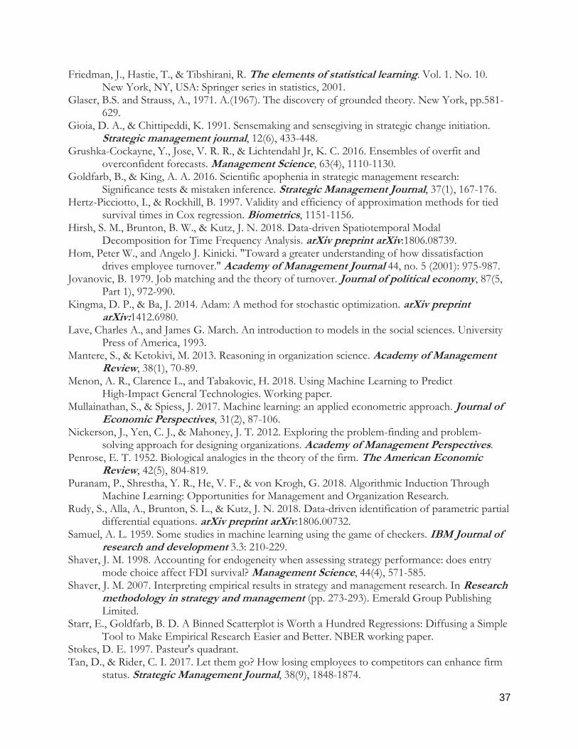
37

Friedman, J., Hastie, T., & Tibshirani, R. The elements of statistical learning. Vol. 1. No. 10. New York, NY, USA: Springer series in statistics, 2001.

Glaser, B.S. and Strauss, A., 1971. A.(1967). The discovery of grounded theory. New York, pp.581-629.

Gioia, D. A., & Chittipeddi, K. 1991. Sensemaking and sensegiving in strategic change initiation. Strategic management journal, 12(6), 433-448.

Grushka-Cockayne, Y., Jose, V. R. R., & Lichtendahl Jr, K. C. 2016. Ensembles of overfit and overconfident forecasts. Management Science, 63(4), 1110-1130.

Goldfarb, B., & King, A. A. 2016. Scientific apophenia in strategic management research: Significance tests & mistaken inference. Strategic Management Journal, 37(1), 167-176.

Hertz-Picciotto, I., & Rockhill, B. 1997. Validity and efficiency of approximation methods for tied survival times in Cox regression. Biometrics, 1151-1156.

Hirsh, S. M., Brunton, B. W., & Kutz, J. N. 2018. Data-driven Spatiotemporal Modal Decomposition for Time Frequency Analysis. arXiv preprint arXiv:1806.08739.

Hom, Peter W., and Angelo J. Kinicki. "Toward a greater understanding of how dissatisfaction drives employee turnover." Academy of Management Journal 44, no. 5 (2001): 975-987.

Jovanovic, B. 1979. Job matching and the theory of turnover. Journal of political economy, 87(5, Part 1), 972-990.

Kingma, D. P., & Ba, J. 2014. Adam: A method for stochastic optimization. arXiv preprint arXiv:1412.6980.

Lave, Charles A., and James G. March. An introduction to models in the social sciences. University Press of America, 1993.

Mantere, S., & Ketokivi, M. 2013. Reasoning in organization science. Academy of Management Review, 38(1), 70-89.

Menon, A. R., Clarence L., and Tabakovic, H. 2018. Using Machine Learning to Predict High-Impact General Technologies. Working paper.

Mullainathan, S., & Spiess, J. 2017. Machine learning: an applied econometric approach. Journal of Economic Perspectives, 31(2), 87-106.

Nickerson, J., Yen, C. J., & Mahoney, J. T. 2012. Exploring the problem-finding and problem-solving approach for designing organizations. Academy of Management Perspectives.

Penrose, E. T. 1952. Biological analogies in the theory of the firm. The American Economic Review, 42(5), 804-819.

Puranam, P., Shrestha, Y. R., He, V. F., & von Krogh, G. 2018. Algorithmic Induction Through Machine Learning: Opportunities for Management and Organization Research.

Rudy, S., Alla, A., Brunton, S. L., & Kutz, J. N. 2018. Data-driven identification of parametric partial differential equations. arXiv preprint arXiv:1806.00732.

Samuel, A. L. 1959. Some studies in machine learning using the game of checkers. IBM Journal of research and development 3.3: 210-229.

Shaver, J. M. 1998. Accounting for endogeneity when assessing strategy performance: does entry mode choice affect FDI survival? Management Science, 44(4), 571-585.

Shaver, J. M. 2007. Interpreting empirical results in strategy and management research. In Research methodology in strategy and management (pp. 273-293). Emerald Group Publishing Limited.

Starr, E., Goldfarb, B. D. A Binned Scatterplot is Worth a Hundred Regressions: Diffusing a Simple Tool to Make Empirical Research Easier and Better. NBER working paper.

Stokes, D. E. 1997. Pasteur's quadrant. Tan, D., & Rider, C. I. 2017. Let them go? How losing employees to competitors can enhance firm

status. Strategic Management Journal, 38(9), 1848-1874.

38

Ton, Zeynep, and Robert S. Huckman. "Managing the impact of employee turnover on performance: The role of process conformance." Organization Science 19, no. 1 (2008): 56-68.

Wiseman, R. M. 2009. On the use and misuse of ratios in strategic management research. In Research methodology in strategy and management (pp. 75-110). Emerald Group Publishing Limited.

39

FIGURE 1

Illustrative Depiction of Bias-Variance Tradeoff in One Dimension

FIGURE 2

Training and Validation Loss as a Function of Hyperparameter Tuning for Logistic Regression (left) and Random Forest (right)

Note: For illustrative purposes, the random forest model does not contain any regularization other than tree depth. The random forest model used later in the paper differs slightly due to adjustment of other regularization hyperparameters.

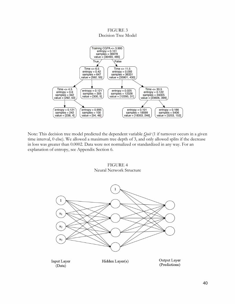
40

FIGURE 3 Decision Tree Model

Note: This decision tree model predicted the dependent variable Quit (1 if turnover occurs in a given time interval, 0 else). We allowed a maximum tree depth of 3, and only allowed splits if the decrease in loss was greater than 0.0002. Data were not normalized or standardized in any way. For an explanation of entropy, see Appendix Section 6.

FIGURE 4 Neural Network Structure

41

FIGURE 5 Partial Dependence Plots

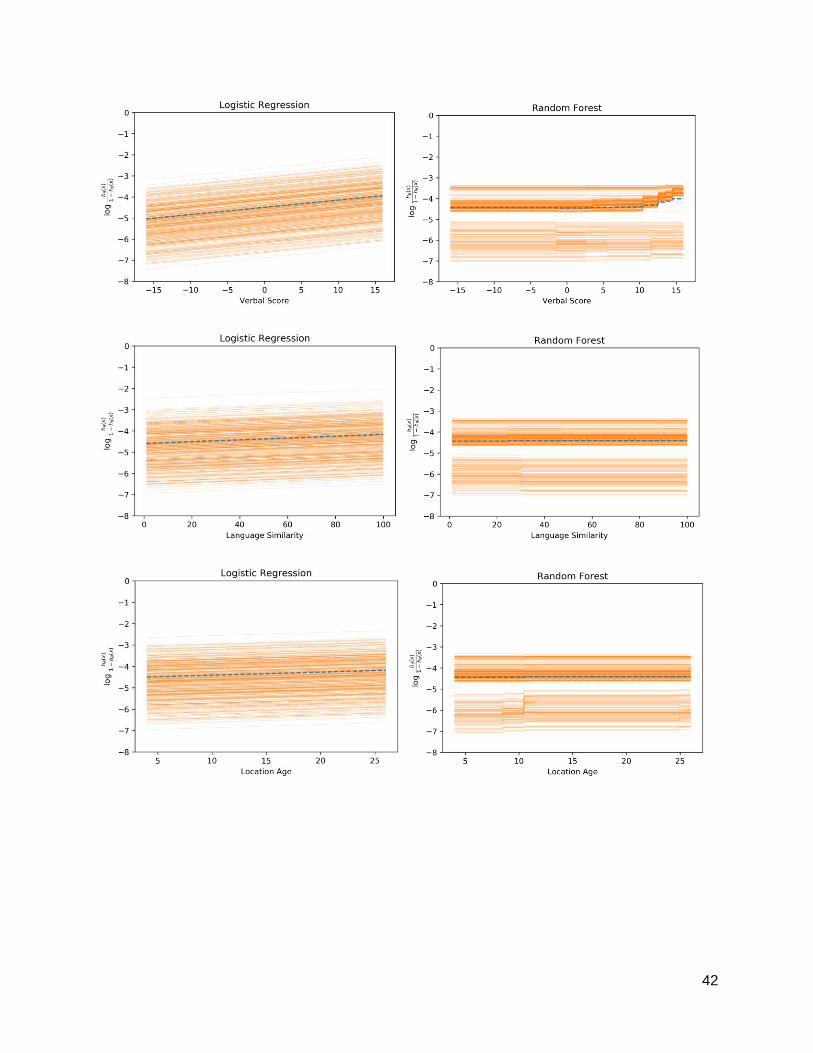
42

43

Note: The plot for each variable was generated by randomly selecting 500 samples from the full dataset, and, for each sample, predicting the outcome using different values of the variable across the entire variable range while holding all other variable values fixed. The predictions from each sample are represented by an orange line across the entire range. The result is a distribution of 500 orange lines in each plot, one for each sample. Each plot also shows the typical partial dependence of the hazard: the average over all the samples drawn (the dotted blue line). Logistic regression predictions appear in the left-hand plots; random forest predictions appear in the right-hand plots. Each vertical axis is on the same scale, with units as the log of the odds ratio of the predicted probability of an event.

44

FIGURE 6 Heat Map of Predicted Probability of Turnover for Training CGPA vs. Time

Note: Heat maps represent the probability of turnover predicted by each model, along the dimensions Training CGPA and Time. Other variable values are held constant at typical (average) values. All plots are on the same scale. Higher probabilities are represented in yellow; the lowest probabilities are represented in dark blue.

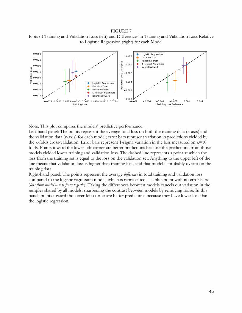
45

FIGURE 7 Plots of Training and Validation Loss (left) and Differences in Training and Validation Loss Relative

to Logistic Regression (right) for each Model

Note: This plot compares the models’ predictive performance. Left-hand panel: The points represent the average total loss on both the training data (x-axis) and the validation data (y-axis) for each model; error bars represent variation in predictions yielded by the k-folds cross-validation. Error bars represent 1-sigma variation in the loss measured on k=10 folds. Points toward the lower-left corner are better predictions because the predictions from those models yielded lower training and validation loss. The dashed line represents a point at which the loss from the training set is equal to the loss on the validation set. Anything to the upper left of the line means that validation loss is higher than training loss, and that model is probably overfit on the training data. Right-hand panel: The points represent the average difference in total training and validation loss compared to the logistic regression model, which is represented as a blue point with no error bars (loss from model – loss from logistic). Taking the differences between models cancels out variation in the samples shared by all models, sharpening the contrast between models by removing noise. In this panel, points toward the lower-left corner are better predictions because they have lower loss than the logistic regression.

46

TABLE 1 Roadmap for Developing Theories using Machine Learning

Step Activities Reason

1. Begin with a question and data

Determine a research question Find an appropriate setting and appropriate data to

answer the question Select variables of interest from the data

Motivates and lends focus to the analysis

Quality data matter in any analysis—the size of the data set doesn’t matter if the data can’t answer the question

2. Estimate using traditional methods

Estimate relationships in the data using traditional models appropriate for the data structure, such as OLS, fixed effects, logistic regression or survival analysis

Establishes a baseline relationship to build understanding and to compare with ML models

3. Build machine learning models

3.1 Select a loss function 3.2 Select features (covariates) 3.3 Select a model (e.g., decision tree, neural

network) 3.4 Choose regularization 3.5 Partition data for training, validation and

test sets 3.6 Fit model on the training set; evaluate with

predictions on the validation set 3.7 Repeat steps 1-6, varying model, feature,

regularization and other hyperparameters to find the best-performing model

3.8 Evaluate on test set

Builds a model from the data in a relatively unbiased and unconstrained way. By finding the best way to predict the outcome, we gain insight into how each variable may directly affect the outcome, how variables interact and how that relationship changes over time

4. Build theory Compare ML insights with prior literature Compare ML insights with traditional methods Specify a new traditional model (i.e., OLS, logistic,

survival analysis) using insights from the ML models. For example, stratify the data or add dummy variables to isolate heterogeneous effects or model time more appropriately

Because ML models don’t generate consistent estimates for causal analysis, we use such insights to build a better traditional model to generate estimates and hypothesis tests

5. Estimate effects using an updated traditional model

Use an updated traditional model to get parameter effect estimates and significance

Using the updated traditional model, we can generate a more reliable estimate of the magnitude and confidence of the relevant relationships in the data, while incorporating nuances uncovered by ML

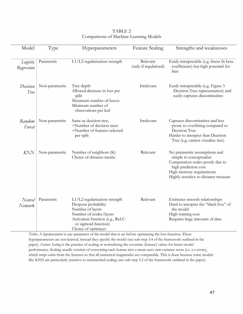
47

TABLE 2 Comparisons of Machine Learning Models

Model Type Hyperparameters Feature Scaling Strengths and weaknesses

Logistic Regression

Parametric L1/L2 regularization strength Relevant (only if regularized)

Easily interpretable (e.g. linear fit beta coefficients) but high potential for bias

Decision Tree

Non-parametric Tree depth Allowed decrease in loss per

split Maximum number of leaves Minimum number of

observations per leaf

Irrelevant Easily interpretable (e.g. Figure 3 Decision Tree representation) and easily captures discontinuities

Random Forest

Non-parametric Same as decision tree, +Number of decision trees +Number of features selected

per split

Irrelevant Captures discontinuities and less prone to overfitting compared to Decision Tree.

Harder to interpret than Decision Tree (e.g. cannot visualize tree)

KNN Non-parametric Number of neighbors (K) Choice of distance metric

Relevant No parametric assumptions and simple to conceptualize

Computation scales poorly due to high prediction cost

High memory requirements Highly sensitive to distance measure

Neural Network

Parametric L1/L2 regularization strength Dropout probability Number of layers Number of nodes/layers Activation function (e.g., ReLU

or sigmoid function) Choice of optimizer

Relevant Estimates smooth relationships Hard to interpret the “black box” of

the model High training cost Requires large amounts of data

Notes. A hyperparameter is any parameter of the model that is set before optimizing the loss function. These

hyperparameters are not learned; instead they specify the model (see sub-step 3.4 of the framework outlined in the

paper). Feature Scaling is the practice of scaling or normalizing the covariate (feature) values for better model

performance. Scaling usually consists of converting each feature into a mean-zero unit-variance score (i.e. a z-score),

which strips units from the features so that all numerical magnitudes are comparable. This is done because some models

like KNN are particularly sensitive to mismatched scaling (see sub-step 3.2 of the framework outlined in the paper).

48

TABLE 3 Comparison of the Original Logistic Regression and Logistic Regression with Piecewise Estimation

for Training CGPA and Time

Old Model First 6 months After 6 months (1) (2) (3)

Training CGPA -0.887*** 0.327 0.389* (0.182) (1.174) (0.181) Low CGPA 11.131* 1.850 (5.552) (4.144) Low CGPA x CGPA -1.219 -0.291 (1.298) (1.182) Logical Score -0.022 -0.037 -0.016 (0.013) (0.051) (0.014) Verbal Score 0.035** -0.009 0.035** (0.012) (0.043) (0.013) Average Literacy 0.015* 0.034 0.014* (0.006) (0.022) (0.007) Male 0.038 0.260 -0.047 (0.100) (0.358) (0.104) Production Center Age 0.014* -0.005 0.017* (0.006) (0.022) (0.007) Distance 0.115 0.250 0.091 (0.100) (0.470) (0.106) Language Similarity 0.004* 0.002 0.003 (0.002) (0.007) (0.002)

First 6 Months N/A yes no Time Fixed Effects yes yes yes Month of Arrival Fixed Effects yes yes yes N 34596 4655 29869

Estimates with robust standard errors reported in parentheses.