Developing Synthetic Logs Using Artificial Neural Network: Application to Knox County in Kentucky Fedra Ghavami Problem Report submitted to the College of Engineering and Mineral Resources at West Virginia University in partial fulfillment of the requirements for the degree of Master of Science in Petroleum & Natural Gas Engineering Committee: Professor Samuel Ameri, Chair Dr. Khashayar Aminian Dr. Razi Gaskari Department of Petroleum and Natural Gas Engineering Morgantown, West Virginia 2011 Keywords: Reservoir; Well Logs; West Virginia; Artificial Neural Network

Welcome message from author
This document is posted to help you gain knowledge. Please leave a comment to let me know what you think about it! Share it to your friends and learn new things together.
Transcript

Developing Synthetic Logs Using Artificial Neural Network:
Application to Knox County in Kentucky
Fedra Ghavami
Problem Report submitted to the
College of Engineering and Mineral Resources
at West Virginia University
in partial fulfillment of the requirements
for the degree of
Master of Science
in
Petroleum & Natural Gas Engineering
Committee:
Professor Samuel Ameri, Chair
Dr. Khashayar Aminian
Dr. Razi Gaskari
Department of Petroleum and Natural Gas Engineering
Morgantown, West Virginia
2011
Keywords: Reservoir; Well Logs; West Virginia; Artificial Neural Network

ABSTRACT
Developing Synthetic Logs Using Artificial Neural Network: Application to Knox County in Kentucky
Fedra Ghavami
The purpose of this study was to examine missing data from oil production logs as well as
predict oil reservoir production levels. Historically, data logs contain gaps or missing data
points due to limitations of the tools and methodologies that are used to collect the data. To help
predict and examine the gaps with no data points, Back Propagation was used to extrapolate both
existing and non-existing data.
Stemming from the research that was performed using the Back Propagation method, missing
data was identified. To validate and confirm the accuracy of the data, the extrapolated data was
compared against actual data logs from core samples.
A methodology to generate synthetic wireline logs is presented. Synthetic logs can help to
analyze the oil reservoir properties in areas where the set of logs that are necessary, are absent or
incomplete. The approach presented involves the use of Artificial Neural Networks, as the main
tool, in conjunction with data obtained from conventional wireline logs. Implementation of this
approach aims to reduce operation costs to companies.
There is a synthetic methodology to generate wireline logs. In some cases, we need to have
absent or incomplete logs. Synthetic logs will help to analyze the reservoir properties in this
manner. Artificial Neural Networks have been implemented as the main model to predict
wireline logs. Implementation of this technique will reduce the operation costs for oil and gas
companies.

Development of the neural network model was completed using a back propagation and five oil
wells. Data collected from the five wells was collected using the following logs:
1. Gamma ray,
2. Density,
3. Neutron,
4. Caliper logs.
Synthetic logs were generated through two different exercises. Exercise one involved four wells
for development and training of the network. Exercise two included four wells in series and one
well out.
Developing of the artificial neural networks model is implemented using a Backprpagation of
Artificial Neural Network and five wells that included gamma ray, neutron, density, and
resistivity logs. Synthetic logs are generated through two experiments. Experiment one has
involved five wells for training and development of the network.
Verification was used for each well to train the network. The second experiment involved four
wells for the development and training of the network. A fifth well that was not applied during
calibration and training was selected for verification. Four mixtures of inputs/outputs are
selected to train the network. Mixture “A” consists of the neutron log which contains the output
as well as density, gamma ray, and density caliper logs, which comprises the input.
In conclusion, it is demonstrated that the quality of data has an important role in the
implementation of the neural network model. It is really important to do a careful quality control
of the data before building a neural network model. It is concluded conversely; that the neural
network modeling doesn’t affect the performance of having lithologic heterogeneities in the
reservoir in generation of synthetic logs.

iv
Acknowledgments
First I thank god for giving me the capability and the courage to finish my thesis and complete
my MS in Petroleum and Natural Gas Engineering.
I would like to dedicate this thesis to my parents, who always gave me their support and
encouragement, and most importantly, their love. It kept me going during some of the difficult
moments of this work. I appreciate you and I love you.
I don’t have the words to express my thanks and appreciation to Professor Sam Ameri, chair of
my committee, who brought me to the Petroleum and Natural Gas Engineering Department and
encouraged me to complete my master’s degree. I wouldn’t be able accomplish this without his
support and advice, not only during this work but also throughout the time I spent at the
department.
I want to extend my sincere appreciation and gratitude to my research advisor Dr. Razi Gaskari,
for introducing me to the fascinating area of Natural Networks, for his friendship, and for his
continuous guidance, encouragement, support and patience throughout this work.
Special thanks to Dr. Khashayar Aminian for being on my committee and for the enriching
contributions and comments to this work.
Finally, my deepest gratitude to Mrs. Beverly Matheny for her assistance and enthusiasm during
every semester spent in the department.

v
TABLE OF CONTENTS
1. INTRODUCTION ................................................................................................................................ 1
2. BACKGROUND .................................................................................................................................. 2
2.1. Geological Setting ......................................................................................................................... 2
2.1.1. Description of Knox county in Kentucky ............................................................................. 2
2.2. Well logs fundamentals ................................................................................................................. 9
2.2.1. Gamma Ray .......................................................................................................................... 9
2.2.2. Caliper log ........................................................................................................................... 12
2.2.3. Density-Porosity logs .......................................................................................................... 12
2.2.4. Neutron Log ........................................................................................................................ 14
2.3. Artificial neural network ............................................................................................................. 14
2.3.1. Characterization of Neural Network ......................................................................................... 15
2.3.2. Biological Neural Network ................................................................................................. 15
2.3.3. Typical Architectures .......................................................................................................... 18
2.3.4. Single-Layer Net ................................................................................................................. 20
2.3.5. Multilayer Net ..................................................................................................................... 21
2.3.6. Setting the Weights ............................................................................................................. 21
2.3.7. Supervised Training ............................................................................................................ 22
2.3.8. Unsupervised Training ........................................................................................................ 22
2.3.9. Fixed-weight Nets ............................................................................................................... 23
2.3.10. Common Activation Functions ........................................................................................... 23
3. LITERATURE REVIEW ................................................................................................................... 28
4. METHODOLOGY ............................................................................................................................. 40
4.2. Data Preparation ............................................................................................................................... 41
4.2.1. Exercise 1: filling the Gaps (Five Wells Combined) .......................................................... 52
4.2.2. Exercise 2: Four Wells Combined, one well out ................................................................. 53
5. RESULTS ........................................................................................................................................... 54
5.1. Exercise 1. Results ........................................................................................................................... 54
5.2. Exercise 2. Results ........................................................................................................................... 57
5.2.1. Result of R-Sauer for Training, Calibration, and Verification .................................................. 57
6. Conclusion .......................................................................................................................................... 64

vi
7. REFERENCES ................................................................................................................................... 65
LIST OF FIGURES
Figure 2.1.1. Cambrian and Deeper Tests of Kentucky, 1999. ..................................................................... 2 Figure 2.1.2. has shown the location of the Kentucky River and Irvine-Paint Creek Fault Systems. .......... 3 Figure 2.1.3. the Knox Group is composed of a thick sequence of dolomite of Cambrian and Ordovician age that underlies the entire state of Kentucky. ............................................................................................ 5 Figure 2.1.4. stratigraphic correlation chart for Cambrian rocks in the Rome Trough study area. Modified from Harris and Baranoski (1996). ............................................................................................................... 7 Figure 2.1.5. stratigraphic model for Conasauga Group in the outcrop belt in eastern Tennessee. .............. 8 Middle Cambrian paleogeography ................................................................................................................ 8 Figure 2.1.6. Middle Cambrian Paleogeography. ......................................................................................... 9 Figure 2.2.1. Gamma ray and sonic logs from the Alberta basin, and their response ................................. 11 to different lithologies (adopted from Cant, 1992). .................................................................................... 11 Figure 2.2.2. Gamma ray emission spectra of K-40, uranium, and thorium series ..................................... 12 (adopted from Bassiouni, 1994). ................................................................................................................. 12 Figure 2.3.1. biological neuron. .................................................................................................................. 17 Figure 2.3.2. A very simple neural network. .............................................................................................. 19 Figure 2.3.3. A single-layer neural net. ....................................................................................................... 20 Figure 3.2.10. identify function. ................................................................................................................. 24 Figure 3.2.11. Binary step function............................................................................................................. 24 Figure 3.2.12. Binary sigmoid, range (0-1) ................................................................................................. 25 Figure 3.2.13. Bipolar Sigmoid. .................................................................................................................. 26 Figure 3.2.14. Backpropagation neural network with one hidden layer. .................................................... 30 Figure 4.2.2. Density-Porosity log for five verified wells. ......................................................................... 44 Figure 4.2.3. Caliper log for five verified wells. ......................................................................................... 45 Figure 4.2.4. Neutron log for five verified wells. ....................................................................................... 46 Figure 4.2.6. Logs of Patterson well. .......................................................................................................... 48 Figure 4.2.7. Logs of Gibson well. ............................................................................................................. 49 Figure 4.2.8. Logs of Partin well. ............................................................................................................... 50 Figure 4.2.9. Logs of Gambrie well. ........................................................................................................... 51 Figure 4.2.10. illustrates distribution of wells used for training /testing and Production dataset through exercise 1. ................................................................................................................................................... 52 Figure 4.2.11. illustrates distribution of wells used for training /testing and Production dataset through exercise 2. ................................................................................................................................................... 53 Figure 5.1.1. result of R-squared for five wells in function of neutron vs. depth. ...................................... 55 Figure 5.1.2. Training R-Square in the application graph........................................................................... 56 Figure 5.1.3. Calibration R-Square in the application graph. ..................................................................... 56 Figure 5.1.4. Verification R-Square in the application graph. .................................................................... 57 Figure 5.2.1. actual and virtual results comparison in Well Hilton. ........................................................... 58 Figure 5.2.2. actual and virtual results comparison in Well Patterson. ....................................................... 59 Figure 5.2.3. actual and virtual results comparison in Well Partin. ............................................................ 61

vii
Figure 5.2.4. actual and virtual results comparison in Well Gibson. .......................................................... 62 Figure 5.2.5. actual and virtual results comparison in Well Gambrie. ........................................................ 63
LIST OF TABLES
Table 2.2.1. The values of matrix density for the type of different rocks… ................................................................ 13
Table 4.2.1. Segment of the matrix prepared for well HELTON ................................................................................ 42
Table 5.2.1. Results of R-Squered for training, calibration, and verification of the five wells.................................... 57

1
INTRODUCTION
Prediction of hydrocarbon production from geological formations using computer modeling
techniques has become very popular and widely accepted in the petroleum industry. There is an
analysis tool, known as artificial neural networks (ANNs), which imitates the thought process of
the human brain. Neural networks can be a useful tool to predict oil, gas or water in formations
using data from well logs and core samples. Traditional models have been used for many years
to make predictions from well logs, which are measurements of formation properties as a
function of depth. Well logging is performed with devices lowered into a well to measure
properties of the formations via electrical, nuclear or acoustic methods. Well logging is primarily
used after drilling a well or during the drilling of a well to determine the production potential in
hydrocarbon reservoirs. This data may be used to determine the feasibility of drilling additional
wells in the area, to select the final depth of the well being drilled, etc.
Moreover, the application of neural network in the oil and gas industry has increased rapidly in
recent years. Neural network results can be interpreted in terms of models that can be compared
with real or statistical data in well logs.

2
BACKGROUND
1.1. Geological Setting
1.1.1. Description of Knox county in Kentucky
The Rome Trough is a basement structural feature filled with Precambrian and Paleozoic
sequences. The mostly dolomitic carbonate sequence that spans the Lower Ordovician and Upper
Cambrian periods in Kentucky is the Knox Group. The Lower Ordovician Beekmantown
Dolomite is the upper part of the Knox Group and the Upper Cambrian Copper Ridge Dolomite
is the lower part of the Knox Group. (Figures 2.1.1, and Figures 2.1.2)
Figure 2.1.1. Cambrian and Deeper Tests of Kentucky, 1999.

3
Due to a pre-Conasauga unconformity the upper Rome carbonate and lower Conasauga units
are absent on the shelf between these faults. Deeper in the trough, a full Rome section is
present. The upper Rome carbonate grades laterally into shale in an interpreted intrashelf
basin in south-central Kentucky (SW).
Figure 2.1.2. has shown the location of the Kentucky River and Irvine-Paint Creek Fault Systems.
Exploration Recommendations
Several recommendations for continued exploration in the Rome Trough area can be made based
on the results of this work.

4
Reservoir Trends
The percentage of sandstones commonly is showing 6-10% porosity in the Rome Formation and
Maryville Limestone of the Conasauga Group. In the high sandstone percentage areas there is a
risk that porosity development does not appear. In this study has shown the sandstone percentage
in the maps that two areas have the best probability for encountering porous sandstones. The
highest sandstone percentages has mapped in the structural shelf between the Kentucky River
Fault System and the Irvine-Paint Creek Fault System for the Rome Formation. Sandstones
increase toward the north against the Kentucky River Fault. This trend is prospective but it
narrows east of the Isonville Fault, into Carter and Boyd Counties.
A north-south sandstone trend has been mapped from the Rome Trough north into Ohio in the
Maryville interval. In the Homer Field in the Homer Field and also the sandstones are porous. An
area in the center part of the Irvine-Paint Creek shelf contains the highest percentage of
sandstone in both Rome and Maryville. The increase chances of multiple layers of good
sandstone quality in the area.
In this study the stratigraphic framework of the Rome Trough has refined greatly. Moreover, it
has been identifying areas with low sandstone potential which are deeper intrashelf basins,
deeper parts of the trough, and also high sandstone potential.
Due to neither porous carbonates nor dolomitized zones were observed, then Cambrian
carbonates are assumed to have a low potential for the reservoir development. Although,
dolomites; Hydrothermal similar to those in Ordovician carbonates have not been observed in
this study. Fractured carbonates are considered high risk but could have potential for reservoir
development, also Fractured Nolichucky is considered high risk shales produce in a well in
Johnson County, Ky. in this type of reservoir. This reservoir is the most attractive reservoir target

5
in the Trough because of abundance of porous sandstones at reasonable drilling depths on the
Irvine-Paint Creek shelf.
Figure 2.1.3. the Knox Group is composed of a thick sequence of dolomite of Cambrian and Ordovician age that underlies the entire state of Kentucky.
Regional Stratigraphy and Depositional History
There is a modification of the stratigraphic correlation chart by Harris and Baranoski (1996) for
the central Appalachian Basin as shown in Figure 2.1.4. There are some Key changes to this
interpretation follow:
1. In the outcrop belt in eastern Tennessee are correlated into eastern Kentucky and they
been defined by the Conasauga Group and its member formations. Rome in Kentucky
was the name of Conasauga that has been interpreted Much of the interval now.

6
2. The Rome Formation is restricted to the Rome Trough and south of the Kentucky River
Fault Zone, and does not extend north in Kentucky.
3. Pumpkin Valley Shale, Rutledge Limestone, and Rogersville Shale are confined to the
deeper parts of the Rome Trough in eastern Kentucky as the oldest 3 formations in the
Conasauga Group. The Maryville Limestone unconformably overlies the Rome
Formation in the place that those three units are absent on the shallower Irvine-Paint
Creek shelf, where. The Maryville Limestone unconformably is named the pre-
Conasauga unconformity.
4. Figure 2.1.4 retains the Mt. Simon Sandstone that is the time-equivalent to the lower
Maryville Limestone to the east and south.The original position of the Middle-Upper
Cambrian boundary from Harris and Baranoski (1996) has shown in Figure 2.1.4. This
boundary may be revised upward to the top of the Maryville Limestone in Ohio and
Kentucky.

7
Figure 2.1.4. stratigraphic correlation chart for Cambrian rocks in the Rome Trough study area. Modified from Harris and Baranoski (1996).

8
There are three major transgressive/regressive cycles that are present, composed of an upper
carbonate formation and lower shale formation. The minor cycle including the Craig Limestone
has not been observed in the Rome Trough area is shown in Figure 2.1.5. (Rankey, 1994).
Figure 2.1.5. stratigraphic model for Conasauga Group in the outcrop belt in eastern Tennessee.
Middle Cambrian paleogeography has shown in Figure 2.1.5 is paleogeography in northeast
Tennessee and southwestern Virginia. A Conasauga carbonate platform existed in Middle
Cambrian, described by cyclic progradation to cratonward into Kentucky. As shown here, the
location of the intrashelf basin has been reinterpreted to the west, in south-central Kentucky and
the cycles of shale-carbonate have been correlated into the Rome Trough.

9
Figure 2.1.6. Middle Cambrian Paleogeography.
2.2. Well logs fundamentals
2.2.1. Gamma Ray
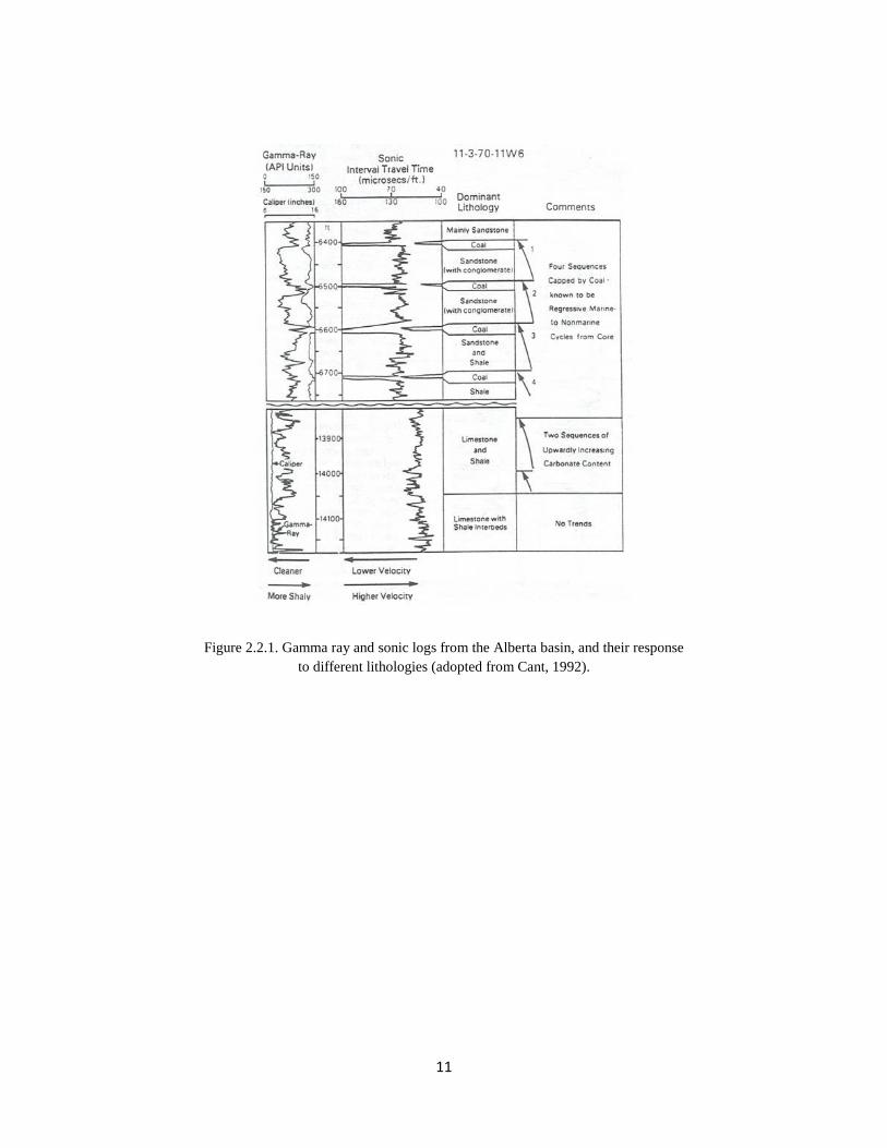
By penetrating the wellbore and sending the natural gamma-ray, emission of the various layers
will be measured using a gamma-ray log. The radiogenic isotopes of potassium, uranium and
thorium will be related to its property. As shown in Figure 2.2.1.
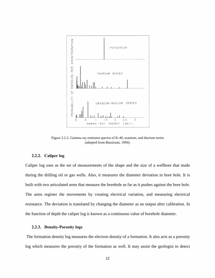
Some tools might perceive gamma ray energies of less than 0.5 to more than 2.5 millivolts.
Figure 2.2.2 also shows the distinctive emission spectra for thorium, uranium, and potassium.
Thorium, uranium, and especially potassium are common in clay evaporates and some minerals.
The successions of terrigenous clastic in the log demonstrate the “shaliness” which is interpreted
as having high radioactivities on the API scale of the rock, averaged over an interval of depth.
This is also known as “cleanness” which illustrates a lack of clays in the formation (Figures 2.2.1

10
and 2.2.3). This characteristic effect on gamma-ray log patterns mimic vertical carbonate-content
or sand-content trends.
It should be emphasized that the gamma-ray reading is the proportion of radioactive elements not
a function of grain size or carbonate content. These readings could also be related to the
proportion of shale content as well. As an example, lime mudstone gives the same response as
grainstone, and also clay free sandstones or conglomerates that are mixed with sand and pebble-
clast sizes on average give similar responses.
There is a relationship between the concentrations of radioactive elements and increasing
compact in shale. Gamma Rays radiates through the Gamma Ray (GR) tool into sedimentary
formations to the penetration of wellbore. Compton-scattering collisions with formation atoms
occur when these gamma rays pass through a formation (Cant, 1992).
Compton-scattering collisions cause the aforementioned gamma rays to subsequently lose energy
(Bassiouni, 1994). These atoms absorb gamma rays energy through the photoelectric effect in
the formation. The function of the formation density is related to the amount of absorption.
Moreover, on the GR log the radioactivity level shown can be different for two formations that
have the different densities with the same amount of radioactive material per unit volume. The
accumulation of radioactive material will typically appear in lower density formations. With the
casing borehole, the application of GR Log is necessary for the tool to run to completion and in
work-over operations. In some cases, for example the SP resolution is poor in either cased holes
or open holes. In such situations the GR log can be run as a substitute for the SP log. In this case
the GR allows for an accurate positioning of perforating guns while run with casing collar
locator logs. Gamma Ray logs are useful for the locating of source beds and for the interpretation
of depositional environment (Ameri, 2009).
11
Figure 2.2.1. Gamma ray and sonic logs from the Alberta basin, and their response to different lithologies (adopted from Cant, 1992).
12
Figure 2.2.2. Gamma ray emission spectra of K-40, uranium, and thorium series (adopted from Bassiouni, 1994).
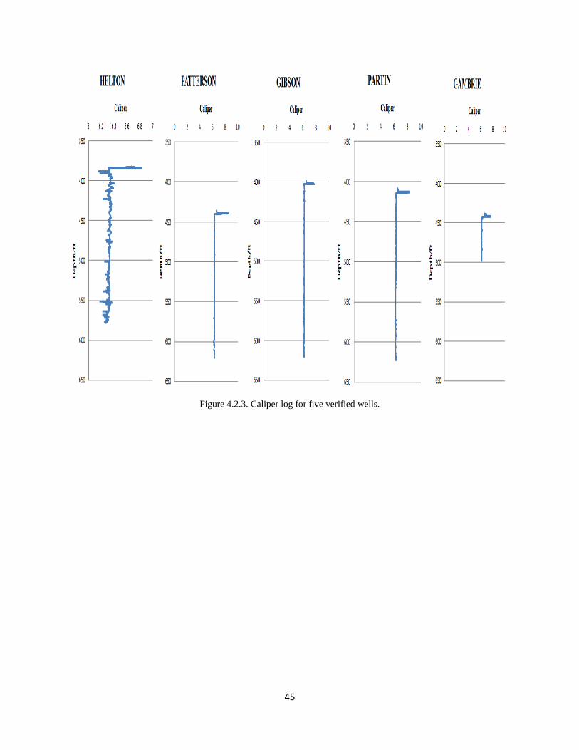
2.2.2. Caliper log
Caliper log uses as the set of measurements of the shape and the size of a wellbore that made
during the drilling oil or gas wells. Also, it measures the diameter deviation in bore hole. It is
built with two articulated arms that measure the borehole as far as it pushes against the bore hole.
The arms register the movements by creating electrical variation, and measuring electrical
resistance. The deviation is translated by changing the diameter as an output after calibration. In
the function of depth the caliper log is known as a continuous value of borehole diameter.
2.2.3. Density-Porosity logs
The formation density log measures the electron density of a formation. It also acts as a porosity
log which measures the porosity of the formation as well. It may assist the geologist to detect

13
gas-bearing zones, determine hydrocarbon density, and evaluate shale sand reservoirs and
complex lithologies.
The gradiomanometer or a nuclear fluid densimeter is a density logging device. It is a contact
tool that consists of a medium-energy gamma ray source. This tool emits gamma rays into a
formation that will be scattered back to the detector to the electron density of the rock. The
electron density is related to the density of the solid material. The amount of density is
determined either by the percentage of pore fluids, or holdup which is the record of the fractions
of different fluids at different depths in the wellbore for the different fluids.
Formation bulk density (ρb) is a function of porosity, density of the fluid in the pores such as salt,
mud, hydrocarbons, or fresh mud, and also matrix density. To determine porosity, the density of
the fluid in the wellbore and/or density of the matrix (ρ ma) should be known.
Table 2.2.1 demonstrates the common value of ρ ma.
Rock Type Matrix density (g/cm3)
Sand or Sandstone 2.65
Limestone 2.71
Dolomite 2.87
Anhydrite 2.98
Table 2.2.1. The values of matrix density for the type of different rocks
Depending on temperature, pressure and salinity, density of formation water ranges various from
0.95 g/cc to 1.10 g/cc. Density of oil varies over an equally wide range and also is lower than
these values. According to Bassiouni (1994), the tool in the investigation ratio is shallow.
Moreover, this investigates in the invaded zone, ρ f is expressed by:

14
ρ f = S xo ρmf + (1 − S )ρ
Where Sxo is the mud filtrate saturation in the invaded, ρ mf is the mud-filtrate density, zone,
and ρh is the invaded zone hydrocarbon density.
2.2.4. Neutron Log
The neutron exhibits a high penetrating potential. This penetration power property is, due to the
neutron’s lack of an electric charge that plays an important role in well logging applications.
Moreover, hydrogen is responsible for measuring the concentration of epithermal neutrons that
indicates the concentration of hydrogen in the material and it also responsible for water-bearing
formations. The concentration of hydrogen reflects the lithology and porosity in shale-free,
water-bearing formations.
The neutron log measures the hydrogen index or hydrogen concentration in the rock. The tool
emits neutrons that will measure the energy of neutrons reflected from the rock. As a result, the
hydrogen concentration might be delineated due to the fact that energy is lost easily to particles
of similar mass.
2.3. Artificial neural network
An artificial neural network is a chain of information in a system that executes the data similarly
to mathematical models of human neural biology. In human cognition some performances occur
which use an artificial neural network as well.
• Neurons are the simplest elements for processing information.
• There are connections between neurons that pass signals.
• Every connection link has an allocated weight which transmits the signal.
15
• Every neuron has a function which is nonlinear to determine an output with input and
summation of weighted input signals
2.3.1. Characterization of Neural Network
A neural network has an arrangement of the connections between the neurons which is called
“Architecture”.
Training or learning algorithm is the method which determines the weight on the connections.
There is an activation function for neural network.
For recognition of artificial neural networks with other systems, information processing provides
an answer of “how” and “when”.
Each neuron is directly connected to another one. It means there is a communication link which
includes the weight. A neural consists of some elements for simple processing which are called
nodes or cells, units, and neurons. In each neural network cycle, weights participate to solve the
problem by using the information. A wide array of problems can be affected on neural networks.
Activation or activity level is an internal state for each neuron. Activation is a function of the
inputs it has received. Activation is defined as a signal from a neuron to the other neurons. Each
neuron can send one signal at a time which it can broadcast to one or several neurons.
2.3.2. Biological Neural Network
For some, a primary concern for neural network models is the extent to which they differ from
biological neural systems; for others, these differences are outweighed by the ability of the net to
play a role in performing certain tasks. There is a similarity between the structure of neuron and
element processing. Individual neurons from different species are much more similar than neural
networks within the same system.

16
A neuron is composed of a soma or cell body and two different types of branches. They are the
dendrites and the axon. The nucleus contains the information in the cell body. The information,
such as plasma, contains the tools for producing what is needed by the neuron.
Dendrites act as the receivers to transmit signals generated by the cell body along the axon
(transmitter) which then separates into strands and sub strands.
Synapses are at the ends of the strands. A synapse is a connection between a dendrite of one and
an axon of another. Neurotransmitters are released when the signal arrives at the synapse’s ends.
These chemicals cross the synaptic gap to improve the neuron’s ability to send impulses,
depending on the kind of synapse. The synapses can be trained to be more efficient by
repetition of these signals. This dependence on history acts as a memory, which is possibly
responsible for human memory.
In humans the cerebral cortex is a thin layer covering the surface of each cerebral hemisphere.
This cerebral cortex contains a vast number of neurons which are interconnected.
Neurons exchange information through a series of very short pulses. The communications of
train pulses in neurons are very short; usually the duration time is measured in milliseconds.
Pulse-transmission frequency modulates the message. This frequency is around a million times
slower than the switching speed of electronic circuits. However, humans are more efficient in
regards to complex perceptual decisions. A good example would be face recognition. Face
recognition for humans occurs within a few hundred milliseconds, even though the operational
speed of the neurons is only a few milliseconds (Figure 2.3.1).

17
Figure 2.3.1. biological neuron.
There is a series of the processing components in neural networks which work on biological
neurons. They are:
1. All signals have to be received and be processed.
2. After releasing signals from a neuron, the signals could be modified by its weight then
receive information through synapse from the other neuron.
3. The summation weight which is merged with weighted inputs has to be included in the
processing element.
4. When the neuron conveys just one single output it shows that there was a sufficient input
to work appropriately.
5. The axon branches from the other neurons reach the output from a transmitter neuron.
6. Memory is distributed:
• There are two kinds of distribution of information which are called long-term
memory and short-term memory. Long-term memory wells or settles in the
weight or synapse and short-term memory is consistent with the signals when the
transmitter neurons send it.
• Short-term memory is the signals sent by the neurons.

18
7. The strength of synapse is not steady, and it could be modified by practical situations.
8. Transmitting on the synapses could be provocative or prohibitive.
There are two types, artificial neural networks that share an ability with biological neural
systems which is called fault tolerance.
1. We can recognize input signals with slight differences from signals we have had before.
As an example, the human ability to distinguish a person from a picture which they have seen
before or distinguish a person after a while.
2. Despite continuing to lose neurons, humans can still learn. In some cases when the neural
is destroyed it can be trained by other neurons to pass over the function of destroyed cells.
Even for uses of artificial neural networks that are not intended primarily to model biological
neural systems, attempts to achieve biological plausibility may lead to improved computational
features.
Attempts to achieve biological plausibility may lead to improved computational features via the
use of artificial neural networks that are not originally intended to model biological neural
systems.
2.3.3. Typical Architectures
Arranging neurons in layers, gives us a good perspective to observe them in a different behavior.
Neurons with the same behaviors usually categorize in the same layer. Key factors are based on
sending and receiving signals; the definition of neurons behavior in their activation function
assembles on connection of weight pattern with sending and receiving signals. For simplicity of
what many neural networks do, is the neurons in the specific layer are either not interconnected

19
or totally interconnected. Each hidden layer is the interconnection layer between input neurons
and output neurons.
The net architecture is the pattern of connections between layers and the neurons arrangement
into layers. In neural networks layer, the activation an input layer is equal to an external input
signal for each unit. In Figure 2.3.2 is a shown combination of input unit, one hidden unit, and
one output unit.
Figure 2.3.2. A very simple neural network.
Neural networks are usually categorized as multilayer or single layer. Definition of the number
of layers is based on the slabs of neurons between weighted interconnection links. The input and
output units are not counted as a layer by themselves. Obviously, the weights that exist in a
network contain very important information. Figure 2.3.3 is shown in two layers of weighted.

20
Figure 2.3.3. A single-layer neural net.
As illustrated in Figures 2.3.2 and 2.3.3 the single-layer and multilayer nets are feedforward nets
which are nets where the signals flow from the input units to the output units, in a forward
direction.
2.3.4. Single-Layer Net
When there is just one layer which is connected to weights called a single-layer net, a single-
layer net is distinguished by input units, that receive signals from the outside of system, and
output units that respond to what be read from the net. A single-layer net, the input units are
totally connected to output units; then there is no connection between two single-layers. As
shown in Figure 2.3.3 this is the typical single layer net.
Each output unit corresponds for the classification pattern, to a particular category to any input
vector that may or may not belong. There are two different patterns effect in a single-layer net.
Obviously, they use different problems based on the behavior of the response of the net. On
classification pattern, each output unit may or may not belong to an input vector. The weights in
a single-layer net for one output unit is fully separated from other output units (it means each

21
weight is dedicated to one output unit and it doesn’t influence to other output unit). On
association patterns, the output signals send the associated response with the input signal which
causes it to be produced.
2.3.5. Multilayer Net
A net with one or more levels (or layers) of nodes and has hidden units is called a multilayer.
Between input layers and output units there is a layer of weights, therefore, the organization of
the multilayer net is input, hidden, and has output levels of units. Apparently, training in a single-
layer has one level of weight rather than multilayer which has a layer of weights. The multilayer
net is much more complicated then the single-layer nets and training in multilayer may be more
difficult. Moreover, training can be successful in some cases, as long as it is able to solve a
problem in multilayer which a single-layer net cannot be trained to perform correctly at all.
2.3.6. Setting the Weights
The architecture of weight settings defines the different characteristics of neural nets. In addition,
the importance is based on distinguishing is based on the method of values setting of the training.
The difference of categorizing makes the distinction of the task in neural nets which can be
trained to arrange to the areas of clustering, mapping and constrained optimization. The common
issue of pattern association and pattern classification might be related to the special form of
mapping input vectors over the specified output vectors.
There are two methods of the training labeling; one of them is supervised and the other is
unsupervised. Also, some researchers believe self-supervised is a useful third category. The point
of training methods is to solve the problems with useful relationship between the type of problem
and the type of suitable training for that related problem.

22
2.3.7. Supervised Training
Supervised training is a process which is accomplished with presetting consequence of training
pattern, related with suitable target output vector. Due to the application of a learning algorithm
the weights are adjusted.
Pattern classification was integrated into the functions of some of the simplest and historically
earlier neural nets. A good example would be the function of classifying input vectors as either
belonging or not belonging to a given category. The output is a bivalent element in this type of
neural net if the input vector belongs to the category or if it does not belong. Such nets are
trained using a supervised algorithm. Pattern classification is the simplest neural networks that
are designed to classify an input pattern and whether it belongs to a given category.
In the mapping problem which is another special form of pattern association, the output doesn’t
define a “yes” or “no”, it defines a pattern. Associative memory is a neural network which is
trained to connect a set of input patterns that are equivalent to a set of output patterns.
Autoassociative memory occurs when the desired output target pattern is equivalent of the input
pattern. Heteroassociative memory occurs when the willing output pattern is differed from the
input pattern. After training, when the given input vector is similar to the vector, it has learned
then an associative memory can be recalled to store the pattern.
2.3.8. Unsupervised Training
Unsupervised training is a self-organized neural network group, which has the most similar input
vectors that participate with no specific training data that involves any usual member of each
vector that belongs to each group. The significance of unsupervised training is to provide input
vectors without specific target vectors. This network modifies the weights and is trained to relate

23
to the input vector that is assigned to the same cluster or output unit. The neural network will
provide a representative vector for each cluster unit generated.
2.3.9. Fixed-weight Nets
There are other types of neural nets that solve restricted optimization problems. Some nets solve
problems which are caused by the difficulty of traditional techniques, such as conflicting
constraints. In some cases the network can find the optimum solution which is satisfaction.
When the networks are designed based on problems, the weights are set to provide the quality of
constraints that can be maximized or minimized.
2.3.10. Common Activation Functions
In most cases, a nonlinear activation function is used. In order to achieve the advantages of
multilayer nets, compared with the limited capabilities of single-layer nets, nonlinear functions
are required due to the fact that as a result of this function the signal must pass through two or
more layers of linear processing elements. As an example, a single layer can obtain the same
results as elements with linear activation functions. The artificial neural operation includes
weight summation with an input signal then applying as output, or activation, function. As
Figure 3.2.10 below this function is the identity function. Neurons in a particular layer can use
the same activation function of a neural net. Activation function often uses a nonlinear function.
(i) Identity function:
f(x)=x for all x.

24
Figure 3.2.10. identify function.
Conventionally a step function is used for converting the net input in a single-layer network.
This function has variables that is valued with an output unit that is either a binary (1 or 0) or
bipolar (1 or -1) continuously, as shown in Figure 3.2.11. Heaviside function or threshold
function is known as the binary step function.
(ii) Binary step function (with threshold θ):
ƒ(x) = �1 if x ≥ θ1 if x < θ
�
Figure 3.2.11. Binary step function.
There are useful types of activation functions which are S-shaped curves or Sigmoid functions.
Also the most common functions are the hyperbolic tangent and the logistic function which are
used in neural networks by backpropagation. Their advantages are the simple relationship

25
between the value of the derivative at the point, and the value of the function at that point
reduces the computational burden during training. Either logistic or binary sigmoid is the logistic
function with range of the sigmoid function. As shown in Figure 3.2.12 this function solves the
values of the steepness parameter δ.
(iii)
ƒ1(x) = 11+exp(−𝛿𝛿𝛿𝛿 )
ƒ′′(x) = δ ƒ(x) [1- ƒ(x)]
Figure 3.2.12. Binary sigmoid, range (0-1)
The logistic sigmoid function often solves any range of values which can be from -1 to 1 that
comprises a bipolar sigmoid. As shown in Figure 3.2.13 for δ=1.

26
Figure 3.2.13. Bipolar Sigmoid.
(iv) Bipolar sigmoid:
g(x) = 2 ƒ(x) -1 = 2
1 +exp (−𝛿𝛿𝛿𝛿 )− 1
= 1−exp (−𝛿𝛿𝛿𝛿 )1+exp (−𝛿𝛿𝛿𝛿 )
g(x) = 𝛅𝛅𝟐𝟐
[1 + g(x)][1− g(x)]
hyperbolic tangent function and bipolar sigmoid are related; when the range of output value is
between -1 and 1 in the activation function.

27
g(x) = 1−exp (−𝛿𝛿)1+exp (−𝛿𝛿)
The hyperbolic tangent is
h(x) = exp (𝛿𝛿)−exp (−𝛿𝛿)exp (𝛿𝛿)+exp (−𝛿𝛿)
= 1−exp (−2𝛿𝛿)1+exp (−2𝛿𝛿)
The derivative of the hyperbolic tangent is
h(x) = [1 + h(x)][1− h(x)]
The value in binary data is within the range from 0 to 1, but it prefers to use the bipolar sigmoid
or hyperbolic tangent which needs to convert to bipolar.

28
LITERATURE REVIEW
Learning Rate
The regulation of changing the weights when the network is trained, prescribes by the learning
rate. There is a relation between the amount of weight modification and the errors, which means
if the learning rate is set 0.5; then the weight modification is a function of the error. Thus, as the
larger the learning rate appears, the larger the change of the weight the learning.
Momentum
There is a variable called Momentum in neural nets. The determination of the proportion of the
last weight is added to the new weight change. Although, this variable is applied to the large
learning rates drive to oscillation of weight changes which results in the learning process never
becoming complete.
Backpropagation Neural Net
The limitation of Single-layer in neural networks led to the creation of a training method is
known as backpropagation or the generalized delta rule. After discovering a general method of
training a multilayer neural network, a wide variety of problems were solved. The
backpropagation training method means there is a multilayer neural network that is trained by
backpropagation. This method helps to solve a variety of problems in different areas. Using the
applications nets provides every field virtually, using neural net problems including mapping
onto a set of inputs to a specified set of outputs. Most cases in neural networks imply to train the
network to achieve reasonable results by keeping the balance between giving rational reasonable
responses to input that is not identical.

29
There are three stages involved by the use of propagation in the training network. The
feedforward of the input training vector; the weight adjustment; and the associated error of the
backpropagation and computation. On training step, application of the network involves the
calculations of the feedforward phase. Backpropation phase has been implemented to improve
the speed of the training procedure.
More than one hidden layer may be beneficial in some applications, but one hidden layer is
sufficient. Although a single-layer net is severely limited in the mappings, it can learn a
multilayer net (with one or more hidden layers) can learn any continuous mapping to an arbitrary
accuracy.
The benefits of some applications are reflected in the differences of their hidden layers. Although
a single-layer net is limited in the mappings, it can learn with one hidden layer that is sufficient
to run an application. The multilayer net can learn mapping with one or more hidden layers.
Architecture
As shown in Figure 2.2.4 in a multilayer neural network, if it is with one layer of hidden units
(the Z units). The unit 𝑌𝑌𝑘𝑘 is bias on a typical output that is denoted by 𝑊𝑊𝑜𝑜𝑘𝑘 ; the unit 𝑍𝑍𝑗𝑗 is bias on
a typical hidden which is denoted 𝑉𝑉𝑜𝑜𝑗𝑗 ; As shown in shown in Figure 2.2.9 those bias terms act
like weights on connections in units that output unit is 1. In Figure 3.2.14 has shown the
feedforward phase of operation in the direction of information flow. Moreover, signals are sent
in the reverse direction during the backpropagation phase of learning.

30
Figure 3.2.14. Backpropagation neural network with one hidden layer.
Algorithm
By using backpropagation in training a network involves three stages: the backpropagation of the
associated error, the adjustment of the weights, and the feedforward of the input training pattern.
Feedward duration broadcasts the receiving signal from input units (Xi) to the each of the hidden
units Z1,…,Zp. The hidden units after receiving data from input units, computes the activation as
well as sending its signal (Zj) to the output unit. Every output unit (Yk) uses the Yk function to
respond for the given input pattern of the net.
Every output unit during training compares its analysis function Yk with target value (tk) to
evaluate the associated error for the pattern with the unit. The factor 𝛿𝛿𝑘𝑘 (k=1, …, m) is
determined by this error. The hidden units which are connected to Yk. Although this 𝛿𝛿𝑘𝑘 factor is
used to distribute the error at output unit Yk, that is received from the hidden units and connected
to Yk, back to all units in the previous (hidden) layer. This factor also will be used to update the
weights that are between the output and hidden layer.
After determining of the all δ factors, the weights for all layers will be adjusted simultaneously.
The weight Wjk will be adjusted from hidden unit Zj to output unit Yk. The weight Wjk is based

31
on the activation 𝑧𝑧𝑗𝑗 and the factor 𝛿𝛿𝑘𝑘 of the hidden unit 𝑧𝑧𝑗𝑗 . The weight Vij will be adjusted from
input Xi to hidden unit 𝑍𝑍𝑗𝑗 . The weight Vij is based on the activation xi and the factor 𝛿𝛿𝑗𝑗 of the
input unit.
Nomenclature
The training algorithm for the backpropagation net describes the nomenclature as follows:
x input training vector:
x= (x1, …, xi , …, xn)
a Output target vector:
a= (a1, …, ak, …, an)
The weight adjustment for 𝑊𝑊𝑗𝑗𝑘𝑘 is portion of error correction which is due to an error at output
unit 𝑌𝑌𝑘𝑘 . Moreover, the error for information at unit 𝑌𝑌𝑘𝑘 which is propagated back to the hidden
units, feeds into𝑌𝑌𝑘𝑘 .
The weight adjustment for 𝑉𝑉𝑖𝑖𝑗𝑗 is the proportion of error connection which is due to error
information of the backpropagation from the output layer to the hidden units 𝑧𝑧𝑗𝑗 .
α Learning rate.
t step of training.
m Momentum
𝛿𝛿1 Input unit i:
𝛿𝛿𝑖𝑖 is considered the same for the input signal and output signal in an input unit.
𝑉𝑉𝑜𝑜𝑗𝑗 Bias on hidden unit j

32
𝑧𝑧𝑗𝑗 Hidden unit j:
The network input 𝑧𝑧𝑗𝑗 is denoted z –𝑖𝑖𝑖𝑖𝑗𝑗 :
z-𝑖𝑖𝑖𝑖𝑗𝑗 = 𝑣𝑣𝑜𝑜 + 𝛴𝛴𝛿𝛿𝑖𝑖𝑣𝑣𝑖𝑖𝑗𝑗
The output activation of 𝑧𝑧𝑗𝑗 is denoted 𝑧𝑧𝑗𝑗 :
𝑧𝑧𝑘𝑘= ƒ(z-𝑖𝑖𝑖𝑖𝑗𝑗 )
𝑤𝑤𝑜𝑜𝑘𝑘 Bias on output unit k:
𝑌𝑌𝑘𝑘 Output unit k:
The network input 𝑌𝑌𝑘𝑘 is denoted y-ink:
y-𝑖𝑖𝑖𝑖𝑘𝑘= 𝑤𝑤𝑜𝑜𝑘𝑘 + 𝛴𝛴𝑧𝑧𝑗𝑗𝑤𝑤𝑗𝑗𝑘𝑘
The output activation 𝑌𝑌𝑘𝑘 is denoted 𝑌𝑌𝑘𝑘 :
𝑦𝑦𝑘𝑘= ƒ(y-𝑖𝑖𝑖𝑖𝑘𝑘)
Activation function
In a backpropagation net an activation function could have several important characteristics; it
could be continued, monotonically non-decreasing and differentiable. Moreover, for calculating
efficiency, the derivative will be easy to compute. The activation functions use the value of the
function which in turn is the value of independent variable. The function is expected to saturate
generally.

33
The binary sigmoid function is one of the most typical activation functions that has range of (0,1)
and is defined as:
ƒ1(x) = 11+exp(−𝛿𝛿)
With
ƒ′(x) = δ ƒ(x) [1- ƒ(x)]
This function is illustrated in Figure 2.2.7.
Bipolar sigmoid is another common activation function that has range of (-1,1) and is defined as:
ƒ2(x) = 11+exp(−𝛿𝛿)
− 1
With
ƒ2′ (x) = 0.5 [1+ ƒ2(x)] [1- ƒ2(x)]
Tanh (x) = 𝑒𝑒𝛿𝛿−𝑒𝑒−𝛿𝛿
𝑒𝑒𝛿𝛿+𝑒𝑒−𝛿𝛿

34
Training Algorithm
The activation functions (in the previous) defined section can be used in the standard
backpropagation algorithm given here. The form of the target values are an important factor in
selecting the suitable function. The exponential function is required to calculate the derivatives
needed in the backpropagation of the algorithm with no additional assessments because there is
the simplest relation between the value of the function and its derivative.
The algorithm is as follows:
1. Initial weights in small random values
2. If stopping condition is false, do step 3-9
3. For every training pair, do step 4-8
4. For every training pair unit (xi, i=1, …, n) receives input vector xi and sends that signal
to all units in the layer above in the hidden units.
5. Every hidden unit (zj, j=1, …, p) sums input signals in its weighted,
z-inj = voj + ∑ 𝛿𝛿𝑖𝑖𝑖𝑖𝑖𝑖=1 𝑣𝑣𝑖𝑖𝑗𝑗
6. Every output unit (𝑌𝑌𝑘𝑘 ,𝑘𝑘 = 1, … ,𝑚𝑚) sums input signals in its weighted,
y-𝑖𝑖𝑖𝑖𝑘𝑘 = 𝑤𝑤𝑜𝑜𝑘𝑘 + ∑ 𝑧𝑧𝑗𝑗𝑤𝑤𝑗𝑗𝑘𝑘𝑝𝑝𝐽𝐽=1
Error in Backpropagation:
7. Every output unit (𝑌𝑌𝑘𝑘 ,𝑘𝑘 = 1, … ,𝑚𝑚) receives a target pattern corresponding to the input
training pattern, computes its error information term,

35
8. Every output unit (𝑌𝑌𝑘𝑘 ,𝑘𝑘 = 1, … ,𝑚𝑚) computes the error information term that receives
from a target pattern to the input training pattern,
𝛿𝛿𝑘𝑘 = (а𝑘𝑘 − 𝑦𝑦𝑘𝑘)ƒ ′(𝑦𝑦 − 𝑖𝑖𝑖𝑖𝑘𝑘)
Calculates weight correction term that is used to update 𝑤𝑤𝑗𝑗𝑘𝑘 later,
∆ 𝑤𝑤𝑗𝑗𝑘𝑘 (t)= α 𝛿𝛿𝑘𝑘𝑧𝑧𝑗𝑗 + m ∆ 𝑤𝑤𝑗𝑗𝑘𝑘 (t-1)
m ∆ 𝑤𝑤𝑗𝑗𝑘𝑘 (t-1) = 𝑤𝑤𝑗𝑗𝑘𝑘 (t-1)- 𝑤𝑤𝑗𝑗𝑘𝑘 (t-2)
Calculates bias correction term that is used to update 𝑤𝑤𝑜𝑜𝑘𝑘 later.
∆ 𝑤𝑤𝑜𝑜𝑘𝑘 (t)= α 𝛿𝛿𝑘𝑘𝑧𝑧𝑗𝑗 + m ∆ 𝑤𝑤𝑜𝑜𝑘𝑘 (t-1)
m ∆ 𝑤𝑤𝑜𝑜𝑘𝑘 (t-1) = 𝑤𝑤𝑜𝑜𝑘𝑘 (t-1)- 𝑤𝑤𝑜𝑜𝑘𝑘 (t-2)
also it sends 𝛿𝛿𝑘𝑘 to units in the layer below.
9. Every hidden unit (zj , j = 1, … , P) sums delta inputs from units in the layer above,
Δ-𝑖𝑖𝑖𝑖𝑘𝑘 = ∑𝑘𝑘=1𝑚𝑚 𝛿𝛿𝑘𝑘𝑤𝑤𝑗𝑗𝑘𝑘
by multiplying the derivative of the activation function to compute the error information term.
𝛿𝛿𝑗𝑗 = 𝛿𝛿 − 𝑖𝑖𝑖𝑖𝑗𝑗 ƒ ′ (Z - 𝑖𝑖𝑖𝑖𝑗𝑗 )
Compute the weight correction term that is used to update 𝑉𝑉𝑖𝑖𝑗𝑗 later,
∆𝑉𝑉𝑖𝑖𝑗𝑗 (𝑡𝑡) = 𝛼𝛼𝛿𝛿𝑗𝑗𝑋𝑋𝑖𝑖 + 𝑚𝑚∆𝑉𝑉𝑖𝑖𝑗𝑗 (𝑡𝑡 − 1)
Computes the bias correction term that is used to update 𝑉𝑉𝑜𝑜 later,
∆𝑉𝑉𝑜𝑜(𝑡𝑡) = 𝛼𝛼𝛿𝛿𝑗𝑗 + 𝑚𝑚∆𝑉𝑉𝑜𝑜(𝑡𝑡 − 1)

36
Update weights and biases
1. Every output unit (𝑌𝑌𝑘𝑘 ,𝑘𝑘 = 1, … ,𝑚𝑚) updates its bias and weights (j = 0,…,P):
𝑤𝑤𝑗𝑗𝑘𝑘 (t)= 𝑤𝑤𝑗𝑗𝑘𝑘 (t-t) + ∆ 𝑤𝑤𝑗𝑗𝑘𝑘 (t-1),”
2. Every hidden units (zj, j = 1, … , P) updates its bias and weights (i= 0,…,n):
Vij (t) = Vij (t − 1) + ∆Vij (t)
3. Test stopping condition.
Note that in implementing this algorithm, as Step 7, 𝛿𝛿𝑘𝑘 separates arrays should be used for
the deltas for the output units and the deltas in Step 8, 𝛿𝛿𝑘𝑘 for the hidden units.
In one cycle through the entire set of training vectors calls epoch. The epochs require the
training in a backprpagation neural net. Each training pattern presents the updates the weights
after the prior algorithm. In batch updating there is a difference which is the weight updates
are accumulates over an entire epoch before being applied.
A gradient descent technique is the optimization mathematical basis for the backpropagation
algorithm. In this case, the function is the error and variables are the weights of the net in
every gradient of a function that gives the direction in which the function increases more
speedily. The reason of updating weight is related to the derivation that should be done after
all of the 𝛿𝛿𝑘𝑘 , and 𝛿𝛿𝑗𝑗 expressions have been calculated, not during backpropagation.
Initial weights and biases
The initial weights will influence whether only a local minimum of the error or the net
reaches a global, if so how quickly it converges. Between two units the update of the weight
depends on both the derivative of the activation the lower unit and the upper unit’s activation
function. Due to this reason, it would better to avoid choices of initial weights that would

37
make it either derivatives of activations or activation’s are zero. The values for the initial
weights must not be the initial input signals to every hidden unit or output unit will be falling
in the region or not be too large. In the other word, the reason that causes the procedure of
learning to be too slow is the initial weights are so small; the net input to a output or hidden
unit will be close to zero.
A procedure is to initialize the weights values between -1 and 1 or some other suitable
randomly interval or between -0.5 and 0.5. The values could be positive or negative due to
the final weights and also could be of either sign.
How Long to Train the Net
For applying a backpropagation net is to achieve a balance between good responses to new
input patterns and correct responses to training patterns. For example, a balance between
memorization and generalization that is not necessarily to continue the training unit in the
function of total squared error actually reaches a minimum. Hecht-Nielscn (1990)
recommends applying two sets of data during the set of training-testing patterns. These two
sets are put out of articulation. On the training patterns weight adjustments are contributed at
the intervals during training. In using the training-testing patterns the error will be computed.
As long as the training pattern continues the error for the training-testing patterns decreases.
Training will be terminated when the error starts to increase; then the net is beginning to
memorize the training patterns and also starting to lose its ability to generalize.
Application
Here is the lists are neural network applications were developed in real life:
Oil exploration, Stock market prediction, Price forecasts, Horse racing picks, Spectral
analysis and interpretation, Disease diagnosis, Magazine sales forecasts, Legal strategies,

38
Commodity trading, Urinalysis results, Credit application processing, Predicting student
performance, Optimizing raw material orders, Psychiatric diagnosis, product identification,
Sales prospect selection, Quality control, Help desk applications, Chemical compound
identification, Employee selection, Screening of estimates for time and material, Glass design,
Capital markets analysis, Response instructions for alarm activity reception operator, Travel
voucher screening, workload prediction, Security risk profiling, Process control, Economic
indicator forecasts, computer-aided design, analytical chemistry applications, NFL
predictions, Troubleshooting of scientific instruments, predicting labor hours required for
industrial processes, Optimizing operation of fusion furnaces, Hypertension therapy, Mental
tests, Bacteria identification, Optimizing scheduled machine maintenance, Real estate sales
forecasting, Drug screening, Physical system modeling, Cost analysis, Fault tracing systems,
Spectral peak recognition, Teaching languages, Screening decisions regarding child abuse
and neglect, Currency movement forecasts, Ground water quality control, Heart murmurs
differential diagnosis, Inventory analysis, Optimizing results of biological experiments,
Property tax analysis, Temperature and force prediction in mills and factories, Teaching
problem solving, Selection of criminal investigation targets, Nutrition analysis, Information
reconstruction, Harness racing, Geophysical and seismological research problems, Mining
education, Factory and shop problem analysis, Travel service recommendations, Cash flow
forecasting, Predicting parolee recidivism, Botanical data analysis, Damaged product
identification, Method selection for chemical characterizations, EKG diagnosis, Optimizing
production scheduling, Molding machine operation, Other sales forecasts, computer aided
instruction, Predicating Employee retention, Purchase order screening, Agriculture

39
experiments, Particle recognition, Teaching AI, college application screening, Mutual fund
picks, Ecosystem evolution, Water resources management.

40
METHODOLOGY
4.1. Neural network model development
The objective of this research was to generate synthetic wireline logs from other conventional
wireline logs to approach that uses an artificial neural network model. Therefore, this technique
intends to generate artificial log of any nonexistent log at any specific location. Developing of
this technique can be computed to measure reservoir characteristics such as fluid saturation, rock
permeability and effective porosity. Execution of this method will reduce the companies’
operation costs.
An application has used in this study related to Artificial Neural Network design has applied to
generate the synthetic logs, IDEA, Intelligent Data Evaluation & Analysis. This application was
used to compute the best model based on given data set to apply for this research. This
application, IDEA, has implied to a set of procedures for building and executing the neural
network modeling due to artificial intelligence techniques such as neural networks, genetic
algorithms and fuzzy logic to solve complex problems for the oil and gas industry.
The application would be able to create and execute a variety of architectures in neural network
through different procedures that allow the user, preparing the input data for training, built the
neural network, apply the model to the new data and analyze the outputs. The outputs can be
computed in terms of R-squared (𝑅𝑅2 ). In the artificial Neural Networks 𝑅𝑅2 is called the
predictive power. The range of 𝑅𝑅2 is measured between 0 and 1. 𝑅𝑅2 in the model defines better
as closer as to one. R-squared is defined as:
𝑅𝑅2 = 1 − 𝑆𝑆𝑆𝑆𝑆𝑆𝑆𝑆𝑆𝑆𝑌𝑌𝑌𝑌
, where
SSE = ∑(𝑦𝑦 − Ў)2

41
𝑆𝑆𝑆𝑆𝑌𝑌𝑌𝑌 = ∑(𝑦𝑦 − )2
y= actual value
Ў= the predicted value of y, and
= the mean of the values.
The indicators assess the quality of results by interpreting R2 values. The indicators are related to
the results produced by the Network. The users measure the given results from the model and
determine whether the network is working properly or not.
This study has used five wells data included gamma ray, density, neutron, and caliper logs.
backpropagation algorithms were checked until the best results in terms of R2 and matching of
the synthetic logs generated by the network versus the actual logs were achieved.
Development of the neural network model was completed using three different model sets. These
model sets are called Intelligent Data Partitioning, Data Randomly Selected, This proprietary
technique makes sure that the data is partitioned in an optimum fashion and that all three
partitions are statistically representative.
In hope to get the best R squared, different range of parameters has been considered. These
parameters were momentum, learning rate, weight decay and hidden layers. The best result was
achieved when momentum was 0.8, decay was 0.3, learning rate was 0.2, and hidden layers were
30.
4.2. Data Preparation
The next step was to prepare a matrix in a spreadsheet to be used in IDEA application. The
matrix for every well contained the well name, the depths, the latitude, the longitude, and the

42
values of the density (DPOR), Density caliper (CLDC), gamma ray (GRGC), and neutron
(NPRL) logs. Figure 4.2.1 is shown as an example of arrangement in the matrices.
Table 4.2.1. Segment of the matrix prepared for well HELTON.

43
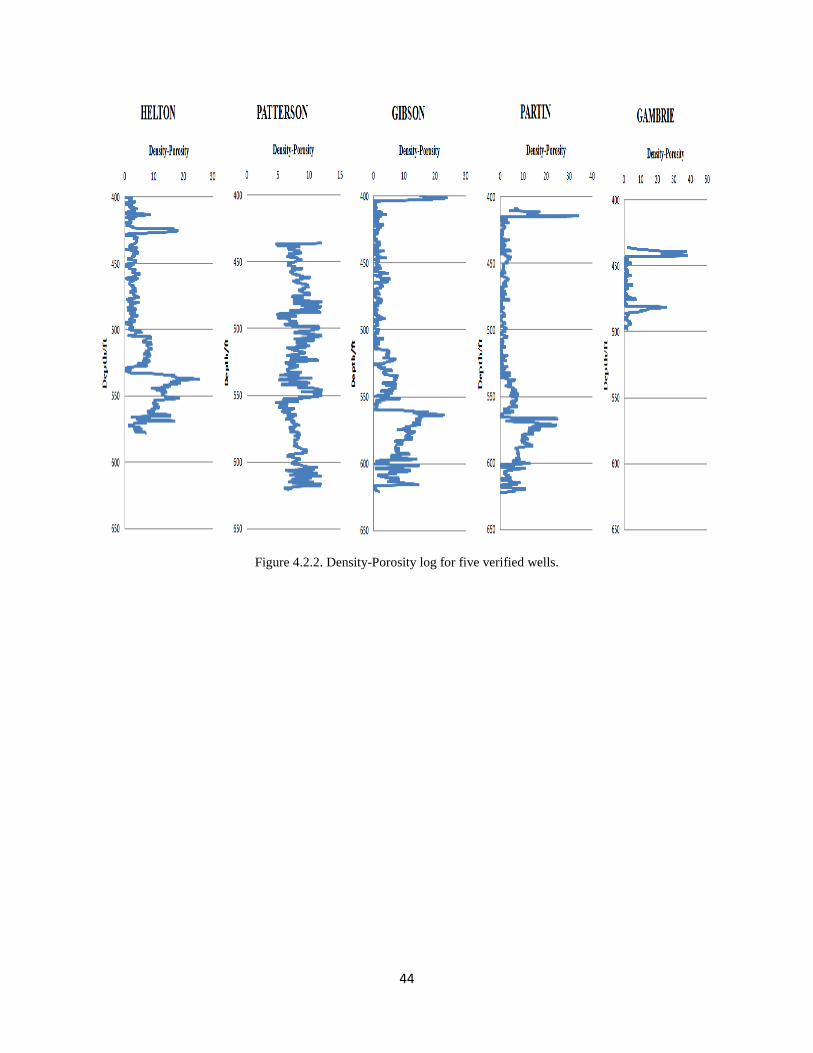
Data logs for the five wells have been showed in Figures 4.2.2, 4.2.3, 4.2.4, and 4.2.5.
Figure 4.2.1. Gamma Ray log for five verified wells.
44
Figure 4.2.2. Density-Porosity log for five verified wells.
45
Figure 4.2.3. Caliper log for five verified wells.

46
Figure 4.2.4. Neutron log for five verified wells.

47
Data logs for every well has been showed in Figures 4.2.6, 4.2.7, 4.2.8, 4.2.9, and 4.2.10.
Figure 4.2.5. Logs of Hilton well.

48
Figure 4.2.6. Logs of Patterson well.

49
Figure 4.2.7. Logs of Gibson well.
50
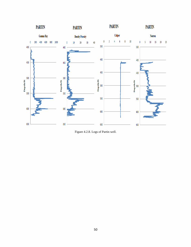
Figure 4.2.8. Logs of Partin well.

51
Figure 4.2.9. Logs of Gambrie well.

52
4.2.1. Exercise 1: filling the Gaps (Five Wells Combined)
The entire set of data, in this exercise, including of five wells. The data set were applied during
development and training of the network. Therefore, each one of these wells was applied to
verify the trained network. The data have been used into the network as inputs/outputs were the
locations of the wells. The inputs defined in terms of the depths, the latitude, the longitude, and
the values of the density (DPOR), density caliper (CLDC), and gamma ray (GRGC) logs value.
Neutron (NPRL) log applied as an output to the model.
In this exercise the data partition was randomly. In this model the coordinates and depths (XYZ),
the values of the density (DPOR), density caliper (CLDC), gamma ray (GRGC) logs value were
used as inputs, and the neutron (NPRL) log value was used as an output. The percentages used
for training, calibration and verification were 65%, 15%, and 30% respectively (Figure 4.2.10).
Figure 4.2.10. illustrates distribution of wells used for training /testing and Production dataset through exercise 1.

53
4.2.2. Exercise 2: Four Wells Combined, one well out
Differing from exercise 1, this exercise used only four wells for development and training of the network
while the fifth well, never applied during training and calibration. The fifth well was selected to generate
synthetic logs out of the other four wells (verification). In this exercise the data partition was
manually. Since the verification data set consisted of a data records never applied during training, and
the model was developed with training and calibration data sets. The percentages used were distributed 60%
for training, 20% for calibration, and 20% for verification, as shown in Figure 4.2.11.
Therefore, wells Helton, Paternson, Gibson, and Patrin where combined to generate logs
in well Gambrie; wells Helton, Paternson, Gibson, and Gambrie where combined to generate
logs in well Patrin; wells Helton, Paternson, Patrin,and Gambrie where combined to generate
logs in well Gibson; and wells Helton, Gibson, Patrin,and Gambrie where combined to generate
logs in well Paternson; and wells Paternson, Gibson, Patrin,and Gambrie where combined to
generate logs in well Helton.
Figure 4.2.11. illustrates distribution of wells used for training /testing and Production dataset through exercise 2.

54
RESULTS
As mentioned before, the neural network used in this work to generate the synthetic logs
involved Backpropagation neural network. During training the network uses a data set consisting
of inputs and outputs. For calibration the data set consists of a similar number of inputs and
outputs, but in this case they are used to validate the network by verifying how well the network
is performing on data that were never seen before during the training process. In this fashion, the
partially constructed network is checked at certain intervals of training by applying the
calibration data set. Finally the verification set is used to prove the ability of the network to
provide accurate results on the unseen data. Therefore, the values of R2 obtained for each of the
dataset mentioned, reflect the performance of the network during training, calibration and
verification.
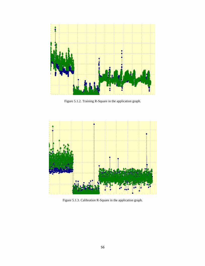
5.1. Exercise 1- Results
In this exercise the R-squared for five wells indicated as, training was 0.8961, calibration was
0.87489, Verification was 0.88542. Figures 5.1.1 has shown R-squared. Figures 5.1.2, 5.1.3, and
5.1.4 have shown the application graphs.

55
Figure 5.1.1. result of R-squared for five wells in function of neutron vs. depth.
56
Figure 5.1.2. Training R-Square in the application graph.
Figure 5.1.3. Calibration R-Square in the application graph.

57
Figure 5.1.4. Verification R-Square in the application graph.
5.2. Exercise 2- Results
5.2.1. Result of R-Sauer for Training, Calibration, and Verification
In this part, the results of second exercise will be verified. Summary of the results is shown in
table 5.2.1 below.
Table 5.2.1. Results of R-Squered for training, calibration, and verification of the five wells.

58
From the table, it can be found that R-squared for all wells are reasonable. However, R-squared
is lower in well Patterson than other wells. Since r-squared is an overall result, the software
output (neutron) and real data should be verified well by well.
The comparison between the best well and the worst well due to synthetic log and actual log are
shown in Figures 5.2.1 and 5.2.2.
Figure 5.2.1. actual and virtual results comparison in Well Hilton.

59
For well Hilton, which has r-squared of 0.9053, the virtual and actual results match very good
with each other. However, when the depth increases (after 500 ft), the actual and virtual results
deviate from each other.
Figure 5.2.2. actual and virtual results comparison in Well Patterson.

60
For well Patterson, which has the lowest amount of r-squared (0.79), it can be seen that by depth
increment, the deviation between actual and virtual results escalates. Since, the actual neutron
log fluctuates severely in this well; it is expectable to get a low amount of r-squared.
Like Hilton, wells Partin, Gambrie and Gibson have reasonable value of R-squared and with
depth increment, the actual and virtual results deviate. The comparison between synthetic logs
and actual logs are shown in Figures 5.2.3, 5.2.4, and 5.2.5.

61
Figure 5.2.3. actual and virtual results comparison in Well Partin.

62
Figure 5.2.4. actual and virtual results comparison in Well Gibson.

63
Figure 5.2.5. actual and virtual results comparison in Well Gambrie.

64
CONCLUSION
This study has demonstrates generation of synthetic logs using Backpropagation Neural Network.
The data set consisting of inputs and outputs have been applied during training of the network.
The data set consisted of a similar number of inputs and outputs for calibration. Although, the
applied data set are used to validate the network by verifying how well the network was
performing on data that were never seen during the training process. In this case, the designed
network is checked partially at certain intervals of training by applying the calibration data set in
the model. The verification data set is used to prove the ability of the network to provide
reasonable results based on the unseen data.
Moreover, the values of R2 reflect the performance of the network during training, calibration
and verification, and also the values of R2 obtained for each of the mentioned dataset.
The neural network model to predict neutron log was built through exercises one and two, as
well as using different combinations inputs and outputs.
Results indicate that the best performance was obtained for Hilton well in exercise two.
Therefore, the results of Gambrie (R2=0.86) and Gibson (R2=0.90) wells were reasonable. In
Patterson (R2=0.78) log was the least predictable as a consequence of radioactive fluctuations of
the source during the logging operation.
This research is demonstrated that the quality of data has involved generation synthetic logs, play
a very important role during the development of the neural network model. Quality of logs would
be determined factor when logs are not available in digital format and have to be digitized.
Moreover, it is recommended to perform a quality control of the data before a neural network
model is built for future works.

65
REFERENCES
Ameri, S., 2009. Notes for the Advanced formation Evaluation course. West VirginiaUniversity,
Morgantown, West Virginia.
Amizadeh, F., 2001. Soft computing information applications for the fusion and analysisof large
data sets: Fact Inc./dGB-USA. University of Berkeley, California.
Banchs, R. and Michelena, R., 2002. From 3D seismic attributes to pseudo-well-logvolumes
using neural networks: Practical considerations. The Leading Edge, Vol. 21, No.10 , pp
996-1001.
Bassiouni, Z., 1994. Theory, measurement, and interpretation of well logs. SPE textbook series,
vol. 4, 372 p.
Bhattacharya A. K., and Venkobachar, C. 1984. Removal of Cadmium by Low Cost
Adsorbents. Journal of Envirnmental Engineering, Vol. 110, No. 1, pp 110-122.
Bhuiyan, M., 2001. An Intelligent System’s Approach to Reservoir Characterization in Cotton
Valley. M.S. Thesis, West Virginia University, Morgantown, West Virginia.
Boswell, R. M., and Donaldson, A. C., 1988. Depositional architecture of the Catskill delta
complex; central Appalachian basin, U.S., in Canadian Society of PetroleumGeologists
Memoir 14, pp. 65-84.
Boswell, R.M., Heim, L.R., Wrightstone, G.R., and Donaldson, A.C., 1996. Play Dvs: Upper
Devonian Venango sandstones and siltstones in Roen, J.B. and Walker, B.J. (Eds), The
Atlas of Major Appalachian Gas Plays, Publication V-25, West Virginia Geological and
Economic Survey, Morgantown, WV. Pp. 63-69.
Cant, D., 1992. Subsurface facies analysis, in Walker, R. and James, N., eds. Facies Models:
response to sea level change. Geological Association of Canada, 454 p.

66
Faucett, L., 1994. Fundamentals of neural networks. Architectures, Algorithms, and applications.
Prentice Hall, Englewood Cliffs. NJ.
Gaskari, R. 1996. Virtual adsorber system for removal of lead, application of artificial neural
networks to a complex environment problem
Hebb, D., 1949. The organization of behavior: Wiley
Jaeger, H., 2002. Supervised training of recurrent neural networks. An INDY Math Booster
tutorial, AIS, September / October 2002.
Kammer, T.W., and Bjerstedt, T.W., 1988. Genetic stratigraphy and depositional systems of
the Upper Devonian-Lower Mississippian Price-Rockwell delta complex in the central
Appalachians. USA: Sedimentary Geology, v. 54, p 265-301.
Lawrence, S., Giles, C. L., and Tsoi, A., 1997. Lessons in Neural Network Training: Training
may be harder than Expected. Proceedings of the Fourteenth National Conference on
Artificial Intelligence, AAAI-97, (pp. 540-545), Menlo Park, California: AAAI Press.
McBride, P., 2004. Facies Analysis of the Devonian Gordon Stray Sandstone in West Virginia.
M.S. Thesis, West Virginia University, Morgantown, West Virginia.
Pofahl, W., Walczak, S., Rhone, E., and Izenberg, S., 1998. Use of an Artificial Neural
Network to Predict Length of Stay in Acute Pancreatitis. American Surgeon, Sep98, Vol.
64 Issue 9, (pp: 868 – 872)
Poulton, M., 2002. Neural networks as an intelligence amplification tool: A review of
applications. Geophysics, Vol. 67, No.3. p 979-993.
Prechelt, L., 1998. Early Stopping-but when? Neural Networks: Tricks of the trade, (pp. 55-69).
Retrieved March 28, 2002 from World Wide Web:
http://wwwipd.ira.uka.de/~prechelt/Biblio/

67
Sarle, W., 1997. Neurak Network FAQ, part 1 of 7: Introduction. Periodic posting to the Usenet
newsgroup comp.ai.neural-nets. URL: http://ftp.sas.com/pub/neural/FAQ.html
Specht, D., 1991. A General Regression Neural Network. IEEE Transactions Of Neural
Networks. Vol 2, No. 6
Tonn, T., 2002. Neural network seismic reservoir characterization in a heavy oil reservoir. The
Leading Edge, Vol 21, No.3 , pp 309-312.
White, D., Aminiam K., Mohaghegh S., & Esposito P., 1995. The application of ANN for
Zone identification in a complex reservoir: Society of Petroleum Engineers. SPE Eastern
Regional Conference & Exhibiton.
Related Documents


