Developing site scale projections of climate change in the Scottish Highlands

CLIMATE RESEARCHClim Res

Vol. 45: 71–85, 2010doi: 10.3354/cr00958

Published online December 30

1. INTRODUCTION

1.1. Maritime upland climates and climate change

Situated on the seaward western edge of north-western Europe and subject to both maritime and con-tinental influences, the climate of the Scottish High-lands and other UK uplands is typified by spatial andtemporal variability. Superimposed on these synopticcontrols, orographic effects produce a locally variableclimate across the region. With more than 4500 km2 ofthe land surface being higher than 600 m above sealevel, such altitudinal gradients of change are an im-

portant control in the spatial pattern of climate acrossScotland (Harrison & Kirkpatrick 2001) and super-impose site-specific local controls on climate across theregion (Coll et al. 2005, Coll 2007). Such high climateheterogeneity makes it difficult to characterise uplandclimates in the present, even before future changes areconsidered (Beniston 2003). Projected temperaturechanges are expected to be greater in mountains athigher northern latitudes than in those in temperateand tropical zones, with the rate of warming in moun-tain systems projected to be 2 to 3 times higher thanthat recorded during the 20th century (Nogués-Bravoet al. 2007). A further feature in some projections is

© Inter-Research 2010 · www.int-res.com*Email: [email protected]

Developing site scale projections of climate changein the Scottish Highlands

John Coll1, 2,*, Stuart W. Gibb2, Martin F. Price3, John McClatchey2, John Harrison2

1Irish Climate Analysis and Research Units (ICARUS), Department of Geography, NUI Maynooth, Maynooth, Co Kildare, Ireland

2Environmental Research Institute, North Highland College, UHI Millennium Institute, Thurso, UK3Centre for Mountain Studies, Perth College, UHI Millennium Institute, Perth, UK

ABSTRACT: With recent warming trends projected to amplify over the coming century, there areconcerns surrounding the impacts on mountain regions. Despite these concerns, global (GCMs) andregional climate models (RCMs) fail to capture local scale-dependent controls on upland climates. Amodelling framework combining climate model outputs and station data is presented and used toexplore possible future changes to temperature with altitude in the Scottish Highlands. The approachwas extended by modelling shifts in seasonal isotherm values associated with existing vegetationzones. To achieve this, temperature lapse rate models (LRMs) were applied to 1961–1990 baseline(BL) observed station data for selected stations in the eastern Highlands using seasonally representa-tive lapse rate values (LRVs) derived from paired station values. Tests against 3 upland stationrecords ranging from 663 to 1245 m indicated a credible model performance for the mean seasonalmaximum (Tmax) and minimum (Tmin) BL values evaluated. Following derivation of seasonal isothermvalues for the present upper limit of vegetation zones via the LRMs, selected scenario data outputsfrom the corresponding Hadley Centre RCM (HadRM3H) 50 × 50 km grid cells were used to projectfuture changes to BL values via the LRMs. The findings suggest substantial shifts in the isothermassociated with each zone for the scenarios selected, with shifts in Tmin more marked than those forTmax, although substantial uncertainties remain. Following an exploration of the results for the region,we suggest that a refinement to the approach linked to a wider modelling effort incorporating otherimportant controlling variables for upland species could inform future management initiatives formountain areas more generally.

KEY WORDS: Maritime uplands · Lapse rates · Modelling · Conservation policy · Uncertainty

Resale or republication not permitted without written consent of the publisher

OPENPEN ACCESSCCESS

Contribution to CR Special 24 ‘Climate change and the British Uplands’

Clim Res 45: 71–85, 2010

that the anticipated warming of the next decades isexpected to be more pronounced in northern hemi-sphere middle and high latitudes (Lean & Rind 2009).However, while most climate models suggest thisamplification of global warming for mountain regions,the observations indicate spatial variation in theamplitude of warming; e.g. areas near the annual0°C isotherm in the extratropics exhibit the strongestwarming rate (Pepin & Lundquist 2008).

The variable climate of the Scottish uplands con-tributes greatly to their biodiversity, with a diverse mixof Atlantic, arctic, arctic-alpine and boreal elementsoccurring within a limited geographical area, andmany species on the edge of their global distributionrange (Birks 1997). Within this continuum of micro-climates, most high-altitude plant species are adaptedto slow growth with survival at a particular altitudedetermined by the altitudinal range over which a spe-cies is adapted, thus they may be unable to competewith upward migrating lowland species. However,landscape change in these sensitive upland environ-ments results from a complex interplay between nat-ural and anthropogenic factors.

There is particular concern that marginal maritimemountains may be especially vulnerable to the impactof climate changes (Ellis & Good 2005, Orr et al. 2008).Scotland’s highest mountains are located within theAtlantic biogeographic zone (European Commission2005), and the relatively mild, wet climate renders spe-cies here particularly sensitive to changes in the winterand spring half year. While it might be expected thatoceanic mountains would be buffered against climaticchange by their more limited annual temperaturerange, by comparison with higher mountains such asthe Alps, the lack of a nival zone limits the potential up-ward migration of species (Crawford 2001), at least formarginal arctic-alpine associations already near theirsouthern range limit and snow bed associations. Addi-tionally, if changes in climate lead to a reduction in theseverity of the abiotic environment, this may lead toincreased inter-specific competition associated with thepossible invasion of species currently limited to lowerelevations (Ellis & Good 2005, Ellis & McGowan 2006).An advancing tree line, for example, or a denser forestbelow the tree line would have important implicationsfor the global carbon cycle (increasing the terrestrialcarbon sink) and for the biodiversity of the alpine eco-tone, possibly ousting rare species and disrupting alpineand arctic plant communities (Grace et al. 2002).

1.2. Observed and projected changes for the uplands

Evidence of recent climate change comes from ob-servations at high-altitude sites across the globe, with

observed changes including increased winter rainfalland rainfall intensity (Groisman et al. 2005, Malby etal. 2007), and temperatures increasing more rapidlythan at lowland sites, particularly through increases inminimum (nocturnal) temperatures (Bradley et al.2006). Changes have also been observed for UK up-lands, including evidence of more rapid warming(Holden & Adamson 2002) and marked precipitationchanges (Barnett et al. 2006, Fowler & Kilsby 2007,Maraun et al. 2008).

Going beyond these observed changes, projectedclimate changes are expected to have a greater impacton biota as the present century progresses (Berry et al.2002, Thomas et al. 2004, Fischlin et al. 2007). Treelines in many mountainous regions have alreadyresponded to recent temperature changes (MacDonaldet al. 1998, Klasner & Fagre 2002, Jump et al. 2007),with trees invading into meadows (Wearne & Morgan2001). The Norwegian mountain flora have shownanalogous changes in species richness and altitudinaldistributions over the last 70 yr in response to a rela-tively small change of 0.4 to 1.2°C in annual tempera-ture (Klanderud & Birks 2003), and the high pine limitassociated with the warm 20th century in the SwedishScandes stands out as an anomaly in the Holocenerecord (Kullman 2002). For Scottish uplands, Ellis &McGowan (2006) estimated that overall, a mean annualincrease of 1°C would be associated with an isothermshift of about 200 to 275 m uphill or 250 to 400 km of amove northwards. Similarly, Hill et al. (1999) estimatedthat a rise in mean temperature of 1.8°C by 2100 wouldequate to an altitudinal isotherm ascent of 300 m foran area such as the Cairngorms.

1.3. Aims and objectives

Here we sought to address some of the challengesassociated with obtaining site-specific climate changeimpact assessments for priority habitats and species inmaritime upland areas. Scale-dependent local con-trols, e.g. on climate in upland regions, are not ade-quately captured in the present generation of globaland regional climate models (GCMs and RCMs, re-spectively) due to the relatively coarse resolution of themodel grids. Therefore, until advances in climate sys-tem modelling improve the representation of local-scale climate processes, there is a need to developmethods to better represent local projections of futurechanges to key climatic variables. One complicationwith using RCM outputs for impact studies in mountainregions relates to the terrain smoothing within themodel; as a result of this, the elevation of specific sitesis poorly represented and the observed climate of spe-cific sites is not accurately reproduced (Coll et al. 2005,

72

Coll et al.: Climate change and upland isotherm shifts

Engen-Skaugen 2007, Beldring et al. 2008). Conse-quently, the approach explored here used locally-resolved temperature lapse rate models (LRMs) vari-ably integrated with temperature change outputs froman RCM and observed station data. Working on thebasis that seasonal temperature regimes are a funda-mental control on present altitudinal zones in maritimeuplands, the LRMs were used to infer future shifts inthe altitudinal bands associated with the present vege-tation zones of the eastern Scottish Highlands based onshifts in key seasonal isotherms. Given the bio-climaticcontrols associated with the more continentally influ-enced eastern hills, for consistency we applied theapproach for locations with similar climatic character-istics within our study region (Fig. 1a).

2. MATERIALS AND METHODS

2.1. Study sites and delineation of vegetation zones

The choice of climatological stations was constrainedby the need to use valley stations with a sufficientlycomplete record and those with a reasonable proximityto the limited number of upland automatic weather sta-tion records available. This approach of using a singlelower level station in conjunction with an upland sta-tion has been used extensively (see for example Hard-ing 1978, Pages & Miro 2010). Situated at 283 m in theGrampian Mountains of the eastern Highlands, thelocation of the Balmoral United Kingdom Meteorologi-cal Office (UKMO) station allows comparison with sta-tion records for a number of upland sites (Fig. 1b). Thisproximity to observed upland records, and the rela-tively low disparity between the Balmoral station ele-vation and that of the corresponding RCM grid cellallows for method evaluation. The stations are alsolocated within some of the region’s highest mountains,and are coincident with a number of designated sites ofhigh conservation value in the surrounding area. Thisproximity to mountains with vegetation zones span-ning elevation ranges typical of the eastern Highlandsprovides further scope for exploring the results. How-ever, some interpretive judgements had to be appliedin relation to delineating altitudinal zones, an issueexplored further in Section 2.5.

2.2. Climate data

Daily temperature data for mean maxima (Tmax) andminima (Tmin) for Balmoral were obtained from theBritish Atmospheric Data Centre (BADC) database.Although the station was identified as having a largelyintact record spanning the 1961–1990 baseline (BL)

period, a number of quality control procedures werealso applied to check for missing values. Thus e.g. foreach year, files were scrutinised for the removal ofdefault –999 missing value entries to avoid these skew-ing any subsequently derived mean values. Thesechecks identified a small range of 2 to 4 missing dailyvalues of Tmax and Tmin across the 1983–1990 daily re-cords requiring backfilling by use of the adjacent dailymean values. Using a 30 yr period for the baseline isalso convenient since by encompassing natural vari-ability, this averaging period effectively captures andsmoothes out noise for use in an impact application(Carter et al. 1999). Following the data quality controlprocedures, annual and seasonal Tmax and Tmin BL val-ues were derived from the station record. Seasonalmeans were derived by climatological convention (e.g.Murphy et al. 2009), hence for winter the preceding

73

Fig. 1. (a) Northern Scotland overlain on a high-resolutiondigital elevation model (DEM). The elevation zones referredto in the text are shaded to indicate their extent, and theHadRM3H grid cells (50 × 50 km) are overlain. Black rect-angle: study region. (b) Study region in more detail. Dots:

stations ; bold numbers: HadRM3H grid square codes

Clim Res 45: 71–85, 2010

year’s December values were added to the Januaryand February values.

Available upland climate data are limited for theHighlands, and no upland station has an intact recordfor the full BL period. However, a BADC search identi-fied 3 candidate stations spanning a range of eleva-tions, and with instrumental records of variablelengths (Table 1). Regional lapse rate values (LRVs)were obtained from the differences in seasonal meanvalues between those of the Balmoral station valuesand those of the highest station—Cairngorm Siesawsat 1245 m—and converted to °C km–1 (Table 2). Simpledeductive LRMs were derived based on the observedseasonal differences of temperature between the val-ley and upland records. These were applied to theobserved BL (BLObs) for Balmoral at 10 m increments toenable the projection of changes with altitude. TheLRMs were also applied to the Hadley Centre RCM(HadRM3H) BL simulated data (BLSim) from the corre-sponding 50 km grid cell (ID 163, 339 m) and these pro-jected at the same 10 m increment. For comparisonwith work elsewhere, the LRVs (°C per 10 m) usedwere compared with seasonal values (Table 2) derivedfrom the recommended monthly lapse rates suggestedby Blandford et al. (2008).

2.3. Linear regression estimates of temperaturewith altitude

Ordinary least squares (OLS) regression was appliedto the 10 m LRM-derived values using altitude as apredictor for temperature on the basis that the SEs ofthis estimate of temperature with altitude would pro-vide estimated confidence limits for the projectedseasonal changes for the scenarios used. The OLSregressions were undertaken for all seasonal Tmax andTmin BL values for both the BLObs and BLSim data. Arith-metic seasonal means (Tmean) were obtained from bothBLObs and BLSim maxima and minima, and the OLSregressions repeated for the seasonalTmean values. The fitted OLS modelswere checked for heteroscedasticity,and the standard residuals versusthe fitted quantile–quantile (QQ) plot,Cook’s distances and scale-locationand residuals leverage plots were scru-tinised in the R statistical computingenvironment to check that the regres-sion assumptions had not been vio-lated (Crawley 2007). Only the modelsummaries for the BLObs OLS-derivedvalues are provided in Table 3, asthese are the values on which the pro-jected future changes are based.

2.4. Climate change data, data matching andscenario selection

The HadRM3H integrations were used to producethe United Kingdom Climate Impacts Programme 2002(UKCIP02) climate change scenarios for the UK(Hulme et al. 2002), although these have now beensuperseded by the new UKCP09 scenarios (Murphy etal. 2009). Boundary conditions for HadRM3H arederived from the global atmosphere model, HadAM3H(Gordon et al. 2000, Pope et al. 2000), which is ofintermediate scale between the coarser-resolutionHadCM3 and the RCM. The double-nesting approachused in the model improves the quality of the simu-lated European climate and allows the UKCIP02 sce-narios to present information with a higher spatial res-olution of 50 km (Fig. 1) rather than 250 to 300 km(Hulme et al. 2002, Fowler et al. 2005).

BLSim values of mean annual and seasonal Tmax andTmin for the 1961–1990 baseline for the HadRM3H50 km grid corresponding to the station location wereobtained from the UKCIP02 database, and the differ-ences between the station and the correspondingHadRM3H 50 km grid cell elevation (Δ m) were re-corded. Compared to Balmoral at 283 m, the

74

Station Period (no. years)

WinterCairngorm Chairlift 1982–1998 (17)Cairnwell 1996–1999 (4)Cairngorm Siesaws 1993–1999 (7)

Other seasons and annualCairngorm Chairlift 1981–1998 (18)Cairnwell 1995–1999 (5)Cairngorm Siesaws 1992–1999 (8)

Table 1. Upland stations and data record summary. Elevation:Cairngorm Chairlift: 663 m; Cairnwell: 933 m; Cairngorm

Siesaws: 1245 m

Season Lapse rate (°C km–1) Lapse rate (°C 10 m–1)Tmax Tmin LRM LRM BLF BLF

Tmax Tmin Tmax Tmin

Spring 9.46 3.27 0.09 0.03 0.06 (0.03) 0.03 (0.00)Summer 11.49 4.27 0.11 0.04 0.07 (0.04) 0.01 (0.03)Autumn 8.64 3.59 0.09 0.04 0.06 (0.03) 0.01 (0.03)Winter 6.96 3.53 0.07 0.04 0.05 (0.02) 0.02 (0.02)

Table 2. Seasonal temperature lapse rate values (km–1) derived from Balmoraland Cairngorm Siesaws paired station values, and seasonal temperature lapserate values (per 10 m) projected in models, and comparison with other recordedvalues (BLF: data from Blandford et al. 2008). Values in brackets: differences.Tmax: maximum temperature; Tmin: minimum temperature; LRM: lapse rate model

Coll et al.: Climate change and upland isotherm shifts

HadRM3H Grid 163 elevation is 339 m (Δ 56 m). Toeliminate any bias due to lapse rate adjustment, theHadRM3H values were fitted to the LRMs from 340 mto correspond with the grid cell elevation, and to allowa direct inter-comparison of the simulated and ob-served values projected through the LRMs and subse-quently fitted to the OLS regression models

Prior to selecting the HadRM3H temperature changeoutputs (ΔT, °C) used for running the climate changesignal through the BL LRMs, some scenario selectioncriteria were applied. Although scenarios across anumber of future time slices represent a range of pos-sible development pathways and encompass differentlevels of uncertainty, results for the 2050s Low and2050s High scenario data are presented. These areused on the basis that the sources and range of uncer-tainties cascade for later century projections, while theabsence of a concerted mitigation response, allied tothe thermal inertia of the climate system and the effec-tive lifetime of some greenhouse gases may contributeto realising the magnitude of warming projected forthe 2050s.

2.5. Delineating vegetation zones

Any classification scheme or delineation point canonly be indicative, since the landscapes of the High-lands have been subject to substantial anthropogenicmodification as a result of e.g. deforestation, burningand grazing management (Orr et al. 2008). As a result,landscapes here lack the typical sequence of altitudi-

nal life zones found in continentalEurope, and the potential upper extentof the tree line is masked due to graz-ing pressure (Thompson et al. 2005,Fischlin et al. 2007).

For the purposes of utility, in theeastern Highlands 600 m is inter-preted as being the upper limit of theforest zone, 900 m as the upper limitof the sub-alpine zone and the lowerlimit of the low-alpine zone, and1200 m as the lower limit of the mid-dle-alpine zone. Ratcliffe & Thompson(1988) and Ratcliffe (1977) preferredto describe the different vegetationzones on mountains as montane whenreferring to Britain. According tothem, the sub-montane zone includesall vegetation derived from forestabove the limits of enclosed farmland,an interpretation which also extendsto other UK upland regions (Orr et al.2008).

However, here we applied a modified interpreta-tion of the (European) continental terminology rec-ommended by Horsefield & Thompson (1996), i.e. thealpine zone has been sub-divided to accommodatethe continental nomenclature, and the same approxi-mate elevation boundaries were applied. However,delineations are only approximate because vegeta-tion zones are at lower elevations in the far northand west of the Highlands, associated with the effectof relatively steep lapse rates superimposed on latitu-dinal controls.

3. RESULTS

3.1. LRM validation using Balmoral station values

The OLS fitted range of seasonal values for Tmax andTmin derived from the 10 m values obtained via theLRMs were projected through the observed seasonalinstrumental upland records (IURs) to provide anassessment of performance (Fig. 2, Table 4). Overall,there was a good agreement of fit around the observedstation values across all seasons for the OLS regressionfitted values of Tmax and Tmin. In general, the BLObs pro-jected values fit more closely to the station points thanthe BLSim projections (Table 5); given that the LRVsused to construct the models were derived from thestation data, this is not surprising. However, the fit forthe BLObs values was generally better for Tmax, withsome cold bias evident for Tmin in autumn and winterwith respect to the station values.

75

Seasonal OLS coefficient Estimate SE ttemperature term

Spring Tmax Intercept 1.183 × 101 6.984 × 10–3 1694Elev –8.889 × 10–3 8.289 × 10–6 –1072

Tmin Intercept 1.790 2.328 × 10–3 768.9Elev –2.963 × 10–3 2.763 × 10–6 –1072.4

Summer Tmax Intercept 1.990 × 101 8.536 × 10–3 2331Elev –1.086 × 10–2 1.013 × 10–5 –1072

Tmin Intercept 8.293 3.104 × 10–3 2672Elev –3.950 × 10–3 3.684 × 10–6 –1072

Autumn Tmax Intercept 1.324 × 101 6.984 × 10–3 1896Elev –8.889 × 10–3 8.289 × 10–6 –1072

Tmin Intercept 4.253 3.104 × 10–3 1370Elev –3.950 × 10–3 3.684 × 10–6 –1072

Winter Tmax Intercept 6.323 5.432 × 10–3 1164Elev –6.913 × 10–3 6.447 × 10–6 –1072

Tmin Intercept –9.069 × 10–1 3.104 × 10–3 –292.2Elev –3.950 × 10–3 3.684 × 10–6 –1072.4

Table 3. Summary of ordinary least squares (OLS) regression coefficients for Bal-moral station seasonal value projections. p (>| t |) <2 × 10–16 (highly significant—at or near 0) for all OLS fitted values. Tmax: maximum temperature; Tmin: mini-

mum temperature

Clim Res 45: 71–85, 2010

By comparison, for the projected BLSim values therewas less overall agreement with the station values. Forexample, there was a cold bias for the summer andautumn Tmax projected values, whereas for the springand winter Tmax projections, there was a warm biascompared to the station and BLObs projected values.There was also an overall warm bias for the projectedBLSim values of Tmin, most notably for spring andwinter. As indicated above, the relatively close corre-spondence of the Balmoral station and HadRM3H grid

elevations allowed for a relatively unambiguous inter-pretation of HadRM3H seasonal temperature simula-tion performance, and this together with upland recordavailability determined the study location. With refer-ence to the station values, HadRM3H underestimatedsummer and autumn mean maxima, while simulatedspring and winter maxima were slightly higher. Thedifferences in summer maxima were quite marked andsuggest that the parameterisations within HadRM3Hmay not be capturing local valley heating effects in the

76

200 400 600 800 1000 1200 200 400 600 800 1000 1200

200 400 600 800 1000 1200 200 400 600 800 1000 1200

Tem

pera

ture

(°C

)

–5

0

5

10

15

Balmoral Tmax

Balmoral Tmin

HadRM3H Tmax

HadRM3H Tmin

1

2

3

1

2

3

1

2

3

1

2

3

Spring

–5

0

5

10

15

Autumn

Altitude (m)

0

5

10

15

20

Summer

–10

–5

0

5

10

Winter

Fig. 2. Balmoral baseline observed (BLObs) and HadRM3H grid ID 163 baseline simulated (BLSim) mean seasonal maximum andminimum temperature (Tmax and Tmin) lapse rate adjusted and projected. Closed circles: upland station Tmax, open circles: Tmin.

1: Cairngorm chairlift, 2: Cairnwell, 3: Cairngorm Siesaws

Station [elevation, m] Spring Summer Autumn WinterTmax Tmin Tmax Tmin Tmax Tmin Tmax Tmin

Cairngorm Chairlift [663] 7.22 (5.95) 0.59 (–0.17) 14.57 (12.71) 7.43 (5.68) 8.51 (7.36) 2.96 (1.64) 3.25 (1.75) –1.83 (–3.52)Cairnwell [933] 1.80 (3.52) –1.02 (–0.98) 8.72 (9.7 4) 5.58 (4.60) 4.49 (4.93) 1.78 (0.56) –0.50 (–0.14) –3.28 (–4.6)0Cairngorm Siesaws [1245] 0.72 (0.73) –2.19 (–1.91) 5.81 (6.33) 3.08 (3.36) 2.44 (2.14) –0.30 (–0.68) –2.31 (–2.31) –5.41 (–5.84)

Table 4. Lapse rate model projected (nearest 10 m) seasonal Balmoral observed baseline (BLObs) values of maximum and minimum temperature (Tmax and Tmin) compared to station values. Model projections in round brackets

Coll et al.: Climate change and upland isotherm shifts

eastern Highlands. By contrast, and with reference tothe station values, HadRM3H overestimated mean Tmin

across the full seasonal range. The marked differencesfor winter and spring Tmin indicate that the HadRM3Hparameterisations did not capture the frost holloweffects associated with this site. The assumption in themodelling approach that temperature is linear withaltitude captures these systematic differences betweenthe BLObs and BLSim values, and projects them throughthe LRMs.

3.2. Projecting seasonal isotherm shifts usingthe models

For these projections, the approximate elevations as-sociated with upland vegetation zones in the easternHighlands detailed above were applied. The seasonalLRVs for both Tmax and Tmin were used in the OLS re-gression models with altitude as a predictor, and theTmax and Tmin isotherm values associated with theupper limit of each vegetation zone derived from theprojected Balmoral BLObs values (Table 6).

The BLObs values for Balmoral were adjusted usingthe HadRM3H grid simulated temperature outputs(HadRM3HSim) for the 2050s scenarios, and the OLS fit-ted values used to project these changes with altitudeat 10 m intervals. The new mean isotherm (Mi) locationfor the upper limit of each vegetation zone was re-calculated, and the new elevation of Mi associated withTmax and Tmin for the climate change projected changeswas recorded together with the vertical migrationinvolved (Table 7). For consistency of interpretation,the derived lower 10 m band was interpreted as the

future location of the Mi values for each zone; for prag-matic purposes, no projections were extended beyond1400 m as this elevation is just above the highest hills.Future isotherm shifts for each scenario at Balmoral aresummarised in Fig. 3, alongside some exaggeratederror bars. Since it is the suite of seasonal changeswhich will drive prospective changes in the uplands,the full range of changes for Tmax and Tmin are pre-sented and the ecological implications of these areexplored further in Section 4.3.

3.3. Climate change projections applied to theBalmoral data

For both scenarios, the greatest uphill shifts were forTmin isotherm values across all seasons, but mostnotably for autumn and spring. The HadRM3HSim val-ues projected autumn shifts of 330 m upslope for the Mi

values associated with the forest–sub-alpine transitionzone, and a corresponding shift for the sub-alpine–low-alpine transition zone isotherm for the 2050s Lowscenario. For the 2050s High scenario, the uphillmigration of the autumn Tmin Mi value for the forest–sub-alpine transition was 530 m, while the sub-alpine–low-alpine transition zone isotherm was projected asbeing above the summits. Compared to shifts in Tmin,those for Tmax were smaller, with HadRM3HSim project-ing a 120 to 160 m shift in range for each zone acrossthe seasons for the 2050s Low scenario, although Mi

shifts for the Tmax isotherms associated with the transi-tion zones were more substantial for the 2050s Highscenario. The vertical migration of the spring Tmin val-ues was also substantial for both scenarios and across

77

Vegetation transition Spring Summer Autumn Winterzone (elevation, m) Tmax Tmin Tmean Tmax Tmin Tmean Tmax Tmin Tmean Tmax Tmin Tmean

Forest – Sub-alpine (600) 6.50 0.01 3.25 13.38 5.92 9.65 7.91 1.88 4.89 2.18 –3.28 –0.55Sub – Low-alpine (900) 3.83 –0.88 1.48 10.12 4.74 7.43 5.24 0.70 2.97 0.10 –4.46 –2.18Low – Middle-alpine (1200) 1.16 –1.77 –0.30 6.86 3.55 5.21 2.57 –0.49 1.04 –1.97 –5.65 –3.81

Table 6. Summary of baseline projected seasonal 1961–1990 isotherm values associated with vegetation zones derived from ordinary least squares regression-projected Balmoral values

Station [elevation, m] Spring Summer Autumn WinterTmax Tmin Tmax Tmin Tmax Tmin Tmax Tmin

Cairngorm Chairlift [663] 7.22 (6.82) 0.59 (1.52) 14.57 (10.93) 7.43 (7.21) 8.51 (5.31) 2.96 (3.06) 3.25 (2.36) –1.83 (–1.45)Cairnwell [933] 1.80 (4.39) –1.02 (0.71)0 8.72 (7.96) 5.58 (6.13) 4.49 (2.88) 1.78 (1.98) –0.50 (0.47) –3.28 (–2.53)Cairngorm Siesaws [1245] 0.72 (1.60) –2.19 (–0.22) 5.81 (4.55) 3.08 (4.89) 2.44 (0.09) –0.30 (0.74)0 –2.31 (–1.7) –5.41 (–3.77)

Table 5. Lapse rate model projected (nearest 10 m) seasonal HadRM3H BLsim values of maximum and minimum temperature (Tmax and Tmin) compared to station values. Model projected values in round brackets

Clim Res 45: 71–85, 2010

the zones. In terms of ecological impacts, such changes,if realised, could be profound, both in terms of theimplications for snow lie and the timing of biologicalactivity in upland areas more generally. A notable fea-ture across both scenarios was the complete loss (atleast in thermal terms) of the entire middle-alpinezone, together with most of the low–middle-alpinetransition zone.

4. DISCUSSION

4.1. Braemar station and UKMO regionally averagedmonthly data comparison

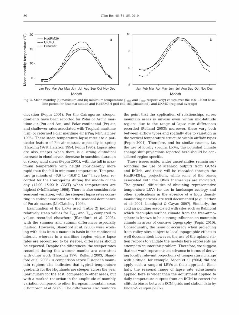
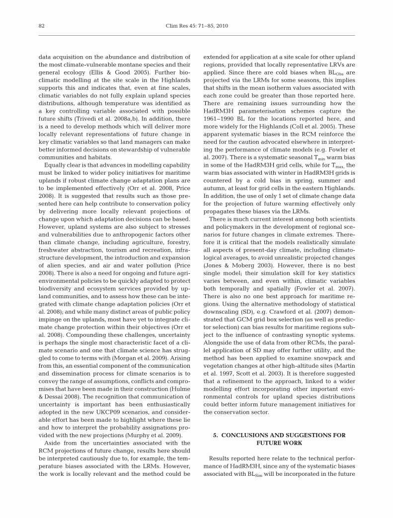
Given the apparent pattern of BLSim not capturingseasonal local valley effects, UKMO data for thenearby Braemar station were used to examine differ-ences at a monthly rather than seasonal resolution. At339 m, Braemar is at the same elevation as theHadRM3H grid 163 (339 m) and allowed direct com-parison with the RCM-simulated monthly outputs for astation also subject to frost hollow effects. Meanmonthly observed Tmax and Tmin values were also ob-tained from the UKMO regionally averaged data andwere plotted alongside the HadRM3H grid-simulatedvalues (Fig. 4).

Fig. 4 highlights that compared to the Braemar ob-served monthly Tmax values, the HadRM3H grid con-sistently underestimated mean Tmax for most of thespring, summer and autumn months, but slightly over-estimated mean Tmax for the winter months. The great-est cold bias for model simulated Tmax was associatedwith the summer (–2.41°C) and autumn (–2.56°C)months, suggesting that the RCM outputs did not cap-

ture localised valley heating effects in these seasons.When compared with the UKMO regionally averageddata, these biases were not so pronounced and theRCM-simulated values were closer to the observedmonthly pattern; unfortunately, however, no mean ele-vation data in relation to the regionally averaged datawere provided by UKMO.

By contrast, for the simulation of Tmin, compared tothe Braemar data there was a more consistent warmbias in the RCM-simulated values, which is mostmarked in the late autumn (+1.19°C) and early spring(+1.52°C) months. However, when compared with theUKMO regionally averaged data, these biases werenot so pronounced, and the RCM-simulated valueswere again closer to the observed data. Firm conclu-sions cannot be drawn due to the different spatialscales of the UKMO regionally averaged data and theHadRM3H grid, and the lack of mean elevation datafor the former. Nonetheless, when comparing stationpoints subject to known and marked seasonal contrastscontrolled largely by local site characteristics, the rela-tively coarse resolution of the HadRM3H grid failed tocapture important seasonal details of local climate.

4.2. Lapse rate models

An environmental lapse rate of ~0.6°C per 100 m iscommonly used to estimate the air temperature atunmeasured locations from available weather stations(Blandford et al. 2008). While it is a simple method thateffectively captures the general temperature–elevationtrend, it may not effectively describe localised temper-ature and elevation trends, and hence offers a poordescription of the spatial temperature structure (Lund-

78

1961–1990 vegetation transition zone Spring Summer Autumn WinterScenario Tmax Tmin Tmax Tmin Tmax Tmin Tmax Tmin

Forest – Low-alpine2050s low 720 (120) 950 (350) 720 (120) 900 (300) 750 (150) 930 (330) i 730 (130) 840 (240)2050s high 800 (200) 1170 (570) 810 (210) 1080 (480)0 850 (250) 1130 (530)00 810 (210) 980 (380)

Sub – Low-alpine2050s low 1030 (130) 1260 (360) 1030 (130) 1200 (300)0 1060 (160) 1230 (330)00 1040 (140) 1140 (240)2050s high 1110 (210) AS (550) 1120 (220) AS (Δ 480) 1160 (260) AS (520) 1120 (220) 1290 (390)

Low – Middle-alpine2050s low AS AS AS AS AS AS AS AS2050s high AS AS AS AS AS AS AS AS

Table 7. Summary of new elevations (m) associated with vegetation zone isotherms for 2050s scenarios based on the HadRM3HSim

projections via the lapse rate models (LRMs). Brackets: projected shift (Δ m) compared to the 1961–1990 isotherm location estimate for each zone. AS: above present summit levels

Coll et al.: Climate change and upland isotherm shifts

quist & Cayan 2007). Instead, lapse rates vary with fac-tors such as latitude and topographic slope, and alsohave a significant seasonal trend (Rolland 2003). Con-sequently, there are numerous simplifying assump-tions in treating the environmental lapse rate as spa-tially and temporally constant. While we attempted todeal with this here by applying locally derived meanseasonal fluctuations to the LRVs used, these still takeno account of important and fluctuating sub-seasonalcontrols such as cloud cover, wind and snow cover,which account for local differences in daytime Tmax atupland sites (Pepin & Seidel 2005). Late-lying snow athigh elevations in spring is also an important control

on lapse rates for upland areas in the Highlands, sinceit cools surface air and steepens local temperature gra-dients (McClatchey 1996). Other physical controls ontemperature change such as the net radiation budget(Pepin & Seidel 2005) were also excluded from the sea-sonal LRVs applied.

Similarly, the application of seasonally resolved val-ues cannot take account of the variability introducedby the synoptic controls associated with certain frontaltypes and the variation these introduce. Air mass char-acteristics are an important control on lapse rates, withsynoptic types comprised of westerly componentsshowing the most rapid decrease of temperature with

79

Sp max

Sp min

Su m

ax

Su m

in

Au m

ax

Au m

in

Wi m

ax

Wi m

in

Sp max

Sp min

Su m

ax

Su m

in

Au m

ax

Au m

in

Wi m

ax

Wi m

in

0

100

200

300

400

500

600

a b

Seasonal value

Iso

therm

shift

(m)

0

100

200

300

400

500

600

Sp max

Sp min

Su m

ax

Su m

in

Au m

ax

Au m

in

Wi m

ax

Wi m

in

Sp max

Sp min

Su m

ax

Su m

in

Au m

ax

Au m

in

Wi m

ax

Wi m

in

0

100

200

300

400

500

600

0

100

200

300

400

500

600

c d

Fig. 3. Projected seasonal isotherm shifts relative to 1961–1990 for the two 2050s scenarios, (a,c) Low; (b,d) High. (a,b) Forest–Sub-alpine transition zone (600 m); (c,d) Sub-alpine–Low-alpine transition zone (900 m). Vertical scale of error bars is greatly

exaggerated (×500) to accommodate the scale mismatch in relation to the prospective isotherm shifts

Clim Res 45: 71–85, 2010

elevation (Pepin 2001). For the Cairngorms, steepergradients have been reported for Polar or Arctic mar-itime air (Pm and Am) and Polar continental (Pc) air,and shallower rates associated with Tropical maritime(Tm) or returned Polar maritime air (rPm; McClatchey1996). These steep temperature lapse rates are a par-ticular feature of Pm air masses, especially in spring(Harding 1978, Harrison 1994, Pepin 1995). Lapse ratesare also steeper when there is a strong altitudinalincrease in cloud cover, decrease in sunshine durationor strong wind shear (Pepin 2001), with the fall in max-imum temperature with height considerably morerapid than the fall in minimum temperature. Tempera-ture gradients of –7.0 to –10.0°C km–1 have been re-corded for the Cairngorms during the middle of theday (12:00–15:00 h GMT) when temperatures arehighest (McClatchey 1996). There is also considerableseasonal variation, with the steepest lapse rates occur-ring in spring associated with the seasonal dominanceof Pm air masses (McClatchey 1996).

Examination of the LRVs used (Table 2) indicatedrelatively steep values for Tmax and Tmin compared tovalues recorded elsewhere (Blandford et al. 2008),with the summer and autumn differences especiallymarked. However, Blandford et al. (2008) were work-ing with data from a mountain basin in the continentalinterior, whereas in a maritime region where lapserates are recognised to be steeper, differences shouldbe expected. Despite the differences, the steeper ratesrecorded during the warmer months are consistentwith other work (Harding 1978, Rolland 2003, Bland-ford et al. 2008). A comparison across European moun-tain regions also indicates that typical temperaturegradients for the Highlands are steeper across the year(particularly for the east) compared to other areas, butwith a marked reduction in the amplitude of monthlyvariation compared to other European mountain areas(Thompson et al. 2009). The differences also reinforce

the point that the application of relationships acrossmountain areas is unwise even within mid-latituderegions due to the range of lapse rate differencesrecorded (Rolland 2003); moreover, these vary bothbetween airflow types and spatially due to variation inthe vertical temperature structure within airflow types(Pepin 2001). Therefore, and for similar reasons, i.e.the use of locally specific LRVs, the potential climatechange shift projections reported here should be con-sidered region specific.

These issues aside, wider uncertainties remain sur-rounding the use of scenario outputs from GCMsand RCMs, and these will be cascaded through theHadRM3HSim projections, while some of the biasesassociated with the LRMs themselves are indicated.The general difficulties of obtaining representativetemperature LRVs for use in landscape ecology andother applications in the absence of a high densitymonitoring network are well documented (e.g. Harlowet al. 2004, Lundquist & Cayan 2007). Similarly, thecold air ponding associated with sites such as Balmoralwhich decouples surface climate from the free-atmo-sphere is known to be a strong influence on mountainclimate in areas of concave topography (Pepin 2010).Consequently, the issue of accuracy when projectingfrom valley sites subject to local topographic effects iswell documented; however, the use of the upland sta-tion records to validate the models here represents anattempt to counter this problem. Therefore, we suggestthat our work represents an advance in terms of deriv-ing locally relevant projections of temperature changewith altitude; for example, Moen et al. (2004) did notapply such a range of LRVs in their approach. Simi-larly, the seasonal range of lapse rate adjustmentsapplied here is wider than the adjustment applied todaily temperature outputs from an RCM to correct foraltitude biases between RCM grids and station data byEngen-Skaugen (2007).

80

Month

b

Month

Jan Feb Mar Apr May Jun Jul Aug Sep Oct Nov Dec Jan Feb Mar Apr May Jun Jul Aug Sep Oct Nov Dec

Mean m

onth

ly t

em

pera

ture

(°C

)

aHadRM3HUKMOBraemar

5

10

15

20

–5

0

5

10

Fig. 4. Mean monthly (a) maximum and (b) minimum temperature (Tmax and Tmin, respectively) values over the 1961–1990 base-line period for Braemar station and HadRM3H grid cell 163 (simulated), and UKMO (regional average)

Coll et al.: Climate change and upland isotherm shifts

4.3. Modelled isotherm shifts and their ecologicalimplications

Aside from climate change uncertainties and thebiases associated with the LRMs, ecosystem responsesto relatively rapid changes in temperature remainpoorly understood. Similarly, it is recognised that atfiner scales, local topographic controls such as aspectand slope would cause microclimatic effects leading toconsiderable variation for any vegetation boundariesdefined by altitude alone. Provided there is an accu-rate assessment of the lapse rate, applying Koppen’srule, for example, approximates the montane tree lineto the 10°C Tmean isotherm for the warmest month inthe year (Koppen 1931). However, at continental scalesthere are indications that mean summer temperaturecorrelates with tree-line position over large scales(Grace et al. 2002, Moen et al. 2004). Thus, while Fig. 4shows a substantial altitudinal shift in mean summerTmax and Tmin (and hence Tmean), vegetation zones willnot move in a direct linear response to temperature. Incontinental areas with a lapse rate of 0.6°C per 100 m,a 1°C increase in temperature would be expected toelevate the tree line by ~170 m; for a higher oceanic-type lapse rate of 0.8°C per 100 m, the same increasewould move the tree line upwards by ~125 m (Craw-ford 2001). However, such a migration in response torecent warming has not been recorded so far (Virtanenet al. 2003), although some studies suggest an acceler-ation of the trend in the upward shift of alpine plantssince the mid-1980s (Walther et al. 2005). In the case ofcontinued warming, while some tree encroachmentinto the sub-alpine zone is likely, this is unlikely tooccur broadly since the altitude of tree lines in theHighlands is significantly affected by wind. Thus theinteraction between local topographic characteristicsand possible wind-field changes are likely to remain amore significant local control under warming scenariosfor the Highlands, although there is some evidence forincreased growth of established trees and shrubs andincreased shrub abundance in response to recent re-gional warming elsewhere (Kullman 2003).

To emphasise the influence of wind on tree line inthe Highlands, the BLObs projections for Balmoral indi-cate the summer 10°C Tmean isotherm is located at~700 m. However, the actual tree line is generallycloser to ~600 m for eastern uplands and more conti-nentally influenced interior regions of the Highlands(Horsfield & Thompson 1996), although in parts of theCairngorms, tree lines are also recorded at higher ele-vations. The HadRM3HSim projections indicate migra-tions of the summer 10°C Tmean isotherm to altitudes of~760 and ~830 m for the 2050s Low and 2050s High,respectively, for the Balmoral baseline values. How-ever, given the limiting factor of wind, it is highly

unlikely that tree lines will shift to these elevations. Amore conspicuous change is likely to be the migrationand expansion of alpine grasslands and dwarf-shrubheaths into higher altitudinal zones (Moen et al. 2004).With confidence in GCM- and RCM-modelled wind-field outputs remaining low (Hulme et al. 2002, Woolf& Coll 2007), the interaction of temperature, wind-fieldchange and the influence of local topography in deter-mining vegetation shifts requires investigation at a sitescale. Certainly there are precedents for historicallyhigher tree lines across the region; palaeoclimaticrecords indicate that tree lines may have been sub-stantially higher than at present during the borealclimatic optimum of the Holocene (Grace et al. 2002).

Some monitoring studies indicate a climate-inducedextirpation of high-elevation floras and a northwardshift in other groupings from the late 1980s (Lesica &McCune 2004), although other work indicates thatmontane pine limits appear to be stabilised by speciesinteractions and may not respond directly to moderateclimatic change (Hättenschwiler & Körner 1995). Otherprocesses such as soil conditions, winter desiccation,seed limitation and competition are also important(Dullinger et al. 2004). It is postulated that in the High-lands, montane habitats of moss heaths and those witharctic-alpine dwarf shrubs such as alpine bearberryArctostaphlos alpinus and the distinctive sub-speciesof crowberry Empetrum nigrum hermaphroditum areexpected to experience a severe decline in range sizewith warming (Ellis & McGowan 2006). Similarly, pop-ulations of arctic and sub-arctic species, such as curvedwood rush Luzula arcuata and drooping saxifrageSaxifraga cernua, which are restricted to altitudesabove 700 m, are expected to decline in extent (Ellis &McGowan 2006). It is clear therefore that detailedmulti-factorial and site-specific models are required,since changes driven by temperature, precipitationand wind field shifts will be superimposed upon otherenvironmental controls, with impacts manifestingthemselves at the species level.

Certainly the possible response to the more dramatictemperature changes across the altitudinal zones indi-cated by the HadRM3HSim projections requires furtherwork. Bio-climatic modelling supports the broad find-ings and conclusions here, e.g. that there is a signifi-cant decrease in suitable climate space for montanehabitats associated with the UKCIP 2050s scenarios(Berry et al. 2005). Overall, however, the response ofmountain plant species in general to climate changeremains poorly understood due to a lack of accurateobservational data on long-term changes and knowl-edge about adaptation; and our understanding of thepotential impacts on ecosystem processes and bioticinteractions in maritime upland regions remains lim-ited (Ellis & McGowan 2006). Hence there is a need for

81

Clim Res 45: 71–85, 2010

data acquisition on the abundance and distribution ofthe most climate-vulnerable montane species and theirgeneral ecology (Ellis & Good 2005). Further bio-climatic modelling at the site scale in the Highlandssupports this and indicates that, even at fine scales,climatic variables do not fully explain upland speciesdistributions, although temperature was identified asa key controlling variable associated with possiblefuture shifts (Trivedi et al. 2008a,b). In addition, thereis a need to develop methods which will deliver morelocally relevant representations of future change inkey climatic variables so that land managers can makebetter informed decisions on stewardship of vulnerablecommunities and habitats.

Equally clear is that advances in modelling capabilitymust be linked to wider policy initiatives for maritimeuplands if robust climate change adaptation plans areto be implemented effectively (Orr et al. 2008, Price2008). It is suggested that results such as those pre-sented here can help contribute to conservation policyby delivering more locally relevant projections ofchange upon which adaptation decisions can be based.However, upland systems are also subject to stressesand vulnerabilities due to anthropogenic factors otherthan climate change, including agriculture, forestry,freshwater abstraction, tourism and recreation, infra-structure development, the introduction and expansionof alien species, and air and water pollution (Price2008). There is also a need for ongoing and future agri-environmental policies to be quickly adapted to protectbiodiversity and ecosystem services provided by up-land communities, and to assess how these can be inte-grated with climate change adaptation policies (Orr etal. 2008); and while many distinct areas of public policyimpinge on the uplands, most have yet to integrate cli-mate change protection within their objectives (Orr etal. 2008). Compounding these challenges, uncertaintyis perhaps the single most characteristic facet of a cli-mate scenario and one that climate science has strug-gled to come to terms with (Morgan et al. 2009). Arisingfrom this, an essential component of the communicationand dissemination process for climate scenarios is toconvey the range of assumptions, conflicts and compro-mises that have been made in their construction (Hulme& Dessai 2008). The recognition that communication ofuncertainty is important has been enthusiasticallyadopted in the new UKCP09 scenarios, and consider-able effort has been made to highlight where these lieand how to interpret the probability assignations pro-vided with the new projections (Murphy et al. 2009).

Aside from the uncertainties associated with theRCM projections of future change, results here shouldbe interpreted cautiously due to, for example, the tem-perature biases associated with the LRMs. However,the work is locally relevant and the method could be

extended for application at a site scale for other uplandregions, provided that locally representative LRVs areapplied. Since there are cold biases when BLObs areprojected via the LRMs for some seasons, this impliesthat shifts in the mean isotherm values associated witheach zone could be greater than those reported here.There are remaining issues surrounding how theHadRM3H parameterisation schemes capture the1961–1990 BL for the locations reported here, andmore widely for the Highlands (Coll et al. 2005). Theseapparent systematic biases in the RCM reinforce theneed for the caution advocated elsewhere in interpret-ing the performance of climate models (e.g. Fowler etal. 2007). There is a systematic seasonal Tmin warm biasin some of the HadRM3H grid cells, while for Tmax, thewarm bias associated with winter in HadRM3H grids iscountered by a cold bias in spring, summer andautumn, at least for grid cells in the eastern Highlands.In addition, the use of only 1 set of climate change datafor the projection of future warming effectively onlypropagates these biases via the LRMs.

There is much current interest among both scientistsand policymakers in the development of regional sce-narios for future changes in climate extremes. There-fore it is critical that the models realistically simulateall aspects of present-day climate, including climato-logical averages, to avoid unrealistic projected changes(Jones & Moberg 2003). However, there is no bestsingle model; their simulation skill for key statisticsvaries between, and even within, climatic variablesboth temporally and spatially (Fowler et al. 2007).There is also no one best approach for maritime re-gions. Using the alternative methodology of statisticaldownscaling (SD), e.g. Crawford et al. (2007) demon-strated that GCM grid box selection (as well as predic-tor selection) can bias results for maritime regions sub-ject to the influence of contrasting synoptic systems.Alongside the use of data from other RCMs, the paral-lel application of SD may offer further utility, and themethod has been applied to examine snowpack andvegetation changes at other high-altitude sites (Martinet al. 1997, Scott et al. 2003). It is therefore suggestedthat a refinement to the approach, linked to a widermodelling effort incorporating other important envi-ronmental controls for upland species distributionscould better inform future management initiatives forthe conservation sector.

5. CONCLUSIONS AND SUGGESTIONS FORFUTURE WORK

Results reported here relate to the technical perfor-mance of HadRM3H, since any of the systematic biasesassociated with BLSim will be incorporated in the future

82

Coll et al.: Climate change and upland isotherm shifts

projections of change from the 2020s to the 2080s. Wedemonstrated that terrain-related local controls onclimate such as valley heating and inversions are notfully captured in the RCM parameterisation schemesfor BLSim. However, even if climate models accuratelyreproduce observed conditions, there has been littleassessment of whether this predicates an ability infuture prediction (Fowler et al. 2007). Nevertheless, ithas been demonstrated that by applying a locally rep-resentative lapse rate adjustment, there is scope to bet-ter represent the range of possible future thermal cli-mate for maritime uplands. However, the results areobviously conditional and based upon the assumptionswithin the LRMs themselves, as well as the wideruncertainties associated with the use of RCM output.Compounding these issues, the BLObs values projectedthrough the LRMs are from a decoupled valley site andmay not accurately represent future warming at higherelevations in the eastern Highlands. Consequently,confidence in the validity of the future projections islimited, and an integrated effort is required from theresearch community if robust projections of changewith altitude are to be delivered. An obvious extensionof the work reported here would be to replicate andrefine some of the procedures using a range of climatechange outputs from different models. This wouldallow an exploration of e.g. whether certain combina-tions of GCM(s) and RCM(s) are more effective thanothers in explaining present upland climate conditions,and whether uncertainties associated with particularelements or seasons can be minimised based on differ-ent combinations of models.

Acknowledgements. Thanks to the UHI Millennium Instituteand North Highland College for providing the funding for thePhD research upon which this work was based. We thank theBADC for providing the Meteorological Data and the UnitedKingdom Climate Impacts Programme for the climate changedata; as well as J. McIlveny for supplying the high resolutiondigital elevation model for the UK and other GIS spatial data.We also thank U. Peterman for supplying the program used toprocess the station temperature records from early in the lifeof the project, and thank the 3 anonymous reviewers who pro-vided valuable feedback and comments on the manuscript.

LITERATURE CITED

Barnett C, Hossell J, Perry M, Procter C, Hughes G (2006) Ahandbook of climate trends across Scotland. SNIFFERProject CC03, Scotland and Northern Ireland Forum forEnvironmental Research. Available at www.sniffer.org.uk/climatehandbook/

Beldring S, Engen-Skaugen T, Forland EJ, Roald LA (2008)Climate change impacts on hydrological processes in Nor-way based on two methods for transferring regional cli-mate model results to meteorological station sites. Tellus60:439–450

Beniston M (2003) Climatic change in mountain regions: a

review of possible impacts. Clim Change 59:5–31Berry PM, Dawson TP, Harrison PA, Pearson RG (2002) Mod-

elling potential impacts of climate change on the biocli-matic envelope of species in Britain and Ireland. Glob EcolBiogeogr 11:453–462

Berry PM, Harrison PA, Dawson TP, Walmsley CA (eds)(2005) Modelling natural resource responses to climatechange (MONARCH). A local approach: development of aconceptual and methodological framework for universalapplication. UKCIP, Oxford

Birks HJB (1997) Scottish biodiversity in a historical context.In: Fleming LV, Newton AC, Vickery JA, Usher MB (eds)Biodiversity in Scotland: status, trends and initiatives. TSOScotland, Edinburgh, p 21–35

Blandford TR, Humes KS, Harshburger BJ, Moore BC,Walden VP (2008) Seasonal and synoptic variations innear-surface air temperature lapse rates in a mountainousbasin. J Appl Meteorol 47:249–261

Bradley RS, Vuille M, Diaz HF, Vergara W (2006) Threatsto water supplies in the tropical Andes. Science 312:1755–1756

Carter TR, Hulme M, Viner D (eds) (1999) Representinguncertainty in climate change scenarios and impact stud-ies. ECLAT-2, Rep No.1, Helsinki Workshop, 14–16 April1999, CRU, Norwich

Coll J (2007) Local scale assessment of climate change andits impacts in the Highlands and Islands of Scotland.PhD thesis, UHI Millennium Institute/The Open University,Milton Keynes

Coll J, Gibb SW, Harrison J (2005) Modelling future climatesin the Scottish Highlands—an approach integrating localclimatic variables and regional climate model outputs. In:Thompson DBA, Price MF, Galbraith CA (eds) Mountainsof northern Europe: conservation, management, peopleand nature. TSO Scotland, Edinburgh, p 103–119

Crawford RM (2001) Plant community responses to Scotland’schanging environment. Bot J Scotl 53:77–105

Crawford T, Betts NL, Favis-Mortlock D (2007) GCM grid-boxchoice and predictor selection associated with statisticaldownscaling of daily precipitation over Northern Ireland.Clim Res 34:145–160

Crawley MJ (2007). The R book. John Wiley & Sons, Chich-ester

Dullinger S, Dirnbock T, Grabherr G (2004) Modellingclimate change-driven treeline shifts: relative effects oftemperature increase, dispersal and invasability. J Ecol 92:241–252

European Commission (2005) Natura 2000 in the AtlanticRegion. European Communities, Luxembourg

Ellis NE, Good JEG (2005) Climate change and effects onmontane ecosystems: a conservation perspective. In:Thompson DBA, Price MF, Galbraith CA (eds) Mountainsof northern Europe: conservation, management, peopleand nature. TSO Scotland, Edinburgh, p 103–119

Ellis N, McGowan G (2006) Climate change. In: Shaw TP,Thompson DBA (eds) The nature of the Cairngorms:diversity in a changing environment. The StationeryOffice, Edinburgh, p 353–365

Engen-Skaugen T (2007) Refinement of dynamically down-scaled precipitation and temperature scenarios. ClimChange 84:365–382

Fischlin A, Midgley GF, Price JT, Leemans R and others(2007) Ecosystems, their properties, goods, and services.In: Parry ML, Canziani OF, Palutikof JP, van der LindenPJ, Hanson CE (eds) Climate change 2007: impacts, adap-tation and vulnerability. Contribution of Working Group IIto the 4th assessment report of the Intergovernmental

83

Clim Res 45: 71–85, 2010

Panel on Climate Change. Cambridge University Press,Cambridge, p 211–272

Fowler HJ, Kilsby CG (2007) Using regional climate modeldata to simulate historical and future river flows in north-west England. Clim Change 80:337–367

Fowler HJ, Ekstrom M, Kilsby CG, Jones PD (2005) New esti-mates of future changes in extreme rainfall across the UKusing regional climate model integrations. 1. Assessmentof control climate. J Hydrol (Amst) 300:212–233

Fowler HJ, Blenkinsop S, Tebaldi C (2007) Linking climatechange modelling to impacts studies: recent advances indownscaling techniques for hydrological modelling. Int JClimatol 27:1547–1578

Gordon C, Cooper C, Senior CA, Banks H, Gregory JM, JohnsTC, Mitchell JFB, Wood RA (2000) The simulation of SST,sea ice extents and ocean heat transports in a version ofthe Hadley Centre coupled model without flux adjust-ments. Clim Dyn 16:147–168

Grace J, Berninger F, Nagy L (2002) Impacts of climatechange on the tree line. Ann Bot (Lond) 90:537–544

Groisman PY, Knight RW, Easterling D, Karl TR, Hegerl GC,Razuvaev VN (2005) Trends in intense precipitation in theclimate record. J Clim 18:1326–1350

Harding RJ (1978) The variation of the altitudinal gradient oftemperature within the British Isles. Geogr Ann 60:43–49

Harlow RC, Burke EJ, Scott RL, Shuttleworth WJ, Brown CM,Petti JR (2004) Derivation of temperature lapse rates insemi-arid south-eastern Arizona. Hydrol Earth Syst Sci 8:1179–1185

Harrison SJ (1994) Air temperatures in the Ochil Hills, Scot-land: problems with paired stations. Weather 49:209–215

Harrison SJ, Kirkpatrick AH (2001) Climatic change and itspotential implications for environments in Scotland. In:Gordon JE, Leys KF (eds) Earth science and the naturalheritage: interactions and integrated management. TSOScotland, Edinburgh, p 296–305

Hättenschwiler S, Körner C (1995) Responses to recent cli-mate warming of Pinus sylvestris and Pinus cembra withintheir montane transition zone in the Swiss Alps. J Veg Sci6:357–368

Hill MO, Downing TE, Berry PM, Coppins BJ and others(1999) Climate changes and Scotland’s natural heritage:an environmental audit. Survey and Monitoring ReportNo. 132, Scottish Natural Heritage, Edinburgh

Holden J, Adamson JK (2002) The Moor House long-term up-land temperature record: new evidence of recent warming.Weather 57:119–127

Horsfield D, Thompson DBA (1996) The Uplands: guidanceon terminology regarding altitudinal zonation and relatedterms. Information and Advisory Note No. 26. ScottishNatural Heritage, Battleby

Hulme M, Dessai S (2008) Negotiating future climates forpublic policy: a critical assessment of the development ofclimate scenarios for the UK. Environ Sci Policy 11:54–70

Hulme M, Jenkins JG, Lu X, Turnpenny JR and others (2002)Climate change scenarios for the United Kingdom: theUKCIP02 scientific report. Tyndall Centre for ClimateChange Research, School of Environmental Sciences, Uni-versity of East Anglia, Norwich

Jones PD, Moberg A (2003) Hemispheric and large-scale sur-face air temperature variations: an extensive review andan update to 2001. J Clim 16:206–213

Jump AS, Hunt JM, Penuelas J (2007) Climate relationships ofgrowth and establishment across the altitudinal range ofFagus sylvatica in the Montseny Mountains, northeastSpain. Ecoscience 14:507–518

Klanderud K, Birks HJB (2003) Recent increases in species

richness and shifts in altitudinal distributions of Norwe-gian mountain plants. Holocene 13:1–6

Klasner FL, Fagre DB (2002) A half century of change inalpine treeline patterns at Glacier National Park, Mon-tana, USA. Arct Antarct Alp Res 34:49–56

Koppen W (1931) Grundriss der Klimakunde. De Gruyer,Berlin

Kullman L (2002) Rapid recent range-margin rise of tree andshrub species in the Swedish Scandes. J Ecol 90:68–77

Kullman L (2003) Recent reversal of Neoglacial climate cool-ing trend in the Swedish Scandes as evidenced by moun-tain birch tree-limit rise. Glob Planet Change 36:77–88

Lean JL, Rind DH (2009) How will Earth’s surface tempera-ture change in future decades? Geophys Res Lett 36:L15708 doi:10.1029/2009GL038932

Lesica P, McCune B (2004) Decline of arctic-alpine plants atthe southern margin of their range following a decade ofclimatic warming. J Veg Sci 15:679–690

Lundquist JD, Cayan DR (2007) Surface temperature patternsin complex terrain: daily variations and long-term changein the central Sierra Nevada, California. J Geophys Res112:D11124 doi:10.1029/2006JD007561

MacDonald GM, Case RA, Szeicz JM (1998) A 538-yearrecord of climate and treeline dynamics from the LowerLena River Region of Northern Siberia, Russia. ArctAntarct Alp Res 30:334–339

Malby AR, Whyatt JD, Timmis R, Wilby RL, Orr HG (2007)Forcing of orographic rainfall and rainshadow processesby climate change: analysis and implications in the Eng-lish Lake District. Hydrol Process 52:276–291

Maraun D, Osborn TJ, Gillett NP (2008) United Kingdomdaily precipitation intensity: improved early data, errorestimates and an update from 2000 to 2006. Int J Climatol28:833–842

Martin E, Timbal B, Brun E (1997) Downscaling of general cir-culation model outputs: simulation of the snow climatol-ogy of the French Alps and sensitivity to climate change.Clim Dyn 13:45–56

McClatchey J (1996) Spatial and altitudinal gradients of cli-mate in the Cairngorms — observations from climatologi-cal and automatic weather stations. Bot J Scotl 48:31–49

Moen J, Aune K, Edenius L, Angerbjorn A (2004) Potentialeffects of climate change on treeline position in theSwedish mountains. Ecol Soc 9:16

Morgan MG, Dowlatabadi H, Henrion M, Keith D, Lempert R,McBride S, Small M, Wilbanks T (2009) Best practiceapproaches for characterizing, communicating and incor-porating scientific uncertainty in climate decision making.US Climate Change Science Program, National Oceanicand Atmospheric Administration, Washington, DC

Murphy JM, Sexton DMH, Jenkins GJ, Boorman PM and oth-ers (2009) UK climate projections science report: climatechange projections. Met Office Hadley Centre, Exeter

Nogués-Bravo D, Araujo MB, Errea MP, Martinez-Rica J(2007) Exposure of global mountain systems to climatewarming during the 21st Century. Glob Environ Change17:420–428

Orr HG, Wilby RL, McKenzie Hedger M, Brown I (2008) Cli-mate change in the uplands: a UK perspective on safe-guarding regulatory ecosystem services. Clim Res 37:77–98

Pages M, Miro JR (2010) Determining temperature lapse ratesover mountain slopes using vertically weighted regres-sion: a case study from the Pyrenees. Meteorol Appl 17:53–63

Pepin NC (1995) The use of GCM scenario output to modeleffects of future climatic change on the thermal climate of

84

Coll et al.: Climate change and upland isotherm shifts

marginal maritime uplands. Geogr Ann 77:167–185Pepin NC (2001) Lapse rate changes in northern England.

Theor Appl Climatol 68:1–16Pepin NC (2010) Changing climate at high elevation stations:

a global perspective. Proc Global Change and the World’sMountains, Perth, UK, September 26–30 2010, ParallelSesson 3.1 (Abstract) (in press)

Pepin NC, Lundquist J (2008) Temperature trends at high ele-vations: patterns across the globe. Geophys Res Lett 35:L14701 doi:10.1029/ 2008GL034026

Pepin NC, Seidel DJ (2005) A global comparison of surfaceand free-air temperatures at high elevations. J GeophysRes 110:D03104 doi:10.1029/2004JD005047

Pope VD, Galliani ML, Rowntree PR, Stratton RA (2000) Theimpact of new physical parameterisations in the HadleyCentre climate model-HadAM3. Clim Dyn 16:123–146

Price MF (2008) Maintaining mountain biodiversity in an eraof climate change. In: Borsdorf A, Stötter J, Veulliet E (eds)Managing alpine future. Proc Innsbruck Conf October15–17, 2007. Austrian Academy of Sciences Press, Vienna,p 17–33

Ratcliffe DA (1977) A nature conservation review, Vol 1. Cam-bridge University Press, Cambridge

Ratcliffe DA, Thompson DBA (1988) The British Uplands;their ecological importance and international significance.In: Ratcliffe DA, Thompson DBA (eds) Ecological changein the uplands. Br Ecol Soc Spec Publ 7. Blackwell Scien-tific Publications, Oxford, p 3–36

Rolland C (2003) Spatial and seasonal variations of airtemperature lapse rates in alpine regions. J Clim 16:1032–1046

Scott D, McBoyle G, Mills B (2003) Climate change and theskiing industry in southern Ontario (Canada): exploringthe importance of snowmaking as a technical adaptation.Clim Res 23:171–181

Thomas CD, Cameron, A, Green RE, Bakkenes M and others(2004) Extinction risk from climate change. Nature 427:145–148

Thompson DBA, Nagy L, Johnson SM, Robertson P (2005)The nature of mountains: an introduction to science, policyand management issues. In: Thompson DBA, Price MF,Galbraith CA (eds) Mountains of northern Europe: conser-vation, management, people and nature. TSO Scotland,Edinburgh, p 43–56

Thompson R, Ventura M, Camarero L (2009) On the climateand weather of mountain and sub arctic lakes in Europeand their susceptibility to future climate change. FreshwBiol 54:2433–2451

Trivedi MR, Morecroft MD, Berry PM, Dawson TP (2008a)Potential effects of climate change on plant communitiesin three montane nature reserves in Scotland, UK. BiolConserv 141:1665–1675

Trivedi MR, Berry PM, Morecroft MD, Dawson TP (2008b)Spatial scale affects bioclimate model projections of cli-mate change impacts on mountain plants. Glob ChangeBiol 14:1089–1103

Virtanen R, Eskelinen E, Gaare E (2003) Long-term changesin alpine plant communities in Norway and Finland. In:Nagy L, Grabherr G, Korner C, Thompson DBA (eds)Alpine biodiversity in Europe. Springer-Verlag, Berlin,p 411–422

Walther BR, Beissner S, Burga CA (2005) Trends in theupward shift of alpine plants. J Veg Sci 16:541–548

Wearne LJ, Morgan JW (2001) Recent forest encroachmentinto subalpine grasslands near Mount Hotham, Victoria,Australia. Arct Antarct Alp Res 33:369–377

Woolf D, Coll J (2007) Impacts of climate change on stormsand waves. In: Buckley PJ, Dye, SR, Baxter JM (eds)Marine climate change impacts annual report card 2007.MCCIP, Lowestoft, Available at www.mccip.org.uk

85

Submitted: November 10, 2009; Accepted: October 19, 2010 Proofs received from author(s): December 14, 2010