Developing equity release markets: Risk analysis for reverse mortgages and home reversions

1

Developing Equity Release Markets:

Risk Analysis for Reverse Mortgages and Home Reversions

Daniel Alai2, Hua Chen

1, Daniel Cho

2, Katja Hanewald

2, and Michael Sherris

2

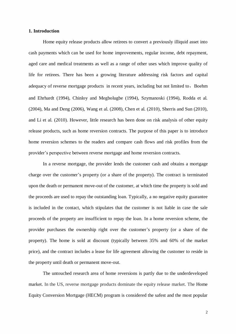
Abstract: Equity release products are sorely needed in an ageing population with high levels

of home ownership. There has been a growing literature analyzing risk components and

capital adequacy of reverse mortgages in recent years. However, little research has been done

on the risk analysis of other equity release products, such as home reversion contracts. This is

partly due to the dominance of reverse mortgage products in equity release markets

worldwide. In this paper, we compare cash flows and risk profiles from the provider‘s

perspective for reverse mortgage and home reversion contracts. An at-home/in long-term care

split termination model is employed to calculate termination rates, and a vector

autoregressive (VAR) model is used to depict the joint dynamics of economic variables

including interest rates, house prices and rental yields. We derive stochastic discount factors

from the no arbitrage condition and price the no negative equity guarantee in reverse

mortgages and the lease for life agreement in the home reversion plan accordingly. We

compare expected payoffs and assess riskiness of these two equity release products via

commonly used risk measures, i.e., Value-at-Risk (VaR) and Conditional Value-at-Risk

(CVaR).

Key Words: Reverse Mortgage, Home Reversion, Vector Autoregressive Models, Stochastic

Discount Factors, Risk-Based Capital

1[Contact author] Department of Risk, Insurance, and Health Management, Temple University 1801

Liacouras Walk, 625 Alter Hall, Philadelphia, PA 19122, United States. Email: [email protected].

2 School of Risk and Actuarial and ARC Centre of Excellence in Population Ageing Research

(CEPAR), University of New South Wales, Sydney NSW 2052, Australia. Email addresses:

[email protected] (Daniel Alai),

[email protected] (Daniel Cho),

[email protected] (Katja Hanewald),

[email protected] (Michael Sherris).

2

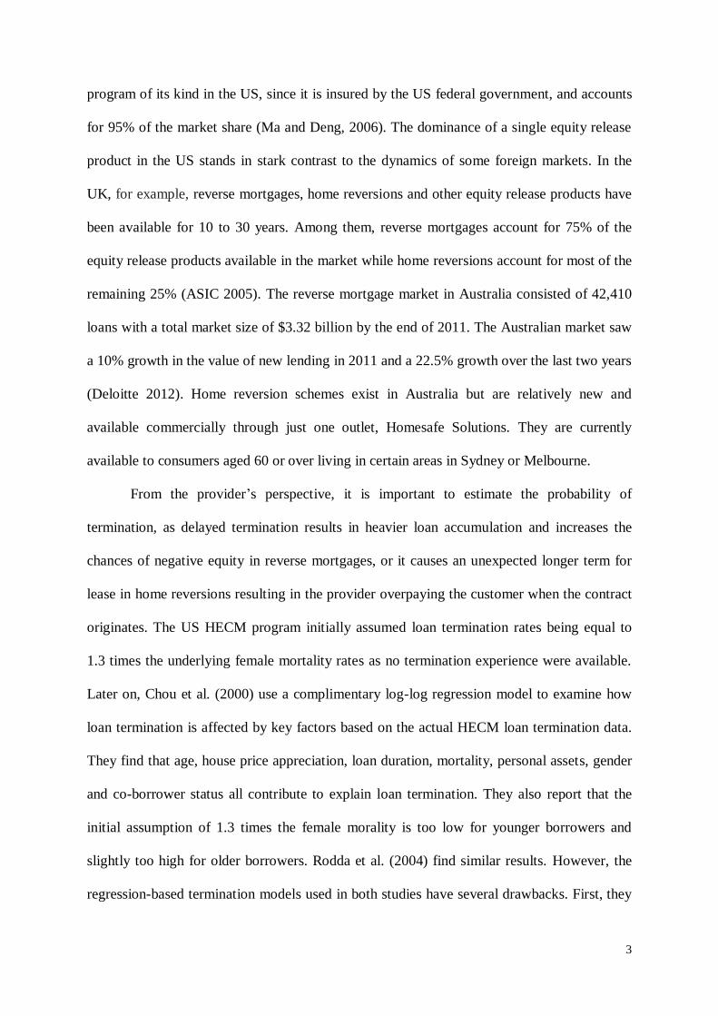
1. Introduction

Home equity release products allow retirees to convert a previously illiquid asset into

cash payments which can be used for home improvements, regular income, debt repayment,

aged care and medical treatments as well as a range of other uses which improve quality of

life for retirees. There has been a growing literature addressing risk factors and capital

adequacy of reverse mortgage products in recent years, including but not limited to，Boehm

and Ehrhardt (1994), Chinloy and Megbolugbe (1994), Szymanoski (1994), Rodda et al.

(2004), Ma and Deng (2006), Wang et al. (2008), Chen et al. (2010), Sherris and Sun (2010),

and Li et al. (2010). However, little research has been done on risk analysis of other equity

release products, such as home reversion contracts. The purpose of this paper is to introduce

home reversion schemes to the readers and compare cash flows and risk profiles from the

provider‘s perspective between reverse mortgage and home reversion contracts.

In a reverse mortgage, the provider lends the customer cash and obtains a mortgage

charge over the customer‘s property (or a share of the property). The contract is terminated

upon the death or permanent move-out of the customer, at which time the property is sold and

the proceeds are used to repay the outstanding loan. Typically, a no negative equity guarantee

is included in the contact, which stipulates that the customer is not liable in case the sale

proceeds of the property are insufficient to repay the loan. In a home reversion scheme, the

provider purchases the ownership right over the customer‘s property (or a share of the

property). The home is sold at discount (typically between 35% and 60% of the market

price), and the contract includes a lease for life agreement allowing the customer to reside in

the property until death or permanent move-out.

The untouched research area of home reversions is partly due to the underdeveloped

market. In the US, reverse mortgage products dominate the equity release market. The Home

Equity Conversion Mortgage (HECM) program is considered the safest and the most popular

3

program of its kind in the US, since it is insured by the US federal government, and accounts

for 95% of the market share (Ma and Deng, 2006). The dominance of a single equity release

product in the US stands in stark contrast to the dynamics of some foreign markets. In the

UK, for example, reverse mortgages, home reversions and other equity release products have

been available for 10 to 30 years. Among them, reverse mortgages account for 75% of the

equity release products available in the market while home reversions account for most of the

remaining 25% (ASIC 2005). The reverse mortgage market in Australia consisted of 42,410

loans with a total market size of $3.32 billion by the end of 2011. The Australian market saw

a 10% growth in the value of new lending in 2011 and a 22.5% growth over the last two years

(Deloitte 2012). Home reversion schemes exist in Australia but are relatively new and

available commercially through just one outlet, Homesafe Solutions. They are currently

available to consumers aged 60 or over living in certain areas in Sydney or Melbourne.

From the provider‘s perspective, it is important to estimate the probability of

termination, as delayed termination results in heavier loan accumulation and increases the

chances of negative equity in reverse mortgages, or it causes an unexpected longer term for

lease in home reversions resulting in the provider overpaying the customer when the contract

originates. The US HECM program initially assumed loan termination rates being equal to

1.3 times the underlying female mortality rates as no termination experience were available.

Later on, Chou et al. (2000) use a complimentary log-log regression model to examine how

loan termination is affected by key factors based on the actual HECM loan termination data.

They find that age, house price appreciation, loan duration, mortality, personal assets, gender

and co-borrower status all contribute to explain loan termination. They also report that the

initial assumption of 1.3 times the female morality is too low for younger borrowers and

slightly too high for older borrowers. Rodda et al. (2004) find similar results. However, the

regression-based termination models used in both studies have several drawbacks. First, they

4

rely heavily on availability of data. Second, they assume the probability of loan termination

remains constant after age 90, which is rather unrealistic. Third, these models do not make

explicit allowance for move-outs, health or non-health related (Ji et al. 2012). Szymanoski et

al. (2007) suggest that termination of reverse mortgage loans should be modeled based on its

key causes: borrower‘s mortality, long-term care move-out, prepayment and refinancing. In

light of this, Ji et al. (2012) develop a semi-Markov model for reverse mortgage terminations

for joint borrowers, which incorporates the aforementioned modes of termination. We adapt

their model to a single female borrower and consider only two reasons: death and entry to

long-term care facility, as prepayment and refinancing are rare for home reversion consumers.

Interest rate risk, house price risk, and rental yield risk are other major risks in equity

release products. The previous literature examining the embedded risks in reverse mortgage

contracts either focus on analysing the house price dynamics alone (see, for example, Chen et

al. 2010 and Li et al. 2010), or modelling the dynamics of house prices and interest rates

independently (Chinloy and Megbolugbe 1994, Ma et al. 2007, Wang et al. 2008, etc). This

approach neglects correlations among these key variables. In addition, the derived risk-

neutral measure fails to represent all sources of uncertainty and the dependency structure

among risks. To overcome this, Huang et al. (2011) implement a two-dimensional volatility

vector linking the house price and interest rate dynamics. Chang et al. (2012) propose a

multidimensional linear regression model that captures the relationship between house prices

and key macroeconomic factors. Sherris and Sun (2010) fit a vector autoregressive (VAR)

model to examine risks embedded in reverse mortgage insurance policies. Despite its

simplicity, a VAR model is sophisticated enough to capture the linear interdependencies

among multiple time series. We adopt a VAR process to jointly model the dynamics of

interest rates, house prices, rental yields and GDP. Our approach is different from Sherris and

Sun (2010) in two major ways. First, GDP is added to the model to acknowledge the impact

5

of macroeconomic factors on other economic variables of interest. Second, we derive

stochastic discount factors based on the VAR model that can capture uncertainty arising from

a range of sources: interest rate, house price and rental yield. This approach has not been used

in Sherris and Sun (2010) or in any other studies in equity release markets before.1

Our methodology is closely related to Ang and Piazzie (2003), who use stochastic

discount factors, or pricing kernels, to extend their VAR model with an affine term structure

of interest rates. In this manner they are able to value all assets and cash flows. Cochrane and

Piazzesi (2005) study time variation in expected excess bond returns. They construct an

affine model, i.e., prices are linear functions of state variables of the VAR model, that

generates the bond yield returns. Hoevenaars (2008) also combines the VAR model with an

affine term structure model of interest rates in such a way that there are no arbitrate

opportunities. He uses the model to generate macroeconomic scenarios that serve as input for

an asset liability management model of a pension fund.

The derived stochastic discount factors are used for pricing the no negative equity

guarantee and the lease for life agreement that are fundamental elements in reverse mortgage

and home reversion schemes, respectively. We then simulate cash flows and calculate the

actuarial present value of net payoffs of the provider. We also quantify risk measures such as

Value-at-Risk (VaR) and Conditional Value-at-Risk (CVaR) at the 99.5% level to illustrate

the amount of solvency capital to be set aside for each type of equity release products.

Sensitivity analysis is conducted to investigate the impacts of the loan-to-value ratio (LVR),

the initial house price, mortality improvements, and the leverage ratio on the payoffs and risk

profiles of reverse mortgage and home reversion contracts.

1 Following our work, Cho (2012) and Shao et al. (2012) use the VAR model and the stochastic discount factor

approach to study other aspects of equity release products. Cho (2012) compares cash flows for reverse

mortgages with different payout designs. Shao et al. (2012) quantify the impact of individual house price risk on

the pricing of equity release products.

6

We find that the maximum LVRs offered to customers in the Australian market is set

so low that reverse mortgage providers bear almost no risk of capital loss. This suggests that

reverse mortgage providers in Australia could increase maximum LVRs to facilitate the

expansion of the reverse mortgage market. Compared to reverse mortgage contracts,

providers of home reversion schemes obtain a lower payoff and assume a higher risk, which

justifies the market dominance of reverse mortgages in Australia. An efficient risk sharing

and risk transfer mechanism needs to be developed to stimulate growth of the home reversion

market. By providing an appropriate framework of regulation, financial literacy education

and by promoting liquidity to investors, governments can encourage private supply of home

reversions at modest public expense.

Interestingly, using higher LVRs in the range of those offered under the US HECM

program, we find exactly opposite results: reverse mortgage contracts are less profitable and

riskier than home reversion contracts. This finding confirms that the insurance of crossover

risk in reverse mortgages provided by the Federal Housing Agency (FHA) is an important

factor in the US market. The finding also indicates that there is a large potential market for

home reversion schemes in the US.

The remaining body of this paper is organized as follows. In Section 2, we review the

basic features of reverse mortgage and home reversion contracts, and discuss risks involved

in these two products. In Section 3, we present a termination model and use a VAR model to

jointly model the dynamics of interest rates, house prices, and rental yields. Stochastic

discount factors are derived based on the VAR model. In Section 4, we develop the pricing

formula for the no negative equity guarantee in reverse mortgages and the lease for life

agreement in home reversions. Cash flow structures are analysed for both contracts. In

Section 5, numerical examples are used to compare these two equity release products in terms

of payoffs and risks. Section 6 concludes the paper.

7

2. Product Review in Australia

2.1. The Reverse Mortgage Market

2.1.1. Product Review

The reverse mortgage market has gained considerable momentum in Australia in

recent years. According to the media release by Deloitte (2012), the market size of reverse

mortgages climbed from $0.9 billion in 2005 to $3.32 billion in 2011. There were 42,410

loans in the market as of the end of 2011 while this number in 2005 was 16,584. The average

loan size was $78,249 in 2011, compared to $51,148 in 2005. While the market is Australia-

wide, three states make up more than 70% of the national market: NSW 35%, QLD 20% and

VIC 18%. The main features of a typical reverse mortgage contract in Australia are reviewed

as follows.

Conditions: All lenders set a minimum age for the youngest person on the title of the

property that is being mortgaged. In most cases, this is 60 years. Some reverse mortgage

providers set the minimum age as 63 or 65 years (Bridges et al. 2010). Although the specific

terms and conditions vary across products, most contracts oblige the consumer to (ASIC

2005):

• maintain insurance for the property,

• pay all outgoings,

• maintain the property to the standard required by the provider,

• not leave the property vacant for more than six to 12 months,

• not allow new non-approved residents to reside in the property, and

• not sell, lease or renovate the property without the provider‘s prior approval.

8

Initial Loans: The loan amount depends primarily on two factors: age and value of the

home.2 The borrower‘s age or the younger borrower‘s age in case of a couple determines the

maximum LVR. The LVR increases as an individual‘s age increases. For example an

individual aged 60 may borrow 15% of the value of their home whereas someone aged 80 or

older can borrow up to 35% of the value of their home.

Payout Options: Depending on the contract, the borrower can withdraw the loan as a lump

sum, income streams, a line of credit, or a combination of these payment plans. As of 2010,

lump sum loans take up 95% of the Australian market and income streams account for 5%.

The proportions of lump sums and income streams have been relatively stable since 2008

(Deloitte 2011a).

Termination: Repayments are generally not made until an individual moves out of the house

or dies. If the home is jointly owned, the loan is only repayable once the last surviving

partner dies or moves out.

Guarantee: In Australia, SEQUAL-accredited members must offer a no negative equity

guarantee which ensures that no matter how long the loan runs for, the borrower can never

owe more than the value of the security, in this case, their house.3 4 However, the no negative

equity guarantee can be negated through a number of actions or inactions on the part of the

borrower, including fraud or misrepresentation, failing to maintain the property in a good

condition, failing to insure the property, or not paying the council rates on the property.

Interest Rates: Interest rates can be variable or fixed. Variable rate loans are the most popular

product in Australia. Variable rates are on average 1% above the standard variable home loan

2 In the US, Federal Housing Administration (FHA) imposes a mortgage limit which is $625,500 for one-family

house. The initial loan amount is determined by the younger borrower‘s age and the adjusted property value. The adjusted property value is defined as the lesser of the appraised value of your home, the FHA HECM

mortgage limit of $625,500 or the sales price. 3 SEQUAL is the abbreviation of the Senior Australians Equity Release Association. In order to protect the

customers, SEQUAL has established a strict Code of Conduct that each SEQUAL-accredited member has to

agree its equity release product(s) adhere to. 4 The no negative equity guarantee is also called a non-recourse provision in the US reverse mortgage market.

9

rate. The margin (or mortgage insurance premium) is charged to manage the risk of providing

the no negative equity guarantee.5 Fixed interest rates can be set for varying terms—generally

5, 10 or 20-years or lifetime. The proportion of fixed interest reverse mortgage loans is

negligible 1% in 2010 (Deloitte 2011a). There is now only one SEQUAL-accredited lender

(RBS) providing a fixed rate option on their products (Bridge et al. 2010).

Fees: There are typically setup fees, ongoing fees and exit fees associated with reverse

mortgages which vary from lender to lender.

2.1.2. Major Risks in Reverse Mortgages

Reverse mortgages differ from traditional forward mortgages in the way that the

outstanding loan balance grows due to principal advances, interest accruals, and other loan

charges over the life of the loan. The loan balance may grow to exceed the property value at

the time of termination because of multiple risks.

Termination Risk: If a borrower lives longer than expected, the principal advances and

interest accruals will continue, which may drive the loan balance exceeding the sale proceeds

of the property. The mobility rate has the same effect on reverse mortgage products.

Borrowers may move out of their homes because of their health condition, marriage, divorce,

death of the spouse, disasters, or simply the desire to live in another place.

Interest Rate risk: Most of reverse mortgage products feature adjustable interest rates.

Therefore, the variation of interest rates imposes additional uncertainty on reverse mortgage

providers. A rise in the interest rate can result in a higher rate of interest accruals on the loan

balance than anticipated, which increases the possibility of partial non-repayment when the

loan eventually terminates.

5 In the US HECM program, mortgage insurance premiums consist of two parts: an up-front charge which is

either 2% (HECM Standard) or 0.01% (HECM Saver) of the adjusted property value, and an annual rate of

1.25% of the outstanding loan balance for the life of the loan. FHA collects all the insurance premiums and

reverse mortgage lenders are allowed to assign the loan to FHA when the loan balance equals the adjusted

property value. FHA takes over the loan and pays an insurance claim to lenders covering their losses. So lenders

are effectively shifting the collateral risk to FHA.

10

House Price Depreciation Risk: The uncertainty in house price depreciation rates is another

risk we need to consider. If the home price remains stagnant or grows at a lower rate than

anticipated, the outstanding loan balance at maturity may exceed the sale proceeds of the

property. Lenders or their insurers may suffer from the losses. As indicated by the recent U.S.

housing market downturn, home price depreciation risk is only partially diversifiable: pooling

mortgage products nationally only reduces the risk of a downturn in the regional housing

market, but cannot diversify the risk of a national economic recession.

2.2. The Home Reversion Market

2.2.1. Product Review

Home reversion schemes allow senior homeowners to sell a proportion of equity in

their home while still living there. Homeowners receive a lump sum payment in exchange for

a fixed proportion of the future value of their home. There are two main types of home

reversion schemes: a sale-and-lease model and a sale-and-mortgage model. In the sale-and-

lease model, the title to the property passes to the provider at the time of purchase and the

property is leased back to the consumer at a nominal rent. The sale-and-lease product

provider in Australia, called Money for Living, went into administration in 2005. The

Australian Securities and Investments Commission (ASIC) issued legal proceedings in the

Federal Court of Australia alleging that Money for Living advertised its product in a

misleading and deceptive manner. A resolution was passed in December 2007, placing the

company into liquidation. In the sale-and-mortgage model, the title to the property remains in

the consumer‘s name even after the provider pays. To protect the provider‘s interest in the

property, the consumer is required to give the provider a mortgage over the property (ASIC,

2005). Homesafe Solutions Pty Ltd, a joint venture of Bendigo and Adelaide Bank Ltd and

11

Athy Pty Ltd, has launched Homesafe Debt Free Equity Release since 2005. We review its

features in the following.6

Conditions: The homeowner must be aged 60 and over. For a couple, the younger partner

must be at least 60. Currently, it is available only to customers residing in certain postcodes

within Melbourne and Sydney. As a general rule, the home needs to be free-standing. Other

property types are subject to approval from Homesafe. The property is the principal place of

residence for at least one homeowner at the time of exchange of contracts. The land value of

the property is 60% or greater of the total value determined by an independent panel valuer.

The homeowner must own the home outright, or use some of the Homesafe funds received to

pay out the existing mortgage.

Funds: Under Homesafe Debt Free Equity Release, it is possible to access any amount

between $25,000 and $1,000,000. The maximum share that homeowners can sell, so-called

acquisition rate, is 65% of the future sale proceeds of the home. Homeowners can enter into

additional contracts over time, up to a total share of 65%. There is no restriction as to how the

funds should be used.

Payout Option: Homesafe currently offers only a lump sum payout option.

Lease: Homeowners receive a discounted lump sum payment (usually 35% or 60%) in

exchange for a fixed proportion of the future value of their home. The discount represents the

value of the lease for life agreement that allows homeowners to live in the house for life or

until voluntarily move-out. Homeowners may be eligible for an early sale rebate if they sell

their home earlier than expected.

Termination: The contract terminates when homeowners die or voluntarily vacate the

property. Homesafe is entitled to the agreed percentage of the sale proceeds of the house and

homeowners retain the share of the sale proceeds that they have not sold to Homesafe.

6 More details can be found on the website of Homesafe Solutions Pty Ltd:

http://www.homesafesolutions.com.au/

12

Title: Homeowners remain on the title, so they have the right to use their home for as long as

they wish. There is no requirement for homeowners to undertake maintenance of the property

after entering into a Homesafe contract. The owners can even rent out the home and keep the

rental income. Homesafe will register a mortgage and lodge a caveat on the title, only to

secure its share of the sale proceeds.

Fees: Homesafe charges a one-off transaction fee of $1,690.

2.2.2. Major Risks in Home Reversions

The provider of home reversion contracts faces house price risk. For the lease for life

agreement, the uncertainty originates from the rental yield, and the duration of the contract.

Termination Risk: In a home reversion contract, the customer is always better off prolonging

the duration of the contract. This is in contrast to a reverse mortgage contract, where early

termination may be beneficial for the customer under certain circumstances. Therefore, when

valuing the lease for life agreement in an annuity setting, it is realistic to assume that the only

modes of termination are death and unavoidable entry into a long-term care facility. It should

be noted that some home reversion contracts provide a rent rebate for contracts that terminate

much earlier than expected, but the amount is not of the magnitude to induce termination.

Rental Yield Appreciation Risk: In a home reversion contract, the property is sold to the

provider at a discounted price. The level of the discount reflects the value of the lease for life

agreement. The provider‘s payoff could be impaired if a low rental yield were assumed when

calculating the value of the lease but the actual rental yield would turn out to be much higher.

House Price Depreciation Risk: Lenders of home reversion contracts are entitled to sell the

property and secure a part of the sale proceeds when borrowers die or voluntarily move out.

Therefore, lenders face the risk of house price depreciation.

2.2.3. Advantages of Home Reversions

13

From the consumer‘s point of view, home reversion products have unbeatable

advantages over reverse mortgages. Oliver Wyman Financial Services (2005) predicted

―though equity solutions have traditionally fared poorly in the US, options such as home

reversion products should find a market – especially among owners of higher-value homes,

for whom equity release may be intended to diversify a portfolio rather than to free up cash‖.

In addition, reverse mortgages involve the accumulation of debt over the life of the contract

while home reversions are debt-free. In order to protect borrowers from negative equity,

reverse mortgage programs usually provide a no negative equity guarantee so loan repayment

is capped by the sale proceeds of the property. This guarantee is financed via mortgage

insurance premiums paid by borrowers. In other words, senior homeowners bear various

risks, including longevity risk, interest rate risk and property value risk under a reverse

mortgage contract. Nevertheless, these risks are partly remitted to providers under home

reversion contracts. Commercial providers are generally better positioned to bear such risks.

For example, they can transfer risks to the capital market more efficiently compared with

senior homeowners. More importantly, the interests of investors and consumers are aligned

under home reversion schemes: both want the value of the home to rise (Oliver Wyman

Financial Services, 2005). Therefore, we believe that there remains room for significant

growth of a diversified equity release market and we see a great potential for the development

of home reversion products.

3. Modelling Framework

3.1. The Termination Model

Though a significant proportion of reverse mortgages are issued to couples (around

40% in the US and 50% in Australia, see Deloitte 2012), the study of joint life dependency is

14

not the focus of this paper.7 For simplicity, we assume a single, female policyholder. The

joint-life multistate termination model can be readily incorporated in our model framework if

necessary. We do not consider voluntary prepayment or refinancing as consumers of home

reversion products are always better off by prolonging the duration of their contracts. In other

words, contract termination is determined by two major factors: death and entry into long-

term care facilities.

We assume a Gompertz structure for the population force of mortality x for females

aged x given by

expx x . (1)

Equity release products are designed for a policyholder living at home. Therefore, she

is susceptible to at-home mortality, which need not equal to female population mortality. Let

denote the proportionality constant that produces at home mortality from population

mortality. That is, the female at-home mortality rates are scaled down by multiplying to

represent the better health of retirees, who do not move out to long-term care. The possibility

of entry into a long-term care facility is represented by a proportionality constant, . These

two parameters can be replaced by one contract-mortality loading factor, . Hence,

the contract force of mortality can be written as follows:

c

x x x , (2)

where c

x denotes the contract termination rate.

The parameters and are estimated using Australian female mortality data for the

period 1950-2009 and age 50-105 from the Human Mortality Database.8 We fit both an

7 Ji et al. (2012) compare the value of the no negative equity guarantee for joint borrowers under the

independence assumption and the semi-Markov assumption. Though the assumption of independence generally

leads to an overestimation of NNEG prices, the difference is not significant (see Figure 3 in Ji et al. 2012). 8 http://www.mortality.org/

15

ordinary linear regression (LR) to the log-transformed mortality rates as well as a Poisson

regression (PR) to death counts with an appropriate exposure offset.

LR: 0 1 ,ln x x tm x (3)

PR: 0 1 ,ln lnx x x tD E x (4)

where ln xE is the offset for the Poisson regression based on the survival counts, xE . Table 1

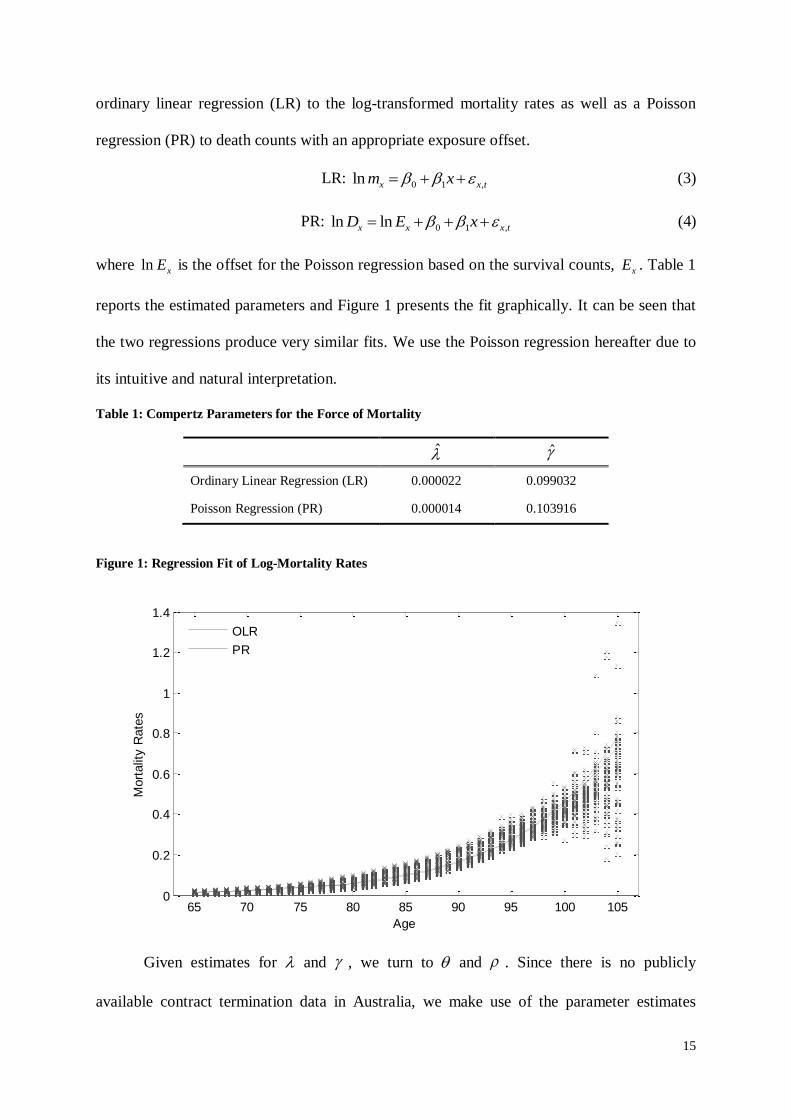
reports the estimated parameters and Figure 1 presents the fit graphically. It can be seen that

the two regressions produce very similar fits. We use the Poisson regression hereafter due to

its intuitive and natural interpretation.

Table 1: Compertz Parameters for the Force of Mortality

Ordinary Linear Regression (LR) 0.000022 0.099032

Poisson Regression (PR) 0.000014 0.103916

Figure 1: Regression Fit of Log-Mortality Rates

Given estimates for and , we turn to and . Since there is no publicly

available contract termination data in Australia, we make use of the parameter estimates

65 70 75 80 85 90 95 100 1050

0.2

0.4

0.6

0.8

1

1.2

1.4

Age

Mort

alit

y R

ate

s

OLR

PR

16

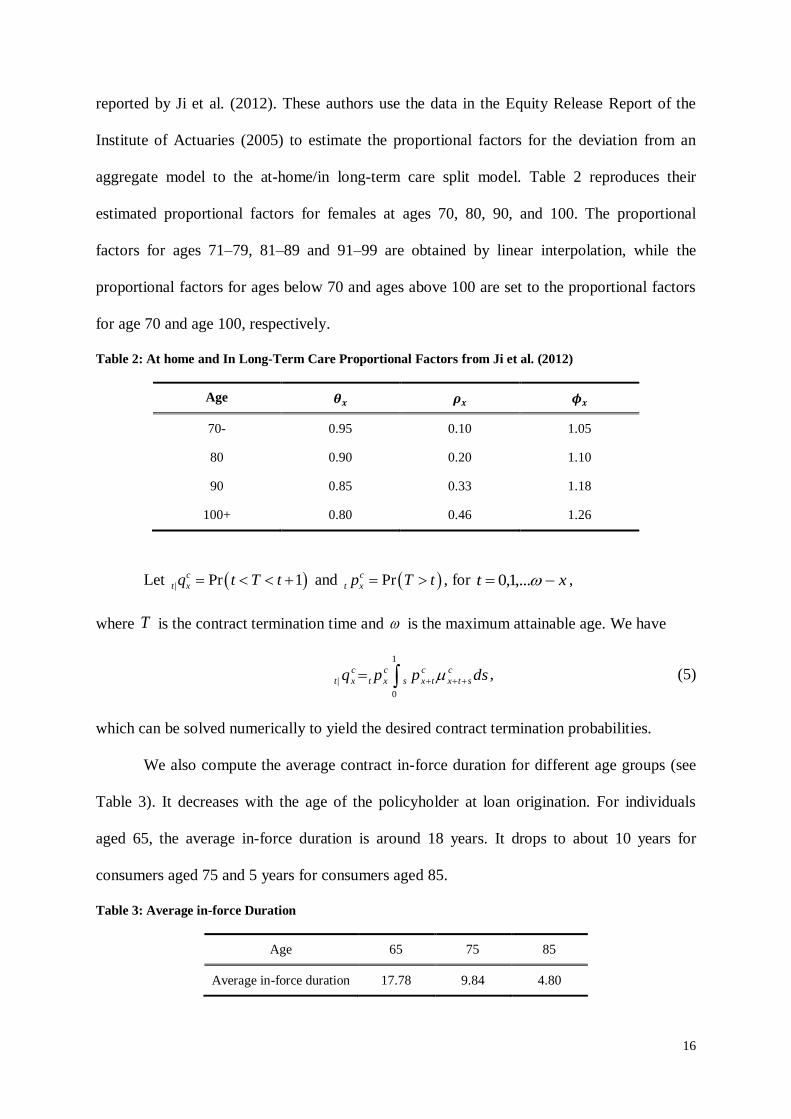
reported by Ji et al. (2012). These authors use the data in the Equity Release Report of the

Institute of Actuaries (2005) to estimate the proportional factors for the deviation from an

aggregate model to the at-home/in long-term care split model. Table 2 reproduces their

estimated proportional factors for females at ages 70, 80, 90, and 100. The proportional

factors for ages 71–79, 81–89 and 91–99 are obtained by linear interpolation, while the

proportional factors for ages below 70 and ages above 100 are set to the proportional factors

for age 70 and age 100, respectively.

Table 2: At home and In Long-Term Care Proportional Factors from Ji et al. (2012)

Age

70- 0.95 0.10 1.05

80 0.90 0.20 1.10

90 0.85 0.33 1.18

100+ 0.80 0.46 1.26

Let | Pr 1c

t xq t T t and Prc

t xp T t , for xt ,...1,0 ,

where T is the contract termination time and is the maximum attainable age. We have

1

0

| dsppq c

stx

c

txs

c

xt

c

xt , (5)

which can be solved numerically to yield the desired contract termination probabilities.

We also compute the average contract in-force duration for different age groups (see

Table 3). It decreases with the age of the policyholder at loan origination. For individuals

aged 65, the average in-force duration is around 18 years. It drops to about 10 years for

consumers aged 75 and 5 years for consumers aged 85.

Table 3: Average in-force Duration

Age 65 75 85

Average in-force duration 17.78 9.84 4.80

17

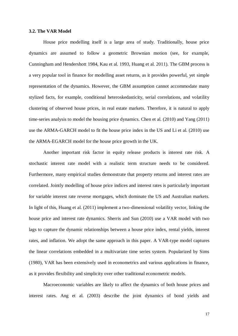
3.2. The VAR Model

House price modelling itself is a large area of study. Traditionally, house price

dynamics are assumed to follow a geometric Brownian motion (see, for example,

Cunningham and Hendershott 1984, Kau et al. 1993, Huang et al. 2011). The GBM process is

a very popular tool in finance for modelling asset returns, as it provides powerful, yet simple

representation of the dynamics. However, the GBM assumption cannot accommodate many

stylized facts, for example, conditional heteroskedasticity, serial correlations, and volatility

clustering of observed house prices, in real estate markets. Therefore, it is natural to apply

time-series analysis to model the housing price dynamics. Chen et al. (2010) and Yang (2011)

use the ARMA-GARCH model to fit the house price index in the US and Li et al. (2010) use

the ARMA-EGARCH model for the house price growth in the UK.

Another important risk factor in equity release products is interest rate risk. A

stochastic interest rate model with a realistic term structure needs to be considered.

Furthermore, many empirical studies demonstrate that property returns and interest rates are

correlated. Jointly modelling of house price indices and interest rates is particularly important

for variable interest rate reverse mortgages, which dominate the US and Australian markets.

In light of this, Huang et al. (2011) implement a two-dimensional volatility vector, linking the

house price and interest rate dynamics. Sherris and Sun (2010) use a VAR model with two

lags to capture the dynamic relationships between a house price index, rental yields, interest

rates, and inflation. We adopt the same approach in this paper. A VAR-type model captures

the linear correlations embedded in a multivariate time series system. Popularized by Sims

(1980), VAR has been extensively used in econometrics and various applications in finance,

as it provides flexibility and simplicity over other traditional econometric models.

Macroeconomic variables are likely to affect the dynamics of both house prices and

interest rates. Ang et al. (2003) describe the joint dynamics of bond yields and

18

macroeconomic variables in a VAR model. Previous studies also argue that house prices are

affected by macroeconomic factors (see, for example, Abraham and Hendershott 1994;

Muellbauer and Murphy 1997). Recent studies have included GDP as a factor in predicting

housing prices (Valadez 2010) and the yield curve (Ang and Piazzesi 2003). For this reason,

we include GDP in our VAR framework.

The raw data used in this study include zero-coupon interest rates (3-month and 10-

year), standard variable mortgage rates (MR), a nominal Sydney house price index (HPI), a

nominal Sydney rental yield index (RYI), and nominal Australian GDP (GDP). Data is

available for the period June 1993 to June 2011. Because the data for GDP is only available

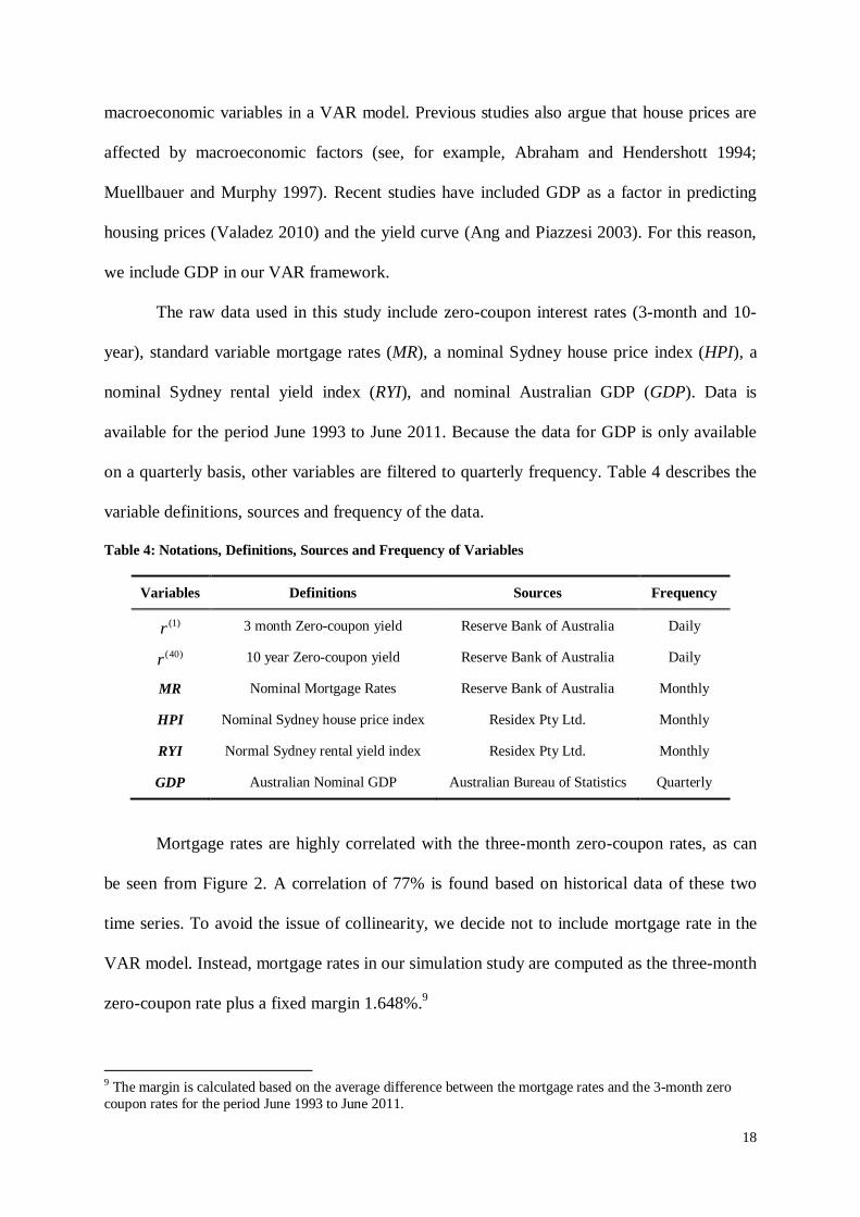
on a quarterly basis, other variables are filtered to quarterly frequency. Table 4 describes the

variable definitions, sources and frequency of the data.

Table 4: Notations, Definitions, Sources and Frequency of Variables

Variables Definitions Sources Frequency

(1)r 3 month Zero-coupon yield Reserve Bank of Australia Daily

(40)r 10 year Zero-coupon yield Reserve Bank of Australia Daily

MR Nominal Mortgage Rates Reserve Bank of Australia Monthly

HPI Nominal Sydney house price index Residex Pty Ltd. Monthly

RYI Normal Sydney rental yield index Residex Pty Ltd. Monthly

GDP Australian Nominal GDP Australian Bureau of Statistics Quarterly

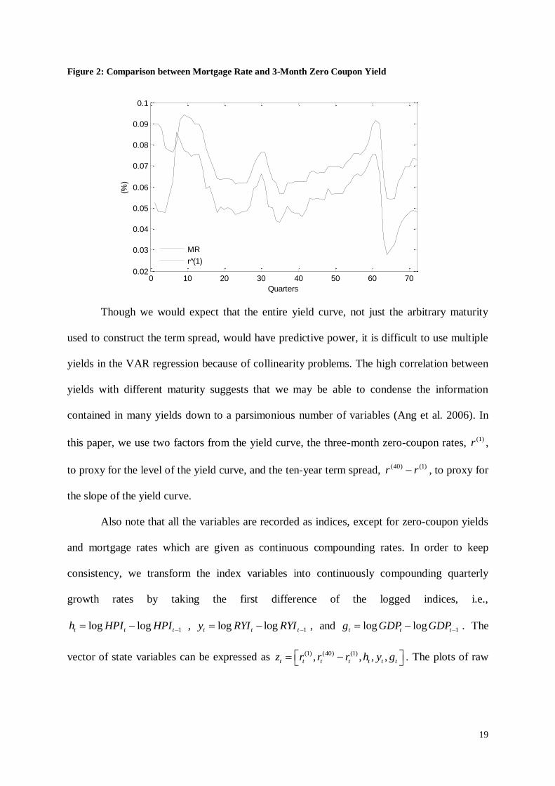
Mortgage rates are highly correlated with the three-month zero-coupon rates, as can

be seen from Figure 2. A correlation of 77% is found based on historical data of these two

time series. To avoid the issue of collinearity, we decide not to include mortgage rate in the

VAR model. Instead, mortgage rates in our simulation study are computed as the three-month

zero-coupon rate plus a fixed margin 1.648%.9

9 The margin is calculated based on the average difference between the mortgage rates and the 3-month zero

coupon rates for the period June 1993 to June 2011.

19

Figure 2: Comparison between Mortgage Rate and 3-Month Zero Coupon Yield

Though we would expect that the entire yield curve, not just the arbitrary maturity

used to construct the term spread, would have predictive power, it is difficult to use multiple

yields in the VAR regression because of collinearity problems. The high correlation between

yields with different maturity suggests that we may be able to condense the information

contained in many yields down to a parsimonious number of variables (Ang et al. 2006). In

this paper, we use two factors from the yield curve, the three-month zero-coupon rates, (1)r ,

to proxy for the level of the yield curve, and the ten-year term spread, (40) (1)r r , to proxy for

the slope of the yield curve.

Also note that all the variables are recorded as indices, except for zero-coupon yields

and mortgage rates which are given as continuous compounding rates. In order to keep

consistency, we transform the index variables into continuously compounding quarterly

growth rates by taking the first difference of the logged indices, i.e.,

1log logt t th HPI HPI , 1log logt t ty RYI RYI , and 1log logt t tg GDP GDP . The

vector of state variables can be expressed as (1) (40) (1), , , ,t t t t t t tz r r r h y g . The plots of raw

0 10 20 30 40 50 60 700.02

0.03

0.04

0.05

0.06

0.07

0.08

0.09

0.1

Quarters

(%)

MR

r (1)

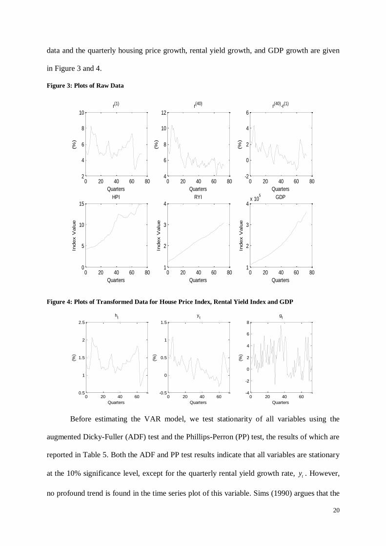
20

data and the quarterly housing price growth, rental yield growth, and GDP growth are given

in Figure 3 and 4.

Figure 3: Plots of Raw Data

Figure 4: Plots of Transformed Data for House Price Index, Rental Yield Index and GDP

Before estimating the VAR model, we test stationarity of all variables using the

augmented Dicky-Fuller (ADF) test and the Phillips-Perron (PP) test, the results of which are

reported in Table 5. Both the ADF and PP test results indicate that all variables are stationary

at the 10% significance level, except for the quarterly rental yield growth rate, ty . However,

no profound trend is found in the time series plot of this variable. Sims (1990) argues that the

0 20 40 60 802

4

6

8

10r(1)

Quarters

(%)

0 20 40 60 804

6

8

10

12r(40)

Quarters

(%)

0 20 40 60 80-2

0

2

4

6r(40)-r(1)

Quarters

(%)

0 20 40 60 800

5

10

15HPI

Quarters

Index V

alu

e

0 20 40 60 801

2

3

4RYI

Quarters

Index V

alu

e

0 20 40 60 801

2

3

4x 10

5 GDP

Quarters

Index V

alu

e

0 20 40 600.5

1

1.5

2

2.5

ht

Quarters

(%)

0 20 40 60-0.5

0

0.5

1

1.5

yt

Quarters

(%)

0 20 40 60-4

-2

0

2

4

6

8

gt

Quarters

(%)

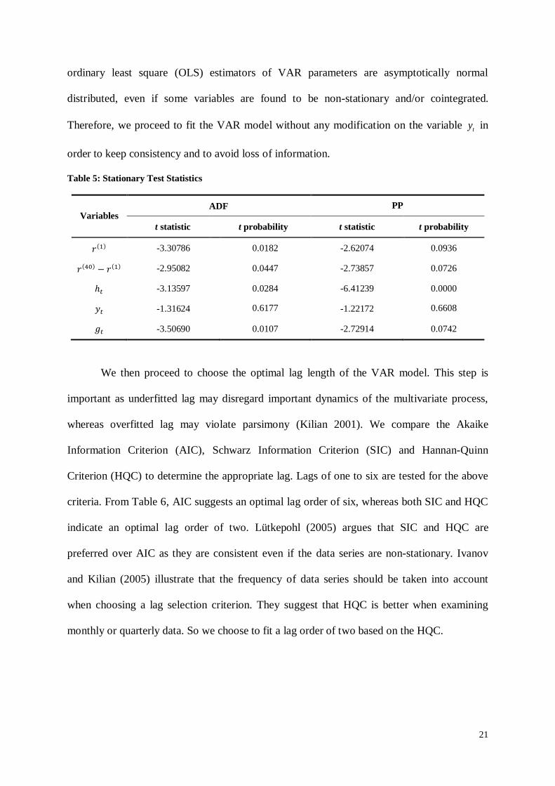
21

ordinary least square (OLS) estimators of VAR parameters are asymptotically normal

distributed, even if some variables are found to be non-stationary and/or cointegrated.

Therefore, we proceed to fit the VAR model without any modification on the variable ty in

order to keep consistency and to avoid loss of information.

Table 5: Stationary Test Statistics

Variables ADF PP

t statistic t probability t statistic t probability

-3.30786 0.0182 -2.62074 0.0936

-2.95082 0.0447 -2.73857 0.0726

-3.13597 0.0284 -6.41239 0.0000

-1.31624 0.6177 -1.22172 0.6608

-3.50690 0.0107 -2.72914 0.0742

We then proceed to choose the optimal lag length of the VAR model. This step is

important as underfitted lag may disregard important dynamics of the multivariate process,

whereas overfitted lag may violate parsimony (Kilian 2001). We compare the Akaike

Information Criterion (AIC), Schwarz Information Criterion (SIC) and Hannan-Quinn

Criterion (HQC) to determine the appropriate lag. Lags of one to six are tested for the above

criteria. From Table 6, AIC suggests an optimal lag order of six, whereas both SIC and HQC

indicate an optimal lag order of two. Lütkepohl (2005) argues that SIC and HQC are

preferred over AIC as they are consistent even if the data series are non-stationary. Ivanov

and Kilian (2005) illustrate that the frequency of data series should be taken into account

when choosing a lag selection criterion. They suggest that HQC is better when examining

monthly or quarterly data. So we choose to fit a lag order of two based on the HQC.

22

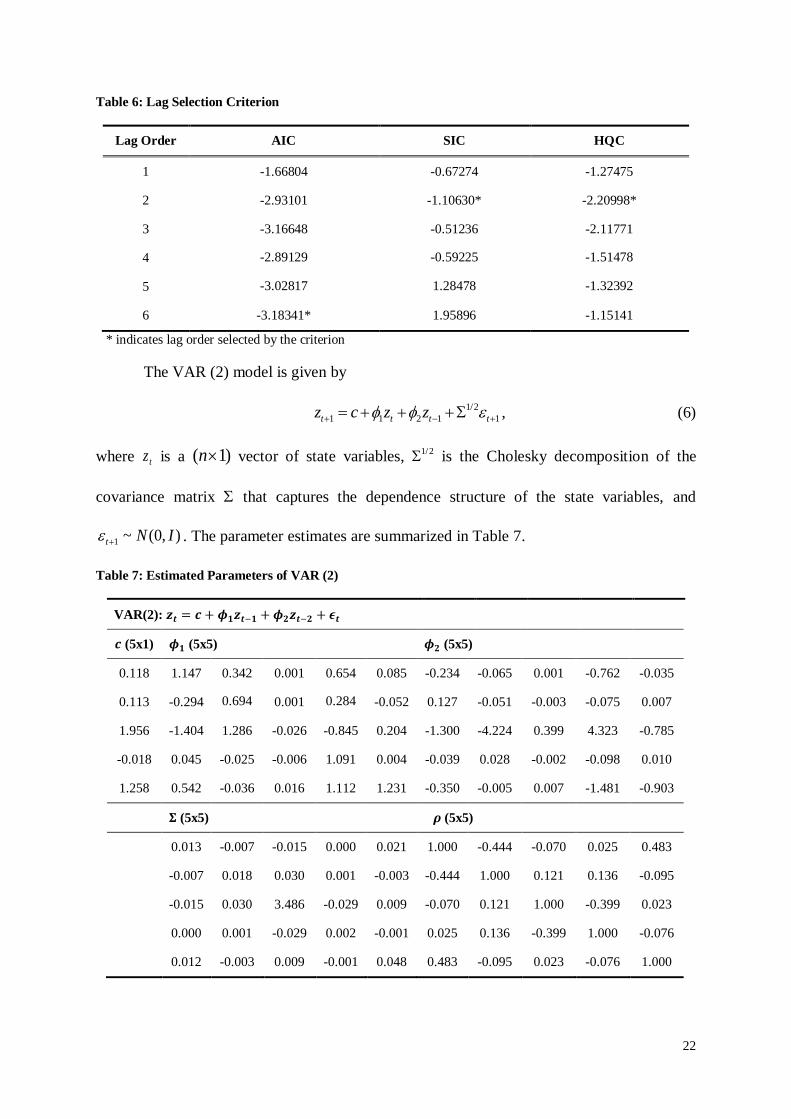
Table 6: Lag Selection Criterion

Lag Order AIC SIC HQC

1 -1.66804 -0.67274 -1.27475

2 -2.93101 -1.10630* -2.20998*

3 -3.16648 -0.51236 -2.11771

4 -2.89129 -0.59225 -1.51478

5 -3.02817 1.28478 -1.32392

6 -3.18341* 1.95896 -1.15141

* indicates lag order selected by the criterion

The VAR (2) model is given by

1/2

1 1 2 1 1t t t tz c z z , (6)

where tz is a )1( n vector of state variables, 1/2 is the Cholesky decomposition of the

covariance matrix that captures the dependence structure of the state variables, and

1 ~ (0, )t N I . The parameter estimates are summarized in Table 7.

Table 7: Estimated Parameters of VAR (2)

VAR(2):

(5x1) (5x5) (5x5)

0.118 1.147 0.342 0.001 0.654 0.085 -0.234 -0.065 0.001 -0.762 -0.035

0.113 -0.294 0.694 0.001 0.284 -0.052 0.127 -0.051 -0.003 -0.075 0.007

1.956 -1.404 1.286 -0.026 -0.845 0.204 -1.300 -4.224 0.399 4.323 -0.785

-0.018 0.045 -0.025 -0.006 1.091 0.004 -0.039 0.028 -0.002 -0.098 0.010

1.258 0.542 -0.036 0.016 1.112 1.231 -0.350 -0.005 0.007 -1.481 -0.903

(5x5) (5x5)

0.013 -0.007 -0.015 0.000 0.021 1.000 -0.444 -0.070 0.025 0.483

-0.007 0.018 0.030 0.001 -0.003 -0.444 1.000 0.121 0.136 -0.095

-0.015 0.030 3.486 -0.029 0.009 -0.070 0.121 1.000 -0.399 0.023

0.000 0.001 -0.029 0.002 -0.001 0.025 0.136 -0.399 1.000 -0.076

0.012 -0.003 0.009 -0.001 0.048 0.483 -0.095 0.023 -0.076 1.000

23

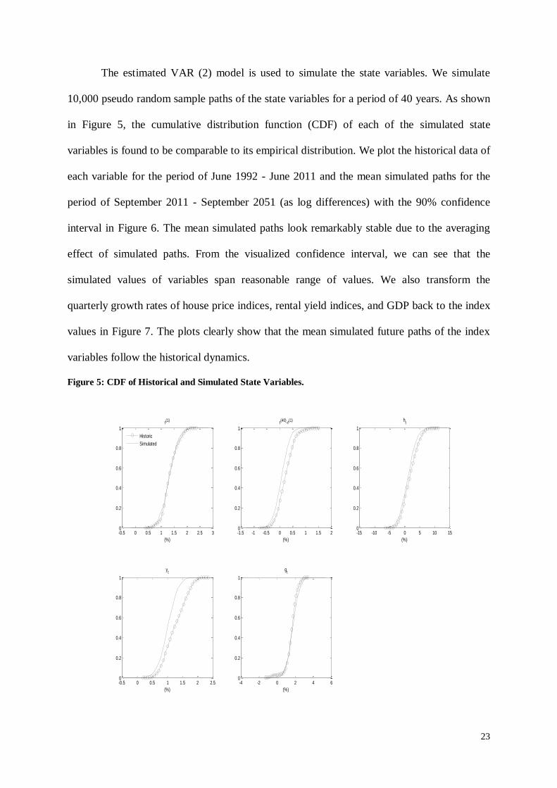
The estimated VAR (2) model is used to simulate the state variables. We simulate

10,000 pseudo random sample paths of the state variables for a period of 40 years. As shown

in Figure 5, the cumulative distribution function (CDF) of each of the simulated state

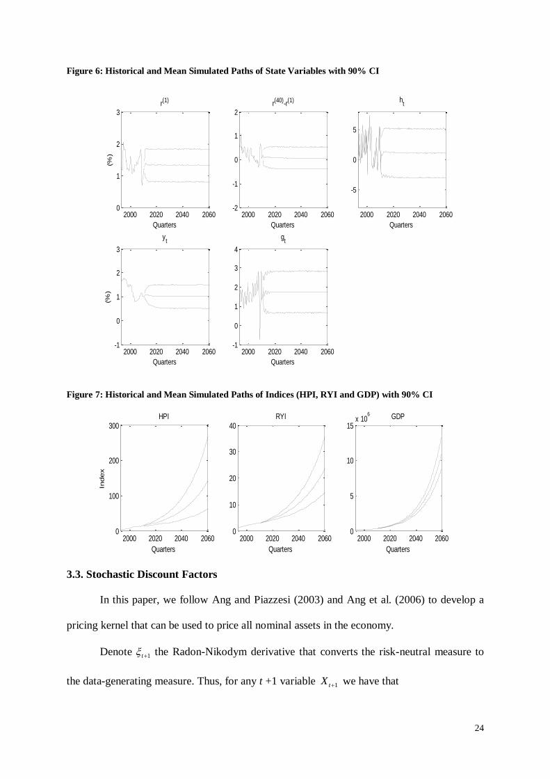
variables is found to be comparable to its empirical distribution. We plot the historical data of

each variable for the period of June 1992 - June 2011 and the mean simulated paths for the

period of September 2011 - September 2051 (as log differences) with the 90% confidence

interval in Figure 6. The mean simulated paths look remarkably stable due to the averaging

effect of simulated paths. From the visualized confidence interval, we can see that the

simulated values of variables span reasonable range of values. We also transform the

quarterly growth rates of house price indices, rental yield indices, and GDP back to the index

values in Figure 7. The plots clearly show that the mean simulated future paths of the index

variables follow the historical dynamics.

Figure 5: CDF of Historical and Simulated State Variables.

-0.5 0 0.5 1 1.5 2 2.5 30

0.2

0.4

0.6

0.8

1r(1)

(%)

Historic

Simulated

-1.5 -1 -0.5 0 0.5 1 1.5 20

0.2

0.4

0.6

0.8

1r(40)-r(1)

(%)

-15 -10 -5 0 5 10 150

0.2

0.4

0.6

0.8

1

ht

(%)

-0.5 0 0.5 1 1.5 2 2.50

0.2

0.4

0.6

0.8

1

yt

(%)

-4 -2 0 2 4 60

0.2

0.4

0.6

0.8

1

gt

(%)

24

Figure 6: Historical and Mean Simulated Paths of State Variables with 90% CI

Figure 7: Historical and Mean Simulated Paths of Indices (HPI, RYI and GDP) with 90% CI

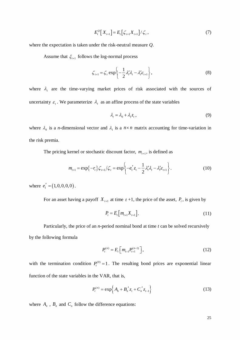
3.3. Stochastic Discount Factors

In this paper, we follow Ang and Piazzesi (2003) and Ang et al. (2006) to develop a

pricing kernel that can be used to price all nominal assets in the economy.

Denote 1t the Radon-Nikodym derivative that converts the risk-neutral measure to

the data-generating measure. Thus, for any t +1 variable 1tX we have that

2000 2020 2040 20600

1

2

3r(1)

Quarters

(%)

2000 2020 2040 2060-2

-1

0

1

2r(40)-r(1)

Quarters

2000 2020 2040 2060

-5

0

5

ht

Quarters

2000 2020 2040 2060-1

0

1

2

3

yt

Quarters

(%)

2000 2020 2040 2060-1

0

1

2

3

4

gt

Quarters

2000 2020 2040 20600

100

200

300HPI

Quarters

Index

2000 2020 2040 20600

10

20

30

40RYI

Quarters

2000 2020 2040 20600

5

10

15x 10

6 GDP

Quarters

25

1 1 1 /Q

t t t t t tE X E X , (7)

where the expectation is taken under the risk-neutral measure Q.

Assume that 1t follows the log-normal process

1 1

1exp

2t t t t t t

, (8)

where t are the time-varying market prices of risk associated with the sources of

uncertainty t . We parameterize t as an affine process of the state variables

0 1t tz , (9)

where 0 is a n-dimensional vector and 1 is a n n matrix accounting for time-variation in

the risk premia.

The pricing kernel or stochastic discount factor, 1tm , is defined as

1 1 1 1

1exp exp

2t t t t t t t t tm r e z

. (10)

where 1 1,0,0,0,0e .

For an asset having a payoff 1tX at time t +1, the price of the asset, tP , is given by

1 1t t t tP E m X . (11)

Particularly, the price of an n-period nominal bond at time t can be solved recursively

by the following formula

( ) ( 1)

1 1

n n

t t t tP E m P

, (12)

with the termination condition (0) 1tP . The resulting bond prices are exponential linear

function of the state variables in the VAR, that is,

( )

1expn

t n n t n tP A B z C z (13)

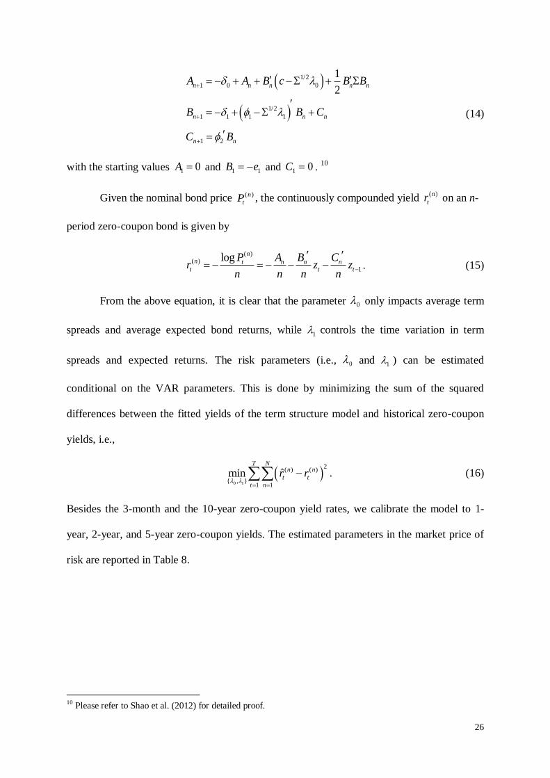
where nA , nB and nC follow the difference equations:

26

1/2

1 0 0

1/2

1 1 1 1

1 2

1

2n n n n n

n n n

n n

A A B c B B

B B C

C B

(14)

with the starting values 1 0A and 1 1B e and 1 0C . 10

Given the nominal bond price ( )n

tP , the continuously compounded yield ( )n

tr on an n-

period zero-coupon bond is given by

( )( )

1

log nn t n n n

t t t

P A B Cr z z

n n n n

. (15)

From the above equation, it is clear that the parameter 0 only impacts average term

spreads and average expected bond returns, while 1 controls the time variation in term

spreads and expected returns. The risk parameters (i.e., 0 and 1 ) can be estimated

conditional on the VAR parameters. This is done by minimizing the sum of the squared

differences between the fitted yields of the term structure model and historical zero-coupon

yields, i.e.,

0 1

2( ) ( )

{ , }1 1

ˆminT N

n n

t t

t n

r r

. (16)

Besides the 3-month and the 10-year zero-coupon yield rates, we calibrate the model to 1-

year, 2-year, and 5-year zero-coupon yields. The estimated parameters in the market price of

risk are reported in Table 8.

10

Please refer to Shao et al. (2012) for detailed proof.

27

Table 8: Estimated Parameters in the Market Price of Risk

Variables (5x1) (5x5)

0.9204 -2.3931 -0.2864 -0.1300 0.8383 1.0222

0.2199 0.1342 -0.0219 -1.1957 1.1733 -1.6144

6.5198 2.2503 1.0482 0.2543 -1.1396 -0.0363

-1.3300 -1.4757 -1.1437 4.2605 -4.2072 4.3283

1.7039 2.2737 -3.5390 0.6715 0.7444 -0.3215

Based on the fitted market price of risk, we calculate the stochastic discount factors

and show its plot in Figure 8. We also show a sample path of simulated stochastic discount

factors in the same figure. The correlations between the fitted stochastic discount factor and

state variables are reported in Table 9. It can be seen that the stochastic discount factor has a

high negative correlation with the short rate, which is intuitive. In addition, the house price

growth positively contributes to the stochastic discount factor.

Figure 8: Stochastic Discount Factors and Bond Risk Premiums

Table 9: Correlations between Stochastic Discount Factors and State Variables

Correlation

SDF -0.94 0.26 0.38 -0.31 -0.23

0 10 20 30 40 50 60 7097

97.5

98

98.5

99Historical SDFs

Quarters

0 20 40 60 80 100 120 140 160 180 20092

93

94

95

96

97

98

99A Sample Path of Simulated SDFs

Quarters

28

4. Risk Analysis

In the previous section, we have described a termination model and a VAR model for

economic variables. We use these models to simulate the input variables and calculate the

provider‘s capital at some future dates. We estimate an empirical distribution of the capital

amount by running the simulation procedure a large number of times. The capital distribution

is then used to calculate the target solvency capital level. This simulation-based approach was

also used in Daykin et al. (1994), Lee (2000) and Tsai et al. (2001). Various measures can be

used to decide risk-based capital level for solvency requirement and there is no general

consensus as to which one is the most appropriate. We consider two commonly used risk

measures, VaR and CVaR, to calculate the solvency capital in this paper.

4.1. Payoff Structure of Reverse Mortgages

4.1.1. Pricing the No Negative Equity Guarantee

In a reverse mortgage contract, borrowers are typically protected by the provision of

the no negative equity guarantee. When the loan terminates, if the net proceeds from the sale

of the property are sufficient to pay the outstanding loan balance, the remaining cash usually

is paid out to the borrower or his/her beneficiaries. If the proceeds are insufficient to cover

the loan balance, the no negative equity guarantee prevents the lender from pursuing other

assets belonging to the borrower. Denote tL and tH the loan outstanding balance and the

value of the property at time t , respectively. Suppose there is a transaction cost of selling the

house, , given by a percentage of the house value. The payoff of the no negative equity

guarantee at loan termination time t is

max 1 ,0t t tNN L H . (17)

In our analysis, we consider a lump sum payout option, which is most popular payout

in Australia. The maximum initial loan amount is determined by the LVR that is set as a

proportion of the value of the property. LVRs increase with the age at which the loan is taken

29

out. Suppose the borrower always takes out 100% of the allowable limit, i.e., 0 0L H LVR .

The loan accrues quarterly with interests and mortgage insurance premiums. As

aforementioned, the variable mortgage rate is computed by adding a fixed margin on top of

the short rate (3-month zero coupon rate). Thus, tL is given by

0

0

expt

s

t i

i

L L r

, (18)

where s

tr denotes the three-month zero-coupon rate, is the lending margin and is the

mortgage insurance premium rate.

As the termination time t is random, we use the probability of contract termination,

|

c

t xq , to model the randomness of loan termination. We then use stochastic discount factors,

tm , to discount the value of the no negative equity guarantee at an arbitrary termination time

t to the time of loan origination, taking into account the uncertainty in the future development

of house prices, rental yields, and interest rates. Hence, the value of the no negative equity

guarantee, NN, is given by

1

|

0 0

max 1 ,0tx

c

s t x t t

t s

NN E m q L H

. (19)

The no negative equity guarantee is usually financed by mortgage insurance premiums

paid by the borrowers. There is no clear mortgage insurance structure in Australia, but

previous studies usually assume a zero up-front premium and a fixed premium rate each

period. The actuarial present value of mortgage insurance premiums, MIP, is then given by

1

1 1

txc

s t x t

t s

MIP E m p L

. (20)

The actuarially fair quarterly premium rate can be calculated by equating the value of

mortgage insurance premiums with the value of the no negative equity guarantee.

4.1.2. Cash Flows of the Reverse Mortgage Contract

30

We assume that the provider of a reverse mortgage contract finances the payout

through its existing capital and leveraging. The proportion of borrowed capital, or the

leverage ratio (LR), is denoted by . The borrowed capital accrues with the short rate.

Therefore, the total financing cost at time t can be written as

0 0

0

exp 1t

RM s

t i

i

C L r L

. (21)

The provider receives min , 1t tL H from the sale proceeds of the property when the

loan terminates. Its net payoff discounted back to time zero can be calculated as

1

|

0 0

exp min , 1x t

c s RM

t x i t t t

t i

RM q r L H C

. (22)

4.2. Payoff Structure of Home Reversions

4.2.1. Pricing the Lease for Life Agreement

Under a home reversion contact, the provider buys a share of the property at a

discounted price and offers the customers a lease for life agreement. The agreement can be

valued using annuity pricing techniques, where the annuity is indexed to the property‘s rental

yield rate. For the purpose of comparison, we assume that the acquisition ratio is the same as

the LVR in the reverse mortgage. For a certain lifespan, the value of the lease for life

agreement at time 0 can be expressed as a function of the termination time T ,

0

0 0

tT

s t t

t s

LL E m H R LVR

, (23)

where tR denotes the rental yield rate in year t .

Again, the termination time T is random. Therefore, the actuarial present value of the

lease for life agreement can be written as

1

0 0

txc

s t x t t

t s

LL E m p H R LVR

. (24)

31

4.2.2. Cash Flows of the Home Reversion Contract

In a home reversion contract, the provider purchases a share of the equity that is worth

0H LVR and discounts it by the value of the lease for life, LL . The resulting lump-sum

payment at contract origination is 0H LVR LL . Again, the provider is assumed to finance

the payout by borrowing % of the required capital. At the time of loan termination t, the

property is sold and the provider receives a share of the sale proceeds, which is tH LVR .

Thus the provider‘ net present value of payoffs at time zero is given by

1

|

0 0

expx t

c s HR

t x i t t

t i

HR q r H LVR C

, (25)

where the total cost 0 0

0

exp 1t

HR s

t i

i

C H LVR LL r H LVR LL

.

5. Numerical Illustration

In this section, we compute the value of the no negative equity guarantee in the

reverse mortgage contract and the value of the lease for life in the home reversion contract.

We then compare these two equity release products with respect to profitability and risk

under various scenarios. We conduct sensitivity analyses to identify the impacts of key

factors, such as age at contract origination, the initial house value, mortality improvement and

the leverage ratio, on cash flows and risk profiles of both equity release products.

5.1. The Base Case Scenario

In the base case scenario, we assume a single female aged 65 residing in Sydney,

Australia, with an initial house value of $600,000.11

To finance her retirement consumption

and/or aged care, she can either enter a reverse mortgage contract or sell a share of the equity

by entering a home reversion contract. If she decides to participate in the home reversion

11

Median Price and Number of Established House Transfer, Australian Bureau of Statistics.

32

scheme, the acquisition ratio is set to be the same as the LVR for the purpose of comparison.

We assume that the equity release provider finances the lump-sum payout to the homeowner

completely through borrowed capital, i.e., the leverage ratio is 100%.

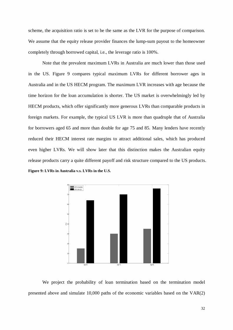
Note that the prevalent maximum LVRs in Australia are much lower than those used

in the US. Figure 9 compares typical maximum LVRs for different borrower ages in

Australia and in the US HECM program. The maximum LVR increases with age because the

time horizon for the loan accumulation is shorter. The US market is overwhelmingly led by

HECM products, which offer significantly more generous LVRs than comparable products in

foreign markets. For example, the typical US LVR is more than quadruple that of Australia

for borrowers aged 65 and more than double for age 75 and 85. Many lenders have recently

reduced their HECM interest rate margins to attract additional sales, which has produced

even higher LVRs. We will show later that this distinction makes the Australian equity

release products carry a quite different payoff and risk structure compared to the US products.

Figure 9: LVRs in Australia v.s. LVRs in the U.S.

We project the probability of loan termination based on the termination model

presented above and simulate 10,000 paths of the economic variables based on the VAR(2)

Age 65 Age 75 Age 850

10

20

30

40

50

60

70

80

(%)

LVR in Australia

LVR in the US

33

model for 40 years. We assume the provider of the reverse mortgage charges a zero up-front

premium and annual premiums with an actuarially fair rate . We then calculate the value of

no negative equity guarantee. For the home reversion, we calculate the value of the lease for

life agreement. We obtain the distribution of the actuarial present value of payoffs of the

provider for both products. Given the payoff distributions, we assess riskiness of each

program by computing VaR and CVaR at the 99.5% level. Table 10 summarizes the results in

the base case scenario.

Table 10: Payoffs and Risks in the Base Case Scenario

Assumption: Age=65, H0=$600,000, LR =100%, No mortality improvement

LVR Reverse Mortgage Home Reversion

NN E[RM] VaR CVaR LL E[HR] VaR CVaR

15% 0 29,623 0 0 35,764 25,906 -3,873 -6,564

64% 39,280 82,155 -78,849 -93,941 152,593 110,533 -16,524 -28,005

Note: NN is the value of the no negative equity guarantee and LL is the value of the lease for life agreement.

E[RM] (or E[HR]) denotes the average actuarial present value of the reverse mortgage (or home reversion)

contract. VaR and CVaR are calculated at the 99.5% level.

When we use the maximum LVR typically found in Australia (15% for age 65), the

no negative equity guarantee has no values, which shows the reverse mortgage loans has

virtually no likelihood of losses. As a result, the actuarially fair premium for the guarantee is

zero. However, the fact is that reverse mortgage providers in Australia charge more than 1%

insurance premiums to protect themselves from crossover risk (Bridge et al. 2010). Our

results show that there is a possibility of reducing interest rates for reverse mortgage loans to

be closer to those for standard home loans. The VaR and CVaR at the 99.5% level are both

zero, implying that reverse mortgage providers do not need to set aside risk-based capital.

This finding is consistent with the comments from many brokers that LVRs in Australia are

set too conservative and that the premium or fees could be lowered given the very low risk of

default or even of negative equity being reached (Bridge et al. 2010). On the contrary, our

34

results show that home reversion providers do bear some risks and need to reserve some

solvency capital. The risk mainly comes from the housing price depreciation. 12

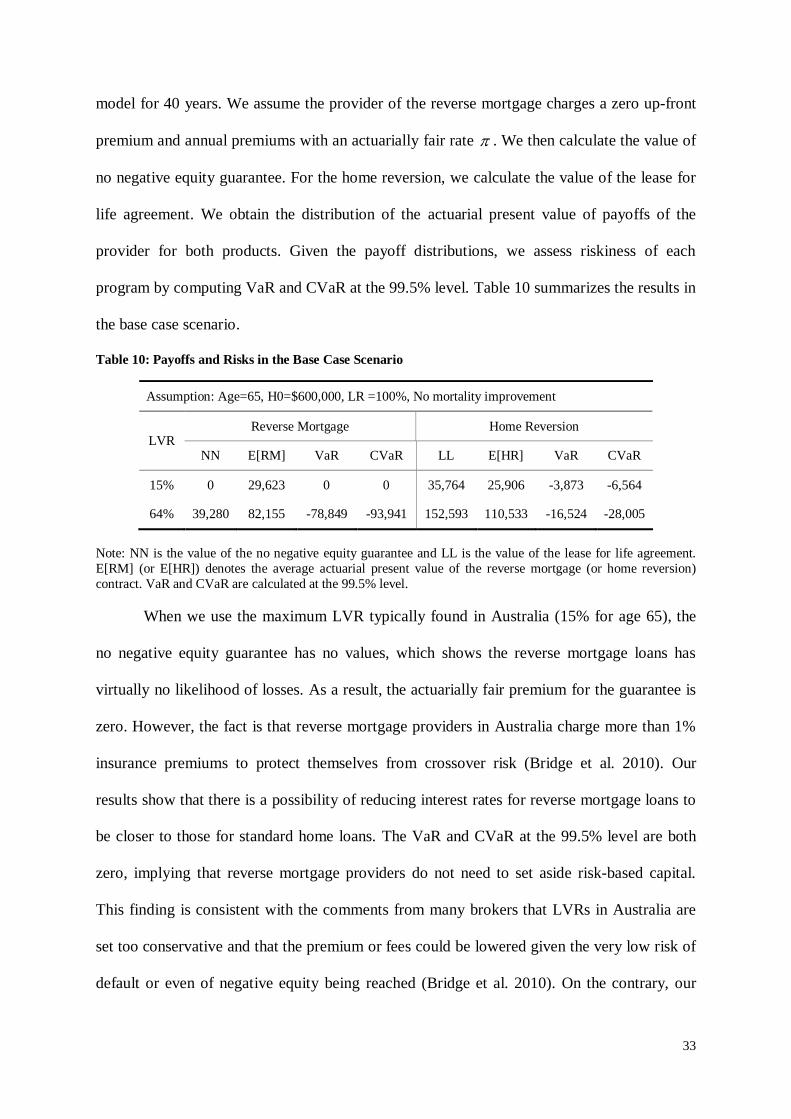
Figure 10: Loan Outstanding Balance tL and the Sale Proceeds of the Property 1 tH (LVR=64%)

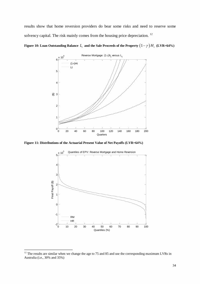
Figure 11: Distributions of the Actuarial Present Value of Net Payoffs (LVR=64%)

12 The results are similar when we change the age to 75 and 85 and use the corresponding maximum LVRs in

Australia (i.e., 30% and 35%)

0 20 40 60 80 100 120 140 160 180 2000

1

2

3

4

5

6x 10

6

Quarters

($)

Reverse Mortgage: (1-)ht versus L

t

(1-r)Ht

Lt

0 10 20 30 40 50 60 70 80 90 100-2

-1

0

1

2

3

4

5x 10

5

Quantiles (%)

Fin

al P

ayoff

($)

Quantiles of EPV: Reverse Mortgage and Home Reversion

RM

HR

35

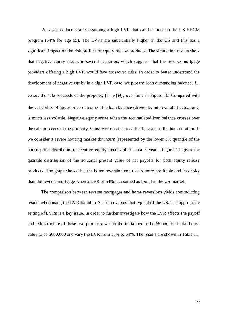
We also produce results assuming a high LVR that can be found in the US HECM

program (64% for age 65). The LVRs are substantially higher in the US and this has a

significant impact on the risk profiles of equity release products. The simulation results show

that negative equity results in several scenarios, which suggests that the reverse mortgage

providers offering a high LVR would face crossover risks. In order to better understand the

development of negative equity in a high LVR case, we plot the loan outstanding balance, tL ,

versus the sale proceeds of the property, 1 tH , over time in Figure 10. Compared with

the variability of house price outcomes, the loan balance (driven by interest rate fluctuations)

is much less volatile. Negative equity arises when the accumulated loan balance crosses over

the sale proceeds of the property. Crossover risk occurs after 12 years of the loan duration. If

we consider a severe housing market downturn (represented by the lower 5% quantile of the

house price distribution), negative equity occurs after circa 5 years. Figure 11 gives the

quantile distribution of the actuarial present value of net payoffs for both equity release

products. The graph shows that the home reversion contract is more profitable and less risky

than the reverse mortgage when a LVR of 64% is assumed as found in the US market.

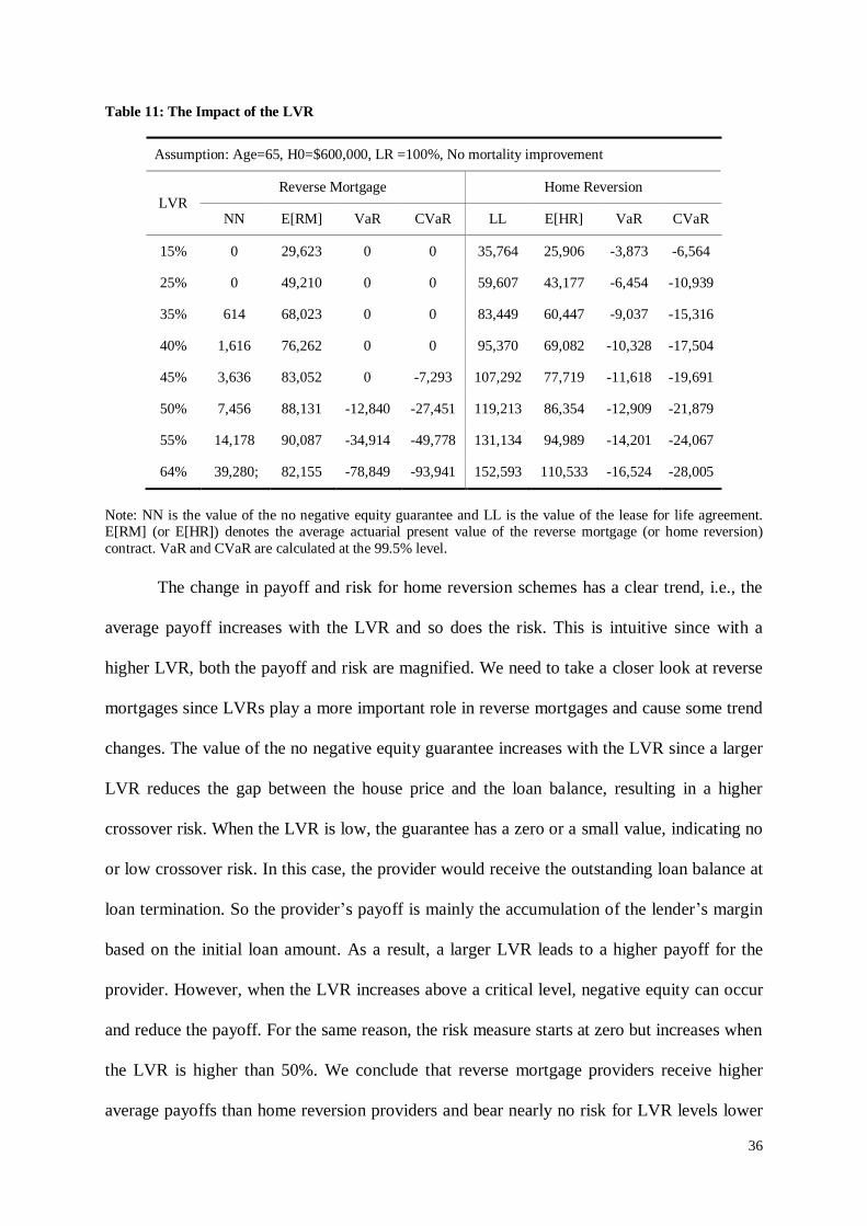
The comparison between reverse mortgages and home reversions yields contradicting

results when using the LVR found in Australia versus that typical of the US. The appropriate

setting of LVRs is a key issue. In order to further investigate how the LVR affects the payoff

and risk structure of these two products, we fix the initial age to be 65 and the initial house

value to be $600,000 and vary the LVR from 15% to 64%. The results are shown in Table 11.

36

Table 11: The Impact of the LVR

Assumption: Age=65, H0=$600,000, LR =100%, No mortality improvement

LVR Reverse Mortgage Home Reversion

NN E[RM] VaR CVaR LL E[HR] VaR CVaR

15% 0 29,623 0 0 35,764 25,906 -3,873 -6,564

25% 0 49,210 0 0 59,607 43,177 -6,454 -10,939

35% 614 68,023 0 0 83,449 60,447 -9,037 -15,316

40% 1,616 76,262 0 0 95,370 69,082 -10,328 -17,504

45% 3,636 83,052 0 -7,293 107,292 77,719 -11,618 -19,691

50% 7,456 88,131 -12,840 -27,451 119,213 86,354 -12,909 -21,879

55% 14,178 90,087 -34,914 -49,778 131,134 94,989 -14,201 -24,067

64% 39,280; 82,155 -78,849 -93,941 152,593 110,533 -16,524 -28,005

Note: NN is the value of the no negative equity guarantee and LL is the value of the lease for life agreement. E[RM] (or E[HR]) denotes the average actuarial present value of the reverse mortgage (or home reversion)

contract. VaR and CVaR are calculated at the 99.5% level.

The change in payoff and risk for home reversion schemes has a clear trend, i.e., the

average payoff increases with the LVR and so does the risk. This is intuitive since with a

higher LVR, both the payoff and risk are magnified. We need to take a closer look at reverse

mortgages since LVRs play a more important role in reverse mortgages and cause some trend

changes. The value of the no negative equity guarantee increases with the LVR since a larger

LVR reduces the gap between the house price and the loan balance, resulting in a higher

crossover risk. When the LVR is low, the guarantee has a zero or a small value, indicating no

or low crossover risk. In this case, the provider would receive the outstanding loan balance at

loan termination. So the provider‘s payoff is mainly the accumulation of the lender‘s margin

based on the initial loan amount. As a result, a larger LVR leads to a higher payoff for the

provider. However, when the LVR increases above a critical level, negative equity can occur

and reduce the payoff. For the same reason, the risk measure starts at zero but increases when

the LVR is higher than 50%. We conclude that reverse mortgage providers receive higher

average payoffs than home reversion providers and bear nearly no risk for LVR levels lower

37

than 50%. For higher LVR levels, expected payoffs from reverse mortgages become less and

the risk turns out to be higher than home reversions.

5.2. Sensitivity Analysis

In the following analysis, we use LVRs set by the US HECM program in order to

avoid zero risk in reverse mortgages and observe clear trends on comparative results.

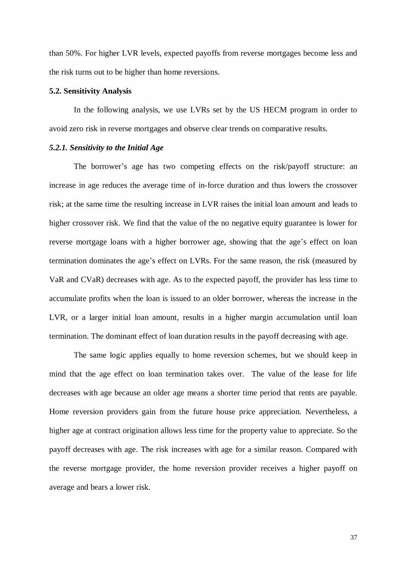
5.2.1. Sensitivity to the Initial Age

The borrower‘s age has two competing effects on the risk/payoff structure: an

increase in age reduces the average time of in-force duration and thus lowers the crossover

risk; at the same time the resulting increase in LVR raises the initial loan amount and leads to

higher crossover risk. We find that the value of the no negative equity guarantee is lower for

reverse mortgage loans with a higher borrower age, showing that the age‘s effect on loan

termination dominates the age‘s effect on LVRs. For the same reason, the risk (measured by

VaR and CVaR) decreases with age. As to the expected payoff, the provider has less time to

accumulate profits when the loan is issued to an older borrower, whereas the increase in the

LVR, or a larger initial loan amount, results in a higher margin accumulation until loan

termination. The dominant effect of loan duration results in the payoff decreasing with age.

The same logic applies equally to home reversion schemes, but we should keep in

mind that the age effect on loan termination takes over. The value of the lease for life

decreases with age because an older age means a shorter time period that rents are payable.

Home reversion providers gain from the future house price appreciation. Nevertheless, a

higher age at contract origination allows less time for the property value to appreciate. So the

payoff decreases with age. The risk increases with age for a similar reason. Compared with

the reverse mortgage provider, the home reversion provider receives a higher payoff on

average and bears a lower risk.

38

Table 12: Sensitivity to the Initial Age

Assumptions: H0=$600,000, LR=100%, No mortality improvement

Age LVR Reverse Mortgage Home Reversion

NN E[RM] VaR CVaR LL E[HR] VaR CVaR

65 64% 39,280 82,155 -78,849 -93,941 152,593 110,533 -16,524 -28,005

75 70% 29,523 59,254 -56,010 -71,390 116,934 85,663 -25,350 -36,086

85 76% 18,131 33,583 -42,686 -51,783 72,186 46,588 -40,972 -48,700

Note: NN is the value of the no negative equity guarantee and LL is the value of the lease for life agreement. E[RM] (or E[HR]) denotes the average actuarial present value of the reverse mortgage (or home reversion)

contract. VaR and CVaR are calculated at the 99.5% level.

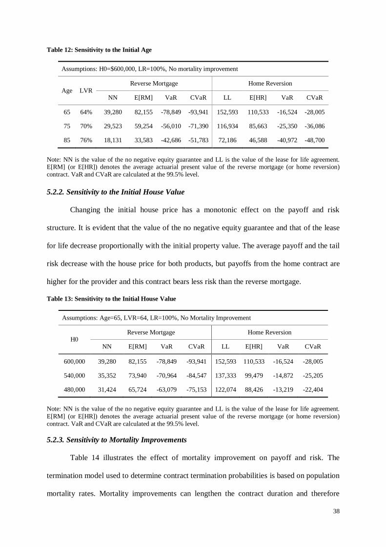
5.2.2. Sensitivity to the Initial House Value

Changing the initial house price has a monotonic effect on the payoff and risk

structure. It is evident that the value of the no negative equity guarantee and that of the lease

for life decrease proportionally with the initial property value. The average payoff and the tail

risk decrease with the house price for both products, but payoffs from the home contract are

higher for the provider and this contract bears less risk than the reverse mortgage.

Table 13: Sensitivity to the Initial House Value

Assumptions: Age=65, LVR=64, LR=100%, No Mortality Improvement

H0 Reverse Mortgage Home Reversion

NN E[RM] VaR CVaR LL E[HR] VaR CVaR

600,000 39,280 82,155 -78,849 -93,941 152,593 110,533 -16,524 -28,005

540,000 35,352 73,940 -70,964 -84,547 137,333 99,479 -14,872 -25,205

480,000 31,424 65,724 -63,079 -75,153 122,074 88,426 -13,219 -22,404

Note: NN is the value of the no negative equity guarantee and LL is the value of the lease for life agreement.

E[RM] (or E[HR]) denotes the average actuarial present value of the reverse mortgage (or home reversion)

contract. VaR and CVaR are calculated at the 99.5% level.

5.2.3. Sensitivity to Mortality Improvements

Table 14 illustrates the effect of mortality improvement on payoff and risk. The

termination model used to determine contract termination probabilities is based on population

mortality rates. Mortality improvements can lengthen the contract duration and therefore

39

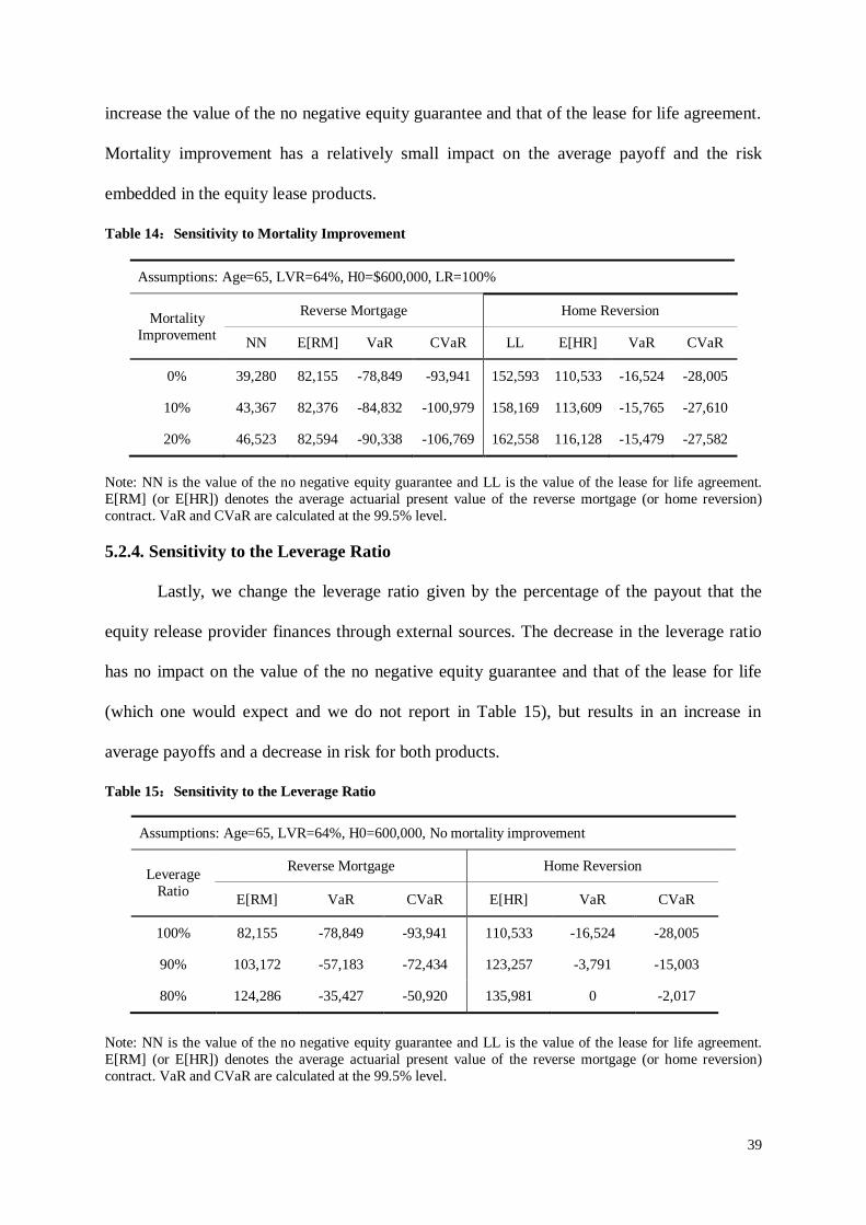
increase the value of the no negative equity guarantee and that of the lease for life agreement.

Mortality improvement has a relatively small impact on the average payoff and the risk

embedded in the equity lease products.

Table 14：Sensitivity to Mortality Improvement

Assumptions: Age=65, LVR=64%, H0=$600,000, LR=100%

Mortality

Improvement

Reverse Mortgage Home Reversion

NN E[RM] VaR CVaR LL E[HR] VaR CVaR

0% 39,280 82,155 -78,849 -93,941 152,593 110,533 -16,524 -28,005

10% 43,367 82,376 -84,832 -100,979 158,169 113,609 -15,765 -27,610

20% 46,523 82,594 -90,338 -106,769 162,558 116,128 -15,479 -27,582

Note: NN is the value of the no negative equity guarantee and LL is the value of the lease for life agreement.

E[RM] (or E[HR]) denotes the average actuarial present value of the reverse mortgage (or home reversion)

contract. VaR and CVaR are calculated at the 99.5% level.

5.2.4. Sensitivity to the Leverage Ratio

Lastly, we change the leverage ratio given by the percentage of the payout that the

equity release provider finances through external sources. The decrease in the leverage ratio

has no impact on the value of the no negative equity guarantee and that of the lease for life

(which one would expect and we do not report in Table 15), but results in an increase in

average payoffs and a decrease in risk for both products.

Table 15：Sensitivity to the Leverage Ratio

Assumptions: Age=65, LVR=64%, H0=600,000, No mortality improvement

Leverage

Ratio

Reverse Mortgage Home Reversion

E[RM] VaR CVaR E[HR] VaR CVaR

100% 82,155 -78,849 -93,941 110,533 -16,524 -28,005

90% 103,172 -57,183 -72,434 123,257 -3,791 -15,003

80% 124,286 -35,427 -50,920 135,981 0 -2,017

Note: NN is the value of the no negative equity guarantee and LL is the value of the lease for life agreement.

E[RM] (or E[HR]) denotes the average actuarial present value of the reverse mortgage (or home reversion)

contract. VaR and CVaR are calculated at the 99.5% level.

40

6. Conclusions and Discussions

The actuarial literature on pricing of equity release products is still rather limited. In

this paper, we analyse cash flows and risk profiles for equity release products from the

provider‘s perspective. We assume a single female policyholder who intends to make use of

either the reverse mortgage or the home reversion scheme to liquidate her equity and finance

her retirement consumption and care costs. We find that with a low LVR, reverse mortgages

provide a higher payoff and deliver less risk to the provider than home reversions. This

finding justifies the dominant market share of reverse mortgage schemes in Australia and

many other countries, such as the UK. When we use a high LVR, as found in the US HECM

program, we find that home reversions are better in terms of the payoff and risk structure for

the provider than reverse mortgages. The appropriate setting of LVRs plays an important role

in the product risks.

Our results indicate that reverse mortgage providers in Australia could consider

increasing maximum LVRs and decreasing insurance premium rates or on-going fees, in

order to expand the reverse mortgage market. Usually, the LVR depends on the age of the

borrower at loan origination. Our sensitivity analysis indicates that among all the factors that

we consider, the initial age of homeowners has a profound and significant impact on payoffs

and risks of equity release product providers. It affects both the contract termination time and

the LVR (thus the initial payout to consumers) and results in two competing effects on the

risk and payoff profile. Caution has to be used when determining the LVR based on age.

Our results have important implications to policymakers and regulators in many other

countries that face the issue of aging population and underfunded pensions. For example, the

UK has a similar, conservative pattern of LVRs as in Australia. UK providers have the

potential to increase LVRs to stimulate the reverse mortgage market. Though our results

indicates a high LVR as found in the US makes reverse mortgage products less profitable and

41

riskier than home reversion schemes, this has been based on economic scenarios from

Australia experience. The US housing market and economic conditions have been quite

different in recent years and this has to be considered when assessing the US markets. In

addition, in the US, the HECM providers are insured by the federal government and can

transfer the risk to FHA.

As a newly developed equity release product, the home reversion scheme has

advantages to both homeowners and investors. It usually sets a limit on the share of equity

that can be sold to a home reversion company, leaving a remainder to consumers which can

be used to fund aged care after the property is sold. As an asset class, much of the risk

attached to ‗traditional‘ property investment is either irrelevant in home reversion contracts

such as tenancy or default risk, or can be diversified in a ‗pooled‘ residential property pool,

for example, duration risk and location risk (Deloitte 2011).

However, the private market for home reversions has been developing slowly. Lack of

awareness and low financial literacy among consumers are the main reasons on the demand

side. In particular, the implicit lease for life agreement in the home reversion contract may be

poorly understood. On the supply side, liquidity is the major concern of investors. In addition

to providing an appropriate framework of regulation and education, governments should

consider policies to support the development of the equity release market such as providing

liquidity for providers.

42

Acknowledgement

The authors acknowledge the support of ARC Linkage Grant Project LP0883398 Managing

Risk with Insurance and Superannuation as Individuals Age with industry partners PwC and

APRA and the Australian Research Council Centre of Excellence in Population Ageing

Research (project number CE110001029). Hua Chen also acknowledges the financial support

from Temple University.

References:

Abraham, J., and P. Hendershott. 1994. Bubbles in Metropolitan Housing Markets. Journal of

Housing Research 7(2): 191-208.

Ang, A., and M. Piazzesi. 2003. A No-Arbitrage Vector Autoregression of Term Structure

Dynamics with Macroeconomic and Latent Variables. Journal of Monetary Economics

50(4): 745-787.

Ang, A., M. Piazzesi, and M. Wei. 2006. What Does the Yield Curve Tell Us about GDP

Growth? Journal of Econometrics 131 (1): 359-403.

ASIC. 2005. Equity Release Product. Australian Securities & Investments Commission

Report 59.

Boehm, T. P., and M. C. Ehrhardt. 1994. Reverse Mortgage and Interest Rate Risk. Journal

of the American Real Estate and Urban Economics Association 22(2), 387-408.

Bridge, C., T. Adams, P. Phibbs, M. Mathews, and H. Kendig. 2010. Reverse Mortgages and

Older People: Growth Factors and Implications for Retirement Decisions. AHURI Final

Report No. 146, Australian Housing and Urban Research Institute.

Chen, H., S. H. Cox, and S. S. Wang. 2010. Is the Home Equity Conversion Program in the

United States Sustainable? Evidence from Pricing Mortgage Insurance Premiums and

Non-Recourse Provisions Using the Conditional Esscher Transform. Insurance:

Mathematics and Economics 46(2): 371-384.

Chinloy, P., and I. F. Megbolugbe. 1994. Reverse Mortgages: Contracting and Crossover

Risk. Real Estate Economics 22(2), 367-386.

Cho, D. 2012. Risk Management and Payout Design of Reverse Mortgage. Honor thesis,

University of New South Wales.

Chow, M. H., E. J. Szymanoski, and T. R. Diventi. 2000. Applying Survival Analysis

Techniques to Loan Terminations for HUD's Reverse Mortgage Insurance Program.

Proceedings of the 13th

Northeast SAS Users Group Conference, available at

http://www.nesug.org/proceedings/nesug00/st/st9003.pdf

43

Cochrane, J. H., and M. Piazzesi. 2005. Bond Risk Premia. American Economic Review 95

(1): 138-160.

Cunningham, D. F., and P. F. Hendershott. 1986. Pricing FHA Mortgage Default Insurance.

NBER Working Paper No. 1382.

Daykin, C. D., T. Pentikainen, and M. Pesonen. 1994. Practical Risk Theory for Actuaries.

London: Chapman and Hall

Deloitte. 2011a. Media Release: Australia‘s reverse mortgage market reaches $3bn at 31

December 2010. SEQUAL Deloitte Research Report, 27 May 2011.

Deloitte. 2011b. Response to Productivity Commission Draft Report: Caring For Older

Australians. Deloitte report prepared for Homesafe Solutions Pty Ltd, 17 March 2011.

Deloitte. 2012. Media Release: Australia's Reverse Mortgage Market Reaches $3.3bn at 31

December 2011. SEQUAL Deloitte Research Report, 4 June 2012.

Hoevenaars, R. (2008). Strategic Asset Allocation and Asset Liability Management. Ph.D.

Dissertation, Maastricht University .

Huang, H.-C., C.-W. Wang, and Y.-C Miao. 2011. Securitization of Crossover Risk in

Reverse Mortgages. The Geneva Papers on Risk and Insurance – Issues and Practice 36

(4): 622-647.

Institute of Actuaries. 2005. Equity release report 2005. Volume 2: Technical supplement:

pricing considerations. Institute of Actuaries, UK.

Ivanov, V., and L. Kilian. 2005. A Practitioner's Guide to Lag Order Selection for VAR

Impulse Response Analysis. Studies in Nonlinear Dynamics and Econometrics 9 (1):

Ji, M., M. R. Hardy, and S. H. Li. 2012. A Semi-Markov Multiple State Model for Reverse

Mortgage Terminations. Annals of Actuarial Science 6(2): 235-257.

Kau, J., D. C. Keenan, W. J. Muller III, and J. F. Epperson. 1992. A Generalized Valuation

Model for Fixed-Rate Residential Mortgages. Journal of Money, Credit and Banking

24(3): 279-299.

Kilian, L. 2001. Impulse Response Analysis in Vector Autoregressions with Unknown Lag

order. Journal of Forecasting 20 (3): 161-179.

Lee, P. 2000. A General Framework for Stochastic Investigations of Mortality and

Investment Risks. Presented at Wilkiefest, Heriot-Watt University.

Li, S. H., M. R. Hardy, and K. S. Tan. 2010. On Pricing and Hedging the No-Negative-

Equity-Guarantee in Equity Release Mechanisms. Journal of Risk and Insurance 77: 499-

522.

Lütkepohl, H. 2005. New Introduction to Multiple Time Series Analysis. Cambridge

University Press

44

Ma, S., G. Kim, and K. Lew. 2007. Estimating Reverse Mortgage Insurer‘s Risk Using

Stochastic Models. Paper presented at the Asia-Pacific Risk and Insurance Association

2007 annual meeting

Ma, S., and Y. Deng. 2006. Insurance Premium Structure of Reverse Mortgage Loans in

Korea. Working paper, available at SSRN: http://ssrn.com/abstract=938213

Muellbauer, J., and A. Murphy. 1997. Booms and Busts in the UK Housing Market. The

Economic Journal 107(445): 1701-1727.

Oliver Wyman Financial Services (2005). Move Beyond the HECM in Equity Release

Markets?, Oliver Wyman Financial Services technique report.

Rodda, D. T., K. Lam, and A. Youn. 2004. Stochastic Modeling of Federal Housing

Administration Home Equity Conversion Mortgages with Low-Cost Refinancing. Real

Estate Economics 32(4), 589-617.

Shao, A., M. Sherris, and K. Hanewald. 2012. Equity Release Products allowing for

Individual House Price Risk. Working paper, University of New South Wales.

Sherris, M., and D. Sun. 2010. Risk Based Capital and Pricing for Reverse Mortgages

Revisited. Working paper, University of New South Wales.

Sims, C. 1980. Macroeconomics and Reality. Econometrica 48(1): 1-48.

Szymanoski, E. J, Jr. 1994. Risk and the Home Equity Conversion Mortgage. Journal of the

American Real Estate and Urban Economics Association 22(2): 347-366.

Szymanoski, E., J. C. Enriquez, and T. R. DiVenti. 2007. Home Equity Conversion Mortgage

Terminations: Information to Enhance the Developing Secondary Market, Cityscape: A

Journal of Policy Development and Research 9 (1): 5-45

Tsai, C., W. Kuo, and W.-K. Chen. 2001. Early Surrender and the Distribution of Policy

Reserves. Insurance: Mathematics and Economics 31:429–445.

Valadez, R. M. 2010. The Housing Bubble and the GDP: A Correlation Perspective. Journal

of Case Research in Business & Economics 3:1-18.

Wang, L., E. A. Valdez, and J. Piggott. 2008. Securitization of Longevity Risk in Reverse

Mortgages. North American Actuarial Journal 12(4): 345-371.

Yang, S. 2011. Securitisation and Tranching Longevity and House Price Risk for Reverse

Mortgage Products. The Geneva Papers on Risk and Insurance-Issues and Practice 36 (4),

648-674.