Developing a Protocol for Observational Comparative ...

Developing a Protocol for Observational Comparative Effectiveness Research

A User’s Guide

The Agency for Healthcare Research and Quality’s (AHRQ) Effective Health Care Program conducts and supports research focused on the outcomes, effectiveness, comparative clinical effectiveness, and appropriateness of pharmaceuticals, devices, and health care services. More information on the Effective Health Care Program and electronic copies of this report can be found at www.effectivehealthcare.ahrq.gov.

This report was produced under contract to AHRQ by the Brigham and Women’s Hospital DEcIDE (Developing Evidence to Inform Decisions about Effectiveness) Methods Center and Quintiles Outcomes under Contract No. 290-2005-0016-I and 290-2005-0035-1. The AHRQ Task Order Officer for this project was Parivash Nourjah, Ph.D. The findings and conclusions in this document are those of the authors, who are responsible for its contents; the findings and conclusions do not necessarily represent the views of AHRQ or the U.S. Department of Health and Human Services. Therefore, no statement in this report should be construed as an official position of AHRQ or the U.S. Department of Health and Human Services.

Persons using assistive technology may not be able to fully access information in this report. For assistance contact [email protected].

None of the investigators have any affiliations or financial involvement that conflicts with the material presented in this report.

Copyright Information:

Developing a Protocol for Observational Comparative Effectiveness Research: A User’s Guide is copyrighted by the Agency for Healthcare Research and Quality (AHRQ). The product and its contents may be used and incorporated into other materials on the following three conditions: (1) the contents are not changed in any way (including covers and front matter), (2) no fee is charged by the reproducer of the product or its contents for its use, and (3) the user obtains permission from the copyright holders identified therein for materials noted as copyrighted by others.

The product may not be sold for profit or incorporated into any profitmaking venture without the expressed written permission of AHRQ. Specifically:

1. When the document is reprinted, it must be reprinted in its entirety without any changes.

2. When parts of the document are used or quoted, the following citation should be used.

Suggested Citation:

Velentgas P, Dreyer NA, Nourjah P, Smith SR, Torchia MM, eds. Developing a Protocol for Observational Comparative Effectiveness Research: A User’s Guide. AHRQ Publication No. 12(13)-EHC099. Rockville, MD: Agency for Healthcare Research and Quality; January 2013. www.effectivehealthcare.ahrq.gov/Methods-OCER.cfm.

Suggested citations for individual chapters are provided after the lists of authors and reviewers.

Developing a Protocol for Observational Comparative Effectiveness Research: A User’s Guide

Prepared for:

Agency for Healthcare Research and Quality U.S. Department of Health and Human Services 540 Gaither Road Rockville, MD 20850 www.ahrq.gov

Prepared by:

Quintiles Outcome Cambridge, MA

Contract No. 290-2005-0016-I and 290-2005-0035-I

Editors:

Priscilla Velentgas, Ph.D. Nancy A. Dreyer, M.P.H., Ph.D.

Parivash Nourjah, Ph.D. Scott R. Smith, Ph.D. Marion M. Torchia, Ph.D.

AHRQ Publication No. 12(13)-EHC099 January 2013

Acknowledgments The editors would like to acknowledge the efforts of the following individuals who contributed to this User’s Guide: Sebastian Schneeweiss, John D. Seeger, and Elizabeth Robinson of the Brigham and Women’s Hospital DEcIDE Methods Center; and Michelle Leavy, Anna Estrella, Aaron Mendelsohn, and Allison Bryant of Quintiles Outcome. We would especially like to thank April Duddy of Quintiles Outcome, who served as the managing editor for this guide.

We also would like to thank the staff of AHRQ’s Office of Communications and Knowledge Transfer, who guided the User’s Guide through the editorial process, starting with the overall guidance provided by Sandy Cummings, the editorial skills provided by Marion Torchia and Chris Heidenrich, and the design and layout provided by Frances Eisel.

And finally, we want to express our appreciation for the multiple contributions of Dr. Patrick Arbogast, author of Chapter 10. We were privileged to work with Patrick, who died before this project was completed. His positive, collegial spirit is very much missed.

ii

iii

Contents

Introduction to Developing a Protocol for Observational Comparative Effectiveness Research: A User’s Guide ............................................................................................................................................. 1

Background ........................................................................................................................................... 1

Aims of the User’s Guide Related to the Design of Observational CER Protocols .............................. 2

Summary and Conclusion ..................................................................................................................... 4

References............................................................................................................................................. 5

Chapter 1. Study Objectives and Questions .......................................................................................... 7

Abstract ................................................................................................................................................. 7

Overview ............................................................................................................................................... 7

Identifying Decisions, Decisionmakers, Actions, and Context ............................................................ 9

Synthesizing the Current Knowledge Base .......................................................................................... 9

Conceptualizing the Research Problem .............................................................................................. 10

Determining the Stage of Knowledge Development for the Study Design ........................................ 11

Defining and Refining Study Questions Using PICOTS Framework ................................................. 12

Endpoints .................................................................................................................................... 13

Discussing Evidentiary Need and Uncertainty ................................................................................... 13

Additional Considerations When Considering Evidentiary Needs ............................................. 15

Specifying Magnitude of Effect .......................................................................................................... 16

Challenges to Developing Study Questions and Initial Solutions ...................................................... 17

Summary and Conclusion ................................................................................................................... 17

Checklist: Guidance and Key Considerations for Developing Study Objectives and Questions for Observational CER Protocols ............................................................................................................. 18

References........................................................................................................................................... 19

Chapter 2. Study Design Considerations ............................................................................................. 21

Abstract ............................................................................................................................................... 21

Introduction......................................................................................................................................... 21

Issues of Bias in Observational CER .................................................................................................. 22

Basic Epidemiologic Study Designs ................................................................................................... 22

Cohort Study Design ................................................................................................................... 24

Case-Control Study Design ........................................................................................................ 25

Case-Cohort Study Design ......................................................................................................... 26

Other Epidemiological Study Designs Relevant to CER .................................................................... 26

Case-Crossover Design ............................................................................................................... 26

Case–Time Controlled Design .................................................................................................... 27

Self-Controlled Case-Series Design ........................................................................................... 27

Study Design Features ........................................................................................................................ 28

Study Setting ............................................................................................................................... 28

Inclusion and Exclusion Criteria ................................................................................................. 28

iv

Developing an Observational CER Protocol: A User’s Guide

Choice of Comparators ............................................................................................................... 28

Other Study Design Considerations.................................................................................................... 29

New User Design ........................................................................................................................ 29

Immortal-Time Bias .................................................................................................................... 29

Conclusion .......................................................................................................................................... 30

Checklist: Guidance and Key Considerations for Study Design for an Observational CER Protocol 31

References........................................................................................................................................... 32

Chapter 3. Estimation and Reporting of Heterogeneity of Treatment Effects ................................. 35

Abstract ............................................................................................................................................... 35

Introduction......................................................................................................................................... 35

Heterogeneity of Treatment Effect .............................................................................................. 36

Treatment Effect Modification .................................................................................................... 36

Goals of HTE Analysis ............................................................................................................... 37

Subgroup Analysis ...................................................................................................................... 38

Types of Subgroup Analysis........................................................................................................ 39

Potentially Important Subgroup Variables .................................................................................. 40

Subgroup Analyses: Special Considerations for Observational Studies ............................................. 40

General Considerations ............................................................................................................... 40

Prediction of Individual Treatment Effects ................................................................................. 41

Value of Stratification on the Propensity Score .......................................................................... 42

Conclusion .......................................................................................................................................... 42

Checklist: Guidance and Key Considerations for the Development of the HTE/Subgroup Analysis Section of an Observational CER Protocol ........................................................................................ 43

References........................................................................................................................................... 43

Chapter 4. Exposure Definition and Measurement ............................................................................. 45

Abstract ............................................................................................................................................... 45

Introduction......................................................................................................................................... 45

Conceptual Considerations for Exposure Measurement ..................................................................... 46

Linking Exposure Measurement to Study Objectives................................................................. 46

Examining the Exposure/Outcome Relationship ........................................................................ 46

Induction and Latent Periods ...................................................................................................... 49

Changes in Exposure Status ........................................................................................................ 50

Data Sources ............................................................................................................................... 50

Creating an Exposure Definition ........................................................................................................ 51

Time Window .............................................................................................................................. 51

Unit of Analysis .......................................................................................................................... 52

Measurement Scale ..................................................................................................................... 52

Dosage and Dose-Response ........................................................................................................ 52

Precision of Exposure Measure .................................................................................................. 54

v

Contents

Exposure to Multiple Therapies .................................................................................................. 54

Issues of Bias ...................................................................................................................................... 54

Measurement Error ..................................................................................................................... 54

Conclusion .......................................................................................................................................... 55

Checklist: Guidance and Key Considerations for Exposure Determination and Characterization in CER Protocols .................................................................................................................................... 56

References........................................................................................................................................... 57

Chapter 5. Comparator Selection ......................................................................................................... 59

Abstract ............................................................................................................................................... 59

Introduction......................................................................................................................................... 59

Choosing the Comparison Group in CER .......................................................................................... 59

Link to Study Question ............................................................................................................... 59

Consequences of Comparator Choice ......................................................................................... 60

Spectrum of Possible Comparisons ............................................................................................ 61

Operationalizing the Comparison Group in CER ............................................................................... 64

Indication .................................................................................................................................... 64

Initiation ...................................................................................................................................... 64

Exposure Time Window .............................................................................................................. 65

Nonadherence ............................................................................................................................. 65

Dose/Intensity of Drug Comparison ........................................................................................... 65

Considerations for Comparisons Across Different Treatment Modalities .................................. 66

Conclusion .......................................................................................................................................... 68

Checklist: Guidance and Key Considerations for Comparator Selection for an Observational CER Protocol ............................................................................................................................................... 68

References........................................................................................................................................... 68

Chapter 6. Outcome Definition and Measurement ............................................................................. 71

Abstract ............................................................................................................................................... 71

Introduction......................................................................................................................................... 71

Conceptual Models of Health Outcomes ............................................................................................ 72

Outcome Measurement Properties ...................................................................................................... 73

Clinical Outcomes .............................................................................................................................. 74

Definitions of Clinical Outcomes ............................................................................................... 74

Selection of Clinical Outcome Measures .................................................................................... 77

Interactions With the Health Care System .................................................................................. 77

Humanistic Outcomes ......................................................................................................................... 78

Health-Related Quality of Life ................................................................................................... 78

Patient-Reported Outcomes ........................................................................................................ 78

Types of Humanistic Outcome Measures ................................................................................... 79

Other Attributes of PROs ............................................................................................................ 80

Interpretation of PRO Scores ...................................................................................................... 81

vi


Selection of a PRO Measure ....................................................................................................... 82

Economic and Utilization Outcomes .................................................................................................. 83

Types of Health Resource Utilization and Cost Measures .......................................................... 83

Selection of Resource Utilization and Cost Measures ................................................................ 84

Study Design and Analysis Considerations ........................................................................................ 85

Study Period and Length of Followup ........................................................................................ 85

Avoidance of Bias in Study Design ............................................................................................ 85

Analytic Considerations .............................................................................................................. 87

Conclusion .......................................................................................................................................... 88

Future Directions ........................................................................................................................ 88

Summary ..................................................................................................................................... 88

Checklist: Guidance and Key Considerations for Outcome Selection and Measurement for an Observational CER Protocol ............................................................................................................... 89

References........................................................................................................................................... 90

Chapter 7. Covariate Selection ............................................................................................................. 93

Abstract ............................................................................................................................................... 93

Introduction......................................................................................................................................... 93

Causal Models and the Structural Relationship of Variables .............................................................. 94

Treatment Effects ........................................................................................................................ 94

Risk Factors ................................................................................................................................. 94

Confounding ............................................................................................................................... 94

Intermediate Variables ................................................................................................................. 96

Time-Varying Confounding ........................................................................................................ 97

Collider Variables ........................................................................................................................ 98

Instrumental Variables ................................................................................................................. 99

Proxy, Mismeasured, and Unmeasured Confounders ....................................................................... 100

Selection of Variables To Control Confounding ............................................................................... 100

Variable Selection Based on Background Knowledge .............................................................. 100

Empirical Variable Selection Approaches ................................................................................. 102

A Practical Approach Combining Causal Analysis With Empirical Selection ......................... 104

Conclusion ........................................................................................................................................ 104

Checklist: Guidance and Key Considerations for Covariate Selection for CER Protocols .............. 105

References......................................................................................................................................... 105

Chapter 8. Selection of Data Sources ................................................................................................. 109

Abstract ............................................................................................................................................. 109

Introduction....................................................................................................................................... 109

Data Options ..................................................................................................................................... 110

Primary Data ............................................................................................................................. 110

Secondary Data ......................................................................................................................... 111

Considerations for Selecting Data .................................................................................................... 116

vii

Contents

Required Data Elements ........................................................................................................... 116

Time Period and Duration of Followup ............................................................................................ 117

Ensuring Quality Data ...................................................................................................................... 118

Missing Data ............................................................................................................................. 118

Changes That May Alter Data Availability and Consistency Over Time .................................. 119

Validity of Key Data Definitions ............................................................................................... 119

Data Privacy Issues ........................................................................................................................... 119

Emerging Issues and Opportunities .................................................................................................. 120

Data from Outside of the United States .................................................................................... 120

Point of Care Data Collection and Interactive Voice Response/Other Technologies ................ 121

Data Pooling and Networking ................................................................................................... 122

Personal Health Records ........................................................................................................... 123

Patient-Reported Outcomes ...................................................................................................... 123

Conclusion ........................................................................................................................................ 124

Checklist: Guidance and Key Considerations for Data Source Selection for a CER Protocol ....... 125

References......................................................................................................................................... 125

Chapter 9. Study Size Planning .......................................................................................................... 129

Abstract ............................................................................................................................................. 129

Introduction....................................................................................................................................... 129

Study Size and Power Calculations in RCTs .................................................................................... 129

Considerations For Observational CER Study Size Planning .......................................................... 131

Case Studies .............................................................................................................................. 131

Considerations That Differ for Nonrandomized Studies .......................................................... 131

Conclusion ........................................................................................................................................ 132

Checklist: Guidance and Key Considerations for Study Size Planning in Observational CER Protocols ........................................................................................................................................... 133

References......................................................................................................................................... 134

Chapter 10. Considerations for Statistical Analysis .......................................................................... 135

Abstract ............................................................................................................................................. 135

Introduction....................................................................................................................................... 135

Descriptive Statistics/Unadjusted Analyses ...................................................................................... 135

Adjusted Analyses............................................................................................................................. 136

Traditional Multivariable Regression........................................................................................ 136

Choice of Regression Modeling Approach ............................................................................... 136

Model Assumptions .................................................................................................................. 138

Time-Varying Exposures/Covariates ........................................................................................ 138

Propensity Scores ...................................................................................................................... 139

Disease Risk Scores .................................................................................................................. 139

Instrumental Variables ............................................................................................................... 140

Missing Data Considerations ............................................................................................................ 141

viii


Conclusion ........................................................................................................................................ 141

Checklist: Guidance and Key Considerations for Developing a Statistical Analysis Section of an Observational CER Protocol ............................................................................................................. 142

References......................................................................................................................................... 142

Chapter 11. Sensitivity Analysis .......................................................................................................... 145

Abstract ............................................................................................................................................. 145

Introduction....................................................................................................................................... 145

Unmeasured Confounding and Study Definition Assumptions ........................................................ 146

Unmeasured Confounding ........................................................................................................ 146

Comparison Groups .................................................................................................................. 146

Exposure Definitions ................................................................................................................. 146

Outcome Definitions ................................................................................................................. 147

Covariate Definitions ................................................................................................................ 147

Summary Variables ................................................................................................................... 147

Selection Bias ........................................................................................................................... 147

Data Source, Subpopulations, and Analytic Methods....................................................................... 148

Data Source ............................................................................................................................... 148

Key Subpopulations .................................................................................................................. 149

Cohort Definition and Statistical Approaches ........................................................................... 150

Statistical Assumptions ..................................................................................................................... 152

Covariate and Outcome Distributions ....................................................................................... 152

Functional Form ........................................................................................................................ 153

Special Cases ............................................................................................................................ 153

Implementation Approaches ............................................................................................................. 153

Spreadsheet-Based Analysis ..................................................................................................... 153

Statistical Software-Based Analysis .......................................................................................... 154

Presentation....................................................................................................................................... 155

Tabular Presentation.................................................................................................................. 155

Graphical Presentation .............................................................................................................. 155

Conclusion ........................................................................................................................................ 157

Checklist: Guidance and Key Considerations for Sensitivity Analyses in an Observational CER Protocol ............................................................................................................................................ 158

References......................................................................................................................................... 158

Supplement 1. Improving Characterization of Study Populations: The Identification Problem .. 161

Abstract ............................................................................................................................................. 161

Introduction....................................................................................................................................... 161

Background ....................................................................................................................................... 162

Properties of the Study Population ................................................................................................... 164

Relationship of Estimation Methods to Patient Subsets ................................................................... 165

Assumptions Required To Yield Unbiased Estimates ....................................................................... 166

ix

Contents

Identification of Research Objectives Other Than ATT or LATE ..................................................... 166

Checklist: Guidance and Key Considerations for Identifying a Research Objective in a an Observational CER Protocol ............................................................................................................. 167

Appendix to Supplement 1: Treatment Choice/Outcome Model Specifications, Estimators, and Identification ..................................................................................................................................... 168

Model Scenarios ............................................................................................................................... 169

References......................................................................................................................................... 174

Supplement 2. Use of Directed Acyclic Graphs ................................................................................. 177

Abstract ............................................................................................................................................. 177

Introduction....................................................................................................................................... 177

Estimating Causal Effects ................................................................................................................. 177

DAG Terminology ............................................................................................................................. 178

Independence Relationships ..................................................................................................... 179

Using DAGs To Select Covariates and Diagnose Bias ..................................................................... 180

Using DAGs To Diagnose Selection Bias ......................................................................................... 181

Conclusion ........................................................................................................................................ 182

Checklist: Guidance and Key Considerations for DAG Development and Use in CER Protocols .. 183

References......................................................................................................................................... 183

Authors .................................................................................................................................................. 185

Reviewers .............................................................................................................................................. 189

Suggested Citations .............................................................................................................................. 191

Figures

Figure 1.1. Conceptualization of clinical decisionmaking ................................................................. 15

Figure 4.1. Examples of exposure(s) and risk/benefit associations .................................................... 47

Figure 4.2. Timeline of exposure, induction period, latent period, and outcome ................................ 50

Figure 6.1. The ECHO model ............................................................................................................ 73

Figure 7.1. Causal graph illustrating a randomized trial where assigned treatment (A0) has a causal

effect on the outcome (Y1) .................................................................................................................. 94

Figure 7.2. Causal graph illustrating a baseline risk factor (C0) for the outcome (Y

1) ....................... 94

Figure 7.3. A causal graph illustrating confounding from the unmeasured variable U2 .................... 95

Figure 7.4. A causal graph representing an intermediate causal pathway .......................................... 97

Figure 7.5. A causal diagram illustrating the problem of adjustment for the intermediate variable, low birth weight (M

1), when evaluating the causal effect of maternal smoking (A

0) on infant mortality (Y

1)

after adjustment for measured baseline confounders (C0) between exposure and outcome ............... 97

Figure 7.6. A simplified causal graph illustrating adherence to initial antihypertensive therapy as a time-varying treatment (A

0, A

1), joint predictors of treatment adherence and the outcome

(C0, C

1) ................................................................................................................................................ 98

Figure 7.7. Hypothetical causal diagram illustrating M-type collider stratification bias .................... 98

Figure 7.8. Bias is amplified (Z-bias) when an instrumental variable (Z0) is added to a model with

unmeasured confounders (U1) ............................................................................................................ 99

Figure 8.1. How pharmacy benefits managers fit within the payment system for prescription drugs ................................................................................................................................................. 115

x


Figure 11.1. Smoothed plot of alcohol consumption versus annualized progression of CAC with 95% CIs ..................................................................................................................................................... 156

Figure 11.2. Plot to assess the strength of unmeasured confounding necessary to explain an observed association......................................................................................................................................... 157

Figure S1.1. Model of treatment choice and outcome ..................................................................... 168

Figure S2.1. Hypothetical DAG illustrating causal relationships among formulary policy (C1) and

treatment with a CCB (A) and treatment for erectile dysfunction (C4) ........................................... 179

Figure S2.2. Hypothetical DAG used to illustrate the open backdoor path rule............................... 180

Figure S2.3. DAG illustrating causal relationships among formulary policy (C1) and treatment with a

CCB (A) and treatment for erectile dysfunction (C4) ...................................................................... 181

Figure S2.4. DAG illustrating selection bias .................................................................................... 182

Tables

Table 1.1. Framework for developing and conceptualizing a CER research protocol .......................... 8

Table 1.2. PICOTS typology for developing research questions ........................................................ 13

Table 1.3. Examples of individual versus population decisions ......................................................... 16

Table 2.1. Definition of epidemiologic terms ..................................................................................... 23

Table 3.1. Essential characteristics of three types of subgroup analyses ............................................ 40

Table 6.1. Wilson and Cleary’s taxonomy of biomedical and health-related quality of life outcomes 72

Table 6.2. Clinical outcome definitions and objective measures ....................................................... 77

Table 8.1. Data elements available in electronic health records and/or in administrative claims data .................................................................................................................................................... 112

Table 8.2. Questions to consider when choosing data ...................................................................... 117

Table 9.1. Example study size table for an RCT comparing the risk of death for two alternative therapies ............................................................................................................................................ 130

Table 10.1. Summary of modeling approaches as a function of structure of outcome measure and followup assessments ........................................................................................................................ 137

Table 11.1. Study aspects that can be evaluated through sensitivity analysis ................................... 152

Table S1.1. Definitions of key concepts relevant to the identification process ................................. 164


1

Introduction to Developing a Protocol for Observational Comparative Effectiveness Research: A User’s Guide

Scott R. Smith, Ph.D. Agency for Healthcare Research and Quality, Rockville, MD

Background

When making health care decisions, patients, health care providers, and policymakers routinely seek unbiased information about the effects of treatment on a variety of health outcomes. Nonetheless, it is estimated that more than half of medical treatments lack valid evidence of effectiveness,1-3 particularly for long-term and patient-centered outcomes. These outcomes include humanistic measures such as the effects of treatment on quality of life, which may be among the most important factors that affect patients’ decisions about whether to use a treatment. In addition, therapies that demonstrate efficacy in well-controlled experimental settings like randomized controlled trials may perform differently in general clinical practice, where there is a wider diversity of patients, providers, and health care delivery systems.4-5 The effects of these variations on treatment are sometimes unknown but can significantly influence the net benefits and risks of different therapy options in individual patients.

Moreover, efficacy studies designed to optimize internal validity often make tradeoffs with respect to external validity or the generalizability of the results to patients, providers, and settings that are different from those which were studied. The absence of patient-relevant and unbiased information about the effectiveness of treatments across the range of potential users can create uncertainty about what outcomes will occur in different patient populations who seek care in general practice. Unfortunately, the lack of relevant information is often highest for patient groups with the greatest need for health care, such as the elderly, people with disabilities, or people with complex health conditions. Uncertainty about the effects of treatment on patient outcomes may lead to the overuse of ineffective or potentially harmful therapies, the underuse of effective therapies, and empiric treatment or off-label use for conditions for which the therapies have not been rigorously studied;

the latter situation may be a risky gamble, since the true balance of treatment harms and benefits may be unknown or poorly understood.

In addition, new drugs and other interventions often lack comparative efficacy data to quantify a therapy’s equivalence or superiority to existing treatments.6 This lack of information contributes to the uncertainty about whether a new therapy will be better, worse, or the same as existing treatment options. In some cases, it may also positively skew patient or provider demand in favor of newer therapies and technologies because of expectations that these therapies are inherently better than those that are already available. An artificially high demand for new technologies creates a conundrum for society, which seeks to foster innovation and the development of substantially better therapies—while avoiding the harms and inefficient use of resources that occurs when ineffective or harmful therapies are used in patients who receive little or no benefit.

In the United States and internationally, decisions based on the principles of evidence-based health care have guided health care practice, education, and policy for more than 25 years.7 The core principles of evidence-based health care are that decisions should be made using the best available scientific evidence in light of an individual patient and that patient’s values. At the policy level, these decisions are usually focused on specific populations, such as Medicare or Medicaid enrollees, and may include considerations about costs and the availability of resources. Evidence is usually derived from critical appraisal of all relevant research, as is done in a systematic review of the literature. Evidence is generally considered strong when appraised studies show consistent results, are well designed to minimize bias, and are from representative patient populations. Treatment decisions are generally guided by assessing the certainty that a course of therapy will lead to the outcomes of interest to the patient, and the likelihood that this conclusion will be affected by the results of future studies.

2


High-quality research can reduce uncertainty about the net benefits of treatment by providing scientific evidence and other objective information for informing health care decisions. As findings from well controlled studies are published in the health care literature, knowledge accumulates about the effects of treatment on health outcomes in different patient populations and settings of care. This knowledge can be used to inform patient decisionmaking so that the most appropriate treatment for an individual patient is provided. Yet it is rare that any one study addresses all dimensions of a health care issue, and there are often knowledge gaps in areas where no research has been conducted. Likewise, some published findings may be flawed or have biases that limit or invalidate its conclusions. In both cases, knowledge gaps and poor quality research restrict the conclusions that may be drawn based on the evidence base. This requires that patients, other stakeholders, systematic reviewers, and researchers work collaboratively to develop new studies and programs of research that can be used to inform the most important decisions facing patients about their health care.

Recognizing the need for outcomes research, Section 1013 of the Medicare Prescription Drug, Improvement, and Modernization Act (MMA) authorized AHRQ in 2003 to conduct studies designed to improve the quality, effectiveness, and efficiency of Medicare, Medicaid, and the State Children’s Health Insurance Program (SCHIP).8 The essential goals of Section 1013 are to develop and disseminate valid scientific evidence about the comparative effectiveness of different treatments and appropriate clinical approaches to difficult health problems. To implement Section 1013, AHRQ established the Effective Health Care (EHC) Program, which supports a variety of activities aimed at synthesizing, generating, and disseminating scientific evidence to patients, providers, and policymakers.9 Subsequent legislation, including the American Recovery and Reinvestment Act of 2009 and the Patient Protection and Affordable Care Act of 2010 (ACA), provided expanded legislative provisions for AHRQ to conduct comparative effectiveness and patient-centered outcomes research. In addition, the ACA established a new nongovernmental research institute, the Patient-

Centered Outcomes Research Institute (PCORI). The Institute is an independent organization created to sponsor research that can be used to inform health care decisions. The ACA includes statutory roles for AHRQ and the National Institutes of Health in PCORI, providing a unique relationship for collaboration between government and nongovernment entities.

A component of AHRQ’s EHC Program that is devoted to the generation of new scientific evidence is the DEcIDE Research Network. DEcIDE is an acronym for Developing Evidence to Inform Decisions about Effectiveness. It is a collaborative research program that currently involves 11 research centers.10 These centers primarily focus on conducting observational CER studies and methodological activities in collaborations with patients, other stakeholders, and AHRQ. Through the DEcIDE Network, new scientific evidence is developed to address knowledge gaps that are critical to improving the quality, effectiveness, and efficiency of health care delivered in the United States. Examples of research that has been produced through the DEcIDE Network include examinations of the health outcomes of drug-eluting stent implantation,11 antipsychotic medication use in the elderly,12 medication use in chronic obstructive pulmonary disease,13 carotid revascularization among Medicare beneficiaries,14 prescription drugs in pregnancy,15 ADHD treatment in children16 and adults,17 radiation therapy in the treatment of prostate cancer,18 and research methods.19-20

Aims of the User’s Guide Related to the Design of Observational CER Protocols

The goal of the AHRQ DEcIDE Program is to generate scientific evidence that improves knowledge and informs decisions about the outcomes and effectiveness of health care. Evidence is generated by supporting the development of scientifically rigorous research that is designed to produce new knowledge and reduce uncertainty about the effects on patient health outcomes of treatments, prevention, or other interventions. One of the most important components of research design is the creation of a

3

Introduction to the User’s Guide

study protocol, which is the researchers’ blueprint to guide and govern all aspects of how a study will be conducted. A study protocol directs the execution of a study to help ensure the validity of the final study results. It also provides transparency as to how the research is conducted and improves the reproducibility and replicability of the research by others, thereby potentially increasing the credibility and validity of a study’s findings.

For studies designed as randomized clinical trials, research protocols are common and standards have been developed for the content of these protocols. However, for other study designs, such as observational research, there are few standards specifically for what elements are recommended for inclusion in a study protocol. As a result, there is a wide range of practices among investigators.21 Research financially supported through grant or contract funding is usually awarded based on a study proposal or grant application, which may contain many aspects of a protocol. However, funding proposals may also lack specificity in analysis plans, procedures, measurements, instrumentation, and other key design considerations needed to carry out the study and potentially replicate it for independent verification of the results. Furthermore, funding proposals are not usually publicly available because the proposals may contain proprietary information.

In addition, a core principle of comparative effectiveness research, patient-centered outcomes research, and other forms of translational research is that collaborations between researchers and stakeholders should be formed so the outputs of research are relevant, applicable, and potentially useable for informing stakeholder decisions or actions. A study with a protocol developed through the guidance of accepted scientific standards is better served in minimizing the risk of biases, and it holds potential to produce more valid research. In addition, written guidance for protocol development helps facilitate communication between researchers and stakeholders so that they can work collaboratively to design new research in a way that protects against biases being introduced into the study design. The absence of standards for developing protocols may open opportunities for biases being introduced into study design either inadvertently or, however subtly, intentionally if researchers, stakeholders, or others have specific

interests in directing research to favor certain outcomes.

The overall aims of this Observational CER User’s Guide for the design of comparative effectiveness research protocols are to identify both minimal standards and best practices for designing observational comparative effectiveness research (CER) studies in the DEcIDE Network. In addition, other researchers who are not affiliated with the DEcIDE Network may also wish to use this User’s Guide and adapt or expand upon the principles described in the document. CER is still a relatively new field of inquiry that has its origins across multiple disciplines, including health technology assessment, clinical research, epidemiology, economics, and health services research. Although the definition of CER and the body of work it represents is likely to evolve and be refined over time, a central focus that has emerged is the development of better scientific evidence on the effects of treatment on patient-centered health outcomes. For this version of the User’s Guide, the definition of CER from the Institute of Medicine (IOM) report will be used.22 The IOM report states that CER is the “generation and synthesis of evidence that compares the benefits and harms of alternative methods to prevent, diagnose, treat, and monitor a clinical condition or to improve delivery of care. The purpose of CER is to assist consumers, clinicians, purchasers, and policymakers to make informed decisions that will improve care both at the individual and the population levels.”

The User’s Guide was created over a period of approximately 2 years by researchers affiliated with AHRQ’s EHC Program, particularly those in the DEcIDE Network. A goal was for investigators to articulate key considerations for observational CER study design within the DEcIDE Program to strengthen research in the program and improve the transparency of the methods that are applied. The User’s Guide was modeled on similar AHRQ initiatives to publish methods guides for conducting comparative effectiveness systematic reviews23 and patient registries.24 Investigators worked together to write each of the chapters, which were subject to multiple internal and external independent reviews. All investigators had the opportunity to discuss, review, and comment on the recommendations that are provided in this document. Undoubtedly, new approaches to

4


research will develop, and the minimal standards of practice will change or evolve over time, necessitating periodic update of the User’s Guide. Nonetheless, this document brings together the knowledge of the current DEcIDE Program researchers to begin laying the groundwork for writing better research protocols for observational CER studies.

To summarize, the goals for the Observational CER User’s Guide are to:

• Supportthedevelopmentofscientificallyrigorous observational research that produces valid new knowledge and reduces uncertainty about the effects of interventions on patient health outcomes.

• Increasethecollaborationbetweenresearchers,patients, and other decisionmakers in designing valid studies that generate new scientific evidence for informing health care decisions.

• Increasethetransparencyofmethodologiesand study designs that are used in comparative effectiveness and patient-centered outcomes research.

• Improvethequalityandconsistencyofresearchby eliminating or reducing inappropriate variation in the design of studies.

• Stimulateresearchersandstakeholderstoconsider important principles when designing a comparative effectiveness study and writing a study protocol.

Summary and Conclusion

The Observational CER User’s Guide serves as a resource for investigators and stakeholders when designing observational CER studies, particularly those with findings that are intended to translate into decisions or actions. The User’s Guide provides principles for designing research that will inform health care decisions of patients and other stakeholders. Furthermore, it serves as a reference for increasing the transparency of the methods used in a study and standardizing the review of protocols through checklists provided in every chapter.

The Observational CER User’s Guide draws from the literature and complements other guidance on conducting observational research.25 However,

it is unique in that it is focused on developing study protocols that lead to valid research findings relevant to the important health care decisions facing patients, providers, and policymakers. In addition, the authors of the User’s Guide are researchers knowledgeable about the literature on methods for observational studies as well as about the technical and practical aspects of implementing observational CER studies. Nevertheless, as the first guidance for developing CER protocols, this document will need to be evaluated, tested, and revised over time before widespread adoption is recommended. Notwithstanding this caveat, researchers and their collaborators may wish to consider the principles discussed in the User’s Guide when designing new observational CER studies, and may wish to specify the final study design in a written protocol that is publicly available.

Since the design of a new research study involves critical thinking, making important decisions, and accepting some limitations, the Observational CER User’s Guide is intended to serve as a reference for researchers and stakeholders in thinking through the tradeoffs of key issues when designing a new research study. The User’s Guide is not meant to be prescriptive and is one of many resources for designing CER and other observational studies that investigators and stakeholders should consult when designing an observational CER study. Examples of these other resources include the Good ReseArch for Comparative Effectiveness (GRACE) Principles,26 the ISPE (International Society for Pharmacoepidemiology) Guidelines for Good Pharmacoepidemiology Practices,27-28 the Strengthening the Reporting of Observational Studies in Epidemiology (STROBE) guidelines,29 the ISPOR (International Society for Pharmacoeconomics and Outcomes Research) Good Research Practices reports,30 the Guide on Methodological Standards in Pharmacoepidemiology by the European Network of Centres for Pharmacoepidemiology and Pharmacovigilance (ENCePP),31 and Methodological Standards for Patient-Centered Outcomes Research by PCORI.32 Ultimately, the research team is responsible for the validity and integrity of its final study design. As a result, the research team should bring together a variety of resources and expertise to design and execute an observational CER study.

5

Introduction to the User’s Guide

The User’s Guide was written with the intent of improving the overall quality of research in the DEcIDE Program and other similar observational research networks. The goal is to support the development of scientifically rigorous research that provides new knowledge for informing health care decisions and protects against bias being introduced into the research. As new research methods, standards, and statistical tools develop, this User’s Guide will need to be periodically updated. It is hoped that researchers and stakeholders will find the User’s Guide useful. Comments from investigators, stakeholders, and other users are welcome so they can be considered for incorporation into future versions of the User’s Guide.

References1. IOM (Institute of Medicine). Initial National

Priorities for Comparative Effectiveness Research. Washington, DC: The National Academies Press; 2009.

2. Petitti DB, Teutsch SM, Barton MB, et al. Update on the methods of the U.S. Preventive Services Task Force: insufficient evidence. Ann Intern Med. 2009;150(3):199-205.

3. Doust J. Why do doctors use treatments that do not work? BMJ. 2004;328:474.

4. Tunis SR, Stryer DB, Clancy CM. Practical clinical trials: increasing the value of clinical research for decision making in clinical and health policy. JAMA. 2003;290(12):1624-32.

5. Slutsky JR, Clancy CM. Patient-centered comparative effectiveness research: essential for high-quality care. Arch Intern Med. 2010;170(5):403-4.

6. Goldberg NH, Schneeweiss S, Kowal MK, et al. Availability of comparative efficacy data at the time of drug approval in the United States. JAMA. 2011;305(17):1786-9.

7. Montori VM, Guyatt GH. Progress in evidence-based medicine. JAMA. 2008;300(15):1814-6.

8. Medicare Prescription Drug, Improvement, and Modernization Act of 2003, Public Law No. 108-173, § 1013, 42 USC 299b-7, Stat. 2438 (117).

9. Effective Health Care Program. Agency for Healthcare Research and Quality. U.S. Department of Health and Human Services. http://effectivehealthcare.ahrq.gov/. Accessed March 25, 2012.

10. About the DEcIDE Network. Effective Health Care Program. Agency for Healthcare Research and Quality. U.S. Department of Health and Human Services. http://www.effectivehealthcare.ahrq.gov/index.cfm/who-is-involved-in-the-effective-health-care-program1/about-the-decide-network/. Accessed March 25, 2012.

11. Eisenstein EL, Anstrom KJ, Kong DF, et al. Clopidogrel use and long-term clinical outcomes after drug-eluting stent implantation. JAMA. 2007;297(2):159-68.

12. Setoguchi S, Wang PS, Brookhart MA, et al. Potential causes of higher mortality in elderly users of conventional and atypical antipsychotic medications. J Am Geriatr Soc. 2008;56(9):1644-50.

13. Lee TA, Wilke C, Joo M, et al. Outcomes associated with tiotropium use in patients with chronic obstructive pulmonary disease. Arch Intern Med. 2009;169(15):1403-10.

14. Patel MR, Greiner MA, DiMartino LD, et al. Geographic variation in carotid revascularization among Medicare beneficiaries, 2003-2006. Arch Intern Med. 2010;170(14):1218-25.

15. Li DK, Yang C, Andrade S, et al. Maternal exposure to angiotensin converting enzyme inhibitors in the first trimester and risk of malformations in offspring: a retrospective cohort study. BMJ. 2011;343:d5931.

16. Cooper WO, Habel LA, Sox CM, et al. ADHD drugs and serious cardiovascular events in children and young adults. N Engl J Med. 2011;365(20):1896-904.

17. Habel LA, Cooper WO, Sox CM, et al. ADHD medications and risk of serious cardiovascular events in young and middle-aged adults. JAMA. 2011;306(24):2673-83.

18. Sheets NC, Goldin GH, Meyer A, et al. Intensity modulated radiation therapy, proton therapy, or conformal radiation therapy and morbidity and disease control in localized prostate cancer. JAMA. 2012; 307(15):1611-20.

19. Xu S, Shetterly S, Powers D, et al. Extension of kaplan-meier methods in observational studies with time-varying treatment. Value Health 2012;15(1):167-74.

20. Greevy RA Jr, Huizinga MM, Roumie CL, et al. Comparisons of persistence and durability among three oral antidiabetic therapies using electronic prescription-fill data: the impact of adherence requirements and stockpiling. Clin Pharmacol Ther 2011;90(6):813-9.

6

21. Dreyer NA, Schneeweiss S, McNeil BJ, et al. Research Support, Non-U.S. Gov’t United States. Am J Manag Care. 2010;16(6):467-71.

22. IOM (Institute of Medicine). Initial National Priorities for Comparative Effectiveness Research. Washington, DC: The National Academies Press; 2009.

23. Methods Guide for Effectiveness and Comparative Effectiveness Reviews. AHRQ Publication No. 10(11)-EHC063-EF. Rockville, MD: Agency for Healthcare Research and Quality; August 2011. Chapters available at: www.effectivehealthcare.ahrq.gov. Accessed April 26, 2012.

24. Gliklich RE, Dreyer NA, eds. Registries for Evaluating Patient Outcomes: A User’s Guide. 2nd ed. (Prepared by Outcome DEcIDE Center [Quintiles Outcome] under Contract No. HHSA 290-20-050035-I-TO3.) AHRQ Publication No.10-EHC049. Rockville, MD: Agency for Healthcare Research and Quality; September 2010.

25. Dreyer NA. Making observational studies count: shaping the future of comparative effectiveness research. Epidemiology 2011;22(3):295-7.

26. Information about the GRACE principles—the Good ReseArch for Comparative Effectiveness initiative. http://www.graceprinciples.org/index.html. Accessed March 26, 2012.

27. ISPE. Guidelines for good pharmacoepidemiology practices (GPP). Pharmacoepidemiol Drug Saf. 2008;17(2):200-8.

28. Information about the International Society for Pharmacoepidemiology (ISPE) Guidelines for Good Pharmacoepidemiology Practices. http://pharmacoepi.org/resources/guidelines_08027.cfm. Accessed March 26, 2012.

29. von Elm E, Altman DG, Egger M, et al. STROBE Initiative. The Strengthening the Reporting of Observational Studies in Epidemiology (STROBE) statement: guidelines for reporting observational studies. Ann Intern Med. 2007;147(8):573-7.

30. Berger ML, Dreyer N, Anderson F, et al. Prospective observational studies to assess comparative effectiveness: The ISPOR Good Research Practices Task Force Report. Value Health. 2012;15(2):217-30.

31. Information about the European Network of Centres for Pharmacoepidemiology and Pharmacovigilance (ENCePP) Guide on Methodological Standards in Pharmacoepidemiology. http://www.encepp.eu/. Accessed March 27, 2012.

32. Information about the Methodological Standards for Patient-Centered Outcomes Research by PCORI. http://www.pcori.org/. Accessed March 27, 2012.

Developing an Observational CER Protocol; A User’s Guide

7

Abstract

The steps involved in the process of developing research questions and study objectives for conducting observational comparative effectiveness research (CER) are described in this chapter. It is important to begin with identifying decisions under consideration, determining who the decisionmakers and stakeholders in the specific area of research under study are, and understanding the context in which decisions are being made. Synthesizing the current knowledge base and identifying evidence gaps is the next important step in the process, followed by conceptualizing the research problem, which includes developing questions that address the gaps in existing evidence. Understanding the stage of knowledge that the study is designed to address will come from developing these initial questions. Identifying which questions are critical to reduce decisional uncertainty and minimize gaps in the current knowledge base is an important part of developing a successful framework. In particular, it is beneficial to look at what study populations, interventions, comparisons, outcomes, timeframe, and settings (PICOTS framework) are most important to decisionmakers in weighing the balance of harms and benefits of action. Some research questions are easier to operationalize than others, and study limitations should be recognized and accepted from an early stage. The level of new scientific evidence that is required by the decisionmaker to make a decision or to take action must be recognized. Lastly, the magnitude of effect must be specified. This can mean defining what is a clinically meaningful difference in the study endpoints from the perspective of the decisionmaker and/or defining what is a meaningful difference from the patient’s perspective.

Chapter 1. Study Objectives and QuestionsScott R. Smith, Ph.D.

Agency for Healthcare Research and Quality, Rockville, MD

Overview

The foundation for designing a new research protocol is the study’s objectives and the questions that will be investigated through its implementation. All aspects of study design and analysis are based on the objectives and questions articulated in a study’s protocol. Consequently, it is exceedingly important that a study’s objectives and questions be formulated meticulously and written precisely in order for the research to be successful in generating new knowledge that can be used to inform health care decisions and actions.

An important aspect of CER1 and other forms of translational research is the potential for early involvement and inclusion of patients and other stakeholders to collaborate with researchers in identifying study objectives, key questions, major study endpoints, and the evidentiary standards that are needed to inform decisionmaking. The involvement of stakeholders in formulating the research questions increases the applicability of the

study to the end-users and facilitates appropriate translation of the results into health care practice and use by patient communities. While stakeholders may be defined in multiple ways, for the purposes of this User’s Guide, a broad definition will be used. Hence, stakeholders are defined as individuals or organizations that use scientific evidence for decisionmaking and therefore have an interest in the results of new research. Implicit in this definition of stakeholders is the importance for stakeholders to understand the scientific process, including considerations of bioethics and the limitations of research, particularly with regard to studies involving human subjects. Ideally, stakeholders also should express commitment to using objective scientific evidence to inform their decisionmaking and recognize that disregarding sound scientific methods often will undermine decisionmaking. For stakeholder organizations, it is also advantageous if the organization has well-established processes for transparently reviewing and incorporating research findings into decisions as well as organized channels for disseminating research results.

8


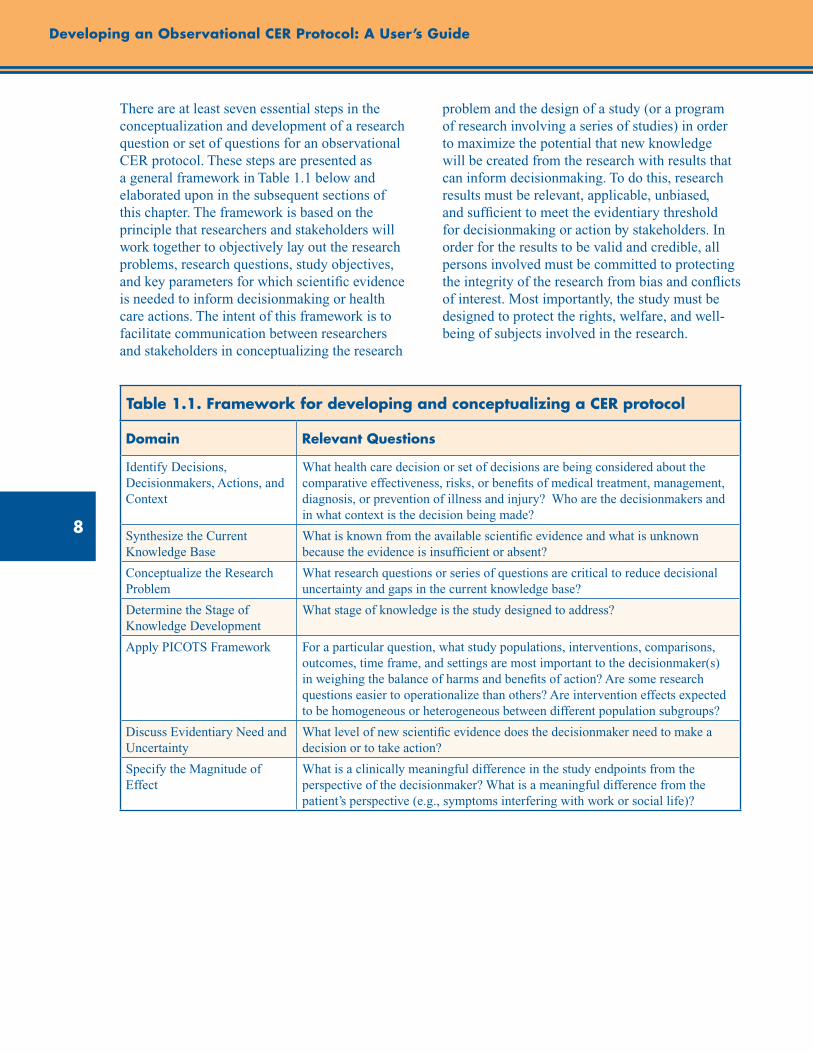
There are at least seven essential steps in the conceptualization and development of a research question or set of questions for an observational CER protocol. These steps are presented as a general framework in Table 1.1 below and elaborated upon in the subsequent sections of this chapter. The framework is based on the principle that researchers and stakeholders will work together to objectively lay out the research problems, research questions, study objectives, and key parameters for which scientific evidence is needed to inform decisionmaking or health care actions. The intent of this framework is to facilitate communication between researchers and stakeholders in conceptualizing the research

problem and the design of a study (or a program of research involving a series of studies) in order to maximize the potential that new knowledge will be created from the research with results that can inform decisionmaking. To do this, research results must be relevant, applicable, unbiased, and sufficient to meet the evidentiary threshold for decisionmaking or action by stakeholders. In order for the results to be valid and credible, all persons involved must be committed to protecting the integrity of the research from bias and conflicts of interest. Most importantly, the study must be designed to protect the rights, welfare, and well-being of subjects involved in the research.

Table 1.1. Framework for developing and conceptualizing a CER protocol

Domain Relevant Questions

Identify Decisions, Decisionmakers, Actions, and Context

What health care decision or set of decisions are being considered about the comparative effectiveness, risks, or benefits of medical treatment, management, diagnosis, or prevention of illness and injury? Who are the decisionmakers and in what context is the decision being made?

Synthesize the Current Knowledge Base

What is known from the available scientific evidence and what is unknown because the evidence is insufficient or absent?

Conceptualize the Research Problem

What research questions or series of questions are critical to reduce decisional uncertainty and gaps in the current knowledge base?

Determine the Stage of Knowledge Development

What stage of knowledge is the study designed to address?

Apply PICOTS Framework For a particular question, what study populations, interventions, comparisons, outcomes, time frame, and settings are most important to the decisionmaker(s) in weighing the balance of harms and benefits of action? Are some research questions easier to operationalize than others? Are intervention effects expected to be homogeneous or heterogeneous between different population subgroups?

Discuss Evidentiary Need and Uncertainty

What level of new scientific evidence does the decisionmaker need to make a decision or to take action?

Specify the Magnitude of Effect

What is a clinically meaningful difference in the study endpoints from the perspective of the decisionmaker? What is a meaningful difference from the patient’s perspective (e.g., symptoms interfering with work or social life)?

9

Chapter 1. Study Objectives and Questions

Identifying Decisions, Decisionmakers, Actions, and Context

In order for research findings to be useful for decisionmaking, the study protocol should clearly articulate the decisions or actions for which stakeholders seek new scientific evidence. While only some studies may be sufficiently robust for making decisions or taking action, statements that describe the stakeholders’ decisions will help those who read the protocol understand the rationale for the study and its potential for informing decisions or for translating the findings into changes in health care practices. This information also improves the ability of protocol readers to understand the purpose of the study so they can critically review its design and provide recommendations for ways it may be potentially improved. If stakeholders have a need to make decisions within a critical time frame for regulatory, ethical, or other reasons, this interval should be expressed to researchers and described in the protocol. In some cases, the time frame for decisionmaking may influence the choice of outcomes that can be studied and the study designs that can be used. For some stakeholders’ questions, research and decisionmaking may need to be divided into stages, since it may take years for outcomes with long lag times to occur, and research findings will be delayed until they do.

In writing this section of the protocol, investigators should ask stakeholders to describe the context in which the decision will be made or actions will be taken. This context includes the background and rationale for the decision, key areas of uncertainty and controversies surrounding the decision, ways scientific evidence will be used to inform the decision, the process stakeholders will use to reach decisions based on scientific evidence, and a description of the key stakeholders who will use or potentially be affected by the decision. By explaining these contextual factors that surround the decision, investigators will be able to work with stakeholders to determine the study objectives and other major parameters of the study. This work also provides the opportunity to discuss how the tools of science can be applied to generate new evidence for informing stakeholder decisions and what limits may exist in those tools. In addition, this initial step begins to clarify the number of analyses necessary

to generate the evidence that stakeholders need to make a decision or take other actions with sufficient certainty about the outcomes of interest. Finally, the contextual information facilitates advance planning and discussions by researchers and stakeholders about approaches to translation and implementation of the study findings once the research is completed.

Synthesizing the Current Knowledge Base

In designing a new study, investigators should conduct a comprehensive review of the literature, critically appraise published studies, and synthesize what is known related to the research objectives. Specifically, investigators should summarize in the protocol what is known about the efficacy, effectiveness, and safety of the interventions and about the outcomes being studied. Furthermore, investigators should discuss measures used in prior research and whether these measures have changed over time. These descriptions will provide background on the knowledge base for the current protocol. It is equally important to identify which elements of the research problem are unknown because evidence is absent, insufficient, or conflicting.

For some research problems, systematic reviews of the literature may be available and can be useful resources to guide the study design. The AHRQ Evidence-based Practice Centers2 and the Cochrane Collaboration3 are examples of established programs that conduct thorough systematic reviews, technology assessments, and specialized comparative effectiveness reviews using standardized methods. When available, systematic reviews and technology assessments should be consulted as resources for investigators to assess the current knowledge base when designing new studies and working with stakeholders.

When reviewing the literature, investigators and stakeholders should identify the most relevant studies and guidelines about the interventions that will be studied. This will allow readers to understand how new research will add to the existing knowledge base. If guidelines are a source of information, then investigators should examine whether these guidelines have been updated to incorporate recent literature. In

10


addition, investigators should assess the health sciences literature to determine what is known about expected effects of the interventions based on current understanding of the pathophysiology of the target condition. Furthermore, clinical experts should be consulted to help identify gaps in current knowledge based on their expertise and interactions with patients. Relevant questions to ask to assess the current knowledge base for development of an observational CER study protocol are:

• Whatarethemostrelevantstudiesandguidelines about the interventions, and why are these studies relevant to the protocol (e.g., because of the study findings, time period conducted, populations studied, etc.)?

• Aretheredifferencesinrecommendationsfromclinical guidelines that would indicate clinical equipoise?

• Whatelseisknownabouttheexpectedeffects of the interventions based on current understanding of the pathophysiology of the targeted condition?

• Whatdoclinicalexpertssayaboutgapsincurrent knowledge?

Conceptualizing the Research Problem

In designing studies for addressing stakeholder questions, investigators should engage multiple stakeholders in discussions about how the research problem is conceptualized from the stakeholders’ perspectives. These discussions will aid in designing a study that can be used to inform decisionmaking. Together, investigators and stakeholders should work collaboratively to determine the major objectives of the study based on the health care decisions facing stakeholders. As pointed out by Heckman,4 research objectives should be formalized outside considerations of available data and the inferences that can be made from various statistical estimation approaches. Doing so will allow the study objectives to be determined by stakeholder needs rather than the availability of existing data. A thorough discussion of these considerations is beyond the scope of this chapter, but some important considerations are summarized in supplement 1 of this User’s Guide.

In order to conceptualize the problem, stakeholders and other experts should be asked to describe the potential relationships between the intervention and important health outcomes. This description will help researchers develop preliminary hypotheses about the stated relationships. Likewise, stakeholders, researchers, and other experts should be asked to enumerate all major assumptions that affect the conceptualization of the research problem, but will not be directly examined in the study. These assumptions should be described in the study protocol and in reporting final study results. By clearly stating the assumptions, protocol reviewers will be better able to assess how the assumptions may influence the study results.

Based on the conceptualization of the research problem, investigators and stakeholders should make use of applicable scientific theory in designing the study protocol and developing the analytic plan. Research that is designed using a validated theory has a higher potential to reach valid conclusions and improve the overall understanding of a phenomenon. In addition, theory will aid in the interpretation of the study findings, since these results can be put in context with the theory and with past research. Depending on the nature of the inquiry, theory from specific disciplines such as health behavior, sociology, or biology could be the basis for designing the study. In addition, the research team should work with stakeholders to develop a conceptual model or framework to guide the implementation of the study. The protocol should also contain one or more figures that summarize the conceptual model or framework as it applies to the study. These figures will allow readers to understand the theoretical or conceptual basis for the study and how the theory is operationalized for the specific study. The figures should diagram relationships between study variables and outcomes to help readers of the protocol visualize relationships that will be examined in the study.

For research questions about causal associations between exposures and outcomes, causal models such as directed acyclic graphs (DAGs) may be useful tools in designing the conceptual framework for the study and developing the analytic plan. The value of DAGs in the context of refining study questions is that they make assumptions explicit

11


in ways that can clarify gaps in knowledge. Free software such as DAGitty is available for creating, editing, and analyzing causal models. A thorough discussion of DAGs is beyond the scope of this chapter, but more information about DAGs is available in supplement 2 of this User’s Guide.

The following list of questions may be useful for defining and describing a study’s conceptual framework in a CER protocol:

• Whatarethemainobjectivesofthestudy,asrelated to specific decisions to be made?

• Whatarethemajorassumptionsofdecisionmakers, investigators, and other experts about the problem or phenomenon being studied?

• Whatrelationships,ifany,doexpertshypothesize exist between interventions and outcomes?

• Whatconceptualmodelwillguidethestudydesign and interpretation?

– What is known about each element of the model?

– Can relationships be expressed by causal diagrams?

Determining the Stage of Knowledge Development for the Study Design

The scientific method is a process of observation and experimentation in order for the evidence base to be expanded as new knowledge is developed. Therefore, stakeholders and investigators should consider whether a program of research comprising a sequential or concurrent series of studies, rather than a single study, is needed to adequately make a decision. Staging the research into multiple studies and making interim decisions may improve the final decision and make judicious use of scarce research resources. In some cases, the results of preliminary studies, descriptive epidemiology, or pilot work may be helpful in making interim decisions and designing further research. Overall, a planned series of related studies or a program of research may be needed to adequately address stakeholders’ decisions.

An example of a structured program of research is the four phases of clinical studies used by the Food and Drug Administration (FDA) to reach a decision about whether or not a new drug is safe and efficacious for market approval in the United States. Using this analogy, the final decision about whether a drug is efficacious and safe to be marketed for specific medical indications is based upon the accumulation of scientific evidence from a series of studies (i.e., not from any individual study), which are conducted in multiple sequential phases. The evidence generated in each phase is reviewed to make interim decisions about the safety and efficacy of a new pharmaceutical until ultimately all the evidence is reviewed to make a final decision about drug approval.

Under the FDA model for decisionmaking, initial research involves laboratory and animal tests. If the evidence generated in these studies indicates that the drug is active and not toxic, the sponsor submits an application to the FDA for an “investigational new drug.” If the FDA approves, human testing for safety and efficacy can begin. The first phase of human testing is usually conducted in a limited number of healthy volunteers (phase 1). If these trials show evidence that the product is safe in healthy volunteers, then the drug is further studied in a small number of volunteers who have the targeted condition (phase 2). If phase 2 studies show that the drug has a therapeutic effect and lacks significant adverse effects, trials with large numbers of people are conducted to determine the drug’s safety and efficacy (phase 3). Following these trials, all relevant scientific studies are submitted to the FDA for a decision about whether the drug should be approved for marketing. If there are additional considerations like special safety issues, observational studies may be required to assess the safety of the drug in routine clinical care after the drug is approved for marketing (phase 4). Overall, the decisionmaking and research are staged so that the cumulative findings from all studies are used by the FDA to make interim decisions until the final decision is made about whether a medical product will be approved for marketing.

While most decisions about the comparative effectiveness of interventions will not need such extensive testing, it still may be prudent to stage research in a way that allows for interim decisions

12


and sequentially more rigorous studies. On the other hand, conditional approval or interim decisions may risk confusing patients and other stakeholders about the extent to which current evidence indicates that a treatment is effective and safe for all individuals with a health condition. For instance, under this staged approach new treatments could rapidly diffuse into a market even when there is limited evidence of long-term effectiveness and safety for all potential users. An illustrative example of this is the case of lung-volume reduction surgery, which was increasingly being used to treat severe emphysema despite limited evidence supporting its safety and efficacy until new research raised questions about the safety of the procedure.6

Below is one potential categorization for the stages of knowledge development as related to informing decisions about questions of comparative effectiveness:

1. Descriptive analysis

2. Hypothesis generation

3. Feasibility studies/proof of concept

4. Hypothesis supporting

5. Hypothesis testing

The first stages (i.e., descriptive analysis, hypothesis generation, and feasibility studies) are not mutually exclusive and usually are not intended to provide conclusive results for most decisions. Instead, these stages provide preliminary evidence or feasibility testing before larger, more resource-intensive studies are launched. Results from these categories of studies may allow for interim decisionmaking (e.g., conditional approval for reimbursement of a treatment while further research is conducted). While a phased approach to research may postpone the time when a conclusive decision can be reached, it does help to conserve resources such as those that may be consumed in launching a large multicenter study when a smaller study may be sufficient. Investigators will need to engage stakeholders to prioritize what stage of research may be most useful for the practical range of decisions that will be made.

Investigators should discuss in the protocol what stage of knowledge the current study will fulfill in light of the actions available to different stakeholders. This will allow reviewers of the protocol to assess the degree to which the evidence generated in the study holds the potential to fill specific knowledge gaps. For studies that are described in the protocol as preliminary, this may also help readers understand other tradeoffs that were made in the design of the study, in terms of methodological limitations that were accepted a priori in order to gather preliminary information about the research questions.

Defining and Refining Study Questions Using PICOTS Framework

As recommended in other AHRQ methods guides,7 investigators should engage stakeholders in a dialogue in order to understand the objectives of the research in practical terms, particularly so that investigators know the types of decisions that the research may affect. In working with stakeholders to develop research questions that can be studied with scientific methods, investigators may ask stakeholders to identify six key components of the research questions that will form the basis for designing the study. These components are reflected in the PICOTS typology and are shown below in Table 1.2. These components represent the critical elements that will help investigators design a study that will be able to address the stakeholders’ needs. Additional references that expand upon how to frame research questions can be found in the literature.8-9

The PICOTS typology outlines the key parts of the research questions that the study will be designed to address.10 As a new research protocol is developed, these questions can be presented in preliminary form and refined as other steps in the process are implemented. After the preliminary questions are refined, investigators should examine the questions to make sure that they will meet the needs of the stakeholders. In addition, they should assess whether the questions can be answered within the timeframe allotted and with the resources that are available for the study.

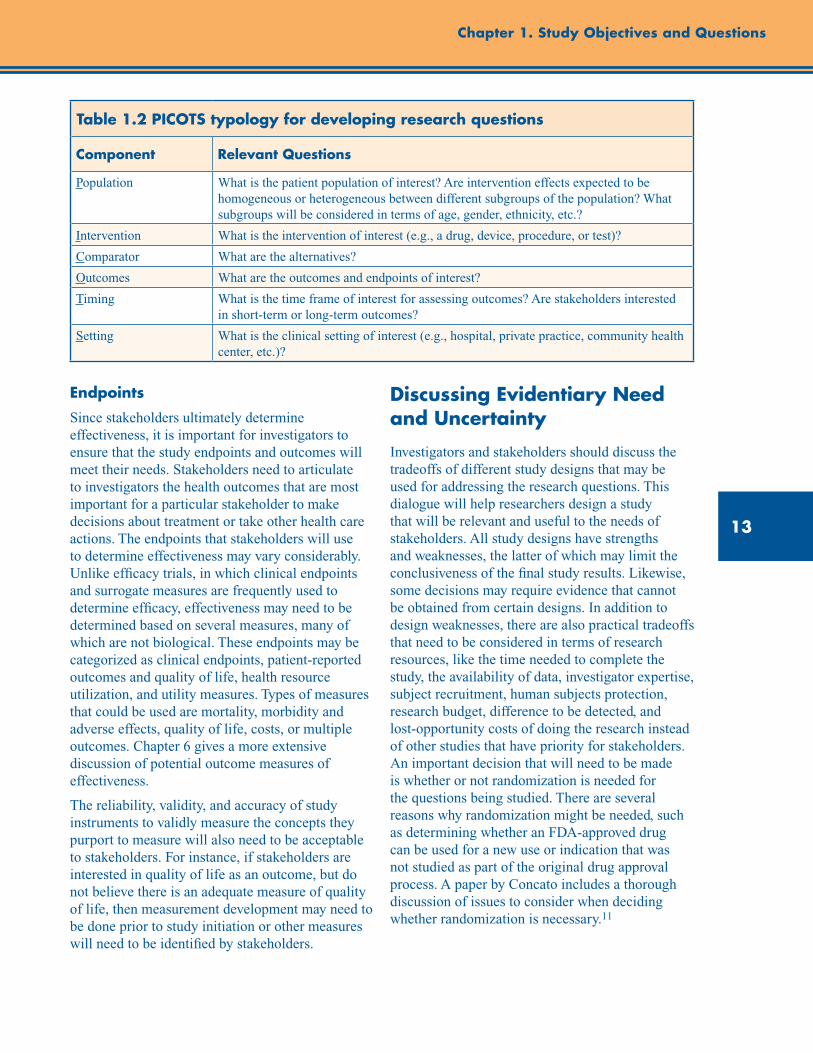
13


Table 1.2 PICOTS typology for developing research questions

Component Relevant Questions

Population What is the patient population of interest? Are intervention effects expected to be homogeneous or heterogeneous between different subgroups of the population? What subgroups will be considered in terms of age, gender, ethnicity, etc.?

Intervention What is the intervention of interest (e.g., a drug, device, procedure, or test)?

Comparator What are the alternatives?

Outcomes What are the outcomes and endpoints of interest?

Timing What is the time frame of interest for assessing outcomes? Are stakeholders interested in short-term or long-term outcomes?

Setting What is the clinical setting of interest (e.g., hospital, private practice, community health center, etc.)?

Endpoints

Since stakeholders ultimately determine effectiveness, it is important for investigators to ensure that the study endpoints and outcomes will meet their needs. Stakeholders need to articulate to investigators the health outcomes that are most important for a particular stakeholder to make decisions about treatment or take other health care actions. The endpoints that stakeholders will use to determine effectiveness may vary considerably. Unlike efficacy trials, in which clinical endpoints and surrogate measures are frequently used to determine efficacy, effectiveness may need to be determined based on several measures, many of which are not biological. These endpoints may be categorized as clinical endpoints, patient-reported outcomes and quality of life, health resource utilization, and utility measures. Types of measures that could be used are mortality, morbidity and adverse effects, quality of life, costs, or multiple outcomes. Chapter 6 gives a more extensive discussion of potential outcome measures of effectiveness.

The reliability, validity, and accuracy of study instruments to validly measure the concepts they purport to measure will also need to be acceptable to stakeholders. For instance, if stakeholders are interested in quality of life as an outcome, but do not believe there is an adequate measure of quality of life, then measurement development may need to be done prior to study initiation or other measures will need to be identified by stakeholders.

Discussing Evidentiary Need and Uncertainty

Investigators and stakeholders should discuss the tradeoffs of different study designs that may be used for addressing the research questions. This dialogue will help researchers design a study that will be relevant and useful to the needs of stakeholders. All study designs have strengths and weaknesses, the latter of which may limit the conclusiveness of the final study results. Likewise, some decisions may require evidence that cannot be obtained from certain designs. In addition to design weaknesses, there are also practical tradeoffs that need to be considered in terms of research resources, like the time needed to complete the study, the availability of data, investigator expertise, subject recruitment, human subjects protection, research budget, difference to be detected, and lost-opportunity costs of doing the research instead of other studies that have priority for stakeholders. An important decision that will need to be made is whether or not randomization is needed for the questions being studied. There are several reasons why randomization might be needed, such as determining whether an FDA-approved drug can be used for a new use or indication that was not studied as part of the original drug approval process. A paper by Concato includes a thorough discussion of issues to consider when deciding whether randomization is necessary.11

14


In discussing the tradeoffs of different study designs, researchers and stakeholders may wish to discuss the principal goals of research and ensure that researchers and stakeholders are aligned in their understanding of what is meant by scientific evidence. Fundamentally, research is a systematic investigation that uses scientific methods to measure, collect, and analyze data for the advancement of knowledge. This advancement is through the independent peer review and publication of study results, which are collectively referred to as scientific evidence. One definition of scientific evidence has been proposed by Normand and McNeil12 as:

. . . the accumulation of information to support or refute a theory or hypothesis. . . . The idea is that assembling all the available information may reduce uncertainty about the effectiveness of the new technology compared to existing technologies in a setting where we believe particular relationships exist but are uncertain about their relevance . . .

While the primary aim of research is to produce new knowledge, the Normand and McNeil concept of evidence emphasizes that research helps create knowledge by reducing uncertainty about outcomes. However, rarely, if at all, does research eliminate all uncertainty around most decisions. In some cases, successful research will answer an important question and reduce uncertainty related to that question, but it may also increase uncertainty by leading to more, better informed questions regarding unknowns. As a result, nearly all decisions face some level of uncertainty even in a field where a body of research has been completed. This distinction is also critical because it helps to separate the research and subsequent actions that decisionmakers may take based on their assessment of the research results. Those subsequent actions may be informed by the research findings but will also be based on stakeholders’ values and resources. Hence, as the definition by Normand and McNeil implies, research generates evidence but stakeholders decide whether to act on the evidence. Scientific evidence informs decisions to the extent it can adequately reduce the uncertainty about the problem for the stakeholder. Ultimately, treatment decisions are only guided by an assessment of the

certainty that a course of therapy will lead to the outcomes of interest and the likelihood that this conclusion will be affected by the results of future studies.

In conceptualizing a study design, it is important for investigators to understand what constitutes sufficient and valid evidence from the stakeholder’s perspective. In other words, what is the type of evidence that will be required to inform the stakeholder’s decision to act or make a conscious decision not to take action? Evidence needed for action may vary by type of stakeholder and the scope of decisions that the stakeholder is making. For instance, a stakeholder who is making a population-based decision such as whether to provide insurance coverage for a new medical device with many alternatives may need substantially robust research findings in order to take action and provide that insurance coverage. In this example, the stakeholder may only accept as evidence a study with strong internal validity and generalizability (i.e., one conducted in a nationally representative sample of patients with the disease). On the other hand, a patient who has a health condition where there are few treatments may be willing to accept lower-quality evidence in order to make a decision about whether to proceed with treatment despite a higher level of uncertainty about the outcome.

In many cases, there may exist a gradient of actions that can be taken based on available evidence. Quanstrum and Hayward13 have discussed this gradient and argued that health care decisionmaking is changing, partly because more information is available to patients and other stakeholders about treatment options. As shown in the upper panel (A) in Figure 1.1, many people may currently believe that health care treatment decisions are basically uniform for most people and under most circumstances. Panel A represents a hypothetical treatment whereby there is an evidentiary threshold or a point at which treatment is always beneficial and should be recommended. On the other hand, below this threshold, care provides no benefits and treatment should be discouraged. Quanstrum and Hayward argue that increasingly health care decisions are more like the lower panel (B). This panel portrays health care treatments as providing a large zone of

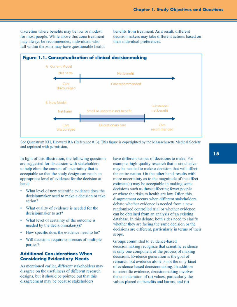
15


discretion where benefits may be low or modest for most people. While above this zone treatment may always be recommended, individuals who fall within the zone may have questionable health

benefits from treatment. As a result, different decisionmakers may take different actions based on their individual preferences.

Figure 1.1. Conceptualization of clinical decisionmaking

See Quanstrum KH, Hayward RA (Reference #13). This figure is copyrighted by the Massachusetts Medical Society and reprinted with permission.

In light of this illustration, the following questions are suggested for discussion with stakeholders to help elicit the amount of uncertainty that is acceptable so that the study design can reach an appropriate level of evidence for the decision at hand:

• Whatlevelofnewscientificevidencedoesthedecisionmaker need to make a decision or take action?

• Whatqualityofevidenceisneededforthedecisionmaker to act?

• Whatlevelofcertaintyoftheoutcomeisneeded by the decisionmaker(s)?

• Howspecificdoestheevidenceneedtobe?

• Willdecisionsrequireconsensusofmultipleparties?

Additional Considerations When Considering Evidentiary Needs

As mentioned earlier, different stakeholders may disagree on the usefulness of different research designs, but it should be pointed out that this disagreement may be because stakeholders

have different scopes of decisions to make. For example, high-quality research that is conclusive may be needed to make a decision that will affect the entire nation. On the other hand, results with more uncertainty as to the magnitude of the effect estimate(s) may be acceptable in making some decisions such as those affecting fewer people or where the risks to health are low. Often this disagreement occurs when different stakeholders debate whether evidence is needed from a new randomized controlled trial or whether evidence can be obtained from an analysis of an existing database. In this debate, both sides need to clarify whether they are facing the same decision or the decisions are different, particularly in terms of their scope.

Groups committed to evidence-based decisionmaking recognize that scientific evidence is only one component of the process of making decisions. Evidence generation is the goal of research, but evidence alone is not the only facet of evidence-based decisionmaking. In addition to scientific evidence, decisionmaking involves the consideration of (a) values, particularly the values placed on benefits and harms, and (b)

A Current Model

Net bene�t

Care recommended

Small or uncertain net bene�t

Discretionary careCare discouraged

Care discouraged

Net harm

Net harm

Substantial net bene�t

Care recommended

B New Model

16


resources.14 Stakeholder differences in values and resources may mean that different decisions are made based on the same scientific evidence. Moreover, differences in values may create conflict in the decisionmaking process. One stakeholder may believe a particular study outcome is most important from their perspective, while another stakeholder may believe a different outcome is the most important for determining effectiveness.

Likewise, there may be inherent conflicts in values between individual decisionmaking and population decisionmaking, even though these decisions are often interrelated. For example, an individual may have a higher tolerance for treatment risk in light of the expected treatment benefits for him or her. On the other hand, a regulatory health authority may determine that the population risk is too great without sufficient evidence that treatment

provides benefits to the population. An example of this difference in perspective can be seen with how different decisionmakers responded to evidence about the drug Avastin® (bevacizumab) for the treatment of metastatic breast cancer. In this case, the FDA revoked their approval of the breast cancer indication for Avastin after concluding that the drug had not been shown to be safe and effective for that use. Nonetheless, Medicare, the public insurance program for the elderly and disabled, continued to allow coverage when a physician prescribes the drug, even for breast cancer. Likewise, some patient groups were reported to be concerned by the decision since it presumably would deny some women access to Avastin treatment. For a more thorough discussion of these issues around differences in perspective, the reader is referred to an article by Atkins15 and the examples in Table 1.3 below.

Table 1.3 Examples of individual versus population decisions (Adapted from Atkins, 2007)15

Decision Types Decision Examples

Individual Decisions

Patient Should I take raloxifene, alendronate, or calcium and vitamin D to prevent osteoporosis?

Physician/health care professional Should I prescribe treatment X vs. Y?

Population Decisions

Approval Is slow-release sodium fluoride usually safe and effective for preventing fractures in comparison with other options?

Coverage Which bisphosphonate drugs should be included on a drug formulary? On what tier or what level of copayment?

Practice guidelines What medications are recommended for initial treatment of women at high risk for osteoporosis?

Risk management What should a health plan do to minimize the risks associated with use of bisphosphonate drugs?

Other health system policies Should a health system promote routine screening for osteoporosis using ultrasound or dual-energy x-ray absorptometry?

Specifying Magnitude of Effect

In order for decisions to be objective, it is important for there to be an a priori discussion with stakeholders about the magnitude of effect that stakeholders believe represents a meaningful difference between treatment options. Researchers will be familiar with the basic tenet that statistically significant differences do not

always represent clinically meaningful differences. Hence, researchers and stakeholders will need to have knowledge of the instruments that are used to measure differences and the accuracy, limitations, and properties of those instruments. Three key questions are recommended to use when eliciting from stakeholders the effect sizes that are important to them for making a decision or taking action:

17


• Howdopatientsandotherstakeholdersdefineameaningful difference between interventions?

• Howdopreviousstudiesandreviewsdefineameaningful difference?

• Arepatientsandotherstakeholdersinterestedin superiority or noninferiority as it relates to decisionmaking?

Challenges to Developing Study Questions and Initial Solutions

In developing CER study objectives and questions, there are some potential challenges that face researchers and stakeholders. The involvement of patients and other stakeholders in determining study objectives and questions is a relatively new paradigm, but one that is consistent with established principles of translational research. A key principle of translational research is that users need to be involved in research at the earliest stages for the research to be adopted.16 In addition, most research is currently initiated by an investigator, and traditionally there have been few incentives (and some disincentives) to involving others in designing a new research study. Although the research paradigm is rapidly shifting,17 there is little information about how to structure, process, and evaluate outcomes from initiatives that attempt to engage stakeholders in developing study questions and objectives with researchers. As different approaches are taken to involve stakeholders in the research process, researchers will learn how to optimize the process of stakeholder involvement and improve the applicability of research to the end-users.

The bringing together of stakeholders may create some general challenges to the research team. For instance, it may be difficult to identify, engage, or manage all stakeholders who are interested in developing and using scientific evidence for addressing a problem. A process that allows for public commenting on research protocols through Internet postings may be helpful in reaching the widest network of interested stakeholders. Nevertheless, finding stakeholders who can represent all perspectives may not always be practical or available to the study team. In addition,

competing interests among stakeholders may make prioritization of research questions challenging. Different stakeholders have different needs and this may make prioritization of research difficult. Nonetheless, as the science of translational research evolves, the collaboration of researchers with stakeholders will likely become increasingly the standard of practice in designing new research.

To assist researchers and stakeholders with working together, AHRQ has published several online resources to facilitate the involvement of stakeholders in the research process. These include a brief guide for stakeholders that highlights opportunities for taking part in AHRQ’s Effective Health Care Program, a facilitation primer with strategies for working with diverse stakeholder groups, a table of suggested tasks for researchers to involve stakeholders in the identification and prioritization of future research, and learning modules with slide presentations on engaging stakeholders in the Effective Health Care Program. 18-19 In addition, AHRQ supports the Evidence-based Practice Centers in working with various stakeholders to further develop and prioritize decisionmakers’ future research needs, which are published in a series of reports on AHRQ’s Web site and on the National Library of Medicine’s open-access Bookshelf.20

Likewise, AHRQ supports the active involvement of patients and other stakeholders in the AHRQ DEcIDE program, in which different models of engagement have been used. These models include hosting in-person meetings with stakeholders to create research agendas;21-22 developing research based on questions posed by public payers such as Centers for Medicare and Medicaid Services; addressing knowledge gaps that have been identified in AHRQ systematic reviews through new research; and supporting five research consortia, each of which involves researchers, patients, and other stakeholders working together to develop, prioritize, and implement research studies.

Summary and Conclusion

This chapter provides a framework for formulating study objectives and questions, for a research protocol on a CER topic. Implementation of the framework involves collaboration between

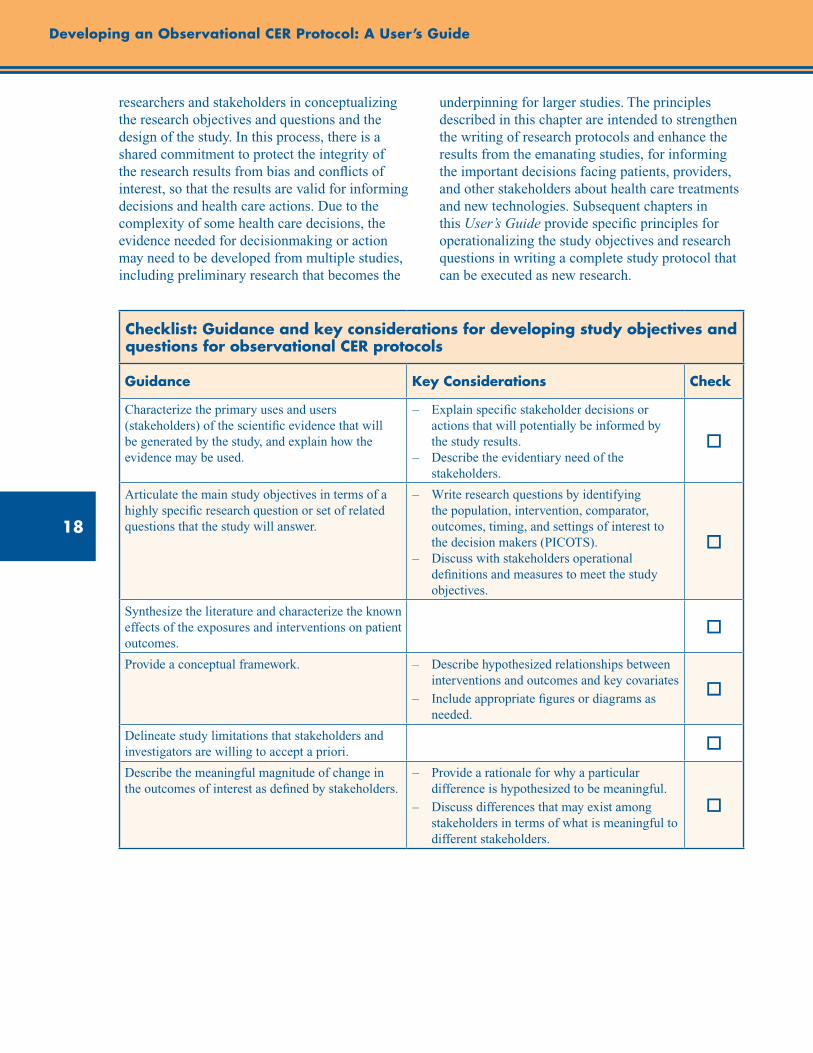
18


researchers and stakeholders in conceptualizing the research objectives and questions and the design of the study. In this process, there is a shared commitment to protect the integrity of the research results from bias and conflicts of interest, so that the results are valid for informing decisions and health care actions. Due to the complexity of some health care decisions, the evidence needed for decisionmaking or action may need to be developed from multiple studies, including preliminary research that becomes the

underpinning for larger studies. The principles described in this chapter are intended to strengthen the writing of research protocols and enhance the results from the emanating studies, for informing the important decisions facing patients, providers, and other stakeholders about health care treatments and new technologies. Subsequent chapters in this User’s Guide provide specific principles for operationalizing the study objectives and research questions in writing a complete study protocol that can be executed as new research.

Checklist: Guidance and key considerations for developing study objectives and questions for observational CER protocols

Guidance Key Considerations Check

Characterize the primary uses and users (stakeholders) of the scientific evidence that will be generated by the study, and explain how the evidence may be used.

– Explain specific stakeholder decisions or actions that will potentially be informed by the study results.

– Describe the evidentiary need of the stakeholders.

o

Articulate the main study objectives in terms of a highly specific research question or set of related questions that the study will answer.

– Write research questions by identifying the population, intervention, comparator, outcomes, timing, and settings of interest to the decision makers (PICOTS).

– Discuss with stakeholders operational definitions and measures to meet the study objectives.

o

Synthesize the literature and characterize the known effects of the exposures and interventions on patient outcomes.

o

Provide a conceptual framework. – Describe hypothesized relationships between interventions and outcomes and key covariates

– Include appropriate figures or diagrams as needed.

o

Delineate study limitations that stakeholders and investigators are willing to accept a priori. o

Describe the meaningful magnitude of change in the outcomes of interest as defined by stakeholders.

– Provide a rationale for why a particular difference is hypothesized to be meaningful.

– Discuss differences that may exist among stakeholders in terms of what is meaningful to different stakeholders.

o

19


References 1. Committee on Comparative Effectiveness Research

Prioritization, Institute of Medicine. Initial National Priorities for Comparative Effectiveness Research. Washington, DC: The National Academies Press; 2009.

2. About Evidence-based Practice Centers (EPCs). Effective Health Care Program. Agency for Healthcare Research and Quality Web site. http://effectivehealthcare.ahrq.gov/index.cfm/who-is-involved-in-the-effective-health-care-program1/about-evidence-based-practice-centers-epcs. Accessed August 13, 2012.

3. The Cochrane Collaboration Web site. www.cochrane.org. Accessed August 13, 2012.

4. Heckman JJ. Econometric causality. Int Statist Rev. 2008;76:1–27.

5. DAGitty Web site. www.dagitty.net. Accessed August 13, 2012.

6. Ramsey SD, Sullivan SD. Evidence, economics, and emphysema: Medicare’s long journey with lung volume reduction surgery. Health Aff (Millwood). 2005 Jan-Feb;24(1):55-66.

7. Methods Guide for Effectiveness and Comparative Effectiveness Reviews. AHRQ Publication No. 10(11)-EHC063-EF. Rockville, MD: Agency for Healthcare Research and Quality; August 2011. Chapters available at www.effectivehealthcare.ahrq.gov.

8. Parfrey P, Ravani P. On framing the research question and choosing the appropriate research design. Methods Mol Biol. 2009;473:1-17.

9. Thabane L, Thomas T, Ye C, et al. Posing the research question: not so simple. Can J Anaesth. 2009 Jan;56(1):71-9.

10. Richardson WS, Wilson MC, Nishikawa J, et al. The well-built clinical question: a key to evidence-based decisions. ACP J Club. 1995 Nov-Dec;123(3):A12-3.

11. Concato J. When to randomize, or ‘Evidence-based medicine needs medicine-based Evidence.’ Pharmacoepidemiol Drug Saf. 2012 May; 21 Suppl 2:6-12.

12. Normand SL, McNeil BJ. What is evidence? Stat Med. 2010 Aug 30;29(19):1985-8.

13. Quanstrum KH, Hayward RA. Lessons from the mammography wars. N Engl J Med. 2010 Sep 9;363(11):1076-9.

14. Muir Gray JA. Evidence-Based Healthcare and Public Health. 3rd ed., Churchill Livingstone; 1997.

15. Atkins D. Creating and synthesizing evidence with decision makers in mind: integrating evidence from clinical trials and other study designs. Med Care. 2007 Oct;45(10 Suppl 2):S16-22.

16. Rogers E. Diffusions of Innovations. 5th ed. New York, NY: Free Press; 2003.

17. Anonymous. Translational research and experimental medicine in 2012. Lancet. 2012 Jan 7;379(9810):1.

18. Resources for Getting Involved and Involving Others. Agency for Healthcare Research and Quality. Effective Health Care Program. www.effectivehealthcare.ahrq.gov/tools-and-resources/how-to-get-involved-in-the-effective-health-care-program. Accessed August 13, 2012.

19. O’Haire C, McPheeters M, Nakamoto EK, et al. Methods for engaging stakeholders to identify and prioritize future research needs. Methods Future Research Needs Report No. 4. (Prepared by the Oregon Evidence-based Practice Center and the Vanderbilt Evidence-based Practice Center under Contract No. 290-2007-10057-I.) AHRQ Publication No. 11-EHC044-EF. Rockville, MD: Agency for Healthcare Research and Quality; June 2011. www.effectivehealthcare.ahrq.gov/ehc/products/200/698/MFRNGuide04--Engaging_Stakeholders--6-10-2011.pdf.

20. Future Research Needs—Methods Research Series. Agency for Healthcare Research and Quality Web site. Effective Health Care Program. http://effectivehealthcare.ahrq.gov/index.cfm/search-for-guides-reviews-and-reports/?pageaction=displayProduct&productID=481. Accessed April 3, 2012.

21. Pickard AS, Lee TA, Solem CT, et al. Prioritizing comparative-effectiveness research topics via stakeholder involvement: an application in COPD. Clin Pharmacol Ther. 2011 Dec;90(6):888-92.

22. Gliklich RE, Leavy MB, Velentgas P, et al. Identification of Future Research Needs in the Comparative Management of Uterine Fibroid Disease: A Report on the Priority-Setting Process, Preliminary Data Analysis, and Research Plan. Effective Healthcare Research Report No. 31. (Prepared by the Outcome DEcIDE Center, under Contract No. HHSA 290-2005-0035-I, TO5). AHRQ Publication No. 11- EHC023-EF. Rockville, MD: Agency for Healthcare Research and Quality; March 2011. http://effectivehealthcare.ahrq.gov/reports/final.cfm.

21

Abstract

The choice of study design often has profound consequences for the causal interpretation of study results. The objective of this chapter is to provide an overview of various study design options for nonexperimental comparative effectiveness research (CER), with their relative advantages and limitations, and to provide information to guide the selection of an appropriate study design for a research question of interest. We begin the chapter by reviewing the potential for bias in nonexperimental studies and the central assumption needed for nonexperimental CER—that treatment groups compared have the same underlying risk for the outcome within subgroups definable by measured covariates (i.e., that there is no unmeasured confounding). We then describe commonly used cohort and case-control study designs, along with other designs relevant to CER such as case-cohort designs (selecting a random sample of the cohort and all cases), case-crossover designs (using prior exposure history of cases as their own controls), case–time controlled designs (dividing the case-crossover odds ratio by the equivalent odds ratio estimated in controls to account for calendar time trends), and self-controlled case series (estimating the immediate effect of treatment in those treated at least once). Selecting the appropriate data source, patient population, inclusion/exclusion criteria, and comparators are discussed as critical design considerations. We also describe the employment of a “new user” design, which allows adjustment for confounding at treatment initiation without the concern of mixing confounding with selection bias during followup, and discuss the means of recognizing and avoiding immortal-time bias, which is introduced by defining the exposure during the followup time versus the time prior to followup. The chapter concludes with a checklist for the development of the study design section of a CER protocol, emphasizing the provision of a rationale for study design selection and the need for clear definitions of inclusion/exclusion criteria, exposures (treatments), outcomes, confounders, and start of followup or risk period.

Chapter 2. Study Design ConsiderationsTil Stürmer, M.D., M.P.H., Ph.D.

University of North Carolina at Chapel Hill Gillings School of Global Public Health Chapel Hill, NC

M. Alan Brookhart, Ph.D. University of North Carolina at Chapel Hill Gillings School of Global Public Health

Chapel Hill, NC

Introduction

The objective of this chapter is to provide an overview of various study design options for nonexperimental comparative effectiveness research (CER), with their relative advantages and limitations. Of the multitude of epidemiologic design options, we will focus on observational designs that compare two or more treatment options with respect to an outcome of interest in which treatments are not assigned by the investigator but according to routine medical practice. We will not cover experimental or quasi-experimental designs, such as interrupted time

series,1 designed delays,2 cluster randomized trials, individually randomized trials, pragmatic trials, or adaptive trials. These designs also have important roles in CER; however, the focus of this guide is on nonexperimental approaches that directly compare treatment options.

The choice of study design often has profound consequences for the causal interpretation of study results that are irreversible in many settings. Study design decisions must therefore be considered even more carefully than analytic decisions, which often can be changed and adapted at later stages

22


of the research project. Those unfamiliar with nonexperimental design options are thus strongly encouraged to involve experts in the design of nonexperimental treatment comparisons, such as epidemiologists, especially ones familiar with comparing medical treatments (e.g., pharmacoepidemiologists), during the planning stage of a CER study and throughout the project. In the planning stage of a CER study, researchers need to determine whether the research question should be studied using nonexperimental or experimental methods (or a combination thereof, e.g., two-stage RCTs).3-4 Feasibility may determine whether an experimental or a nonexperimental design is most suitable, and situations may arise where neither approach is feasible.

Issues of Bias in Observational CER

In observational CER, the exposures or treatments are not assigned by the investigator but rather by mechanisms of routine practice. Although the investigator can (and should) speculate on the treatment assignment process or mechanism, the actual process will be unknown to the investigator. The nonrandom nature of treatment assignment leads to the major challenge in nonexperimental CER studies, that of ensuring internal validity. Internal validity is defined as the absence of bias; biases may be broadly classified as selection bias, information bias, and confounding bias. Epidemiology has advanced our thinking about these biases for more than 100 years, and many papers have been published describing the underlying concepts and approaches to bias reduction. For a comprehensive description and definition of these biases, we suggest the book Modern Epidemiology.5 Ensuring a study’s internal validity is a prerequisite for its external validity or generalizability. The limited generalizability of findings from randomized controlled trials (RCTs), such as to older adults, patients with comorbidities or comedications, is one of the major drivers for the conduct of nonexperimental CER.

The central assumption needed for nonexperimental CER is that the treatment groups compared have the same underlying risk for the outcome within subgroups definable by measured

covariates. Until recently, this “no unmeasured confounding” assumption was deemed plausible only for unintended (usually adverse) effects of medical interventions, that is, for safety studies. The assumption was considered to be less plausible for intended effects of medical interventions (effectiveness) because of intractable confounding by indication.6-7 Confounding by indication leads to higher propensity for treatment or more intensive treatment in those with the most severe disease. A typical example would be a study on the effects of beta-agonists on asthma mortality in patients with asthma. The association between treatment (intensity) with beta-agonists and asthma mortality would be confounded by asthma severity. The direction of the confounding by asthma severity would tend to make the drug look bad (as if it is “causing” mortality). The study design challenge in this example would not be the confounding itself, but the fact that it is hard to control for asthma severity because it is difficult to measure precisely. Confounding by frailty has been identified as another potential bias when assessing preventive treatments in population-based studies, particularly those among older adults.8-11 Because frail persons (those close to death) are less likely to be treated with a multitude of preventive treatments,8 frailty would lead to confounding, which would bias the association between preventive treatments and outcomes associated with frailty (e.g., mortality). Since the bias would be that the untreated cohort has a higher mortality irrespective of the treatment, this would make the drug’s effectiveness look too good. Here again the crux of the problem is that frailty is hard to control for because it is difficult to measure.

Basic Epidemiologic Study Designs

The general principle of epidemiologic study designs is to compare the distribution of the outcome of interest in groups characterized by the exposure/treatment/intervention of interest. The association between the exposure and outcome is then assessed using measures of association. The causal interpretation of these associations is dependent on additional assumptions, most notably that the risk for the outcome is the same

23

Chapter 2. Study Design Considerations

in all treatment groups compared (before they receive the respective treatments), also called exchangeability.12-13 Additional assumptions for a causal interpretation, starting with the Hill criteria,14 are beyond the scope of this chapter, although most of these are relevant to many CER settings. For situations where treatment effects are heterogeneous, see chapter 3.

The basic epidemiologic study designs are usually defined by whether study participants are sampled based on their exposure or outcome of interest. In a cross-sectional study, participants are sampled independent of exposure and outcome, and prevalence of exposure and outcome are assessed at the same point in time. In cohort studies, participants are sampled according to their

exposures and followed over time for the incidence of outcomes. In case-control studies, cases and controls are sampled based on the outcome of interest, and the prevalence of exposure in these two groups is then compared. Because the cross-sectional study design usually does not allow the investigator to define whether the exposure preceded the outcome, one of the prerequisites for a causal interpretation, we will focus on cohort and case-control studies as well as some more advanced designs with specific relevance to CER.

Definitions of some common epidemiologic terms are presented in Table 2.1. Given the space constraints and the intended audience, these definitions do not capture all nuances.

Table 2.1. Definition of epidemiologic terms

Term Definition Comments

Incidence Occurrence of the disease outcome over a specified time period. Incidence is generally assessed as a risk/proportion over a fixed time period (e.g., risk for 1-year mortality) or as a rate defined by persons and time (e.g., mortality rate per person-year). Incidence is often defined as first occurrence of the outcome of interest, a definition that requires prior absence of the outcome.

Etiologic studies are based on incidence of the outcome of interest rather than prevalence, because prevalence is a function of disease incidence and duration of disease.

Prevalence Proportion of persons with the exposure/outcome at a specific point in time.

Because prevalence is a function of the incidence and the mean duration of the disease, incidence is generally used to study etiology.

Measures of association

Measures needed to compare outcomes across treatment groups. The main epidemiologic measures of association are ratio measures (risk ratio, incidence rate ratio, odds ratio, hazard ratio) and difference measures (risk difference, incidence rate difference).

Difference measures have some very specific advantages over ratio measures, including the possibility of calculating numbers needed to treat (or harm) and the fact that they provide a biologically more meaningful scale to assess heterogeneity.5 Ratio measures nevertheless abound in medical research. All measures of association should be accompanied by a measure of precision, e.g., a confidence interval.

Confounding Mixing of effects. The effect of the treatments is mixed, with the effect of the underlying risk for the outcome being different in the treatment groups compared.

Confounding leads to biased treatment effect estimates unless controlled for by design (randomization, matching, restriction) or analysis (stratification, multivariable models).

24


Table 2.1. Definition of epidemiologic terms (continued)

Term Definition Comments

Selection bias Distortion of treatment effect estimate as a result of procedures used to select subjects, and distortion of factors that influence study participation.

While procedures to select subjects usually lead to confounding that can be controlled for, factors affecting study participation cannot be controlled for. Factors affecting study participation are referred to as selection bias throughout this chapter to differentiate selection bias from confounding.

Information bias Distortion of treatment effect estimate as a result of measurement error in any variable used in a study; i.e., exposure, confounder, outcome.

Often measurement error is used for continuous variables, and misclassification for categorical variables. It is important to separate nondifferential from differential measurement error. Nondifferential measurement error in exposures and outcomes tends to bias treatment effect estimates towards the null (no effect); nondifferential measurement error in confounders leads to residual confounding (in any direction); differential measurement error leads to bias in any direction.

Cohort Study Design

Description

Cohorts are defined by their exposure at a certain point in time (baseline date) and are followed over time after baseline for the occurrence of the outcome. For the usual study of first occurrence of outcomes, cohort members with the outcome prevalent at baseline need to be excluded. Cohort entry (baseline) is ideally defined by a meaningful event (e.g., initiation of treatment; see the section on new user design) rather than convenience (prevalence of treatment), although this may not always be feasible or desirable.

Advantages

The main advantage of the cohort design is that it has a clear timeline separating potential confounders from the exposure and the exposure from the outcome. Cohorts allow the estimation of actual incidence (risk or rate) in all treatment groups and thus the estimation of risk or rate differences. Cohort studies allow investigators to assess multiple outcomes from given treatments. The cohort design is also easy to conceptualize and readily compared to the RCT, a design with which most medical researchers are very familiar.

Limitations

If participants need to be recruited and followed over time for the incidence of the outcome, the cohort design quickly becomes inefficient when the incidence of the outcome is low. This limitation has led to the widespread use of case-control designs (see below) in pharmacoepidemiologic studies using large automated databases. With the IT revolution over the past 10 years, lack of efficiency is rarely, if ever, a reason not to implement a cohort study even in the largest health care databases if all the data have already been collected.

Important Considerations

Patients can only be excluded from the cohort based on information available at start of followup (baseline). Any exclusion of cohort members based on information accruing during followup, including treatment changes, has a strong potential to introduce bias. The idea to have a “clean” treatment group usually introduces selection bias, such as by removing the sickest, those with treatment failure, or those with adverse events, from the cohort. The fundamental principle of the cohort is the enumeration of people at baseline (based on inclusion and exclusion criteria) and reporting losses to followup for everyone enrolled at baseline.

25


Clinical researchers may also be tempted to assess the treatments during the same time period the outcome is assessed (i.e., during followup) instead of prior to followup. Another fundamental of the cohort design is, however, that the exposure is assessed prior to the assessment of the outcome, thus limiting the potential for incorrect causal inference if the outcome also influences the likelihood of exposure. This general principle also applies to time-varying treatments for which the followup time needs to start anew after treatment changes rather than from baseline.

Cadarette et al.15 employed a cohort design to investigate the comparative effectiveness of four alternative treatments to prevent osteoporotic fractures. The four cohorts were defined by the initiation of the four respective treatments (the baseline date). Cohorts were followed from baseline to the first occurrence of a fracture at various sites. To minimize bias, statistical analyses adjusted for risk factors for fractures assessed at baseline. As discussed, the cohort design provided a clear timeline, differentiating exposure from potential confounders and the outcomes.

Case-Control Study Design

Description

Nested within an underlying cohort, the case-control design identifies all incident cases that develop the outcome of interest and compares their exposure history with the exposure history of controls sampled at random from everyone within the cohort still at risk for developing the outcome of interest. Given proper sampling of controls from the risk set, the estimation of the odds ratio in a case-control study is a computationally more efficient way to estimate the otherwise identical incidence rate ratio in the underlying cohort.

Advantages

The oversampling of persons with the outcome increases efficiency compared with the full underlying cohort. As outlined above, this efficiency advantage is of minor importance in many CER settings. Efficiency is of major importance, however, if additional data (e.g., blood levels, biologic materials, validation data) need to be collected. It is straightforward to assess multiple exposures, although this will quickly become very complicated when implementing a new user design.

Limitations

The case-control study is difficult to conceptualize. Some researchers do not understand, for example, that matching does not control for confounding in a case-control study, whereas it does in a cohort study.16 Unless additional information from the underlying cohort is available, risk or rate differences cannot be estimated from case-control studies. Because the timing between potential confounders and the treatments is often not taken into account, current implementations of the case-control design assessing confounders at the index date rather than prior to treatment initiation will be biased when controlling for covariates that may be affected by prior treatment. Thus, implementing a new user design with proper definition of confounders will often be difficult, although not impossible. If information on treatments needs to be obtained retrospectively, such as from an interview with study participants identified as cases and controls, there is the potential that treatments will be assessed differently for cases and controls, which will lead to bias (often referred to as recall bias).

Important Considerations

Controls need to be sampled from the “risk set,” i.e., all patients from the underlying cohort who remain at risk for the outcome at the time a case occurs. Sampling of controls from all those who enter the cohort (i.e., at baseline) may lead to biased estimates of treatment effects if treatments are associated with loss to followup or mortality. Matching on confounders can improve the efficiency of estimation of treatment effects, but does not control for confounding in case-control studies. Matching should only be considered for strong risk factors for the outcome; however, the often small gain in efficiency must be weighed against the loss of the ability to estimate the effect of the matching variable on the outcome (which could, for example, be used as a positive control to show content validity of an outcome definition).17 Matching on factors strongly associated with treatment often reduces efficiency of case-control studies (overmatching). Generally speaking, matching should not routinely be performed in case-control studies but be carefully considered, ideally after some study of the expected efficiency gains.16, 18

26


Martinez et al.19 conducted a case-control study employing a new user design. The investigators compared venlafaxine and other antidepressants and risk of sudden cardiac death or near death. An existing cohort of new users of antidepressants was identified. (“New users” were defined as subjects without a prescription for the medication in the year prior to cohort entry). Nested within the underlying cohort, cases and up to 30 randomly selected matched controls were identified. Potential controls were assigned an “index date” corresponding to the same followup time to event as the matched case. Controls were only sampled from the “risk set.” That is, controls had to be at risk for the outcome on their index date, thus ensuring that bias was not introduced via the sampling scheme.

Case-Cohort Study Design

In the case-cohort design, cohorts are defined as in a cohort study, and all cohort members are followed for the incidence of the outcomes. Additional information required for analysis (e.g., blood levels, biologic materials for genetic analyses) is collected for a random sample of the cohort and for all cases. (Note that the random sample may contain cases.) This sampling needs to be accounted for in the analysis,20 but otherwise this design offers all the advantages and possibilities of a cohort study. The case-cohort design is intended to increase efficiency compared with the nested case-control design when selecting participants for whom additional information needs to be collected or when studying more than one outcome.

Other Epidemiological Study Designs Relevant to CER

Case-Crossover Design

Faced with the problem of selection of adequate controls in a case-control study of triggers of myocardial infarction, Maclure proposed to use prior exposure history of cases as their own controls.21 For this study design, only patients with the outcome (cases) who have discrepant exposures during the case and the control period contribute information. A feature of this design is that it is self-controlled, which removes the

confounding effect of any characteristic of subjects that is stable over time (e.g., genetics). For CER, the latter property of the case-crossover design is a major advantage, because measures of stable confounding factors (to address confounding) are not needed. The former property or initial reason to develop the case-crossover design, that is, its ability to assess triggers of (or immediate, reversible effects of, e.g., treatments on) outcomes may also have specific advantages for CER. The case-crossover design is thought to be appropriate for studying acute effects of transient exposures.

While the case-crossover design has been developed to compare exposed with unexposed periods rather than compare two active treatment periods, it may still be valuable for certain CER settings. This would include situations in which patients switch between two similar treatments without stopping treatment. Often such switching would be triggered by health events, which could cause within-person confounding, but when the causes of switching are unrelated to health events (e.g., due to changes in health plan drug coverage), within-person estimates of effect from crossover designs could be unbiased. More work is needed to evaluate the potential to implement the case-crossover design in the presence of treatment gaps (neither treatment) or of more than two treatments that need to be compared.

Description

Exactly as in a case-control study, the first step is to identify all cases with the outcome and assess the prevalence of exposure during a brief time window before the outcome occurred. Instead of sampling controls, we create a separate observation for each case that contains all the same variables except for the exposure, which is defined for a different time period. This “control” time period has the same length as the case period and needs to be carefully chosen to take, for example, seasonality of exposures into account. The dataset is then analyzed as an individually matched case-control study.

Advantages

The lack of need to select controls, the ability to assess short-term reversible effects, the ability to inform about the time window for this effect using various intervals to define treatment, and the control for all, even unmeasured, factors that

27


are stable over time are the major advantages of the case-crossover design. The design can also be easily added to any case-control study with little (if any) cost.

Limitations

Because only cases with discrepant exposure histories contribute information to the analysis, the case-crossover design is often not very efficient. This may not be a major issue if the design is used in addition to the full case-control design. While the design avoids confounding by factors that are stable over time, it can still be confounded by factors that vary over time. The possibility of time-varying conditions leading to changes in treatment and increasing the risk for the outcome (i.e., confounding by indication) would need to be carefully considered in CER studies.

The causal interpretation changes from the effect of treatment versus no treatment on the outcome to the short-term effect of treatment in those treated. Thus, it can be used to assess the effects of adherence/persistence with treatment on outcomes in those who have initiated treatment.22

Case–Time Controlled Design

One of the assumptions behind the case-crossover design is that the prevalence of exposure stays constant over time in the population studied. While plausible in many settings, this assumption may be violated in dynamic phases of therapies (after market introduction or safety alerts). To overcome this problem, Suissa proposed the case–time controlled design.23 This approach divides the case-crossover odds ratio by the equivalent odds ratio estimated in controls. Greenland has criticized this design because it can reintroduce confounding, thus detracting from one of the major advantages of the case-crossover design.24

Description

This study design tries to adjust for calendar time trends in the prevalence of treatments that can introduce bias in the case-crossover design. To do so, the design uses controls as in a case-control design but estimates a case-crossover odds ratio (i.e., within individuals) in these controls. The case-crossover odds ratio (in cases) is then divided by the case-crossover odds ratio in controls.

Advantages

This design is the same as the case-crossover design (with the caveat outlined by Greenland) with the additional advantage of not being dependent on the assumption of no temporal changes in the prevalence of the treatment.

Limitations

The need for controls removes the initial motivation for the case-crossover design and adds complexity. The control for the time trend can introduce confounding, although the magnitude of this problem for various settings has not been quantified.

Self-Controlled Case-Series Design

Some of the concepts of the case-crossover design have also been adapted to cohort studies. This design, called self-controlled case-series,25 shares most of the advantages with the case-crossover design but requires additional assumptions.

Description

As with the case-crossover design, the self-controlled case-series design estimates the immediate effect of treatment in those treated at least once. It is similarly dependent on cases that have changes in treatment during a defined period of observation time. This observation time is divided into treated person-time, a washout period of person-time, and untreated person-time. A conditional Poisson regression is used to estimate the incidence rate ratio within individuals. A SAS macro is available with software to arrange the data and to run the conditional Poisson regression.26-27

Advantages

The self-controlled design controls for factors that are stable over time. The cohort design, using all the available person-time information, has the potential to increase efficiency compared with the case-crossover design. The design was originally proposed for rare adverse events in vaccine safety studies for which it seems especially well suited.

Limitations

The need for repeated events or, alternatively, a rare outcome, and the apparent need to assign person-time for treatment even after the outcome of interest occurs, limits the applicability of the

28


design in many CER settings. The assumption that the outcome does not affect treatment will often be implausible. Furthermore, the design precludes the study of mortality as an outcome. The reason treatment information after the outcome is needed is not obvious to us, and this issue needs further study. More work is needed to understand the relationship of the self-controlled case-series with the case-crossover design and to delineate relative advantages and limitations of these designs for specific CER settings.

Study Design Features

Study Setting

One of the first decisions with respect to study design is consideration of the population and data source(s) from which the study subjects will be identified. Usually, the general population or a population-based approach is preferred, but selected populations (e.g., a drug/device or disease registry) may offer advantages such as availability of data on covariates in specific settings. Availability of existing data and their scope and quality will determine whether a study can be done using existing data or whether additional new data need to be collected. (See chapter 8 for a full discussion of data sources.) Researchers should start with a definition of the treatments and outcomes of interest, as well as the predictors of outcome risk potentially related to choice of treatments of interest (i.e., potential confounders). Once these have been defined, availability and validity of information on treatments, outcomes, and confounders in existing databases should be weighed against the time and cost involved in collecting additional or new data. This process is iterative insofar as availability and validity of information may inform the definition of treatments, outcomes, and potential confounders. We need to point out that we do not make the distinction between retrospective and prospective studies here because this distinction does not affect the validity of the study design. The only difference between these general options of how to implement a specific study design lies in the potential to influence what kind of data will be available for analysis.

Inclusion and Exclusion Criteria

Every CER study should have clearly defined inclusion and exclusion criteria. The definitions need to include details about the study time period and dates used to define these criteria. Great care should be taken to use uniform periods to define these criteria for all subjects. If this cannot be achieved, then differences in periods between treatment groups need to be carefully evaluated because such differences have the potential to introduce bias. Inclusion and exclusion criteria need to be defined based on information available at baseline, and cannot be updated based on accruing information during followup. (See the discussion of immortal time below.)

Inclusion and exclusion criteria can also be used to increase the internal validity of non-experimental studies. Consider an example in which an investigator suspects that an underlying comorbidity is a confounder of the association under study. A diagnostic code with a low sensitivity but a high specificity for the underlying comorbidity exists (i.e., many subjects with the comorbidity aren’t coded; however, for patients who do have the code, nearly all have the comorbidity). In this example, the investigator’s ability to control for confounding by the underlying comorbidity would be hampered by the low sensitivity of the diagnostic code (as there are potentially many subjects with the comorbidity that are not coded). In contrast, restricting the study population to those with the diagnostic code removes confounding by the underlying condition due to the high specificity of the code.

It should be noted that inclusion and exclusion criteria also affect the generalizability of results. If in doubt, potential benefits in internal validity will outweigh any potential reduction in generalizability.

Choice of Comparators

Both confounding by indication and confounding by frailty may be strongest and most difficult to adjust for when comparing treated with untreated persons. One way to reduce the potential for confounding is to compare the treatment of interest with a different treatment for the same indication or an indication with a similar potential for confounding.28 A comparator treatment within the

29


same indication is likely to reduce the potential for bias from both confounding by indication and confounding by frailty. This opens the door to using nonexperimental methods to study intended effects of medical interventions (effectiveness). Comparing different treatment options for a given patient (i.e., the same indication) is at the very core of CER. Thus both methodological and clinical relevance considerations lead to the same principle for study design.

Another beneficial aspect of choosing an active comparator group comprised of a treatment alternative for the same indication is the identification of the point in time when the treatment decision is made, so that all subjects may start followup at the same time, “synchronizing” both the timeline and the point at which baseline characteristics are measured. This reduces the potential for various sources of confounding and selection bias, including by barriers to treatment (e.g., frailty).8, 29 A good source for active comparator treatments are current treatment guidelines for the condition of interest.

Other Study Design Considerations

New-User Design

It has long been realized that the biologic effects of treatments may change over time since initiation.30 Guess used the observed risk of angioedema after initiation of angiotensin-converting enzyme inhibitors, which is orders of magnitude higher in the first week after initiation compared with subsequent weeks,31 to make the point. Nonbiologic changes of treatment effects over time since initiation may also be caused by selection bias.8, 29, 32 For example, Dormuth et al.32 examined the relationship between adherence to statin therapy (more adherent vs. less adherent) and a variety of outcomes thought to be associated with and not associated with statin use. The investigators found that subjects classified as more adherent were less likely to experience negative health outcomes unlikely to be caused by statin treatment.

Poor health, for example frailty, is also associated with nonadherence in RCTs33 and thus those adhering to randomized treatment will appear to

have better outcomes, including those adhering to placebo.33 This selection bias is most pronounced for mortality,34 but extends to a wide variety of outcomes, including accidents.31 The conventional prevalent-user design is thus prone to suffer from both confounding and selection bias. While confounding by measured covariates can usually be addressed by standard epidemiologic methods, selection bias cannot. An additional problem of studying prevalent users is that covariates that act as confounders may also be influenced by prior treatment (e.g., blood pressure, asthma severity, CD4 count); in such a setting, necessary control for these covariates to address confounding will introduce bias because some of the treatment effect is removed.

The new-user design6, 30-31, 35-36 is the logical solution to the problems resulting from inclusion of persons who are persistent with a treatment over prolonged periods because researchers can adjust for confounding at initiation without the concern of selection bias during followup. Additionally, the new-user approach avoids the problem of confounders’ potentially being influenced by prior treatment, and provides approaches for structuring comparisons which are free of selection bias, such as first-treatment-carried-forward or intention-to-treat approaches. These and other considerations are covered in further detail in chapter 5. In addition, the new user design offers a further advantage in anchoring the time scale for analysis at “time since initiation of treatment” for all subjects under study. Advantages and limitations of the new-user design are clearly outlined in the paper by Ray.36 Limitations include the reduction in sample size leading to reduced precision of treatment effect estimates and the potential to lead to a highly selected population for treatments often used intermittently (e.g., pain medications).37 Given the conceptual advantages of the new-user design to address confounding and selection bias, it should be the default design for CER studies; deviations should be argued for and their consequences discussed.

Immortal-Time Bias

While the term “immortal-time bias” was introduced by Suissa in 2003,38 the underlying bias introduced by defining the exposure during the followup time rather than before followup was

30


first outlined by Gail.39 Gail noted that the survival advantage attributed to getting a heart transplant in two studies enrolling cohorts of potential heart transplant recipients was a logical consequence of the study design. The studies compared survival in those who later got a heart transplant with those who did not, starting from enrollment (getting on the heart transplant list). As one of the conditions to get a heart transplant is survival until the time of surgery, this survival time prior to the exposure classification (heart transplant or not) should not be attributed to the heart transplant and is described as “immortal.” Any observed survival advantage in those who received transplants cannot be clearly ascribed to the intervention if time prior to the intervention is included because of the bias introduced by defining the exposure at a later point during followup. Suissa38 showed that a number of pharmacoepidemiologic studies assessing the effectiveness of inhaled corticosteroids in chronic obstructive pulmonary disease were also affected by immortal-time bias. While immortal person time and the corresponding bias is introduced whenever exposures (treatments) are defined during followup, immortal-time bias can also be introduced by exclusion of patients from cohorts based on information accrued after the start of followup, i.e., based on changes in treatment or exclusion criteria during followup.

It should be noted that both the new-user design and the use of comparator treatments reduce the potential for immortal-time bias. These design options are no guarantee against immortal-time bias, however, unless the corresponding definitions of cohort inclusion and exclusion criteria are based exclusively on data available at start of followup (i.e., at baseline).40

Conclusion

This chapter provides an overview of advantages and limitations of various study designs relevant to CER. It is important to realize that many see the cohort design as more valid than the case-control design. Although the case-control design may be more prone to potential biases related to control

selection and recall in ad hoc studies, if a case-control study is nested within an existing cohort (e.g., based within a large health care database) its validity is equivalent to the one of the cohort study under the condition that the controls are sampled appropriately and the confounders are assessed during the relevant time period (i.e., before the treatments). Because the cohort design is generally easier to conceptualize, implement, and communicate, and because computational efficiency will not be a real limitation in most settings, the cohort design will be preferred when data have already been collected. The cohort design has the added advantage that absolute risks or incidence rates can be estimated and therefore risk or incidence rate differences can be estimated, which have specific advantages as outlined above. While we would always recommend including an epidemiologist in the early planning phase of a CER study, an experienced epidemiologist would be a prerequisite outside of these basic designs.

Some additional study designs have not been discussed. These include hybrid designs such as two-stage studies,41 validation studies,42 ecologic designs arising from natural experiments, interrupted time series, adaptive designs, and pragmatic trials. Many of the issues that will be discussed in the following chapters about ways to deal with treatment changes (stopping, switching, and augmenting) also will need to be addressed in pragmatic trials because their potential to introduce selection bias will be the same in both experimental and nonexperimental studies.

Knowledge of study designs and design options is essential to increase internal and external validity of nonexperimental CER studies. An appropriate study design is a prerequisite to reduce the potential for bias. Biases introduced by suboptimal study design cannot usually be removed during the statistical analysis phase. Therefore, the choice of an appropriate study design is at least as important, if not more important, than the approach to statistical analysis.

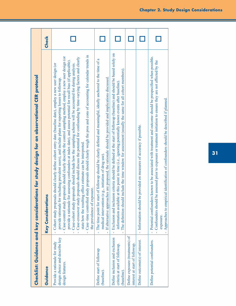
31


Chec

klis

t: G

uid

ance

and k

ey c

onsi

der

ations

for

study d

esig

n f

or

an o

bse

rvational C

ER p

roto

col

Guid

ance

Key

Consi

der

ations

Chec

k

Pro

vide

a r

atio

nale

for

stu

dy

desi

gn c

hoic

e an

d de

scri

be k

ey

desi

gn f

eatu

res.

- C

ohor

t stu

dy p

ropo

sals

sho

uld

clea

rly

defi

ne c

ohor

t ent

ry d

ate

(bas

elin

e da

te),

em

ploy

a n

ew u

ser

desi

gn (

or

p

rovi

de r

atio

nale

for

incl

udin

g pr

eval

ent u

sers

), a

nd in

clud

e pl

ans

for

repo

rtin

g lo

sses

to f

ollo

wup

. -

Cas

e-co

ntro

l stu

dy p

ropo

sals

sho

uld

clea

rly

desc

ribe

the

cont

rol s

ampl

ing

met

hod,

em

ploy

a n

ew u

ser

desi

gn (

or

p

rovi

de a

rat

iona

le f

or a

sses

sing

con

foun

ders

at i

ndex

dat

e), a

nd a

sses

s po

tent

ial f

or r

ecal

l bia

s (i

f ap

plic

able

).

- C

ase-

coho

rt s

tudy

pro

posa

ls s

houl

d in

clud

e ho

w th

e sa

mpl

ing

sche

me

wil

l be

acco

unte

d fo

r du

ring

ana

lysi

s.

- C

ase-

cros

sove

r st

udy

prop

osal

s sh

ould

dis

cuss

the

pote

ntia

l for

con

foun

ding

by

tim

e-va

ryin

g fa

ctor

s an

d cl

earl

y

s

tate

how

the

resu

ltin

g ef

fect

est

imat

e ca

n be

inte

rpre

ted.

-

Cas

e–ti

me

cont

roll

ed s

tudy

pro

posa

ls s

houl

d cl

earl

y w

eigh

the

pros

and

con

s of

acc

ount

ing

for

cale

ndar

tren

ds in

the

prev

alen

ce o

f ex

posu

re.

o

Defi

ne s

tart

of

foll

owup

(b

asel

ine)

.-

The

tim

e po

int f

or s

tart

of

foll

owup

sho

uld

be c

lear

ly d

efine

d an

d m

eani

ngfu

l, id

eally

anc

hore

d to

the

tim

e of

a

m

edic

al in

terv

enti

on (

e.g.

, ini

tiat

ion

of d

rug

use)

. -

If

alte

rnat

ive

appr

oach

es a

re p

ropo

sed,

the

rati

onal

e sh

ould

be

prov

ided

and

impl

icat

ions

dis

cuss

ed.

oD

efine

incl

usio

n an

d ex

clus

ion

crit

eria

at s

tart

of

foll

owup

. (b

asel

ine)

.

- E

xclu

sion

and

incl

usio

n cr

iter

ia s

houl

d be

defi

ned

at th

e st

art o

f fo

llow

up (

base

line

) an

d sh

ould

be

base

d so

lely

on

info

rmat

ion

avai

labl

e at

this

poi

nt in

tim

e (i

.e.,

igno

ring

pot

enti

ally

kno

wn

even

ts a

fter

bas

elin

e).

- T

he d

efini

tion

sho

uld

incl

ude

the

tim

e w

indo

w f

or a

sses

smen

t (us

ually

the

sam

e fo

r al

l coh

ort m

embe

rs).

oD

efine

exp

osur

e (t

reat

men

ts)

of

inte

rest

at s

tart

of

foll

owup

.o

Defi

ne o

utco

me(

s) o

f in

tere

st.

- I

nfor

mat

ion

shou

ld b

e pr

ovid

ed o

n m

easu

res

of a

ccur

acy

if p

ossi

ble.

oD

efine

pot

enti

al c

onfo

unde

rs.

- P

oten

tial

con

foun

ders

kno

wn

to b

e as

soci

ated

wit

h tr

eatm

ent a

nd o

utco

me

shou

ld b

e pr

espe

cifi

ed w

hen

poss

ible

. -

Con

foun

ders

sho

uld

be a

sses

sed

prio

r to

exp

osur

e or

trea

tmen

t ini

tiat

ion

to e

nsur

e th

ey a

re n

ot a

ffec

ted

by th

e

e

xpos

ure.

-

App

roac

hes

to e

mpi

rica

l ide

ntifi

cati

on o

f co

nfou

nder

s sh

ould

be

desc

ribe

d if

pla

nned

.

o

32


References1. Schneeweiss S, Maclure M, Walker AM, et al.

On the evaluation of drug benefits policy changes with longitudinal claims data: the policy maker’s versus the clinician’s perspective. Health Policy. 2001 Feb;55(2):97-109.

2. Maclure M, Carleton B, Schneeweiss S. Designed delays versus rigorous pragmatic trials: lower carat gold standards can produce relevant drug evaluations. Med Care. 2007 Oct;45 (10 Supl 2):S44-9.

3. Rücker G. A two-stage trial design for testing treatment, self-selection and treatment preference effects. Stat Med. 1989 Apr;8(4):477-85.

4. Fava M, Rush AJ, Trivedi MH, et al. Background and rationale for the sequenced treatment alternatives to relieve depression (STAR*D) study. Psychiatr Clin North Am. Jun 2003;26(2): 457-494.

5. Rothman KJ, Greenland S, Lash T. (Eds.). Modern Epidemiology. 3rd ed. Philadelphia, PA: Lippincott, Williams & Wilkins; 2008.

6. Miettinen OS, Caro JJ. Principles of nonexperimental assessment of excess risk, with special reference to adverse drug reactions. J Clin Epidemiol. 1989;42(4):325-31.

7. Yusuf, S., Collins, R. Peto, R. (1984). Why do we need some large, simple randomized trials? Statistics in Medicine. 1984;3:409–20.

8. Glynn RJ, Knight EL, Levin R, et al.. Paradoxical relations of drug treatment with mortality in older persons. Epidemiology. 2001 Nov;12(6):682-9.

9. Stürmer T, Schneeweiss S, Brookhart MA, et al.. Analytic strategies to adjust confounding using exposure propensity scores and disease risk scores: nonsteroidal antiinflammatory drugs and short-term mortality in the elderly. Am J Epidemiol. 2005;161:891-8.

10. Stürmer T, Rothman KJ, Avorn J, et al. Treatment effects in the presence of unmeasured confounding: Dealing with observations in the tails of the propensity score distribution – a simulation study. Am J Epidemiol. 2010;172: 843-54.

11. Jackson LA, Jackson ML, Nelson JC, et al. Evidence of bias in estimates of influenza vaccine effectiveness in seniors. Int J Epidemiol. 2006 Apr;35(2):337-44. Epub 2005 Dec 20.

12. Greenland S, Robins JM. Identifiability, exchangeability, and epidemiological confounding. Int J Epidemiol. 1986 Sep;15(3):413-9.

13. Greenland S, Robins JM. Identifiability, exchangeability and confounding revisited. Epidemiol Perspect Innov. 2009 Sep 4;6:4.

14. Hill, Austin Bradford. “The environment and disease: association or causation?” Proceedings of the Royal Society of Medicine 1965;58:295–300.

15. Cadarette SM, Katz JN, Brookhart MA, et al. Relative effectiveness of osteoporosis drugs for nonvertebral fracture prevention: a cohort study. Ann Intern Med. 2008;148:637-46.

16. Stürmer T, Poole C. Matching in cohort studies: return of a long lost family member. [Symposium] Am J Epidemiol. 2009;169(Suppl):S128.

17. Stürmer T, Brenner H. Degree of matching and gain in power and efficiency in case-control studies. Epidemiology. 2001; 12: 101-8.

18. Stürmer T, Brenner H. Flexible matching strategies to increase power and efficiency to detect and estimate gene-environment interactions in case-control studies. Am J Epidemiol. 2002;155: 593-602.

19. Martinez C, Assimes TL, Mines D, et al. Use of venlafaxine compared with other antidepressants and the risk of sudden cardiac death or near death: a nested case-control study. BMJ. 2010 Feb 5;340:c249. doi: 10.1136/bmj.c249.

20. Prentice RL. A case-cohort design for epidemiologic cohort studies and disease prevention trials. Biometrika. 1986;73:1–11.

21. Maclure M. The case-crossover design: a method for studying transient effects on the risk of acute events. Am J Epidemiol. 1991 Jan 15;133(2): 144-53.

22. Maclure M. ‘Why me?’ versus ‘why now?’--differences between operational hypotheses in case-control versus case-crossover studies. Pharmacoepidemiol Drug Saf. 2007 Aug;16(8):850-3.

23. Suissa S. The case-time-control design. Epidemiology. 1995 May;6(3):248-53.

24. Greenland S. Confounding and exposure trends in case-crossover and case-time-control designs. Epidemiology. 1996 May;7(3):231-9.

33


25. Farrington CP. Control without separate controls: evaluation of vaccine safety using case-only methods. Vaccine. 2004;22(15-16):2064-70.

26. Whitaker HJ, Farrington CP, Spiessens B, et al. Tutorial in biostatistics: the self-controlled case series method. Stat Med. 2006; May 30;25(10):1768-97.

27. Gibson JE, Hubbard RB, Smith CJP, et al. The use of self-controlled analytical techniques to assess the temporal association between use of prescription medications and the risk of motor vehicle crashes. Am J Epidemiol. 2009;169(6): 761-8.

28. Glynn RJ, Schneeweiss S, Stürmer T. Indications for propensity scores and review of their use in pharmacoepidemiology. Basic and Clinical Pharmacology and Toxicology. 2006;98:253-9.

29. Patrick AR, Shrank WH, Glynn RJ, et al. The association between statin use and outcomes potentially attributable to an unhealthy lifestyle in older adults. Value Health. 2011 Jun;14(4):513-20. Epub 2011 Apr 22.

30. Kramer MS, Lane DA, Hutchinson TA. Analgesic use, blood dyscrasias, and case-control pharmacoepidemiology. A critique of the international agranulocytosis and aplastic anemia study. J Chron Dis. 1987;40:1073-81.

31. Guess HA. Behavior of the exposure odds ratio in a case-control study when the hazard function is not constant over time. J Clin Epidemiol. 1989;42:1179-84.

32. Dormuth CR, Patrick AR, Shrank WH, et al. Statin adherence and risk of accidents: a cautionary tale. Circulation. 2009 Apr 21;119(15):2051-7. Epub 2009 Apr 6.

33. Simpson SH, Eurich DT, Majumdar SR, et al. A meta-analysis of the association between adherence to drug therapy and mortality. BMJ. 2006;333:15.

34. Andersen M, Brookhart MA, Glynn RJ, et al. Practical issues in measuring cessation and re-initiation of drug use in databases. [abstract] Pharmacoepidemiol Drug Saf. 2008;17 (suppl 1):S27.

35. Moride Y, Abenhaim L. Evidence of the depletion of susceptibles effect in non-experimental pharmacoepidemiologic research. J Clin Epidemiol. 1994 Jul;47(7):731-7.

36. Ray WA. Evaluating medication effects outside of clinical trials: new-user designs. Am J Epidemiol. 2003;158:915-20.

37. Valkhoff VE, Romio SA, Schade R, et al. Influence of run-in period on incidence of NSAID use in European population in the SOS project. Pharmacoepidemiol Drug Saf. 2011;20 (supl 1):S250.

38. Suissa S. Effectiveness of inhaled corticosteroids in chronic obstructive pulmonary disease: immortal time bias in observational studies. Am J Respir Crit Care Med. 2003;168(1):49-53.

39. Gail MH. Does cardiac transplantation prolong life? A reassessment. Ann Intern Med. 1972;76(5):815-7.

40. Pocock SJ, Smeeth L. Insulin glargine and malignancy: an unwarranted alarm. Lancet. 2009;374(9689):511-3.

41. Collet JP, Schaubel D, Hanley J, et al. Controlling confounding when studying large pharmacoepidemiologic databases: a case study of the two-stage sampling design. Epidemiology. 1998 May;9(3):309-15.

42. Stürmer T, Glynn RJ, Rothman KJ, et al. Adjustments for unmeasured confounders in pharmacoepidemiologic database studies using external information. Med Care. 2007;45 (10 Supl 2):S158-65.

35

Abstract

Patient populations within a research study are heterogeneous. That is, they embody characteristics that vary between individuals, such as age, sex, disease etiology and severity, presence of comorbidities, concomitant exposures, and genetic variants. These varying patient characteristics can potentially modify the effect of a treatment on outcomes. Despite the presence of this heterogeneity, many studies estimate an average treatment effect (ATE) that implicitly assumes a similar treatment effect across heterogeneous patient characteristics. While this assumption may be warranted for some treatments, for others the treatment effect within subgroups may vary considerably from the ATE. This treatment effect heterogeneity may arise from an underlying causal mechanism or may be due to artifacts of measurements or methods (e.g., chance, bias, or confounding). Heterogeneity of treatment effect (HTE) is the nonrandom, explainable variability in the direction and magnitude of treatment effects for individuals within a population. The main goals of HTE analysis are to estimate treatment effects in clinically relevant subgroups and to predict whether an individual might benefit from a treatment. Subgroup analysis is the most common analytic approach for examining HTE. Selection of subgroups should be based on mechanism and plausibility (including clinical judgment), taking into account prior knowledge of treatment effect modifiers. This chapter focuses on defining and describing HTE and offers guidance on how to evaluate and report such heterogeneous effects using subgroup analysis. Understanding HTE is critical for decisions that are based on knowing how well a treatment is likely to work for an individual or group of similar individuals, and is relevant to most stakeholders, including patients, clinicians, and policymakers. The chapter concludes with a checklist of key considerations for discussion of HTE and for addressing planned subgroup analysis in an observational comparative effectiveness research (CER) protocol.

Chapter 3. Estimation and Reporting of Heterogeneity of Treatment Effects

Ravi Varadhan, Ph.D. Johns Hopkins University School of Medicine, Baltimore, MD

John D. Seeger, Pharm.D., Dr.P.H. Harvard Medical School and Brigham and Women’s Hospital, Boston, MA

“If it were not for the great variability between individuals, medicine might as well be a science, not an art” (William Osler, 1892).

Introduction

Randomized controlled trials (RCTs) and observational studies of comparative effectiveness usually report an average treatment effect (ATE), even though experience suggests that the same treatment can have varying impacts in different people. The clinical experience and expectation that differences in patient prognostic characteristics will lead to heterogeneous responses to therapy is mainly

why medicine is as much an art as it is science. Yet, studies tend to emphasize a single measure of the impact of treatment, the ATE, which is a summary of individual treatment effects (which cannot be examined directly without making untestable assumptions). Variation is often undesirable in studies and is reduced by excluding people with characteristics that are thought to cause variations in responses to treatment. This intentional restriction in patient heterogeneity within RCTs contributes to their limited generalizability. Determining whether a treatment works for people in a target population that differs from the study population requires additional information and methods.1

36


Heterogeneity of Treatment Effect

All studies have variability in the data. Random variability is generally not a concern because it is uncorrelated with explanatory variables and can be handled well with statistical approaches for quantifying uncertainty. We focus on the nonrandom variability in treatment effects that can be attributed to patient factors. We define HTE as nonrandom variability in the direction or magnitude of a treatment effect, in which the effect is measured using clinical outcomes (either a clinical event such as myocardial infarction or a change in a continuous clinical measure such as level of pain).2

Understanding HTE is critical for decisions that are based on knowing how well a treatment is likely to work for an individual or group of similar individuals, and is relevant to stakeholders including patients, clinicians, and policymakers. It also has implications for applicability to individual patients (personalized medicine) of findings from pragmatic trials and observational comparative effectiveness research (CER). Pragmatic trials are large and simple experiments on treatments, with broad eligibility criteria, from which evidence is expected to be generalizable. While these designs incorporate heterogeneity in the risk of outcome among the subjects, they may also lead to HTE for the treatments that are applied. These studies may be more likely to yield null ATE than efficacy trials, where stricter inclusion criteria produce relatively homogeneous study populations. Therefore, understanding major sources of variations in treatment response is essential. For a formal general definition of HTE, see Box 3.1.

There are numerous cases in which the effectiveness of specific therapies may be heterogeneous. For example, children may respond differently to therapy via different response to treatment or to aspects of dosing that are not realized. Older adults may have worse outcomes from surgeries and devices as well as more drug side effects or drug-drug interactions so that therapies may be less effective. Individuals with multiple conditions may be on several therapies that interfere with the new treatment (or each other), resulting in a different treatment effect in these patients. Genes may also influence response

to therapy; since genetic differences (differences in allele frequencies) may cluster by race or ethnicity, these characteristics may represent proxies for genetic differences that are more difficult to measure directly.

Treatment Effect Modification

If two or more exposure variables act in concert to cause disease, we will observe that the effect of exposure on outcome (treatment effect) differs according to the level of the other factor(s). A number of terms have been used to describe this phenomenon, including “joint” effects, “synergism,” “antagonism,” “interaction,” “effect

Box 3.1. Formal definition of HTE

Let an individual or a targeted subgroup with specific levels of characteristics be denoted by i. Let z stand for treatment at two levels {1, 2}; for example, being given aspirin (z =1) or not (z =2). Let the potential outcomes corresponding to the two treatment levels be denoted as {Y

i(1), Y

i(2)}. The individual

treatment effect can be defined as the contrast: θ

i = g(E[Y

i(1)]) – g(E[Y

i(0)]). The potential

outcomes Yi can be continuous, categorical,

or binary. When Yi is binary, E[Y

i(z)] denotes

prob(Yi = 1) under treatment z. The function

g(.) can be identity, log, or logit. For the absolute risk model, the individual treatment effect is θ

i = Prob(Y

i(2)=1) – Prob

( Yi(1)=1). For the relative risk model, u

i =

log [prob(Yi(2)=1)] – log[prob(Y

i(1)=1)].

Individual variability of treatment effect occurs if the variance (u

i) > 0. Group variability (HTE)

occurs if the variance of individual treatment effect is nonrandom (i.e. correlated with explanatory variables) so that u

subgroup1 (average

θi for a subgroup defined by level 1 of an

explanatory variable) ≠ usubgroup2

(average ui for

a subgroup defined by level 2 of an explanatory variable). When this variability encompasses treatment effects of different directions, i.e., both benefit and harm, this is sometimes called a qualitative treatment interaction, whereas differences in the magnitude of treatment effect in the same direction are called quantitative interactions.

37


modification,” and “effect measure modification.” Where effect modification exists, sound inferences will require accounting for factors that modify the effect of the exposure of primary interest. Accounting for this HTE may be required even when the variable that modifies treatment effect is not a risk factor for the outcome in the untreated group (e.g., a receptor that determines how a drug is metabolized).

Four perspectives have been advanced on the concept of interaction and the relevance of the effect modification in terms of its implication:3

Biological perspective: This perspective is that the interaction elucidates how factors act at the biological (mechanistic) level. The implications of this perspective are that the interaction is a representation of an underlying causal structure. Example: The finding that hypertension and smoking have a greater than additive effect on heart attack risk is a representation of some underlying biological processes that may enhance our understanding of heart attack etiology.

Statistical perspective: This perspective is that the interactions represent nonrandom variability in data unaccounted for by a model that contains only first-order terms (main effects). The implication is that the model needs to be reformulated to more accurately reflect the data. Example: A differently structured model will appropriately account for the underlying variability in the data on hypertension, smoking, and heart attack risk.

Public health perspective: This perspective is that the interactions represent a departure from additivity and highlight populations (subgroups) in which an intervention can be expected to have particularly beneficial effects. Example: The finding that hypertension and smoking have a greater than additive effect on heart attack risk suggests that limited public health resources might be most efficiently directed at patients who have hypertension and are smokers.

The individual decisionmaking perspective: This perspective is that the interactions represent a departure from additivity so that combined effects in an individual are greater than their sum. Example: Someone with hypertension can reduce heart attack risk even more by quitting smoking than someone with normal blood pressure.

Since an effect modifier changes the magnitude or direction of the association under study, different study populations may yield different results concerning the association of interest. Therefore, HTE is often suggested as a reason for differences in findings across studies. If two studies include people with different characteristics and the effect of the treatment is different in the portion of the population that differs between the studies, then HTE is a plausible explanation of the difference. Furthermore, HTE can be an explanation of differences in treatment effect between interventional and observational studies, since observational studies often include patients with different characteristics than interventional studies. Such a hypothesis might be addressed through reweighting subgroup effects according to prevalence (standardization) across studies.

Unlike potential confounders, modifying variables cannot create the appearance of an association (for exposed vs. unexposed) where none exists. But the proportion of the study population that has a greater susceptibility will influence the strength of the association. Therefore, to achieve comparability across studies, it is necessary to control for the effect of the modifying variables, generally by carrying out a separate analysis at each level of the modifier.

Additionally, the different strength of association between the exposure and outcome within strata of the effect modifier may lead to a need to be more precise in the measurement and specification of the exposure variable (such as more clearly within strata of the effect modifier).

Goals of HTE Analysis

There are two main goals of HTE analyses: (1) to estimate treatment effects in clinically relevant subgroups (subgroup analysis) and (2) to predict whether an individual might benefit from a treatment (predictive learning).2 The first goal of HTE is highlighted in the definition of CER) proposed by the Congressional Budget Office: “An analysis of comparative effectiveness is simply a rigorous evaluation of the impact of different treatment options that are available for treating a given medical condition for a particular set of patients.”1 The second goal of HTE analysis is individual-level prediction. Predicting beneficial

38


and adverse responses of individuals to different treatments in terms of multiple endpoints is essential for informing individualized treatment decisions. One version of this goal has been described as answering the question: “Who will benefit most from Treatment A and who will benefit most from Treatment B?”4 Creating such a narrowly defined subgroup (the individual patient) leads to an extremely challenging problem, which has not been adequately studied and for which there are few reliable methods that provide protection against spurious findings.5 Subgroup analysis, on the other hand, has been extensively studied.6 Hence, we will focus on subgroup analysis.

Subgroup Analysis

Subgroup analysis is the most commonly used analytic approach for examining HTE. This method usually evaluates the treatment effect for a number of subgroups, one variable at a time, usually a baseline or pretreatment variable. A test for interaction is conducted to evaluate if a subgroup variable has a statistically significant interaction with the treatment indicator. If the interaction is significant, then the treatment effect is estimated separately at each level of the categorical variable used to define mutually exclusive subgroups (e.g., men and women).

It should be cautioned, however, that the interaction test generally has low power to detect differences in subgroup effects.7 For example, when compared with the sample size required for detecting ATE of a particular size, a sample size roughly four times as large is required for detecting a difference in subgroup effects of the same magnitude as ATE for a 50:50 subgroup split; a sample size approximately 16 times as large is required for detecting a difference that is half of ATE (at significance level 0.05).

Even though the interaction test has low power to detect a true difference in subgroup effects, there is a danger of falsely detecting a difference in subgroup effects if we perform separate interaction tests for multiple subgrouping variables. That is, suppose we perform separate interaction tests for 100 subgroup variables. The interaction test will be statistically significant (at a significance level of 0.05), on average, for about five subgroup

variables, when in truth the treatment effect is homogeneous. If we make a Bonferroni correction for multiple testing in order to maintain the correct Type-I error probability, we would be further increasing the Type-II error probability, which increases the likelihood of not identifying true heterogeneity in subgroup effects.

It should also be noted that a statistical test of interaction does not correspond to an assessment of biological interaction. The presence or absence of statistical interaction depends on various mathematical aspects of the regression model (e.g., scale of dependent variable, covariates present in the model, distributional assumptions). These considerations are largely irrelevant for biological interactions.3

A useful illustration of the potential for subgroup analyses (and implied HTE) to lead to erroneous inferences came from a large randomized trial of therapies for myocardial infarction. In 1988, the results of the Second International Study of Infarct Survival (ISIS-2) study, a randomized 2x2 factorial study of the effect of streptokinase and aspirin for treatment of myocardial infarction, were published.8 This study provided evidence indicating that either streptokinase or aspirin reduced mortality following myocardial infarction, and that the combination of streptokinase and aspirin improved survival over either treatment alone. In the aspirin-treated subjects, there was a reduction in mortality (804 deaths among 8,587 people, 9.4%) relative to subjects not treated with aspirin (1,016 deaths among 8,600 people, 11.8%, p<0.05). Numerous subgroup analyses were conducted, most of which indicated relatively consistent effects of aspirin. However, one particular subgroup analysis, astrological birth sign, suggested heterogeneity of effect. In the subgroup of patients born under the astrological sign Gemini or Libra, there were more deaths (150 of 1,357, 11.1%) among the aspirin-treated patients than there were among the non–aspirin-treated patients (147 of 1,442, 10.2%) (p not significant).

This apparent heterogeneity in the effect of aspirin served as a caution about the causal interpretation of findings from unfocused, exploratory subgroup analyses. Rather than inferring that aspirin should not be used in the treatment of

39


myocardial infarction if the patient is a Gemini or a Libra, the authors pointed to the potential for overinterpreting results of subgroup analyses. When the ATE is clearly positive (both aspirin and streptokinase reduce mortality in patients with myocardial infarction) and many subgroup analyses are conducted, false positive or negative findings are to be expected. Findings from such unfocused, exploratory subgroup analyses should be interpreted with caution even if a plausible biologic mechanism exists, and with greater caution if the apparent heterogeneity of treatment is not supported by a plausible mechanism (as with the astrological sign subgroup).

The ISIS-2 study conducted additional subgroup analyses to assess the consistency of the subgroup findings from an earlier randomized trial of streptokinase (GISSI) that found no benefit of streptokinase among persons older than 65, those with a previous infarct, and those presenting more than 6 hours after the onset of pain. In contrast to GISSI, the ISIS-2 study found a mortality benefit for streptokinase among these subgroups, a finding that further underscores the need for caution when drawing inferences from subgroup results.When there are plausible a priori reasons that a treatment may not be effective (such as in patients with contraindications to the therapy) and subgroup analyses find no benefit in that subgroup, stronger inferences might be drawn.

Types of Subgroup Analysis

Three different types of subgroup analyses may be distinguished: (a) confirmatory, (b) descriptive, and (c) exploratory.2 See Table 3.1 for a summary of the essential characteristics of these three types of subgroup analyses.

Confirmatory Subgroup Analysis

The main goal is to test and confirm hypotheses about subgroup effects. The essential elements of this type of analysis are: clear definition and prespecification of subgroups; clear definition and prespecification of endpoints related to outcomes; prespecification of a small number of hypotheses about subgroup effects, including the direction in which the effects are expected to vary in subgroups; availability of strong a priori biological

and epidemiological evidence; detailed description of a statistical analysis plan for how testing will be done; and adequate power to test subgroup hypotheses. Essentially, the study intent, design, and analysis are all focused on the subgroup hypotheses to be tested. Due to these stringent requirements, the findings from a confirmatory analysis are potentially actionable.

Descriptive Subgroup Analysis

The main goal of descriptive subgroup analysis is to describe the subgroup effects for future evaluation and synthesis. The essential elements of this type of analysis are: clear definition and prespecification of subgroups, clear definition and prespecification of endpoints related to outcomes, prespecification of hypotheses relating to subgroup effects, and detailed description of a statistical analysis plan for how testing will be done. The results of these subgroup analyses may be presented as a table in the main report and as a forest plot, with a vertical line representing the overall treatment effect (ATE). See Antman et al. for a good example of such a forest plot.9 Alternatively, the results may be made available as an appendix or as electronic supplemental material in order to facilitate future evaluation and for synthesis and meta-analysis by systematic reviewers. A detailed discussion of descriptive subgroup analysis is presented in Varadhan et al.2

Exploratory Subgroup Analysis

Exploratory subgroup analyses are done mainly to identify subgroup hypotheses for future evaluation. Typically, exploratory subgroups are not prespecified. Compared to confirmatory and descriptive HTE analyses, exploratory analyses enjoy more flexibility for identifying baseline characteristics that interact with treatment. Definition of subgroups, endpoints, hypotheses, and modeling parameters are usually derived in response to the data. An example of this would be the use of a stepwise model selection approach to identify treatment by covariate interactions. A major problem with these analyses is that it is extremely difficult to obtain the sampling properties of subgroup effect estimators (e.g., standard errors). Often, it is not clear how many hypotheses were tested (e.g., using stepwise model

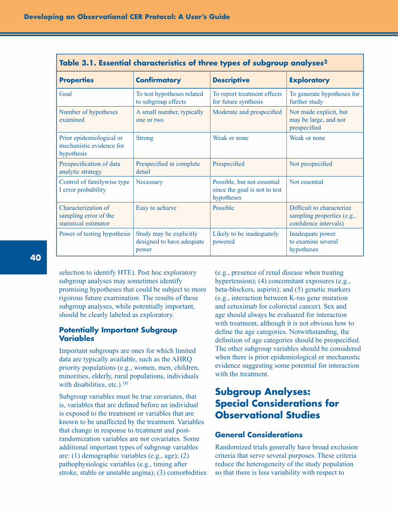
40


selection to identify HTE). Post hoc exploratory subgroup analyses may sometimes identify promising hypotheses that could be subject to more rigorous future examination. The results of these subgroup analyses, while potentially important, should be clearly labeled as exploratory.

Potentially Important Subgroup Variables

Important subgroups are ones for which limited data are typically available, such as the AHRQ priority populations (e.g., women, men, children, minorities, elderly, rural populations, individuals with disabilities, etc.).10

Subgroup variables must be true covariates, that is, variables that are defined before an individual is exposed to the treatment or variables that are known to be unaffected by the treatment. Variables that change in response to treatment and post-randomization variables are not covariates. Some additional important types of subgroup variables are: (1) demographic variables (e.g., age); (2) pathophysiologic variables (e.g., timing after stroke, stable or unstable angina); (3) comorbidities

(e.g., presence of renal disease when treating hypertension); (4) concomitant exposures (e.g., beta-blockers, aspirin); and (5) genetic markers (e.g., interaction between K-ras gene mutation and cetuximab for colorectal cancer). Sex and age should always be evaluated for interaction with treatment, although it is not obvious how to define the age categories. Notwithstanding, the definition of age categories should be prespecified. The other subgroup variables should be considered when there is prior epidemiological or mechanistic evidence suggesting some potential for interaction with the treatment.

Subgroup Analyses: Special Considerations for Observational Studies

General Considerations

Randomized trials generally have broad exclusion criteria that serve several purposes. These criteria reduce the heterogeneity of the study population so that there is less variability with respect to

Table 3.1. Essential characteristics of three types of subgroup analyses2

Properties Confirmatory Descriptive Exploratory

Goal To test hypotheses related to subgroup effects

To report treatment effects for future synthesis

To generate hypotheses for further study

Number of hypotheses examined

A small number, typically one or two

Moderate and prespecified Not made explicit, but may be large, and not prespecified

Prior epidemiological or mechanistic evidence for hypothesis

Strong Weak or none Weak or none

Prespecification of data analytic strategy

Prespecified in complete detail

Prespecified Not prespecified

Control of familywise type I error probability

Necessary Possible, but not essential since the goal is not to test hypotheses

Not essential

Characterization of sampling error of the statistical estimator

Easy to achieve Possible Difficult to characterize sampling properties (e.g., confidence intervals)

Power of testing hypothesis Study may be explicitly designed to have adequate power

Likely to be inadequately powered

Inadequate power to examine several hypotheses

41


outcome measures, thereby improving statistical power for a given sample size. Exclusion criteria also serve to protect patients who might be harmed by a treatment (such as those with a contraindication to the treatment). Since the aim of many observational studies is to describe the effect of treatment as actually used, fewer exclusions are typically applied, and those that are often applied are for the purpose of improved confounder control. As a result, observational studies often include patients for whom no randomized data of treatment effect exists. For example, a patient with a relative contraindication for a treatment might be excluded from a randomized trial, but a treating clinician may decide that the benefits outweigh the risks for this patient and apply the therapy.

The study of treatment effects can be challenging in observational studies. Observational studies are susceptible to confounding by indication, ascertainment biases in exposure to treatment, measurement error in assessment of health outcomes, and lack of information on important prognostic variables (in studies using existing data). These biases and measurement errors can introduce apparent HTE when in fact none is present, or conversely, obscure true HTE. Because heterogeneity in observational studies can be due to chance or bias, investigators must evaluate the observed HTE to determine whether a finding is indicative of true heterogeneity. To do this, chance findings should be evaluated by testing for interaction; biases should be avoided by adhering to sound study design principles and by evaluating balance on covariates within subgroups to assess the potential for confounding.

There are several potential sources of heterogeneity in observational studies, and these tend to mirror the potential explanations for a finding of an overall effect (ATE). As such, many of the approaches for reducing the potential for an incorrect inference are the same. Careful attention to study design principles is an important starting point for avoiding incorrect inferences with respect to overall findings and also benefits the identification of potential HTE. The use of the incident (new) user design reduces the potential for inclusion of immortal person-time (i.e., person-time during which a study outcome cannot occur; see chapter 4 for a detailed discussion).11 Contemporaneous followup of exposed and

unexposed subjects (parallel group design) avoids calendar time differences in exposure/covariate/outcome identification. Measures of exposure, outcome, and covariates should address misclassification and seek to limit potential for information bias.

Despite the challenges in using observational data for HTE analysis, randomized experiments cannot be performed to answer all clinically important questions regarding HTE attributable to patient characteristics. Therefore, a huge demand will be placed on observational studies to produce evidence to inform decisions. Hence, procedures must be put in place to ensure that the results from observational studies are trustworthy. A key principle here is that the observational studies should be designed and analyzed in the same manner as randomized controlled experiments. Some potential steps include registering observational CER studies prospectively, publishing the study protocol (including clear definitions of subgroups and outcomes, prespecified hypotheses, and power calculations), and developing a detailed analytic plan (including how confounding, missing data, and loss to followup will be handled). Sox has called for registration of observational studies, along the lines of the National Institutes of Health’s clinical trials registry.12 Rubin has put forth an interesting proposal for “objective causal inference,” in which greater emphasis is placed on understanding treatment selection. The modeler is blinded to outcomes until the treatment assignment modeling is completed and made available to scrutiny.13 This places the emphasis on study design and treatment assignment, and the investigator only observes outcomes at the end, as in randomized experiments. This ensures some degree of objectivity in the outcome modeling. These proposals are worth serious consideration.

Prediction of Individual Treatment Effects

This chapter has focused on analytic approaches to subgroups within a population, but variations of effect can also occur within individuals. The individual causal effects (Box 3.1), θ

i = g(E[Y

i(1)])

– g(E[Yi(0)]), are not identifiable from the data

without untestable assumptions. For acute or transient outcomes, methods such as crossover

42


designs or N-of-1 trials may be appropriate for estimating individual effects. For nonacute outcomes, prediction models may be developed for predicting the response of individuals to different treatments. Prediction of individual responses can also be viewed as an extreme version of subgroup analysis, where individuals are cross-classified by a large number of covariates. It is quite likely that most covariate profiles viewed as cells in a high-dimensional contingency table would be either empty or sparsely populated. Consequently, individual-level predictions can be highly variable and sensitive to modeling assumptions. An example of a prediction model is by Dorresteijn et al., who predicted the effect of rosuvastatin on cardiovascular events for individual patients using data from an RCT.14 They evaluated the net benefit of treatment decisions for individuals based on predicted risk difference (absolute risk reduction) due to the treatment. They used existing risk models (Framingham and Reynolds risk scores), as well as a prediction model developed using the trial data to calculate baseline risk of cardiovascular outcomes for all individuals without treatment. The average treatment effect (ATE) (relative risk) was applied to calculate individual treatment effects (ITE) (ITE = baseline risk * (1-ATE)). It is important to note that prediction models must be appropriately validated in order for them to be acceptable.

Value of Stratification on the Propensity Score

A study by Kurth and colleagues illustrates the use of summary score stratification as a means to assess HTE in observational studies.15 Since many strokes are the result of thrombosis in cerebral or precerebral arteries, a highly specific thrombolytic therapy became available in the form of recombinant tissue plasminogen activator (TPA). Three randomized studies showed that TPA neither decreased nor increased mortality substantially in people who had recently experienced a stroke. However, observational studies of the same question consistently indicated that TPA therapy increased mortality, and the reasons for the discrepancy in results between observational and interventional studies were not readily apparent. With data sourced from a German stroke registry, Kurth and colleagues were able to reproduce the

observational effect of an increase in mortality with TPA with careful attention to study design and regardless of adjustment for measured covariates. However, different analytic approaches (particularly matching on the propensity score) provided results more comparable to the randomized trials than was obtainable from adjusted analyses. By stratifying patients according to propensity to receive TPA and conducting analyses of TPA effect within strata, this study found that much of the observational result was being driven by a few subjects with low propensity to receive TPA who were highly influential in analyses that included them (the covariate–adjusted, propensity score–adjusted, propensity score–stratified, and the inverse probability–weighted analyses). However, the propensity score–matched analyses excluded these influential subjects, and the standardized mortality ratio results downweighted their influence so that these results were similar to the RCTs. As a summary of propensity to receive a medication or strength of indication, propensity score identifies clinically relevant subgroups. If heterogeneity is observed in the propensity score, further investigation is warranted. Stratification of results by summary variables such as propensity scores or disease risk scores, or other clinically relevant profiles may inform the analysis.

Conclusion

RCTs often exclude individuals with characteristics that may cause variation in response to treatment, limiting the generalizability of findings from these studies. Observational studies often have broad inclusion/exclusion criteria, allowing for the assessment of comparative effectiveness in large, diverse populations in “real-world” settings. With the increase in generalizability comes the potential for HTE. Investigators should understand the potential for HTE prior to conducting an observational CER study, and clearly state if and how subgroups will be defined and analyzed. If subgroup analysis is intended to be confirmatory, investigators should ensure adequate statistical power to detect proposed subgroup effects, and adjust for multiple testing as appropriate. When an interaction test is significant, subgroup effects should be reported, and a discussion of the potential clinical importance of the findings

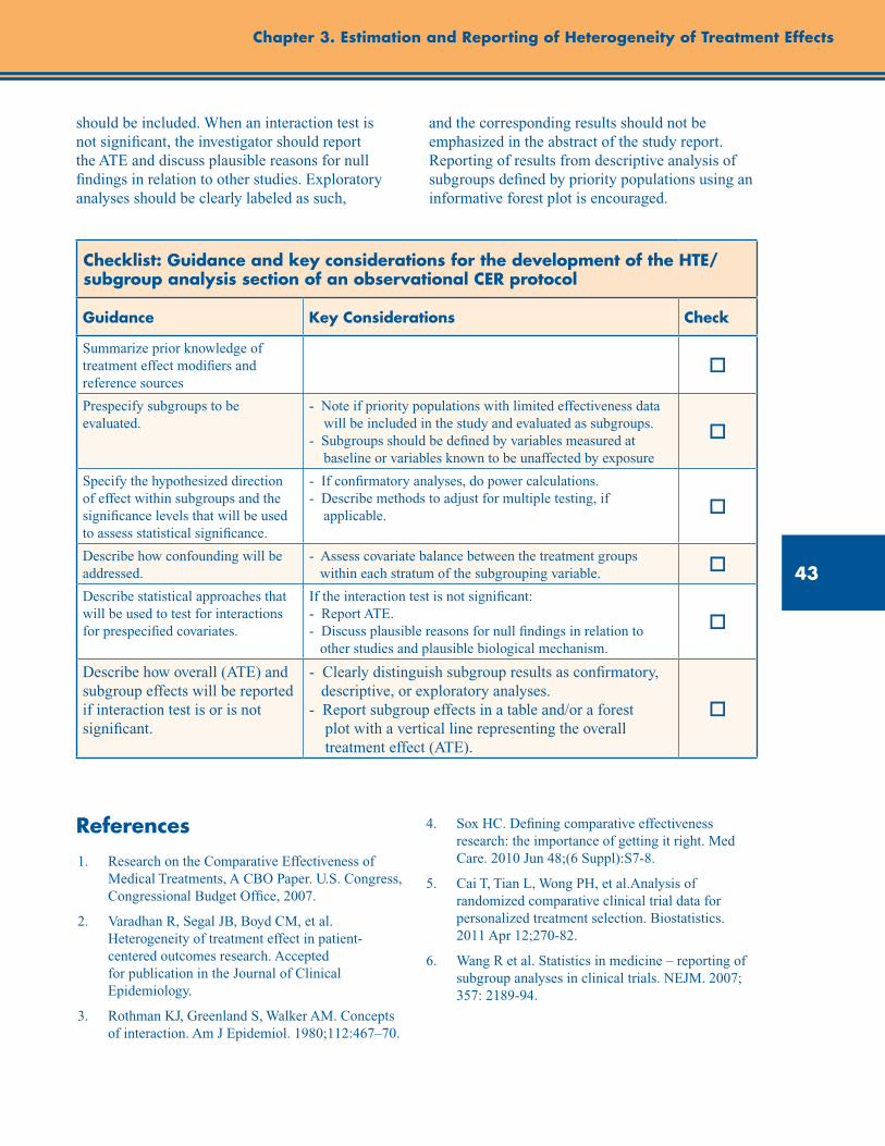
43


should be included. When an interaction test is not significant, the investigator should report the ATE and discuss plausible reasons for null findings in relation to other studies. Exploratory analyses should be clearly labeled as such,

and the corresponding results should not be emphasized in the abstract of the study report. Reporting of results from descriptive analysis of subgroups defined by priority populations using an informative forest plot is encouraged.

Checklist: Guidance and key considerations for the development of the HTE/subgroup analysis section of an observational CER protocol


Summarize prior knowledge of treatment effect modifiers and reference sources

o

Prespecify subgroups to be evaluated.

- Note if priority populations with limited effectiveness data will be included in the study and evaluated as subgroups. - Subgroups should be defined by variables measured at baseline or variables known to be unaffected by exposure

o

Specify the hypothesized direction of effect within subgroups and the significance levels that will be used to assess statistical significance.

- If confirmatory analyses, do power calculations. - Describe methods to adjust for multiple testing, if applicable. o

Describe how confounding will be addressed.

- Assess covariate balance between the treatment groups within each stratum of the subgrouping variable. o

Describe statistical approaches that will be used to test for interactions for prespecified covariates.

If the interaction test is not significant: - Report ATE. - Discuss plausible reasons for null findings in relation to other studies and plausible biological mechanism.

o

Describe how overall (ATE) and subgroup effects will be reported if interaction test is or is not significant.

- Clearly distinguish subgroup results as confirmatory, descriptive, or exploratory analyses. - Report subgroup effects in a table and/or a forest plot with a vertical line representing the overall treatment effect (ATE).

o

References1. Research on the Comparative Effectiveness of

Medical Treatments, A CBO Paper. U.S. Congress, Congressional Budget Office, 2007.

2. Varadhan R, Segal JB, Boyd CM, et al. Heterogeneity of treatment effect in patient-centered outcomes research. Accepted for publication in the Journal of Clinical Epidemiology.

3. Rothman KJ, Greenland S, Walker AM. Concepts of interaction. Am J Epidemiol. 1980;112:467–70.

4. Sox HC. Defining comparative effectiveness research: the importance of getting it right. Med Care. 2010 Jun 48;(6 Suppl):S7-8.

5. Cai T, Tian L, Wong PH, et al.Analysis of randomized comparative clinical trial data for personalized treatment selection. Biostatistics. 2011 Apr 12;270-82.

6. Wang R et al. Statistics in medicine – reporting of subgroup analyses in clinical trials. NEJM. 2007; 357: 2189-94.

44

7. Brookes ST, Whitley E, Peters TJ, et al. Subgroup analyses in randomised controlled trials: quantifying the risks of false-positives and false-negatives. Health Technology Assessment. 2001;5:1-56.

8. ISIS-2 (Second International Study of Infarct Survival) collaborative group. Randomised trial of intravenous streptokinase, oral aspirin, both, or neither among 17 187 cases of suspected acute myocardial infarction. Lancet. 1988; ii:349-60.

9. Antman EM et al. Enoxaparin versus unfractionated heparin with fibrinolysis for ST-elevation myocardial infarction. NEJM. 2006;354:1477-88.

10. Agency for Healthcare Research and Quality. Health Care: Priority Populations Index Page. Retrieved from http://www.ahrq.gov/populations/. Accessed September 21, 2012.

11. Suissa S. Immortal time bias in pharmaco-epidemiology. Am J Epidemiol. 2008;167:492-9.

12. Sox HC, Helfand M, Grimshaw J, Dickersin K; PLoS Medicine Editors, Tovey D, Knottnerus JA, Tugwell P. Comparative effectiveness research: challenges for medical journals. Am J Manag Care. 2010. May;1;16(5):e131-3

13. Rubin DB. For objective causal inference, design trumps analysis. Ann Appl Stat. 2008; 2(3):808–40.

14. Dorresteijn JAN, Visseren FLJ, Ridker PM, et al. Estimating treatment effects for individual patients based on the results of randomized clinical trials. Br Med J. 2011;343:d5888.

15. Kurth T, Walker AM, Glynn RJ, et al. Results of multivariable logistic regression, propensity matching, propensity adjustment, and propensity-based weighting under conditions of nonuniform effect. Am J Epidemiol. 2006;163:262–70.


45

Abstract

Characterization of exposure is a central issue in the analysis of observational data; however, no “one size fits all” solution exists for exposure measurement. In this chapter, we discuss potential exposure measurement approaches for observational comparative effectiveness research (CER). First, it is helpful to lay out a theoretical link between the exposure and the event/outcome of interest that draws from the study’s conceptual framework. For interventions that target health and well-being, the physiological or psychological basis for the mechanism of action, whether known or hypothesized, should guide the development of the exposure definition. When possible, an operational definition of exposure that has evidence of validity with estimates of sensitivity, specificity, and positive predictive value should be used. Other important factors to consider when defining exposure are the timeframe (induction and latent periods), changes in exposure status or exposure to other therapies, and consistency and accuracy of exposure measurement. The frequency, format, and intensity of the exposure is another important consideration for the measurement of exposure in CER studies, which is applicable to medications (e.g. dose) as well as health service interventions that may require multiple sessions, visits, or interactions. This chapter also discusses methods for avoiding nondifferential and differential measurement error, which can introduce bias, and describes the importance of determining the likelihood of bias and effects on study results. We conclude with a checklist of key considerations for the characterization and operationalization of exposure in CER protocols.

Chapter 4. Exposure Definition and MeasurementTodd A. Lee, Pharm.D., Ph.D.

University of Illinois at Chicago, Chicago, IL

A. Simon Pickard, Ph.D. University of Illinois at Chicago, Chicago, IL

Introduction

In epidemiology, the term “exposure” can be broadly applied to any factor that may be associated with an outcome of interest. When using observational data sources, researchers often rely on readily available (existing) data elements to identify whether individuals have been exposed to a factor of interest. One of the key considerations in study design is how to determine and then characterize exposure to a factor, given knowledge of the strengths and limitations of the data elements available in existing observational data.

The term “exposure” can be applied to the primary explanatory variable of interest and to other variables that may be associated with the outcome, such as confounders or effect modifiers, which also must be addressed in the analysis of the primary outcome. For example, in a study of the comparative effectiveness of proton pump inhibitors and

antibiotic treatment of H. pylori for the prevention of recurrent gastrointestinal (GI) bleeding, the primary exposures of interest are proton pump inhibitors and the antibiotics for H. pylori. However, it would also be important to measure exposure to aspirin and nonsteroidal anti-inflammatory drugs (NSAIDs), which would increase the risk of GI bleeding independent of treatment status. Similarly, in a comparative evaluation of cognitive behavioral therapy (CBT) for treatment of depression compared with no CBT, it would be important to measure not only the exposure to CBT (e.g., number and/or type of therapy sessions), but also exposure to other factors such as antidepressant medication.

Each intervention (e.g., medication, surgery, patient education program) requires a unique and thoughtful approach to exposure ascertainment. While it may only be necessary to identify if and when an intervention occurred to assign individuals to the appropriate comparison group for one-

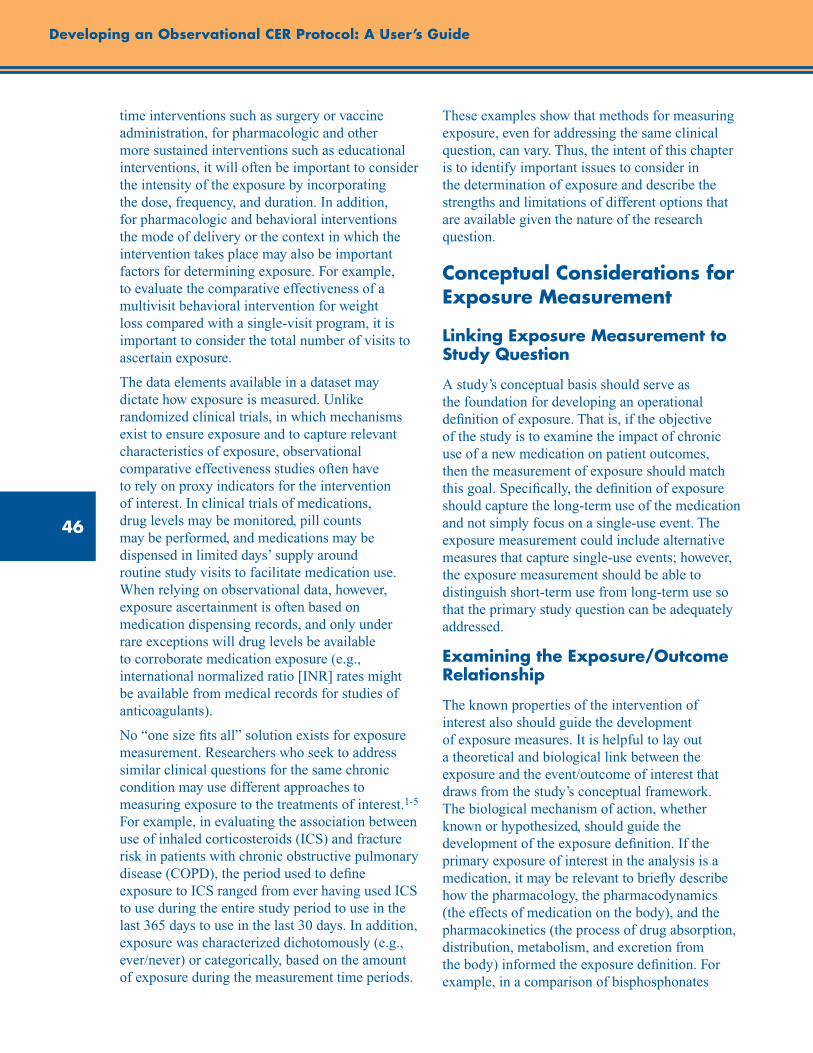
46


time interventions such as surgery or vaccine administration, for pharmacologic and other more sustained interventions such as educational interventions, it will often be important to consider the intensity of the exposure by incorporating the dose, frequency, and duration. In addition, for pharmacologic and behavioral interventions the mode of delivery or the context in which the intervention takes place may also be important factors for determining exposure. For example, to evaluate the comparative effectiveness of a multivisit behavioral intervention for weight loss compared with a single-visit program, it is important to consider the total number of visits to ascertain exposure.

The data elements available in a dataset may dictate how exposure is measured. Unlike randomized clinical trials, in which mechanisms exist to ensure exposure and to capture relevant characteristics of exposure, observational comparative effectiveness studies often have to rely on proxy indicators for the intervention of interest. In clinical trials of medications, drug levels may be monitored, pill counts may be performed, and medications may be dispensed in limited days’ supply around routine study visits to facilitate medication use. When relying on observational data, however, exposure ascertainment is often based on medication dispensing records, and only under rare exceptions will drug levels be available to corroborate medication exposure (e.g., international normalized ratio [INR] rates might be available from medical records for studies of anticoagulants).

No “one size fits all” solution exists for exposure measurement. Researchers who seek to address similar clinical questions for the same chronic condition may use different approaches to measuring exposure to the treatments of interest.1-5 For example, in evaluating the association between use of inhaled corticosteroids (ICS) and fracture risk in patients with chronic obstructive pulmonary disease (COPD), the period used to define exposure to ICS ranged from ever having used ICS to use during the entire study period to use in the last 365 days to use in the last 30 days. In addition, exposure was characterized dichotomously (e.g., ever/never) or categorically, based on the amount of exposure during the measurement time periods.

These examples show that methods for measuring exposure, even for addressing the same clinical question, can vary. Thus, the intent of this chapter is to identify important issues to consider in the determination of exposure and describe the strengths and limitations of different options that are available given the nature of the research question.

Conceptual Considerations for Exposure Measurement

Linking Exposure Measurement to Study Question

A study’s conceptual basis should serve as the foundation for developing an operational definition of exposure. That is, if the objective of the study is to examine the impact of chronic use of a new medication on patient outcomes, then the measurement of exposure should match this goal. Specifically, the definition of exposure should capture the long-term use of the medication and not simply focus on a single-use event. The exposure measurement could include alternative measures that capture single-use events; however, the exposure measurement should be able to distinguish short-term use from long-term use so that the primary study question can be adequately addressed.

Examining the Exposure/Outcome Relationship

The known properties of the intervention of interest also should guide the development of exposure measures. It is helpful to lay out a theoretical and biological link between the exposure and the event/outcome of interest that draws from the study’s conceptual framework. The biological mechanism of action, whether known or hypothesized, should guide the development of the exposure definition. If the primary exposure of interest in the analysis is a medication, it may be relevant to briefly describe how the pharmacology, the pharmacodynamics (the effects of medication on the body), and the pharmacokinetics (the process of drug absorption, distribution, metabolism, and excretion from the body) informed the exposure definition. For example, in a comparison of bisphosphonates

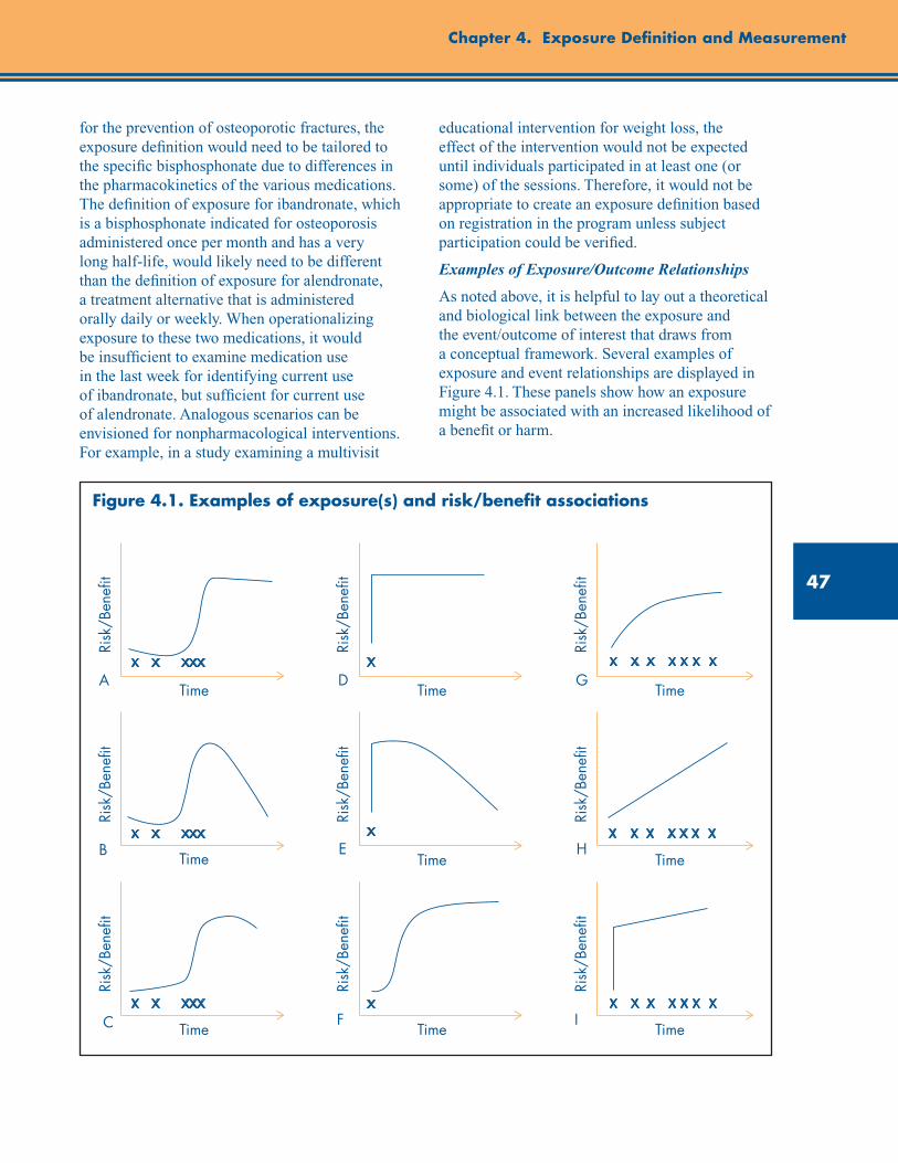
47

Chapter 4. Exposure Definition and Measurement

Time

Time

Risk

/Ben

efit

Time

Risk

/Ben

efit

Time

Risk

/Ben

efit

Risk

/Ben

efit

Time

Risk

/Ben

efit

Time

Risk

/Ben

efit

Time

Risk

/Ben

efit

Time

Risk

/Ben

efit

Time

Risk

/Ben

efit

A

B

C

D

E

F

G

H

I

for the prevention of osteoporotic fractures, the exposure definition would need to be tailored to the specific bisphosphonate due to differences in the pharmacokinetics of the various medications. The definition of exposure for ibandronate, which is a bisphosphonate indicated for osteoporosis administered once per month and has a very long half-life, would likely need to be different than the definition of exposure for alendronate, a treatment alternative that is administered orally daily or weekly. When operationalizing exposure to these two medications, it would be insufficient to examine medication use in the last week for identifying current use of ibandronate, but sufficient for current use of alendronate. Analogous scenarios can be envisioned for nonpharmacological interventions. For example, in a study examining a multivisit

educational intervention for weight loss, the effect of the intervention would not be expected until individuals participated in at least one (or some) of the sessions. Therefore, it would not be appropriate to create an exposure definition based on registration in the program unless subject participation could be verified.

Examples of Exposure/Outcome Relationships

As noted above, it is helpful to lay out a theoretical and biological link between the exposure and the event/outcome of interest that draws from a conceptual framework. Several examples of exposure and event relationships are displayed in Figure 4.1. These panels show how an exposure might be associated with an increased likelihood of a benefit or harm.

Figure 4.1. Examples of exposure(s) and risk/benefit associations

48


The first column (A–C) shows multiple exposures over time where the timing of the exposure is not consistent and stops midway through the observation period. Panel A shows a scenario in which there is a “threshold effect”—where the benefit (or risk) associated with the exposure increases after a specific amount of exposure and the level of benefit/risk is maintained from that point forward. In defining exposure under this scenario, it would be important to define the cumulative amount of exposure. For example, if evaluating the comparative effectiveness of antibiotics for the treatment of acute infection, there may be a threshold of exposure above which the medication is considered effective treatment. In this case, the exposure measurement should measure the cumulative exposure to the medication over the observation timeframe and define individuals as exposed when the threshold is surpassed (if the exposure variable is dichotomized).This situation contrasts with that in Panel B, in which the association between the exposure and the effect decreases rapidly after the exposure is removed. This type of association could be encountered when evaluating the comparative effectiveness of antihypertensive medications for blood pressure control. In this case, there may be (a) some minimum amount of exposure necessary for the medication to begin to have an effect and (b) an association between the frequency of administration and effectiveness. When the exposure is removed, however, blood pressure may no longer be controlled and effectiveness decreases rapidly. In operationalizing this exposure-event association it would be necessary to measure the amount of exposure, the frequency with which it occurred, and when exposure ended. In panel C, there is an increase in the likelihood of the outcome with each exposure that diminishes after the exposure is removed. This may represent an educational weight loss intervention. In this example, continued exposure improves the effectiveness of the intervention, but when the intervention is removed, there is a slow regain of weight. Similarly to Panel B, it is important to consider both the timing and the amount of exposure for the weight loss intervention. Because the effectiveness diminishes slowly only after the exposure is removed, it is important to consider a longer exposure window than when effectiveness diminishes rapidly.

The second column shows scenarios where the exposure of interest occurs at a single point in time, such as a surgical procedure or vaccination. The relationship in panel D shows an immediate and sustained effect following exposure. This could represent a surgical procedure and is a situation in which the measurement of exposure is straightforward as long as the event can be accurately identified, as exposure status would not vary across the observation period. Measurement of exposure in panels E and F is more complex. In panel E, the exposure is a single event in time with an immediate effect that diminishes over time. An example of this could be a percutaneous coronary intervention (PCI) where the time scale on the x-axis is measured in years. There is an immediate effect from the exposure (intervention) of opening the coronary arteries that contributes to a reduced risk of acute myocardial infarction (AMI). However, the effectiveness of the PCI decreases over time, with the risk of AMI returning to what it was prior to the intervention. In this example, it is clearly important to identify and measure the intervals at which the risk is modified by PCI. After a sufficient amount of time has passed from the initial PCI, it may not be appropriate to consider the individual exposed. At the very least, the amount of time that has passed postexposure should be considered when creating the operational definition of exposure. Panel F represents a scenario where the effect from a single exposure is not immediate but happens relatively rapidly and then is sustained. Such a situation could be imagined in a comparative effectiveness study of a vaccination. The benefits of the vaccination may not be realized until there has been an appropriate immunological response from the individual, and the exposure definition should be created based on the expected timing of the response, consistent with clinical pharmacological studies of the vaccine.

The final column of Figure 4.1 represents scenarios in which there are multiple exposures over time with different exposure-risk/benefit relationships. In each of these examples, it is important to consider the cumulative amount of exposure when developing the exposure definition. In panel G, the depicted relationship shows a dose-response in which the risk or benefit increases at a slower rate after a threshold of exposure is

49


reached. An example of this could be a behavioral intervention that includes personal counseling for lifestyle modifications to improve hypertension management. There may be a minimum number of sessions needed before the intervention has any effect and, after a threshold is reached, the incremental effectiveness of a single session (exposure) is diminished. In measuring exposure in this example, it would be important to determine the number of sessions that an individual participated in, especially if multiple exposure categories are being created. Panel H shows a linear increase in the risk/benefit associated with exposure. This example may be best illustrated by a comparative safety evaluation of the impact of oral corticosteroids on fracture risk. Continued exposure to oral corticosteroids may continue to increase the risk of fracture associated with their use. In this example, it would be necessary to characterize cumulative exposure when creating exposure definitions, as there will be a difference in the risk of those exposed to “a little” in comparison to those exposed to “a lot.” The final scenario is panel I, which shows a large change in risk/benefit upon initial exposure and then an increase in the risk/benefit at a slower rate with each subsequent exposure. For panel I, it would be most important to determine if the exposure occurred (as this is associated with the largest change in risk/benefit), and then quantify the amount of exposure.

Induction and Latent Periods

In creating exposure definitions, it is also important to consider the induction and latent periods associated with the exposure and outcome of interest.6 The induction period is the time from when the causal effects of the exposure have been completed to the start of the event or outcome. During the induction period, additional exposures will not influence the likelihood of an event or outcome because all of the exposure necessary to cause the event or outcome has been completed. For example, additional exposure to the vaccine for mumps during childhood will not increase or decrease the likelihood of getting mumps once the initial exposure to the vaccine has occurred.

The latent period is the time from when the outcome starts to when the outcome is identified.

In other words, it is the period between when the disease or outcome begins and when the outcome is identified or diagnosed. Similar to the induction period, exposures during the latent period will not influence the outcome. Practically, it may be very difficult to distinguish between latent and induction periods, and it may be particularly difficult to identify the beginning of the latent period. However, both periods should be considered and ultimately not included in the measurement of exposure. In practical terms, it is sufficient to consider the induction and latent period as a single time period over which exposures will not have an effect on the outcome. A timeline depicting multiple exposures, the induction period, the latent period, and the outcome of interest is shown in Figure 4.2.

As an example of the incorporation of both the induction and latent periods in exposure measurement, consider the evaluation of the comparative effectiveness of a cholesterol-lowering medication for the prevention of myocardial infarction. First, the induction period for the medication could be lengthy if the effectiveness is achieved through lowering cholesterol to prevent atherosclerosis. Second, there is likely a very small latent period from disease onset to identification/diagnosis. That is, the time from when the myocardial infarction starts to when it is identified will be relatively short. Any medication use that occurs during the induction and latent periods should not be included in the operational definition of exposure. For this example, it would be inappropriate to consider an individual exposed to the medication of interest if they had a single dose of the medication the day prior to the event, as this would not have contributed to any risk reduction for the event. Because of the short latent period, it would be unlikely that exposures occurred during that timeframe. Exposure should be measured during a time period when the use of lipid-lowering medications is expected to have an effect on the outcome. Therefore, the exposure definition should encompass a timeframe where the benefit of lipid-lowering medications is expected, and this should be justified based on what is known about the link between atherosclerosis and myocardial infarction and the known biological action of lipid lowering medications.

50


Each ‘x’ represents exposure to treatment/intervention of interest

Induction Period

Latent Period

x x x xx x xxx xxx xxxxxx x xxxx xx xx O

Start of outcome

Outcome Identi�ed/Diagnosed

E�ects of exposure in causing outcome of

interest complete

Figure 4.2. Timeline of exposure, induction period, latent period, and outcome

Adapted with permission from White E, Armstrong BK, Saracci R. Principles of exposure measurement in epidemiology. 2nd edition, New York: Oxford University Press Inc.; 2008.

Changes in Exposure Status Another relevant consideration when developing exposure measurement relates to changes in exposure status, particularly if patients switch between active exposures when two or more are being investigated. While medication or exposure switching may be more relevant for design and/or analysis chapters in this guidance, it is also important to consider how it might relate to exposure measurement. One of the important factors associated with medication switching when creating exposure definitions is to determine if “spillover” effects might persist from the medication that was discontinued. If this is true, it would be necessary to extend the measurement of exposure beyond the point when the switch occurred. Similarly, depending upon the effects of the intervention that was started, it is important to consider its biological effects when developing the exposure definition following a switch. Importantly, these issues do not apply only to medications; “spillover” effects can also be observed with behavioral or other interventions where the effect extends beyond the last observed contact.

Data Sources

Exposure Measurement Using Existing Electronic Data

The ability to measure exposures based on available data is also an important consideration when creating an operational definition of exposure. Is there a consistent and accurate way to identify the exposure in the dataset? If the exposure of interest is a surgical procedure, for example, is there a single code that is used to identify that procedure or is it necessary to expand the identification beyond a single code? If using more than one code, do the codes only identify the procedure of interest or is there variability in the procedures identified? For medications, the data likely reflect prescriptions or medication orders (EHR) or pharmacy dispensings (PBM or health insurer administrative claims) but not actual use. Is it necessary to know whether a given medication was taken by the patient on a particular day or time of day?

To illustrate these issues, consider the case in which the primary intervention of interest is colonoscopy. Depending on the source of the

51


data, colonoscopies may be identified with a CPT code (e.g., CPT 45355 Colonoscopy, rigid or flexible, transabdominal via colostomy, single or multiple), an HCPCS code (e.g., G0105 Colorectal cancer screening; colonoscopy on individual at high risk), or an ICD-9 procedure code (e.g., 45.23 Colonoscopy). To accurately identify this procedure, it is necessary to consider more than one type of procedure code when classifying exposure. All of these may reliably identify exposure to the procedure, but use of only one may be insufficient to identify the event. This may be influenced by the source of the data and the purpose of the data. For example, one set of codes from the list may be useful if using hospital billing data, while another may be useful for physician claims data. When making this decision, it is important for the investigators to balance the selection of the codes and the accurate identification of the exposure or intervention; creating a code list that is too broad will introduce exposure misclassification. Overall, it will be important to provide evidence on the most accurate and valid mechanism for the identification of the exposure or intervention across the datasets being used in the analysis. Researchers should therefore cite any previous validation studies or perhaps conduct a small validation study on the algorithm proposed for the exposure measurement to justify decisions regarding exposure identification. Issues in selection of a data source are covered in detail in chapter 8 (Data Sources).

Exposure Measurement via Prospective Data Collection

In addition to using existing data sources, it may be feasible or necessary to prospectively collect exposure information, in some circumstances from patients or physicians, for use in an observational comparative effectiveness study. Abstraction of (paper) medical records is a type of prospective data collection that draws on existing medical records that have not been compiled in a research-ready format.

The validity and accuracy of self-reported exposure information may depend on the type of exposure information being collected (i.e., medication use versus history of a surgical procedure), or on whether the information is focused on past exposures or is prospectively

collected contemporary exposure information. The characteristics of the exposure and the patient population are likely to influence the validity of the information that is collected. The recall of information on a surgical procedure may be much more accurate than the recall of the use of medications. For example, women may be able to accurately recall having had a hysterectomy or tubal sterilization,7 while their ability to recall prior use of NSAIDs may be quite inaccurate.8 In these examples, the accuracy of recall for hysterectomy was 96 percent while only 57 percent of those who had a dispensing record for an NSAID reported use of an NSAID—a disparity that shows the potential for exposure misclassification when using self-reported recall for medication use. In the medication example, factors associated with better recall were more recent use of a medication and repeated use of a medication. Similar to the use of other sources of data for exposure measurement, use of this type of data should be supported by evidence of its validity.

Creating an Exposure Definition

Time Window

A key component in defining exposure is the time period during which exposure is defined, often referred to as the time window of exposure. The exposure time window should reflect the period during which the exposure is having its effects relevant to the outcome of interest.6 In defining the exposure time window, it is necessary to consider the induction and latent periods. As noted in the statin example above, the exposure time window to evaluate the effectiveness of statins for preventing AMIs should be over the time period that statins can have their impact on cardiovascular events, which would be over the preceding several years rather than, for instance, over the 2 weeks immediately preceding an event.

There is no gold standard for defining the exposure time window, but the period selected should be justified based on the biologic and clinical pathways between the intervention/exposure and the outcome. At the same time,

52


practical limitations of the study data should be acknowledged when defining the exposure time window. For example, lifetime exposure to a medication may be the ideal definition for an exposure in some circumstances but most existing datasets will not contain this information. It then becomes necessary to justify a more pragmatic approach to defining exposure given the length of followup on individuals available in the dataset. A variety of approaches to defining exposure time windows have been used in both cohort and case-control studies. As highlighted in the introductory section of this chapter, investigators have selected different exposure time windows even when examining the same clinical question. In most of these examples, the choice of the exposure time window is not clearly justified. Ideally, this choice should be related back to the conceptual framework and biological plausibility of the question being addressed. However, as noted above, there are pragmatic limitations to the ability to measure exposure, and in the case where selection of the exposure time window is arbitrary or limited by data, sensitivity analyses should be performed in order to evaluate the robustness of the results to the time window.

Unit of Analysis

When creating a definition for an exposure measurement, it is necessary to consider the unit of analysis for the study and the measurement precision possible within the constraints of the data. The nature of the intervention largely dictates the appropriate unit of analysis. If the intervention of interest does not vary with time, the unit of measurement can be defined at the patient level because exposure status can be accurately classified for the duration of the analysis. This may be the case for surgical procedures or other interventions that occur at a single point in time and that have a persistent effect (panel D in Figure 4.1). For other interventions or exposures, units of analysis may be more appropriately defined in terms of person-time, as the exposure status of individuals may vary over the course of the study period. This is a common approach for defining exposure in studies of medication treatment outcomes, as medication regimens often involve addition or discontinuation of medications, suboptimal adherence, dosage changes, or other factors that may cause changes in exposure to the intervention of interest.

Measurement Scale

The scale of the exposure measure should be operationalized in a manner that makes the most use of the information available. The more precisely an exposure is measured, the less measurement error. In many observational CER studies, the intervention of interest can be measured as a dichotomous variable (i.e., exposed or not exposed). For example, an individual either had or did not have a surgical procedure.

For other types of exposures/interventions in observational CER, it may be desirable to measure exposure as a continuous covariate, particularly when there is a dose-response relationship (e.g., panel H of Figure 4.1). However, the ability to operationalize exposure as a continuous variable may be limited by the availability of the exposure data and uncertainty surrounding its accuracy. Under cases of nondifferential misclassification in a continuous exposure variable, the degree of bias toward the null hypothesis is impacted by the precision of the exposure measurement, not by the bias in the exposure measure.9 Therefore, if the accuracy of the classification can be improved by using an alternative approach to scaling (e.g., measuring exposure as a categorical variable), it is possible to introduce less bias towards the null than is associated with the continuous measure. For example, if an individual was dispensed three separate prescriptions, each with a 30-day medication supply, she may not have taken the entire 90-day supply, but it is likely that she took more than a 60-day supply. In this case, an ordinal scaling of exposure measure for the number of doses of a medication may be preferable when it may not be possible to accurately identify the actual number of doses taken.

Dosage and Dose-Response

The concept of dose is an important consideration for the measurement of exposure in observational comparative effectiveness studies. Indeed, as shown in each of the event and exposure relationships depicted in the first column of Figure 4.1, the cumulative dose, or total amount of exposure over a specified time period, is often optimal for adequately defining exposure. To calculate cumulative dose, three elements of exposure are necessary: (1) the frequency of exposure, (2) the

53


amount/dose of each exposure occurrence, and (3) the duration of exposure. Importantly, the concept of dose is applicable not only to medications but also to health services interventions that require multiple sessions, visits, or interactions. With respect to medications, it may be possible to obtain all the information necessary to calculate cumulative exposure to a specific prescribed medication from pharmacy claims data, where such data are typically collected for billing purposes. Information on the dose of each dispensed medication in the United States is available through the National Drug Code (NDC) for the product. Upon extracting information on the strength of each dose from the NDC code, dose strength can be combined with quantity dispensed and days’ supply to determine the amount of each exposure event and the frequency of the exposure. When using data outside of the United States, the World Health Organization’s Anatomical Therapeutic Chemical (ATC) Classification System may be used to measure exposure based on defined daily doses (DDDs), which are the assumed average maintenance doses per day for a drug used based on its main indication in adults (http://www.whocc.no/ddd/definition_and_general_considera/). Cumulative dose exposure definitions can be used to explore a dose-response relationship between the exposure and the event. Cumulative dose can also be used to determine if there is a threshold effect.

While cumulative exposure may be an important concept in many comparative effectiveness studies of medications, it may not be as relevant in other studies. There may be medications where use is so intermittent that it is not possible or relevant to capture cumulative exposure. This is also the case with one-time interventions like surgical procedures, where the concept of dose has less meaning.

Modes of administration and different dosage forms can present complexities in operationalizing a definition of exposure when using administrative data. For example, a study using observational data to examine the effectiveness of hydrocortisone as a treatment for irritable bowel disease (IBD) would seek to identify only those prescriptions for hydrocortisone that were used for IBD treatment. This could be accomplished by focusing only on specific dosage forms that would be used in

the treatment of IBD, to avoid misclassification of exposure to other forms of hydrocortisone. Therefore, the definition of exposure needs to be specific to the exposure of interest and avoid misclassification due the availability of other dosage forms or routes of administration. Conversely, it may be necessary to create a wider definition that looks across multiple dosage forms if the question of interest is focused on a systemic effect of a medication that could be delivered in multiple forms.

Similarly, behavioral factors might modify the effect of the observed association. These can include factors such as medication adherence, which may be considered in the definition of exposure. Several examples of observational studies of medications exist that required a specific level of adherence prior to categorizing an individual as exposed. For example, a study may require that an individual use at least 75 percent of their prescribed medication on a regular basis before they are considered exposed. This is most frequently operationalized by calculating the medication possession ratio and determining if it crosses a threshold before categorizing an individual as exposed; again, the approach should be linked to the hypothesized mechanism of effect. More detailed descriptions of approaches to analyzing medication compliance and persistence using retrospective databases are available.10 Currently, there is no gold standard that indicates what amount of a given medication needs to be used prior to its having its effect. The choice of a threshold should be supported by a rationale for the level that is selected. In addition, while a measure of adherence can be used as a measure of amount of exposure or the dose, it is also important to consider differences in adherent versus nonadherent patients. That is, patients who are adherent to their treatment regimens may be systematically different from those who are nonadherent to treatment. These differences impact the outcomes being measured, independent of the exposure measurement. These factors should be considered when deciding whether or not to incorporate adherence as part of the exposure measure.

54


Precision of Exposure Measure

The source of the data being used for the analysis can limit the ability to precisely characterize exposure. For instance, EMR data may provide only information on medication orders or active drug lists, which would not allow for accurate classification of exposure on a daily basis. Attempting to do so would likely introduce high levels of exposure misclassification. The use of administrative claims data that provide information on medication dispensing may provide a more accurate estimate of the use of medications on a more routine basis. However, this data source will only reflect the dispensing of medications and not actual medication use. Multiple dispensings may provide greater assurance that the individual is being routinely exposed to the medication but cannot guarantee the patient has taken the medication. A more accurate measure of medication use would be information on medication assays. However, only a select number of medications have routine labs drawn to ascertain levels, and this does not present a practical solution in most observational CER projects. Thus, while dispensing data may provide a more accurate measurement on a more routine basis than other sources of data, assumptions about actual use are still inherent in the use of these data to determine exposure status. Investigators should understand the benefits and limitations associated with the data source being used, and should ensure that the exposure can be measured with sufficient precision to answer the research question of interest.

Exposure to Multiple Therapies

A complexity in observational CER is the lack of control over other medications used by individuals in the study, and the fact that exposure to other medications is unlikely to be randomly distributed among the exposed and unexposed groups. Therefore, when characterizing the primary exposure of interest, it is also important to consider the influence of other exposures on the outcome. Multiplicative or additive effects may be possible. For example, it may be important to consider the joint antihypertensive effects of various classes of antihypertensive medications in a comparative effectiveness study, as these medications will frequently be used in combination.

Issues of Bias

Measurement Error

In observational CER studies, both nondifferential and differential measurement error can introduce bias. Differential misclassification occurs when the error in the exposure measurement is dependent on the event of interest. This measurement error can result in biased estimates either away from or towards the null, making the observed association look stronger or weaker than the true underlying association. Differential measurement error can even lead to observed associations that are in the opposite direction of the true underlying association. Nondifferential measurement error occurs when errors in the measurement of exposure are proportionally the same in both the group that does and the group that does not experience the outcome of interest. For the most part, this type of measurement error will bias the results toward the null hypothesis, causing an underestimate of the true effect of the association.

The goal of any measurement of exposure is to minimize the amount of misclassification that occurs as part of the study design. For dichotomous measures, investigators should attempt to maximize the sensitivity and specificity of the measure to minimize the amount of misclassification. One source of misclassification in observational studies results from the failure to account for changes in exposure to medication during the observational period. Such a situation would support a person-time unit of analysis. In cohort studies, exposure status may be determined at a single point in time; this may not be reflective of use of the medication over the study period. There may be frequent changes to medication regimens during followup; simply classifying patients as exposed or not exposed at the onset of the study period can lead to a high degree of misclassification that is nondifferential.11 This may be true for exposures that occur intermittently and those that occur on a more frequent basis but are associated with high rates of nonadherence.

The potential influence on misclassification of choices made in operationalizing the exposure definition should be considered by the investigators when designing the study. For example, what is the potential for misclassification of exposure with a given choice of the exposure

55


time window? Will selecting a relatively short exposure time window produce a high degree of misclassification of exposure that would potentially lead to a biased effect estimate? Investigators should consider the practical limitations of the data and the influence that these limitations might have on the measurement error. There are many other potential sources of misclassification when measuring exposure, including: (1) measurement of exposure during induction or latent periods, (2) failure to incorporate the sustained effects of the medication or other intervention when creating an exposure definition, and (3) use of health care services not captured in the data source. To expand upon the latter issue, data from health systems like insurance companies often lack the ability to capture out-of-system health care utilization. Many administrative claims databases also do not capture in-hospital medication use. Such exposures will not be recorded in the data source and may lead to misclassification known as immeasurable time bias, which occurs when exposure during a period such as hospitalization cannot be measured, and is not accounted for in the analysis of study data.12

Over-the-counter (OTC) medications present a scenario in which misclassification is particularly problematic. Measurements based on administrative or EMR data will underestimate the use of OTC products and lead to misclassification of exposure to those medications. The inability to measure exposure during the observation period can also be problematic if the available data do not fully capture all sources of exposure. The use of OTC medication as an exposure is but one example of not being able to accurately capture all exposures, but this can occur in other circumstances. For example, hospital billing data will usually not include detailed information on the medications used during the inpatient stay, which can lead to misclassification of exposure during a hospitalization. So while the individual is using health care that is captured by the data source, there is insufficient detail to accurately capture exposure. Therefore, investigators should determine if there are periods of time in which

the exposure status of individuals cannot be ascertained in the data being used in the analysis, and should evaluate the potential impact on exposure measurement.

A specific type of measurement bias for exposures that has received a lot of attention in recent literature is immortal time bias.13 This bias occurs when person-time is inappropriately assigned to an exposure category. A common example of immortal time bias occurs when exposure is defined based on the requirement of two dispensings of a medication. The time period between those two dispensings represents an immortal period, in which events among exposed individuals (e.g., death) would not be attributed to exposure because the individuals exposed to only one dispensing have not qualified as exposed according to the definition. Clearly, this introduces a bias into the observed association and is remedied by correctly classifying person-time from the beginning of the exposure period (i.e., the first dispensing in this example). For time-based, event-based, and exposure-based cohort definitions, the bias in the rate ratio that arises from the immortal time increases with duration of immortal time.13

Conclusion

In this chapter, we have introduced many issues to consider in creating definitions for exposure when conducting CER using observational data. The operationalization of exposure should be guided by the clinical pathways/conceptual framework that motivate a CER question, knowledge of the characteristics of the exposure/intervention and outcome of interest, awareness of the level of detail on exposure in a dataset and of options for characterizing exposure, and deliberation over approaches to limit the potential for bias and measurement error. Below, we have created recommendations in the form of a checklist that encompasses many of the key considerations raised in this chapter to guide the operationalization of exposure.

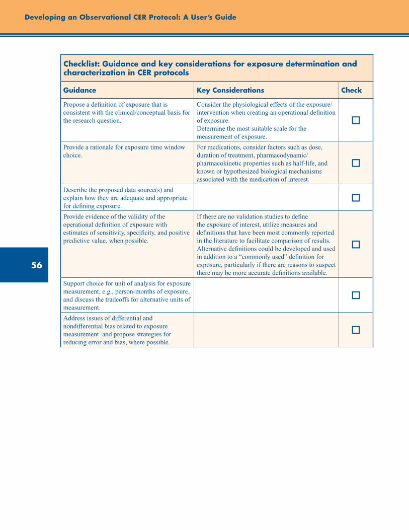
56


Checklist: Guidance and key considerations for exposure determination and characterization in CER protocols


Propose a definition of exposure that is consistent with the clinical/conceptual basis for the research question.

Consider the physiological effects of the exposure/intervention when creating an operational definition of exposure. Determine the most suitable scale for the measurement of exposure.

o

Provide a rationale for exposure time window choice.

For medications, consider factors such as dose, duration of treatment, pharmacodynamic/pharmacokinetic properties such as half-life, and known or hypothesized biological mechanisms associated with the medication of interest.

o

Describe the proposed data source(s) and explain how they are adequate and appropriate for defining exposure.

o

Provide evidence of the validity of the operational definition of exposure with estimates of sensitivity, specificity, and positive predictive value, when possible.

If there are no validation studies to define the exposure of interest, utilize measures and definitions that have been most commonly reported in the literature to facilitate comparison of results. Alternative definitions could be developed and used in addition to a “commonly used” definition for exposure, particularly if there are reasons to suspect there may be more accurate definitions available.

o

Support choice for unit of analysis for exposure measurement, e.g., person-months of exposure, and discuss the tradeoffs for alternative units of measurement.

o

Address issues of differential and nondifferential bias related to exposure measurement and propose strategies for reducing error and bias, where possible.

o

57


References 1. Hubbard R, Tattersfield A, Smith C, et al. Use of

inhaled corticosteroids and the risk of fracture. Chest. 2006;130:1082-8.

2. Johannes CB, Schneider GA, Dube TJ, et al. The risk of nonvertebral fracture related to inhaled corticosteroid exposure among adults with chronic respiratory disease. Chest. 2005;127:89-97.

3. Lee TA, Weiss KB. Fracture risk associated with inhaled corticosteroid use in chronic obstructive pulmonary disease. Am J Respir Crit Care Med. 2004;169:855-9.

4. Miller DP, Watkins SE, Sampson T, et al. Long-term use of fluticasone propionate/salmeterol fixed-dose combination and incidence of nonvertebral fractures among patients with COPD in the UK General Practice Research Database. Phys Sportsmed. 2010;38:19-27.

5. Vestergaard P, Rejnmark L, Mosekilde L. Fracture risk in patients with chronic lung diseases treated with bronchodilator drugs and inhaled and oral corticosteroids. Chest. 2007;132:1599-607.

6. Rothman KJ. Induction and Latent Periods. Am J Epidemiol. 1981;114(2):253-9.

7. Green A, Purdie D, Green L, et al. Validity of self-reported hysterectomy and tubal sterilisation. The Survey of Women’s Health Study Group. Aust N Z J Public Health. 1997;21:337-40.

8. West SL, Savitz DA, Koch G, et al. Recall accuracy for prescription medications: self-report compared with database information. Am J Epidemiol. 1995;142:1103-12.

9. White E, Armstrong BK, Saracci R. Principles of exposure measurement in epidemiology. 2nd ed., New York: Oxford University Press Inc.; 2008.

10. Peterson AM, Nau DP, Cramer JA, et al. A checklist for medication compliance and persistence studies using retrospective databases. Value in Health. 2007;10(1):3-12.

11. Ray WA, Thapa PB, Gideon P. Misclassification of current benzodiazepine exposure by use of a single baseline measurement and its effects upon studies of injuries. Pharmacoepidemiol Drug Saf. 2002;11:663-9.

12. Suissa S. Immeasureable time bias in observational studies of drug effects on mortality. Am J Epidemiol. 2008;168(3):329-35.

13. Suissa S. Immortal time bias in pharmacoepidemiology. Am J Epidemiol. 2008;167(4):492-9.

59

Abstract

This chapter discusses considerations for comparator selection in observational comparative effectiveness research (CER). Comparison groups should reflect clinically meaningful choices in real world practice and be chosen based on the study question being addressed. Recognizing the implications and potential biases associated with comparator selection is necessary to ensure validity of study results; confounding by indication or severity and selection bias (e.g., healthy user bias) is particularly challenging, especially with comparators of different treatment modalities. Confounding by indication can be minimized by choosing a comparator that has the same indication, similar contraindications, and a similar treatment modality (when possible). In fact, comparing a treatment with a clinically meaningful alternative treatment within the same or a similar indication is the most common scenario in CER, and also typically the least biased possible comparison.When carefully planned, comparisons of different treatment types are possible with adequate study design, execution, and appropriate analytic methods. However, we note that certain comparisons or study questions may not be feasible or valid to be answered in observational CER studies due to potentially uncontrollable bias. Other aspects to consider when choosing a comparator include clearly defining the indication, initiation period, and exposure window for each group. The appropriate dose/intensity of each exposure should be as comparable as possible and nonadherence should be considered (although not necessarily adjusted for). This chapter concludes with guidance and key considerations for choosing a comparison group for an observational CER protocol or proposal.

Chapter 5. Comparator SelectionSoko Setoguchi, M.D., Dr.P.H.

Duke Clinical Research Institute, Durham, NC

Tobias Gerhard, Ph.D. Rutgers University, New Brunswick, NJ

Introduction

In comparative effectiveness research (CER), the choice of comparator directly affects the validity of study results, clinical interpretations, and implications. When formulating a research question, therefore, careful attention to proper comparator selection is necessary.

Treatment decisions are based on numerous factors associated with the underlying disease and its severity, general health status or frailty, quality of life, and patient preferences—a situation that leads to the potential for confounding by indication or severity and selection bias. Recognizing the implications and potential biases associated with comparator selection is critical for ensuring the internal validity of observational CER studies. The first section of this chapter, “Choosing the Comparison Group in CER,” begins by describing these biases, and discusses the potential for bias associated with different

comparison groups (e.g., no intervention, usual care, historical controls, and comparison groups from other data sources).

Defining the appropriate dose, intensity of treatment, and exposure window for each comparator group is also critical for ensuring the validity of observational CER.The second section of this chapter, “Operationalizing the Comparison Group in CER,” discusses these considerations for operationalizing comparison groups, and concludes with special considerations that apply to CER studies comparing different treatment modalities.

Choosing the Comparison Group in CER

Link to Study Question

In CER, comparison groups should reflect clinically meaningful choices in real world practice. The

60


selection of comparison group(s) is thus directly linked to the study question being addressed. Importantly, some comparisons or study questions may not be feasible or valid to be answered in observational CER studies due to expected intractable bias or confounding.

Consequences of Comparator Choice

Confounding

Confounding arises when a risk factor for the study outcome of interest (benefit or harm) directly or indirectly affects exposure (e.g., treatment assignment). Because clinicians routinely make treatment decisions based on numerous factors associated with the underlying disease and its severity, confounding by indication or severity poses a significant threat to the validity of observational CER (see chapter 2 for a detailed discussion). It is therefore vital to appreciate the relationship between confounding and comparator choice. The existence and magnitude of confounding for any given pair of treatments and outcome is directly affected by the choice of the comparator. For example, when comparing the adverse metabolic consequences of individual antipsychotic medications in patients with schizophrenia or bipolar disorder, body mass index (BMI) is an important potential confounder because it is a strong and established risk factor for adverse metabolic outcomes such as type 2 diabetes and plausibly affects the choice of agent. However, the expected magnitude of confounding by BMI strongly depends on the specific drugs under study. A comparison between aripiprazole, an antipsychotic agent with a relatively favorable metabolic safety profile, and olanzapine, an agent that exhibits substantial metabolic adverse effects, may be strongly confounded by BMI, as most clinicians will try to avoid olanzapine in patients with increased BMI. In contrast, a comparison between aripiprazole and another antipsychotic agent with less metabolic concerns than olanzapine, such as ziprasidone, may be subject to confounding by BMI but to a much lesser degree.

The magnitude of potential confounding generally is expected to be smaller when the comparator (1) has the same indication, (2) has similar contraindications, (3) shares the same treatment modality (e.g., tablet or capsule), and (4) has

similar adverse effects. Therefore, selection of a comparator of the same treatment modality (e.g., drug vs. drug) and same class within the modality (e.g., b-blocker) may result in less confounding than comparison across different treatment modalities or drug classes in general. However, many exceptions exist (e.g., the antipsychotic example above), and assessments should be made individually for each treatment comparison of interest. To understand the potential consequences of comparator choices on confounding, a thorough understanding of clinical practice, data sources, and methods is necessary. If suspected confounders are available in the data, investigators can empirically evaluate the extent that the distribution of these confounders differs between the exposure of interest and the comparator(s).

Propensity score distribution plots by exposure status are particularly useful in this context because they allow simple evaluation of the joint differences of many potential confounders between treatments. Areas of nonoverlap between the propensity score distribution in the treatment and comparator group identify individuals who, based on their baseline characteristics, would either always or never be exposed to the treatment under study, and thus cannot be compared without potential for significant bias.1 If potential confounders are not available in the data, practical clinical insight and qualitative health services research should be used to form an impression of the expected magnitude of confounding for a given treatment comparator pair. Sensitivity analyses should then be used to quantify the effects of such unmeasured confounding under different sets of assumptions. (See chapter 11 for further discussion).2

While a thorough understanding of the impact of comparator choice on the expected magnitude of confounding is critical, the comparator choice should be primarily driven by a comparative effectiveness question that has been prioritized by the informational need of the stakeholder community. We do not advocate for minimizing confounding through a comparator choice that might change the original study question. A critical assessment of the expected magnitude of confounding for the comparison group of choice, however, should guide decisions of study design, particularly (1) the need to obtain additional

61

Chapter 5. Comparator Selection

covariate information if confounding is judged to be uncontrollable in the available data (despite use of advanced analytic methods, such as propensity scores and other approaches described further in chapter 10); and (2) the need for randomization if confounding is judged uncontrollable in any observational study design even with additional data collection (despite use of advanced analytic methods).

Misclassification

Misclassification is one of the major threats to validity in observational CER studies and is discussed in more detail in chapter 4 and chapter 6. In the context of selecting comparison groups for CER, it is important to appreciate that exposure misclassification is often not binary but rather more complex, as each group (exposure and comparison group) typically represents an active treatment, and as nonuse of the exposure treatment does not imply use of the comparator treatment. For example, consider an epidemiologic study of the effect of treatment A (exposed) on outcome Y. If nonexposure to A is the comparison of interest, this category of exposure is directly dependent on exposure to A, as each subject is either exposed or unexposed to A. Therefore, misclassification of exposure A would affect the number of those identified as having A (exposure group) and those without A (comparison group). However, in a CER comparing the effects of drug A versus drug B, misclassification of exposure A would not necessarily affect the number of patients with drug B (comparison), as exposure to A is largely independent of exposure to B.

In observational CER, the assessment of exposure misclassification has to be made for the exposure and comparison group independently, and it is important to recognize that the degree of misclassification can be different in the two groups, especially when the comparison groups come from different treatment modalities (e.g., drug vs. device). Generally, the more similar the treatment under study and the comparator are in terms of treatment modality and dosage form, the less likely it is that exposure or comparator misclassification is different. For example, there is little reason to expect that the degree of exposure misclassification would substantially differ between the comparison groups in a claims-based study comparing two oral pharmacologic treatments, as information on

drug exposure is equally retrieved from pharmacy billing claims for both groups. However, in a comparison between an oral medication for chronic diseases and a long-term injectable, the degree of misclassification may be significantly larger for patients treated with the oral dosage form mainly due to the different way of administering the drugs (patient vs. physician) and sources of information (drug dispensing records vs. office visit records).

Spectrum of Possible Comparisons

Comparison interventions may include medications, procedures, medical and assistive devices and technologies, behavioral change strategies, and delivery systems. Under certain circumstances, no intervention, usual care, historical controls, or comparison groups from other data sources may be appropriate and justified for comparative effectiveness questions. It is again important to recognize that comparator choice is directly linked to the comparative effectiveness question under study. In this section, we will discuss methodological considerations for the choice of different comparison groups.

Alternative Treatments

Comparison of a treatment with a clinically meaningful alternative treatment within the same or a similar indication is the most common scenario in CER and also typically the least biased comparison. Multiple modalities and options are often available to treat or diagnose the same condition or indication. Therefore, in many clinical circumstances, “no treatment” or “no testing” may not meet usual standards of care, and comparisons with alternative treatment options may be more clinically meaningful and methodologically valid. Comparison with alternative treatment or testing within the same or similar indication is usually a better choice from a methodologic standpoint than comparison with an untreated/not tested group, as confounding by indication may be nonexistent or at least reduced in the former comparison. However, when different treatments or testing modalities are recommended for patients with varying levels of severity of the underlying condition, comparisons within the same indication may still result in confounding by severity when not adequately controlled through design or analysis.

62


No Treatment

Comparison with no treatment or no testing may be appropriate in certain clinical situations. When a comparison with no treatment is a clinically appropriate question, researchers may define the no-treatment group as the absence of exposure or, alternatively, as the absence of exposure and use of an unrelated treatment (an active comparator) within the same source population. Active comparators are users of treatments that are not associated with indications for the exposure treatment and, importantly, have no effect on the outcome of interest (supported by available evidence).3 The goal of employing active comparators who are likely to have similar characteristics with the exposure treatment users is to remove or minimize bias due to unobserved or incompletely observed differences between treated and untreated patients. For example, in a study assessing the risk of cancer in statin use,4 users of glaucoma drugs (like statins, a preventive medication class less likely to be used in frail elderly patients5), were employed as an active comparison group with an aim to control for potential bias due to statin users’ being more health-seeking and more adherent to screening procedures and other recommendations than nonusers.3 While this approach is likely to have greater applicability to questions of safety than CER, it may warrant consideration in addressing some CER questions.

Another important consideration, when “no treatment” is appropriate as a comparison group, is how to select time zero for the no-treatment group. When an active comparison group is employed, the choice of time zero is naturally determined as the start of the active treatment. When a no-treatment comparison group is selected, one way to choose time zero is to identify the day a health care professional made a no-treatment decision. This way, both cohorts will have a meaningful inception date for the start of exposure status and outcome identification. However, in many clinical scenarios, such a date may not exist, as no treatment is often considered for patients in early stage of disease progression. Additionally, even if such a date exists, it may be difficult to identify in the available data. A second way to handle this is to allow a different time zero for the treatment and no-treatment groups (time-varying exposure

status), and to carefully consider allocation of person-time to avoid immortal person-time bias.6 In a third design strategy, it is possible to align the person-time and events appropriately by a choice of time scale in a Cox proportional hazard regression.7 Researchers should realize that the choice of time zero in a no-treatment comparison group can induce bias, and careful considerations are needed to select clinically appropriate time zero and/or to avoid immortal person-time bias, as choice for no treatment is often related to disease stage and progression and therefore outcomes.

Usual or Standard Care

When a new treatment or testing modality becomes available, patients and health care providers may ask a question about the effectiveness of the new treatment when added to the usual or standard care. While this question is legitimate and important, operationalizing the question into an answerable research question requires a clear definition of “usual or standard care,” including a valid operational definition of when usual care was initiated. The standard care could be no treatment or no testing, a single treatment or testing, or a set of existing treatment or testing modalities. In the real world, patients are self-selected or selected by their physicians into various treatments for reasons (disease severity, contraindications, socioeconomic status, overall prognosis, comorbidities, anticipation of adverse events, quality of life issues, coverage design, and provider preference) that are often associated with the outcomes. As the first step, researchers may have to describe and recognize the diversity in the existing treatment regimens or testing modalities in usual care. Then, a thorough understanding of how treatment selection is made in the real world is necessary for accurate definition and operationalization of “usual or standard care.” Note that standards of care may vary across geographic regions and treatment settings, or may change over time. It is important to recognize that a “waste basket definition” of “usual or standard care” (any users of any existing treatments) should be avoided for the reasons mentioned above. Lastly, it is important to recognize that comparisons may be impossible when suspected or observed differences between the exposure and comparison groups are associated with the outcome of interest and cannot be adequately adjusted for and controlled through study design or analytic

63


approaches (i.e., in situations with intractable confounding).

Historical Comparison

A historical comparison group may seem to be a natural choice when there is a dramatic shift from one treatment to another (e.g., rapid diffusion of a new treatment in practice, or sudden change in treatment utilization due to evidence or practice changes). It may also be the only choice when there is such strong selection for the new treatment that it is uncontrollable even with rigorous methods and randomization, is unethical, or is not realistic for other reasons. However, in any situation, the use of a historical control needs to be justified after considering associated methodological issues.

Historical comparison groups will still be vulnerable to confounding by indication or severity when information on indication or severity is unmeasured. To overcome this limitation, an instrumental variable (IV) analysis using calendar time as an instrument has been applied.8-11 Even in analyses using calendar time as an IV, confounding by indication may still arise if time is associated with severity and outcomes of interest. When historical comparison groups are used, any changes in the severity or operational definitions of the target condition as well as changes in outcome rates or outcome definitions over time could introduce bias into the analyses and must be adequately controlled. If these time-varying factors are not controllable, the use of a historical comparison group cannot be justified.

Comparison Groups From Different Data Sources

Situations may arise when the desired comparison groups are not available within the same data sources as the exposure groups. Multiple data sources can be linked to enhance the validity of observational comparative effectiveness and safety studies.12-14 Registries have been linked to other data sources (e.g., Medicare data, HMO administrative data) to identify long-term clinical outcomes.12-13 Although device or drug registries may provide detailed data on the use of drugs, biologics, and devices and on the severity of underlying disease and related comorbidities, registries are often limited to one product or a class of product, and therefore may not contain information on the comparison group of interest.

In this situation, other existing disease, drug, or device registries have been considered to identify comparison groups.13-14 Suppose, for example, that researchers linked a registry for a device and a separate clinical registry for the target condition to Medicare data to identify the exposure and comparison group within Medicare-linked patients. In this study, both exposure and comparison groups are obtained from the same source population (Medicare); however, sampling of each group may be different, as each registry may have collected data through a different mechanism.

At least two potential issues need to be considered when using comparison groups from different databases: (1) residual confounding and (2) generalizability (a concept related to target populations). Residual confounding could arise in comparisons across different data sources for two reasons. First, residual confounding might occur due to incomparability of information in exposure and comparison groups. It is common that information about the patient, exposure or comparison treatment, and/or outcome is collected differently across different databases, and therefore is not comparable between the exposed group and comparison group. This noncomparability of available information for confounder adjustment may lead to increased residual confounding when common variables available across the databases are limited. Second, increased residual confounding is also possible because exposed patients and comparison patients may be different in observed and unobserved domains because they are sampled differently or because they may come from a different source population.15 In the previous example of a study using two registries linked to Medicare, it is possible that two groups are different with respect to demographic characteristics and/or geographic regions even though they are all Medicare patients. Because many factors associated with socioeconomic status that might be associated with treatment choice and outcomes are unmeasured, comparisons across different databases could cause increased residual confounding. The problem may be minimized by adequate consideration of hospital clusters and with attempts to control for surrogates for socioeconomic status.

64


A separate issue of generalizability could arise as estimation of a causal effect in observational studies or trials necessitates a target population16,17 and many methods of adjusting for confounding such as standardization and inverse-probability-of-treatment-weighting are based on the idea of estimating average treatment effect in a target population.18-19 Describing a finite population that the effect estimates would be computed for and apply to may be challenging when exposure groups and comparison groups come from different databases. In the previous example study of device and clinical registries linked to Medicare, the finite target population could be defined as Medicare patients. However, when each registry is not a random sample of Medicare patients but selects a very different sample, the generalizability of the findings from the study (assuming that residual confounding is taken care of) could be complex to understand. When using comparison groups from multiple databases, researchers need to clearly describe the methods and consider and discuss the issues outlined here to increase the validity and interpretability of their findings.

Operationalizing the Comparison Group in CER

A number of important considerations regarding the definition, measurement, and operationalization of exposure are discussed in chapter 4, and apply equally to the operationalization of comparator group(s). Below, we discuss issues that specifically affect the operationalization of the comparator(s).

Indication

As discussed, the overriding consideration that should guide comparator choice is the generation of evidence that directly informs decisions on treatments, testing, or health care delivery systems as defined in the study question. Thus, another treatment used for the same indication as the exposure treatment will typically be used as the comparison group for assessing comparative effectiveness. When a treatment and a comparison treatment have a single and specific indication, such as insulin and glitazones for diabetes, and are not commonly used off-label for other conditions,

the indication may simply be inferred by the initiation of the treatment. However, because many treatments, particularly drugs, are approved for and/or clinically used to treat multiple indications, the appropriate indication will often have to be ensured by defining the indication and restricting the study population. Defining the indication typically involves requirement for the presence of certain diagnoses, the absence of diagnoses for alternative indications, or a combination of both,20 but also depends on how the comparative effectiveness question was formulated, that is, what the target population is and whether the population is defined by indications and contraindications. It is important to recognize that restriction of the study population to patients with the same indication does not necessarily remove confounding by severity.21

For clinical effectiveness or safety questions, nonusers or users of other treatments (active comparators) with different indications may be considered as comparison groups. For nonuser comparisons, restriction of nonusers to those with similar indications is advisable. However, such restriction is unlikely to fully address healthy user bias, and randomization may be necessary to study such clinical effectiveness questions.22 Active comparators, as explained in the previous section, are generally more appropriate, particularly for safety questions, and their use may reduce or eliminate healthy user bias.

Initiation

There are well-recognized advantages in studying new initiators of treatments, which is why the new user design is considered the gold standard in pharmacoepidemiology.23 Specifically, a new user design prevents under-ascertainment of early events and avoids problems arising from confounders that may be affected by treatment in prevalent users.23 It also prevents bias arising from prevalent users being long-term adherers who may also follow other healthy behaviors.4, 24 See chapter 2 for a complete discussion of the new user design.

Inclusion of prevalent users may be justified, however, when outcomes of interest are extremely rare or occur after long periods of use, so that a new user design may not be feasible. The benefits and potential bias arising from the inclusion

65


of prevalent users should be carefully weighed, and the evidence generated by the design may be considered hypothesis generating rather than hypothesis testing. Comparisons between incident and prevalent users should be avoided. As for the exposure of interest, introduction of immortal time through incorrect classification of person-time has to be avoided for both the exposure and comparison group.6

Exposure Time Window

As discussed in chapter 4, each exposure group requires the definition of an exposure-time window that corresponds to the period where therapeutic benefit and/or risk would plausibly occur, and that could substantially differ from the actual exposure to the treatment.25 Importantly, this exposure window can differ between the exposure of interest and the comparator(s), and the determination of the appropriate time window should be made individually for each group based on the pharmacologic or therapeutic profile of the intervention. Time-to-event analyses including Cox proportional hazard regression may be appropriate when comparing two treatments with expected differences in the timing of beneficial or safety outcomes.

In situations where there is uncertainty regarding the appropriate duration of the exposure window(s), sensitivity analyses should be performed to assess whether results are sensitive to different specifications of the exposure window(s). In addition, performing both an as-treated analysis (where patients are censored at the end of the exposure-time window) as well as an intention-to-treat (ITT, i.e., first-exposure-carried-forward analysis) may help understand the impact of nonadherence, misclassification, and censoring on the observed results. However, it is important to recognize that the utility of ITT analyses are generally limited when assessing long-term effects. Conversely, as-treated analyses could cause bias due to informative censoring (when stopping is associated with the outcome of interest), so methods to model and address informative censoring should be considered.26 Comparisons between implantable devices and drug treatments present a special case of ITT analysis, as the “as treated” and ITT specifications will result in very similar exposure durations for devices (because

of the inability to discontinue an implantable device other than in cases of device failure/removal), but may result in dramatically different exposure durations for drug treatments with high discontinuation rates; this must be taken into account when determining the followup periods that should be included in study analyses for both comparators.

Nonadherence

Nonadherence to prescribed medications is common and a recognized problem for the health care system. Nonadherence may be different between treatment and comparator(s) due to differences in complexity of dosing regimens, side effect profiles, and patient preferences. Because CER aims to compare benefits and harms of different interventions in real-world conditions, treatment effects should be compared at adherence levels observed in clinical practice rather than adjusting for the difference in adherence. When adherence to a comparator is lower than adherence to the exposure treatment of interest and both treatments have similar benefits when used as prescribed, the benefit of the exposure treatment will be superior due to better adherence. Since the aim of the study is estimation of drug effects in real world situation and patients, the results are valid. However, it is important to report adherence measures for each of the treatments as part of the study results so that findings can be interpreted under appropriate consideration of the observed adherence patterns. Requiring run-in periods to assure that adherence is satisfactory and more equal across groups27 may be problematic because such practice could introduce immortal time bias (if the run-in period is included in the analysis) or be unable to estimate effects in the early phase of treatment (if the run-in period is excluded from analysis).

Dose/Intensity of Drug Comparison

After the study population has been defined and exposure and comparison groups have been chosen, it is important to appreciate the effects of dose on outcomes. When there is a dose effect on the outcome of interest, the dose of the exposure and comparison drug(s) will drive the direction and the magnitude of effects. A lower-dose comparison drug may make the study drug look more effective,

66


while a higher-dose comparison drug may make the study drug look safer. Therefore, researchers first should assess and report the dose in each group. When appropriate and possible, comparisons should be made for exposure and comparison group at various clinically equivalent dose levels. It is important to recognize that comparisons between different dose levels may potentially result in confounding by severity, as higher doses are likely to be given to patients with more severe disease.

Considerations for Comparisons Across Different Treatment Modalities

Many principles in the previous sections are discussed primarily in the context of medications. In this section we focus specifically on the important methodological issues for comparisons across different treatment modalities.

Confounding by Indication or Severity

For some conditions, drugs may be used for patients with a milder disease, and surgery may be reserved for those with more severe disease. In many circumstances, a step-wise approach to treat a condition may be recommended or practiced (e.g., consider a surgery if a drug treatment failed). For other diseases like cancer, early-stage disease may be treated with surgical procedures, whereas more advanced disease may be treated with chemotherapy and/or radiation or combinations of multiple modalities. Although not different from within-drug or within-procedure/surgery comparisons, understanding the recommendations from guidelines and standards of practice is necessary to assess the direction and magnitude of potential confounding by indication or severity when comparing across different treatment modalities.

Selection of Healthier Patients into More Invasive Treatments

While invasiveness of surgeries and procedures varies, they typically pose short-term risks in exchange for long-term benefits. Therefore, patients who are not in good general condition due to severe target disease or comorbidities are less likely to be considered for invasive procedures. This potential bias due to selection of healthier patients into more invasive treatment is more problematic in comparisons across different

treatment modalities, especially when indications and severity are not adequately accounted for in the selection of exposure and comparison groups. Being selected for surgeries or procedures may be a surrogate for better general conditions, including having less severe disease and comorbid conditions as well as better functional and psychological well-being. Furthermore, surgery/procedures are more expensive and typically offered through specialists’ care. Therefore, selection of wealthier and more health-seeking patients into surgery/procedures may be expected.

The direction of bias may be unpredictable when both confounding by indication/severity and healthy user bias come into play. In general, controlling for healthy user bias is challenging and may only be achieved in observational studies when information on health behaviors or their surrogates are available in all or a subset of patients, or a good instrument exists to allow a valid instrumental variable analysis. Sensitivity analyses assessing the impact of healthy user bias is necessary and more research is needed to understand factors associated with the selection of patients into surgery/procedures to understand the magnitude of potential healthy user bias in the device-drug comparison settings.

Time from Disease Onset to a Treatment

If not appropriately accounted for, lag times between date of initial diagnosis and date of treatment may create bias in studies assessing comparative or clinical effectiveness. For example, when assessing comparative survival after heart transplantation, there is a waiting time between referral to surgery and receipt of transplantation.28 Currently, most patients are treated with (or bridged by) left ventricular assist devices (LVAD). Comparing the survival after LVAD to that after transplantation will be biased (i.e., immortal time bias) if researchers fail to take the sequence of these treatments into account and adequately allocate person-time on the first treatment (LVAD).

Another pertinent example of immortal person-time bias in clinical effectiveness research is the comparison of survival for responders and nonresponders to chemotherapy.29 As responders to chemotherapy have to survive through the period of responding to chemotherapy to be identified as responders, this comparison will suffer from

67


“time-to-response” or immortal person-time bias if not adequately controlled.29 This problem has recently been described by Suissa using pharmacoepidemiological examples.The same problem arises with even greater magnitude when a medical treatment is compared to a surgical treatment and patients are treated with the medical treatment prior to being referred to the surgery if surgery is considered for more advanced disease (or vice versa). Careful attention to the time from initial diagnosis and general sequence of different treatment modalities is needed to prevent immortal person-time bias.

Different Magnitude of Misclassification in Drug Exposure Versus Procedure Comparison

Assessment of drug exposure in existing data sources always requires assumptions, as longitudinal records that measure patients’ actual intake of medications are not available in large databases. Pharmacy records in many administrative databases for government or commercial insurance agencies are considered the “gold standard” in pharmacoepidemiology as they capture longitudinal pharmacy dispensing in a large number of subjects. However, pharmacy dispensing does not provide information on the actual intake of medications by patients, and most drug exposure is chronic rather than acute. Therefore, defining drug exposure using dispensing data requires certain assumptions and some degree of exposure misclassification is always expected. On the other hand, assessment of exposure to surgery or procedure (especially major procedures that are well reimbursed or clinically important) is more straightforward, and their identification is likely to be less affected by misclassification as these one-time or acute major clinical events are usually accurately recorded in administrative databases or registries. When comparing drug exposures with surgeries or procedures, researchers need to recognize that misclassification is likely not comparable in both groups, and they need to assess how this potential misclassification affects their results.

Provider Effects in Devices or Surgeries

Characteristics of the operating physician and institution where the device implantation or surgery was carried out are important factors to consider when evaluating the comparative

effectiveness of medical devices or surgeries. Certain physician and institutional characteristics such as experience and specialty are known to affect outcomes, particularly during the periprocedural period. A direct relationship between level of physician experience and better patient outcomes has been documented for technically complex procedures and implantations like angioplasty, stenting, and various surgeries.30-33 A relationship between larger hospital volume and favorable patient outcomes for a variety of procedures is also well documented.31-32, 34-38 While these factors are more likely to behave as confounders than as effect measure modifiers, stratification must first be carried out to inform decisions on how to handle these factors.Therefore, it is necessary to be able to identify physicians and institutes for a device implantation or surgery and characteristics such as volume of procedures that are known to affect outcomes. In addition, exploring physician effects in the study population to account for provider effects is necessary to conduct valid comparisons including devices or surgeries.

Adherence to Drugs and Device Failure or Removal

Patients who are on medications could have various degrees of adherence, from completely stopping, skipping doses, to taking medications as prescribed. Measuring adherence is not impossible but requires assumptions in most data sources. On the other hand, implantable devices or surgical procedures do not generally have adherence issues unless there is a device failure or a complication that requires device removal. For most implantable devices, removal is a major procedure and therefore likely to be captured accurately. However, a unique problem could arise for devices with a function to be turned off (without being removed). How to take adherence and device failure or removal into account depends on the goal of each study and how the researchers define effectiveness. If the goal is to assess effectiveness in real-world patients and practice where nonadherence is common and some degree of device failure or removal is expected, simply comparing two different modalities without adjusting for adherence or device failure should be appropriate. It is recommended that both adherence and device failure rates are assessed and reported. However, if

68


the goal is to compare the conditional effectiveness assuming perfect adherence or no device failure, the question should be clearly stated and the appropriate design and/or method for adjustment needs to be employed.

Conclusion

Understanding the impact of comparator choice on study design is important when conducting observational CER. While this choice affects the potential for and magnitude of confounding and other types of bias, the selection of a comparator

group should be primarily driven by a comparative effectiveness question that has been prioritized by the informational need of the stakeholder community. The overriding consideration that should guide comparator choice is the generation of evidence that directly informs decisions on treatments, testing, or health care delivery systems as defined by the study question. Researchers engaged in observational CER need to keep in mind that there may be questions (comparisons) not validly answered due to intractable bias in observational CER.

Checklist: Guidance and key considerations for comparator selection for an observational CER protocol


Choose concurrent, active comparators from the same source population (or justify use of no-treatment comparisons/historical comparators/ different data sources).

- Comparator choice should be primarily driven by a comparative effectiveness question prioritized by informational needs of the stakeholder community and secondarily as a strategy to minimize bias.

o

Discuss potential bias associated with comparator choice and methods to minimize such bias, when possible.

- Be sure to also describe how study design/analytic methods will be used to minimize bias. o

Define time zero for all comparator groups in describing planned analyses.

- Choice of time zero, particularly in no-treatment or usual care, should be carefully considered in light of potential immortal person-time bias and prevalent user bias. - Employ a new user design as a default, if possible.

o

References1. Glynn RJ, Schneeweiss S, Sturmer T. Indications

for propensity scores and review of their use in pharmacoepidemiology. Basic Clin Pharmacol Toxicol. Mar 2006;98(3):253-9.

2. Schneeweiss S. Sensitivity analysis and external adjustment for unmeasured confounders in epidemiologic database studies of therapeutics. Pharmacoepidemiol Drug Saf. May 2006;15(5):291-303.

3. Redelmeier DA, Tan SH, Booth GL. The treatment of unrelated disorders in patients with chronic medical diseases. N Engl J Med. May 21, 1998;338(21):1516-20.

4. Setoguchi S, Glynn RJ, Avorn J, et al. Statins and the risk of lung, breast, and colorectal cancer in the elderly. Circulation. Jan 2, 2007;115(1):27-33.

5. Glynn RJ, Knight EL, Levin R, et al. Paradoxical relations of drug treatment with mortality in older persons. Epidemiology. Nov 2001;12(6):682-9.

6. Suissa S. Immortal time bias in pharmaco-epidemiology. Am J Epidemiol. Feb 15, 2008;167(4):492-9.

7. Pencina MJ, Larson MG, D’Agostino RB. Choice of time scale and its effect on significance of predictors in longitudinal studies. Statistics in Medicine. 2007;26(6):1343-59.

8. Cain LE, Cole SR, Greenland S, et al. Effect of highly active antiretroviral therapy on incident AIDS using calendar period as an instrumental variable. Am J Epidemiol. May 1, 2009;169(9):1124-32.

69


9. Johnston KM, Gustafson P, Levy AR, et al. Use of instrumental variables in the analysis of generalized linear models in the presence of unmeasured confounding with applications to epidemiological research. Statistics in Medicine. 2008;27(9):1539-56.

10. Rascati KL, Johnsrud MT, Crismon ML, et al. Olanzapine versus risperidone in the treatment of schizophrenia: A comparison of costs among Texas Medicaid recipients. PharmacoEconomics. 2003;21(10):683-97.

11. Shetty KD, Vogt WB, Bhattacharya J. Hormone replacement therapy and cardiovascular health in the United States. Med Care. May 2009;47(5): 600-6.

12. Hernandez AF, Fonarow GC, Hammill BG, et al. Clinical effectiveness of implantable cardioverter-defibrillators among Medicare beneficiaries with heart failure. Circulation: Heart Failure. January 1, 2010;3(1):7-13.

13. Setoguchi S. AHRQ Effective Health Care Program Ongoing Study: Real World Effectiveness of Implantable Cardioverter Defibrillators (ICDs) in Medicare Patients. 2010. Available at: http://www.effectivehealthcare.ahrq.gov/index.cfm/search-for-guides-reviews-and-reports/?pageaction=displayproduct&productid=431. Accessed May 24, 2011.

14. Askling J, van Vollenhoven RF, Granath F, et al. Cancer risk in patients with rheumatoid arthritis treated with anti–tumor necrosis factor a therapies: Does the risk change with the time since start of treatment? Arthritis & Rheumatism. 2009;60(11):3180-9.

15. Hammill B, Curtis LH, Setoguchi S. Performance of propensity score methods when comparison groups originate from different data sources. Pharmacoepidemiol Drug Saf. 2012;21 Suppl 2:81-9.

16. Maldonado G, Greenland S. Estimating causal effects. Int J Epidemiol. April 1, 2002;31(2):422-9.

17. Shahar E. Estimating causal parameters without target populations. J Eval Clin Pract. 2007;13(5):814-6.

18. Robins JM, Hernán MÁ, Brumback B. Marginal structural models and causal inference in epidemiology. Epidemiology. 2000;11(5):550-60.

19. Sato T, Matsuyama Y. Marginal structural models as a tool for standardization. Epidemiology. 2003;14(6):680-6.

20. Schneeweiss S, Patrick AR, Sturmer T, et al. Increasing levels of restriction in pharmacoepidemiologic database studies of elderly and comparison with randomized trial results. Med Care. Oct 2007;45(10 Supl 2):S131-42.

21. Salas M, Hofman A, Stricker BH. Confounding by indication: an example of variation in the use of epidemiologic terminology. Am J Epidemiol. 1999 Jun 1;149(11):981-3.

22. Shrank WH, Patrick AR, Brookhart MA. Healthy user and related biases in observational studies of preventive interventions: a primer for physicians. J Gen Intern Med. 2011 May;26(5):546-50. Epub 2011 Jan 4.

23. Ray WA. Evaluating medication effects outside of clinical trials: new-user designs. Am J Epidemiol. Nov 1, 2003;158(9):915-20.

24. Setoguchi SA, Schneeweiss S. Statins and the Risk of Colorectal Cancer. N Engl J Med. 2005;353(9):952-4.

25. van Staa TP, Abenhaim L, Leufkens H. A study of the effects of exposure misclassification due to the time-window design in pharmacoepidemiologic studies. J Clin Epidemiol. Feb 1994;47(2):183-9.

26. Hernan MA, Hernandez-Diaz S, Robins JM. A structural approach to selection bias. Epidemiology. Sep 2004;15(5):615-25.

27. Cox E, Martin BC, Van Staa T, et al. Good research practices for comparative effectiveness research: Approaches to mitigate bias and confounding in the design of nonrandomized studies of treatment effects using secondary data sources: The International Society for Pharmacoeconomics and Value in Health (Wiley-Blackwell). 2009;12(8):1053-61.

28. Mantel N, Byar DP. Evaluation of response-time data involving transient states: An illustration using heart-transplant data. Journal of American Statistical Association. 1974;69:81-6.

29. Anderson J, Cain K, Gelber R. Analysis of survival by tumor response. J Clin Oncol. November 1, 1983;1(11):710-9.

30. Jollis JG, Peterson ED, Nelson CL, et al. Relationship between physician and hospital coronary angioplasty volume and outcome in elderly patients. Circulation. Jun 3, 1997;95(11):2485-91.

70

31. McGrath PD, Wennberg DE, Dickens JD, Jr., et al. Relation between operator and hospital volume and outcomes following percutaneous coronary interventions in the era of the coronary stent. JAMA. Dec 27, 2000;284(24):3139-44.

32. Hannan EL, Racz M, Ryan TJ, et al. Coronary angioplasty volume-outcome relationships for hospitals and cardiologists. JAMA. Mar 19, 1997;277(11):892-8.

33. Birkmeyer JD, Stukel TA, Siewers AE, et al. Surgeon volume and operative mortality in the United States. N Engl J Med. Nov 27, 2003;349(22):2117-27.

34. Luft HS, Bunker JP, Enthoven AC. Should operations be regionalized? The empirical relation between surgical volume and mortality. N Engl J Med. Dec 20, 1979;301(25):1364-9.

35. Showstack JA, Rosenfeld KE, Garnick DW, et al. Association of volume with outcome of coronary artery bypass graft surgery. Scheduled vs nonscheduled operations. JAMA. Feb 13, 1987;257(6):785-9.

36. Cebul RD, Snow RJ, Pine R, et al. Indications, outcomes, and provider volumes for carotid endarterectomy. JAMA. Apr 22-29, 1998;279(16):1282-7.

37. Urbach DR, Baxter NN. Does it matter what a hospital is “high volume” for? Specificity of hospital volume-outcome associations for surgical procedures: analysis of administrative data. Qual Saf Health Care. Oct 2004;13(5):379-83.

38. Birkmeyer JD, Siewers AE, Finlayson EV, et al. Hospital volume and surgical mortality in the United States. N Engl J Med. Apr 11, 2002;346(15):1128-37.


71

Abstract

This chapter provides an overview of considerations for the development of outcome measures for observational comparative effectiveness research (CER) studies, describes implications of the proposed outcomes for study design, and enumerates issues of bias that may arise in incorporating the ascertainment of outcomes into observational research, and means of evaluating, preventing and/or reducing these biases. Development of clear and objective outcome definitions that correspond to the nature of the hypothesized treatment effect and address the research questions of interest, along with validation of outcomes or use of standardized patient reported outcome (PRO) instruments validated for the population of interest, contribute to the internal validity of observational CER studies. Attention to collection of outcome data in an equivalent manner across treatment comparison groups is also required. Use of appropriate analytic methods suitable to the outcome measure and sensitivity analysis to address varying definitions of at least the primary study outcomes are needed to draw robust and reliable inferences. The chapter concludes with a checklist of guidance and key considerations for outcome determination and definitions for observational CER protocols.

Chapter 6. Outcome Definition and MeasurementPriscilla Velentgas, Ph.D.

Quintiles Outcome, Cambridge, MA

Nancy A. Dreyer, M.P.H., Ph.D. Quintiles Outcome, Cambridge, MA

Albert W. Wu, M.D., M.P.H. Johns Hopkins Bloomberg School of Public Health, Baltimore, MD

Introduction

The selection of outcomes to include in observational comparative effectiveness research (CER) studies involves the consideration of multiple stakeholder viewpoints (provider, patient, payer, regulatory, industry, academic and societal) and the intended use for decisionmaking of resulting evidence. It is also dependent on the level of funding and scope of the study. These studies may focus on clinical outcomes, such as recurrence-free survival from cancer or coronary heart disease mortality; general health-related quality of life measures, such as the EQ-5D and the SF-36; or disease-specific scales, like the uterine fibroid symptom and quality of life questionnaire (UFS-QOL); and/or health resource utilization or cost measures. As with other experimental and observational research studies, the hypotheses or study questions of interest must be translated to one or more specific outcomes with clear definitions.

The choice of outcomes to include in a CER study will in turn drive other important design considerations such as the data source(s) from which the required information can be obtained (see chapter 8), the frequency and length of followup assessments to be included in the study following initial treatment, and the sample size, which is influenced by the expected frequency of the outcome in addition to the magnitude of relative treatment effects and scale of measurement.

In this chapter, we provide an overview of types of outcomes (with emphasis on those most relevant to observational CER studies); considerations in defining outcomes; the process of outcome ascertainment, measurement and validation; design and analysis considerations; and means to evaluate and address bias that may arise.

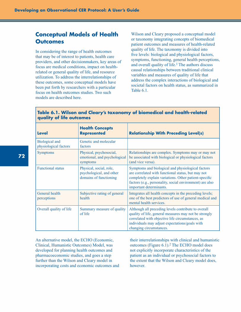
72


Conceptual Models of Health Outcomes

In considering the range of health outcomes that may be of interest to patients, health care providers, and other decisionmakers, key areas of focus are medical conditions, impact on health-related or general quality of life, and resource utilization. To address the interrelationships of these outcomes, some conceptual models have been put forth by researchers with a particular focus on health outcomes studies. Two such models are described here.

Wilson and Cleary proposed a conceptual model or taxonomy integrating concepts of biomedical patient outcomes and measures of health-related quality of life. The taxonomy is divided into five levels: biological and physiological factors, symptoms, functioning, general health perceptions, and overall quality of life.1 The authors discuss causal relationships between traditional clinical variables and measures of quality of life that address the complex interactions of biological and societal factors on health status, as summarized in Table 6.1.

Table 6.1. Wilson and Cleary’s taxonomy of biomedical and health-related quality of life outcomes

LevelHealth Concepts Represented Relationship With Preceding Level(s)

Biological and physiological factors

Genetic and molecular factors

Symptoms Physical, psychosocial, emotional, and psychological symptoms

Relationships are complex. Symptoms may or may not be associated with biological or physiological factors (and vice versa).

Functional status Physical, social, role, psychological, and other domains of functioning

Symptoms and biological and physiological factors are correlated with functional status, but may not completely explain variations. Other patient-specific factors (e.g., personality, social environment) are also important determinants.

General health perceptions

Subjective rating of general health

Integrates all health concepts in the preceding levels; one of the best predictors of use of general medical and mental health services.

Overall quality of life Summary measure of quality of life

Although all preceding levels contribute to overall quality of life, general measures may not be strongly correlated with objective life circumstances, as individuals may adjust expectations/goals with changing circumstances.

An alternative model, the ECHO (Economic, Clinical, Humanistic Outcomes) Model, was developed for planning health outcomes and pharmacoeconomic studies, and goes a step further than the Wilson and Cleary model in incorporating costs and economic outcomes and

their interrelationships with clinical and humanistic outcomes (Figure 6.1).2 The ECHO model does not explicitly incorporate characteristics of the patient as an individual or psychosocial factors to the extent that the Wilson and Cleary model does, however.

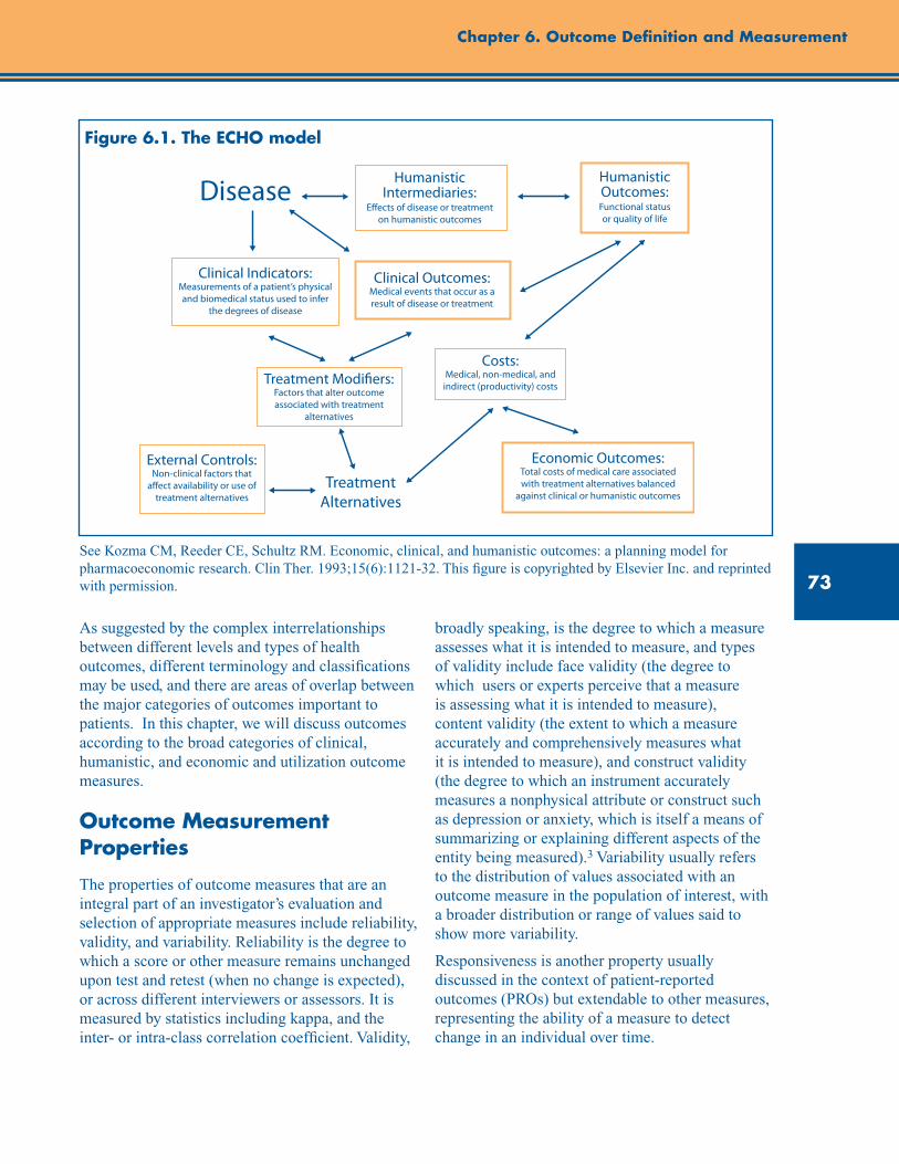
73

Chapter 6. Outcome Definition and Measurement

Figure 6.1. The ECHO model

Economic Outcomes:Total costs of medical care associated with treatment alternatives balanced

against clinical or humanistic outcomes

Costs:Medical, non-medical, and

indirect (productivity) costsTreatment Modi�ers:Factors that alter outcome associated with treatment

alternatives

Clinical Outcomes:Medical events that occur as a result of disease or treatment

Clinical Indicators:Measurements of a patient’s physical and biomedical status used to infer

the degrees of disease

Humanistic Intermediaries:

E�ects of disease or treatment on humanistic outcomes

Humanistic Outcomes:Functional status or quality of life

External Controls:Non-clinical factors that

a�ect availability or use of treatment alternatives

Disease

Treatment Alternatives

See Kozma CM, Reeder CE, Schultz RM. Economic, clinical, and humanistic outcomes: a planning model for pharmacoeconomic research. Clin Ther. 1993;15(6):1121-32. This figure is copyrighted by Elsevier Inc. and reprinted with permission.

As suggested by the complex interrelationships between different levels and types of health outcomes, different terminology and classifications may be used, and there are areas of overlap between the major categories of outcomes important to patients. In this chapter, we will discuss outcomes according to the broad categories of clinical, humanistic, and economic and utilization outcome measures.

Outcome Measurement Properties

The properties of outcome measures that are an integral part of an investigator’s evaluation and selection of appropriate measures include reliability, validity, and variability. Reliability is the degree to which a score or other measure remains unchanged upon test and retest (when no change is expected), or across different interviewers or assessors. It is measured by statistics including kappa, and the inter- or intra-class correlation coefficient. Validity,

broadly speaking, is the degree to which a measure assesses what it is intended to measure, and types of validity include face validity (the degree to which users or experts perceive that a measure is assessing what it is intended to measure), content validity (the extent to which a measure accurately and comprehensively measures what it is intended to measure), and construct validity (the degree to which an instrument accurately measures a nonphysical attribute or construct such as depression or anxiety, which is itself a means of summarizing or explaining different aspects of the entity being measured).3 Variability usually refers to the distribution of values associated with an outcome measure in the population of interest, with a broader distribution or range of values said to show more variability.

Responsiveness is another property usually discussed in the context of patient-reported outcomes (PROs) but extendable to other measures, representing the ability of a measure to detect change in an individual over time.

74


These measurement properties may affect the degree of measurement error or misclassification that an outcome measure is subject to, with the consideration that the properties themselves are specific to the population and setting in which the measures are used. Issues of misclassification and considerations in reducing this type of error are discussed further in the section on “avoidance of bias in study design.”

Clinical Outcomes

Clinical outcomes are perhaps the most common category of outcome to be considered in CER studies. Medical treatments are developed and must demonstrate efficacy in preapproval clinical trials to prevent the occurrence of undesirable outcomes such as coronary events, osteoporosis, or death; to delay disease progression such as in rheumatoid arthritis; to hasten recovery or improve survival from disease, such as in cancer or H5N1 influenza; or to manage or reduce the burden of chronic diseases including diabetes, psoriasis, Parkinson’s disease, and depression. Postapproval observational CER studies are often needed to compare newer treatments against the standard of care; to obtain real-world data on effectiveness as treatments are used in different medical care settings and broader patient populations than those studied in clinical trials; and to increase understanding of the relative benefits and risks of treatments by weighing quality of life, cost, and safety outcomes alongside clinical benefits. For observational studies, this category of outcome generally focuses on clinically meaningful outcomes such as time between disease flares; number of swollen, inflamed joints; or myocardial infarction. Feasibility considerations sometimes dictate the use of intermediate endpoints, which are discussed in further detail later in the chapter.

Definitions of Clinical Outcomes

Temporal Aspects

The nature of the disease state to be treated, the mechanism, and the intended effect of the treatment under study determine whether the clinical outcomes to be identified are incident (a first or new diagnosis of the condition of interest), prevalent (existing disease), or recurrent (new occurrence or exacerbation of disease in a patient

who has a previous diagnosis of that condition). The disease of interest may be chronic (a long-term or permanent condition), acute (a condition with a clearly identifiable and rapid onset), transient (a condition that comes and goes), or episodic (a condition that comes and goes in episodes), or have more than one of these aspects.

Subjective Versus Objective Assessments

Most clinical outcomes involve a diagnosis or assessment by a health care provider. These may be recorded in a patient’s medical record as part of routine care, coded as part of an electronic health record (EHR) or administrative billing system using coding systems such as ICD-9 or ICD-10, or collected specifically for a given study.

While there are varying degrees of subjectivity involved in most assessments by health care providers, objective measures are those that are not subject to a large degree of individual interpretation, and are likely to be reliably measured across patients in a study, by different health care providers, and over time. Laboratory tests may be considered objective measures in most cases and can be incorporated as part of a standard outcome definition to be used for a study when appropriate. Some clinical outcomes, such as all-cause mortality, can be ascertained directly and may be more reliable than measures that are subject to interpretation by individual health care providers, such as angina or depression.

Instruments have been developed to help standardize the assessment of some conditions for which a subjective clinical assessment might introduce unwanted variability. Consider the example of a study of a new psoriasis treatment. Psoriasis is a chronic skin condition that causes lesions affecting varying amounts of body surface area, with varying degrees of severity. While a physician may be able to assess improvement within an individual patient, a quantifiable measure that would be reproducible across patients and raters improves the information value of comparative trials and observational studies of psoriasis treatment effectiveness. An outcome assessment that relies on purely subjective assessments of improvement such as, “Has the patient’s condition improved a lot, a little, or not at all?” is vulnerable to measurement error that arises from subjective judgments or disagreement among

75


clinicians about what comprises the individual categories and how to rate them, often resulting in low reproducibility or inter-rater reliability of the measure. In the psoriasis example, an improved measure of the outcome would be a standardized assessment of the severity and extent of disease expressed as percentage of affected body surface area, such as the Psoriasis Area Severity Index or PASI Score.4 The PASI score requires rating the severity of target symptoms [erythema (E), infiltration (I), and desquamation (D)] and area of psoriatic involvement (A) for each of four main body areas [head (h), trunk (t), upper extremities (e), lower extremities (l)]. Target symptom severity is rated on a 0–4 scale; area of psoriatic involvement is rated on a 0–6 scale, with each numerical value representing a percentage of area involvement.4 The final calculated score ranges from 0 (no disease) to 72 (severe disease), with the score contribution of each body area weighted by its percentage of total body area (10, 20, 30, and 40% of body area for head, upper extremities, trunk, and lower extremities, respectively).4 Compared with subjective clinician assessment of overall performance, using changes in the PASI score increases reproducibility and comparability across studies that use the score.

Relatedly, the U.S. Food and Drug Administration (FDA) has provided input on types of Clinical Outcome Assessments (COAs) that may be considered for qualification for use in clinical trials, with the goals of increasing the reliability of such assessments within a specific context of use in drug development and regulatory decisionmaking to measure a specific concept with a specific interpretation. Contextual considerations include the specific disease of interest, target population, clinical trial design and objectives, regionality, and mode of administration. The types of COAs described are:5

Patient-reported outcome (PRO) assessment: A measurement based on a report that comes directly from the patient (i.e., the study subject) about the status of particular aspects of or events related to a patient’s health condition. PROs are recorded without amendment or interpretation of the patient’s response by a clinician or other observer. A PRO measurement can be recorded by the patient directly, or recorded by an interviewer,

provided that the interviewer records the patient’s response exactly.

Observer-reported outcome (ObsRO) assessment: An assessment that is determined by an observer who does not have a background of professional training that is relevant to the measurement being made, i.e., a nonclinician observer such as a teacher or caregiver. This type of assessment is often used when the patient is unable to self-report (e.g., infants, young children). An ObsRO assessment should only be used in the reporting of observable concepts (e.g., signs or behaviors); ObsROs cannot be validly used to directly assess symptoms (e.g., pain) or other unobservable concepts.

Clinician-reported outcome (ClinRO) assessment: An assessment that is determined by an observer with some recognized professional training that is relevant to the measurement being made.

Other considerations related to use of PROs for measurement of health-related quality of life and other concepts are addressed later on in this chapter.

Composite Endpoints

Some clinical outcomes are composed of a series of items, and are referred to as composite endpoints. A composite endpoint is often used when the individual events included in the score are rare, and/or when it makes biological and clinical sense to group them. The study power for a given sample size may be increased when such composite measures are used as compared with individual outcomes, since by grouping numerous types of events into a larger category, the composite endpoint will occur more frequently than any of the individual components. As desirable as this can be from a statistical point of view, challenges include interpretation of composite outcomes that incorporate both safety and effectiveness, and broader adoption of reproducible definitions that will enhance cross-study comparisons. For example, Kip and colleagues6 point out that there is no standard definition for MACE (major adverse cardiac events), a commonly used outcome in clinical cardiology research. They conducted analyses to demonstrate that varying definitions of

76


composite endpoints, such as MACE, can lead to substantially different results and conclusions. The investigators utilized the DEScover registry patient population, a prospective observational registry of drug-eluting stent (DES) users, to evaluate differences in 1-year risk for three definitions of MACE in comparisons of patients with and without myocardial infarction (MI), and patients with multi-lesion stenting versus single-lesion stenting (also referred to as percutaneous coronary intervention or PCI). The varying definitions of MACE included one related to safety only [composite of death, MI, and stent thrombosis (ST)], and two relating to both safety and effectiveness [composite of death, MI, ST, and either (1) target vessel revascularization (TVR) or (2) any repeat vascularization]. When comparing patients with and without acute MI, the three definitions of MACE yielded very different hazard ratios. The safety-only definition of MACE yielded a hazard ratio of 1.75 (p<0.05), indicating that patients with acute MI were at greater risk of 1-year MACE. However, for the composite of safety and effectiveness endpoints, the risk of 1-year MACE was greatly attenuated and no longer statistically significant. Additionally, when comparing patients with single versus multiple lesions treated with PCI, the three definitions also yielded different results; while the safety-only composite endpoint demonstrated that there was no difference in 1-year MACE, adding TVR to the composite endpoint definition led to a hazard ratio of 1.4 (p<0.05) for multi-lesion PCI versus single-lesion PCI. This research serves as a cautionary tale for the creation and use of composite endpoints. Not only can varying definitions of composite endpoints such as MACE lead to substantially different results and conclusions; results must also be carefully interpreted, especially in the case where safety and effectiveness endpoints are combined.

Intermediate Endpoints

The use of an intermediate or surrogate endpoint is more common in clinical trials than in observational studies. This type of endpoint is often a biological marker for the condition of interest, and may be used to reduce the followup period required to obtain results from a study of

treatment effectiveness. An example would be the use of measures of serum lipids as endpoints in randomized trials of the effectiveness of statins, for which the major disease outcomes of interest to patients and physicians are a reduction in coronary heart disease incidence and mortality. The main advantages of intermediate endpoints are that the followup time required to observe possible effects of treatment on these outcomes may be substantially shorter than for the clinical outcome(s) of primary interest, and if they are measured on all patients, the number of outcomes for analysis may be larger. Much as with composite endpoints, using intermediate endpoints will increase study power for a given sample size as compared with outcomes that may be relatively rare, such as primary myocardial infarction. Surrogate or intermediate outcomes, however, may provide an incomplete picture of the benefits or risk. Treatment comparisons based on intermediate endpoints may differ in magnitude or direction from those based on major disease endpoints, as evidenced in a clinical trial of nifedipine versus placebo7- 8 as well as other clinical trials of antihypertensive therapy.9 On one hand, nifedipine, a calcium channel blocker, was superior to placebo in reduction of onset of new coronary lesions; on the other hand, mortality was sixfold greater among patients who received nifedipine versus placebo.7

Freedman and colleagues have provided recommendations regarding the use of intermediate endpoints.10 Investigators should consider the degree to which the intermediate endpoint is reflective of the main outcome, as well as the degree to which effects of the intervention may be mediated through the intermediate endpoint. Psaty and colleagues have cautioned that because drugs have multiple effects, to the extent that a surrogate endpoint is likely to measure only a subset of those effects, results of studies based on surrogate endpoints may be a misleading substitute for major disease outcomes as a basis for choosing one therapy over another.9

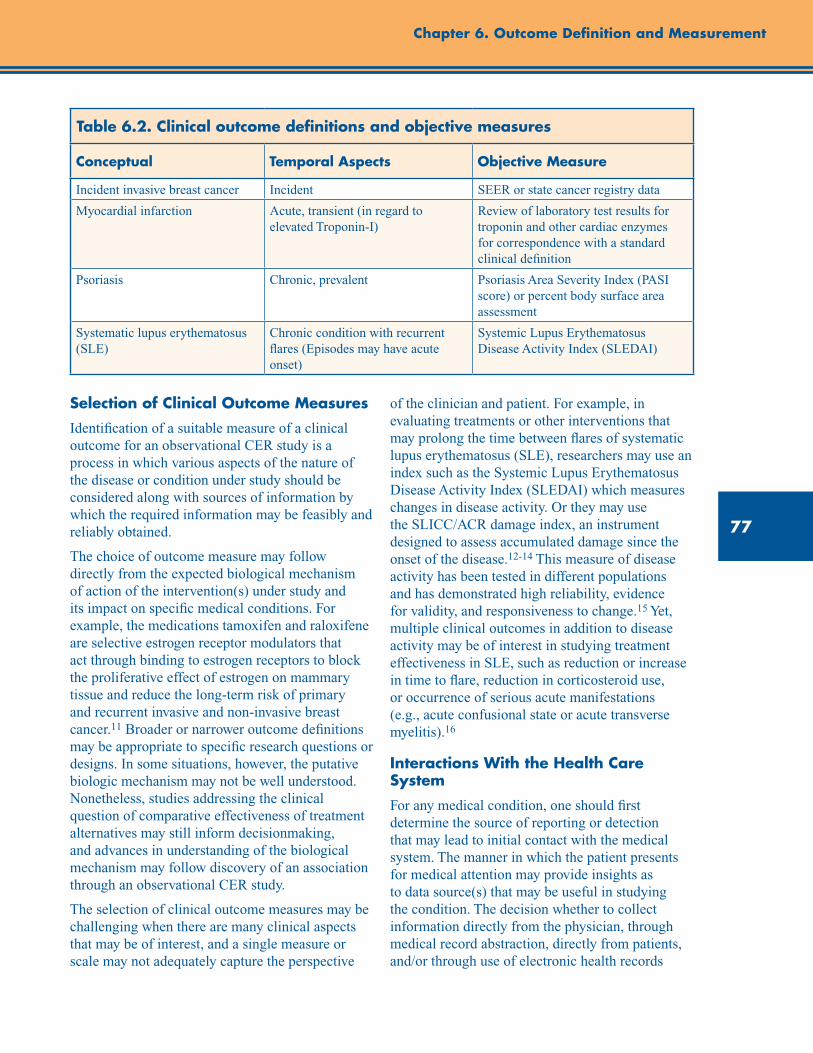
77


Table 6.2. Clinical outcome definitions and objective measures

Conceptual Temporal Aspects Objective Measure

Incident invasive breast cancer Incident SEER or state cancer registry data

Myocardial infarction Acute, transient (in regard to elevated Troponin-I)

Review of laboratory test results for troponin and other cardiac enzymes for correspondence with a standard clinical definition

Psoriasis Chronic, prevalent Psoriasis Area Severity Index (PASI score) or percent body surface area assessment

Systematic lupus erythematosus (SLE)

Chronic condition with recurrent flares (Episodes may have acute onset)

Systemic Lupus Erythematosus Disease Activity Index (SLEDAI)

Selection of Clinical Outcome Measures

Identification of a suitable measure of a clinical outcome for an observational CER study is a process in which various aspects of the nature of the disease or condition under study should be considered along with sources of information by which the required information may be feasibly and reliably obtained.

The choice of outcome measure may follow directly from the expected biological mechanism of action of the intervention(s) under study and its impact on specific medical conditions. For example, the medications tamoxifen and raloxifene are selective estrogen receptor modulators that act through binding to estrogen receptors to block the proliferative effect of estrogen on mammary tissue and reduce the long-term risk of primary and recurrent invasive and non-invasive breast cancer.11 Broader or narrower outcome definitions may be appropriate to specific research questions or designs. In some situations, however, the putative biologic mechanism may not be well understood. Nonetheless, studies addressing the clinical question of comparative effectiveness of treatment alternatives may still inform decisionmaking, and advances in understanding of the biological mechanism may follow discovery of an association through an observational CER study.

The selection of clinical outcome measures may be challenging when there are many clinical aspects that may be of interest, and a single measure or scale may not adequately capture the perspective

of the clinician and patient. For example, in evaluating treatments or other interventions that may prolong the time between flares of systematic lupus erythematosus (SLE), researchers may use an index such as the Systemic Lupus Erythematosus Disease Activity Index (SLEDAI) which measures changes in disease activity. Or they may use the SLICC/ACR damage index, an instrument designed to assess accumulated damage since the onset of the disease.12-14 This measure of disease activity has been tested in different populations and has demonstrated high reliability, evidence for validity, and responsiveness to change.15 Yet, multiple clinical outcomes in addition to disease activity may be of interest in studying treatment effectiveness in SLE, such as reduction or increase in time to flare, reduction in corticosteroid use, or occurrence of serious acute manifestations (e.g., acute confusional state or acute transverse myelitis).16

Interactions With the Health Care System

For any medical condition, one should first determine the source of reporting or detection that may lead to initial contact with the medical system. The manner in which the patient presents for medical attention may provide insights as to data source(s) that may be useful in studying the condition. The decision whether to collect information directly from the physician, through medical record abstraction, directly from patients, and/or through use of electronic health records

78


(EHRs) and/or administrative claims data will follow from this. For example, general hospital medical records are unlikely to provide the key components of an outcome such as respiratory failure, which requires information about use of mechanical ventilation. In contrast, hospital medical records are useful for the study of myocardial infarction, which must be assessed and treated in a hospital setting and are nearly always accompanied by an overnight stay. General practice physician office records and emergency department records may be useful in studying the incidence of influenza A or urticaria, with selection of which of these sources depending on the severity of the condition. A prospective study may be required to collect clinical assessments of disease severity using a standard instrument, as these are not consistently recorded in medical practice and are not coded in administrative data sources. The chapter on data sources (chapter 8) provides additional information on selection of appropriate sources of data for an observational CER study.

Humanistic Outcomes

While outcomes of interest to patients generally include those of interest to physicians, payers, regulators, and others, they are often differentiated by two characteristics: (1) they are clinically meaningful with practical implications for disease recognition and management (i.e., patients generally have less interest in intermediate pathways with no clear clinical impact); and (2) they include reporting of outcomes based on a patient’s unique perspective, e.g., patient-reported scales that indicate pain level, degree of functioning, etc. This section deals with measures of health-related quality of life (HRQoL) and the range of measures collectively described as patient-reported outcomes (PROs), which include measures of HRQoL. Other humanistic perspectives relevant to patients (e.g., economics, utilization of health services, etc.) are covered elsewhere.

Health-Related Quality of Life

Health-related quality of life (HRQoL) measures the impact of disease and treatment on the lives of patients and is defined as “the capacity to perform the usual daily activities for a person’s age and major social role.”17 HRQoL commonly

includes physical functioning, psychological well-being, and social role functioning. This construct comprises outcomes from the patient perspective and are measured by asking the patient or surrogate reporters about them.

HRQoL is an outcome increasingly used in randomized and non-randomized studies of health interventions, and as such FDA has provided clarifying definitions of HRQoL and of improvements in HRQoL. The FDA defines HRQoL as follows:

HRQL is a multidomain concept that represents the patient’s general perception of the effect of illness and treatment on physical, psychological, and social aspects of life. Claiming a statistical and meaningful improvement in HRQL implies: (1) that all HRQL domains that are important to interpreting change in how the clinical trial’s population feels or functions as a result of the targeted disease and its treatment were measured; (2) that a general improvement was demonstrated; and (3) that no decrement was demonstrated in any domain.18

Patient-Reported Outcomes

Patient-reported outcomes (PROs) include any outcomes that are based on data provided by patients or by people who can report on their behalf (proxies), as opposed to data from other sources.19 PROs refer to patient ratings and reports about any of several outcomes, including health status, health-related quality of life, quality of life defined more broadly, symptoms, functioning, satisfaction with care, and satisfaction with treatment. Patients can also report about their health behaviors, including adherence and health habits. Patients may be asked to directly report information about clinical outcomes or health care utilization and out-of-pocket costs when these are difficult to measure through other sources. The FDA defines a PRO as “a measurement based on a report that comes directly from the patient (i.e., study subject) about the status of a patient’s health condition without amendment or interpretation of the patient’s response by a clinician or anyone else. A PRO can be measured by self-report or by interview provided that the interviewer records only the patient’s response.”18

79


In this section we focus mainly on the use of standard instruments for measurement of PROs, in domains including specific disease areas, health-related quality of life, and functioning. PRO measures may be designed to measure the current state of health of an individual or to measure a change in health state. PROs have similarities to other outcome variables measured in observational studies. They are measured with components of both random and systematic error (bias). To be most useful, it is important to have evidence about the reliability, validity, responsiveness, and interpretation of PRO measures, discussed further later in this section.

Types of Humanistic Outcome Measures

Generic Measures

Generic PRO questionnaires are measurement instruments designed to be used across different subgroups of individuals, and contain common domains that are relevant to almost all populations. They can be used to compare one population with another, or to compare scores in a specific population with normative scores. Many have been used for years, and have well established and well understood measurement properties.

Generic PRO questionnaires can focus on a comprehensive set of domains, or on a narrow range of domains such as symptoms or aspects of physical, mental, or social functioning. An example of a generic PRO measure is the Sickness Impact Profile (SIP), one of the oldest and most rigorously developed questionnaires, which measures 12 domains that are affected by illness.20 The SIP produces two subscale scores, one for physical and one for mental health, and an overall score. Another questionnaire, the SF-36, measures eight domains including general health perceptions, pain, physical functioning, role functioning (as limited by physical health), social functioning, mental health, and vitality.21 The SF-36 produces a Physical Component Score and a Mental Component Score.22 The EQ-5D is another generic measure of health-related quality of life, intended for self-completion, that generates a single index score. This scale defines health in terms of 5 dimensions: mobility, self-care, usual activities, pain/discomfort, and anxiety/depression.

Each dimension has three response categories corresponding to no problem/some problem/extreme problem. Taken as a whole, the EQ-5D defines a total of 243 possible states, to which two further states (dead and unconscious) have been added.23 Another broadly used indicator of quality of life relates to the ability to work. The Work Productivity Index (WPAI) was created as a patient-reported quantitative assessment of the amount of absenteeism, presenteeism, and daily activity impairment attributable to general health (WPAI:GH) or to a specific health problem (WPAI:SHP) (see below), in an effort to develop a quantitative approach to measuring the ability to work.24

Examples of generic measures that assess a more restricted set of domains include the SCL-90 to measure symptoms,25 the Index of Activities of Daily Living to measure independence in performing basic functioning,26 the Psychological General Well-Being Index to measure psychological well-being (PGWBI),27 and the Beck Depression Inventory.28

Disease- or Population-Specific Measures

Specific PRO questionnaires are sometimes referred to as “disease-specific.” While a questionnaire can be disease- or condition-specific (e.g., chronic heart failure), it can also be designed for use in a specific population (e.g., pediatric, geriatric), or for use to evaluate a specific treatment (e.g., renal dialysis). Specific questionnaires may be more sensitive to symptoms that are experienced by a particular group of patients. Thus, they are thought to detect differences and changes in scores when they occur in response to interventions.

Some specific measurement instruments assess multiple domains that are affected by a condition. For example, the Arthritis Impact Measurement Scales (AIMS) includes nine subscales that assess problems specific to the health-related quality of life of patients with rheumatoid arthritis and its treatments.29 The MOS-HIV Health Survey includes 10 domains that are salient for people with HIV and its treatments.30

Some of these measures take a modular approach, including a core measure that is used for assessment of a broader set of conditions, accompanied by modules that are specific to

80


disease subtypes. For example, the FACIT and EORTC families of measures for evaluating cancer therapies each include a core module that is used for all cancer patients, and specific modules for each type of cancer, such as a module pertaining specifically to breast cancer.31-33

Other measures focus more narrowly on a few domains most likely to be affected by a disease, or most likely to improve with treatment. For example, the Headache Impact Test includes only six items.34 In contrast, other popular measures focus on symptoms that are affected by many diseases, such as the Brief Pain Inventory and the M.D. Anderson Symptom Inventory (MDASI), which measure the severity of pain and other symptoms and the impact of symptoms on function, and have been developed, refined, and validated in many languages and patient subgroups over three decades.35-36

It is possible, though not always advisable, to design a new PRO instrument for use in a specific study. The process of developing and testing a new PRO measure can be lengthy—generally requiring at least a year in time–and there is no guarantee that a new measure will work as well as more generic but better tested instruments. Nonetheless, it may be necessary to do so in the case of an uncommon condition for which there are no existing PRO measures, for a specific cultural context that differs from the ones that have been studied before, and/or to capture effects of new treatments that may require a different approach to measurement. However, when possible, in these cases it is still prudent to include a PRO measure with evidence for reliability and validity, ideally in the target patient population, in case the newly designed instruments fail to work as intended. This approach will allow comparisons with the new measure to assess content validity if there is some overlap of the concepts being measured.

Item Response Theory (IRT) and Computer Adaptive Testing (CAT)

Item Response Theory (IRT) is a framework for the development of tests and measurement tools, and for the assessment of how well the tools work. Computer Adaptive Testing (CAT) represents an area of innovation in measuring PROs. CAT allows items to be selected to be administered so that questions are relevant to the

respondent and targeted to the specific level of the individual, with the last response determining the next question that is asked. Behind the scenes, items are selected from “item banks,” comprising collections of dozens to hundreds of questions that represent the universe of potential levels of the dimension of interest, along with an indication of the relative difficulty or dysfunction that they represent. For example, the Patient-Reported Outcomes Measurement Information System (PROMIS) item bank for physical functioning includes 124 items that range in difficulty from getting out of bed to running several miles.37 This individualized administration can both enhance measurement precision and reduce respondent burden.38 Computer adaptive testing is based on IRT methods of scaling items and drawing subsets of items from a larger item bank.39 Considerations around adaptive testing involve balancing the benefit of tailoring the set of items and measurements to the specific individual with the risk of inappropriate targeting or classification if items answered incorrectly early on determine the later set of items to which a subject is able to respond. PROMIS40 is a major NIH initiative that leverages these desirable properties for PROs in clinical research and practice applications.

Descriptive Versus Preference Format

Descriptive questionnaires ask about general or common domains and complaints, and usually provide multiple scores. Preference-based measures, generally referred to as utility measures, provide a single score, usually on a 0–1 scale, that represents the aggregate of multiple domains for an overall estimate of burden.

Most of the questionnaires familiar to clinical researchers fall into the category of descriptive measures, including all of those mentioned in the preceding paragraphs. Patients or other respondents are asked to indicate the extent to which descriptions of specific feelings, abilities, or behaviors apply to them. Utility measures are discussed further in the following section.

Other Attributes of PROs

Within each of the above options, there are several attributes of PRO instruments to consider. These include response format (numeric scales vs. verbal descriptors or visual analogue scales), the focus

81


of what is being assessed (frequency, severity, impairment, all of the above), and recall period. Shorter, more recent recall periods more accurately capture the individual’s actual experience, but may not provide as good an estimate of their typical activities or experiences. (For example, not everyone vacuums or has a headache every day.)

Content Validity

Content validity is the extent to which a PRO instrument covers the breadth and depth of salient issues for the intended group of patients. If a PRO instrument is not valid with respect to its content, then there is an increased chance that it may fail to capture adequately the impact of an intervention. For example, in a study to compare the impact of different regimens for rheumatoid arthritis, a PRO that does not assess hand function could be judged to have poor content validity, and might fail to capture differences among therapies. FDA addresses content validity as being of primary interest in assessing a PRO, with other measurement properties being secondary. and defines content validity as follows:

Evidence from qualitative research demonstrating that the instrument measures the concept of interest including evidence that the items and domains of an instrument are appropriate and comprehensive relative to its intended measurement concept, population, and use. Testing other measurement properties will not replace or rectify problems with content validity.18

Content validity is generally assessed qualitatively rather than statistically. It is important to understand and consider the population being studied, including their usual activities and problems, the condition (especially its impact on the patient’s functioning), and the interventions being evaluated (including both their positive and adverse effects).

Responsiveness and Minimally Important Difference

Responsiveness is a measure of a PRO instrument’s sensitivity to changes in health status or other outcome being measured. If a PRO is not sufficiently responsive, it may not provide

adequate evidence of effectiveness in observational studies or clinical trials. Related to responsiveness is the minimally important difference that a PRO measure may detect. Both the patient’s and the health care provider’s perspectives are needed to determine if the minimally important difference detectable by an instrument is in fact of relevance to the patient’s overall health status.41

Floor and Ceiling Effects

Poor content validity can also lead to a mismatch between the distribution of responses and the true distribution of the concept of interest in the population. For example, if questions in a PRO to assess ability to perform physical activities are too “easy” relative to the level of ability in the population, then the PRO will not reflect the true distribution. This problem can present as a “ceiling” effect, where a larger proportion of the sample reports no disability. Similarly, “floor” effects are seen when questions regarding a level of ability are skewed too difficult for the population and the responses reflect this lack of variability.

Interpretation of PRO Scores

Clinicians and clinical researchers may be unfamiliar with how to interpret PRO scores. They may not understand or have reference to the usual distribution of scores of a particular PRO in a clinical or general population. Without knowledge of normal ranges, physicians may not know what cutpoints of scoring indicate that action is warranted. Without reference values from a comparable population, researchers will not know whether an observed difference between two groups is meaningful, and whether a given change within or between groups is important. The task of understanding the meaning of scores is made more difficult by the fact that different PRO measurement tools tend to use different scoring systems. For most questionnaires, higher scores imply better health, but for some, a higher score is worse. Some scales are scored from 0 to 1, where 0=dead and 1=perfect health. Others are scores on a 0–100 scale, where 0 is simply the lowest attainable score (i.e., the respondent indicates the “worst” health state in response to all of the questions) and 100 is the highest. Still others are “normalized,” so that, for example, a score of

82


50 represents the mean score for the healthy or nondiseased population, with a standard deviation of 10 points. It is therefore crucial for researchers and users of PRO data to understand the scoring system being used for an instrument and the expected distribution, including the distributional properties.

For some PRO instruments, particularly generic questionnaires that have been applied to large groups of patients over many years, population norms have been collected and established. These can be used as reference points. Scoring also can be recalculated and “normalized” to a “T-score” so that a specific score (often 50 or 100) corresponds to the mean score for the population, and a specific number of points (often 5 or 10) corresponds to 1 standard deviation unit in that population.

Selection of a PRO Measure

There are a number of practical considerations to take into account when selecting PRO measures for use in a CER study. The measurement properties discussed in the preceding sections also require evaluation in all instances for the specific instrument selected, within a given population, setting, and intended purpose.

Population

It is important to understand the target population that will be completing the PRO assessment. These may range from individuals who can self-report, to individuals requiring the assistance of a proxy or medical professional (e.g., children, mentally or cognitively limited individuals, visually impaired individuals). Some respondents may be ambulatory individuals living in the community, whereas others may be inpatients or institutionalized individuals.

If a PRO questionnaire is to be used in non–English-speaking populations or in multiple languages, it is necessary to have versions appropriately adapted to language and culture. One should have evidence for the reliability and validity of the translated and culturally adapted version, as applied to the concerned population. One also should have data showing the comparability of performance across different language and cultural groups. This is of special importance when pooling data across language versions, as in a multinational clinical trial or registry study.

Burden

It is important to match the respondent burden created by a PRO instrument to the requirements of the population being studied. Patients with greater levels of illness or disability are less able to complete lengthy questionnaires. In some cases, the content or specific questions posed in a PRO may be upsetting or otherwise unacceptable to respondents. In other cases, a PRO questionnaire may be too cognitively demanding or written at a reading level that is above that of the intended population. The total burden of study-related data collection on patients and providers must also be considered, as an excessive number of forms that must be completed are likely to reduce compliance.

Cost and Copyright

Another practical consideration is the copyright status of a PRO being considered for use. Some PRO questionnaires are entirely in the public domain and are free for use. Others are copyrighted and require permission and/or the payment of fees for use. Some scales, such as the SF-12 and SF-36, require payment of fees for scoring.

Mode and Format of Administration

As noted above, there are various options for how a questionnaire should be administered and how the data should be captured, each method having both advantages and disadvantages. A PRO questionnaire can be (1) self-administered at the time of a clinical encounter, (2) administered by an interviewer at the time of a clinical encounter, (3) administered with computer assistance at the time of a clinical encounter, (4) self-administered by mail, (5) self-administered on-line, (6) interviewer-administered by telephone, or (7) computer-administered by telephone. Self-administration at the time of a clinical encounter requires little technology or up-front cost, but requires staff for supervision and data entry and can be difficult for respondents with limited literacy or sophistication. Face-to-face administration engages respondents and reduces their burden but requires trained interviewers. Computer-assisted administration provides an intermediate solution but also requires capital investment. Mailed surveys afford more privacy to respondents, but they generate mailing expenses and do not eliminate problems with

83


literacy. Paper-based formats require data entry, scoring, and archiving and are prone to calculation errors. Online administration is relatively inexpensive, especially for large surveys, and surveys can be completed any time, but not all individuals have Internet access. Administration by live telephone interview is engaging and allows interviewer flexibility but is also expensive. “Cold calls” to potential study participants may result in low response rates, given the increased prevalence of caller ID screening systems and widespread skepticism about “telemarketing.”

Interactive voice response systems (or IVRS) can also be used to conduct telephone interviews, but it can be tedious to respond using the telephone key pad, and this format strikes some as impersonal.

Static Versus Dynamic Questionnaires

Static forms are the type of questionnaire that employs a fixed-format set of questions and response options. They can be administered on paper, by interview, or through the Internet. Dynamic questionnaires select followup questions to administer based on the responses already obtained for previous questions. Since they are more efficient, more domains can be assessed.

Economic and Utilization Outcomes

While clinical outcomes represent the provider and professional perspective, and humanistic outcomes represent the patient perspective, economic outcomes, including measures of health resource utilization, represent the payer and societal perspective. In the United States, measures of cost and cost-effectiveness are often excluded from government-funded CER studies. However, these measures are important to a variety of important stakeholders such as payers and product manufacturers, and are routinely included in cost-effectiveness research in countries such as Australia, the United Kingdom, Canada, France, and Germany.42

Research questions addressing issues of cost-effectiveness and resource utilization may be formulated in a number of ways. Cost identification studies measure the cost of applying a specified treatment to a population under a certain set of conditions. These studies describe the cost incurred without comparison to alternative interventions.

Some cost identification studies describe the total costs of care for a particular population, whereas others isolate costs of care related to a specific condition; this latter approach requires that each episode of care be ascribed as having been related or unrelated to the illness of interest and involves substantial review.43 Cost-benefit studies are typically measured in dollars or other currency. These studies compare the monetary costs of an intervention against the standard of care with the cost savings that result from the benefits of that treatment. In these studies, mortality is also assigned a dollar value, although techniques for assigning value to a human life are controversial. Cost-effectiveness is a relative concept, and its analysis compares the costs of treatments and benefits of treatments in terms of a specified outcome, such as reduced mortality or morbidity, years of life saved, or infections averted.

Types of Health Resource Utilization and Cost Measures

Monetary Costs

Studies most often examine direct costs (i.e., the monetary costs of the medical treatments themselves, potentially including associated costs of administering treatment or conditions associated with treatment), but may also include measures of indirect costs (e.g., the costs of disability or loss of livelihood, both actual and potential). Multiple measures of costs are commonly included in any given study.

Health Resource Utilization

Measures of health resource utilization, such as number of inpatient or outpatient visits, total days of hospitalization in a given year, or number of days treated with IV antibiotics, are often used as efficient and easily interpretable proxies for measuring cost, since actual costs are dependent on numerous factors (e.g., institutional overhead, volume discounts) and can be difficult to obtain, since they often may be confidential, since, in part, they reflect business acumen in price negotiation. Costs may also vary by institution or location, such as the cost of a day in the hospital or a medical procedure. Resource utilization measures may be preferred when a study is intended to yield results that may be generalizable to health systems or

84


reimbursement systems other than those under study, as they are not dependent on a particular reimbursement structure such as Medicare. Alternatively, a specific cost or reimbursement structure, such as the amount reimbursed by the Centers for Medicare and Medicaid Services (CMS) for specific treatment items, or average wholesale drug costs, may be applied to units of health resource use when conducting studies that pool data from different health systems.

Utility and Preference-Based Measures

PROs and cost analyses intersect around the calculation of cost-utility. Utility measures are derived from economic and decision theory. The term utility refers to the value placed by the individual on a particular health state. Utility is summarized as a score ranging from 0.0 representing death to 1.0 representing perfect health.

In health economic analyses, utilities are used to justify devoting resources to a treatment. There are several widely used preference-based instruments that are used to estimate utility.

Preference measures are based on the fundamental concept that individuals or groups have reliable preferences about different health states. To evaluate those preferences, individuals rate a series of health states: for example, a person with specific levels of physical functioning (able to walk one block but not climb stairs), mental health (happy most of the time), and social role functioning (not able to work due to health). The task for the individual is to directly assign a degree of preference to that state. These include the Standard Gamble and Time Tradeoff methods, 44-45 the EQ-5D, also referred to as the Euroqol,23 the Health Utilities Index,46-47 and the Quality of Well-Being Scale.48

Quality-Adjusted Life Years (QALYs)

Utility scores associated with treatment can be used to weight the duration of life according to its quality, and are thereby used to generate QALYs. Utility scores are generally first ascertained directly in a sample of people with the condition in question, either cross-sectionally or over time with a clinical trial. Utility values are sometimes

estimated indirectly using other sources of information about the health status of people in a population. The output produced by an intervention can be calculated as the area under the cost-utility curve.

For example, if the mean utility score for patients receiving antiretroviral treatment for HIV disease is 0.80, then the outcome for a treated group would be survival time multiplied by 0.80.

Disability-Adjusted Life Years (DALYs)

DALYs are another measure of overall disease burden expressed as the number of years lost to poor health, disability, or premature death.49 As with QALYs, mortality and morbidity are combined in a single metric. Potential years of life lost to premature death are supplemented with years of health life lost due to less than optimal health. Whereas 1 QALY corresponds to one year of life in optimal health, 1 DALY corresponds to one year of healthy life lost.

An important aspect of the calculation of DALYs is that the value assigned to each year of life depends on age. Years lived as a young adult are valued more highly than those spent as a young child or older adult, reflecting the different capacity for work productivity during different phases of life. DALYs are therefore estimated for different chronic illnesses by first calculating the age- and sex-adjusted incidence of disease. A DALY is calculated as the sum of the average years of life lost, and the average years lived with a disability. For example, to estimate the years of healthy life lost in a region due to HIV/AIDS, one would first estimate the prevalence of the disease by age. The DALY value is calculated by summing the average of years of life lost and the average number of years lived with AIDS, discounted based on a universal set of standard weights based on expert valuations.

Selection of Resource Utilization and Cost Measures

The selection of measures of resource utilization or costs should correspond to the primary hypothesis in terms of the impact of an intervention. For example, will treatment reduce the need for hospitalization or result in a shorter length of stay?

85


Or, will treatment or other intervention reduce complications that require hospitalization? Or, will a screening method reduce the total number of diagnostic procedures required per diagnosis?

It is useful to consider what types of costs are of interest to the investigators and to various stakeholders. Are total costs of interest, or costs associated with specific resources (e.g., prescription drug costs)? Are only direct costs being measured, or are you also interested in indirect costs such as those related to days lost from work?

When it is determined that results will be presented in terms of dollars rather than units of resources, several different methods can be applied. In the unusual case that an institution has a cost-accounting system, cost can be measured directly. In most cases, resource units are collected, and costs are assigned based on local or national average prices for the specific resources being considered, for example, reimbursement from CMS for a CT scan, or a hospital day. Application of an external standard cost system reduces variability in costs due to region, payer source, and other variables that might obscure the impact of the intervention in question.

Study Design and Analysis Considerations

Study Period and Length of Followup

In designing a study, the required study period and length of followup are determined by the expected time frame within which an intervention may be expected to impact the outcome of interest. A study comparing traditional with minimally invasive knee replacement surgery will need to follow subjects at least for the duration of the expected recovery time of 3 to 6 months or longer. The optimal duration of a study can be problematic when studying effects that may become manifest over a long time period, such as treatments to prevent or delay the onset of chronic disease. In these cases, data sources with a high degree of turnover of patients, such as administrative claims databases from managed care organizations, may not be suitable. For example, in the case of Alzheimer’s disease, a record of health care is likely to be present in health insurance

claims. However, with the decline in cognitive function, patients may lose ability to work and may enter assisted care facilities, where utilization is not typically captured in large health insurance claims systems. Some studies may be undertaken for the purpose of determining how long an intervention can be expected to impact the outcome of interest. For example, various measures are used to aid in reducing obesity and in smoking cessation, and patients, health care providers, and payers are interested in knowing how long these interventions work (if at all), for whom, and in what situations.

Notwithstanding the limitations of intermediate endpoints (discussed in a preceding section), one of the main advantages of their use is the potential truncation of the required study followup period. Consider, for example, a study of the efficacy of the human papilloma virus vaccine, for which the major medical endpoint of interest is prevention of cervical cancer. The long latency period (more than 2 years, depending on the study population) and the relative infrequency of cervical cancer raise the possibility that intermediate endpoints should be used. Candidates might include new diagnoses of genital warts, or new diagnoses of the precancerous conditions cervical intraepithelial neoplasia (CIN) or vaginal intraepithelial neoplasia (VIN), which have shorter latency periods of less than 1 year or 2 years (minimum), respectively. Use of these endpoints would allow such a study to provide meaningful evidence informing the use of the HPV vaccine in a shorter timeframe, during which more patients might benefit from its use. Alternatively, if the vaccine is shown to be ineffective, this information could avoid years of unnecessary treatment and the associated costs as well as the costs of running a longer trial.

Avoidance of Bias in Study Design

Misclassification

The role of the researcher is to understand the extent and sources of misclassification in outcome measurement, and to try to reduce these as much as possible. To ensure comparability between treatment groups with as little misclassification (also referred to as measurement error) of outcomes as possible, a clear and objective (i.e., verifiable and not subject to individual

86


interpretation insofar as possible) definition of the outcome of interest is needed. An unclear outcome definition can lead to misclassification and bias in the measure of treatment effectiveness. When the misclassification is nondifferential, or equivalent across treatment groups, the estimate of treatment effectiveness will be biased toward the null, reducing the apparent effectiveness of treatment, which may result in an erroneous conclusion that no effect (or one smaller than the true effect size) exists. When the misclassification differs systematically between treatment groups, it may distort the estimate of treatment effectiveness in either direction.

For clinical outcomes, incorporation of an objective measure such as a validated tool that has been developed for use in clinical practice settings, or an adjudication panel for review of outcomes with regard to whether they meet the predetermined definition of an event, would both be approaches that increase the likelihood that outcomes will be measured and classified accurately and in a manner unlikely to vary according to who is doing the assessment. For PROs, measurement error can stem from several sources, including the way in which a question is worded and hence understood by a respondent, how the question is presented, the population being assessed, the literacy level of respondents, the language in which the questions are written, and elements of culture that it represents.

To avoid differential misclassification of outcomes, care must also be taken to use the same methods of ascertainment and definitions of study outcomes whenever possible. For prospective or retrospective studies with contemporaneous comparators, this is usually not an issue, since it is most straightforward to utilize the same data sources and methods of outcome ascertainment for each comparison group. A threat to validity may arise in use of a historical comparison group, which may be used in certain circumstances. For example, this occurs when a new treatment largely displaces use of an older treatment within a given indication, but further evidence is needed for the comparative effectiveness of the newer and older treatments, such as enzyme replacement for lysosomal storage disorders. In such instances, use

of the same or similar data sources and equivalent outcome definitions to the extent possible will reduce the likelihood of bias due to differential outcome ascertainment.

Other situations that may give rise to issues of differential misclassification of outcomes include: when investigators are not blinded to the hypothesis of the study, and “rule-out” diagnoses are more common in those with a particular exposure of interest; when screening or detection of outcomes is more common or more aggressive in those with one treatment than another (i.e., surveillance bias, e.g., when liver function testing are preferentially performed in patients using a new drug compared to other treatments for that condition); and when loss to followup occurs that is related to the risk of experiencing the outcome. For example, once a safety signal has been identified and publicized, physicians have been alerted and then look more proactively for clinical signs and symptoms in treated patients. This situation is even greater for products that are subject to controlled distribution or Risk Evaluation and Mitigation Strategies (REMS). Consider clozapine, an anti-schizophrenia drug that is subject to controlled distribution through a “no blood, no drug” monitoring program. The blood testing program was implemented to detect early development of agranulocytemia. When comparing patients treated with clozapine with those treated with other antischizophrenics, those using clozapine may appear to have a worse safety profile with respect to this outcome.

Sensitivity analyses may be conducted in order to estimate the impact of different levels of differential or nondifferential misclassification on effect estimates from observational CER studies. These approaches are covered in detail in chapter 11.

Validation and Adjudication

In some instances, additional information must be collected (usually from medical records) to validate the occurrence of the outcome of interest, including to exclude erroneous or “rule-out” diagnoses. This is particularly important for medical events identified in administrative claims databases, for which a diagnosis code associated with a medical encounter may represent

87


a “rule out” diagnosis or a condition that does not map to a specific diagnosis code. For some complex diagnoses, such as unstable angina, a standard clinical definition must be applied by an adjudication panel that has access to detailed records inclusive of subjects’ relevant medical history, symptomatic presentation, diagnostic work-up, and treatment. Methods of validation and adjudication of outcomes strengthen the internal validity and therefore the evidence that can be drawn from a CER study. However, they are resource-intensive.

Issues Specific to PROs

PROs are prone to several specific sources of bias. Self-reports of health status are likely to differ systematically from reports by surrogates, who, for example, are likely to report less pain than the individuals themselves.50 Some biases may be population-dependent. For example, there may be a greater tendency of some populations to succumb to acquiescence bias (agreeing with the statements in a questionnaire) or social desirability bias (answering in a way that would cast the respondent in the best light).51 In some situations, however, a PRO may be the most useful marker of disease activity, such as with episodic conditions that cause short-duration disease flares such as low back pain and gout, where patients may not present for health care immediately, if at all.

The goal of the researcher is to understand and reduce sources of bias, considering those most likely to apply in the specific population and topics under study. In the case of well understood systematic biases, adjustments can be made so that distributions of responses are more consistent. In other cases, redesigning items and scales, for example, by including both positively and negatively worded items, can reduce specific kinds of bias.

Missing data, an issue covered in more detail in chapter 10, pose a particular problem with PROs, since PRO data are usually not missing at random. Instead, respondents whose health is poorer are more likely to fail to complete an assessment. Another special case of missing data occurs when a patient dies and is unable to complete an assessment. If this issue is not taken into account

in the data analysis, and scores are only recorded for living patients, incorrect conclusions may be drawn. Strategies for handling this type of missing data include selection of an instrument that incorporates a score for death, such as the Sickness Impact Profile 20, 52 or the Quality of Well-Being Scale,48 or through an analytic strategy that allows for some missing values.

Failure to account for missing PRO data that are related to poor health or death will lead to an overestimate of the health of the population based on responses from subjects who do complete PRO forms. Therefore, in research using PROs, it is very important to understand the extent and pattern of missing data, both at the level of the individual as well as for specific items or scales on an instrument.53

A strategy should be put in place to handle missing data when developing the study protocol and analysis plans. Such strategies that pertain to use of PROs in research are discussed in further detail in publications such as the book by Fairclough and colleagues.

Analytic Considerations

Form of Outcome Measure and Analysis Approach

To a large extent, the form of the primary outcome of interest—that is, whether the outcome is measured and expressed as a dichotomous or polytomous categorical variable or a continuous variable, and whether it is to be measured at a single time point, measured repeatedly at fixed intervals, or measured repeatedly at varying time intervals—determines the appropriate statistical methods that may be applied in analysis. These topics are covered in detail in chapter 10.

Sensitivity Analysis

One of the key factors to address in planned sensitivity analyses for an observational CER study is how varying definitions of the study outcome or related outcomes will affect the measures of association from the study. These investigations include assessing multiple related outcomes within a disease area; for example, assessing multiple measures of respiratory function such as FEV1, FEV1% predicted, and FVC in studies of asthma

88


treatment effectiveness in children; assessing the effect of different cutoffs for dichotomized continuous outcome measures; for example, the use of Systemic Lupus Erythematosus Disease Activity Index-2000 scores to define active disease in lupus treatment studies,54 or the use of different sets of diagnosis codes to capture a condition such as influenza and related respiratory conditions, in administrative data. These and other considerations for sensitivity analyses are covered in detail in chapter 11.

Conclusion

Future Directions

Increased use of EHRs as a source of data for observational research, including registries, other types of observational studies, and specifically for CER, has prompted initiatives to develop standardized definitions of key outcomes and other data elements that would be used across health systems and different EHR platforms to facilitate comparisons between studies and pooling of data. The National Cardiovascular Research Infrastructure partnership between the American College of Cardiology and Duke Clinical Research Institute, which received American Recovery and Reinvestment Act funding to establish intra-operable data standards based on the National

Cardiovascular Data Registry, is an example of such a current activity.55

Summary

This chapter has provided an overview of considerations in development of outcome definitions for observational CER studies; has described implications of the nature of the proposed outcomes for the study design; and has enumerated issues of bias that may arise in incorporating the ascertainment of outcomes into observational research. It has also suggested means of preventing or reducing these biases.

Development of clear and objective outcome definitions that correspond to the nature of the hypothesized treatment effect and address the research questions of interest, along with validation of outcomes where warranted or use of standardized PRO instruments validated for the population of interest, contribute to the internal validity of observational CER studies. Attention to collection of outcome data in an equivalent manner across treatment comparison groups is also required. Use of appropriate analytic methods suitable to the outcome measure, and sensitivity analysis to address varying definitions of at least the primary study outcomes, are needed to make inferences drawn from such studies more robust and reliable.

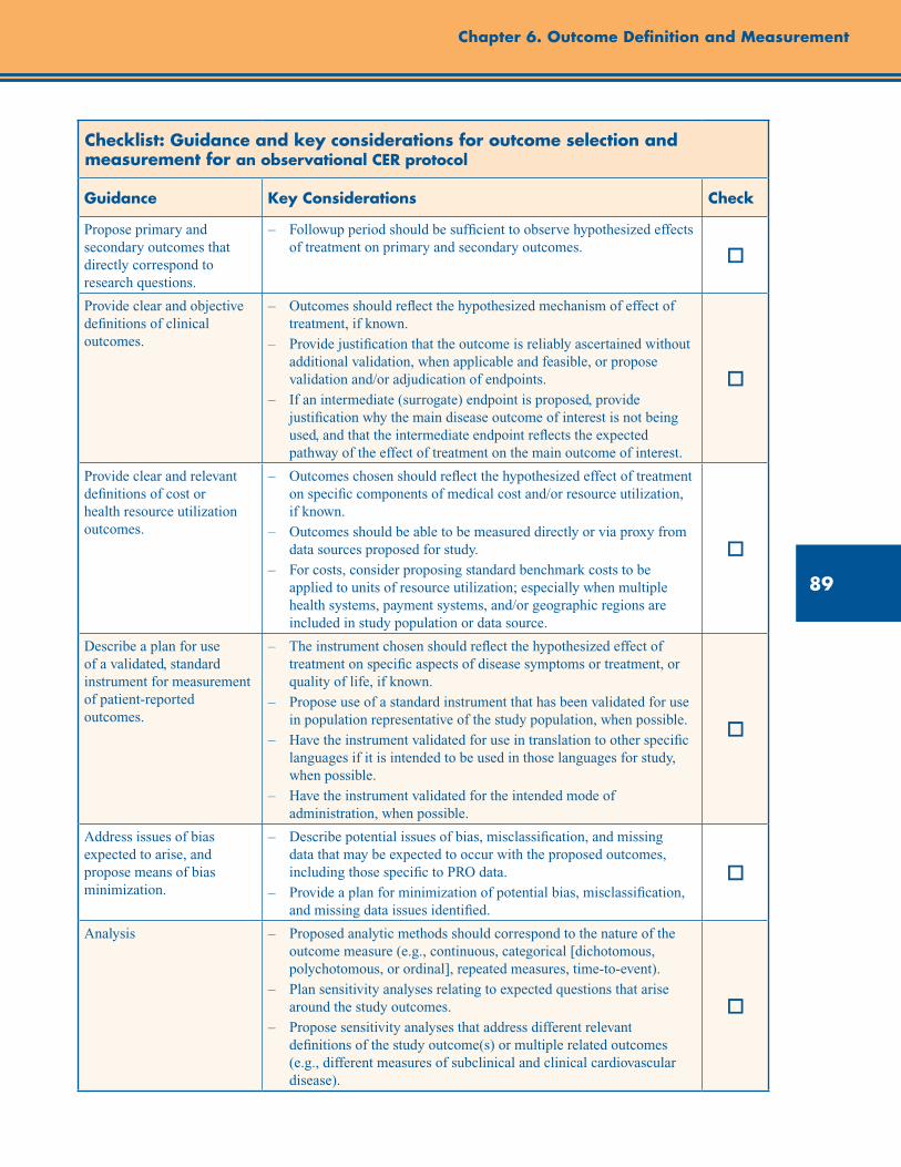
89


Checklist: Guidance and key considerations for outcome selection and measurement for an observational CER protocol


Propose primary and secondary outcomes that directly correspond to research questions.

– Followup period should be sufficient to observe hypothesized effects of treatment on primary and secondary outcomes. o

Provide clear and objective definitions of clinical outcomes.

– Outcomes should reflect the hypothesized mechanism of effect of treatment, if known.

– Provide justification that the outcome is reliably ascertained without additional validation, when applicable and feasible, or propose validation and/or adjudication of endpoints.

– If an intermediate (surrogate) endpoint is proposed, provide justification why the main disease outcome of interest is not being used, and that the intermediate endpoint reflects the expected pathway of the effect of treatment on the main outcome of interest.

o

Provide clear and relevant definitions of cost or health resource utilization outcomes.

– Outcomes chosen should reflect the hypothesized effect of treatment on specific components of medical cost and/or resource utilization, if known.

– Outcomes should be able to be measured directly or via proxy from data sources proposed for study.

– For costs, consider proposing standard benchmark costs to be applied to units of resource utilization; especially when multiple health systems, payment systems, and/or geographic regions are included in study population or data source.

o

Describe a plan for use of a validated, standard instrument for measurement of patient-reported outcomes.

– The instrument chosen should reflect the hypothesized effect of treatment on specific aspects of disease symptoms or treatment, or quality of life, if known.

– Propose use of a standard instrument that has been validated for use in population representative of the study population, when possible.

– Have the instrument validated for use in translation to other specific languages if it is intended to be used in those languages for study, when possible.

– Have the instrument validated for the intended mode of administration, when possible.

o

Address issues of bias expected to arise, and propose means of bias minimization.

– Describe potential issues of bias, misclassification, and missing data that may be expected to occur with the proposed outcomes, including those specific to PRO data.

– Provide a plan for minimization of potential bias, misclassification, and missing data issues identified.

o

Analysis – Proposed analytic methods should correspond to the nature of the outcome measure (e.g., continuous, categorical [dichotomous, polychotomous, or ordinal], repeated measures, time-to-event).

– Plan sensitivity analyses relating to expected questions that arise around the study outcomes.

– Propose sensitivity analyses that address different relevant definitions of the study outcome(s) or multiple related outcomes (e.g., different measures of subclinical and clinical cardiovascular disease).

o

90


References1. Wilson IB, Cleary PD. Linking clinical variables

with health-related quality of life. A conceptual model of patient outcomes. JAMA. 1995 Jan 4; 273:59-65.

2. Kozma CM, Reeder CE, Schultz RM. Economic, clinical, and humanistic outcomes: a planning model for pharmacoeconomic research. Clin Ther. 1993;15(6):1121-32.

3. Streiner DL, Norman GR. Health Measurement Scales: a Practical Guide to their Development and Use. 4th ed. Oxford University Press; 2008.

4. Fredriksson T, Pettersson U. Severe psoriasis--oral therapy with a new retinoid. Dermatologica. 1978;157(4):238-44.

5. U.S. Department of Health and Human Services, Food and Drug Administration. Clinical Outcome Assessment Qualification Program. April 2012. www.fda.gov/Drugs/DevelopmentApprovalProcess/DrugDevelopmentToolsQualificationProgram/ucm284077.htm?utm_source=fdaSearch&utm_medium=website&utm_term=drug development tools qualification program&utm_content=2. Accessed April 16, 2012.

6. Kip KE, Hollabaugh K, Marroquin OC, et al. The problem with composite end points in cardiovascular studies. The story of major adverse cardiac events and percutaneous coronary intervention. J Am Coll Cardiol. 2008;51:701-7.

7. Lichtlen PR, Hugenholtz PG, Rafflenbeul W, et al. Retardation of angiographic progression of coronary artery disease by nifedipine: results of the International Nifedipine Trial on Antiatherosclerotic Therapy (INTACT). Lancet. 1990;335:1109-13.

8. Psaty BM, Siscovick DS, Weiss NS, et al. Hypertension and outcomes research. From clinical trials to clinical epidemiology. Am J Hypertens. 1996;9:178-83.

9. Psaty BM, Lumly T. Surrogate end points and FDA approval: a tale of 2 lipid-altering drugs. JAMA. 2008; 299(12):1474-6.

10. Freedman LS, Graubard BI, Schatzkin A. Statistical validation of intermediate endpoints for chronic diseases. Stat Med. 1992 Jan 30;11(2):167-78.

11. Vogel VG, Costantino JP, Wickerham DL, et al. Update of the National Surgical Adjuvant Breast and Bowel Project Study of Tamoxifen and Raloxifene (STAR) P-2 trial: preventing breast cancer. Cancer Prev Res. (Phila) 2010 Jun;3(6):696-706.

12. Gladman DD, Urowitz MB. The SLICC/ACR damage index: progress report and experience in the field. Lupus. 1999;8:632-7.

13. Bombardier C, Gladman DD, Urowitz MB, et al.; the Committee on Prognosis Studies in SLE. Derivation of the SLEDAI: a disease activity index for lupus patients. Arthritis Rheum. 1992;35:630-40.

14. Gladman DD, Ibanez D, Urowitz MB. Systemic lupus erythematosus disease activity index 2000. J Rheumatol. 2002;29:288-91.

15. Griffiths B, Mosca M, Gordon C. Assessment of patients with systemic lupus erythematosus and the use of lupus disease activity indices. Best Pract Res Clin Rheumatol. 2005 Oct;19(5):685-708.

16. U.S. Department of Health and Human Services, Food and Drug Administration. Guidance for Industry Systemic Lupus Erythematosus — Developing Medical Products for Treatment. June 2010. www.fda.gov/downloads/Drugs/GuidanceComplianceRegulatoryInformation/Guidances/ucm072063.pdf. Accessed February 3, 2012.

17. Guyatt GH, Feeny DH, Patrick DL. Measuring health-related quality of life. Ann Intern Med. 1993 Apr 15;118(8):622-9.

18. U.S. Department of Health and Human Services, Food and Drug Administration. Guidance for Industry Patient Reported Outcome Measures: Use in Medical Product Development to Support Labelling Claims. December 2009. www.ispor.org/workpaper/FDA%20PRO%20Guidance.pdf. Accessed October 30, 2012.

19. Acquadro C, Berzon R, Dubois D, et al. Incorporating the patient’s perspective into drug development and communication: an ad hoc task force report of the Patient-Reported Outcomes (PRO) Harmonization Group meeting at the Food and Drug Administration, February 16, 2001. Value Health. 2003 Sep;6:522-31.

20. Bergner M, Bobbitt RA, Carter WB, et al. The Sickness Impact Profile: development and final revision of a health status measure. Med Care. 1981 Aug;19(8):787-805.

91


21. Ware JE Jr, Sherbourne CD. The MOS 36-item short-form health survey (SF-36). I. Conceptual framework and item selection. Med Care. 1992 Jun;30(6):473-83.

22. Ware JE Jr, Kosinski M, Bayliss MS, et al. Comparison of methods for the scoring and statistical analysis of SF-36 health profile and summary measures: summary of results from the Medical Outcomes Study. Med Care. 1995 Apr;33(4 Suppl):AS264-79.

23. EuroQol--a new facility for the measurement of health-related quality of life. The EuroQol Group. Health Policy. 1990 Dec;16(3):199-208.

24. Reilly MC, Zbrozek AS, Dukes EM. The validity and reproducibility of a work productivity and activity impairment instrument. Pharmacoeconomics. 1993 Nov;4(5):353-65.

25. Derogatis LR, Cleary PA. Factorial invariance across gender for the primary symptom dimensions of the SCL-90. Br J Soc Clin Psychol. 1977 Nov;16(4):347-56.

26. Katz S, Akpom CA. 12. Index of ADL. Med Care. 1976 May;14(5 Suppl):116-8.

27. Dupuy HJ. The Psychological General Well-Being (PGWB) Index. In: Assessment of Quality of Life in Clinical Trials of Cardiovascular Therapies. Edited by Wenger NK, Mattson ME, Furberg CD, et al. Le Jacq Publishing; 1984; Chap 9:170-83.

28. Beck AT, Ward CH, Mendelson M, et al. An inventory for measuring depression. Arch Gen Psychiatry. 1961;4:561-71.

29. Meenan RF, Gertman PM, Mason JH. Measuring health status in arthritis. The arthritis impact measurement scales. Arthritis Rheum. 1980 Feb;23(2):146-52.

30. Wu AW, Revicki DA, Jacobson D, et al. Evidence for reliability, validity and usefulness of the Medical Outcomes Study HIV Health Survey (MOS-HIV). Qual Life Res. 1997 Aug;6(6):481-93.

31. Cella D, Nowinski CJ. Measuring quality of life in chronic illness: the functional assessment of chronic illness therapy measurement system. Arch Phys Med Rehabil. 2002 Dec;83(12 Suppl 2):S10-7.

32. Aaronson NK, Ahmedzai S, Bergman B, et al. The European Organization for Research and Treatment of Cancer QLQ-C30: a quality-of-life instrument for use in international clinical trials in oncology. J Natl Cancer Inst. 1993 Mar 3;85(5):365-76.

33. Sprangers MA, Cull A, Groenvold M, et al. EORTC Quality of Life Study Group. The European Organization for Research and Treatment of Cancer approach to developing questionnaire modules: an update and overview. Qual Life Res. 1998 May;7(4):291-300.

34. Kosinski M, Bayliss MS, Bjorner JB, et al. A six-item short-form survey for measuring headache impact: the HIT-6. Qual Life Res. 2003 Dec;12(8):963-74.

35. Cleeland CS. Symptom burden: multiple symptoms and their impact as patient-reported outcomes. J Natl Cancer Inst Monogr. 2007;37:16-21.

36. Cleeland CS, Ryan KM. Pain assessment: global use of the Brief Pain Inventory. Ann Acad Med Singapore. 1994;23(2):129-38.

37. Hung M, Clegg DO, Greene T, et al. Evaluation of the PROMIS physical function item bank in orthopaedic patients. J Orthop Res. 2011;29(6):947-53.

38. Bjorner JB, Chang CH, Thissen D, et al. Developing tailored instruments: item banking and computerized adaptive assessment. Qual Life Res. 2007;16 Suppl 1:95-108.

39. Reise SP. Item response theory: fundamentals, applications, and promise in psychological research. Current Directions in Psychological Science. 2005 April;14(2):95-101.

40. Reeve BB, Hays RD, Bjorner JB, et al. Psychometric evaluation and calibration of health-related quality of life item banks: plans for the Patient-Reported Outcomes Measurement Information System (PROMIS). Med Care. 2007 May;45:S22-S31.

41. Revicki DA, Cella D, Hays RD, et al. Responsiveness and minimal important differences for patient reported outcomes. Health Qual Life Outcomes. 2006; 4:70.

42. Chalkidou K, Tunis S, Lopert R, et al. Comparative effectiveness research and evidence-based health policy: experience from four countries. Milbank Q. 2009 Jun;87(2):339-67.

43. Lanes SF, Lanza LL, Radensky, et al. Resource utilization and cost of care for rheumatoid arthritis and osteoarthritis in a managed care setting: the importance of drug and surgery costs. Arthritis and Rheumatism. 1997;40(8):1475-81.

44. Torrance GW. Measurement of health state utilities for economic appraisal. J Health Econ. 1986 Mar;5(1):1-30.

92

45. Torrance GW. Utility approach to measuring health-related quality of life. J Chronic Dis. 1987;40(6):593-603.

46. Feeny D, Furlong W, Boyle M, et al. Multi-attribute health status classification systems. Health Utilities Index. Pharmacoeconomics. 1995 Jun;7(6):490-502.

47. Feeny D, Furlong W, Saigal S, et al. Comparing directly measured standard gamble scores to HUI2 and HUI3 utility scores: group- and individual-level comparisons. Soc Sci Med. 2004 Feb;58(4):799-809.

48. Kaplan RM, Anderson JP. The General Health Policy Model: an integrated approach. In: Lenert L, Kaplan RM. Validity and interpretation of preference-based measures of health-related quality of life. Med Care. 2000 Sep;38: II138-II150.

49. Murray CJ. Quantifying the burden of disease: the technical basis for disability-adjusted life years. Bull World Health Organ. 1994;72(3):429-45.

50. Wilson KA, Dowling AJ, Abdolell M, et al. Perception of quality of life by patients, partners and treating physicians. Qual Life Res. 2000;9(9):1041-52.

51. Ross CK, Steward CA, Sinacore JM. A comparative study of seven measures of patient satisfaction. Med Care. 1995 Apr;33(4):392-406.

52. Bergner M, Bobbitt RA, Pollard WE, et al. The sickness impact profile: validation of a health status measure. Med Care. 1976 Jan;14:57-67.

53. Fairclough DL. Design and Analysis of Quality of Life Studies in Clinical Trials. 2nd ed. Boca Raton: Chapman and Hall/CRC Press; 2010.

54. Yee CS, Farewell VT, Isenberg DA, et al. The use of Systemic Lupus Erythematosus Disease Activity Index-2000 to define active disease and minimal clinically meaningful change based on data from a large cohort of systemic lupus erythematosus patients. Rheumatology (Oxford). 2011 May;50(5):982-8.

55. National Cardiovascular Research Infrastructure (NCRI). Available at: https://www.ncrinetwork.org/. Accessed February 3, 2012.


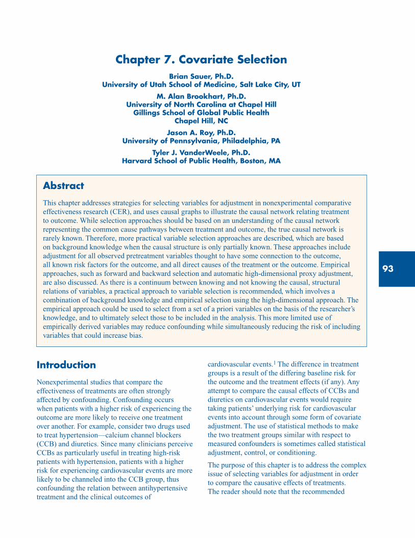
93

Abstract

This chapter addresses strategies for selecting variables for adjustment in nonexperimental comparative effectiveness research (CER), and uses causal graphs to illustrate the causal network relating treatment to outcome. While selection approaches should be based on an understanding of the causal network representing the common cause pathways between treatment and outcome, the true causal network is rarely known. Therefore, more practical variable selection approaches are described, which are based on background knowledge when the causal structure is only partially known. These approaches include adjustment for all observed pretreatment variables thought to have some connection to the outcome, all known risk factors for the outcome, and all direct causes of the treatment or the outcome. Empirical approaches, such as forward and backward selection and automatic high-dimensional proxy adjustment, are also discussed. As there is a continuum between knowing and not knowing the causal, structural relations of variables, a practical approach to variable selection is recommended, which involves a combination of background knowledge and empirical selection using the high-dimensional approach. The empirical approach could be used to select from a set of a priori variables on the basis of the researcher’s knowledge, and to ultimately select those to be included in the analysis. This more limited use of empirically derived variables may reduce confounding while simultaneously reducing the risk of including variables that could increase bias.

Chapter 7. Covariate SelectionBrian Sauer, Ph.D.

University of Utah School of Medicine, Salt Lake City, UT

M. Alan Brookhart, Ph.D. University of North Carolina at Chapel Hill

Gillings School of Global Public Health Chapel Hill, NC

Jason A. Roy, Ph.D. University of Pennsylvania, Philadelphia, PA

Tyler J. VanderWeele, Ph.D. Harvard School of Public Health, Boston, MA

Introduction

Nonexperimental studies that compare the effectiveness of treatments are often strongly affected by confounding. Confounding occurs when patients with a higher risk of experiencing the outcome are more likely to receive one treatment over another. For example, consider two drugs used to treat hypertension—calcium channel blockers (CCB) and diuretics. Since many clinicians perceive CCBs as particularly useful in treating high-risk patients with hypertension, patients with a higher risk for experiencing cardiovascular events are more likely to be channeled into the CCB group, thus confounding the relation between antihypertensive treatment and the clinical outcomes of

cardiovascular events.1 The difference in treatment groups is a result of the differing baseline risk for the outcome and the treatment effects (if any). Any attempt to compare the causal effects of CCBs and diuretics on cardiovascular events would require taking patients’ underlying risk for cardiovascular events into account through some form of covariate adjustment. The use of statistical methods to make the two treatment groups similar with respect to measured confounders is sometimes called statistical adjustment, control, or conditioning.

The purpose of this chapter is to address the complex issue of selecting variables for adjustment in order to compare the causative effects of treatments. The reader should note that the recommended

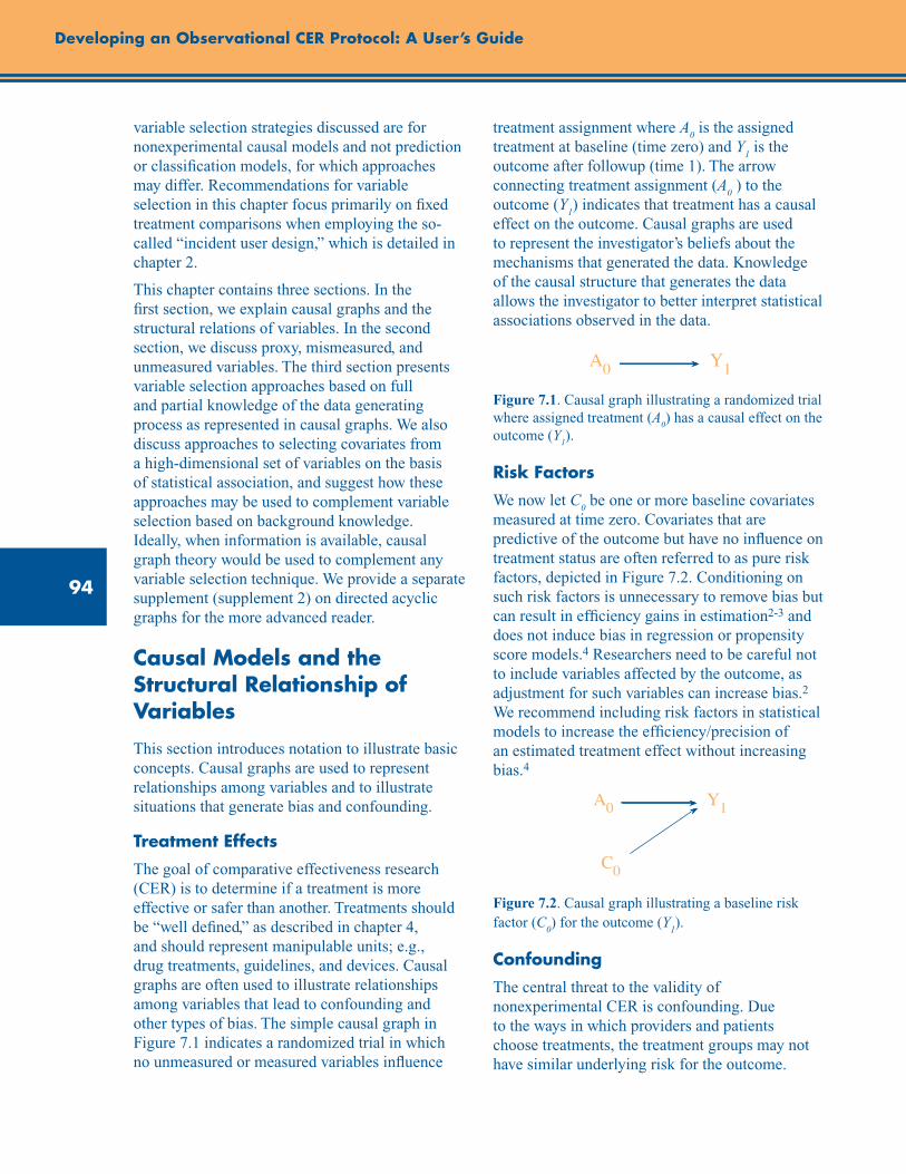
94


variable selection strategies discussed are for nonexperimental causal models and not prediction or classification models, for which approaches may differ. Recommendations for variable selection in this chapter focus primarily on fixed treatment comparisons when employing the so-called “incident user design,” which is detailed in chapter 2.

This chapter contains three sections. In the first section, we explain causal graphs and the structural relations of variables. In the second section, we discuss proxy, mismeasured, and unmeasured variables. The third section presents variable selection approaches based on full and partial knowledge of the data generating process as represented in causal graphs. We also discuss approaches to selecting covariates from a high-dimensional set of variables on the basis of statistical association, and suggest how these approaches may be used to complement variable selection based on background knowledge. Ideally, when information is available, causal graph theory would be used to complement any variable selection technique. We provide a separate supplement (supplement 2) on directed acyclic graphs for the more advanced reader.

Causal Models and the Structural Relationship of Variables

This section introduces notation to illustrate basic concepts. Causal graphs are used to represent relationships among variables and to illustrate situations that generate bias and confounding.

Treatment Effects

The goal of comparative effectiveness research (CER) is to determine if a treatment is more effective or safer than another. Treatments should be “well defined,” as described in chapter 4, and should represent manipulable units; e.g., drug treatments, guidelines, and devices. Causal graphs are often used to illustrate relationships among variables that lead to confounding and other types of bias. The simple causal graph in Figure 7.1 indicates a randomized trial in which no unmeasured or measured variables influence

treatment assignment where A0 is the assigned

treatment at baseline (time zero) and Y1 is the

outcome after followup (time 1). The arrow connecting treatment assignment (A

0 ) to the

outcome (Y1) indicates that treatment has a causal

effect on the outcome. Causal graphs are used to represent the investigator’s beliefs about the mechanisms that generated the data. Knowledge of the causal structure that generates the data allows the investigator to better interpret statistical associations observed in the data.

Figure 7.1. Causal graph illustrating a randomized trial where assigned treatment (A

0) has a causal effect on the

outcome (Y1).

Risk Factors

We now let C0 be one or more baseline covariates

measured at time zero. Covariates that are predictive of the outcome but have no influence on treatment status are often referred to as pure risk factors, depicted in Figure 7.2. Conditioning on such risk factors is unnecessary to remove bias but can result in efficiency gains in estimation2-3 and does not induce bias in regression or propensity score models.4 Researchers need to be careful not to include variables affected by the outcome, as adjustment for such variables can increase bias.2 We recommend including risk factors in statistical models to increase the efficiency/precision of an estimated treatment effect without increasing bias.4

Figure 7.2. Causal graph illustrating a baseline risk factor (C

0) for the outcome (Y

1).

Confounding

The central threat to the validity of nonexperimental CER is confounding. Due to the ways in which providers and patients choose treatments, the treatment groups may not have similar underlying risk for the outcome.

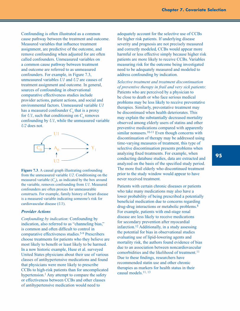
95

Chapter 7. Covariate Selection

Confounding is often illustrated as a common cause pathway between the treatment and outcome. Measured variables that influence treatment assignment, are predictive of the outcome, and remove confounding when adjusted for are often called confounders. Unmeasured variables on a common cause pathway between treatment and outcome are referred to as unmeasured confounders. For example, in Figure 7.3, unmeasured variables U1 and U2 are causes of treatment assignment and outcome. In general, sources of confounding in observational comparative effectiveness studies include provider actions, patient actions, and social and environmental factors. Unmeasured variable U1 has a measured confounder C

0 that is a proxy

for U1, such that conditioning on C0 removes

confounding by U1, while the unmeasured variable U2 does not.

Figure 7.3. A causal graph illustrating confounding from the unmeasured variable U2. Conditioning on the measured variable (C

0), as indicated by the box around

the variable, removes confounding from U1. Measured confounders are often proxies for unmeasurable constructs. For example, family history of heart disease is a measured variable indicating someone’s risk for cardiovascular disease (U1).

Provider Actions

Confounding by indication: Confounding by indication, also referred to as “channeling bias,” is common and often difficult to control in comparative effectiveness studies.5-9 Prescribers choose treatments for patients who they believe are most likely to benefit or least likely to be harmed. In a now historic example, Huse et al. surveyed United States physicians about their use of various classes of antihypertensive medications and found that physicians were more likely to prescribe CCBs to high-risk patients than for uncomplicated hypertension.1 Any attempt to compare the safety or effectiveness between CCBs and other classes of antihypertensive medication would need to

adequately account for the selective use of CCBs for higher risk patients. If underlying disease severity and prognosis are not precisely measured and correctly modeled, CCBs would appear more harmful or less effective simply because higher risk patients are more likely to receive CCBs. Variables measuring risk for the outcome being investigated need to be adequately measured and modeled to address confounding by indication.

Selective treatment and treatment discontinuation of preventive therapy in frail and very sick patients: Patients who are perceived by a physician to be close to death or who face serious medical problems may be less likely to receive preventative therapies. Similarly, preventative treatment may be discontinued when health deteriorates. This may explain the substantially decreased mortality observed among elderly users of statins and other preventive medications compared with apparently similar nonusers.10-11 Even though concerns with discontinuation of therapy may be addressed using time-varying measures of treatment, this type of selective discontinuation presents problems when analyzing fixed treatments. For example, when conducting database studies, data are extracted and analyzed on the basis of the specified study period. The more frail elderly who discontinued treatment prior to the study window would appear to have never received treatment.

Patients with certain chronic diseases or patients who take many medications may also have a lower probability of being prescribed a potentially beneficial medication due to concerns regarding drug-drug interactions or metabolic problems.8 For example, patients with end-stage renal disease are less likely to receive medications for secondary prevention after myocardial infarction.12 Additionally, in a study assessing the potential for bias in observational studies evaluating use of lipid-lowering agents and mortality risk, the authors found evidence of bias due to an association between noncardiovascular comorbidities and the likelihood of treatment.11 Due to these findings, researchers have recommended statin use and other chronic therapies as markers for health status in their causal models.11, 13

96


Patient Actions

Healthy user/adherer bias: Patients who initiate a preventive therapy may be more likely than other patients to engage in other healthy, prevention-oriented behaviors. Patients who start a preventive medication may have a disposition that makes them more likely to seek out preventive health care services, exercise regularly, moderate their alcohol consumption, and avoid unsafe and unhealthy activities.14 Incomplete adjustment for such behaviors representative of specific personality traits can make preventative medications spuriously or more strongly associated with reduced risk of a wide range of adverse health outcomes.

Similar to patients who initiate preventive medications, patients who adhere to treatment may also engage in more healthful behaviors.14-15 Strong evidence of this “healthy adherer” effect comes from a meta-analysis of randomized controlled trials where good adherence to placebo was found to be associated with mortality benefits and other positive health outcomes.16 The benefit can be explained by the healthy behaviors of the patients who use the medication as prescribed rather than placebo effects. Treatment adherence is an intermediate variable between treatment assignment and health outcomes. Any attempt to evaluate the effectiveness of treatment rather than the effect of assigned treatment would require time-varying treatment analysis where subjects are censored when treatment is discontinued. Proper adjustment for predictors of treatment discontinuation is required to resolve the selection bias that occurs when conditioning on patients who adhered to assigned treatment.17-18

Physician assessment that patients are functionally impaired (defined as having difficulty performing activities of daily living) may also influence their treatment assignment and health outcomes. Functionally impaired patients may be less able to visit a physician or pharmacy; therefore, such patients may be less likely to collect prescriptions and receive preventive health care services.8 This phenomenon could exaggerate the benefit of prescription medications, vaccines, and screening tests.8

Environmental and Social Factors

Access to health care: Within large populations analyzed in multi-use health care databases, patients may vary substantially in their ability to access health care. Patients living in rural areas, for example, may have to drive long distances to receive specialized care.8 Other patients face different obstacles to accessing health care, such as cultural factors (e.g., trust in the medical system), economic factors (e.g., ability to pay), and institutional factors (e.g., prior authorization programs, restrictive formularies), all of which may have some direct or indirect relation to treatment and study outcomes.8

Intermediate Variables

An intermediate variable is generally thought of as a post-treatment variable influenced by treatment that may or may not lie on the causal pathway between the treatment and the outcome. Figures 7.4 and 7.5 illustrate variables affected by treatment. In Figure 7.4, C

0 is a baseline

confounder and must be adjusted for, but a subsequent measurement of the variable at a later time (C

1) is on the causal pathway between

treatment and outcome. For example, consider the study previously described comparing classes of antihypertensive medications (A

0 ) on the risk for

cardiovascular events (Y1). The baseline measure

of blood pressure is represented by C0. Blood

pressure measured after treatment is initiated, with adequate time for the treatment to reach therapeutic effectiveness and before the outcome assessment, is considered an intermediate variable and is represented by C

1 in Figure 7.4. When the

goal of CER is to estimate the total causal effect of the treatment on the outcome, adjustment for variables on the causal pathway between treatment and outcome, such as blood pressure after treatment is initiated (C

1), is unnecessary

and is likely to induce bias2 toward a relative risk of 1.0, though the direction can sometimes be in the opposite direction. The magnitude of bias is greatest if the primary mechanism of action is through the intermediate pathway. Thus, it would be incorrect to adjust for blood pressure measured after the treatment was initiated (C

1), because

most of the medication’s effects on cardiovascular

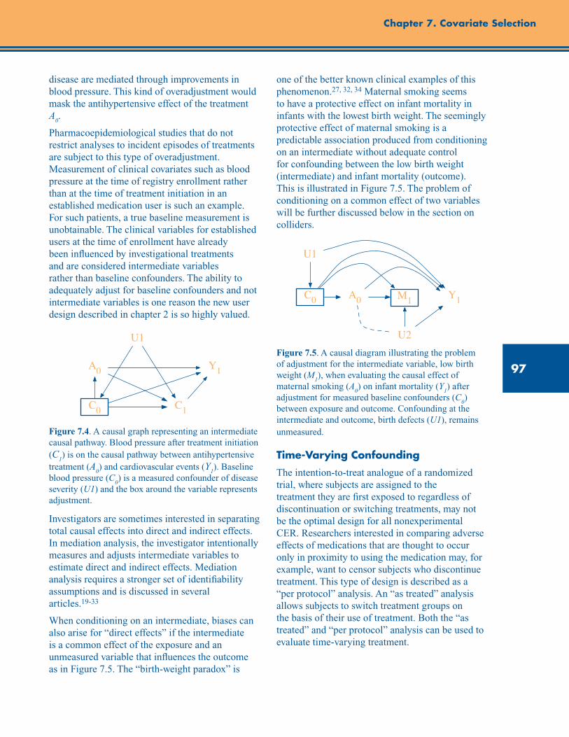
97


disease are mediated through improvements in blood pressure. This kind of overadjustment would mask the antihypertensive effect of the treatment A

0.

Pharmacoepidemiological studies that do not restrict analyses to incident episodes of treatments are subject to this type of overadjustment. Measurement of clinical covariates such as blood pressure at the time of registry enrollment rather than at the time of treatment initiation in an established medication user is such an example. For such patients, a true baseline measurement is unobtainable. The clinical variables for established users at the time of enrollment have already been influenced by investigational treatments and are considered intermediate variables rather than baseline confounders. The ability to adequately adjust for baseline confounders and not intermediate variables is one reason the new user design described in chapter 2 is so highly valued.

Figure 7.4. A causal graph representing an intermediate causal pathway. Blood pressure after treatment initiation (C

1) is on the causal pathway between antihypertensive

treatment (A0) and cardiovascular events (Y

1). Baseline

blood pressure (C0) is a measured confounder of disease

severity (U1) and the box around the variable represents adjustment.

Investigators are sometimes interested in separating total causal effects into direct and indirect effects. In mediation analysis, the investigator intentionally measures and adjusts intermediate variables to estimate direct and indirect effects. Mediation analysis requires a stronger set of identifiability assumptions and is discussed in several articles.19-33

When conditioning on an intermediate, biases can also arise for “direct effects” if the intermediate is a common effect of the exposure and an unmeasured variable that influences the outcome as in Figure 7.5. The “birth-weight paradox” is

one of the better known clinical examples of this phenomenon.27, 32, 34 Maternal smoking seems to have a protective effect on infant mortality in infants with the lowest birth weight. The seemingly protective effect of maternal smoking is a predictable association produced from conditioning on an intermediate without adequate control for confounding between the low birth weight (intermediate) and infant mortality (outcome). This is illustrated in Figure 7.5. The problem of conditioning on a common effect of two variables will be further discussed below in the section on colliders.

Figure 7.5. A causal diagram illustrating the problem of adjustment for the intermediate variable, low birth weight (M

1), when evaluating the causal effect of

maternal smoking (A0) on infant mortality (Y

1) after

adjustment for measured baseline confounders (C0)

between exposure and outcome. Confounding at the intermediate and outcome, birth defects (U1), remains unmeasured.

Time-Varying Confounding

The intention-to-treat analogue of a randomized trial, where subjects are assigned to the treatment they are first exposed to regardless of discontinuation or switching treatments, may not be the optimal design for all nonexperimental CER. Researchers interested in comparing adverse effects of medications that are thought to occur only in proximity to using the medication may, for example, want to censor subjects who discontinue treatment. This type of design is described as a “per protocol” analysis. An “as treated” analysis allows subjects to switch treatment groups on the basis of their use of treatment. Both the “as treated” and “per protocol” analysis can be used to evaluate time-varying treatment.

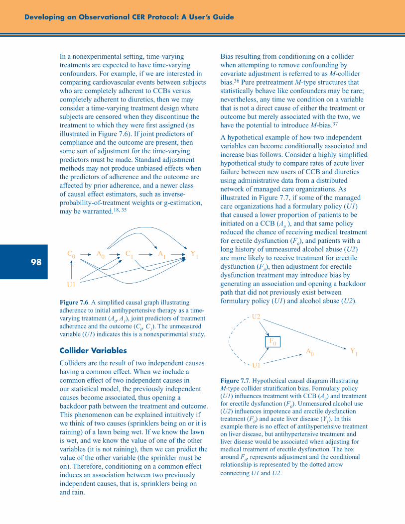
98


In a nonexperimental setting, time-varying treatments are expected to have time-varying confounders. For example, if we are interested in comparing cardiovascular events between subjects who are completely adherent to CCBs versus completely adherent to diuretics, then we may consider a time-varying treatment design where subjects are censored when they discontinue the treatment to which they were first assigned (as illustrated in Figure 7.6). If joint predictors of compliance and the outcome are present, then some sort of adjustment for the time-varying predictors must be made. Standard adjustment methods may not produce unbiased effects when the predictors of adherence and the outcome are affected by prior adherence, and a newer class of causal effect estimators, such as inverse-probability-of-treatment weights or g-estimation, may be warranted.18, 35

Figure 7.6. A simplified causal graph illustrating adherence to initial antihypertensive therapy as a time-varying treatment (A

0, A

1), joint predictors of treatment

adherence and the outcome (C0, C

1). The unmeasured

variable (U1) indicates this is a nonexperimental study.

Collider Variables

Colliders are the result of two independent causes having a common effect. When we include a common effect of two independent causes in our statistical model, the previously independent causes become associated, thus opening a backdoor path between the treatment and outcome. This phenomenon can be explained intuitively if we think of two causes (sprinklers being on or it is raining) of a lawn being wet. If we know the lawn is wet, and we know the value of one of the other variables (it is not raining), then we can predict the value of the other variable (the sprinkler must be on). Therefore, conditioning on a common effect induces an association between two previously independent causes, that is, sprinklers being on and rain.

Bias resulting from conditioning on a collider when attempting to remove confounding by covariate adjustment is referred to as M-collider bias.36 Pure pretreatment M-type structures that statistically behave like confounders may be rare; nevertheless, any time we condition on a variable that is not a direct cause of either the treatment or outcome but merely associated with the two, we have the potential to introduce M-bias.37

A hypothetical example of how two independent variables can become conditionally associated and increase bias follows. Consider a highly simplified hypothetical study to compare rates of acute liver failure between new users of CCB and diuretics using administrative data from a distributed network of managed care organizations. As illustrated in Figure 7.7, if some of the managed care organizations had a formulary policy (U1) that caused a lower proportion of patients to be initiated on a CCB (A

0 ), and that same policy

reduced the chance of receiving medical treatment for erectile dysfunction (F

0), and patients with a

long history of unmeasured alcohol abuse (U2) are more likely to receive treatment for erectile dysfunction (F

0), then adjustment for erectile

dysfunction treatment may introduce bias by generating an association and opening a backdoor path that did not previously exist between formulary policy (U1) and alcohol abuse (U2).

Figure 7.7. Hypothetical causal diagram illustrating M-type collider stratification bias. Formulary policy (U1) influences treatment with CCB (A

0) and treatment

for erectile dysfunction (F0). Unmeasured alcohol use

(U2) influences impotence and erectile dysfunction treatment (F

0) and acute liver disease (Y

1). In this

example there is no effect of antihypertensive treatment on liver disease, but antihypertensive treatment and liver disease would be associated when adjusting for medical treatment of erectile dysfunction. The box around F

0, represents adjustment and the conditional

relationship is represented by the dotted arrow connecting U1 and U2.

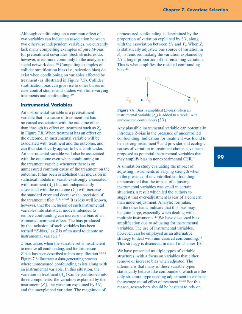
99


Although conditioning on a common effect of two variables can induce an association between two otherwise independent variables, we currently lack many compelling examples of pure M-bias for pretreatment covariates. Such structures do, however, arise more commonly in the analysis of social network data.38 Compelling examples of collider stratification bias (i.e., selection bias) do exist when conditioning on variables affected by treatment (as illustrated in Figure 7.5). Collider stratification bias can give rise to other biases in case-control studies and studies with time-varying treatments and confounding.39

Instrumental Variables

An instrumental variable is a pretreatment variable that is a cause of treatment but has no causal association with the outcome other than through its effect on treatment such as Z

0

in Figure 7.8. When treatment has an effect on the outcome, an instrumental variable will be associated with treatment and the outcome, and can thus statistically appear to be a confounder. An instrumental variable will also be associated with the outcome even when conditioning on the treatment variable whenever there is an unmeasured common cause of the treatment on the outcome. It has been established that inclusion in statistical models of variables strongly associated with treatment (A

0 ) but not independently

associated with the outcome (Y1) will increase

the standard error and decrease the precision of the treatment effect.2, 4, 40-41 It is less well known, however, that the inclusion of such instrumental variables into statistical models intended to remove confounding can increase the bias of an estimated treatment effect. The bias produced by the inclusion of such variables has been termed “Z-bias,” as Z is often used to denote an instrumental variable.8

Z-bias arises when the variable set is insufficient to remove all confounding, and for this reason Z-bias has been described as bias-amplification.42-43 Figure 7.8 illustrates a data-generating process where unmeasured confounding exists along with an instrumental variable. In this situation, the variation in treatment (A

0 ) can be partitioned into

three components: the variation explained by the instrument (Z

0), the variation explained by U1,

and the unexplained variation. The magnitude of

unmeasured confounding is determined by the proportion of variation explained by U1, along with the association between U1 and Y

1. When Z

0

is statistically adjusted, one source of variation in A

0 is removed making the variation explained by

U1 a larger proportion of the remaining variation. This is what amplifies the residual confounding bias.44

Figure 7.8. Bias is amplified (Z-bias) when an instrumental variable (Z

0) is added to a model with

unmeasured confounders (U1).

Any plausible instrumental variable can potentially introduce Z-bias in the presence of uncontrolled confounding. Indication for treatment was found to be a strong instrument45 and provider and ecologic causes of variation in treatment choice have been proposed as potential instrumental variables that may amplify bias in nonexperimental CER.8

A simulation study evaluating the impact of adjusting instruments of varying strength when in the presence of uncontrolled confounding demonstrated that the impact of adjusting instrumental variables was small in certain situations, a result which led the authors to suggest that over-adjustment is less of a concern than under-adjustment. Analytic formulae, on the other hand, indicate that this bias may be quite large, especially when dealing with multiple instruments.42 We have discussed bias amplification due to adjusting for instrumental variables. The use of instrumental variables, however, can be employed as an alternative strategy to deal with unmeasured confounding.46 This strategy is discussed in detail in chapter 10.

We have presented multiple types of variable structures, with a focus on variables that either remove or increase bias when adjusted. The dilemma is that many of these variable types statistically behave like confounders, which are the only structural type needing adjustment to estimate the average causal effect of treatment.47-48 For this reason, researchers should be hesitant to rely on

100


statistical associations alone to select variables for adjustment. The variable structure must be considered when attempting to remove bias through statistical adjustment.

Proxy, Mismeasured, and Unmeasured Confounders

It is not uncommon for a researcher to be aware of an important confounding variable and to lack data on that variable. A measured proxy can sometimes stand in for an unmeasured confounder. For example, use of oxygen canisters could be a proxy for failing health and functional impairment; use of preventive services, such as flu shot, is sometime thought to serve as a proxy for healthy behavior and treatment adherence. Likewise, important confounders sometimes are measured with error. For example, self-reported body mass index will often be subject to underreporting.

Researchers routinely adjust analyses using proxy confounders and mismeasured confounders. Adjusting for a proxy or mismeasured confounder will reduce bias relative to the unadjusted estimate, provided the effect of the confounder on the treatment and the outcome are “monotonic.”48 In other words, any increase in the confounder should on average always affect treatment in the same direction, and should always affect the outcome in the same direction for both the treated and untreated groups. If an increase in the confounder increased the outcome for the treated group and decreased the outcome for the untreated group, then adjustment for the proxy or mismeasured confounder can potentially increase bias. Unfortunately, there are cases, even when the measurement error of the confounder is nondifferential (i.e., does not depend on treatment or outcome), where adjustment for proxy or mismeasured confounders can increase, rather than decrease, bias.49

Another common problem in trying to estimate causal effects is that of unmeasured confounding. Sensitivity analysis techniques have been developed to address misclassified and unmeasured confounding. The reader is referred to chapter 11 for further discussion of sensitivity analyses.

Selection of Variables To Control Confounding

We present two general approaches to selecting variables in order to control confounding in nonexperimental CER. The first approach selects variables on the basis of background knowledge about the relationship of the variable to treatment and outcome. The second approach relies primarily on statistical associations to select variables for control of confounding, using what can be described as high-dimensional automatic variable selection techniques. The use of background knowledge and causal graph theory is strongly recommended when there is sufficient knowledge of the causal structure of the variables. Sufficient knowledge, however, is likely rare when conducting studies across a wide geography and many providers and institutions. For this reason, we also present practical approaches to variable selection that empirically select variables on the basis of statistical associations.

Variable Selection Based on Background Knowledge

Causal Graph Theory

Assuming that a well-defined fixed treatment employing an intention-to-treat paradigm and no set of covariates predicts treatment assignment with 100 percent accuracy, control of confounding is all that is needed to estimate causal effects with nonexperimental data.47-48 The problem, as described above, is that colliders, intermediate variables, and instruments can all statistically behave like confounders. For this reason, an understanding of the causal structure of variables is required to separate confounders from other potential bias-inducing variables. This dilemma has led many influential epidemiologists to take a strong position for selecting variables for control on the basis of background knowledge of the causal structure connecting treatment to outcome.50-54

When sufficient knowledge is available to construct a causal graph, a graphical analysis of the structural basis for evaluating confounding is the most robust approach to selecting variables for adjustment. The goal is to use the graph to identify a sufficient set of variables to achieve unconfoundedness, sometimes also called

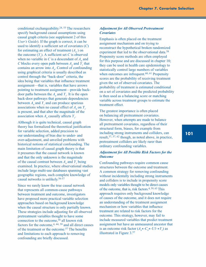
101


conditional exchangeability.24, 55 The researchers specify background causal assumptions using causal graph criteria (see supplement 2 of this User’s Guide). If the graph is correct, it can be used to identify a sufficient set of covariates (C) for estimating an effect of treatment (A

0 ) on

the outcome (Y1). A sufficient set C is observed

when no variable in C is a descendant of A0 and

C blocks every open path between A0 and Y

1 that

contains an arrow into A0. Control of confounding

using graphical criteria is usually described as control through the “back-door” criteria, the idea being that variables that influence treatment assignment—that is, variables that have arrows pointing to treatment assignment—provide back-door paths between the A

0 and Y

1. It is the open

back-door pathways that generate dependencies between A

0 and Y

1 and can produce spurious

associations when no causal effect of A0 on Y

1

is present, and that alter the magnitude of the association when A

0 causally affects Y

1.

Although it is quite technical, causal graph theory has formalized the theoretical justification for variable selection, added precision to our understanding of bias due to under- and over-adjustment, and unveiled problems with historical notions of statistical confounding. The main limitation of causal graph theory is that it presumes that the causal network is known and that the only unknown is the magnitude of the causal contrast between A

0 and Y

1 being

examined. In practice, where observational studies include large multi-use databases spanning vast geographic regions, such complete knowledge of causal networks is unlikely.56-57

Since we rarely know the true causal network that represents all common-cause pathways between treatment and outcome, investigators have proposed more practical variable selection approaches based on background knowledge when the causal structure is only partially known. These strategies include adjusting for all observed pretreatment variables thought to have some connection to the outcome,58 all known risk factors for the outcome,4, 44, 59 and all direct causes of the treatment or the outcome.57 The benefits and limitations to each approach to removing confounding are briefly discussed.

Adjustment for All Observed Pretreatment Covariates

Emphasis is often placed on the treatment assignment mechanism and on trying to reconstruct the hypothetical broken randomized experiment that led to the observational data.58 Propensity score methods are often employed for this purpose and are discussed in chapter 10; they can be used in health care epidemiology to statistically control large numbers of variables when outcomes are infrequent.60, 61 Propensity scores are the probability of receiving treatment given the set of observed covariates. The probability of treatment is estimated conditional on a set of covariates and the predicted probability is then used as a balancing score or matching variable across treatment groups to estimate the treatment effect.

The greatest importance is often placed on balancing all pretreatment covariates. However, when attempts are made to balance all pretreatment covariates, regardless of their structural form, biases, for example from including strong instruments and colliders, can result,37, 57, 62 though, as noted above, in practice, pretreatment colliders are likely rarer than ordinary confounding variables.

Adjustment for All Possible Risk Factors for the Outcome

Confounding pathways require common cause structures between the outcome and treatment. A common strategy for removing confounding without incidentally including strong instruments and colliders is to include in propensity score models only variables thought to be direct causes of the outcome, that is, risk factors.4, 59, 63 This approach requires only background knowledge of causes of the outcome, and it does not require an understanding of the treatment assignment mechanism or how variables that influence treatment are related to risk factors for the outcome. This strategy, however, may fail to include measured variables that predict treatment assignment but have an unmeasured ancestor that is an outcome risk factor (A

0←C

0←U1→Y

1) as

illustrated in Figure 3.57

102


Disjunctive Cause Criterion

The main practical use of causal graphs is to ensure adjustment for confounders and avoid adjusting for known colliders.51 In practice, one only needs to partly know the causal structure of variables relating treatment to the outcome. The disjunctive cause criterion is a formal statement of the conditions in which variable selection based on partial knowledge of the causal structure can remove confounding.57 It states that all observed variables that are a cause of treatment, a cause of outcome, or a cause of both should be included for statistical adjustment. It can be shown that when any subset of observed variables is sufficient to control confounding, the set obtained by applying the disjunctive cause criteria will also constitute a sufficient set.57 This approach requires more knowledge of the variables’ relationship to the treatment and outcome using all pretreatment covariates, or all risk factors, but less knowledge than the back-door path criterion.

Whenever there exists some set of observed variables that block all back-door paths (even if the researcher does not know which subset this is), the disjunctive cause criterion when applied correctly by the investigators will identify a set of variables that also blocks all back-door paths. The other variable selection criteria based on all pretreatment covariates and risk factors do not have this property.57 The approach performs well when the measured variables include some sufficient set, but presents problems when unmeasured confounding remains. In this case, conditioning on an instrument can amplify the bias due to unmeasured confounding. Thus, in practice, known instruments should be excluded before applying the criterion. The best approach to variable selection is less clear when unmeasured confounding may remain after statistical adjustment for measured variables, which is often expected in nonexperimental CER. In this case, every variable selection approach will result in bias. The focus would then be on minimizing bias, which requires thoughtful consideration of the tradeoff between over- and underadjustment. Strong arguments exist for error on the side of overadjustment (adjusting for instruments and colliders) rather than failing to adjust for measured confounders (underadjustment).36, 44 Nevertheless,

adjustments for instrumental variables have been found to amplify bias in practice.45

Empirical Variable Selection Approaches

Historically, data for nonexperimental studies was primarily collected prospectively, and thoughtful planning was needed to ensure complete measurement of all important study variables. We now live in an era where every interaction between the patient and the health care system produces hundreds, if not thousands, of data points that are recorded for clinical and administrative purposes.64 These large multi-use data sources are highly dimensional in that every disease, medication, laboratory result, and procedure code, along with any electronically accessible narrative statements, can be treated as variables.

The new challenge to the researcher is to select a set of variables from this high-dimensional space that characterizes the patient’s baseline status at the time of treatment selection to enable identification of causal effects, or that at least produces the least biased estimates. Advances in computer performance and the availability of high-dimensional data have provided unprecedented opportunities to use data empirically to “learn” associational relationships. Empiric variable selection techniques include identifying a subset of variables of statistical associations with the treatment and/or outcome from the original set on the basis of background knowledge of the relationship with treatment and/or outcome, as well as methods that are considered fully automated, where all variables are initially selected on the basis of statistical associations.

Forward and Backward Selection Procedures

When using traditional regression it is not uncommon to use, for the purposes of covariate selection, what are sometimes called forward and backward selection procedures. Forward selection procedures begin with an empty set of covariates and then consider whether for each covariate, the covariate is associated with the outcome conditional on treatment (usually using a p-value cutoff in a regression model of 0.05 or 0.10). The variable that is most strongly associated with outcome (based on having the smallest p-value

103


below the cutoff) is then added to the collection of variables for which control will be made. Then the process begins again, and one considers whether each covariate is associated with the outcome conditional on the treatment and the covariate already selected; the next covariate that is most strongly associated is again added to the list. The process repeats until all remaining covariates are independent of the outcome conditional on the treatment and the covariates that have been previously selected for control.

Backward selection begins with all covariates in the model; then the investigator considers whether, for each covariate, that covariate is independent of the outcome conditional on the treatment and all other covariates (generally using a p-value cutoff in a regression model of 0.05 or 0.10). The covariate with the largest p-value above the cutoff is then discarded from the list of covariates for which control is made. The process begins again, and the investigator considers whether, for each covariate, that covariate is independent of the outcome, conditional on the treatment and the other covariates not yet discarded; the next covariate with the weakest association with the outcome based on p-value is again discarded. The process repeats itself until all variables still in the list are associated with the outcome conditional on the treatment and the other covariates that have not been discarded.

Provided that the original set of covariates with which one begins suffices for unconfoundedness of treatment effects estimates, then if the backward selection process correctly discards variables that are independent of the outcome conditional on the treatment and other covariates, the final set of covariates selected by the backwards selection procedure will also yield a set of covariates that suffices for conditional exchangeability.57 Likewise, under an additional assumption of “faithfulness,”57 the forward selection procedure will identify a set of covariates that suffices for unconfoundedness provided that the original set of covariates with which one begins suffices to achieve unconfoundedness and that the forward selection process correctly identifies the variables that are and are not independent of the outcome conditional on the treatment and other covariates. The forward and backward procedures can thus

be useful for covariate reduction, but both of them suffer from the need to specify a set of covariates to begin with that suffice for unconfoundedness. Thus, even if an investigator intends to employ forward or backward selection procedures for covariate reduction, other approaches will be needed to decide on what set of covariates these forward and backward procedures should begin with. Moreover, when the initial set of covariates does not suffice for unconfoundedness, it is not clear how forward and backward selection procedures will perform. Variable selection procedures also suffer from the fact that estimates about treatment effects are made after having already used the data to decide on covariates.

Similar but more sophisticated approaches using machine learning algorithms such as boosting, random forest, and other ensemble methods have become increasingly common, as have sparsity-based methods such as LASSO, in dealing with high-dimensional data.65 All of these empirically driven methods are limited, however, in that they are in general unable to distinguish between instruments, colliders, and intermediates on the one hand and genuine confounders on the other. Such differentiation needs to be made a priori on substantive grounds.

Automatic High-Dimensional “Proxy” Adjustment

In an attempt to capture important proxies for unmeasured confounders, Schneeweiss and colleagues proposed an algorithm that creates a very large set of empirically defined variables from health care utilization data.56 The created variables capture the frequency of codes for procedures, diagnoses, and medication fills during a pre-exposure period. The variables created by the algorithm are required to have a minimum prevalence in the source population and to have some marginal association with both treatment and outcome. After they are defined, the variables can be entered into a propensity score model. In several example studies where the true effect of a treatment was approximately known from randomized controlled trials, the algorithm appeared to perform as well as or better than approaches based on simply adjusting for an a priori set of variables.45, 66 By defining variables prior to treatment, propensity score methods will

104


not “over-adjust” by including causal intermediates. Using statistical associations to select potential confounders can result in selection and adjustment of colliders and instruments. Therefore, the analyst should attempt to remove such variables from the set of identified variables. For example, variables that are strong predictors of treatment but have no obvious relation to the outcome should be considered potential sources of Z-bias.

A Practical Approach Combining Causal Analysis With Empirical Selection

There is a continuum between knowing and not knowing the causal, structural relations of variables. We suggest that a practical approach to variable selection may involve a combination of (1) a priori variable selection based on the researcher’s knowledge of causal relationships together with (2) empirical selection using the high-dimensional approach described above.8 The empirical approach could be used to select from a set of a priori variables on the basis of the researcher’s knowledge, and to ultimately select those to be included in the analysis. This more limited use of empirically derived variables may reduce confounding while simultaneously reducing the risk of including variables that could increase bias.

Conclusion

In practice, the particular approach that one adopts for observational research will depend on the researcher’s knowledge, the data quality, and the number of covariates. A deep understanding of the specific clinical and public health risks and opportunities that lie behind the research question often drives these decisions.

Regardless of the strategy employed, researchers should clearly describe how variables are measured and provide a rationale for a priori selection of potential confounders, ideally in the form of a causal graph. If the researchers decide to further eliminate variables using an empiric variable selection technique, then they should present both models and describe what criteria were used to determine inclusion and exclusion. Researchers should consider whether or not they believe adequate measurement is available in the dataset when employing a specific variable selection strategy. In addition, all variables included for adjustment should be listed in the manuscript or final report. When empirical selection procedures are newly developed or modified, researchers are encouraged to make the protocol and code publicly available to improve transparency and reproducibility.

Even when researchers use the methods we describe in this chapter, confounding can persist. Sensitivity analysis techniques are useful for assessing residual confounding resulting from unmeasured and imperfectly measured variables.67-75 Sensitivity analysis techniques assess the extent to which an unmeasured variable would have to be related to the treatment and outcome of interest in order to substantially change the conclusions drawn about causal effects. We refer the reader to chapter 11 for discussion of sensitivity analysis techniques.

105


Checklist: Guidance and key considerations for covariate selection in CER protocols


Describe the data source(s) that will be used to identify important covariates.

– Provide information about the source(s) of data for key covariates, acknowledging the strengths and weaknesses of the data source (e.g., administrative claims, EMRs, chart review, patient self-report) for measuring each type of covariate.

o

Discuss the potential for unmeasured confounding and misclassification.

– Discuss the potential impact of unmeasured confounders and misclassification or measurement error.

– Propose specific formal sensitivity analysis of the impact of unmeasured confounders or misclassified variables.

o

Describe the approach to be used to select covariates for statistical models.

– Discuss approaches based on background knowledge (e.g., selection of all hypothesized common causes, disjunctive cause criterion, directed acyclic graphs, or selection of all variables thought to be risk factors for the outcome.

– Describe model reduction techniques to be used (e.g., forward or backward selection).

– Describe empirical variable selection techniques and how variables were removed from consideration when they were thought to be bias-inducing rather than bias-reducing variables.

o

References1. Huse DM, Roht LH, Hartz SC. Selective use

of calcium channel blockers to treat high-risk hypertensive patients. Pharmacoepidemiol Drug Saf. 2000;9(1):1-9.

2. Schisterman EF, Cole SR, Platt RW. Overadjustment bias and unnecessary adjustment in epidemiologic studies. Epidemiol. 2009;20(4):488-95.

3. Robins JM, Greenland S. The role of model selection in causal inference from nonexperimental data. Am J Epidemiol. 1986;123(3): 392-402.

4. Brookhart MA, Schneeweiss S, Rothman KJ, et al. Variable selection for propensity score models. Am J Epidemiol. 2006;163(12):1149-56.

5. Greenland S, Robins JM. Identifiability, exchangeability, and epidemiological confounding. Int J Epidemiol. 1986;15(3):413-9.

6. Greenland S, Neutra R. Control of confounding in the assessment of medical technology. Int J Epidemiol. 1980;9(4):361-7.

7. Blais L, Ernst P, Suissa S. Confounding by indication and channeling over time: the risks of beta 2-agonists. Am J Epidemiol. 1996;144(12):1161-9.

8. Brookhart MA, Stürmer T, Glynn RJ, et al. Confounding control in healthcare database research: challenges and potential approaches. Med Care. 2010;48(6 Suppl):S114-20.

9. Joffe MM. Confounding by indication: the case of calcium channel blockers. Pharmacoepidemiol Drug Saf. 2000;9(1):37-41.

10. Glynn RJ, Schneeweiss S, Sturmer T. Indications for propensity scores and review of their use in pharmacoepidemiology. Basic Clin Pharmacol Toxicol. 2006;98(3):253-9.

11. Glynn RJ, Schneeweiss S, Wang PS, et al. Selective prescribing led to overestimation of the benefits of lipid-lowering drugs. J Clin Epidemiol. 2006;59(8):819-28.

12. Winkelmayer WC, Levin R, Setoguchi S. Associations of kidney function with cardiovascular medication use after myocardial infarction. Clin J Am Soc Nephrol. 2008;3(5):1415-22.

13. Glynn RJ, Knight EL, Levin R, et al. Paradoxical relations of drug treatment with mortality in older persons. Epidemiol. 2001;12(6):682-9.

106


14. Brookhart MA, Patrick AR, Dormuth C, et al. Adherence to lipid-lowering therapy and the use of preventive health services: an investigation of the healthy user effect. Am J Epidemiol. 2007;166(3):348-54.

15. White HD. Adherence and outcomes: it’s more than taking the pills. Lancet. 2005;366(9502):1989-91.

16. Simpson SH, Eurich DR, Majumdar SR, et al. A meta-analysis of the association between adherence to drug therapy and mortality. BMJ. 2006;333(7557):15.

17. Hernan MA, Hernandez-Diaz S. Beyond the intention-to-treat in comparative effectiveness research. ClinTrials. 2012; 9(1):48-55.

18. Toh S, Hernan MA. Causal inference from longitudinal studies with baseline randomization. Int J Biostat. 2008;4(1):Article22.

19. Vanderweele TJ, Vansteelandt S. Odds ratios for mediation analysis for a dichotomous outcome. Am J Epidemiol. 2010;172(12):1339-48.

20. VanderWeele TJ. Mediation and mechanism. Eur J Epidemiol. 2009;24(5):217-24.

21. Vanderweele TJ. Causal mediation analysis with survival data. Epidemiol. 2011;22(4):582-5.

22. Vanderweele TJ. Subtleties of explanatory language: what is meant by “mediation”? Eur J Epidemiol. 2011;26(5):343-6.

23. VanderWeele TJ. Bias formulas for sensitivity analysis for direct and indirect effects. Epidemiol. 2010;21(4):540-51.

24. Pearl J. An introduction to causal inference. Int J Biostat. 2010;6(2):Article7.

25. Moodie EE, Stephens DA. Using directed acyclic graphs to detect limitations of traditional regression in longitudinal studies. Int J Public Health. 2010;55(6):701-3.

26. Hafeman DM. Confounding of indirect effects: a sensitivity analysis exploring the range of bias due to a cause common to both the mediator and the outcome. Am J Epidemiol. 2011;174(6):710-7.

27. Whitcomb BW, Schisterman EF, Perkins NJ, et al. Quantification of collider-stratification bias and the birthweight paradox. Paediatr Perinat Epidemiol. 2009;23(5):394-402.

28. Shpitser I, Vanderweele TJ. A complete graphical criterion for the adjustment formula in mediation analysis. Int J Biostat. 2011;7(1):16.

29. Robins JM, Greenland S. Identifiability and exchangeability for direct and indirect effects. Epidemiol. 1992;3(2):143-55.

30. Pearl J. Causal inference from indirect experiments. Artificial intelligence in medicine 1995;7(6):561-82.

31. Young GP, St John DJ, Cole SR, et al. Prescreening evaluation of a brush-based faecal immunochemical test for haemoglobin. J Med Screen. 2003;10(3):123-8.

32. Vanderweele TJ, Mumford SL, Schisterman EF. Conditioning on intermediates in perinatal epidemiology. Epidemiol. 2012;23(1):1-9.

33. Robins J. The control of confounding by intermediate variables. Stat Med. 1989;8(6): 679-701.

34. Hernandez-Diaz S, Schisterman EF, Hernan MA. The birth weight “paradox” uncovered? Am J Epidemiol. 2006;164(11):1115-20.

35. Cain LE, Cole SR. Inverse probability-of-censoring weights for the correction of time-varying noncompliance in the effect of randomized highly active antiretroviral therapy on incident AIDS or death. Stat Med. 2009;28(12):1725-38.

36. Greenland S. Quantifying biases in causal models: classical confounding vs collider-stratification bias. Epidemiol. 2003;14(3):300-6.

37. Pearl J. Myth, confusion, and science of causal analysis [Unpublished Manuscript]. Los Angeles, CA: University of California; 2009. http://ftp.cs.ucla.edu/pub/stat_ser/r348-warning.pdf. Accessed March 29, 2012.

38. Shalizi C, Thomas A. Homophily and contagion are generically confounded in observational social network studies. Sociol Methods Res. 2011;40(2):211-39.

39. Hernan MA, Hernandez-Diaz S, Robins JM. A structural approach to selection bias. Epidemiol. 2004;15(5):615-25.

40. Robinson LD, Jewell NP. Covariate adjustment. Biometrics. 1991;47(1):342-3.

41. Austin PC. The performance of different propensity score methods for estimating marginal odds ratios. Stat Med. 2007;26(16):3078-94.

42. Pearl J. Invited commentary: understanding bias amplification. Am J Epidemiol. 2011;174(11):1223-7.

107


43. Wooldridge J. Should instrumental variables be used as matching variables? [Unpublished Manuscript]. East Lansing, MI: Michigan State University; 2009. https://www.msu.edu/~ec/faculty/wooldridge/current%20research/treat1r6.pdf. Accessed March 29, 2012.

44. Myers JA, Rassen JA, Gagne JJ, et al. Effects of adjusting for instrumental variables on bias and precision of effect estimates. Am J Epidemiol. 2011;174(11):1213-22.

45. Patrick AR, Schneeweiss S, Brookhart MA, et al. The implications of propensity score variable selection strategies in pharmacoepidemiology: an empirical illustration. Pharmacoepidemiol Drug Saf. 2011;20(6):551-9.

46. Angrist JG, Imbens GW, Rubin DB. Identification of causal effects using instrumental variables. J Am Stat Assoc. 1996;91:28.

47. Rubin DB. Causal inference using potential outcomes: design, modeling, decisions. J Am Stat Assoc. 2005;100(469):10.

48. Hernán MA, Alonso A, Logan R, et al. Observational studies analyzed like randomized experiments: an application to postmenopausal hormone therapy and coronary heart disease. Epidemiol. 2008;19(6):766-79.

49. Brenner H. Bias due to non-differential misclassification of polytomous confounders. J Clin Epidemiol. 1993;46(1):57-63.

50. Greenland S, Pearl J, Robins JM. Causal diagrams for epidemiologic research. Epidemiol. 1999;10(1):37-48.

51. Hernán MA, Hernández-Díaz S, Werler MM, et al. Causal knowledge as a prerequisite for confounding evaluation: an application to birth defects epidemiology. Am J Epidemiol. 2002;155(2):176-84.

52. Robins JM. Data, design, and background knowledge in etiologic inference. Epidemiol. 2001;12(3):313-20.

53. Pearl J. Causal diagrams for empirical research. Biometrika. 1995;82:669-88.

54. Glymour MM, Weuve J, Chen JT. Methodological challenges in causal research on racial and ethnic patterns of cognitive trajectories: measurement, selection, and bias. Neuropsychology Rev. 2008;18(3):194-213.

55. Shrier I, Platt RW. Reducing bias through directed acyclic graphs. BMC Med Res Methodol. 2008;8:70.

56. Schneeweiss S, Rassen JA, Glynn RJ, et al. High-dimensional propensity score adjustment in studies of treatment effects using health care claims data. Epidemiol. 2009;20(4):512-22.

57. Vanderweele TJ, Shpitser I. A new criterion for confounder selection. Biometrics. 2011;67(4):1406-13.

58. Rubin DB. The design versus the analysis of observational studies for causal effects: parallels with the design of randomized trials. Stat Med. 2007;26(1):20-36.

59. Hill J. Discussion of research using propensity-score matching: comments on ‘A critical appraisal of propensity-score matching in the medical literature between 1996 and 2003’ by Peter Austin, Statistics in Medicine. Stat Med 2008;27(12): 2055-61; discussion 2066-9.

60. Rubin DB. Estimating causal effects from large data sets using propensity scores. Ann Int Med.1997;127(8 Pt 2):757-63.

61. Cepeda MS, Boston R, Farrar JT, Strom BL. Comparison of logistic regression versus propensity score when the number of events is low and there are multiple confounders. Am J Epidemiol.2003;158(3):280-7.

62. Pearl J. Remarks on the method of propensity score. Stat Med. 2009;28:1415-24.

63. Myers JA, Rassen JA, Gagne JJ, et al. Myers et al. respond to “understanding bias amplification.” Am J Epidemiol. 2011;174(11):1228-9.

64. D’Avolio LW, Farwell WR, Fiore LD. Comparative effectiveness research and medical informatics. Am J Med. 2010;123(12 Suppl 1):e32-7.

65. Tibshirani R. Regression shrinkage and selection via the Lasso. J R Stat Soc Series B Stat Methodol. 1996;58(1):267-288.

66. Rassen JA, Glynn RJ, Brookhart MA, Schneeweiss S. Covariate selection in high-dimensional propensity score analyses of treatment effects in small samples. Am J Epidemiol. 2011;173(12):1404-13.

67. Vanderweele TJ, Arah OA. Bias formulas for sensitivity analysis of unmeasured confounding for general outcomes, treatments, and confounders. Epidemiol. 2011;22(1):42-52.

108

68. Vanderweele TJ. Sensitivity analysis: distributional assumptions and confounding assumptions. Biometrics. 2008;64(2):645-9.

69. Schneeweiss S. Sensitivity analysis and external adjustment for unmeasured confounders in epidemiologic database studies of therapeutics. Pharmacoepidemiol Drug Saf. 2006;15(5): 291-303.

70. Rosenbaum PR. Sensitivity analysis for m-estimates, tests, and confidence intervals in matched observational studies. Biometrics. 2007;63(2):456-64.

71. Rosenbaum PR. Sensitivity analysis for matched case-control studies. Biometrics. 1991;47(1):87-100.

72. Greenland S. Useful methods for sensitivity analysis of observational studies. Biometrics. 1999;55(3):990-1.

73. Greenland S. Basic methods for sensitivity analysis of biases. Int J Epidemiol. 1996. 25(6):1107-16.

74. Brumback BA, Hernán MA, Haneuse SJ, et al. Sensitivity analyses for unmeasured confounding assuming a marginal structural model for repeated measures. Stat Med. 2004;23(5):749-67.

75. Arah OA, Chiba Y, Greenland S. Bias formulas for external adjustment and sensitivity analysis of unmeasured confounders. Ann Epidemiol. 2008;18(8):637-46.


109

Abstract

The research question dictates the type of data required, and the researcher must best match the data to the question or decide whether primary data collection is warranted. This chapter discusses considerations for data source selection for comparative effectiveness research (CER). Important considerations for choosing data include whether or not the key variables are available to appropriately define an analytic cohort and identify exposures, outcomes, covariates, and confounders. Data should be sufficiently granular, contain historical information to determine baseline covariates, and represent an adequate duration of followup. The widespread availability of existing data from electronic health records, personal health records, and drug surveillance programs provides an opportunity for answering CER questions without the high expense often associated with primary data collection. If key data elements are unobtainable in an otherwise ideal dataset, methods such as predicting absent variables with available data or interpolating for missing time points may be used. Alternatively, the researcher may link datasets. The process of data linking, which combines information about one individual from multiple sources, increases the richness of information available in a study. This is in contrast to data pooling and networking, which are normally used to increase the size of an observational study. Each data source has advantages and disadvantages, which should be considered thoroughly in light of the research question of interest, as the validity of the study will be dictated by the quality of the data. This chapter concludes with a checklist of key considerations for selecting a data source for a CER protocol.

Chapter 8. Selection of Data SourcesCynthia Kornegay, Ph.D.*

U.S. Food and Drug Administration, Silver Spring, MD

Jodi B. Segal, M.D., MPH Johns Hopkins University, Baltimore, MD

Introduction

Identifying appropriate data sources to answer comparative effectiveness research (CER) questions is challenging. While the widespread availability of existing data provides an opportunity for answering CER questions without the high expense associated with primary data collection, the data source must be chosen carefully to ensure that it can address the study question, that it has a sufficient number of observations, that key variables are available, that there is adequate confounder control, and that there is a sufficient length of followup.

This chapter describes data that may be useful for observational CER studies and the sources of these data, including data collected for both research and

nonresearch purposes. The chapter also explains how the research question should dictate the type of data required and how to best match data to the issue at hand. Considerations for evaluating data quality (e.g., demonstrating data integrity) and privacy protection provisions are discussed. The chapter concludes by describing new sources of data that may expand the options available to CER researchers to address questions. Recommendations for “best practices” regarding data selection are included, along with a checklist that researchers may use when developing and writing a CER protocol. To start, however, it is important to consider primary data collection for observational research, since the use of secondary data may be impossible or unwise in some situations.

*Disclaimer: The views expressed are the authors’ and not necessarily those of the Food and Drug Administration.

110


Data Options

Primary data are data collected expressly for research. Observational studies, meaning studies with no dictated intervention, require the collection of new data if there are no adequate existing data for testing hypotheses. In contrast, secondary data refer to data that were collected for other purposes and are being used secondarily to answer a research question. There are other ways to categorize data, but this classification is useful because the types of information collected for research differ markedly from the types of information collected for nonresearch purposes.

Primary Data

Primary data are collected by the investigator directly from study participants to address a specific question or hypothesis. Data can be collected by in-person or telephone interviews, mail surveys, or computerized questionnaires. While primary data collection has the advantage of being able to address a specific study question, it is often time consuming and expensive. The observational research designs that often require primary data collection are described here. While these designs may also incorporate existing data, we describe them here in the context of primary data collection. The need to use these designs is determined by the research question; if the research question clearly must be answered with these designs below, primary data collection may be required. Additional detail about the selection of suitable study design for observational CER is presented in chapter 2.

Prospective Observational Studies

Observational studies are those in which individuals are selected on the basis of specific characteristics and their progress is monitored. A key concept is that the investigator does not assign the exposure(s) of interest. There are two basic observational designs: (1) cohort studies, in which selection is based on exposure and participants are followed for the occurrence of a particular outcome, and (2) case-control studies, where selection is based on a disease or condition and participants are contacted to determine a particular exposure.

Within this framework, there is a wide variety of possible designs. Participants can be individuals or groups (e.g., schools or hospitals); they can be followed into the future (prospective data collection) or asked to recall past events (retrospective data collection); and, depending on the specific study questions, elements of the two basic designs can be combined into a single study (e.g., case-cohort or nested case-control studies). If information is also collected on those who are either not exposed or do not have the outcome of interest, observational studies can be used for hypothesis testing.

An example of a prospective observational study is a recent investigation comparing medication adherence and viral suppression between once-daily and more-than-once daily pill regimens in a homeless and near-homeless HIV-positive population.1 Adherence was measured using unscheduled pill-count visits over the six-month study period while viral suppression was determined at the end of the study. The investigators found that both adherence and viral suppression levels were higher in the once-daily groups compared to the more-than-once-daily groups. The results of this study are notable as they indicate an effective method to treat HIV in a particularly hard-to-reach population.

Registries

In the most general sense, a registry is a systematic collection of data. Registries that are used for research have clearly stated purposes and targeted data collection.

Registries use an observational study design that does not specify treatments or require therapies intended to change patient outcomes. There are generally few inclusion and exclusion criteria to make the results broadly generalizable. Patients are typically identified when they present for care, and the data collected generally include clinical and laboratory tests and measurements. Registries can be defined by specific diseases or conditions (e.g., cancer, birth defects, or rheumatoid arthritis), exposures (e.g., to drug products, medical devices, environmental conditions, or radiation), time periods, or populations. Depending on their purpose and the information collected, registry data can potentially be used for public health

111

Chapter 8. Selection of Data Sources

surveillance, to determine incidence rates, to perform risk assessment, to monitor progress, and to improve clinical practice. Registries can also provide a unique perspective into specialized subpopulations. However, like any long-term study, they can be very expensive to maintain due to the effort required to remain in contact with the participants over extended periods of time.

Registries have been used extensively for CER. As an example, the United States Renal Data System (USRDS) is a registry of individuals receiving dialysis that includes clinical data as well as medical claims. This registry has been used to answer questions about the comparative effectiveness and safety of erythropoiesis-stimulating agents and iron in this patient population,2 the comparative effectiveness of dialysis chain facilities,3 and the effectiveness of nocturnal versus daytime dialysis.4 Another registry is the Surveillance, Epidemiology, and End Results (SEER) registry, which gathers data on Americans with cancer. Much of the SEER registry’s value for CER comes from its linkage to Medicare data. Examples of CER studies that make use of this linked data include an evaluation of the effectiveness of radiofrequency ablation for hepatocellular carcinoma compared to resection or no treatment5 and a comparison of the safety of open versus radical nephrectomy in individuals with kidney cancer.6 A third example is a study that used SEER data to evaluate survival among individuals with bladder cancer who underwent early radical cystectomy compared to those patients who did not.7

Secondary Data

Much secondary data that are used for CER can be considered byproducts of clinical care. The framework developed by Schneeweiss and Avorn is a useful structure with which to consider the secondary sources of data generated within this context.8 They described the “record generation process,” which is the information generated during patient care. Within this framework, data are generated in the creation of the paper-based or electronic medical (health) record, claims are

generated so that providers are paid for their services, and claims and dispensing records are generated at the pharmacy at the time of payment. As data are not collected specifically for the research question of interest, particular attention must be paid to ensure that data quality is sufficient for the study purpose.

A thorough understanding of the health system in which patients receive care and the insurance products they use is needed for a clear understanding of whether the data are likely to be complete or unavailable for the population of interest. Integrated health delivery systems such as Kaiser Permanente, in which patients receive the majority of their care from providers and facilities within the system, provide the most complete picture of patient medical care.

Electronic Health Record (EHR) Data

Electronic health records (EHRs) are used by health care providers to capture the details of the clinical encounter. They are chiefly clinical documentation systems. They are populated with some combination of free text describing findings from the history and the physical examination; results inputted with check-boxes to indicate positive responses; patient-reported responses to questions for recording symptoms or for screening; prefilled templates that describe normal and abnormal findings; imported text from earlier notes on the patient; and linkages to laboratory results, radiology reports and images; and specialized testing results (such as electrocardiograms, echocardiograms, or pulmonary function test results). Some EHRs include other features, such as flow sheets of clinical results, particularly those results used in inpatient settings (e.g., blood pressure measurements); problem and habits lists, electronic medication administration records; medication reconciliation features; decision support systems and/or clinical pathways and protocols; and specialty features for the documentation needs of specialty practices. The variables that might be accessible from EHR data are shown in Table 8.1.

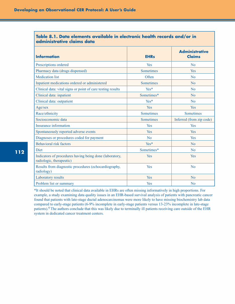
112


Table 8.1. Data elements available in electronic health records and/or in administrative claims data

Information EHRsAdministrative

Claims

Prescriptions ordered Yes No

Pharmacy data (drugs dispensed) Sometimes Yes

Medication list Often No

Inpatient medications ordered or administered Sometimes No

Clinical data: vital signs or point of care testing results Yes* No

Clinical data: inpatient Sometimes* No

Clinical data: outpatient Yes* No

Age/sex Yes Yes

Race/ethnicity Sometimes Sometimes

Socioeconomic data Sometimes Inferred (from zip code)

Insurance information Yes Yes

Spontaneously reported adverse events Yes Yes

Diagnoses or procedures coded for payment No Yes

Behavioral risk factors Yes* No

Diet Sometimes* No

Indicators of procedures having being done (laboratory, radiologic, therapeutic)

Yes Yes

Results from diagnostic procedures (echocardiography, radiology)

Yes No

Laboratory results Yes No

Problem list or summary Yes No

*It should be noted that clinical data available in EHRs are often missing informatively in high proportions. For example, a study examining data quality issues in an EHR-based survival analysis of patients with pancreatic cancer found that patients with late-stage ductal adenocarcinomas were more likely to have missing biochemistry lab data compared to early-stage patients (6-9% incomplete in early-stage patients versus 13-23% incomplete in late-stage patients).9 The authors conclude that this was likely due to terminally ill patients receiving care outside of the EHR system in dedicated cancer treatment centers.

113


As can be seen from the variable list, the details about an individual patient may be extensive. The method of data collection is not standardized and the intervals between visits vary for every patient in accordance with usual medical practice. Of note, medication information captured in EHRs differs from data captured by pharmacy claims. While pharmacy claims contain information on medications dispensed (including the national drug code [NDC] to identify the medication, dispensing date, days’ supply, and amount dispensed), EHRs more typically contain information on medications prescribed by a clinician. Medication data from EHRs are often captured as part of the patient’s medication list, which may include the medication name, order date, strength, units, quantity, and frequency. Again depending on the specific EHR system, inpatient medication orders may or may not be available but are not typically. As EHRs differ substantially, it is important to understand what fields are captured in the EHR under consideration, and to realize that completeness of specific fields may vary depending on how individual health care providers use the EHR.

An additional challenge with EHR data is that patients may receive care at different facilities, and information regarding their health may be entered separately into multiple systems that are not integrated and are inconsistent across practices. If a patient has an emergency room visit at a hospital that is not his usual site of care, it is unlikely to be recorded in the electronic medical record that houses the majority of his clinical information. Additionally, for a patient who resides in two or more cities during the year, the electronic medical record at each institution may be incomplete if the institutions do not share a common data system.

Paper-Based Records

Although time-intensive to access, the use of paper-based records is sometimes required. Many practices still do not have EHRs; in 2009, it was estimated that only half of outpatient practices in the U.S. were using EHRs.10 Exclusion of sites without electronic records may bias study results because these sites may have different patient populations or because there may be regional differences in practice. These data may be particularly valuable if patient-reported information is needed (such as severity of pain,

quality of symptoms, mental health concerns, and habits). The richness of information in paper-based records may exceed that in EHR data particularly if the electronic data is template driven. Additionally, paper-based records are valuable as a source of primary data for validating data that is available elsewhere such as in administrative claims. With a paper medical record, the researcher can test the sensitivity and specificity of the information contained in claims data by reviewing the paper record to see if the diagnosis or procedure was described. In that situation, the paper-based record would be considered the reference standard for diagnoses and procedures.

Administrative Data

Administrative health insurance data are typically generated as part of the process of obtaining insurance reimbursement. Presently, medical claims are most often coded using the International Classification of Disease (ICD) and the Common Procedural Terminology (CPT) systems. The ICD, Ninth Revision, Clinical Modification (ICD-9-CM) is the official system of assigning codes to diagnoses and procedures associated with hospital utilization in the United States. Much of Europe is using ICD-10 already, while the United States currently uses ICD-9 for everything except mortality data; the United States will start using ICD-10 in October 2013.11 The ICD coding terminology includes a numerical list of codes identifying diseases, as well as a classification system for surgical, diagnostic, and therapeutic procedures. The National Center for Health Statistics and the Centers for Medicare and Medicaid Services (CMS) are responsible for overseeing modifications to the ICD. For outpatient encounters, the CPT is used for submitting claims for services. This terminology was initially developed by the American Medical Association in 1966 to encourage the use of standard terms and descriptors to document procedures in the medical record, to communicate accurate information on procedures and services to agencies concerned with insurance claims, to provide the basis for a computer-oriented system to evaluate operative procedures, and for actuarial and statistical purposes. Presently, this system of terminology is the required nomenclature to report outpatient medical procedures and services to U.S. public and private health insurance programs, as the

114


ICD is the required system for diagnosis codes and inpatient hospital services.12 The diagnosis-related group (DRG) classification is a system to classify hospital cases by their ICD codes into one of approximately 500 groups expected to have similar hospital resource use; it was developed for Medicare as part of the prospective payment system. The DRG system can be used for research as well, but with the recognition that there may be clinical heterogeneity within a DRG. There is no correlate of the DRG for outpatient care.

When using these claims for research purposes, the validity of the coding is of the highest importance. This is described in more detail below. The validity of codes for procedures exceeds the validity of diagnostic codes, as procedural billing is more closely tied to reimbursement. Understandably, the motivation for coding procedures correctly is high. For diagnosis codes, however, a diagnosis that is under evaluation (e.g., a medical visit or a test to “rule out” a particular condition) is indistinguishable from a diagnosis that has been confirmed. Consequently, researchers tend to look for sequences of diagnoses, or diagnoses followed by treatments appropriate for those diagnoses, in order to identify conditions of interest. Although Medicare requires an appropriate diagnosis code to accompany the procedure code to authorize payment, other insurers have looser requirements. There are few external motivators to code diagnoses with high precision, so the validity of these codes requires an understanding of the health insurance system’s approach to documentation.13-20 Investigators using claims data for CER should validate the key diagnostic and procedure codes in the study. There are many examples of validation studies in the literature upon which to pattern such a study.18, 21-22

Additional codes are available in some datasets—for example, the “present on admission” code that has been required for Medicare and Medicaid billing since October 2007—which may help in further refinement of algorithms for identifying key exposures and outcomes.

Pharmacy Data

Outpatient pharmacy data include claims submitted to insurance companies for payment as well as the records on drug dispensing kept

by the pharmacy or by the pharmacy benefits manager (PBM). Claims submitted to the insurance company use the NDC as the identifier of the product. The NDC is a unique, 10-digit, 3-segment number that is a standard product identifier for human drugs in the United States. Included in this number are the active ingredient, the dosage form and route of administration, the strength of the product, and the package size and type. The U.S. Food and Drug Administration (FDA) has authority over the NDC codes. Claims submitted to insurance companies for payment for drugs are submitted with the NDC code as well as information about the supply dispensed (e.g., how many days the prescription is expected to cover), and the amount of medication dispensed. This information can be used to provide a detailed picture of the medications dispensed to the patient. Medications for which a claim is not submitted or is not covered by the insurance plan (e.g., over-the-counter medications) are not available. It should be noted that claims data are generally weak for medical devices, due to a lack of uniform coding, and claims often do not include drugs that are not dispensed through the pharmacy (e.g., injections administered in a clinic).

Large national PBMs, such as Medco Health Solutions or Caremark, administer prescription drug programs and are responsible for processing and paying prescription drug claims. They are the interface between the pharmacies and the payers, though some larger health insurers manage their own pharmacy data. PBM models differ substantially, but most maintain formularies, contract with pharmacies, and negotiate prices with drug manufacturers. The differences in formularies across PBMs may offer researchers the advantage of natural experiments, as some patients will not be dispensed a particular medication even when indicated, while other patients will be dispensed the medication, solely due to the formulary differences of their PBMs. Some PBMs own their own mail-order pharmacies, eliminating the local pharmacies’ role in distributing medications. PBMs more recently have taken on roles of disease management and outcomes reporting, which generates additional data that may be accessible for research purposes. Figure 8.1 illustrates the flow of information into PBMs from health plans, pharmaceutical

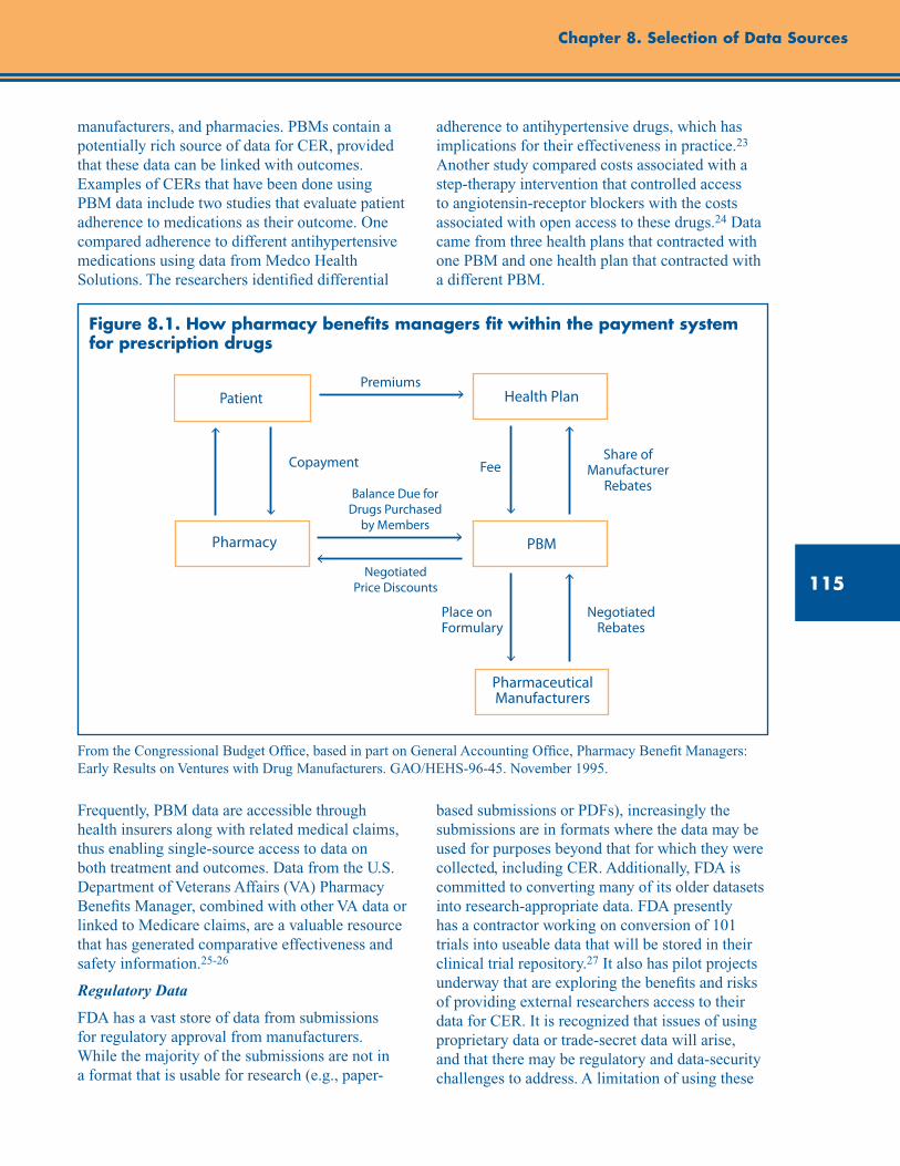
115


Health Plan

PBMPharmacy

Pharmaceutical Manufacturers

Negotiated Rebates

Place on Formulary

Share of Manufacturer

RebatesFeeCopayment

Premiums

Balance Due for Drugs Purchased

by Members

NegotiatedPrice Discounts

Patient

manufacturers, and pharmacies. PBMs contain a potentially rich source of data for CER, provided that these data can be linked with outcomes. Examples of CERs that have been done using PBM data include two studies that evaluate patient adherence to medications as their outcome. One compared adherence to different antihypertensive medications using data from Medco Health Solutions. The researchers identified differential

adherence to antihypertensive drugs, which has implications for their effectiveness in practice.23 Another study compared costs associated with a step-therapy intervention that controlled access to angiotensin-receptor blockers with the costs associated with open access to these drugs.24 Data came from three health plans that contracted with one PBM and one health plan that contracted with a different PBM.

Figure 8.1. How pharmacy benefits managers fit within the payment system for prescription drugs

From the Congressional Budget Office, based in part on General Accounting Office, Pharmacy Benefit Managers: Early Results on Ventures with Drug Manufacturers. GAO/HEHS-96-45. November 1995.

Frequently, PBM data are accessible through health insurers along with related medical claims, thus enabling single-source access to data on both treatment and outcomes. Data from the U.S. Department of Veterans Affairs (VA) Pharmacy Benefits Manager, combined with other VA data or linked to Medicare claims, are a valuable resource that has generated comparative effectiveness and safety information.25-26

Regulatory Data

FDA has a vast store of data from submissions for regulatory approval from manufacturers. While the majority of the submissions are not in a format that is usable for research (e.g., paper-

based submissions or PDFs), increasingly the submissions are in formats where the data may be used for purposes beyond that for which they were collected, including CER. Additionally, FDA is committed to converting many of its older datasets into research-appropriate data. FDA presently has a contractor working on conversion of 101 trials into useable data that will be stored in their clinical trial repository.27 It also has pilot projects underway that are exploring the benefits and risks of providing external researchers access to their data for CER. It is recognized that issues of using proprietary data or trade-secret data will arise, and that there may be regulatory and data-security challenges to address. A limitation of using these

116


trials for CER is that they are typically efficacy trials rather than effectiveness trials. However, when combined using techniques of meta-analysis, they may provide a comprehensive picture of a drug’s efficacy and short-term safety.

Repurposed Trial Data or Data From Completed Observational Studies

A vast amount of data is collected for clinical research in studies funded by the Federal government. By law, these data must be made available upon request to other researchers, as this was information collected with taxpayer dollars. This is an exceptional source of existing data. To illustrate, the Cardiovascular Health Study is a large cohort study that was designed to identify risk factors for coronary heart disease and stroke by means of a population-based longitudinal cohort study.28 The study investigators collected diverse outcomes including information on hospitalization, specifically heart failure associated hospitalizations. Thus, the data from this study can be used to answer comparative effectiveness questions about interventions and their effectiveness on preventing heart failure complications, even though this was not a primary aim of the original cohort study. A limitation is that the researcher is limited to only the data that were collected—an important consideration when selecting a dataset. Some of the datasets have associated biospecimen repositories from which specimens can be requested for additional testing.

Completed studies with publicly available datasets often can be identified through the National Institutes of Health institute that funded the study. For example, the National Heart Lung and Blood Institute has a searchable site (at https://biolincc.nhlbi.nih.gov/home/) where datasets can be identified and requested. Similarly, the National Institute of Diabetes and Digestive and Kidney Diseases has a repository of datasets as well as instructions for requesting data (at https://www.niddkrepository.org/niddk/jsp/public/resource.jsp).

Considerations for Selecting Data

Required Data Elements

The research question must drive the choice of data. Frequently, however, as the question is

developed, it becomes clear that a particular piece of information is critical to answering the question. For example, a question about interventions that reduce the amount of albuminuria will almost certainly require access to laboratory data that include measurement of this outcome. Reliance on ICD-9 codes or use of a statement in the medical record that “albuminuria decreased” will be insufficiently specific for research purposes. Similarly, a study question about racial differences in outcomes from coronary interventions requires data that include documentation of race; this requirement precludes use of most administrative data from private insurers that do not collect this information. If the relevant data are not available in an existing data source, this may be an indication that primary data collection or linking of datasets is in order. It is recommended that the investigator specify a priori what the minimum requirements of the data are before the data are identified, as this will help avoid the effort of making suboptimal data work for a given study question.

If some key data elements seem to be unobtainable in an otherwise suitable dataset, one might consider ways to supplement the available data. These strategies may be methodological, such as predicting absent data variables with data that are available, or interpolating for missing time points. The authors recently completed a study in which the presence of obesity was predicted for individuals in the dataset based on ICD-9 codes.29 In such instances, it is desirable to provide a reference to support the quality of data obtained by such an approach.

Alternatively, there may be a need to link datasets or to use already linked datasets. SEER-Medicare is an example of an already linked dataset that combines the richness of the SEER cancer diagnosis data with claims data from Medicare.30 Unique patient identifiers that can be linked across datasets (such as Social Security numbers) provide opportunities for powerful linkages with other datasets.31 Other methods have been developed that do not rely on the existence of unique identifiers.32 As described above, linking medical data with environmental data, population-level data, or census data provides rich datasets for addressing research questions. Privacy concerns raised by individual contributors can greatly increase the complexity and time needed for a study with linked data.

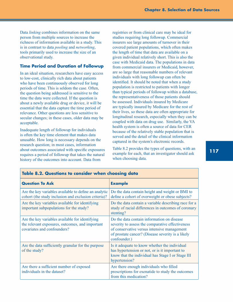
117


Data linking combines information on the same person from multiple sources to increase the richness of information available in a study. This is in contrast to data pooling and networking, tools primarily used to increase the size of an observational study.

Time Period and Duration of Followup

In an ideal situation, researchers have easy access to low-cost, clinically rich data about patients who have been continuously observed for long periods of time. This is seldom the case. Often, the question being addressed is sensitive to the time the data were collected. If the question is about a newly available drug or device, it will be essential that the data capture the time period of relevance. Other questions are less sensitive to secular changes; in these cases, older data may be acceptable.

Inadequate length of followup for individuals is often the key time element that makes data unusable. How long is necessary depends on the research question; in most cases, information about outcomes associated with specific exposures requires a period of followup that takes the natural history of the outcomes into account. Data from

registries or from clinical care may be ideal for studies requiring long followup. Commercial insurers see large amounts of turnover in their covered patient populations, which often makes the length of time that data are available on a given individual relatively short. This is also the case with Medicaid data. The populations in data from commercial insurers or Medicaid, however, are so large that reasonable numbers of relevant individuals with long followup can often be identified. It should be noted that when a study population is restricted to patients with longer than typical periods of followup within a database, the representativeness of those patients should be assessed. Individuals insured by Medicare are typically insured by Medicare for the rest of their lives, so these data are often appropriate for longitudinal research, especially when they can be coupled with data on drug use. Similarly, the VA health system is often a source of data for CER because of the relatively stable population that is served and the detail of the clinical information captured in the system’s electronic records.

Table 8.2 provides the types of questions, with an example for each, that an investigator should ask when choosing data.

Table 8.2. Questions to consider when choosing data

Question To Ask Example

Are the key variables available to define an analytic cohort (the study inclusion and exclusion criteria)?

Do the data contain height and weight or BMI to define a cohort of overweight or obese subjects?

Are the key variables available for identifying important subpopulations for the study?

Do the data contain a variable describing race for a study of racial differences in outcomes of coronary stenting?

Are the key variables available for identifying the relevant exposures, outcomes, and important covariates and confounders?

Do the data contain information on disease severity to assess the comparative effectiveness of conservative versus intensive management of prostate cancer? (Disease severity is a likely confounder.)

Are the data sufficiently granular for the purpose of the study?

Is it adequate to know whether the individual has hypertension or not, or is it important to know that the individual has Stage I or Stage III hypertension?

Are there a sufficient number of exposed individuals in the dataset?

Are there enough individuals who filled prescriptions for exenatide to study the outcomes from this medication?

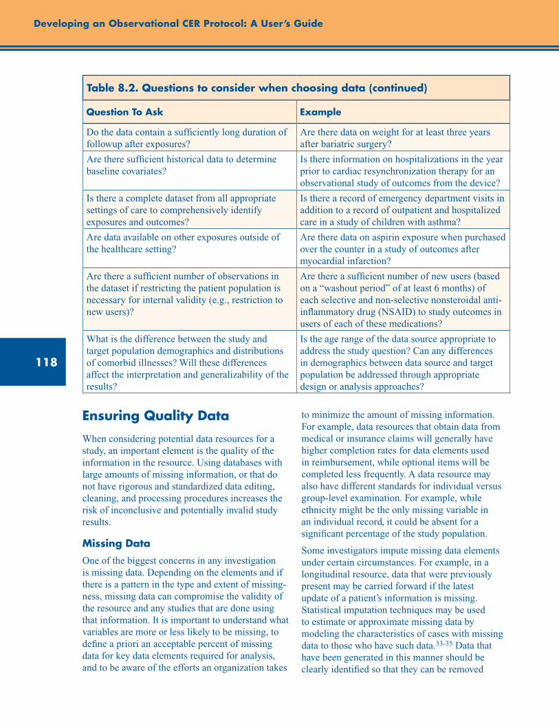
118


Table 8.2. Questions to consider when choosing data (continued)

Question To Ask Example

Do the data contain a sufficiently long duration of followup after exposures?

Are there data on weight for at least three years after bariatric surgery?

Are there sufficient historical data to determine baseline covariates?

Is there information on hospitalizations in the year prior to cardiac resynchronization therapy for an observational study of outcomes from the device?

Is there a complete dataset from all appropriate settings of care to comprehensively identify exposures and outcomes?

Is there a record of emergency department visits in addition to a record of outpatient and hospitalized care in a study of children with asthma?

Are data available on other exposures outside of the healthcare setting?

Are there data on aspirin exposure when purchased over the counter in a study of outcomes after myocardial infarction?

Are there a sufficient number of observations in the dataset if restricting the patient population is necessary for internal validity (e.g., restriction to new users)?

Are there a sufficient number of new users (based on a “washout period” of at least 6 months) of each selective and non-selective nonsteroidal anti-inflammatory drug (NSAID) to study outcomes in users of each of these medications?

What is the difference between the study and target population demographics and distributions of comorbid illnesses? Will these differences affect the interpretation and generalizability of the results?

Is the age range of the data source appropriate to address the study question? Can any differences in demographics between data source and target population be addressed through appropriate design or analysis approaches?

Ensuring Quality Data

When considering potential data resources for a study, an important element is the quality of the information in the resource. Using databases with large amounts of missing information, or that do not have rigorous and standardized data editing, cleaning, and processing procedures increases the risk of inconclusive and potentially invalid study results.

Missing Data

One of the biggest concerns in any investigation is missing data. Depending on the elements and if there is a pattern in the type and extent of missing-ness, missing data can compromise the validity of the resource and any studies that are done using that information. It is important to understand what variables are more or less likely to be missing, to define a priori an acceptable percent of missing data for key data elements required for analysis, and to be aware of the efforts an organization takes

to minimize the amount of missing information. For example, data resources that obtain data from medical or insurance claims will generally have higher completion rates for data elements used in reimbursement, while optional items will be completed less frequently. A data resource may also have different standards for individual versus group-level examination. For example, while ethnicity might be the only missing variable in an individual record, it could be absent for a significant percentage of the study population.

Some investigators impute missing data elements under certain circumstances. For example, in a longitudinal resource, data that were previously present may be carried forward if the latest update of a patient’s information is missing. Statistical imputation techniques may be used to estimate or approximate missing data by modeling the characteristics of cases with missing data to those who have such data.33-35 Data that have been generated in this manner should be clearly identified so that they can be removed

119


for sensitivity analyses, as may be appropriate. Additional information about methods for handling missing data in analysis is covered in chapter 10.

Changes That May Alter Data Availability and Consistency Over Time

Any data resource that collects information over time is likely to eventually encounter changes in the data that will affect longitudinal analyses. These changes could be either a singular event or a gradual shift in the data and can be triggered by the organization that maintains the database or by events beyond the control of that organization including adjustments in diagnostic practices, coding and reimbursement modifications, or increased disease awareness. Investigators should be aware of these changes as they may have a substantial effect on the study design, time period, and execution of the project.

Sudden changes in the database may be dealt with by using trend breaks. These are points in time where the database is discontinuous, and analyses that cross over these points will need to be interpreted with care. Examples of trend break events might be major database upgrades and/or redesigns or changes in data suppliers. Other trend break events that are outside the influence of the maintenance organization might be medical coding upgrades (e.g., ICD-9 to ICD-10), announcements or presentations at conferences (e.g., Women’s Health Initiative findings) that may lead to changes in medical practice, or high profile drug approvals or withdrawals.

More gradual events can also affect the data availability. Software upgrades and changes might result in more data being available for recently added participants versus individuals who were captured in prior versions. Changes in reimbursement and recommended practice could lead to shifts in use of ICD-9 codes, or to more or less information being entered for individuals.

Validity of Key Data Definitions

Validity assessment of key data in an investigation is an important but sometimes overlooked issue in health care research using secondary data. There is a need to assess not only the general definition of key variables, but also their reliability and validity

in the particular database chosen for the analysis. In some cases, particularly for data resources commonly used for research, other researchers or the organization may have validated outcomes of health events (e.g., heart attack, hospitalization, or mortality).36 Creating the best definitions for key variables may require the involvement of knowledgeable clinicians who might suggest that the occurrence of a specific procedure or a prescription would strengthen the specificity of a diagnosis. Knowing the validity of other key variables, such as race/ethnicity, within a specific dataset is essential, particularly if results will be described in these subgroups.

Ideally, validity is examined by comparing study data to additional or alternative records that represent a “gold standard,” such as paper-based medical records. We described in the Administrative Data section above how validity of diagnoses associated with administrative claims might be assessed relative to paper-based records. EHRs and non–claims-based resources do not always allow for this type of assessment, but a more accommodating validation process has not yet been developed. When a patient’s primary health care record is electronic, there may not be a paper trail to follow. Commonly, all activity is integrated into one record, so there is no additional documentation. On the other hand, if the data resource pulls information from a switch company (an organization that specializes in routing claims between the point of service and an insurance company), there may be no mechanism to find additional medical information for patients. In those cases, the information included in the database is all that is available to researchers.

Data Privacy Issues

Data privacy is an ongoing concern in the field of health care research. Most researchers are familiar with the Health Insurance Portability and Accountability Act (HIPAA), enacted in 1996 in part to standardize the security and privacy of health care information. HIPAA coined the term “protected health information” (PHI), defined as any individually identifiable health information (45 CFR 160.103). HIPAA requires that patients be informed of the use of their PHI and that covered

120


entities (generally, health care clearinghouses, employer-sponsored health plans, health insurers, and medical service providers) track the use of PHI. HIPAA also provides a mechanism for patients to report when they feel these regulations have been violated.37

In practical terms, this has resulted in an increase in the amount and complexity of documentation and permissions required to conduct healthcare research and a decrease in patient recruitment and participation levels.38-39 While many data resources have established procedures that allow for access to data without personal identifiers, obtaining permission to use identifiable information from existing data sources (e.g., from chart review) or for primary data collection can be time consuming. Additionally, some organizations will not permit research to proceed beyond a certain point (e.g., beginning or completing statistical analyses, dissemination, or publication of results) without proper institutional review board approvals in place. If a non-U.S. data resource is being used, researchers will need to be aware of differences between U.S. privacy regulations and those in the country where the data resource resides.

Adherence to HIPAA regulations can also affect study design considerations. For example, since birth, admission, and discharge dates are all considered to be PHI, researchers may need to use a patient’s age at admission and length of stay as unique identifiers. Alternatively, a limited data set that includes PHI but no direct patient identifiers such as name, address, or medical record numbers may be defined and transferred with appropriate data use agreements in place. Organizations may have their own unique limits on data sharing and pooling. For example, in the VA system, the general records and records for condition-specific treatment, such as HIV treatment, may not be pooled. Additional information regarding HIPAA regulations as they apply to data used for research may be found on the National Institutes of Health Web site.40

Emerging Issues and Opportunities

Data From Outside of the United States

Where appropriate, non-U.S. databases may be considered to address CER questions, particularly for longitudinal studies. One of the main reasons is that, unlike the majority of U.S. health care systems, several countries with single-payer systems, such as Canada, the United Kingdom, and the Netherlands, have regional or national EMR systems. This makes it much easier to obtain complete, long-term medical records and to follow individuals in longitudinal studies.41

The Clinical Practice Research Datalink (CPRD) is a collection of anonymized primary care medical records from selected general practices across the United Kingdom. These data have been linked to many other datasets to address comparative effectiveness questions. An example is a study that linked the CPRD to the Myocardial Ischaemia National Audit Project registry in England and Wales. The researchers answered questions about the risks associated with discontinuing clopidogrel therapy after a myocardial infarction (performed when the database was called General Practice Research Database).42

While the selection of a non-U.S. data source may be the right choice for a given study, there are a number of things to consider when designing a study using one of these resources.

One of the main considerations is if the study question can be appropriately addressed using a non-U.S. resource. Questions that should be addressed during the study design process include:

• Is the exposure of interest similar between the study and target population? For example, if the exposure is a drug product, is it available in the same dose and form in the data resource? Is it used in the same manner and frequency as in the United States?

121


• Are there any differences in availability, cost, practice, or prescribing guidelines between the study and target populations? Has the product been available in the study population and the United States for similar periods of time?

• What is the difference between the health care systems of the study and target populations? Are there differences in diagnosis methods and treatment patterns for the outcome of interest? Does the outcome of interest occur with the same frequency and severity in the study and target populations?

• Are the comparator treatments similar to those that would be available and used in the United States?

An additional consideration is data access. Access to some resources, such as the United Kingdom’s CPRD, can be purchased by interested researchers. Others, such as Canada’s regional health care resources, may require the personal interest of and an official association with investigators in that country who are authorized to use the system. If a non-U.S. data resource is appropriate for a proposed study, the researcher will need to become familiar with the process for accessing the data and allow for any extra time and effort required to obtain permission to use it.

A sound justification for selecting a non-U.S. data resource, a solid understanding of the similarities and differences of the non-U.S. versus the U.S. systems, as well as careful discussion of whether the results of the study can be generalized to U.S. populations will help other researchers and health care practitioners interpret and apply the results of non-U.S.-based research to their particular situations.

Point of Care Data Collection and Interactive Voice Response/Other Technologies

Traditionally, the data used in epidemiologic studies have been gathered at one point in time, cleaned, edited, and formatted for research use at a later point. As technology has developed, however, data collected close to the point of care increasingly have been available for analysis. Prescription claims can be available for research in as little as one week.

In conjunction with a shortened turnaround time for data availability, the point at which data are coded and edited for research is also occurring closer to when the patient received care. Many people are familiar with health care encounters where the physician takes notes, which are then transcribed and coded for use. With the advent of EHRs, health information is now coded and transcribed into a searchable format at the time of the visit; that is, the information is directly coded as it is collected, rather than being transcribed later.

Another innovation is using computers to collect data. Computer-aided data collection has been used in national surveys since the 1990s43 and also in types of research (such as risky behaviors, addiction, and mental health) where respondents might not be comfortable responding to a personal interviewer.44-46

The advantages of these new and timely data streams are more detailed data, sometimes available in real or near-real time that can be used to spot trends or patterns. Since data can be recorded at the time of care by the health care provider, this may help minimize miscoding and misinterpretation. Computerized data collection and Interactive Voice Response are becoming easier and less expensive to use, enabling investigators to reach more participants more easily. Some disadvantages are that these data streams are often specialized (e.g., bedside prescribing), and, without linkage to other patient characteristics, it can be difficult to track unique patients. Also, depending on the survey population, it can be challenging to maintain current telephone numbers.47-48

Data Pooling and Networking

A major challenge in health research is studying rare outcomes, particularly in association with common exposures. Two methods that can be used to address this challenge are data pooling and networking. Data pooling is combining data, at the level of the unit of analysis (i.e., individual), from several sources into a single cohort for analysis. Pooled data may also include data from unanalyzed and unpublished investigations, helping to minimize the potential for publication bias. However, pooled analyses require close

122


coordination and can be very difficult to complete due to differences in study methodology and collection practices. An example is an analysis that pooled primary data from four cohorts of breast cancer survivors to ask a new question about the effectiveness of physical activity. The researchers had to ensure the comparability of the definitions of physical activity and its intensity in each cohort.49 Another example is a study that pooled data from four different data systems including from Medicare, Medicaid, and a private insurer to assess the comparative safety of biological products in rheumatologic diseases. The authors describe their assessment of the comparability of covariates across the data systems.50 Researchers must be sensitive to whether additional informed consent of individuals is needed for using their data in combination with other data. Furthermore, privacy concerns sometimes do not allow for the actual combination of raw study data.51

An alternative to data pooling is data networking, sometimes referred to as virtual data networks or distributed research networks. These networks have become possible as technology has developed to allow more sophisticated linkages. In this situation, common protocols, data definitions, and programming are developed for several data resources. The results of these analyses are combined in a central location, but individual study data do not leave the original data resource site. The advantage of this is that data security concerns may be fewer. As with data pooling, the differences in definitions and use of terminology requires that there be careful adjudication before the data is combined for analyses. Examples of data networking are the HMO Research Network and FDA’s Sentinel Initiative.52-54

The advantage of these methods is the ability to create large datasets to study rare exposures and outcomes. Data pooling can be preferable to meta-analyses that combine the results of published studies because unified guidelines can be developed for inclusion criteria, exposures, and outcomes, and analyses using individual patient level data allow for adjustment for differences across datasets. Often, creation and maintenance of these datasets can be time consuming and expensive, and they generally require extensive

administrative and scientific negotiation, but they can be a rich resource for CER.

Personal Health Records

Although they are not presently used for research to a significant extent, personal health records (PHRs) an alternative to electronic medical records. Typically, PHRs are electronically stored health records that are initiated by the patient. The patient enters data about his or her health care encounters, test results, and, potentially, responses to surveys or documentation of medication use. Many of these electronic formats are Web-based and therefore easily accessible by the patient when receiving health care in diverse settings. The application that is used by the patient may be one for which he or she has purchased access, or it may be sponsored by the health care setting or insurer with which the patient has contact. Other PHRs, such as HealthVault and NoMoreClipboard, can be accessed freely. One example of a widely used PHR is MyHealtheVet, which is the personal health record provided by the VA to the veterans who use its health care system.55 MyHealtheVet is an integrated system in which the patient-entered data are combined with the EHR and with health management tools.

While there is ongoing research about how to best improve patient outcomes through the creative use of personal health records, there is also interest in how to best use the rich data contained within the personal health records for research. Outstanding issues remain regarding data ownership, but there is consensus that the data entered in the personal health record belongs to the patient and cannot be accessed without patient consent, which may include explicit documentation of the level of data-sharing that the patient would permit, at the time of entering data into the record. Many PHRs request that the patient state to whom he or she grants permission to access portions of the data.

Work is underway to standardize data collection across PHRs through the use of common terminologies such as the SNOMED CT (Systematized Nomenclature of Medicine—Clinical Terms) system. Presently, the National Library of Medicine (NLM) PHR project is validating and improving the NLM’s clinical

123


vocabularies and studying consumers’ use of PHR systems. In 2010, the NLM researchers reviewed and enhanced the controlled vocabulary for more than 2,000 condition names and synonyms and more than 300 surgery procedure names by enriching the synonymy, providing the consumer-friendly name when feasible, and adding SNOMED codes, when available, to these items.56

Patient-Reported Outcomes

Patient-reported outcomes (PROs) may occasionally be available in paper-based records and EHRs, but they are not presently found in administrative data. Wu et al. described several strategies that could be employed to increase the availability of PROs in administrative data.57 The first is to encourage routine collection of PROs in clinical care by requiring it for compliance with data quality assurance guidelines. The Hospital Consumer Assessment of Healthcare Providers and Systems (HCAHPS) survey administered by CMS assesses patient’s perspectives on their hospital care and could be a required activity. Another strategy, as described by Wu et al., is the required participation of all Medicare managed care plans with Medicare Advantage contracts in the Medicare Health Outcomes Survey, which collects data similar to that in the SF-12 Short-Form Health Survey. A third example may be provider reimbursement for collecting symptom-related outcome data, and thus its required reporting in

administrative data. None of these approaches are currently widely used. Creative interventions to increase the availability of PROs in administrative data, ideally collected with validated tools and instruments, would be valuable to CER. Primary data collection of PRO information remains the most common means of ensuring that required PRO data are available on the patient population of interest at the required time points and of adequate completeness in order to conduct CER.

Conclusion

The choice of study data needs to be driven by the research question. Not all research questions can be answered with existing data, and some questions will thus require primary data collection. For questions amenable to the use of secondary data, observational research with existing data can be efficient and powerful. Investigators have a growing number of options from which to choose when looking for appropriate data, from clinical data to claims data to existing trial or cohort data. Each option has strengths and limitations, and the researcher is urged to make a careful match. In the end, the validity of the study is only as good as the quality of the data.

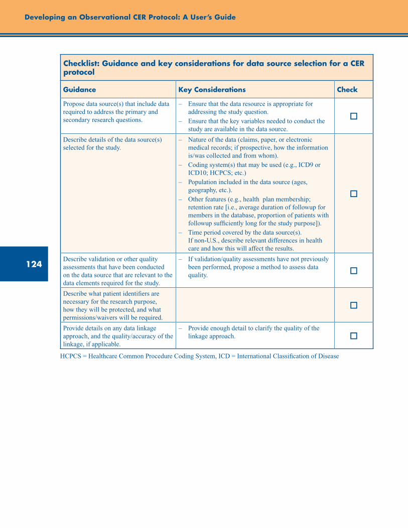
124


Checklist: Guidance and key considerations for data source selection for a CER protocol


Propose data source(s) that include data required to address the primary and secondary research questions.

– Ensure that the data resource is appropriate for addressing the study question.

– Ensure that the key variables needed to conduct the study are available in the data source.

o

Describe details of the data source(s) selected for the study.

– Nature of the data (claims, paper, or electronic medical records; if prospective, how the information is/was collected and from whom).

– Coding system(s) that may be used (e.g., ICD9 or ICD10; HCPCS; etc.)

– Population included in the data source (ages, geography, etc.).

– Other features (e.g., health plan membership; retention rate [i.e., average duration of followup for members in the database, proportion of patients with followup sufficiently long for the study purpose]).

– Time period covered by the data source(s). If non-U.S., describe relevant differences in health care and how this will affect the results.

o

Describe validation or other quality assessments that have been conducted on the data source that are relevant to the data elements required for the study.

– If validation/quality assessments have not previously been performed, propose a method to assess data quality. o

Describe what patient identifiers are necessary for the research purpose, how they will be protected, and what permissions/waivers will be required.

o

Provide details on any data linkage approach, and the quality/accuracy of the linkage, if applicable.

– Provide enough detail to clarify the quality of the linkage approach. o

HCPCS = Healthcare Common Procedure Coding System, ICD = International Classification of Disease

125


References1. Bangsberg DR, Ragland K, Monk A, et al.

A single tablet regimen is associated with higher adherence and viral suppression than multiple tablet regimens in HIV+ homeless and marginally housed people. AIDS. 2010 November 27;24(18):2835-40.

2. Brookhart MA, Schneeweiss S, Avorn J, et al. Comparative mortality risk of anemia management practices in incident hemodialysis patients. JAMA. 2010 March 3;303(9):857-64.

3. Zhang Y, Cotter DJ, Thamer M. The effect of dialysis chains on mortality among patients receiving hemodialysis. Health Serv Res. 2011 June;46(3):747-67.

4. Johansen KL, Zhang R, Huang Y, et al. Survival and hospitalization among patients using nocturnal and short daily compared to conventional hemodialysis: a USRDS study. Kidney Int. 2009 November;76(9):984-90.

5. Massarweh NN, Park JO, Yeung RS, et al. Comparative assessment of the safety and effectiveness of radiofrequency ablation among elderly Medicare beneficiaries with hepatocellular carcinoma. Ann Surg Oncol. 2012 Apr;19(4):1058-65.

6. Tan HJ, Wolf JS, Jr., Ye Z, et al. Complications and failure to rescue after laparoscopic versus open radical nephrectomy. J Urol. 2011 October;186(4):1254-60.

7. Canter D, Egleston B, Wong YN, et al. Use of radical cystectomy as initial therapy for the treatment of high-grade T1 urothelial carcinoma of the bladder: A SEER database analysis. Urol Oncol. 2011 September 7 [epub ahead of print].

8. Schneeweiss S, Avorn J. A review of uses of health care utilization databases for epidemiologic research on therapeutics. J Clin Epidemiol. 2005 April;58(4):323-37.

9. Botsis T, Hartvigsen G, Chen F, et al. Secondary Use of EHR: Data Quality Issues and Informatics Opportunities. AMIA Summits Transl Sci Proc. 2010 Mar 1;2010:1-5.

10. Hsiao C-J, Hing E, Socey TC. Electronic medical record/electronic health record systems of office-based physicians: United States, 2009 and preliminary 2010 state estimates. National Center for Health Statistics. 2009. Hyattsville, MD.

11. Federal Register. 74[11], 3328-332. 1-28-2009.

12. CPT® Process - How a Code Becomes a Code. www.ama-assn.org/ama/pub/physician-resources/solutions-managing-your-practice/coding-billing-insurance/cpt/cpt-process-faq/code-becomes-cpt.shtml. Accessed March 15, 2011.

13. Fisher ES, Whaley FS, Krushat WM, et al. The accuracy of Medicare’s hospital claims data: progress has been made, but problems remain. Am J Public Health. 1992 February;82(2):243-8.

14. Quan H, Parsons GA, Ghali WA. Validity of procedure codes in International Classification of Diseases, 9th revision, clinical modification administrative data. Med Care. 2004 August;42(8):801-9.

15. Quan H, Parsons GA, Ghali WA. Assessing accuracy of diagnosis-type indicators for flagging complications in administrative data. J Clin Epidemiol. 2004 April;57(4):366-72.

16. Quan H, Li B, Saunders LD, et al. Assessing validity of ICD-9-CM and ICD-10 administrative data in recording clinical conditions in a unique dually coded database. Health Serv Res. 2008 August;43(4):1424-41.

17. Segal JB, Ness PM, Powe NR. Validating billing data for RBC transfusions: a brief report. Transfusion. 2001 April;41(4):530-3.

18. Segal JB, Powe NR. Accuracy of identification of patients with immune thrombocytopenic purpura through administrative records: a data validation study. Am J Hematol. 2004 January;75(1):12-7.

19. Strom BL. Data validity issues in using claims data. Pharmacoepidemiol Drug Saf. 2001 August;10(5):389-92.

20. Thirumurthi S, Chowdhury R, Richardson P, et al. Validation of ICD-9-CM diagnostic codes for inflammatory bowel disease among veterans. Dig Dis Sci. 2010 September;55(9):2592-8.

21. Stein BD, Bautista A, Schumock GT, et al. The validity of ICD-9-CM diagnosis codes for identifying patients hospitalized for COPD exacerbations. Chest. 2012 Jan;141(1):87-93.

22. Tollefson MK, Gettman MT, Karnes RJ, et al. Administrative data sets are inaccurate for assessing functional outcomes after radical prostatectomy. J Urol. 2011 May;185(5):1686-90.

23. Wogen J, Kreilick CA, Livornese RC, et al. Patient adherence with amlodipine, lisinopril, or valsartan therapy in a usual-care setting. J Manag Care Pharm. 2003 September;9(5):424-9.

126


24. Yokoyama K, Yang W, Preblick R, et al. Effects of a step-therapy program for angiotensin receptor blockers on antihypertensive medication utilization patterns and cost of drug therapy. J Manag Care Pharm. 2007 April;13(3):235-44.

25. Hachem C, Morgan R, Johnson M, et al. Statins and the risk of colorectal carcinoma: a nested case-control study in veterans with diabetes. Am J Gastroenterol. 2009 May;104(5):1241-8.

26. Iqbal SU, Cunningham F, Lee A, et al. Divalproex sodium vs. valproic acid: drug utilization patterns, persistence rates and predictors of hospitalization among VA patients diagnosed with bipolar disorder. J Clin Pharm Ther. 2007 December;32(6):625-32.

27. JANUS, Data Standard Comparative Effectiveness Research. Available at: www.fda.gov/downloads/AdvisoryCommittees/CommitteesMeetingMaterials/ScienceBoardtotheFoodandDrugAdministration/UCM224277.pdf. Accessed October 23, 2012.

28. Fried LP, Borhani NO, Enright P, et al. The Cardiovascular Health Study: design and rationale. Ann Epidemiol. 1991 February;1(3):263-76.

29. Clark JM, Chang HY, Bolen SD, et al. Development of a claims-based risk score to identify obese individuals. Popul Health Manag. 2010 August;13(4):201-7.

30. National Cancer Institute SEER Training Module. Available at: http://training.seer.cancer.gov/registration/registry/history/. Accessed March 22, 2011.

31. Jutte DP, Roos LL, Brownell MD. Administrative record linkage as a tool for public health research. Annu Rev Public Health. 2011 April 21; 32:91-108.

32. Hammill BG, Hernandez AF, Peterson ED, et al. Linking inpatient clinical registry data to Medicare claims data using indirect identifiers. Am Heart J. 2009 June;157(6):995-1000.

33. Greenland S, Finkle WD. A critical look at methods for handling missing covariates in epidemiologic regression analyses. Am J Epidemiol. 1995 December 15;142(12):1255-64.

34. Klebanoff MA, Cole SR. Use of multiple imputation in the epidemiologic literature. Am J Epidemiol. 2008 August 15;168(4):355-7.

35. Mackinnon A. The use and reporting of multiple imputation in medical research - a review. J Intern Med. 2010 December;268(6):586-93.

36. Foundation for the National Institues of Health. Observational Medical Outcomes Partnership. Available at: http://omop.fnih.org/node/22. Accessed May 8, 2011.

37. Gunn PP, Fremont AM, Bottrell M, et al. The Health Insurance Portability and Accountability Act Privacy Rule: a practical guide for researchers. Med Care. 2004 April;42(4):321-7.

38. Nosowsky R, Giordano TJ. The Health Insurance Portability and Accountability Act of 1996 (HIPAA) privacy rule: implications for clinical research. Annu Rev Med. 2006;57:575-90.

39. O’Keefe CM, Connolly CJ. Privacy and the use of health data for research. Med J Aust. 2010 November 1;193(9):537-41.

40. HIPAA Privacy Rule. National Institutes of Health Web site. http://privacyruleandresearch.nih.gov/. Accessed January 30, 2012.

41. Schneeweiss S, Setoguchi S, Brookhart A, et al. Risk of death associated with the use of conventional versus atypical antipsychotic drugs among elderly patients. CMAJ. 2007 February 27;176(5):627-32.

42. Boggon R, van Staa TP, Timmis A, et al. Clopidogrel discontinuation after acute coronary syndromes: frequency, predictors and associations with death and myocardial infarction—a hospital registry-primary care linked cohort (MINAP-GPRD). Eur Heart J. 2011 October;32(19):2376-86.

43. National Health Interview Survey. www.cdc.gov/nchs/nhis/about_nhis.htm. Accessed March 22, 2011.

44. Perlis TE, Des Jarlais DC, Friedman SR, et al. Audio-computerized self-interviewing versus face-to-face interviewing for research data collection at drug abuse treatment programs. Addiction. 2004 July;99(7):885-96.

45. Fairley CK, Sze JK, Vodstrcil LA, et al. Computer-assisted self interviewing in sexual health clinics. Sex Transm Dis. 2010 November;37(11):665-8.

46. Richens J, Copas A, Sadiq ST, et al. A randomised controlled trial of computer-assisted interviewing in sexual health clinics. Sex Transm Infect. 2010 August;86(4):310-4.

47. Corkrey R, Parkinson L. Interactive voice response: review of studies 1989-2000. Behav Res Methods Instrum Comput. 2002 August;34(3):342-53.

127


48. Abu-Hasaballah K, James A, Aseltine RH, Jr. Lessons and pitfalls of interactive voice response in medical research. Contemp Clin Trials. 2007 September;28(5):593-602.

49. Beasley JM, Kwan ML, Chen WY, et al. Meeting the physical activity guidelines and survival after breast cancer: findings from the after breast cancer pooling project. Breast Cancer Res Treat. 2012 January;131(2):637-43.

50. Herrinton LJ, Curtis JR, Chen L, et al. Study design for a comprehensive assessment of biologic safety using multiple healthcare data systems. Pharmacoepidemiol Drug Saf. 2011 Nov;20(11):1199-209.

51. Blettner M, Sauerbrei W, Schlehofer B, et al. Traditional reviews, meta-analyses and pooled analyses in epidemiology. Int J Epidemiol. 1999 February;28(1):1-9.

52. Selby JV. Linking automated databases for research in managed care settings. Ann Intern Med. 1997 October 15;127(8 Pt 2):719-24.

53. Platt R, Davis R, Finkelstein J, et al. Multicenter epidemiologic and health services research on therapeutics in the HMO Research Network Center for Education and Research on Therapeutics. Pharmacoepidemiol Drug Saf. 2001 August;10(5):373-7.

54. Harcourt SE, Smith GE, Elliot AJ, et al. Use of a large general practice syndromic surveillance system to monitor the progress of the influenza A(H1N1) pandemic 2009 in the UK. Epidemiol Infect. 2011 April 8;1-6.

55. Nazi KM, Hogan TP, Wagner TH, et al. Embracing a health services research perspective on personal health records: lessons learned from the VA My HealtheVet system. J Gen Intern Med. 2010 January;25 Suppl 1:62-7.

56. The Lister Hill National Center for Biomedical Communications. Annual Report FY 2010. Available at: www.lhncbc.nlm.nih.gov/lhc/docs/reports/2010/tr2010003.pdf. Accessed April 22, 2011.

57. Wu AW, Snyder C, Clancy CM, et al. Adding the patient perspective to comparative effectiveness research. Health Aff (Millwood) 2010 October;29(10):1863-71.

129

Abstract

The feasibility of a study often rests on whether the projected number of accrued patients is adequate to address the scientific aims of the study. Accordingly, a rationale for the planned study size should be provided in observational comparative effectiveness research (CER) study protocols. This chapter provides an overview of study size and power calculations in randomized controlled trials (RCTs), specifies considerations for observational comparative effectiveness research (CER) study size planning, and highlights study size considerations that differ between RCTs and observational studies of comparative effectiveness. The chapter concludes with a checklist of key considerations for study size planning for a CER protocol.

Chapter 9. Study Size PlanningEric S. Johnson, Ph.D., M.P.H.

Kaiser Permanente Northwest, Portland, OR

M. Alan Brookhart, Ph.D. University of North Carolina at Chapel Hill Gillings School of

Global Public Health, Chapel Hill, NC

Jessica A. Myers, Ph.D. Harvard Medical School and Brigham and Women’s Hospital, Boston, MA

Introduction

An important aspect of the assessment of study feasibility is whether the projected number of accrued patients is adequate to reasonably address the scientific aims of the study. Many journals have endorsed reporting standards that ask investigators to report the rationale for the study size. For example, the Strengthening the Reporting of Observational Studies in Epidemiology (STROBE) checklist asks investigators to report their rationale, which may include a statistical power calculation. However, such a rationale is often missing from study protocols. This is problematic when investigators interpret study findings in terms of the statistical significance in relation to the null hypothesis, which implies both a prespecified hypothesis and adequate statistical power (e.g., ≥80% for detecting a clinically important increase in harm). Without the context of a numeric rationale for the study size, readers may misinterpret the lack of a statistically significant difference in effect as false reassurance of lack of harm, or falsely conclude that there is no benefit when comparing two interventions.

Study Size and Power Calculations in RCTs

The study planning needed to achieve various study sizes and an understanding of statistical power that a given study size can yield are important aspects in the design of randomized controlled trials (RCTs). Reporting on the rationale underlying the size of treatment arms is clearly specified in the Consolidated Standards of Reporting Trials (CONSORT) and STrengthening the Reporting of OBservational studies in Epidemiology (STROBE) reporting guidelines, and institutional review boards (IRBs) often require such statements in a study protocol before data collection can begin.1 The rationale for study size in an RCT usually depends on calculations of the study size needed to achieve a specified level of statistical power for the primary hypothesis under study, defined as the probability of rejecting the null hypothesis when a specific alternative hypothesis (the primary hypothesis under study) is true. In the case of a trial comparing treatments, this is the probability of finding a statistically significant difference between treatments in the primary outcome if the treatments do indeed

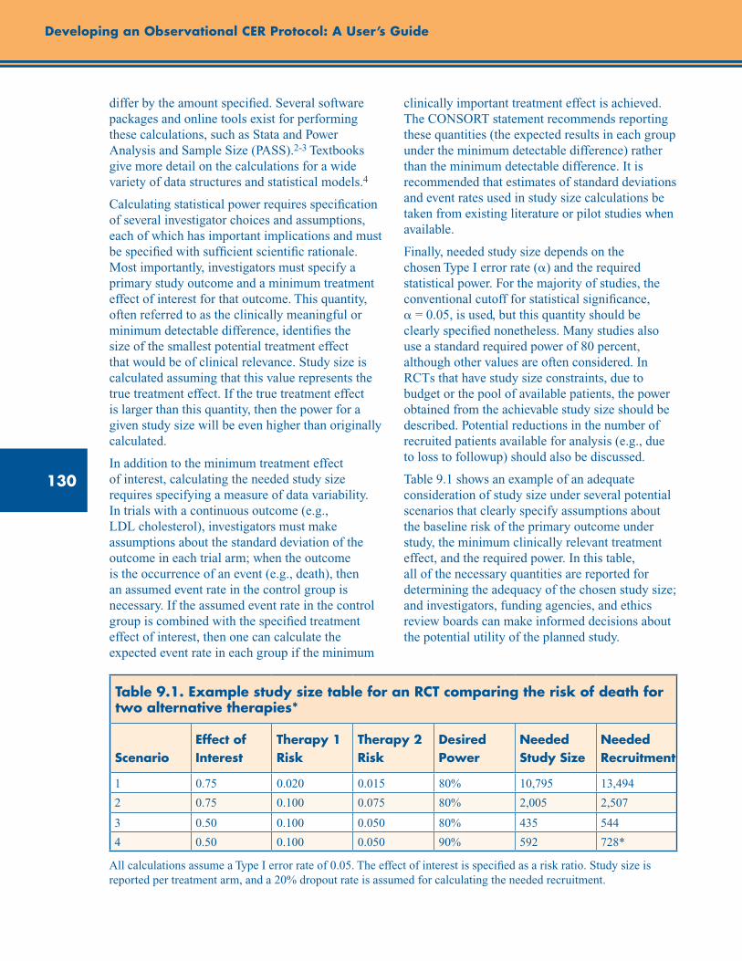
130


differ by the amount specified. Several software packages and online tools exist for performing these calculations, such as Stata and Power Analysis and Sample Size (PASS).2-3 Textbooks give more detail on the calculations for a wide variety of data structures and statistical models.4

Calculating statistical power requires specification of several investigator choices and assumptions, each of which has important implications and must be specified with sufficient scientific rationale. Most importantly, investigators must specify a primary study outcome and a minimum treatment effect of interest for that outcome. This quantity, often referred to as the clinically meaningful or minimum detectable difference, identifies the size of the smallest potential treatment effect that would be of clinical relevance. Study size is calculated assuming that this value represents the true treatment effect. If the true treatment effect is larger than this quantity, then the power for a given study size will be even higher than originally calculated.

In addition to the minimum treatment effect of interest, calculating the needed study size requires specifying a measure of data variability. In trials with a continuous outcome (e.g., LDL cholesterol), investigators must make assumptions about the standard deviation of the outcome in each trial arm; when the outcome is the occurrence of an event (e.g., death), then an assumed event rate in the control group is necessary. If the assumed event rate in the control group is combined with the specified treatment effect of interest, then one can calculate the expected event rate in each group if the minimum

clinically important treatment effect is achieved. The CONSORT statement recommends reporting these quantities (the expected results in each group under the minimum detectable difference) rather than the minimum detectable difference. It is recommended that estimates of standard deviations and event rates used in study size calculations be taken from existing literature or pilot studies when available.

Finally, needed study size depends on the chosen Type I error rate (a) and the required statistical power. For the majority of studies, the conventional cutoff for statistical significance, a = 0.05, is used, but this quantity should be clearly specified nonetheless. Many studies also use a standard required power of 80 percent, although other values are often considered. In RCTs that have study size constraints, due to budget or the pool of available patients, the power obtained from the achievable study size should be described. Potential reductions in the number of recruited patients available for analysis (e.g., due to loss to followup) should also be discussed.

Table 9.1 shows an example of an adequate consideration of study size under several potential scenarios that clearly specify assumptions about the baseline risk of the primary outcome under study, the minimum clinically relevant treatment effect, and the required power. In this table, all of the necessary quantities are reported for determining the adequacy of the chosen study size; and investigators, funding agencies, and ethics review boards can make informed decisions about the potential utility of the planned study.

Table 9.1. Example study size table for an RCT comparing the risk of death for two alternative therapies*

ScenarioEffect of Interest

Therapy 1 Risk

Therapy 2 Risk

Desired Power

Needed Study Size

Needed Recruitment

1 0.75 0.020 0.015 80% 10,795 13,494

2 0.75 0.100 0.075 80% 2,005 2,507

3 0.50 0.100 0.050 80% 435 544

4 0.50 0.100 0.050 90% 592 728*

All calculations assume a Type I error rate of 0.05. The effect of interest is specified as a risk ratio. Study size is reported per treatment arm, and a 20% dropout rate is assumed for calculating the needed recruitment.

131

Chapter 9. Study Size Planning

These considerations in sample size and power in the context of RCTs are also relevant for nonrandomized studies, but their application in nonrandomized studies may differ. The following section is for additional consideration, particularly for nonrandomized studies.

Considerations for Observational CER Study Size Planning

Bland has commented that funding agencies and journals put investigators in an inconsistent position: Funding agencies ask for statistical power calculations to test one hypothesis for the primary outcome, yet journals ask for confidence intervals.5 In his commentary, Bland proposed that we resolve that inconsistency by asking investigators to base their study size on the expected precision of all relevant comparisons. Goodman and Berlin recommended a similar idea in 1994 (page 204 of their article):6

In our experience, expressing the implications of sample size calculations in the same language as is used in a published paper, instead of the language of power and detectable differences, helps researchers to understand the implications more clearly and take them more seriously. This in turn can produce meaningful discussions about the aims of the study, which power considerations rarely seem to inspire.

Basing the study size on the expected width of confidence intervals offers another advantage: Investigators no longer need to commit to a primary outcome and a primary comparison (e.g., among alternative interventions).

Many funding agencies, however, rely on the conventional power calculations advocated by most trialists. Therefore, this section primarily focuses on power calculations and adapts trialists’ conventional advice to nonrandomized or observational studies because they introduce complexities that randomized trials do not need to consider. For example, investigators may not be able to estimate the power or precision of their proposed comparisons until they have generated the propensity score and constructed matched cohorts, which may exclude patients and interventions that appeared eligible when the cohort was assembled.

Case Studies

Schneeweiss and colleagues published one of the first Developing Evidence to Inform Decisions about Effectiveness (DEcIDE) Program studies on comparative effectiveness; they compared the short-term risk of mortality in elderly patients who started a conventional versus an atypical antipsychotic medication regimen,7 reproducing an earlier study by Wang and colleagues.8 Consistent with most nonexperimental studies, especially in the pre-STROBE era, their methods section does not offer a rationale for the cohort study’s size. Based on their patient counts for each class of antipsychotic medication and the number of deaths observed during the first 180 days after starting medication, we calculated the statistical power for their study question: Do conventional antipsychotic medications pose a higher risk than atypical antipsychotic medications as measured by all-cause mortality?

We considered an inferiority hypothesis by using the crude mortality risk observed in the control cohort of atypical medication patients (9.58 percent), and then assigning the conventional medication cohort a 10-percent higher risk (10.54 percent), a clinically important excess risk. Based on the numbers of patients and deaths noted above, Stata’s sample size command, sampsi, reported statistical power of 0.83. Their subgroup analyses would have had lower power, but the main study was appropriately powered for its primary outcome and comparison.

Considerations That Differ for Nonrandomized Studies

Power calculations may require additional considerations for application to nonrandomized studies. For a well planned and conducted RCT, the Type I and Type II errors (i.e., false positive or false negative) rank higher as possible explanations for a finding of “no statistically significant difference” because randomization has overcome the potential confounding, the protocol has reduced measurement error, et cetera. But for nonrandomized studies, Type I and Type II errors rank lower on the list of possible explanations for such a negative result. Confounding bias, measurement error, and other biases should concern investigators more than the expected precision when they consider the feasibility of a

132


comparative effectiveness study. For example, the new user design trades precision for a reduction in confounding bias by restricting the study to incident users of the interventions under study. (See chapter 2 for a discussion of new user design.)9 As retrospective database studies become larger through distributed networks, insufficient statistical power of comparative effectiveness estimates will diminish in importance as a competing explanation for negative results—at least for the primary comparison of common interventions—and readers will need to consider whether small observed clinical differences matter for decisionmaking. For example, database studies may identify small excess risks of about 5 percent that would fall below the minimum clinically important difference specified in a prospective study.

In some cases, controlling for confounding can also reduce the precision of estimated effects. The reduction in precision is perhaps most clearly seen in studies that use propensity score matching. With propensity score matching and strong preferential prescribing in relation to patient characteristics (i.e., less overlap in propensity score distributions across cohorts), many patients will drop out of the analysis.10 For example, Solomon and colleagues identified a cohort of 23,647 patients who were eligible for a comparative effectiveness study, but only 12,840 (54 percent) contributed to the final analysis after matching on the propensity score.11 Inconveniently, the development of the propensity score occurs after the study protocol has been written, and the investigators have invested considerable time and effort toward completion of the comparative effectiveness study. Consequently, investigators should consider incorporating sensitivity analyses when calculating the expected

precision of effects and study size estimates. For example, they might ask, “If 25 percent of the cohort were to drop out of the analysis after incorporating the propensity score, how would that reduced study size impact the expected precision?”

Because retrospective studies lack a protocol for data collection, they often suffer a higher frequency of missing data, especially for clinical examination values (e.g., blood pressure, body mass index, and laboratory results). Investigators who undertake a completed-cases analysis, which excludes patients with any missing data for key variables, may suffer from a smaller study size than they anticipated when they wrote the study protocol.12 Depending on the nature of the missingness, it may be possible for investigators to impute certain values and retain patients in the final analysis. But as with the development of propensity scores, multiple imputation is labor intensive, and its success in retaining patients will only be known after the protocol has been written.

Conclusion

In order to ensure adequate study size, investigators should provide a rationale for study size during the planning stages of an observational CER study. All definitions and assumptions should be specified, including the primary study outcome, clinically important minimum effect size, variability measure, and Type I and Type II error rates. Investigators should also consider other factors that may reduce the effective sample size, such as loss to followup, reductions due to statistical methods to control confounding, and missing data, when making their initial assessment as to whether the sample size necessary to detect a clinically meaningful difference can be achieved.

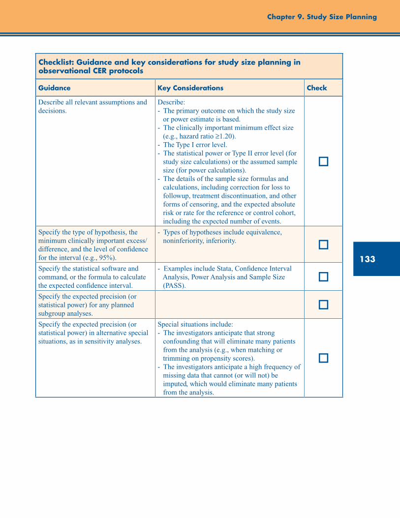
133


Checklist: Guidance and key considerations for study size planning in observational CER protocols


Describe all relevant assumptions and decisions.

Describe: - The primary outcome on which the study size or power estimate is based. - The clinically important minimum effect size (e.g., hazard ratio ≥1.20). - The Type I error level. - The statistical power or Type II error level (for study size calculations) or the assumed sample size (for power calculations). - The details of the sample size formulas and calculations, including correction for loss to followup, treatment discontinuation, and other forms of censoring, and the expected absolute risk or rate for the reference or control cohort, including the expected number of events.

o

Specify the type of hypothesis, the minimum clinically important excess/difference, and the level of confidence for the interval (e.g., 95%).

- Types of hypotheses include equivalence, noninferiority, inferiority. o

Specify the statistical software and command, or the formula to calculate the expected confidence interval.

- Examples include Stata, Confidence Interval Analysis, Power Analysis and Sample Size (PASS).

oSpecify the expected precision (or statistical power) for any planned subgroup analyses.

oSpecify the expected precision (or statistical power) in alternative special situations, as in sensitivity analyses.

Special situations include: - The investigators anticipate that strong confounding that will eliminate many patients from the analysis (e.g., when matching or trimming on propensity scores). - The investigators anticipate a high frequency of missing data that cannot (or will not) be imputed, which would eliminate many patients from the analysis.

o

134

References1. Schulz KF, Altman DG, Moher D; CONSORT

Group. CONSORT 2010 statement: updated guidelines for reporting parallel group randomized trials. Ann Intern Med. 2010 Jun 1;152(11): 726-32.

2. StataCorp. Stata Statistical Software: Release 11. College Station, TX: StataCorp; 2009.

3. Hintze, J. PASS 11. NCSS, LLC. Kaysville, Utah; 2011. www.ncss.com. Accessed September 21, 2012.

4. Friedman LM, Furberg CD, DeMets DL. Sample size (chapter 8). In: Fundamentals of Clinical Trials. 4th edition. New York: Springer; 2010: 133-167.

5. Bland JM. The tyranny of power: Is there a better way to calculate sample size? BMJ. 2009;339:b3985.

6. Goodman SN, Berlin JA. The use of predicted confidence intervals when planning experiments and the misuse of power when interpreting results. Ann Intern Med. 1994;121:200-6.

7. Schneeweiss S, Setoguchi S, Brookhart A, et al. Risk of death associated with use of conventional versus atypical antipsychotic drugs among elderly patients. CMAJ. 2007;176:627-32.

8. Wang PS, Schneeweiss S, Avorn J, et al. Risk of death in elderly users of conventional vs. atypical antipsychotic medications. N Engl J Med. 2005 Dec 1;353(22):2335-41.

9. Ray WA. Evaluating medication effects outside of clinical trials: new user designs. Am J Epidemiol. 2003;158:915-20.

10. Schneeweiss S. A basic study design for expedited signal evaluation based on electronic healthcare data. Pharmacoepidemiol Drug Saf. 2010;19: 858-68.

11. Solomon DH, Rassen JA, Glynn RJ, et al. The comparative safety of analgesics in older adults with arthritis. Arch Intern Med. 2010;170: 1968-78.

12. Sterne JA, White IR, Carlin JB, et al. Multiple imputation for missing data in epidemiologic and clinical research: potential and pitfalls. BMJ. 2009;338:b2393.


135

Abstract

This chapter provides a high-level overview of statistical analysis considerations for observational comparative effectiveness research (CER). Descriptive and univariate analyses can be used to assess imbalances between treatment groups and to identify covariates associated with exposure and/or the study outcome. Traditional strategies to adjust for confounding during the analysis include linear and logistic multivariable regression models. The appropriate analytic technique is dictated by the characteristics of the study outcome, exposure of interest, study covariates, and the underlying assumptions underlying the statistical model. Increasingly common in CER is the use of propensity scores, which assign a probability of receiving treatment, conditional on observed covariates. Propensity scores are appropriate when adjusting for large numbers of covariates and are particularly favorable in studies having a common exposure and rare outcome(s). Disease risk scores estimate the probability or rate of disease occurrence as a function of the covariates and are preferred in studies with a common outcome and rare exposure(s). Instrumental variables, which are measures that are causally related to exposure but only affect the outcome through the treatment, offer an alternative to analytic strategies that have incomplete information on potential unmeasured confounders. Missing data in CER studies is not uncommon, and it is important to characterize the patterns of missingness in order to account for the missing data in the analysis. In addition, time-varying exposures and covariates should be accounted for to avoid bias. The chapter concludes with a checklist including guidance and key considerations for developing a statistical analysis section of an observational CER protocol.

Chapter 10. Considerations for Statistical AnalysisPatrick G. Arbogast, Ph.D. (deceased)

Kaiser Permanente Northwest, Portland, OR


Introduction

Comparative effectiveness research utilizing observational data requires careful and often complex analytic strategies to adjust for confounding. These can include standard analytic strategies, such as traditional multivariable regression techniques, as well as newer, more sophisticated methodologies, such as propensity score matching and instrumental variable analysis. This chapter covers data analysis strategies from simple descriptive statistics to more complex methodologies. Also covered are important considerations such as handling missing data and analyzing time-varying exposures and covariates.

While this chapter provides a high-level summary of considerations and issues for statistical analysis in observational CER, it is not intended to be a comprehensive treatment of considerations and approaches. We encourage the reader to explore

topics more fully by referring to the references provided.

Descriptive Statistics/Unadjusted Analyses

Appropriate descriptive statistics and graphical displays for different types of data have been presented in numerous textbooks.1 These include measures of range, dispersion, and central tendency for continuous variables, number and percent for categorical variables, and plots for evaluating data distributions. For comparative effectiveness research (CER), it is important to consider useful and informative applications of these descriptive statistics. For instance, for a cohort study, describing study covariates stratified by exposure levels provides a useful means to assess imbalances in these measures. For a propensity–matched-pairs dataset, summarizing study covariates by exposure group aids in detecting residual imbalances.

136


Univariate or unadjusted hypothesis testing, such as two-sample t-tests, can be conducted to identify covariates associated with the exposure and/or the study outcome. Since CER studies will need to consider potential confounding from a large number of study covariates, the descriptive statistics should provide a broad picture of the characteristics of the study subjects.

Adjusted Analyses

Traditional Multivariable Regression

Regression analysis is often used in the estimation of treatment effects to control for potential confounding variables.2 In general, control is made for pretreatment variables that are related to both the treatment of interest and the outcome of interest. Variables that are potentially on the pathway from treatment to outcome are not controlled for, as control for such intermediate variables could block some of the effect of the treatment on the outcome. See chapter 7 (Covariate Selection) for further discussion. Traditional multiple regression, in which one uses regression models to directly adjust for potential confounders and effect modification, has long been used in observational studies and can be applied in CER. When applying regression modeling, careful attention must be paid to ensure that corresponding model assumptions are met.3 For example, for linear regression, the assumption that the mean of the outcome is a linear function of the covariates should be assessed. Whether regression techniques or other approaches are preferred also depends in part on the characteristics of the data. For logistic regression, as long as the number of outcome events per covariate included in the regression model is sufficient (e.g., a rule of thumb is 10 or more) and the exposure of interest is not infrequent, traditional multiple regression is a reasonable strategy and could be considered for the primary analysis.4-5 However, when this is not the situation, other options should be considered. Regression methods also have the disadvantage that they may extrapolate to regions where data are not available; other techniques such as propensity scores (discussed below) more easily diagnose this issue.

When there are many covariates, one approach has been to develop more parsimonious models using methods such as stepwise regression. However, this may involve subjective decisions such as the type of variable selection procedure to use, whether to base selection upon p-values or change in exposure parameter estimates, and where to set numeric cutoffs (e.g., p=0.05, 0.10, 0.20) for variable inclusion and retention in the model. For covariates that confer relatively modest increases in disease risk, some variable selection procedures, such as stepwise regression, may exclude important covariates from the final model.

Furthermore, stepwise regression has limitations that can lead to underestimation of standard errors for exposure estimates.6 Other analytical strategies which have become more common in recent years include using summary variables, such as propensity scores and disease risk scores, which are described below. Propensity scores often perform better than logistic regression when the outcome is relatively rare (e.g., fewer than 10 events per covariate as noted above), whereas logistic regression tends to perform better than propensity score analysis when the outcome is common but the exposure is rare.7

Choice of Regression Modeling Approach

The forms of the study outcome, exposure of interest, and study covariates will determine the regression model to be used. For independent, non–time-varying exposures and study covariates, generalized linear models (GLMs) such as linear or logistic regression can be used. If the study outcome is binary with fixed followup and is rare, Poisson regression with robust standard errors can be used to estimate relative risks and get correct confidence intervals.8-9 For count data, Poisson regression can also be used but is susceptible to problems of overdispersion, wherein the variance of the outcomes is larger than what is given by the Poisson model. Failure to account for this can lead to underestimation of standard errors. A negative binomial regression model can help address the issue of overdispersion.10 If the value 0 occurs more frequently than is predicted by the Poisson or negative binomial model, the zero-inflated Poisson and zero-inflated negative binomial models can be used.11

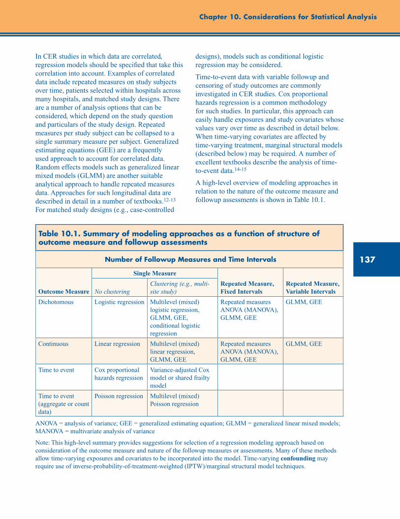
137

Chapter 10. Considerations for Statistical Analysis

In CER studies in which data are correlated, regression models should be specified that take this correlation into account. Examples of correlated data include repeated measures on study subjects over time, patients selected within hospitals across many hospitals, and matched study designs. There are a number of analysis options that can be considered, which depend on the study question and particulars of the study design. Repeated measures per study subject can be collapsed to a single summary measure per subject. Generalized estimating equations (GEE) are a frequently used approach to account for correlated data. Random effects models such as generalized linear mixed models (GLMM) are another suitable analytical approach to handle repeated measures data. Approaches for such longitudinal data are described in detail in a number of textbooks.12-13 For matched study designs (e.g., case-controlled

designs), models such as conditional logistic regression may be considered.

Time-to-event data with variable followup and censoring of study outcomes are commonly investigated in CER studies. Cox proportional hazards regression is a common methodology for such studies. In particular, this approach can easily handle exposures and study covariates whose values vary over time as described in detail below. When time-varying covariates are affected by time-varying treatment, marginal structural models (described below) may be required. A number of excellent textbooks describe the analysis of time-to-event data.14-15

A high-level overview of modeling approaches in relation to the nature of the outcome measure and followup assessments is shown in Table 10.1.

Table 10.1. Summary of modeling approaches as a function of structure of outcome measure and followup assessments

Number of Followup Measures and Time Intervals

Outcome Measure

Single Measure

Repeated Measure, Fixed Intervals

Repeated Measure, Variable IntervalsNo clustering

Clustering (e.g., multi-site study)

Dichotomous Logistic regression Multilevel (mixed) logistic regression, GLMM, GEE, conditional logistic regression

Repeated measures ANOVA (MANOVA), GLMM, GEE

GLMM, GEE

Continuous Linear regression Multilevel (mixed) linear regression, GLMM, GEE

Repeated measures ANOVA (MANOVA), GLMM, GEE

GLMM, GEE

Time to event Cox proportional hazards regression

Variance-adjusted Cox model or shared frailty model

Time to event (aggregate or count data)

Poisson regression Multilevel (mixed) Poisson regression

ANOVA = analysis of variance; GEE = generalized estimating equation; GLMM = generalized linear mixed models; MANOVA = multivariate analysis of variance

Note: This high-level summary provides suggestions for selection of a regression modeling approach based on consideration of the outcome measure and nature of the followup measures or assessments. Many of these methods allow time-varying exposures and covariates to be incorporated into the model. Time-varying confounding may require use of inverse-probability-of-treatment-weighted (IPTW)/marginal structural model techniques.

138


Model Assumptions

All analytic techniques, including regression, have underlying assumptions. It is important to be aware of those assumptions and to assess them. Otherwise, there are risks with regards to interpretation of study findings. These assumptions and diagnostics are specific to the regression technique being used and will not be listed here. They are covered in numerous textbooks, depending on the methods being used. For example, if Cox proportional hazards regression is used, then the proportional hazards assumption should be assessed. If the validity of this assumption is questionable, then alternatives such as time-dependent covariates may need to be considered.

Time-Varying Exposures/Covariates

In most CER studies, it is unrealistic to assume that exposures and covariates remain fixed throughout followup. Consider, for example, HIV patients who may be treated with antiretroviral therapy. The use of antiretroviral therapy may change over time and decisions about therapy may in part be based on CD4 count levels, which also vary over time. As another illustration, consider a study of whether proton pump inhibitors (PPIs) prevent clopidogrel-related gastroduodenal bleeding. In this situation,warfarin may be started during followup. Should one adjust for this important potential confounder? Failure to account for the time-varying status of such exposures and confounders (i.e., by fixing everyone’s exposure status at baseline) may severely bias study findings.

As noted above, for time-to-event study outcomes, time-dependent Cox regression models can be used to account for time-varying exposures and covariates. However, difficult issues arise when both treatment and confounding variables vary over time. In the HIV example, CD4 count may be affected by prior therapy decisions, but CD4 count levels may themselves go on to alter subsequent therapy decisions and the final survival outcome. In examining the effects of time-varying treatment, a decision must be made as to whether to control for CD4 count. A difficulty arises in that CD4 count is both a confounding variable

(for subsequent therapy and final survival) and also an intermediate variable (for the effect of prior treatment). Thus, control for CD4 count in a time-varying Cox model could potentially lead to bias because it is an intermediate variable and could thus block some of the effect of treatment; but failure to control for CD4 count in the model will result in confounding and thus bias for the effect of subsequent treatment. Both analyses are biased. Such problems arise whenever a variable is simultaneously on the pathway from prior treatment and also affects both subsequent treatment and the final outcome.

These difficulties can be addressed by using inverse-probability-of-treatment weighting (IPTW),16 rather than regression adjustment, for confounding control. These IPTW techniques are used to estimate the parameters of what is often called a marginal structural model, which is a model for expected counterfactual outcomes. The marginal-structural-model/IPTW approach is essentially a generalization of propensity-score weighting to the time-varying treatment context. The IPTW technique assumes that at each treatment decision, the effect of treatment on the outcome is unconfounded given the past covariate and treatment history. A similar weighting approach can also be used to account for censoring as well.16 This marginal-structural-model/IPTW approach has been developed for binary and continuous outcomes,16 time-to-event outcomes,17 and repeated measures data.18

Another consideration for time-varying exposures is accounting for exposure effect (e.g., the effect of medication use) after the subject stopped receiving that exposure. One approach is to create another exposure level that is a carryover of a biologically plausible number of days after exposure use has ended and incorporate it as a time-varying exposure level in the analysis. Another approach is an intent-to-treat analysis in which exposure status (e.g., treatment initiation) is assumed throughout followup. Cadarette and colleagues (2008) used this approach in a study of fracture risk.19 The motivation was that treatment adherence may be low and accounting for on-treatment status may result in information bias.

139


Propensity Scores

Propensity scores are an increasingly common analytic strategy for adjusting for large numbers of covariates in CER. The use of the propensity score for confounding control was proposed by Rosenbaum and Rubin.20 The propensity score is defined as the probability of receiving treatment (or exposure) conditional on observed covariates, and it is typically estimated from regression models, such as a logistic regression of the treatment conditional on the covariates. Rosenbaum and Rubin showed that if adjustment for the original set of covariates suffices to control for confounding, then adjustment for just the propensity score also would suffice as well. This strategy is particularly favorable in studies having a common exposure and rare outcome or possibly multiple outcomes.7 Propensity scores can be used in subclassification or stratification,21 matching,22 and weighting,23 and further adjustment can be done using regression adjustment.24 Stürmer and colleagues provide a review of the application of propensity scores.25

If adjustment using the propensity score is used, balance in study covariates between exposure groups should be carefully assessed. This can include, but is not limited to, testing for differences in study covariates by exposure group after adjusting for propensity score. Another common assessment of the propensity score is to visually examine the propensity score distributions across exposure groups. It has been demonstrated that if there is poor overlap in these distributions, there is a risk of biased exposure estimates when adjusting for the propensity score in a regression model.26 One remedy for this is to restrict the cohort to subjects whose propensity score overlaps across all exposure groups.27-28

When feasible, matching on the propensity score offers several advantages. Matching subjects across exposure groups on propensity score ensures, through restriction, that there will be good overlap in the propensity score distributions. In addition, the presentation of a summary of subject characteristics by exposure groups in a propensity-matched design allows a reader to assess the balance in study covariates achieved by matchingin a similar manner to the comparison of randomized treatment groups from a randomzed clinical trial. This can be done graphically or

by comparing standardized differences across groups. However, in a propensity-matched design, one can only ensure that measured covariates are being balanced. The consequences of unmeasured confounding will need to be assessed using sensitivity analysis. See chapter 11 for further details. Matching techniques for causal effects are described in detail in Rubin29 and best practices for constructing a matched control group are provided by Stuart and Rubin.30 Care must be taken when estimating standard errors for causal effects when using matching,31-32 though software is now available that makes this task easier.33

A tradeoff between using regression adjustment on the full cohort and a propensity-matched design is that in the former there may still be imbalances in study covariates, and in the latter sample size may be reduced to the extent that some of the subjects cannot be matched. Connors and colleagues34 used both analytic strategies in a cohort study of the effectiveness of right heart catheterization and reported similar findings from both analyses. Use of multiple analytic strategies as a form of sensitivity analysis may serve as a useful approach, drawing from the strengths of both strategies.

Brookhart and colleagues35 investigated variable selection approaches and recommend that the covariates to be included in the propensity score model either be true confounders or at least related to the outcome; including covariates related only to the exposure has been shown to increase the variance of the exposure estimate.

Disease Risk Scores

The disease risk score (DRS) is an alternative to the propensity score.36-37 Like the propensity score, it is a summary measure derived from the observed values of the covariates. However, the DRS estimates the probability or rate of disease occurrence as a function of the covariates. The DRS may be estimated in two ways. First, it can be calculated as a “full-cohort” DRS, which is the multivariate confounder score originally proposed by Miettinen in 1976.38 This score was constructed from a regression model relating the study outcome to the exposure of interest and the covariates for the entire study population. The score was then computed as the fitted value from that regression model for each study subject, setting the exposure status to nonexposure. The

140


subjects were then grouped into strata according to the score and a stratified estimate of the exposure effect was calculated. The DRS may also be estimated as an “unexposed-only” DRS, from a regression model fit only for the unexposed population, with the fitted values then computed for the entire cohort.

The DRS is particularly favorable in studies having a common outcome and rare exposure or possibly multiple exposures. It is useful for summarizing disease risk and assessing effect modification by disease risk. Ray and colleagues39 reported effect modification by cardiovascular disease risk, derived and summarized using DRS, in a study of antipsychotics and sudden cardiac death. Also, in the presence of a multilevel exposure in which some of the levels are infrequent, the DRS may be a good alternative to propensity scores.

Instrumental Variables

A limitation of study designs and analytic strategies in CER studies, including the use of traditional multiple regression, propensity scores, and disease risk scores, is incomplete information on potential unmeasured confounders. An alternative approach to estimate causal effects, other than confounding/covariate control, is the use of instrumental variables.40 An “instrument” is a measure that is causally related to exposure but only affects the outcome through the treatment and is also unrelated to the confounders of the treatment-outcome relationship. With an instrument, even if there is unmeasured confounding of the treatment-outcome relationship, the effect of the instrument on the treatment, and the effect of the instrument on the outcome can together be used to essentially back out the effect of the treatment on the outcome. A difficulty of this approach is identifying a high-quality instrument.

An instrument must be unrelated to the confounders of the treatment and the outcome; otherwise, instrumental variable analyses can result in biases. An instrument also must not affect the outcome except through the treatment. This assumption is generally referred to as the “exclusion restriction.” Violations of this exclusion restriction can likewise result in biases. Finally,

the instrument must be related to the treatment of interest. If the association between the instrument and the treatment is weak, the instrument is referred to as a “weak instrument.” Finite-sample properties of estimators using weak instruments are often poor, and weak instruments moreover tend to amplify any other biases that may be present.41-44 If a variable is found that satisfies these properties, then it may be used to estimate the causal effect of treatment on the outcome. However, such a variable may be difficult or impossible to identify in some settings. Moreover, the assumptions required for a variable to be an instrument cannot be fully verified empirically.

Two-stage least squares techniques are often employed when using instrumental variables, though with a binary treatment, ratio estimators are also common.40 For estimates to be causally interpretable, often a monotonicity assumption must also be imposed; that is, that the effect of instrument on the treatment only operates in one direction (e.g., that it is causative or neutral for all individuals). Assumptions of homogeneous treatment effects across individuals also are commonly employed to obtain causally interpretable estimates. When homogeneity assumptions are not employed, the resulting causal effect estimate is generally only applicable for certain subpopulations consisting of those individuals for whom the instrument is able to change the treatment status.40 Such effects are sometimes referred to as “local average treatment effects.” When the treatment is not binary, interpretation of the relevant subpopulation becomes more complex.45 Moreover, when two-stage least squares procedures are applied to binary rather than continuous outcomes, other statistical biases can arise.46

Brookhart and colleagues47 applied this approach in a study of COX-2 inhibitors with nonselective, nonsteroidal anti-inflammatory drugs (NSAIDs) on gastrointestinal complications. Their instrument was the prescribing physician’s preference for a COX-2 inhibitor relative to an NSAID. The results of the instrumental variable analysis were statistically similar to results from two clinical trials, and contrary to the traditional multiple regression analysis that was also conducted.

141


Schneeweiss and colleagues48 examined the use of aprotinin during coronary-artery bypass grafting and risk of death. Their primary analysis was a traditional multiple regression. In addition to the primary analysis, they also conducted a propensity score matched-pairs analysis as well as an instrumental variable analysis. All three analyses had similar findings. This methodology of employing more than one analytical approach may be worth consideration, since the propensity score matching does not rely on the exclusion restriction and other instrumental variable assumptions, whereas instrumental variable analysis circumvents the biases introduced by unmeasured confounders, provided a good instrument is identified. When results differ, careful attention needs to be given to what set of assumptions is more plausible.

Missing Data Considerations

It is not uncommon in CER to have missing data. The extent of missingness and its potential impact on the analysis needs to be considered. Before proceeding with the primary analyses, it is important to characterize the patterns of missingness using exploratory data analyses. This step can provide insights into how to handle the missing data in the primary analysis.

For the primary analysis, a common analytical approach is to analyze just those subjects who have no missing data—called a complete-case analysis. However, an initial limitation of this approach is that sample size is reduced, which affects

efficiency even if data are missing completely at random. If subjects with missing data differ from subjects with complete data, then exposure estimates may be biased. For example, suppose blood pressure is a potential confounder, and it is missing in very ill subjects. Then, excluding these subjects can bias the exposure estimate.

Little and Rubin’s textbook describes several analytic approaches for handling missing data.49 One common approach to filling in missing data when they are “missing completely at random” or “missing at random” is imputation, which the book describes in detail. In chapter 3 of Harrell’s textbook, he describes missing data and imputation and also provides some guidelines for handling such data.50 Inverse-probability-weighting techniques, described below, can also be employed to address issues of missing data.

Conclusion

This chapter has provided a brief overview of statistical methods, as well as suggestions and recommendations to address the complex challenges of analyzing data from observational CER studies. Both traditional approaches such as multivariable regression and novel but established methods such as propensity scores and instrumental variable approaches may be suitable to address specific data structures, under certain assumptions. Thoughtful application of these approaches can help the investigator improve causal inference.

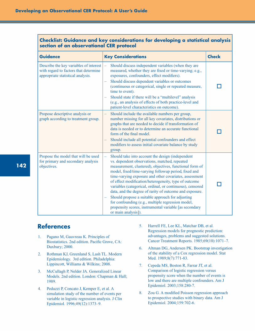
142


Checklist: Guidance and key considerations for developing a statistical analysis section of an observational CER protocol


Describe the key variables of interest with regard to factors that determine appropriate statistical analysis.

– Should discuss independent variables (when they are measured, whether they are fixed or time-varying; e.g., exposures, confounders, effect modifiers).

– Should discuss dependent variables or outcomes (continuous or categorical, single or repeated measure, time to event).

– Should state if there will be a “multilevel” analysis (e.g., an analysis of effects of both practice-level and patient-level characteristics on outcome).

o

Propose descriptive analysis or graph according to treatment group.

– Should include the available numbers per group, number missing for all key covariates, distributions or graphs that are needed to decide if transformation of data is needed or to determine an accurate functional form of the final model.

– Should include all potential confounders and effect modifiers to assess initial covariate balance by study group.

o

Propose the model that will be used for primary and secondary analysis objectives.

– Should take into account the design (independent vs. dependent observations, matched, repeated measurement, clustered), objectives, functional form of model, fixed/time-varying followup period, fixed and time-varying exposure and other covariates, assessment of effect modification/heterogeneity, type of outcome variables (categorical, ordinal, or continuous), censored data, and the degree of rarity of outcome and exposure.

– Should propose a suitable approach for adjusting for confounding (e.g., multiple regression model, propensity scores, instrumental variable [as secondary or main analysis]).

o

References1. Pagano M, Gauvreau K. Principles of

Biostatistics. 2nd edition. Pacific Grove, CA: Duxbury; 2000.

2. Rothman KJ, Greenland S, Lash TL. Modern Epidemiology. 3rd edition. Philadelphia: Lippincott, Williams & Wilkins; 2008.

3. McCullagh P, Nelder JA. Generalized Linear Models. 2nd edition. London: Chapman & Hall; 1989.

4. Peduzzi P, Concato J, Kemper E, et al. A simulation study of the number of events per variable in logistic regression analysis. J Clin Epidemiol. 1996;49(12):1373–9.

5. Harrell FE, Lee KL, Matchar DB, et al. Regression models for prognostic prediction: advantages, problems and suggested solutions. Cancer Treatment Reports. 1985;69(10):1071–7.

6. Altman DG, Andersen PK. Bootstrap investigation of the stability of a Cox regression model. Stat Med. 1989;8(7):771-83.

7. Cepeda MS, Boston R, Farrar JT, et al. Comparison of logistic regression versus propensity score when the number of events is low and there are multiple confounders. Am J Epidemiol. 2003;158:280-7.

8. Zou G. A modified Poisson regression approach to prospective studies with binary data. Am J Epidemiol. 2004;159:702-6.

143


9. Lumley T, Kronmal R, Ma S. Relative risk regression in medical research: models, contrasts, estimators, and algorithms. UW Biostatistics Working Paper Series. University of Washington. Paper 293;2006.

10. Lawless, Jerald F. Negative binomial and mixed Poisson regression. Can J Statistics. 1987;15: 209-25.

11. Hall DB. Zero-inflated Poisson and binomial regression with random effects: a case study. Biometrics. 2000: 56S:1030-9.

12. Diggle PJ, Heagerty P, Liang K-Y, et al. Analysis of Longitudinal Data. 2nd edition. New York: Oxford University Press; 2002.

13. Fitzmaurice GM, Laird NM, Ware JH. Applied Longitudinal Analysis. New Jersey: Wiley; 2004.

14. Klein JP, Moeschberger ML. Survival Analysis: Techniques for Censored and Truncated Data. New York: Springer-Verlag; 1997.

15. Hosmer DW, Lemeshow S, May S. Applied Survival Analysis. 2nd edition. New Jersey: Wiley; 2008.

16. Robins JM, Hernán MÁ, Brumback B. Marginal structural models and causal inference in epidemiology. Epidemiol. 2000;11:550-60.

17. Hernán MA, Brumback B, Robins JM. Marginal structural models to estimate the causal effect of zidovudine on the survival of HIV-positive men. Epidemiol. 2000;11:561-70.

18. Hernán MA, Brumback B, Robins JM. Estimating the causal effect of zidovudine on CD4 count with a marginal structural model for repeated measures. Stat Med. 2002;21:1689-709.

19. Cadarette SM, Katz JN, Brookhart MA, et al. Relative effectiveness of osteoporosis drugs for preventing nonvertebral fracture. Ann Intern Med. 2008;148:637-46.

20. Rosenbaum PR, Rubin DB. The central role of the propensity score in observational studies for causal effects. Biometrika. 1983;70(1):41-55.

21. Rosenbaum PR, Rubin DB. Reducing bias in observational studies using subclassification on the propensity score. J Am Stat Assoc. 1984;79: 516-524.

22. Rosenbaum PR, Rubin DB. Constructing a control group using multivariate matched sampling methods that incorporate the propensity score. Am Stat. 1985;39:33-8.

23. Hernán MA, Robins JM. Estimating causal effects from epidemiological data. J Epidemiol Community Health. 2006;60:578-86.

24. Reinisch J, Sanders S, Mortensen E, et al. In-utero exposure to phenobarbital and intelligence deficits in adult men. JAMA. 1995;274:1518-25.

25. Stürmer T, Joshi M, Glynn RJ, et al. A review of the application of propensity score methods yielded increasing use, advantages in specific settings, but not substantially different estimates compared with conventional multivariable methods. J Clin Epidemiol. 2006;59:437-47.

26. Kurth T, Walker AM, Glynn RJ, et al. Results of multivariable logistic regression, propensity matching, propensity adjustment, and propensity-based weighting under conditions of nonuniform effect. Am J Epidemiol. 2006;163:262-70.

27. Joffe MM, Rosenbaum PR. Invited commentary: Propensity scores. Am J Epidemiol. 1999;15: 327-33.

28. Schneeweiss S. A basic study design for expedited safety signal evaluation based on electronic healthcare data. Pharmacoepidemiol Drug Saf. 2010;19:858-68.

29. Rubin DB. Matched Sampling for Causal Effects. Cambridge: Cambridge University Press; 2006.

30. Stuart EA, Rubin DB. Best practices in quasi-experimental designs: matching methods for causal inference. In: Best Practices in Quantitative Methods. Ed. J. Osborne. Thousand Oaks, CA: Sage Publications; 2008;155-76.

31. Abadie A, Imbens GW. Large sample properties of matching estimators for average treatment effects. Econometrica. 2006;74:235-67.

32. Abadie A, Imbens GW. On the failure of the bootstrap for matching estimators. Econometrica. 2008;76:1537-57.

33. Sekhon JS. Multivariate and propensity score matching software with automated balance optimization: the matching package for R. J Stat Softw. 2011;42(7):1-52.

34. Connors AF, Speroff T, Dawson NV, et al. The effectiveness of right heart catheterization in the initial care of critically ill patients. JAMA. 1996;276:889-97.

35. Brookhart MA, Schneeweiss S, Rothman KJ, et al. Variable selection for propensity score models. Am J Epidemiol. 2006;163(12):1149-56.

144

36. Arbogast PG, Kaltenbach L, Ding H, et al. Adjustment for multiple cardiovascular risk factors using a summary risk score. Epidemiol. 2008;19(1):30-7.

37. Arbogast PG, Ray WA. Use of disease risk scores in pharmacoepidemiologic studies. Stat Methods Med Res. 2009;18(1):67-80.

38. Miettinen OS. Stratification by a multivariate confounder score. Am J Epidemiol. 1976;104(6):609–20.

39. Ray WA, Meredith S, Thapa PB, et al. Antipsychotics and the risk of sudden cardiac death. Arch Gen Psychiatry. 2001;58:1161-7.

40. Angrist JD, Imbens, GW, Rubin DB. Identification of causal effects using instrumental variables (with discussion). J Am Stat Assoc. 1996;91: 444-72.

41. Nelson CR, Startz R. The distribution of the instrumental variables estimator and its t-ratio when the instrument is a poor one. J Bus. 1990;63(1):S125-40.

42. Bound J, Jaeger DA, Baker RM. Problems with instrumental variables estimation when the correlation between the instruments and the endogeneous explanatory variable is weak. J Am Stat Assoc. 1995;90(430): 443-50.

43. Stock JH, Yogo M. Testing for Weak Instruments in Linear IV Regression. Cambridge, MA: National Bureau of Economic Research; November 2002.

44. Stock JH, Wright JH, Yogo M. A survey of weak instruments and weak identification in generalized method of moments. J Bus Econ Stat. 2002;20(4):518-29.

45. Angrist JD, Imbens GW. Two-stage least squares estimation of average causal effects in models with variable treatment intensity. J Am Stat Assoc. 1995;90:431-42.

46. Rassen JA, Schneeweiss S, Glynn RJ, et al. Instrumental variable analysis for estimation of treatment effects with dichotomous outcomes. Am J Epidemiol. 2009;169(3): 273-84.

47. Brookhart MA, Wang PS, Solomon DH, et al. Evaluating short-term drug effects using a physician-specific prescribing preferences as an instrumental variable. Epidemiol. 2006;17: 268-75.

48. Schneeweiss S, Seeger JD, Landon J, et al. Aprotinin during coronary-artery bypass grafting and risk of death. New Eng J Med. 2008;358: 771-83.

49. Little RJA, Rubin DB. Statistical Analysis with Missing Data. 2nd edition. Hoboken, NJ: John Wiley & Sons; 2002.

50. Harrell FE. Regression Modeling Strategies. New York: Springer-Verlag; 2001.


145

Abstract

This chapter provides an overview of study design and analytic assumptions made in observational comparative effectiveness research (CER), discusses assumptions that can be varied in a sensitivity analysis, and describes ways to implement a sensitivity analysis. All statistical models (and study results) are based on assumptions, and the validity of the inferences that can be drawn will often depend on the extent to which these assumptions are met. The recognized assumptions on which a study or model rests can be modified in order to assess the sensitivity, or consistency in terms of direction and magnitude, of an observed result to particular assumptions. In observational research, including much of comparative effectiveness research, the assumption that there are no unmeasured confounders is routinely made, and violation of this assumption may have the potential to invalidate an observed result. The analyst can also verify that study results are not particularly affected by reasonable variations in the definitions of the outcome/exposure. Even studies that are not sensitive to unmeasured confounding (such as randomized trials) may be sensitive to the proper specification of the statistical model. Analyses are available that can be used to estimate a study result in the presence of an hypothesized unmeasured confounder, which then can be compared to the original analysis to provide quantitative assessment of the robustness (i.e., “how much does the estimate change if we posit the existence of a confounder?”) of the original analysis to violations of the assumption of no unmeasured confounders. Finally, an analyst can examine whether specific subpopulations should be addressed in the results since the primary results may not generalize to all subpopulations if the biologic response or exposure may differ in these subgroups. The chapter concludes with a checklist of key considerations for including sensitivity analyses in a CER protocol or proposal.

Chapter 11. Sensitivity AnalysisJoseph A.C. Delaney, Ph.D.

University of Washington, Seattle, WA

John D. Seeger, Pharm.D., Dr.P.H. Harvard Medical School and Brigham and

Women’s Hospital, Boston, MA

Introduction

Observational studies and statistical models rely on assumptions, which can range from how a variable is defined or summarized to how a statistical model is chosen and parameterized. Often these assumptions are reasonable and, even when violated, may result in unchanged effect estimates. When the results of analyses are consistent or unchanged by testing variations in underlying assumptions, they are said to be “robust.” However, violations in assumptions that result in meaningful effect estimate changes provide insight into the validity of the inferences that

might be drawn from a study. A study’s underlying assumptions can be altered along a number of dimensions, including study definitions (modifying exposure/outcome/confounder definitions), study design (changing or augmenting the data source or population under study), and modeling (modifying a variable’s functional form or testing normality assumptions), to evaluate robustness of results.

This chapter considers the forms of sensitivity analysis that can be included in the analysis of an observational comparative effectiveness study, provides examples, and offers recommendations about the use of sensitivity analyses.

146


Unmeasured Confounding and Study Definition Assumptions

Unmeasured Confounding

An underlying assumption of all epidemiological studies is that there is no unmeasured confounding, as unmeasured confounders cannot be accounted for in the analysis and including all confounders is a necessary condition for an unbiased estimate. Thus, inferences drawn from an epidemiologic study depend on this assumption. However, it is widely recognized that some potential confounding variables may not have been measured or available for analysis: the unmeasured confounding variable could either be a known confounder that is not present in the type of data being used (e.g., obesity is commonly not available in prescription claims databases) or an unknown confounder where the confounding relation is unsuspected. Quantifying the effect that an unmeasured confounding variable would have on study results provides an assessment of the sensitivity of the result to violations of the assumption of no unmeasured confounding. The robustness of an association to the presence of a confounder,1-2 can alter inferences that might be drawn from a study, which then might change how the study results are used to influence translation into clinical or policy decisionmaking. Methods for assessing the potential impact of unmeasured confounding on study results, as well as quasi-experimental methods to account for unmeasured confounding, are discussed later in the chapter.

Comparison Groups

An important choice in study design is the selection of suitable treatment and comparison groups. This step can serve to address many potential limitations of a study, such as how new user cohorts eliminate the survivor bias that may be present if current (prevalent) users are studied. (Current users would reflect only people who could tolerate the treatment and, most likely, for whom treatment appeared to be effective).3

However, this “new user” approach can limit the questions that can be asked in a study, as excluding prevalent users might omit long-term

users (which could overlook risks that arise over long periods of use). For example, when Rietbrock et al. considered the comparative effectiveness of warfarin and aspirin in atrial fibrillation4 in the General Practice Research Database, they looked at current use and past use instead of new use. This is a sensible strategy in a general practice setting as these medications may be started long before the patient is diagnosed with atrial fibrillation. Yet, as these medications may be used for decades, long-term users are of great interest. In this study, the authors used past use to address indication, by comparing current users to past users (an important step in a “prevalent users” study).

One approach is to include several different comparison groups and use the observed differences in potential biases with the different comparison groups as a way to assess the robustness of the results. For example, when studying the association between thiazide diuretics and diabetes, one could create reference groups including “nonusers,” “recent past users,” “distant past users,” and “users of other antihypertensive medications.” One would presume that the risk of incident diabetes among the “distant past users” should resemble that of the “nonusers”; if not, there is a possibility that confounding by indication is the reason for the difference in risk.

Exposure Definitions

Establishing a time window that appropriately captures exposure during etiologically relevant time periods can present a challenge in study design when decisions need to be made in the presence of uncertainty.5 Uncertainty about the most appropriate way to define drug exposure can lead to questions about what would have happened if the exposure had been defined a different way. A substantially different exposure-outcome association observed under different definitions of exposure (such as different time windows or dose [e.g., either daily or cumulative]) might provide insight into the biological mechanisms underlying the association or provide clues about potential confounding or unaddressed bias. As such, varying the exposure definition and re-analyzing under different definitions serves as a form of sensitivity analysis.

147

Chapter 11. Sensitivity Analysis

Outcome Definitions

The association between exposure and outcome can also be assessed under different definitions of the outcome. Often a clinically relevant outcome in a data source can be ascertained in several ways (e.g., a single diagnosis code, multiple diagnosis codes, a combination of diagnosis and procedure codes). The analysis can be repeated using these different definitions of the outcome, which may shed light on the how well the original outcome definition truly reflects the condition of interest.

Beyond varying a single outcome definition, it is also possible to evaluate the association between the exposure and clinically different outcomes. If the association between the exposure and one clinical outcome is known from a study with strong validity (such as from a clinical trial) and can be reproduced in the study, the observed association between the exposure of interest and an outcome about which external data are not available becomes more credible. Since some outcomes might not be expected to occur immediately after exposure (e.g., cancer), the study could employ different lag (induction) periods between exposure and the first outcomes to be analyzed in order to assess the sensitivity of the result to the definition. This result can lead either to insight into potential unaddressed bias or confounding, or it could be used as a basis for discussion about etiology (e.g., does the outcome have a long onset period?).

Covariate Definitions

Covariate definitions can also be modified to assess how well they address confounding in the analysis. Although a minimum set of covariates may be used to address confounding, there may be an advantage to using a staged approach where groups of covariates are introduced, leading to progressively greater adjustment. If done transparently, this approach may provide insight into which covariates have relatively greater influences on effect estimates, permitting comparison with known or expected associations or permitting the identification of possible intermediate variables.

Finally, some covariates are known to be misclassified under some approaches. A classic example is an “intention to treat” analysis that assumes that each participant continues to

be exposed once they have received an initial treatment. Originally used in the analysis of randomized trials, this approach has been used in observational studies as well.6 It can be worthwhile to do a sensitivity analysis on studies that use an “intention to treat” approach to see how different an “as treated” analysis would be even if intention to treat is the main estimate of interest, mostly in cases where there is differential adherence in the data source between two therapeutic approaches.7

Summary Variables

Study results can also be affected by the summarization of variables. For example, time can be summarized, and differences in the time window during which exposure is determined can lead to changes in study effect estimates. For example, the risk of venous thromboembolism rises with duration of use for oral contraceptives;8 an exposure definition that did not consider the cumulative exposure to the medication might underestimate the difference in risk between two different formulations of oral contraceptive. Alternately, effect estimates may vary with changes in the outcome definition. For example, an outcome definition of all cardiovascular events including angina could lead to a different effect estimate than an outcome definition including only myocardial infarction. Sensitivity analyses of the outcome definition can allow for a richer understanding of the data, even for models based on data from a randomized controlled trial.

Selection Bias

The assessment of selection bias through sensitivity analysis involves assumptions regarding inclusion or participation by potential subjects, and results can be highly sensitive to assumptions. For example, the oversampling of cases exposed to one of the drugs under study (or, similarly, an undersampling) can lead to substantial changes in effect measures over ranges that might plausibly be evaluated. Even with external validation data, which may work for unmeasured confounders,9 it is difficult to account for more than a trivial amount of selection bias. Generally, if there is strong evidence of selection bias in a particular data set it is best to seek out alternative data sources.

148


One limited exception may be when the magnitude of bias is known to be small.10 This may be true for nonrandom loss to followup in a patient cohort. Since the baseline characteristics of the cohort are known, it is possible to make reasonable assumptions about how influential this bias can be. But, in the absence of such information, it is generally better to focus on identifying and eliminating selection bias at the data acquisition or study design stage.

Data Source, Subpopulations, and Analytic Methods

The first section of this chapter covered traditional sensitivity analysis to test basic assumptions such as variable definitions and to consider the impact of an unmeasured confounder. These issues should be considered in every observational study of comparative effectiveness research. However, there are some additional sensitivity analyses that should be considered, depending on the nature of the epidemiological question and the data available. Not every analysis can (or should) consider these factors, but they can be as important as the more traditional sensitivity analysis approaches.

Data Source

For many comparative effectiveness studies, the data used for the analysis were not specifically collected for the purpose of the research question. Instead, the data may have been obtained as part of routine care or for administrative purposes such as medical billing. In such cases, it may be possible to acquire multiple data sources for a single analysis (and use the additional data sources as a sensitivity analysis). Where this is not feasible, it may be possible to consider differences between study results and results obtained from other papers that use different data sources.

While all data sources have inherent limitations in terms of the data that are captured by the database, these limitations can be accentuated when the data were not prospectively collected for the specific research purpose.11 For example, secondary use of data increases the chances that a known but unmeasured confounder may explain part or all of an observed association. A straightforward example of the differences in data capture can be seen by comparing data from

Medicare (i.e., U.S. medical claims data) and the General Practice Research Database (i.e., British electronic medical records collected as part of routine care).11 Historically, Medicare data have lacked the results of routine laboratory testing and measurement (quantities like height, weight, blood pressure, and glucose measures), but include detailed reporting on hospitalizations (which are billed and thus well recorded in a claims database). In a similar sense, historically, the General Practice Research Database has had weaker reporting on hospitalizations (since this information is captured only as reports given back to the General Practice, that usually are less detailed), but better recording than Medicare data for routine measurements (such as blood pressure) that are done as part of a standard medical visit.

Issues with measurement error can also emerge because of the process by which data are collected. For example, “myocardial infarction” coded for the purposes of billing may vary slightly or substantially from a clinically verified outcome of myocardial infarction. As such, there will be an inevitable introduction of misclassification into the associations. Replicating associations in different data sources (e.g., comparing a report to a general practitioner [GP] with a hospital ICD-9 code) can provide an idea of how changes to the operational definition of an outcome can alter the estimates. Replication of a study using different data sources is more important for less objectively clear outcomes (such as depression) than it is for more objectively clear outcomes (such as all-cause mortality).

An analysis conducted in a single data source may be vulnerable to bias due to systematic measurement error or the omission of a key confounding variable. Associations that can be replicated in a variety of data sources, each of which may have used different definitions for recording information and which have different covariates available, provide reassurance that the results are not simply due to the unavailability of an important confounding variable in a specific data set. Furthermore, when estimating the possible effect of an unmeasured confounder on study results, data sets that measure the confounder may provide good estimates of the confounder’s association with exposure and outcome (and provide context for results in data sources without the same confounder information).

149


An alternative to looking at completely separate datasets is to consider supplementing the available data with additional information from external data sources. An example of a study that took the approach of supplementing data was conducted by Huybrechts et al.12 They looked at the comparative safety of typical and atypical antipsychotics among nursing home residents. The main analysis used prescription claims (Medicare and Medicaid data) and found, using high-dimensional propensity score adjustment, that conventional antipsychotics were associated with an increase in 180-day mortality risk (a risk difference of 7.0 per 100 persons [95% CI: 5.8, 8.2]). The authors then included data from MDS (Minimum Data Set) and OSCAR (Online Survey, Certification and Reporting), which contains clinical covariates and nursing home characteristics.12 The result of including these variables was an essentially identical estimate of 7.1 per 100 people (95% CI: 5.9, 8.2).12 This showed that these differences were robust to the addition of these additional covariates. It did not rule out other potential biases, but it did demonstrate that simply adding MDS and OSCAR data would not change statistical inference.

While replicating results across data sources provides numerous benefits in terms of understanding the robustness of the association and reducing the likelihood of a chance finding, it is often a luxury that is not available for a research question, and inferences may need to be drawn from the data source at hand.

Key Subpopulations

Therapies are often tested on an ideal population (e.g., uncomplicated patients thought to be likely to adhere to medication) in clinical trials. Once the benefit is clearly established in trials, the therapy is approved for use and becomes available to all patients. However, there are several cases where it is possible that the effectiveness of specific therapies can be subject to effect measure modification. While a key subpopulation may be independently specified as a population of interest, showing that results are homogeneous across important subpopulations can build confidence in applying the results uniformly to all subpopulations. Alternatively, it may highlight the presence of effect measure modification and

the need to comment on population heterogeneity in the interpretation of results. As part of the analysis plan, it is important to state whether measures of effect will be estimated within these or other subpopulations present in the research sample in order to assess possible effect measure modification:

Pediatric populations. Children may respond differently to therapy from adults, and dosing may be more complicated. Looking at children as a separate and important sub-group may make sense if a therapy is likely to be used in children.

Genetic variability. The issue of genetic variability is often handled only by looking at different ethnic or racial groups (who are presumed to have different allele frequencies). Some medications may be less effective in some populations due to the different polymorphisms that are present in these persons, though indicators of race and ethnicity are only surrogates for genetic variation.

Complex patients. These are patients who suffer from multiple disease states at once. These disease states (or the treatment[s] for these disease states) may interfere with each other, resulting in a different optimal treatment strategy in these patients. A classic example is the treatment of cardiovascular disease in HIV-infected patients. The drug therapy used to treat the HIV infection may interfere with medication intended to treat cardiovascular disease. Treatment of these complex patients is of great concern to clinicians, and these patients should be considered separately where sample size considerations allow for this.

Older adults. Older adults are another population that may have more drug side effects and worse outcomes from surgeries and devices. Furthermore, older adults are inherently more likely to be subject to polypharmacy and thus have a much higher risk of drug-drug interactions.

Most studies lack the power to look at all of these different populations, nor are they all likely to be present in a single data source. However, when it is feasible to do so, it can be useful to explore these subpopulations to determine if the overall associations persist or if the best choice of therapy is population dependent. These can be important clues in determining how stable associations are likely to be across key subpopulations. In particular, the researcher should identify

150


segments of the population for which there are concerns about generalizing results. For example, randomized trials of heart failure often exclude large portions of the patient population due to the complexity of the underlying disease state.13

It is critical to try to include inferences to these complex subpopulations when doing comparative effectiveness research with heart failure as the study outcome, as that is precisely where the evidence gap is the greatest.

Cohort Definition and Statistical Approaches

If it is possible to do so, it can also be extremely useful to consider the use of more than one cohort definition or statistical approach to ensure that the effect estimate is robust to the assumptions behind these approaches. There are several options to consider as alternative analysis approaches.

Samy Suissa illustrated how the choice of cohort definition can affect effect estimates in his paper on immortal time bias.14 He considered five different approaches to defining a cohort, with person time incorrectly allocated (causing immortal time bias) and then repeated these analyses with person time correctly allocated (giving correct estimates). Even in this straightforward example, the corrected hazard ratios varied from 0.91 to 1.13 depending on the cohort definition. There were five cohort definitions used to analyze the use of antithrombotic medication and the time to death from lung cancer: time-based cohort, event-based cohort, exposure-based cohort, multiple-event–based cohort, and event-exposure–based cohort. These cohorts produce hazard ratios of 1.13, 1.02, 1.05, 0.91, and 0.95, respectively. While this may not seem like an extreme difference in results, it does illustrate the value of using varying assumptions to hone in on an understanding of the stability of the associations under study with different analytical approaches, as in this example where point estimates varied by about +/- 10% depending in how the cohort was defined.

One can also consider the method of covariate adjustment to see if it might result in changes in the effect estimates. One option to consider as an adjunct analysis is the use of a high-dimensional propensity score,15 as this approach is typically applicable to the same data upon which a

conventional regression analysis is performed. The high-dimensional propensity score is well suited to handling situations in which there are multiple weak confounding variables. This is a common situation in many claims database contexts, where numerous variables can be found that are associated (perhaps weakly) with drug exposure, and these same variables may be markers for (i.e., associated with) unmeasured confounders. Each variable may represent a weak marker for an unmeasured confounder, but collectively (such as through the high-dimensional propensity score approach) their inclusion can reduce confounding from this source. This kind of propensity score approach is a good method for validating the results of conventional regression models.

Another option that can be used, when the data permit it, is an instrumental variable (IV) analysis to assess the extent of bias due to unmeasured confounding (see chapter 10 for a detailed discussion of IV analysis).16 While there have been criticisms that use of instruments such as physician or institutional preference may have assumptions that are difficult to verify and may increase the variance of the estimates,17 an instrumental variable analysis has the potential to account for unmeasured confounding factors (which is a key advantage), and traditional approaches also have unverifiable assumptions. Also, estimators resulting from the IV analysis may differ from main analysis estimators (see Supplement, “Improving Characterization of Study Populations: The Identification Problem”), and investigators should ensure correct interpretation of results using this approach.

Examples of Sensitivity Analysis of Analytic Methods

Sensitivity analysis approaches to varying analytic methods have been used to build confidence in results. One example is a study by Schneeweiss et al.18 of the effectiveness of aminocaproic acid compared with aprotinin for the reduction of surgical mortality during coronary-artery bypass grafting (CABG). In this study, the authors demonstrated that three separate analytic approaches (traditional regression, propensity score, and physician preference instrumental variable analyses) all showed an excess risk of death among the patients treated with aprotinin (estimates ranged from a relative risk of 1.32

151


[propensity score] to a relative risk of 1.64 [traditional regression analysis]). Showing that different approaches, each of which used different assumptions, all demonstrated concordant results was further evidence that this association was robust.

Sometimes a sensitivity analysis can reveal a key weakness in a particular approach to a statistical problem. Delaney et al.19 looked at the use of case-crossover designs to estimate the association between warfarin use and bleeding in the General Practice Research Database. They compared the case-crossover results to the case-time-control design, the nested case control design, and to the results of a meta-analysis of randomized controlled trials. The case-crossover approach, where individuals serve as their own controls, showed results that differed from other analytic approaches. For example, the case-crossover design with a lagged control window (a control window that is placed back one year) estimated a rate ratio of 1.3 (95% CI: 1.0, 1.7) compared with a rate ratios of 1.9 for the nested case-control design, 1.7 for the case-time-control design and 2.2 for a meta-analysis of clinical trials.18 Furthermore, the results showed a strong dependence on the length of the exposure window (ranging from a rate ratio of 1.0 to 3.6), regardless of overall time on treatment. These results provided evidence that results from a case-crossover approach in this particular

situation needed a cautious interpretation, as different approaches were estimating incompatible magnitudes of association, were not compatible with the estimates from trials, and likely violated an assumption of the case-crossover approach (transient exposure). Unlike the Schneeweiss et al. example,18 for which the results were consistent across analytic approaches, divergent results require careful consideration of which approach is the most appropriate (given the assumptions made) for drawing inferences, and investigators should provide a justification for the determination in the discussion.

Sometimes the reasons for differential findings with differences in approach can be obvious (e.g., concerns over the appropriateness of the case-crossover approach, in the Delaney et al. example above).19 In other cases, differences can be small and the focus can be on the overall direction of the inference (like in the Suissa example above).14 Finally, there can be cases where two different approaches (e.g., an IV approach and a conventional analysis) yield different inferences and it can be unclear which one is correct. In such a case, it is important to highlight these differences, and to try to determine which set of assumptions makes sense in the structure of the specific problem.

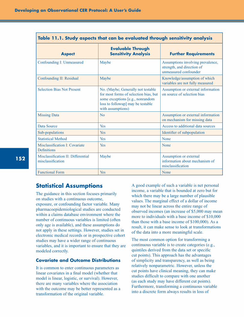
152


Table 11.1. Study aspects that can be evaluated through sensitivity analysis

AspectEvaluable Through Sensitivity Analysis Further Requirements

Confounding I: Unmeasured Maybe Assumptions involving prevalence, strength, and direction of unmeasured confounder

Confounding II: Residual Maybe Knowledge/assumption of which variables are not fully measured

Selection Bias Not Present No. (Maybe; Generally not testable for most forms of selection bias, but some exceptions [e.g., nonrandom loss to followup] may be testable with assumptions)

Assumption or external information on source of selection bias

Missing Data No Assumption or external information on mechanism for missing data

Data Source Yes Access to additional data sources

Sub-populations Yes Identifier of subpopulation

Statistical Method Yes None

Misclassification I: Covariate Definitions

Yes None

Misclassification II: Differential misclassification

Maybe Assumption or external information about mechanism of misclassification

Functional Form Yes None

Statistical AssumptionsThe guidance in this section focuses primarily on studies with a continuous outcome, exposure, or confounding factor variable. Many pharmacoepidemiological studies are conducted within a claims database environment where the number of continuous variables is limited (often only age is available), and these assumptions do not apply in these settings. However, studies set in electronic medical records or in prospective cohort studies may have a wider range of continuous variables, and it is important to ensure that they are modeled correctly.

Covariate and Outcome Distributions

It is common to enter continuous parameters as linear covariates in a final model (whether that model is linear, logistic, or survival). However, there are many variables where the association with the outcome may be better represented as a transformation of the original variable.

A good example of such a variable is net personal income, a variable that is bounded at zero but for which there may be a large number of plausible values. The marginal effect of a dollar of income may not be linear across the entire range of observed incomes (an increase of $5,000 may mean more to individuals with a base income of $10,000 than those with a base income of $100,000). As a result, it can make sense to look at transformations of the data into a more meaningful scale.

The most common option for transforming a continuous variable is to create categories (e.g., quintiles derived from the data set or specific cut points). This approach has the advantages of simplicity and transparency, as well as being relatively nonparametric. However, unless the cut points have clinical meaning, they can make studies difficult to compare with one another (as each study may have different cut points). Furthermore, transforming a continuous variable into a discrete form always results in loss of

153


information that is better to avoid if possible. Another option is to consider transforming the variable to see if this influences the final results. The precise choice of transformation requires knowledge of the distribution of the covariate. For confounding factors, it can be helpful to test several transformations and to see the impact of the reduction in skewness, and to decide whether a linear approximation remains appropriate.

Functional Form

The “functional form” is the assumed mathematical association between variables in a statistical model. There are numerous potential variations in functional form that can be the subject of a sensitivity analysis. Examples include the degree of polynomial expressions, splines, or additive rather than multiplicative joint effects of covariates in the prediction of both exposures and outcomes. In all of these cases, the “functional form” is the assumed mathematical association between variables, and sensitivity analyses can be employed to evaluate the effect of different assumptions. In cases where nonlinearity is suspected (i.e., a nonlinear relationship between a dependent and independent variable in a model), it can be useful to test the addition of a square term to the model (i.e., the pair of covariates age + age2 as the functional form of the independent variable age). If this check does not influence the estimate of the association, then it is unlikely that there is any important degree of nonlinearity. If there is an impact on the estimates for this sort of transformation, it can make sense to try a more appropriate model for the nonlinear variable (such as a spline or a generalized additive model).

Transformations should be used with caution when looking at the primary exposure, as they can be susceptible to overfit. Overfit occurs when you are fitting a model to random variations in the data (i.e., noise) rather than to the underlying relation; polynomial-based models are susceptible to this sort of problem. However, if one is assessing the association between a drug and an outcome, this can be a useful way to handle parameters (like age) that will not be directly used for inference but that one wishes to balance between two exposure groups. These transformations should also be considered as possibilities in the creation of a probability of treatment model (for a propensity

score analysis). If overfit of a key parameter that is to be used for inference is of serious concern, then there are analytic approaches (like dividing the data into a training and validation data set) that can be used to reduce the amount of overfit. However, these data mining techniques are beyond the scope of this chapter.

Special Cases

Another modeling challenge for epidemiologic analysis and interpretation is when there is a mixture of informative null values (zeroes) and a distribution. This occurs with variables like coronary artery calcium (CAC), which can have values of zero or a number of Agatston units.20 These distributions are best modeled as two parts: (1) as a dichotomous variable to determine the presence or absence of CAC; and (2) using a model to determine the severity of CAC among those with CAC>0. In the specific case of CAC, the severity model is typically log-transformed due to extreme skew.20 These sorts of distributions are rare, but one should still consider the distribution and functional form of key continuous variables when they are available.

Implementation Approaches

There are a number of approaches to conducting sensitivity analyses. This section describes two widely used approaches, spreadsheet-based and code-based analyses. It is not intended to be a comprehensive guide to implementing sensitivity analyses. Other approaches to conducting sensitivity analysis exist and may be more useful for specific problems.2

Spreadsheet-Based Analysis

The robustness of a study result to an unmeasured confounding variable can be assessed quantitatively using a standard spreadsheet.21 The observed result and ranges of assumptions about an unmeasured confounder (prevalence, strength of association with exposure, and strength of association with outcome) are entered into the spreadsheet, and are used to provide the departure from the observed result to be expected if the unmeasured confounding variable could be accounted for using standard formulae for confounding.22 Two approaches are available within the spreadsheet: (1) an “array” approach;

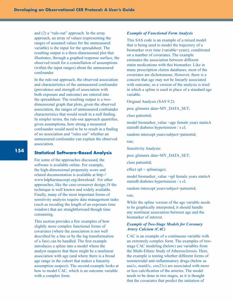
154


and (2) a “rule-out” approach. In the array approach, an array of values (representing the ranges of assumed values for the unmeasured variable) is the input for the spreadsheet. The resulting output is a three-dimensional plot that illustrates, through a graphed response surface, the observed result for a constellation of assumptions (within the input ranges) about the unmeasured confounder.

In the rule-out approach, the observed association and characteristics of the unmeasured confounder (prevalence and strength of association with both exposure and outcome) are entered into the spreadsheet. The resulting output is a two-dimensional graph that plots, given the observed association, the ranges of unmeasured confounder characteristics that would result in a null finding. In simpler terms, the rule-out approach quantifies, given assumptions, how strong a measured confounder would need to be to result in a finding of no association and “rules out” whether an unmeasured confounder can explain the observed association.

Statistical Software–Based Analysis

For some of the approaches discussed, the software is available online. For example, the high-dimensional propensity score and related documentation is available at http://www.hdpharmacoepi.org/download/. For other approaches, like the case-crossover design,18 the technique is well known and widely available. Finally, many of the most important forms of sensitivity analysis require data management tasks (such as recoding the length of an exposure time window) that are straightforward though time consuming.

This section provides a few examples of how slightly more complex functional forms of covariates (where the association is not well described by a line or by the log transformation of a line) can be handled. The first example introduces a spline into a model where the analyst suspects that there might be a nonlinear association with age (and where there is a broad age range in the cohort that makes a linearity assumption suspect). The second example looks at how to model CAC, which is an outcome variable with a complex form.

Example of Functional Form Analysis

This SAS code is an example of a mixed model that is being used to model the trajectory of a biomarker over time (variable=years), conditional on a number of covariates. The example estimates the association between different statin medications with this biomarker. Like in many prescription claims databases, most of the covariates are dichotomous. However, there is a concern that age may not be linearly associated with outcome, so a version of the analysis is tried in which a spline is used in place of a standard age variable.

Original Analysis (SAS 9.2):

proc glimmix data=MY_DATA_SET;

class patientid;

model biomarker_value =age female years statinA statinB diabetes hypertension / s cl;

random intercept years/subject=patientid;

run;

Sensitivity Analysis:

proc glimmix data=MY_DATA_SET;

class patientid;

effect spl = spline(age);

model biomarker_value =spl female years statinA statinB diabetes hypertension / s cl;

random intercept years/subject=patientid;

run;

While the spline version of the age variable needs to be graphically interpreted, it should handle any nonlinear association between age and the biomarker of interest.

Example of Two-Stage Models for Coronary Artery Calcium (CAC)

CAC is an example of a continuous variable with an extremely complex form. The examples of two-stage CAC modeling (below) use variables from the Multi-Ethnic Study of Atherosclerosis. Here, the example is testing whether different forms of nonsteroidal anti-inflammatory drugs (below as asa1c, nsaid1c, cox21c) are associated with more or less calcification of the arteries. The model needs to be done in two stages, as it is thought that the covariates that predict the initiation of

155


calcification may differ from those that predict how quickly calcification progresses once the process has begun.20

First, a model is developed for the relative risk of having a CAC score greater than zero (i.e., that there is at least some evidence of plaques in a CT scan of the participant’s coronary arteries). The variable for CAC is cac (1=CAC present, 0=CAC not present). The repeated statement is used to invoke robust confidence intervals (as there is only one subject for each unique participant ID number, designated as the variable idno).

SAS 9.2 code example:

proc genmod data = b descending;

class idno race1;

model cac=age1c male bmi1c race1

male diabetes smoker ex_smoker sbp1c dbp1c

hdl1 ldl1 TRIG1STTN1C asa1c nsaid1c cox21c

/ dist = poisson link = log;

repeated subject = idno/ type =ind;

estimate ‘asa1c’ asa1c 1 -1/ exp;

estimate ‘nsaid1c’ nsaid1c 1 -1/ exp;

estimate ‘cox21c’ cox21c 1 -1/ exp;;

run;

Among those participants with CAC (as measured by an Agatston score, agatpm1c), greater than zero, the amount present is then modeled. As this variable is highly skewed, the amount of CAC present is transformed using a log transformation.

SAS 9.2 code example:

proc genmod data = b descending;

class idno race1;

where agatpm1c ne 0;

model log_transformed_CAC=age1c male bmi1c race1

male diabetes smoker ex_smoker sbp1c dbp1c

hdl1 ldl1 TRIG1STTN1C asa1c nsaid1c cox21c;

repeated subject = idno/ type = unstr;

run;

The modeling of CAC is a good example of one of the more complicated continuous variables that can be encountered in CER.20 To properly model this association, two models were needed (and the second model required transformation of the exposure). Most comparative effectiveness projects will involve much simpler outcome variables, and the analyst should be careful to include more complex models only where there is an important scientific rationale.

Presentation

Often sensitivity analyses conducted for a specific CER study can simply be summarized in the text of the paper, especially if the number of scenarios is small.17 In other cases, where a broad range of scenarios are tested,2 it may be more informative to display analyses in tabular or graphical form.

Tabular Presentation

The classic approach to presenting sensitivity analysis results is a table. There, the author can look at the results of different assumptions and/or population subgroups. Tables are usually preferred in cases where there is minimal information being presented, as they allow the reader to very precisely determine the influence of changes in assumptions on the reported associations. This is the approach used by Suissa14 to show differences in results based on different approaches to analyzing a cohort of lung cancer patients.

Graphical Presentation

One reason to use graphical methods is that the variable being modeled is itself a continuous variable, and presenting the full plot is more informative than forcing a categorization scheme on the data. One example, from Robyn McClelland and colleagues (Figure 11.1),23 is a sensitivity analysis to see if the form in which alcohol is consumed changes its association with levels of CAC. The analyst, therefore, plots the association with total alcohol consumed overall and by type of alcohol (beer, wine, hard alcohol). Here, both the exposure and the outcome are continuous variables, and so it is much easier to present the results of the sensitivity analysis as a series of plots.

156


150

100

50

0

total intake of alcohol per day (g)

Total Alcohol

Aver

age

Ann

ual C

AC C

hang

e

0 20 40 60

150

100

50

0

total intake of alcohol from beer per day (g)

Beer

Aver

age

Ann

ual C

AC C

hang

e

0 20 40 60

150

100

50

0

total intake of alcohol from liquor per day (g)

Liquor

Aver

age

Ann

ual C

AC C

hang

e

0 20 40 60

150

100

50

0

total intake of alcohol from wine per day (g)

Wine

Aver

age

Ann

ual C

AC C

hang

e

0 10 20 30 40 50

Figure 11.1. Smoothed plot of alcohol consumption versus annualized progression of CAC with 95% CIs

See McClelland RL, Bild DE, Burke GL, et al. Alcohol and coronary artery calcium prevalence, incidence, and progression: results from the Multi-Ethnic Study of Atherosclerosis (MESA). Am J Clin Nutr 2008 Dec;88(6):1593-601. This figure is copyrighted by the American Society for Nutrition and reprinted with permission.

Another reason for a graphical display is to present the conditions that a confounder would need to meet in order to be able to explain an association. As discussed, the strength of a confounder depends on its association with the exposure, the outcome, and its prevalence in the population. Using the standard spreadsheet discussed earlier,20 these conditions can be represented as a plot. For example, Figure 11.2 presents a plot based on data from Psaty et al.1, 24

Figure 11.2 plots the combination of the odds ratio between the exposure and the confounder (OREC) and the relative risk between the confounder and the outcome (RRCD) that would be required to explain an observed association between the exposure and the outcome by confounding alone. There are two levels of association considered

(ARR=1.57 and ARR=1.3) and a separate line plotted for each. These sorts of displays can help illustrate the strength of unmeasured confounding that is required to explain observed associations, which can make the process of identifying possible candidate confounders easier (as one can reference other studies from other populations in order to assess the plausibility of the assumed strength of association). Spreadsheets that facilitate the conduct of these sensitivity analyses are available. (http://www.drugepi.org/dope-downloads/#Sensitivity Analysis)

Other tools for sensitivity analysis are available, such as the one from Lash et al. (http://sites.google.com/site/biasanalysis/).10

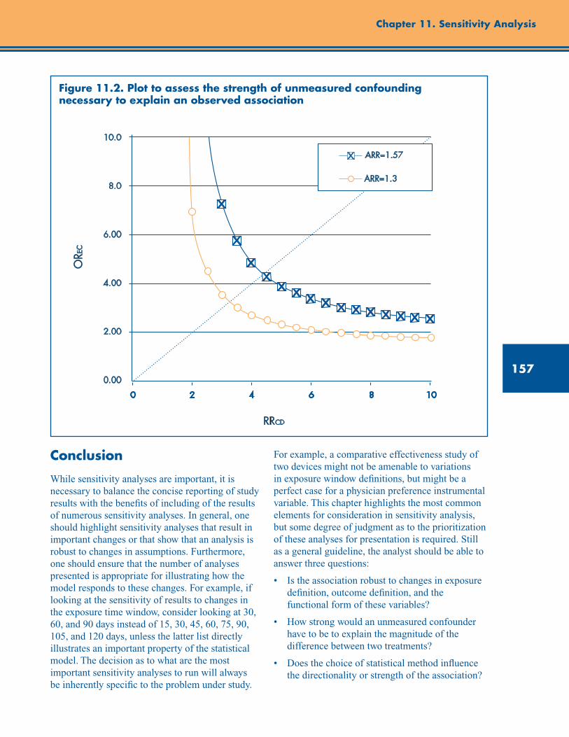
157


RRCD

ORE

C

10.0

8.0

6.00

4.00

2.00

0.00

0 2 4 6 8 10

ARR=1.57

ARR=1.3

Figure 11.2. Plot to assess the strength of unmeasured confounding necessary to explain an observed association

Conclusion

While sensitivity analyses are important, it is necessary to balance the concise reporting of study results with the benefits of including of the results of numerous sensitivity analyses. In general, one should highlight sensitivity analyses that result in important changes or that show that an analysis is robust to changes in assumptions. Furthermore, one should ensure that the number of analyses presented is appropriate for illustrating how the model responds to these changes. For example, if looking at the sensitivity of results to changes in the exposure time window, consider looking at 30, 60, and 90 days instead of 15, 30, 45, 60, 75, 90, 105, and 120 days, unless the latter list directly illustrates an important property of the statistical model. The decision as to what are the most important sensitivity analyses to run will always be inherently specific to the problem under study.

For example, a comparative effectiveness study of two devices might not be amenable to variations in exposure window definitions, but might be a perfect case for a physician preference instrumental variable. This chapter highlights the most common elements for consideration in sensitivity analysis, but some degree of judgment as to the prioritization of these analyses for presentation is required. Still as a general guideline, the analyst should be able to answer three questions:

• Istheassociationrobusttochangesinexposuredefinition, outcome definition, and the functional form of these variables?

• Howstrongwouldanunmeasuredconfounderhave to be to explain the magnitude of the difference between two treatments?

• Doesthechoiceofstatisticalmethodinfluencethe directionality or strength of the association?

158


A plan for including some key sensitivity analysis in developing study protocols and analysis plans should be formed with a clear awareness of the limitations of the data and the nature of the problem. The plan should be able to answer these three basic questions and should be a key feature of any comparative effectiveness analysis. The use

of sensitivity analysis to examine the underlying assumptions in the analysis process will build confidence as to the robustness of associations to assumptions and be a crucial component of grading the strength of evidence provided by a study.

Checklist: Guidance and key considerations for sensitivity analyses in an observational CER protocol


Propose and describe planned sensitivity analyses.

- Consider the effect of changing exposure, outcome, confounder, or covariate definitions or classifications. - Assess expected impact of unmeasured confounders on key measures of association.

o

Describe important subpopulations in which measures of effect will be assessed for homogeneity.

- Consider pediatric, racial/ethnic subgroups, patients with complex disease states. - Consider inclusion of AHRQ Priority Populations (http://www.ahrq.gov/populations/).

o

State modeling assumptions and how they will be tested. o

Indicate whether the study will be replicated in other databases, if available and feasible.

o

References 1. Schneeweiss S. Sensitivity analysis and external

adjustment for unmeasured confounders in epidemiologic database studies of therapeutics. Pharmacoepidemiol Drug Saf. 2006;15(5): 291-303.

2. McCandless LC, Gustafson P, Levy A. Bayesian sensitivity analysis for unmeasured confounding in observational studies. Stat Med. 2007;26(11): 2331-47.

3. Ray WA. Evaluating medication effects outside of clinical trials: new-user designs. Am J Epidemiol. 2003;158:915-20.

4. Rietbrock S, Plumb JM, Gallagher AM, van Staa TP. How effective are dose-adjusted warfarin and aspirin for the prevention of stroke in patients with chronic atrial fibrillation? An analysis of the UK General Practice Research Database. Thromb Haemost. 2009;101(3):527-34.

5. Schneeweiss S. A basic study design for expedited safety signal evaluation based on electronic healthcare data. Pharmacoepidemiol Drug Saf. 2010;19:858-68.

6. Hernán MA, Alonso A, Logan R, Grodstein F, Michels KB, Willett WC, Manson JE, Robins JM.Observational studies analyzed like randomized experiments: an application to postmenopausal hormone therapy and coronary heart disease. Epidemiology. 2008 Nov;19(6): 766-79.

7. Hernán MA, Hernández-Díaz S. Beyond the intention-to-treat in comparative effectiveness research.Clin Trials. 2011 doi: 0.1177/1740774511420743.

8. Suissa S, Blais L, Spitzer WO, et al. First-time use of newer oral contraceptives and the risk of venous thromboembolism. Contraception. 1997;56(3): 141-6.

159


9. Stürmer T, Glynn RJ, Rothman KJ, et al. Adjustments for unmeasured confounders in pharmacoepidemiologic database studies using external information. Med Care. 2007;45 (10 Suppl 2):S158-65.

10. Lash TL, Fox MP, Fink AK. Applying Quantitative Bias Analysis to Epidemiologic Data. New York: Springer; 2009.

11. Suissa S, Garbe E. Primer: administrative health databases in observational studies of drug effects—advantages and disadvantages. Nat Clin Pract Rheumatol. 2007;3(12):725-32.

12. Huybrechts KF, Brookhart MA, Rothman KJ, et al. Comparison of different approaches to confounding adjustment in a study on the association of antipsychotic medication with mortality in older nursing home patients. Am J Epidemiol. 2011;174(9):1089-99.

13. Cherubini A, Oristrell J, Pla X, et al. The persistent exclusion of older patients from ongoing clinical trials regarding heart failure. Arch Intern Med. 2011 Mar 28;171(6):550-6.

14. Suissa S. Immortal time bias in pharmacoepidemiology. Am J Epidemiol. 2008;167(4):492-9.

15. Schneeweiss S, Rassen JA, Glynn RJ, et al. High-dimensional propensity score adjustment in studies of treatment effects using health care claims data. Epidemiology. 2009 Jul;20(4):512-22.

16. Brookhart MA, Rassen JA, Schneeweiss S. Instrumental variable methods in comparative safety and effectiveness research. Pharmacoepidemiol Drug Saf. 2010;19(6):537-54.

17. Ionescu-Ittu R, Delaney JA, Abrahamowicz M. Bias-variance trade-off in pharmacoepidemiological studies using physician-preference-based instrumental variables: a simulation study. Pharmacoepidemiol Drug Saf. 2009 Jul;18(7):562-71.

18. Schneeweiss S, Seeger JD, Landon J, et al. Aprotinin during coronary-artery bypass grafting and risk of death. N Engl J Med. 2008;358(8): 771-83.

19. Delaney JA, Suissa S. The case-crossover study design in pharmacoepidemiology. Stat Methods Med Res. 2009;18(1):53-65.

20. Kronmal RA, McClelland RL, Detrano R, Shea S, Lima JA, Cushman M, Bild DE, Burke GL. Risk factors for the progression of coronary artery calcification in asymptomatic subjects: results from the Multi-Ethnic Study of Atherosclerosis (MESA). Circulation 2007;115(21):2722-30.

21. Division of Pharmacoepidemiology & Pharmacoeconomics, Department of Medicine, Brigham and Women’s Hospital and Harvard Medical School. http://www.drugepi.org/dope-downloads/#Sensitivity Analysis. Accessed January 3, 2012.

22. Walker AM. Observation and inference. An introduction to the methods of epidemiology. Newton Lower Falls, MA: Epidemiology Resources, Inc.;1991.

23. McClelland RL, Bild DE, Burke GL, et al.; Multi-Ethnic Study of Atherosclerosis. Alcohol and coronary artery calcium prevalence, incidence, and progression: results from the Multi-Ethnic Study of Atherosclerosis (MESA). Am J Clin Nutr. 2008 Dec;88(6):1593-601.

24. Psaty BM, Koepsell TD, Lin D, et al. Assessment and control for confounding by indication in observational studies. J Am Geriatri Soc. 1999;47:749-54.

161

Abstract

The identification process is an a priori assessment of the treatment effect estimates that can be produced by a given research design, and of the assumptions required for these estimates to yield accurate assessments of a given CER objective. This supplement describes the factors that a researcher should consider when proposing a research design to address (or “identify”) a given CER research objective. Investigators should assess the characteristics of the patient sample relative to the study objective, identify the subset(s) of patients whose treatment variation is exploited by the research design, and identify the assumptions that are required to ensure that (1) the research design produces unbiased treatment effect estimates for the patient subsets, and that (2) the treatment effect estimates produced provide a valid assessment of the study objective. In short, investigators must ensure that the effect estimates produced by a given research design and analysis answer the research question of interest and are interpreted appropriately. This supplement concludes with a checklist of guidance and key considerations for identifying research objectives for observational CER protocols.

Supplement 1. Improving Characterization of Study Populations: The Identification Problem

John M. Brooks, Ph.D. University of Iowa College of Pharmacy, Iowa City, IA

Introduction

Comparative effectiveness research (CER) is defined by the Federal Coordinating Council for Comparative Effectiveness Research as “the conduct and synthesis of research comparing the benefits and harms of different interventions and strategies to prevent, diagnose, treat and monitor health conditions in ‘real world’ settings.” As such, in its most basic sense, CER requires treatment variation across patients in the real world in order to estimate the comparative effects of alternative treatments. The identification process is an a priori assessment of the treatment effect estimates that can be produced by a given research design, and of the assumptions required for these estimates to yield accurate assessments of a given CER objective. Identification has been a key component in econometrics since being introduced by Koopmans in 1949,1 and a formal definition can be found in the textbook by Cameron and Trivedi.2 Economist Charles Manski states that “studies of identification seek to characterize the conclusions that could be drawn if one could use a sampling process to obtain an unlimited number of

observations.”3 Or, as described by Peter Kennedy, “identification is knowing that something is what you say it is.”4

CER researchers should provide a thorough discussion of the circumstances in which treatment variation isolated within their research designs is sufficient to make inferences relative to their specific CER objective. Part of this discussion will necessarily deal with sample size issues and statistical inference for the parameters estimated. However, at a more basic level, researchers should describe circumstances under which the parameters estimated can actually identify their CER research objective. The next section provides background on the importance of identification in CER relative to various possible CER research objectives and introduces the issues that a researcher should consider when assessing whether a proposed research design identifies a given CER research objective. The background section is followed by sections that focus on each issue.

162


Background

In the traditional CER model in which investigators compare the effectiveness of a treatment (T) versus an alternative (A) for a set of clinically similar patients in the real world, specific CER objectives can include assessments of any of the following:

1. The effect of removing access to T (currently used universally) and switching all patients to A.

2. The effect of T relative to A for those patients that used T; for example, T is currently used by a subset of patients and a policy is considered to remove patients’ access to T.

3. The effect of T relative to A for those patients that used A; for example, T is currently used by a subset of patients and a policy is considered to switch all users of A to T.

4. The effect of a change in the T utilization rate (which thereby changes the A rate); for example, T is currently used by a subset of patients and the effects of a general change in T utilization rates are considered.

5. The effect of a change in the T utilization rate (which thereby changes the A rate) that results from a given behavioral or policy intervention; for example, T is currently used by a subset of patients and the effects of a T rate change resulting from a copayment change are considered.

6. The effect of any of the above for specific subpopulations of the set of clinically similar patients; for example, T is currently used by a subset of patients over age 75, and the effects of a T utilization rate change that could result from a copayment change for these patients are considered.

Objective 1 involves finding the average treatment effect estimate across the entire population of clinically similar patients. For example, T could be a treatment used currently by all patients and a more expensive alternative has become available. A CER objective could be to evaluate a policy to switch all patients from T to the new alternative.

Objective 2 requires finding the average effect of T relative to A for the subset of patients who were treated with T. For example, if T is currently used by a subset of patients, a CER objective could be to evaluate a policy to remove patient access to T, which only will affect the subset of patients using T.

Alternatively, objective 3 requires finding the average effect of T relative to A for the subset of patients who were treated with A. For example, if T is not used currently by a subset of patients, a CER objective could be to estimate a policy of expanding T usage to all patients.

Objective 4 relates to evaluating the effects of treatment rate changes. Often the relevant question for policymakers is not whether a treatment should be used at all, but whether a treatment is over- or underused in practice. Many years ago, John Wennberg correctly posed objective 4 with the question “Which rate is right?”5 For example, if 80 percent of patients use a beta blocker after acute myocardial infarction, a CER objective may be to assess the effect of increasing the beta blocker treatment rate to 85 percent. Objective 4 is equivalent to objectives 2 and 3 if the specified T rate change means moving from the existing T utilization to either zero or 100 percent, respectively. Note that objective 4 is defined purposely without describing how the T treatment rates would be changed and can perhaps be best conceptualized as the effect of rate changes over time as a new treatment diffuses across a clinically similar population. The patient subset within a clinically similar population that only receives T when it is fully diffused may differ from the patient subset that is apt to receive T when it is newly introduced.

In contrast, objective 5 is defined with respect to the patient subset whose choice of T relative to A can be modified with a specific behavioral or policy intervention. At a specific T utilization rate, the patients defined in objective 5 can be thought of as a subset of the patients defined in objective 4, except that distinct patients may be affected by distinct interventions.6 For example, an information-based intervention may affect a different patient subset from an intervention focused on increasing access to treatment or an

163


intervention to change copayment rates. Objective 6 applies to any of the first four objectives with respect to defined subsets of the original clinically similar group (e.g., males vs. females, young vs. old, insured vs. uninsured).

The importance of identification with respect to these various CER objectives is highlighted when one reviews a seminal instrumental variable (IV) study in health care.7 In an examination of the mortality risk associated with more intensive treatment for acute myocardial infarction (AMI) in the elderly, McClellan and colleagues focused on the ability of IV estimators to reduce confounding bias in observational health care studies. While their study produced IV estimates that suggested that surgical interventions for AMI did not lessen patient mortality risk, the authors provided the qualification that their IV estimates should be used as evidence of mortality changes only if population surgery rates were modified (objective 4).7 Their estimates did not provide evidence of the average benefit of surgery for those that received surgery (objective 2), the average benefit of surgery over all AMI patients (objective 1), or the average benefit of surgery for all those patients not receiving surgery (objective 3). Without a discussion of the patient subset whose surgery effects were identified by these IV estimates, their results could have misled decisionmakers. Other authors who have compared treatment effect estimates across estimators using observational data have demonstrated comparisons that lack context without a discussion of the treatment effect concepts identified by each estimator.8-10

The concept of identification is closely akin to the ideas of external validity or applicability, in that it asks researchers to address the question “For whom can the treatment effect estimates be generalized?”3, 11-13 However, the classic discussions of these concepts mainly focus on the extent to which estimates from randomized studies can be appropriately applied to patients dissimilar to study populations.11-13 Alternatively, assessment of real-world treatment effectiveness in CER will often rely on treatment variation generated by the real-world treatment choices found in observational databases. Identification takes a broader view and relates to the extent of inferences that can be made using estimates from various estimators in the context of real-world treatment decisionmaking.

To make a case that a research design has the ability to identify a parameter sufficient to assess a specific CER objective, researchers should describe: (1) the characteristics of the patient sample used in the research relative to the objective; (2) the subset of patients within the sample whose treatment variation was exploited by the research design; (3) the assumptions required to ensure that the research design produces unbiased average treatment effect estimates for this patient subset; and (4) the assumptions required so that the treatment effect estimates produced will provide a valid assessment of the researcher’s CER objective. Each of these issues is discussed further in separate sections below.

To support the reader, Table S1.1 provides a summary of key concepts and acronyms used throughout the sections below.

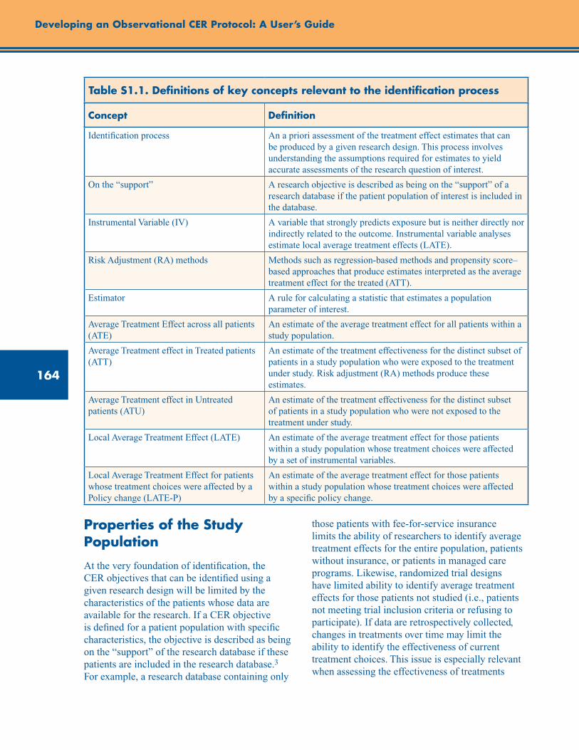
164


Table S1.1. Definitions of key concepts relevant to the identification process

Concept Definition

Identification process An a priori assessment of the treatment effect estimates that can be produced by a given research design. This process involves understanding the assumptions required for estimates to yield accurate assessments of the research question of interest.

On the “support” A research objective is described as being on the “support” of a research database if the patient population of interest is included in the database.

Instrumental Variable (IV) A variable that strongly predicts exposure but is neither directly nor indirectly related to the outcome. Instrumental variable analyses estimate local average treatment effects (LATE).

Risk Adjustment (RA) methods Methods such as regression-based methods and propensity score–based approaches that produce estimates interpreted as the average treatment effect for the treated (ATT).

Estimator A rule for calculating a statistic that estimates a population parameter of interest.

Average Treatment Effect across all patients (ATE)

An estimate of the average treatment effect for all patients within a study population.

Average Treatment effect in Treated patients (ATT)

An estimate of the treatment effectiveness for the distinct subset of patients in a study population who were exposed to the treatment under study. Risk adjustment (RA) methods produce these estimates.

Average Treatment effect in Untreated patients (ATU)

An estimate of the treatment effectiveness for the distinct subset of patients in a study population who were not exposed to the treatment under study.

Local Average Treatment Effect (LATE) An estimate of the average treatment effect for those patients within a study population whose treatment choices were affected by a set of instrumental variables.

Local Average Treatment Effect for patients whose treatment choices were affected by a Policy change (LATE-P)

An estimate of the average treatment effect for those patients within a study population whose treatment choices were affected by a specific policy change.

Properties of the Study Population

At the very foundation of identification, the CER objectives that can be identified using a given research design will be limited by the characteristics of the patients whose data are available for the research. If a CER objective is defined for a patient population with specific characteristics, the objective is described as being on the “support” of the research database if these patients are included in the research database.3 For example, a research database containing only

those patients with fee-for-service insurance limits the ability of researchers to identify average treatment effects for the entire population, patients without insurance, or patients in managed care programs. Likewise, randomized trial designs have limited ability to identify average treatment effects for those patients not studied (i.e., patients not meeting trial inclusion criteria or refusing to participate). If data are retrospectively collected, changes in treatments over time may limit the ability to identify the effectiveness of current treatment choices. This issue is especially relevant when assessing the effectiveness of treatments

165


whose benefits take many years to observe. For example, 10 years of followup may be necessary to demonstrate survival differences between surgery and radiation treatments for early-stage prostate cancer. However, at the end of the study it may be unclear as to whether the study identified the comparative effectiveness of current surgical and radiation technologies.

In the study by McClellan and colleagues cited above, the authors estimated the effectiveness of surgical treatments for AMI for fee-for-service Medicare beneficiaries. It is unclear whether this study identified the effectiveness of surgery for younger AMI patients or those with insurance coverage distinct from Medicare. In a followup IV study using data for younger AMI patients from Washington State, Brooks et al. showed that surgery effectiveness estimates from AMI patients with more generous insurance coverage would understate the effectiveness of surgery for AMI patients with less generous coverage.14

Relationship of Estimation Methods to Patient Subsets

Once a research database is specified and the study population is defined by inclusion criteria, the researcher must then make the case that the parameter estimates produced the estimators chosen are sufficient to identify the CER objective. It has been shown that the estimators available to estimate treatment effectiveness produce average estimates for distinct subsets of patients in the study population. Risk adjustment (RA) methods, including regression-based methods and propensity score-based approaches,15-17 produce estimates that are properly interpreted as the average treatment effect for the treated patients in a population (ATT).18-22 In contrast, IV estimators yield estimates of an average treatment effect for those patients whose treatment choices were affected by a set of instrumental variables or “instruments.”7,

14, 23-25 Because of this limitation, IV estimates are described as estimates of local average treatment effects (LATE).25

If the CER objective is to assess treatment effectiveness for the subset of patients who were treated (objective 2), a risk-adjusted estimate of

ATT may be suitable to address this objective. As will be discussed further below, identification would also require the researcher to justify the RA estimator assumptions that are necessary to avoid bias. If the CER objective is to assess average treatment effectiveness for the subset of patients whose treatment choices were modifiable by an instrument (the LATE for that instrument), an IV estimator is appropriate. A LATE estimate is potentially suitable for evaluating objective 5 if the instrument chosen is related to the specified behavioral or policy intervention being evaluated. For example, suppose a CER objective is to estimate the outcome change that will result from a policy of subsidizing treatment T relative to treatment A. An instrument is a measured factor related to treatment choice, but assumed not to have a direct relationship with outcomes or other unmeasured factors related to outcomes. A researcher could use observed variation in relative copayment rates for T and A for patients across distinct insurance plans as the basis for an instrument. The IV estimates produced using this instrument would be the average treatment effects for the subset of patients whose treatment choices are mutable with respect to financial incentives and may be suitable to identify the policy objective. In addition, as with RA estimators, identification with IV estimators requires the researcher to justify the IV assumption set that the instrument does not have a direct relationship with outcomes or other unmeasured factors related to outcomes.

The McClellan AMI study produced both RA estimates using analysis of variance (ANOVA) estimators, and IV estimates using measures of patient geographic access to key providers as instruments. McClellan’s RA estimates of ATT showed statistically significant reductions in mortality associated with surgery for Medicare beneficiaries with AMI, whereas their IV LATE estimates showed no mortality reduction from surgery. Conditional on the validity of assumptions underlying each estimator, the RA estimates directly identified a parameter suitable to assess the effects of surgery for those that had surgery (objective 2), whereas the IV LATE estimate identified a parameter potentially suitable to assess objective 5 for a policy related to modification of provider access (e.g., providing greater geographic

166


dispersion of catheterization labs). This estimate combination suggests that, for the most part, the surgery rates for AMI Medicare patients in the late 1980s through the early 1990s reflected proper sorting of surgery across patients—that the patients who received treatment benefited, but that expanding treatment rates would yield little additional benefit. These estimates do not directly identify any other CER objectives without further assumptions.

Assumptions Required To Yield Unbiased Estimates

For RA estimators to yield unbiased estimates of ATT, it must be assumed that unmeasured factors affecting treatment choice are unrelated to outcomes (or are “ignorable”) after conditioning on measured factors.16, 26 Similarly, for IV estimators to yield a consistent estimate of LATE, an instrument must not be directly or indirectly related to outcomes. In the McClellan study, unbiased estimates of ATT from their ANOVA RA estimator rested on the assumption that all unmeasured factors affecting surgery choice had no direct or indirect relationship with mortality. Likewise, for the McClellan study to have produced consistent estimates of LATE, it must be assumed that the instruments used in the study had no direct relationship with mortality and were also unrelated to any remaining unmeasured factors related to both surgery choice and mortality.

Identification of Research Objectives Other Than ATT or LATE

If the CER objective requires estimation of a treatment effect for a patient population not represented in the research database, or if it requires a parameter distinct from ATT or LATE, identification requires the researcher to assess the validity of extrapolating estimates to their CER objective. Extrapolation will require assumptions that should be directly stated and thoughtfully defended based on clinical plausibility and treatment choice theory.

However, if the CER objective is to estimate a treatment effect parameter distinct from ATT or LATE, identification requires that the researcher explicitly provide the assumptions that are necessary for estimates of ATT or LATE to be validly applied to the set of patients described by the research objective. Examples of other treatment effect parameters that may be needed across CER objectives include the average treatment effect on the untreated (ATU) for objective 3, the average treatment effect across all patients in the population (ATE) for objective 1, or the average treatment effect for the subset of patients whose treatment choices would be affected by a specific policy change (LATE-P) for objective 5. Key assumptions to stipulate before extrapolating ATT or LATE estimates to other CER objectives are related to:

• theheterogeneityorhomogeneityoftreatmenteffects across patients; and

• thereasonswhytreatedanduntreatedpatientswere observed to make different treatment choices.

For example, to assume that an unbiased estimate of ATT is a valid estimate of ATU, a researcher would need to provide a compelling theory as to why the untreated patients did not chose a given treatment for reasons other than expected differences in treatment effectiveness. An unbiased estimate of ATT would provide sufficient information to identify ATU if the researcher can make the case that either: (1) treatment effects are homogeneous across patients and factors unrelated to treatment effectiveness are the cause of disparate treatment choices in the population or (2) treatment effects are heterogeneous across a population but that providers do not react to the treatment effect heterogeneity when making treatment choices. Condition 2 is the notion of “nonessential heterogeneity.”20, 27 Under either of these conditions, it could also be argued that an estimate of ATT identifies the ATE in a population and the average treatment effects that would result from a policy intervention affecting treatment choice (LATE-P). In contrast, if treatment choice was based on expected treatment effectiveness and the patients who were expected to gain most from treatment received treatment (essential

167


heterogeneity),27-28 ATT estimates would likely overstate and not identify the true ATE, ATU, and LATE-P in a population. Similar assumptions are required for LATE estimates from a given instrument set to be used to identify ATT, ATU, ATE, and LATE-P. To make the case for the validity of these assumptions, researchers have to provide a theory to suggest why the patients whose treatment choices varied with the value of their instrument are indistinct from the set of patients underlying these parameters.

In the study by McClellan and colleagues, the authors implied that providers considered the effectiveness of surgery for each AMI patient when making surgery recommendations and that the AMI patients most likely to benefit from surgery were those that received surgery. As such, the authors cautioned against assuming their IV estimates could be used to identify ATE, ATU, or ATT. However, the authors suggested that their IV estimates using instruments based on provider access provide more suitable answers to address the question of whether

surgery rates from AMI patients should increase (objective 4) in comparison to existing randomized controlled trial (RCT) evidence. Essentially, the authors argued that their IV estimates identified the treatment effect parameter required to assess objective 4.

The Appendix to this supplement contains a general model of treatment choice and outcomes that can be used to clarify the model assumptions required to identify CER objectives using estimates of ATT from RA estimators or estimates of LATE from IV estimators. The general model contains a series of factors related to treatment effectiveness, treatment choice, and outcomes directly. Twelve hypothetical empirical scenarios are derived by assumptions that relate to the existence of these factors. Scenarios differ by whether treatment effects are assumed to be homogeneous or heterogeneous, whether treatment decisions are based on treatment effect heterogeneity, and which of the model factors are measured.

Checklist: Guidance and key considerations for identifying a research objective in an observational CER protocol


Describe the characteristics of the patient sample used in the research relative to the objective.

Is extrapolation required, and what assumptions are needed to support this? o

Describe how the estimates from the proposed estimation methods (i.e., RA or IV methods) address the CER objective.

Does the researcher acknowledge to whom the estimates for the method directly apply? o

Describe the assumptions required to ensure that the research design produces unbiased average treatment effect estimates for this patient sample.

Does the researcher acknowledge the assumptions required from each estimator to yield unbiased or consistent estimates?

o

Describe the assumptions required so that the treatment effect estimates produced will provide a valid assessment of the researcher’s CER objective.

Does the researcher state whether the clinical and behavioral assumptions necessary for their estimates identify their CER objective? o

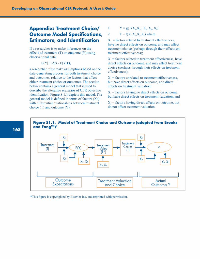
168


OutcomeExpectations

Treatment Valuation and Choice

Actual Outcome Y

Treatment (T)

Treatment Value (T*)

P(Y) YTreatment Choice

(T)

X1X1

X2 X2X3, X5

X3, X4

X3, X5

Appendix: Treatment Choice/Outcome Model Specifications, Estimators, and Identification

If a researcher is to make inferences on the effects of treatment (T) on outcome (Y) using observational data:

E(Y|T+t) - E(Y|T),

a researcher must make assumptions based on the data-generating process for both treatment choice and outcomes, relative to the factors that affect either treatment choice or outcomes. The section below contains a general model that is used to describe the alterative scenarios of CER objective identification. Figure S.1.1 depicts this model. The general model is defined in terms of factors (Xs) with differential relationships between treatment choice (T) and outcome (Y):

1. Y = g(T(X1,X

2), X

2, X

3, X

5)

2. T = f(X1,X

2,X

3,X

4) where:

X1 = factors related to treatment effectiveness,

have no direct effects on outcome, and may affect treatment choice (perhaps through their effects on treatment effectiveness);

X2 = factors related to treatment effectiveness, have

direct effects on outcome, and may affect treatment choice (perhaps through their effects on treatment effectiveness);

X3 = factors unrelated to treatment effectiveness,

but have direct effects on outcome, and direct effects on treatment valuation;

X4 = factors having no direct effects on outcome,

but have direct effects on treatment valuation; and

X5 = factors having direct effects on outcome, but

do not affect treatment valuation.

Figure S1.1. Model of Treatment Choice and Outcome (adapted from Brooks and Fang28)*

*This figure is copyrighted by Elsevier Inc. and reprinted with permission.

169


In a given empirical scenario, the ability to identify and estimate various possible average effects of T on Y (average treatment effect [ATE]; average treatment effect on the treated [ATT]; average treatment effect on the untreated [ATU]; local average treatment effect for a specific instrument [LATE]) is a function of: (1) the assumed relationships between treatment choice and outcomes; (2) which of the factors are measured and unmeasured; and (3) the extent of variation in observed factors. The discussion below details the characteristics required for identification of CER concepts using risk adjustment (RA) and instrumental variable (IV) estimators across variants of this general model. For each factor “X

i”, distinctions are made for measured (X

iM) and

unmeasured (XiU) factors.

Model Scenarios

1. Treatment effect is homogeneous (no X1 and X

2

factors exist), and no factors affecting treatment choice (T) have a direct effect on outcome (Y).

Y = g(T,X5M

,X5U

)

T = f(X4M

,X4U

)

a. Direct RA estimation of Y equation statistically controlling for X

5M:

i. Sufficient variation in X4 so that different

treatment choices are observed in the data.

ii. An assumption of no correlation between X

4 and factors in X

5U will yield an unbiased

estimate of ATT. ATE and ATU are “identified” by this ATT estimate through the assumed homogeneity of treatment effect.

b. IV estimation statistically controlling for X5M

and using X

4M as an instrument:

i. Sufficient variation in X4M

so that different treatment choices are observed in the data for patients stratified by X

4M.

ii. An assumption of no correlation between X

4M and factors in X

5U will yield a

consistent estimate of LATE specific to the patients whose treatment choices were affected by the factors within X

4M. ATE

and ATU are “identified” by this LATE

estimate through the assumed homogeneity of treatment effect.

2. Treatment effect is homogeneous (no X1 and

X2 factors exist). Certain factors affecting

treatment choice have direct effects on outcome (X

3).

Y = g(T,X3M

,X3U

,X5M

,X5U

)

T = f(X3M

,X3U

,X4M

,X4U

)


3M and X

5M:


treatment choices are observed in the data after controlling for X

3M when estimating

the outcome equation.

ii. Assumptions that no X3U

variables exist and that there are no correlations between X

4

and factors in X5U

will yield an unbiased estimate of ATT. ATE and ATU are “identified” by the ATT estimate through assumed homogeneity of treatment effect.

b. IV estimation statistically controlling for X

3M and X

5M and using measured X

4M as an

instrument:


so that different treatment choices are observed in the data across X

4M strata after controlling for X

3M.

ii. Assumptions of no correlation between X

4M and factors in X

3U and X

5U will yield

a consistent estimate of LATE specific to the set of patients whose T choices were affected by X

4M after controlling for X

3M

and X5M

. ATE and ATU are “identified” by this LATE estimate through the assumed homogeneity of treatment effect.

3. Treatment effect is heterogeneous, and the factors affecting treatment effectiveness have no direct effect on Y (X

1 exists; no X

2

factors exist). Moreover, heterogeneity is nonessential: Decisionmakers do not have sufficient knowledge of the X

1 factors affecting

heterogeneity to affect treatment choice, and X1

factors are unmeasured by the researcher.

Y = g(T(X1U

),X5M

,X5U

)

T = f(X4M

,X4U

)

170



5M:



ii. Assumption of no correlations between X

4 and X

5U will yield an unbiased estimate

of ATT. ATE and ATU are “identified” by estimating ATT through the assumption that providers do not have knowledge of how X

1U relates to treatment effectiveness.

However, if X4 was somehow correlated

with X1U

, average X1U

would vary between treated and untreated patients and the RA estimate of ATT would not be biased; however, it would not be possible to identify either ATE or ATU.


and using X



so different treatment choices are observed in the data across X

4M strata.

ii. Assumption of no correlation between X

4M and factors in X

5U yields a consistent

estimate of LATE specific to the set of patients whose T choices were affected by factors within X

4M. ATE and ATU

are “identified” by this LATE estimate through the assumption that providers do not have knowledge of how X

1U relates to

treatment effectiveness. However, if X4M

factors are somehow correlated with X

1U,

then the patients whose treatment choices vary with X

4M will differ from the rest of

the patient population with regard to X1U

. In this case, the IV LATE estimate would not identify either ATE or ATU.

4. Treatment effect is heterogeneous, and factors affecting treatment effectiveness have no direct effect on Y (X

1 exists; no X

2


1 factors affecting

heterogeneity to affect treatment choice. However, certain suspected X

1M factors are

measured by the researcher.

Y = g(T(X1M

,X1U

),X5M

,X5U

)

T = f(X4M

,X4U

)


5M for patient groups stratified

by X1M

:

i. Sufficient variation in X4 exists so that

different treatment choices are observed in the data within each stratum of X

1M.

ii. Assumption of no correlation between X4

and X5U

in each X1M

stratum will yield an unbiased estimate of ATT within each X

1M

stratum. ATE and ATU are “identified” by estimating ATT through the assumption that providers do not have knowledge of how X

1U relates to treatment effectiveness

within each X1M

stratum.

b. IV estimation for patient groups stratified by X

1M and statistically controlling for X

5M and

using X4M

as an instrument:


exists so that different treatment choices are observed in the data across X

4M strata within each X

1M

stratum.


4M and X

5U in each X

1M stratum will yield

a consistent estimate of LATE specific to the set of patient whose T choices were affected by measured factors within X

4M.

ATE and ATU are “identified” by this LATE estimate through the assumption that providers do not have knowledge of how X

1U relates to treatment effectiveness

within each X1M

stratum.

5. Treatment effect is heterogeneous, and all factors affecting treatment effectiveness have no direct effect on Y (X

1 exists; no X

2 factors

exist). Moreover, heterogeneity is essential: Decisionmakers have knowledge of certain X

1

factors affecting treatment effectiveness that is sufficient to affect treatment choice, but these factors are unmeasured by the researcher.

Y = g(T(X1U

),X5M

,X5U

)

T = f(X1U

,X4M

,X4U

)


5M:



171



4 and X

5U yields an unbiased estimate

of ATT. Because X1U

is used in treatment choice, the distribution of X

1U will differ

between the treated patients and untreated patients. Therefore, the ATE and ATU are unidentified by the ATT estimate.


and using X




4M strata.

ii. Assumption of no correlation between X4M

and X

5M yields a consistent estimate of

LATE specific to the set of patient whose T choices were affected by X

4M. Because

the value of X1U

will define the subset of patients for whom X

4M factors affect their

treatment choices (e.g., X4M

will less likely affect the treatment choices for patients with extreme X

1U values), the distributions

of X1U

will differ among treated, untreated, and those patient used to estimate LATE. Therefore, the LATE estimate would not identify ATT, ATU, or ATE.

6. Treatment effect is heterogeneous, and factors affecting treatment effectiveness have no direct effect on Y(X

1 exists; no X

2 factors

exist). Moreover, heterogeneity is essential: Decisionmakers have knowledge of the X

1

factors affecting heterogeneity sufficient to affect treatment choice, and all X

1 factors are


Y = g(T(X1M

) ,X5M

,X5U

)

T = f(X1M

,X4M

,X4U

)


5M within each X

1M stratum:

i. Sufficient variation in X4 exists within

each X1M

stratum so that different treatment choices are observed within each X

1M stratum.

ii. Assumed no correlation between X4 and

X5U

in each X1M

stratum yields an unbiased estimate of ATT within each X

1M stratum.

Within each X1M

stratum, the ATE and ATU are “identified” by estimating ATT through the assumed homogeneity of

treatment effect within the X1M

stratum.

b. Estimation for patient groups stratified by X1M

and statistically controlling for X

5M and using

X4M

as an instrument:




1M stratum.

ii. Assumed no correlation between X4M

and X

5U in each X

1M stratum yields a consistent

estimate of LATE specific to the set of patient whose T choices were affected by X

4M. ATE and ATU are “identified” within

each X1M

stratum by estimating this LATE through the assumed homogeneity of treatment effect within each X

1M stratum.

Moreover, with X1M

measured it would be possible to identify population-level values of ATT, ATE, and ATU, using LATE estimates based on X

4M.27, 29, 30

7. Treatment effect is heterogeneous, and factors affecting treatment effectiveness have no direct effect on Y (X

1 exists; no X

2 factors


1

factors affecting heterogeneity sufficient to affect treatment choice. Only certain X

1 factors

are measured by the researcher.

Y = g(T(X1M

,X1U

) ,X5M

,X5U

)

T = f(X1M

,X1U

,X4M

,X4U

)


5M within each X

1M stratum:

i. Sufficient variation in X4 or X

1U exists

within each X1M


1M stratum.

ii. Assumed no correlation between X4

andX1U

and X5U

in each X1M

stratum yields unbiased estimates of ATT in each X

1M

stratum. However, within each X1M

stratum, ATE and ATU that are not identified as X

1U

will be distributed differently for treated and untreated patients within each X

1M

stratum.



5M and

using X4M

as an instrument:

172





1M stratum.


and X

5U in each X

1M stratum yields consistent

estimates of LATE in each X1M

stratum that are specific to the set of patient whose T choices were affected by X

4M. ATE and

ATU are not “identified” within each X1M

stratum, as the distribution of X

1U will vary

between treated and untreated patients within each X

1M stratum.

8. Treatment effect is heterogeneous, and the factors affecting treatment effectiveness have direct effects on Y (no X

1 factors exist; X

2


2 factors affecting

heterogeneity to affect treatment choice and X2

factors are unmeasured by the researcher.

Y = g(T(X2U

), X2U

,X5M

,X5U

)

T = f(X4M

,X4U

)


5M:



ii. Assumed no correlations between X4 and

X2U

and X5M

yields an unbiased estimate of ATT. ATE and ATU are “identified” by estimating ATT through the assumption that X

4 and X

2U are uncorrelated. If X

4 was

correlated with X2U

, average X2U

would vary between treated and untreated patients, and the RA estimate of ATT would be biased (which is distinct from scenario 3).


and using X




4M strata.


and X

2U and X

5U yields a consistent estimate

of LATE specific to the set of patient whose T choices were affected by factors within X

4M. ATE and ATU are “identified”

by estimating this LATE through the

assumption that X4M

and X2U

factors are uncorrelated. If X

4M factors are correlated

with X2U

, then the IV LATE estimate would be inconsistent.

9. Treatment effect is heterogeneous, and factors affecting treatment effectiveness have direct effect on Y (no X

1 factors exists; X

2


2 factors affecting

heterogeneity to affect treatment choice. However, certain suspected X

2M factors are


Y = g(T(X2M

,X2U

), X2M

,X2U

,X5M

,X5U

)

T = f(X4M

,X4U

)


5M for patient groups stratified

by X2M

:

i. Sufficient variation in X4 exists so that

different treatment choices are observed in the data within each stratum of X

2M.


X2U

and X5U

in each X2M

stratum yields unbiased estimates of ATT within each X

2M stratum. Within each X

2M stratum,

the ATE and ATU are “identified” by the ATT estimate through the assumed lack of provider knowledge of treatment effect heterogeneity related to X

2U when making

treatment choices within each X2M

stratum.

b. IV estimation for patient groups stratified by X2M

and statistically controlling for X

5M and using

X4M

as an instrument:


exists so that different treatment choices are observed in the data across X


2M

stratum.


and X

2U and X

5U in each X

2M stratum yields

consistent estimates of LATE, specific in each X

2M stratum for the set of patient

whose treatment choices were affected by factors within X

4M. ATE and ATU are

“identified” by LATE within each X2M

stratum through the assumed lack of provider knowledge of treatment effect

173


heterogeneity related to X2U

when making treatment choices within each X

2M stratum.

10. Treatment effect is heterogeneous, and all factors affecting treatment effectiveness have no direct effect on Y (no X

1 factors exists;

X2 factors exist). Moreover, heterogeneity is

essential: Decisionmakers have knowledge of certain X

2 factors affecting treatment

effectiveness that is sufficient to affect treatment choice, but these factors are unmeasured by the researcher.

Y = g(T(X2U

),X2U

,X5M

,X5U

)

T = f(X2U

,X4M

,X4U

)


5M:



ii. Because X2U

is unmeasured and is related to both Y and T, the RA estimator will be a biased estimate of ATT. Accordingly, ATE and ATU will be unidentified by the biased ATT estimate.


and using X




4M strata.


and X

2U and X

5U yields consistent estimates

of LATE specific to the patients whose treatment choices were affected by X

4M.

Because the value of X2U

will define the subset of patients for whom X

4M factors

affect their treatment choices (e.g., X4M

will less likely affect the treatment choices for patients with extreme X

2U values),

the distributions of X2U

will differ among treated, untreated, and those patients used to estimate LATE. Therefore, LATE, while consistent, would not identify ATT, ATU, or ATE.

11. Treatment effect is heterogeneous, and factors affecting treatment effectiveness have no direct effect on Y (no X

1 factors exists; X

2 factors


2

factors affecting heterogeneity sufficient to

affect treatment choice, and all X2 factors are


Y = g(T(X2M

) ,X2M

,X5M

,X5U

)

T = f(X2M

,X4M

,X4U

)


5M within each X

2M stratum:

i. Sufficient variation in X4 exists within

each X2M


2M

stratum.


X5U

in each X2M

stratum yields unbiased estimate of ATT within each X

2M stratum.

Within each X2M

stratum, the ATE and ATU are “identified” by estimating ATT through assumed homogeneity of treatment effect within each X

2M stratum.



5M and

using X4M

as an instrument:




2M stratum.


and X

5U in each X

2M stratum yields consistent

estimates of LATE in each X2M

stratum specific to the patients whose treatment choices were affected by X

4M. ATE and

ATU are “identified” within each X2M

stratum by this LATE estimate through assumed homogeneity of treatment effect within each X

2M stratum.

12. Treatment effect is heterogeneous, and factors affecting treatment effectiveness have no direct effect on Y (no X

1 factors exists; X

2 factors


2

factors affecting heterogeneity sufficient to affect treatment choice. Only certain X

2 factors

are measured by the researcher.

Y = g(T(X2M

,X2U

),X2M

,X2U

,X5M

,X5U

)

T = f(X2M

,X2U

,X4M

,X4U

)


5M within each X

2M stratum:

i. Sufficient variation in X4 or X

2U exists

within each X2M

stratum so that different

174


treatment choices are observed within each X

1M stratum.

ii. Because X2U

is related to both Y and T and is unmeasured, the RA estimator yields a biased estimate of ATT within each X

2M

stratum. Accordingly, ATE and ATU will be unidentified by the biased ATT estimate within each X

2M stratum.



5M and

using X4M

as an instrument:




2M stratum.


and X

2U and X

5U in each X

2M stratum yields

consistent estimates of LATE in each X2M

stratum specific to the patients whose treatment choices were affected by X

4M.

ATE and ATU are not “identified” within each X

2M stratum as the distribution of X

2U

will vary between treated and untreated patients within each X

2M stratum.

References1. Koopmans TC. Identification problems in

economic model construction. Econometrica. 1949;17:125-44.

2. Cameron AC, Trivedi PK. Microeconometrics: Methods and Applications. New York: Cambridge University Press; 2005.

3. Manski CF. Identification for Prediction and Decision. Cambridge, MA: Harvard University Press; 2007.

4. Kennedy P. A Guide to Econometrics. 4th Edition ed. Cambridge, MA: The MIT Press; 1998.

5. Wennberg JE. Which rate is right? N Engl J Med. 1986;315(13):810-5.

6. Heckman JJ. Building bridges between structural and program approaches to evaluating policy. J Econ Lit. June 2010;68(2):356-98.

7. McClellan M, McNeil BJ, Newhouse JP. Does more intensive treatment of acute myocardial-infarction in the elderly reduce mortality? Analysis using instrumental variables. JAMA. 1994 Sep 21;272(11):859-66.

8. Stukel TA, Fisher ES, Wennberg DE, et al. Analysis of observational studies in the presence of treatment selection bias: effects of invasive cardiac management on AMI survival using propensity score and instrumental variable methods. JAMA. 2007 Jan 17;297(3):278-85.

9. Zeliadt SB, Potosky AL, Penson DF, et al. Survival benefit associated with adjuvant androgen deprivation therapy combined with radiotherapy for high and low-risk patients with nonmetastatic prostate cancer. Int J Radiat Oncol Biol Phys. 2006;66(2):395-402.

10. Lu-Yao GL, Albertson PC, Moore DF, et al. Survival following primary androgen deprivation therapy among men with localized prostate cancer. JAMA. 2008 Jul 9;300(2):173-81.

11. Shadish WR, Cook TD, Campbell DT. Experimental and Quasi-experimental Designs for Generalized Causal Inferences. Boston: Houghton Mifflin Company; 2002.

12. Atkins D, Chang SM, Gartlehner G, et al. Assessing applicability when comparing medical interventions: AHRQ and the Effective Health Care Program. J Clin Epidemiol. 2011 Nov;64(11):1198-207.

13. Guyatt GH, Sinclair J, Cook DJ, et al. Users’ guides to the medical literature: XVI. How to use a treatment recommendation. JAMA. 1999 May 19;281(19):1836-43.

14. Brooks JM, McClellan M, Wong HS. The marginal benefits of invasive treatments for acute myocardial infarction: does insurance coverage matter? Inquiry. 2000 Spring;37(1):75-90.

15. Rosenbaum PR, Rubin DB. The central role of the propensity score in observational studies for causal effects. Biometrika. 1983 Apr 1;70(1):41-55.

16. Rubin DB. Estimating causal effects from large data sets using propensity scores. Ann Intern Med. 1997 Oct 15;127(8 Pt 2):757-63.

17. Little RJ, Rubin DB. Causal effects in clinical and epidemiological studies via potential outcomes: concepts and analytical approaches. Annu Rev Public Health. 2000;21:121-45.

18. Angrist JD. Treatment effect heterogeneity in theory and practice. Economic Journal. 2004;114(494):C52-C83.

175


19. Brooks JM, Chrischilles EA. Heterogeneity and the interpretation of treatment effect estimates from risk adjustment and instrumental variable methods. Med Care. 2007 Oct;45(10 Supl 2):S123-30.

20. Heckman JJ, Urzua S, Vytlacil E. Understanding instrumental variables in models with essential heterogeneity. Review of Economics and Statistics. 2006;88(3):389-432.

21. Greenland S, Morgenstern H. Confounding in health research. Annu Rev Public Health. 2001;22:189-212.

22. Heckman JJ, Robb R. Alternative Methods for Evaluating the Impact of Interventions. In: Heckman JJ, Singer B, eds. Longitudinal Analysis of Labor Market Data. New York: Cambridge University Press; 1985:156-245.

23. Newhouse JP, McClellan M. Econometrics in outcomes research: the use of instrumental variables. Annu Rev Public Health.1998;19:17-34.

24. Harris KM, Remler DK. Who is the marginal patient? Understanding instrumental variables estimates of treatment effects. Health Serv Res. 1998 Dec;33(5 Pt 1):1337-60.

25. Imbens GW, Angrist JD. Identification and estimation of local average treatment effects. Econometrica. 1994;62(2):467-75.

26. Rubin DB. The central role of the propensity score in observational studies for causal effects. Biometrika. 1983;70:41-55.

27. Basu A, Heckman JJ, Navarro-Lozano S, et al. Use of instrumental variables in the presence of heterogeneity and self-selection: an application to treatments of breast cancer patients. Health Econ. 2007 Nov;16(11):1133-57.

28. Brooks JM, Fang G. Interpreting treatment-effect estimates with heterogeneity and choice: simulation model results. Clin Ther. 2009 Apr;31(4):902-19.

29. Angrist JD, Fernandez-Val I. Extrapolate-ing: External Validity and Overidentification in the LATE Framework. National Bureau of Economic Research Working Paper. Cambridge, MA; 2010.

30. Heckman JJ, Vytlacil E. Structural equations, treatment effects, and econometric policy evaluation. Econometrica. 2005 May;73(3): 669-738.

177

Abstract

This supplement describes how counterfactual theory is used to define causal effects and the conditions in which observed data can be used to estimate counterfactual-based causal effects. Basic definitions and language used in causal graph theory are then presented. The graphical separation rules linking the causal assumptions encoded in a diagram to the statistical relations implied by the causal diagrams are then presented. The supplement concludes with a description of how Directed Acyclic Graphs (DAGs) can be used to select covariates for statistical adjustment, identify sources of bias, and support causal interpretation in comparative effectiveness studies.

Supplement 2. Use of Directed Acyclic GraphsBrian Sauer, Ph.D.

University of Utah School of Medicine, Salt Lake City, UT


Introduction

Under the rubric of structural equation modeling, causal diagrams were historically used to illustrate qualitative assumptions in linear equation systems. Judea Pearl extended the interpretation of causal diagrams to probability models, a development that has enabled the use of graph theory in probabilistic and counterfactual inference.1 Epidemiologists then recognized that these diagrams could be used to illustrate sources of bias in epidemiological research,2 and for this reason have recommended the use of causal graphs to illustrate sources of bias and to determine if the effect of interest can be identified from available data.3-6

This supplement begins with a brief overview of how counterfactual theory is used to define causal effects and of the conditions under which observed data can be used to estimate counterfactual-based causal effects. We then present the basic definitions and language used in causal graph theory. Next we describe the construction of causal diagrams and the graphical separation rules linking the causal assumptions encoded in a diagram to the statistical relations implied by the diagram. The supplement concludes with a description of how Directed Acyclic Graphs (DAGs) can be used to select covariates for statistical adjustment, identify sources of bias, and support causal interpretation in comparative effectiveness studies.

Estimating Causal Effects

The primary goal of nonexperimental comparative effectiveness research is to compare the effect of study treatments on the risk of specific outcomes in a target population. To determine if a treatment had a causal effect on an outcome of interest, we would like to compare individual-level outcomes under each treatment level. Unfortunately, an individual’s outcome can only be observed under one treatment condition, which is often referred to as the factual outcome. Outcomes under treatment conditions not actually observed are referred to as counterfactual or potential outcomes.7-8 Using counterfactual theory, we would say that a treatment had a causal effect on an individual’s outcome if the outcome experienced would have been different under an alternative treatment level. For example, we would conclude that treatment A had a causal effect on the outcome Y if, say, an individual died 5 days after taking the drug (a=1), but would have remained alive on day 5 if he had not taken the medication (a=0). Due to the missing counterfactual data, causal effect measures cannot be directly computed for individual people without very strong assumptions. Nevertheless, average causal effects can be consistently estimated in randomized experiments and nonexperimental studies under certain assumptions.7-8

178


Assuming that we can simultaneously estimate the outcome risk for the entire population under different treatment conditions, then an average causal effect occurs when the outcome risk is not equal across levels of treatment. Using a dichotomous treatment (A) and outcome (Y) as the example, the causal effect in a population is the probability of the outcome occurring when the entire population is treated Pr[Ya=1=1] minus the probability of the outcome occurring when the entire population is untreated Pr[Ya=0=1]. Populations, like individuals, cannot simultaneously receive different levels of treatment. We can, however, use observed data to draw inferences about the probability distributions or expectations over a population of counterfactual variables. One of the important assumptions required for using only observed data (factual data) to estimate average causal effects is exchangeability.

In an ideal randomized experiment, treatment assignment is independent of the counterfactual outcomes, and therefore the two groups are exchangeable.7, 9 This means that the risk of experiencing the outcome in the two groups at the time of treatment assignment is equal to the risk in the full population. The equivalency to the full population allows us to use the observed data from the treated group to estimate what the treatment effect would have been if the entire population was treated, and it also allows us to use the observed data from the untreated group to estimate the effect of no treatment in the full population. In addition, because the outcome risks in the subpopulations are equivalent at the time treatment is assigned, the observed risk difference between the treatment groups can be attributed to treatment effects.10 In an ideal randomized trial, the outcome experience had the entire population been treated (Pr[Ya=1=1]) is equal to the probability of the outcome occurring in the subset of the population who received treatment (Pr[Y=1|A=1]), and the same holds for the untreated group. Using the risk difference scale, this means that the conditional risk difference can be used to estimate the marginal causal risk difference (Pr[Y=1|A=1] - Pr[Y=1|A=0]) = (Pr[Ya=1=1]- (Pr[Ya=0=1]).

In nonexperimental studies, marginal exchangeability can rarely be assumed, since patients and providers typically select treatments based on their belief about the risk of specific outcomes. In this case marginal exchangeability does not hold, but exchangeability may hold within levels of risk factors pertaining to the outcome. Causal inference from nonexperimental data is based on the critical assumption that within levels of important risk factors, treatment assignment is effectively randomized. This assumption is also referred to as “conditional exchangeability,” “conditional unconfoundedness,” or the assumption of “conditionally ignorable treatment assignment.”8, 10 When we assume that treatment was randomly assigned conditional on a set of covariates, causal inference for nonexperimental comparative effectiveness studies requires some form of covariate adjustment.

The question then concerns the adjustments that must be made in order to generate conditional exchangeability and avoid bias. DAGs have been found to be particularly helpful in diagnosing sources of bias and helping investigators select a set of covariates that allow the estimation of causal effects from observed data. Using DAG theory, confounding bias can be characterized as an unblocked “backdoor” path from the treatment to the outcome. The next section presents terminology for DAGs and their utility in selecting covariates for statistical adjustment.

DAG Terminology

DAGs are used to encode researchers’ a priori assumptions about the relationships between and among variables in causal structures. DAGs contain directed edges (arrows), linking nodes (variables), and their paths. A path is an unbroken sequence of distinct nodes connected by edges; a directed path is a path that follows the edges in the direction indicated by the arrows, such as the path from A to C (A→B→C). An undirected path does not follow the direction of the arrows, such as the following A to C path (A→B→C). Kinship terms are often used to represent relationships within a path. If there exists a directed path from A to C, then A is an ancestor of C and C is a descendent of A. Using the directed path example of A→B→C,

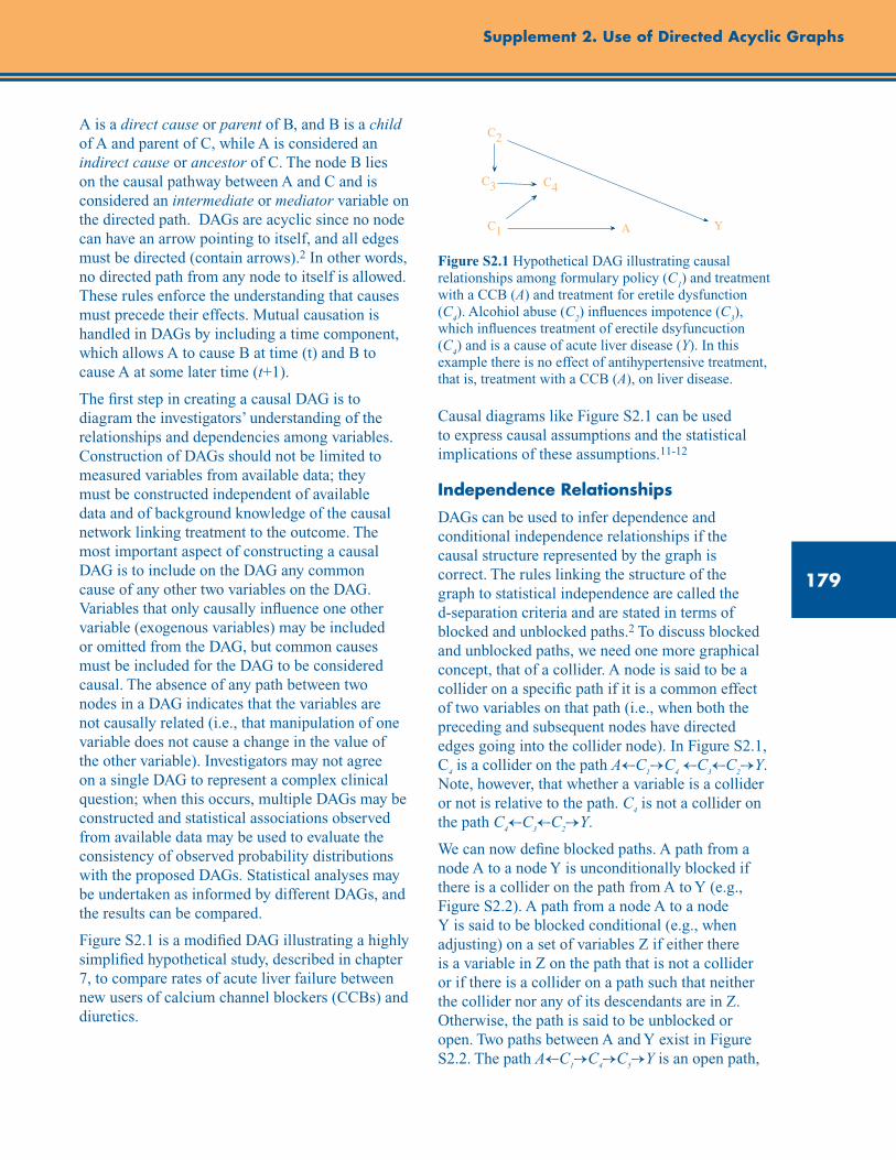
179

Supplement 2. Use of Directed Acyclic Graphs

A is a direct cause or parent of B, and B is a child of A and parent of C, while A is considered an indirect cause or ancestor of C. The node B lies on the causal pathway between A and C and is considered an intermediate or mediator variable on the directed path. DAGs are acyclic since no node can have an arrow pointing to itself, and all edges must be directed (contain arrows).2 In other words, no directed path from any node to itself is allowed. These rules enforce the understanding that causes must precede their effects. Mutual causation is handled in DAGs by including a time component, which allows A to cause B at time (t) and B to cause A at some later time (t+1).

The first step in creating a causal DAG is to diagram the investigators’ understanding of the relationships and dependencies among variables. Construction of DAGs should not be limited to measured variables from available data; they must be constructed independent of available data and of background knowledge of the causal network linking treatment to the outcome. The most important aspect of constructing a causal DAG is to include on the DAG any common cause of any other two variables on the DAG. Variables that only causally influence one other variable (exogenous variables) may be included or omitted from the DAG, but common causes must be included for the DAG to be considered causal. The absence of any path between two nodes in a DAG indicates that the variables are not causally related (i.e., that manipulation of one variable does not cause a change in the value of the other variable). Investigators may not agree on a single DAG to represent a complex clinical question; when this occurs, multiple DAGs may be constructed and statistical associations observed from available data may be used to evaluate the consistency of observed probability distributions with the proposed DAGs. Statistical analyses may be undertaken as informed by different DAGs, and the results can be compared.

Figure S2.1 is a modified DAG illustrating a highly simplified hypothetical study, described in chapter 7, to compare rates of acute liver failure between new users of calcium channel blockers (CCBs) and diuretics.

Figure S2.1 Hypothetical DAG illustrating causal relationships among formulary policy (C

1) and treatment

with a CCB (A) and treatment for eretile dysfunction (C

4). Alcohiol abuse (C

2) influences impotence (C

3),

which influences treatment of erectile dsyfuncuction (C

4) and is a cause of acute liver disease (Y). In this

example there is no effect of antihypertensive treatment, that is, treatment with a CCB (A), on liver disease.

Causal diagrams like Figure S2.1 can be used to express causal assumptions and the statistical implications of these assumptions.11-12

Independence Relationships

DAGs can be used to infer dependence and conditional independence relationships if the causal structure represented by the graph is correct. The rules linking the structure of the graph to statistical independence are called the d-separation criteria and are stated in terms of blocked and unblocked paths.2 To discuss blocked and unblocked paths, we need one more graphical concept, that of a collider. A node is said to be a collider on a specific path if it is a common effect of two variables on that path (i.e., when both the preceding and subsequent nodes have directed edges going into the collider node). In Figure S2.1, C

4 is a collider on the path A←C

1→C

4 ←C

3←C

2→Y.

Note, however, that whether a variable is a collider or not is relative to the path. C

4 is not a collider on

the path C4←C

3←C

2→Y.

We can now define blocked paths. A path from a node A to a node Y is unconditionally blocked if there is a collider on the path from A to Y (e.g., Figure S2.2). A path from a node A to a node Y is said to be blocked conditional (e.g., when adjusting) on a set of variables Z if either there is a variable in Z on the path that is not a collider or if there is a collider on a path such that neither the collider nor any of its descendants are in Z. Otherwise, the path is said to be unblocked or open. Two paths between A and Y exist in Figure S2.2. The path A←C

1→C

4→C

5→Y is an open path,

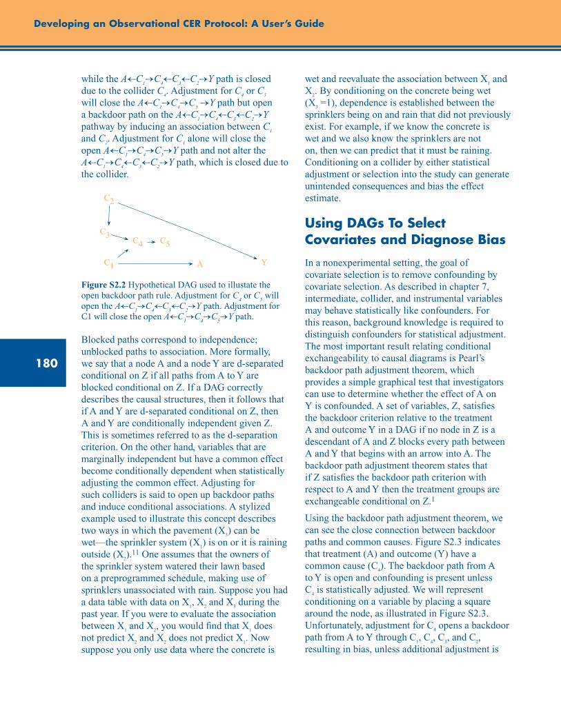
180


while the A←C1→C

4←C

3←C

2→Y path is closed

due to the collider C4. Adjustment for C

4 or C

5

will close the A←C1→C

4→C

5 →Y path but open

a backdoor path on the A←C1→C

4←C

3←C

2→Y

pathway by inducing an association between C1

and C2. Adjustment for C

1 alone will close the

open A←C1→C

4→C

5→Y path and not alter the

A←C1→C

4←C

3←C

2→Y path, which is closed due to

the collider.

Figure S2.2 Hypothetical DAG used to illustate the open backdoor path rule. Adjustment for C

4 or C

5 will

open the A←C1→C

4←C

3←C

2→Y path. Adjustment for

C1 will close the open A←C1→C

4→C

5→Y path.

Blocked paths correspond to independence; unblocked paths to association. More formally, we say that a node A and a node Y are d-separated conditional on Z if all paths from A to Y are blocked conditional on Z. If a DAG correctly describes the causal structures, then it follows that if A and Y are d-separated conditional on Z, then A and Y are conditionally independent given Z. This is sometimes referred to as the d-separation criterion. On the other hand, variables that are marginally independent but have a common effect become conditionally dependent when statistically adjusting the common effect. Adjusting for such colliders is said to open up backdoor paths and induce conditional associations. A stylized example used to illustrate this concept describes two ways in which the pavement (X

3) can be

wet—the sprinkler system (X1) is on or it is raining

outside (X2).11 One assumes that the owners of

the sprinkler system watered their lawn based on a preprogrammed schedule, making use of sprinklers unassociated with rain. Suppose you had a data table with data on X

1, X

2 and X

3 during the

past year. If you were to evaluate the association between X

1 and X

2, you would find that X

1 does

not predict X2 and X

2 does not predict X

1. Now

suppose you only use data where the concrete is

wet and reevaluate the association between X1 and

X2. By conditioning on the concrete being wet

(X3 =1), dependence is established between the

sprinklers being on and rain that did not previously exist. For example, if we know the concrete is wet and we also know the sprinklers are not on, then we can predict that it must be raining. Conditioning on a collider by either statistical adjustment or selection into the study can generate unintended consequences and bias the effect estimate.

Using DAGs To Select Covariates and Diagnose Bias

In a nonexperimental setting, the goal of covariate selection is to remove confounding by covariate selection. As described in chapter 7, intermediate, collider, and instrumental variables may behave statistically like confounders. For this reason, background knowledge is required to distinguish confounders for statistical adjustment. The most important result relating conditional exchangeability to causal diagrams is Pearl’s backdoor path adjustment theorem, which provides a simple graphical test that investigators can use to determine whether the effect of A on Y is confounded. A set of variables, Z, satisfies the backdoor criterion relative to the treatment A and outcome Y in a DAG if no node in Z is a descendant of A and Z blocks every path between A and Y that begins with an arrow into A. The backdoor path adjustment theorem states that if Z satisfies the backdoor path criterion with respect to A and Y then the treatment groups are exchangeable conditional on Z.1

Using the backdoor path adjustment theorem, we can see the close connection between backdoor paths and common causes. Figure S2.3 indicates that treatment (A) and outcome (Y) have a common cause (C

4). The backdoor path from A

to Y is open and confounding is present unless C

4 is statistically adjusted. We will represent

conditioning on a variable by placing a square around the node, as illustrated in Figure S2.3. Unfortunately, adjustment for C

4 opens a backdoor

path from A to Y through C1, C

4, C

3, and C

2,

resulting in bias, unless additional adjustment is

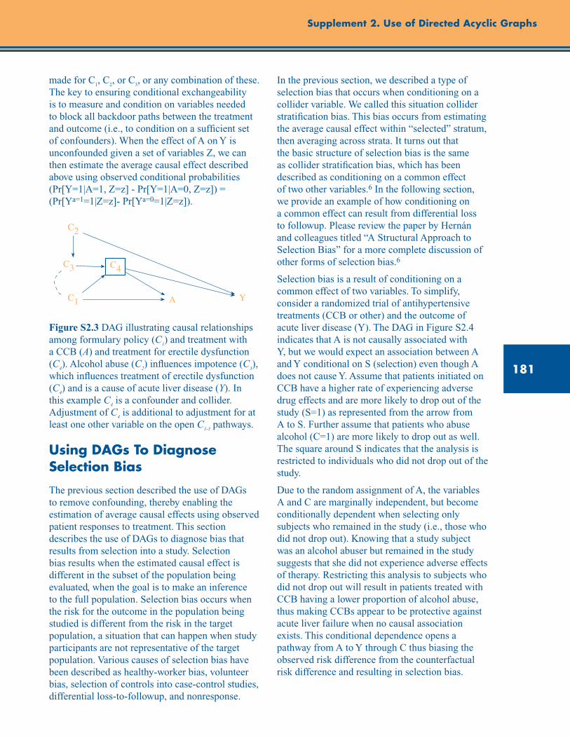
181


made for C1, C

2, or C

3, or any combination of these.

The key to ensuring conditional exchangeability is to measure and condition on variables needed to block all backdoor paths between the treatment and outcome (i.e., to condition on a sufficient set of confounders). When the effect of A on Y is unconfounded given a set of variables Z, we can then estimate the average causal effect described above using observed conditional probabilities (Pr[Y=1|A=1, Z=z] - Pr[Y=1|A=0, Z=z]) = (Pr[Ya=1=1|Z=z]- Pr[Ya=0=1|Z=z]).

Figure S2.3 DAG illustrating causal relationships among formulary policy (C

1) and treatment with

a CCB (A) and treatment for erectile dysfunction (C

4). Alcohol abuse (C

2) influences impotence (C

3),

which influences treatment of erectile dysfunction (C

4) and is a cause of acute liver disease (Y). In

this example C4 is a confounder and collider.

Adjustment of C4 is additional to adjustment for at

least one other variable on the open C1-3

pathways.

Using DAGs To Diagnose Selection Bias

The previous section described the use of DAGs to remove confounding, thereby enabling the estimation of average causal effects using observed patient responses to treatment. This section describes the use of DAGs to diagnose bias that results from selection into a study. Selection bias results when the estimated causal effect is different in the subset of the population being evaluated, when the goal is to make an inference to the full population. Selection bias occurs when the risk for the outcome in the population being studied is different from the risk in the target population, a situation that can happen when study participants are not representative of the target population. Various causes of selection bias have been described as healthy-worker bias, volunteer bias, selection of controls into case-control studies, differential loss-to-followup, and nonresponse.

In the previous section, we described a type of selection bias that occurs when conditioning on a collider variable. We called this situation collider stratification bias. This bias occurs from estimating the average causal effect within “selected” stratum, then averaging across strata. It turns out that the basic structure of selection bias is the same as collider stratification bias, which has been described as conditioning on a common effect of two other variables.6 In the following section, we provide an example of how conditioning on a common effect can result from differential loss to followup. Please review the paper by Hernán and colleagues titled “A Structural Approach to Selection Bias” for a more complete discussion of other forms of selection bias.6

Selection bias is a result of conditioning on a common effect of two variables. To simplify, consider a randomized trial of antihypertensive treatments (CCB or other) and the outcome of acute liver disease (Y). The DAG in Figure S2.4 indicates that A is not causally associated with Y, but we would expect an association between A and Y conditional on S (selection) even though A does not cause Y. Assume that patients initiated on CCB have a higher rate of experiencing adverse drug effects and are more likely to drop out of the study (S=1) as represented from the arrow from A to S. Further assume that patients who abuse alcohol (C=1) are more likely to drop out as well. The square around S indicates that the analysis is restricted to individuals who did not drop out of the study.

Due to the random assignment of A, the variables A and C are marginally independent, but become conditionally dependent when selecting only subjects who remained in the study (i.e., those who did not drop out). Knowing that a study subject was an alcohol abuser but remained in the study suggests that she did not experience adverse effects of therapy. Restricting this analysis to subjects who did not drop out will result in patients treated with CCB having a lower proportion of alcohol abuse, thus making CCBs appear to be protective against acute liver failure when no causal association exists. This conditional dependence opens a pathway from A to Y through C thus biasing the observed risk difference from the counterfactual risk difference and resulting in selection bias.

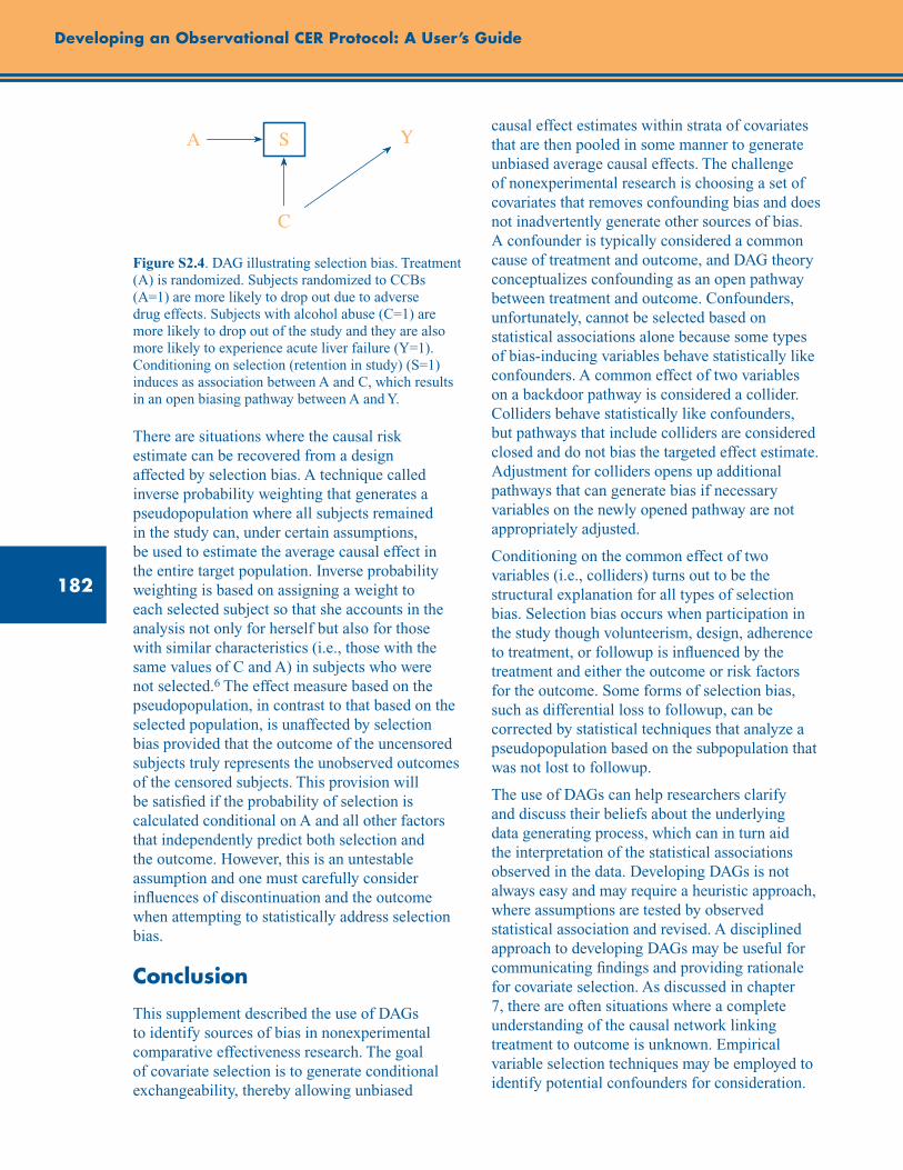
182


Figure S2.4. DAG illustrating selection bias. Treatment (A) is randomized. Subjects randomized to CCBs (A=1) are more likely to drop out due to adverse drug effects. Subjects with alcohol abuse (C=1) are more likely to drop out of the study and they are also more likely to experience acute liver failure (Y=1). Conditioning on selection (retention in study) (S=1) induces as association between A and C, which results in an open biasing pathway between A and Y.

There are situations where the causal risk estimate can be recovered from a design affected by selection bias. A technique called inverse probability weighting that generates a pseudopopulation where all subjects remained in the study can, under certain assumptions, be used to estimate the average causal effect in the entire target population. Inverse probability weighting is based on assigning a weight to each selected subject so that she accounts in the analysis not only for herself but also for those with similar characteristics (i.e., those with the same values of C and A) in subjects who were not selected.6 The effect measure based on the pseudopopulation, in contrast to that based on the selected population, is unaffected by selection bias provided that the outcome of the uncensored subjects truly represents the unobserved outcomes of the censored subjects. This provision will be satisfied if the probability of selection is calculated conditional on A and all other factors that independently predict both selection and the outcome. However, this is an untestable assumption and one must carefully consider influences of discontinuation and the outcome when attempting to statistically address selection bias.

Conclusion

This supplement described the use of DAGs to identify sources of bias in nonexperimental comparative effectiveness research. The goal of covariate selection is to generate conditional exchangeability, thereby allowing unbiased

causal effect estimates within strata of covariates that are then pooled in some manner to generate unbiased average causal effects. The challenge of nonexperimental research is choosing a set of covariates that removes confounding bias and does not inadvertently generate other sources of bias. A confounder is typically considered a common cause of treatment and outcome, and DAG theory conceptualizes confounding as an open pathway between treatment and outcome. Confounders, unfortunately, cannot be selected based on statistical associations alone because some types of bias-inducing variables behave statistically like confounders. A common effect of two variables on a backdoor pathway is considered a collider. Colliders behave statistically like confounders, but pathways that include colliders are considered closed and do not bias the targeted effect estimate. Adjustment for colliders opens up additional pathways that can generate bias if necessary variables on the newly opened pathway are not appropriately adjusted.

Conditioning on the common effect of two variables (i.e., colliders) turns out to be the structural explanation for all types of selection bias. Selection bias occurs when participation in the study though volunteerism, design, adherence to treatment, or followup is influenced by the treatment and either the outcome or risk factors for the outcome. Some forms of selection bias, such as differential loss to followup, can be corrected by statistical techniques that analyze a pseudopopulation based on the subpopulation that was not lost to followup.

The use of DAGs can help researchers clarify and discuss their beliefs about the underlying data generating process, which can in turn aid the interpretation of the statistical associations observed in the data. Developing DAGs is not always easy and may require a heuristic approach, where assumptions are tested by observed statistical association and revised. A disciplined approach to developing DAGs may be useful for communicating findings and providing rationale for covariate selection. As discussed in chapter 7, there are often situations where a complete understanding of the causal network linking treatment to outcome is unknown. Empirical variable selection techniques may be employed to identify potential confounders for consideration.

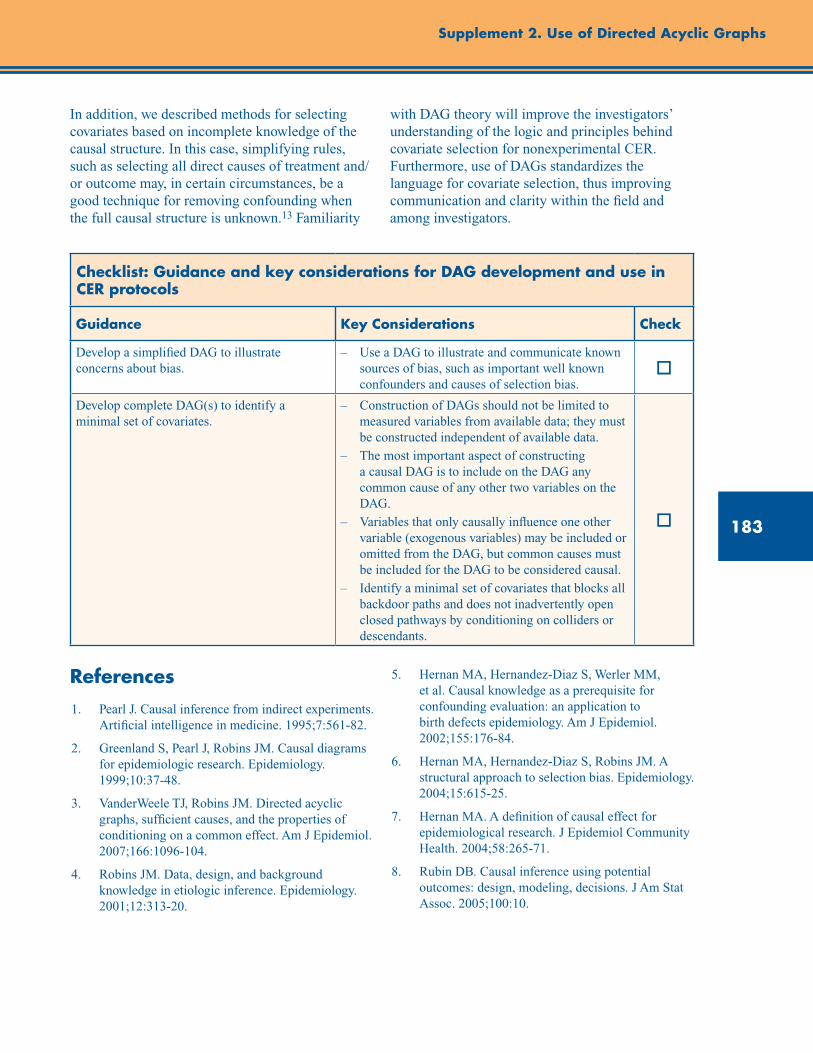
183


In addition, we described methods for selecting covariates based on incomplete knowledge of the causal structure. In this case, simplifying rules, such as selecting all direct causes of treatment and/or outcome may, in certain circumstances, be a good technique for removing confounding when the full causal structure is unknown.13 Familiarity

with DAG theory will improve the investigators’ understanding of the logic and principles behind covariate selection for nonexperimental CER. Furthermore, use of DAGs standardizes the language for covariate selection, thus improving communication and clarity within the field and among investigators.

Checklist: Guidance and key considerations for DAG development and use in CER protocols


Develop a simplified DAG to illustrate concerns about bias.

– Use a DAG to illustrate and communicate known sources of bias, such as important well known confounders and causes of selection bias.

o

Develop complete DAG(s) to identify a minimal set of covariates.

– Construction of DAGs should not be limited to measured variables from available data; they must be constructed independent of available data.

– The most important aspect of constructing a causal DAG is to include on the DAG any common cause of any other two variables on the DAG.

– Variables that only causally influence one other variable (exogenous variables) may be included or omitted from the DAG, but common causes must be included for the DAG to be considered causal.

– Identify a minimal set of covariates that blocks all backdoor paths and does not inadvertently open closed pathways by conditioning on colliders or descendants.

o

References1. Pearl J. Causal inference from indirect experiments.

Artificial intelligence in medicine. 1995;7:561-82.

2. Greenland S, Pearl J, Robins JM. Causal diagrams for epidemiologic research. Epidemiology. 1999;10:37-48.

3. VanderWeele TJ, Robins JM. Directed acyclic graphs, sufficient causes, and the properties of conditioning on a common effect. Am J Epidemiol. 2007;166:1096-104.

4. Robins JM. Data, design, and background knowledge in etiologic inference. Epidemiology. 2001;12:313-20.

5. Hernan MA, Hernandez-Diaz S, Werler MM, et al. Causal knowledge as a prerequisite for confounding evaluation: an application to birth defects epidemiology. Am J Epidemiol. 2002;155:176-84.

6. Hernan MA, Hernandez-Diaz S, Robins JM. A structural approach to selection bias. Epidemiology. 2004;15:615-25.

7. Hernan MA. A definition of causal effect for epidemiological research. J Epidemiol Community Health. 2004;58:265-71.

8. Rubin DB. Causal inference using potential outcomes: design, modeling, decisions. J Am Stat Assoc. 2005;100:10.

184

9. Greenland S, Robins JM. Identifiability, exchangeability, and epidemiological confounding. Int J Epidemiol. 1986;15:413-9.

10. Hernan MA, Robins JM. Estimating causal effects from epidemiological data. J Epidemiol Community Health. 2006;60:578-86.

11. Pearl J. Section 1.5: Causal Versus Statistical Terminology. In: Causality: Models, Reasoning and Inference. New York: Cambridge University Press; 2000.

12. Glymour MM, Weuve J, Berkman LF, et al. When is baseline adjustment useful in analyses of change? An example with education and cognitive change. Am J Epidemiol. 2005;162:267-78.

13. VanderWeele TJ, Shpitser I. A new criterion for confounder selection. Biometrics. 2011;67: 1406-13.


185

Authors


Scott R. Smith, Ph.D. Program Director Center for Outcomes and Evidence Agency for Healthcare Research and Quality Baltimore, MD


Til Stürmer, M.D., M.P.H., Ph.D. Professor, Department of Epidemiology University of North Carolina at Chapel Hill Gillings School of Global Public Health Chapel Hill, NC

M. Alan Brookhart, Ph.D. Associate Professor, Department of Epidemiology University of North Carolina at Chapel Hill Gillings School of Global Public Health Chapel Hill, NC


Ravi Varadhan, Ph.D. Assistant Professor Brookdale Leadership in Aging Fellow Division of Geriatric Medicine and Gerontology and the Center on Aging and Health Johns Hopkins University School of Medicine Baltimore, MD

John D. Seeger, Pharm.D., Dr.P.H. Assistant Professor of Medicine Harvard Medical School Pharmacoepidemiologist Division of Pharmacoepidemiology and Pharmacoeconomics Department of Medicine Brigham and Women’s Hospital Boston, MA


Todd A. Lee, Pharm.D., Ph.D. Assistant Director Center for Pharmacoeconomic Research Associate Professor Departments of Pharmacy Practice and Pharmacy Administration College of Pharmacy University of Illinois at Chicago Chicago, IL

A. Simon Pickard, Ph.D. Assistant Director Center for Pharmacoeconomic Research Associate Professor Departments of Pharmacy Practice and Pharmacy Administration College of Pharmacy University of Illinois at Chicago Chicago, IL


Soko Setoguchi, M.D., Dr.P.H. Associate Professor of Medicine Duke Clinical Research Institute Duke University School of Medicine Durham, NC

Tobias Gerhard, Ph.D. Assistant Professor Ernest Mario School of Pharmacy and Institute for Health, Health Care Policy, and Aging Research Rutgers University New Brunswick, NJ


*Priscilla Velentgas, Ph.D. Director of Epidemiology Quintiles Outcome Cambridge, MA

* Indicates lead author

186


Nancy A. Dreyer, M.P.H., Ph.D. Chief of Scientific Affairs Quintiles Outcome Cambridge, MA

Albert W. Wu, M.D., M.P.H. Professor and Director Center for Health Services and Outcomes Research Johns Hopkins Bloomberg School of Public Health Baltimore, MD


*Brian Sauer, Ph.D. Assistant Professor Division of Epidemiology Department of Internal Medicine University of Utah School of Medicine Salt Lake City, UT

M. Alan Brookhart, Ph.D. Associate Professor Department of Epidemiology University of North Carolina at Chapel Hill Gillings School of Global Public Health Chapel Hill, NC

Jason A. Roy, Ph.D. Assistant Professor Center for Clinical Epidemiology and Biostatistics University of Pennsylvania Philadelphia, PA

Tyler J. VanderWeele, Ph.D. Associate Professor Departments of Epidemiology and Biostatistics Harvard School of Public Health Boston, MA


Cynthia Kornegay, Ph.D. Epidemiologist Office of Surveillance & Evaluation Office of Pharmacovigilance & Epidemiology Center for Drug Evaluation and Research U.S. Food and Drug Administration Silver Spring, MD

Jodi B. Segal, M.D., M.P.H. Associate Professor of Medicine Johns Hopkins University Baltimore, MD


*Eric S. Johnson, Ph.D., M.P.H. Investigator, The Center for Health Research Kaiser Permanente Northwest Portland, OR

M. Alan Brookhart, Ph.D. Associate Professor Department of Epidemiology University of North Carolina at Chapel Hill Gillings School of Global Public Health Chapel Hill, NC

Jessica A. Myers, Ph.D. Instructor of Medicine Harvard Medical School Biostatistician Division of Pharmacoepidemiology and Pharmacoeconomics Department of Medicine Brigham and Women’s Hospital Boston, MA


*Patrick G. Arbogast, Ph.D. (deceased) Senior Investigator (Biostatistician) The Center for Health Research Kaiser Permanente Northwest Portland, OR



Joseph A. C. Delaney, Ph.D. Research Assistant Professor of Epidemiology University of Washington Seattle, WA


187

Authors, Reviewers, and Suggested Citations

John D. Seeger, PharmD, Dr.P.H. Assistant Professor of Medicine Harvard Medical School Pharmacoepidemiologist Division of Pharmacoepidemiology and Pharmacoeconomics Department of Medicine Brigham and Women’s Hospital Boston, MA


*John M. Brooks, Ph.D. Professor Program in Pharmaceutical Socioeconomics University of Iowa College of Pharmacy Iowa City, IA


*Brian Sauer, Ph.D. Assistant Professor Division of Epidemiology, Department of Internal Medicine University of Utah School of Medicine Salt Lake City, UT



189

Reviewers

Jesse Berlin, Sc.D. Vice President Pharmacoepidemiology Johnson & Johnson Pharmaceutical Research and Development Philadelphia, PA

Brian Bradbury, M.A., D.Sc. Adjunct Assistant Professor in Epidemiology School of Public Health University of California, Los Angeles Los Angeles, CA

Elizabeth Chrischilles, M.S., Ph.D. Professor and Chair in Public Health Department of Epidemiology Director Health Effectiveness Research Center University of Iowa Iowa City, IA

Lesley Curtis, Ph.D. Associate Professor Duke University School of Medicine Durham, NC

Dean Follman, M.S., Ph.D. Assistant Director Biostatistics Chief of Biostatistics Research Branch National Institute of Allergy and Infectious Diseases National Institutes of Health Bethesda, MD

David Graham, M.D., M.P.H. Associate Director Office of Drug Safety U.S. Food and Drug Administration Silver Spring, MD

Marie R. Griffin, M.D., M.P.H. Professor of Medicine Vanderbilt University School of Medicine Nashville, TN

Miguel Hernan, M.D., Dr.P.H. Professor of Epidemiology Harvard School of Public Health Boston, MA

Adrian V. Hernandez, M.D., Ph.D. Cardiovascular Epidemiologist Chair Cardiovascular Meta-analyses Research Group Cleveland, OH

Lisa Herrinton, Ph.D. Senior Research Scientist Kaiser Permanente Division of Research Oakland, CA

Eric S. Johnson, Ph.D., M.P.H. Investigator, The Center for Health Research Kaiser Permanente Northwest Portland, OR

Stephen S. Lane, M.D. Adjunct Professor Ophthalmology Department University of Minnesota Minneapolis, MN

Bradley C. Martin, Pharm.D., Ph.D. Professor Division Head of Pharmaceutical Evaluation and Policy Department of Pharmacy Practice University of Arkansas for Medical Sciences Little Rock, AR

Sharon-Lise Normand, Ph.D. Professor of Health Care Policy (Biostatistics) Department of Health Care Policy Harvard Medical School Department of Biostatistics Harvard School of Public Health Boston, MA

Jeremy A. Rassen, Sc.D. Assistant Professor of Medicine Harvard Medical School Director of Computational Pharmacoepidemiology Division of Pharmacoepidemiology and Pharmacoeconomics Brigham and Women’s Hospital Boston, MA

190

Robert Reynolds, Sc.D. Senior Director, Global Head Epidemiology Safety and Risk Management Pfizer, Inc. New York, NY

Mary Beth Ritchey, M.S.P.H., Ph.D. Epidemiologist U.S. Food and Drug Administration Silver Spring, MD

Michael Rothberg, M.D., M.P.H. Associate Professor of Medicine Sackler School of Graduate Biomedical Sciences Tufts University Boston, MA

Kenneth G. Saag, M.D. Professor of Medicine and Epidemiology Director, Center for Education and Research on Therapeutics (CERTs) of Musculoskeletal Disorders University of Alabama Birmingham, AL

Glen T. Schumock, Pharm.D., M.B.A. Professor of Pharmacy Practice and Pharmacy Administration University of Illinois Chicago, IL

Beth Virnig, Ph.D. Professor and Director Public Health Administration and Policy Program School of Public Health University of Minnesota Minneapolis, MN

Alexander Walker, Dr.P.H. Adjunct Professor of Epidemiology Department of Epidemiology Harvard School of Public Health Boston, MA

Noel S. Weiss, M.D., Dr.P.H. Professor of Epidemiology School of Public Health University of Washington Seattle, WA

Marianne Ulcickas Yood, D.Sc., M.P.H. Principal Epidemiologist EpiSource Associate Research Scientist Epidemiology and Public Health Yale University School of Medicine New Haven, CT


191

Suggested Citations

Please cite this User’s Guide as follows:

Velentgas P, Dreyer NA, Nourjah P, Smith SR, Torchia MM, eds. Developing a Protocol for Observational Comparative Effectiveness Research: A User’s Guide. AHRQ Publication No. 12(13)-EHC099. Rockville, MD: Agency for Healthcare Research and Quality; January 2013.

Please cite individual chapters as follows:

Introduction:

Smith SR. Introduction to Developing a Protocol for Observational Comparative Effectiveness Research: A User’s Guide. In: Velentgas P, Dreyer NA, Nourjah P, et al., eds. Developing a Protocol for Observational Comparative Effectiveness Research: A User’s Guide. AHRQ Publication No. 12(13)-EHC099. Rockville, MD: Agency for Healthcare Research and Quality; January 2013: Introduction, pp. 1-6.

Chapter 1:

Smith SR. Study objectives and questions. In: Velentgas P, Dreyer NA, Nourjah P, Smith SR, Torchia MM., eds. Developing a Protocol for Observational Comparative Effectiveness Research: A User’s Guide. AHRQ Publication No. 12(13)-EHC099. Rockville, MD: Agency for Healthcare Research and Quality; January 2013: Chapter 1, pp. 7-20.

Chapter 2:

Stürmer T, Brookhart A. Study design considerations. In: Velentgas P, Dreyer NA, Nourjah P, et al., eds. Developing a Protocol for Observational Comparative Effectiveness Research: A User’s Guide. AHRQ Publication No. 12(13)-EHC099. Rockville, MD: Agency for Healthcare Research and Quality; January 2013: Chapter 2, pp. 21-34.

Chapter 3:

Varadhan R, Seeger J. Estimation and reporting of heterogeneity of treatment effects. In: Velentgas P, Dreyer NA, Nourjah P, et al., eds. Developing a Protocol for Observational Comparative Effectiveness Research: A User’s Guide. AHRQ Publication No. 12(13)-EHC099. Rockville, MD: Agency for Healthcare Research and Quality; January 2013: Chapter 3, pp. 35-44.

Chapter 4:

Lee TA, Pickard AS. Exposure definition and measurement. In: Velentgas P, Dreyer NA, Nourjah P, et al., eds. Developing a Protocol for Observational Comparative Effectiveness Research: A User’s Guide. AHRQ Publication No. 12(13)-EHC099. Rockville, MD: Agency for Healthcare Research and Quality; January 2013: Chapter 4, pp. 45-58.

Chapter 5:

Setoguchi S, Gerhard T. Comparator selection. In: Velentgas P, Dreyer NA, Nourjah P, et al., eds. Developing a Protocol for Observational Comparative Effectiveness Research: A User’s Guide. AHRQ Publication No. 12(13)-EHC099. Rockville, MD: Agency for Healthcare Research and Quality; January 2013: Chapter 5, pp. 59-70.

Chapter 6:

Velentgas P, Dreyer NA, Wu AW. Outcome definition and measurement. In: Velentgas P, Dreyer NA, Nourjah P, et al., eds. Developing a Protocol for Observational Comparative Effectiveness Research: A User’s Guide. AHRQ Publication No. 12(13)-EHC099. Rockville, MD: Agency for Healthcare Research and Quality; January 2013: Chapter 6, pp. 71-92.

192

Chapter 7:

Sauer B, Brookhart MA, Roy JA, et al. Covariate selection. In: Velentgas P, Dreyer NA, Nourjah P, et al., eds. Developing a Protocol for Observational Comparative Effectiveness Research: A User’s Guide. AHRQ Publication No. 12(13)-EHC099. Rockville, MD: Agency for Healthcare Research and Quality; January 2013: Chapter 7, pp. 93-108.

Chapter 8:

Kornegay C, Segal JB. Selection of data sources. In: Velentgas P, Dreyer NA, Nourjah P, et al., eds. Developing a Protocol for Observational Comparative Effectiveness Research: A User’s Guide. AHRQ Publication No. 12(13)-EHC099. Rockville, MD: Agency for Healthcare Research and Quality; January 2013: Chapter 8, pp. 109-28.

Chapter 9:

Johnson ES, Brookhart MA, Myers JA. Study size planning. In: Velentgas P, Dreyer NA, Nourjah P, et al., eds. Developing a Protocol for Observational Comparative Effectiveness Research: A User’s Guide. AHRQ Publication No. 12(13)-EHC099. Rockville, MD: Agency for Healthcare Research and Quality; January 2013: Chapter 9, pp. 129-34.

Chapter 10:

Arbogast PG, VanderWeele TJ. Considerations for statistical analysis. In: Velentgas P, Dreyer NA, Nourjah P, et al., eds. Developing a Protocol for Observational Comparative Effectiveness Research: A User’s Guide. AHRQ Publication No. 12(13)-EHC099. Rockville, MD: Agency for Healthcare Research and Quality; January 2013: Chapter 10, pp. 135-44.

Chapter 11:

Delaney JAC, Seeger J. Sensitivity analysis. In: Velentgas P, Dreyer NA, Nourjah P, et al., eds. Developing a Protocol for Observational Comparative Effectiveness Research: A User’s Guide. AHRQ Publication No. 12(13)-EHC099. Rockville, MD: Agency for Healthcare Research and Quality; January 2013: Chapter 11, pp. 145-60.

Supplement 1:

Brooks J. Improving characterization of study populations: the identification problem. In: Velentgas P, Dreyer NA, Nourjah P, et al., eds. Developing a Protocol for Observational Comparative Effectiveness Research: A User’s Guide. AHRQ Publication No. 12(13)-EHC099. Rockville, MD: Agency for Healthcare Research and Quality; January 2013: Supplement 1, pp. 161-76.

Supplement 2:

Sauer B, VanderWeele TJ. Use of Directed Acyclic Graphs. In: Velentgas P, Dreyer NA, Nourjah P, et al., eds. Developing a Protocol for Observational Comparative Effectiveness Research: A User’s Guide. AHRQ Publication No. 12(13)-EHC099. Rockville, MD: Agency for Healthcare Research and Quality; January 2013: Supplement 2, pp. 177-84.

The following Web site should be added to each chapter citation: www.effectivehealthcare.ahrq.gov/Methods-OCER.cfm


U.S. Department of Health and Human Services

Agency for Healthcare Research and Quality 540 Gaither Road Rockville, MD 20850

AHRQ Pub. No. 12(13)-EHC099 January 2013

ISBN: 978-1-58763-420-8

Developing a Protocol for Observational Comparative ...

Documents