Developing a Poverty Map for Indonesia - World Banksiteresources.worldbank.org/ASEM/Resources/Poverty+Map+Indonesia+I.pdf · Developing a Poverty Map for Indonesia: An Initiatory

DRAFT

Developing a Poverty Map for Indonesia:An Initiatory Work in Three Provinces

Asep Suryahadi, Wenefrida WidyantiDaniel Perwira, Sudarno Sumarto

The SMERU Research Institute

Chris ElbersVrije Universiteit, Amsterdam

Menno PradhanThe World Bank

The SMERU Research InstituteJakarta

January 2003

DRAFT

The SMERU Research Institute, January 2003i

Table of Contents

Abstract ii

I. Introduction 1

II. The Method 4A. The Consumption Model 4B. The Estimators 5

III. Data Sources 7

IV. Model Application 9A. Stage 1: Matching Variables in the Survey and the Census 9B. Stage 2: Selecting Explanatory Variables for the Consumption Model 9C. Stage 3: Estimating the Consumption Model 11D. Stage 4: Simulations on Census Data 13E. Stage 5: Calculation of Poverty and Inequality Indicators 15

V. Poverty and Inequality Maps 17A. Poverty Estimates and Their Standard Errors 17B. District, Subdistrict, and Village Poverty Maps 19C. Examples for Further Applications 25

VI. Concluding Remarks 29

Appendix 30

References 69

DRAFT

The SMERU Research Institute, January 2003ii

Developing a Poverty Map for Indonesia:An Initiatory Work in Three Provinces

Asep Suryahadi, Wenefrida WidyantiDaniel Perwira, Sudarno Sumarto

The SMERU Research Institute

Chris ElbersFree University, Amsterdam

Menno PradhanThe World Bank

Abstract

This report presents the results of applying a recently developed technique forobtaining high-resolution poverty maps to the provinces of East Kalimantan,Jakarta, and East Java in Indonesia. The purpose of this exercise is to try out theapplicability of the poverty mapping method given the available data in Indonesia.The report is consisted of two parts. Part I is a technical report describing the stepsthat have been taken in the exercise. Part II presents the results of the exercise ofpoverty and inequality point estimates and standard errors. The results appear tosupport the extension of the method application to the rest of the country.

DRAFT

1 The SMERU Research Institute, January 2003

I. Introduction

Experience shows that locating the poor is one of the most crucial and difficultproblems in the implementation of programs aimed at targeting the poor. InIndonesia, a country which is very large in size and where poverty statistics arereliable only up to the provincial-urban/rural level, geographic targeting of thepoor is even more difficult. As poverty reduction efforts will continue to be animportant endeavor in Indonesia even long into the future, there is clearly aneed to develop tools for more effective geographic targeting than those thathave been used in the past.

Ideally, geographic targeting would be based on a description of poverty incidenceand other indicators of economic welfare at small areas or low administrative levels.More generally, the analysis of poverty and welfare in a country could benefittremendously from detailed and disaggregated data on the distribution of economicwelfare. In the context of Indonesia administrative levels go from the national levelall the way down to the ‘village’ level (desa/kelurahan).1

One could of course obtain village level information on the distribution of economicwelfare by carrying out a household survey with a sample which is representative forall villages in Indonesia. However, with almost 70,000 of total number of villages inIndonesia, such a household survey is prohibitively huge and expensive. Forcomparison, the current poverty statistics in Indonesia are based on the consumptionmodule of the National Socio-Economic Survey (SUSENAS), which has a samplesize of around 65,000 households.

Fortunately, as a result of recent methodological advances in this area, a newmethodology has been developed to estimate such description from statistical datacollections that are normally available in a country. The core of the method is tocombine the information obtained from a household survey with the informationcollected through a population census. A household survey usually collects verydetailed information on household characteristics, including consumption level, butthe coverage is generally limited and only representative at a relatively largegeographical unit. On the other hand, a population census has a complete coverageof all households, but usually collects very limited information on householdcharacteristics. Hence, the method tries to combine the advantage of detailedinformation on household characteristics obtained from a household survey with thecomplete coverage of a population census.

1 The hierarchy of government administrative units in Indonesia below the central government areprovinces (propinsi), districts (kabupaten) or cities (kota), sub-districts (kecamatan), and villages. Avillage which is located in a rural area is called a desa, while a village which is located in an urbanarea is called a kelurahan.

DRAFT

The SMERU Research Institute, January 20032

Essentially, the method imputes estimates of per capita consumption for eachhousehold in the population by applying observed correlation patterns betweenhousehold characteristics and household per capita consumption to census data onhousehold characteristics. The correlation patterns are estimated on the basis ofhousehold survey data.

This study is a pilot and the first attempt to apply the method in Indonesia. Theobjective is to obtain estimates of poverty incidence at geographical units smallerthan a province-urban/rural area, which is the lowest level of aggregation for whichreliable (but still very imprecise) poverty statistics are currently available. Theproject has two stages. The first stage is a pilot study to test the feasibility of themethod in the context of Indonesia. It uses data from only three provinces: EastKalimantan, Jakarta, and East Java. The results of this pilot study are summarized inthis report. The pilot study has been carried out by SMERU Research Institute. Thenext scale will entail a larger-scale application to Indonesia’s remaining provincesand will be carried out by Statistics Indonesia (BPS), building on the experiencegained during the pilot phase.

The rests of the report is organized as follows. Chapter two discusses in brief themethod used to obtain these estimates. Chapter three discusses the sources of datautilized in this exercise. Chapter four discusses the model application and theprocedures for implementing it. Chapter five presents the results of the exercise inthe forms of poverty and inequality maps from the province level down to the villagelevel. Finally, chapter six provides the concluding remarks. In addition, Part II ofthis report also provides the poverty mapping results in the forms of tables.

DRAFT


II. The Method

The method used in this study basically involves a two-step procedure. First, a modelof consumption determination is estimated using the data from household survey. Inthe second step, the parameters estimated in the first step are then transferred to thedata from the population census to simulate the consumption level of each and everyhousehold enumerated in the population census. The simulated householdconsumption is then used as the basis for calculating poverty and other welfareindicators.

A. The Consumption Model

Following Elbers et al. (2001, 2002), the empirical model of household consumptionis defined as:

vhvhhvh uxyEy += )|(ln ν (1)

where vhyln is the logarithm of per capita consumption of household h in village v,

vhx is a vector of observed characteristics of this household (including village level

variables), and vhu is the error term. Note that vhu is uncorrelated with vhx . Thismodel is simplified by using a linear approximation to the conditional expectation

)|( vhh xyE ν and decomposing vhu into uncorrelated terms:

vhvvhu εη += (2)

where of vη represents a village level error term common to all households within

the village, and vhε is a household specific error terms. It is further assumed that the

vη are uncorrelated across villages and the vhε are uncorrelated across households.

With these assumptions, equation (1) reduces to

.ln vhvvhvh xy εηβ ++= (3)

Estimation of the parameters underlying this equation, in particular the vector ofparameters β and the distributional characteristics of the error terms, can be doneby using standard tools from econometric analysis (see Elbers et al., 2002).

B. The Estimators

The consumption model specification in equation (3) allows for an intra-villagecorrelation in the error terms. Household income or consumption is certainlyaffected by the location where the household lives. Even though vhx has somevariables representing village level characteristics, it is quite plausible that some ofthe location effects will remain unexplained. The consequence of failing to take intoaccount this within-village correlation of the error terms can result in biased welfare

DRAFT


estimates (in particular for inequality indicators) and will generally lead tounderestimation of the standard errors of welfare estimates.

Take village averages over equation (2):

•• += vvvu εη (4)

where a subscript “ • ” indicates an average over the index. Since the two errorcomponents are uncorrelated, then:

[ ] ( ) ( ) 222 varvarE ••• +=+= vvvu τσεη η (5)

An unbiased estimator for 2ησ can be defined as:

( )( )

( )∑∑

∑∑

−−

−−

=

∧

•∧

j jj

vvvv

j jj

v vv

ww

ww

ww

uw

1

1

1

222 τ

σ η (6)

where:

( ) ( )∑ •

∧−

−=

hvvh

vv

vnn

22

1

1 εετ (7)

and w is a set of non-negative weights summing to one.

Elbers et al. (2001, 2002) give the following formula for the sampling variance of2ˆησ :

( )∑

+≈

∧

•

∧

v

vvvv bua2

2222

varvarvar τσ η

,1

22

22

2222222

2∑

−

+

+

+

≈

∧

∧∧∧∧

v v

v

vvvv nba

ττστσ ηη (10)

where ∑ −

=j jj

vv ww

wa

)1( and

∑ −−

=j jj

vvv ww

wwb

)1(

)1(.

DRAFT


III. Data Sources

Four sources of data are used in this study: (i) Consumption Module SUSENAS1999, (ii) Core SUSENAS 1999, (iii) Population Census 2000, and (iv) PODES(Village Potential) 1999. In the consumption model estimation, the data onhousehold consumption is obtained from the Consumption Module SUSENAS, thedata on household characteristics is obtained from the Core SUSENAS, and thedata on village-level characteristics is obtained from the PODES and village meansof the population census.

SUSENAS, the National Socio-Economic Survey, is a nationally representativehousehold survey, covering all areas of the country. A part of the SUSENAS isconducted every year in the month of February, collecting information on thecharacteristics of over 200,000 households and over 800,000 individuals. This part ofthe SUSENAS is known as the ‘Core’ SUSENAS. Another part of the SUSENASis conducted every three years, specifically collecting information on very detailedconsumption expenditure from around 65,000 households. These households are arandomly selected subset of the 200,000 households in the Core SUSENAS sampleof the same year. This consumption module part of the SUSENAS is popularlyknown as the ‘Module’ SUSENAS.

Population census 2000 is the fifth population census conducted in Indonesia afterindependence. The previous censuses were conducted in 1961, 1971, 1980, and1990. The 2000 population census was conducted in the month of June, covering allpopulation living in the territory of Indonesia and including foreigners. Data on 15demographic, social, and economic variables at both individual and household levelswere collected in the census.

PODES, meanwhile, is a complete enumeration of villages throughout Indonesia.The information collected through this survey only includes village characteristicssuch as size of area, population, infrastructure, and local industries characteristics.The questionnaires are filled out by the local sub-district officials who areresponsible for collecting statistical data (mantri statistik). The information isobtained from official village documents as well as interviews with village officials.The PODES survey is usually conducted three times in every ten years, usually priorto and as a preparation for an agricultural census, an economic census, or apopulation census. A PODES survey was conducted in the months of September andOctober 1999 as a preparation for the population census in 2000. In total, the 1999PODES enumerates 68,783 villages.2

2 Officially it is called PODES 2000.

DRAFT


IV. Model Application

This chapter outlines the stages and procedures implemented in applying the modelto obtain poverty maps for three provinces: East Kalimantan, Jakarta, and East Java.For each province, the estimations for urban and rural areas are implementedseparately, except for Jakarta which is a wholly urban area. The poverty line for eachregion is taken from Pradhan et al. (2001).

A. Stage 1: Matching Variables in the Survey and the Census

In order to obtain rigorous estimates of consumption levels of the households in thecensus, the explanatory variables selected in the consumption determination modelhave to exist and are measured in the same way in both the household survey and inthe census. If the sample of the household survey was randomly selected andnationally representative, the distribution of each explanatory variable in thehousehold survey can be expected to be the same as its distribution in the census.

The means and standard deviations of the matched variables in SUSENAS andPopulation Census data are shown in the Appendix: Table A1 for urban EastKalimantan, Table A2 for rural East Kalimantan, Table A3 for Jakarta, Table A4 forurban East Java, and Table A5 for rural East Java.

B. Stage 2: Selecting Explanatory Variables for the Consumption Model

The procedure in selecting the explanatory variables of equation (3) starts byrunning a regression of log consumption on the matched variables identified inStage 1, plus some variables that can be created from those variables such as thesquare and cube of household size or the square and cube of age of household head.3

In order to obtain a robust specification, variables are only selected for inclusion inequation (3) if they contribute significantly to the explanation of (log) per capitaconsumption. Hence variables with low t-values are dropped.

After a promising set of variables has been selected in this way, the regression is runagain and the residuals of this regression are saved. These residuals need to bescrutinized to check if there are some outliers in the observation. If indeed there aresome residual values which are far out of the range of most residual values, thenthese observations must be checked for coding or other errors. Ultimately it may benecessary to delete them from the data. Fortunately, this is extremely rare.

3 Experience with poverty mapping in other countries suggests that these regressions should beweighted using cluster expansion factors. In the case of SUSENAS, cluster expansion factors withinurban or rural areas in a province are all equal. Since the estimations are implemented at this level,the issue of weighting does not arise.

DRAFT


The next step is to select village-level independent variables to complete theconsumption model specification. The village level variables are obtained fromeither the census data aggregated at the village level (for example the totalnumber of individuals in the population or means of age of household heads ineach village) or from the PODES data. These variables are then grouped intoseveral sets such as demographic variables, village infrastructure variables, andvillage economic variables.

The residuals of the last regression are then aggregated at the village level tocalculate the mean of these residuals for each village. The variable selection is thendone by running separate regressions of the village-level mean of residuals on eachset of the village-level variables. The variables with significant t-values are selectedas the candidates for inclusion in the consumption model.

The feasibility of including these candidate village-level variables in theconsumption model is tested by running regressions of village dummy variable onthese variables. One regression is run for each candidate independent variable. If thecoefficient of a certain variable in a regression is one, it shows that there is a perfectmulticollinearity between this variable and the village dummy variable. This willhappen if, for example, a village has a certain infrastructure while no other villageshave, or on the other hand, all villages except one have a certain infrastructure.Such variables are necessarily excluded from the model. This test may explain whyfor example electricity is included in the model for rural areas but excluded from themodel for urban areas.

C. Stage 3: Estimating the Consumption Model

The result of stage 2 is a complete specification of the consumption model,incorporating both household-level and village-level independent variables of themodel. The next step is to test whether there is heteroskedascity in the data. Thiswill determine the method to be employed to estimate the model. The first step todo this is to estimate the model of equation (3) using Ordinary Least Squares (OLS)

and save the residuals as a variable huν∧

.

Based on equation (2) the residuals huν∧

are then decomposed into uncorrelatedcomponents as

vhvvvhvh euuuu +=

−+=

∧•

∧∧•

∧ηνˆ (11)

To investigate the presence of heteroskedasticity in the data, a set of potentialvariables that best explain the variations in 2

heν are used to estimate the followinglogistic model:

vhTvh

vh

vh rzeA

e+=

−

∧α

2

2

ln (12)

DRAFT


where we take A equal to { }2max*05.1 vhe as in Elbers et al., (2002). This

specification puts bounds on the predicted variance of 2hνε .

The results of the OLS and heteroscedasticity regressions are shown in theAppendix: Table B1 for urban East Kalimantan, Table B2 for rural East Kalimantan,Table B3 for Jakarta, Table B4 for urban East Java, and Table B5 for rural East Java.In the case where homoskedasticity is rejected, a household specific varianceestimator for vhε is calculated as:

( )( )

+

−+

+=

∧∧

3

2

,

1

)1(Var

2

1

1 B

BABr

B

ABvhεσ (13)

where

=

∧αT

vhzB exp . The consumption model is then re-estimated using

Generalized Least Squares (GLS) method, utilizing the estimated variance-

covariance matrix, ∧Σ , resulting from equation (13) and weighted by the population

weight, vhl . The estimated parameters, GLS

∧β , and their variance,

∧

GLSβVar , are

saved for use in the simulation. The results of these GLS regressions are shown inthe Appendix: Table C1 for urban East Kalimantan, Table C2 for rural EastKalimantan, Table C3 for Jakarta, Table C4 for urban East Java, and Table C5 forrural East Java.

D. Stage 4: Simulations on Census Data

The purpose of this procedure is to apply the parameters estimated in the previousprocedure to the census data. However, since the values of these parameters areobtained through estimations, they are not the precise values of these parametersand subject to sampling error. This needs to be taken into account in applying theparameters to the census data by taking into account the sampling error of thecoefficient estimates. To start, recall that the purpose is to calculate the simulatedversion of equation (3):

svh

sv

svh

svh xy εηβ ++=ln (14)

where the superscript s refers to simulated version of each parameter or variable andnow vhx refers to characteristics of the households in the population census data.

Simulation of β

The simulated value of β is obtained through a random draw, assuming

∧∧

GLSGLSN βββ Var,~ . Note that the draw has to take into account the

covariance across β’s. The randomly drawn parameter is defined as sβ . The next

DRAFT


step is then to apply this simulated parameter to each household in the census datato calculate the value of s

vhx β .

Simulation of vη

The process of obtaining the simulated value of vη requires two steps of simulations.

This is because the variance of η itself is estimated with error. Hence, the first step isto obtain the simulated variance of η, s2

ησ . Elbers et al. (2002) propose to draw s2ησ

from a gamma distribution: ( )

∧∧2

22 Var,~ ηηη σσσ G . Accordingly, a random draw of

the variance for the whole sample is exercised and its mean is defined as s2ησ . Then

the second step is to randomly draw svη for each village in the census data, assuming

( )svv N 2,0~ ση .

Simulation of vhε

The process of obtaining the simulated value of vhε requires the use of the results of

estimation of equation (12). Assuming

∧∧ααα Var,~ N , a random draw of α is

made and defined as sα . Like in the case of β, the draw has to take into account thecovariance across α’s. The simulated parameter is then used to simulate thehousehold specific variance estimator for vhε as defined in equation (13) for eachhousehold in the census data. Finally, the simulated value of household specificidiosyncratic shock, s

vhε , for every household in the census data is obtained by taking

a random draw, assuming ( )svhvh N 2,0~ σε .4

Collecting

Now all the three components of equation (14) have been simulated, the value ofsvhyln for all households in the census data can be calculated by summing up the

values of svhx β , s

vη , and svhε that have been obtained. The whole set of simulations

is then repeated a number (100) of times, so that in the end a database of 100simulated values of (log) per capita household expenditure of all the households inthe census data is created.

4 Elbers et al. (2002) mention alternatives for the assumption that the error component terms follownormal distributions. In separate sets of simulations we have experimented with these alternativeassumptions. In no case did this lead to significantly different results.

DRAFT


E. Stage 5: Calculation of Poverty and Inequality Indicators

The final output of stage 4, a database of 100 simulated values of householdexpenditure of all households in the census data, is used as the basis for calculatingvarious poverty and inequality measures at the provincial, district, sub-district, andvillage levels. The point estimate of each measure is the mean of the calculatedmeasure over the 100 simulation values. Meanwhile, the standard error of thisestimate is equal to the standard deviation of the calculated measure over the 100simulation values.5

A word of warning should be issued here on interpreting the results obtained fromthis exercise. Suppose a headcount poverty indicator of 0.10 is listed for a location,along with a standard error of 0.03. This should be taken to mean that if there wereto be found other locations, with similar patterns of household characteristics, and ifone had direct measurements of poverty headcount in these locations, then wewould predict that the poverty headcount in these locations are likely to fallbetween 0.07 and 0.13 (with a 70% confidence interval). In particular, we do notclaim that all these similar locations share the same headcount, nor is there a goodreason to attach too much significance to the ‘point estimate’ of 0.10.

The pair of point estimate and standard error express that, conditionally on theinformation about the location that we have, it is just as likely that its headcount isbetween 0.07 and 0.13, as that it would be ‘centered’ in the slightly narrower intervalbetween 0.095 and 0.105. This uncertainty in the poverty estimates reflects the fact thatthe parameters of the consumption model (3) cannot be estimated with infiniteprecision, and that there is no way to deduce the error terms huν from the available data.

Similarly, to conclude that the headcount in one location (A) is bigger than inanother (B), it is not sufficient to note that the point estimate for the headcountin A is higher than the one for B. Again, one has to take into account the errormargins on the point estimates. For example, suppose that the headcount in A is

Ah with a standard error of As and similarly for location B with Bh and BS ,where A’s point estimate is higher: .BA hh > Then one can only conclude withreasonable confidence (more than 70%) that A’s true headcount is higher thanB’s if .BBAA shsh +>− In other words one should account for the possibility thatthe estimated headcount for A is an overestimate, while B’s estimate is anunderestimate.

5 The application of this poverty mapping exercise from stage 3 to 5 is implemented using a softwarepackage called PovMap (Version 1.0 BETA), developed by Qinghua Zhao at the World Bank.

DRAFT


V. Poverty and Inequality Maps

Poverty analysis is often based on national level indicators that are compared overtime or across countries. The broad trends that can be identified using aggregateinformation are useful for evaluating and monitoring the overall performance of acountry. For many policy and research applications, however, the information thatcan be extracted from aggregate indicators is not sufficient, since they hidesignificant local variation in living conditions within countries. The detailedpoverty maps at small administrative areas that are the ultimate output of thisexercise provide benefits to help address this shortcoming of aggregate povertyanalysis. This chapter provides the poverty and inequality maps at variousadministrative levels as the results of this exercise.

A. Poverty Estimates and Their Standard Errors

In addition to the estimates of poverty and inequality indicators as usuallypresented, the results of this poverty mapping exercise also provide the standarderrors of these estimates as a measure of their precision. Table 1 compares theestimated headcount poverty rate for East Kalimantan, Jakarta, and East Java ascalculated directly from the SUSENAS data and those estimated from thePopulation Census data through the poverty mapping method. Note the increasein precision of the census-based estimates compared to the SUSENAS basedestimates. This is a well-known phenomenon, employed extensively in thestatistical technique of ‘small area estimation’.6

6 However, when the sample size in the SUSENAS is sufficiently large, such as in the case of EastJava, the increase in the precision of the estimates is not large.

DRAFT


Table 1. Estimates of Headcount Poverty Rate in East Kalimantan, Jakarta, andEast Java Based on Susenas and Poverty Mapping Method

Standard Error (%) Sample SizeArea

PovertyRate (%) Points Proportion Household Individual

East Kalimantan:SUSENAS 1999:- Urban 9.09 3.38 37.18 442 1,882- Rural 33.33 4.61 13.83 561 2,409- Total 21.05 3.38 15.94 1,003 4,291

Census 2000:- Urban 10.50 1.26 12.00 349,323 1,399,814- Rural 33.72 3.28 9.73 271,593 1,062,777- Total 20.52 2.35 11.45 620,916 2,462,591

Jakarta:SUSENAS 1999 2.82 0.62 21.99 2,959 12,460Census 2000 2.98 0.53 17.78 2,204,219 8,246,736

East Java:SUSENAS 1999:- Urban 19.51 1.73 8.87 3,250 12,535- Rural 40.94 1.55 3.79 5,285 19,593- Total 33.34 1.24 3.72 8,535 32,128

Census 2000:- Urban 20.32 1.33 6.55 3,703,652 13,761,133- Rural 40.07 1.29 3.22 5,655,930 20,730,848- Total 32.10 1.31 4.08 9,359,582 34,131,981

Source: Authors’ computations. The standard errors on the Susenas-based headcounts are calculatedby bootstrapping.

Table 1 shows the advantage of using the poverty mapping method to increase theprecision of poverty estimates. However, the real advantage of the method is itsability to produce poverty estimates and other welfare indicators at much smallerareas than the one presented in Table 1. A separate volume as a part of this reportprovides estimates of poverty headcount (P0), poverty gap (P1), poverty severity (P2),

DRAFT


and Gini ratio at the provincial, district, subdistrict, and village level in the threeprovinces.7

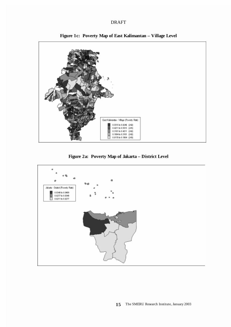
B. District, Subdistrict, and Village Poverty Maps

The first time availability of accurate welfare indicators at district, subdistrict, andvillage levels is already sensational, but the real power of mapping is by presentingthe outcomes in a geographical map, making it possible to overlay the poverty datawith all kinds of spatial characteristics.

Figure 1a shows the distribution of poverty in the province of East Kalimantan bydistrict. Figure 1b provides the same information but calculated at subdistrict level.Comparing the two figures clearly indicates that the heterogeneity of poverty withindistricts is so large, so that the information on the distribution of poverty in thisprovince conveyed by the two figures differ markedly. Figures 1c provides theinformation at even finer village level, which differs even more markedly fromFigure 1a. Figure 2a – 2c show the same maps for the province of Jakarta, whileFigure 3a – 3c for the province of East Java.

7 See Part II: Report (Tables of Poverty and Inequality Estimates).

DRAFT


Figure 1a: Poverty Map of East Kalimantan – District Level

Figure 1b: Poverty Map of East Kalimantan – Subdistrict Level

DRAFT


Figure 1c: Poverty Map of East Kalimantan – Village Level

Figure 2a: Poverty Map of Jakarta – District Level

DRAFT


Figure 2b: Poverty Map of Jakarta – Subdistrict Level

Figure 2c: Poverty Map of Jakarta – Village Level

DRAFT


Figure 3a: Poverty Map of East Java – District Level

Figure 3b: Poverty Map of East Java – Subdistrict Level

DRAFT


Figure 3c: Poverty Map of East Java – Village Level

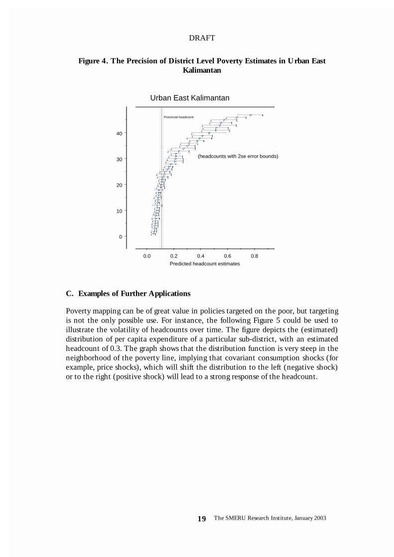
When inspecting these maps it should be kept in mind that they have been createdusing the expected headcount. The true headcount for a location will differ from theexpected headcount because of sampling and modeling error. The maps do not takeerrors into account. To show what precision can be achieved at the sub-districtlevel, Figure 4 shows the district level predicted poverty headcount in urban EastKalimantan along with brackets giving a 70 percent confidence interval from onestandard error below to one standard error above the point estimate. For reference,the provincial (urban) headcount has been included. Clearly, on the basis of thisgraph there is a large group of subdistricts for which one cannot tell with reasonableconfidence that they have below- or above-average headcounts.

DRAFT


Figure 4. The Precision of District Level Poverty Estimates in Urban EastKalimantan

0.0 0.2 0.4 0.6 0.8

Predicted headcount estimates

0

10

20

30

40

Urban East Kalimantan

(headcounts with 2se error bounds)

Provincial headcount

C. Examples of Further Applications

Poverty mapping can be of great value in policies targeted on the poor, but targetingis not the only possible use. For instance, the following Figure 5 could be used toillustrate the volatility of headcounts over time. The figure depicts the (estimated)distribution of per capita expenditure of a particular sub-district, with an estimatedheadcount of 0.3. The graph shows that the distribution function is very steep in theneighborhood of the poverty line, implying that covariant consumption shocks (forexample, price shocks), which will shift the distribution to the left (negative shock)or to the right (positive shock) will lead to a strong response of the headcount.

DRAFT


Figure 5. Cumulative Distribution Function of Consumption

0 50000 100000 150000 200000 250000 300000 350000

consumption

0.0

0.2

0.4

0.6

0.8

1.0

frac

tion

Illustrating vulnerability to shocksUrban East Kalimantan, subd=1070

Poverty line

Simulated expenditure

distribution

positive shocks

negative shocks

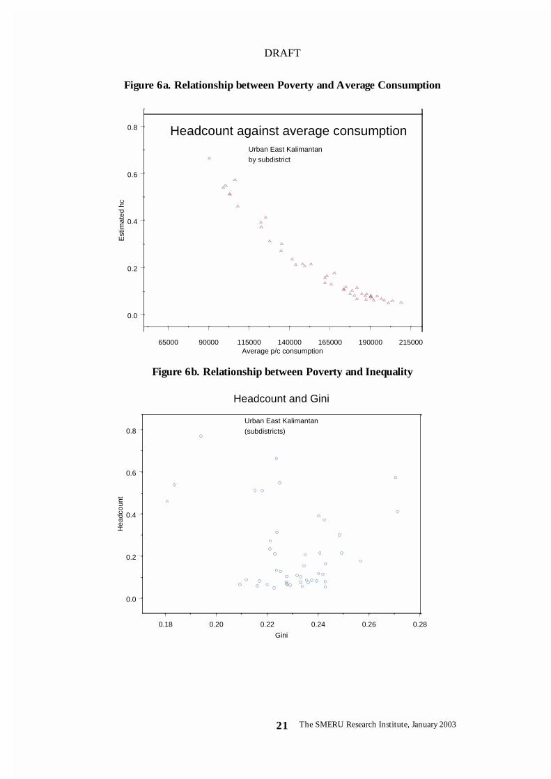
An obvious application of the newly created data on economic welfare atdisaggregated scale, is to correlate the data to other disaggregated statistics. Forinstance, a long-standing debate in development concerns the relative importance ofa ‘pro-growth’ policy and a policy aimed at reducing inequality. The following Figure6a and 6b show that in urban East Kalimantan there is a strong negative relationshipbetween average per capita consumption expenditure and the poverty headcount,while the relationship between poverty and inequality is virtually non-existent.

DRAFT


Figure 6a. Relationship between Poverty and Average Consumption

65000 90000 115000 140000 165000 190000 215000Average p/c consumption

0.0

0.2

0.4

0.6

0.8E

stim

ated

hc

Headcount against average consumptionUrban East Kalimantan

by subdistrict

Figure 6b. Relationship between Poverty and Inequality

0.18 0.20 0.22 0.24 0.26 0.28

Gini

0.0

0.2

0.4

0.6

0.8

Hea

dcou

nt

Headcount and Gini

Urban East Kalimantan

(subdistricts)

DRAFT


The Gini coefficients are generally fairly low, suggesting that the scope for povertyreduction by redistributing income is limited. Note however that such graphics,suggestive as they are, cannot substitute for careful economic research into suchimportant issues.

DRAFT


VI. Concluding Remarks

Poverty reduction efforts will continue to be an important endeavor in Indonesiaeven long into the future. Learning from past experiences in targeting difficulties,this implies that there is a need to develop tools for more effective geographictargeting than those that have been used in the past. Ideally, geographic targetingwould be based on a description of poverty incidence and other indicators ofeconomic welfare at small areas or low administrative levels.

This study is a pilot and the first attempt to apply the recently developed povertymapping method in Indonesia. The objective is to obtain estimates of povertyincidence at geographical units smaller than a province-urban/rural area, which isthe lowest level of aggregation for which reliable (but still very imprecise) povertystatistics are currently available. This pilot study uses data from three provinces: EastKalimantan, Jakarta, and East Java.

The results of this pilot study have strongly shown that the poverty mapping method– developed to estimate poverty measures and other welfare indicators for small areasusing data that already available – can be successfully applied in Indonesia. Usingdata from the three pilot provinces, this study has successfully calculated variouspoverty and inequality indicators at the provincial, district, subdistrict, and villagelevels with reasonable – and better than SUSENAS based calculations – standarderrors. The proven applicability and the usefulness of its results appear to support theextension of the application of the poverty mapping method to the remainingprovinces.

DRAFT


Appendix

Table A1. Mean and Standard Deviation of Matched Variables, East Kalimantan - Urban

SUSENAS CensusVariables

Mean S.D. Mean S.D.Household size 4.26 1.88 4.03 1.95Household living in permanent house 0.97 0.18 0.95 0.23Household living in owned house 0.59 0.49 0.58 0.49Household living in rented house 0.26 0.44 0.31 0.46Housing facilities: - Clean water 0.96 0.19 0.76 0.43- Toilet 0.83 0.37 0.81 0.39- Electricity 1.00 0.07 0.91 0.29Household head characteristics: - Age (years) 41.55 12.60 39.43 11.99- Female 0.10 0.30 0.10 0.29- Married 0.84 0.37 0.84 0.37 Education level of household head: > Incomplete primary education or lower 0.12 0.33 0.08 0.27 > Completed primary education 0.25 0.43 0.27 0.44 > Lower secondary education 0.17 0.37 0.18 0.38 > Upper secondary education 0.34 0.48 0.38 0.48 > Tertiary education 0.12 0.32 0.10 0.29 Years of education of household head 9.43 3.97 9.24 4.02 Working status of household head: > Unemployed 0.14 0.34 0.09 0.28 > Self employed/employer 0.31 0.46 0.34 0.47 > Employee/salaried workers 0.55 0.50 0.57 0.50 > Family workers/non salaried workers 0.01 0.09 0.01 0.09 Occupation sector of household head: > Agriculture 0.07 0.26 0.11 0.31 > Industry 0.08 0.28 0.12 0.32 > Trade 0.20 0.40 0.14 0.35 > Services 0.65 0.48 0.63 0.48Spouse of household head characteristics: - Age (years) 29.45 16.89 27.87 16.34Education level of spouse of household head: > Incomplete primary education or lower 0.15 0.36 0.07 0.26 > Completed primary education 0.22 0.42 0.28 0.45 > Lower secondary education 0.15 0.35 0.17 0.37 > Upper secondary education 0.25 0.43 0.24 0.43 > Tertiary education 0.05 0.21 0.05 0.21Years of education of spouse of householdhead 6.89 4.81 6.81 4.81

DRAFT


Table A1. Continued


Mean S.D. Mean S.D.Working status of spouse of household head: > Unemployed 0.49 0.50 0.60 0.49 > Self employed/employer 0.13 0.34 0.08 0.27 > Employee/salaried workers 0.12 0.33 0.09 0.29 > Family workers/non salaried workers 0.07 0.26 0.04 0.19Occupation sector of spouse of householdhead: > Agriculture 0.02 0.15 0.03 0.16 > Industry 0.03 0.16 0.02 0.14 > Trade 0.15 0.35 0.07 0.25 > Services 0.62 0.49 0.69 0.46Average years of study for adult 8.86 3.02 8.98 3.17Proportion of adults who are employed 0.59 0.28 0.57 0.28Proportion of 6-24 years old who are enrolledin schools 0.50 0.45 0.42 0.45Proportion of children 5 years old or younger 0.11 0.14 0.12 0.17Proportion of male 0.52 0.23 0.52 0.23Proportion of less than 15 years old or 65years old or older (Dependency ratio) 0.28 0.22 0.29 0.24

DRAFT


Table A2. Mean and Standard Deviation of Matched Variables, East Kalimantan -Rural


Mean S.D. Mean S.D.Household size 4.29 1.71 3.91 1.85Household living in permanent house 0.88 0.33 0.83 0.37Household living in owned house 0.83 0.37 0.78 0.41Household living in rented house 0.07 0.26 0.07 0.25Housing facilities:- Clean water 0.65 0.48 0.52 0.50- Toilet 0.55 0.50 0.47 0.50- Electricity 0.74 0.44 0.63 0.48Household head characteristics:- Age (years) 41.98 11.87 40.19 12.87- Female 0.08 0.27 0.07 0.25- Married 0.87 0.34 0.86 0.35Education level of household head: > Incomplete primary education or lower 0.36 0.48 0.26 0.44 > Completed primary education 0.32 0.47 0.41 0.49 > Lower secondary education 0.12 0.33 0.14 0.34 > Upper secondary education 0.16 0.37 0.17 0.38 > Tertiary education 0.04 0.19 0.03 0.16Years of education of household head 6.64 3.93 6.15 4.35Working status of household head: > Unemployed 0.05 0.22 0.03 0.16 > Self employed/employer 0.60 0.49 0.68 0.47 > Employee/salaried workers 0.35 0.48 0.27 0.45 > Family workers/non salaried workers 0.01 0.08 0.02 0.14Occupation sector of household head: > Agriculture 0.52 0.50 0.64 0.48 > Industry 0.10 0.30 0.06 0.24 > Trade 0.08 0.27 0.05 0.21 > Services 0.30 0.46 0.25 0.43Spouse of household head characteristics:- Age (years) 30.54 15.49 28.60 16.51Education level of spouse of household head: > Incomplete primary education or lower 0.35 0.48 0.24 0.43 > Completed primary education 0.32 0.47 0.39 0.49 > Lower secondary education 0.09 0.29 0.11 0.31 > Upper secondary education 0.07 0.25 0.08 0.27 > Tertiary education 0.03 0.17 0.01 0.10Years of education of spouse of householdhead 4.99 3.94 4.42 4.10

DRAFT


Table A2. Continued



DRAFT


Table A3. Mean and Standard Deviation of Matched Variables, Jakarta


Mean S.D. Mean S.D.Household size 4.21 1.89 3.74 1.89Household living in permanent house 0.98 0.12 0.92 0.27Household living in owned house 0.64 0.48 0.52 0.50Household living in rented house 0.29 0.46 0.40 0.49Housing facilities:- Clean water 1.00 0.06 0.81 0.39- Toilet 0.78 0.42 0.79 0.41- Electricity 1.00 0.03 0.97 0.18Household head characteristics:- Age (years) 43.87 13.15 40.01 13.03- Female 0.14 0.34 0.13 0.34- Married 0.81 0.39 0.80 0.40Education level of household head: > Incomplete primary education or lower 0.11 0.31 0.06 0.23 > Completed primary education 0.21 0.41 0.23 0.42 > Lower secondary education 0.19 0.39 0.19 0.39 > Upper secondary education 0.35 0.48 0.38 0\.49 > Tertiary education 0.14 0.35 0.13 0.34Years of education of household head 9.79 4.02 9.82 0.39Working status of household head: > Unemployed 0.17 0.38 0.10 0.30 > Self employed/employer 0.34 0.47 0.27 0.44 > Employee/salaried workers 0.49 0.50 0.62 0.49 > Family workers/non salaried workers 0.00 0.05 0.01 0.10Occupation sector of household head: > Agriculture 0.00 0.06 0.02 0.12 > Industry 0.13 0.34 0.14 0.35 > Trade 0.28 0.45 0.21 0.41 > Services 0.59 0.49 0.63 0.48Spouse of household head characteristics:- Age (years) 30.24 18.62 26.19 18.53Education level of spouse of household head: > Incomplete primary education or lower 0.14 0.35 0.06 0.24 > Completed primary education 0.28 0.45 0.30 0.46 > Lower secondary education 0.21 0.41 0.22 0.41 > Upper secondary education 0.28 0.45 0.33 0.47 > Tertiary education 0.08 0.27 0.09 0.29Years of education of spouse of household head 6.83 4.95 6.63 5.19

DRAFT


Table A3. Continued


Mean S.D. Mean S.D.Working status of spouse of household head: > Unemployed 0.70 0.46 0.70 0.46 > Self employed/employer 0.12 0.33 0.08 0.27 > Employee/salaried workers 0.14 0.35 0.17 0.37 > Family workers/non salaried workers 0.04 0.19 0.05 0.21Occupation sector of spouse of householdhead: > Agriculture - - 0.00 0.05 > Industry 0.04 0.20 0.04 0.20 > Trade 0.16 0.37 0.08 0.27 > Services 0.80 0.40 0.87 0.33Average years of study for adult 9.11 3.01 9.57 3.04Proportion of adults who are employed 0.57 0.27 0.63 0.29Proportion of 6-24 years old who areenrolled in schools 0.44 0.45 0.36 0.44Proportion of children 5 years old or younger 0.09 0.14 0.09 0.15Proportion of male 0.50 0.23 0.52 0.26Proportion of less than 15 years old or 65years old or older (Dependency ratio) 0.25 0.22 0.23 0.24

DRAFT


Table A4. Mean and Standard Deviation of Matched Variables, East Java - Urban


Mean S.D. Mean S.D.Household size 3.86 1.79 3.72 1.70Household living in permanent house 0.88 0.33 0.89 0.32Household living in owned house 0.76 0.43 0.77 0.42Household living in rented house 0.17 0.38 0.15 0.36Housing facilities:- Clean water 1.00 0.02 0.78 0.42- Toilet 0.57 0.50 0.66 0.47- Electricity 0.99 0.11 0.86 0.34Household head characteristics:- Age (years) 45.31 14.24 44.17 14.45- Female 0.16 0.37 0.15 0.36- Married 0.79 0.41 0.81 0.39 Education level of household head: > Incomplete primary education or lower 0.25 0.43 0.18 0.39 > Completed primary education 0.29 0.46 0.35 0.48 > Lower secondary education 0.16 0.37 0.15 0.36 > Upper secondary education 0.23 0.42 0.24 0.43 > Tertiary education 0.06 0.24 0.07 0.25 Years of education of household head 7.70 4.41 7.46 4.56 Working status of household head: > Unemployed 0.16 0.37 0.12 0.33 > Self employed/employer 0.37 0.48 0.40 0.49 > Employee/salaried workers 0.46 0.50 0.46 0.50 > Family workers/non salaried workers 0.01 0.11 0.01 0.10 Occupation sector of household head: > Agriculture 0.11 0.31 0.21 0.41 > Industry 0.15 0.36 0.11 0.31 > Trade 0.18 0.39 0.16 0.36 > Services 0.56 0.50 0.53 0.50Spouse of household head characteristics:- Age (years) 30.11 19.46 28.97 19.32Education level of spouse of household head: > Incomplete primary education or lower 0.29 0.45 0.17 0.37 > Completed primary education 0.33 0.47 0.41 0.49 > Lower secondary education 0.16 0.36 0.17 0.37 > Upper secondary education 0.18 0.38 0.20 0.40 > Tertiary education 0.05 0.21 0.05 0.22Years of education of spouse of household head 5.35 4.67 5.47 4.81

DRAFT


Table A4. Continued



DRAFT


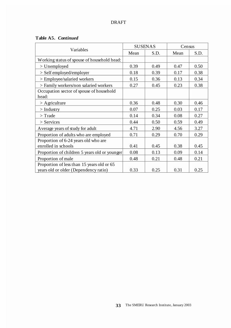
Table A5. Mean and Standard Deviation of Matched Variables, East Java - Rural


Mean S.D. Mean S.D.Household size 3.71 1.59 3.60 1.56Household living in permanent house 0.57 0.50 0.63 0.48Household living in owned house 0.96 0.19 0.95 0.22Household living in rented house 0.01 0.10 0.01 0.10Housing facilities:- Clean water 0.99 0.12 0.61 0.49- Toilet 0.41 0.49 0.39 0.49- Electricity 0.89 0.31 0.69 0.46Household head characteristics:- Age (years) 48.31 14.39 46.06 14.31- Female 0.15 0.36 0.14 0.35- Married 0.83 0.37 0.85 0.36Education level of household head: > Incomplete primary education or lower 0.55 0.50 0.43 0.50 > Completed primary education 0.31 0.46 0.43 0.49 > Lower secondary education 0.07 0.25 0.07 0.26 > Upper secondary education 0.06 0.25 0.06 0.23 > Tertiary education 0.01 0.12 0.01 0.11Years of education of household head 4.47 3.72 4.09 3.95Working status of household head: > Unemployed 0.10 0.30 0.06 0.23 > Self employed/employer 0.60 0.49 0.68 0.47 > Employee/salaried workers 0.29 0.46 0.25 0.43 > Family workers/non salaried workers 0.01 0.09 0.01 0.12Occupation sector of household head: > Agriculture 0.56 0.50 0.68 0.47 > Industry 0.06 0.25 0.03 0.18 > Trade 0.11 0.31 0.08 0.27 > Services 0.27 0.44 0.21 0.41Spouse of household head characteristics:- Age (years) 32.60 19.70 31.10 19.05Education level of spouse of household head: > Incomplete primary education or lower 0.55 0.50 0.39 0.49 > Completed primary education 0.32 0.47 0.48 0.50 > Lower secondary education 0.08 0.26 0.08 0.27 > Upper secondary education 0.04 0.20 0.04 0.20 > Tertiary education 0.01 0.09 0.01 0.09Years of education of spouse of household head 3.42 3.54 3.41 3.72

DRAFT


Table A5. Continued


Mean S.D. Mean S.D.Working status of spouse of household head: > Unemployed 0.39 0.49 0.47 0.50 > Self employed/employer 0.18 0.39 0.17 0.38 > Employee/salaried workers 0.15 0.36 0.13 0.34 > Family workers/non salaried workers 0.27 0.45 0.23 0.38Occupation sector of spouse of householdhead: > Agriculture 0.36 0.48 0.30 0.46 > Industry 0.07 0.25 0.03 0.17 > Trade 0.14 0.34 0.08 0.27 > Services 0.44 0.50 0.59 0.49Average years of study for adult 4.71 2.90 4.56 3.27Proportion of adults who are employed 0.71 0.29 0.70 0.29Proportion of 6-24 years old who areenrolled in schools 0.41 0.45 0.38 0.45Proportion of children 5 years old or younger 0.08 0.13 0.09 0.14Proportion of male 0.48 0.21 0.48 0.21Proportion of less than 15 years old or 65years old or older (Dependency ratio) 0.33 0.25 0.31 0.25

DRAFT


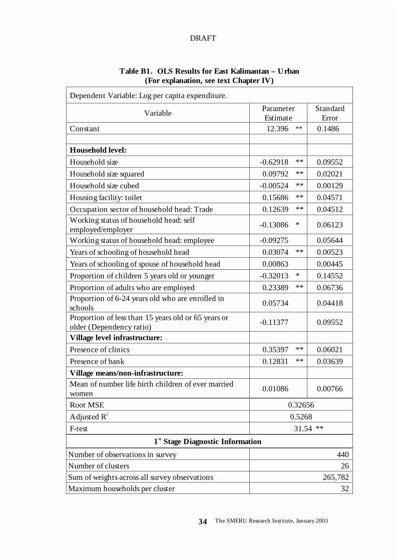
Table B1. OLS Results for East Kalimantan – Urban(For explanation, see text Chapter IV)

Dependent Variable: Log per capita expenditure.

VariableParameterEstimate

StandardError

Constant 12.396 ** 0.1486

Household level:

Household size -0.62918 ** 0.09552

Household size squared 0.09792 ** 0.02021

Household size cubed -0.00524 ** 0.00129

Housing facility: toilet 0.15686 ** 0.04571

Occupation sector of household head: Trade 0.12639 ** 0.04512Working status of household head: selfemployed/employer -0.13086 * 0.06123

Working status of household head: employee -0.09275 0.05644

Years of schooling of household head 0.03074 ** 0.00523

Years of schooling of spouse of household head 0.00863 0.00445

Proportion of children 5 years old or younger -0.32013 * 0.14552

Proportion of adults who are employed 0.23389 ** 0.06736Proportion of 6-24 years old who are enrolled inschools 0.05734 0.04418

Proportion of less than 15 years old or 65 years orolder (Dependency ratio) -0.11377 0.09552

Village level infrastructure:

Presence of clinics 0.35397 ** 0.06021

Presence of bank 0.12831 ** 0.03639Village means/non-infrastructure:Mean of number life birth children of ever marriedwomen 0.01086 0.00766

Root MSE 0.32656

Adjusted R2 0.5268

F-test 31.54 **

1st Stage Diagnostic Information

Number of observations in survey 440Number of clusters 26Sum of weights across all survey observations 265,782Maximum households per cluster 32

DRAFT


Table B1. Continued

Minimum households per cluster 10Max observed left hand side value in survey 13.706738472Min observed left hand side value in survey 10.787813187Maximum total residual from OLS model 1.1579629559Minimum total residual from OLS model -0.78851085Maximum household component of residual 0.9895228673Minimum household component of residual -0.758217768Maximum cluster component of residual 0.2111920808Minimum cluster component of residual -0.232690124Total sigma from OLS model 0.3265599409Sigma-eta 0.0802765886Ratio of SigmaEta**2/MSE 0.0604299172Variance of sigma-eta-squared 0.0000135306

Heteroscedasticity Regression

Dependent variable: see report.

Variable Label ParameterEstimate

StandardError

Constant -3.69673 ** 0.19558

(Occupation sector of HH head=trade) *(Number of life birth children of evermarried women)

-0.19105 0.09998

(Occupation sector of HH head = trade) *(Years of education of household head) 0.11773 ** 0.04428

(Years of education of household head) *(Number of life birth children of evermarried women)

0.02480 ** 0.00776

(Housing facility: toilet) * (Proportion of 6-24 years old enrolled in schools) 1.60020 ** 0.52869

(Household size) * (Proportion of 6-24 yearswho are enrolled in schools) -0.85401 ** 0.21213

(Occupation sector of head = trade) *(Working status of household head =employee/salaried workers)

-1.05809 0.58562

(Years of education of spouse of householdhead) * (Number of life birth children ofever married women)

-0.02039 * 0.00906

DRAFT


Table B1. Continued

Variable LabelParameterEstimate

StandardError

(Household size ^ 2) * (Proportion of 6-24years old enrolled in schools)

0.08311 ** 0.02493

Root MSE 2.30565Adjusted R2 0.0750F-test 4.37 **

Note:** significant at 1 percent level* significant at 5 percent level

DRAFT


Table B2. OLS Results for East Kalimantan – Rural(For explanation, see text Chapter IV)



StandardError

Constant 12.18071 ** 0.14528

Household level:

Household size -0.31852 ** 0.03784


Occupation sector of household head: Trade 0.11395 * 0.05555

Occupation sector of household head: Services 0.06346 0.03752

Household head characteristics: married 0.08527 0.04737

Education level of household head: upper secondary 0.09298 * 0.04301

Education level of household head: tertiary 0.34335 ** 0.07976

Household living in permanent house 0.18026 ** 0.04518

Household living in owned house 0.03034 0.04378

Housing facility: toilet 0.04115 0.03200

Housing facility: electricity 0.16314 ** 0.03557

Proportion of adults who are employed 0.13363 * 0.05862Proportion of 6-24 years old who are enrolled inschools 0.14463 ** 0.03936

Proportion of less than 15 years old or 65 years or older -0.41973 ** 0.07510Proportion of male 0.15709 * 0.07143Village level infrastructure:

Distance of village to sub-district capital 0.00291 ** 0.00082

Proportion of agriculture household -0.20128 ** 0.06110

Population density 0.01219 ** 0.00423

Energy for cooking: kerosene/gas 0.07546 0.04548

Presence of public health center in village 0.13401 * 0.05422Village means/non-infrastructure:

Proportion of permanent house in village -0.16789 * 0.06819

Root MSE 0.32957

Adjusted R2 0.5278

F-test 30.80 **

DRAFT


Table B2. Continued


Number of observations in survey 561Number of clusters 34Sum of weights across all survey observations 264,263Maximum households per cluster 32Minimum households per cluster 14Max observed left hand side value in survey 13.209498405Min observed left hand side value in survey 10.561680794Maximum total residual from OLS model 1.3265882613Minimum total residual from OLS model -1.030168735Maximum household component of residual 1.1611067134Minimum household component of residual -0.906374023Maximum cluster component of residual 0.4374508661Minimum cluster component of residual -0.336961862Total sigma from OLS model 0.3295661755Sigma-eta 0.1552102131Ratio of SigmaEta**2/MSE 0.2217968256Variance of sigma-eta-squared 0.0000553922



Variable Label ParameterEstimate

StandardError

Constant -4.84198 ** 0.19355

(Education level of household head = uppersecondary) * (Proportion of 6-24 years oldwho are enrolled in schools)

-9.72501 * 3.95900

(Household head characteristics = married)*(Education level of household head =tertiary)

3.18591 * 1.37819

(Household facility = electricity) *(Dependency ratio ^ 2) -3.21966 ** 0.95738

DRAFT


Table B2. Continued

Variable LabelParameterEstimate

StandardError

(Education level of household head = uppersecondary) * (Proportion of 6-24 years oldwho are enrolled in schools)

9.14908 * 3.95437

(Owned house) * (Household facility =electricity)

0.70805 ** 0.23690

(Occupation sector of household head =services) * (Rented house)

-1.28811 0.69913

(Occupation sector of household head =trade) * (Dependency ratio ^ 2)

3.93098 2.13506

(Education level of household head = uppersecondary) * (Population density)

0.10228 0.07403

(Housing facilities = toilet) * (Presence ofpublic health center in village) 0.66462 * 0.29106

(Housing facilities = toilet) * (Dependencyratio ^ 2) 4.95624 * 2.25854

(Household size) * (Rented house) 0.24390 0.14429

(Occupation sector of household head =trade) * (Household head characteristics =married)

1.85100 * 0.71795

(Occupation sector of household head =trade) * (Housing facilities = electricity) -2.35954 ** 0.73938

(Housing facility = toilet) * (Dependencyratio) -2.92977 * 1.44595

(Proportion of male) * (Proportion of 6-24 years oldwho are enrolled in schools ^2) 1.48770 ** 0.44674

(Household size) * (Education level ofhousehold head = tertiary) -0.72089 * 0.28077

(Education level of household head = uppersecondary) * (Proportion of adults who areemployed)

-0.91042 0.59163

(Housing facility = electricity) * (Educationlevel of household head = upper secondary) 1.02132 0.52653



DRAFT


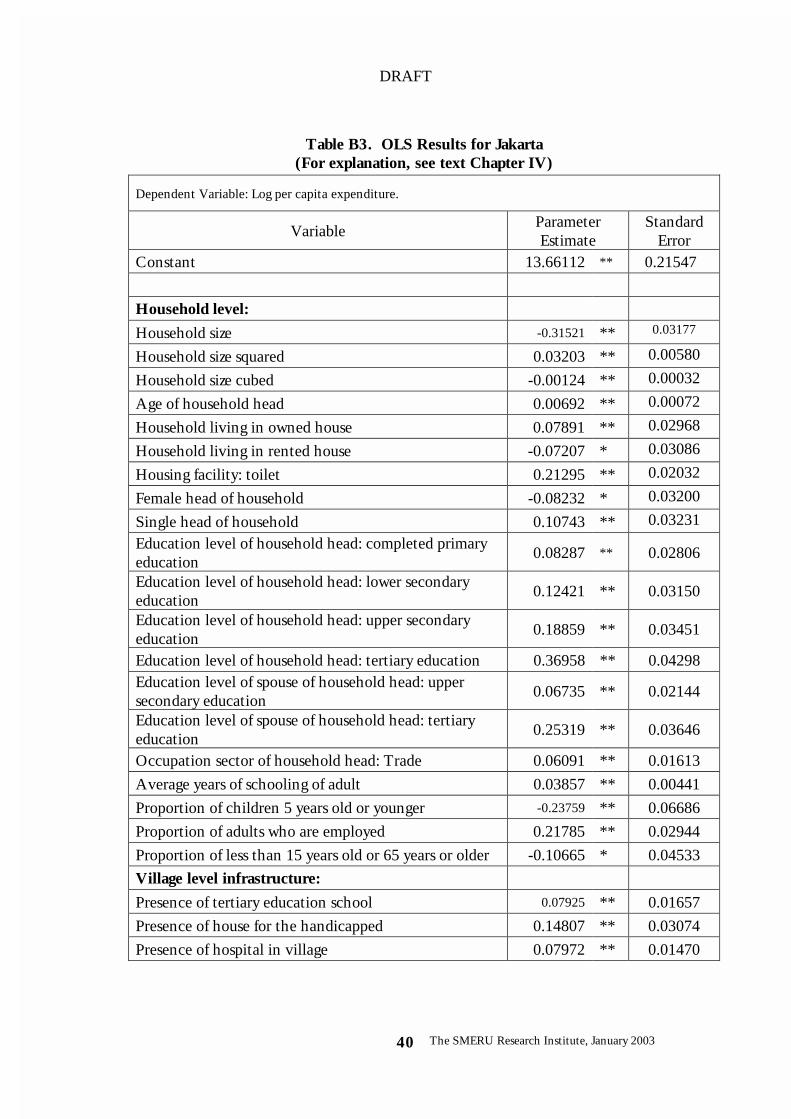
Table B3. OLS Results for Jakarta(For explanation, see text Chapter IV)



StandardError

Constant 13.66112 ** 0.21547

Household level:

Household size -0.31521 ** 0.03177



Age of household head 0.00692 ** 0.00072

Household living in owned house 0.07891 ** 0.02968

Household living in rented house -0.07207 * 0.03086


Female head of household -0.08232 * 0.03200

Single head of household 0.10743 ** 0.03231

Education level of household head: completed primaryeducation 0.08287 ** 0.02806

Education level of household head: lower secondaryeducation 0.12421 ** 0.03150

Education level of household head: upper secondaryeducation 0.18859 ** 0.03451

Education level of household head: tertiary education 0.36958 ** 0.04298Education level of spouse of household head: uppersecondary education 0.06735 ** 0.02144

Education level of spouse of household head: tertiaryeducation 0.25319 ** 0.03646

Occupation sector of household head: Trade 0.06091 ** 0.01613

Average years of schooling of adult 0.03857 ** 0.00441

Proportion of children 5 years old or younger -0.23759 ** 0.06686

Proportion of adults who are employed 0.21785 ** 0.02944

Proportion of less than 15 years old or 65 years or older -0.10665 * 0.04533Village level infrastructure:

Presence of tertiary education school 0.07925 ** 0.01657

Presence of house for the handicapped 0.14807 ** 0.03074

Presence of hospital in village 0.07972 ** 0.01470

DRAFT


Table B3. Continued

VariableParameterestimate

StandardError

Village means/non-infrastructure:

Population density -0.00020 ** 0.00005

Village mean of proportion of male -3.06947 ** 0.38369Village mean of tertiary educated people (aged > 20years)

0.47178 ** 0.09991

Root MSE 0.38096

Adjusted R2 0.5429

F-test 136.14 **


Number of observations in survey 2,959Number of clusters 140Sum of weights across all survey observations 2,208,256Maximum households per cluster 47Minimum households per cluster 13Max observed left hand side value in survey 15.142329216Min observed left hand side value in survey 11.036549568Maximum total residual from OLS model 1.8888788164Minimum total residual from OLS model -1.340939709Maximum household component of residual 1.5629351087Minimum household component of residual -1.116646653Maximum cluster component of residual 0.9383526449Minimum cluster component of residual -0.594724273Total sigma from OLS model 0.3809567452Sigma-eta 0.2201030164Ratio of SigmaEta**2/MSE 0.3338110075Variance of sigma-eta-squared 0.0000458914



Variable Parameter Estimate Standard Error

Constant -4.19952 ** 0.18805

(Occupation sector of HH head = trade) *(Proportion of adults who are employed ^ 2) -2.45888 * 0.95872

DRAFT


Table B3. Continued


(Proportion of children <= 5 years) ^ 3 4.14304 2.23667(Education level of spouse of HH head =upper secondary) * Hospital

0.68564 ** 0.18702

(Education level of spouse of HH head =tertiary) * (Proportion of adults who areemployed ^ 3)

8.42829 * 4.03983

(Dependency Ratio ^ 2) -9.94796 ** 2.48405(Dependency Ratio ^ 3) 10.44737 ** 2.31618Household Size * Age of household head -0.00273 ** 0.00094888(Education level of HH head = uppersecondary) * (Proportion of adults who areemployed ^ 3)

-9.80496 ** 3.43170

(Education level of HH head = tertiary) *Female head 3.13535 2.37019

(Education level of HH head = tertiary) *Village mean of proportion of male 4.65105 2.44136

Toilet * Village mean of proportion of male -2.28872 ** 0.55855Household size * (Education of head =tertiary) 0.09977 ** 0.03539

(Education of head = upper secondary) *(Village mean of proportion of tertiaryeducated people)

2.23725 ** 0.81689

(Proportion of children <= 5 years) *(Presence of tertiary school in village) -1.63279 ** 0.58322

Age of head * Toilet 0.03061 ** 0.00671Household size * Owned house 0.09729 * 0.03804(Education level of HH head = uppersecondary) * (Proportion of adults who areemployed ^ 2)

16.39895 ** 5.10598

Owned house * (Proportion of children <= 5years) 1.60464 * 0.65668

(Education level of spouse of HH head =upper secondary) * Owned house -0.44875 ** 0.16144

Age of household head * Mean years of studyof adult -0.00141 ** 0.00046145

(Occupation sector of HH head = trade) *(Proportion of adults who are employed) 3.02581 * 1.17625

(Education level of spouse of HH head =upper secondary) * Rented house -0.51753 * 0.22452

Household size * Dependency ratio 0.27973 * 0.12501

DRAFT


Table B3. Continued


(Education level of HH head = uppersecondary) * (Proportion of adults who areemployed)

-6.72210 ** 1.80738

(Education level of spouse of HH head =tertiary) * Toilet

-1.60744 1.16716

Mean years of study of adults * Dependencyratio

0.24325 ** 0.05777

(Occupation sector of HH head = trade) *(Education level of HH head = uppersecondary)

0.41394 * 0.20580

(Occupation sector of HH head = trade) *Rented house

-0.79403 * 0.36340

Rented house * Presence of tertiary school invillage 0.62979 ** 0.17162

(Proportion of children <= 5 years) *(Proportion of adults who are employed) -2.97146 ** 0.89633

(Occupation sector of HH head = trade) *Owned house -1.05632 ** 0.34978

(Education level of spouse of HH head =tertiary) * (Proportion of adults who areemployed ^ 2)

-8.93018 4.57147

Owned house * Dependency ratio -1.50485 ** 0.48499



DRAFT


Table B4. OLS Results for East Java – Urban(For explanation, see text Chapter IV)



StandardError

Constant 12.30789 ** 0.11880

Household level:

Household size -0.38841 ** 0.03223




Household living in owned house -0.09226 ** 0.02755

Household living in rented house -0.12375 ** 0.03074


Housing facility: electricity 0.16159 * 0.06680Education level of household head: completed primaryeducation 0.05774 ** 0.02114

Education level of household head: lower secondaryeducation 0.05568 * 0.02705

Education level of household head: upper secondaryeducation 0.17779 ** 0.03113

Education level of household head: tertiary education 0.34968 ** 0.04574Education level of spouse of household head: uppersecondary education 0.05348 * 0.02419


Occupation sector of household head: Trade 0.14606 ** 0.02186

Occupation sector of household head: Services 0.07946 ** 0.01744

Occupation sector of spouse of household head: Trade 0.05081 * 0.01990


Proportion of children 5 years old or younger -0.22012 ** 0.06458

Proportion of adults who are employed 0.05106 0.02612

Proportion of 6-24 years old who are enrolled in schools 0.06931 ** 0.01851

Proportion of less than 15 years old or 65 years or older -0.17245 ** 0.03813Village level infrastructure:

Industrial index * toilet facility 0.07661 ** 0.01958

Common sector of income of village people: services 0.05654 ** 0.01576

DRAFT


Table B4. Continued


StandardError

Presence of tertiary education in village 0.12197 ** 0.01937

Presence of market in village 0.07726 ** 0.01662

Proportion of agriculture household -0.21100 ** 0.03277Village means/non-infrastructure:

Village mean of household size -0.06042 * 0.02626Village mean of proportion of 6 – 24 years who areenrolled in school

-0.61153 ** 0.11075

Village mean of proportion of children 5 years oryounger

1.32257 * 0.64184

Root MSE 0.37983

Adjusted R2 0.5164

F-test 111.07 **


Number of observations in survey 3,094Number of clusters 181Sum of weights across all survey observations 3,174,147Maximum households per cluster 32Minimum households per cluster 11Max observed left hand side value in survey 14.261955261Min observed left hand side value in survey 10.459640503Maximum total residual from OLS model 2.4251350726Minimum total residual from OLS model -0.997549968Maximum household component of residual 2.3402287628Minimum household component of residual -1.095993227Maximum cluster component of residual 0.7677288977Minimum cluster component of residual -0.476817353Total sigma from OLS model 0.379825218Sigma-eta 0.1940121383Ratio of SigmaEta**2/MSE 0.2609096925Variance of sigma-eta-squared 0.0000229342

DRAFT


Table B4. Continued




Constant -6.00822 ** 0.30678

(Education level of household head = tertiary) *(Education level of spouse of household head =tertiary)

-1.98107 1.17249

Owned house * (Industrial index * toiletfacility)

-0.40024 ** 0.14466

(Average years of study for adults) * (Presence of tertiaryeducation in village) -0.05697 * 0.02579

(Education level of spouse of household head =tertiary) * (Occupation sector of householdhead = trade)

1.28577 * 0.65589

Owned house * (Village mean of proportion ofchildren of 5 years or younger) -17.10848 ** 3.91019

Rented house * (Village mean of proportion ofchildren of 5 years or younger) -13.31108 ** 5.02875

(Dependency ratio ^ 2) 1.57060 * 0.62903(Education level of spouse of household head =tertiary) * (Industrial index * toilet facility) 0.91815 * 0.45734

(Owned house) * (Proportion of children 5years old or younger) 1.81318 ** 0.69994

(Average years of study for adult)* (Proportionof 6-24 years old who are enrolled in schools) 0.07280 * 0.02969

(Education level of spouse of household head =upper secondary) * (Proportion of agriculturehousehold)

-1.26881 * 0.54994

(Housing facility = electricity) * (Village meanof proportion of children 5 years or younger) 26.25682 ** 6.63363

(Proportion of 6-24 years who are enrolled inschools) * (Village mean of proportion of 6-24years who are enrolled in schools).

-1.38845 * 0.57597

(Rented house) * (Occupation sector of spouseof household head = trade) -0.84595 ** 0.29864

(Dependency ratio) * (Proportion of agriculturehousehold) -1.77741 ** 0.63505

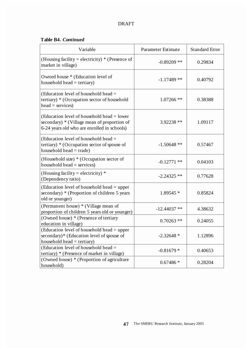
DRAFT


Table B4. Continued


(Housing facility = electricity) * (Presence ofmarket in village)

-0.89209 ** 0.29834

Owned house * (Education level ofhousehold head = tertiary)

-1.17489 ** 0.40792

(Education level of household head =tertiary) * (Occupation sector of householdhead = services)

1.07266 ** 0.38388

(Education level of household head = lowersecondary) * (Village mean of proportion of6-24 years old who are enrolled in schools)

3.92238 ** 1.09117

(Education level of household head =tertiary) * (Occupation sector of spouse ofhousehold head = trade)

-1.50648 ** 0.57467

(Household size) * (Occupation sector ofhousehold head = services) -0.12771 ** 0.04103

(Housing facility = electricity) *(Dependency ratio) -2.24325 ** 0.77628

(Education level of household head = uppersecondary) * (Proportion of children 5 yearsold or younger)

1.89545 * 0.85824

(Permanent house) * (Village mean ofproportion of children 5 years old or younger) -12.44037 ** 4.38632

(Owned house) * (Presence of tertiaryeducation in village) 0.70263 ** 0.24055

(Education level of household head = uppersecondary)* (Education level of spouse ofhousehold head = tertiary)

-2.32648 * 1.12896

(Education level of household head =tertiary) * (Presence of market in village) -0.81679 * 0.40653

(Owned house) * (Proportion of agriculturehousehold) 0.67486 * 0.28204

DRAFT


Table B4. Continued


(Housing facility = toilet) * (Occupationsector of household head = trade)

0.87372 ** 0.21186

(Household size) * (Presence of market invillage)

0.11091 ** 0.03627

(Education level of spouse of household head= upper secondary) * (Occupation sector ofhousehold head = trade)

-0.74680 * 0.34366

(Housing facility = toilet) * (Education levelof spouse of household head = uppersecondary)

-0.48841 0.27376

(Education level of household head = uppersecondary) * (Education level of spouse ofhousehold head = tertiary)

-5.24654 ** 1.94223

(Permanent house) * (Owned house) 1.34002 ** 0.35690(Permanent house) * (Rented house) 1.06630 * 0.45532(Occupation sector of household head =services) * (Industrial index * housing facility= toilet)

0.45620 ** 0.16856

(Education level of household head = uppersecondary) * (Average years of study foradults)

-0.11231 ** 0.03990

(Education level of household head = lowersecondary) * (Village mean of proportion ofchildren 5 years or younger)

-16.34155 ** 5.13383

(Rented house) * (Presence of tertiaryeducation in village) 0.76800 * 0.32841

(Education level of household head = tertiaryeducation) * (Village mean of proportion of 6- 24 years who are enrolled in schools)

3.30583 ** 1.08600

(Occupation sector of household head =trade) * (Presence of market in village) 0.39202 * 0.19396

(Education level of household head = uppersecondary) * Dependency ratio -1.61418 ** 0.61104

(Housing facility: electricity) * (Villagemean of proportion of 6-24 years old who areenrolled in school)

-1.67777 * 0.82513

(Permanent house) * (Occupation sector ofhousehold head = services) -0.47481 * 0.23226

DRAFT


Table B4. Continued


(Education level of spouse of household head= upper secondary) * (Occupation sector ofhousehold head = trade)

0.99539 ** 0.33713

(Education level of household head =tertiary) * (Proportion of 6 – 24 years whoare enrolled in school)

-0.76972 0.40985

(Education level of household head =tertiary) * (Average of years of education foradults)

0.15694 0.08209

(Education level of household head = uppersecondary) * (Average of years of educationfor adults)

0.08367 ** 0.02531

(Occupation sector of household head =services) * (Village mean of proportion ofunder 5 years old or younger)

10.61531 ** 2.74230

(Owned house) * (Occupation sector ofhousehold head = trade) -0.74355 ** 0.21123

Dependency ratio * (Village mean ofproportion of 6 – 24 years who are enrolledin school)

4.07848 * 2.00573

(Proportion of under 5 years old or younger)* (Village mean of proportion of 6 – 24 yearswho are enrolled in school)

-3.81615 * 1.61171

Permanent house * Market 0.47447 0.28821

(Education level of household head =tertiary) * (Village mean of proportion of 6 –24 years who are enrolled in school)

3.05026 * 1.20757



DRAFT


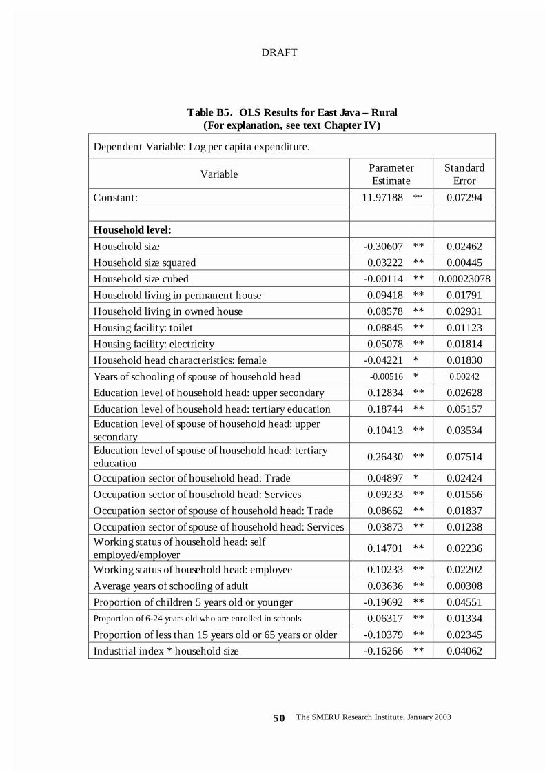
Table B5. OLS Results for East Java – Rural(For explanation, see text Chapter IV)



StandardError

Constant: 11.97188 ** 0.07294

Household level:

Household size -0.30607 ** 0.02462




Household living in owned house 0.08578 ** 0.02931


Housing facility: electricity 0.05078 ** 0.01814

Household head characteristics: female -0.04221 * 0.01830

Years of schooling of spouse of household head -0.00516 * 0.00242

Education level of household head: upper secondary 0.12834 ** 0.02628

Education level of household head: tertiary education 0.18744 ** 0.05157Education level of spouse of household head: uppersecondary 0.10413 ** 0.03534


Occupation sector of household head: Trade 0.04897 * 0.02424

Occupation sector of household head: Services 0.09233 ** 0.01556

Occupation sector of spouse of household head: Trade 0.08662 ** 0.01837

Occupation sector of spouse of household head: Services 0.03873 ** 0.01238Working status of household head: selfemployed/employer 0.14701 ** 0.02236

Working status of household head: employee 0.10233 ** 0.02202


Proportion of children 5 years old or younger -0.19692 ** 0.04551Proportion of 6-24 years old who are enrolled in schools 0.06317 ** 0.01334

Proportion of less than 15 years old or 65 years or older -0.10379 ** 0.02345

Industrial index * household size -0.16266 ** 0.04062

DRAFT


Table B5. Continued


StandardError

Industrial index * (household size ^ 2) 0.03454 ** 0.01041

Industrial index * (household size ^ 3) -0.00237 ** 0.00078449

Industrial index * permanent house 0.05452 0.03003

Industrial index * (Housing facility =electricity) 0.14890 ** 0.04913

Mountain * household size -0.08192 ** 0.01031

Mountain * (household size ^ 2) 0.00884 ** 0.00169

Mountain * permanent house 0.09968 ** 0.02259Mountain * (Sector occupation of household head =trade)

0.08147 * 0.03401

Coastal village 0.08140 ** 0.02025

Village mean of permanent house -0.05796 * 0.02394

Village mean of years of study of household head -0.04447 ** 0.01662

Village mean of years of study of adult 0.05099 ** 0.01750Village mean of tertiary educated people (aged > 20years) 3.12595 ** 0.55729

Proportion of agriculture household -0.14872 ** 0.03096

Presence of lower secondary school in village -0.03449 ** 0.01095

Presence of public motorized transportation in village 0.03712 * 0.01643

Village mean of dependency ratio -0.82483 ** 0.14946Village mean of education level of household head =upper secondary education 0.05482 ** 0.01427

District dummy for District 3 -0.18846 ** 0.04069

District dummy for District 4 0.24984 ** 0.03387






Root MSE 0.33114

Adjusted R2 0.4321

F-test 69.59 **


Number of observations in survey 4419Number of clusters 280Sum of weights across all survey observations 5039475

DRAFT


Table B5. Continued

Maximum households per cluster 32Minimum households per cluster 11Max observed left hand side value in survey 14.016383171Min observed left hand side value in survey 10.187086105Maximum total residual from OLS model 2.0861312566Minimum total residual from OLS model -1.184569068Maximum household component of residual 2.1143365852Minimum household component of residual -1.151620273Maximum cluster component of residual 0.4465563246Minimum cluster component of residual -0.56328487Total sigma from OLS model 0.3311352542Sigma-eta 0.1635432794Ratio of SigmaEta**2/MSE 0.2439240171Variance of sigma-eta-squared 7.5751029E-6



Variable Label Parameter Estimate Standard Error

Constant -5.87934 ** 0.08278

(Proportion of children <= 5 years) ^ 2 -8.89581 * 3.46425

(Proportion of children <= 5 years) ^ 3 16.19228 * 6.77412Permanent house * (Education level ofspouse of HH head = tertiary) -1.68255 1.25708

(Education level of spouse of HH head =secondary) * (Industrial Index * Householdsize)

7.46563 ** 2.24444

Household size * Dummy District 25 0.25115 * 0.10145Permanent house * (Education level of HHhead = upper secondary) 0.84886 ** 0.20084

(Housing facility: electricity) * Mean years ofstudy for adults -0.12313 ** 0.02180

(Working status of HH head = selfemployed/employer) * Dummy District 4 1.24688 ** 0.28993

(Education level of HH head = uppersecondary) * District Dummy 25 -1.61665 * 0.77596

(Education level of spouse of HH head =upper secondary) * (Mountain * Permanenthouse )

1.36568 * 0.55792

DRAFT


Table B5. Continued


Proportion of children 6 – 24 years who areenrolled in school * (Industrial index *electricity)

-0.79053 * 0.34479

Permanent house * (Education level of spouseof HH head = upper secondary)

-1.55759 ** 0.48888

(Housing facility: electricity) * (Occupationsector of spouse of HH head = trade)

0.82221 ** 0.20677

(Education level of spouse of HH head =upper secondary) * District Dummy 25

2.22796 * 0.95787

(Education level of spouse of HH head =upper secondary) * Industrial Index *(Household size ^ 2)

-3.64196 ** 1.14908

Permanent house * (Occupation sector ofspouse of HH head = trade) -0.87381 ** 0.24551

Mean years of study for adults * IndustrialIndex * (Household size ^ 2) -0.01263 ** 0.00402

Mean years of study for adults * Village meanof permanent house 0.15885 ** 0.02913

(Proportion of children <= 5 years )*Industrial Index * (Household size ^ 3) -0.08405 ** 0.03033

(Occupation sector of HH head = Services) *(Proportion of children <= 5 years) 2.05215 ** 0.57486

(Proportion of children 6 – 24 years who areenrolled in school) * (Industrial Index *Permanent house)

1.04838 ** 0.38999

(Education level of spouse of HH head =upper secondary) * District Dummy 29 2.05885 1.22356

(Education level of spouse of HH head =upper secondary) * District Dummy 19 1.90615 1.02733

(Housing facility: electricity) * (Educationlevel of spouse of HH head = tertiary) 2.08807 1.20912

(Proportion of children <= 5 years) *Industrial Index * (Household size ^ 2) 0.64607 ** 0.21166

(Working status of head = selfemployed/employer) * (Proportion of children<= 5 years)

1.44796 ** 0.49573

(Education level of spouse of HH head =upper secondary) * District Dummy 18 2.70055 * 1.24613

(Occupation sector of HH head = Services) *District Dummy 18 -0.79526 * 0.37139

(Education level of HH head = uppersecondary) * District Dummy 19 -2.70456 ** 0.84013

DRAFT


Table B5. Continued


Permanent house * (Housing facility:electricity)

0.65462 ** 0.09127

(Proportion of children <= 5 years) *Industrial Index * (Housing facility:electricity)

-5.24141 ** 1.52963

(Housing facility: electricity ^ 2) * IndustrialIndex

1.05296 ** 0.23006

Mean years of study for adults * IndustrialIndex * (Household size ^ 3)

0.00165 ** 0.00053295

(Permanent house ^ 2) * Industrial Index -0.82046 ** 0.25633Toilet * (Housing facility: electricity) 0.38337 ** 0.09037Household size * (Village mean of permanenthouse) -0.11490

** 0.03313

Toilet * Industrial Index * (Housing facility =electricity) -0.67205 ** 0.19652

(Education level of spouse of HH head =upper secondary) * Industrial Index *(Household Size ^ 3)

0.46007**

0.14653

Owned house * District Dummy 25 -1.28840 * 0.52234



DRAFT


Table C1. GLS Results for East Kalimantan – Urban(For explanation, see text Chapter IV)

Coefficients and standard errors from GLS model.Dependent variable: log per capita consumption


Standard Error

Constant 12.2232 0.1394

Household size -0.5011 0.0866

Household size squared 0.0781 0.0189

Household size cubed -0.0043 0.0013


Occupation sector of household head: Trade 0.1068 0.0380Working status of household head: selfemployed/employer -0.1579 0.0544

Working status of household head: employee -0.1018 0.0496

Years of schooling of household head 0.0303 0.0045

Years of schooling of spouse of household head 0.0056 0.0038

Proportion of children 5 years old or younger -0.4633 0.1106

Proportion of adults who are employed 0.2574 0.0574Proportion of 6-24 years old who are enrolledin schools 0.0394 0.0384

Proportion of less than 15 years old or 65 yearsor older -0.1054 0.0794

Presence of clinics in village 0.3884 0.0711

Presence of bank in village 0.1102 0.0462

Mean of number life birth children 0.0058 0.0071

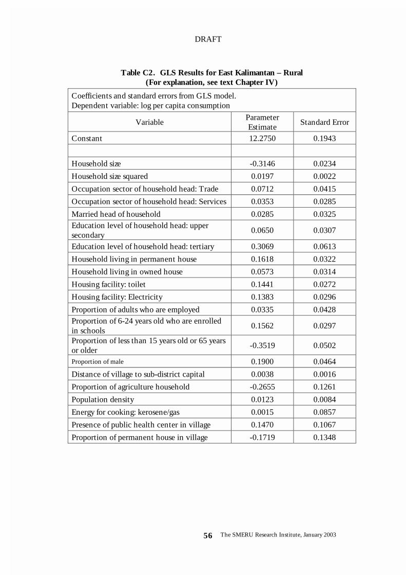
DRAFT


Table C2. GLS Results for East Kalimantan – Rural(For explanation, see text Chapter IV)



Standard Error

Constant 12.2750 0.1943



Occupation sector of household head: Trade 0.0712 0.0415

Occupation sector of household head: Services 0.0353 0.0285

Married head of household 0.0285 0.0325Education level of household head: uppersecondary 0.0650 0.0307

Education level of household head: tertiary 0.3069 0.0613

Household living in permanent house 0.1618 0.0322



Housing facility: Electricity 0.1383 0.0296

Proportion of adults who are employed 0.0335 0.0428Proportion of 6-24 years old who are enrolledin schools 0.1562 0.0297

Proportion of less than 15 years old or 65 yearsor older -0.3519 0.0502

Proportion of male 0.1900 0.0464

Distance of village to sub-district capital 0.0038 0.0016

Proportion of agriculture household -0.2655 0.1261

Population density 0.0123 0.0084

Energy for cooking: kerosene/gas 0.0015 0.0857

Presence of public health center in village 0.1470 0.1067

Proportion of permanent house in village -0.1719 0.1348

DRAFT


Table C3. GLS Results for Jakarta(For explanation, see text Chapter IV)



Constant 13.7226 0.5303




Age of household head 0.0048 0.0005


Household living in rented house -0.0608 0.0247


Female head of household -0.0145 0.0239

Single head of household 0.0358 0.0238Education level of household head:completed primary education 0.0741 0.0208

Education level of household head: lowersecondary education 0.1149 0.0234

Education level of household head: uppersecondary education 0.1474 0.0255

Education level of household head: tertiaryeducation 0.2894 0.0329

Education level of spouse of householdhead: upper secondary education 0.0576 0.0148

Education level of spouse of householdhead: tertiary education 0.1821 0.0267

Occupation sector of household head:Trade 0.0492 0.0116

Average years of schooling for adults 0.0409 0.0034Proportion of children 5 years old oryounger -0.3222 0.0479

Proportion of adults who are employed 0.1817 0.0219Proportion of less than 15 years old or 65years or older -0.0815 0.0363

DRAFT


Table C3. Continued


Population density -0.0002 0.0001Presence of tertiary education school invillage

0.0774 0.0456

Presence of house of handicapped in village 0.1607 0.0780

Presence of hospital in village 0.0926 0.0413

Village mean of proportion of male -2.9312 1.0057Village mean of tertiary educated people(aged > 20 years)

0.5149 0.2731

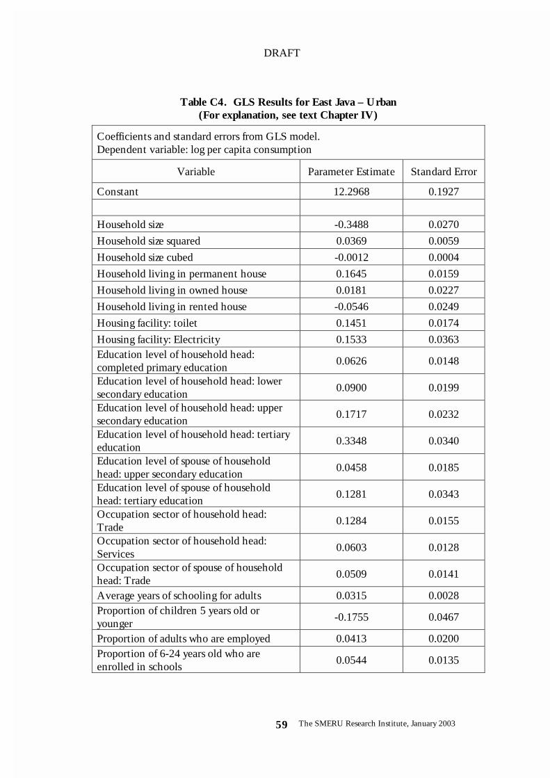
DRAFT


Table C4. GLS Results for East Java – Urban(For explanation, see text Chapter IV)



Constant 12.2968 0.1927






Household living in rented house -0.0546 0.0249


Housing facility: Electricity 0.1533 0.0363Education level of household head:completed primary education 0.0626 0.0148

Education level of household head: lowersecondary education 0.0900 0.0199

Education level of household head: uppersecondary education 0.1717 0.0232


Education level of spouse of householdhead: upper secondary education 0.0458 0.0185

Education level of spouse of householdhead: tertiary education 0.1281 0.0343

Occupation sector of household head:Trade 0.1284 0.0155

Occupation sector of household head:Services 0.0603 0.0128

Occupation sector of spouse of householdhead: Trade 0.0509 0.0141

Average years of schooling for adults 0.0315 0.0028Proportion of children 5 years old oryounger -0.1755 0.0467

Proportion of adults who are employed 0.0413 0.0200Proportion of 6-24 years old who areenrolled in schools 0.0544 0.0135

DRAFT


Table C4. Continued


Proportion of less than 15 years old or 65years or older

-0.1460 0.0296

Industrial index * toilet facility 0.0528 0.0216Common sector of income of village people:services

0.0769 0.0353

Presence of tertiary education school invillage

0.1344 0.0429

Presence of market in village 0.0762 0.0363


Village mean of household size -0.0818 0.0554Village mean of proportion of children aged6 – 24 years who are enrolled in school

-0.6670 0.2326

Village mean of proportion of children 5years or younger 1.1552 1.3920

DRAFT


Table C5. GLS Results for East Java – Rural(For explanation, see text Chapter IV)



Standard Error

Constant 12.0235 0.1153







Housing facility: Electricity 0.0768 0.0171

Household head characteristics: female -0.0606 0.0133

Years of schooling of spouse of household head -0.0024 0.0018Education level of household head: uppersecondary 0.1192 0.0218


Education level of spouse of household head:upper secondary 0.0663 0.0271

Education level of spouse of household head:tertiary education 0.3242 0.0651

Occupation sector of household head: Trade 0.0509 0.0179

Occupation sector of household head: Services 0.0725 0.0118Occupation sector of spouse of household head:Trade 0.0728 0.0146

Occupation sector of spouse of household head:Services 0.0197 0.0091

Working status of household head: selfemployed/employer 0.0943 0.0166

Working status of household head: employee 0.0493 0.0164

Average years of schooling for adults 0.0325 0.0024

Proportion of children 5 years old or younger -0.1308 0.0329

Proportion of 6-24 years old who are enrolled in schools 0.0695 0.0098

DRAFT


Table C5. Continued


Standard Error

Proportion of less than 15 years old or 65 years orolder

-0.1413 0.0175

Industrial index * household size -0.0841 0.0408

Industrial index * (household size ^ 2) 0.0174 0.0097

Industrial index * (household size ^ 3) -0.0012 0.0007

Industrial index * permanent house 0.0379 0.0231

Industrial index * (Housing facility: electricity) 0.0250 0.0509

Mountain * household size -0.0610 0.0120

Mountain * (household size ^ 2) 0.0063 0.0016

Mountain * permanent house 0.0340 0.0181Mountain * (Sector occupation of householdhead = trade) 0.0437 0.0262

Coastal village 0.0727 0.0419

Village mean of permanent house -0.0462 0.0462

Village mean of years of study of household head -0.0602 0.0341

Village mean of years of study of adult 0.0691 0.0353Village mean of tertiary educated people (aged >20 years) 3.4340 1.1511


Presence of lower secondary school in village -0.0348 0.0227Presence of public motorized transportation invillage 0.0427 0.0337

Village mean of dependency ratio -0.8875 0.3027Village mean of education level of householdhead = upper secondary education 0.0490 0.0294

District dummy for District 3 -0.2038 0.0778

District dummy for District 4 0.1936 0.0716






DRAFT


References

Bigman, David and Hippolyte Fofack (2000), ‘Geographical Targeting for PovertyAlleviation: An Introduction to the Special Issue’, The World Bank EconomicReview, 14(1), pp. 129-145.

Elbers, Chris, Jean O. Lanjouw, and Peter Lanjouw (2001), Welfare in Villages andTowns: Micro-Level estimation of Poverty and Inequality, Vrije Universiteit,Amsterdam, mimeo.

Elbers, Chris, Jean O. Lanjouw, and Peter Lanjouw (2002), Micro-level Estimation ofWelfare, Unpublished mimeo.

Foster, J., Greer, J., and Thorbecke, E. (1984), ‘A Class of Decomposable PovertyMeasures’, Econometrica, 52, pp. 761-66.

Hentschel, Jesko, Jean Olson Lanjouw, Peter Lanjouw, and Javier Poggi (2000),‘Combining Census and Survey Data to Trace the Spatial Dimensions ofPoverty: A Case Study of Ecuador’, The World Bank Economic Review, 14(1),pp. 147-165.

Pradhan, Menno, Asep Suryahadi, Sudarno Sumarto, and Lant Pritchett (2001),‘Eating Like Which 'Joneses'? An Iterative Solution to the Choice of PovertyLine Reference Group’, The Review of Income and Wealth, 47(4), pp. 473-487.

Ravallion, Martin 2000), ‘Monitoring Targeting Performance When DecentralizedAllocations to the Poor are Unobserved’, The World Bank Economic Review,14(2), pp. 331-345.

van de Walle, Dominique (1998), ‘Targeting Revisited’, The World Bank ResearchObserver, 13(2), pp. 231-248.

Developing a Poverty Map for Indonesia - World Banksiteresources.worldbank.org/ASEM/Resources/Poverty+Map+Indonesia+I.pdf · Developing a Poverty Map for Indonesia: An Initiatory

Documents