Developing a Hydro-quality Simulation Model - CORE

Utah State University Utah State University

DigitalCommons@USU DigitalCommons@USU

Reports Utah Water Research Laboratory

January 1970

Developing a Hydro-quality Simulation Model Developing a Hydro-quality Simulation Model

Neal P. Dixon

David W. Hendricks

A. Leon Huber

Jay M. Bagley

Follow this and additional works at: https://digitalcommons.usu.edu/water_rep

Part of the Civil and Environmental Engineering Commons, and the Water Resource Management

Commons

Recommended Citation Recommended Citation Dixon, Neal P.; Hendricks, David W.; Huber, A. Leon; and Bagley, Jay M., "Developing a Hydro-quality Simulation Model" (1970). Reports. Paper 511. https://digitalcommons.usu.edu/water_rep/511

This Report is brought to you for free and open access by the Utah Water Research Laboratory at DigitalCommons@USU. It has been accepted for inclusion in Reports by an authorized administrator of DigitalCommons@USU. For more information, please contact [email protected].

DEVELOPING A HYDRO-QUALITY SIMULATION MODEL

by

Neal P. Dixon David W. Hendricks

A. Leon Huber Jay M. Bagley

Utah Water Research Laboratory College of Engineering Utah State University Logan, Utah 84321

June 1970 PRWG67-1

$2.50

PROJECT ORGANIZATION

The project reported herein was gegun in February 1966 upon award of a demonstration grant by the Division of Water Supply and Pollution Control, U.S. Public Health Service. Sub­sequent renewal grants were made by the Federal Water Pollution Control Administration, the third and last being grant number WPD-17-03.

Individuals who have assisted in various phases of the project include:

Mr. Eugene Israelsen-who initiated field studies at the beginning of the project.

Dr. Harvey Millar-who assisted in establishing laboratory chemical analyses procedures and in training the laboratory chemical analyst.

Dr. Frederick Post-who trained laboratory personnel to perform bacteriological analyses, and who initiated the concept of massive data scanning to explore for possible correlations between water quality variables (developed as Appendix H of this report). Dr. Post's motivation was oriented toward explaining bacterial counts in the stream.

Mrs. Ling Chu-who performed most of the chemical and bacteriological analyses on weekly water samples.

Dr. Allen Kartchner-who had the responsibilities of setting up two continuous monitoring field stations and for procuring and analyzing data from same (in collaboration with another project).

Appreciation is expressed to the U.S. Geological Survey, Logan Office, under the supervision of Mr. Wallace Jibson, who under special contract with the project set up four additional gaging stations and made available all current streamflow records in the project area.

Author responsibilities

Jay M. Bagley-conceived the project, initiated the hydrology phases of the study, and was project director at the beginning of the project (until July 1966 when he became Director, Utah Water Research Laboratory).

David W. Hendricks-initiated the water quality phases of the study and was project director, subsequent to Dr. Bagley.

Leon Huber-developed the hydrologic submodel, and was responsible for developing data processing procedures, and for acquisition of hydrologic data.

Neal P. Dixon-developed the water quality submodels, and was responsible for water quality sampling and analyses (Mr. Dixon's doctoral dissertation was based upon his contributions to the project).

iii

,

•

TABLE OF CONTENTS

Chapter I

INTRODUCTION

Chapter II

Background l\leed for modeling Objective Scope .....

PLAN OF OPERATION

Chapter III

Conspectus . . . The prototype system Resolution Submodels .... Simulation algorithm

THE HYDROLOGYSUBMODEL

Chapter IV

Model structure . . . . . Stochastic aspects . . . . Hydrology modeling of the study area Hydrology submodel results Hydraulic considerations . . . . .

SALII\lITY SUBMODEL

Chapter V

I nput conductances Stream conductance I n-transit conductance changes

Reservoir routing Simulation algorithm

STREAM TEMPERATURE SIMULATION

The temperature problem . . . . . Month Iy water temperature simu lation Adjustment of discrete sampling data Reservoirs .......... . Algorithm for simu lation . . . . . Diurnal water temperature simulation

v

1 2

.3

.3

.3

.4

.4

.4

.9

.9 13 13 15 15

23

23 25 26 26 26

29

29 29 34 34 35 37

Chapter VI

DISSOLVED OXYGEN SIMULATION

Chapter VII

I n-transit changes

Suspended BOD Determination of rate constants Discrete BOD loads in the Little Bear River Combination of hydrologic inputs

The annual cycle

Inputs Reservoir effects Simulation algorithm

Diurnal dissolved oxygen .

Diurnal patterns of hydrologic inputs Reservoirs . . . . . . . . . . . . In-transit changes and the diurnal effect Simu lation algorithm . . . . . . . .

EXPLORATION FOR A COLIFORM SUBMODEL

Literature search Alternatives considered

Chapter V III

SIMULATION RESULTS-LITTLE BEAR RIVER

System delineation ..... Establishing model coefficients

Electrical conductance Monthly water temperature Monthly dissolved oxygen Diurnal water temperature Diurnal dissolved oxygen

Verification of model constants and coefficients

Chapter IX

Electrical conductance Monthly water temperature Month Iy dissolved oxygen Diurnal water temperature Diurnal dissolved oxygen

SUMMARY AI\J D COI\JCLUSIONS

LITERATURE CITED

vi

45

45

47 48 49 51

51

52 55 55

58

61 63 64 64

69

69 70

73

73 73

73 74 74 76 77

77

78 78 78 79 79

83

85

APPENDIX A: DESCRIPTIOI\I OF THE PROTOTYPE SYSTEM

Location and geography Geology ..... Climate and hydrology Canal diversions Reservoirs . . . . . Cultural development Sources of pollution

APPEI\IDIX B: DATA COLLECTION SYSTEM

Stream gaging Weather observation Weekly quality sampling Continuous quality monitoring Quality of data . . . . . . .

APPENDIX C: WATER QUALITY DATA PROCESSING PROGRAMS-

· A-1

· A-1 · A-1 · A-1 · A-1 · A-1 · A-6 · A-9

B-1

B-1 B-1 B-1 B-7 B-7

for discrete sample data ......... C-1

1. QU LPRT, Specific instructions 2. SCAN, Specific instructions 3. PRTPL T, Specific instructions

APPEI\IDIX 0: FOURIER SERIES CURVE FITTING

APPEI\IDIX E: OPERATION OF THE WATER QUALITY SIMULATION MODEL

The program . . . . . Computer requirements Program options Data requirements

System definition Equilibrium temperature Diurnal temperature and D.O. model parameters Hydraulic relationships ........ . Month Iy water qual ity submodel parameters Reservoir data Atmospheric data Month Iy data . .

APPEI\IDIX F: COMPARISON OF OBSERVED AND SIMULATED 1968 WATER QUALITY PROFILES ................. .

APPEI\IDIX G: HYDROLOGY MODEL COMPUTER PROGRAMS-(1) HYDRO, (2) BUDGET-INSTRUCTIONS FOR USE ............... .

· C-1 · C-1 . C-3

0-1

E-1

E-1 E-1 E-2 E-2

E-2 E-2 E-2 E-2 E-2 E-3 E-4 E-4

. . . . . F-1

. G-1

APPEI\IDIX H: STATISTICAL ANALYSIS OF LITTLE BEAR RIVER WATER QUALITY DATA .......... .

The broad spectrum search Specific parameter models Summary ...... .

vii

H-1

H-1 H-4 H-4

LISTOF FIGURES

Figure

One branch system schematic

2 Typical nonreservoir reach flow components

3 System control model simulation procedure

4 Hydro(ogic model schematic of a water resource system

5 Flow chart for hydro model

6 Two hydrologic subareas

7 Temperature comparisons-Utah State University Climatological Station and E. K. Israelsen Farm in Hyrum . . . .

8 Phreatophyte growth stage coefficient curves

9 Gaged and computed outflows for both hydrologic subareas

10 Specific electrical conductance vs. discharge for station S-27.0 on the Little Bear River ............. .

11 Simu lation algorithm for electrical conductance submodel

12 Typical annual stream temperature variation at station S-12.8

13 Annual stream temperature variation at SEC-4.3 below Porcupine Reservoir with best fit four-term Fourier series curve

14 Simulation algorithm for monthly water temperature

15 Water temperature variations for the period 22-29 April 1968 with Fourier series model . . . . . . . . . . . . . . . . . . .

16 Annual variations in diurnal temperature index model parameters

17 Diurnal temperature index models for each month of the year

18 Comparison of stream temperature index patterns on the Little Bear River at Wellsville and Parad ise on 11-12 Oct. 1968 ...... .

19 Graphical representation of diurnal temperature computations

20 Simulation algorithm for diurnal water temperature .....

21 Dissolved oxygen variations at station S-12.8 for 1966-67 with best fit

Page

5

5

6

10

11

14

15

17

19

25

28

30

35

36

38

39

41

41

42

44

Fou rier series cu rve ....... 47

viii

22 BOD survey below trout farm 50

23 Sphaerotilis growth on rocks downstream from trout farm discharge 51

24 BOD variations at station S-12.8 for 1966-67 with best fit Fourier series curve 52

25 Annual BOD cycle, station S-12.8 54

26 Comparison of D.O. concentrations observed below Porcupine Reservoir in 1967 with saturation concentration . . . . . . . . 55

27 Generalized monthly D.O. flow chart

28 0 issolved oxygen variations for the period 22-29 Apri I 1968 with Fourier series model . . . . . . . . . . . . . . .

29 Annual variation in diurnal D.O. index model parameters

30 Diurnal D.O. index curves for each month of the year

31 Comparison of D.O. index patterns on the Little Bear River at Wellsville and Paradise on 11-12 October 1968

32 Flow and strength variations in domestic waste

33 Graphical representation of diurnal D.O. computation

34 Generalized flow chart for diurnal D.O. simulation

35 Space profile of log (coliform count) for 11 September 1968

36 Annual variation in log (coliform count) at station S-12.5 for 1966-67

37 Log (coliform count) vs. stream temperature (station S-12.8)

38 BOD deviation vs. log (coliform) deviation (station S-12 .8)

57

59

60

62

62

63

65

67

70

70

71

72

39 Little Bear River system schematic ..... 73

40 Electrical conductance correspondence graphs for stations SEC-4.3, S-24.6, S-21.3 and S-12.8 from the final model development run (1966-67 data) ..... 75

41 Comparison of observed and simulated electrical conductance profiles for January and July, 1967 .................. . . . . 75

42 Water temperature correspondence graphs for stations SEC-4.3, S-24.6, S-21.3 and S-12.8 from the final model development run (1966-67 data) ......... 75

43 Comparison of observed and simu lated water temperature profiles for January and July, 1967 .............................. 75

44 Dissolved oxygen correspondence graphs for stations SEC-4.3, S-24.6, S-21.3 and S-12.8 from the final model development run (1966-67 data) .... 76

45 Comparison of observed and simulated D.O. profiles for January and July, 1967 . . . . . . . . . . . . . . . . . . . . . . . . 76

46 May 1967 diurnal water temperature index pattern for station S-12.8 77

ix

47 May 1967 diurnal dissolved oxygen index pattern for station S-12.8 . . . . . . . . 77

4B E Itldrical conductance correspondence graphs from the model verification rlill (1~)(i7 68 duta) ..................... . .... 78

49 C()mp&isoll of observed and simulated electrical conductance profiles tor Jdlluary and July 1968 .............. . . . . . . . 78

50 Annual electrical conductance distribution of stations S-12.8 dfld SEC-1.4 .................... . . . . . . . 79

51 Water temperature correspondence graphs from the model verification run (1967 -68 data) ............................ 79

52 Comparison of observed and simulated water temperature profiles for January and July, 1968 . . . . . . . . . . . . . . . . . . . . 80

53 Annual water temperatu re distribution at stations S-12.8 and SEC-0.4 80

54 Dissolved oxygen correspondence graphs from the model verification run (1967-68 data) ............................ 81

55 Comparison of observed and simulated D.O. profiles for January and July,1968 ... . . . . . . . . . . . . . . . . . . . . . 81

56 Annual dissolved oxygen distribution at stations S-12.8 and SEC-O.4 82

57 May 1968 diurnal water temperature index pattern for station S-12.8 82

58 May 1968 diurnal dissolved oxygen index pattern for station S-12.8 82

A-1 Little Bear River study area A-3

A-2 Representative east-west geologic section of Cache Valley and watershed A-5

A-3 Average monthly atmospheric temperatures for stations near the Little Bear River basin . . . . . . . . . . . . . . . .. ......... A-5

A-4 Average monthly precipitation for stations near the Little Bear River basin . . . . . . . . . . . . . . . . . . . . . . A-6

A-5 Normal annual precipitation isohyetals for the Little Bear River basin A-7

A-6 Mean monthly flow at two points on the Little Bear River A-9

A-7 Canal system for Little Bear River system A-l0

B-1 Location of U.S.G.S. stream gaging stations B-3

B-2 Location of water quality sampling stations B-5

B-3 Temperature correction for conductivity bridge B-9

B-4 Conductivity bridge calibration curve for standard samples at 25 DC .B-l0

C-1 Analysis summary sheet for individual water sample-sample output from QULPRT ..................... . ....... C-l

C-2 Nomograph used in QULPRT to obtain percent dissolved oxygen saturation ......... C-2

C-3 List of water quality data by station for a given date-sample output from SCAN ............................ C-3

C-4 List of water quality data by date for a given station-sample output from SCAN ............................ C-4

C-5 Graphical display of water quality data by station for a given date-sample output from PRTPL T . . . . . . . . " ........... C-5

C-6 Graphical display of water quality data by date for a given station-sample output from PRTPL T ........ C-6

C-7 Program listing of OU LPRT -and input data set-up for run C-7

C-8 Deck set-up for OU LPRT data input .C-10

C-9 Program listing of SCAN-and input data set-up for a run .C-11

C-l0 Deck set-up for SCAN data input .C-13

C-11 Program listing of PRTPL T -and input data set-up of run .C-14

C-12 Deck set-up for PRTPL T data input .C-16

D·1 Graphical representation of a two-term Fourier series D-1

E-1 WAOUA L computer program listing E-5

E-2 Sample WAOUAL data deck E-9

E-3 Sample WAOUAL output . .E-10

F-1 Comparison of observed and simulated 1968 electrical conductance profiles F-1

F-2 Comparison of observed and simu lated 1968 stream temperature profiles F-3

F-3 Comparison of observed and simulated 1968 dissolved oxygen profiles F-5

G-1 Schematic diagram of hydrologic mass balance model G-2

G-2 HYD RO-B U DGET computer program flow chart G-3

G-3 Deck set-up for running HYD RO or BUDG ET G-18

G-4 Listing of program HYD RO with data input and program output G-19

G-5 Listing of program BUDGET with data deck set-up G-25

G-6 Sample output for BUDGET G-32

H-1 Venn diagram for a four variable system with X 2 as the dependent variable . H-2

xi

Table

LIST OF TABLES

Water related land use acreage for the Paradise and Wellsville subareas of the Little Bear River basin ... . . . . . . . . . . .

2 Flow values in cfs for use in the water quality submodels

3 Relationship of electrical conductance to rate of discharge on the Little Bear River system ........... .

4 Electrical conductance at groundwater sampling points

5 Representation of annual changes in mean daily water temperature

6 Prediction of stream temperatures from atmospheric temperatures

7 Annual temperature variations of groundwater . . . . . . . .

8 Summary of mean monthly temperature equations for hydrologic inputs

9 Heat exchange coefficients

10 Diurnal temperature index (DTI) model parameters

11 Representation of annual changes in diurnal water temperature index model parameters . . . . . . . . . . . . . . . . . . . . . .

12 Estimated monthly values of diurnal temperature index model parameters

13 Diurnal temperature input models

14 Fourier series modeling of annual fluctuations in dissolved oxygen concentration

15 Fourier series modeling of annual variations in BOD (5 day, 20 0 C)

16 Summary of input D.O. and BOD equations over the annual cycle

17 Diurnal dissolved oxygen index model parameters

Page

16

20

24

26

31

32

32

34

34

38

40

40

40

53

54

56

59

18 Representation of annual changes in diurnal D.O. index model parameters 61

19 Estimated monthly values of diurnal D.O. index model parameters by Equation 54 using coefficients from Table 18 61

20 Little Bear River reach description 74

A-1 Characteristics of Little Bear River system, Cache Valley, Utah A-2

A-2 Grazing use patterns on watershed area A·11

xii

A-3 Estimated livestock numbers in pastures immediately adjacent to streams A-ll

8-1 Surface water gaging stations B-1

8-2 Weather observation stations B-2

B-3 Little Bear River water quality sampling stations B-2

8-4 Groundwater sampling stations B-7

C-l I nput data cards for program QU LPRT C-g

C-2 I nput data cards for program SCAN .C-13

C-3 I nput data cards for program PRTPL T .C-15

E-l WAQUAL subprograms . . . . . . E-l

E-2 Summary of simulation model dimensions E-2

E-3 WAQUAL simulation model data deck set up .E -11

G-l Notation used in HYDRO and BUDGET computer programs . G-7

G-2 Preparation instructions for Group I input cards G-l0

G-3 Preparation instructions for Group II input cards G-12

G-4 Preparation instructions for Group III input cards for data vectors G-15

G-5 Iteration specification codes (ISENS) that may be selected for HYD RO G-16

H-l Example of correlation coefficient table (A) and corresponding table of coefficients of determination (B) . . . . . . . . . . . . . . . . . . . . H-1

H-2 Correlation table for 25 variables, using data composite from three stations on the Little Bear River . . . . . . . . . . . . . . H-3

H-3A Composite data from the three stations, S-12.5, S-15.2, and S-27.5 H-5

H-3B Data from station S-12.5, 63 observations H-5

H-3C Data from station S-15.2, 54 observations H-6

H-3D Data from station S-27.5, 30 observations H-6

H-4 Summary of results of regression analysis for four quality parameters H-7

xiii

NOTATIONS

Symbol Definition

A Fourier series phase angle shift (radians) a regression coefficient

: :~:::::::I:~r::::(:~l ~f) b regression exponent BOD mean monthly biochemical oxygen demand (mg/I) BOD mean annual biochemical oxygen demand (mg/I) C Fourier series coefficient cf pressure correction factor for dissolved oxygen saturation concentration Cs dissolved oxygen saturation concentration (mg/I) o dissolved oxygen deficit (mg/I) d number of days counted back from the "k th" day DDOtdiurnal dissolved oxygen index (DOj /00) DGW interflow addition to groundwater during one time increment DO dissolved oxygen concentration (mg/I) DO mean daily and mean monthly dissolved oxygen concentration (mg/I) 00 mean annual dissolved oxygen concentration DTI diurnal temperature index (Tj If) (rng/I) E equilibrium water temperature (OC) e naperian log base EC electrical conductance within a reach (11 mhos/cm) ECBRelectrical conductance of branch inflow (11 mhos/cm) ECEFelectrical conductance of waste discharges (11 mhos/cm) ECGI electrical conductance of groundwater inflows (11 mhos/cm) ECI N electrical conductance of combined reservoir inflows (11 mhos/cm) ECI R electrical conductance of irrigation return flows (11 mhos/cm) ECS electrical conductance of diffuse natural surface inflows (11 mhos/cm) ECSTelectrical conductance of water stored in surface reservoirs (11mhos/cm) f constant f monthly consumptive use factor g regression coefficient H mean stream depth (ft.) Hm mean stream depth (meters) h regression coefficient

hour of the day, subscript flow input designation

k consumptive use coefficient kg interflow groundwater decay constant ks snowmelt constant ~m snowmelt constant K K1 + Kr + K3 ke heat exchange coefficient (ft./hr.) Kr the difference between the actual in-stream deoxygenation rate constant and the laboratory

rate constant (base e, day -1 )

K 1 laboratory deoxygenation rate constant (base e, day -1 )

k 1 laboratory deoxygenation rate constant (base 10, day -1 )

K2 reoxygenation rate constant (base e, day -1 )

xiv

k 2 reoxygenation rate constant (base 10, day -1 ) K3 rate constant for BOD removal by sedimentation and/or adsorption (base e, day-1 ) K4 rate constant for the anaerobic fermentation of organic benthal deposits (base e, dai 1

La ultimate first stage BOD in solution and suspension (mg/I) Ld areal BOD of the benthic zone (g/sq. meter) m month of the year subscript, beginning with October N number of coliform bacteria left in the stream after a given time interval No maximum coliform density n coefficient of nonuniformity or retardation nc number of inflow components for a particular reach Op photosynthetically produced oxygen (mg/I) P atmospheric pressure (millimeters of mercury) p rate of addition of BOD to the stream water from the benthose (mg/loday) Pf photosynthetic oxygen productivity factor (used as a scaling constant) pv vapor pressure (millimeters of mercury) o rate of stream flow (cfs) Oc groundwater contribution to flow (cfs) 0, interflow contribution to flow (cfs) Os surface contribution to flow (cfs) OB R tributary branch inflow (cfs) 00 diversions (cfs) OEF municipal-industrial effluent discharges (cfs) OCI groundwater inflow (cfs) 01 R irrigation return flow (cfs) OS natural diffuse surface inflow (cfs) qj discharge rate of the "j th" component of flow (cfs) r regression coefficient R 2 coefficient of determination (percent of total variance explained by the model) R h horizontal surface radiation index Rs the local radiation index S salinity SM snowmelt s exponent llT difference between mean monthly and snow threshold temperature T stream temperature (oC) T mean daily and mean monthly stream temperature (oC) T mean annual stream temperature (oC) T a atmospheric temperature (0 F) 1;; snowmelt threshold temperature t time (hours or days) u monthly consumptive use of the crop in inches V velocity of flow (ft./sec.) VIN monthly volume of reservoir inflow (acre-feet) VOUTmonthly volume of reservoir outflow (acre-feet) VST volume of reservoir storage (acre-feet) w average surface width for a river reach (ft.) x number of days since October first y number of coliform bacteria removed during the time of flow below the point of maximum

bacterial density T j temperature of the /lj th" component of flow (oC) T j mean daily and mean monthly temperature of the /lj th" component of flow (oC)

xv

CHAPTER I

II\ITRODUCTION

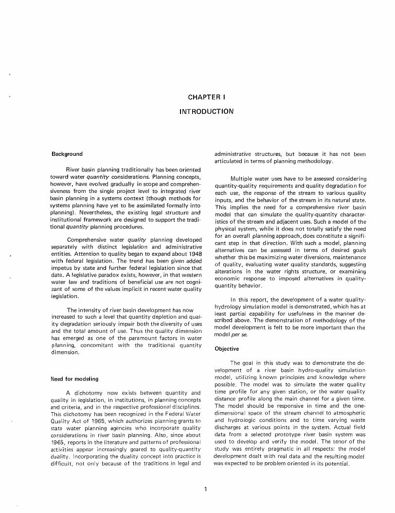
Background

River basin planning traditionally has been oriented toward water quantity considerations. Planning concepts, however, have evolved gradually in scope and comprehen­siveness from the single project level to integrated river basin planning in a systems context (though methods for systems planning have yet to be assimilated formally into planning). Nevertheless, the existing legal structure and institutional framework are designed to support the tradi­tional quantity planning procedures.

Comprehensive water quality planning developed separately with distinct legislation and administrative entities. Attention to quality began to expand about 1948 with federal legislation. The trend has been given added impetus by state and further federal legislation since that date. A legislative paradox exists, however, in that western water law and traditions of beneficial use are not cogni­zant of some of the values implicit in recent water quality legislation.

The intensity of river basin development has now increased to such a level that quantity depletion and qual­ity degradation seriously impair both the diversity of uses and the total amount of use. Thus the quality dimension has emerged as one of the paramou nt factors in water p lanning, concomitant with the trad itional quantity dimension.

I\leed for model ing

A dichotomy now exists between quantity and quality in legislation, in institutions, in planning concepts and criteria, and in the respective professional disciplines. This dichotomy has been recognized in the Federai Water Qual ity Act of 1965, which authorizes planning grants to state water planning agencies who incorporate quality considerations in river basin planning. Also, since about 1965, reports in the literature and patterns of professional activities appear increasingly geared to quality-quantity duality. Incorporating the duality concept into practice is difficult, not only because of the traditions in legal and

administrative structures, but because it has not been articulated in terms of planning methodology.

Multiple water uses have to be assessed considering quantity-quality requirements and quality degradation for each use, the response of the stream to various quality inputs, and the behavior of the stream in its natural state. This implies the need for a comprehensive river basin model that can simulate the quality-quantity character­istics of the stream and adjacent uses. Such a model of the physical system, while it does not totally satisfy the need for an overall planning approach, does constitute a signifi­cant step in that direction. With such a model, planning alternatives can be assessed in terms of desired goals whether this be maximizing water diversions, maintenance of quality, evaluating water quality standards, suggesting alterations in the water rights structure, or examining economic response to imposed alternatives in quality­quantity behavior.

In th is report, the development of a water quality­hydrology simulation model is demonstrated, which has at least partial capability for usefulness in the manner de­scribed above. The demonstration of methodology of the model development is felt to be more important than the model per se.

Objective

The goal in this study was to demonstrate the de­velopment of a river basin hydro-quality simu lation model, utilizing known principles and knowledge where possible. The model was to simu late the water quality time profile for any given station, or the water quality distance profile along the main channel for a given time. The model should be responsive in time and the one­dimensional space of the stream channel to atmospheric and hydrologic conditions and to time varying waste discharges at various points in the system. Actual field data from a selected prototype river basin system was used to develop and verify the model. The tenor of the study was entirely pragmatic in a" respects: the model development dealt with real data and the resulting model was expected to be problem oriented in its potential.

Scope

Although the model is developed for a specific prototype system, the Little Bear River in this case, the approach, the methods, and the conceptual framework can be transferable to other systems, hopefu lIy with less effort than needed for the original study. The model is deterministic in nature. The stochastic nature of some in­puts such as atmospheric temperature and basin inflows has not been sirnu lated, ttwuqh tht~ Jll()d(~1 could accom­modate this feature.

The qUill ity parameters st!lm:[t~d for simuldtion in­clude specific electrical conductivity, diss()lvt~d oxygen, Jnd temperdture, BOD, alHi coliform Ullllll. Althou9h not d complete definition of watm qllali t y, ttwS(~ iJarameters: (1) dre reasonably reiJreSt~IHdtivt~ 01 the rdll!Jt! ill cvpes of water quality parameters, with rt!Spt~ct to strt~alll lwhdvior and nature of the parameter; (2) an! si!lllificalll nWdsures

2

of water quality, and (3) could be measured. Item (1) is particu larly important because a pattern of modeling can be established which is reasonably representative of im­portant water quality parameters. The modeling effort for the latter two parameters, BOD and coliform count, was not as exhaustive as for the first three, primarily because of time limitations and the less certain promise of success.

The development of equations for individual water quality parameters is not a primary goal of this study as long as reaso!,)ably adequate relationships are available. Therefore, when previously developed equations satis­factorily represented the behavior of a given parameter (as determined by their application to data gathered from the prototype system) they were incorporated into the overall river basin simulation model, as individual parameter sub­models. When available relationships did not appear to fit the prototype data, or if no suitable submodel was found, a relationship was developed if this was feasible.

CHAPTER II

PLAN OF OPERATIOI\l

COIlSpoctliS

V ('I Y tjl tlssly, Ilw development of the water quality SIIlllll.11 f( 111 -Ill(ldd consisted of defining the following

(~II~lllt' III S_

I_ Tlw prototype system. The river basin system was defilH'd with n~spect to all characteristics that might reldtl~ 10 the ljlldlity-quantity response in the main stream. The process included obtaining all relevant hydrologic data, delineating agricultural patterns, and defining waste inputs. III additioll, a monitoring program was established to measure surface inflows and outflows, climatological data, alld to sample water quality at important spatial node points at regular time intervals.

2. Parameter simulation. For each of the water quality parameters simulated, relationships from the liter­ature were utilized insofar as possible. The first year data from the prototype system were used to determine the most suitable equations and to define coefficients.

3. Hydrology submodel. The system hydrology was developed as a model responsive to inputs of surface in­flow and capable of yield ing any flow quantities (ground­water or surface) required for simulation of the water quality parameters.

4. Simulation algorithm. Each of the submodels was programmed in Fortran I V for incorporation into an algorithm for simu lating the time and space behavior of each parameter. This algorithm comprises the hydro­quality simulation model.

The prototype system

The Little Bear River basin at the southern extrem­ity of Cache Valley in northern Utah was selected as the

prototype from wh ich data were obtained for model de­velopment and verification. This basin was chosen be­cause: (1) its size and definition permitted the meeting of data requirements; (2) problems of nominal magnitude exist in the basin, and its cultural characteristics, hydro­logic features, and values of concern were of sufficient

3

variety to be of interest without anyone dominating the system; (3) it is reasonably close to Logan.

This basin, described in detail in Appendix A, is a typical intermountain valley, encompassing some 245 square miles. The topography ranges from rolling to rug­ged with elevations from 4500 feet to 9445 (Figure A-1). The portion of the basin referred to herein as the valley floor generally lies below the 5000 ft. contour, with the area above this elevation being designated as the water­shed.

The climate of the region is temperate and semi­arid, with well defined seasons. Monthly averages of mean daily temperature range from 21°F in January to 73°F in July at the nearby Logan, USU weather station (Figure A-3). Normal annual precipitation at this station is 16.6 inches per year, occurring primarily as winter snowfall and spring rains (Figure A-4). Figure A-5 shows the orographic influence of the mountains on the areal distribution of precipitation. Normal annual runoff is on the order of 50,000 acre feet per year, with the bulk of the runoff taking place during the spring snow melt period (Figure A-6).

The project area is predominantly agricultural, containing about 13,000 acres that are farmed, of which 8,100 acres are irrigated. Hay, grain, pasture, and corn are the principal crops. I ndustries include a cheese plant, two meat packing plants, a rendering plant and a commercial fish farm. The streams, reservoirs, and mountain areas of the system sustain considerable recreational activity, con­sisting of trout fish ing in the stream and the two reser­voirs, and boating and water skiing at Hyrum Reservoir, Hyrum State Park. The watershed area and flood plain are heavily utilized for domestic livestock grazing. Tables A-l and A-2 show estimated numbers and time distribution of grazing units on these areas.

Factors contributing to the organic, chemical, and thermal degradation of the water quality of this system include natural inputs, livestock grazing, return flows from agricultural irrigation, industry, municipal waste dis­charges, garbage dumps, and recreation. These inputs are both discrete and diffuse in nature.

The city of Wellsville discharges untreated domestic sewage from about one third of its 1500 population, com­bined with the liquid waste from the cheese factory lo­cated there, in a small stream that is tributary to the Little Bear River just below Wellsville. The discharge from the trout farm is the only other discrete input. The other two basin communities (Hyrum and Paradise) and their rural residents employ septic tanks and leach fields for waste disposal. Each of these towns maintains an open garbage dump on the bluffs along the river.

The data collection network established on or near the Little Bear River system is composed of eight stream­flow gaging stations, one reservoir stage observation point, five weather stations, 17 weekly water qual ity sampl ing stations and two continuous quality monitoring stations. The stream gaging network was designed to account for all surface flows into and out of the basin, plus changes in the main channel. The water quality monitoring system was set up to account for all discrete inputs in the main channel, and important changes in the channel such as reservoirs. These networks are described in detail in Appendix B. Locations and periods of record are shown in Figures B-1 and B-2 and Tables B-1 through B-4.

Resolution

Resolution has to do with the amount of detail in time or space which the model will provide. This must be consistent with needs and with funds of those applying the model. In this model, two levels of time resolution are used -the month and the hour. Th is was necessary to adequately describe dissolved oxygen and temperature, since they exhibit diurnal variations whose characteristics changed monthly. For electrical conductivity the month was an adequate time increment.

For the space resolution, the main channel and its immediate large tributaries was focused on with respect to water use. Thus the water quality submodels are oriented about the stream channel. The channel was divided into reaches with node points at the significant changes in the channel. This isolates reservoirs and marks discrete inputs into the main channel.

These resolutions in time and space were consistent with the pragmatic tenor of the study-fine enough to be useful but not so fine as to constitute an unwise expendi­ture of funds.

Submodels

A submodel is defined here as the set of equations and coordinating statements that simulate the behavior of a particu lar parameter in time and space. The parameters for which submodels were synthesized in this study are: (1) hydrology, (2) electrical conductivity, (3) tempera­ture, and (4) dissolved oxygen. Attempts to develop BOD and coliform submodels were less successful.

4

Submodel equations were taken from the literature if they existed and were suitable. Considerations used in determining suitability included: (1) ease, feasibility, and cost of data procurement, (2) reliability in simulations using project data, and (3) mathematical complexity. When mathematical equations for phemonena behavior do not exist, such as in diurnal dissolved oxygen and tem­perature simulation, they were project-developed using project data. Pragmatism was the underlying philosophy, whether the equations ultimately used were project­develo ped or· extracted from the I iterature and whether empirical or rational.

Equation coefficients and constants were estab­I ished by regression analysis of first-year field data or by adjusting coefficients such that submodel output cor­responded with field measurements. The latter approach was used almost exclusively in the hydrology submodel verification.

Sophistication in theory is justified herein only as (1) data requirements are realistic and obtainable, and (2) the results are commensurate with pragmatic objectives.

I n each submodel, the solution consists of two basic parts: (1) the time variation in the respective quality para­meters for the incoming flow components for each reach, and (2) the changes in the quality parameter along the reach. For each parameter, the alternative modeling approaches are reviewed, the modeling assumptions are outlined, the approach selected is justified in terms of field data from the Little Bear River, and the simu lation algorithm is summarized. Thus, the phenomenological behavior of each component is described in terms of suit­able mathematical descriptions and the logic for utilizing those mathematical descriptions in parameter simu lation.

Simulation algorithm

The system control model is a set of statements designed to: (1) control the manner of operation of the ind ividual submodels, (2) specify the inputs needed to operate the submodels, and (3) provide the necessary

feedback between submodels. The Fortran IV program that accomplishes this is given the name WAQUAL. This program contains each of the five submodels.

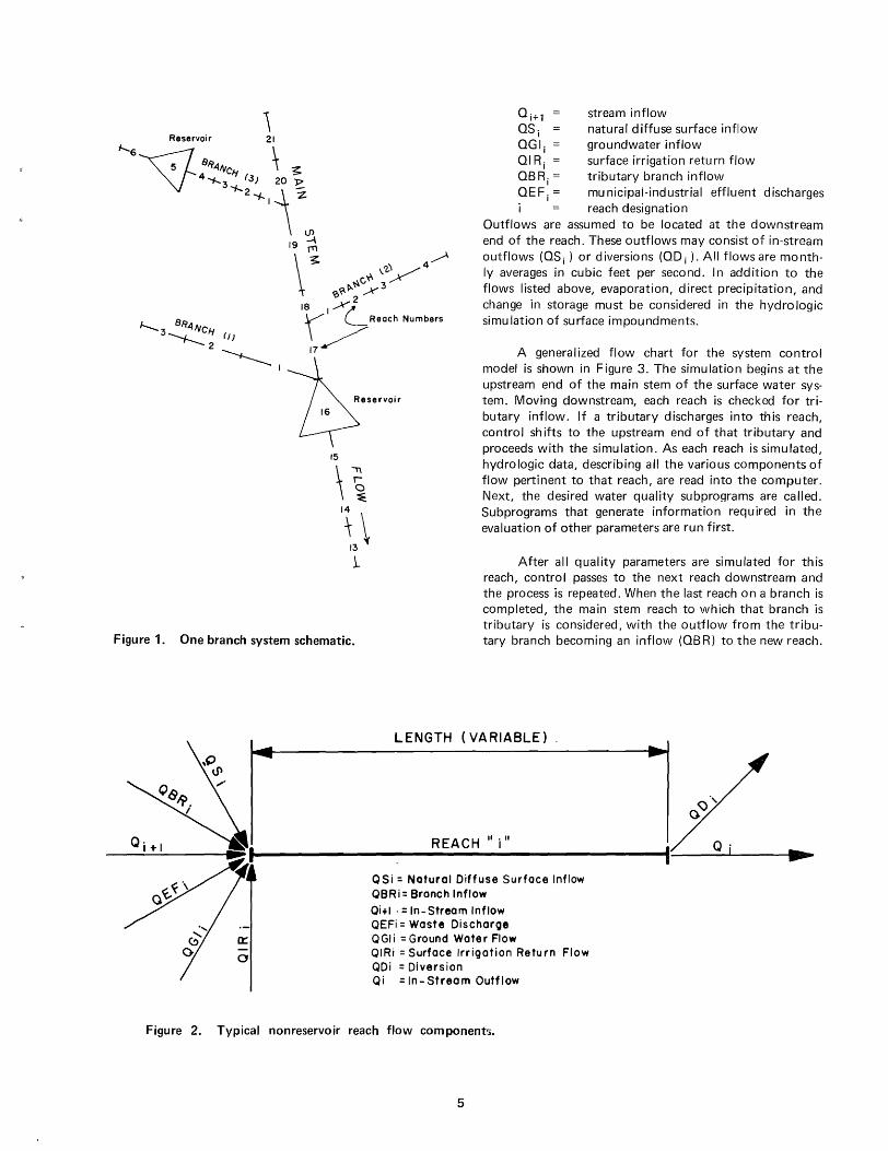
The system control model embodies the river basin configuration shown in Figure 1, consisting of the main stem and any number of tributaries. The main stem and tributaries are divided into numbered reaches, ascending numerically in the upstream direction. Reservoirs may be included also.

I nputs to the typical nonreservoir reach, as sketched in Figure 2, are considered to be concentrated at the up­stream end of the reach and may consist of anyone or more of the following:

Reservoir 21

~6v \ 5 81T4101CIj "\-;

4"""1-..3-..,.....~J) 120 ~ """1-.

1 Z

lJ)

~

Qj+1 stream inflow QS j natural diffuse surface inflow QG I j groundwater inflow QI Rj surface irrigation return flow QB Rj = tributary branch inflow QE F j = mu nicipal-industrial effluent discharges i reach designation

'\~ '2.'1 ............... .4 ~ \......x-

~\).~~3

Outflows are assumed to be located at the downstream end of the reach. These outflows may consist of in-stream outflows (QS j ) or diversions (QD j ). All flows are month­ly averages in cubic feet per second. In addition to the flows listed above, evaporation, direct precipitation, and change in storage must be considered in the hydrologic simulation of surface impoundments.

'¢ 2 18 l.x? r ~ Reach Numbers

17~

Figure 1. One branch system schematic.

A generalized flow chart for the system control model is shown in Figure 3. The simu lation begins at the upstream end of the main stem of the surface water sys­tem. Moving downstream, each reach is checked for tri­butary inflow. If a tributary discharges into this reach, control sh ifts to the upstream end of that tributary and proceeds with the simulation. As each reach is simulated, hydrologic data, describing all the various components of flow pertinent to that reach, are read into the computer. Next, the desired water quality subprograms are called. Subprograms that generate information required in the evaluation of other parameters are run first.

After all quality parameters are simulated for this reach, control passes to the next reach downstream and the process is repeated. When the last reach on a branch is completed, the main stem reach to which that branch is tributary is considered, with the outflow from the tribu­tary branch becoming an inflow (QBR) to the new reach.

LENGTH (VA RIABLE) ,

REACH" i"

QSi,: Noturol Diffuse Surface Inflow QBRi = Branch Inflow Oi+1 . = In-Stream Inflow OEFi = Waste Discharge QGIi ': Ground Water Flow QIRi = Surface Irrigation Return Flow QDi = Diversion Qi = In - Stream Outflow

Figure 2. Typical nonreservoir reach flow component'.).

5

INPUT SIMULATION CONTROL DATA

Start With Uppermost Reach On The Main Stem.

Yes

~ __________ -r ______________ ~~ __ ~~~ ______ ~GoToUppermost Reach On This

Procede To The Next Branch

Go To The Next Reach.

Start Agoin At The

Uppermost Reach On

The Moin Stem For The Next Month.

Start AQain At The Up-rmolt Reach On The

Main Stem For The Fi rst Month Of The Next Year.

Go To The Next Reach.

No

No

No

No

No

Compute E C, Temperature And D. O.

yes

Output Monthly Space Profiles And Repeated Diurnal Pot-femsAt Controt Points.

Yes

Output Annual Time Profile At Control Points.

9 Stop

Figure 3. System control model simulation procedure.

6

Branch.

After the last reach on the main stem has been simu­lated, monthly spatial profiles are printed out in tabular form as shown in Appendix E. These profiles list monthly average values for flow rate, conductivity, temperature, dissolved oxygen, BOD, and percent D.O. saturation at both ends of every reach, as well as the magnitude of these parameters in all hydrologic inputs to the reach. If diurnal representation of stream temperature and/or dis­solved oxygen is requested, the predicted diurnal varia-

7

tions in temperature, dissolved oxygen, and percent D.O. saturation are printed out for each predesignated control point.

This procedure is followed until the entire period of simulation has been covered. In addition, annual time pro­files of rate of flow, conductivity, temperature, D.O., percent D.O. saturation, and BOD are printed out for predesignated control points at the end of each year of simulation.

CHAPTER III

THE HYDROLOGYSUBMODEL

The hydrologic mass-balance submodel is a central component of the hydro-quality simulation model devel­oped during the project. The hydrology submodel simu­lates the area through which the river flows and provides the qual ity submodels with the flow components that occur as tributary items along the channel. The criteria that had to be satisfied by the submodel were:

1. It had to simu late the hydrologic mass balance of a typical Utah river basin utilizing monthly climatological data, and to yield monthly streamflow data that could be input to the water quality submodels under concurrent development.

2. It had to identify and rapid Iy evaluate the hydrologic effect of alternative conditions that might or could be imposed upon the study area.

The equation of continuity,

Output = Input - Changes in Storage ... (1)

applied to the mass of water flowing within and through the geographic boundaries of the area provides the con­ceptual framework for the hydrology submodel. The size of the area to which this submodel may be satisfactorily applied is primarily limited by the degree of spatial resolu­tion required to meet the overall objectives of a particular simulation effort.

For this study, system hydrologic inputs consist of precipitation (PR EC), measured stream inflow in the main channel (R I F), measured surface imports (SI MP), and un­measured surface and subsurface inflow (TI F). The crop­land diversions (CD), reservoir storage (R ES), municipal and industrial diversions (EM I D) net consumptive munici­pal and industrial use (EM I), pumped water (PW), surface exports (EXPO), and air temperature (TEMP) are other variab les suppl ied as input data to the model.

The system outputs consisted of reservoir evapora­tion (EVAP), cropland consumptive use (ACU), wetland consumptive use (AWLCU), surface exports (EXPO),

9

municipal and industrial consumptive use (EM I), surface outflow (SOF), and subsurface outflow (GWOF).

The hydrology submodel accounts for monthly changes in: reservoir storage (DRES), cropland soil moisture storage (ASMS), interflow groundwater storage (SGW), wetland soils moisture storage (AWLSM), and groundwater storage (DELGW).

The outflow values are obtained by routing and storing the input quantities through the four principal components of the system which are:

1. Surface water reservoirs 2. Cropland area 3. I nterflow routing and groundwater storage 4. Wetland area

A schematic diagram of the hydrology submodel is shown in Figure 4 and a macro flow chart is included as Figure 5. A micro flow chart, computer program notation, data card preparation, user instructions, and problem solutions are given in Appendix G.

Model structure

I n any simulation effort, each component of Equa­tion 1 must be carefully selected and evaluated. The vari­ous components appearing in Figures 4 and 5 are de­scribed in the following paragraphs.

Precipitation

Precipitation IS Important to the surface reservoir, cropland, and wetland components of the submodel. Its allocation to rain or snow storage is achieved by com­paring the mean monthly air temperature with a snow threshold temperature. Any precipitation occurring when the temperature is less than the threshold temperature is accumulated in snow storage and routed through a snow­melt equation of the form

SM k SeT - T ) sm a sm

.... (2)

o

a:: w f­<l: ~

o w Q. ~ :::l Q.

PUMP

INTER

WETLAND ADDITION TO GROIINnwIlT~~

,--r-,.......r-~

( WETLAND ")

( PRECIPITATION r ~::~~~1

S

Figure 4. Hydrologic model schematic of a water resource system.

o z <l: ...J f­w ~

o f-

>­...J Q. Q. :::l en

~ o ...J LL a:: w f­~

AGRICUL TUR ilL

INTERFLOW

SUPPLY TO SURFACE

//I~ WETLAND

SURFACE

M 81

RETURN FLOW

;:::::=m:=~:]'~. EXPORT S

WETLAND CONSUMPTIVE

) USE J

AVAILABLE

WATER

r ~ '):;l RESERVOIR

~II'I.J PRECIPITATION

IIIII

SURFAC~ g WATER Jl RESERVOIRS

AND

INDUSTRIAL CONSUMPTIVE USE

RESERVOIR

SCHEMATIC DIAGRAM OF HYDROLOGIC

MASS BALANCE MODEL

ALH-1968

I READ OUTPUT LABEL CARDS, PARAMETER 1 INITIALIZATION CARDS AND INPUT DATA

CALCULATE POTENTIAL EVAPOTRANSPIRATION BY THE MODIFIED BLANEY-CRIDDLE METHOD FOR RESERVOIRS, CROPLAND AND WETLAND

ACCUMULATE SNOW STORAGE AND CALCULATE SNOW MELT ON THE CROPLAND AND WETLAND (USE SNOW MELT MODEL)

RILEY

ROUTE CROPLAND DIVERSIONS THROUGH ROOT ZONE SOIL MOISTURE MODEL TO OBTAIN ACTUAL CROP-LAND CONSUMPTI VE USE, SURFACE AND GROUNDWATER RETURN FLOW AND DEEP PERCOLATION

ROUTE DEEP PERCOLATION, CROPLAND GROUNDWATER RETURN FLOW AND GROUNDWATER INFLOW THROUGH INTERFLOW STORAGE WHICH HAS OPTIONALLY SPEC-IFIED FIXED DELAYS SUPERIMPOSED UPON AN EXPON-ENTIAL DECAY STORAGE FUNCTION TO YIELD INTERFLOW ADDITION TO GROUNDWATER AND INTERFLOW ADDITION TO SURFACE WATER

CALCULATE AND ROUTE WETLAND SUPPLY THROUGH WETLAND SOIL MOISTURE MODEL TO YIELD ACTUAL WETLAND CONSUMPTI VE USE AND SURFACE AND GROUNDWATER RESIDUALS

CALCULATE TOTAL USEABLE WATER BY SUMMING ALL SURFACE INPUTS AND RETURN FLOWS; SURFACE OUT-FLOW BY SUBRACTING ALL DIVERSIONS FROM TOTAL USEABLE WATER AND TOTAL OUTFLOW AS THE RESIDUAL OF THE MASS BALANCE COMPUTATIONS

CALCULATE GROUNDWATER OUTFLOW AND CHANGE IN GROUNDWATER STORAGE BY APPLYING THE CONTINUITY EQUATION TO TOTAL OUTFLOW, SURFACE OUTFLOW AND ADDITION TO GROUNDWATER

,Ir

SELECT DESIRED OUTPUT OPl'ION AND LIST ACCORDINGLY MONTHLY VALUES OF:

1. DETAILED MASS BALANCE WATER BUDGET IN ACRE-FT 2. SUMMARY OF OUTFLOW ITEMS IN ACRE-FT OR 3. MAIN STEM SURFACE COMPONENTS USED AS INPUTS

FOR THE WATER QUALITY MODEL IN CFS OR 4. SUM OF SQUARED DEVIATIONS BETWEEN MODEL AND

OBSERVED HYDROGRAPH--(ITERATION MODE OF HYDRO)

SEE APPENDIX G FOR DETAILED INSTRUCTIONS CONCERNING MODELING AND OUTPUT OPTIONS.

Figure 5. Flow chart for hydro model,

OR

11

in which

SM snowmelt ksm a constant S accumulated snow storage through the

end of the month T a mean monthly air temperature in de­

grees F T sm sn ow me I t threshold temperature in

degrees F The rain and snowmelt are then routed through the crop­land and wetland components of the system.

Consumptive use

The potential consumptive use by cropland and wet­land and the potential evaporation from the reservoirs are obtained by using the method developed by Blaney and Criddle (1950) and modified by the U.S. Soil Conserva­tion Service (1964). The basic Blaney-Criddle equation is:

u kf ........ (3)

in which u the monthly consumptive use of the

crop in inches k an empirically determined consumptive

use crop coefficient f a monthly consumptive use factor de­

fined as the product of the mean monthly air temperature and the monthly proportion of daylight hours of the year (p)

The Soil Conservation Service modification consists of evaluating k as the product of two other coefficients k t and kc , where k t is a climatic coefficient related to the mean monthly air temperature by the equation k t = 0.0173 Ta - 0.314 and k c is a coefficient reflecting the growth stage of the crop. Crop growth stage curves have been developed by the Soil Conservation Service (1964) for a variety of crops and phreatophytes.

Upon substituting the equivalent expressions for k and f, Equation 3 becomes:

u k p(0.0173 T 2 - 0.314 T) . (4) c a a

where all symbols are as defined previously.

The total potential consumptive use by the cropland and that by the wetland are obtained as the sum of the potential consumptive use by all crops and by all phreato­phytes, respectively. These amounts are used as depletive factors in the routing and storage phases of the cropland and wetland components of the submodel. Potential water surface evaporation is treated similarly within the reser­voir component of the system. The actual consumptive

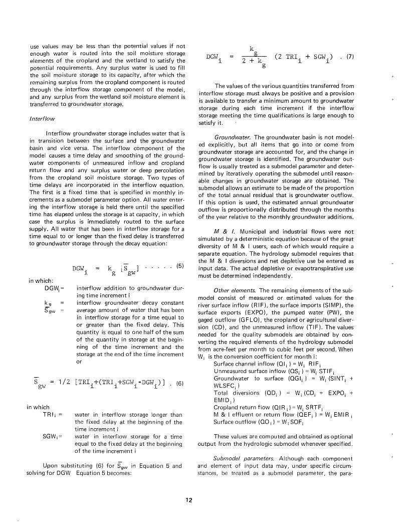
use values may be less than the potential values if not enough water is routed into the soil moisture storage elements of the cropland and the wetland to satisfy the potential requirements. Any surplus water is used to fill the soil moisture storage to its capacity, after which the remaining surplus from the cropland component is routed through the interflow storage component of the model, and any surplus from the wetland soil moisture element is transferred to groundwater storage.

Interflow

I nterflow groundwater storage includes water that is in transition between the surface and the groundwater basin and vice versa. The interflow component of the model causes a time delay and smoothing of the ground­water components of unmeasured inflow and cropland return flow and any surplus water or deep percolation from the cropland soil moisture storage. Two types of time delays are incorporated in the interflow equation. The first is a fixed time that is specified in monthly in­crements as a submodel parameter option. All water enter­ing the interflow storage is held there until the specified time has elapsed unless the sto~age is at capacity, in which case the surplus is immediately routed to the surface supply. All water that has been in interflow storage for a time equal to or longer than the fixed delay is transferred to groundwater storage through the decay equation:

in which: DGWj=

DGW. 1

..... (5)

interflow addition to groundwater dur­ing time increment i interflow groundwater decay constant average amount of water that has been in interflow storage for a time equal to or greater than the fixed delay. This quantity is equal to one half of the sum of the quantity in storage at the begin­ning of the time increment and the storage at the end of the time increment or

S gw 1/2 [TRI.+(TRI.+SGW.-DGW.)]. (6)

111 1

in which TRlj water in interflow storage longer than

the fixed delay at the beginning of the time increm811t i water in interflow storage for a time equal to the fixed delay at the beginning of the time increment i

Upon substituting (6) for Sgw in Equation 5 and solving for DGW Equation 5 becomes:

12

DGW. 1

k _.....loogl--- (2 TRI. + SGW.) . (7) 2 + k 1 1 g

The values of the various quantities transferred from interflow storage must always be positive and a provision is available to transfer a minimum amount to groundwater storage during each time increment if the interflow storage meeting the time qualifications is large enough to satisfy it.

Groundwater. The groundwater basin is not model­ed explicitly, but all items that go into or come from groundwater storage are accounted for, and the change in groundwater storage is identified. The groundwater out­flow is usually treated as a submodel parameter and deter­mined by iteratively operating the submodel until reason­able changes in groundwater storage are obtained. The submodel allows an estimate to be made of the proportion of the total annual residual that is groundwater outflow. If this option is used, the estimated annual groundwater outflow is proportionally distributed through the months of the year relative to the monthly groundwater additions.

M & I. Municipal and industrial flows were not simulated by a deterministic equation because of the great diversity of M & I users, each of which would require a separate equation. The hydrology submodel requires that the M & I diversions and net depletive use be entered as input data. The actual depletive or evapotranspirative use must be determined independently.

Other elements. The remaining elements of the sub­model consist of measured or estimated values for the river surface inflow (RIF), the surface imports (SIMP), the surface exports (EXPO), the pumped water (PW), the gaged outflow (GFLO), the cropland or agricultural diver­sion (CD), and the unmeasured inflow (TIF). The values needed for the quality submodels are obtained by con­verting the required elements of the hydrology submodel from acre-feet per month to cubic feet per second. When W j is the conversion coefficient for month i:

Surface channel inflow (Qlj) = Wj RIF j Unmeasured surface inflow (QS j ) = Wj STIF j Groundwater to surface (QGlj) = Wj (SINT j + WLSFC j ) Total diversions (QDj) = Wj (CD j + EXPO j + EMID j ) Cropland return flow (QI R j) = Wj SRTF j M & I effluent or return flow (QEFj ) = Wj EMI R j Surface outflow (QO j ) = W j SOF j

These values are computed and obtained as optional output from the hydrologic submodel whenever specified.

Submodel parameters. Although each component and element of input data may, under specific circum­stances, be treated as a submodel parameter, the para-

meters ordinarily consist of coefficients of routing func­tions, threshold values for selective routing, storage capacities and boundary conditions of the various sub­model components. These parameters are explained in detail in the user instructions contained in Appendix G.

Stochastic aspects

The stochastic aspect of the hydrology submodel can be achieved by inputing historical data for a long period of years and then calcu lating the mean and stand­ard deviation of every element in the resulting mass budgets. The entire output resu Iting from the historical data input is available for either calculating higher order moments to more fully characterize the distribution or rank ing the data to obtain the empirical probability d istri­butions.

The above method for obtain ing stochastic informa­tion was selected because of major limitations in the other two methods that were considered. The first alternative method (inputing data, all having the same probability level of occurrence that had been derived from probability analyses) was rejected because of no satisfactory method for handling the interactions between the probability distributions of the various input elements such as pre­cipitation, temperature, and streamflow.

The second alternative method evaluated used ran­dom process generating techniques to supply the input data to the model. Th is method was rejected because when these techniques were applied to Utah streams, they failed to synthesize realistic sequences of extreme events. Since these are the critical values about wh ich information is needed, the validity of the method was questionable. A study which supports th is conclusion is reported by Jeppson and Clyde (1969). Mandelbrot and Wallis (1968) have observed the same limitation and are working on techniques that may eventually improve the situation.

Two versions of the hydrology submodel were pro­grammed (Appendix G). The same input data are used by both computer programs supplied in the same format. The! first program (HYDRO) provides only one year of simula­tion but has the capability of iterating along many of the model parameters, which is helpful during the validation process. The other program (BUDGET) does not have the iteration capability but allows simu lation of up to 30 years and provides a mean mass balance budget and stand­ard deviation budget.

Hydrology modeling of the study area

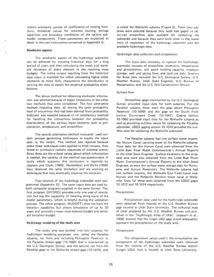
The study area was divided into two subareas for hydrologic modeling purposes: one, called the Paradise subarea, ran from and including Porcupine Reservoir to the Paradise stream gage (10-1060) that is maintained by the U.S. Geological Survey; and the second, ran from the Parad ise gage to the Wellsville stream gage (10-1076), and

13

is called the Wellsville subarea (Figure 6). These two ~ub areas were selected because they both had gaged or ob served streamflow data available for validating the submodel and because they were both close to the lower limit of resolution of the hydrology submodel and the available hydrologic data.

Hydrologic data collection and compilation

The input data necessary to operate the hydrologic subniodel consists of streamflow, diversions, temperature and precipitation, soil water holding capacity, reservoir storage, well and spring flow, and land use data. Source~ for these data included the U.S. Geological Survey, U.S. Weather Bureau, Utah State Engineer, U.S. Bureau of Reclamation, and the U.S. Soil Conservation Service.

Surface flow

Streamflow gages maintained by the U.S. Geological Survey provided input data for both subareas. For the Paradise subarea these were the gage above Porcupine Reservoir (10-1049) and the gage on the South Fork below Davenport Creek (10-1047). Gaging station 10-1060 provided input data for the Wellsville subarea as well as providing outflow values for validating the Paradise submodel. USGS gaging station 10-1076 provided the out­flow data for validating the Wellsville submodel.

The Paradise subarea had one surface water export, the Hyrum Canal, carrying water to the Wellsville subarea. Flow data for the Hyrum Canal were obtained from the Little Bear River Water Commissioner's Annual Reports to the Utah State Engineer. Surface diversions to the crop­land area were also obtained from the Little Bear River Water Commissioner's Annual Reports to the Utah State Engineer, as were the surface water storage data for Porcu­pine and Hyrum' Reservoirs. The Wellsville subarea had two surface exports, the Wellsville East Field Canal near Hyrum and the Wellsville Mendon lower canal at Wells­ville. Data for these were obtained from the USGS gages 10-1072 and 10-1074 respectively.

Precipitation

Precipitation data used for the hydrologic submodel were obtained from records of the U.S. Weather Bureau gage located at Utah State University. The isohyetal map of Utah prepared by the U.S. Weather Bureau and pub­lished in the "Hydrologic Atlas of Utah" (Jeppson et al., 1968) showed that the Logan USU gage would adequately represent the precipitation on the study area.

Temperature

The temperature values used in the consumptive use component of the hydrologic submodel were obtained from the records of the U.S. Weather Bureau station (Logan USU) that is located at Utah State University.

...10

~

Figure 6. Two hydrologic subareas.

LITTLE BEAR RIVER STUDY AREA o 2 3 MILES II .. ,

, -~ ·X

~J2~~;C::~ "I.",",

.) L" ~ I :.Y--'

•

~ USGS GAGING STATION

o

I J -I 046 South Fo rk Little Bear River I J -I 047 Little Bear River blw Davenport Cr. I J -I049 East Fork Little Bear River 1') -1 060 Little Bear River nr Paradise 1) -1 0 70 Hyrum Reservoir nr Hyrum l J -I 0 72 Wellsville East Field Canal I J- 1074 Wellsvil Ie-Mendon Lower Canal I J -1 0 75 Little Bear River nr Hyrum 1: -1 0 76 Little Bear River at Wellsville

I 2

~~ I~C IPAL CANAL DIVERSIONS Hiohline Canal H'I~um Canal

C Paradi se Canal Lofthouse Ditch ~hit e ' s Tr out Far m Di version ',e I I s v il l e E as t Fie 1 d Can a 1 ,.ellsville-Mendon Upper (Pump) ~ellsville-Mendon L O~/er Canal ~ y r~~ Lit t le Feeder Ditch Carl e y Di t ch

Canal

DE;ELOPED LAND I N WELLS VILLE SUBAREA

DEJE LOPED LAND IN PARADISE SUBAREA

wA TE RSH ED AR EA TRIBUTARY TO WELLSVILLE SUBAREA

WATERSHED AREA TRIBUTARY TO PARADISE SUBARE A

These data were used because a comparison of the mean monthly maximum and minimum temperatures at Logan USU and at the E. K. Israelsen farm near Paradise (Figure 7) indicated that the USU data were sufficiently represen­tative of the model area to be used without adjustment.

.c ClI

;;

• · :a

100

80

ClI 60 i

~ . 40 ~ • Monthly maximum temperature.

:! Z ~

" Monthly minimum temperature.

• Q.

E {!. 20

o

y. 0 Monthly average temperature.

20 40 60 80 100

Temp erature ( 0 F ) at Logan U SU.

Figure 7. Temperature comparisons-Utah State Univer­sity Climatological Station and E. K. Israelsen Farm in Hyrum.

Land use

There are eight crop categories; data for determining acreages were obtained from the report "Water Related Land Use in the Bear River Drainage Area" by Haws (1969). Data on the five classes of phreatophyte uses in the wetlands and the surface water evaporating from the two reservoirs (Table 1) were also obtained from Haws (1969).

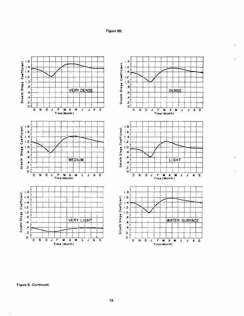
The growth stage coefficient curves for the crops, phreatophytes and water surface were modifications of those developed by the Soil Conservation Service (1964) for California. The information contained in Technical Publication No.8 of the Utah State Engineer (1962) was utilized in effecting the modifications. The growth stage coefficient curves developed for use in the submodel are given in Figure 8.

Unmeasured or tributary inflow

T he first values used for the unmeasured or tributary inflow were those obtained from the mean annual iso-runoff map in the "Hydrologic Atlas of Utah"

15

(Jeppson et aI., 1969). The map shows runoff distributed through the months and proportioned by the year at the same level as the sum of the two virgin gaged inflows to the Paradise subarea. Model validation could not be achieved with these data. The values that were finally used were obtained by treating unmeasured inflow as a model parameter until validation was achieved. The resultant values were then extended to obtain monthly propor­tionality coefficients for relating unmeasured inflow to measured inflow. The measured inflow to the Paradise subarea was used as the basis for estimating the unmea­sured inflow in both subareas because it represented virgin flow conditions .

Municipal and industrial use

Apart from agricultural uses which were expl icitly modeled by the cropland component of the submodel, the only significant M & I diversion in the Paradise subarea consisted of a trout farm. Input data for this element of the model were derived from actual measurements of the diversion and return flows where these occurred within the system. The Wellsville subarea had one effluent point (the Wellsville stream) which was also measured and thus provided the input data for the M & I component of that subarea.

Hydrology submodel results

After collecting the records from various sources, the data were prepared for input to the computer. As the validation process proceeded, some of the basic data were found to be in error and thus had to be changed. How­ever, the process by which the errors were discovered aided materially in understanding the systems.

The general procedure followed in validating the hydrology submodel was to first achieve a balance in the annual figures and then work on the monthly distribution. By iteratively operating the submodel, validation was achieved (Figure 7). Figure 9 gives a comparison between the gaged and computed outflow for both subareas for the water years 1967 and 1968. A summary of the flow values generated for the water quality submodels is given in Table 2. A complete listing of the input data, water budgets, consumptive use calculations, and water quality hydrologic data is included in Appendix G.

Hydraulic considerations

I n-transit changes in water quality often depend directly upon the mechanics of flow in the stream. The reaeration coefficient of the dissolved oxygen model is dependent upon velocity and depth of flow; the rate of temperature change depends upon, among other things, the surface area of the stream; and time of travel through a reach is determined by the velocity of flow. Because of these dependencies, depth and velocity of flow and sur­face width must be defined.

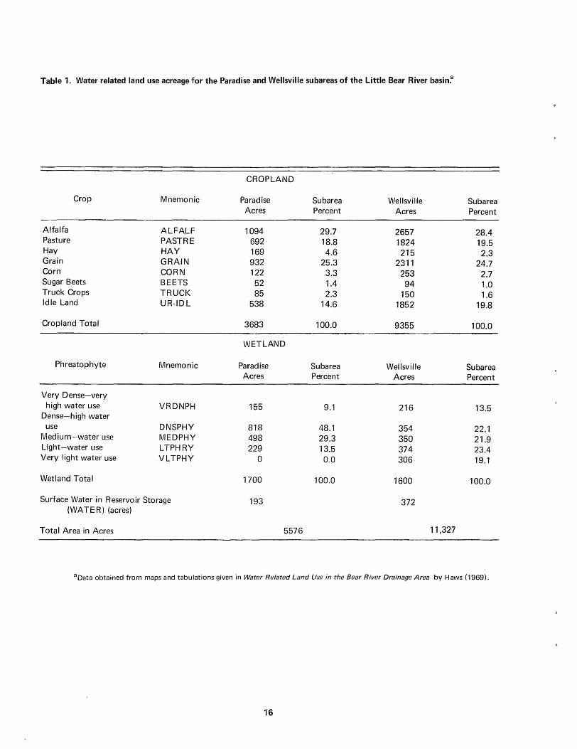
Table 1. Water related land use acreage for the Paradise and Wellsville subareas of the Little Bear River basin~

CROPLAI\ID

Crop Mnemonic Paradise Subarea Wellsville Subarea Acres Percent Acres Percent

Alfalfa ALFALF 1094 29.7 2657 28.4 Pasture PASTRE 692 18.8 1824 19.5 Hay HAY 169 4.6 215 2.3 Grain GRAIN 932 25.3 2311 24.7 Corn COR 1\1 122 3.3 253 2.7 Sugar Beets BEETS 52 1.4 94 1.0 Truck Crops TRUCK 85 2.3 150 1.6 Idle Land UR-IDL 538 14.6 1852 19.8

Cropland Total 3683 100.0 9355 100.0

WETLAND

Phreatophyte Mnemonic Paradise Subarea Wellsville Subarea Acres Percent Acres Percent

Very Dense-very high water use VR DI\IPH 155 9.1 216 13.5

Dense-high water use DNSPHY 818 48.1 354 22.1

Medium-water use IVIEDPHY 498 29.3 350 21.9 Light-water use LTPH RY 229 13.5 374 23.4 Very light water use VLTPHY 0 0.0 306 19.1

Wetland Total 1700 100.0 1600 100.0

Surface Water in Reservoir Storage 193 372 (WATER) (acres)

Total Area in Acres 5576 11,327

aOata obtained from maps and tabulations given in Water Related Land Use in the Bear River Drainage Area by Haws (1969).

16

18 I..

• I b ~) .... 14 ... u S 12

• I l) CJt

2 8 en

o

It!

~16

~ 14

~ 1.2 D CI I a ~ 8

VJ

-:: 6 ~ 4 ~ (!) .2

-rrr ALFALFA .. ___ ._ --.,I-+--

-

r t ~. - --.-

o N 0 J F M A M J J A S Time (Month)

o ND J FM AM J JA S Time (Month)

. 1.8 =~---- ----- -1-1-~-- f r . ·f~---=---~ 1.6 1------ - --

CORN ~ 1.41----- J-~ 1.2 ~- -- I I - l--

i ':~ poo...,h.\r-+---+---+. i-~v V l/i"'---.

~ ~ / ~.6 \ V --~.4 \ U -f---~ ~--~~~--~ ~ .2~~~--4--+--~--F~--4---+--+--r--

OL--L~L-~~--L--L--L-~~--~-L~

ON D J F M AM J J AS Time (Month)

1.8 -c 1.6 C>

'u 1.4 00-Q) 1.2 0 (,) ., 1.0 at

~.- i--- I 1 Iff ' I f---- f--- - +- -- __ +-------_L_

ITRUCK CROPS I-- ------ !

I -- -- --- f---- ---

! I i I

I -~ .8 C/)

.6 -!: } .4 e l? .2

0

1 / '\ V I '\

-VI I I \'\ -- i

! .....

ON DJ F M AM J J AS Time (Month)

Figure 8A.

~ 1.8 • 'u 1.6 ~

• 14 8 1.2

• 01.0 o U; .8

It; .6 -• .4 0 .. (!) .2

0

- I 8 c •

:-t-- -, T- -I--t-- .

PASTURE

-.-/" -I--- l"-I"""--- j"'-..:-.,. ./

V

"'" ~

ON OJ FMA MJ JA 5 Time(Month)

1--- - t- _. ------1--_+_-+-+--+-~f-----+--+--I

~ 1.6 GRAIN :; 1.4 r----+--+-+----+-----4-+--=-,...~r__:_,-r--"r--+--I

o L~ D I. 2 1---- ;_--+--+---I-_\---+-~If__/~+_"\-+---+-~----I

& 1.0 ~-_+_~i-.-_+_--+-+_~.-J/-_+_-~-+__+_~

2 8 ~_+_~--_+_-+-+_-+-~H-I_+-~~l--+__+_~ (/) . /-'\ £ 6 ~-+-~---+--~--+--~f--Vr~-+--+-~,+--+-~

~ 4 --- --- -----1--- c- __ _+_-/./r--+--+---+--+i\.'\.-+--~ ~ . 2 ~ ----- -- - .------t-----+-j----- ----t---t---;-... ____ ~

o L--L~ __ ~-L~~-L.-J __ ~~_L--L~

o N 0 J F M A ,. J J A S Time (Month)

I ~

18 --

• 1.6 u ;;: 1.4 -

---

~- ----.- -SUGAR BEETS

• 0 1.2 u • 1.0 co 0

.8 en s::. .6 i .4 0

l? .2

r--- -- t ---!----

"-I ./""" ~

M~ V )7

t\ / '\ J ,.....,

0 ON 0 J F MA M J J AS

Time (Month)

I. 8 ~ I _-~----+[-----+-I -+1-----+----+-1 ---+---+--+-----+[----1 c: r-T- iii : ! : I J • 1.6 >- - 1 -+ ---' ~---+-----+-~ __ ~ __ ~-----L_+--_

~ I. 4 ~--l ---~--";"'-----t--i--LJJ? L E LAN 0 ~ U:' I I I I I D 1.2 ~; iii! I II 1.0 ;--r 1, I : .8 ~ . i u; I I I

.6 I ! I I i

.4~ _l--~I I

. ~ 1 __ :~~-Lt -,---l--------1--------,----1 -------L------.J

ON OJ F M AM J J AS

--Time (Month)

Figure 8. Phreatophyte growth stage coefficient curves.

17

_ 1.8 c: • ;; 1.6 _ 1.4

• ~ 1.2

• 1.0 .,. .! .8 (/)

= .6 ~ .4 ~

(!) .2 o

..: 1.8 c: I)

1.6 'u - 1.4 -I) 0 1.2 (.)

• 1.0 0-0 .8 Cii

.6 s:. -~ .4 0 ~

.2 C)

0

- 1.8 c: I) 1.6 'u ;;: 1.4 -I) 0 1.2 (.)

I) 1.0 .,. 0 .8 en s:. .6 ..

.4 0

" .2

0

V -to---~ i""---.. / I--

I" V

VERY DENSE

ON 0 J F MA M J J AS Time (Month)

l..-

V -r-- i""-o '-.....

'" /

" / MEDIUM

ON OJ F MA M J J AS Time (Month)

VERY LIGHT

........;; 1'--- ~

... ON OJ F M AM J J AS

Time (Month)

Figure 8. Continued.

Figure 8B.

1.8 -c: 1.6 .!

.~ 1.4 --• 1.2 0 (.)

1.0 •

1/ ....... r--..... ~ i'-.... V -

I'" J QI .8 2

(/) .6 DrNSE

; ~ .4 0

" .2 0

ON 0 J F M AM J J AS Time (Month)

1.8 -c: I) 1.6 u - 1.4 -I) 1.2 0

(.)

I) 1.0 QI

2 .8 (/)

= .6 ~ .4 e

---/~ ..... 1"-r--.. ~ i"" If'

" J LIGHT

C) .2 0

ON OJ FMAMJ J AS Time (Month)

1.8

- 1.6 c: I)

'u 1.4 ;0::: - 1.2 I)

0 u 1.0

v- i"""'-~ --r--I'..... V -~ 7

~ I)

co .8 ~ (/) .6 WATER SURFACE .s::. i .4 e .2 C)

0 ON OJ FMAM J J AS

Time (Month)

18

~ ~ , ~ u

<{

'0 en

" c:: o en

30

25

20

6 15 ..c:: I-

.:: 3 o

;;:::

~ 10

~ (j)

5

Figure 9A.

Paradise Subarea (Station 10-1060)

1967 - 1968 Water Years +--+ COMPUTED

OBSERVED

o ~L-~ __ ~~~ __ ~ __ ~ __ ~ __ ~ __ ~ __ ~ __ L-__ ~~ __ ~ __ ~-.~ __ ~ __ -L __ ~ __ ~ __ ~ __ L-__ L-~ __

OCT NOV DEC: JAN FEB MAR APR MAY JUN JLY AUG SEP OCT NOV DEC i JAN FEB MAR ApR MAY JUN JLY AUG SEp

OJ OJ ....

"­o en

"C c:: o en

30

25

6 15 ..c:: I-

3 o

;;:::

§ 10 (j)

(j)

5

1966 I 1967 I 1968

Figure 98.

Wellsville Subarea (Station 10-1076)

1967 - 1968 Water Years +--+ COMPUTED

OBSERVED

O~L-__ L-__ ~ __ ~ __ ~ __ ~ __ ~ __ ~ __ ~ __ ~ __ ~ __ ~ __ ~ __ ~ __ ~ ____ L-__ L-__ ~ __ ~ __ ~ __ ~ __ ~ __ ~ __ ~

OCT NOV DEC: JAN FEB MAR APR MAY JUN JLY AUG SEP OCT NOV DEC: JAN FEB MAR APR MAY JUN JL Y AUG SEP I

1966 1967 1968

Figure 9. Gaged and computed outflows for both hydrologic subareas.

19

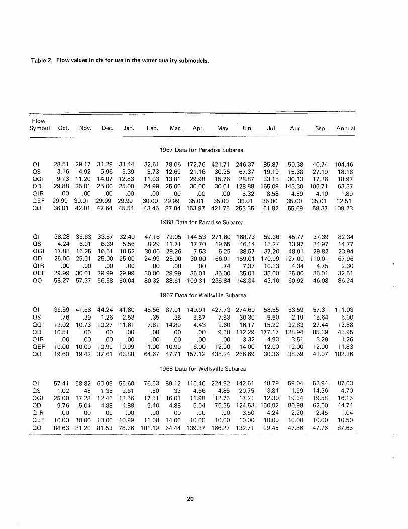
Table 2. Flow values in cfs for use in the water quality submodels.

Flow Symbol Oct. Nov. Dec. Jan. Feb. Mar. Apr. May Jun. Jul. Aug. Sep. Annual

1967 Data for Paradise Subarea

01 28.51 29.17 31.29 31.44 32.61 78.06 172.76 421.71 246.37 85.87 50.38 40.74 104.46 OS 3.16 4.92 5.96 5.39 5.73 12.69 21.16 30.35 67.37 19.19 15.38 27.19 18.18 OGI 9.13 11.20 14.07 12.83 11.03 13.81 29.98 15.76 28.87 33.18 30.13 17.26 18.97 OD 29.88 25.01 25.00 25.00 24.99 25.00 30.00 30.01 128.88 165.09 143.30 105.71 63.37 OIR .00 .00 .00 .00 .00 .00 .00 .00 5.32 8.58 4.59 4.10 1.89 OEF 29.99 30.01 29.99 29.99 30.00 29.99 35.01 35.00 35.01 35.00 35.00 35.01 32.51 00 36.01 42.01 47.64 45.54 43.45 87.04 153.97 421.75 253.35 61.82 55.69 58.37 109.23

1968 Data for Paradise Subarea

01 38.28 35.63 33.57 32.40 47.16 72.05 144.53 271.60 168.73 59.36 45.77 37.39 82.34 OS 4.24 6.01 6.39 5.56 8.29 11.71 17.70 19.55 46.14 13.27 13.97 24.97 14.77 OGI 17.88 16.25 16.51 10.52 30.06 29.26 7.53 5.25 38.57 37.20 48.91 29.82 23.94 OD 25.00 25.01 25.00 25.00 24.99 25.00 30.00 66.01 159.01 170.99 127.00 110.01 67.96 OIR .00 .00 .00 .00 .00 .00 .00 .74 7.37 10.33 4.34 4.75 2.30 OEF 29.99 30.01 29.99 29.99 30.00 29.99 35.01 35.00 35.01 35.00 35.00 35.01 32.51 00 58.27 57.37 56.58 50.04 80.32 88.61 109.31 235.84 148.34 43.10 60.92 46.08 86.24

1967 Data for Wellsville Subarea

01 36.59 41.68 44.24 41.80 45.56 87.01 149.91 427.73 274.60 58.55 63.59 57.31 111.03 OS .76 .39 1.26 2.53 .35 .35 5.57 7.53 30.30 5.50 2.19 15.64 6.00 OGI 12.02 10.73 10.27 11.61 7.81 14.89 4.43 2.60 16.17 15.22 32.83 27.44 13.88 OD 10.51 .00 .00 .00 .00 .00 .00 9.50 112.29 177.17 128.94 85.39 43.95 OIR .00 .00 .00 .00 .00 .00 .00 .00 3.32 4.93 3.51 3.29 1.26 OEF 10.00 10.00 10.99 10.99 11.00 10.99 16.00 12.00 14.00 12.00 12.00 12.00 11.83 00 19.60 19.42 37.61 63.88 64.67 47.71 157.12 438.24 266.69 30.36 38.59 42.07 102.26

1968 Data for Wellsville Subarea

01 57.41 58.82 60.99 56.60 76.53 89.12 116.46 224.92 142.51 48.79 59.04 52.94 87.03 OS 1.02 .48 1.35 2.61 .50 .33 4.66 4.85 20.75 3.81 1.99 14.36 4.70 OGI 25.00 17.28 12.46 12.56 17.51 16.01 11.98 12.75 17.21 12.30 19.34 19.58 16.15 OD 9.76 5.04 4.88 4.88 5.40 4.88 5.04 75.35 124.53 150.92 80.98 62.00 44.74 OIR .00 .00 .00 .00 .00 .00 .00 .00 3.50 4.24 2.20 2.45 1.04 OEF 10.00 10.00 10.00 10.99 11.00 14.00 10.00 10.00 10.00 10.00 10.00 10.00 10.50 00 84.63 81.20 81.53 78.36 101.19 64.44 139.37 166.27 132.71 29.45 47.86 47.76 87.65

20

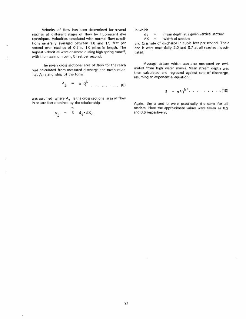
Velocity of flow has been determined for several reaches at different stages of flow by fluorescent dye techniques. Velocities associated with normal flow condi­tions generally averaged between 1.0 and 1.5 feet per second over reaches of 0.2 to 1.0 miles in length. The highest velocities were observed during high spring runoff, with the maximum being 5 feet per second.

The mean cross sectional area of flow for the reach was calculated from measured discharge and mean veloc­ity. A relationship of the form

Af a Qb ........ (8)

was assumed, where Af is the cross sectional area of flow in square feet obtained by the relationship

n L: d. • L.X.

1- 1-

21

in which d i mean depth at a given vertical section L.X i width of section

and Q is rate of discharge in cubic feet per second. The a and b were essentially 2.0 and 0.7 at all reaches investi­gated.

Average stream width was also measured or esti­mated from high water marks. Mean stream depth was then calculated and regressed against rate of discharge, assuming an exponential equation:

d a'Qb' ......... (10)

Again, the a and b were practically the same for all reaches. Here the approximate values were taken as 0.2 and 0.6 respectively.

CHAPTER IV

SALINITY SUBMODEL

Dissolved mineral concentration (salinity) is an important measure of water quality, particularly for irri­gated agriculture and, in some cases, for municipal and industrial water supplies. Specific electrical conductance (hereafter referred to as EC) is used as the salinity indi­cator because: (1) it is easily and accurately determined; (2) it is a better index of total ionic activity of dissolved salts than is a total dissolved solids (TDS) rating; and (3) the TDS test, as outlined in Standard Methods (American Public Health Association, 1965) may, in certain cases, result in sign ificant diminution of dissolved mineral weight by volatilization of carbon dioxide (U.S. Salinity Laboratory Staff, 1954).

Electrical conductance was simulated by first de­veloping relationships between EC and flow for each hydrologic input and then combining these inflows at the upstream end of the reach to yield a weighted average conductivity value for that reach. No "in-transit" equa­tion is required, as conductance is a conservative water quality parameter.

Input conductances

As shown in Figure 2, the inflow to any reach (i) is composed of one or more of six inflow components: out­flow from the reach immediately upstream on the same branch (Oi+l,j); outflow from river branches which are tributary to the reach being studied (OB R i,j ); other nat­ural su rface inflow to the reach (OS i,j ); surface irrigation return flow (01 R i,j ); groundwater inflow (OG I i,j ); and municipal and industrial releases (OEFj,j ). The conduct­ance of each of these hydrologic inputs must be deter­mined to permit evaluation of the conductance of the combined flow.

Reach inflc ViI

The conductance of the outflow from the upstream reach is taken as that resu Iting from the simu lation of the upstream reach.

23

Branch inflow

Here again, the conductance is taken as that pre­viously found for the tributary branch.

Surface inflow

Analysis of project data indicates that the conduct­ance of natural diffuse surface waters is closely related to rate of flow. Coefficients of correlation range from .69 to .90 (Figures H-4, H-5, and H-6). These orders of magni­tudes were supported in the review of published literature on the subject. Although the literature in th is area is somewhat sparse, researchers have long recognized the relationship between salinity and rate of flow. In fact, Lentz a nd Sawyer (1944) attem pted to esti mate flow rates from salinity data for streams in the Madison Lakes area.

In what is generally regarded as the pioneering work in this field, Durum (1953) established that chloride con­centrations in the Saline River, Kansas, were inversely related to flow. He found that the total salt load (salinity times flow rate) was nearly constant, though it did tend to be slightly higher during periods of high flow.

Extending on the work of Durum and using data from the Arkansas and Red Rivers, Ward (1958) proposed an exponential relationship of the form

in which S o

S aoQb ........ (11)

salt concentration rate of flow

a and b = constants

Ledbetter and Gloyna (1964) extended the simple exponential model advanced by Ward by allowing "b" to vary with rate of flow, according to the relationsh ip

b poQS ........ (12)

in which b Q

exponent for Equation 11 rate of flow

p and s = constants As an alternate to this relationship, especially applicable with reference to rivers of the arid southwest, they suggest that "b" be related to current rate of flow and antecedent flow conditions by the equation

in which bk

d

Q

exponent for Equation 10

antecedent flow index (3);0) Qd

d=1 d

the number of days, counted back from the "k th" day rate of flow

f, g, hand s = constants

Ledbetter and Gloyna, Hart, King, and Tchobang­laus (1964) state that they have adequately represented changes in the salinity of the Russian River of northern California by breaking the total flow of the river into its component parts:

s

in which S qg qi qs

salt concentration the groundwater component of flow the interflow component of flow the surface contribution to flow

a j and b j = constants

Gunnerson (1967) in a study of Columbia River data found that variation from the exponential prediction equation of Ward (Equation 11) tended to follow a seasonal elliptical donut pattern; with winter and spring values generally plotting above the prediction line and summer and autumn points below. Each sampling point examined had a unique variation pattern.

I n addition to the models outlined above, a simple semi-log relationship of the form

in which S

S a + b -log Q ...... (15)

salinity

24

Q flow rate a and b = constants

was fitted to the data.

The more complex relationships (Equations 12,13, and 14) failed to demonstrate any significant improve­ment over the simple exponential and semi-log relation­ships in fitting data available from the current project. Ward's exponential formulation (Equation 11) fit the data slightly better than did Equation 15, the semi-log form. The values of .the constants "a" and "b," as determined by least squares fitting of Equation 11 are given in Table 3, along with the coefficients of determination for several of the sampling points in the Little Bear River system. The constants a and b may vary considerably with in the stream system, as illustrated in Table 3; data upon which Table 3 is based are from the period June 1966 to De­cember 1967.

Table 3. Relationship of electrical conductance to rate of discharge on the Little Bear River system. (EC =aOb)

Station

$-12.5 S-15.2 S-27.0 $-27.5 $D-O.O SEC-6.2

a

a (constant)

1000 505 815 781 568 363

b R 2b

(constant) (%)

-.16 66. -.06 47. -.34 92. -.31 84. -.17 69. -.002 00.

aData were taken only during periods of relatively low flow due to access problems during the spring high water period.

bpercent of total squared variation in the dependent variable explained by the model.

Figure 10 is a log-log plot of conductance vs. flow rate for data obtained from station $-27.0, for the period June 1966 to June 1967. Equation 11 is plotted also with constants determined by least squares regression analysis of data.

Irrigation return flow

On the average, about one-third to two-thirds of the water diverted for agricultural irrigation is used consump­tively. The remainder finds its way back to the resource pool as deep percolation to groundwater, overflow from the d'istribution system, or surface runoff from irrigated fields (McGauhey, 1968).

600 6 ........; VI 0 500 5 .&::

E 0 ~

c..> " . ~ 400 4

Q) = 855'0-. 257 c..> c c 300 3 • -c..> ::J • "C C • 0 • U

c 200 2 .2 ~ -c..> Q)

ijj

<.> ;;:: '0 Q) Q.

CJ)

100 10 20 30 40 50 60 70 80 100 200 300 400

Flow Rate

Figure 10. Specific electrical conductance vs. discharge for station S-27.0 on the Little Bear River.

Eldridge (1963) states that "return -Flows from irri­gation projects contain at least three, and often as high as ten times the concentration of mineral salts as that of the initial irrigation water. II The Utah State University Foun­dation (1969) suggests that a more realistic range of salin­ity multipliers might be two to seven. Undoubtedly, the highest concentrations occur in the percolating segment of the return, as this will carry with it a portion of the soil solution in which the salinity has been increased by trans­piration, as well as any salts leached from the soil profile.

For purposes in this study, the deep percolating por­tion of the return flow is assumed to be included in groundwater; thus the salinity multipliers have auto­matically been restricted to the low end of the range mentioned above. A multiplier of approximately two has been assumed. This value is lower than mentioned in the literature, but seems to be more consistent with project data. This is supported particularly by comparing data from groundwater sampling point U-2510, as shown in Table 4, with conductance values of irrigation waters which are on the order of 300 to 400 ]J mhos/cm.

Groundwater inflow

Four groundwater sampling points have been estab­lished along the Little Bear River system. These sampling

25

points include one natural spring, an improved spring, an artesian well, and a field drain.

Although the data for ind ivid ual sampling points showed considerable scatter, no significant variation oc­curred with time of year. Considerable differences were observed between sampling points (Table 4). On the basis of this information, constant electrical conductance levels have been assigned to groundwater inflow to a given reach. The value assigned varies from reach to reach, in conformance to the tendencies disclosed in Table 4.

Municipal and industrial releases

The characteristics of municipal and industrial wastes are highly variable. I ndustrial wastes, however are highly specific to the type of industry from which they derive. The most logical approach to the simu lation prob­lem is to require data inputs to define the quantity and qual ity characteristics of each effluent being discharged into the stream system.

Stream conductance

Equation 16 calculates the conductance for reach i by the weighted average of all flow inputs for that reach. Stated algebraically:

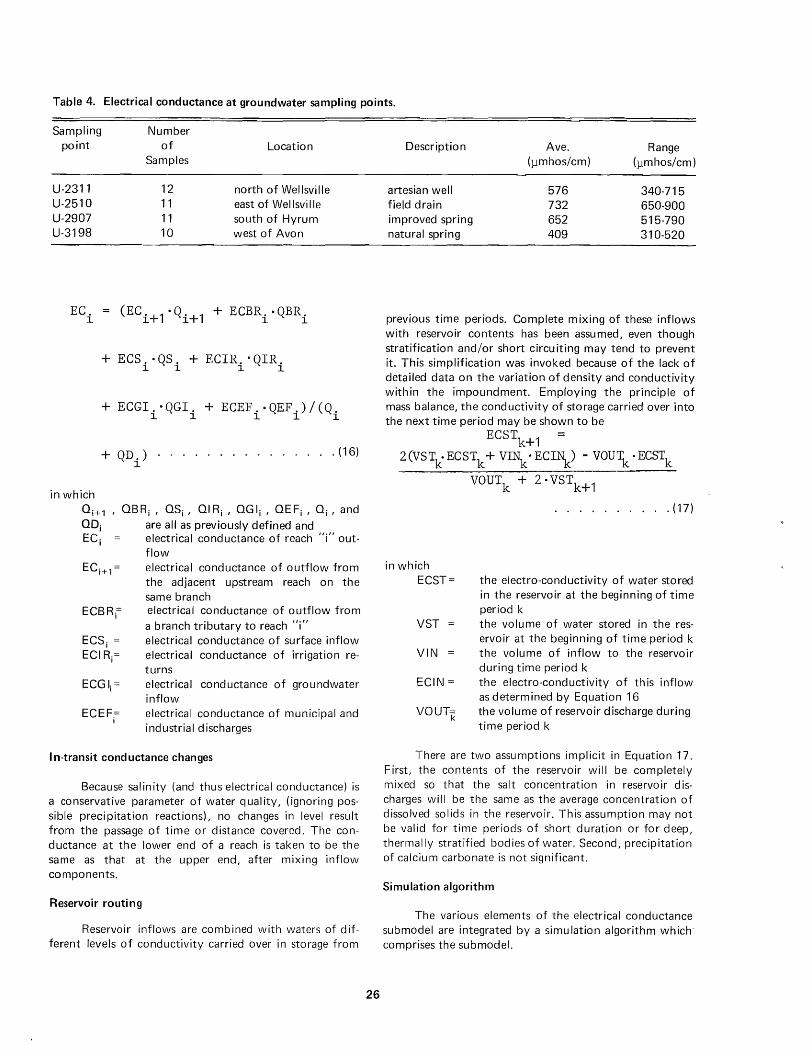
Table 4. Electrical conductance at groundwater sampling points.

Sampling Number point of Location

Samples

U-2311 12 north of Wellsville U-2510 11 east of Wellsvi lie U-2907 11 south of Hyrum U-3198 10 west of Avon

+ ECS.-QS. + ECIR.-QIR. l l l l

+ ECGI.oQGI. + ECEF"QEF.)/(Q. l l l l l

+ QD.) ............... (16) l

in which OJ+1 , QBRj , OSj, OIR j , OGl j , OEF j , OJ, and ODj are all as previously defined and EC j electrical conductance of reach "i" out­

flow

ECEF.= I

electrical conductance of outflow from the adjacent upstream reach on the same branch electrical conductance of outflow from a branch tributary to reach "i" electrical conductance of surface inflow electrical conductance of irrigation re­turns electrical conductance of groundwater inflow electrical conductance of municipal and industrial discharges

In-transit cond uctance changes

Because salinity (and thus electrical conductance) is a conservative parameter of water quality, (ignoring pos­sible precipitation reactions), no changes in level result from the passage of time or distance covered. The con­ductance at the lower end of a reach is taken to be the same as that at the upper end, after mixing inflow components.

Reservoir routing

Reservoir inflows are combined with waters of d if­ferent levels of conductivity carried over in storage from

26

Description Ave. Range (}lmhos/cm) (}lm hos/ cm )

artesian well 576 340-715 field drain 732 650-900 improved spring 652 515-790 natural spring 409 310-520

previous time periods. Complete mixing of these inflows with reservoir contents has been assumed, even though stratification and/or short circuiting may tend to prevent it. This simplification was invoked because of the lack of detailed data on the variation of density and conductivity within the impoundment. Employing the principle of mass balance, the conductivity of storage carried over into the next time period may be shown to be

ECSTk+1 2(VSTk-ECSTk + VINk-ECI~) - VOU\ -ECSTk

in which ECST=

VST

VIN

ECIN =

VOUT'k

VOUTk + 2-VSTk+1 . . . . . . (17)

the electro-conductivity of water stored in the reservoir at the beginning of time period k the volume of water stored in the res­ervoir at the beginning of time period k the volume of inflow to the reservoir during time period k the electro-conductivity of th is inflow as determined by Equation 16 the volume of reservoir discharge during time period k

There are two assu mptions implicit in Equation 17. First, the contents of the reservoir will be completely mixed so that the salt concentration in reservoir dis­charges will be the same as the average concentration of dissolved solids in the reservoir. This assumption may not be valid for time periods of short duration or for deep, thermally stratified bodies of water. Second, precipitation of calciu m carbonate is not significant.

Simulation algorithm

The various elements of the electrical conductance submodel are integrated by a simu lation algorithm which comprises the submodel.

Briefly, the simulation algorithm for monthly stream conductivity, for a given reach, consists of the fol­lowing procedure, which is outlined also in Figure 11.

1. Obtain hydrologic input flows for each reach for each monthly time period of interest using hydrologic submodel.

2. Establish, by regression analysis using field data, the constants a and b for Equation 15, for appropriate hydrologic flow inputs.

3. Define salinity by card input for flows not amen­able to Equation 15 application.

4. If reach is a reservoir, use Equation 17, which

27

mixes over two time periods. 5. Apply Equation 16 to all reach inputs to obtain

reach salinity. 6. Go to next reach and repeat procedure beginning

with step 1. 7. Go to next time period beginning with step 1.

The procedure for computer simulation of the above algorithm is described in Appendix E, where it is incorporated into the WAQUAL main program as the sub­program ELCON. Steps 3,4,5 are done by ELCON; steps 1, 6, and 7 by the system control model, and step 2 is done by the user, prepartory to simulation.

Go to next

reach

Establish Equation (15) constants by regression

analysis of field data for each flow input

category

no

Call HYDRO to obtain input flows for (1) reach inflow (2) branch inflows (3) groundwater inflow (4) M & I releases

Compute salinity for each input using Equation (15)

Compute reach salinity by Equation (16)

Figure 11. Simulation algorithm for electrical conductance submodel.

28

yes

ompute cond. of res outflow by

Equation (17)

CHAPTER V

STREAM TEMPERATURE SIMULATION

The temperature problem

The factor of stream temperature has evolved only recently to a perspective commensurate with its environ­mental effects. This is partially because the current and projected magnitudes of the temperature problem are such that it cannot be ignored. In 1964 the cooling water intake by industries amounted to 50,065 billion gallons (FWPCA, 1968). The U.S. Senate Select Committee on National Water Resources in 1960 projected cooling with­drawals of 576 billion gallons per day by 2000.

Thermal pollution, as it is now called, exerts a pro­found influence upon the receiving water body. First, the direct and indirect effects on the biotic communities may in some instances be quite severe. The ecology of the water body may be changed entirely. Decreased oxygen solubility, increased oxygen demand, increased growth of some algae species, and increased toxicity to some sub­stances are some of the peripheral synergistic effects. The mutual effects upon other cooling water users, and the change in palatability of the water for municipal use are among a few of the many additional considerations.

A natural stream will exhibit temperature behavior characteristics in both time and space, and these can have a significant bearing upon its reaction to thermal dis­charges. These characteristics include: (1) a diurnal tem­perature variation in the stream, (2) an annual cycle of mean daily stream temperatures, and (3) an in-transit decay of any point imposed temperature differentials. These characteristics are, of course, because the stream water body is virtually never at temperature equilibrium with its surroundings; thus the problem is one of heat transfer. Therefore, all of the factors relevant to heat transfer are pertinent to the problem of temperature be­havior of a stream. These factors include: (a) size of stream, (b) turbulence characteristics of the stream, (c) solar insolation, (d) atmospheric turbulence, (e) tempera­ture differential between the atmosphere and stream water body, and (f) mass inputs of new water. Inclusion of these factors is necessary to a rational comprehensive modeling treatment.

29

This comprehensive approach would not necessarily fit the philosophy of the project objective, however, which was to find a way to simulate the three effects listed above in the most pragmatic manner possible. The law of heat transfer is the basis for the empirical approach also, but applied in an empirical manner. In essence atmospheric temperatures (obtained from weather station records) are matched against correspond ing stream tem­peratures and the stream temperature response is thus "calibrated." Obviously this method is gross as all of the many independent variables of heat transfer are absorbed and integrated in a single coefficient. Nevertheless it works and is empirically feasible-which is the principal objective.

The simulation procedure was divided into two basic phases: (1) computer simulation of mean monthly water temperature by a program called WATEMP, and (2) computer simulation of diurnal water temperature for each month, by a program called D ITEMP. Each of these basic algorithms considers: (1) the time variations in temperature of all hydrologic mass inputs-discrete and diffuse, (2) in-transit changes with in a reach, and (3) the effect of reservo irs.

Monthly water temperature simulation

The monthly temperature simulation model (WATEMP) accomplishes three tasks. First, it can simulate the mean monthly stream temperature through the annual cycle. Second, it can simulate the stream in-transit re­sponse to any imposed heat load. And third, it can call up the diurnal submodel, DITEMP (by meansof WAQUAL). This section describes the equations used and how they operate to accomplish these tasks.

Temperature simulation of reach inputs

Each hydrologic input to a river reach has a unique pattern of temperature variation with time. Alternative methods of representing these variations for each input are outlined below. After each input temperature is simu­lated the weighted average of inputs equates with the temperature at the upstream end of the reach (Equation 16 applies).

River inflow. The simu lation procedure begins at the upper extremity of each branch, and proceeds in a downstream direction. Results from the simulation of the adjacent upstream reach are always available as an input for the simulation of the next reach downstream. For the first reach analyzed on a branch, the stream inflow is assumed to be zero and all natural surface inflows are lumped together in the "surface inflow" category (OS). The method of approximating the temperature of this component is discussed below.

Branch inflow. Branches tributary to a reach are simulated before the reach is analyzed. The temperature of inflow from tributary branches is therefore available for incorporation into the analysis.

Surface inflow. The temperature of inflowing d if­fuse surface waters follows a sinusoidal pattern through the annual cycle. Superimposed upon this annual varia­tion, there is a diurnal cycle, discussed in detail in the section following. Figure 12 illustrates the sinusoidal variation of water temperature through the year. Mea­sured water temperatures have been adjusted to mean

20

daily values to remove the influence of diurnal fluctua­tions.

Ward (1963) fitted a sine curve of the form

T = T + C'Sin (3261[5 'X + A) ... (181

to temperatur.e data from unheated natural streams by least squares procedures in which

T mean daily stream temperature f mean annual stream temperature x day of the year after October 1

The terms C and A are, respectively, a constant arid a phase shift angle determined by least squares analysis. Ward found this model to fit temperature data well with little between-years variation in model constant and phase shift. Jaske (1968) employed the same method of char acterizing annual water temperature variations in his study of the temperature characteristics of the Columbia River .

• • • • • •

• 2rr • • T=10.8 +9.50 Sin (l2·m+2.63) • - • u 15

~ • Q)

~

:::s • -0 _ _A__

~

10 Q) • 0-

f Q) - • • ~ • • • Q) 5 • • -0 • • • • ~

• •

0 Oc t. Nov. o IC. Jan. Fe b. Ma r. Apr. May June July Aug. Sept.

Mont h

Figure 12. Typical annual stream temperature variation at station S-12.8.

30

Table 5 shows the results of applying Equation 18 to temperature data from the Little Bear River. The fit of Equation 18 to the data, as measured by the coefficient of determination (R2), is consistently high at all but one of the twelve sampling points. The station for which the poor fit was obtained is the one designated SEC-4.3, lo­cated immediately downstream from the Porcupine Reser­voir outlet works. Expanding Equation 18 into two and three-term Fourier series did improve the fit at this station (but not at the other stations).

Utilization of the procedure outlined above requires a record of stream temperatures at the point in question. Observations should be taken at least weekly over a period of one or more years. As noted in Table 5, data from the Little Bear River system indicate that the constant C and the phase sh ift angle A do not differ greatly from one station to another in the system, if the waters being com­pared are of the same basic make-up, i.e., have about the same proportions of groundwater at the two points, etc. It should be possible then, if judgment and discretion are exercised, to transfer these two coefficients from one sta­tion to another within a small hydrologic system.

A major disadvantage of the Equation 18 approach is that it ties water temperature directly to time of year, rather than to atmospheric temperature. This hinders the assessment of the effect of stochastic variations in month­ly atmospheric temperature upon stream temperature. In add ition, at least one complete cycle of stream tempera­ture data is required to adequately determine the sine curve parameters.

Another approach in the modeling of surface inflow temperatures, is to correlate stream temperature and

atmospheric temperature. Where the modeling increment is one month, the monthly average of atmospheric tem­perature can be used to estimate mean monthly stream temperatures. Intervals shorter than one month, however, would require that antecedent atmospheric temperatures be considered.

Monthly averages of stream temperatures, adjusted to mean daily values, have been regressed against mean monthly atmospheric temperatures from the Logan USU Weather Bureau station located about ten miles north of the project area. A linear equation of the form

T a+b·T +s···· .. (19) a

is assu.med in which T mean monthly water temperature (0 C) Ta mean monthly atmospheric temperature

(OF) s

a and b

deviation of observed water temperature from pred icted values

regression constants

Equation 19 is a desirable alternate because it more clearly portrays the cause-effect relationship responsible for changes in stream temperature. It should also be possible to satisfactorily define the coefficients for this equation with something less than a fu II annual cycle of data as long as the temperature measurements cover a period including both high and low stream and atmos­pheric temperatures. The results of applying Equation 19 to data from 14 water quality sampling stations are tabu­lated in Table 6.

Table 5. [e~e,enta:n of annual Ca;!e, in mean )JY water temperature.

T = T + c· Sin 365 . x + A _.

Station T C A R2 Comments (oC) (constant) (radians) (%)

S-12.7 10.7 7.135 2.675 88. S-12.8 10.8 9.505 2.630 90. S-15.2 10.5 9.102 2.573 92. S-16.8 10.2 14.477 2.515 88. reservo i r su rface S-21.3 8.7 7.209 2.659 90. S-24.6 8.7 7.466 2.663 87. S-27.5 9.4 6.565 2.670 85. SO-O.O 7.8 8.652 2.674 85. SEC-4.3 8.3 11.208 2.068 71. reservoir outflow SEC-6.2 7.1 7.288 2.604 85. S\I\I-0.1 11.2 5.278 2.684 83. largely spring fed STF-O.O 8.8 6.977 2.653 86. trout farm discharge

31

Table 6. Prediction of stream temperature from atmos­pheric temperatu res. (T = a + b T a )

Station a b R2 Notes (constant) (constant) (%)

S-12.7 - 4.09DC . 310 97 . S-12.8 - 7.53 . 387 93 . S-15.2 - 6.90 . 373 93 . S-16.S -10.22 .475 8S . reservo ir su rface S-21.3 - 6.01 .312 95. S-24.6 - 5.92 .310 94. S-27.0 - 5.90 . 30S 93 . S-27.5 - 2.24 . 252 93 . SD-O.O - 8.77 . 356 95 . SEC-O.4 - 5.08 .295 90 . SEC-4.3 - 1.75 .211 57. reservo ir discharge SEC-6.2 - 5.10 .270 71. SW-0.1 0.63 . 221 87 . largely spring fed STF-O.O - 5.54 .304 94.

Again, a degree of consistency was noted in the re­lationships between air and water temperatures at all sta­tions except those at which the stream is affected by reservoirs or proportionately large groundwater contribu­tions. The coefficients of determination (R2) are uni­formly high, except at two stations on the East Fork of the Little Bear River (SEC-4.3 and SEC-6.2). At station SEC-4.3 the flow is composed almost entirely of waters released from Porcupine Reservoir. These releases do not correlate well with atmospheric temperature. No explana­tion has been found for the relatively poor fit at SEC-6.2 which is upstream from Porcupine Reservoir.

Comparing the R2 values in Tables 5 and 6, Equa­tion 19 would appear to be a slightly better fit than Equa­tion 18. Equation 19 also has the advantage of being based upon mean monthly air temperature and therefore Equation 19wasused.

Irrigation return flow. Surface return flows from irrigation are also assumed to be I inearly related to atmos­pheric temperature as described by Equation 19. Because temperatures of these flows were not measured, it has been necessary to assume values for the model constants.

Eldridge (1963) suggests that the contributions of irrigation retu rn flows to the thermal behavior of a stream are of minor importance. I n considering surface retu rn flows, it was assumed that such flows are warmer than natural surface inflows. Equation 19 was adopted to simu­late the temperature behavior of return flows. Because temperatures of these flows were not measured, it has been necessary to assume values for the Equation 19 con­stants.

Groundwater inflow. Table 7 gives the results of fitting groundwater temperatures at four groundwater

32

Table 7. Annual temperature variations of groundwater.

[T= T + eoSin (i6~ x + A)] Sampling T C A R2 Description

point (DC) (Constant) (radians) (%)

U-2311 10.5 1.519DC 2.367 58. artesian well U-2510 10.5 2.706 1.892 91. field drain U-2907 11.4 1.419 2.230 55. improved spring U-3198 10.8 1.993 2.239 87. natural spring

sampling points in the project area to Equation 18. Al­though the determination coefficients for the artesian well and the improved spring are not good, the seasonal varia­tion in temperature at these points is significant. At these two locations, the small proportion of the total variation explained by the seasonal model is probably due to the relatively great depths at which the flows originate. Be­cause no distinction has been made in the simulation pro­gram as to the depth from which groundwater originates, the prediction model used is a composite of those ob­tained from the four sampling points.

Municipal and industrial releases. The thermal quali­ties of municipal and industrial waste waters discharged to the stream must be provided as a data input for each simulation run of the model.

In-transit temperature changes

The temperature of a moving body of water is sub­ject to many influences along its course. Solar radiation and atmospheric convection tend to increase the tem pera­ture during daylight hours, while evaporation and other phenomena tend to decrease it. Until recently, relatively little work has been published concerning this important process in natural streams.

The American Society of Civil Engineers Committee on Thermal Pollution (1967) has assembled an extensive bibliography on thermal pollution. Publications listed in this bibliography, and other published material on this topic, fall generally into three classifications: (1) the occurrence of thermal pollution; (2) the effects of thermal pollution upon the aquatic environment; and (3) temper­ature prediction in natural and thermally polluted bodies of water. The latter class is notable for the relatively small number of contributions.

Most of the early work on temperature prediction techniques was done on cooling ponds and reservoirs. The first of these studies was by Ruggles (1912). Subsequent investgations were performed by Lima (1936), Thorne (1951), Langhaar (1953), and others.

The initial work on stream temperature prediction was published by LeBosquet (1946). He assumed an ex­ponential decay of warm water toward the prevailing air temperature. His derived relationship was of the form

in which !J.l\

( o023S-ke-w -H)

,,- - Q .. (20) uTI -e

"excess" temperature of water over air at the initial point "1" (OF) "excess" temperature of water over air a distance "D" miles downstream from the initial point "2" (OF) heat loss coefficient (BTU/sq. ft./hr./°F of "excess" temperature)

w average stream width (ft.) Q average discharge (cfs) H mean stream depth (ft.)

LeBosquet found values of the heat loss coefficient rang­ing from 6 to 18 BTU/sq. ft./hr./°F (0.2 to 0.6 ft./hr.).

This technique has been criticized on two counts. First, values of the heat loss coefficient must either be guessed or calculated from measurements after the ther­mal pollution has occurred. It would seem that this dif­ficu Ity could be partially mitigated by experimental analysis. The second question concerns the assumption that in the absence of thermal pollution, air and water temperatures would tend to be equal. Although air temperature is an important factor in determining the temperature of a body of water, other variables, such as evaporation, back radiation, etc., tend to lower the "equi­I ibrium" temperature of the stream below atmospheric temperature.

Gameson, Hall, and Preddy (1957) used essentially the same approach as that advocated by LeBosq uet to ana Iyze the thermal characteristics of the Thames estuary. They avoided the second criticism of LeBosquet's model by using temperature excess above some "equilibrium" water temperature instead of the excess of water tem pera­ture over air temperature. From estimated rates of heat add ition by urban and industrial developments along the estuary, they estimated the coefficient of heat loss at 4.0 centimeters (0.13 feet) per hour. For the River Lea, Gameson, Gibbs, and Barret (1959) found heat loss coeffi­cients, averaged over four days for four different reaches, to range from 1.66 to 3.83 cm/hr. (.054 to .126 ft./hr.). The overall average for the river was 2.6 cm/hr. (.085 ft./hr.) .

Recent work has been directed to the heat-budget analysis approach. Among those contributing to the litera­ture on th is topic are: Velz and Gannon (1960), the Johns

33

Hopkins Advanced Seminar (1961), Ed inger and Geyer (1965), Edinger, Brady, and Graves (1968), and others. The heat-budget method requires data on solar radiation and wind velocities which are not generally available. No data of this nature were taken during this project so the heat-budget approach was eliminated from consideration for purposes of this work.

Duttweiler (1963) has developed a procedure, wherein the exponential decay theory is employed with "equ'ilibrium" temperatures and heat exchange coeffi­cients being estimated from heat-budget considerations. This is a rather rigorous approach which would seem to possess certain merit as a modeling technique. However, for application to the data available from the current pro­ject it was of limited usefulness because of the lack of more detailed climatological data such as windspeed and radiation.

The simulation procedure finally adapted for this work satisfied the pragmatic criteria of reliability and data availability. This procedure involved the LaBosquet Equa­tion 20, for predicting decay of temperature excess, in conjunction with Equation 19 for assessing stream equi­librium temperature. Equation 19, which gives mean monthly stream temperature, was felt to be as reasonable estimate of equilibrium temperature as feasible.

I n mathematical form, the complete model for a nonreservoir reach is

Cne

1.: q. - T •

_ j=1 J J -¢ + E -e 2 - Q

in which

3.i Tj

Q

nc

E

~)

. . (21)

rate of flow for input j mean monthly temperature of input j

n 1.: q.

j=1 J number of hydrologic inputs to the reach mean monthly stream temperature at the downstream end of the reach "equilibrium" temperature

o023S ok eow

Q ·D

In Equation 21, the subscript 1 indicates the upstream end of the reach, while 2 denotes the downstream end. All flows and temperatures are monthly averages for the month of simulation. Mean monthly input tempera­tures, ~, are estimated according to the equations shown in Table 8.

Table 8. Summary of mean monthly temperature equa­tions for hydrologic inputs.

Input

River inflow

Model

output from previous simulation

output from previous simulation

T5= a +b-Ta

Branch inflow

Surface inflow

Irrigation return flow

Groundwater inflow

M & I releases

I a 2 'IT T. = a + beT (

1'""g= ~+ OSin 12 om + A) card input

Heat exchange constants for streams of this system were approximated from the river reach downstream from Porcupine Reservoir. During the summer irrigation season, releases from the reservoir originate in the cold hypo­limnetic zone, reSUlting in significant temperature deficits at the reservoir outlet. The rate at which these deficits approach zero, as these cold waters are warmed toward the "equilibrium" temperature in the reach below the res­ervoir, was employed in the evaluation of the heat ex­change constant, ke .

On seven different days during the summer of 1968, temperature observations were made at the outlet from Porcupine Reservoir and at Avon, 3.9 miles downstream. Temperature deficits (D. T 1 and D.T 2) were taken as the difference between temperatures observed at the points in question and those measured at nearby sampling points not affected by reservoir releases, respectively. These deficits were then inserted into Equation 20, the ex­ponential decay expression, which was solved for k e. Values obtained are compared with those reported by other researchers in Table 9. A heat exchange constant of 0.20 has been assumed in the development of the present model. Provision is made to allow this "constant" to vary with rate of discharge, accord ing to a hypothetical re­lationship of the form

Table 9. Heat exchange coefficients.

Researcher Min. Max. Water body

(ft./hr.) (ft./hr. )

LeBosquet (1946) 0.2 0.6

Gameson et al. (1957) 0.13 Thames estuary

Gameson et al. (1959) 0.054 0.13 River Lea

Duttweiler (1963) 0.047 0.15 Winter's Run

Edinger et al. (1968) 0.12 Cooling pond

Current research 0.09 0.40 Little Bear River

34

k b

aoQ ......... (22) e

Because of the dearth of data here and the lack of a significant source of thermal pollution on which to test a prediction equation, a constant level for the exchange co­efficient is all that is justified.

Adjustment of discrete sampling data

As depiCted in Figure 19, temperatures during the 8:00 a.m. to 5:00 p.m. working day, when samples were gathered, vary over a large part of the amplitude of the diu rnal fluctuation. Because temperatures were not measured at the same time at each sampling point, a more or less random appearing error was introduced into the data. Had a rigid time schedule been followed, so that each site was always visited at the same hour, the diurnal effect would have imparted a systematic downward bias for those points sampled early in the day, while those sampled later in the day would have been biased upward.

To isolate the diurnal component of variation, the model of diurnal fluctuations (called DITEMP and dis­cussed in the following section) was utilized. By employ­ing the diurnal model to adjust all descrete temperature data to mean daily values, it was possible to achieve con­siderable improvement in the fit of the inflow tempera­ture prediction relationships over that resulting from the use of unadjusted data. Consequently, all stream tempera­tures, obtained by discrete measurement, have been ad­justed to mean daily stream temperature.

Reservoirs

The primary effect of impoundments on down­stream temperatures is that of cooling during summer irri­gation months if, as is true in the case of Porcupine Reser­voir, releases are discharged from the hypolimnion directly into the stream channel below the dam. Tempera­ture data from station SEC-4.3, below Porcupine Dam, are shown in Figure 13. These data have not been adjusted for diurnal effects because the deep waters of the hypo­limnion are not subjected to diurnally varying factors. As a result, temperatures in this zone are constant through the diurnal cycle.

These data fit nicely into a theory presented by Churchill (1965) in which he considers the reservoir as being thermally stratified during summer months. He assumes the outlet works to draw only from a relatively thin layer at the depth of the discharge, so that during the irrigation season coldest waters are released first. Released water temperatures gradually increase as the reservoir level recedes and the warm upper layers fall to the level of the discharge opening. Although temperature data available for the station below Porcupine Reservoir indicate that this procedure would apply, it has not been employed because its application requires a complete thermal map-

T:8.31 ... 5.30ISin(3652TT .X+2.304>+.823Sin(~ ,X+1.809)+2.675Sin( 6lT 25 365.25 365.25

.X + I. 449)

• (,)

+2.017Sin ( 8 IT .X + 3.838) 365.25

0 15 • OBSERVED WATER TEMPERATURE.

• w Q: :::::l .... <t

10 a: w Q. ~ W .... • a: IJJ 5 .... <t ~

0~0~C~T~'~2NO~V~.~_D~E~C~.~~~~F~E~B~.~~M~A~R~.~~~~~~~~~~~~~~~~~ o 50 100 150 250 300 350

Days After October.

Figure 13. Annual stream temperature variation at SEC-4.3 below Porcupine Reservoir with best fit four-term Fourier series cu rve.

ping of the reservoir each spring to define the temperature-depth profile throughout the reservoir at the beginning of the irrigation season. Such a survey was beyond the scope and economic resources of this project.

The proced ure finally adopted is that of obtaining a temperature record for reservoir releases covering at least one fu II year and fitting a four term Fourier series model

T T + i CJ. Sin G26~ j·x + A

J.) .(23)

j=1

to the data, as outlined in Appendix D. The best fit Fourier series prediction is shown in Figure 13, super­imposed on the observed temperature of released waters. The lack of data during winter and spring months, caused by difficult access during this period, allowed the Fourier series best-fit curve to drop again in early spring. This would not be expected in actual field observation. Had data been available for this time of year, the curve would have been forced to follow the data, rather than being free to take the path of least resistance.

The curve-fitting approach means, of course, that unless more than one year's data are available, data from

35

that year must be accepted as representative of all years of data. This may be a serious limitation if the operating procedures for the reservoir are subject to significant change from year to year.

Algorithm for simulation

Figure 14 outlines the simulation algorithm for monthly stream temperature and this algorithm also is summarized below.

1. Obtain monthly flow values for all inputs from hydrologic model.

2. Establish constants a and b in Equation 19 for each inflow by regression analysis of data.

3. Compute temperature of each input to reach for month in question using Equation 19-where appl icable; otherwise define flow input temperature by punched cards; use ,Equation 18 for shallow groundwater inputs.

4. Co m p ute stream temperature, consisting of combined inflows, using Equation 16.

5. If reach is a reservoir apply Equation 23 to obtain temperature of outflow and simulate next reach beginning with step 1 again.

6. For non-reservoir reaches, if a "temperature ex­cess" (difference between mean monthly water tempera­ture and mean monthly equilibrium water temperature)

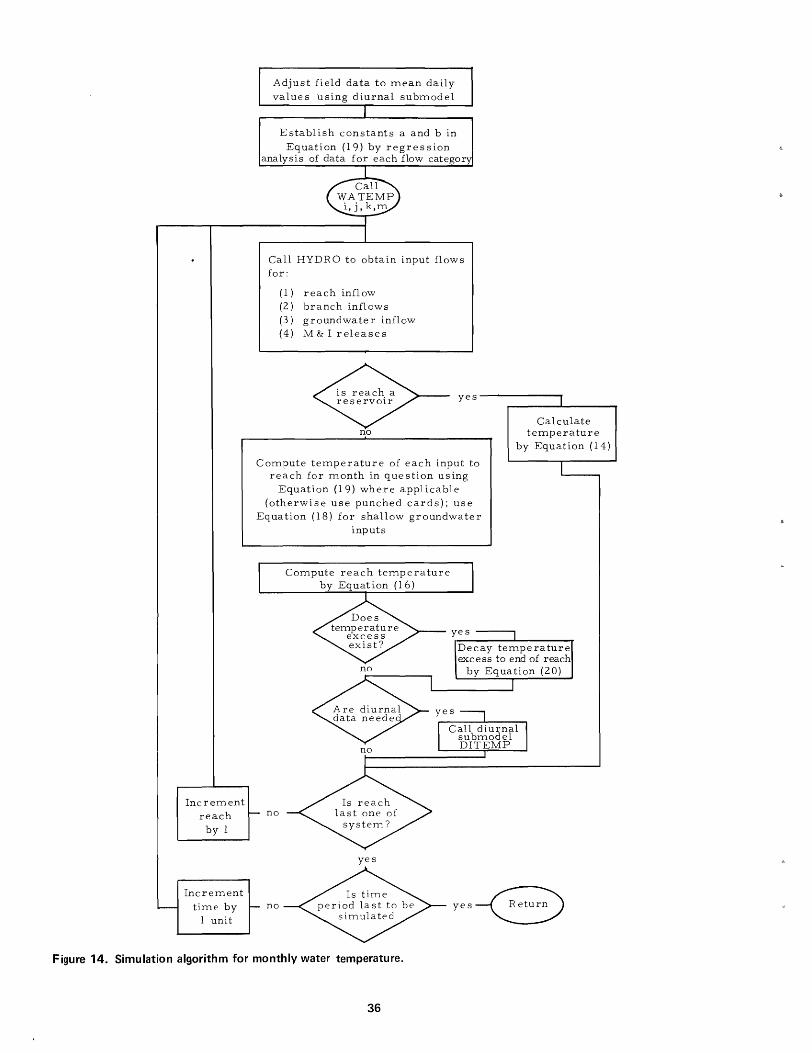
Increment

Adjust field data to mean daily values using diurnal submodel

E stabl ish constants a and b in

Equation (19) by regression analysis of data for each flow categor

Call HYDRO to obtain input flows for:

(1) reach inflow (2) branch inflows (3) groundwate r inflow (4) M & I releases

yes

Compute temperature of each input to reach for month in question using

Equation (19) where appl icable (otherwise use punched cards); use

Equation (18) for shallow groundwater inputs

Compute reach temperature by Equation (16)

yes

Calculate temperature

by Equation (14)

no

Decay temperature excess to end of reach

by Equation (20)

reach no

by 1

Increment

time by 1 unit

yes

no

Figure 14. Simulation algorithm for monthly water temperature.

36

yes-G

exists at beginning of reach, apply Equation 20 to decay the excess temperature to the end of the reach.

7. Call diurnal submodel if desired. 8. Go to next reach and return to step 1. 9. If last reach is simulated, increment time by one

month and return to step 1.

Steps 1,7, 8,and 9 are done by WAQUAL; step 2 is done by the investigator in data preparation; steps 3, 4, 5, and 6 are done by WATEMP.

Diurnal water temperature simulation

Two continuous modeling stations were established at S-12.5 and S-20.5, respectively, to ascertain diurnal fluctuations and any stochastic effects for temperature, dissolved oxygen, pH, and conductivity. Analysis of thermographs from the continuous monitoring station at S-12.5 (which has about 18 months record) disclosed significant amplitudes in the 24 hour cycles in stream temperature. Since the diurnal temperature effect may well overshadow an annual variation or effects due to point discharges, any comprehensive model should include the diurnal effect for temperature. Thus a simulation pro­cedure for assessing the temperature variation for the 24 hour cycle has been developed.

Researchers reporting diurnal variations in surface water temperature include Macan (1954), who has ob­served daily patterns of variation in water temperature of small streams in Britain. Duttweiler (1963) used diurnal variations in water temperature of a small stream in Mary­land to estimate values of the heat exchange constant for that stream. Thomann (1967), on the other hand, found no significant 24 hour cycles in data from the Potomac estuary. This literature contains little information on the characterization of diurnal water temperature variations.

Establishing diurnal temperature equations

Thermographs were obtained at station S-125 in continuous blocks of from three to seven days in length. Twenty of these blocks of temperature data were re­corded intermittently over an 18-month period. The diurnal data for each of these data blocks were then fitted to Equation 24, a two term Fourier series.

T. 1

In Equation 24 Tj

.......... (24)

observed stream temperature at the "i th" hour (OC)

37

T mean daily stream temperature (Oe) hour of the day (measured continuously through the day, beginning with 0100 at 1 :00 a.m. and ending with 2400 at mid­night) deviation of the observed temperature for the "i th" hour from the model pre­diction for that hour

C. and A. = coefficient and phase sh ift for the "j J J

th" term of the Fourier series, as deter-mined by least squares analysis

Figure 15 shows hourly stream temperatures from a typi­cal seven day continuous thermograph, with the best-fit Fourier series curve superimposed. During this particular period, the range of maximum stream temperatures was relatively high, as illustrated by the broad band of obser­vation points about the curve. In spite of these relatively large deviations, Table 1 0 shows the coefficient of deter­mination for this set of data to be 74 percent, meaning that Equation 24 explains 74 percent of the total varia­tion in stream temperature during this period.

Dividing Equation 24 through by the mean daily temperature yields a predictive equation for the ratio of hourly to mean daily stream temperature

DTI. 1

1.0 + ~ CJ"Sin (~:j ·i + AJ.)

j=1

+ E. 1

........... (25)

where now C. and E. have been coded by division by J .... I

T, and DTl j = T j /T. With patterns of diurnal temperature variation given in terms of this diurnal temperature index (DTI), the stream temperature at' any hour of the day may be estimated by multiplying the mean daily temperature by the DTI for the hour in question.

Table 10 lists constants, C 1 and C2 , and phase angles, A 1 and A 2 , for each of the two Fourier series terms and coefficient of determination, and average stream temperature over the period and corresponding average mean daily atmospheric temperature. It is interest­ing to note the apparent annual cyclic tendency in each of the Fourier series model parameters. This tendency is more obvious in Figure 16, where each model parameter is plotted as a function of time of year. These cyclic pat­terns probably resu It from seasonal variations in the number of daylight hours per day and intensity of solar radiation.

The Fourier series has again been employed in the characterization of the annual cyclic variations for each of the Equation 25 coefficients. Mean daily atmospheric temperature has also been incorporated to yield another Fourier series having the form

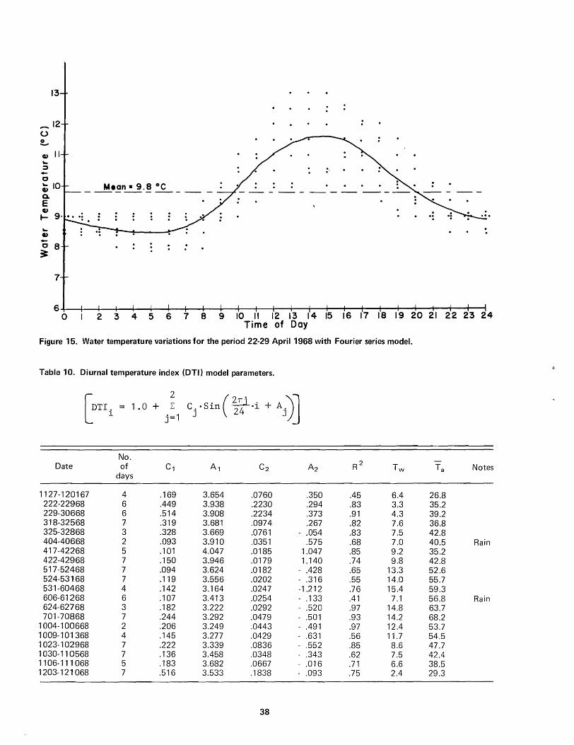
13

_12 u

CI) II ... j -a ~ 10 Q.

E CI)

I-... CI) -a 8 ~

7

Mean. 9.8 °c ----------- -

. .

6~~--~~~--+__+--~~~--+__+--~~~--4__+--+_~~~~~--+__r~ o 2 3 4 5 6 7 8 9 10 II 12 13 14 15 16 17 18 19 20 21 22 23 24

Time of Day

Figure 15. Water temperature variations for the period 22-29 April 1968 with Fourier series model.

Table 10. Diurnal temperature index (DTI) model parameters.

fDT1 . = 1.0 + ~ C .. Sin( ~? ·i + A.")l L l j=1 J J}J

No. Date of C1 A1 C2 A2

days

1127 -120167 4 .169 3.654 .0760 .350 222-22968 6 .449 3.938 .2230 .294 229-30668 6 .514 3.908 .2234 .373 318-32568 7· .319 3.681 .0974 .267 325-32868 3 .328 3.669 .0761 - .054 404-40668 2 .093 3.910 .0351 .575 417-42268 5 .101 4.047 .0185 1.047 422-42968 7 .150 3.946 .0179 1.140 517-52468 7 .094 3.624 .0182 - .428 524-53168 7 .119 3.556 .0202 - .316 531-60468 4 .142 3.164 .0247 -1.212 606-61268 6 .107 3.413 .0254 - .133 624-62768 3 .182 3.222 .0292 - .520 701-70868 7 .244 3.292 .0479 - .501

1004-100668 2 .206 3.249 .0443 - .491 1009-101368 4 .145 3.277 .0429 - .631 1023-102968 7 .222 3.339 .0836 - .552 1030-110568 7 .136 3.458 .0348 - .343 1106-111 068 5 .183 3.682 .0667 - .016 1203-121 068 7 .516 3.533 .1838 - .093

38

R2 Tw

.45 6.4

.83 3.3

.91 4.3

.82 7.6

.83 7.5

.68 7.0

.85 9.2

.74 9.8

.65 13.3

.55 14.0

.76 15.4

.41 7.1

.97 14.8

.93 14.2

.97 12.4

.56 11.7

.85 8.6

.62 7.5

.71 6.6

.75 2.4

Ta Notes

26.8 35.2 39.2 36.8 42.8 40.5 Rain 35.2 42.8 52.6 55.7 59.3 56.8 Rain 63.7 68.2 53.7 54.5 47.7 42.4 38.5 29.3

C.= -.131+.334 Sin( ~ K+5.913)+.126 Sin(¥K+3.918 )+.OO87Ta.

(R 2=.805)

u

. 5

.4

.3

.2 .-Ie • _ 4

·1

o o

•

0

•

N

• -r-- e

-,.-.-

I--

I" • '----i-

•• ~t • • D J F M A M J

100 200 Days After I October.

-I--

• '---

J A S

300

5. A.=4.719+.254Sin(J!.'K+3.440)+.096Sin(~.K+2J55)-.0252Ta' ~R2=. 826)

4.

•

D

100

•

• •

Days After I October .

300

• 25 C=-.060+.I58Sin(JI...K+5.929 )+.06ISin (.1!.K+3.909).j..0034Ta. A =4.972+1.7345in( TT6

.K+2.844) .... 5I4Sin(1!3 .K+2.645)-.I07lTo' 2 6 (R2=.883) 3 +10 I

N U

.20

. 15

. 10 •

OONDJFM o 100 200 300

Days After I Octobe r.

+.5

N 0 <t

-.5 • -LO

o 0 0

• • • • • • ••

N D J 100 200 300

Days After I October.

Figure 16. Annual variations in diurnal temperature index model parameters.

y C o + ~ C

J,· Sin (~~ § . x + a

J,)

j=1

+ r' T + E ............. (26)

in which y

a

diurnal index equation coefficient, A 1 ,

A 2 , C 1 or C2 for a given month days since 1 October mean daily atmospheric temperature for a given month (0 F) deviation of pred icted model parameter value for a given date from the value calculated from diurnal variations ob­served on that date

co' c j' a j and r = constants and phase sh ift as deter­mined by least squares analysis for the respective Y

Monthly values of the DTI model parameters (A 1 '

A2 , C1 and C2 ), as estimated by Equation 26 are shown in Figure 16 as bars and are listed also in Table 12. The dearth of data points in Figure 16 for the months of

39

January, August, and September was caused by malfunc­tions in the continuous monitoring instrumentation for those months.

Table 11 lists the coefficients co' a1 , a2 , c1 and c 2 belonging to Equation 26. These coefficients were ob­tained by regression analysis of each coefficient repre­sented by Y in Equation 26.

Figure 17 shows graphically Equation 25 for each month of the year. The seasonal pattern exhibited in the monthly diurnal index sine curves is allowed by the monthly assessment of Equation 25 coefficients, which is done by Equation 26. To convert from index display to real temper~ure it is necessary only to multiply each ordinate by T, the mean monthly stream temperature.

Diurnal stream temperature simulation

The diu rnal distribution of temperature and flow in all hydrologic input streams must be defined before hourly variations in stream temperature may be approxi­mated. All natural surface inflows to the system are assumed to exhibit the same hourly distribution of temperature indexes. Figure 18 shows substantial similar­ity in patterns of variation at stations S-12.5 and S-20.5

Table 11. Representation of annual chang~s in diurnal water temperature index model parameters for Equation 26.

Parameter Co c, a, c2 a2 r R2 (constant) (constant) (radians) (constant) (radians) (constant) (%)

y = C, - .131 .334 5.913 .126 3.918 .009 80. Y = A, 4.719 .254 3.440 .096 2.155 -.025 83 . Y = C2 - .060 . 158 5.929 .061 3.908 .003 88. Y = A2 4.972 1.734 2.844 .514 2.645 -.107 79.

Table 12. Estimated monthly values of diurnal temperature index model parameters for Equation 25, calculated by Equation 26 using Table 11 coefficients.

Month C, A, C2 A2 (constant) (radians) (constant) (radians)

October .160 3.333 .039 - .476 November .230 3.531 .083 - .161 December .420 3.647 .179 .000 January .530 3.860 .235 .703 February .513 3.934 .223 .839 March .357 3.896 .140 .547 April .227 3.618 .067 - .536 May .139 3.463 .020 - .731 June .191 3.257 .042 - .875 July .300 3.037 .088 -1.156 August .281 3.077 .082 - .747 September .191 3.216 .046 - .419

on October 11-12, 1968. While the agreement is not exact, the approximation is satisfactory for the purposes of this study. Hourly temperatures, L, of natural surface inflows are estimated by multiplying the mean monthly temperature, 1; for these inflows, taken from the monthly simulation, by the diurnal temperature index. Table 13 summarizes the methods employed in simulating hourly time variations in the temperature of the hydrologic in­puts to the reach. Diurnal fluctuations in expected "equi­librium" stream temperature are also assumed to be characterized by this same temperature index distribution; mean monthly water temperature,T, from Equation 19 is the basis for applying the DT I for the input in question.

Table 13. Diurnal temperature input models.

It is shown in Table 13 that groundwater flows are assumed free from diurnal influences. Also shown in Table 13 is the card input characterization of municipal­industrial discharges.

40

Input

River inflow Branch inflow

Surface inflow Irrigation return flow

Groundwater inflow M & I releases

Model

previous simulation of upstream reach previous simulation of upstream reach

Ls= TsDTI L i = T(DTI

Lg=."'t card Input

Reservoir releases mayor may not exhibit diurnal variations, depending upon the depth from which they are drawn. Waters spilled from the upper several feet of reser­voir storage would be expected to show diurnal patterns of variation in response to the influence of daily cycles in

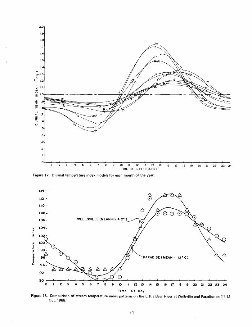
2.0

1.9

1.8

1.7

1.6

1.5

1.4

Ito-I.3 "-

to- 12

X 1.1 w 0 z

0: :i: w to-

...J ct Z a:: :::> 0

.5

.4

.3

.2

.1

.0 2 3 4 5 6 7 8 9 10 II 12 13 14 15 16 17 18 19 20 21 22 23 24

TIME OF DAY ( HOURS)

Figure 17. Diurnal temperature index models for each month of the year.

1.14

1.12

1.10

1.08

1.06

)( 1.04 G)

" -= 1.0

~ ::3 .. 0 .. G)

0.

E PARADISE ( MEAN = ILl· C ).

G) ....

.92

.90 0 2 3 4 5 6 7 8 9 10 II 12 13 14 15 16 17 18 19 20 21 22 23 24

Ti me Of Day

Figure 18. Comparison of stream temperature index patterns on the Little Bear River at Wellsville and Paradise on 11.12 Oct. 1968.

41

atmospheric conditions. Waters originating in the hypo­limnion, on the other hand, are shielded from the effect of atmospheric conditions so that diurnal fluctuations are not observed.

Each of the inputs described above are "mixed" on an hour by hour basis in accordance with Equation 16 (again used with temperatures); this gives the hourly stream temperature distribution at the upstream end of the reach.

A graphical example of the combination of a natural stream inflow and a municipal waste discharge is pre­sented in parts (a), (b) and (c) of Figure 19. Diurnal temperature distributions for the two components of flow (OS and OEF) are depicted in (a) and (b) respectively. The distribution of rate of waste discharge is also shown

18 (a)

0

~ 16 a.. ~ 14 LLJ t-

12 0 2 4 6 8 10 12 14 16 18 20 22 24

TIME (HOUR)

(b)

EFFLUENT 24 14

0 22 12 °

20 10 a.. ~ RATE OF ~ LLJ 18 DISCHAR~I 8 t-

--" 6 16

14 0 2 4 6 8 10 12 14 16 18 20 22 24

TIME (HOUR)

20'-(C)

0 18

~ 16 _ ~~A_N~ 1.§.:3~ C -Q.

~ 14 LLJ t-

12

10 0 2 4 6 10 12 14 16 18 20 22 24

TI M E (HOUR) REMAINING TEMPERATURE 18 TEMPERATURE OF EXCESS (d )

OUTFLOW DOWNSTREAM ~ 16 MEAN=15.4°C FROM

- - - - - - REACH

100~-2~-47-~6~~8~~'0~~12~~14~~16~~18~2~0~2~2-724 TIME (HOUR)

~ ~ uJ c.!)

~ :r 0 (f)

0 uJ l-(f)

~ u.. 0 LLJ

~ 0:

Figure 19. Graphical representation of diurnal tempera­ture computations.

42

in part (b). Ordinates to the hourly temperature distribu­tion for the combined flow, shown in part (c), are calcu­lated for each hour by the mixing formula (Equation 16), with hourly temperatures for each of the components being substituted for conductivity.

In-transit and diurnal changes

Diurnal changes in water temperature within a river reach are determined in the same manner as in the month­ly temperature simulation, except that any "temperature excess" due to heat inputs into the stream must be routed through the reach except that in routing the temperature excess through the reach time of travel must be consid­ered. The simulation is performed hour-by-hour over the full 24 hour cycle. The procedure is illustrated with con­ditions and results shown in Figure 19. Figure 19a is the diurnal temperature pattern of the "natural" stream. Figure 19b is the diurnal patterns of temperature and flow for a hypothetical municipal input. Figure 19c shows the temperature variation of the combined flow in the top boundary, calculated by Equation 16 for each hour. The bottom boundary is the "equilibrium temperature," which was obtained by multiplying the hourly diurnal temperature index, DTI i' by the mean monthly tempera­ture obtained from Equation 19. The difference between these boundaries is the "temperature excess," at the up­stream end of the reach. Figure 19d is the temperature pattern at the downstream end of the reach, which is assumed two hours in travel time from the upstream end. This result is obtained by decaying the excess in Figure 19c by Equation 27. Repeating this procedure for each hour of the day gives the hourly distribution of tempera­tures at the downstream end of the reach.

in which Ti (t) =

qj (t) = T

j (t) =

o

[q.(t.)-T.(tl)] J 1 J

Q

time distribution of stream temperature at point i, evaluated at time t time distribution of "equilibrium" tem­perature at point i, and time t; [E i (t) = Ei· DTI i (t)] rate of flow of input j at time t temperature of input j at time t

n I:

j=1 q. (t)

J

nc number of hydrologic inputs to the reach

¢ .023S·k·W .n Q

t 1 time of inflow at upstream end of reach t2 time of outflow at downstream end of

reach In this formulation the subscript 1 designates the up­stream end of the reach, while 2 indicates the downstream end. Allowing t 1 to vary in increments of one hour through 24 resu Its in the definition of the diurnal temper­ature distribution at the downstream end of the reach at one hour intervals, The difference between t 1 and t 2 is the travel time through the reach.

Algorithm for simulation

Figure 20 conceptually outlines the simulation algorithm for monthly stream temperature, and is sum­marized below.

1. Obtain monthly flow values for all inputs from hydrologic model.

2. Feed in mean daily atmospheric temperature for each month.

3. Obtain mean monthly temperature for month in question using monthly model WATEIVIP.

43

4. Obtain Fourier coefficients a1 , a2' C1 ,c2 for Equation 26 by regression analysis.

5. Compute monthly values of Fourier coeffi­cients C1 , C2, A 1 , A 2 , for Equation 25.

6. Compute diurnal temperature index, DTl j ,

for each hour of day (for the given month) by Equation 25.

7. Compute hourly temperatures by multiplying DTI j by mean daily water temperature for month in question.

8. For each hour compute temperature of all inputs and obtain mixed stream temperature as per Equation 16.

9. For each hour decay any temperature excess at beginning of reach to the downstream end of reach-as per Equation 27; using proper values of equilibrium temperature for the hour in question.

10. Retu rn to step 1 and repeat procedure for following reach.

11. If entire stream is simulated go to step 1 and repeat, incrementing time by one month.

Steps 4 and 5 are the data preparation steps; steps 1, 2, 3, 10, 11 are done by WAQUAL; steps 6, 7, 8, and 9 are done by DITEMP.

Feed in mean daily atmospheric temperatures for all months

Obtain mean daily water temperature s for all months by W ATEMP submodel

Obtain Fourie r coefficients, a l' a2, c 1 ' c2' for Equation (26) by regression

analysis using field data

.-------ves

Compute hourly

values of discharge

temperatures

Assume no decimal variations

in discharge tern erature

Compute monthly value s of Fourier coefficients,

A!, A 2 , C l, C 2 , for Equation (25)

Compute decimal temperature index, DTIi , for each hour

of day (for the given month) for each input, by Equation (25)

Compute hourly temperatures for each input,

by product of DTIi , and mean daily water temperature for the month

Increment time by

1 unit

no

no

For each hour obtain mixed stream temperature by Equation (16)

no

~ ~

Compute decay of temperature excess to end of reach by

Equation (27); use proper values for equilibrium temperature

for hour in que stion

Figure 20. Simulation algorithm for diurnal water temperature.

44

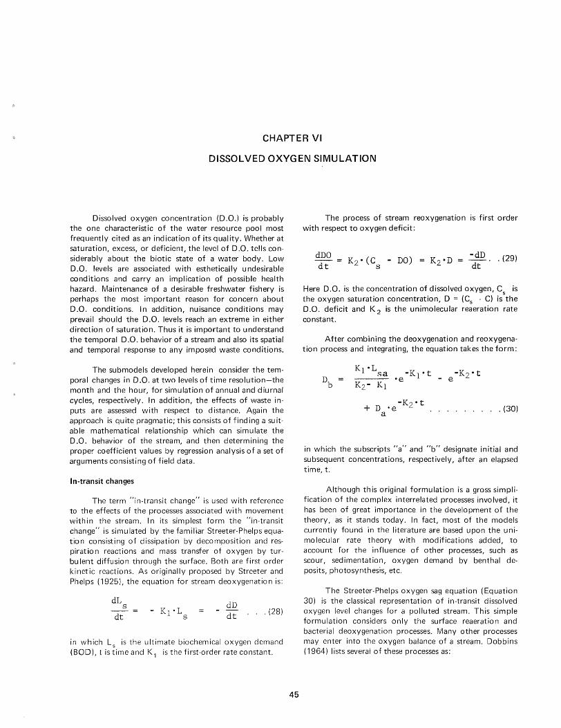
CHAPTER VI

DISSOLVED OXYGEI\I SIIVIULATION

Dissolved oxygen concentration (D.O.) is probably the one characteristic of the water resource pool most frequently cited as an indication of its quality. Whether at saturation, excess, or deficient, the level of D.O. tells con­siderably about the biotic state of a water body. Low D.O. levels are associated with esthetically undesirable conditions and carry an implication of possible health hazard. Maintenance of a desirable freshwater fishery is perhaps the most important reason for concern about D.O. conditions. In addition, nuisance conditions may prevail should the D.O. levels reach an extreme in either direction of saturation. Thus it is important to understand the temporal D.O. behavior of a stream and also its spatial and temporal response to any imposed waste conditions.

The submodels developed herein consider the tem­poral changes in D.O. at two levels of time resolution-the month and the hour, for simulation of annual and diurnal cycles, respectively. In addition, the effects of waste in­puts are assessed with respect to distance. Again the approach is quite pragmatic; this consists of find ing a su it­able mathematical relationship which can simulate the D.O. behavior of the stream, and then determining the proper coefficient values by regression analysis of a set of arguments consisting of field data.

In-transit changes

The term "in-transit change" is used with reference to the effects of the processes associated with movement with in the stream. I n its simplest form the "in-transit change" is simulated by the familiar Streeter-Phelps equa­tion consisting of dissipation by decomposition and res­piration reactions and mass transfer of oxygen by tur­bulent diffusion through the surface. Both are first order kinetic reactions. As originally proposed by Streeter and Phelps (1925), the equation for stream deoxygenation is:

dL s

dt dD dt ... (28)

in which Ls is the ultimate biochemical oxygen demand (BOD), t is time and K 1 is the first-order rate constant.

45

The process of stream reoxygenation is first order with respect to oxygen deficit:

dDO = K - (C - DO) dt 2 s

-dD dt

. (29)

Here D.O. is the concentration of dissolved oxygen, Cs is the oxygen saturation concentration, 0 = (Cs - C) is the D.O. deficit and K 2 is the unimolecular reaeration rate constant.

After combining the deoxygenation and reoxygena­tion process and integrating, the equation takes the form:

-K2- t + D °e ......... (30) a

in which the subscripts "a" and "b" designate initial and subsequent concentrations, respectively, after an elapsed time, t.

Although this original formulation is a gross simpli­fication of the complex interrelated processes involved, it has been of great importance in the development of the theory, as it stands today. I n fact, most of the models currently found in the literature are based upon the uni­molecular rate theory with modifications added, to account for the influence of other processes, such as scour, sedimentation, oxygen demand by benthal de­posits, photosynthesis, etc.

The Streeter-Phelps oxygen sag equation (Equation 30) is the classical representation of in-transit dissolved oxygen level changes for a polluted stream. This simple formulation considers only the surface reaeration and bacterial deoxygenation processes. Many other processes may enter into the oxygen balance of a stream. Dobbins (1964) lists several of these processes as:

1. Sedimentation or adsorption of BOD. 2. Resuspension of settled organic deposits by

scour action on benthal deposits or upward diffusion of partly decomposed organic mat­ter from the stream benthos.

3. BOD increase by local runoff. 4. Oxygen demand by the aerobic zone of the

benthal layer. 5. Oxygen removal by the stripping action of

gases rising from the anaerobic decomposition of the benthal layer.

6. Photosynthetic oxygen production by plank­ton and periphyton.

7. Oxygen removal by respiration of plankton and periphyton.

8. Longitudinal dispersion.

Several researchers have proposed modifications to the Streeter-Phelps equation to integrate into it one or more of the above processes (Thomas, 1948; Li, 1962; Dobbins, 1964; Camp, 1965; and O'Connor, 1967). The work of Hansen and Frankel (1965) brings together, in a rather concise form and in a consistent set of nomencla­ture, most of the basic concepts presented by their pred­ecessors. In addition, they propose a cyclic expression to

represent diurnal variations in photosynthetic production and respiratory uptake of oxygen by photosynthetic organisms. Their equation in integrated form is:

(Kl + K )·(1 + K3/K) -K2-t r

D = D -e + ------~----~-------b a (K2 - K)

K + 4

K2 K - 4

+ a [K2 cos(wt + S) + w sin (wt +S)]

in which

Da

. . . . (31)

oxygen deficit of a volume of water as it enters the reach (mg/I) oxygen deficit of the same volume as it leaves the reach (mg/I)

46

K p

t

H a a

w B It

ultimate first stage BOD in solution and suspension as the flow enters the reach (mg/I) [

initial areal BOD of the benthic zone (g/sq -meter)

laboratory rate of deoxygenation (base e, day -1 )

reoxygenation rate constant (base e, day -1 )

rate constant for BOD removal by sedi­mentation and/or adsorption (base e, day -1 )

rate constant for the anaerobic fermen­tation of benthal deposits (base e, day -1 )

the difference between the actual in­stream deoxygenation constant and lab­oratory rate constant (base e, day -1 )

K 1 +K r +K 3 rate of addition of BOD to the stream water from the benthal layer (mg/I-day) travel time through the reach (days) stream depth (meters) a/(w 2+ K2 ) (mg/I-day)

2 maximum rate of production (consump-tion) of oxygen by photosynthesis (res­piration) (mg/'-day) 2'1T/24 2'1T/24 -It lag time at which respiration of aquatic organisms in the stream below the trib­utary is a maximum

Assuming no net increase in D.O. due to the activity of photosynthetic organisms over the typical 24 hour cycle, the monthly average of changes in D.O. within a reach may be represented by the first three terms of Equa­tion 31, which is restated as Equation 32:

(Kl + Kr )·(1 + K3/K)

(K2 - K)

Equation 32 was programmed as a part of the dissolved oxygen submodel used in this work.

The assumption of no net effect due to photo­synthetic organisms may require further justification. During daylight hours, photosynthetic oxygen production exceeds the respiratory requirements of the aquatic com­munity as indicated in Figure 21. These same photo­synthetic organisms become users of oxygen during periods of darkness. The net effect of the photosynthetic organisms over a 24 hour cycle is the difference between the amount of oxygen produced during the day (the cross hatched area under the curve) and the amount consumed at night (the cross hatched and stippled area above the curve).

c: 0

U :::I

"8 d:

c:

~ ~ '0. I/) Q)

a::

0

0

~ Photosynthetic Oxygen Production,

Assumed Constont

Respirotion Rote For Non

Photosynthetic OrQonisms,

24

[fA Respirotion By Photosynthetic OrQonisms,

D Community Respirotion

Figure 21. Dissolved oxygen variations at station S-12.8 for 1966-67 with best fit Fourier series curve.

Studies have been conducted to assess the produc­tivity of certain streams. Hosk in (1960) reports photo­synthetic oxygen production rates of 87.7 pounds per acre of stream surface per day and community respiration rates of 192 pounds per acre per day in streams of North Carol ina. Edwards and Owens (1962) found oxygen pro­duction in an English chalk stream to vary from 28.6 to 158 pounds per acre per day while community respiration ranged between 59.9 and 139 pounds per acre per day. It should be emphasized that the above respiration figures relate to the combined respiration of photosynthetic and nonphotosynthetic organisms, represented in Figure 21 as the area bounded by the assumed respiration rate for non­photosynthetic organisms and the zero abscissa, plus the stippled area.

47

O'Connell and Thomas (1965), in their study of the Truckee River below Reno, Nevada, found oxygen pro­duction to average about 72.5 pounds per acre per day, while respiration of photosynthetic organisms proceeded at the rate of 65.4 pounds per acre per day. While the figures of O'Connell and Thomas indicate a possible net production of oxygen by photosynthesis, some of the oxygen produced undoubtedly escapes to the atmosphere.

Suspended BOD

Changes in dissolved and suspended BOD within a reach have been represented as

-K·t ·e + ....E- .. (33)

K

by Hansen and Frankel (1965) where LSb is the BOD of the flow as it leaves the reach being stud ied and other variables are as defined above.

For the case where scour is taking place (K3 = 0), but not sedimentation (pJ 0), the change in BOD of the benthal deposit within the reach was represented by Hansen and Frankel as

-K4-t m

O ) H·p

- 1 - e . -K- .... (p :f 0,

0) ........ (34)

in which Ldo

is the initial areal BOD of the benthic de­posit and Ld in the areal BO 0 of the deposit after time "t." This equation may be applied directly to the simula­tion of month to month changes in the benthal BOD of a stream simply by letting t = 30 days.

In the case of sedimentation (K3f 0 and p = 0), Hansen and Frankel assume that the rate of deposition is exactly balanced by the rate of anaerobic fermentation so that there is no net buildup of organic material in the benthal region. This assumption seems unduly restrictive for modeling over an extended period. To fill the need for a model to simu late possible increases in benthal BOD during certain periods of the year, the following has been developed.

It is obvious that BOD removed from suspension by sed imentation and/or adsorption must appear as increased

benthal BOD. Assuming that this removal rate is ade­quately represented by a first order kinetics model of the form

dL s

dt

integration yields

L s

a ...... (35)

The change in L s ' due to sedimentation and adsorption, as the flow passes through the reach a-b is

6L s

Ls • (1 - e -K3 • t) a

...... (36)

where Ls is measured in mg/I or gm/mcter3. On an areal

basis this means that the amount of BOD deposited is (assum ing uniform deposition over the benthal region of the reach):

Hmo 6L s

........ (37)

Using monthly averages, the amount deposited in this reach per month is

HmoL s

a

( -30 0 K3) \1 - e .. (38)

in which H is the monthly average of the mean stream depth (in meters), and LSa is the monthly average of sus­pended and dissolved BOD in the flow entering the reach.

Assuming areal BOD of the benthos at the beginning of the month to be Ld

o and that during the month one

half of the amount of BOD deposited is subjected to anaerobic decomposition for a period of 30 days, the equivalent initial areal BOD (L do ) may be written

+ 1/2 HmoL s a

e -30K3)

.... (39)

48

Substituting into the integrated first order reaction equation for anaerobic fermentation for p = 0:

gives

°e

...... (40)

[LdO

+ 1/2 Hm'Lsa

'(1 e-30K3J] ....... (41)

-30K4

This expression predicts Ld at the beginning of the following month when p = 0 and K3 =F O. Equation 34 applies where pi 0 but K3 = O. If both K3 and p are zero this means that only anaerobic fermentation is affecting the amount of organic material in the benthal deposit. Both Equations 34 and 41 reflect this situation.

Determination of rate constants

The in-transit dissolved oxygen equation of Hansen and Frankel contains many rate constants and other para­meters. Estimation procedures for a few of these are found in the literature. Those for which estimation pro­cedures are available include oxygen saturation concentra­tion (C s )' stream reaeration rate constant (K2 ), ultimate dissolved and suspended BOD (Ls) and laboratory de­oxygenation rate constant (K 1 ). The relationships employed herein for the estimation of these parameters are discussed below.

Oxygen saturation. The ASCE Committee on Sani­tary Engineering Research (1960) has established the re­lationship between oxygen saturation concentration, Cs '

and water temperatures, T (in degrees Centigrade), for fresh water exposed to standard atmospheric at mean sea level as

c s

14.652 - .41022 T + .0079910 T2

- .000077774 T3 .......... (42)

Saturation concentrations calculated from this expression differ slightly from those published in Standard Methods for the Examination of Water and Wastewater (American Publ ic Health Association, 1965).

Saturation concentrations obtained from Equation 42 are for sea level (760 millimeters of mercury) and may be adjusted for other atmospheric pressures by mu Itiply­ing by the following pressure correction factor (cf):

cf P - pv 760 - pv

...... (43)

in which P is the observed atmospheric pressure in milli­meters of mercury and pv is the vapor pressure of water at the prevailing water temperature. Figure E-2, Appendix E, is a nomograph showing such relationships.

Reoxygenation rate constant. The reoxygenation rate constant has been demonstrated to be closely related to the flow characteristics of the stream. Owens, Edwards, and Gibbs (1964) have integrated data collected by them­selves and others, covering a wide range in flow condi­tions, in the derivation of the expression

.67 _1.85 9 • 4 1 • V • H . . . (44)

in which k2 (20) is the reoxygenation rate constant (base 10) for a natural stream at 20 DC, V is the mean velocity of flow (ft./sec.) and H is the mean flow depth (ft.). The relationship between the rate constant and water tempera­ture has been characterized as

k 2 (20) -1 • 024 1 (T - 20 ) . . (45)

by Elmore and West (1961). This expression was later used by Churchill et al. (1962) in their exhaustive study of the reaeration of natural streams. I n Equation 45 T is water temperature (DC) and k 2 (T) is the rate constant at temperature T (base 10, day -1 ). Because the reaeration rate constant is a characteristic of the channel reach and not of in flowing waters, it was not necessary to define this variable for each inflow.

Deoxygenation rate constant. The deoxygenation rate constant is affected by water temperature, as de­picted by the expression

kl(20).e(T-20) .... (46)

where k1 (20) is the rate constant for 200C and k 1 (T) is

that for the temperature under which the actual oxygen consuming reaction takes place. Fair, Geyer, and Okun (1968) report values of e ranging from 1.15 at 50 C to 0.97 of 350 C. This variation has been approximated in this study as follows:

49

e 1.065-.0012-(T-5) for T < 20°C } e 1 .047

..... (47)

The rate of oxygen demand is governed by the rate of aerobic decomposition of organic materials dissolved or suspended in the water, which is influenced by the density and type of microbial population, concentration and com­position of the waste, water temperature, etc. Deoxygena­tion rate constants found in the literature vary widely. Hansen and Frankel (1965) used values of K1 + Kr (de­oxygenation rate in the stream) of from 0.30 to 0.42 (day -1). Fair, Geyer, and Okun (1968) and McGauhey (1968) cite a value of 0.23 as the "nominal" value for K1 (base e) for waters receiving settled domestic waste water. Kothandaraman (1968) cites data from the Ohio River in which K1 varies -From 0.31 to 0.05 (day -1 ).

These are equivalent to base 10 constants (k 1) of 0.134 and 0.022 respectively.

Several procedures for estimating the ultimate BOD and the rate constant have been presented in the literature (Thomas, 1937; Moore, Thomas and Snow, 1950; and Sheehy, 1960). Attempts to apply these methods to the low level BOD's of this system were largely unsuccessful because the BOD's were below the range for which the techniques were established. In a short reach immediately below the trout farm discharge, BOD levels were found to be high enough to allow the application of these proce­dures.

Samples from several points on the river down­stream from the trout farm exhibited laboratory rate constants, k 1 (base 10), ranging from 0.15 to 0.08 day -1 .

Figure 22 shows the resu Its of these tests. Similar values were obtained below the Wellsville sewer outfall, though here again low BOD levels rendered the computational procedure approximate at best. Values for the deoxygena­tion rate constant (base 10) in surface inflows were assu med to be 0.15 (day -1 ) for th is work.

Discrete BOD loads in the Little Bear River

To assess the effect of a municipal or industrial waste on the oxygen resource of a river system, the initial dissolved oxygen concentration, BOD level, and de­oxygenation rate constant of the waste stream need to be defined. Data from the two concentrated waste sources on the Little Bear River show a small annual variation in oxygen concentration. Concentrations ranged from 6.8 to 11.5 mg/I at the Wellsville discharge and from 3.7 to 10.6 mg/I at the trout farm.

Though BOD levels in the two effluents are not high, as municipal and industrial wastes go, they are sig-

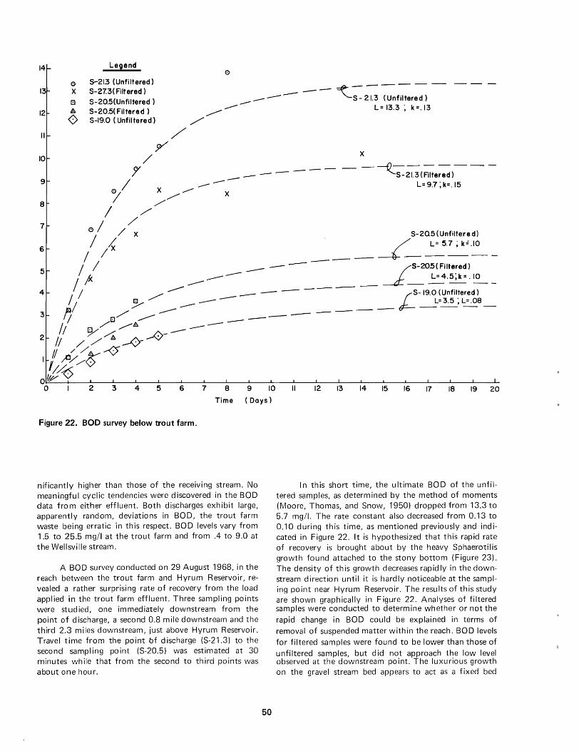
Legend o 14

13 o X

5-213 (Unfiltered) S-27.3( Filtered) S-20.5(Unfiltered ) S-20.5( Filtered) S-19.0 (Unfiltered)

_--- -- ~~~~filtered) - - -­

...----_____ L= 13.3 ~ k=.13 12

II

10

9

8

7

/ /'

y /

7 / --o X,.__--

'I ./'" /"

/ ./

X

X

----- ~ ------- ~21.3(Filtered)

L= 9.7 ~ k=. 15

0/ // X S-2Q5(Unfiltered) / /( . ---i- L" 5.7 ; k=~ _ 6

5 / / __ - - ---- /S-20.5~Filte~e~)

/ f ___ ------ J- L-4.5,k-.10

/ ___ - - ---- -- is-19.0~unfil!er~d-}--1/ 8./ /"" -- L-3.5 ,L-.08

Ii 8/./ ------- _------- -----

4

3

/1 9-"/"..-A A- -----

2 /1 /./~ -<7-'V II / /y~

I I ,;0//0 /~

O/jp' 012 3 4 5 6 7 8 9 10

Time ( Days)

Figure 22. BOD survey below trout farm.

nificantly higher than those of the receiving stream. No meaningful cyclic tendencies were discovered in the BOD data from either effluent. Both discharges exhibit large, apparently random, deviations in BOD, the trout farm waste being erratic in this respect. BOD levels vary from 1.5 to 25.5 mg/I at the trout farm and from .4 to 9.0 at the Wellsville stream.

A BOD survey conducted on 29 August 1968, in the reach between the trout farm and Hyrum Reservoir, re­vealed a rather su rprising rate of recovery from the load applied in the trout farm effluent. Three sampling points were studied, one immediately downstream from the point of discharge, a second 0.8 mile downstream and the third 2.3 miles downstream, just above Hyrum Reservoir. Travel time from the point bf discharge (S-21.3) to the second sampl ing point (S-20.5) was estimated at 30 minutes while that from the second to third points was about one hour.

50

II 12 13 14 15 16 17 18 19 20

In this short time, the ultimate BOD of the unfil­tered samples, as determined by the method of moments (Moore, Thomas, and Snow, 1950) dropped from 13.3 to 5.7 mg/1. The rate constant also decreased from 0.13 to 0.10 during this time, as mentioned previously and indi­cated in Figure 22. It is hypothesized that this rapid rate of recovery is brought about by the heavy Sphaerotilis growth found attached to the stony bottom (Figure 23), The density of this growth decreases rapid Iy in the down­stream direction until it is hardly noticeable at the sampl­ing point near Hyrum Reservoir. The results of this study are shown graphically in Figure 22. Analyses of filtered samples were conducted to determine whether or not the

rapid change in BOD could be explained in terms of

removal of suspended matter within the reach. BOD levels for filtered samples were found to be lower than those of

unfiltered samples, but did not approach the low level observed at the downstream point. The luxurious growth on the gravel stream bed appears to act as a fixed bed

Figure 23. Sphaerotilis growth on rocks downstream from trout farm discharge.

reactor, quickly removing a large proportion of the or­ganic matter carried into the stream by the trout farm discharge.

Combination of hydrologic inputs

Dissolved oxygen and BOD concentrations at the upstream end of the reach are calculated by the Equation 16 mixing formu la. The deoxygenation rate constant of the combined flows is assumed to be the weighted average of the rate constants for all components of inflow, where the weighting factor is the total BO 0 contributed by each input:

in which

nc L

j=1 K1 • q . • BOD.

. J J

nc L

j=1

J

q .• BOD. J J

. . . . (48)

51

n

The annual cycle

deoxygenation rate constant of the combined inflow (base 10) number of hydrologic inputs to the reach deoxygenation rate constant for the "j th" hydrologic input (base 1 0) rate of flow for the " j th" hydrologic input mean monthly BOD of the "j th" hydrologic input

Mean daily dissolved oxygen exhibits an annual cycle. Figure 24 illustrates the pattern, which is sinu­soidal. Simulation of this pattern is of value for its own sake to give the time distribution in dissolved oxygen at a given station; however, the value derived is also the initial D.O. input for the in-transit simulation. The annual D.O . simulation is the composite of the simu lation of many individual inputs, described subsequently.

The simulation computer program for this phase is called MIDOX, implying monthly dissolved oxygen. This program, which is a part of the system program

• 14

13 • • •

12 • • • 9.49+2.30. Sin (2TT . x - .208 )

365

II • , • • 0'1 E • •

- ---- ----0 9 • 0

7

•

• •

---- ---- -----

• • •

• • •

•

•

• s--------~----------------~------~--------~------~ ________ ~_

o 150 200 250 300 3S0

Da ys Since October First

Figure 24. BOD variations at stations S-12.8 for 1966-67 with best fit Fourier series curve.

WAOUAL, also absorbs the "in-transit" and "diurnal" components; in aggregate then, MDISOX is the dissolved oxygen submodel.

Inputs

Adjustment of discrete sampling data. D.O. data from the week Iy sampling program were adjusted for the effect of diurnal variation and varying sampling time by dividing by the diurnal D.O. index (0001) for the time at which the grab sample was taken. The 0001 is the ratio of observed D.O. concentration at the time of observation to mean daily concentration, as determined from contin­uous monitoring data. This adjustment considerably improved the fit of the annual cycle D.O. model over that attained using the raw D.O. data. Thus for all data dis­cussed, which is to be representative of a single sample, it will be understood that the value reported is an adjusted mean daily value.

River inflow. The simu lation procedure begins at the upper extremity of each branch, proceeding down­stream. Results from the simulation of the adjacent up-

52

stream reach are employed as input for the simulation of the next reach downstream. For the first reach analyzed on a branch, the stream inflow is assumed to be zero and all natural surface inflows are lumped together in the "sur­face inflow" category (OS). The method of approximating D.O., BOD, and deoxygenation rate constant for this component is discussed below.

Branch inflow. Branches tributary to a reach are simulated before the analysis of that reach is attempted. The D.O., BO 0, and deoxygenation rate constant of in­flow from tributary branches are therefore available for incorporation into the analysis.

Surface inflow. Field data from analysis of weekly samples showed significant annual cycles for mean daily dissolved oxygen, with high values during winter months, which decreased to minimums in the summer and early fall. Figure 24 illustrates the trend using representative field data. The data were adjusted to mean daily values by dividing observed concentrations by the diurnal dissolved oxygen index (discussed later) for the time of sampling. A simple sine-curve linearizing equation:

DO = DO + C· Sin (2 'IT • X + A'\ + I 365 ')

.. (49)

was fitted to the adjusted data by least squares analysis, where D.O. is mean daily dissolved oxygen conc(~ntrdtion (mg/I) on the "x th" day of the year, D.O. is the medfl annual D.O. concentration, x is the number of days since October 1, C and A are parameters detennilwd by I(~ast

squares regression procedures, and f is Llw (kvidlion of the oxygen concentration observed on Ilw "x til" day of the year from the model prediction for lilal (ldl<~. FOllri(~r series containing more terms were tri(~d, 1>111 wilhollt any significant improvement in fit. Tlw IlH)(kl hilS 1)(~t~1l pro grammed, however, to allow a Iwo I<~rlll FOllrit~1 s(~ri(~s

should it be needed.

Table 14 lists the results of Ihis FOlil WI st~rlt~s CllrVt~

fitting at 12 sampling points 011 tlw syslt~lll.llw dt~Wt~t~ of fit, as measured by R 2, is not h i~Jil, blll Sid I isl ieri .I1l;lIyst~s indicate that Equation 31 does (~xpldill iI SiqlliflCtllll pm tion of the total annual varidtioll ill 0.0 .II ,iii sldtitlllS. Figure 24 illustrates the relativ(~ly Idr~w I t~SHltlill tkvidt iOlls from the model. These variations dppt\lr 10 Iw rdlHlolll III

nature, possibly resulting from r.IIHlolll Sdlllpllll~1 t~rrors

and variations in oxygen concentratiolls CdllSt~d by rdll domness in such controlling varidblt~s <IS wdlt~r 1t~lllpt~rd

ture and cloud cover.

Equation 49 has been adopted for Ilw pn~d iel iOIl 0 r mean monthly D.O. concentrations in ndturdl sllrfan! ill­flows despite the typically low R2 becaust~ it d()(~s rep­resent a significant cyclic annual variation 1.11 ali poinls sampled.

In some cases, discernible annual cycles were also observed in the weekly BOD data (Figure 25). Thereforc, a sine-curve equation, similar to that applied in the case of

dissolved oxygen concentrations, was fitted to weekly BOD data from 12 sampling points in the Little Bear River drainage:

BOD BOD + C·Sin (2'IT ·x + A) + € 365

............ (50)

As shown in Table 15, the degree of fit varied consider­ably from one location to another. Statistical significance could be claimed for eight of the twelve sets of data.

Thouqh the degree of correlation between time of year and BOD concentration was not high, a significant port ion of ttl(! lotal variation at a majority of the sampl ing points was explained by Equation 50. Because a better proc(!durt! for predicting BOD concentrations in surface Inflows was not forthcoming, Equation 50 has been in­corporal(!d illio the simulation to approximate annual cycl(~s for Iht~ BOD of natural surface inflows.

Irrig(Jtio/l return flow. Dissolved oxygen concen­lral ions in surface irrigation return flows are assumed rel-

1.11 iv(!ly constant over the three or four month irrigation sedSOll, thouqh nrovision is made in the modeling program 10 dllow variat ion with time.

The BOD of return flow is also considered constant. Becduse waters applied to agricultural lands have more opportunity to pick up organic matter from animal and vegelal matter in and on the soil, the level of oxygen demand in return flows is assumed to be somewhat above that found in natural surface inflows. The deoxygenation rate constant for irrigation return flows is assumed to be the same as that for natu ra I su rface inflows.

Groundwater inflow. Dissolved oxygen concen­trations in groundwater inflows were not sampled during

Table 14. Fourier series simulation of annual fluctuations in dissolved oxygen concentration.

[no ~ no + e·Sin G'~15 ·X + ~ J Station

S-12.7 S-12.8 S-15.2 S-16.8 S-21.3 S-24.6 S-27.5 SO-O.O SEC-4.3

SEC-6.2 STF -0.0 SW-O.1

-=-.;::::-=-

DO (mg/I)

8.55 9.49 9.97 8.77 7.23

8.95 8.61 8.82 8.59 8.48 6.35 8.08

C (constant)

1.517 2.303

1.808 1.863 1.591 1.321 1.032 1.896

.998 1.163 1.520 1.126

53

A (radians)

.407 - .208

.573

.897

.660 - .148

.247

.401 -1.243

.394

.773

.425

56. 66. 36. 74. 61. 60. 52. 62 . 27. 62. 31. 62.

Comments

below sewer outfall

reservo ir su rface

below trout farm

below reservoir

trout farm effluent

sewer outfall

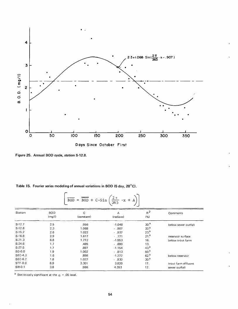
....... D E

o d al

4

3

•

2

•

. .

• 2·3+1.068· Sin (~:s ·x- .907)

•

......... ---.---- ---- ----

•

. .

OL-______ L-______ ~ ______ ~--____ ~ ______ ~ ________ L_ ______ ~ __

o 50 100 150 200 250

Days Since October First

Figure 25. Annual BOD cycle, station S-12.8.

Table 15. Fourier series modeling of annual variations in BOD (5 day, 20o e).

[BOD = = en ·X + ~J BOD + e·Sin

365

Station BOD C A R2

(mgtl) (constant) (radians) (%)

S-12.7 2.5 .956 -1.048 30.a

S-12.8 2.3 1.068 - .907 32.a S-15.2 2.6 1.022 - .937 23.a

S-16.8 2.9 1.617 - .171 21.a S-21.3 6.8 1.772 -1.553 16. S-24.6 1.7 .485 - .690 13. S-27.5 1.7 .897 -1.154 43.a

SO-O.O 1.9 1.002 - .813 50.a

SEC-4.3 1.6 .898 -1.272 62.a SEC-6.2 1.8 1.022 - .930 30.a

STF-O.O 8.9 3.301 3.820 17. SW-0.1 3.8 .986 4.353 12.

a Statistically significant at the a = .05 level.

54

300 350

Comments

below sewer outfall

reservo ir su rface below trout farm

below reservoir

trout farm effluent sewer outfall

this project. A sinusoidal pattern of annual variation, similar to that found in natural surface inflows, was assumed for groundwater inflows.

Biochemical oxygen demand of groundwater was not measured, but is assumed to be zero. This assumption is based upon the ability of the biologically active soil mantle to stabilize dissolved organics as the water passes through enroute to the groundwater aquifer. Suspended organics are removed by the screening action of soil par­ticles. For modeling purposes, the BOD of groundwater inflows is taken as zero.

Municipal and industrial releases. Annual variations in mu nicipal and industrial releases are simu lated by card input based upon historical records where possible.

Summary. Table 16 summarizes the simulation for each hydrologic input. The stream is considered reach by reach along the main stem and immediate tributaries; all or part of these inputs may be significant for any given reach. The mean daily dissolved oxygen value, D.O., for that reach is calculated by the weighted average of all inputs.

Reservoir effects Of the two reservoirs on the Little Bear River, only

Porcupine Reservoir was sampled to assess the effect of the impoundment on the oxygen resource of the stream. Dissolved oxygen concentrations at the sampling point immediately below Porcupine Reservoir were consistently at or near the level of saturation as indicated in Figure 26. This is reasonable for this situation, even though releases from this reservoir are from the hypolimnion, because of the intense turbulence in the discharge stilling basin.

II

10

9

...; 8

.J

.... C>

2: -" 6 . ~ " c 5 ., u c

" 4 ()

.., .. :5 > ., ..

.0 2 0

246 10

Saturation Concentration (M GIL)

Figure 26. Comparison of D.O. concentrations observed below Porcupine Reservoir in 1967 with satura­tion concentration.

55

Therefore a simulation run was made with the D.O. in the reservoir discharge set equal to the saturation con­centration. This assumption resulted in significant devia­tions of simulated concentrations from measured values, both at the reservoir discharge and at points downstream.

Time series analysis of weekly D.O. data from Por­cupine Reservoir discharge disclosed a small, but statisti­cally significant correlation between time of year, and D.O. concentration, represented by the equation

This time series equation improved the correspondence between simu lated and measured D.O. concentrations at reservoir discharges and at points downstream. Therefore, Equation 51 was used to simulate D.O. concentrations in reservoir releases, rather than to assume saturation.

Because of the high degree of randomness in the BOD data, it was difficult to determine precisely what hydrologic or hydraulic parameters relate best to the BOD load in released water. Again, some degree of time de­pendence was observed. A simple sine-curve representa­tion of monthly variations in BOD at reservoir releases was incorporated into the simulation model.

To summarize: monthly variations in D.O. and BOD of reservoir releases were both assumed to follow a sinu­soidal pattern through the annual cycle. The annual mean, coefficient, C, and phase shift, A, were determined by the least squares fitting of Equation 51 to observed D.O. and BOD data for the reservoir release.

Simulation algorithm

Figure 27 outlines the simulation algorithm for mean monthly dissolved oxygen. This algorithm is sum­marized below.

1. Obtain monthly flow values for all inputs listed in Table 16 from the hydrologic model.

2. Establish mean annual D.O., and Fourier con­stants, A and C, for Equation 49 by regression analysis of field data; do I ikewise for Equation 50 .

3. Compute D.O. and BOD of each input to reach for month in question by Equations 49 and 50, respec­tively; use card input where these equations are not applicable .

4. Compute stream D.O., consisting of combined inflows, by Equation 16 .

5. If each is a reservoir, calculate output D.O. by Equation 15, skipping steps 6, 7,8,9, 10, 11, 12, 13.

6. Compute weighted deoxygenation rate constant, k l' by Equation 48, and correct for temperature by Equa­tions 46 and 47.

7. Estimate the reo.xygenation rate constant, k2 ,

using Equation 44 and adjust for temperature by Equa­tion 45.

8. Calculate saturation concentration for reach using output of temperature simulation as argument for Equa­tion 42; also adjust for altitude pressure by Equation 43; alternately, Figure E-2 may be used.

9. Calculate oxygen deficit at the upstream end of the reach (D a = CSa - DOa ) and apply the sag equation (Equation 32).

10. Subtract the remaining deficit from the satura­tion concentration at the downstream end of the reach to estimate the dissolved oxygen concentration at the out­flow fro m the reach.

11 . Determine residual BOD in reach outflow (Equation 36).

12. Compute areal BOD of the benthos at the end of the month (Equation 34 or 41).

13. Call diurnal submodel if desired. 14. Go to next reach and return to step 1. 15. If last reach is simu lated, increment time by one

month and return to step 1.

- Step 2 is input preparation; steps 1, 13, 14, and 15 are done by WAQUAL; steps 3-12 are done by DDISOX.

Table 16. Summary of input D.O. and BOD equations over the annual cycle.a

Input Parameter Model

D.O.

} BOD

K1

River inflow

result from previous simulation

D.O.

} BOD

K1

Branch inflow

result from previous simu lation

Surface inflow D.O.

BOD

K1

I rrigation return flow D.O.

BOD ) K1 card input

Groundwater inflow D.O. DDg~ DOg+C'Sinn; "m + A)

BOD ) K1 card input

D.O.

} BOD

K1

Municipal and industrial release

card input

aSubmodel constants (lj"Q and BOiJ), coefficients (e) and phase shifts (A) are determined by analysis of field data and provided to the simulation program by punched card input.

56

,.

Compute D.O., BOD and rate con­stant for components of f I ow.

Estimate ~.O., BOD and rate con­stant for combined inflow.

y es ~

a reservoir ..... N 0

r Compute saturation concentra-tion at both ends of the reach .

• Establish parameters for the

Estimate ~.O., BOD and Oxygen sag model. rate constant in reservoir discharge.

-"

Compute D.O. deficit at up.-stream end of reach and apJ)ly oxygen sag model to get def-icit at downstream end of reach . • Subtract deficit at downstream end of reach from saturation concentration at this poi nt to get D.O. concentration in out-flow.

- Return - --

Figure 27. Generalized monthly D.O. flow chart.

57

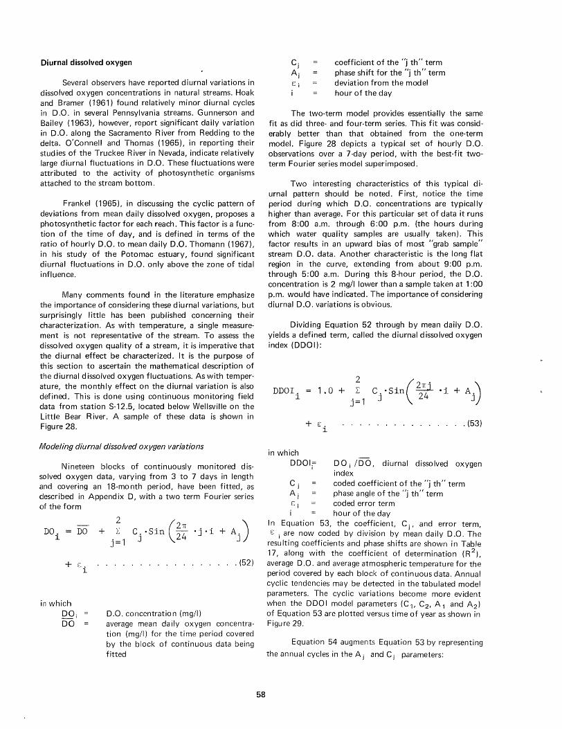
Diurnal dissolved oxygen

Several observers have reported diurnal variations in dissolved oxygen concentrations in natural streams. Hoak and Bramer (1961) found relatively minor diurnal cycles in D.O. in several Pennsylvania streams. Gunnerson and Bailey (1963), however, report significant daily variation in D.O. along the Sacramento River from Redding to the delta. O'Connell and Thomas (1965), in reporting their studies of the Truckee River in Nevada, indicate relatively large diurnal fluctuations in D.O. These fluctuations were attributed to the activity of photosynthetic organisms attached to the stream bottom.

Frankel (1965), in discussing the cyclic pattern of deviations from mean daily dissolved oxygen, proposes a photosynthetic factor for each reach. Th is factor is a fu nc­tion of the time of day, and is defined in terms of the ratio of hourly D.O. to mean daily D.O. Thomann (1967), in his study of the Potomac estuary, found significant diurnal fluctuations in D.O. only above the zone of tidal influence.

Many comments found in the literature emphasize the importance of considering these diurnal variations, but surprisingly little has been published concerning their characterization. As with temperature, a single measure­ment is not representative of the stream. To assess the dissolved oxygen quality of a stream, it is imperative that the diurnal effect be characterized. It is the purpose of this section to ascertain the mathematical description of the diurnal dissolved oxygen fluctuations. As with temper­ature, the monthly effect on the diurnal variation is also defined. This is done using continuous monitoring field data from station S-12.5, located below Wellsville on the Little Bear River. A sample of these data is shown in Figure 28.

Modeling diurnal dissolved oxygen variations

Nineteen blocks of continuously monitored dis­solved oxygen data, varying from 3 to 7 days in length and covering an 18-month period, have been fitted, as described in Appendix 0, with a two term Fourier series of the form

DO. 1

DO + ~ CJ .. Sin (~2 ·j·i + Aj) j=1

+ E. l

in which DO i

DO

............. (52)

D.O. concentration (mg/l) averqge mean daily oxygen concentra­tion (mg/l) for the time period covered by the block of continuous data being fitted

58

C j coefficient of the "j th" term Aj phase shift for the "j th" term E i deviation from the model i hour of the day

The two-term model provides essentially the same fit as did three- and four-term series. This fit was consid­erably better than that obtained from the one-term model. Figure 28 depicts a typical set of hourly D.O. observations over a 7-day period, with the best-fit two­term Fourier s~ries model superimposed.

Two interesting characteristics of this typical di­urnal pattern should be noted. First, notice the time period during which D.O. concentrations are typically higher than average. For this particular set of data it runs from 8:00 a.m. through 6:00 p.m. (the hours during which water quality samples are usually taken). This factor results in an upward bias of most "grab sample" stream D.O. data. Another characteristic is the long flat region in the curve, extending from about 9:00 p.m. through 5:00 a.m. During this 8-hour period, the D.O. concentration is 2 mgll lower than a sample taken at 1 :00 p.m. would have indicated. The importance of considering diurnal D.O. variations is obvious.

Dividing Equation 52 through by mean daily D.O. yields a defined term, called the diurnal dissolved oxygen index (0001):

DDOI. l

in which

1.0 +

+ E. l

~ C S' (2'TTj el', + A) L, J" In 24 J'

j=1

........... (53)

ODOlF DO i 100, diurnal dissolved oxygen index

C j coded coefficient of the "j th" term A j phase angle of the "j th" term E i coded error term i hour of the day

I n Equation 53, the coefficient, C j' and error term, E i are now coded by division by mean daily D.O. The

resulting coefficients and phase shifts are shown in Table 17, along with the coefficient of determination (R 2

),

average D.O. and average atmospheric temperature for the period covered by each block of continuous data. Annual cyclic tendencies may be detected in the tabulated model parameters. The cyclic variations become more evident when the 0001 model parameters (C 1, C2 , A1 and A 2 )

of Equation 53 are plotted versus time of year as shown in Figu re 29.

Equation 54 augments Equation 53 by representing

the annual cycles in the A j and C j parameters:

13

12

c:

~ " o L.. -c: Q)

o c: o U

: : · . · · I

. . Series Model

. - ---------

. i · · · 9~~ __ ~~ __ ~ __ L__L __ ~~ __ ~_L__L __ ~~_~_L__L_~~ __ ~_L__L __ ~~_~

o 2 3 4 5 6 7 8 9 10 II 12 13 14 15 16 17 18 19 20 21 22 23 24

Time of Day

Figure 28. Dissolved oxygen variations for the period 22-29 April 1968 with Fourier series model.

Table 17. Diurnal dissolved oxygen index model parameters.

[DDOl i =

2 (N + AJ] 1 .0 + L: C.· Sin -i j=1 J 24

No. Date of C 1 A1 C2 A2 R2 DO Ta Notes

days (constant) (radians) (constant) (radians) (%)

1127-120167 4 .0767 4.405 .0400 . 844 74 . 10.0 26.8 222-22968 6 .0304 4.777 .0144 1.287 67. 11.3 35.2 229-30668 6 .0284 4.829 .0117 1.205 53. 11.0 39.2 318-32568 7 .0596 4.865 .0220 1.032 66. 9.9 36.8 325-32868 3 .0666 4.868 .0295 1.013 87. 9.5 42.8 404-40668 2 .0196 4.483 .0047 . 723 73 . 10.0 40.5 Rain 417-42268 5 .0752 4.518 .0220 1.211 80. 9.9 35.2 422-42968 7 .0999 4.422 .0271 . 956 91 . 10.1 42.8 517-52468 7 .1197 4.307 .0302 .734 61. 7.9 52.6 524-53168 7 .1542 4.169 .0364 . 612 67 . 8.5 55.7 531-60468 4 .2060 4.194 . 0564 .275 83 . 7.3 59.3 606-61268 6 .0450 4.104 .0082 -.114 60. 9.3 56.8 Rain 624-62768 3 .2005 4.457 .0481 .450 94 . 7.6 63.7

1004- 1 00668 2 .0921 4.468 .0503 .251 55. 9.2 53.7 1009-101368 4 .1053 4.315 .0560 . 350 91 . 8.6 54.5 1023-102968 7 .0736 4.448 .0429 . 675 89 . 9.3 47.7 1030-11 0568 7 .0690 4.374 .0396 .521 74. 9.6 42.4 1106-111068 5 .0995 4.455 . 0567 .814 89 . 10.2 38.5 1203-1 21 068 7 .1008 4.399 .0588 . 787 94 . 12.1 29.3

59

.25 C, = -.035+.009Sin( ~.m"5.76)+.035Sin(~.m +5.430)+0027Ta5

.0

A,=4.53S ... I65S~l~,!,+5.70S) +;lo7Sin( lm+2.788)-.00049Ta ( R2

=. 593) ,L:..:... (R =.S26)

.20 • • r--

.15

• 4.5

I-- .---r--~.r- • • • • « ~. .---

• ~ , r •

4.0 0 N D J F M A M J J A S

0 100 .200 300 Days After October. Days After I October.

.10 C2= -·009.0IS Sin( ~.m+.330 )+.OIlSin (-¥.f1l+5.S44h.00092T a

2 (R =.611)

• 1.0 N • • • • •

• « • .5 . 05

N • • U • • •

0 • 0

0 0 N

100 300 ON DJ FMAM J

-.50 100 200 Days Since I October. Days Since I October.

Figure 29. Annual variation in diurnal D.O. index model parameters.

y C o + ~ C

J" 'Sin (;~~ 'X + a

J")

j=1 \~

+ Ta + t: ............... (54)

in which y

x Ta

diurnal D.O. index model parameter (A1, A2, C 1 or C2) days since 1 October mean daily atmospheric temperature (oF)

deviation of predicted diurnal D.O. model parameter from that calculated from diurnal D.O. variations observed

and a j = constant, coefficient and phase shift, respectively as determined from least squares analyses of diurnal data blocks

Equations 53 and 54 comprise the augmented Fourier series simulation equations for diurnal dissolved oxygen. Table 18 shows the constant, co' coefficient, c j ,

and phase shift, a j' for an annual cycle; these values were determined by least squares analysis of the data blocks indicated in Table 17 for A 1, A 2, C 1, and C 2 respectively. From th is analysis of Table 17 data blocks, the annual cycle in Co, Cj , and Aj is as~igned monthly values which

60

are shown in Table 19; the Table 19 values were calcu­lated by Equation 54 using coefficients from Table 18. Figure 29 shows a comparison of the application of these assigned monthly values, indicated by the bar lengths, to values from the data block analyses shown in Table 17, and indicated as plotted points in Figure 29.

Graph ical representation of the diurnal dissolved oxygen index (0001), Equation 53, for each month of the year is shown in Figure 30. These curves display the patterns of D.O. variation to be expected for each month of the year. Seasonal differences in the relative magni­tudes of daily D.O. swings are also shown. A phase shift of about two hours in time appears between the curves, representing winter and early spring months and those for summer months. Considerable deviation from this "typi­cal" pattern should be expected during periods of exten­sive cloud cover.

Hourly estimates of dissolved oxygen concentration may be made by multiplying the hourly ordinates to the 0001 curve by mean daily D.O. In the simulation pro­cedure, the mean daily D.O. concentration is taken as the same as the mean monthly value provided by the monthly D.O. simulation model.

Table 18. Representation of annual changes in diurnal D.O. index model parameters.

2

[Y en aj ) + Ta l c + L: c. - Sin 36S-x + 0 i=1 J

Parameter Co c 1 a1 c 2 a2 r R2 (constant) (constant) (radians) (constant) (radians) (radians) (%)

y = C1 - .035 .009 5.746 .035 5.430 .0027 59. Y = A1 4.538 .165 5.708 .201 2.788 -.0005 83. Y = C2 - .009 .018 .330 .011 5.844 .0009 61. Y= A2 1.157 .369 5.394 .067 1.567 -.0111 75.

Table 19. Estimated monthly values of diurnal D.O. index model parameters by Equation 54 using coefficients from Table 18.

Month C1 A1 C2 A2 (constant) (radians) (constant) (radians)

October November December January February March April

.0900 4.428 .0496 .428

.0877 4.366 .0503 .717

.0827 4.479 .0443 .931

.0491 4.717 .0272 1.132

.0276 4.873 .0159 1.206

.0366 4.796 .0154 1.142

.0932 4.529 .0292 .867 May .1388 4.287 .0373 .566 June .1667 4.241 .0416 .235 July August September

.1666 4.379 .0436 - .017

.1280 4.530 .0403 - .010

.0948 4.539 .0420 .177

Diurnal patterns of hydrologic inputs

Diurnal patterns of D.O. variation for each of the various hydrologic inputs to a given stream reach must be known in order to simulate hourly changes in dissolved oxygen concentration for that reach. The diurnal index concept analysis is the basis for doing this.

Surface inflow. The diurnal dissolved oxygen index simu lation of the Wellsville continuous monitoring sta­tion is assumed to represent the hourly variation in D.O. in all natural surface inflows to the system. Figure 31 compares the index patterns for the Wellsville and Para­dise continuous monitoring stations; though the cor­respondence is not one to one, it does ind icate at least a reasonable similarity and indicates the order of magnitude of possible deviations. Spot checks on the Little Bear River system have also confirmed this degree of confi­dence.

61

Hourly D.O. concentrations in surface inflows are approximated by multiplying the index value for each hour of the day by the mean monthly D.O. concentration for the input stream. Mean monthly D.O. is taken as pre­viously calculated by the monthly D.O. model. BOD and deoxygenation rate constants are assumed to be constant over the "typical" 24 hour period. These variables are evaluated in the monthly D.O. model.

Irrigation return flow. The lack of data on surface irrigation return flows prevents any authoritative assertion as to the pattern of diurnal D.O. variation to be expected in this input. The extent of photosynthetic activity in the return flow stream would depend on the nature of the channel and upon stream turbidity. Both of these factors are expected to be highly variable. For example, return flows from well stabilized hay and pasture land would be expected to be relatively low in turbidity, wh ile those from more extensively cu Itivated croplands (row crops

I~ "­d ci

1.2

)(1.04---­CD 'a

.: d ci c E ::I

0.9

o 2· 3 4 5 6 7 8 9 10 " 12 13 14 15 16 17 18 19 20 21 22 23 24

Tim e (hours)

Figure 30. Diurnal D.O. index curves for each month of the year.

>< II)

"'0 c:

1.2

1.1

o 0 1.0

o c: .... ::I

o

.9

·A · Parad ise ./ mean=8.02~

/. y/.-

--------.. ~-• _ ~ 6

-.---- - 6 6

6

Wellsville / mean = 8.35 mg/I

o 2 3 4 5 6 7 8 9 10 II 12 13 14 15 16 17 18 19 20 21 22 23 24

Figure 31. Comparison of D.O. index patterns on the Little Bear River at Wellsville and Paradise on 11·12 October 1968.

62

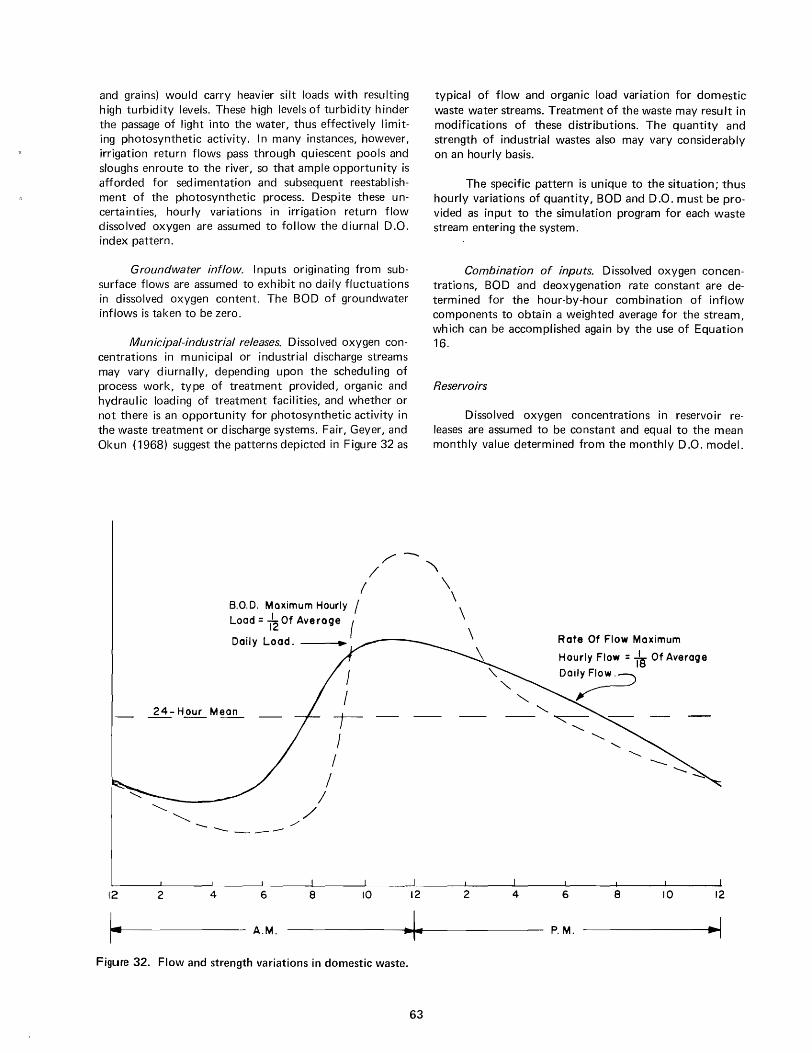
and grains) would carry heavier silt loads with resulting high turbidity levels. These high levels of turbidity hinder the passage of light into the water, thus effectively limit­ing photosynthetic activity. In many instances, however, irrigation return flows pass through quiescent pools and sloughs enroute to the river, so that ample opportunity is afforded for sedimentation and subsequent reestablish­ment of the photosynthetic process. Despite these un­certainties, hourly variations in irrigation return flow dissolved oxygen are assumed to follow the diurnal D.O. i nd ex pattern.

Groundwater inflow. I nputs originating from sub­surface flows are assumed to exhibit no daily fluctuations in dissolved oxygen content. The BOD of groundwater inflows is taken to be zero.

Municipal-industrial releases. Dissolved oxygen con­centrations in municipal or industrial discharge streams may vary diurnally, depending upon the scheduling of process work, type of treatment provided, organic and hydraulic loading of treatment facilities, and whether or not there is an opportunity for photosynthetic activity in the waste treatment or discharge systems. Fair, Geyer, and Okun (1968) suggest the patterns depicted in Figure 32 as

12 2 4

B.O.D. Maximum Hourly I Load = 112 Of Average {

Daily Load. •

I I

I

I I /

I /

/ ./

/'" /

6 8 10

A.M.

Figure 32. Flow and strength variations in domestic waste.

12

63

typical of flow and organic load variation for domestic waste water streams. Treatment of the waste may result in modifications of these distributions. The quantity and strength of industrial wastes also may vary considerably on an hourly basis.

The specific pattern is unique to the situation; thus hourly variations of quantity, BOD and D.O. must be pro­vided as input to the simulation program for each waste stream entering the system.

Combination of inputs. Dissolved oxygen concen­trations, BOD and deoxygenation rate constant are de­termined for the hour-by-hour combination of inflow components to obtain a weighted average for the stream, which can be accomplished again by the use of Equation 16.

Reservoirs

Dissolved oxygen concentrations in reservoir re­leases are assumed to be constant and equal to the mean monthly value determined from the monthly D.O. model.

" \ \ \

\ ~

2 4

Rate Of Flow Maximum

Hourly Flow = -m Of Average

Dai~

6 8 10

P.M.

12

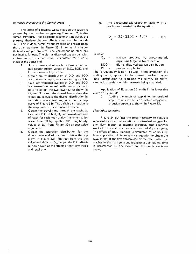
In-transit changes and the diurnal effect

The effect of a discrete waste input on the stream is assessed by the dissolved oxygen sag Equation 32, as dis­cussed previously. For a realistic assessment, however, the photosynthesis-respiration effects must also be consid­ered. This is done herein by superposing one result upon the other as shown in Figure 33, in terms of a hypo­thetical example problem. The corresponding steps are outlined as follows. The diurnal dissolved oxygen behavior at two ends of a stream reach is simulated for a waste input at the upper end.

1. At upstream end of reach, determine and in­put hourly stream values of D.O., BOD, and k 1, as shown in Figure 33a.

2. Obtain hourly distribution of D.O. and BOD for the waste input, as shown in Figure 33b.

3. Calculate weighted average of D.O. and BOD for streamflow mixed with waste for each hour to obtain the two lower curves shown in Figure 33c. From the diurnal temperature dis­tribution, calculate the diurnal distribution in saturation concentrations, which is the top curve of Figure 33c. The deficit distribution is

4.

5.

the amplitude of the cross hatched area. Obtain the travel time through the reach, tt. Calculate D.O. deficit, Db' at downstream end of reach for each hour of day (incremented by travel time, ttl by Equation 32, using hourly values of Da from Figure 33c as successive arguments. Obtain the saturation distribution for the downstream end of the reach; th is is the top curve in Figure 33d. Subtract from this the calculated deficits, Db, to get the D.O. distri­bution devoid of the effects of photosynthesis and respiration.

64

6.

in which

The photosynthesis-respiration activity in a reach is represented by the equation:

o Pf· (DDOI - 1.0) " . . (55) P

o p 0 xygen produced by photosynthetic organisms (negative for respiration)

0001= diurnal dissolved oxygen distribution Pf productivity factor

The "productivity factor," as used in this simu lation, is a scaling factor, applied to the diurnal dissolved oxygen index distribution to represent the activity of photo­synthetic organisms within the reach being simulated.

Application of Equation 55 resu Its in the lower sine curve of Figure 33d.

7. Adding the result of step 6 to the result of step 5 results in the net dissolved oxygen dis­tribution curve, also shown in Figure 33d.

Simulation algorithm

Figure 34 outlines the steps necessary to simulate representative diurnal variations in dissolved oxygen for any given month or months specified. This algorithm works for the main stem or any branch of the main stem. The effect of BOD loadings is simulated by an hour by hour application of the oxygen sag equation to obtain the D.O. effect at the downstream end of the reach. After the reaches in the main stem and branches are simu lated, time is incremented by one month and the simulation is re­peated.

- D. O. In Stream Inflow (a) -= ........ D E - ~O. M.qn-=..:..I7:.a..:.::.:..&.~ __ _

6.0 ........ at E -

d 7.0 ---------~B-0~7n~;;eam - 0

c:i 0 CD k,= .10

~~2--~4--~6---8~~,0--~12---,~4--~,6~~,8--~---2~2--~2~·O 6.00

5.0 -"" C' 40 E . -

Note: See Fig.l4(b)for Temp. and Rate of Flow Distribution

Ti me (Hour) .

--- -, 1/ ,./ Effluent BOD

I \ "" -I "t:Effluent D.O. 3.5 mgll

(b) 20.0 -

........ at .

15.0 E -o 3.0 BOD t!iean = I0..10-1!!,gf 11 __ ---~ ........ ---- 10.0 ---

o o CD

c:i -- .",/ 2.0

0 5.0

2 4 6 8 10 12 14 16 18 20 22 24

9.0

-""- 8.0 0» E - 7.0

0 c:i

9.0

-""-Ot

.§ 7.0

o o

Time (Hour) (c)

Saturation Concentration (CSI) Upstream End of Reach (Combined FI w)

CSI Mean = 8.2 mall -=-""-C'

..5 c 0

10.0 CD

5.0 2 8 12 18

Time (Hour)

(d)

( Saturation Contration (C.S.) Downstream End of Reach

'--"~~~ C S Mea n = 8._4-:::::=m~g;::/~' ~~~ 3.0

2.0 ------1.0 ~_

~ -CL.~

r-'""7'"":'~--r'7~..,....-:"~~~~~....JIo....~----L~"----..a....-..;..a......~~":'"7'"'---"---',....-t O· - E ci­t/)

--"------------"------------.......... - .......... --------1-1.0 G) 8 10 12 14 16 18 20 22 24 0::: 024 6

Time (Hour) Figure 33. Graphical representation of diurnal D.O. computation.

65

CHAPTER VII

EXPLORATION FOR A COLIFORM SUBMODEL

The concentration of coliform organisms is often cited as a parameter of water quality. Though coliform organisms themselves are not pathogenic, their presence in a water supply is generally taken as presumptive evidence of possible contamination by pathogenic bacteria, as some coliform organisms and pathogenic bacteria originate in the intestines of warm blooded animals and exhibit approximately the same die-away characteristics in the aquatic environment. Some coliform bacteria, however, originate in the soil and are carried into the stream by surface runoff and shallow interflow. Virus organisms do not exhibit the same die-away characteristics as coliform bacteria. For these reasons, many authorities argue against the use of the coliform organism as an indicator of patho­genic organisms. However, because coliform count is the parameter in most prevalent use at the present time, and because it is so frequently cited in water quality literature as an index to the bacterial quality of water supplies, coliform count has been studied for possible incorpora­tion into the water quality simu lation model.

Literature search

Relatively few works related to the modeling of coliform organisms in natural streams are discussed inthe literature. Kunkle and Meiman (1968) have stud ied the behavior of coliform, fecal coliform, and fecal strepto­cocci in a small high mountain stream flowing through an irrigated meadow pasture. At one of their points of ob­servation, they found analytical technique to be the most significant source of variation in coliform numbers, wh ile at the other location, analytical technique was second on Iy to time-of-day as a source of variation. They made no attempt at establishing a mathematical representation of coliform behavior in the stream.

Frankel (1965), in his study of water quality evalua­tion, discusses the problem of modeling coliform die­away, finally using Equation 56, as presented by Fair and Geyer (1954). This formulation, also contained in Fair, Geyer, and Okun (1968) is

eN - y)/N = N/N 000

-1/n (1 + nOKot)

......... (56)

69

in which No original number of bacteria in the

y

N

stream number of bacteria removed during time of flow (t) below the point of maximum bacterial density number of bacteria left in the stream after time of travel (t)

t time in days K initial rate of die-away for a specific

bacterial population in the environment of the receiving stream

n associated coefficient of nonuniformity or retardation

In this die-away equation, both K and n are functions of the bacterial population being studied and the environ­ment of the receiving stream into which this population is introduced. These important model parameters must be quantified analytically from samples taken from the stream at points downstream from the point of maximu m coliform number. To adequately define the die-away curve, it is necessary to sample over a relatively long flow time, which is the case of the Little Bear River. Its high velocity of flow means that the length of stream sampled should be relatively great.

Because of the location of sources of concentrated bacterial pollution, it was impossible to adequately sample the stream below the points of discharge. The first source of large numbers of coliform is the trout farm which is located about 2.8 miles upstream from Hyrum Reservoir. This distance represents a travel time of approximately 1 to 1.5 hours, depending on the rate of discharge; consid­erably less than the 10-12 hours suggested by Fair, Geyer, and Okun (1968) as that required to reach maximum coli­form density below a sewer outfall.

The second source of concentrated bacterial pollu­tion is the stream into which untreated waste from the town of Wellsville is released. This discharge is located only a few hundred yards upstream from the lower limit of the project study area, with another reservoir pool not far downstream. The inability to establish K and n for Equation 56 have frustrated attempts to simulate bacterial die-away by this approach. This representation of bacter-

---'0 u

ial die-away appears to be the best that is currently avail­able in the literature.

Figure 35 shows the profile of the logarithm of coli­form count, as observed along the length of the main stem of the Little Bear River on 11 September 1968. This pro­file should not be taken as typical of the pattern of spatial variation; however, as large, apparently random, devia­tions occur at each individual station. Figure 36 for sta­tion 12.5 is a typical annual distribution of the logarithm of the coliform count, showing the stochastic deviation from the mean.

3.6 nPorcuPine Reservoir

3.4

3.2

3.0

2.8

• 2.6 •

Trout Farm

Discharge

co 0 ...J

2.4

2.2

2.0 31.9 30.1 25.7 20.5 16.7

Distance From River Mouth (miles)

II

12.8 12.5

Figure 35. Space profile of log (coliform count) for 11 September 1968.

The density of coliform organisms in a given bacter­ial sample was assessed by the membrane filter technique. Multiple dilutions of a single replicate sample were pro­cessed simultaneously. Bacterial samples were limited to about 10 per weekly sampling period, because of time limitations in the laboratory. This restriction resulted in a rotating schedu Ie for the 16 sampl ing stations.

Alternatives considered

Post (1968) indicated that the logarithm of coliform density in waste stabilization ponds had been found to be

70

closely related to water temperature. On the strength of this suggestion, an attempt was made to relate the loga­rithm of coliform density to stream temperature at several locations along the stream. Figure 37 is typical of the results obtained.

I n searching for some means to explain the large amount of variation remaining after regressing with water temperature, it was suggested that possibly the random nature of bacterial loading could be the source of at least part of the residual variance. This hypothesis was tested by comparing' the residual of the log col iform variation with that of BOD after the influence of temperature had been removed from both. This test was based upon the assumption that both col iform and BOD originate at the same source, i.e. the intestines of warm blooded animals. Figure 38 depicts the result obtained at station S-12.8, which is typical of the stations studied. There is no apparent positive correlation between log of coliform density and BOD. In fact, this particular set of data dis­plays what might be taken as a slight tendency toward negative correlation (larger positive log coliform devia­tions being associated with negative BOD deviations). These observations tend to eliminate random loading as the major source of residual variation in either coliform or BOD if the assumption of common sources for the two pollutants is valid.

No coliform model, that could be adequately de­fined from available project data, was discovered in the literature. Analysis of project data failed to produce an equation capable of representing a significant portion of the total variation in coliform count. A random probabil­ity model based upon the statistics of available data would suffice as well as any.

Further research in this area would be helpful. Prob­ably the most fruitful approach would be the quantifica­tion of relationships governing the die-away rate constant (K) and coefficient of nonuniformity (n) of Equation 56. Fair, Geyer, and Okun (1968) have suggested that these model parameters are influenced by the bacterial popula­tion and the characteristics of the stream into which the bacteria have been injected. In any future investigation involving the coliform count, the data of Kunkel and lVleiman (1968) would suggest that replicate laboratory tests be conducted for each dilution to facilitate the assessment of the variance component attributable to analytical technique.

6.0 •

- • -c: :::J • 0 u 5.0 • •

•

• • -.

•

• • •

• •

• E • • • • • • ... • • 0 \t-

• o u 4.0

C')

0 ..J

3.0 • •

o 50 100 150 200 250

Days Since October First

Figure 36. Annual variation in log (coliform count) at station 8-12.5 for 1966-67.

6

0)

0) 0 0 5 0)

0 0 G

E 4

8 0) "- 0)

# G) 0

>- 3 (0 & G 0) @ 0) -'iii c: G)

0

E ... 0

2 -'0 0 -0

C' 0 ..J

0 2 3 4 5 6 7 8 9 10 " 12 13 14 Stream Temperature (o'C)

Figure 37. Log (coliform count) vs. stream temperature (station 8-12.8L

71

0

0)

15

• • • •

• • • • •

Mean = 5.08736

•

300 350

0) 0 0) 0

0

0 LoO C~if= 3.557+.0613T

R =0.169

16 rr 18 19 20

6

r::1 5 Q.

E CD

..... 4 CD o ~ I' 3

;;: rr) II

Q Q

~ E e

LL. c o

o o

2

-I

CD -2

o @ -3 ____ ~ __ ~ ____ ~ __ _L ____ ~ __ ~ __ ~ ____ ~ __ _L __ ~~ __ ~ __ ~ ____ ~ __ ~ ___

-1.2 -1.0 -.S -.6 -.4 -.2 0 .2 .4 .6 .S 1.0 1.2 1.4 1.6

L09(CoIif.) Deviation From [LOCj(Colif.)=3.557+.0613 rem€J

Figure 38. BOD deviation vs. log (coliform) deviation (station S-12.8).

72

CHAPTER VIII

SIMULATION RESULTS-LITTLE BEAR RIVER

Establishing a simulation model can be summarized as two steps: (1) establishment of model constants and coefficients, and (2) verification of the resulting model. This was done using 1966-1967 and 1967-68 data for the first and second steps respectively. The following is a dis­cussion of results. The submodels and procedures outlined in the previous chapter were used to derive all results presented herein.

System delineation

The Little Bear River system, shown in Figure 59, is represented schematically in Figure 39. This sketch shows the breakdown of the stream system into major tributary

PORCUPINE RESII 21

LEGEND

o Branch No.

o Reach No

6. Efflvent Discharoe No.

o Control Point No.

HYRUM CANAL DIVERSION

HYRUM RESERVOIR (~,)

Figure 39. Little Bear River system schematic.

73

branches and reaches, as well as locations of reservoirs, waste discharge points, and control points. Node points between reaches fall at hydrologically significant break points in the system. Reach eight on the main stem, for instance, extends from Porcupine Reservoir discharge on the upstream end to the Paradise Canal diversion at the downstream end of the reach. Locations and designations of system node points are tabulated in Table 20.

Establishing model coefficients

Submodel coefficients have been determined, where possible, by least squares analysis of 1966-67 data using equations selected and described in the previous chapter. Where data required for evaluation of constants and co­efficients were not available, estimated values were used in the simu lation. These estimates were revised, where neces­sary, to ach ieve correspondence between simu lated water quality and monthly averages of observed data. Pro­cedures followed and results obtained are outlined below for each submodel.

Electrical conductance

Electrical conductance was found to be quite sensi­tive to changes in the ratios of grou ndwater to surface water inflows. After the first simulation run, the ground­water coefficients in the hydrologic submodel were altered to change the proportions of these unmeasured inflows. Estimates of irrigation return flow conductivity were also revised downward to achieve better correspond­ence between observed and simulated conductivities. Correspondence graphs from the last 1966-67 run are shown in Figure 40 for four typical observation stations along the Little bBear River main stem.

Sample simu lation profiles are shown in Figure 41 for the months of January and July, 1968. A full year of profiles is shown in Appendix F. Average values of field data, for corresponding months, are also shown for com­parison. The gradual build-up in electrical conductance in the downstream direction is characteristic of the field data. Drops at stations 30.1 and 16.7 are due to carryover of low-conductance spring runoff in Porcupine and Hyrum Reservoirs, respectively.

Table 20. Little Bear River reach description.

Branch Reach From To Locationa Length No. No. (mi.)

Wellsville telemetry site 1.125 0.3

2 Hyrum dam Wellsville 1.128 3.9

3 -Hyrum Reservoir 1.167 1.8

4 trout farm Hyrum res. 1.185 2.8 discharge

5 trout farm trout farm 1.213 1.1 diversion discharge

6 South Fork trout farm 1.224 3.2 diversion

7 Paradise South Fork 1.257 1.3 canal diversion

8 Porcupine dam Paradise canal 1.270 3.1 diversion

9 -Porcupine Reservoir- 1.301 1.8

2 Hyrum canal Avon 2.000 1.0 diversion

2 2 Davenport Creek Hyrum canal 2.010 0.3 diversion

aThe location designation is "b.xxx" where b is the branch number and xxx is the distance from the mouth of the branch, in tenths of a mile (2.010 = one mile above the mouth of branch two).

Monthly water temperature

After the initial adjustment of hydrologic inputs, using conductance data as a gu ide,' no further changes were made in the system hydrology. The simu lation sub­model for water temperature was adjusted by changing the "equilibrium" water temperature model coefficients and the heat exchange coefficient.

Typical correspondence graphs from the final model development run are shown in Figure 42. The maximum deviation from stream temperatures, measured at eight observation points along the stream is about 4

0 C at

station S-12.8. Departures of this magnitude occur during May and June; simulated temperatures being high in May and low in June at this particular location. These larger deviations at the lower sampl ing points are probably attri-

74

butable to the approximate nature of the simu lation of release water temperatures at Hyrum Reservoir.

Comparisons of simulated and observed stream temperature profiles for the months of January and July are depicted in Figure 43. It is interesting to note that in January the influence of groundwater inputs on stream temperature is positive, while in July it is negative. Sharp temperature drops through the thermally stratified reser­voirs are prominent in the July profile.

Monthly dissolved oxygen

For the low BOD levels observed in the Little Bear River, the D.O. simulation was more sensitive to changes in D.O. inputs than to changes in oxygen sag model para­meters. Had BOD levels been higher, it is quite likely that

400 STATION SEC4 3 (1IIOut.

0 W I-« -.J 300 :)

~ if)

300

OBSERVED

500 STATION SEC-21.3

{4.11 In.

0 .. W I- 400 « -.J :)

~ (f)

300

200 300

OBSERVED

400 STATION SEC-24.6 .' .

(6.1) In.

200 400 200 300

OBSERVED

700

600

400 500

o

STATION SEC-12.8

(2.1) Oul.

'.

400

~ 400 f----:r~-----­« ...J :)

~ if)

300 300 400 500 600

OBSERVE D Figure 40. Electrical conductance correspondence graphs

....:. E u

" ., o r. E .>. II CJ C

~ ::I

-g o

(,)

J ., 0

! -" II CJ C 0

u ::I

"'0 C 0

(,)

0 0

~ u II

W

100

for stations SEC-4.3, S-24.6, S-21.3 and S-12.8 from the final model development run (1966-67 data).

January 1967

'" Monthly Averaoe Of Observed E. C.

1iOO.0 Simulated E.C. 1.3

Distance From Mouth Of Branch 2 (Miles)

O~ __ L-____ ~ __ L-~ __ ~ __ L-____ ~ __ ~ __ L-__ --H 31.9 30.1

600

500

400

3()()

200

100

0 31.9 30.1

27.0 25.724.6 22.4 21.3 18.5 16.7 15.2 12. 12.5

Diltance From Mouth (River Miles)

1700.0 1.3

Distance From Mouth Of l!Iranch 2 (Mil .. )

210 ~.7 2-4.6 22.-4 21.3

July 1967

'" Monthl y Avera 041 Of

Observed E. C. Simulated E.C.

18.5 16.7 15.2 12 12.5

Distance From Mouth ( River Mil .. )

Figure 41. Comparison of observed and simulated electri-cal conductance profiles for January and July, 1967.

75

20 20 STATION SEC-4.3 ~TATION S-24.6

(9.I)Out (6.1) In.

0 0 W f- W <! 10 f- 10

<! .....J .....J ;:) ;:) :E :E U5 V5 .

0 0 0 10 20 0 10 20

OBSERVED OBSERVED

20 20

STAllON S- 21.3 STATION S-12.8

0 (-4.1) In. (2.1) Out W 0 f-<! w .....J f-;:) 10 <! 10

~ .....J ;:)

(f) .. :s! (f)

0 0 0 10 20 0 10 ·20

OBSERVED OBSERVED

Figure 42. Water temperature correspondence graphs for

() . II

'" ~ . 0-E .. I--

stations SEC-4.3, from the final (1966-67 data).

10

8 1,:0 ~ 1.3

4

2

S-24.6, S-21.3 and S-12.8 model development

January 1967

'" Monthly Averaoe Of Observed Temperature.

- Simulat,d Temperature .

run

O~ __ L-____ ~~ __ L-__ -L-L ____ ~ __ -L __ ~ __ --p

31.9 30.1 27.0 25.7 24.6 22.4 21.3 18.5 16.7 15.2 12.8 12.6 Distance From River Mouth (Miles )

26

24

22 [ToO 1·3

20

18

16

14

12

.. 10 '0 ~

8

6

4

2

July 1167

Monthly AveraQe Of Oblerved

Temperature Simulated Temperature

OL-__ L-____ -L __ L-~ __ ~ __ L_ ____ ~ __ ~~~ __ ~

31.9 30·1 27.0 25.7 24.6 22.4 21.3 1&5 11.7 1!l.2 12.1 12..5

Distance From River Mouth (Milel)

Figure 43. Comparison of observed and simulated water temperature profiles for January and July, 1967.

adjustment of the oxygen sag model parameters would have significantly improved the model results.

Dissolved oxygen correspondence graphs are shown in Figure 44 for 1966-67 data. With the exception of

10 Cl IJ.I 1-':1 <:{ ...J .:J t:I :!' (j) 1

STATI7N SEC·4 3 (':II) Out

.. 10

Cl IJ.I I- 9 « ..J .:J 8 :!' (j)

STATION SEC·246 (61) In

..

~- ~~-6

9 10

OBSERVED

10 _STATION 5£("21:/_ (4 I) In •

Cl IJ.I 9 .. I-

:38 :> ... = 1 (j)

6

. /

6 8 10

OBSERVED

13

12

" 10

Cl

~ 8 <:{ ...J .:J

~ (j) 6

6 7 8 9 10 "

OBSERVED

STA nON SEC· 12 8 \2.1) Out.

9 10 " 12 13

OBSERVED

Figure 44. Dissolved oxygen correspondence graphs for stations SEC-4.3, S-24.6, S-21.3 and S-12.8 from the final model development run (1966-67 data).

station S-12.8, simu lated D.O. concentrations were gen­erally within 1 mg/I of observed concentrations. Depar­tures on the order of 2 mg/I may be noted at S-12.8. These greater deviations occurred during the months of October, November, and January. Observed data show a high degree of supersaturation during these three months. As will be shown later (Figure 54) these heavy super­saturations were not observed in 1967-68 data. The de­partures at station S-12.8 in 1966-67 are unexplained at this point.

The simulated D.O. profiles for January and July exhibit discontinuities at node points between branches (Figure 45). These discontinuities result from the assump­tion that oxygen deficient groundwater inflows are con­centrated at the upstream end of the reach. Combining this concentrated low D.O. inflow with the other inflows at the upstream end of the reach results in a noticeable

76

16

14

12 " CI'

E 10 c . ~

8

0 6

" ~ 4 : 0 2

0 31.9

16

14

12

" CI' 10 E -c

8 · 0 :>-)(

0 6

: 4 0 · · 0

2

0 319

30.1

30.1

~O 1.3

Distance From Mouth Of . Bronch 2 (Mil •• )

..

.. ..

January 1967

.. Monthly A~r4" Of Observed D.O.

- Simulated D. O.

27.0 25.7 24.6 22.4 21.3 185 16.7 IU 12.1 125

DI.tance From River Moutll (Mil .. )

1wo 1.3

Distance From Mouth Of Branch 2 (Mil .. >

July 1967

.. Monthly Averaoe Of Observed D. O.

- Simuloted D. O.

..

27.0 25.7 24.6 22.4 21.3 18.~ 18.7 15.2 12. 12.5 Distance From River Mouth (Mlle.)

Figure 45. Comparison of observed and simulated D.O. profiles for January and July, 1967.

depression of the D.O. profile at this point. This is par­ticularly true where groundwater inflow makes up a signif­icant portion of the total input to the reach, as it does in many reaches of th is system during periods of low stream­flow. The downward step in D.O. at station 21.3 results from the release of large quantities of oxygen deficient waters from the ponds and channels of the commercial fish farm. The relatively large deviations at station 15.2 are apparently caused by a small quiescent pool immedi­ately upstream from the field observation point. During low flow periods, velocity is low through this pool and photosynthetic organisms abound.

A full year of simulated D.O. profiles for 1967-68 years are shown in Appendix F. These profiles are based upon coefficients establ ished using 1966-67 data.

Diurnal water temperature

It has been assumed that the hourly distribution of the ratio of observed temperature to mean daily tempera­ture should be approximately the same at any point in the stream system as was recorded at Wellsville. In the case of the Little Bear River, where there are no concentrated

sources of thermal pollution, this assumption is justifiable. Some departure from this relationship should be ex­pt~cted, however, especially immediately downstream from surface impoundments.

The variation pattern for the simu lated diurnal It~l11perature index, at control points not immediately downstream from reservoirs, was adjusted to conform to [he pattern calculated from continuous monitoring data at S 12.5. The simulated diurnal temperature index was found to be quite sensitive to the heat exchange coeffi­Clt~nt and the magnitude of "equilibrium" temperature variations. Trial and error adjustment of these factors was the principal means of adjusting the simulated tempera­ture index distribution. In Figure 46 the simu lated and measured diurnal temperature index patterns for station S-12.8 are shown for the month of May 1967.

11-

t;-)( Q)

"" c

~ .z o .... Ol a. E Ol

c; c ... ::l

o

1.2

DTI curve from 5-1.25

Simulate d patt.rn

o 2 4 6 8 10 12 14 16 18 20 22 24

Time (hours)

Figure 46. May 1967 diurnal water temperature index pattern for station S-12.8.

Diurnal dissolved oxygen

As with diurnal modeling of water temperature, the basis for adjusting the simulated dissolved oxygen index distribution was the assumption that this distribution should approximate that calculated from continuous data from the Wellsville monitoring station. Differing environ­mental conditions, such as prevailing direction of flow, bank vegetation and topographic relief, result in spatial variations in light intensity patterns through the day.

77

These influences may be expected to impart deviations from the relationship assumed.

The simulated D.O. distributions were found to be sensitive to changes in the diurnal temperature distribu­tion, primarily because of the dependent relationship between oxygen saturation concentration and water temperature. After attaining a satisfactory distribution of water temperature, D.O. distributions were adjusted by altering the "productivity coefficient" on a month-by­month basis for each reach. This "productivity coeffi­cient" is the scaling factor in Equation 55, enabling the diurnal dissolved oxygen index curve to be used to simu­late photosynthetic activity within a stream reach.

The diurnal D.O. index pattern for station S-12.8 is shown for the month of May 1967, in Figure 47, along with the index curve derived from continuously moni­tored D.O. data. A consistent tendency toward somewhat later peaks in the simulated diurnal D.O. distribution pat­tern was observed.

1.2

...... 1.1

o o JC • ."

c: 1.0+--­c: CI 01 » )(

o

"'0

~ .9 o ., .. "'0

.8

0001 curv .. for 5-12.5

Simulated pattern

.7+-~~-r--+-~--~--+-~--~--+--4--~~ o 2 4 6 8 10 12 14 16 18 20 22 24

TI m. (hours>

Figure 47. May 1967 diurnal dissolved oxygen index pat­tern for station S-12.8.

Verification of model constants and coefficients

For verification, the completed water qual ity model was applied to hydrologic data taken during the 1967-68 water year and compared to 1967-68 water quality data. The results from each submodel will be discussed briefly.

Electrical conductance

Hydrologic coefficients and inputs for the hydro­logic simulation submodel were adjusted using 1966-67 data. No further changes were made in the hydrologic sub model. The correspondence graphs for six stations (Figure 48) show roughly the same degree of scatter for the 1967-68 run as were observed in Figure 40 from the last 1966-67 run. The inadvertent omission of tempera­ture compensiation on a conductivity meter for the period June 1966 through February 1968, undoubtedly contri­butes somewhat to the deviations for exact correspon­dence observed in Figure 48.

400

o w • • ~ . :3 300 :::> :!; u;

o

200 300

OBSERVED

400

~ 300 ••• <{ ...J :::> ~ u;

. .

. . 400

. .

2oo~ ____ ~ ______ ~ 200

600

o W 500 t-<{ ...J :::> :!; u;

400

300 400

OBSERVED

o w ~

500

500

<{ , ...J4oo :::> :!; u;

300

600

• 0500 W

~ ...J :::> ~ (fl

400

SEC-O.4

S-21.3

400

OBSERVED

. ...

500

400 500

OBSERVED

350 ~----'-______ --'-__ -----J

500 600 350 400 500 600 OBSERVED OBSERVED

Figure 48. Electrical conductance correspondence graphs from the model verification run (1967-68 data).

Conductivity profiles for the months of January and July, 1968, are shown in Figure 49 as samples of the profiles resulting from the model verification run. A com­plete set of plotted conductivity profiles is included in Figure F-1 of Appendix F. Comparison of simulated and observed annual distributions of mean monthly conductiv­ity is featured in Figure 50 for quality sampling stations S-12.8 and SEC-O.4. The good correspondence between

78

E ~600 CI)

o ..c E500 ,

-~ 300 "0 c: o u 200

c (J

.!: 100 (J C)

•

JANUARY 1968

~ , Dis'f~nc~ from mouth

of Branch No.2 (miles)

• Monthly average of observed E. C.

- Simulated E. C.

W O~-...l _____ ~-L~ ___ L-~ ____ ~ __ L-~ ___ ~

31.9 30.1 27.0 25.724.6 22.4 21.3 IS.5

E ~SOO CI)

o ..c E 500 ~

-~ 300 "0 c: o U200

c (J

.!: 100 (J C)

Distance From River Mouth (miles)

Distance from mouth of Branch No.2 (miles)

.. Monthly average of observed E_ C.

-Simulated E. C.

w O~_L-__ ~-L~ ____ ~...l-__ ~ __ ~-...l ____ ~

31.9 30.1 27.0 25.724.S 22.4 21.3 IS~ IS.7 152 12.5

Distance From River Mouth (mi les) 12.S

Figure 49. Comparison of observed and simulated electri­cal conductance profiles for January and July 1968.

observed and simulated electrical conductance values is readily apparent in all of these figures .

Monthly water temperature

The simulated 1967-68 stream temperatures cor­respond well with observed temperatures as Figure 51 shows. This correspondence is similar to that depicted in Figure 42 for the last 1966-67 run. Sample stream temper­ature profi les for the months of January and July, 1968, are illustrated in Figure 52. Figure F-2, Appendix F, pro­vides a complete set of plotted stream temperature pro­files for each month of the simulation year. Observed and simulated annual distributions of mean monthly stream temperature are compared in Figure 53.

Monthly dissolved oxygen

Relatively good correspondence was found between observed and simulated dissolved oxygen concentrations as shown in Figure 54. This agreement, however, should

Groundwater quality sampling points were estab­lished at four locations in the valley floor area, as shown in Figure B-2. These sampling sites are described in Table B-4. Groundwater samples were taken at monthly inter­vals.

In setting up the water quality monitoring network it was necessary to consider such factors as accessibility and winter conditions in addition to the obvious require­ment of sampling to indicate sources of pollution and stream reaction to th is and external factors. Those sta­tions for which winter access was limited were sampled as conditions permitted. Station SEC 6.2 above Porcupine Reservoir was sampled irregu larly during winter months due to the road being snowbound.

Continuous quality monitoring

Continuous water quality monitoring stations were installed at stations S-12.5 below Wellsville and S-20.5 near Paradise in cooperation with a water quality telem­etry project at Utah Water Research Laboratory (Woffin­den and Kartchner, 1968). The initial intent was to provide continuous strip chart recording at both sites, but excessive power consumption of the system installed at the Paradise site prevented its continuous operation from battery power supply. Specific electrical conductance, pH, dissolved oxygen concentration, and water temperature were monitored with commercially obta ined battery powered electronic sensing systems. For a detailed des­cription of the electronic systems employed, refer to the work of Woffinden and Kartchner (1968).

Table B-4. Groundwater sampling stations.

Because of instrument malfunction and problems re­lating to the adaptation of instruments for telemetry transmission, extended periods have occurred during which no valid continuous monitoring records were ob­tained. Reliable recordings were made, in blocks of from three to seven days in length, over a period extending from November 1967 through January 1969 at the Wells­ville station. Periods of missing data occurred during the winter of 1967-68 and the summer of 1968. The Paradise continuous monitoring station was set up in April 1968, but reliable readings were obtained only during relatively short periods. Despite the difficulties sufficient data were available to allow comparisons between stations and to establish a pattern over the annual cycle using data from the Wellsville station.

Quality of data

Stream gaging was done by the USGS using rating curves and stage recorders. They felt the data provided were reliable and good and with in normal tolerences.

Weekly sampling data from water quality sampling were provided by both field and laboratory analyses. Field tests were pH (by colorimetric kit), dissolved oxygen (Winkler-- fixed in the field), carbon dioxide (pheno­thalein titration), and alkalinity (methyle orange titra­tion); and temperature. Figure C-1, Appendix C, shows all tests conducted and summarizes all data taken for each sample. Test results reported with and (F) indicate field measurement. Laboratory tests for chemical species were

Station Coordinates Description of Sampling Point Period of Sampling No. (Meters)

U-2311 235110 Artesian well discharging to stock watering 101767 - 121868 trough about 75 yd. east of the first road east of Wellsville lower road bridge at about 200 yd. north of Highway.

U-2510 258108 Manhole for subsurface field drain about 101767 - 121868 100 yd. north of the railroad track and 100 yd. east of the Wellsville East Field Canal directly east of Greens Corner.

U-2907 294068 Spring House overflow on north side of 101767 - 121868 spring house located just north of E. K. Israelsen's home on west side of highway about 1.5 miles south of Hyrum, Utah.

U-3198 312985 Seeping spring area inside curve in Forsberg 101767 - 121868 Road northwest of Avon about 0.2 miles east of Little Bear River.

B-7

conducted in accordance with Standard Methods 1965 edition. There is no reason to suspect the quality of these data, with the exception of the specific electrical conduc­tivity test results. The values reported for the period June 1966 to January 1968 were not corrected for temperature deviations from 25°C at the time of measurement. The room in which this measurement was taken would deviate about ±2° C from th is temperature, though it was prob­ably close to 25°C most of the time. After January 1968

8-8

all subsequent EC values are reported as EC at 25° C. The temperature calibration for the instrument used is shown in Figure B-3. Figure B-4 shows the instrument calibration against a standard sample at 25°C.

Total count and coliform counts were done by the membrane filter method. Samples were collected using a sterile bottle, which was handled in accordance with usual sterile technique.

Ci!

'.70

1.1:/) -----+---\----+-------i-------r--_---==E~===-==r=~~=t:::::==-\

I. SO-A-------~ II J=OR. \..,0&.15 J~.IAl. I ~sT'~umIHlls

COhlOIJCT'VI:rct BR.IOGE.

\--i-----t--------t------- -- - - 30-2#314 Ie; Fee. 19h8

~

1.4fJ--------~------4-_\_---_+_----_t_-----t_-------- , !

To 'D, " .. itT E. c.1T T"'''''' i

0THE~ THA.U 2S0C TO E.C. AT 2 Soc , -----------+-------'-1-----------t--'vfuLT, pi:,.-Y;-s Y-Co Q.Q.e.c. ''(''0 t.J f=A.(..Toic.i }.30

~ --------~-----------------i-U I I f:I'A !roP .... ,I I

11= E.C. Me.A"&"2.e.p A.T I~°C. It.

lilO mIGIlOil'ru,40S/CM) T~& VA.LUE. « I I

L l20~----------~---- ~--4 GOct~.C'-..Te·O TO ,soc. -'5 (1.2.3)(SIO)

::2 Q

h \) llJ Cl.I

~I/O~-------------~---------~~----.-,

~

oR b28 M'GR.o-mwos/em.

1.00 -------~-------.....:..--------;----~-----------.:~---------------------j

.90~--------------------------- -------------

o 5 10 15 20 25 30 .3S

Figure 8-3. Temperature correction for conductivity bridge.

8-9

C A.L \ Bg,AT'O~ C UR,VE.

F"O R.. I ~DUSTR.JA,L 'No STR.U N\E:tJ.1s

CO'" Due T \ Y \ 1'( B R.J DGa.E.

~~_'_~~I~~~ __ ~~~~~~_O_-_2~i-~3_~~,~~~~~~~ ___ ~ __ ._

I I

1300-·---~i-----------~--~ ;

I ,

1200 -T~---:-I 100- -- - - -, I :

I ! I uJooo- --i- ----t-- ~ f- ----- - f

u Ii:;

~900 I I ~ "

~~ ,~-:---1_~_~L_---o I u , ~ 700 i---+-----I-----"'------,---!---u~O~----+----I----+----+----+----,i'- I--~---------t___~----~ ....... ----........ ---.-

t.U 0.

(j)soo-

o l1J

---+---+------+----+-------¥-----~-\-----I---------. ---

a4~1----4---+----4--~y~~~---~---~---~--------~ :l I i I 'I I ' , i. I I i c; I: I I i I: i

uJ3(}()- ----+----+----~-------I-i- -~1~--; ----- ... -r----.. -- r-----· ~ 1/: I ' i

~-!./~r----L-- I 'j--I~~-I

/ i I I -+-~r--/ I I I I

100-

501.Ul 'O !J CtiZ...uc..

0.01 m .ooS .002«; .0010

I 200

I I

300 400 700 600 700 I

800 9

ACTUAL SPECI Fie CO)JDUCTAkiCE

AC.1"Al.. S.c.. 14-13 718 3"0 /47

Q 8'S . A "o.cd 1 ~es -28 -1.98 710 - e -/./2 3S8 - 2 -o.~ IS" - 1/ -7.S0

1 S FE 8. r 9" S 7pB

Figure 8-4. Conductivity bridge calibration curve for standard samples at 25°C.

8-10

~-.--- -~

1000 I{OO

(2S oC),*

i _____ ....l.-__ ._

I

1200 1300 14bo

APPENDIX C

WATER QUALITY DATA PROCESSING PROGRAMS

For Discrete Sample Data

Three basic utility programs were written to process weekly sampling data from 10 to 15 stations on the Little Bear River. These programs were:

(1) QU LPRT -which: (a) produces an analysis summary sheet, Figure C-1, for an individual water sample; (b) calculates me/L for each an­ion and cation, sums total anions and total cations, and (c) calculates percent dissolved oxygen as function of temperature and eleva­tion, as outlined in Figure C-2.

(2) SCMI-produces a list of all water quality data arranged consecutively by: (a) station for a given date, Figure C-3, and (b) chronologi­cally by date for each station, Figure C-4.

(3) PRTPL T -produces a graphical display of de­sired sample data points by: (a) station for a given date, Figure C-5, or (b) chronologically by date for each station, Figure C-6. (Both plots may be produced from the same data if the data are rearranged as specified and separ­ate runs are made.)

The first program, QULPRT, was useful in produc­ing an orderly summary of a given sample; also several computations were done, and the output provided a means for verification of card punching. The second and third programs provided a means for visually scanning the water quality data for the Little Bear River in both time and space; this type of output was important in looking for any cyclic trends with time or in correlations between variables. Instructions for using each of these programs 1

are outlined in the following sections.

1. QULPRT

Figure C-7 is a program listing of QULPRT as pro­grammed in Fortran V, and run on the Univac 11 OS. Fol­lowing the program listing is a listing of input cards used by the program. The details of the input cards are de­scribed in the following section. Figure C-1 is a sample of pro~ra m output.

Specific instructions

Program QULPRT requires three groups of data in­put cards to follow the Fortran snurce deck. Table C-1

1 Each of these programs could be improved or modified

should a user so desire. For example the four weather and water

quality comment cards used in QULPRT could be omitted by

categorizing and number coding comments. Also the PRTPL T pro­

gram has been substantially modified (by Professor Post) to add

greater generality and usefulness to the program.

C-1

specifies the exact sequence and format for each card Figure C-S shows the deck arrangement for each of the three groups, along with the complete deck set-up for running the program.

Group I consists of a single control card, containing the single variable, NSTATS, which is the number of sta­tions for which sample data are punched. Group II con­tains NSTATS cards, each containing the mnemonic sta­tion identification designation, the UMT station coordin­ates, and the description of the station (i.e. S1276259093 Little Bear River at Salt Lake Meridian). Group III con­sists of NSTATS number of lots having six data cards (described above) for each lot; each lot of six represents one station.

2. SCAN

Figure C-9 is a program listing of SCAN as program­med in Fortran V and run on the Univac 110S. Following the program listing is a listing of input cards used by the program. Figures C-3 and C-4 are the two options of pro­gram output; either or both options may be specified.

Specific instructions

Program SCAN requires four groups of data input cards to follow the Fortran source deck. Table C-2 speci­fies the exact sequence and format for each card. Figure

5152 ~~qO<J.3 L1TTlt BfAR RIVER AT SALT lAKE MERIDIAN STATION 51:'2 DATl 071.367 TI"E 1020 DAY OF YEAR 1'14 APPEARANCE CllAll LOllECTlOt, POINT flD..JACENT TO HRIDGl "EATHER CONClTIOtJS ClLAR COMIJEtJTS

"'l/L ANIONS r.oG/L

CA ~0.4U 2.51 Cl 11.~n • .3? Cli "'bSlt.G CATA CO~ .00 .00 n r.oISSH,G CATA HCO,3 .355.02 5.1l2 "'G 3IJoilO 3.19 N03 1.90 .03 K .3.10 .Oil ..,04 .00 .00 Nfl lC.20 .:'3 S04 13.30 .211

TOTAL lAT IONS bd2 t·E/L TOTAL AtllONS 0.45 /I·E/l C,ASES' GO Y.6 ~G/l 12U.o peT'SAT NH:" .6 "G/l C02 ',.n "(;1 OhGArdC /.lATTER ORGAf'.ISMS

1000 I.tlu "'G/L

COLGR - ~. CODALT UNITS

LOL /.IISSING LATA

CI'lvHOPHYLL OHllf< PARA"'f TUiS

~ ISS!NG DATA

TrTAL COUNT

COLlf Of/"S

0~()onO.1l0(1"l

1 00n0(1./1 orwL

"'ISSIN(- [lATA

f'HI, ) 7.7 H"'PE.RATlIP(I~) If'.O UEG. Crt'Tlr,fUIIJF

TLJfJHll.!lY TOS

~dl. U"'HOS ~!02 1'>. R r.oG/L

TOTAL f·AHO~.lSS t,S (A(03 2t\~.(lU "GIL

Figure C-1. Analysis summary sheet for individual water sample-sample output from QULPRT.

... "'-'" ::::IIIE

z Q

~ C ac: ...... :z: 1.1.1 Co)

Z

n 0

N C,)

1.1.1 ...... :;:)

-' Q en CICI cr:

o

•

6

• 9

10

II

12

13

.. 15

16

\ 7

1~

19

20

,0 q\}'

EXAMPLE I

GIVEN'

I. ALTITUDE = 4500 FT.

2. WATER TEMPERATURE I: 18°C

:5. OBSERVED D. O. CONCENTRATION

.f!!:!Q...~

I. SATURATION CONCENTRATION

2. DE8REE OF SATURATION

SOLUTION:

I. SATURATION COCENTRATION = 7.1' Mg/L

2. DEGREE OF SATURATION II 76 %

15~i----------------------------------------------------------------------------~

~ ~ ~

,. -S 13

1'" w

- ~ 4_ ....

'-"" cJI ' 11'

" ~

::::IIIE

12 ~ ~:.e.. ""'" ""'" ""'" ,,~~

!l '''1 SAlIH.ITV CORRECTIlN FACTOR

'" ';. z "

~ ~ cr:

:= 10 ,0' "" ~ " (.)

" :z: ~, 8 9

" " "

,()()

"'I

:z: Q

i= cr: a::: :;:)

!c en

6

0

t IEUEU UNTI'UIE I

I

5 10 IS 11

CHlORIlE ('./l)

o • 6 I 10 12 ,. 16 II 20 22 24 26 -- 21 -- :: 51 II II III! III 1111111111'1 II I II IIIIII~

35 40 45 50 55 60 65 70 75 10 as IEUUS FAHIENIUIl

WATER TEMPERATURE

Figure C-2. Nomograph used in QULPRT to obtain percent dissolved oxygen saturation.

C-10 shows the deck arrangement for each of the four groups, along with the program source deck and run con­trol cards.

Group I consists of a single control card containing three variables, NSTATS, NWEEKS, and lOUT, which are described in Table C-2, Group II contains the station des­ignation and descriptions, one for each station from which a sample was obtained, with a total of NSTATS cards in this group. Group III consists of NWEEKS/B cards con­taining the data and corresponding day of the year, ar­ranged in the sequential order in which output is desired. Group IV consists of subgroup A and subgroup B. Sub­group A contains two cards of chemical and bacteriologi­cal data for each date for the designated station (Group III cards 5 and 6 from au LPRT); these cards are arranged consecutively in order of date for a given station. Sub­group B consists of two trailer cards which are control cards for indicating that all data cards containing water quality for a given station have been read. The subgroup B trailer cards for the last station are punched differently in the last column to indicate all data have been read.

3. PRTPLT

Figure C-11 is a program listing of PRTPLT as pro­grammed in Fortran V and run on the Univac 11 OB. Fol­lowing the program listing is a listing of input cards used by the program. The details of the input cards are de­scribed in the following section. Program PRTPL T out­puts a plot of data contained in a 54 by 120 size matrix on a 9 x 12 inch rectangular area, as shown by Figures C-5 and C-6 (reduced in size).

Two Y axis transformation options are available: one allows plotting up to 10 Y variables against a common X variable; another obtains a log transformation of any Y variable. Separate runs are required for Figures C-5 and

DATA FOR THE WEfK r71367 (lAY OF YfAP 1~"

U T! (\N5 ( MG/LI

5 TA TION f)ATE TI I<r C A CII FE ~G N A CL

S 127 C71367 1 aDo 1;".4 38. ~ 5. r 19.5 13.5

S 128 r 71367 1010 2 ~. 6 6~ .0 S.O 1 ~. 6 5.3 SIS , 071367 1020 5 r.. 4 3B.8 3.1 12.2 11.:

5169 0713£, 7 1 a .. o 1 ~. n 30.4 1.2 5.9 9.3

5213 (,1713\;7 11 ~" .. 2.6 ..... 43.0 ? ~ 11.2 1 ~.3 52_6 01131;7 12?'l 33.8 "0.3 1.8 7. b 9.5 5270 071307 133C 7.(1

5275 0713,,1 1250 30.2 ?7.8 • 6 7.2 ~. q

SEC"3 0713b 1 13SC 3".8 13.0 .6 4.1 6.5 '5EC6;> a 71 367 141" 17.4 43.0 1.2 q .7 6.0 SO~O 071361 130" "3.2 23.6 .6 ~ .1 5.8

S TFOO 0713&7 1200 55.8 ~3 .0 1.8 9.6 13.5 ~\lO I r71 367 J945 53. J "5.6 ~. r 21.2 17.8

<;L ROC 071367 085C 41. r 21.R .6 2.4 3.5

C-6 respectively, each requlrmg different control card specifications and arrangement of data cards.

Specific instructions

Program PRTPL T requires two groups of data input cards to follow the Fortran source deck. Table C-3 speci­fies the exact sequence and format for each card. Figure C-12 shows the deck arrangement for each of the two groups, along with the deck set-up for running the pro­gram.

Group I consists of six control cards which must precede the data to be plotted. These control cards are made out in form (a) or form (b), which specifies whether the Figure C-5 type plot or the Figure C-6 type of plot will be produced; data cards must be arranged commen­surately as outlined in Table C-3 and in Figure C-12.

Group II consists of three subgroups, A, B, and C. For the first station subgroups A and B are absent (actual­ly Group I control cards replaces subgroups A and B for the first station). Subgroup A consists of a single dummy data card, which must have a zero or nine punch in col­umn BO. If the column BO punch is 0, then subgroup B consists of control card 1-1 (but made out for the data in the subgroup C following); if this punch is 9, then sub­group C consists of control cards 1-1 to 1-6 (but made out for the specific manner in which the data in the subpro­gram C following is to be plotted). Subgroup C contains the water quality data cards (they can be cards 111-5 and 111-6 from Table C-1). Only ten variables may be plotted on anyone plot and the selection is done by means of the format statement (see Table C-3, card 1-2). The data cards are arranged in two alternate ways depending upon wheth­er the. Figure C-5 or Figure C-6 types of plots are desired; Table C-3 and Figure C-12 outline the manner of data arrangement.

Ar;ION~ (MG/L I OTHER PARA METE R5

HCG3 C03 N03 PO .. SOq P4F t'HL HARD Q

~9S. '3 .0 4.7 .F 15. f· 7.9 8.3 320.0 27 .0 ~%.5 .U 1.3 .1 1q .0 7. ~ 8.3 305.0

355.0 .0 1.9 .0 13.3 7.7 8. J 285.0 ~'J 7.09.8 7.2 .6 .r 9.0 P .• 4 8 ... 195.0 · .... 333.1 .0 3.7 .1 I ~ .8 7. B 8.1 283.0 .. , .. 3nI.3 ? "

1 • 7 • 0 8 .0 Q.l 8.3 250.0 • .-i •• 9. " !>, .0

212.3 6.0 .7 .8 ~. 5 ~. " 8. ~ 190.0 19.0

201.3 3.6 1.0 .(1 G.7 8.1 8. " 165.0 ..... 2S8. <; 3.6 .0 • 0 7.5 8.2 8 ... 22U .0 ~t :~ 230. ~ Q.8 .1 .0 5.7 ·.4 8.5 205.0

333.1 .0 4.0 • ? 16.\ 7.S 8.2 275.0 ..... 384.3 .0 6.2 .7 2U .6 7.8 801 320.0 · .... 220. p 3.6 .3 .0 ~. q ~. 0 8.4 192.0 .....

GA 5 ES (>1G/L I OT HER P~RAHETERS ('1G/L I O:;GA"'IC MATTfR (HG IL I ORGANI SHS

5 TA TIDN OA TE TIl<, "0 PCT SAT '1H3 CO2 TURS ONO TDS T: ~IP ')IO? 800 C JLOR TOTCNT COLI F M

UI1HOS/C!'! DEG. C /I OOHL 1100l1L

5127 071367 1000 7.3 86.3 • J 5.0 2 'S • 6" 5. "2" .1') 15.0 19.1 1.7 S. 19 ... UOOOO. luGOOOO.

S 128 0713~ 7 1010 7. <; '14.2 .7 3.0 25. 55 O. 3(\1.0 1 ~.') 15.8 1.0 - 5. 1 "1.I000l: • "SOOOO.

SIS ? 0 7 1367 10<[1 'l.6 120.6 • 6 5. a 2" • 528. 331.r 18.11 15. A 1.8 5. S~OOOO. 100000.

S 16P 071367 104n 7.6 103. J .1 • J ? S • 300. 211.(1 22.0 S. " 1.1 5. ~lO 000. 2000.

5213 r1! 367 11 r,c 6. 'l 83.3 .3 ". I) 2 ~. SIS. 33J .J 1'; .~ 9.\ 5 • 'I 5. 60000000. 6UOOOOU.

5246 0 7 1367 122C A.? I 03. ~ • 6 3.J 25 • 435. 27q .0 lA.O 10.7 • 8 ~ . 5270 0713G7 1330 330. 18.0

S 275 071367 t 2~r 9.5 1 1 'l. 3 .5 • Q ? 5 • 30 O. 20~ .0 lA. n 7.8 l.u 5. 12(,,:'00. 20000.

SEC", (171367 1350 ~. 7 111.1 .7 7.0 25. 2'32. I ~7.0 15.0 7.2 . ~ S •

'5EC62 071367 1"1<", 8. 'l 111.8 • J • 0 - 25 • 370. 227 .0 18. ') 5.0 1.5 5.

SOOO 071367 130<; 8.0 98.5 .1 • 0 - 2 S. 33'1 • 209.0 17 .0 5.2 • 5 5. 2"OlJOO • 67000.

S T FO~ 071367 I zor. &. " 86.7 • J 6.0 25 • 51 'I. 321.0 18.0 12.7 , ... S 5. 183uOOOO. 7000000.

swa I r71 367 0945 7.3 84. , • 1 ~. D lS • 618. 4 qq. 0 14.0 21. q Ll , . 6000UOO. 1900000.

SL ROO 0713£1 085~ 9.2 97. q • 3 .. • 0 25 • ~o O • 179.0 10.n 4.0 • 7 , . 30000. 10ooe.

Figure C-3. List of water quality data by station for a given date-sample output from SCAN.

C-3

STATION 5157 25,,093 LYTTLE BEAR flIVER AT SALT LAKE MERIOIAN

CATIONS {IiG/LI ANIONS (HG/L I S T4 TION DATE TI ME CA

5157 011267 1430 112.0 5152 011967 114" 72.r S152 n121;67 II"S 60.0 S152 0~0261 1600 54.4 S152 ()?0967 102" SE.2 S152 021667 1000 57.B 5152 0:?2367 l11U 51.6 5152 030267 IBn 70.4 5152 030967 1010 38.6 SIS? '131667 134~ 50.2 5152 032967 1520 55.4 5152 040667 111<; 48.0 S152 041367 1600 51.4 5152 r4?0f;7 164(' 24.4 5152 042767 17?" 51.4 S152 050367 17311 68.8 S152 051167 1810 ?7.4 5152 0"1867 172"" 23.8 S152 052567 1705 44.4 S152 060167 1175 18.2 5152 060867 1150 ~l.P 5152 061567 120n 2.0 5152 0<;7.267 150(' 12.1 5152 002'167 G'lS" n.? 5152 070667 O~<;C 39.8 5152 071367 102n 50.4 5157 1:77.06; 10r,(' 65.8 5157 077767 101r 7J.4 5152 CG"1367 IGr~ 62.4 5152 0 0 (1%7 151(' 6'l.2 5152 0~1767 Oq<;~ 70.2 5152 082367 091r 3'l.7 SIS" 0 0 2967 0'33(' 61.2 5152 fl'lfl%7 :)9S0 63.4 5!52 09J367 09'" 58.4 5152 092067 lore, 5-1.7 5152 I~G467 1005 5<;.8 5152 1'11067 120[1 5".4 5152 181767 100r 3.8 5152 In~467 101~ 5(1.2 S15? 11'1167 JG7f' ?7.3 S1S2 J l'l~67 11nr, 5?2 SIS? 11146711,:[, 23.0 5152 I! 206 7 1 1 Hi 15.5 S15? lIn67 1 o~r 48.4 5152 le n 567 104(' 11.5 5157 P13f7 1:J4~ ?F;.4

cu .0 .0 .0 .0 .0 .0 .n .0 .0 .0 .0 .8 .0 .0 .0 .0

FE Ii G .0 23.2

• rJ ?2.3 .0 26.8 .0 25.3 .0 21.8 • G 23.2 • n 25.8 • n 15.<; .0 32.0 · ° 27.8 .0 30.8 • (1 76.e .0 22.8 • 0 3~. 8 · ° 13.S .0 8.'

32.0 33.0 16.0 27 .8 2D.8 40.3 34.0 37.6 48.3 38.8 33.J 32.0 38.8 23.6 ?7 .P 46.4 23.6 ~2. 0 31.4 ~3 .0 33.5 32.8 07.3 77 .8 44.2 7.7 .8 45.6 51.4 31.4 SI.4 42.4

K

2.2 2.2 2.2 1.8 1.5 1.5 1.5 1.8 1.5 1.8 2.8 2.8 1.5 1.8 I. S 1. ~ 1.2 1.2

1.2 1.2 .9 .0,

q .3 9.E> 9.6 9.0 5.9 9.0 8.3 8.3 P03 9.0 9.6

D.8 10.2 10.8 'l.6

1 ~. 2 7 a6 7.8 5.3 5. '3 5.'3 ~,. 9

10.8 12.2 IIJ.'! P.7 11 .5 5.7 6.3 9.E>

13.5 10.7 9.6 9 .5 9.0 1.0

7.4 R.3 7. B ~ .1 7.3 4.l. 7. S g.3 7.8

CL 12.0 12.5 12.5 13.0 11.3 12.0 12.0 12.0 12.3 12.6 14.3 12.3 12.0 12.5 12.3 12. A 11.0 10.5 8.5 5.8 7.0 7. a 7.5

10.3 11.0 11.5 12.3

6.5 12.5 12.2 12.5 12.5 18.0

3.5 12. C 13.0 13.5 1 1.5 14. '> 12. (l 11.5 1;:.5 13.3 15.8 16.0 1 ~. 5 10.5

HC03 430.7 275.7 272.1 257.4 246.4 24<; .2 241.6 2'17.7 24P, .'3 251.3 294.0 244.r] 258.1i 252. <; 2"6.4 241 .~ 740. '5 228.1 2(10.1 201.3 187.9 201.3 207.4 270. ~ 320.'l 35 S.O 359. C)

395. ~ 389.2 322.1 35~ .f)

341.6 313.5 38'3. ? 341.5 341.6 330.6 312. , 287.9 281.8 292 .~ 7£,4.7 272.1 2'10.4 281 • ~ 2h8.4 2b8.4

C03 N03 21.6 1.3 ~. 4 .5

12.0 .1 13.2 .6 1 C.8 .4 14.4 .7 14.4 1.0 10.8 .4

7.2 .4 '3.6 .2 3.6 2.5 4.8 .5 1.2 .7 .0 .4 .0 .8

3.6 .8 1.2 .7 1.2 .5 1.2 1.9 .0 .8

f,.0 .5 .0 .4

?4 .9 .0 7.3 .tJ 2.1 .0 1.9 .0 1.3 .0 2.6 .0 1.:3 . ° .5 .0 1.0 .0 1.~

.0 1.5

.0 1.0

.0 .6

.0 .S 3.5 .6

• J 1.3 1.2 1.1 3.6 .8 7. ~ .1;

c .. 6 1.0 n.6 .A

.0 1.2 3.6 1.3 '.6 ?J 'l.G 1.5

STATION 5152 75 C 093 LITTLE ~[AR RIVER AT SALT LAKE ~E~rorAN

5152 CII267 143 n

515~ '111967 114< SIS? [,J2667 lIS< 5152 ('.,n267 IfO r

5152 020%7 107" SI~? 021£67 lr~!"'

5152 072367 l11C' SI<? 030267 113r 5152 030%7 101 r

SIS? 031(;67 134<; 5152 032967 Is"r 5152 C40&67 1 7 1-S1S2 041367 lEsr S157 042067 IG"~

5152 042767 17?c 5152 r.S0367 1 nr 5157 0511&7 1810 51<;2 r~,IBG7 172 c

SIS? 052567 1 7 r::'-5 1"2 Ohnl~7 117': 5 IS? 000%7 11S,l S152 ~G1567 12f10 515;> OF;226 7 152~

5152 C62967 09S n

5152 07%b7 8,?~5

5152 (,7131'>7 lcn 5152 0720&7 105'1 5152 072767 101C 5152 080367 loon S152 OBn967 ISle S 152 Dill 7F 7 ~,!5C

5152 037367 :;93(\ 5152 OQ2%7 093C 5152 0'J0!'67 O'lS(l 51S? O'l1367 093<, 5152 0970&7 1000 5152 1'10467 10(1<; 5152 10lCG7 120C S IS? 101 767 100 (\ 5152 11)2467 10l C

S152 11'1167 102(' S152 110867 1100 5152 111467 110r 5152 112067 l11r S152 112867 10 7 0 S152 171]567 1040 5152 1<1367 1045

'10

14. 7

14. 1 I? ~

lC. n 1::.') 11.r. 1 (1.3 1 ? 0

10. h 9.0

1 G. q

I r. ' 10. S 11.2 0.7

1 C. r 10.2 1 r. n

".1 ~. " p. f; 8. IJ <:!.LI 7.3 ? F '1.3 8.2 7. r,

7. r,

E. ~ 5.4 ~. 6 P..(J 7.6 7.5 B. 'l 7.8 A. b

10.5 12.6 11. 'l 12.0 11.2 12.3

GAS[S (MClL)

ocr SA T NH3

134. J 125.8 1 I'l. ~

9; 60 12S.7 1 O~. 7

3F.4 123. , 1(11.-

92.2 J 01.1 104. J 10£.J 113.1 10D.4 105.9 105.5 1 10. S 110 • .1 1 US. 3 113.5

39. F;

'36 .. 6 118.1

88.1 128. b 1 14. S 101. J

7.6

86.7 8201 66.5 81.3 8.J

86.1 e30l

103.0 86.5 93.2

111.2 130.4 123.1 121.2 107.6 113. b

01 • 0

· " .2

• a .0 .0 .0 • 2 .0 • 5 .0 .0 • J .J .6 • 0 .0 .t .5

. " • 5 ." .1 .6 .t .t • 2 .4 .7 • 0 .2 • 5 • 3 • q

• 3 .3 • 3 • 0

1.1 .2 • 4 • 5 • 2 • 2 .3

,02

• r .1

.0 • 0 .0 • J

.0 • r .0 • 0 • 0

') .0

• 0 .0 .0 .Q

• a .0 • c • 0

5.0 3.0 5.0 9.0 P.3

1~ .0 c:; .0 F.O 7.0 <; .0 G .1 ~.O -q .0 9.0 4.0

• 0 .~ .~

.~

.0

.n

.0 • 0

? ~.

25. 2 S. 25. 2 e.

2,). z s. 26. 25 • 6 !. 25.

? 5. 25. 25.

91. 25. 25. :' 5 • 25 • 25. 25 • ?5. 25. 25. 75. 25. ?C;. 25. 25.

OTHER PARAHfTF:?, (I1G/L)

rONG T "s TL MP llMH05/CM uEC. C

4,3.275.0 4.0

47 S. 4') ~ •

412 • 3~5 •

'" r • 314. 371-39'i • 4'33. 432 • 42 O. 362. 390. 35 ~ • 352. 3b 3. 310. 281. 2'38. 302 • 315 • 43P. 47 e. S2 8. se? • Sa 3. 537 • ') 13. 515. 470. 45 O. 535. 408. 429. 490. 450 • 44 D.

395. 440. 450. 450. 45 O • 42 C. 400. 442.

2 A7. r.: 2 ~'l • Cl ;' >;3. ~ 21Q. G 760. ') 2P4. n

257." 764. r 28~ .1 31? .'1 2 4? ~

'2 "5~ .c 23f .c 21 q.r. 763 .~ 2 I ~.ll 227.0 18" .J 216. Il 190 .0 173.1) 178.0 2S5.J 286.:J 3 31 .~ 351.0 376.(1 364.D 315. tJ 335. f1 31<; .0 3 4r]. 0 327.0 ?7Q .0 330.U 32!J .J 285.0 271.n 2 AO .C 273.0 25'1.0 285.0 2AS .0 25'1.0 273 .0 257.0

3.0 S .n 5.1 4.0 ~ .0 <; .n ;; .r] ~ .r,

F • a 5.r, P .9 t1 .D e .r q .r

IJ .n 3.0

12.0 14.0 14.0 1<; .0 14.r 16.0 1 q.o 16.0 13. ~ 17. (1

17 .0

2'1. r 17. r IS .r, 17 .0 17.0

13.1' 12.0 14.0 l?O 11.0 10.0 9.0 9.0 8.0 6.0 4.5 2.0

p.. "2 14. ~ 1'. <;

11.'1 11. 5 11 • C Ie. " 10. " 10. e,

12.1 20. ? 12.1 12.0 10. S 13.1 I? .1 11.3 1~. E 10. ? 9.1 8.2 P..4 q. Q

10.5 14. 9 15. q 14.5 1 ~ .4 15.8 17.1 16. 3 14.7 1?1 17.1 16.8 18. J 19.1 22.5 16.n 12.0 12.3 10.4 10.2 10.5 ).;.6 13.8 11.6

P04

• ;> .1 .0 .0 .c .0 .0 .! .0 .0 .2 .1 .1

• ? .2 .1 .1 .1 .1 .0 .0 .1

• r .1 .1 .n • c .0 .0

• fl .1 .<; .3 .1 .1 .1 .0 .2

• ? .r .5 .1 .1 .1 .1 .1 .1

SO, 11".'3 IG .6 11.3 15.3 11.3 12.2 14.0 13.1 !U.S !(j .6 7.3 8.5 ':I.E>

11.6 liJ.O '3.8 9.(1

8.3 9.0 8.5 6.4 7.5 S .5 ':l.8 9.C

13 .3 J ~.1 1.1.1 15.3 12.2 12.8 IU .~ 1l.9 12. ~ lQ .3 9.C

11.9 11.0 12.8 11.9 ~. ~

oj.3 8.3 9.R 8.8

10 .0 7.5

PHF 8.0 ~.2

8.2

9.2 8.2 9.2 8.6 A .2 Q.2 8.0 8.0 7.8 8.0 8.0 8.2 8.6 g.o a .U p .4

8.4 B .1 Ad 7.9 7.7 7.7 7.6 7.4 7.8 7.S 7. E 7.E> ~ .4 7.6

7.6 7.7 7.8 g. E>

~. 7 R.2 Q.l e.4 7.9

OTHER PARAMETERS PHL HARD 8.0 280.0 8.3 <:70.C 8.3 260.0 8.4 £40.0 8.3 230.0 801 240.0 8.~ 235.0 8.4 240.0 8.4 228.0 8.2 24u.0 8.2 255.0 g.3 23u.0 8.3 222.0 8.2 220.0 8.2 210.u aoS .206.0 8.~ 2uO.o 8.4 195.0 8.4 177.0 8.4 16u.0 8.5 165.0 8.2 17U.0 8.4 170.0 8.2 220.0 8.2 lSS.li 8.J ::85.0 e • ..; 300.0 7. ':J 310.0 7.8 315.0 801 2·7;;,.0 8.L 290.0 dol 290.0 8.l 25G.G 8." 290.0 7.5 275.0 8.0 285.0 8.3 280.n 8.2 270.0 8.5 245.0 a.~ 240.0 a.~ 25(;.0 8.4 245.0 5.~ 245.U 8.4 ,,50.0 3.~ ,,50.0 g.~ 240.U 8.4 2 4(J.U

~".O ~o.o

51.0 53.0 44.0 46.0 ~4 .0 53.0 48.0 30.0 3.3

92.0 99.0

195.0 163.0 185.u 44U.O 390.0 654.0 212.0 218.0 418.0 256.0 185.0

3.6 3.3 5.0 3.4 1.3 1.4

.9 3 .~ 9.9 3.8 5.0 3.2 3.a

IlJ.O 73.0 71.0 57.u 55.0 5~ .0 55.0 5~ .0 58.0 56.0

OQGANIC M~TT"R (MG/Ll ORGANISMS

POD COLOR TCTCNT coLIfH

2.9 1 .7

4. u

" . ~ u .U I .9 3. 7

4.2 4. u

3. I

5.8 ? .4

2.4 ?2 2 .0 2.3 Z.7 Z .a ? .2 20.1

.2 I .8 1.8 1.0 I.S 1.0 c...6

.2

.0 1.3 1.4 1.3

• 8 2.1 2 .~ 6.4 2.8 2.0 2.3 2.2 2.7 2.3 2.9 3.9

/lwGHL / IDOl'lL 5 • 5 •

;;'''COG. 310GO. ~u~lJl .. U. 430UO.

5. 5. 5. 5. 5. 5. 5.

SlJuuu. 1U00.

3wLruOu. 'seOCGu.

4000. 3GOJOlJ •

5. ?2000 • 5. S. 32UOuiJ • s. 70uoe • s. 1 U;:'OOli. 5. U3LJuL:. 5. ~. 4lULUL. 5. ;0000. 5. 4;0000. 5. 70uOO. 5. 900GO. S. 7000r,. 5. 5. 21l!000. 5. 8JJOOO. S. 65000U. 5. 24UUOOO. 5. 1U30UOOC. 5. 57000. 5. 5. 5. 60UOOL. 5. 38UOOO. 5. 200GuOO. 5. 900,,(.;. 5. 1100eo. 5. QlrJULJOC. S. S. 35GOOOO. 5. 2000 • 5. 12GO. 5. 14000. 5 • 5. ;40000. S. 4000L • 5. 3400CJ • 5. "100G.

lLJ60uO. 10UO. 1000. IGLO.

30uO.

IBLuC. 5UOO. 4000. 10uO •

luuO. lOuD. lULO. 4uLO.

12000. 12uuO •

54uuO. 1360CJO. 1 OGOOO. 160GOO.

2L20LUO. 1900CO.

BOOOO • 11 uDOll. 310000 •

50000 • 1LOUO •

77LJOLO.

150UO • 1000. 5000. lOuD.

11000. 200. 100 • 8GO.

Figure C-4 List of water quality data by date for a given station-sample output from SCAN.

C-4

"I.!LTtPLr PLO T OAT A fOr. DATE 1'71367. X AX 1S C'ISTANCE ONE INCH 1 .7 HILES. Noas lq

~ARIA"LE COHO lOS PHI"" rLOII ,'LOT CHAR C S P Q

~qGH. 125 O. O. .0 .0 v"ITS/ rr:eH 100 tOO 10 '10 Ii lSS ING 0 1 a

c- I Z7 I Z5 6 .. 5. 425. 1.9 27.0 <,1.i> 128 550. 391. 7.9 S 152 152 528. 33t. 7.1 3.3 qG~ 168 300. 211. 8.4 S 213 213 515. 330. 7.8 52 q G 246 Q3S. 27~. e .1 ~270 17Q ll(). O •• 56.0 '275 275 300. ZOO. S .q 19.0

'>':C4 J 298 7.97. • 187. e .1 <:':C:32 317 no. 227. 8.2 2:!.o

sooe 276 B'3. 209. S ._

37.0 5TFCC :>15 519. 37.t. 7.8

';\,01 127 ("'18. z,talJ. 7.0 ;(.R:i(l ~ ~~ lOQ. 179. B.O

OHE 071367 OyST VS CONO C TOS S PHI'! P 'LOw 0 .. !_ .. - ------ -- -------- ----- ---- .-.. ----- -- ----- ---- -- ------ -----------_.-- ---- ----- ---------- -------- --_ .. -- -------- ------_ ..

I I I I I

-I PPI>

1 ! 1 I

-I I

re -I

I I I C I I

-I I

IS 1 S

-I I S I I

T -I

1

- !

-1 I I I 1 I

I> PI"

pp

cc

-1--- -------- ------ ... ------ ---- .. -- ... ----- ----_ ... --- .... -- ---- ---.. ---------- ... -_ ... -- --- -- -- ...... -- -- -.. -...... -... --- ..... -- ---.- -- ---- .. ----y 1 I I I I t I : I I

125 1~2 1~9 !7~ 123 210 Z27 Z~4 2el 27S 295 312

Figure C-5. Graphical display of water quality data by station for a given date-sample output from PRTPL T.

C-5

HUl T IPlE PLO r DA TA FOR ~ TA TI ON S 15 2. YE All 1%7. TIME ON E INCH 30.0 DAYS. NOR ~ 47

VARI ABU COND 1 DS PI-j( FJ FLOW PLOT CHAP C <; Il ORIG IN r. o. .Q .0 UNI TSI INCH 100 I flO ao NO HISSING (, 0 011267 I? 43 g. 27 Cio. A .r! 40.0 0119G7 1 Q 4r.. ". le 7. S .2 '10 .'J o I 7~ 67 2 c 47" • 7" tJ. • .2 51.0 0202 G 7 3' 4(11. ze 3. R .4 S3.n. 'lZ09b7 4~ 417. '34. P .2 44.3 !l21 &67 47 3'lS. 2& O. p .2 %.0 022367 54 4~ r. 2~ 4. ~ .2 44.0 030267 hI 314. 2~ 7. ~ .f 53.0 03('1967 68 377. 2& 4. A .2 48.0 031667 75 V15. 2d O. R .2 ~[l.n

037':167 I'R 4<>". !12. l\ .n 3.3 04G667 % 43 0

• 'q <:1. e .0 92.n ('1Q I '''7 I Cl 42 r. ::'540- 7.0 'lq .S 042067 110 3;" 2. 235. ".f' I15.f' 0427,,7 I 17 ~o!, • 21 p.. P .f) 1;3.'1 050367 17:1 3~ '1. "03. ~ .2 1 ~~.n 05111;7 I 31 't~? ?I J. ~ .~ 440./) 05181;7 13 0 3f 3. 227. <l.r 3 ~o.o 052567 14~ 11 P. IS ~. ~ .8 f, 54.f) 06'lIP 1 '5:'> 2:.1 1. :?lo. A .0 212.: 060'167 15'1 ?Il o. I~ C. p ." 7 Id.~ 061S67 166 307. 173. P .1 o 18.r:: 062267 I7~ 3!!' • 17 ~. ~ .1 75b .1)

062967 1 'lO 438. 255. 7.9 1 ~S.O 070667 1 ~ 7 4 7Q. 7.~ b. 7.7 3 .~ 011367 1 'l4 52 P • 331. 7.7 3.3 (17?C'57 2PI S? 2. 351. 7 .~ '; .r-072767 21')~ 5F, ~. 37 &. 7.4 ! .4 fleo 3 6 7 2l? ~'7 • 1'f, 4. 7. Q 1.3 080967 ? 71 51 ~. 315. 7.~ 1.4 08171;7 ?2'1 51 f;;. 53 5. 7 .~ 082367 ;' 3~ 4 7 ~. 335. 7 .~ 3.7. 087'3Q 24\ q~ r. ,4 :~. R .4 'l.a

09(1667 24q S ~<. 327. 7.6 J .P 091367 7'3f; tjll,Q. >7t.:. 5.0 OQ20f;7 ?!' I ~ i' CJ. :3 n. 7.h 3.7 10(1467 277 4': r. ~£:' L. 7.7 3 ~v 10 lr [,7 ?~3 14,"}r'. '85. 7. 0 It) .0 10 I 767 2~n 44 C. 77l. ?f.. 73 .G 107467 297 3t:: c • ?:lO. P .7 H.r 1101 li7 30<; 44 r. '7 5. o .7 "7.f) II CB67 H? 4 t:; '::. 7~ q. F .2 Sb .('1

111467 31 " 4C" r. ?c..,::>. P.l 55.r 1 POG7 3?4 4~ r- a '~ 3. c .4 S;' .r. 112a1;7 3>? 4cr. ?:,-3. 7.,? 1:)4.t:

12'15 ;,7 33 0 4 f1 1'. '7 5. 58.0 121367 ~47 44:' • '0 7 • 56.0

STATION <;lc?I%7 UNO rrs <, PI-'(F) P FLOW Q

- I - - - -- -- - - - - -- -' -. _ ... - - -- - - _. - - -. _. - - - - -- - - -. -. -- - - - - -- -- - - _. - - - - - - - - - - _. --. - - - - - -' _. -- - - - - - - - - - - _ ... - . - - - _ .. - .. _ .. - - --

r r I I P P 1 po PI' pp 1'1'

-J'" ~ p ~ p p p

I T 1 r I

- I r 1 T T I

-I I I I 1 I

- 1 1 I I 1 1

-I 1 I 1 I 1

- 1 r I I T 1

-\ I r r r I

- I 1 I r 1

s 0

n Q

Cl (l

Q Q

P P P P ~

c c

I Q ~

c c

o 0

; r - -. -- - - -- - - -- - - -. -- - - . - -- - - -? -- • - • - - - - - - - - - - - - - -- - - - .• - -- -- _. Q - -" - 0- Q - Q _. Q - Q .Q - - - - a - ~ - - a - - - 0- - - - - - - • - - - - - _ ••• - - - _. - . -' • r I J 1 I 1 I I I I I I

3U ~n ~D 12C 150 180 7lfJ 7q(1 no .leo j3u

Figure C-6. Graphical display of water quality data by date for a given station-sample output from PRTPL T.

C-6

• I FOR QULI-'RT. QULPRT C C QUALITY DATA PRIf\oTOUT AND VERIFICATION

DIMEf\oSION APPEAR (15) ,COLL( 15) .WCOND( 15) ,CMNTS( 15) REAL K dIG, NA, N03. NH3, MGl,K 1 ,NAI ,N031 INTEGER NAtJ,E(18,31),KTR(31).LL(31),STl HEAD (5,99) f\lSTATS .BK

99 FORMAT(I~"A6) N=NSTATS+l 00 2 -.1=1.18 NAME(-.I.f\o)=OK Z=l. Zl=l. Z2=1. Z3=1. DO 300 I=l,NSTATS

300 READ(5,100) (NAMf:.{-.ld), -.I=ltl8) 100 FORMAT(A6, 2X, A6, 16A4)

1 READ(5,101)STl, DATE,TIME,APPEAR, L 101 FORMAT(A6. 2X, A6.2Xtl4, 14A4,A3tlU

IF(L.NE.l) GO TO 80 READ(5,102) COLL.L

102 FORMAT(20X, 14A4,A3. II) 1F(L.NE.2)GO TO 60 READ(5,102) WCOND,L IF(L.NE.3) GO TO 80 REA[)(5d02) CMNTS, L IF(L.NE.4) GO TO 80 HEAD (5,103) -.lULDAY, CA ,CU, FE ,MG,K ,NA ,CL,B, A. N03, P04 ,S04 ,PHF, Q.L

103 FORtJAT (13XI3 ,4X13F4.1 ,F6.1, lXIl) IF(L.NE.5) GO TO 80 READ (5,104) DO, Nh3, C02, PHH. TURBL. TURA ,COND, TDS, T .HARD, S102 .POD.

lCOLORL, COLOR, TOTCNT, COLIFM. PLANKT, L 104 FORtJAT (16X4F4.1 ,AI ,F3. 0,F4.0 ,2F4.1 ,F4. 0,2F4.1 ,AI ,F3.0,3F.5. 0.11)

IF(L.NE.6)GO TO 80 DO :, I=l.NSTATS IF(NMJE<1rI).EO.STllGO TO 10

5 CONTINUE r=NSTATS+l NA~E (1 rI) =STl

10 WRITE(/),200) (NAME. (-.ld) ,J=l rl8) 200 FORMAT(lHl, A6. "X, A6, 2X, 16A4)

wRITE(6,201) STl, DATE,T1ME, JULDAY 201 FORMAT (9H STATlOt, A6,5X5HDATE ,A6,5X4HTlME,I5,5XllHDAY OF YEAR,I4)

v.RITE(6,202) APPEAR 202 FORMAT (Uf-' APPEAhANCE, 9X,14A4,A3)

wRITE(6,203) COLL 203 FORMAT(17H COLLECTION POINT, 3X, 14A4,A3)

wRITE(6,204)WCOt',D 204 FORMAT <l9f-' wEATf-'ER CONDITIONS, IX, 14A4, A3)

WRITE(6,205)CMNTS 205 FORtJAT(9H COMMEt',TS, 11X, 14A4, A3)

WRI TE (6,206) 206 FORMAT (8HOCATIONS5X4HMG/L5X4HME/11 OX6HAN IONS5X4HMG/L5X4HME/L)

llO 15 1=1,31 15 KTfdI>=l

SC=O SA=O Z=SIGN(Z,CA) IF(Z.L1.O.)GO TO 20 CAl=CA*.04990 SC=SC+CAI KTR(1)=O

20 Z=SIGN(Z,CU) IF(Z;L1.O.)GO TO 21 CU1=CU*.03148 SC=SC+Cl;l "TR(2)=0

21 Z=SIGtdZ,FE>

22

23

24

25

2b

27

28

29

IF(Z.L1.U.)GO TO 22 FEl=FE*.05372 SC=SC+FU KTR(31=U Z=SIGN(Z,MG) IF(Z.L 1.0. )GO T0 23 "'G1='-'G*.08226 SC=SC+MGl K TR (4) =0 2=SIGI'dZ,K) IF(Z.LT.O.)GO TO 24 Kl=K*.02557 SC=SC+K 1 KTk(5)=0 2=S I Gt-"( Z. t.A) IF(Z.LT.O. )GO TO 25 f\JAl=NA*.04350 SC=SC+NAI KTH(h)=O Z=SIGN(Z,CLl IF(Z.LT.O.)GO TO 26 CLl=CL* .02821 SA=SA+CLI KTI, (7) =0 2=5 I GN ( Z , A ) IF(Z.LT.O. )GC TO 27 C03=12.*A C031=C03*.03333 SA=SA+C031 KTI{(Il)=O Z=SIGf\(Z,B) IF(Z.LT.0.)G0 TO 21l HCc;3=12.2*(B-2.*A) t-<C\;31=.01639*f-'C03 SA=SA+HC031 KTR(9)=0 2=SIGf\(Z,N03) IF(Z.LT.O.)GO Te 20 1\,031=.01613*~03

SA=SA+NO.31 KTP(10)=0 2=S10N (2., ro,,) IF(Z.LT.O.)GO TC 30 P041=f04*.03159 SA=SA+P041 KTfdl1l=O

30 Z=SIGN(Z,S04) IF(Z.LT.O.)GO TO .31 S041=S04*.02083 SA=SA+S041 KTR(12)=0

31 DO 35 1=1.6 35 LL<I)=KTR(I)*2+KTR(Ii6)*1+1

LL1=LL< 1> GO TO (36,37,38 • .39).LL1

36 WRITE(6.207) CA, CAl, CL, CLI 207 FORMAT (IHO, 3X, 2HCA. F11. 2, F9. 2, 12X, 2HCL, F 12.2, F9. 2)

GO TO 152 37 WRITE(6,20B)CA. CAL

208 FORMAT'( IHO, 3X, 2HCA, F 11. 2. F9. 2, 12X, 2HCL, 8X, 12HMISSING DATA) GO TO 152

38 WRITE(6,209) CL, CLI 209 FORMAT (lHO, 3X, 2HCA. 8X, 12HM ISSING DATA, 12X. 2HCL, F12.2 ,F9 .2)

GO TO 152 39 WRITE(6,210)

210 FORMAT(1HO, 3X, 2HCA. 8X, 12HMISSING DATA, 12X, 2HCL, 8X, 112HMISSING DATA)

152 LL2=LL (2) GO TO (40,41,42,43) ,LL2

40 wRITE(6,211)CU,CUl,C03, C031 211 FORMAT (lH t3X ,2HCU, Fl1.2, F9. 2, 12X, 3HC03,Fl1.2 ,F9.2)

GO TO 153 41 wR'ITE(6,212)CU,CUI

212 FORMAT(IH ,3X,2hCU,Fll.2,F9.2.12X,3HC03,7X,12HMISSING ,DATAl GO TO 153

42 WRITE(6,213)C03,C031 213 FORtJAT(1H t3X,2HCU,8Xtl2HMISSING DATAtl2X,3HC0.3,Fll.2,F9.2)

GO TO 153 43 WRITE(6,214)

214 FORMAT(IH ,3X,2HCU,8Xol2HMISSING DATA,12X,3HC03,7X, 112HMISSING DATA)

153 LL3=LL(3) GO TO(44,45,46,47) ,LL3

44 WRITE'(6,215)FE,FE.1,HC03,HC031 215 FORMAT (lH , 3X ,2HFE, F 11.2, F9.2, 12X, 4HHC03,F 10.2 ,F9.2)

GO TO 154 45 WRITE(6,216)FE.Fll

216 FORMAT(lH ,.3X.2HFE,F11.2,F9.2tl2X,4HHC03.6Xtl2HMISSING DATA) GO TO 154

46 wRITE(6,217)HC03,HC031 217 FORtJAT(1H .3X,2HFE,8X,12HMISSING DATA,12X,4HHC03,FI0.2,FCJ.2)

GO TO 154 47 I'IRITE(6.218)

218 FORMAT< IH ,3X,2HFE,8Xrl2HtJISSING DATAtl2X,4HHC03,6X. 112HMISSING DATA)

154 LL4=LL(4) GO TO(48,49,50,51l ,LL4

48 wRITE (6,219)MG.M61 ,N03,N031 219 FORMAT (IH • 3X ,2H/I,G,Fll.2 .F9. 2, 12X dHN03,F 11. 2 ,F9.2)

GO TO 155 49 WRlTE(6,220)MG,tJGl

220 FORMAT(IH ,3X,2HMG,Fll.2,F9.2,12X,3HN03,7X,12HMISSING DATA) GO TO 155

50 wRITE(6,221>N03,1'<031 221 FORMAT< IH , 3X, 2 Ht-'rG , 8X, 12HM ISSING DATA, I2X, 3HN03, Fli. 2, F9. 2)

GO TO 155 51 WRITE(6,222)

222 FORMAT<lH ,3X,2HfJG,8Xd2HMISSING DATAtl2X,3HN03,7X, 112HfJISSING DATA)

155 LL5=LL< 5) GO TO(52.53,54,55) ,LL5

52 wRITU6,2?3)K,Kl,P04,P041 223 FORtJAT (lH , 3X, 1HK,F 12.2, F9.2, 12X, 3hP04 ,Fll.2, F9.2)

GO TO 156 53 WRITE(6,224)K,Kl

224 FORMAT(IH t3XtlhK.Fll.2,F9.2rl.3X,3HP04,7Xd2HMISSING DATA) GO TO 156

54 I'IR 1 TE (6,225) P04, F-041 225 FORMAT(lH t.3XdHK,9Xrl2HtJISSING I'lATAtl2X,3HP04,F11.2,FCJ.2)

GO TO 156 55 wRITE(6,226)

226 FORMAT<1H ,3XdHK,9Xd2HMISSING [lATAtl2X,3HP04,7X, 112HfJISSING DATA)

156 LL6=LL(6) 60 TO(56,57,58,5':) ,LL6

56 wRITf(6,227)NA.I'<Al,S04,S041 227 FORfJAT(lH ,3X,2HI'.A,F11.2,F9.2,12X,3HS04,Fll.2,F9.2)

GO TO 157 57 wRITE(6,228)NA,f\Al

228 FORfJAT(lh t.3X,2hNA,Fll.?,F9.2rl2X,3HS04,7Xrl::'f-'fJISSING [lATA) 60 TO 157

58 wRITE(6.229)S04,S041 229 FORiIIAT(lH ,3X.2H~.A,8Xrl2HfJISSING DATArl2Xt.3HS04,Fl1.?F9.2)

GO TO 157 50 ~RITE (6,230)

230 FORfJAT<1f- t.3X,2f-t,A,8Xrl2IWISSING OATArl2XdhS04,7X, 112HfJISSIN6 DATA)

157 .. RITE(6,250) SC, SA 250 FGfmAT (Ir<3.13HTOTAL CATIONS,FI' .2, 1X,4f-'iIIE/L,9X, 12f-'TOT~L MJINJS,

1F8.2rlX,41-</JE/ll 001=1000.0/(81.3+(2.462*1) ) (;01=(00/001)*100.0 Zl=SIGN(Zl,DO) Z2=5 161, (Z2, NH3) Z3=5IGN(Z3,C02) KLK=Zl+Z1+Z2+.5*L3+4.55 GO TO (490.491.496,402,495,497,404,493) ,I<li<

,,90 "RITe (6.470) 4711 FORfJATllt-<3.bf-'GASlS .2X,12HDO Nf-'3 CO?,2Xrl2HtJISSH,G [,)~TA)

GO Te' 50.3 491 wPITllb.471)C02 471 FORfJAT<1H3.6f-GASlS ,2X,71,DO ~'f-'3'2Xrl2HfJISSING DATA,5X,3f-C02,F6.j,

11 X. 41<fJG/L) GO Te 503

492 ~RITf(6.472)t-.1-<3,C02

472 FORIIAT(11-<3.61-<6ASlS .2X,2HOOrlXrl2HMIS<;ING DJlTJI.2X.3HNH?<,F6.1dX, 14f-'fJG/L, 5'(, 3HC02,F 6 .1. IX, 4HfJG/L)

GO TO 503 493 "RITf(6'47.3)DO,C('1,~.H3.C02

473 FORIJAT(11-<3,6hGASl5 ,2X,2HCO,F5.1,lX,4IWG/L,F9.1,lX,7HPCT SAT.4X,

Figure C-7. Program listing of QULPRT -and input data set-up for run.

C-7

13HNH3,F5.1, 1X, 4HMG/L, 5X, 3HC02 ,F5.1, 1 X, 4HMG/L) GO TO 503

494 WR ITf I b, 4 74) [10,001, NH3 474 FOHMAl I UL',t,HGA!.lS ,ji'X,2ttDO,F5.1, lX,4HM'/L,F7.2, lX,7HPCT 5AT,6X,

UHNH),f 'I. I, I X, 4HMG/L ,2X, .'Heo2, 1)(, 12HMtSStN6 DATA) GO TO ~llj

4Q~ wRITtl~'1I7")UO,nOI 47!1 ~OIHU'IIHj'ntltlA .. t" ,~)('2tIOO,HI.I,lX'4HMG/L,F7.2,lX,7HPCT 5AT,6X,

laHNlt) lO:!,~~, 1.:IIMI·.·.INtI PAIA) till III 'lll.'

"~f'I wtn It In ... If'I INI1'\ 'tIn h'ft"'A! (ItI'\,oll('A".t~ .i!I(,i!IIOO,;.'X,I2fiMISSING DATA,2X,3HNH3,F5.1r1X,

11111"'0'1 • .:\.:'lH( lIc.<:'x.ltHIlo4I .. ·.IN(; OATAI 0" I,' !1(l,i

't,;, 1111( Il ~ 10 ... ·' IIIJlldll'l. u't ... f ~(II("'Al (IH.1"'l/16A':.t':. ,.:)(.?H{)(l,t!i.I, lX,4HMG/L,F1.2, lX,1HPCT 5AT,2X,

I ~'INtI.1, p. l':II"'t':. ... INo lIAIA,jO ... 'HC02,F~.1' lX,4HMG/LI ~1I1 wKlnio.,:oll tnt 1",'/1"'''1 I Ih.i.141!\IKtlANI, Ilo4Aflrk.ly)(,9HOHGANYSMS)

:1-:'lbNlttotW{)1 tt-,:>!&Nllt. {,'ICN1' ~L~-tlt.ti.ttta.~h "II Illlh04.50h.b06.bOll,~t~

~(l" wrttH.lo.b601 'HIli I"OI'tIlo4A! 11HO.~)(. :lhtlll{'.oX, Ii'HMI~"lNh UATA, l1X, I1HTOTAL COUNT,6X,

Ilctt"'I.,.,.IN6 DAlAI ,,,, I,. "I"

!1,'" wKI II:. lo.olHI fOllNI ~.,II nIKMAI'ItHI.,,~. jt1l1\11I.r ..... IttjMh'>ING DATA, l1X, IlHTOTAL COUNT,F17.0,

lIOI1/1,,"M\' ,,,, 1(, "'1,.

""b IIIKllt 'c..b,'::1I1\11I c.lIc tOtlMAI I \tllJ .... ' •. 1"t1\)II.III.t.I~"IIIM()/L.lnX' I1HTOTAL COUNT,6X,

tltliMh.,INb OA1AI 1)0 III ~llJ 'I,., \IIH11f lb,611.:1lhOI', fllll NI

oil 1 t l'HIoIA I I litO. ,,~, .\1111011. t II •• •• I'll., "'IMu/L. 16X. 11HTOTAL COUNT ,F17.0, loHi 1,I(lMl I

~ H' t 1 -">I 0N It I" LIL OH 1 /2=" 11>/liI/".COI 11"1011 I'.ll<.=.:' It. ~.t2.2. h~ GO TOI~ 14 .~I'.'1.!'ilc. 517).H K

"II" .Rlft Ic,bOIl) t'lll'l FORMAT I ltlO.:;X.~hlOl Of{ ... ~. L?H"'lc.~ING DATA,11)(,'lHCOLIFORMS,8X,

112t1Ilo4I<;.,IN6 DATA I ,,0 TO ~211

!:>l!) iIIRlTtlt,,60'>"OLH'M bO~ FORMA T I 1HO, "X, fltiCOLOH, 4)(, 12HMI ~c, ING OAT A. 11)(. 'lHCOL IFORMS,FI9. 0,

IbH/l0UMU GO TO '>20

!:lIb wRIH.lo.bOt'lICOLOkl.CLlLOR bOb FORMAT 11HO,.,X,5HCOLl)R.1X,AI ,F4.0.IX.12HCOflALT UNITS,AX,

1911Ci.lL IFORMS. AI(. 1':111011 ~<,JNG llATA) GO TO !120

517 wR 1 TE. 10' bO 7l COLOKL. COL OR .COL IFM 601 FOR"AT I lttO,5)(,SHCOLOR.1X,Al ,F4.0, IX, 12HCOBALT UNITS,8X,

19HCOL IFORMS,F 19. U ,6hl 1 OOML) !:>20 11=SIGN(ZI"il)

I2=S IG/II (12, PLANKT) KLI<.=llt • .,.l2t2.5!:> GO TOI~24,52!:>,52t,.527) ,KLK

!:>24 wRITt: Ib,bOd) b08 FOf{IoIA1I1HO,5X.3h Q .bX,!<?h"'ISSING DATAdIX,'lHPlANI<TERS,AX.

112H"'ISSING DATA) GO TO ~,30

!:>25 "RI TE Ib'bO'l)PLAN~ T n09 I-OR"ATlltW.!:>X,3tl Q ,oX,12HMISSING DATA.I tx.'lHPLANI<TERS.F19.0,

1.3H/"L) GO TO 5.30

!:l2b wRITElo'bIOIQ blO FORMAT l IHO,5X. 3tl Q .FA.I ,2)(. 3HCFS.16X.'lHPLANI<TfRS,aX,

112H"'ISSING DATA) GO TO 5.30

527 wRITllo,611)Q,PlAN~T bll FORIoIATllHO,5X,3h Q .F/l.l.ZX.,3HCFS,16X.'lHPLANKTfRS,FI9.0,3H/MLl 5.30 Z=SIGl'ilz.rHA)

iI,", x (l I 0 U\ "" I

'.1 ?c)

\\.' 1

\1 .?~ ~I c"

<'1 f,~ ,'(h

\.' I l ,:, l~ \ 71ft.

<.! 1C1 ,,71'+

<;~ 7~

'fC04

.'1"I\e IITll! fHA'l Dlvfn AT IIfll<;VILLl !fLrMfTRY \TTf

.'111')'1 L[ITI! PfAQ HvfR RflOIi IItLLSVILLf :'1:'101 LIITU flfAP PIVEI> AT wElISVILlf LOlolfl> rRlfJGf ?~q'l'lJ L III( t ~fAR P1VfQ AI ,At I LAK£ ~fPI(l[AN

Z1'lnR~ HyRUM ~f'>fPVOIR AI SIAlf PAPK ROAT RAMP 7R1'1~1 L1TTlt RfAR IlIY[R AT PUAOrc;E HLf"fIIH SITf :'~71];-e LITIL( RfAR RlVfQ AT PARADISE LOW[P ARIOr.( 2'1'>017 LITTll REAR PlvfR AT IIHITf'> TPOliT fAoM OIVfP';JON JO'l'Je4 LPIlf RfAR RIVER Al IIE<'1 (APo/YO,", 8ELOII AVON ~7"'l57 lITlLl BEAQ RivER AfLOIi OAYPIPOPI (RrfK NfA'l AVON I?? 'I ~ 0 SO lJ 1 H F OR I( lIT TL f BrA 'I P I v f R B fl Ow 0 AV f N PO R I (iif f K

pn'l4Q ,OlJl~ fOPl( LYTTlf tHIR PIVfR ABOy[ OAvf,",PUin CWffK l?I<171 [A'>1 fORK 1 ITTLf RfAR RlvfR AT AVU,",

<;tr." I t]f,'lb5 [A<;1 FOPI( 1 I TTL[ RfAR RIvfR AfLOW pooKUPPH nlM 'de .. ' q(1~'lt~ EAST FOR~ LITTlf REAP PIV[P ABOVE poqKlJPTNf RE<;fRVOIR

<;,:" ~?"1~5 OAvfNPOPI CPf[K AT <;OlJTH rORK LITTLf AfAR RivE" <;wnl n'1I06 WfLl<;vIlL[ qR[AM AT LOIIER II(LL,VILLE ROAD

<;Ir('\ll ?RRn28 IIHITf~ T'lf'lJI fAR" AT PARAOISf LOWER '1'lIr1!'f SIQ(l:-J ~4K~IJ LOGAN 'lIVER AT HIGHIIAY BPIDGf APOVE <;TAT[ '1A"I lI"ll 7>'110 ARTfSIAN wflL EAST or ARCHIBALD POAf' U.'" 1 I 7~81(18 FIElf' ORAl" 1 "Ilf [AST Of GREENS COR"EQ U?QD7 ?'H(16A SPRING AT f K I,PAELSEN FARM Uq'lS H?'l85 SPRING AI fOQS8['lG ROAD U?SlO lSRID7 LAOFLL ANOERSO" FIELD DRAIN

5125 07 n lF.8 094(' SLIGHTLY TUIlRID S 125 (J 7 nib 8 0 'l~ (1 TEL f" fT R' S I TF <;125 (,H1168 0940 CLEAR <; 125 070168 (1 9Q 0

211 330 f;J 186 ~ 5 201 !)O 7 r; 06 131

IF(Z.LT.O.)GO TO 531 WRITEI6,612)PHB

612 FORMAT(lHO,5Xtl3HPH DEl IN LAB,FA.2) GO TO 501

531 WRITE(6,613) 613 FORMAT(lHO,5X,24HPH NOT DETERMINED IN LAn) 501 WRITE(6,265) 265 FORMAT IlH3, 16HOTHER PARAM£TERS)

Zl=SIGN(Zl,PHF) Z2=SI6N(Z2,Tl KLK=Z1 +. 5*Z2+2. 55 GO TO(534,535,536,537) ,I<LI<

534 WRITE(6,614) 614 FORMAT(lHO.5X,5HPH(F) ,6Xtl2HMI55ING OATA,I'>)I, I .. HI,·",.·t,IATI'ltt II) .1,)1.

112HMISSING DATA) GO TO 540

535 IIIRITE(6,615lT 615 FORMAT(lHO,5X,5HPH(F) .6Xtl2HMI55ING [)ATA.t,~. JllltT,,,,,'rItATII,., It).

IF7.1,lXtl5HDEG. CENTIGRADf) GO TO 540

536 liR ITE (6,616) PHF 616 FORMAT(lHO,5X,5HPH(F) ,FI6.1,IlX,14HTfMPfHATIJI<t" ) .t,1.

112HMISSING DATA) GO TO 540

537 WRITE(6,617)PHF,T 611 FORMATIIHO, 5X,5HPHCF),FI6ol,/lXolIIHHMPfflATIJl1fll I.t 1.1011.

115HDEG. CENTI GRADE) 540 Zl=SI6N(Zl,TURB)

Z2=S IGN (Z2, T05) I<LI<=Zl +. 5*Z2+2. 55 GO TO(544,5115,54t,,547) ,KLK

544 WRITE(6,618) 618 FORMAT I IHO, 5X, 9HTURBIDITY ,6)(, 12HM ISS ING OA TA. 71.. '11 ro·,. "1.

112HMISSING DATA) GO TO 550

545 WRITE(6,619)TD5 619 FORMATllHO,5X,9HTURBIDIlY,6X,12HMISSING 01oTA.71. IHTn'," 111.1.11.

14HMG/Ll GO TO 550

546 WR I TE C 6,620) TURBL, TURB 620 FORMAT(lhO,5X,'lHTURBIDITY,6X,Al,F4.0,'lX,3HTns."x.12H'"~~'Nn OATA)

GO TO 550 541 WRITE(6,621lTURBL,TURB,TDS 621 FORMAT(lHO,5X,9HTURAIDITY,6X,Al,F4.0,'lX. 3HTD'"FIIl,I.I)I,'IH""'/L) 550 Zl=SIGNIZl,CONO)

Z2=SIGNIZ2,SI02) I<LI<=ZI +. 5*Z2+2. 55 GO TO(554,555,556,5571,I<LI<

554 wRITE 16,622) 622 FOR"'AT I IHO, 5X, 12HCONDUCTIV ITY, 3X, 12HMye;S ING DATA. 2X, 4H<;I02, f,X,

112HMISSING DATA) GO TO 560

555 \l/RITE(6,62.3)SI02 623 FORMAT I IHO, 5x, 12HCONDUCTI V ITV, 3X, 12HMYSS ING DATA. 2X, 4He; 11)2. F 17. 1.

11 X, 4H"G/Ll GO TO 560

556 WRITEI6,624)COND 624 FORMAT (lHO, 5X, 12HCONDUCT IVITY, F8. 0, IX, 5HUMHoe;, 3X. 4HS 102, f,X.

112H"ISSING DATA) GO TO 560

557 wRITE(6,625)COND,SI02 625 FORMAT (IHO, 5X, 12HCONDUCTIVITY ,Fa. 0, IX. 5H(JMHOC;. 3X ,4HS IO?F 1 7.1. 1)(,

14HMG/Ll 560 Z=SIGI'i(Z,HARD)

IFIZ.LT.O.)GO TO 565 wRITE 16,626)HARo

626 FORMATIIHO,5X,23HTOTAL HARDNESS AS CAC03,F7.2dX,4H"G/Ll GO TO 570

565 wRlTE(6,627) 627 FORMATllhO,5X,2.3HTOTAL HARDNESS Ae; CAC03,f,X.12H"'ISSHJG DATA) 5 70 GO TO 1

80 I1IRlTEI6,400) L 400 FOR"ATl14H1DATA CARD NO •• 13, 16H IS OUT OF ORDER)

GO TO gO gO STOP

END

l

78 S 1 25 f' 7 (J 16 8 18 3D ,!q 0 <;125 070168183 S6 S12Q 010168 0955 ,\28 010168 o'!~s

03 8q- 25 530J ~5 0 13[1 1 qO II ~ 11 - 5176(4 J20E2

5128 070lt8 O'!SS SI28 070168 0'155 <;128 070Ih81S,?Oq~S

SI28 87(J168183 e'l iii qEMOTf STOP

C Lf All A OJ AC EN T SUI/N'

24 ? (1J

Figure C-7. Continued.

TO Bil 10 Gf

35 Z 60 11; _

8 J- 2 ~ 56 OJ 81 0 90 22 ~ 00 n rl I? 8 77

140 285 101 02- 51 "oEnoor 1

c-s

Table C-1. I nput data cards for Program au LPRT.

Group Card Column Name Format Description

NSTATS 15 Number of stations for which sample data are punched

II 2 to 1-6 Name, A6 Mnemonic station designation 2 NSTATS 7-8 blank 2X blank

8-13 l\Jame 2 A6 UMT grid coordinates of station 14-78 l\Jame3 -Name 18 16A4 Station name and description

III 1-6 STI A6 Six character station mnemonic 9-14 DATE A6 Date of sample collection as

MO/DA/YR 17-20 TIME A4 Time sample was taken in

military time 21-79 APPEAR 14A4,A3 Appearance of the sampled water

80 l 11 1, signifying card one of data group III

2 1-20 Same as on Card 1 above 21-79 COll 14A4,A3 Detailed description of the point

of collection of the sample SO l 11 2, signifying card two of data

group III

3 1-20 Same as on Card 1 above 21-79 WCOND 14A4,A3 Weather condition at time sample

taken SO l 11 3, signifying card three of data

group III

4 1-20 Same as on Card 1 above 21-79 CMNTS 1.4A4,A3 Comments describing any unusual

circumstances concerning the sample

5 1-6 ST1 A6 Six character station mnemonic S-13 DATE A6 Date of sample in MO/DA/YR

14-16 JUlDAY A3 Consecutive day of year 17-20 TIME A4 Time of day of sample in

military time 21-24 CA F4.1 Calicium in milligrams per liter

(mg/I) 25-28 CU F4.1 Copper in mg/I 29-32 FE F4.1 Iron in mg/I 33-36 MG F4.1 Magnesium in mg/I 37-40 K F4.1 Potassium in mg/I 41-44 I\JA F4.1 Sodium in mg/I 45-48 Cl F4.1 Chloride in mg/I 49-52 B F4.1 Total ml .02N acid titration to

reach methyl range end point 53-56 A F4.1 ml .02N acid titrant to reach

phenolphthalein end point 57-60 N03 F4.1 nitrate in mg/I 61-64 P04 F4.1 phosphate in mg/I 65-68 S04 F4.1 su I fate in mg/I 69-72 PHF F4.1 field pH

C-9

Table C-1. Continued.

Group Card Column Name Format Description

6 1-16 Same as card 5 above 17-20 DO F4.1 Dissolved oxygen in mg/I 21-24 NH3 F4.1 Ammonia in mg/I 25-28 CO2 F4.1 Carbon dioxide in mg/I 29-32 Ph F4.1 pH in the laboratory sample

33 TURBl A1 inequality condition for turbidity measurement + for > and - for <

34-36 TURB F3.0 Turbidity 37-40 COND F4.0 Electrical conductivity in

l1mhos/cm 41-44 TDS F4.1 Total dissolved solids in mg/I 45-48 T F4.1 Field temperature in aC. 49-52 HARD F4.0 Total hardness as CaC03 in mg/I 53-56 SI02 F4.1 silicon dioxide in mg/I 57-60 BOD F4.1 Biological oxygen demand in mg/I

61 COlORl A1 inequality condition for color measurement + for>, - for <

62-64 COLOR F3.0 Color in cobalt units 65-69 TOTCNT E5.0* Total organism count per 100 ml 70-74 COLlFM E5.0 Coliform count per 100 ml 75-79 FECOl E5.0 Fecal coliform count per 100 ml

80 II 11 6, signifying card 6 of data group III

*Example: if total count is measured as 5,800,000 per 100 ml, the card would be punched: 580 + 4, with the 5 in column 65.

FOR QULPRT

1108 RUN CARD

vv REMOTE STOP c=:; STATION - 3

STATION - 2

INPUT DATA

~~DS MNEMONIC DESCRIPTION OF /' THE SAMPLE STATIONS

1121 LITTLE: IE:AIIt .. IVE: .. HE ... Wf:LLSVILLE ~:DS

SOURCE DECK

~~D5 ~OUPlJ

NSTATS CARDS

\r GROUP r ONE CARD

Figure C-8. Deck set-up for QULPRT data input.

C-10

IN

'1 FOR SCAN,SCAN C C SCAN OF QUALITY DATA 8Y DATE AND STATION C READ STATION NA~E CARDS FOR ~T LEAST ALL STATIONS SCANNED C READ DATE CARDS FOR ALL iiEEKS DESIRED SCANNED C DATA INPUT SORTED ACCORDING TO STATION iiITH DATES CHRONOLOGICAL

DATA FOR STATIONS SEPARATED 8Y 2 CARDS iiITH 0'5 IN COL 80 LAST 2 CARDS SHOULD HAVE 0 IN COL 80 AND 9 IN COL 80 RESPECTIVELY DATA OUTPUT IS IN SAME SEQUENCE AS READ IN INPUT REAL MG(25,53) .K(25,53) ,NA(25.53) .N03(25,53) ,NH3(25,53) ,Q(25.53),

1CA(25,53) .CU(25,53) ,FE(25.53) .CU25,53) ,8(25.53) ,A(25.53). 2P04(25,53) .PHF(25,53) ,HARD(25,53) ,00(25,53) ,001(25,53) .C02(25,53), 3PH(25,53) ,TUR8U25,53) ,TUR8(25,53) .COND(25,53) ,TDS(25,53) .T(25,53) 4,5102(25,53) ,BOD(25,53) ,COLORU25,53) ,COLOR(25,53) .TOTCNT(25,53), 5COLIFM(25,53) ,504(25.53) .HC03(25.53) .C03(25.53)

INTEGER ST1(25) .NAME(25.18) ,N(25) ,JULDAY<25,53), IJUL (53), 11DATE(53) ,DATE(25.53) .TIME(25,53)

OAT A BLANK/5H / 1 READ (5,2011 NSTATS,NIfIEEKS, lOUT

201 FOR~AT<:3I5) [)O 51 I=l,NSTATS

51 READ(5,202) (NAME(I,J) ,J=lol8) 202 FOR",AT(A6,2X,A6ol6A4)

READ (5,205) (IDATE(J), IJUUJ) ,J=l ,NwEEKS) 205 FOR~AT(8( lXA6,A3»

NIMAX=O NS=O Z=1. DO 10 1=1,25 DO 11 J=1,53 READ (5,100) STl (I) , DATE ( I, J) , JULDAY (I, J) , TIME (I. J) • CA (I. J) , CU ( I, J) ,

IFE( 1 ,J) ,~G( 1 ,J).K (I ,J) ,NA( I ,J) ,CU I ,J) ,B( I ,J) ,A( I ,J) ,N03( I,J) ,P04( 2 I, J) , S04 (I, J) • PHF ( I , J) , Q (I, J) , L. DO ( I, J) , NH3 (I, J) , C02 (I, J) , 3PH ( I , J) , TURBL (I, J) , TUR8 ( I, J) , COND ( I, J) • TDS ( I, J) , T ( I, J) , 4HARD (I. J) ,5102 (I, J) , BOD (I, J) , COLORL ( I, J) , COLOR (I, J) , TOTCNT ( I, J) , 5COLIFM(I,J),LL

100 FOR~AT (A6. 1X,A6,A3,A4, 13F4.1 ,F6.1, lX, I 1/16X ,4F4.1, A1 ,F3. O,F4. 0, 12F4.1 ,F4.0,2F4.1 ,A1 ,F3.0,2E5.0 ,5x, 11)

IF(L.NE.O) GO TO 40 N (I) =J-1 IF(N(I).LT.NI"'AX)GO TO 12 NIMAX=N(I) MAXS=I GO TO 12

40 IF(L.NE.5)GO TO 1000 IF(LL.NE.6)GO TO 1000

11 CONTINUE 12 NS=NS+1

IF(LL.EQ.9)GO TO 61 10 CONTINUE 61 DO 20 I=l,NS

M=N (1) DO 20 J=l,'" Z=SIGN (Z,CA (I .J» IF(Z .LT.O. )CA( 1 ,J)=100000000. Z=SIGN(Z,CU(I,J) ) IF(Z .LT .0. )CU(I ,J)=100000000. Z=S 1 GN (Z, FE ( I , J) ) IF(Z.LT .0. )FE( I ,J)=100000000. Z=SIGN(Z,~G<I,J) ) IF (Z. LT. 0.) MG (I, J) =100000000. Z=SIGN(Z,K(I,J» IF(Z.LT.0.)K(I,J)=100000000. Z=S I GN (Z, NA ( I, J) ) IF(Z.lT .0. )NA( I ,J)=100000000. Z=SIGN(Z,CL< 1 ,J» IF(Z .LT .0. )CU I,J)=100000000. HC03 (I ,J)=12.2*(B( I,J)-2.0*A( I ,J» Z=SIGN(Z,B(I,J) ) IF(Z.LT .0. )HC03( I ,J)=100000000. C03( I ,J)=12:*A( I ,J) Z=S I GN (Z , A ( r , J) ) IF(Z.LT .0. )C03( I ,J)=100000000. Z=SIGN(Z,N03( !oJ» IF(Z.LT .0. )N03( I ,J)=100000000. Z=SIGN(Z,P04(I,J) ) IF(Z.LT .0. )P04( I ,J)=100000000. Z=SIGN(Z,S04 (r ,J» IF (Z. LT. o. ) S04 (I, J) =1 00000000. Z=SIGN(Z,PHF<I,J) ) IF (Z • LT. O. ) PHF ( I , J) = 1 0 a 0 00 0 a a • Z=SIGN(Z,Q(I,J» IF(Z.LT.0.)Q(I,J)=100000000. Z=SIGN(Z,HARD(I,J) ) IF (Z • LT. O. ) HARD ( I, J) = 1 a 000 0 0 00. 001 ( I ,J) =1000. / (81.3+ (2. 462*T (I, J) ) ) 001 ( I , ,J) = <DO ( I, J) 1001 ( I , J) ) *100. Z=SIGN(Z,DO(I,J» IF (Z • LT. o. ) DO ( I , "") = 1 0 0 0 0 0 0 0 1 • Z=SIGN(Z,T( I .J» IF (Z.LT .0.lT( I ,J)=100000000. IF (Z • LT. 0 •• OR. DC ( I ,J) • G T .10000000 a • ) DO 1 ( I , J) =00 ( I , J) Z=SIGI\(Z,NH3(I,J) ) IF (Z • LT. 0 • ) NH3 ( I , J) = 1 a 0 0 0 00 a o. Z=SIGf\(Z,C02(I,v» IF (Z • LT. O. ) C02 ( I , J) = 1 0 0 0 0 0 0 0 0 • Z=SIGN(Z,PH(I,J) ) IF (Z • LT. 0 • ) PH ( I , J ) = 1 00000000. Z=SIGN(Z,TURB( I ,J» IF (Z • LT. 0 • ) TURB ( I , ,J) = 1 0 0 0 00 0 a o. Z=SIGN(Z,COND<I,J) ) IF (l • LT. 0 • ) COND ( I • J) = 1 00 0 0 0 0 00. Z=SIGN(Z,TDS(I,J» IF (Z • LT. 0 • lTDS ( I, J) = 1 0 0 0 0 00 0 O. Z=SIGN(Z,SI02 (I ,J» IF(Z.LT.0.)SI02(I,J)=100000000. Z=S I GN (Z, BOD ( I, J) ) IF (Z • LT. O. ) BOD ( I , J) = 1 0 0000 0 a 00 O. Z=SIGI\(Z,COLOR(I,J) ) IF (Z • LT. 0 • ) COLOR ( I , J) = 1 0 0 00 0 0 000 0 • Z=SIGN(Z,TOTCNT(I,J) ) IF (Z • LT. O. ) TOTCNT ( I , J) = 1 0 0000 000 0 0 00. Z=SIGN(Z,COLIF~(I,J) ) IF (Z • LT. 0 • ) COLIF ~ ( I , J) = 1 000 0 00 0 0 00 a •

20 CONTINUE

iiRlTE(6,401)MAXS,NS, (N( 1),1=1 ,NS) 401 FORMAT(lHl,7H MAXS =oI4,5H NS =oI4,7H N<I) =,3014)

GO TO(130ol300150) dOUT 130 DO 22 I=l,NS

KK=O DO 135 Kl=l,NSTATS IF(STUI).EG.NAME(Klo1» GO TO 131

135 CONTINUE IfIRITE (601002) STl (I)

1002 FORMAT<lHl,8HSTATION ,A6015H NA"'E NOT FOUND) KK=1 GO TO 136

131 WRITE(6,104) (NAIo4E(Kl,J) ,J=1ol8) 104 FORMAT(1H1,8HSTATION ,A6,2X,A6,1X016A4) 136 WR ITE (6 olO 11 101 FOR"A T< 1HO, 30X ol2HGASES (MG/Ll, 19X, 16HOTHER PARAMETERS,

17H (MG/Ll ,9X,21HORGANIC MATTER (MG/Ll ,4X,9HORGANISMS) wRITE:: (6, 110) v.RIT£(6,111) /,=t, ( I) DO 23 J=l,M

23 wR ITE (6,112) STl ( I) , DATE ( I, J) , TIIo4E (I, J) , DO (I, J) ,001 (I, J) , NH3 ( I, J) , 1 C 02 I I , J) , TURBL< I , J) , TURB ( I , J) , COND ( I , J) , TDS ( I , J) , T ( I ,.J) , S I 02 ( I , J) , 3BOD( I ,J) ,COLORL< I ,J) ,COLOR( I ,J) ,TOTCNT( I ,J) ,COLIFM( I ,J)

IF (KK) 137,138,137 137 wRITE(6,1002)STl(I) 138 IF(KK.EG.0)WRITE(6ol04) (NAME(K1,J) ,J=1018)

WRITE (6, 301) 301 FOR"AT(1HO,34X,14HCATIONS (MG/Ll ,28Xol3HANIONS (~G/Ll ,21X,

116HOTHER PARAMETERS) WRITE(6ol06) DO 22 J=1,M wR tTE (6,303) 5T 1 ( I) , DATE (1, J) , TIME (I, J) , CA (I, J) , CU (I, J) , FE ( I, J) ,

IMG( I ,J) ,K( I ,J) ,NA( I ,J) ,CL< I ,J-) ,HC03( I ,J) ,C03( I,J) ,N03( I ,J), 2P04 ( I, J) ,504 ( I, J) , PHF (I, J) , PH (I, J) , HARD (I, J) , G ( r, J)

303 FORMAT(2XA6,lXA6,lXA4,lXF5.1,11(2XF5.1),3XF3.1,4XF3.1,3XF5.1,3XF5. 11)

22 cornINUE GO TO (150ol,150)oIOUT

150 DO 24 K1=1,NWEEKS KK1=1 DO 25 1=1,N5 ,,=r,( I) GO 125 J=l,~ IF (ABS I JULDAY (I, J) -IJUL< K1) ) -2) 310,310,125

125 CONTINUE GO TO 25

310 GO TO (311,312) ,KK1 .311 KK1=2

wRITE(60109) IDATE(Kll, IJUL<Kl) 109 FORMAT(1H1018HDATA FOR THE WEEK ,A6012H DAY OF YEAR,lXA3)

wRITE(6,301 ) WRITE(6ol06)

1 06 FOR~AT (8H STAT ION6H DATE2X4HTIIo4E3X2HCA5X2HCU5X2HFE5X2H~G6X1HK~X, 12HNA, 5X ,2HCL, 4X ,4HHC03, 4X, 3HC03, 4X, 3HN03, 4X, 3HP04, 4X, 3HS04, 3X, 23HPHF, 4X, 3HPHL, 4X4HHARD, 6X1HG)

312 WR ITE (6,303) STl ( I) , DATE ( I, J) , TI"E (I, J) , Ctl ( I, J) , CU ( I, J) , FE ( I, J) ,

1~G ( I, J) , K (I, J) , NA (I, J) , CL< I, J) , HC03 (I, J) , C03 ( I, J) , N03 ( I , J) , 2P04 ( I, J) ,504 (I, J) , PHF ( I, J) • PH (I, J) , HARD (I, J) , G ( I, J)

25 CONTINUE KK1=1

110 FORMAT (8H STATIOl';6H DATE,2X4HTWE6X2HD03X7HPCT SAT4X3HNH35X3HC02, 14X4HTURB, 4X, 4HCOND, 5X, 3HTD5, 4X, 4HTH'P, 4X, 4HS 102, 5X, 3HBOD, 4X, 15HCOLOR, 5X, 6HTOTCNT, 5X, 6HCOL IFM)

111 FOR~AT(1H ,62X,8HUMHOS/CM,9X,6HDEG. C,29X,6H/100ML,5X,6H/100MLl DO 26 I=l,NS M=N( I) DO 126 J=l,M IF (ABS (JULDAY (I,J) -IJUUKll ) -2) 320,320,126

126 CONTINUE GO TO 26

320 GO TO (321,322) ,KK1 321 KK1=2

wRITE (6,101) WRITE(60110) WRITE(6, 111)

322 wRITEI6, 112)ST1 (I) ,DATE( I,J) ,TI~E( I ,J) ,DO( I ,J) ,001 (I ,J) ,NH3( I ,J), lC02( I ,J) , TURBL< I ,J), TURB (I ,J) ,Corm( I ,J) ,TDS( I ,J) ,T( I ,J) ,SI02( I ,J), 3BOD ( I , J) , COLORL ( I, J) , COLOR ( I, J) , TOTcrn ( I, J) , COL IF~ ( I, J)

112 F OR~A T (2 XA6, 1 XA6, 1 XA4, 2XF6 • 1 ,4 XF5. 1 , 3XF5. 1 , 3 XF5. 1 ,2 X A 1, F 5.0,2 XF 6.0 1,3X,4(F5.1,3X) olXAlo1XF3.0,2(2XF9.0»

26 CONTINUE 24 CONTINUE

GO TO 1 1000 WRITE (6, 113)

113 FORMAT(lHl,20HCARD IS OUT OF ORDER) STOP END

Figure C-9. Program listing of SCAI\I and input data set-up for a run.

C-11

iN ~QT 50111 ~4 28 1 __ Group J - ('on irol C a-rd'

512') nOlI? LITTLE BEAR IlIVE"P AT WEllSVILLE TELEMfTlH 'iITE 5127 ?3110'3 LITTLE BEAR RIVER BELOw wELLSVILLE <;l?~ 21?I07 LITTLE BEAR RIVER .t.T WELLSVILLE LOWER RRIOGE 51!'>? ?5qO~!3 LITTLE BEAR RIVEP AT SALT LAKE MERIDIAN <;!b8 27'10811 HYRU" RESERVOIR AT STATf PARK BOAT laMP S?05 ?870'1l LITTLE BEAR RIVER AT PARADISE TELEMfTRY SITE <;213 ?R7028 LITTLE BEAR RIVfD AT PARADISE LOWER BRIDGE 522" 2'501Z LITTLE BEIR RIVER AT WHITES TROUT FUM OIVER<;ION S246 30'1'18_ LITTLE BEAR RIvr o AT WEST CANYON BELOW AVON 5270 n'lq57 LITTLE BEAR RIVER BELOII DAVENPORT CREEl( NE AR IVON 5274 32Zq50 SOUTH FORI< LITTlE BEAR RIVER BELOW DAVENPORT CREn 5275 320'1"" SOUTH FORI< LITTLE BEAR RIVER ABOVE DAVENPORT CREEl<

SECO'! 1Z3q77 EAST FOm< LITTLE BEAR RIVER AT AVON SEC43 376"165 EAST FORK L TTHE BEAR RIVfl'l BELOW PORKUPINE OAI1 SEC62 'I1J5q63 EAST FORI< L TTTLf BEAR RIVER ABOVE PORKLJPINE RE<;ERVOIR

5000 323"1115 DAVENPORT CREEK AT SOUTH FORK LITTLE BfAR RIVER <;\/01 229106 WELLSVILLE STREAH AT lOWER WELLSVIllE ROAO

5TFOO 288028 I/HITES TROUT fAIII' AT PA"AOISE LOWER 8RIrr;r 5LROO 3116213 LOG'~! RIVER H YISHI<AY 9PI06E A'lOVE <;TATE OAI' U2311 235110 ARTESIAN WfLL EAST OF ARCHIBALD ROAD U2611 258108 FIELD ORA IN I 'ULE fAST Of GREE"IS COR"I'R U2907 2"1~1J68 SPRING AT £ K ISDAELSEN I'ARI1 U3199 312'185 SPRING AT fOPSBfRG ROAD U25JO 258107 LAOELL ANDERSON FIELD DRAIN 06036615406166611;7062366174063066181 070766188 071~6619!'i 072166202077866200

0~n"66711; "8111;62230111861;230 0112566237 09016624'1 09n866251 n'''l56h25~ Oqz.z66265 09;>71;6270 100"66277 10111;6284 1018b62"l1 102566298 11(11663(15 110866312 111566319 11296633312066634" 121466348 121'?66353

"1;>7 O1;0~6610;40915 00000000 ~D730110~0900250'10[13[JlnJOlIO?15 7,8 <;t 27 060 ~6E.15 40 08 0;000 ~O no '10 08'1-0250 40 83 97 5013 00 325 002" SI27 06161;61671345 00'100000 ~C1610270J05[10255(H103nlr(100n5DI88 74 SI27061666167:JOf40Jf1lnnonoop.?-0?S0344368(101ROGH'l 0'113 900f2 SI27 n6236E.1741 131' JQ7QO?88023R02l4,l n0700nl;{)0f1S[l196 80 <;IZ7 06231;(;174'187cj"ro"~r'10081-02506383565J 1500310 '1021 16 2E! <;t2706lO661111111'> r'1r(]ooor 00f'807P7003A0287'10060007QG040201 S(" 5127 0630661810 OF 40n r ~r DC 00 081-0253 51 5433501700325 0014 '5127 0707!;6181H 100 onooooOo J088D325002502'lRnr060 14710130177

15 DE 3 SO

16Sr 3 SO

<;127 0707'i6IS800~600f14000n0080-02<;:J61 3399001500 nn 0011 <;\27 071111;61'351100 ')0000000 006RO?Rm04nOZqnoo08nO'l7DOIODI64 5127 07111661'l50085a00400f'l'100A3-02 c 06Z03795C1170C310 ~DIO 14 DE 3 <;127 07211;~?~21115 0'1000000 107qD330JDI<;0287000~·0I0400090151 80

28 2f 3 SO

51 Z7 07716(;20200 0 <;0'1'14000 no oe ~- O?<;a 51l 03 'l6 <;) 1700320 OOO? <;t27 072R6620911n~ Onn'10000 OORRD340003s03nOOnn401?flOnR0150 5127 07246620qOOp ID0r1300000J7'l-0250 640404 03 17002QO 0015 5127 12146634111115 A75 ('1 DO 232 <'I 112 420 261 07 70 04 116

1~ OE I SO

'il27 12141;6348 qC; O~ 00 84- 2') 5703680 70 lOO 168 5 51271;>1'1663530910; on 00 248 15 95 375 247 os <;8 04 84 78 5127 121q663S~ 'l4 05 00 84- 25 5702260 5'1 310 167 O~- 5400EHOOE2 5127 5127

SOOO 121 '366 35 31 155 00 00 364 04 3S 140 193 14 01 01 50 82

5000 121q6635J 123 08 00 91- 25 3901760 00 Z50 75 09- 5290 £ 355 Of 2

SOOO snoo

5 TfOO 101166Z841335 00 00 30 115 Z45 Z52 00 f.8 03 13 0

S TfOO 181166284 5"1 17 SO 81- 25 4603120 110 28 [1 400£532IE<;

5 TF 0[1 1075662'1813110 00 00 1 R 11 2 270 238 no 64 05 90 76

5 TFfJO 10Z566Zq8 1;0 05 ~O 85- 25 45 02 9~ 0 140 270 46 115E4120[3

S TF 00 11[111;630514;:>0 168 5 I "IS 155 217 00 24 OS 90 76

5 TFOI] 110166305 52 07 40 R 5- 25 4702 %0 090 260 + S 3 <; TF 00 1108663171420 24 I 35 13 0 155 217 00 49 OS 80 76 <; Tf 00 1108(;6312 75 15 50 82- 25 3902 'l1 0 070 250 24

os TFOD 1115(;631 '3141 5 no 00 Z44 "17 30 0 470 239 00 2<; 03 75 76

S TF 00 111566319 72 In 50 80- Z 5 :>4 07 70 a 0'l0 290 30-

5 TFC'l 1129663331400 00 00 Z20 70 75 140 235 00 31 07 96 76

5 TFOO 112'166 B3 EOq 15 110 '11- 25 45(11720 070 '16 (1 5

5 TFOO 120666311013115 00 00 190 08 38 180 1'34 00 30 0'3 106 76

5 TFOO 1706663110 ?? 70 '17- 25 39 '1372 0 SO 270 130 ~E;- 5

5 TfOO 121Q1;634'11BO 850 Z48 12 50 175 2Z 8 00 73 03 '36 76

S TFOO 121466348 71 ns 30 85- 25 4'102720 50 300 115 5

5 TFOO 12196635 31 OS~ 00 00 120 [HI 50 165 Z3 n 03 75 03 74 78

') TfOO 171'166353 100 14 00 84- 25 4<' 02 20 0 20 250 116 23- 5420 [4 IS DE 1

S TFOO S TFOO

swo I IOO466Z771200 00 00 75 225 610 2116 05 1) 2 03 11 5 78

SWOl 10n466777 ~7 0 7 on 86- 25 610'11;20 Iq 0 280 35 241E4780f2

5WOl 101166281112)0 51 280 '135 281 04 1(17 r'3 160

~WO 1 I(1U<;62A4 'II; 0'1 00 85- 25 5753590 120 265 f,1I0E3236f3

SWO I 1075662981220 00 00 "0 260 575 250 04 13S 03 106 78

SliD 1 102566298 SR 01 00 8A- 25 5003960 110 Z80 1"1

SliD 1 11016630512115 '10 00 108 "1 2~ 0 500 235 04 '14 n3 30 78

<;1101 110166305 '10 07 00 85- 25 5703630 Ino 211 0 IS swO I 1108663121210 00 OOZE. 8 63 280 '17 5 235 04 112 113 172 78

SoiOI 110866312 'l2 06 (10 83- 25 5003730 0'10 305 Oil SI/O 1 1115f.631912"5 on 00 28" 45 30 865 2'12 Oil 56 03 96 76 ,)WOl 111566319 06 00 113- 25 66 02220 100 100 5 <;WO 1 112qI;6333123n 00 0(1 168 "5 200 460 237 06 97 04 30 78 <;\/0·1 llZqC;6331 ''3 n7 00 88- 25 6002520 090 190 5 <;1101 1201;<;631101225 00 no 21; 8 2S '35 1165 2113 (15 10 .. n5 P5 78

5WOI 1206663110 J? 00 95- 2S 5601160 90 311 0 153 04 110 51/01 121'1<;6311811<;0 840 226 71 112 455 2511 06 liP '14 'If; 80 5WOl 121'16634" '14 11'3 00 88- 25 5503580 80 290 154 5 51/01 121 '16615 30'320 36 " 1'1 11 2 900 25" 03 M '15 OQ 78 5WOl 121966153 qZ 17 00 86- 25 60031 .. 0 60 100 H2 04 - SHOE4320E3 5wOl SwOt

ilil REMor E 5 TOP

Figure C-9. Continued.

C-12

240

260

:>50

230

220

500

111

5 6 5

6 5 6 5 6 5 f;

5

Gr()(J/J 1I- Nome Cords

&r()vj) .lIT - Da te Cards

Stt/;9r()ClP A - l)qt-a in

Order /:'1' Ill'st {,/,n;,l')d/oyico I

station

2 tra,ler t'ards

Std>9roajJs A ~ <9

r;,r cnf);er sta6·o/)s

S"iJ51rdf.l,D .r;>- era/ieI' Ct?r<7s "I' SDOO

S .. d,9ro '<I" /I

S(LP9r~",.o B

S"b9ro~,.o A

5ub9ro(.l,P 8- .2 trClr'/er Card's w/c.h

.9 /;" c,,1 .!!o ,,/ Set::ontY' ou·o/ s&/J/,y.-'h;

enol ~,c /11,.tJ~C:- aar4

Table C-2. I nput data cards for program SCAN.

Group Card Column Name Format Description

1-5 NSTATS 15 Number of stations for which data is being appended (1 ~ NSTA TS ~ 25)

6-10 NWEEKS 15 Number of weeks for which scan by date is desired (1 ~ NWEEKS ~ 53)

11-15 lOUT 15 Output option: If 1, scan by station and scan by date. If 2, scan by station only. If 3, scan by date only.

111 2, to 1-6 Name 1 A6 Mnemonic station designation

2 NSTATS 7-8 blank 2X blank 8-13 Name2 A6 UMT grid coordinates of station

14-78 Name3 -I\lame 18 16A4 Station name and description

III 3, to 1-80 IDATE,IJUL (8(1X, Date (mo/day/year) and day of year

3~.f."EKS.... A6,A3)) for which scan output is to include,2 8 punched consecutively 8 per card

IV [(4 1 1-80 quality data same as card II 1-5, Table C-1 -42 ) 1-80 quality data same as card 111-6, Table C-1

5 1-5 Name1 A5 Station designation 80 O(zero)

6] NSTATS 1-5 Name 1 A5 Station designation 80 O(zero); except 9 if last trailer

card

1 Same as Group II cards for au LPRT (see Table C-1).

21f sample was obtained on a date different than specified by IDATE, IJUL, and output is desired for this sample, two days latitude

is allowed; for example if 1/25/6925 is specified the sample could be obtained 1/23/69 or 1/27/69 and still be included in the output.

VV REMOTE STOP

9 o

o

1108 RUN CARD

r~T 0T~~~ON

~~E 0T~~:ON

~SUBGROUP B • /) 2 TRAILER CARDS

~~UBGROUP A a DATA IN CHRONOLOGICAL ORDER

~ GROUP m. DATE CARDS-

ONE CARD FOR EVERY 8 DATES

GRoup II. NAME CARDS-~ ONE CARD FOR EVERY STATION

INPUT DATA

/

A-I STA- I

." STATION - I

/ DATE CARDS /

X QT SCAN

SCAN FORTRAN SOURCE DECK

FOR SCAN

GROUP I - ONE CARD

Figure C-10. Deck set-up for SCAN data input.

C-13

IolN FOR PRTPL T C C PRINTER PLOT

OI~ENSION NX<:300) ,Y<300,10) ,A(125,60) ,AO(300, 10) ,FIN(L'\) ,NO(12), IB(60), IIX(300), IIY(300dO) dTEST(10) ,VAR( 10) ,PT(10) ,Y~IN(10), 2NMIS( 10) ,NYL (10), IS( 10) ,DATE (300) ,F~T (14)

DATA BLANK, ZERO, DASH, TICK, OR IG/ll-< , IHO, IH-, IHI, 6HORIGINI Z=l. LL=9 00 5 1=1,121 00 5 J=l, 60 B (J) =BLANK

5 A ( I , J) =BLANK 00 35 J=1,55

35 A(2,J)=TICK 00 65 J=1,55,6

65 A!1, J) =OASH 00 31 1=3,121 A (I, ll=OASH

31 A(I,55)=OASH 00 52 1=2,121dO

52/dl,56):TICK 1 READ (5,201) ST", YEAR, N~P ,LP, SCLX ,N~IN

201 FOR~AT(A6,A4'215,F10.0,110) IF(LL.NE.9)GO TO 71 REAO(5,109)NY,FIN READ (50113) FMT

113 FOR~AT(13A6,A2) 109 FOR~AT<I2d3A6)

READ (5,11 0) (VAR ( 1 ) , PH I ) , !TEST ( I ) ,1=1, NY) 110 FORMAT! 10 (A6, AId 1»

REAO(5,111) (y~IN(J) ,J=l,NYl REAO(5,112) (NYUJ) ,J=l,NYl

111 FOR~AT(10FII.0) 112 FORMAT(10I5)

71 1=0 30 1=1+1

REAO(5,FIN)OATE(I) ,NX( Il, (Y(I,J) ,J=l,NY) ,LL IF(LL.EG.0.OR.LL.EO.9) GO TO 32 GO TO 30

32 N=I-1 IF (N.LE.O) GO TO 1 SCXX=10 ./SCLX 00 22 I:1,N I IX (I )=SCLX* (NX (I )-NMIN) +2.5 IF ( I I X ( I ) • GT .121 ) II X ( I ) = 121 IF (I IX (!l.LT.1) I IX (I) =1

22 CONT INUE 00 4 J=l,NY

4 I'<M1S(",)=0. NO (1) =NMIN 00 41 I=2d2

41 NO(I)=NO(I-1l+SCXX+.5 00 70 J=l,NY IF(ITE5T(J).EG.0)GO TO 78 00 77 I=l,N IF(Y(I,J).LE.O.)GO TO 77 Y(I,J)=ALOG10(Y<I.J) )

77 CONTINUE 78 YMAX=Yl 1. J)

00 10 1=2.N IF (y (I .J) .GT .YMAX) YMAX=Y (I .J)

10 CONT INUE S=(YMAX-YMIt«J) )/9. 1=1 IF( 5.LEol)GO TO 75 ISI=NYL(,,) DO 66 I=ISI .10000. lSI IF( S.LE.! )GO TO 75

66 CONT INUE 75 S=I

I5(J)=I SCLY = 6.0/S

,.t< XGT PRTPL T Sl271966 0 1 .33333333 0

b(7XA6, 13 .4XF5.1. 5XF4. O. 5XF6.1.F4.1.F6.1.E5. 0 .19XIl) (lXA6, 14,F 10.2 ,FlO. 0 ,Flu. 1 ,FI0.0,FlO.l ,5FI0.5)

DO .0 CONO*O TEMPXO BOOOO FLOWQOLG COLC 1 0 100 0 0 0 0

2 2 5 S127 0603661540915 85 9630408 0325 1300028 S127 0616661671345 84 10550344 0340 1800013 900E2 S127 0623661741130 75 8870638 0330 1500021 162[3 S127 0630661811115 84 10340515 0325 1 00014 240150[3 5127 0707661881100 86 10170613 0330 1500011 240168[3 5127 0714661951100 85 10470620 0310 1700010 260140E3 5127 0721662021115 85 10470580 0320 1700002 250282[3 5127 0728662091105 81 9980640 0290 1700015 230100El 5127 0804662161200 81 998 548 330 170 08 260240E2 5127 0811b62231100 85 1026 559 320 160 11 220157E3 S127 0818662301145 75 905 275 310 160 23 270780E2 5127 0825662370905 80 906 305 330 130 20 250160[3 S127 0901662440900 b7 776 245 300 14 05 270120[3 5127 0908662511015 78 922 310 320 150 08 230980[3 S127 0915662580930 84 910 325 320 110 23 310140[3 5127 0922662650925 89 1008 618 320 130 32 280460[3 S127 0927662701020 88 975 640 310 120 30 2801 5E4 S127 100466<'771155 94 1042 ')90 300 120 20 290135[3 S127 1011662841205 99 1073 650 285 110 300420E3

51271966 1 1 .33333333 0 5127 1025662981215 96 1017 580 280 100 13 220890E2 5127 1101663051230 95 1006 580 320 100 17 200200E2 S127 1108663121220 103 1040 600 300 80 25 240720E2 5127 1115b63191230 113 1197 610 310 100 21 200178E3 5127 112966.3331220 96 993 610 370 90 200 S127 1206663401220 590 305 80 16 270850E3 S127 1214663481115 95 936 570 300 70 220 5127 1219663530915 94 880 570 310 50 06 ,)00700E2

Figure C-11. Program listing of PRTPL T and input data set-up of run.

C-14

IF(M'P.N£.O)GC TO 21 B(I):YMIt«J) DO 20 J1=7.55.6

20 B(JIl=B(JI-6)+S 21 DO 15 I=l.N

I IY (I .J) =5CLY* (Y (I ,J) -Y~IN(J» +1. 5 1F(IIY(I,J).GT.55)IIY(I.J)=55 IF(IIYlI.J).LT.1)IIY(I.J)=1 IX=I IX (I) IY=IIYlI,J) AO ( I. J) =A ( I x. I Y) Z=S I GN (Z. Y ( I , J) ) IF(Z) 13d4.14

13 N~IS(J)=NMIS(J)+1 Y<I.J):10.E+20 GO TO 15

14 A<IXdYl=PT(J) 15 CONTINUE

IF(NMP.NE.O)GO TO 68 WRITE(6.101) 5TA.YEAR,VAR(J) .IS(J) .SCXX.N.NMIS(J)

101 FORMAT(11-<117HOATA FOR ST"TION ."6,2H .A6.2H ,A6.2X10HONE INCH =, 1I4,7H UNITSd6H TI~E ONE INCH =.F5.1.5H 0"YS,5X6HNOBS =.15. 22X6HNMIS :15)

DO 85 L=I.55 IF(B(56-Ll.EO.BLANK) GO TO 81

80 WRITE(6.103)B(56-Ll.('dI,56-Ll.I=1.121) GO TO 85

81 WRITE(6d04) (A(I.56-Lld=ld21l 85 CONTINUE

103 FOR~AT(lX.F4.0d21!A1» wRITE (6 .104) (A (1.56).1=1.121)

104 FOR~AT(5Xd21All wRITE(6d08) (NO(I). 1=1012)

108 FOR~AT!1H .3Xd2(I4,6X» DO 67 I=I.N IX=IIX(!l IY=IIY(I.J)

67 A(IXdY):AO(I.J) IF(LP.EO.O)GO TO 70 IF(J.EQ.NYlGO TO 69 GO TO 70

68 IF(J.NE.NYlGO TO 70 69 wRITE(6d15)STA.YEAR.SCXX,N

115 FORMAT(32H1MULTIPLE PLOT DATA FOR STATIOt, A6.81-<. YEAR A4017H. TIl' IE ONE INCH =.F5.1,61-< OAYS.2X6HNOBS =015)

WRITE(6.116) (VAR(K) .K=l,NYl 116 FORMAT(9HOVARIABLf.,10(4XA6»

WRITE(6d17) (PT(K) ,K=l.NYl 117 FORMAT(l1H PLOT CHAR 5XA1,9(9XA1»

wRITE(6.FMT)ORIG,NMIN, (YMIN(K) ,K=l,NYl wRITE(6.120) (IS(K) ,K=l,NYl

120 FORMAT(l1H UNITS/INCHI6,9II0) WRITE(6d21l (NMIS(K) ,K=l.NYl

121 FORMAT(11H NO MISSINGd6,9I10) DO 86 I=l,N

86 wRITE(6,F"'T)OATE( I) ,NX(!l, (YO,K) ,K=l,NY) IF(NMP.EQ.O)GO TO 70 wRITE (6, 119)STA, YEAR, (VAR (I) ,PTe I). I=l.NY)

119 FORMAT(8HlSTATION,A6,A6, 10(lXA6,lXA2» DO 90 L=5501,-1

90 wRITE(60104)(A(I.Ll.I=1.121) wR ITE (6,104) (A ( I .:'6) , 1=1.121 ) wRITE(6.108) (NO(I),I=1.12) DO 91 I=l,N DO 91 K=NYd.-1 IX=I IX (I) IY=IIYlI,K)

91 A<IXo1Yl=AO(I.K) 70 CONT INUE

GO TO 1 END

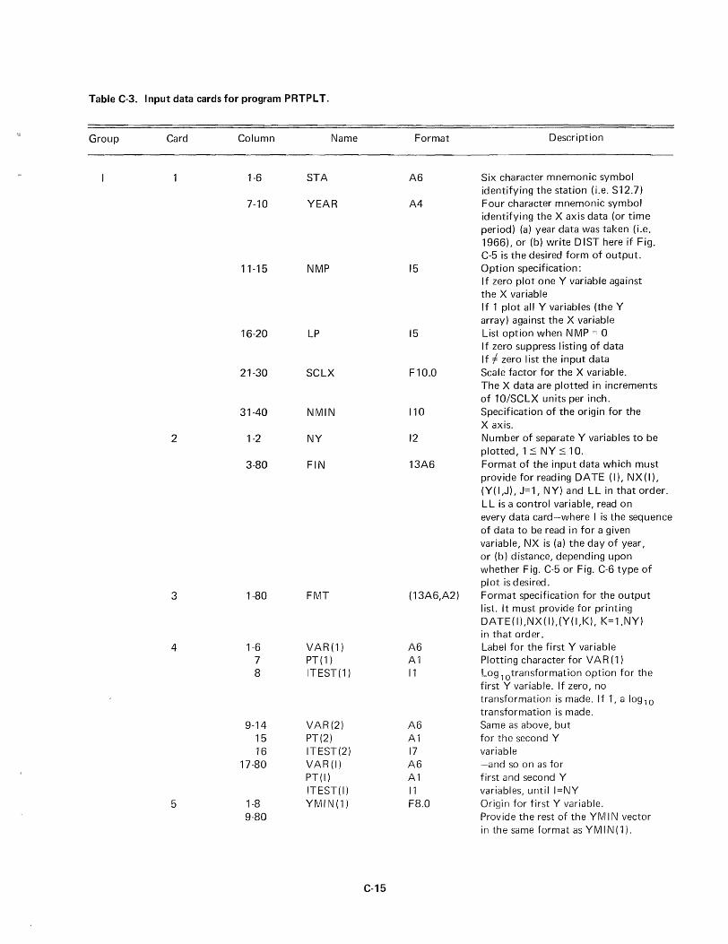
Table C-3. Input data cards for program PRTPL T.

Group Card Column Name Format Description

1-6 STA A6 Six character mnemonic symbol identifying the station (i.e. S12.7)

7-10 YEAR A4 Four character mnemonic symbol identifying the X axis data (or time period) (a) year data was taken (i.e. 1966), or (b) write DIST here if Fig. C-5 is the desired form of output.

11-15 I\JMP 15 Option specification: If zero plot one Y variable against the X variable If 1 plot all Y variables (the Y array) against the X variable

16-20 LP 15 List option when N MP = 0 If zero suppress listing of data If =f. zero list the input data

21-30 SCLX Fl0.0 Scale factor for the X variable. The X data are plotted in increments of 10/SCLX units per inch.

31-40 NIVIIN 110 Specification of the origin for the X axis.

2 1-2 NY 12 Number of separate Y variables to be plotted, 1 ::; NY::; 10.

3-80 FIN 13A6 Format of the input data which must provide for reading DATE (I), NX(I), (Y( I ,J), J=l, I\JY) and LL in that order. LL is a control variable, read on every data card-where I is the sequence of data to be read in for a given variable, NX is (a) the day of year, or (b) distance, depending upon whether Fig. C-5 or Fig. C-6 type of plot is desired.

3 1-80 FMT (13A6,A2) Format specification for the output list. It must provide for printing DATE(I),NX(I),(Y(I,K), K=l,NY) in that order.

4 1-6 VAR(l) A6 Label for the first Y variable 7 PT(l ) Al PI otti ng character for V A R (1 ) 8 ITEST(l) 11 Log

lOtransformation option for the

first Y variable. If zero, no transformation is made. If 1, a log 10

transformation is made. 9-14 VAR(2) A6 Same as above, but

15 PT(2) Al for the second Y 16 ITEST(2) 17 variable

17-80 VAR(I) A6 -and so on as for PT(I) Al first and second Y ITEST(I) 11 variables, until I=NY

5 1-8 YIVIII\J(l) F8.0 Origin for first Y variable. 9-80 Provide the rest of the YM I N vector

in the same format as YM I N (1).

C-15

Table C-3. Continued.

Group Card Column

6 1-5

6-10

11-50

IIA See Fig. 80 C-12

liB See Fig. C-12

IIC See Fig. C-12

Name

I\JYL(1) 15

I\JYL(2) 15

I\JYL(I ) 15

Format Description

Incrementing index for scaling the first Y variable. Incrementing index for scaling the second Y variable. -and so on for as for first and second NYL variables, until I=NY

o or 9 punch; if punch is 0, subgroup II B consists one card, 1-1; if punch is 9, subgroup II B consists of cards 1-1 to 1-6 to control the plots for the next data set.

same as control card 1-1

(a) Data to be plotted by time for a given station, arranged in any date order for a given station; cards 111-5 and 111-6, Table C-1 may be used if desired if card 1-2 above specifies a format to read up to any NY variables on these cards. (b) If data are to be plotted by station for a given date, then group IIIC cards are arranged by station for a given date. The LL control variable must appear on every data card.

VV REMOTE STOP

DATA CARD 9

DATA FOR STATION - 2

NO. I - I

FOR STATION - I

SIX CONTROL CARDS FOR ~BGROUPC ............ SUBGROUP B PRTPLT

PRTPLT ~-L __ ~~ ________________ ~~

PRTPL T FORTRAN SOURCE DECK

VI FOR PRTPLT rl08 RUN CARD

Figure C-12. Deck set-up for PRTPL T data input.

C-16

.............. SUBGROUP A

aBGRQUP C"-FIRST STATION

~OUPI

GROUP .n

~ Suboroup C, Consists of Data Cards

Arranged by (a) Date For a Given Station,

or (b) Station For a Given Date.

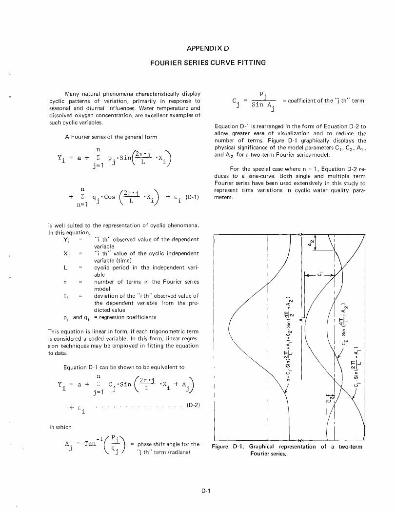
APPENDIX D

FOURIER SERIES CURVE FITTING

Many natural phenomena characteristically display cyclic patterns of variation, primarily in response to seasonal and diurnal influences. Water temperature and dissolved oxygen concentration, are excellent examples of such cyclic variables.

A Fourier series of the general form

n (~) Y. = a + L: p.-Sin ·X. ~ . 1 J L ~

n + L:

n=1

J=

+ E. (0-1) ~

is well suited to the representation of cyclic phenomena. In this equation,

Yi

L

"i th" observed value of the dependent variable "i th" value of the cyclic independent variable (time) cyclic period in the independent vari­able

n number of terms in the Fourier series model

Ej deviation of the "i th" observed value of the dependent variable from the pre­dicted value

Pj and q j = regression coefficients

This equation is linear in form, if each trigonometric term is considered a coded variable. In th is form, linear regres­sion techniques may be employed in fitting the equation to data.

Equation 0-1 can be shown to be equivalent to

n a + Y.

~ j=1

. (~X A) CJ .• S ~n L • i + j

+ E. ~

in which

A. Tan J

_l(~) qj

... (0-2)

phase sh ift angle for the

"j th" term (radians)

0-1

C. J

= coefficient of the "j th" term Sin A.

J

Equation 0-1 is rearranged in the form of Equation 0-2 to allow greater ease of visualization and to reduce the number of terms. Figure 0-1 graph ically displays the physical significance of the model parameters C1 , C2 , A 1 ,

and A2 for a two-term Fourier series model.

For the special case where n = 1, Equation 0-2 re­duces to a sine-curve. Both single and multiple term Fourier series have been used extensively in this study to represent time variations in cyclic water quality para­meters.

N <{

N

~IN <{

c U5 N c

u U5 ;:. <{-

+

~I..J <{

+ c ~1..J U5

U c (/)

Figure 0-1. Graphical representation of a two-term Fourier series.

APPENDIX E

OPERATION OF THE WATER QUALITY SIMULATIOI\l MODEL

The water quality simulation model has been devel­oped as a tool, to be used in studying problems of water resources planning and management, as they relate to water quality. The following sections explain procedures involved in using the computer program WAOUAL which is comprised of the individual water quality submodels. Specific instructions for using the program include a dis­cussion of the computational facilities required, directions for specifying simulation options and a description of the data deck requ irements.

The Program

Figure E-1 is a listing of the computer program WAOUAL which is the integrated water quality simula­tion model. This program consists of algorithms for five submodels, listed in Table E-1; the subprogram names, given to each of these submodel algorithms, are also listed. Figure E-1, the WAOUAL program listing, plainly marks each subprogram. The "prior simu lation requirements" column I ists the subprograms that must be run prior to the one indicated in order to provide the necessary input information to the subprogram in question. The hydrol­ogy submodel HYDRO is an independent program de­scribed in Appendix G. The output from HYDRO is fed into WAOUAL in the form of punched cards. This in­dependence is not necessary; it is merely the mode of operation found most convenient during development. The "system model" terms connotes HYDRO as a sub­program to WAOUAL, even though they are physically separate program decks.

The program WAOUAL will: (1) simulate, for the main channel and selected

branches, the distance profiles for each month of the year for: (a) mean monthly specific electrical conductance (b) mean monthly stream temperature (c) mean monthly dissolved oxygen

Table E-1. WAOUAL subprograms.

(2) simulate for the main channel and selected branches, the representative monthly diurnal pro­files at selected system node points: (a) hourly temperatures over the 24 hour period (b) hourly values of dissolved oxygen over the 24

hour period

A sample of the computer printout is shown in Figure E-3. The stream profiles displayed graphically in Appendix F were plotted from such printout information. The printout, in addition to providing the simulation in­formation from WAOUAL also provides the D.O. simula­tion in the "percent saturation" form and also repeats information used as input.

I nstructions for using th is program and further explanations are given in the following sections. These instructions include: (a) discussion of the computer facility required, (b) directions for specifying WAOUAL program options, and (c) definitions of input variables and format specification for each variable.

Computer Requirements

WAOUAL has been programmed in Fortran V for the Univac 1108 electronic digital computer; Figure E-1 is a listing of the program. WAOUAL is dimensioned to hand Ie four branches adjacent to the main stem, with 15 reaches for each branch, and five reservoirs and five effluent discharges. Table E-2 summarizes this capability, which of course can be changed to suit any situation by

merely altering the corresponding dimension statements.

Dimensioned in the manner indicated, the program requires approximately 20,000 thirty-two-bit words of memory storage. Complete ru nning time of the 1108 for a one year simulation of the 11 reach Little Bear River system is 28 seconds (14 seconds compilation and 14

Submodel Subprogram NamePrior Simulation Requirements

Conductivity Monthly temperature Diurnal temperature Monthly D.O. Diurnal D.O.

ELCOI\J WATEMP DITEMP MDISOX DDISOX

E-1

HYDRO HYDRO

HYDRO,WATEMP HYDRO,WATEMP

HYDRO,WATEMP,DITEMP

Table E-2. Summary of simulation model dimensions.

System component

branches reaches per branch reservoirs M & I discharges control points

a Including the main stem.

Number

5 a

15 5 5 5

seconds execution). The program is in punched-card form and utilizes punched-card data. Tape storage has not been used.

Without the program list option, the output for a one year simulation run, calling for all five water quality subprograms may be as little as 55 pages or as much as 130 pages, depending on the number of reaches being simulated.

Program Options

The program user has the option of specifying the incorporation or exclusion of any of the five subprograms listed in Table E-1. The electrical conductance and month­ly water temperature subprograms may be included or deleted entirely at the discretion of the program user, except when prerequisite to another specified model, as indicated in Table E-1. The procedure for entering model option specifications on punched cards is detailed in Table E-3.

Data Requirements

Data are supplied to the water quality simulation program in punched-card form. Details concerning card formats, variable names, etc., are in Table E-3. The data required may be divided into eight groups. These groups will be discussed in order of their appearance in the data deck.

System definition

The program user must specify the number of branches in the river system being simu lated, number of years to be simu lated, number of control points, number of reservoirs, number of municipal and industrial waste discharges, mean altitude of the prototype system, model option indicators and location of tributaries, division points between reaches, control points, reservoirs, and waste discharge points.

A convenient coding system has been derived to specify the location of any point on the river system, in

terms of the branch on which it is situated and river miles from the mouth of that branch. The format of the loca­tion designation is b.xxx. Where "b" is the number of the branch on which the point is situated and "xxx" is the distance from the mouth of the branch in tenths of a mile. For example, the designation 2.062 means that the point is located 6.2 miles from the mouth of branch two.

The serial specification of the months of the simula­tion year are required for labeling purposes. In the current study the water year, beginning with October first, has been used as the simulation year.

Equilibrium temperature

Here, a constant and coefficient are provided for Equation 19, to define monthly variations in equil ibrium stream temperature at every node point in the system. If the monthly water temperature submodel is not a speci­fied option these cards may be omitted.

Diurnal temperature and D. O. model parameters

Next, each of the four parameters (C 1, A 1 , C2 , and A2) for the two-term Fourier series diurnal temperature index submodel (Equation 25) is given for each month of the simu lation. Twelve month Iy values of each DTI model parameter are entered on one card. The four cards are arranged in the order indicated above. This is followed by the parameters for the diurnal dissolved oxygen index model (Equation 53) for each month. If either or both of the diurnal models are excluded from the simu lation, the parameter cards pertaining to that model may be omitted.

Hydraulic relationships

Multipliers and exponents for Equation 8 are pro­vided here to define the relationships between flow rate

. and cross sectional area of flow. Coefficients and expo­nents must also be provided for the exponential relation­ship similar to Equation 8 for mean depth of flow.

E-2

Monthly water quality submodel parameters

Each of the water quality submodels requires a reach-by-reach definition of input and transport para­meters. The data to be read in consists of submodel para­meters for conductivity, month Iy temperature, monthly BOD, and monthly D.O., in that order, for every reach in the system. The input format calls for reading the cards in sets, beginning with the first set, corresponding to lowest reach on the main stem, proceeding to the highest reach on the main stem, then from the lowest reach on the lowest tributary branch in the system to the most up­stream reach on that branch, followed by the lowest reach on the next tributary upstream, etc., finally ending with the highest reach on the most upstream tributary of the hydroloqic system. Each set consists of four cards, com­pletely defining the input and in-transit models for that

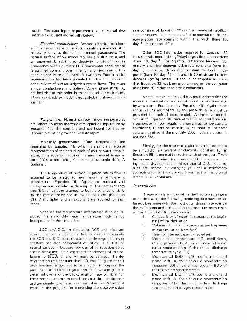
reach. The data input requirements for a typical river reach are discussed individually below.

Electrical conductance. Because electrical conduct­ance is essentially a conservative quality parameter, it is necessary only to define input model parameters. The natural surface inflow model requires a multiplier, a, and an exponent, b, relating conductivity to rate of flow, in accordance with Equation 11. Groundwater conductance is assumed constant over time for any given reach. This conductance is read in here. A two-term Fourier series representation has been provided for the simulation of conductivity of surface irrigation return flows. The mean annual conductance, multipliers, C, and phase shifts, A, are included at this point in the data deck for each reach. I f the conductivity model is not called, the above data are omitted.

Temperature. Natural surface inflow temperatures are related to mean monthly atmospheric temperature by Equation 19. The constant and coefficient for this re­lationship must be provided via data input.

M 0 n th Iy groundwater inflow temperatures are simulated by Equation 18, which is a simple sine-curve representation of the annual cycle of groundwater temper­ature. This equation requires the mean annual tempera­ture (OC), a multiplier, C, and a phase angle shift, A (radians).

The temperature of surface irrigation return flow is assumed to be related to mean monthly atmospheric temperature (Equation 19). Again, the constant and multiplier are provided as data input. The heat exchange coefficient has been assumed to be related exponentially to the rate of combined inflow to the reach (Equation 21). A multiplier and an exponent are required for each reach.

None of the temperature information is to be in­cluded if the monthly water temperature model is not incorporated in the simulation.

BOD and D.O. In simulating BOD and dissolved oxygen changes in a reach, the first step is to approximate the BOD and D.O. concentration and deoxygenation rate constant for each component of inflow. The BOD of natural surface inflows are represented in Equation 50 as simple sine-~r~. Each characteristic element of th is re­lationship (BOD, C, and A) must be defined. The de­oxygenation rate constant (base 10, day -1 ), given at th is deck location, is assu med to be constant throughout the year. BOD of surface irrigation return flows and ground­water inflows and the deoxygenation rate constant for these components are assumed constant through the year and are simply read in as mean annual values. Provision is made in the program for decreasing the deoxygenation

E-3

rate constant of Equation 32 as organic material stabiliza­tion proceeds. The amount of decrementation in de­oxygenation rate constant within the reach (base 10, day -1 ) must be specified.

Other BOD information required for Equation 32 is: scour rate constant (mg/I/day) deposition rate constant (base 10, day -1) for organics, difference between lab­oratory and river deoxygenation rate constants (base 10, day-1 ), anaerobic decay rate constant for benthic de­posits (base 10, day -1 ), and areal BOD of stream bottom deposits (gm/sq. meter). It should be emphasized, here, that Equation 32 has been programmed on the computer using base 10, rather than base e exponents.

Annual cycles in dissolved oxygen concentrations of natural surface inflow and irrigation return are simulated by a two-term Fourier series (Equation 49). Again, mean annual values, multipliers, C, and phase shifts, A, must be provided for each of these models. A sine-curve model, similar to Equation 49, simulates D.O. concentrations in groundwater inflow, requiring mean annual temperature, a coefficient, C, and phase shift, A, as input. All of these data are omitted if the monthly D.O. modeling option is not specified.

Finally, for the case where diurnal variations are to be simulated, an average productivity constant (pf in Equation 55) is entered for each month of the year. These factors are determined by a process of trial and error dur­ing model development in which diurnal D.O. model re­sults are altered by changing pf until a satisfactory approximation of the observed annual pattern for diurnal stream D.O. is obtained.

Reservoir data

I f reservoirs are included in the hydrologic system to be simulated, the following modeling data must be ob­tained, beginning with the most downstream reservo ir 0 n the main stem and ending with the most upstream reser­voir on the highest tributary stream:

1. Conductivity of water in storage at the begin­ning of the simulation

2. Volume of water in storage at the beginning of the simulation (acre-feet)

3. Reservoir storage capacity (acre-feet) 4. Mean annual temperature (OC), coefficients,

C, and phase shifts, A, for a four-term Fourier series representation of the annual discharge temperature cycle (0 C)

5. Mean annual BOD (mg/I), coefficient, C, and phase shift, A, for sine-curve representation (Equation 50) of the annual cycle in BO 0 of the reservoir discharge stream

6. Mean annual D.O. (mg/I), coefficient, C, and phase shift, A, for sine-curve representation (Equation 51) of the annual cycle in discharge stream dissolved oxygen concentration

If any monthly water quality submodel is not included in the simulation, reservoir data relating to that submodel may be entered on the data card as zeroes.

Atmospheric temperature

If monthly stream temperatures are to be simulated, mean monthly atmospheric temperatures ( F) must be provided for each mont~ of the year.

Monthly data

For every month of simulation a quantitative and qualitative description of each municipal-industrial waste discharge must be provided as an input to the simulation program. The water quality simulation model employs the results of a reach-by-reach hydrologic simulation model, in punched card form, to define the hydrologic inputs to the system.

The data input format calls for all municipal and industrial (M & I) waste discharge data for any given month to precede the system hygrologic data for that month. The data required in each of these categories are discussed briefly in the following paragraphs.

Municipal and industrial waste discharges. Monthly definition of M & I waste discharge flow and quality char­acteristics consists of the following:

1. Mean monthly rate of discharge (cfs) 2. Mean month Iy conductivity of the waste

stream (micro-mhos/cm) 3. Mean monthly waste stream temperature (0 C) 4. Mean monthly waste stream D.O. concentra-

tion (mg/I) 5. Mean monthly waste stream BOD (mg/I) 6. Deoxygenation rate constant (base 10, day-1 7. Hourly diurnal discharge indexes 8. Hourly diurnal temperature indexes 9. Hourly diurnal D.O. indexes

10. Hourly diurnal BOD indexes

E·4

If any of the monthly quality submodels are not to be included in the simulation, the parameters relating to this submodel may be punched as zeroes. If any of the diurnal submodels are to be excluded from the simulation, the associated hourly diurnal index card should be omit­ted. This information must be provided for all effluent discharge points in the system prior to the hydrologic data.

Hydrologic data. Month Iy hydrologic data consists of a reach-by-reach tabulation of natural surface inflow (cfs), surface irrigation return flow (cfs), groundwater in­flow (cfs) and diversions (cfs). For reaches representing surface impoundments, the above data are supplemented by net direct precipitation (cfs), reservoir storage at the end of the month (acre-feet), and reservoir depth above the discharge inlet (ft.). l\Jet direct precipitation is defined as precipitation falling directly on the water surface less evaporation loss.

As shown in Table E-3, hyd rologic data for one reach is presented on a single card. The hydrologic data must be assembled in the order of reach simulation, that is, beginning with the most upstream reach on the main stem and proceed ing downstream to the point of con­fluence with the most upstream tributary, sh ifting to the upper end of that branch, proceed ing to the reach end ing at its mouth, then shifting to the main stem reach to which that branch is tributary and proceeding on down­stream until the next tributary branch is encountered or until the last reach on the main stem has been simulated.

The hydrologic data input is provided on punched cards generated by the hydrology submodel. The hydro­logic data must be integrated into the data deck for the water quality simulation in the manner described above. Figure E-2 is a listing of the data deck, as it was assembled for a one month (October, 1968) simulation of the Little Bear River system.

\ '-

ccecercce C

~cccccccccc cceeccceeecccccc c

C C C C c e c C')U"MonrlS t~clu"'ro 1'" TH( "oorl C "'OJlfHl' ELfCT"lCAL ro~nUCrAt.4C( (F.'LeOtH c .. nt~h" ... Y .... fE~ lr...pr.eI'uupr (WATEfIIIP I C OIUQNll wlrro HMlH'JHTUQr tOtT!:MP) C Nl')tltwty O'''fi''LV(f> 'JII:"'I'G(N (IotOI4iQIfI C ntu"''''I.L n,c;,~"l WEn "."'G(~ fO('lt~~xl

c c e c

C C ceeecrcrcrec(ceecccc ~cccecccccccceec

Ot"'f"~lO" [C"PJ,C;.111.OCDfIS.l?t.fCPtCS.l1t.OOCPlf!uIZt. IBODCPT ft;. 1:!1 ,~1Jf" l( «;1 ."UNOO (~t OtME"~JO'" "lCJ(,"t' ~I .N~QClifS •• ~TRcwl~I.D£'SLOC(~}.

lr"lOt:' f '), I. CPH OCt c., .O~HLO("I t (u SI .f)C"'l~ (I S. 5 t. 01' s •• It, (5" Rtc It!». S». 1PK II ~. ~ I • 'HI f ~ 1 ,p WI ., I • leI",.", • &1( C 1 ~. 5 I .W'1 5.5" Q, 1',5 If OS , l!)t ~ •• lOt RC J S. ~ I .0 G J f 15. t; , • OQq t "it 5 I. ocr f 1 5, S 1,110, I!, I) '" II S' It IS, •• W ~ , 15 •• If'II'Ulf .". ,I>I')( c". (r.« 1F .~I .r('~ I p".St .rctR'( 15. at). reGIIIS. SI ,[CRAt t ~,s h -If r r." t t c,. St. [r"" t c. 5' • "r.:«l tt ~ .1 11 ., rCfl I IS.. ~. SI • oCON f t ~. Ii. t 2' I .AMO. I" I f. • A [(" Tq • Iii. S.!o' ,T j 1 Of I :i") , tt 1 F). tj I • Ttl) t 1 ~,~d .' tR' C l!t. S I ,A rCG t f t 15. S I • 1TGtt tc;.51 If"'"" ls.s,.rrf. IS.S,.TO. ,S.S ••• Tlli.?S) .'T4j,"S.~.21, fit. TIP t t t;.1) .l) ... TO It IS.!. 11. AT r" I H- • c;" 11 ,1(\ ell." I, nT I NO' 2fIJ • ~ 0 '(lito. I). '11) ,"',,"rc !o," ••• TrF' 1 f~. Z-' ,nn'H 1!. .!- •• ~OOOt 1 5.C;1, 100 ttc;. 11, .... no f tE •• 51 ,en f I ,.~ J .rn~ I, 1:;, C;, .l\OD~f t"uS) .RIS t IS .51, ?I)('IIO f t5,51,A"'rq~ I P;,.r.1 .~llo'I"i, «;),;)('(;1' I'j,,'il ,qOOG[ f IS.S I. lQtGtftC,~ •• Dt'.c'll1\i,~t,t")('IPRtlC" 5- •• o1ttQ'II),~J .Oter.IS.5t. ttAODC" t Pi. t;) ,0 IfF fl c.," •• QPfl S. lit. ,0 H l!..~ I ,I>2( I tj" ~1.8aOOt 15,51. SQ .. I' c. ~) • Alq fIe. 5" P I -If IS, ~ It '411 'i. S 1. I OOC) c 11). ,), ~ •• PC)' fC 5 •• ~aOOT ° f 15. S. 51 • an", 1 2." I .1'10 T-..r (z .. , • O()r f J C S • l' I. poor.r I f r:;, 2' I • '00 S. f r:;. 1111 10"" f 1 ~, !' ," 4t I .'" • I!,. 5. ')" 1.0' pf'(, t 161 t, (C I Nt 15. st. 4Q(rr'';'.1.', T'~(I').5I,r.OTf!lfl!>., ••• n"IN(ls.S.I.~IN'IS.~I. '18nn~1 )'\,c;,. 3"j~ro ,-;., ~).jn!')olc)t JI,A!"H;lf1C..SlJ"f'Ulon(l~,~.li1'

C R[AO IN <;t'-ULA""',. t~n">""ATr"~ aNa ,"'Ift&lI'E I~"f'r'i rtf AI') f S.I!"f'1) ... ,,~ .~.,p • ..,cPtt; .NPf'(, ,"'E'r .AL T. rv. IW. IX. Tw.1? ."r. 'OQ .... ' I~t~ .r~.n,c;tc.. "'P(~ 71>!l.-'l h •• ""';t, .. -AlJ .1. 1:'(.'" It('If'! f~,t"7' I~O-.Ufl., .... qr.HIIAI."'T;)e~tf'h U:.l,W'UU

1~2 rnltNA' ,''iI.' 00 II;. .Je:l,ttqo KR '!NlPCM' J. t -N~Q CI-i to,,- t ., 1tF' 10 t", 11')" ,,0(" HL ~r I r" • ..19 I, Ill: I. Mill)

J"" 'OOllltf:I'ifS." ''''_1: "'8-1 DC 1 ,aflt: 1.'1'-1 DCMl'-l' ta- .Jq 1= CD CPltr", .JR.1, JIi I-C('Ht.nCf IA - • ."et 1*1 no.

l CON' ,,.ur 5 CO~II~ue

R£IO 1~.I..,~t fCDll""'''IfCt-rr:J,,..c,,lt;t J"'! rOOM", f"F!,.~1

IF I~Dr !\.lC: ."1 'l('l J r .,. C:('!' f~.tll')€) '"'~filn"fJ(,I. J":l.N",rSt

'. !F .",(r .Lr ."t f'., T" ,r O(.n I ~. 1'" r,) t r" lO ":1 K(" t. ~ r ~ 1 ,..,r~ I

In" '"0"" 1 ~"C..:'fl '60(10 (C..c},u fA vn'll).La':Jd7.. qf) '0""'&' f) 'Ui.

.I = 1 • :1 l : I4Qp

... : I f:~~C"f11 ~~CQCHtl'" nc 7C, ';(1= 1,t.jqO

IQ : "'lQI;'~ IJ"'" !P : 'Ilul('''tCJ''l III ': r n - 1'" ., I~:TIJ'l I')IYIJ •• H;l - [ •• rrlff.CO.tlllltJ,JI"', If I TII.r:'l .. J 1 ,,(, 111,.,J"'. : U.') I' 1 ''''.£1.11 r n 'I') ..

r:;(\ '1'1 II

! J: I II If. JO I :: ". 'oJ on, JtI.J(" - ... '1 "~O( I'''J''1 ':' p.n Ir 1 f'(.(n.ll 1';0 T~ :Iot,') Gn T I') '"

,Co2 Ol"l .:'45 t J':' J ,"14 OAflOntJIJ"J.JfI :' ".

,C; 1 001)1 II,.J". JT I :. ". w C(lN'r"'Ur

IF" It'.f,).I."O TOO:

')1 T n ?')~

:,r.' 1)('1 ;"151.1 J' ,:1.-;O1l

'7r, .. ''IT tTli. J('I. J. t : n .. :"'Ir, C"'~' ''',ur

1)(. 711 1(': 1. If,

orr. J"'.J" I -: ".11 OP1:n to,J"1 : .... , If (''' .. rl').JI rr Ttl" r;r: 11'\ 1

r. TCrt In.J''q : I".r: T~ All 11\. Jf'li : f'\."

7 CO~T "lIf(

IF' f IV.r". II (0" '" ,.

GO I" 11 " (err I TO. Jnl :' ;J,'"

(CAP" I). J("I' : .,. ~ '1 C~'4T T~Uf

tF ,Yw .f".ll r 0 'r. II ~~ 'n ,-.

1 ~ 0" rr t to. JO I ~ fl,": ROCIC" JCI.J'" ~ "." I:'Hr'Tf'),Jnl ':' n.r

~_"~~:~:~~:~~I ~: o~~" ~1p:Pfln'J"1 ~.I"I

"t; en ... ' ,t.ll'( (" INPUT f'n~""A~'\ .~n t:nf,rlrJr"'T('.

yr I Y v .(".11 ,." '0 ':1

j:.l on f=.') l 8-: t. NPf'I

t' : ~lpr"'llPl - .,"O"",fL Jl"1 • 2 0[10 (1\0)"" ,.Hr"'lflJ.',l'htltl P :l,y'1

1 r I ror>lII., tI "r c.11 D[At tC"lt\Oll UJrfitln'l.l"I,l', L&:l:"lfl

I'H'1 roo N .' fIU'\.tt '7 CO~I Ivue

IF fI,.",r.)1 ro 'n 11 Cl~ Tr"I Nt':' 1." PC AD • "'.1 'lC 11 ,PH""', MIl. 101 0:.1, 111

lr" 1 '~O".T '1'" ft. "'I 10 C~NI ,~U(

" C"~T!~ue If f 1lI.Nr .11 roO TI'\ !", 00 ,." Ml= It. Itr at) t !)tll] I f A!')(\f 1ft' .MU. litO = I. li't

Figure E-1. WAQUAL computer program listing.

E-5

III FORHA! IIZF'.ll •• cnNT I~ur ~s CO~IINUf

00 ~3 L8:1o~ •• IS:~LOCHIL91-Nb.e~ IL'!'1 ~E"O (5 .. 7.01 J)j.HlDhn~(Lf:\I.q"(lql,PIILPI

110 FO •• " IOF5.11 00 ~, LP:\. to:.. '\ IFft'll.EO.I) t'(IOtS.l!'111 (AECC',fLl~,LR,HN). MN:l.71.A(C~tfUltl8J.

1 (AEC I~ IlQ .lP ."'KI, "'I< = t. S 1 101 FORMaT crS.Q,r.s. :-;.FS.!ltZF'S.":l.F10.8.F5.n,'J(J.·"1

IrfIw.(O.ll PEIOe",I''') UTSfLQ,Lq.L~I.lN':.1.71.

1 fA TG It UhlB .t .... l1l4 =It''' I aT lQ fl" ,L q.lK I, La(: It?) ,wI( 'LR .LBt .PM: ILh', Zl'1 ''''1 fORMA' {F~.1'''5."I.1F~.1.rtn.R.rl).1.rC;.3.lr:~.11

IF 11 •• Nr.ll (.0 '0 q Q[lO .5.12111&900<; flo.Lq.LNt .LN:J ." .cnC;'LP.LI\).BOOfRIUhl8J.

tRt J" fLQ,l' J .-.('1 OG I( lP.l at ,1)1 G If LQ,t 8 t ,Dl &ILQ.L81.ilPILQ,LlH. lP1 fLQ'.l~' .OQ It R.l~ 1 .D"tLQ.Lf'I.~~()nfLI? ,LSI

111 FOPflAT tlfS.l.FS,3.r-;.2,ltrS.l.f"c.11.Qr5.2.Fs • .,.r-S.t I R['D .5.12'21 I 'OOll)tL0.lR.l~t ,IN:) .ljl. Ur.(\TQ(lj).LA.LHt.L":I.SI. tUDOG!tlO.U~'LOI .lO':l.3)

1'2 fORMAl '1(rC;.1.lIfc;.ll,r5.1.'2f~.JI

R(aOfS.l"JJ fPCO~(lP.LB,LMI,L":l,I?J

103 FO~M" 11:>f"~.11

GJ CO~I I~UE IF I~P£S.H.nl GO 'n ,~

OC' ,;~ L~="NQF'i R[ AD {iii .1lCtl ~ ell) '{ l~. II • liS TI tl PI. V 101 A r flO 1, tAT( lI'h I. HRI • HO: 1.1), •

1 fa Tf l j). '2.,.0 J ,~Q= 1 ,., I • f &SI'IQ It R.l '11.l~: 1 • .31 • ( lOOP (LA. L PI • L B= 1 • ~ I

110 fl)m4Af Ir~.:J.'F~.",t;"S.1.q'S,'/}F5.1,flj.".2F~.I"'i.ll

•• CONIINU( lS IFfJy.rO.lI ~rIOfc'.l1(n CTAtQCI(I).KT:l.PI

1" FOR"I! IIlF<.11 • CO~I I~U(

IF IP.(O.11 ron'~ 1_ GO 10 7J

10 00 1 .1:1.2" lM = M1 .lNGl ': .1~11q~3q.f".I"(1(.21

IH61 : .~~!~OIlt78.'''' •• nCK.q. Dflll!,)'"T) = 1.(1.'f'IK.1"SHlC.lNGI).I"IK.l)*(,.1~(J'-ICZl

I CONII~ur

IF fIx .Nr.ll (if) 1(\ '''' n., ,.; MT: 1,1-TN: "'1 INI;} : .1r,I,OQltJ.,M.''''0(1(.21 1N~1 "; .1i?,'IjQIt:'~''''''I''O''':'''1 f'OrNnt"'TJ = 1.t".U'('tI.,..II.SIN"~G11+lnn(M:.31*~IN(IN('2'

'f CON' '~ur 7 J CO~I l~ur

Jf e,.", .It.O) 50 T("I " 00 ~~ l8:1.~rr JFF : [FLOCIt" 1 HR = NlPtHIJr~) - ND 1>(' I'te Jrr, • l 00 H IfF:I.N' tF' COCHl(\Curr.ldrr).fQ.frlnf'ClFtll ~O '00'

~~ CO~I INUE GO 10 50

~7 Clr&D e5.1n'H "(F' 11''''.)£' t,rrlFfHF.Jfr).u:rc Yff.JEr). l00EF IIEr • .Jrr I. 80 or r. IFF • .JFFI .OHQ Iff .J£F I

tn. rolltllU' trc;,.l.FS.I'\'~"'\.I.rt;.I' liE AD , 'if 11"1 {nrrr flD .... ,) .H': 1.2_) IF' t Io? ,""1.11 ~r"{' II!. 1l't I f T[r III D ... , I .HT: .2111 Jr '\J.Nr.ll r,O In .' Rf ID C I§ .1llt) t (1('1,," It l q .... TI. tI': • "" I ~£ 10 t 115 II !., I t 90!:lr r I tl q. NT h 'oj T: ., If)

1"" '0»"11' f 111" J.' I J7 CO NI!~UE U CO~I lNUt 12 CONIINue

C IS THr~( •• ~A·~CM fQY"UTIRY TO l'~IS D~"CM

10 Ir I~U.r.O.lI GO Ir, ,~

00 I? J"C-:?""t'I~ IP : r 'HqO(,H f 1.- 1 IFIlIq.EO.NI~CHIJ.(tI.'NO.IJ.fO.JtI G~ TO 15

12 CO~ItNur GO In 70

1 ~ 11 : I I:Nl ~CMt L J -~"QCH Il '1101 .I = l

'n CONI I~UE e I~ IHI~ oraCH • -rSf"vOI.

If'tND(\.rO.ol r;,o '(10 ~~~

00 ". I.J:l.NP(S If C~CHlnccr.Jt.rl').or"lOCIIJIl ~o TO ]76 ,>. CONT I~u(

1~' CON' I~U( prAO f5,10'" ~SC r.JI • .,YRtl,Jl.QtjIIJ.Jt.QOCI.Jl

ln~ ,-nAM" t~"".l,".r."F.}1 ot.", r. JI =n~ f 'I oJ) • ., TD r t. J I, Qct It I, J I ,Q ~~ C I. J ). of' C I. Jt .0 t f. 1 • .J t TP'fl)nII.JI.GT.OINtI.JII Goer •• ,. = Ol-."I.J1 QI f.JI :otNtr.JJ-OOII.J) At I.JI : CUC.)I.nt~n.JI •• OlIJI He f,JI ': OH(J) .Ot~f ... .JI •• PHCJI WI I. JI : • fI,J .,Iof, t, JI GO I ~ Jl~

ll' _[aD tS.1nSI 05.f I.J) ,OIRfI,JltOGlfJ • ..JI.OO'I • .JI.OEy,Y'ST fI.J).ACC 1..1) Ott4f I • .JI =0\' Y.JI .OIPfT • .,JI.ntill !.JI.Ol\qtt,..JhoCrtl.JI.Ct l+l.J)

DUM"'Y = nUHt,Jt -arY.CV5TI CIJ1-V~·IJJI Jlfil). If'OOII.JI.GT.OU~.1 nOfl.JI : Ou ..... ., O'''JI : ",..,tJ.JI~OOfT.JI.'y~'rcIJI-Y~ICrJIJ/FiO.-O(1J

3H eONTI~lIr tf IIV.H~.11 GO TO II")"

Ceec(ceCcrCCCCCCCccc cccccccecccceccc C e c r l CON C C C CCccccccecccrccecccc ccccccecceccccec C COM'UI£ r.C. or eo .... ~~r~g OF Hrw

E_ =-PI:n .~2 J~'~'"' E-IfIO~II • .JI.Gr.I.1 C.O '0 otll [CC., 1,..1) :HC\C I • ..J") 50 I~ _~?

'01 [C4ifJ •• JI :: Irt~(r.J")·O!dt.JJ •• 1r:CSII.J,2J _ 02 CO NI I~U[

rCIIII.JI : arCGIII.JI l' "', It. J). IN O. It( .l r • e 'I rio TO' OJ [Ctttct .J.::A[C'I~I I. J, 11.'£Cl_'I.J. ?h\IJrtfPT .&ECIRf [ • .,J.]II (>

,.[ c! ftC I. J. ... , .~ I~ f 21 .... t • A (C I~ 1 t ,..J. 1\ I) 50 10 • 0_

.nJ (Clllt.J),:n.o "" "~':[ClI.t.J"Q' 1.1,JI

"SF:rCStt,J)*Q\II.JI M'Jt:(CII.t.JI*OIRII.JI 1M I: EC Q I IT • .I I' OG II I. J 1 .... :cc .. lttI,Jt.OIRf I,JI MIE':lCr, " • .1 It 0['1 I.JI SU" : M\T.M'i'.MlfI.MfiY.MSQ.M(r rc IN If • J I : ~U./ 01 NI , • J 1 I' 1~lIfs.U.nl GO I~ • II

C T'l RrlrH 'I' " I:oP) [P VnyP 00 41 n J 00 = t .~Jq[ C)

IF(~CHlnffl.JI,£Q.prqocttPRJI G('I TO 1,t15

I,t I n CO NT J~'lH '111 COf.lT J"Juf

[C IT oJ I ~ reT"" II.J 1 GO TO I,tSr'l

415 fONT PW[ IF f II( .F'l. I' .UJO.f .... f-!f .. 1)1 (;C TO L/!'c,

tI'n VIN :- OIN( J • .11 _f'.n. £( 'S T I' PP.Io(. 1 ,: 2. - ( VC; T r I t ~~ I- J'" r: <;. T I I PP.. I< " v t N. (C 1 N ft. J l- a ( I. J 1.60,.

IfT';T ITRP.I(II/I?f I.JI.[.l).".-V<;TfIPO) I Gn 1'1) tjtjf,

tn''") [(';1' tTPp.~ J:rrSl cr o P.1H [,0 Tn I,tl""t

4"" fe IT .J) ';' I(r< II JPf).l(q ,.rr')T( IRQ.KI Jl2. ... S rr fI JI - .,o;,T It JI

LiC,[' CO~l J~II(

~·r.or T. J) -t't:1 T. JI "qq CONT T"Iuf

IF f 1Y ~Nr • 1 I (, ('! T'1 c; .... '1

C C C ( C r ( (' ere r r :: c C r ( r [ C C ( C C C C C C C ( C C C C C C c r C r r ( C C C C f C (' r r r err c r ~ r ere c c c C r (" c C c c ( C C C (

PI :- n. Ii? 1"i 1Q. 7 ~. fi( Ak f r .J I ';' ~I( I J .J I' Of !Ill t. JI •• f'1( I J. J I

f ~ -: t' X 0 I I - 1 • 4';' AIo( I I • J , • \J I I • J I • P r I-IL ~~ fT. J I J 10 I N I I • .1 J I TC, I I.J I = AT<;I I. J.l1 • aT" (' oJ. 11 t llIP IK I 1IIH I.JI -: AfTQ, T.J.)' • ATIP'I,J."I _ T"'PIKI Ie; T I r. JI :: AT':. TIt. J. 11 •. ", T .'~ 1« J. J.? I ." Tf'.! IP I ... AT SI It. J. J I) T[ fl A ffQ ([ oj 01 I • ! HQ 1 1 • .1.71 tTl:! IQllo,)

If ot - ,. T[" I , .. 1,.Jot' • a Tf 01 J-1 .J .71 • T A tD(K I

H' -:T IT -I. ,J ,- ')( I" I •• JI HT"i- t<"; II.J ,.":,, It.J I HTlf)::nnCT.JI'(){?1 T.JI HTGJ -!Gt 11". J I. f)G II J. JI

HI [F ::T(f II IJ I" offf r. Jl HT!=iR -:fFR 1'" J " ~RP( 11.11 TT~(I,J) : IHT.!iTo;.HT-:J.HT[f.4T9 0 .HTI o I/QI .... 'T.JI rF(W'r~.rf)."'J r," Tn C, I'>

C II) THro; Df'ACH A MV~'V'1Ir?

0('1 c,'0 I pC': 1."0,< IF f C'fHL ""'1 r. J J. rC.o r~Lf}rt If;';'11 (('\ TO ".1Ir'1

I:j?n CO'Jf INUf SIS C(HHPltlf

TfXT ~ fTNIT.J)~TF'rlJ

T=:r ': 1 f ~ r ' '.: TII.JI::- T[Y. Trl'l

t;fl '" <iSI"I ",49 (Of-IT INU£

~~lGt : pr.~T frs::;-p.?11 ANr,? - 2.,Or,ftTCTI"'P.".!1

AN(.l :: 3'P j. ft T I J 0". '. 71 ANf4 : li"O I. /I T 11 PI). 7.'~ I TI1 • .)1 : 4TfJ~Q.I.ll·AT(JDQ.I.?I.O;-.'NI .. Nr:11.A'ITOP.1.~I ... \J~IANG1I'

1 AT (rOO. 1.4 ,- <, NI AfI4( 'I_ AT I t Po. 1. Sit -:, f"!( AN(.4 I

I:j<;n CONT t'JlJf 1),)9 CO~T l'lur

tf' (P.N' .11 rr TO (C):'l

C C C C (' f (r ': (c r r'" (C C C err c: c C err (' ere c c c c c ( (

C C

C C

C C C C r (( (f r (' (' r r r err ((" I': C (r c (r (c c r (c C C C TF fN~r ~ .. r f). '11 ili'} 1 f' ('""

C T, T!.It 0;, Q' "(,H &. Pf' o;r ov"l'') f)r (,"'1 r0:-l."r-rC; lr ( O[Hl"r{ T. J' .r 1': .. "f ",l 'If I I C'I I r.n ''') f. 5"

f-rn CO",T I "".If Fo":' (f'''J'' ... ·Of

( C '1. MJ Vl L"r fT y r" II p. I·~('~JOI

Y - f 1 j t..I IT • J " A, r • J I I. ~ _ j: .l ~

C r TPt.yr, T T"'r IW")U':O::; J

"'YT C(l--tl·;(I.JJ/y.r .. <:,

'In (;> 0; ... f T ~ I ..... 4

... T: IoOTT • "'T f"'! 1- 1"" .. S'.?lI! ".0 11" f 1'1

GO Tn f.(",

fl1l.i "'1

Tf'I t.tj?

'\ 0 '. IT_ 11 " f''' :.,. L , ... T J I ':'.~ •• , r 'J 1

G ~ T" (. lIl,

l·lI ~ [11 rr Al,S I r 1"1 ,. "1 P "I "4f 1+2.:--' r. ': r: 1I 4 CO "J 1 I ~IIII

yf (')II_\.JI.I'."".' "" Ie hrl : '1lf·!·JI.nTr[ .. !.),".qll

f. H. Tf ,"'f I r. Jl.1 r • '.: ",.,. TI) f '\ "11.,JI.('11,,"'I""ll-,I(I}.JI

h t\ 1..1., ..

rot? Ir 11ft'" .Jl.l ~ ...... I 11'\ fr f P

II'

~I co T I ~ I ! • Jl .: r r 'i( 1M r I ,. 11 (. f ! •. J I r" 1"

(;0 '" .. 3r~ yeT • r I' \~'" l •. j J .1 r • "'. I r f' ! r r ,1 "'r ~ I 1 I r - I • 'if ~

1 f' I f I' l I' r I ~ r I • r ': ." ".; I -: t I !. I , J' )

f· J? r r ,~ II r ... ,. i I ~ T rr (f • ~J I • tr r I II f .... , 1 I \.Ir F "f r I ! •. J' .. ~ rf r I • r • " l T I • r;r f r ( i £ • ~ 1 I I GO IN • r) T ~j I ! • J I - if r ( I • .J I _ fl. -G[ ~ 1 f J r ,104 , T I , G!' 1 "I f. ~ ~

r:. '7 Hr r :. DO l~' : 'i I "II T • .J I T J'" {f).l P" I ! • . J I • t. r • n. I .. , '1 f!'l f, ~ <'l

r·" "I <;. j n. - .~ • ~,o ~ IT., r Q r j.j f T D I ~'J ·:0 ru ( I ).1 lF f l.r~.fll [(1 l" qf

r,r, tl'\ l-l"

G,,jr-, I.JI -"111. Pl,"'Tl)

G" T" r·(j'"

[1Tnr r" loO rT' nT r x' :. L'1 QI " f ~T 11 _ '" T _ 'il {,nrr· riryr·Fy

,Figure E-1. Continued.

E-G

OT It •. J.HYI = r)T[x.rHrl')

615 CONT lW[ GO Tn 6SQ

650 (ONT T"'uE C TS THE f?£S[RVOI~ ";PIllINr.

TF (t t Vo; TI (I PJ .V Sf I I DI II? ), CT .V"" A)'« II') 11 (,a fa ~f, 1 C IS RESERVOIR 'J[PTH lj~rA'r~ T~~'J :"''1 Ffr:'T

IF (ROf!'H .GT.20.1 C(I TC 6tj5 C R[SER'V()tP OEpTH IS lFSc:. Y~AN 1"l rr(f

653 CONT t"Jl1( 00 ~I; t 1'11=1."" OTH.J.t<I" = ltI.JltnTIfllnPHJ

fil:jl CONT tNUE GO f'l 6S"

6'5 CONTlNU[ C R[SERVOIQ oro,,,,, IS GR'r,HF" rH4N ?'l ff'rT

00 FI:,7 MT:l."" orn.J.Mll : TtI.JI

r;C;7 CONT T'\,Iur £,RQ 00 Fqn JT:l.;>.:.

IF fflYII,J.JTI,LT."l,1 I;qQ CONT JNU[

GO T') 6qq

c;ql SHT = O. 00' ~q? K T: 1."" IF for tI.J.W: T 1 .l T.", J OT, r.J.t< 1'J

[lq2 S'" T ::- Stoff .l1l (J ,j.1< T1 Y ( t. J' : O;'4r I?~.

,;qq CONT INtlf IF (lW_J.lf. J I r;(l fl" 7 Q "

( ( C C C C c r. ere (' ( ,. ( C C ( ((" r C ( r. ( ( r c C C C C C c ( C C C C "'1" lc-," 'I' C C ( C (C (( r (C ere (,. c c c c (c ere r: r c c (C C C C r (c C C

rs : SArrl)t.j( OPEl) ,l It •. 1 II

ROO~fI.JJ : An OOqT.'.lJ""i3n('>(',II •. jon-C::I"IIt'r_Af'(lfH;»lr.Jo3J1 BOf'I "J I I. J t : (dO 01 '. I 0 JI or. I 1'1. J 1 • n('l f'\\ ( r .. J ,. ~') It. J) + rOi;' 10 t If J It

101P.1 r • .)I.Ilnnr;r ({ oj 1+')( II r.JI ,0("l)r,. tr.,J}.f"JFfl f.JI_aOOri.lll.,JI' .?ORPI t.JIIIOINf I.JI

O(l<'(J • .1) = A"'nSII .. J.II.AOOc:.flIJ • .".o;-,tflcpr'AOO",(TIJI31,. 1 AO 0<. tT • j. t.I }. ~,f t.J( 7 ... P Tt A 'lOS ( I • J • 1)1 , OOrQIf.JI = "I"OlnfI •. JoII.A"l'lr~II.J.n'SI~IPt'ArOIJHI.J.311'

lAI) Oyr>r I, J. 'II .<, IN I'.' CI I • A~H'I 'P IT, J. C.II DOG111.JI= A"'('(,ltl • .). I,. AeOGle J .J.i'I.('pn P I+Ul("GI( r,J.3t'

C C Co",puTr ')ATUt'1t.TION rr"rpdOATt(\N M' nt<;'C::OlV[O oHrp4 Do 1"< ff ,J) :: { !"~ It • I ,J " Q I I- I • JI - '1"<:' Cl .. J J - C'S I I. J J - ')0 PH 1 ••. J! • J I k I I. J I

1 +00('" t.J' .'}t'rll.J )'''''4Q( T.J ,.O.)I">( I.jl .I)OClIt 1.,JltOGI fT.JI )/GINf ItJ ?

R I J~ -:Q 1 It. I • JI ./1 n~ (J - I. J I. III I. J ,J' .Q r 0::; ( t • J ,. Q.,n" I I, J I. r,,) I 11 J) RI Hl:-~I J~HQ 1fT II.J 1_1'l')f)Gtt t .J} _"ry I r.JI

RIIN:oJPHR' 1 IO fl.J l.on:1[')( J .JI .olIo I :.JI R I TN:') J I ~J_Q 1t'C' (r .J ,. ',r!",: f ( I, JI _':}f f' fl. J I Ql l'-J:fR1Tt.J_f'I')RII.J) ·I)~~~·'II.J 1_('toRe J • .)) 1/IIll)·)I~llt.Jl.QlN( I.JI·' Ifl~Qf~.'t} .. nl ~>(\ l"l '111 nr. 7:11 {o:\ ,MPE')

It (QCHlnrII.JI.t'f).QF'LO((I'?11 (,('I 10 nn 7r..1 co'~' !Nur 711 (o..,y T~Uf

( r T Ii 1 S Qf II C \.I I <; ~J or to ? f' ". r '1 vn r Q

C<" -: c::." t(IPuf'lnr S. TI \!t i .JI ) H~ : • 305-1-f( I. JI

C C MfAN yrl(lc:tlv IN ~rr T/~fC,

VEL : or~(J.JI/AfT.j)

C C T lfolf O. T OAVr. t t·) ay O::;~

T r = ~('Hl 'l (1 • .J II Ivrl • If.1.I J

lAY -: C Y I~: ( 1 • J I' T I J , J' I I ., • ~l

Of.t' ::- 'AV- 'r!. 0 Tr (lav.(:( _ 2"', 01 r,. 1" 71 r, THf' -: 1 .. Of. ,-. "n I?' ( l ~ y- S.J) (;f) 'I') 117

71t; lUfT = 1.1141

117 (ONt lr..:u( ({'It'T ';' THrT- t( TA v· ('r. f' I Q liN ~ (''lr T. u 1 [N

lCOP';' ! .. '11f"."[Lf C (' p~AroefJ('" ':'Pl",l'-)!T ,"<,r

~? I I oj I - (q. 11'\1 ft ........ f 71/ , ... , r • .J I' • I • ~r- )

R?ff''> :- n)fI. J I. Tr "Co

C (O),y rr ~ r'E r' r Il !tJ t -If' l ...... 1" or al .J

DA C(,J-,nltl;ll.J' Tf In/\.L T ..... I f'A - "'.

Q :: oOfI,Jlt"IP..,.<)'f' • .11 flo; 1 -: f 'I' P f - r: _ ;'. ~ I • TTl

fl(7 ': rYf'll_o""'OI).;,.".lT, rt<tj ';' f p"l_fHr(!. ".;". 'I' TT I

(or 1 - 101 T·'.f' QI •• .11 1'1 I .. ~"l 1, ! • J I I:) II 10 ? C;\!) -I" I

fOr' ';' Ol.i I 1 ,.11 /I ~ ,,("'1.' I" ~ IT. J 'I ')~ ... r,(~ I)ff t r: l to" I"IJT q r;" rr.:1'" 'lie ,,. ltd

[)P:-"" A. r \0/" ,:"r I _I 111"'" 'I' I. Jl • :>J'>I I.," '1.'. ' I.~ )) • f r ~ 1- f";>1 1 .C OF :-. I RII",I', T • .11 I~'" "'1.> I! .J II I ' • .s' _" '.;1 I • J') I- I r" I.I-[~; I

C C /) l<:;<,", Vr I) (l~ yrt' 'oJ t'J ".·Tfl f'\", (f'('M ! '-d'., 11 'r~

Dr II. 'I .. (C,_'-!.l

C C'~ • c .r.. Pf'''''' I ~l ! ' .. (, ! 'I (' J 1 r I 1.. f ~(l'" '~r ') 'J r A(,.. Hfr"IfJ. 1I.lf.·1.11 rl'\ ''': 7'" i

,C'''I CI M' T. J, -!Jill 1. ,II I I") •• t. n ) J • I' I'{ I ,p IJ 11. JI I( ~ •• l.p I (,1"1 Tn. 7':1.1

1 f1 ~ roo cr. J I : 1"" I:~ I , •• 1 I

7"4 CO'" T'lluf 1f ,QP If • .J I • r'" .~) • I 'c. 1(' ,r',

tDufI. r,q l f\ ., ~.,

'11"10:, (ONlf ... tI[

H' 1 lil (." Of ~rl~ • oJ I. I r/"'" riD I I • J ! I I ~. t I • r; I.i , 1 • J I I J _ r '! ... f ~ (, r, .. ~ •

C (' 1"4('\ C)('1\1R ll·n"', O[Af" PAOnl! .JI : f .... ~nf'\f T. JI ~.(J"HIo4''''''''l~Jlr. J)_II.:)_f·yp{_r,~."k!( 1 • .1) II ,.

l[rOI-t:.q .. l.r'I.ICT.JII

PI (f •• 11 Q I ""C 'IF 1- ~ 1 fT. oJ 1

GI) T'1 7\"

'10 (flNl f'Jllf t r T H T" D[ A C'" 1', ~ Cl r" r fl y" I!~

00 'f • J 1 :: I.') ('1f'" I Ie. I I •• [ "p I 1('> ..... I .. <:. r .~ f n T • AO (' '? ( 1 I) • , ) 1 p,,: 0 r T • J 1 :- A t'\" 0 I I'" • I I' ~ 1:11 1 ' • l I • <: y.' It) J • A tliJP tiP. ~, ,

PIIT • .!): '1.1'" 7 \.." ('ICCI J ... )I ~ fH'l 1. J)

qonf' (t.J I : rrf)c J. JI 1"1') (('NT , ... ur

If It'(."If.11 ".., TO "),,, C C ((' r r r (' .. (' -: r. r (( f (' ((' r r C (' (r l r c '= r. (C (( { ..

C ( t' :) f C; ... ~

C C ( C ( r c err r C C ( ~ C ( \ C

IFI"I1)fs.rr;."11 (·0 1" Q.J"

'1{1 q"l 10:1,"0(\ rr I oCHL "C IT.J I. rf).r r",lor (Ifill e,1" )(1 It.? 1

A:"II (I'I"'T 1"u£ ( (' THT~ 0rAC,", 1~) N~I !\ Q;<;,;-~YOlf1

Al"1 ((""IT p.;ur

{

c ere c (. (C C l C (C

C C COlofpo'f OJWH!lIL ()~f). f'I5TRI6urJQN AT q(ArH 'I' OF" BRANCH'J'. 00 A20 "HI :-1.'4 HT ::: JOt ."TT

A?l Jt 'MT .. G'~?fn rIo tr q?lI GO TO R2S

ll'" "f ::: IH-2" GO ,. n R7~

~?r, CONT T~lIJE C C COJolP:IT( TI-4( ~ITUPATrnN CO"'CfNTRATION Of 0.0 ..

CO; :: ('ATCO"J(PP('S.!)f( J.J.Mlll coe; I :: SATeD"! lORE S. OTDr"G (MY J I I IF (Q(}'l.JI .. L[.O.1 G') TO POll

TRanT = Q(lq,Jl'')f!t''l'fI+J,J.'''TJI TRtt :: rcPll)l.Q II t.!. JI TOOT:: OI[.I.JI,narIfIq.J,MTll GO f(l ao'-

a r']tj r 9 0(· T : 0 ~ a TA'1 I ::: 0.0-T(lOI :- O .. n

p.ns JF (~oc; (J .J) .If .n ~ I 000(' :: O('l<;II.JI'OOJ~s')(~TI)

TAOD'" ::: O'll I •. J I' R('ID'" fT ,J I 1P)S -: TFlMIC;.Pt'dl.JI TOoe; -: OSI f.JI .onn'" 60 1 f) 1\07

ern TfH'{)~ :: 'l~C

TR IS :: O.'} TOO~ , 0,0

8rH IF I nflH T .J' .. l(. fl. I I)" lO BOP 0001 0 :: nOJPII.JI·nOIr-J(it"Tli lBOOto :: OIQff.JI.AonTp.(J.JI TR lIP ::- TqI)Qrn.q)J D' J • ...11 TOOIR ::. QIRtT.JI .nn{lTQ

GO TO eoq pna ,qOD Iq :: n. n

lR lfP :: 'J.O 11)010 :: n.O

P!1'l CONT I~UE IF (r-JfF .rt') .01 ot") '1117 Irf: I."'U JF (PCHLnc {I .. t.J I. rQ .'"rl DC (Jr, 1 t

8"2 CONT I~ur 00 I'" Q I~ fI • J 1 GO T,., 81"

818 DOnE r :. l"la(F It.J I· prorr It IrF" .)·H 11 ORoorF = R~lOff II.J ).f-InO(FI (1[F".MlJ J

TO (If r ..:. orF (J. JI .fl!10FF .oCF t I rfr .... T J I TROOfF : arF".J ,. rR"O£F ,oEr If IfF _"'T I I lQ IE F" = TRIJQI'"F".Q 1t""F"( r .JI OIJP' ";" GPHI.JI-nffl tIJI'fl.-t)[FTfTt""F.~TJt) GO Tn eo!

Alij 1ROOrF":: '1.0 1C? IE F ";" n.~

TOOE F :: n.o fll13 IF f o1G If I.JI.I r. n. I "',0 T r A 11

TOOGY : 1)C;[tJ.JI.nnGII I.J) lROQGT : nr1 { (r • ..1)' nn'")( I It, JI TRHjI ";" re"tnfJr,J.iJtGIf T.JI GO Tn Atl

T!JOG 1 :: ".0 TBOO')1 : fl. n lQ1GJ - n.'1

flll IF f t')~p cr. JI .l. r .11. 1 r:.ro TOe I? TOoqQ : 1)8Q( T. JI '1"'('\0 I I.J I .I"T II TQ('lono = ')r~p f r • ..1 ). OP "I") ( 1.J 1 t"'1' I I TO lQP :. 1 ~'"!n(l" .0 Jnt'( 10 J I GO TO RJl

Al2 lOOAP : '1.1 HIOOf1D:: n .. n TR JFt::? :: 1.[,

s:t Il CaNT J'JUf

00 t :- 'Ton I - 'n'j$." nc 10'. T rJ{')fr..roO( J .rf'03P lfaO I'" Rno! : 11A'11')f. rqOI),)- T InOIP.Tr.or:rr-re~nOGr.T~O""qRI/Or}I"l PIIN ";" tTPlt'TRI';_TPlH'_r9Jr,r.fl.nrr.lPleoIIlFla~I.nOIf.,j1

T A \I : 11~ T Q[" G I ~ TI II nT I r. J.'" T I 1/2." IF 11av.r,f.:"ISI f:r TI) J:l16 TH [' - 1. r.t; 5 -. ~'11 ? ( T ... V - ~. n 1 GO T () P 17

P.lf. THrT :: 1."to 1

"17 CO"JTJlllJf (r.F"f : TI-lt""T •• ITAv<'r..n, R t IN :: COFT. t' 1 fro. Do - DP, 1 oJ I If) 1 J "" Q ~ I I. J I nE"t T 1 av - 2"'. 0 1f. np = 1. r11 f, ... nE LT

C r. q£j(OATIO~ r::O~)';TA"'T (""'SE 1:11 nQ7 : Q? II. J I. TC:1P FI<1 - ryPf_np.;'.'I·TTI [K? : rxPlv .... Q ?)'. q,lT I

COF I : f 0 1 1'11.1) ~I !. JI ,- I 1.0, Q ~ ( I .J I 1'10 I I( r·o.? ')P I

C0F"?:: OQI].JI/I'1"'"J-?"ll.JII rr.MPllT( "T <"')"t vf 0 ox v'iEIll IN Ou TFI"'w rp('1ot T HI (. RF ACH 01 = r:~I -'"In! If ' ..... '.IT.".I ro,\ • Of! -: ')A. t" I(? [I"' Fl' ( 0" "T -PPI 1 • ..11 It? .' 1 _ 00 I I_ I( ~ I v fK;' I I CeF ?

I' HIl/"lf' , J. J I/HIotI oP I r .J ) I ( 2.31 • p~ I I. J' I j. Il K 4 -f t(;' t ;-r.:.n('l : PfO"l{ 1. J. ><) .1 .... "INC'i lot r 1_ 1.'"11 0("101 Y. J.I-4T I (<) .ron .. r>'J"lf)

IF" W'lr; l! I J."1I .L f • ~ • I GO TOP~:J

IQ"PT-l) n lJ,JI/12."I·nO}I.rKI.OPIT.JI'I/.3l·01-i1

qt.1 tf.J,""1

~'I !NUF ':l?O cn~l ,'Juf

G("I T" F/'lQ

Q - I (" () N 1 f ~1 U E C ! h '<' 0 f A ("'1-1 I ~ ~ p,; (, r ::l v 0 I P

I, r"'F f"'!wfP r'JQ ,... f Y1'l<:' nr .lCli

r:- t1 tr:.I.r-J("PT'; Ii" {Q-Hllr".Jl.r'1.C nt lOCIIllll

21 (';r-J'I"llJf (j:) TO 23

J.' (f)\JT I'JUE" 0(0'110.1(1: I)II.J) If I Iw .fl'). I) r,O TO !1 Gr. TO I ~

17 G')CP TI ID.I( I :J') I r.J I RODf DT f Ph K I ~·('In ft·.J ,

: Po CO~T '''ur IF {IV .rD. II r r:CPf I r ".)1, I If (IY.(O.11 'CPlITr-,o(I:: T(I.JI

If IIl.EO.II;'O to 1M GO T I) 7):

t (; or "") 7 p.!1 T: I • ?~ Or(MO{ IO.MTI - 0 T( 1. J.,..r 1

'"'7 CO~T INU( 'c I lX .r-J( .11 r 0 Tn 31 SO ~ tI H T : t. ?II. OOC;x (10." l I :: no Of r • J. ~ t ,

Figure E-1. Continued.

E-7

3'B CONT Y .... U( ~~ CO NT YNU[ 23 CaNT TNUf

CARE Wf ON THE MAl N ST f'" IF (J. [G. 1 • r; 0 TO ~r

C IS THT'S THE' LA,)T PEACH ~~ rHl~ "o~~CH

IF t I .£n .. 1) Gf" TO ?c, 1=1-) GO TO 20

"")5 G8R! lId) :- (If I.JI Jl : J IF I p'.fn .. )I fl'Hl tll 01 , :: lfldl If" f Tv .. [0. 11 f C~ 01 I l. II : Eel I,..J 1 IF f TW.Nr:.ll 1)0 TO B OO~P'rtd' :: ~O( I.JI BOOA,?,}1.t) ";" Bon(I.JI Rtl3P ('J). J , :: cq(l. JI

"1:3 J:: II J:: 1 L = l-) GO TO 20

~o CO NT I",ur ( IS THI" THE LA,)' qEAe~ {W lHf MAl"'" c:;tp-:

IF, r .. [ 0 .. 1 I G('I 1(1 ~(l

I: I-I GO TO 10

110 Co NT I'lU( C OuTPuT PQOfILf or (AC~ OADAI"'fT(P

IJPTTf 16.1111 111 FOR~UTIIHto2(..x,'''(lNT~lV qq(A'" f"lnw PRClfILftl

wRITf (f,;.\l?,1 '" II? fOPIH, T (211·H'!yr AP nr '; PHIL AT ION -:

wRllr (~, 11 H ."01 M'1 113 rop"" Tll£,4 "roN TI-! OF vr Aq :

WRIff 'f..lt'" 11" rOP"Arlll·tr'.I[",x,'LOCATION I---------INPUT<.,--

l-~auTPur~-J')

WR ITf (6.115) )l~ FOP .... TIIH .t BRANC~ O(ACH I R Rf"' Gw

ICH M. J 5 TRM r- TV 'I wQ Iff (6,11 hI

IIi; fOPf044T {\H • ?Qr.· '1 IN PO til Jf:: toNPI;'

tft"" =11l.P(H (J( I -NAR CH (J(). I 00 "7 )£1:1,\011'" H:";" KE-Tfl" Pl nt? = fRCHlOC( If .JF) -Jf I, P10. RL OC I ::. fPCHl i)CI IF" 't.J£ I -Jf I.)') O. Ic ::(f- 1·\IflPCI-'f J( J

wPlfC c6.117tJr.YC,PlI)C?RlO(1.DTr-.:ITf.Jfl.O,)CI(.JEldHRIIE,..1fl, IQGH IF ,Jf) ,t')tlp IIf. Jf) .rH:FIIF",Jll.n t rr .JE 1 .QOt H .J( I

117 roP" 1 T (1 H .";11 hi Zf 7. t ,I;I 1 x. F"r).1 I • ~X. r S. 1. I x. r ':>. t I

"2 CONT I"Iuf Lli CO~lPw(

If I Tv .Nr. I 1 r,o TO 7r:. 1J0ITf (htlF>nl

Jr.u FOPIo44T (ll~'1II7Ir.'MOf.'THLV [LfCTRTf'"AL cr'tNou(TANCf pqOfIlE') 1 h. II JI M

WR TTf 1 fiolt 31 ""'0(10<1

WQITf (f..II"1 W~ J r £ t f,;, tiS I wRIT£ (f..If,11

If: I fORMAT f IH ."'Yr. 'F r l"J EC~ (err> r[Gt rCf:lQ rerF (r au T (CD

I'll 00 ,,~ JF:: I. N"'l )([ :-~lRCH IJf 1 -r-JHqC~ IJrl. 1 DO ,,~ IE':: 1 ,lIf 1(:)(C-I£I'1 IF co (If .JE I.lf .C!.I r 1'1 IF: .Jf 1 :Q'l')9QQ". If fO';( ·IE.Jrl.lE..C!. I .n,! J( ,J£I :~qqqqc:l"'. IF (QPI{( .Jt:.I. LE .0 .. 1 fe IP' JE.Jfl-"'t]':t'3'3r:1<l. TF IOPPllr .Jf II Lf. .n.1 fCRPC rr.Jfl::99'l9'3Qq. rf(OrF'Jr.JrJ.LF.(l.1 cLfF,rf.J(I::qgQQ99<;l. TF 10 Gr II E • JF I. lE .n., r C r; I ( T f. Jf" I -:1~Q9'3 <:)').

If U)I"1( If • Jf I .1 f.. n. I (rl"' ( If.J ~ I : ~q qQq<j Q. Ql(!(?: fQCHl~")(( It .JEI-J[I·IOO. olOCI :.(RCHlO(( IE q .Jfl ·..1[1 '11f"1. IC =IF- I·NflRCJ..f1 ..£ I WR IT[( Eo.1 f,21 J(. I( .PlnCl,t;'loe !IFCPI( If .JE I .f r ,; I rr .Jf). (elR I rE .Jf I.

I [CGI I Ie. JF I .rCAD I r f. Jr It (CfF" I r (.Jr l.rC {If. J( I, f ::-rll (,J( I IF.] r(lOMAr t 11"+ ."Tf.,?F"7.1.J;( IXoF"ch'Jl. Hoi C;~:1.1x.r,.rl

~"J CO"lrHwf 7ft CO",fTr-JUf

JF" 1 IV .f-.< •• 11 r;o HI 77 wP If f (F.oI701

1"0 fORp.!1Ar IIHI."~X. 'HO~JTI-Ilt wArfP Tr~Pf~ATU~F" pOOrrl(O,

wPlTr If"tl:') ..

wP J r r (f,. 11 11 A~ 01 It I \IIR lrr (F.. 11 'II ,",RITf IF.. 111:" wRlfF HoI11l

171 rn P" A T" f I H .?fl'.' T J~

00 q~ J( -: I ,,..I:tp

)«( ::~lPCI-II Jf I -"I AD (Ii I.J r I + I

00 IIQ I£I:l.wr If-:Kf-IElq II'"IQ(J(.JEI.U.n.) 11 TrfOSIIf,Jfl.l(.'l.1 lCI

If fOTR(tf.Jrl.Lf.fl.1 IF I o~q 1 Ir • Jf I. lE .n. I JF" 10 f F" fI f • ~I fl. Lf • n • 1 IF{Qr.IITf,JEI.I.F.').J TOfJ(.Jfl -: T'IE.Jr, tFfQDIJf.Jfl.L[.O.1 'nlI'.Jf) RL or?: (PCI-lLO(1 If .JE 1 -Jf 1 .In''''. Rlf'lCI:,D(Hl0(IIf·t.Jr"I-J[,-li""""",.

tC::t(-j""'!1 P (,4,Jfl WD t T f (~. 11 ,. I.J f, rr .01 '" C "). PI" r , 'to' ~ .. I. f C, ! f r , .J~ I • 1 r 0 ! 1

1 lr. 1 ( 1~ ,,Jf I • r Q;O ! r f •• I[ 1 • tt ~ I 1 f ,J, I • T 1 '[ • "f ' • T D ! I: '., r I

"" CONt '''Iuf 17 CONT INUf

If Itw.,..r.1I rn Tn" l1

C (ouTPUT <'PlTIAL "Poriit'; OJ" R.r..!·. A"JO roo THf MUNh wPIT( 1f..ISSI

, 5 5 r 0 Rp.!1 • TIl HOI 11 8 ~ , • ""-" 'I T ~L yr. r. <; A T uP A T 1 r ~ r' ... • M ! 1_ r ' t

wRITf 1f-,lt?1 104 wPITf (holt H ,1,104('1(1(\

wP ITf (6. t t!oJ I wPTTJ"(E..JISI "PIlf 16.156)

Ir,E. FaRHAT f)1-4 .?7x.·,",~ T~J p'orl".' (...(.(,1 po; Ol~r pI)!""

)"

00 Cj~ J(: I, ".no J<f : NlP':I·H.!rl-NPOP-II.J[111 DO C;~ 1E I: I .I(r J(";" tff-trJ'"

/'10 CC:; : SATCONrr'O(~.T p, (rr pc; I~ -: In,"! •• '-" IN It f. Jr tr (0 (tr. Jf 1. (r .0.1 GO "5 :: <:t~9qq~q.

GO TO 1)-.

~ C; ATe 0 fI1 I PO [; • f (f r • .JE II

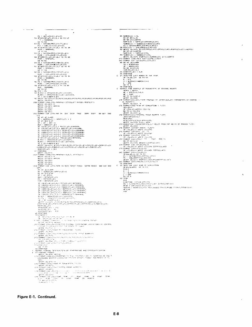
PO:; :: tOo .. -cortr.Jf ttr·,) IffRc)ftf,.JfJ .. GT .. O. J GO TO 51 ~ c:: :: Q'JIJ't}'9.

GD TO SII! ')7 C'So ': <;1'CONf~r5 .'~I !f'.J[' I

PS<' :: 100 ... ),'Sflf.JfllC5 SA 1f IQYIUr(.JE).GT.O.' GO TO S,

P'ST'? ':: ~ .. ,~qq,. '-0 rn ;;p,

1)'3 CS :: SATCONI,.q[S.fIPII(.JE)1 psrR :: l!')I'J.-OOT~fTr.Jf"I/CS

f>8 IFfOIllPCIE.J( ... GT.O.l 1';0 TO 69 P';l\o :: tJflI,III4t __ •

GO fO 'I ~q CS :: ~.lrCO"IPp(S.'ftP(t£.J£)l

P~8" : Inn .. _l"'n~ ur.Jfl/C'S 'H TFfO[Fflr.J(I.fiT.').1 GO Tn q]

PS(I=" ': 'lQQ"}qqo.

GO 1 r I) 1 ~] CS : <j.HCONfOO[S.Tff:'(fr • .JEti

P'ifF ::' If]o •• rH'(f nf.J" JlCS 4;j3 IF (or.! fIr .JF:) .. GT .0.1 GO TO qq

PSG! : ,q ~,qqlllloo GO f n 91)

qq CS : S.Q'{"ONI~[S.TG!(JF'.JfI'

"'5Et : 1''J''1 ... r''G( IT r • ...I'" IICS '15 IFfI'H"1£.Jfl .. r1oor., r;(' TO qf,

PSO - "9q,'3"'~oo GO Tn (H

qfo, PC;O : P5

q 7 Rl ('C2 :: 1i){Hl(\CI IE .Jf' -J()' l:1n. Rl DC t : I~CHl rCI IE. 1. J[' -JE I -1:1~. IC = f£- I ·~~l)r>1( .Jf' I

c;£ wRJTf (6.IJ1IJ[.rC.QlnC.?,RlOC1.p<;r~.p<iS,PS!Q,PSGI.P<'RR.p~Er,PS.PC;O

wf? H( Ib.1Sa) ISO fOPlllll1f (IHl.7?x.'",(\to!THlY nl<;<,OlVrr" 1'\1rYG(N p~orJu'')

wR rTf (F.. II 7) ", wQTTr IS.}t ~I ..,,,,,non wR T f~ If,. 114 I WR IfF If .. II S) \liP Y1' [ I 6, 1~ 1 )

IC;I fOR-,ur (1M .71x, '00 J~ on<, OO[P f')nGt OO~p nOfr 00 OUT 000

I"

Kf : IiilRC"IJrJ - NllprHIJ"') • t DO "It IE I -=1 .Jtr If: 10([ - lEl.1 OG J -: 00(;( (rr. Jf ) IF fO(lf.J"'.l£.O. I 1'I!,)(I£.JEI:9~qqqqq.

If I:1Sllr,Jfl.lF'.O.1 oo~'rf.J(I:Oq~~c)<M.

If !OPHt£.Jrt.lf.IJ.1 OOIlHlf.J(I:')QQQ9-,q. Jf." I"R~(fr,Jr'.L"'.!"J.) nO~~(!('Jf':'lqq'9~.

IF I.,~r( rr.Jfl .lLO.1 nOfF! rr.Jrl=1~qq'3'lq .. Jf ''1r; I f If.",Jf I .l (. o. I nOG! r Tf ,JE'1 :qQ~q'9qq. If {f'lrq Tf:'.Jf) .. l r.~. I ".,01 IE.J(I :q«t0'3qq~. Rl n(,? : IPCIH~CI Jt:' .Jr I-J( I.lnr. RlOCl : (OCHl(\C( If.I .Jll -J£ 1.10 D. Ie : I£-l·~PPCIiI Jf I wPIT" 16.1)7, J(dr. f1!OC2. 0l(lCl,t}('JNtI(.Jfl.nOSIJf.Jn.Dor!;"cIf • ..J[1

1.0nGIf I(.Jf.I.r:OBP( IF.J(I.norfl If.Jf, .f')OII£.Jfl.0':)O(tr.J£J DOEr f 1(. J£ I : Dr.,

4' (ONT YNUE WRI'F ff;.lC)"1

WQ I'''' IF.. IJ -:' I lo4

WI?!ff Ir., 11 HaM"! 1(1 wP If r to.. II ~, wPITF' (J;.ltlil WP lfr 1'::'.1') l)

JS3 F'rH?"''' (tH .2C'x. 'Rl'If] TN '100S ROnt O aOOGI 90nAI? fl.ODff 900 OuT 900

on lie. J( = I. ~AP Kf : "IlR(HCJfl-NoprH'.J[I.l no "r. I" 1:1 ,K'" !f." -: Kf-JrY.l fl.G r -: RcnGlC Je- .Jrl P\ -: q-f!fI~ flr.Jf I

f'I·TJOI =- RO':'P?ITr,Jfl

IF (Qt If .Jf I .. l f. n .. I r:I(\p( IF' .J[ I: q(><'Iq<fqq. TF' (OOCOflf,Jfl.lr.O.1 °OI1')llf.Jrl:-QQQ'l~qq.

T~Ir~IQlrf.J[I.lf.fI.1 °OnJP(Ir.Jfl-:99CJqq~q.

If I QF'RI If ,Jr) .L r. n. I A0'10D( tr. Jr I: q(H~qq'3 '1. IF 11ffIIr.Jrl .. Lf.'1.1 ~OO£:fllr.JfI·qQqq:qq .... Tf" ((Jr, T ( T r. JF' I .. l f ...... ' ~O{'\I". J t rr .. ..I" I: 'v., QQ qa <:I.

t,.. '."1" tY~oo H J. I,r ,r. I '10')/"11 If •. Ill - <'lQQQ qqq.

wG> f' J' t~, .. 11 " I I P '" r~ ~ ~ f ! r • .1f I "RI';f'!l'Iclf.Jrl O"''1(jT(lf.,Jr, cr"'<'I'r.Jfl !l'l I"'~ 0 ( 1 r • ,)f 1 ~ F'

:&f, ("('IHf l~l'f

."""'!'1C rr .Jf' d-lOO<::( IE ,J( J. I r 'Jf I • ~~n"'F ff f. Jf I, ROO f If.J () •

I ...... ·..,r"·.;/)'r •• -:·"!.·- · .. r ""','''' "1" ',Ahl 010 r'f Ie:. .. .,., !' ..

}") ., .... 0 ... II f ( 1~". '" r A D "<::" r 1"4,11 AT 11" '. r? I

;~ I r:"l Plot A,! I 1 HII • 1 ~ , •• r i'" r •• 1") Y •• ("',' :"" l ;->" l N' Nl! ",nr D' ,

WQ TTr f(, ........ 'tl

7r3 fn~.AT ( ·\·.~'t.·~·,'J.·~·.71.·i,·.~\.·<:·,'

I)'" ,,"'c:.

.' .. r" 0"11 ( • I lr.·'. r ).1. "C' II. I'

q I C~&lT r~u1'

': I')U'''ut .... JU"Q"'Ill '" <,1 Dr"'jl!"", or Tr-"PC'O.T'J~f AND l')t~).OLVrn G't'l'r,(~

( ., ro ~fQOt r") IN T\ wP fTr "", t?51 &""('110

1~S f""'O"OItt' (ll-l·'.tll,'rtOrr'fO~: ro"AI ";')'~1"!"'!0~1 ~-: '£,,"Pf;:llTlIOr tt~<::'nt~fO :')'Xyr,r .... ·.'/1C,t.·P r"',T:<",j p ... r .... r·, r"IP["- T",[ "'(''''j'~ )f ' •

., .. ",

1 ;> 1 r'" l"' .. ~, f 1104" • .., ... J •• - ,,~ ,n ("t. PO r ~, 'III) J f r I ~. I? 0 I

\ '1\ "('1""'1' I lH • pr.· ;­-----f r·--·

1"" r"',.. •• f 111.1 .!r.·lr",r t:I~, • r • r .. r

r'" ." t;--

Figure E-1. Continued.

-- --1- -- -- - T : -- -, - ~ - - - - -- ~ I • I

ftc] SUMQOftCI :: o.

00 "'" "'=-1.2'" 00 H LC=IoHCPIS SUMTflCI :: '5UMtflC»'fHP4PClC,HJI ~uHOO(lC' :: ~UKOOILCI.OO')xClC."T)

COS :: S .. lCnNC .... (S.Ol(MPClC.MTII J ~8 P'S"flCI :: lnO ... OOc;.XllC.MTI/C'S 82' Wfttf( 1t>.1~21 MT.cOTfMPllC'''Tl.0n')l(l(",MTI.PS''JClChlt.:l,JtCPTSJ

on "" lC::ltNCP1'5 'SUPtTflCI :: ~U"TflC)/7_ ..

'I] c;.U~OClCI :: SUMOOflC)fl14. wRPf t6.151' t<;UMTflC).~U"OOClC). lC::t,NCPJC:;1

."7 ro~"UT (tHO,'rlf lVG'.5f?F£'.1.7IH

.111 roR1'lu t 1~ .11.5fZff..l,f7.11 I eo 00 8'5 JO=l.HtIIP

10 :: NlRCHfJOI IP = N8PCH f JM 00 " .. 10:IP ,Yn TB'U 10 .JOI =0.0

A' fCe~f(O.JOJ ::' 0 4 0

AS co"'' INUE C 1<; THYS ·THf LA'iT MONf'" Of

IF f K.£O .1') GO TO 'io" 1(:: K-t I :- Nl PC H f 1 J -N 8P C,", ( I ,4o 1

l = N"R GO TO ']

--0 CONT INUf C OUTPUT Tf"f PRortLF or P1RAfoIfffP<; AT (Of.lfROl POINTe:;

rCPTS :: ~CPT<;

foIC : rep TS 12. n *o.~ He :: 2."'1'.: 00 1)1) IG= I.NC. 2 wI? JTf u;. nOI

lW F('IP,",&Tf P"I1e10Y.' TfNF or;.ofll£ or WaT[R OU1LIl"f' PAPAMETER') AT CONTRO • II PO fN1<;' I

WR fTf (6.1311 104 1~1 'OR"'ITflHO.'YrA~ or '5IfoIUlITION : ·.J?I

161: yr..l IF (fGl.GT .. NCP TS I IG 1 -: TG 00 !'S II =Jr., yr.} w~ rT r (F., t~ 2"' II

n:z rnpp.rATIlHooo·rrN,pol oOI~T NUMnrp

JRCH=CPTln(f II J PCH":JI?CI-I Cl OC::( CPTlOC nll -P(H '-Ion. WPlff (Fi, 13 31 nor.. JOCt.f

111 FOP,.UtlH ,'lOCATEO',rs.!,' ~Tl[<; 1'POM THf' MOUIH or f.lRANCH '.!71 WP I' r 16. 13 ~ I

I~q 'OR""f (JHf'}SX' ",(»0.:'14 How'l IF «rV.[r'~.11 \JRJ 'E (kd V""

ItS fOR"'" 11H.}F.r' fC .) If fTY .. fQ.ll w~Ifr fktl~b'

JlF. n'U~"'JT (1j.f4o??X' TriolO " if (lIJ.[1').1I wRITf fl=.ol nl

1 ~ 1 fORfIII.I: f (1,.. •• ?Q r,' ... ,.. 00 C;C; KG::- t, I? wR 11'[ cr::.. I ~ a.) A"O( 1([ J .O(Of III ,1((; I

1 ~A fOP'''' f (1 H ,I)" ,I Ci, f{,. t 1 lr (Jv.(n.11 IJRfH' fJ;ollol [crPfltl,M('j1

l1;q rOQ~'" T f 14.,1 J=... 't. rr::..n J

JF fJY.EI').11 vprTf (j:, 0) lJOI TCPTfll,I(~1

1110 FOQI'II f ('''''_. 77 ... F~. t 1 IF' tJW.N(. 11 G(I f 0 'is C') :' ')ATCON{OPf').T rp T f II .10,) I

PS : tOO •• (')(~('~ l( II .1( [II IC')

wP IT f f6. 14 II ancp T (I.L.I( (,l .p<',I'lCl"lrflT ILL .k', J

141 fOR"t.T lJi-I .. :'RX. (f..T. "'1.1.F 6.11 C:S CONT YNlJf

C l~ THJ~ 'HE l4ST yEAP t'\r Sr~lIlt.fTO~

E-8

IF 1M oo(Q.NYQ) GO TC t'Jl

"'::,..·1 M:' t r :: Nl ~C4( 1 I -to.! qR CI.i t 1'· I l :: N~R

(:.0 fO q

~O c;. f np rNa fUNCTION <::,P(ON {DOdDI pv = ".1)1q. TO. (. l:S 14' r P. f '. l~r J. T P.l. 1 qf - 41 1 pcop : (PP-f'lVI I( H."' .... • ~I/ 1 c;.A fc:n"J : pcnQ. C 1~. (<;? TP. ( ." 11lll- T 1"'. c 7. q'1I0( - 't' -T P. 7.771 qf- ~, I I Rf HIPN

r.o

m cO

'I 1175 1128 2000 2010 1125 lin 1167 1301 11281211

2 2 4500 1 2

1 167 1185 1213 1?2 4 1257 1 270 1301 1 31 9 W13 122412571301

OCT NOV OEf. JAN HIl MARCH APRIL MAY JUNE JULY AUG -170 -120 -110 -100 -100 -100 -100 -100 -100 -100 ~IO 510 .. 80 44" 420 400 400 400 400 400

-100 -100 -100 400 _00 400

160 230 420 530 514 357 227 139 I'll 30n 281 3077 3333 J5~1 3647 3860 3'134 3896 3618 3463 3257 3037

039 083 17'! 235 223 140 067 020 042 088 082 -476 -161 000 03 839 547 -536 -731 -875 -1156 -74 7

128 4530

040 -010

090 OSq 083 049 4717

027 1137

028 037 093 139 167 167 4428

050 4361;

n50 "28 7 1 7

447 0

044 'Ill

7 20 350 n 620 -25 250 105

70 10 - 900 115 1500 -400 10

400 -25

20

'10 90 o 620

250 105 10 - 900

85 1500 -_00 110 115 110 _00 0 600 -25 25[' 105

70 10 - 900 AS 1500 - 4 00

105 110 lin 4no 0 ';5n -75 25n lOS

70 10 - 90n 8<; 1<;00 -400

100100 90 350 0 550 -35 260 105

70 10 -90n II 5 1 c;00 -" 00

1'10 100 85 3<;0 n 500 -'5260 1 DC;

20 10 - '100 85 1500 -40n 75 90 75

7 550

7(1 223(1 15

(1

170 6';0

45 (1

13(1

20 2230 IS 45

I ~ (1 650

Ie;';

?O 223[J 15 4'>

'1 I ~[J 130 b50

20 223(1 15

110 55 r

4<; n

115

?n 2230 15 4<;

n 10'; IHl 650

?O 2no 15 o

4<;

PO

4873 (11b

1706

4796 015

1142

452 'l 029 lib 7

- 1 00 45 a 1 3 (1 70 1800 -400

120 80 5 (1

13 -100

o 45 n

n 70 1800 -40(1

150 120 100

13 - 1 [JO

a 450

(1

70 1800 - 40 0 130 105 80

- 1 00 45 [' 13 n n 70 1800 -4QO

135 70 40

- I 00 4S a 13 (1 (1 70 1800 -40n

125 60 ~o

- I no 45 n 11 70 1800 -4'10

11 5 50 4 n

Figure E-2. Sample WAQUAL data deck.

4287 037 556

3 2 o

45

3 2 a

50

100 100

80

a 30

3 2 a

3D

o 30

105

85

o a o

85

75

4241 047 235

4379 044

-017

a 4 70 3000 -400 70 70

4 70 3000 -'loa

IDS 105,

4 70 3000 - 400

IDS 105

a 4

70 2000 -400 85 85

o 4 701500-400 An 80

4 70 I 500 - 4 00 75 80

SEPT

I'll 3216

046 -4) 9

095 4539 O~ 2 177

300 0 500 650 -~o 280 105 20 223n -110 480

20 10 - 900 15 45 1 3 0 0 85 1500 -400 0 [' 70 1800 -400 65 80 65 RS 110 105 60 30

300 0 500 650 -50 300 105 20 2230

20 10 -900 15 45 "5 ) 5 a 0 - 4 00 0 " 55 65 55 75 100

490 -114 500 650 -50 300 105 20 2230

18 10 -930 15 45 85 1500 -400 0 n 45 55 45 65 '10

2 6 20 7 300 0 500 650 -45 290 105 2n 2230

20 10 - 900 1 5 45 87 1500 -320 n 0 q5 50 50 70 90

810 -246 500 650 -45 290 105 7rJ 2230

-1104an 13 e 0 70 1800 -400 95 55 20

-110 480 13 0 0 70 1800 - 40 0 85 45 30

-110 480 13 0 0 70 1800 -400 85 50 35

-100 480

2 o

30

3 2 o

30

3 2 o

30

35

o 1>5

o o o

50

o o o

40

45

o 4 70 1500 - 4 00 60 6(1

o 4 0 70 1500 -400 50 50

040 70 1500 -400 40 40

4 0 70 1500 -400 45 45

18 10 -10 00 ) 5 45 13 0 0 " 87 1500 -320 0 0 70 1800 -400 0 0 70 1500 -400 40 45 45 65 9n 85 45 30 30 40 40 40

380 10610 15280 83 53 27 20 2304 1809 1449 3838 26 9-1272 86 30-1243

300 H40 12800 83 53 27 20 2304 1809 14~9 3838 15 9-1272 86 1(}-1243

499 396 215 197 2q4 403 417 543 627 729 661 590 100 565 110 78 52 15

100100100100)0010010010010010010010010(1100100100100100100lnOl00100100100 93 9190 a9 88 86 86 86 88 91961011071121171191201181141101051019795

1001001001001001001001001001001001COI001nOl00l00l00100100100100100100100 757065605858 fO 65 901801~52001801601~01l5106100 'l6 93 90 868380

300 466 96 53 144 15 lUOI00100100100100100100100100100100100100100100100100100100100100100100

'13 9190 8'1 88 86 A6 86 AA 91 9610110711211711912011811411010510197 95 1001001001001001001001001001001001001001001001001001001001nOl00100100100 1001001001001001001nOI['0100100100100100100100100100100100100100100100100

103 0 47 0 -1 3818 795 5 31 2

290

17 31 2<; (1

I> ?O 0 5 0 19 o 0 24 I r 4 - I I '1520 6(10 5 0 116 o 17

't'£ A ~ OC ~ 1 1'4 III '1 Ill" "If/NtH Uf Yf aR .0(1

I, ; I,I.J

INPUP··· -- - --J IR Rfl rlw bRANCH H.r

uflR O[r

I--OU TPuTS-I ')TRH 0 Iv Q au T 00

803

"'O~lHLY 0YSSolvrr- OlCYr'i(N PRCFIlf

'ffAR OF' STf1:UlAtIOJl :: 1 MONtH OF' Y[AR -:OC'

lorATI~ BRaNCH R( ACH TO

J- ---- -- ---{NPuT<;- -. - -- - - I C;TQM ",Rfr tl) Q[, Gw BRANCH H+1

00 IN 005 OOIR DOGI OORR rou 30.1 q.q ~.3 13.7 7.7 •••••

(I .• ) I

1'1.1)

11.S •• 1 1.1 .11

.n

.0 1l.9 .n 77 .. 11 3n.1 7.8 8.7 )S.'

'fllC? Of \ '''\'1 1.1 1\1 ...

M()~ I H (\ r '~AW

IiJ..lAN( ~I ~t 'Ct.

,),"" I.',,",

'f f 'C? Of \ I'" I't ,T 1 " ~ "('1111 'H Of Yr 'k

,),01

I'.' I."

,fA\.? fir (,t"fUlA'!'" j'qINlr\ ,., yr AI) rr I

I.·.· I:.' I."

,. <

, I

, ~. t f • I • ( I .. I ( • \

.0 Iii.!

.0 .[1

lO.!' .0 • 0

• [I .n 10.n .J .n.n

PROf Il f

INPuf ~ .. - --I 1° "'I I hw AR ANfli !of. r

12.9 .0 22.' 2S.0

.0 S7." .0 SI.D In .. 4 63. t .n 71.1.8 .n 79.0 ;?~. 7

I --OUTPUT'S- r C)TRM 0 tv

'2':'. 7 ~n.:J

27." 25. 7

?l.J 22'." J S. 'l , 1 • ~ If .. 7 Ip. S J2.F. 11=..'" 12'.S 12.Q I. r ). ~

1.0

YfA R OF' 'S tMUl A r to"! MONTH or YEAR ::OCI

BRANCI-I Pf lCH

q.3 9 .. 7 °.1 Q.2

P.O

<.8 7.8· .. ••• •• 0

q.I'

7.7 1.7 9.7 1.2

1.' 1.' 7.4 7.8

7 .. 1····· MO~T '"+l Y ~.r. '1. PQor {lE

1- ---- -- ---If..lP:JT<;--- ---- - --I C;TP'" <i~rr l~ I~(T Ijw BRANCli 'HI

"It-I !ClIl rCAI? (CEf Fe OUT (CO ~I)O ,,~ 11 "'0<; ~('IOIQ t=lor~Gl eoo~r,> POCO

'I j .;\

il.l

I.' I.

I.; ,

'''\

, ., 11.1

, , II.',

I.J.'

t·"

f,')D. ••••• 5b 5.

150 •••••• 24A •••••• 2f':," • ••••• ",1.10. 3qn. 1')7 •••••• 421 ...... . 190.. l~n. ;?71 ••••••

3S6 ••••• ,

INAIII(·-·--:·---f I--OUTPur<;-I r.w rlP A~fH H" t <;1 UI1 01 V 'r, 1 'R~ T (r T OU T T fI

11.1 11.3 11.' Ir..n 11.' 1 1 .. ~

11.1 11. 1

11.' 11.0

t Nrt LIT ~, .• -- -- - -- I

':1 .. 6·'··· 10.0 ••••• IrJ.n ••••• 1'1.r: 1".'1 11.1····'

lI.S II • ~ to.!' 10.0

1- -OU l,:ou1<'-1

n .. t'l l.i) 1.11 .n 3r.1 .7 I.f ."

71 • .,. ~7. tI

1 q. r. 71 • ~ IR .. 5

12. 0

12.5 I:'.Q

I.'

Y(AR rtF' S I"IJUta, TI)N:: I

CON1RCtL Pr"J!NT ~lJM!!IrQ 1

l.f. .1 I.r. .J I.J

.q 1.:::' ."'1 7.'1 I'i." 1."

I." 7.1 1.3 1.3

• 1 .1

LOClf(O 12.') "'lLr~ FqOM l'jr ~OUTH 0f nOANCI4 1

~Ct~ll-i rLOw r r OCT '1'1. 11 • ~ NOV 141'). 7.6 <J.fl Of C 71:. Allin. ?] 1 '1. ~

JAN 1f:.. S pC!.. 1.2' 11.7 rEB CJn.7 I 'jD. '>.Z lao s ~aQCI.f 71. I ]1;2. C).q q."I

APPIL 131.} f.l. 7.1 10 .. 0 I'tA Y t 60. 7 71 .. 11.1.1 a.6 JUNf 1 ]".r. I":.) 7.3 JUl" 1f1.! 1.101. 1°.!; 7.<-AUG t',~. 3 "54. 7.e

f;R.' ')'lS. 1t:.1) 7.2

CONJP"L POINT ~JU"'Q.Q ? lOCATfO 12.8 foIIlEoc, F'PO"" THr ~()uTI.i Or

~ONIH FLO,. rc H'fP

POD 2.0 2. ~ 2.'

q q.f. 3.", q 7. I I.S

2.5 q 7.7 3.7 go.n 2'.f' P7.CJ 2.1

111 '/11 (,101 J..\Q ANCH "" .. r <dRI1 uIV OC T 6 ~. J 2'1. 11.S 7.il 1.< 2.1 2.5 7.7

'.r 2.5 3.1 ?r. 2.1 1.7 1.1

fl"'

·11 II I."

1 1'1.(,

11.10 ,".f

I"'." P 1 ...... 1,

<l In.Q l' 11.4

" L' 1 .... '1

Il 1' .. 1 14 Il.4 1"- ll.b lj:;, Il."

ILl 1 il l'.o. Iq 1.'.0 7r 11." .?1 }1.11 II '1 .. 7

1'1,':'

lVG

P<'R:? PC;[F p,\ Ouf P';!" NOV !;Z.8 F)'i. 7. J '9.!J 77.7.· ••••••• , OfC f,".? ~I}. 1.S 1:1.Q 71.7 .......... . JA~ f':,Q.1 101'). 11.4 77.7 .......... . r(Po 7R .. ? 7L '>.2 In.7

",)11

77.1:.

<:1.4 g1.1 'L1 In].7 '=t." IQ"'t.? q,C) l"n.O; q_l tl(.'

:I.. 'i ~ 0;.7 7.M. 07.0;

7.' 7j:;,.R 6.il 1?1J.

1'1.1 Hi. II

f..Q 17.--a: 7.1

qs.) QS.I 97.Q ••••• 8h.7 ••••• f;<J.l fq.)

(')"Jlrol'l "('lpn >.jUMlllR

t-tAQCH C)'). q If, I.

APRfl 120.7 I J\. ,... Y J 'in. 4 ~4.

JUf..I( ) Z".6 'tlf, •

AuG lin. 7. 77F.. Sf;.'\ lq7.

".3 la.3 1;.9 10.7

ttl.3 17. q 1. ~

7.1 lA.4 1.r. 1 S .. ~ 7. I

I· ·---·--7---····1 I·-··----J·-·--I 1--------"-----·-1 I···--"-S-' •• - •. I Tr",p :)0 P<:'Al T£toIp PO P';AJ TfMP nQ P,)AT HHP no P';AT

1.7 II. ~ 91. ') q.? '1.3 C:j5. '3 9.8 J\Z. '9 '\ 1.1 '1.7 A. q 92.3 g.) q.1.I q1. n Q,l.'

In.f. 7.7 -'31.c;. 'J.O ~.1 Q3.4 ct.n q.S qr.1 7.0 'U.q tn.l) 7 .. 7 .q1.3 ti.1 9.) 131.1.1 'i.CJ q.S 'n.~ 7.9 82.CI 10.5 7.f, d. q q. I 9i1. iI 8.8 q7. A q .. ~ 7.1 ql.q 1~\.1) ~,n.iI 8.1 q.t 94.7 8 .. 7 q.~ '97.7 9.8 7.9 81.q 1Cl. ') '. 0.1 8. F. '3~.0 P. 7 '37.q q. ~ ill. 9 1'1.7 7.7 qc;. e Po. 8 9~. 7 ~. 8 7. q fll. '9 II. I 7. f'j ~".. 2 9. iI '97.0 9.n 1 no. c 9.8 7. <.J ~l. '3 I J, b q 7.? 1.' 9. '5 3A.Q 13 •. l q.R 101.1 Q .. A 82.13 12 • .' 'In.,, 9 .. 1 q.8 ) 01. 1 9.8 1'1.0 1::1 5. 4 q.8 7.q A2.q IZ.~ qJ..? IO.~ lO.n )G~.'" 1".11 I"'.) If)I.I.1 9.A 7.9 QZ.9 I 3. 3 "J .!"'1 '3 II. 9 1 n • II 1 o. 1 1 os • '2 1 n • q In. 2 105. 0 9. A 7 • q 81.9 tLE, ~.D 15.0 ll.~ Ie.? lC6.C J).iI 1"1.1 10".Z 9 .. R 7.q IIIZ.9 1'1:. 7 a • fI q ~. q 1 1 • 7 In .. 1 1 0" .. 1 11. A 13 .. q 10"2. Cj q. 8 7 .. q ~1 .. 9 13.e. 'I.e. qO.3 11.9 9 .. 8 101.1t 12.0 100.1 q.8 7.q '12.9 I '.0 a.l eG .. 2 J I.q 9R.) 11.q 97.4 q.A 7.q 131.13 l~'.S ~?n 94.9 11.1 'iI.S '1.8 7.9 82.9

7.LI 78.3 R.q 9Z.l 11.3 ~ .. !""I '1Z.II q.~ A1.'1 7 .. 7 lO.C! 8.9 '0.9 In.A e.9 91.4 '1.8 7.0 R2.13

Jr •• Q 7.1 I u.S 10.3 130.9 9.e 7 .. '3 Bl.' Ir:. ') 1.1 7 S_ I I 'l. 1 R. fi q.q 91.':' 9. II. 7.<:1 Q2.9 lr..~ 7f.'oO'5 ~.1 f.I.6 Rq.1I 9.6 92.7 9.8 1.'9 "2.11J H'." 7R .. 3 9.5 8.7 ':JO.t 9.3 ·:h.3 C) .. 8 7.9 82.'

IO .. r

Figure E·3. Sample WAQUAL output.

E·10

r --Ou TPUT~- I SIRH 0 Iv 00 OUT 0"0

7.q ••••• 9 .. 5 •• • ••

" .. 5··'·· 9 .. 3 q.!

7.13 •••••

9.1

I--OUTPuT')- I <;TR"t or'll

~oo our BOOD

1.0 .9····· 7.7·,···

1.1i ••• , • 1.0 ••••• ).!

Table E-3. WAQUAL simulation model data deck set-up.

Card Col Format Variable Name Definition Remarks

1-5 15 I\lBR No. of branches in the system not more than 5 6-10 15 I\lYR No. of years to be simulated

11-15 15 I\lCPTS No. of control points designated not more than 5 16-20 15 NRES No. of reservoirs not more than 5 21-25 15 NEF No. of M & I effluent discharges not more than 5 26-30 15 ALT Mean altitude of the hydrologic system 31-35 15 IV Conductivity model option indicator 0= No; 1 = Yes 36-40 15 IW Monthly D.O. model option indicator 0= No; 1 = Yes 41-45 15 IX Diurnal D.O. model option indicator 0= No; 1 = Yes 46-50 15 IY Monthly water temperature model option

indicator 0= No; 1 = Yes 51-55 15 IZ Diurnal water temperature model option

indicator 0= No; 1 = Yes

2 1-4 14 NBRCH(J) No. of beginning reach on branch " J" 5-8 14 NLRCH(J) 1\10. of last reach on branch "J" repeat for J=1

through NB R on th is a ne card

9-12 14 NTRCH(J) No. of main stem reach to which branch "J" is tributary (0 for J=1)

3 1-80 15F5.3 RCLOC(I,J) Location of downstream end of reach All reaches on "I" and upstream end of uppermost one branch on one reach card: As many cards

as there are branches

4 1-25 5F5.3 CPTLOC(IC) Location of control points "IC" a IC=1 to NCPTS

5 1-25 5F5.3 RESLOC(I R) Location of reservoir "I R" a IR=1 to NRES; Omits of NRES=O

6 1-25 5F5.3 EFLOC(IE) Location of effluent discharge IE=l to NEF point "E" a

7 1-72 12A6 AMO(K) Abbreviation of month no. "K" K=l to 12

8 1-80 16F5.l ATEO(I,J,l ) Equilibrium temperature constant one pair for both ends of every reach. One set of cards for each branch. Omit if IY=O

9 1-80 16F5.3 ATEO(I,J,2) Equi I ibriu m temperature coefficient

10 1-72 12F6.3 AD(K,l )

11 1-72 12F6.3 AD(K,2) Diurnal temperature index model omit 10-13 if IZ=O

12 1-72 12F6.3 AD(K,3) parameter for each month

13 1-72 12F6.3 AD(K,4)

E-11

Table E-3. Continued.

Card Col Format Variable Name Definition Remarks

14 1-72 12F6.3 ADO(K,1)

15 1-72 12F6.3 ADO(K,2) Diurnal dissolved oxygen index model omit 14-16 if IX=O

16 1-72 12F6.3 ADO(K,3) parameters for each month

17 1-72 12F6.3 ADO(K,4)

18 1-5 F5.1 RH(J) Mean depth multiplier b

6-10 F5.1 PH(J) Mean depth exponent 11-15 F5.1 RA(J) Area of flow section mu Itiplier 16-20 F5.1 PA(J) Area of flow section exponent

19 1-5 F5.0 AECS(I,J,1) Surface inflow conductivity constant b

6-10 F5.3 AECS(I,J,2) Surface inflow conductivity exponent 11-15 F5.0 AECGI(I,J) Groundwater conductivity (f.l mhos/cm) 16-20 F5.0 A E C I R (I ,J, 1 ) Mean annual irrigation flow conductance 21-25 F5.0 A Eel R ( I ,J, 2) First term irrig. return flow

conductivity coefficient omit 19 if IV=O

26-35 F10.8 AECI R (I,J,3) First term irrig. return flow conductivity phase shift

36-40 F5.0 A E C I R ( I ,J ,4) Second term irrig. return flow conductivity coefficient

41-50 F10.8 AECI R(I,J,5) Second term irrig. return flow conductivity phase shift

20 1-5 F5.1 ATS(I,J,1) Surface inflow temperature constant b

6-10 F5.3 ATS(I,J,2) Surface inflow temperature coefficient 11-15 F5.1 ATG I(I,J, 1) Groundwater temperature constant 16-20 F5.1 ATGI(I,J,2) Groundwater temperature coefficient 21-30 F10.8 ATGI(I,J,3) Groundwater temperature phase shift omit 20 if IY=O

31-35 F5.1 A T I R ( I ,J , 1) Irrigation return flow temperature constant

36-40 F5.3 ATI R(I,J,2) Irrigation return flow temperature coefficient

41-45 F5.1 R K(I,J) Heat exchange coefficient multiplier 46-50 F5.1 PK(I,J) Heat exchange coefficient exponent

21 1-5 F5.1 ABODS(I,J,l ) Surface inflow mean annual ultimate BOD b

6-10 F5.1 ABODS(I,J,2) Surface inflow ultimate BOD coefficient 11-15 F5.3 ABODS(I,J,3) Surface inflow ultimate BOD phase shift 16-20 F5.2 R1S(I,J) Surface inflow deoxygenation rate

constant (base 10) 21-25 F5.1 BODIR(I,J) Irrigation return flow ultimate BOD 26-30 F5.2 R1IR(I,J) Irrigation return flow deoxygenation

rate constant (base 10) 31-35 F5.1 BODG 1(1 ,J) Groundwater ultimate BOD omit 21 if IW=O

36-40 F5.2 R1GI(I,J) Groundwater deoxygenation rate constant (base 10)

41-45 F5.2 R 1 B(I,J) Deoxygenation rate decrement (base 10)

46-50 F5.2 RP(I,J) Scour rate constant 51-55 F5.2 R3(I,J) Deposition rate constant for organics 56-60 F5.2 RR(I,J) Difference between lab and river

deoxygenation rate constants (base 10)

E-12

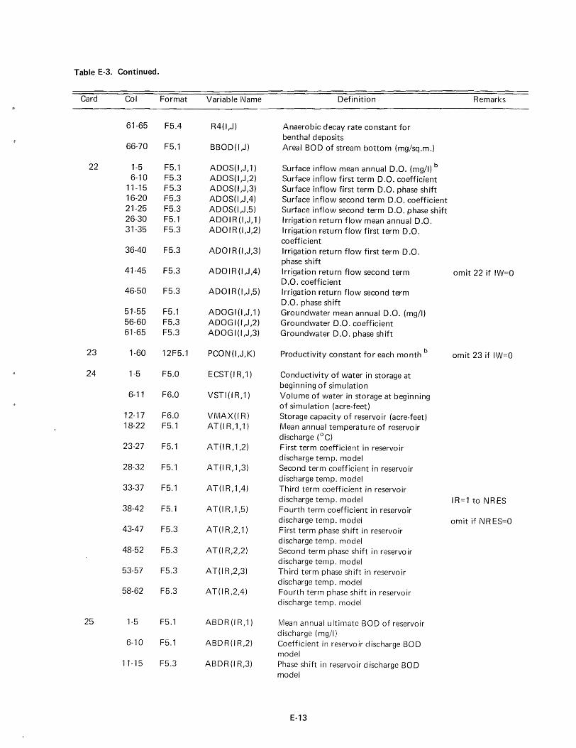
Table E-3. Continued.

Card Col Format Variable I\lame Definition Remarks

61-65 F5.4 R4(I,J) Anaerobic decay rate constant for benthal deposits

66-70 F5.1 BBOD(I,J) Areal BOD of stream bottom (mg/sq.m.)

22 1-5 F5.1 ADOS(I,J,l) Surface inflow mean annual D.O. (mg/l) b

6-10 F5.3 ADOS(I,J,2) Surface inflow first term D.O. coefficient 11-15 F5.3 ADOS(I,J,3) Surface inflow first term D.O. phase shift 16-20 F5.3 ADOS(I,J,4) Surface inflow second term D.O. coefficient 21-25 F5.3 ADOS(I,J,5 ) Surface inflow second term D.O. phase shift 26-30 F5.1 ADOIR(I,J,l) Irrigation return flow mean annual D.O. 31-35 F5.3 ADOIR(I,J,2} Irrigation return flow first term D.O.

coefficient 36-40 F5.3 ADOIR(I,J,3} Irrigation return flow first term D.O.

phase shift 41-45 F5.3 ADOIR(I,J,4} Irrigation return flow second term omit 22 if IW=O

D.O. coefficient 46-50 F5.3 ADOIR(I,J,5} Irrigation return flow second term

D.O. phase shift 51-55 F5.1 ADOGI(I,J,l} Groundwater mean annual D.O. (mg/I) 56-60 F5.3 ADOGI(I,J,2} Groundwater D.O. coefficient 61-65 F5.3 ADOGI(I,J,3) Groundwater D.O. phase shift

23 1-60 12F5.1 PCON(I,J,K) Productivity constant for each month b omit 23 if IW=O

24 1-5 F5.0 ECST(I R, 1} Conductivity of water in storage at beginning of simulation

6-11 F6.0 VSTI(I R, 1} Volume of water in storage at beginning of simulation (acre-feet)

12-17 F6.0 VMAX(IR) Storage capacity of reservo ir (acre-feet) 18-22 F5.1 AT(IR,l,l) Mean annual temperature of reservoir

discharge (OC) 23-27 F5.1 AT(I R, 1 ,2} First term coefficient in reservoir

discharge temp. model 28-32 F5.1 AT(IR,1,3) Second term coefficient in reservoir

discharge temp. model 33-37 F5.1 AT(IR,l,4) Third term coefficient in reservoir

discharge temp. model IR=l to NRES 38-42 F5.1 AT(IR,1,5) Fourth term coefficient in reservoir

discharge temp. model omit if NR ES=O 43-47 F5.3 AT(IR,2,1) First term phase shift in reservoir

discharge temp. model 48-52 F5.3 AT(I R,2,2} Second term phase shift in reservoir

discharge temp. model 53-57 F5.3 AT(IR,2,3} Third term phase shift in reservoir

discharge temp. model 58-62 F5.3 AT(IR,2,4} Fourth term phase shift in reservoir

discharge temp. model

25 1-5 F5.1 ABDR(IR,l) Mean annual ultimate BOD of reservoir discharge (mg/I)

6-10 F5.1 ABDR(IR,2) Coefficient in reservoir discharge BOD model

11-15 F5.3 ABDR(I R,3) Phase shih in reservoir discharge BOD model

E-13

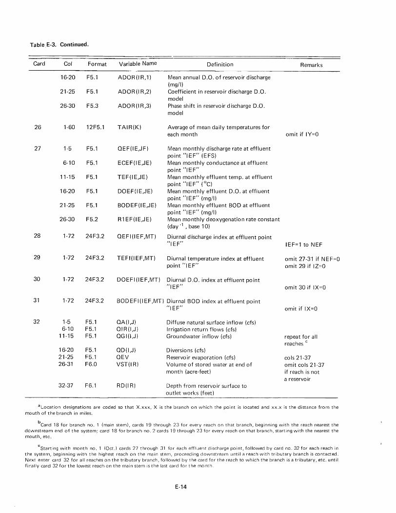
Table.E-3. Continued.

Card Col Format

16-20 F5.1

21-25 F5.1

26-30 F5.3

26 1-60 12F5.1

27 1-5 F5.1

6-10 F5.1

11-15 F5.1

16-20 F5.1

21-25 F5.1

26-30 F5.2

28 1-72 24F3.2

29 1-72 24F3.2

30 1-72 24F3.2

31 1-72 24F3.2

32 1-5 F5.1 6-10 F5.1

11-15 F5.1

16-20 F5.1 21-25 F5.1 26-31 F6.0

32-37 F6.1

Variable Name

ADOR(lR,1)

ADOR(IR,2)

ADOR(IR,3)

TAIR(K)

OEF(IE,JF)

ECEF(I E,JE)

TEF(IE,JE)

DOEF(I E,JE)

BODEF(I E,JE)

WI EF(lE,JE)

OEFI(IEF,MT)

TEFI(IEF,MT)

DOEF I (I E F ,MT)

BODEFI(IEF,MT)

OA(I,J) OIR(I,J) OGI(I,J)

OD(I,J) OEV VST(IR)

RD(IR)

Definition

Mean annual D.O. of reservoir discharge (mg/I) Coefficient in reservoir discharge D.O. model Phase sh ift in reservo ir discharge D.O. model

Average of mean daily temperatures for each month

Mean monthly discharge rate at effluent point "IEF" (EFS) lVIean monthly conductance at effluent po int "1 E F" Mean monthly effluent temp. at effluent point "1 E F" (DC) lVIean monthly effluent D.O. at effluent point "1 E F" (mg/I) Mean monthly effluent BOD at effluent point "1 E F" (mg/I) Mean monthly deoxygenation rate constant (day -1 , base 10)

Diurnal discharge index at effluent point "IEF"

Diurnal temperature index at effluent point "1 EF"

Diurnal D.O. index at effluent point "1 EF"

Diurnal BOD index at effluent point "1 EF"

Diffuse natural surface inflow (cfs) Irrigation return flows (cfs) Groundwater inflow (cfs)

Diversions (cfs) Reservoir evaporation (cfs) Volume of stored water at end of month (acre-feet)

Depth from reservoir surface to outlet works (feet)

Remarks

omit if IY=O

IEF=1 to NEF

omit 27 -31 if I\J E F=O omit 29 if I Z=O

omit 30 if IX=O

omit if IX=O

repeat for all reaches C

cols 21-37 omit cols 21-37 if reach is not a reservoir

aLocation designations are coded so that X.xxx, X is the branch on which the point is located and xx.x is the distance from the mouth of the branch in miles.

beard 18 for branch no. 1 (main stem), cards 19 through 23 for every reach on that branch, beginning with the reach nearest the downstream end of the system; card 18 for branch no. 2 cards 19 through 23 for every reach on that branch, starting with the nearest the mouth, etc.

"Starting with month no. 1 (Oct.) cards 27 through 31 for each effluent discharge point, followed by card no. 32 for each reach in the system, beginning with the highest reach on the main stem, proceeding downstream until a reach with tributary branch is contacted. Next enter card 32 for all reaches on the tributary branch, followed by the card for the reach to which the branch is a tributary, etc. until finally card 32 for the lowest reach on the main stem is the last card for the month.

E-14

APPENDIX F

COMPARISOI\l OF OBSERVED AND SIMULATED 1968 WATER QUALITY PROFILES

';) 600 0 .c E 500 ~ CI

~ 400

~ U :::J 300

't:J c: 0 u 200

c u "- 100 +-u Q)

LlJ 0 31.9

~ 600 IJl o .c E 500 ~

Q)

~ 400 c +­(.)

::I 300 't:J c: o () 200

C (.)

.... 100 (.)

4l

30.1

(a) OCTOBER 1967

1.0 0

~ 1.3

Distance from mouth

It. Monthly average of observed E. C

_ Simulated E. C.

of Branch No.2 (miles)

27.0 2S.7 24.6 22.4 21.3 185 16.7 15.2 12.5 12.8

Distance From River Mouth (miles)

1.0 0

~ 1.3

(b) NOVEMBER 1967

It. Monthly average of observed E. C.

Simulated E. C. Distance from mouth

of Branch No.2 (miles)

LlJ O~ __ L-____ -L~ __ L-__ -L_L ____ _L __ _L __ ~ __ ~~

E u

....... ."

~600 E 3-50 cv u c 2 400

u :::I

-g 300 0 U

20 0 u

''::: 100

(.)

cv W 0

31.9 30.1 27.0 25.724.6 22.4 21.3 18.5 16.7 15.2

Distance From River Mouth (Miles).

12.5 12.8

31.9 30.1

1.0 0

~ 1.3

(c) DECEMBER 1967

It. Monthly average of observed E. C.

-- Simulated E C.

Distance from mouth of Branch No.2 (miles)

27.0 25724.6 22.4 21.3 18.S 16.7 15.2

Distance From River Mouth (miles)

12.S

12.8

E (J

....... III o ..c. 600 E ~. Q) SOO (J

c ~ 400 (J

;:J -0

~ 300 u

"0 200 (J

!: 100 (J

Q)

1.0 0

jH 1.3

(d) JANUARY 1968

Monthly average of observed E. C.

-- Simu lated E.C.

Distance from mouth of Branch No.2 (miles)

w OL---L-----~_L~ ____ L_~ ____ L_ __ L__L ____ +L-

E (J

-;;'600 o

..c. E 3-soo

Q)

~400 ~ (.)

;:J 300 -0 C o

U 20

c (J

.;: 100

U

31.9 30.1 27.0 2S.7 24.6 22.4 21.3 18.S 16.7 IS.2

Distance From River Mouth (miles)

1.0 0

~ 1.3

( e) FEBRUARY 1968

Monthly average observed E.C.

Simulated E.C.

Distance from mouth of Branch No.2 (miles)

12.S

12.8

~ w OL---L-____ ~~ __ L_ __ _L~ ____ ~ __ _L __ ~ ____ ~

E ~ tI)

o

E600

~ Gl 500 (J

c o 7)400 :::I -0

~30 u

"0 200 (J

~ 100 Q)

W

3/.9 30.1 27.0 25.7 24.6 22.4 21.3 18.5 16.7 15.2

Distance From River Mouth (miles)

(f) MARCH 1968

12.5 12.8

1.0 0

jH Monthly average ·of

observed E. C.

--- Simulated E.C. 1.3 Distance from mouth

of Branch No.2 (miles) OL---L------L~--L_ __ _L~ ____ ~ __ ~ __ ~ ____ P_-

31.9 30.1 27.0 25.724.6 22.4 21.3 18.5 16.7 15.2

Distance From River Mouth (miles)

2.5 12.8

Figure F-1. Comparison of observed and simulated 1968 electrical conductance profiles.

F-1

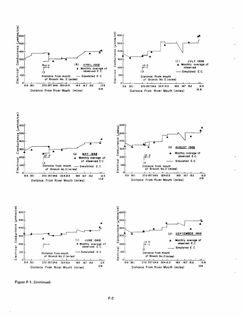
E ~ UI

~SOO E 3 500

Q)

u c: 0400 -u :::I

~300 o U

o u

200

~ 100 u ~

(Q) APRIL 1968 A Monthly averaQe of

observed E. C.

Distance from mouth - Simulated E. C. of Branch No. 2. (miles)

W O~~~----~~--~ __ ~~ ____ ~ __ ~ __ ~ ____ u--

E ~ UI o eSoo

~ Q)5oo u c: o -400 u :::I

1:1

~300 U

-200 o u

.!: 100 u t)

31.9 30.1 27.0 25.7 24.S 22.4 21.3 18.5 IS.7 152

Distance From River MQuth (miles)

12.5 12.8

~ 1.3

(h) MAY 1968 A Monthly average of

of observed E. C.

Distance from mouth - Simulated E. C. of Branch No. 2. (miles)

W O~ __ L-____ -L~ __ ~ __ -L~ ____ ~ __ ~ __ ~ ____ ~

E u ~ 600 o

.s::

E 500 3-.. ~ 400 o -u .; 300 c:: o u

o u

200

!: 100 u ..

31.9 30.1 27.0 25.724.6 2214 21.3 18.5 15.7 152 12.5 12.8

Distance From River Mouth (miles)

(I) JUNE 1968 j Monthly average of

observed E. C.

Distance from mouth - Simulated E. C. of Branch No. 2. (mi les)

W O ____ L-____ -L~ __ L_ __ _L~ ____ ~ __ ~ __ ~ ____ ~_

31.9 30.1 27.0 25.724.6 22421.3 18.5 15.7 152

Distance From River Mouth (miles)

Figure F-1. Continued.

12.5 12.8

F-2

]600 "­III o

.t:: E 500 ~

~ 400 c:: o U ::J 300

"0 c:: o u 200 c u

U QI

W

100

1.00

~ 1.3

Distance From mouth

0) JULY 1968 A Monthly average of

observed

- Simulated E.C.

of Branch No. 2. (miles)

31.9 30./ 27.025.724.5 22.4 21.3 18.5 16.7 15.2 12.5 12.8

~soo III o

.s:: E500 ~ QI

~400 ~ u ~300 c:: o u

o u

200

E 100 u ..

Distance From River Mouth (miles)

(k) AUGUST 1968

~ 1.3 Distance from mouth

Monthly average of observed E. C.

Simulated E.C.

of Branch No. 2. (miles) W O~ __ L-____ -L~ __ L-__ ~~ ____ ~ __ -L __ ~ ____ U--

E u ~600 o

.s:: E 500 ~ .. g400 o u ::J300

"0 c:: o u

o u

200

.;: 100

u QI

31.9 30.1 27.0 25.724.6 2214 21.3 18.5 16.7 15.2

Distance From River Mouth (miles)

•

12.5 12.8

U) SEPTEMBER 1968

If • Monthly average of

observed E. C.

__ Simulated E. C.

Distance from mouth of Branch No. 2. (miles)

W OL-__ L-____ ~~ __ ~ __ _L_L ____ _L __ ~ __ ~ __ ~u__

31.9 30.1 27.0 25.724.6 22.421.3 18.5 16.7 15.2

Distance From River Mouth (miles)

12.5

12.8

16

14

U 12 o

6

... 4 ! ~ 2

~ 1.3

Distance from mouth of Branch No.2 (miles)

(a) OCTOBER 1117

• Monthly avera .. of observed teMperature

- Simulated te".,.rature

OL_ __ L_ ____ ~~~~ __ ~_L ____ _L __ _L __ L_ __ ~

31.9 30.1 27.0 25724.6 22.4 21.3 18.5 16.7 15.2 12..5

16

14

~ 12

~ 10 ::s

~ 8 II)

Co E 6 II)

I-

41 4 ..-0

~ 2

Distance From River Mouth (miles) 12.1

• (b) NOVEMBER 1117

• Monthly average of observed temperature

Distance from mouth - Simulated temperature of Branch No.2 (miles)

31.9 30.1 27.0 25.7 24.6 22;4 21.3 18.5 16.7 15.2 12.5 12.8

14

U !.. 12 CI) ...

10 Z ~ lID 8 Q.

e lID .... ... ! 0 ~

0 31.1

Distance From River Mouth (miles)

30.1

1.0 0

~ 1.3

(c) DECEMBER 1967

'" Monthly overage of observed temperature

- Simulated temperature

Distance from mouth of Branch No.2 (miles)

27.0 25.724.6 22.421.3 18.5 16.7 15.2

Distance From River Mouth (miles)

12.5

12.8

14 (d) JANUA RY 1968

U L 12

• Monthly average of observed temperature

- Simulated temperature lID ... ~ 10 o

~ ... • Q.

e ~ ... • '0

• 1.3 • DI.tance from mouth

of Branch No.2 (miles)

~ 2

U ~

~ ::::I -~ Q)

0-E Q)

I-

.... ~ 0

~

U 0

Q) .... ::::I

~ Q)

a. E ~ .... ~ 0

~

U !..

~ ~

f {!.

~

! ., ~

0~--~----~~~~ __ ~~~ ____ J-__ -L __ L-__ -1~

14

12

10

8

14

12

2

0

31.1 30.1 27.0 25.7 24.6 22.4 21.3 12.5 12.8 Distance From River Mouth (mi les)

•

( e)

1.00

~ 1.3

Distance from mouth of Branch No.2 (miles)

FEBRUARY 1968

Monthly overage of observed temperature

Simul ated temperature

3/.9 30.1 27.0 25.724.6 22.421.3 18.5 16.7 15.2 12.5 12.8 Distance From River Mouth (miles)

• 1.00 •• ~

1.3

(f) MARCH 1968

• Monthly average of observed temperature

- Simulated temperature

Distance from mouth of Branch No.2 (mi les)

319 30.1 27.0 25.7 24.6 22.421.3 18.5 16.7 15.2 12.5 12.8

14

12

10

• • 4

2

Distance From Ri ver Mouth (miles)

1.00 ~

1.3

(g) APRIL 1968

" Monthly average of observed temperature

-- Simulated temperature

Distance from mouth of Branch No.2 (miles)

0~_L-___ -L~ __ L-_~-L ___ ~_~_4-_~U-

31.1 30.1 27.0 25.7 24.6 22.4 21.3 18.5 16.7 15.2

Distance From River Mouth (miles)

12.5 12.8

Figure F-2. Comrlarison of observed and simulated 1968 stream temperature profiles.

F-3

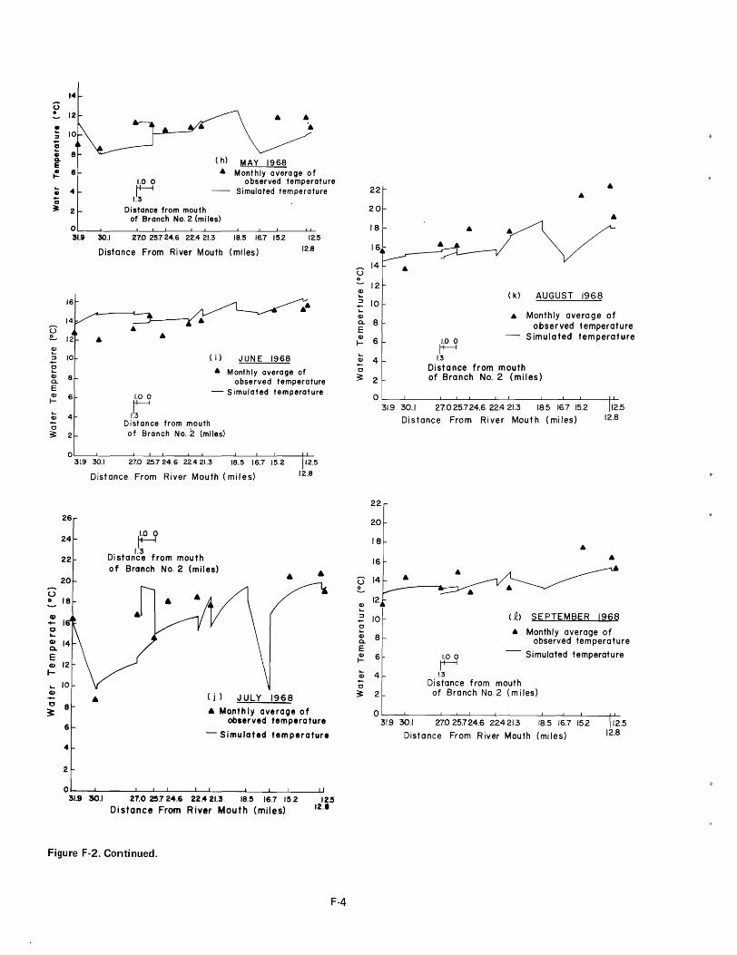
" . ~ ::I -~ • Q.

E {!. ... • -0

!t

U ~

~ ~ ~ Q)

0. E Q)

I-

.... Q)

c ~

u o

CD -c .... CD a. E CD t-

.... CD ..-

14

4

2

0 31.i

16

14

12

10

8

6

4

2

0 31.9

26

24

22

20

1.0 0

I~ Distance from mouth

• • • (h) MAY 1968 • Monthly average of

observed temperature Simulated temperature

of Branch No.2 (miles)

30.1 27.0 251 24.6 22.4 21.3 18.5 16.7 15.2 12.5

12.8 Distance From River Moutb (miles)

• • •

( i) JUNE 1968

• Monthly average of observed temperature

1.00 - Simulated temperature

Ir Distance from mouth of Branch No.2 (miles)

30.1 27.0 25.724.6 22.421.3 18.5 16.7 15.2 12.5

Distance From River Mouth (miles) 12.8

~ Distanlc~ from mouth of Branch No.2 (miles) • •

(j) JULY 1968 c 8 ~

• • Month Iy average of

observed temperature 6

- Simulated temperature

4

2

o~-~----~~_L-_~~ ____ ~_~~L-_-U 31.9 30.1 27.0 25.724.6 22.421.3 18.5 16.7 15.2 12.5

Distance From River Mouth (miles) 12.'

Figure F-2. Continued.

F-4

22[ • •

20

• 18 • 16

U 14 •

~ 12 ~ ( k) AUGUST 1968 :::I 10 -.... Monthly average of Q) • 0. 8 observed temperature E Q)

6 ~

Simulated temperature I-

.... Q) 4 1.3

c Distance from mouth ~ 2 of Branch No.2 (miles)

0 31.9 30.1 21025.7 24.6 22.4 21.3 18.5 16.7 15.2 12.5

Distance From River Mouth (miles) 12.8

22

20

18 • 16 •

U 14 • • ~ • 12 Q) .... :::I 10 ( .Q) SEPTEMBER 19fH3 ~ • Monthly average of Q) 8 0. observed temperature E

- Simulated temperature Q) 6 1.00 I- r .... Q) 4 1.3

c Distance from mouth ~ 2 of Branch No.2 (m i les)

0 31.9 30.1 2:7.025.724.6 22.421.3 18.5 16.7 152 12.5

Distance From River Mouth (miles) 12.8

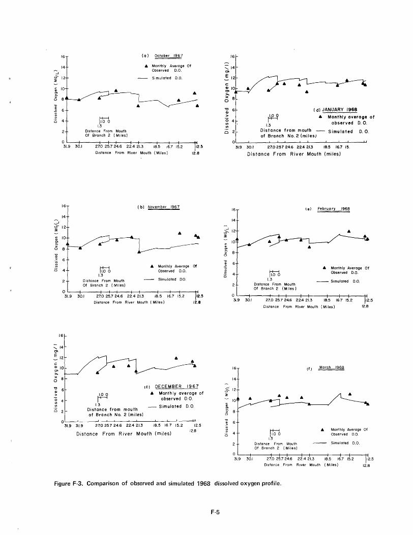
16

14

":J ~ ::l!

12

c:: 10 ... '" >. ><

8 0

~ 6

~ 0 4

2

0 31.9

16

14 ":J ci-- 12 :::l!

c:: 10 ... ~ 0 8 "C

'" :> 6

~ Ci 4

2

0 31.9

16

:::: 14 01

.: 12

c Q) 10 0> >-o 8

" 6 Q)

> "0 4 VI VI

0 2

0 31.9

30.1

(a) October 1967

titi 1.3

Distance From Mouth Of Branch 2 (Miles)

27.0 25.724.6 22.4 21.3

A Monthly Averoge Of Observed D.O.

Simuloted D.O.

18.5 16.7 15.2

Distance From River Mouth (Miles)

( b) November 1967

A

tto1 A Monthly Averoge

Observed D.O. 1.3

Distance From Mouth Simulated D.O.

Of Branch 2 ( Miles)

12.5

12.8

.. Of

30.1 27.0 25.7 24.6 22.421.3 18.5 1€.7 15.2 12.5

Distance From River Mouth ( Miles) 12.8

P 1.3

Distance from mou th of Branch No.2 (miles)

Ie) DECEMBER 1967

• Monthly average of observed D. O.

- Simulated D.O.

31.9 27.025.7 24.6 22.421.3 18.5 16.7 15.2 12.5

12.8 Distance From River Mouth (miles)

16

::::: 14 01

!: 12

c: Q) 10 A 01 >-)(

0

"0 Q)

> 0 en en

0

-1

0--::l!

c:: ., '" >. >< 0

"C ... :>

~ 0

...J

0--::l!

c:: ., '" >.

'" 0

.., ... :>

.~ 0

8

6

4

2

~ 1.3

( d) JANUARY 1968

A Monthly average of observed D. O.

Distance from mouth -- Simulated D. O. of Branch No.2 (miles)

OL-_~ __ ~ __ ~-L ____ L-~ ____ -L_-L __ ~ ____ U

31.9 30.1 27.0251 24.6 22.4 21.3 18.5 16.7 15.

16

14

12

10

8

6

4

2

0 31.9

16

14

12

10

8

6

4

Distance From River Mouth (miles)

30.1

Ie) Februa ry 1968

A

A Month Iy Average Of

tto6 Observed D.O.

1.3 -- Simulated D.O. Distance From Mouth Of Branch 2 (Miles)

27.0 25.724.6 22.421.3 18.5 16.7 15.2 12.5

Distance From River Mouth ( Miles) 12.8

~ 1.3

Distance From Of Branch 2

(f)

•

Mouth ( Miles)

March 1968

• Monthly Average Of Observed D.O.

Simulated D.O.

o L-__ ~ ______ ~~~ ____ ~~~ ____ ~ __ ~ __ ~ __ ~

31.9 30.1 27.0 25.724.6 22.4 21.3 18.5 16.7 15.2 12.5

Distance From River Mouth (Miles) 12.8

Figure F-3. Comparison of observed and simulated 1968 dissolved oxygen profile.

F-5

16

14

:-:::::'2 <.!> ::::;:

10 c

'" 0> 8 >.

0 -0 6 '" >

~ 4 Ci

2

0 31.9 30.1

16

14

--.:J 12 0--::::;:

10 c

'" '" 8 >.

0 -0 6 '" >

~ 4 Ci

0 31.9 30.1

16

14 =-"-E'12

e:: 10 (1)

0> >. 8 x

0

"0 6 (1)

> '0 4 (/) (/)

0 2

~O 1.3

Distance From Mouth Of Branch 2 (Miles)

IQ) April 1968

Simulated D.O.

27.0 25.724.6 22.4 21.3 18.5 16.7 15.2

Distance From River Mouth (Miles)

Ih) May 1968

• Monthly Average Of Observed D.O.

Simulated D.O.

Iit6 1.3

Distance From Mouth Of Branch 2 ( Miles)

27.0 25.724.6 22.4 21.3 18.5 16.7 15.2

Distance From River Mouth (Miles)

(il JUNE 1968

• Monthly average observed D.O.

Simulated D.O.

• 1.00

~ 1.3

Distance from mouth of Bronch No.2 (miles)

12.5

12.8

12.5

12.8

of

O ____ L-____ ~~~ ____ L_~ ____ i_ __ ~_L ____ ~

31.9 30.1 27.0 25.724.6 22.421.3 18.5 16.7 15.2 12.5

Distance From River Mouth (miles) 12.8

Figure F-3. Continued.

F-G

16

::::- 14 '-0> E 12

~ 10 0> >. )( 8 0

"0 6 (1)

> 0 4 (/)

.~ 0 2

•

D'is ta nce from mouth of Branch No. (miles)

(il

• JULY 1968

Monthly average of observed D. O.

Simulated D.O.

OL-__ ~ ____ ~ __ L--L ____ L-J-____ -L __ -L __ L-__ ~W

31.9 30.1 27.0 25.724.6 22.4 21.3 18.5 16.7 15.2 12.5 12.8

16

~ 14 0>

E 12

~ 10 0> >. )( 8 0

"0 6 Q)

> 0 4 (/) (/)

0 2

0 31.9

/6

:::: 14 "-0> E 12

e:: 10 (1)

0>

~8 0

"0 6 (1)

> '0 4 IJ) IJ)

0 2

0 31.9

Distance From River Mouth (miles)

30.1

1.00

~ 1.3

Distance from mouth of Branch No.2 (miles)

27.0 25.7 24.6 22.4 21.3

(k) AUGUST 1968

A Monthly average of observed D. O.

-- Simulated D. O.

18.5 16.7 /5.2

Distance From River Mouth (miles)

12.5

/2.8

•

30./

1.00

J+-i 1.3

Distance from mouth

(l) SEPTEMBER 1968

A Monthly average of observed D. O.

-- Simulated D. O.

of Branch No.2 (miles)

27.0 25.724.6 22.4 21.3 /8.4 16.7 /5.2

Distance From River Mouth (miles)

/2.5

12.8

APPENDIX G

HYDROLOGY MODEL COMPUTER PROGRAMS-(1) HYDRO, (2) BUDGET-INSTRUCTIONS FOR USE

The computer progr~ms for the hydrologic model of a river basin were coded in Fa RTRAN V for use on the UN IVAC 1108 digital computer. Both programs require the same deck set-up and yield the same results except that HYDRO is designed for using only data for one year at a time and can iterate over selected model parameters whereas BUDG ET can take input data for up to 30 years and output a mean and standard deviation budget for the data input. The program BUDGET is designed for use primarily after a particular model has been validated and stochastic information about the system is desired.

A schematic diagram of the model is given in Figure G-1 with the flow chart shown in Figure G-2. Table G-1 gives the notation used in the programming of the model.

Both programs are designed to run in a batch mode, that is, after completing one simulation run control is passed to the start of the program to start another run if data are supplied for it. The data are separated into three

G-1

groups of cards. The first group, consisting of 20 cards, merely contains labels for the tabu lar budget which will be output and are read only once during a run. The sec­ond group consisting of 8 cards, is the control and para­meter initialization cards for the particular river basin being simulated. The last group contains the actual input data for that run.

Detailed instruction for preparing the three groups of data cards needed as input to the program are given in Tables G-2, G-3, and GA respectively. Table G-5 gives the valid iteration codes that may be specified when using HYDRO.

A diagram of the correct deck set-up for a ru n is shown in Figure G-3. A listing of program HYDRO with sample problem input data is shown in Figure GA. A listing of program BUDGET with a listing of the correct deck set-up for simulating the two study areas is shown in Figure G-5. The computer output for the run set up in Figure G-5 is included in Figure G-6.

G> N

0:: W I­<t: ~

8 Cl. ~ => Cl.

PUMP

0:: W I­<t: ~

o Z => o 0:: <.!l

SURFACE WATER

r /)r'f' ~ r-- ') \

( CROPLAND )

CROPLAND ~ PRECIPITATION .J

I ~ETURN FW .... I.!... ~I:-II :1 :-1 I

S

o Z <t: oJ t-

~ o I-

~ oJ Cl. Cl. => CJl

~ o ..: 0:: w I-~

//1

Figure G-l. Schematic diagram of hydrologic mass balance model.

AGRICUL TURAL

!NTERFLOW

SUPp~y TO SURFACE

WETLAND SURFACE

M 81

RETURN FLOW

,----Jl'ZL--=-l::::::::::::::: EX PO R T S

r) WETLAND CONSUMPTIVE

) USE J

MEASURED SURFACE

0'-'----'-__ --"3 IMPORTS

Q MEASURED SURFACE

l!J Ci " INFLOW

111\

AVAILABLE

WATER

C i

,.- ~') ::> RESERVOIR

~'\r I,.J PRECIPITATION

1, 111

SURFAC~ g WATER )l RESERVOIRS

~)) , MUNICIPAL AND

INDUSTRIAL CONSUMPTIVE USE

SCHEMATIC DIAGRAM OF HYDROLOGIC

MASS BALANCE MODEL

ALH-1968

HYDROLOGIC MASS BALANCE MODEL

~:..:....:-.:..:..::~~...:....: __ ....::....: __ n'.~) J'_l-~ ~ rEL_·

• '11[·, 'ell, o'lT J f- , ,. r, L f- ( . , ''-'~'J ,

·<U, ~:1C J ,

_, i~ \', L ~~ 11 I ,

PRINT INITIALIZATIO'! on" AS H!PUT

.. ----I I I .. _-

-----I I I I I ... ---

DO i 0 1,1 G

DO i = 1,1 G

WRITE INITIAL INTERFLOW STORAGE, STW, IF NPRtO

READ PROPORTION DAYLIGHT HOIJ'S. AND ASSOCIATED GROWTH ~TAGE IGEn-l OF PHREATOPHYTES ANn t,SSOC]AT[D G"<OwH., GROWTH STAGE COEFFICIE'HS ~ESE~ JOl[' viAE"

C!lLCULAT[ I Nl T III L

AC2,,' PAC2,. TAviL

j c J, :,( J J ,",(2

." 1"T<);[ C"PACl TY ,"'W .[ tim j LiHJn

SSC I 1 .• c/l~

figure G-2. HYDRO-BUDGET computer program flow chart.

G-3

YE S

CONTINUE PRINTING INITIALlZilTIO\J DATA

T[ST viNETHER TJ-IIS IS P,ITIAL ITERATION

Y~ S

~[AD 'OLLO\'iING DATA n,' ,UBROUTINE INPUT AND WR I IE I T A S READ I r NPr" 0

~ 1 F I' CD i' PI-I i' PRE C i. IE 11 Pi, E '11 0 i, E 1>11 i ,

T1F i • GWINi. RESi, EXPUi, GFLOi, GWUFi

i 0 I, IMT

G--

P~IT IALIZE ANNUAL VALUES FOR DATA NOT INPUT vIA SUBROUTINE INPUT TO

ZlRO

CALCULATE CHANGE H~ RESERVOIR STORAGE

CALCULATE POTENTIAL CONSU~1PTl VE USE.

PCUU;,i= F; "EKT"AGSC;,j

PCU; ,j = PCUUi ,j ,', AClj/12

SPCU; = 2. PCUi ,j

WLCUU; ,k = F; .'. EI\T ,', PGSC; ,k

WLCU; ,k = WLCUU;, k ,', AC2k/12

SWLCU;= ~ WLCU;,k

j = 1 ,NC 1 k=1,NC2

YES EVAP i = 0

:>11--------4 WE VA P ; = 0

CALCULATE PRECIPITATION ON AND EVAPORATION FROM RESERVOIRS

WEVAP i = F i'" EKT .:, WGSC;

EVAP; = WEVAP; ,', TARES/12

PRES; = PREC; ,', CPR ,', TARES/12

CALCULATE SNOW STORAGE AND SNOW MELT

PCL; = PREC; ,', CC ,', TAC/12

PWL; = PREC; ,', CW ,', TAWL/12

Figure G-2. Continued.

PRES;=O

G-4

SMA; = EKS ,', (TAVE; - TSM) ,', SSC;+l

" (T AVE; - T SM) ,', SSW; + 1

SSC;+l = SSC;+l

SSWi+l = SSW;+l

SEPARATE UNMEASURED INFLOW INTO SURFACE AND GW COMPONENTS

STIF; = TIF; .:, STFK;

AGW; = 0

GW IN; = T IF; - S Tl F;

CALCULATE ROOT ZONE SUPPLY AND CROPLAND RETURN FLOW

DWRZ i = CD; .:, EFCV .:, EFOF

TSRZ i = DWRZ; + PCL; - DSC; + St~Ai

St·1S; = TSRZ; - SPCU;

RTFLO i = CD i - DWRZ;

GWRT; = RTK; ", RTFLO;

DEF; = SMS; + ASMS;

ACU i = SPCU i ... DEF;

CALCULATE I NTERFLOW GROUNDWATER STORAGE CHANGES, INTERFLOW SUPPLY TO THE WETLAND AND INTERFLOW

ADDITION TO GROUNDW,ATER

YE S

GIN = AGW; + GWRT; + GWI N;

EKGW2 -= EKGW ... 2

SINT;= 0

~---------1~ SGW;+l = ((2 - EKGW) ,',

~----------------~--------~

YE S

SGW i + 1 = GWCAP

DGW i = (SGWi + GWCAP)' .5 ,', EKGW

S I NT ";Gvl i + GIN - OGvl i - GWCA P

,5 '. l"Cw

YE ~

CALCULATE wETLA~,D ~OOT lCJNl USE. SURFACE RETURN

WLAGW i = 0

SWLi = SINTi= j-SWLj

TSWl i = SWL i + P\'IL i -DSw i + Srl",

WLSt~i = TSWL j -SvllCU i

WLDEF j = WLSM i .,. AWLSMi

A\-JLCU i = SWLCU i + WLDEF i

SEPARATE WLAGW INTO SURFACE AND GROUNDWATER COMPONENTS

GWWL = (AWLSM j + AWLSI'\_I) .• 5"· WGWK

WLSFC i = WLAGW j - GWwL

CALCULATE GW TO SURFACE, M AND I RETURN FLOW, TOTAL USEABLE WATER, SURFACE OUTFLOW, TOTAL GW ADDITION, TOTAL OUTFLOW AND ERRO'" CRITERION

GWTS i = SINT,+ WLSFCi EMIRi = U1ID; -[t1] i

USW j 'lIFi + TIF i + PRES i + PWi - L

+ S RTF i + E I,i 1 R 1 '+ t-i! F l

SOF i = USW i - RES i - CD i - expo,

TGWr:, i WLAGill i + D· ,,'j i

DCG i ~ SOFi - GFLOi

lRk = ERR + DCG OCC.

ERR 1 ERR 1 + ABS( DCC, I)

Figure G-2. Continued.

" ..

G-5

CLLCUL:i IL i,imUAL FOR FOLLo\·IiNG VARIABLES ,'W, ~l"D 1 N v].~ liJPUT (I~LL EQUATIONS OF THE FORI' Z HH = Z HH + 7 i )

P~l_. ·til\';<P, EvAP, PCl, SI·lo, TAvl, F, DWRZ, Gill'lT, :RTF, TSRZ, RTFlO, DlF, SPCU, ACU, AGW, S\'iLCU, P'dL, ~OF, WLSFC TOF, 0:,(" OSw, St'lA, S~1W,

OGw, ~WL, TSWL, TGwA R PCUU, PCU, VILCUU, WLCU, AWLCU, I-ILDEF

------GJ

SELECT AND WRITE FOR PARAMETERS SPECIFIED FOR ITERATION DURING OPTIMIZATION RUN AS DETERMINED BY THE VALUE OF ISENS

WRITE HEADINGS FOR TABULAR MASS BALANCE BUDGET ( L YR, VAR 1 )

YES

WRITE MASS BALANCE TABULAR VALUES IN THE FOLLOWING ORDER:

RIF, TIF, GWIN, RES, PRES, EVAP, ORES, PW, SRTF, WLSFC, EMIR, USW, EXPO, EMID, EMI, CD, DWRZ, RTFLO, PCL, DSC, SSC, SMA, TSRZ, SPCU, SMS, ASMS, DEF, ACU, AGW, GWRT, SGW, SWL, PWL, DSW, SSW, SMW, TSWL, SWLCU, WLSM, AWLSM, WLDEF, AWLCU, WLSFC, WLAGW, DGW, TGWA

WRITE SUMMARY VALUES OF MASS BALANCE MODEL

TOF, GWOF, DELGW, SOF, GFLO, DCG, ERR, ERRl

YE S

WRITE INTERFLOW GROUNDWATER STORAGE VALUES

STW i (i= 1,IG), TRI, SGWIMT

.. ----I I I .. ---

WRITE FINAL INTERFLOW GROUNDWATER COEFFICIENTS

S TW i (i = 1, I G ... l )

YE S

OUTPUT DETAILED CO'JSUMPT] JE USE D!lT.'\

PREC,. TAVEi. F i • PCUUi.j' PCUi.j'

SPCU i • !lCU i • WLCUUi .k' "LeU'.k'

SWLCU i • AWLCUi, WEVAP i , EVAP i

i = 1,rr-H j = 1, fJC J ~=I,NC2

Figure G-2. Continued.

NO

G-G

YES

CALCULATE FLOW VALUES NEEDED FOR QUALITY MODEL IN CFS

QIi = RIFi "'Wi

QSi=TIFi~'Wi

-----------

QRES; = (PRES; - EVAP; - ORES;) -{'Wi

QGI; = WLSFC; * W;

QD; ,= (CD; + EXPO i + EMID i) ;, W;

QIR; = SRTF; *W;

QEF; = EMIR; *W;

QPW; =PWi ,Ie Wi

QTOF i = TOF i ~, Wi

QGWOF i = GWOF i ,', Wi

QDELGW i = DELGW i ~'Wi

QGFLO i = GFLO; -{, Wi

QDIFFi = DCG i ;'W i

WRITE TITLE AND HEADINGS FOR OUTPUTTING FLOW VALUES FOR WATER QUALITY MODEL

WR. TE THE FLOw JALUES FOR WATER QUALITY MODEL

QI i' QS;, QPWi' QRES i , QGI i' QD i , QIR;,

QEF i , QTOF i , QGWOF i , QDELGWi, QOi'

QGFLOi, QDIFFi i = 1, IMT

YE S

LL ., ° NPRIT= NPRIT-l

; T = IT + J

SELECT AND UPDATE ITERATION PARAMETERS !lS SPECIFIED BY ]SENS

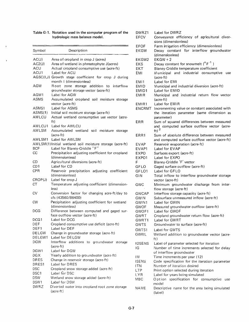
Table G-1. Notation used in the computer program of the hydrologic mass balance model.

Symbol

AC(J) AC2(J) ACU ACU1

Description

Area of cropland in crop J (acres) Area of wetland in phreatophyte J(acres) Actual cropland consumptive use (acre-ft) Label for ACU

AGSC(I,J) Growth stage coefficient for crop J during

AGW

AGW1 ASMS

ASMS1

month I (dimensionless) Root zone storage addition to groundwater storage vector (acre-ft) Label for AGW

interflow

Accumulated cropland soil moisture storage vector (acre-ft) Label for ASMS

ASMS(1) Initial soil moisture storage (acre-ft) AWLCU Actual wetland consumptive use vector (acre­

ft) AWLCU1 Label for AWLCU AWLSM Accumulated wetland soil moisture storage

(acre-ft) AWLSM1 Label for AWLSM AWLSM (1) Initial wetland soil moisture storage (acre-ft) BCF Label for Blaney-Criddle "F" CC Precipitation adjusting coefficient for cropland

CD CD1 CPR

CROP(J) CT

CV

CW

DCG

DCG1 DEF DEF1 DELGW DELGW1 DGW

DGW1 DGX DRES DRES1 DSC DSC1 DSW DSW1 DWRZ

(dimensionless) Agricu Itural diversions (acre-ft) Label for CD Reservoir precipitation adjusting coefficient (dimensionless) Label for crop J Temperature adjusting coefficient (dimension­less) Conversion factor for changing acre-ft/day to cfs (43560/86400) Pecipitation adjusting coefficient for wetland (d imensionless) Difference between computed and gaged sur­face outflow vector (acre-ft) Label for DCG Cropland consumptive use deficit (acre-ft) Label for DE F Change in groundwater storage (acre-ft) Label for DE LGW Interflow additions to groundwater storage (acre-h) Label for DGW Yearly addition to groundwater (acre-ft) Change in reservoir storage (acre-ft) Label for DR ES Cropland snow storage added (acre-ft) Label for DSC Wetland snow storage added (acre-ft) Label for DSW Diverted water into cropland root zone storage (acre-ft)

G-7

DWRZ1 EFCV

EFOF EKGW

EKGW2 EKS EKT EMI

EMI1 EMID EMID1 EMIR

EMI R1 EI\JCRMT

ERR

ERR1

EVAP EVAP1 EXPO EXP01 F GFLO GFL01 GIN

GWC

GWCAP GWIN GWIN1 GWOF GWOF1 GWRT GWRT1 GWTS

GWTS1 GWWL

IDSEI\JS IG

1M ISENS !Tf'J LTP LYR MBC

NAME

Label for DWR Z Conveyance efficiency of agricu Itural diver­sions (dimensionless) Farm irrigation efficiency (dimensionless) Decay constant for interflow groundwater (dimensionless) EKGW + 2

o -1 Decay constant for snowmelt ( F Blaney-Criddle temperature coefficient IVI u n icipal and industrial consumptive use (acre-ft) Label for EM I Municipal and industrial diversion (acre-ft) Label for EMID Municipal and industrial return flow vector (acre-ft) Label for EM I R Incrementing value or constant associated with the iteration parameter (same dimension as parameter) Sum of squared differences between measured and computed surface outflow vector (acre­ft) 2

Sum of absolute difference between measured and computed surface outflow vector (acre-ft) Reservoir evaporation (acre-ft) Label for EVAP Surfaces export (acre-ft) Label for EXPO Blaney-Criddle 'F' vector Gaged surface outflow (acre-ft) Label for G F LO Total inflow to interflow groundwater storage vector (acre-ft) Minimum groundwater discharge from inter­flow storage (acre-ft) I nterflow storage capacity (acre-ft) Subsurface unmeasured inflow (acre-ft) Label for GWI N Measured groundwater outflow (acre-ft) Label for GWOF Cropland groundwater return flow (acre-ft) Label for GWRT Groundwater to surface (acre-ft)

Label fo r GWTS Wetland addition to groundwater vector (acre­ft) Label of parameter selected for iteration l\Jumber of time increments selected for delay of interflow groundwater Time increments per year (12) Code specification for the iteration parameter ~Jumbcr of iteration desired Print option selected during iteration Label for years being simulated Opt i on specification for consumptive use model Descriptive name for the area being simulated (label)

Table G-1. Continued. NCD Number of agricultural diversions NCU Print option for detailed consumptive use out­

NCl NC2 NEXPO NGFlO NGWOF

NMI

NMID NPR NPRIT

NPW NOO

NRES 1\1 RI F

NSIIVIP NTIF

NYR PACl (J) PAC2(J) PCl PCL 1 PCU

PCUU

PDH(I) PGSC(I,J)

PHR(J) PKGW

PREC PRECl PRES PRESl PW PWl PWL PWL 1 OCD OCDl 00 001 OOELGW

put Number of agricultural crop classifications Number of phreatophytes classifications Number of exports Number of measured surface outflows Number of measured or estimated ground-water outflows Number of municipal and industrial con­sumptive uses Number of municipal and industrial diversions Print option for input data Number of initial data printouts desired durinq iteration Number of pumps Print option for obtaining values needed for water quality model in cfs Number of reservoirs in the system Number of measured surface inflows (main stem primarily) Number of measured surface imports Number of unmeasured ground and surface water inflows Number of years to be simulated Proportion of cropland in crop J Proportion of wetland in phreatophyte J Cropland precipitation (inches) Label for PCL Cropland potential consumptive unit use array (acre-ft)

Cropland potential consumptive unit use array (inches) Proportion of daylight hours for month I Growth stage coefficient for phreatophyte J during month I Label for phreatophyte J Ratio of yearly groundwater outflow to yearly addition to groundwater Unadjusted monthly precipitation (inches) Label for PREC Reservoir precipitation (inches) Label for PRES Pumped water (acre-ft) Label for PW Wetland precipitation (inches) Label for PWL Cropland diversions (cfs) Label for OCD Total diversions (cfs) Label for OD Change in groundwater storage (average cfs for time period specified in output)

ODELGW1 Label for ODELGW 001 FF Difference between computed and gaged sur-

face outflow (cfs) ODIFF1 LabeiforODIFF OEF OEF1

Municipal and industrial return flow (cfs) Label for OE F

G-B

OEX Export vector (cfs) OEX 1 Label for OEX OG FLO Gaged urface outflow vector (cfs) OGFL01 Label for OGFLO OG I Groundwater to surface vector (cfs) OG 11 Label for OG I OGWO F Groundwater outflow vector (cfs) OGWOF 1 Label for OGWOF 01 Measured surface inflow in main channel

vector (cfs) 011 Lal;>el for 01 QIR OIRl OMID OMIDl 00 001 OPW OPWl ORES ORESl OS

OSl OTOF OTOF1 RES RES1 RESF RIF

RIFl RTFLO RTFLOl RTK(I)

RZD SGW

SGW1 SGW(l) SIMP SIMP1 SINT

SINT1 SKW(I)

SMA SMA1 SMC SMCl

SMS

SMS1 SMW SMW1 SOF

Cropland surface return flow vector (cfs) Label for 0 I R Municipal and industrial diversion vector (cfs) Label for OM I D Computed surface outflow vector (cfs) Label for 00 Pumped water vector (cfs) label for OPW Change in reservoir storage vector (cfs) Label for 0 R ES Unmeasured surface inflow to main channel vector (cfs) Label for OS TOF vector converted (cfs) Label for OTO F Reservoir storage (acre-ft) Label for RES I nitial reservoir storage (acre-ft) Measured surface inflow in the main stem (acre-ft) Label for R IF Cropland return flow (acre-ft) Label for RTF LO Cropland groundwater return flow coefficient for month I Root zone depth (feet) Accumu lated interflow groundwater storage (acre-ft) Label for SGW Initial interflow groundwater storage (acre-ft) Measured surface imports (acre-ft) Label for SIMP I nterflow grou ndwater storage transferred to surface (acre-ft) Label for SI NT Initialization coefficients for interflow ground­water storage for compartment I Cropland snowmelt (acre-ft) Label for SMA Cropland soil moisture capacity (acre-ft) Water holding capacity of the root zone (inches/foot) Change in cropland soil moisture storage vec­tor (acre-ft) Label for SMS Wetland snowmelt (acre-ft) Label for SMW Computed surface outflow vector (acre-ft)

Table G-l. Continued.

SOFl Label for SOF SPCU Sum of cropland potential consumptive use

SPCUl SRTF SRTFl SSC

SSCl SSO SSW(I)

STA

STAl

STA2

STFK(I)

STIF STI Fl STW(I)

SWL SWL 1 SWLCU

SWLCUl SWCK(I)

TAC TARES TAVE TAWC TEMP TEMPl TGWA

TGWA1 TIF

TIF1

(acre-h) Label for SPCU Cropland surface return flow (acre-h) Label for SRTF Cropland accumulated snow storage at begin­ning of month (acre-h) vector

Label for SSC I nitial snow storage (inches) Wetland accumulated snow storage at begin­ning of month I (acre-h) Six character code for name for the area being simulated Six character code for name for the area being simulated Six character code for name for the area being simulated Surface unmeasured inflow coefficient for month I Surface unmeasured inflow (acre-h) Label for STI F Interflow groundwater in compartment I of interflow storage (acre-h) I nterflow surface supply to wetland (acre-h) Label for SW L Sum of wetland potential consumptive use (acre-ft)

Label for SWLCU Interflow supply to wetland coefficient for month I (acre-ft) Cropland area (acres) Tota I area of reservoirs (acres) Adjusted temperature (0 F) Wetland area (acres) Unadjusted monthly temperature (0 F) Label for TEMP Total addition to groundwater storage vector (acre-ft) Label for TGWA Unmeasured surface and subsurface inflow (acre-h) Label for TI F

G-g

TKGW

TOF

TOF1 TP TRI

TSM TSRZ

TSRZl TSWL TSWLl USW USWl

VARl

WEVAP WGSC

WGWK

W(I)

WLAGW

WLAGWl WLCU

WLCUU

WLDEF

WLDEF1 WLSFC WLSFCl WLSM

WLSM1 WLSMC WTR

Proportion of total outflow passing ungayed below the gage control as interflow or ground­water flow (acre-h) Total outflow plus change in groundwater stor­age vector (acre-h) Label for TOF Threshold temperature for snow storage (0 F) Interflow groundwater in last compartment of interflow storage (acre-ft) Threshold temperature for snowmelt (oF) Total supply to cropland root zone storage (acre-ft) Label for TSRZ Total supply to wetland (acre-ft) Label for TSW L Total available surface water vector (acre-ft) Label for USW

Labels for months and year for column head­ings of output Reservoir evaporation vector (inches) Pseudo growth stage coefficient vector for reservoir water Decay constant for wetland groundwater out­flow Conversion factor for changing acre-ft/month to cfs for month I Wetland addition to groundwater storage (acre-h) Label for WLAGW Wetland potential consumptive unit use array (acre-h) Wetland potential consumptive unit use array (inches) Wetland soil moisture storage deficit vector (acre-ft) Label for WLD EF Wetland surface return flow (acre-ft) Label for WLSFC Change in wetland soil moisture storage (acre­h) Label for WLSM Wetland soil moisture capacity (acre-h) Label for reservoir water

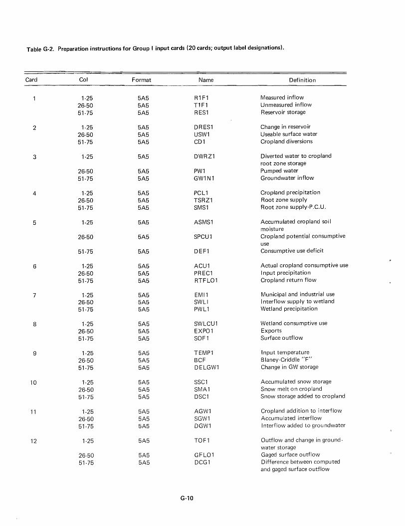
Table G·2. Preparation instructions for Group I input cards (20 cards; output label designations).

Card Col Format Name Definition

1-25 5A5 R1 F1 Measured inflow

26-50 5A5 T1F1 Unmeasured inflow

51-75 5A5 RES1 Reservoir storage

2 1-25 5A5 DRES1 Change in reservoir 26-50 5A5 USW1 Useable surface water 51-75 5A5 CD1 Cropland diversions

3 1-25 5A5 DWRZ1 Diverted water to cropland root zone storage

26-50 5A5 PW1 Pumped water 51-75 5A5 GW1N1 Groundwater inflow

4 1-25 5A5 PCl1 Cropland precipitation

26-50 5A5 TSRZ1 Root zone supply

51-75 5A5 SMS1 Root zone supply-P.C.U.

5 1-25 5A5 ASMS1 Accumulated cropland soil moisture

26-50 5A5 SPCU1 Cropland potential consumptive use

51-75 5A5 DEF1 Consumptive use deficit

6 1-25 5A5 ACU1 Actual cropland consumptive use

26-50 5A5 PREC1 I nput precipitation

51-75 5A5 RTFlO1 Cropland return flow

7 1-25 5A5 EMI1 Municipal and industrial use 26-50 5A5 SWll I nterflow supply to wetland

51-75 5A5 PWl1 Wetland precipitation

8 1-25 5A5 SWlCU1 Wetland consumptive use

26-50 5A5 EXP01 Exports

51-75 5A5 SOF1 Surface outflow

9 1-25 5A5 TEMP1 I nput temperature

26-50 5A5 BCF Blaney-Criddle /IF"

51-75 5A5 DElGW1 Change in GW storage

10 1-25 5A5 SSC1 Accumulated snow storage

26-50 5A5 SMA1 Snow melt on cropland

51-75 5A5 DSC1 Snow storage added to cropland

11 1-25 5A5 AGW1 Cropland addition to interflow

26-50 5A5 SGW1 Accumulated interflow

51-75 5A5 DGW1 Interflow added to groundwater

12 1-25 5A5 TOF1 Outflow and change in ground-water storage

26-50 5A5 GFlO1 Gaged surface outflow

51-75 5A5 DCG1 Difference between computed and gaged surface outflow

G-10

Table G-2. Continued.

13 1-25 5A5 GWOF1 Groundwater outflow 26-50 5A5 GWRT1 Cropland groundwater return flow 51-75 5A5 SRTF1 Cropland surface return flow

14 1-25 5A5 DSW1 Snow storage on wetland 26-50 5A5 SMW1 Snow melt on wetland 51-75 5A5 TGWA1 Total addition to groundwater

storage

15 1-25 5A5 PRES1 Reservoir precipitation 26-50 5A5 EVAP1 Reservoir evaporation 51-75 5A5 WLSM1 Wetland supply-potential wetland

consumptive use

16 1-25 5A5 AWLCU1 Actual wetland consumptive use 26-50 5A5 AWLSIVI1 Accumulated wetland soil

moisture 51-75 5A5 WLDEF1 Wetland consumptive use deficit

17 1-25 5A5 WLAGW1 Wetland addition to groundwater 26-50 5A5 TSWL1 Total supply to the wetland 51-75 5A5 SIMP1 Important surface water

18 1-25 5A5 EMID1 Municipal and industrial diversions

26-50 5A5 EMIR1 Municipal and industrial return flow

51-75 5A5 WLSFC1 Wetland surface outflow

19 1-25 5A5 STIF1 Unmeasured surface inflow 26-50 5A5 GWTS1 GW to su rface water 51-75 5A5 SINT1 I nterflow to su rface water

20 1-75 13A6 VAR.1 13 time increment (months) labels heading their respective columns in the budget output

G-"

Table G-3. Preparation instructions for Group II input cards (8 cards; control and parameter initialization)~

Card Col Format Name Definition

1-80 20A4 NAME Area name and identification designation

2 1-06 A6 STA Area identification (mnemonic) 7-08 12 NYR No. of years :s 30 9-10 12 1M Time increments per year

l:s 1M ::;12 11-12 12 NC1 No. of agricu Itural crops :s 13 13-14 12 NC2 No. of phreatophytes :s 9 15-16 12 MBC O(zero) value for Blaney-Criddle

method of CU calculation 1 (one) for modified Blaney-Criddle method

17-18 12 I\lPR 1 for printing input data o for suppressing printing of input data

19-20 12 l\l R I F No. of measured inflows 21-22 12 I\lCD No. of cropland diversions 23-24 12 I\lPW No. of wells (pumped water

measurement) 25-26 12 I\lMID No. of municipal & industrial

use diversions 27-28 12 NMI No. of municipal & industrial

uses 29-30 12 NTIF No. of unmeasured surface inflows 31-32 12 NIMP No. of surface imports 33-34 12 NRES No. of reservoirs 35-36 12 NEXPO No. of measured surface exports 37-38 12 NGFLO No. of gaged outflows 39-40 12 NGWOF No. of groundwater outflows 41-42 12 IG No. of time increments for delay

in transitional groundwater sto rage :s 1M

43 11 NCU 1 for printing consumptive use and interflow storage detail o for suppressing above printing

44-46 F3.2 EFOF Farm irrigation efficiency 47-49 F3.2 EFCV Conveyance efficiency for water

diverted to cropland 50-54 F5.3 CC Adjusting coefficient for crop-

land precipitation 55-59 F5.3 CW Adjusting coefficient for wetland

precipitation 60-64 F5.3 CT Adjusting coefficient for crop-

land temperature 65-68 F4.3 EKGW Decay constant for interflow added

to groundwater 69-72 F4.3 EKS Decay constant for snowmelt 73-76 F4.1 TP Threshold temperature for snow

storage 77-80 F4.1 TSM Threshold temperature for snow

G·12

Table G-3. Continued.

Card Col Format

3 1-06 A6 7-14 FS.O

15-22 F8.0 23-30 FS.O

31-36 F6.0

37-41 F5.2 42-46 F5.2

47-51 F5.2

52-59 FS.O

60-67 FS.O

6S-72 F5.3

73-80 FS.O

4 1-6 A6 7-8 12

11-15 F5.3

16-20 F5.3

21-30 F10.0 31-40 F10.0

41-50 F10.0

Name

STA1 TAC TAWL RESF

ASMS 1,1

RZD SMC1

SSO

SGW 1,1

GWC

TKGW

GWCAP

STA2 NOO

CPR

WGWK

TARES AWLSM 1,1

WLSMC

Definition

Area identification Area of cropland in acres Area of wetland in acres Reservoir storage at beginning of period in acre-feet I nitial value of soil moisture storage in acre-feet Root zone depth in feet Water hold ing capacity of root zone in inches/ft. Initial value of snow storage in inches Initial value of interflow storage in acre-feet Minimum discharge from interflow in acre-feet Proportion of outflow going under the gage as groundwater outflow Capacity of interflow storage

Area identification Print option for water qual ity hydrology output if non zero (If> 1 then only those values used by WAOUAL as output) Adjusting coefficient for reservoir precipitation Decay constant for wetland GVV outflow Total area of reservoirs in acres I nitial value of wetland soil moisture storage in acre-feet Wetland soil moisture capacity in acre-feet

If selective iteration is desired when using HYDRO, then the following variables must be supplied on card 4. If supplied they are ignored by BUDGET.

4 51-56 A6

57-5S 12

59-60 12

61-62 12

IDSENS

NPRIT

ISENS

LTP

G-13

Identification label of the parameter selected for iteration Number of input data printouts desired after initial printout if NPR~O Code specification for the para­meter selected for iteration. See Table A-5 for val id specification codes. Prints entire BUDGET without iteration information. Prints entire B UDG ET with iteration information. Prints only last with 5 line 7 Budget.

Table G-3. Continued.

Card Col

63-65 66-75

Format

13 F10.0

Name

ITN ENCRIVIT

Definition

I\lumber of iterations desired I ncrementing interval or constants associated with the parameter selected for iteration.

5 Initialization coefficients for the interflow storage (STW) punched in FORMAT(14X,12F5.3). This card is needed only when IG#O.

6 Cropland groundwater return flow coefficients (RTK) punched in FORMAT(14X,12F5.3).

7 Unmeasured surface inflow coefficients (STFK) punched in FORMAT(14X,12F5.3).

8 Supply to wetland coefficients (SWLK) punched in FORMAT(14X,12F5.3).

a All unmeasured values are initial estimates, modified by trial as validation proceeds.

G-14

·Table G-4. Preparation instructions for Group III input cards for data vectors (number of cards is de­pendent upon amount of data used).

2

21 to 2NC1

3

Proportion of daylight hours (PDH) punch­ed in FORMAT (14X,12F5.4).

Proportion of crop area (AC1) FO RMAT (10X,13F5.3).

Crop label and growth stage coefficients (CROP; AGSC) punched in FORMAT (8X,A6,12F5.3). Include only if NC1 > O.

Proportion of phreatophyte area (AC2) punched in FORMAT (10X,13F5.3).

31 to 3 NC2 Phreatophyte label and growth stage co­efficients (PHR;PGSC) punched in FOR­IVIAT (98X,A6,12F5.2). Include only if I\lC2 > O.

4 Label and use coefficients for reservoir water (WTR;WGSC) punched in FORMAT. (8X,A6,12F5.2). Include only if NRES > O.

5 Label for years, mean, and standard devia­tion punched in FORMAT (10X,14A5). (Should have I\lYR+2 labels punched).

6 FORIVIAT specification for reading RIF vector (include only if I\IRIF > 0).

61 to 6NRIF Measured inflow data in acre-ft.

7 FORMAT specification for reading SIMP vector (include only if 1\11 MP > 0).

71 to 7 N IMP Surface input in acre-ft.

8 FORMAT specification for reading CD vec­tor (include only if I\lCD > 0).

81 to 8NCD Cropland diversion data in acre-ft.

9 FORMAT specification for reading PW vec­tor (include only if 1\1 PW > 0).

9 1 to 9 NPW Pumped water data in acre··ft.

10 FORMAT specification for reading PREC vector (must be included).

10 1 Precipitation data in inches.

11 FORMAT specification for reading TEMP vector (must be included).

111 Temperature data in F.

12 FORMAT specification for reading EM I D vector (include only if NMID > 0).

121 to 12N IMoMunicipal & industrial diversion data in acre-ft.

13 FORMAT specification for reading EM I vector (include only if NMI > 0).

131 to 13NMI Municipal and industrial use (depletion) data in acre-ft.

14 FORMAT specification for reading TIF vector (include only if NTI F > 0).

141 to 14NTIF Unmeasured inflow data in acre-ft.

15 FORMAT specification for reading RES vector (include only if NRES > 0).

15, to 15N R EsReservoir storage at end of month in acre­ft.

16 FORMAT specification for reading EXPO vector (include only if N EXPO> 0).

161 to 16NExp~easured export data in acre-ft.

17 FORMAT specification for reading GFLO vector (include only if NGF LO > 0).

171 to 17 Gaged outflow data in acre-ft NFGLO .

18 FORMAT specification for reading GWOF vector (include only if NGWOF > 0).

181 to 18 Groundwater outflow data in acre-ft. NGWOF

aSubscripts refer to number of cards used for a given vector.

G-15

Table G-S. Iteration specification codes (lSENS) that may be selected for HYDRO.

Code

2

3

4

5

6

7

8

9

10

11

12

Parameter Affected

Description

IG&SKW Change time increment of interflow GW storage delay by ENCRMT each iteration. Specification of th is option requires reading ITN-2 cards designing values to the interflow GW coefficient (SKW 1) following the regu lar G rou p III data card s specified hereafter-FORMAT for reading SKW is (14X,12F5.3).

EFOF Change farm irrigation application efficiency by EI\lCRMT each itera­tion.

SGW(1)& Change interflow GW cap by GWCAP ENCRMT each iteration and keep

initial condition of interflow stor­age at capacity.

CC

CW

CT

EKGW

EKS

TP

Change cropland precipitation ad­justment coefficient by ENCRMT each iteration.

Change wetland precipitation ad­justment coefficient by ENCRMT each iteration.

Change temperature adjustment coefficient by EI\lCRMT each itera­tion.

Change exponential decay constant for interflow storage added to GW by EI\lCRMT each iteration.

Change exponential decay constant for snowmelt by ENCRMT each iteration.

Change threshold temperature for snow storage by ENCRMT each iteration.

TSM Change threshold temperature for snowmelt by ENCRMT each itera­tion.

ASMS(1) Change initial cropland soil mois­ture storage by E NCR MT each iter­ation.

RZD Change cropland root zone depth by ENCRMT each iteration.

G-16

13

14

15

16

17

18

19

20

21

22

23

24

25

26

SMC1

SSO

Change root zone water holding capacity by ENCR MT each itera­tion.

Change initial snow storage by ENCRMT each iteration.

SGW( 1) Change initial interflow storage by ENCRMT each iteration.

GWC Change minimum GW discharge from interflow storage by ENCRMT each iteration.

TKGW Change proportion of total outflow assumed to be GW outflow by EI\lCR MT each iteration.

GWCAP Change capacity of interflow stor­age by EI\lCR MT each iteration.

CPR

WGWK

Change adjustment coefficient for reservoir precipitation by EI\lCRMT each iteration.

Change exponential decay constant for wetland soil moisture added to GW by ENCR MT each iteration.

AWLSM( 1 )Change initial wetland soil moisture storage by ENCRMT each iteration.

WLSMC Change wetland soil moisture ca­pacity by EI\lCRMT each iteration.

RTK j Change cropland groundwater re­turn flow coefficients by reading in a new set each iteration. Require ITN-1 cards trailing the regular Group I" data deck. Read FOR­MAT for RTK is (14X,12F5.3).

AWLSM( 1 )Change wetland soil moisture ca­WLSMC pacity by ENCRMT each iteration

and keep initial condition at WLSMC.

SWLK j

Change inflow coefficients by read­ing a new set of each iteration. Re­quires ITN-1 cards trailing regular Group III data deck punched in FORMAT (14X,12F5.3).

Change wetland supply coefficients by reading a new set each iteration. Require ITN-1 cards trailing the regular Group III data deck punch­ed in FORMAT (14X,12F5.3).

Table G·5. Continued.

Code

27

28

29

Parameter Affected

TIF

GWOF

PREC

Description

Change amount of unmeasured sur­face inflow by a multiplication fac­tor increased by ENCRMT each iteration.

Change amount of groundwater outflow by a multiplicative factor increased by ENCRMT each itera­tion.

Change unadjusted input precipita­tion by reading a new set of values each iteration punched in FOR­MAT (14X,13F5.2). This option re­quires that ITN-1 PREC cards trail the Group III input data.

G-17

30 TEMP

31 PAC1

32 PAC2

Change unadjusted temperature by reading a new set of values each iteration punched in FOR MAT (14X, 13F5.1). This option requires that ITN-1 TEMP cards trail the re­gular Group III input data.

Change percent distribution of cropland areas by reading a new set of values each iteration. Input FORMAT is (10X,14F5.3). This option requires ITI\I-1 PAC1 cards trail the regular Group III input data.

Change present distribution of wet­land areas by reading a new set of values each iteration. Input FOR­MAT is (10X,14F5.3). This option requires ITN-1 PAC2 cards trail the regular Group III input data.

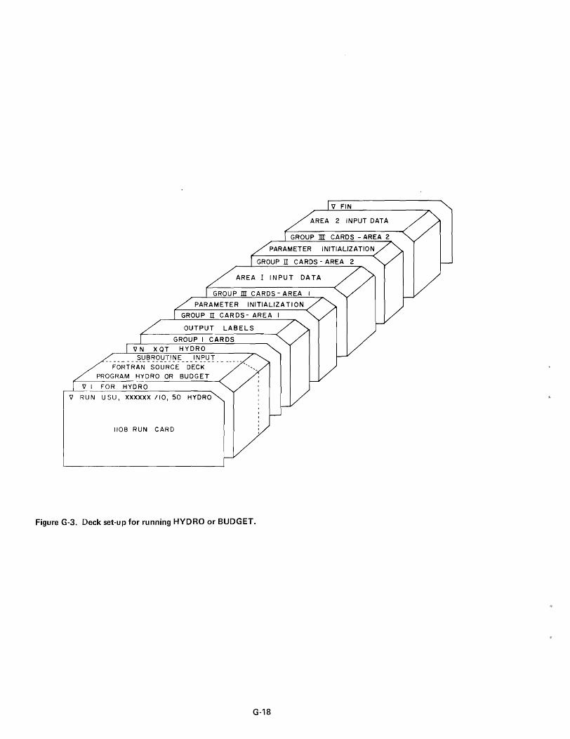
'V FIN

AREA 2 INPUT DATA

AREA I INPUT DATA

GROUP m CARDS - AREA I

PARAMETER INITIALIZA TI ON

GROUP nCAR DS - AREA

OUTPUT LABELS

GROUP I CARDS

VN XQT HYDRO ________ ~~1?~9Y}J ~~ ___ '_N~~! ______ _

FORTRAN SOURCE DECK

PROGRAM HYDRO OR BUDGET

V I FOR HYDRO

V RUN U SU, XXXXXX 110, 50 HYDRO

1108 RUN CARD

FigUl'e G-3. Deck set-up for running HYDRO or BUDGET.

G-18

iI RUN U5U,XXXXXx,ltlOO .. lZ LEON HUBER iI DPR ill FOR HYDRO,HYDRO C C HYDROLOGIC HA5S BALANCE HODEL PROGRAH

COHMON L YR

C

INTEGER NAHE I ZDI 01 HE N5 ION PO HI lZ I , AC 1 I 14 I, R I F 11 31, F ( 1 31 ,CO ( 13 I ,PW I 1 3" PR EC I 13 I ,

1 PC If 131,0 WR l I 131 ,G WO F I 1 3 I, TS Rl I 13 I ,T E HP I 1 3" A G5 C I lZ ,14 I , T A VE ( 13 I , ZPC UU I 13,1" I ,PC UI 13, 141 ,p G5 C ( 1 Z, 13 I , AC Z I 13 I ,wL CU ( 1 3, 131 ,PWL ( 13 I , 3Wl CUU I 13, 131 ,S PC U( J 31 ,S W LC U ( 1 31 ,5MS I 1 31 ,A S 145 I 131 , DE F I 13 I , ACU ( 13 I , 4 A6 WI 131 ,[HI I 131, TI FI I ~ I , Sw III 31 ,S 0 F 11 31 ,S GW ( 1 31 ,0 Gw I 1 3 I ,RT FL 0 ( 1 3) , 5RE S( n I ,E XPO ( 131 ,T OF' 13) ,G WR Tf 1 31, <;R TF ( 13) ,S Til ( lZ) ,SKW I I ~ I, PHR • 131 6, CROP I J 4 I ,DR ES I 131 ,usw I 131 ,G FL O' I 3) ,0 CG • 1 3) , sse. 1 31 , ~5 W. 1 3) , 7 SH A. J 31, SHW. I 31,05 CI 1 31 ,Os w. J 31 ,FHK 11 Z) ,GW IN. 131 , 8 AWLC U' 131 ,PR ES • 13) ,E V A P ( 131 ,WGS C I lZI ,WL 514 • 1 3) , All L SM' 1 3) , ilL A G W' 1 3 ) , 9 WI.. DE F I 131 ,T S WL • I 3) ,S TFK ( lZ) ,S WL K • lZ1 , EM 10 I 1 3 I , [14 I R • 13' ,W [V A P • 13 I

DIHEN5IONRIF 11 51 ,TIFlf 51 ,RESI IS I ,DRESI' 51, USWlf 51,C01(51 ,PWl'51, lOW R l 1 • 5 I • G II 0 fl' 5 " PC L 1 ( 5 " T S R Z1 ( 5 I , S M S 1 ( 5 I ,A 5 M 5 I ( 5 I , 5P CUI • 5 I , ZoEFtIS I ,ACU 1.5 I, AGII 1151, RTFLOI. 5) ,EMIl' 51. 5Wll (51. PWLl' 51 ,55C 115). 3SIILC U 1 .51. [X PO 11 5 I ,T E"P 11 5 I ,BCF (5 I , oGW 1 .51 ,50 FI ( 51 , 4 PR [C 1 • 51 ,GFL 0 1 • 5" DC G 1 • 5 I, SM AI. 5 I ,OS C I • S I, SGW I • 5) • TOft. 5 I , S G W R T 1 • 5 I ,S R T Fl • 5 ) , SM II 1 ( 5 "05 W 1 ( 5) , V A R I • 1:1' I ,G WIN I • 5) , 6'" WLC U 1 • 5 ) ,PR fS 1 ( 5 I • E v A PI. 5 I ,ilL SM 1 ( 5 I • AWL S 14 1.5 I • WLo[ F I ( 5 I • 7 ilL AG WI. S I ,T 5 WLlI 51 ,T GilA 1 (51 , EM I 01 • S I , EM I R 1 • S I • WL SF C 1 (SI ,0 [lG 1/ I .5 I • 8 II ( 13 I ,0 I ( 13 I .0 S. 131 • OG I ( I 3 I • GO • 13 I ,G I R • I ~ I • G f F ( 13 I , GO. I 31 , 9 Wl SF C ( 1 3 ) .0 E L Gil. 1 3 I , Cl q [5 • 13 I , G P II • 13 I , T G W A • I 3 I • PAC I • 14 I • PAC 2 • I 3 I , 1 Q T OF ( 13 I • GGIIClF ( 1 31 ,(WE L G W. 1 3 I, GGFL 0 • 1 31 ,GO IFF' 1 31, Q CO( 1 31 • G EX. 1 3 I. ZOM ID ( 131 ,S I MP, 13" SIMP 1 ( 51 ,5 TI F 11 5 I • S TI F • 131 • GilT S 1 • 5" G W T<; • 1 ~ I • 3SINT 11 SI .SINT .13 I

DATA GIl,GSl,OGII,OOI.GIRI,OEFI,.ClOI,OR[SI.0PIII. GTOfl,GGWOFI. 1 GoGw 1, GGfLO I.G 01 FF I/:?HG I. ZHGS oJ HOG I ,Z HGO, 3HG IQ. 3HGEF .ZHGO, 4 HGRES • 23HOPII. 4HOTOF,5HClGI;OF ,4HGOGII. 5HGGFlO, 5HGDIFF /

OAT ... GCol.GEXl,GMIol/3HGCD,5HGEXPO.4HGMIo/

C RE"'O L"'B[LS fOR BUDGET OUTPUT C

READ .5.5001 PIFl.TIFl.RESI RE AD • S • 500 I OP ES 1 • us II 1. COl READ (5,50'11 aIlRll,pwl.GwINI RE AD .5.S00lPCL 1. TSllll ,SMSI RE",0.S,5001 ASMSl.SPCUI,DEfl RE AD .5.500 I "'C U 1 • P Pf C 1, R TF lO I RE"'o (S,5001 E"ll ,SWll ,PWl! READ '5,5001 SlilCUl.fXPOI,SOFI REAo(S,5001 TEMPI,BCF.DElGWI READ ,5,5001 SSCl.5"Al,DSCI READ'S,5001 AGWl.SGWI,DGWl

·REAo(S,500) TOFl,GFLOltDCGI RE"'D(5,50'11 GWOFl,Gw'lTl,SRTFI REAo.5.500lDSIIl.S01WI,TGWAI RE AD • S , 50 0 I PR ES I , f V A PI. III S M I RE "'0 'S, 500 I All lC U I, A ilL SM I ,WL Off I RE AD (5,5001 ilL AGWI, TSWLl,S IMPI RE AD (S, SOO IE"I 01 ,E MIR 1, WLSFC 1 REAO(5,SoOl5Ttfl,GIIT<;I.5INTI

SOD fORMAT.15A51 RE AD (S. 50 1 I V A R 1

501 FOR"AT'I3461 CV =43560./1 3600.024. I W.1I =tV/31. W' 21 =tY/30. w. 3) =W. I I W' 41 =W (1 I W. 51 =tV/Z~. W. 61 =W .11 W(11=W(ZI W( 81 =W. I) 11.91 =W. Z} W. 10 I=W.lI w.ll1=WI11 W.121=W(ZI II' 1 3 1= C V / ~6 5 •

1 READ .5dO 11 NAME 101 FORMAl'ZOA"I

IT =1 II =1 CMUL T=I.

READ INITIALIZATION PARAMETEP<;

RE ... 0 • 5 , 10:?l S T A ,N YR. 101. NC I • NC? • M BC , NP R ,NR IF, N rD. N P W • NM 10, NM I • NT IF. I NS 1M P. NR E <; • N E X PO .N GF L 0, N GW OF. I G • NC U ,E FOF • E F C V • C C • C II. CT • E K Gil, E K S • 2TP ,TSM

102 FORMAT'A6,1812.r),?F~.Z.3F5.3.2F4.3,ZF4.)} RE ... 0 IS, 103 I 5 14 1 • TA C. T A lolL, R f 5 F • A 5"5 I I I ,R ZD. <;M C) • <; SO, S GW • I I • G W C • T K Gw

I ,6 wc AP 103 FORMATIA6,3FR.0.Fh.0.3fS.2.2FR.0,F~.3,Fs.nl

RE AD (5, 1071 S TA Z. NG 0, CPR. IIG WK • T A R[ <; • AWL <; M • ) I, WL 5M C • 10<;, NS • NP R IT. I 15 ENS, L T P , I TN, EN CR '1 T

101 FORMAT .... 6,14.ZFS.3,3FI0.0.A6.3I:?oI3.FIJ.:J1 If .L TP • L E .01 L T P= I

RE ... D INITIALIZAT ION COEFFICIENTS FOR INTEPrLOW GW STORAGE

If'I6.EIl.OI GO TO 2 READ.5d04I1SKW( I1,J=I.IGI

104 FORMH'14Xl2F5.~I 2 2114= 1M

IMT=IM+l

READ CROPLAND GROUNDWATER RETURN FLOW COEFFICIfNT<;

RE AD • 5 , 104 I • R T K. I I , I = I, I M I

READ SURFACE UNMEASURED INFLOW COEFFICIENTS

RE AD I r; • 1 n 4 I 1ST FK • I I • I:: ) • 1M I

READ INTERfLOIi 5uPPLY TO WETLAND COEFFICIENTS

READ 15,104 I (<;WlK II 1,1=). 1M I

READ PROPORTION OF DAYLIGHT HouRS

RE "'0 • 5, 130 I ( PO H ( II ,I = I, I M I 130 FORMAT .14XIZfS.4 I

REAO PROPORTION CROP AREAS AND GROWTH STAGE COEfFICIENTS

IF'NCIIIotlO,5 5 REAo.r;d06I1PACl.JI,J::I,NClI

106 FORMAT (lOX, 14F5. 31 DO 6 J=t.NC 1 RE AD .s.t 05 I CR OP (J I .c A GS C. I, J I , I:: Id 14 I

lOS fOR"AT.8XA6dZFS.Z) 6 AClIJI=TAC.PAClIJI

RE"'o PROPORTION PHREATOPHYTE AREAS AND GROWTH STAGE COEFFICIENTS

IOIF.NCZII5tl5.tl 11 REAo(5d[l6I1PACZ'JI,J::I,NC21

DO 12 J=I,NCZ RE AD • 5, LO 5 I P HR .J I •• P 6SC • I. J I • I:: t. I'll

lZ ACZ(JI=TAWLoPAC2.JI

READ RESERVOIR wATER 5URFACE GROWTH <;rAGE COEFFICIENTS

15 IF'NRES.NE.OI READ(5d051 IITR.cwGSC(I1, I=ldMI

RE AO I NP U T 0 A T A

REAo.5dOOOlLYR 1000 FORMAT .10X, 14A51

C C CALCULATE CROPLAND SOIL MOISTURE CAPACITY AND INITIAL SNOW 5TORAGE C THE CROPLAND AND wOLAND

C 5MC=RlO'SMCloTAC Il? SSC.l I =S500TACIl? SSW, 1 I =SSI1.TAWlIIZ.

PRINT ORIGINAL INPUT DATA IF NPR NE '1

998 IF. N PR IT .L T • 0 I N PR:: n ER R= O. ERRI =0. IF'NPR.EG.OI GO TO 13 WRITE.6,S071 NAMf

507 fORMAl"IINPliT OATA FOR 'ZOA41 WR ITE( 6,5081 ST A, NYR. 1M, NCI ,NC2, Mf'r.NPR, NRIF, NCO. NPW, NM IO,NM I. NT IF.

INS I"IP ,NRES. NEX PO.N GF LO, N GIIOF, I G, NCU ,fFOF, fFCV, CC. CW, CT ,EKGII. EKS,

2TP ,T5M 50S FOR"AT.IXA6,J9I3,ZF5.?3F5.3.:?F6.3.2FG.II

WR IT E • 6,5091 5 TAl. T A C • T A ilL. Rf SF. A5M S • I I • R 1 O. 5 14 Cl • SS 0, S(' W I I I • GW C. ITKGW,GWCAP,SMC,5<;C'11.SSW'I}

509 FOR"ATIIXA6,3FJO.0,FQ.0,3FG.2,2FJO.fl,F8.3,4FJO.OI IIR IT E I G ,701 1<; T A Z • N 110 • CPR, W Gw K , TARE 5. A WL 5'1 • 11 • WL 5 MC, IDS ENS. N P R IT •

I ISENS,l TP, !TN, EN 0;>,.,' 7['1 FORMAT'IXAG'I4'ZFIO.:I'.3FIO.0,ZXA~.3J3.15,FI5.51

13 IFIIG.EG.OI GO TO 14 5KII'IG+1I=1. 00 7 1=1, I G

7 SKWI IG+I I=SKIII IG+I'-<;KW( Il IF • N PR • N[ • 0 I WR IT E. 6 , S 11 I • S K W • I I , I =1 • I G I ,5 K II' I G + I )

511 fORMUIIX'INIfRFLOIi GW <;TORAGE COEf·13FR.31 00 8 I:: I, I G

S STW.I1=5I(wlIhSGw'1I TR 1= SG W. I I • S K ~ • I G+ II IF • N PR • NE .01 WR IT [I 5.5 12 I .S T W • I } • I =J , I G I , TR I

512 fORMAT'IX'INITIAl INTFRFlOIi qORAGE·13F3.01 14 IF'NPR.EG.OI GO TO ?'lfl

wRITEI6,560} LYR.VARI IIR IT E I 6, S 10 I I P TK • I I , I = I , 1M I

510 FORMAT (IX?5HCPOP GW-RETURN FLO COEf .r ZFP.31 WR ITEI 6,5171 (5 TFKI II. I:: I. IMI

511 fOR,.,AT.txZ5HSURFACE TIF COEFFICIfNT5 dZfS.31 WR IT E I G. 5 I B I IS WL K. Il .r = 1 .r M I

518 FOR"AT.IXZ5HINTERFLO SilL COEFFICIENTSdZFQ.31 WR IT f 16,5 O? I I P DH I I I , I:: 1 • 1M I

50Z FORMAT .IX25HPPOPOQTION DAYLIGHT flOURS'] ZFR.41 IF INCI.EIl.OI GO TO 91 IIRITE.6.S031I P ACIIJI.J=I.NCII

S03 FORMATI2X'PROP CROPS'14FA.31 IIR IT E lb. 5 ;:>0 I I A C I I J I • J:-l , NC ) I , T A C

5?0 FOR"AT ,zx'CPOP APEAS''} 5F~.OI WR IT fIG. 5 '14 I I J • CPO 0 I J I • I AG SCI I • J I • 1=1 • I MI. J = I ,N C I I

S04 fORM AT I I X I 3 .r x A 5 , 7 H ~ CO [F .l1X ,} ZF 8. 71

'lJ IF 'Ne2.EIl.01 GO TO '13 WRIT f • f, • 5 n 5 I • PAC? I J I ,J = I • ~~ C 21

S(15 FOP~AT I IX 15HP O OP WLPH AREAS 01 3F a. 31 IIR IT E I I; , 5 ? 1 I I A C 2 I J I • J= I • NC 2 I ., A ilL

S?I FORMATlfiX'WU'H AOfA<;·'}4fQ.O} WR IT E I h .5 '14 I I J ,p HR I J I , • P G S C • I • J I , I = I. 1'1 I • J = 1 • N C Z I

'13 IF'NRES.NE.OI .RITf'h.SZ21 wTR •• WGSClIld=I,JMI 572 fORMATlIHO"'h. 7H K CO[F til X d?FA.n 200 IFILl.EO.OI G" TO III

IF. N R IF. N f • o. A NO • N P R • N E • n I II R IT [ I G • S Ofi I R IF 1 snh fO"'1ATI2SX5A~1

CALL INPurcl;"IFolol .... oIF.NPRI IF 'N<;IMP.NE.fJ. ANO.Npo.NE .'llwRITEIf'.516ISIMPI CAll INPUTIN<;IMPd.I'1,SI01P.NPPI If I NCO. NE • n. AN O. NP P. NF • 0 I \I R I If • 6. so 0 I CO I CALL INPUTINCOd,[;I.CD.NPPI If IN p W • NE • n. A"l o. "lP R. N, • 0 I II R IT f • h. 5:1 hIP W I CALL INPUTINPlld,[M.PW.Npol IF IN PR. NE. 0 I liP IT E I h • ~ fJf, I po [C I CALL INPUTllol.r"'.PREC"'~PPI

I FIN po. N E • 0 I W R IT E lb' S flb I T E '1 ° 1 CALL INPUTllold"'oTr",p.NPRI IF IN '1 I D. NE • O. A NO • N 0 P • 'I E • [) I IIR r IE I h .5 '1<; 1[14 In 1 CAll INPUTIN"IO.I.I".rMIo.NPRI IF I N "II • 'IE. n. ~N O. NP P. NF • 0 I II R I Tf • b. 5J hI E'1 I ) CALL INPUTlN"IdoIM.f"r.NP", I fIN T If. N £ • 0 • A NO • N P R • N E • :J I W R I TEl h • S 06 I T I, I

Figure G-4. Listing of program HYDRO with data input and program output.

G·19

CALL INPUTlNTIFd.IM.TIF.NPRI IF INRES.NE. O.A NO .NPR .NE.D I WR HE 16.5061 RES I CALL INPUT INRES.I. IM.RES.NPR I IF (NOPO.NE.O. AND. NPR.NE .0IWRITEI6. 5D61EXPOl CALL INPUTINEXPOtl.IM.EXPO.NPRI IF INGFLO.NE.D. AND. NPR.NE.0IWRITEI6. 5D61GFLOl CALL INPUTINGFLO.l.IM.GFLO.NPRI IFINGWOF.NE.O.AND.NPR.NE.OI WRITE16.5061 GWOFI CALL INPUTINGWOF .1oI'I.GWOF.NPR I

INITIALIZATION OF ANNUAL COLUMN AND TOTALS FOR ALL ITEMS NOT CALLED BY SU~ROUTINE INPUT

18 SSCII'ITI=O. ST IF IIMT 1-::0. GWIN IIMT 1=0. GWTS IIMT 1=0. SINT IIMT 1=0. SSWI IMTI =0. SMAI IMTl =0. OS CI I'IT I =0. SMWI IMT I =0. OSWI I'IT I =0. SGWI I'IT 1=0. OGIII I'ITl =0. OCGI I'ITl =0. ORES IPH 1=0. USIIII'ITI:O. OWRZIIMTI=O. PCLlIMTI:O. TSRZIIMTI=O. SPCU IIMT 1=0. E"'1RII".TI:0. SMSI 1"lT 1:0. DE F 11M T I = O. ACUI IMTl =0. AGWI1MTI=0. R T FL 0 I 1M T I = O. SWL( 1MT 1:0. PilL( IMTI :0. AWLCUI 1MT 1:0. SWLCUI IMT I =0. TA VE II MT 1:0. FIIMTI:O. SOFIJ'ITI=O. TOFI II1TI :0. GWRT IIMT 1=0. SRTF IIMT 1=0. PRES IIMT 1=0. [YAP IIMT 1:0. WEVAPI IMTI =0. WLSp.4III'!TI-::O. WL AG WI I".T I :0. TGWAIIMTI-::O. ilL SF C I 1M T I = O. OELGWIIMTI:O. IF INC112}.2l.19

19 00 20 K=l.NCI PCUU IIMT.K 1-::0.

10 PCUI 1MT.K I =0. ?l IFINC2124.:>4.22 22 00 23 K=1.NC7

WL CU U I UH • K I : 0 • 23 WLCU IIMT.KI=O. 24 CONT INUE

CALCULATE CHANGE IN RESERVOIR STORAGE. RfSI II IS STORAGE AT END OF PERIOD I.

OR ES I 11: R E <; I II -R ES F 00 16 I:2dM

1 f> ORES II I:RES I I I -R ES IT -II RES! IMTI:RESIIMI ORES IIMT I:RESI 1M I-Rf~F

BUDGET CALCULA TI ONS "fGIN HERE

EK T: 1. 00601::1.1"1

CALCUL ATE POTENT UL CIlNSUMPT IvE USE

TA VE II I:CT.TEMPI II FI II :TAVEIIl.POMII I IF 1M AC .NE. 0 I EK T:: .0113. TA VE I I 1- • 3} 4 I FIE K T • LT •• 3 IE K T :. 3 SPCU II 1:0. IF INClI29.2'3.77

77 DO?A K:l.NCI PC UU I I • K I: F I I I oE KT • A GS C I I. K I PCUI I.KI:PCllUI I.KI.AClIK I/IZ.

28 SPCUII I:SPCUII I+PCUI I.KI 29 SWLCUI II :0.

IFINC213Z03ZdO 30 00 31 K::l.NC2

WL CU U I 1 • K I :F I I I, EK ToP G SCI I • K I WL Cll I I • K I: WL CU UI I. K I • A C Z IK 1/12.

31 SWLCUIII:SWLCUIII+WLCUII.KI

CALCULATE PRECIPITATION AND EVAPORATION FROM RESERVOIR

12 EVAPIII:O. WE V A P I I I : 0 • PRES II 1:1). IF INRES.EQ.OI GO TO 705 wE VAPI II:F II I. EK T.WG~C I I I EVAPIII-::wEVAPIII·TARES/12. PRES II I:PREC II I'CPR'T~RES/12.

CALCUL ATE SNOW STORAGE AND SNOW I4ELT

Figure G~4. Continued.

G-20

205 PCl! II ::PRECI II .C C' TAClI2. PWl! II ::PRECI II oCWo TAWL/12. IFITAVEIII.GT.TPI GO TO 301 OSCI II =PCL II I DSWI II ::PWLIl I GO TO 302

301 DSCI!l=D. DSWI!l:O.

302 SSCII+II=SSCIII+OSCIIl SSWI 1+11 =SSWIII+OSWI II IFITAVEIII.GT.TSMI GO TO 305 SI4AIII=O. SMWI II :0. GO TO 310

305 SMAIII:EKSoITAVEIII-TSHloSSCII+11 SI4 WI !l =EK <; 0 I TA vE II 1- TS '1 I 'S S W II + 11 IF IS MA I I I. G T • S SC II +11 I SM AI I I =S SCI r .11 IF IS MW II I. GT • SSW II + III SM WI II =S S W I 1.1 I

310 SSCI 1+1 I =SSC II +II-SMAI II SSWII+II=SSwlI+II-SMWIII

CALCULATE SYRFACE UNHEASURED INFLOW AND GW INFLOW

S T IF II 1= TI F I I loS TF K I I I GWIN II l=lIFI II-STIFI II

CALCUL ATE ROOT ZONE SUPPLY AND CROPLAND RETURN FLOW

DWR21I1-::COII "EFCV.EFOF TSRllI I-::OWRZII I+PCl! Il-DSC I I I+SMAI II SMSI II =TSRlI II-SPCUI II RTFLOI II =CDI II-DWRZI II GWRT II I=RTK I II oR TFLO II 1 SR TF II 1-:: R T FL 0 I II -G WR TI I I IF IS H~ II I 133.33.35

33 IF ISMS II I+ASMS II 1134. 311035 34 ASHS II +1 1=0.

AGWIII:O. DEFI II :5MSII I+&SHSIII ACUI II =SPCUI II +OEF II I

GO TO" 5 35 ASH51I+II:ASMSIII+SMSIII

IF IA SM S I I + II -S HC I 38.38.40 38 AGwIII=O.

GO TO" 3 "0 AGWIII:ASMSII+II-5MC

ASMS II +ll=SMC "3 ACUIIl:SPCUIJ)

DEFI II :0.

CALCULATE IN1ERFLOW GW STORAGE CHANGES. INTERFLOW TO SURFACE AND INTERFLOW ADDITION TO GROUNOWATER

45 GIN=AGWIII+GWRTlII+GWINIJ) EKGW2=EKGW+2. 5!NT II 1=0. IFIIG.EG.OI GO TO 66 OGWIII=ITRI+TRI+STWIIGII'EKGW/EKGW2 IF ID GW II I. G T .G we I GO TO 62 DGWI II :GWC IF ITRI+STWIIGI.L T. DGWI II I DGWIII=TRI+STwIIGI

62 TR I: TR I + S T W I IG 1- DG W I II IFIIG.EG.ll GO TO 65 00 63 K= IG. 20-1

63 STWIKI~TWIK-l1 65 SGWI I+lI=SGWII I+G!N-DGwI II

GO TO 67 6f> SGWI 1+11:1 12.-[KGWI'SGWI II +GIN+GINIIEKGw2

IF IS6WII + 1I.U .GWCAP I GO TO q 6 SGI/I I'll =GWCAP DG II I I I : I SG II I I I +G WC A P I 0 • 5 o[ KG W SINT II I=SGWI II +GIN-OGWI! I-GWCAP GO TO 6"

46DGWIII:ISGWIII+SGWI!+11Io.5.EKGW 64 IFIOGWIII.GE.GWCI GO TO 67

DGWI II :GWC SGWI 1+11 =SGWII I+GIN-GwC IFISGWII+ll.GE.O.I GO TO 67 SGWI 1+11 :0. DGWI II :S6WII I'GIN GO TO 68

67 IFISGWII+II.LE.GWCAPI GO TO 68 SINT II I=S6WI 1+ 11 -GWCAP SGWI 1>1 I :GWCAP

68 STWI 11 =GIN-SINTI II WLAGwIII:O. WLSFCIII:O. IF INC;>.EG.OI GO TO 253

CAlCUL ATE INTERFLOW SUPPLY TO wETLAND AND INTERFLOW TO SuRFACE CALeUL ATE WETL AND ROOT ZONE STORAGE. CONSUMPTIVE USE. WETLAND SURFACE RETURN FLOW AND GROUNOWATER ADDITION

SWl{ II =SINTI I1.SwLKI II SINT II I=SINT II I-SWl{ II TSWLII I:SWL I II .PIIl I I I-DSWI II .SMW II I WL SM II 1-:: T<; W 1I I I -5 WL CUI I I IF I II L5 '1 I I I I 215.215.;> 20

21 5 IF I W L 5 M I I I • A ilL SM II I I 216 • 216 .220 21f> AWLSMIY+II=O.

WLAGWIII=O. WL DE F I I I :WL S HI I I +A WL SM II I AWLCUI I I:: SI/LCUI II +wLDEF II I GO TO 250

220 AWLSHI 1+11 = AWLSHI rHWL5MIIl IF IA WL S 14 I I • 1 1- WL SM C I 22 5. 22 5. 230

225 IILAGWI II =0. GO TO 235

230 IILAGWIII: AWL5"lII'II-WLSMC AWLSMI 1+11: WL SMC

235 AWLCUIII: SWLCUIII WL DE F I I I : O.

in which X .,1 DAY TIME

is the water quality parameter is the consecutive day of the year is time of day

Th e multiple correlation coefficients of these models were taken as the correlation coefficient of the parameter being studied with date and time, respectively. All variables were subjected to this analysis, but no such analysis was conducted for cross correlation between date and time of sampling.

Distance is the river miles above the mouth of the river. Station S-12.5 was moved from river mile 12.7 to river mile 12.5 after about one year of data had been collected. These two records have been combined to form one continuous record. Total meq. denotes total milliequi­valents of dissolved salts and was computed as the average of total anions and total cations. Any set of data in which one of the parameters was not reported, or in which total anions differed by more than 10 percent from total ca­tions was discarded.

The correlation coefficients displayed in Table H-2 show the degree of intercorrelation among the 25 vari-

I. Date

2. Time

3. Distance

4. Calcium

5. Magnesium

6. Potassium

7. Sodium

8. Chloride

9. Bicarbonate

10. CarbonatE'

II. Nitrate

12. Phosphate

13. Sulfate

14. pH

15. Discharge

16. D.O.

17. AmITIOnia

18. Conductivity

19. TDS

zo. Temperature

21. Hardness

22. BOD

23. Log (T. Count)

24. L"g (Colif. )

25. Total MEQ

abies for a composite of data from the three stations. This and the following tables contain a great deal of informa­tion about the statistical relationships between water qual­ity parameters. For instance, Table H-2 reveals that most of the variables are negatively correlated with distance, which means that the parameters are increasing in the downstream direction. Temperature and pH are notable exceptions. As expected, a high degree of positive correla­tion is shown between TDS, conductivity, hardness, total meq., and bicarbonates. The anticipated high correlation of both water temperature and dissolved oxygen concen­tration with date may also be noted. Another interesting item shown by the correlation tables is the complete lack of positive correlation between BOD and other pollution indicators, such as coliform count, total bacterial plate count, conductivity, chlorides, etc. In most instances, there is even a tendency toward negative correlation with these parameters and a positive relationship with dissolved oxygen concentration. This apparent anomaly casts doubt on the adequacy of BOD as a pollution indicator at these low levels of organic loading.

An example of the need for judiduus interpretation of this information, is the high correlation between dis-

Table H-2. Correlation table for 25 variables, using data composite from three stations on the Little Bear River.

H-3

charge and time of day. This is due, not to large diurnal variations in streamflow, as might be supposed (examina­tion of recorder tapes showed almost no diurnal variations in flow), but rather to changes in the time of sampling which happened to coincide with date.

Total meq. was dropped in further analyses because, as indicated by the high correlation coefficient, most in­formation contributed by this computed variable is al­ready available through directly measured variables, such as hardness, conductivity and TDS. The reduced set of 24 variables was analyzed, using a composite of data from three stations and data from each of the three stations independently. The resulting correlation tables, Table H-3, are generally comparable, with the following differences. The correlation pattern between the logarithm of coliform count and other variables is entirely different for station S-27.5 than those shown for the other two stations. Also, the correlation between dissolved oxygen and the chemi­cal parameters at station S-27.5 differs greatly from those at the two lower stations. Correlations between D.O. and date, time and temperature are consistent from station to station, however. Analysis of the composite data indicates a high correlation between TDS or conductivity and ni­trates and phosphates. This correlation disappears in the individual analysis of station S-27.5 and is much lower at station S-15.2. The high correlation is maintained at S-12.5. This indicates that care must be exercised in lump­ing data from more than one station to determine re­lationships among the water quality variables.

Specific parameter models

The correlation tables were used in screening the variables which could be included in linear models to de­scribe the important water quality parameters. Parameters for which models are particularly needed include coliform

H-4

count, hardness, TDS, pH, phosphate, and nitrate. The correlation tables indicated the futility of trying to ex­press either phosphates or nitrates in terms of variables measured during this study. Therefore, relationships were determined by regression analysis only for the total dis­solved solids (TDS), hardness (H), pH, and coliform count. The results of the analysis are summarized in Table H-4. The regression coefficients differed to some extent from station to station due to variations in the water qual­ity regimen from upper to lower reaches of the system.

All of the models shown are statistically significant, especially those of the TDS and hardness models. Al­though the pH and coliform count models are statistically significant, a large amount of unexplained variation still remains. The high buffering capacity of this system, as illustrated by the high bicarbonate concentration, results in very little variation in pH levels. Some of the reported variation in pH may be caused by the colorimetric method of determination of pH which was used during much of the data gathering phase of the project. I n the particular pH range encountered, it was extremely difficult to dis­cern color changes corresponding to a pH change of 0.2 to 0.4 pH units. At a later date an electronic pH meter was obtained which improved the accuracy of pH measure­ment.

Summary

Complete tables of correlation coefficients have been prepared using data from 3 stations on the Little Bear River. These tables display, in a compact and concise format, information depicting the interdependence among water quality variables. The application of these tables as tools in the development of specific relationships between water quality parameters has been demonstrated.

I. Date

2. Time

3. Distance

.). Calcium

5. MagnesIum

6. Potassium

7. Sodlunl

8. Chlortde

9. Bicarbonat('

10. Carbonate

II. Nitrate'

12. Phosphate

13. Sulfate

14. pH

15. Discharge

16. D.O.

17. Amnlonia

18. Conductivity

19. TDS

20. Temperature

21. Hardness

22. BOD

23. Log (T. Count)

2.). Log (Coli[.)

Table H-3A. Composite data from the three stations, S-12.5, S-15.2, and S-27.5.

Date

2. Time

3. Distance

4. Calciurn

5. i\1agne S lun,

6. PotaSSlum

7. Sodium

8. Chloride

9. Bicarbonate

10. Carbonate

11 Nitrate

12. Phosphate

13. Sulfa te

14. pH

IS. Discharge

16. D.O.

17. AmlYlOnla

18. ConductiVity

19. TDS

20. T (>ynpcraturc

2l. Hardnt's~

22. ROD

23.

24 Log

Table H-3B. Data from station S-12.5, 63 observations.

H-5