Developing a flexible and expressive realtime polyphonic ...

Edith Cowan University Edith Cowan University

Research Online Research Online

Theses: Doctorates and Masters Theses

2005

Developing a flexible and expressive realtime polyphonic wave Developing a flexible and expressive realtime polyphonic wave

terrain synthesis instrument based on a visual and terrain synthesis instrument based on a visual and

multidimensional methodology multidimensional methodology

Stuart G. James Edith Cowan University

Follow this and additional works at: https://ro.ecu.edu.au/theses

Part of the Music Commons

Recommended Citation Recommended Citation James, S. G. (2005). Developing a flexible and expressive realtime polyphonic wave terrain synthesis instrument based on a visual and multidimensional methodology. https://ro.ecu.edu.au/theses/107

This Thesis is posted at Research Online. https://ro.ecu.edu.au/theses/107

Edith Cowan University  

Copyright Warning      

You may print or download ONE copy of this document for the purpose 

of your own research or study.  

The University does not authorize you to copy, communicate or 

otherwise make available electronically to any other person any 

copyright material contained on this site.  

You are reminded of the following:  

Copyright owners are entitled to take legal action against persons who infringe their copyright. 

A reproduction of material that is protected by copyright may be a 

copyright infringement. Where the reproduction of such material is 

done without attribution of authorship, with false attribution of 

authorship or the authorship is treated in a derogatory manner, 

this may be a breach of the author’s moral rights contained in Part 

IX of the Copyright Act 1968 (Cth). 

Courts have the power to impose a wide range of civil and criminal 

sanctions for infringement of copyright, infringement of moral 

rights and other offences under the Copyright Act 1968 (Cth). 

Higher penalties may apply, and higher damages may be awarded, 

for offences and infringements involving the conversion of material 

into digital or electronic form.

USE OF THESIS

The Use of Thesis statement is not included in this version of the thesis.

DEVELOPING A FLEXIBLE AND EXPRESSIVE REALTIME POLYPHONICWAVE TERRAIN SYNTHESIS INSTRUMENT BASED ON A VISUAL AND

MULTIDIMENSIONAL METHODOLOGY

Stuart George JamesBachelor Degree with First Class Honours in Music Composition,

University of Western AustraliaCertificate in Jazz Piano, Western Australian Academy of Performing Arts

This thesis is presented in fulfilment of the requirements for the degree ofMaster in Creative Arts

Faculty of Western Australian Academy of Performing ArtsEdith Cowan University

February 2005

iii

ABSTRACT

The Jitter extended library for Max/MSP is distributed with a gamut of tools for the

generation, processing, storage, and visual display of multidimensional data structures.

With additional support for a wide range of media types, and the interaction between

these mediums, the environment presents a perfect working ground for Wave Terrain

Synthesis. This research details the practical development of a realtime Wave Terrain

Synthesis instrument within the Max/MSP programming environment utilizing the Jitter

extended library. Various graphical processing routines are explored in relation to their

potential use for Wave Terrain Synthesis.

Relevant problematic issues and their solutions are discussed with an overall intent to

maintain both flexible and expressive parameter control. It is initially shown, due to the

multidimensional nature of Wave Terrain Synthesis, that any multi-parameter system can

be mapped out, including existing sound synthesis techniques such as wavetable,

waveshaping, modulation synthesis, scanned synthesis, additive synthesis, et cetera. While the

research initially makes some general assessments between the topographical features of

terrain functions and their resulting sound spectra, the thesis proceeds to cover some

more practical and useful examples for developing further control over terrain

structures. Such processes useful for Wave Terrain Synthesis include convolution, spatial

remapping, video feedback, recurrence plotting, and OpenGL NURBS functions. The

research also deals with the issue of micro to macro temporal evolution, and the use of

complex networks of quasi-synchronous and asynchronous parameter modulations in

order to create the effect of complex timbral evolution in the system. These approaches

draw from various methodologies, including low frequency oscillation, break point

functions, random number generators, and Dynamical Systems Theory. Furthermore, the

research proposes solutions to a number of problems due to the frequent introduction of

undesirable audio artifacts. Methods of controlling the extent of these problems are

discussed, and classified as either Pre or Post Wave Terrain Synthesis procedures.

iv

DECLARATION

I certify that this thesis does not, to the best of my knowledge and belief:

(i) incorporate without acknowledgment any material previously submitted for a

degree or diploma in any institution of higher education.

(ii) contain any material previously published or written by another person except

where due reference is made in the text; or

(iii) contain any defamatory material.

I also grant permission for the Library at Edith Cowan University to make duplicate

copies of my thesis as required.

Signature: …………………………………….

Date: ……………………………..

v

ACKNOWLEDGEMENTS

Special thanks go to research supervisor Dr Malcolm Riddoch and the support of Mr

Lindsay Vickery and Associate Professor Roger Smalley. Thanks to the encouragement

of Emeritus Professor David Tunley, Dr Maggi Phillips, and colleague Hannah Clemen.

vi

TABLE OF CONTENTS

USE OF THESIS ............................................................................ iiABSTRACT .................................................................................. iiiDECLARATION............................................................................. ivACKNOWLEDGEMENTS ................................................................v1. Introduction to Wave Terrain Synthesis....................................1

1.1.. Wave Terrain Synthesis ................................................................................... 11.1.1 Conceptual Definition.......................................................................... 21.1.2 Theoretical Definition.......................................................................... 3

1.1.2.1 Continuous Maps ........................................................................ 71.1.2.2 Discrete Maps.............................................................................. 8

1.1.3 Previously Documented Research ....................................................... 91.1.4 Previous Implementations.................................................................. 12

1.1.4.1 LADSPA Plugin Architecture for Linux Systems...................... 131.1.4.2 Csound....................................................................................... 131.1.4.3 PD and Max/MSP.................................................................... 141.1.4.4 Pluggo ........................................................................................ 14

1.1.5 The Aim of this Research................................................................... 151.2.. The Development of a Realtime Wave Terrain Sound Synthesis....... Instrument ...................................................................................................... 15

1.2.1 Technological Developments for Realtime Software SoundSynthesis ............................................................................................. 16

1.2.2 The application of Basic Wave Terrain Synthesis usingMax/MSP.......................................................................................... 18

1.2.3 The Jitter Extended Library for Max/MSP ...................................... 201.2.3.1 Wave Terrain Synthesis utilizing Jitter...................................... 221.2.3.2 Graphical Generative Techniques and their Application to

Wave Terrain Synthesis............................................................. 231.2.3.3 Developing Further Control over the Wave Terrain

Synthesis Shaping Function utilizing Multi-SignalProcessing Techniques .............................................................. 24

1.2.4 Instrument Schematic ........................................................................ 241.2.5 Developing a Parameter Control Map .............................................. 261.2.6 Flexibility versus Computational Efficiency....................................... 271.2.7 Graphical User Interface.................................................................... 281.2.8 Synopsis.............................................................................................. 29

2. A Visual Methodology for Wave Terrain Synthesis ................... 312.1.. Color Space and Color Scale ......................................................................... 312.2.. Relationships between Images, Light, and Sound ......................................... 33

2.2.1 Graphical forms of Sound Synthesis .................................................. 352.2.2 The Interpretation of Images Using Discrete Methodology.............. 372.2.3 Extent of Correlation between Image and Sound via Wave

Terrain Synthesis ............................................................................... 402.3.. Problems in Theoretical Classification........................................................... 43

2.3.1 Visualising Parameter Spaces of Existing Sound Synthesis Types .... 442.3.1.1 Additive Synthesis, Vector Synthesis, and DC Offset ............... 452.3.1.2 Amplitude Modulation Synthesis: Unipolar AM ...................... 462.3.1.3 Ring Modulation Synthesis: Bipolar Amplitude Modulation ... 472.3.1.4 Phase Distortion Synthesis......................................................... 48

vii

2.3.1.5 Frequency Modulation Synthesis .............................................. 492.3.1.6 Waveshaping Synthesis.............................................................. 50

2.3.2 Synthesizer or Effect? Generative or Transformative? ...................... 512.3.3 Predicting Spectra .............................................................................. 522.3.4 Conceptual Debate on the Relative Importance of Terrain andTrajectory Structures...................................................................................... 56

3. Terrain Function Generation and Control – Low Frequencyand Haptic Rate Processing .................................................. 59

3.1.. Previously explored methodology for generating Terrain Functions............. 593.1.1 Choosing a Transfer Function ........................................................... 603.1.2 Functions Derived from Wavetables.................................................. 623.1.3 Two-Dimensional Functions.............................................................. 643.1.4 Higher Dimensional Surfaces ............................................................ 663.1.5 Dynamically Modulated Surfaces ...................................................... 66

3.2.. Graphical Generative Techniques and their Application to Wave Terrain....... Synthesis ......................................................................................................... 67

3.2.1 Video Capture and Playback ............................................................. 693.2.2 Perlin Noise Functions ....................................................................... 723.2.3 Recurrence Plots ................................................................................ 753.2.4 OpenGL NURBS Surfaces................................................................ 77

3.3.. Developing Further Control over the Wave Terrain Synthesis Shaping....... Function utilizing Multi-Signal Processing Techniques................................. 79

3.3.1 Color Space Conversion .................................................................... 803.3.2 Convolution........................................................................................ 813.3.3 Spatial Remapping............................................................................. 843.3.4 Video Feedback.................................................................................. 85

4. Trajectory Generation and Control – Audio Rate Processing ..... 874.1.. Previously Explored Methodology for Generating Trajectory Functions...... 884.2.. Temporal Evolution ....................................................................................... 89

4.2.1 Periodic Trajectories .......................................................................... 914.2.2 Quasi-Periodic Trajectories ............................................................... 94

4.2.2.1 Driving the System .................................................................... 944.2.2.2 Tracing the Surface of a Higher Dimensional Object .............. 96

4.2.3 Chaotic Trajectories......................................................................... 1034.2.3.1 Continuous Differential Function Systems.............................. 1084.2.3.2 Discrete Iterative Function Systems ........................................ 109

4.2.4 Stochastic Trajectories ..................................................................... 1144.3.. Establishing Further Means for Control over the Temporal Evolution....... of the System – Expressive Control.............................................................. 115

4.3.1 Geometric Transformation .............................................................. 1164.3.2 Additive and Multiplicative Poly-Trajectories ................................. 1184.3.3 Audio Effects .................................................................................... 1184.3.4 Trajectory Feedback ........................................................................ 1204.3.5 Synchronous, Quasi-Synchronous, and Asynchronous

Techniques ....................................................................................... 1204.3.6 Spatial Evolution for Multi-Channel Audio..................................... 122

5. Wave Terrain Synthesis Processing Solutions .........................1235.1.. Frequency Artifacts ...................................................................................... 123

5.1.1 Interpolating between Points in a Cartesian Array.......................... 1235.1.2 Aliasing through the Large Scale Transformation of Trajectory

Signals .............................................................................................. 1255.1.3 Avoiding Stepwise Frequency Artifacts from Video ........................ 1275.1.4 The Trajectory Boundary Problem ................................................. 130

viii

5.2.. Amplitude..................................................................................................... 1315.2.1 Avoiding Extreme Changes in Audio Signal Level:

RMS compensation.......................................................................... 1315.2.2 The Reversal of Dynamic Implications ........................................... 132

5.3.. DC Offset ..................................................................................................... 1336. Instrument Interface, Design, and Structure ..........................134

6.1.. Instrument Design ........................................................................................ 1346.1.1 Maintaining Computational Efficiency............................................ 1346.1.2 Synthesizer versus Effect – Instrument Concept.............................. 1376.1.3 Design Schematics............................................................................ 137

6.2.. Introducing Polyphony into the Model........................................................ 1396.3.. Parameter Map ............................................................................................ 1416.4.. Graphical User Interface (GUI) ................................................................... 146

7. Conclusions .......................................................................149APPENDIX A: Catalogue of Mathematically Derived Wave TerrainSurfaces .....................................................................................154APPENDIX B: Catalogue of Trajectory Curves: Periodic, Quasi-Periodic, Chaotic, Random...........................................................161

Periodic ................................................................................................................ 161Quasi-Periodic...................................................................................................... 169Chaotic ................................................................................................................. 170Stochastic ............................................................................................................. 174

APPENDIX C: Catalogue of Arithmetic Examples with SpectralAnalyses .....................................................................................175APPENDIX D: Higher Dimensional Terrain Surfaces ..........................181Bibliography...............................................................................187

Chronology of Research in Wave Terrain Synthesis........................................... 187Authored References............................................................................................ 190UnAuthored References....................................................................................... 199Software................................................................................................................ 200

1

1. Introduction to Wave Terrain Synthesis

1.1 Wave Terrain Synthesis

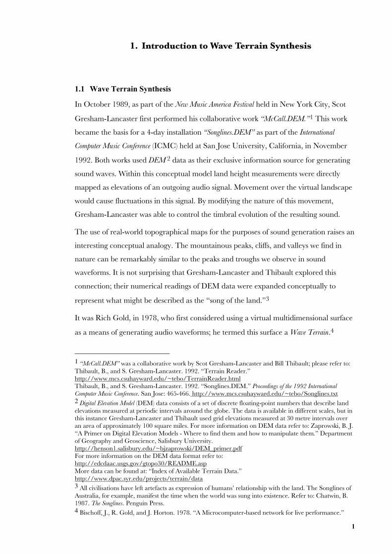
In October 1989, as part of the New Music America Festival held in New York City, Scot

Gresham-Lancaster first performed his collaborative work “McCall.DEM.”1 This work

became the basis for a 4-day installation “Songlines.DEM” as part of the International

Computer Music Conference (ICMC) held at San Jose University, California, in November

1992. Both works used DEM 2 data as their exclusive information source for generating

sound waves. Within this conceptual model land height measurements were directly

mapped as elevations of an outgoing audio signal. Movement over the virtual landscape

would cause fluctuations in this signal. By modifying the nature of this movement,

Gresham-Lancaster was able to control the timbral evolution of the resulting sound.

The use of real-world topographical maps for the purposes of sound generation raises an

interesting conceptual analogy. The mountainous peaks, cliffs, and valleys we find in

nature can be remarkably similar to the peaks and troughs we observe in sound

waveforms. It is not surprising that Gresham-Lancaster and Thibault explored this

connection; their numerical readings of DEM data were expanded conceptually to

represent what might be described as the “song of the land.”3

It was Rich Gold, in 1978, who first considered using a virtual multidimensional surface

as a means of generating audio waveforms; he termed this surface a Wave Terrain.4

1 “McCall.DEM” was a collaborative work by Scot Gresham-Lancaster and Bill Thibault; please refer to:Thibault, B., and S. Gresham-Lancaster. 1992. “Terrain Reader.”http://www.mcs.csuhayward.edu/~tebo/TerrainReader.htmlThibault, B., and S. Gresham-Lancaster. 1992. “Songlines.DEM.” Proceedings of the 1992 InternationalComputer Music Conference. San Jose: 465-466. http://www.mcs.csuhayward.edu/~tebo/Songlines.txt2 Digital Elevation Model (DEM) data consists of a set of discrete floating-point numbers that describe landelevations measured at periodic intervals around the globe. The data is available in different scales, but inthis instance Gresham-Lancaster and Thibault used grid elevations measured at 30 metre intervals overan area of approximately 100 square miles. For more information on DEM data refer to: Zaprowski, B. J.“A Primer on Digital Elevation Models - Where to find them and how to manipulate them.” Departmentof Geography and Geoscience, Salisbury University.http://henson1.salisbury.edu/~bjzaprowski/DEM_primer.pdfFor more information on the DEM data format refer to:http://edcdaac.usgs.gov/gtopo30/README.aspMore data can be found at: “Index of Available Terrain Data.”http://www.dpac.syr.edu/projects/terrain/data3 All civilisations have left artefacts as expression of humans’ relationship with the land. The Songlines ofAustralia, for example, manifest the time when the world was sung into existence. Refer to: Chatwin, B.1987. The Songlines. Penguin Press.4 Bischoff, J., R. Gold, and J. Horton. 1978. “A Microcomputer-based network for live performance.”

2

Within a year, Gold published a “Terrain Reader” program.5 In this implementation, a

travelling pointer moved rapidly over a virtual terrain stored in 256 bytes of a KIM-1

computer’s 1024 total bytes of memory. In 1989, Gresham-Lancaster and Thibault

extended on this model. Using half a million bytes of memory for their DEM data, they

used two Amiga computers that were each allocated audio and graphical processing

tasks respectively. The graphical renderings proved complementary to the process,

allowing the audience to observe the moving pointers traveling over the terrain map in

realtime.

1.1.1 Conceptual Definition

Nelson has described Wave Terrain Synthesis as being analogous to the rolling of a ball

over a hilly landscape,6 though of course we are not dealing with a system concerned

with physical world parameters such as gravity, friction, and inertia. Both the terrain

and the path by which the ball moves over the landscape are defined completely

independently of one another. However, both structures are mutually dependent in

finding an outcome, and any changes that occur in either system affect the resulting

waveform signal.

For the purposes of consistency, we will refer to the movement of this ball as the

trajectory7. By establishing further control over the movement we can control how and

where the trajectory passes through regions of the contour map. For example, we might

decide to focus more specifically on a mountainous region of the terrain. Generally, the

greater the difference between mountaintop and the base of an adjacent valley, the

greater the intensity of the resulting signal;8 it can also be said that the steeper and more

mountainous the region, the greater the spectral complexity. On the other hand, if the

region were a flat desolate plane, it would result in a signal of low dynamic intensity. If

this plane were completely flat, we would be left with silence: a signal of no energy.

Certainly, the topographical representation proves to be a fitting analogy to the process.

In practice, however, most documented approaches to Wave Terrain Synthesis have not

Computer Music Journal 2(3): 24-29.5 Gold, R. 1979. “A Terrain Reader.” In C. P. Morgan, ed. The BYTE Book of Computer Music. BytePublications, Petersborough, NH.6 Nelson, J. C. 2000. “Understanding and Using Csound’s GEN Routines.” In R. Boulanger, ed. TheCSound Book: perspectives in software synthesis, sound design, signal processing, and programming. Cambridge,Massachusetts: MIT Press: 65-97.7 Curtis Roads has termed this scan an orbit. Since this term implies both an elliptical function, and theidea of periodicity, we will use the term trajectory since it is more indiscriminatory. Refer to: Roads, C., etal. 1996. The Computer Music Tutorial. Cambridge, Massachusetts: MIT Press: 163.8 An increase in signal intensity due to an increase in maxima and minima points of amplitude.

3

only used topographical mappings as the basis for their terrain contours but a whole

variety of multi-parameter functions and maps. In fact, most implementations have used

simple mathematical functions in the hope of establishing a general theory for Wave

Terrain Synthesis.9

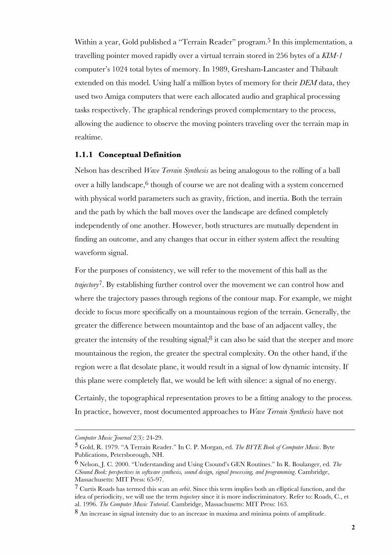
Figure 1. GTOPO30 is aglobal data set coveringthe full extent of latitude90 degrees south to 90degrees north, and thefull extent of longitudefrom 180 degrees west to180 degrees east.Horizontal grid spacingis 30-arc seconds(0.008333333333333degrees) resulting in aDEM of dimensions21,600 rows and 43,200columns. Data isconventionally stored in16-bit signed integerformat.10

1.1.2 Theoretical Definition

As we have already established, Wave Terrain Synthesis relies on two independent

structures for generating sound: a terrain function and a trajectory signal. The trajectory

defines a series of coordinates that are used to read from a terrain function of n

variables, for example f x1, x2 ,..., xn( ) . If this terrain function is stored in memory, the

process is synonymous to Wavetable Lookup11 where amplitude values are accessed by a

streaming series of index values.12 Wave Terrain Synthesis extends upon this principle to

the scanning of multidimensional surfaces using multi-signal streams. Most common

approaches to Wave Terrain Synthesis use surfaces described by functions of two variables,

that is f x, y( ) .13

9 The advantage of using simple mathematical functions meant that it was possible to predict exactly theoutput waveform and spectrum generated by a given terrain. Roads, C., et al. 1996. The Computer MusicTutorial. Cambridge, Massachusetts: MIT Press: 164.10 For combinations of ocean bathymetric and land topographic maps, refer to: “Global ElevationDatabase.” http://www.ngdc.noaa.gov/11 Such as any digital sampling based technology including both single and multiple wavetable, waveterrain, and granular techniques.12 By convention, an indexed table of values is scanned by a linear trajectory generated by incrementingin the positive or negative direction. This is the fundamental basis of the “phase driven” oscillator. Forsmall wavetables that are driven by the periodic repetition of a trajectory, a static waveform will result.13 Wave Terrain Synthesis has been termed Two-Variable Function Synthesis (Mitsuhashi 1982, Borgonovo andHaus 1984, 1986). It has also been termed simply Terrain Mapping Synthesis (Mikelson 2000).

4

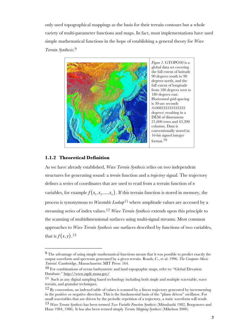
Figure 2a. A wave terrain functiondefined by the polynomialf x, y( )= 53 x− y( ) x2 −1( ) y2 −1( )

Figure 2b. A wave terrain defined by theequation f x, y( )=sin 2π x( )sin 2π y( )

The equations describing the trajectory curve define the temporal evolution of the

system. This curve has been typically expressed as a set of n Parametric equations

specifying the coordinates (x, y)with respect to time (t). For example, a function of two

variables would need to be driven by two trajectory signals defined x = f (t) and

y = g(t) . Parameters are determined independently from one another within the n-

dimensional space, allowing for an infinite variety of trajectories: straight lines, curved

lines, random walks and chaotic attractors are some of the many geometric phenomena

applicable to Wave Terrain Synthesis.14

Figure 3a. An elliptical trajectorydefined by the parametric equations

x = sin 2π t+π5⎛⎝⎜

⎞⎠⎟ , y = sin 2π t( )

Figure 3b. A linear trajectorydefined by the parametric

equations x =π t5 , y = t − 1

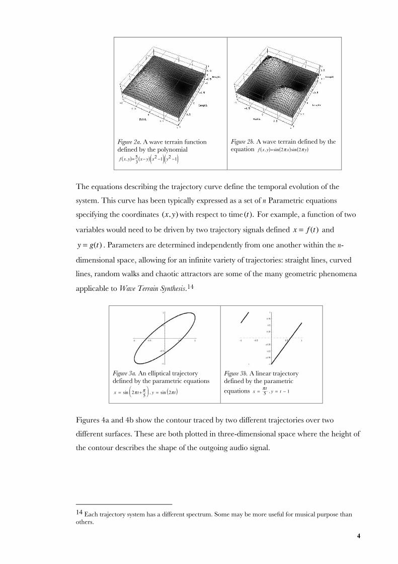
Figures 4a and 4b show the contour traced by two different trajectories over two

different surfaces. These are both plotted in three-dimensional space where the height of

the contour describes the shape of the outgoing audio signal.

14 Each trajectory system has a different spectrum. Some may be more useful for musical purpose thanothers.

5

Figure 4a. A 3D parametric plot of thewave terrain shown in Figure 2atraced by the trajectory found inFigure 3a

Figure 4b. A 3D parametric plot ofthe wave terrain shown in Figure 2btraced by the trajectory found inFigure 3b

By substituting the terrain function variables with their respective parametric trajectory

equations, we can obtain a mathematical function describing the resulting waveform

with respect to time (t).

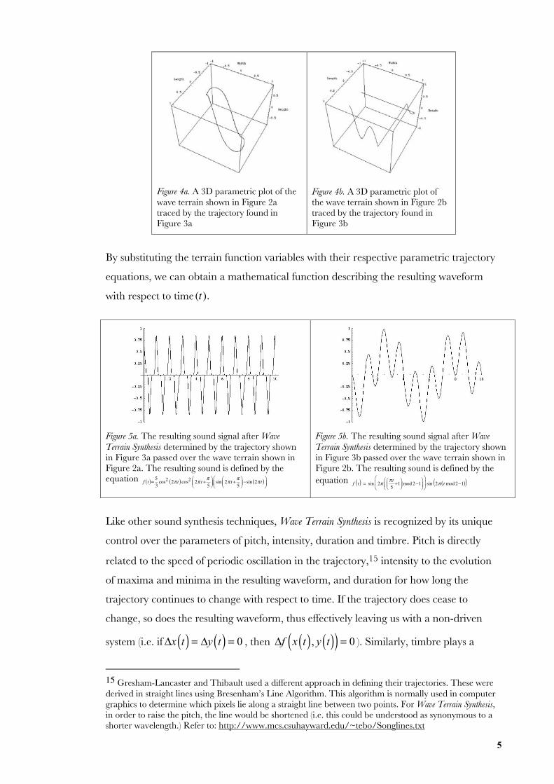
Figure 5a. The resulting sound signal after WaveTerrain Synthesis determined by the trajectory shownin Figure 3a passed over the wave terrain shown inFigure 2a. The resulting sound is defined by theequation f t( )= 5

3cos2 2π t( ) cos2 2π t+

π5

⎛⎝⎜

⎞⎠⎟ sin 2π t+

π5

⎛⎝⎜

⎞⎠⎟ −sin 2π t( )⎛

⎝⎜⎞⎠⎟

Figure 5b. The resulting sound signal after WaveTerrain Synthesis determined by the trajectory shownin Figure 3b passed over the wave terrain shown inFigure 2b. The resulting sound is defined by theequation f t( ) = sin 2π

π t5+1⎛

⎝⎜⎞⎠⎟ mod 2−1

⎛⎝⎜

⎞⎠⎟

⎛

⎝⎜

⎞

⎠⎟ sin 2π tmod 2−1( )( )

Like other sound synthesis techniques, Wave Terrain Synthesis is recognized by its unique

control over the parameters of pitch, intensity, duration and timbre. Pitch is directly

related to the speed of periodic oscillation in the trajectory,15 intensity to the evolution

of maxima and minima in the resulting waveform, and duration for how long the

trajectory continues to change with respect to time. If the trajectory does cease to

change, so does the resulting waveform, thus effectively leaving us with a non-driven

system (i.e. if Δx t( ) = Δy t( ) = 0 , then

Δf x t( ), y t( )( ) = 0 ). Similarly, timbre plays a

15 Gresham-Lancaster and Thibault used a different approach in defining their trajectories. These werederived in straight lines using Bresenham’s Line Algorithm. This algorithm is normally used in computergraphics to determine which pixels lie along a straight line between two points. For Wave Terrain Synthesis,in order to raise the pitch, the line would be shortened (i.e. this could be understood as synonymous to ashorter wavelength.) Refer to: http://www.mcs.csuhayward.edu/~tebo/Songlines.txt

6

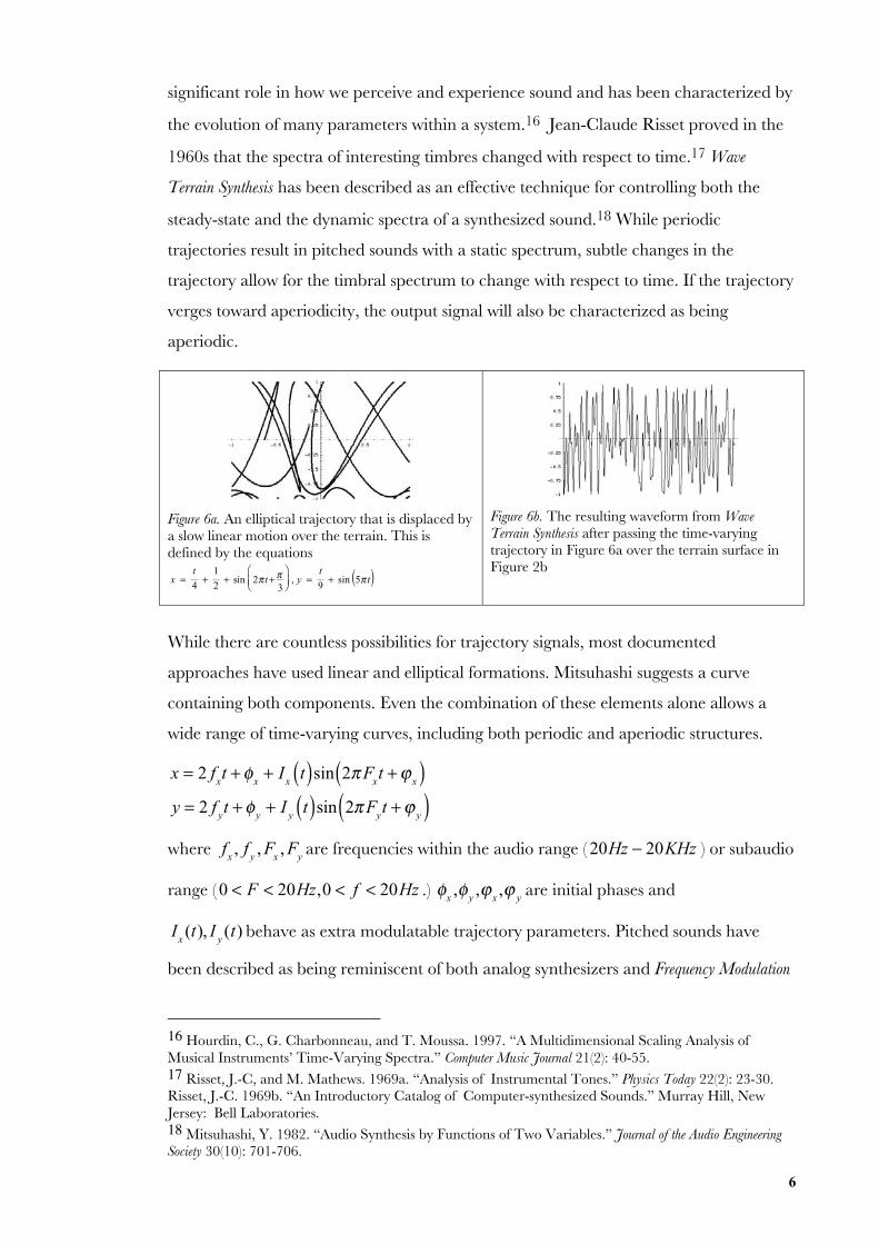
significant role in how we perceive and experience sound and has been characterized by

the evolution of many parameters within a system.16 Jean-Claude Risset proved in the

1960s that the spectra of interesting timbres changed with respect to time.17 Wave

Terrain Synthesis has been described as an effective technique for controlling both the

steady-state and the dynamic spectra of a synthesized sound.18 While periodic

trajectories result in pitched sounds with a static spectrum, subtle changes in the

trajectory allow for the timbral spectrum to change with respect to time. If the trajectory

verges toward aperiodicity, the output signal will also be characterized as being

aperiodic.

Figure 6a. An elliptical trajectory that is displaced bya slow linear motion over the terrain. This isdefined by the equations

x =

t

4+

1

2+ sin 2π t+π

3

⎛⎝⎜

⎞⎠⎟ , y =

t

9+ sin 5π t( )

Figure 6b. The resulting waveform from WaveTerrain Synthesis after passing the time-varyingtrajectory in Figure 6a over the terrain surface inFigure 2b

While there are countless possibilities for trajectory signals, most documented

approaches have used linear and elliptical formations. Mitsuhashi suggests a curve

containing both components. Even the combination of these elements alone allows a

wide range of time-varying curves, including both periodic and aperiodic structures.

x = 2 f

xt + φ

x+ I

xt( )sin 2πF

xt +ϕ

x( ) y = 2 f

yt + φ

y+ I

yt( )sin 2πF

yt +ϕ

y( )where

f

x, f

y, F

x, F

yare frequencies within the audio range ( 20Hz − 20KHz ) or subaudio

range ( 0 < F < 20Hz,0 < f < 20Hz .) φ

x,φ

y,ϕ

x,ϕ

yare initial phases and

I

x(t), I

y(t) behave as extra modulatable trajectory parameters. Pitched sounds have

been described as being reminiscent of both analog synthesizers and Frequency Modulation

16 Hourdin, C., G. Charbonneau, and T. Moussa. 1997. “A Multidimensional Scaling Analysis ofMusical Instruments’ Time-Varying Spectra.” Computer Music Journal 21(2): 40-55.17 Risset, J.-C, and M. Mathews. 1969a. “Analysis of Instrumental Tones.” Physics Today 22(2): 23-30.Risset, J.-C. 1969b. “An Introductory Catalog of Computer-synthesized Sounds.” Murray Hill, NewJersey: Bell Laboratories.18 Mitsuhashi, Y. 1982. “Audio Synthesis by Functions of Two Variables.” Journal of the Audio EngineeringSociety 30(10): 701-706.

7

Synthesis. Many of these sounds have been characterized as being drone like, pulsing, and

harmonically rich.19 Depending on the terrain surface, unpitched sounds have been as

various as sounds suggestive of glitch and noise based sample loops, as well as textures

much like rain, cracking rocks, thunder, electrical intermittent noises, and insects.20

1.1.2.1 Continuous Maps

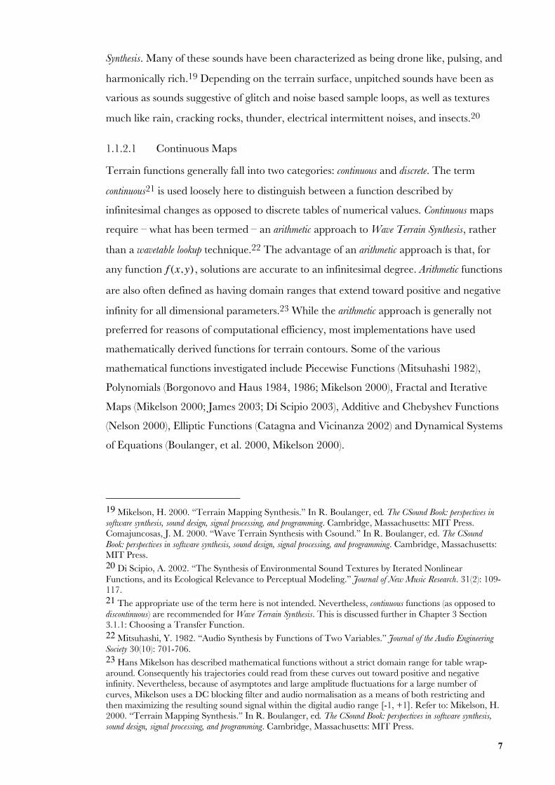
Terrain functions generally fall into two categories: continuous and discrete. The term

continuous21 is used loosely here to distinguish between a function described by

infinitesimal changes as opposed to discrete tables of numerical values. Continuous maps

require – what has been termed – an arithmetic approach to Wave Terrain Synthesis, rather

than a wavetable lookup technique.22 The advantage of an arithmetic approach is that, for

any function f (x, y) , solutions are accurate to an infinitesimal degree. Arithmetic functions

are also often defined as having domain ranges that extend toward positive and negative

infinity for all dimensional parameters.23 While the arithmetic approach is generally not

preferred for reasons of computational efficiency, most implementations have used

mathematically derived functions for terrain contours. Some of the various

mathematical functions investigated include Piecewise Functions (Mitsuhashi 1982),

Polynomials (Borgonovo and Haus 1984, 1986; Mikelson 2000), Fractal and Iterative

Maps (Mikelson 2000; James 2003; Di Scipio 2003), Additive and Chebyshev Functions

(Nelson 2000), Elliptic Functions (Catagna and Vicinanza 2002) and Dynamical Systems

of Equations (Boulanger, et al. 2000, Mikelson 2000).

19 Mikelson, H. 2000. “Terrain Mapping Synthesis.” In R. Boulanger, ed. The CSound Book: perspectives insoftware synthesis, sound design, signal processing, and programming. Cambridge, Massachusetts: MIT Press.Comajuncosas, J. M. 2000. “Wave Terrain Synthesis with Csound.” In R. Boulanger, ed. The CSoundBook: perspectives in software synthesis, sound design, signal processing, and programming. Cambridge, Massachusetts:MIT Press.20 Di Scipio, A. 2002. “The Synthesis of Environmental Sound Textures by Iterated NonlinearFunctions, and its Ecological Relevance to Perceptual Modeling.” Journal of New Music Research. 31(2): 109-117.21 The appropriate use of the term here is not intended. Nevertheless, continuous functions (as opposed todiscontinuous) are recommended for Wave Terrain Synthesis. This is discussed further in Chapter 3 Section3.1.1: Choosing a Transfer Function.22 Mitsuhashi, Y. 1982. “Audio Synthesis by Functions of Two Variables.” Journal of the Audio EngineeringSociety 30(10): 701-706.23 Hans Mikelson has described mathematical functions without a strict domain range for table wrap-around. Consequently his trajectories could read from these curves out toward positive and negativeinfinity. Nevertheless, because of asymptotes and large amplitude fluctuations for a large number ofcurves, Mikelson uses a DC blocking filter and audio normalisation as a means of both restricting andthen maximizing the resulting sound signal within the digital audio range [-1, +1]. Refer to: Mikelson, H.2000. “Terrain Mapping Synthesis.” In R. Boulanger, ed. The CSound Book: perspectives in software synthesis,sound design, signal processing, and programming. Cambridge, Massachusetts: MIT Press.

8

Figure 7. A wave terrain characterized with an infinitedomain range defined by the equation

f x, y( )= cos 12 sin( x−1( )2 + y2 −4 tan−1y+1x

⎛⎝⎜

⎞⎠⎟

⎛⎝⎜

⎞⎠⎟

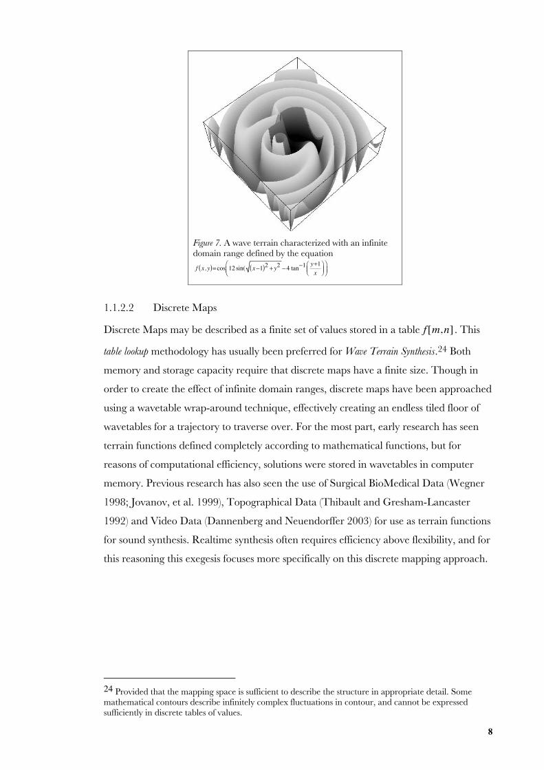
1.1.2.2 Discrete Maps

Discrete Maps may be described as a finite set of values stored in a table f [m,n] . This

table lookup methodology has usually been preferred for Wave Terrain Synthesis.24 Both

memory and storage capacity require that discrete maps have a finite size. Though in

order to create the effect of infinite domain ranges, discrete maps have been approached

using a wavetable wrap-around technique, effectively creating an endless tiled floor of

wavetables for a trajectory to traverse over. For the most part, early research has seen

terrain functions defined completely according to mathematical functions, but for

reasons of computational efficiency, solutions were stored in wavetables in computer

memory. Previous research has also seen the use of Surgical BioMedical Data (Wegner

1998; Jovanov, et al. 1999), Topographical Data (Thibault and Gresham-Lancaster

1992) and Video Data (Dannenberg and Neuendorffer 2003) for use as terrain functions

for sound synthesis. Realtime synthesis often requires efficiency above flexibility, and for

this reasoning this exegesis focuses more specifically on this discrete mapping approach.

24 Provided that the mapping space is sufficient to describe the structure in appropriate detail. Somemathematical contours describe infinitely complex fluctuations in contour, and cannot be expressedsufficiently in discrete tables of values.

9

Figure 8. A wave terrain defined by a finite domain range using a table wrap-aroundtechnique at each boundary point. This effectively creates an infinitely tiled surface ofwavetables. Here we see a tiled terrain of wavetables determined by the equation

f x, y( )= x− y( ) x−1( ) x+1( ) y−1( ) y+1( )2

1.1.3 Previously Documented Research

Wave Terrain Synthesis was initially investigated by a small number of computer music

researchers, including Gold, through consultation with Leonard Cottrell,25

Mitsuhashi,26 and Borgonovo and Haus.27 Most of this early research focussed on both

simple polynomial and trigonometric functions for use as terrain contours. Latter

research appears to have been more adventurous. Mikelson has used linear trajectories

over the Julia set.28 Di Scipio has used low frequency linear trajectories over solutions to

the nonlinear sine map model in Phase Space.29 Vittorio Cafagna and Domenico

Vicinanza have looked at Wave Terrain Synthesis using Jacobi’s sn u, cn u, and

Weierstrass’℘(z)elliptic functions.30 Not all of this research has been directed toward

25 Bischoff, J., R. Gold, and J. Horton. 1978. “A Microcomputer-based network for live performance.”Computer Music Journal 2(3): 24-29.26 Mitsuhashi, Y. 1982. “Audio Synthesis by Functions of Two Variables.” Journal of the Audio EngineeringSociety 30(10): 701-706.27 Borgonovo, A., and G. Haus. 1984. “Musical Sound Synthesis by means of Two-Variable Functions:experimental criteria and results.” In D. Wessel, ed. Proceedings of the 1984 International Computer MusicConference. San Francisco: International Computer Music Association. pp. 35-42.Borgonovo, A., and G. Haus. 1986. “Sound Synthesis by means of Two-Variable Functions: experimentalcriteria and results.” Computer Music Journal 10(4): 57-71.28 Mikelson, H. 1999. “Sound Generation with the Julia Set.” The Csound Magazine.http://www.csounds.com/ezine/summer1999/synthesis/29 The mapping of xn+1 = sin(rxn ) within the parameter space r versus x0 . The contour of the terrain

is determined by the solutions to xn , where n is the number of iterations applied. Refer to: Di Scipio, A.2002. “The Synthesis of Environmental Sound Textures by Iterated Nonlinear Functions, and itsEcological Relevance to Perceptual Modeling.” Journal of New Music Research. 31(2): 109-117.30 Cafagna, V., and D. Vicinanza. 2002. “Audio Synthesis by Means of Elliptic Functions.” Second

10

specific kinds of two-dimensional curves either; Nelson and Mikelson have both

experimented using higher-dimensional surfaces.31

While a great deal of focus has been spent on the exploration of various kinds of terrain

functions, less emphasis appears to have been placed on the choice of trajectory curve.

James discusses this situation, as well as a need for greater flexibility in terms of the way

in which trajectory structures are generated.32 On the whole they have been described

by linear and elliptical functions. Mikelson has also used various kinds of Polar

functions,33 and Hsu has experimented using a flexible interface in Max/MSP allowing a

user to draw their own trajectory curves and modify transformational parameters

interactively.34 Hsu’s interface was developed in combination with the Wacom Intuos2

graphics tablet and pen, a controller that seems to effectively complement this process.

All of the above approaches to Wave Terrain Synthesis extend from the idea that timbral

evolution is controlled entirely by movement and transformation in the trajectory signal.

Curtis Roads, on the other hand, alludes to the idea of time-varying terrain structures.

In this situation, we could imagine a trajectory tracing the curves of an undulating

surface.35 This has become the basis of another sound generative technique known as

Scanned Synthesis.36 In practice, this process uses a dynamical wavetable that describes an

evolving system, most commonly a physical model, although inputs from a video camera

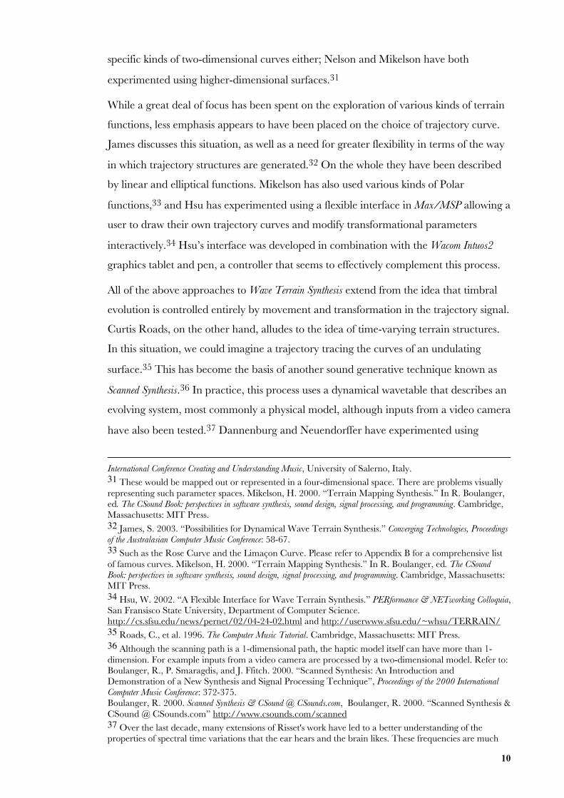
have also been tested.37 Dannenburg and Neuendorffer have experimented using

International Conference Creating and Understanding Music, University of Salerno, Italy.31 These would be mapped out or represented in a four-dimensional space. There are problems visuallyrepresenting such parameter spaces. Mikelson, H. 2000. “Terrain Mapping Synthesis.” In R. Boulanger,ed. The CSound Book: perspectives in software synthesis, sound design, signal processing, and programming. Cambridge,Massachusetts: MIT Press.32 James, S. 2003. “Possibilities for Dynamical Wave Terrain Synthesis.” Converging Technologies, Proceedingsof the Australasian Computer Music Conference: 58-67.33 Such as the Rose Curve and the Limaçon Curve. Please refer to Appendix B for a comprehensive listof famous curves. Mikelson, H. 2000. “Terrain Mapping Synthesis.” In R. Boulanger, ed. The CSoundBook: perspectives in software synthesis, sound design, signal processing, and programming. Cambridge, Massachusetts:MIT Press.34 Hsu, W. 2002. “A Flexible Interface for Wave Terrain Synthesis.” PERformance & NETworking Colloquia,San Fransisco State University, Department of Computer Science.http://cs.sfsu.edu/news/pernet/02/04-24-02.html and http://userwww.sfsu.edu/~whsu/TERRAIN/35 Roads, C., et al. 1996. The Computer Music Tutorial. Cambridge, Massachusetts: MIT Press.36 Although the scanning path is a 1-dimensional path, the haptic model itself can have more than 1-dimension. For example inputs from a video camera are processed by a two-dimensional model. Refer to:Boulanger, R., P. Smaragdis, and J. Ffitch. 2000. “Scanned Synthesis: An Introduction andDemonstration of a New Synthesis and Signal Processing Technique”, Proceedings of the 2000 InternationalComputer Music Conference: 372-375.Boulanger, R. 2000. Scanned Synthesis & CSound @ CSounds.com, Boulanger, R. 2000. “Scanned Synthesis &CSound @ CSounds.com” http://www.csounds.com/scanned37 Over the last decade, many extensions of Risset's work have led to a better understanding of theproperties of spectral time variations that the ear hears and the brain likes. These frequencies are much

11

images of wave motion in a water bowl captured by a digital video recorder; from here

they used variations in color intensity as the basis of contour maps for Wave Terrain

Synthesis.38 Independent research into time-varying surfaces performed by Hans

Mikelson has seen the utilization of dynamical systems as a means of modulating

parameters of a terrain function arithmetically.39 Other research by James has discussed

the potential use of various other kinds of dynamical processes for Wave Terrain Synthesis,

including successive iterations of the Mandelbrot, two-dimensional cellular automata,

and video feedback.40 One of the more significant developments must be Dan

Overholt’s work in building the MATRIX controller. With an array of 144 continuous

controllers, this device is capable of dynamically generating and distorting the geometry

of two-dimensional contour maps.41

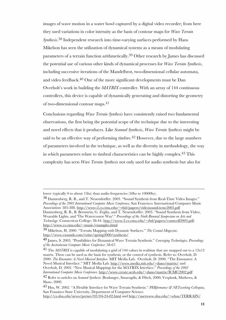
Conclusions regarding Wave Terrain Synthesis have consistently raised two fundamental

observations, the first being the potential scope of the technique due to the interesting

and novel effects that it produces. Like Scanned Synthesis, Wave Terrain Synthesis might be

said to be an effective way of performing timbre.42 However, due to the large numbers

of parameters involved in the technique, as well as the diversity in methodology, the way

in which parameters relate to timbral characteristics can be highly complex.43 This

complexity has seen Wave Terrain Synthesis not only used for audio synthesis but also for

lower (typically 0 to about 15hz) than audio frequencies (50hz to 10000hz).38 Dannenberg, R. B., and T. Neuendorffer. 2003. “Sound Synthesis from Real-Time Video Images.”Proceedings of the 2003 International Computer Music Conference, San Francisco: International Computer MusicAssociation: 385-388. http://www-2.cs.cmu.edu/~rbd/papers/videosound-icmc2003.pdfDannenberg, R. B., B. Bernstein, G. Zeglin, and T. Neuendorffer. 2003. “Sound Synthesis from Video,Wearable Lights, and 'The Watercourse Way'.” Proceedings of the Ninth Biennial Symposium on Arts andTechnology. Connecticut College: 38-44. http://www-2.cs.cmu.edu/~rbd/papers/conncoll2003.pdf;http://www.cs.cmu.edu/~music/examples.html39 Mikelson, H. 2000. “Terrain Mapping with Dynamic Surfaces.” The Csound Magazine.http://www.csounds.com/ezine/spring2000/synthesis/40 James, S. 2003. “Possibilities for Dynamical Wave Terrain Synthesis.” Converging Technologies, Proceedingsof the Australasian Computer Music Conference: 58-67.41 The MATRIX is capable of modulating a grid of 144 values in realtime that are mapped out to a 12x12matrix. These can be used as the basis for synthesis, or the control of synthesis. Refer to: Overholt, D.2000. The Emonator: A Novel Musical Interface. MIT Media Lab. Overholt, D. 2000. “The Emonator: ANovel Musical Interface.” MIT Media Lab. http://www.media.mit.edu/~dano/matrix/ andOverholt, D. 2002. “New Musical Mappings for the MATRIX Interface.” Proceedings of the 2002International Computer Music Conference. http://www.create.ucsb.edu/~dano/matrix/ICMC2002.pdf42 Refer to articles on Scanned Synthesis (Boulanger, Smaragdis, & Ffitch, 2000; Verplank, Mathews, &Shaw, 2000)43 Hsu, W. 2002. “A Flexible Interface for Wave Terrain Synthesis.” PERformance & NETworking Colloquia,San Fransisco State University, Department of Computer Science.http://cs.sfsu.edu/news/pernet/02/04-24-02.html and http://userwww.sfsu.edu/~whsu/TERRAIN/

12

the synthesis of control structures.44 The technique has also been considered a useful

system applicable to medicine where audio feedback may be used in surgery.45

The second observation has been the need for more thorough research in order to

establish an overall conceptual and scientific theory detailing the extended practical use

of such a technique. On a conceptual level, Anderson Mills and Rodolfo Coelho de

Souza describe Wave Terrain Synthesis as being gestural by nature due to the direct

mapping of the multi-directional parameter space to the sound synthesis process itself.46

They also discuss the limitations in existing implementations and the need for more

varied terrain functions, more complex orbital paths, as well as the need for further

knowledge with respect to the use of multiple trajectories for multichannel output. It

seems that some conclusions have shown signs of contradiction regarding their

definitions of Wave Terrain Synthesis. Depending on the methodology, both the concept as

well as the results of this technique seem to have hovered somewhere within the realms

of Wavetable Lookup, Wavetable Interpolation and Vector Synthesis, Amplitude Modulation Synthesis,

Frequency Modulation Synthesis, Ring Modulation Synthesis, Waveshaping and Distortion Synthesis,

Additive Synthesis, Functional Iteration Synthesis47 and Scanned Synthesis.48 If this is the case,

there begs the question: what exactly might Wave Terrain Synthesis actually be? Perhaps it

is fair to assume, due to its multi-parameter structure, that it potentially represents a

“synthesis” of elements drawn from all of these techniques.

1.1.4 Previous Implementations

Nearly all documented implementations of Wave Terrain Synthesis have been developed

using software systems rather than hardware. The first available code listings were

developed and published by both R. Gold, and Borgonovo and Haus. More recently

44 Sedes, A., B. Courribet, and J.-B. Thiébaut. 2004. “The Visualisation of Sound to Real-TimeSonification: different prototypes in the Max/MSP/Jitter environment.” Proceedings of the 2004 InternationalComputer Music Conference. Miami, USA. http://jbthiebaut.free.fr/visualization_of_sound.pdf45 The rigid body angle of the instrument is measured with respect to the surface of the anatomicalobject. This angle determines the angle of the terrain surface for Wave Terrain Synthesis with an ellipticalfunction. The surgical instrument describes an angle to the anatomical surface. The wave terrain issampled relative to this angle.Wegner, K. 1998. “Surgical Navigation System and Method Using Audio Feedback.” ICAD. ComputerAided Surgery Incorporated, New York, U.S.A.http://www.icad.org/websiteV2.0/Conferences/ICAD98/papers/WEGNER.pdf46 Mills, A. and R. C. De Souza. 1999. “Gestural Sounds by Means of Wave Terrain Synthesis.” CongressoNacional da Sociedade Brasileira de Computação XIX.http://gsd.ime.usp.br/sbcm/1999/papers/Anderson_Mills.html47 Di Scipio, A. 2002. “The Synthesis of Environmental Sound Textures by Iterated NonlinearFunctions, and its Ecological Relevance to Perceptual Modeling.” Journal of New Music Research. 31(2): 109-117.48 James, S. 2003. “Possibilities for Dynamical Wave Terrain Synthesis.” Converging Technologies, Proceedings

13

Pinkston, Mikelson, Nelson, and Comajuncosas have published code in association with

the readily available Csound, a freeware programming application interface (API) that

accompanies a far-reaching community of computer music enthusiasts who share their

work online. This language has also recently seen the inclusion of a basic Wave Terrain

Synthesis opcode within canonical version 4.19 by Matthew Gillard.49 Other

implementations include the terrain~ object as part of the PeRColate library for

Max/MSP/Nato and Pure Data,50 the 2d.wave~ object bundled with Max/MSP,51 the

waveTerrain LADSPA plugin for Linux systems,52 and Gravy for Pluggo.53 While the

implementations listed here are all software based, Wave Terrain Synthesis has also been

tested using hardware such as the Nord Modular54 and the Fairlight55 platform.

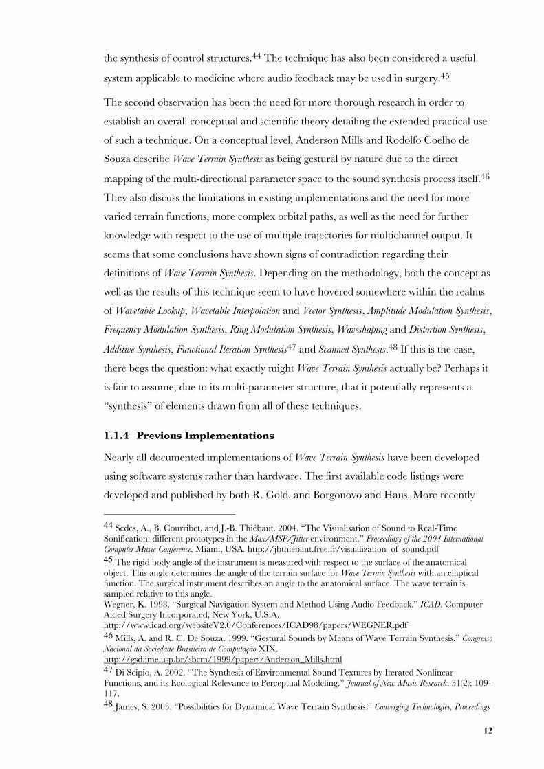
1.1.4.1 LADSPA Plugin Architecture for Linux Systems

Probably the simplest implementation is Steve Harris’ waveTerrain56 LADSPA plugin. In

this implementation, Harris uses a fixed terrain function defined by

f x, y( ) = x − y( ) x −1( ) x +1( ) y −1( ) y +1( ) . The plugin allows one to control the x and y

trajectory signals at audio or control rate, their transformation in scale

(multiplication/division), and transposition or translation (addition/subtraction).

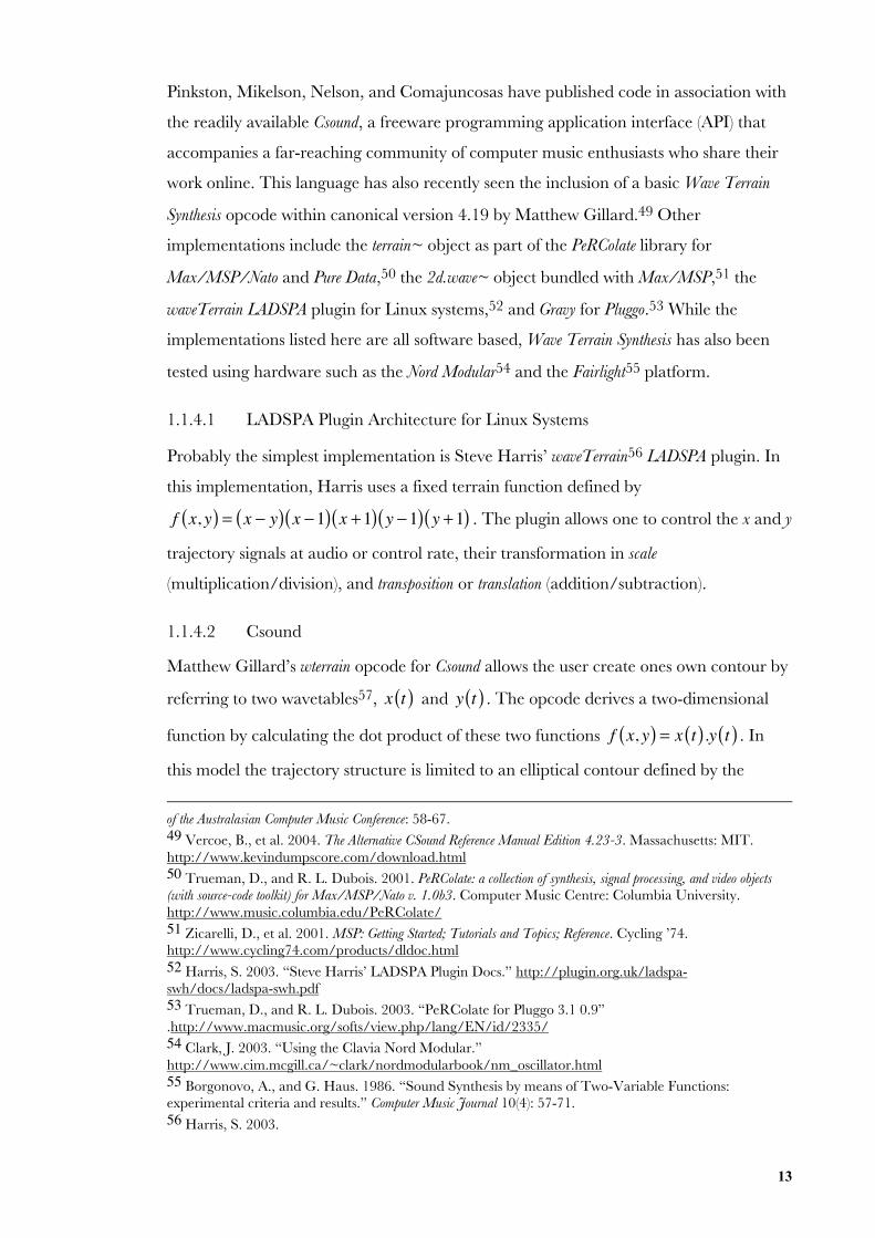
1.1.4.2 Csound

Matthew Gillard’s wterrain opcode for Csound allows the user create ones own contour by

referring to two wavetables57, x t( ) and y t( ) . The opcode derives a two-dimensional

function by calculating the dot product of these two functions f x, y( ) = x t( ).y t( ) . In

this model the trajectory structure is limited to an elliptical contour defined by the

of the Australasian Computer Music Conference: 58-67.49 Vercoe, B., et al. 2004. The Alternative CSound Reference Manual Edition 4.23-3. Massachusetts: MIT.http://www.kevindumpscore.com/download.html50 Trueman, D., and R. L. Dubois. 2001. PeRColate: a collection of synthesis, signal processing, and video objects(with source-code toolkit) for Max/MSP/Nato v. 1.0b3. Computer Music Centre: Columbia University.http://www.music.columbia.edu/PeRColate/51 Zicarelli, D., et al. 2001. MSP: Getting Started; Tutorials and Topics; Reference. Cycling ’74.http://www.cycling74.com/products/dldoc.html52 Harris, S. 2003. “Steve Harris’ LADSPA Plugin Docs.” http://plugin.org.uk/ladspa-swh/docs/ladspa-swh.pdf53 Trueman, D., and R. L. Dubois. 2003. “PeRColate for Pluggo 3.1 0.9”.http://www.macmusic.org/softs/view.php/lang/EN/id/2335/54 Clark, J. 2003. “Using the Clavia Nord Modular.”http://www.cim.mcgill.ca/~clark/nordmodularbook/nm_oscillator.html55 Borgonovo, A., and G. Haus. 1986. “Sound Synthesis by means of Two-Variable Functions:experimental criteria and results.” Computer Music Journal 10(4): 57-71.56 Harris, S. 2003.

14

equations x = α x cos 2πFt( ) + φx and y = α y cos 2πFt( ) + φy . One has control over the

parameters of scale, α x ,α y , and the translation, φx ,φy , of this function in both x and y

dimensions. The frequency of the trajectory is controlled by a global parameter F .

1.1.4.3 PD and Max/MSP

The terrain~58 object for Max/MSP and PD, as well as the 2d.wave~ object for Max/MSP,

split a waveform into a series of frames.59 These are each linearly interpolated in order to

create a two-dimensional surface. Of the implementations described thus far, terrain~

and 2d.wave~ provide the most freedom regarding both the nature of the terrain and

trajectory contours. The terrain is derived from a standard audio wavetable, and the

trajectory may be programmed to function exactly as the user prefers utilizing any of the

audio signal processing functions available within Max/MSP or PD.

1.1.4.4 Pluggo

Gravy and Gravy_noSync may be found as part of the Percolate60 freeware library for Pluggo.

This implementation has been setup as a live performance plugin. Based on the same

principles as terrain~ and 2d.wave~, the tool allows for live realtime audio sampling,

taking up to five seconds of audio at any one time. This audio is cut up into frames and

interpolated to generate a terrain function. Unlike the terrain~ and 2d.wave~ objects for

Max/MSP and PD, however, the user has limited control over the nature of trajectory

structures. Nevertheless, one can still control both how fast the plugin moves through

each discrete slice, and how fast the plugin crossfades between the different slices held in

memory.

This implementation includes a useful parameter for switching between real mode and

oscillator mode. Oscillator mode is the conventional approach to Wave Terrain Synthesis where

one uses a high frequency trajectory that determines the pitch. Real mode is where the

57 Known as f-tables or function tables in Csound.58 PeRColate is an open-source distribution of a variety of synthesis and signal processing algorithms forMax/MSP.59 Terrain functions are defined in piecewise fashion according to the number of audio frames. In theterrain~ scenario, these are scaled according to the “fixed” sample window size. In 2d.wave~, this scale isvariably dependent on the frame size and the overall start and end points of the sample used. The framesize is automatically determined by the sample length in 2d.wave~ if the start and end points both remainat 0 or the same value (depending on the buffer~ size, or the length of the entire sample). Alternatively, theuser may choose to specify start and end points for the region, which is then divided up according to thespecified frame number.60 Trueman, D., and R. L. Dubois. 2003. “PeRColate for Pluggo 3.1 0.9”.http://www.macmusic.org/softs/view.php/lang/EN/id/2335/

15

frequency is determined by the wavetable itself by driving the system with a low

frequency linear trajectory; this approach is more as one would expect from a traditional

sampling instrument.

1.1.5 The Aim of this Research

The aim of this research is to settle on a flexible methodology for Wave Terrain Synthesis,

develop upon existing methodology for the deriving of terrain and trajectory structures,

and to construct a realtime polyphonic instrument that reflects the primary aim of

developing a powerful, expressive and flexible sound design tool. This instrument should

exhibit a variety in methodology in both the way in which terrain and trajectory systems

are derived, as well as the parameters involved in geometrically and arithmetically

transforming them. This research also documents some testing of new processing

methods and control parameters that may be useful for Wave Terrain Synthesis.

1.2 The Development of a Realtime Wave Terrain Sound Synthesis Instrument

It seems that in the wake of efficient and versatile models such as Frequency Modulation

Synthesis and sound sampling during the 1980s, Wave Terrain Synthesis might have

appeared rather novel; it was largely overlooked due to a lack of knowledge about the

technique and how to control it effectively. What is more, without public accessibility to

pre-programmed hardware tools for realtime control, sound generation was limited to a

small number of non-realtime experiments using computer software. Nevertheless, with

realtime software sound synthesis being as much a reality as it is today, experiments in

Wave Terrain Synthesis seem to have become more prevalent. It is now a possibility for

practitioners to build experimental synthesis systems, create a series of results, and then

ask the appropriate questions later. While much of synthesis relies on specific functional

algorithms, Wave Terrain Synthesis is not entirely bound by any specific functional models;

it may be approached in a myriad of ways. Certainly, it is reasonable to say that it has

been the unpredictable and experimental nature of the technique that has attracted

curiosity among synthesists, resulting in its renewed popularity; though it has only been

due to the proliferation of tools to build such a model that this situation has eventuated.

On the whole, publicly available implementations explore only a single aspect of Wave

Terrain Synthesis. It needs to be stated that by using only a single methodology, one limits

the sonic potential for such a model. Publicly available implementations certainly do not

reflect the diversity of research in the technique. The paradox of Wave Terrain Synthesis is

that the method immediately places restrictions on the scope of the technique. Method

16

is generated by the means, and not necessarily vice versa, and the means are determined

by the idiosyncrasies of the programming system one is using to implement it.

Due to the unpredictable nature of the technique, it seems that a visual interface would

aid in understanding the multidimensional parameter spaces. By visualizing terrain and

trajectory structures, one is able to observe relationships and connections between the

structures and modify their control parameters, observing their transformation

accordingly in realtime as they are applied.

The practical construction of such an instrument introduces some problems. How does

one deal with issues of computational efficiency for realtime systems? Surely for a system

that is as multi-parameter as Wave Terrain Synthesis one may feel that a non-realtime

approach is more appropriate; non-realtime processing allows one to build models that

are more demanding than what processors are capable of dealing with in realtime.

Nevertheless, for this research project one of our primary objectives is to build a

realtime model. So for these intents and purposes, sacrifices must be made in order to

achieve the efficiency required for such a model. The development of a realtime

instrument presents some restrictions in methodology. What is the core construction of

such an instrument and how do these inner workings function? What kind of user

interface would be suitable for such a process? What is the best programming system to

use? Is computational efficiency largely a problem? If so, what sorts of methodological

compromises must be made in order to maintain flexibility and expressivity?

1.2.1 Technological Developments for Realtime Software Sound Synthesis

Realtime processing has become all the more possible due to both the increase in

processing speed of microprocessors, as well as the affordability of this technology. It was

only toward the end of the 1980s, when processors started to become fast enough to

perform floating-point processing on a set schedule, that realtime performance started to

become a reality.61 Realtime synthesis has opened a new door of possibilities for sound

synthesis in live performance. While CPU processing power remains the main

bottleneck for intensive processing tasks, computers are becoming all the more able to

deal with tasks originally unintended for realtime application. What is more, increasing

61 In 1990 Barry Vercoe introduced the realtime engine into Csound. Please refer to:Vercoe, B. The History of Csound. Vercoe, B. “The History of Csound.”http://www.csounds.com/cshistory/index.htmlVercoe, B., and D. Ellis. 1990. “Real-time Csound: Software synthesis with sensing and control.”Proceedings of the International Computer Music Conference. Glasgow: 209-211.

17

memory capacities are allowing fast access to audio, video, and other media in the

gigabyte.

Software sound compilers like Csound and Common Lisp Music have had a long history of

development that can be traced back to Max Mathew’s MUSIC series of programs.

While software like Max/MSP62, Jmax, and PD also stem from this development, these

software applications have three main differences that set them apart from the others:

realtime signal processing within a graphical patching environment and a more

comprehensive support for an object-oriented programming style.63 The object-oriented

programming style allows for the encapsulation64 of objects, as well as some powerful

programming techniques known as composition65, refinement66 and abstraction67.

With the addition of a vast library of objects efficiently designed for a wide range of

sound processing tasks, the user is put in an ideal position of ease of use whilst retaining

a high level of programming flexibility. The graphical patching style is an educational

way to learn about signal networks and messaging, and can help to graphically describe

a given process. Many of these applications also accompany a wide reaching community

of users that create their own objects68, abstractions, patches and instruments.

While there are many powerful freeware alternatives, Max/MSP has some extra features

that make it particularly useful. Max/MSP has a debugging messaging window to assist

the user in finding the source of errors within their patch. The program also provides

the user an option to compile a standalone application from an existing patch. The

environment is distributed with a large range of graphical user interface objects for

developing patcher GUIs. Patches may also contain embedded Java or Javascript code.

With the addition of the Pluggo library for Max/MSP, users may compile their own

patches for use as VST69, RTAS70, and Mac AU71 plugins. Furthermore, Max/MSP has

62 In 1995, the development of PD was started by Miller Puckette. Reusing the PD audio part, DavidZicarelli released late 1997 the MSP (“Max Signal Processing”) package for Max/Opcode that brings real-time synthesis and signal processing to Max/Opcode on Macintosh platforms; and more recently toWindows XP systems.63 “freesoftware@ircam.” http://freesoftware.ircam.fr/article.php3?id_article=5;Lazzarini, V 2002. “Audio Signal Processing and Object Oriented Systems.” Proceedings Dafx02, Hamburg.http://www.unibw-hamburg.de/EWEB/ANT/dafx2002/papers/DAFX02_Lazzarini_audio_object.pdf64 Lazzarini, V. 2002.65 The reuse of existing classes as attributes of a new class66 A derived class with extra support for a number of features not present in the base class67 The developing a model (or abstract) class that can serve as the basis for a number of complex andspecialized classes68 The user may code and compile objects in C using the included Software Development Kit (SDK)69 For Macintosh and Windows users; Virtual Studio Technology is a trademark of the Steinberg Corporation70 For Macintosh and Windows users; RTAS is a trademark of the Digidesign Corporation

18

extensive support for importing and exporting various media in a wide range of file

formats. This is a highly adaptable working ground for realtime synthesis and may

appeal to a wide range of computer music specialists and enthusiasts. For these reasons,

Max/MSP is the preferred choice for this research exegesis.

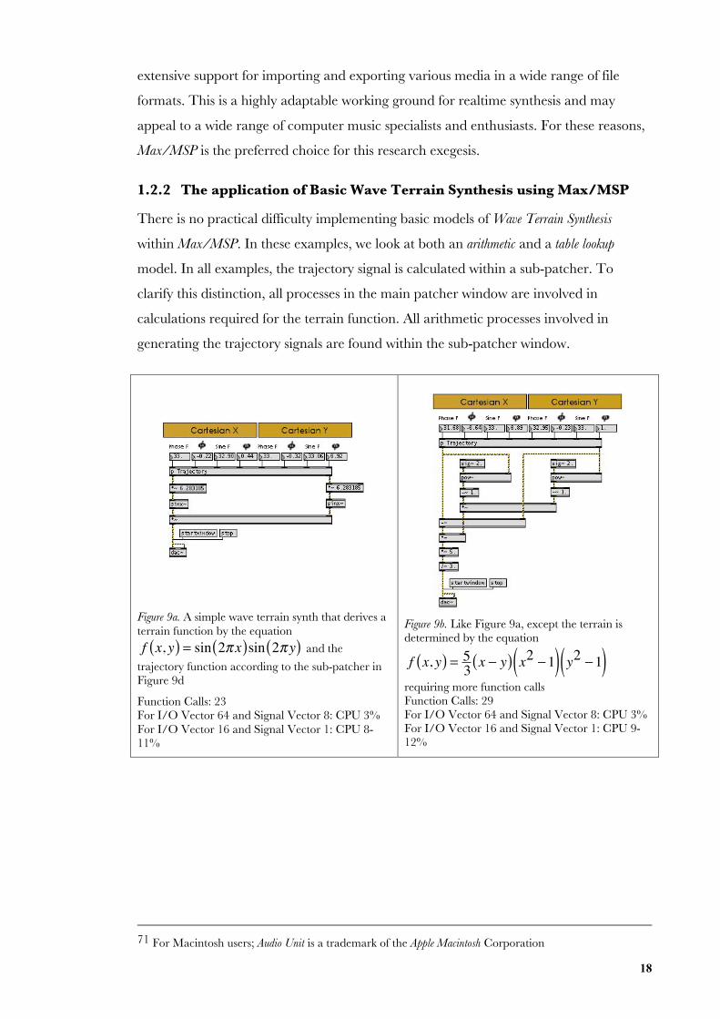
1.2.2 The application of Basic Wave Terrain Synthesis using Max/MSP

There is no practical difficulty implementing basic models of Wave Terrain Synthesis

within Max/MSP. In these examples, we look at both an arithmetic and a table lookup

model. In all examples, the trajectory signal is calculated within a sub-patcher. To

clarify this distinction, all processes in the main patcher window are involved in

calculations required for the terrain function. All arithmetic processes involved in

generating the trajectory signals are found within the sub-patcher window.

Figure 9a. A simple wave terrain synth that derives aterrain function by the equationf x, y( ) = sin 2π x( )sin 2π y( ) and the

trajectory function according to the sub-patcher inFigure 9d

Function Calls: 23For I/O Vector 64 and Signal Vector 8: CPU 3%For I/O Vector 16 and Signal Vector 1: CPU 8-11%

Figure 9b. Like Figure 9a, except the terrain isdetermined by the equation

f x, y( ) = 53 x − y( ) x2 −1( ) y2 −1( )requiring more function callsFunction Calls: 29For I/O Vector 64 and Signal Vector 8: CPU 3%For I/O Vector 16 and Signal Vector 1: CPU 9-12%

71 For Macintosh users; Audio Unit is a trademark of the Apple Macintosh Corporation

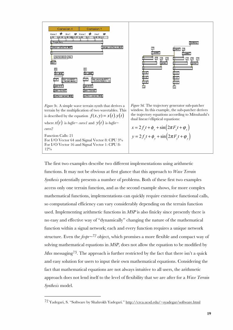
19

Figure 9c. A simple wave terrain synth that derives aterrain by the multiplication of two wavetables. Thisis described by the equation f (x, y) = x t( ).y t( )where x t( ) is buffer~ curve1 and y t( ) is buffer~

curve2

Function Calls: 21For I/O Vector 64 and Signal Vector 8: CPU 3%For I/O Vector 16 and Signal Vector 1: CPU 8-12%

Figure 9d. The trajectory generator sub-patcherwindow. In this example, the sub-patcher derivesthe trajectory equations according to Mitsuhashi’sdual linear/elliptical equations:

x = 2 fxt + φ

x+ sin 2πF

xt +ϕ

x( )y = 2 f

yt + φ

y+ sin 2πF

yt +ϕ

y( )

The first two examples describe two different implementations using arithmetic

functions. It may not be obvious at first glance that this approach to Wave Terrain

Synthesis potentially presents a number of problems. Both of these first two examples

access only one terrain function, and as the second example shows, for more complex

mathematical functions, implementations can quickly require extensive functional calls,

so computational efficiency can vary considerably depending on the terrain function

used. Implementing arithmetic functions in MSP is also finicky since presently there is

no easy and effective way of “dynamically” changing the nature of the mathematical

function within a signal network; each and every function requires a unique network

structure. Even the fexpr~72 object, which promises a more flexible and compact way of

solving mathematical equations in MSP, does not allow the equation to be modified by

Max messaging73. The approach is further restricted by the fact that there isn’t a quick

and easy solution for users to input their own mathematical equations. Considering the

fact that mathematical equations are not always intuitive to all users, the arithmetic

approach does not lend itself to the level of flexibility that we are after for a Wave Terrain

Synthesis model.

72 Yadegari, S. “Software by Shahrokh Yadegari.” http://crca.ucsd.edu/~syadegar/software.html

20

On the other hand, the wavetable lookup approach, as is found in the third example,

proves to be more adaptable and requires less function calls. Nevertheless, this lookup

process still requires at least one arithmetic stage, as well as a cubic interpolation routine

when reading from the lookup table.

For all of these approaches to Wave Terrain Synthesis, and similarly for the other

implementations in Csound, LADSPA, Max/MSP, and Pluggo, it would help to visually

observe the terrain function. In all of the above implementations, we have a situation

that is comparable to a “black box” technique: we have no knowledge about what is

happening underneath the surface. Without being able to visually observe the terrain

and trajectory structures, the user has an unguided idea about the process that is

unfolding. A visual interface may also benefit the accessibility of the technique. It could

be said that for more complex terrain and trajectory structures, it will aid in the

comprehension of complex evolutionary systems, and for the user to respond to these

processes interactively. Each terrain and trajectory structure introduces a new set of

parameters and variables, and developing upon this visual feedback mechanism will

establish the ability for the performer to respond to these unique parameter situations

more quickly and effectively.

1.2.3 The Jitter Extended Library for Max/MSP

While we have seen a proliferation in tools for software sound synthesis, in recent years

we have seen these systems expanded to allow for the realtime processing of all kinds of

media in multi-signal networks on the one machine. The thought of extensive

multidimensional signal processing techniques is not out of the question. Software such

as Max/MSP in conjunction with Jitter, as well as PD in conjunction with GEM74, allow

the user extensive freedom in designing their own interactive multimedia software due

to a universal matrix data format that can store any kind of data of various dimension.

These include video and still images, 3D geometry, text, spreadsheet data, and audio.

The narrowing bridge and amalgamation of these various multimedia forms is allowing

for more flexibility and innovation with regard to what creative artists wish to build for

multimedia purposes. It is possible to create a patch where the audio system controls the

video content, and vice versa.

73 An object in Max/MSP responds to a message sent to it; the response varies depending on the object74 GEM is a collection of externals that allow the user to render OpenGL graphics within PD, a programfor real-time audio processing by Miller Puckette. Originally written by Mark Danks, it is now maintainedby IOhannes m zmölnig. http://gem.iem.at/manual/Intro.html

21

Jitter allows the user to store data in a matrix; these matrices may have up to 32

dimensions, and up to 32 planes,75 and may store data in any one of the following data

types: char, long, float32, or float64.

DataType

Range Size(bytes)

Precision Description

char 28 = 0 – 255 1 1 Unsigned 8-bit Integer.Usual size of numberstaken from files andcameras, and written tofiles and windows.

long ±231 = -2147483648 –2147483647

4 1 Signed 32-bit Integer.Used for mostcomputations.

float32 ±10±38 4 23 bits(about 7digits)

32-bit floating point.

float64 ±10±308 8 52 bits(about 15digits)

64-bit floating point.

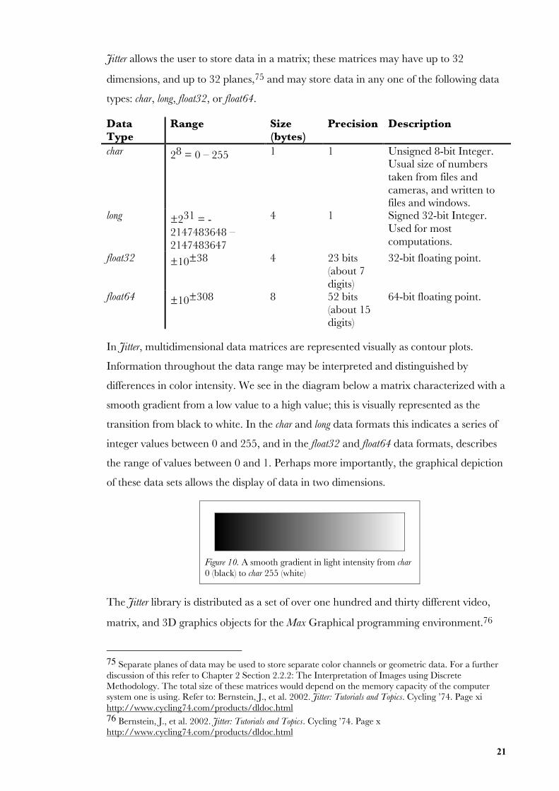
In Jitter, multidimensional data matrices are represented visually as contour plots.

Information throughout the data range may be interpreted and distinguished by

differences in color intensity. We see in the diagram below a matrix characterized with a

smooth gradient from a low value to a high value; this is visually represented as the

transition from black to white. In the char and long data formats this indicates a series of

integer values between 0 and 255, and in the float32 and float64 data formats, describes

the range of values between 0 and 1. Perhaps more importantly, the graphical depiction

of these data sets allows the display of data in two dimensions.

Figure 10. A smooth gradient in light intensity from char0 (black) to char 255 (white)

The Jitter library is distributed as a set of over one hundred and thirty different video,

matrix, and 3D graphics objects for the Max Graphical programming environment.76

75 Separate planes of data may be used to store separate color channels or geometric data. For a furtherdiscussion of this refer to Chapter 2 Section 2.2.2: The Interpretation of Images using DiscreteMethodology. The total size of these matrices would depend on the memory capacity of the computersystem one is using. Refer to: Bernstein, J., et al. 2002. Jitter: Tutorials and Topics. Cycling ’74. Page xihttp://www.cycling74.com/products/dldoc.html76 Bernstein, J., et al. 2002. Jitter: Tutorials and Topics. Cycling ’74. Page xhttp://www.cycling74.com/products/dldoc.html

22

The Jitter objects extend the functionality of Max/MSP with flexible means to generate,

analyse, process, and manipulate matrix data. For realtime video processing, audio-

visual interaction, as well as data visualization, Jitter is a perfect complement to Wave

Terrain Synthesis. With access to all Quicktime supported file formats, importing and

exporting capabilities, and DV input and output via Firewire, we have access to a

powerful series of tools for Wave Terrain Synthesis.

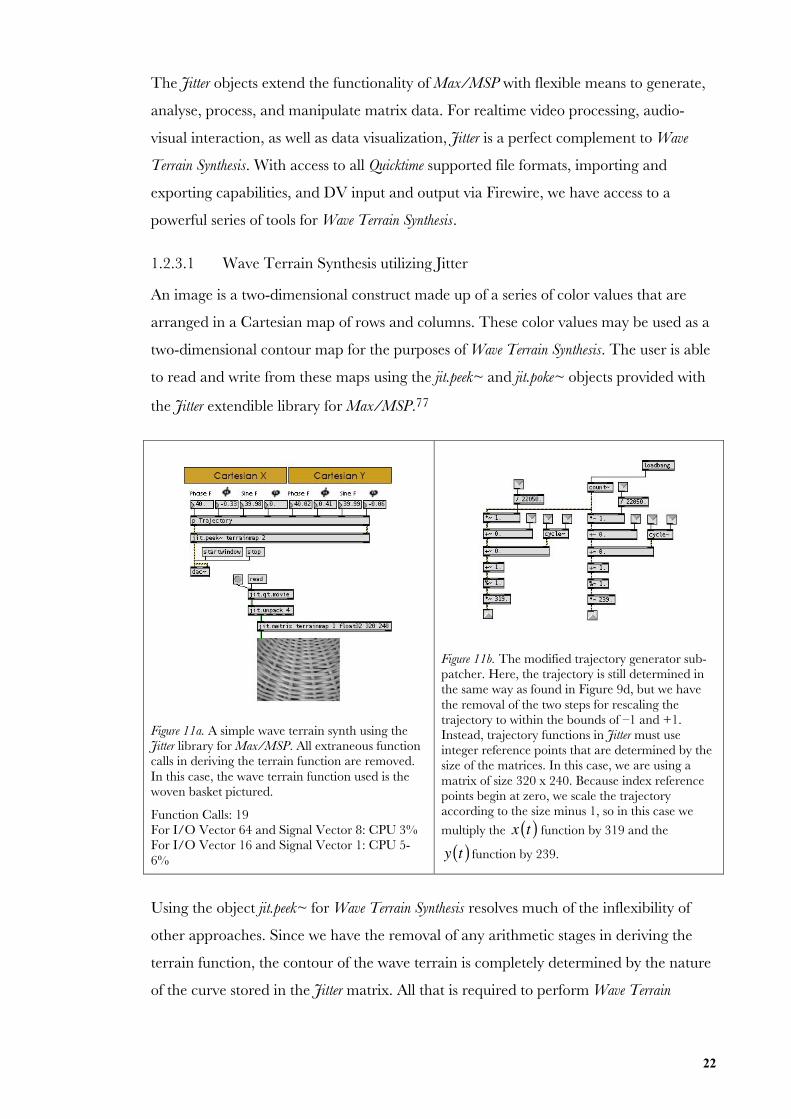
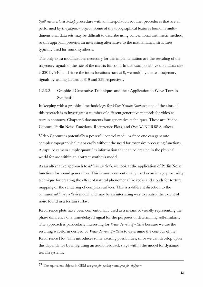
1.2.3.1 Wave Terrain Synthesis utilizing Jitter

An image is a two-dimensional construct made up of a series of color values that are

arranged in a Cartesian map of rows and columns. These color values may be used as a

two-dimensional contour map for the purposes of Wave Terrain Synthesis. The user is able

to read and write from these maps using the jit.peek~ and jit.poke~ objects provided with

the Jitter extendible library for Max/MSP.77

Figure 11a. A simple wave terrain synth using theJitter library for Max/MSP. All extraneous functioncalls in deriving the terrain function are removed.In this case, the wave terrain function used is thewoven basket pictured.

Function Calls: 19For I/O Vector 64 and Signal Vector 8: CPU 3%For I/O Vector 16 and Signal Vector 1: CPU 5-6%

Figure 11b. The modified trajectory generator sub-patcher. Here, the trajectory is still determined inthe same way as found in Figure 9d, but we havethe removal of the two steps for rescaling thetrajectory to within the bounds of –1 and +1.Instead, trajectory functions in Jitter must useinteger reference points that are determined by thesize of the matrices. In this case, we are using amatrix of size 320 x 240. Because index referencepoints begin at zero, we scale the trajectoryaccording to the size minus 1, so in this case wemultiply the x t( ) function by 319 and the

y t( ) function by 239.

Using the object jit.peek~ for Wave Terrain Synthesis resolves much of the inflexibility of

other approaches. Since we have the removal of any arithmetic stages in deriving the

terrain function, the contour of the wave terrain is completely determined by the nature

of the curve stored in the Jitter matrix. All that is required to perform Wave Terrain

23

Synthesis is a table lookup procedure with an interpolation routine; procedures that are all

performed by the jit.peek~ object. Some of the topographical features found in multi-

dimensional data sets may be difficult to describe using conventional arithmetic method,

so this approach presents an interesting alternative to the mathematical structures

typically used for sound synthesis.

The only extra modifications necessary for this implementation are the rescaling of the

trajectory signals to the size of the matrix function. In the example above the matrix size

is 320 by 240, and since the index locations start at 0, we multiply the two trajectory

signals by scaling factors of 319 and 239 respectively.

1.2.3.2 Graphical Generative Techniques and their Application to Wave Terrain

Synthesis

In keeping with a graphical methodology for Wave Terrain Synthesis, one of the aims of

this research is to investigate a number of different generative methods for video as

terrain contours. Chapter 3 documents four generative techniques. These are: Video

Capture, Perlin Noise Functions, Recurrence Plots, and OpenGL NURBS Surfaces.

Video Capture is potentially a powerful control medium since one can generate

complex topographical maps easily without the need for extensive processing functions.

A capture camera simply quantifies information that can be created in the physical

world for use within an abstract synthesis model.

As an alternative approach to additive synthesis, we look at the application of Perlin Noise

functions for sound generation. This is more conventionally used as an image processing

technique for creating the effect of natural phenomena like rocks and clouds for texture

mapping or the rendering of complex surfaces. This is a different direction to the

common additive synthesis model and may be an interesting way to control the extent of

noise found in a terrain surface.

Recurrence plots have been conventionally used as a means of visually representing the

phase difference of a time-delayed signal for the purposes of determining self-similarity.

The approach is particularly interesting for Wave Terrain Synthesis because we use the

resulting waveform derived by Wave Terrain Synthesis to determine the contour of the

Recurrence Plot. This introduces some exciting possibilities, since we can develop upon

this dependence by integrating an audio feedback stage within the model for dynamic

terrain systems.

77 The equivalent objects in GEM are gem.pix_pix2sig~ and gem.pix_sig2pix~

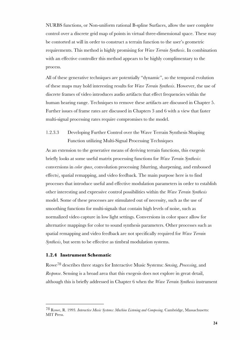
24

NURBS functions, or Non-uniform rational B-spline Surfaces, allow the user complete

control over a discrete grid map of points in virtual three-dimensional space. These may

be contorted at will in order to construct a terrain function to the user’s geometric

requirements. This method is highly promising for Wave Terrain Synthesis. In combination

with an effective controller this method appears to be highly complimentary to the

process.

All of these generative techniques are potentially “dynamic”, so the temporal evolution

of these maps may hold interesting results for Wave Terrain Synthesis. However, the use of

discrete frames of video introduces audio artifacts that effect frequencies within the

human hearing range. Techniques to remove these artifacts are discussed in Chapter 5.

Further issues of frame rates are discussed in Chapters 3 and 6 with a view that faster

multi-signal processing rates require compromises to the model.

1.2.3.3 Developing Further Control over the Wave Terrain Synthesis Shaping

Function utilizing Multi-Signal Processing Techniques

As an extension to the generative means of deriving terrain functions, this exegesis

briefly looks at some useful matrix processing functions for Wave Terrain Synthesis:

conversions in color space, convolution processing (blurring, sharpening, and embossed

effects), spatial remapping, and video feedback. The main purpose here is to find

processes that introduce useful and effective modulation parameters in order to establish

other interesting and expressive control possibilities within the Wave Terrain Synthesis

model. Some of these processes are stimulated out of necessity, such as the use of

smoothing functions for multi-signals that contain high levels of noise, such as

normalized video capture in low light settings. Conversions in color space allow for

alternative mappings for color to sound synthesis parameters. Other processes such as

spatial remapping and video feedback are not specifically required for Wave Terrain

Synthesis, but seem to be effective as timbral modulation systems.

1.2.4 Instrument Schematic

Rowe78 describes three stages for Interactive Music Systems: Sensing, Processing, and

Response. Sensing is a broad area that this exegesis does not explore in great detail,

although this is briefly addressed in Chapter 6 when the Wave Terrain Synthesis instrument

78 Rowe, R. 1993. Interactive Music Systems: Machine Listening and Composing. Cambridge, Massachusetts:MIT Press.

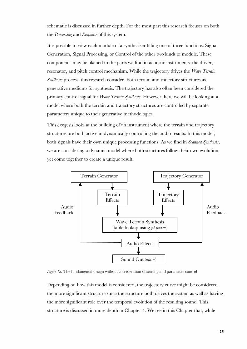
25

schematic is discussed in further depth. For the most part this research focuses on both

the Processing and Response of this system.

It is possible to view each module of a synthesizer filling one of three functions: Signal

Generation, Signal Processing, or Control of the other two kinds of module. These

components may be likened to the parts we find in acoustic instruments: the driver,

resonator, and pitch control mechanism. While the trajectory drives the Wave Terrain

Synthesis process, this research considers both terrain and trajectory structures as

generative mediums for synthesis. The trajectory has also often been considered the

primary control signal for Wave Terrain Synthesis. However, here we will be looking at a

model where both the terrain and trajectory structures are controlled by separate

parameters unique to their generative methodologies.

This exegesis looks at the building of an instrument where the terrain and trajectory

structures are both active in dynamically controlling the audio results. In this model,

both signals have their own unique processing functions. As we find in Scanned Synthesis,

we are considering a dynamic model where both structures follow their own evolution,

yet come together to create a unique result.

Figure 12. The fundamental design without consideration of sensing and parameter control

Depending on how this model is considered, the trajectory curve might be considered

the more significant structure since the structure both drives the system as well as having

the more significant role over the temporal evolution of the resulting sound. This

structure is discussed in more depth in Chapter 4. We see in this Chapter that, while

Terrain Generator Trajectory Generator

TerrainEffects

TrajectoryEffects

Wave Terrain Synthesis(table lookup using jit.peek~)

Audio Effects

AudioFeedback

AudioFeedback

Sound Out (dac~)

26

there are numerous possibilities for generating terrain functions, the trajectory system is

faced by this very same problem.

1.2.5 Developing a Parameter Control Map

Musical mapping systems today reflect two different models: those that are discrete, and

those that are continuous. The discrete model is based on the idea that each individual

value of this controller data refers to a separate and specific event or occurrence, such as

the MIDI on and off setting of a pitched note. On the other hand, continuous mappings

refer to control parameters that require dynamic and variable movement in parameter

value; parameters such as frequency, volume, filter cutoff, or phase are considered

continuous parameter spaces. Nearly all synthesis techniques rely on both models to

varying degrees. Wave Terrain Synthesis, however, relies on the dynamical control of

nearly all parameters. As soon as the system becomes static we have a static and sterile

sound, or at worst silence.

Most of the control parameters available to the user are determined by the

methodology, and the parameter map depends completely on the processes introduced

into the system. Changes in methodology may also impact the extent of these

parameters. Advantages of techniques like Scanned Synthesis are such that, while the inner

controller network may be quite complex, the system is to a large extent automated.

This is often essential for realtime live performance, so that the performer is not

required to control a myriad of parameters. While a large number of these may be

automated, the performer can focus more specifically on control parameters for

expressive and sonic effect. Parameters for generating terrain and trajectory structures

are discussed in Chapters 3 and 4.

While automation is an essential part of such a model, we also want to maintain as

much flexibility for parameter modulation as possible whilst retaining overall functional

simplicity. In order to maximise this flexibility we have an adaptable routing network of

parameters and control functions. These may be mapped and configured to the

performer’s wishes, and may be stored as presets within the instrument. In this way we

do not restrict the user to a small number of predefined parameter mappings, hence

allowing the performer creative freedom with what should be a flexible sound design

tool. Essentially the power of a technique like Wave Terrain Synthesis may emerge whilst

allowing for these parameters to be “configurable” by the user. This control interface is

discussed in more depth in Chapter 6.

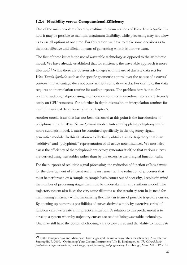
27

1.2.6 Flexibility versus Computational Efficiency

One of the main problems faced by realtime implementations of Wave Terrain Synthesis is

how it may be possible to maintain maximum flexibility, while processing may not allow

us to use all options at one time. For this reason we have to make some decisions as to

the most effective and efficient means of generating what it is that we want.

The first of these issues is the use of wavetable technology as opposed to the arithmetic

model. We have already established that for efficiency, the wavetable approach is more

effective.79 While there are obvious advantages with the use of discrete data sets for

Wave Terrain Synthesis, such as the specific geometric control over the nature of a curves’

contour, this advantage does not come without some drawbacks. For example, this data

requires an interpolation routine for audio purposes. The problem here is that, for

realtime audio signal processing, interpolation routines in two-dimensions are extremely

costly on CPU resources. For a further in depth discussion on interpolation routines for

multidimensional data please refer to Chapter 5.

Another crucial issue that has not been discussed at this point is the introduction of

polyphony into the Wave Terrain Synthesis model. Instead of applying polyphony to the

entire synthesis model, it must be contained specifically in the trajectory signal

generative module. In this situation we effectively obtain a single trajectory that is an

“additive” and “polyphonic” representation of all active note instances. We must also

assess the efficiency of the polyphonic trajectory generator itself, so that various curves

are derived using wavetables rather than by the excessive use of signal function calls.

For the purposes of real-time signal processing, the reduction of function calls is a must

for the development of efficient realtime instruments. The reduction of processes that

must be performed on a sample-to-sample basis comes out of necessity, keeping in mind

the number of processing stages that must be undertaken for any synthesis model. The

trajectory system also faces the very same dilemma as the terrain system in its need for

maintaining efficiency whilst maximising flexibility in terms of possible trajectory curves.

By opening up numerous possibilities of curves derived simply by extensive series’ of

function calls, we create an impractical situation. A solution to this predicament is to

develop a system whereby trajectory curves are read utilizing wavetable technology.

One may still have the option of choosing a trajectory curve and the ability to modify its

79 Both Comajuncosas and Mitsuhashi have suggested the use of wavetables for efficiency. Also refer to:Smaragdis, P. 2000. “Optimizing Your Csound Instruments”, In R. Boulanger, ed. The CSound Book:perspectives in software synthesis, sound design, signal processing, and programming. Cambridge, Mass: MIT: 123-135.

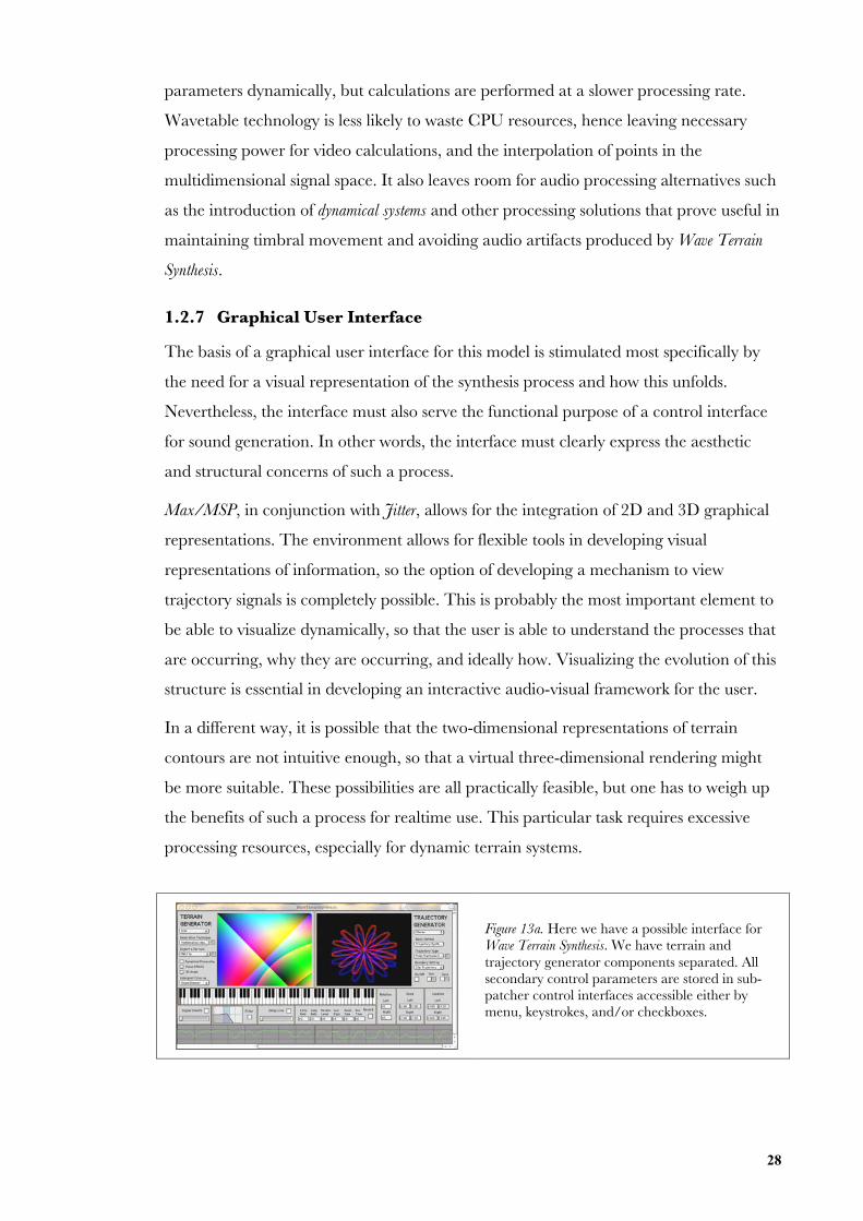
28

parameters dynamically, but calculations are performed at a slower processing rate.

Wavetable technology is less likely to waste CPU resources, hence leaving necessary

processing power for video calculations, and the interpolation of points in the

multidimensional signal space. It also leaves room for audio processing alternatives such

as the introduction of dynamical systems and other processing solutions that prove useful in

maintaining timbral movement and avoiding audio artifacts produced by Wave Terrain

Synthesis.

1.2.7 Graphical User Interface

The basis of a graphical user interface for this model is stimulated most specifically by

the need for a visual representation of the synthesis process and how this unfolds.

Nevertheless, the interface must also serve the functional purpose of a control interface

for sound generation. In other words, the interface must clearly express the aesthetic

and structural concerns of such a process.

Max/MSP, in conjunction with Jitter, allows for the integration of 2D and 3D graphical

representations. The environment allows for flexible tools in developing visual

representations of information, so the option of developing a mechanism to view

trajectory signals is completely possible. This is probably the most important element to

be able to visualize dynamically, so that the user is able to understand the processes that

are occurring, why they are occurring, and ideally how. Visualizing the evolution of this

structure is essential in developing an interactive audio-visual framework for the user.

In a different way, it is possible that the two-dimensional representations of terrain

contours are not intuitive enough, so that a virtual three-dimensional rendering might

be more suitable. These possibilities are all practically feasible, but one has to weigh up

the benefits of such a process for realtime use. This particular task requires excessive

processing resources, especially for dynamic terrain systems.

Figure 13a. Here we have a possible interface forWave Terrain Synthesis. We have terrain andtrajectory generator components separated. Allsecondary control parameters are stored in sub-patcher control interfaces accessible either bymenu, keystrokes, and/or checkboxes.

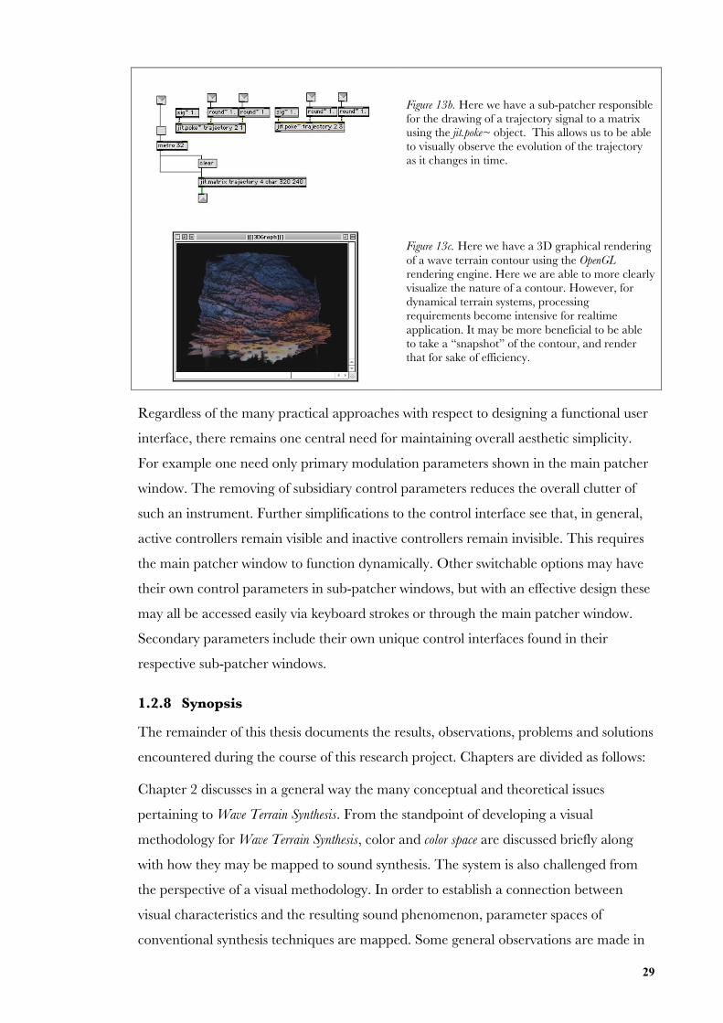
29

Figure 13b. Here we have a sub-patcher responsiblefor the drawing of a trajectory signal to a matrixusing the jit.poke~ object. This allows us to be ableto visually observe the evolution of the trajectoryas it changes in time.

Figure 13c. Here we have a 3D graphical renderingof a wave terrain contour using the OpenGLrendering engine. Here we are able to more clearlyvisualize the nature of a contour. However, fordynamical terrain systems, processingrequirements become intensive for realtimeapplication. It may be more beneficial to be ableto take a “snapshot” of the contour, and renderthat for sake of efficiency.

Regardless of the many practical approaches with respect to designing a functional user

interface, there remains one central need for maintaining overall aesthetic simplicity.

For example one need only primary modulation parameters shown in the main patcher

window. The removing of subsidiary control parameters reduces the overall clutter of

such an instrument. Further simplifications to the control interface see that, in general,

active controllers remain visible and inactive controllers remain invisible. This requires

the main patcher window to function dynamically. Other switchable options may have

their own control parameters in sub-patcher windows, but with an effective design these

may all be accessed easily via keyboard strokes or through the main patcher window.

Secondary parameters include their own unique control interfaces found in their

respective sub-patcher windows.

1.2.8 Synopsis

The remainder of this thesis documents the results, observations, problems and solutions

encountered during the course of this research project. Chapters are divided as follows:

Chapter 2 discusses in a general way the many conceptual and theoretical issues

pertaining to Wave Terrain Synthesis. From the standpoint of developing a visual

methodology for Wave Terrain Synthesis, color and color space are discussed briefly along

with how they may be mapped to sound synthesis. The system is also challenged from

the perspective of a visual methodology. In order to establish a connection between

visual characteristics and the resulting sound phenomenon, parameter spaces of

conventional synthesis techniques are mapped. Some general observations are made in

30

order to establish the nature of these various modulation processes and how they might

relate to more complex multidimensional parameter spaces.

Chapter 3 briefly summarizes previous approaches to terrain generation and then

moves on to the generation and processing of multidimensional data within the Jitter

library for Max/MSP. Here we see the application of graphical processing functions for

use in sound generation. Are they practical for sound synthesis? Are they too inefficient?

What advantages are gained in this way? The primary purpose here is to develop upon

existing methodology concerning terrain function generation and control processes from

the perspective that, as in Scanned Synthesis, the terrain is central to the idea of performing

timbre.80

Chapter 4 categorises various kinds of trajectory structures that may be used to drive

Wave Terrain Synthesis, as well as further control sources that may be used as a means of

influencing the evolution of the system. Here, the notion of periodicity, quasi-

periodicity, chaos, and randomness are discussed, as well as the need for complex

controller networks and automation for this system. Advantages to quasi-synchronous

and asynchronous controller networks are discussed, as well as some possibilities for

multi-trajectory systems for multichannel audio.

Chapter 5 deals almost completely with processing solutions for avoiding audio artifacts

that commonly arise through the Wave Terrain Synthesis process. Issues of audio

interpolation, video streaming, amplitude fluctuation, and aliasing are discussed, as well

as various means of removing stepwise frequency artifacts and DC offsets.

Chapter 6 discusses the building of a user interface for Wave Terrain Synthesis. In

combining all of the sub-components discussed throughout the previous Chapters of this

thesis, this particular Chapter deals with the construction of a parameter map, and the

compromises necessary for maintaining both flexibility and efficiency in a realtime

model. We also have a brief discussion on the “polyphonic” trajectory generator, as well

as a report detailing the basic development of a graphical user interface.

Finally, Chapter 7 concludes this research. Findings are discussed and possibilities for

future work are brought forward for consideration.

80 Boulanger, R., P. Smaragdis, and J. Ffitch. 2000. “Scanned Synthesis: An Introduction andDemonstration of a New Synthesis and Signal Processing Technique”, Proceedings of the 2000 InternationalComputer Music Conference: 372-375.

31

2. A Visual Methodology for Wave Terrain Synthesis

2.1 Color Space and Color Scale

As Sir Isaac Newton has said, “Indeed rays, properly expressed, are not colored.”81

Color exists only as an experience in human perception. It is a physical sensation when

light of varying wavelength is observed on the retina of the eye.82 The human retina has

three types of color photoreceptor cone cells, each maximally sensitive to different

wavelengths of light. While these cells have their maximal peaks at blue, green and

yellow, their overlap allows us to see the full range of color we understand as being the

visible light spectrum. Because there are exactly three types of color photoreceptor,

three numerical components are necessary and sufficient to describe a color.83

A colorspace is a method by which we can specify, create and visualize a gamut of

colors; a number of color space models have been developed. The HSV84 – hue, saturation

and value – color model was designed intentionally to mimic the way humans perceive

color. Within the eye, the rods provide the ability to detect brightness, and the cones allow

us to perceive color, hence the HSV color space defines a color in a similar way by

means of hue, saturation and brightness. The term brightness, or what is alternatively named

value, describes the intensity of a color, saturation or chroma defines the purity or vividity of

the color, and hue the dominant color as perceived by an observer.

Color spaces are not only used for the recreation of color which, as humans, we

experience in the physical world, but can also be used as an effective and compact way

of representing and interpreting large data sets. For example, in topographic data, hue

may be used to show the direction of slopes, saturation the steepness of the slope, and

brightness the illumination of the shape of the contour. With these three variables, the

81 Found in Newton’s Opticks; refer to Goethe, Johann Wolfgang von. 1970. Theory of Colours. Cambridge,Massachusetts: MIT Press. Page vi82 Bourgin, D. 1995. “Color spaces FAQ.” http://www.poynton.com/notes/Timo/colorspace-faq;Poynton, C. A. 1997. “Colorspace-faq: Frequently asked questions about Gamma and Color.”http://www.faqs.org/faqs/graphics/colorspace-faq/83 In 1931, the Commission Internationale de L'Eclairage (CIE) proposed a series of curves that describehow light of varying wavelength may be transformed into a set of three numbers specifying a color. Referto: Bourgin, D. 1995. “Color spaces FAQ.” http://www.poynton.com/notes/Timo/colorspace-faq84 The value or brightness of the color varies from zero to one along the axis, and the saturation of the colorvaries as the radial distance from the center axis. The hue is represented as an angle starting from red atzero degrees.

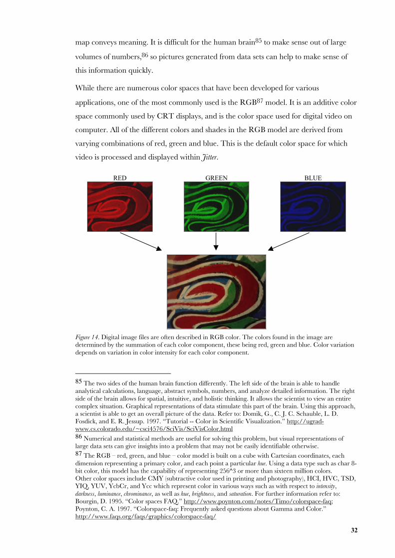
32

map conveys meaning. It is difficult for the human brain85 to make sense out of large

volumes of numbers,86 so pictures generated from data sets can help to make sense of

this information quickly.

While there are numerous color spaces that have been developed for various

applications, one of the most commonly used is the RGB87 model. It is an additive color

space commonly used by CRT displays, and is the color space used for digital video on

computer. All of the different colors and shades in the RGB model are derived from

varying combinations of red, green and blue. This is the default color space for which

video is processed and displayed within Jitter.

RED GREEN BLUE

Figure 14. Digital image files are often described in RGB color. The colors found in the image aredetermined by the summation of each color component, these being red, green and blue. Color variationdepends on variation in color intensity for each color component.

85 The two sides of the human brain function differently. The left side of the brain is able to handleanalytical calculations, language, abstract symbols, numbers, and analyze detailed information. The rightside of the brain allows for spatial, intuitive, and holistic thinking. It allows the scientist to view an entirecomplex situation. Graphical representations of data stimulate this part of the brain. Using this approach,a scientist is able to get an overall picture of the data. Refer to: Domik, G., C. J. C. Schauble, L. D.Fosdick, and E. R. Jessup. 1997. “Tutorial -- Color in Scientific Visualization.” http://ugrad-www.cs.colorado.edu/~csci4576/SciVis/SciVisColor.html86 Numerical and statistical methods are useful for solving this problem, but visual representations oflarge data sets can give insights into a problem that may not be easily identifiable otherwise.87 The RGB – red, green, and blue – color model is built on a cube with Cartesian coordinates, eachdimension representing a primary color, and each point a particular hue. Using a data type such as char 8-bit color, this model has the capability of representing 256^3 or more than sixteen million colors.Other color spaces include CMY (subtractive color used in printing and photography), HCI, HVC, TSD,YIQ, YUV, YcbCr, and Ycc which represent color in various ways such as with respect to intensity,darkness, luminance, chrominance, as well as hue, brightness, and saturation. For further information refer to:Bourgin, D. 1995. “Color spaces FAQ.” http://www.poynton.com/notes/Timo/colorspace-faq;Poynton, C. A. 1997. “Colorspace-faq: Frequently asked questions about Gamma and Color.”http://www.faqs.org/faqs/graphics/colorspace-faq/

33

2.2 Relationships between Images, Light, and Sound

Connections between images, light and sound have been made numerous times.88

Composers, visual artists, scientists, philosophers, and theorists have all contributed to

this ongoing fascination: from the colors we find written in the musical scores of Olivier

Messiaen, to the musical references we find in the paintings of Wassily Kandinsky and

Roy De Maistre; from the studies of Michel Chion exploring the complex symbioses of

sound, music and film,89 to the physical realizations of Iannis Xenakis’ Polytòpes where

light, sound, and space merge;90 from the scientific method of music information

retrieval, to the theory of synaesthesia91; from the colored lights Skryabin intended for

his work Prometheus (1910), to the festive high budget firework shows that synchronise

visual lights with music. Mythologically, the connection between color and sound has

parallels to what the Ancient Greeks described as being the Music of the Spheres: the

connection and interrelationship of all things according to the governing and divine

principles of ratio and number.92 This association has brought a diverse movement

through the ages up to the present day.

While the aesthetic of visualizing the phenomenon of sound appears to be quite a

current issue in computer music, the need for devising visual methods of representing

sound has quite an extensive history. Perhaps due to the intangible quality of sound, it

was thought that the ability to visualise something we normally associate with our ears

may add to its phenomenology. The famous Chladni93 figures and Lissajous94 figures

demonstrated visual methods for representing vibrations. This theory has influenced the

88 Collopy, F. 2003. “Lumia.” http://rhythmiclight.com89 Chion, M. 1990. AudioVision: Sound on Screen. Reprinted in C. Gorbman, ed. and trans. 1994. New York:Columbia University Press.90 Harley, J. 2002. “The Electroacoustic Music of Iannis Xenakis.” Computer Music Journal 26(1): 41-42,46-51; Oswalt, P. 1991. “Iannis Xenakisis’ Polytopes.” http://www.oswalt.de/en/text/txt/xenakis.html;Xenakis, I. 1971. Formalized Music; thought and mathematics in composition. Bloomington University: IndianaPress.91 According to the Online Grove Dictionary of Music and Musicians, synaesthesia is the perception of onemode of sensation aroused by the stimulation of another sense. It must meet at least four of the followingfive criteria: it must be involuntary but elicited, projected, durable and discrete, memorable, emotional.The most usual form of synaesthesia consists of hearing a sound or a piece of music in terms of colors, aphenomenon known as “color-hearing.” It is not known how frequently synaesthesia occurs in thepopulation. Estimates differ widely from 1 in 25,000 to 1 in 500. Refer to:“Grove Music Online.” http://www.grovemusic.com/grovemusic/home/92 James, J. 1993. The Music of the Spheres: Music, Science, and the Natural Order of the Universe. New York:Grove Press.93 The famous Chladni Figures were discovered by Ernst Florenz Friedrich Chladni (1756-1827). Thisphenomenon became the basis for Cymatics, the visualisation of the organizing power of sound andvibration after Hans Jenny’s (1904 -1972) work in developing Chladni’s technique.94 Lissajous Figures were discovered by French physicist and mathematician Jules Antoine Lissajous(1822-1880)

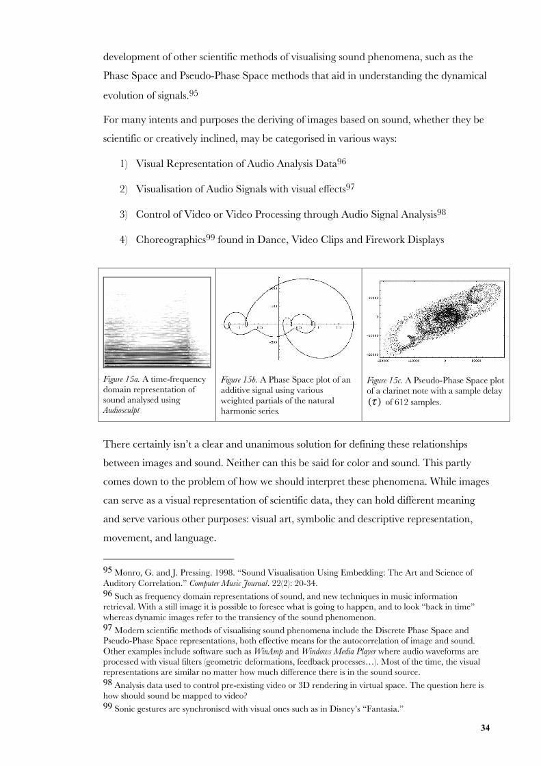
34

development of other scientific methods of visualising sound phenomena, such as the

Phase Space and Pseudo-Phase Space methods that aid in understanding the dynamical

evolution of signals.95

For many intents and purposes the deriving of images based on sound, whether they be

scientific or creatively inclined, may be categorised in various ways:

1) Visual Representation of Audio Analysis Data96

2) Visualisation of Audio Signals with visual effects97

3) Control of Video or Video Processing through Audio Signal Analysis98

4) Choreographics99 found in Dance, Video Clips and Firework Displays

Figure 15a. A time-frequencydomain representation ofsound analysed usingAudiosculpt

Figure 15b. A Phase Space plot of anadditive signal using variousweighted partials of the naturalharmonic series.

Figure 15c. A Pseudo-Phase Space plotof a clarinet note with a sample delay(τ ) of 612 samples.

There certainly isn’t a clear and unanimous solution for defining these relationships

between images and sound. Neither can this be said for color and sound. This partly

comes down to the problem of how we should interpret these phenomena. While images

can serve as a visual representation of scientific data, they can hold different meaning

and serve various other purposes: visual art, symbolic and descriptive representation,

movement, and language.

95 Monro, G. and J. Pressing. 1998. “Sound Visualisation Using Embedding: The Art and Science ofAuditory Correlation.” Computer Music Journal. 22(2): 20-34.96 Such as frequency domain representations of sound, and new techniques in music informationretrieval. With a still image it is possible to foresee what is going to happen, and to look “back in time”whereas dynamic images refer to the transiency of the sound phenomenon.97 Modern scientific methods of visualising sound phenomena include the Discrete Phase Space andPseudo-Phase Space representations, both effective means for the autocorrelation of image and sound.Other examples include software such as WinAmp and Windows Media Player where audio waveforms areprocessed with visual filters (geometric deformations, feedback processes…). Most of the time, the visualrepresentations are similar no matter how much difference there is in the sound source.98 Analysis data used to control pre-existing video or 3D rendering in virtual space. The question here ishow should sound be mapped to video?99 Sonic gestures are synchronised with visual ones such as in Disney’s “Fantasia.”

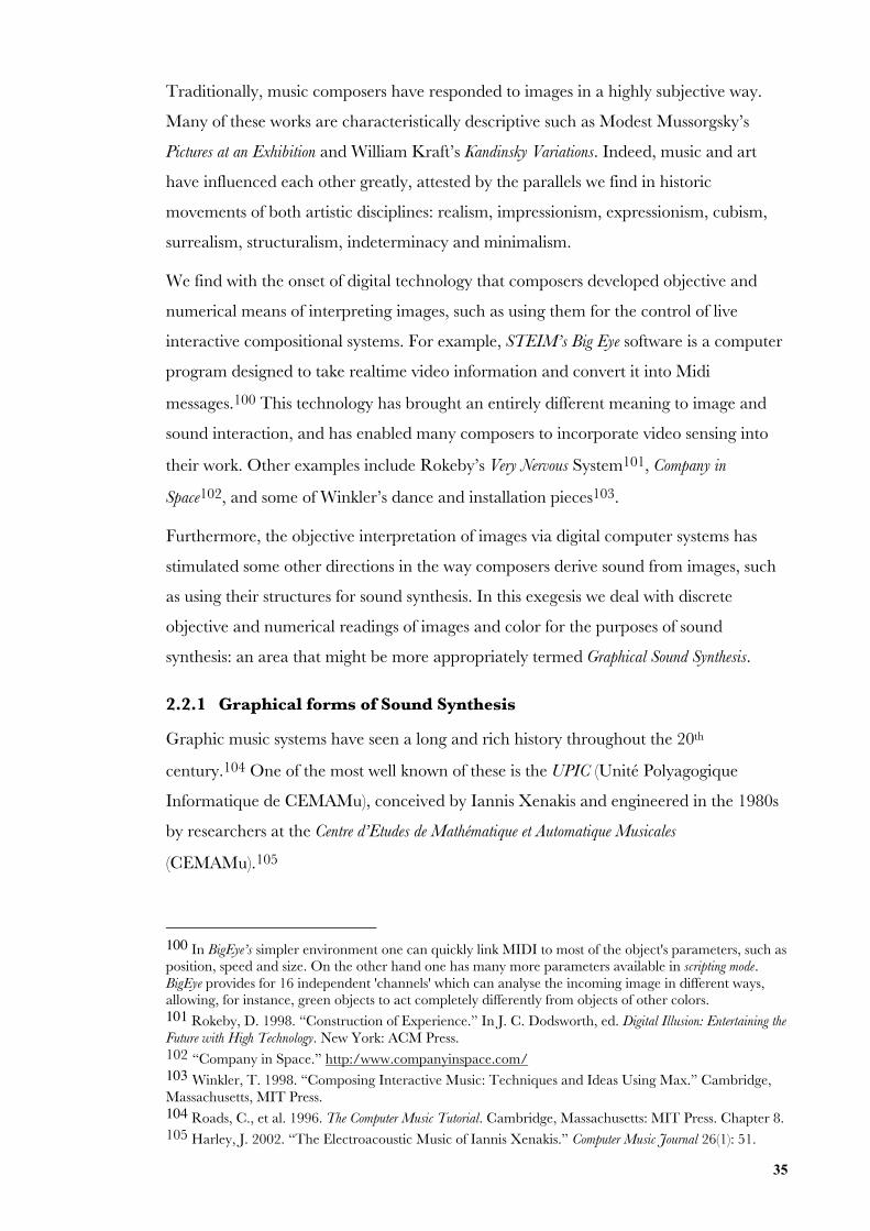
35

Traditionally, music composers have responded to images in a highly subjective way.

Many of these works are characteristically descriptive such as Modest Mussorgsky’s

Pictures at an Exhibition and William Kraft’s Kandinsky Variations. Indeed, music and art

have influenced each other greatly, attested by the parallels we find in historic

movements of both artistic disciplines: realism, impressionism, expressionism, cubism,

surrealism, structuralism, indeterminacy and minimalism.

We find with the onset of digital technology that composers developed objective and

numerical means of interpreting images, such as using them for the control of live

interactive compositional systems. For example, STEIM’s Big Eye software is a computer

program designed to take realtime video information and convert it into Midi

messages.100 This technology has brought an entirely different meaning to image and

sound interaction, and has enabled many composers to incorporate video sensing into

their work. Other examples include Rokeby’s Very Nervous System101, Company in

Space102, and some of Winkler’s dance and installation pieces103.

Furthermore, the objective interpretation of images via digital computer systems has

stimulated some other directions in the way composers derive sound from images, such

as using their structures for sound synthesis. In this exegesis we deal with discrete

objective and numerical readings of images and color for the purposes of sound

synthesis: an area that might be more appropriately termed Graphical Sound Synthesis.

2.2.1 Graphical forms of Sound Synthesis

Graphic music systems have seen a long and rich history throughout the 20th

century.104 One of the most well known of these is the UPIC (Unité Polyagogique

Informatique de CEMAMu), conceived by Iannis Xenakis and engineered in the 1980s

by researchers at the Centre d’Etudes de Mathématique et Automatique Musicales

(CEMAMu).105

100 In BigEye’s simpler environment one can quickly link MIDI to most of the object's parameters, such asposition, speed and size. On the other hand one has many more parameters available in scripting mode.BigEye provides for 16 independent 'channels' which can analyse the incoming image in different ways,allowing, for instance, green objects to act completely differently from objects of other colors.101 Rokeby, D. 1998. “Construction of Experience.” In J. C. Dodsworth, ed. Digital Illusion: Entertaining theFuture with High Technology. New York: ACM Press.102 “Company in Space.” http:/www.companyinspace.com/103 Winkler, T. 1998. “Composing Interactive Music: Techniques and Ideas Using Max.” Cambridge,Massachusetts, MIT Press.104 Roads, C., et al. 1996. The Computer Music Tutorial. Cambridge, Massachusetts: MIT Press. Chapter 8.105 Harley, J. 2002. “The Electroacoustic Music of Iannis Xenakis.” Computer Music Journal 26(1): 51.

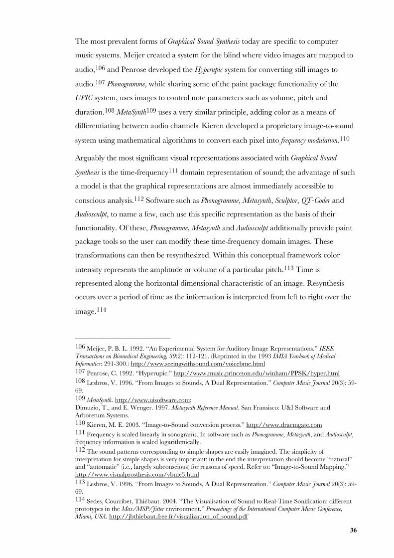
36

The most prevalent forms of Graphical Sound Synthesis today are specific to computer

music systems. Meijer created a system for the blind where video images are mapped to

audio,106 and Penrose developed the Hyperupic system for converting still images to

audio.107 Phonogramme, while sharing some of the paint package functionality of the

UPIC system, uses images to control note parameters such as volume, pitch and

duration.108 MetaSynth109 uses a very similar principle, adding color as a means of

differentiating between audio channels. Kieren developed a proprietary image-to-sound

system using mathematical algorithms to convert each pixel into frequency modulation.110

Arguably the most significant visual representations associated with Graphical Sound

Synthesis is the time-frequency111 domain representation of sound; the advantage of such

a model is that the graphical representations are almost immediately accessible to

conscious analysis.112 Software such as Phonogramme, Metasynth, Sculptor, QT-Coder and

Audiosculpt, to name a few, each use this specific representation as the basis of their

functionality. Of these, Phonogramme, Metasynth and Audiosculpt additionally provide paint

package tools so the user can modify these time-frequency domain images. These

transformations can then be resynthesized. Within this conceptual framework color

intensity represents the amplitude or volume of a particular pitch.113 Time is

represented along the horizontal dimensional characteristic of an image. Resynthesis

occurs over a period of time as the information is interpreted from left to right over the

image.114

106 Meijer, P. B. L. 1992. “An Experimental System for Auditory Image Representations.” IEEETransactions on Biomedical Engineering, 39(2): 112-121. (Reprinted in the 1993 IMIA Yearbook of MedicalInformatics: 291-300.) http://www.seeingwithsound.com/voicebme.html107 Penrose, C. 1992. “Hyperupic.” http://www.music.princeton.edu/winham/PPSK/hyper.html108 Lesbros, V. 1996. “From Images to Sounds, A Dual Representation.” Computer Music Journal 20(3): 59-69.109 MetaSynth. http://www.uisoftware.com;Dimuzio, T., and E. Wenger. 1997. Metasynth Reference Manual. San Fransisco: U&I Software andArboretum Systems.110 Kieren, M. E. 2003. “Image-to-Sound conversion process.” http://www.draemgate.com111 Frequency is scaled linearly in sonograms. In software such as Phonogramme, Metasynth, and Audiosculpt,frequency information is scaled logarithmically.112 The sound patterns corresponding to simple shapes are easily imagined. The simplicity ofinterpretation for simple shapes is very important; in the end the interpretation should become “natural”and “automatic” (i.e., largely subconscious) for reasons of speed. Refer to: “Image-to-Sound Mapping.”http://www.visualprosthesis.com/vbme3.html113 Lesbros, V. 1996. “From Images to Sounds, A Dual Representation.” Computer Music Journal 20(3): 59-69.114 Sedes, Courribet, Thiébaut. 2004. “The Visualisation of Sound to Real-Time Sonification: differentprototypes in the Max/MSP/Jitter environment.” Proceedings of the International Computer Music Conference,Miami, USA. http://jbthiebaut.free.fr/visualization_of_sound.pdf

37

2.2.2 The Interpretation of Images Using Discrete Methodology

The resulting sound from a Graphical Sound Synthesis process depends on how the image is

interpreted. A computer cannot simply interpret an image out of free will; rather a

computer must be given instructions as to how to interpret any image.

It is worth noting that photos are inadequate for describing a space in which we

experience the world. Instead photographs represent a “flattened” version of the space

we are familiar with in our everyday experience.

image x, y( ) = color

While images may contain many subjective layers of meaning for us, and that there is

technology in development based on more abstract and descriptive analyses of

images,115 the digital representation of an image is simply a two-dimensional matrix of

numerical color values. These values are stored according to a dual-index. This is

sometimes referred to as the m-dimensional space; these coordinates are called

independent.116

bitmap x, y[ ] = color

A video screen is made up of individual pixels that each display a specific color.117 A

standard frame of video is composed of 640 x 480 = 307,200 pixels. Most software

stores the color of pixels as four separate numbers, representing the red, green and blue

color channels, as well as a transparency/opacity component known as the alpha

channel. This four-channel color representation scheme is commonly referred to as

ARGB. These four values are in the range of 0 to 255 for char and long data types, and 0

and 1 for float32 and float64 data types.

Data sets may consist of a collection of sampled data. Each sample is an n-dimensional

data item. These n dimensions are called dependant variables. In Jitter these variables are

115 A large part of sight-to-sound technology, as Jonathan Mustard has put it, relies on the descriptiveanalysis of images for the control of synthesis or some other process. Both the manipulation and analysisof multidimensional signals has been divided into three categories: 1) Image Processing: Image In ->Image Out, 2) Image Analysis: Image In -> Measurements Out, 3) Image Understanding: Image In ->High-Level Description Out. Refer to: Young, I. T., J. J. Gerbrands, and L. J. van Vliet. “ImageProcessing Fundamentals.” http://www.ph.tn.tudelft.nl/Courses/FIP/noframes/fip.html andMustard, J. 2003. “Aesthetics in Sight-to-Sound Technology and Artwork: “Why do we do it?”” ConvergingTechnologies, Proceedings of the 2003 Australasian Computer Music Conference: 81-87.116 Wegenkittl, R., H. Löffelmann, and E. Gröller. !1997. “Visualising the Behaviour of HigherDimensional Dynamical Systems.” The Proceedings IEEE Visualization: 119-126.http://www.cg.tuwien.ac.at/research/vis/dynsys/ndim/ndim_crc.pdf117 On a computer screen the resolution is usually some size like 1024 pixels wide by 768 pixels high, or800 x 600, or 640 x 480.

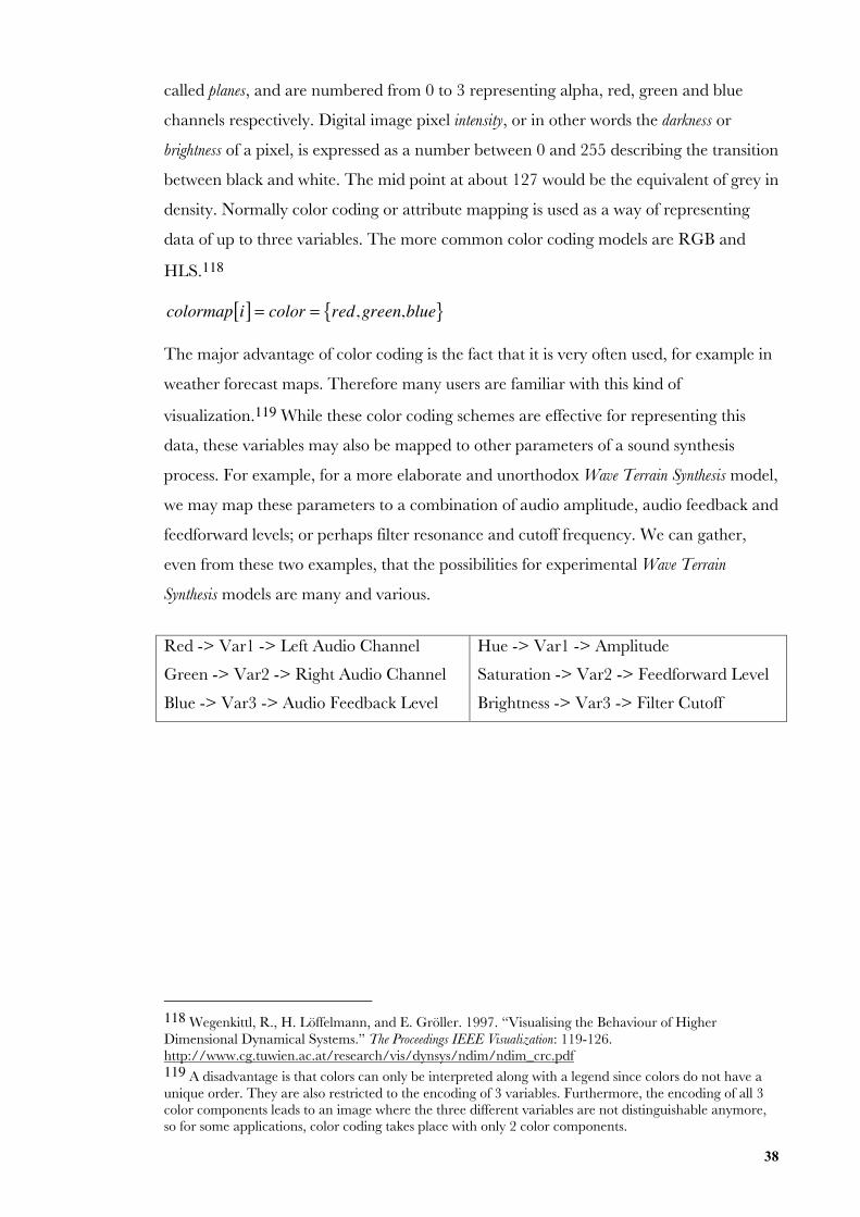
38

called planes, and are numbered from 0 to 3 representing alpha, red, green and blue

channels respectively. Digital image pixel intensity, or in other words the darkness or

brightness of a pixel, is expressed as a number between 0 and 255 describing the transition

between black and white. The mid point at about 127 would be the equivalent of grey in

density. Normally color coding or attribute mapping is used as a way of representing

data of up to three variables. The more common color coding models are RGB and

HLS.118

colormap i[ ] = color = red,green,blue{ }

The major advantage of color coding is the fact that it is very often used, for example in

weather forecast maps. Therefore many users are familiar with this kind of

visualization.119 While these color coding schemes are effective for representing this

data, these variables may also be mapped to other parameters of a sound synthesis

process. For example, for a more elaborate and unorthodox Wave Terrain Synthesis model,

we may map these parameters to a combination of audio amplitude, audio feedback and

feedforward levels; or perhaps filter resonance and cutoff frequency. We can gather,

even from these two examples, that the possibilities for experimental Wave Terrain

Synthesis models are many and various.

Red -> Var1 -> Left Audio Channel

Green -> Var2 -> Right Audio Channel

Blue -> Var3 -> Audio Feedback Level

Hue -> Var1 -> Amplitude

Saturation -> Var2 -> Feedforward Level

Brightness -> Var3 -> Filter Cutoff

118 Wegenkittl, R., H. Löffelmann, and E. Gröller. !1997. “Visualising the Behaviour of HigherDimensional Dynamical Systems.” The Proceedings IEEE Visualization: 119-126.http://www.cg.tuwien.ac.at/research/vis/dynsys/ndim/ndim_crc.pdf119 A disadvantage is that colors can only be interpreted along with a legend since colors do not have aunique order. They are also restricted to the encoding of 3 variables. Furthermore, the encoding of all 3color components leads to an image where the three different variables are not distinguishable anymore,so for some applications, color coding takes place with only 2 color components.

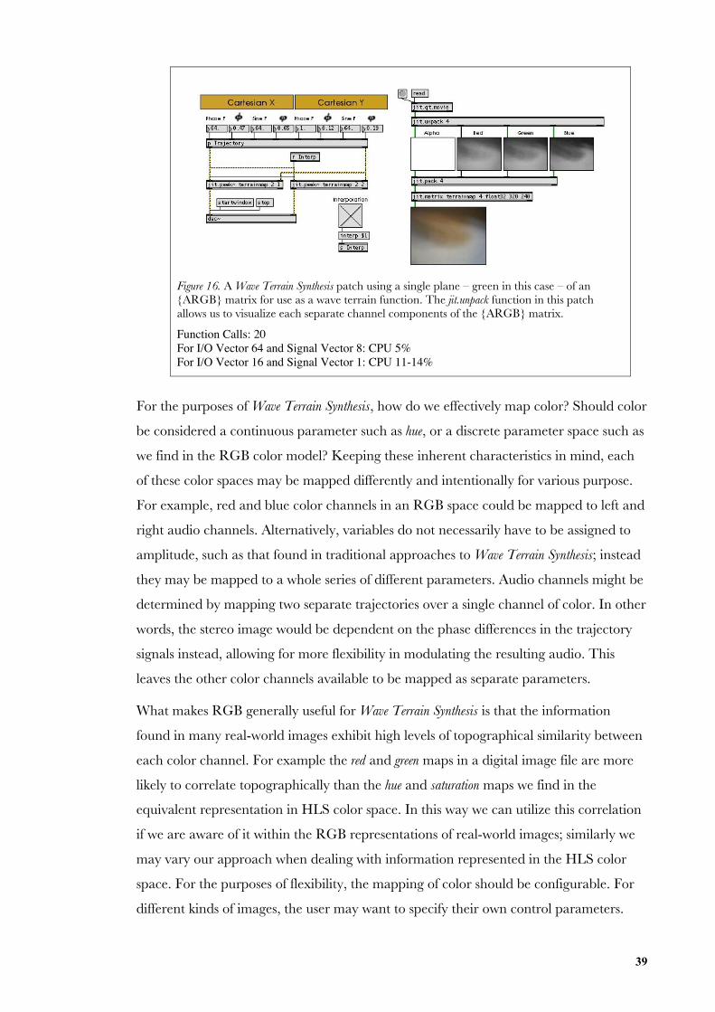
39

Figure 16. A Wave Terrain Synthesis patch using a single plane – green in this case – of an{ARGB} matrix for use as a wave terrain function. The jit.unpack function in this patchallows us to visualize each separate channel components of the {ARGB} matrix.

Function Calls: 20For I/O Vector 64 and Signal Vector 8: CPU 5%For I/O Vector 16 and Signal Vector 1: CPU 11-14%

For the purposes of Wave Terrain Synthesis, how do we effectively map color? Should color

be considered a continuous parameter such as hue, or a discrete parameter space such as

we find in the RGB color model? Keeping these inherent characteristics in mind, each

of these color spaces may be mapped differently and intentionally for various purpose.

For example, red and blue color channels in an RGB space could be mapped to left and

right audio channels. Alternatively, variables do not necessarily have to be assigned to

amplitude, such as that found in traditional approaches to Wave Terrain Synthesis; instead

they may be mapped to a whole series of different parameters. Audio channels might be

determined by mapping two separate trajectories over a single channel of color. In other

words, the stereo image would be dependent on the phase differences in the trajectory

signals instead, allowing for more flexibility in modulating the resulting audio. This

leaves the other color channels available to be mapped as separate parameters.

What makes RGB generally useful for Wave Terrain Synthesis is that the information

found in many real-world images exhibit high levels of topographical similarity between

each color channel. For example the red and green maps in a digital image file are more

likely to correlate topographically than the hue and saturation maps we find in the

equivalent representation in HLS color space. In this way we can utilize this correlation

if we are aware of it within the RGB representations of real-world images; similarly we

may vary our approach when dealing with information represented in the HLS color

space. For the purposes of flexibility, the mapping of color should be configurable. For

different kinds of images, the user may want to specify their own control parameters.

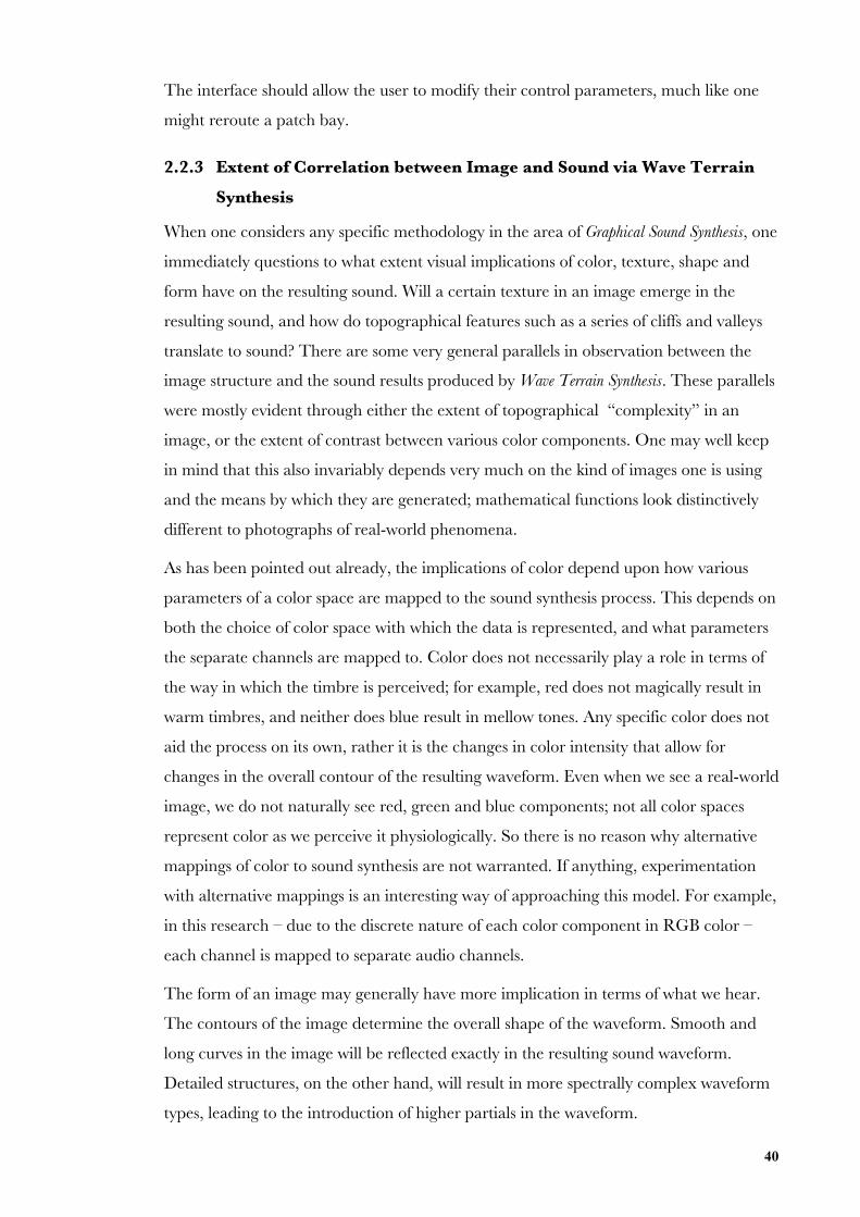
40

The interface should allow the user to modify their control parameters, much like one

might reroute a patch bay.

2.2.3 Extent of Correlation between Image and Sound via Wave Terrain

Synthesis

When one considers any specific methodology in the area of Graphical Sound Synthesis, one

immediately questions to what extent visual implications of color, texture, shape and

form have on the resulting sound. Will a certain texture in an image emerge in the

resulting sound, and how do topographical features such as a series of cliffs and valleys

translate to sound? There are some very general parallels in observation between the

image structure and the sound results produced by Wave Terrain Synthesis. These parallels

were mostly evident through either the extent of topographical “complexity” in an

image, or the extent of contrast between various color components. One may well keep

in mind that this also invariably depends very much on the kind of images one is using

and the means by which they are generated; mathematical functions look distinctively

different to photographs of real-world phenomena.

As has been pointed out already, the implications of color depend upon how various

parameters of a color space are mapped to the sound synthesis process. This depends on

both the choice of color space with which the data is represented, and what parameters

the separate channels are mapped to. Color does not necessarily play a role in terms of

the way in which the timbre is perceived; for example, red does not magically result in

warm timbres, and neither does blue result in mellow tones. Any specific color does not

aid the process on its own, rather it is the changes in color intensity that allow for

changes in the overall contour of the resulting waveform. Even when we see a real-world

image, we do not naturally see red, green and blue components; not all color spaces

represent color as we perceive it physiologically. So there is no reason why alternative

mappings of color to sound synthesis are not warranted. If anything, experimentation

with alternative mappings is an interesting way of approaching this model. For example,

in this research – due to the discrete nature of each color component in RGB color –

each channel is mapped to separate audio channels.

The form of an image may generally have more implication in terms of what we hear.

The contours of the image determine the overall shape of the waveform. Smooth and

long curves in the image will be reflected exactly in the resulting sound waveform.

Detailed structures, on the other hand, will result in more spectrally complex waveform

types, leading to the introduction of higher partials in the waveform.

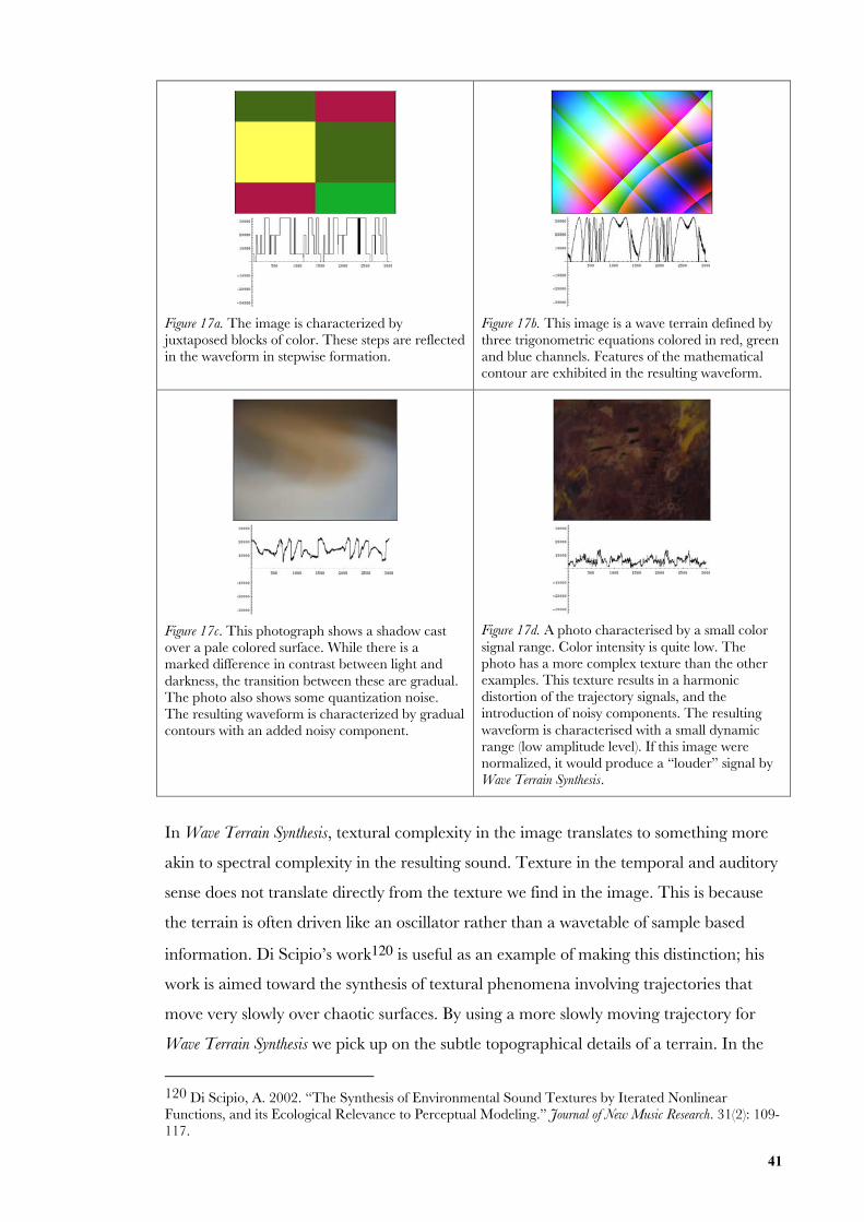
41

Figure 17a. The image is characterized byjuxtaposed blocks of color. These steps are reflectedin the waveform in stepwise formation.

Figure 17b. This image is a wave terrain defined bythree trigonometric equations colored in red, greenand blue channels. Features of the mathematicalcontour are exhibited in the resulting waveform.

Figure 17c. This photograph shows a shadow castover a pale colored surface. While there is amarked difference in contrast between light anddarkness, the transition between these are gradual.The photo also shows some quantization noise.The resulting waveform is characterized by gradualcontours with an added noisy component.

Figure 17d. A photo characterised by a small colorsignal range. Color intensity is quite low. Thephoto has a more complex texture than the otherexamples. This texture results in a harmonicdistortion of the trajectory signals, and theintroduction of noisy components. The resultingwaveform is characterised with a small dynamicrange (low amplitude level). If this image werenormalized, it would produce a “louder” signal byWave Terrain Synthesis.

In Wave Terrain Synthesis, textural complexity in the image translates to something more

akin to spectral complexity in the resulting sound. Texture in the temporal and auditory

sense does not translate directly from the texture we find in the image. This is because

the terrain is often driven like an oscillator rather than a wavetable of sample based

information. Di Scipio’s work120 is useful as an example of making this distinction; his

work is aimed toward the synthesis of textural phenomena involving trajectories that

move very slowly over chaotic surfaces. By using a more slowly moving trajectory for

Wave Terrain Synthesis we pick up on the subtle topographical details of a terrain. In the

120 Di Scipio, A. 2002. “The Synthesis of Environmental Sound Textures by Iterated NonlinearFunctions, and its Ecological Relevance to Perceptual Modeling.” Journal of New Music Research. 31(2): 109-117.

42

traditional approach to Wave Terrain Synthesis however, we have a trajectory that is

determined by Parametric equations oscillating within the audible frequency range. It is

worth noting here that since Wave Terrain Synthesis is driven by a Parametric system for

deriving trajectory curves, one parameter may move more slowly while the other travels

at a periodic rate within the audible frequency range. We have an interesting situation

here, since we have the unique ability in Wave Terrain Synthesis to use two separate

control parameters for the generation of sound. We may use one parameter for deriving

pitch, and the other for deriving a temporal evolution of the system by modulating the

system at slower rates. Certainly we can say that, regardless of the trajectory signal, the

more rugged the terrain the more harmonically rich the resulting sound. However we

will see that even simple terrain functions may lend themselves to complex spectra in the

resulting waveform, depending on the harmonic and evolutionary complexity of the

trajectory signal.

We also find that in the case of Dannenburg and Neuendorffer’s work, the correlation

between images made in a water bowl with the sound produced by Wave Terrain Synthesis

were not at all obvious. Their findings were such that even while there was obvious

wave motion in the image, the generated sound was relatively static.121 There are

several possible reasons for this outcome. Firstly, if the spectral complexity does not

change significantly enough between video frames, the listener will be unable to make

significant distinctions about the nature of the resulting timbral evolution. In other

words, in the case of Dannenburg and Neuendorffer’s work, we may experience some

general contortions in the phase of various lower frequency components due to the wave

motion in the bowl, but the higher frequency components remain the dominating

partials due to the reflections of light over the surface of the water. These consequently

create high levels of signal distortion and aliasing.

Secondly, the methodology of Wave Terrain Synthesis reduces the importance of the image

for sound synthesis, as it is the trajectory instead – a completely independent structure –

that has the dominant influence over the evolution of the system. Consequently the

image has a secondary impact on the resulting sound. While the characteristics of the

image affect the timbre produced, these distinctions are not always easily identified, and

may be difficult to discern; sometimes even for topographical extremities such as sharp

contours versus smoother ones. If the trajectory system remains static in evolution, the

121 Dannenberg, R.B., and T. Neuendorffer. 2003. “Sound Synthesis from Real-Time Video Images.”Proceedings of the 2003 International Computer Music Conference, San Francisco: International Computer MusicAssociation: 385-388. http://www-2.cs.cmu.edu/~rbd/papers/videosound-icmc2003.pdf

43

sonic result – even for some dynamic terrain systems – will also reflect this lack of

timbral movement. We must not get carried away with a misconception that the image

alone determines the sound. Certainly, features such as the texture of an image will

affect timbre in particular ways; but if the trajectory is moving at rates within our

audible hearing range, the textures and changes in contour within the image will be

reproduced as higher frequency partials. It needs to be said, perhaps even with respect

to Dannenburg and Neuendorffer’s work, that care must be taken with respect to the

level of complexity introduced in both the terrain and trajectory structures. A successful

Wave Terrain Synthesis model surely depends on the extent of control the user has over the

topographical and spectral complexity found in both of these structures.

In Wave Terrain Synthesis the frequency and temporal aspects are derived almost

completely from an arbitrary structure, the trajectory. The trajectory determines the

fundamental pitch/frequency, duration, temporal evolution and the initial timbre before

reshaping occurs. The terrain on the other hand determines the dynamic intensity, and

has a secondary influence over the timbre. In this way, the terrain plays an equal hand

in determining the temporal evolution of the sound, but is secondary as this evolution is

dependent on the geometric evolution of the trajectory signals.

2.3 Problems in Theoretical Classification

While there may be some reasons why it is reasonable to find relationships between

images used for terrain synthesis and the sonic results, the process is fraught with

problems. What also holds true is that if Wave Terrain Synthesis holds parallels with many

other existing sound synthesis techniques, then what visual parameter spaces do we find

in these models? While other synthesis techniques derive sound through mathematical

routines, it may be worth considering the topographical structures that are exhibited for

these, to inform us of what contour relationships to expect from different arithmetic

processes. From here, it may be easier to interpret the contours found in real-world and

other complex data maps, and make predictions as to what one might expect from such

surfaces.

Perhaps one of the major reasons why Wave Terrain Synthesis may be an interesting course

of investigation is the potential for multiplicity with respect to parameter modulation. It

is a multiple construction that may only be effectively classified in terms of modulation and

Waveshaping Synthesis. Nevertheless, it represents a crossroad between many different

kinds of generative methodology in sound synthesis.

44

By substituting the parametric trajectory equations into the terrain function, one can

determine the resulting waveform and the sound synthesis procedures that are used in

order to create that sonic outcome. For wave terrains that are derived by the

multiplication of wavetables, we will result in something that is reminiscent of Ring

Modulation Synthesis. If we were to use a phase driven oscillator for our trajectory signals,

we would also have something reminiscent of traditional Wavetable Lookup. It is difficult

to say how real-world images used as terrain functions affect the resulting sound

according to traditional synthesis theory; they are a complex multiplicity of many

different kinds of modulations. Changes in the trajectory signals may have a large

impact on the outcome of these various modulations. There must be a distinction made

between different kinds of input; that is a sinusoidal function versus a linear phase driven

signal. A linear trajectory represents the harmonic complexity of a wave terrain in a

literal way: the contours are determined strictly by a cross-section through the terrain.

On the other hand, the use of a sinusoidal or elliptical trajectory over a curved surface

will result in an effect characteristic of Frequency Modulation Synthesis.122

2.3.1 Visualising Parameter Spaces of Existing Sound Synthesis Types

Applying real-world images as data sets for Wave Terrain Synthesis creates a complex

sound-generative situation. It is not so much the case whether a terrain may or may not

result in say Frequency Modulation or Ring Modulation Synthesis, but rather the resulting

waveform is created by a multifarious interaction of various synthesis routines that may

be – only in isolation – attributable to traditional sound synthesis theory.

While these synthesis procedures are more effectively approached arithmetically, for the

practical purposes of visualizing their parameter spaces for sound synthesis enables us to

make some observations as to the visual and topographical features we might expect to

be characteristic of their quality and type. It is worth looking at what features are

characteristic of particular types of sounds. If we are aware of the kinds of topographical

structures to expect, given various fundamental methodologies of existing sound

synthesis techniques, we may be able to make some assumptions as to what to expect

between the visual and auditory characteristics we find for more complex examples.

This is a very generalized view of these techniques, though the sole purpose is to make

note of the basic arithmetic operation required to perform such a technique, and see

how the equivalent is represented in a parameter space.

122 Comajuncosas, J. M. 2000. “Wave Terrain Synthesis with Csound.” In R. Boulanger, ed. The CSoundBook: perspectives in software synthesis, sound design, signal processing, and programming. Cambridge, Massachusetts:

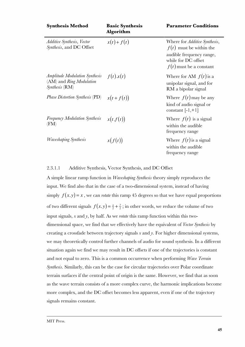
45

Synthesis Method Basic SynthesisAlgorithm

Parameter Conditions

Additive Synthesis, VectorSynthesis, and DC Offset

x t( ) + f t( ) Where for Additive Synthesis,f t( ) must be within the

audible frequency range,while for DC offsetf t( )must be a constant

Amplitude Modulation Synthesis(AM) and Ring ModulationSynthesis (RM)

f t( ).x t( ) Where for AM f t( ) is aunipolar signal, and forRM a bipolar signal

Phase Distortion Synthesis (PD) x t + f t( )( ) Where f t( )may be anykind of audio signal orconstant [-1,+1]

Frequency Modulation Synthesis(FM)

x t. f t( )( ) Where f t( ) is a signalwithin the audiblefrequency range

Waveshaping Synthesis x f t( )( ) Where f t( ) is a signalwithin the audiblefrequency range

2.3.1.1 Additive Synthesis, Vector Synthesis, and DC Offset

A simple linear ramp function in Waveshaping Synthesis theory simply reproduces the

input. We find also that in the case of a two-dimensional system, instead of having

simply f x, y( ) = x , we can rotate this ramp 45 degrees so that we have equal proportions

of two different signals f x, y( ) = x2 +

y2 ; in other words, we reduce the volume of two

input signals, x and y, by half. As we rotate this ramp function within this two-

dimensional space, we find that we effectively have the equivalent of Vector Synthesis by

creating a crossfade between trajectory signals x and y. For higher dimensional systems,

we may theoretically control further channels of audio for sound synthesis. In a different

situation again we find we may result in DC offsets if one of the trajectories is constant

and not equal to zero. This is a common occurrence when performing Wave Terrain

Synthesis. Similarly, this can be the case for circular trajectories over Polar coordinate

terrain surfaces if the central point of origin is the same. However, we find that as soon

as the wave terrain consists of a more complex curve, the harmonic implications become

more complex, and the DC offset becomes less apparent, even if one of the trajectory

signals remains constant.

MIT Press.

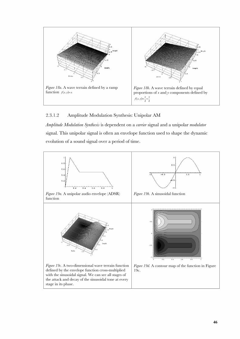
46

Figure 18a. A wave terrain defined by a rampfunction f x, y( )= x

Figure 18b. A wave terrain defined by equalproportions of x and y components defined by

f x, y( )= x2+y2

2.3.1.2 Amplitude Modulation Synthesis: Unipolar AM

Amplitude Modulation Synthesis is dependent on a carrier signal and a unipolar modulator

signal. This unipolar signal is often an envelope function used to shape the dynamic

evolution of a sound signal over a period of time.

Figure 19a. A unipolar audio envelope (ADSR)function

Figure 19b. A sinusoidal function

Figure 19c. A two-dimensional wave terrain functiondefined by the envelope function cross-multipliedwith the sinusoidal signal. We can see all stages ofthe attack and decay of the sinusoidal tone at everystage in its phase.

Figure 19d. A contour map of the function in Figure19c.

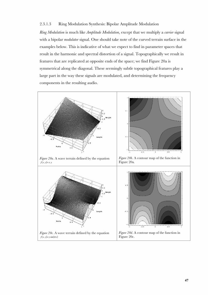
47

2.3.1.3 Ring Modulation Synthesis: Bipolar Amplitude Modulation

Ring Modulation is much like Amplitude Modulation, except that we multiply a carrier signal

with a bipolar modulator signal. One should take note of the curved terrain surface in the

examples below. This is indicative of what we expect to find in parameter spaces that

result in the harmonic and spectral distortion of a signal. Topographically we result in

features that are replicated at opposite ends of the space; we find Figure 20a is

symmetrical along the diagonal. These seemingly subtle topographical features play a

large part in the way these signals are modulated, and determining the frequency

components in the resulting audio.

Figure 20a. A wave terrain defined by the equationf x, y( )= x.y

Figure 20b. A contour map of the function inFigure 20a.

Figure 20c. A wave terrain defined by the equationf x, y( )= y sin π x( )

Figure 20d. A contour map of the function inFigure 20c.

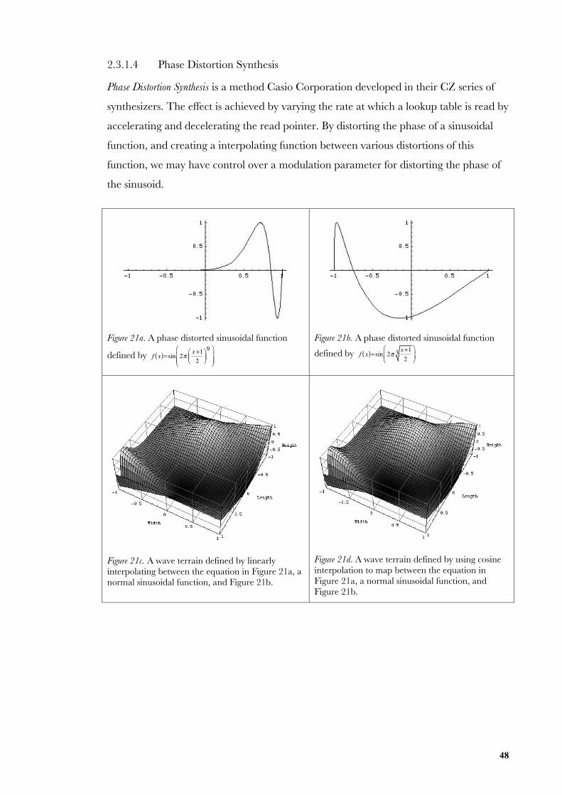
48

2.3.1.4 Phase Distortion Synthesis

Phase Distortion Synthesis is a method Casio Corporation developed in their CZ series of

synthesizers. The effect is achieved by varying the rate at which a lookup table is read by

accelerating and decelerating the read pointer. By distorting the phase of a sinusoidal

function, and creating a interpolating function between various distortions of this

function, we may have control over a modulation parameter for distorting the phase of

the sinusoid.

Figure 21a. A phase distorted sinusoidal function

defined by f x( )=sin 2πx+12

⎛⎝⎜

⎞⎠⎟9⎛

⎝⎜⎜

⎞

⎠⎟⎟

Figure 21b. A phase distorted sinusoidal function

defined by f x( )=sin 2πx+12

3⎛⎝⎜

⎞⎠⎟

Figure 21c. A wave terrain defined by linearlyinterpolating between the equation in Figure 21a, anormal sinusoidal function, and Figure 21b.

Figure 21d. A wave terrain defined by using cosineinterpolation to map between the equation inFigure 21a, a normal sinusoidal function, andFigure 21b.

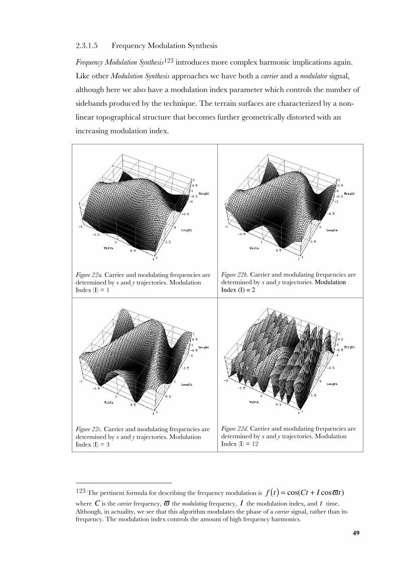
49

2.3.1.5 Frequency Modulation Synthesis

Frequency Modulation Synthesis123 introduces more complex harmonic implications again.

Like other Modulation Synthesis approaches we have both a carrier and a modulator signal,

although here we also have a modulation index parameter which controls the number of

sidebands produced by the technique. The terrain surfaces are characterized by a non-

linear topographical structure that becomes further geometrically distorted with an

increasing modulation index.

Figure 22a. Carrier and modulating frequencies aredetermined by x and y trajectories. ModulationIndex (I) = 1

Figure 22b. Carrier and modulating frequencies aredetermined by x and y trajectories. ModulationIndex (I) = 2

Figure 22c. Carrier and modulating frequencies aredetermined by x and y trajectories. ModulationIndex (I) = 3

Figure 22d. Carrier and modulating frequencies aredetermined by x and y trajectories. ModulationIndex (I) = 12

123 The pertinent formula for describing the frequency modulation is f t( ) = cos(Ct + I cosϖt)where C is the carrier frequency, ϖ the modulating frequency, I the modulation index, and t time.Although, in actuality, we see that this algorithm modulates the phase of a carrier signal, rather than itsfrequency. The modulation index controls the amount of high frequency harmonics.

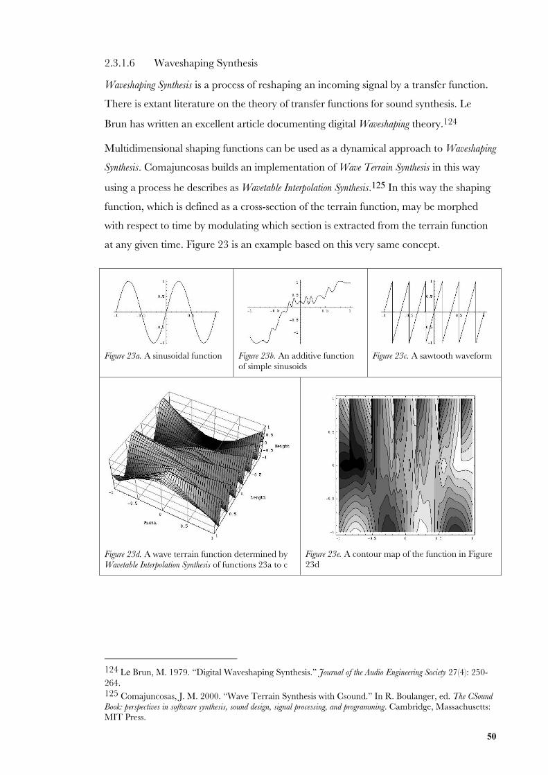
50

2.3.1.6 Waveshaping Synthesis

Waveshaping Synthesis is a process of reshaping an incoming signal by a transfer function.

There is extant literature on the theory of transfer functions for sound synthesis. Le

Brun has written an excellent article documenting digital Waveshaping theory.124

Multidimensional shaping functions can be used as a dynamical approach to Waveshaping

Synthesis. Comajuncosas builds an implementation of Wave Terrain Synthesis in this way

using a process he describes as Wavetable Interpolation Synthesis.125 In this way the shaping

function, which is defined as a cross-section of the terrain function, may be morphed

with respect to time by modulating which section is extracted from the terrain function

at any given time. Figure 23 is an example based on this very same concept.

Figure 23a. A sinusoidal function

Figure 23b. An additive functionof simple sinusoids

Figure 23c. A sawtooth waveform

Figure 23d. A wave terrain function determined byWavetable Interpolation Synthesis of functions 23a to c

Figure 23e. A contour map of the function in Figure23d

124 Le Brun, M. 1979. “Digital Waveshaping Synthesis.” Journal of the Audio Engineering Society 27(4): 250-264.125 Comajuncosas, J. M. 2000. “Wave Terrain Synthesis with Csound.” In R. Boulanger, ed. The CSoundBook: perspectives in software synthesis, sound design, signal processing, and programming. Cambridge, Massachusetts:MIT Press.

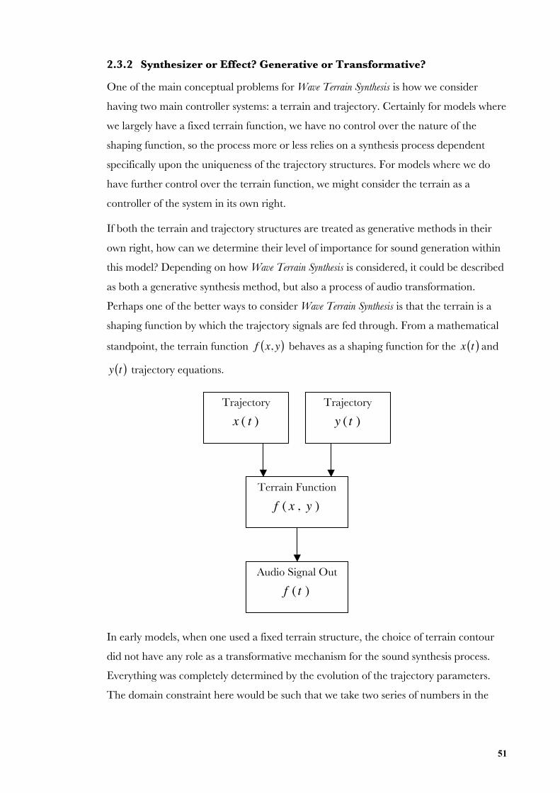
51

2.3.2 Synthesizer or Effect? Generative or Transformative?

One of the main conceptual problems for Wave Terrain Synthesis is how we consider

having two main controller systems: a terrain and trajectory. Certainly for models where

we largely have a fixed terrain function, we have no control over the nature of the

shaping function, so the process more or less relies on a synthesis process dependent

specifically upon the uniqueness of the trajectory structures. For models where we do

have further control over the terrain function, we might consider the terrain as a

controller of the system in its own right.

If both the terrain and trajectory structures are treated as generative methods in their

own right, how can we determine their level of importance for sound generation within

this model? Depending on how Wave Terrain Synthesis is considered, it could be described

as both a generative synthesis method, but also a process of audio transformation.

Perhaps one of the better ways to consider Wave Terrain Synthesis is that the terrain is a

shaping function by which the trajectory signals are fed through. From a mathematical

standpoint, the terrain function f x, y( ) behaves as a shaping function for the x t( ) and

y t( ) trajectory equations.

In early models, when one used a fixed terrain structure, the choice of terrain contour

did not have any role as a transformative mechanism for the sound synthesis process.

Everything was completely determined by the evolution of the trajectory parameters.

The domain constraint here would be such that we take two series of numbers in the

Trajectory

x ( t )Trajectory

y ( t )

Terrain Function

f ( x , y )

Audio Signal Out

f ( t )

52

range [-1+1] and return a result in the same range, what is called the signed unit

interval.126

Variable terrain surfaces refer to the idea that the terrain is now a transformative

mechanism for changing timbre, whether it is under user control or automated. The

distinction must be made here that in early models evolutionary complexity was

introduced via the transformative processes as applied to the trajectory signals. In later

dynamical models demonstrated by Comajuncosas127 and Mikelson,128 evolutionary

complexity is also introduced by the wave terrain functions.

2.3.3 Predicting Spectra

As Curtis Roads has explained:

….systematic investigations of the technique have focused on wave terrainsgenerated by relatively simple mathematical functions. As in techniques likefrequency modulation and waveshaping, the advantages of using simplemathematical functions is that it is possible to predict exactly the outputwaveform and spectrum generated by a given terrain. Mitsuhashi (1982c) andBorgonovo and Haus (1986) devised smooth mathematical wave terrainfunctions in the range [-1 ≤ x ≤ 1, -1 ≤ y ≤ 1].129

An important factor in the utility of any synthesis technique is the degree of control that

the user can exercise over the nature of the sound it produces. Like the importance of

the Chebyshev polynomials in Waveshaping theory130, a technique must be predictable

126 As is found in Waveshaping Synthesis theory. Except this is normally accomplished using one-dimensional arrays that contain the values of f at equally spaced points through the signed unit interval.

When time comes to compute f x( ) , we look up the values in the table corresponding to x in f , possiblyinterpolating to get the “in between” values. We call f the shaping function, since its effect is to change

the shape of the input wave x. We start with a pure sinusoidal signal, for example x = cosθ where

θ =ϖt , and where ϖ is the radian frequency and t is the time. x varies with the range [-1+1], that is, at

any given time -1 ≤ x ≤ +1. We take this signal and compute by some other function of x, that is f x( ) .127 Comajuncosas, J. M. 2000. “Wave Terrain Synthesis with Csound.” In R. Boulanger, ed. The CSoundBook: perspectives in software synthesis, sound design, signal processing, and programming. Cambridge, Massachusetts:MIT Press.128 Mikelson, H. 2000. “Terrain Mapping with Dynamic Surfaces.” The Csound Magazine.http://www.csounds.com/ezine/spring2000/synthesis/129 Roads, C. The Computer Music Tutorial. Page 164.130 Waveshaping theory discusses the creation of a shaping function that yields a particular spectrum. This

is sometimes called Spectrum Matching. These are determined by Chebychev polynomials, Tk(x) , which

have the following useful properties:

T

k(cosθ )=cosk θ

T

k +1( x)=2xT

k( x)−T

k −1( x)

One can use this following property to construct a polynomial from a set of desired harmonic amplitudes:

f ( x)=

h02

T0

( x)+h1T1

( x)+h2

T2

( x)+h3T3

( x)...

53

enough in order to establish a theory that can accommodate the scope of the technique.

With functional forms, or abstract mathematical models, one can work out exactly

which synthesis procedures are applied, and identify the modulation parameters. For

discrete maps, the distinguishing of synthesis processes becomes more obscured.

Nevertheless, there are a number of general observations that have been made with

respect to Waveshaping Synthesis theory that may also be applicable to Wave Terrain

Synthesis.

1) Discontinuities in the transfer function produce discontinuities in the output of

Wave Terrain Synthesis, and therefore, aliasing.

2) Discontinuities in either trajectory signal will produce discontinuities in the

output of Wave Terrain Synthesis, and therefore, aliasing.

3) A polynomial transfer function of order N will, when driven with a sinusoidal

input, produce a waveform with harmonics of the input up to the Nth.

4) Transfer functions that generate a lot of energy in high harmonics tend to yield

dynamic spectra that evolve erratically and not smoothly.

5) Transfer functions that generate spectra that decay rapidly with increasing

harmonic number tend to yield smoothly-evolving dynamic spectra.

6) Changing the sign of the target harmonic amplitudes will not perceptually

change the sound of the output for index a=1, but will change the evolution of

dynamic spectra for variable a.

The harmonic complexity of the resulting tones depend largely on both the harmonic

complexities of the terrain and trajectory signals. If these are both complex, the result is

significantly more complex. It is probably easier to define the parameters in terms of

another synthesis paradigm, such as Additive Synthesis. The example below shows a

contour plot of an additive terrain surface. It may not be quite so obvious to the eye that

the function has been derived in such a way.

Deriving functions

T

N( x)=T

N(cosθ )=cos nθ

Functions for deriving the pure nth harmonic when used as shaping function:Chebyshev Recursive Formula

T

N +1( x)=2xT

N( x)−T

N −1( x)

This is applied to calculate successive TN.

Phase Quadrature is the process by which one can specify the steady-state amplitudes HKand any

arbitrary phase φKas well:

S

N +1=2xS

N−S

N −1

These polynomials are termed the Chebyshev Polynomials of the Second kind.

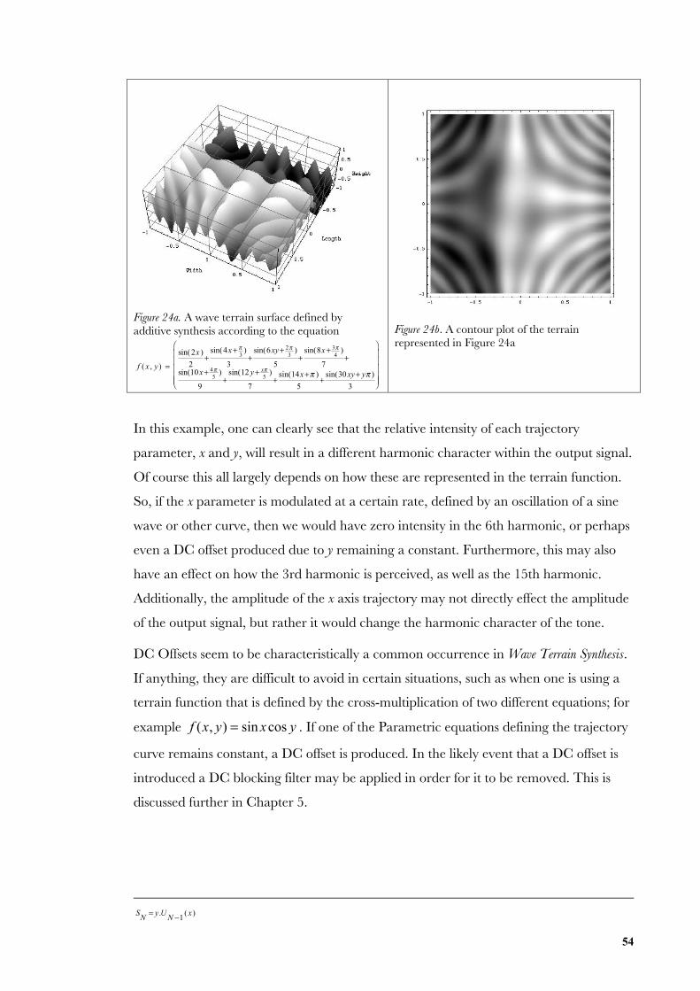
54

Figure 24a. A wave terrain surface defined byadditive synthesis according to the equation

f ( x , y) =

sin(2x )

2+

sin(4x+ π3

)

3+

sin(6xy+ 2π3

)

5+

sin(8x+ 3π4

)

7+

sin(10x+ 4π5

)

9+

sin(12 y+ xπ5

)

7+

sin(14x+π )

5+

sin(30xy+ yπ )

3

⎛

⎝

⎜⎜⎜⎜⎜

⎞

⎠

⎟⎟⎟⎟⎟

Figure 24b. A contour plot of the terrainrepresented in Figure 24a

In this example, one can clearly see that the relative intensity of each trajectory

parameter, x and y, will result in a different harmonic character within the output signal.

Of course this all largely depends on how these are represented in the terrain function.

So, if the x parameter is modulated at a certain rate, defined by an oscillation of a sine

wave or other curve, then we would have zero intensity in the 6th harmonic, or perhaps

even a DC offset produced due to y remaining a constant. Furthermore, this may also

have an effect on how the 3rd harmonic is perceived, as well as the 15th harmonic.

Additionally, the amplitude of the x axis trajectory may not directly effect the amplitude

of the output signal, but rather it would change the harmonic character of the tone.

DC Offsets seem to be characteristically a common occurrence in Wave Terrain Synthesis.

If anything, they are difficult to avoid in certain situations, such as when one is using a

terrain function that is defined by the cross-multiplication of two different equations; for

example f (x, y) = sin xcos y . If one of the Parametric equations defining the trajectory

curve remains constant, a DC offset is produced. In the likely event that a DC offset is

introduced a DC blocking filter may be applied in order for it to be removed. This is

discussed further in Chapter 5.

S

N= y.U

N −1( x)

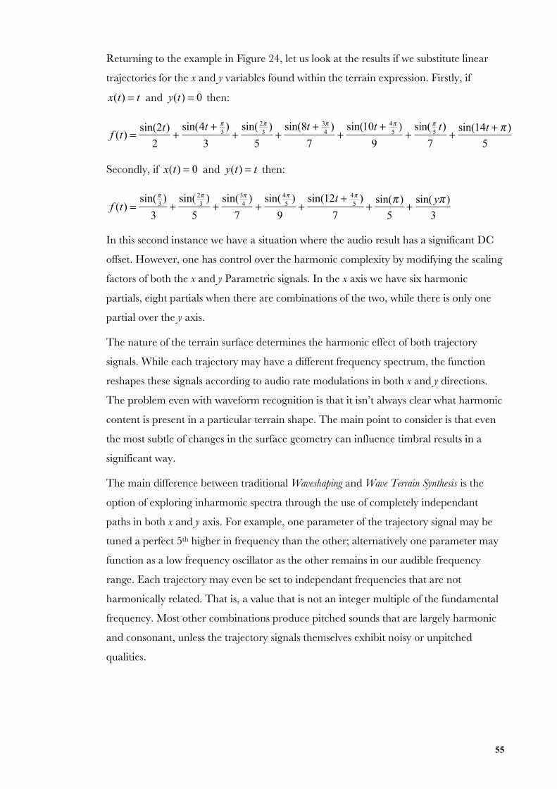
55

Returning to the example in Figure 24, let us look at the results if we substitute linear

trajectories for the x and y variables found within the terrain expression. Firstly, if

x(t) = t and y(t) = 0 then:

f (t) =

sin(2t)

2+

sin(4t + π3)

3+

sin( 2π3

)

5+

sin(8t + 3π4

)

7+

sin(10t + 4π5

)

9+

sin( π5

t)

7+

sin(14t + π )

5

Secondly, if x(t) = 0 and y(t) = t then:

f (t) =

sin(π3)

3+

sin( 2π3

)

5+

sin(3π4

)

7+

sin( 4π5

)

9+

sin(12t + 4π5

)

7+

sin(π )

5+

sin( yπ )

3

In this second instance we have a situation where the audio result has a significant DC

offset. However, one has control over the harmonic complexity by modifying the scaling

factors of both the x and y Parametric signals. In the x axis we have six harmonic

partials, eight partials when there are combinations of the two, while there is only one

partial over the y axis.

The nature of the terrain surface determines the harmonic effect of both trajectory

signals. While each trajectory may have a different frequency spectrum, the function

reshapes these signals according to audio rate modulations in both x and y directions.

The problem even with waveform recognition is that it isn’t always clear what harmonic

content is present in a particular terrain shape. The main point to consider is that even

the most subtle of changes in the surface geometry can influence timbral results in a

significant way.

The main difference between traditional Waveshaping and Wave Terrain Synthesis is the

option of exploring inharmonic spectra through the use of completely independant

paths in both x and y axis. For example, one parameter of the trajectory signal may be

tuned a perfect 5th higher in frequency than the other; alternatively one parameter may

function as a low frequency oscillator as the other remains in our audible frequency

range. Each trajectory may even be set to independant frequencies that are not

harmonically related. That is, a value that is not an integer multiple of the fundamental

frequency. Most other combinations produce pitched sounds that are largely harmonic

and consonant, unless the trajectory signals themselves exhibit noisy or unpitched

qualities.

56

2.3.4 Conceptual Debate on the Relative Importance of Terrain and

Trajectory Structures

An effective Wave Terrain Synthesis instrument depends on the ability for the user to

control the extent of complexity that is introduced at any stage of the model. By

controlling the extent of complexity introduced the user is essentially influencing the

accumulation of complexity in the resulting waveform. If one uses the transient

complexity of real-world sounds as a means of driving Wave Terrain Synthesis through

processes such as the Phase Space and Pseudo-Phase Space representation of signals, it

is unnecessary for the rest of the model to reflect structures of high complexity.

Frequency artifacts such as aliasing and distortion would be extremely difficult to avoid

even with simple terrain structures when driven by real-world high transient signals.

It seems there is a need for establishing what roles the trajectory and terrain functions

serve for the purposes of both fine-tuning and maximizing the expressive potential of the

technique. It is the trajectory that completely determines to what bearing the terrain

function has on the system. With many of the conventionally used approaches – for the

purposes of creating pitched sounds for musical application – it is becoming clear that

Wave Terrain Synthesis technique has been largely restricted to the world of simple

oscillator types due to the way in which trajectory orbits have been derived; a situation

that – on the surface – seems to render the possibility of using a terrain data array

impractical. For example, a small trichromatic 24-bit image file of dimensions 320 x

240, requiring 230,400 bytes of memory, seems far too large a wavetable if the result is

much like a simple oscillator. This is largely problematic when the trajectory orbit is

periodic, as only a small percentage of the terrain data is accessed for the resulting

sound.

Nevertheless, the user must be careful as to where complexity is introduced in the Wave

Terrain Synthesis model. There are many ways for complex evolutions in parameter to be

introduced regardless of whether these are generative or transformative. Taking

Frequency Modulation for example, it is not long before harmonic qualities of the original

signals are distorted beyond recognition, especially with increasing levels of the

modulation index parameter. Similarly for Wave Terrain Synthesis, effective approaches to

sound design using this methodology would suggest following a process where one starts

with a simpler model. One may then subsequently extend upon this model by pushing

the bar toward more complex territories.

57

Due to the multi-parameter nature of Wave Terrain Synthesis, the theory could potentially

go on indefinitely since whatever approach exists there are numerous possibilities as to

how it may be applied to sound synthesis. One may consider the many generative

options, not just for signal synthesis, but multi-signal synthesis, and how these may be

applicable to Wave Terrain Synthesis; although the parameters involved in generating these

signals are not always going to be useful for sound synthesis. The disadvantage of such a

wide-reaching proposal is that the system becomes fraught with difficulty as the entire

model is subject to change for each unique generative situation, meaning a unique set of

variables must be established. This kind of approach requires an interface that is

versatile enough to account for this.

Previous research into Wave Terrain Synthesis has shown – more often than not – that it

has been most useful for creating slowly evolving drones of sound. These have been

derived from scanning trajectories that reflect this slowly transforming and “sustained”

character. If one analyses the harmonic spectrum of the trajectory components, x and y,

one can immediately relate these temporal features. In other words the trajectory

essentially determines the overall transitory evolution of the sound, whereas the terrain

changes the way in which this information is reshaped. The terrain reshapes the

trajectory according to its own contour, so if the image is full of noise, the resulting

sound will reflect this noisy character. Alternatively, if the terrain has a smoother

consistency, such as a blurred image, the terrain reshapes the waveform in a more

harmonically simple way.

In order to steer away from similar models of Waveshaping and Scanned Synthesis, Wave

Terrain Synthesis must approach complexity from the standpoint of the trajectory system.

Hopefully, in this way, we will access more unknown combinations in modulation

synthesis, and continue to establish Wave Terrain Synthesis as a method in its own right, set

aside from these other forms. For a further and in depth discussion on the various

approaches to trajectory synthesis refer to Chapter 4.

Part of the conceptual problem when applying a visual methodology for Wave Terrain

Synthesis, is that the image has a secondary role in the system. When we see other forms

of Graphical Sound Synthesis methods, we immediately consider the image as being the

single and primary source for generating the resulting audio; in other words, we have an

expectation that the image contains all the relevant information needed for generating

what we hear as a result. In the case of Wave Terrain Synthesis on the other hand, we need

to be able to see both the terrain and trajectory structures dynamically. When we see the

58

evolution of the trajectory signal, auditory changes and how they relate to the image

begin to make more sense. This is something that the GUI will have to reflect: the fact

that the trajectory is the primary generative and driving mechanism for Wave Terrain

Synthesis. Nevertheless, without discounting the fact that the terrain plays a large part in

how these signals are perceived. The terrain in fact controls how the interaction of these

parameters fuse together to generate sound.

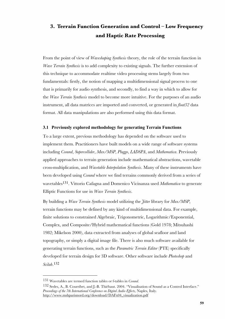
59

3. Terrain Function Generation and Control – Low Frequency

and Haptic Rate Processing

From the point of view of Waveshaping Synthesis theory, the role of the terrain function in

Wave Terrain Synthesis is to add complexity to existing signals. The further extension of

this technique to accommodate realtime video processing stems largely from two

fundamentals: firstly, the notion of mapping a multidimensional signal process to one

that is primarily for audio synthesis, and secondly, to find a way in which to allow for

the Wave Terrain Synthesis model to become more intuitive. For the purposes of an audio

instrument, all data matrices are imported and converted, or generated in float32 data

format. All data manipulations are also performed using this data format.

3.1 Previously explored methodology for generating Terrain Functions

To a large extent, previous methodology has depended on the software used to

implement them. Practitioners have built models on a wide range of software systems

including Csound, Supercollider, Max/MSP, Pluggo, LADSPA, and Mathematica. Previously

applied approaches to terrain generation include mathematical abstractions, wavetable

cross-multiplication, and Wavetable Interpolation Synthesis. Many of these instruments have

been developed using Csound where we find terrains commonly derived from a series of

wavetables131. Vittorio Cafagna and Domenico Vicinanza used Mathematica to generate

Elliptic Functions for use in Wave Terrain Synthesis.

By building a Wave Terrain Synthesis model utilizing the Jitter library for Max/MSP,

terrain functions may be defined by any kind of multidimensional data. For example,

finite solutions to constrained Algebraic, Trigonometric, Logarithmic/Exponential,

Complex, and Composite/Hybrid mathematical functions (Gold 1978; Mitsuhashi

1982; Mikelson 2000), data extracted from analyses of global seafloor and land

topography, or simply a digital image file. There is also much software available for

generating terrain functions, such as the Parametric Terrain Editor (PTE) specifically

developed for terrain design for 3D software. Other software include Photoshop and

Scilab.132

131 Wavetables are termed function tables or f-tables in Csound.132 Sedes, A., B. Courribet, and J.-B. Thiébaut. 2004. “Visualisation of Sound as a Control Interface.”Proceedings of the 7th International Conference on Digital Audio Effects, Naples, Italy.http://www.mshparisnord.org/download/DAFx04_visualization.pdf

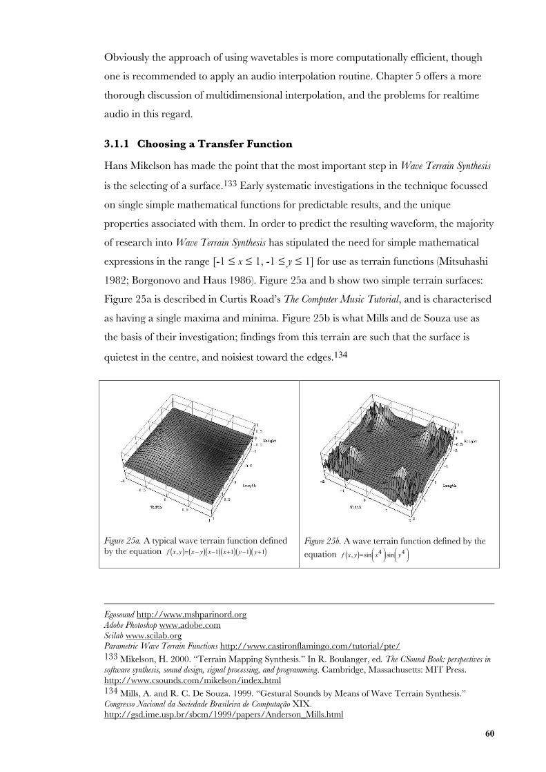
60

Obviously the approach of using wavetables is more computationally efficient, though

one is recommended to apply an audio interpolation routine. Chapter 5 offers a more

thorough discussion of multidimensional interpolation, and the problems for realtime

audio in this regard.

3.1.1 Choosing a Transfer Function

Hans Mikelson has made the point that the most important step in Wave Terrain Synthesis

is the selecting of a surface.133 Early systematic investigations in the technique focussed

on single simple mathematical functions for predictable results, and the unique

properties associated with them. In order to predict the resulting waveform, the majority

of research into Wave Terrain Synthesis has stipulated the need for simple mathematical

expressions in the range [-1 ≤ x ≤ 1, -1 ≤ y ≤ 1] for use as terrain functions (Mitsuhashi

1982; Borgonovo and Haus 1986). Figure 25a and b show two simple terrain surfaces:

Figure 25a is described in Curtis Road’s The Computer Music Tutorial, and is characterised

as having a single maxima and minima. Figure 25b is what Mills and de Souza use as

the basis of their investigation; findings from this terrain are such that the surface is

quietest in the centre, and noisiest toward the edges.134

Figure 25a. A typical wave terrain function definedby the equation f x , y( )= x− y( ) x−1( ) x+1( ) y−1( ) y+1( )

Figure 25b. A wave terrain function defined by theequation

f x , y( )=sin x4⎛

⎝⎜⎞⎠⎟ sin y4⎛

⎝⎜⎞⎠⎟

Egosound http://www.mshparinord.orgAdobe Photoshop www.adobe.comScilab www.scilab.orgParametric Wave Terrain Functions http://www.castironflamingo.com/tutorial/pte/133 Mikelson, H. 2000. “Terrain Mapping Synthesis.” In R. Boulanger, ed. The CSound Book: perspectives insoftware synthesis, sound design, signal processing, and programming. Cambridge, Massachusetts: MIT Press.http://www.csounds.com/mikelson/index.html134 Mills, A. and R. C. De Souza. 1999. “Gestural Sounds by Means of Wave Terrain Synthesis.”Congresso Nacional da Sociedade Brasileira de Computação XIX.http://gsd.ime.usp.br/sbcm/1999/papers/Anderson_Mills.html

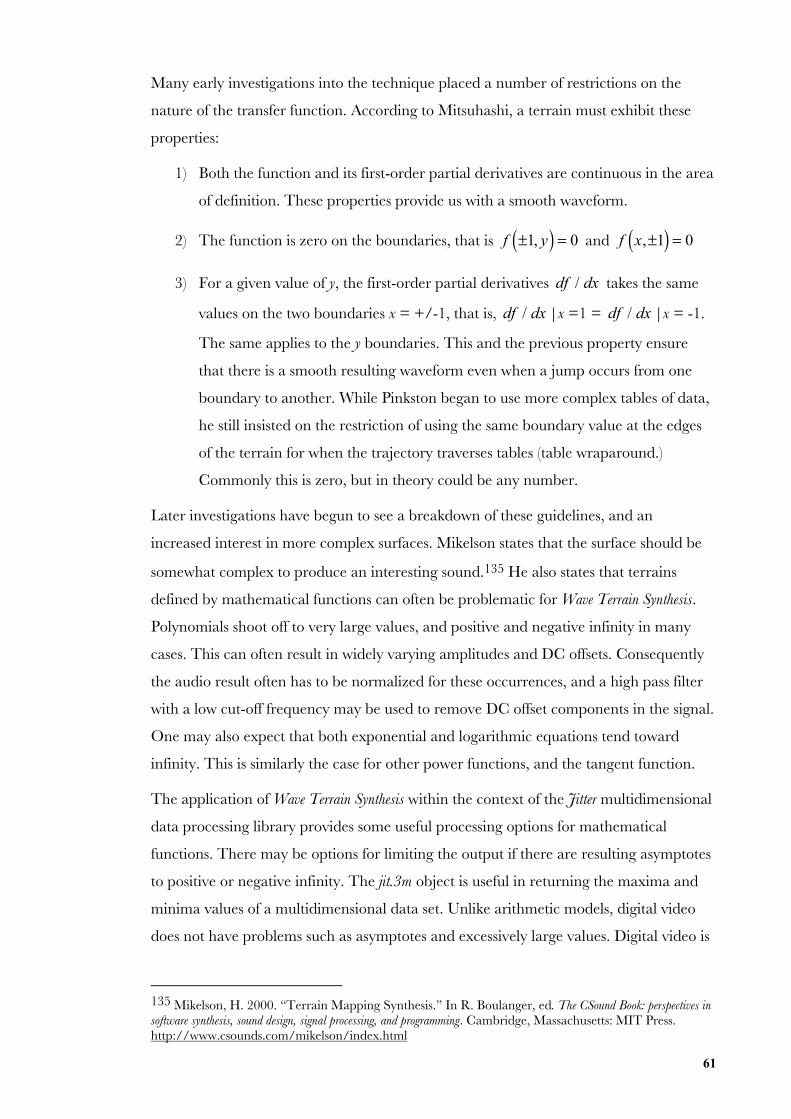
61

Many early investigations into the technique placed a number of restrictions on the

nature of the transfer function. According to Mitsuhashi, a terrain must exhibit these

properties:

1) Both the function and its first-order partial derivatives are continuous in the area

of definition. These properties provide us with a smooth waveform.

2) The function is zero on the boundaries, that is f ±1, y( ) = 0 and

f x,±1( ) = 0

3) For a given value of y, the first-order partial derivatives df / dx takes the same

values on the two boundaries x = +/-1, that is, df / dx |x =1 = df / dx |x = -1.

The same applies to the y boundaries. This and the previous property ensure

that there is a smooth resulting waveform even when a jump occurs from one

boundary to another. While Pinkston began to use more complex tables of data,

he still insisted on the restriction of using the same boundary value at the edges

of the terrain for when the trajectory traverses tables (table wraparound.)

Commonly this is zero, but in theory could be any number.

Later investigations have begun to see a breakdown of these guidelines, and an

increased interest in more complex surfaces. Mikelson states that the surface should be

somewhat complex to produce an interesting sound.135 He also states that terrains

defined by mathematical functions can often be problematic for Wave Terrain Synthesis.

Polynomials shoot off to very large values, and positive and negative infinity in many

cases. This can often result in widely varying amplitudes and DC offsets. Consequently

the audio result often has to be normalized for these occurrences, and a high pass filter

with a low cut-off frequency may be used to remove DC offset components in the signal.

One may also expect that both exponential and logarithmic equations tend toward

infinity. This is similarly the case for other power functions, and the tangent function.

The application of Wave Terrain Synthesis within the context of the Jitter multidimensional

data processing library provides some useful processing options for mathematical

functions. There may be options for limiting the output if there are resulting asymptotes

to positive or negative infinity. The jit.3m object is useful in returning the maxima and

minima values of a multidimensional data set. Unlike arithmetic models, digital video

does not have problems such as asymptotes and excessively large values. Digital video is

135 Mikelson, H. 2000. “Terrain Mapping Synthesis.” In R. Boulanger, ed. The CSound Book: perspectives insoftware synthesis, sound design, signal processing, and programming. Cambridge, Massachusetts: MIT Press.http://www.csounds.com/mikelson/index.html

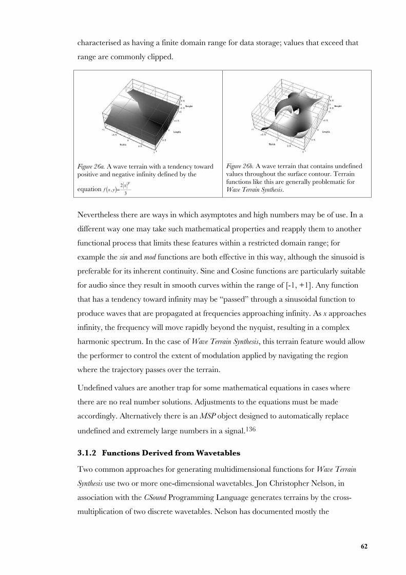
62

characterised as having a finite domain range for data storage; values that exceed that

range are commonly clipped.

Figure 26a. A wave terrain with a tendency towardpositive and negative infinity defined by the

equation f x , y( )= 2 x

y

3

Figure 26b. A wave terrain that contains undefinedvalues throughout the surface contour. Terrainfunctions like this are generally problematic forWave Terrain Synthesis.

Nevertheless there are ways in which asymptotes and high numbers may be of use. In a

different way one may take such mathematical properties and reapply them to another

functional process that limits these features within a restricted domain range; for

example the sin and mod functions are both effective in this way, although the sinusoid is

preferable for its inherent continuity. Sine and Cosine functions are particularly suitable

for audio since they result in smooth curves within the range of [-1, +1]. Any function

that has a tendency toward infinity may be “passed” through a sinusoidal function to

produce waves that are propagated at frequencies approaching infinity. As x approaches

infinity, the frequency will move rapidly beyond the nyquist, resulting in a complex

harmonic spectrum. In the case of Wave Terrain Synthesis, this terrain feature would allow

the performer to control the extent of modulation applied by navigating the region

where the trajectory passes over the terrain.

Undefined values are another trap for some mathematical equations in cases where

there are no real number solutions. Adjustments to the equations must be made

accordingly. Alternatively there is an MSP object designed to automatically replace

undefined and extremely large numbers in a signal.136

3.1.2 Functions Derived from Wavetables

Two common approaches for generating multidimensional functions for Wave Terrain

Synthesis use two or more one-dimensional wavetables. Jon Christopher Nelson, in

association with the CSound Programming Language generates terrains by the cross-

multiplication of two discrete wavetables. Nelson has documented mostly the

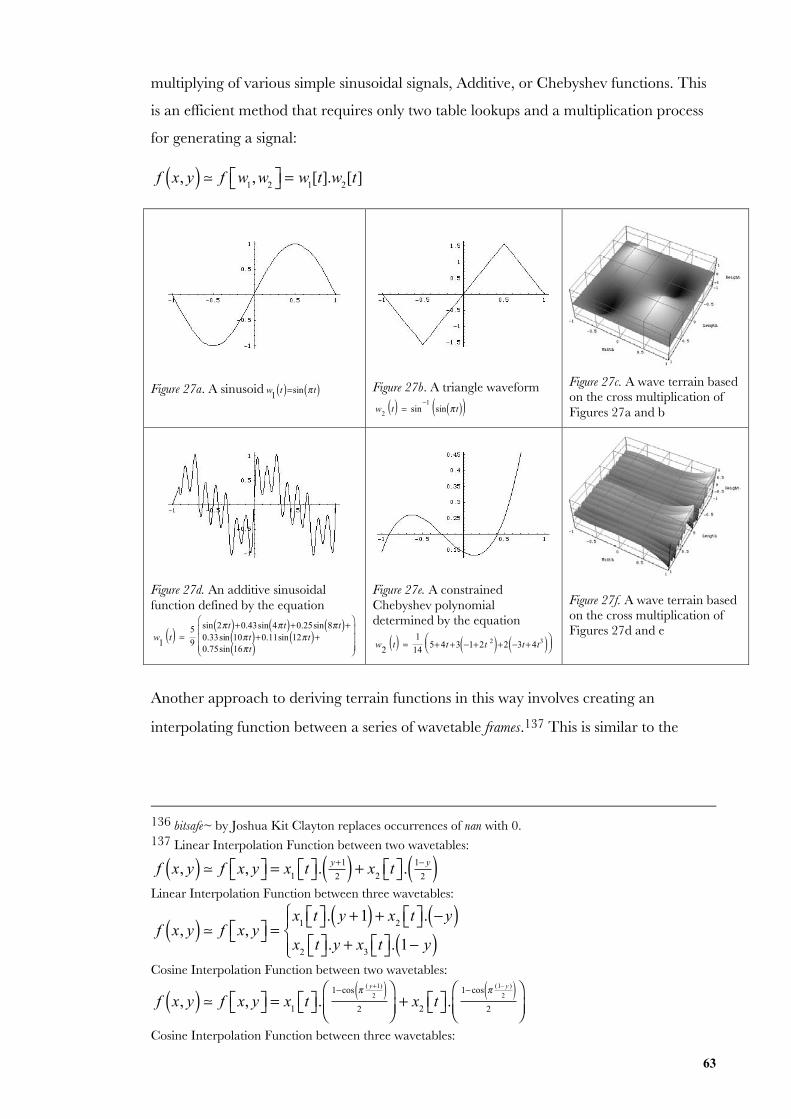
63

multiplying of various simple sinusoidal signals, Additive, or Chebyshev functions. This

is an efficient method that requires only two table lookups and a multiplication process

for generating a signal:

f x, y( ) f w

1, w

2⎡⎣ ⎤⎦ = w

1[t].w

2[t]

Figure 27a. A sinusoid w

1t( )=sin π t( )

Figure 27b. A triangle waveform

w2t( ) = sin

−1sin π t( )( )

Figure 27c. A wave terrain basedon the cross multiplication ofFigures 27a and b

Figure 27d. An additive sinusoidalfunction defined by the equation

w

1t( ) =

5

9

sin 2π t( )+0.43sin 4π t( )+0.25sin 8π t( )+0.33sin 10π t( )+0.11sin 12π t( )+0.75sin 16π t( )

⎛

⎝

⎜⎜⎜

⎞

⎠

⎟⎟⎟

Figure 27e. A constrainedChebyshev polynomialdetermined by the equation

w

2t( ) =

1

145+4t+3 −1+2t 2( )+2 −3t+4t3( )⎛⎝⎜

⎞⎠⎟

Figure 27f. A wave terrain basedon the cross multiplication ofFigures 27d and e

Another approach to deriving terrain functions in this way involves creating an

interpolating function between a series of wavetable frames.137 This is similar to the

136 bitsafe~ by Joshua Kit Clayton replaces occurrences of nan with 0.137 Linear Interpolation Function between two wavetables:

f x, y( ) f x, y⎡⎣ ⎤⎦ = x

1t⎡⎣ ⎤⎦. y+1

2( ) + x2

t⎡⎣ ⎤⎦. 1− y

2( )Linear Interpolation Function between three wavetables:

f x, y( ) f x, y⎡⎣ ⎤⎦ =x

1t⎡⎣ ⎤⎦. y +1( ) + x

2t⎡⎣ ⎤⎦. − y( )

x2

t⎡⎣ ⎤⎦.y + x3

t⎡⎣ ⎤⎦. 1− y( )⎧⎨⎪

⎩⎪Cosine Interpolation Function between two wavetables:

f x, y( ) f x, y⎡⎣ ⎤⎦ = x

1t⎡⎣ ⎤⎦.

1−cos π ( y+1)

2( )2

⎛⎝⎜

⎞⎠⎟+ x

2t⎡⎣ ⎤⎦.

1−cos π (1− y )

2( )2

⎛⎝⎜

⎞⎠⎟

Cosine Interpolation Function between three wavetables:

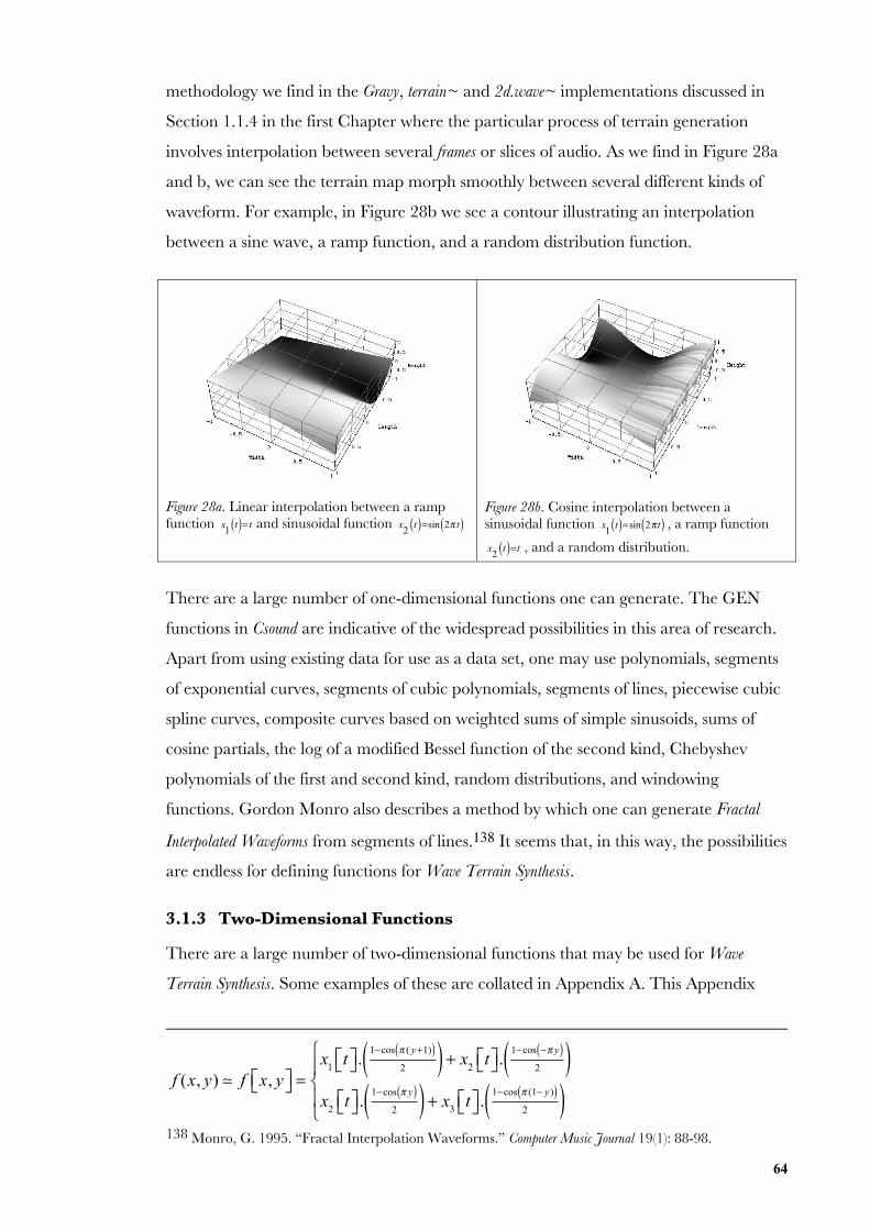
64

methodology we find in the Gravy, terrain~ and 2d.wave~ implementations discussed in

Section 1.1.4 in the first Chapter where the particular process of terrain generation

involves interpolation between several frames or slices of audio. As we find in Figure 28a

and b, we can see the terrain map morph smoothly between several different kinds of

waveform. For example, in Figure 28b we see a contour illustrating an interpolation

between a sine wave, a ramp function, and a random distribution function.

Figure 28a. Linear interpolation between a rampfunction

x1

t( )= t and sinusoidal function x2

t( )=sin 2π t( )

Figure 28b. Cosine interpolation between asinusoidal function

x1

t( )=sin 2π t( ) , a ramp function

x2

t( )=t , and a random distribution.

There are a large number of one-dimensional functions one can generate. The GEN

functions in Csound are indicative of the widespread possibilities in this area of research.

Apart from using existing data for use as a data set, one may use polynomials, segments

of exponential curves, segments of cubic polynomials, segments of lines, piecewise cubic

spline curves, composite curves based on weighted sums of simple sinusoids, sums of

cosine partials, the log of a modified Bessel function of the second kind, Chebyshev

polynomials of the first and second kind, random distributions, and windowing

functions. Gordon Monro also describes a method by which one can generate Fractal

Interpolated Waveforms from segments of lines.138 It seems that, in this way, the possibilities

are endless for defining functions for Wave Terrain Synthesis.

3.1.3 Two-Dimensional Functions

There are a large number of two-dimensional functions that may be used for Wave

Terrain Synthesis. Some examples of these are collated in Appendix A. This Appendix

f (x, y) f x, y⎡⎣ ⎤⎦ =x

1t⎡⎣ ⎤⎦.

1−cos π ( y+1)( )2( ) + x

2t⎡⎣ ⎤⎦.

1−cos −π y( )2( )

x2

t⎡⎣ ⎤⎦.1−cos π y( )

2( ) + x3

t⎡⎣ ⎤⎦.1−cos π (1− y)( )

2( )⎧

⎨⎪

⎩⎪

138 Monro, G. 1995. “Fractal Interpolation Waveforms.” Computer Music Journal 19(1): 88-98.

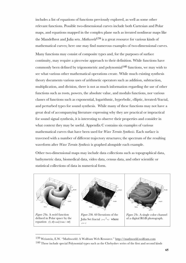
65

includes a list of equations of functions previously explored, as well as some other

relevant functions. Possible two-dimensional curves include both Cartesian and Polar

maps, and equations mapped in the complex plane such as iterated nonlinear maps like

the Mandelbrot and Julia sets. Mathworld139 is a great resource for various kinds of

mathematical curves; here one may find numerous examples of two-dimensional curves.

Many functions may consist of composite types and, for the purposes of surface

continuity, may require a piecewise approach to their definition. While functions have

commonly been defined by trigonometric and polynomial140 functions, we may wish to

see what various other mathematical operations create. While much existing synthesis

theory documents various uses of arithmetic operators such as addition, subtraction,

multiplication, and division, there is not as much information regarding the use of other

functions such as roots, powers, the absolute value, and modulo functions, nor various

classes of functions such as exponential, logarithmic, hyperbolic, elliptic, iterated/fractal,

and perturbed types for sound synthesis. While many of these functions may not have a

great deal of accompanying literature expressing why they are practical or impractical

for sound signal synthesis, it is interesting to observe their properties and consider in

what context they may be useful. Appendix C contains six examples of various

mathematical curves that have been used for Wave Terrain Synthesis. Each surface is

traversed with a number of different trajectory structures; the spectrum of the resulting

waveform after Wave Terrain Synthesis is graphed alongside each example.

Other two-dimensional maps may include data collections such as topographical data,

bathymetric data, biomedical data, video data, census data, and other scientific or

statistical collections of data in numerical form.

Figure 29a. A swirl functiondefined in Polar space by theequation f r ,θ( )=cos 12sin r−4θ( )

Figure 29b. 60 Iterations of the

Julia Set fractal z= z 2+c where c=− i

Figure 29c. A single color channelof a digital RGB photograph.

139 Weisstein, E.W. “Mathworld: A Wolfram Web Resource.” http://mathworld.wolfram.com140 These include special Polynomial types such as the Chebyshev series of the first and second kinds

66

3.1.4 Higher Dimensional Surfaces

Both Jon Christopher Nelson and Hans Mikelson have investigated terrain surfaces of

higher dimension. Theoretically this is not problematic for arithmetic approaches, but for

discrete wavetable methodology the size of memory requirements jump exponentially.

For a wavetable with size S and dimension N our memory requirements would be

SN . Another problem with higher dimensional surfaces is their representation. It

becomes increasingly difficult to visualize the extent of the space. Visualising data of

higher dimensions still largely remains a problem to this day.

The design of higher dimensional surfaces may be approached keeping existing sound

synthesis theory in mind. Alternatively one could develop a completely abstract model

for Wave Terrain Synthesis. Appendix D contains some examples of higher dimensional

systems and how to easily and systematically go about creating such curves.

3.1.5 Dynamically Modulated Surfaces

The notion of a dynamical terrain seems to have been first mentioned in a section of

Curtis Roads’ The Computer Music Tutorial.141 There are a number of ways in which

various practitioners have approached this problem.

Mikelson creates dynamical terrains by using the planet and lorenz Csound opcodes to

modulate parameters of a discrete linear function.142 Firstly, this discrete linear function

is extended to account for a higher dimensional space. Secondly these newly extended

parameters are then controlled by the time-series solutions of the lorenz and planet

opcodes. In this way, features that might have been introduced by a linear equation –

such as the curved surfaces produced by sine, cosine, and logarithmic functions –

become subject to dynamical motion over the terrain resulting in an ever evolving

landscape. Within this conceptual framework, the dynamical system controls the

positions of various hills, ridges and valleys that describe the terrain contour.

By separating various components of the equation through processes of addition or

subtraction – rather than multiplication or division – certain features of the curve may

be controlled independently. Terrain synthesis results in a large number of control

141 Roads, C., et al. 1996. The Computer Music Tutorial. Cambridge, Massachusetts: MIT Press.142 Parameters of the surface are modulated by the output of the planet opcode. The position of the hill iscontrolled by the coordinates of planet. The frequency of the ridges is controlled by the z coordinate ofplanet. The overall amplitude of the surface is controlled by the sum of the x, y, z coordinates. Mikelson

uses functions like

1

1+ x2 to add hills to the surface. Refer to: Mikelson, H. 2000. “Terrain Mapping with

Dynamic Surfaces.” The Csound Magazine. http://www.csounds.com/ezine/spring2000/synthesis/

67

parameters, and Mikelson states that dynamical systems are an interesting way to

control these large numbers of parameters.143

Another alternative is the dynamic modulation of two streaming audio signals.

Traditionally, the linear process of multiplying two waveforms has been understood as

the digital form of Ring Modulation Synthesis. The addition of a trajectory system that

modulates the index value of each buffer value introduces a distortion of the wavelength

of the recorded audio stream with respect to time, resulting in Frequency Modulation.144

Dannenburg and Neuendorffer explore a dynamical system using live video capture for

Wave Terrain Synthesis. The use of a video signal as a dynamic terrain function for sound

synthesis emphasizes the structure as being a significant modulatable control system

within the instrument model by allowing a performer to specifically modify timbre. The

success of such a dynamical model, considering the practicalities of managing frames of

video and other multidimensional signal streams, depends on the dynamic system

moving at effective rates of vibration. As is found with Scanned Synthesis, these rates are

said to be most effective at low frequencies of vibration below 15Hz.145

3.2 Graphical Generative Techniques and their Application to Wave Terrain

Synthesis

The implementation of Wave Terrain Synthesis within Max/MSP in conjunction with the

Jitter extendible library presents some interesting possibilities for integrating video

processing within an audio synthesis model. Importantly, we may see how some of the

multidimensional generative routines might apply to Wave Terrain Synthesis, and whether

any of them prove useful and practical for the generation of audio. For this research, we

are looking primarily at jit.noise for the generation of Perlin noise functions, jit.gl.nurbs for

143 Mikelson, H. 2000. “Terrain Mapping with Dynamic Surfaces.” The Csound Magazine.http://www.csounds.com/ezine/spring2000/synthesis/144 Chowning, J. 1973. “The Synthesis of Complex Spectra by means of Frequency Modulation.” Journalof the Audio Engineering Society 21(7): 526-534. Reprinted in C. Roads and J. Strawn, eds. 1985. Foundations ofComputer Music. Cambridge, Massachusetts: The MIT Press: 6-29.James, S. 2003. “Possibilities for Dynamical Wave Terrain Synthesis.” Converging Technologies, Proceedings ofthe Australasian Computer Music Conference: 58-67.145 A unique feature of Scanned Synthesis is its emphasis on the performer's control of timbre. Thevibrations of the system are a function of the initial conditions, the forces applied by the performer, andthe dynamics of the system. Examples include slowly vibrating strings and two dimensional diffusionequations. Experiments have been performed using various two dimensional objects and equationsincluding a gong, a set of coupled strings and the heat equation with boiling. Other work has beenperformed using chaotic equations such as the Kuramoto-Shivashinski equation. To make audiblefrequencies, the “shape” of the dynamic system, along a closed path, is scanned periodically. The pitch isdetermined by the speed of the scanning function. Refer to: Boulanger, R., Smaragdis, P., & Ffitch, J.2000. “Scanned Synthesis: An Introduction and Demonstration of a New Synthesis and Signal Processing

68

the generation of NURBS surfaces, the use of jit.poke~ and jit.op functions for

Recurrence Plotting, and the jit.qt.grab and jit.qt.movie objects for video capture and

playback.

Many of the existing approaches to sound synthesis have a reasonable amount of

theoretical substance, such as the use of Chebyshev polynomial types in Waveshaping

theory. Are standard video playback and processing functions applicable to Wave Terrain

Synthesis? Whatever the case may be, the possibility of using other sources of data for

terrain synthesis is of genuine interest. For example, digitized real-life photographs often

contain data structures that may be extremely difficult to approach from an arithmetic

point of view. By using these alternative generative mediums for sound synthesis we

open up new possibilities in terms of their multiplicity and potential for complex

arithmetic modulation. Nevertheless, the model still retains the ability to reproduce

parameter spaces of simpler models, hence bridging the gap between these various

parameter spaces, and allowing for more specific control over the nature of the

information represented within the parameter space.

The generative techniques discussed in this Sub-Chapter are all potentially dynamic.

One of the more problematic outcomes of applying dynamic terrain systems to Wave

Terrain Synthesis is that there are resulting frequency artifacts. The main problem with

any of these dynamical techniques is dealing with low frame rates of video relative to

high sample rates of audio. Solutions to this problem are discussed in Chapter 5. A

scheduling system is employed to synchronise an audio crossfade between video frames

in order to prevent the introduction of these audio artifacts.

In the course of research into Scanned Synthesis theory, it was found that convincing rates

of timbral movement are less than 15Hz; these have been described as Haptic rates.

However, it seems that if efficiency is not kept in mind with respect to the Wave Terrain

Synthesis model, we may be looking at frame rates of 1 or 2Hz. Instead of unnecessarily

overloading computational resources one may use matrices of size 80 x 80 in preference

to common video frame sizes of 320 x 240 or 640 x 480;146 this ensures that the

processing of this information is significantly more manageable for realtime

computation. It is here that we touch upon one of the more significant issues in this

research: maintaining efficiency and speed for realtime processing. This is discussed in

more depth in Section 6.1.1 of Chapter 6 where necessary methodological compromises

Technique”, Proceedings of the 2000 International Computer Music Conference, San Francisco: InternationalComputer Music Association: 372-375.

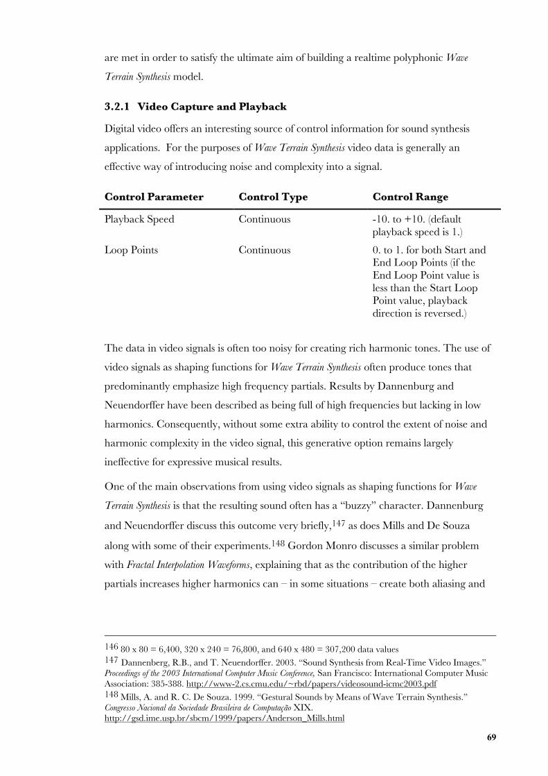
69

are met in order to satisfy the ultimate aim of building a realtime polyphonic Wave

Terrain Synthesis model.

3.2.1 Video Capture and Playback

Digital video offers an interesting source of control information for sound synthesis

applications. For the purposes of Wave Terrain Synthesis video data is generally an

effective way of introducing noise and complexity into a signal.

Control Parameter Control Type Control Range

Playback Speed Continuous -10. to +10. (defaultplayback speed is 1.)

Loop Points Continuous 0. to 1. for both Start andEnd Loop Points (if theEnd Loop Point value isless than the Start LoopPoint value, playbackdirection is reversed.)

The data in video signals is often too noisy for creating rich harmonic tones. The use of

video signals as shaping functions for Wave Terrain Synthesis often produce tones that

predominantly emphasize high frequency partials. Results by Dannenburg and

Neuendorffer have been described as being full of high frequencies but lacking in low

harmonics. Consequently, without some extra ability to control the extent of noise and

harmonic complexity in the video signal, this generative option remains largely

ineffective for expressive musical results.

One of the main observations from using video signals as shaping functions for Wave

Terrain Synthesis is that the resulting sound often has a “buzzy” character. Dannenburg

and Neuendorffer discuss this outcome very briefly,147 as does Mills and De Souza

along with some of their experiments.148 Gordon Monro discusses a similar problem

with Fractal Interpolation Waveforms, explaining that as the contribution of the higher

partials increases higher harmonics can – in some situations – create both aliasing and

146 80 x 80 = 6,400, 320 x 240 = 76,800, and 640 x 480 = 307,200 data values147 Dannenberg, R.B., and T. Neuendorffer. 2003. “Sound Synthesis from Real-Time Video Images.”Proceedings of the 2003 International Computer Music Conference, San Francisco: International Computer MusicAssociation: 385-388. http://www-2.cs.cmu.edu/~rbd/papers/videosound-icmc2003.pdf148 Mills, A. and R. C. De Souza. 1999. “Gestural Sounds by Means of Wave Terrain Synthesis.”Congresso Nacional da Sociedade Brasileira de Computação XIX.http://gsd.ime.usp.br/sbcm/1999/papers/Anderson_Mills.html

70

the clear audible separation of high-pitched notes.149 We find that the application of

audio interpolation in the wavetable lookup process can go a long way toward reducing

these artifacts. Section 5.1.1 shows some results of various two-dimensional interpolation

routines, and how these can significantly reduce high frequency artifacts.

In order to avoid aliasing in the images, they must be imported in their original format

and scaled down within Jitter with an interpolation routine applied. For further

information regarding the prevention of aliasing when performing Wave Terrain Synthesis,

refer to Section 5.1.2 of Chapter 5. For a general overview regarding the prevention of

frequency artifacts refer to the entire Sub-Chapter 5.1 of this research exegesis.

One of the effective ways to control the extent of high frequencies for spectrally rich

shaping functions is to downsize the trajectory to within a suitable domain range of the

terrain function, provided there is enough difference between maxima and minima

along the contour. The scaling function is applied to the trajectory signal as a

transformational mechanism. This mechanism is itself dependent on the fundamental

frequency of revolution in the trajectory signal; its purpose being to avoid the

introduction of partials beyond the nyquist. The idea is to reduce harmonic complexity

in a terrain function by using a variable size lookup, and interpolating the in-between

values. It is likely that the terrain function may also need to be normalized in the

scenario where the difference between maxima and minima is too small; this may well

be the case for images that are taken in low light settings.

Another alternative may be to reduce high frequency components in both the terrain

and trajectory structures via the application of smoothing functions. Effective techniques

for smoothing terrain maps are discussed in Section 3.3.2 of Chapter 3. Smoothing

functions for trajectory signals are also discussed in Section 4.3.3 of Chapter 4.

A separate problematic issue for video and images is that their data formats are 8 bit

unsigned integer, meaning color variation ranges from 0 to 255 by default. This is

effectively a range between 0 and 1 for floating point data types and thus audio resulting

from Wave Terrain Synthesis when using digital video streams is similarly between the

range of 0 and 1. Solutions to this problem are discussed in Sections 5.1.4 where we

multiply the video signal with a [–1, +1] shaping function. Section 5.2.2 discusses a way

in which to “tilt” a terrain function. Alternatively, the application of a DC offset filter

may be a further solution to this problem. This is discussed is Sub-Chapter 5.3.

149 Monro, G. 1995. “Fractal Interpolation Waveforms.” Computer Music Journal 19(1): 88-98.

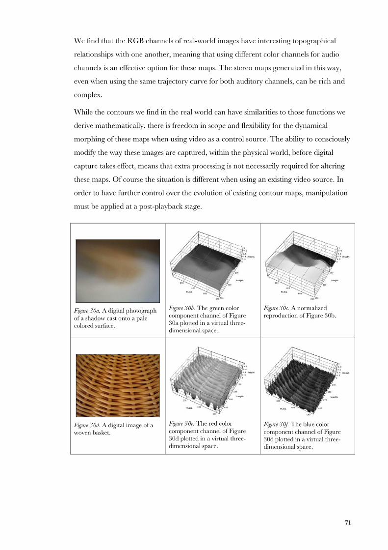
71

We find that the RGB channels of real-world images have interesting topographical

relationships with one another, meaning that using different color channels for audio

channels is an effective option for these maps. The stereo maps generated in this way,

even when using the same trajectory curve for both auditory channels, can be rich and

complex.

While the contours we find in the real world can have similarities to those functions we

derive mathematically, there is freedom in scope and flexibility for the dynamical

morphing of these maps when using video as a control source. The ability to consciously

modify the way these images are captured, within the physical world, before digital

capture takes effect, means that extra processing is not necessarily required for altering

these maps. Of course the situation is different when using an existing video source. In

order to have further control over the evolution of existing contour maps, manipulation

must be applied at a post-playback stage.

Figure 30a. A digital photographof a shadow cast onto a palecolored surface.

Figure 30b. The green colorcomponent channel of Figure30a plotted in a virtual three-dimensional space.

Figure 30c. A normalizedreproduction of Figure 30b.

Figure 30d. A digital image of awoven basket.

Figure 30e. The red colorcomponent channel of Figure30d plotted in a virtual three-dimensional space.

Figure 30f. The blue colorcomponent channel of Figure30d plotted in a virtual three-dimensional space.

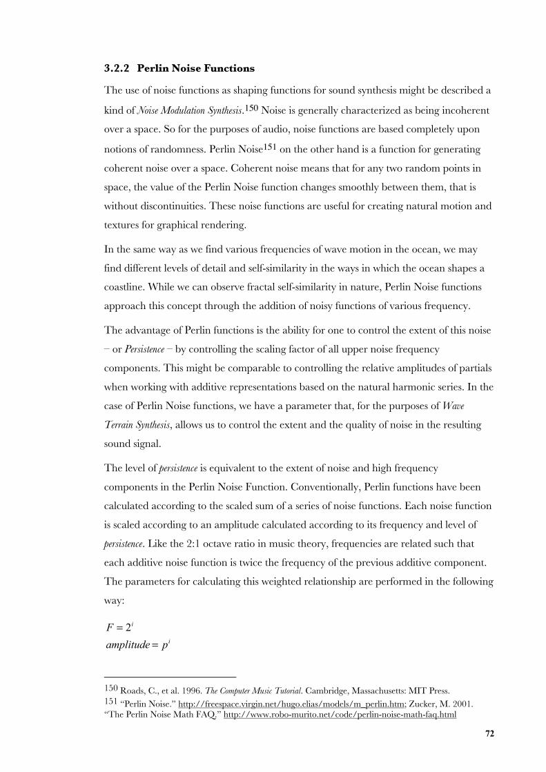
72

3.2.2 Perlin Noise Functions

The use of noise functions as shaping functions for sound synthesis might be described a

kind of Noise Modulation Synthesis.150 Noise is generally characterized as being incoherent

over a space. So for the purposes of audio, noise functions are based completely upon

notions of randomness. Perlin Noise151 on the other hand is a function for generating

coherent noise over a space. Coherent noise means that for any two random points in

space, the value of the Perlin Noise function changes smoothly between them, that is

without discontinuities. These noise functions are useful for creating natural motion and

textures for graphical rendering.

In the same way as we find various frequencies of wave motion in the ocean, we may

find different levels of detail and self-similarity in the ways in which the ocean shapes a

coastline. While we can observe fractal self-similarity in nature, Perlin Noise functions

approach this concept through the addition of noisy functions of various frequency.

The advantage of Perlin functions is the ability for one to control the extent of this noise

– or Persistence – by controlling the scaling factor of all upper noise frequency

components. This might be comparable to controlling the relative amplitudes of partials

when working with additive representations based on the natural harmonic series. In the

case of Perlin Noise functions, we have a parameter that, for the purposes of Wave

Terrain Synthesis, allows us to control the extent and the quality of noise in the resulting

sound signal.

The level of persistence is equivalent to the extent of noise and high frequency

components in the Perlin Noise Function. Conventionally, Perlin functions have been

calculated according to the scaled sum of a series of noise functions. Each noise function

is scaled according to an amplitude calculated according to its frequency and level of

persistence. Like the 2:1 octave ratio in music theory, frequencies are related such that

each additive noise function is twice the frequency of the previous additive component.

The parameters for calculating this weighted relationship are performed in the following

way:

F = 2i

amplitude = pi

150 Roads, C., et al. 1996. The Computer Music Tutorial. Cambridge, Massachusetts: MIT Press.151 “Perlin Noise.” http://freespace.virgin.net/hugo.elias/models/m_perlin.htm; Zucker, M. 2001.“The Perlin Noise Math FAQ.” http://www.robo-murito.net/code/perlin-noise-math-faq.html

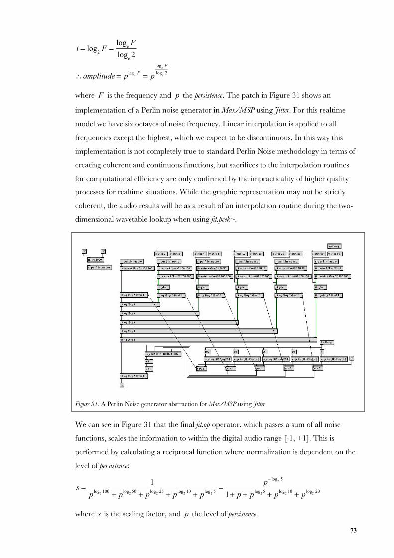
73

i = log2

F =log

eF

loge2

∴amplitude = plog2 F = p

loge F

loge 2

where F is the frequency and p the persistence. The patch in Figure 31 shows an

implementation of a Perlin noise generator in Max/MSP using Jitter. For this realtime

model we have six octaves of noise frequency. Linear interpolation is applied to all

frequencies except the highest, which we expect to be discontinuous. In this way this

implementation is not completely true to standard Perlin Noise methodology in terms of

creating coherent and continuous functions, but sacrifices to the interpolation routines

for computational efficiency are only confirmed by the impracticality of higher quality

processes for realtime situations. While the graphic representation may not be strictly

coherent, the audio results will be as a result of an interpolation routine during the two-

dimensional wavetable lookup when using jit.peek~.

Figure 31. A Perlin Noise generator abstraction for Max/MSP using Jitter

We can see in Figure 31 that the final jit.op operator, which passes a sum of all noise

functions, scales the information to within the digital audio range [-1, +1]. This is

performed by calculating a reciprocal function where normalization is dependent on the

level of persistence:

s =

1

p log2 100 + plog2 50 + plog2 25 + plog2 10 + plog2 5=

p− log2 5

1+ p + p log2 5 + plog2 10 + p log2 20

where s is the scaling factor, and p the level of persistence.

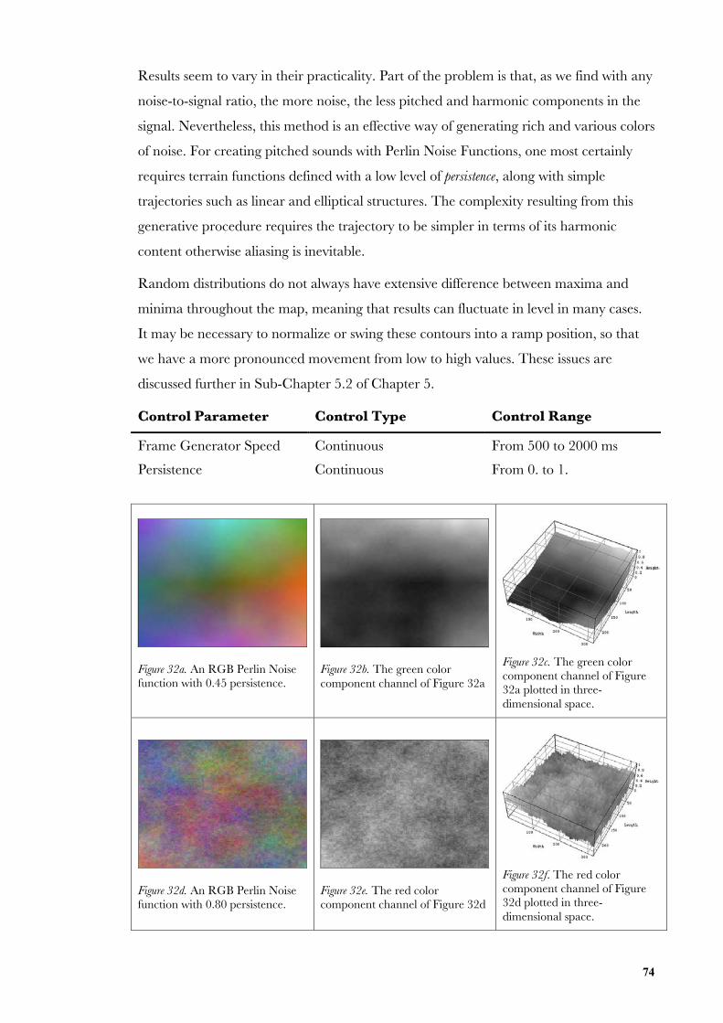
74

Results seem to vary in their practicality. Part of the problem is that, as we find with any

noise-to-signal ratio, the more noise, the less pitched and harmonic components in the

signal. Nevertheless, this method is an effective way of generating rich and various colors

of noise. For creating pitched sounds with Perlin Noise Functions, one most certainly

requires terrain functions defined with a low level of persistence, along with simple

trajectories such as linear and elliptical structures. The complexity resulting from this

generative procedure requires the trajectory to be simpler in terms of its harmonic

content otherwise aliasing is inevitable.

Random distributions do not always have extensive difference between maxima and

minima throughout the map, meaning that results can fluctuate in level in many cases.

It may be necessary to normalize or swing these contours into a ramp position, so that

we have a more pronounced movement from low to high values. These issues are

discussed further in Sub-Chapter 5.2 of Chapter 5.

Control Parameter Control Type Control Range

Frame Generator Speed Continuous From 500 to 2000 ms

Persistence Continuous From 0. to 1.

Figure 32a. An RGB Perlin Noisefunction with 0.45 persistence.

Figure 32b. The green colorcomponent channel of Figure 32a

Figure 32c. The green colorcomponent channel of Figure32a plotted in three-dimensional space.

Figure 32d. An RGB Perlin Noisefunction with 0.80 persistence.

Figure 32e. The red colorcomponent channel of Figure 32d

Figure 32f. The red colorcomponent channel of Figure32d plotted in three-dimensional space.

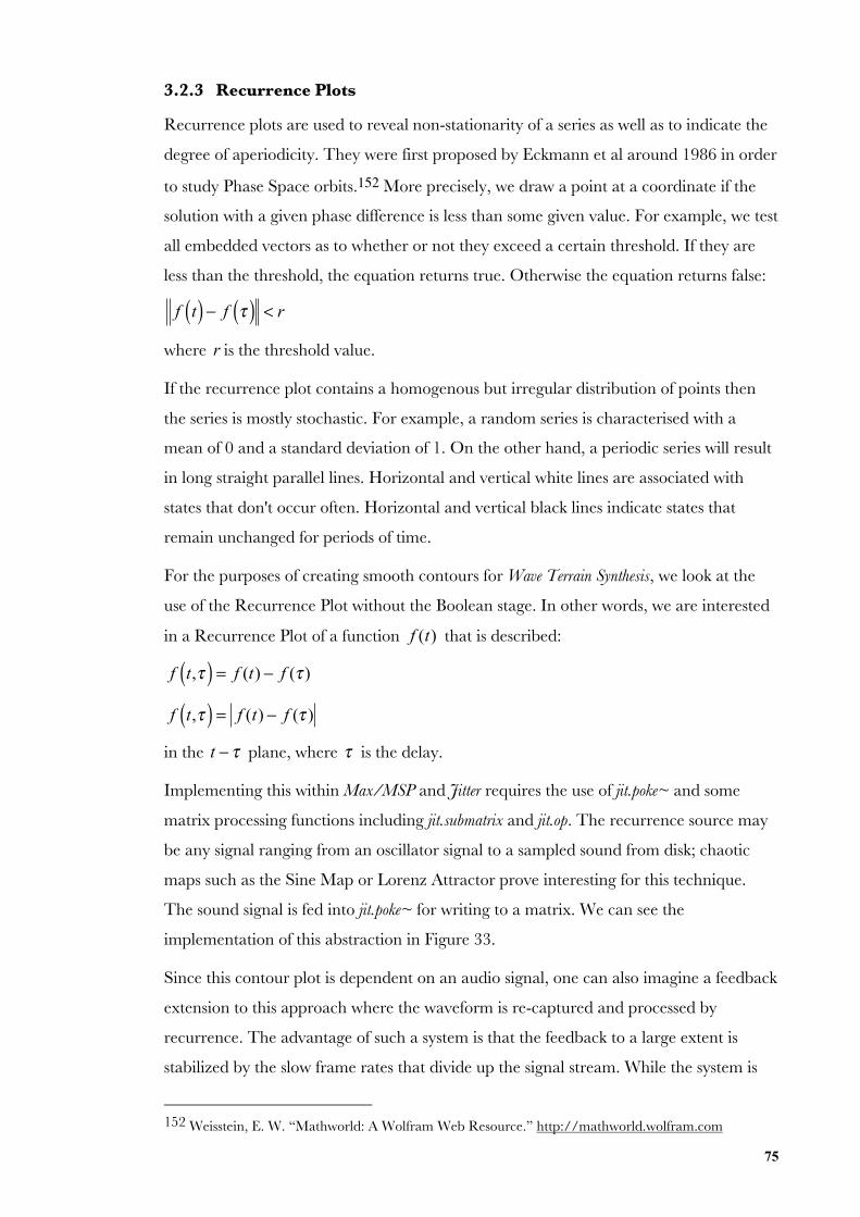
75

3.2.3 Recurrence Plots

Recurrence plots are used to reveal non-stationarity of a series as well as to indicate the

degree of aperiodicity. They were first proposed by Eckmann et al around 1986 in order

to study Phase Space orbits.152 More precisely, we draw a point at a coordinate if the

solution with a given phase difference is less than some given value. For example, we test

all embedded vectors as to whether or not they exceed a certain threshold. If they are

less than the threshold, the equation returns true. Otherwise the equation returns false:

f t( ) − f τ( ) < r

where r is the threshold value.

If the recurrence plot contains a homogenous but irregular distribution of points then

the series is mostly stochastic. For example, a random series is characterised with a

mean of 0 and a standard deviation of 1. On the other hand, a periodic series will result

in long straight parallel lines. Horizontal and vertical white lines are associated with

states that don't occur often. Horizontal and vertical black lines indicate states that

remain unchanged for periods of time.

For the purposes of creating smooth contours for Wave Terrain Synthesis, we look at the

use of the Recurrence Plot without the Boolean stage. In other words, we are interested

in a Recurrence Plot of a function f (t) that is described:

f t,τ( ) = f (t) − f (τ )

f t,τ( ) = f (t) − f (τ )

in the t − τ plane, where τ is the delay.

Implementing this within Max/MSP and Jitter requires the use of jit.poke~ and some

matrix processing functions including jit.submatrix and jit.op. The recurrence source may

be any signal ranging from an oscillator signal to a sampled sound from disk; chaotic

maps such as the Sine Map or Lorenz Attractor prove interesting for this technique.

The sound signal is fed into jit.poke~ for writing to a matrix. We can see the

implementation of this abstraction in Figure 33.

Since this contour plot is dependent on an audio signal, one can also imagine a feedback

extension to this approach where the waveform is re-captured and processed by

recurrence. The advantage of such a system is that the feedback to a large extent is

stabilized by the slow frame rates that divide up the signal stream. While the system is

152 Weisstein, E. W. “Mathworld: A Wolfram Web Resource.” http://mathworld.wolfram.com

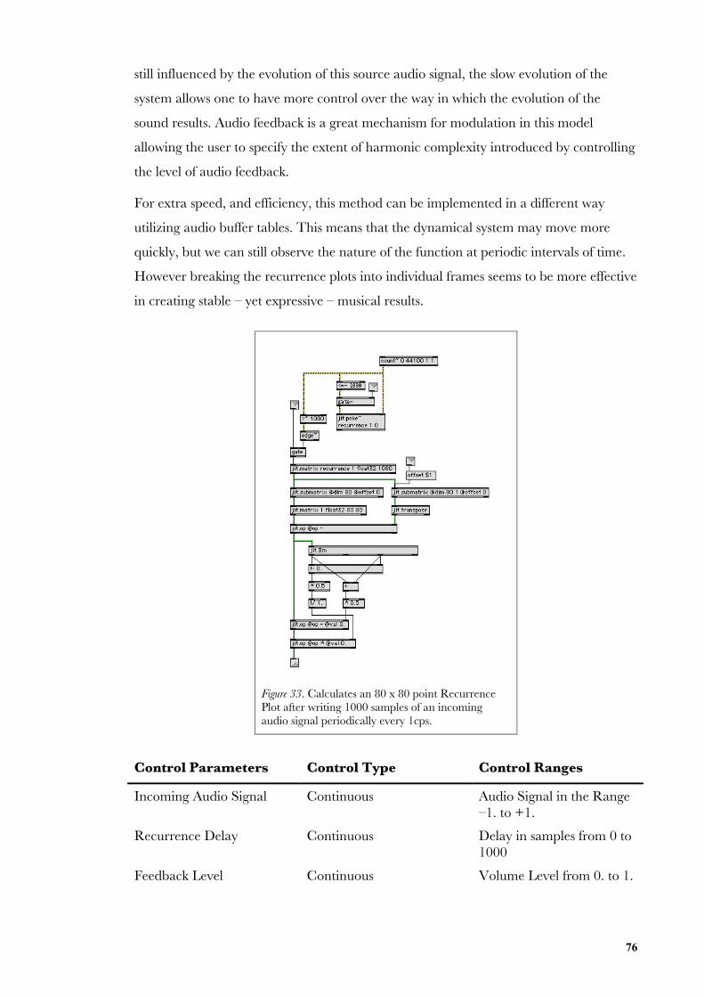
76

still influenced by the evolution of this source audio signal, the slow evolution of the

system allows one to have more control over the way in which the evolution of the

sound results. Audio feedback is a great mechanism for modulation in this model

allowing the user to specify the extent of harmonic complexity introduced by controlling

the level of audio feedback.

For extra speed, and efficiency, this method can be implemented in a different way

utilizing audio buffer tables. This means that the dynamical system may move more

quickly, but we can still observe the nature of the function at periodic intervals of time.

However breaking the recurrence plots into individual frames seems to be more effective

in creating stable – yet expressive – musical results.

Figure 33. Calculates an 80 x 80 point RecurrencePlot after writing 1000 samples of an incomingaudio signal periodically every 1cps.

Control Parameters Control Type Control Ranges

Incoming Audio Signal Continuous Audio Signal in the Range–1. to +1.

Recurrence Delay Continuous Delay in samples from 0 to1000

Feedback Level Continuous Volume Level from 0. to 1.

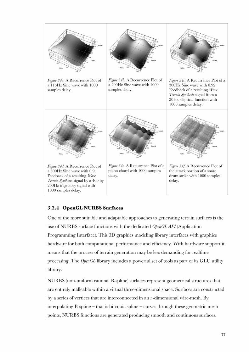
77

Figure 34a. A Recurrence Plot ofa 115Hz Sine wave with 1000samples delay.

Figure 34b. A Recurrence Plot ofa 200Hz Sine wave with 1000samples delay.

Figure 34c. A Recurrence Plot of a300Hz Sine wave with 0.92Feedback of a resulting WaveTerrain Synthesis signal from a30Hz elliptical function with1000 samples delay.

Figure 34d. A Recurrence Plot ofa 300Hz Sine wave with 0.9Feedback of a resulting WaveTerrain Synthesis signal by a 400 by200Hz trajectory signal with1000 samples delay.

Figure 34e. A Recurrence Plot of apiano chord with 1000 samplesdelay.

Figure 34f. A Recurrence Plot ofthe attack portion of a snaredrum strike with 1000 samplesdelay.

3.2.4 OpenGL NURBS Surfaces

One of the more suitable and adaptable approaches to generating terrain surfaces is the

use of NURBS surface functions with the dedicated OpenGL API (Application

Programming Interface). This 3D graphics modeling library interfaces with graphics

hardware for both computational performance and efficiency. With hardware support it

means that the process of terrain generation may be less demanding for realtime

processing. The OpenGL library includes a powerful set of tools as part of its GLU utility

library.

NURBS (non-uniform rational B-spline) surfaces represent geometrical structures that

are entirely malleable within a virtual three-dimensional space. Surfaces are constructed

by a series of vertices that are interconnected in an n-dimensional wire-mesh. By

interpolating B-spline – that is bi-cubic spline – curves through these geometric mesh

points, NURBS functions are generated producing smooth and continuous surfaces.

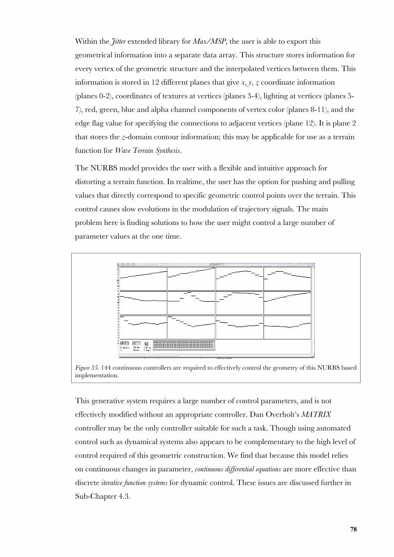
78

Within the Jitter extended library for Max/MSP, the user is able to export this

geometrical information into a separate data array. This structure stores information for

every vertex of the geometric structure and the interpolated vertices between them. This

information is stored in 12 different planes that give x, y, z coordinate information

(planes 0-2), coordinates of textures at vertices (planes 3-4), lighting at vertices (planes 5-

7), red, green, blue and alpha channel components of vertex color (planes 8-11), and the

edge flag value for specifying the connections to adjacent vertices (plane 12). It is plane 2

that stores the z-domain contour information; this may be applicable for use as a terrain

function for Wave Terrain Synthesis.

The NURBS model provides the user with a flexible and intuitive approach for

distorting a terrain function. In realtime, the user has the option for pushing and pulling

values that directly correspond to specific geometric control points over the terrain. This

control causes slow evolutions in the modulation of trajectory signals. The main

problem here is finding solutions to how the user might control a large number of

parameter values at the one time.

Figure 35. 144 continuous controllers are required to effectively control the geometry of this NURBS basedimplementation.

This generative system requires a large number of control parameters, and is not

effectively modified without an appropriate controller. Dan Overholt’s MATRIX

controller may be the only controller suitable for such a task. Though using automated

control such as dynamical systems also appears to be complementary to the high level of

control required of this geometric construction. We find that because this model relies

on continuous changes in parameter, continuous differential equations are more effective than

discrete iterative function systems for dynamic control. These issues are discussed further in

Sub-Chapter 4.3.

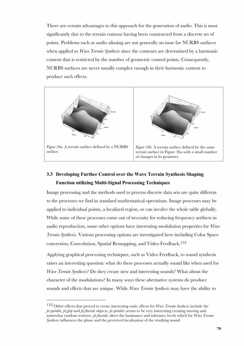
79

There are certain advantages to this approach for the generation of audio. This is most

significantly due to the terrain contour having been constructed from a discrete set of

points. Problems such as audio aliasing are not generally an issue for NURBS surfaces

when applied to Wave Terrain Synthesis since the contours are determined by a harmonic

content that is restricted by the number of geometric control points. Consequently,

NURBS surfaces are never usually complex enough in their harmonic content to

produce such effects.

Figure 36a. A terrain surface defined by a NURBSsurface.

Figure 36b. A terrain surface defined by the sameterrain surface in Figure 36a with a small numberof changes in its geometry.

3.3 Developing Further Control over the Wave Terrain Synthesis Shaping

Function utilizing Multi-Signal Processing Techniques

Image processing and the methods used to process discrete data sets are quite different

to the processes we find in standard mathematical operations. Image processes may be

applied to individual points, a localized region, or can involve the whole table globally.

While some of these processes come out of necessity for reducing frequency artifacts in

audio reproduction, some other options have interesting modulation properties for Wave

Terrain Synthesis. Various processing options are investigated here including Color Space

conversion, Convolution, Spatial Remapping, and Video Feedback.153

Applying graphical processing techniques, such as Video Feedback, to sound synthesis

raises an interesting question: what do these processes actually sound like when used for

Wave Terrain Synthesis? Do they create new and interesting sounds? What about the

character of the modulations? In many ways these alternative systems do produce

sounds and effects that are unique. While Wave Terrain Synthesis may have the ability to

153 Other effects that proved to create interesting sonic effects for Wave Terrain Synthesis include thejit.sprinkle, jit.glop and jit.fluoride objects. jit.sprinkle: seems to be very interesting creating moving andsomewhat random textures. jit.fluoride: alters the luminance and tolerance levels which for Wave TerrainSynthesis influences the phase and the perceived localization of the resulting sound.

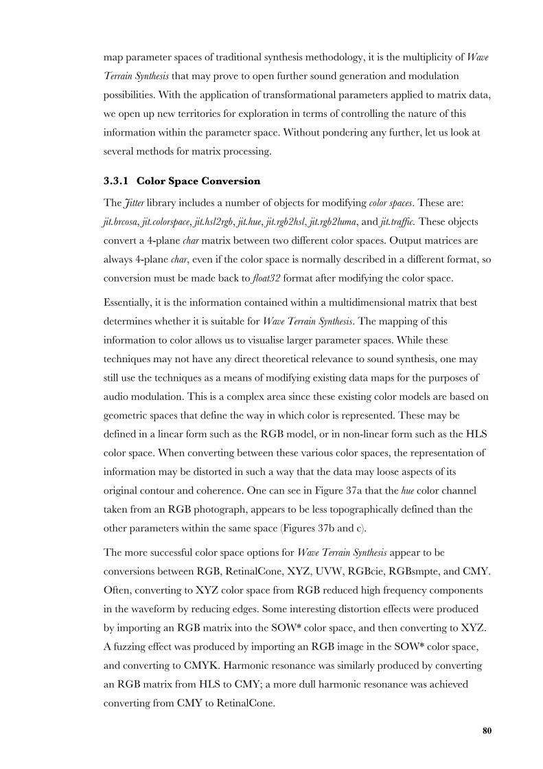
80

map parameter spaces of traditional synthesis methodology, it is the multiplicity of Wave

Terrain Synthesis that may prove to open further sound generation and modulation

possibilities. With the application of transformational parameters applied to matrix data,

we open up new territories for exploration in terms of controlling the nature of this

information within the parameter space. Without pondering any further, let us look at

several methods for matrix processing.

3.3.1 Color Space Conversion

The Jitter library includes a number of objects for modifying color spaces. These are:

jit.brcosa, jit.colorspace, jit.hsl2rgb, jit.hue, jit.rgb2hsl, jit.rgb2luma, and jit.traffic. These objects

convert a 4-plane char matrix between two different color spaces. Output matrices are

always 4-plane char, even if the color space is normally described in a different format, so

conversion must be made back to float32 format after modifying the color space.

Essentially, it is the information contained within a multidimensional matrix that best

determines whether it is suitable for Wave Terrain Synthesis. The mapping of this

information to color allows us to visualise larger parameter spaces. While these

techniques may not have any direct theoretical relevance to sound synthesis, one may

still use the techniques as a means of modifying existing data maps for the purposes of

audio modulation. This is a complex area since these existing color models are based on

geometric spaces that define the way in which color is represented. These may be

defined in a linear form such as the RGB model, or in non-linear form such as the HLS

color space. When converting between these various color spaces, the representation of

information may be distorted in such a way that the data may loose aspects of its

original contour and coherence. One can see in Figure 37a that the hue color channel

taken from an RGB photograph, appears to be less topographically defined than the

other parameters within the same space (Figures 37b and c).

The more successful color space options for Wave Terrain Synthesis appear to be

conversions between RGB, RetinalCone, XYZ, UVW, RGBcie, RGBsmpte, and CMY.

Often, converting to XYZ color space from RGB reduced high frequency components

in the waveform by reducing edges. Some interesting distortion effects were produced

by importing an RGB matrix into the SOW* color space, and then converting to XYZ.

A fuzzing effect was produced by importing an RGB image in the SOW* color space,

and converting to CMYK. Harmonic resonance was similarly produced by converting

an RGB matrix from HLS to CMY; a more dull harmonic resonance was achieved

converting from CMY to RetinalCone.

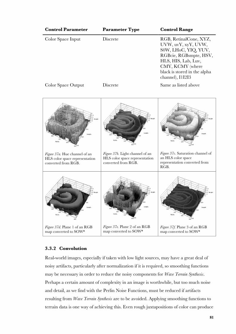
81

Control Parameter Parameter Type Control Range

Color Space Input Discrete RGB, RetinalCone, XYZ,UVW, uvY, xyY, UVW,S0W, LHoC, YIQ, YUV,RGBcie, RGBsmpte, HSV,HLS, HIS, Lab, Luv,CMY, KCMY (whereblack is stored in the alphachannel), I1I2I3

Color Space Output Discrete Same as listed above

Figure 37a. Hue channel of anHLS color space representationconverted from RGB.

Figure 37b. Light channel of anHLS color space representationconverted from RGB.

Figure 37c. Saturation channel ofan HLS color spacerepresentation converted fromRGB.

Figure 37d. Plane 1 of an RGBmap converted to SOW*

Figure 37e. Plane 2 of an RGBmap converted to SOW*

Figure 37f. Plane 3 of an RGBmap converted to SOW*

3.3.2 Convolution

Real-world images, especially if taken with low light sources, may have a great deal of

noisy artifacts, particularly after normalization if it is required, so smoothing functions

may be necessary in order to reduce the noisy components for Wave Terrain Synthesis.

Perhaps a certain amount of complexity in an image is worthwhile, but too much noise

and detail, as we find with the Perlin Noise Functions, must be reduced if artifacts

resulting from Wave Terrain Synthesis are to be avoided. Applying smoothing functions to

terrain data is one way of achieving this. Even rough juxtapositions of color can produce

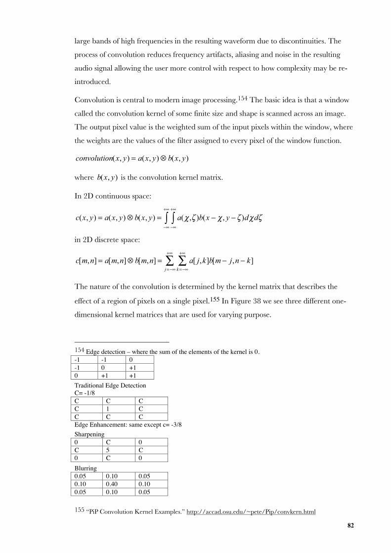
82

large bands of high frequencies in the resulting waveform due to discontinuities. The

process of convolution reduces frequency artifacts, aliasing and noise in the resulting

audio signal allowing the user more control with respect to how complexity may be re-

introduced.

Convolution is central to modern image processing.154 The basic idea is that a window

called the convolution kernel of some finite size and shape is scanned across an image.

The output pixel value is the weighted sum of the input pixels within the window, where

the weights are the values of the filter assigned to every pixel of the window function.

convolution(x, y) = a(x, y)⊗ b(x, y)

where b(x, y) is the convolution kernel matrix.

In 2D continuous space:

c(x, y) = a(x, y)⊗ b(x, y) = a(χ ,ζ )b(x − χ , y −ζ )dχdζ

−∞

+∞

∫−∞

+∞

∫

in 2D discrete space:

c[m,n] = a[m,n]⊗ b[m,n] = a[ j,k]b[m − j,n − k]

k=−∞

+∞

∑j=−∞

+∞

∑

The nature of the convolution is determined by the kernel matrix that describes the

effect of a region of pixels on a single pixel.155 In Figure 38 we see three different one-

dimensional kernel matrices that are used for varying purpose.

154 Edge detection – where the sum of the elements of the kernel is 0.-1 -1 0-1 0 +10 +1 +1Traditional Edge DetectionC= -1/8C C CC 1 CC C CEdge Enhancement: same except c= -3/8Sharpening0 C 0C 5 C0 C 0Blurring0.05 0.10 0.050.10 0.40 0.100.05 0.10 0.05

155 “PiP Convolution Kernel Examples.” http://accad.osu.edu/~pete/Pip/convkern.html

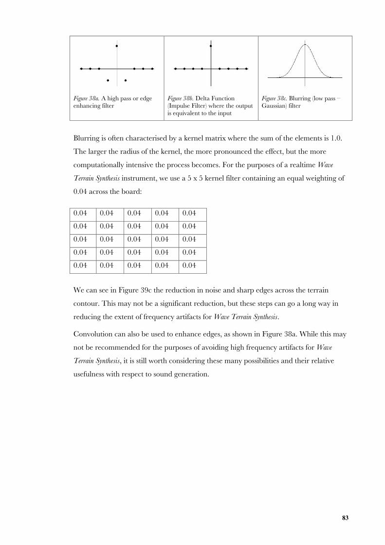
83

Figure 38a. A high pass or edgeenhancing filter

Figure 38b. Delta Function(Impulse Filter) where the outputis equivalent to the input

Figure 38c. Blurring (low pass –Gaussian) filter

Blurring is often characterised by a kernel matrix where the sum of the elements is 1.0.

The larger the radius of the kernel, the more pronounced the effect, but the more

computationally intensive the process becomes. For the purposes of a realtime Wave

Terrain Synthesis instrument, we use a 5 x 5 kernel filter containing an equal weighting of

0.04 across the board:

0.04 0.04 0.04 0.04 0.04

0.04 0.04 0.04 0.04 0.04

0.04 0.04 0.04 0.04 0.04

0.04 0.04 0.04 0.04 0.04

0.04 0.04 0.04 0.04 0.04

We can see in Figure 39c the reduction in noise and sharp edges across the terrain

contour. This may not be a significant reduction, but these steps can go a long way in

reducing the extent of frequency artifacts for Wave Terrain Synthesis.

Convolution can also be used to enhance edges, as shown in Figure 38a. While this may

not be recommended for the purposes of avoiding high frequency artifacts for Wave

Terrain Synthesis, it is still worth considering these many possibilities and their relative

usefulness with respect to sound generation.

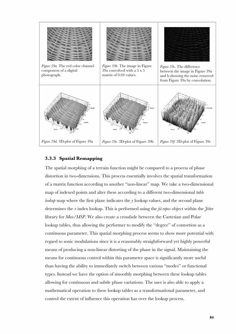
84

Figure 39a. The red color channelcomponent of a digitalphotograph.

Figure 39b. The image in Figure39a convolved with a 5 x 5matrix of 0.04 values.

Figure 39c. The differencebetween the image in Figure 39aand b showing the noise removedfrom Figure 39a by convolution.

Figure 39d. 3D-plot of Figure 39a

Figure 39e. 3D-plot of Figure 39b

Figure 39f. 3D-plot of Figure 39c

3.3.3 Spatial Remapping

The spatial morphing of a terrain function might be compared to a process of phase

distortion in two-dimensions. This process essentially involves the spatial transformation

of a matrix function according to another “non-linear” map. We take a two-dimensional

map of indexed points and alter these according to a different two-dimensional table

lookup map where the first plane indicates the y lookup values, and the second plane

determines the x index lookup. This is performed using the jit.repos object within the Jitter

library for Max/MSP. We also create a crossfade between the Cartesian and Polar

lookup tables, thus allowing the performer to modify the “degree” of contortion as a

continuous parameter. This spatial morphing process seems to show more potential with

regard to sonic modulations since it is a reasonably straightforward yet highly powerful

means of producing a non-linear distorting of the phase in the signal. Maintaining the

means for continuous control within this parameter space is significantly more useful

than having the ability to immediately switch between various “modes” or functional

types. Instead we have the option of smoothly morphing between these lookup tables

allowing for continuous and subtle phase variations. The user is also able to apply a

mathematical operation to these lookup tables as a transformational parameter, and

control the extent of influence this operation has over the lookup process.

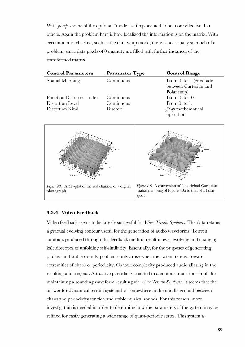
85

With jit.repos some of the optional “mode” settings seemed to be more effective than

others. Again the problem here is how localized the information is on the matrix. With

certain modes checked, such as the data wrap mode, there is not usually so much of a

problem, since data pixels of 0 quantity are filled with further instances of the

transformed matrix.

Control Parameters Parameter Type Control Range

Spatial Mapping Continuous From 0. to 1. (crossfadebetween Cartesian andPolar map)

Function Distortion Index Continuous From 0. to 10.Distortion Level Continuous From 0. to 1.Distortion Kind Discrete jit.op mathematical

operation

Figure 40a. A 3D-plot of the red channel of a digitalphotograph.

Figure 40b. A conversion of the original Cartesianspatial mapping of Figure 40a to that of a Polarspace.

3.3.4 Video Feedback

Video feedback seems to be largely successful for Wave Terrain Synthesis. The data retains

a gradual evolving contour useful for the generation of audio waveforms. Terrain

contours produced through this feedback method result in ever-evolving and changing

kaleidoscopes of unfolding self-similarity. Essentially, for the purposes of generating

pitched and stable sounds, problems only arose when the system tended toward

extremities of chaos or periodicity. Chaotic complexity produced audio aliasing in the

resulting audio signal. Attractive periodicity resulted in a contour much too simple for

maintaining a sounding waveform resulting via Wave Terrain Synthesis. It seems that the

answer for dynamical terrain systems lies somewhere in the middle ground between

chaos and periodicity for rich and stable musical sounds. For this reason, more

investigation is needed in order to determine how the parameters of the system may be

refined for easily generating a wide range of quasi-periodic states. This system is

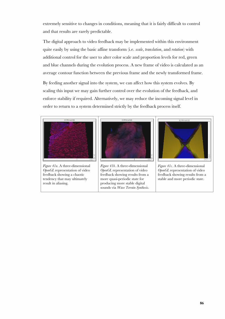
86

extremely sensitive to changes in conditions, meaning that it is fairly difficult to control

and that results are rarely predictable.

The digital approach to video feedback may be implemented within this environment

quite easily by using the basic affine transform (i.e. scale, translation, and rotation) with

additional control for the user to alter color scale and proportion levels for red, green

and blue channels during the evolution process. A new frame of video is calculated as an

average contour function between the previous frame and the newly transformed frame.

By feeding another signal into the system, we can affect how this system evolves. By

scaling this input we may gain further control over the evolution of the feedback, and

enforce stability if required. Alternatively, we may reduce the incoming signal level in

order to return to a system determined strictly by the feedback process itself.

Figure 41a. A three-dimensionalOpenGL representation of videofeedback showing a chaotictendency that may ultimatelyresult in aliasing.

Figure 41b. A three-dimensionalOpenGL representation of videofeedback showing results from amore quasi-periodic state forproducing more stable digitalsounds via Wave Terrain Synthesis.

Figure 41c. A three-dimensionalOpenGL representation of videofeedback showing results from astable and more periodic state.

87

4. Trajectory Generation and Control – Audio Rate

Processing

In Wave Terrain Synthesis the trajectory system determines the way in which information is

extracted from a terrain function. The trajectory controls the system by determining the

fundamental frequency, influencing elements of the timbre with respect to harmonic

content, and plays the central and most significant role in determining the temporal

evolution of the resulting sound. Since the trajectory system is what drives the Wave

Terrain Synthesis model, evolving at the fastest rate of change, this system must be

responsible for the most intricate and complex dynamics in the evolution of the system.

Ideally, the trajectory should be capable of introducing transient shifts and other

phenomena that are characteristic of the rich and dynamic qualities that we appreciate

in real-world sounds.

Of the infinite variety of curves, and their importance to sound generation in Wave

Terrain Synthesis, we have to make a number of decisions as to the most effective

methodology for creating a structure of multiplicity that can satisfy the characteristics we

would normally categorize as being periodic, quasi-periodic, chaotic, or stochastic.

Periodic systems are characterised by a fixed path geometry. Quasi-periodic, chaotic

and stochastic systems are all characterised with an evolution that changes with respect

to time. Chaotic systems are not only effective for introducing automation but they often

respond to a series of variable parameters that may be modified by the user, and which

influence the way in which the dynamical system evolves. Geometric transformational

parameters may also be useful, especially in developing upon possibilities for expressive

control parameters.

The application of dynamical systems and autonomous systems for controlling

parameters for sound synthesis is nothing new. Cellsound was the first in a series of

experiments using cellular automata to control sound in Max/MSP. The New Gendyn

Program – a re-implementation of Dynamic Stochastic Synthesis in a graphical, interactive,

real-time environment – is a composition tool that generates random walks correlating

to an image on the screen.156 The amplitude random walks are plotted on the x-axis,

and the time random walks on the y-axis. The result is a non-linear stochastic distortion

of the shape of the waveform over time.

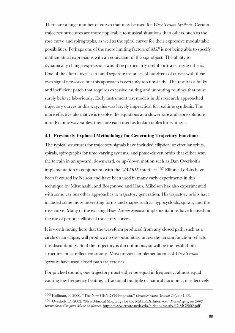
88

There are a huge number of curves that may be used for Wave Terrain Synthesis. Certain

trajectory structures are more applicable to musical situations than others, such as the

rose curve and spirographs, as well as the spiral curves for their expressive modulatable

possibilities. Perhaps one of the more limiting factors of MSP is not being able to specify

mathematical expressions with an equivalent of the expr object. The ability to

dynamically change expressions would be particularly useful for trajectory synthesis.

One of the alternatives is to build separate instances of hundreds of curves with their

own signal networks; but this approach is certainly too unwieldy. The result is a bulky

and inefficient patch that requires excessive muting and unmuting routines that must

surely behave laboriously. Early instrument test models in this research approached

trajectory curves in this way; this was largely impractical for realtime synthesis. The

more effective alternative is to solve the equations at a slower rate and store solutions

into dynamic wavetables; these are each used as lookup tables for synthesis.

4.1 Previously Explored Methodology for Generating Trajectory Functions

The typical structures for trajectory signals have included elliptical or circular orbits,

spirals, spirographs for time varying systems, and phase-driven orbits that either scan

the terrain in an upward, downward, or up/down motion such as Dan Overholt’s

implementation in conjunction with the MATRIX interface.157 Elliptical orbits have

been favoured by Nelson and have been used in many early experiments in this

technique by Mitsuhashi, and Borgonovo and Haus. Mikelson has also experimented

with some various other approaches to trajectory generation. His trajectory orbits have

included some more interesting forms and shapes such as hypocycloids, spirals, and the

rose curve. Many of the existing Wave Terrain Synthesis implementations have focused on

the use of periodic elliptical trajectory curves.

It is worth noting here that the waveform produced from any closed path, such as a

circle or an ellipse, will produce no discontinuities, unless the terrain function reflects

this discontinuity. So if the trajectory is discontinuous, so will be the result; both

structures must reflect continuity. Most previous implementations of Wave Terrain

Synthesis have used closed path trajectories.

For pitched sounds, one trajectory must either be equal in frequency, almost equal

causing low frequency beating, a fractional multiple or natural harmonic, or effectively

156 Hoffman, P. 2000. “The New GENDYN Program.” Computer Music Journal 24(2): 31-38.157 Overholt, D. 2002. “New Musical Mappings for the MATRIX Interface.” Proceedings of the 2002International Computer Music Conference. http://www.create.ucsb.edu/~dano/matrix/ICMC2002.pdf

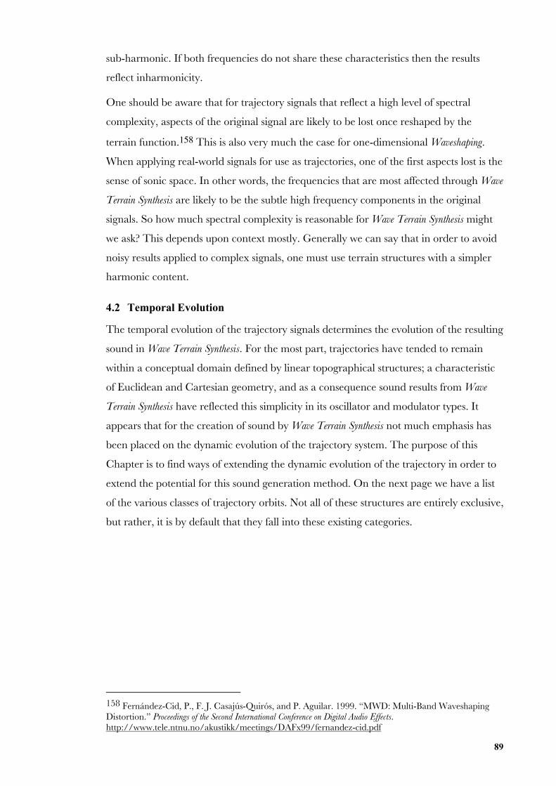
89

sub-harmonic. If both frequencies do not share these characteristics then the results

reflect inharmonicity.

One should be aware that for trajectory signals that reflect a high level of spectral

complexity, aspects of the original signal are likely to be lost once reshaped by the

terrain function.158 This is also very much the case for one-dimensional Waveshaping.

When applying real-world signals for use as trajectories, one of the first aspects lost is the

sense of sonic space. In other words, the frequencies that are most affected through Wave

Terrain Synthesis are likely to be the subtle high frequency components in the original

signals. So how much spectral complexity is reasonable for Wave Terrain Synthesis might

we ask? This depends upon context mostly. Generally we can say that in order to avoid

noisy results applied to complex signals, one must use terrain structures with a simpler

harmonic content.

4.2 Temporal Evolution

The temporal evolution of the trajectory signals determines the evolution of the resulting

sound in Wave Terrain Synthesis. For the most part, trajectories have tended to remain

within a conceptual domain defined by linear topographical structures; a characteristic

of Euclidean and Cartesian geometry, and as a consequence sound results from Wave

Terrain Synthesis have reflected this simplicity in its oscillator and modulator types. It

appears that for the creation of sound by Wave Terrain Synthesis not much emphasis has

been placed on the dynamic evolution of the trajectory system. The purpose of this

Chapter is to find ways of extending the dynamic evolution of the trajectory in order to

extend the potential for this sound generation method. On the next page we have a list

of the various classes of trajectory orbits. Not all of these structures are entirely exclusive,

but rather, it is by default that they fall into these existing categories.

158 Fernández-Cid, P., F. J. Casajús-Quirós, and P. Aguilar. 1999. “MWD: Multi-Band WaveshapingDistortion.” Proceedings of the Second International Conference on Digital Audio Effects.http://www.tele.ntnu.no/akustikk/meetings/DAFx99/fernandez-cid.pdf

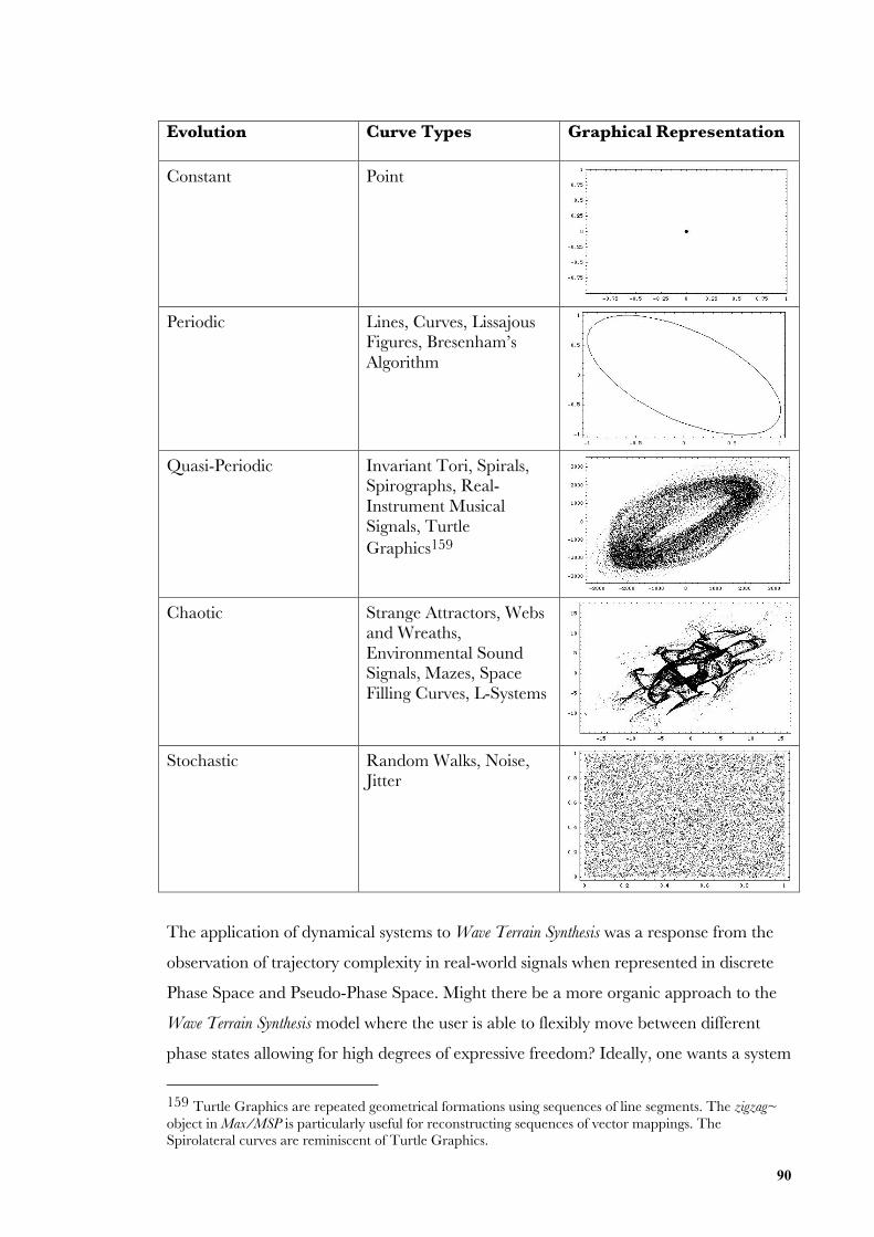
90

Evolution Curve Types Graphical Representation

Constant Point

Periodic Lines, Curves, LissajousFigures, Bresenham’sAlgorithm

Quasi-Periodic Invariant Tori, Spirals,Spirographs, Real-Instrument MusicalSignals, TurtleGraphics159

Chaotic Strange Attractors, Websand Wreaths,Environmental SoundSignals, Mazes, SpaceFilling Curves, L-Systems

Stochastic Random Walks, Noise,Jitter

The application of dynamical systems to Wave Terrain Synthesis was a response from the

observation of trajectory complexity in real-world signals when represented in discrete

Phase Space and Pseudo-Phase Space. Might there be a more organic approach to the

Wave Terrain Synthesis model where the user is able to flexibly move between different

phase states allowing for high degrees of expressive freedom? Ideally, one wants a system

159 Turtle Graphics are repeated geometrical formations using sequences of line segments. The zigzag~object in Max/MSP is particularly useful for reconstructing sequences of vector mappings. TheSpirolateral curves are reminiscent of Turtle Graphics.

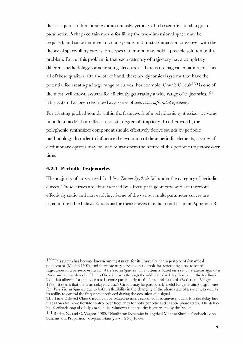
91

that is capable of functioning autonomously, yet may also be sensitive to changes in

parameter. Perhaps certain means for filling the two-dimensional space may be

required, and since iterative function systems and fractal dimension cross over with the

theory of space-filling curves, processes of iteration may hold a possible solution to this

problem. Part of this problem is that each category of trajectory has a completely

different methodology for generating structures. There is no magical equation that has

all of these qualities. On the other hand, there are dynamical systems that have the

potential for creating a large range of curves. For example, Chua’s Circuit160 is one of

the most well known systems for efficiently generating a wide range of trajectories.161

This system has been described as a series of continuous differential equations.

For creating pitched sounds within the framework of a polyphonic synthesizer we want

to build a model that reflects a certain degree of simplicity. In other words, the

polyphonic synthesizer component should effectively derive sounds by periodic

methodology. In order to influence the evolution of these periodic elements, a series of

evolutionary options may be used to transform the nature of this periodic trajectory over

time.

4.2.1 Periodic Trajectories

The majority of curves used for Wave Terrain Synthesis fall under the category of periodic

curves. These curves are characterized by a fixed path geometry, and are therefore

effectively static and non-evolving. Some of the various multi-parameter curves are

listed in the table below. Equations for these curves may be found listed in Appendix B:

160 This system has become known amongst many for its unusually rich repertoire of dynamicalphenomena (Madan 1992), and therefore may serve as an example for generating a broad set oftrajectories and periodic orbits for Wave Terrain Synthesis. The system is based on a set of continuous differentialstate equations that describe Chua’s Circuit; it was through the addition of a delay element in the feedbackloop that allowed for this system to become particularly useful for sound synthesis (Rodet and Vergez1999). It seems that the time-delayed Chua’s Circuit may be particularly useful for generating trajectoriesfor Wave Terrain Synthesis due to both its flexibility in the changing of the phase state of a system, as well asits ability to control the frequency produced during the evolution of a signal.The Time-Delayed Chua Circuit can be related to many sustained instrument models. It is the delay-linethat allows for more flexible control over frequency for both periodic and chaotic phase states. The delay-line feedback loop also helps to stabilize whatever nonlinearity is generated by the system.161 Rodet, X., and C. Vergez. 1999. “Nonlinear Dynamics in Physical Models: Simple Feedback-LoopSystems and Properties.” Computer Music Journal 23(3):18-34.

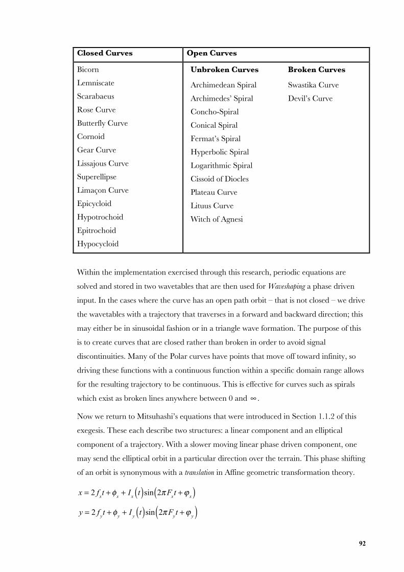
92

Closed Curves Open Curves

Bicorn

Lemniscate

Scarabaeus

Rose Curve

Butterfly Curve

Cornoid

Gear Curve

Lissajous Curve

Superellipse

Limaçon Curve

Epicycloid

Hypotrochoid

Epitrochoid

Hypocycloid

Unbroken Curves Broken Curves

Archimedean Spiral

Archimedes’ Spiral

Concho-Spiral

Conical Spiral

Fermat’s Spiral

Hyperbolic Spiral

Logarithmic Spiral

Cissoid of Diocles

Plateau Curve

Lituus Curve

Witch of Agnesi

Swastika Curve

Devil’s Curve

Within the implementation exercised through this research, periodic equations are

solved and stored in two wavetables that are then used for Waveshaping a phase driven

input. In the cases where the curve has an open path orbit – that is not closed – we drive

the wavetables with a trajectory that traverses in a forward and backward direction; this

may either be in sinusoidal fashion or in a triangle wave formation. The purpose of this

is to create curves that are closed rather than broken in order to avoid signal

discontinuities. Many of the Polar curves have points that move off toward infinity, so

driving these functions with a continuous function within a specific domain range allows

for the resulting trajectory to be continuous. This is effective for curves such as spirals

which exist as broken lines anywhere between 0 and ∞ .

Now we return to Mitsuhashi’s equations that were introduced in Section 1.1.2 of this

exegesis. These each describe two structures: a linear component and an elliptical

component of a trajectory. With a slower moving linear phase driven component, one

may send the elliptical orbit in a particular direction over the terrain. This phase shifting

of an orbit is synonymous with a translation in Affine geometric transformation theory.

x = 2 f

xt + φ

x+ I

xt( )sin 2πF

xt +ϕ

x( )

y = 2 f

yt + φ

y+ I

yt( )sin 2πF

yt +ϕ

y( )

93

where f

x, f

y, F

x, F

yare frequencies within the audio range ( 20Hz − 20KHz ) or subaudio

range ( 0 < F < 20Hz,0 < f < 20Hz .) φ

x,φ

y,ϕ

x,ϕ

yare initial phases and

I

x(t), I

y(t) behave as extra modulatable trajectory parameters.

The overall topography and harmonic content of a curve affects the nature of the

resulting sound for Wave Terrain Synthesis. Polar trajectories seem to have a special kind of

modulation, they respond differently to the standard Cartesian maps. For example, the

number of petals in the Rose Curve determines the relative partial according to the

natural harmonic series. This is also dependent and relative to the fundamental

frequency of the trajectory. Other Polar maps do not behave so straightforwardly.

The Max/MSP patch allows for these curves to be dynamically written to two

wavetables for table lookup. In this way, we may derive these curves at a slower rate of

processing so that we are not calculating similar points repeatedly for periodic curves.

The following Figure 42 shows the Butterfly Curve, which is solved in Figure 42b using

the Max expr object. This is a compact way of solving more complex sets of equations

that would otherwise require a large network of objects to create. This example alone

shows why solving using a signal chain would be extremely expensive for CPU in

realtime situations.

Figure 42a. The Butterfly Curve determined by the

Polar equation r= ecosθ −2cos 4θ( )+sin5 θ

12⎛⎝⎜

⎞⎠⎟

Figure 42b. A Max patch which stores solutions to theButterfly Curve in two tables containing 4092 valuesof Cartesian coordinates

Probably one of the more exciting combinations is the use of Jean-Michel Couturier’s

wacom object for Wave Terrain Synthesis.162 This controller is an effective way for a user to

draw ones own trajectory curve. There is also the insprock object that allows game

controllers such as joysticks, game pads, to be used as input devices for Max, though

162 Couturier, J.-M. “Computer Music at LMA.” http://www.lma.cnrs-mrs.fr/~IM/en_telecharger.htm

94

these additionally require Apple's Input Sprocket operating system extensions to be

installed.163

4.2.2 Quasi-Periodic Trajectories

Quasi-periodic signals are characterized by Phase Space plots that do not remain static,

yet have strong orbits of attraction. Part of the problem in classifying quasi-periodicity

lies in the fact that it is a grey area between what we classify as being periodic and

aperiodic. It is a phase state that retains elements of both, but it cannot explain the

nature of these extremes, nor can it explain how they interact. When does one decide

that something exhibits too little periodicity or aperiodicity in order for it to fall into this

non-specific middle ground that seems to classify most pitched musical instrument

sounds? It is such an important area of study and research, and further understanding

may provide solutions to this complex problem.

The methodology used to derive these trajectories generally determines the “character”

of their quasi-periodicity. To some extent many periodic functions can show a quasi-

periodic tendency when two different parameters are distantly related, such as pi and 1.

Pi is characterized by an infinite decimal, whereas the number 1 is adequately defined as

an integer. The ratio produced by the combination of these numbers creates a system

that is perpetually out of phase.

4.2.2.1 Driving the System

For conventional techniques in sound synthesis the use of an LFO may be applied in

order to create movement within a sound that may normally have been static. This has

traditionally been applied to filtration, or to frequency modulation or amplitude

modulation systems for vibrato and tremolo effects but may also have application in

Wave Terrain Synthesis for trajectory parameters. These equations may be modified or

“modulated” according to standard transformation processes of scale, translation, and

rotation. So if one were to apply an LFO to these various parameters, one might be able

to create and control a sound that is more complex in terms of its timbral evolution.

By interpolating a series of points between a “list” of floating point numbers one may

also allow for more varied and less predictable outcomes in parameter modulation. In

this way the rate of reproduction of this list of samples can be controlled. These may be

reproduced at any rate to create various outcomes. The data used may be sourced from

163 Schabtach, A. “c74/share – adam.” http://www.cycling74.com/share/adam/

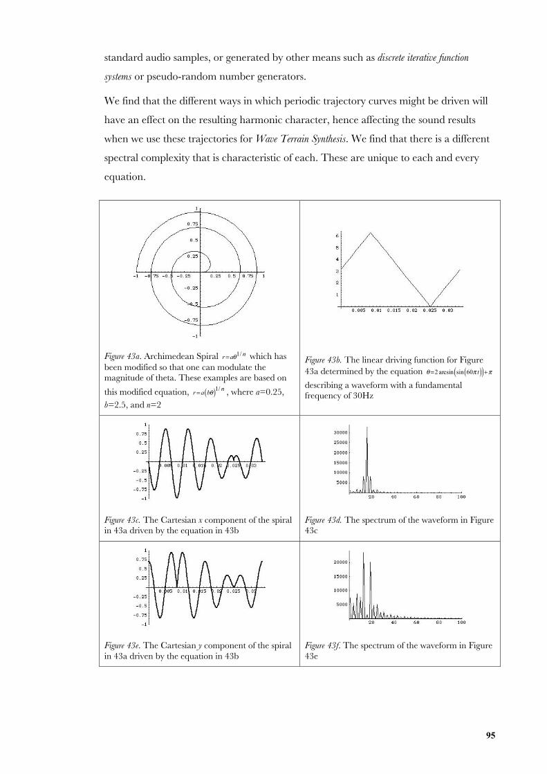
95

standard audio samples, or generated by other means such as discrete iterative function

systems or pseudo-random number generators.

We find that the different ways in which periodic trajectory curves might be driven will

have an effect on the resulting harmonic character, hence affecting the sound results

when we use these trajectories for Wave Terrain Synthesis. We find that there is a different

spectral complexity that is characteristic of each. These are unique to each and every

equation.

Figure 43a. Archimedean Spiral r=aθ1/ n which hasbeen modified so that one can modulate themagnitude of theta. These examples are based on

this modified equation, r=a bθ( )1/ n , where a=0.25,b=2.5, and n=2

Figure 43b. The linear driving function for Figure43a determined by the equation θ=2 arcsin sin 60π t( )( )+πdescribing a waveform with a fundamentalfrequency of 30Hz

Figure 43c. The Cartesian x component of the spiralin 43a driven by the equation in 43b

Figure 43d. The spectrum of the waveform in Figure43c

Figure 43e. The Cartesian y component of the spiralin 43a driven by the equation in 43b

Figure 43f. The spectrum of the waveform in Figure43e

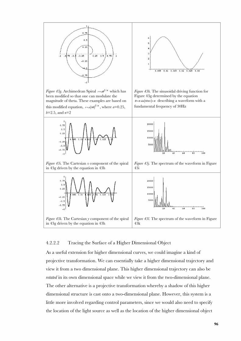
96

Figure 43g. Archimedean Spiral r=aθ1/ n which hasbeen modified so that one can modulate themagnitude of theta. These examples are based on

this modified equation, r=a bθ( )1/ n , where a=0.25,b=2.5, and n=2

Figure 43h. The sinusoidal driving function forFigure 43g determined by the equation

θ=π sin 60π t( )+π describing a waveform with afundamental frequency of 30Hz

Figure 43i. The Cartesian x component of the spiralin 43g driven by the equation in 43h

Figure 43j. The spectrum of the waveform in Figure43i

Figure 43k. The Cartesian y component of the spiralin 43g driven by the equation in 43h

Figure 43l. The spectrum of the waveform in Figure43k

4.2.2.2 Tracing the Surface of a Higher Dimensional Object

As a useful extension for higher dimensional curves, we could imagine a kind of

projective transformation. We can essentially take a higher dimensional trajectory and

view it from a two dimensional plane. This higher dimensional trajectory can also be

rotated in its own dimensional space while we view it from the two-dimensional plane.

The other alternative is a projective transformation whereby a shadow of this higher

dimensional structure is cast onto a two-dimensional plane. However, this system is a

little more involved regarding control parameters, since we would also need to specify

the location of the light source as well as the location of the higher dimensional object

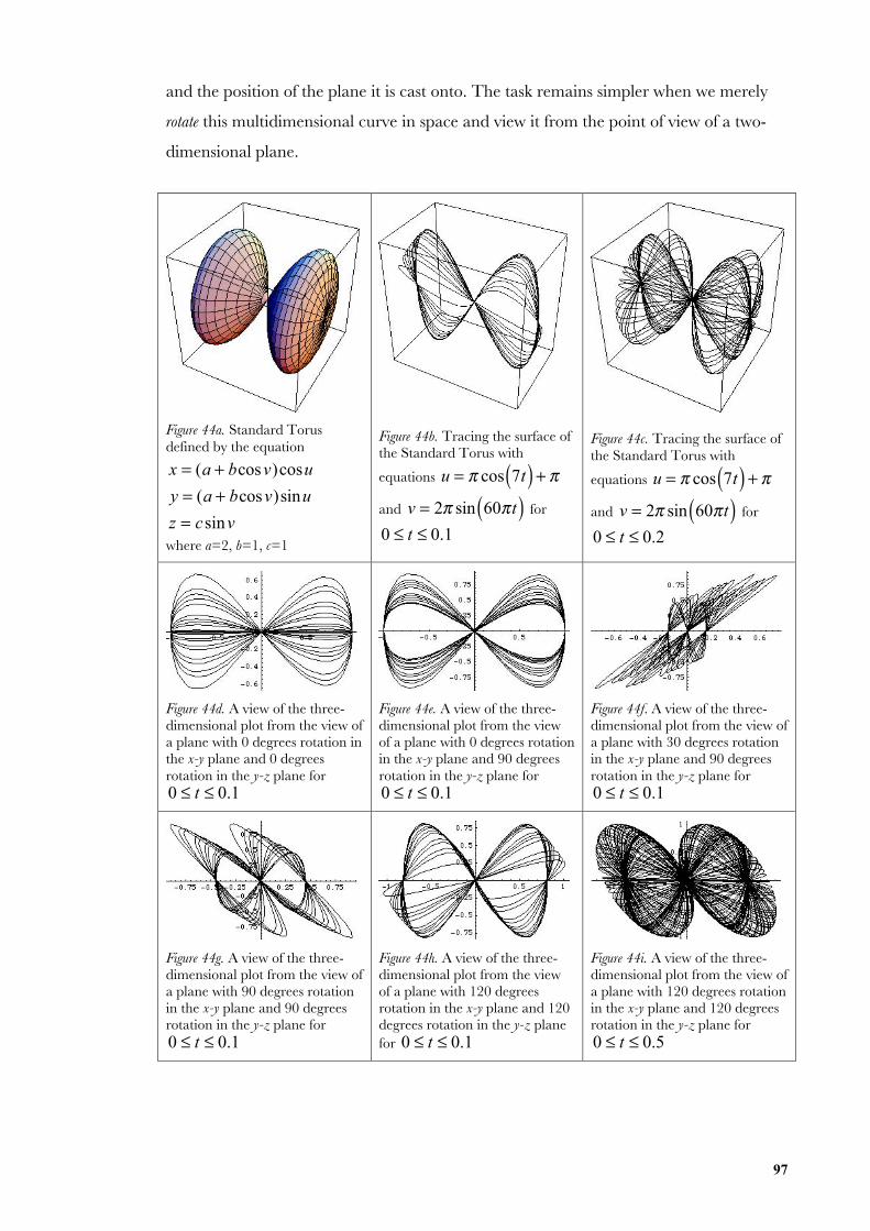
97

and the position of the plane it is cast onto. The task remains simpler when we merely

rotate this multidimensional curve in space and view it from the point of view of a two-

dimensional plane.

Figure 44a. Standard Torusdefined by the equation

x = (a + bcosv)cosu

y = (a + bcosv)sinu

z = csinvwhere a=2, b=1, c=1

Figure 44b. Tracing the surface ofthe Standard Torus with

equations u = π cos 7t( ) + π

and v = 2π sin 60πt( ) for

0 ≤ t ≤ 0.1

Figure 44c. Tracing the surface ofthe Standard Torus with

equations u = π cos 7t( ) + π

and v = 2π sin 60πt( ) for

0 ≤ t ≤ 0.2

Figure 44d. A view of the three-dimensional plot from the view ofa plane with 0 degrees rotation inthe x-y plane and 0 degreesrotation in the y-z plane for

0 ≤ t ≤ 0.1

Figure 44e. A view of the three-dimensional plot from the viewof a plane with 0 degrees rotationin the x-y plane and 90 degreesrotation in the y-z plane for

0 ≤ t ≤ 0.1

Figure 44f. A view of the three-dimensional plot from the view ofa plane with 30 degrees rotationin the x-y plane and 90 degreesrotation in the y-z plane for

0 ≤ t ≤ 0.1

Figure 44g. A view of the three-dimensional plot from the view ofa plane with 90 degrees rotationin the x-y plane and 90 degreesrotation in the y-z plane for

0 ≤ t ≤ 0.1

Figure 44h. A view of the three-dimensional plot from the viewof a plane with 120 degreesrotation in the x-y plane and 120degrees rotation in the y-z planefor 0 ≤ t ≤ 0.1

Figure 44i. A view of the three-dimensional plot from the view ofa plane with 120 degrees rotationin the x-y plane and 120 degreesrotation in the y-z plane for

0 ≤ t ≤ 0.5

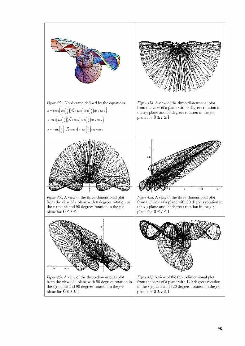
98

Figure 45a. Nordstrand defined by the equations

x = cos u cos u2

⎛⎝⎜

⎞⎠⎟ 2+cos v( )+sin u

2⎛⎝⎜

⎞⎠⎟ sin v cos v

⎛

⎝⎜⎞

⎠⎟

y=sin u cos u2

⎛⎝⎜

⎞⎠⎟ 2+cos v( )+sin u

2⎛⎝⎜

⎞⎠⎟ sin v cos v

⎛⎝⎜

⎞⎠⎟

z = − sin u2

⎛⎝⎜

⎞⎠⎟ 2 +cos v( ) + cos u

2

⎛⎝⎜

⎞⎠⎟ sin v cos v

Figure 45b. A view of the three-dimensional plotfrom the view of a plane with 0 degrees rotation inthe x-y plane and 30 degrees rotation in the y-zplane for 0 ≤ t ≤ 1

Figure 45c. A view of the three-dimensional plotfrom the view of a plane with 0 degrees rotation inthe x-y plane and 90 degrees rotation in the y-zplane for 0 ≤ t ≤ 1

Figure 45d. A view of the three-dimensional plotfrom the view of a plane with 30 degrees rotation inthe x-y plane and 90 degrees rotation in the y-zplane for 0 ≤ t ≤ 1

Figure 45e. A view of the three-dimensional plotfrom the view of a plane with 90 degrees rotation inthe x-y plane and 90 degrees rotation in the y-zplane for 0 ≤ t ≤ 1

Figure 45f. A view of the three-dimensional plotfrom the view of a plane with 120 degrees rotationin the x-y plane and 120 degrees rotation in the y-zplane for 0 ≤ t ≤ 1

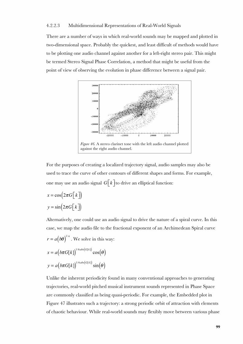
99

4.2.2.3 Multidimensional Representations of Real-World Signals

There are a number of ways in which real-world sounds may be mapped and plotted in

two-dimensional space. Probably the quickest, and least difficult of methods would have

to be plotting one audio channel against another for a left-right stereo pair. This might

be termed Stereo Signal Phase Correlation, a method that might be useful from the

point of view of observing the evolution in phase difference between a signal pair.

Figure 46. A stereo clarinet tone with the left audio channel plottedagainst the right audio channel.

For the purposes of creating a localized trajectory signal, audio samples may also be

used to trace the curve of other contours of different shapes and forms. For example,

one may use an audio signal G k⎡⎣ ⎤⎦ to drive an elliptical function:

x = cos 2πG k⎡⎣ ⎤⎦( ) y = sin 2πG k⎡⎣ ⎤⎦( )Alternatively, one could use an audio signal to drive the nature of a spiral curve. In this

case, we map the audio file to the fractional exponent of an Archimedean Spiral curve

r = a bθ( )1/ n

. We solve in this way:

x = a bπG[k]( )1/6abs G[k ]( )

cos θ( )

y = a bπG[k]( )1/6abs G[k ]( )

sin θ( )Unlike the inherent periodicity found in many conventional approaches to generating

trajectories, real-world pitched musical instrument sounds represented in Phase Space

are commonly classified as being quasi-periodic. For example, the Embedded plot in

Figure 47 illustrates such a trajectory: a strong periodic orbit of attraction with elements

of chaotic behaviour. While real-world sounds may flexibly move between various phase

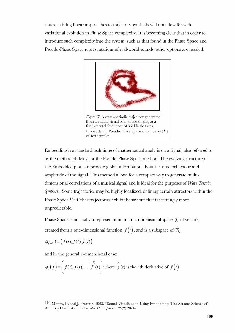
100

states, existing linear approaches to trajectory synthesis will not allow for wide

variational evolution in Phase Space complexity. It is becoming clear that in order to

introduce such complexity into the system, such as that found in the Phase Space and

Pseudo-Phase Space representations of real-world sounds, other options are needed.

Figure 47. A quasi-periodic trajectory generatedfrom an audio signal of a female singing at afundamental frequency of 364Hz that wasEmbedded in Pseudo-Phase Space with a delay (τ )of 485 samples.

Embedding is a standard technique of mathematical analysis on a signal, also referred to

as the method of delays or the Pseudo-Phase Space method. The evolving structure of

the Embedded plot can provide global information about the time behaviour and

amplitude of the signal. This method allows for a compact way to generate multi-

dimensional correlations of a musical signal and is ideal for the purposes of Wave Terrain

Synthesis. Some trajectories may be highly localized, defining certain attractors within the

Phase Space.164 Other trajectories exhibit behaviour that is seemingly more

unpredictable.

Phase Space is normally a representation in an n-dimensional space φn of vectors,

created from a one-dimensional function f t( ) , and is a subspace of ℜn

.

φ

3( f ) = f (t), f (t), f (t)( )

and in the general n-dimensional case:

φ

nf( ) = f (t), f (t),..., f

(n−1)

(t)⎛

⎝⎜⎞

⎠⎟where f

( n)

(t) is the nth derivative of f t( ) .

164 Monro, G. and J. Pressing. 1998. “Sound Visualisation Using Embedding: The Art and Science ofAuditory Correlation.” Computer Music Journal. 22(2):20-34.

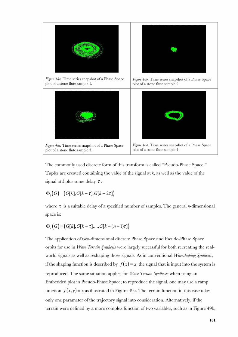
101

Figure 48a. Time series snapshot of a Phase Spaceplot of a stone flute sample 1.

Figure 48b. Time series snapshot of a Phase Spaceplot of a stone flute sample 2.

Figure 48c. Time series snapshot of a Phase Spaceplot of a stone flute sample 3.

Figure 48d. Time series snapshot of a Phase Spaceplot of a stone flute sample 4.

The commonly used discrete form of this transform is called “Pseudo-Phase Space.”

Tuples are created containing the value of the signal at k, as well as the value of the

signal at k plus some delay τ .

Φ

3G( ) = G[k],G[k − τ ],G[k − 2τ ]( )

where τ is a suitable delay of a specified number of samples. The general n-dimensional

space is:

Φ

nG( ) = G[k],G[k − τ ],...,G[k − (n −1)τ ]( )

The application of two-dimensional discrete Phase Space and Pseudo-Phase Space

orbits for use in Wave Terrain Synthesis were largely successful for both recreating the real-

world signals as well as reshaping those signals. As in conventional Waveshaping Synthesis,

if the shaping function is described by f x( ) = x the signal that is input into the system is

reproduced. The same situation applies for Wave Terrain Synthesis when using an

Embedded plot in Pseudo-Phase Space; to reproduce the signal, one may use a ramp

function f x, y( ) = x as illustrated in Figure 49a. The terrain function in this case takes

only one parameter of the trajectory signal into consideration. Alternatively, if the

terrain were defined by a more complex function of two variables, such as in Figure 49b,

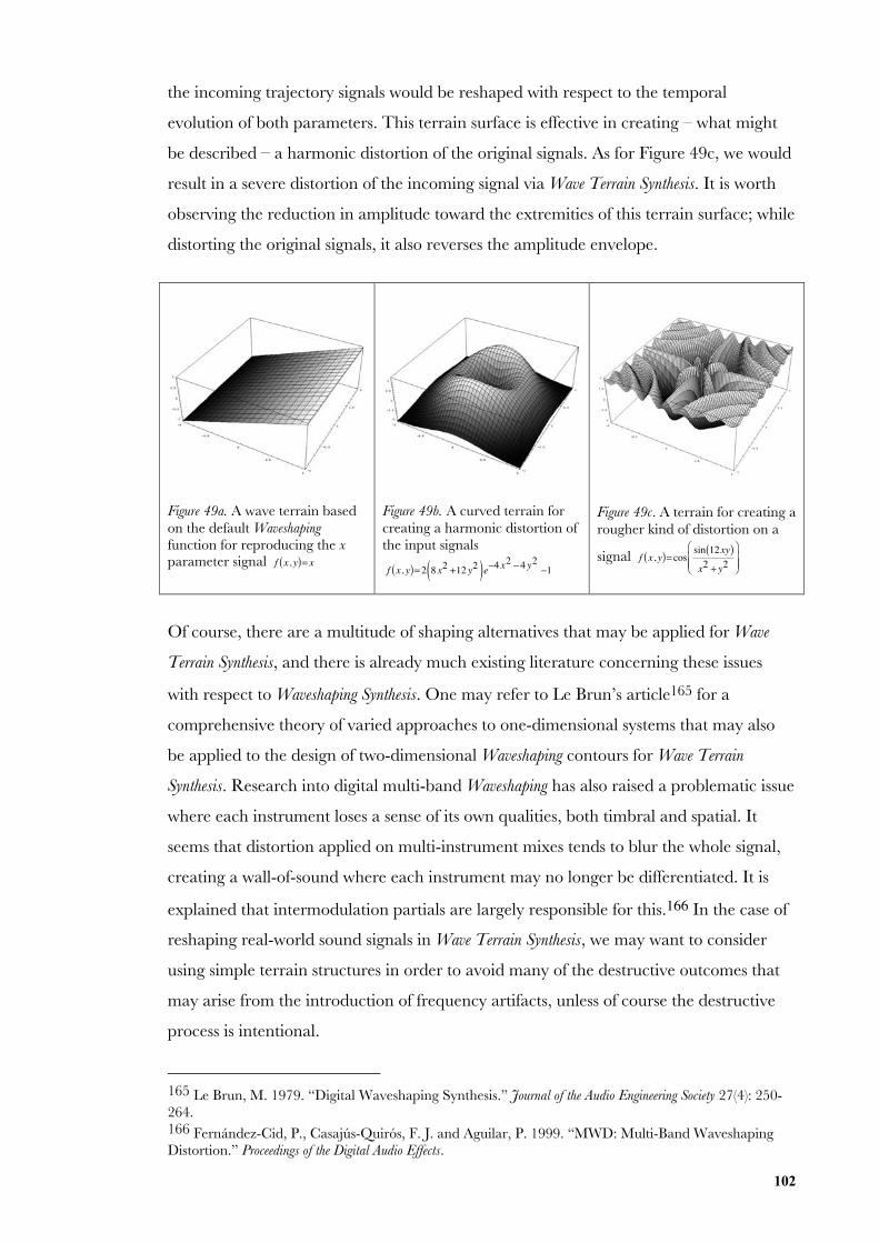
102

the incoming trajectory signals would be reshaped with respect to the temporal

evolution of both parameters. This terrain surface is effective in creating – what might

be described – a harmonic distortion of the original signals. As for Figure 49c, we would

result in a severe distortion of the incoming signal via Wave Terrain Synthesis. It is worth

observing the reduction in amplitude toward the extremities of this terrain surface; while

distorting the original signals, it also reverses the amplitude envelope.

Figure 49a. A wave terrain basedon the default Waveshapingfunction for reproducing the xparameter signal f x, y( )= x

Figure 49b. A curved terrain forcreating a harmonic distortion ofthe input signals

f x, y( )=2 8 x2 +12 y2( )e−4 x2 −4 y2 −1

Figure 49c. A terrain for creating arougher kind of distortion on a

signal f x, y( )= cos sin 12xy( )x2 + y2

⎛

⎝⎜⎜

⎞

⎠⎟⎟

Of course, there are a multitude of shaping alternatives that may be applied for Wave

Terrain Synthesis, and there is already much existing literature concerning these issues

with respect to Waveshaping Synthesis. One may refer to Le Brun’s article165 for a

comprehensive theory of varied approaches to one-dimensional systems that may also

be applied to the design of two-dimensional Waveshaping contours for Wave Terrain

Synthesis. Research into digital multi-band Waveshaping has also raised a problematic issue

where each instrument loses a sense of its own qualities, both timbral and spatial. It

seems that distortion applied on multi-instrument mixes tends to blur the whole signal,

creating a wall-of-sound where each instrument may no longer be differentiated. It is

explained that intermodulation partials are largely responsible for this.166 In the case of

reshaping real-world sound signals in Wave Terrain Synthesis, we may want to consider

using simple terrain structures in order to avoid many of the destructive outcomes that

may arise from the introduction of frequency artifacts, unless of course the destructive

process is intentional.

165 Le Brun, M. 1979. “Digital Waveshaping Synthesis.” Journal of the Audio Engineering Society 27(4): 250-264.166 Fernández-Cid, P., Casajús-Quirós, F. J. and Aguilar, P. 1999. “MWD: Multi-Band WaveshapingDistortion.” Proceedings of the Digital Audio Effects.

103

4.2.3 Chaotic Trajectories

If time dependant, a dynamical system is characterized by a state that evolves with

respect to time. This temporal evolution may be determined both by the current state of

the system, as well as by the state of any input parameters used for influencing how the

system responds during this evolution. These systems are conventionally described by a

series of discrete iterative functions or continuous differential equations; the inclusion of a

nonlinear element introduces complexity and sensitivity in terms of how the system

evolves and responds to input parameter changes.

Depending on the level of attractive stability inherent within a system, dramatic changes

in the input parameters may give rise to a complex behaviour known as chaos. It is

important to understand the fundamental difference between what is chaotic, and what

is described as being random. Chaos is a completely deterministic phenomenon reserved

for those problems where extreme complexity results from a sensitivity to initial

conditions as applied to nonlinear equations.167 Randomness and chance on the other

hand are understood to be stochastic processes for which not all parameters can ever be

entirely known.

The fundamental problem is that for whatever scientific problem, there is no universal

mathematical proof or equation to model all possible outcomes. Finding such a truth

might be synonymous to finding the Holy Grail. In many ways any dynamical system

could be applied to Wave Terrain Synthesis for experimental purposes. Certainly, not all

systems may be worthwhile for the purposes of sound generation. Many discrete iterative

systems may be categorised as being noise-like for sound synthesis. Though this does not

apply in all situations.

What sort of scientific theory justifies whether any dynamical system is more significant

for Wave Terrain Synthesis than any other? While the theoretical basis for using particular

dynamical systems for trajectory generation is not completely foolproof, it goes without

saying that it is the evolutionary behaviour that arises through the process of dynamics

that is useful for Wave Terrain Synthesis. Dynamical systems provide a compact way of

generating complexity via simple means, and are often effective in generating automated

evolution systems for control parameters.

While there is no real scientific basis for using many of these systems for Wave Terrain

Synthesis, some systems have been proven useful for musical application, particularly

167 Hilborn, R. C. 1994. Chaos and Nonlinear Dynamics: an introduction for scientists and engineers. New York,

104

those involved with Physical Modeling Synthesis. We come to an interesting question here in

terms of the context from which Wave Terrain Synthesis might be approached. Ffitch and

Dobson raise this same issue within a different context: the idea of developing the basis

of a dynamical arithmetic instrument as distinct from a physical model. Both use

complex dynamical systems as their basis but have a different predilection.168 In order

to keep the methodology distinctively separate from Physical Modeling we want to

consider dynamics strictly as a control and modulation system for Wave Terrain Synthesis.

We do not want to lose sight of the significance of the terrain structure for Wave Terrain

Synthesis. Neither do we want a situation where we have two separate and distinct

elements in our model such as a generative component that can be effectively defined as

a physical model, which is then subsequently reshaped accordingly.

Certainly, the introduction of nonlinear dynamical systems to the Wave Terrain Synthesis

model may be a logical step toward introducing flexibility into what is already a hugely

multi-parameter system. It is through the application of dynamical systems theory that one

may be able to use simple mathematical structures for producing a great range of

complexity.169 As recent research has proved, dynamical systems theory has continued to

reveal new ways of understanding the temporal evolution of physical systems. It is the

possibility for these systems to move between various phase states, by controlling the

relative proportions of periodic and chaotic components in a signal, which is why they

have been recognised as being of importance to both the synthesis of sound and the

modeling of real-world instruments. Despite many approaches to the modeling and

synthesis of natural sounds having already been developed, researchers have continued

to establish new possibilities, some of which have fulfilled some fundamental

characteristic properties of real musical instruments: richness of the sonic space,

expressivity, flexibility, predictability, and ease of control of sonic results.170 Whatever

the case may be, it seems that new and experimental investigations into approaches of

generating sound may be encouraged for the means of potentially enlarging the scope of

available sound processing methods.171

Oxford: Oxford University Press.168 Dobson, R., and J. Ffitch. 1995. “Experiments with Chaotic Oscillators.” Proceedings of the InternationalComputer Music Conference, Banff Conference: 45-48. http://www.bath.ac.uk/~masjpf/fractal_rev.html169 Rodet, X., and C. Vergez. 1999. “Nonlinear Dynamics in Physical Models: Simple Feedback-LoopSystems and Properties.” Computer Music Journal 23(3): 18-34.170 Rodet, X., and C. Vergez. 1999. “Nonlinear Dynamics in Physical Models: Simple Feedback-LoopSystems and Properties.” Computer Music Journal 23(3): 18-34.171 Röbel, A. 2001. “Synthesizing Natural Sounds Using Dynamic Models of Sound Attractors.”Computer Music Journal 25(2): 46-61.

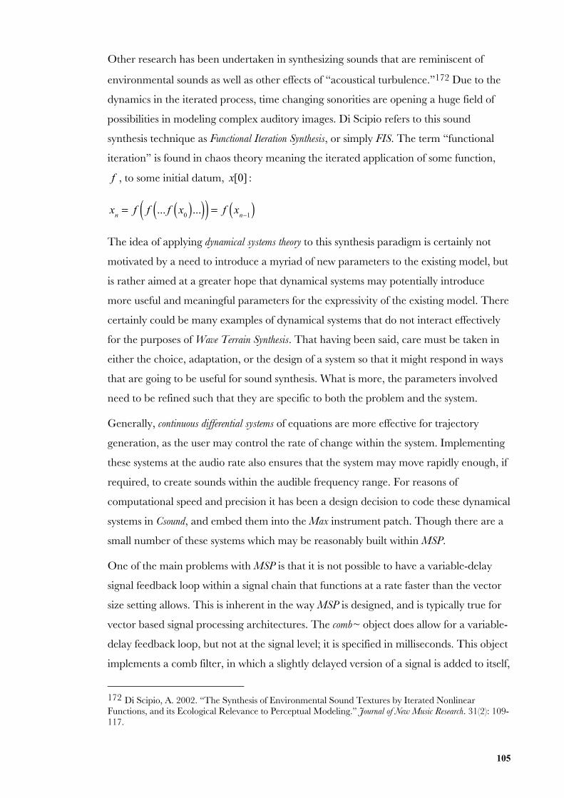
105

Other research has been undertaken in synthesizing sounds that are reminiscent of

environmental sounds as well as other effects of “acoustical turbulence.”172 Due to the

dynamics in the iterated process, time changing sonorities are opening a huge field of

possibilities in modeling complex auditory images. Di Scipio refers to this sound

synthesis technique as Functional Iteration Synthesis, or simply FIS. The term “functional

iteration” is found in chaos theory meaning the iterated application of some function,

f , to some initial datum, x[0] :

x

n= f f ... f x

0( )...( )( ) = f xn−1( )

The idea of applying dynamical systems theory to this synthesis paradigm is certainly not

motivated by a need to introduce a myriad of new parameters to the existing model, but

is rather aimed at a greater hope that dynamical systems may potentially introduce

more useful and meaningful parameters for the expressivity of the existing model. There

certainly could be many examples of dynamical systems that do not interact effectively

for the purposes of Wave Terrain Synthesis. That having been said, care must be taken in

either the choice, adaptation, or the design of a system so that it might respond in ways

that are going to be useful for sound synthesis. What is more, the parameters involved

need to be refined such that they are specific to both the problem and the system.

Generally, continuous differential systems of equations are more effective for trajectory

generation, as the user may control the rate of change within the system. Implementing

these systems at the audio rate also ensures that the system may move rapidly enough, if

required, to create sounds within the audible frequency range. For reasons of

computational speed and precision it has been a design decision to code these dynamical

systems in Csound, and embed them into the Max instrument patch. Though there are a

small number of these systems which may be reasonably built within MSP.

One of the main problems with MSP is that it is not possible to have a variable-delay

signal feedback loop within a signal chain that functions at a rate faster than the vector

size setting allows. This is inherent in the way MSP is designed, and is typically true for

vector based signal processing architectures. The comb~ object does allow for a variable-

delay feedback loop, but not at the signal level; it is specified in milliseconds. This object

implements a comb filter, in which a slightly delayed version of a signal is added to itself,

172 Di Scipio, A. 2002. “The Synthesis of Environmental Sound Textures by Iterated NonlinearFunctions, and its Ecological Relevance to Perceptual Modeling.” Journal of New Music Research. 31(2): 109-117.

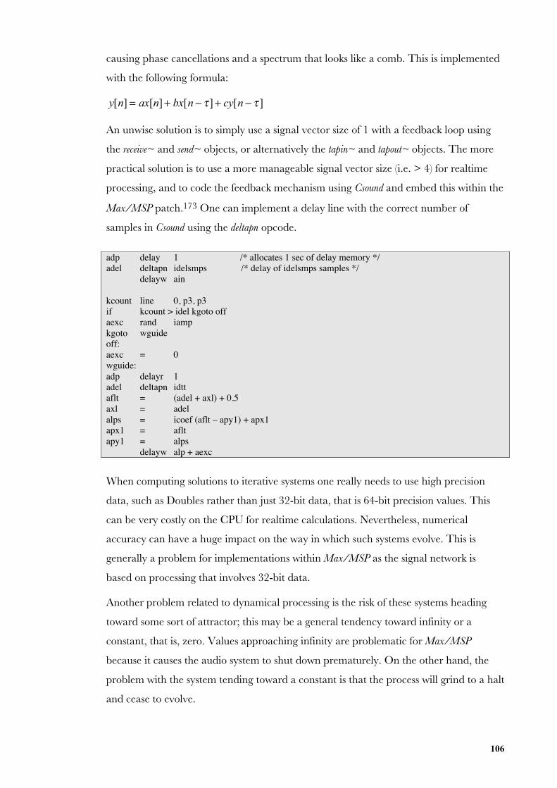
106

causing phase cancellations and a spectrum that looks like a comb. This is implemented

with the following formula:

y[n] = ax[n]+ bx[n − τ ]+ cy[n − τ ]

An unwise solution is to simply use a signal vector size of 1 with a feedback loop using

the receive~ and send~ objects, or alternatively the tapin~ and tapout~ objects. The more

practical solution is to use a more manageable signal vector size (i.e. > 4) for realtime

processing, and to code the feedback mechanism using Csound and embed this within the

Max/MSP patch.173 One can implement a delay line with the correct number of

samples in Csound using the deltapn opcode.

adp delay 1 /* allocates 1 sec of delay memory */adel deltapn idelsmps /* delay of idelsmps samples */

delayw ain

kcount line 0, p3, p3if kcount > idel kgoto offaexc rand iampkgoto wguideoff:aexc = 0wguide:adp delayr 1adel deltapn idttaflt = (adel + axl) + 0.5axl = adelalps = icoef (aflt – apy1) + apx1apx1 = afltapy1 = alps

delayw alp + aexc

When computing solutions to iterative systems one really needs to use high precision

data, such as Doubles rather than just 32-bit data, that is 64-bit precision values. This

can be very costly on the CPU for realtime calculations. Nevertheless, numerical

accuracy can have a huge impact on the way in which such systems evolve. This is

generally a problem for implementations within Max/MSP as the signal network is

based on processing that involves 32-bit data.

Another problem related to dynamical processing is the risk of these systems heading

toward some sort of attractor; this may be a general tendency toward infinity or a

constant, that is, zero. Values approaching infinity are problematic for Max/MSP

because it causes the audio system to shut down prematurely. On the other hand, the

problem with the system tending toward a constant is that the process will grind to a halt

and cease to evolve.

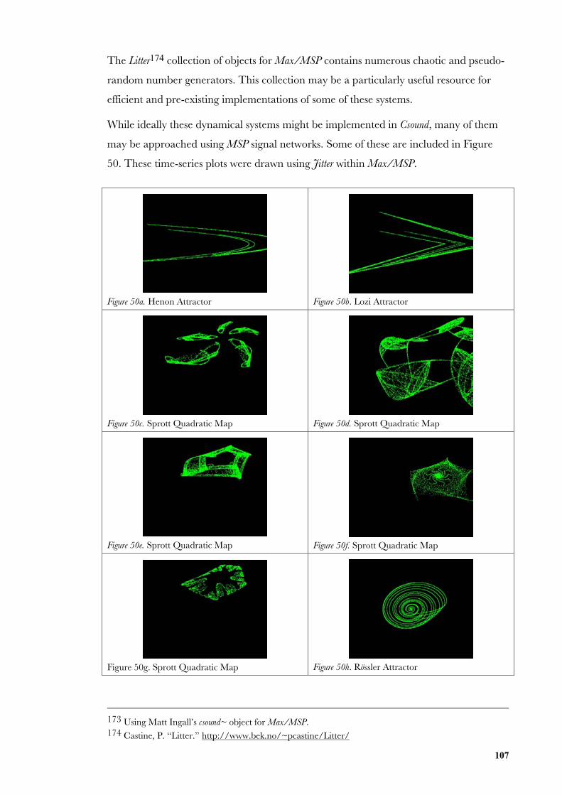
107

The Litter174 collection of objects for Max/MSP contains numerous chaotic and pseudo-

random number generators. This collection may be a particularly useful resource for

efficient and pre-existing implementations of some of these systems.

While ideally these dynamical systems might be implemented in Csound, many of them

may be approached using MSP signal networks. Some of these are included in Figure

50. These time-series plots were drawn using Jitter within Max/MSP.

Figure 50a. Henon Attractor Figure 50b. Lozi Attractor

Figure 50c. Sprott Quadratic Map Figure 50d. Sprott Quadratic Map

Figure 50e. Sprott Quadratic Map Figure 50f. Sprott Quadratic Map

Figure 50g. Sprott Quadratic Map Figure 50h. Rössler Attractor

173 Using Matt Ingall’s csound~ object for Max/MSP.174 Castine, P. “Litter.” http://www.bek.no/~pcastine/Litter/

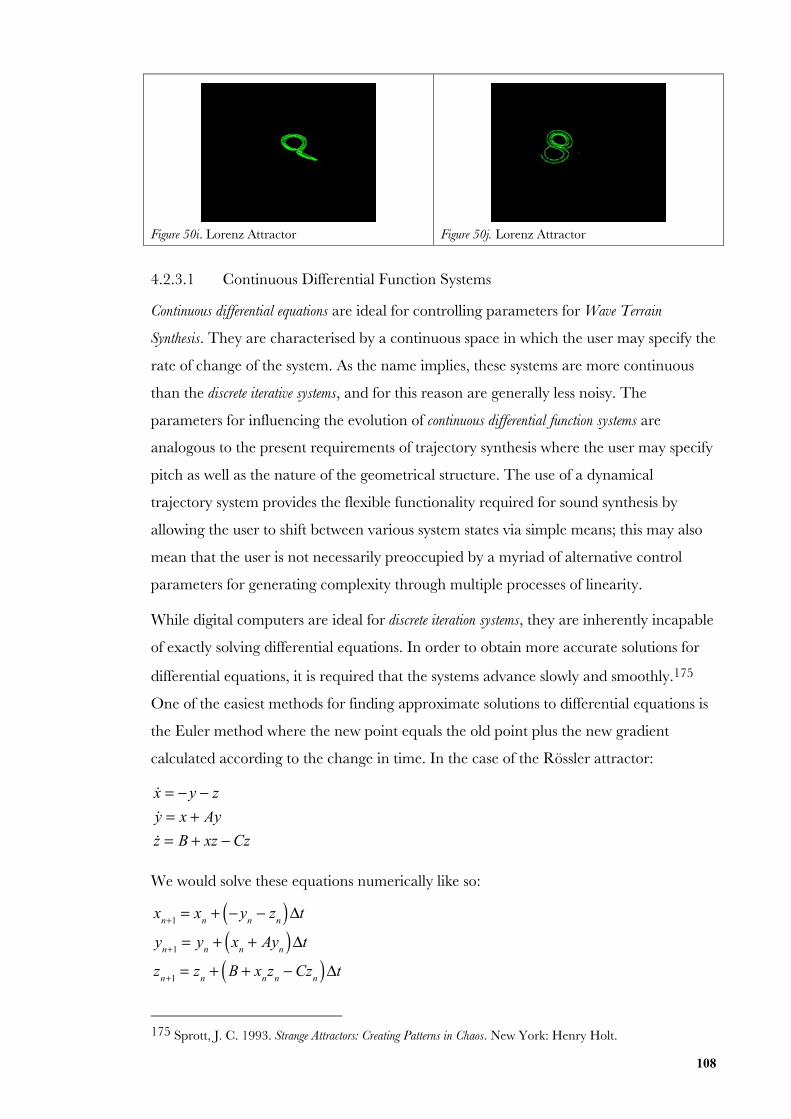
108

Figure 50i. Lorenz Attractor Figure 50j. Lorenz Attractor

4.2.3.1 Continuous Differential Function Systems

Continuous differential equations are ideal for controlling parameters for Wave Terrain

Synthesis. They are characterised by a continuous space in which the user may specify the

rate of change of the system. As the name implies, these systems are more continuous

than the discrete iterative systems, and for this reason are generally less noisy. The

parameters for influencing the evolution of continuous differential function systems are

analogous to the present requirements of trajectory synthesis where the user may specify

pitch as well as the nature of the geometrical structure. The use of a dynamical

trajectory system provides the flexible functionality required for sound synthesis by

allowing the user to shift between various system states via simple means; this may also

mean that the user is not necessarily preoccupied by a myriad of alternative control

parameters for generating complexity through multiple processes of linearity.

While digital computers are ideal for discrete iteration systems, they are inherently incapable

of exactly solving differential equations. In order to obtain more accurate solutions for

differential equations, it is required that the systems advance slowly and smoothly.175

One of the easiest methods for finding approximate solutions to differential equations is

the Euler method where the new point equals the old point plus the new gradient

calculated according to the change in time. In the case of the Rössler attractor:

x = − y − z

y = x + Ay

z = B + xz − Cz

We would solve these equations numerically like so:

xn+1

= xn+ − y

n− z

n( )Δt

yn+1

= yn+ x

n+ Ay

n( )Δt

zn+1

= zn+ B + x

nz

n− Cz

n( )Δt

175 Sprott, J. C. 1993. Strange Attractors: Creating Patterns in Chaos. New York: Henry Holt.

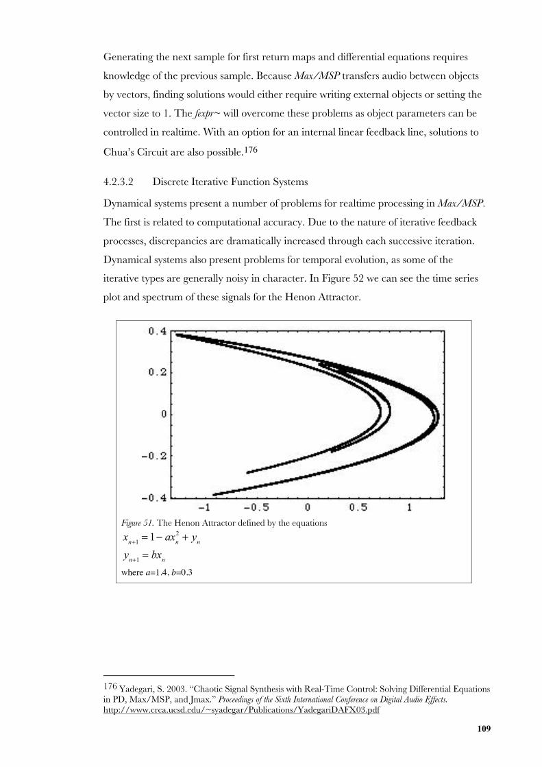
109

Generating the next sample for first return maps and differential equations requires

knowledge of the previous sample. Because Max/MSP transfers audio between objects

by vectors, finding solutions would either require writing external objects or setting the

vector size to 1. The fexpr~ will overcome these problems as object parameters can be

controlled in realtime. With an option for an internal linear feedback line, solutions to

Chua’s Circuit are also possible.176

4.2.3.2 Discrete Iterative Function Systems

Dynamical systems present a number of problems for realtime processing in Max/MSP.

The first is related to computational accuracy. Due to the nature of iterative feedback

processes, discrepancies are dramatically increased through each successive iteration.

Dynamical systems also present problems for temporal evolution, as some of the

iterative types are generally noisy in character. In Figure 52 we can see the time series

plot and spectrum of these signals for the Henon Attractor.

Figure 51. The Henon Attractor defined by the equations

xn+1

= 1− axn2 + y

n

yn+1

= bxn

where a=1.4, b=0.3

176 Yadegari, S. 2003. “Chaotic Signal Synthesis with Real-Time Control: Solving Differential Equationsin PD, Max/MSP, and Jmax.” Proceedings of the Sixth International Conference on Digital Audio Effects.http://www.crca.ucsd.edu/~syadegar/Publications/YadegariDAFX03.pdf

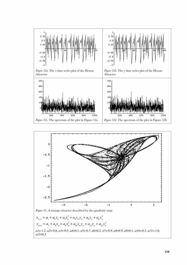
110

Figure 52a. The x time series plot of the HenonAttractor

Figure 52b. The y time series plot of the HenonAttractor

Figure 52c. The spectrum of the plot in Figure 52a

Figure 52d. The spectrum of the plot in Figure 52b

Figure 53. A strange attractor described by the quadratic map

xn+1

= a1+ a

2x

n+ a

3x

n2 + a

4x

ny

n+ a

5y

n+ a

6y

n2

yn+1

= a7+ a

8x

n+ a

9x

n2 + a

10x

ny

n+ a

11y

n+ a

12y

n2

a1=-1.2, a2=-0.6, a3=-0.5, a4=0.1, a5=-0.7, a6=0.2, a7=-0.9, a8=0.9, a9=0.1, a10=-0.3, a11=-1.0,a12=0.3

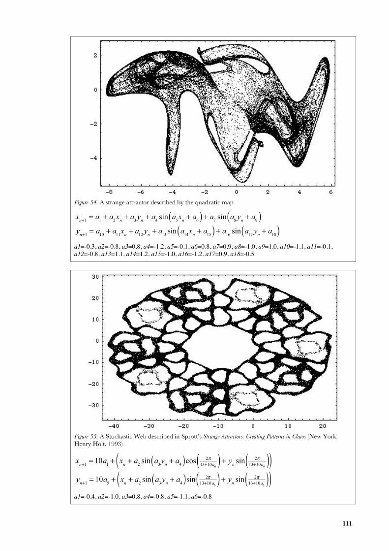
111

Figure 54. A strange attractor described by the quadratic map

xn+1

= a1+ a

2x

n+ a

3y

n+ a

4sin a

5x

n+ a

6( ) + a7

sin a8y

n+ a

9( )y

n+1= a

10+ a

11x

n+ a

12y

n+ a

13sin a

14x

n+ a

15( ) + a16

sin a17

yn+ a

18( )a1=-0.3, a2=-0.8, a3=0.8, a4=-1.2, a5=-0.1, a6=0.8, a7=0.9, a8=-1.0, a9=1.0, a10=-1.1, a11=-0.1,a12=-0.8, a13=1.1, a14=1.2, a15=-1.0, a16=-1.2, a17=0.9, a18=-0.5

Figure 55. A Stochastic Web described in Sprott’s Strange Attractors: Creating Patterns in Chaos (New York:Henry Holt, 1993)

xn+1

= 10a1+ x

n+ a

2sin a

3y

n+ a

4( )cos 2π13+10a6( ) + y

nsin 2π

13+10a6( )( )

yn+1

= 10a5+ x

n+ a

2sin a

3y

n+ a

4( )sin 2π13+10a6( ) + y

nsin 2π

13+10a6( )( )

a1=-0.4, a2=-1.0, a3=0.8, a4=-0.8, a5=-1.1, a6=-0.8

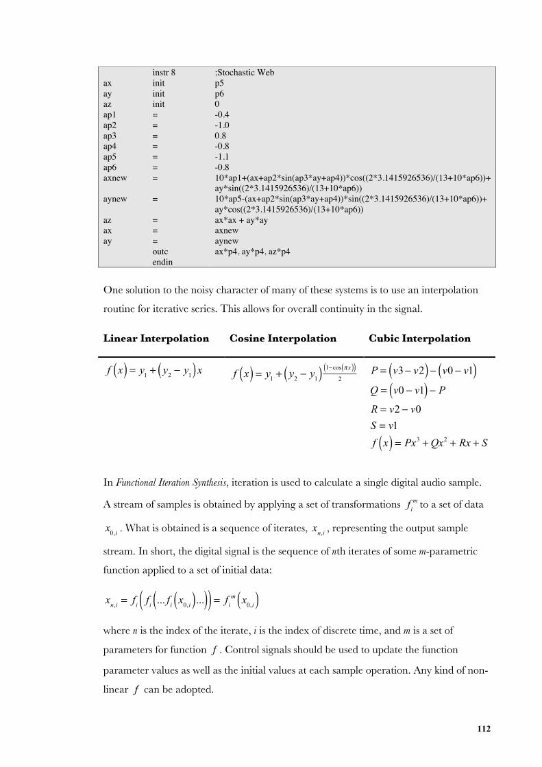
112

axayazap1ap2ap3ap4ap5ap6axnew

aynew

azaxay

instr 8initinitinit=======

=

===outcendin

;Stochastic Webp5p60-0.4-1.00.8-0.8-1.1-0.810*ap1+(ax+ap2*sin(ap3*ay+ap4))*cos((2*3.1415926536)/(13+10*ap6))+ay*sin((2*3.1415926536)/(13+10*ap6))10*ap5-(ax+ap2*sin(ap3*ay+ap4))*sin((2*3.1415926536)/(13+10*ap6))+ay*cos((2*3.1415926536)/(13+10*ap6))ax*ax + ay*ayaxnewaynewax*p4, ay*p4, az*p4

One solution to the noisy character of many of these systems is to use an interpolation

routine for iterative series. This allows for overall continuity in the signal.

Linear Interpolation Cosine Interpolation Cubic Interpolation

f x( ) = y

1+ y

2− y

1( )x f x( ) = y

1+ y

2− y

1( ) 1−cos π x( )( )2

P = v3− v2( ) − v0 − v1( )Q = v0 − v1( ) − P

R = v2 − v0

S = v1

f x( ) = Px3 + Qx2 + Rx + S

In Functional Iteration Synthesis, iteration is used to calculate a single digital audio sample.

A stream of samples is obtained by applying a set of transformations fim to a set of data

x

0,i. What is obtained is a sequence of iterates,

x

n,i, representing the output sample

stream. In short, the digital signal is the sequence of nth iterates of some m-parametric

function applied to a set of initial data:

x

n,i= f

if

i... f

ix

0,i( )...( )( ) = fim x

0,i( )where n is the index of the iterate, i is the index of discrete time, and m is a set of

parameters for function f . Control signals should be used to update the function

parameter values as well as the initial values at each sample operation. Any kind of non-

linear f can be adopted.

113

Di Scipio uses the iterated sine map:

x

n,i= sin r

ix

n−1,i( )Within the context of Wave Terrain Synthesis, the output signal is the equivalent of a

sampled trajectory scanning over the Phase Space of the sine map,177 where the Phase

Space plot serves as the terrain function.

It can be fruitful looking at other maps such as the logistic map, another

monoparametric map:

xn= rx

n−1(1− x

n−1)

This is a completely different dynamical system. It brings different interdependencies

among synthesis parameters. Di Scipio suggests that some of these sounds and textures

are better produced by means of time-domain processing synthesis rather than spectral

modelling, especially due to transient detail and spectral movement.178

For these monoparametric maps the iterate order, n, significantly affects the spectrum

bandwidth. Larger values cause wider oscillations. Eventually the spectrum becomes

dense and noise is obtained. Higher iterates invariably cause the foldover phenomenon.

In these cases one is recommended to use a higher sampling frequency.

In Di Scipio’s research, sounds produced have been reminiscent of boiling water,

cracking of rocks and icebanks, the sound of wind, various kinds of sonorous powders,

burning materials, certain kinds of insects, thunder, electrical noises, sulphureous or

volcanic events, the wind flapping against thin but large plastic plates. With higher order

iterates, such as when n > 9, the audio is reminiscent of a large fire, rain or hail, or

frying oil – these effects can be enhanced by injecting a very small amount of noise or

jitter into the iterated map, deliberately augmenting the error diffusion in the

computational process.

177 Di Scipio, A. 2002. “The Synthesis of Environmental Sound Textures by Iterated NonlinearFunctions, and its Ecological Relevance to Perceptual Modeling.” Journal of New Music Research. 31(2):109-117.178 Di Scipio, A. 2002. “The Synthesis of Environmental Sound Textures by Iterated NonlinearFunctions, and its Ecological Relevance to Perceptual Modeling.” Journal of New Music Research. 31(2):109-117.

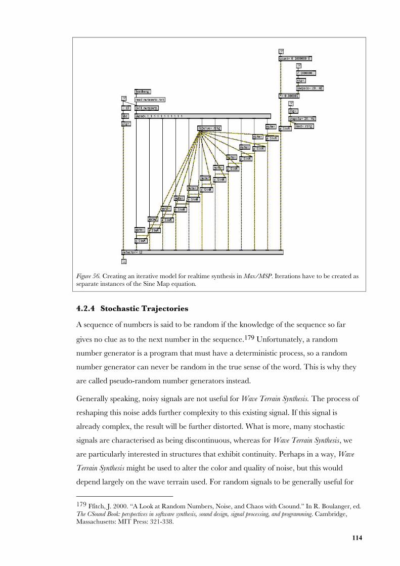
114

Figure 56. Creating an iterative model for realtime synthesis in Max/MSP. Iterations have to be created asseparate instances of the Sine Map equation.

4.2.4 Stochastic Trajectories

A sequence of numbers is said to be random if the knowledge of the sequence so far

gives no clue as to the next number in the sequence.179 Unfortunately, a random

number generator is a program that must have a deterministic process, so a random

number generator can never be random in the true sense of the word. This is why they

are called pseudo-random number generators instead.

Generally speaking, noisy signals are not useful for Wave Terrain Synthesis. The process of

reshaping this noise adds further complexity to this existing signal. If this signal is

already complex, the result will be further distorted. What is more, many stochastic

signals are characterised as being discontinuous, whereas for Wave Terrain Synthesis, we

are particularly interested in structures that exhibit continuity. Perhaps in a way, Wave

Terrain Synthesis might be used to alter the color and quality of noise, but this would

depend largely on the wave terrain used. For random signals to be generally useful for

179 Ffitch, J. 2000. “A Look at Random Numbers, Noise, and Chaos with Csound.” In R. Boulanger, ed.The CSound Book: perspectives in software synthesis, sound design, signal processing, and programming. Cambridge,Massachusetts: MIT Press: 321-338.

115

Wave Terrain Synthesis, one would need to interpolate between a slower series of random

values. This would create a more useful signal that maintains essentially the character of

something that is random, yet maintaining overall signal continuity. These signals would

be most effective for controlling and modulating transformational parameters and

effects.

Random walks are much more useful for Wave Terrain Synthesis. We want signals that

reflect continuity, so that the resulting waveform after Wave Terrain Synthesis is also

continuous. Random walks are one possibility for such trajectories. These probabilistic

systems have been popular for composer Iannis Xenakis. One such implementation

within Max/MSP, called jitter~, randomly varies an input by a small amount.

4.3 Establishing Further Means for Control over the Temporal Evolution of the

System – Expressive Control

More research is needed in order to re-create complex signals like those of real-world

sounds such as speech and acoustical instruments.180 Part of the problem is the difficulty

in recreating the transient and spectral complexity of these sounds.181 It appears that

dynamical systems, or ways of recreating the transient complexity within the trajectory

signal, may be the more useful processes for Wave Terrain Synthesis. It appears that

transient complexity should be dictated by the trajectory model; it cannot be dictated by

a slowly moving “dynamical” terrain structure as this system is unable to reproduce the

speed of evolution that is required for such transient shifts.

One of the primary issues pertaining to Wave Terrain Synthesis is how to shift effectively

between various periodic, quasi-periodic, chaotic, and random states. It seems that one

is not necessarily in control of the way in which these elements fuse together. Therefore

one needs a flexible system where the user can reroute control signals for sound

synthesis, such as determining how chaotic systems impact on the instrument model. In

other words, whether a generative methodology like a chaotic system is used as a

primary means for generating the trajectory curve, or whether it is used as a means of

modulating or transforming the trajectory signals geometrically. What needs to be

expanded on from here are techniques that may be used for transforming the trajectory

signals geometrically. The following sections document some approaches to this

problem.

180 Roads, C., et al. 1996. The Computer Music Tutorial, Cambridge, Massachusetts: MIT Press.181 James, S. 2003. “Possibilities for Dynamical Wave Terrain Synthesis.” Converging Technologies,Proceedings of the Australasian Computer Music Conference: 58-67.

116

4.3.1 Geometric Transformation

The scale (x, y), translation (x, y), and rotation (q) of an existing trajectory curve may be

altered within the two-dimensional space. By altering the variables involved with the

generating or processing of the trajectory, the timbre of a generated tone by Wave Terrain

Synthesis may be modified with respect to time. Otherwise if the orbit remains periodic,

the resulting sound is characterized by a simple oscillator type with a fixed and static

waveform.

Scale, translation and rotation are all parameters attributable to Affine Transformation.

Geometric contraction, expansion, dilation, reflection, rotation, shear, similarity

transformations, spiral similarities, and translation are all affine transformations, as are

their combinations. In general, an affine transformation is a composition of rotations,

translations, dilations, and shears.

One can immediately see how transformational parameters could be useful within the

two-dimensional plane. So the use of transformations of scale, translation and rotation in

both x and y axes may well be useful for expressive control. How do these affect the

harmonic character of each discrete trajectory signal before reshaping? Obviously scale

alters the initial amplitude, and translation changes the DC offset. Rotation effectively

crossfades between two trajectory signals. The order of these processes as applied to the

trajectory signals is important: 1) Scale, 2) Reflect, 3) Rotate, and 4) Translate. These

are powerful transformational parameters in Wave Terrain Synthesis. While they may only

change the amplitude and DC offset of the trajectory signal, the way these

transformations influence the table lookup process is quite different.

One of the more characteristic parameters in Wave Terrain Synthesis is the shifting of the

phase in the trajectory signal. By translating the trajectory motion over the surface of the

terrain, we create complex harmonic modulations. This is also dependent on the relative

intensities of the x and y trajectory signals.

In Waveshaping Synthesis one can cause the spectrum to vary in an interesting and musical

way by means of multiplying the input signal x by some value a within the unit interval

[0 1] before applying f to it. The function f (ax) is then applied. The same can be said

for Wave Terrain Synthesis, the difference being that the scaling factor can be applied in

two or more directions for both x and y parameters within the two-dimensional

Cartesian space. Interestingly enough, for many terrain surface types, one might expect

the parameter to eventually correlate with that of the resulting amplitude. It certainly

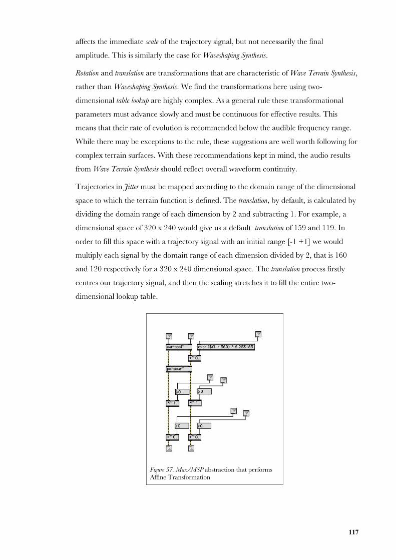
117

affects the immediate scale of the trajectory signal, but not necessarily the final

amplitude. This is similarly the case for Waveshaping Synthesis.

Rotation and translation are transformations that are characteristic of Wave Terrain Synthesis,

rather than Waveshaping Synthesis. We find the transformations here using two-

dimensional table lookup are highly complex. As a general rule these transformational

parameters must advance slowly and must be continuous for effective results. This

means that their rate of evolution is recommended below the audible frequency range.

While there may be exceptions to the rule, these suggestions are well worth following for

complex terrain surfaces. With these recommendations kept in mind, the audio results

from Wave Terrain Synthesis should reflect overall waveform continuity.

Trajectories in Jitter must be mapped according to the domain range of the dimensional

space to which the terrain function is defined. The translation, by default, is calculated by

dividing the domain range of each dimension by 2 and subtracting 1. For example, a

dimensional space of 320 x 240 would give us a default translation of 159 and 119. In

order to fill this space with a trajectory signal with an initial range [-1 +1] we would

multiply each signal by the domain range of each dimension divided by 2, that is 160

and 120 respectively for a 320 x 240 dimensional space. The translation process firstly

centres our trajectory signal, and then the scaling stretches it to fill the entire two-

dimensional lookup table.

Figure 57. Max/MSP abstraction that performsAffine Transformation

118

4.3.2 Additive and Multiplicative Poly-Trajectories

Mills and De Souza describe an orbit where one uses a compound path formed by a

larger circular or elliptical path, usually at a slower sub-audio rate, as well as a local

smaller and faster circular orbit. In this way the faster orbit is what we hear in the

audible frequency range, and the slow orbit modulates the position of this faster orbit

affecting timbral evolution of the resulting waveform with respect to time t.182 This

process is achieved simply by adding two different trajectories together such that:

x t( ) = a1x

1t( ) + b

1x

2t( )

y t( ) = a2y

1t( ) + b

2y

2t( )

where x

1t( ) and

y

1t( ) are the periodic trajectories within the audible frequency range,

and x

2t( ) and

y

2t( ) are systems that are characterized by either quasi-periodic,

chaotic, or stochastic behaviours. One can also apply a multiplication process instead of

an addition, except one then loses the ability to control the level of each element in

separation. With the a scaling parameters the user may control the level of periodicity in

the system, and with the b parameter alter the amount of quasi-periodicity, chaos, or

randomness. In order to avoid having levels for each of these behaviours, the quasi-

periodic, chaotic, and stochastic components are grouped together. The user may select

which system best serves their purpose. Figure 68 in Chapter 6 may put some

perspective on this approach in methodology.

4.3.3 Audio Effects

Max/MSP is bundled with a number of objects for performing modifications on an

audio signal. Some of these include: rampsmooth~, delta~, deltaclip~, trunc~, round~,

downsamp~, and degrade~. While it is not always recommended to use various

“destructive” methods of audio modification within the context of Wave Terrain Synthesis,

it is interesting to observe some of the outcomes. Like many of the other geometrical

transformations to trajectory signals, such as the scale, translation, and rotation parameters

discussed in Sub-Section 4.3.1 of this Chapter, the results from these destructive

methods show more possibilities in signal transformation. The results are sonically rich

and may be useful in developing various kinds of distortion.

182 Mills, A. and R. C. De Souza. 1999. “Gestural Sounds by Means of Wave Terrain Synthesis.”Congresso Nacional da Sociedade Brasileira de Computação XIX.http://gsd.ime.usp.br/sbcm/1999/papers/Anderson_Mills.html

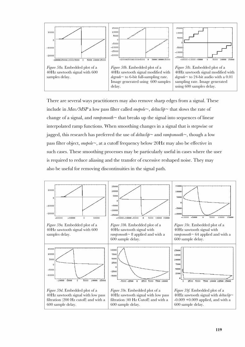
119

Figure 58a. Embedded plot of a40Hz sawtooth signal with 600samples delay.

Figure 58b. Embedded plot of a40Hz sawtooth signal modified withdegrade~ to 6-bit full-sampling rate.Image generated using 600 samplesdelay.

Figure 58c. Embedded plot of a40Hz sawtooth signal modified withdegrade~ to 24-bit audio with a 0.01sampling rate. Image generatedusing 600 samples delay.

There are several ways practitioners may also remove sharp edges from a signal. These

include in Max/MSP a low pass filter called onepole~, deltaclip~ that slows the rate of

change of a signal, and rampsmooth~ that breaks up the signal into sequences of linear

interpolated ramp functions. When smoothing changes in a signal that is stepwise or

jagged, this research has preferred the use of deltaclip~ and rampsmooth~, though a low

pass filter object, onepole~, at a cutoff frequency below 20Hz may also be effective in

such cases. These smoothing processes may be particularly useful in cases where the user

is required to reduce aliasing and the transfer of excessive reshaped noise. They may

also be useful for removing discontinuities in the signal path.

Figure 59a. Embedded plot of a40Hz sawtooth signal with 600samples delay.

Figure 59b. Embedded plot of a40Hz sawtooth signal withrampsmooth~ 8 applied and with a600 sample delay.

Figure 59c. Embedded plot of a40Hz sawtooth signal withrampsmooth~ 64 applied and with a600 sample delay.

Figure 59d. Embedded plot of a40Hz sawtooth signal with low passfiltration (200 Hz cutoff) and with a600 sample delay.

Figure 59e. Embedded plot of a40Hz sawtooth signal with low passfiltration (40 Hz Cutoff) and with a600 sample delay.

Figure 59f. Embedded plot of a40Hz sawtooth signal with deltaclip~-0.009 +0.009 applied, and with a600 sample delay.

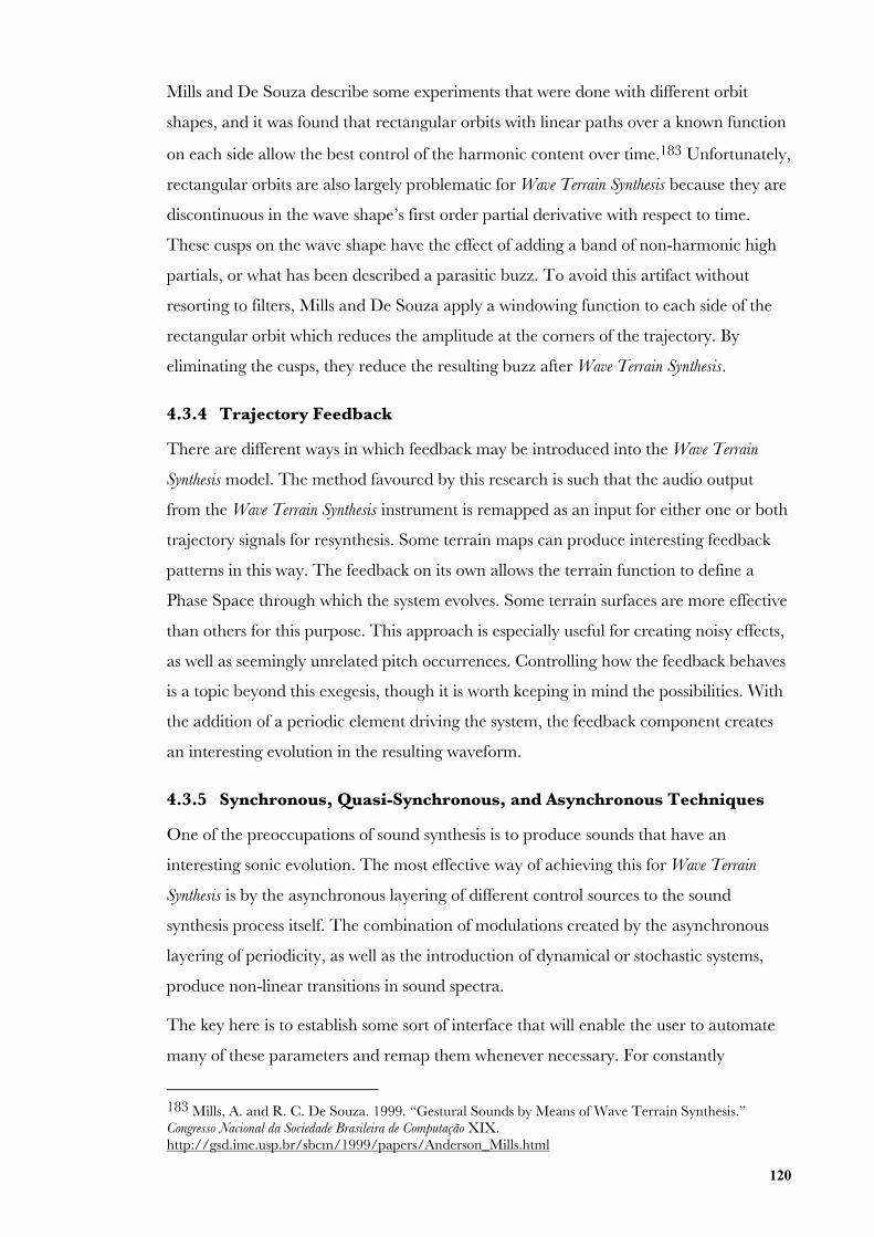
120

Mills and De Souza describe some experiments that were done with different orbit

shapes, and it was found that rectangular orbits with linear paths over a known function

on each side allow the best control of the harmonic content over time.183 Unfortunately,

rectangular orbits are also largely problematic for Wave Terrain Synthesis because they are

discontinuous in the wave shape’s first order partial derivative with respect to time.

These cusps on the wave shape have the effect of adding a band of non-harmonic high

partials, or what has been described a parasitic buzz. To avoid this artifact without

resorting to filters, Mills and De Souza apply a windowing function to each side of the

rectangular orbit which reduces the amplitude at the corners of the trajectory. By

eliminating the cusps, they reduce the resulting buzz after Wave Terrain Synthesis.

4.3.4 Trajectory Feedback

There are different ways in which feedback may be introduced into the Wave Terrain

Synthesis model. The method favoured by this research is such that the audio output

from the Wave Terrain Synthesis instrument is remapped as an input for either one or both

trajectory signals for resynthesis. Some terrain maps can produce interesting feedback

patterns in this way. The feedback on its own allows the terrain function to define a

Phase Space through which the system evolves. Some terrain surfaces are more effective

than others for this purpose. This approach is especially useful for creating noisy effects,

as well as seemingly unrelated pitch occurrences. Controlling how the feedback behaves

is a topic beyond this exegesis, though it is worth keeping in mind the possibilities. With

the addition of a periodic element driving the system, the feedback component creates

an interesting evolution in the resulting waveform.

4.3.5 Synchronous, Quasi-Synchronous, and Asynchronous Techniques

One of the preoccupations of sound synthesis is to produce sounds that have an

interesting sonic evolution. The most effective way of achieving this for Wave Terrain

Synthesis is by the asynchronous layering of different control sources to the sound

synthesis process itself. The combination of modulations created by the asynchronous

layering of periodicity, as well as the introduction of dynamical or stochastic systems,

produce non-linear transitions in sound spectra.

The key here is to establish some sort of interface that will enable the user to automate

many of these parameters and remap them whenever necessary. For constantly

183 Mills, A. and R. C. De Souza. 1999. “Gestural Sounds by Means of Wave Terrain Synthesis.”Congresso Nacional da Sociedade Brasileira de Computação XIX.http://gsd.ime.usp.br/sbcm/1999/papers/Anderson_Mills.html

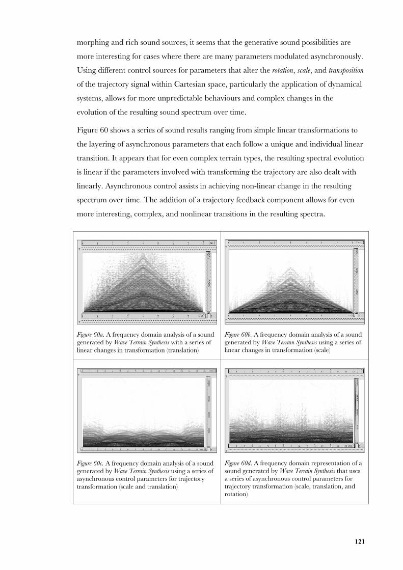
121

morphing and rich sound sources, it seems that the generative sound possibilities are

more interesting for cases where there are many parameters modulated asynchronously.

Using different control sources for parameters that alter the rotation, scale, and transposition

of the trajectory signal within Cartesian space, particularly the application of dynamical

systems, allows for more unpredictable behaviours and complex changes in the

evolution of the resulting sound spectrum over time.

Figure 60 shows a series of sound results ranging from simple linear transformations to

the layering of asynchronous parameters that each follow a unique and individual linear

transition. It appears that for even complex terrain types, the resulting spectral evolution

is linear if the parameters involved with transforming the trajectory are also dealt with

linearly. Asynchronous control assists in achieving non-linear change in the resulting

spectrum over time. The addition of a trajectory feedback component allows for even

more interesting, complex, and nonlinear transitions in the resulting spectra.

Figure 60a. A frequency domain analysis of a soundgenerated by Wave Terrain Synthesis with a series oflinear changes in transformation (translation)

Figure 60b. A frequency domain analysis of a soundgenerated by Wave Terrain Synthesis using a series oflinear changes in transformation (scale)

Figure 60c. A frequency domain analysis of a soundgenerated by Wave Terrain Synthesis using a series ofasynchronous control parameters for trajectorytransformation (scale and translation)

Figure 60d. A frequency domain representation of asound generated by Wave Terrain Synthesis that usesa series of asynchronous control parameters fortrajectory transformation (scale, translation, androtation)

122

4.3.6 Spatial Evolution for Multi-Channel Audio

The spatial localization and phase of a sound generated via Wave Terrain Synthesis is a

topic beyond this exegesis. Nevertheless, there are some general observations worth

mentioning. Keeping in mind the theory that has already been presented, if color is

mapped discretely to specific audio channels, we find that by altering the hue of this map

we have control over the localization of a resulting sound. One could imagine that this

could be extended in some way to multi-speaker setups. Nevertheless, we must

interpolate for values that occur between the discrete channels of red, green, and blue

for multi-speaker setups; otherwise we only have values for three discrete channels.

While we are effectively dealing with the localization of a sound source, what is

particularly interesting in this case is that the geometrical transformations applied to the

matrix data, as a result of modifying the color space, directly affect the way in which the

audio spatialization is controlled. Similarly we can say that the way in which the sound

synthesis process is mapped to color space directly impacts how color transformations

are reproduced sonically.

Besides the mapping of discrete color channels to audio channels, there is a great deal of

flexibility in creating sounds with a complex stereo or multichannel image. The phase

relationships can be quite complex. And there are numerous ways in which this

relationship may be explored. Another effect explored through the Wave Terrain Synthesis

implementation covered in this research is the introduction of spatial movement by

displacing multiple trajectory orbits over a single terrain function. This system can be

static, or potentially dynamic. We use a small spatial offset between multiple trajectory

orbits. The difference in the perceived spectral evolution of multiple channels of audio

generated using multiple trajectories creates a complex spatial evolution in the resulting

audio. The phasing and harmonic interactions can be highly complex. Nevertheless, as

the spatial offset between trajectory signals becomes larger, each channel of audio

becomes more dissociated in terms of its timbral evolution, spectrum, and phase. Small

differences however create sounds with a great deal of spatial depth. If these differences

between trajectory signals are dynamical in their behaviour, the sonic evolution of the

results can be highly interesting indeed.

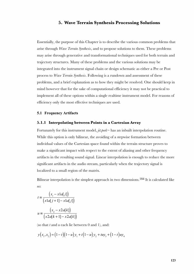
123

5. Wave Terrain Synthesis Processing Solutions

Essentially, the purpose of this Chapter is to describe the various common problems that

arise through Wave Terrain Synthesis, and to propose solutions to them. These problems

may arise through generative and transformational techniques used for both terrain and

trajectory structures. Many of these problems and the various solutions may be

integrated into the instrument signal chain or design schematic as either a Pre or Post

process to Wave Terrain Synthesis. Following is a rundown and assessment of these

problems, and a brief explanation as to how they might be resolved. One should keep in

mind however that for the sake of computational efficiency it may not be practical to

implement all of these options within a single realtime instrument model. For reasons of

efficiency only the most effective techniques are used.

5.1 Frequency Artifacts

5.1.1 Interpolating between Points in a Cartesian Array

Fortunately for this instrument model, jit.peek~ has an inbuilt interpolation routine.

While this option is only bilinear, the avoiding of a stepwise formation between

individual values of the Cartesian space found within the terrain structure proves to

make a significant impact with respect to the extent of aliasing and other frequency

artifacts in the resulting sound signal. Linear interpolation is enough to reduce the more

significant artifacts in the audio stream, particularly when the trajectory signal is

localized to a small region of the matrix.

Bilinear interpolation is the simplest approach in two dimensions.184 It is calculated like

so:

t ≡x

1− x1a[ j]( )

x1a[ j +1]− x1a[ j]( )

u ≡x

2− x2a[k]( )

x2a[k +1]− x2a[k]( )(so that t and u each lie between 0 and 1), and:

y x

1, x

2( ) = 1− t( ) 1− u( ) y1+ t 1− u( ) y

2+ tuy

3+ 1− t( )uy

4

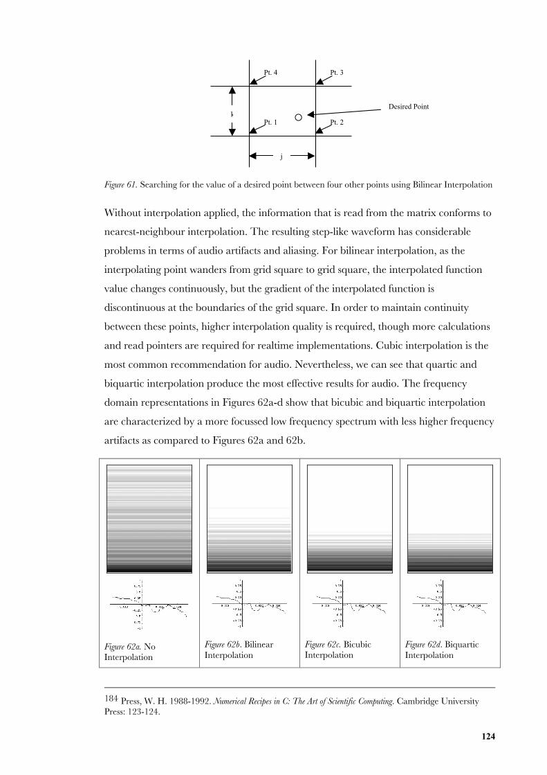
124

Figure 61. Searching for the value of a desired point between four other points using Bilinear Interpolation

Without interpolation applied, the information that is read from the matrix conforms to

nearest-neighbour interpolation. The resulting step-like waveform has considerable

problems in terms of audio artifacts and aliasing. For bilinear interpolation, as the

interpolating point wanders from grid square to grid square, the interpolated function

value changes continuously, but the gradient of the interpolated function is

discontinuous at the boundaries of the grid square. In order to maintain continuity

between these points, higher interpolation quality is required, though more calculations

and read pointers are required for realtime implementations. Cubic interpolation is the

most common recommendation for audio. Nevertheless, we can see that quartic and

biquartic interpolation produce the most effective results for audio. The frequency

domain representations in Figures 62a-d show that bicubic and biquartic interpolation

are characterized by a more focussed low frequency spectrum with less higher frequency

artifacts as compared to Figures 62a and 62b.

Figure 62a. NoInterpolation

Figure 62b. BilinearInterpolation

Figure 62c. BicubicInterpolation

Figure 62d. BiquarticInterpolation

184 Press, W. H. 1988-1992. Numerical Recipes in C: The Art of Scientific Computing. Cambridge UniversityPress: 123-124.

L

Pt. 4 Pt. 3

Pt. 1 Pt. 2k

j

Desired Point

125

Calculations for performing higher interpolation orders become increasingly more

intensive for realtime calculation. The main problem with interpolation routines for

structures of higher dimensions is the sheer increase in the processing required to solve

these sorts of estimations. For simple bilinear interpolation, the calculation requires

reading up to four values at a time as well as eighteen arithmetic stages for simply one

numerical result. For sinc interpolation one requires sixteen values for one numerical

result in two dimensions, cubic interpolation sixteen values, and for quartic twenty-five

values.

More elaborate interpolation procedures may, of course, be applied for non-realtime

systems, until computational power justifies the use of more intensive procedures for

realtime application. Obviously in Csound and in Max/MSP, if one wanted to render

audio in non-real-time mode, a more complex interpolation procedure could be applied

instead of bilinear.

5.1.2 Aliasing through the Large Scale Transformation of Trajectory

Signals

There are three factors to consider when avoiding aliasing with Wave Terrain Synthesis:

the extent of harmonic complexity in the terrain function, the level of complexity in the

trajectory – that is keeping in mind both the fundamental frequency and the extent of

higher partials – and the scaling factor of the trajectory signal. The first two issues have

been discussed throughout Chapters 3 and 4. This Section deals with the scaling factor

used for transforming the trajectory signal.

It is easy to generate high-frequency components using real-world images for Wave

Terrain Synthesis, and in some situations frequency components can be too high for sound

synthesis, that is, higher than the Nyquist frequency. We are able to control this

according to a function that calculates a scaling factor dependent on the fundamental

frequency of the trajectory as well as the size of the terrain matrix.

The idea behind this scaling function is that the scaling factor increases in size for lower

fundamental frequencies so that more harmonic detail is “picked up” during the course

of a periodic revolution. When the fundamental frequency increases in pitch, the scaling

factor is reduced so that aliasing does not result for complex terrain functions. In this

model, frequency and scale are connected. While this need not apply for simpler terrain

structures, the scaling system is necessary for more complex topographical maps.

126

One way of considering this problem is to firstly imagine observing a rugged terrain

from a distance. As one investigates this terrain more closely, one finds that what

appears to have been sharp contours from a distance turn into less abrasive collections

of hills and valleys that when looked at even more closely turn out to be quite smooth

gradations. If one moves too close there may not be much gradation at all. One can also

imagine the opposite problem when the trajectory signal is too large that it cannot

represent all of the detail it passes on its course. This means there are gaps in the

complete representation of an audio signal causing frequencies to be reflected back into

the audible frequency range producing lower frequency artifacts. In other words we

want to avoid either extremity such that the trajectory is never too small in scale,

creating weak signals via Wave Terrain Synthesis, nor do we want the situation where the

trajectory is scaled too large resulting in a spectral complexity that cannot be effectively

represented using the sampling rate of the overall system (i.e. 44100Hz).

For linear trajectories the scaling function used is described:

s =

Nf+1

w

for 1w< s < 22050

w−1, where N is the Nyquist frequency, f is the frequency of the

trajectory, and w is the size of the matrix such that for a table sized 80 x 80 w = 80 .

For elliptical trajectories, determining this scaling function may be a little more

complex. At least for circular patterns we can calculate:

s =

Nf+1

πw

for

1πw

< s < 22050πw−1

.

The reason for audio aliasing is that the trajectory lookup process cannot reproduce the

contour detail represented in the wave terrain. When the cyclical motion becomes faster

on a set sampling schedule, there is a decrease in the number of samples for each

periodic cycle of the trajectory, hence there are less table lookups for each periodic cycle

too. Of course, both the combination of large scaling factors and frequencies in

trajectories signals may result in an increased risk of aliasing, but is this avoidable in any

other way? A large part of this problem depends on the nature of the terrain itself. The

more rugged the terrain the more risk of aliasing and the converse equally applies. Real-

life images for use as terrain functions usually contain a great level of harmonic

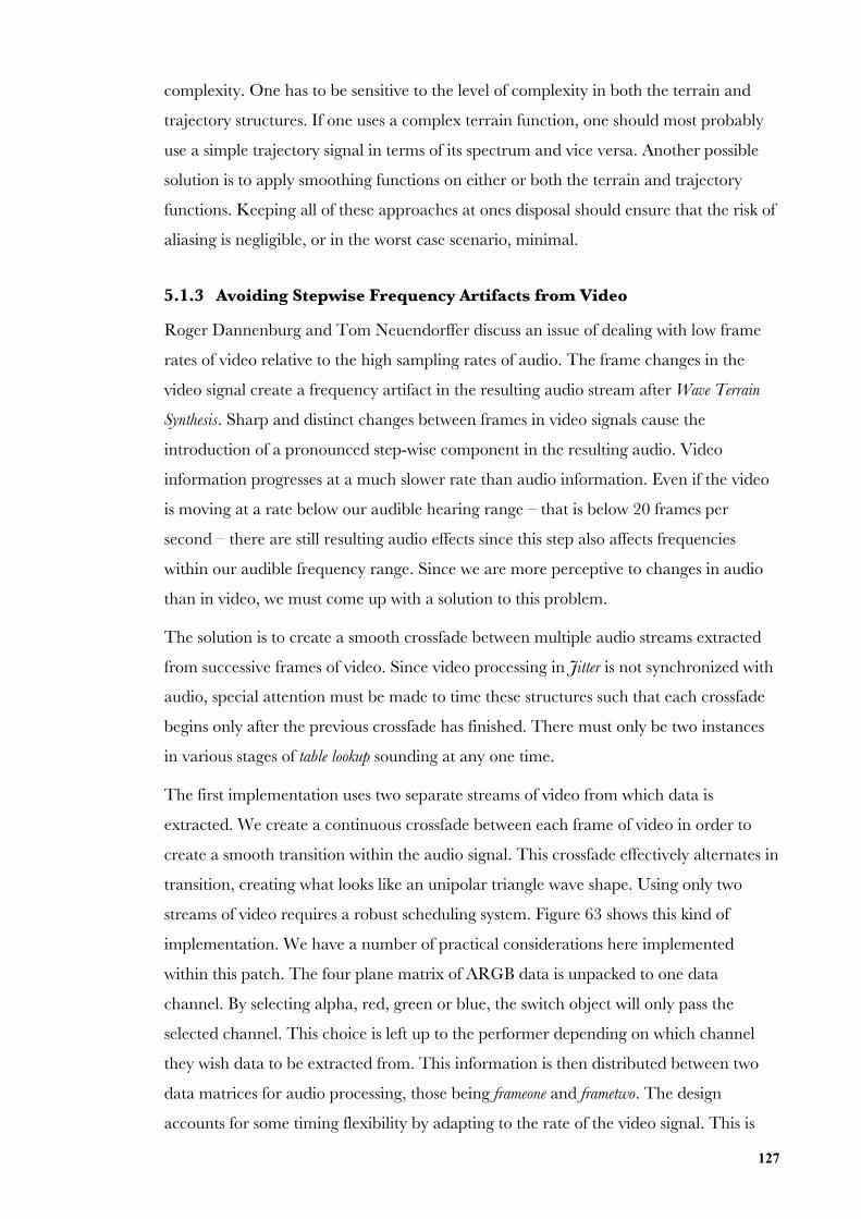
127

complexity. One has to be sensitive to the level of complexity in both the terrain and

trajectory structures. If one uses a complex terrain function, one should most probably

use a simple trajectory signal in terms of its spectrum and vice versa. Another possible

solution is to apply smoothing functions on either or both the terrain and trajectory

functions. Keeping all of these approaches at ones disposal should ensure that the risk of

aliasing is negligible, or in the worst case scenario, minimal.

5.1.3 Avoiding Stepwise Frequency Artifacts from Video

Roger Dannenburg and Tom Neuendorffer discuss an issue of dealing with low frame

rates of video relative to the high sampling rates of audio. The frame changes in the

video signal create a frequency artifact in the resulting audio stream after Wave Terrain

Synthesis. Sharp and distinct changes between frames in video signals cause the

introduction of a pronounced step-wise component in the resulting audio. Video

information progresses at a much slower rate than audio information. Even if the video

is moving at a rate below our audible hearing range – that is below 20 frames per

second – there are still resulting audio effects since this step also affects frequencies

within our audible frequency range. Since we are more perceptive to changes in audio

than in video, we must come up with a solution to this problem.

The solution is to create a smooth crossfade between multiple audio streams extracted

from successive frames of video. Since video processing in Jitter is not synchronized with

audio, special attention must be made to time these structures such that each crossfade

begins only after the previous crossfade has finished. There must only be two instances

in various stages of table lookup sounding at any one time.

The first implementation uses two separate streams of video from which data is

extracted. We create a continuous crossfade between each frame of video in order to

create a smooth transition within the audio signal. This crossfade effectively alternates in

transition, creating what looks like an unipolar triangle wave shape. Using only two

streams of video requires a robust scheduling system. Figure 63 shows this kind of

implementation. We have a number of practical considerations here implemented

within this patch. The four plane matrix of ARGB data is unpacked to one data

channel. By selecting alpha, red, green or blue, the switch object will only pass the

selected channel. This choice is left up to the performer depending on which channel

they wish data to be extracted from. This information is then distributed between two

data matrices for audio processing, those being frameone and frametwo. The design

accounts for some timing flexibility by adapting to the rate of the video signal. This is

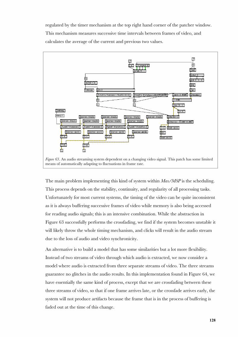
128

regulated by the timer mechanism at the top right hand corner of the patcher window.

This mechanism measures successive time intervals between frames of video, and

calculates the average of the current and previous two values.

Figure 63. An audio streaming system dependent on a changing video signal. This patch has some limitedmeans of automatically adapting to fluctuations in frame rate.

The main problem implementing this kind of system within Max/MSP is the scheduling.

This process depends on the stability, continuity, and regularity of all processing tasks.

Unfortunately for most current systems, the timing of the video can be quite inconsistent

as it is always buffering successive frames of video while memory is also being accessed

for reading audio signals; this is an intensive combination. While the abstraction in

Figure 63 successfully performs the crossfading, we find if the system becomes unstable it

will likely throw the whole timing mechanism, and clicks will result in the audio stream

due to the loss of audio and video synchronicity.

An alternative is to build a model that has some similarities but a lot more flexibility.

Instead of two streams of video through which audio is extracted, we now consider a

model where audio is extracted from three separate streams of video. The three streams

guarantee no glitches in the audio results. In this implementation found in Figure 64, we

have essentially the same kind of process, except that we are crossfading between these

three streams of video, so that if one frame arrives late, or the crossfade arrives early, the

system will not produce artifacts because the frame that is in the process of buffering is

faded out at the time of this change.

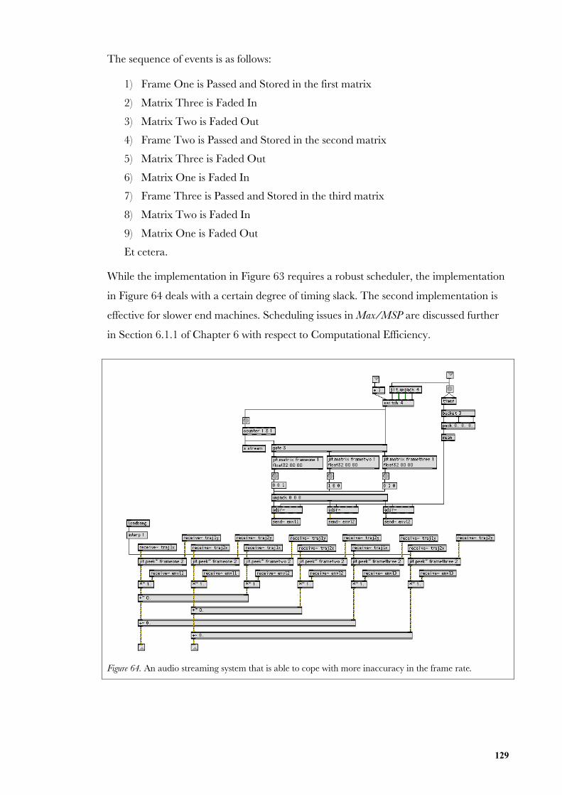
129

The sequence of events is as follows:

1) Frame One is Passed and Stored in the first matrix

2) Matrix Three is Faded In

3) Matrix Two is Faded Out

4) Frame Two is Passed and Stored in the second matrix

5) Matrix Three is Faded Out

6) Matrix One is Faded In

7) Frame Three is Passed and Stored in the third matrix

8) Matrix Two is Faded In

9) Matrix One is Faded Out

Et cetera.

While the implementation in Figure 63 requires a robust scheduler, the implementation

in Figure 64 deals with a certain degree of timing slack. The second implementation is

effective for slower end machines. Scheduling issues in Max/MSP are discussed further

in Section 6.1.1 of Chapter 6 with respect to Computational Efficiency.

Figure 64. An audio streaming system that is able to cope with more inaccuracy in the frame rate.

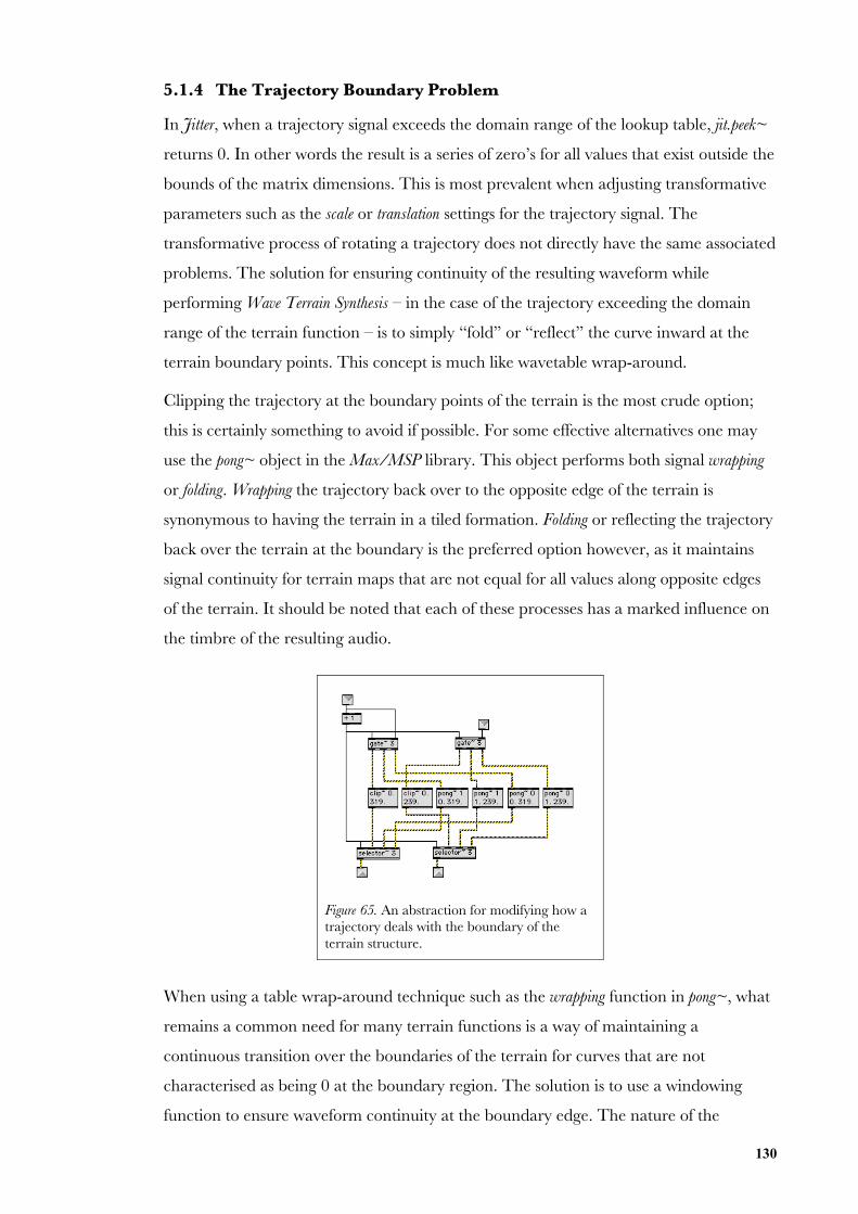
130

5.1.4 The Trajectory Boundary Problem

In Jitter, when a trajectory signal exceeds the domain range of the lookup table, jit.peek~

returns 0. In other words the result is a series of zero’s for all values that exist outside the

bounds of the matrix dimensions. This is most prevalent when adjusting transformative

parameters such as the scale or translation settings for the trajectory signal. The

transformative process of rotating a trajectory does not directly have the same associated

problems. The solution for ensuring continuity of the resulting waveform while

performing Wave Terrain Synthesis – in the case of the trajectory exceeding the domain

range of the terrain function – is to simply “fold” or “reflect” the curve inward at the

terrain boundary points. This concept is much like wavetable wrap-around.

Clipping the trajectory at the boundary points of the terrain is the most crude option;

this is certainly something to avoid if possible. For some effective alternatives one may

use the pong~ object in the Max/MSP library. This object performs both signal wrapping

or folding. Wrapping the trajectory back over to the opposite edge of the terrain is

synonymous to having the terrain in a tiled formation. Folding or reflecting the trajectory

back over the terrain at the boundary is the preferred option however, as it maintains

signal continuity for terrain maps that are not equal for all values along opposite edges

of the terrain. It should be noted that each of these processes has a marked influence on

the timbre of the resulting audio.

Figure 65. An abstraction for modifying how atrajectory deals with the boundary of theterrain structure.

When using a table wrap-around technique such as the wrapping function in pong~, what

remains a common need for many terrain functions is a way of maintaining a

continuous transition over the boundaries of the terrain for curves that are not

characterised as being 0 at the boundary region. The solution is to use a windowing

function to ensure waveform continuity at the boundary edge. The nature of the

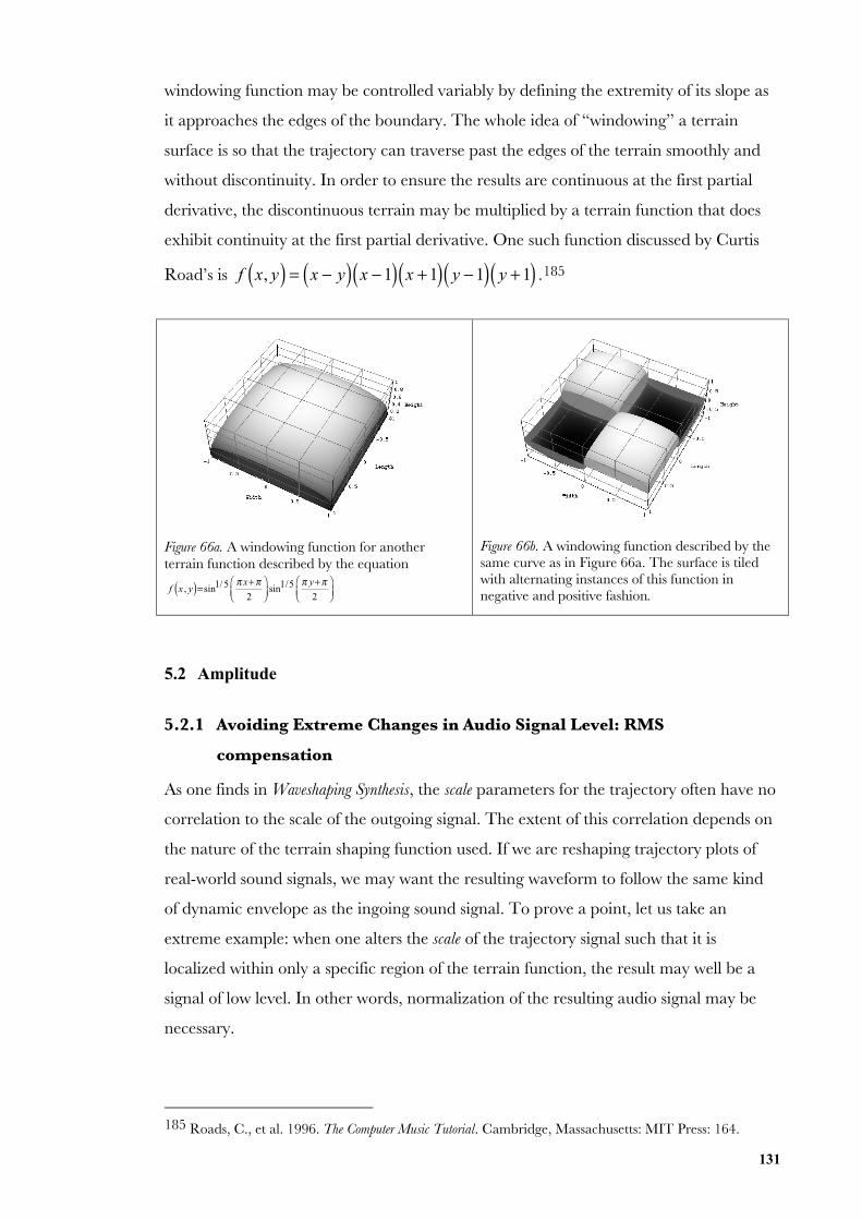
131

windowing function may be controlled variably by defining the extremity of its slope as

it approaches the edges of the boundary. The whole idea of “windowing” a terrain

surface is so that the trajectory can traverse past the edges of the terrain smoothly and

without discontinuity. In order to ensure the results are continuous at the first partial

derivative, the discontinuous terrain may be multiplied by a terrain function that does

exhibit continuity at the first partial derivative. One such function discussed by Curtis

Road’s is f x, y( ) = x − y( ) x −1( ) x +1( ) y −1( ) y +1( ) .185

Figure 66a. A windowing function for anotherterrain function described by the equation

f x , y( )=sin1/5 π x+π

2

⎛⎝⎜

⎞⎠⎟

sin1/5 π y+π2

⎛⎝⎜

⎞⎠⎟

Figure 66b. A windowing function described by thesame curve as in Figure 66a. The surface is tiledwith alternating instances of this function innegative and positive fashion.

5.2 Amplitude

5.2.1 Avoiding Extreme Changes in Audio Signal Level: RMS

compensation

As one finds in Waveshaping Synthesis, the scale parameters for the trajectory often have no

correlation to the scale of the outgoing signal. The extent of this correlation depends on

the nature of the terrain shaping function used. If we are reshaping trajectory plots of

real-world sound signals, we may want the resulting waveform to follow the same kind

of dynamic envelope as the ingoing sound signal. To prove a point, let us take an

extreme example: when one alters the scale of the trajectory signal such that it is

localized within only a specific region of the terrain function, the result may well be a

signal of low level. In other words, normalization of the resulting audio signal may be

necessary.

185 Roads, C., et al. 1996. The Computer Music Tutorial. Cambridge, Massachusetts: MIT Press: 164.

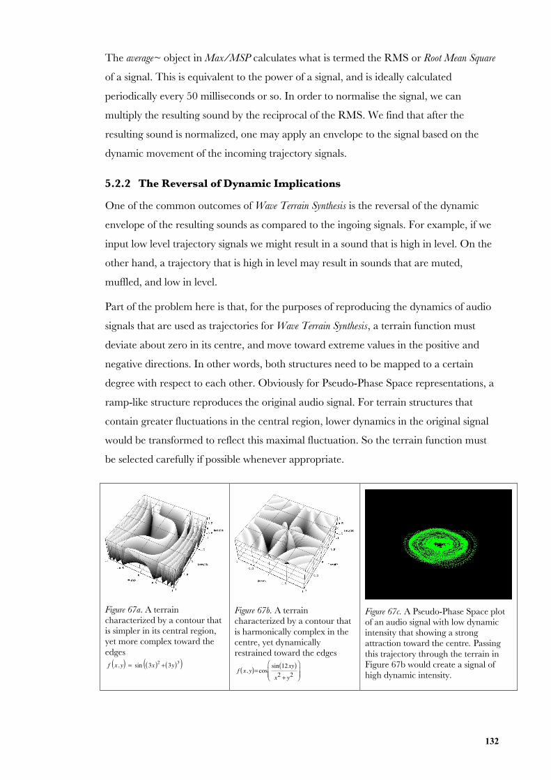
132

The average~ object in Max/MSP calculates what is termed the RMS or Root Mean Square

of a signal. This is equivalent to the power of a signal, and is ideally calculated

periodically every 50 milliseconds or so. In order to normalise the signal, we can

multiply the resulting sound by the reciprocal of the RMS. We find that after the

resulting sound is normalized, one may apply an envelope to the signal based on the

dynamic movement of the incoming trajectory signals.

5.2.2 The Reversal of Dynamic Implications

One of the common outcomes of Wave Terrain Synthesis is the reversal of the dynamic

envelope of the resulting sounds as compared to the ingoing signals. For example, if we

input low level trajectory signals we might result in a sound that is high in level. On the

other hand, a trajectory that is high in level may result in sounds that are muted,

muffled, and low in level.

Part of the problem here is that, for the purposes of reproducing the dynamics of audio

signals that are used as trajectories for Wave Terrain Synthesis, a terrain function must

deviate about zero in its centre, and move toward extreme values in the positive and

negative directions. In other words, both structures need to be mapped to a certain

degree with respect to each other. Obviously for Pseudo-Phase Space representations, a

ramp-like structure reproduces the original audio signal. For terrain structures that

contain greater fluctuations in the central region, lower dynamics in the original signal

would be transformed to reflect this maximal fluctuation. So the terrain function must

be selected carefully if possible whenever appropriate.

Figure 67a. A terraincharacterized by a contour thatis simpler in its central region,yet more complex toward theedgesf x, y( ) = sin 3x( )2 + 3y( )3( )

Figure 67b. A terraincharacterized by a contour thatis harmonically complex in thecentre, yet dynamicallyrestrained toward the edges

f x, y( )= cos sin 12xy( )x2 + y2

⎛

⎝⎜⎜

⎞

⎠⎟⎟

Figure 67c. A Pseudo-Phase Space plotof an audio signal with low dynamicintensity that showing a strongattraction toward the centre. Passingthis trajectory through the terrain inFigure 67b would create a signal ofhigh dynamic intensity.

133

Mapping all distributions to a ramp function, that is f x, y( ) = x + g x, y( ) or

f x, y( ) = x2 +

y2 + g x, y( ) where g x, y( ) is the terrain function we wish to use for Wave

Terrain Synthesis, will guarantee that the resulting audio may retain many aspects of the

original dynamic features in the trajectory signals. Alternatively the audio result from

Wave Terrain Synthesis may be normalised and shaped by an envelope determined by the

level of the inputs as described in Section 5.2.1.

5.3 DC Offset

DC offset is usually a problem due to the introduction of a constant voltage offset to a

recorded sound. When processing sound, it is more desirable to have the waveform

centred about the zero point; otherwise the sound has a greater chance of clipping,

especially if you add several sounds together. It also means that one cannot effectively

normalize these signals either. To get rid of DC offsets in sound signals they must be

filtered.

There are three paths in a DC blocking filter. The simplest and most effect way of

filtering out the low frequencies is with the following filter described by the difference

equation:

y[n] = x[n]− x[n −1]+ ay[n −1]

where y n[ ] is the output at the current time n, and x n[ ] is the input at the current time

n. This can be implemented using biquad~ with coefficients [1.0, –1.0, 0.0, 0.995, 0.0].

For more efficiency, one can use Eric Lyon’s killdc~ object available for both Mac OS9

and OSX.186 There is also dcblock~ in the Percolate library of objects for Max/MSP that

has also been ported to PD.

For values where a approaches 1, the filter will affect only lower frequencies. As a tends

toward 0, more and more frequencies are noticeably affected by the filter. For musical

purposes a is usually set to 0.995; at this level only frequencies below 30Hz or so will be

significantly reduced, while higher frequencies will remain mostly unaffected by the

filter. Due to the large prevalence of DC offsets in Wave Terrain Synthesis, the DC

blocking filter is applied in this instrument by default.

186 killdc~ for Max/MSP. http://arcana.dartmouth.edu/~eric/MAX/

134

6. Instrument Interface, Design, and Structure

6.1 Instrument Design

In constructing a complete and functional instrument there are a number of practical

considerations that must be made. To begin with, for realtime processing there must be

an emphasis on efficiency first and foremost. Nevertheless, the premise of this research

stipulated the need for maintaining methodological flexibility for reasons of developing a

tool with a wide scope for sound design. Secondly, the polyphonic trajectory generator

must be discussed. Thirdly, there is a need for a design concept and schematic for

describing the complete structure of the instrument. This Chapter moves on to

discussing the parameter control map, controller sources and finally, the graphical user

interface.

6.1.1 Maintaining Computational Efficiency

The main point to make here is that in order to maintain computational efficiency for a

realtime instrument model, we must settle upon methodological compromises. In

creating an instrument that is practically feasible, there is not much point providing

access to every feature documented in this exegesis. Rather, we have to make a decision

as to the most effective ways of achieving what it is we want for a sonic instrument and

its expressive control. Instead of using a range of methodology for a single problem we

must invariably choose a single methodology that most effectively achieves what it is that

we require.

One of the main problems for maintaining efficiency in the trajectory system is both

trying to maintain efficiency while providing as much choice and flexibility in trajectory

curves. By utilizing “wavetable” technology, one may have the option of “drawing” a

trajectory curve. Alternatively one may choose an existing trajectory curve and modify

its parameters. The curve is “dynamically” written to two separate wavetables. This

process reduces the number of processing steps so that mathematical equations

involving multiple arithmetic stages do not have to be calculated on a sample-per-

sample basis. However, one does have to compromise some numerical accuracy for such

an approach. This approach is certainly more practical from the standpoint of

developing an efficient polyphonic synthesizer. Wavetable is less likely to use excessive

CPU resources, hence leaving necessary processing power for other calculations such as

video processing, and the interpolation of points in the multidimensional signal space. It

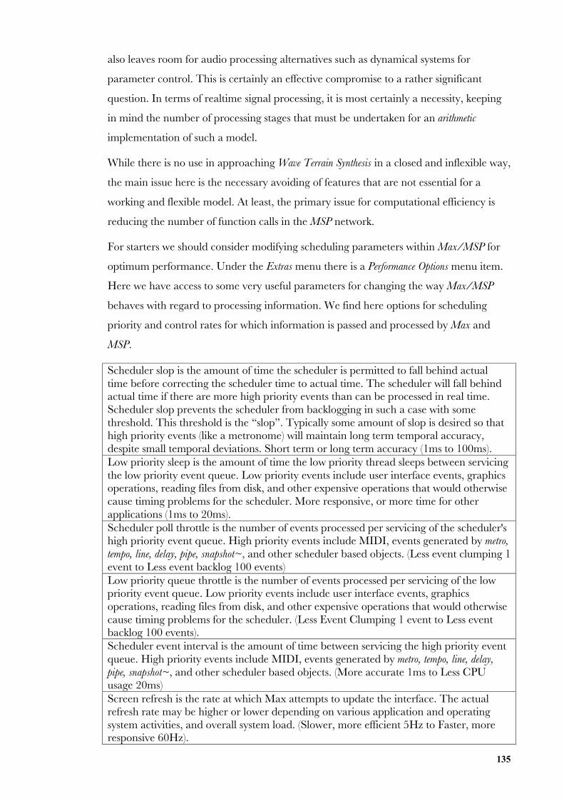
135

also leaves room for audio processing alternatives such as dynamical systems for

parameter control. This is certainly an effective compromise to a rather significant

question. In terms of realtime signal processing, it is most certainly a necessity, keeping

in mind the number of processing stages that must be undertaken for an arithmetic

implementation of such a model.

While there is no use in approaching Wave Terrain Synthesis in a closed and inflexible way,

the main issue here is the necessary avoiding of features that are not essential for a

working and flexible model. At least, the primary issue for computational efficiency is

reducing the number of function calls in the MSP network.

For starters we should consider modifying scheduling parameters within Max/MSP for

optimum performance. Under the Extras menu there is a Performance Options menu item.

Here we have access to some very useful parameters for changing the way Max/MSP

behaves with regard to processing information. We find here options for scheduling

priority and control rates for which information is passed and processed by Max and

MSP.

Scheduler slop is the amount of time the scheduler is permitted to fall behind actualtime before correcting the scheduler time to actual time. The scheduler will fall behindactual time if there are more high priority events than can be processed in real time.Scheduler slop prevents the scheduler from backlogging in such a case with somethreshold. This threshold is the “slop”. Typically some amount of slop is desired so thathigh priority events (like a metronome) will maintain long term temporal accuracy,despite small temporal deviations. Short term or long term accuracy (1ms to 100ms).Low priority sleep is the amount of time the low priority thread sleeps between servicingthe low priority event queue. Low priority events include user interface events, graphicsoperations, reading files from disk, and other expensive operations that would otherwisecause timing problems for the scheduler. More responsive, or more time for otherapplications (1ms to 20ms).Scheduler poll throttle is the number of events processed per servicing of the scheduler'shigh priority event queue. High priority events include MIDI, events generated by metro,tempo, line, delay, pipe, snapshot~, and other scheduler based objects. (Less event clumping 1event to Less event backlog 100 events)Low priority queue throttle is the number of events processed per servicing of the lowpriority event queue. Low priority events include user interface events, graphicsoperations, reading files from disk, and other expensive operations that would otherwisecause timing problems for the scheduler. (Less Event Clumping 1 event to Less eventbacklog 100 events).Scheduler event interval is the amount of time between servicing the high priority eventqueue. High priority events include MIDI, events generated by metro, tempo, line, delay,pipe, snapshot~, and other scheduler based objects. (More accurate 1ms to Less CPUusage 20ms)Screen refresh is the rate at which Max attempts to update the interface. The actualrefresh rate may be higher or lower depending on various application and operatingsystem activities, and overall system load. (Slower, more efficient 5Hz to Faster, moreresponsive 60Hz).

136

There are some extra DSP options within the Audio Settings item under the Options menu

also. For all processes that require the implementation of dynamical systems in the

signal chain, these are built within Csound and embedded within Max/MSP. For stable

results on an iBook G4 1Ghz one may use the following Max/MSP settings: a sampling

rate of 44100 Hz, and a signal vector size and an I/O vector size of 128 samples. For

synchronising multidimensional signal processing with audio, we want the least amount

of scheduler slop and backlogging as possible. Another important consideration to make

here is that signal vector sizes of less than 16 in OSX will see CPU usage peak if the

application scheduler has the audio interrupt setting switched to off.

We now have to consider the removal of some stages in the model for gaining optimum

performance. This requires a decision as to the most effective way of leaving us with

maximum options and flexibility for sound synthesis. The first and most crucial step is

the polyphonic component. The application of a single dynamical matrix for each and

every note instance within Wave Terrain Synthesis is totally impractical. Reading from a

matrix using a different trajectory system for each note instance is still rather processor

intensive, and may be alternatively restricted to a system where all note instances are

summated through additive means in order to create a single additive version of the

individual trajectories. Where does this stage occur in the overall system? It seems that

the only efficient way is to have this stage after general note-to-note polyphonic

processing. This also means that all modulation parameters are applied to the collection

of active notes globally rather than applied to each and every note instance.

Another compromise to the model involves optimising dynamical multidimensional

processing. Integrating Haptic Rate processing, for example, requires a simplification of

the entire patch. The generation of two-dimensional data can be an intensive process,

and will only be successfully achieved at higher rates of change if other processes are

sacrificed for these means. For example, we may choose to use smaller matrices of 80 x

80 or 40 x 40 data points. On the other side of the coin, if we were required to use

larger data arrays we would be forced to work at slower video processing rates between

2 and 4Hz. While more research is needed in order to establish an optimum balance

between speed and efficiency, particular here with regard to the implementation of

video and audio processing in a Wave Terrain Synthesis instrument model, one ought to

keep in mind the increase in processing speed for future computing machines.

One of the other compromises in the model is the removal of color association for

processing efficiency. The transfer of a single plane matrix results in more effective

137

frame speeds, and also means further instances of jit.peek~ are not necessary. This does

close the possibility for mapping audio channels to color. Though the advantages for

processing far exceed what is gained through this amalgam at this point in time.

6.1.2 Synthesizer versus Effect – Instrument Concept

The premise here is that two instrument models can be developed based on material

discussed in Section 2.3.2 of Chapter 2. We may consider the Wave Terrain Synthesis as

both a generative as well as a transformative technique in sound synthesis. Based on this

notion we may have two models: one that functions as a multidimensional Waveshaping

tool for incoming audio signals utilizing the Pluggo VST library for Max/MSP, and a

standalone application that essentially functions like a polyphonic synthesizer. For the

purposes of this research, we are looking specifically at the building of a polyphonic

synthesizer based on a generative model.

6.1.3 Design Schematics

The ordering of each processing stage within the Wave Terrain Synthesis instrument is

crucial for achieving the desired results. For video processing, convolution needs to be

lower in the signal chain, as once it is applied, signal quality is lost. The application of

the windowing function just before Wave Terrain Synthesis ensures that the windowing

serves the purpose it is meant for. The audio streaming and crossfading comes

immediately after Wave Terrain Synthesis occurs so that all other post-processes are

applied to two individual stereo signals rather than six separate signal chains. Audio

normalization is applied last, specifically after the DC blocking routine. This ordering is

necessary in order to both maximize the resulting signal yet retain its essential quality.

Below, in Figure 68, is a design schematic for the entire instrument. This diagram is a

collation of the most effective processes documented throughout this thesis. These

components, their control parameters, and their function are discussed throughout

Chapters 3, 4 and 5.

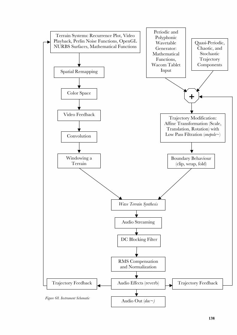
138

Figure 68. Instrument Schematic

Windowing aTerrain

Audio Streaming

DC Blocking Filter

RMS Compensationand Normalization

Video FeedbackTrajectory Modification:

Affine Transformation (Scale,Translation, Rotation) with

Low Pass Filtration (onepole~)

Wave Terrain Synthesis

Convolution

Trajectory Feedback

Terrain Systems: Recurrence Plot, VideoPlayback, Perlin Noise Functions, OpenGLNURBS Surfaces, Mathematical Functions

Spatial Remapping

Color Space

Periodic andPolyphonicWavetableGenerator:

MathematicalFunctions,

Wacom TabletInput

Quasi-Periodic,Chaotic, and

StochasticTrajectory

Components

+

Boundary Behaviour(clip, wrap, fold)

Audio Effects (reverb)

Audio Out (dac~)

Trajectory Feedback

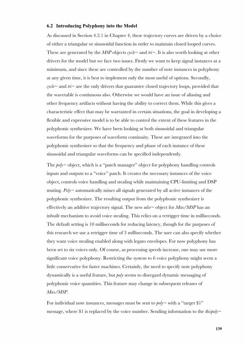
139

6.2 Introducing Polyphony into the Model

As discussed in Section 4.2.1 in Chapter 4, these trajectory curves are driven by a choice

of either a triangular or sinusoidal function in order to maintain closed looped curves.

These are generated by the MSP objects cycle~ and tri~. It is also worth looking at other

drivers for the model but we face two issues. Firstly we want to keep signal instances at a

minimum, and since these are controlled by the number of note instances in polyphony

at any given time, it is best to implement only the most useful of options. Secondly,

cycle~ and tri~ are the only drivers that guarantee closed trajectory loops, provided that

the wavetable is continuous also. Otherwise we would have an issue of aliasing and

other frequency artifacts without having the ability to correct them. While this gives a

characteristic effect that may be warranted in certain situations, the goal in developing a

flexible and expressive model is to be able to control the extent of these features in the

polyphonic synthesizer. We have been looking at both sinusoidal and triangular

waveforms for the purposes of waveform continuity. These are integrated into the

polyphonic synthesizer so that the frequency and phase of each instance of these

sinusoidal and triangular waveforms can be specified independently.

The poly~ object, which is a “patch manager” object for polyphony handling controls

inputs and outputs to a “voice” patch. It creates the necessary instances of the voice

object, controls voice handling and stealing while maintaining CPU-limiting and DSP

muting. Poly~ automatically mixes all signals generated by all active instances of the

polyphonic synthesizer. The resulting output from the polyphonic synthesizer is

effectively an additive trajectory signal. The new adsr~ object for Max/MSP has an

inbuilt mechanism to avoid voice stealing. This relies on a retrigger time in milliseconds.

The default setting is 10 milliseconds for reducing latency, though for the purposes of

this research we use a retrigger time of 3 milliseconds. The user can also specify whether

they want voice stealing enabled along with legato envelopes. For now polyphony has

been set to six voices only. Of course, as processing speeds increase, one may use more

significant voice polyphony. Restricting the system to 6 voice polyphony might seem a

little conservative for faster machines. Certainly, the need to specify note polyphony

dynamically is a useful feature, but poly seems to disregard dynamic messaging of

polyphonic voice quantities. This feature may change in subsequent releases of

Max/MSP.

For individual note instances, messages must be sent to poly~ with a “target $1”

message, where $1 is replaced by the voice number. Sending information to the thispoly~

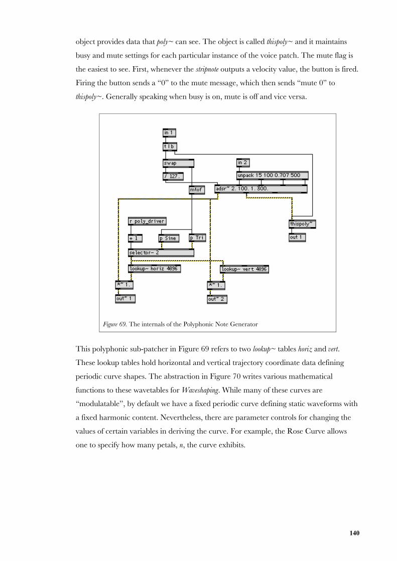
140

object provides data that poly~ can see. The object is called thispoly~ and it maintains

busy and mute settings for each particular instance of the voice patch. The mute flag is

the easiest to see. First, whenever the stripnote outputs a velocity value, the button is fired.

Firing the button sends a “0” to the mute message, which then sends “mute 0” to

thispoly~. Generally speaking when busy is on, mute is off and vice versa.

Figure 69. The internals of the Polyphonic Note Generator

This polyphonic sub-patcher in Figure 69 refers to two lookup~ tables horiz and vert.

These lookup tables hold horizontal and vertical trajectory coordinate data defining

periodic curve shapes. The abstraction in Figure 70 writes various mathematical

functions to these wavetables for Waveshaping. While many of these curves are

“modulatable”, by default we have a fixed periodic curve defining static waveforms with

a fixed harmonic content. Nevertheless, there are parameter controls for changing the

values of certain variables in deriving the curve. For example, the Rose Curve allows

one to specify how many petals, n, the curve exhibits.

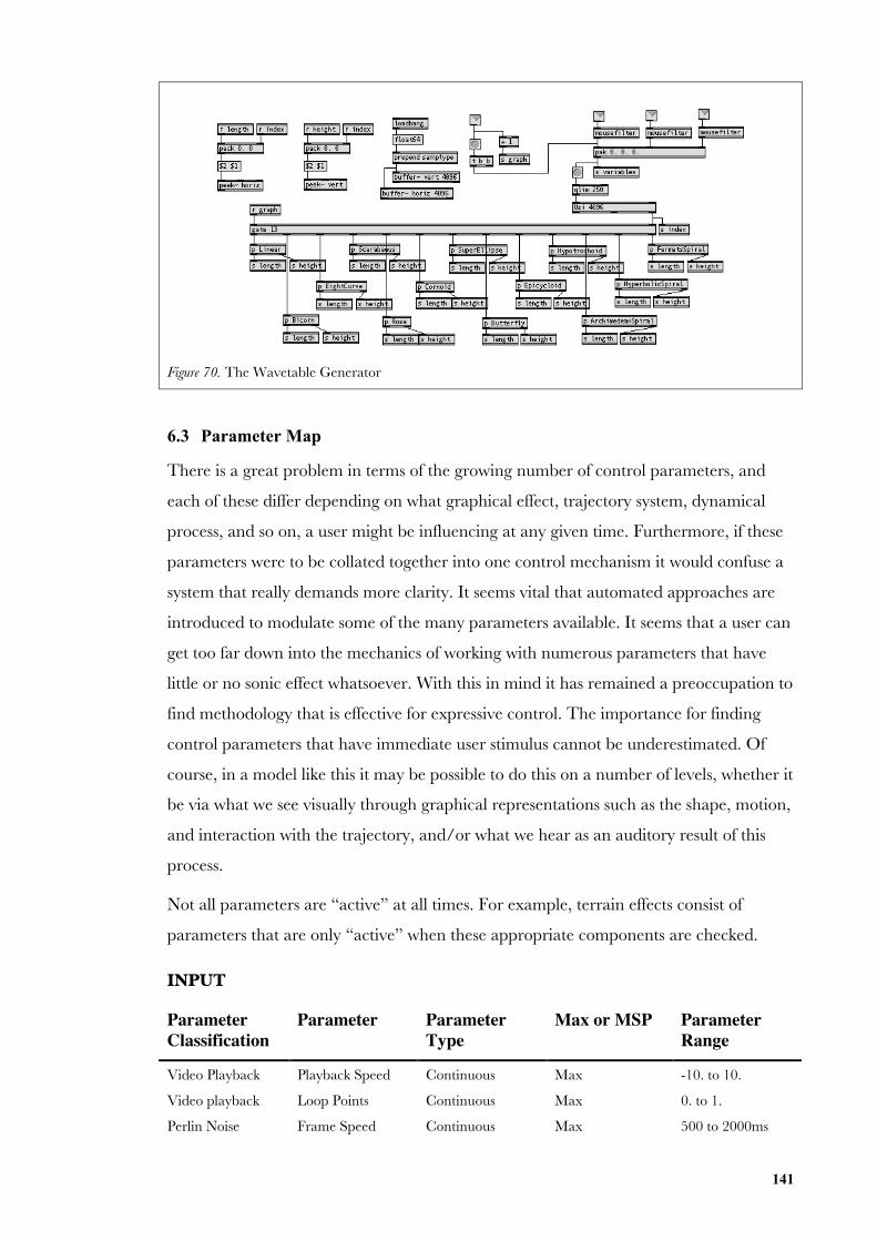
141

Figure 70. The Wavetable Generator

6.3 Parameter Map

There is a great problem in terms of the growing number of control parameters, and

each of these differ depending on what graphical effect, trajectory system, dynamical

process, and so on, a user might be influencing at any given time. Furthermore, if these

parameters were to be collated together into one control mechanism it would confuse a

system that really demands more clarity. It seems vital that automated approaches are

introduced to modulate some of the many parameters available. It seems that a user can

get too far down into the mechanics of working with numerous parameters that have

little or no sonic effect whatsoever. With this in mind it has remained a preoccupation to

find methodology that is effective for expressive control. The importance for finding

control parameters that have immediate user stimulus cannot be underestimated. Of

course, in a model like this it may be possible to do this on a number of levels, whether it

be via what we see visually through graphical representations such as the shape, motion,

and interaction with the trajectory, and/or what we hear as an auditory result of this

process.

Not all parameters are “active” at all times. For example, terrain effects consist of

parameters that are only “active” when these appropriate components are checked.

INPUT

ParameterClassification

Parameter ParameterType

Max or MSP ParameterRange

Video Playback Playback Speed Continuous Max -10. to 10.

Video playback Loop Points Continuous Max 0. to 1.

Perlin Noise Frame Speed Continuous Max 500 to 2000ms

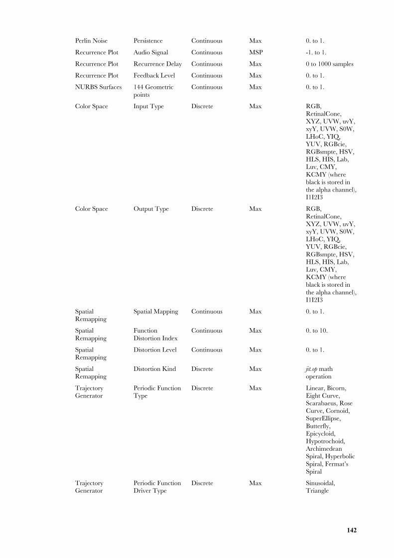
142

Perlin Noise Persistence Continuous Max 0. to 1.

Recurrence Plot Audio Signal Continuous MSP -1. to 1.

Recurrence Plot Recurrence Delay Continuous Max 0 to 1000 samples

Recurrence Plot Feedback Level Continuous Max 0. to 1.

NURBS Surfaces 144 Geometricpoints

Continuous Max 0. to 1.

Color Space Input Type Discrete Max RGB,RetinalCone,XYZ, UVW, uvY,xyY, UVW, S0W,LHoC, YIQ,YUV, RGBcie,RGBsmpte, HSV,HLS, HIS, Lab,Luv, CMY,KCMY (whereblack is stored inthe alpha channel),I1I2I3

Color Space Output Type Discrete Max RGB,RetinalCone,XYZ, UVW, uvY,xyY, UVW, S0W,LHoC, YIQ,YUV, RGBcie,RGBsmpte, HSV,HLS, HIS, Lab,Luv, CMY,KCMY (whereblack is stored inthe alpha channel),I1I2I3

SpatialRemapping

Spatial Mapping Continuous Max 0. to 1.

SpatialRemapping

FunctionDistortion Index

Continuous Max 0. to 10.

SpatialRemapping

Distortion Level Continuous Max 0. to 1.

SpatialRemapping

Distortion Kind Discrete Max jit.op mathoperation

TrajectoryGenerator

Periodic FunctionType

Discrete Max Linear, Bicorn,Eight Curve,Scarabaeus, RoseCurve, Cornoid,SuperEllipse,Butterfly,Epicycloid,Hypotrochoid,ArchimedeanSpiral, HyperbolicSpiral, Fermat’sSpiral

TrajectoryGenerator

Periodic FunctionDriver Type

Discrete Max Sinusoidal,Triangle

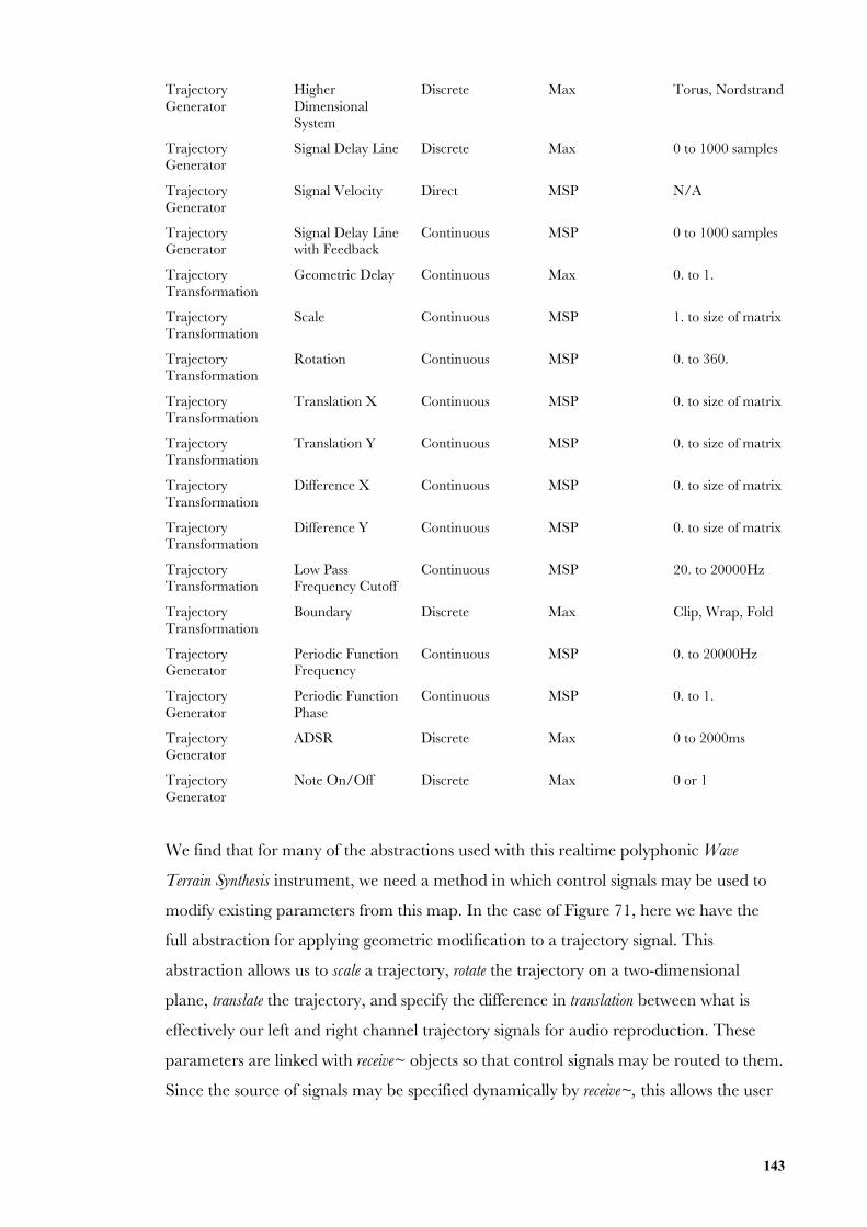
143

TrajectoryGenerator

HigherDimensionalSystem

Discrete Max Torus, Nordstrand

TrajectoryGenerator

Signal Delay Line Discrete Max 0 to 1000 samples

TrajectoryGenerator

Signal Velocity Direct MSP N/A

TrajectoryGenerator

Signal Delay Linewith Feedback

Continuous MSP 0 to 1000 samples

TrajectoryTransformation

Geometric Delay Continuous Max 0. to 1.

TrajectoryTransformation

Scale Continuous MSP 1. to size of matrix

TrajectoryTransformation

Rotation Continuous MSP 0. to 360.

TrajectoryTransformation

Translation X Continuous MSP 0. to size of matrix

TrajectoryTransformation

Translation Y Continuous MSP 0. to size of matrix

TrajectoryTransformation

Difference X Continuous MSP 0. to size of matrix

TrajectoryTransformation

Difference Y Continuous MSP 0. to size of matrix

TrajectoryTransformation

Low PassFrequency Cutoff

Continuous MSP 20. to 20000Hz

TrajectoryTransformation

Boundary Discrete Max Clip, Wrap, Fold

TrajectoryGenerator

Periodic FunctionFrequency

Continuous MSP 0. to 20000Hz

TrajectoryGenerator

Periodic FunctionPhase

Continuous MSP 0. to 1.

TrajectoryGenerator

ADSR Discrete Max 0 to 2000ms

TrajectoryGenerator

Note On/Off Discrete Max 0 or 1

We find that for many of the abstractions used with this realtime polyphonic Wave

Terrain Synthesis instrument, we need a method in which control signals may be used to

modify existing parameters from this map. In the case of Figure 71, here we have the

full abstraction for applying geometric modification to a trajectory signal. This

abstraction allows us to scale a trajectory, rotate the trajectory on a two-dimensional

plane, translate the trajectory, and specify the difference in translation between what is

effectively our left and right channel trajectory signals for audio reproduction. These

parameters are linked with receive~ objects so that control signals may be routed to them.

Since the source of signals may be specified dynamically by receive~, this allows the user

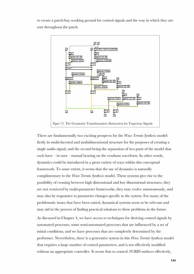
144

to create a patch-bay working ground for control signals and the way in which they are

sent throughout the patch.

Figure 71. The Geometric Transformation Abstraction for Trajectory Signals

There are fundamentally two exciting prospects for the Wave Terrain Synthesis model:

firstly its multi-facetted and multidimensional structure for the purposes of creating a

single audio signal, and the second being the separation of two parts of the model that

each have – in turn – mutual bearing on the resultant waveform. In other words,

dynamics could be introduced in a great variety of ways within this conceptual

framework. To some extent, it seems that the use of dynamics is naturally

complimentary to the Wave Terrain Synthesis model. These systems give rise to the

possibility of crossing between high dimensional and low dimensional structures, they

are not restricted by multi-parameter frameworks, they may evolve autonomously, and

may also be responsive to parameter changes specific to the system. For many of the

problematic issues that have been raised, dynamical systems seem to be relevant and

may aid in the process of finding practical solutions to these problems in the future.

As discussed in Chapter 4, we have access to techniques for deriving control signals by

automated processes, some semi-automated processes that are influenced by a set of

initial conditions, and we have processes that are completely determined by the

performer. Nevertheless, there is a generative system in this Wave Terrain Synthesis model

that requires a large number of control parameters, and is not effectively modified

without an appropriate controller. It seems that to control NURBS surfaces effectively,

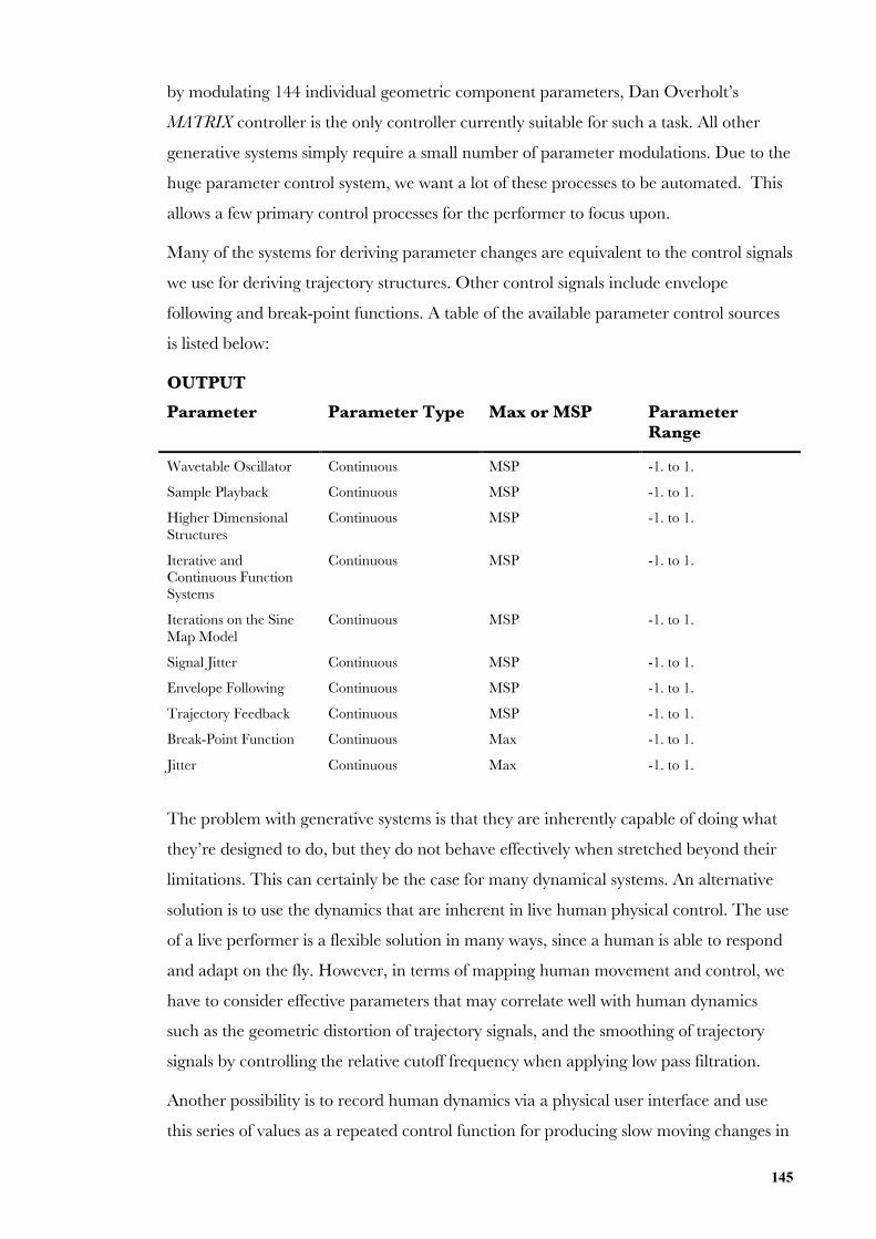
145

by modulating 144 individual geometric component parameters, Dan Overholt’s

MATRIX controller is the only controller currently suitable for such a task. All other

generative systems simply require a small number of parameter modulations. Due to the

huge parameter control system, we want a lot of these processes to be automated. This

allows a few primary control processes for the performer to focus upon.

Many of the systems for deriving parameter changes are equivalent to the control signals

we use for deriving trajectory structures. Other control signals include envelope

following and break-point functions. A table of the available parameter control sources

is listed below:

OUTPUT

Parameter Parameter Type Max or MSP ParameterRange

Wavetable Oscillator Continuous MSP -1. to 1.

Sample Playback Continuous MSP -1. to 1.

Higher DimensionalStructures

Continuous MSP -1. to 1.

Iterative andContinuous FunctionSystems

Continuous MSP -1. to 1.

Iterations on the SineMap Model

Continuous MSP -1. to 1.

Signal Jitter Continuous MSP -1. to 1.

Envelope Following Continuous MSP -1. to 1.

Trajectory Feedback Continuous MSP -1. to 1.

Break-Point Function Continuous Max -1. to 1.

Jitter Continuous Max -1. to 1.

The problem with generative systems is that they are inherently capable of doing what

they’re designed to do, but they do not behave effectively when stretched beyond their

limitations. This can certainly be the case for many dynamical systems. An alternative

solution is to use the dynamics that are inherent in live human physical control. The use

of a live performer is a flexible solution in many ways, since a human is able to respond

and adapt on the fly. However, in terms of mapping human movement and control, we

have to consider effective parameters that may correlate well with human dynamics

such as the geometric distortion of trajectory signals, and the smoothing of trajectory

signals by controlling the relative cutoff frequency when applying low pass filtration.

Another possibility is to record human dynamics via a physical user interface and use

this series of values as a repeated control function for producing slow moving changes in

146

various parameters. This may be more interesting than simply using an LFO which

follows a predictable and periodic pattern. The Wacom Tablet is a controller that may be

useful in such an implementation. The device may be used to draw trajectory structures,

or may be used to control various parameters for transforming the trajectory signal.

Some tablets have the option of giving pressure and pen tilt information as well as x and

y coordinate information.

Continuous parameters may be controlled via MIDI interface and discrete parameters

by the computer keyboard. MIDI may be used to control parameters that are variable.

And due to a large number of these parameters, a MIDI performance controller would

be highly recommended. The computer keyboard, on the other hand, is used to trigger

processes or open sub-patcher windows. These are parameters that effectively require

user control.

6.4 Graphical User Interface (GUI)

Avoid writing software that already exists…[and] provide comprehensive andcomplete documentation for all tools so that the conscientious user cancomprehend and anticipate the limits of operation, and so programmers canidentify suspected bugs with confidence.187

In order to write music productively, one does not necessarily want to be designing a

patch from scratch, nor fiddling around with a myriad of parameters for sound

synthesis. The idea is to find sonic possibilities quickly, and to use tools that provides one

with the ability to effectively do what it is one requires, allowing the creative artist or

performer to follow through with an idea and realize it.

The various interfaces that this research has come up with for Wave Terrain Synthesis

express different concerns and performance considerations. The first example in Figure

72a is based on development of a standalone synthesizer, and the other Figure 72b

functions much like an effects unit. Modifications to these user interfaces may be

necessary in order to make more of a feature of the trajectory signal since it acts as the

primary driving signal for Wave Terrain Synthesis. Since the terrain function works in a

secondary stage capacity in Wave Terrain Synthesis it is worth considering the placement of

this visual window so that it is not so prominent as compared to the visual window of the

trajectory system.

187 Huron, D. B. 2002. “Music Information Processing Using the HUMDRUM Toolkit: Concepts,Examples, and Lessons.” Computer Music Journal 26(2): 24.

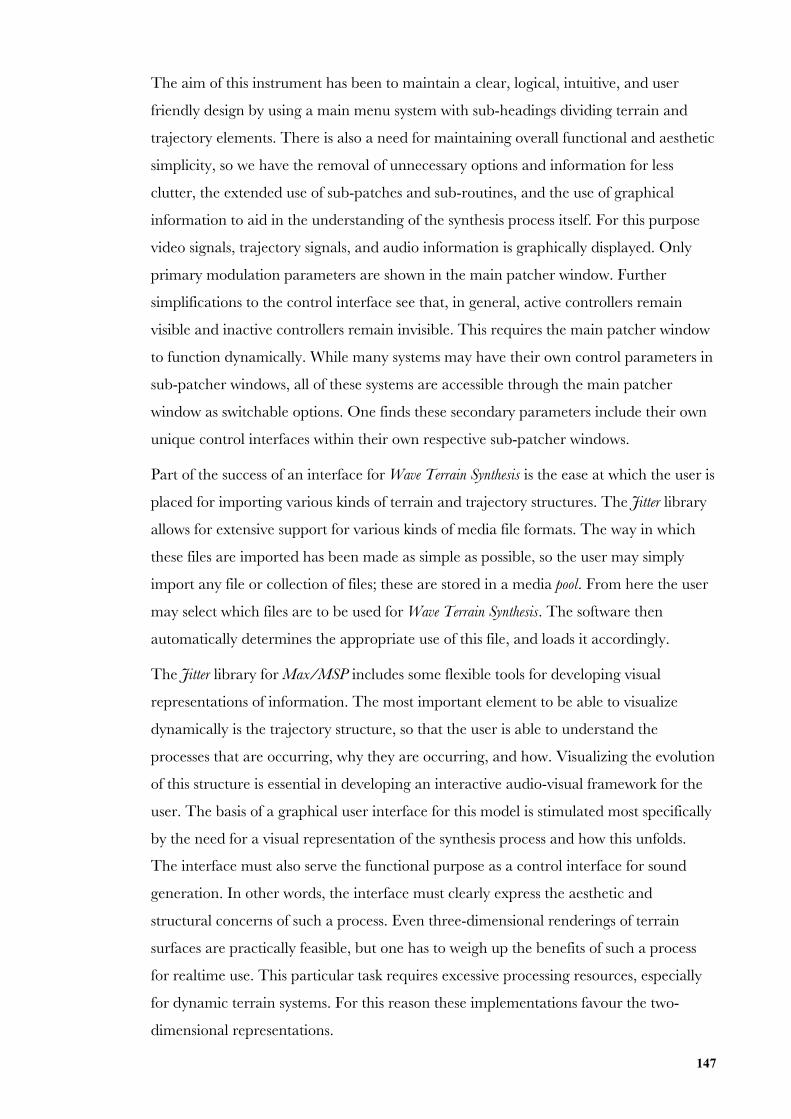
147

The aim of this instrument has been to maintain a clear, logical, intuitive, and user

friendly design by using a main menu system with sub-headings dividing terrain and

trajectory elements. There is also a need for maintaining overall functional and aesthetic

simplicity, so we have the removal of unnecessary options and information for less

clutter, the extended use of sub-patches and sub-routines, and the use of graphical

information to aid in the understanding of the synthesis process itself. For this purpose

video signals, trajectory signals, and audio information is graphically displayed. Only

primary modulation parameters are shown in the main patcher window. Further

simplifications to the control interface see that, in general, active controllers remain

visible and inactive controllers remain invisible. This requires the main patcher window

to function dynamically. While many systems may have their own control parameters in

sub-patcher windows, all of these systems are accessible through the main patcher

window as switchable options. One finds these secondary parameters include their own

unique control interfaces within their own respective sub-patcher windows.

Part of the success of an interface for Wave Terrain Synthesis is the ease at which the user is

placed for importing various kinds of terrain and trajectory structures. The Jitter library

allows for extensive support for various kinds of media file formats. The way in which

these files are imported has been made as simple as possible, so the user may simply

import any file or collection of files; these are stored in a media pool. From here the user

may select which files are to be used for Wave Terrain Synthesis. The software then

automatically determines the appropriate use of this file, and loads it accordingly.

The Jitter library for Max/MSP includes some flexible tools for developing visual

representations of information. The most important element to be able to visualize

dynamically is the trajectory structure, so that the user is able to understand the

processes that are occurring, why they are occurring, and how. Visualizing the evolution

of this structure is essential in developing an interactive audio-visual framework for the

user. The basis of a graphical user interface for this model is stimulated most specifically

by the need for a visual representation of the synthesis process and how this unfolds.

The interface must also serve the functional purpose as a control interface for sound

generation. In other words, the interface must clearly express the aesthetic and

structural concerns of such a process. Even three-dimensional renderings of terrain

surfaces are practically feasible, but one has to weigh up the benefits of such a process

for realtime use. This particular task requires excessive processing resources, especially

for dynamic terrain systems. For this reason these implementations favour the two-

dimensional representations.

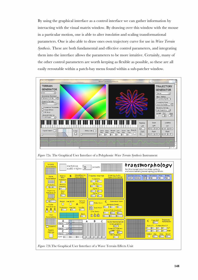
148

By using the graphical interface as a control interface we can gather information by

interacting with the visual matrix window. By drawing over this window with the mouse

in a particular motion, one is able to alter translation and scaling transformational

parameters. One is also able to draw ones own trajectory curve for use in Wave Terrain

Synthesis. These are both fundamental and effective control parameters, and integrating

them into the interface allows the parameters to be more intuitive. Certainly, many of

the other control parameters are worth keeping as flexible as possible, so these are all

easily reroutable within a patch-bay menu found within a sub-patcher window.

Figure 72a. The Graphical User Interface of a Polyphonic Wave Terrain Synthesis Instrument

Figure 72b.The Graphical User Interface of a Wave Terrain Effects Unit

149

7. Conclusions

The main purpose for this research was to document the development of a flexible and

expressive Wave Terrain Synthesis instrument based on a visual and multidimensional

methodology. By constructing this instrument utilizing the Jitter video processing library

for Max/MSP, we have arrived at a model that reflects the diversity in approaches to

Wave Terrain Synthesis as well as the various modulation possibilities associated with the

technique. However it also raises the question as to where the bounds of Wave Terrain

Synthesis theory should end. It has the potential to map out the parameter spaces of many

simpler synthesis models, as well as a myriad of other possible numerical combinations.

Perhaps Wave Terrain Synthesis will always be plagued by the idea of “possibilities.” There

hardly is a right or wrong approach to its methodology though there are more efficient

and effective ways of going about a number of these specific approaches. As far as the

technique is concerned, its functioning depends on the methodology. Since it is a

potential meeting ground for a number of multi-parameter synthesis processes, it is likely

that Wave Terrain Synthesis will not lose its allusive and somewhat indiscriminatory

character. In a way this is merely a beginning of synthesis possibilities. The extensive and,

shall we say, extendable nature of synthesis allows for ongoing chains of generators,

controllers and processes; Wave Terrain Synthesis might be used as a controller for another

methodology such as convolution in the frequency domain.

It seems that Wave Terrain Synthesis is dominated by problems of efficiency due to the

multi-signal nature of the technique. In order to maintain efficiency, parts of the model

are simplified in order to retain maximum flexibility yet without taking up excessive

computational resources. Weighing this up against the argument that Wave Terrain

Synthesis has great potential means that perhaps we will only see the technique come to

fruition sometime in the future when it is possible to have more flexible control over

various generators and signal processing effects in realtime. Despite this I believe that it is

worth building more complex models in non-realtime using Max/MSP and Csound with

the aim to build upon the existing knowledge about this sound synthesis technique in

general.

150

By using a discrete map of data values, we have access to a wide range of generative and

processing functions for multidimensional signals. This research has looked at a number

of generative mediums for Wave Terrain Synthesis including Video Capture and Playback,

Perlin Noise Functions, Recurrence plots, and OpenGL NURBS Surfaces. We have also

looked at some other processing functions. The application of video processing to sound

generation introduces an interesting relationship. Exploring this relationship presents

some alternatives to sound generation, particularly to modulation systems.

While the graphical approach to Wave Terrain Synthesis seems to be appealing from a visual

point of view, the processes of multidimensional data still cause stress on the fastest

desktop systems we have today. We must ask ourselves, are these processes necessary? Are

the sound results and modulations worthy of these complex processing functions? Perhaps

Wave Terrain Synthesis is again plagued by its inherent complexity and novelty rather than

its practicality for sound generation. This problem of complexity also has to be weighed

up against issues of audio quality. Cubic interpolation, for example, a one-dimensional

system requires four initial table lookups and nine arithmetic processes. The equivalent in

two-dimensional systems is significantly more extensive.

It is unfortunate that the mapping of color is such a difficult issue. The role of color in the

representation of multidimensional spaces presents problems since the objective and

numerical interpretation of images do not necessarily correlate with our own subjective

interpretations. Nevertheless visualizing the process dynamically serves toward clarifying

a system that has remained a “black-box” technique. More experimentation could be

undertaken with the various ways in which color is mapped in such a model. While many

color spaces produce excessive distortion due to incoherent and non-linear

transformations of signals, there is a great deal of promise for the transformation

processes used for multidimensional signals in any multidimensional process. At the very

least, the results are of great interest.

Like Waveshaping Synthesis, the results from Wave Terrain Synthesis are dependent on the

harmonic content of both the terrain shaping function and the trajectory signals. While

there is extensive documentation on Waveshaping theory, particularly with respect to the

way in which one may reshape a signal based on harmonic content, we have in Wave

151

Terrain Synthesis a situation concerning the reshaping of two independent signals. The

terrain function in this case has a large number of extra possible modulation and

distortion possibilities. Furthermore, Wave Terrain Synthesis introduces a further phasing

parameter uncharacteristic of Waveshaping where the performer may translate or shift the

trajectory across the surface of the terrain creating rich modulations in the signal.

However the extent and quality of these modulations depends largely on the nature of the

terrain surface. The trajectory signal has the most significant control over the system,

while the terrain reshapes this structure accordingly. The terrain determines the point-to-

point weighted sum of each trajectory component. The way in which this relationship

results can be highly complex.

In the unique example where we have simply an elliptical trajectory made up of two

sinusoidal components, we have the basis of using a shaping function that is completely in

control of the timbral result. From here if we were to have a dynamic terrain shaping

function, we end up with a two-dimensional form of Scanned Synthesis. In this Wave Terrain

Synthesis model, we are looking at dynamical systems in both terrain and trajectory

structures. This confuses the conceptual definition and the methodology used for the

technique. Furthermore, instead of having a clear and defined idea about the role of each

parameter, we have an obscuring of parameter possibilities. What may be incredibly

uninteresting in one parameter situation may be serendipitous in another.

Wave Terrain Synthesis is particularly useful as a method of distorting signals. It might be

comparable to a destructive process of audio generation due to the wide and various

possibilities of introducing aliasing along with the ease of introducing too much spectral

complexity in the model. Discontinuities in the resulting waveform are a common

occurrence whenever one uses control signals that do not reflect continuity. This is

generally why, with exception to the trajectory control signals that define the fundamental

frequency of the system, low frequency rates of change are more satisfactory for Wave

Terrain Synthesis. The point must also be made that all parameters involved in generating

and transforming the trajectory signals must be continuous. Many or all of the control

signals may be in the audible frequency range, and interact with one another in an

interesting way. The beating effects resulting from slight phase differences in signals can

be reflected in the result and reshaped accordingly.

152

This research has settled on a flexible methodology for Wave Terrain Synthesis for

constructing a realtime polyphonic instrument. This instrument reflects the concerns for

developing a powerful, expressive and flexible sound design tool by having a user

controlled and configurable parameter map. The instrument also exhibits a variety in

methodology in both the way in which terrain and trajectory systems are contrived, as

well as the parameters involved in geometrically and arithmetically transforming them.

We have dealt with issues of computational efficiency for realtime systems. The

development of a realtime instrument presents some restrictions in methodology. The

research has dealt with the core construction of all significant components in the Wave

Terrain Synthesis model. This has culminated in a proposed design schematic, and

parameter map of control input and output within the instrument based on the specific

generator and processing methodologies used in conjunction with the Jitter graphical

processing library. A visual interface was motivated by the need for the user to be able to

comprehend the multidimensional parameter spaces in use for Wave Terrain Synthesis. By

visualizing these terrain and trajectory structures, one is able to observe relationships and

connections between the structures and modify their control parameters while observing

their transformation accordingly in realtime as they are applied.

Technology is making ongoing advances in system architecture, processor speed, memory

speed and capacity. All of these factors are promising bigger and better things for realtime

systems. While in 1989 Gresham-Lancaster and Thibault explored a connection between

contours of the land and their resulting waveforms on two Amiga computers, systems are

becoming all the more capable of processing multiple packets of information

simultaneously. The potential for graphical and audio rendering in realtime is part of an

ongoing development promising further possibilities for realtime processing systems. The

advantage of these systems for multidimensional models is that we are now dealing with a

scenario where we can explore dynamical multidimensional data spaces at more

significant speed. Realtime processing on these systems is now feasible and shall become

increasingly more so. This future situation will allow techniques like Wave Terrain Synthesis

to be explored more thoroughly and in depth. It is hoped that the work in this thesis may

encourage further research and interest in the area of Wave Terrain Synthesis.

153

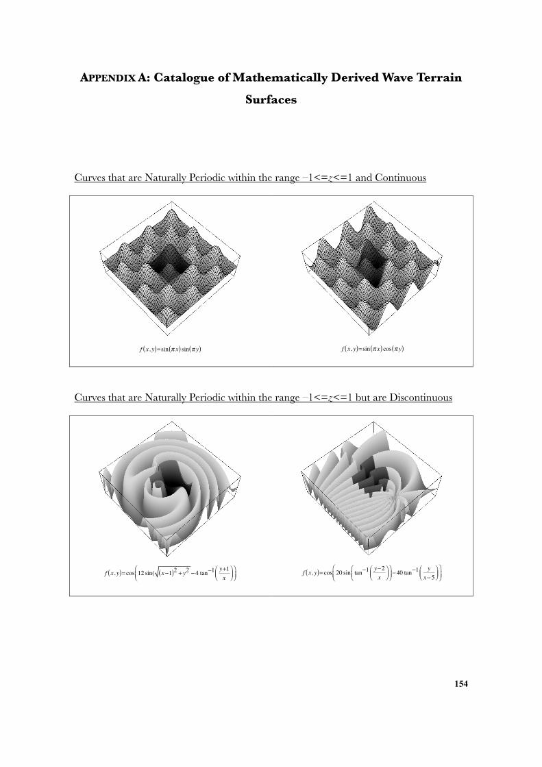
154

APPENDIX A: Catalogue of Mathematically Derived Wave Terrain

Surfaces

Curves that are Naturally Periodic within the range –1<=z<=1 and Continuous

f x, y( )=sin π x( ) sin π y( )

f x, y( )=sin π x( ) cos π y( )

Curves that are Naturally Periodic within the range –1<=z<=1 but are Discontinuous

f x, y( )= cos 12 sin( x−1( )2 + y2 −4 tan−1y+1x

⎛⎝⎜

⎞⎠⎟

⎛⎝⎜

⎞⎠⎟

f x, y( )= cos 20 sin tan−1y−2x

⎛⎝⎜

⎞⎠⎟

⎛⎝⎜

⎞⎠⎟−40 tan−1

yx−5

⎛⎝⎜

⎞⎠⎟

⎛⎝⎜

⎞⎠⎟

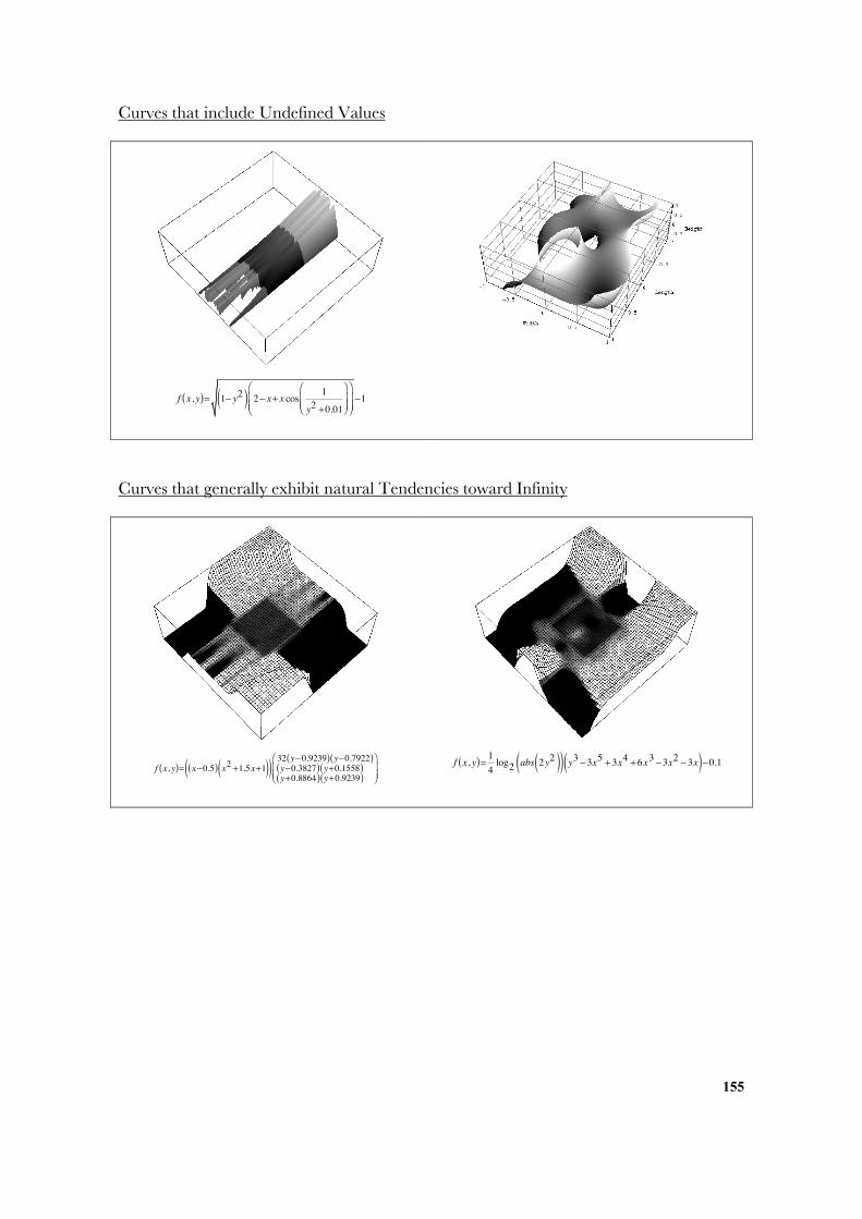
155

Curves that include Undefined Values

f x, y( )= 1− y2( ) 2− x+ x cos 1

y2 +0.01

⎛

⎝⎜⎜

⎞

⎠⎟⎟

⎛

⎝⎜⎜

⎞

⎠⎟⎟−1

Curves that generally exhibit natural Tendencies toward Infinity

f x, y( )= x−0.5( ) x2 +1.5x+1( )( ) 32 y−0.9239( ) y−0.7922( )y−0.3827( ) y+0.1558( )y+0.8864( ) y+0.9239( )

⎛

⎝⎜⎜

⎞

⎠⎟⎟

f x, y( )= 14log2 abs 2y2( )( ) y3 −3x5 +3x4 +6x3 −3x2 −3x( )−0.1

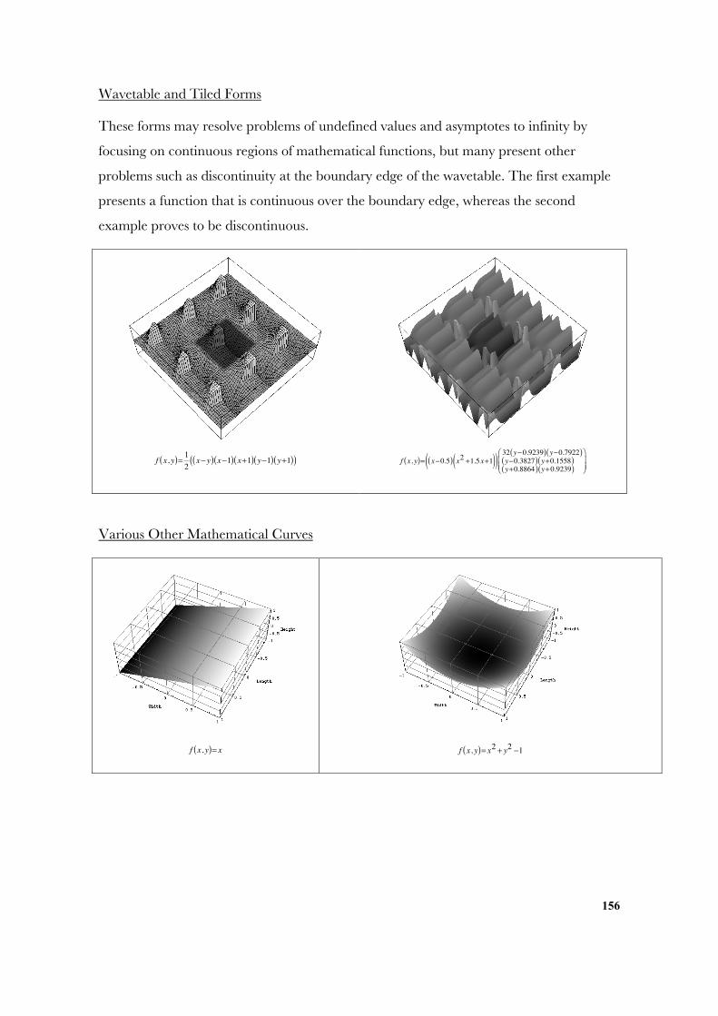
156

Wavetable and Tiled Forms

These forms may resolve problems of undefined values and asymptotes to infinity by

focusing on continuous regions of mathematical functions, but many present other

problems such as discontinuity at the boundary edge of the wavetable. The first example

presents a function that is continuous over the boundary edge, whereas the second

example proves to be discontinuous.

f x, y( )= 12

x− y( ) x−1( ) x+1( ) y−1( ) y+1( )( )

f x, y( )= x−0.5( ) x2 +1.5x+1( )( ) 32 y−0.9239( ) y−0.7922( )y−0.3827( ) y+0.1558( )y+0.8864( ) y+0.9239( )

⎛

⎝⎜⎜

⎞

⎠⎟⎟

Various Other Mathematical Curves

f x, y( )= x

f x, y( )= x2 + y2 −1

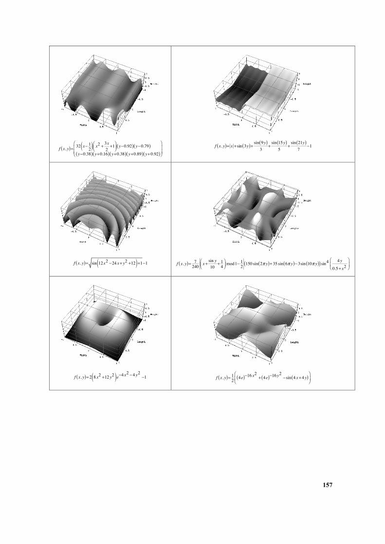
157

f x, y( )= 32 x− 12( ) x2 + 3x

2+1⎛

⎝⎜⎞⎠⎟ y−0.92( ) y−0.79( )

y−0.38( ) y+0.16( ) y+0.38( ) y+0.89( ) y+0.92( )

⎛

⎝⎜⎜

⎞

⎠⎟⎟

f x, y( )= x +sin 3y( )+ sin 9y( )3

+sin 15y( )

5+sin 21y( )

7−1

f x, y( )= sin 12x2 −24 x+ y2 +12( )+1−1

f x, y( )= 7240 x+

sin y10

+ 14⎛⎝⎜

⎞⎠⎟ mod1−

12 150 sin 2π y( )+35 sin 6π y( )−3sin 10π y( )( ) sin4 4 y

0.5+ x2⎛

⎝⎜⎞

⎠⎟

f x, y( )=2 8 x2 +12 y2( )e−4 x2 −4 y2 −1

f x, y( )= 12 4e( )−16 x2+ 4e( )−16y

2−sin 4 x+4 y( )⎛

⎝⎜⎞

⎠⎟

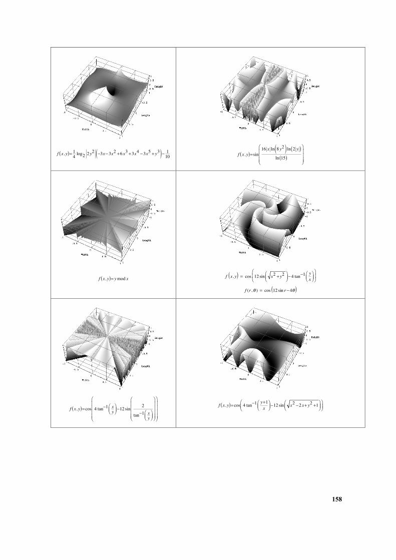
158

f x, y( )= 14 log2 2y2 −3x−3x2 +6 x3 +3x4 −3x5 + y3( )− 110

f x, y( )=sin16 x ln 8 y2( ) ln 2 y( )

ln 15( )

⎛

⎝

⎜⎜⎜

⎞

⎠

⎟⎟⎟

f x, y( )= ymod x

f x, y( ) = cos 12 sin x2 + y2⎛⎝⎜

⎞⎠⎟ −4 tan

−1 yx

⎛⎝⎜

⎞⎠⎟

⎛

⎝⎜

⎞

⎠⎟

f (r ,θ ) = cos 12 sin r−4θ( )

f x, y( )= cos 4 tan−1 xy

⎛⎝⎜

⎞⎠⎟ −12 sin

2

tan−1 xy

⎛⎝⎜

⎞⎠⎟

⎛

⎝

⎜⎜⎜⎜

⎞

⎠

⎟⎟⎟⎟

⎛

⎝

⎜⎜⎜⎜

⎞

⎠

⎟⎟⎟⎟

f x, y( )= cos 4 tan−1 y+1x

⎛⎝⎜

⎞⎠⎟ −12 sin x2 −2 x+ y2 +1⎛

⎝⎜⎞⎠⎟

⎛⎝⎜

⎞⎠⎟

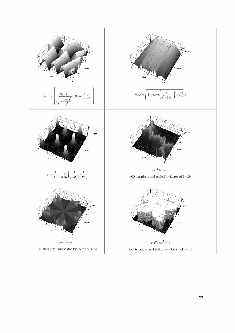
159

f x, y( )= cos 20y−40

x 1+y−2( )2

x2

−40 tan−1y

x−5⎛⎝⎜

⎞⎠⎟

⎛

⎝

⎜⎜⎜⎜⎜⎜

⎞

⎠

⎟⎟⎟⎟⎟⎟

f x, y( )= 2− x+ x cos1

y2 +0.01

⎛

⎝⎜⎜

⎞

⎠⎟⎟

⎛

⎝⎜⎜

⎞

⎠⎟⎟1− y2( )−1

℘ =1

x2+

1

(z−ϖ )2−1

ϖ 2⎛

⎝⎜⎜

⎞

⎠⎟⎟ϖ∈ ′L

∑

z= z2 + c;c=− i

(60 iterations and scaled by factor of 1/15)

z= z5 + c;c=− i

(60 iterations and scaled by factor of 1/5)

z= z6c+ zc2 ;c=1

(60 iterations and scaled by a factor of 1/30)

160

f (x,y)=35cos tan−1

yx

⎛⎝⎜

⎞⎠⎟ −2 sin e

1

1+ y2

x2

−2 cos 4 tan−1yx

⎛⎝⎜

⎞⎠⎟

⎛⎝⎜

⎞⎠⎟+sin5 1

12 tan−1 y

x⎛⎝⎜

⎞⎠⎟

⎛⎝⎜

⎞⎠⎟

⎛

⎝

⎜⎜⎜⎜⎜⎜

⎞

⎠

⎟⎟⎟⎟⎟⎟

⎛

⎝

⎜⎜⎜⎜⎜⎜

⎞

⎠

⎟⎟⎟⎟⎟⎟

+random()

2

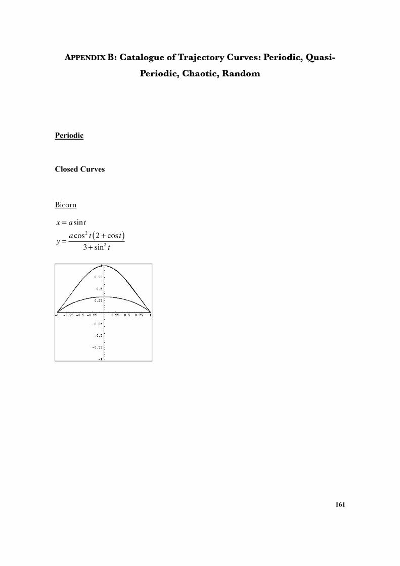
161

APPENDIX B: Catalogue of Trajectory Curves: Periodic, Quasi-

Periodic, Chaotic, Random

Periodic

Closed Curves

Bicorn

x = asint

y =acos2 t 2 + cos t( )

3+ sin2 t

162

Eight Curve – Gerono Lemniscate

x = asinty = asint cos t

Scarabaeus

r = bcos 2θ( ) − acosθwhere a,b ≠ 0

Rose Curve

r = acos nθ( )

n=1/4

n=1/3

n=1/2

n=2/3

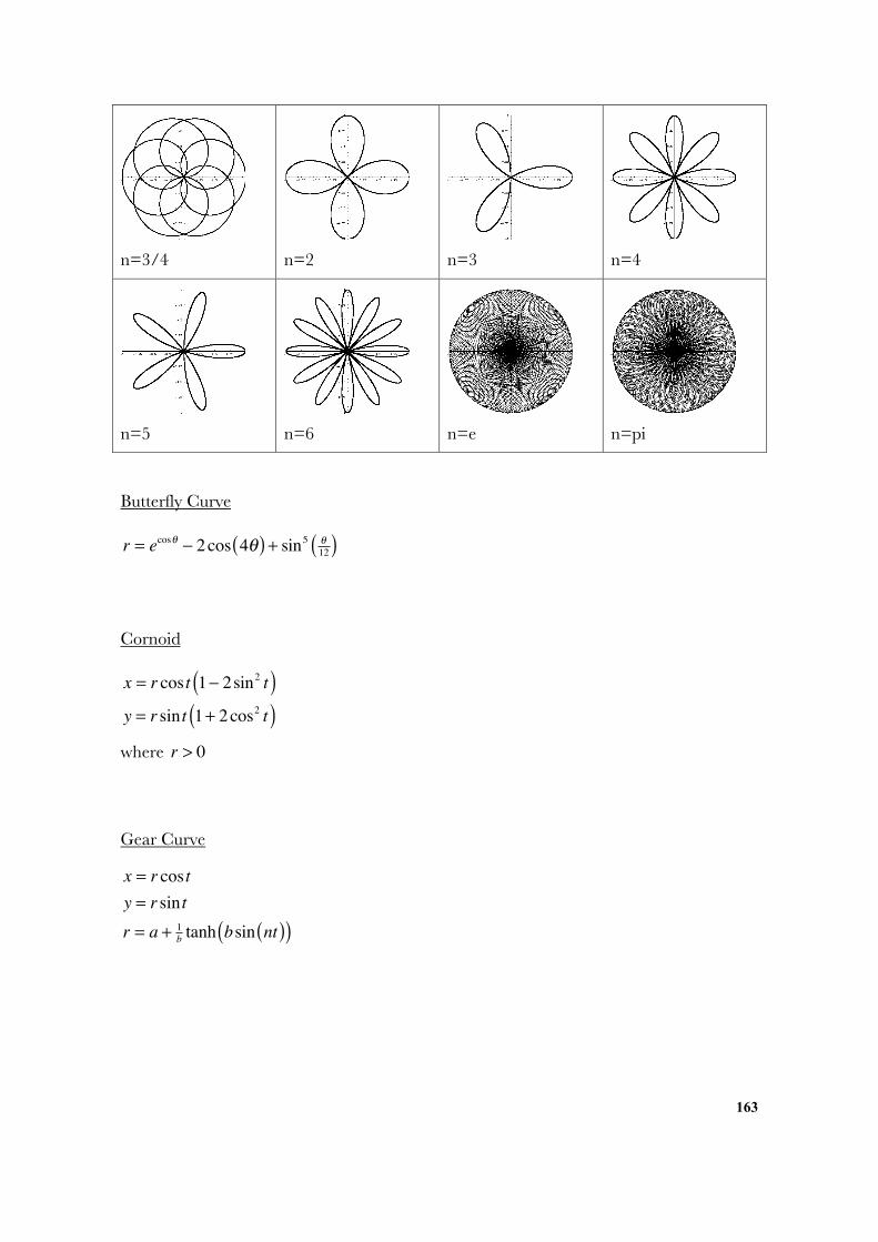
163

n=3/4

n=2

n=3

n=4

n=5

n=6

n=e

n=pi

Butterfly Curve

r = ecosθ − 2cos 4θ( ) + sin5 θ12( )

Cornoid

x = r cos t 1− 2sin2 t( )y = r sint 1+ 2cos2 t( )where r > 0

Gear Curve

x = r cos ty = r sintr = a + 1

b tanh bsin nt( )( )

164

Lissajous Curve

x = ax cos bxt + cx( )y = ay cos byt + cy( )

SuperEllipse

x = acos2r t

y = bsin2r t

Limaçon Curve

r = b + asinθ

Epicycloid

x = a + b( )cos t − bcos a + bb

t⎛⎝⎜

⎞⎠⎟

y = a + b( )sin t − bsin a + bb

t⎛⎝⎜

⎞⎠⎟

Hypotrochoid

x = a − b( )cos t + hcos a − bb

t⎛⎝⎜

⎞⎠⎟

y = a − b( )sin t − hsin a − bb

t⎛⎝⎜

⎞⎠⎟

165

Epitrochoid

x = a + b( )cos t − hcos a + bb

t⎛⎝⎜

⎞⎠⎟

y = a + b( )sin t − hsin a + bb

t⎛⎝⎜

⎞⎠⎟

Hypocycloid

x = a − b( )cos t + bcos a − bb

t⎛⎝⎜

⎞⎠⎟

y = a − b( )sin t − bsin a − bb

t⎛⎝⎜

⎞⎠⎟

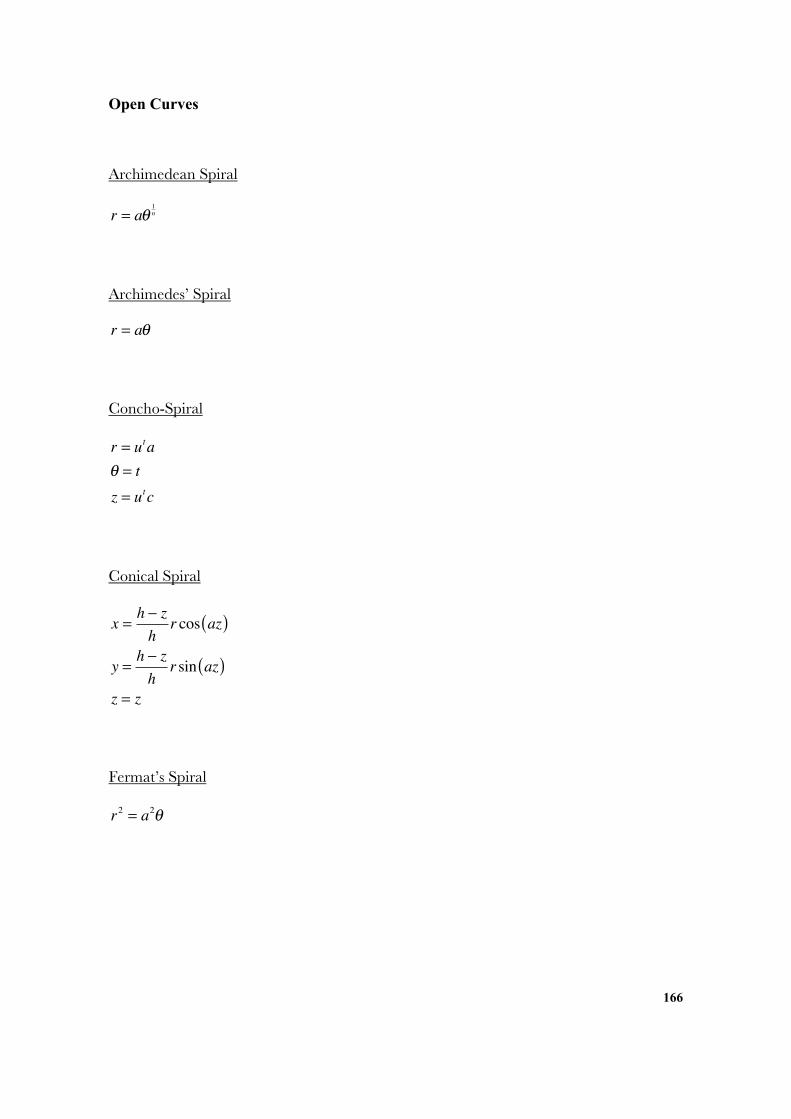
166

Open Curves

Archimedean Spiral

r = aθ1n

Archimedes’ Spiral

r = aθ

Concho-Spiral

r = utaθ = tz = utc

Conical Spiral

x =h − zh

r cos az( )

y =h − zh

r sin az( )z = z

Fermat’s Spiral

r2 = a2θ

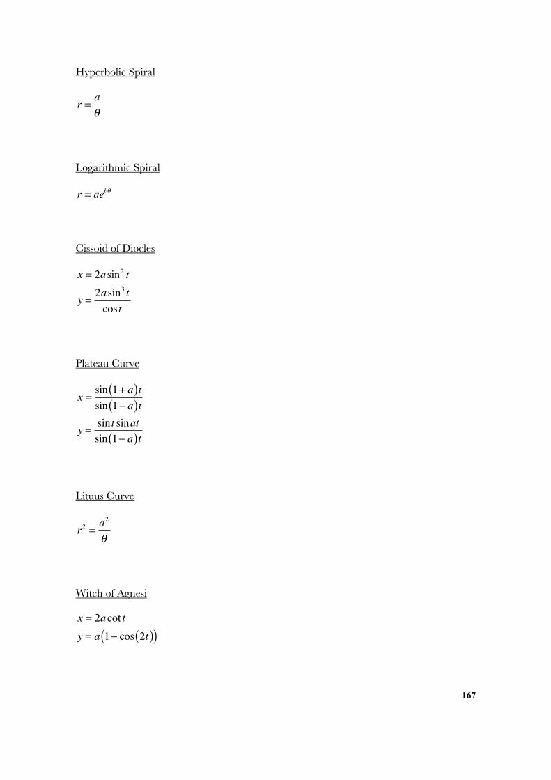
167

Hyperbolic Spiral

r =aθ

Logarithmic Spiral

r = aebθ

Cissoid of Diocles

x = 2asin2 t

y =2asin3 tcos t

Plateau Curve

x =sin 1+ a( )tsin 1− a( )t

y = sin t sinatsin 1− a( )t

Lituus Curve

r2 =a2

θ

Witch of Agnesi

x = 2acot ty = a 1− cos 2t( )( )

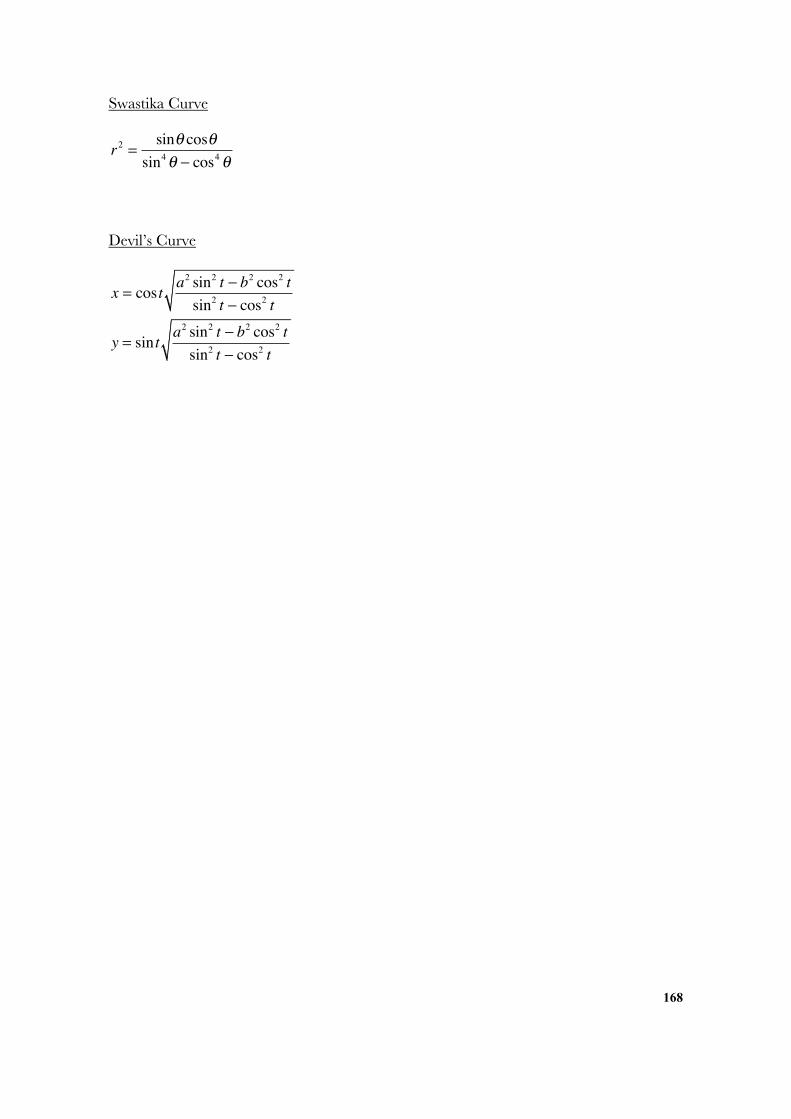
168

Swastika Curve

r2 =sinθ cosθ

sin4θ − cos4θ

Devil’s Curve

x = cos t a2 sin2 t − b2 cos2 tsin2 t − cos2 t

y = sint a2 sin2 t − b2 cos2 tsin2 t − cos2 t

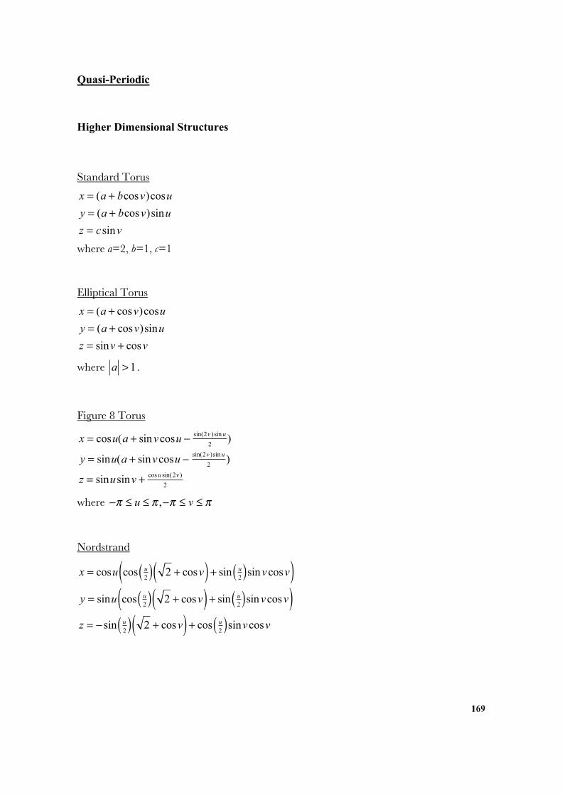
169

Quasi-Periodic

Higher Dimensional Structures

Standard Torus

x = (a + bcosv)cosu

y = (a + bcosv)sinu

z = csinv

where a=2, b=1, c=1

Elliptical Torus

x = (a + cosv)cosu

y = (a + cosv)sinu

z = sinv + cosv

where a > 1 .

Figure 8 Torus

x = cosu(a + sinvcosu − sin(2v )sin u

2)

y = sinu(a + sinvcosu − sin(2v )sin u

2)

z = sinusinv + cos u sin(2v )

2

where −π ≤ u ≤ π ,−π ≤ v ≤ π

Nordstrand

x = cosu cos u2( ) 2 + cosv( ) + sin u

2( )sin vcosv( )y = sinu cos u

2( ) 2 + cosv( ) + sin u2( )sin vcosv( )

z = − sin u2( ) 2 + cosv( ) + cos u

2( )sinvcosv

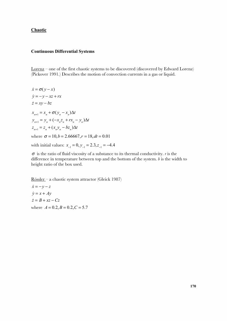
170

Chaotic

Continuous Differential Systems

Lorenz – one of the first chaotic systems to be discovered (discovered by Edward Lorenz)(Pickover 1991.) Describes the motion of convection currents in a gas or liquid.

x = σ ( y − x)

y = − y − xz + rx

z = xy − bz

xn+1

= xn+σ ( y

n− x

n)Δt

yn+1

= yn+ (−x

nz

n+ rx

n− y

n)Δt

zn+1

= zn+ (x

ny

n− bz

n)Δt

where σ = 10,b = 2.66667,r = 18,dt = 0.01

with initial values: x−1= 0, y−1

= 2.3, z−1= −4.4

σ is the ratio of fluid viscosity of a substance to its thermal conductivity. r is thedifference in temperature between top and the bottom of the system. b is the width toheight ratio of the box used.

Rössler – a chaotic system attractor (Gleick 1987)

x = − y − z

y = x + Ay

z = B + xz − Cz

where A = 0.2, B = 0.2,C = 5.7

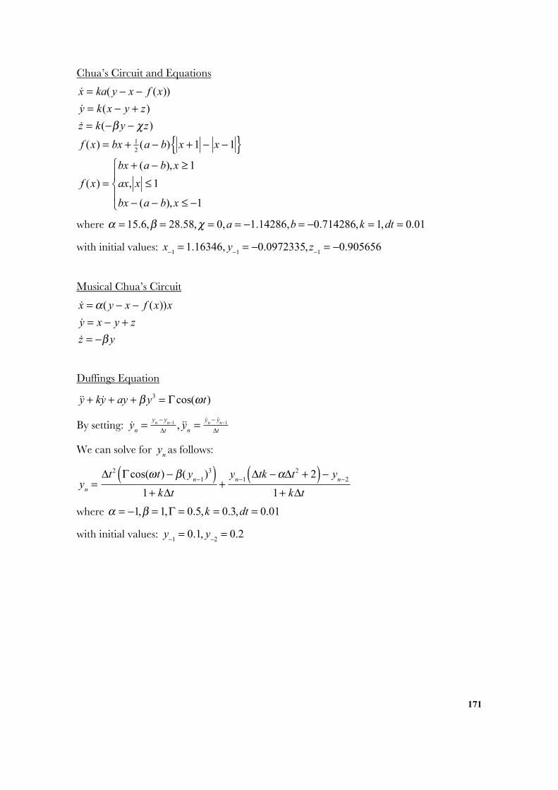
171

Chua’s Circuit and Equations

x = ka( y − x − f (x))

y = k(x − y + z)

z = k(−β y − χz)

f (x) = bx + 12(a − b) x +1 − x −1{ }

f (x) =bx + (a − b), x ≥ 1

ax, x ≤ 1

bx − (a − b), x ≤ −1

⎧

⎨⎪

⎩⎪

where α = 15.6,β = 28.58,χ = 0,a = −1.14286,b = −0.714286,k = 1,dt = 0.01

with initial values: x−1= 1.16346, y−1

= −0.0972335, z−1= −0.905656

Musical Chua’s Circuit

x = α( y − x − f (x))x

y = x − y + z

z = −β y

Duffings Equation

y + ky + ay + β y3 = Γcos(ωt)

By setting: y

n= yn − yn−1

Δt, y

n= yn − yn−1

Δt

We can solve for ynas follows:

y

n=Δt2 Γcos(ωt) − β( y

n−1)3( )

1+ kΔt+

yn−1

Δtk −αΔt2 + 2( ) − yn−2

1+ kΔt

where α = −1,β = 1,Γ = 0.5,k = 0.3,dt = 0.01

with initial values: y−1= 0.1, y−2

= 0.2

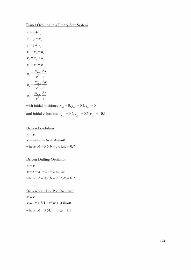
172

Planet Orbiting in a Binary Star System

x = x + vx

y = y + vy

z = z + vz

vx= v

x+ a

x

vy= v

y+ a

y

vz= v

z+ a

z

ax=

mstar

r 2

Δx

r

ay=

mstar

r 2

Δy

r

az=

mstar

r 2

Δz

r

with initial positions: x−1= 0, y−1

= 0.1, z−1= 0

and initial velocities: v

x −1= 0.5,v

y−1= 0.6,v

z−1= −0.1

Driven Pendulum

x = v

v = − sin x − bv + Asinωt

where A = 0.6,b = 0.05,ω = 0.7

Driven Duffing Oscillator

x = v

v = x − x3 − bv + Asinωt

where A = 0.7,b = 0.05,ω = 0.7

Driven Van Der Pol Oscillator

x = v

v = −x + b(1− x2 )v + Asinωt

where A = 0.61,b = 1,ω = 1.1

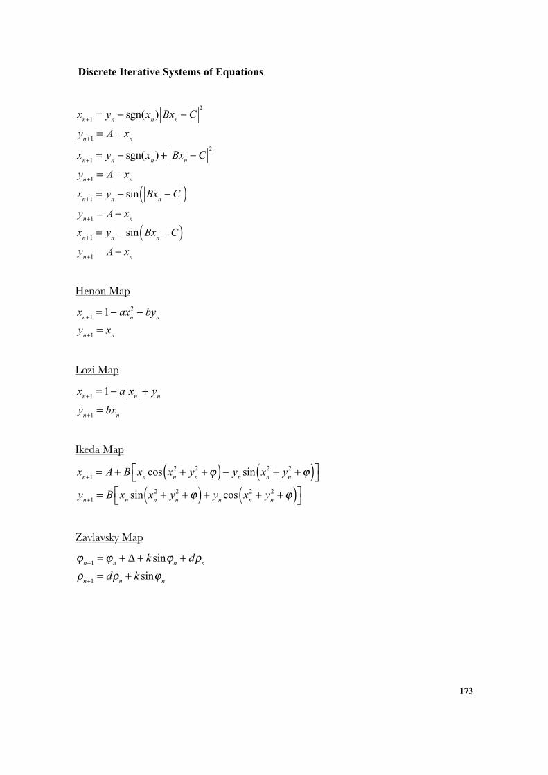
173

Discrete Iterative Systems of Equations

xn+1

= yn− sgn(x

n) Bx

n− C

2

yn+1

= A− xn

xn+1

= yn− sgn(x

n) + Bx

n− C

2

yn+1

= A− xn

xn+1

= yn− sin Bx

n− C( )

yn+1

= A− xn

xn+1

= yn− sin Bx

n− C( )

yn+1

= A− xn

Henon Map

xn+1

= 1− axn2 − by

n

yn+1

= xn

Lozi Map

xn+1

= 1− a xn+ y

n

yn+1

= bxn

Ikeda Map

xn+1

= A+ B xncos x

n2 + y

n2 +ϕ( ) − y

nsin x

n2 + y

n2 +ϕ( )⎡⎣ ⎤⎦

yn+1

= B xnsin x

n2 + y

n2 +ϕ( ) + y

ncos x

n2 + y

n2 +ϕ( )⎡

⎣⎤⎦

Zavlavsky Map

ϕn+1

= ϕn+ Δ + k sinϕ

n+ dρ

n

ρn+1

= dρn+ k sinϕ

n

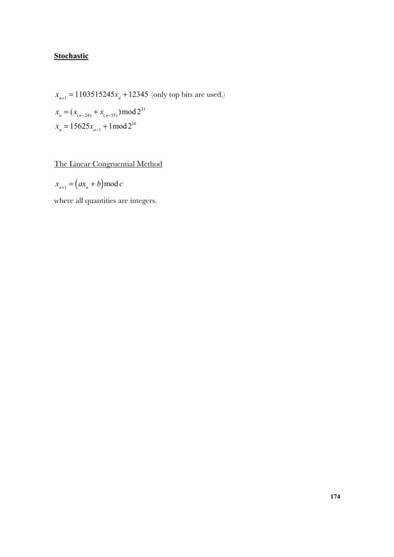
174

Stochastic

xn+1= 1103515245x

n+12345 (only top bits are used.)

xn= (x

(n−24)+ x

( n−55))mod 231

xn= 15625x

n−1+1mod 216

The Linear Congruential Method

x

n+1= ax

n+ b( )mod c

where all quantities are integers.

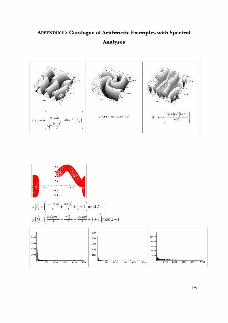
175

APPENDIX C: Catalogue of Arithmetic Examples with Spectral

Analyses

f x, y( )= cos 20y−40

x 1+y−2( )2

x2

−40 tan−1y

x−5⎛⎝⎜

⎞⎠⎟

⎛

⎝

⎜⎜⎜⎜⎜⎜

⎞

⎠

⎟⎟⎟⎟⎟⎟

f (r ,θ ) = cos 12 sin r−4θ( )

f x, y( )=sin16 x ln 8 y2( ) ln 2 y( )

ln 15( )

⎛

⎝

⎜⎜⎜

⎞

⎠

⎟⎟⎟

x t( ) = cos 100π t( )8

+sin π

2t( )

2+ t

2+1⎛

⎝⎜⎞⎠⎟ mod 2 −1

y t( ) = cos 100π t( )8

+sin π

2t( )

2+ sin 2π t( )

4+ t

5+1⎛

⎝⎜⎞⎠⎟ mod 2 −1

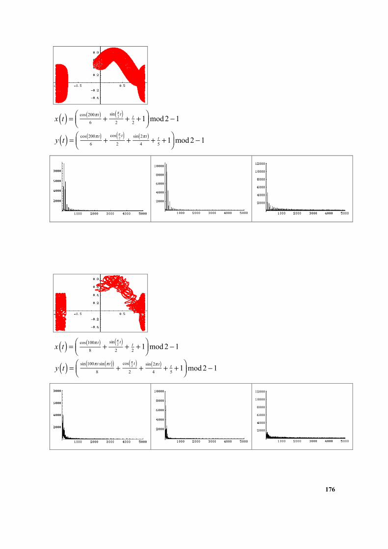
176

x t( ) = cos 200π t( )6

+sin π

2t( )

2+ t

2+1⎛

⎝⎜⎞⎠⎟ mod 2 −1

y t( ) = cos 200π t( )6

+cos π

2t( )

2+ sin 2π t( )

4+ t

5+1⎛

⎝⎜⎞⎠⎟ mod 2 −1

x t( ) = cos 100π t( )8

+sin π

2t( )

2+ t

2+1⎛

⎝⎜⎞⎠⎟ mod 2 −1

y t( ) = sin 100π t sin π t( )( )8

+cos π

2t( )

2+ sin 2π t( )

4+ t

5+1⎛

⎝⎜⎞⎠⎟ mod 2 −1

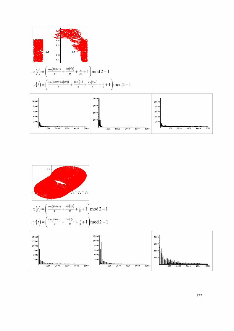
177

x t( ) = cos 100π t( )4

+sin π

2t( )

π + t2e+1⎛

⎝⎜⎞⎠⎟ mod 2 −1

y t( ) = sin 100π t sin π t( )( )8

+cos π

2t( )

2+ sin 2π t( )

4+ t

5+1⎛

⎝⎜⎞⎠⎟ mod 2 −1

x t( ) = cos 100π t( )4

+sin π

2t( )

32+ t

8+1⎛

⎝⎜⎞⎠⎟ mod 2 −1

y t( ) = sin 100π t( )8

+cos π

2t( )

32+ t

8+1⎛

⎝⎜⎞⎠⎟ mod 2 −1

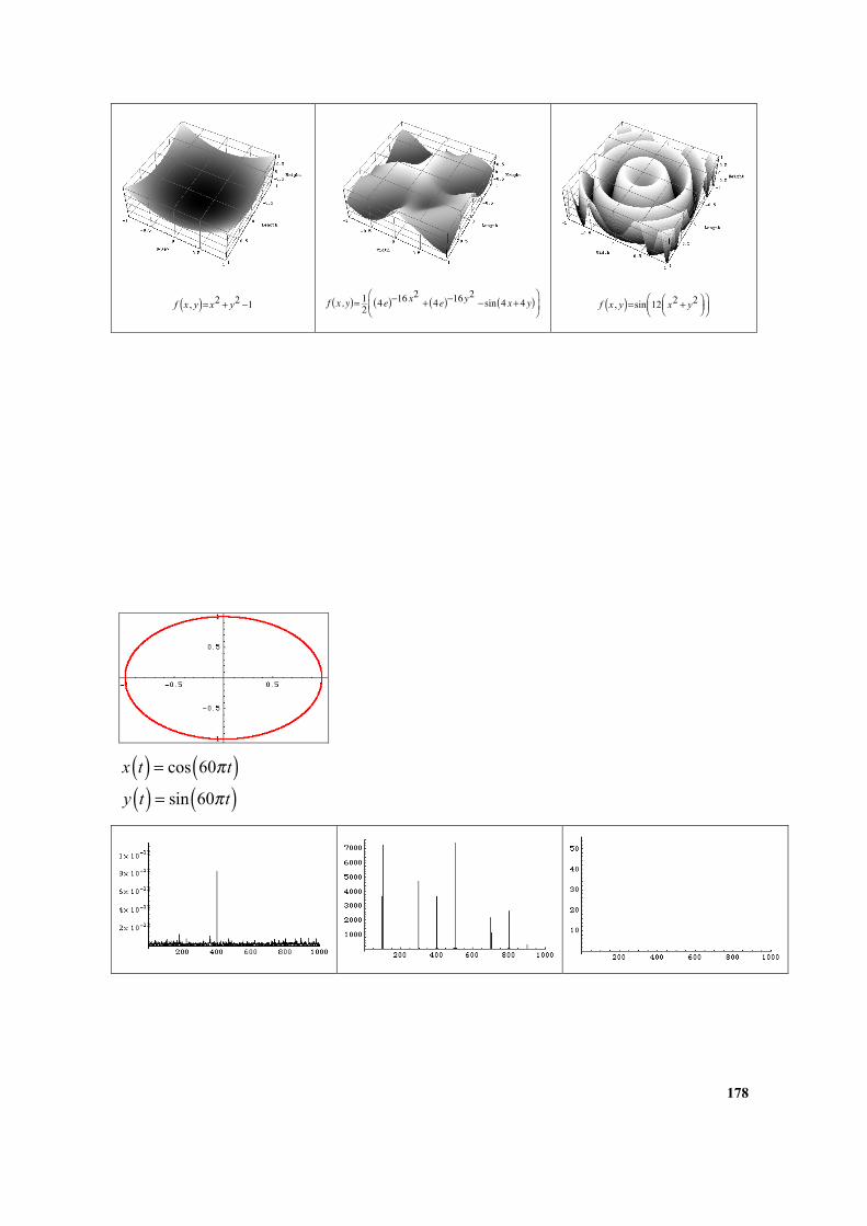
178

f x , y( )= x2 + y2 −1

f x, y( )= 12 4e( )−16 x2+ 4e( )−16y

2−sin 4 x+4 y( )⎛

⎝⎜⎞

⎠⎟

f x , y( )=sin 12 x2 + y2⎛

⎝⎜⎞⎠⎟

⎛⎝⎜

⎞⎠⎟

x t( ) = cos 60πt( )y t( ) = sin 60πt( )

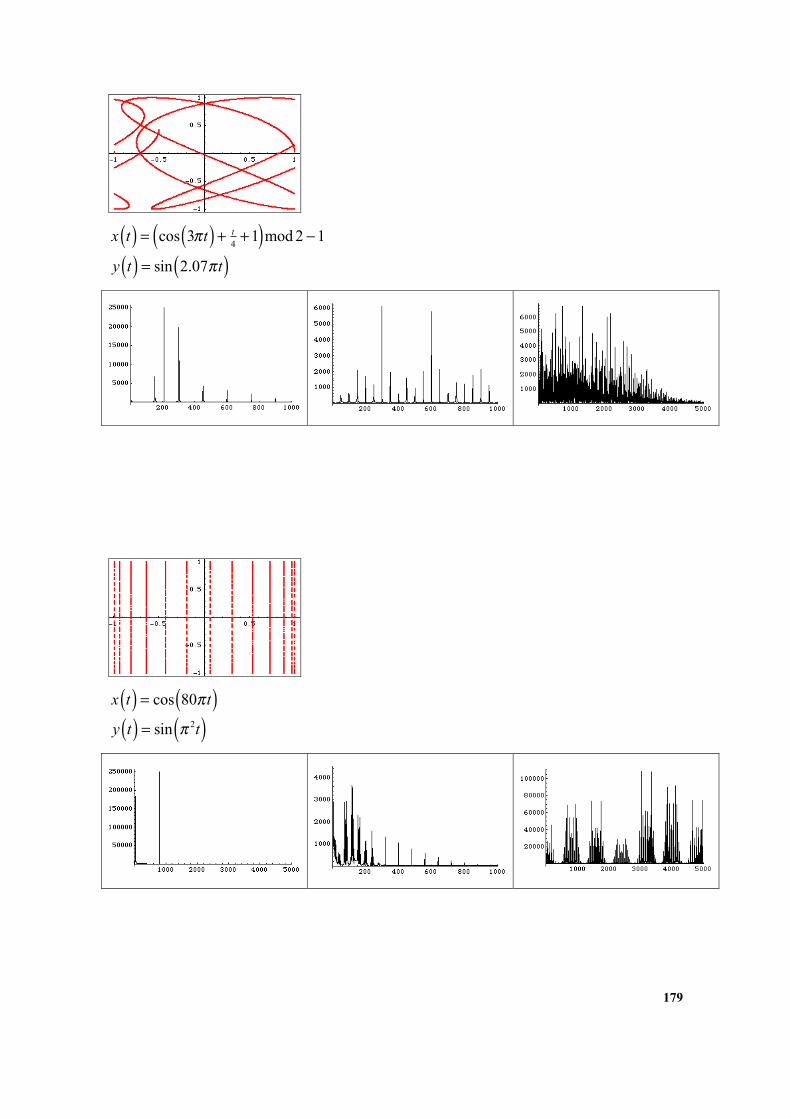
179

x t( ) = cos 3πt( ) + t4+1( )mod 2 −1

y t( ) = sin 2.07πt( )

x t( ) = cos 80πt( )y t( ) = sin π 2t( )

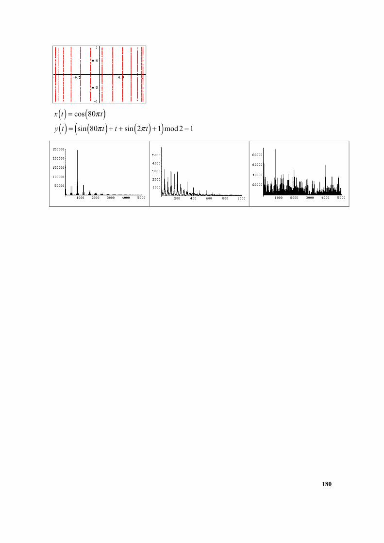
180

x t( ) = cos 80πt( )y t( ) = sin 80πt( ) + t + sin 2πt( ) +1( )mod 2 −1

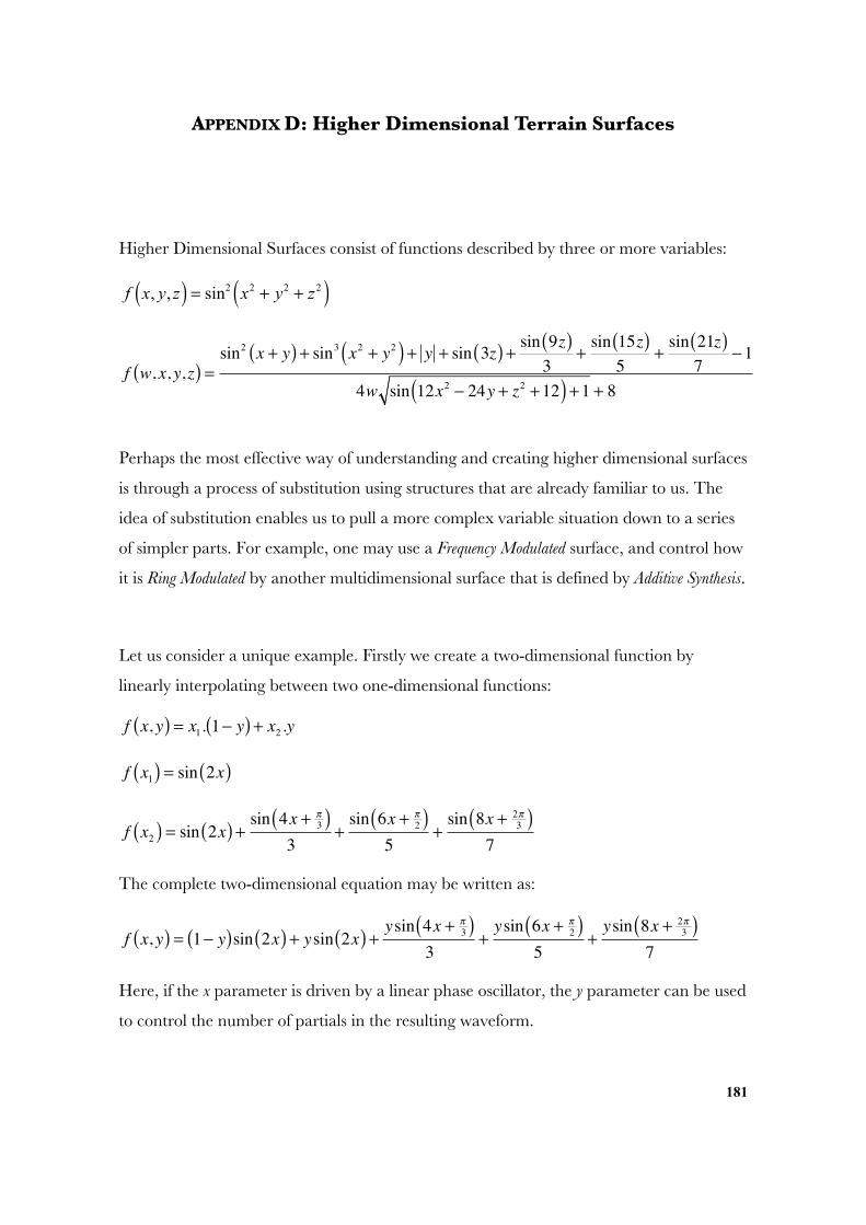
181

APPENDIX D: Higher Dimensional Terrain Surfaces

Higher Dimensional Surfaces consist of functions described by three or more variables:

f x, y, z( ) = sin2 x2 + y2 + z2( )

f w, x, y, z( ) =sin2 x + y( ) + sin3 x2 + y2( ) + y + sin 3z( ) + sin 9z( )

3+sin 15z( )5

+sin 21z( )7

−1

4w sin 12x2 − 24y + z2 +12( ) +1 + 8

Perhaps the most effective way of understanding and creating higher dimensional surfaces

is through a process of substitution using structures that are already familiar to us. The

idea of substitution enables us to pull a more complex variable situation down to a series

of simpler parts. For example, one may use a Frequency Modulated surface, and control how

it is Ring Modulated by another multidimensional surface that is defined by Additive Synthesis.

Let us consider a unique example. Firstly we create a two-dimensional function by

linearly interpolating between two one-dimensional functions:

f x, y( ) = x1. 1− y( ) + x2 .y

f x1( ) = sin 2x( )

f x2( ) = sin 2x( ) + sin 4x +π3( )

3+sin 6x + π

2( )5

+sin 8x + 2π

3( )7

The complete two-dimensional equation may be written as:

f x, y( ) = 1− y( )sin 2x( ) + ysin 2x( ) + ysin 4x + π3( )

3+ysin 6x + π

2( )5

+ysin 8x + 2π

3( )7

Here, if the x parameter is driven by a linear phase oscillator, the y parameter can be used

to control the number of partials in the resulting waveform.

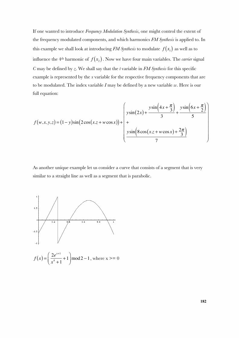
182

If one wanted to introduce Frequency Modulation Synthesis, one might control the extent of

the frequency modulated components, and which harmonics FM Synthesis is applied to. In

this example we shall look at introducing FM Synthesis to modulate f x1( ) as well as to

influence the 4th harmonic of f x2( ) . Now we have four main variables. The carrier signal

C may be defined by z. We shall say that the t variable in FM Synthesis for this specific

example is represented by the x variable for the respective frequency components that are

to be modulated. The index variable I may be defined by a new variable w. Here is our

full equation:

f w, x, y, z( ) = 1− y( )sin 2cos x.z + wcos x( )( ) +ysin 2x( ) +

ysin 4x + π3( )

3+ysin 6x + π

2( )5

+

ysin 8cos x.z + wcos x( ) + 2π3( )7

⎛

⎝

⎜⎜⎜⎜⎜⎜⎜

⎞

⎠

⎟⎟⎟⎟⎟⎟⎟

As another unique example let us consider a curve that consists of a segment that is very

similar to a straight line as well as a segment that is parabolic.

f x( ) = 2ex+1

x4 +1+1

⎛⎝⎜

⎞⎠⎟mod2 −1 , where x >= 0

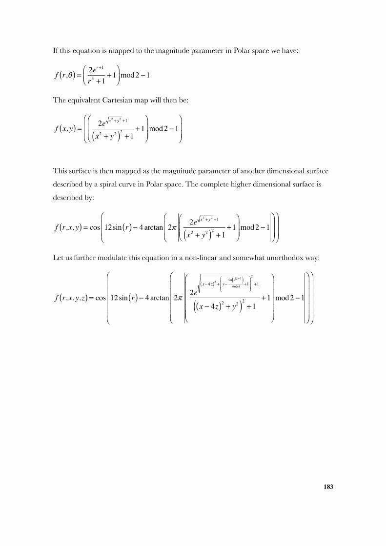
183

If this equation is mapped to the magnitude parameter in Polar space we have:

f r,θ( ) = 2er+1

r 4 +1+1

⎛⎝⎜

⎞⎠⎟mod2 −1

The equivalent Cartesian map will then be:

f x, y( ) = 2e x2 + y2 +1

x2 + y2( )2 +1+1

⎛

⎝⎜⎜

⎞

⎠⎟⎟mod2 −1

⎛

⎝⎜⎜

⎞

⎠⎟⎟

This surface is then mapped as the magnitude parameter of another dimensional surface

described by a spiral curve in Polar space. The complete higher dimensional surface is

described by:

f r, x, y( ) = cos 12sin r( ) − 4 arctan 2π 2e x2 + y2 +1

x2 + y2( )2 +1+1

⎛

⎝⎜⎜

⎞

⎠⎟⎟mod2 −1

⎛

⎝⎜⎜

⎞

⎠⎟⎟

⎛

⎝

⎜⎜

⎞

⎠

⎟⎟

Let us further modulate this equation in a non-linear and somewhat unorthodox way:

f r, x, y, z( ) = cos 12sin r( ) − 4 arctan 2π 2ex−4 z( )2 + y−

sin e z +1⎛⎝⎜

⎞⎠⎟

sin e( ) +1⎛

⎝⎜⎜

⎞

⎠⎟⎟

2

+1

x − 4z( )2 + y2( )2 +1+1

⎛

⎝

⎜⎜⎜⎜⎜

⎞

⎠

⎟⎟⎟⎟⎟

mod2 −1

⎛

⎝

⎜⎜⎜⎜⎜

⎞

⎠

⎟⎟⎟⎟⎟

⎛

⎝

⎜⎜⎜⎜⎜

⎞

⎠

⎟⎟⎟⎟⎟

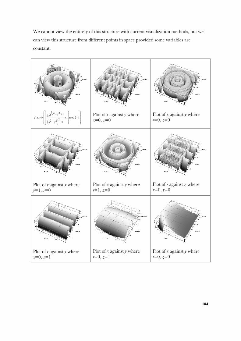
184

We cannot view the entirety of this structure with current visualization methods, but we

can view this structure from different points in space provided some variables are

constant.

f x, y( )= 2e x2 + y2 +1

x2 + y2( )2 +1+1

⎛

⎝

⎜⎜⎜⎜

⎞

⎠

⎟⎟⎟⎟mod 2−1

⎛

⎝

⎜⎜⎜⎜

⎞

⎠

⎟⎟⎟⎟

Plot of r against y wherex=0, z=0

Plot of x against y wherer=0, z=0

Plot of r against x wherey=1, z=0

Plot of x against y wherer=1, z=0

Plot of r against z wherex=0, y=0

Plot of r against y wherex=0, z=1

Plot of x against y wherer=0, z=1

Plot of x against y wherer=0, z=0

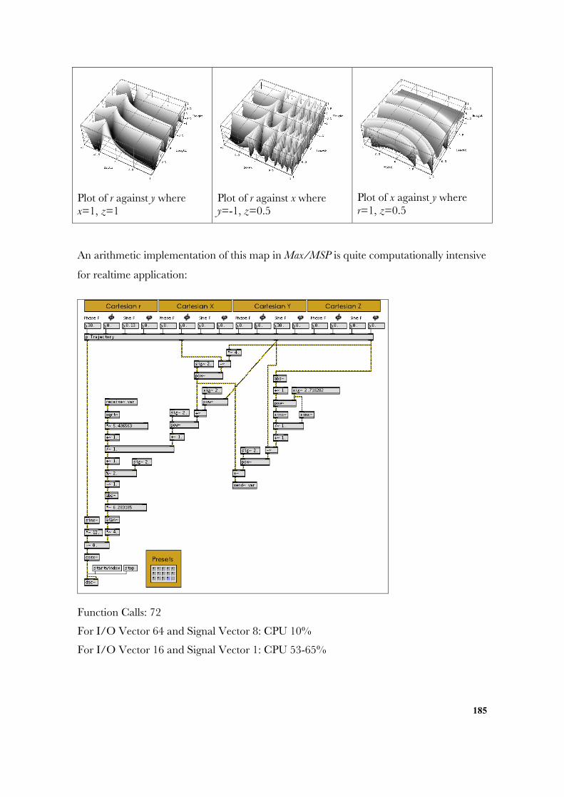
185

Plot of r against y wherex=1, z=1

Plot of r against x wherey=-1, z=0.5

Plot of x against y wherer=1, z=0.5

An arithmetic implementation of this map in Max/MSP is quite computationally intensive

for realtime application:

Function Calls: 72

For I/O Vector 64 and Signal Vector 8: CPU 10%

For I/O Vector 16 and Signal Vector 1: CPU 53-65%

186

187

Bibliography

Chronology of Research in Wave Terrain Synthesis

Bischoff, J., R. Gold, and J. Horton. 1978. “A Microcomputer-based network for liveperformance.” Computer Music Journal 2(3): 24-29.

Gold, R. 1979. “A Terrain Reader.” In C. P. Morgan, ed. The BYTE Book of ComputerMusic. Byte Publications, Petersborough, NH.

Mitsuhashi, Y. 1982. “Audio Synthesis by Functions of Two Variables.” Journal of theAudio Engineering Society 30(10): 701-706.

Borgonovo, A., and G. Haus. 1984. “Musical Sound Synthesis by means of Two-VariableFunctions: experimental criteria and results.” In D. Wessel, ed. Proceedings of the 1984International Computer Music Conference: 35-42.

Borgonovo, A., and G. Haus. 1986. “Sound Synthesis by means of Two-VariableFunctions: experimental criteria and results.” Computer Music Journal 10(4): 57-71.

Thibault, B., and S. Gresham-Lancaster. 1992. “Terrain Reader.”http://www.mcs.csuhayward.edu/~tebo/TerrainReader.html

Thibault, B., and S. Gresham-Lancaster. 1992. “Songlines.DEM.” Proceedings of the 1992International Computer Music Conference. San Jose: 465-466.http://www.mcs.csuhayward.edu/~tebo/Songlines.txt

Roads, C., et al. 1996. The Computer Music Tutorial. Cambridge, Massachusetts: MIT Press.

Wegner, K. 1998. “Surgical Navigation System and Method Using Audio Feedback.”ICAD. Computer Aided Surgery Incorporated, New York, U.S.A.http://www.icad.org/websiteV2.0/Conferences/ICAD98/papers/WEGNER.pdf

Jovanov, E., K. Wegner, V. Radivojevic, D. Starcevic, M. S. Quinn, and D. B. Karron.1999. “Tactical Audio and Acoustic Rendering in Biomedical Applications.” IEEETransactions on Information Technology in Biomedicine 3(2): 109-118.

188

Mikelson, H. 1999. “Sound Generation with the Julia Set.” The Csound Magazine.http://www.csounds.com/ezine/summer1999/synthesis/

Pinkston, R. 1999. “Example of Wave Terrain Synthesis Instrument.”http://www.utexas.edu/cofa/music/ems/mus329m/ClassStuff/terrain.html

Mills, A. and R. C. De Souza. 1999. “Gestural Sounds by Means of Wave TerrainSynthesis.” Congresso Nacional da Sociedade Brasileira de Computação XIX.http://gsd.ime.usp.br/sbcm/1999/papers/Anderson_Mills.html

Comajuncosas, J. M. 2000. “Wave Terrain Synthesis with Csound.” In R. Boulanger, ed.The CSound Book: perspectives in software synthesis, sound design, signal processing, and programming.Cambridge, Massachusetts: MIT Press.

Mikelson, H. 2000. “Terrain Mapping Synthesis.” In R. Boulanger, ed. The CSound Book:perspectives in software synthesis, sound design, signal processing, and programming. Cambridge,Massachusetts: MIT Press. http://www.csounds.com/mikelson/index.html

Mikelson, H. 2000. “Terrain Mapping with Dynamic Surfaces.” The Csound Magazine.http://www.csounds.com/ezine/spring2000/synthesis/

Verplank. W., M. Mathews. and R. Shaw. 2000. “Scanned Synthesis.” Proceedings of the2000 International Computer Music Conference: 368-371.http://www.billverplank.com/ScannedSynthesis.PDF

Boulanger, R., P. Smaragdis, and J. Ffitch. 2000. “Scanned Synthesis: An Introductionand Demonstration of a New Synthesis and Signal Processing Technique”, Proceedings ofthe 2000 International Computer Music Conference: 372-375.

Boulanger, R. 2000. “Scanned Synthesis & CSound @ CSounds.com”http://www.csounds.com/scanned

Nelson, J. C. 2000. “Understanding and Using Csound’s GEN Routines.” In R.Boulanger, ed. The CSound Book: perspectives in software synthesis, sound design, signal processing,and programming. Cambridge, Massachusetts: MIT Press: 65-97.

189

Overholt, D. 2000. “The Emonator: A Novel Musical Interface.” MIT Media Lab.http://www.media.mit.edu/~dano/matrix/

Trueman, D., and R. L. Dubois. 2001. PeRColate: a collection of synthesis, signal processing, andvideo objects (with source-code toolkit) for Max/MSP/Nato v. 1.0b3. Computer Music Centre:Columbia University. http://www.music.columbia.edu/PeRColate/

Cafagna, V., and D. Vicinanza. 2002. “Audio Synthesis by Means of Elliptic Functions.”Second International Conference Creating and Understanding Music, University of Salerno, Italy.http://www.dmi.unisa.it/sound/ellipticspringer.pdf

Di Scipio, A. 2002. “The Synthesis of Environmental Sound Textures by IteratedNonlinear Functions, and its Ecological Relevance to Perceptual Modeling.” Journal ofNew Music Research. 31(2): 109-117.

Hsu, W. 2002. “A Flexible Interface for Wave Terrain Synthesis.” PERformance &NETworking Colloquia, San Fransisco State University, Department of Computer Science.http://cs.sfsu.edu/news/pernet/02/04-24-02.html andhttp://userwww.sfsu.edu/~whsu/TERRAIN/

Overholt, D. 2002. “New Musical Mappings for the MATRIX Interface.” Proceedings of the2002 International Computer Music Conference.http://www.create.ucsb.edu/~dano/matrix/ICMC2002.pdf

James, S. 2003. “Possibilities for Dynamical Wave Terrain Synthesis.” ConvergingTechnologies, Proceedings of the Australasian Computer Music Conference: 58-67.

Clark, J. 2003. “Using the Clavia Nord Modular.”http://www.cim.mcgill.ca/~clark/nordmodularbook/nm_oscillator.html

Dannenberg, R. B., and T. Neuendorffer. 2003. “Sound Synthesis from Real-TimeVideo Images.” Proceedings of the 2003 International Computer Music Conference, San Francisco:International Computer Music Association: 385-388. http://www-2.cs.cmu.edu/~rbd/papers/videosound-icmc2003.pdf

190

Dannenberg, R. B., B. Bernstein, G. Zeglin, and T. Neuendorffer. 2003. “SoundSynthesis from Video, Wearable Lights, and 'The Watercourse Way'.” Proceedings of theNinth Biennial Symposium on Arts and Technology. Connecticut College: 38-44. http://www-2.cs.cmu.edu/~rbd/papers/conncoll2003.pdf;http://www.cs.cmu.edu/~music/examples.html

Trueman, D., and R. L. Dubois. 2003. “PeRColate for Pluggo 3.1 0.9”.http://www.macmusic.org/softs/view.php/lang/EN/id/2335/

Harris, S. 2003. “Steve Harris’ LADSPA Plugin Docs.” http://plugin.org.uk/ladspa-swh/docs/ladspa-swh.pdf

Sedes, A., B. Courribet, and J.-B. Thiébaut. 2004. “The Visualisation of Sound to Real-Time Sonification: different prototypes in the Max/MSP/Jitter environment.” Proceedings ofthe 2004 International Computer Music Conference. Miami, USA.http://jbthiebaut.free.fr/visualization_of_sound.pdf

Digital Cinema Arts. “Csound and Houdini.”http://www.digitalcinemaarts.com/dev/csound/

Authored References

Bernstein, J., et al. 2002. Jitter: Tutorials and Topics. Cycling ’74.http://www.cycling74.com/products/dldoc.html

Bischoff, J., R. Gold, and J. Horton. 1978. “A Microcomputer-based network for liveperformance.” Computer Music Journal 2(3): 24-29.

Borgonovo, A., and G. Haus. 1984. “Musical Sound Synthesis by means of Two-VariableFunctions: experimental criteria and results.” In D. Wessel, ed. Proceedings of the 1984International Computer Music Conference: 35-42.

Borgonovo, A., and G. Haus. 1986. “Sound Synthesis by means of Two-VariableFunctions: experimental criteria and results.” Computer Music Journal 10(4): 57-71.

Boulanger, R., P. Smaragdis, and J. Ffitch. 2000. “Scanned Synthesis: An Introductionand Demonstration of a New Synthesis and Signal Processing Technique”, Proceedings ofthe 2000 International Computer Music Conference: 372-375.

191

Boulanger, R. 2000. “Scanned Synthesis & CSound @ CSounds.com”http://www.csounds.com/scanned

Bourgin, D. 1995. “Color spaces FAQ.”http://www.poynton.com/notes/Timo/colorspace-faq

Cafagna, V., and D. Vicinanza. 2002. “Audio Synthesis by Means of Elliptic Functions.”Second International Conference Creating and Understanding Music, University of Salerno, Italy.http://www.dmi.unisa.it/sound/ellipticspringer.pdf

Castine, P. “Litter.” http://www.bek.no/~pcastine/Litter/

Chatwin, B. 1987. The Songlines. Penguin Press.

Chion, M. 1990. AudioVision: Sound on Screen. Reprinted in C. Gorbman, ed. and trans.1994. New York: Columbia University Press.

Chowning, J. 1973. “The Synthesis of Complex Spectra by means of FrequencyModulation.” Journal of the Audio Engineering Society 21(7): 526-534. Reprinted in C. Roadsand J. Strawn, eds. 1985. Foundations of Computer Music. Cambridge, Massachusetts: TheMIT Press: 6-29.

Clark, J. 2003. “Using the Clavia Nord Modular.”http://www.cim.mcgill.ca/~clark/nordmodularbook/nm_oscillator.html

Collopy, F. 2003. “Lumia.” http://rhythmiclight.com

Comajuncosas, J. M. 2000. “Wave Terrain Synthesis with Csound.” In R. Boulanger, ed.The CSound Book: perspectives in software synthesis, sound design, signal processing, and programming.Cambridge, Massachusetts: MIT Press.

Castine, P. “Litter.” http://www.bek.no/~pcastine/Litter/

Couturier, J.-M. “Computer Music at LMA.” http://www.lma.cnrs-mrs.fr/~IM/en_telecharger.htm

192

Dannenberg, R. B., and T. Neuendorffer. 2003. “Sound Synthesis from Real-TimeVideo Images.” Proceedings of the 2003 International Computer Music Conference, San Francisco:International Computer Music Association: 385-388. http://www-2.cs.cmu.edu/~rbd/papers/videosound-icmc2003.pdf

Dannenberg, R. B., B. Bernstein, G. Zeglin, and T. Neuendorffer. 2003. “SoundSynthesis from Video, Wearable Lights, and 'The Watercourse Way'.” Proceedings of theNinth Biennial Symposium on Arts and Technology. Connecticut College: 38-44. http://www-2.cs.cmu.edu/~rbd/papers/conncoll2003.pdf;http://www.cs.cmu.edu/~music/examples.html

Demeyer, T. 1996. “Bigeye (Version 1.10).” STEIM.http://www.steim.org/steim/bigeye.html

Digital Cinema Arts. “Csound and Houdini.”http://www.digitalcinemaarts.com/dev/csound/

Dimuzio, T., and E. Wenger. 1997. Metasynth Reference Manual. San Fransisco: U&ISoftware and Arboretum Systems.

Di Scipio, A. 2002. “The Synthesis of Environmental Sound Textures by IteratedNonlinear Functions, and its Ecological Relevance to Perceptual Modeling.” Journal ofNew Music Research. 31(2): 109-117.

Dobson, R. and J. Ffitch. 1995. “Experiments with Chaotic Oscillators.” The Proceedings ofthe 1995 International Computer Music Conference, Banff Conference: 45-48.http://www.bath.ac.uk/~masjpf/fractal_rev.html

Domik, G., C. J. C. Schauble, L. D. Fosdick, and E. R. Jessup. 1997. “Tutorial -- Colorin Scientific Visualization.” http://ugrad-www.cs.colorado.edu/~csci4576/SciVis/SciVisColor.html

Fernández-Cid, P., F. J. Casajús-Quirós, and P. Aguilar. 1999. “MWD: Multi-BandWaveshaping Distortion.” Proceedings of the Second International Conference on Digital AudioEffects. http://www.tele.ntnu.no/akustikk/meetings/DAFx99/fernandez-cid.pdf

193

Ffitch, J. 2000. “A Look at Random Numbers, Noise, and Chaos with Csound.” In R.Boulanger, ed. The CSound Book: perspectives in software synthesis, sound design, signal processing,and programming. Cambridge, Massachusetts: MIT Press: 321-338.

Goethe, J. W. von. 1970. Theory of Colours. Cambridge, Massachusetts: MIT Press.

Gold, R. 1979. “A Terrain Reader.” In C. P. Morgan, ed. The BYTE Book of ComputerMusic. Byte Publications, Petersborough, NH.

Harley, J. 2002. “The Electroacoustic Music of Iannis Xenakis.” Computer Music Journal26(1): 33-57.

Harris, S. 2003. “Steve Harris’ LADSPA Plugin Docs.” http://plugin.org.uk/ladspa-swh/docs/ladspa-swh.pdf

Hilborn, R. C. 1994. Chaos and Nonlinear Dynamics: an introduction for scientists and engineers.New York, Oxford: Oxford University Press.

Hoffman, P. 2000. “The New GENDYN Program.” Computer Music Journal 24(2): 31-38.

Hourdin, C., G. Charbonneau, and T. Moussa. 1997. “A Multidimensional ScalingAnalysis of Musical Instruments’ Time-Varying Spectra.” Computer Music Journal 21(2): 40-55.

Hsu, W. 2002. “A Flexible Interface for Wave Terrain Synthesis.” PERformance &NETworking Colloquia, San Fransisco State University, Department of Computer Science.http://cs.sfsu.edu/news/pernet/02/04-24-02.html andhttp://userwww.sfsu.edu/~whsu/TERRAIN/

Huron, D. B. 2002. “Music Information Processing Using the HUMDRUM Toolkit:Concepts, Examples, and Lessons.” Computer Music Journal 26(2): 11-26.

Kieren, M. E. 2003. “Image-to-Sound conversion process.” http://www.draemgate.com

Lazzarini, V. 2002. “Audio Signal Processing and Object Oriented Systems”. Proceedings ofthe 5th International Conference on Digital Audio Effects. http://www.unibw-hamburg.de/EWEB/ANT/dafx2002/papers/DAFX02_Lazzarini_audio_object.pdf

194

Le Brun, M. 1979. “Digital Waveshaping Synthesis.” Journal of the Audio Engineering Society27(4): 250-264.

Lesbros, V. 1999. “Phonograms, Elastic Couplings, and Trajectories.” Computer MusicJournal, 23(2): 70-79.

Lesbros, V. 1996. “From Images to Sounds, A Dual Representation.” Computer MusicJournal 20(3): 59-69.

James, S. 2003. “Possibilities for Dynamical Wave Terrain Synthesis.” ConvergingTechnologies, Proceedings of the Australasian Computer Music Conference: 58-67.

James, J. 1993. The Music of the Spheres: Music, Science, and the Natural Order of the Universe.New York: Grove Press.

Jovanov, E., K. Wegner, V. Radivojevic, D. Starcevic, M. S. Quinn, and D. B. Karron.1999. “Tactical Audio and Acoustic Rendering in Biomedical Applications.” IEEETransactions on Information Technology in Biomedicine 3(2): 109-118.

Kaas, K. “Secret’s of Simple Image Filtering.”http://www.gamedev.net/reference/programming/features/imagefil/

Madan, R. N. 1992 “Observing and Learning Chaotic Phenomena from Chua’sCircuit.” Proceedings of the 35th Midwest Symposium on Circuits and Systems: 736-745.

Meijer, P. B. L. 1992. “An Experimental System for Auditory Image Representations.”IEEE Transactions on Biomedical Engineering 39(2): 112-121. (Reprinted in the 1993 IMIAYearbook of Medical Informatics: 291-300.) http://www.seeingwithsound.com/voicebme.html

Mikelson, H. 1999. “Sound Generation with the Julia Set.” The Csound Magazine.http://www.csounds.com/ezine/summer1999/synthesis/

Mikelson, H. 2000. “Terrain Mapping Synthesis.” In R. Boulanger, ed. The CSound Book:perspectives in software synthesis, sound design, signal processing, and programming. Cambridge,Massachusetts: MIT Press. http://www.csounds.com/mikelson/index.html

Mikelson, H. 2000. “Terrain Mapping with Dynamic Surfaces.” The Csound Magazine.http://www.csounds.com/ezine/spring2000/synthesis/

195

Mills, A. and R. C. De Souza. 1999. “Gestural Sounds by Means of Wave TerrainSynthesis.” Congresso Nacional da Sociedade Brasileira de Computação XIX.http://gsd.ime.usp.br/sbcm/1999/papers/Anderson_Mills.html

Mitsuhashi, Y. 1982. “Audio Synthesis by Functions of Two Variables.” Journal of theAudio Engineering Society 30(10): 701-706.

Monro, G. and J. Pressing. 1998. “Sound Visualisation Using Embedding: The Art andScience of Auditory Correlation.” Computer Music Journal 22(2): 20-34.

Monro, G. 1995. “Fractal Interpolation Waveforms.” Computer Music Journal 19(1): 88-98.

Mustard, J. 2003. “Aesthetics in Sight-to-Sound Technology and Artwork: “Why do wedo it?”” Converging Technologies, Proceedings of the 2003 Australasian Computer Music Conference:81-87.

Nelson, J. C. 2000. “Understanding and Using Csound’s GEN Routines.” In R.Boulanger, ed. The CSound Book: perspectives in software synthesis, sound design, signal processing,and programming. Cambridge, Massachusetts: MIT Press: 65-97.

Oswalt, P. 1991. “Iannis Xenakisis’ Polytopes.”http://www.oswalt.de/en/text/txt/xenakis.html

Overholt, D. 2000. “The Emonator: A Novel Musical Interface.” MIT Media Lab.http://www.media.mit.edu/~dano/matrix/

Overholt, D. 2002. “New Musical Mappings for the MATRIX Interface.” Proceedings of the2002 International Computer Music Conference.http://www.create.ucsb.edu/~dano/matrix/ICMC2002.pdf

Penrose, C. 1992. “Hyperupic.”http://www.music.princeton.edu/winham/PPSK/hyper.html

Pinkston, R. 1999. “Example of Wave Terrain Synthesis Instrument.”http://www.utexas.edu/cofa/music/ems/mus329m/ClassStuff/terrain.html

196

Pocino, M. A. 2000. “Efficient Implementation of Analog Waveshaping in Csound”, InR. Boulanger, ed. The CSound Book: perspectives in software synthesis, sound design, signalprocessing, and programming. Cambridge, Massachusetts: MIT Press: 563-573.

Poynton, C. A. 1997. “Colorspace-faq: Frequently asked questions about Gamma andColor.” http://www.faqs.org/faqs/graphics/colorspace-faq/

Press, W. H. 1988-1992. Numerical Recipes in C: The Art of Scientific Computing. CambridgeUniversity Press.

Puckette, M., and D. Zicarelli. 1990. MAX – An Interactive Graphic Programming Environment.Menlo Park, Calif.: Opcode Systems.

Risset, J.-C, and M. Mathews. 1969a. “Analysis of Instrumental Tones.” Physics Today22(2): 23-30.

Risset, J.-C. 1969b. “An Introductory Catalog of Computer-synthesized Sounds.”Murray Hill, New Jersey: Bell Laboratories.

Roads, C., et al. 1996. The Computer Music Tutorial. Cambridge, Massachusetts: MIT Press.

Rokeby, D. 1998. “Construction of Experience.” In J. C. Dodsworth, ed. Digital Illusion:Entertaining the Future with High Technology. New York: ACM Press.

Röbel, A. 2001. “Synthesizing Natural Sounds Using Dynamic Models of SoundAttractors.” Computer Music Journal 25(2): 46-61.

Rodet, X., and C. Vergez. 1999. “Nonlinear Dynamics in Physical Models: SimpleFeedback-Loop Systems and Properties.” Computer Music Journal 23(3): 18-34.

Rokeby, D. 1998. “Construction of Experience.” In J. C. Dodsworth, ed. Digital Illusion:Entertaining the Future with High Technology. New York: ACM Press.

Rowe, R. 1993. Interactive Music Systems: Machine Listening and Composing. Cambridge,Massachusetts: MIT Press.

197

Schabtach, A. “c74/share – adam.” http://www.cycling74.com/share/adam/

Sedes, A., B. Courribet, and J.-B. Thiébaut. 2004. “The Visualisation of Sound to Real-Time Sonification: different prototypes in the Max/MSP/Jitter environment.” Proceedings ofthe 2004 International Computer Music Conference. Miami, USA.http://jbthiebaut.free.fr/visualization_of_sound.pdf

Sedes, A., B. Courribet, and J.-B. Thiébaut. 2004. “Visualisation of Sound as a ControlInterface.” Proceedings of the 7th International Conference on Digital Audio Effects. Naples, Italy.http://www.mshparisnord.org/download/DAFx04_visualization.pdf

Smaragdis, P. 2000. “Optimizing Your Csound Instruments”, In R. Boulanger, ed. TheCSound Book: perspectives in software synthesis, sound design, signal processing, and programming.Cambridge, Massachusetts: MIT Press: 123-135.

Sprott, J. C. 1993. Strange Attractors: Creating Patterns in Chaos. New York: Henry Holt.http://sprott.physics.wisc.edu/sa.htm

Sprott, J. C. 1993. “Automatic Generation of Strange Attractors.” Computer & Graphics 17:325-332. Reprinted in C. A. Pickover, ed. 1998. Chaos and Fractals, A Computer GraphicalJourney: Ten Year Compilation of Advanced Research. Amsterdam, Netherlands: Elsevier: 53-60.

Thibault, B., and S. Gresham-Lancaster. 1992. “Terrain Reader.”http://www.mcs.csuhayward.edu/~tebo/TerrainReader.html

Thibault, B., and S. Gresham-Lancaster. 1992. “Songlines.DEM.” Proceedings of the 1992International Computer Music Conference. San Jose: 465-466.http://www.mcs.csuhayward.edu/~tebo/Songlines.txt

Trueman, D., and R. L. Dubois. 2003. “PeRColate for Pluggo 3.1 0.9”.http://www.macmusic.org/softs/view.php/lang/EN/id/2335/

Trueman, D., and R. L. Dubois. 2001. PeRColate: a collection of synthesis, signal processing, andvideo objects (with source-code toolkit) for Max/MSP/Nato v. 1.0b3. Computer Music Centre:Columbia University. http://www.music.columbia.edu/PeRColate/

Vercoe, B., et al. 2004. The Alternative CSound Reference Manual Edition 4.23-3.Massachusetts: MIT. http://www.kevindumpscore.com/download.html

198

Vercoe, B., and D. Ellis. 1990. “Real-time Csound: Software synthesis with sensing andcontrol.” Proceedings of the International Computer Music Conference. Glasgow: 209-211.

Vercoe, B. “The History of Csound.” http://www.csounds.com/cshistory/index.html

Verplank. W., M. Mathews. and R. Shaw. 2000. “Scanned Synthesis.” Proceedings of the2000 International Computer Music Conference: 368-371.http://www.billverplank.com/ScannedSynthesis.PDF

Wegenkittl, R., H. Löffelmann, and E. Gröller. !1997. “Visualising the Behaviour ofHigher Dimensional Dynamical Systems.” The Proceedings IEEE Visualization: 119-126.http://www.cg.tuwien.ac.at/research/vis/dynsys/ndim/ndim_crc.pdf

Wegner, K. 1998. “Surgical Navigation System and Method Using Audio Feedback.”ICAD. Computer Aided Surgery Incorporated, New York, U.S.A.http://www.icad.org/websiteV2.0/Conferences/ICAD98/papers/WEGNER.pdf

Weisstein, E. W. “Mathworld: A Wolfram Web Resource.”http://mathworld.wolfram.com

Winkler, T. 1998. “Composing Interactive Music: Techniques and Ideas Using Max.”Cambridge, Massachusetts, MIT Press.

Wong, S. “Snot Wong’s Max MSP Patches.”http://www.geocities.com/snottywong_1999/maxmsp/

Xenakis, I. 1971. Formalized Music; thought and mathematics in composition. BloomingtonUniversity: Indiana Press.

Yadegari, S. 2003. “Chaotic Signal Synthesis with Real-Time Control: SolvingDifferential Equations in PD, Max/MSP, and Jmax.” Proceedings of the 6th InternationalConference on Digital Audio Effects.http://www.crca.ucsd.edu/~syadegar/Publications/YadegariDAFX03.pdf

Yadegari, S. “Software by Shahrokh Yadegari.”http://crca.ucsd.edu/~syadegar/software.html

199

Young, I. T., J. J. Gerbrands, and L. J. van Vliet. “Image Processing Fundamentals.”http://www.ph.tn.tudelft.nl/Courses/FIP/noframes/fip.html

Zaprowski, B. J. “A Primer on Digital Elevation Models - Where to find them and how tomanipulate them.” Department of Geography and Geoscience, Salisbury University.http://henson1.salisbury.edu/~bjzaprowski/DEM_primer.pdf

Zicarelli, D., et al. 2001. MSP: Getting Started; Tutorials and Topics; Reference. Cycling ’74.http://www.cycling74.com/products/dldoc.html

Zucker, M. 2001. “The Perlin Noise Math FAQ.”http://www.robo-murito.net/code/perlin-noise-math-faq.html

UnAuthored References

“CICM / Telechargements.” http://www.mshparisnord.org/cicm/dl_en.htm

“Company in Space.” http:/www.companyinspace.com/

“Convolution & VideoScript.”http://www.videoscript.com/VideoScript/VideoSource/Convolution.html

“freesoftware@ircam.” http://freesoftware.ircam.fr/article.php3?id_article=5

“Global Elevation Database.” http://www.ngdc.noaa.gov/

“Grove Music Online.” http://www.grovemusic.com/grovemusic/home/

“Image Processing Fundamentals.”http://www.ph.tn.tudelft.nl/Courses/FIP/noframes/fip-Contents.html

“Index of Available Terrain Data.” http://www.dpac.syr.edu/projects/terrain/data

“Image-to-Sound Mapping.” http://www.visualprosthesis.com/vbme3.html

200

“Instruments to Perform Color-Music.”http://rhythmiclight.com/articles/InstrumentsToPerformColor.pdf

“NGDC/WDC MGG, Boulder – ETOPO2 2 Minute Worldwide.”http://www.ngdc.noaa.gov/mgg/fliers/01mgg04.html

“Parametric Wave Terrain Functions.” http://www.castironflamingo.com/tutorial/pte/

“Perlin Noise.” http://freespace.virgin.net/hugo.elias/models/m_perlin.htm

“PiP Convolution Kernel Examples.” http://accad.osu.edu/~pete/Pip/convkern.html

Software

Adobe Photoshop. http://www.adobe.com

Audiosculpt. http://forumnet.ircam.fr/349.html?&L=1

Bigeye. http://www.steim.org/steim/bigeye.html

Csound. http://www.csounds.com

csound~ for Max/MSP. http://www.csounds.com/matt/csound~/

Egosound. http://www.mshparinord.org

GEM. http://gem.iem.at/

expr~ and fexpr~ for Max/MSP and PD. http://crca.ucsd.edu/~syadegar/software.html

Jitter. http://www.cycling74.com/products/jitter

killdc~ for Max/MSP. http://arcana.dartmouth.edu/~eric/MAX/

201

Litter. http://www.bek.no/~pcastine/Litter/

Mathematica. http://www.wolfram.com/

Max/MSP. http://www.cycling74.com/products/maxmsp

MetaSynth. http://www.uisoftware.com

Parametric Wave Terrain Function Editor. http://www.castironflamingo.com/tutorial/pte/

Pluggo. http://www.cycling74.com/products/pluggo

PD. http://puredata.info/

Scilab. http://www.scilab.org

PeRColate. http://www.music.columbia.edu/PeRColate/

wacom for Max/MSP. http://www.lma.cnrs-mrs.fr/~IM/en_telecharger.htm