Determining Software Time-to-Market and Testing Stop ... - DOI

International Journal of Mathematical, Engineering and Management Sciences

Vol. 5, No. 2, 208-224, 2020

https://doi.org/10.33889/IJMEMS.2020.5.2.017

208

Determining Software Time-to-Market and Testing Stop Time when

Release Time is a Change-Point

Ompal Singh

Department of Operational Research,

University of Delhi, Delhi, India.

E-mail: [email protected]

Saurabh Panwar Department of Operational Research,

University of Delhi, Delhi, India.

Corresponding author: [email protected]

P. K. Kapur Amity Center for Interdisciplinary Research,

Amity University, Noida, Uttar Pradesh, India.

E-mail: [email protected]

(Received April 4, 2019; Accepted September 11, 2019)

Abstract

In software engineering literature, numerous software reliability growth models have been designed to evaluate and

predict the reliability of the software products and to measure the optimal time-to-market of the software systems. Most

existing studies on software release time assessment assumes that when software is released, its testing process is

terminated. In practice, however, the testing team releases the software product first and continues the testing process for

an added period in the operational phase. Therefore, in this study, a coherent reliability growth model is developed to

predict the expected reliability of the software product. The debugging process is considered imperfect as new faults can

be introduced into the software during each fault removal. The proposed model assumes that the fault observation rate of

the testing team modifies after the software release. The release time of the software is therefore regarded as the change-

point. It has been established that the veracity of the performance of the growth models escalates by incorporating the

change-point theory. A unified approach is utilized to model the debugging process wherein both testers and users

simultaneously identify the faults in the post-release testing phase. A joint optimization problem is formulated based on

the two decision criteria: cost and reliability. In order to assimilate the manager’s preferences over these two criteria, a

multi-criteria decision-making technique known as multi-attribute utility theory is employed. A numerical illustration is

further presented by using actual data sets from the software project to determine the optimal software time-to-market

and testing termination time.

Keywords- Field environment, Imperfect debugging, Multi-attribute utility theory (MAUT), Testing termination time,

Software reliability.

1. Introduction System and programming software are pivotal components of computer systems that provide an

effective platform to regulate activities and functions among various programs. The successful

operation of any application in the computer system chiefly depends on the software systems.

Breakdown of these systems may lead to disruption of the necessary information and ultimately

project failures. Therefore, it is imperative to control the quality and reliability of the software

product during the software development process. Thus, software reliability is one of the prominent

aspects of the software development life cycle. Besides, users of the system often expect newly

launched software to work successfully without any breakdown. Any instance of failure in the

mailto:[email protected]




Vol. 5, No. 2, 208-224, 2020


209

software causing catastrophic results could propel them to discontinue it. Consequently, software

firms should release products with high reliability to avoid loss of market share, brand value, and

long-term gains (Wang et al., 2015).

Software development comprises a series of activities, which are executed, with a risk of fault

introduction in the system. Faults occur in the system owing to mistakes and errors made by the

developers in performing the software tasks. Therefore, the company gives a lot of attention to the

testing process to avoid the introduction of new faults during software development and to

eliminate latent faults before delivering the product to users (Kapur et al., 2005). Aside

from reliability, the cost function associated with software testing and the debugging process is a

decisive attribute for the company. The quality and productivity of the software system depend

directly on the cost function. Improving the quality and reliability of the software incurs high

development cost; therefore, developers have to attain a trade-off between these two key attributes.

Software failure occurrence is a requisite area of research because it facilitates accurate prediction

of software reliability, fault contents, and mean time between failures. In software engineering

literature, researchers have offered a great number of software reliability growth models (SRGMs)

to predict the failure occurrence phenomenon quantitatively. SRGMs are a mathematical tool that

supports developers in measuring the bug content and reliability of the software products. The

SRGMs based on non-homogenous process (NHPP) have practical application in the software

industry. In NHPP based SRGMs, the mean value function is utilized to evaluate the expected

number of failures observed in the software system in a particular time-interval (Kapur et al., 1999).

Goel and Okumoto (1979) proposed the most fundamental software reliability growth model that

formed the basis of future research. They described the fault detection behavior using the

exponential distribution function. Yamada et al. (1983) developed the mathematical model to

explicate the failure occurrence phenomenon using delayed S-shaped curve. Some authors have

also suggested the models that are flexible and capable of describing both exponential and S-shaped

failure pattern (Ohba, 1984). Later, Kapur and Garg (1992) explored the phenomenon of dependent

and independent faults and explained the fault detection occurrence using a logistic distribution

function. Several other studies were carried out in the last forty years in software reliability

engineering to model the software reliability growth function mathematically. Majority of these

studies were based on the supposition that the fault debugging process is perfect, i.e., the all the

identified faults are removed perfectly from the system without introducing new bugs (Yamada et

al., 1983; Kapur et al., 2006). However, this assumption is purely theoretical and has no practical

implication (Kapur et al., 2011). Therefore, some researchers have incorporated the concept of

imperfect debugging in the modeling the software reliability function (Pham et al., 1999; Xie and

Yang, 2003; Kapur et al., 2010, 2011; Roy et al., 2014; Wang et al., 2015; Zhu and Pham, 2018b).

Besides, measuring the fault levels in the software system, another essential feature of the software

product is its release time in the market. As the testing resources are finite for every software

development project, it is necessary for software developers to know when to stop the testing

process and when to deliver the software to its users. Thus, for software firms, the optimal software

time-to-market plays a decisive role in achieving long term earnings. In software engineering

literature, academicians have suggested various models and policies for evaluating the optimal

release time of the software (Kapur et al., 2011). According to the traditional approach, the testing

stop time and software release time should coincide, i.e., company should stop the testing process

as soon as it delivers the product to its customers (Okumoto and Goel, 1980; Yamada and Osaki,

1987; Dalal and Mallows, 1988; McDaid and Wilson, 2001; Kapur et al., 2014, 2015). However,


Vol. 5, No. 2, 208-224, 2020


210

according to some researchers, the software engineers should adopt the policy of releasing the

software early and continue the testing process even after the software release to attain the desired

reliability aspiration level (Arora et al., 2006; Jiang et al., 2012; Majumdar et al., 2017; Kapur et

al., 2019). The benefit of releasing software early is that the competitors will be unable to exploit

the market. Moreover, by continuing the testing process in the field environment, testers will be

able to achieve the desired level of software reliability and avoid market share loss due to failures

in operational phase.

Considering this strategy, the present study formulates a joint optimization problem to determine

the optimal software time-to-market and testing termination time. In this paper, the failure

occurrence is modeled by dividing the fault debugging process into three phases. The first phase is

known as the pre-release phase or testing period of software system wherein developers

methodically detect and remove the latent faults from the system. To depict the practical software

industry scenario, the debugging process is assumed imperfect, i.e., while removing the observed

fault, new faults may arise in the system. This phenomenon is also called error generation. In

addition, the probability of completely removing a detected fault is not always one. The second

phase of the developed model is termed as the post-release phase. This phase starts at a release

time of the software and ends when the developers terminate the testing process. During this phase,

both users and testers observe the failures in the system. Users on encountering a software failure

will report it to the testing team who then immediately remove the fault from the system. On

correcting the fault, the developers send patches to its users for updating the software system. After

a fixed time-interval, testers should stop the testing process as prolong testing will result in high

development cost. However, when testers terminate the testing process, the users continue

observing the faults and reporting it to the testers. Therefore, in the third phase, post-testing phase

users detect the bugs and testing team correct the faults.

Further, to avoid failures at the user's end, the developers modify its fault detection intensity in the

post-release phase. Therefore, the release of the software is considered as a change-point. The time-

point at which the fault detection rate alters is termed as a change-point (Kapur et al., 2008).

Besides, the new release time policy with field-testing (FT) phase is deduced and compared with

the traditional release time policy with no-field testing (NFT) phase. For optimization purpose, two

key attributes, namely, reliability indicator and the cost function is considered. To determine a

trade-off between these two attributes, multi-attribute utility theory (MAUT), a decision-making

approach is employed. A practical implication of the study is provided using a numerical

illustration.

2. Model Development In this section, a unified approach is employed to model the software reliability growth process. A

generalized SRGM is suggested to quantify the faults debugging phenomenon during the entire

product lifecycle. In the proposed framework, it is assumed that the software developers continue

the testing process of the software for a specific period even after its market-entry. Therefore, the

fault debugging process is summarized into three phases, namely, pre-release testing phase, post-

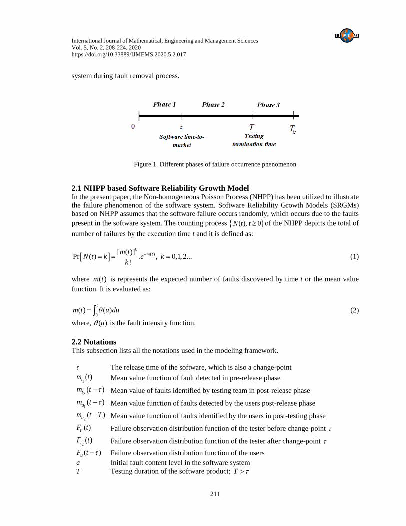
release testing phase and post-testing phase. These phases are graphically depicted in Figure 1.

Moreover, in factual testing scenario, the debugging process can never be perfect, i.e. not all

detected faults will be completely removed from the system. This can be due to tester’s proficiency

level and faults characteristics (Zhu and Pham 2018a). In addition, some faults that were not present

in the system earlier may become apparent after the debugging process. Therefore, in the present

study, the debugging process is considered imperfect as some new bugs may be induced in the


Vol. 5, No. 2, 208-224, 2020


211

system during fault removal process.

Figure 1. Different phases of failure occurrence phenomenon

2.1 NHPP based Software Reliability Growth Model In the present paper, the Non-homogeneous Poisson Process (NHPP) has been utilized to illustrate

the failure phenomenon of the software system. Software Reliability Growth Models (SRGMs)

based on NHPP assumes that the software failure occurs randomly, which occurs due to the faults

present in the software system. The counting process ( ), 0N t t of the NHPP depicts the total of

number of failures by the execution time t and it is defined as:

( )[ ( )]Pr ( ) . , 0,1,2...

!

km tm t

N t k e kk

(1)

where ( )m t is represents the expected number of faults discovered by time t or the mean value

function. It is evaluated as:

0( ) ( )

t

m t u du (2)

where, ( )u is the fault intensity function.

2.2 Notations This subsection lists all the notations used in the modeling framework.

The release time of the software, which is also a change-point

1( )tm t Mean value function of fault detected in pre-release phase

2( )tm t Mean value of faults identified by testing team in post-release phase

1( )um t Mean value function of faults detected by the users post-release phase

2( )um t T Mean value function of faults identified by the users in post-testing phase

1( )tF t Failure observation distribution function of the tester before change-point

2( )tF t Failure observation distribution function of the tester after change-point

( )uF t Failure observation distribution function of the users

a Initial fault content level in the software system

T Testing duration of the software product; T


Vol. 5, No. 2, 208-224, 2020


212

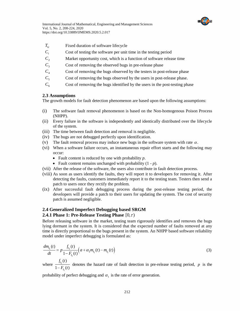
lcT Fixed duration of software lifecycle

1C Cost of testing the software per unit time in the testing period

2C Market opportunity cost, which is a function of software release time

3C Cost of removing the observed bugs in pre-release phase

4C Cost of removing the bugs observed by the testers in post-release phase

5C Cost of removing the bugs observed by the users in post-release phase.

6C Cost of removing the bugs identified by the users in the post-testing phase

2.3 Assumptions The growth models for fault detection phenomenon are based upon the following assumptions:

(i) The software fault removal phenomenon is based on the Non-homogenous Poison Process

(NHPP).

(ii) Every failure in the software is independently and identically distributed over the lifecycle

of the system.

(iii) The time between fault detection and removal is negligible.

(iv) The bugs are not debugged perfectly upon identification.

(v) The fault removal process may induce new bugs in the software system with rate .

(vi) When a software failure occurs, an instantaneous repair effort starts and the following may

occur:

Fault content is reduced by one with probability p.

Fault content remains unchanged with probability (1 - p).

(vii) After the release of the software, the users also contribute in fault detection process.

(viii) As soon as users identify the faults, they will report it to developers for removing it. After

detecting the faults, customers immediately report it to the testing team. Testers then send a

patch to users once they rectify the problem.

(ix) After successful fault debugging process during the post-release testing period, the

developers will provide a patch to their users for updating the system. The cost of security

patch is assumed negligible.

2.4 Generalized Imperfect Debugging based SRGM

2.4.1 Phase 1: Pre-Release Testing Phase [0, )

Before releasing software in the market, testing team rigorously identifies and removes the bugs

lying dormant in the system. It is considered that the expected number of faults removed at any

time is directly proportional to the bugs present in the system. An NHPP based software reliability

model under imperfect debugging is formulated as:

1 1

1 1

1

1

( ) ( )( ) ( )

1 ( )

t t

t t

t

dm t f tp a m t m t

dt F t

(3)

where 1

1

( )

1 ( )

t

t

f t

F t denotes the hazard rate of fault detection in pre-release testing period, p is the

probability of perfect debugging and 1 is the rate of error generation.


Vol. 5, No. 2, 208-224, 2020


213

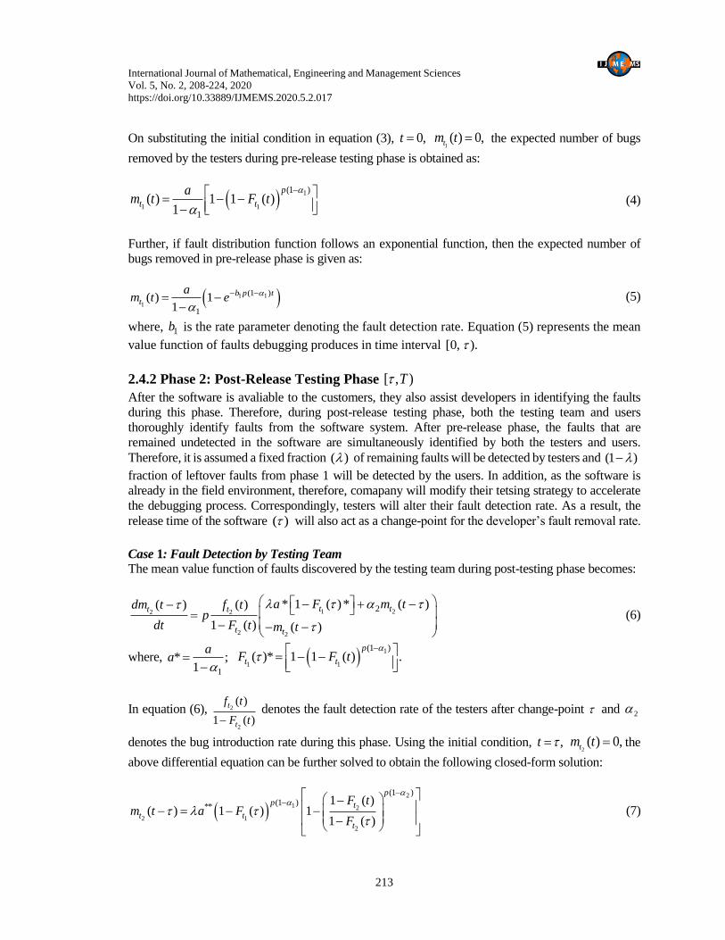
On substituting the initial condition in equation (3), 0,t 1( ) 0,tm t the expected number of bugs

removed by the testers during pre-release testing phase is obtained as:

1

1 1

(1 )

1

( ) 1 1 ( )1

p

t t

am t F t

(4)

Further, if fault distribution function follows an exponential function, then the expected number of

bugs removed in pre-release phase is given as:

1 1

1

(1 )

1

( ) 11

b p tt

am t e

(5)

where, 1b is the rate parameter denoting the fault detection rate. Equation (5) represents the mean

value function of faults debugging produces in time interval [0, ).

2.4.2 Phase 2: Post-Release Testing Phase [ , )T

After the software is avaliable to the customers, they also assist developers in identifying the faults

during this phase. Therefore, during post-release testing phase, both the testing team and users

thoroughly identify faults from the software system. After pre-release phase, the faults that are

remained undetected in the software are simultaneously identified by both the testers and users.

Therefore, it is assumed a fixed fraction ( ) of remaining faults will be detected by testers and (1 )

fraction of leftover faults from phase 1 will be detected by the users. In addition, as the software is

already in the field environment, therefore, comapany will modify their tetsing strategy to accelerate

the debugging process. Correspondingly, testers will alter their fault detection rate. As a result, the

release time of the software ( ) will also act as a change-point for the developer’s fault removal rate.

Case 1: Fault Detection by Testing Team

The mean value function of faults discovered by the testing team during post-testing phase becomes:

1 22 2

2 2

2* 1 ( )* ( )( ) ( )

1 ( ) ( )

t tt t

t t

a F m tdm t f tp

dt F t m t

(6)

where, 1

* ;1

aa

1

1 1

(1 )( )* 1 1 ( ) .

p

t tF F t

In equation (6), 2

2

( )

1 ( )

t

t

f t

F t denotes the fault detection rate of the testers after change-point and 2

denotes the bug introduction rate during this phase. Using the initial condition, ,t 2( ) 0,tm t the

above differential equation can be further solved to obtain the following closed-form solution:

2

1 2

2 1

2

(1 )

(1 )**1 ( )

( ) 1 ( ) 11 ( )

p

p t

t t

t

F tm t a F

F

(7)


Vol. 5, No. 2, 208-224, 2020


214

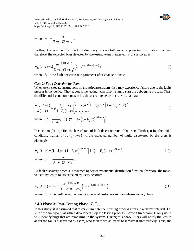
where, **

1 2

.(1 )(1 )

aa

Further, it is assumed that the fault discovery process follows an exponential distribution function,

therefore, the expected bugs detected by the testing team in interval [ , )T is given as:

1 1

2 2

2

(1 )(1 )( )

1 2

( ) 1(1 )(1 )

b pb p t

t

aem t e

(8)

where, 2b is the fault detection rate parameter after change-point .

Case 2: Fault Detection by Users

When users execute instructions on the software system, they may experience failure due to the faults

present in the device. They report it the testing team who instantly start the debugging process. Thus,

the differential equation representing the users bug detection rate is given as:

1 11

1

2(1 ) * 1 ( )* ( )( ) ( )

( ) 1 ( ) ( )

t uu u

u u

a F m tdm t f tp

d t F t m t

(9)

where, 1

* ;1

aa

1

1 1

(1 )( )* 1 1 ( ) .

p

t tF F t

In equation (9), signifies the hazard rate of fault detection rate of the users. Further, using the initial

condition, that at ,t 1( ) 0,um t the expected number of faults discovered by the users is

obtained:

1 2

1 1

(1 ) (1 )**( ) (1 ) 1 ( 1 1 ( )p p

u t um t a F F t

(10)

where, **

1 2

.(1 )(1 )

aa

As fault discovery process is assumed to depict exponential distribution function, therefore, the mean

value function of faults detected by users becomes:

1 1

3 2

1

(1 )(1 )( )

1 2

( ) (1 ) 1(1 )(1 )

b pb p t

u

aem t e

(11)

where, 3b is the fault detection rate parameter of customers in post-release testing phase.

2.4.3 Phase 3: Post-Testing Phase [ , ]lcT T

In this study, it is assumed that testers terminate their testing process after a fixed time interval. Let

T be the time-point at which developers stop the testing process. Beyond time-point T, only users

will identify bugs that are remaining in the system. During this phase, users will notify the testers

about the faults discovered by them, who then make an effort to remove it immediately. Thus, the


Vol. 5, No. 2, 208-224, 2020


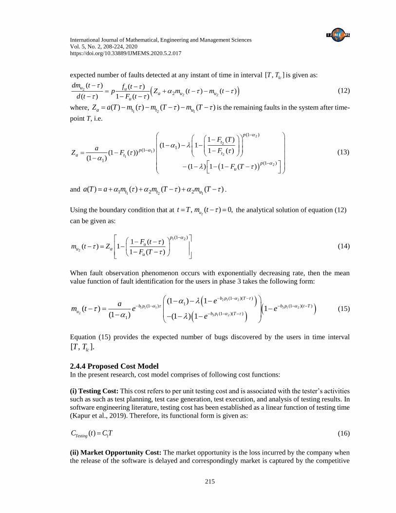
215

expected number of faults detected at any instant of time in interval [ , ]lcT T is given as:

2

2 22

( ) ( )( ) ( )

( ) 1 ( )

u ua u u

u

dm t f tp Z m t m t

d t F t

(12)

where, 1 2 1

( ) ( ) ( ) ( )a t t uZ a T m m T m T is the remaining faults in the system after time-

point T, i.e.

2

2

12

1

2

(1 )

1(1 )

1(1 )

1 ( )(1 ) 1

1 ( )(1 ( ))(1 )

(1 ) 1 1 ( )

p

t

pta t

p

u

F T

a FZ F

F T

(13)

and 1 2 11 2 2( ) ( ) ( ) ( )t t ua T a m m T m T .

Using the boundary condition that at 2

, ( ) 0,ut T m t the analytical solution of equation (12)

can be given as:

1 2

2

(1 )1 ( )

( ) 11 ( )

p

uu a

u

F tm t Z

F T

(14)

When fault observation phenomenon occurs with exponentially decreasing rate, then the mean

value function of fault identification for the users in phase 3 takes the following form:

2 1 2

3 1 21 1 1

23 1 2

(1 )( )

1(1 )( )(1 )

(1 )( )1

(1 ) 1( ) 1

(1 ) (1 ) 1

b p T

b p t Tb p

ub p T

eam t e e

e

(15)

Equation (15) provides the expected number of bugs discovered by the users in time interval

[ , ].lcT T

2.4.4 Proposed Cost Model In the present research, cost model comprises of following cost functions:

(i) Testing Cost: This cost refers to per unit testing cost and is associated with the tester’s activities

such as such as test planning, test case generation, test execution, and analysis of testing results. In

software engineering literature, testing cost has been established as a linear function of testing time

(Kapur et al., 2019). Therefore, its functional form is given as:

1( )TestingC t C T (16)

(ii) Market Opportunity Cost: The market opportunity is the loss incurred by the company when

the release of the software is delayed and correspondingly market is captured by the competitive


Vol. 5, No. 2, 208-224, 2020


216

firms. Market opportunity cost is the increasing function of the release time of the software. It is a

crucial parameter to take into consideration for decision makers as it assists in examining the market

manipulation by the competitors. In the past literature, the market opportunity cost is considered as

a quadratic function of the software time-to-market (Jiang et al., 2012). Therefore, following

functional form is used in the present study:

2

_ 2( )Market OppC t C (17)

(iii) Cost of Faults Removal in Pre-Release Testing Phase: This attribute comprises direct cost

associated with detecting and debugging the faults during the time interval [0, ). It is assumed a

linear function of the expected number of faults discovered during this period. Its functional form

is given as:

13( ) ( )pre release tC t C m (18)

(iv) Cost of Faults Removal in Post-Release Testing Phase: After the release of the software at

, both testers and customers identify the faults present in the system. Therefore, the cost function

during this phase is divided into two components. First component describes the cost of debugging

faults that were detected by the testers. The second component represents the cost of faults

debugging, which were identified by the users and then removed by the testing team. Therefore,

the functional form of the debugging cost during post-release testing phase becomes:

2 14 5( ) ( ) ( )post release t uC t C m T C m T (19)

(v) Cost of Faults Removal in Post-Testing Phase: After the testers stops the testing process at

time T, users may still encounter failure of the software system due to the bugs that were remained

undetected in the previous phases. Thus, users identify these bugs and immediately report it to the

developers who then quickly remove them. Therefore, the cost of debugging the faults detected

during period [ , ]lcT T is given as:

26( ) ( )post testing u lcC t C m T T (20)

Therefore, the total cost structure when field-testing is considered is given as:

1 2 1 2

2

1 2 3 4 5 6( , ) ( ) ( ) ( ) ( )ut t u lcC T C T C C m C m T C m T C m T T

(21)

Now, in the conventional approach, * *,T i.e. testing stop time and software release time

coincides. Then, the cost structure in no-field testing scenario will be:

1 2

2

1 2 3 6( ) ( ) ( )ut lcC C C C m C m T (22)

3. Optimization Model using Multi-Attribute Utility Theory The objective of the present study is to optimize software time-to-market and optimal testing

duration based on the cost-efficiency and reliability measures by considering the software release

time as change point for tester’s fault detection rate. Further, the proposed release time policy is


Vol. 5, No. 2, 208-224, 2020


217

compared with the traditional release time policy where no-field testing is involved. Therefore, two

optimization problems are formulated using the Multi-attribute utility theory (MAUT). MAUT is

a multi-criteria decision-making (MCDM) approach used for solving the optimization problem

considering multiple attributes with conflicting objectives (Keeney, 1971). Li et al. (2011) was the

first to incorporate this MCDM technique in the research field of software reliability. MAUT

comprises of following steps:

Step 1: Identify the appropriate factors for the study under consideration.

Step 2: Formulate the single attribute utility function (SAUF) for each factor.

Step 3: Estimate the weight parameters for each factor involved in the study.

Step 4: Develop the multi-attribute utility function (MAUF).

For the present study, the optimization problem can be explained using these four steps.

3.1 Selection of Attributes The critical factors that have the most relevance to the study should be considered in the

optimization model. These attributes should be quantifiable in a meaningful and practical way. The

principal concern of the software firms is to provide software to its users that are both reliable and

secure. Therefore, maximizing the reliability of the software product is the prime objective of the

decision makers when assessing the release time and testing duration of the system. A most

common indicator of reliability of a software system is the ratio of the expected number of bugs

removed by time t to the total fault content present in the software (Li et al., 2011). Thus, the first

factor included in the present study is:

For field-testing (FT) policy:

Maximize( , )

( )

m TR

a T

, i.e. (23)

Maximize 1 2 1

1 2 11 2

( ) ( ) ( )

( ) ( ( ) ( ))

t t u

t t u

m m T m TR

a m m T m T

(24)

For no-field testing (NFT) policy

Maximize 1

11

( )( )R

( ) ( )

t

t

mm

a a m

(25)

where, R is a reliability indicator used as a key factor in MAUT. It value ranges from 0 1.R As

the reliability is an increasing function of time, it reaches the maximum value when time goes to

infinity.

The second critical factor is the cost function associated with testing and debugging process. The

software firm wants to improve the quality of its product but at the minimal cost. Therefore, for

decision makers, the analysis of cost budget consumption plays an important role. Thus, the second

attribute cost function is given as:


Vol. 5, No. 2, 208-224, 2020


218

Under field-testing (FT) policy:

minimize ( , )

b

C TC

C

(26)

where, 1 2 1 2

2

1 2 3 4 5 6( , ) ( ) ( ) ( ) ( )ut t u lcC T C T C C m C m T C m T C m T T and bC

is

the companies budget allocated for testing and debugging process.

Under no field-testing (NFT) policy:

minimize ( )

b

CC

C

(27)

where, 1 2

2

1 2 3 6( ) ( ) ( )ut lcC C C C m C m T

3.2 Evaluate SAUF In MAUT, utility functions are used to depict goal of each factor. In literature, two functional forms

of utility function are commonly used: linear and exponential type (Kapur et al., 2019). The general

form of linear function is ( )u x l mx and of exponential is ( ) .pxu x l me For a particular study,

the functional form is determined using the interviews with the experts, survey or through lottery.

For the current research, linear form has been utilized based on the opinion of software experts and

analysts. Thus, the utility function of two factors, namely, reliability indicator and cost function is:

( ) c cu C l u C and ( ) r ru R l m R (28)

In addition, the utility function is bounded with the best, ( ) 1bestu x and the worst, ( ) 0worstu x

case scenario for each factor under consideration. Further, the bounds are measured based on the

managers and decision maker’s aspirations:

a) For the reliability indictor factor, minimum 60% of the faults must be detected and maximum

aspiration level is 100%.

b) For cost factor, the minimum budget requirement is 60% and the maximum obligation is 100%.

Therefore, the bounds for each factor is: 0.6worstC , 1,bestC 0.6worstR and 1.bestR Using

these boundary conditions, the SAUF for the two attributes will the following functional form:

( ) 2.5 1.5U C C and ( ) 2.5 1.5U R R (29)

3.3 Assign Weight Parameters to Each Attribute The weight parameter signifies the relative importance of an attribute over other attributes in the

optimization problem. When number of factors under consideration is small, lottery method or

management’s discretion is suggested. As in the present paper, only two factors have been utilized,

the priority to the factor is assigned on the management’s judgment. According to software

development managers, more importance should be given to the reliability indicator. Consequently,

weight given to reliability indicator is 0.6.Rw Additionally, the sum of the weight parameters


Vol. 5, No. 2, 208-224, 2020


219

should be 1. Thus, the weight assigned to cost factor is 0.4.cw

3.4 Formulation of MAUF Multi-attribute utility function is the arithmetic sum of all the single utility functions (SAUF). Thus,

the additive form of MAUF for the present study is given as:

( , ) ( ) ( )R CMax U R C w U R w U C (30)

where 1R cw w and U(R) and U(C) describes the single utility functions for factor reliability

indicator and cost respectively.

The objective of the software developers is to maximize the reliability indicator and minimize the

cost function. Therefore, to reflect the aim of minimizing the cost attribute, negative assign is

multiplied with cost component. On solving the above maximization problem, the optimal values

of decision variables * and *T will be obtained. From substituting the values from previous

steps, following functional form is attained:

( , ) 0.6 (2.5 1.5) 0.4 (2.5 1.5)Max U R C R C (31)

where

1R cw w and ( , )

1b

C T

C

(32)

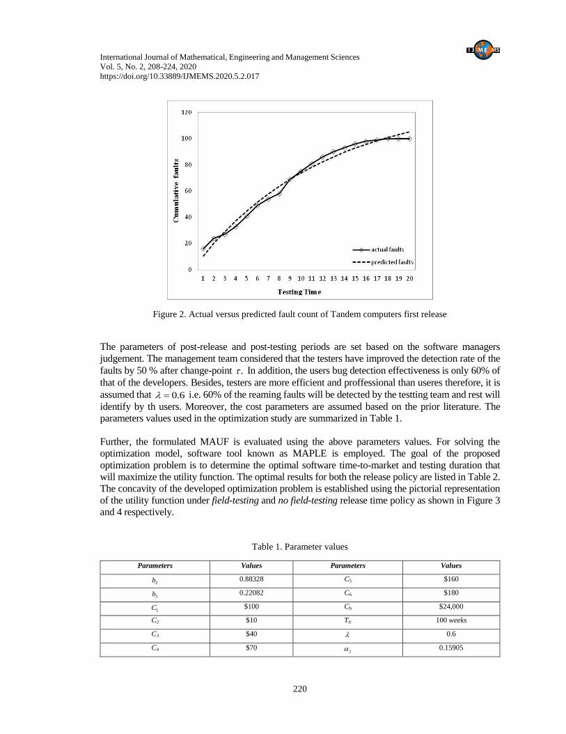
4. Numerical Illustration The estimation efficiency and prediction accuracy of the developed SRGM is asserted using the

actual fault count data of Tandem computers, which has been collected for the pre-release testing

period. Tandem computers data consists of four successive release failure data (Wood, 1996). As

the first release data follows an exponential growth pattern, therefore, for the current problem, the

first release data has been utilized. In the first release failure data, 100 faults were debugged in 20

weeks of testing period. The parameters estimation is carried-out using the nonlinear least square

(NLLS) regression technique (Marquardt, 1963). The complete empirical analysis is executed using

the software package known as SAS (SAS/ETS User’s Guide, 2004). The estimated values of the

model parameters are: 1 1107.65, 0.55205, = 0.185, = 0.15905.a b p To examine the

prediction capability of the model, two statistical measures, namely root mean square error (RMSE)

and R-square are determined. The values of goodness-of-fit measures are RMSE =3.607 and R2 =

0.986. The graphical depiction of actual versus predicted fault count is shown in Figure 2.


Vol. 5, No. 2, 208-224, 2020


220

Figure 2. Actual versus predicted fault count of Tandem computers first release

The parameters of post-release and post-testing periods are set based on the software managers

judgement. The management team considered that the testers have improved the detection rate of the

faults by 50 % after change-point . In addition, the users bug detection effectiveness is only 60% of

that of the developers. Besides, testers are more efficient and proffessional than useres therefore, it is

assumed that 0.6 i.e. 60% of the reaming faults will be detected by the testting team and rest will

identify by th users. Moreover, the cost parameters are assumed based on the prior literature. The

parameters values used in the optimization study are summarized in Table 1.

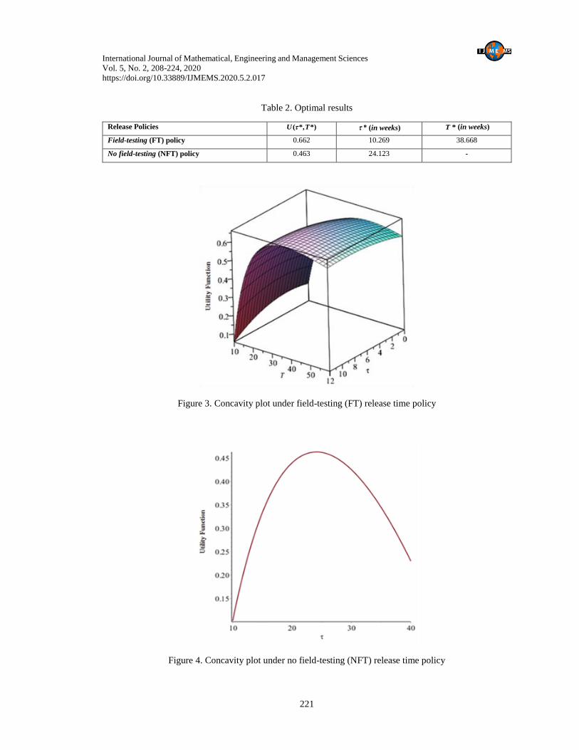
Further, the formulated MAUF is evaluated using the above parameters values. For solving the

optimization model, software tool known as MAPLE is employed. The goal of the proposed

optimization problem is to determine the optimal software time-to-market and testing duration that

will maximize the utility function. The optimal results for both the release policy are listed in Table 2.

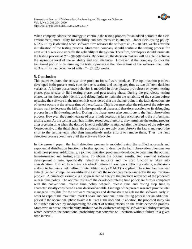
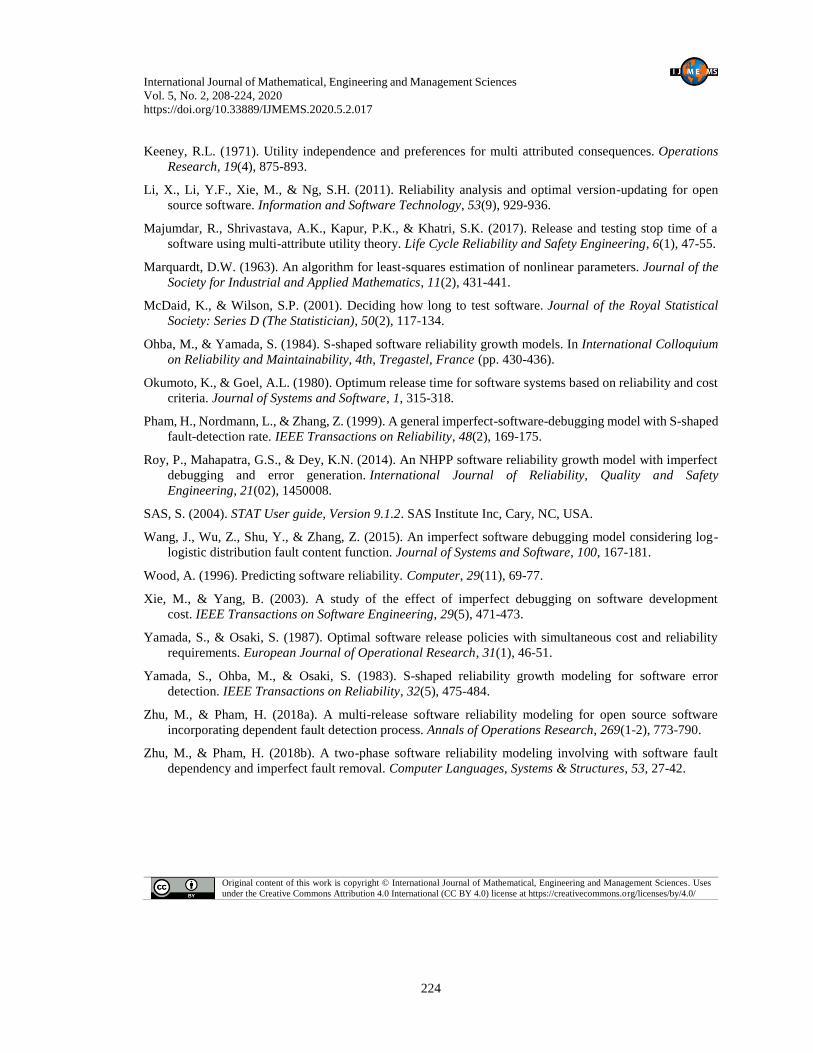
The concavity of the developed optimization problem is established using the pictorial representation

of the utility function under field-testing and no field-testing release time policy as shown in Figure 3

and 4 respectively.

Table 1. Parameter values

Parameters Values Parameters Values

2b 0.88328 C5 $160

3b 0.22082 C6 $180

1C $100 Cb $24,000

C2 $10 Tlc 100 weeks

C3 $40 0.6

C4 $70 2 0.15905


Vol. 5, No. 2, 208-224, 2020


221

Table 2. Optimal results

Release Policies ( *, *)U T * (in weeks) *T (in weeks)

Field-testing (FT) policy 0.662 10.269 38.668

No field-testing (NFT) policy 0.463 24.123 -

Figure 3. Concavity plot under field-testing (FT) release time policy

Figure 4. Concavity plot under no field-testing (NFT) release time policy


Vol. 5, No. 2, 208-224, 2020


222

When company adopts the strategy to continue the testing process for an added period in the field

environment, more utility for reliability and cost measure is attained. Under field-testing policy,

66.2% utility is obtained when software firm releases the software at * 10.012 weeks after the

initialization of the testing process. Moreover, company should continue the testing process for

next 28.399 weeks to improve the reliability of the system. Therefore, developers should terminate

the testing process at * 38.668T weeks. By doing so, the decision makers will be able to achieve

the aspiration level of the reliability and cost attributes. However, if the company follows the

traditional policy of terminating the testing process at the release time of the software, then only

46.3% utility can be achieved with * 24.123 weeks.

5. Conclusion This paper explores the release time problem for software products. The optimization problem

developed in the present study considers release time and testing stop time as two different decision

variables. A failure occurrence behavior is modeled in three phases: pre-release or system testing

phase, post-release or field-testing phase, and post-testing phase. During the pre-release testing

phase, testers thoroughly identify and debug faults to maintain the reliability of the system before

releasing the software in the market. It is considered that the change-point in the fault detection rate

of testers occurs at the release time of the software. This is because, after the release of the software,

testers want to decrease the failure in the operational phase and therefore, accelerates its debugging

process in the field-testing period. During this phase, users also contribute to the fault observation

process. However, the combined rate of user’s fault detection is less as compared to the professional

testing team. As the testing team has limited resources, therefore, they terminate the testing process

after a certain time when the desired level of reliability is attained after the release of the software.

Consequently, in the third phase, the post-testing phase only users observe the faults and report the

error to the testing team who then immediately make efforts to remove them. Thus, the fault

detection process continues until the software lifecycle.

In the present paper, the fault detection process is modeled using the unified approach and

exponential distribution function is further applied to describe the fault observation phenomenon

in all three phases. Additionally, a joint optimization problem is developed to determine the optimal

time-to-market and testing stop time. To obtain the optimal results, two essential software

development criteria, specifically, reliability indicator and the cost function is taken into

consideration. Further, to achieve a trade-off between these two conflicting criteria, a decision-

making technique called multi-attribute utility theory (MAUT) is applied. The actual fault content

data of Tandem computers are utilized to estimate the model parameters and solve the optimization

problem. A numerical example is also presented to analyze the practical relevance of the proposed

release time policy. The optimal results of the developed release time policy are further compared

with the conventional release time policy wherein release time and testing stop time is

characteristically considered as one decision variable. Findings of the present research provide vital

managerial insights for the software managers and demonstrate to release the software early in

order to capture the maximum market share and continue to the testing process for an additional

period in the operational phase to avoid failures at the user end. In addition, the proposed study can

be further extended by incorporating the effect of testing efforts on the faults detection process.

Moreover, in future, the reliability attribute can be evaluated using the software reliability function,

which describes the conditional probability that software will perform without failure in a given

time interval.


Vol. 5, No. 2, 208-224, 2020


223

Conflict of Interest

The authors declare that there is no conflict of interest for this publication.

Acknowledgment

The research work presented in this paper is supported by grants to the first author from DST via DST PURSE phase II,

India.

References

Arora, A., Caulkins, J.P., & Telang, R. (2006). Research note-sell first, fix later: impact of patching on

software quality. Management Science, 52(3), 465-471.

Dalal, S.R., & Mallows, C.L. (1988). When should one stop testing software? Journal of the American

Statistical Association, 83(403), 872-879.

Goel, A.L., & Okumoto, K. (1979). Time-dependent error-detection rate model for software reliability and

other performance measures. IEEE Transactions on Reliability, 28(3), 206-211.

Jiang, Z., Sarkar, S., & Jacob, V.S. (2012). Postrelease testing and software release policy for enterprise-

level systems. Information Systems Research, 23(3-part-1), 635-657.

Kapur, P.K., & Garg, R.B. (1992). A software reliability growth model for an error-removal

phenomenon. Software Engineering Journal, 7(4), 291-294.

Kapur, P.K., Gupta, A., & Singh, O. (2005). On discrete software reliability growth model & categorization

of faults. Opsearch, 42(4), 340-354.

Kapur, P.K., Gupta, A., Yadavalli, V.S.S., & Claasen, S.J. (2006). Flexible software reliability growth

models. South African Journal of Industrial Engineering, 17(2), 109-125.

Kapur, P.K., Khatri, S.K., Tickoo, A., & Shatnawi, O. (2014). Release time determination depending on

number of test runs using multi attribute utility theory. International Journal of System Assurance

Engineering and Management, 5(2), 186-194.

Kapur, P.K., Kumar, S., & Garg, R.B. (1999). Contributions to hardware and software reliability. World

Scientific, Singapore.

Kapur, P.K., Panwar, S., Singh, O., & Kumar, V. (2019). Joint release and testing stop time policy with

testing-effort and change point. In Risk Based Technologies (pp. 209-222). Springer, Singapore.

Kapur, P.K., Pham, H., Anand, S., & Yadav, K. (2011). A unified approach for developing software reliability

growth models in the presence of imperfect debugging and error generation. IEEE Transactions on

Reliability, 60(1), 331-340.

Kapur, P.K., Pham, H., Gupta, A., & Jha, P.C. (2011). Software reliability assessment with OR applications.

Springer, London.

Kapur, P.K., Singh, J.N., & Singh, O. (2015). Application of multi attribute utility theory in multiple releases

of software. International Journal of System Assurance Engineering and Management, 6(1), 61-70.

Kapur, P.K., Singh, O., Garmabaki, A.S., & Singh, J. (2010). Multi up-gradation software reliability growth

model with imperfect debugging. International Journal of System Assurance Engineering and

Management, 1(4), 299-306.

Kapur, P.K., Singh, V.B., Anand, S., & Yadavalli, V.S.S. (2008). Software reliability growth model with

change-point and effort control using a power function of the testing time. International Journal of

Production Research, 46(3), 771-787.


Vol. 5, No. 2, 208-224, 2020


224

Keeney, R.L. (1971). Utility independence and preferences for multi attributed consequences. Operations

Research, 19(4), 875-893.

Li, X., Li, Y.F., Xie, M., & Ng, S.H. (2011). Reliability analysis and optimal version-updating for open

source software. Information and Software Technology, 53(9), 929-936.

Majumdar, R., Shrivastava, A.K., Kapur, P.K., & Khatri, S.K. (2017). Release and testing stop time of a

software using multi-attribute utility theory. Life Cycle Reliability and Safety Engineering, 6(1), 47-55.

Marquardt, D.W. (1963). An algorithm for least-squares estimation of nonlinear parameters. Journal of the

Society for Industrial and Applied Mathematics, 11(2), 431-441.

McDaid, K., & Wilson, S.P. (2001). Deciding how long to test software. Journal of the Royal Statistical

Society: Series D (The Statistician), 50(2), 117-134.

Ohba, M., & Yamada, S. (1984). S-shaped software reliability growth models. In International Colloquium

on Reliability and Maintainability, 4th, Tregastel, France (pp. 430-436).

Okumoto, K., & Goel, A.L. (1980). Optimum release time for software systems based on reliability and cost

criteria. Journal of Systems and Software, 1, 315-318.

Pham, H., Nordmann, L., & Zhang, Z. (1999). A general imperfect-software-debugging model with S-shaped

fault-detection rate. IEEE Transactions on Reliability, 48(2), 169-175.

Roy, P., Mahapatra, G.S., & Dey, K.N. (2014). An NHPP software reliability growth model with imperfect

debugging and error generation. International Journal of Reliability, Quality and Safety

Engineering, 21(02), 1450008.

SAS, S. (2004). STAT User guide, Version 9.1.2. SAS Institute Inc, Cary, NC, USA.

Wang, J., Wu, Z., Shu, Y., & Zhang, Z. (2015). An imperfect software debugging model considering log-

logistic distribution fault content function. Journal of Systems and Software, 100, 167-181.

Wood, A. (1996). Predicting software reliability. Computer, 29(11), 69-77.

Xie, M., & Yang, B. (2003). A study of the effect of imperfect debugging on software development

cost. IEEE Transactions on Software Engineering, 29(5), 471-473.

Yamada, S., & Osaki, S. (1987). Optimal software release policies with simultaneous cost and reliability

requirements. European Journal of Operational Research, 31(1), 46-51.

Yamada, S., Ohba, M., & Osaki, S. (1983). S-shaped reliability growth modeling for software error

detection. IEEE Transactions on Reliability, 32(5), 475-484.

Zhu, M., & Pham, H. (2018a). A multi-release software reliability modeling for open source software

incorporating dependent fault detection process. Annals of Operations Research, 269(1-2), 773-790.

Zhu, M., & Pham, H. (2018b). A two-phase software reliability modeling involving with software fault

dependency and imperfect fault removal. Computer Languages, Systems & Structures, 53, 27-42.

Original content of this work is copyright © International Journal of Mathematical, Engineering and Management Sciences. Uses

under the Creative Commons Attribution 4.0 International (CC BY 4.0) license at https://creativecommons.org/licenses/by/4.0/

Determining Software Time-to-Market and Testing Stop ... - DOI

Documents