Determination of water quality parameters in Indian ponds using remote sensing methods

© EARSeL and Warsaw University, Warsaw 2005. Proceedings of 4th EARSeL Workshop on Imaging Spectroscopy. New quality in environmental studies. Zagajewski B., Sobczak M., Wrzesień M., (eds)

DETERMINATION OF WATER QUALITY PARAMETERS IN INDIAN PONDS USING REMOTE SENSING METHODS

Mathias Kneubühler1, Christian Gemperli1, Daniel Schläpfer1, Rainer Zah2 and Klaus Itten1

1. Remote Sensing Laboratories (RSL), University of Zürich, Winterthurerstrasse 190, 8057 Zürich, Switzerland, [email protected]

2. Swiss Federal Laboratories for Materials Testing and Research (EMPA), Lerchenfeldstrasse 5, 9014 St. Gallen, Switzerland

ABSTRACT This paper presents a water quality study performed on five small domestic ponds and one bayou of the Ganga river in the State of West Bengal, India. The concept of eutrophication is used to de-scribe water quality by using chlorophyll as an indicator for the presence of algae in the water.

During a field campaign in May 2003, reflectance spectra were measured 1m above the water sur-face using a handheld spectroradiometer. Concentration of Total Chlorophyll Content (TCHL) and other limnological standard parameters such as Secchi Disk Depth (SDD), nutrient content, Total Organic Content (TOC) and Dissolved Organic Content (DOC) were determined using laboratory analysis and a colorimetric testkit. A comparison of several existing semi-empirical algorithms to determine chlorophyll content was made by applying them to the spectra and chlorophyll meas-urements collected in-situ. Simple Reflectance Band Ratio and Continuum Interpolated Band Ratio (CIBR) were tested at several wavelengths. Another three tested algorithms rely on the reflectance peak at 700 nm whose shape and position depend strongly upon chlorophyll concentration: The Area and Magnitude of the Peak above a Baseline as well as the Position of the Peak show a lin-ear relationship to CHL-a concentration from laboratory spectrophotometric measurements. All algorithms proved to be of value. Best results were obtained by using the algorithms Peak Magni-tude above a Baseline and CIBR, which yielded R2 around 0.97 and mean deviations around 20 µg/l.

The algorithms were further applied to spectra convolved to the bands of the hyperspectral sen-sors APEX, HyMap and Hyperion. A comparison of the spectral characteristics of the chosen sen-sors was made in regard of their suitability for water quality determination. The differences on the outcome of the sensors were small, but the results indicate that an intermediate band width of around 10 nm seems appropriate. All sensors showed an adequate band positioning for the algo-rithms based on the peak near 700 nm. Using Simple Band Ratios and CIBR, APEX and Hyperion perform slightly better than HyMap.

1. INTRODUCTION The scope of this study is to investigate the potential of algorithms for monitoring water quality pa-rameters in West Bengal ponds, many of them being used for jute retting. The concept of eutrophi-cation was chosen to describe water quality, using chlorophyll as indicator for the presence of al-gae in the water. A semi-empirical approach was used to determine the parameter. The algorithms chosen from the literature had to perform well in other studies on water bodies with comparable limnological characteristics.

The aims of the study are:

the assessment of the trophic state of the ponds,

the evaluation of semi-empirical algorithms for determining CHL-a content using spectral reflectance data collected with a handheld field-spectroradiometer,


the application of these algorithms to the spectra convolved to the bands of selected sen-sors,

the evaluation of the most suitable sensors and applied algorithms for determining CHL-a content in the study area.

1.1. Water Quality There is no single definition of water quality, as it depends on the respective processes and on the intended use of the water. In this work the focus is laid on the process of eutrophication. Trophic state is an absolute scale that describes the biological condition of a water body and does not im-ply a normative statement per se. It has to be stressed that trophic state is not the same thing as water quality but trophic state certainly is one aspect of water quality.

Eutrophication The term ‘eutrophication’ means nutrient enrichment of lakes and describes the processes in water caused through over-enrichment by nutrients. Too much nutrient input causes a chain of events that may have undesirable effects on lakes, e.g. growth of algae and macrophytes. The enhanced rates of decomposition and attendant consumption of oxygen lead finally to oxygen depletion in the hypolimnion, decreasing the number of species. Eutrophication can occur under natural conditions, but often the process is induced by anthropological factors, such as fertilizers and sewage [4]. Or-ganic matter introduced to surface waters (e.g. jute), leads to enhanced rates of decomposition and attendant consumption of oxygen.

2. DATA ACQUISITION BASELINE 2.1. Study Area The study area is situated in the state of West Bengal (Nadia District), India. Agriculture plays a pivotal role in the state's income, and nearly three out of four persons in the state are directly or indirectly involved in agriculture. The state accounted for 66.5 % of the country's jute production including mesta in 1993-1994.

The summer months are from March to June. The monsoon season lasts from June to September and brings heavy rain. The monsoon brings respite to the parched plains but they often cause floods and landslides. The winter months are from October to February. Summer temperatures range from 24˚C to 40˚C and winter temperatures from 7˚C to 26˚C. The yearly average rainfall is around 175 cm.

Nadia District is located in the low-land basin of the Ganga river northeast of the state’s capital, Kolkata. As it can be seen in Fig.1 (left), the rural area is scattered with small ponds and bayous (oxbow lakes) of the Hooghly river which crosses the district in the south. Their sizes vary between a few square meters to several square kilometers. Many of them are man made, serving as water reservoirs for various purposes, such as washing, bathing, irrigation, fishing and jute retting.

Between May 23, and June 6, 2003, a field campaign was organized in the above mentioned area. The aims of the campaign were to collect physical-chemical parameters and spectral data on jute fields and water bodies of this region. As there was very little knowledge about the water bodies and the general circumstances prior to the campaign, the selection of the water bodies had to be made during the campaign. The following criteria were considered:

All ponds must be suitable for jute retting, being a major cause for eutrophication.

Minimum size must be 150 m x 100 m.

The water bodies must be easily accessible.

The permission of the owner must be obtained.

A broad range of estimated reflectance spectra should be in the samples of the selected water bodies (estimation through water color and turbidity).

302


All ponds have neither an in- nor an outlet and are only fed by rainwater and by periodical flooding during monsoon season. It can be assumed that the limnological cycle varies strongly during the year. In autumn, the heavy monsoon floods fill the ponds and large amounts of nutrients are probably washed into the ponds from the neighboring fields. At this time, the water bodies have been described to be very clear by the local farmers. In spring, with rising temperatures, bio-activity of the ponds rise and evaporation and human use causes the water level to fall several meters.

2.2. Field Measurement Data 2.2.1. Spectral Data The radiometric characterization of the selected ponds was determined by using a FieldSpec Pro FR Spectroradiometer from Analytical Spectral Devices (ASD) [1]. Reflectance measurements were made at 400 to 2500 nm at a spectral resolution of 1nm, with a fore-optic FOV of 8˚. Spectra were recorded using a white reference panel (spectralon) to obtain absolute reflectance values. The spectral measurements took place between 10 am and 14 pm. The sky conditions were for the most parts hazy with some high-level clouds, as it is typical before the arrival of the monsoon. Spectral data was taken from 6 ponds, four of them were covered with 1-2 transects using a boat (P1, P2, P5, P6). At two ponds (P3, P4), measurements were made only at the shoreline. At each pond, approximately 150 single spectra were recorded (see Fig.1).

2.2.2. Water Constituents Data It was the aim of the campaign to get a broad overview of the general state of the water bodies, upon which several limnological parameters were determined. The limnological sampling was per-formed on the same day as spectral characterization of the water. In all ponds, one water sample was taken at a location in the middle of the water body; in bigger ponds, an additional sample was taken nearer to the shoreline. Due to the shallowness of the ponds and low SDD values, mixed samples were taken from the surface to SDD (Integrated SDD). Storage of the samples deter-mined in India was done according to the procedure described by Lindell et al. [16]. Immediately after sampling and during transport, all samples were stored cool using ice. Within 4 hours, they were either brought to the laboratory and deep frozen until parameter determination or analyzed in the field using a colorimetric testkit.

Fig. 1: Left: Landsat ETM panchromatic image of the study site, acquired on April 22, 2002; right: averaged spectra of each water body. The numbers indicate its CHL concentration in µg/L. The concentration in brackets was determined one week before and was not included into analysis.

The determination of TCHL, DOC and TOC was done by the Department of Agricultural Chemi-cals, University of Bidhan Chandra Krishi Viswavidyalaya, Mohanpur. It was intended to use the standard method according ISO 10260 [16] for determination of CHL-a, but as the laboratory was not used to this method, Annon’s method was applied. Chlorophyll content of the samples was

303


assessed by spectrophotometric determination of the acetone extract of the sample at 645 and 663 nm. Dissolved organic carbon was determined by using the dichromate oxidation method of Vance et al. Total organic carbon was determined using the Nelson Somer’s method. Secchi Disk Depth was recorded using the procedure described by Lindell et al. [16].

Hence, all of the ponds were very shallow at the time of the campaign. Maximum measured depth did not exceed 1m in all of the ponds. Large amounts of yellow substances and inorganic solids are suspended in the water leading to a very poor visibility. SDD did not exceed 0.12 m in the do-mestic ponds, in P5 it was approx. 0.9 m (Fig.1). In the domestic ponds, (all ponds, excluding P5) measured concentrations of TCHL were extremely high, most with contents between 300 and 520 µg/L (see Fig.1, right). Such high concentrations normally characterize a bloom situation, which should be indicated by scum on the surface. This could only be observed in P3.

A concentration of 0 µg/L was determined for both samples of P5, but analysis of the spectra show that there must be at least small contents of chlorophyll. Either laboratory analysis failed or the concentrations were below the detection limit. Regarding these contradictions, there rests an un-certainty about the accuracy of the chlorophyll determination at the laboratory.

Given the fact that the vast majority of algae in a water body are cyanobacteria that only contain CHL-a [16], the TCHL concentration measured in the laboratory is assumed to represent the con-centration of CHL-a, solely.

A variety of further limnological parameters (e.g., nutrient content, organic carbon, pH, total hard-ness, heavy metals, water temperature), that were also determined during the field campaign are not presented in this paper.

3. METHODOLOGY OF PARAMETER RETRIEVAL 3.1. Methods used in this study A wide range of different algorithms and models can be found in literature to estimate chlorophyll content in Case II waters. The semi-analytical algorithms applied in this work are all based on the use of reflectance data in the red and NIR range of the electromagnetic spectrum, since other por-tions of the spectrum are not suitable for chlorophyll estimation in Case II waters [6][10].

Since there was no knowledge about the general state of the water bodies, appropriate models had do be selected after the campaign. Semi-empirical models were chosen as an intermediate stage between the complex physical approaches and empirical approaches. Since chemical-physical in-situ data indicated a hypertrophic state of most of the sampled water bodies, the focus had to be laid on models which were already successfully tested in previous studies on water bod-ies with very high CHL content.

However, very few studies can be found in literature which have dealt with hyper-eutrophic water bodies with CHL concentrations over 100 µg/L. The only study which used semi-empirical algo-rithms other than simple band ratios, was done by Gitelson. He applied several algorithms, which are all related to the peak near 700 nm. All of them were successfully used to estimate CHL con-centrations in water bodies of different trophic states, e.g. in wastewater ponds, where chloro-phytes algae dominated with extremely high CHL-a concentrations ranging from 70 to 520 µg/L [8][9][10][19].

Simple band ratios were chosen because they are robust and easily applicable. In addition, they had already been applied in numerous studies on water bodies of all trophic states [6][10][13][14][16][20].

Finally the Continuum Interleaved Band Ratio (CIBR) was selected because it was used in a previ-ous study to estimate chlorophyll concentration in inland water [14]. However, in contrary to the Indian ponds, the CHL concentration in that study from a Swiss lake was very low. Thus, it is nec-essary to verify if the algorithm could be applied on water bodies with high concentrations.

304


3.2. Chlorophyll Determination Algorithms Simple Band Ratio Band ratios determine the amount of absorption by the use of a measurement channel, which is divided through a reference channel.

)()(

r

m

RR

BRλλ

= ,

where R is the Reflectance, m indicates the measurement channel and r the reference channel.

The reflectance in the measurement channel should only be influenced by the absorption of the parameter. The reflectance of the reference channel should not be influenced by any kind of water constituents [14].

Fig. 2: Simple Band Ratio Algorithm.

Various authors such as Dekker [6], Koponen et al. [13] and Yacobi et al. [22] concluded that for the retrieval of CHL-a concentration, a ratio of channels centered at about 675 and 705 nm is ap-propriate in several lake types ranging from oligotrophic to hypertrophic state (Fig.2). As the band combination depends on the chlorophyll content range of the water bodies and therefore on the position of the reflectance peak, the used wavelength of the algorithm have to be slightly modified in most cases [12].

Continuum Interpolated Band Ratio (CIBR) The Continuum Interpolated Band Ratio uses two reference bands instead of one. The advantage of the method over a simple band ratio is that the unequal influence of scattering by other water constituents on the reference and the absorption band is eliminated.

)()()(

2211 rr

m

RcRcR

CIBRλλ

λ+

= ,

where R is the reflectance at a given wavelength �, index m indicates the absorption band. r1 and r2 indicate the two reference channels, given through

)()(

,)(

)(

12

12

22

11

rr

rm

rr

m ccλλλλ

λλλλ

−−

=−−

= .

By using linear interpolation between two reference bands at each side of the absorption band, a reference value with 'normalized influence of scattering' is simulated on the absorption band. The absorption value is then divided by a reference value similarly affected by scattering, diminishing the influence of scattering on the ratio [14]. This method, originally applied by Bruegge et al. [3] in order to estimate water vapor in the atmosphere, was used for the first time by Kurer [14] for de-termination of CHL-a concentration.

305


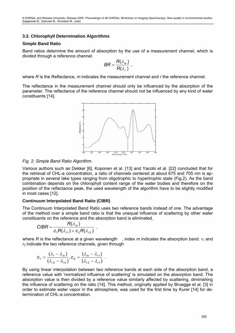
Fig. 3: Continuum Interpolated Band Ratio (CIBR).

Area above a Baseline Gitelson et al. [10] proposed an algorithm based on the area delimited by the reflectance curve and a baseline drawn from 670 to 750 nm (Fig.4):

∫ −=b

a

dxxgxfA )()( ,

with [a,b] as delimiters on the reflectance curve and f, g on [a,b] with f(x) ≥ g(x) ≥ 0.

The developed algorithm was tested and validated by Gitelson et al. [10] in several water bodies ranging from oligotrophic to hypertrophic state. They found linear relationships between the area above the base line and CHL concentration with high R2 around 0.9. The algorithms were also used to determine CHL content in wastewater with CHL concentrations ranging between 70-520 µg/L, which is comparable to the content of the ponds in West Bengal. They yielded correlation coefficients R2 of 0.88, with a standard error of 59 µg/L [10].

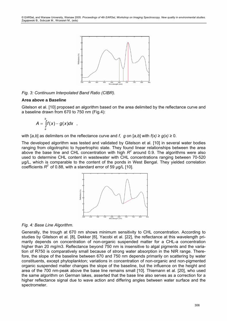
Fig. 4: Base Line Algorithm.

Generally, the trough at 670 nm shows minimum sensitivity to CHL concentration. According to studies by Gitelson et al. [8], Dekker [6], Yacobi et al. [22], the reflectance at this wavelength pri-marily depends on concentration of non-organic suspended matter for a CHL-a concentration higher than 20 mg/m3. Reflectance beyond 750 nm is insensitive to algal pigments and the varia-tion of R750 is comparatively small because of strong water absorption in the NIR range. There-fore, the slope of the baseline between 670 and 750 nm depends primarily on scattering by water constituents, except phytoplankton; variations in concentration of non-organic and non-pigmented organic suspended matter changes the slope of the baseline, but the influence on the height and area of the 700 nm-peak above the base line remains small [10]. Thiemann et al. [20], who used the same algorithm on German lakes, asserted that the base line also serves as a correction for a higher reflectance signal due to wave action and differing angles between water surface and the spectrometer.

306


Peak Magnitude above a Baseline The height of the mentioned peak above a baseline was related to CHL-a concentration for the first time by Neville and Gower [17]:

)()( mmPeak gfM λλ −= ,

where f(λm) is the spectrum curve and g(λm) the baseline; (λm) defines the wavelength of the maxi-mum reflectance of the peak.

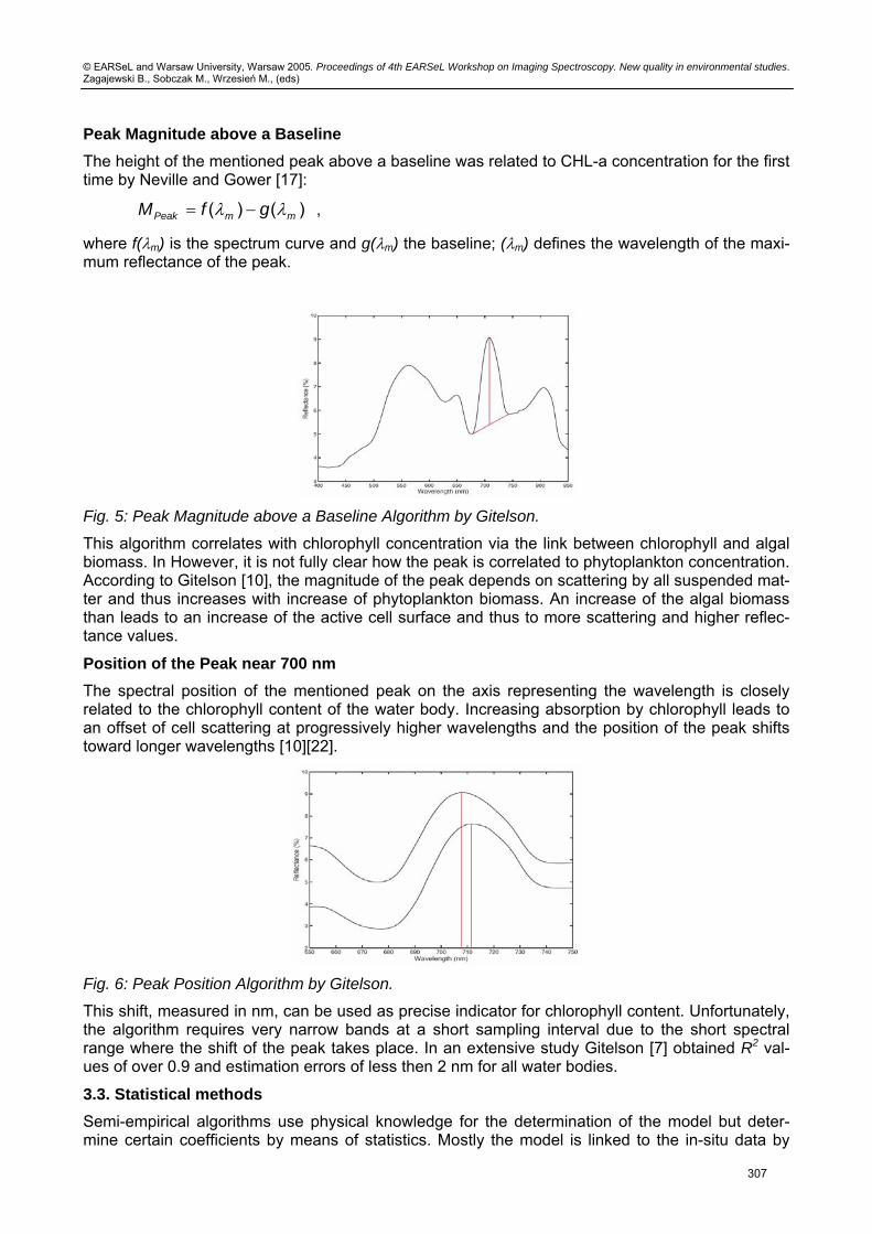
Fig. 5: Peak Magnitude above a Baseline Algorithm by Gitelson.

This algorithm correlates with chlorophyll concentration via the link between chlorophyll and algal biomass. In However, it is not fully clear how the peak is correlated to phytoplankton concentration. According to Gitelson [10], the magnitude of the peak depends on scattering by all suspended mat-ter and thus increases with increase of phytoplankton biomass. An increase of the algal biomass than leads to an increase of the active cell surface and thus to more scattering and higher reflec-tance values.

Position of the Peak near 700 nm The spectral position of the mentioned peak on the axis representing the wavelength is closely related to the chlorophyll content of the water body. Increasing absorption by chlorophyll leads to an offset of cell scattering at progressively higher wavelengths and the position of the peak shifts toward longer wavelengths [10][22].

Fig. 6: Peak Position Algorithm by Gitelson.

This shift, measured in nm, can be used as precise indicator for chlorophyll content. Unfortunately, the algorithm requires very narrow bands at a short sampling interval due to the short spectral range where the shift of the peak takes place. In an extensive study Gitelson [7] obtained R2 val-ues of over 0.9 and estimation errors of less then 2 nm for all water bodies.

3.3. Statistical methods Semi-empirical algorithms use physical knowledge for the determination of the model but deter-mine certain coefficients by means of statistics. Mostly the model is linked to the in-situ data by

307


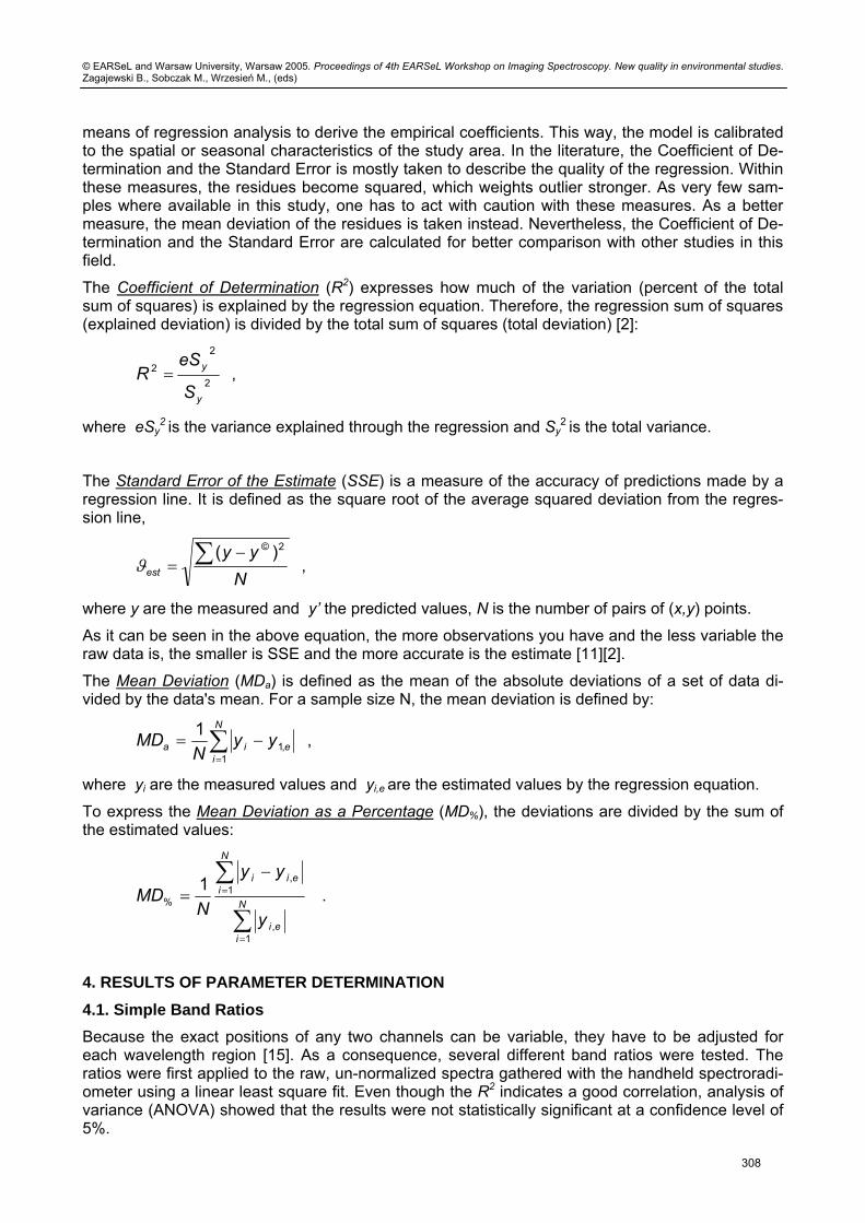
means of regression analysis to derive the empirical coefficients. This way, the model is calibrated to the spatial or seasonal characteristics of the study area. In the literature, the Coefficient of De-termination and the Standard Error is mostly taken to describe the quality of the regression. Within these measures, the residues become squared, which weights outlier stronger. As very few sam-ples where available in this study, one has to act with caution with these measures. As a better measure, the mean deviation of the residues is taken instead. Nevertheless, the Coefficient of De-termination and the Standard Error are calculated for better comparison with other studies in this field.

The Coefficient of Determination (R2) expresses how much of the variation (percent of the total sum of squares) is explained by the regression equation. Therefore, the regression sum of squares (explained deviation) is divided by the total sum of squares (total deviation) [2]:

2

2

2

y

y

S

eSR = ,

where eSy2 is the variance explained through the regression and Sy

2 is the total variance.

The Standard Error of the Estimate (SSE) is a measure of the accuracy of predictions made by a regression line. It is defined as the square root of the average squared deviation from the regres-sion line,

Nyy

est∑ −

=2© )(

ϑ ,

where y are the measured and y’ the predicted values, N is the number of pairs of (x,y) points.

As it can be seen in the above equation, the more observations you have and the less variable the raw data is, the smaller is SSE and the more accurate is the estimate [11][2].

The Mean Deviation (MDa) is defined as the mean of the absolute deviations of a set of data di-vided by the data's mean. For a sample size N, the mean deviation is defined by:

∑=

−=N

ieia yy

NMD

1,1

1 ,

where yi are the measured values and yi,e are the estimated values by the regression equation.

To express the Mean Deviation as a Percentage (MD%), the deviations are divided by the sum of the estimated values:

∑

∑

=

=

−= N

iei

N

ieii

y

yy

NMD

1,

1,

%1

.

4. RESULTS OF PARAMETER DETERMINATION 4.1. Simple Band Ratios Because the exact positions of any two channels can be variable, they have to be adjusted for each wavelength region [15]. As a consequence, several different band ratios were tested. The ratios were first applied to the raw, un-normalized spectra gathered with the handheld spectroradi-ometer using a linear least square fit. Even though the R2 indicates a good correlation, analysis of variance (ANOVA) showed that the results were not statistically significant at a confidence level of 5%.

308


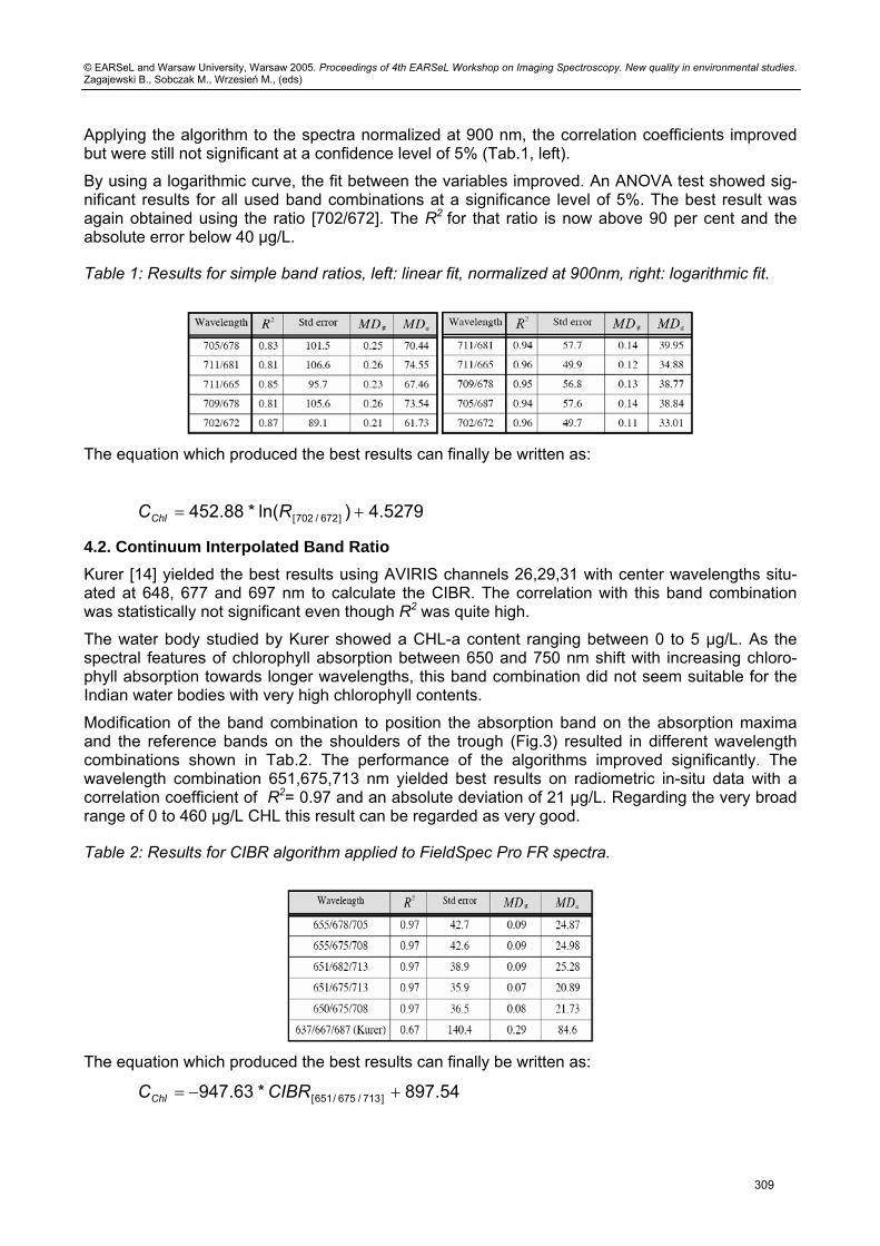
Applying the algorithm to the spectra normalized at 900 nm, the correlation coefficients improved but were still not significant at a confidence level of 5% (Tab.1, left).

By using a logarithmic curve, the fit between the variables improved. An ANOVA test showed sig-nificant results for all used band combinations at a significance level of 5%. The best result was again obtained using the ratio [702/672]. The R2 for that ratio is now above 90 per cent and the absolute error below 40 µg/L.

Table 1: Results for simple band ratios, left: linear fit, normalized at 900nm, right: logarithmic fit.

The equation which produced the best results can finally be written as:

5279.4)ln(*88.452 ]672/702[ += RCChl

4.2. Continuum Interpolated Band Ratio Kurer [14] yielded the best results using AVIRIS channels 26,29,31 with center wavelengths situ-ated at 648, 677 and 697 nm to calculate the CIBR. The correlation with this band combination was statistically not significant even though R2 was quite high.

The water body studied by Kurer showed a CHL-a content ranging between 0 to 5 µg/L. As the spectral features of chlorophyll absorption between 650 and 750 nm shift with increasing chloro-phyll absorption towards longer wavelengths, this band combination did not seem suitable for the Indian water bodies with very high chlorophyll contents.

Modification of the band combination to position the absorption band on the absorption maxima and the reference bands on the shoulders of the trough (Fig.3) resulted in different wavelength combinations shown in Tab.2. The performance of the algorithms improved significantly. The wavelength combination 651,675,713 nm yielded best results on radiometric in-situ data with a correlation coefficient of R2= 0.97 and an absolute deviation of 21 µg/L. Regarding the very broad range of 0 to 460 µg/L CHL this result can be regarded as very good.

Table 2: Results for CIBR algorithm applied to FieldSpec Pro FR spectra.


54.897*63.947 ]713/675/651[ +−= CIBRCChl

309


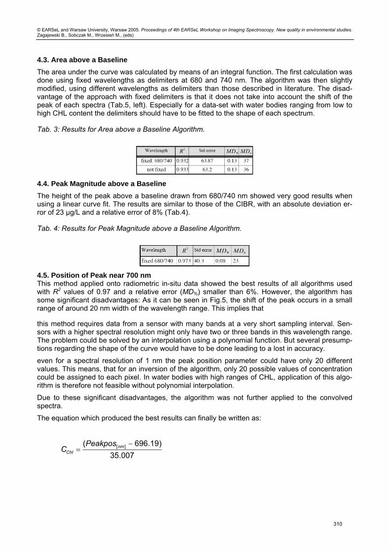
4.3. Area above a Baseline The area under the curve was calculated by means of an integral function. The first calculation was done using fixed wavelengths as delimiters at 680 and 740 nm. The algorithm was then slightly modified, using different wavelengths as delimiters than those described in literature. The disad-vantage of the approach with fixed delimiters is that it does not take into account the shift of the peak of each spectra (Tab.5, left). Especially for a data-set with water bodies ranging from low to high CHL content the delimiters should have to be fitted to the shape of each spectrum.

Tab. 3: Results for Area above a Baseline Algorithm.

4.4. Peak Magnitude above a Baseline The height of the peak above a baseline drawn from 680/740 nm showed very good results when using a linear curve fit. The results are similar to those of the CIBR, with an absolute deviation er-ror of 23 µg/L and a relative error of 8% (Tab.4).

Tab. 4: Results for Peak Magnitude above a Baseline Algorithm.

4.5. Position of Peak near 700 nm This method applied onto radiometric in-situ data showed the best results of all algorithms used with R2 values of 0.97 and a relative error (MD%) smaller than 6%. However, the algorithm has some significant disadvantages: As it can be seen in Fig.5, the shift of the peak occurs in a small range of around 20 nm width of the wavelength range. This implies that

this method requires data from a sensor with many bands at a very short sampling interval. Sen-sors with a higher spectral resolution might only have two or three bands in this wavelength range. The problem could be solved by an interpolation using a polynomial function. But several presump-tions regarding the shape of the curve would have to be done leading to a lost in accuracy.

even for a spectral resolution of 1 nm the peak position parameter could have only 20 different values. This means, that for an inversion of the algorithm, only 20 possible values of concentration could be assigned to each pixel. In water bodies with high ranges of CHL, application of this algo-rithm is therefore not feasible without polynomial interpolation.

Due to these significant disadvantages, the algorithm was not further applied to the convolved spectra.


007.35)19.696( ][ −

= nmChl

PeakposC

310


Tab. 5: Range of the position of the peaks near 700 nm on the wavelength axis (left), and results for Position of Peak near 700 nm Algorithm (right).

4.6. Application of Algorithms to Sensor-specific Convolved Spectra In order to determine the suitability of existing (Hyperion [21] and HyMap [5]) and future (APEX [18]) imaging spectrometers, the algorithms which performed best on ASD FieldSpec Pro FR spec-tra were applied to convolved spectra of the three sensors with regard to their center wavelengths and FWHM’s. If there was no center wavelength at the desired position the next adjacent band was taken.

For the best performing Simple Band Ratio at the wavelengths 702/672, no significant difference between Fieldspec, APEX and Hyperion can be detected. The difference between the results is less than 2%. HyMap does not have the bands at this wavelength but adjacent bands performed similarly as well. It it is surprising that the difference between the results is rather small. It must be taken into consideration, that the width of the bands varies from 1 nm (Fieldspec) to 10 nm (Hype-rion) and 15 nm (HyMap).

CIBR shows similar results: There is almost no difference between Fieldspec, APEX and Hyperion, whereas HyMap does not have its bands right positioned for this algorithm. Again, the differences are surprisingly small.

When applying the Area above a Baseline Algorithm to the convolved spectra, wider bands per-formed clearly better. The outcome of Hyperion and HyMap with the delimiters at the same wave-lengths are clearly better than the result from unconvolved FieldSpec data. It seems that the more the shape of the curve is generalized through less bands, the better the outcome (see Fig. 7).

The results of the Peak Magnitude above a Baseline Algorithm have the same tendency but less clearly. Again, wider bands performed better.

Tab. 6: Results for Simple Band Ratios, logarithmic fit (left), and for CIBR, linear fit (right).

311


Tab. 7: Results for Area above a Baseline Algorithm (left), and for Peak Magnitude above a Base-line Algorithm (right); f. denotes “fixed”, nf. Denotes “not fixed”.

Fig. 7: Spectral Data convolved to the bands of the sensors under investigation. Dots denote band center wavelengths.

Tab.8 shows the position of the bands which are required for a good outcome of the algorithms. The central wavelength of the band is indicated:

Tab. 8: Positions of required bands and their availability for the sensors under investigation.

Regarding the comparison of the selected sensors, the following conclusions can be drawn:

If the bands are rightly positioned, a better spectral resolution does not increase the quality of the results significantly for spectral bandwidths below 10 nm. Quite the contrary has been observed, in most cases wider bands performed slightly better.

There was no significant difference between choosing the bands in a fixed mode or bands adjusted to each spectrum individually (see Chapter 5.3).

For the algorithms Peak Magnitude above a Baseline and Area above a Baseline all sen-sors have their bands at the needed wavelength position (Tab. 8). HyMap does not have the optimal configuration for Simple Band Ratios and CIBR for the observed hypertrophic Indian waters, even though the differences are small.

It has to be noted that the original bandwidth of the sensors was taken. APEX has the advantage in that it is fully programmable. Bands can be convolved and the width of each band can be cus-

312


tomized for the desired purpose. Hence, APEX has all the capabilities of HyMap and Hyperion to-gether with its new features, including better spectral resolution.

5. CONCLUSIONS All algorithms applied proved to be of value. Given the large range of observed TCHL concentra-tions (0–460 µg/L), the yielded R2 were high and mean deviations low. However, certain presump-tions had to be made (e.g., use of TCHL instead of CHL-a in the modelling) and there still remain limitations concerning the used input data. In general, the measured nutrient levels seem too low in regard to CHL concentration. Visually, no algal scum, indicating a bloom, could be observed. Nonetheless, spectral analysis and comparison with similar spectra [9] indicate that quite high con-centrations of CHL can be expected, although they were visually not clearly detectable. Macro-phytes density supports the assumption of high bio-activity. Therefore, all domestic ponds would be classified as hypertrophic. The trophic state of P5 is not classifiable.

It has to be kept in mind, that the trophic state classification system was developed for larger lakes in the Western hemisphere. In these lakes, the limnological cycle is completely different in terms of seasonality, discharge and lack of monsoon. The classification system, thus, may not be applica-ble to small and shallow ponds in the tropics.

Moreover, this study represents a point-in-time measurement being performed at the end of the dry season. At this time, several meters of the water column had already evaporated, hence the con-centration rises. Regarding the cycle of these ponds, a regular monitoring over different seasons would be necessary to draw further conclusions.

Concerning the outcome of the comparison of selected possible hyperspectral sensors for water quality determination, it can be mentioned that the differences were small. An intermediate band-width of 10 nm seems appropriate for application of the selected algorithms. All sensors showed an adequate band positioning for the algorithms based on the peak near 700 nm. Using Simple Band Ratios and CIBR, APEX and Hyperion performed slightly better than HyMap.

To verify whether the chosen algorithms are suitable for an operative monitoring of ponds in the study area, further verification data is indispensable. Implementation of an operative monitoring of water quality in the region remains challenging in regard of seasonal difficulties during the mon-soon season and the spatial resolution of current spaceborne sensors.

6. ACKNOWLEDGMENTS We would like to thank the staff of Bidhan Chandra Krishi Viswavidyalaya University, Mohanpur, for the cooperation and infrastructure. Special thanks go to Prof. Dr. Hussein and Dr. Saha.

7. References

1. Analytical Spectral Devices (ASD), 1999: Technical Guide. 3rd Ed. Section 5-7.

2. Bohley, P., 1989: Statistik – Einfuehrendes Lehrbuch fuer Wirtschafts- und Sozialwissenschaft-ler. 3. Ed., Muenchen, Wien: Oldenbourg-Verlag.

3. Bruegge C.J., Conel J.E., Margolis J.S., Green R.O., Toon G., Carrere V., Holm R.G. and Hoo-ver G., 1990: In-situ atmospheric water-vapor retrieval in support of AVIRIS validation. SPIE Vol. 1298 Imaging Spectroscopy of the Terrestrial Environment, pp. 150 – 163.

4. Carlson, R.E. and Simpson, J., 1996: A coordinator’s guide to volunteer lake monitoring meth-ods. North American Lake Management Society. pp. 96.

5. Cocks, T., R., Jensen, R., Stewart, A., Wilson, I. and T. Sheilds, T. 1998: The HyMap Airborne Hyperspectral Sensor: The system, calibration and performance. Proc. 1st EARSEL Workshop on Imaging Spectroscopy, Zurich, October 1998, pp. 37-42.

313


6. Dekker, A. G., 1993: Detection of optical water quality parameters for eutrophic waters by high resolution remote sensing. PhD thesis, Free University, Amsterdam.

7. Gitelson, A., 1993: The nature of the peak near 700 nm on the radiance spectra and its appli-cation for remote estimation of phytoplankton pigments in inland waters. Optical Engineering and Remote Sensing, SPIE 1971, pp. 170-179.

8. Gitelson, A., Garbuzov, G., Szilagyi, F., Mittenzwey, K-H., Karnieli A. and A. Kaiser, 1993: Quantitative remote sensing methods for real-time monitoring of inland water quality. Interna-tional Journal of Remote Sensing, 14, pp. 1269-1295.

9. Gitelson, A.A., Stark, R. and I. Dor, 1997: Quantitative near-surface remote sensing of waste-water quality in oxidation ponds and reservoirs: A case study of the Naan system. Water Environment Research, Vol. 69, No. 7, pp. 1263-1271.

10. Gitelson, A.A., Yacobi, Y.Z., Rundquist, D. C., Stark, R., Han, L., and D. Etzion, 2000: Remote estimation of chlorophyll concentration in productive waters: Principals, algorithm development and validation. NWQMC Conference Proceedings 2000. Available at: http://www.nwqmc.org/2000proceeding/ table_of_contents.htm [Access: March 2005].

11. Hyperstat Online: http://www.ruf.rice.edu/~lane/hyperstat/A120567.html [Access: March 2005].

12. Kallio, K., Kutser. T., Hannonen, T., Koponen, S., Pulliainen, J., Vepsaelaeinen, J. and T. Pyhaelahti, 2001: Retrieval of water quality by airborne imaging spectrometer in various lake types at different seasons. The Science of the Total Enviroment, Vol. 268, 1-3, pp. 59-77.

13. Koponen, S., Pulliainen, J., Kallio, K., M. Hallikainen, 2002: Lake water quality classification with airborne hyperspectral spectrometer and simulated MERIS data. Remote Sensing of Envi-ronment 79, pp. 51-59.

14. Kurer, U., 1994: Bestimmung der Chlorophyllkonzentration im Zugersee anhand von AVIRIS-Bildspektrometriedaten. MSc. Thesis. Dept. of Geography, University of Zuerich.

15. Kutser, T., Herlevi, A., Kallio, K. and H. Arst, 2001: A hyperspectral model for interpretation of passive optical remote sensing data from turbid lakes. The Science of the Total Environment 268, pp. 47-58.

16. Lindell, T., Pierson D., Premazzi, G. and E. Zilioli, 1999: Manual for monitoring European lakes using remote sensing techniques. Report EUR 18665 EN, Luxembourg: European Commis-sion.

17. Neville, R.A. and J.F.R. Gower, 1977: Passive remote sensing of phytoplankton via chlorophyll-a fluorescence. Jornal of Geophysical Research 82: 3487-3493, pp. 709-722.

18. Nieke, J., Itten, K.I., Debruyn, W. and the APEX Team, 2005: Status of the Airborne Imaging Spectrometer APEX. Presented at the 4th EARSeL Workshop on Imaging Spectroscopy, War-saw, April 27-29, 2005.

19. Oron, G. and A. Gitelson, 1996: Real-time quality monitoring by remote sensing of contami-nated water bodies: Waste Stabilization Pond Effluent. Water Research, Vol. 30 (12), 3106-3114.

20. Thiemann, S. and H. Kaufmann, 2002: Lake water quality monitoring using hyperspectral air-borne data- a semi-empirical multisensor and multitemporal approach for the Mecklenburg Lake District, Germany. Remote Sensing of Environment 81, pp. 228-237.

21. USGS, EO-1 Website. http://eo1.gsfc.nasa.gov/Technology/Hyperion.html [Access: March 2005].

22. Yacobi, Y. Z., Gitelson, A. and M. Mayo, 1995: Remote sensing of chlorophyll in Lake Kinneret using high spectral resolution radiometer and Landsat TM: Spectral features of reflectance and algorithm development. Journal of Plankton Research 17, pp. 2155-2173.

314


15. Kutser, T., Herlevi, A., Kallio, K. and H. Arst, 2001: A hyperspectral model for interpretation of passive optical remote sensing data from turbid lakes. The Science of the Total Environment 268, pp. 47-58.

16. Lindell, T., Pierson D., Premazzi, G. and E. Zilioli, 1999: Manual for monitoring European lakes using remote sensing techniques. Report EUR 18665 EN, Luxembourg: European Commis-sion.

17. Neville, R.A. and J.F.R. Gower, 1977: Passive remote sensing of phytoplankton via chlorophyll-a fluorescence. Jornal of Geophysical Research 82: 3487-3493, pp. 709-722.

18. Nieke, J., Itten, K.I., Debruyn, W. and the APEX Team, 2005: Status of the Airborne Imaging Spectrometer APEX. Presented at the 4th EARSeL Workshop on Imaging Spectroscopy, War-saw, April 27-29, 2005.

19. Oron, G. and A. Gitelson, 1996: Real-time quality monitoring by remote sensing of contami-nated water bodies: Waste Stabilization Pond Effluent. Water Research, Vol. 30 (12), 3106-3114.

20. Thiemann, S. and H. Kaufmann, 2002: Lake water quality monitoring using hyperspectral air-borne data- a semi-empirical multisensor and multitemporal approach for the Mecklenburg Lake District, Germany. Remote Sensing of Environment 81, pp. 228-237.

21. USGS, EO-1 Website. http://eo1.gsfc.nasa.gov/Technology/Hyperion.html [Access: March 2005].

22. Yacobi, Y. Z., Gitelson, A. and M. Mayo, 1995: Remote sensing of chlorophyll in Lake Kinneret using high spectral resolution radiometer and Landsat TM: Spectral features of reflectance and algorithm development. Journal of Plankton Research 17, pp. 2155-2173.

315

Determination of water quality parameters in Indian ponds using remote sensing methods

Documents