Determination of the body force of a two-dimensional isotropic elastic body

arX

iv:0

705.

2107

v2 [

mat

h.A

P] 1

5 Ju

l 200

8

Determination of the body force of a two−dimensional

isotropic elastic body

DANG DUC TRONGa, PHAM NGOC DINH ALAINb,

PHAN THANH NAMa and TRUONG TRUNG TUYENc

aMathematics Department, HoChiMinh City National University, Viet NambMathematics Department, Mapmo UMR 6628, BP 67-59, 45067 Orleans cedex, FrancecDepartment of mathematics, Indiana University, Rawles Hall , Bloomington, IN 47405

Abstract

Let Ω represent a two−dimensional isotropic elastic body. We consider the prob-lem of determining the body force F whose form ϕ(t)(f1(x), f2(x)) with ϕ be giveninexactly. The problem is nonlinear and ill-posed. Using the Fourier transform, themethods of Tikhonov’s regularization and truncated integration, we construct a regu-larized solution from the data given inexactly and derive the explicitly error estimate.

MSC 2000: 35L20, 35R30, 42B10, 70F07, 74B05.Key words: body force, elastic body, Fourier transform, ill−posed problem, Tikhonov’s

regularization, truncated integration.

1. Introduction

Let Ω = (0, 1) × (0, 1) represent a two−dimensional isotropic elastic body. For eachx := (x1, x2) ∈ Ω, we denote by u = (u1(x, t), u2(x, t)) the displacement, where uj is thedisplacement in the xj− direction, for all j ∈ 1, 2. As known, u satisfies the Lame system(see, e.g., [1, 2])

∂2u

∂t2= µ∆u + (λ + µ)∇ (div(u)) + F

where F := (F1, F2) is the body force, div(u) = ∇ · u = ∂u1/∂x1 + ∂u2/∂x2, and λ, µ areLame constants. We shall assume that the boundary of the elastic body is clamped and theinitial conditions are given.

In this paper, we shall consider the problem of determining the body force F . Theproblem is a kind of inverse source problems. The inverse source problems are investigatedin many aspects such as the uniqueness, the stability and the regularization. There aremany papers devoted to the uniqueness and the stability problem. In [7], Isakov disscusedthe problem of finding a pair of functions (u, f) satisfying

cutt − ∆u = f

1

where f is independent of t. He proved that using some preassumptions on f , from thefinal overdetermination

u(x, T ) = h(x)

, we get the uniqueness of (u, f).As shown in [9], the body force (in the form φ(t)f(x)) will be defined uniquely from an

observation of surface stress (the lateral overdetermination) given on a suitable boundaryof Ω × (0, T ). In the paper, the authors also gave an abstract formula of reconstruction.

Another inverse source problem is one of finding the heat source F (x, t, u) satisfying

ut − ∆u = F.

The problem was considered intensively in the last century. The problem with the finaloverdetermination was studied by Tikhonov in 1935 (see [8]). He proved the uniqueness ofproblem with prescribed lateral and final data. In the last three decades, the problem isconsidered by many authors (see [3, 4, 11, 12, 13, 14]). Although we have many works on theuniqueness and the stability of inverse source problems, the literature on the regularizationproblem is quite scarce. Very recently, in [3, 4] , the authors considered the regularizationproblem under both the lateral and the final overdetermination. The ideas of using theFourier transform and truncated integration in the two papers are used in the presentpaper. We also consider the regularization problem under the final data and prescribedsurface stress.

To get the lateral overdetermination, some mechanical arguments are in order. Letσ1, σ2, τ be the stresses (see [1, 2]) defined by

τ = µ

(∂u1

∂x2+

∂u2

∂x1

)

σj = λdiv(u) + 2µ∂uj

∂xj, j ∈ 1, 2

We shall assume that the surface stress is given on the boundary of the body, i.e.,(

σ1 τ

τ σ2

)(n1

n2

)=

(X1

X2

)

where X = (X1,X2) is given on ∂Ω, and n = (n1, n2) is the outward unit normal vector of∂Ω.

As discussed, our problem is severely ill-posed. Hence, to simplify the problem, apreassumption on the form of the body force is needed. We shall use the separable formforce as in [9]

(F1(x, t), F2(x, t)) = ϕ(t)(f1(x), f2(x))

where ϕ is given inexactly. The form is issued from an approximated model for elastic wavegenerated from a point dislocation source (see, e.g., [9, 10]). But, since ϕ is inexact, ourproblem is nonlinear. Morever, the problem is still ill-posed because the measured data is

2

not only inexact but also non-smooth.Precisely, we consider the problem of identifying a pair of functions (u, f) satisfying the

system:∂2uj

∂t2= µ∆uj + (λ + µ)

∂

∂xjdiv(u) + ϕ(t)fj(x),∀j ∈ 1, 2 (1)

for (x, t) ∈ Ω × (0, T ), where µ, λ are real constants satisfying µ > 0 and λ + 2µ > 0.Since the boundary of the elastic body is clamped, the displacement u = (u1, u2) satisfiesthe boundary condition

(u1(x, t), u2(x, t)) = (0, 0), x ∈ ∂Ω (2)

In addition, the initial and final displacement are given in Ω

(u1(x, 0), u2(x, 0)) = (u01(x), u02(x))(

∂u1

∂t(x, 0),

∂u2

∂t(x, 0)

)= (u∗

01(x), u∗02(x))

(u1(x, T ), u2(x, T )) = (uT1(x), uT2(x))

(3)

Finally, the surface stress is given on ∂Ω

n1σ1 + n2τ = X1

n2σ2 + n1τ = X2(4)

We shall assume that the data of the system (1) − (4)

I = (ϕ,X, u0, u∗0, uT ) ∈

(L1(0, T ), (L1(0, T, L1(∂Ω)))2, (L1(Ω))2, (L1(Ω))2, (L1(Ω))2

)

are given inexactly since they are results of experimental measurements. The system (1)−(4)usually has no solution; moreover, even if the solution exists, it does not depend continouslyon the given data. Hence, a regularization is in order. Denoting by Iex the exact data, whichare probably unknown, corresponding to an exact solution (uex, fex) of the system (1)− (4), from the inexact data Iε approximating Iex, we shall construct a regularized solution fε

approximating fex .In fact, using the Fourier transform, we shall reduce our problem to finding the solu-

tions of the binomial equations whose binomial term is an entire function (see Lemma 1).In this case, the problem is unstable in the neighborhood of zeros of the entire function.The zeroes can be seen as singular values. Using the method of Tikhonov’s regularizationand truncated integration, we shall eliminate the singular values to regularize our problem.Error estimates are given.

The remainder of the paper is divided into two sections. In Section 2, we shall set somenotations and state our main results. In Section 3, we give the proofs of the results.

2. Notations and main results

3

We recall that Ω = (0, 1)×(0, 1). We always assume that the data I = (ϕ,X, u0, uT , u∗T )

belong to (L1(0, T ), (L1(0, T, L1(∂Ω)))2, (L1(Ω))2, (L1(Ω))2, (L1(Ω))2

)

For all ξ = (ξ1, ξ2), ζ = (ζ1, ζ2) ∈ R2, we set ξ · ζ = ξ1ζ1 + ξ2ζ2 and |ξ| =√

ξ · ξ.We first have the following lemma.

Lemma 1. If u ∈ (C2([0, T ];L2(Ω)) ∩ L2(0, T ;H2(Ω)))2, f ∈ (L2(Ω))2 satisfy (1) − (4)corresponding the data I, then for all α = (α1, α2) ∈ R2\0, we have

2D(I).

∫

Ω

fj(x). cos(α · x)dx = gj(I), ∀j ∈ 1, 2

where

D(I) = D1(I).D2(I), gj(I) =2

|α|2 (αjD2(I)h0 + D1(I)hj)

with

D1(I) =

T∫

0

ϕ(T − t) sin(√

λ + 2µ |α| t)dt,D2(I) =

T∫

0

ϕ(T − t) sin(√

µ |α| t)dt

h0(I) = − sin(√

λ + 2µ|α|T ).

∫

Ω

(α · u∗0). cos(α · x)dx

+√

λ + 2µ.|α|.∫

Ω

(α · uT ). cos(α · x)dx

−√

λ + 2µ.|α|. cos(√

λ + 2µ|α|T ).

∫

Ω

(α · u0). cos(α · x)dx

−T∫

0

∫

∂Ω

sin(√

λ + 2µ|α|(T − t))(α · X). cos(α · x)dωdt

hj(I) = − sin(√

µ|α|T ).

∫

Ω

(|α|2u∗0j − αj(α · u∗

0)). cos(α · x)dx

+√

µ.|α|.∫

Ω

(|α|2uTj − αj(α · uT )). cos(α · x)dx

−√µ.|α|. cos(√µ|α|T ).

∫

Ω

(|α|2u0j − αj(α · u0)). cos(α · x)dx

−T∫

0

∫

∂Ω

sin(√

µ|α|(T − t))(|α|2Xj − αj(α · X)). cos(α · x)dωdt,∀j ∈ 1, 2.

4

From Lemma 1, we consider the function

D(I) =

T∫

0

ϕ(T − t) sin(√

λ + 2µ |α| t)dt.

T∫

0

ϕ(T − t) sin(√

µ |α| t)dt

The problem is unstable in the neighborhood of zeros of this function. However, from theproperties of analytic function, we can show that if ϕ 6≡ 0 then this function differ from 0for almost every where in R3. Furthermore, using the idea of Theorem 4 in [5], we get thefollowing lemma.

Lemma 2. Let τ, q be positive constants, ϕ0 ∈ L1(0, T )\0 and D(ϕ0, τ) : R2 → R

D(ϕ0, τ)(α) =

T∫

0

ϕ0(t) sin(√

τ |α|t)dt

Then D(ϕ0, τ) 6= 0 for a.e α ∈ R2. Moreover, if we put

Rε =q

9eT.

ln(ε−1)

ln(ln(ε−1)), ∀ε > 0

then the Lebesgue measure of the set

B(ϕ0, τ, ε) = α ∈ B(0, Rε), |D(ϕ0, τ)(α)| ≤ εq

is less than R−1ε for ε > 0 small enough, where B(0, Rε) is the open ball in R2 .

Lemma 1 and Lemma 2 imply immediately the uniqueness result.

Theorem 1. Let u, u∗ ∈ (C2([0, T ];L2(Ω))∩L2(0, T ;H2(Ω)))2, f, f∗ ∈ (L2(Ω))2. If (u, f),(u∗, f∗) satisfy (1) − (4) corresponding the same data I, and ϕ 6≡ 0, then

(u, f) = (u∗, f∗)

Let (uex, fex) be the exact solution of the system (1)− (4) corresponding the exact dataIex = (ϕex,Xex, uex

0 , u∗ex0 , uex

T ). Notice that, if we assume

uex ∈ (C2([0, T ];L2(Ω)) ∩ L2([0, T ];H2(Ω)))2, fex ∈ (L2(Ω))2, ϕex ∈ L1(0, T )\0 (5)

then for all j ∈ 1, 2,

F (fjex)(α) = 2

∫

Ω

fjex(x) cos(α · x)dx =gj(Iex)

D(Iex)

5

for a.e α ∈ R2, where gj , D are defined by Lemma 1, fjex : R2 → R is defined by fjex(x) =χ(Ω)fjex(x) + χ(−Ω)fjex(−x), and F is the Fourier transform in R2.

From approximate data Iε = (ϕ,X, u0, u∗0, uT ) satisfying

‖ϕ − ϕex‖L1(0,T ) ≤ ε,∥∥Xj − Xex

j

∥∥L1(0,T,L1(∂Ω))

≤ ε,∥∥u0j − uex

0j

∥∥L1(Ω)

≤ ε∥∥u∗

0j − u∗ex0i

∥∥L1(Ω)

≤ ε,∥∥uTj − uex

Tj

∥∥L1(Ω)

≤ ε, ∀j ∈ 1, 2(6)

, we construct a regularized solution fε = (f1ε, f2ε) whose Fourier transform is

F (fjε)(α) = χ(B(0, Rε)).gj(Iε).D(Iε)

δε + (D(Iε))2 ,∀α ∈ R2\0

where

q =1

7, δε = ε

1+6q

2 , Rε =q

9eT.

ln(ε−1)

ln(ln(ε−1))(7)

We have two regularization results.

Theorem 2. Let (uex, fex) be the exact solution of the system (1) − (4) corresponding theexact data Iex, and (5) hold. Then from the given data Iε satisfying (6), we can constructa regularized solution fε ∈ (C(Ω))2 such that

limε→0

‖fjε − fjex‖L2(Ω) = 0, ∀j ∈ 1, 2

If we assume, in addition, that fex ∈ (H1(Ω))2,then

‖fjε − fjex‖2L2(Ω) ≤ 63eT

(66 ‖fjex‖2

H1(Ω) + (2π)−2)

.ln(ln(ε−1))

ln(ε−1), ∀j ∈ 1, 2

for ε > 0 small enough.

Theorem 3. Let (uex, fex) be the exact solution of the system (1) − (4) corresponding theexact data Iex, and (5) hold. We assume, in addition, that

∫

R2

∣∣∣∣∣∣

∫

Ω

fjex(x). cos(α · x)dx

∣∣∣∣∣∣dα < ∞, ∀j ∈ 1, 2

Then from the given data Iε satisfying (6), we can construct a regularized solution fε ∈(C(Ω))2, which coincides the one in Theorem 2, such that

limε→0

‖fjε − fjex‖L∞(Ω) = 0, ∀j ∈ 1, 2

3. Proofs of the results

Proof of Lemma 1

6

Proof. Let α = (α1, α2) ∈ R2 and G = cos(α · x). Notice that the j−th equation of thesystem (1) can rewrite

∂2uj

∂t2=

∂σj

∂xj+

∂τ

∂xk+ ϕ(t)fj(x), j, k = 1, 2

Getting the inner product (in L2(Ω)) of the equation and G and using the condition (2),for j, k = 1, 2, we get

d

dt2

∫

Ω

ujG =

∫

∂Ω

(njσj + nkτ)Gdω −∫

Ω

σj∂G

∂xjdx −

∫

Ω

τ∂G

∂xkdx + ϕ(t)

∫

Ω

fjGdx

=

∫

∂Ω

XjGdω − µ |α|2∫

Ω

ujGdx − (λ + µ)αj

∫

Ω

(α · u)Gdx + ϕ(t)

∫

Ω

fjGdx

(8)

Multiplying (8) by αj, then getting the sum for j = 1, 2, we obtain

d

dt2

∫

Ω

(α · u)Gdx =

∫

∂Ω

(α · X)Gdω − (λ + 2µ)|α|2∫

Ω

(α · u)Gdx + ϕ(t)

∫

Ω

(α · f)Gdx (9)

Multiplying (8) by |α|2 and multiplying (9) by −αj , then getting the sum of them, we have

d

dt2

∫

Ω

(|α|2 uj − αj . (α · u)

)Gdx =

∫

∂Ω

(|α|2 Xj − αj. (α · X)

)Gdx

−µ |α|2∫

Ω

(|α|2 uj − αj. (α · u)

)Gdx + ϕ(t)

∫

Ω

(|α|2 fj − αj . (α · f)

)Gdx

(10)

We consider (9) and (10) as the differential equations whose form

y′′ + η2y = h(t) (11)

where η is a real constant and y(0), y′(0), y(T ) are given. Getting the inner product (inL2(0, T )) of (11) and sin(η(T − t)), we have

− y′(0)sin(ηT ) + ηy(T ) − ηy(0)cos(ηT ) =

T∫

0

h(T − t) sin(ηt)dt (12)

Applying (12) to (9) with η =√

(λ + 2µ)|α| and y =∫Ω

(α · u).Gdx, we get

D1(I).

∫

Ω

(α · f).Gdx = h0(I) (13)

7

where D1(I), h0(I) are defined by Lemma 1.Similarly, applying (12) to (10) with η =

√µ|α| and y =

∫Ω

(|α|2uj − αj .(α · u)).Gdx, we get

D2(I).

∫

Ω

(|α|2fj − αj(α · f)).Gdx = hj(I), ∀j ∈ 1, 2 (14)

where D2(I), hj(I) are defined by Lemma 1.Multiplying (13) by αjD2(I) and multiplying (14) by D1(I), then getting the sum of

them, we obtain the result of Lemma 1.

Proof of Lemma 2

Proof. Put ϕ0 : R → R

ϕ0(t) =1

2

ϕ0(t) t ∈ (0, T )

−ϕ0(−t) t ∈ (−T, 0)

0 t /∈ (−T, T )

and φ : C → C

φ(z) =

∞∫

−∞

e−itzϕ0(t)dt =

T∫

−T

e−itzϕ0(t)dt

Then φ is an entire function and D(ϕ0, τ)(α) = iφ(√

τ |α|). Because ϕ0 6≡ 0, its Fouriertransform (in R) does not coincide 0. Therefore, there exists z0 ∈ R such that |φ(z0)| =C1 > 0. Thus φ 6≡ 0. Since φ is an entire function, its zeros set is either finite or countable.Consequently, D(ϕ0, τ)(α) 6= 0 for a.e α ∈ R2.

To estimate the measure of B(ϕ0, τ, ε), we shall use the following result (see Theorem 4of $11.3 in [6]).

Lemma 3. Let f(z) be a function analytic in the disk z : |z| ≤ 2eR, |f(0)| = 1, and letη be an arbitrary small positive number. Then the estimate

ln |f(z)| > − ln(15e3

η). ln(Mf (2eR))

is valid everywhere in the disk z : |z| ≤ R except a set of disks (Cj) with sum of radii∑rj ≤ ηR. Where Mf (r) = max

|z|=r|f(z)|.

Returning Lemma 2, we put φ1 : C → C

φ1(z) =φ(z + z0)

C1

8

Then φ1 is an entire function, φ1(0) = 1, and for all z ∈ C, |z| ≤ 2eR,

C1 |φ1(z)| =

∣∣∣∣∣∣

T∫

−T

e−it(z+z0)ϕ0(t)

∣∣∣∣∣∣≤ e2eRT .

T∫

−T

|ϕ0(t)| dt = e2eRT ‖ϕ0‖L1(0,T )

For ε > 0 small enough, applying Lemma 3 with R = 43Rε and η =

√τ

8πR3ε, we get

ln |φ1(z)| > −[3 ln Rε + ln(

8π√τ) + ln(15e3)

].

[8

3.eTRε + ln

(‖ϕ0‖L1(0,T )

C1

)]

> −17

2T.Rε ln Rε > −q ln(ε−1) − ln(C1) = ln(

εq

C1)

for all |z| ≤ 43Rε except a set of disks B(zj , rj)j∈J with sum of radii

∑ri ≤ ηR =

√τ

6πR2ε.

Consequently, for ε > 0 small enough, we have |z0| < 13Rε and |φ(z)| = C1. |φ1(z − z0)| ≥

εq for all |z| ≤ Rε except the set ∪j∈J

B(zj + z0, rj) . Hence, B(ϕ0, τ, ε) is contained in the

set ∪j∈J

Bj , where

Bj = α ∈ B(0, Rε),∣∣√τ |α| − yj

∣∣ ≤ rjwith yj = Re(zj + z0).

If yj >√

τRε + rj then Bj = ∅. If yj ≤ rj then Bj ⊂ B(0,2rj√

τ), so m(Bj) ≤ 4πr2

j

τ . If

rj < yj ≤√

τRε + rj then

Bj ⊂ B(0,yj + rj√

τ)\B(0,

yj − rj√τ

)

hence

m(Bj) ≤π(yj + rj)

2

τ− π(yj − rj)

2

τ=

4πyjrj

τ≤ 4π(

√τRε + rj)rj

τ

Thus we get

m(B(ϕ, τ, ε)) ≤∑ 4π(

√τRε + rj)rj

τ+∑ 4πr2

j

τ

≤ 4πRε√τ

∑rj +

8π

τ(∑

rj)2 ≤ 4πRε√

τ.

√τ

6πR2ε

+8π

τ.(

√τ

6πR2ε

)2 <1

Rε

for ε > 0 small enough. The proof of Lemma 2 is completed.

Proof of theorem 1

9

Proof. Put w = u−u∗ and v = f − f∗ then (w, v) satisfies (1)− (4) corresponding the data

I = (ϕ, (0, 0), (0, 0), (0, 0), (0, 0))

Let vj : R2 → R be defined by vj(x) = χ(Ω)vj(x) + χ(−Ω)vj(−x). Lemma 1 implies that,for all j ∈ 1, 2, for all α ∈ R2\0, we get

D(I).F (vj)(α) = 2D(I).

∫

Ω

vj(x) cos(α · x)dx = gj(I) = 0

Applying Lemma 2 with ϕ0(t) = ϕ(T − t), we get D(I) 6= 0 for a.e α ∈ R2. Therefore,F (vj) ≡ 0, and it implies that vj ≡ 0. Thus v ≡ (0, 0). Hence, w satisfies that

∂2w

∂t2= µ∆w + (λ + µ)∇ (div(w)) (15)

Getting the inner product (in (L2(Ω))2) of (15) and ∂w/∂t, we have

1

2.d

dt

2∑

j=1

∥∥∥∥∂wj

∂t

∥∥∥∥2

L2(Ω)

= −µ

2.d

dt

2∑

j=1

‖∇wj‖2L2(Ω) −

λ + µ

2.d

dt‖div(w)‖2

L2(Ω)

Integrating this equality in (0, t), we get

2∑

j=1

∥∥∥∥∂wj

∂t

∥∥∥∥2

L2(Ω)

+ µ

2∑

j=1

‖∇wj‖2L2(Ω) + (λ + µ) ‖div(w)‖2

L2(Ω) = 0 (16)

for all t ∈ (0, T ). Using the condition (2), we have

‖div(w)‖2L2(Ω) =

2∑

j=1

∥∥∥∥∂wj

∂xj

∥∥∥∥2

L2(Ω)

+ 2

∫

Ω

∂w1

∂x1.∂w2

∂x2=

2∑

j=1

∥∥∥∥∂wj

∂xj

∥∥∥∥2

L2(Ω)

+ 2

∫

Ω

∂w1

∂x2.∂w2

∂x1

≤2∑

j=1

∥∥∥∥∂wj

∂xj

∥∥∥∥2

L2(Ω)

+

(∥∥∥∥∂w1

∂x2

∥∥∥∥2

L2(Ω)

+

∥∥∥∥∂w2

∂x1

∥∥∥∥2

L2(Ω)

)=

2∑

j=1

‖∇wj‖2L2(Ω)

Since µ > 0 and λ + 2µ > 0, the above inequality implies that

µ2∑

j=1

‖∇wj‖2L2(Ω) + (λ + µ) ‖div(w)‖2

L2(Ω) ≥ 0

From (16), we obtain ∂w/∂t = (0, 0). Since w(x, 0) = (0, 0), the proof is completed.

To prove two main regularization results, we state and prove some preliminary lemmas.

10

Lemma 4. Let (uex, fex) be the exact solution of (1)− (4) corresponding the exact data Iex

satisfying (5), and the given data Iε satisfying (6). Using notations of (7), we put

Gj(Iε) = χ(B(0, Rε)).gj(Iε)D(Iε)

δε + (D(Iε))2

Then for all j ∈ 1, 2, we have Gj(Iε) ∈ L1(R2)∩L2(R2); moreover, there exists a constantC0 depend only on Iex such that for all ε ∈ (0, e−e),

∣∣∣Gj(Iε) − F (fjex)∣∣∣ ≤ χ(B(0, Rε))C0Rεε

1−6q2

+2χ(Bε) ‖fjex‖L2(Ω) + χ(R2\B(0, Rε))∣∣∣F (fjex)

∣∣∣

where Bε =α ∈ B(0, Rε), |D(Iex)(α)| ≤ ε2q

.

Proof. First, we show that there exists a constant C2 > 0 depend only on Iex such that forall ε ∈ (0, e−e), r > r0 = q/(9T ), j ∈ 1, 2,

‖D(Iex)‖L∞(R2) ≤ C2, ‖D(Iε) − D(Iex)‖L∞(R2) ≤ C2ε

‖gj(Iex)‖L∞(B(0,r)) ≤ C2r, ‖gj(Iε) − gj(Iex)‖L∞(B(0,r)) ≤ C2rε

Recall that D1(I),D2(I), h0(I), hj(I) are defined by Lemma 1. For all α ∈ R3 we have

|Dk(Iex)| ≤ ‖ϕex‖L1(0,T ) , |Dk(Iε) − Dk(Iex)| ≤ ‖ϕε − ϕex‖L1(0,T ) ≤ ε

for all k ∈ 1, 2. Hence, |D(Iex)| ≤ ‖ϕex‖2L1(0,T ) and

|D(Iε) − D(Iex)| = |D1(Iε) − D1(Iex)| . |D2(Iε)| + |D1(Iex)| . |D2(Iε) − D2(Iex)|≤ ε.(‖ϕex‖L1(0,T ) + ε) + ‖ϕex‖L1(0,T ) .ε ≤ (2 ‖ϕex‖L1(0,T ) + e−e).ε

A straightforward calculation show that, for all α ∈ B(0, r)\0, we have

|αjh0(Iex)| ≤ C3r |α|2 , |αj(h0(Iε) − h0(Iex))| ≤ C3r |α|2 ε,

|hj(Iex)| ≤ C3r |α|2 , |hj(Iε) − hj(Iex)| ≤ C3r |α|2 ε

for all j ∈ 1, 2, where C3 is a positive constant depending only on Iex. Therefore,

|gj(Iex)| ≤ |αjh0(Iex)||α|2

. |D2(Iex)| + |hj(Iex)||α|2

. |D1(Iex)| ≤ 2C3 ‖ϕex‖L1(0,T ) r

and

|gj(Iε) − gj(Iex)| ≤ |αj(h0(Iε) − h0(Iex))||α|2

. |D2(Iε)| +|αjh0(Iex)|

|α|2. |D2(Iε) − D2(Iex)|

+|hj(Iε) − h0(Iex)|

|α|2. |D1(Iε)| +

|hj(Iex)||α|2

. |D1(Iε) − D1(Iex)|

≤ C3rε.(‖ϕex‖2

L1(0,T ) + ε)

+ C3r.ε + C3rε.(‖ϕex‖2

L1(0,T ) + ε)

+ C3r.ε

≤ 2C3

(‖ϕex‖2

L1(0,T ) + e−e + 1)

rε

11

Returning Lemma 4, for all j ∈ 1, 2, we get Gj(Iε) ∈ L1(R2) ∩ L2(R2) because the

support of Gj(Iε) is contained in B(0, Rε) and Gj(Iε) ∈ L∞(R2). Moreover,

∣∣∣Gj(Iε) − F (fjex)∣∣∣ ≤ χ(B(0, Rε))

∣∣∣∣gj (Iε) D(Iε)

δε + (D(Iε))2 − gj (Iex) D(Iex)

δε + (D(Iex))2

∣∣∣∣

+χ(B(0, Rε))

∣∣∣∣gj (Iex)D(Iex)

δε + (D(Iex))2 − gj (Iex)

D(Iex)

∣∣∣∣+ χ(R2\B(0, Rε)).∣∣∣F (fjex)

∣∣∣

We shall estimate each of the terms of the right-hand side. We have∣∣∣∣

gj (Iε)D(Iε)

δε + (D(Iε))2 − gj (Iex) D(Iex)

δε + (D(Iex))2

∣∣∣∣ ≤δε |gj (Iε)D(Iε) − gj (Iex) D(Iex)|(δε + (D(Iε))

2)(

δε + (D(Iex))2)

+|D(Iε)| . |D(Iex)| . |gj (Iε) D(Iex) − gj (Iex) D(Iε)|(

δε + (D(Iε))2)(

δε + (D(Iex))2)

≤ |gj (Iε) D(Iε) − gj (Iex) D(Iex)|δε

+|gj (Iε) D(Iex) − gj (Iex)D(Iε)|

δε

If ε ∈ (0, e−e) then Rε > r0, so for all α ∈ B(0, Rε) we get

|gj(Iε)D(Iε) − gj(Iex)D(Iex)|≤ |gj(Iε) − gj(Iex)| . |D(Iε)| + |gj(Iex)| . |D(Iε) − D(Iex)|≤ C2Rεε.(C2 + ε) + C2Rεε ≤ (C2 + 1)2Rεε

and similarly,|gj(Iε)D(Iex) − gj(Iex)D(Iε)| ≤ (C2 + 1)2Rεε

Consequently, for all ε ∈ (0, e−e), we can estimate the first term

χ(B(0, Rε))

∣∣∣∣gj (Iε) D(Iε)

δε + (D(Iε))2 − gj (Iex) D(Iex)

δε + (D(Iex))2

∣∣∣∣ ≤ χ(B(0, Rε)).2(C2 + 1)2Rεε

δε

Considering the second term, we have∣∣∣∣gj (Iex)D(Iex)

δε + (D(Iex))2− gj (Iex)

D(Iex)

∣∣∣∣ =δε |gj (Iex)|(

δε + (D(Iex))2)

. |D(Iex)|

We always have

δε |gj (Iex)|(δε + (D(Iex))2

). |D(Iex)|

≤∣∣∣∣gj (Iex)

D(Iex)

∣∣∣∣ = 2

∣∣∣∣∣∣

∫

Ω

fjex(x) cos(α · x)dx

∣∣∣∣∣∣≤ 2 ‖fjex‖L2(Ω)

Furthermore, if α ∈ B(0, Rε)\Bε then

δε |gj (Iex)|(δε + (D(Iex))2

). |D(Iex)|

≤ δε |gj (Iex)||D(Iex)|3

≤ δεC2Rε

ε6q

12

Therefore, for all ε ∈ (0, e−e), we can estimate the second term

χ(B(0, Rε))

∣∣∣∣gj (Iex) D(Iex)

δε + (D(Iex))2 − gj (Iex)

D(Iex)

∣∣∣∣ ≤ 2χ(Bε) ‖fjex‖L2(Ω) + χ(B(0, Rε))δεC2Rε

ε6q

Thus, for all ε ∈ (0, e−e), we have

∣∣∣Gj(Iε) − F (fjex)∣∣∣ ≤ χ(B(0, Rε))

(2(C2 + 1)2Rεε

δε+

δεC2Rε

ε6q

)

+2χ(Bε) ‖fjex‖L2(Ω) + χ(R2\B(0, Rε))∣∣∣F (fjex)

∣∣∣

Choosing δε = ε6q+1

2 and C0 = 2(C2 + 1)2 + C2, we complete the proof.

It is obvious that, for all j ∈ 1, 2, by Lebesgue’s dominated convergence theorem,

χ(R2\B(0, Rε))∣∣∣F (fjex)

∣∣∣ converges to 0 in L2(R2) when ε → 0. However, to get an explicitly

estimate for it, some a-priori information about fex must be assume.

Lemma 5. Let a ∈ R, Q be an measurable subset of Rn (n ≥ 1), and w ∈ L1(Q) ∩ L2(Q).Then

∫

Rn

∣∣∣∣∣∣∣

∫

Q

w(x) sin(a +

n∑

k=1

αkxk)dx

∣∣∣∣∣∣∣

2

dα = 2n−1πn ‖w‖2

L2(Q)

Proof. We first prove in the case a = 0. Put w : Rn → R

w(x) = χ(Q)w(x) − χ(−Q)w(−x)

Then w ∈ L1(Rn) ∩ L2(Rn) and

Fn(w)(α) = 2i

∫

Q

w(x) sin(

n∑

k=1

αkxk)dx

where Fn is the Fourier transform in Rn. Using Paserval equality, we get

∫

Rn

∣∣∣∣∣∣∣

∫

Q

w(x) sin(n∑

k=1

αkxk)dx

∣∣∣∣∣∣∣

2

dα =1

4‖Fn(w)‖2

L2(Rn) =(2π)n

4‖w‖2

L2(Rn) = 2n−1πn ‖w‖2L2(Q)

Similarly, we also have

∫

Rn

∣∣∣∣∣∣∣

∫

Q

w(x) cos(

n∑

k=1

αkxk)dx

∣∣∣∣∣∣∣

2

dα = 2n−1πn ‖w‖2L2(Q)

13

Now, we notice that

∣∣∣∣∣∣∣

∫

Q

w(x) sin(a +

n∑

k=1

αkxk)dx

∣∣∣∣∣∣∣

2

= (cos(a))2

∣∣∣∣∣∣∣

∫

Q

w(x) sin(

n∑

k=1

αkxk)dx

∣∣∣∣∣∣∣

2

+(sin(a))2

∣∣∣∣∣∣∣

∫

Q

w(x) cos(

n∑

k=1

αkxk)dx

∣∣∣∣∣∣∣

2

+ v(α)

where

v(α) = sin(2a).

∫

Ω

w(x) sin(

n∑

k=1

αkxk)dx.

∫

Ω

w(x) cos(

n∑

k=1

αkxk)dx

Since v(−α) = −v(α) for all α ∈ Rn, we get∫

Rn

v(α)dα = 0. Thus

∫

Rn

∣∣∣∣∣∣∣

∫

Q

w(x) sin(a +

n∑

k=1

αkxk)dx

∣∣∣∣∣∣∣

2

dα

= (cos(a))2.2n−1πn ‖w‖2L2(Q) + (sin(a))2.2n−1πn ‖w‖2

L2(Q) = 2n−1πn ‖w‖2L2(Q)

The proof is completed.

Using Lemma 5, we have the following result.

Lemma 6. Let w ∈ H1(Ω) and r > π/(2√

2). Then

∫

R2\B(0,r)

∣∣∣∣∣∣

∫

Ω

w(x) cos(α · x)dx

∣∣∣∣∣∣

2

dα ≤ 72√

2π

r‖w‖2

H1(Ω)

Proof. Since

∫

R2\B(0,r)

∣∣∣∣∣∣

∫

Ω

w(x) cos(α · x)dx

∣∣∣∣∣∣

2

dα ≤2∑

j=1

∫

|αj |≥r/√

2

∣∣∣∣∣∣

∫

Ω

w(x) cos(α · x)dx

∣∣∣∣∣∣

2

dα

, the proof will be completed if we show that, for all j ∈ 1, 2,

∫

|αj |≥r/√

2

∣∣∣∣∣∣

∫

Ω

w(x) cos(α · x)dx

∣∣∣∣∣∣

2

dα ≤ 24√

2π

r

(‖w‖2

L2(Ω) + 2

∥∥∥∥∂w

∂xj

∥∥∥∥2

L2(Ω)

)

14

We will prove for the case j = 1, and the other cases are similar. We have

∫

Ω

w(x) cos(α · x)dx =

1∫

0

[w(x)

sin(α · x)

α1

]x1=1

x1=0

dx2 −∫

Ω

∂w

∂x1.sin(α · x)

α1dx

so ∣∣∣∣∣∣

∫

Ω

w(x) cos(α · x)dx

∣∣∣∣∣∣

2

≤ 3

α21

∣∣∣∣∣∣

1∫

0

w(1, x2) sin(α1 + α2x2)dx2

∣∣∣∣∣∣

2

+3

α21

∣∣∣∣∣∣

1∫

0

w(0, x2) sin(α2x2)dx2

∣∣∣∣∣∣

2

+3

α21

∣∣∣∣∣∣

∫

Ω

∂w

∂x1. sin(α · x)dx

∣∣∣∣∣∣

2

Therefore,

∫

|α1|≥r/√

2

∣∣∣∣∣∣

∫

Ω

w(x) cos(α · x)dx

∣∣∣∣∣∣

2

dα ≤ 6

r2

∫

R2

∣∣∣∣∣∣

∫

Ω

∂w

∂x1(x). sin(α · x)dx

∣∣∣∣∣∣

2

dα

+

∫

|α1|≥r/√

2

3

α21

dα1.

∞∫

−∞

∣∣∣∣∣∣

1∫

0

w(1, x2) sin(α1 + α2x2)dx2

∣∣∣∣∣∣

2

dα2

+

∫

|α1|≥r/√

2

3

α21

dα1.

∞∫

−∞

∣∣∣∣∣∣

1∫

0

w(0, x2) sin(α2x2)dx2

∣∣∣∣∣∣

2

dα2

=12π2

r2

∥∥∥∥∂w

∂x1

∥∥∥∥2

L2(Ω)

+6√

2π

r‖w(1, .)‖2

L2(0,1) +6√

2π

r‖w(0, .)‖2

L2(0,1)

Noting that

w(1, x2) =

1∫

0

∂

∂x1(x1w(x)) dx1 =

1∫

0

(w(x) + x1

∂w

∂x1(x)

)dx1

, we get

|w(1, x2)|2 ≤1∫

0

(2 |w(x)|2 + 2

∣∣∣∣∂w

∂x1(x)

∣∣∣∣2)

dx1

Hence,1∫

0

|w(1, x2)|2 dx2 ≤ 2 ‖w‖2L2(Ω) + 2

∥∥∥∥∂w

∂x1

∥∥∥∥2

L2(Ω)

15

Similarly,

1∫

0

|w(0, x2)|2 dx2 =

1∫

0

∣∣∣∣∣∣

1∫

0

∂

∂x1((1 − x1)w(x)) dx1

∣∣∣∣∣∣

2

dx2

≤1∫

0

1∫

0

(2 |w(x)|2 + 2

∣∣∣∣∂w

∂x1(x)

∣∣∣∣2)

dx1dx2 = 2 ‖w‖2L2(Ω) + 2

∥∥∥∥∂w

∂x1

∥∥∥∥2

L2(Ω)

Thus, we have

∫

|α1|≥r/√

2

∣∣∣∣∣∣

∫

Ω

w(x) cos(α · x)dx

∣∣∣∣∣∣

2

dα ≤ 12π2

r2

∥∥∥∥∂w

∂x1

∥∥∥∥L2(Ω)

+

+24√

2π

r

(‖w(1, .)‖2

L2(Ω) +

∥∥∥∥∂w

∂x1

∥∥∥∥2

L2(Ω)

)≤ 24

√2π

r

(‖w(1, .)‖2

L2(Ω) + 2

∥∥∥∥∂w

∂x1

∥∥∥∥2

L2(Ω)

)

The proof is completed.

Remark 1. By the same way, we can show that, if w ∈ H1(Ω) and r > π/(2√

2) then

∫

R2\B(0,r)

∣∣∣∣∣∣∣

∫

Q

w(x1, x2) cos(α1x1) cos(α2x2)dx

∣∣∣∣∣∣∣

2

dα ≤ 16√

2π

r‖w‖2

H1(Q)

This result improves immediately the results of [4].

Proof of theorem 2

Proof. Recall that q, δε, Rε are defined by (7), and Gj(Iε), Bε are defined by Lemma 4. Forall j ∈ 1, 2, we define fjε : R2 → R

fjε(ξ) =1

4π2

∫

R2

Gj(Iε)(α)ei(ξ·α)dα

Applying Lemma 4, we have Gj(Iε) ∈ L1(R2) ∩ L2(R2) , so fjε ∈ C(R2) ∩ L2(R2) andF (fjε) = Gj(Iε). Applying Lemma 4 again, for all ε ∈ (0, e−e), we get

∣∣∣F (fjε) − F (fjex)∣∣∣ ≤ χ(B(0, Rε))C0Rεε

1−6q

2

+2χ(Bε) ‖fjex‖L2(Ω) + χ(R2\B(0, Rε))∣∣∣F (fjex)

∣∣∣(17)

16

where C0 is a positive constant depending only Iex. It implies that

∣∣∣F (fjε) − F (fjex)∣∣∣2≤ 2χ(B(0, Rε))C

20R2

εε1−6q

+4χ(Bε) ‖fjex‖2L2(Ω) + 2χ(R2\B(0, Rε))

∣∣∣F (fjex)∣∣∣2

Hence,

∥∥∥F (fjε) − F (fjex)∥∥∥

2

L2(R2)≤ 2C2

0πR4εε

1−6q + 4m(Bε) ‖fjex‖2L2(Ω) + 2

∫

R2\B(0,Rε)

∣∣∣F (fjex)∣∣∣2dα

It is obvious that 2C20πR4

εε1−6q ≤ R−1

ε for ε > 0 small enough. Moreover, since

Bε ⊂ (α ∈ B(0, Rε), |D1(Iex)(α)| ≤ εq ∪ α ∈ B(0, Rε), |D2(Iex)(α)| ≤ εq)

, we apply Lemma 2 (with ϕ0(t) = ϕex(T − t)) to get that m(Bε) ≤ 2R−1ε for ε > 0 small

enough. Thus, for ε > 0 small enough, we get

∥∥∥F (fjε) − F (fjex)∥∥∥

2

L2(R2)≤ 1

Rε+

8

Rε‖fjex‖2

L2(Ω) + 2

∫

R2\B(0,Rε)

∣∣∣F (fjex)∣∣∣2dαdβ

By Parseval equality, we have

‖fjε − fjex‖2L2(Ω) ≤

∥∥∥fjε − fjex

∥∥∥2

L2(R2)=

1

4π2

∥∥∥F (fjε) − F (fjex)∥∥∥

2

L2(R2)

≤ 1

4π2

1

Rε+

8

Rε‖fjex‖2

L2(Ω) + 2

∫

R2\B(0,Rε)

∣∣∣F (fjex)∣∣∣2dα

(18)

for ε > 0 small enough. Since F (fjex) ∈ L2(R2), we obtain that

limε→0

‖fjε − fjex‖L2(Ω) = 0

If fjex ∈ H1(Ω) then using (18) and Lemma 6, we get

‖fjε − fjex‖2L2(Ω) ≤

1

4π2

(1

Rε+

8

Rε‖fjex‖2

L2(Ω) + 2.4.72√

2π

Rε‖fjex‖2

H1(Ω)

)

≤(

66 ‖fjex‖2H1(Ω) +

1

4π2

).

1

Rε= 63eT

(66 ‖fjex‖2

H1(Ω) +1

4π2

).ln(ln(ε−1))

ln(ε−1)

for ε > 0 small enough. This complete the proof.

Proof of Theorem 3

17

Proof. We shall use the notations of the proof of Theorem 2. Notice that the assumtion

∫

R2

∣∣∣∣∣∣

∫

Ω

fjex(x). cos(α · x)dx

∣∣∣∣∣∣dα < ∞,

is equivalent to F (fjex) ∈ L1(R2). Since fjex, F (fjex) ∈ L1(R2) ∩ L2(R2), we get

fjex(ξ) =1

4π2

∫

R2

F (fjex)(α)ei(α·ξ)dα

Therefore,

4π2 ‖fjε − fjex‖L∞(Ω) ≤ 4π2∥∥∥fjε − fjex

∥∥∥L∞(R2)

≤∥∥∥F (fjε) − F (fjex)

∥∥∥L1(R2)

(19)

From (17), we have∥∥∥F (fjε) − F (fjex)

∥∥∥L1(R2)

≤ C0πR3εε

1−3q

2 + 2m(Bε) ‖fjex‖L2(Ω) +

∫

R2\B(0,Rε)

∣∣∣F (fjex)∣∣∣ dα

For ε > 0 small enough, we have C0πR3εε

1−3q2 ≤ R−1

ε and m(Bε) ≤ 2R−1ε . Thus, from (19),

for ε > 0 small enough, for all j ∈ 1, 2, we get

4π2 ‖fjε − fjex‖L∞(Ω) ≤1

Rε+

4

Rε‖fjex)‖L2(Ω) +

∫

R2\B(0,Rε)

∣∣∣F (fjex)∣∣∣ dα

Since F (fjex) ∈ L1(R2), we obtain that limε→0

‖fjε − fjex‖L∞(Ω) = 0 for all j ∈ 1, 2.

Remark 2. We can replace Rε defined by (7) by

Rε = 10(ln(ε−1)

)9/10

to construct a better regularized solution in the case that ε is not too small.

4. A numerical experience

Assume that T = 1, µ = 1/12, λ = −1/8.We consider the exact data Iex = (ϕ,X, u0, u

∗0, uT ) given by

ϕ =π2

3sin(πt),

X1 =π

6sin(πt). [sin(2πx2)n1 + sin(4πx1)n2] ,

X2 =π

6sin(πt). [sin(2πx1)n2 + sin (4πx2) n1] ,

u0 = uT = (0, 0),

u∗0 = (π sin(4πx1) sin(2πx2), π sin(2πx1) sin(4πx2)) .

18

Then the corresponding exact solution of the system (1) − (4) is

uex = (sin(πt) sin(4πx1) sin(2πx2), sin(πt) sin(4πx1) sin(2πx2)) ,

fex = (cos(2πx1) cos(4πx2), cos(4πx1) cos(2πx2)) .

For each n = 1, 2, 3, ..., we consider the inexact data In = (ϕn,Xn, un0 , u∗n

0 , unT ) given by

ϕn = ϕ,

Xn1 = X1 +

π

12√

nsin(πt). [sin(2nπx2)n1 + 2 sin(2nπx1)n2] ,

Xn2 = X2 +

π

12√

nsin(πt). [sin(2nπx1)n2 + 2 sin(2nπx2)n1] ,

un0 = un

T = (0, 0),

u∗n0 = u∗

0 +π

n√

nsin(2nπx1) sin(2nπx2) (1, 1) .

Then the corresponding disturbed solution of the system (1) − (4) is

un = uex +1

n√

nsin(πt) sin(2nπx1) sin(2nπx2) (1, 1) ,

fndi = fex +

[(3

2

√n − 3

n√

n

)sin(2nπx1) sin(2nπx2) +

√n

2cos(2nπx1) cos(2nπx2)

](1, 1) .

We getϕn = ϕ,∥∥Xn

j (t, .) − Xexj (t, .)

∥∥L1(0,T,∂Ω)

=2

π√

n,

un0 = u0, u

nT = uT ,

∥∥u∗n0j − u∗

0j

∥∥L1(Ω)

=4

πn√

n,∀j ∈ 1, 2,

and ∥∥fnjdi − fjex

∥∥2

L2(Ω)=

5

8n − 9

4n+

9

4n3.

Hence, when n is large, a small error of data will cause a large error of solution. It showthat the problem is ill−posed, and a regularization is necessary.

We shall construct the regularized solution as in Theorem 1 corresponding ε = n−1/2.From the straightforward calculation, we obtain that

D(In)(α) =32π6 sin

(|α|2√

6

)sin(

|α|2√

3

)

(|α|2 − 24π2

).(|α|2 − 12π2

) ,

g1(In)(α) = D(In)(α) × (sin(α1) sin(α2) − (1 − cos(α1))(1 − cos(α2)))×

×(

2α1α2

(α21 − 4π2)(α2

2 − 16π2)+

√n(α1α2 + 12π2(2 − n2))

(α21 − 4n2π2)(α2

2 − 4n2π2)

).

19

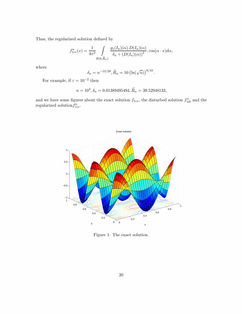
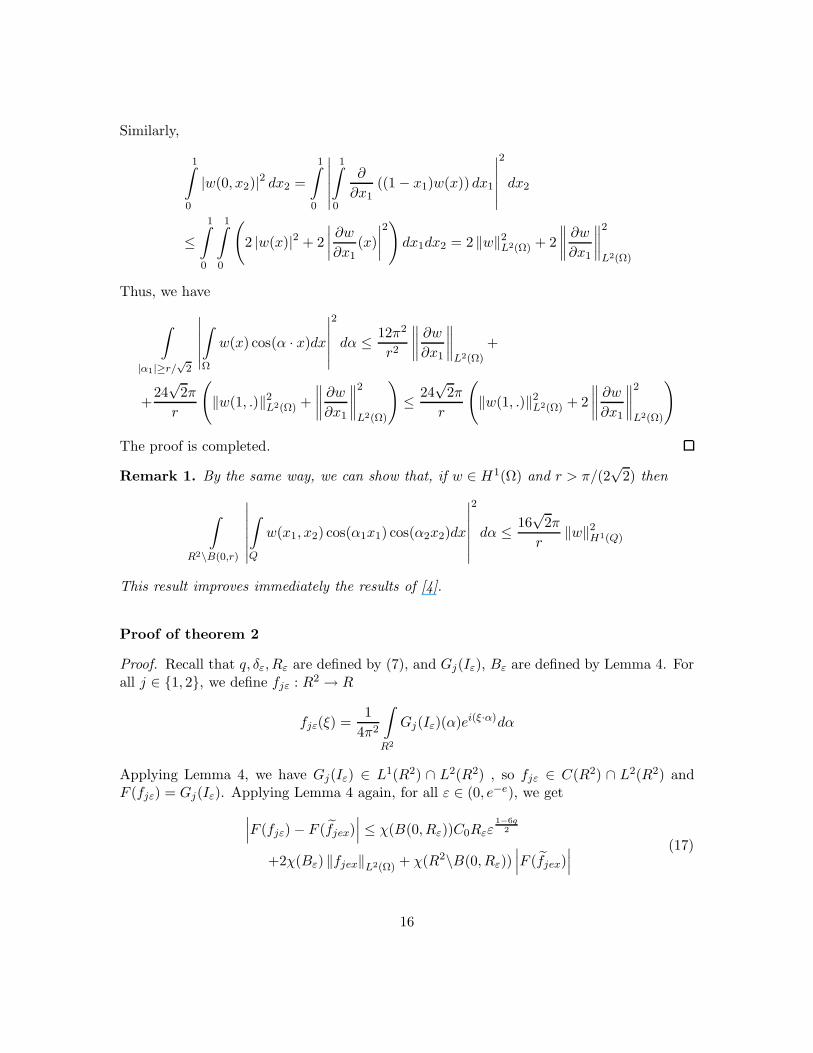
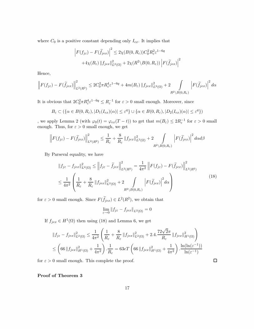
Thus, the regularized solution defined by

fn1re(x) =

1

4π2

∫

B(0, eRn)

g1(In)(α).D(In)(α)

δn + (D(In)(α))2. cos(α · x)dα,

whereδn = n−13/28, Rn = 10

(ln(

√n))9/10

.

For example, if ε = 10−2 then

n = 104, δn = 0.01389495494, Rn = 39.52948133,

and we have some figures about the exact solution f1ex, the disturbed solution fn1di and the

regularized solutionfn1re.

00.2

0.40.6

0.81

0

0.2

0.4

0.6

0.8

1−1

−0.5

0

0.5

1

x

Exact solution

y

Figure 1. The exact solution.

20

00.2

0.40.6

0.81

0

0.2

0.4

0.6

0.8

1−10

−8

−6

−4

−2

0

2

4

6

8

x

Disturbed solution

y

Figure 2. The disturbed solution.

Figure 3. The Fourier transform of the exact solution.

21

Figure 4. The Fourier transform of the regularized solution.

References

[1] Timoshenko, S. and J. N. Goodier, Theory of Elasticity, New York, Mc Graw-Hill 1970.

[2] Martin H. Sadd, Elasticity Theory, Applications, and Numerics, Elsevier 2005.

[3] Dang Duc Trong, Nguyen Thanh Long, Pham Ngoc Dinh Alain, Nonhomogeneous heatequation: Identification and regularization for the inhomogeneous term, J. Math. Anal.Appl. 312 (2005), 93-104.

[4] D.D.Trong, P.H.Quan, P.N.Dinh Alain, Determination of a two-dimentional heatsource: Uniqueness, regularization and error estimate, J. Comp. Appl. Math,191(2006), 50-67.

[5] Dang Duc Trong and Truong Trung Tuyen, Error of Tikhonov’s regularization forintergral convolution equation, arXiv:math.NA/0610046 v1 1 Oct 2006.

[6] B.Ya.Levin, Lectures on Entire Functions, Trans Math Monographs, Vol.150, AMS,Providence, Rhole Island, 1996.

22

[7] Isakov, V., Inverse source problems, Math. surveys and monographs series, Vol.34,AMS, Providence, Rhode Island, 1990, chap.7, page. 166

[8] Tikhonov A. N.,Theoremes d’unicite pour l’equation de la chaleur, Math. Sborn.42(1935), 199-216

[9] M. Grasselli, M. Ikehata, M. Yamamoto, An inverse source problem for the Lamesystem with variable coefficients, Applicable Analysis. 84(4)(2005), 357-375.

[10] Aki, K. and Richards, P.G., 1980, Quantitative Seismology Theory and Methods, Vol.I, New York, Freeman.

[11] M.I. Ivanchov, The inverse problem of determining the heat source power for a parabolicequation under arbitrary boundary conditions, J. Math. Sci (New York) 88(3)(1998),432-436.

[12] M.I. Ivanchov, Inverse problem for a multidimensional heat equation with an unknowsource function, Mat. Stud. 16(1)(2001), 93-98.

[13] D.U. Kim, Construction of the solution of a certain system of heat equations with heatsources that depend on the temperature, Izv. Akad. Nauk. Kazak. SSR Ser. Fiz-Mat.(1)(1971), 49-53.

[14] G.S. Li, L.Z. Zhang, Exixtence of a nonlinear heat source in invarse heat conductionproblems, Hunan Ann. Math. 17(2)(1997), 19-24

23