Determination of optimal build orientation for additive ...

Vol.:(0123456789)1 3

Journal of Intelligent Manufacturing (2019) 30:3015–3034 https://doi.org/10.1007/s10845-019-01497-6

Determination of optimal build orientation for additive manufacturing using Muirhead mean and prioritised average operators

Yuchu Qin1 · Qunfen Qi1 · Paul J. Scott1 · Xiangqian Jiang1

Received: 26 March 2019 / Accepted: 21 September 2019 / Published online: 5 October 2019 © The Author(s) 2019

AbstractBuild orientation determination is one of the essential process planning tasks in additive manufacturing since it has crucial effects on the part quality, post-processing, build time and cost, etc. This paper introduces a method based on fuzzy multi-attribute decision making to determine the optimal build orientation from a finite set of alternatives. The determination process includes two major steps. In the first step, attributes that are considered in the determination and heterogeneous relationships of which are firstly identified. A fuzzy decision matrix is then constructed and normalised based on the values of the identified attributes, which are quantified by a set of fuzzy numbers. In the second step, two fuzzy number aggregation operators are developed to aggregate the fuzzy information in the normalised matrix. By comparing the aggregation results, a ranking of all alternative build orientations can then be generated. Two determination examples are used to demonstrate the working process of the proposed method. Qualitative and quantitative comparisons between the proposed method and other methods are carried out to demonstrate its feasibility, effectiveness, and advantages.

Keywords Additive manufacturing · Build orientation determination · Optimal build orientation · Correlative relationship · Priority relationship · Fuzzy multi-attribute decision making

List of symbolsΞi A fuzzy numberμi The degree of membership of a fuzzy

number<μi> A fuzzy number whose degree of member-

ship is μiS An ordered set of fuzzy numbersSk The k-th partition of S|Sk| The cardinality of SkØ Empty setδ|Sk| The |Sk|-th real number corresponding to

Ξ|Sk|δk A collection of δ1, δ2, …, δ|Sk|Δ A collection of δ1, δ2, …, δNp(ik) A permutation of (1, 2, …, |Sk|)P|Sk| A set of all permutations of (1, 2, …, |Sk|)Ξi ⊕ Ξj The sum operation of Ξi and Ξj

Ξi ⊗ Ξj The product operation of Ξi and ΞjaΞr The multiplication operation of ΞrΞs

b The power operation of Ξswi The weight of ΞiTT(Ξi) The TT value of a fuzzy numberξp(ik) The power weight of p(ik)DIST(Ξi, Ξj) The distance between Ξi and ΞjSUPP(Ξi, Ξj) The support degree for Ξi from ΞjSi ≻ Sj Si is preferred over SjS0 The fuzzy number <1>Sk The fuzzy number <max(μ1, μ2, …, μ|Sk|)>Tk The fuzzy number S0 ⊗ S1 ⊗⋯⊗ Sk−1ξik The power weight of ikOi An option or an orientationO A set of options or orientationsAj An attributeA A set of attributesw A set of weightsM A decision matrixvi,j The value of the j-th attribute of the i-th

optionri,j The ratio of vi,jMF A fuzzy decision matrixMN A normalised fuzzy decision matrix

* Qunfen Qi [email protected]

1 EPSRC Future Advanced Metrology Hub, Centre for Precision Technologies, School of Computing and Engineering, University of Huddersfield, Huddersfield HD1 3DH, UK

http://orcid.org/0000-0001-5936-1714

http://crossmark.crossref.org/dialog/?doi=10.1007/s10845-019-01497-6&domain=pdf

3016 Journal of Intelligent Manufacturing (2019) 30:3015–3034

1 3

Ai ≻ Aj Ai is preferred over AjOi ≻ Oj Oj ranks behind Oi

Introduction

Additive manufacturing (AM), which is commonly known as three-dimensional (3D) printing, refers to the processes of accumulating materials layer upon layer to 3D objects from 3D model data (ISO/ASTM 52900 2015). AM processes provide better flexibility in 3D model design, generate fewer waste byproducts in part manufacturing, and require less time and cost in product development, over conventional subtractive manufacturing processes. In addition, AM pro-cesses enables the fabrication of components with complex geometries, heterogeneous materials, and user-customisa-ble properties (Gibson et al. 2015). Some have anticipated that AM processes would bring revolutionary changes to the industry (Gao et al. 2015). Despite this, ensuring the repeatability of AM processes and the reproducibility of AM products is still considered as one of the biggest challenges to make the processes widely applied in the real world indus-try (Kim et al. 2017; Qin et al. 2019).

To tackle this challenge, substantial work needs to be car-ried out at a number of aspects (e.g. design and simulation for AM, process planning for AM, qualification and certifi-cation of AM parts, standardisation of AM processes, AM materials, and AM digital thread) (Kim et al. 2015, 2017), in which process planning is one of the most important aspects. Process planning for AM is the use of specific techniques to generate the process plans for building a part, which mainly include build orientation, support structure, 3D model slic-ing, and tool-path, according to the 3D model data of the part (Kulkarni et al. 2000; Ahsan et al. 2015; Liang 2018). It consists of a set of successive preparation steps before building the part, and determine the build orientation is the first step. Build orientation has direct influence on the subse-quent preparation steps, namely support structure generation (Jiang et al. 2018a, b, 2019a, b, c), 3D model slicing (Xu et al. 2018), and tool-path planning (Xiao and Joshi 2018).

In the process of AM, the build orientation is the accu-mulating orientation of materials when building the part. The quality of a build orientation has important influence on the part quality, post-processing, build time and cost, etc. (Taufik and Jain 2013). Build orientation determina-tion refers to the use of specific techniques to identify a proper orientation to build an AM part from an infinite number of theoretical orientations. It consists of two major tasks. One is to generate a certain number of alternative build orientations (ABOs) from the infinite set. The other is to determine the optimal build orientation (OBO) from the generated ABOs (Kulkarni et al. 2000). At present, build orientations are manually specified by AM machine

operators according to their expertise. Under the same cir-cumstances, different operators may be in favour of dif-ferent build orientations, which may greatly increase the uncertainty of process planning and directly affect the build cost, build time, accuracy, and quality of the parts (Zhang et al. 2018).

To provide an effective tool for automatic determination of build orientations, a method based on fuzzy multi-attrib-ute decision making is proposed in this paper. The method focuses on the second task in build orientation determina-tion and assumes that the ABOs are known. It is carried out in two steps. In the first step, attributes that are considered in the determination and their relationships are identified. Values of the identified attributes will be obtained from vendor documents, benchmark data, experiments, or expert evaluation. The values are then fuzzified using a ratio model as a membership function. As such each attribute value is quantified by a fuzzy number (FN), which enables the use of aggregation operators upon the fuzzified values. In the second step, a fuzzy weighted power partitioned Muirhead mean (FWPPMM) operator and a fuzzy weighted power prioritised average (FWPPA) operator, are developed to aggregate all FNs of each ABO. The overall attribute value of each ABO can then be finally quantified by a single FN. By comparing these FNs (from high to low), a ranking of all ABOs can then be generated, and the one which is ranked first is then proposed as the OBO.

The remainder of the paper is organised as follows. An overview of related work is provided in section “Related work”. “OBO determination method” section explains the details of the proposed OBO determination method. Two examples and qualitative and quantitative comparisons are presented to illustrate and demonstrate the method in “Examples and comparisons” section. “Conclusion” section ends the paper with a conclusion.

Related work

An ideal method for OBO determination is preferably a standardised method for practical applications. The latest AM process standards (ISO 17296-2 2015; ISO 17296-3 2014) provide a classification of AM processes, an introduc-tion to the principle of each AM process, and a description to the performance test methods of AM processes, but have not yet enclosed a practical method for OBO determination.

To provide an effective tool for OBO determination, a number of methods have been presented during the past two decades. These methods can be classified into the following two categories on the basis of their used techniques:

(1) Multi-objective optimisation (MOO) methods. The fundamental principle of this category of methods is to use specific MOO techniques to find out a build orientation

3017Journal of Intelligent Manufacturing (2019) 30:3015–3034

1 3

that enables one or more specific objectives (i.e. attributes of build orientations), such as design requirements, build cost, build time, part accuracy, mechanical properties, and thermodynamic properties, to be optimal from an infinite number of theoretical orientations or a certain number of alternative orientations. The methods based on this prin-ciple mainly include the methods proposed by Cheng et al. (1995), Lan et al. (1997), Alexander et al. (1998), McClurkin and Rosen (1998), Hur and Lee (1998), Xu et al. (1999), Hur et al. (2001), Masood et al. (2003), Thrimurthulu et al. (2004), Pandey et al. (2004), Kim and Lee (2005), Ahn et al. (2007), Canellidis et al. (2009), Padhye and Deb (2011), Strano et al. (2011), Zhang and Li (2013), Paul and Anand

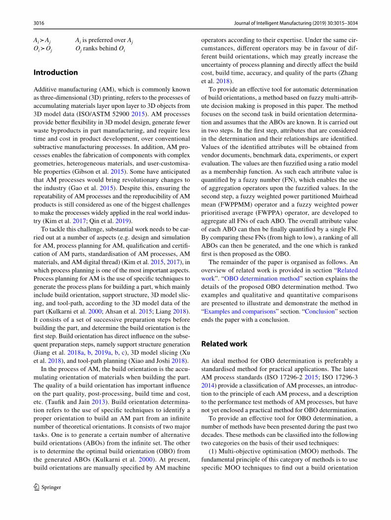
(2015), Ezair et al. (2015), Delfs et al. (2016), Luo and Wang (2016), Zhang et al. (2017), Brika et al. (2017), Chowd-hury et al. (2018), Mi et al. (2018), Jaiswal et al. (2018), Al-Ahmari et al. (2018), Huang et al. (2018), Raju et al. (2018), and Golmohammadi and Khodaygan (2019). A brief summarisation of these methods is provided in Table 1. As can be seen from the table, different MOO techniques and optimised objectives were used. Among the used MOO techniques, genetic algorithm is the most frequently used technique, in which Brika et al. (2017) and Chowdhury et al. (2018) have considered significantly more numbers of opti-mised objectives than the others. This means that the two methods can achieve better optimisation results than other

Table 1 A brief summarisation of some typical MOO methods

Notes: Golmohammadi (2019) is short for Golmohammadi and Khodaygan (2019); PSO particle swarm optimisation; BFO bacterial foraging optimisation

MOO method Used MOO techniques Optimised objectives

Cheng et al. (1995) Weighted sum function Part accuracy; build timeLan et al. (1997) Self-developed algorithm Surface quality; build time; complexity of support structureAlexander et al. (1998) Self-developed algorithm Cost; support volume; contact area with support; surface accuracyMcClurkin and Rosen (1998) Self-developed algorithm Build time; accuracy; surface finishHur and Lee (1998) Genetic algorithm Part accuracy; build time; support structure volumeXu et al. (1999) Self-developed algorithm Build cost; build time; building inaccuracy; surface finishHur et al. (2001) Genetic algorithm Build time; surface qualityMasood et al. (2003) Generic mathematical algorithm Volumetric errorThrimurthulu et al. (2004) Genetic algorithm Surface finish; build timePandey et al. (2004) Genetic algorithm Surface roughness; build timeKim and Lee (2005) Genetic algorithm Post-processing time and costAhn et al. (2007) Genetic algorithm Post-machining timeCanellidis et al. (2009) Genetic algorithm Build time; surface roughness; post-processing timePadhye and Deb (2011) Genetic algorithm and particle swarm

algorithmSurface roughness; build time

Strano et al. (2011) Genetic algorithm Surface roughness; energy consumptionZhang and Li (2013) Genetic algorithm Volumetric errorPaul and Anand (2015) Genetic algorithm Cylindricity and flatness errors; support structure volumeEzair et al. (2015) Self-developed algorithm Support structure volumeDelfs et al. (2016) Self-developed algorithm Surface quality; build timeLuo and Wang (2016) Principal component analysis Volumetric errorZhang et al. (2017) Genetic algorithm Build time; build cost; production qualityBrika et al. (2017) Genetic algorithm Surface roughness; build time; build cost; yield strength; tensile

strength; elongation; vickers hardness; amount of support structure

Chowdhury et al. (2018) Genetic algorithm Support structure volume; support structure accessibility; surface area contacting support; number of build layers; number of small openings; number of sharp corners; mean cusp height

Mi et al. (2018) Point clustering algorithm Number of material changesJaiswal et al. (2018) Surrogate model Material error; geometric errorAl-Ahmari et al. (2018) Weighted sum function Geometric dimensioning and tolerancing value; production timeHuang et al. (2018) Genetic algorithm Adaptive feature roughness; build timeRaju et al. (2018) Hybrid PSO-BFO algorithm Hardness; flexural modulus; tensile strength; surface roughnessGolmohammadi (2019) Taguchi method Amount of support material; mean roughness of the product


1 3

methods under the same conditions. However, considering more number of objectives is likely to generate large number of Pareto-optimal solutions (most of them are not the real optimal solutions) (Ancău and Caizar 2010), and will greatly extend the convergence time of the optimisation algorithm. These can hardly be accepted for the actual OBO determina-tion (Zhang et al. 2018).

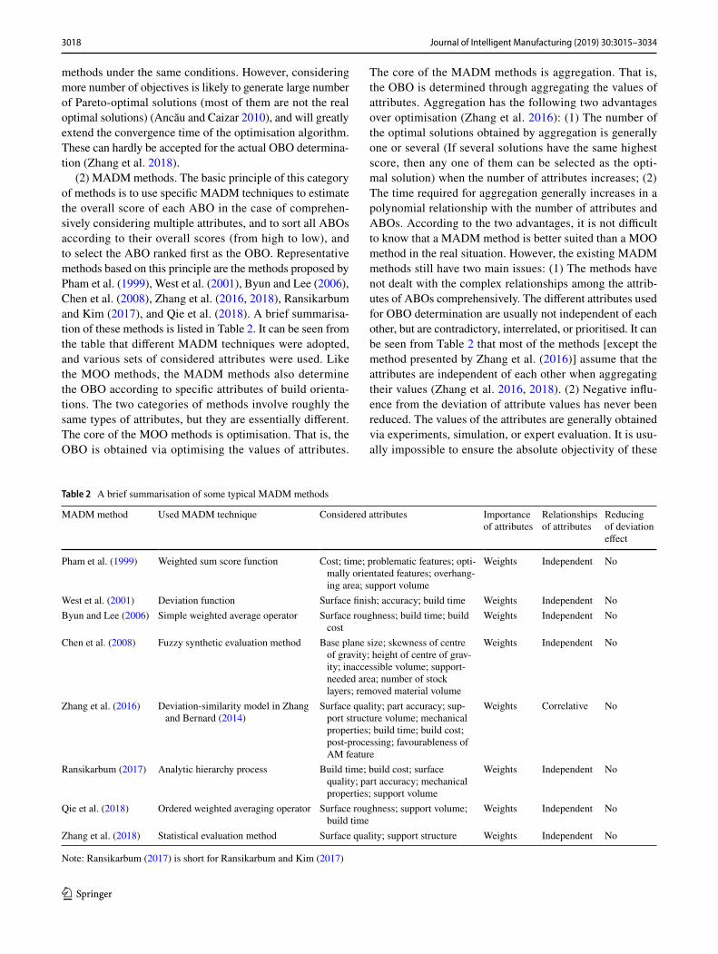
(2) MADM methods. The basic principle of this category of methods is to use specific MADM techniques to estimate the overall score of each ABO in the case of comprehen-sively considering multiple attributes, and to sort all ABOs according to their overall scores (from high to low), and to select the ABO ranked first as the OBO. Representative methods based on this principle are the methods proposed by Pham et al. (1999), West et al. (2001), Byun and Lee (2006), Chen et al. (2008), Zhang et al. (2016, 2018), Ransikarbum and Kim (2017), and Qie et al. (2018). A brief summarisa-tion of these methods is listed in Table 2. It can be seen from the table that different MADM techniques were adopted, and various sets of considered attributes were used. Like the MOO methods, the MADM methods also determine the OBO according to specific attributes of build orienta-tions. The two categories of methods involve roughly the same types of attributes, but they are essentially different. The core of the MOO methods is optimisation. That is, the OBO is obtained via optimising the values of attributes.

The core of the MADM methods is aggregation. That is, the OBO is determined through aggregating the values of attributes. Aggregation has the following two advantages over optimisation (Zhang et al. 2016): (1) The number of the optimal solutions obtained by aggregation is generally one or several (If several solutions have the same highest score, then any one of them can be selected as the opti-mal solution) when the number of attributes increases; (2) The time required for aggregation generally increases in a polynomial relationship with the number of attributes and ABOs. According to the two advantages, it is not difficult to know that a MADM method is better suited than a MOO method in the real situation. However, the existing MADM methods still have two main issues: (1) The methods have not dealt with the complex relationships among the attrib-utes of ABOs comprehensively. The different attributes used for OBO determination are usually not independent of each other, but are contradictory, interrelated, or prioritised. It can be seen from Table 2 that most of the methods [except the method presented by Zhang et al. (2016)] assume that the attributes are independent of each other when aggregating their values (Zhang et al. 2016, 2018). (2) Negative influ-ence from the deviation of attribute values has never been reduced. The values of the attributes are generally obtained via experiments, simulation, or expert evaluation. It is usu-ally impossible to ensure the absolute objectivity of these

Table 2 A brief summarisation of some typical MADM methods

Note: Ransikarbum (2017) is short for Ransikarbum and Kim (2017)

MADM method Used MADM technique Considered attributes Importance of attributes

Relationships of attributes

Reducing of deviation effect

Pham et al. (1999) Weighted sum score function Cost; time; problematic features; opti-mally orientated features; overhang-ing area; support volume

Weights Independent No

West et al. (2001) Deviation function Surface finish; accuracy; build time Weights Independent NoByun and Lee (2006) Simple weighted average operator Surface roughness; build time; build

costWeights Independent No

Chen et al. (2008) Fuzzy synthetic evaluation method Base plane size; skewness of centre of gravity; height of centre of grav-ity; inaccessible volume; support-needed area; number of stock layers; removed material volume


Zhang et al. (2016) Deviation-similarity model in Zhang and Bernard (2014)

Surface quality; part accuracy; sup-port structure volume; mechanical properties; build time; build cost; post-processing; favourableness of AM feature

Weights Correlative No

Ransikarbum (2017) Analytic hierarchy process Build time; build cost; surface quality; part accuracy; mechanical properties; support volume


Qie et al. (2018) Ordered weighted averaging operator Surface roughness; support volume; build time


Zhang et al. (2018) Statistical evaluation method Surface quality; support structure Weights Independent No


1 3

ways, which means that there will often be deviation in one or several attribute values. To obtain reasonable OBO under such circumstance, it is of necessity to reduce the effect of deviation on the aggregation result. But none of the methods in Table 2 can achieve this.

Aiming at the two issues in the existing MADM meth-ods for OBO determination, FS (Dubois and Prade 1980), the MM operator (Muirhead 1902), the PA operator (Yager 2008), the power average operator (Yager 2001), and the partitioned average operator (Dutta and Guha 2015) are introduced in this paper to construct a FWPPMM opera-tor and a FWPPA operator to aggregate the values of the attributes of ABOs. An OBO determination method based on fuzzy MADM and the constructed operators is proposed. FS is a mathematical tool that can normalise the values of attributes into the numbers in [0, 1] to make them easy to handle. The MM operator is an aggregation operator that is applicable whenever all attributes are independent of each other, or there are correlative relationships between any two attributes, or any three or more attributes. The PA opera-tor can capture priority relationships among attributes. The power average operator is an aggregation operator that can reduce the negative effect of the deviation of one or several argument values on the aggregation result. The partitioned average operator can handle the heterogeneous relationships among the aggregated arguments. Because of the combina-tion of the MM, PA, power average, and partitioned aver-age operators in the constructed operators, the proposed method can deal with the heterogeneous correlative relation-ship (HCR) and heterogeneous priority relationship (HPR)

among the attributes of ABOs, while can also reduce the negative influence of the deviation of attribute values. Here HCR (or HPR) means that the attributes are partitioned into different partitions and the attributes in the same partitions are correlative with each other (have the same priority) whereas the attributes in different partitions are independ-ent of each other (have different priority).

OBO determination method

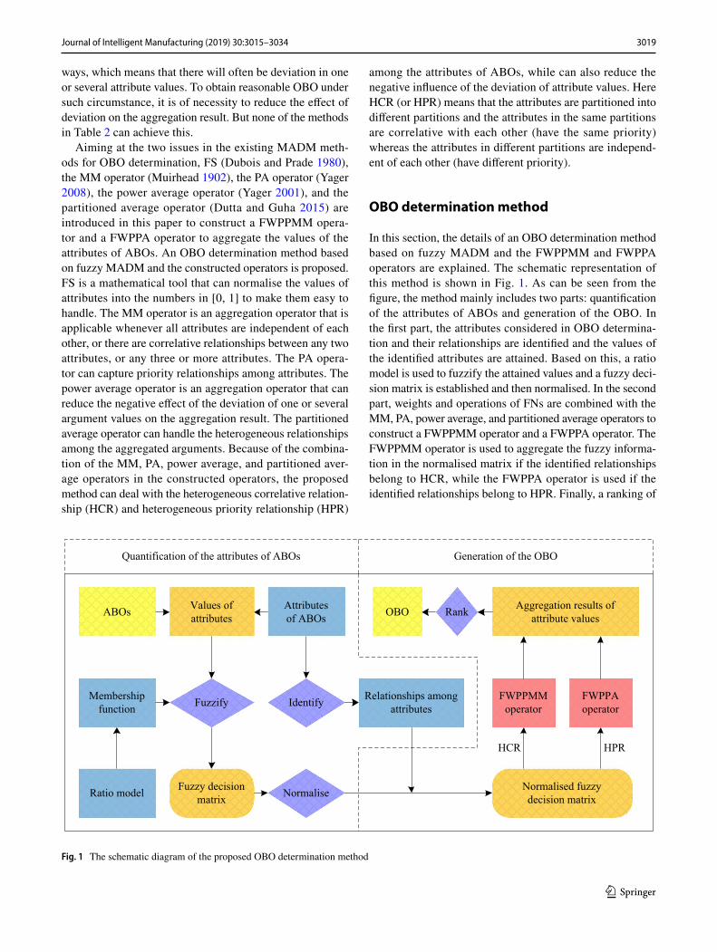
In this section, the details of an OBO determination method based on fuzzy MADM and the FWPPMM and FWPPA operators are explained. The schematic representation of this method is shown in Fig. 1. As can be seen from the figure, the method mainly includes two parts: quantification of the attributes of ABOs and generation of the OBO. In the first part, the attributes considered in OBO determina-tion and their relationships are identified and the values of the identified attributes are attained. Based on this, a ratio model is used to fuzzify the attained values and a fuzzy deci-sion matrix is established and then normalised. In the second part, weights and operations of FNs are combined with the MM, PA, power average, and partitioned average operators to construct a FWPPMM operator and a FWPPA operator. The FWPPMM operator is used to aggregate the fuzzy informa-tion in the normalised matrix if the identified relationships belong to HCR, while the FWPPA operator is used if the identified relationships belong to HPR. Finally, a ranking of

ABOs Values of attributes

Attributesof ABOs

FWPPMMoperator

FWPPAoperator

Membershipfunction

Fuzzy decision matrix Normalise

Fuzzify

Normalised fuzzydecision matrix

Aggregation results ofattribute valuesOBO Rank

Relationships among attributesIdentify

Ratio model

HCR HPR

Quantification of the attributes of ABOs Generation of the OBO

Fig. 1 The schematic diagram of the proposed OBO determination method


1 3

ABOs is obtained via comparing the aggregation results and the then OBO can be determined according to the ranking.

Based on the description above, the present section is divided into three subsections, which explain the details of the FWPPMM and FWPPA operators, quantification of the attributes of ABOs, and generation of the OBO, respectively.

FWPPMM and FWPPA operators

Preliminaries

(1) Definition of FS In mathematics, a FS is a set whose ele-ments have membership degrees, which indicate the degrees to which the elements belong to the set (Zadeh 1965). It can be formally defined as follow.

Definition 1 A FS S in a finite universe of discourse X is: S = {<x, µS(x)> | x∈X}, where µS : X → [0, 1] denotes the membership degree of x∈X to S, with the condition that 0 ≤ µS(x) ≤ 1.

(2) Definition of FN Generally, the values of the member-ship function µS(x) are called as FNs. The definition of a FN can be naturally obtained as follow.

Definition 2 A FN Ξ on a FS S = {<x, µS(x)> | x∈X} is: Ξ = <µS(x)>. For the sake of simplicity, the FN is usually denoted as Ξ = <µ> .

(3) Comparison rules of FNs Any two FNs can be com-pared via comparing their membership degrees. For exam-ple, suppose Ξ1 = <µ1> and Ξ2 = <µ2> are two arbitrary FNs, then Ξ1 < Ξ2 if and only if µ1 < µ2; Ξ1 > Ξ2 if and only if µ1 > µ2; and Ξ1 = Ξ2 if and only if µ1 = µ2.

(4) Operational rules of FNs Generally, the operations between FNs and between real numbers and FNs are based on specific family of T-norm and T-conorm. The following four operational rules, which are based on the Algebraic T-norm and T-conorm, respectively define the sum and product operations between FNs and the multiplication and power operations between real numbers and FNs (Dubois and Prade 1980):

where Ξ = <μ> , Ξ1 = <μ1> , and Ξ2 = <μ2> are three arbi-trary FNs, and a and b are two arbitrary real numbers and a, b > 0.

(1)Ξ1Ξ2 = <𝜇1 + 𝜇2 − 𝜇1𝜇2>

(2)Ξ1Ξ2 = <𝜇1𝜇2>

(3)aΞ = <1 − (1 − 𝜇)a>

(4)Ξb = <𝜇b>

(5) Distance between FNs The distance between two FNs can be measured by the absolute value of the difference of their membership degrees (Dubois and Prade 1980). For example, suppose Ξ1 = <µ1> and Ξ2 = <µ2> are two arbitrary FNs, then the distance between these two FNs is:

(6) MM operator The MM operator was firstly introduced to aggregate crisp numbers by Muirhead (1902). It is an all-in-one aggregation operator for capturing the relationships among multiple aggregated arguments, since it is applicable in the cases where all arguments are independent of each other, there are interrelationships between any two arguments, and there are interrelationships among any three or more argu-ments. The formal definition of the MM operator is as follow.

Definition 3 Let (Ω1, Ω2, …, Ωn) be a collection of crisp numbers, Δ = (δ1, δ2, …, δn) (where δ1, δ2, …, δn ≥ 0 but not at the same time δ1 = δ2 = ··· = δn = 0) be a collection of n real numbers, p(i) be a permutation of (1, 2, …, n), and Pn be the set of all permutations of (1, 2, …, n). Then the aggregation function

is called the MM operator. In this operator, the values of δi (i = 1, 2, …, n) are used to specify the relationships among aggregated arguments: (1) If δ1> 0 and δ2 = δ3 = ··· = δn = 0, then the arguments are independent of each other; (2) If δ1, δ2 > 0 and δ3 = δ4 = ··· = δn = 0, then the correlative rela-tionships between two arguments are considered; (3) If δ1, δ2, …, δk > 0 (k = 3, 4, …, n) and δk+1 = δk+2 = ··· = δn = 0, then the correlative relationships among k arguments are considered.

(7) PA (prioritised average) operator The PA operator, introduced by Yager (2008), has the capability of dealing with the HPR among the aggregated arguments. Its formal definition is as follow.

Definition 4 Let (Ω1, Ω2, …, Ωn) be a collection of crisp numbers, S = {Ω1, Ω2, …, Ωn} be a set, Sk = {Ω1, Ω2, …, Ω|Sk|} (k = 1, 2, …, N) be N partitions of S (i.e. S1 ∪ S2 ∪ ··· ∪ SN = S and S1 ∩ S2 ∩ ··· ∩ SN = Ø), S1 ≻ S2 ≻ ··· ≻ SN be the priority relationship among S1, S2, …, SN, S0 = 1 and Sk = max(Ω1, Ω2, …, Ω|Sk|) (k = 1, 2, …, N), and Tk = S0S1…Sk−1. Then the aggregation function

is called the PA operator.

(5)DIST(Ξ1, Ξ2

)= ||�1 − �2

||

(6)MMΔ(Ω1,Ω2,… ,Ωn) =

�1

n!

�p∈Pn

n�i=1

Ω�i

p(i)

� 1∑ni=1

�i

(7)PA(Ω1,Ω2,… ,Ωn) =

N�k=1

⎛⎜⎜⎝Tk

⎛⎜⎜⎝

�Sk��ik=1

Ωik

⎞⎟⎟⎠

⎞⎟⎟⎠


1 3

(8) Power average operator The power average operator, introduced by Yager (2001), can assign weights to the aggre-gated arguments via computing the support degrees between these arguments. This makes it possible to reduce the nega-tive influence of the unduly high or unduly low argument values on the aggregation results. The formal definition of the power average operator is as follow.

Definition 5 Let (Ω1, Ω2, …, Ωn) be a collection of crisp numbers, SUPP(Ωi, Ωj) = 1 − DIST(Ωi, Ωj) (i, j = 1, 2, …, n and j ≠ i; D(Ωi, Ωj) is the distance between Ωi and Ωj) be the support degree for Ωi from Ωj, and

Then the aggregation function

is called the power average operator.

(9) Partitioned average operator The partitioned average operator (Dutta and Guha 2015) can aggregate the argu-ments in different partitions using the same aggregation

operator and aggregate the aggregation results of different partitions using the ordinary arithmetic mean operator. By this way, the HCR among arguments can be considered. The formal definition of the partitioned average operator is as follow.

Definition 6 Let (Ω1, Ω2, …, Ωn) be a collection of crisp numbers, S = {Ω1, Ω2, …, Ωn} be a set of Ω1, Ω2, …, Ωn, Sk = {Ω1, Ω2, …, Ω|Sk|} (k = 1, 2, …, N) be N partitions of S (i.e. S1 ∪ S2 ∪ ··· ∪ SN = S and S1 ∩ S2 ∩ ··· ∩ SN = Ø), and AO be a specific aggregation operator. Then the aggregation function

is called the partitioned average operator.

(8)TT(Ωi) =

n∑j=1,j≠i

SUPP(Ωi, Ωj)

(9)PwA(Ω1,Ω2,… ,Ωn) =

∑n

i=1

��1 + TT(Ωi)

�Ωi

�∑n

i=1

�1 + TT(Ωi)

�

(10)PtA(Ω1,Ω2,… ,Ωn) =1

N

N∑k=1

(|Sk|AOik=1

(Ωik

))

FWPPMM operator

To handle the HCR among the attributes of ABOs and mean-while reduce the negative effect of the deviation of attribute values on the OBO determination result, weights and the MM, power average, and partitioned average operators of FNs are combined to construct a FWPPMM operator. Based on the definitions of these operators (see Definitions 3, 5, and 6), the FWPPMM operator can be defined as follow.

Definition 7 Let (Ξ1, Ξ2, …, Ξn) (Ξi = <μi>, i = 1, 2, …, n) be a collection of n FNs, S = {Ξ1, Ξ2, …, Ξn} be an ordered set, Sk = {Ξ1, Ξ2, …, Ξ|Sk|} (k = 1, 2, …, N) be N partitions of S (i.e. S1 ∪ S2 ∪ ··· ∪ SN = S and S1 ∩ S2 ∩ ··· ∩ SN = Ø), δ1, δ2, …, δ|Sk| (k = 1, 2, …, N and δ1, δ2, …, δ|Sk| ≥ 0 but not at the same time δ1 = δ2 = ··· = δ|Sk| = 0) be |Sk| real numbers that respectively correspond to Ξ1, Ξ2, …, Ξ|Sk|, δk = (δ1, δ2, …, δ|Sk|) be a collection of δ1, δ2, …, δ|Sk|, Δ = (δ1, δ2, …, δN) be a collection of δ1, δ2, …, δN, p(ik) be a per-mutation of (1, 2, …, |Sk|), P|Sk| be a set of all permutations of (1, 2, …, |Sk|), Ξi ⊕ Ξj and Ξi ⊗ Ξj (i, j = 1, 2, …, n) be respectively the sum and product operations of Ξi and Ξj, aΞr and Ξs

b (r, s = 1, 2, …, n; a, b > 0) be respectively the multi-plication operation of Ξr and the power operation of Ξs, and w1, w2, …, wn be respectively the weights of Ξ1, Ξ2, …, Ξn such that 0 ≤ w1, w2, …, wn ≤ 1 and w1 + w2 + ··· + wn = 1. Then the aggregation function

is called the FWPPMM operator. In this operator, the values of δik (ik = 1, 2, …, |Sk|) are used to specify the relationships among the aggregated FNs in each of the N partitions S: (1) If δ1> 0 and δ2 = δ3 = ··· = δ|Sk| = 0, then the FNs in the k-th partition Sk are independent of each other; (2) If δ1, δ2 > 0 and δ3 = δ4 = ··· = δ|Sk| = 0, then the correlative relationships between two FNs in Sk are considered; (3) If δ1, δ1, …, δt > 0 (t = 3, 4, …, n) and δt+1 = δt+2 = ··· = δ|Sk| = 0, then the correla-tive relationships among t FNs in Sk are considered.

Equation (11) is a generalised form of the FWPPMM operator. If specific rules are assigned to the sum, product, multiplication, and power operations in it, then specific FWPPMM operators can be constructed. For instance, if

(11)FWPPMM�(Ξ1,Ξ2,… ,Ξn) =1

N

⎛⎜⎜⎜⎝

N

⊕k=1

⎛⎜⎜⎝

1

��Sk��!⊕

p∈P�Sk�

�Sk�⊗ik=1

�nwp(ik)

�1 + TT(Ξp(ik)

)�

∑n

j=1

�wj

�1 + TT(Ξj)

��Ξp(ik)

�𝛿ik ⎞⎟⎟⎠

1

∑�Sk�ik=1

𝛿ik

⎞⎟⎟⎟⎠


1 3

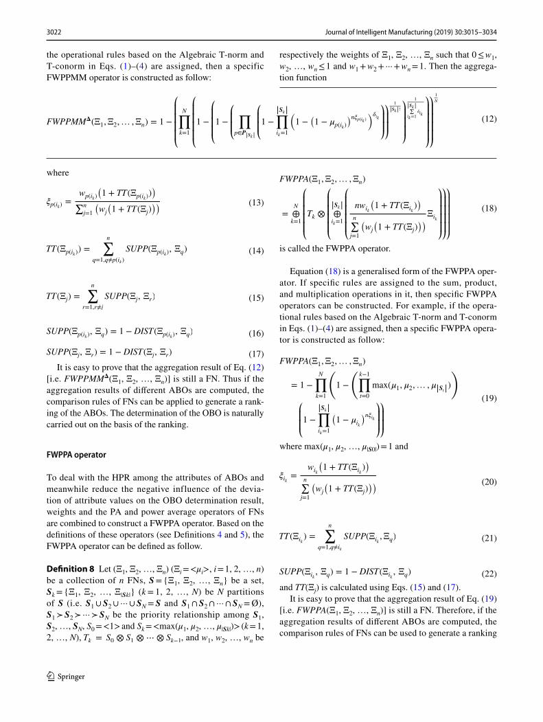
the operational rules based on the Algebraic T-norm and T-conorm in Eqs. (1)–(4) are assigned, then a specific FWPPMM operator is constructed as follow:

where

It is easy to prove that the aggregation result of Eq. (12) [i.e. FWPPMMΔ(Ξ1, Ξ2, …, Ξn)] is still a FN. Thus if the aggregation results of different ABOs are computed, the comparison rules of FNs can be applied to generate a rank-ing of the ABOs. The determination of the OBO is naturally carried out on the basis of the ranking.

FWPPA operator

To deal with the HPR among the attributes of ABOs and meanwhile reduce the negative influence of the devia-tion of attribute values on the OBO determination result, weights and the PA and power average operators of FNs are combined to construct a FWPPA operator. Based on the definitions of these operators (see Definitions 4 and 5), the FWPPA operator can be defined as follow.

Definition 8 Let (Ξ1, Ξ2, …, Ξn) (Ξi = <μi>, i = 1, 2, …, n) be a collection of n FNs, S = {Ξ1, Ξ2, …, Ξn} be a set, Sk = {Ξ1, Ξ2, …, Ξ|Sk|} (k = 1, 2, …, N) be N partitions of S (i.e. S1 ∪ S2 ∪ ··· ∪ SN = S and S1 ∩ S2 ∩ ··· ∩ SN = Ø), S1 ≻ S2 ≻ ··· ≻ SN be the priority relationship among S1, S2, …, SN, S0 = <1> and Sk = <max(μ1, μ2, …, μ|Sk|)> (k = 1, 2, …, N), Tk = S0 ⊗ S1 ⊗⋯⊗ Sk−1 , and w1, w2, …, wn be

(12)FWPPMM�(Ξ1,Ξ2,… ,Ξn) = 1 −

⎛⎜⎜⎜⎜⎝

N�k=1

⎛⎜⎜⎜⎜⎝1 −

⎛⎜⎜⎜⎝1 −

⎛⎜⎜⎝�

p∈P�Sk�

⎛⎜⎜⎝1 −

�Sk��ik=1

�1 −

�1 − �p(ik)

�n�p(ik )��ik⎞⎟⎟⎠

⎞⎟⎟⎠

1

�Sk�! ⎞⎟⎟⎟⎠

1

�Sk�∑ik=1

�ik

⎞⎟⎟⎟⎟⎠

⎞⎟⎟⎟⎟⎠

1

N

(13)�p(ik) =wp(ik)

�1 + TT(Ξp(ik)

)�

∑n

j=1

�wj

�1 + TT(Ξj)

��

(14)TT(Ξp(ik)) =

n∑q=1,q≠p(ik)

SUPP(Ξp(ik), Ξq)

(15)TT(Ξj) =

n∑r=1,r≠j

SUPP(Ξj, Ξr)

(16)SUPP(Ξp(ik), Ξq) = 1 − DIST(Ξp(ik)

, Ξq)

(17)SUPP(Ξj, Ξr) = 1 − DIST(Ξj, Ξr)

respectively the weights of Ξ1, Ξ2, …, Ξn such that 0 ≤ w1, w2, …, wn ≤ 1 and w1 + w2 + ··· + wn = 1. Then the aggrega-tion function

is called the FWPPA operator.

Equation (18) is a generalised form of the FWPPA oper-ator. If specific rules are assigned to the sum, product, and multiplication operations in it, then specific FWPPA operators can be constructed. For example, if the opera-tional rules based on the Algebraic T-norm and T-conorm in Eqs. (1)–(4) are assigned, then a specific FWPPA opera-tor is constructed as follow:

where max(μ1, μ2, …, μ|S0|) = 1 and

and TT(Ξj) is calculated using Eqs. (15) and (17).It is easy to prove that the aggregation result of Eq. (19)

[i.e. FWPPA(Ξ1, Ξ2, …, Ξn)] is still a FN. Therefore, if the aggregation results of different ABOs are computed, the comparison rules of FNs can be used to generate a ranking

(18)

FWPPA(Ξ1,Ξ2,… ,Ξn)

=N

⊕k=1

⎛⎜⎜⎜⎜⎝Tk ⊗

⎛⎜⎜⎜⎜⎝

�Sk�⊕ik=1

⎛⎜⎜⎜⎜⎝

nwik

�1 + TT(Ξik

)�

n∑j=1

�wj

�1 + TT(Ξj)

��Ξik

⎞⎟⎟⎟⎟⎠

⎞⎟⎟⎟⎟⎠

⎞⎟⎟⎟⎟⎠

(19)

FWPPA(Ξ1,Ξ2,… ,Ξn)

= 1 −

N�k=1

�1 −

�k−1�t=0

max(�1,�2,… ,��St�)�

⎛⎜⎜⎝1 −

�Sk��ik=1

�1 − �

ik

�n�ik ⎞⎟⎟⎠

⎞⎟⎟⎠

(20)�ik =

wik

�1 + TT(Ξik

)�

n∑j=1

�wj

�1 + TT(Ξj)

��

(21)TT(Ξik) =

n∑q=1,q≠ik

SUPP(Ξik,Ξq)

(22)SUPP(Ξik, Ξq) = 1 − DIST(Ξik

, Ξq)


1 3

of the ABOs. The determination of the OBO is naturally carried out based on the ranking.

Quantification of attributes of ABOs

Quantification of the attributes of ABOs aims to quantify the values of the attributes of ABOs in FNs. It takes a certain number of ABOs as input and output a normalised fuzzy decision matrix that quantifies the attributes of these ABOs. The quantification of the attributes of ABOs mainly consists of three tasks. The first one is identification of the attributes of ABOs and their relationships. Acquisition of the values of the identified attributes is the second task. The third task is transformation of the acquired values.

For the identification of the attributes of ABOs, there are already a number of research results available for reference. In the existing OBO determination methods in Tables 1 and 2, a variety of attributes of ABOs that are affected by build orientations has been identified, which mainly include cost, time, surface quality, accuracy, mechanical properties, sup-port structure, and geometric features. Further, ISO 17296-3 (2014) has identified surface quality, dimensional and geo-metrical tolerance, mechanical properties, and build material requirements as the attributes that are affected by AM pro-cess. Based on these research results, the attributes affected by build orientation mainly include the followings (Taufik and Jain 2013; Zhang et al. 2016):

(1) Surface roughness. Build orientation has an impor-tant effect on surface roughness because of the layer upon layer building manner of AM processes. For exam-ple, planes or surfaces that are parallel or perpendicular to build orientation would have smaller roughness than those that have an angle with build orientation. Declining faces would be more seriously affected by stair-step effect (Zhang et al. 2016). When determining the build orienta-tion, surface roughness should always be considered as a key factor. Most of the methods listed in Table 1 and Table 2 have taken into account this factor.

(2) Part accuracy. Part accuracy mainly contains dimen-sional error, geometric error, and volumetric error. Build orientation affects shrinkage, curling, and distortion, which are the major factors influencing part accuracy (Zhang et al. 2016). Thus, part accuracy is another impor-tant attribute for build orientation determination. Many existing orientation methods, which mainly include the methods of Cheng et al. (1995), McClurkin and Rosen (1998), Hur and Lee (1998), West et al. (2001), Masood et al. (2003), Zhang and Li (2013), Paul and Anand (2015), Luo and Wang (2016), Zhang et al. (2016), Ransikarbum and Kim (2017), Jaiswal et al. (2018), and Al-Ahmari et al. (2018), have studied the relationship between this attribute and build orientation.

(3) Volume of support structure. In general, support struc-ture is needed when there are overhanging areas or declining faces. It is quite intuitive that different build orientations require different amount of supports. An ideal orientation should require as little support as possible, since support would affect build time, build cost, post-processing, and surface roughness (Jiang et al. 2018a, b, 2019a, b, c). In the orientation methods of Alexander et al. (1998), Hur and Lee (1998), Pham et al. (1999), Chen et al. (2008), Paul and Anand (2015), Ezair et al. (2015), Zhang et al. (2016), Brika et al. (2017), Ransikarbum and Kim (2017), Chowd-hury et al. (2018), Qie et al. (2018), Zhang et al. (2018), and Golmohammadi and Khodaygan (2019), volume of support structure is considered as a key attribute.

(4) Mechanical strength. The mechanical strength of a part manufactured by AM process is generally anisotropic. The tensile strength and yield strength in horizontal orienta-tion are often greater than they in vertical orientation (Zhang et al. 2016). The KARMA knowledge base (http://karma .aimme .es) constructed based on a large number of practical experiments suggests that build orientation has direct impact on mechanical strength. The orientation methods presented by Zhang et al. (2016), Brika et al. (2017), Ransikarbum and Kim (2017), and Raju et al. (2018) have identified mechani-cal strength as an important attribute when dealing with the orientation problem.

(5) Build time. Build time mainly consists of layer scan-ning time, layer preparation time, and recoating time. It is not difficult to imagine that build orientation directly affects build time due to the layer by layer nature of AM technolo-gies. Most of the orientation methods listed in Tables 1 and 2 have considered build time.

(6) Build cost. Build cost calculates all resources required in building a part, such as materials, machine, energy, and labour. It is also influenced by build orientation because dif-ferent orientations would cause different support volume, material consumption, build time, and post-processing. Build cost has also been regarded as an important factor in most of the orientation methods listed in Tables 1 and 2.

(7) Post-processing. Post-processing is an important AM process activity. One of its purposes is to improve the sur-face quality and mechanical properties of the manufactured part. Build orientation has direct or indirect effect on this activity since it directly affects surface quality and mechani-cal properties. However, only a few orientation methods, such as the methods of Kim and Lee (2005), Canellidis et al. (2009), and Zhang et al. (2016), have considered post-pro-cessing. The reason could be the difficulty in establishing computable post-processing models or representing related experience.

(8) Geometric features. Geometric features can be sim-ply understood as the geometric shapes that constitutes a part. As investigated by Pham et al. (1999) and Zhang et al.

http://karma.aimme.es

http://karma.aimme.es


1 3

(2016), geometric features are also affected by build orienta-tion. But very limited number of orientation methods have investigated the relationship between them.

(9) Need for filler material. Apart from the above attrib-utes, need for filler material can also be selected as attributes when determining build orientation for specific AM pro-cesses (Singh et al. 2017). However, few orientation methods have taken into account this attribute separately. The reason could be the combination of this factor into build cost, since the needed filler material can be seen as one types of con-sumption materials.

In practice, the attributes of ABOs in specific situations can be identified via experiments, simulation, or expert experience. The complex relationships among the attributes of ABOs generally include independent relationship, cor-relative relationship, and priority relationship, where each relationship could possibly be heterogeneous. The independ-ent and correlative relationships can be identified by expert evaluation and actual experiments. The priority relationship is the reflection of the preference of users and is generally specified by users.

For the acquisition of the values of attributes, various ways have been presented in the existing methods in Tables 1 and 2. They can be classified into acquisition from vendor documents and benchmark data, estimation based on experi-ments, prediction based on simulation, and evaluation based on expert experience according to their nature. In the pro-posed OBO determination method, the values of the attrib-utes of ABOs can also be obtained by these ways.

For the transformation of the values of attributes into FNs, a specific membership function is required since the values of attributes are generally in crisp numbers. Brauers et al. (2008) tested the total ratio, Scharlig ratio, Weitendorf ratio, Van Delft and Nijkamp ratio, Juttler ratio, Stopp ratio, Korth ratio, and Peldschus ratio models and found that the best ratio model for transforming crisp numbers into FNs in MADM is the square root of the sum of squares of each option per attribute for such denominator. This ratio model is used as the membership function to transform attribute values into FNs in the proposed method.

On the basis of the description above and the basic prin-ciple of MADM, the quantification of attributes of ABOs in the proposed method is carried out according to the fol-lowing steps:

(1) Identify the attributes of ABOs and their relationships.(2) Obtain the values of the attributes of ABOs.(3) Describe an OBO determination problem formally.

In general, a MCDM problem can be described by a set of options O = {O1, O2, …, Om}, a set of attributes A = {A1,

A2, …, An}, a vector of weights w = [w1, w2, …, wn], and a decision matrix M = [vi,j]m×n (i = 1, 2, …, m; j = 1, 2, …, n), where O1, O2, …, Om are m different options, A1, A2, …, An are n different attributes, w1, w2, …, wn are respectively the weights of A1, A2, …, An such that 0 ≤ w1, w2, …, wn ≤ 1 and w1 + w2 +… + wn = 1, and vi,j is the numerical value of the j-th attribute of the i-th option. According to the set O, the set A, and the matrix M, the MADM problem can be described as: Making a decision with the help of a rank-ing of the elements of O based on A, w, and M. For an OBO determination problem, the ABOs, the attributes of ABOs, the relative importance of the attributes of ABOs, and the values of the attributes of ABOs can be respectively regarded as the options (O1, O2, …, Om), the attributes (A1, A2, …, An), the weights of attributes (w1, w2, …, wn), and the values of attributes (vi,j) of a MADM problem. Based on this, the OBO determination problem is formally described as: Determining the OBO with the help of a ranking of the elements of O based on A, w, and M.

(4) Transform the values of the attributes of ABOs into FNs. Using the following ratio model, the values of the attributes of ABOs are transformed into FNs:

where i = 1, 2, …, m, j = 1, 2, …, n, and ri,j is the ratio of vi,j. It is not difficult to prove that 0 ≤ ri,j ≤ 1. Therefore, the crisp value vi,j can be described by the FN <ri,j> .

(5) Construct a fuzzy decision matrix. According to the transformation results, a fuzzy decision matrix is constructed as MF = [ri,j]m×n (i = 1, 2, …, m; j = 1, 2, …, n).

(6) Normalise the fuzzy decision matrix. A MADM prob-lem may have two types of attributes, i.e. benefit attributes and cost attributes. They respectively have positive and negative influences on decision making. To remove the influences of different types of attributes, the fuzzy decision matrix MF is normalised as MN = [Ξi,j]m×n (i = 1, 2, …, m; j = 1, 2, …, n), where Ξi,j is <ri,j> for benefit attribute Aj and is <1 − ri,j> for cost attribute Aj.

Generation of the OBO

Generation of the OBO aims to generate the OBO from a certain number of ABOs. It takes the normalised fuzzy deci-sion matrix and the identified relationships among the attrib-utes of ABOs as input and output the OBO among the given ABOs. Based on the constructed FWPPMM and FWPPA

(23)ri,j =

vi,j�∑m

i=1v2i,j


1 3

operators, the generation of the OBO can be carried out according to the following steps:

(1) Calculate the support degrees. Based on the nor-malised fuzzy decision matrix MN, the support degrees SUPP(Ξi,j, Ξi,k) (i = 1, 2, …, m; j, k = 1, 2, …, n) are com-puted using:

where DIST(Ξi,j, Ξi,k) is the distance between Ξi,j and Ξi,k.(2) Calculate the TT values. On the basis of the computed

support degrees SUPP(Ξi,j, Ξi,k), the TT values TT(Ξi,j) are computed using:

(3) Calculate the power weights. Based on the computed TT values TT(Ξi,j), the power weights ξi,j are computed using:

(4) Calculate the overall attribute values of the given ABOs. If the relationships among attributes belong to HCR, then the FWPPMM operator in Eq. (12) is used to compute the overall attribute value Ξi. If the relationships among attributes belong to HPR, then the FWPPA operator in Eq. (19) is used to compute the overall attribute value Ξi.

(5) Rank the given ABOs. On the basis of the calculated overall attribute values Ξi, the given ABOs are ranked from high membership degree to low membership degree using the comparison rules of FNs.

(6) Determine the OBO. The OBO is determined as the ABO ranked first.

Examples and comparisons

In this section, two examples are firstly leveraged to illus-trate the working procedure of the proposed OBO deter-mination method. Then the effectiveness of the method is demonstrated via qualitative and quantitative comparisons to the existing methods for OBO determination.

(24)SUPP(Ξi,j, Ξi,k) = 1 − DIST(Ξi,j, Ξi,k)

(25)TT(Ξi,j) =

n∑k=1,k≠j

SUPP(Ξi,j, Ξi,k)

(26)�i,j =

wj

�1 + TT(Ξi,j)

�n∑j=1

�wj

�1 + TT(Ξi,j)

��

Examples

Example 1

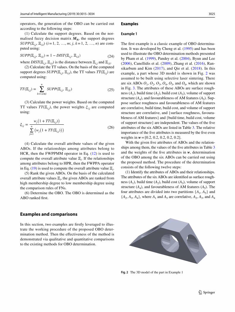
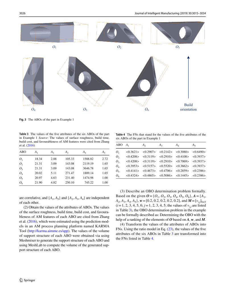
The first example is a classic example of OBO determina-tion. It was developed by Cheng et al. (1995) and has been used to illustrate the OBO determination methods presented by Pham et al. (1999), Pandey et al. (2004), Byun and Lee (2006), Canellidis et al. (2009), Zhang et al. (2016), Ran-sikarbum and Kim (2017), and Qie et al. (2018). In this example, a part whose 3D model is shown in Fig. 2 was assumed to be built using selective laser sintering. There are six ABOs O1, O2, O3, O4, O5, and O6, which are shown in Fig. 3. The attributes of these ABOs are surface rough-ness (A1), build time (A2), build cost (A3), volume of support structure (A4), and favourableness of AM features (A5). Sup-pose surface roughness and favourableness of AM features are correlative, build time, build cost, and volume of support structure are correlative, and {surface roughness, favoura-bleness of AM features} and {build time, build cost, volume of support structure} are independent. The values of the five attributes of the six ABOs are listed in Table 3. The relative importance of the five attributes is measured by the five even weights in w = [0.2, 0.2, 0.2, 0.2, 0.2].

With the given five attributes of ABOs and the relation-ships among them, the values of the five attributes in Table 3 and the weights of the five attributes in w, determination of the OBO among the six ABOs can be carried out using the proposed method. The procedure of the determination consists of the following twelve steps:

(1) Identify the attributes of ABOs and their relationships. The attributes of the six ABOs are identified as surface rough-ness (A1), build time (A2), build cost (A3), volume of support structure (A4), and favourableness of AM features (A5). The four attributes are divided into two partitions {A1, A5} and {A2, A3, A4}, where A1 and A5 are correlative, A2, A3, and A4

Fig. 2 The 3D model of the part in Example 1


1 3

are correlative, and {A1, A5} and {A2, A3, A4} are independent of each other.

(2) Obtain the values of the attributes of ABOs. The values of the surface roughness, build time, build cost, and favoura-bleness of AM features of each ABO are cited from Zhang et al. (2016), which were estimated using the prediction mod-els in an AM process planning platform named KARMA Tool (http://karma .aimme .es/app). The values of the volume of support structure of each ABO were obtained via using Meshmixer to generate the support structure of each ABO and using MeshLab to compute the volume of the generated sup-port structure of each ABO.

(3) Describe an OBO determination problem formally. Based on the given O = {O1, O2, O3, O4, O5, O6}, A = {A1, A2, A3, A4, A5}, w = [0.2, 0.2, 0.2, 0.2, 0.2], and M = [vi,j]6×5 (i = 1, 2, 3, 4, 5, 6; j = 1, 2, 3, 4, 5; the values of vi,j are listed in Table 3), the OBO determination problem in the example can be formally described as: Determining the OBO with the help of a ranking of the elements of O based on A, w, and M.

(4) Transform the values of the attributes of ABOs into FNs. Using the ratio model in Eq. (23), the values of the five attributes of the six ABOs in Table 3 are transformed into the FNs listed in Table 4.

O1 O2 O3

O4 O5 O6

Buildorientation

Fig. 3 The ABOs of the part in Example 1

Table 3 The values of the five attributes of the six ABOs of the part in Example 1 Source: The values of surface roughness, build time, build cost, and favourableness of AM features were cited from Zhang et al. (2016)

ABO A1 A2 A3 A4 A5

O1 18.34 2.88 105.33 1588.82 2.72O2 21.31 3.09 143.08 2119.19 1.65O3 21.31 3.09 143.08 3646.78 1.65O4 20.02 5.11 271.47 1889.14 1.65O5 20.97 4.63 231.40 1474.98 1.00O6 21.90 4.82 250.10 745.22 1.00

Table 4 The FNs that stand for the values of the five attributes of the six ABOs of the part in Example 1

ABO A1 A2 A3 A4 A5

O1 <0.3621> <0.2907> <0.2142> <0.3080> <0.6490>O2 <0.4208> <0.3119> <0.2910> <0.4108> <0.3937>O3 <0.4208> <0.3119> <0.2910> <0.7069> <0.3937>O4 <0.3953> <0.5157> <0.5520> <0.3662> <0.3937>O5 <0.4141> <0.4673> <0.4706> <0.2859> <0.2386>O6 <0.4324> <0.4865> <0.5086> <0.1445> <0.2386>

http://karma.aimme.es/app


1 3

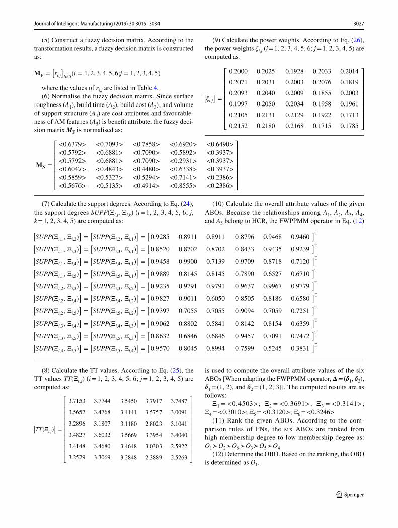
(5) Construct a fuzzy decision matrix. According to the transformation results, a fuzzy decision matrix is constructed as:

where the values of ri,j are listed in Table 4.(6) Normalise the fuzzy decision matrix. Since surface

roughness (A1), build time (A2), build cost (A3), and volume of support structure (A4) are cost attributes and favourable-ness of AM features (A5) is benefit attribute, the fuzzy deci-sion matrix MF is normalised as:

(7) Calculate the support degrees. According to Eq. (24), the support degrees SUPP(Ξi,j, Ξi,k) (i = 1, 2, 3, 4, 5, 6; j, k = 1, 2, 3, 4, 5) are computed as:

(8) Calculate the TT values. According to Eq. (25), the TT values TT(Ξi,j) (i = 1, 2, 3, 4, 5, 6; j = 1, 2, 3, 4, 5) are computed as:

��=[ri,j

]6×5

(i = 1, 2, 3, 4, 5, 6;j = 1, 2, 3, 4, 5)

��=

⎡⎢⎢⎢⎢⎢⎢⎣

<0.6379> <0.7093> <0.7858> <0.6920> <0.6490>

<0.5792> <0.6881> <0.7090> <0.5892> <0.3937>

<0.5792> <0.6881> <0.7090> <0.2931> <0.3937>

<0.6047> <0.4843> <0.4480> <0.6338> <0.3937>

<0.5859> <0.5327> <0.5294> <0.7141> <0.2386>

<0.5676> <0.5135> <0.4914> <0.8555> <0.2386>

⎤⎥⎥⎥⎥⎥⎥⎦

[SUPP(Ξ

i,1, Ξi,2)]=[SUPP(Ξ

i,2, Ξi,1)]=[0.9285 0.8911 0.8911 0.8796 0.9468 0.9460

]T[SUPP(Ξ


i,3, Ξi,1)]=[0.8520 0.8702 0.8702 0.8433 0.9435 0.9239

]T[SUPP(Ξ


i,4, Ξi,1)]=[0.9458 0.9900 0.7139 0.9709 0.8718 0.7120

]T[SUPP(Ξ


i,5, Ξi,1)]=[0.9889 0.8145 0.8145 0.7890 0.6527 0.6710

]T[SUPP(Ξ


i,3, Ξi,2)]=[0.9235 0.9791 0.9791 0.9637 0.9967 0.9779

]T[SUPP(Ξ


i,4, Ξi,2)]=[0.9827 0.9011 0.6050 0.8505 0.8186 0.6580

]T[SUPP(Ξ


i,5, Ξi,2)]=[0.9397 0.7055 0.7055 0.9094 0.7059 0.7251

]T[SUPP(Ξ


i,4, Ξi,3)]=[0.9062 0.8802 0.5841 0.8142 0.8154 0.6359

]T[SUPP(Ξ


i,5, Ξi,3)]=[0.8632 0.6846 0.6846 0.9457 0.7091 0.7472

]T[SUPP(Ξ


i,5, Ξi,4)]=[0.9570 0.8045 0.8994 0.7599 0.5245 0.3831

]T

�TT(Ξi,j)

�=

⎡⎢⎢⎢⎢⎢⎢⎢⎢⎢⎢⎣

3.7153 3.7744 3.5450 3.7917 3.7487

3.5657 3.4768 3.4141 3.5757 3.0091

3.2896 3.1807 3.1180 2.8023 3.1041

3.4827 3.6032 3.5669 3.3954 3.4040

3.4148 3.4680 3.4648 3.0303 2.5922

3.2529 3.3069 3.2848 2.3889 2.5263

⎤⎥⎥⎥⎥⎥⎥⎥⎥⎥⎥⎦

(9) Calculate the power weights. According to Eq. (26), the power weights ξi,j (i = 1, 2, 3, 4, 5, 6; j = 1, 2, 3, 4, 5) are computed as:

(10) Calculate the overall attribute values of the given ABOs. Because the relationships among A1, A2, A3, A4, and A5 belong to HCR, the FWPPMM operator in Eq. (12)

is used to compute the overall attribute values of the six ABOs [When adapting the FWPPMM operator, Δ = (δ1, δ2), δ1 = (1, 2), and δ2 = (1, 2, 3)]. The computed results are as follows:

Ξ1 = <0.4503>; Ξ2 = <0.3691>; Ξ3 = <0.3141>; Ξ4 = <0.3010>; Ξ5 = <0.3120>; Ξ6 = <0.3246>

(11) Rank the given ABOs. According to the com-parison rules of FNs, the six ABOs are ranked from high membership degree to low membership degree as: O1 ≻ O2 ≻ O6 ≻ O3 ≻ O5 ≻ O4

(12) Determine the OBO. Based on the ranking, the OBO is determined as O1.

��i,j

�=

⎡⎢⎢⎢⎢⎢⎢⎢⎢⎣

0.2000 0.2025 0.1928 0.2033 0.2014

0.2071 0.2031 0.2003 0.2076 0.1819

0.2093 0.2040 0.2009 0.1855 0.2003

0.1997 0.2050 0.2034 0.1958 0.1961

0.2105 0.2131 0.2129 0.1922 0.1713

0.2152 0.2180 0.2168 0.1715 0.1785

⎤⎥⎥⎥⎥⎥⎥⎥⎥⎦


1 3

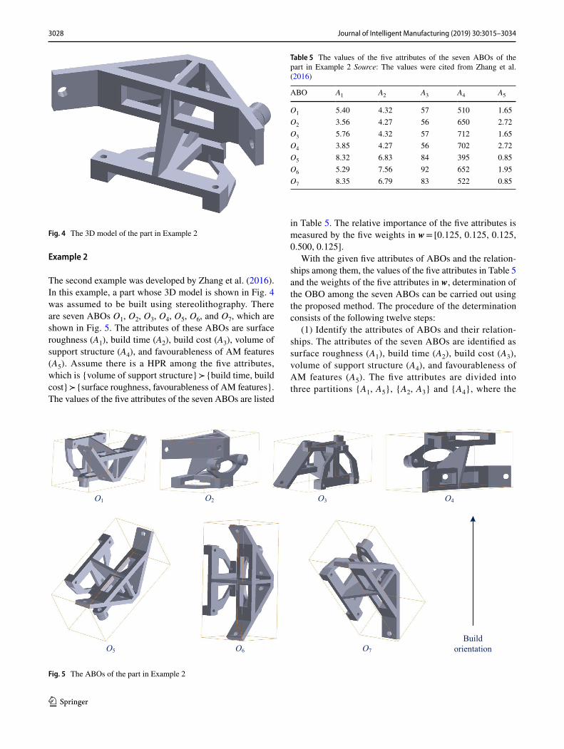
Example 2

The second example was developed by Zhang et al. (2016). In this example, a part whose 3D model is shown in Fig. 4 was assumed to be built using stereolithography. There are seven ABOs O1, O2, O3, O4, O5, O6, and O7, which are shown in Fig. 5. The attributes of these ABOs are surface roughness (A1), build time (A2), build cost (A3), volume of support structure (A4), and favourableness of AM features (A5). Assume there is a HPR among the five attributes, which is {volume of support structure} ≻ {build time, build cost} ≻ {surface roughness, favourableness of AM features}. The values of the five attributes of the seven ABOs are listed

in Table 5. The relative importance of the five attributes is measured by the five weights in w = [0.125, 0.125, 0.125, 0.500, 0.125].

With the given five attributes of ABOs and the relation-ships among them, the values of the five attributes in Table 5 and the weights of the five attributes in w, determination of the OBO among the seven ABOs can be carried out using the proposed method. The procedure of the determination consists of the following twelve steps:

(1) Identify the attributes of ABOs and their relation-ships. The attributes of the seven ABOs are identified as surface roughness (A1), build time (A2), build cost (A3), volume of support structure (A4), and favourableness of AM features (A5). The five attributes are divided into three partitions {A1, A5}, {A2, A3} and {A4}, where the

Fig. 4 The 3D model of the part in Example 2

O1 O2 O3 O4

O5 O6 O7

Build orientation

Fig. 5 The ABOs of the part in Example 2

Table 5 The values of the five attributes of the seven ABOs of the part in Example 2 Source: The values were cited from Zhang et al. (2016)

ABO A1 A2 A3 A4 A5

O1 5.40 4.32 57 510 1.65O2 3.56 4.27 56 650 2.72O3 5.76 4.32 57 712 1.65O4 3.85 4.27 56 702 2.72O5 8.32 6.83 84 395 0.85O6 5.29 7.56 92 652 1.95O7 8.35 6.79 83 522 0.85


1 3

relationship among these partitions is the heterogeneous priority relationship {A4} ≻ {A2, A3} ≻ {A1, A5}.

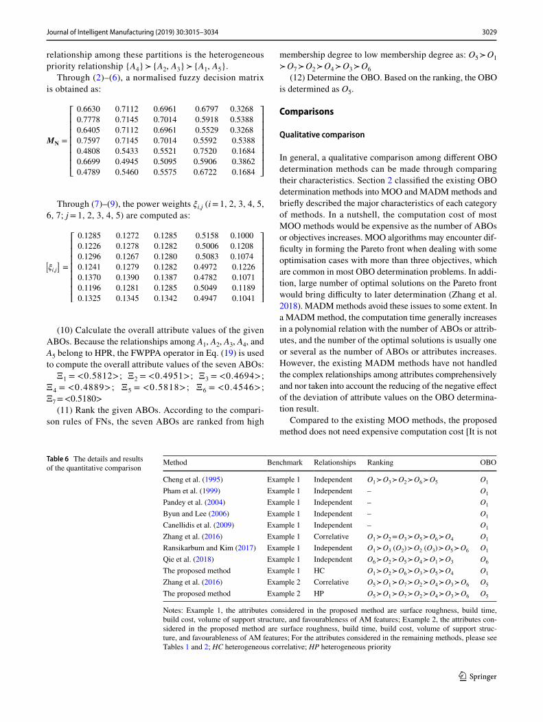
Through (2)–(6), a normalised fuzzy decision matrix is obtained as:

Through (7)–(9), the power weights ξi,j (i = 1, 2, 3, 4, 5, 6, 7; j = 1, 2, 3, 4, 5) are computed as:

(10) Calculate the overall attribute values of the given ABOs. Because the relationships among A1, A2, A3, A4, and A5 belong to HPR, the FWPPA operator in Eq. (19) is used to compute the overall attribute values of the seven ABOs:

Ξ1 = <0.5812>; Ξ2 = <0.4951>; Ξ3 = <0.4694>; Ξ4 = <0.4889>; Ξ5 = <0.5818>; Ξ6 = <0.4546>; Ξ7 = <0.5180>

(11) Rank the given ABOs. According to the compari-son rules of FNs, the seven ABOs are ranked from high

M�=

⎡⎢⎢⎢⎢⎢⎢⎢⎣

0.6630 0.7112 0.6961 0.6797 0.3268

0.7778 0.7145 0.7014 0.5918 0.5388

0.6405 0.7112 0.6961 0.5529 0.3268

0.7597

0.4808

0.6699

0.4789

0.7145

0.5433

0.4945

0.5460

0.7014

0.5521

0.5095

0.5575

0.5592

0.7520

0.5906

0.6722

0.5388

0.1684

0.3862

0.1684

⎤⎥⎥⎥⎥⎥⎥⎥⎦

��i,j

�=

⎡⎢⎢⎢⎢⎢⎢⎢⎣

0.1285 0.1272 0.1285 0.5158 0.1000

0.1226 0.1278 0.1282 0.5006 0.1208

0.1296 0.1267 0.1280 0.5083 0.1074

0.1241

0.1370

0.1196

0.1325

0.1279

0.1390

0.1281

0.1345

0.1282

0.1387

0.1285

0.1342

0.4972

0.4782

0.5049

0.4947

0.1226

0.1071

0.1189

0.1041

⎤⎥⎥⎥⎥⎥⎥⎥⎦

membership degree to low membership degree as: O5 ≻ O1 ≻ O7 ≻ O2 ≻ O4 ≻ O3 ≻ O6

(12) Determine the OBO. Based on the ranking, the OBO is determined as O5.

Comparisons

Qualitative comparison

In general, a qualitative comparison among different OBO determination methods can be made through comparing their characteristics. Section 2 classified the existing OBO determination methods into MOO and MADM methods and briefly described the major characteristics of each category of methods. In a nutshell, the computation cost of most MOO methods would be expensive as the number of ABOs or objectives increases. MOO algorithms may encounter dif-ficulty in forming the Pareto front when dealing with some optimisation cases with more than three objectives, which are common in most OBO determination problems. In addi-tion, large number of optimal solutions on the Pareto front would bring difficulty to later determination (Zhang et al. 2018). MADM methods avoid these issues to some extent. In a MADM method, the computation time generally increases in a polynomial relation with the number of ABOs or attrib-utes, and the number of the optimal solutions is usually one or several as the number of ABOs or attributes increases. However, the existing MADM methods have not handled the complex relationships among attributes comprehensively and nor taken into account the reducing of the negative effect of the deviation of attribute values on the OBO determina-tion result.

Compared to the existing MOO methods, the proposed method does not need expensive computation cost [It is not

Table 6 The details and results of the quantitative comparison

Notes: Example 1, the attributes considered in the proposed method are surface roughness, build time, build cost, volume of support structure, and favourableness of AM features; Example 2, the attributes con-sidered in the proposed method are surface roughness, build time, build cost, volume of support struc-ture, and favourableness of AM features; For the attributes considered in the remaining methods, please see Tables 1 and 2; HC heterogeneous correlative; HP heterogeneous priority

Method Benchmark Relationships Ranking OBO

Cheng et al. (1995) Example 1 Independent O1 ≻ O3 ≻ O2 ≻ O6 ≻ O5 O1

Pham et al. (1999) Example 1 Independent – O1

Pandey et al. (2004) Example 1 Independent – O1

Byun and Lee (2006) Example 1 Independent – O1

Canellidis et al. (2009) Example 1 Independent – O1

Zhang et al. (2016) Example 1 Correlative O1 ≻ O2 = O3 ≻ O5 ≻ O6 ≻ O4 O1

Ransikarbum and Kim (2017) Example 1 Independent O1 ≻ O3 (O2) ≻ O2 (O3) ≻ O5 ≻ O6 O1

Qie et al. (2018) Example 1 Independent O6 ≻ O2 ≻ O5 ≻ O4 ≻ O1 ≻ O3 O6

The proposed method Example 1 HC O1 ≻ O2 ≻ O6 ≻ O3 ≻ O5 ≻ O4 O1

Zhang et al. (2016) Example 2 Correlative O5 ≻ O1 ≻ O7 ≻ O2 ≻ O4 ≻ O3 ≻ O6 O5

The proposed method Example 2 HP O5 ≻ O1 ≻ O7 ≻ O2 ≻ O4 ≻ O3 ≻ O6 O5


1 3

difficult to obtain that the time complexity of the proposed method is polynomial from Eqs. (12) and (19)] and will not generate those Pareto-optimal solutions that make determi-nation difficult when the number of attributes is more than three. Compared to the existing MADM methods, the pro-posed method not only can deal with the complex relation-ships among the attributes of ABOs, but also reduce the influence of the deviation of attribute values on the OBO determination result.

Quantitative comparison

A quantitative comparison among different OBO determina-tion methods can be carried out using the same benchmark. Since there is currently no common open-source benchmark, Example 1 is used as a benchmark to compare the methods of Cheng et al. (1995), Pham et al. (1999), Pandey et al.

(2004), Byun and Lee (2006), Canellidis et al. (2009), Zhang et al. (2016), Ransikarbum and Kim (2017), and Qie et al. (2018) (The reason for selecting these methods in the com-parison is that all of them used Example 1 to demonstrate their effectiveness) and the proposed method, and Example 2 is used as another benchmark to compare the method of Zhang et al. (2016) and the proposed method. The details and results of the comparison are shown in Table 6.

As can be seen from Table 6, the OBO of the proposed method is the same as the OBOs of the methods of Cheng et al. (1995), Pham et al. (1999), Pandey et al. (2004), Byun and Lee (2006), Canellidis et al. (2009), Zhang et al. (2016), and Ransikarbum and Kim (2017) when the used benchmark is Example 1. These indicate its feasibility and effectiveness. In addition, the ranking of the proposed method is exactly the same as the ranking of the method of Zhang et al. (2016)

Table 7 The details of the two additional comparison experiments

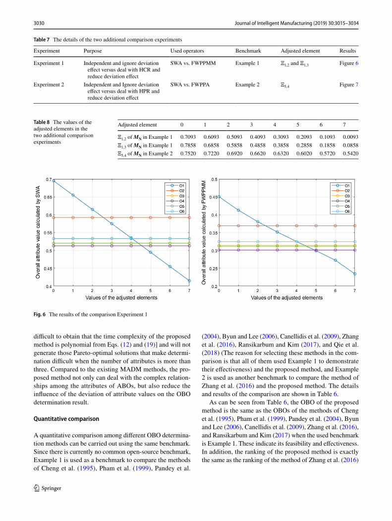
Experiment Purpose Used operators Benchmark Adjusted element Results

Experiment 1 Independent and ignore deviation effect versus deal with HCR and reduce deviation effect

SWA vs. FWPPMM Example 1 Ξ1,2 and Ξ1,3 Figure 6

Experiment 2 Independent and Ignore deviation effect versus deal with HPR and reduce deviation effect

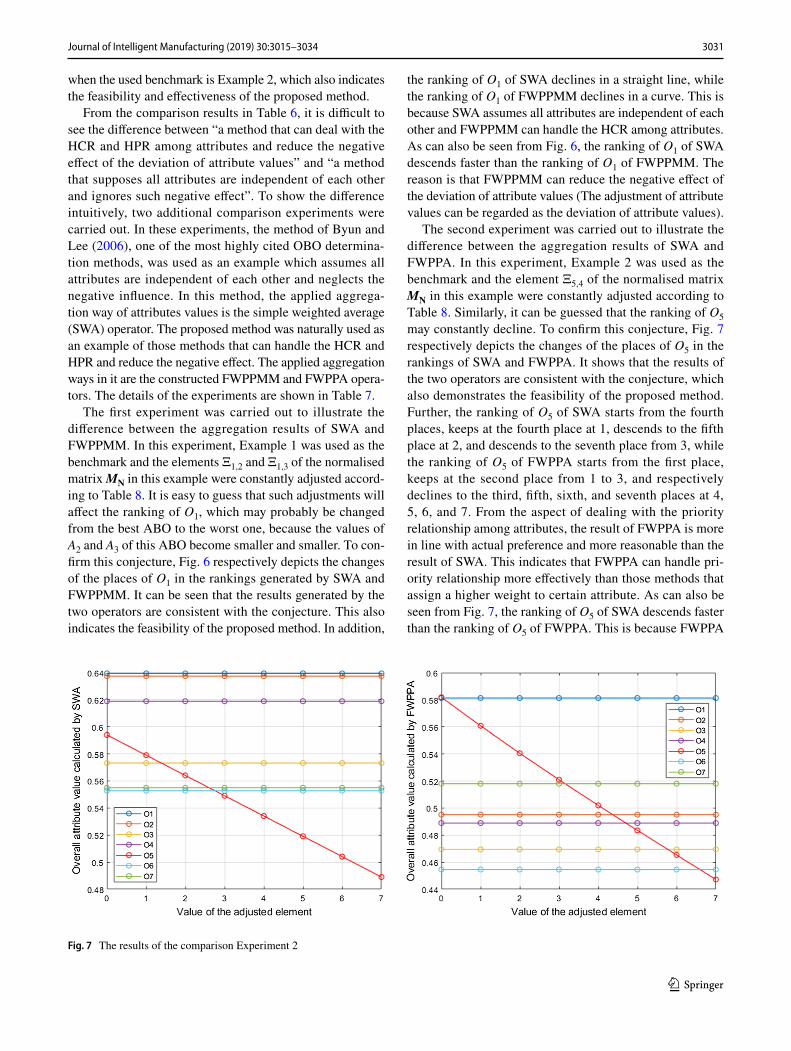
SWA vs. FWPPA Example 2 Ξ5,4 Figure 7

Table 8 The values of the adjusted elements in the two additional comparison experiments

Adjusted element 0 1 2 3 4 5 6 7

Ξ1,2 of MN in Example 1 0.7093 0.6093 0.5093 0.4093 0.3093 0.2093 0.1093 0.0093Ξ1,3 of MN in Example 1 0.7858 0.6858 0.5858 0.4858 0.3858 0.2858 0.1858 0.0858Ξ5,4 of MN in Example 2 0.7520 0.7220 0.6920 0.6620 0.6320 0.6020 0.5720 0.5420

Fig. 6 The results of the comparison Experiment 1


1 3

when the used benchmark is Example 2, which also indicates the feasibility and effectiveness of the proposed method.

From the comparison results in Table 6, it is difficult to see the difference between “a method that can deal with the HCR and HPR among attributes and reduce the negative effect of the deviation of attribute values” and “a method that supposes all attributes are independent of each other and ignores such negative effect”. To show the difference intuitively, two additional comparison experiments were carried out. In these experiments, the method of Byun and Lee (2006), one of the most highly cited OBO determina-tion methods, was used as an example which assumes all attributes are independent of each other and neglects the negative influence. In this method, the applied aggrega-tion way of attributes values is the simple weighted average (SWA) operator. The proposed method was naturally used as an example of those methods that can handle the HCR and HPR and reduce the negative effect. The applied aggregation ways in it are the constructed FWPPMM and FWPPA opera-tors. The details of the experiments are shown in Table 7.

The first experiment was carried out to illustrate the difference between the aggregation results of SWA and FWPPMM. In this experiment, Example 1 was used as the benchmark and the elements Ξ1,2 and Ξ1,3 of the normalised matrix MN in this example were constantly adjusted accord-ing to Table 8. It is easy to guess that such adjustments will affect the ranking of O1, which may probably be changed from the best ABO to the worst one, because the values of A2 and A3 of this ABO become smaller and smaller. To con-firm this conjecture, Fig. 6 respectively depicts the changes of the places of O1 in the rankings generated by SWA and FWPPMM. It can be seen that the results generated by the two operators are consistent with the conjecture. This also indicates the feasibility of the proposed method. In addition,

the ranking of O1 of SWA declines in a straight line, while the ranking of O1 of FWPPMM declines in a curve. This is because SWA assumes all attributes are independent of each other and FWPPMM can handle the HCR among attributes. As can also be seen from Fig. 6, the ranking of O1 of SWA descends faster than the ranking of O1 of FWPPMM. The reason is that FWPPMM can reduce the negative effect of the deviation of attribute values (The adjustment of attribute values can be regarded as the deviation of attribute values).

The second experiment was carried out to illustrate the difference between the aggregation results of SWA and FWPPA. In this experiment, Example 2 was used as the benchmark and the element Ξ5,4 of the normalised matrix MN in this example were constantly adjusted according to Table 8. Similarly, it can be guessed that the ranking of O5 may constantly decline. To confirm this conjecture, Fig. 7 respectively depicts the changes of the places of O5 in the rankings of SWA and FWPPA. It shows that the results of the two operators are consistent with the conjecture, which also demonstrates the feasibility of the proposed method. Further, the ranking of O5 of SWA starts from the fourth places, keeps at the fourth place at 1, descends to the fifth place at 2, and descends to the seventh place from 3, while the ranking of O5 of FWPPA starts from the first place, keeps at the second place from 1 to 3, and respectively declines to the third, fifth, sixth, and seventh places at 4, 5, 6, and 7. From the aspect of dealing with the priority relationship among attributes, the result of FWPPA is more in line with actual preference and more reasonable than the result of SWA. This indicates that FWPPA can handle pri-ority relationship more effectively than those methods that assign a higher weight to certain attribute. As can also be seen from Fig. 7, the ranking of O5 of SWA descends faster than the ranking of O5 of FWPPA. This is because FWPPA

Fig. 7 The results of the comparison Experiment 2


1 3

also has the capability of reducing the negative influence of the deviation of attribute values.

As can be summarised from the quantitative comparison and the two experiments, the proposed method is feasible and effective for solving the OBO determination problems, and has distinctive capabilities of dealing with the HCR and HPR among attributes and reducing the effect of the devia-tion of attribute values compared to the existing methods.

Conclusion

In this paper, a method for determining the optimal build orientations from a finite set of alternatives is proposed based on fuzzy multi-attribute decision making. This method firstly quantifies the attributes of all alternative build orienta-tions, and then generates the optimal build orientations from the alternatives. The quantification of attributes transforms the values of attributes into fuzzy numbers using a ratio model. A fuzzy decision matrix is constructed and normal-ised based on the fuzzy numbers. Later, two fuzzy number aggregation operators (i.e. FWPPMM and FWPPA) have been constructed to aggregate the fuzzy information in the normalised matrix. All attribute values of each alternative are aggregated into a fuzzy number using these aggregation operators. By comparing the fuzzy numbers, the optimal solution is determined.

The major contribution of the paper is the development of a multi-attribute decision making based method for determi-nation of the optimal build orientation from a set of alterna-tives. Compared with the existing methods, the developed method does not need expensive computation cost, can deal with complex relationships among the attributes of alter-native build orientations, and at the same time can reduce negative influence of the distortion of attribute values. To the best of the knowledge, the method is the first multi-attribute decision making based build orientation determina-tion method that considers both the handling of the complex relationships of build orientation attributes and the reducing of the effect of attribute value deviation.

As the present paper addresses only the determination of the optimal build orientation, future work will aim espe-cially at the study of the generation of alternative build ori-entations. In process planning for AM, there are four basic tasks, which are build orientation determination, support structure generation, 3D model slicing, and tool-path plan-ning. To develop a complete build orientation determination method for AM, the method would be extended to include support structure generation, 3D model slicing, and tool-path planning.

Supplementary material

The authors are releasing the Java implementation code of the proposed OBO determination method at GitHub. Every reader can freely access https ://githu b.com/Yuchu Ching Qin/Optim alBOD eterm inati on to download the code. The authors hope that the implemented method will provide a reliable basis for other decision-making tasks in manufactur-ing environment and foster further research in the develop-ment of other new OBO determination methods.

Acknowledgements The authors are very grateful to Dr. Yicha Zhang at the Department of Mechanical Engineering and Design, University of Technology of Belfort-Montbéliard, France for his help in provid-ing the STL files of the 3D models of the two parts in this paper and Dr. Peizhi Shi at the School of Computer Science, The University of Manchester, UK for his help in writing the implementation code of the constructed FWPPMM operator. The authors also would like to acknowledge the insightful comments from the two anonymous review-ers for the improvement of the paper and the financial supports by the EPSRC UKRI Innovation Fellowship (Ref. EP/S001328/1), the EPSRC Fellowship in Manufacturing (Ref. EP/R024162/1), and the EPSRC Future Advanced Metrology Hub (Ref. EP/P006930/1).

Open Access This article is distributed under the terms of the Crea-tive Commons Attribution 4.0 International License (http://creat iveco mmons .org/licen ses/by/4.0/), which permits unrestricted use, distribu-tion, and reproduction in any medium, provided you give appropriate credit to the original author(s) and the source, provide a link to the Creative Commons license, and indicate if changes were made.

References

Ahn, D., Kim, H., & Lee, S. (2007). Fabrication direction optimisa-tion to minimise post-machining in layered manufacturing. Inter-national Journal of Machine Tools and Manufacture, 47(3–4), 593–606.

Ahsan, A. N., Habib, M. A., & Khoda, B. (2015). Resource based process planning for additive manufacturing. Computer-Aided Design, 69, 112–125.

Al-Ahmari, A. M., Abdulhameed, O., & Khan, A. A. (2018). An auto-matic and optimal selection of parts orientation in additive manu-facturing. Rapid Prototyping Journal, 24(4), 698–708.

Alexander, P., Allen, S., & Dutta, D. (1998). Part orientation and build cost determination in layered manufacturing. Computer-Aided Design, 30(5), 343–356.

Ancău, M., & Caizar, C. (2010). The computation of Pareto-optimal set in multicriterial optimisation of rapid prototyping processes. Computers & Industrial Engineering, 58(4), 696–708.

Brauers, W. K. M., Zavadskas, E. K., Peldschus, F., & Turskis, Z. (2008). Multi-objective decision-making for road design. Trans-port, 23(3), 183–193.

Brika, S. E., Zhao, Y. F., Brochu, M., & Mezzetta, J. (2017). Multi-objective build orientation optimisation for powder bed fusion by laser. Journal of Manufacturing Science and Engineering, 139(11), 111011.

Byun, H. S., & Lee, K. H. (2006). Determination of the optimal build direction for different rapid proto-typing processes using multi-criterion decision making. Robotics and Computer-Integrated Manufacturing, 22(1), 69–80.

https://github.com/YuchuChingQin/OptimalBODetermination

https://github.com/YuchuChingQin/OptimalBODetermination

http://creativecommons.org/licenses/by/4.0/

http://creativecommons.org/licenses/by/4.0/


1 3

Canellidis, V., Giannatsis, J., & Dedoussis, V. (2009). Genetic-algo-rithm-based multi-objective optimisation of the build orientation in stereolithography. International Journal of Advanced Manu-facturing Technology, 45(7–8), 714–730.

Chen, Y. H., Yang, Z. Y., & Ye, R. H. (2008). A fuzzy decision making approach to determine build orientation in automated layer-based machining. In Proceedings of the 2008 IEEE international confer-ence on automation and logistics (pp. 1–6).

Cheng, W., Fuh, J. Y., Nee, A. Y., Wong, Y. S., Loh, H. T., & Miyazawa, T. (1995). Multi-objective optimisation of part-building orienta-tion in stereolithography. Rapid Prototyping Journal, 1(4), 12–23.

Chowdhury, S., Mhapsekar, K., & Anand, S. (2018). Part build orienta-tion optimisation and neural network-based geometry compensa-tion for additive manufacturing process. Journal of Manufacturing Science and Engineering, 140(3), 031009.

Delfs, P., Tows, M., & Schmid, H. J. (2016). Optimised build orienta-tion of additive manufactured parts for improved surface quality and build time. Additive Manufacturing, 12, 314–320.

Dubois, D., & Prade, H. (1980). Fuzzy sets and systems: Theory and applications. New York: Academic Press.

Dutta, B., & Guha, D. (2015). Partitioned Bonferroni mean based on linguistic 2-tuple for dealing with multi-attribute group decision making. Applied Soft Computing, 37, 166–179.

Ezair, B., Massarwi, F., & Elber, G. (2015). Orientation analysis of 3D objects toward minimal support volume in 3D printing. Computers & Graphics, 51, 117–124.

Gao, W., Zhang, Y., Ramanujan, D., Ramani, K., Chen, Y., Williams, C. B., et al. (2015). The status, challenges, and future of additive manufacturing in engineering. Computer-Aided Design, 69(12), 65–89.

Gibson, I., Rosen, D. W., & Stucker, B. (2015). Additive manufacturing technologies: 3D printing, rapid prototyping, and direct digital manufacturing (2nd ed.). New York: Springer.

Golmohammadi, A. H., & Khodaygan, S. (2019). A framework for multi-objective optimisation of 3D part-build orientation with a desired angular resolution in additive manufacturing processes. Virtual and Physical Prototyping, 14(1), 19–36.

Huang, R., Dai, N., Li, D., Cheng, X., Liu, H., & Sun, D. (2018). Parallel non-dominated sorting genetic algorithm-II for optimal part deposition orientation in additive manufacturing based on functional features. Proceedings of the Institution of Mechanical Engineers, Part C: Journal of Mechanical Engineering Science, 232(19), 3384–3395.

Hur, S. M., Choi, K. H., Lee, S. H., & Chang, P. K. (2001). Deter-mination of fabricating orientation and packing in SLS process. Journal of Materials Processing Technology, 112(2–3), 236–243.

Hur, J., & Lee, K. (1998). The development of a CAD environment to determine the preferred build-up direction for layered manufactur-ing. International Journal of Advanced Manufacturing Technol-ogy, 14(4), 247–254.

ISO 17296-2. (2015). Additive manufacturing—General principles—Part 2: Overview of process categories and feedstock. Geneva: International Organisation for Standardisation.

ISO 17296-3. (2014). Additive manufacturing—General principles—Part 3: Main characteristics and corresponding test methods. Geneva: International Organisation for Standardisation.

ISO/ASTM 52900. (2015). Additive manufacturing—General prin-ciples—Terminology. Geneva: International Organisation for Standardisation.

Jaiswal, P., Patel, J., & Rai, R. (2018). Build orientation optimisa-tion for additive manufacturing of functionally graded material objects. International Journal of Advanced Manufacturing Tech-nology, 96(1–4), 223–235.

Jiang, J., Lou, J., & Hu, G. (2019a). Effect of support on printed proper-ties in fused deposition modelling processes. Virtual and Physical Prototyping. https ://doi.org/10.1080/17452 759.2019.15688 35.

Jiang, J., Stringer, J., & Xu, X. (2019b). Support optimization for flat features via path planning in additive manufacturing. 3D Printing and Additive Manufacturing. https ://doi.org/10.1089/3dp.2017.0124.

Jiang, J., Stringer, J., Xu, X., & Zhong, R. (2018a). Investigation of printable threshold overhang angle in extrusion-based additive manufacturing for reducing support waste. International Journal of Computer Integrated Manufacturing, 31(10), 961–969.

Jiang, J., Xu, X., & Stringer, J. (2018b). Support structures for additive manufacturing: A review. Journal of Manufacturing and Materi-als Processing, 2(4), 64.

Jiang, J., Xu, X., & Stringer, J. (2019c). Optimisation of multi-part production in additive manufacturing for reducing support waste. Virtual and Physical Prototyping. https ://doi.org/10.1080/17452 759.2019.15855 55.

Kim, H. C., & Lee, S. H. (2005). Reduction of post-processing for stereolithography systems by fabrication direction optimisation. Computer-Aided Design, 37(7), 711–725.

Kim, D. B., Witherell, P., Lipman, R., & Feng, S. C. (2015). Stream-lining the additive manufacturing digital spectrum: A systems approach. Additive Manufacturing, 5(1), 20–30.

Kim, D. B., Witherell, P., Lu, Y., & Feng, S. C. (2017). Toward a digital thread and data package for metals-additive manufacturing. Smart and Sustainable Manufacturing Systems, 1(1), 75–99.

Kulkarni, P., Marsan, A., & Dutta, D. (2000). A review of process planning techniques in layered manufacturing. Rapid Prototyping Journal, 6(1), 18–35.

Lan, P. T., Chou, S. Y., Chen, L. L., & Gemmill, D. (1997). Deter-mining fabrication orientations for rapid prototyping with ste-reolithography apparatus. Computer-Aided Design, 29(1), 53–62.

Liang, J. S. (2018). An ontology-oriented knowledge methodology for process planning in additive layer manufacturing. Robotics and Computer-Integrated Manufacturing, 53(10), 28–44.

Luo, N., & Wang, Q. (2016). Fast slicing orientation determining and optimising algorithm for least volumetric error in rapid prototyp-ing. International Journal of Advanced Manufacturing Technol-ogy, 83(5–8), 1297–1313.

Masood, S. H., Rattanawong, W., & Iovenitti, P. (2003). A generic algorithm for a best part orientation system for complex parts in rapid prototyping. Journal of Materials Processing Technology, 139(1–3), 110–116.

McClurkin, J. E., & Rosen, D. W. (1998). Computer-aided build style decision support for stereolithography. Rapid Prototyping Journal, 4(1), 4–13.

Mi, S., Wu, X., & Zeng, L. (2018). Optimal build orientation based on material changes for FGM parts. International Journal of Advanced Manufacturing Technology, 94(5–8), 1933–1946.

Muirhead, R. F. (1902). Some methods applicable to identities and inequalities of symmetric algebraic functions of n letters. Pro-ceedings of the Edinburgh Mathematical Society, 21, 144–162.

Padhye, N., & Deb, K. (2011). Multi-objective optimisation and multi-criteria decision making in SLS using evolutionary approaches. Rapid Prototyping Journal, 17(6), 458–478.

Pandey, P. M., Thrimurthulu, K., & Reddy, N. V. (2004). Opti-mal part deposition orientation in FDM by using a multicri-teria genetic algorithm. International Journal of Production Research, 42(19), 4069–4089.

Paul, R., & Anand, S. (2015). Optimisation of layered manufac-turing process for reducing form errors with minimal support structures. Journal of Manufacturing Systems, 36(7), 231–243.

Pham, D. T., Dimov, S. S., & Gault, R. S. (1999). Part orientation in stereolithography. International Journal of Advanced Manufac-turing Technology, 15(9), 674–682.

Qie, L., Jing, S., Lian, R., Chen, Y., & Liu, J. (2018). Quantita-tive suggestions for build orientation selection. International

https://doi.org/10.1080/17452759.2019.1568835

https://doi.org/10.1089/3dp.2017.0124

https://doi.org/10.1089/3dp.2017.0124

https://doi.org/10.1080/17452759.2019.1585555

https://doi.org/10.1080/17452759.2019.1585555


1 3

Journal of Advanced Manufacturing Technology, 98(5–8), 1831–1845.

Qin, Y., Qi, Q., Scott, P. J., & Jiang, X. (2019). Status, comparison, and future of the representations of additive manufacturing data. Computer-Aided Design, 111(6), 44–64.

Raju, M., Gupta, M. K., Bhanot, N., & Sharma, V. S. (2018). A hybrid PSO–BFO evolutionary algorithm for optimisation of fused depo-sition modelling process parameters. Journal of Intelligent Manu-facturing. https ://doi.org/10.1007/s1084 5-018-1420-0.

Ransikarbum, K. & Kim, N. (2017). Multi-criteria selection problem of part orientation in 3D fused deposition modelling based on analytic hierarchy process model: A case study. In Proceedings of the 2017 IEEE international conference on industrial engineering and engineering management (pp. 1455–1459).

Singh, S., Ramakrishna, S., & Singh, R. (2017). Material issues in additive manufacturing: A review. Journal of Manufacturing Pro-cesses, 25, 185–200.

Strano, G., Hao, L., Everson, R. M., & Evans, K. E. (2011). Multi-objective optimisation of selective laser sintering processes for surface quality and energy saving. Proceedings of the Institution of Mechanical Engineers, Part B: Journal of Engineering Manu-facture, 225(9), 1673–1682.

Taufik, M., & Jain, P. K. (2013). Role of build orientation in layered manufacturing: A review. International Journal of Manufacturing Technology and Management, 27(1–3), 47–73.

Thrimurthulu, K. P., Pandey, P. M., & Reddy, N. V. (2004). Opti-mum part deposition orientation in fused deposition modelling. International Journal of Machine Tools and Manufacture, 44(6), 585–594.

West, A. P., Sambu, S. P., & Rosen, D. W. (2001). A process planning method for improving build performance in stereolithography. Computer-Aided Design, 33(1), 65–79.

Xiao, X., & Joshi, S. (2018). Automatic toolpath generation for het-erogeneous objects manufactured by directed energy deposition additive manufacturing process. Journal of Manufacturing Sci-ence and Engineering, 140(7), 071005.

Xu, J., Gu, X., Ding, D., Pan, Z., & Chen, K. (2018). A review of slic-ing methods for directed energy deposition based additive manu-facturing. Rapid Prototyping Journal, 24(6), 1012–1025.

Xu, F., Loh, H. T., & Wong, Y. S. (1999). Considerations and selec-tion of optimal orientation for different rapid prototyping systems. Rapid Prototyping Journal, 5(2), 54–60.

Yager, R. R. (2001). The power average operator. IEEE Transactions on Systems, Man, and Cybernetics-Part A: Systems and Humans, 31(6), 724–731.

Yager, R. R. (2008). Prioritised aggregation operators. International Journal of Approximate Reasoning, 48(1), 263–274.

Zadeh, L. A. (1965). Fuzzy sets. Information and Control, 8, 338–353.Zhang, Y., & Bernard, A. (2014). An integrated decision-making model

for multi-attributes decision-making (MADM) problems in addi-tive manufacturing process planning. Rapid Prototyping Journal, 20(5), 377–389.

Zhang, Y., Bernard, A., Gupta, R. K., & Harik, R. (2016). Feature based building orientation optimisation for additive manufactur-ing. Rapid Prototyping Journal, 22(2), 358–376.

Zhang, Y., Bernard, A., Harik, R., & Karunakaran, K. P. (2017). Build orientation optimisation for multi-part production in addi-tive manufacturing. Journal of Intelligent Manufacturing, 28(6), 1393–1407.

Zhang, Y., Harik, R., Fadel, G., & Bernard, A. (2018). A statistical method for build orientation determination in additive manufac-turing. Rapid Prototyping Journal, 25(1), 187–207.

Zhang, J., & Li, Y. (2013). A unit sphere discretisation and search approach to optimise building direction with minimised volumet-ric error for rapid prototyping. International Journal of Advanced Manufacturing Technology, 67(1–4), 733–743.

Publisher’s Note Springer Nature remains neutral with regard to jurisdictional claims in published maps and institutional affiliations.

https://doi.org/10.1007/s10845-018-1420-0

Determination of optimal build orientation for additive ...

Documents