Determination of Odor Air Quality Index (OAQII) Using Gas ...

Citation: Dobrzyniewski, D.;

Szulczynski, B.; Gebicki, J.

Determination of Odor Air Quality

Index (OAQII ) Using Gas Sensor

Matrix. Molecules 2022, 27, 4180.

https://doi.org/10.3390/

molecules27134180

Academic Editor: Gavino Sanna

Received: 30 May 2022

Accepted: 27 June 2022

Published: 29 June 2022

Publisher’s Note: MDPI stays neutral

with regard to jurisdictional claims in

published maps and institutional affil-

iations.

Copyright: © 2022 by the authors.

Licensee MDPI, Basel, Switzerland.

This article is an open access article

distributed under the terms and

conditions of the Creative Commons

Attribution (CC BY) license (https://

creativecommons.org/licenses/by/

4.0/).

molecules

Article

Determination of Odor Air Quality Index (OAQII) Using GasSensor MatrixDominik Dobrzyniewski , Bartosz Szulczynski * and Jacek Gebicki

Department of Process Engineering and Chemical Technology, Faculty of Chemistry, Gdansk University ofTechnology, 11/12 G, Narutowicza Str., 80-233 Gdansk, Poland; [email protected] (D.D.);[email protected] (J.G.)* Correspondence: [email protected]

Abstract: This article presents a new way to determine odor nuisance based on the proposed odorair quality index (OAQII), using an instrumental method. This indicator relates the most importantodor features, such as intensity, hedonic tone and odor concentration. The research was conductedat the compost screening yard of the municipal treatment plant in Central Poland, on which a self-constructed gas sensor array was placed. It consisted of five commercially available gas sensors:three metal oxide semiconductor (MOS) chemical sensors and two electrochemical ones. To calibrateand validate the matrix, odor concentrations were determined within the composting yard using thefield olfactometry technique. Five mathematical models (e.g., multiple linear regression and principalcomponent regression) were used as calibration methods. Two methods were used to extract signalsfrom the matrix: maximum signal values from individual sensors and the logarithm of the ratioof the maximum signal to the sensor baseline. The developed models were used to determine thepredicted odor concentrations. The selection of the optimal model was based on the compatibilitywith olfactometric measurements, taking the mean square error as a criterion and their accordancewith the proposed OAQII . For the first method of extracting signals from the matrix, the best modelwas characterized by RMSE equal to 8.092 and consistency in indices at the level of 0.85. In the case ofthe logarithmic approach, these values were 4.220 and 0.98, respectively. The obtained results allowto conclude that gas sensor arrays can be successfully used for air quality monitoring; however, thekey issues are data processing and the selection of an appropriate mathematical model.

Keywords: gas sensors; sensor matrix; odor concentration; field olfactometry; odor index

1. Introduction

The dynamic development of modern civilization and the increasing level of con-sumption generate the problem of a huge amount of waste, which is a deadly threat to theenvironment and human health. Currently, in addition to depositing waste in municipallandfills, great emphasis is placed on the issues related to their sorting, recycling andcomposting. However, all these processes can cause some negative consequences. One ofthem is the introduction of solid, liquid or gaseous pollutants to the natural environment,which poison the soil, water and the atmosphere [1–7]. Among gaseous air pollutants,there is a group of compounds characterized additionally by odor nuisance. This groupincludes the volatile components of air pollutants that have toxic properties, are detectableat relatively low concentrations, and cause undesirable odor sensations. Volatile chemicalsthat make up the gases emitted into the atmosphere can be divided into volatile organiccompounds (VOCs) and volatile inorganic compounds (VICs).

Odorants emitted to the atmosphere may be of natural or anthropogenic origin.Sources of odor-forming substances, which are a side effect of human activity, are mainlythe chemical industry [8], food industry [9], fuel industry [10], municipal sewage treat-ment plants [11,12], fragrance industry [13,14], composting facilities [15–17], municipal

Molecules 2022, 27, 4180. https://doi.org/10.3390/molecules27134180 https://www.mdpi.com/journal/molecules

Molecules 2022, 27, 4180 2 of 25

landfills [18,19] and swine farming and breeding [20–22]. The nature of odors generated bymunicipal waste management facilities depends on many factors, such as type of waste,method of storage, compost production techniques, etc. However, all these facilities emitpollutants of similar qualitative composition, and the odor nuisance is mainly related tothe presence of the following compounds: disulfides, amines, sulfides, ammonia, thiols,alcohols, carboxylic acids, aldehydes, ketones, phenols, and aliphatic amines [13,19,23–35].The ranges of olfactory detection threshold and the perceived odor character for exemplaryodorants are presented in Table 1.

Table 1. The olfactory threshold for exemplary odorants [36–39].

Chemical Compound Olfactory Threshold Unit Odor Character

Acetaldehyde 0.015–0.066 ppm Fruity, appleFormaldehyde 0.50–0.80 ppm Pungent, suffocating

Acrolein 0.0036–0.16 ppm Pungent, suffocatingPhenol 0.0056–0.040 ppm Pungent

Hydrogen sulfide 0.41–0.81 ppb Rotten eggsCarbon disulfide 0.11–0.21 ppm Rotten vegetablesDimethyl sulfide 2.70–3.00 ppb Rotten vegetables, garlic

Ammonia 1.50–5.20 ppm Sharp, pungentMethylamine 0.035–4.70 ppm Fish, piscine

Dimethylamine 0.033–0.34 ppm Fish, piscineAcetone 13.00–42.00 ppm Fruity, sweet

Acetic acid 0.0060–0.48 ppm VinegarAcetonitrile 13–170 ppm Etheric

Propionic acid 0.0057–0.16 ppm PungentAcrylonitrile 1.60–17.0 ppm Etheric

Sulfur dioxide 0.87–1.10 ppm Pungent, suffocatingEthyl mercaptan 0.0087–0.76 ppb Rotten eggs, rotten cabbageNitrogen dioxide 0.12–0.36 ppm Harsh

Pyridine 0.063–0.17 ppm Strong sickeningHexane 1.5–130 ppm slightly disagreeable

Cyclohexane 2.5–25 ppm SweetToluene 0.33–2.50 ppm Paint thinnersBenzene 2.70–12.00 ppm Sweet, aromatic, gasoline

In order to properly assess the environmental effects of odorants emitted into theatmosphere, measurement techniques are used that allow for both quantitative and qual-itative analyses of the composition of polluted air. There are two basic techniques fordetermining odor nuisance: sensory techniques and instrumental (analytical) ones. Insensory techniques, such as dynamic olfactometry or field olfactometry, the role of thedetector is played by the human sense of smell. Analytical techniques focus primarily onthe use of gas chromatography or gas sensor arrays that are gaining in popularity. Theyenable a holistic analysis of the composition of the gas mixture without dividing it intoindividual components, and the analysis time is much shorter. Gas sensor matrices alsoprovide the ability to monitor industrial processes continuously without any sampling.Obviously, in terms of the accuracy of the obtained results, they do not match the chromato-graphic techniques; however, in cases requiring, for example, quick reaction of industrialfacilities, staff sensor arrays are an excellent alternative. Their high application potentialhas been proven for processes such as monitoring of biofiltration [40–46], monitoring ofmethane reforming process [47], monitoring of sanitary conditions [48], monitoring andidentification of air pollutants and hazardous substances [49–52], quality assessment offood products [53–58], detection of drugs and explosives [59–61], in medicine as a non-invasive diagnostics systems for analysis of breath or urine [62–66], to control indoor airquality [67–69] or in the perfume industry to confirm the authenticity of products [55,70].

The main difference between the sensory and instrumental techniques is that theanalytical measurements focus on individual odorants, while sensory measurements are

Molecules 2022, 27, 4180 3 of 25

mainly concerned with general odor sensations. However, in order to develop innovativeand effective odor quality monitoring systems, a complementary and integrated approachbased on the synergy of their operation is necessary. Attempts to combine the advantagesof both groups of techniques were already being made, for example in the form of gaschromatography coupled with olfactometry (GC-O) [71–75] or by trying to demonstratethe validity of using sensor arrays for odor monitoring by comparing them with gaschromatography–mass spectrometry (GC-MS) [30,76,77].

As mentioned before, determining the impact of the industrial or municipal plants onthe odor nuisance of a given area requires taking into account several key parameters ofthe smell. Among them, the following should be particularly distinguished:

• Hedonic tone—pleasant or unpleasant sensations during inhalation of a gaseous mixture;• Odor intensity—relative strength of the odor stimulus induced by a particular odorant;• Odor threshold—the minimum concentration of a substance at which most test sub-

jects can identify the odor.

These three parameters are crucial to establish the relationship between odor concen-tration and the odor nuisance, and they make it possible to better understand the interactionbetween emitted odorants. For this reason, in order to estimate the odor nuisance of amunicipal plant, it is necessary to use indices and indexes embodying all of them. Sofar, several indexes have already been proposed and presented, showing the correlationbetween sensorial and analytical characterization of odors. The most common indices usedto assess odor nuisance include the following:

• Specific odor emission rate (SOER)

SOER =Qair ∗ Cod

Abase(1)

where:Abase—base area [m2]Cod—odor concentration

[ oum3

]Qair—air flow

[m3

s]

• Odor emission rate (OER)

OER = SOER ∗ Aland f ill (2)

where:Aland f ill—emitting surface of the considered area [m2]

• Odor emission factor (OEF)

OEF =OER

AI(3)

where:AI—representative “activity index” of the plant. It can be represented by e.g., plantcapacity, landfill surface, mass of processed material or yearly treatment capac-ity [78–82].

• Analytical odor index (AOI)/odor activity value (OAV)

AOI/OAV =n

∑i=1

(Cy

OTy

)(4)

where:Cy—concentration of y-th substances detected by GC techniques [ppm]OTy—relative Odor Threshold [ppm]

• Sensorial odor index (SOI)

SOIi =UiUs

(5)

Molecules 2022, 27, 4180 4 of 25

where:Ui—concentration of odor at i-th sampling point

[ oum3

]Us—standard concentration of odor detectable by sensorial analysis

[ oum3

]• Odor index (OI)

OI = 10log(Cod) (6)

where:Cod—odor concentration

[ oum3

]• Odor annoyance index (OAI)

OAI =1

Nt

n

∑i=1

wi Ni (7)

where:Nt—total number of observations for the investigated zone or periodNi—number of observations corresponding to the odor rating i (i = 0–6)wi—corresponding weighting factors

Table 2 provides examples of industrial and municipal facilities for which an odornuisance assessment was conducted using the indicators listed above.

Table 2. Indicators and indexes used for evaluation of odor nuisance of exemplary industrial andmunicipal facilities.

Facility Index Scope of Research References

WWTP 1 AOI SOIInvestigation of correlation between odors concentrationmeasured by means of dynamic olfactometry (DO) andchromatographic GC-MS-FID analysis

[83]

MSWTP 2 SOEF OER OEFA study of large anaerobic–aerobic treatment plant,identifying its odor sources, characterizing them in terms ofodor concentration and emissions using dynamic olfactometry

[78]

Industrial park OAI13 potential odor emitting facilities; assessment of the odorannoyance using the residents as measuring tools—residentdiary method

[84]

MSWTP OER OEF

Mechanical and biological MSWTPs; calculation of OEFs,based on the results of olfactometric measurements, as afunction of plants capacity which differ in constructionalfeatures, in type of treated waste and geographical locationsin Italy

[79]

Compost facility OAIAssessment of odor annoyance generated by the compostingfacility and demonstration of the feasibility of gas sensor arrayto monitor the emission of the odorous substances

[85]

MSW landfills SOER OER OEFEstimation of odor emissions from landfills, focusing on theodor related to the emissions of landfill gas (LFG) fromplant surface

[80]

MSW landfills SOER OEFSeven dimensionally different landfills, the odor concentrationwas calculated as the geometric mean of the odor thresholdvalues of each panelist, using dynamic olfactometry

[81]

MRP 3 SOER OER OEF

Determination of odor nuisance from the rendering industrybased on experimental data obtained by means of dynamicolfactometry, mass of processed material was used as “activityindex” for OEF calculation

[82]

Molecules 2022, 27, 4180 5 of 25

Table 2. Cont.

Facility Index Scope of Research References

WWTP OEF

Calculation of OEFs based on the results of olfactometricmeasurements that were carried out on a significant numberof WWTPs, which differ in constructional features, in type oftreated wastewater and in geographical locations in Italy;yearly treatment plant capacity was used as “activity index”

[86]

WWTP OIInvestigation of the relationship odor index assessed byJapanese standard methods (triangle odor bag method) andodor concentrations measured with dynamic olfactometry

[87]

WWTP OI

Relationship between odor concentrations emitted by WWTPassessed by Japanese standard methods and odorconcentrations measured with dynamic olfactometry andcompared to the measurement carried out by novel prototypeof e-nose

[87]

WWTP AOI SOI

Comparison and evaluation of the principal odormeasurement methods (GC-MS, dynamic olfactometry,electronic nose) used to identify and characterize the odoremission from a WWTP with the aim of analyzing theweaknesses and strengths of the different techniques

[88]

Compost facility OAV

The ability of OAV to predict odor concentrations duringcomposting of six solid wastes and three digestates wasevaluated, dynamic olfactometry and GC-MS were used asmeasurement methods

[89]

MSW landfills OAV

Evaluation of odorant interaction effect to accurately estimatethe contribution of odors, samples from a food wastetreatment plant were analyzed by instrumental and olfactorymethods, an odorant coefficient was proposed to assess thetype and level of binary interaction effects based onOAV variation

[90]

1 Wastewater Treatment Plant, 2 Municipal Solid Waste Treatment Plant, 3 Meat Rendering Plant.

This article presents a proposal for a new odor air quality index (OAQII) which wasdetermined on the basis of the emission measurements of odorants in the environment.The basic assumption of the proposed index is the ability to simultaneously interpret all ofthe major odor features: hedonic tone, intensity and odor concentrations. In other words,based on the proposed index, the determination of one of these parameters enables theestimation of the others. The first two parameters were determined using parametricsensory measurements (numerical scales). The odor load that was released into the air as aresult of the emission (odor concentration) was measured using field olfactometry and agas sensor array.

The application of a gas sensor matrix to estimate odor concentration would enableair quality monitoring in terms of odor nuisance continuously (online mode) with easyand quick access to the collected data. Such usages of sensor arrays have already beenreported in the literature, for example, for quantitative evaluation of pond odors frompiggeries [91]. Odor concentrations were determined by dynamic olfactometry, and anartificial neural network (ANN) was used to correlate them with the signals received fromsensors. It has been shown that a sensor matrix connected to a trained ANN is able topredict odor concentrations with a low root mean square error (RMSE) and a coefficient ofdetermination (R2) between olfactometric measurements and the predicted concentrationsin unknown samples at the level of 0.92.

Molecules 2022, 27, 4180 6 of 25

Another example could be sensor-based measurements of odor concentrations ingrasslands after using cattle slurry on them [92]. In this study, a comparison was madebetween a commercially available gas sensor array and self-built device. In order todetermine the odor concentrations in the analyzed samples, dynamic olfactometry (DO)was used again. On the basis of the principal component analysis (PCA) of actual sensorresponse patterns, linear relationships were established between odor concentrations andaverage response of conductive polymer type sensors. A single line fitted to the data fromall experiments had a percentage of the variance accounted for 59% and 62% depending onthe device.

In other literature reports, the possibility of using sensor arrays for continuous moni-toring of odors from wastewater treatment plant or composting plant (WWTP) was inves-tigated [93,94]. In these works, a lot of attention was paid to the selection of appropriateidentification methods, definitions and optimization of the process of creating a dataset fortraining the sensor array to enhance its ability to correctly estimate odor concentrations.In addition, qualitative classification of the analyzed samples was performed using threedifferent sensor arrays, consisting of six metal oxide semiconductor (MOS) type sensorseach. The application of this type of sensors had made the devices sensitive to many groupsof volatile chemicals, which is decent in terms of the complex gas mixtures found in thistype of plants. After selecting the optimal algorithm, a qualitative classification accuracy of96.4% and a correlation between actual and predicted odor concentrations expressed by adetermination coefficient of 0.90172 were obtained.

The study conducted in [95] also assessed the odors from WWTP with the use of12 conductive polypyrrole polymer sensors. As a statistical technique for data analysis,canonical discriminator (CD) and canonical correlation (CC) were used, which are similarto the assumptions of PCA, except that CC is the correlation that is maximized instead ofvariance. Linear relationships were created between odor concentrations (determined byDO) and explanatory variables (sensor signals). The research was carried out in severalWWTPs in an attempt to create and demonstrate one generalized relationship betweensensor array response and odor concentration from such facilities. It was noted that such acorrelation is extremely difficult to achieve; however, when the approach was changed andthe odor concentrations from individual treatment plants were analyzed, much strongerrelationships were obtained.

Sensor matrices applications for continuous odor monitoring in poultry are alsoknown [96]. The approach in this work is similar to the previously cited studies and involvesdetermining odor concentrations using DO and modeling the correlation between themand a sensor array composed of 24 MOS type detectors. Data were collected continuouslyand due to the large number of them, PCA was applied to reduce the multidimensionalityof the dataset. Then, a linear model for odor concentrations prediction was developed usingpartial least square regression (PLSR). Sensor resistances were used as input to the model.RMSE and root-mean square error of cross validation (RMSECV) were used to evaluate theaccuracy of the prepared model. Their values were 179.9 and 182.23, respectively, which,with the coefficient of determination of the calibration curve at the level of 0.94, confirmedthat it is possible to create a mathematical model that, when implemented in a sensor array,will enable the real-time measurements of odor concentrations.

All these studies demonstrated the possibility of using gas sensor arrays to predictthe odor concentrations in various plants associated as sources of odor emissions. Ad-ditionally, all of them used dynamic olfactometry to determine the odor concentrationsof the analyzed samples. The undoubted advantage of this method is that it is only onethat is fully standardized, but on the other hand, a sampling stage is required, which isalways troublesome, as well as the need for a trained team of assessors. Another thingthey have in common is the development of linear predictive mathematical models of odorconcentrations based on various methods of analyzing sensor array data. The purposeof this research was to develop such a predictive model for a self-constructed gas sensormatrix, but as a reference technique, field olfactometry was used. The constructed gas

Molecules 2022, 27, 4180 7 of 25

sensor array was located in the compost screening yard and consisted of commerciallyavailable chemical sensors. The article describes the calibration of the prepared matrixusing five mathematical models and the subsequent validation of the models developed.The calibration and validation of the models were carried out on the basis of periodicolfactometric measurements; therefore, the odor concentration was a dependent variable(model response), while the signals from the sensors were treated as explanatory variables.

The applicability and accuracy of the prepared models with respect to olfactometricmeasurements and their compatibility with the proposed OAQII were evaluated. Themain presumption of the suggested index was to correlate and combine the predicted odorconcentrations with other air quality parameters, which may be more transparent to themajority of the society unfamiliar with the concept of odor concentrations.

2. Materials and Methods

The measurements and research were conducted at a municipal solid waste treatmentplant in Central Poland (Figure 1).

Figure 1. A map showing the location of the municipal treatment plant where the research was conducted.

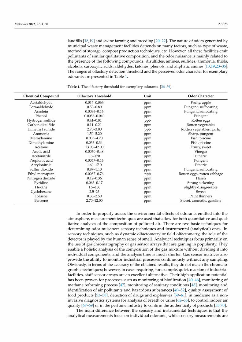
The sensor array was placed in the compost screening yard. This localization providedepisodic high odor concentrations associated with the operation of the compost screeningprocess, while during the rest of the time, the odor concentrations were relatively low.Periodically, the field olfactometry measurements were carried out at the sensor matrixlocation using a Nasal Ranger olfactometer. Data processing, analysis and other calculationswere performed using RStudio Desktop (v.1.0.143) software. The concept of the conductedresearch is presented graphically in the Figure 2.

Figure 2. The concept of the conducted research.

2.1. Field Olfactometry

The gas sensor matrix was calibrated using the Nasal Ranger field olfactometers (St.Croix Sensory, Inc., Stillwater, MN, USA). This approach was aimed at linking signalsfrom gas sensors with specific odor concentrations. The olfactometric measurements werecarried out each time with the participation of at least two people. During the analysis,all recommendations regarding the measurement procedure were followed. The result

Molecules 2022, 27, 4180 8 of 25

of the field olfactometry measurement is the numerical value of the dilution to olfactorythreshold (D/T) ratio, read from the dilution dial on the front of the olfactometer. Thisparameter should be interpreted as the number of dilutions needed to make the odor ofcontaminated air undetectable [97]. The D/T values correspond, after conversion, to theZITE value (individual estimation of the dilution to threshold) defined in EN 13725. ZITEwas calculated for each team member separately according to the relationships:

ZYES = (D/T)YES + 1 (8)

ZNO = (D/T)NO + 1 (9)

ZITE =√

ZYES ∗ ZNO (10)

where:ZYES—the dilution level at which the odor is detectableZNO—the dilution level at which the odor is undetectable

The odor concentration value was calculated as the geometric mean of the set ofindividual estimates collected by the team.

Cod = n

√n

∏i=1

ZITEn (11)

where:n—number of people participating in olfactometric measurements

In total, 60 series of olfactometric measurements were performed, which were dividedinto three stages. In each stage, 20 series were performed, divided equally into twomeasurement days. The first 20 measurements were taken in September 2021 (autumnperiod), the second phase was conducted in December 2021 (winter period) and the third inMarch 2022 (spring period). The first two stages were used to calibrate the matrix, and thethird one was used to validate the proposed models. The field olfactometry measurementstaken in April 2022 were used to check the reliability of odor concentrations returned bythe models, with the actual condition occurring at the site.

2.2. Sensory Matrix Development and Measurement

Five commercially available chemical gas sensors were chosen for operation in theconstructed sensor array. Three metal oxide semiconductor sensors (TGS2602, TGS2603and TGS2612) and two electrochemical sensors (NH3 and H2S) were selected. The basiccharacteristics of the selected sensors are presented in Table 3.

Since the constructed gas sensor array was placed on the compost screening site, thegas sensors were selected to best match the characteristics of the investigated environment.Therefore, two electrochemical sensors were used that were able to detect hydrogen sulfideand ammonia, gases whose concentrations were expected to exceed their olfactory thresh-old. The other sensors were non-selective semiconductor sensors that respond to organic airpollutants. Lack of selectivity does not render these sensors useless because grouping theminto an array makes the resulting signal multidimensional. Additionally, these studies didnot focus on precise determination of concentrations of individual odorants, but only onthe evaluation of odor nuisance, which is caused by the synergic action of all compoundsforming a gaseous mixture.

However, the high sensitivity of TGS-type sensors to the presence of methane must betaken into account. This gas belongs to a group of compounds called aliphatic hydrocarbonsand is known to be colorless and odorless. For this reason, its presence in the air will notaffect the level of odor nuisance. This means that methane will not be detected duringfield olfactometry measurements, but may significantly affect the signals received from thegas sensor array. Therefore, during the analysis of the collected signals from the matrix,

Molecules 2022, 27, 4180 9 of 25

those that were represented by low odor concentrations and incomparably high valuesfrom analog-to-digital converters were rejected.

Table 3. Basic characteristics of selected chemical gas sensors.

SensorType Manufacturer Model Detected Gases Signal

Processing

MOS 1 Figaro Engineering Inc.(Osaka, Japan) TGS2602 [98]

hydrogen (1–30 ppm), toluene (1–30 ppm),ethanol (1–30 ppm), ammonia (1–30 ppm),hydrogen sulfide (0.1–3 ppm)

Voltagedivider

MOS 1 Figaro Engineering Inc.(Osaka, Japan) TGS2603 [99]

hydrogen (1-30 ppm), hydrogen sulfide(0.3–3.0 ppm), ethanol (1–30 ppm), methylmercaptan (0.3–3.0 ppm), trimethyl amine(0.1–3.0 ppm)

Voltagedivider

MOS 1 Figaro Engineering Inc.(Osaka, Japan) TGS2612 [100]

methane (300–10,000 ppm), propane(300–10,000 ppm), ethanol (300–10,000 ppm),iso-butane (300–10,000 ppm)

Voltagedivider

EC 2 Alphasense (Braintree,United Kingdom) H2S-A4 [101] hydrogen sulfide (limit of performance

warranty 0–50 ppm)I-U

converter

EC 2 Alphasense (Braintree,United Kingdom) NH3-B1 [102] ammonia (limit of performance warranty

0–100 ppm)I-U

converter1 Metal Oxide Semiconductor, 2 Electrochemical.

2.3. Signals’ Features Extraction

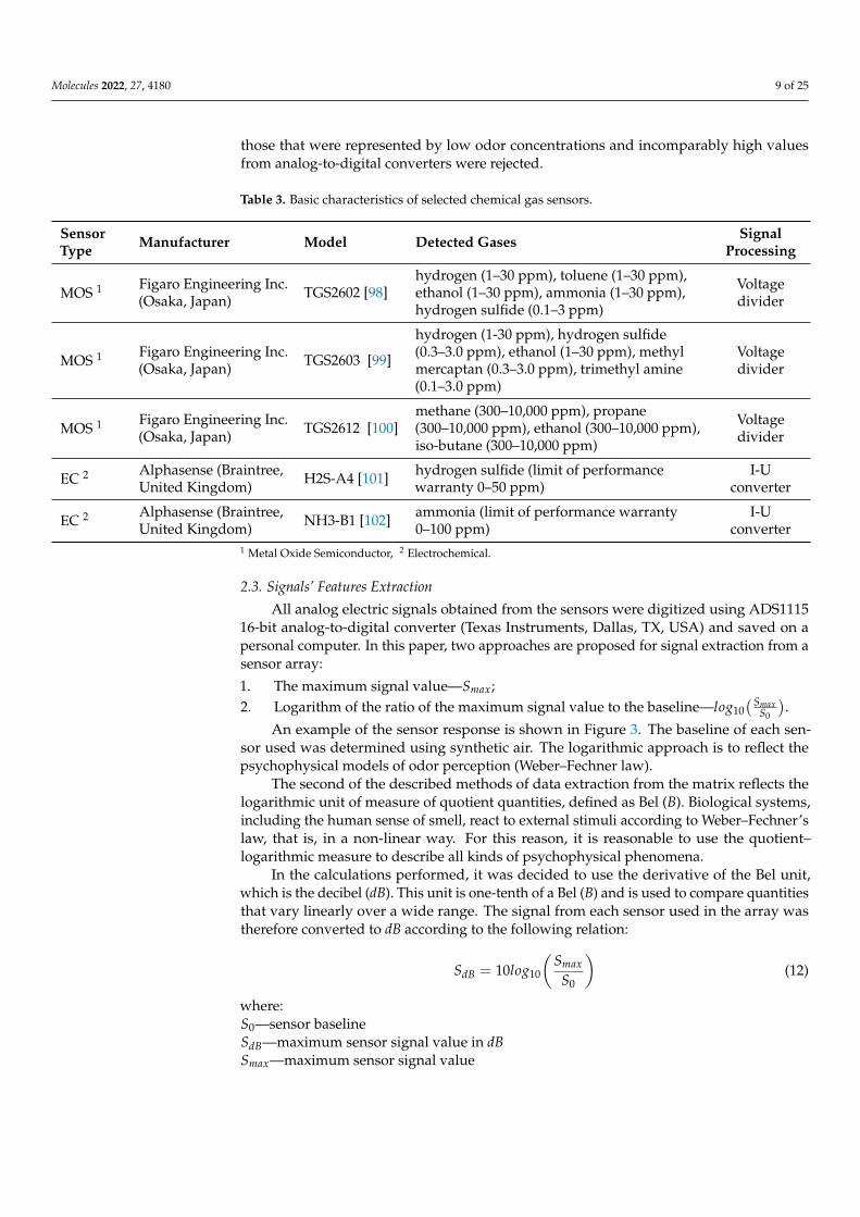
All analog electric signals obtained from the sensors were digitized using ADS111516-bit analog-to-digital converter (Texas Instruments, Dallas, TX, USA) and saved on apersonal computer. In this paper, two approaches are proposed for signal extraction from asensor array:

1. The maximum signal value—Smax;2. Logarithm of the ratio of the maximum signal value to the baseline—log10

( SmaxS0

).

An example of the sensor response is shown in Figure 3. The baseline of each sen-sor used was determined using synthetic air. The logarithmic approach is to reflect thepsychophysical models of odor perception (Weber–Fechner law).

The second of the described methods of data extraction from the matrix reflects thelogarithmic unit of measure of quotient quantities, defined as Bel (B). Biological systems,including the human sense of smell, react to external stimuli according to Weber–Fechner’slaw, that is, in a non-linear way. For this reason, it is reasonable to use the quotient–logarithmic measure to describe all kinds of psychophysical phenomena.

In the calculations performed, it was decided to use the derivative of the Bel unit,which is the decibel (dB). This unit is one-tenth of a Bel (B) and is used to compare quantitiesthat vary linearly over a wide range. The signal from each sensor used in the array wastherefore converted to dB according to the following relation:

SdB = 10log10

(Smax

S0

)(12)

where:S0—sensor baselineSdB—maximum sensor signal value in dBSmax—maximum sensor signal value

Molecules 2022, 27, 4180 10 of 25

Figure 3. Example of the TGS2602 sensor response with marked signal parameters used in furtherdata analysis.

2.4. Mathematical Models for Odor Concentration Determination

A total of 60 olfactometric measurements was made, which allowed to distinguisha training set (40 measurements) and a test set (20 measurements). Based on the trainingdata, the mathematical calibration models were drawn up linking the odor concentrationsdetermined olfactometrically with sensor signals operating in the matrix. It was decidedto use the following statistical techniques that use explanatory variables (senor signals) topredict the outcome of the response variable (odor concentration):

• Model 1: Multiple Linear Regression (MLR)MLR is a statistical technique based on the generation of a linear relationship betweenthe independent variables (sensor signals) and the dependent variable (odor concen-tration). It is important that the explanatory variables are not correlated with eachother and their number is smaller than the number of observations (measurements)made. The general equation is as follows:

Cod = a0 +n

∑i=1

(ai ∗ Si) (13)

where:a0—interceptai—regression coefficientsSi—sensor signal (depending on the method of signal’s features extraction)n—number of explanatory variables

• Model 2: Principal Component Regression (PCR)PCR allows for the selection of explanatory variables that have a significant impact onthe value of the dependent variable; these are called principal components (PC). PCselection is performed using principal component analysis (PCA) and then the MLRmodel is created in which PCs are used as explanatory variables. Formally, PCR isdefined as follows:

Cod = a0 +n

∑i=1

(ai ∗ PCi) (14)

Molecules 2022, 27, 4180 11 of 25

where:a0—interceptai—regression coefficientsPCi—principal componentsn—number of principal components

• Model 3: Stevens’ power law with a single sensor signal as a power exponentSignals from individual sensors were used as an exponent of the proposed relationship.The model best suited to the training dataset was selected based on the value of thecoefficient of determination (R2). Despite the fact that this coefficient ignores theadjustment of the model to data outside the training set, it is one of the basic measuresof the quality of the model matching to this data set. The odor concentration wasdetermined according to the following formula:

Cod = abS (15)

where:a—first model coefficientb—second model coefficientS—sensor signal (depending on the method of signal’s features extraction)

• Model 4: Stevens’ power law with the geometric mean of the sensor signals as apower exponentThis approach was used only for the second method of extracting signals from thesensor array (SdB). The geometric mean of the signals from the individual sensorswas used as the exponent of the function in accordance with relation

Cod = abn√

∏ni=1 SdBi (16)

where :a—first model coefficientb—second model coefficientSdBi

—sensor signal value in dBn—number of sensor in the matrix

• Model 5: Stevens’ power law combined with Principal Component Analysis (PCA)The first principal component (PC1) of the dataset was used as the exponent of theproposed function. PC1 was calculated using PCA and performing mean centeringand scaling to unit variance. It shows the direction of the maximum variance in thedata and best approximates the data in least squares terms. The odor concentrationwas computed as follows:

Cod = abPC1 (17)

where:a—first model coefficientb—second model coefficientPC1—first principal component

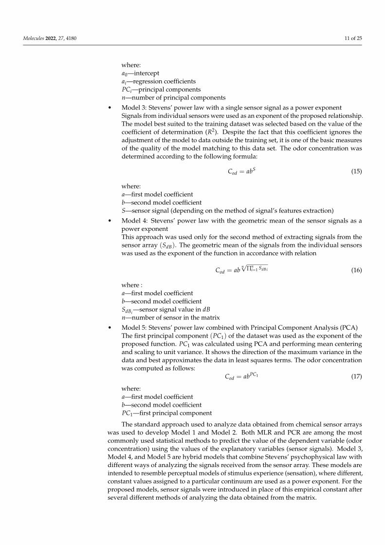
The standard approach used to analyze data obtained from chemical sensor arrayswas used to develop Model 1 and Model 2. Both MLR and PCR are among the mostcommonly used statistical methods to predict the value of the dependent variable (odorconcentration) using the values of the explanatory variables (sensor signals). Model 3,Model 4, and Model 5 are hybrid models that combine Stevens’ psychophysical law withdifferent ways of analyzing the signals received from the sensor array. These models areintended to resemble perceptual models of stimulus experience (sensation), where different,constant values assigned to a particular continuum are used as a power exponent. For theproposed models, sensor signals were introduced in place of this empirical constant afterseveral different methods of analyzing the data obtained from the matrix.

Molecules 2022, 27, 4180 12 of 25

Once the calibration models were prepared, they were validated on the basis of thedata test set. To assess the compliance, usefulness and accuracy of the prepared (trained)models with the olfactometric measurements, the root mean square error (RMSE) was used.This is one of the most common methods to determine model error in predicting outputvariables. RMSE was calculated according to the following formula:

RMSE =

√n

∑i=1

(xi − yi)2

n(18)

where:xi—odor concentration determined from olfactometric measurementsyi—odor concentration determined from gas sensor arrayn—number of olfactometric measurements

Mathematically, RMSE is the Euclidean distance between a vector of observed valuesand a vector of predicted values multiplied by the square root of the inverse of the numberof observations. In other words, the lower the RMSE values, the better the model is atpredicting the observed data. Higher RMSE values should be interpreted as the modelfailing to account for important features underlying the data.

2.5. Odor Air Quality Index

The proposed odor air quality index (OAQII) scale is based on the odor features: odorintensity and hedonic tone. On the basis of 240 measurements carried out at the municipaltreatment plant, during which the odor intensity, its hedonic tone and odor concentrationwere assessed, a plot (Figure 4) was prepared of the dependence of the odor intensity andhedonic tone on the logarithm of the odor concentration (according to Weber–Fechner’slaw, this relationship should be linear). The obtained equations were used to determine theodor concentrations corresponding to the values of odor intensity and hedonic tone.

Figure 4. Dependence of odor intensity and hedonic tone on odor concentration carried out at themunicipal treatment plant.

Appropriate odor concentration ranges were assigned to the determined indexes inaccordance with Table 4.

Molecules 2022, 27, 4180 13 of 25

Table 4. Proposed odor air quality index (OAQII) scale and its parameters.

OAQII Scale Odor Intensity Hedonic Tone Proposed COD Range

0—very good non-perceptible and very weak neutral and slightly unpleasant 0 < COD ≤ 31—moderate weak moderately unpleasant 3 < COD ≤ 10

2—bad distinct and strong very unpleasant 10 < COD ≤ 603—very bad very and extremely strong extremely unpleasant COD > 60

The validation of the models in terms of compliance in the OAQII was assessed usingthe accordance parameter, according to the following formula:

Accordance =ncorrect

N(19)

where:

N—total number of measurementsncorrect—the number of measurements classified by both the model and the olfactometricmeasurements to the same index scale.

3. Results3.1. Models Development

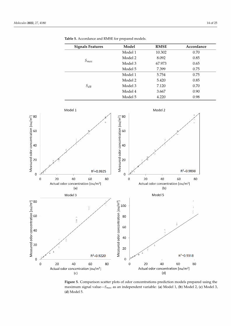
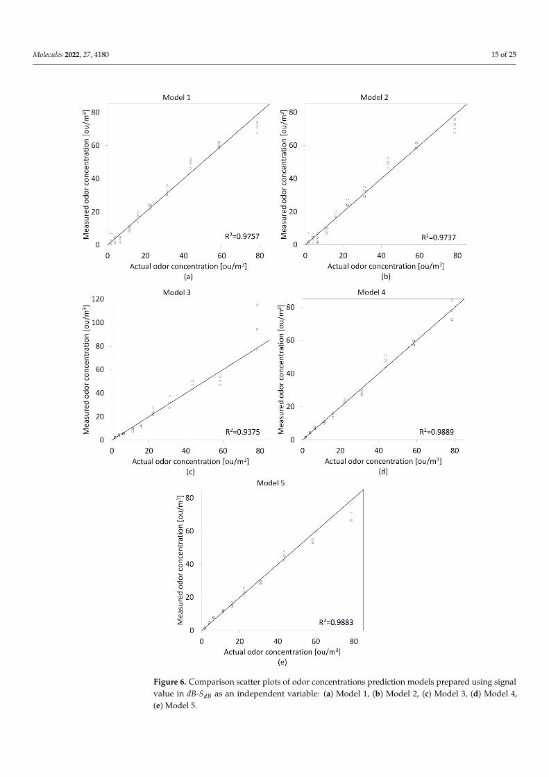
In the first stage of the conducted research, the calibration models were preparedbased on the recorded responses from the gas sensor array and olfactometric measurements(training dataset). Four calibration models were prepared using the maximum signalsvalues from individual sensors and five using a logarithmic approach to extract signals fromthe matrix. Comparison scatter plots of the prepared models are shown in Figures 5 and 6.For Model 3, the TGS2602 sensor signal was used as a function exponent for the first methodof extracting signals from the sensor array (Smax), and the ammonia sensor signal for thesecond method of acquiring signals from the matrix (SdB). It was dictated by obtainingthe highest values of the coefficient of determination (R2) with the use of signals fromthese sensors.

3.2. Models Validation

In the next stage of the research, the prepared models were validated. The validationof these models were performed on the basis of correlation plots. Figures 7 and 8 present theodor concentrations determination using a gas sensor matrix and test set of olfactometricmeasurements for both methods of extracting signals from the matrix.

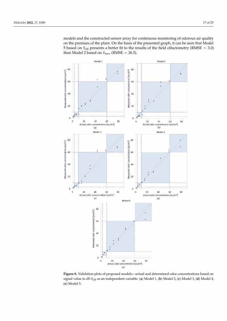
Validation charts presented in Figures 7 and 8 were prepared on the basis of anolfactometric data test set (stage three of the measurements campaign). The blue rectangleson the charts reflect the proposed odor air quality index scale presented in Table 4. Theblack and red points in the graphs correspond to the predicted odor concentrations. Thepoints marked in black are within the appropriate scale ranges of the proposed index, whilethose marked in red exceed the adopted ranges.

Root mean square error (RMSE) was chosen as the numerical tool for the selection ofthe optimal model in terms of matching the predicted odor concentrations to the actualresults of olfactometric measurements. The adaptation of individual models was alsodetermined on the basis of the proposed OAQII . A parameter called "accordance" wasestablished, which reported the percentage of the odor concentrations determined by themathematical models that coincided with the actual values within the proposed concor-dance intervals. Table 5 presents the results of these two parameters calculated for theprepared models.

Molecules 2022, 27, 4180 14 of 25

Table 5. Accordance and RMSE for prepared models.

Signals Features Model RMSE Accordance

Smax

Model 1 10.302 0.70Model 2 8.092 0.85Model 3 67.973 0.65Model 5 7.399 0.75

SdB

Model 1 5.754 0.75Model 2 5.420 0.85Model 3 7.120 0.70Model 4 3.667 0.90Model 5 4.220 0.98

Figure 5. Comparison scatter plots of odor concentrations prediction models prepared using themaximum signal value—Smax as an independent variable: (a) Model 1, (b) Model 2, (c) Model 3,(d) Model 5.

Molecules 2022, 27, 4180 15 of 25

Figure 6. Comparison scatter plots of odor concentrations prediction models prepared using signalvalue in dB-SdB as an independent variable: (a) Model 1, (b) Model 2, (c) Model 3, (d) Model 4,(e) Model 5.

Molecules 2022, 27, 4180 16 of 25

Figure 7. Validation plots of proposed models—actual and determined odor concentrations based onthe maximum signal value—Smax as an independent variable: (a) Model 1, (b) Model 2, (c) Model 3,(d) Model 5.

Based on the table above, it was found that when using the maximum sensor signalsas an explanatory variable in the models, the best fit to the actual odor concentration valuesis Model 2, i.e., principal component regression (PCR). It is characterized by both the lowestRMSE and the highest accordance value. If the SdB is used as the independent variable, theselection of the optimal model is somewhat more difficult. All of them are characterized bysimilar RMSE values, but for Model 4 and Model 5, they are the lowest. As can be seen,Model 4 has a slightly lower RMSE than Model 5, but the difference in accordance makesthe latter appear more optimal.

In the final stage of the study, after selecting the optimal model for both sensor arraysignals extraction methods, the changes in odor concentrations at the compost screeningsite were recorded. Figure 9 shows weekly courses of changes in the odor concentrationwithin the compost yard for both models. Moreover, during these seven days, olfactometricmeasurements were performed daily at the municipal solid waste treatment plant. Thiswas to be used to verify and possibly confirm or deny the usefulness of the developed

Molecules 2022, 27, 4180 17 of 25

models and the constructed sensor array for continuous monitoring of odorous air qualityon the premises of the plant. On the basis of the presented graph, it can be seen that Model5 based on SdB presents a better fit to the results of the field olfactometry (RMSE = 3.0)than Model 2 based on Smax (RMSE = 26.5).

Figure 8. Validation plots of proposed models—actual and determined odor concentrations based onsignal value in dB-SdB as an independent variable: (a) Model 1, (b) Model 2, (c) Model 3, (d) Model 4,(e) Model 5.

Molecules 2022, 27, 4180 18 of 25

Figure 9. Weekly changes in odor concentrations at the compost screening site calculated using thebest model developed using the maximum signal value and signal value in dB compared with fieldolfactometry measurements.

4. Discussion

This article presents a new way to determine odor nuisance based on the proposedodor air quality index (OAQII). During its development, odor features, such as hedonictone, odor intensity and odor concentration, were taken into account. A custom-builtsensor array consisting of five commercially available chemical sensors (three metal oxidesemiconductor sensors and two electrochemical) was used to determine odor concentrationsin the compost screening yard at the municipal solid waste treatment plant. In order tocalibrate the sensor array, odor concentrations were measured on the MSWTP site nearits location using field olfactometry. This allowed a correlation to be found between themultidimensional output signal from the sensor array and the actual odor concentration.Five statistical mathematical models were used for two methods of extracting signals fromthe sensor matrix. In the first approach, the maximum value of the signal from individualsensors (Smax) was used as independent variables in the developed models. In the secondone, the logarithmic approach was used (SdB), determining the ratio of the maximumsignal from the sensor to its baseline. The selection of the optimal model was made on thebasis of two parameters: root mean square error (RMSE) as the benchmark determiningthe compatibility of the prepared models with the olfactometric measurements, and thecriterion called accordance which allowed for the validation of the models in terms ofcompliance in the OAQII .

The conducted research showed that when using the maximum value of the signalfrom the sensors, Model 2 was characterized by the best fit in relation to the real measure-ments. It achieved the lowest RMSE value in its group (Smax), amounting to 8.092, and thehighest compliance in the proposed OAQII , equal to 85%. Using the second method ofextracting data from the sensor matrix, the best model turned out to be Model 5, which is ahybrid model combining Stevens’ power law with one of the basic methods of multivariatedata analysis, which was principal component analysis (PCA). The RMSE thus obtainedwas 4.220, and the index compliance level reached as much as 98%. It should be notedthat among the model in this group (SdB), the lowest RMSE value was obtained for Model4 (3.667), which used the geometric mean of the signals from the sensors installed in thearray as a exponent in Stevens’ power law. However, compared to the Model 5, it was

Molecules 2022, 27, 4180 19 of 25

characterized by a lower compliance in the proposed OAQII , which was 90%. The differ-ence in the prediction of odor concentration and its actual value between these two modelswas not significant enough to compensate for the difference of eight percentage points incompliance with the OAQII index. Therefore, Model 5 was selected as the optimal modelfrom the SdB group.

In both the Smax and SdB model groups, Model 3 should be regarded as the modelwith the worst attunement to the actual measured values. The RMSE values for this modelwere the highest in the given group, and the agreement with the OAQII was at the lowestlevel of compliance. This model, like Model 4 and Model 5, was a hybrid model; however,a single sensor signal was used as an exponent of Steven’s power law. This shows that it isreasonable and fully justifiable to use gas sensor arrays to monitor air quality in terms ofodor nuisance caused mostly by gaseous mixtures of complex composition. Their principleof operation is based on the overlapping of the detection ranges of individual sensors,which may help avoid problems associated with synergistic interactions between odorants(masking, neutralization, and amplification), which might significantly affect the signalfrom a single sensor.

Moreover, each of the models from the SdB group was characterized by a lower RMSEvalues than the most optimal model from the Smax group (Model 2). This means that usinga logarithmic method to extract signals from the sensor matrix which was meant to reflectthe non-linear response to external stimuli of the human sense of smell (Weber–Fechnerlaw), together with appropriate mathematical models, allows, with a higher accuracy, topredict the value of odor concentration.

In the last stage of the research, the constructed sensor matrix was used to control theodor air quality at the compost screening site in online mode (continuous monitoring). Onemathematical model from each of the two proposed sensor signal acquisition groups wasused to control the odor nuisance. Obviously, the models that were considered optimal onthe basis of previous observations and measurements were applied, so they were Model 2from the Smax group and Model 5 from the SdB group. This phase lasted one week, andadditional olfactometric measurements were taken daily in the vicinity of the sensor arrayfor subsequent verification of the odor concentration values returned by the implementedmodels. Figure 9 shows the weekly course of changes in the odor concentration within thecomposting yard for both models and the values measured using field olfactometry, whichwas treated as the reference method.

As can be seen, the values of the odor concentration indicated by both models differquite significantly. The values obtained by Model 2 practically do not fall below 20 ou/m3

in the entire period covered by this part of the research. Olfactometric measurements allowto conclude that the odor nuisance did not remain at such a high level all the time, butrather showed a variable character, which was probably related to the shift work mode atthe municipal treatment plant and conducting compost screening processes in the afternoonor evening hours. This nature of the plant operation could also be confirmed by the odorconcentration values obtained using Model 5. On the one hand, they showed a bettermatch with the olfactometric measurements performed, and on the other, they allowed theidentification of periods of increased odor nuisance, which usually occurred in the eveningor at night. The overestimated odor concentration values obtained using Model 2 werelikely due to the presence of odorless landfill gases, such as methane. Such gases will causea significant increase in the maximum signal for a given sensor while not contributing to theodor nuisance. The phenomenon of saturation of the sensors might then occur, which willresult in their transition to a non-linear operating range and can have a negative impact onthe functioning of the developed model. Model 5 based on the dB scale appears to have lessability to overestimate the results which may mean that the dB scale along with a properlydeveloped mathematical model used for continuous odor concentration monitoring at themunicipal treatment plant is an appropriate approach.

It should additionally be noted that the values of the odor concentration indicatedby the prepared models very rarely showed values below 3 ou/m3. This obviously could

Molecules 2022, 27, 4180 20 of 25

be due to inaccuracies, overestimations or underestimations of the values returned by themodels. A solution improving the quality of sensor matrices and increasing the accuracy ofimplemented mathematical models could be the use of additional temperature, pressureand humidity sensors and modules that maintain stable working conditions inside thematrix’s measuring chamber. Another possible reason for the prepared models rarelyindicating low odor concentration values could be the impact of facilities adjacent to thecomposting site, such as, for example, waste sorting buildings or green waste storage yards.Therefore, a comprehensive approach would seem to be to place several or more sensorarrays within the MSWTP so that odor air quality could be monitored throughout the plant.Establishing such a network of sensor meters would enable odor nuisance monitoring on acontinuous basis and provide plant owners with information on the most odor sensitivepoints or processes. Moreover, measuring an odor emitting facility can be helpful if there isa lot of public pressure from residents living in the neighborhoods adjacent to the facilitywhere the waste is stored and processed. Such a facility will be fully transparent to society,and the measurements taken will help verify the validity of incoming complaints anddiscourage people from overusing such odor nuisance countermeasures.

5. Conclusions

This paper proposes a new four-step odor air quality index (OAQII) that includes threeodor parameters: intensity, hedonic tone and odor concentration. Due to the subjectiveassessment of odor parameters by humans, a gas sensor array was constructed whichwas adapted to determine the above-mentioned index in an instrumental manner. Forthis purpose, continuous measurements were carried out at the municipal solid wastetreatment plant (MSWTP), using the developed sensor matrix, which was calibrated withfield olfactometry. On the basis of collected data, five different mathematical models weretested to correlate the multidimensional output signal from the sensor array with theodor concentration of the sample. Two approaches were proposed for signals extractionfrom a sensor array: (i) the maximum signal value from an individual sensor—Smax, and(ii) the logarithm of the ratio of the maximum sensor signal value to its baseline which wasdetermined by passing synthetic air through the sensors—SdB. The second method usedwas to reflect the non-linear relationship between the measure of the olfactory stimulusand the response of the human sense of smell (Weber–Fechner law).

Standard approaches used for processing and analysis of data obtained from gassensor matrix, such as multiple linear regression (MLR) or principal component regression(PCR), were applied to develop the models (Model 1 and Model 2). Additionally, modelsthat resemble perceptual models of stimulus perception (Stevens’ law) were proposed(Model 3, Model 4 and Model 5). In these models, the empirical constant depending on thetype of external stimulus was replaced by the signal from the sensor array after appropriatedata processing. These three models represent a hybrid approach that combines the sellingpoints of multidimensional sensor data analysis and the advantages of the psychophysicalphenomenon for stimulus perception and processing in the human brain.

The research showed that the best model in terms of compatibility with the OAQIIclass was a hybrid model (Model 5) in which the logarithmic approach to extract signalsfrom the matrix was used. This model was prepared to reflect the effects of externalstimulus on human perception (Weber–Fechner’s Law) in the form of a logarithmic wayof sourcing signals from the matrix, the intensity of the perceived olfactory impression(Stevens’ law) in the form of a proposed equation, and the benefits of multivariate dataanalysis in the form of principal component analysis (PCA) and the use of first principalcomponent (PC1) as an exponent of a power in the prepared equation. The use of this modelensured a 98% consistency in classification into the classes of the proposed index. Model 3was determined to be the worst in terms of agreement with the OAQII class in both modelgroups (Smax and SdB). Admittedly, this was a hybrid model; however, it used single sensorsignals without prior analysis and processing of the data acquired from the array.

Molecules 2022, 27, 4180 21 of 25

The application of the developed model (Model 5) for the continuous monitoring ofodorous air quality (odor concentration) in compost screening yard indicated that the dBscale was an appropriate choice. The dB-based model does not tend to overestimate theresults. The overstating results for tha Smax models are probably caused by the presence ofgases at the site, which are odorless, but cause the applied sensors to react (e.g., methane).Presentation of the values of the signals from the sensor matrix in dB scale allows for lowervariability in the case of the above mentioned situation.

Author Contributions: Conceptualization, J.G.; methodology, J.G. and B.S.; software, D.D.; investiga-tion, B.S. and D.D.; data curation, B.S. and D.D.; original draft preparation, D.D.; review and editing,B.S. and J.G.; visualization, D.D.; supervision, J.G.; funding acquisition, J.G. All authors have readand agreed to the published version of the manuscript.

Funding: This research was funded by National Science Center Poland grant number UMO-2015/19/B/ST4/02722.

Institutional Review Board Statement: Not applicable.

Informed Consent Statement: Not applicable.

Data Availability Statement: Not applicable.

Conflicts of Interest: The authors declare no conflict of interest.

Sample Availability: Samples of the compounds are not available from the authors.

References1. Vodyanitskii, Y.N. Biochemical processes in soil and groundwater contaminated by leachates from municipal landfills (Mini

review). Ann. Agrar. Sci. 2016, 14, 249–256. [CrossRef]2. Saarela, J. Pilot investigations of surface parts of three closed landfills and factors affecting them. Environ. Monit. Assess. 2003,

84, 183–192. [CrossRef] [PubMed]3. Teta, C.; Hikwa, T. Heavy Metal Contamination of Ground Water from an Unlined Landfill in Bulawayo, Zimbabwe. J. Health

Pollut. 2017, 7, 18–27. [CrossRef] [PubMed]4. Alam, R.; Ahmed, Z.; Howladar, M.F. Evaluation of heavy metal contamination in water, soil and plant around the open landfill

site Mogla Bazar in Sylhet, Bangladesh. Groundw. Sustain. Dev. 2020, 10, 100311. [CrossRef]5. Malovanyy, M.; Korbut, M.; Davydova, I.; Tymchuk, I. Monitoring of the Influence of Landfills on the Atmospheric Air Using

Bioindication Methods on the Example of the Zhytomyr Landfill, Ukraine. J. Ecol. Eng. 2021, 22, 36–49. [CrossRef]6. Mepaiyeda, S.; Madi, K.; Gwavava, O.; Baiyegunhi, C. Geological and geophysical assessment of groundwater contamination at

the Roundhill landfill site, Berlin, Eastern Cape, South Africa. Heliyon 2020, 6, e04249. [CrossRef]7. Talaiekhozani, A.; Nematzadeh, S.; Eskandari, Z.; Aleebrahim Dehkordi, A.; Rezania, S. Gaseous emissions of landfill and

modeling of their dispersion in the atmosphere of Shahrekord, Iran. Urban Clim. 2018, 24, 852–862. [CrossRef]8. Autelitano, F.; Giuliani, F. Influence of chemical additives and wax modifiers on odor emissions of road asphalt. Constr. Build.

Mater. 2018, 183, 485–492. [CrossRef]9. Liu, C.; Yang, P.; Wang, H.; Song, H. Identification of odor compounds and odor-active compounds of yogurt using DHS, SPME,

SAFE, and SBSE/GC-O-MS. LWT 2022, 154, 112689. [CrossRef]10. Nordin, S.; Lidén, E. Environmental odor annoyance from air pollution from steel industry and bio-fuel processing. J. Environ.

Psychol. 2006, 26, 141–145. [CrossRef]11. Sá, M.F.; Castro, V.; Gomes, A.I.; Morais, D.F.; Silva Braga, R.V.; Saraiva, I.; Souza-Chaves, B.M.; Park, M.; Fernández-Fernández, V.;

Rodil, R.; et al. Tracking pollutants in a municipal sewage network impairing the operation of a wastewater treatment plant. Sci.Total. Environ. 2022, 817, 152518. [CrossRef] [PubMed]

12. Agus, E.; Zhang, L.; Sedlak, D.L. A framework for identifying characteristic odor compounds in municipal wastewater effluent.Water Res. 2012, 46, 5970–5980. [CrossRef] [PubMed]

13. Schilling, B.; Kaiser, R.; Natsch, A.; Gautschi, M. Investigation of odors in the fragrance industry. Chemoecology 2010, 20, 135–147.[CrossRef]

14. Weihua, Y.; Xiande, X.; Gen, W.; Jie, M.; Zengxiu, Z.; Jiayin, L. Emission characteristics of volatile odorous organic compounds infragrance and flavor industry. Environ. Chem. 2021, 1071–1077. .

15. Han, Z.; Qi, F.; Li, R.; Wang, H.; Sun, D. Health impact of odor from on-situ sewage sludge aerobic composting throughoutdifferent seasons and during anaerobic digestion with hydrolysis pretreatment. Chemosphere 2020, 249, 126077. [CrossRef]

16. Schlegelmilch, M.; Streese, J.; Biedermann, W.; Herold, T.; Stegmann, R. Odour control at biowaste composting facilities. WasteManag. 2005, 25, 917–927. [CrossRef]

Molecules 2022, 27, 4180 22 of 25

17. Han, Z.; Qi, F.; Wang, H.; Li, R.; Sun, D. Odor assessment of NH3 and volatile sulfide compounds in a full-scale municipal sludgeaerobic composting plant. Bioresour. Technol. 2019, 282, 447–455. [CrossRef]

18. Cheng, Z.; Sun, Z.; Zhu, S.; Lou, Z.; Zhu, N.; Feng, L. The identification and health risk assessment of odor emissions from wastelandfilling and composting. Sci. Total. Environ. 2019, 649, 1038–1044. [CrossRef]

19. Zhang, Y.; Ning, X.; Li, Y.; Wang, J.; Cui, H.; Meng, J.; Teng, C.; Wang, G.; Shang, X. Impact assessment of odor nuisance, healthrisk and variation originating from the landfill surface. Waste Manag. 2021, 126, 771–780. [CrossRef]

20. Kim, J.R.; Dec, J.; Bruns, M.A.; Logan, B.E. Removal of odors from swine wastewater by using microbial fuel cells. Appl. Environ.Microbiol. 2008, 74, 2540–2543. [CrossRef]

21. Guffanti, P.; Pifferi, V.; Falciola, L.; Ferrante, V. Analyses of odours from concentrated animal feeding operations: A review. Atmos.Environ. 2018, 175, 100–108. [CrossRef]

22. Wang, Y.C.; Han, M.F.; Jia, T.P.; Hu, X.R.; Zhu, H.Q.; Tong, Z.; Lin, Y.T.; Wang, C.; Liu, D.Z.; Peng, Y.Z.; et al. Emissions,measurement, and control of odor in livestock farms: A review. Sci. Total. Environ. 2021, 776, 145735. [CrossRef] [PubMed]

23. Shareefdeen, Z.; Herner, B.; Wilson, S. Biofiltration of nuisance sulfur gaseous odors from a meat rendering plant. J. Chem. Technol.Biotechnol. Int. Res. Process. Environ. Clean Technol. 2002, 77, 1296–1299. [CrossRef]

24. Amon, M.; Dobeic, M.; Sneath, R.W.; Phillips, V.; Misselbrook, T.H.; Pain, B.F. A farm-scale study on the use of clinoptilolitezeolite and De-Odorase® for reducing odour and ammonia emissions from broiler houses. Bioresour. Technol. 1997, 61, 229–237.[CrossRef]

25. Kusic, H.; Koprivanac, N.; Bozic, A.L. Minimization of organic pollutant content in aqueous solution by means of AOPs: UV- andozone-based technologies. Chem. Eng. J. 2006, 123, 127–137. [CrossRef]

26. Yao, H.; Feilberg, A. Characterisation of photocatalytic degradation of odorous compounds associated with livestock facilities bymeans of PTR-MS. Chem. Eng. J. 2015, 277, 341–351. [CrossRef]

27. Andersen, K.B.; Beukes, J.A.; Feilberg, A. Non-thermal plasma for odour reduction from pig houses—A pilot scale investigation.Chem. Eng. J. 2013, 223, 638–646. [CrossRef]

28. Kim, K.Y.; Ko, H.J.; Kim, H.T.; Kim, Y.S.; Roh, Y.M.; Lee, C.M.; Kim, C.N. Odor reduction rate in the confinement pig building byspraying various additives. Bioresour. Technol. 2008, 99, 8464–8469. [CrossRef]

29. Lewkowska, P.; Cieslik, B.; Dymerski, T.; Konieczka, P.; Namiesnik, J. Characteristics of odors emitted from municipal wastewatertreatment plant and methods for their identification and deodorization techniques. Environ. Res. 2016, 151, 573–586. [CrossRef]

30. Zarra, T.; Naddeo, V.; Belgiorno, V.; Reiser, M.; Kranert, M. Odour monitoring of small wastewater treatment plant located insensitive environment. Water Sci. Technol. 2008, 58, 89–94. [CrossRef]

31. Franco-Luesma, E.; Ferreira, V. Reductive off-odors in wines: Formation and release of H2S and methanethiol during theaccelerated anoxic storage of wines. Food Chem. 2016, 199, 42–50. [CrossRef] [PubMed]

32. Paiva, R.; Wrona, M.; Nerín, C.; Bertochi Veroneze, I.; Gavril, G.L.; Andrea Cruz, S. Importance of profile of volatile and off-odorscompounds from different recycled polypropylene used for food applications. Food Chem. 2021, 350, 129250. [CrossRef] [PubMed]

33. Vera, P.; Canellas, E.; Nerín, C. Compounds responsible for off-odors in several samples composed by polypropylene, polyethylene,paper and cardboard used as food packaging materials. Food Chem. 2020, 309, 125792. [CrossRef] [PubMed]

34. Tansel, B.; Inanloo, B. Odor impact zones around landfills: Delineation based on atmospheric conditions and land use characteris-tics. Waste Manag. 2019, 88, 39–47. [CrossRef] [PubMed]

35. Liu, Y.; Yang, H.; Lu, W. VOCs released from municipal solid waste at the initial decomposition stage: Emission characteristicsand an odor impact assessment. J. Environ. Sci. 2020, 98, 143–150. [CrossRef]

36. Anet, B.; Lemasle, M.; Couriol, C.; Lendormi, T.; Amrane, A.; Le Cloirec, P.; Cogny, G.; Fillières, R. Characterization of gaseousodorous emissions from a rendering plant by GC/MS and treatment by biofiltration. J. Environ. Manag. 2013, 128, 981–987.[CrossRef]

37. Amoore, J.E.; Hautala, E. Odor as an ald to chemical safety: Odor thresholds compared with threshold limit values and volatilitiesfor 214 industrial chemicals in air and water dilution. J. Appl. Toxicol. 1983, 3, 272–290. [CrossRef]

38. Wysocka, I.; Gebicki, J.; Namiesnik, J. Technologies for deodorization of malodorous gases. Environ. Sci. Pollut. Res. 2019,26, 9409–9434. [CrossRef]

39. Nagata, Y.; Takeuchi, N. Measurement of odor threshold by triangle odor bag method. Odor Meas. Rev. 2003, 118, 118–127.40. Szulczynski, B.; Gebicki, J.; Namiesnik, J. Monitoring and efficiency assessment of biofilter air deodorization using electronic

nose prototype. Chem. Pap. 2018, 72, 527–532. [CrossRef]41. López, R.; Cabeza, I.; Giráldez, I.; Díaz, M. Biofiltration of composting gases using different municipal solid waste-pruning

residue composts: Monitoring by using an electronic nose. Bioresour. Technol. 2011, 102, 7984–7993. [CrossRef] [PubMed]42. Sohn, J.H.; Dunlop, M.; Hudson, N.; Kim, T.I.; Yoo, Y.H. Non-specific conducting polymer-based array capable of monitoring

odour emissions from a biofiltration system in a piggery building. Sens. Actuators B Chem. 2009, 135, 455–464. [CrossRef]43. Cabeza, I.; López, R.; Giraldez, I.; Stuetz, R.; Díaz, M. Biofiltration of α-pinene vapours using municipal solid waste (MSW)—

Pruning residues (P) composts as packing materials. Chem. Eng. J. 2013, 233, 149–158. [CrossRef]44. Rolewicz-Kalinska, A.; Lelicinska-Serafin, K.; Manczarski, P. Volatile organic compounds, ammonia and hydrogen sulphide

removal using a two-stage membrane biofiltration process. Chem. Eng. Res. Des. 2021, 165, 69–80. [CrossRef]

Molecules 2022, 27, 4180 23 of 25

45. Liang, Z.; Wang, J.; Zhang, Y.; Han, C.; Ma, S.; Chen, J.; Li, G.; An, T. Removal of volatile organic compounds (VOCs) emittedfrom a textile dyeing wastewater treatment plant and the attenuation of respiratory health risks using a pilot-scale biofilter. J.Clean. Prod. 2020, 253, 120019. [CrossRef]

46. Rybarczyk, P.; Szulczynski, B.; Gebicki, J. Simultaneous Removal of Hexane and Ethanol from Air in a Biotrickling Filter—ProcessPerformance and Monitoring Using Electronic Nose. Sustainability 2020, 12, 387. [CrossRef]

47. Dobrzyniewski, D.; Szulczynski, B.; Dymerski, T.; Gebicki, J. Development of gas sensor array for methane reforming processmonitoring. Sensors 2021, 21, 4983. [CrossRef]

48. Zhou, J.; Welling, C.M.; Vasquez, M.M.; Grego, S.; Chakrabarty, K. Sensor-Array optimization based on time-series data analyticsfor sanitation-related malodor detection. IEEE Trans. Biomed. Circuits Syst. 2020, 14, 705–714. [CrossRef]

49. Romero-Flores, A.; McConnell, L.L.; Hapeman, C.J.; Ramirez, M.; Torrents, A. Evaluation of an electronic nose for odorant andprocess monitoring of alkaline-stabilized biosolids production. Chemosphere 2017, 186, 151–159. [CrossRef]

50. Guz, Ł.; Łagód, G.; Jaromin-Glen, K.; Suchorab, Z.; Sobczuk, H.; Bieganowski, A. Application of gas sensor arrays in assessmentof wastewater purification effects. Sensors 2014, 15, 1–21. [CrossRef]

51. Shooshtari, M.; Salehi, A. An electronic nose based on carbon nanotube-titanium dioxide hybrid nanostructures for detection anddiscrimination of volatile organic compounds. Sens. Actuators B Chem. 2022, 357, 131418. [CrossRef]

52. Gebicki, J.; Dymerski, T.; Namiesnik, J. Monitoring of odour nuisance from landfill using electronic nose. Chem. Eng. Trans. 2014,40, 85–90.

53. Matindoust, S.; Baghaei-Nejad, M.; Abadi, M.H.S.; Zou, Z.; Zheng, L.R. Food quality and safety monitoring using gas sensorarray in intelligent packaging. Sens. Rev. 2016, 36, 169–183. [CrossRef]

54. Xiao-Wei, H.; Xiao-Bo, Z.; Ji-Yong, S.; Zhi-Hua, L.; Jie-Wen, Z. Colorimetric sensor arrays based on chemo-responsive dyes forfood odor visualization. Trends Food Sci. Technol. 2018, 81, 90–107. [CrossRef]

55. Carrasco, A.; Saby, C.; Bernadet, P. Discrimination of Yves Saint Laurent perfumes by an electronic nose. Flavour Fragr. J. 1998,13, 335–348. [CrossRef]

56. Mohd Ali, M.; Hashim, N.; Abd Aziz, S.; Lasekan, O. Principles and recent advances in electronic nose for quality inspection ofagricultural and food products. Trends Food Sci. Technol. 2020, 99, 1–10. [CrossRef]

57. Tan, J.; Xu, J. Applications of electronic nose (e-nose) and electronic tongue (e-tongue) in food quality-related propertiesdetermination: A review. Artif. Intell. Agric. 2020, 4, 104–115. [CrossRef]

58. Dymerski, T.; Gebicki, J.; Wardencki, W.; Namiesnik, J. Quality evaluation of agricultural distillates using an electronic nose.Sensors 2013, 13, 15954–15967. [CrossRef]

59. Haddi, Z.; Amari, A.; Alami, H.; El Bari, N.; Llobet, E.; Bouchikhi, B. A portable electronic nose system for the identification ofcannabis-based drugs. Sens. Actuators B Chem. 2011, 155, 456–463. [CrossRef]

60. Brudzewski, K.; Osowski, S.; Pawlowski, W. Metal oxide sensor arrays for detection of explosives at sub-parts-per millionconcentration levels by the differential electronic nose. Sens. Actuators B Chem. 2012, 161, 528–533. [CrossRef]

61. Patil, S.J.; Duragkar, N.; Rao, V.R. An ultra-sensitive piezoresistive polymer nano-composite microcantilever sensor electronicnose platform for explosive vapor detection. Sens. Actuators B Chem. 2014, 192, 444–451. [CrossRef]

62. de Oliveira, L.F.; Mallafré-Muro, C.; Giner, J.; Perea, L.; Sibila, O.; Pardo, A.; Marco, S. Breath analysis using electronic nose andgas chromatography-mass spectrometry: A pilot study on bronchial infections in bronchiectasis. Clin. Chim. Acta 2022, 526, 6–13.[CrossRef] [PubMed]

63. Smulko, J.; Chludzinski, T.; Majchrzak, T.; Kwiatkowski, A.; Borys, S.; Lisset Jaimes-Mogollón, A.; Manuel Durán-Acevedo, C.;Geovanny Perez-Ortiz, O.; Ionescu, R. Analysis of exhaled breath for dengue disease detection by low-cost electronic nose system.Measurement 2022, 190, 110733. [CrossRef]

64. Saidi, T.; Moufid, M.; de Jesus Beleño-Saenz, K.; Welearegay, T.G.; El Bari, N.; Lisset Jaimes-Mogollon, A.; Ionescu, R.; Bourkadi,J.E.; Benamor, J.; El Ftouh, M.; et al. Non-invasive prediction of lung cancer histological types through exhaled breath analysis byUV-irradiated electronic nose and GC/QTOF/MS. Sens. Actuators B Chem. 2020, 311, 127932. [CrossRef]

65. Bax, C.; Prudenza, S.; Gaspari, G.; Capelli, L.; Grizzi, F.; Taverna, G. Drift compensation on electronic nose data for non-invasivediagnosis of prostate cancer by urine analysis. iScience 2022, 25, 103622. [CrossRef]

66. Zaim, O.; Diouf, A.; El Bari, N.; Lagdali, N.; Benelbarhdadi, I.; Ajana, F.Z.; Llobet, E.; Bouchikhi, B. Comparative analysis ofvolatile organic compounds of breath and urine for distinguishing patients with liver cirrhosis from healthy controls by usingelectronic nose and voltammetric electronic tongue. Anal. Chim. Acta 2021, 1184, 339028. [CrossRef]

67. Ma, H.; Wang, T.; Li, B.; Cao, W.; Zeng, M.; Yang, J.; Su, Y.; Hu, N.; Zhou, Z.; Yang, Z. A low-cost and efficient electronic nosesystem for quantification of multiple indoor air contaminants utilizing HC and PLSR. Sens. Actuators B Chem. 2022, 350, 130768.[CrossRef]

68. Zhang, L.; Tian, F.; Liu, S.; Guo, J.; Hu, B.; Ye, Q.; Dang, L.; Peng, X.; Kadri, C.; Feng, J. Chaos based neural network optimizationfor concentration estimation of indoor air contaminants by an electronic nose. Sens. Actuators B Chem. 2013, 189, 161–167.[CrossRef]

69. Zhang, L.; Tian, F.; Nie, H.; Dang, L.; Li, G.; Ye, Q.; Kadri, C. Classification of multiple indoor air contaminants by an electronicnose and a hybrid support vector machine. Sens. Actuators B Chem. 2012, 174, 114–125. [CrossRef]

70. Gebicki, J.; Szulczynski, B.; Kaminski, M. Determination of authenticity of brand perfume using electronic nose prototypes. Meas.Sci. Technol. 2015, 26, 125103. [CrossRef]

Molecules 2022, 27, 4180 24 of 25

71. Ferrari, G.; Lablanquie, O.; Cantagrel, R.; Ledauphin, J.; Payot, T.; Fournier, N.; Guichard, E. Determination of key odorantcompounds in freshly distilled cognac using GC-O, GC-MS, and sensory evaluation. J. Agric. Food Chem. 2004, 52, 5670–5676.[CrossRef] [PubMed]

72. Zhang, S.; Cai, L.; Koziel, J.A.; Hoff, S.J.; Schmidt, D.R.; Clanton, C.J.; Jacobson, L.D.; Parker, D.B.; Heber, A.J. Field air samplingand simultaneous chemical and sensory analysis of livestock odorants with sorbent tubes and GC–MS/olfactometry. Sens.Actuators B Chem. 2010, 146, 427–432. [CrossRef]

73. Plutowska, B.; Wardencki, W. Application of gas chromatography–olfactometry (GC–O) in analysis and quality assessment ofalcoholic beverages—A review. Food Chem. 2008, 107, 449–463. [CrossRef]

74. Brattoli, M.; Cisternino, E.; Dambruoso, P.R.; De Gennaro, G.; Giungato, P.; Mazzone, A.; Palmisani, J.; Tutino, M. Gaschromatography analysis with olfactometric detection (GC-O) as a useful methodology for chemical characterization of odorouscompounds. Sensors 2013, 13, 16759–16800. [CrossRef] [PubMed]

75. van Ruth, S.M. Methods for gas chromatography-olfactometry: A review. Biomol. Eng. 2001, 17, 121–128. [CrossRef]76. Romain, A.C.; Godefroid, D.; Nicolas, J. Monitoring the exhaust air of a compost pile with an e-nose and comparison with

GC–MS data. Sens. Actuators B Chem. 2005, 106, 317–324. [CrossRef]77. Bylinski, H.; Kolasinska, P.; Dymerski, T.; Gebicki, J.; Namiesnik, J. Determination of odour concentration by TD-GC× GC–TOF-

MS and field olfactometry techniques. Monatshefte Chem.-Chem. Mon. 2017, 148, 1651–1659. [CrossRef]78. Zarra, T.; Naddeo, V.; Oliva, G.; Belgiorno, V. Odour emissions characterization for impact prediction in anaerobic-aerobic

integrated treatment plants of municipal solid waste. Chem. Eng. Trans. 2016, 54, 91–96.79. Sironi, S.; Capelli, L.; Céntola, P.; Del Rosso, R.; Il Grande, M. Odour emission factors for the prediction of odour emissions from

plants for the mechanical and biological treatment of MSW. Atmos. Environ. 2006, 40, 7632–7643. [CrossRef]80. Lucernoni, F.; Tapparo, F.; Capelli, L.; Sironi, S. Evaluation of an Odour Emission Factor (OEF) to estimate odour emissions from

landfill surfaces. Atmos. Environ. 2016, 144, 87–99. [CrossRef]81. Sironi, S.; Capelli, L.; Céntola, P.; Del Rosso, R.; Grande, M.I. Odour emission factors for assessment and prediction of Italian

MSW landfills odour impact. Atmos. Environ. 2005, 39, 5387–5394. [CrossRef]82. Sironi, S.; Capelli, L.; Céntola, P.; Del Rosso, R.; Grande, M.I. Odour emission factors for assessment and prediction of Italian

rendering plants odour impact. Chem. Eng. J. 2007, 131, 225–231. [CrossRef]83. Zarra, T.; Naddeo, V.; Belgiorno, V.; Reiser, M.; Kranert, M. Instrumental characterization of odour: A combination of olfactory

and analytical methods. Water Sci. Technol. 2009, 59, 1603–1609. [CrossRef] [PubMed]84. Nicolas, J.; Cors, M.; Romain, A.C.; Delva, J. Identification of odour sources in an industrial park from resident diaries statistics.

Atmos. Environ. 2010, 44, 1623–1631. [CrossRef]85. Nicolas, J.; Romain, A.C.; Ledent, C. The electronic nose as a warning device of the odour emergence in a compost hall. Sens.

Actuators B Chem. 2006, 116, 95–99. [CrossRef]86. Capelli, L.; Sironi, S.; Del Rosso, R.; Céntola, P. Predicting odour emissions from wastewater treatment plants by means of odour

emission factors. Water Res. 2009, 43, 1977–1985. [CrossRef]87. Naddeo, V.; Zarra, T.; Kubo, A.; Uchida, N.; Higuchi, T.; Belgiorno, V. Odour measurement in wastewater treatment plant using

both European and Japanese standardized methods: Correlation and comparison study. Glob. Nest J. 2016, 18, 728–733.88. Zarra, T.; Reiser, M.; Naddeo, V.; Belgiorno, V.; Kranert, M. Odour emissions characterization from wastewater treatment plants

by different measurement methods. Chem. Eng. Trans. 2014, 40, 37–42.89. Rincón, C.A.; De Guardia, A.; Couvert, A.; Wolbert, D.; Le Roux, S.; Soutrel, I.; Nunes, G. Odor concentration (OC) prediction

based on odor activity values (OAVs) during composting of solid wastes and digestates. Atmos. Environ. 2019, 201, 1–12.[CrossRef]

90. Wu, C.; Liu, J.; Yan, L.; Chen, H.; Shao, H.; Meng, T. Assessment of odor activity value coefficient and odor contribution based onbinary interaction effects in waste disposal plant. Atmos. Environ. 2015, 103, 231–237. [CrossRef]

91. Sohn, J.; Smith, R.; Yoong, E.; Leis, J.; Galvin, G. Quantification of Odours from Piggery Effluent Ponds using an Electronic Noseand an Artificial Neural Network. Biosyst. Eng. 2003, 86, 399–410. [CrossRef]

92. Misselbrook, T.; Hobbs, P.; Persaud, K. Use of an Electronic Nose to Measure Odour Concentration Following Application ofCattle Slurry to Grassland. J. Agric. Eng. Res. 1997, 66, 213–220. [CrossRef]

93. Capelli, L.; Sironi, S.; Céntola, P.; Del Rosso, R.; Il Grande, M. Electronic noses for the continuous monitoring of odours from awastewater treatment plant at specific receptors: Focus on training methods. Sens. Actuators B Chem. 2008, 131, 53–62. [CrossRef]

94. Sironi, S.; Capelli, L.; Céntola, P.; Del Rosso, R. Development of a system for the continuous monitoring of odours from acomposting plant: Focus on training, data processing and results validation methods. Sens. Actuators B Chem. 2007, 124, 336–346.[CrossRef]

95. Stuetz, R.; Fenner, R.; Engin, G. Assessment of odours from sewage treatment works by an electronic nose, H2S analysis andolfactometry. Water Res. 1999, 33, 453–461. [CrossRef]

96. Sohn, J.H.; Hudson, N.; Gallagher, E.; Dunlop, M.; Zeller, L.; Atzeni, M. Implementation of an electronic nose for continuousodour monitoring in a poultry shed. Sens. Actuators B Chem. 2008, 133, 60–69. [CrossRef]

97. Brattoli, M.; De Gennaro, G.; De Pinto, V.; Demarinis Loiotile, A.; Lovascio, S.; Penza, M. Odour detection methods: Olfactometryand chemical sensors. Sensors 2011, 11, 5290–5322. [CrossRef]

98. Available online: https://www.figaro.co.jp/en/product/entry/tgs2602.html (accessed on 21 June 2022).

Molecules 2022, 27, 4180 25 of 25

99. Available online: https://www.figaro.co.jp/en/product/entry/tgs2603.html. (accessed on 21 June 2022).100. Available online: https://www.figaro.co.jp/en/product/entry/tgs2612-D00.html (accessed on 21 June 2022).101. Available online: https://www.alphasense.com/wp-content/uploads/2019/10/H2S-A4.pdf (accessed on 21 June 2022).102. Available online: https://www.alphasense.com/wp-content/uploads/2021/05/NH3-B1.pdf (accessed on 21 June 2022).