Determination of a shallow velocity-depth model from seismic refraction data by coherence inversion1

Geophysical Prospecting, 1995,43, 177-190

Determination of a shallow velocity-depth model f rom seismic ref raction data by coherence invetsionl Evgeny Landa,’ Shemer Keydar’ and Alex Kravtcov’

Abstract

Seismic refractions have different applications in seismic prospecting. The travel- times of refracted waves can be observed as first breaks on shot records and used for field static calculation. A new method for constructing a near-surface model from refraction events is described. It does not require event picking on prestack records and is not based on any approximation of arrival times. It consists of the maximization of the semblance coherence measure computed using shot gathers in a time window along refraction traveltimes. Time curves are generated by ray tracing through the model. The initial model for the inversion was constructed by the intercept-time method. Apparent velocities and intercept times were taken from a refraction stacked section. Such a section can be obtained by appling l inea moveout corrections to common-shot records. The technique is tested successfully on synthetic and real data. An important application of the proposed method for solving the statics problem is demonstrated.

Introduction

The reflection survey is the dominant method used in seismic prospecting. However, reflected waves alone are not always effective when studying the upper part of the sub-surface. Past experience in seismics has shown that strong surface waves and non-ray effects prevent stable and reliable results being obtained in the upper part of the seismic reflection section. Unlike reflections, refracted waves can be observed outside the zone of interference between surface and reflected waves. Seismic refracted waves have different applications in seismic prospecting.

First breaks are the most useful arrivals on shot records for solving the problem of field static corrections. A number of methods have been described for the com- putation of field static corrections (Singh 1978; Palmer 1986; Russell 1989). In general, most of these methods are based on first-arrival picking. Static corrections are then computed to remove the effects of the weathering layer.

’ Received November 1993, revision accepted July 1994. Institute for Petroleum Research and Geophysics, PO Box 2286, Hamashbir st., 1, Holon 58122, Israel.

177

178 E . Landa, S. Keydar and A. Kravtsov

Seismic refraction techniques have recently been used in ground-water, engin- eering and mineral exploration. These techniques also depend on first-break picks for near-surface Studies of depth and velocity. Refraction tomography has been used for several years to compute multilayer, near-surface models (Hampson and Russell 1984; Schneider and Kuo 1985; de Amorim, Hubral and Tygel 1987; Olsen 1989; Docherty 1992).

Although, in some cases, the first breaks can be easily identified and even picked automatically (Spagnolini 1991 ; Murat and Rudman 1992), with a small signal-to- noise ratio, event picking is not only a time-consuming procedure, but it is also subject to systematic errors that can seriously limit the reliability of the results.

We propose a new method for the construction of a 2D near-surface velocity- depth model from refraction events. This method does not require event picking on unstacked seismic records and is not based on any approximations of arrival times. We consider the method as a refraction coherence inversion (unlike the reflection coherence inversion of Landa et al. 1988). It is formulated as an opti- mization algorithm producing a velocity-depth model which maximizes the sem- blance coherence measure computed for common-shot gathers in a time window along refraction traveltime curves generated by ray tracing through the model. The inversion includes the estimation of refraction velocities in the layers and depth location of refraction interfaces. The input includes common-shot gathers and an initial model. Inversion is performed iteratively. During each iteration, refraction traveltimes are calculated and a semblance value is then computed along the arrival-time curves on common-shot gathers. It is assumed that semblance reaches a maximum value when the calculated arrival curves match the arrival times of the events on the field data. Since semblance maximization is a highly non-linear process, simple gradient-type optimization techniques are not appropriate to the problem. In this work we use a combination of two non-linear optimization methods, namely Monte Carlo and Nelder-Mead (Simplex). The former has recently been successfully used for residual statics estimation (Rothman 1985 ; Normark and Mosegaard 1993), and for reference velocity model estimation (Landa, Beydoun and Tarantola 1989). The latter has been used for macromodel estimation (Landa et al. 1988). We describe the method and demonstrate its appli- cation to both synthetic and field data. The method could be generalized to 3D models.

Initial model construction

We assume that the shallow part of the subsurface can be adequately modelled as a series of isotropic layers separated by refraction interfaces. The velocity within each layer can vary laterally, and interface geometry and velocities are represented by spline functions. For the initial model construction we use the intercept-time method. This is probably the best-known technique (Palmer 1986) of seismic ref- raction interpretation. It is simple to use and it provides a satisfactory initial model

Velocity-depth determination 179

for our inversion procedure as described below. The input includes the apparent velocities and the intercept times for refracted waves. The intercept-time method applies Snell’s law in order to define a multiple-layer model in two stages, with the computation of seismic velocities and related parameters followed by depth compu- tations (for more details of the algorithm, see Palmer 1986). For apparent velocities and intercept-times estimation, we developed an interactive computer procedure without event tracking on common-shot records. It consists of obtaining a stacked time section for refraction waves, where each trace of the section represents the result of the summing of a common-shot gather after linear normal moveout cor- rection. The stacking velocity analysis procedure in this case is similar to that in conventional data processing for reflected waves and a simple expression for the linear NMO correction is

t = t , + xfv,p,

where t0 is the intercept time, x is the distance between short and receiver, and vaP is the stacking velocity which, in fact, represents the apparent velocity of refracted waves. This stacking procedure is extremely fast and needs only very limited oper- ator intervention. The stacked section is then interpreted and the intercept times are determined by picking the refraction events for selected horizons. Using this information together with the apparent velocities obtained from the stacking veloc- ity analysis, a velocity-depth model is constructed using the intercept-time method. We use this model as an initial model for the interactive inversion pro- cedure described below.

Inversion procedure

Inversion consists of finding a multilayered velocity-depth model which maximizes the semblance function calculated for all shot gathers in a time window along ref- raction traveltime curves generated by ray tracing. Each iteration of the inversion procedure is performed in two steps : first, refraction traveltimes are calculated for all the layers by ray tracing and then a semblance value is calculated for shot gathers along a time curve corresponding to the first-arrival times. The maximiza- tion of semblance in order to obtain the best model could be performed by using any optimization method. In fact, the semblance function has secondary maxima. We chose to simplify the optimization process. First we invert iteratively layer after layer. This requires the interactive involvement of an interpreter to define the target layers and to choose the offset range on the common-shot gathers for the semblance calculation for each layer. This choice is made so as to include in the semblance calculation only those traces where the refracted waves from the layer under consideration appear in the first arrivals. It is important to note that it is a much easier procedure to choose an offset range than to define the break points in first-arrival picking. The inclusion of more traces in the inversion will decrease a semblance value due to interference between the refracted and reflected waves,

180 E . Landa, S . Keydar and A. Kravtsov

20

E 40- v

f a 13 60

80-

100

while the inclusion of less traces will decrease the statistical summing effect. Neither case significantly degrades the results of inversion (unlike an incorrect seg- mentation of first-arrival curves). Conventional processing, such as muting, filter- ing, deconvolution, etc. can be applied to shot gathers.

In the second step we perform global optimization for all the layers simulta- neously searching for velocities and depth positions of the model using the model obtained in the previous step as an initial model for global optimization.

For semblance maximization we use a combination of two optimization tech- niques, namely, Monte Carlo random walk in the first stage of the search and Simplex (Nelder and Mead method) in the final stage. The Monte Carlo method samples the semblance objective function in the space of independent variables. The advantage of this method is its ability to migrate through a sequence of local extrema, but it suffers from slow convergence. In practice, the random walk is terminated when an arbitrary number of trials (20-50) fails to produce an accept- able point. The Simplex method converges much faster than the Monte Carlo method and the directions for maximization are determined only from successive evaluations of the objective function (Himmelblau 1972; Landa et al. 1988).

-

-

-

V

Exarnples

Synthetic example

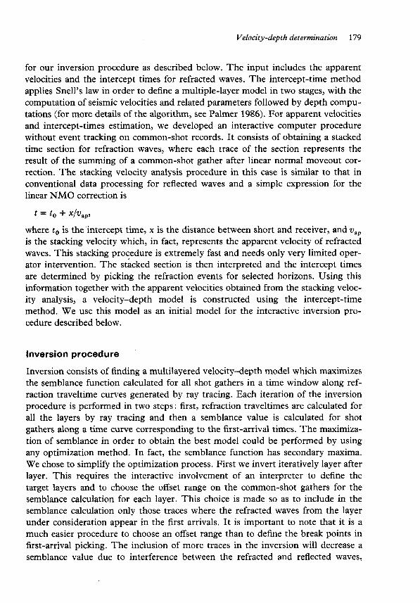
We applied our inversion technique to the two-layer model shown in Fig. 1 . Inter- val velocities in the first layer and in the half-space below the second layer are

Distance(m)

1 0 0 200 300 400 500 600 I-I--- T - - - - - T V

1000

2000 2000 2100 2300 2000 1800

3500

Figure 1. Two-layer synthetic model.

0 0 m II x

0 0 m II x

8 c N

Velocity-depth determination 18

h

v n

1

- - 2

E 0 wl rn II x a

A

v m ..

9 E

II

0 0 rn

x

182 E . Landa, S . Keydar and A . Kravtsov

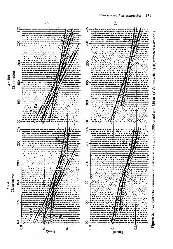
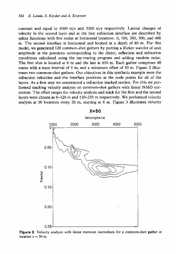
constant and equal to 1000 m/s and 3500 m/s respectively. Lateral changes of velocity in the second layer and at the first refraction interface are described by spline functions with five nodes at horizontal locations: 0, 100, 200, 300, and 400 m. The second interface is horizontal and located at a depth of 80 m. For this model, we generated 120 common-shot gathers by putting a Ricker wavelet of unit amplitude at the positions corresponding to the direct, reflection and refraction traveltimes calculated using the ray-tracing program and adding random noise. The first shot is located at 0 m and the last at 650 m. Each gather comprises 48 traces with a trace interval of 5 m, and a minimum offset of 50 m. Figure 2 illus- trates two common-shot gathers. Our objectives in this synthetic example were the refraction velocities and the interface positions at the node points for all of the layers. As a first step we constructed a refraction stacked section. For this we per- formed stacking velocity analysis on common-shot gathers with linear NMO cor- rection. The offset ranges for velocity analysis and stack for the first and the second layers were chosen as 0-120 m and 120-235 m respectively. We performed velocity analysis at 30 locations every 20 m, starting at 0 m. Figure 3 illustrates velocity

1( 0.

0.05.

0.10. - Y v>

E i=

0.1 5.

0.20.

0.25

X=50 Velocity(m/s)

0 2000 3000 4000 5i 10

Figure 3. Velocity analysis with linear moveout corrections for a common-shot gather at location x = 50 m.

Velocity-depth determination

Distance(m)

100 200 300 4 0 0 500 600

100 200 300 400 500 600

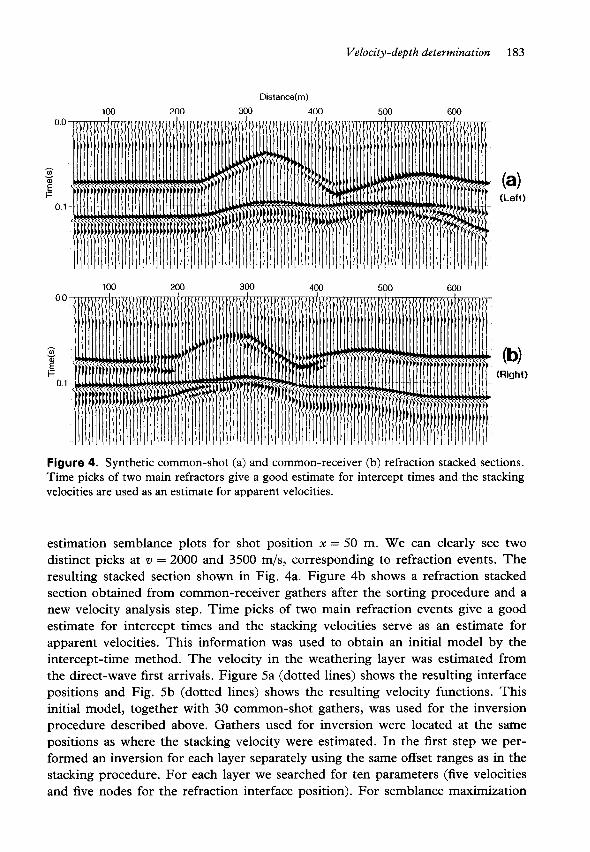
Figure 4. Synthetic cornmon-shot (a) and cornmon-receiver (b) refraction stacked sections. Tirne picks of two main refractors give a good estirnate for intercept times and the stacking velocities are used as an estimate for apparent velocities.

estimation semblance plots for shot position x = 50 m. We can clearly see two distinct picks at ZJ = 2000 and 3500 m/s, corresponding to refraction events. The resulting stacked section shown in Fig. 4a. Figure 4b shows a refraction stacked section obtained from common-receiver gathers after the sorting procedure and a new velocity analysis step. Time picks of two main refraction events give a good estimate for intercept times and the stacking velocities serve as an estimate for apparent velocities. This information was used to obtain an initial model by the intercept-time method. The velocity in the weathering layer was estimated from the direct-wave first arrivals. Figure 5a (dotted lines) shows the resulting interface positions and Fig. 5b (dotted lines) shows the resulting velocity functions. This initial model, together with 30 common-shot gathers, was used for the inversion procedure described above. Gathers used for inversion were located at the same positions as where the stacking velocity were estimated. In the first step we per- formed an inversion for each layer separately using the same offset ranges as in the stacking procedure. For each layer we searched for ten parameters (five velocities and five nodes for the refraction interface position). For semblance maximization

184 E . Landa, S. Keydar and A. Kravtsov

1600

2000

- ,“ 2400- E Y > - .- 3

3 2800-

Distance(m)

0 100 200 300 400 500 600 I I I I I 1 +

(4

- I I 1 1 1 * (b)

-

........... .... ...... ...... .... .-., *. .,.

*.. ”&d..*..”””N ............

.’% ../.*... .... .-“ ......................... .....

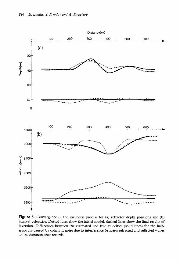
Figure 5. Convergence of the inversion process for (a) refractor depth positions and (b) interval velocities. Dotted lines show the initial model, dashed lines show the final results of inversion. Differences between the estimated and true velocities (solid lines) for the half- space are caused by coherent noise due to interference between refracted and reflected waves on the common-shot records.

Velocity-depth determination 185

we ran 300 iterations of the Monte Carlo method and then 100 iterations of the Simplex method. In the second step we looked for a global model (twenty parameters) running 200 iterations of the Monte Carlo method and 100 iterations of the Simplex method. The initial value of semblance was 0.15 and the final value was 0.53. The final model is shown in Fig. 5 (dashed lines). The final velocity function for the second layer and the geometry for both interfaces are very close to the true one (solid lines in Fig. 5). Slight differences (up to 3%) between the esti- mated and the true velocities for the half-space are caused by coherent noise due to interference effects between refracted and reflected waves (for comparison see Fig. 2b showing the wavefield calculated for the refracted waves only).

Field data example

Following the successful experiments on synthetic data, we applied velocity inver- sion to real data. The input data consist of 200 common-shot gathers, located between 0 and 4000 m, with a 20 m spacing. Each single-end shot gather comprises 60 traces with a 20 m spacing and 50 m minimum offset. Figure 6a shows the common-shot refraction stacked section obtained from this data after velocity analysis and linear moveout correction. Figure 6b shows a refraction stacked section obtained from the same data set after sorting to common-receiver gathers. Two refraction interfaces were picked by interpreting these sections. At the right side of the sections, events have times of approximately 0.05 and 0.1 s, respectively.

Disiance(m1

(0 o 4 w 800 1200 1600 2000 2400 2800 3200 3600 4000

0.0

0.1

0.2

0 S . j

Figure 6. Real data common-shot (a) and common-receiver (b) refraction stacked sections. Two refraction events (about 0.05 s and 0.1 s at the right side of the section) were picked for the initial model construction.

- 50- E

(a) 50 250

2280 2260 2160 2150 2590 2520 2530 2460 2410 2730

Distance(m)

150

450

-

650 850

\', c . .L

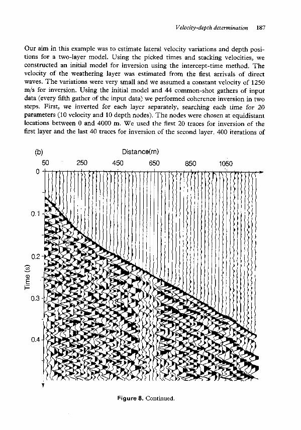
Figure 8. (a) and (b) Shot records for the real data example. The refraction traveltime curves for semblance computation are shown in thick Iines.

Velocity-depth determination 187

Our aim in this example was to estimate lateral velocity variations and depth posi- tions for a two-layer model. Using the picked times and stacking velocities, we constructed an initial model for inversion using the intercept-time method. The velocity of the weathering layer was estimated from the first arrivals of direct waves. The variations were very small and we assumed a constant velocity of 1250 m/s for inversion. Using the initial model and 44 common-shot gathers of input data (every fifth gather of the input data) we performed coherence inversion in two steps. First, we inverted for each layer separately, searching each time for 20 parameters (10 velocity and 10 depth nodes). The nodes were chosen at equidistant locations between 0 and 4000 m. We used the first 20 traces for inversion of the first layer and the last 40 traces for inversion of the second layer. 400 iterations of

0

0.1

0.2 h

Y cn

z F

0.3

0.4

50 250 450

i 650 850

5 1050

ii

t

1

B

Figure 8. Continued.

188 E . Landa, S . Keydar and A. Kravtsov

Distance(m)

(a)O 1ooO 2000 3000 4000 5000 6000 7000 8MM 9ooo 1oooO 11wO 0.0

0.1

0 0.2

F

- f

0.3

0.4

0.5

0.6

0.7

0.8

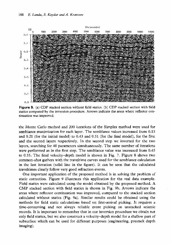
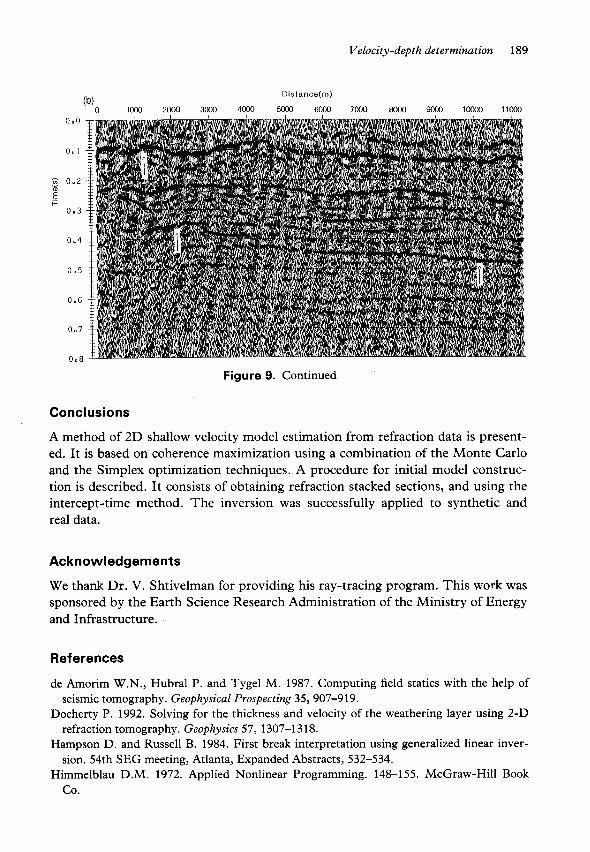
Figure 9. (a) CDP stacked section without field statics. (b) CDP stacked section with field statics computed by the inversion procedure. Arrows indicate the areas where reflector con- tinuation was improved.

the Monte Carlo method and 200 iterations of the Simplex method were used for semblance maximization for each layer. The semblance values increased from 0.15 and 0.21 (for the initial model) to 0.43 and 0.51 (for the final model), for the first and the second layers respectively. In the second step we inverted for the two layers, searching for 40 parameters simultaneously. The same number of iterations were performed as in the first step. The semblance value was increased from 0.45 to 0.55, The final velocity-depth model is shown in Fig. 7. Figure 8 shows two common-shot gathers with the traveltime curves used for the semblance calculation in the last iteration (solid line in the figure). It can be seen that the calculated traveltimes clearly follow very good refraction events.

One important application of the proposed method is in solving the problem of static correction. Figure 9 illustrates this application for the real data example. Field statics were calculated using the model obtained by the proposed method. A CMP stacked section with field statics is shown in Fig. 9b. Arrows indicate the areas where reflector continuation was improved, compared to the stacked section calculated without statics (Fig. 9a). Similar results could be obtained using the methods for field static calculations based on first-arrival picking. It requires a time-consuming and not always reliable event picking on unstacked seismic records. It is important to remember that in our inversion procedure we obtain not only field statics, but we also construct a velocity-depth model for a shallow part of subsurface which can be used for different purposes (engineering, prestack depth imaging).

Velocity-depth determination 189

Dislance(m)

(b)O 1000 Z o o 0 3000 4000 5000 6000 7000 8ooo 9ooo 1oooO 11000 0.0

0 . I

;i 0.2

F

- E

0.3

0.4

0.5

0.6

0.7

0.8

Figure 9. Continued

Conclusions

A method of 2D shallow velocity model estimation from refraction data is present- ed. It is based on coherence maximization using a combination of the Monte Carlo and the Simplex optimization techniques. A procedure for initial model construc- tion is described. It consists of obtaining refraction stacked sections, and using the intercept-time method. The inversion was successfully applied to synthetic and real data.

Acknowledgements

We thank Dr. V. Shtivelman for providing his ray-tracing program. This work was sponsored by the Earth Science Research Administration of the Ministry of Energy and Infrastructure.

Ref erences

de Amorim W.N., Hubral P. and Tygel M. 1987. Computing field statics with the help of

Docherty P. 1992. Solving for the thickness and velocity of the weathering layer using 2-D

Hampson D. and Russell B. 1984. First break interpretation using generalized linear inver-

Himmelblau D.M. 1972. Applied Nonlinear Programming. 148-155. McGraw-Hill Book

seismic tomography. Geophysical Prospecting 35,907-919.

refraction tomography. Geophysics 57, 1307-1318.

sion. 54th SEG meeting, Atlanta, Expanded Abstracts, 532-534.

Co.

190 E. Landa, S. Keydar and A. Kravtsov

Landa E., Beydoun W. and Tarantola A. 1989. Reference velocity model estimation from prestack wave froms : Coherency optimization by simulated annealing. Geophysics 54, 984- 990.

Landa E., Kosloff D., Keydar S., Koren Z . and Reshef M. 1988. A method for determi- nation of velocity and depth from seismic reflection data. Geophysical Prospecting 36, 223- 243.

Murat M. and Rudman A. 1992. Automated first arrival picking: a neural network approach. Geophysical Prospecting 40, 587-604.

Normark E., and Mosegaard K. 1993. Residual static estimation : scaling temperature using simulated annealing. Geophysical Propecting 41, 565-578.

Olsen K.B. 1989. A stable and flexible procedure for the inverse modelling of seismic first arrivals. Geophysical Prospecting 37, 455-465.

Palmer D. 1986. Refraction Seismic. Seismic Exploration, vol. 13. Geophysical Press. Rothman D. 1985. Nonlinear inversion, statistical mechanics and residual statics estimation.

Singh S. 1978. An iterative method for detailed depth determination from refraction data for

Russell B.H. 1989. Static correction - A tutorial. Canadian Society of Exploration Geophys-

Schnieder W. and Kuo S. 1985. Refraction modeling for static corrections. 55th SEG

Spagnolini, U. 1991. Adaptive picking of refracted first arrival. Geophysical Prospecting 39,

Geophysics 50, 2784-2796.

an uneven interface. Geophysical Prospecting 26, 303-31 1.

cists Recorder, 16-30.

meeting, Washington, Expanded Abstracts, 295-299.

293-3 12.