Determinants of the Current Account Balance in the U.S

Determinants of the Current Account Balance in the U.S.

Tuvshintugs Batdelger* and Magda Kandil**

*Boston University

**International Monetary Fund1

March 22, 2006

Abstract This paper studies the role of public and private imbalances in the behavior of the current account balance in the United States in the context of an intertemporal model. The estimation evaluates the effects of public and private imbalances on the dynamics of the current account. Correlation coefficients support the Ricardian equivalence. Higher budget deficit correlates with a reduction in private consumption and an increase in private savings. Government saving does not vary significantly with macroeconomic variables in the short or in the long-run. In contrast, fluctuations in government investment vary significantly with a number of economic variables in the long and in the short-run. Accordingly, fluctuations in the budget deficit are likely to be driven by fluctuations in public investment. In contrast to government savings, private savings vary significantly with macro variables in the long and in the short-run. Fluctuations in private investment appear less evident compared to that in private savings. Overall, fluctuations in the current account balance appear to be more tied to movements in the budget deficit. Nonetheless, fluctuations in the budget deficit are moderated by an increase in private savings and a reduction in private investment, moderating fluctuations in the current account balance.

JEL Classification Numbers:

Keywords:

Authors’ E-Mail Addresses: [email protected]; [email protected]

1 The views expressed in the paper are those of the authors and do not necessarily represent those of the IMF or IMF policy.

2

I. Introduction

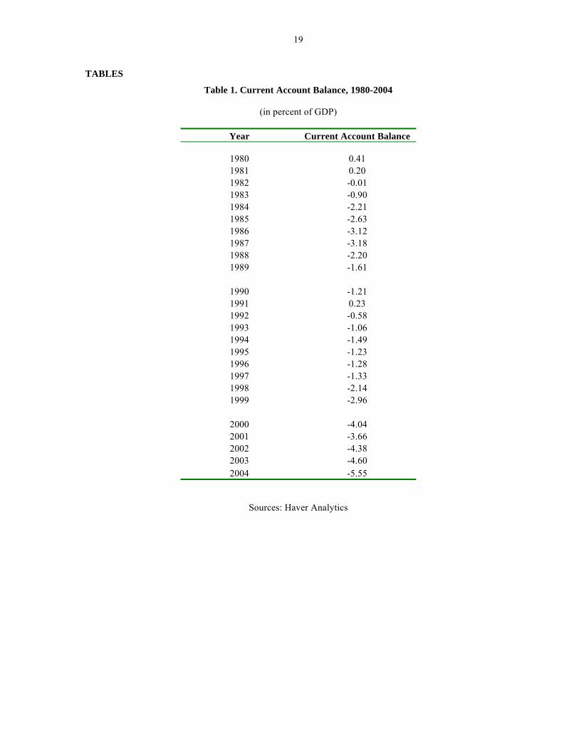
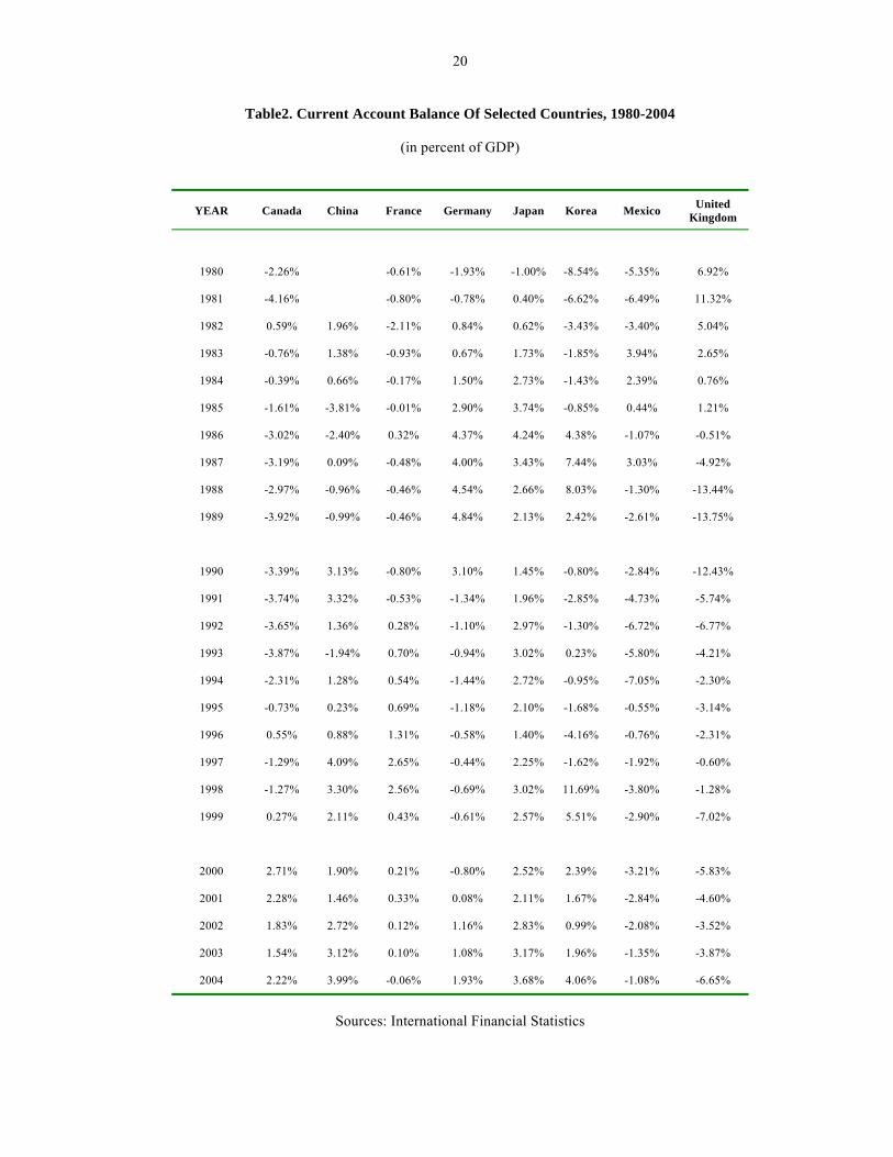
The United States has experienced current account deficits exceeding 1 percent of GDP during all but only five of the years during the last two decades. (Table 1). In 2000, the current account deficit reached 4.04 percent of GDP. Although it declined in 2001 to 3.66 percent of GDP, reflecting the economic slowdown, the ratio has since increased to 4.38 percent in 2002, 4.60 percent in 2003, and even higher deficit to GDP in 2004, 5.55 percent. More recently, the current account balance in the U.S. has further deteriorated in 2005 and preliminary data show that it reached 6.4 percent of GDP. Some projections show the current account deficit averaging above 4.5 percent over the next decade (Mann, 2001). Although the levels experienced thus far are not large compared to those experienced by some industrial countries, such as Australia and New Zealand, and many developing countries, they are high compared to the current account balances of the larger industrial countries (Table 2). Thus, questions have arisen about the sustainability of current account deficits exceeding 4 percent of GDP over the medium to long term in the sense of Milesi-Ferretti and Razin (1996), meaning that they can be maintained without the need for drastic changes in domestic macroeconomic policy.2 For example, Obstfeld and Rogoff (2000), writing before the start of the 2001 recession in the United States, argued that the U.S. current account balance was quite likely to reverse by 2010, predicting that a rapid adjustment could lead to a real depreciation of the dollar by more than 20 percent.3

Contemporary economic theory views current account sustainability as a medium-term issue, turning on the ability of countries to generate sufficient current account surpluses in future years to offset present deficits (Chinn and Prasad, 2000; Faruquee and Debelle, 2000; and Arora, Dunaway, and Faruquee, 2001). Nevertheless, economists have found that the current account position of industrial countries varies with the state of the business cycle. Faruqee and Debelle (1996), for example, have observed that the business cycle, as measured by the output gap and the real exchange rate, had significant short-term effects on the current account balance for a number of industrial countries during the 1971–93 period. Freund (2000) has noted that, in industrial countries, a common pattern during the 1980–97 period was for the current account deficit to begin reversing after reaching a level of about 5 percent of GDP and to continue improving over a period of several years. The reversal typically accompanied a slowing in the real GDP growth rate, which Freund interprets as meaning that strong income growth led to a current account deficit, while a growth slowdown or recession usually accompanied an improvement in the balance to a more sustainable level. In addition, most countries experienced a decline in the national savings rate before the reversal, and a drop in the investment rate afterwards (with no 2 The IMF’s Executive Board, for example, questioned the sustainability of the U.S. external current account deficit over the longer term during the IMF’s 2001 Article IV Consultation with the United States (International Monetary Fund, 2001b). More recently, the IMF has raised concerns about the deficit as part of a broader concern over global macroeconomic imbalances that threaten world prosperity (see, for example, International Monetary Fund, 2005). 3 Between 2001 and 2004, the dollar depreciated relative to the euro by 24 percent, in real terms, and by 27.5 percent, in nominal terms.

3

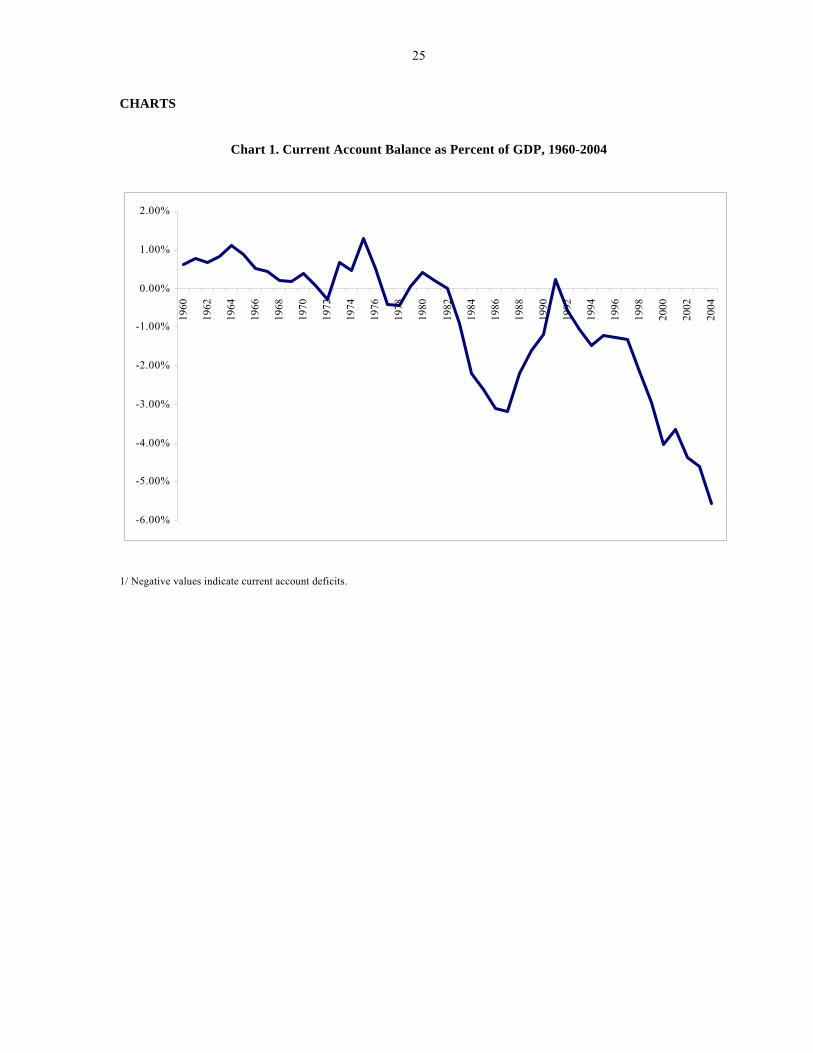
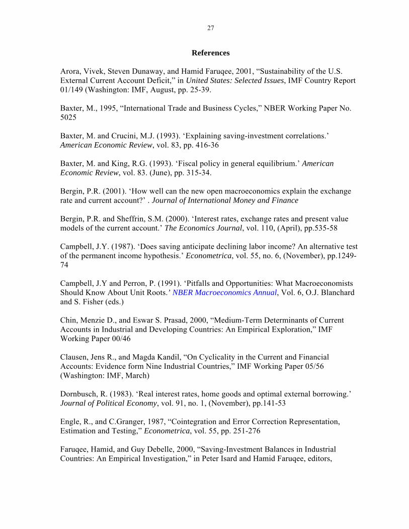
further change in the savings rate). This coincides with the view that current account worsening and improvement are usually counter-cyclical. Besides the growth effects, the average country experienced a cumulative real depreciation of about 20 percent beginning in the year before the maximum current account deficit. Data for the United States also suggest a strong cyclical influence on the current account. As Chart 1 indicates, the current account balance has often recorded surpluses during recessions, such as 1974–75, 1980, and 1991, and deficits during periods of strong economic growth (e.g., 1994–99). However, the relationship is not exact, since some boom years (e.g., 1973) have recorded surpluses, while some recession years (e.g., 1982) have recorded deficits. In this paper, however, we try to explain the dynamics of the current account in relation to the behavior in public and private imbalances and its underlying components. We show that:

o Changes in the budget deficit are important in explaining the dynamics of the current account. In particular, fluctuations in the government investment drive the budget deficit and therefore, the current account.

o Private saving is an important determinant of the current account behavior. o We study what factors affect the components of the current account. In particular,

we show which components of the current account significantly respond to the cyclical changes in macroeconomic variables.

The paper is organized as follows. In Section II we formulate the model, which provides us with consistent background of the story. Section III consists of four parts. We describe data and look at contemporaneous correlations of the variables. The empirical counterpart of the model, estimation methodology and the results are also reported in this section. Section IV concludes and summarizes the findings.

II. Modeling Cyclicality in the U. S. Current Account Both economic theory and the work of other researchers suggest that the current account of the U.S. balance of payments should be sensitive to domestic economic conditions. As noted earlier, Freund (2000) has commented that the current account balances of most industrial countries have responded to changes in real GDP growth rates, with deficits typically widening during the expansionary part of a business cycle and contracting or becoming surpluses as real GDP growth declines. Baxter (1995) and Prasad (1999) provide a thorough discussion of the theory that links current accounts to the business cycle. The literature, studying current account fluctuations, often employs intertemporal models of the current account. Starting with Sheffrin and Woo (1990) and Otto (1992), researchers emphasize that the optimal saving behavior of households is a promising and theoretically consistent way of explaining the fluctuations. Recently, these models have been modified in different directions.

4

Earlier models work with the assumptions of a small open economy, though they were implemented for various countries. These models had a limited role for government savings in determining the current account balance. Hence, it is no surprise that the empirical estimation of these models yielded mixed results. For example, Sheffrin and Woo (1990) analyzed data for Canada, the U.K., Denmark and Belgium. They find that the performance of the model varies depending on the country under consideration. Otto (1992), in contrast, implements the model for the US and finds a fairly close match to the data. In this paper, we want to focus on the role of government interventions in the household’s optimal decision making. In particular, in the framework of an optimal intertemporal decision-making, households solve an optimal saving problem to smooth their consumption in the presence of government interventions. We know from the basic national accounting principles that the CA can be decomposed into private and government net savings (the saving-investment balance).

(1) igtctyisisCA GGPP −−+−−=−+−= )()()()( where, CA current account balance,

ctys P −−= , private savings, where y national income income taxes private consumption private investment

public savings, where

tc

PigtsG −=

g government consumption public investment

total investment Public saving/investment balance, i.e., the government budget balance Private saving/investment balance

GiGP iii +=

GG is −PP is −

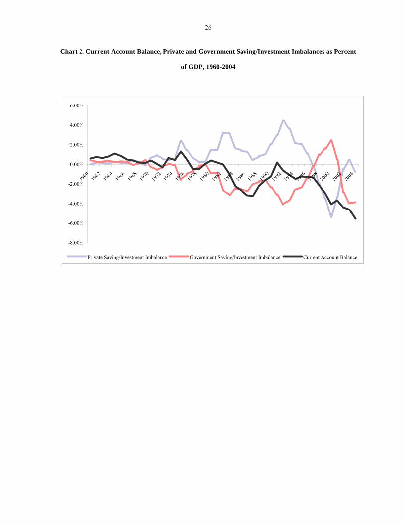
As we will see, both private and public saving/investment balances (the resource gap) play equally important roles in determining fluctuations of the current account balance. To illustrate the point graphically, Chart 2 portrays fluctuations in private and public imbalances, coupled with the current account balance in the U.S. using historical data between 1960 and 2004. Starting with the great depression, the current account balance in the U.S. was mostly in balance till the beginning of the 1940s. Nonetheless, in three episodes the surplus in the public gap was matched by a deficit in private resources. The negative correlation between the private and public resource gaps is evident throughout the series (the correlation coefficient is –0.91). It is noticeable, however, that the current account deficit prevailed for most of the period under consideration, although the deficit widened to unprecedented

5

historical level more recently. The only exception is the period 1998-2001 where the government budget registered surplus for the first time in three decades, while the resource gap for the private sector registered the largest unprecedented deficit over time. Judged by the graphical illustration and the time-series correlation, it is apparent that the budget deficit significantly affects the current account as well as the optimal private saving behavior and, in turn, the resource gap of the private sector. To capture channels underlying these interactions, we formulate an intertemporal model of the current account.

The Model There are two sectors in the economy, private and public. Private Sector Households maximize their lifetime utility function subject to the budget constraint.

⎟⎠

⎞⎜⎝

⎛∑∞

=00 )(max

tt

t cuE β s.t.

Ptttt

Pt

Pt ictybrb −−−=+−− + ))1(( 1 (2)

where E the expectation operator

tc consumption utility function (.)u

β discount factor borrowing by the household, therefore is saving by the household

interest rate on borrowing

Ptb P

tb−

tr In this endowment economy, the household’s future output endowments, y, private investments, , and taxes, t, are uncertain. Therefore, the expectation operator in the lifetime utility function is with respect to shocks to these variables.

Pi

Assuming the quadratic utility function and 1)1( =+ rβ , we get the following optimality condition for consumption.

tt ccE =+ )( 1 (3) The optimality condition shows that households will find it optimal to smooth their consumption over time, which is a central feature of the optimal decision in neoclassical models such as ours. Intertemporal Budget Constraint

6

Solving the household’s budget constraint forward and imposing net borrowings in the long

run to be equal to zero, 01

1lim =⎟⎠⎞

⎜⎝⎛+∞→

Pt

t

tb

r, we get following intertemporal budget

constraint:

)(1)( Pt

t

Ptt

t

t ityEbcE ττττ

ττ

τ

ββ

β −−+−= ∑∑∞

=

∞

=

(4)

This constraint shows that, in the long run, households will consume what they produce. That is, the net present value (NPV) of all future consumption should be equal to the current savings, , plus the NPV of all future income, y, minus the NPV of payments for future taxes, t, and investment, i.

tb−

Needless to say, in the short run, households optimally borrow, lend and invest in order to smooth their consumption. Public Sector The government can run deficit at time t. In particular, the government budget constraint at time t can be described as follows.

tigbrb Gtt

Gt

Gt −+=+−+ )1(1 (5)

where

government bonds issued at time t-1 and maturing at time t interest payment for the bond

Gtb

Gtrb

The right hand side of the equation represents the budget deficit if positive (and budget surplus if negative), whereas the left hand side term implies that the government finances its budget deficit by issuing more bonds. Assuming no-Ponzi game condition, the intertemporal budget constraint of the government can be written as:

∑∑∞

=

−∞

=

− +−=t

Gt

tt

tGt igtb

τττ

τ

τ

τ βββ

)(1 (6)

As we know, this condition states that the current decrease or increase in government consumption or in investment will be offset by adjustments in future government consumption or investment, assuming that taxes will not change. The same logic applies to taxes. That is, today’s reduction in taxes will be offset by future increases in taxes, given that government consumption and investment stay the same.

7

Simply put, the government can finance their current deficit either by increasing lump sum taxes or by issuing more bonds but at the end they have to reverse it for equation (6) to hold. This Ricardian equivalence will have important implications in this model. Since households know that the Ricardian equivalence hold they also know that the current reduction in taxes or an increase in the expenditure will be offset by future counter movements in taxes or in expenditures. This implies that the consumption smoothing decision will not be affected by the timing of taxes or expenditures. More importantly, the equivalence allows the model to have a budget deficit (surplus) at time t and it can affect the optimal saving decision of the household if no future adjustments are expected. Consumption Function Substituting the optimal consumption rule, equation (3), and the Ricardian Equivalence, equation (6), into the intertemporal budget constraint, equation (4), we get the following consumption function:

(7)

where total borrowing by the household and the government from abroad.

∑∞

=

− −−−+−=t

tt

tt giyErbcτ

ττττββ )()1(

Gt

Ptt bbb +=

The intuition of the consumption function is that today’s consumption will depend on current as well as on a stream of all expected future incomes available for private consumption. Thus, the consumption function reflects the consumption smoothing incentive for households. The government’s future expenditure affects the optimal consumption and it does not matter for the household whether the government finances the expenditure through lump sum taxes or by issuing more bonds. Notice, we can also express the term inside the bracket as:

ttttt BDNOgiy −=−− where is net output devoted to the household consumption P

tttt ityNO −−=Gt

Gtt isBD −= is government budget balance, i.e. budget surplus if positive

and deficit if negative This expression will be helpful for studying the effect of the government budget deficit on the consumption decision and therefore on the current account. Current Account

8

Notice that the household budget constraint, equation (2), can also be written as: (2'). tt

Pt

Ptt

Pt

Pt ctirbybb −−−−=−− + )( 1

If we define gross income, ttt rbyGI −= , and incorporate the government budget constraint, equation (5), into equation (2') then we get:

ttttttt cgiGIbbCA −−−=−−= + )( 1 (8) This equation is identical to the current account definition, given by equation (1). It also implies the current account imbalance will be financed through borrowings by the household and/or by the government. Substituting the consumption function, equation (7), into the current account function, equation (8), we get

∑∞

+=

− −−−−=1

)()1()(t

tt

ttt BDNOEBDNOCAτ

τττβββ (9)

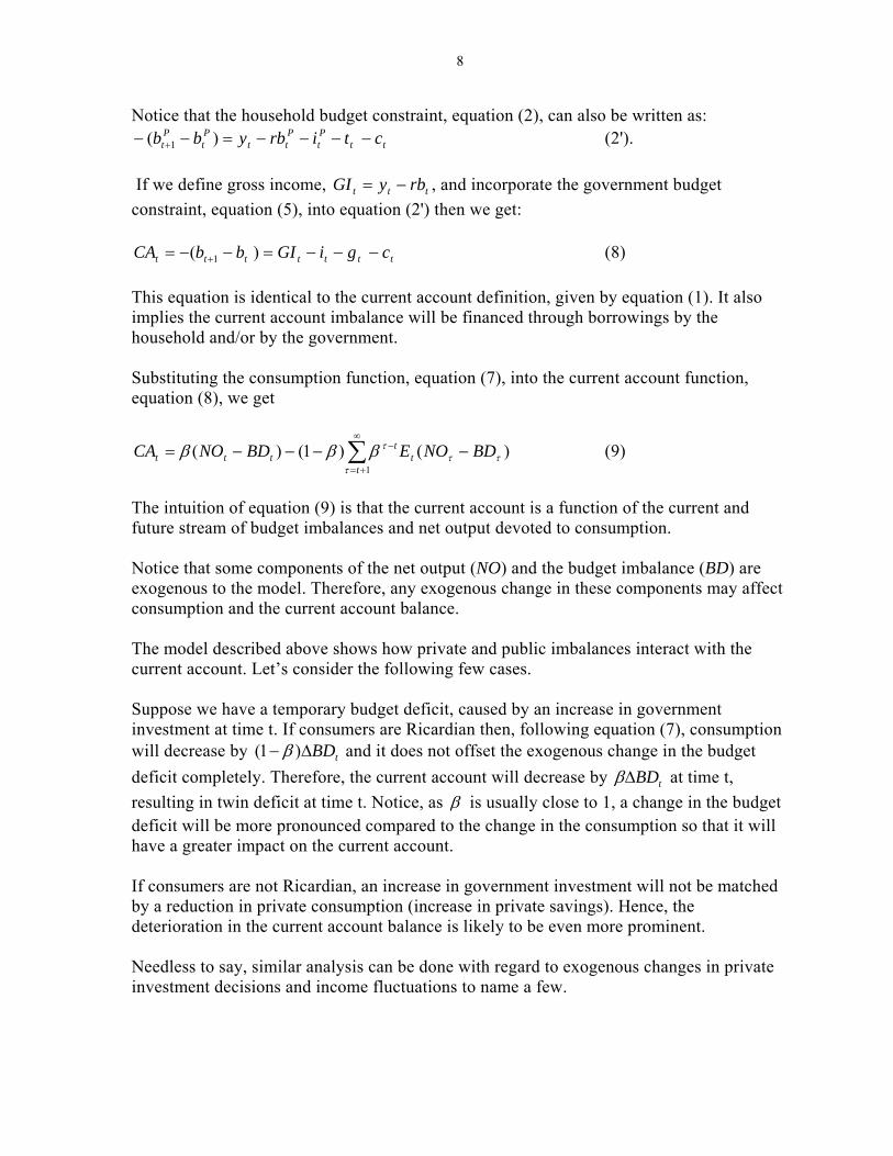
The intuition of equation (9) is that the current account is a function of the current and future stream of budget imbalances and net output devoted to consumption. Notice that some components of the net output (NO) and the budget imbalance (BD) are exogenous to the model. Therefore, any exogenous change in these components may affect consumption and the current account balance. The model described above shows how private and public imbalances interact with the current account. Let’s consider the following few cases. Suppose we have a temporary budget deficit, caused by an increase in government investment at time t. If consumers are Ricardian then, following equation (7), consumption will decrease by tBDΔ− )1( β and it does not offset the exogenous change in the budget deficit completely. Therefore, the current account will decrease by tBDΔβ at time t, resulting in twin deficit at time t. Notice, as β is usually close to 1, a change in the budget deficit will be more pronounced compared to the change in the consumption so that it will have a greater impact on the current account. If consumers are not Ricardian, an increase in government investment will not be matched by a reduction in private consumption (increase in private savings). Hence, the deterioration in the current account balance is likely to be even more prominent. Needless to say, similar analysis can be done with regard to exogenous changes in private investment decisions and income fluctuations to name a few.

9

Based on this framework, our aim is to study determinants of the current account deficit. We will study CA fluctuations in the long-run and in the short-run and will explain fluctuations in the CA by analyzing movements in underlying components: public and private savings as well as investments and resulting imbalances. In particular, we are interested in the interaction between the government budget deficit, the private saving/investment balance, and the current account balance.

III. Data and Estimation

A. Data For the estimation purposes, we use seasonally adjusted annual data from 1960 to 2004 provided by the Bureau of Economic Analysis. We construct variable INDEX by taking geometric average of real GDP of major trading partners of US weighed by their share in the total basket.

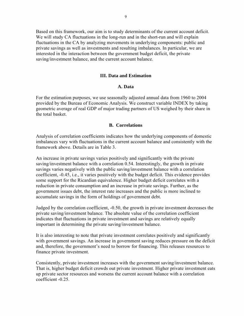
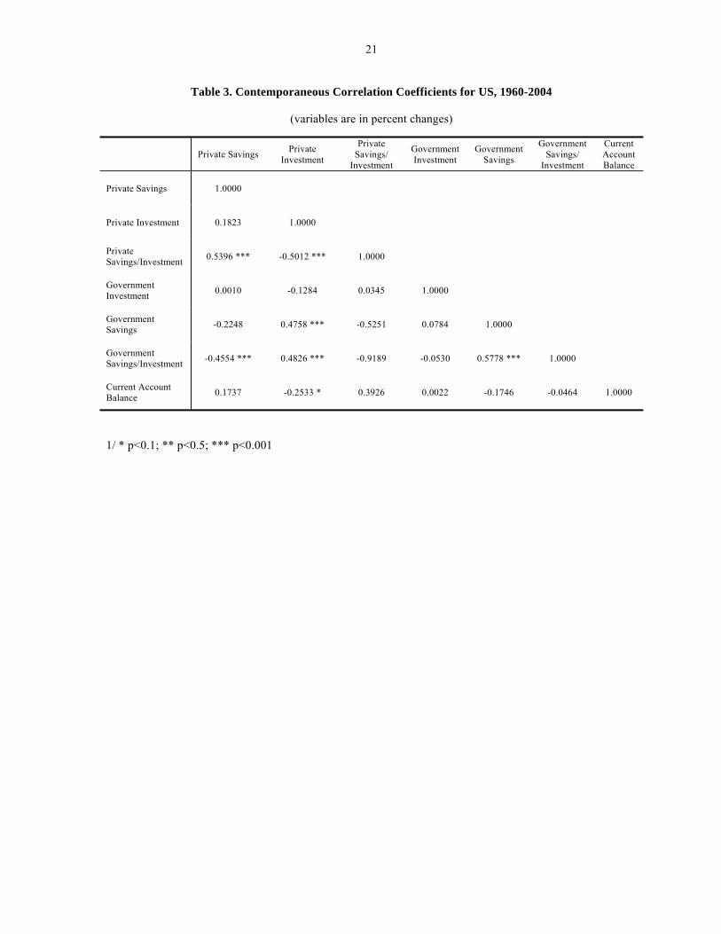
B. Correlations Analysis of correlation coefficients indicates how the underlying components of domestic imbalances vary with fluctuations in the current account balance and consistently with the framework above. Details are in Table 3. An increase in private savings varies positively and significantly with the private saving/investment balance with a correlation 0.54. Interestingly, the growth in private savings varies negatively with the public saving/investment balance with a correlation coefficient, -0.45, i.e., it varies positively with the budget deficit. This evidence provides some support for the Ricardian equivalence. Higher budget deficit correlates with a reduction in private consumption and an increase in private savings. Further, as the government issues debt, the interest rate increases and the public is more inclined to accumulate savings in the form of holdings of government debt. Judged by the correlation coefficient, -0.50, the growth in private investment decreases the private saving/investment balance. The absolute value of the correlation coefficient indicates that fluctuations in private investment and savings are relatively equally important in determining the private saving/investment balance. It is also interesting to note that private investment correlates positively and significantly with government savings. An increase in government saving reduces pressure on the deficit and, therefore, the government’s need to borrow for financing. This releases resources to finance private investment. Consistently, private investment increases with the government saving/investment balance. That is, higher budget deficit crowds out private investment. Higher private investment eats up private sector resources and worsens the current account balance with a correlation coefficient -0.25.

10

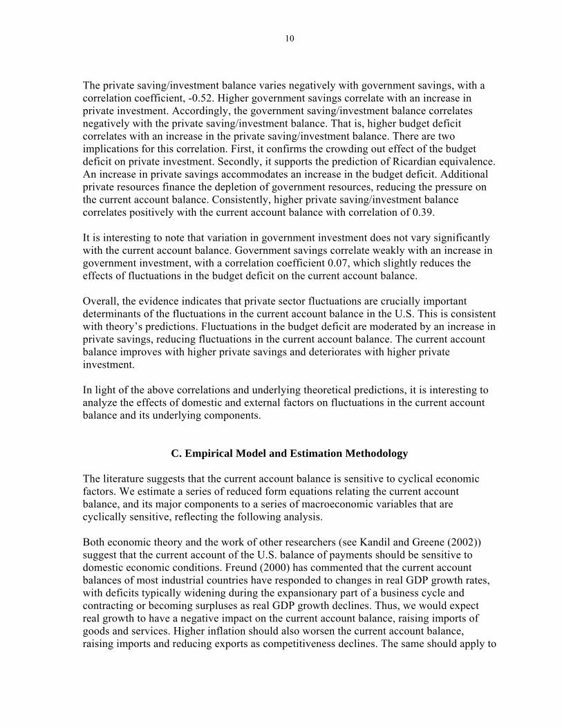
The private saving/investment balance varies negatively with government savings, with a correlation coefficient, -0.52. Higher government savings correlate with an increase in private investment. Accordingly, the government saving/investment balance correlates negatively with the private saving/investment balance. That is, higher budget deficit correlates with an increase in the private saving/investment balance. There are two implications for this correlation. First, it confirms the crowding out effect of the budget deficit on private investment. Secondly, it supports the prediction of Ricardian equivalence. An increase in private savings accommodates an increase in the budget deficit. Additional private resources finance the depletion of government resources, reducing the pressure on the current account balance. Consistently, higher private saving/investment balance correlates positively with the current account balance with correlation of 0.39. It is interesting to note that variation in government investment does not vary significantly with the current account balance. Government savings correlate weakly with an increase in government investment, with a correlation coefficient 0.07, which slightly reduces the effects of fluctuations in the budget deficit on the current account balance. Overall, the evidence indicates that private sector fluctuations are crucially important determinants of the fluctuations in the current account balance in the U.S. This is consistent with theory’s predictions. Fluctuations in the budget deficit are moderated by an increase in private savings, reducing fluctuations in the current account balance. The current account balance improves with higher private savings and deteriorates with higher private investment. In light of the above correlations and underlying theoretical predictions, it is interesting to analyze the effects of domestic and external factors on fluctuations in the current account balance and its underlying components.

C. Empirical Model and Estimation Methodology The literature suggests that the current account balance is sensitive to cyclical economic factors. We estimate a series of reduced form equations relating the current account balance, and its major components to a series of macroeconomic variables that are cyclically sensitive, reflecting the following analysis. Both economic theory and the work of other researchers (see Kandil and Greene (2002)) suggest that the current account of the U.S. balance of payments should be sensitive to domestic economic conditions. Freund (2000) has commented that the current account balances of most industrial countries have responded to changes in real GDP growth rates, with deficits typically widening during the expansionary part of a business cycle and contracting or becoming surpluses as real GDP growth declines. Thus, we would expect real growth to have a negative impact on the current account balance, raising imports of goods and services. Higher inflation should also worsen the current account balance, raising imports and reducing exports as competitiveness declines. The same should apply to

11

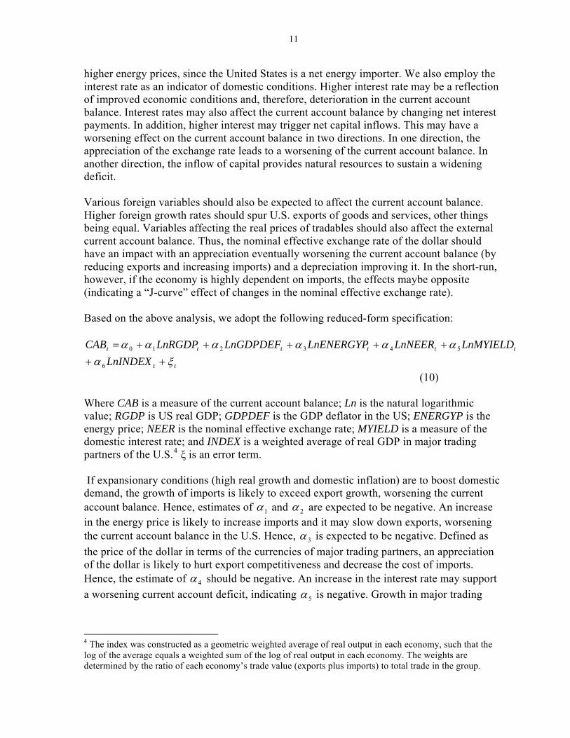
higher energy prices, since the United States is a net energy importer. We also employ the interest rate as an indicator of domestic conditions. Higher interest rate may be a reflection of improved economic conditions and, therefore, deterioration in the current account balance. Interest rates may also affect the current account balance by changing net interest payments. In addition, higher interest may trigger net capital inflows. This may have a worsening effect on the current account balance in two directions. In one direction, the appreciation of the exchange rate leads to a worsening of the current account balance. In another direction, the inflow of capital provides natural resources to sustain a widening deficit. Various foreign variables should also be expected to affect the current account balance. Higher foreign growth rates should spur U.S. exports of goods and services, other things being equal. Variables affecting the real prices of tradables should also affect the external current account balance. Thus, the nominal effective exchange rate of the dollar should have an impact with an appreciation eventually worsening the current account balance (by reducing exports and increasing imports) and a depreciation improving it. In the short-run, however, if the economy is highly dependent on imports, the effects maybe opposite (indicating a “J-curve” effect of changes in the nominal effective exchange rate). Based on the above analysis, we adopt the following reduced-form specification:

tt

tttttt

LnINDEXLnMYIELDLnNEERLnENERGYPLnGDPDEFLnRGDPCAB

ξααααααα

+++++++=

6

543210

(10) Where CAB is a measure of the current account balance; Ln is the natural logarithmic value; RGDP is US real GDP; GDPDEF is the GDP deflator in the US; ENERGYP is the energy price; NEER is the nominal effective exchange rate; MYIELD is a measure of the domestic interest rate; and INDEX is a weighted average of real GDP in major trading partners of the U.S.4 ξ is an error term. If expansionary conditions (high real growth and domestic inflation) are to boost domestic demand, the growth of imports is likely to exceed export growth, worsening the current account balance. Hence, estimates of 1α and 2α are expected to be negative. An increase in the energy price is likely to increase imports and it may slow down exports, worsening the current account balance in the U.S. Hence, 3α is expected to be negative. Defined as the price of the dollar in terms of the currencies of major trading partners, an appreciation of the dollar is likely to hurt export competitiveness and decrease the cost of imports. Hence, the estimate of 4α should be negative. An increase in the interest rate may support a worsening current account deficit, indicating 5α is negative. Growth in major trading

4 The index was constructed as a geometric weighted average of real output in each economy, such that the log of the average equals a weighted sum of the log of real output in each economy. The weights are determined by the ratio of each economy’s trade value (exports plus imports) to total trade in the group.

12

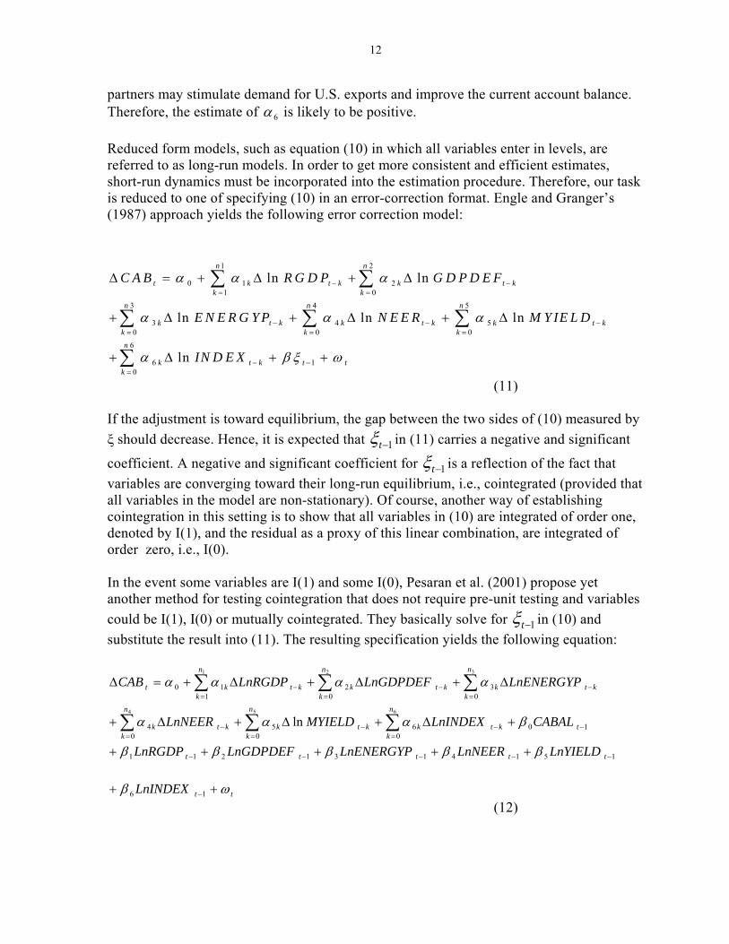
partners may stimulate demand for U.S. exports and improve the current account balance. Therefore, the estimate of 6α is likely to be positive. Reduced form models, such as equation (10) in which all variables enter in levels, are referred to as long-run models. In order to get more consistent and efficient estimates, short-run dynamics must be incorporated into the estimation procedure. Therefore, our task is reduced to one of specifying (10) in an error-correction format. Engle and Granger’s (1987) approach yields the following error correction model:

1 2

0 1 21 0

3 4 5

3 4 50 0 0

6

0

ln

lnn

k

C A B

=

Δ =

+ Δ

+ Δ∑ 6 1

ln ln

ln ln

n n

t k t k k t kk k

n n n

k t k k t k k t kk k k

k t k t t

R G D P G D P D E F

E N E R G Y P N E E R M Y IE L D

IN D E X

α α α

α α α

α β ξ ω

− −= =

− − −= = =

− −

+ Δ + Δ

+ Δ + Δ

+ +

∑ ∑

∑ ∑ ∑

(11) If the adjustment is toward equilibrium, the gap between the two sides of (10) measured by ξ should decrease. Hence, it is expected that 1tξ − in (11) carries a negative and significant

coefficient. A negative and significant coefficient for 1tξ − is a reflection of the fact that variables are converging toward their long-run equilibrium, i.e., cointegrated (provided that all variables in the model are non-stationary). Of course, another way of establishing cointegration in this setting is to show that all variables in (10) are integrated of order one, denoted by I(1), and the residual as a proxy of this linear combination, are integrated of order zero, i.e., I(0). In the event some variables are I(1) and some I(0), Pesaran et al. (2001) propose yet another method for testing cointegration that does not require pre-unit testing and variables could be I(1), I(0) or mutually cointegrated. They basically solve for 1tξ − in (10) and substitute the result into (11). The resulting specification yields the following equation:

tt

ttttt

t

n

kktk

n

kktkkt

n

kk

n

kktk

n

kktkkt

n

kkt

LnINDEX

LnYIELDLnNEERLnENERGYPLnGDPDEFLnRGDP

CABALLnINDEXMYIELDLnNEER

LnENERGYPLnGDPDEFLnRGDPCAB

ωβ

βββββ

βααα

αααα

++

+++++

+Δ+Δ+Δ+

Δ+Δ+Δ+=Δ

−

−−−−−

−=

−=

−−=

=−

=−−

=

∑∑∑

∑∑∑

16

1514131211

10

060

50

4

03

02

110

654

321

ln

(12)

13

Equation (12) is somewhat different than a standard VAR model in that it includes a linear combination of the lagged variables themselves, rather than the lagged error correction term from (10). Pesaran et al. (2001) propose applying the familiar F test for the joint significance of the lagged level variables. The test implies if the lagged level variables are jointly significant then there is a single level relationship between the dependent variable (i.e., they adjust jointly towards full-equilibrium). Note that the F test that Pesaran et al. (2001) propose has new critical values that they tabulate using Monte Carlo experiment. By assuming all variables to be I(1), they provide an upper bound critical value and by assuming all variables are I(0), a lower bound critical value is also provided. For cointegration, the calculated F-statistic should be greater than the upper bound critical value. Once cointegration is established, the long-run effects of independent variables on the dependent variable are inferred by the size and significance of 61 ββ − . Alternatively, we can normalize these estimates by 0β to get a larger estimate for the explanatory variables. The short-run effects are inferred by the size and significance of .61 kk αα −

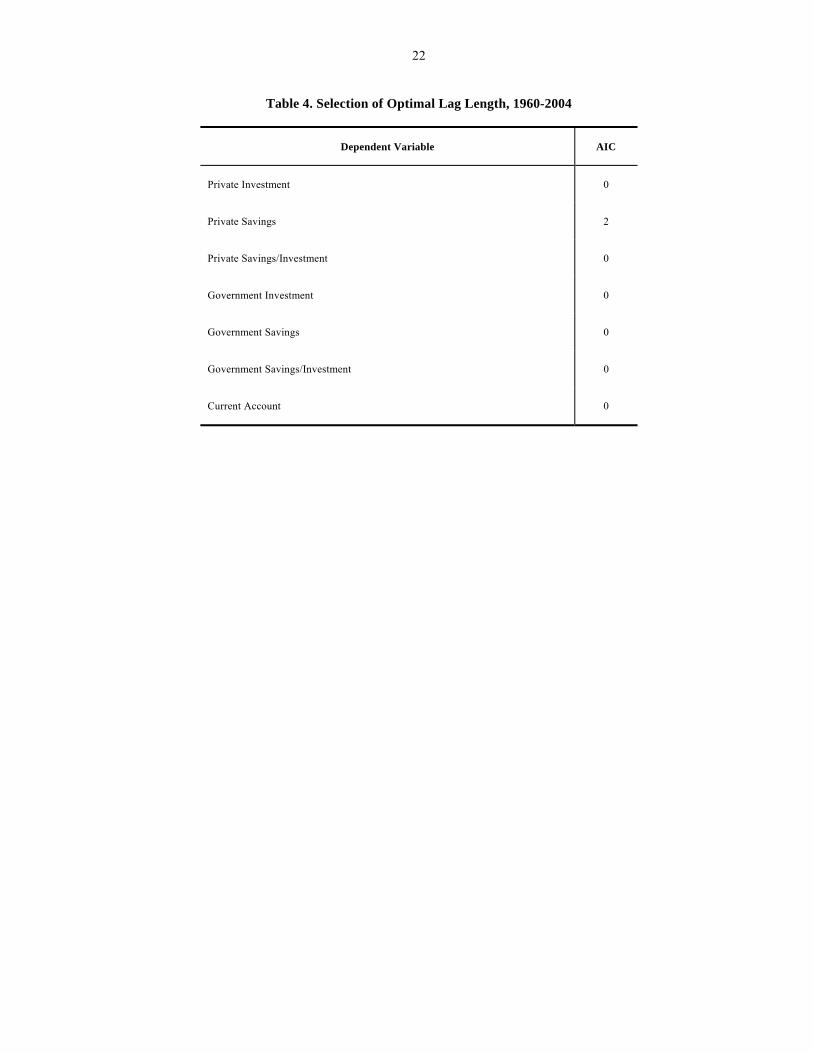
D. Results Although we do not need to do pre-unit root testing on the variables, we nevertheless did it to see if these variables are at most I(1). Having done this, we proceed to determine the optimal lag length of the regression proposed above. Employing the Akaike Information Criterion (AIC), we determine the lag length of the original model. The results of this optimum specification are reported in Table 4. The next step is the estimation of the model where we determine whether there is a long-run relationship between the variables and which factors affect the dependent variables in the long-run as well as in the short-run. To see the significance of the long-run relationship, we calculate the F-statistic for the lagged level variables and compare it against the critical values devised by Pesaran et al. The error correction model outlined by equation (11) and its different variants are also subject to empirical analysis in this section. Annual data over the 1960-2004 period are used to carry out the empirical analysis. On the domestic side, a surplus (deficit) of the current account balance would indicate that output supply exceeds (falls short of) domestic absorption. The corollary to this internal imbalance is the resource gap where a surplus (deficit) of the current account would indicate excess (shortfall) in national savings relative to domestic investment, resulting in excess (shortfall) of resources. Government savings are determined by revenues minus current expenditures (government consumption), where the government saving-investment imbalance is identical to the

14

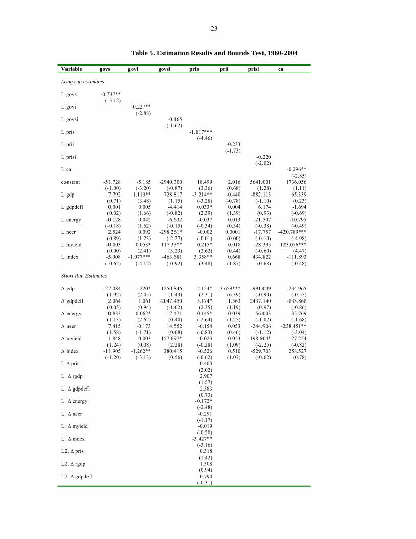
budget balance (surplus or deficit). Similarly, private savings are determined by private income minus private consumption. To understand how internal imbalances determine the current account balance, we estimate equation (12) replacing the dependent variable (the current account balance) with the following underlying components of domestic imbalances: government savings government investment ( the government resource gap ( private savings

( ) private investment , and the private resource gap ( .

),( GS),GI )GG IS −

,PS )( PI )PP IS − The first step in applying the bounds testing approach is to test for the existence of a single level relationship (cointegration) between each dependent variable and the right hand-side variables. Judging by the joint significance of lagged level variables, if the F-statistic exceeds the upper bound critical value for government investment, the private saving-investment balance, and the current account balance, then we conclude that it provides an evidence of cointegration. Also, judging by statistical significance of the error correction term, joint cointegration is established for each of government savings, private savings, private investment, the private saving/investment balance and the current account balance, with the right hand-side variables. Hence, the results are robust in support of cointegration between each of the private and public saving/investment balance and the current account balance on one hand, and the right hand-side variables (real GDP, the price level, the energy price, the nominal exchange rate, the interest rate, and the index of output in major trading partners) on the other hand. We report estimation results of equation (12) in Table 5. Determinants of fluctuations in the short and in the long-run suggest the following. Government Saving Government saving (revenues minus current expenditure) does not vary significantly with macroeconomic variables in the short or in the long-run. Fluctuations in revenues are matched by fluctuations in current expenditure, rendering the effects of economic variables neutral on government savings in the short and in the long-run. Government Investment In contrast, fluctuations in government investment vary significantly with a number of economic variables in the long and in the short-run. Higher domestic growth has a positive long-lasting significant effect on government investment. Contrary to expectations, higher interest rate has a long-lasting positive effect on government investment. Higher interest rate is necessary to finance the increased budget deficit implied by higher government investment. There is also a negative significant effect of the growth in trading partners on government investment in the U.S. This negative relation may be an indication of the stabilizing effect of public investment. Public investment increases when growth in trading partners and, in turn, exports is low, warranting a larger role of domestic spending to stimulate the economy.

15

The short-run estimates also indicate the cyclicality of government investment with respect to a number of factors. Real GDP growth increases the growth in government investment, indicating larger return on investment during periods of economic expansion. Higher energy price also correlates with an increase in government spending on investment. Two factors may be underlying this positive relationship. Higher energy price may increase the cost of government investment. Also, higher energy price may slow down economic activity, necessitating an increase in government investment to stimulate the economy. Consistent with the long-run evidence, the growth in major trading partners has a negative effect on government investment. The Budget Deficit The above evidence indicates larger fluctuations in government investment compared to savings. Accordingly, fluctuations in the budget deficit (the government saving/investment gap) are likely to be largely driven by fluctuations in public investment. In the long run, appreciation of the nominal effective exchange rate has a negative effect on the saving/investment gap, i.e., it increases the budget deficit. Higher exchange rate stimulates spending by the government, particularly on imported goods, which are important for investment. Similarly, higher interest rate stimulates government spending on investment and increases the budget deficit. In the short-run, fluctuations in the interest rate seem the most important to cyclical fluctuations in the budget deficit. Hence, a higher interest rate is an important factor in financing a widening budget deficit. Private Savings In contrast to government savings, private savings vary significantly with macro variables in the long and in the short-run. In the long-run, real GDP has a negative effect on private savings. Given the large marginal propensity to consume, high real GDP stimulates consumers’ confidence and decreases private savings. High prices (GDP deflator) decreases consumption and increases private savings, which is significant in the long-run. An increase in the interest rate stimulates private savings, which is significant in the long-run. An increase in output in major trading partners has a positive effect on private savings in the U.S. through the positive spill over effect. Private savings in the U.S. are also highly cyclical. An increase in real GDP growth increases income and private savings. An increase in price inflation discourages consumption and increases private savings. An increase in the energy price increases the cost of fuel consumption, forcing a reduction in private savings. The distributed lags are significant for some variables. For example, an increase in the energy price has a lagged significant negative effect on private savings. An increase in output in major trading partners has, however, a negative lagged effect on private savings, indicating that the positive spill over effect on private savings is of short duration.

16

Private Investment Fluctuations in private investment appear less evident compared to private savings. In contrast to public investment, private investment does not vary significantly with many factors. The only driving engine for investment growth is real GDP growth, as private investment picks up during expansions and deteriorates during contractions. Private Saving/Investment Balance Fluctuations in private savings and investment cancel out for the most part. The only significant coefficient is for the lagged interest rate which has a negative significant effect on the private saving/investment balance. An increase in the interest rate may be correlated with a boom that increases investment relative to savings. The Current Account Overall, fluctuations in the current account balance appear to be closely related to movements in the budget deficit. Higher exchange rate (appreciation) increases the budget deficit and worsens the current account balance in the long-run. Appreciation slows down exports and increases imports. Concurrently, government spending (consumption) on imported goods increases, increasing the deficit. If the economy slows down with currency appreciation, government revenues decrease and government spending increases. An increase in the interest rate improves the current account balance significantly in the long-run. In the long-run, higher interest rate increases the cost of borrowing, decreasing government spending and exerting pressure on the budget deficit. As the latter decreases, higher interest rate improves the current account balance in the long-run. Overall, the empirical analysis reveals that fluctuations in the government budget deficit are driven by government investment, as opposed to government savings. In contrast, fluctuations in the private saving/investment balance are driven by fluctuations in private savings. Nonetheless, fluctuations in the current account balance appear to be mostly driven by fluctuations in the budget deficit.

IV. Conclusion The goal of this paper has been to assess the cyclical sensitivity of the U.S. current account balance and explain fluctuations in the current account by movements in underlying domestic imbalances. The current account balance is the mirror image of the resource gap in the economy, which determines adequacy of output supply (income) to accommodate aggregate demand (spending). A deficit in the current account balance indicates shortage of the output supply relative to aggregate demand, necessitating reliance on resources in the rest of the world to fill in supply shortage and finance excess spending. Hence, the current account balance is a measure of the resource gap in a given economy. Underlying this resource gap is the saving/investment balance. A deficit in the current account balance indicates inadequate savings to finance investment spending, necessitating reliance on external sources of financing. Underlying the saving/investment balance is the resource gap

17

for the private and public sectors. For each sector, savings fluctuate with changes in consumption relative to income. The adequacy of savings relative to investment determines the resource gap for each sector. To explain cyclical fluctuations in the current account balance, we assess the cyclical sensitivity of key components underlying domestic imbalances using annual data for the United States over 1960-2004. Determinants of fluctuations in the current account balance include real GDP, the price level, the nominal exchange rate, the energy price, and a weighted index of output in various trading partners. Theory and past research suggest that the current account balance responds to domestic and external factors. We attempt to shed light on these relations and pinpoint to the underlying movements in domestic imbalances that explain how domestic conditions shape these relations over time. To understand how domestic imbalances determine the current account balance, we develop an inter-temporal model that explains developments in the budget deficit and accompanying effects on the private resource gap and the current account balance. Subsequently, we measure and evaluate correlation coefficients between the change in the current account balance and underlying components. To explain determinants of the short and long-run movements in the current account balance and underlying components, we employ a new test for cointegration. We test the existence of a single level relationship, without invoking any prior test, i.e., assuming the series are stationary, non-stationary or mutually co-integrated. Our Neoclassical intertemporal model reveals the interaction between private and public imbalances. Suppose that an exogenous increase in government investment or spending results in an increase in the budget deficit. If agents are Ricardian, higher deficit maybe partially offset by a reduction in consumption, and the current account balance fluctuates less. However, if the reduction in consumption does not offset the increase in the budget deficit at all then the current account balance will deteriorate, resulting in twin deficits. If consumers are not Ricardian, the increase in government spending will not be matched by a reduction in private consumption (increase in private savings). Hence, the deterioration in the current account balance is likely to be more pronounced. We also analyzed contemporaneous correlation coefficients that indicate how the components underlying domestic imbalances vary with fluctuations in the current account balance consistent with our theoretical results. The evidence provides support for the Ricardian equivalance. Higher budget deficit correlates with a reduction in private consumption and an increase in private savings. The increase in private savings improves the current account balance. Higher budget deficit correlates with an increase in the private saving/investment balance. There are two implications for this correlation. First, it confirms the crowding out effect of the budget deficit on private investment. Secondly, it supports the prediction of Ricardian equivalence. An increase in private savings accommodates an increase in the budget deficit. Additional private resources finance the depletion of government resources, reducing pressure on the current account balance.

18

Determinants of fluctuations in the short and in the long-run suggest the following. Government saving (revenues minus current expenditure) does not vary significantly with macroeconomic variables in the short or in the long-run. In contrast, fluctuations in government investment vary significantly with a number of economic variables in the long and in the short-run. The evidence indicates larger fluctuations in government investment compared to savings. Accordingly, fluctuations in the budget deficit (the government saving/investment gap) are likely to be driven by fluctuations in public investment. In contrast to government savings, private savings vary significantly with macro variables in the long and in the short-run. Fluctuations in private investment appear less evident compared to private savings. Overall, fluctuations in the current account balance appear to be more tied to movements in the budget deficit. Higher exchange rate (appreciation) increases the budget deficit and worsens the current account balance in the long-run. The analysis reveals that fluctuations in the government budget deficit are driven by government investment, as opposed to government savings. In contrast, fluctuations in the private saving/investment balance are driven by fluctuations in private savings. Nonetheless, fluctuations in the current account balance appear to be mostly driven by fluctuations in the budget deficit. An increase in private savings and a reduction in private investment accompany fluctuations in the budget deficit, moderating fluctuations in the current account balance.

19

TABLES

Table 1. Current Account Balance, 1980-2004

(in percent of GDP)

Year Current Account Balance

1980 0.41 1981 0.20 1982 -0.01 1983 -0.90 1984 -2.21 1985 -2.63 1986 -3.12 1987 -3.18 1988 -2.20 1989 -1.61

1990 -1.21 1991 0.23 1992 -0.58 1993 -1.06 1994 -1.49 1995 -1.23 1996 -1.28 1997 -1.33 1998 -2.14 1999 -2.96

2000 -4.04 2001 -3.66 2002 -4.38 2003 -4.60 2004 -5.55

Sources: Haver Analytics

20

Table2. Current Account Balance Of Selected Countries, 1980-2004

(in percent of GDP)

YEAR Canada China France Germany Japan Korea Mexico United Kingdom

1980 -2.26% -0.61% -1.93% -1.00% -8.54% -5.35% 6.92%

1981 -4.16% -0.80% -0.78% 0.40% -6.62% -6.49% 11.32%

1982 0.59% 1.96% -2.11% 0.84% 0.62% -3.43% -3.40% 5.04%

1983 -0.76% 1.38% -0.93% 0.67% 1.73% -1.85% 3.94% 2.65%

1984 -0.39% 0.66% -0.17% 1.50% 2.73% -1.43% 2.39% 0.76%

1985 -1.61% -3.81% -0.01% 2.90% 3.74% -0.85% 0.44% 1.21%

1986 -3.02% -2.40% 0.32% 4.37% 4.24% 4.38% -1.07% -0.51%

1987 -3.19% 0.09% -0.48% 4.00% 3.43% 7.44% 3.03% -4.92%

1988 -2.97% -0.96% -0.46% 4.54% 2.66% 8.03% -1.30% -13.44%

1989 -3.92% -0.99% -0.46% 4.84% 2.13% 2.42% -2.61% -13.75%

1990 -3.39% 3.13% -0.80% 3.10% 1.45% -0.80% -2.84% -12.43%

1991 -3.74% 3.32% -0.53% -1.34% 1.96% -2.85% -4.73% -5.74%

1992 -3.65% 1.36% 0.28% -1.10% 2.97% -1.30% -6.72% -6.77%

1993 -3.87% -1.94% 0.70% -0.94% 3.02% 0.23% -5.80% -4.21%

1994 -2.31% 1.28% 0.54% -1.44% 2.72% -0.95% -7.05% -2.30%

1995 -0.73% 0.23% 0.69% -1.18% 2.10% -1.68% -0.55% -3.14%

1996 0.55% 0.88% 1.31% -0.58% 1.40% -4.16% -0.76% -2.31%

1997 -1.29% 4.09% 2.65% -0.44% 2.25% -1.62% -1.92% -0.60%

1998 -1.27% 3.30% 2.56% -0.69% 3.02% 11.69% -3.80% -1.28%

1999 0.27% 2.11% 0.43% -0.61% 2.57% 5.51% -2.90% -7.02%

2000 2.71% 1.90% 0.21% -0.80% 2.52% 2.39% -3.21% -5.83%

2001 2.28% 1.46% 0.33% 0.08% 2.11% 1.67% -2.84% -4.60%

2002 1.83% 2.72% 0.12% 1.16% 2.83% 0.99% -2.08% -3.52%

2003 1.54% 3.12% 0.10% 1.08% 3.17% 1.96% -1.35% -3.87%

2004 2.22% 3.99% -0.06% 1.93% 3.68% 4.06% -1.08% -6.65%

Sources: International Financial Statistics

21

Table 3. Contemporaneous Correlation Coefficients for US, 1960-2004

(variables are in percent changes)

Private Savings Private Investment

Private Savings/

Investment

Government Investment

Government Savings

Government Savings/

Investment

Current Account Balance

Private Savings 1.0000

Private Investment 0.1823 1.0000

Private Savings/Investment 0.5396 *** -0.5012 *** 1.0000

Government Investment 0.0010 -0.1284 0.0345 1.0000

Government Savings -0.2248 0.4758 *** -0.5251 0.0784 1.0000

Government Savings/Investment -0.4554 *** 0.4826 *** -0.9189 -0.0530 0.5778 *** 1.0000

Current Account Balance 0.1737 -0.2533 * 0.3926 0.0022 -0.1746 -0.0464 1.0000

1/ * p<0.1; ** p<0.5; *** p<0.001

22

Table 4. Selection of Optimal Lag Length, 1960-2004

Dependent Variable AIC

Private Investment 0

Private Savings 2

Private Savings/Investment 0

Government Investment 0

Government Savings 0

Government Savings/Investment 0

Current Account 0

23

Table 5. Estimation Results and Bounds Test, 1960-2004

Variable govs govi govsi pris prii prisi ca Long run estimates L.govs -0.737** (-3.12) L.govi -0.227** (-2.88) L.govsi -0.165 (-1.62) L.pris -1.117*** (-4.46) L.prii -0.233 (-1.73) L.prisi -0.220 (-2.02) L.ca -0.296** (-2.85) constant -51.728 -5.185 -2940.300 18.499 2.016 5641.001 1736.056 (-1.00) (-3.20) (-0.87) (3.36) (0.68) (1.28) (1.11) L.gdp 7.792 1.119** 728.817 -3.214** -0.440 -882.113 65.339 (0.71) (3.48) (1.15) (-3.28) (-0.78) (-1.10) (0.23) L.gdpdefl 0.001 0.005 -4.414 0.033* 0.004 6.174 -1.694 (0.02) (1.66) (-0.82) (2.39) (1.39) (0.93) (-0.69) L.energy -0.128 0.042 -6.632 -0.037 0.013 -21.507 -10.795 (-0.18) (1.62) (-0.15) (-0.34) (0.34) (-0.38) (-0.49) L.neer 2.524 0.092 -298.261* -0.002 0.0001 -17.757 -420.789*** (0.89) (1.23) (-2.27) (-0.01) (0.00) (-0.10) (-4.98) L.myield -0.003 0.053* 117.33** 0.215* 0.018 -28.395 123.076*** (0.00) (2.41) (3.23) (2.62) (0.44) (-0.60) (4.47) L.index -5.908 -1.077*** -463.681 3.358** 0.668 434.822 -111.893 (-0.62) (-4.12) (-0.92) (3.48) (1.87) (0.68) (-0.48) Short Run Estimates Δ gdp 27.084 1.220* 1250.846 2.124* 3.659*** -991.049 -234.965 (1.92) (2.45) (1.43) (2.31) (6.39) (-0.90) (-0.55) Δ gdpdefl 2.064 1.061 -2047.450 5.174* 1.563 2437.140 -833.868 (0.05) (0.94) (-1.02) (2.35) (1.19) (0.97) (-0.86) Δ energy 0.833 0.062* 17.471 -0.145* 0.039 -56.003 -35.769 (1.13) (2.62) (0.40) (-2.64) (1.25) (-1.02) (-1.68) Δ neer 7.415 -0.173 14.552 -0.154 0.053 -244.906 -238.451** (1.58) (-1.71) (0.08) (-0.83) (0.46) (-1.12) (-3.04) Δ myield 1.848 0.003 157.697* -0.023 0.053 -198.604* -27.254 (1.24) (0.08) (2.28) (-0.28) (1.09) (-2.25) (-0.82) Δ index -11.905 -1.262** 380.415 -0.526 0.510 -529.703 258.527 (-1.20) (-3.13) (0.56) (-0.62) (1.07) (-0.62) (0.78) L.Δ pris 0.403 (2.02) L. Δ rgdp 2.907 (1.57) L. Δ gdpdefl 2.383 (0.73) L. Δ energy -0.172* (-2.48) L. Δ neer -0.291 (-1.17) L. Δ myield -0.019 (-0.20) L. Δ index -3.427** (-3.16) L2. Δ pris 0.318 (1.42) L2. Δ rgdp 1.308 (0.94) L2. Δ gdpdefl -0.794 (-0.31)

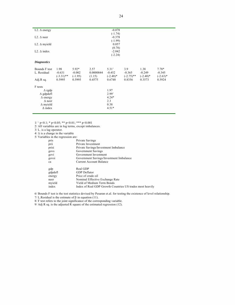
24

L2. Δ energy -0.078 (-1.74) L2. Δ neer -0.378 (-1.99) L2. Δ myield 0.057 (0.78) L2. Δ index -2.042 (-2.24) Diagnostics Bounds F test 1.98 5.92* 2.57 5.31’ 3.9 1.38 7.78* L. Residual -0.631 -0.002 0.0000844 -0.452 -0.365 -0.249 -0.345 (-3.31)** (-1.95) (1.15) (-2.48)* (-2.75)** (-2.40)* (-2.63)* Adj.R sq. 0.5995 0.5995 0.4575 0.6748 0.8356 0.3573 0.5924

F tests

Δ rgdp 1.97 Δ gdpdefl 2.99’ Δ energy 4.24* Δ neer 2.3

Δ myield 0.38 Δ index 4.51*

1/ ‘ p<0.1; * p<0.05; ** p<0.01; *** p<0.001 2/ All variables are in log terms, except imbalances. 3/ L. is a lag operator. 4/ Δ is a change in the variable 5/ Variables in the regression are:

pris Private Savings prii Private Investment prisi Private Savings/Investment Imbalance govs Government Savings govi Government Investment govsi Government Savings/Investment Imbalance ca Current Account Balance

gdp Real GDP gdpdefl GDP Deflator

energy Price of crude oil neer Nominal Effective Exchange Rate myield Yield of Medium Term Bonds index Index of Real GDP Growth Countries US trades most heavily

6/ Bounds F test is the test statistics devised by Pesaran et.al. for testing the existence of level relationship. 7/ L.Residual is the estimate of β in equation (11). 8/ F test refers to the joint significance of the corresponding variable. 9/ Adj R sq. is the adjusted R square of the estimated regression (12).

25

CHARTS

Chart 1. Current Account Balance as Percent of GDP, 1960-2004

-6.00%

-5.00%

-4.00%

-3.00%

-2.00%

-1.00%

0.00%

1.00%

2.00%

1960

1962

1964

1966

1968

1970

1972

1974

1976

1978

1980

1982

1984

1986

1988

1990

1992

1994

1996

1998

2000

2002

2004

1/ Negative values indicate current account deficits.

26

Chart 2. Current Account Balance, Private and Government Saving/Investment Imbalances as Percent

of GDP, 1960-2004

-8.00%

-6.00%

-4.00%

-2.00%

0.00%

2.00%

4.00%

6.00%

1960

1962

1964

1966

1968

1970

1972

1974

1976

1978

1980

1982

1984

1986

1988

1990

1992

1994

1996

1998

2000

2002

2004

Private Saving/Investment Imbalance Government Saving/Investment Imbalance Current Account Balance

27

References Arora, Vivek, Steven Dunaway, and Hamid Faruqee, 2001, “Sustainability of the U.S. External Current Account Deficit,” in United States: Selected Issues, IMF Country Report 01/149 (Washington: IMF, August, pp. 25-39. Baxter, M., 1995, “International Trade and Business Cycles,” NBER Working Paper No. 5025 Baxter, M. and Crucini, M.J. (1993). ‘Explaining saving-investment correlations.’ American Economic Review, vol. 83, pp. 416-36 Baxter, M. and King, R.G. (1993). ‘Fiscal policy in general equilibrium.’ American Economic Review, vol. 83. (June), pp. 315-34. Bergin, P.R. (2001). ‘How well can the new open macroeconomics explain the exchange rate and current account?’ . Journal of International Money and Finance Bergin, P.R. and Sheffrin, S.M. (2000). ‘Interest rates, exchange rates and present value models of the current account.’ The Economics Journal, vol. 110, (April), pp.535-58 Campbell, J.Y. (1987). ‘Does saving anticipate declining labor income? An alternative test of the permanent income hypothesis.’ Econometrica, vol. 55, no. 6, (November), pp.1249-74 Campbell, J.Y and Perron, P. (1991). ‘Pitfalls and Opportunities: What Macroeconomists Should Know About Unit Roots.’ NBER Macroeconomics Annual, Vol. 6, O.J. Blanchard and S. Fisher (eds.) Chin, Menzie D., and Eswar S. Prasad, 2000, “Medium-Term Determinants of Current Accounts in Industrial and Developing Countries: An Empirical Exploration,” IMF Working Paper 00/46 Clausen, Jens R., and Magda Kandil, “On Cyclicality in the Current and Financial Accounts: Evidence form Nine Industrial Countries,” IMF Working Paper 05/56 (Washington: IMF, March) Dornbusch, R. (1983). ‘Real interest rates, home goods and optimal external borrowing.’ Journal of Political Economy, vol. 91, no. 1, (November), pp.141-53 Engle, R., and C.Granger, 1987, “Cointegration and Error Correction Representation, Estimation and Testing,” Econometrica, vol. 55, pp. 251-276 Faruqee, Hamid, and Guy Debelle, 2000, “Saving-Investment Balances in Industrial Countries: An Empirical Investigation,” in Peter Isard and Hamid Faruqee, editors,

28

Exchange Rate Assessment: Extensions of the Macroeconomic Balance Approach, Occasional Paper 176 (Washington: International Monetary Fund), ch. VI, PP. 35-55. Freund, Caroline L., 2000, “Current Account Adjustment in Industrial Countries,” unpub., International Finance Discussion Paper 692, Board of Governors of the Federal Reserve System (Washington), December Gruber, J.W. (2004). ‘A Present Value Test of Habits and the Current Account.’ mimeo, Johns Hopkins University (November). Hall, R.E. (1988). ‘Intertemporal substitution in consumption.’ Journal of Political Economy, vol. 96, no. 2, (April), pp.339-57 Kandil, Magda, and Joshua Greene, 2002, “The Impact of Cyclical Factors on the U.S. balance of Payments,” IMF Working Paper 02/45 (Washington: IMF, March). Mann, Catherine, 2001, “Is the US Trade Deficit Sustainable? An Update,” presentation made at an Institute for International Economics Seminar, the St. Regis Hotel, Washington, DC, March 1. Milessi-Ferretti, Gian Maria, and Assaf Razin, 1996, “Current Account Sustainability,” Princeton, N.J.: International Finance Section, Department of Economics, Princeton University, October. Nason, J.M. and Rogers, J.H. (2003). ‘The Present Value Model of the Current Account Has Been Rejected: Round up the Usual Suspects?’ Federal Reserve Board: International Finance Discussion Paper. Obstfeld, M. and Rogoff, K. (2000). “Perspectives on OECD Economic Integration: Implications for US Current Account Adjustment,” unpub., revised paper originally presented at the Federal Reserve Bank of Kansas City symposium on “Global Economic Integration: Opportunities and Challenges,” Jackson Hole, Wyoming, August 24-26 Obstfeld, M. and Rogoff, K. (1996). Foundations of International Macroeconomics. Cambridge, MA: the MIT Press Otto, G. (1992). ‘Testing a present value model of the current account: evidence from U.S. and Canadian time series.’ Journal of International Monet and Finance, vol. 11, no. 5, (October), pp. 414-30 Pesaran, M.H., Y.Shin, and R.J.Smith, 2001, “Bounds Testing Approaches to the Analysis of Level Relationships,” Journal of Applied Econometrics, vol. 16, pp. 289-326 Prasad, Eswar S., 1999, “International Trade and the Business Cycle,” IMF Working Paper 99/56 (Washington: IMF, April)

29

Sheffrin, S.M. and Woo, W.T. (1990). ‘Present value tests of an intertemporal model of the current account.’ Journal of International Economics, vol. 29, no. 3-4, (November), pp. 237-53 Stock, J.H. (1986). "Unit roots, structural breaks and trends," Handbook of Econometrics, in: RF Engle & D. McFadden (ed.), Handbook of Econometrics, edition 1, volume 4, chapter 46, pp. 2739-2841