DETERMINANTS OF MALAYSIA HOUSING PRICE BY CHENG LI WEI CHONG PEI SHIN JOANE CHEONG PUI KEI TIANG XUE HONG WONG MUN YEE A research project submitted in partial fulfillment of the requirement for the degree of BACHELOR OF FINANCE (HONS) UNIVERSITI TUNKU ABDUL RAHMAN FACULTY OF BUSINESS AND FINANCE DEPARTMENT OF FINANCE APRIL 2016 B14

Welcome message from author
This document is posted to help you gain knowledge. Please leave a comment to let me know what you think about it! Share it to your friends and learn new things together.
Transcript
DETERMINANTS OF MALAYSIA HOUSING PRICE
BY
CHENG LI WEI
CHONG PEI SHIN
JOANE CHEONG PUI KEI
TIANG XUE HONG
WONG MUN YEE
A research project submitted in partial fulfillment of the
requirement for the degree of
BACHELOR OF FINANCE (HONS)
UNIVERSITI TUNKU ABDUL RAHMAN
FACULTY OF BUSINESS AND FINANCE
DEPARTMENT OF FINANCE
APRIL 2016
B14

Determinants of Malaysia Housing Price
ii
Copyright @ 2016
ALL RIGHTS RESERVED. No part of this paper may be reproduced, stored in a
retrieval system, or transmitted in any form or by any means, graphic, electronic,
mechanical, photocopying, recording, scanning, or otherwise, without the prior
consent of the authors.

Determinants of Malaysia Housing Price
iii
DECLARATION
We hereby declare that:
(1) This undergraduate research project is the end result of our own work and that
due acknowledgement has been given in the references to ALL sources of
information be they printed, electronic, or personal.
(2) No portion of this research project has been submitted in support of any
application for any other degree or qualification of this or any other university,
or other institutes of learning.
(3) Equal contribution has been made by each group member in completing the
research project.
(4) The word count of this research report is 18750 words.
Name of Student: Student ID: Signature:
1. CHENG LI WEI 12ABB03009 __________________
2. CHONG PEI SHIN 12ABB03640 __________________
3. JOANE CHEONG PUI KEI 12ABB03189 __________________
4. TIANG XUE HONG 12ABB03290 __________________
5. WONG MUN YEE 12ABB03289 __________________
Date: 16th April 2016

Determinants of Malaysia Housing Price
iv
ACKNOWLEDGEMENT
We would take this opportunity to express our gratitude and appreciation to all those
who gave us the possibility to complete this report. A special gratitude we give to our
final year project supervisor, Cik Nabihah Binti Aminaddin and Puan Siti Nur Amira
who was abundantly helpful and offered invaluable assistance, support and guidance,
as well as sharing his expertise and knowledge to us in order to enhance the research
report quality.
Besides, we would like to thank UTAR in providing us sufficient facility in order to
carry out the research. The database provided by the university enables us to obtain
relevant data and materials while preparing this research project.
Furthermore, we would like to thank our project coordinator, Cik Nurfadhilah bt Abu
Hasan for coordinating everything pertaining to be completion undergraduate project
and keeping us updated with the latest information.
Last but not least, we would like to thank all of the group members for giving their best
effort in completing this final year project.

Determinants of Malaysia Housing Price
v
DEDICATION
We would like to dedicate this final year project to:
Puan Siti Nur Amira Binti Othman
Our supervisor who has provided us with useful guidance, valuable supports,
constructive feedbacks and precious encouragement to us.
Team Members
All the members who have played different roles while completing this research project
and the full cooperation given at all times.
Thank You.

Determinants of Malaysia Housing Price
vi
TABLE OF CONTENTS
Page
Copyright Page …………………………………………….…………………...... ii
Declaration …….…………………………………………………………………iii
Acknowledgement ………………..…………………….……………………….. iv
Dedication ………………………..………………………….……………………v
Table of Contents ……..…………………………………….……………………vi
List of Figures and Tables …………………………..…………………………… ix
List of Abbreviations ………………………………………….………………… x
Preface ……………………………………..…………………………………… xi
Abstract ……………………………..………………………………………… xii
CHAPTER 1 INTRODUCTION ……………..……………………………. 1
1.0 Research Background...…………...……………………………………….. 1
1.1 Problem Statement ……………………………………………………………11
1.2 Objectives of the Study …………………………………...……..……………12
1.2.1 General Objectives………………………………...…………………12
1.2.2 Specific Objectives ………………………………..…………………12
1.3 Research Questions ……………………………………………...……………12
1.4 Hypotheses of the Study ………………………………………………………13
1.5 Significance of the Study ………………………………………..……………15
1.6 Chapter Layout ………………………………………….……………………16

Determinants of Malaysia Housing Price
vii
1.7 Conclusion ……………………………………………………………………17
CHAPTER 2 LITERATURE REVIEW …………………….……………………18
2.0 Introduction …………………………………………………..………………18
2.1 Review of Literature …………………….……………………………………18
2.2 Review of Relevant Theoretical Models ……………………………………..28
2.3 Conclusion …………………………………………………….……………...30
CHAPTER 3 METHODOLOGY ……………………………….………………..31
3.0 Introduction …………………………………………………………………..31
3.1 Research Design …………………………………...…………………………32
3.1.1 Data Collection Methods………………………….………………….32
3.2 Variables Specification Of Measurements……………………………………32
3.2.1 House Price Index …………………………………………………...32
3.2.2 Consumer Price Index ……………………………………………….33
3.2.3 Gross Domestic Product …………………………….……………….34
3.2.4 Lending Interest Rate ………………..………………………………34
3.2.5 Population …………………………………………………………...35
3.3 Flows of Methodology ……………………………………………………….36
3.4 Methodology …………………………………………………………………36
3.4.1 Unit Root Test ……………………………………………………….36
3.4.2 Johasen & Juselius Cointegration Test ……………….……………...39
3.4.3 Vector Error Correction Model(VECM) …………….………………41
3.4.4 Granger Causality Test …………………………….………………...42
3.4.5 Variance Decomposition …..………………………………………...44

Determinants of Malaysia Housing Price
viii
3.4.6 Impulse Response Function ……..…………………………………...45
3.5 Conclusion………….…………………………………………………………46
CHAPTER 4: DATA ANALYSIS ……………………………………….………47
4.0 Introduction…………………………………………………………………...47
4.1 Unit Root Test………………………………………………………………...47
4.2 Johasen & Juselius Cointegration Test ………………………………..………50
4.3 Vector Error Correction Model (VECM) & Granger Causality Test ………….52
4.4 Variance Decomposition ……………………….…………………………….55
4.5 Impulse Response Function …………………….…………………………….60
4.6 Discussions of Major Findings ……………………….……………………….61
4.7 Conclusion ……………………………………………………….…………...65
CHAPTER 5: CONCLUSION, IMPLICATIONS, LIMITATIONS &
RECOMMENDATIONS…………………………………………………………66
5.0 Summary of Statistical Analyses ……………………………………………..66
5.1 Implications of Study ………………………………………………………..67
5.2 Limitations of Study …………………………………………………………69
5.3 Recommendations for Future Research …………………….………………...70
5.4 Conclusion ……………………………………………………………………71
References ……………………………………………………………………… 72
Determinants of Malaysia Housing Price
ix
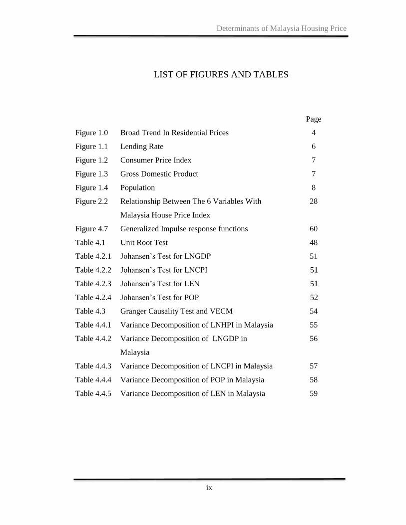
LIST OF FIGURES AND TABLES
Page
Figure 1.0 Broad Trend In Residential Prices 4
Figure 1.1 Lending Rate 6
Figure 1.2 Consumer Price Index 7
Figure 1.3 Gross Domestic Product 7
Figure 1.4 Population 8
Figure 2.2 Relationship Between The 6 Variables With
Malaysia House Price Index
28
Figure 4.7 Generalized Impulse response functions 60
Table 4.1 Unit Root Test 48
Table 4.2.1 Johansen’s Test for LNGDP 51
Table 4.2.2 Johansen’s Test for LNCPI 51
Table 4.2.3 Johansen’s Test for LEN 51
Table 4.2.4 Johansen’s Test for POP 52
Table 4.3 Granger Causality Test and VECM 54
Table 4.4.1 Variance Decomposition of LNHPI in Malaysia 55
Table 4.4.2 Variance Decomposition of LNGDP in
Malaysia
56
Table 4.4.3 Variance Decomposition of LNCPI in Malaysia 57
Table 4.4.4 Variance Decomposition of POP in Malaysia 58
Table 4.4.5 Variance Decomposition of LEN in Malaysia 59

Determinants of Malaysia Housing Price
x
LIST OF ABBREVIATIONS
ADF Augmented Dickey-Fuller Test
CPI Consumer Price Index
DV Dependent Variable
GDP Gross Domestic Product
HPI House Price Index
IV Independent Variable
LEN Lending Rate
LN natural logarithm
PP Phillips-Perron Test
POP Population
VAR Vector Autoregressive Model
VECM Vector Error Correction Model
Determinants of Malaysia Housing Price
xi
PREFACE
The global house prices have been going up tremendously since year 2000. Most of the
real estate investors invest in Asia Pacific countries, especially after the subprime
mortgage crisis in year 2008. As Malaysian residential housing market represents one
of the most important industries which significant affected the economics of Malaysia,
it is important to pay an attention on it.
The Malaysian housing price has gradually kept increasing from 1990 until 2015. It is
important to take note that the Malaysian housing price has experienced a rapid
increased since year 2008 compared to year before. Economists believed that the rapid
increased of housing price will lead to housing bubble which were consequently have
destructive effect toward the Malaysia economics. Hence, the trend of house price must
be concerned and the factors that lead to the increased of residential house price must
be determined.
This research will investigate the relationship between the fluctuation of house price
index in Malaysia with the macroeconomic determinants such as consumer price index
(CPI), lending interest rate (LEN), population (POP) and gross domestic product
(GDP). This research will provide a clearly picture and empirical results for readers,
such as policy makers, investors, homebuyers and homeowners about the connection
between these variables towards the house price index in Malaysia.
Determinants of Malaysia Housing Price
xii
ABSTRACT
This study examines the relationship between macroeconomic determinants with
residential housing price in Malaysia from period year 1998 first quarter to year 2015
fourth quarter, which consist of quarterly data of 68 observations. This study used the
Time Series Econometrics to capture the effect of macroeconomic on the Malaysian
residential housing price. Besides investigate the relationship, this study also examined
the long run, short run, causality direction, dynamic stability and shocks of the
empirical model of this study.
Determinants such as consumer price index (CPI), lending interest rate (LEN),
population (POP) and gross domestic product (GDP) are significant toward the
Malaysian residential housing price. Besides, consumer price index (CPI), population
(POP) and gross domestic product (GDP) showed positive relationships with the house
price index, whereas lending interest rate (LEN) showed a negative relationship with
the house price index.

Determinants of Malaysia Housing Price
Page 1 of 80
CHAPTER 1: RESEARCH OVERVIEW
1.0 Research Background
Recently, the demand of housing had increase as the number of people of each
country increased. Thus, there is plenty of real estate companies started launching
new houses in different areas. Although the business market and structure of
housing is almost the same with any other business, but in this housing market, it
involves a large transactions amount in consumer’s spending. The houses future
market price is nearly to be expensive and it is going to increase significantly over
the period. The reason behind that cause the housing price to increase is the inflation,
population growth, and raw material costs used in the real estate industry. The
demands and supplies of the houses in Malaysia are being influenced by the
determinants stated above and some other different factors.
In term of GDP, Malaysia’s house price is continued to increase gradually due to a
slight GDP slowdown from 7.2% in year 2010 to 5.1% in year 2011. Besides, while
excluding the period of recent surge, houses prices in Malaysia have also affected
by inflation over the past 10 years.
Housing price is just similar with other type of goods and services in a market which
are affected by the movement of demand and supply. The demand for owned a
housing is basically influenced by housing price, population, lending interest rate,
inflation rate and GDP.
Since the beginning of year 2012, Bank Negara Malaysia (BNM) has tightened the
regulations and procedure on lending. A person who wants to obtain mortgage loan
from bank will be harder because they have to pass the mortgage affordability test.
It is an assessment to evaluate their performance based on their net income,
Employees Provident Fund (EPF) contributions, statutory tax deductions and all
other debt obligations. Moreover, in February 2012, the new rules and regulations
have already impacted lending rate and lowered down the residential loan approvals.

Determinants of Malaysia Housing Price
Page 2 of 80
As refer to CB Richard Ellis (CBRE-Malaysia), the approval rate was below 50%
comparing to mid-2008 was over 62%. The outstanding mortgage loans had arrived
MYR 222.2 billion (US$69.9 billion) in year 2011 which is around 26.1% of GDP.
Based on Sutton (2002), the long term asset which gives consumption services is a
house. Its implicit value is the expected service stream’s discounted value. However
Ooi and Le (2011) claimed that, the burden housing loan is the household’s most
expensive expenditure which leads to the problem of uneasy in buying a house. At
the same time, most people think that the housing loan is the largest investment
decisions in buying a house. Moreover, Datuk Chor Cheee Heung, who is the
Housing Minister, stated that government in Malaysia will not try to intervene in
controlling the property prices as Malaysia is viewed as an economy freely country
(Cagamas,2013). Consequently, Malaysia housing price is said to be in the mode of
freely floating. In other words, the housing prices are changing according to its
determinants.
The increase in residential housing demand within Malaysia urban areas has caused
the country economic to develop rapidly in these recent years. From the Malaysia
housing prices review, the housing prices have gone through a dramatically
appreciation which depending on specific location no matter in cities or small towns.
Based on iProperty.com Malaysia, Malaysians are not frighten by the fluctuation of
the economy which disclosure by No.1 property portal in Malaysia. They remain
steady and still confident with the housing market. Property demand is correlated
to property price. Malaysia’s property price has been on the rising trend since 15
years ago.
According to Asian Development Outlook Report 2011, Asian Development Bank
depicted that Kuala Lumpur property prices are the second lowest in South East
Asia, which was slightly more expensive than in Yangon, Myanmar. In terms of
price per square feet, Kuala Lumpur property prices are lower than other capital
cities in South East Asia such as Jakarta, Bangkok, Ho Chi Min City, Manila and
even Phnom Penh. This means that Kuala Lumpur properties have a marked
difference in prices compared to Singapore where properties are at least 10. 2 times
Determinants of Malaysia Housing Price
Page 3 of 80
more expensive and have been recognized as one of the most expensive properties
in Asia. Reading the report from Valuation and Property Services Department
(JPPH) revealing that from year 2000 to year 2010, the average houses price has
rising non-stop which contributed an increase of 45% between these years.
In the past few years, the Malaysia housing market has a significant price growth.
In truth, Malaysia had encountered a rapid increase in housing prices. Based on
Malaysia Deputy Finance Minister (2011), housing prices growing up around 20%
average per year after year 2007. This is a distressing situation for lenders it had led
to a huge problem. Many people think that their annual income increase still unable
to cover the high annual increases in house prices in the general population. In
reality, most of the residents are worrying that they not able to deal with the property
which keeps rising in price.
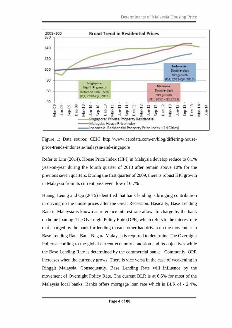
The house value is predicted to undergo considerable growth in these future years
as the economy is strong and domestic housing demand is expanding. Malaysia
house prices are being driven by its economic growth. However, the housing price
would still be affected by other macroeconomic determinants such as the Gross
Domestic Product, interest rate, costs of construction, inflation rate and population.
These determinants could contribute in helping relevant group to calm the housing
prices and manage the condition before the situation becoming worse. The
economic distortion condition could be reflected by current housing environment
situation.
Determinants of Malaysia Housing Price
Page 4 of 80
Figure 1: Data source: CEIC http://www.ceicdata.com/en/blog/differing-house-
price-trends-indonesia-malaysia-and-singapore
Refer to Lim (2014), House Price Index (HPI) in Malaysia develop reduce to 8.1%
year-on-year during the fourth quarter of 2013 after remain above 10% for the
previous seven quarters. During the first quarter of 2009, there is robust HPI growth
in Malaysia from its current pass event low of 0.7%
Huang, Leung and Qu (2015) identified that bank lending is bringing contribution
in driving up the house prices after the Great Recession. Basically, Base Lending
Rate in Malaysia is known as reference interest rate allows to charge by the bank
on home loaning. The Overnight Policy Rate (OPR) which refers to the interest rate
that charged by the bank for lending to each other had driven up the movement in
Base Lending Rate. Bank Negara Malaysia is required to determine The Overnight
Policy according to the global current economy condition and its objectives while
the Base Lending Rate is determined by the commercial banks. Commonly, OPR
increases when the currency grows. There is vice versa in the case of weakening in
Ringgit Malaysia. Consequently, Base Lending Rate will influence by the
movement of Overnight Policy Rate. The current BLR is at 6.6% for most of the
Malaysia local banks. Banks offers mortgage loan rate which is BLR of - 2.4%,

Determinants of Malaysia Housing Price
Page 5 of 80
therefore the actual interest rate for resident’s home loan would be 4.2% (6.6% –
2.4%).
Bank Negara Malaysia (BNM) is expected by majority of the analyst and market
players to raise Overnight Policy Rate in the following periods. The reasons behind
is that Ringgit Malaysia is weakening against United States dollar plus the
increasing in Malaysia’s inflation. The base lending rate would be driven up by the
increase in Overnight Policy Rate.
The question “How do the Base Lending Rate increases impact the residents?” has
risen. The Lending Rate fluctuation would absolutely affect both of the current and
new borrowers of mortgage loan. The Based Lending Rate movement could
influence the movement changes on home loan interest charges rate as basically
home loan packages of most of the local bank are pegged to Malaysia BLR rate
(Chin, 2014). It will ultimately affect in the changes of the borrowers’ installment
payments for their mortgage loan.
Shi, Jou and Tripe (2014) examined that the impact on house price growth based on
the interest for both floating and fixed rates is a strongly positively correlated on
significant at the 1% level.
In the long run, inflation will affect the housing prices. The rising in housing prices
could bring indication of the improvement in real estate market; however, the
housing price increase affected by inflation is not really that beneficial for the
economy. Appreciation in house value with time eventually remain similar when
you consider the impact of inflation, explains by Phil Pustejovsky, author of “How
to Be a Real Estate Investor,” in a guest post for RealEstate.com.

Determinants of Malaysia Housing Price
Page 6 of 80
1.0.1 Lending Interest rate
Based on the graph below, from year 1996 to year 1998, the lending rate had
dramatically increased form 9% to nearly 14%. On the other hand, form year 1998
to year 1999, the lending rate in Malaysia had drop sharply to 6% and then continue
to drop slowly until year 2005. In the fourth quarter of year 2005, the lending rate
rose to 7% and started to decrease in year 2007. Besides, the lending interest rate
had stable in year 2009 until now which is around 4% to 5%.
1.0.2 Inflation
The inflation in Malaysia has fluctuation throughout the years. Base on the data
showed in the graph, the consumer price index (CPI) has a movement of going up
and down across the year. The sharp dropped of consumer price index has occurred
during the year 2009, this showed that deflation occurred. On the other hand,
consumer price index peak has occurred in the year 2010. This indicate high
inflation rose during the particular year.
INTEREST RATES: LENDING RATE 22/11/15
96 97 98 99 00 01 02 03 04 05 06 07 08 09 10 11 12 13 14 15
4
5
6
7
8
9
10
11
12
13
14
MY INTEREST RATES: LENDING RATE NADJ
MY INTEREST RATES: LENDING RATE NADJ
Source: Thomson Reuters Datastream

Determinants of Malaysia Housing Price
Page 7 of 80
1.0.3 Gross Domestic Product (GDP)
According to the Thomson Reuters Datastream, Gross Domestic Product in
Malaysia had increase significantly from year 1997 which is RM60000 to RM
300000 in year 2015. On the other hand, in year 2008 the financial crisis, the GDP
had drop from RM 200,000 to RM 160,000 in the end of year 2008. After that, the
GDP had started to rise from year 2009 until now.
CONSUMER PRICES, ALL ITEMS 08/11/15
2009 2010 2011 2012 2013 2014
40.00
40.50
41.00
41.50
42.00
42.50
43.00
43.50
44.00
44.50
MY CONSUMER PRICES, ALL ITEMS NADJ (~S$)
Source: Thomson Reuters Datastream
G D P 8 /1 1 /1 5
9 6 9 7 9 8 9 9 0 0 0 1 0 2 0 3 0 4 0 5 0 6 0 7 0 8 0 9 1 0 1 1 1 2 1 3 1 4 1 5
0 0 0 'S
5 0
1 0 0
1 5 0
2 0 0
2 5 0
3 0 0
3 5 0
M Y G D P C U R N ( ~ M $ )
So u r c e : T h o m s o n R e u te r s D a ta s tr e a m

Determinants of Malaysia Housing Price
Page 8 of 80
1.0.4 Population
According to the graph generated of the data extracted from Thomson Reuters
DataStream, we can observe that the population in Malaysia had increased steadily
from year to year. There are directly proportional positively relationship between
years and the population. Malaysia’s population had incline of 10 thousands
between the years 1996 to year 2015. On average, there is an approximately 667 of
rise in population within Malaysia.
Rising Interest Rates
As refer to Greg McBride, senior financial analyst for Bankrate.com said that when
there is a high inflation in the country, the cost and expenses of buying a house
increases. If there is a rise in inflation, the dollar will loses some of its purchasing
power which leads to any savings that you had put aside for a down payment loses
value as well. When a person considering of buying a house in the situation where
inflation rate is high, the chances that the person will be facing rising house prices
and higher interest rates, which tend to increase the cost of borrowing of the person.
Determinants of Malaysia Housing Price
Page 9 of 80
Effect of Supply and Demand
When the Federal lowers down the federal funds rate, which means the interest rates
had decrease and it makes cheaper for consumers to borrow. A low interest rates
will tends to decrease the cost of borrowing of a person to buy a home which means
the person will be more affordable to own a house and indirectly it will attract more
buyers. For instance, drop in interest rates will affect supply of housing market
become limited, the housing price will increase significantly which had stated in
2013 Bloomberg report. On the other hand, when the houses are in a higher price;
there will more sellers in the market selling out their properties, which cause the
increasing of supply. Generally, while market inventory increases, the housing
prices will tend to be level off and remain steady.
Inflationary Effects on New Construction
The major measure of the state of the nation’s economy will be the construction of
new houses, when there is an increase in inflation rate, the cost of new construction
would be rather high. Inflation also have causes the cost of materials, labour cost to
rise- notes executives at Leopardo Cos., one of the nation’s largest construction
firms, in a column for Commercial Property Executive. When the construction
process started to slows, it will reduce the supply of house and it will push up the
prices on existing properties which are houses.
In contrast, the supply of house has significant effect on the demand of house in the
long run and the number of houses in an area will almost reflect the number of
households. Jeanty, Partridge and Irwin (2010) found that if there is a change in
population growth in both the own and neighboring tracts, the average of the
housing price that within a census tract will be affected. Jeanty, Partridge and Irwin
(2010) are suggesting that both researchers and policymakers should consider these
spill overs in their deliberations.
According to Wen and Goodman (2013), in urban area, housing price is determined
by economic fundamentals. In their research, the empirical studies are starting with

Determinants of Malaysia Housing Price
Page 10 of 80
the main component which is the supply and demand, followed by exogenous
macroeconomic factors, such as population, income and cost of construction to
determine housing price. The changes on housing price are often forecasted due to
the factors included in their studies are reflecting to the demand and supply of the
local housing market. Besides, in urban economic elemental determinants would be
significant and it could be explain differences between intercity housing prices.
Mankiw and Weil (1989) had observed the significant relationship on housing price
in United States. Income is a strongly positive correlated with housing price
(Fortura& Kushner, 1986). Besides that, Manning (1986) also described the
intercity variation in increasing of housing price by using single equation to form
equilibrium model. In their research, the empirical result had studies around sixteen
independent variables of demand and supply of house, and also report for 68.8% of
increasing in house price. In addition, based on Shen and Liu (2004) had also
developed empirical research about the significant correlation between housing
prices and economic variables by using panel data of 14 cities in China from 1995
to 2002. Besides, the logarithmic model describes that the four economic factors of
urban households such as household income, unemployment rate, population and
employment rate are significantly impact and can be clarify about 60% of the
housing price.
According to Case and Shiller (1989, 1990) along with Hort (1998), they had
revealed that the housing prices are serially correlated. Besides, Englund and
Ioannides (1997) claim that during the development in year 1970 to 1992, the 15
member-countries of the Organization for Economic Co-operation had changes on
the housing price. Quigley (1999) had used some other variables such as household
income, number of households, employment rate, and construction permits for the
research purposes. A very simple model shows that these variables can give an
explanation for 10 to 40% of the housing price variation. According to Wen and
Goodman (2013), the indicative power of the combined models will become better
and the fitness coefficients of regression equations were all greater than 0.95 which
associated with lagged housing price. Therefore, lagged housing prices are
significant indicator of housing price in the current economic condition.
Determinants of Malaysia Housing Price
Page 11 of 80
1.1 Problem Statements
The researcher, Ong (2013) said that the rapid increasing of housing price had
brought difficulties to Malaysian in purchasing a house. According to Tawil,
Suhaida, Hamzah, Che-Ani, Basri and Yuzainee (2011), housing is the basic needs
for a human and it is also the important components in this urban economy. Besides,
development and socioeconomic stability of one country can be viewed through
housing affordability. Hashim (2010) explained that people tend to have the
perception that house price will keep burst and unable to afford during the strong
economic growth. However, the household will think that the housing will remains
to be a primary essential of family desire and consider an expensive investment.
According to Williams (2003), the phenomenon of the affordable housing crisis
happened for many years and seriously causes the owners in lower income group
facing affordability problems. Especially for the elderly homeowners with their
increasing health care costs, it is also a burden as they have to pay higher cost for
housing.
Housing can be considered as the largest expenditure item in the budgets of most
families and individuals. The high proportions suggested that little changes in
housing prices will have large impacts on the citizens. In this twentieth century, one
of the most significant social changes in global was the growth of home-ownership
difficulties which caused many citizens of most countries facing difficulties to own
a house (Quigley &Raphael, 2004).
So, this paper will carry out to determine the impact of macroeconomic factors on
housing price. Interest rate, gross domestic product (GDP), inflation and population
will be used as the macroeconomic factors to influence the housing price. This has
supported by the past researchers (Min & Kim, 2011; Frappa & Mesonnier, 2010;
Beltratti & Morana, 2010; Agnello & Schuknecht, 2011).

Determinants of Malaysia Housing Price
Page 12 of 80
1.2 Objective of the study
1.2.1 General objective
To investigate the relationship between the macroeconomic factors namely
lending interest rate, inflation, Gross Domestic Product (GDP) and
population and housing price in Malaysia.
1.2.2 Specific Objectives
1. To identify long run relationship between housing prices and
macroeconomic factors namely lending interest rate, inflation, Gross
Domestic Product (GDP) and population.
2. To examine the causality among the housing prices and macroeconomic
factors namely lending interest rate, inflation, Gross Domestic Product
(GDP) and population.
3. To measure the dynamic interaction among housing price and
macroeconomic factors namely lending interest rate, inflation, Gross
Domestic Product (GDP) and population.
1.3 Research question
1. Does macroeconomic factors namely lending interest rate, inflation, Gross
Domestic Product (GDP) and population have long run relationship on
housing prices in Malaysia?
2. Does macroeconomic factors namely lending interest rate, inflation, Gross
Domestic Product (GDP) and population have causality on housing prices
in Malaysia?
3. Does macroeconomic factors namely lending interest rate, inflation, Gross
Domestic Product (GDP) and population have dynamic interaction on
housing prices in Malaysia?

Determinants of Malaysia Housing Price
Page 13 of 80
1.4 Hypothesis of study
Based on this study, there are four hypotheses to identify the relationship between
the macroeconomic variables and the housing price in the Malaysia.
1.4.1 Lending Interest rate
Based on the finding obtained from Tang and Tan (2015), interest rate has a
negative impact on housing price in Malaysia. This statement explained that
monthly payment of mortgage is influenced by interest rates. The higher the interest
rates, it will tend to increase the cost of mortgage payments and hence it will lead
to lower demand for purchase a house. Increase in interest rates make less attractive
to own a house. Lower demand for buying a house eventually will lead to decreasing
the housing price.
𝐻0: There is no significant relationship between interest rate and housing price in
Malaysia.
𝐻1: There is a significant relationship between interest rate and housing price in
Malaysia.
1.4.2 Inflation Rate
Piazzesi and Schneider (2009) mentioned that there has a significant correlation
between inflation and housing price and they are also mentioned that higher
expected inflation tends to an increase in the price of houses. In others word, when
inflation rate getting higher, the price of raw material needed for house construction
will getting expensive. Hence, it will cause the housing price goes up as inflation
rate increases.

Determinants of Malaysia Housing Price
Page 14 of 80
𝐻0: There is no significant relationship between inflation rate and housing price in
Malaysia.
𝐻1: There is a significant relationship between inflation rate and housing price in
Malaysia
1.4.3 Gross Domestic Product (GDP)
Guo and Wu (2013) stated the relationship between GDP and housing price is
positive. The reason behind is that there is a high GDP growth rate as well as a good
economic development condition which tend to push the rising of housing price. In
other words, the increases in demand of property, with the limited of the housing
supply, it makes housing price to boost. GDP will affect the housing price indirectly
through several details and variables and a large degree, thus it becomes one of the
significant factors affecting housing prices.
𝐻0: There is no significant relationship between Gross Domestic Product (GDP)
and housing price in Malaysia.
𝐻1: There is a significant relationship between Gross Domestic Product (GDP) and
housing price in Malaysia.
1.4.4 Population Growth
Miles (2012) stated that there has a positive correlation between population and
housing price. When population trend is moving upward, incomes will increase and
generate the demand for housing. Rises in population density make will cause the
housing price increases.
𝐻0: There is no significant relationship between population and housing price in
Malaysia.
𝐻1: There is a significant relationship between population and housing price in
Malaysia.

Determinants of Malaysia Housing Price
Page 15 of 80
1.5 Significance of the study
The major objective for this study is to discover the factors which contribute to the
risen in housing price. In this study, reference will be taken from the previous
researchers' idea. We have updated the data to the latest in order to obtain more
accurate and better result in this study.
First of foremost, this study would be able to provide people of the idea on how the
factors such as lending interest rate, inflation rate, gross domestic product(GDP)
and population growth will influence the housing price. Consumers will have the
knowledge about what actually causing the housing bubble to happen.
Besides, this study would contribute benefit in the area of the financial economic
system on how the housing prices influence the consumers. Currently most of the
citizens are facing the difficulties in purchasing a house. By doing this research, we
can reveal more about what causing the generation nowadays having low house
affordability.
Moreover, this study may able to give signals to the governments. By viewing this
research, the authorities may have awareness on this issue hence create alternatives
to solve this problem. As to the policy maker or financial minister, they could get
some ideas from this study in designing the problem solving scheme, in order to
deal with the hash rising in house price.
Other than that, this study could provide information to those house industry
marketers. When they understand well what factors actually affecting the house
prices which influence the house consumption, they could come out with more
effective marketing strategy. The marketing maker could change the consumer's
prior concerns for example house price to another, by emphasizing on other factors.
From the speculators or investors perspectives, this study may be contributed to
them. If they know well what actually affecting the house price, they could have
come out with more accurate house price estimation. Hence, they would have higher
possibility in getting large capital gain.

Determinants of Malaysia Housing Price
Page 16 of 80
Last but not least, for the undergraduates and researchers in the area of financial
economic, they would benefit from this study as well. The students could take this
as references for their school assignment which related to housing. The researchers
who interested in this housing issue could also refer to this paper in their further
research.
1.6 Chapter Layout
Chapter 1 explains the detail of the research background and the research problem.
This chapter discussed about the research objectives, hypotheses, research questions,
and the significance of the study. Lastly, this chapter will be concluded with a brief
summary of this study.
Chapter 2 provides the review of literature in this study. The review of literature
presents clear and relevant theoretical models or conceptual framework, proposed
theoretical or conceptual framework, hypotheses development, and concludes with
a summary of the literature review.
Chapter 3 displays the overview of methodology used in this study. For instance,
this chapter explains the method of the study been carried out which is in terms of
research design, data collection methods, sampling design, research instrument and
method of data analysis, and concludes with a summary of the chapter.
Chapter 4 presents the significance of independent variables, the statistical outcome
of the model specification test, as well as the diagnostic checking results. Apart
from that, some suggestions are given in solving the econometric problems found
in this paper. Lastly, this chapter will be concluded with a short summary of the
study.
Chapter 5 consists of conclusion and policy implication chapter. It is to summarize
all findings from chapter 4 and interpret the results consistent with the objective of

Determinants of Malaysia Housing Price
Page 17 of 80
this study. In addition, some recommendations which may be useful for policy
makers or investors will be explained in this chapter. Lastly, we will discuss about
the limitation and future study of this research.
1.7 Conclusion
This study are mainly describes on the housing market in Malaysia with various
significant macroeconomic variables. According to the empirical study, it is
important to analysis how the factors such as lending interest rate, inflation, gross
domestic product, and population are significant relationship towards factor of
house price index of Malaysia. Therefore, in the end of the studies, it will be able
to help to determine the cause behind the irrational rise of house price index in
Malaysia in recent years.

Determinants of Malaysia Housing Price
Page 18 of 80
CHAPTER 2: LITERATURE REVIEW
2.0 Introduction
There are many different viewpoints on the relationship between macroeconomic
and financial variables towards the housing prices in Malaysia. Therefore, in this
chapter the literature review regarding the relationship between dependent
variable (HPI) and independent variables namely the Lending Interest Rate
(LEN), Inflation Rate (CPI) Gross Domestic Product (GDP), and Population
(POP) will be discussed in detail. Initially, this chapter will review past
researcher’s literature and identify the relationship between dependent variable
and independent variables. After that, this chapter will discussed the relevant
theoretical framework of house price index with the macroeconomic and financial
factors. The last part of this chapter will be the proposal of the theoretical model
of this study and the brief summary of this chapter.
2.1 Literature Review
2.1.1 The relationship between inflation and house price index
Inflation refers to an increase in general price level of goods and services in the host
country of an economy (Labonte, 2011). It used to determine the economic stability
of a country. Some economist stated that inflation occur in the country is depends
on the purchasing power of consumers on goods and services (Badar&Javid, 2013).
In this study, proxy for inflation was the consumer price index. The level of inflation
rate will directly affect the country economy condition therefore it is very important
to be control by the government and central bank. Increase in economic growth will

Determinants of Malaysia Housing Price
Page 19 of 80
lead to high inflation rate whereas decease in economic growth will bring to a low
inflation rate.
There are two categories of inflation are involved such as demand pull inflation and
cost push inflation (Hussain & Malik, 2011). Demand-pull inflation occurred due
to the increase in demand for services and goods as well. In means that the aggregate
demand is greater than aggregate supply. As increase in goods and services ‘demand,
supplier will tend to mark up the price of goods and services since they unable to
produce more to meet the consumer need. This statement has supported by the
Tsatsaronis and Zhu (2004) and Liew and Haron (2013). On the other hand, cost-
push inflation refers to the cost of materials increase will lead to the cost of finished
goods increase (Hussain& Malik, 2011). These two factors draw the prices of goods
and services rise, and eventually inflation will happen.
The next explanation is relationship between the impact of inflation and the real
payments on long-term fixed-rate mortgage (Frappa & Mesonnier, 2010). If the
inflation happens, the financing mortgage will decreases then rise shall happen to
the housing price. If one would expect housing demand, and thus real house prices
will respond to changes in inflation (Beltratti & Morana, 2010).More specifically,
mortgage rates will follow a case which low mortgage rates contributing to greater
real housing prices, while higher mortgage leading to low real housing prices
(Apergis, 2003). Besides that, inflation will influence by the current financing
conditions, which have the directly impact on the housing demand. The theory
behind this statement is common for households to reduce their risk by investing in
residential real estate other than other financial instrument. Such high inflation
condition able to attract investors by high level of uncertainty and hence will bring
to increase in house price. Thus, inflation is positively related to the price of houses.
Besides, researcher revealed that price level and inflation rate in Europe in year
1999 were negative correlated (Rogers, 2001). It mentioned that inflation will
happen in certain country to have low price initially when levels of price are not
similar across the euro area. Therefore, different level in inflation is quite important
economically explained by the price level coverage. Besides, Tsatsaronis and Zhu
(2004) have supported the negative impact hypothesis. Journal explained two

Determinants of Malaysia Housing Price
Page 20 of 80
factors affect the negative relationship. First, when high inflation happens the
economy may show a risk signal due to uncertainty risk may face by house agent.
In order to reduce the risk, housing agents tend to lower the housing price by mark
up the risk premium to attract the buyers. Next explanation is high inflation rate
may draw an economic downturn sign that will eventually lower the house price
due to buyers do not dare to invest (Brunnermeier& Julliard, 2007).
However, some researchers mentioned that inflation has no relationship with the
housing price. According to Tan (2011), it stated that the finding results mean that
inflation rate brought a lagged effect towards house price. The output is derives
from multiple regression analysis, named hedonic pricing model, to compare the
variations of the economic variables. Moreover, Ong (2013) analyzed the
macroeconomic factors of houses in Malaysia during a certain periods and the
outcome was found that inflation rate is not significantly determining the house
price.
In a conclusion, inflation rate may have negative or positive affect and significant
or insignificant toward house price. Even though there are still a lot of discovered
and undiscovered factors, one thing that is undeniable is inflation rate is one of the
main factors for housing price movement.
2.1.2 The relationship between population and house price index
Datuk Seri Michael Yam, the Real Estate and Housing Developers' Association
(Rehda) president mentioned that Malaysia residential market was facing shortage
problem since year 2009 (The Sun Daily, 2013). Datuk Seri NajibRazak, Prime
Minister of Malaysia announced to build 123, 000 units of 123,000 units
inexpensive and affordable houses around the country in order to reduce the housing
shortage problem in Malaysia.
Increasing in household number is higher than the rise in population due to there is
greater growth on single occupancy households. However, an increase in population
Determinants of Malaysia Housing Price
Page 21 of 80
will put even more pressure on housing price (Pettinger, 2013). Hence, willingness
to build is slower than rising in demand of households. This shortage causes an
increase in long-term house prices and reducing affordable homes. In a situation
where Malaysia population keeps on to grow will increase the housing price. There
will involve a big housing policy adjustment and could necessitate more new
housing areas to keep up with the shortfall.
Besides, when increase in the population the increase in housing demand drive the
housing price upward. It is a positive relationship. There are few circumstances to
determine the relationship between population and price of houses. Firstly, when
demand greater than housing supply, housing price will increase in order to reduce
demand of house. Secondly, when there is less supply within housing market,
people will spend extra money in purchasing house which in turn causing house
price to rise (Ong, 2013).Thirdly, if housing supply fails to come across the growing
in the households number, the cost of living will rise. Hence, housing prices will
follow to increase which caused the renting cost to continue rising as well (Pettinger,
2013).
As of 1 January 2015, the population clock published on the Malaysia Statistics
Department website, the population of Malaysia was forecasted to be 30 644 293
people and expected grow rate is 2.5 percent per annum. Malaysia has around 65%
citizens are below age 35 and it might be create a strong demand in housing market.
Based on research, these people who willing to have their own sweet home with
pricing around RM 200,000 to RM 300,000, and less than 5 percent peoples who
are not affordable or unwilling to have their own home. There is only 25 percent or
less people is willing to purchase a home which cost them around RM 500,000 and
above. Other than that, if the pricing was set as RM100, 000 up and down, there
will be a strong demand for a new housing or home. But in this category, it will lead
to unbalance of housing market and high shortage of housing in the market.
On the other hand, the relationship between population and housing is obvious as
people live in households and households absolutely need housing (Mulder, 2006).
However, there have two sided of the relationship between population and housing.
First, changes in population lead to changes in demand for houses. Besides,

Determinants of Malaysia Housing Price
Page 22 of 80
population growth which means growth in the household’s number causes an
increase housing demand (United Nations, 2009). More People exist in households
and require more housing.
Nowadays, there are continuing rises of population in Malaysia. However, many
laws, rules and regulations are implemented related to the houses and consequently
causes productivity of housing is slow (Paz, 2003). In addition the consumers will
be taken advantage by the developer since they realize that household desire to own
a house as their mainly shelter. Undoubtedly the cost of the construction and the
land price are high, besides increase in population cause the developer to take
advantages on consumer. Another factor of housing price is the area of house that
being develops. It would reflect that the behavior of house prices in Malaysia also
being follow by a broad fluctuation in aggregate house price (Hui, 2010).
In contrast, Chen, Gibb, Leishman and Wright (2012) suggest that population
ageing puts downward pressure on house prices because the correlation between
house prices changes and the average on age of the population changes is negative.
In a nutshell, there will be more individual who want to own a house with the
growing numbers of population which contributed to the growing in cities. When
the city grows, more houses are demanded. Thus, the developers tend to develop
more houses in order to satisfy the needs of household. Conclusively, housing price
rose due to the high demand for houses. Therefore, population with the house price
is apparently has a positive relationship.
Determinants of Malaysia Housing Price
Page 23 of 80
2.1.3 The relationship between lending interest rates and house
price index
China housing price are largely affected by the macroeconomic factors, but real
interest rates are statistically significant and small negative impact on housing price
(Li & Chand, 2013). Although there is a rapid growth in housing price in New
Zealand during period 2001 - 2007 which are the real interest rates were positively
relationship with the real house price growth, but is expected negative relationships
(Shi, Jou& Tripe, 2014). According to Shi et al. (2014), they found that there is still
a question on how effective and how strong the interest rates to effect are the rising
of housing price. This is because they only found that 20% of the increasing housing
price could only explain by the decreases in interest rates.
On the other hand, Agnello and Schukneht (2011), they used real housing prices
data annually that contributed by the bank of international settlement (BIS) to do
their analysis, using years 1970 to 2007 for the 18 industrialized countries. A simple
statistical approach was used and explains boosts in real housing prices as major.
Their findings on the variables (interest rate, money and credit supply) has the
opposite impact on the chances of occurring of housing burst, therefore they can
conclude that if there is a decrease in interest rates, there will be a higher chance
that the housing price will boom. Besides, Agnello and Schukneht (2011) also
conclude that among the determinants of housing price, domestic liquidity and
short- term interest rates have strong effects on the chances of housing booms and
bursts will occur.
Adams and Fuss (2010) claims long term interest rates are one of the
macroeconomic effects towards the housing market. They found that if there is a
rise in the long term interest rates, will influence the demand to own a house. This
means that a higher long term interest rates, it will increase the return of other fixed-
income assets which relative to return of real estate, therefore it will shift the
demand from real estate into other assets (Adam & Fuss, 2010). In other words,
higher long term interest rates caused other fixes -income assets becomes
Determinants of Malaysia Housing Price
Page 24 of 80
attractively, reducing the demand on this investment will cause the housing price to
reduce in the long run. In their research, the demand and housing price eventually
decrease due to a greater long term interest rate that reflected in higher mortgage
rates.
Other than that, according to Fitwi, Hein and Mercer (2015), they found out that the
Federal Reserve policymakers are partially responsible for the housing price
increase due to maintaining a low interest rate for too long. They claim that housing
demand will affect the housing price. Fitwi et al. (2015) stated if there is decrease
in short term interest rates, the cost of housing purchases will also decrease which
will drive the demand for housing to increase and it cause the increasing of the
housing price. Due to the short term interest rates will affect the interest rates in
long term. According to Wadud, Bashar and Ahmed (2012), when the short- term
interest rate increases, long term interest rates will also tends to increase which is
affected by future expected. It also causes the average mortgage rate higher and
leads to more user cost of capital on housing.
Korea has experienced a large increase in housing price due to the interest rate
decreases since 1998. According to Kim and Min (2011), this phenomena is caused
by the rapid increase in lease prices and driven the interest rate to increase. During
1997 – 1998, the housing price in Korea declined due to the interest rate increases
the caused by financial crisis. Besides, Kim and Min (2011) claims that the drop in
interest rates during the financial crisis led to excess liquidity, which increased the
housing price. In their research, they stated that if there is high interest rate, it will
encourage household to save more and this will increase the trend of “buying a
house by saving’’. On the other hand, Kim and Min (2011) also stated that the
favorable monetary policy will also encourage household borrowing due to the
lower interest rates and tend to increase “owning a house by borrowing”. Usually,
owning a house by borrowing will cause the housing price increase significantly.
According to Wadud, Bashar and Ahmed (2012), the increasing housing price
during year 2002 – 2008 periods had made the housing affordability problem
worsen in Australia. Wadud et al. (2012) claims that if there is an increase in interest
rates, mortgage repayments will eventually been reduce the credit constrained

Determinants of Malaysia Housing Price
Page 25 of 80
household’s cash flow which will in turn reducing the housing demand and price,
vice versa. Tan (2010) found if there is a falling interest rates, it will lead many
homeowners refinance their mortgages and leaving additional spending money to
purchase another house. Besides, higher interest and inflation rates will have
positive and adverse effects on the housing price (Wadud et al., 2012). In other
words, if there is increase in interest rates, householders will postpone moving to a
new house which is they will generate negative relationship between interest rates
and housing transactions (Tan, 2010). Throughout Tan (2010) findings, household
will have incentive to buy house by borrowing money in the periods of low interest
rates. The main contributor to the United Kingdom and United States of America
in rising house price will be the historically low interest rates in the late 1990s and
early 2000s.
Zhang, Hua, and Zhao (2012), they mentioned that liquidity and interest rates were
the most significant variables in driving the housing price high in United States
housing market. According to Zhang et al. (2012) theproved and descriptions for
the boom in Chinese house market is the monetary policy push. In their empirical
results shows that the lower interest rates will cause a rapidgrowth in money supply
and relaxing requirement of mortgage down payment that will increase the housing
price, vice versa. In Finland, Germany, Norway and United Kingdom, the housing
price response to interest rate is larger and more persistent in periods by liberalized
financial markets.
Tse, Rodgers, and Niklewski (2014), they applies a dynamic conditional correlation
based on methodology to examine the impact of the 2007 financial crisis on the
impact of real mortgage interest rates towards the real house prices. The findings
suggested the monetary policy’s interest rate held a vital role in the housing market.
Therefore, the relationships between the mortgage interest rates and house price
should not be neglected because their relationship is remains significant. To support
this statement, Wang and Zhang (2014) stated that interest rate is also the important
determinants that will influence housing price.
Determinants of Malaysia Housing Price
Page 26 of 80
2.1.4 The relationship between Gross Domestic Product (GDP) and
house price index
Gross Domestic Products (GDP) can be defined as the produced final goods and
services’market value in a country within a given period (Abbas, Akbar, Nasir,
Ullah &Naseem, 2011). According to Abbas and the other researchers (2011),
stated that GDP consists of all goods and services that are produce to fulfill
consumer demand, at the same time it could improve the economic revenue through
several sections such as personal consumption expenditures (C), investment (I), net
exports (NX) and government securities(G).
𝐺𝐷𝑃 = 𝐶 + 𝐺 + 𝐼 + 𝑁𝑋
GDP is the most broadly measure of economic performance. Based on Wheeler and
Chowdhury (1993) mentioned that GDP is a famous indictor due to there has
existing relationship between the macroeconomic variable and housing price. There
have various inputs in a country GDP which are inflation rate, unemployment,
import and export, foreign direct investment and others. For instance, electronic
equipment, petroleum and wood products are the major export in Malaysia whereas
the major import was steel products, vehicles and iron machinery from foreign
countries (Property Frontier, 2010).
Recently, house prices continuously risingplus the correlation between the
economic variable with housing price fluctuation that bring more than 50 percent
large impact to the house market (Chen, 2004). According Paz (2013) said the house
price will be influenced when Gross Domestic Product GDP level occurs. In
addition, the housing demand is having close relation with income. Because of
greater GDP in a country lead to higher economic growth and consequently income
level will increase also, people has the ability on spending more to buy a house
therefore demand of the house will raise and follow by the housing price will
increase as well. Indeed, demand for housing is considered as income elastic, the
more incomes people earns cause a large proportion of income spending on housing

Determinants of Malaysia Housing Price
Page 27 of 80
(Pettinger, 2013). At last, Gross Domestic Product has a significant positive
relationship with the housing price.
Regarding to Coulson and Kim (2000), consumption contributes a large portion to
GDP, so it is reasonable to determine that housing prices will have a leading
relationship to GDP. At the same time, residential price affected GDP in an
economy (Hui and Yiu 2003). From the other research prepare by Chau and Lam
(2001) stated that they speculated the property prices in Hong Kong shows that
nominal GDP is a leading indicator of housing price. There has a direct effect from
housing prices found in consumption, housing prices, and collateral constraints by
using the Euler equation for consumption (Iacoviello, 2003).
In the literature, the strong relationship between GDP and the housing market has
been determined. Iacoviello and Neri (2008) identify the response of GDP to
housing market movements and Mikhed and Zemcik (2009) explained that in USA
a decline in home prices affected by the negatively the consumption and GDP.
Besides, et al (2010) concluded that the Gross Domestic Product growth has
impacted the housing market. Many studies (Davis and Heathcote, 2003; Goodhart
and Hofmann, 2008; Madsen, 2012) agreed that a strong positive short-term
relationship exist between housing market and GDP. While Madsen (2012)
indicates that in the long term this nexus becomes weak. Merikas et al (2010) found
a directional causality with a strong positive impact of housing investment on the
GDP. As a result, GDP of a country is an important indicator to identify the
movement of house price.
Determinants of Malaysia Housing Price
Page 28 of 80
2.2 Review of Relevant Theoretical Models
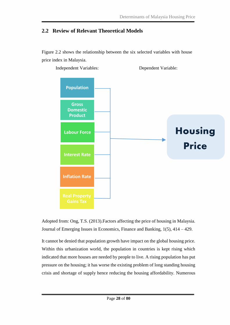
Figure 2.2 shows the relationship between the six selected variables with house
price index in Malaysia.
Independent Variables: Dependent Variable:
Adopted from: Ong, T.S. (2013).Factors affecting the price of housing in Malaysia.
Journal of Emerging Issues in Economics, Finance and Banking, 1(5), 414 – 429.
It cannot be denied that population growth have impact on the global housing price.
Within this urbanization world, the population in countries is kept rising which
indicated that more houses are needed by people to live. A rising population has put
pressure on the housing; it has worse the existing problem of long standing housing
crisis and shortage of supply hence reducing the housing affordability. Numerous
Population
GrossDomestic Product
Labour Force
Interest Rate
Real Property Gains Tax
Inflation Rate
Housing
Price

Determinants of Malaysia Housing Price
Page 29 of 80
regulations, laws, and policy relating to the house building brought the issue of slow
housing production (Ong, 2013).
Gross domestic product (GDP) is refer total value of a country's finished goods and
products, has been considered as a vital indicator as it has significant relationship
with the housing price. GDP included few elements such as expenditure and
investment, which will affect the economy significantly. As illustration when
consumption on house increases, this will increase the house price as well.
According to Ong (2013), the amount of terraced, semi-detached houses is
fluctuated along with the Gross domestic product. The number of terrace houses
built is found to be increased when the GDP is growing. On the other hand, the
researcher proved that the increase in house price and housing demand also
contributed in the growing of GDP.
Ong (2013) had did research on how the labour force supplied will affect the
housing price. The researcher examined that the cost of housing will rise if a larger
number labour force involved in the house construction. Other than that, there is a
fact stated that when the house construction involved many high level educated
professional workers, will lead to increase in the cost of building. Ended up, the
burden of high cost will be bear by the consumers as the constructor will charged
higher price on them. Therefore, researcher claimed that the house building activity
is motivated by high growth inemployment. By the way, there is also argument
against regarding the relationship between labour forced and housing price.
Based on Ong (2013), it stated that interest rate has no significant impact on the
housing price. One of the reasons behind is that the demand and supply are not
balanced during healthy economy. This is a situation where the investors are too
confident and optimistic about the housing market. According to Ong (2013), the
speculators may not want to hold houses for the long period and sell it in short
period while the buyers will pay extra to satisfy the desired type of house. For
homeowners, they are focusing on changing interest rates because it will influence
the real estate price which will also influence the availability of capital and the
demand of investment. These capital flows will directly affect the demand supply

Determinants of Malaysia Housing Price
Page 30 of 80
for house that will influence the property price. Therefore, Ong (2013) concluded
that there is strong proved that the price of the houses will rise.
In economics, inflation means general level of price of the goods and services is
raising, which drive the purchasing power of currency falling. According to Ong
(2013), during the inflation period, it is also to be told that the cost of raw materials
for building a house will also be increased. On the other hand, Ong (2013)
mentioned that there are only Gross Domestic Product, population and RPGT were
revealed to have significant positive relationship with housing price.
Based on Ong (2013), the reposition of the real property gain tax by the government
in year 2010 is negative impact and show significant relationship with the housing
price which the findings are deny in the previous study. This real property gain tax
refers to that payment of 5% tax will be subjected with any given arising from
property disposal within five years. According to Ong (2013), the RPGT reposition
has no influence in Malaysia housing price due to the 5% RPGT imposed is too less
for high-income citizens or speculators whereas that are willing to pay when they
realize the earning from increase in house price to be sufficient to offset the RPGT
and still contribute them with an eye-catching earning.
2.3 Conclusion
In brief, this chapter has explained the relationship of the house price index and
macroeconomic and financial factors based on the literature from previous
researchers. Throughout the discussion above, those studies have stated the strong
correlation among dependent variable (HPI) and independent variables namely the
Lending Interest Rate (LEN), Population (POP), Gross Domestic Product (GDP),
and Inflation Rate (CPI) do exist. This chapter also reviewed the theoretical
framework between house price index and its determinants. For the next chapter,
this study will discuss the methodology and technique used for the estimation of the
relationship of HPI and other variables in Malaysia.

Determinants of Malaysia Housing Price
Page 31 of 80
CHAPTER 3: METHODOLOGY
3.0 Introduction
In chapter 3, this study discusses on the research methodologies. This study
primarily tends to investigate the relationship between the housing price in the
Malaysia and its macroeconomic variables, namely GDP, CPI, LEN and POP. It is
very important to have a well-designed research methodology that includes
macroeconomic variables in order to helps determine how accurate the results of a
research method are.
Basically, this study was to identify the determinants of residential housing price
with four independent variables includes gross domestic product, consumer price
index, interest rate, and population volume. The frequency of the data in this study
is quarterly data for 16 years from 1998Q1 to 2014Q3, a total of 64 observations.
This study applied time series econometric models for interpreting, analyzing and
testing hypothesis concerning with the data used in this research.
3.1 Research Design
As this study is to identify the relationship between the fluctuations of housing
price in the Malaysia and its macroeconomic variables, the literature review places
emphasis on the dependent variable (Housing Price) and independent variables
(GDP, CPI, LEN, and POP). The empirical model of this study can be specified
as below:
𝒍𝒏𝑯𝑷𝑰𝒕=𝜷𝟎+𝜷𝟏𝒍𝒏𝑮𝑫𝑷𝒕+𝜷𝟐𝒍𝒏𝑪𝑷𝑰𝒕+𝜷𝟑LEN𝒕+𝜷𝟒𝑷O𝑷𝒕+𝒖𝒕
Where,
HPI = House price index in Malaysia (index, 2000=100)
GDP = Gross domestic product by expenditure in Malaysia (millions
Malaysia Ringgit)

Determinants of Malaysia Housing Price
Page 32 of 80
CPI = Consumer price index in Malaysia (index, 2010=100)
LEN = Interest Rate (percentage)
POP = Population (thousands of citizen)
3.2 Variables Specifications of Measurements
3.2.1 House Price Index
In reality, housing price is the main concern by the citizens in the country. Besides,
it shows the overall condition of economy in a country. Thus, to study the
determination of housing price, HPI is used as a proxy to measure the price of
housing in the country. According to researcher Tse, Ho and Gansesan (1999),
they stated that unstable housing price has significant influence towards the
economic state regarding GDP and demographic changes. Recently, demand of
housing is increasing over the years. Therefore, the housing price is expected to
increase when the housing market have more home buyers than sellers there and
it will causes imbalance between home buyers and sellers.
In Malaysia, HPI is a broad measure of fluctuation of single-family house price
and it is measuring the weighted average price change in repeat sales (Department
of Statistics of Malaysia, 2015). According to McQuinn and O’Reilly (2005), they
conducted the study about theoretical of model in house price determination by
using HPI as their proxy. In addition, past researcher took HPI to capture the
relationship between macroeconomic activity and housing prices (Hott, 2009).
The researchers came out with similar conclusion, they claimed that independent
variables such as GDP, exchange rates, employment rate, personal income and
inflation have positive and significant relationship against HPI, however, interest
rate shows negative relationship towards HPI. In this study, GDP, population and
inflation are expected to have positive relationship with HPI and base lending rate
to have negative relationship against HPI.
Determinants of Malaysia Housing Price
Page 33 of 80
3.2.2 Consumer Price Index
Normally, inflation rate is measured by CPI (Consumer Price Index). CPI can be
defined as the measurement of price of change of services and goods that
household consumed in index form. However, CPI only refers to the average
measurement of goods because not all of them are changed at the same velocity. It
is closely linked to real purchasing power. This is because real purchasing power
links the strength of a currency with the price of services and goods. As we know,
an increase in CPI will decrease the intensity of consumers’ real purchasing power.
Department of Statistics Malaysia had applied the internationally accepted
statistical methodologies for computation of inflation rate from the International
Monetary Fund. The formula of CPI for multiple items provided below:
The expected sign of inflation rate in this research is positive sign
3.3.3 Gross Domestic Product (GDP)
Gross domestic product (GDP) was described as the market value of the entire
authoritatively recognized final goods and services which were supplied by a
nation in a specified period. In other hand, GDP per expenditure is commonly
measured as an indicator of a country’s standard of living and a country’s GDP
will reflect their economic condition. According to Pour et al. (2013), he claimed
that economic performance of a country plays an important role to affect the
housing market.
When a country is an export dominant country such as Malaysia, the depreciation
of a country’s currency might be a good news for the country because when then
currency of the country becomes weaker as compared with other countries such
as United State. Foreign currencies that were not affected by depreciation of its
value will be attracted by cheaper price of goods in Malaysia. Thus, the exporting
country will get higher amount of Balance of Payment (BOP) than previous year
Determinants of Malaysia Housing Price
Page 34 of 80
due to the increased number of exports to other countries. In a nutshell, positive
balance of payment will stimulate the country’ economic condition since exports
is more than imports, which is highly influence the GDP of a country. Based on
the result from Adam and Fuss (2010), he found that GDP per expenditure is
negative and has significant influence toward residential housing price in their
country. Thus, in this study, GDP per expenditure is used as the proxy for GDP
and the expected sign for GDP per expenditure would be negatively toward
housing price.
3.2.4 Lending Interest Rate
In this study, base lending rate (BLR) in Malaysia is used as the proxy for interest
rate. In Malaysia, BLR is the lowest interest rate that is computed by financial
institutions in terms of a designated formula. The institutions cost of funds and
other administrative costs will be counted in the fixed formula in order to construct
BLR. However, throughout Monetary Policy Meeting, the BLR is practically
determined by Bank Negara Malaysia (BNM). In such cases, after monetary
policy was adjusted, the availability of credit of banks is increased; those banks
are able to offer lower bank lending rates, as a result of encouraging more people
to participate in current and future housing market (Ong, 2013; Zainuddin, 2010).
Therefore, any variation toward BLR will significantly influence the pricing of
both existing and latest floating interest rate home borrowings. As well, this study
will forecast if there is a negative significant relationship between interest rate and
housing prices.
The formula to compute the BLR would be revised as follows:
𝐼𝑛𝑡𝑒𝑟𝑣𝑒𝑛𝑡𝑖𝑜𝑛 𝑟𝑎𝑡𝑒 × 0.8 + 2.25%
1 − 𝑆𝑡𝑎𝑡𝑢𝑡𝑜𝑟𝑦 𝑅𝑒𝑠𝑒𝑟𝑣𝑒 𝑅𝑒𝑞𝑢𝑖𝑟𝑒𝑚𝑒𝑛𝑡

Determinants of Malaysia Housing Price
Page 35 of 80
3.2.5 Population
The proxy used in this study is that the number of people living in Malaysia
expressed in thousands. Cvijanovic (2012) found that population growth drives
house price appreciation. The world is becoming much more populated compare
to before and it would create more demands for assets. Hence, the expected sign
of population in this research is positive sign. We can forecast the average
population growth by apply the following formula and solve for r.
𝑷𝒕=𝑷0× 𝐞𝐫𝐭
𝑷𝒕 is the population # at the last year for which there is data
𝑷0 is the population # at the first year for which there is data
e is the natural logarithmic constant
r is the unknown annual rate of growth
t is the number of years between 𝑷𝒕and𝑷0

Determinants of Malaysia Housing Price
Page 36 of 80
3.3 Methodology
3.3.1 Unit Root Tests
Throughout this study, unit root test is conducted to analyze whether the series in the
group (or it is first or second difference) are stationary. The purpose of this test is to
prevent the any biased and invalid results.
Three probable cases as below,
1st - |∅| < 1 and therefore the series are stationary.
2nd - |∅| > 1 where in this case the series explodes.
3rd - |∅| = 1 where in this case the series contains a unit root and is non- stationary.
At level,
𝑌𝑡= |∅|𝑌𝑡−1+ 𝑢𝑡
At 1st difference, having ϕ =1 and subtracting 𝑌𝑡−1 from both side equation,
𝑦− 𝑦𝑡−1=𝑦− 𝑦+ 𝑒𝑡
Δ𝑦𝑡= 𝑒𝑡
Since 𝑒𝑡 is a white noise error term, hence Δ𝑦𝑡 is a stationary series. After differencing
𝑦𝑡 can obtain stationary.
Hypotheses:
H0: There is a unit root (Non-stationary)
H1: There is no unit root (Stationary)
Decision rule: Reject null hypothesis if the result in P-value is less than the significant
level, otherwise, do not reject null hypothesis.

Determinants of Malaysia Housing Price
Page 37 of 80
In general, Unit root test is applied to determine whether there are stationary or non-
stationary trend of time series data for all variables. Also, an order of each of the
variables integration is used to examine in this test. Gujarati and Porter (2009)
mentioned that the mean, variance, covariance of series are persistent across different
periods are known as stationary trend. On the other hand, non-stationary trend will show
vary or non-constant mean, variance and covariance across different periods. The
results will show spurious and invalid problem if non-stationary model occur in the
research. It will cause the normal assumptions of the analysis become not precise and
inaccurate as well as spurious regression. In such situation, researchers should
determine whether a time series is stationary or non-stationary by using unit root test
(Hill, Griffiths & Lim, 2007).
In addition, most of the macroeconomic variables are non-stationary and seemed to be
varied over time (Asteriou& Hall, 2007). Based on Ray (2012), in order to prevent such
econometric problems and invalid results, unit root test must be carried out to make
sure there is stationary model and robustness of results. In this study, both Augmented
Dickey-Fuller (ADF) and Phillips-Peron (PP) test which are under the category of unit
root test will be conducted to test whether there is stationary or non-stationary in time
series data.
Augmented Dickey-Fuller test (ADF)
Based on a statistics and econometrics, Augmented Dickey–Fuller test (ADF) is a test
for a unit root in a larger and more complicated set of time series models.
Three probable modus of ADF:
Δ𝑦𝑡 = γ𝑦𝑡−1+ ∑ 𝛽𝑖𝑛𝑖=0 Δ𝑦𝑡−1+ 𝑢𝑡
Δ𝑦𝑡 = 𝛼0+ γ𝑦𝑡−1+ ∑ 𝛽𝑖𝑛𝑖=0 Δ𝑦𝑡−1+ 𝑢𝑡
Δ𝑦𝑡 = 𝛼0+ γ𝑦𝑡−1+𝛼2𝑡+ ∑ 𝛽𝑖𝑛𝑖=0 Δ𝑦𝑡−1+ 𝑢𝑡
Hypotheses:
H0: There is a unit root (Non-stationary)
H1: There is no unit root (Stationary)

Determinants of Malaysia Housing Price
Page 38 of 80
In statically, Augmented Dickey-Fuller test (ADF) is a parametric test used in time
series data for unit root. It can refer to an augmented version of simple Dickey-Fuller
test for complicated and larger set of time series models (Dickey & Fuller, 1979).
Regarding to Asteriou and Hall (2007), ADF assumes normal distribution and includes
extra lagged terms of the dependent variable to remove autocorrelation effect. The lag
length on the extra terms can be determined by Akaike Information Criterion (AIC) or
Schwartz Bayesian Criterion (SBC). In this study, SBC also called Schwarz
Information Criterion (SIC) will bring into the lag length selection in this test due to it
is most common and suitable lag length selection in ADF test (Asghar&Abid, 2007;
Cheung & Lai, 1997).
There are two types of model in the ADF test which the first is the model with constant
and without trend and second is the model with constant and with trend. According to
the rule of thumb, it states that there will always be a negative numerated value of
Augmented Dickey–Fuller (ADF) statistic in the test.The smaller the negative values,
the more likely the null hypothesis being rejected and hence it can be concluded that
there is no exist of unit root in this study’s estimated model (Asteriou& Hall, 2007; Hill,
Griffiths & Lim, 2007).
Phillips-Perron test (PP)
PP test is roughly similar with the ADF test, but it integrates an automatic correction to
the DF technique to allow for auto correlated residuals. Thus, PP test can be useful test
for a unit root in time series models, as well as strengthen the evidence of stationarity
of the series in this study.
Test regression for PP as below,
Δ𝑦𝑡−1= 𝛼0+𝛾𝑦𝑡−1+ 𝑢𝑡
Hypotheses:
H0: There is a unit root (Non-stationary)
H1: There is no unit root (Stationary)

Determinants of Malaysia Housing Price
Page 39 of 80
Phillips-Perron test (PP) is non-parametric test carry out in time series data for test unit
root, but it also similar to Augmented Dickey-Fuller test (ADF). Whereas, the PP does
not take into account of lagged difference terms as ADF, but it makes a correction to
the t statistic of the coefficient to control serial correlation. The PP statistics are
modifications of the ADF's t statistics that take into account the less restrictive nature
of error process, as well as investigate any serial correlation and heteroscedasticity error
(Gujarati & Porter, 2009). The PP is carried out with the inclusion of a constant and
linear trend, or neither in the test regression model (Asteriou& Hall, 2007). Besides,
this study will follow the most researchers that tend to choose (Newey-West automatic)
using Bartlett kernel in Phillips- Perron test (Çağlayan&Saçıldı, 2010; Cheung & Lai,
1997; Dritsaki, C., &Dritsaki, M., 2010).
3.4.2 Johansen & Juselius Cointegration Test
First of all, Johansen Cointegration test is very sensitive towards the lag length. One of
the most difficult cases is to determine the lag length.Therefore an optimal lag length
must be chosen. There is different type of information criteria were measured for
different time lags such as Likelihood Ratio (LR), Akaike Information Criteria (AIC),
Schwarz Information Criteria (SC), and Hannan-Quinn information criteria (HQ)
(Gutiérrez, 2007). The number of lags required in the Cointegration test is set to follow
the appropriate lag from criteria.
In this study, SIC is used to find the lag length because it found to be the suitable for
large samples and criteria is useful for selecting true lag length in presence of shocks to
the system.
According to Asghar and Abid (2007), possible results are as follows in order toidentify
the probability of correct estimation for each ofthese criteria:
1) If this probability equal to 1 then it is an excellent criteria because the criterion
picks up the true lag length in all the cases
2) If the probability is close to 1 or greater than 0.5 then it is good criteria because
the criterion manages to pick up the true lag length in most of the cases

Determinants of Malaysia Housing Price
Page 40 of 80
3) If the probability is close to zero or less than 0.5 then it is not a good criteria
because the criterion fails to select the true lag length in most of the cases.
4) If this probability is zero it is poor criteria because the criterion fails to pick up
the true lag length in all the cases.
After the optimum lag length is determined, following by cointegration test. The idea
of cointegration refers to the stochastic drift of error terms when more than one
individual time series are integrated. Cointegration test is commonly used to test
whether there is statistically significant between independent variables and dependent
variable. In order to examine the significant or equilibrium model, it is important to
carry out the cointegration test in regression model. If variables do not cointegrated, it
will lead to the problem of spurious regression.
Typically, there is involved of three methods in the cointegration tests which is Engle-
Granger two-step method, Johansen test and Philips-Quliar is cointegration test. In this
research, Johansen test was suggested due to its multivariate tests natural, for example
consist of two or more variable quantities in our sample size (Alexander, 1999). The
reason Engle-Granger two-step method do not indicated in this research is because this
method is more preferable on single equation model (bivariate). Furthermore, Lee et al.
(2005) had stated that 𝑥𝑡 and 𝑦𝑡 must be in nature random walk in order to carry out
Johansen test to avoid spurious regression problem. Also, cointegration has strong
relationship to vector error correction model (Asteriou & Hall, 2007).
H0 = There is no cointegrating vector (r=0)
H1 = There is cointegrating vector (r>0)
When test statistic value is less than critical value, null hypothesis will be rejected. If
there is a case of do not reject the null hypothesis, the cointegrating vector can be
analyzed until the last value of the number. Next, once the cointegration test estimate
is being determined, the model can proceed to the Vector Error Correction model
(VECM) or Vector Autoregressive Model (VAR). If the results found any cointegrating
vector, Vector Error Correction Model (VECM) is applied to analyze the long-run
relationship between residential housing price and independent variables. In contrast,
Determinants of Malaysia Housing Price
Page 41 of 80
Vector Autoregressive Model (VAR) is performed to analyze the short run relationship
if there is no cointegraing vector in cointegration test.
3.4.3 Vector Error Correction Model
Based on Johansen (1991), it stated that Vector Error Correction Model (VECM) is
applied on response variable as estimation in returns to equilibrium once there is a
change in an estimate variable by using multiple time series model. In another word,
the purpose of Vector Error Correction Model is to determine whether response
variables and explanatory variables have long run relationship or short run relationship
after co-integration happened in between (Asari, Baharuddin, Jusoh, Mohamad,
&Jusoff, 2011). The inclusion of long-run equilibrium ([Yt-1 – α – βXt-1]) and short-
run which represented by difference term have provided VECM the ability to examine
the long run and short run relationship.
In general, a few advantages is determined when carry out the VECM test. First, when
all the error terms in VECM model are found stationary,standard OLS estimation will
bevalid.Next, it is a useful and appropriate method when come to determine the
correction term from non-equilibrium comparing to others. If exist cointegrated in the
model, VECM have to ability to solve the spurious regression problem by formulate in
first difference. Last but not least, Asteriou and Hall (2007) mentioned that
disequilibrium error terms in VECM are known as stationary variable. It naturally to
prevent errors become complex in long-run relationship. Other than that, it provides a
clearer context on long term estimating and any non-stationary series by using the test.
Theoretical equation provided as below:
Δ𝑦𝑡= 𝑎𝑜+ 𝑏1 Δ𝑥𝑡− 𝜋�̂�𝑡−1 + 𝑦𝑡
B1= impact multiplier (measures immediate impact when a change in x will cause a
change in y)
Π= feedback effect (show how much of disequilibrium being corrected)
Determinants of Malaysia Housing Price
Page 42 of 80
Based on this study, there is a determination in the effect of independent variables on
house price in long run relationship. Thus, Vector Error Correction Model was
performed to analyze the important of explanatory variables which are interest rate,
GDP, population and inflation rate on response variable which is residential house price.
As per Mahalik and Mallick (2011) past account, they applied Vector Error Correction
Model by using quarterly data of independent variables and house price shown co-
integrated and significant result in long run relationship.
3.4.4 Granger causality test
Granger causality test naturally is run to test for the dynamic movement of causality
relationship between all stationary variables in this study.
Below is the estimation of the following VAR model,
∆𝑦𝑡= 𝛼1+ ∑ 𝛽1𝑛𝑖=1 ∆𝑥𝑡−𝑖+ ∑ 𝛽2∆𝑛
𝑖=1 𝑦𝑡−1+ 𝜀1𝑡
∆𝑥𝑡= 𝛼2+ ∑ 𝛽3∆𝑛𝑖=1 𝑥𝑡−𝑖+ ∑ 𝛽4∆𝑛
𝑖=1 𝑦𝑡−1+ 𝜀2𝑡
Four probable results as below:
a) 𝒚𝒕causes 𝑥𝑡
-the lagged y terms in eq2 may be statistically vary from zero as a group, and the lagged
x terms in eq1 not statistically vary from zero.
b) 𝑥𝑡 causes 𝒚𝒕
-the lagged x terms in eq1 may be statistically vary from zero as a group, and the lagged
y terms in eq2 not statistically vary from zero.
c) There is a bi-directional feedback (causality among the variables)
-both sets of x and y terms are statistically vary from zero in eq1 and eq2.
d) The 2 variables are independent
-both sets of x and y terms are not statistically vary from zero in eq1 and eq2.
Hypotheses:

Determinants of Malaysia Housing Price
Page 43 of 80
H0: X does not Granger cause on Y
H1: X does Granger cause on Y
And
H0: Y does not Granger cause on X
H1: Y does Granger cause on X
Decision rule: null hypothesis will be rejected if Chi-square test is greater than critical
value at 1%, 5% or 10% level of significance.
Granger (1969) had proposed Granger Causality Test to execute in 1969 in order to test
for the causality relationship between two time series. A brief explanation by Harasheh
and Abu-Libdeh (2011) is the test applied to determine the causality relationship
between variables in time series as well as to identify whether one variable can be
applied in estimating another variable.
In this study, Granger Causality Test is conducted to achieve the objective of study
which is to examine whether there is causality relationship between our variables.
Granger Causality Test is one of the common tests applied by past researchers to
determine causality relationship between house price and its determinants (Chen &
Patel, 1998; Chui & Chau, 2005; Lee, 2009; Leo, Liu & Picken, 2007; Mahalik &
Mallick, 2011).
In a nutshell, VEC Granger Causality / Block Exogeneity Wald Tests will be carried
out in this study to analyzewhether the presence of causality relationship between all
variables. Besides, this test is competent to indicate the direction of causality between
all variables, as well as detects whether the variables are having unidirectional causality,
bi-directional causality or independent (Asteriou & Hall, 2007).
Determinants of Malaysia Housing Price
Page 44 of 80
3.4.5 Variance Decomposition
Variance decomposition also known as forecast error variance decomposition is used
to examine the response of dependent variables that explained by the shock that caused
by its ‘own’ shock and also shocks that transmitted from other variables in the model
either in short run or in long run dynamics between the variable in the system (Brooks,
2008). Besides that, variance decomposition is also used to measure the amount of
shocks of macroeconomic and financial variables towards the fluctuation of HPI in the
form of a proportion of movement accordingly by percentages. By this way, the
researchers are able to figure out how’s the macroeconomic and financial variable
individually shocked each other in the vector autoregressive (VAR) model.
The benefit of variance decomposition can show the movement of dependents variables
due to their own shocks and also shocks from other variables at the meantime. In general,
variance decomposition and impulse response give almost similar statistic (Brooks,
2008). According to Runkle (1987), he argue that for both variance decomposition and
impulse response are extremely hard to differentiate exactly between each other and the
confidence bands around variance decomposition and impulse response should be
created in all the time. Thus, this paper applied variance decomposition with following
hypotheses.
Hypotheses:
H0: LNCPI/ LNGDP/ POP/ BLR do not have an impact on LNHPI
H1: LNCPI/ LNGDP/ POP/ BLR have an impact on LNHPI
Note:
LNHPI= Natural Log of Housing Price Index
LNCPI = Natural Log of Consumer Price index
LNGDP = Natural Log of Gross Domestic Product
POP = Population
BLR = Base Lending Rate

Determinants of Malaysia Housing Price
Page 45 of 80
3.4.6 Impulse Response Function
The impulse response function is used to identify the responsiveness of the dependent
variables in VAR system towards macroeconomic shocks (Brooks, 2008). Furthermore,
the impulse response function is said to be reliable only when the time series data
become stationary after passing through second difference. It acts as an economic
function which has been used to identify the impact caused to all variable in VAR model
when the variable faces some impulses (Elder, 2003). In Addition, the impulse response
function can detect the impact of any variable towards the all other variables in the
system (Lin, 2006).
Moreover, the ordering for variables is very important to identify the impulse response
function, because it may affect outcome from the test even though same data set has
been used. The different between standard impulse response function and generalized
impulse response function is that standard impulse response is sensitive to the ordering
of variables, however the later does not. Besides that, generalized impulse response
function does not assume that when one variable is shocked, all other variables are
switched off. According to Masih and Masih (2001), he said that generalized impulse
response function does not require or thogonalization in the VAR system. So, in order
to avoid this problem, this paper will apply the generalized impulse response analysis
which recommended by Pesaran and Shin (1997) and Borok et al. (2005).
Next, the use of generalized impulse response function describes the reaction of the
endogenous variable which in this case refers to the macroeconomic variables through
the time when there is a shock. Hence, each changes of the macroeconomic variable
can be detected separately according to period with the existence of shock that occur in
a specific period. However, the level of affecting housing prices by this shock may or
may not affect the macroeconomic variables. The previous researcher Engsted, Hviid
and Pedersen (2015) used the impulse response function to investigate the housing
market volatility in OECD countries.
Determinants of Malaysia Housing Price
Page 46 of 80
3.5 Conclusion
In a conclusion, this chapter discusses about the data sources and methodology has been
used to test for the result. This study has clearly described the proxy used for each of
the variables. The research collection method included in this study has also been
clearly determined and explained in this chapter.All of the data are collected from
DataStream. The Eviews 9 software is carried out in this study to conduct the data
analysis. The next following chapter will be further explored about the empirical result
and output of each methodology.
Determinants of Malaysia Housing Price
Page 47 of 80
CHAPTER 4: DATA ANALYSIS
4.0 Introduction
In Chapter 4, this paper will focus on examining, interpreting and reporting the
empirical result from previous methodology. Chapter 4.1 presents the Unit Root Test
by using Augmented Dickey Fuller (ADF) test and Philips Perron (PP) test. From
chapter 4.2 to chapter 4.5 will discuss the empirical results based on Johansen &Juselius
Cointegration test, Vector Error Correction Model, Variance Autoregression model,
Granger Causality test, Variance Decomposition and Impulse Response. We have
attached through detail of explanation after each of the empirical test’s results. While
brief conclusion of the test results is concluded in final section.
4.1 Unit Root Test
The table 4.1 shows the result generated from Augmented Dickey Fuller (ADF) and
Philips Perron (PP) unit root test. The table below shows that all of the variables
(housing price index - LNHPI, gross domestic products - LNGDP, consumer price
index - LNCPI, population growth - POP, lending rate - LEN) in Augmented Dickey
Fuller (ADF) unit root test conducted are unable to reject null hypothesis. Because the
p-value of all the variables is more than 0.05 significant levels, which illustrates that all
the variables are not stationary and contain of unit root in the level from. On the other
hand, Philips Perron (PP) unit root test, the variables that are unable to reject null
hypothesis were the housing price index (LNHPI), consumer price index (LNCPI), and
lending rate (LEN) because the p-value is larger than 0.05 significant level. Philips
Perron (PP) unit root test are able to reject the null hypothesis of the gross domestic
product (GDP) and population growth (POP). This is because the p-value is less than

Determinants of Malaysia Housing Price
Page 48 of 80
0.05 significant level, which means that these two variables are stationary and do not
contain of unit root at level form.
Table 4.1: Unit Root Test
Augmented Dickey Fuller
(ADF)
Phillips Perron (PP)
Level
Variable Constant
Without Trend
t-statistic
Constant With
Trend
t-statistic
Constant
Without Trend
t-statistic
Constant With
Trend
t-statistic
LNHPI 3.602855 0.229164 3.602855 -7.128541
GDP -0.438629 -2.939013 -0.121406 -13.95726***
LNCPI -0.538665 -3.025443 -0.538747 -6.733446
POP -2.007625 -2.843242 -4.697009*** -4.634935**
LEN -2.385955 -3.202891 -2.564952 -4.733399
First Difference
LNHPI -6.853155*** -8.012532*** 0.196132*** -8.014846***
LNGDP -5.146057*** -5.105924*** -5.173280*** -13.76474***
LNCPI -6.889999*** -6.827790*** -2.504194*** -6.643683***
POP -4.067452*** -4.132624*** -3.478581*** -6.028948***
LEN -5.867218*** -6.012457*** -2.021678*** -4.809736***
Note: ***, ** and * denotes significant at 1%, 5% and 10% significance level,
respectively.

Determinants of Malaysia Housing Price
Page 49 of 80
When proceed to the first difference of the Augmented Dickey Fuller (ADF) and Philips
Perron (PP) unit root test, all variables are able to reject the null hypothesis. This shows
that all the p-values are less than 0.05 significant levels. In conclusion, all the variables
are stationary and do not contain of unit root in the first difference in Augmented
Dickey Fuller (ADF) and Philips Perron (PP) unit root test.
Therefore, this study must ensure that all the variables are able to reject the null
hypothesis at the level form. However, the results are only being rejected after the first
difference and hence the results are unable to provide valuable long-run information.
To examine the long-run equilibrium relationship, Johansen & Julselius Cointegration
test had used to test in order to capture both short run and long run effects. All the
variables are able to perform Johansen &Julselius Cointegration test because the criteria
to perform this test had fulfill which where the variables must be stationary only at the
first difference.

Determinants of Malaysia Housing Price
Page 50 of 80
4.2 Johansen &Juselius Cointegration Test
VAR method was applied to determine the optimum lags. VAR is run in level model
with the lag length of 6. The result lead to choosing the lag length that SIC was
minimized in the VAR model. Based on the table of VAR Lag Order Selection Criteria,
the lag of 2 was chosen due to the minimum result of Schwarz information criterion
(SIC). In order to get the optimum lag to proceed in the Johansen and Juselius test, the
lag number chosen through the VAR Lag Order Selection Criteria need to be added one
additional lag. So the optimum 3 lag lengths were achieved in this case.
Johansen and Juselius Cointegration test was applied to determine whether there is a
co-integrating relationship and how many of the co-integrating vector between the
macroeconomic variables (Johansen & Juselius, 1990). In order to determine the
number of co-integrating relations by referring to co-integrating vector, there are two
statistics can refer to which is maximal eigenvalue statistic and trace statistic.
According to Onay and Unal (2012), maximum eigenvalue statistic and trace statistic
were used to compare with critical values under 5% significance level in order to make
decision order on hypothesis.
Based on tables, result shown trace statistics and maximal eigenvalue statistic indicated
same co-integrating relationship or co-integrating vector in this model which is two co-
integrating vectors in this model. In addition, based on Dao and Wolters (2008), trace
statistics is superior to maximum eigenvalue in term of smallest value. Moreover,
Lutkepohl et al. (1991) supported that trace statistics is better than maximum eigenvalue
in term of power.
Therefore, in this model two co-integrating relationship were determined between the
variables after applied Johansen and Juselius cointegration test. The test was performed
at 5% level of significant, and the null hypothesis of no cointegration vector between
all variables was rejected.

Determinants of Malaysia Housing Price
Page 51 of 80
Table 4.2.1: Johansen’s Test for LNGDP
Order of
cointegration
Null
Critical value (trace) Critical value (Max eigenvalue)
(Alternative)
Hypothesis
Trace 95% λ 95%
r = 0 (r > 0) 11.60391* 15.49471 6.066012 14.26460
r ≤ 1 (r >1 ) 5.030211** 3.841466 5.030211** 3.841466
Note: ***, ** and * denotes significant at 1%, 5% and 10% significance level,
respectively.
Table 4.2.2: Johansen’s Test for LNCPI
Order of
cointegration
Null
Critical value (trace) Critical value (Max eigenvalue)
(Alternative)
Hypothesis
Trace 95% λ 95%
r = 0 (r > 0) 12.90295* 15.49471 6.019313 14.26460
r ≤ 1 (r >1 ) 4.190039** 3.841466 4.985081** 3.841466
Note: ***, ** and * denotes significant at 1%, 5% and 10% significance level,
respectively.
Table 4.2.3: Johansen’s Test for LEN
Order of
cointegration
Null
Critical value (trace) Critical value (Max eigenvalue)
(Alternative)
Hypothesis
Trace 95% λ 95%
r = 0 (r > 0) 14.57933* 15.49471 9.295931 14.26460
r ≤ 1 (r >1 ) 5.283396** 3.841466 5.283396** 3.841466
Note: ***, ** and * denotes significant at 1%, 5% and 10% significance level,
respectively.
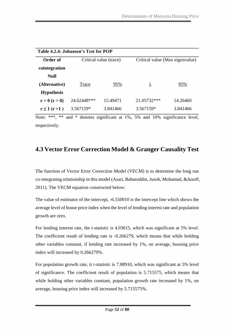
Determinants of Malaysia Housing Price
Page 52 of 80
Table 4.2.4: Johansen’s Test for POP
Order of
cointegration
Null
Critical value (trace) Critical value (Max eigenvalue)
(Alternative)
Hypothesis
Trace 95% λ 95%
r = 0 (r > 0) 24.62448*** 15.49471 21.05732*** 14.26460
r ≤ 1 (r >1 ) 3.567159* 3.841466 3.567159* 3.841466
Note: ***, ** and * denotes significant at 1%, 5% and 10% significance level,
respectively.
4.3 Vector Error Correction Model & Granger Causality Test
The function of Vector Error Correction Model (VECM) is to determine the long run
co-integrating relationship in this model (Asari, Baharuddin, Jusoh, Mohamad, &Jusoff,
2011). The VECM equation constructed below:
The value of estimator of the intercept, -6.550010 is the intercept line which shows the
average level of house price index when the level of lending interest rate and population
growth are zero.
For lending interest rate, the t-statistic is 4.03615, which was significant at 5% level.
The coefficient result of lending rate is -0.266279, which means that while holding
other variables constant, if lending rate increased by 1%, on average, housing price
index will increased by 0.266279%.
For population growth rate, it t-statistic is 7.88910, which was significant at 5% level
of significance. The coefficient result of population is 5.715575, which means that
while holding other variables constant, population growth rate increased by 1%, on
average, housing price index will increased by 5.715575%.

Determinants of Malaysia Housing Price
Page 53 of 80
For consumer price index, the t-statistic is 6.83710, which was significant at 5% level.
The coefficient result of consumer price index is 0.361445, which means that while
holding other variables constant, if consumer price index increased by 1%, on average,
housing price index will increased by 0.361445%.
For gross domestic product, the t-statistic is 5.91033, which was significant at 5% level.
The coefficient result of gross domestic product is 0.452813, which means that while
holding other variables constant, if gross domestic product increased by 1%, on average,
housing price index will increased by 0.452813%.
Short – term granger causality test result:
𝐻0 = The dependent variable has no Granger cause relationship on independent
variables in short run.
𝐻1 =The dependent variable has Granger cause relationship on independent variable in
short run.
Table below illustrate the Granger Causality results for the research model. The null
hypothesis refers to no causality of explanatory variables towards response variables.
The null hypothesis of POP and LEN does not granger cause on LNHPI is rejected. It
is because the p-value of POP and LEN are 0.0438 and 0.0212 respectively which are
less than 5% significant level. Hence, there is enough evidence to conclude that uni-
directional granger causality is happening from POP to LNHPI or LEN to LNHPI in
the short run at 5% significant level. On the other hand, LNGDP and LNCPI are not
granger cause LNHPI at 5% significant level.
Others than that, the null hypothesis of LNGDP does not granger cause on POP and
LEN are rejected due to the p-value is less than 5% significant level. There is sufficient
evidence to conclude that enough evidence to conclude that uni-directional granger
causality is occurring from LNGDP to POP and LNGDP to LEN. Moreover, null
hypothesis of POP does not granger cause on LNGDP is rejected since the p-value is
less than 5% significant level. This means that the POP has short run dynamic granger
cause on LNGDP. Lastly, the null hypothesis of LEN does not granger cause on LNHPI,

Determinants of Malaysia Housing Price
Page 54 of 80
LNGDP, LNCPI and POP are rejected since the p-value are all less than 5% significant
level. This means that all variables have short run dynamic granger cause on LEN.
In conclusion, all the dynamic causal interactions among the variables are figured out
and reported. Otherwise, the rest of the variables do not have any granger cause
relationship among the variables due to the null hypothesis cannot be rejected since the
p-value are all less than 5% significant level.
Table 4.3: Granger Causality Test and VECM
Independent Variables
Dependent
Variable
Granger Causality Test lagged coefficients p-value 𝐸𝐶𝑇𝑡−1 coefficie
nt variable (t-
stat)
∆LNHPI ∆LNGDP ∆LNCPI ∆POP ∆LEN
LNHPI - 1.415682
7.125810
8.107383**
9.705126**
0.028659**
[ 2.20536]
LNGDP 2.110359
- 2.110359
46.44895***
9.839724**
0.012202
[ 0.67496]
LNCPI 1.098828
1.386247
- 0.863270
3.323729
-0.013785
[-1.55542]
POP 3.617072
95.76587***
4.461314
- 5.149091
-0.003818**
[-3.79183]
LEN 10.10620**
28.38477***
10.43126**
19.59895***
- 0.387205**
[ 3.44939]
Note: ***, ** and * denotes significant at 1%, 5% and 10% significance level, respectively. The
figure in the squared brackets […] represent as p-value

Determinants of Malaysia Housing Price
Page 55 of 80
4.4 Variance Decomposition
To consider the dynamic interaction of the variables which is beyond the sample period,
the Forecast Error Variance Decomposition is implied. The variance decomposition is
a tool that used to define how the housing price index is affected by the shock of
macroeconomic and financial variable in using percentage form. The aim of using this
test is to detect how important is the LNCPI shocks, LNGDP shocks, LEN shocks, and
POP shocks that accounting for observed fluctuation in LNHPI in Malaysia.
Table 4.4.1: Variance Decomposition of LNHPI in Malaysia
Percentage of Forecast Variance explained by Innovations
Period LNHPI LNGDP LNCPI LEN POP
1 100.0000 0.000000 0.000000 0.000000 0.000000
2 96.88062 0.150532 1.762260 1.121026 0.085560
3 95.12985 0.738039 3.006564 1.069314 0.056236
4 94.58991 0.874556 3.489590 1.005787 0.040161
5 94.43336 0.735407 3.789328 1.008339 0.033563
6 94.09928 0.656828 4.188404 1.021011 0.034477
7 93.53440 0.704653 4.745808 0.986748 0.028392
8 93.02977 0.744572 5.247952 0.953440 0.024266
9 92.68202 0.711129 5.649239 0.936196 0.021416
10 92.37096 0.677600 6.007840 0.924698 0.018904
Table 4.4.1 tabulates the variance decomposition of each variable for ten periods, and
then the results were reported based on short run towards long runs. From the table, we
can see that, in the first period, all the independent variables do not transmit any shocks
from each of them to LNHPI. Starting from the second period, shock to LNHPI account
for 96.88 percent variation of the fluctuation of LNHPI, in the other word, which is
called as own shock. Next, in quarter two, the percentage of LNGDP to the variation
LNHPI is 0.15 percent; shock to LNCPI can cause 1.76 percent of fluctuation in
LNHPI; impulse to LEN can cause 1.12 percent of fluctuation towards LNHPI which

Determinants of Malaysia Housing Price
Page 56 of 80
is considering as low impact; impulse to POP account for 0.08556 percent variation of
the fluctuation in LNHPI
Table 4.4.2: Variance Decomposition of LNGDP in Malaysia
Percentage of Forecast Variance explained by Innovations
Period LNHPI LNGDP LNCPI LEN POP
1 5.133827 94.86617 0.000000 0.000000 0.000000
2 10.97489 82.13982 0.015396 1.970821 4.899064
3 13.13242 74.78635 5.867453 1.800289 4.413481
4 12.79489 72.39800 8.567141 1.880004 4.359968
5 11.51064 75.53277 7.501136 1.673103 3.782354
6 11.58562 76.64930 5.873169 1.967724 3.924184
7 12.56157 74.71675 7.142695 1.885049 3.693933
8 12.52507 73.53054 8.473828 1.842271 3.628289
9 12.08240 74.16407 8.503159 1.746708 3.503663
10 11.96007 75.27145 7.593809 1.830706 3.343958
From the table 4.4.2, we can see that in period 3, LNHPI, LNCPI, and LEN in
explaining the variability of LNGDP has increase significantly in the long run. However,
shock to LEN provides smallest percentage of impact towards LNGDP compare with
remaining independent variables, which is not achieving 1.8 percent in long run. Then,
Shock to LNHPI can contribute 13.13 percent fluctuation in the variance of LNGDP in
period 3. Furthermore, impulse to LNCPI can cause 5.87 percent fluctuation in LNGDP
in the long run.

Determinants of Malaysia Housing Price
Page 57 of 80
Table 4.4.3: Variance Decomposition of LNCPI in Malaysia
Percentage of Forecast Variance explained by Innovations
Period LNHPI LNGDP LNCPI LEN POP
1 0.000765 8.844378 91.15486 0.000000 0.000000
2 0.000569 7.939089 91.51171 0.308966 0.239663
3 0.073214 7.930358 91.29924 0.270144 0.427042
4 0.212774 8.190666 90.79541 0.220733 0.580418
5 0.307638 8.204251 90.56655 0.189906 0.731655
6 0.339522 8.161389 90.34690 0.179372 0.972818
7 0.357667 8.261363 90.03496 0.166044 1.179964
8 0.377118 8.444253 89.62986 0.154539 1.394229
9 0.384138 8.546541 89.32346 0.147843 1.598015
10 0.378973 8.610852 89.01762 0.146313 1.846246
From table 4.4.3 above, we can explain that the influence of LNGDP to LNCPI is the
most significant, which is from 8.844378 percent at the first period to 8.610852
percent in tenth period. In overall point of view, the volatility of LNCPI is mainly
affected by its own discrepancy.

Determinants of Malaysia Housing Price
Page 58 of 80
Table 4.4.4: Variance Decomposition of POP in Malaysia
Percentage of Forecast Variance explained by Innovations
Period LNHPI LNGDP LNCPI LEN POP
1 4.644898 16.11326 2.044590 0.000000 77.19725
2 12.45519 19.13763 1.964047 0.255298 66.18783
3 10.79562 9.020466 7.785800 0.197778 72.20034
4 10.86170 6.079017 11.86114 0.199973 70.99816
5 9.354246 4.219040 19.73775 0.153755 66.53520
6 10.29197 4.046996 23.82031 0.169846 61.67088
7 10.29164 2.950345 27.10041 0.185860 59.47175
8 10.66093 2.292388 29.49987 0.158428 57.38839
9 10.40843 1.850978 32.23524 0.179282 55.32607
10 10.77524 1.716634 34.24265 0.205216 53.06026
Table 4.4.4 tabulates the variance decomposition of each variable for ten periods, and
the results were reported. In the first period, LNHPI, LNCPI, and LNGDP have
transmitted shocks towards POP which is less than 1 percent. However, only LEN does
not transmit any shocks from itself towards POP. In second period, shock to LNGDP
account for 16.11 percent variation of the fluctuation of POP, in the other word, for
short run, shock on LNGDP cause highest impact among other variables to POP

Determinants of Malaysia Housing Price
Page 59 of 80
Table 4.4.5: Variance Decomposition of LEN in Malaysia
Percentage of Forecast Variance explained by Innovations
Period LNHPI LNGDP LNCPI LEN POP
1 0.074116 8.611694 2.569014 70.45275 18.29243
2 4.923491 14.95066 1.764553 52.11819 26.24311
3 6.485626 20.15727 2.366366 39.30601 31.68473
4 7.331850 19.69096 8.893554 30.50505 33.57859
5 7.398018 17.86603 15.39633 24.57681 34.76280
6 7.148342 17.18973 19.73072 20.53090 35.40030
7 6.797032 17.21331 22.62903 17.50927 35.85136
8 6.493827 17.04452 25.39948 15.21232 35.84986
9 6.160937 16.52312 28.00299 13.46731 35.84565
10 5.826501 16.12195 30.31958 12.10388 35.62810
From the table 4.4.5, it can be conclude that in period 10, LNHPI, LNCPI, LNGDP,
and POP in explaining the variability of LEN has increase significantly in the long run.
However, shock to POP and LNCPI provides high percentage of impact towards LEN
compare with the other two variables, which are more than 20 percent in long run
respectively.

Determinants of Malaysia Housing Price
Page 60 of 80
4.5 Impulse Response Function
According to Figure 2.3, generalized IRFs from shock by one standard deviation to
individually of four independent variables (LNGDP, LNCPI, POP, and LEN) are traced
out. We can observe that the one standard deviation of LNCPI and POP will cause a
positive impact to LNHPI. The LNCPI significantly increased from the first period until
the tenth period, in other words; LNCPI gives positive impact towards LNHPI. While
the response of LNHPI to LEN tend to have positive impact in a beginning period and
declining to zero after that, it turns to become negative impact towards LNHPI. On the
other hand, the response of LNHPI to LNGDP shows the negative impulse stating from
the first period. The response drops and then reverts upwards in long run relationship
after about fourth period. Responses of shock from LNHPI to LEN have positive impact
in the first eight periods, after that it returns to the negative downward sloping on period
8th onwards. In the final analysis, just LNGDP and LEN have negative impact towards
LNHPI, while LNCPI and POP have positive impact towards LNHPI.
Figure 4.7 : Generalized Impulse response functions for ten periods

Determinants of Malaysia Housing Price
Page 61 of 80
4.6 Discussions of Major Findings
4.6.1 Interest Rate
Based on the results of this study, lending rate (LEN) has negative relationship with the
housing price (HPI) at 5 % of significance level. It implied that when the lending rate
decreases, the housing price will be increase. It implied that interest rate has a
significant impact towards the housing price in Malaysia with our previous finding. It
shows consistent to have negative relationship with our result in this study according to
the finding in past researcher done in previous chapter(Li & Chand, 2013;
Agnello&Schukneht, 2011; Adam & Fuss, 2010).
According to Agnello and Schukneht (2011), they used real housing prices data
annually that contributed by the bank of international settlement (BIS) to do their
analysis. Their findings on the variables (interest rate, money and credit supply) has the
opposite impact on the chances of occurring of housing burst, therefore they can
conclude that if there is a decrease in interest rates, there will be a higher chance that
the housing price will boom. Besides, Agnello and Schukneht (2011) also conclude that
among the determinants of housing price, domestic liquidity and short- term interest
rates have strong effects on the chances of housing booms and bursts will occur.
In addition, based on Adams and Fuss (2010), long term interest rates are one of the
macroeconomic effects towards the housing market. They found that if there is a rise in
the long term interest rates, will influence the demand to own a house. This means that
higher long term interest rates caused other fixes-income assets becomes attractively,
reducing the demand on this investment will cause the housing price to reduce in the
long run. In their study, the demand and housing price eventually decrease due to a
greater long term interest rate that reflected in higher mortgage rates.
Other than that, according to Fitwi, Hein and Mercer (2015), they found out that the
Federal Reserve policymakers are partially responsible for the housing price increase
due to maintaining a low interest rate for too long. They claim that if there is decrease
Determinants of Malaysia Housing Price
Page 62 of 80
in short term interest rates, the cost of housing purchases will also decrease which will
drive the demand for housing to increase and it cause the increasing of the housing price.
4.6.2 Inflation Rate
This study found that the inflation rate is significant at 5% significance level. Moreover,
it is positively affecting the house price in Malaysia in long run. The finding in this
study was consistent with the expected sign as stated in previous chapter. In previous
research finding, there was a positive relationship between inflation rate (INF) and
housing price index (HPI).
As refer to previous researcher Hussain and Malik (2011), there are two categories of
inflation are involved such as demand pull inflation and cost push inflation. Demand-
pull inflation occurred due to the increase in demand for services and goods as well. In
means that the aggregate demand is greater than aggregate supply. As increase in goods
and services’ demand, supplier will tend to mark up the price of goods and services
since they are unable to produce more to meet the consumer need. This statement has
supported by the Tsatsaronis and Zhu (2004) and Liew and Haron (2013). On the other
hand, cost-push inflation refers to the cost of materials increase will lead to the cost of
finished goods increase (Hussain & Malik, 2011). These two factors draw the prices of
goods and services rise, and eventually inflation will happen.
The next explanation is relationship between the impact of inflation and the real
payments on long-term fixed-rate mortgage (Frappa & Mesonnier, 2010). If the
inflation happens, the financing mortgage will decreases then rise shall happen to the
housing price. If one would expect housing demand, and thus real house prices will
respond to changes in inflation (Beltratti & Morana, 2010).More specifically, mortgage
rates will follow a case which low mortgage rates contributing to greater real housing
prices, while higher mortgage leading to low real housing prices (Apergis, 2003).
Besides that, inflation will influence by the current financing conditions, which have
the directly impact on the housing demand. The theory behind this statement is common
for households to reduce their risk by investing in residential real estate other than other
financial instrument. Such high inflation condition able to attract investors by high level

Determinants of Malaysia Housing Price
Page 63 of 80
of uncertainty and hence will bring to increase in house price. Thus, inflation is
positively related to the price of houses.
4.6.3 Gross Domestic Product (GDP)
Based on empirical result of the study, there is a positively relationship between GDP
and HPI. It implies that when GDP increases will lead housing price to increase or vice
versa. By then, it also proves that this study is consistent with the research as stated in
previous chapter. There have few researches which can determine GDP is positively
affected housing price. Firstly, according to Ong (2013) mentioned that GDP is found
to be significant positively correlated with the housing price in Malaysia. Secondly, the
housing price will be influenced when level of Gross Domestic Product GDP occurs
(Paz, 2003). Thirdly, based on Piazzesi & Schneider (2009), it mentioned that the
housing price has strong positive relationship with GDP rate. Last but not least, the
housing market and housing price pointed out a very strong positive correlation with
GDP rate in Asia (Zhu, 2006).
The reason that GDP in Malaysia has the positive relationship to housing price is
because increase in personal consumption. According to Chioma (2009), economic
growth, and the consumption expenditure can be measured because of there is a causal
relationship with the gross domestic product, which grows as a result of the increase in
consumption expenditure. In particular, when a country having a low GDP level during
economic downtown, it will directly causes increase in job uncertainty which means
high unemployment rate in the economy. Hence, resulted in decrease demand for
houses and subsequently the housing price will drop as well.
In addition, housing investment considered as an element of the GDP. Thus, rising in
investment on housing property will cause the GDP move up or vice versa. Furthermore,
an increase in GDP reflect a favorable economy, all people has the ability to buy a
house. People will tend to make an investment on fixed asset such as residential house
property because they believe that the housing market is doing well during favorable

Determinants of Malaysia Housing Price
Page 64 of 80
economy and they will get a favorable return on investment in future. Therefore, the
demand of housing will exceed supply of housing market.
4.6.4 Population
According to the empirical in chapter, we found sufficient evidence that the relationship
from population (POP) to housing price index (HPI) significant in the short run at 5%
significant level and it is a positively relationship between POP and HPI. Since many
authors said that rising populations boost the housing prices, makes overpopulation in
town areas and making number of houses undersupplied. That is the reason home price
keeps on growing.
Besides, another reason why population can positively affect housing price is that the
population growth is much greater than the growth in housing supply. In general
economics concept, the law of supply and demand illustrates if excess demand will be
occurred within the economy will drive up the house price since product are limited.
Hence, we know that when the population rises, it will drive up the housing price
accordingly.
On the other hand, increasing population will drive house prices higher and higher. The
study in previous chapter also mentioned that GDP and population have causal
interaction between them. One of the reasons for high population result rapid house
price is that there is rapid expansion economy. This means that higher GDP causes
people has more income and hence the market has higher willingness to expand their
family size and to pay more premium prices. Thus, there is higher housing price while
the population of that country is growing.

Determinants of Malaysia Housing Price
Page 65 of 80
4.7 Conclusion
In a nutshell, this study intend to use a series of time series econometrics test to analyze
the dynamics of the data. This study apply unit root tests in figuring out whether the
variables are stationary or non-stationary. The unit root test result from E-view is being
reviewed based on the Augmented Dickey Fuller and Philips Perron tests. Two of the
variables are non-stationary at level, except GDP and Population. After the first
difference of both ADF test and PP test, all of the four independent variables are
stationary. Then we proceed to Johansen & Juselius Cointegraton test and in order to
determine and select the lag length, we applied VAR lag order criteria selection. From
this study we found that with lag length of 3 is the best for undergoing this cointegration
test.
Based on our trace statistics and maximal eigenvalue statistics, it showed us that the
empirical model has two co-integrating vector from both statistics. Hence, along run
relationship do exist in this model. Next, this study proceeded with VECM approach
since there is a long run relationship in this model. The VECM results showed that
lending rate, population, GDP and consumer price index are significant to house price
index. The sign of coefficient for growth domestic product, consumer price index and
population is positively related to House Price Index while lending rate is negatively
related to House Price Index.
Granger Causality is being used for the determination of short run and causality
direction of the model. From the results, it clearly showed that from population growth
and lending rate are uni-directional towards the housing price index. Therefore, we
made a conclusion that only gross domestic product and Consumer Price Index do not
have granger causality and short run relationship to the HPI.
Conclusively, this chapter has simplified all of the empirical results and findings in
figure, diagram and table form. The specific explanations are written below on each of
the test results in order to provide a clearer picture of it. The limitations, suggestions
and findings of the whole study will be explained and discussed in the chapter 5.
Determinants of Malaysia Housing Price
Page 66 of 80
CHAPTER 5: CONCLUSION, IMPLICATIONS,
LIMITATIONS & RECOMMENDATIONS
5.0 Summary of Statistical Analyses
The main objective of this study is to investigate the determinant of residential housing
price in Malaysia based on four factors. This chapter comprised the empirical result
from previous chapter and the detail will be explained accordingly. Our new empirical
model is form after the unit root test and the selected factors are inflation rate, GDP
growth, population and lending interest rate are separated and formed four equation
models. The implication of this study and the limitations that occurred in the study will
be thoroughly discussed. Lastly, recommendations for future studies also will be
provided.
Due to some of the macroeconomic variables are non-stationary, the unit root tests
carried out in order to prevent from spurious regressions. Each of the variables is test
for stationarity by using the ADF and PP test.
Based on the result show that all the five variables include HPI, CPI, GDP, LEN, and
POP are stationary at first difference. Hence, this study will proceed with Johenson &
Juselius Cointegration test. It is a test to measure the long run relationship between the
variables. Optimum lag length is determine by VAR model before proceed to Johenson
&Juselius Cointegration test.
Moreover, the lag number has added one additional lag through the VAR Lag Order
Selection Criteria. The empirical results of Johenson & Juselius test show that the
model has long run equilibrium relationship between HPI with LEN and POP.
Therefore, this study will proceed by using VECM model to determine the long run
cointegrating relationship in this model.
From the VECM result, the two variables (LEN and POP) are significant to the HPI.
The other two variables (CPI and GDP) show short run equilibrium relationship with

Determinants of Malaysia Housing Price
Page 67 of 80
HPI in this model. As a result, VAR model will be carried out to test for the short run
equilibrium. Next, the causality direction and the short run relationship of the model
will be determined by using Granger Causality test.
According to variance decomposition results, the volatility of LNHPI is mainly affect
by its own shocks, after follow by LNGDP, LNCPI, POP and LEN. For generalized
impulse response function, just LNGDP and LEN have negative impact towards LNHPI,
while LNCPI and POP have positive impact towards LNHPI.
5.1 Implications of the Study
This study is mainly concentrates on the relationship of macroeconomic variables such
as lending interest rate, inflation, Gross Domestic Product (GDP) and population
growth which is affected the housing price in Malaysia. Hence, there are several
participant involved in this study are investors, potential homebuyers, government,
policymakers and also future researcher.
Residential housing in Malaysia is getting attractive to investors and potential
homebuyers, Because of housing in Malaysia can be considered as a significant
component of investment, therefore, investors and homebuyers must have a basic
knowledge about housing factors to make decisions before take part in the Malaysia
housing market. Furthermore, investors should be cautious when investing in Malaysia
housing properties. The housing market may be reaching a peak as interest rates cannot
stay low for much longer. As indicated by the short term analysis, any increase in
interest rates will result in a corresponding change in house prices in the next quarter
(Pillaiyan, 2015). Households and investors (speculators) can technically predict the
house prices movements and actualize their planned expenditure (Tuck & Tan, 2015).
Investors and homebuyers can evaluate the house price movement by using this study
since the results prove that the macroeconomic variables (LEN, CPI, GDP and POP)
are significantly correlated with housing prices. As stated in the previous chapter, GDP
increases will causes housing prices increase and CPI as well as POP increases will lead

Determinants of Malaysia Housing Price
Page 68 of 80
to housing prices increase as well. On the other hand, LEN shows negative relationship
which means LEN increases, housing price will decrease.
In the recent years, Malaysia housing market has become one of the important
industries in Malaysia economy. The Government of Malaysia recognizes that housing
is a primary necessary for every citizen. It is also an important category of the urban
economy (Ong, 2013).
By taking into account the factors discussed in this study, government and policymakers
are recommended to refer this study for the estimation of housing price movement
based on macroeconomic variables (LEN, CPI, GDP and POP).From this study,
government and policymakers could gain a better understanding on the housing market
dynamics. Others than that, government and policymakers able to make an analysis on
the supply and demand of housing price in Malaysia and decide a most suitable policy
to be implemented in order to ensure a stable housing market in Malaysia. In addition,
policymakers can improve the housing market efficiency by lower bureaucracy in the
government regulations and policies which can control the housing market. Eventually,
the implementation of these initiatives would able to control the financial stability in
the housing market and improve transparency of information to investors, homebuyers
and policymakers in Malaysia, thus it lead to increase the efficiency in the housing
market ( Zainddin, 2010).
There are many arguments on the topic of housing market and some of the researchers
have their own viewpoint and different conclusion as well. Regarding to Ong (2013),
the population is significant positive correlated with the housing price. This could be
due to the fact that when the number of citizen increases, demand for house will
definitely increase in order to satisfy the consumers’ need. Although this study has
different perspective compared to various researchers, this study also can provide
another perspective for the argument. In a nutshell, this study could be used as a guide
for determine the relationship of macroeconomic variables and housing prices in future
research.

Determinants of Malaysia Housing Price
Page 69 of 80
5.2 Limitations of Study
We have found out several limitations throughout this study which can impede this
research to optimize its results and step forward to become an ideal research. As well,
it was rare to find a perfect research without any limitation in reality.
Firstly, there was a limitation that insufficient theory of all variables in this study. In
practice, there are a lot of theories of house prices are based on primary data rather than
secondary data, as well as less relevant theories can be found. Hence, this study unable
to carry out an adequate review of relevant theoretical models to support the selected
variables. Moreover, due to the limited knowledge of econometrics tests, this research
was not able to explore and carry out more advanced tests to examine the relationship
between the response variable and the explanatory variables. Consequently, it
obstructed the enhancement and consistency of the empirical results.
In addition, this study encountered problem that the limited data can be obtained from
UTAR library DataStream. This study only used the time series data from year 1998 to
year 2015 as the study period. Besides, this study used the quarterly data as the sampling
method and provides 64 observations have been introduced for each variable. It has
control the extent of study period and the validity of this study. Our sample size is
considered small, it will be tough to discovery significant correlation from our data, as
statistical tests usually require a larger sample size to make sure that a representative
distribution of the population then only will be considered meaningful to those people
to whom our results will be transmitted and being read.

Determinants of Malaysia Housing Price
Page 70 of 80
5.3 Recommendations for Future Research
It is an important part of a project of avoiding mistakes to be repeated and provide a
better result for future research. Research recommendations generate an idea about
what can be improve in this research and what could future studies practice in order to
create a better study. So, future researches are recommended to carry out some of more
advance test statistics in order to obtain accurate result in testing about the long run and
short run relationships between the variables. It also may be better for them to check
the consistency of the data in the test to acquire a better result.
In the future, it is recommended that researchers can attempt to collect the data from
other reliable sources such as the World Bank and Asian Development Bank if they are
interested to include more data. Future research is being suggested with the possibility
of inclusion of more relevant variables if possible in order to obtain better research
outcomes. However, the variables chosen to be used must be relevant with the study in
order to show significant and able to enhance the model.
Moreover, the future researchers may advise to use other types of research method for
data collection such as primary research for data method. Primary research involves
collecting data about a given specific subject directly from the outside the world. It
consists of information about interviews, surveys, observations, and analysis.
Interviews are classified as qualitative methods which able to provide expert or
knowledgeable opinion on a subject and a lot of information from a small group of
people. By using questionnaire, it can provide information about a larger population
thinks differently based on the subject. In the other hand, observations provide deeper
understanding about certain of people, events, or locales without the unfair judgment
of an interview. While the analysis involves gathering data and allocating it based on
standard required to have a clearer picture of some trend or pattern.

Determinants of Malaysia Housing Price
Page 71 of 80
5.4 Conclusion
In the final investigation, it is important to know the determinants of macroeconomic
and financial factors to the residential property markets, especially for the policy
makers, government, investors, homeowners and homebuyers. The study reviews a
certain among of past research paper and journals in order to get overall picture of the
residential property markets. The theoretical framework of the house price index also
had been widely discussed.
Besides of investigate the relationship between macroeconomic determinants and
housing market in Malaysia, this research also identified the long run, short run,
causality direction, and shocks of the empirical model in this study. All of the
methodologies of this time series data analysis with a complete detail are discussed in
this paper.
Lastly, as refer to the empirical results and discussion, this research conclude that
lending interest rate, inflation, gross domestic product (GDP) and population growth
are significant determinants of Malaysian house price index (HPI). The major findings,
implication, limitation and future studies have been widely discussed in the last chapter
of this study.

Determinants of Malaysia Housing Price
Page 72 of 80
References
Adams, Z., & Füss, R. (2010). Macroeconomic determinants of international housing
markets.Journal of Housing Economics, 19(1), 38-50.
Alexander, C. (1999). Optimal hedging using cointegration. The Royal Society, 2039-
2058. Retrieved from
http://www.carolalexander.org/publish/download/JournalArticles/PDFs/PhilT
rans_357_1758.pdf
Apergis, N. (2003). Housing Prices and Macroeconomic Factors: Prospects within the
European Monetary Union. International Real Estate Review, 6(1), 63 - 74.
Asari, F. F. A. H., Baharuddin, N. S., Jusoh, N., Mohamad, Z., & Jusoff, N. S. K.
(2011). A Vector Error Correction Model (VECM) Approach in Explaining the
Relationship Between Interest Rate and Inflation Towards Exchange Rate
Volatility in Malaysia.World Applied Sciences Journal, 12, 49-56.
Asghar, Z., & Abid, I. (2007). Performance of lag length selection criteria in three
different situations. MPRA paper. Retrieved from https://mpra.ub.uni-
muenchen.de/40042/
Asteriou, D., & Hall, S. G. (2007). Applied econometrics: A modern approach using
EViews and Microfit,Revised Edition. Palgrave Macmillan.
Badar, M., & Javid, A. Y. (2013). Impact of Macroeconomic Forces on
Nonperforming Loans: An Empirical Study of Commercial Banks in
Pakistan. WSEAS TRANSACTIONS on BUSINESS and ECONOMICS, 1(10).
Retrieved from
http://www.wseas.org/multimedia/journals/economics/2013/56-259.pdf
Bank Negara Malaysia. (2012). Risk Development and Assessment of Financial
Stability in 2012. In Financial stability and payment systems report 2011.
Beltratti, A., & Morana, C. (2010). International house prices and macroeconomic
fluctuations.Journal of Banking & Finance, 34(3), 533-545.
doi:10.1016/j.jbankfin.2009.08.020
Brooks, C. (2008). Introductory econometrics for finance (2nd ed.). Cambridge:
Cambridge University Press.

Determinants of Malaysia Housing Price
Page 73 of 80
Brunnermeier, M. K., & Julliard, C. (2007). Money Illusion and Housing
Frenzies. Rev. Financ. Stud, 21(1), 135-180. doi:10.1093/rfs/hhm043
Cağlayan, E., & Saçıldı, I. S. (2010). Does purchasing power parity hold in OECD
countries?International Research Journal of Finance and Economics, 37, 138-
146.
Chen, M. C., & Patel, K. (1998). House Price Dynamics and Granger Causality: An
Analysis of Taipei New Dwelling Market. Journal Of The Asian Real Estate
Society, 1(1), 101 - 126.
Chen, Y., Gibb, K., Leishman, C., & Wright, R. (2012). The Impact of Population
Ageing on House Prices: A Micro-simulation Approach. Scott J Polit
Econ, 59(5), 523-542. doi:10.1111/j.1467-9485.2012.00593.x
Cheung, Y., & Lai, K. S. (1997). Bandwidth Selection, Prewhitening, and the Power
of the Phillips-Perron Test. Econ. Theory, 13(05), 679.
doi:10.1017/s0266466600006137
Chui, L., & Chau, K. W. (2005). An Empirical Study of the Relationship between
Economic Growth, Real Estate Prices and Real Estate Investments in Hong
Kong. Journal Of Surveying and Built Environment, 16(2), 19-32.
Cvijanovic, D. (2012, April 15). Real estate finance: How demographics drive housing
prices. Retrieved from http://www.hec.edu/Knowledge/Finance-
Accounting/Financial-Markets/Real-estate-finance-How-demographics-drive-
housing-prices
Dickey, D. A., & Fuller, W. A. (1979). Distribution of the Estimators for
Autoregressive Time Series with a Unit Root. Journal of the American
Statistical Association, 74(366a), 427-431.
doi:10.1080/01621459.1979.10482531
Dritsaki, C., & Dritsaki, M. (2010). Government Expenditure and National Income:
Causality Tests for Twelve New Members of E.E. The Romanian Economic
Journal, 13(38), 67-89.
Elder, J. (2003). An impulse-response function for a vector autoregression with
multivariate GARCH-in-mean. Economics Letters, 79(1), 21-26.

Determinants of Malaysia Housing Price
Page 74 of 80
Engsted, T., Hviid, S. J., & Pedersen, T. Q. (2015). Explosive Bubbles in House Prices?
Evidence from the OECD Countries. SSRN Electronic Journal.
doi:10.2139/ssrn.2548466
Factors that affect the housing market | Economics Help. (n.d.). Retrieved from
http://www.economicshelp.org/blog/377/housing/factors-that-affect-the-
housing- market/
Fitwi, A. M., Hein, S. E., & Mercer, J. M. (2015). The U.S. housing price bubble:
Bernanke versus Taylor. Journal of Economics and Business, 80, 62-80.
doi:10.1016/j.jeconbus.2015.05.001
Frappa, S., & Mésonnier, J. (2010). The housing price boom of the late 1990s: Did
inflation targeting matter? Journal of Financial Stability, 6(4), 243-254.
doi:10.1016/j.jfs.2010.06.001
Granger, C. W. (1969). Investigating Causal Relations by Econometric Models and
Cross-spectral Methods. Econometrica, 37(3), 424. doi:10.2307/1912791
Gujarati, D. N., & Porter, D. C. (2009). Essentials of econometrics (3rd ed.). New
York: McGraw-Hill/Irwin.
Guo, M. Z., & Wu, Q. (2013). The Empirical Analysis of Affecting Factors of Shanghai
Housing Prices , 4(14). Retrieved from
http://ijbssnet.com/journals/Vol_4_No_14_November_2013/27.pdf
Gutiérrez, C. E. (2007). Selection of Optimal Lag Length in Cointegrated VAR
Models with Weak Form of Common Cyclical Features. Working Paper.
Retrieved from https://www.bcb.gov.br/pec/wps/ingl/wps139.pdf
Hashim, Z. A. (2010). House Price and Affordability in Housing in Malaysia.
Retrieved from
http://www.ukm.my/penerbit/akademika/ACROBATAKADEMIKA78/akade
mik a78[03]A4.pdf
Hawa, M. R. (2013). The Effect of Macroeconomic Variables Toward Housing Prices
in Malaysia . Retrieved from
Determinants of Malaysia Housing Price
Page 75 of 80
https://www.academia.edu/11788805/MACROECONOMIC_VARIABLES_E
FF ECT_TOWARDS_HOUSING_PRICES
Hill, R. C., Griffiths, W. E., & Lim, G. C. (2007). Principles of Econometrics. Third
(3rd) Edition.
House Prices in Malaysia | Malaysian Real Estate Prices. (n.d.). Retrieved from
http://www.globalpropertyguide.com/Asia/Malaysia/Price-History
Hui, H. (2010). House price diffusions across three urban areas in
Malaysia. International Journal of Housing Markets and Analysis, 3(4), 369-379.
doi:10.1108/17538271011080664
Hussain, S., & Malik, S. (2011). Inflation and Economic Growth: Evidence from
Pakistan.International Journal of Economics and Finance, 3(5).
doi:10.5539/ijef.v3n5p262
Johansen, S. (1991). Estimation and Hypothesis Testing of Cointegration Vectors in
Gaussian Vector Autoregressive Models. Econometrica, 59(6), 1551-1580.
doi:10.2307/2938278
Kearl, J. R. (1979). Inflation, Mortgage, and Housing. Journal of Political
Economy, 87(5, Part 1), 1115-1138. doi:10.1086/260815
Keilis-Borok, V., Soloviev, A., Allègre, C., Sobolevskii, A., & Intriligator, M. (2005).
Patterns of macroeconomic indicators preceding the unemployment rise in
Western Europe and the USA. Pattern Recognition, 38(3), 423-435.
Kim, B.H., & Min, H.G. (2011). Household lending, interest rates and housing price
bubbles in korea: Regime switching model and kalman filter approach.
Economic Modelling, 28, 1415 – 1423.
Labonte, M. (2011). nflation: Causes, Costs, and Current Status. Congressional
Research Service. Retrieved from
https://www.fas.org/sgp/crs/misc/RL30344.pdf
LaCour-Little,M., Calhoun,C.A.& Yu,W. (2011). What role did piggyback lending
play in the housing bubble and mortgage collapse? Journal of Housing Economics,
20, 81–100.

Determinants of Malaysia Housing Price
Page 76 of 80
Larock, D. (2010). Do Higher Interest Rates Cause Lower House Prices? Dave The
Mortgage Planner.
Lee, C. L. (2009). Housing price volatility and its determinants. International Journal
of Housing Markets and Analysis, 2(3), 293-308.
doi:10.1108/17538270910977572
Lee, Y., Kim, T., & Newbold, P. (2005). Spurious nonlinear regressions in
econometrics.Economics Letters, 87(3), 301-306.
doi:10.1016/j.econlet.2004.10.016
Li, Q. & Chand,S. (2013). House prices and market fundamentals in urban China.
Habitat International, 40 , 148-153.
Libdeh, H. A., & Harasheh, M. (2011). Testing for correlation and causality
relationships between stock prices and macroeconomic variables The case of
Palestine Securities Exchange. International Review of Business Research
Papers, 7(5), 141-154.
Liew, C., & Haron, N.A. (2013). Factors influencing the rise of house price in klang
valley. International Journal of Research in Engineering and Technology,
2(10), 261 – 272.
Lin, J. L. (2006). Teaching notes on impulse response function and structural VAR.
Retrieved from
http://econ.ccu.edu.tw/academic/master_paper/060503seminar(impulse).pdf
Luo, Z., Liu, C., & Picken, D. (2007). Granger Causality Among House Price and
Macroeconomic Variables in Victoria. Pacific Rim Property Research
Journal, 13(2), 234-256. doi:10.1080/14445921.2007.11104232
Mahalik, M. K., & Mallick, H. (2011). What Causes Asset Price Bubble in an
Emerging Economy? Some Empirical Evidence in the Housing Sector of
India. International Economic Journal, 25(2), 215-237.
doi:10.1080/10168737.2011.586806

Determinants of Malaysia Housing Price
Page 77 of 80
Mallick, H., & Mahalik, M. K. (2012). Fundamental or speculative factors in the
housing markets of emerging economies? Some lessons from China. Journal
of Economic Policy Reform, 15(1), 57-67. doi:10.1080/17487870.2011.642580
Masih, R., & Masih, A. M. (2001). Long and short term dynamic causal transmission
amongst international stock markets. Journal of International Money and
Finance, 20(4), 563-587.
Mcleod, S. (2014). Maslow’s hierarchy of needs. Retrieved June 23, 2015, from
http://www.simplypsychology.org/maslow.html
Miles, D. (2012). Population Density, House Prices and Mortgage Design. Scott J Polit
Econ,59(5), 444-466. doi:10.1111/j.1467-9485.2012.00589.x
Ming, N. (2013). Impact of changing interest rates on house prices. Atchison
Consultants. Retrieved from http://atchison.com.au/wp-
content/uploads/2013/06/Property-Observer-Correlation-of-mortgage-rates-
and-residential-property-prices-2013-08-14.pdf
Mulder, C. H. (2006). Population and housing. Demographic Research, 15, 401-412.
doi:10.4054/demres.2006.15.13
Ong, T.S. (2013). Factors affecting the price of housing in malaysia. Journal of
Emerging Issues in Economics, Finance and Banking, 1(5), 414 – 429.
Ong, T.S. (2013). Factors affecting the price of housing in malaysia. Journal of
Emerging Issues in Economics, Finance and Banking, 1(5), 414 – 429.
Pesaran, M. H., & Shin, Y. (1997). Generalized impulse response analysis in linear
multivariate models. Economics Letters, 58(1), 17-29.
Pettinger, T. (2013, November 26). Factors that affect the housing market. Retrieved
from http://www.economicshelp.org/blog/377/housing/factors-that-affect-the-
housing-market/
Piazzesi, M., & Schneider, M. (2009). Momentum Traders in the Housing Market:
Survey Evidence and a Search Model, 99(2). Retrieved from
http://www.aeaweb.org/articles.php?doi=10.1257/aer.99.2.406

Determinants of Malaysia Housing Price
Page 78 of 80
Pillaiyan, S. (2015). Macroeconomic Drivers of House Prices in Malaysia, 11(9).
Retrieved from
http://www.cscanada.net/index.php/css/article/viewFile/7482/7482pdf
Poterba, J. M. (1992). Tax reform and the housing market in the late 1980’s: who knew
what, and when did they know it?, in L. Browne and E. S. Rosegren (eds.). Real
Estate and Credit Crunch, Federal Reserve Bank of Boston Conference
Series, 36, 230-251.
Printzis, T., & Printzis, P. (2015). On the macroeconomic determinants of the housing
market in Greece: A VECM approach . Retrieved from
http://www.lse.ac.uk/europeanInstitute/research/hellenicObservatory/CMS%2
0pd f/Publications/GreeSE/GreeSE-No88.pdf
Rahamn, M. M., Khanam, R., & Xu, S. (2012). The Factors Affecting Housing Price
in Hangzhou: An Empirical Analysis. International Journal of Economic
Perspectives,6(4), 57-66.
Ray, M. V. (2012). The housing bubble and the GDP: a correlation perspective.
Retrieved from http://www.aabri.com/manuscripts/10490.pdf
Ray, S. (2012). Testing Granger Causal Relationship between Macroeconomic
Variables and Stock Price Behaviour: Evidence from India. Advances in
Applied Economics and Finance (AAEF), 3(1), 470-481. Retrieved from
www.worldsciencepublisher.org
Rogers, J. H. (2001). Price Level Convergence, Relative Prices, and Inflation in
Europe. SSRN Electronic Journal. doi:10.2139/ssrn.266505
Runkle, D. E. (1987). Vector Autoregressions and Reality. Federal Reserve Bank of
Minneapolis and Brown University. Retrieved from
https://www.minneapolisfed.org/research/sr/sr107.pdf
Sekaran, K. (2015). Bajet2016: Harga rumah tinggi, tidak mampu dimiliki-Netizen,
Retrieved October 10, 2015, from

Determinants of Malaysia Housing Price
Page 79 of 80
http://www.astroawani.com/berita- bisnes/bajet2016-harga-rumah-tinggi-tidak-
mampu-dimiliki-netizen-75396
Shafie, R. (2015). Tegas tangani isu harga rumah, Retrieved October 10, 2015, from
http://www.utusan.com.my/rencana/tegas-tangani-isu-harga-rumah-1.133558
Shi,S.,Jou, J. & Tripe, D. (2014), Can interest rates really control house prices?
Effectiveness and implications for macroprudential policy. Journal of Banking
& Finance, 47, 15–28.
Taltavull de La Paz, P. (2003). Determinants of housing prices in Spanish
cities. Journal of Property Investment & Finance, 21(2), 109-135.
doi:10.1108/14635780310469102
Tan, T.H. (2010). Base lending rate and housing prices: Their impacts on residential
housing activities in malaysia. Journal of Global Business and Economics, 1(1),
1 – 14.
Tan, Y. K. (2011). An Hedonic Model For House Prices In Malaysia. Working Paper.
Retrieved from
http://www.prres.net/papers/tan_an_hedonic_model_for_house_prices_in_ma
laysia.pdf
Tang, T. C., & Tan, P. P. (2015). Real Interest Rate and House Prices in Malaysia: An
Empirical Study, 35(1). Retrieved from
http://www.accessecon.com/Pubs/EB/2015/Volume35/EB-15-V35-I1-P30.pdf
Tsatsaronis, K., & Zhu, H. (2004). What drives housing price dynamics: cross-country
evidence.BIS Quarterly Review. Retrieved from
http://www.bis.org/publ/qtrpdf/r_qt0403f.pdf
Tse, C., Rodgers, T., Niklewski, J. (2014). The 2007 financial crisis and the UK
residential housing market: Did the relationship between interest rates and
house prices change? Economic Modelling, 37 ,518–530.
United Nations. (2009). Housing and demographics changes. THE RELATIONSHIP
BETWEEN POPULATION AND HOUSING, 8.

Determinants of Malaysia Housing Price
Page 80 of 80
Valuation and Property Services Department. (2012). The Malaysian house price index
[Brochure]. Malaysia: Kementrain Kewangan Malaysia.
Wadud, I.M., Bashar, O.H. & Ahmed,H.J.A. (2012).Monetary policy and the housing
market in Australia. Journal of Policy Modeling 34,849–863.
Wanga, Z. & Zhang, Q. (2014). Fundamental factors in the housing markets of China.
Journal of Housing Economics, 25, 53–61.
Zainuddin, Z. (2010). An Empirical Analysis of Malaysian Housing Market: Switching
and Non-Switching Models. Retrieved from
https://researcharchive.lincoln.ac.nz/bitstream/handle/10182/3511/Zainuddin_
phd .pdf?sequence=3
Zandi, G., Mahadaran, S., Aslam, A., & Lai, K. T. (2015). The Economical Factors
Affecting Residential Property Price: The Case of Penang Island , 7(12).
Retrieved from
http://www.ccsenet.org/journal/index.php/ijef/article/viewFile/55163/29446
Zhang,Y., Hua, X., Zhao, L. (2012). Exploring determinants of housing prices: A case
study of Chinese experience in 1999–2010. Economic Modelling, 29, 2349–
2361.
Zhu, H. (2006). The structure of housing finance markets and house prices in Asia.
Retrieved from http://www.bis.org/publ/qtrpdf/r_qt0612g.pdf
Related Documents