Detection of wave movements - control.isy.liu.se

Detection of wave movements

Hossein Sohrabi

Enes Rahic

LiTH-ISY-EX-3478-2004

Linköping 2004-05-14

ii

iii

Detection of wave movements

Master Thesis in Automatic Control

Department of Electrical Engineering,

Linköping University

by

Hossein Sohrabi Enes Rahic

LiTH-ISY-EX-3478-2004

Supervisor: Anders Sundberg Mikael Norrlöf

Examiner: Svante Gunnarsson

Linköping, 14 maj 2004.

iv

v

Abstract

The aim of the thesis has been to study methods to minimize the slosh when moving liquid-filled packages in packaging machines. An automatic method for generation of the movement of a package in a packaging machine is of growing importance. The main reason is that reduced slosh leads to increased production rate. Progress within measurement technology creates possibilities for new solutions. One purpose has been to find methods and equipment to detect the height of the wave, perhaps at several places or alternatively the entire liquid surface shape. When suitable equipment for detection of the wave movements was found, collected measurements were analyzed and criteria for describing improvements of the slosh properties have been formulated. Initially a sensor specification was written in order to simplify the search for suitable equipment. Sources of information have mainly been catalogues and Internet. The search resulted in that a number of sensors were borrowed for tests. The results of the tests supported the choice of the most suitable sensor, in this case a laser sensor. The main reason is that the sensors detection ability is good compared to its price. An analysis of the sensors most important properties confirmed the choice of the laser sensor. To be able to compare waves, criteria for what is considered to be good wave properties have been formulated and evaluated. The work has confirmed that it is difficult to find a simple and cheap solution for wave detection given that the solution should have good detection ability. It has also been difficult to formulate simple but working criteria for wave performance, and this has led to a compromise between the complexity of the criterion functions and the result of the wave score. Ideas about how an automatic method, based on the chosen sensor and the criterion functions, can be implemented, have been introduced. During the work, some interesting discoveries have been made. These have led to better understanding of how some parameters should be chosen, to better understanding of wave movements and to better choice of future work.

vi

vii

Contents

1. Introduction ....................................................................................................1

1.1 Aim and purpose...........................................................................................................1 1.2 Limitation.....................................................................................................................2 1.3 Disposition of the thesis work.......................................................................................2 1.3.1 System structure ........................................................................................................2

1.3.1.1 Construction of the method for defining a motion profile.................................2 1.3.1.2 Structure of the actual auto method .................................................................3 1.3.1.3 Structure of the on-line auto method................................................................3

1.3.2 Modifications of the program, MinEnergy .................................................................4 1.3.2.1 Development of a path profile before modification..........................................4 1.3.2.2 Development of a path profile after modification.............................................4

2. Sensor specifications ......................................................................................5 2.1 Description of the problem ...........................................................................................5 2.2 Working range..............................................................................................................6 2.3 Sampling interval..........................................................................................................7 2.4 Resolution ....................................................................................................................8 2.5 Dimensions...................................................................................................................8 2.6 Environment view ........................................................................................................9 2.7 Outputs.........................................................................................................................9 2.8 Other ............................................................................................................................9

3. Overview over the available sensors on the market.......................................10 3.1 Searching methods......................................................................................................10 3.2 Touch sensors.............................................................................................................11

3.2.1 Capacitance based measurement.......................................................................11 3.2.2 Float method ....................................................................................................11

3.3 Non –touch sensors.....................................................................................................12 3.3.1 Ultrasonic based measurement .........................................................................12 3.3.2 Infrared laser based measurement.....................................................................12 3.3.3 Radioactive level measurements.......................................................................13 3.3.4 Vision system...................................................................................................14 3.3.5 A combination of infrared laser based measurement and a float........................14

viii

4. Choice of sensors for experimental evaluation..............................................16 4.1 Background ................................................................................................................16 4.2 A short description about the products from table 2 ....................................................17

4.2.1 Shape Compact (Shapeline)..............................................................................17 4.2.2 IVP Ranger M50 (IVP) ....................................................................................17 4.2.3 Ultrasonic sensors ............................................................................................17 4.2.4 Laser sensor .....................................................................................................17 4.2.5 Summary..........................................................................................................18

5. Formulation, realization and result of experiments .......................................20 5.1 Laboratory environment..............................................................................................20 5.2 Vision system M50.....................................................................................................20

5.2.1 Formulation .....................................................................................................20 5.2.2 Performance of the experiment.........................................................................21 5.2.3 Result and summary.........................................................................................23

5.3 Experiments with ultrasonic sensor.............................................................................24 5.3.1. Formulation.....................................................................................................24 5.3.2 Execution of the experiment.............................................................................24

5.3.2.1 Analysis of the ultrasonic signals contact interruption................................26 5.3.3 Result and summary.........................................................................................28

5.4 Experiment with laser sensor from Baumer Electric, OADM 2016441/S14F ..............29 5.4.1 Introduction .....................................................................................................29 5.4.2 Formulation and performance of the experiment...............................................30 5.4.3 Result and summary.........................................................................................31

5.5 Experiment with laser sensor from Wenglor, CP35MHT80.........................................31 5.5.1 Design and execution of the experiment with a laser sensor..............................31 5.5.2 Result and summary.........................................................................................32

5.6 Laser triangulation together with float ........................................................................32 5.7 Final choice of sensor .................................................................................................34

6. Analysis of the chosen laser sensor...............................................................35 6.1 The output signals correctness ....................................................................................35 6.2 Reaction time..............................................................................................................37 6.3 How exact can the laser sensor measure?....................................................................38

6.3.1 Measuring two millimetres distance-change .....................................................39 6.3.2 Measuring four millimetres distance-change ....................................................39 6.3.3 Measuring five millimetres distance-change.....................................................40

6.4 Confirming about the laser sensors resolution .............................................................41 6.4.1 Measuring with 0.1 millimetre distance-change................................................41

6.5 Analysis of the curve shape ........................................................................................42 6.6 Repeatability ..............................................................................................................43

7. Signal scoring ...............................................................................................45 7.1 Signal distribution.......................................................................................................45 7.2 The signal score of part 1............................................................................................46 7.3 The signal score of part 2............................................................................................48 7.3.1 The methods of scoring............................................................................................48

7.3.1.1 Scoring using the whole part two and area.....................................................48 7.3.1.2 Scoring using a period...................................................................................49

7.3.2 Nonlinearities influence on the scoring ....................................................................49 7.3.3 The choice of scoring method ..................................................................................52 7.3.4 FFT- method for development of period length and scoring .....................................53 7.4 Score combination of parts 1 and 2 .............................................................................54

ix

7.5 Experiments................................................................................................................54 7.5.1 Performance of the experiment ................................................................................54 7.5.2 Validation with help of the sensor output signals .....................................................54

7.5.2.1 Agreement for the output signals from the first part.......................................54 7.5.2.2 The second part of the output signal ..............................................................56 7.5.2.3 Conclusions...................................................................................................58

7.5.3 Validation by recording wave movements................................................................58 7.5.3.1 Conclusion ....................................................................................................61

7.6 Comment to the scoring ..............................................................................................62 8. Concluding remarks......................................................................................64

8.1 Conclusion..................................................................................................................64 8.2 Other remarks and future work ...................................................................................65 Appendix 1 – The program MinEnergy............................................................................67 Appendix 2 – Understanding of how calculation frequency influences the path profiles...70 Appendix 3 – The source code for macro BuildCurve......................................................72 Appendix 4 – Sensors data sheets ....................................................................................74 Bibliography ...................................................................................................................80

x

Notations

Symbols w0 - calculation frequency. ti - index time – movement time. wm, fm - maximal oscillation frequency for a liquid in rad/s and Hz. respectively. Ts - Sample interval. ws, fs - Sample frequency in rad/s and Hz respectively. α

b - Ultrasonic beam angle. σ - The standard deviation. ai - The wave amplitude for experiment i. me - The amplitude mean value for all experiments. �

t - The maximal allowed wave amplitude for part 1. At - The maximal allowed wave amplitude for part 1, when consideration to the foam factor ff is taken. A1 - The actual maximal wave amplitude from part 1 for a signal. ε - The difference between At and A1. ff - Foam factor. b1 - Score for part 1. b2 - Score for part 2. Y2 - The signal of part two. tp - Period time for last period from part 2. Ytp - The signal of last period from part 2. A2 - The maximal wave amplitude of the last period from part 2 for a

signal. s - The difference between A2 and the maximal wave amplitude from part 3 .

0̂w - The frequency where the Fourier-transform has been calculated.

N - The number of signal values.

1

1

Introduction This thesis considers the problem to move an unsealed package, filled with liquid, between two positions, the filling position and the sealing position. The movement should be done at the shortest possible time. This is often done in two steps - indexes, i.e. there is an in-between stop position. It is essential to perform the indexing motion in such a way that the liquid does not splash out of the package and contaminate the machine or soak the sealing areas of the package. In this case it is necessary to limit the liquid wave level in the package. In order to become independent of the time when the package is motionless at a possible in-between position it is essential that the wave is as small as possible after the index motion. One method to achieve this is already in use. This method was developed by Mattias Grundelius,[1]. The model that is used in this method is a simplified picture of the reality. The package is configured by a linear two- dimensional model with parallel walls and infinite length across the movement direction. It is assumed that the package contains a liquid with infinitely low viscosity. It is still possible to improve the results from this method by a faster movement and by modifying the movement and then experimentally observe the behaviour of the liquid. For this improvement it is important to have a package with realistic shape and a representative liquid in the package with a relevant viscosity.

1.1 Aim and purpose At Tetra Pak there are some activities in finding a method that enables a reduction of the indexing time. Today the experiments are done in the packaging machine. It is often done by testing different motion profiles until acceptable results are reached. A change of the package contents may lead to a situation where the used motion profile is not suitable any longer. A big assortment of packing articles results in a necessity of an automatic method for finding an optimal motion profile. Studies show that a decrease of the indexing time with 10% leads to an increase of the production rate with 4 to 6%. The aim of this work is to develop an automatic method for decreasing the indexing time in a packaging machine. The ideal method shall work during continuous production, i.e. an on-line method. At the moment there is no consideration taken to the machine space that an on-line method needs. If it is desired to implement an on-line method in present packaging machines

2

sufficient space1 must be created. This puts a demand on the equipment that an on-line method will make use of. The critical issue is the size of the equipment and the possibility to move the equipment together with the package. The ideal solutions often lead to difficulty and are sometimes unapproachable. In such cases it may be suitable to select a less ideal solution. One difference could be that the method would not work during continuous production.

1.2 Limitation The main restriction was the budget that we could use for buying equipments for our application. Even if an expensive product may not give a complete solution for our application, it will at least give us new ideas concerning the problem or may be used for other applications within the company. Another limitation was the time that we could spend for the project, since the work was very extensive. This has led to the fact that we were not able to finish all the three parts of the work that we had set up in order of priority. We only managed to completely finish the two first parts.

1.3 Disposition of the work This work is divided into three intermediate goals, in order of priority. The first step is to develop a new method and equipment for detecting and measuring the wave level, possibly on several places on the liquid surface, alternatively the shape of the whole liquid surface. The next step is to analyze and evaluate the collected data. Finally, a method for defining a motion profile, which gives a better result than the existing method, shall be developed.

1.3.1 System structure

1.3.1.1 Construction of the method for defining a motion profile A Microsoft Excel program, MinEnergy2, that consists of several Excel pages is available and is based on Mattias Grundelius method. 1. Specification – Here are input variables to the program denoted, some executed

calculation and also some calculation formulas for some quantities. The inputs stand for: • Package description. • Calculation frequency3. • Transportation time.

The calculations stand for: • Calculation frequency. • The maximal amplitude of the waves.

2. Index diagram- Figure of the acceleration, velocity and position. 3. Index diagram slosh - Figure of the slosh4 and the position is shown.

1 In this case with space we mean the space between fill position and sealing position in a package machine. 2 The Excel program MinEnergy is in appendix 1. 3 For a better understanding of how calculation frequency influences the path profile see appendix 2. 4 Here, slosh represents amplitude of a wave as function of time.

3

4. Tables- Calculation of the acceleration, position and slosh. 5. CamConvert- Transformation of the position, from millimetres to steps, a step is equal to

0.01953 mm. Those steps represent the position path that is used for controlling the linear motor that accomplishes the desirable motion.

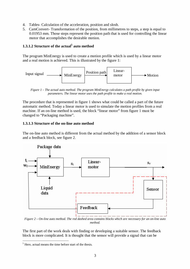
1.3.1.2 Structure of the actual5 auto method The program MinEnergy is used to create a motion profile which is used by a linear motor and a real motion is achieved. This is illustrated by the figure 1:

Figure 1 – The actual auto method. The program MinEnergy calculates a path profile by given input parameters. The linear motor uses the path profile to make a real motion.

The procedure that is represented in figure 1 shows what could be called a part of the future automatic method. Today a linear motor is used to simulate the motion profiles from a real machine. If an on-line method is used, the block “linear motor” from figure 1 must be changed to “Packaging machine”.

1.3.1.3 Structure of the on-line auto method The on-line auto method is different from the actual method by the addition of a sensor block and a feedback block, see figure 2.

Figure 2 – On-line auto method. The red dashed area contains blocks which are necessary for an on-line auto method.

The first part of the work deals with finding or developing a suitable sensor. The feedback block is more complicated. It is thought that the sensor will provide a signal that can be 5 Here, actual means the time before start of the thesis.

MinEnergy

Linear- motor

Position path Motion Input signal

4

analyzed. The analysis will result in the score of the sensors output signals. The feedback block will provide a connection between the output of the sensor and the program MinEnergy. In that way the program MinEnergy will get the necessary information that will lead to an improvement of the motion profile. The parameters that can be changed apart from the package parameters and the liquid parameters are the calculation frequency w0 and indexing time ti. A question that comes up is: “Are there any useful connections between the sensor outputs and the calculation frequency or indexing time?” It is obvious that such connection would be important and helpful. The system would probably work as follows: The program MinEnergy computes a theoretical or desired motion profile, by given input parameters and an input from the feedback block, which is based on the sensor signal, i.e. the appearance of the waves. The linear motor uses the theoretical motion profile to execute a movement that indirectly influences the sensors output signal. A score of the sensor output results in a modification of the input signal/s to the program MinEnergy. With that a closed loop is achieved. How much iterations that are needed to get an acceptable output signal depends on the algorithms in the block feedback.

1.3.2 Modifications of the program, MinEnergy The program MinEnergy has been slightly modified by us. The modification consists of a Macro and implies a simplification when a path profile needs to be developed. The simplification is explained by a description about what needs to be done before a complete path profile is achieved.

1.3.2.1 Development of a path profile before modification MinEnergy and CamConvert are two different Excel programs. MinEnergy gives the position in millimetres which should be transformed to steps and to do that we were bounded to manually copy the position values from the program MinEnergy to the program CamConvert. The new path profile, expressed in steps where one step corresponds to 0.01953mm, shall now be copied to a new Excel document and be saved there. The number of position values depends on the movement time, i.e. “index time” in MinEnergy, see the specification sheet in appendix 1. It means that each variation of movement time leads to different number of copied cells each time.

1.3.2.2 Development of a path profile after modification The only thing that needs to be specified in this case is the path-directory, where the completed path profile should be saved. When the choice of parameters is done it only remains to type “ctrl +a” to get a complete path profile which is saved on the desired memory place. The development of the macro has helped us very much when large-scale experiments have been done. In these experiments we changed the calculation frequency and the index time. Our hope is that the macro should be frequently used in the future and possibly be a part of an automatic method used to develop a “good” motion. The macro BuildCurve6 is programmed in Visual Basic.

6 The source code of the macro BuildCurve can be found in appendix 3.

5

200 mm

200 mm

[mm]

2

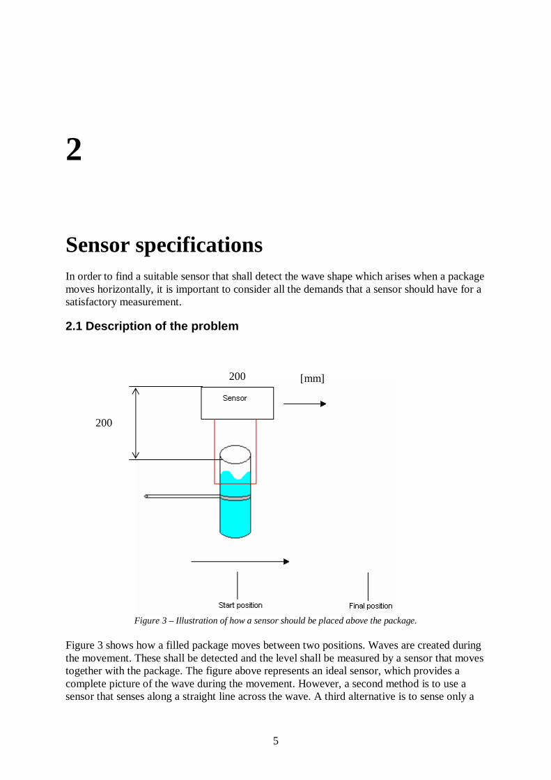
Sensor specifications In order to find a suitable sensor that shall detect the wave shape which arises when a package moves horizontally, it is important to consider all the demands that a sensor should have for a satisfactory measurement.

2.1 Description of the problem

Figure 3 – Illustration of how a sensor should be placed above the package.

Figure 3 shows how a filled package moves between two positions. Waves are created during the movement. These shall be detected and the level shall be measured by a sensor that moves together with the package. The figure above represents an ideal sensor, which provides a complete picture of the wave during the movement. However, a second method is to use a sensor that senses along a straight line across the wave. A third alternative is to sense only a

6

single point on the liquid surface. If contact-techniques are used for wave shape detection the size of the sensor becomes a critical factor since the size of the sensor can affect the wave shape. Several sensors can be used if the sensor size is not a problem. The dimensions in figure 3 do not represent the real size of the sensor, rather the space that is available in the packaging machine for placing a sensor.

2.2 Working range The desirable measurement range for the sensor should be around 82 mm. Figure 4 shows a part of the package with some relevant levels and a sensor with their desired measurement range. A typical wave shape is shown in the package in figure 4. Usually the package is filled to the “Normal filling level”. The highest level that a wave can reach is marked with “Highest level”. It can be a problem with the sealing if the wave should exceed the highest level, because the sealing areas could be wet. The third level is indicated by “Lowest level”. One can define this level by using the symmetry around the “Normal filling level” together with the distance from “Highest level” to “Normal filling level”. The distance between Highest level and Lowest level is the measurement range for the desirable sensor. In figure 4 one can see that the distance is 82 mm. Observe that this distance is valid only for this package. When working with other packages one has to know that this distance can be different. Therefore the distance 82 mm corresponds to the lowest acceptable measurement range.

1 9

41

41

Highest level

Lowest level

Normal filling level.

Sensor [mm]

10

92

Package

Figure 4 – Determination of sensor range using some package levels.

7

2.3 Sampling interval To define a suitable sampling interval we assumed that the sensor shall detect the changes that come from the oscillating waves. According to chapter 3.3 in [1], the frequency of the natural oscillation of the waves was found to be wm = 21 rad /s, which is equivalent to fm = 3.34 Hz. The transfer from rad/s to Hz was done according to the well known equation:

Hzfff mm

mmm 34.32

21

22 =

⋅=⇒

⋅=⇔⋅⋅=

ππωπω (1)

In order to achieve a correct description of the wave oscillations, from the sampled signal, wm it has to be sampled with the frequency ws which should be chosen to avoid alias effect, i.e. the following must be valid:

}{

(2) 1496.06845.6

11

6845.6 / 42 / 21 ;2 2

sf

T

Hzfsradwsradwwww

w

ss

ssmmss

m

==<⇒

<⇒>⇒=⋅>⇒<

It means that the longest sample interval that can be used without alias effects is Ts = 0.1496 s. In order to be able to detect also the first harmonic of the wave the sampling interval has been halved, i.e. 0.0748 s. Experience tells it is better to sample too fast than too slow, and therefore the sampling interval has been rounded downwards to Ts =0.07 s. In order to be able to use system identification methods in the future, the sampling interval must be adapted for that case. A reason for that is that the accuracy of the developed model in relation to real case is partly depending on how the sampling interval is chosen. The following rule of thumb can be applied. If the highest frequency of the oscillation is known, the sampled frequency may be calculated by following formula:

wws ⋅= 20 rad/s (3)

Using w = 21 rad/s in equation (3) ws = 420 rad/s is achieved. A transformation from rad/s to Hz gives fs ≈ 67 Hz. A sampling interval is achieved by inserting fs = 67 Hz in equation (2), Ts = 0.014, that is rounded down, which is usual in those connection as mentioned before. This figure says how fast sampling is necessary for archiving sufficient information for the system identification. It means that a sensor needs to have a samplings interval similar to Ts or shorter at system identification. It is not necessary to find a senor that shall be used for system identification in the first step. Therefore the sampling interval is chosen to Ts = 0.07 s.

8

Sensor 2

Sensor 1

r

Package

2.4 Resolution The amplitude of the wave in the actual package is 82 mm. To be certain that we are on the right side we chose a slightly bigger difference, which is 100 mm. The question is: “How small waves need to be detected in this range?” To give an answer to this question we studied some valid wave criteria. A basic criterion can be summarized as follows:

• From fill position to seal position there are two steps, i.e. the filled package is moved from fill position to an in-between position before it arrives to the seal position. Before the package is moved from the in-between position further to the seal position it is desirable to have wave amplitude close to zero. Since the stop time at in-between position is about 740 ms, it’s hardly enough for waves to become desirably small. Therefore a certain size of the wave amplitude has to be accepted at the in-between position at the moment when the next move is initiated. Previous experiments have shown that the wave amplitude may be as small as 5 mm at that moment.

Experience tells us that resolution should be about 10 times less then the lowest amplitude which needs to be detected. This fact together with criterion above sets the resolution requirement to 5/10 = 0.5 mm.

2.5 Dimensions The sensors dimensions can be very different, depending of which measurement principle the sensor is using. The sensors dimension and the detection area is conclusive for how many sensors that can be used at the same time. Accordingly the sensor size should be as small as possible. Figure 5 give an example of two sensors that are placed above a package. The sensors dimension and size can affect the wave shape in the case when the sensor is in contact with the liquid that it is measuring. Using a sensor with a diameter equal to the package radius implies a huge damping for the wave. This will lead to an incorrect output.

Figure 5 - A principal placement of two similar sensors, sensor 1 and sensor 2, above a round package with a radius that can be as small as 27.5mm.

9

2.6 Environment view It is desired that the sensors shall have high protection against humidity, high temperatures and corrosive liquids. In addition that it is required to be water resistant, according to protection class IP67 [2]. It is expected that the sensor shall manage to measure in pure water, but also in other liquids too, transparent as well as coloured, with various viscosity.

2.7 Outputs The outputs shall be analogue, independent of the reading unit and reading limits.

2.8 Other In certain cases a sensor needs to be mounted at a special angle in order to get better measurement values, for example, a laser sensor needs to have the right angle on the laser beam to get a good reflection back. It is important that the adaptation of the angle should be quick and flexible. The desired supply voltage is 24 VDC.

10

3

Overview over the available sensors on the market The starting point for the search has been sensors for level measurement. Those sensors can be divided into two categories:

• Level meter – Continuous measurement of levels, with an analogue output. • Level watcher – Discrete measurement that only gives a signal when a certain level is

exceeded. Sensors from both categories above have been examined, even if our interest lied most in the first group. An analogue output gives us much more information about the observed systems behaviour then a digital signal does.

3.1 Searching methods The information has generally been acquired from catalogues and Internet search. Even literature studies and a trade fair, Tech Messe in Herning, in Denmark, have constituted our search materials. The catalogue has been used to find those companies who had the suitable technology and sensors. Internet search has been used for completing the details about the products and resulted in the discovery of new companies that were not in the catalogues. In those cases where Internet search or search in a catalogue has discovered an interesting product a personal contact has been taken with the company for verifying of information and completing of the information. Literature studies contain a quantity of periodicals, which revealed some new sensors, and several books, see [3]-[7], whose contents have resulted in a better understanding for those methods and principles that the sensors are using. The visit to Tech Messe in Herning has been valuable because we got an overview of the available sensors in the market, but the visit has also given a picture of the sensors limitations in some kind of applications problems. Sensors for level measurement can be divided into two groups, depending if it is in contact with the liquid that it is measuring or not:

11

• Touch sensors • Non – touch sensors

3.2 Touch sensors

3.2.1 Capacitance based measurement Level measurement by capacitance methods, makes use of the capacitance between the package wall and a dipped electrode. Since the liquid in a package has a larger dielectric constant than air, the capacitance will rise with rising liquid level and constitute an indicator for it. The electrode can be shaped as a stick, or a wire. The shape and the size of the package determine the shape of the electrode. A metal wire can be used if the liquid content in the package is not conducting and chemically indifferent.

Figure 6 - The principle for level measurement with capacitive methods. The electrode must be isolated if the content is conductive.

If the content is conductive the electrode must be isolated with a coating of PVC, Teflon or glass. It is the chemical property that decides which material that should be used. Figure 6 illustrates the principle for how the electrode can be located in the package. The reason that high frequency is used for measuring is because of the very small capacitance, which is rated at some hundred pF. The variation of the liquids dielectric constant affects the measurement result. Conductive liquids can easy build a film on the surface of the electrode isolation. In that case the capacitance will get a bigger value than what is represented by the level of the liquid surface.

3.2.2 Float method Level measurement methods with a float are manufactured by many companies, with the result that the range of sensors is huge in the market. The measurement principle is quite simple, a float lies on the liquid surface and is at the same time connected to an instrument that transforms the level position to a signal. The connection is often a wire. It is important to realize that most of the level measurement systems of this kind are most suitable for slow dynamic conditions. A case of fast dynamics makes it difficult for the float to stay at a constant level on the surface. It is difficult to keep the float at the same place in a package, during the measurement, and to measure close to the package edge. Neither of those

C

12

difficulties had persuaded us to give up this method. We have therefore spent plenty of time in finding out a suitable float since the method is cheap and challenging. The difficulty for making the float to stay at a suitable place and eliminating the problem with constant sink of a float during the level measurement was challenging.

3.3 Non –touch sensors

3.3.1 Ultrasonic based measurement The measurement principle is based on the fixed velocity of sound. By measuring the time that it takes for an acoustic pulse to travel a certain distance, one can calculate how long the pulse has been travelling. A pulse is sent from a transmitter / receiver in a level measurement component that is placed above the surface of the liquid. The pulse hits the surface and is reflected back. The time measurement stops when the pulse hits the transmitter / receiver again, and a time that is equivalent to the double distance will be registered. This value multiplied with the velocity of sound represents the actual distance. Still, it can be a problem if the sound velocity is not constant. The temperature affects the sound velocity with approximately 0.2 % per ºC, which is quite much. Most of the sensors are nowadays equipped with temperature -compensation, so we did not worry about that when we decided to use an ultrasonic sensor. Most of the ultrasonic sensors have nowadays a button that is called “teach in”. This button enables the user to adjust the sensor for a specific sensing distance. Figure 7 represents the principle for ultrasonic based measurement.

Figure 7 - The figure illustrates an ultrasonic sensor which measures liquid surface.

3.3.2 Infrared laser based measurement Practically two technologies are generally used: Pulse time measurement and laser displacement. The first method measures how long time it takes for a pulse to travel to an object and back. For this kind of laser sensors the absolute error in measured length is independent of the distance. The transit time method does not work well for the measurement of short distances. Therefore another method is used that measures the base of a pointed triangle, where one point constitutes the target. Figure 8 illustrates the measurement principle.

13

Figure 8 - The principle for measurement with laser based measurement. A light spot is projected at an object. The light that is reflected back is collected by a lens and projected on a position sensing detector i.e. senses where the light spots centre of gravity is. It will lie in the prolongation of the beam which goes through the middle of the lens, which means that the small triangle s/f will be homogeneous with the big a/L i.e. sfaL /⋅= . Concerning the measurement error it will be increasing with the measured distance.

3.3.3 Radioactive level measurements The principle for radioactive measurements of levels imply that a gamma ray from a radioactive object passes through the package wall and hits a detector of the packages opposite side. The gamma ray transmitter and detector are placed in such way, that they allow detection of the desirable level, as shown in figure 9. When the liquid level varies, a larger or minor part of the detector is hit by the radiation, caused by a variation of radiation absorption and thereby the output from the detector will vary. We will not go deeply into describing details how the radiation transmitter and detector work, but we have to warn that one should follow the safety regulations when working with this kind of method. The gamma radiation from the radioactive preparation is harmless for all materials except living tissue. There is also no risk for a radioactive damage on the package or its contents.

a b Figure 9- This figure illustrates continuous radioactive measurement. Figure a shows a line indicating sensor

while b shows the principle for a point indicated sensor.

Gamma ray- transmitter Detector

Gamma ray- transmitter

Detector

14

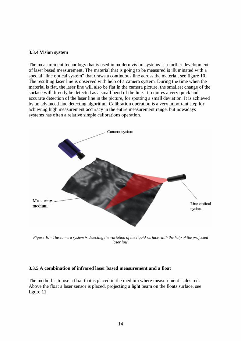
3.3.4 Vision system The measurement technology that is used in modern vision systems is a further development of laser based measurement. The material that is going to be measured is illuminated with a special “line optical system” that draws a continuous line across the material, see figure 10. The resulting laser line is observed with help of a camera system. During the time when the material is flat, the laser line will also be flat in the camera picture, the smallest change of the surface will directly be detected as a small bend of the line. It requires a very quick and accurate detection of the laser line in the picture, for spotting a small deviation. It is achieved by an advanced line detecting algorithm. Calibration operation is a very important step for achieving high measurement accuracy in the entire measurement range, but nowadays systems has often a relative simple calibrations operation.

Figure 10 - The camera system is detecting the variation of the liquid surface, with the help of the projected

laser line.

3.3.5 A combination of infrared laser based measurement and a float The method is to use a float that is placed in the medium where measurement is desired. Above the float a laser sensor is placed, projecting a light beam on the floats surface, see figure 11.

15

Liquid level b

Float

Figure 11 - The principle for laser and float, where a corresponds to the distance from the laser to the float, b corresponds to the distance from the floats upper edge to the liquid surface.

The distance from the laser sensor to the liquid surface is found when distances a and b are added. Without any experimenting we noted that it would be difficult to keep the float at the same place during measurement, which is necessary. In other case an erratic signal is achieved. We can also imagine that the distance b will not be constant at a fast dynamic, which would lead to incorrect signals from the sensor. The question that appears is:

• How much does the distance b vary during a liquid level measurement? • Is the variation negligible?

The method has its disadvantages and difficulty, but it is interesting since a combination of a laser sensor and a float is used at liquid level detecting.

Laser sensor

Float

Liquid level

a

16

4

Choice of sensors for experimental evaluation

4.1 Background The meaning with having a table describing products and their properties is for the ability to examine a number of products in a systematic way, when the time is ready for it. The evaluation can be a simple thing, for example, that the products characteristic is assigned by different points or weight. The product with most points is chosen as the best, from their property. The evaluation can be developed by adding other factors, which represent for example:

• How important it is to use some particular technology? • How dangerous it is to work with some technology?

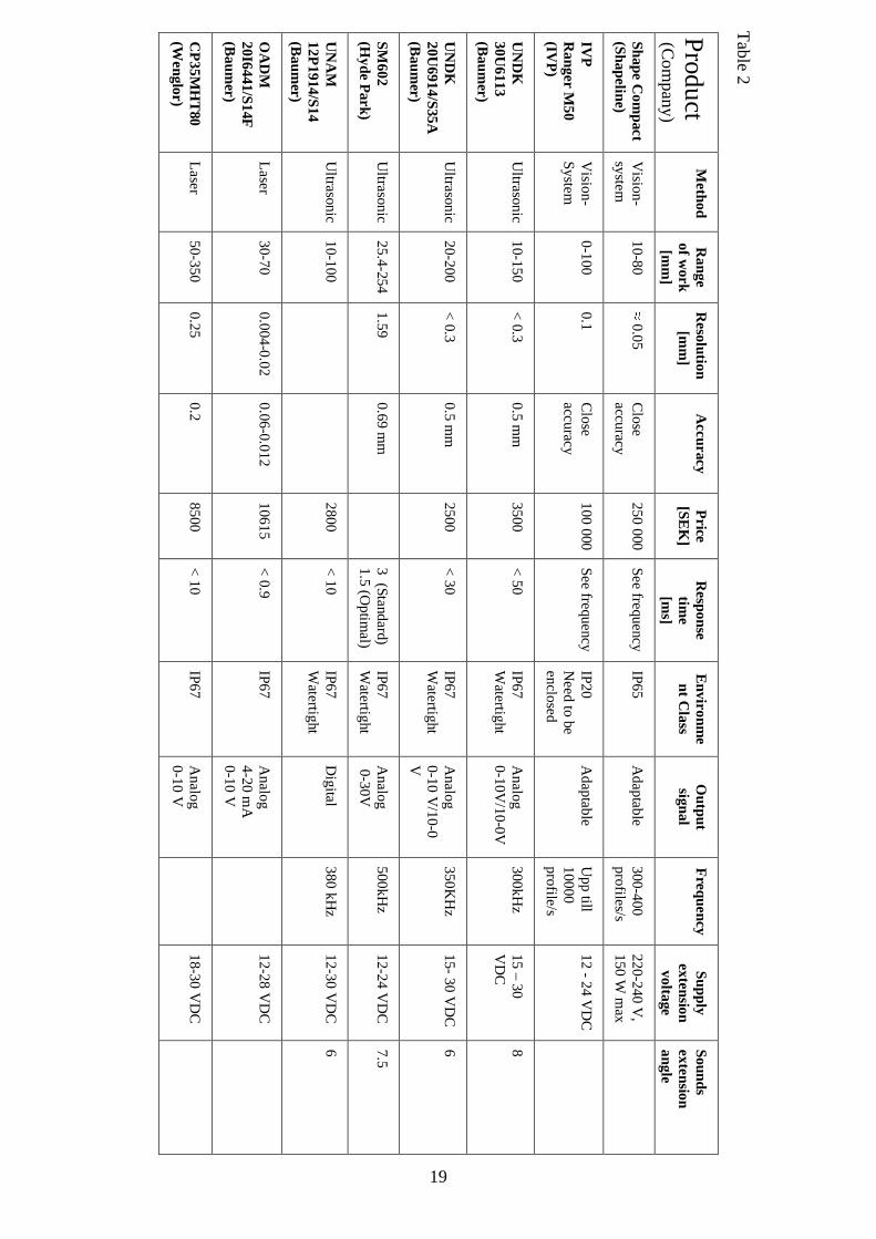
The aim of the last question is above all concerning the radio-activity technology but also technology where laser technology can be dangerous. It is easily realised that such a table also gives an overview that can be used for taking important decisions. Those can further lead to elimination of some technology and/or products, which is/are consider being different from the other. Considering Table 2 there are some empty cells, which mostly depend on the fact that there are no data about the product characteristic to talk about, or there is not any available information. Some technologies, which are described in chapter 2, are not represented in table 2. This is because no products that are based on those technologies have been found suitable for our application. It is often a case of products that are suitable for big packages with slower dynamics. It means that these products’ specifications are far away from the desired specification, from Chapter 2. Therefore there are no such products in table 2. There can be products or technologies on the market that we have not found. The reasons why we have not found them can depend on several factors, but it is important to indicate that if a technology is not represented in table 2 in form of some products, it does not mean that the technology does not work. The reason is that there has not been any need to develop a product that is built on some special technology that can fit our application. An example is radioactive level measurement. Some characteristic can be typical for one technique. An example is the characteristic, “sound translations angle”, for ultra sonic technology. It is

17

difficult to compare such characteristic to other technologies. If several products with the same technology are available, then it is possible to compare those products. Therefore those technologies are represented in Table 2.

4.2 A short description of the products in table 2

4.2.1 Shape Compact (Shapeline) This product has most of the desired characteristic points in the specification. The biggest disadvantage with this product is the price, which is too high and it is also too big in size.

4.2.2 IVP Ranger M50 (IVP) This is a high class vision system, which has good characteristics. The disadvantages are the price and its low protection against humid environment. The price is higher than the company, Tetra Pak, wants to pay. Finally it was decided that a camera should be ordered for tests. An advantage, worth to mention, with vision systems is that they can be used for many other applications.

4.2.3 Ultrasonic sensors Several ultrasonic sensors were found, and those are represented in table 2. It feels quite obvious to try at least one of the ultrasonic sensors. The price is low, and the rest of the characteristics seem to be good. When we should choose a suitable ultrasonic sensor for the test, we considered the sound pulse sending frequency and extension angle. The frequency should be as high as possible and the angle as small as possible.

4.2.4 Laser sensor A laser sensor built on triangulation principles can be used for measuring the liquid level. It had already been tested, see sensors specifications in Appendix 4. The problem with the laser sensor has been that it momentarily loses the optical contact with the liquid level, which leads to disturbance in the output signal, in form of big peaks. Another problem has been that considerable time is spent for adjusting the right position and right angle for the light beam, in order to achieve a good signal. The sensor that is used in the previous experiments is a laser sensor, with the model YT87MGV80 Appendix 4. Considering the age of the sensor and the development in this area, it felt natural to check the modern sensors in this area. During the discussion the main consideration was that the sensor could solve both of the mentioned problems, the problem with disturbances in the output signal and also a simple adjustment of the laser light beam angle for a good output signal. Considering level measurement with laser there is a problem that we in the present situation cannot avoid. The problem is that the medium must reflect some part of the light to the receiver, so that a signal can be registered. Since water is transparent and therefore does not reflect sufficient light back to the sensor there is a big problem for the output signal. A

18

solution for it is to colour the medium, which actually means that it becomes easier to use the laser sensor in a laboratory environment than in the machine environment.

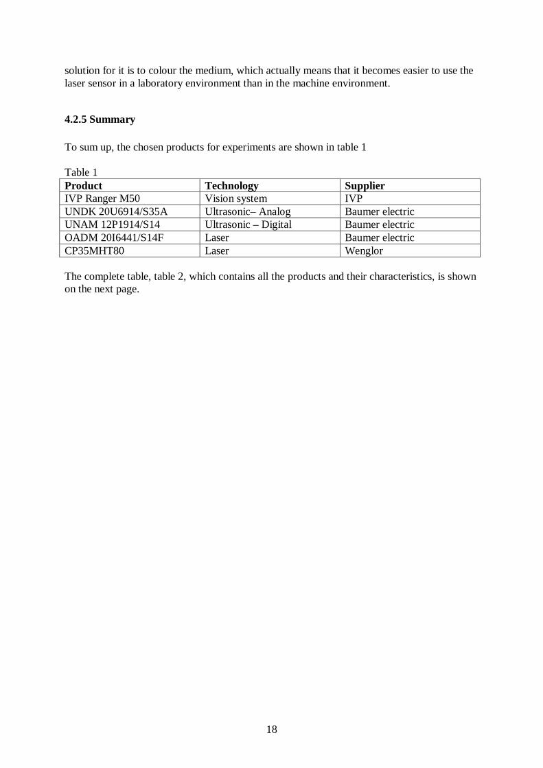
4.2.5 Summary To sum up, the chosen products for experiments are shown in table 1 Table 1 Product Technology Supplier IVP Ranger M50 Vision system IVP UNDK 20U6914/S35A Ultrasonic– Analog Baumer electric UNAM 12P1914/S14 Ultrasonic – Digital Baumer electric OADM 20I6441/S14F Laser Baumer electric CP35MHT80 Laser Wenglor The complete table, table 2, which contains all the products and their characteristics, is shown on the next page.

19

CP

35MH

T80

(Wenglor)

OA

DM

20I6441/S

14F

(Baum

er) U

NA

M

12P1914/S

14 (B

aumer)

SM

602 (H

yde Park)

UN

DK

20U

6914/S35A

(B

aumer)

UN

DK

30U

6113 (B

aumer)

IVP

R

anger M50

(IVP

)

Shape C

ompact

(Shapeline)

Prod

uct

(Com

pany)

La

ser

La

ser

Ultra

sonic

Ultra

sonic

Ultra

sonic

Ultra

sonic

Vision-

Syste

m

Vision-

system

Method

50-350

30-70

10-100

25.4-254

20-200

10-150

0-100

10-80

Range

of work

[mm

]

0.25

0.004-0.02

1.59

< 0.3

< 0.3

0.1 ≈ 0.05 R

esolution [m

m]

0.2

0.06-0.012

0.69 mm

0.5 mm

0.5 mm

Close

accuracy

Close

accuracy

Accuracy

8500

10615

2800

2500

3500

100 000

250 000

Price

[SE

K]

< 10

< 0.9

< 10

3 (Sta

ndard)

1.5 (Optim

al)

< 30

< 50

Se

e fre

quency

Se

e fre

quency

Response tim

e [m

s]

IP67

IP67

IP67

Wate

rtight

IP67

Wate

rtight

IP67

Wate

rtight IP

67 W

atertight

IP20

Ne

ed to be

e

nclosed

IP65

Environm

ent C

lass

Ana

log 0-10 V

Ana

log 4-20 m

A

0-10 V

Digita

l

Ana

log 0-30V

Ana

log 0-10 V

/10-0 V

Ana

log 0-10V

/10-0V

Ada

ptable

Ada

ptable

Output

signal

380 kHz

500kHz

350KH

z

300kHz

Upp till

10000 profile

/s

300-400 profile

s/s

Frequency

18-30 VD

C

12-28 VD

C

12-30 VD

C

12-24 VD

C

15- 30 VD

C

15 – 30 V

DC

12 - 24 VD

C

220-240 V,

150 W m

ax

Supply

extension voltage

6 7.5

6 8 Sounds

extension angle [º] *

Table 2

20

5

Formulation, realization and result of experiments This chapter describes the experimental procedure. The purpose with the experiments is to test the products described in chapter 4, see table 1. The results from the experiments can later be used for a final sensor choice.

5.1 Laboratory environment The test setup in the Tetra Pak R&D laboratory environment consists of a linear electric motor, of type LinMot [8], and an oscilloscope, Appendix 4, where the signals from sensors can be followed. A linear movement in one dimension is achieved with the motor and a motion control system. Finally there is a computer that is connected to the motion control system and the oscilloscope. Software for controlling the electric motor and software for sensor signal reading exists in the computer.

5.2 Vision system M50

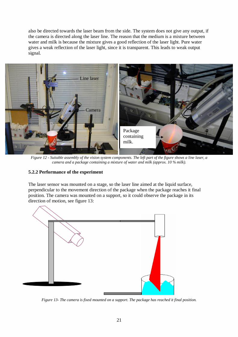
5.2.1 Formulation The reason why it is so interesting to examine the camera IVP M50, see Appendix 4, is that it can detect a full wave surface in a three-dimensional outline across the direction of motion, with very high speed. Apart from a picture from the waves extension in the travel direction and traverse direction it is also possible to record a vertical picture. This separates this camera technology from the two-dimensional camera technology. The system is built on the fact that the camera analyses the contour of the laser line. It is important to have a correct assembly of the camera and the laser line, see Figure 12. The left part of figure 12 shows a line sensor, a camera and a coca-cola package with a mixture of water and milk (approximately 10% milk). The laser sensor is placed above the package, while the camera is placed in an angle that makes it possible to look inside the package. The right part of figure 12 shows that, apart from looking into the package, it must

21

also be directed towards the laser beam from the side. The system does not give any output, if the camera is directed along the laser line. The reason that the medium is a mixture between water and milk is because the mixture gives a good reflection of the laser light. Pure water gives a weak reflection of the laser light, since it is transparent. This leads to weak output signal.

Figure 12 - Suitable assembly of the vision system components. The left part of the figure shows a line laser, a camera and a package containing a mixture of water and milk (approx. 10 % milk).

5.2.2 Performance of the experiment The laser sensor was mounted on a stage, so the laser line aimed at the liquid surface, perpendicular to the movement direction of the package when the package reaches it final position. The camera was mounted on a support, so it could observe the package in its direction of motion, see figure 13:

Figure 13- The camera is fixed mounted on a support. The package has reached it final position.

Line laser

Camera

Package containing milk.

22

After a suitable assembly of the optical components has been done, the next important factor comes for achieving a good output signal, namely threshold value. The values for level of laser light and background light become conclusive for the setting of the threshold value. The value is found in an experimental way, see figure 14.

Figure 14- Development of the right threshold value. The test is done on an adaptor with table as background.

The actual strength of light in a certain point is given by clicking with the mouse on several places in figure 14, which is a picture that the camera provides. The experiment shows that the laser light has strength of 255 while the background has strength of light of 71. The threshold value should lie in between those values. The explanation for this is that the camera must feel the strength of light that it has to analyse. With a few tries a graph like in figure 15 can be achieved, and it illustrates a profile of the liquid level, when it is in motion. Figure 15 shows a good profile of the liquid surface, without disturbance. It is not similar for all the profiles. By reproducing several profiles some disturbances can be found. This is of course not good, since those profiles are used when a 2D figure shall be described. The way to first build up a profile and later build a 2D figure from that, reduce the total work of building up a good 2D figure, since profiles gives a knowledge about the quality of the 2D figure. This means that if profiles are good then the 2D figure will also be good and vice versa.

23

Figure 15- A profile of a liquid surface.

5.2.3 Result and summary It has been rather simple to use the vision system. It has occurred that the Ranger GUI software has been shut down without any user action. IVP has always been willing to help us with computer support and has shown interest for our application. What we can read from figure 16 is that some disturbances exist in the signal, and these appear like big peaks, which show up from time to time. From the beginning it was not clear what it depended on. It was realised very soon that there was a connection between the fuss that occurs in the signal and the reflection from the laser. Since a liquid with relative good reflection is lighted in a package with relative small diameter, 57 mm, is it obvious that there will be undesired reflections from the laser sensor. In an attempt to change that several parameters were changed, from number of rows that the camera is working with, to the share of milk in the water- milk mixture. Choosing number of rows implies that sooner or later a limit will be reached. Too few rows do not give a sufficient measurement range vertically, but a reduction of the number of rows led definitely to a better output signal, since it almost eliminated the environment light. When we tried to adjust the reflection from the mixture by changing the share of milk when the liquid was in rest, we achieved a profile with very little disturbance. The problem cannot be completely avoided, since a liquid in motion means that the reflection from the laser sensor is going in all possible directions and sooner or later will end up in the camera as undesired information. The fact that the package inside is covered with aluminium is also a complication. It means that the reflection from the laser sensor will not be absorbed by the wall of the package. Increasing the share of milk improves the output signal a little bit.

24

It showed us that it was more difficult to get a good output signal than we had thought from the beginning. After some parameter changes a relatively good output signal can be achieved, see figure 16.

Figure 16 - 2D figure that is built on the surface profile from figure 15. The high peaks are disturbances in form of reflection from the laser light.

5.3 Experiments with ultrasonic sensor

5.3.1. Formulation The reason that an ultrasonic sensor was considered to be a possible solution was that it did carry out all the tasks that were requested for a sensor. Furthermore the ultrasonic sensor is cheaper compared to the other sensors. It is important to have a good mounting of the ultrasonic sensor in order to receive a good output signal. The sensor was mounted on a stand in such way, that it was close above the package. As figure 17 is showing, a stand was placed on a table at the final package position.

5.3.2 Execution of the experiment There was a digital and an analogue ultrasonic sensor, see Appendix 4 for specifications, that we evaluated. The experiment started with the digital ultrasonic sensor and the content in the package was pure water. Unfortunately we could only use the sensor to check if the liquid level was exceeding a certain level or not. We knew that from the beginning, but the reason why we used the digital sensor was just to test if the sonic beam angle was small enough for level detection.

25

Figure 17 - A wave is created in the package when it is moved. Up to the right side you can see an ultrasonic

sensor that shall detect the wave motions. The examination of the analogue ultrasonic sensor, with water, gave fairly good results. The disadvantage was that the sensor did lose the signal during some cycles of a measurement sequence. This sensor had a function, teach in, and by using that we achieved more accurate measurements. The experiment turned out much better after we had been using this tool, but the sensor did still lose the signal, as shown in figure 18:

Figure 18 - This figure illustrates the analogue ultrasonic sensor. The experiment is done with pure water. A vertical square corresponds to 1V and a horizontal square corresponds to 500 ms. The “Teach in” button is

used here. The Ordinary range of work is 20-200 mm, but now it is 20-80 mm.

Start position Final position

26

5.3.2.1 Analysis of the ultrasonic signals contact interruption The reason why the ultrasonic sensor loses the signal during some measurement periods is that the liquid surface deviates too much from the right angle. We have called it the critical angle and it is indicated with the symbol α

b. To calculate at which angle the signal disappears, i.e. the signal is not registered by the receiver in the ultrasonic sensor, we did an experiment, as shown in figure 19.

Figure 19 - The experimental setup for determination of the angle α b. The pulse from the ultrasonic sensor, the

plane object, point M, distance a, b and c are shown at the same time. A flat surface was moved towards the ultrasonic sensor until the object reached the sensors measurement range. The pulse from the ultrasonic sensor hits the flat object which can turn around at the point M. Too much turning means that the pulse at the reflection from the plane surface misses the receiver/ultrasonic sensor, which will result in an incorrect output. This is indicated by a light on the sensor. The distance b can be calculated at the same time as the lamp goes out, while the distance a, is the same during the experiment. When the distance b, is known from equation 4, it can be used to compute the searched angle α

b.

=a

bb arctanα (4)

By changing the ultrasonic distance range with the button “ Teach in“ and then repeat the experiment, the results according to Table 3 were acquired: Table 3 Range of

measurement [mm]

c * [mm]

αb **

[º]

110 7.92 Exp 1 20-200 65 7.92 60 10.2 Exp 2 20-100 40 10.2 50 11.3 Exp 3 20-80 35 11.3

* - The distance from the ultrasonic sensor to the flat object. ** - The critical angles that appear when the receiver/transmitter no longer gets the reflected pulse.

A plane object

M αb

a

b

Ultrasonic sensor

c

27

It is clear from Table 3 that a reduction of the measurement range means an increasing angle αb. At each experiment the distance from the ultrasonic sensor to the flat object has been

changed to check a possible effect of the distance on the critical angle. Table 3 shows the critical angle α

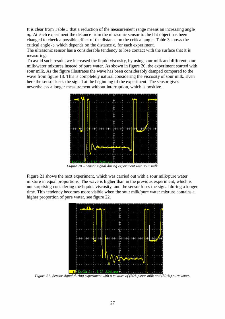
b which depends on the distance c, for each experiment. The ultrasonic sensor has a considerable tendency to lose contact with the surface that it is measuring. To avoid such results we increased the liquid viscosity, by using sour milk and different sour milk/water mixtures instead of pure water. As shown in figure 20, the experiment started with sour milk. As the figure illustrates the wave has been considerably damped compared to the wave from figure 18. This is completely natural considering the viscosity of sour milk. Even here the sensor loses the signal at the beginning of the experiment. The sensor gives nevertheless a longer measurement without interruption, which is positive.

Figure 20 – Sensor signal during experiment with sour milk. Figure 21 shows the next experiment, which was carried out with a sour milk/pure water mixture in equal proportions. The wave is higher than in the previous experiment, which is not surprising considering the liquids viscosity, and the sensor loses the signal during a longer time. This tendency becomes more visible when the sour milk/pure water mixture contains a higher proportion of pure water, see figure 22.

Figure 21- Sensor signal during experiment with a mixture of (50%) sour milk and (50 %) pure water.

28

Figure 22 - Sensor signal during experiment with a mixture of (25%) sour milk and (75%) water. No matter if sour milk or pure water is used, the ultrasonic sensor can not detect the waves that exceed a certain amplitude. The amplitude size is bounded to the angle of inclination α

b. It means that the sensor cannot detect the waves that occur in the beginning of the measurement sequence. It means that a part of important information about the waves performance will be lost.

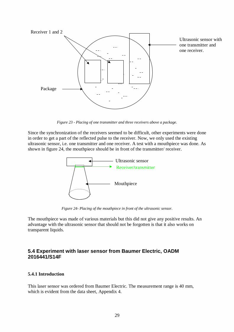
5.3.3 Result and summary It has been relatively easy to use the ultrasonic sensor. The sensor does not work for wave amplitudes that exceed approximately 15 mm. We tried therefore to change the sensors measurement range, which did lead to an improvement of the sensors output. The experiment with different viscosity showed that the sensor does not give a satisfactory result even when only sour milk is used. The reason why the ultrasonic sensor loses the contact with the medium is that the pulse sent from the sensor never comes back to the receiver. To get the pulse back to the sensor during all circumstances is difficult, especially when working with an ultrasonic sensor which has a big spreading angle. A change, which could improve the reflection, is an increase of the frequency. From table 2 one can find the frequency to be 380 kHz, which is high. Other ultrasonic sensors with higher frequency hardly exist today in the same price range. Another idea is to have several receivers at the same time but still one transmitter. An example can be one transmitter and three receivers, as shown in figure 23. The ultrasonic sensor, that was tested, has one transmitter and one receiver. A good signal can be achieved by synchronizing the receivers. A problem that has occurred in earlier similar experiments is that the pulse from the transmitter is reflected in all possible directions. It is really difficult to keep track of the relevant reflected pulse and thereby the real output.

29

Figure 23 - Placing of one transmitter and three receivers above a package. Since the synchronization of the receivers seemed to be difficult, other experiments were done in order to get a part of the reflected pulse to the receiver. Now, we only used the existing ultrasonic sensor, i.e. one transmitter and one receiver. A test with a mouthpiece was done. As shown in figure 24, the mouthpiece should be in front of the transmitter/ receiver.

Figure 24- Placing of the mouthpiece in front of the ultrasonic sensor. The mouthpiece was made of various materials but this did not give any positive results. An advantage with the ultrasonic sensor that should not be forgotten is that it also works on transparent liquids.

5.4 Experiment with laser sensor from Baumer Electr ic, OADM 2016441/S14F

5.4.1 Introduction This laser sensor was ordered from Baumer Electric. The measurement range is 40 mm, which is evident from the data sheet, Appendix 4.

Receiver 1 and 2

Package

Ultrasonic sensor with one transmitter and one receiver.

Ultrasonic sensor

Mouthpiece

Receiver/transmitter

30

If we compare it with the desired range, 82 mm, we see that the sensor does not fulfil the requirement. The reason why we actually ordered the sensor was the good indications that we got about the sensors qualities, and if it should not work, the company did have a sensor with acceptable measurement range that we could buy instead. The tests were carried out with the sensor OADM 2016441/S14F, which we could change to a sensor that had the desirable range, if the measurement range was not sufficient. We could just order the sensor with the assumption that we were sure to buy it, because Baumer Electric did not have the sensor here in Sweden and then they were forced to order it from Switzerland. We did not want to buy the sensor before we had tested it. The other demands were fulfilled, which was positive. A drawback that is already known was that the laser sensor could not detect the waves performance on the pure water surface or other transparent liquid surfaces. It requires us to find a suitable liquid, i.e. a kind of liquid that has the same property as water. Such resemblance can be achieved by mixing a small quantity of milk or white colour with the pure water, because of a little quantity milk or colour in the water gives a negligible change on the waters viscosity. This means that the laser sensor cannot be used in continuous production.

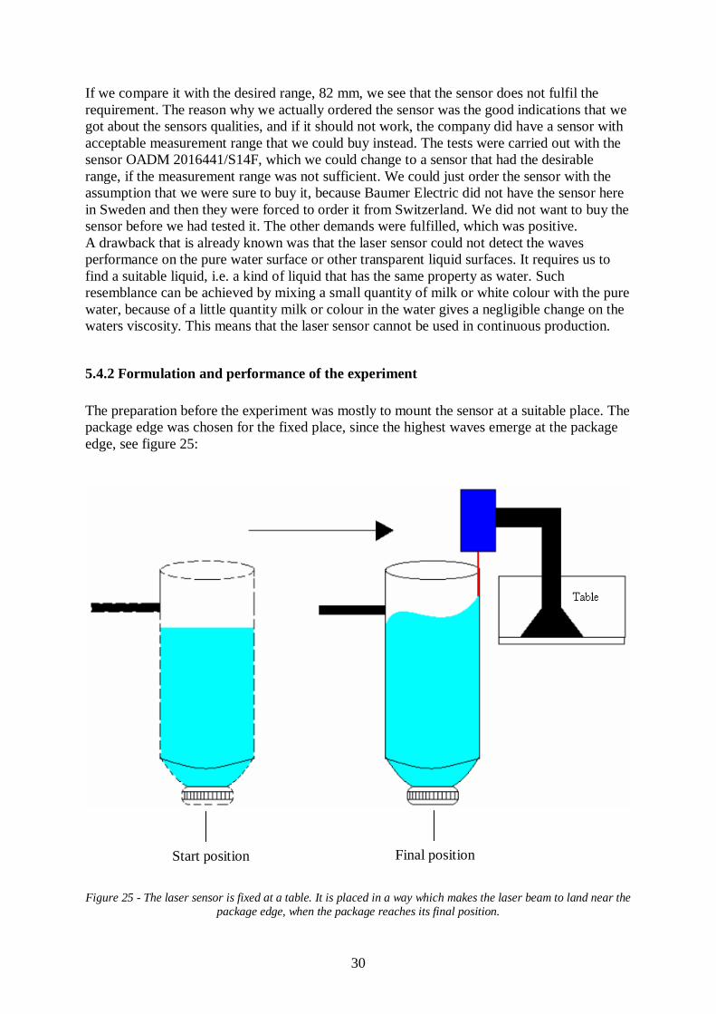
5.4.2 Formulation and performance of the experiment The preparation before the experiment was mostly to mount the sensor at a suitable place. The package edge was chosen for the fixed place, since the highest waves emerge at the package edge, see figure 25:

Figure 25 - The laser sensor is fixed at a table. It is placed in a way which makes the laser beam to land near the

package edge, when the package reaches its final position.

Start position Final position

31

The package was moved from the start position to the final position. The laser sensor could detect the waves at the final position. This was executed several times.

5.4.3 Result and summary The experiment to detect the waves was limited because the measurement range was too small for the waves. It was not possible to mount the sensor in a way which makes the output complete. What we could see was a part of the vertical output, i.e. short waves could be detected but not high waves. It was not a concern, because we already knew that the range of measurement was too small. Something that concerned us was the character of the output, which had a lot of interruptions in form of unexpected high peaks. Probably, the peaks come from direct reflection of the laser beam which comes in to the sensor and is registered as incorrect information. It was hard to avoid such reflections, since the laser sensor could not do that. The sensor had probably no algorithms to do that.

5.5 Experiment with laser sensor from Wenglor, CP35 MHT80 This laser sensor did clearly fulfil the formal technical and economical demands on a desirable sensor, see Appendix 4 for specifications.

5.5.1 Design and execution of the experiment with a laser sensor In order to detect the wave performance during the entire movement process, the laser sensor was steadily assembled on the movable stand that moves the package and represents the movement, see figure 26. The laser sensor was placed such that it could detect the highest waves that could occur on the liquid level, accordingly at the package edge. As shown in the figure 26, there is an in-between stop position. The figure represents the complete movement process for an actual packaging machine. The liquid in the package consisted of a water-milk mixture, with 95 % water and 5 % milk. The reason for that was to achieve a viscosity that was close to the water viscosity. This was due to the fact that water gives the highest waves compared to other liquids during a movement process.

Figure 26- The laser sensor is mounted on a moveable state which moves the package. The laser beam shall land

near the edge of the package, where the biggest waves appear.

PPosition at sealing Position between filling and sealing Position at filling

32

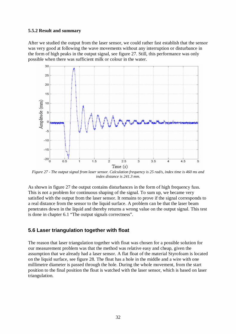
5.5.2 Result and summary After we studied the output from the laser sensor, we could rather fast establish that the sensor was very good at following the wave movements without any interruption or disturbance in the form of high peaks in the output signal, see figure 27. Still, this performance was only possible when there was sufficient milk or colour in the water.

Figure 27 - The output signal from laser sensor. Calculation frequency is 25 rad/s, index time is 460 ms and index distance is 241.3 mm.

As shown in figure 27 the output contains disturbances in the form of high frequency fuss. This is not a problem for continuous shaping of the signal. To sum up, we became very satisfied with the output from the laser sensor. It remains to prove if the signal corresponds to a real distance from the sensor to the liquid surface. A problem can be that the laser beam penetrates down in the liquid and thereby returns a wrong value on the output signal. This test is done in chapter 6.1 “The output signals correctness”.

5.6 Laser triangulation together with float The reason that laser triangulation together with float was chosen for a possible solution for our measurement problem was that the method was relative easy and cheap, given the assumption that we already had a laser sensor. A flat float of the material Styrofoam is located on the liquid surface, see figure 28. The float has a hole in the middle and a wire with one millimetre diameter is passed through the hole. During the whole movement, from the start position to the final position the float is watched with the laser sensor, which is based on laser triangulation.

33

Figure 28 - In the figure can we see a float on the actual medium. We can see that the float keeps a certain

distance to the package edge. Figure 29 illustrates the output signal of the laser sensor during movement process. The float movements are caused by the waves on the liquid surface and from the output signal we can see that the laser sensor detects the float movements surprisingly well. This is not sufficient, since we do not know the answer to the most important question yet and that is: “How high are the waves close the package edge”? It is not possible to place the float sufficiently close to the package edge, since the float has a circular appearance and will create friction with the package edge. Further the plate will get an inclination and thereby create friction with the metal wire. If we compare figure 29 with figure 27, that illustrates the experiment with only laser sensor, we clearly see that the amplitude is much higher in figure 27. It is nevertheless logical, since we in this case do not measure close to the package edge. It leads to lower indicated amplitude of the waves.

Figure 29- The output signal from the laser sensor when laser is used together with a float.

34

5.7 Final choice of sensor The following was used to finally choose a sensor

• Chapter 3.1 an outline of the table, together with table 2. • Experimental results and summaries. • Tips and advices from experienced engineers.

We did choose the laser sensor CP35MHT80 from the company Wenglor. This laser sensor had several advantages compared to the other sensors:

• It was really easy to see were on the liquid surface the laser sensor was measuring and at the same time we could measure close to the package edge.

• It gave a stable output signal. • It was relatively cheap. • It worked very well on liquid mixtures with low percentage milk or a small amount

of colour in pure water, so that the mixture viscosity could be assumed to be the same as pure waters viscosity.

• It was not time consuming to adjust the laser sensor for getting a good output. • The laser sensor had good protection against the machine environment.

Of course, the laser sensor had naturally some possible or clear disadvantages:

• It measures only in one point. It complicates the general picture for the wave movement.

• The laser beam might penetrate through the liquid and consequently give a wrong output signal.

• It does not work with transparent liquids. It will complicate a future online implementation of the laser sensor in a packaging machine.

Having a good sensor at our disposal gave us new hope that the continuation of this work would give us good results.

35

6

Analysis of the chosen laser sensor The analysis deals with how to choose the most important sensor property and thereby examine those with different experiments. In the end some of the achieved results from the experiments can be compared to the data sheet from Wenglor. The best way to verify the sensor quality is to start out from the sensor application and the data sheet for the sensor. When this is done, the sensor properties below appear as important:

• The output signals correctness*. • Reaction time or response time. • Absolute accuracy and relative accuracy. • Resolution. • Algorithm**.

*- The signals correctness is a property that has been mentioned in chapter 5.5.2. It is important to find out a suitable way to examine the laser beam and find out if it penetrates through the liquid before it reflects back. **- Almost every sensor uses an estimation algorithm that can be more or less complex. The last property depends on what the sensor shall manage. From the sensors data sheet we can get the information that the laser sensor CP35MHT80 has several functions. Those are used for:

• Adjustment of the sensors range of measurement. • Selection of the sensors output signal, 0-10V or 4-20mA. • Filtering position 1, 2 and 3.

6.1 The output signals correctness In the following chapter the output signals conformance with the reality is examined. The main reason is to check if the laser beam penetrates through the liquid, which would imply that the output signal from the laser sensor is incorrect. A well-known property from physics says that it is very difficult for sound to penetrate in liquid, [9]. It means that the ultrasonic sensor, UNDK 20U6914/S35A, becomes suitable for a correct measurement of distance l, see

36

figure 30. The output signal from the ultrasonic sensor shall then be compared to the output signal from the laser sensor. This should verify the laser sensors reliability. A problem with the ultrasonic sensor was that it was not possible to see where on the surface the sonic pulse is reflected. Therefore it becomes difficult to measure exactly at the same place with the laser sensor and the ultrasonic sensor. Instead of that we decided to measure with the sensors as figure 30 shows. The distance from the laser beam to the package edge and the distance from ultrasonic pulse to the other package edge was the same and are indicated with x in figure 30. A force F, which is directed into the paper, is used to make waves in the package. All that was done just for that the waves in the package should be as similar as possible, where the sensor was measuring. The distance x was chosen to 15 mm, because it was the most suitable.

Figure 30 - The experiments principal appearance. To be able to compare the output signals from the sensors, the range of measurement for the sensors was changed to the same, 50-200 mm. In the beginning of the experiment a force F was used to create waves in the package. We realised that only small waves could be measured. The ultra sonic sensor could not detect the waves when they became bigger. Therefore it was decided that the package should be moved up and down, while the sensors were measuring from above the package. It means that the liquid surface in the package did not tilt itself sufficiently enough so that the ultrasonic sensor could lose the contact with the liquid surface. The result of a measurement is represented in figure 31. From figure 31 we can conclude that the laser sensor was measuring at least as well as the ultrasonic sensor. There is a little phase difference between the outputs. This is explained by the coming experiment, which shows that the laser sensor reacts faster than the ultrasonic sensor does.

l

Package x x

F

Laser sensor Ultrasonic sensor

Up and down pull up.

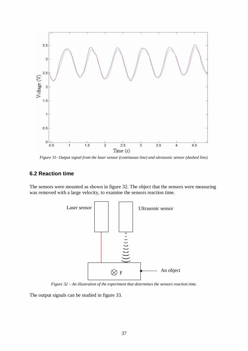
37

Figure 31- Output signal from the laser sensor (continuous line) and ultrasonic sensor (dashed line).

6.2 Reaction time The sensors were mounted as shown in figure 32. The object that the sensors were measuring was removed with a large velocity, to examine the sensors reaction time.

Figure 32 – An illustration of the experiment that determines the sensors reaction time. The output signals can be studied in figure 33.

Laser sensor

F An object

Ultrasonic sensor

38

Laser sensor Micrometer

Figure 33 - Output signal from the laser sensor (continuous line) and ultrasonic sensor (dashed line). The slope of the continuous line is steeper than the dashed one.

It is clearly evident that the laser sensor reacts faster than the ultrasonic sensor. See figure 33. It is in accordance with the data sheet for the sensors, see Appendix 4.

6.3 How exact can the laser sensor measure? The following experimental setup was used to examine how accurately the laser sensor can measure. See figure 34. We used a micrometer, as a direct reading apparatus for measurements, together with the laser sensor.

Figure 34 - The experimental setup. The laser sensor is pointing at the object that is connected to the

micrometer. The true value for the change of distance can be verified by measuring a distance-change with a micrometer. The micrometers moving piston can be moved with a screw. The screw has a scale where one turn corresponds to 0.5 mm that gives a desirable measurement value in combination with a longitudinal millimetre scale. During time the laser sensor detects the change of distance, which is expressed in volts. Three experiments were carried out, where the laser sensor detected three different distances that had been accomplished with the micrometer. Those were two, four and five millimetres. The laser sensor was adjusted to the measurement range, 50 mm to 200 mm. Since the output signal from the laser sensor is from 0-10 V, this means that 1 Volt corresponds to

39

(200-50)/10=15 mm. The ability to achieve a level of agreement, between the true values for the change of distance and the measurement test result from the laser sensor gives an expression for the measurement accuracy.

6.3.1 Measuring two millimetres distance-change The output signal from the laser sensor decreases from 4.112 to 3.972 V, which corresponds to a difference of 0.14 volt, se figure 35. It means that the laser sensor registers a change of

mm 1.21514.0 =⋅ . An error in measurement, of 0.1 mm is achieved, i.e. the absolute accuracy is 0.1 mm while the relative accuracy is the ratio of the absolute accuracy and the actual change of distance value. In this case the relative accuracy is 0.1/2 = 0.05, i.e. 5%.

Figure 35 - Output signal from the laser sensor, when the distance from the laser sensor to the micrometer is

changed. The actual distance change is 2 mm.

6.3.2 Measuring four millimetres distance-change In figure 36 below it can be seen that the signal increases from 3.972 to 4.112 V, which correspond to a difference of 0.26 volt. It means that the laser sensor registers a change of

mm. 9.31526.0 =⋅ The reason why the output signal from the laser sensor was rising instead of decreasing was that the micrometer screw was turned opposite, compared to the last experiment, compare figure 35 to figure 36. Like in the last experiment, a measurement error of 4.0 – 3.9 = 0.1 mm is achieved, i.e. it represents a measure of the absolute accuracy. The relative accuracy is 0.1/4 = 0.025, i.e. 2, 5%. The reason why the relative error has gone from 5% to 2.5% can depend on reading errors.

40

Figure 36 – Laser sensor output. The distance change is 4 mm.

6.3.3 Measuring five millimetres distance-change According to figure 37 below, the signal increases from 3.963 to 4.305 V. It means that the laser sensor registers a distance-change of mm 13.515342.0 =⋅ .

Figure 37 - Laser sensors output. The distance change is 5 mm.

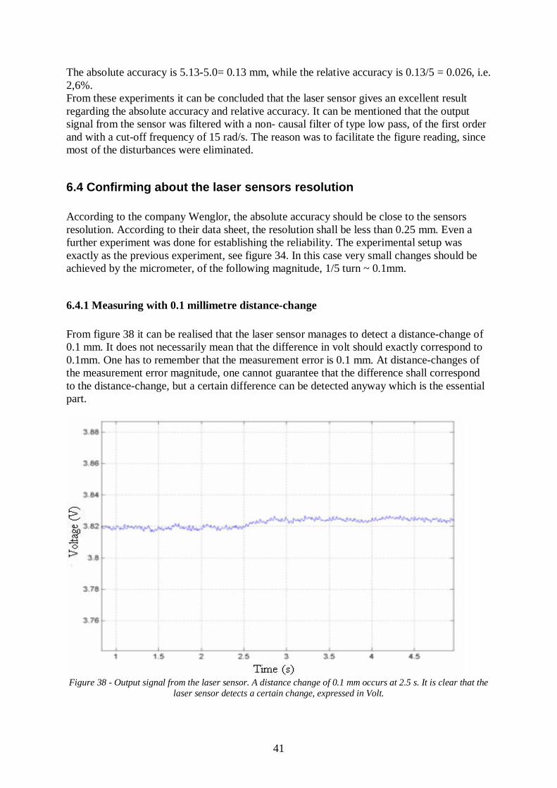
41

The absolute accuracy is 5.13-5.0= 0.13 mm, while the relative accuracy is 0.13/5 = 0.026, i.e. 2,6%. From these experiments it can be concluded that the laser sensor gives an excellent result regarding the absolute accuracy and relative accuracy. It can be mentioned that the output signal from the sensor was filtered with a non- causal filter of type low pass, of the first order and with a cut-off frequency of 15 rad/s. The reason was to facilitate the figure reading, since most of the disturbances were eliminated.

6.4 Confirming about the laser sensors resolution According to the company Wenglor, the absolute accuracy should be close to the sensors resolution. According to their data sheet, the resolution shall be less than 0.25 mm. Even a further experiment was done for establishing the reliability. The experimental setup was exactly as the previous experiment, see figure 34. In this case very small changes should be achieved by the micrometer, of the following magnitude, 1/5 turn ~ 0.1mm.

6.4.1 Measuring with 0.1 millimetre distance-change From figure 38 it can be realised that the laser sensor manages to detect a distance-change of 0.1 mm. It does not necessarily mean that the difference in volt should exactly correspond to 0.1mm. One has to remember that the measurement error is 0.1 mm. At distance-changes of the measurement error magnitude, one cannot guarantee that the difference shall correspond to the distance-change, but a certain difference can be detected anyway which is the essential part.

Figure 38 - Output signal from the laser sensor. A distance change of 0.1 mm occurs at 2.5 s. It is clear that the

laser sensor detects a certain change, expressed in Volt.

42

In order to make it possible to detect a difference the sensor signal has to be filtered. It is impossible to read the figures without filtering, due to all the disturbances. Also here a non-causal low-pass filter of first order is used, with a cut-off frequency of 10 rad/s. Also here it can be established that the laser sensor has a good resolution. Everything is in agreement with the data sheet.

6.5 Analysis of the curve shape After examining the curves that were recorded with the oscilloscope, it could be realized that the chosen sensor, CP35MHT80, followed the waves that were created during the indexing movement. The setup is represented in figure 39:

Figure 39- Connection of the measurement equipment. In order to prevent the sealing surface from being soaked with liquid drops, there are two important characteristics that have to be considered, namely the maximal amplitude and the damping of the liquid. In order to get an indication of the wave height, we can carefully measure how high the wave liquid level is when the package is at rest and further measure the sealing surface, see figure 40. Quite intuitively we can see from figure 40, that the wave height cannot increase higher than 41mm, since the sealing surface will be soaked. 9 41

Figure 40 - The limitation for the wave high. It is limited by the packages sealing surface.

Oscilloscope

Computer

The package sealing surface

Normal liquid level when the package is at rest.

43

It is very important that the wave is damped as much as possible after the movement process. The reason is that the liquid shall rest on the normal liquid level before the next indexing motion. If not, it is likely that the second movement will induce a higher wave than the first one. Those facts will be the basis for scoring of waves.

6.6 Repeatability Before we could go on with next part of the thesis, which is scoring of waves, we had to check the repeatability of the waves. The reason is simple but important. If we could prove that the repeatability of the waves was high then we could go on with next part. Otherwise, there is no meaning with scoring of waves, which is quite obvious. The repeatability of the waves was investigated by running an identical experiment several times. The index time was 460 ms and the calculation frequency 25 rad/s. Figure 41 and 42 show the experimental results:

Figure 41 - The wave amplitude from one experiment. Index time = 460 ms and the calculation frequency w0 = 25 rad/s.

The number of executed experiments was 10. In the next figure only five experiments are represented, see figure 42. It is the reason why the figure is fairly sharp. If signals from all experiments should be plotted in same figure, then this would lead to an unclear figure. When the measurement from the five experiments is plotted on top of each other it is seen that the measurements are very close. To get a measure of how close the experiments are, the standard deviation is calculated for each time instant. The calculation of the standard deviation σ (t) is given by,

( ) ∑∑==

=−=10

1

10

1

2 )(101

)( here t,)()(91

)(i

iei

ei tatmtmtatσ

44

ai(t) is the wave amplitude of experiment i = 1…10, and me(t) is the average of all experiments. The standard deviation is shown in figure 43 which shows that the standard deviation is approx. 1 mm for large oscillations and 0.2 for small oscillations. It was established that the standard deviation is small compared to the wave amplitude that is shown in figure 41. The conclusion is that the repeatability for the waves is very high. This means that we can go further with the scoring of the signals.

Figure 42 - The wave amplitudes from five experiments. Index time = 460 ms and calculation frequency w0 =25rad/s.

Figure 43- The standard deviation from 10 experiments. Calculation frequency is 25 rad/s, index time is 460 ms and indexing distance is 241.3 mm.

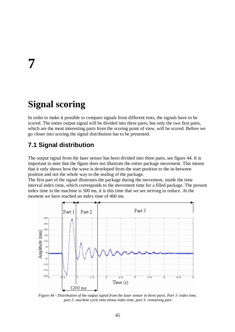
45

7

Signal scoring In order to make it possible to compare signals from different tests, the signals have to be scored. The entire output signal will be divided into three parts, but only the two first parts, which are the most interesting parts from the scoring point of view, will be scored. Before we go closer into scoring the signal distribution has to be presented.

7.1 Signal distribution The output signal from the laser sensor has been divided into three parts, see figure 44. It is important to note that the figure does not illustrate the entire package movement. This means that it only shows how the wave is developed from the start position to the in-between position and not the whole way to the sealing of the package. The first part of the signal illustrates the package during the movement, inside the time interval index time, which corresponds to the movement time for a filled package. The present index time in the machine is 500 ms, it is this time that we are striving to reduce. At the moment we have reached an index time of 460 ms.

Figure 44 - Distribution of the output signal from the laser sensor in three parts. Part 1- index time, part 2- machine cycle time minus index time, part 3- remaining part.

46

The second part shows how the wave is developed when the package has stopped. It is occurring during the time that corresponds to the machine cycle time minus index time, in this case 740 ms. The next package in a packaging machine will be filled during those milliseconds. The machine cycle time is constant (1200 ms). It is important to mention that a decrease of the index time leads to an increase of the filling time. So if the index time can be decreased there will be more time left for filling.

7.2 The signal score of part 1

During the first part of the sensor signal it is important to keep the wave under the sealing surface. Assume that the distance between the liquid surface and the sealing surface is called �

t. For the package in figure 4 that distance is equal to 4.1 cm. Foam is created in the package, during the filling process. To take consideration for that a foam factor has been introduced, which is represented by ff . A lot of factors influence the foam height and thereby the factor ff. Some of those factors are the package dimensions, the liquids filling velocity and the characteristics of the filling liquid. For the package in figure 4 the foam factor is approximately 0.6 cm. With consideration to that the distance between the liquid surface and the “sealing areas” is reduced to 3.5 cm. This distance is corresponding to the highest amplitude that a wave can have during indexing of a package, from the filling position to the sealing position when consideration to the foam factor is taken. It is even called for the maximal allowed amplitude, which is expressed by At. When we produce a measure for the wave size, we use the maximum amplitude as an upper limit for the wave. With help of such a limit the following demands can be implemented in a function, whose task is to score the actual wave amplitude compared to the maximal allowed amplitude:

1. Actual wave amplitude which is higher than the maximal allowed amplitude leads to a low score. An even larger excess leads to an even lower score. Since a wave with an amplitude which exceeding the maximal allowed amplitude is not desired we want the reduction of the score to occur exponentially.

2. A wave with actual amplitude smaller than 3.5 cm shall have a good score. The larger the difference is between the actual wave amplitude and the distance 3.5 cm the better the score should get. The increase of the score shall be linear.

To illustrate it further a function is formulated which fulfils those demands. Assume that the actual maximal wave amplitude is represented by A1. Then the difference between At and A1 can be indicated by ε . Now we search for a function f that shall describe how good an output signal is for different value of ε . According to figure 45 the function f(ε ) is a compounded function, i.e. we have: During the first interval we have a decreasing exponential function that decreases very rapidly when ε moves from 0 to -0.5 cm. At approx. -0.5 cm is f(ε ) ≈ 0. It means that if the actual wave amplitude increases over the permitted amplitude with 0.5 cm or more, the score for the

<<+⋅≤<⋅

==⋅

[cm] 3.5 0 for

[cm] 0 1.5-for )(1 εεγ

εαεεβ

m

efb (5)

47

output signal will be close to zero. All that agrees with demand one. That the interval reaches only -1.5 cm is explained with fact that a bigger difference implies that the actual wave amplitude is coming outside of the package.

Figure 45 – Score function for part 1 as function of ε . The constant α is used when we want to adjust a level where the function f(ε ) initiates when ε is equal to zero and it is in principle similar to the constant m that occurs in the function for the second part. The constant

β is used for determining how fast the exponential function will

decrease. A bigger value of β gives faster decrease towards zero. Figure 45 shows the

appearance for the compounded scoring function for the first part of the sensor signal. For ε less than or equal to zero we have an exponential function and for positive ε we have an increasing linear function. The other interval is reached to 3.5 cm, even if we know that ε will never reach that value since it means that the amplitude for the actual wave would be very close to zero. The constant γ is used to change the slope of that line which represents the function f(ε ) during the second interval. Figure 45 shows the function f for the parameter values: α

= m = 3 γ = 1 The constant

β is not so easy to see in the figure 45. To make the exponential function

decrease as in the figure 45 we have used β = 11. The choice of these constants is only one

possible choice. There is not any bigger idea behind the choice of those values, but they were chosen in order to make it possible to create figure 45.

m

εβα ⋅⋅em+⋅εγ

)(εf

[cm] ε

Score

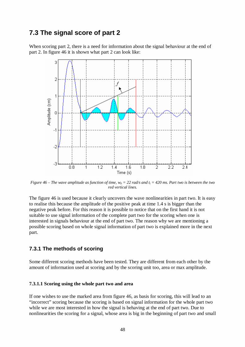
48

7.3 The signal score of part 2 When scoring part 2, there is a need for information about the signal behaviour at the end of part 2. In figure 46 it is shown what part 2 can look like: Figure 46 – The wave amplitude as function of time, w0 = 22 rad/s and ti = 420 ms. Part two is between the two

red vertical lines. The figure 46 is used because it clearly uncovers the wave nonlinearities in part two. It is easy to realise this because the amplitude of the positive peak at time 1.4 s is bigger than the negative peak before. For this reason it is possible to notice that on the first hand it is not suitable to use signal information of the complete part two for the scoring when one is interested in signals behaviour at the end of part two. The reason why we are mentioning a possible scoring based on whole signal information of part two is explained more in the next part.

7.3.1 The methods of scoring Some different scoring methods have been tested. They are different from each other by the amount of information used at scoring and by the scoring unit too, area or max amplitude.

7.3.1.1 Scoring using the whole part two and area If one wishes to use the marked area from figure 46, as basis for scoring, this will lead to an “incorrect” scoring because the scoring is based on signal information for the whole part two while we are most interested in how the signal is behaving at the end of part two. Due to nonlinearities the scoring for a signal, whose area is big in the beginning of part two and small

49

in the end of part two, should be the same for a signal whose area is small in the beginning of part two and big in the end of part two. This is “incorrect” from our point of view. The scoring can be improved by multiplying part two with a function f which is small in the beginning of part two but is getting bigger towards the end of part two, see figure 46. The function f must not necessarily be a linear one. For example some other useable functions are x2 and the exponential function. With those functions it will be possible to estimate the later part of part two more than early part of part two which leads to a better representation on scoring.

7.3.1.2 Scoring using a period Because we are in principle interested in knowing the signal behaviour near the end of the part two, it is meaningful to use the last period of part two as signal information when scoring the waves. To calculate the length of a period several methods have been used:

• By starting at the end of part two and then moving left the two zero positions, which are lying near each other, can be found. The difference in time between two zero positions lying near each other is corresponding to approximately half a period. The reason that the difference is not exact depends on nonlinearities. To get a whole period the difference is multiplied by two.

• If a third zero position is found the length of a period should correspond to the

difference between the first and the third zero position.

• Each time a new zero position is found the length of a half of position can be calculated. With these half periods a mean value can be calculated and finally the whole period.

• Using FFT - Fast Fourier Transforms to identify the dominant frequency for part two

and then calculate the length of period.

• Using the derivative of the signal and checking the zero positions for the derivative the positions for peaks can be found. In this case a half of period corresponds to the time between two peaks. When more zero positions are introduced in calculations the similar discussion is valid as for the original signal.

Observe that the signal value almost never is equal to zero at the end of the part two. Peak values do not occur at the end of part two. The first zero position or peak value occur to the left of the end of part two. Consideration for the difference between the end of part two and the first zero position or peak value has to be done when the start for a period has to be calculated. Once the period is known the maximum amplitude has to be found. The received amplitude represents the base of the scoring. The mentioned methods use a whole period for the calculation of the maximal amplitude and with it the scoring. One can mention that when calculating the length of a period in some cases the whole signal information from part two is used.

7.3.2 Nonlinearities influence on the scoring In figure 46 the most part of the nonlinearities lie in part two. This is not always the case. In figure 47 the same problem is shown, but in this case the nonlinearities appear in a different

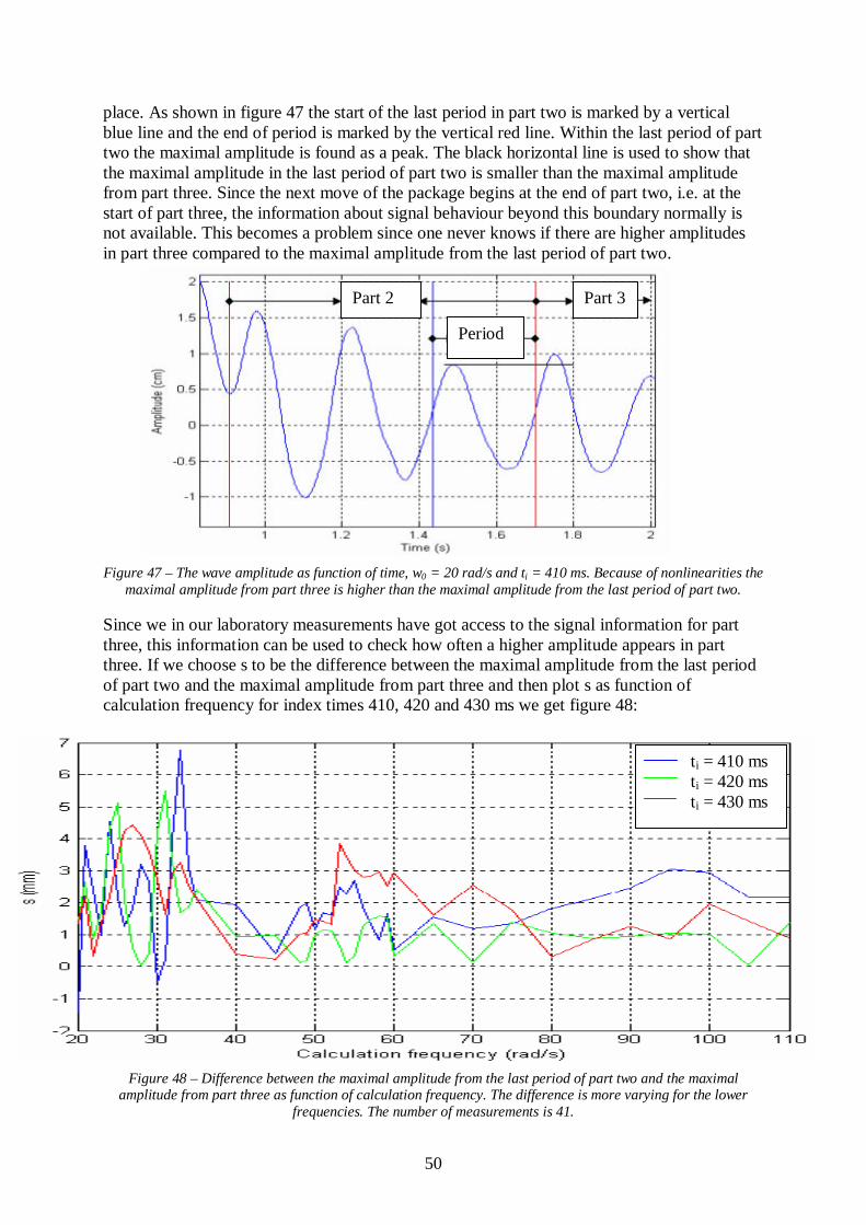
50

place. As shown in figure 47 the start of the last period in part two is marked by a vertical blue line and the end of period is marked by the vertical red line. Within the last period of part two the maximal amplitude is found as a peak. The black horizontal line is used to show that the maximal amplitude in the last period of part two is smaller than the maximal amplitude from part three. Since the next move of the package begins at the end of part two, i.e. at the start of part three, the information about signal behaviour beyond this boundary normally is not available. This becomes a problem since one never knows if there are higher amplitudes in part three compared to the maximal amplitude from the last period of part two. Figure 47 – The wave amplitude as function of time, w0 = 20 rad/s and ti = 410 ms. Because of nonlinearities the

maximal amplitude from part three is higher than the maximal amplitude from the last period of part two. Since we in our laboratory measurements have got access to the signal information for part three, this information can be used to check how often a higher amplitude appears in part three. If we choose s to be the difference between the maximal amplitude from the last period of part two and the maximal amplitude from part three and then plot s as function of calculation frequency for index times 410, 420 and 430 ms we get figure 48:

Figure 48 – Difference between the maximal amplitude from the last period of part two and the maximal amplitude from part three as function of calculation frequency. The difference is more varying for the lower

frequencies. The number of measurements is 41.

Part 2 Part 3

Period

ti = 410 ms ti = 420 ms ti = 430 ms

51

Figure 48 is showing, for ti = 410 ms, s being negative in two cases of 41 which corresponds to approximately 5 %. (Observe that during the experiments 41 calculation frequencies have been tested in the interval 20 to 110 rad/s.) The fact that s is negative in some cases means that the maximal amplitude from part three exceeds the maximal amplitude from the last period of part two. In the first case, at 20 rad/s, the excess is 1.4 mm while in the other case, at 30 rad/s, the excess is 0.5 mm. It shows that when index time ti = 410 ms there are a few cases where s is negative and at the same time the size of s in this cases is small. The difference, s, is never negative for index times ti = 420 ms and ti = 430 ms, which is good. The remaining index times which we have studied are represented in figure 49:

Figure 49 – Difference s as function of calculation frequency. The number of measurements is 24. Concerning the difference, s, for index time ti = 440 ms then one can see from figure 49 that s is negative for four calculation frequencies of totally 24 measurements. That corresponds to approximately 17 % and is a quite high value. A quite positive fact is that the negative s value is going down only to -0.773 mm when w0 = 80 rad/s, that is approximately 7 % of the maximal amplitude from the last period of part two. The difference, s, for index time ti = 450 ms appears to be negative only in one case of 24, at w0 = 23 rad/s, which is about 4 %. The negative s value at w0 = 23 rad/s is -0.3 mm which is approximately 2.6 % of the maximal amplitude from the last period of part two. For index time ti = 460 ms no negative s values appear, which is good. Another property of the difference, s, which becomes visible in figure 49, is that the s value varies more for lower calculation frequencies. An important fact which is possible to realize by studying figure 49 is that the curves seem to follow each other relatively well in some short intervals, while in the other intervals this does not appear at all. This is an indication of how difficult it can be to discover when s is getting negative without using the signal information from part three. We have studied the behaviour of curves more and the aim was to try to figure out when s is getting negative. Some ideas have appeared and have been tested:

• Is there some nonlinearity and in that case where?

ti = 440 ms ti = 450 ms ti = 460 ms

52

Since nonlinearities can appear in part two it is recommended to check if there are any. The closer a nonlinearity is to the end of part two the bigger is the probability for s to be negative. If nonlinearity does not shows up in part two when nonlinearity has appeared in the end of part one, is it going to appear in part three or is it going to not appear at all? If nonlinearity should appear in the first part then we know there is a probability that another smaller nonlinearity appears in the end of part two. If nonlinearity does not appear in part one or part three then we don’t know anything about the sign of s in a machine environment.

• Does the difference between positive and negative peaks influence the sign of s?

By studying some signals one can quickly realize that there is no connection between this difference and the sign of s, even when area is used for connection seeking. Afterwards it is easy to declare that there is no easy way to find out when s is getting negative provided that signal information from part three is not in use. Obviously, this fact means that nonlinearities can lead to worse scoring.

7.3.3 The choice of scoring method The reason that we pick up nonlinearity in our explanation is the fact that it has been used to choose scoring method. Something that is important for the scoring of part 2 is that the signal information that has been used for examining, shall lie close the end of part 2, but not too close and not too far. Since the end of the signal information is determined by the machine cycle time it is necessary that the position of start of the signal information is determined. If the start of the signal information lies too close to part two then the share of negative s will increase and if it lies too far the risk of non-desirable areas taken into the scoring will increase. A non-desired area is an area that deviates much from the signals behaviour close to the end of part 2. The method that manages to solve both conflicts in the best way, negative s and “correct” information area, is the FFT method. This method is the basis for computing s in figures 48 and 49, whose results have shown to be best. To show that the FFT- method is most convenient regarding the undesired areas is not easy. One way is to compare the different signals for different methods for a number of cases and from that conclude the most suitable method. Another way is elimination of methods. The method which uses two zero positions to calculate the period length leads to that the amount of negative s increases dramatically. Therefore we did not use this method. A similar discussion holds for methods that use two zero positions for the derivate of the signal for calculating the period length. A slightly better result is achieved when three zero positions are used for calculating a period length, especially when the zero position is used for the derivate, i.e. the period starts two peaks and one valley or one peak and two valleys to the left of the end of part two. The FFT method is even better since it gave the same start position for the last period in part 2 irrespectively of the calculation frequency w0, which results in fewer calculations when several signals shall be evaluated at the same time. Another characteristic for the FFT-method is that it in all cases for one and the same index time and independent of the calculation frequency, gives the natural frequency of the oscillation for the package content.

53

The third and decisive advantage with FFT-method is that the signal interval that it generated is most suitable for scoring and that the method generates a small number of negative s that can be neglected.

7.3.4 FFT- method for development of period length and scoring The first thing is to low-pass filter the sensor signal with a non causal filter. A first order filter with cut-off frequency of approx. 100 rad/s was used. It is easy to get a period length when the index time, ti, and the machine cycle are known, since those define part 2. Suppose that the signal for part 2 is represented with a vector Y2. The absolute value for the Fourier transform for the Y2 is achieved by writing Y2_fft = abs(fft(Y2)) in Matlab7. By choosing the frequency points

0̂0̂

)1(,...,,0 wNww −=

where

sNTw

π20̂

=

and where N is the number of signals value and Ts is the sample interval. A vector w is generated and contains frequencies where the Fourier transform is calculated. With help of the following commands the position for the maximal value for Y2_fft can be found: [maxvalue pos] = max(Y2_fft) The position for the maximal value in vector Y2_fft shows where the dominant frequency is in the vector w. When the searched frequency is achieved by the command f = w(pos) the searched period length can be computed with the following formula:

tp = 2π /f where f is in [rad/s] With help of tp the time position when the last period in part 2 starts can be computed. Then the signal of the last period of part 2 will be known and it can be represented by a vector called Ytp. From the signal, Ytp, the maximal absolute amplitude can be found and called A2. Finally the following simple formula is used for scoring:

2

22 A

bδ= (6)

The amplitude value, A2, is in the denominator since a bigger amplitude value should give a worse score value and opposite. In order to recognize this relation in equation (6) the relation has not been included in constant

δ2 which is used to suit the achieved score value for the

output signals of second part to the score value for the output signals of first part.

7 More information about Matlab can be found in [10].

54

7.4 Score combination of parts 1 and 2 Our goal is to score the entire wave. Therefore the scoring from part 1 and 2 can be compared in some way. The most suitable and simplest way is to add part 1 and part 2. A constant that we call

δ1 can be used for adaptation of score level for part 1 while the constant

δ2 is used for

adaptation of score level for part 2. Sometimes it can be desirable to compare score values from part one for different calculation frequencies and then it is necessary to hold score values of the first part separated from score values of the second part.

7.5 Experiments In order to get a set of output signals from the laser sensor extensive experiments have been done. The experiments were done systematically where the index time and the calculation frequencies were changed. The index time was changed from 410 ms to 460 ms with 10 ms increment, while the calculation frequency was changed from 20 rad/s up to 110 rad/s occasionally with a less well defined increment. Sometimes the increment was 1 rad/s and sometimes 5 rad/s. The increment magnitude depends on the difference between the sensors output signals for different calculation frequencies. In some cases the difference between two nearby calculation frequencies was small. It led to the fact that we used a bigger increment in the calculation frequency. When the difference was big a smaller increment in the calculation frequency was used.

7.5.1 Performance of the experiment A change of the index time and the calculation frequency in the Excel program MinEnergy gave different position profiles. They were used in the software LinMot for down loading profiles to the control system that gave the desired motion. The laser sensor output signals were saved as text documents, *.csv, which later could be treated in MatLab. In that way we could use several output signals that could be scored.

7.5.2 Validation with help of the sensor output sig nals In the beginning we had chosen to examine the similarity between the results from equation 5 and 6 with the laser sensors output signals that is scored.

7.5.2.1 Agreement for the output signals from the first part Figure 50 shows the scoring for the output signals of the first part as function of calculation frequency. The curve from figure 50 is valid for scoring of the first part for the output signals of the laser sensor, i.e. during the first 420 ms of the motion. The horizontal red line is corresponding to wave amplitude equal to 3.5 cm, i.e. to the maximal allowed wave amplitude. We can see that the scoring function has some positive and negative peaks. According to the definition of the function the output signal from the laser sensor shall be good at the positive peaks and worse at the negative peaks. We have used the output signals

55

from the laser sensor for some different calculation frequencies to examine it. The first comparison shows results for frequencies where the lowest and the highest score occurs, i.e. frequency 45 rad/s and 55 rad/s respectively.

Figure 50 – Score for part 1 as function of the calculation frequency. The index time is 420 ms, the indexing distance is 241.3 mm and parameters from part 7.2 are used.

In figure 51 output signals from the laser sensor are shown for those frequencies. The motion starts at 0.5 s, where the output signals first part starts. The vertical red line shows where the second part of output signals starts while the horizontal line shows the maximal wave amplitude, At. It is clearly evident from figure 51 that the green curve, that has the calculation frequency 55 rad/s, is better out of scoring aspect. It is clearly shown in figure 50 also. It shows that the scoring works.

Figure 51 - The wave amplitudes as function of the time for w0 = 45 rad/s and w0 = 55 rad/s. Index time is 420 ms and the indexing distance is 241.3 mm.

45 rad/s 55 rad/s

56

The next comparison shows results for the frequencies 20 rad/s and 21 rad/s. According to figure 50 the difference in the output signals amplitude should be very small. Figure 52 shows a comparison between those frequencies. By studying figure 52 it can be observed that the difference between the amplitudes is small too. By taking a closer look, we can see that the green curve has its maximal amplitude over the blue curve in part 1, which means that the blue curve shall have a better score than the green curve. It is reflected in scoring, see figure 50. Of course a large selection of calculation frequencies has been compared and there is no doubts that figure 50 is built on the signals that we achieved from the laser sensor. At the same time the simple equation 5 is confirmed, that it can be used for scoring of part 1.

Figure 52 – The wave amplitude as function of time for w0 = 20 rad/s and w0 = 21 rad/s. The index time is 420 ms and the indexing distance is 241.3 mm.

7.5.2.2 The second part of the output signal A similar examination is done of the second part. In figure 53 we show a scoring for the second part as function of the calculation frequency. The calculation frequencies that have been chosen are 23 rad/s, 34 rad/s and 48 rad/s respectively. The two first corresponds to the peaks one and two in figure 53 while the last correspond the fourth peak. The wave amplitude difference should not be big between the signals with the calculation frequencies 23 and 34 rad/s but a bit bigger between those and the signal with the calculation frequency of 48 rad/s.

20 rad/s 21 rad/s

57

Figure 53 – The score for part 2 as function of the calculation frequency. The index time is 420 ms and the indexing distance is 241.3 mm.

Figure 54 shows signals for the chosen calculation frequencies: Figure 54 – The wave amplitude as function of time for w0 = 23 rad/s, w0 = 34 rad/s and w0 = 48 rad/s. The two

vertical lines mark the beginning respectively the end of the last period of part 2. If we take a closer look at the amplitudes, around time 1.5 s, we can see that the green curve has “biggest” minimum, the blue comes after and the red is the last one. Observe that the red curve has it absolute maximal amplitude value exactly at the beginning of the period. It is an example of that the scoring does work even when the maximal amplitude value for different

23 rad/s 34 rad/s 48 rad/s

58

signals lie at different point of times. We do not exclude that there may be signals that generate incorrect scores because of this. We have not done very much to examine that accurately, but we think that it is important to examine that before one can establish that the scoring method works for all signals. On those signals that we have had access to, the scoring has worked fairly well. The example from figure 54 shows that the scoring algorithm is correct, but there is a sense that the score for the red curve should be better since the amplitude for it at approximately 1.5 s is lower than at the start of the period. We can say that in the example from figure 54 we want to score the red curve according to its amplitude at the time 1.5 s and not according to the amplitude at the start of the period. But if we do that it will increase the risk for influence from negative s values. We are forced to do it in that way since we do not know the third part of the laser sensor signals in a packaging machine. We motivate the choice of our scoring method with the fact that it is simple and easy to understand and make use of.

7.5.2.3 Conclusions By using curves from scoring and curves from the laser sensor we have shown that scoring functions for part one and part two give good results, especially for part one. One can certainly wonder what happens when scoring of a whole wave is applied. Similar analysis clearly shows good results that should be intuitive. When validity is used for scoring functions in the real machine application we are of course not satisfied with signals from a laser sensor that is measuring only one point on the surface. Complex behaviour of the waves in a package can lead to mismatch of waves behaviour that can be negative for the scoring process.

7.5.3 Validation by recording wave movements Another way to compare the scoring functions with reality is to record wave movements. For example a digital video camera can be used. For a good scoring process the function from figure 45 should be reflected in the pictures from a recorded film which shows the maximal wave amplitudes. The following is valid for the figures which show recorded wave movements:

• Index time for all movements is 420 ms.

• The white arrow in figures shows direction of package motion.

• The figure to the left shows the wave 1/25 s before the maximal wave amplitude is registered – the figure in the middle. In the figure to the right the wave is shown 1/25 s after the maximal wave amplitude.

• An especially chosen liquid, which gives nice pictures, has been used when recording

wave movements.

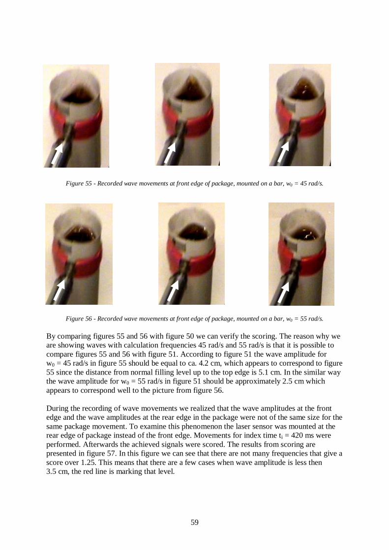
59

Figure 55 - Recorded wave movements at front edge of package, mounted on a bar, w0 = 45 rad/s.

Figure 56 - Recorded wave movements at front edge of package, mounted on a bar, w0 = 55 rad/s.

By comparing figures 55 and 56 with figure 50 we can verify the scoring. The reason why we are showing waves with calculation frequencies 45 rad/s and 55 rad/s is that it is possible to compare figures 55 and 56 with figure 51. According to figure 51 the wave amplitude for w0 = 45 rad/s in figure 55 should be equal to ca. 4.2 cm, which appears to correspond to figure 55 since the distance from normal filling level up to the top edge is 5.1 cm. In the similar way the wave amplitude for w0 = 55 rad/s in figure 51 should be approximately 2.5 cm which appears to correspond well to the picture from figure 56. During the recording of wave movements we realized that the wave amplitudes at the front edge and the wave amplitudes at the rear edge in the package were not of the same size for the same package movement. To examine this phenomenon the laser sensor was mounted at the rear edge of package instead of the front edge. Movements for index time ti = 420 ms were performed. Afterwards the achieved signals were scored. The results from scoring are presented in figure 57. In this figure we can see that there are not many frequencies that give a score over 1.25. This means that there are a few cases when wave amplitude is less then 3.5 cm, the red line is marking that level.

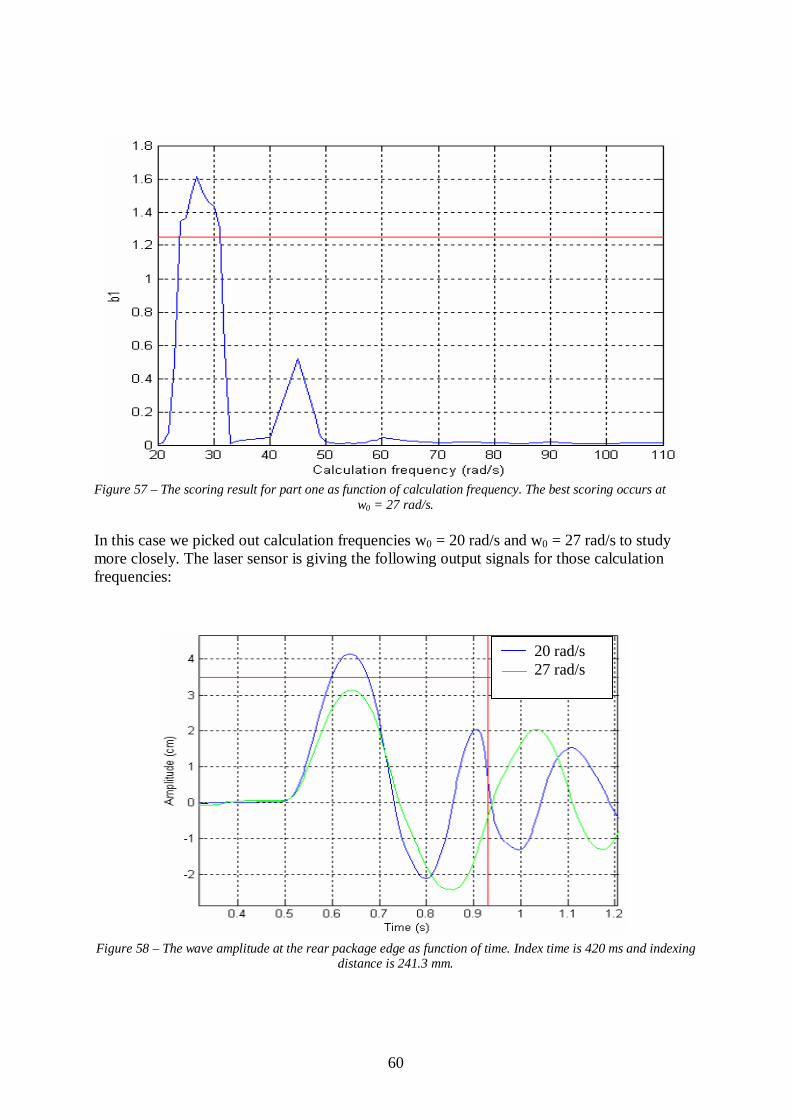
60

Figure 57 – The scoring result for part one as function of calculation frequency. The best scoring occurs at w0 = 27 rad/s.

In this case we picked out calculation frequencies w0 = 20 rad/s and w0 = 27 rad/s to study more closely. The laser sensor is giving the following output signals for those calculation frequencies:

Figure 58 – The wave amplitude at the rear package edge as function of time. Index time is 420 ms and indexing distance is 241.3 mm.

20 rad/s 27 rad/s

61

The wave amplitudes for those calculation frequencies are shown in figures 59 and 60:

Figure 59 - Recorded wave movements at rear edge of package, mounted on a bar, w0 = 20 rad/s.

Figure 60 - Recorded wave movements at rear edge of package, mounted on a bar, w0 = 27 rad/s. By comparing figures 59 and 60 with figure 58 a similar discussion about recording wave movements at the rear package edge is as valid as the discussion about recording wave movements at the front package edge. Because of the complexity which appears when waves of the second part of the output signal appear, we were able to record wave movements only for the first part of the laser output signal and thereby we were able to verify scoring for the first part only. Validation of the second part was done by a comparison between scoring, i.e. the laser output signals, and what we saw with our eyes.

7.5.3.1 Conclusion By recording the wave movement with a digital SONY video camera, we could take a closer look at the wave behaviour during the movement process for the package. Thereafter we could establish that the laser sensor could catch up the highest peaks of the waves most of the time. One reason why it is not like that for all the cases is that the wave which is on its way up starts to rotate, which leads to that the highest peak is not showing up on one and the same place in the package. A solution to improve the situation is to buy an extra sensor that could be mounted beside the existing sensor. It would certainly catch up some of the highest amplitude but with help of two laser sensors that are placed beside each other a possible

62

rotation of the waves can be detected. It would naturally lead to better understanding for the behaviour of the waves.

7.6 Comment to the scoring To evaluate how good a wave is, it is not enough to only look at the waves at the front of the package edge, or the waves at the rear edge. This is clearly evident from figure 61:

Figure 61 – The scoring of part 1 for index time 420 ms. It is clearly evident that the waves performance at the

front edge is considerably separated from the waves performance at the rear edge. It is clearly shown that a good score is almost impossible to achieve for index time 420 ms, since the score at the front edge and the back edge respectively counteract each other. The scoring for the front edge has two clear peaks, one at 20 rad/s and one at 35 rad/s, while the scoring for the rear edge has one clear peak at 27 rad/s. We can say that when the scoring is good for the front edge then it is poor for the rear edge. Something that is interesting and should be observed is the scoring for high calculation frequencies. It is clearly evident from figure 61 that for ca. w0 = 52 rad/s and higher the scoring is quite stable. But if we for example choose the calculation frequency at w0 = 27 rad/s to get best value of the green curve then we have to consider following. Because of mechanical system in a packaging machine the acceleration path got to be changed from the ideal. This means that in the reality we get an acceleration path which corresponds to calculation frequency bigger or less then 27 rad/s. Because such calculation frequencies are in a very unstable region, i.e. the scoring variations are big, then such a choice can lead to a real bad score and by that to big wave amplitude. At the same time this example shows that sometimes there is no good score for calculation frequencies bigger then 52 rad/s, see the green curve in figure 61. All this leads to following

Front edge Rear edge

63

conclusion. When the choice of the calculation frequency has to be made then it is recommended to start with a high value. If a good score for higher frequencies dose not exist then lower calculation frequencies can be examined, but now we have to take consideration to the mechanical system which can change the ideal acceleration path. All this is shown to be typical for index times, 410, 420 and 430 ms. In the future our hope is to be able to identify when good scoring pattern appears. If this could be possible then the choice of the calculation frequency would be drastically simplified. By choosing a high enough calculation frequency the probability of good scoring will be better and thereby a better wave behaviour can be obtained. A proposal to simplify the choice of calculation frequency is to do an extensive set of experiments. With those experiments it will be possible to develop tables, which should show the choice of calculation frequency for different packages, viscosity and index times. Such experiments would take long time but they would be meaningful.

64

8

Concluding remarks Mattias Grundelius has, in his doctors’ theses, described several methods to develop the acceleration paths when the parameters, w0 and ti, are known. One of these methods is known as “Minimum energy solution” and the idea behind this method is based on the criterion that it is desirable to get as small energy as possible at the end of the movement, i.e. when a new movement is to be started. The calculations of the minimum energy acceleration reference have been implemented in an Excel spreadsheet. The method “Minimum energy solution” assumes that the calculation frequency has to be the natural frequency of the content in the package. Experiments have shown that in reality a frequency which is 10 % less then the natural frequency gives the best result, i.e. the best wave performance. A way to get this frequency automatically is to analyze the frequency of the content in a package with a sensor. When the natural frequency is known then it is easy to estimate 90 % of it and use it as an input to the program MinEnergy. To be able to get the natural frequency it is necessary to do two steps:

• Develop equipment for detecting the wave movements. • Analyze the output signal and develop a method to be able to score the outputs.

Because of lack of time we could not reach the third part of the theses which is the biggest and probably most interesting part, but we know that we have improved the chances for dealing with this part of theses. In the next part of this chapter the two first parts of work are concluded.

8.1 Conclusion To get a direction for what kind of equipment we were looking after we made a picture of the desired sensor with specifications. When this was done we started to search after the desired sensor. In the beginning we used catalogues and Internet as searching methods and even a trade fair in Herning in Danmark was visited. All this helped us to get a complete picture of the accessible sensors on the market. At the same time we realized sensor possibilities and limitations for our application. Because the development is going forward within some techniques we decided to test the sensors which seemed to be most suitable for our application. After an experimental examination of the chosen sensors the laser sensor from the

65

company Wenglor was our choice as the most suitable sensor. This sensor gave an output which we thought was good enough for the price. Next part dealt with analysis of the laser sensor output signals. The interesting and meaningful sensor performances were tested by some experiments. The result from those experiments was used to verify sensor performances from data sheet. This verification proved that the results from the experiments agreed with the data sheet. A repeatability test was necessary since we wanted to be convinced about that the scoring of the sensor output signals was meaningful. Before we begun with scoring it was suitable to split the output signal into the three parts. Only the two first parts were scored since those two contain almost all necessary information when the whole signal should be scored. Score of part one has been simple since a relatively simple function was used. To score part two has been a real challenge, since some of the nonlinearities appear randomly during part two of the sensor output signal and destroy a simple scoring based on the area below part two of the signal. A scoring whose idea is based on the maximal wave amplitude from the last period of part two has been tested instead. Several methods for finding the length of the last period of part two were tested and the most suitable method was FFT. By recording wave movements with a digital camera we have successfully showed that the scoring agrees with the reality. Because of the complexity which appears when waves of the second part of the output signal appear, we were able to record wave movements only for the first part of the laser output signal and thereby we were able to verify scoring for the first part only. Validation of the second part was done by a comparison between scoring, i.e. the laser output signals, and what we saw with our eyes.

8.2 Other remarks and future work During recording of the wave movements we have discovered that the waves at the rear edge of a package are different from the waves at the front edge of the same package. This is evident in figure 61. Of course, this means that it is not enough to use only one sensor for scoring of whole wave. In the lab environment it is possible to measure in two different ways to see the shape of the waves at the other edge of the package, i.e. where the laser sensor is not placed:

1. Move the laser sensor to the other edge of the package.

2. Let laser sensor be at same edge of the package but change the direction of the package movements.

Since none of these methods can be used in a machine environment one has to have two laser sensors. Another interesting discovery, which has been done during recording of wave movements, is that the maximal wave amplitude doesn’t appear at the same place in a package all the time. By experiments one can prove how big the probability is for the maximal wave amplitude to appear at the same place using different inputs. If the probability is big then it is acceptable to have only one sensor at same edge of a package. Otherwise the need for two laser sensors at the same edge of a package is increasing, i.e. four sensors totally. To have four laser sensors detecting over a package is almost impossible since the space over a package which have a diameter of 57 mm is quite small. Another disadvantage is the increased cost. The advantage with having two sensors near each other gives possibilities to detect wave rotations in a package.

66

When the scoring functions were completed we needed some signals which should be scored. Experiments were made before the scoring functions were completed. During those experiments some positive discoveries have been made. For example, we could see that an increase of the calculation frequency, w0, for some index times leads to better wave movements. The thing which we could not miss was the stability for higher calculation frequencies, see figure 61. Because of lack of time we have not examined when those cases appear and why? If one is able to give an answer to this question then the choice of inputs to the program MinEnergy should certainly be automatic and thereby the auto method from figure 2 should be complete. An important observation concerning simplification of the choice of inputs to the Excel program MinEnergy has been done. The future wave performance after that the package has stopped depends on the wave performance an instant before the package has been stopped. If the wave behaviour, before the package is stopped, seems to be in a certain way then this leads to small wave amplitudes after the package is stopped. By choosing w0 one can iteratively try to control the desirable behaviour before the package is stopped. This can possibly be automatic since a good detection of wave behaviour is possible and working criteria about what means an improvement of wave behaviour is accessible and included in our scoring functions. Several important discoveries have been done during the work. Discoveries show how hard it is to reach the goal with a complete method according to figure 2, especially a continuous production working method. The positive thing is that we have successfully developed equipment for detection of wave movements and criteria about what means an improvement of wave behaviour is accessible and included in our scoring functions. Furthermore there are many ways to go on with the work. Several interesting theoretical or experimental ways are mentioned in Mattias doctors’ theses in chapter 7.3. An important thing is the fact that Mattias method, Minimum energy solution, is only one method for developing accelerations paths. Irrespective of which way one chooses to work further there is still much to do and to examine.

67

Appendix 1 – The program MinEnergy Sheet 1- Specifications

Sheet 2 – Index diagram

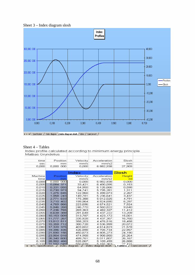
68

Sheet 3 – Index diagram slosh

Sheet 4 – Tables

69

Sheet 5 – CamConvert

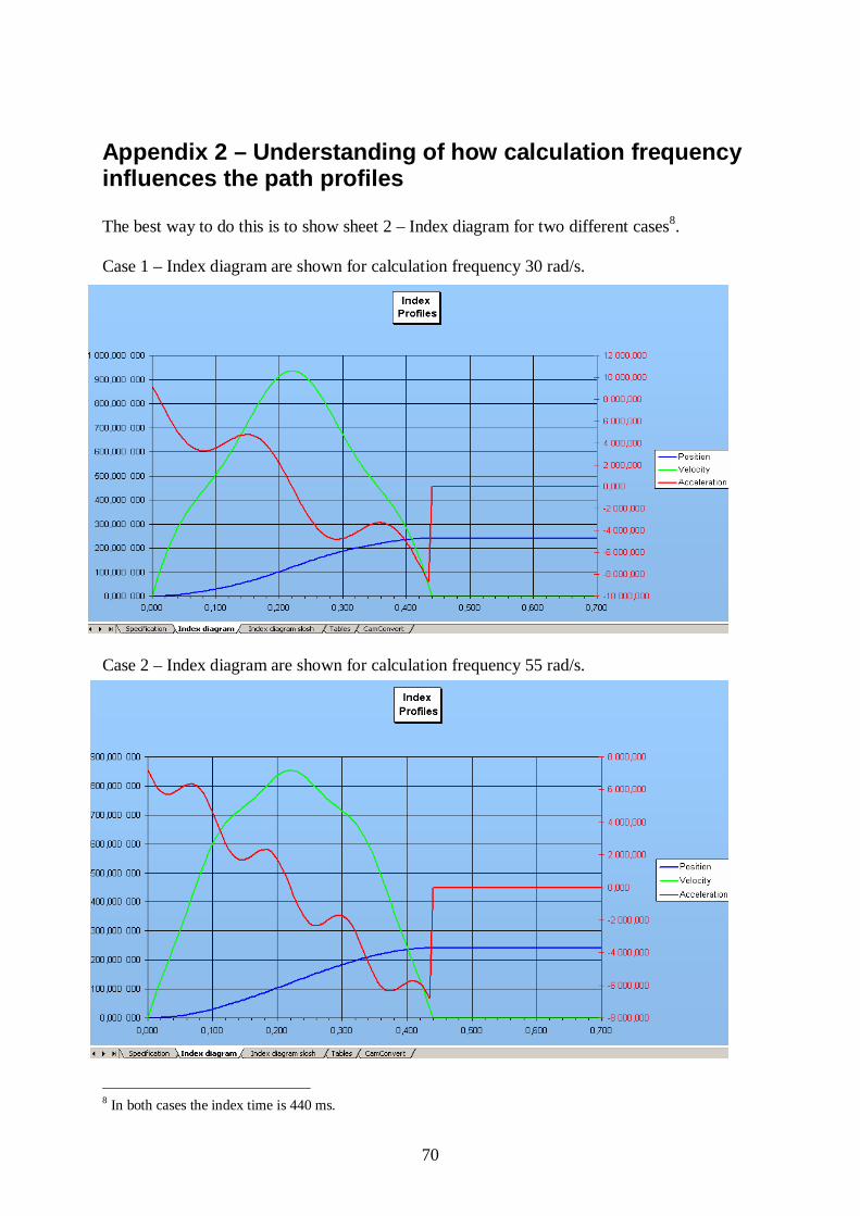
70

Appendix 2 – Understanding of how calculation frequ ency influences the path profiles The best way to do this is to show sheet 2 – Index diagram for two different cases8. Case 1 – Index diagram are shown for calculation frequency 30 rad/s.

Case 2 – Index diagram are shown for calculation frequency 55 rad/s.

8 In both cases the index time is 440 ms.

71

By studying case 1 and case 2 several conclusions can be made:

1. It is clear that a different choice of calculation frequency gives different acceleration paths and velocity paths.

2. An acceleration path with calculation frequency 55 rad/s has more peaks and valleys

than an acceleration path with calculation frequency 30 rad/s. This leads to that the difference in acceleration values between two near peaks or valleys is less when calculation frequency at 55 rad/s is used.

3. Bigger maximal velocity appears when calculation frequency at 30 rad/s is used.

Conclusions 1 and 2 are more important than conclusion 3. The most important thing to remember when one is trying to understand how calculation frequency influences the paths can be summarized by following words: Different calculation frequencies can be used to change the number of peaks and valleys, on an acceleration path, during index time. This leads to that the size of amplitude for acceleration or velocity can be changed too. Observe, it is not completely known how one should choose calculation frequency to get a desired acceleration or velocity path.

72

Appendix 3 – The source code for macro BuildCurve Sub BuildCurve() ' ' Short command: Ctrl+a ' ' Variables definitions Dim SlutPos, SlutPosString, StartPos, AntalCeller, EndPos Dim Omrode As String, SavePlace As String, SaveName As String, WholeName As String Dim s1 As String ' Selecting "MinEnergy.xls" window, changing some colours and reading the save path Sheets("Specification").Select ' Selecting the sheet "Specification" Range("J21").Select ' Selecting the cell "J21" ActiveCell.Clear ' Clearing the cell With Selection.Interior ' Fixing the background colour of the cell .ColorIndex = 34 ' -||- .Pattern = xlSolid ' -||- End With ' Fixing the background colour of the cell SavePlace = Range("I20") ' Reading the path there the curve will be saved SaveName = Range("H21") ' Reading the name of the curve WholeName = SavePlace & "\" & SaveName & ".svk" ' Making whole path name ' Clears old cell values there new values should be read Sheets("CamConvert").Select ' Switch to the window "CamConvert" Range("A6:A1000").Select ' Selecting cells "A6:A1000" Selection.Formula = "=0" ' Selected cells gets value zero Range("F7:F1000").Select ' Selecting cells "F7:F1000" Selection.Clear ' Selected cells are cleared ' Selecting desired area in sheet "Tables" which should be copied Sheets("Tables").Select ' Switch to the sheet "Tables" StartPos = Range("G8") ' Getting start position of selected area SlutPos = Range("G10") ' Getting end position of selected area AntalCeller = SlutPos - StartPos ' Calculates the number of selected cells SlutPosString = Format(SlutPos) ' Integer to string Omrode = "B" & StartPos & ":" & "B" & SlutPosString ' Making the string "Omrode" Range(Omrode).Select ' Selecting Omrode which should be copied Selection.Copy ' Selected Omrode is copied ' Switches to the sheet "ComConvert" and past the copied cells starting at right position Sheets("CamConvert").Select ' Switching Range("A1").ClearComments s1 = Range("A1").Value s2 = Sheets("CamConvert").Range("A2") s3 = Sheets("CamConvert").Range("A3") s4 = Sheets("CamConvert").Range("A4") Range("F7").Select ' Selects start position

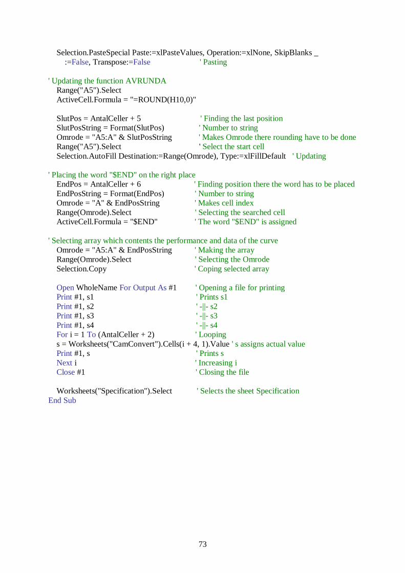
73

Selection.PasteSpecial Paste:=xlPasteValues, Operation:=xlNone, SkipBlanks _ :=False, Transpose:=False ' Pasting ' Updating the function AVRUNDA Range("A5").Select ActiveCell.Formula = "=ROUND(H10,0)" SlutPos = AntalCeller + 5 ' Finding the last position SlutPosString = Format(SlutPos) ' Number to string Omrode = "A5:A" & SlutPosString ' Makes Omrode there rounding have to be done Range("A5").Select ' Select the start cell Selection.AutoFill Destination:=Range(Omrode), Type:=xlFillDefault ' Updating ' Placing the word "$END" on the right place EndPos = AntalCeller + 6 ' Finding position there the word has to be placed EndPosString = Format(EndPos) ' Number to string Omrode = "A" & EndPosString ' Makes cell index Range(Omrode).Select ' Selecting the searched cell ActiveCell.Formula = "$END" ' The word "$END" is assigned ' Selecting array which contents the performance and data of the curve Omrode = "A5:A" & EndPosString ' Making the array Range(Omrode).Select ' Selecting the Omrode Selection.Copy ' Coping selected array Open WholeName For Output As #1 ' Opening a file for printing Print #1, s1 ' Prints s1 Print #1, s2 ' -||- s2 Print #1, s3 ' -||- s3 Print #1, s4 ' -||- s4 For i = 1 To (AntalCeller + 2) ' Looping s = Worksheets("CamConvert").Cells(i + 4, 1).Value ' s assigns actual value Print #1, s ' Prints s Next i ' Increasing i Close #1 ' Closing the file Worksheets("Specification").Select ' Selects the sheet Specification End Sub

74

Appendix 4 – Sensors data sheets

75

Analog ultrasonic sensor, UNDK 20U6914/S35A

76

Digital ultrasonic sensor, UNAM 12P1914/S14

77

Laser sensorn OADM 20I6441/S14F

78

Laser sensor, YT87MGV80 – old version Laser sensor, CP35MHT80

79

Oscilloscope, Tek THS7

80

Bibliography [1] Matias Grundelius, (2001): Method for control of liquid slosh, PhD thesis ISRN LUTFD2/TFRT--1062--SE. [2] IEC 60529. [3] Per-Erik Lindahl, William Sandquist,(1996): Mätgivare, Mätning av mekaniska storheter, Studentlitteratur. [4] Karl-Erik Nordgren, (1997): Industriell mätteknik, Liber utbildning. [5] www.ivp.se [6] www.baumerelectric.com [7] www.wenglor.com [8] LinMot PS01 – 37 x 240. www.linmot.com [9] Göran Gönsson, (1988): Elementär våglära, Teach Support . [10] www.mathworks.com

81

82

På svenska Detta dokument hålls tillgängligt på Internet – eller dess framtida ersättare – under en längre tid från publiceringsdatum under förutsättning att inga extra-ordinära omständigheter uppstår.

Tillgång till dokumentet innebär tillstånd för var och en att läsa, ladda ner, skriva ut enstaka kopior för enskilt bruk och att använda det oförändrat för ickekommersiell forskning och för undervisning. Överföring av upphovsrätten vid en senare tidpunkt kan inte upphäva detta tillstånd. All annan användning av dokumentet kräver upphovsmannens medgivande. För att garantera äktheten, säkerheten och tillgängligheten finns det lösningar av teknisk och administrativ art.

Upphovsmannens ideella rätt innefattar rätt att bli nämnd som upphovsman i den omfattning som god sed kräver vid användning av dokumentet på ovan beskrivna sätt samt skydd mot att dokumentet ändras eller presenteras i sådan form eller i sådant sammanhang som är kränkande för upphovsmannens litterära eller konstnärliga anseende eller egenart.

För ytterligare information om Linköping University Electronic Press se förlagets hemsida http://www.ep.liu.se/ In English The publishers will keep this document online on the Internet - or its possible replacement - for a considerable time from the date of publication barring exceptional circumstances.

The online availability of the document implies a permanent permission for anyone to read, to download, to print out single copies for your own use and to use it unchanged for any non-commercial research and educational purpose. Subsequent transfers of copyright cannot revoke this permission. All other uses of the document are conditional on the consent of the copyright owner. The publisher has taken technical and administrative measures to assure authenticity, security and accessibility.

According to intellectual property law the author has the right to be mentioned when his/her work is accessed as described above and to be protected against infringement.

For additional information about the Linköping University Electronic Press and its procedures for publication and for assurance of document integrity, please refer to its WWW home page: http://www.ep.liu.se/

© [Hossein Sohrabi, Enes Rahic]